arX

iv:1

312.

6849

v2 [

cs.C

L] 3

0 M

ar 2

015

1

Phoneme Classification in High-Dimensional Linear FeatureDomains

Matthew Ager, Zoran CvetkovicSenior Member, IEEE,and Peter Sollich

Abstract—Phoneme classification is investigated for linear featuredomains with the aim of improving robustness to additive noise. Inlinear feature domains noise adaptation is exact, potentially leading tomore accurate classification than representations involving non-linearprocessing and dimensionality reduction. A generative framework isdeveloped for isolated phoneme classification using linearfeatures. Initialresults are shown for representations consisting of concatenated framesfrom the centre of the phoneme, each containingf frames. As phonemeshave variable duration, no singlef is optimal for all phonemes, thereforean average is taken over models with a range of values off . Resultsare further improved by including information from the enti re phonemeand transitions. In the presence of additive noise, classification in thisframework performs better than an analogous PLP classifier,adaptedto noise using cepstral mean and variance normalisation, below 18dBSNR. Finally we propose classification using a combination of acousticwaveform and PLP log-likelihoods. The combined classifier performsuniformly better than either of the individual classifiers across all noiselevels.

Index Terms—phoneme classification, speech recognition, robustness,additive noise

I. I NTRODUCTION

STUDIES have shown that automatic speech recognition (ASR)systems still lack performance when compared to human listeners

in adverse conditions that involve additive noise [1], [2],[3]. Suchsystems can improve performance in those conditions by usingadditional levels of language and context modelling. However, thiscontextual information will be most effective when the underlyingphoneme sequence is sufficiently accurate. Hence, robust phonemerecognition is a very important stage of ASR. Accordingly, thefront-end features must be selected carefully to ensure that thebest phoneme sequence is predicted. In this paper we investigatethe performance of front-end features, isolated from the effect ofhigher level context. Phoneme classification is commonly used forthis purpose.

We are particularly interested in linear feature domains, i.e. featuresthat are a linear function of the original acoustic waveformsignal.In these domains, additive noise acts additively and consequentlythe noise adaptation for statistical models of speech data can beperformed exactly by a convolution of the densities. This ease of noiseadaptation in linear feature domains contrasts with the situation forcommonly used speech representations. For instance, mel-frequencycepstral coefficients (MFCC) and perceptual linear prediction coeffi-cients (PLP) [4] both involve non-linear dimension reduction whichmakes exact noise adaptation very difficult in practice. In order to useacoustic waveforms and realise the potential benefits of exact noiseadaptation, a modelling and classification framework is required, andexploring the details of such a framework is one of the objectives ofthis paper.

Linear representations have been considered previously byotherauthors, including Poritz [5] and Ephraim and Roberts [6].

M. Ager and P. Sollich are with the Department of Mathematicsand Z.Cvetkovic is with the Department of Electronic Engineering, King’s CollegeLondon, Strand, London WC2R 2LS, UK

Zoran Cvetkovic would like to thank Jont Allen and Bishnu Atal for theirencouragement and inspiration.

This project is supported by EPSRC Grant EP/D053005/1.

Sheikhzadeh and Deng [7] apply hidden filter models directlyonacoustic waveforms, avoiding artificial frame boundaries and there-fore allowing better modelling of short duration events. They considerconsonant-vowel classification and illustrate the importance of powernormalisation in the waveform domain, although a full implementa-tion of the method and tests on benchmark tasks like TIMIT remain tobe explored. Mesot and Barber [8] later proposed the use of switchinglinear dynamical systems (SLDS), again explicitly modelling speechas a time series. The SLDS approach exhibited significantly bet-ter performance at recognising spoken digits in additive Gaussiannoise when compared to standard hidden Markov models (HMMs);however, it is computationally expensive even when approximateinference techniques are used. Turner and Sahani proposed usingmodulation cascade processes to model natural sounds simultaneouslyon many time-scales [9], but the application of this approach toASR remains to be explored. In this paper we do not directly usethe time series interpretation and impose no temporal constraints onthe models. Instead, we investigate the effectiveness of the acousticwaveform front-end for robust phoneme classification usingGaussianmixture models (GMMs), as those models are commonly used inconjunction with HMMs for practical applications.

In Section II we show results of exploratory data analysis whichfirst investigates non-linear structures in data sets formed by re-alisations of individual phonemes across many different speakers.Specifically we consider here phoneme segments of fixed duration.The results suggest that the data may lie on non-linear manifoldsof lower dimension than the linear dimension of the phonemesegments. However, given that available training data is limited andthe estimated values of the non-linear dimension are still relativelylarge, it is not possible to accurately characterise the manifolds to thepoint where they can be used to improve classification. In preliminaryexperiments on a small subset of phonemes, we therefore employstandard GMM classifiers using full covariance matrices followedby lower-rank approximations derived from probabilistic principalcomponent analysis (PPCA) [10]. The latter can account for linearmanifold structures in the data. The results of these experimentsshow that acoustic waveforms have the potential to provide robustclassification, but also that the high dimensional data is too sparseeven for mixtures of PPCA to be trained accurately.

Next, in Section III we develop these fixed duration segmentmodels using GMMs with diagonal covariance matrices. This reducesthe number of parameters required to specify the models further,beyond what can be achieved with PPCA. To make diagonal covari-ance matrices a good approximation requires a suitable orthogonaltransform of the acoustic waveforms. Among different transformsof this type that achieve an approximate decorrelation of waveformfeatures we identify the discrete cosine transform (DCT) asthe mosteffective. The exact noise adaptation method used in the preliminaryexperiments extends immediately to the resulting DCT features. Asthere are no analogues of delta features for acoustic waveforms, weinstead consider longer duration segments so as to include the sameinformation used by the delta features. We find that the preliminaryconclusions about noise robustness of linear features remain validfor more realistic situations, including the standard TIMIT test

2

benchmark with additive pink noise.In Section IV we investigate the effect of the segment duration on

classification error. The findings show that no single segment durationis optimal for all phoneme classes, but by taking an average over theduration, the error rate can be significantly reduced. The related issueof variable phoneme length is addressed by incorporating informationfrom five sectors of the phoneme. When this frame averaging andsector sum are both implemented using a PLP+∆+∆∆ front-end,we obtain an error rate of 18.5% in quiet conditions, better thanany previously reported results using GMMs trained by maximumlikelihood. At all stages we consistently find that classification usingthe PLP+∆+∆∆ representation is most accurate in quiet conditions,with acoustic waveform being more robust to additive noise.Fi-nally, we consider the combination of PLP+∆+∆∆ and acousticwaveform classifiers to gain the benefit of both representations. Theresulting combined classifier achieves excellent performance, slightlyimproving on the best PLP+∆+∆∆ classifier to give 18.4% in quietconditions and being significantly more robust to additive noise thanexisting methods.

II. EXPLORATORY DATA ANALYSIS

Before constructing probabilistic models of high-dimensional lin-ear feature speech representations, let us first investigate possiblelower dimensional structure in the phoneme classes. Supposing thatsuch structure exists and can be characterised then it couldbe used tofind better representations for speech, and to construct more accurateprobabilistic models. Many speech representations reducethe dimen-sion of speech signals using non-linear processing, prominent exam-ples being MFCC and PLP. Those methods do not directly incorporateinformation about the structure of the phoneme class distributionsbut instead model the properties of speech perception. Herewe areinitially interested in data-driven methods of dimensionality reductionas explored in [11], [12], including linear discriminant analysis [13](LDA), locally linear embedding [14] (LLE) and Isomap [15].Withlinear approaches like LDA, a projected feature space of reduceddimension could be defined that would preserve the benefits ofalinear feature representation. However, LDA itself is not useful forour case as the waveform distribution for each class has zeromean(see comments after equation (2)) so that LDA cannot discriminatebetween classes. Non-linear methods are more powerful, butif theywere used to reduce the dimension of the feature space then the non-linear mapping to the new features would make exact noise adaptationimpossible (see Section II-B3). Instead one would aim to findnon-linear low dimensional structures in the phoneme distributions, andexploit this information to build better models that remaindefinedin the original high dimensional space. This could include Gaussianprocess latent variable models [16] (GP-LVM), which require as inputan estimate of the dimension of the non-linear feature space. It will beshown below that although intrinsic dimension estimates suggest thatlow dimensional structures exist in the phoneme distributions, thereis insufficient data to adequately sample them in a manner whichwould be practical for automatic speech recognition purposes.

A. Finding Non-linear Structures

Starting with the acoustic waveform representation, we want toexplore if the phoneme class distributions can be approximated bylow dimension manifolds. In particular, given a phoneme class k,we form a set,Sk, of fixed length-segments extracted from thecentre of each realisation of the phoneme in a database and scaledto fixed vector norm. We use1024-sample segments, correspondingto 64ms at a16kHz sampling rate, from the TIMIT database.Sk

thus captures all the variability of the phoneme due to different

speakers, pronunciations, and instances. We want to determine if Sk

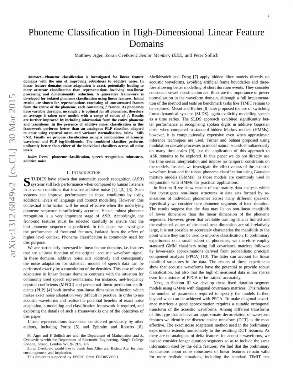
can be modelled by a low-dimensional submanifold ofIR1024, and ifsuch a submanifold could be characterised in a manner which wouldfacilitate accurate statistical modelling of the data. We first applied anumber of intrinsic dimension estimation techniques to theextractedsetsSk. Principal component analysis (PCA) was the first methodconsidered, which assumes the data is contained in a linear subspace.The dimension of the subspace can be estimated by requiring that itshould contain most of the average phoneme energy and we set thisthreshold at 90%. This PCA dimension estimate will be used asareference to compare with three methods for non-linear dimensionestimation. In particular we investigate estimators developed by Heinet al. [17], Costa et al. [18] and Takens [19] and applied themto thephomeme class data.

Figure 1 shows the result of dimension estimation for six phonemesfrom different consonant groups. The findings here agree with theintuition that vowel-like phonemes should have a lower dimensionthan the fricatives. A typical dimension for a semivowel or anasalphoneme, given these estimates, would be around 10; the caseof/m/ is shown in Figure 1. For fricatives like /f/, the dimensionis much higher. Given that the non-linear dimension estimates aremostly consistent and significantly lower than the PCA estimates weconclude that the phoneme distributions can be modelled as lower-dimensional non-linear manifolds.

A number of techniques have recently been developed to find suchnon-linear manifold structures in data [20]. After an extensive studyof the benefits and limitations of these methods, Isomap [15]andLLE [14][21] were selected for application to the phoneme dataset.They were considered especially suitable for the task having suc-cessfully found low-dimensional structure in images of human facesand handwritten digits in other studies. As explained above, althoughthe methods can find structure, there is no straightforward way toapply noise adaptation if we were to use non-linearly reduced featuresets. We would therefore seek to identify the non-linear structures,and exploit them to constrain density models on the originallinearfeature space. As we now show, however, the dimensions of thenon-linear structures in our case are still too high for them to belearnedaccurately with the available quantity of data.

Isomap is a method for finding a lower dimensional approximationof a dataset using geodesic distance estimates. Our initialcomparisonwith PCA output showed that for a given embedding dimension theapproximation provided by Isomap was better in terms of theL2

error [15] for our data. As in PCA we look for a step change inthe spectrum of an appropriate Gram matrix to find the dimensionestimate. However, this was not possible for the phoneme data asthe spectra of the Gram matrices were smooth for all phonemes. Wefound similar results for LLE and suspected that in both cases thecause was undersampling of the manifold.

These findings motivated the study of an artificial problem, toestimate how much data might be required to sufficiently samplethe phoneme manifolds. The simple example of uniform probabilitydistributions over hyperspheres with a given dimension wascon-sidered. A smooth histogram of pairwise distances among sampledpoints, in accordance with the theoretically expected form, thenindicates a sufficient sampling of the uniform target distribution,whereas strong peaks – resulting from the fact that random vectorsin high dimensional spaces are typically orthogonal to eachother– suggest undersampling. Initially, when we set the dimension ofthe hypersphere to be comparable to that of the phoneme dimensionestimates, and used a similar number of data points (∼ 1000), suchpeaks in the distance histograms were indeed present. When thedimension of the hypersphere was reduced to five, the peaks weresmoothed out, suggesting that this five-dimensional manifold was

3

/b/ /f/ /m/ /r/ /t/ /z/0

10

20

30

40

50

60

70

80

90

100

Phoneme

Dim

ensi

on e

stim

ate

IntrinsicCorrelationTakensPCA (90%)

0

50

100

150

200

250

300

350

400

450

500

PC

A d

imen

sion

est

imat

e

Fig. 1. Intrinsic dimension estimates of example phoneme classes.The legendindicates the method of estimation. PCA estimates are plotted using the righthand scale

sufficiently sampled with a number of data points similar to thenumber of phoneme examples per class.

In summary, the findings of the experiments suggest that if speechdata manifolds exist in the acoustic waveform domain then they areunder-sampled because of their relatively high intrinsic dimension.The number of required data points,n, could be expected to varyexponentially with the intrinsic dimensions,d, i.e. n ∼ αd for someconstantα. In the hypersphere experimentsα was approximately four,consequently the estimated quantity of data required to sufficientlysample a phoneme manifold withd ∼ 10 . . . 60 would be unrealistic,particularly at the upper end of this range. Given that the data-drivendimensionality reduction methods we have explored are not practicalfor the task considered, we now turn to more generic density modelsfor the problem of phoneme classification in the presence of additivenoise. In particular we will construct generative classifiers in the high-dimensional space which do not attempt to exploit any submanifoldstructure directly. We will see that approximations are required, againdue to the sparseness of the data, but also because of computationalconstraints.

B. Generative Classification

Generative classifiers use probability density estimates,p(x),learned for each class of the training data. The predicted classof a test point,x, is determined as the classk with the greatestlikelihood evaluated atx. Typically the log-likelihood is used for thecalculation; we denote the log-likelihood ofx by L(x) = log(p(x)).Classification is performed using the following function:

AL(x) = arg maxk=1,...,K

L(k)(x) + log(πk) (1)

where x can be predicted as belonging to one ofK classes. Theinclusion above ofπk, the prior probability of classk, means thatwe are effectively maximising the log-posterior probability of classk given x.

1) Gaussian Mixture Models:Without assuming any additionalprior knowledge about the phoneme distributions we use Gaussianmixture models (GMMs) to model phoneme densities. The modelsare trained using the expectation maximisation (EM) algorithm tomaximise the likelihood of the training data for the relevant phonemeclass. The training algorithm determines suitable parameters for theprobability density function,p : R

d → R, of a Gaussian mixture

model. For the case ofc mixture components this function has theform:

p(x) =

c∑

i=1

wi

(2π)d

2 |Σi|1

2

exp[

− 1

2(x− µi)

TΣ

−1i (x− µi)

]

(2)

wherewi, µi and Σi are the weight, mean vector and covariancematrix of the ith mixture component respectively. In the case ofacoustic waveforms we additionally impose a zero mean constraintfor models as a waveformx will be perceived the same as−x. Withthis constraint the corresponding models represent all informationabout the phoneme distributions in the covariance matricesandcomponent weights.

2) Probabilistic Principal Component Analysis:In the preliminaryexperiments, we initially modelled the phoneme class densities usingGMMs with full covariance matrices. However, it was not possibleto accurately fit models with more than two components in the highdimensional space of acoustic waveforms, whered = 1024. Insteadwe considered using density estimates derived from mixtures of prob-abilistic principal component analysis (MPPCA) [10]. Thismethodhas a dimensionality reduction interpretation and produces a Gaussianmixture model where the covariance matrix of each componentisregularised by replacement with a rank-q approximation:

Σ = r2I+WWT (3)

Here theith column of thed × q matrix W is given as√λivi

corresponding to theith eigenvalue,λi, and eigenvector,vi, ofthe empirical covariance matrix, with the eigenvalues arranged indescending order. The regularisation parameterr2 is then taken asthe mean of the remainingd− q eigenvalues:

r2 =1

d− q

d∑

i=q+1

λi (4)

3) Noise Adaptation:The primary concern of this paper is toinvestigate the performance of the trained classifiers in the presenceof additive Gaussian noise. Generative classification is particularlysuited for robust classification as the estimated density models cancapture the distribution of the noise corrupted phonemes. As the noiseis additive in the acoustic waveform domain, signal and noise modelscan be specified separately and then combined exactly by convolution.In the experiments of this section, phoneme data is normalised at thephoneme segment level with the SNR being specified relative to thesegment rather than the whole sentence. This is clearly unrealistic asthe mean energy of phonemes differs significantly between classes.However, it does provide a situation where each phoneme classis affected by the same local SNR. We can also think of thisgeometrically: for each phoneme class, the class densityp(x) isblurred in the same way by convolution with an isotropic Gaussianof variance set by the SNR. The effect of the noise on classificationthen indirectly provides information on how well separateddifferentphoneme classes are in the space of acoustic waveformsx. The whiteGaussian noise model results in a covariance matrix that is amultipleof the identity matrix,σ2

I, whereσ2 is the noise variance. We assumethroughout that this is known, as it can be estimated reliably duringperiods without speech activity or using other techniques [22]. Hencethe noise adaptation for the acoustic waveform representation is givenby replacing each covariance matrixΣ with Σ(σ2):

Σ(σ2) =Σ+ σ2

I

1 + σ2(5)

Speech waveforms are normalised to unit energy per sample. Clearlysome normalisation of this type is needed to avoid adverse effectsof irrelevant differences in speaker volume on classification perfor-mance, an issue that has been carefully studied in previous work [7].

4

The normalisation leads in the density models to covariancematricesΣ with traced, the dimension of the data. Adding the noise as in thenumerator of the equation above would give an average energypersample of1+σ2. We also normalise noisy speech to unit energy persample, and hence rescale the adapted covariance matrix by1 + σ2

as indicated above.There is no exact method for combining models of the trainingdata

with noise models in the case of MFCC and PLP features, as theserepresentations involve non-linear transforms of the waveform data.Parallel model combination as proposed by Gales and Young [23] isan approximate approach for MFCC. A commonly used alternativemethod for adapting probabilistic models to additive noiseis cepstralmean and variance normalisation (CMVN) [24], and we will considerthis method in subsequent sections. At this exploratory stage, westudy instead the matched condition scenario, where training andtesting noise conditions are the same and a separate classifier istrained for each noise condition. In practice it would be difficultand computationally expensive to have a distinct classifierfor everynoise condition, in particular if noise of varying spectralshape isincluded in the test conditions. Matched conditions are neverthelessuseful in our exploratory classification experiments: because trainingdata comes directly from the desired noisy speech distribution,then assuming enough data is available to estimate class densitiesaccurately this approach provides the optimal baseline forall noiseadaptation methods [23],[25].

C. Results of Exploratory Classification in PLP and AcousticWave-form Domains

In the exploratory study we consider only realisations of sixphonemes (/b/, /f/, /m/, /r/, /t/, /z/) that were extracted from the TIMITdatabase [26]. This set includes examples from fricatives,nasals,semivowels and voiced and unvoiced stops. These classes providepairwise discrimination tasks of a varying level of difficulty. Forexample /b/ vs. /t/ is a more challenging discrimination than /m/vs. /z/. The phoneme examples are represented by the centre64mssegment of the acoustic waveform corresponding to1024 samplesat 16kHz. Additionally the stops, /b/ and /t/ are aligned at therelease point as prescribed by the given TIMIT segmentation. Thedata vectors are then normalised to have squared norm equal to thedimension of the segment corresponding to unit energy per sample asexplained above. These initial experiments focus only on the centreof the phonemes to investigate the effectiveness of noise adaptation.As is well known, discrimination can be improved by consideringthe information provided by the transitions from one phonemes tothe next. We will explore this in Section IV and see that it doesindeed significantly help classification.

Each phoneme class consists of approximately1000 representa-tives, of which 80% were used for training and 20% for testing. Theclassification error bars, where indicated, were derived byconsideringfive different such splits and give an indication of the significance ofany differences in the accuracy of classifiers. A range of SNRs waschosen to explore classification errors all the way to chancelevel,i.e. 83.3% in the case of six classes. In total this gave six testing andtraining conditions;−18dB, −12dB, −6dB, 0dB, 6dB and quiet.At this exploratory stage only white Gaussian noise is considered.We use the same number of examples from each class, thus the priorprobabilitiesπk are all equal to1/6 and have no effect on predictionsaccording to (1).

For comparison the default 12th order PLP cepstra were computedfor the 64ms segments. A sliding 25ms Hamming window was usedwith an overlap of 15ms leading to four frames of 13 coefficients [27].These four frames were concatenated to give a PLP representation

−18 −12 −6 0 6 Quiet0

10

20

30

40

50

60

70

80

90

Test SNR [dB]

Err

or [%

]

Quiet 6dB 0dB−6dB−12dB−18dB

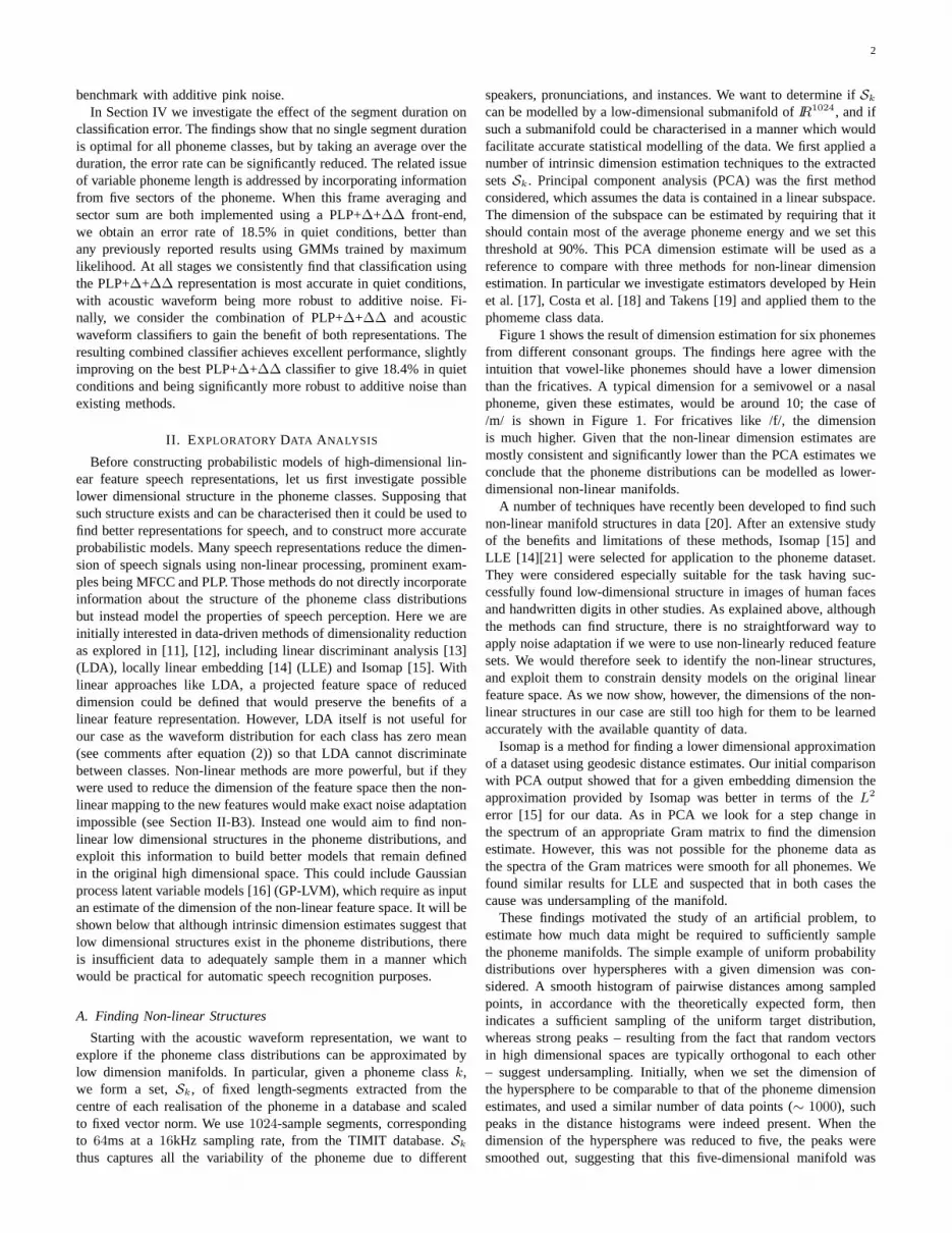
Fig. 2. Error of PLP classifiers as a function of test SNR. Each curve showsthe error of the classifier trained at the SNR indicated by thecurve marker. Thecurves show the sensitivity of PLP classifiers when there is amismatch betweentraining and testing noise conditions. In particular the classifiers trained at 0dBand 6dB performs much worse when the test noise level is lowerthan thetraining level.

in R52. The data was then standardised prior to training so that each

of the 52 features had zero mean and unit variance across the entiretraining set that was considered. We discuss variants of this featurestandardisation in Section III-A3.

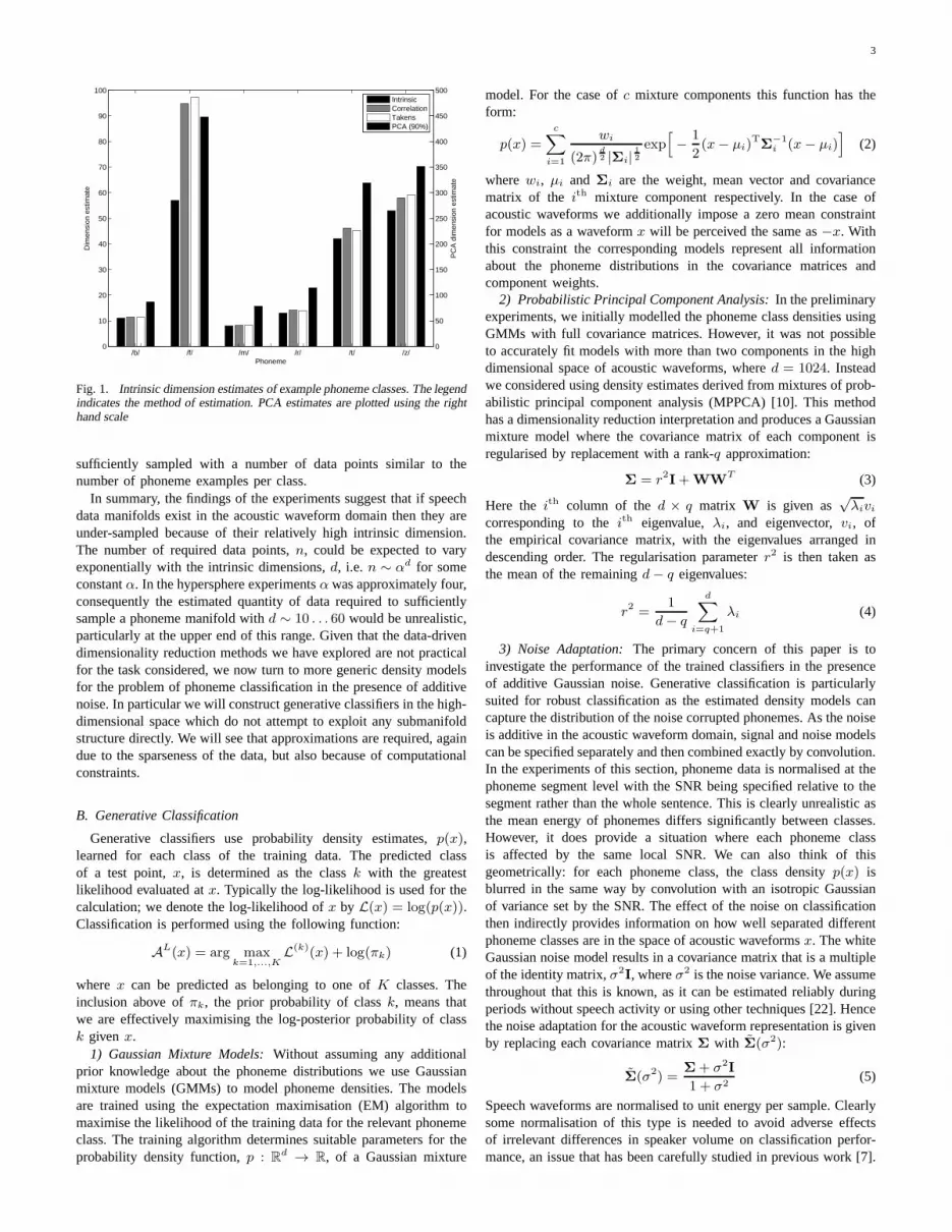
The PLP phoneme distributions were modelled using a singlecomponent PPCA mixture with a principal dimension of 40, i.e.c = 1 and q = 40; we experimented with other values but theseparameters gave the best results. Figure 2 shows the test results forclassifiers trained on data corrupted at the different noiselevels. Eachof the curves thus represents a different training SNR. It isclear thatPLP classifiers are highly sensitive to mismatch between training andtesting noise conditions. For example, when conditions arematchedat 6dB SNR, the error is very low at 2.8%. However, if the sameclassifier is tested in quiet conditions this value increases significantly,to 53.7%. The analogous plot for waveform classifiers is shown inFigure 3, where the phoneme classes were modelled withc = 4 andq = 500.

Acoustic waveform classifiers are less sensitive to mismatch be-tween the assumed noise level to which they were adapted using (5),and the true testing conditions. Taking the classifier adapted to 6dBSNR as an example, we see that if assumed and true testing conditionsare matched the error is 5.1% and when testing in quiet, it remainsas low as 8.4%. Although the error for matched conditions is higherthan that of PLP at this noise level, the increase due to mismatch isdrastically reduced.

We next consider the scenario where the true testing conditionsare matched to those the models were trained in (PLP) or adaptedto (waveforms). This is equivalent to taking the lower envelopes ofFigures 2 and 3. In this case PLP gives a lower error rate thanwaveforms above 0dB SNR, while the opposite is true below thisvalue. These results suggest that we should seek to combine theclassification strengths of each representation, specifically the highaccuracy of PLP classifiers at high SNRs and the robustness ofacoustic waveform classifiers at all noise levels. Ideally this willresult in a single combined classifier that only needs to be trainedin quiet conditions and can be easily adapted to a range of noiseconditions. To investigate this concept we consider the following

5

−18 −12 −6 0 6 Quiet

10

20

30

40

50

60

70

80

90

Test SNR [dB]

Err

or [%

]

Quiet 6dB 0dB−6dB−12dB−18dB

Fig. 3. Error of acoustic waveform classifiers as a function of test SNR. Thecurve marker indicates the assumed SNR to which the classifier was adaptedusing (5). The error rate is less sensitive to mismatch between the assumed andthe true SNR when compared to the curves in Figure 2.

convex combination of the two log-likelihoods with each term beingnormalised by the relevant representation dimension. LetLplp(x)and Lwave(x) be the log-likelihoods of a phoneme class, then thecombined log-likelihoodLα(x) parameterised byα is given as:

Lα(x) =(1− α)

dplpLplp(x) +

α

dwaveLwave(x) (6)

where dplp = 52 and dwave = 1024 are the dimensions of thePLP and acoustic waveform representations, respectively.We wouldexpectα to be almost zero for high SNRs and close to one for lowSNRs in order to give the desired improvement in accuracy, and usethis information to fit a combination function,α(σ2). A suitable rangeof possible values ofα was identified at each noise level from thecondition that the error rate is no more than 2% above the error forthe bestα. This range is broad, so the particular form of the fittedcombination function is not critical [28]. We choose the followingsigmoid function with two parametersσ2

0 andβ:

α(σ2) =1

1 + eβ(σ2

0−σ2)

(7)

A fit through the numerically determined suitable ranges ofα thengivesσ2

0 = 11dB, β = 0.3. We also consider combinations involvingPLP classifiers trained in quiet conditions and adapted to noise usingCMVN, where a similar fit givesσ2

0 = 11dB, β = 0.7.The above combination in (6) is equivalent to using multiple

streams of features, one consisting of the waveform and the other ofthe PLP features derived from the same waveform segment. Data fu-sion at the feature level that concatenates the vectors of features fromeach source would be an alternative method of combining the tworepresentations. However, such a method would not be suitable for thecombination of PLP and acoustic waveforms, predominantly becausethe contribution to the resulting likelihood from each representationis approximately proportional to the feature space dimension. Hencethe likelihood contribution from the acoustic waveform portion of thefused vector would dominate.

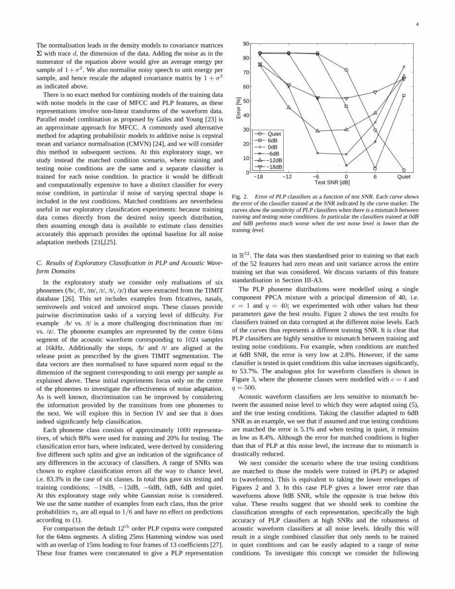
Figure 4 shows the result of the combination, when the acousticwaveform classifiers are trained in quiet conditions and then adaptedto noise according to (5), while the PLP classifiers are trained undermatched conditions. We see in the main plot that the combined

−18 −12 −6 0 6 Quiet0

10

20

30

40

50

60

70

80

90

Test SNR [dB]

Err

or [%

]

CombinedWaveformPLP

−18 −12 −6 0 6 Quiet0

10

20

30

40

50

60

70

Combined MatchedCombined Quiet

Fig. 4. Performance of the combined classifier when PLP models trained undermatched conditions are used. The combined classifier is uniformly at least asaccurate as those it is derived from and gives significant improvement around−6dB SNR. Inset: Comparison with the combined classifier trained only inquiet conditions.

classifier has uniformly lower error rate across the full range ofnoise conditions. In particular, around−6dB SNR the combinationperforms significantly better than either of the underlyingclassifiers.This is interesting because it means that the combination achievesmore than a hard switch between PLP and waveform classifiers could.The inset shows a comparison of combined classifiers involving PLPtrained in matched conditions and PLP trained in quiet and adaptedusing CMVN respectively. These two approaches to PLP trainingshould represent the extremes of performance, with noise adaptationtechniques more advanced than CMVN expected to lie in between.Encouragingly, the inset to Figure 4 shows that by an appropriatecombination with waveform classifiers the performance gap betweenhaving only PLP models trained in quiet conditions and thosetrainedin matched conditions is dramatically reduced.

D. Conclusions of Exploratory Data Analysis

The exploratory data analysis shows that acoustic waveformclassi-fiers, which can be exactly adapted to noise when the noise conditionsare known, are also more robust to mismatch between assumed andtrue testing conditions. The combined classifier retains the accuracyof PLP in quiet conditions whilst simultaneously providingtherobustness of acoustic waveforms in the presence of noise. In orderto confirm these conclusions a more realistic test is required. Asdescribed above, we also found that the best model fits were obtainedwith only a small number of mixture components, whether usingfull covariance matrices or more restricted density modelsin theform of MPPCA. In both cases too many model parameters arerequired to specify each mixture component, meaning that mixtureswith many components cannot be learned reliably from limited data.In the next section, the issue of parameter count reduction will beeven more acute as many of the phoneme classes have even fewerexamples than those considered so far. The problem will be addressedby using diagonal covariance matrices in the GMMs, with the dataappropriately rotated into a basis which approximately decorrelatesthe data. Additionally the SNRs will be specified at sentencelevelwhich can cause local SNR mismatch and will provide a morechallenging test of the robustness of the classifiers. We will alsoinvestigate the length of the segments used to represent thephonemes.

6

This is particularly relevant when comparing the acoustic waveformclassifiers to those of PLP+∆+∆∆ as the deltas use informationfrom neighbouring frames. It will be shown that by optimising thenumbers of frames for each representation we get a similar benefit forphoneme classification as when using deltas. Finally we willshowthe effect of including information from the whole phoneme ratherthan just the frames from the centre.

III. F IXED DURATION REPRESENTATION WITHREFINED MODELS

In this section we consider how to enhance the generative modelsso that they can deal with more realistic classification tasks. Allprevious experiments are now repeated on the standard TIMITbenchmark [29] with noise added so that the SNR is specified atsentence level. This means that the local SNR of the phonemesegments can differ significantly from the sentence level value. Thereis a large variation in the size of the phoneme classes hence thoserelative frequencies have a greater effect as the prior in (1). Wealso consider model averaging, which removes the need to selectthe number of components in mixture models.

A. Model Refinements

1) Diagonal Covariance Matrices:We observed in the preliminaryexploration that even PPCA requires an excessive number of param-eters compared to the quantity of available data. Hence, GMMs withdiagonal covariance matrices are used for all following experiments.This is a common modelling approximation when training dataissparse. Diagonal covariances matrices will be a good approximationprovided the data is presented in a basis where correlationsbetweenfeatures are weak. For the acoustic waveform representation, this isclearly not the case on account of the strong temporal correlations inspeech waveforms. We therefore systematically investigated candidatelow-correlation bases derived from PCA, wavelet transforms andDCTs. Although the optimal basis for decorrelation on the trainingset is indeed formed by the phoneme-specific principal components,we found that the lowest test error is in fact achieved with a DCTbasis. The density model used for the phoneme classes in the acousticwaveform domain now becomes:

p(x) =c

∑

i=1

wi

(2π)d

2 |Di|1

2

exp[

− 1

2(x− µi)

TC

TD

−1i C(x− µi)

]

(8)where wi, µi and Di are the weight, mean vector and diagonalcovariance matrix of theith mixture component respectively.C isan orthogonal transformation selected to decorrelate the data at leastapproximately. In the case of acoustic waveforms we chooseC to bea DCT matrix, as explained above. Preliminary experiments showedthat, instead of performing a single DCT on an entire phonemesegment, it is advantageous to separate DCTs in non-overlapping sub-segments of length 10ms, mirroring (except for the lack of overlaps)the frame decomposition of MFCC and PLP. For a sampling rateof 16kHz as in our data, the transformation matrixC is then blockdiagonal consisting of160 × 160 DCT blocks. For the MFCC andPLP representations we chooseC to be the identity matrix as theyalready involve some form of DCT and the features are approximatelydecorrelated.

2) Model Average:In general, more variability of the training datacan be captured with an increased number of mixture components;however, if too many components are used over-fitting will occur.The best compromise is usually located by cross validation usingthe classification error on a development set. The result is asinglevalue for the number of components required. We use an alternativeapproach and take the model average over the number of components,

effectively a mixture of mixtures [30]. We start from a selection ofmodels parameterised by the number of components,c, which takesvalues inC = {1, 2, 4, 8, 16, 32, 64, 128} or subsets of it. The entriesin this set are uniformly distributed on a log scale to give a good rangeof model complexity without including too many of the complexmodels. We compute the model average log-likelihoodM(x) as:

M(x) = log(

∑

c∈C

ucexp(Lc(x)))

(9)

with the model weightsuc = 1|C|

andLc(x) being the log-likelihoodof x given thec-component model.

Alternatively the mixture weights allocated to each model couldbe determined from the posterior densities of the models on adevelopment set to give a class dependent weighting, i.e.

uc =

∑

x∈D exp(Lc(x))∑

d∈C

∑

x∈D exp(Ld(x))(10)

whereD is a development set. Preliminary experiments suggestedthat using those posterior weights only gives a slight improvementover (9). We therefore adopt those uniform weights (uc = 1

|C|) for

all results shown in this paper.3) Noise adaptation for sentence-normalised data:Now we con-

sider the more realistic case where the SNR is only known atsentence-level. All sentences will therefore be normalised to have unitenergy per sample in quiet and noisy conditions. Different phonemeswithin these sentences can have higher or lower energies, asreflectedin the density models by covarianceD with trace above or belowd,whered is the dimension of the feature vectors. The relative energyof each phoneme class, which we had discarded in Section II-C, canthus be used during classification. The adaptation to noise has thesame form as in (5):

D(σ2) =D+ σ2

N

1 + σ2(11)

whereN is the covariance matrix of the noise transformed byC,normalised to have traced. For white noise,N is the identity matrix,otherwise it is estimated empirically from noise samples. In general afull covariance matrix will be required to specify the noisestructure.However, with a suitable choice ofC the resultingN will be closeto diagonal, and indeed whenC is a segmented DCT we find this tobe true in our experiments with pink noise. To avoid the significantcomputational overheads of introducing non-diagonal matrices, wetherefore retain only the diagonal elements ofN. The normalisationby 1+σ2 arises as before: on average, a clean sentence to which noisehas been added has energy1+ σ2 per sample and the normalisationto unit energy of both clean and noisy data requires dividingallcovariances by this factor. In contrast to our exploratory study inSection II, and because of the varying local SNR, the traces of D

andD are then no longer necessarily equal.We now consider noise compensation techniques for MFCC and

PLP features. As mentioned above, cepstral mean and variance nor-malisation (CMVN) [24] is an approach commonly used in practice tocompensate noise corrupted features. This method requiresestimatesof the mean and variance of the features, usually calculatedsentence-wise on the test data or with a moving average over a similar timewindow. We take this to be a realistic baseline. Alternatively therequired statistics can be estimated from a training set that has beencorrupted by the same type and level of noise as used in testing.(For large data sets, these statistics should be essentially the sameas on the noisy test set, barring systematic effects from e.g. differenttraining and test speakers.) Clearly both approaches have merit. Forexample, sentence level CMVN requires no direct knowledge of thetest conditions, and can remove speaker specific variation from the

7

−18 −12 −6 0 6 12 18 24 30 Quiet20

30

40

50

60

70

80

90

SNR [dB]

Err

or [%

]

//

PLP (Standardised)PLP+∆+∆∆ (Standardised)PLP (Sentence)PLP+∆+∆∆ (Sentence)

Fig. 5. Comparison of sentence level cepstral mean and variance normalisation(dashed) and training set (solid) standardisation for PLP and PLP+∆+∆∆.

data. The estimates will be less accurate and as a consequence it isdifficult to standardise all components in long feature vectors obtainedby concatenating frames; instead, we standardise frame by frame.Using a noisy training set for CMVN requires that the test conditionsare known so that either data can be collected or generated for trainingunder the same conditions. The feature means and variances canbe obtained accurately, and in particular we can standardise longerfeature vectors. However, as the same standardisation is used for allsentences, any variation due to individual speakers will persist.

A comparison of the two standardisation techniques is showninFigure 5. Curves are displayed for both methods, using PLP featureswith and without∆+∆∆. Standardisation on the noisy training setgives lower error rates both in quiet conditions and in noise, henceall results for CMVN given below use this method.

B. Experimental setup

Realisations of phonemes were extracted from the SI and SXsentences of the TIMIT [26] database. The training set consistsof 3,696 sentences sampled at 16kHz. Noisy data is generatedbyapplying additive Gaussian noise at nine SNRs. Recall that theSNRs were set at the sentence level, therefore the local SNR ofthe individual phonemes may differ significantly from the set value,causing mismatch in the classifiers. In total ten testing andtrainingconditions were run;−18dB to 30dB in 6dB increments and quiet(Q). Following the extraction of the phonemes there are a total of140,225 phoneme realisations. The glottal closures are removed andthe remaining classes are then combined into 48 groups in accordancewith [29], [31]. Even after this combination some of the resultinggroups have too few realisations. The smallest groups with fewerthan 1,500 realisations were increased in size by the addition oftemporally shifted versions of the data. i.e. ifx is an example in oneof the small training classes then the phoneme segments extractedfrom positions shifted byk = −100, −75, −50, . . . , 75, 100samples were also included for training. This increase in the sizeof the smaller training classes ensures that the training procedure isstable. For the purposes of calculating error rates, some very similarphoneme groups are further regarded as identical, resulting in 39groups of effectively distinguishable phonemes [29]. PLP features areobtained in the standard manner from frames of width 25ms, with ashift of 10ms between neighbouring frames and correspondingly an

1 2 4 8 16 32 6425

30

35

40

45

50

55

60

65

Err

or [%

]

Number of Components

Waveform

PLP

MFCC

PLP+∆+∆∆MFCC+∆+∆∆

Individual models

Component average

Fig. 6. Model averaging for acoustic waveforms, MFCC and PLP models,all trained and tested in quiet conditions. Solid: GMMs withnumber ofcomponents shown; dashed: average over models up to number of componentsshown. The model average reduces the error rate in all cases.

overlap of 15ms. We also include now in our comparisons MFCCfeatures. Standard implementations [27] of MFCC and PLP withdefault parameter values are used to produce a 13-dimensional featurevector from each time frame. The inclusion of∆ + ∆∆ increasesthe dimension to 39.

Our exploratory results in Section II gave successful classificationfor acoustic waveforms using a 64ms window. For the MFCC andPLP representations, we therefore consider the five frames closestto the centre of each phoneme, covering 65ms, and concatenatetheir feature vectors. Results are shown for the representations withand those without∆ + ∆∆ , giving feature vector dimensions of5× 39 = 195 and5× 13 = 65, respectively. The acoustic waveformrepresentation is obtained by dividing each sentence into asequenceof 10ms non-overlapping frames, and then taking the seven frames(70ms) closest to the centre of each phoneme, resulting in a 1120-dimensional feature vector. Each frame is individually processedusing the 160-point DCT. We present results for white and pink noiseand will see that the approximation using diagonal covariancesD inthe DCT basis is sufficient to give good performance. The impactof the number of frames included in the MFCC, PLP and acousticwaveform representations is investigated in the next section.

C. Results

Gaussian mixture models were trained with up to 64 compo-nents for all representations. We comment briefly on the resultsfor individual mixtures, i.e. with a fixed number of components.Typically performance on quiet data improved with the number ofcomponents, although this has significant cost for both training andtesting. The optimal number of components for MFCC and PLPmodels in quiet conditions was 64, the maximum considered here.However, in the presence of noise the lowest error rates wereobtainedwith few components; typically there was no improvement beyondfour components.

As explained in Section III-A2, rather than working with modelswith fixed numbers of components, we average over models, i.e.over the number of mixture components, in all the results reportedbelow. Figure 6 shows that the improvement obtained by this in quietconditions is approximately 2% for both acoustic waveformsand PLP

8

with a small improvement seen for MFCC also. The model averagesimilarly improved results in noise and this will be discussed furtherin the next section.

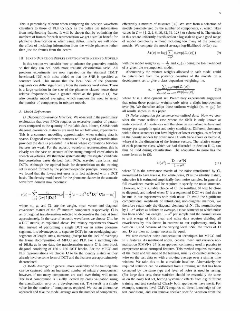
One set of key results comparing the error rates in noise forphoneme classification in the three domains is shown in Figure 7.The MFCC and PLP classifiers are adapted to noise using CMVN.This method is comparable with the adapted waveform models asit only relies on the models trained in quiet conditions. Thecurvefor acoustic waveforms is for models trained in quiet conditions andthen adapted to the appropriate noise level using (11). Comparingwaveforms first to MFCC and PLP without∆+∆∆, we see that inquiet conditions the PLP representation gives the lowest error. Theerror rates for MFCC and PLP are significantly worse in the presenceof noise, however, with acoustic waveforms giving an absolutereduction in error at 0dB SNR of 40.6% and 41.9% compared toMFCC and PLP respectively. These results strengthen the case thatthe adaptability of acoustic waveform models gives them a definiteadvantage in the presence of noise with the crossover point occurringabove 30dB SNR. Curves are also shown for MFCC+∆+∆∆ andPLP+∆+∆∆. Again the same trend holds; performance is goodin quiet conditions but quickly deteriorates as the SNR decreases.The crossover point is around 24dB for both representations. Thechance-level error rate of 93.5% can be seen below 0dB SNR fortheMFCC and PLP representations without deltas and below 6dB SNRwhen deltas are included, whereas the acoustic waveform classifierperforms significantly better than chance with an error of 76.7%even at−18dB SNR. The dashed curves in Figure 7 represent theerror rates obtained for classifiers trained in matched conditions withand without∆+∆∆. The results show that the waveform classifiercompares favourably to MFCC and PLP below 24dB SNR when nodeltas are appended. Including∆+∆∆ does reduce the error ratessignificantly and the crossover then occurs between 0dB and 6dBSNR. It is these observations that mainly motivate our further modelsdevelopment below: clearly we should aim to include informationsimilar to deltas in the waveform representation.

The same experiment was repeated using pink noise extractedfromthe NOISEX-92 database [32]. The results for both noise types weresimilar for the waveforms classifiers. For PLP+∆+∆∆, adapted tonoise using CMVN, there is a larger difference between the two noisetypes, with pink noise leading to lower errors. Nevertheless, the betterperformance is achieved by acoustic waveforms below 18dB SNR.Results for GMM classification on the TIMIT benchmark in quietconditions have previously been reported in [31], [33] witherrors of25.9% and 26.3% respectively. To ensure that our baseline isvalid wecompared our experiment in quiet conditions for PLP+∆+∆∆ andobtained a comparable error rate of 26.3% as indicated in thebottomright corner of Figure 7.

Following these encouraging results we seek to explore the effectof optimising the number of frames and the inclusion of informationfrom the entire phoneme. The expectation is that including moreframes in the concatenation for acoustic waveforms will have asimilar effect to adding∆+∆∆ for MFCC and PLP. A directanalogue of deltas is unlikely to be useful for waveforms: MFCCand PLP are based on log magnitude spectra that change littleduring stationary phonemes, so that local averaging or differencingis meaningful. For waveforms, where we effectively retain not justFourier component amplitudes but also phases, these phasescombineessentially randomly during averaging or differencing, rendering theresulting delta-like features useless.

−18 −12 −6 0 6 12 18 24 30 Q20

30

40

50

60

70

80

90

100

Test SNR [dB]

Err

or [%

]

//

WaveformMFCCPLPMFCC+∆+∆∆PLP+∆+∆∆

Fig. 7. Comparison of adapted acoustic waveform classifiers with MFCC andPLP classifiers trained in quiet conditions adapted by feature standardisation.All classifiers use the model average of mixtures up to 64 components. Dottedline indicates chance level at 93.5%. When the SNR is less that 24dB, acousticwaveforms are the significantly better representation, with an error rate belowchance even at -18dB SNR. Dashed curves show results of matched training forcorresponding MFCC and PLP representations.

IV. SEGMENT DURATION, VARIABLE DURATION PHONEME

MAPPING AND CLASSIFIERCOMBINATION

A. Segment Duration

Ideally all relevant information should be retained by our phonemerepresentation, but as it is difficult to determine exactly which infor-mation is relevant we initially choose to takef consecutive framesclosest to the centre of each phoneme and concatenate them. Whilstthe precise number of frames required for accurate classificationcould in principle be inferred from the statistics of the phonemesegment durations, we see in Table I that those durations notonlyvary significantly between classes but also that the standard deviationwithin each class is at least 24ms. Therefore no single length can besuitable for all classes. The determination of an optimalf from thedata statistics would be even more more complicated when∆+∆∆are included, because these incorporate additional information aboutthe dynamics of the signal outside thef frames.

Assuming that no single value off will be optimal for all phonemeclasses we instead consider the sum of the mixture log-likelihoodsMf , as defined in (9) but now indexed by the number of framesused. The sum is taken over the setF which contains the valuesof f with the lowest corresponding error rate, for exampleF ={7, 9, 11, 13, 15} for PLP:

R(x) =∑

f∈F

Mf (xf ) (12)

where x = {xf |f ∈ F}, with xf being the vector withf frames.Note that we are adding the log-likelihoods for differentf , whichamounts to assuming independence between the differentxf in x.Clearly this an imperfect model, as e.g. all components ofx7 are alsocontained inx11 and so are fully correlated, but our experiments showthat it is useful in practice. We also implemented the alternative ofconcatenating thexf into one longer feature vector and then traininga joint model on this, but the potential benefits of accounting forcorrelations are far outweighed by the disadvantages of having tofit density models in higher dimensional spaces. Consistentwith theindependence assumption in (12), in noise we adapt the models Mf

9

/t/ /ay/ /f/

40ms 40ms

30% 40% 30%

15% 35% 35% 15%

A B C D E

time

f framesX

A

f framesX

Ef framesX

B

f framesX

C f framesX

D

Fig. 8. Comparison of phoneme representations. Top: Division describedin [33] resulting in five sectors, three covering the duration of the phonemeand two of 40ms duration around the transitions. Bottom:f frames closest tothe five points A, B, C, D and E (which correspond to the centresof the regionsabove) are selected to map the phoneme segment to five featurevectorsxA,xB , xC , xD andxE .

separately and then combine them as above. The same applies to thefurther combinations discussed next.

TABLE IDuration statistics [ms] of the training data grouped by broad phonetic class.

Group Min Mean± std. Max

Vowels 2.2 86.0± 46.7 438.6

Nasals 7.6 54.5± 25.6 260.6

Strong Fricatives 14.9 99.5± 38.9 381.2

Weak Fricatives 4.5 68.2± 37.3 310.0

Stops 2.9 39.3± 24.0 193.8

Silence 2.0 94.9± 107.5 2396.6

All 2.0 79.4± 63.4 2396.6

B. Sector sum

Although phonemes vary in duration, GMMs require data thathas a consistent dimension. We next establish a method to mapthevariable length phoneme segments to a fixed length representationfor classification. In the previous subsection only frames from thecentre of the phoneme segments were used to represent a phoneme.We extend that centre-only concatenation to use information fromthe entire segment by takingf frames with centres closest to eachof the time instants A,B,C,D and E that are distributed alongtheduration of the phoneme as shown in Figure 8. In this manner therepresentation consists of five sequences off frames per phoneme.Those sets of frames are then concatenated to give five vectors xA,xB, xC , xD and xE. We train five models on those sectors andthen combine the information they provide about each sector, againassuming independence by taking the sum of the log-likelihoods ofthe sectors:

S(x) =∑

s∈{A,B,C,D,E}

Ms(xs) (13)

where x = {xA, xB, xC , xD, xE} and Ms denotes the model forsectors, using some fixed number of framesf . Both improvementscan be combined by taking the sum of thef -averaged log-likelihoods,Rs(xs), over the five sectorss:

T (ˆx) =∑

s∈{A,B,C,D,E}

Rs(xs) (14)

where xs = {xfs |f ∈ F} with xf

s being the vector withf framescentred on sectors, and ˆx gathers allxs. Given the functions derivedabove, the class of a test point can be predicted using one of thefollowing:

AMf (x) = arg max

k=1,...,KM(k)

f (x) + log(πk) (15)

AR(x) = arg maxk=1,...,K

R(k)(x) + log(πk) (16)

ASf (x) = arg max

k=1,...,KS(k)f (x) + log(πk) (17)

AT (ˆx) = arg maxk=1,...,K

T (k)(ˆx) + log(πk) (18)

whereπk is the prior probability of predicting classk as in (1).

C. Results

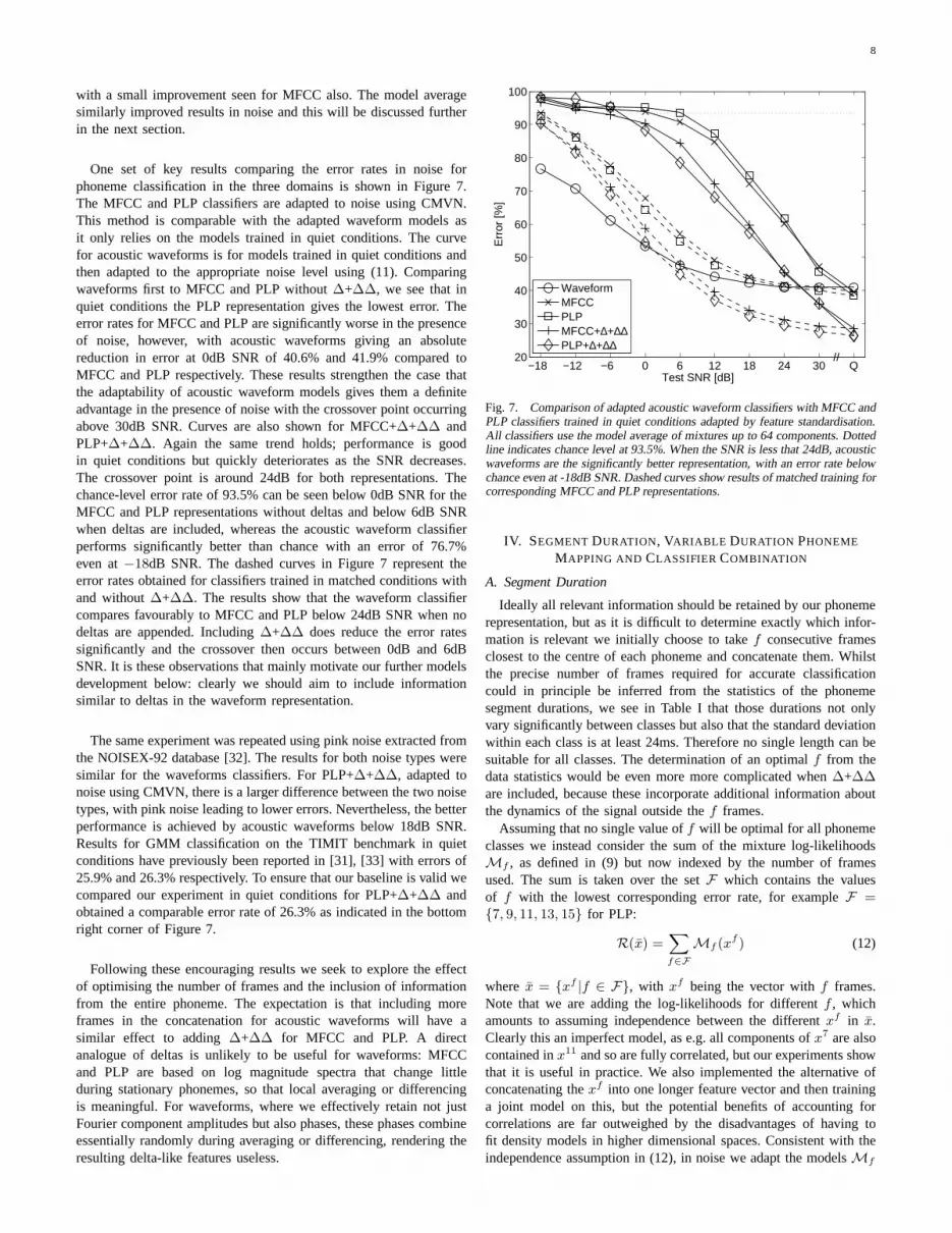
Figure 9 shows the impact of the number of frames concatenatedfrom each sector on the classification error, focusing on quiet condi-tions. We see that the best results for acoustic waveform classifiersare achieved around 9 frames, and around 11 frames for PLP withoutdeltas. The PLP+∆+∆∆ features are less sensitive to the number offrames with little difference in error from 1 to 13 frames. Wecannow also assess quantitatively the performance benefit of includingthe deltas. If we consider the best results obtained for PLP withoutdeltas, 22.4% using 11 frames, with the best for PLP+∆+∆∆, 21.8%with 7 frames, then the performance gap of 0.6% is much smallerthan if we were to compare error rates where both classifiers usedthe same number of frames. Clearly it is not surprising that fewerPLP+∆+∆∆ frames are required for the same level of performanceas the deltas are a direct function of the neighbouring PLP frames.It is still worth noting that in terms of the ultimate performance onthis classification task the error rates with and without deltas aresimilar. The results discussed above are directly comparable with theGMM baseline results from other studies, shown in Table III.Theerror rates obtained using thef -average over the five best values off are 32.1%, 21.4% and 18.5% for acoustic waveforms, PLP andPLP+∆+∆∆ respectively.

Table II shows the absolute percentage error reduction for eachof the four classifiers (15)–(18) in quiet conditions, compared tothe GMM with the single best number of mixture components andnumber of framesf . The relative benefits of thef -average and thesector sum are clear. The sector sum gives the bigger improvementson its own in all cases compared to only thef -average, but thecombination of the two methods is better still throughout. The samequalitative trend holds true in noise.

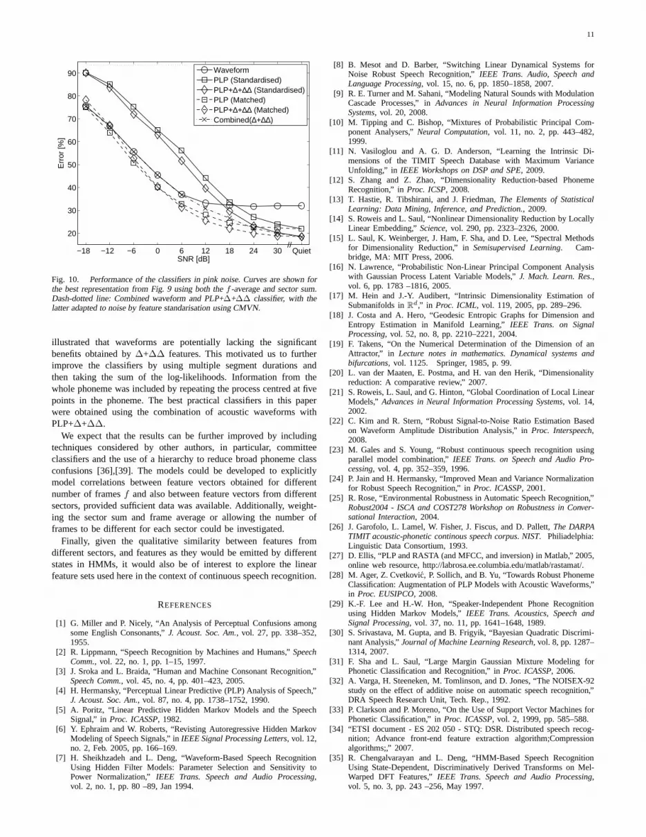
Figure 10 compares the performance of the final classifiers, in-cluding both thef -average and the sector sum, on data corruptedby pink noise. The solid curves give the results for the acousticwaveform classifier adapted to noise using (11), and for the PLPclassifier with and without∆+∆∆ trained in quiet conditions andadapted to noise by CMVN. The errors are generally significantlylower than in Figure 7, showing the benefits off -averaging and thesector sum. PLP+∆+∆∆ remains the better representation for verylow noise, but waveforms give lower errors beyond a crossover pointbetween 12dB and 18dB SNR, depending on whether we compareto PLP with or without∆+∆∆. As before, they also perform betterthan chance down to−18dB SNR.

The dashed lines in Figure 10 show for comparison the perfor-mance of PLP classifiers trained in matched conditions. As explained,the CMVN and matched curves for PLP provide the extremesbetween which we would expect a PLP classifier to perform ifmodel adaption analogous to that used with the acoustic waveformswas possible, or some other method to improve robustness was

10

1 3 5 7 9 11 13 1515

20

25

30

35

40

45

50

55

60

Number of frames

Err

or [%

]WaveformPLPPLP+∆+∆∆Model avg.Sector sum

Fig. 9. Error rates of the different representations in quiet conditions, asa function off , the number of frames considered. Dashed: prediction (15)using only the central sector. Dotted: prediction (16) using the sum over allfive sectors, leading to a clear improvement in all cases.

employed such as the ETSI advanced front-end (AFE) [34]. Asexpected, the matched conditions PLP+∆+∆∆ classifier has the bestperformance for all SNR. However, in noise the adapted acousticwaveform classifier is significantly closer to matched PLP+∆+∆∆than PLP+∆+∆∆ with CMVN.

TABLE IIAbsolute reduction in percentage error for each of the classifiers (15)–(18) in

quiet conditions.

Model Waveform PLP PLP+∆+∆∆

Model average (AM ) 1.6 2.8 4.4

f -average (AR) 5.6 6.0 6.3

Sector sum (AS ) 6.7 8.4 8.7

f -average + sector sum (AT ) 9.9 10.0 10.4

D. Combination of PLP and Acoustic Waveform Classifiers

We see from the results shown so far that, as in the preliminaryexperiments, PLP performs best in quiet conditions with acousticwaveforms being more robust to additive noise. To gain the benefitsof both representations, we propose to merge them via a linearcombination of the corresponding log-likelihoods, parameterised bya coefficientα:

Tα(x) = (1− α)Tplp(x) + αTwave(x) (19)

where Tplp(x) and Twave(x) are the log-likelihoods of a pointx.Tα(x) is then used in place ofT (x) in (18) to predict the class.The combination differs from (6) as the effect of the prior classprobabilities is more relevant now and the absolute log-likelihoodsmust be used rather than the scaled quantities. This is againequivalentto a multistream model, where each sector and value off is anindependent stream. A noise-dependentα(σ2) is determined asexplained in Section II-C, giving parameter values (σ2 = 17dB,β = 0.3) in (7).

The error of the combined classifier using models trained inquiet conditions is shown as the dash-dotted curve in Figure10.In quiet conditions the combined classifier is slightly moreaccurate(18.4%) than PLP+∆+∆∆ alone, corresponding to a small value

TABLE IIIExisting error rates obtained in other studies for a range ofclassification

methods on the TIMIT core test set. Results in this paper are most comparableto the GMM baselines.

Method Error [%]

HMM (Minimum Classification Error) [35] 31.4

GMM baseline [33] 26.3

GMM baseline [36] 24.1

GMM baseline [37] 23.4

GMM ( f -average + sector sum) PLP+∆+∆∆ 18.5

SVM, 5th order polynomial kernel [33] 22.4

Large Margin GMM (LMGMM) [31] 21.1

Regularized least squares [37] 20.9

Hidden conditional random fields [38] 20.8

Hierarchical LMGMM H(2,4) [36] 18.7

Optimum-transformed HMM with context (THMM) [35] 17.8

Committee hierarchical LMGMM H(2,4) [36] 16.7

of α = 0.003. When noise is present the combined classifier is atleast as accurate as the acoustic waveform classifier, and significantlybetter around 18dB SNR. The combined classifier does improveuponPLP+∆+∆∆ classifiers trained in matched conditions at very lowSNR and narrows the performance gap to the order of no more than9% throughout, rather than 22% when comparing to PLP+∆+∆∆adapted by CMVN.

V. CONCLUSION & D ISCUSSION

In this paper we have studied some of the potential benefits ofphoneme classification in linear feature domains directly related tothe acoustic waveform, with the aim of implementing exact noiseadaptation of the resulting density models. In Section II weoutlinedthe results of our exploratory data analysis, where we foundintrinsicnonlinear dimension estimates lower than linear dimensionestimatesfrom PCA. That observation suggested that it should be possibleto construct low dimensional embeddings to be used later withgenerative classifiers. However, existing techniques failed to findenough structure in the phoneme dataset as it is too sparse toaccurately define the embeddings. Consequently we used GMMsto model the phoneme distributions in acoustic waveform andPLPdomains. Additionally, a combined classifier was used to incorporatethe performance of PLP in quiet conditions with the noise robustnessof acoustic waveforms.

Given the encouraging results from these experiments on a smallset of phonemes we progressed to a more realistic task and extendedthe classification problem to include all phonemes from the TIMITdatabase. This gave results that could be directly comparedto theexisting results in Table III, classifiers representing current progresson the TIMIT benchmark. All of the entries show the error for isolatedphoneme classification except for the optimum-transformedHMM(THMM) [35] that uses context information derived from continuousspeech. The inclusion of context for the HMM classifiers reduces theerror rate from 31.4% to 17.8%. This dramatic reduction suggeststhat if the other classifiers were also developed to directlyincorporatecontextual information, significant improvements could beexpected.

We used the standard approximation of diagonal covariance ma-trices to reduce the number of parameters required to specify theGMMs. The issue of selecting the number of components in themixture models was approached by taking the model average withrespect to the number of components for a sufficiently large setof values. The results supported our earlier conclusions, but also

11

−18 −12 −6 0 6 12 18 24 30 Quiet

20

30

40

50

60

70

80

90

SNR [dB]

Err

or [%

]

//

WaveformPLP (Standardised)PLP+∆+∆∆ (Standardised)PLP (Matched)PLP+∆+∆∆ (Matched)Combined(∆+∆∆)

Fig. 10. Performance of the classifiers in pink noise. Curves are shown forthe best representation from Fig. 9 using both thef -average and sector sum.Dash-dotted line: Combined waveform and PLP+∆+∆∆ classifier, with thelatter adapted to noise by feature standarisation using CMVN.

illustrated that waveforms are potentially lacking the significantbenefits obtained by∆+∆∆ features. This motivated us to furtherimprove the classifiers by using multiple segment durationsandthen taking the sum of the log-likelihoods. Information from thewhole phoneme was included by repeating the process centredat fivepoints in the phoneme. The best practical classifiers in thispaperwere obtained using the combination of acoustic waveforms withPLP+∆+∆∆.

We expect that the results can be further improved by includingtechniques considered by other authors, in particular, committeeclassifiers and the use of a hierarchy to reduce broad phonemeclassconfusions [36],[39]. The models could be developed to explicitlymodel correlations between feature vectors obtained for differentnumber of framesf and also between feature vectors from differentsectors, provided sufficient data was available. Additionally, weight-ing the sector sum and frame average or allowing the number offrames to be different for each sector could be investigated.

Finally, given the qualitative similarity between features fromdifferent sectors, and features as they would be emitted by differentstates in HMMs, it would also be of interest to explore the linearfeature sets used here in the context of continuous speech recognition.

REFERENCES

[1] G. Miller and P. Nicely, “An Analysis of Perceptual Confusions amongsome English Consonants,”J. Acoust. Soc. Am., vol. 27, pp. 338–352,1955.

[2] R. Lippmann, “Speech Recognition by Machines and Humans,” SpeechComm., vol. 22, no. 1, pp. 1–15, 1997.

[3] J. Sroka and L. Braida, “Human and Machine Consonant Recognition,”Speech Comm., vol. 45, no. 4, pp. 401–423, 2005.

[4] H. Hermansky, “Perceptual Linear Predictive (PLP) Analysis of Speech,”J. Acoust. Soc. Am., vol. 87, no. 4, pp. 1738–1752, 1990.

[5] A. Poritz, “Linear Predictive Hidden Markov Models and the SpeechSignal,” in Proc. ICASSP, 1982.

[6] Y. Ephraim and W. Roberts, “Revisting Autoregressive Hidden MarkovModeling of Speech Signals,” inIEEE Signal Processing Letters, vol. 12,no. 2, Feb. 2005, pp. 166–169.

[7] H. Sheikhzadeh and L. Deng, “Waveform-Based Speech RecognitionUsing Hidden Filter Models: Parameter Selection and Sensitivity toPower Normalization,” IEEE Trans. Speech and Audio Processing,vol. 2, no. 1, pp. 80 –89, Jan 1994.

[8] B. Mesot and D. Barber, “Switching Linear Dynamical Systems forNoise Robust Speech Recognition,”IEEE Trans. Audio, Speech andLanguage Processing, vol. 15, no. 6, pp. 1850–1858, 2007.

[9] R. E. Turner and M. Sahani, “Modeling Natural Sounds withModulationCascade Processes,” inAdvances in Neural Information ProcessingSystems, vol. 20, 2008.

[10] M. Tipping and C. Bishop, “Mixtures of Probabilistic Principal Com-ponent Analysers,”Neural Computation, vol. 11, no. 2, pp. 443–482,1999.

[11] N. Vasiloglou and A. G. D. Anderson, “Learning the Intrinsic Di-mensions of the TIMIT Speech Database with Maximum VarianceUnfolding,” in IEEE Workshops on DSP and SPE, 2009.

[12] S. Zhang and Z. Zhao, “Dimensionality Reduction-basedPhonemeRecognition,” inProc. ICSP, 2008.

[13] T. Hastie, R. Tibshirani, and J. Friedman,The Elements of StatisticalLearning: Data Mining, Inference, and Prediction., 2009.

[14] S. Roweis and L. Saul, “Nonlinear Dimensionality Reduction by LocallyLinear Embedding,”Science, vol. 290, pp. 2323–2326, 2000.

[15] L. Saul, K. Weinberger, J. Ham, F. Sha, and D. Lee, “Spectral Methodsfor Dimensionality Reduction,” inSemisupervised Learning. Cam-bridge, MA: MIT Press, 2006.

[16] N. Lawrence, “Probabilistic Non-Linear Principal Component Analysiswith Gaussian Process Latent Variable Models,”J. Mach. Learn. Res.,vol. 6, pp. 1783 –1816, 2005.

[17] M. Hein and J.-Y. Audibert, “Intrinsic DimensionalityEstimation ofSubmanifolds inRd,” in Proc. ICML, vol. 119, 2005, pp. 289–296.

[18] J. Costa and A. Hero, “Geodesic Entropic Graphs for Dimension andEntropy Estimation in Manifold Learning,”IEEE Trans. on SignalProcessing, vol. 52, no. 8, pp. 2210–2221, 2004.

[19] F. Takens, “On the Numerical Determination of the Dimension of anAttractor,” in Lecture notes in mathematics. Dynamical systems andbifurcations, vol. 1125. Springer, 1985, p. 99.

[20] L. van der Maaten, E. Postma, and H. van den Herik, “Dimensionalityreduction: A comparative review,” 2007.

[21] S. Roweis, L. Saul, and G. Hinton, “Global Coordinationof Local LinearModels,” Advances in Neural Information Processing Systems, vol. 14,2002.

[22] C. Kim and R. Stern, “Robust Signal-to-Noise Ratio Estimation Basedon Waveform Amplitude Distribution Analysis,” inProc. Interspeech,2008.

[23] M. Gales and S. Young, “Robust continuous speech recognition usingparallel model combination,”IEEE Trans. on Speech and Audio Pro-cessing, vol. 4, pp. 352–359, 1996.

[24] P. Jain and H. Hermansky, “Improved Mean and Variance Normalizationfor Robust Speech Recognition,” inProc. ICASSP, 2001.

[25] R. Rose, “Environmental Robustness in Automatic Speech Recognition,”Robust2004 - ISCA and COST278 Workshop on Robustness in Conver-sational Interaction, 2004.

[26] J. Garofolo, L. Lamel, W. Fisher, J. Fiscus, and D. Pallett, The DARPATIMIT acoustic-phonetic continous speech corpus. NIST. Philiadelphia:Linguistic Data Consortium, 1993.

[27] D. Ellis, “PLP and RASTA (and MFCC, and inversion) in Matlab,” 2005,online web resource, http://labrosa.ee.columbia.edu/matlab/rastamat/.

[28] M. Ager, Z. Cvetkovic, P. Sollich, and B. Yu, “Towards Robust PhonemeClassification: Augmentation of PLP Models with Acoustic Waveforms,”in Proc. EUSIPCO, 2008.

[29] K.-F. Lee and H.-W. Hon, “Speaker-Independent Phone Recognitionusing Hidden Markov Models,”IEEE Trans. Acoustics, Speech andSignal Processing, vol. 37, no. 11, pp. 1641–1648, 1989.

[30] S. Srivastava, M. Gupta, and B. Frigyik, “Bayesian Quadratic Discrimi-nant Analysis,”Journal of Machine Learning Research, vol. 8, pp. 1287–1314, 2007.

[31] F. Sha and L. Saul, “Large Margin Gaussian Mixture Modeling forPhonetic Classification and Recognition,” inProc. ICASSP, 2006.

[32] A. Varga, H. Steeneken, M. Tomlinson, and D. Jones, “TheNOISEX-92study on the effect of additive noise on automatic speech recognition,”DRA Speech Research Unit, Tech. Rep., 1992.

[33] P. Clarkson and P. Moreno, “On the Use of Support Vector Machines forPhonetic Classification,” inProc. ICASSP, vol. 2, 1999, pp. 585–588.

[34] “ETSI document - ES 202 050 - STQ: DSR. Distributed speech recog-nition; Advance front-end feature extraction algorithm;Compressionalgorithms;,” 2007.

[35] R. Chengalvarayan and L. Deng, “HMM-Based Speech RecognitionUsing State-Dependent, Discriminatively Derived Transforms on Mel-Warped DFT Features,”IEEE Trans. Speech and Audio Processing,vol. 5, no. 3, pp. 243 –256, May 1997.

12

[36] H. Chang and J. Glass, “Hierarchical Large-Margin Gaussian MixtureModels For Phonetic Classification,” inProc. IEEE ASRU Workshop,2007, pp. 272–275.

[37] R. Rifkin, K. Schutte, M. Saad, J. Bouvrie, and J. Glass,“NoiseRobust Phonetic Classification with Linear Regularized Least Squaresand Second-Order Features,” inProc. ICASSP, 2007, pp. IV–881–IV–884.

[38] D. Yu, L. Deng, and A. Acero, “Hidden Conditional RandomField withDistribution Constraints for Phone Classification,” inProc. Interspeech,2009.

[39] F. Pernkopf, T. Pham, and J. Bilmes, “Broad Phonetic Classificationusing Discriminative Bayesian Networks,”Speech Comm., vol. 51, no. 2,2009.

arX

iv:1

312.

6849

v2 [

cs.C

L] 3

0 M

ar 2

015

1

Speech Recognition Front End Without InformationLoss

Matthew Ager, Zoran CvetkovicSenior Member, IEEE,and Peter Sollich

Abstract—Speech representation and modelling in high-dimensional spaces of acoustic waveforms, or a linear transfor-mation thereof, is investigated with the aim of improving therobustness of automatic speech recognition to additive noise.The motivation behind this approach is twofold: (i) the infor-mation in acoustic waveforms that is usually removed in theprocess of extracting low-dimensional features might aid robustrecognition by virtue of structured redundancy analogous tochannel coding, (ii) linear feature domains allow for exactnoiseadaptation, as opposed to representations that involve non-linearprocessing which makes noise adaptation challenging. Thus, wedevelop a generative framework for phoneme modelling in high-dimensional linear feature domains, and use it in phoneme clas-sification and recognition tasks. Results show that classificationand recognition in this framework perform better than analogousPLP and MFCC classifiers below 18dB SNR. A combinationof the high-dimensional and MFCC features at the likelihoodlevel performs uniformly better than either of the individu alrepresentations across all noise levels.

Index Terms—phoneme classification, speech recognition, ro-bustness, noise.

I. I NTRODUCTION

A major problem faced by state-of-the-art automaticspeech recognition (ASR) systems is a lack of robustness,

manifested as a substantial performance degradation due tocommon environmental distortions, due to a discrepancy be-tween training and run-time conditions, or due to spontaneousconversational pronunciation [2], [3]. It was long believedthat context and language modelling would provide ASR withthe level of robustness inherent to human speech recognition,hence substantial research efforts have been invested in thesehigher levels of speech recognition systems. At the same time,the importance of robust recognition of isolated phonemes,syllables and nonsense words has not been fully investigated,while it is well known that humans attain a major portion oftheir robustness in speech recognition early on in the process,before and independently of context effects [4], [5]. Moreover,for language and context modelling to work optimally, elemen-tary speech units need to be recognised sufficiently accurately.In recognising syllables or isolated words, the human auditorysystem performs above chance level already at−18 dB SNR(signal-to-noise ratio) and significantly above it at−9 dB SNR[4], [5]. Recent more detailed studies show that human speechrecognition remains unaffected by noise down to−2 dB SNR

This work was done while M. Ager was with the Department of Mathemat-ics, King’s College London. P. Sollich is with the Department of Mathematicsand Z. Cvetkovic is with the Department of Informatics, King’s CollegeLondon, Strand, London WC2R 2LS, UK.

This project was supported by EPSRC Grant EP/D053005/1.This work was presented in part at ISIT 2011 [1].

[6], [7]. No automatic speech classifier is able to achieveperformance close to that of the human auditory system inrecognising such isolated words or phonemes under severenoise conditions [8]. ASR systems deliver top performanceowing to sophisticated language models, combined with hid-den Markov model (HMM) advances [9]. However, the prob-lem of robustness of ASR, or the lack thereof, still persists,and the underlying concern of robustly recognising isolatedphonetic units remains an important unresolved issues. Hence,in this study we explore a novel approach to representingand modelling speech and investigate its effectiveness in thecontext of phoneme classification and recognition.

While there are many reasons for the lack of robustnessin ASR, one of the major factors could be the excessivenonlinear compression that takes place in the front-end ofASR systems. As the first step in all speech recognition algo-rithms, consecutive speech segments are represented by low-dimensional feature vectors, most commonlycepstralfeaturessuch as Mel-Frequency Cepstral Coefficients (MFCC) [10] orPerceptual Linear Prediction (PLP) coefficients [11]. Usinglow-dimensional features was unavoidable when initially intro-duced in the 1970s [12], as it removes non-lexical variabilityirrelevant to recognition, and enables learning of statisticalmodels from limited data and using very limited computationalresources. However, this paradigm, which resulted in a majorperformance boost a few decades ago, might be a bottle-neck towards achieving robustness nowadays, when massiveamounts of training data are available and computers are ordersof magnitude more powerful.

In the process of discarding components of the speech signalthat are considered unnecessary for recognition, some informa-tion that makes speech such a robust message representationmight be lost. It is commonly believed that speech repre-sentations that are used for compression also provide goodfeature vectors for speech recognition. The rationale is that,since speech can be reconstructed from its compressed formto sound like natural speech that the human auditory systemcan recognise quite reliably, then no relevant informationislost due to the compression. Speech production/recognitionis, however, analogous to a channel coding/decoding problem,while speech compression is a source coding problem, andthese two are fundamentally different. In particular, speechproduction embeds redundancy in speech waveforms in ahighly structured manner, and distributions of different pho-netic units can withstand a significant amount of additivenoise and distortion before they overlap significantly. Speechcompression and standard ASR front-ends, on the other hand,remove most of this redundancy in a manner that is optimal

2

from a source coding perspective, and represent speech in aspace of a relatively low dimension where different speechunits, although separated, may not be sufficiently far apartfrom each other; they may then overlap considerably alreadyat lower noise levels than in the original domain of acousticwaveforms. Human speech perception studies have shownexplicitly that the information reduction that takes placeinthe conventional front-ends leads to a severe degradation inhuman speech recognition performance and, furthermore, thatin noisy environments there is a high correlation betweenhuman and machine errors in recognition of speech withdistortions introduced by typical ASR front-end processing[13], [14], [15], [16]. Hence, in this paper we study models ofspeech in the high-dimensional domain of acoustic waveformsor some linear transform thereof. An additional benefit fromconsidering uncompressed waveforms is that modelling ofnoisy data, given models in quiet, is straightforward. Thisis in contrast with cepstral representations where, due to thenonlinearities involved, distributions change considerably bothwith noise type and level. This then makes efficient adaptionofspeech models to different noise conditions very challenging.

Linear representations have been considered previously byother authors. Sheikhzadeh and Deng [17] apply hidden filtermodels directly to acoustic waveforms, avoiding artificialframe boundaries and therefore allowing better modelling ofshort duration events. They consider consonant-vowel classifi-cation and illustrate the importance of power normalisation inthe waveform domain, although a full implementation of themethod and tests on benchmark tasks remain to be explored.Poritz [18], and later Ephraim and Roberts [19], considermodelling speech explicitly as a time series using autore-gressive hidden Markov models. Their work inspired morerecent advances in that direction by Mesot and Barber [20]who develop a switching linear dynamical systems (SLDS)framework. The SLDS approach exhibited significantly betterperformance at recognising spoken digits in additive Gaussiannoise when compared to standard hidden Markov models(HMMs) used in combination with cepstral features; however,it is computationally very expensive even when approximateinference techniques are used. Turner and Sahani proposedusing modulation cascade processes to model natural soundssimultaneously on many time-scales [21], but the applicationof this approach to ASR remains to be explored. In thispaper we do not directly use the time series interpretationand impose no temporal constraints on the models. Instead,we investigate the effectiveness of the acoustic waveformfront-end for robust phoneme classification and recognitionusing Gaussian mixture models (GMMs), as those modelsare commonly used in conjunction with HMMs in practicalsystems.

To assess the merits of representing speech without informa-tion loss and non-linear transformation, without the potentiallyinterfering effects of segmentation, in Section II we firstdevelop Gaussian mixture models for fixed-length segments ofspeech and use them for phoneme classification in the presenceof additive noise. Next in Section III we investigate the effectof the segment duration on classification error. In the samesection we compare the new high-dimensional representation

with PLP features in a phoneme classification task that usesinformation from entire phonemes. Finally in Section IV weconsider phoneme recognition from continuous speech in thestandard HMM-GMM framework. In all scenarios that weinvestigate we find that PLP and MFCC features excel in low-noise conditions while high-dimensional linear representationachieve better results at higher noise levels, starting already ataround 18dB SNR. We then demonstrate that a combination ofhigh-dimensional linear and cepstral features achieves betterresults than either of the individual representations across allnoise levels. Recently Power Normalised Cepstral Coefficients(PNCC) features [22] were proposed for robust speech recog-nition, but we became aware of these features at the timeof the submission of this paper, hence these features are notconsidered in this study.

II. M ODELS OFFIXED-LENGTH SEGMENTS OFSPEECH

Generative classifiers use probability density estimates,p(x), learned for each class of the training data. The predictedclass of a test point,x, is determined as the classk with thegreatest likelihood evaluated atx. Typically the log-likelihood,L(x) = log(p(x)), is used for the calculation. A test pointx isthus assigned to one ofK classes using the following function:

AL(x) = arg maxk=1,...,K

L(k)(x) + log(πk) . (1)

The inclusion above ofπk, the prior probability of classk,means that we are effectively maximising the log-posteriorprobability of classk givenx. In this section we build proba-bilistic models of fixed-length segments of acoustic waveformsof phoneme classes. Each waveform segmentx is thus a vectorin R

d, whered is the number of time samples in the segment.

A. Exploratory Data Analysis

Towards constructing probabilistic models of high-dimensional speech representations in the acoustic waveformdomain, it is of interest to investigate possible lowerdimensional structures in the phoneme classes. Supposingthat such structure exists and can be characterised thenit could be used to find better representations for speech,and to construct more accurate probabilistic models. Wethus initially deployed data-driven methods for learningpossible low-dimensional manifolds, as explored in [23], [24],including locally linear embedding [25] and Isomap [26].Many speech representations, typically some variant of MFCCor PLP, reduce the dimension of speech signals using non-linear processing. Those methods do not directly incorporateinformation about the structure of the phoneme classdistributions, but model the properties of speech perception.The involved non-linear processing, however, makes exactnoise adaptation very challenging (see Section II-D). Insteadone would aim to find non-linear low-dimensional structuresin the phoneme distributions, and exploit this informationto build better models that remain defined in the originalhigh-dimensional space. This could include Gaussian processlatent variable models [27] (GP-LVM), which require asinput an estimate of the dimension of the non-linear feature

3

space. However, while we found that intrinsic dimensionestimates suggest the existence of low dimensional nonlinearstructures in the phoneme distributions, our investigationalso showed that these structures still had sufficiently manydimensions to make it impractical to sample them adequatelyfor ASR purposes [1]. Hence we turn to more generic densitymodels. In particular we will construct generative modelsin the high-dimensional space which do not attempt toexploit any submanifold structure directly. We will see thatapproximations are still required, again due to the sparsenessof the data and because of computational constraints.

B. Gaussian Mixture Models

Without assuming any additional prior knowledge aboutthe phoneme distributions, we use Gaussian mixture models(GMMs) to model phoneme densities. For the case ofcmixture components this function has the form:

p(x) =

c∑

i=1

wi

(2π)d

2 |Σi| 12exp

[

− 1

2(x−µi)

TΣ

−1i (x−µi)

]

(2)

where wi, µi and Σi are the weight, mean vector andcovariance matrix of theith mixture component respectively.We additionally impose a zero mean constraint for models asa waveformx will be perceived the same as−x. With thisconstraint, the corresponding models represent all informationabout the phoneme distributions via the covariance matricesand component weights.

Reliable estimation of full covariance matrices is challeng-ing even in the case of standard low-dimensional featureswhen the number of components in the mixture becomeslarge. The problem is even more pronounced in the case ofhigh-dimensional waveform features, where at 16kHz alreadywith 70ms segments the dimension of the feature spacebecomesd = 1020. We therefore considered using densityestimates derived from mixtures of probabilistic principal com-ponent analysis (MPPCA) [28], [29]. This method producesa Gaussian mixture model where the covariance matrix ofeach component is regularised by replacement with a rank-q approximation, whereq < d. However, even PPCA requiresan excessive number of parameters compared to the typicalamount of available data [29]. Finally GMMs with diagonalcovariance matrices were investigated, a common modellingapproximation when training data is sparse, used also instate-of-the-art ASR systems for modelling distributionsofcepstral features. This modelling approach achieved lowestclassification error, so in all experiments reported in thispaperGMMs with diagonal covariance matrices are used.

Diagonal covariance matrices will be a good approximationprovided the data is presented in a basis where correlationsbetween features are weak. For the acoustic waveform repre-sentation, this is clearly not the case on account of the strongtemporal correlations in speech waveforms. The density modelused for the phoneme classes thus becomes:

p(x) =

c∑

i=1

wi

(2π)d

2 |Di| 12exp

[

− 1

2(x−µi)

TC

TD

−1i C(x−µi)

]

(3)

whereC is an orthogonal transformation selected to decor-relate the data at least approximately, whilewi, µi and Di

are the weight, mean vector and diagonal covariance matrixof the ith mixture component, respectively. We systematicallyinvestigated candidate decorrelating bases derived from PCA,wavelet transforms and DCTs. Although the optimal basisfor decorrelation on the training set is indeed formed by thephoneme-specific principal components, we found that thelowest test error is achieved with a DCT basis. Preliminaryexperiments with acoustic waveforms showed that, instead ofperforming a DCT on an entire phoneme segment, it is advan-tageous to separate DCTs into non-overlapping sub-segments.We systematically investigated different block lengths, andfound that best classification results were obtained with 10ms blocks, mirroring (except for the lack of overlaps) theframe decomposition of MFCC and PLP. For a sampling rateof 16 kHz, the transformation matrixC is then block diagonalconsisting of160× 160 DCT blocks.

While the DCT in the density modelling in (3) was mo-tivated by the need to decorrelate the data, and thus makethe approximation of covariance matrices by diagonal onesmore accurate, one may view the end result as a representationof speech waveforms via some form of short-time spectra,analogous to what is done towards extracting cepstral features.There is however a fundamental difference between the block-DCT transform in (3) and the short-time magnitude spectraused to derive PLP and MFCC features: the former is anorthonormal transform, that is, just a rotation of the coordinatesystem that preserves all the information, whereas the latter isa non-linear transform that incurs a dramatic information loss.In particular, while the discrete Fourier transform is alsoanorthogonal transform, retaining only its magnitude – as PLPand MFCC do – is equivalent to mapping at each discretefrequency a whole circle inR2 to just the value of its radius.

GMMs as given in (3) are also used for the MFCC and PLPfeatures, except that component means are not constrained tobe zero, andC is chosen to be the identity matrix, sincethese features already involve some form of DCT and areapproximately decorrelated.

C. Model Average

In general, more variability of the training data can becaptured with an increased number of mixture components;however, if too many components are used over-fitting willoccur. The best compromise is usually located by cross vali-dation using the classification error on a development set. Theresult is a single value for the number of components required.However, we observed that the optimal number of componentsdecreases with SNR, hence we use an alternative approachand take the model average over the number of components,effectively a mixture of mixtures [30]; this gave consistentclassification improvements over individual mixtures acrossall noise levels. Thus, we start from a selection of modelsparameterised by the number of components,c, which takesvalues inC = {1, 2, 4, 8, 16, 32, 64, 128} or subsets of it. Theentries in this set are uniformly distributed on a log scale togive a good range of model complexity without including too

4

many of the complex models. We compute the model averagelog-likelihoodM(x) as:

M(x) = log(

∑

c∈C

ucexp(Lc(x)))

(4)

with the model weightsuc = 1|C| and Lc(x) being the log-

likelihood of x given thec-component model. Alternativelythe mixture weightsuc could be determined from the posteriordensities of the models on a development set to give a classdependent weighting, i.e.

uc =

∑

x∈D exp(Lc(x))∑

d∈C

∑

x∈D exp(Ld(x))(5)

whereD is a development set. Preliminary experiments sug-gested that using those posterior weights only gives a slightimprovement overuc =

1|C| . We therefore adopt those uniform

weights for all results shown in this paper.

D. Noise adaptation

The primary concern of this paper is to investigate theperformance of the trained classifiers in the presence ofadditive noise. Throughout this study, when noise is presentin testing, it is assumed that it can be modelled by a Gaussiandistribution and that the covariance matrix is known exactlyor as an estimate. This assumption may not be valid forreal world scenarios but is a good approximation, providingthe noise is stationary at the phoneme level. In practice thenoise variance would have to be estimated from the inputsignal and there are many methods available that provide goodestimates of the SNR [31], [32]. Two noise types are studied:white Gaussian noise, where the variance is known exactly,and pink noise extracted from NOISEX-92 [33] data base,which is not Gaussian and therefore tests the robustness ofthe system in the case where the Gaussian noise assumptiondoes not hold. The distribution of the noise is then estimatedvia a Gaussian model that is later used for noise adaptation.Generative classification is particularly suited for achievingrobustness as the estimated density models can capture thedistribution of the noise corrupted phonemes. As the noise isadditive in the acoustic waveform domain, signal and noisemodels can be specified separately and then combined exactlyby convolution.

We consider the case where the SNR is set at sentence-level.All sentences will therefore be normalised to have unit energyper sample in quiet and noisy conditions. Different phonemeswithin these sentences can have higher or lower energies, asreflected in the density models by covarianceD with traceabove or belowd, whered is the dimension of the featurevectors. The relative energy of each phoneme class is thusimplicitly used during classification.

The adaptation to noise of phonetic classes in the acousticwaveform domain is performed by replacing each covariancematrix D with D(σ2):

D(σ2) =D+ σ2

N

1 + σ2(6)

whereN is the covariance matrix of the noise transformed byC, normalised to have traced, andσ2 is the noise variance. For

white noise,N is the identity matrix, otherwise it is estimatedempirically from noise samples. In general a full covariancematrix will be required to specify the noise structure. However,with a suitable choice ofC the resultingN will be closeto diagonal, and indeed whenC is a segmented DCT wefind this to be true in our experiments with pink noise. Toavoid the significant computational overheads of introducingnon-diagonal matrices, we therefore retain only the diagonalelements ofN.

The normalisation by1+ σ2 arises as follows. Consideringthat sentences are normalised to unit energy per sample, avectorx containingd samples from the sentence has squarednorm d. A vector n of d noise samples, of varianceσ2,will have average squared normE(‖n‖2) = dσ2. Becausethe noise is assumed Gaussian, it can be shown that thefluctuations of ‖n‖2 away from its average are small, ofrelative order1/

√d, or order

√d overall [34]. The cross-term

in the squared norm of the noisy sentence vector,

‖y‖2 = ‖x+ n‖2 = ‖x‖2 + 2xTn+ ‖n‖2

is easily shown to be also of orderO(√d) [34]. Thus alto-

gether,‖y‖2 = d+dσ2+O(√d), so that the energy per sample

is‖y‖2d

= 1 + σ2 +O

(

1√d

)

.

For large,d as in our case, normalisingy to unit energyper sample is therefore equivalent to rescaling by1/

√1 + σ2.

When this rescaling is applied to the noisy phoneme models,it gives precisely the normalisation factor in (6).

There is no exact method for combining models of thetraining data with noise models in the case of MFCC and PLPfeatures, as these representations involve non-linear transformsof the waveforms. Cepstral mean and variance normalisation(CMVN) [35] is an approach commonly used in practice tocompensate noise corrupted features. This method requiresestimates of the mean and variance of the features, usuallycalculated sentence-wise on the test data or with a movingaverage over a similar time window. We take this to be arealistic baseline. Alternatively the required statistics can beestimated from a training set that has been corrupted by thesame type and level of noise as used in testing. Clearly bothapproaches have merit. For example, sentence level CMVNrequires no direct knowledge of the test conditions, and canremove speaker specific variation from the data. The estimateswill be less accurate and as a consequence it is difficult tostandardise all components in long feature vectors obtainedby concatenating frames; instead, we considered standardisingframe by frame. Using a noisy training set for CMVN requiresthat the test conditions are known so that data can be eithercollected or generated for training under the same conditions.The feature means and variances can be obtained accurately,and in particular we can standardise longer feature vectors.However, as the same standardisation is used for all sentences,any variation due to individual speakers will persist. We foundthat standardisation on the noisy training set gives lower errorrates both in quiet conditions and in noise [34], hence allresults for CMVN given below use this method.

5

At this exploratory stage, we study also the matched-condition scenario, where training and testing noise conditionsare the same and a separate classifier is trained for eachnoise condition. While in practice it would be impossible tohave a distinct classifier for every noise condition, matchedconditions are nevertheless useful in our exploratory classifi-cation experiments: because training data comes directly fromthe desired noisy speech distribution, then assuming enoughdata is available to estimate class densities accurately thisapproach provides the optimal baseline for all noise adaptationmethods [36], [37].

E. Classification Results

For all experiments reported in this paper realisations ofphonemes were extracted from the SI and SX sentences of theTIMIT database. The training set consists of 3,696 sentencessampled at 16 kHz. Noisy data is generated by applyingadditive noise at nine SNRs. Recall that the SNRs were set atthe sentence level, therefore the local SNR of the individualphonemes may differ significantly from the set value, causingmismatch in the classifiers. In total ten testing and trainingconditions were run:−18dB to 30dB in 6dB increments andquiet (Q). Following the extraction of the phonemes there area total of 140,225 phoneme realisations. The glottal closuresare removed and the remaining classes are then combinedinto 48 groups in accordance with [38], [39]. Even afterthis combination some of the resulting groups have too fewrealisations. To ensure that the training procedure is stable,the smallest groups with fewer than 1,500 realisations wereincreased in size by the addition of temporally shifted versionsof the data,i.e. if x is an example in one of the small trainingclasses then the phoneme segments extracted from positionsshifted byk = −100, −75, −50, . . . , 75, 100 samples werealso included for training. For the purposes of calculatingerror rates, some very similar phoneme groups are furtherregarded as identical, resulting in 39 groups of effectivelydistinguishable phonemes [38]. PLP and MFCC features areobtained in the standard manner from frames of width 25ms, with a shift of 10 ms between neighbouring frames.Standard implementations [40] of MFCC and PLP with defaultparameter values are used to produce a 13-dimensional featurevector from each time frame. The inclusion of dynamic∆+∆∆ features [41] increases the dimension to 39.

For the MFCC and PLP representations, we consider inthis experiment the five frames closest to the centre ofeach phoneme, covering 65 ms, and concatenate their featurevectors. Results are shown for the representations with andthose without∆+∆∆, giving feature vector dimensions of5 × 39 = 195 and 5 × 13 = 65, respectively. The acousticwaveform representation is obtained by dividing each sentenceinto a sequence of 10ms non-overlapping frames, and thentaking the seven frames (70ms) closest to the centre of eachphoneme, resulting in a 1120-dimensional feature vector. Eachframe is individually processed using the 160-point DCT. Wepresent results for white and pink noise and will see thatthe approximation using diagonal covariancesD in the DCTbasis is sufficient to give good performance. The impact of the

1 2 4 8 16 32 6425

30

35

40

45

50

55

60

65

Err

or [%

]

Number of Components

Waveform

PLP

MFCC

PLP+∆+∆∆MFCC+∆+∆∆

Individual models

Component average

Fig. 1. Model averaging for acoustic waveforms, MFCC and PLP models,all trained and tested in quiet conditions. Solid: GMMs withnumber ofcomponents shown; dashed: average over models up to number of componentsshown. The model average reduces the error rate in all cases.

number of frames included in the MFCC, PLP and acousticwaveform representations is investigated in the next section.

We comment briefly on the results for individual mixtures,i.e. with a fixed number of components. Gaussian mixturemodels were trained with up to 64 components for all rep-resentations. Typically performance on quiet data improvedwith the number of components, although this has significantcost for both training and testing. The optimal number ofcomponents for MFCC and PLP models in quiet conditionswas 64, the maximum considered here. However, in thepresence of noise the lowest error rates were obtained with fewcomponents; typically there was no improvement beyond fourcomponents. As explained in Section II-C, rather than workingwith models with fixed numbers of components, we averageover models in all the results reported below. Figure 1 showsthat the improvement obtained by this in quiet conditions isapproximately 2% for both acoustic waveforms and PLP witha small improvement seen for MFCC also. The model averagesimilarly improved results in noise.

One set of key results comparing the error rates in whiteGaussian noise for phoneme classification in the three domainsis shown in Figure 2. The MFCC and PLP classifiers areadapted to noise using CMVN. This method is comparablewith the adapted waveform models as it only relies on themodels trained in quiet conditions. The curve for acousticwaveforms is for models trained in quiet conditions and thenadapted to the appropriate noise level using (6). Comparingwaveforms first to MFCC and PLP without∆+∆∆, we seethat in quiet conditions the PLP representation gives the lowesterror. The error rates for MFCC and PLP are significantlyworse in the presence of noise, however, with acoustic wave-forms giving an absolute reduction in error at 0dB SNR of40.6% and 41.9% compared to MFCC and PLP, respectively.Curves are also shown for MFCC+∆+∆∆ and PLP+∆+∆∆,although these representations include information aboutun-

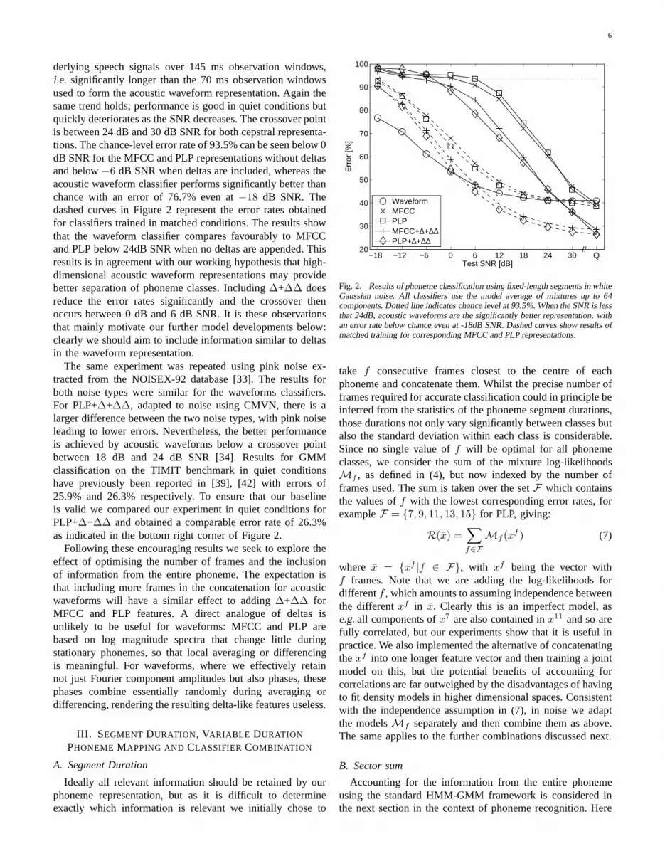
6

derlying speech signals over 145 ms observation windows,i.e. significantly longer than the 70 ms observation windowsused to form the acoustic waveform representation. Again thesame trend holds; performance is good in quiet conditions butquickly deteriorates as the SNR decreases. The crossover pointis between 24 dB and 30 dB SNR for both cepstral representa-tions. The chance-level error rate of 93.5% can be seen below0dB SNR for the MFCC and PLP representations without deltasand below−6 dB SNR when deltas are included, whereas theacoustic waveform classifier performs significantly betterthanchance with an error of 76.7% even at−18 dB SNR. Thedashed curves in Figure 2 represent the error rates obtainedfor classifiers trained in matched conditions. The results showthat the waveform classifier compares favourably to MFCCand PLP below 24dB SNR when no deltas are appended. Thisresults is in agreement with our working hypothesis that high-dimensional acoustic waveform representations may providebetter separation of phoneme classes. Including∆+∆∆ doesreduce the error rates significantly and the crossover thenoccurs between 0 dB and 6 dB SNR. It is these observationsthat mainly motivate our further model developments below:clearly we should aim to include information similar to deltasin the waveform representation.

The same experiment was repeated using pink noise ex-tracted from the NOISEX-92 database [33]. The results forboth noise types were similar for the waveforms classifiers.For PLP+∆+∆∆, adapted to noise using CMVN, there is alarger difference between the two noise types, with pink noiseleading to lower errors. Nevertheless, the better performanceis achieved by acoustic waveforms below a crossover pointbetween 18 dB and 24 dB SNR [34]. Results for GMMclassification on the TIMIT benchmark in quiet conditionshave previously been reported in [39], [42] with errors of25.9% and 26.3% respectively. To ensure that our baselineis valid we compared our experiment in quiet conditions forPLP+∆+∆∆ and obtained a comparable error rate of 26.3%as indicated in the bottom right corner of Figure 2.

Following these encouraging results we seek to explore theeffect of optimising the number of frames and the inclusionof information from the entire phoneme. The expectation isthat including more frames in the concatenation for acousticwaveforms will have a similar effect to adding∆+∆∆ forMFCC and PLP features. A direct analogue of deltas isunlikely to be useful for waveforms: MFCC and PLP arebased on log magnitude spectra that change little duringstationary phonemes, so that local averaging or differencingis meaningful. For waveforms, where we effectively retainnot just Fourier component amplitudes but also phases, thesephases combine essentially randomly during averaging ordifferencing, rendering the resulting delta-like features useless.

III. SEGMENT DURATION, VARIABLE DURATION

PHONEME MAPPING AND CLASSIFIER COMBINATION

A. Segment Duration

Ideally all relevant information should be retained by ourphoneme representation, but as it is difficult to determineexactly which information is relevant we initially chose to

−18 −12 −6 0 6 12 18 24 30 Q20

30

40

50

60

70

80

90

100

Test SNR [dB]

Err

or [%

]

//

WaveformMFCCPLPMFCC+∆+∆∆PLP+∆+∆∆

Fig. 2. Results of phoneme classification using fixed-length segments in whiteGaussian noise. All classifiers use the model average of mixtures up to 64components. Dotted line indicates chance level at 93.5%. When the SNR is lessthat 24dB, acoustic waveforms are the significantly better representation, withan error rate below chance even at -18dB SNR. Dashed curves show results ofmatched training for corresponding MFCC and PLP representations.

take f consecutive frames closest to the centre of eachphoneme and concatenate them. Whilst the precise number offrames required for accurate classification could in principle beinferred from the statistics of the phoneme segment durations,those durations not only vary significantly between classesbutalso the standard deviation within each class is considerable.Since no single value off will be optimal for all phonemeclasses, we consider the sum of the mixture log-likelihoodsMf , as defined in (4), but now indexed by the number offrames used. The sum is taken over the setF which containsthe values off with the lowest corresponding error rates, forexampleF = {7, 9, 11, 13, 15} for PLP, giving:

R(x) =∑

f∈F

Mf (xf ) (7)

where x = {xf |f ∈ F}, with xf being the vector withf frames. Note that we are adding the log-likelihoods fordifferentf , which amounts to assuming independence betweenthe differentxf in x. Clearly this is an imperfect model, ase.g.all components ofx7 are also contained inx11 and so arefully correlated, but our experiments show that it is usefulinpractice. We also implemented the alternative of concatenatingthexf into one longer feature vector and then training a jointmodel on this, but the potential benefits of accounting forcorrelations are far outweighed by the disadvantages of havingto fit density models in higher dimensional spaces. Consistentwith the independence assumption in (7), in noise we adaptthe modelsMf separately and then combine them as above.The same applies to the further combinations discussed next.

B. Sector sum

Accounting for the information from the entire phonemeusing the standard HMM-GMM framework is considered inthe next section in the context of phoneme recognition. Here

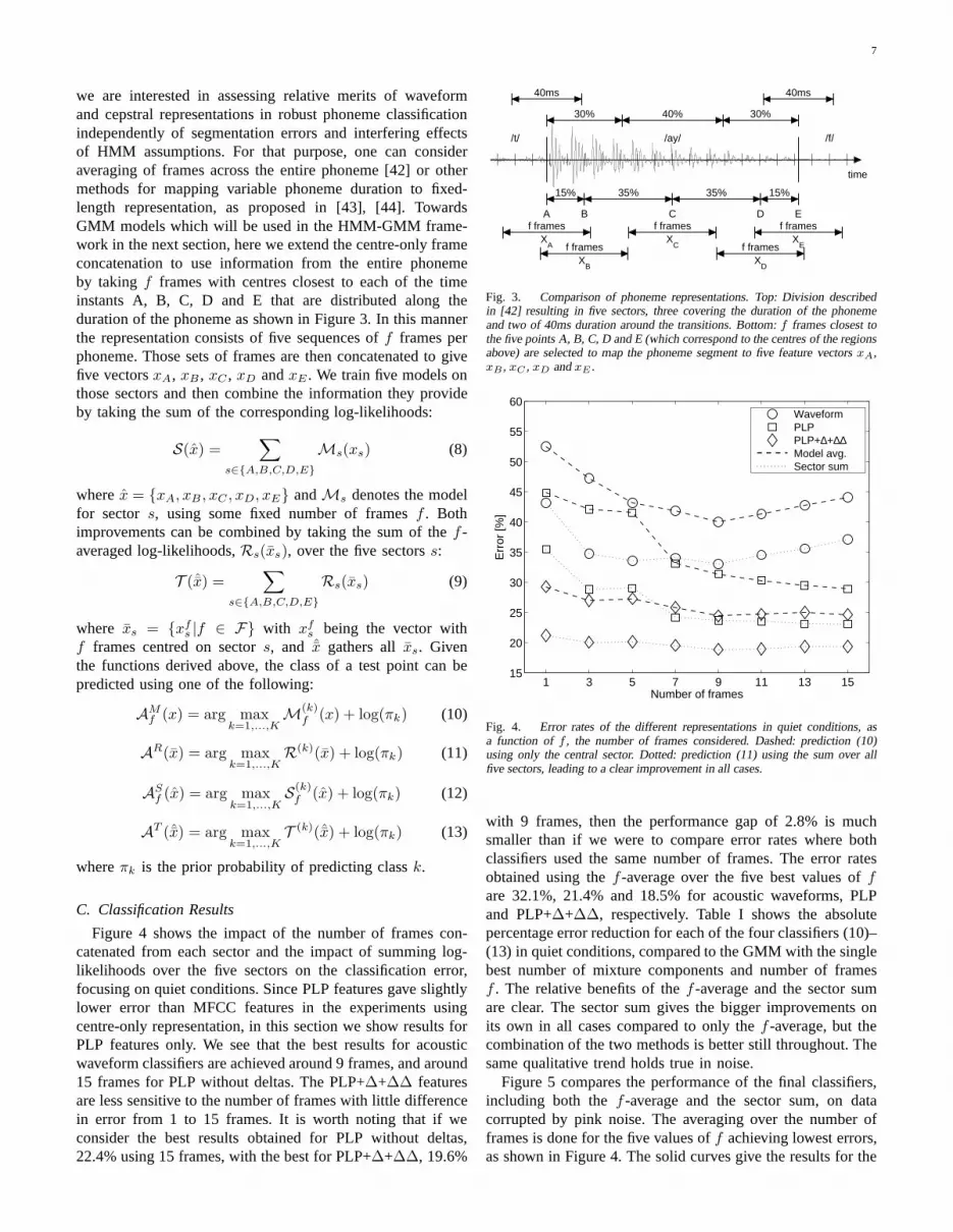
7

we are interested in assessing relative merits of waveformand cepstral representations in robust phoneme classificationindependently of segmentation errors and interfering effectsof HMM assumptions. For that purpose, one can consideraveraging of frames across the entire phoneme [42] or othermethods for mapping variable phoneme duration to fixed-length representation, as proposed in [43], [44]. TowardsGMM models which will be used in the HMM-GMM frame-work in the next section, here we extend the centre-only frameconcatenation to use information from the entire phonemeby taking f frames with centres closest to each of the timeinstants A, B, C, D and E that are distributed along theduration of the phoneme as shown in Figure 3. In this mannerthe representation consists of five sequences off frames perphoneme. Those sets of frames are then concatenated to givefive vectorsxA, xB , xC , xD andxE . We train five models onthose sectors and then combine the information they provideby taking the sum of the corresponding log-likelihoods:

S(x) =∑

s∈{A,B,C,D,E}

Ms(xs) (8)

wherex = {xA, xB , xC , xD, xE} andMs denotes the modelfor sector s, using some fixed number of framesf . Bothimprovements can be combined by taking the sum of thef -averaged log-likelihoods,Rs(xs), over the five sectorss:

T (ˆx) =∑

s∈{A,B,C,D,E}

Rs(xs) (9)

where xs = {xfs |f ∈ F} with xf

s being the vector withf frames centred on sectors, and ˆx gathers allxs. Giventhe functions derived above, the class of a test point can bepredicted using one of the following:

AMf (x) = arg max

k=1,...,KM(k)

f (x) + log(πk) (10)

AR(x) = arg maxk=1,...,K

R(k)(x) + log(πk) (11)

ASf (x) = arg max

k=1,...,KS(k)f (x) + log(πk) (12)

AT (ˆx) = arg maxk=1,...,K

T (k)(ˆx) + log(πk) (13)

whereπk is the prior probability of predicting classk.

C. Classification Results

Figure 4 shows the impact of the number of frames con-catenated from each sector and the impact of summing log-likelihoods over the five sectors on the classification error,focusing on quiet conditions. Since PLP features gave slightlylower error than MFCC features in the experiments usingcentre-only representation, in this section we show results forPLP features only. We see that the best results for acousticwaveform classifiers are achieved around 9 frames, and around15 frames for PLP without deltas. The PLP+∆+∆∆ featuresare less sensitive to the number of frames with little differencein error from 1 to 15 frames. It is worth noting that if weconsider the best results obtained for PLP without deltas,22.4% using 15 frames, with the best for PLP+∆+∆∆, 19.6%

/t/ /ay/ /f/

40ms 40ms

30% 40% 30%

15% 35% 35% 15%

A B C D E

time

f framesX

A

f framesX

Ef framesX

B

f framesX

C f framesX

D

Fig. 3. Comparison of phoneme representations. Top: Division describedin [42] resulting in five sectors, three covering the duration of the phonemeand two of 40ms duration around the transitions. Bottom:f frames closest tothe five points A, B, C, D and E (which correspond to the centresof the regionsabove) are selected to map the phoneme segment to five featurevectorsxA,xB , xC , xD andxE .

1 3 5 7 9 11 13 1515

20

25

30

35

40

45

50

55

60

Number of frames

Err

or [%

]

WaveformPLPPLP+∆+∆∆Model avg.Sector sum

Fig. 4. Error rates of the different representations in quiet conditions, asa function off , the number of frames considered. Dashed: prediction (10)using only the central sector. Dotted: prediction (11) using the sum over allfive sectors, leading to a clear improvement in all cases.

with 9 frames, then the performance gap of 2.8% is muchsmaller than if we were to compare error rates where bothclassifiers used the same number of frames. The error ratesobtained using thef -average over the five best values offare 32.1%, 21.4% and 18.5% for acoustic waveforms, PLPand PLP+∆+∆∆, respectively. Table I shows the absolutepercentage error reduction for each of the four classifiers (10)–(13) in quiet conditions, compared to the GMM with the singlebest number of mixture components and number of framesf . The relative benefits of thef -average and the sector sumare clear. The sector sum gives the bigger improvements onits own in all cases compared to only thef -average, but thecombination of the two methods is better still throughout. Thesame qualitative trend holds true in noise.

Figure 5 compares the performance of the final classifiers,including both thef -average and the sector sum, on datacorrupted by pink noise. The averaging over the number offrames is done for the five values off achieving lowest errors,as shown in Figure 4. The solid curves give the results for the

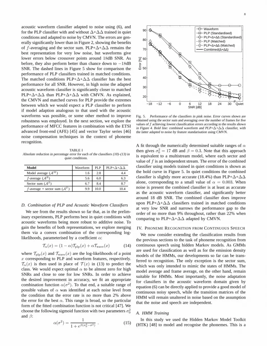
8

acoustic waveform classifier adapted to noise using (6), andfor the PLP classifier with and without∆+∆∆ trained in quietconditions and adapted to noise by CMVN. The errors are gen-erally significantly lower than in Figure 2, showing the benefitsof f -averaging and the sector sum. PLP+∆+∆∆ remains thebest representation for very low noise, but waveforms givelower errors below crossover points around18dB SNR. Asbefore, they also perform better than chance down to−18dBSNR. The dashed lines in Figure 5 show for comparison theperformance of PLP classifiers trained in matched conditions.The matched conditions PLP+∆+∆∆ classifier has the bestperformance for all SNR. However, in high noise the adaptedacoustic waveform classifier is significantly closer to matchedPLP+∆+∆∆ than PLP+∆+∆∆ with CMVN. As explained,the CMVN and matched curves for PLP provide the extremesbetween which we would expect a PLP classifier to performif model adaption analogous to that used with the acousticwaveforms was possible, or some other method to improverobustness was employed. In the next section, we explore theperformance of MFCC features in combination with the ETSIadvanced front-end (AFE) [45] and vector Taylor series [46]noise compensation techniques in the context of phonemerecognition.

TABLE IAbsolute reduction in percentage error for each of the classifiers (10)–(13) in

quiet conditions.

Model Waveform PLP PLP+∆+∆∆

Model average (AM ) 1.6 2.8 4.4

f -average (AR) 5.6 6.0 6.3

Sector sum (AS ) 6.7 8.4 8.7

f -average + sector sum (AT ) 9.9 10.0 10.4

D. Combination of PLP and Acoustic Waveform Classifiers

We see from the results shown so far that, as in the prelim-inary experiments, PLP performs best in quiet conditions withacoustic waveforms being more robust to additive noise. Togain the benefits of both representations, we explore mergingthem via a convex combination of the corresponding log-likelihoods, parameterised by a coefficientα:

Tα(x) = (1− α)Tplp(x) + αTwave(x) (14)

whereTplp(x) andTwave(x) are the log-likelihoods of a pointx corresponding to PLP and waveform features, respectively.Tα(x) is then used in place ofT (x) in (13) to predict theclass. We would expect optimalα to be almost zero for highSNRs and close to one for low SNRs. In order to achievethe desired improvement in accuracy, we fit an appropriatecombination functionα(σ2). To that end, a suitable range ofpossible values ofα was identified at each noise level fromthe condition that the error rate is no more than 2% abovethe error for the bestα. This range is broad, so the particularform of the fitted combination function is not critical [47].Wechoose the following sigmoid function with two parametersσ2

0

andβ:

α(σ2) =1

1 + eβ(σ2

0−σ2)

. (15)

−18 −12 −6 0 6 12 18 24 30 Quiet

20

30

40

50

60

70

80

90

SNR [dB]

Err

or [%

]

//

WaveformPLP (Standardised)PLP+∆+∆∆ (Standardised)PLP (Matched)PLP+∆+∆∆ (Matched)Combined(∆+∆∆)

Fig. 5. Performance of the classifiers in pink noise. Error curves shown areobtained using the sector sum and averaging over the number of frames for fivevalues off achieving lowest classification errors according to the results shownin Figure 4. Bold line: combined waveform and PLP+∆+∆∆ classifier, withthe latter adapted to noise by feature standarisation usingCMVN.

A fit through the numerically determined suitable ranges ofαthen givesσ2

0 = 17 dB andβ = 0.3. Note that this approachis equivalent to a multistream model, where each sector andvalue off is an independent stream. The error of the combinedclassifier using models trained in quiet conditions is shownasthe bold curve in Figure 5. In quiet conditions the combinedclassifier is slightly more accurate (18.4%) than PLP+∆+∆∆alone, corresponding to a small value ofα = 0.003. Whennoise is present the combined classifier is at least as accurateas the acoustic waveform classifier, and significantly betteraround 18 dB SNR. The combined classifier does improveupon PLP+∆+∆∆ classifiers trained in matched conditionsat very low SNR and narrows the performance gap to theorder of no more than 9% throughout, rather than 22% whencomparing to PLP+∆+∆∆ adapted by CMVN.

IV. PHONEME RECOGNITION FROMCONTINUOUS SPEECH

We now consider extending the classification results fromthe previous sections to the task of phoneme recognition fromcontinuous speech using hidden Markov models. As GMMsare used for classification as well as for the emission densitymodels of the HMMs, our developments so far can be trans-ferred to recognition. The only exception is the sector sum,which was only intended to mimic the states of HMMs. Themodel average and frame average, on the other hand, remainsuitable for HMMs. Most importantly, the noise adaptationfor classifiers in the acoustic waveform domain given byequation (6) can be directly applied to provide a good model ofcontinuous noisy speech, while the transition matrices of theHMM will remain unaltered in noise based on the assumptionthat the noise and speech are independent.

A. HMM Training

In this study we used the Hidden Markov Model Toolkit(HTK) [48] to model and recognise the phonemes. This is a

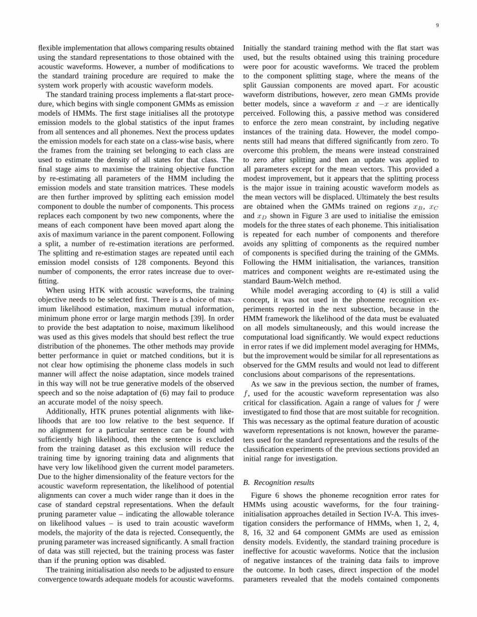
9

flexible implementation that allows comparing results obtainedusing the standard representations to those obtained with theacoustic waveforms. However, a number of modifications tothe standard training procedure are required to make thesystem work properly with acoustic waveform models.

The standard training process implements a flat-start proce-dure, which begins with single component GMMs as emissionmodels of HMMs. The first stage initialises all the prototypeemission models to the global statistics of the input framesfrom all sentences and all phonemes. Next the process updatesthe emission models for each state on a class-wise basis, wherethe frames from the training set belonging to each class areused to estimate the density of all states for that class. Thefinal stage aims to maximise the training objective functionby re-estimating all parameters of the HMM including theemission models and state transition matrices. These modelsare then further improved by splitting each emission modelcomponent to double the number of components. This processreplaces each component by two new components, where themeans of each component have been moved apart along theaxis of maximum variance in the parent component. Followinga split, a number of re-estimation iterations are performed.The splitting and re-estimation stages are repeated until eachemission model consists of 128 components. Beyond thisnumber of components, the error rates increase due to over-fitting.

When using HTK with acoustic waveforms, the trainingobjective needs to be selected first. There is a choice of max-imum likelihood estimation, maximum mutual information,minimum phone error or large margin methods [39]. In orderto provide the best adaptation to noise, maximum likelihoodwas used as this gives models that should best reflect the truedistribution of the phonemes. The other methods may providebetter performance in quiet or matched conditions, but it isnot clear how optimising the phoneme class models in suchmanner will affect the noise adaptation, since models trainedin this way will not be true generative models of the observedspeech and so the noise adaptation of (6) may fail to producean accurate model of the noisy speech.

Additionally, HTK prunes potential alignments with like-lihoods that are too low relative to the best sequence. Ifno alignment for a particular sentence can be found withsufficiently high likelihood, then the sentence is excludedfrom the training dataset as this exclusion will reduce thetraining time by ignoring training data and alignments thathave very low likelihood given the current model parameters.Due to the higher dimensionality of the feature vectors for theacoustic waveform representation, the likelihood of potentialalignments can cover a much wider range than it does in thecase of standard cepstral representations. When the defaultpruning parameter value – indicating the allowable toleranceon likelihood values – is used to train acoustic waveformmodels, the majority of the data is rejected. Consequently,thepruning parameter was increased significantly. A small fractionof data was still rejected, but the training process was fasterthan if the pruning option was disabled.

The training initialisation also needs to be adjusted to ensureconvergence towards adequate models for acoustic waveforms.

Initially the standard training method with the flat start wasused, but the results obtained using this training procedurewere poor for acoustic waveforms. We traced the problemto the component splitting stage, where the means of thesplit Gaussian components are moved apart. For acousticwaveform distributions, however, zero mean GMMs providebetter models, since a waveformx and −x are identicallyperceived. Following this, a passive method was consideredto enforce the zero mean constraint, by including negativeinstances of the training data. However, the model compo-nents still had means that differed significantly from zero.Toovercome this problem, the means were instead constrainedto zero after splitting and then an update was applied toall parameters except for the mean vectors. This provided amodest improvement, but it appears that the splitting processis the major issue in training acoustic waveform models asthe mean vectors will be displaced. Ultimately the best resultsare obtained when the GMMs trained on regionsxB , xC

andxD shown in Figure 3 are used to initialise the emissionmodels for the three states of each phoneme. This initialisationis repeated for each number of components and thereforeavoids any splitting of components as the required numberof components is specified during the training of the GMMs.Following the HMM initialisation, the variances, transitionmatrices and component weights are re-estimated using thestandard Baum-Welch method.

While model averaging according to (4) is still a validconcept, it was not used in the phoneme recognition ex-periments reported in the next subsection, because in theHMM framework the likelihood of the data must be evaluatedon all models simultaneously, and this would increase thecomputational load significantly. We would expect reductionsin error rates if we did implement model averaging for HMMs,but the improvement would be similar for all representations asobserved for the GMM results and would not lead to differentconclusions about comparisons of the representations.

As we saw in the previous section, the number of frames,f , used for the acoustic waveform representation was alsocritical for classification. Again a range of values forf wereinvestigated to find those that are most suitable for recognition.This was necessary as the optimal feature duration of acousticwaveform representations is not known, however the parame-ters used for the standard representations and the results of theclassification experiments of the previous sections provided aninitial range for investigation.

B. Recognition results

Figure 6 shows the phoneme recognition error rates forHMMs using acoustic waveforms, for the four training-initialisation approaches detailed in Section IV-A. This inves-tigation considers the performance of HMMs, when 1, 2, 4,8, 16, 32 and 64 component GMMs are used as emissiondensity models. Evidently, the standard training procedure isineffective for acoustic waveforms. Notice that the inclusionof negative instances of the training data fails to improvethe outcome. In both cases, direct inspection of the modelparameters revealed that the models contained components

10

with mean vectors that are significantly different from zero.To overcome this issue, the next method forces the means tozero after each stage of component splitting. This gives muchbetter performance when few components are used. However,the improvement is minor when the models consist of 64components. The final training method, denoted asGMM init.in the legend of Figure 6, initialises the emission models usingthe GMMs trained in Section III. In this case the error ratesare significantly lower than all of the other methods for everynumber of components. This initialisation method reduces theerror rate, ranging from 54.3% with a single component to34.4% with 64 components.

1 2 4 8 16 32 6430

35

40

45

50

55

60

65

70

75

80

Number of components

Pho

nem

e re

cogn

ition

err

or [%

]

StandardNegativeForced zeroGMM init.10ms30ms50ms

Fig. 6. Comparison of the four training approaches for the acousticwaveformrepresentation in quiet conditions: default training procedure with componentsplitting (Standard), default with negative instances added to the training data(Negative), default with emission model mean vectors forced to zero aftersplitting (Forced zero), and emission models initialised using the zero-meansector models from Section III (GMM init.). Three curves areshown for each ofthe methods, corresponding to different number of frames inthe concatenation.

The model training process for acoustic waveforms wasinitially considered forf = 1, f = 3 and f = 5 frames,corresponding to feature vectors covering10 ms, 30 ms and50 ms in duration, respectively, extracted every 10 ms. Theduration of 10 ms corresponds to no overlap of adjacentfeature vectors, while30 ms is closest to the standard cepstralrepresentation. The effect of the number of frames is alsoillustrated in Figure 6. It can be observed that the resultsimprove when going fromf = 1 to f = 3 andf = 5, with noindication thatf = 5 is the optimal value. This suggests thatit is necessary to investigate the acoustic waveform represen-tation using more than five frames to find the optimum. In theprevious section representations up tof = 15 were consideredfor classification, and this range was sufficient to find theoptimal value off . Figure 7 shows the results for the phonemerecognition task over the range fromf = 1 to f = 13. Eachcurve represents one fixed global SNR of additive pink noise.There is a slight improvement of around 1.1% that results fromincreasing the acoustic waveform duration from 50 ms to 90ms. Beyond this duration, the error rates increase, which couldbe due to the representation becoming less localised.

1 3 5 7 9 11 1330

35

40

45

50

55

60

65

70

75

−6dB SNR

0dB SNR

6dB SNR

12dB SNR

18dB SNR24dB SNR30dB SNRQuiet

Number of frames [10ms]

Pho

nem

e re

cogn

ition

err

or [%

]

Fig. 7. The effect of representation duration, denoted by number of10 msframes concatenated. Curves are shown for quiet conditions, and in additivepink noise for seven values of SNR. Overall the best performance is obtainedusing 9 frames, a 90ms duration representation.

A comparison between acoustic waveforms and cepstralbaselines is shown in Figure 8. The models for acoustic wave-forms are adapted to additive noise according to (6), while inthe case of cepstral features, we now consider standard noisecompensation techniques: the ETSI advanced front-end [45]and vector Taylor series [46], in conjunction with MFCCfeatures to obtain noise-compensated cepstral representationsMFCC-AFE and MFCC-VTS, respectively. The compensatedfeatures are then standardised using sentence-wise cepstralmean and variance normalisation (CMVN) as that significantlyimproved performance [34]. A single frame is used for MFCCand its variants, with∆+∆∆ computed in the usual manner.This corresponds to a time interval of 25 ms for the frame,105 ms for∆ and 145 ms for∆+∆∆. It was assumed thatthese methods provide optimal baselines for comparison asthey are commonly used and have been tuned for the task.Figure 8 shows recognition results obtained with the acousticwaveform representation for 10 ms, 50 ms, 90 ms and 130 ms.Considering the comparison to the cepstral baselines without∆+∆∆, the acoustic waveform representation with 10 msduration gives similar error rates to both cepstral baselinesin quiet conditions and better performance down to 0 dBSNR. Note that a similar observation can be made aboutclassification results obtained with fixed-length segmentsofacoustic waveforms and cepstral features without∆+∆∆ in-formation, as shown in Figure 2. Results shown in Figure8 demonstrate that in phoneme recognition too the additionof ∆+∆∆ features provides a significant performance gainfor cepstral representations. We can observe again that theperformance of cepstral representations with∆+∆∆ infor-mation is significantly better than that achieved with acousticwaveforms at low SNRs, but that the 90 ms acoustic waveformrepresentation improves further in noisy conditions, givinglower error rates than MFCC-AFE+∆+∆∆ and MFCC-VTS+∆+∆∆ between−6 dB and 12 dB SNR.

11

−6 0 6 12 18 24 30 Quiet25

30

35

40

45

50

55

60

65

70

//

SNR [dB]

Pho

nem

e re

cogn

ition

err

or [%

]

Waveform 10msWaveform 50msWaveform 90msWaveform 130msMFCC−VTSMFCC−VTS+∆+∆∆MFCC−AFEMFCC−AFE+∆+∆∆

Fig. 8. Phoneme recognition error rates for the acoustic waveform repre-sentations of different durations. Tests are carried out inadditive pink noise.Noise compensated MFCC features using vector Taylor series(MFCC-VTS)and ETSI advanced front-end (MFCC-AFE) methods are used as baselines.

We also re-investigate in the HMM context the effect ofmodel averaging by combining models corresponding to dif-ferent number of frames used to represent acoustic waveforms.Having established that the lowest error rates are achievedusing f = 9 frames, the models corresponding tof ∈ F ={5, 7, 9, 11, 13} are averaged by a multi-stream process [48]and used for recognition. The resulting acoustic waveformf -average (AWFA) model achieved better performance thanthe individual models with a fixed value off . Finally, were-investigate in the recognition context combining acousticwaveform and MFCC-AFE HMMs according to (14). Noteagain that the largerf -values for waveforms effectively incor-porate information that is provided for MFCCs via∆+∆∆,which is why we do not consider similarf -frame concatena-tions for MFCCs. Phoneme recognition results obtained withthe frame averaging and representation combination in additivepink noise are shown in Figure 9. The acoustic waveform rep-resentation with averaging over the number of frames (AWFA)gives lower error rates than the cepstral representations forSNR below a cross-over point around 18 dB. Error ratesachieved by the combined representation are uniformly lowerthan any of the individual representations considered. As aconsequence, the combined HMM model achieves significantreductions in error rates compared to cepstral-only modelswith standard noise compensation techniques.

V. CONCLUSION AND DISCUSSION

In this paper we have explored the potential of improvingthe robustness of ASR to additive noise by posing the problemdirectly in the space of acoustic waveforms of speech, orsome linear transform thereof which does not incur anyinformation loss. In order to assess the separation of phoneticclasses in the acoustic waveform domain and the domains ofstandard cepstral features, we first considered classificationof phonemes using observations of a given fixed duration.

−6 0 6 12 18 Quiet25

30

35

40

45

50

55

60

//

SNR [dB]

Pho

nem

e re

cogn

ition

err

or [%

]

MFCC−AFEMFCC−VTSAW f−average (AWFA)α(MFCC−AFE) + (1−α)AWFA

Fig. 9. Comparison of phoneme recognition error rates in additive pink noise.Baseline comparisons are provided by MFCC-AFE and MFCC-VTS. Thef -average (AWFA) is taken for the range 50ms - 130ms. Uniformlylower errorrates are achieved by the convex combination of MFCC-AFE andAWFA.

A remarkable result of that experiment is that phonemeclassification in the acoustic waveform domain significantlyoutperforms classification in the cepstral domains alreadyatvery low noise levels, and that even at an SNR as lowas −18 dB it achieves accuracy distinctly above that ofrandom guessing (see Figure 2). A significant performancegain in classification using cepstral features is achieved via∆+∆∆ features, which reflect temporal dynamics of speech.While finding analogous features in the acoustic waveformdomain is a nontrivial open problem, considerations in SectionIII demonstrated that a performance gain in the acousticwaveform domain can be achieved by extending the length ofthe basic observation unit and thus including the informationon the temporal dynamics implicitly. Next, acoustic waveformswere considered in the context of phoneme recognition fromcontinuous speech. To allow a direct comparison with thecepstral features, and compatibility with existing technologies,the recognition was implemented in the standard HMM-GMMframework. Note however that [49]:”The HMM and frame-based cepstra have co-evolved as ASR system components andhence are very much tuned to each other. The use of HMMsas the core acoustic modeling technology might obscure thegains from new features, especially those from long time scales;this may be one reason why progress with novel techniques hasbeen so difficult. In particular, systems incorporating newsignalprocessing methods in the front end are at a disadvantage whentested using standard HMMs.”Still phoneme recognition usingacoustic waveforms achieved lower error rates than cepstralfeatures for noise levels below 18 dB SNR.

Recognition and classification results presented in thisproof-of-concept study demonstrate that representing speechusing high dimensional linear features, which incur no lossof information, is a promising direction towards achievingthe long sought-after robustness of ASR systems. Significantimprovements can potentially be made by more sophisticated

12

modelling of speech in the acoustic waveform domain. Thechoice of decorrelating basis is another area that opens upscope for further work. In these directions methods such asMLLT [50] and semi-tied covariance matrices [51] may lead toimproved results. We conducted some preliminary experimentswith semi-tied covariance matrices in the context of phonemerecognition. This improved recognition performance in quiet,but suffered from increased error levels in noise. However,more extensive investigations may prove fruitful. Even withinthe models introduced in this study, given the wide range ofpossibilities for choice of parameters, many of these have notbeen extensively tuned. This includes the weighting of themodel averaging over the number of components in GMMs,and the averaging over the number of framesf , either in aclass-independent manner, or tuned even further to vary withthe phoneme or phonetic group being evaluated; a uniformweight was assumed throughout (averaging over the numberof components was not explored at all in the recognitionexperiment), but it is likely that the information content usedfor discrimination is not distributed in exactly this way. Thenmodels could potentially also be developed to explicitly modelcorrelations between feature vectors obtained for differentnumber of framesf .

Towards other classes of models, Gaussian scale mixturemodels (GSMMs) are a subset of GMMs that seem particularlysuitable for modelling the distributions of the speech signal.This is motivated by the observation in our experiments thatthe covariance matrices of some of the components wereapproximately scaled copies of each other. Densities of theacoustic waveform representation can thus be modelled usingmixtures of scaled components where again the means areconstrained to zero and the covariance matrices are constrainedto be diagonal. The probability density function of the GSMMis thus given by:

p(x) =

c∑

i=1

S∑

j=1

wivjN (x; 0, s2jC−1

Di(CT)−1)

where the symbols are as in (3), with the addition ofSscales and scale weights,sj and vj , respectively. Here, therange of scales corresponds to a model of the amplitudedistribution for a given phoneme. The eight scale model with128 components provided an error rate that improved by 4.2%in quiet, compared to the standard 128-component GMM whenused for phoneme classification as considered in Section II[34]. Further reductions in the error rates may be expected ifmore scales are used, given that some of the scale distributionsare not adequately modelled with only eight scales. Althoughthese GSMM models achieved lower error rates than thecorresponding GMMs with the same number of components,computational constraints prevented us from exploring thisdirection further. Note that GSMM models are an exampleof a Richter distribution, which have been previously used tomodel heavy tailed distributions [52].

We expect that the results can be further improved, and thatacoustic waveform features may by effective if incorporatedinto techniques considered by other authors, in particular,committee classifiers and the use of a hierarchy to reduce

broad phoneme class confusions [53], [54]. Indeed, in thecontext of phoneme recognition, much lower confusion ratesbetween broad phoneme classes are achieved using acousticwaveforms than cepstral features, as illustrated by resultsshown in Figure 10. Finally considering the success of deepneural networks (DNN) in ASR tasks [55], it is imperativeto explore DNN modelling of acoustic waveforms of speech.While DNNs have exhibited robustness to modest differencesbetween training and test settings, their performance is poor ifthe mismatch is more severe [56]. A recent study by Mitraetal. [57] shows, however, that the choice of features providesscope for improving the robustness of DNNs. Hence it is ofinterest to explore possible gains achievable by using DNNsin conjunction with high dimensional linear representations asconsidered in this study.

−6 0 6 12 18 24 30 Quiet5

10

15

20

25

30

//

SNR [dB]

Bro

ad p

hone

tic c

lass

rec

ogni

tion

erro

r [%

]

Waveform 50msWaveform 90msWaveform 130msMFCC−VTSMFCC−VTS+∆+∆∆MFCC−AFEMFCC−AFE+∆+∆∆

Fig. 10. Broad phoneme class (vowels, nasals, strong fricatives, weakfricatives, stops and silence) recognition error rates.

ACKNOWLEDGMENT

Zoran Cvetkovic would like to thank Jont Allen, BishnuAtal and Herve Bourlard for their encouragement, support andinspiration, and Malcolm Slaney for his valuable suggestionsabout the presentation of this paper.

REFERENCES

[1] M. Ager, Z. Cvetkovic, and P. Sollich, “Combined waveform-cepstralrepresentation for robust speech recognition,” inProc. ISIT, July 2011,pp. 125–128.

[2] J. M. Baker, L. Deng, J. Glass, S. Khudanpur, C. Lee, N. Morgan,and D. O’Shaugnessy, “Research developments and directions in speechrecognition and understanding, part 1,”IEEE Signal Process. Mag.,vol. 26, pp. 75–80, May 2009.

[3] ——, “Updated minds report on speech recognition and understanding,part 2,,” IEEE Signal Process. Mag., vol. 26, pp. 78–85, July 2009.

[4] G. Miller, A. Heise, and W. Lichten, “The Intelligibility of Speech as aFunction of the Context of the Test Material,”J. Exp. Psychol., vol. 41,pp. 329–335, 1951.

[5] G. Miller and P. Nicely, “An Analysis of Perceptual Confusions amongsome English Consonants,”J. Acoust. Soc. Am., vol. 27, pp. 338–352,1955.

[6] R. Singh and J. B. Allen, “The influence of stop consonants’ perceptualfeatures on the articulation index model,”J. Acoust. Soc. Am., vol. 131,no. 4, pp. 3051 – 3068, April 2012.

13

[7] J. C. Toscano and J. B. Allen, “Across and within consonant errors forisolated syllables in noise,”J. Speech, Language, Hearing Res., vol. 57,pp. 2293–2307, December 2014.

[8] J. Sroka and L. Braida, “Human and Machine Consonant Recognition,”Speech Comm., vol. 45, no. 4, pp. 401–423, 2005.

[9] M. J. F. Gales and S. J. Young, “The application of hidden markov mod-els in speech recognition,”Foundations and Trends in Signal Processing,vol. 1, no. 3, pp. 195–304, 2007.

[10] S. Davis and P. Mermelstein, “Comparison of ParametricRepresen-tations for Monosyllabic Word Recognition in ContinuouslySpokenSentences,”IEEE Trans. Acoustics, Speech Signal Process., vol. 28,no. 4, pp. 357–366, 1980.

[11] H. Hermansky, “Perceptual Linear Predictive (PLP) Analysis of Speech,”J. Acoust. Soc. Am., vol. 87, no. 4, pp. 1738–1752, 1990.

[12] B. S. Atal and S. L. Hanauer, “Speech analysis and synthesis by linearprediction of the speech wave,”J. Acoust. Soc. Am., vol. 50, pp. 637–655, 1971.

[13] S. D. Peters, P. Stubley, and J. Valin, “On the Limits of SpeechRecognition in Noise,”Proc. ICASSP, pp. 365–368, 1999.

[14] B. Meyer, M. Wachter, T. Brand, and B. Kollmeier, “Phoneme Confu-sions in Human and Automatic Speech Recognition,” 2007, pp.2740–2743.

[15] K. K. Paliwal and L. D. Alsteris, “On the Usefulness of STFT PhaseSpectrum in Human Listening Tests,”Speech Comm., vol. 45, no. 2, pp.153–170, 2005.

[16] L. D. Alsteris and K. K. Paliwal, “Further Intelligibility Results fromHuman Listening Tests using the Short-Time Phase Spectrum,” SpeechComm., vol. 48, no. 6, pp. 727–736, 2006.

[17] H. Sheikhzadeh and L. Deng, “Waveform-Based Speech RecognitionUsing Hidden Filter Models: Parameter Selection and Sensitivity toPower Normalization,”IEEE Trans. Speech Audio Process., vol. 2, no. 1,pp. 80 –89, Jan 1994.

[18] A. Poritz, “Linear Predictive Hidden Markov Models andthe SpeechSignal,” in Proc. ICASSP, 1982.

[19] Y. Ephraim and W. Roberts, “Revisting Autoregressive Hidden MarkovModeling of Speech Signals,” vol. 12, no. 2, pp. 166–169, Feb. 2005.

[20] B. Mesot and D. Barber, “Switching Linear Dynamical Systems forNoise Robust Speech Recognition,”IEEE Trans. Audio, Speech Lan-guage Process., vol. 15, no. 6, pp. 1850–1858, 2007.

[21] R. E. Turner and M. Sahani, “Modeling Natural Sounds with ModulationCascade Processes,” inAdvances in Neural Information ProcessingSystems, vol. 20, 2008.

[22] C. Kim and R. M. Stern, “Power-normalized cepstral coefficients (pncc)for robust speech recognition,” inProc. ICASSP, March 2012, pp. 4101–4014.

[23] N. Vasiloglou and A. G. D. Anderson, “Learning the Intrinsic Di-mensions of the TIMIT Speech Database with Maximum VarianceUnfolding,” in IEEE Workshops on DSP and SPE, 2009.

[24] S. Zhang and Z. Zhao, “Dimensionality Reduction-basedPhonemeRecognition,” inProc. ICSP, October 2008, pp. 667–670.

[25] S. Roweis and L. Saul, “Nonlinear Dimensionality Reduction by LocallyLinear Embedding,”Science, vol. 290, pp. 2323–2326, 2000.

[26] L. Saul, K. Weinberger, J. Ham, F. Sha, and D. Lee, “Spectral Methodsfor Dimensionality Reduction,” inSemisupervised Learning. Cam-bridge, MA: MIT Press, 2006.

[27] N. Lawrence, “Probabilistic Non-Linear Principal Component Analysiswith Gaussian Process Latent Variable Models,”J. Mach. Learn. Res.,vol. 6, pp. 1783 –1816, 2005.

[28] M. Tipping and C. Bishop, “Mixtures of Probabilistic Principal Com-ponent Analysers,”Neural Computation, vol. 11, no. 2, pp. 443–482,1999.

[29] J. Yousafzai, M. Ager, Z. Cvetkovic, and P. Sollich, “Discriminativeand generative machine learning approaches towards robustphonemeclassification,”Workshop on Information Theory and Applications, ITA,2008.

[30] S. Srivastava, M. Gupta, and B. Frigyik, “Bayesian Quadratic Discrim-inant Analysis,”J. Mach. Learn. Res., vol. 8, pp. 1287–1314, 2007.

[31] C. Kim and R. Stern, “Robust Signal-to-Noise Ratio Estimation Basedon Waveform Amplitude Distribution Analysis,” inProc. INTER-SPEECH, 2008.

[32] J. Tchorz and B. Kollmeier, “Estimation of the signal-to-noise ratio withamplitude modulation spectrograms,”Speech Comm., vol. 38, no. 1, pp.1–17, 2002.

[33] A. Varga, H. Steeneken, M. Tomlinson, and D. Jones, “TheNOISEX-92study on the effect of additive noise on automatic speech recognition,”DRA Speech Research Unit, Tech. Rep., 1992.

[34] M. P. Ager, “Phoneme classification and noise adaptation in linearfeature domains,” Ph.D. dissertation, King’s College London, 2010.

[35] P. Jain and H. Hermansky, “Improved Mean and Variance Normalizationfor Robust Speech Recognition,” inProc. ICASSP, 2001.

[36] M. Gales and S. Young, “Robust continuous speech recognition usingparallel model combination,”IEEE Trans. Speech Audio Process., vol. 4,pp. 352–359, 1996.

[37] R. Rose, “Environmental Robustness in Automatic Speech Recognition,”Robust2004 - ISCA and COST278 Workshop on Robustness in Conver-sational Interaction, 2004.

[38] K.-F. Lee and H.-W. Hon, “Speaker-Independent Phone Recognitionusing Hidden Markov Models,”IEEE Trans. Acoustics, Speech SignalProcess., vol. 37, no. 11, pp. 1641–1648, 1989.

[39] F. Sha and L. Saul, “Large Margin Gaussian Mixture Modeling forPhonetic Classification and Recognition,” inProc. ICASSP, 2006.

[40] D. Ellis, “PLP and RASTA (and MFCC, and inversion) in Matlab,” 2005,online web resource, http://labrosa.ee.columbia.edu/matlab/rastamat/.

[41] S. Furui, “Speaker-Independent Isolated Word Recognition using Dy-namic Features of Speech Spectrum,”IEEE Trans. Acoustics, SpeechSignal Process., vol. 34, no. 1, pp. 52–59, 1986.

[42] P. Clarkson and P. Moreno, “On the Use of Support Vector Machines forPhonetic Classification,” inProc. ICASSP, vol. 2, 1999, pp. 585–588.

[43] M. J. F. Gales and C. Longworth, “Discriminative classifiers with gener-ative kernels for noise robust asr,” inProc. INTERSPEECH, September2008, pp. 1996–1999.

[44] M. Ostendorf and S. Roukos, “A stochastic segment modelfor phoneme-based continuous speech recognition,”IEEE Trans. Acoustics, SpeechSignal Process., vol. 37, no. 12, pp. 1857–1869, December 1989.

[45] “ETSI document - ES 202 050 - STQ: DSR. Distributed speech recog-nition; Advance front-end feature extraction algorithm;Compressionalgorithms;,” 2007.

[46] P. Moreno, B. Raj, and R. M. Stern, “A Vector Taylor Series Approachfor Environment-Independent Speech Recognition,” inProc. ICASSP,vol. 1, 1996, pp. 733–736.

[47] M. Ager, Z. Cvetkovic, P. Sollich, and B. Yu, “Towards Robust PhonemeClassification: Augmentation of PLP Models with Acoustic Waveforms,”in Proc. EUSIPCO, 2008.

[48] S. Young, G. Evermann, M. Gales, T. Hain, D. Kershaw, G. Moore,J. Odell, D. Ollason, D. Povey, V. Valtchev, and P. Woodland,The HTKBook, version 3.4. Cambridge, UK: Cambridge University, 2006.

[49] N. Morgan, Q. Zhu, A. Stolcke, K. Sonmez, S. Sivadas, T. Shinozaki,M. Ostendorf, P. Jain, H. Hermansky, D. Ellis, G. Diddington, B. Chen,O. Cetin, H. Bourlard, and M. Athineos, “Pushing the envelope – aside,”IEEE Signal Process. Mag., pp. 81 – 88, September 2005.

[50] M. J. F. Gales, “Maximum likelihood linear transformations for hmm-based speech recognition,”Computer Speech and Language, vol. 12, pp.75–98, 1998.

[51] ——, “Semi-tied covariance matrices for hidden markov models,” IEEETrans. Speech Audio Process, vol. 7, no. 3, pp. 272–281, May 1999.

[52] M. J. F. Gales and P. A. Olsen, “Tail distribution modelling using therichter and power exponential distributions,” inProc. EUROSPEECH,1999, pp. 1507–1510.

[53] H. Chang and J. Glass, “Hierarchical Large-Margin Gaussian MixtureModels For Phonetic Classification,” inProc. IEEE ASRU Workshop,2007, pp. 272–275.

[54] F. Pernkopf, T. Pham, and J. Bilmes, “Broad Phonetic Classificationusing Discriminative Bayesian Networks,”Speech Comm., vol. 51, no. 2,2009.

[55] G. Hinton, L. Deng, D. Yu, G. E. Dahl, A. rahman Mohamed, N. Jaitly,A. Senior, V. Vanhoucke, P. Nguyen, T. N. Sainath, and B. Kingsbury,“Deep neural networks for acoustic modeling in speech recognition: Theshared views of four research groups,”IEEE Signal Process. Mag., pp.82 – 97, November 2012.

[56] D. Yu, M. Seltzer, J. Li, J.-T. Huang, and F. Seide, “Feature learningin deep neural networks - studies on speech recognition,” inInt. Conf.Learning Representations, May 2013.

[57] V. Mitra, W. Wang, H. Franco, Y. Lei, C. Bartels, and M. Gracia-rena, “Evaluating robust features on deep neural networks for speechrecognition in noisy and channel mismatched conditions,” in Proc.INTERSPEECH, September 2014.