phase behavior of the modified-yukawa fluid and its sticky limit
TRANSCRIPT

Phase behavior of the modified-Yukawa fluid and its sticky limitElisabeth Schöll-Paschinger, Néstor E. Valadez-Pérez, Ana L. Benavides, and Ramón Castañeda-Priego Citation: J. Chem. Phys. 139, 184902 (2013); doi: 10.1063/1.4827936 View online: http://dx.doi.org/10.1063/1.4827936 View Table of Contents: http://jcp.aip.org/resource/1/JCPSA6/v139/i18 Published by the AIP Publishing LLC. Additional information on J. Chem. Phys.Journal Homepage: http://jcp.aip.org/ Journal Information: http://jcp.aip.org/about/about_the_journal Top downloads: http://jcp.aip.org/features/most_downloaded Information for Authors: http://jcp.aip.org/authors
THE JOURNAL OF CHEMICAL PHYSICS 139, 184902 (2013)
Phase behavior of the modified-Yukawa fluid and its sticky limitElisabeth Schöll-Paschinger,1,a) Néstor E. Valadez-Pérez,2,b) Ana L. Benavides,2,c)
and Ramón Castañeda-Priego2,d)
1Department für Materialwissenschaften und Prozesstechnik, Universität für Bodenkultur, Muthgasse 107,A-1190 Wien, Austria2División de Ciencias e Ingenierías, University of Guanajuato, Loma del Bosque 103, 37150 León, Mexico
(Received 29 July 2013; accepted 18 October 2013; published online 8 November 2013)
Simple model systems with short-range attractive potentials have turned out to play a crucial role indetermining theoretically the phase behavior of proteins or colloids. However, as pointed out by D.Gazzillo [J. Chem. Phys. 134, 124504 (2011)], one of these widely used model potentials, namely, theattractive hard-core Yukawa potential, shows an unphysical behavior when one approaches its stickylimit, since the second virial coefficient is diverging. However, it is exactly this second virial coeffi-cient that is typically used to depict the experimental phase diagram for a large variety of complexfluids and that, in addition, plays an important role in the Noro-Frenkel scaling law [J. Chem. Phys.113, 2941 (2000)], which is thus not applicable to the Yukawa fluid. To overcome this deficiency ofthe attractive Yukawa potential, D. Gazzillo has proposed the so-called modified hard-core attractiveYukawa fluid, which allows one to correctly obtain the second and third virial coefficients of adhesivehard-spheres starting from a system with an attractive logarithmic Yukawa-like interaction. In thiswork we present liquid-vapor coexistence curves for this system and investigate its behavior close tothe sticky limit. Results have been obtained with the self-consistent Ornstein-Zernike approximation(SCOZA) for values of the reduced inverse screening length parameter up to 18. The accuracy ofSCOZA has been assessed by comparison with Monte Carlo simulations. © 2013 AIP PublishingLLC. [http://dx.doi.org/10.1063/1.4827936]
I. INTRODUCTION
During the last few years an increasing number of stud-ies has focused on the understanding of the phase behaviorof systems with very short-ranged attractive interactions.1–8
Simple model systems with narrow attractive interactions,like square-well or hard-core attractive Yukawa systems, haveturned out to play a crucial role when one tries to under-stand the phase behavior of protein and colloidal solutions,where the range of the effective interaction is significantlysmaller than the particle diameter that is of nano- or micro-scopic size.9–11
An interesting result on systems with short-ranged attrac-tions has been formulated by Noro and Frenkel (NF) in theirso-called extended law of corresponding states.12 Accordingto the NF scaling law, the details of the functional form of theinteraction potential are irrelevant in determining the struc-ture and thermodynamics of fluids as long as the potentialis short-ranged, i.e., the interaction range is approximatelyless than 15% of the particle diameter.13 Different functionalforms of the interaction yield the same behavior providedthat the following three properties of the potentials are iden-tical: σeff, ε, B
∗2 , where σ eff is the effective hard-sphere diam-
eter of the particles which is obtained by mapping the repul-sive part of the interaction φ(r) onto an effective hard-sphere(HS) diameter,14, 15 ε denotes the depth of the potential, i.e.,
a)Electronic mail: [email protected])Electronic mail: [email protected])Electronic mail: [email protected])Electronic mail: [email protected]
ε = φ(rmin), where rmin is the position of the minimum, andB∗
2 = B2/BHS2 is the reduced second virial coefficient with
BHS2 = 2πσ 3
eff/3 and
B2 = −2π
∫ ∞
0(exp(−βφ(r)) − 1)r2dr,
where β = 1/kBT (kB being Boltzmann’s constant and Tthe absolute temperature). Therefore, all fluids with short-ranged interactions should yield the same thermodynamic andstructural properties when compared at the same value of(ρ∗, T ∗, B∗
2 ), where ρ∗ ≡ ρσ 3eff and T∗ ≡ kBT/ε are the re-
duced density and temperature, respectively. Although it isnot a rigorous law it seems to work remarkably well. A sim-ple corollary of NF’s scaling law was observed in a precedingstudy by Vliegenthart and Lekkerkerker16 who found empir-ically that, although the critical temperature T ∗
c strongly de-creases as the interaction range vanishes, the second virial co-efficient B∗
2 (T ∗c ) evaluated at the critical temperature remains
practically constant, i.e., B∗2 (T ∗
c ) ∼ −1.5, a relation that canbe used to give a robust estimate for the critical temperatureof a short-ranged system. In subsequent work, it was howeverfound that B∗
2 (T ∗c ) ∼ −1.5 is an approximation since B∗
2 (T ∗c )
is depending on the interaction range.1
Various methods of statistical mechanics have been ap-plied to study systems with short-ranged interactions: com-puter simulations and numerical or analytical theoretical ap-proaches including theories based on the Ornstein Zernike(OZ) relation supplemented with a closure relation. Mostof the studies have been dealing with square-well (SW)
0021-9606/2013/139(18)/184902/9/$30.00 © 2013 AIP Publishing LLC139, 184902-1
184902-2 Schöll-Paschinger et al. J. Chem. Phys. 139, 184902 (2013)
potentials1, 7, 8
φSW(r) =
⎧⎪⎨⎪⎩
∞ r < σ
−ε σ ≤ r ≤ λσ
0 r > λσ
, (1)
where λ is the reduced range of the attraction, or hard-coreattractive Yukawa potentials (HCY)2, 3, 6
φYuk(r) ={
∞ r < σ
−εσ exp(−z(r − σ ))/r r ≥ σ, (2)
where z is the inverse screening length.In particular, an accurate localization of the critical tem-
perature and the liquid-vapor coexistence curve becomes verydifficult in the regime of very short-ranged interactions. How-ever, in this regime one can refer to the so-called adhesiveor sticky hard-sphere (SHS) system, a model introduced byBaxter17 that can be interpreted as a system with vanishinginteraction range and an interaction strength that is divergingin such a way that B∗
2 remains finite. Baxter17 started from theSW potential,
φBaxterSW(r) =
⎧⎪⎨⎪⎩
∞ r < σ
−ε σ ≤ r ≤ σ (1 + δ)
0 r > σ (1 + δ)
, (3)
where ε = β−1 ln (1 + 1/12τδ). In the sticky limit, δ → 0,one obtains B∗
2 = 1 − 1/4τ , where τ is the stickiness param-eter. Analytical results are available for the SHS system17
and Monte Carlo (MC) simulations have been performed byMiller and Frenkel20, 21 that provided an estimate of the crit-ical point parameters τ c = 0.1133(5) and ρ∗
c = 0.508(190).The approximate analytic solution within the Percus Yevick(PY) approximation,17 however, suffers from decreasing ac-curacy at high densities and thermodynamic inconsistencyyielding coexistence curves determined via the compressibil-ity and the energy routes that differ significantly; the coex-istence curve obtained from the energy route being in betteragreement with simulation results.
One possibility to obtain the SHS limit was proposedby Baxter17 and starts from the SW interaction of the formabove (see Eq. (3)). If one starts instead with the simple HCYpotential of Eq. (2), where ε = zσε0/12 and ε0 defines theenergy scale, and taking the limit z → ∞ keeping ε0 con-stant, so that again the interaction range is vanishing and thestrength is diverging, Gazzillo has shown for the first time inRefs. 18 and 19 and emphasized recently22 that the exact HCYB∗
2 is diverging so that the latter model is ill defined. Gazz-illo also introduced an alternative model for adhesive hard-spheres called the modified HCY (mHCY) and which is ob-tained by taking the limit of vanishing range of the followinglogarithmic HCY interaction22
φmHCY(r) =⎧⎨⎩
∞ r < σ
−β−1 ln{1 + 1
12T ∗ zσ2 exp(−z(r − σ ))/r
}r ≥ σ
, (4)
where T∗ ≡ kBT/ε0 can be identified as the stickiness param-eter τ . Asymptotically, i.e., for r → ∞, the potential is iden-tical to a HCY potential. By taking the sticky limit z → ∞,B∗mHCY
2 remains finite and yields B∗SHS2 = 1 − 1/4τ . Also the
third virial coefficient of Baxter’s SHS system is correctlyreproduced.18 It is important to emphasize that the equiva-lence of Baxter’s SHS system and the sticky limit z → ∞of the mHCY system has been proven only up to this leveland it is still an open question whether the two models fullycoincide.
The thermodynamic inconsistency present in the PY so-lution of the SHS model, which is not able to provide quanti-tative predictions of the binodal curve, is no longer presentwhen one switches to the well-known self-consistent Orn-stein Zernike approximation (SCOZA),23, 24 which enforcesconsistency between the energy and compressibility route.SCOZA has shown to remain successful in the critical region,where usually conventional liquid-state theories fail, and hasturned out to remain accurate also for short-ranged HCY andAsakura-Oosawa (AO) potentials.3, 5 Recently, SCOZA wasalso tested for narrow SW potentials and in the sticky limit.8
However, in the study by Pini et al.8 it was seen that the over-all agreement with simulation data is not of the same accuracyas for the HCY potential. Results – especially the liquid-vapor
coexistence curve – turned out to be highly sensitive to theboundary condition at high density ρ∗
max ≡ ρmaxσ3, which is
needed when one solves the SCOZA partial differential equa-tion (PDE)—a fact that was already noticed in a precedingstudy25 and confirmed in Ref. 8. However, this strong depen-dence on the high density boundary condition seems to be lessdramatic when one switches to different forms of the interac-tion like the HCY,3 the AO,5 and the mHCY potential. So, inorder to obtain accurate results close to the sticky limit it ismore advantageous to apply SCOZA to the second model po-tential of Eq. (4) proposed by Gazzillo,22 which produces – inthe limit of vanishing interaction range – the second and thirdvirial coefficients of the SHS system.18 We have seen that fornarrow mHCY systems the SCOZA solution is still dependingon the high-density boundary condition, but the dependence ismuch less dramatic and results are no longer sensitive with re-spect to shifting the high density boundary condition to higherdensities if we use ρ∗
max = 1.15 for z∗ ≡ zσ values up to 18.A possible explanation for this peculiar difference of the ac-curacy of SCOZA for the SW and mHCY might be the factthat for the SW fluid of equivalent range the binodal curveis broader—especially the liquid branch is shifted to higherdensities which could explain the larger sensitivity to the highdensity boundary condition as already speculated in Ref. 8.
184902-3 Schöll-Paschinger et al. J. Chem. Phys. 139, 184902 (2013)
In this article, we present SCOZA results for the mHCYsystem up to z∗ = 18 which corresponds to a SW system withδeff = 0.056 if we map the mHCY system at its T ∗
c onto anequivalent SW system according to NF’s scaling law. This in-teraction range is closer to the sticky limit than in the studyof Pini et al.,8 where the case δ = 0.1 was the smallest in-teraction range considered. Results are compared with NVTMC simulations, i.e., simulations in the canonical ensemblewhere you fix the number N of particles, the volume V, andthe temperature T of the system. We used the slab method toassess the accuracy of SCOZA predictions.
In Ref. 8 it was speculated that B∗2 might be diverging in
the sticky limit of the SW system which seems to be a pe-culiarity of the SCOZA closure. Results for the mHCY sys-tem for values of z∗ up to 18 do not support this speculation.Thus we treat in this article the cases z∗ ≤ 18 where this pe-culiarity of SCOZA – if present – is still not relevant and MC
simulations are also still feasible. The investigation of z∗ val-ues closer to the sticky limit with a nonlinear SCOZA closurerelation that might circumvent the divergence of B∗
2 is left tofuture work.
The article is organized as follows. In Sec. II we intro-duce the logarithmic Yukawa potential. In Sec. III we presentthe SCOZA method for this potential. In Sec. IV details ofthe MC simulations are presented, and results are discussedin detail in Sec. V. Our main findings are finally summarizedin Sec. VI.
II. THE LOGARITHMIC YUKAWA POTENTIAL
Gazzillo18, 22 has shown that the correct second and thirdvirial coefficients of the adhesive hard-sphere model can beobtained by taking the limit z → ∞ of the following mHCYpotential:
φ∗mHCY(r) = φmHCY(r)
ε0=
{∞ r < σ
−T ∗ ln{1 + 1
12T ∗ zσ2 exp(−z(r − σ ))/r
}r ≥ σ
, (5)
where T ∗ = kBTε0
corresponds to Baxter’s stickiness parameterτ . The logarithmic part is the analog to the logarithmic welldepth in Baxter’s original SW potential of Eq. (3). The mHCYpotential has the same behavior at large distances as the HCYpotential where – according to the mathematical identity ln (1+ x) ∼ x for x 1 – one obtains
φ∗mHCY(r) ∼ −zσ 2
12exp(−z(r − σ ))/r for r σ. (6)
The difference between the HCY and the mHCY potentialis largest at the contact.22 With this definition of the poten-tial, B∗
2 (T ∗) no longer diverges in the sticky limit z → ∞ buttakes the value of Baxter’s SHS system B∗
2 (T ∗) = 1 − 1/4T ∗.In contrast to a pure HCY system now the potential is explic-itly depending on the temperature. Thus the functional formchanges with temperature which has turned out to be diffi-cult for the numerical solution of the SCOZA PDE, whereone starts at infinite temperature and integrates down to a fi-nite temperature. During the integration with respect to β theinteraction potential is changing its form. Only in the hightemperature regime one recovers again a simple temperature-independent HCY potential.
III. SCOZA
SCOZA is a liquid-state theory that has proven to giveaccurate predictions of the liquid-vapor coexistence curvesand even in the critical region, where SCOZA exhibits someform of scaling with non-classical critical exponents.26 Fora detailed description of SCOZA and its numerical solutionprocedure we refer the reader to the literature23–25 and justoutline here the main ideas of SCOZA. The main ingredientof SCOZA is the self-consistency requirement: most conven-
tional microscopic liquid-state theories like integral equationtheories or perturbation theories suffer from a lack of ther-modynamic consistency, which means that the different sta-tistical mechanical routes (such as the energy, the virial, andthe compressibility route) from the structural properties tothe thermodynamics yield more or less different results.27, 28
In SCOZA, however, self-consistency between the differentroutes is enforced.
The theory has been formulated in different versions forfluids interacting via a spherically symmetric pair potentialu(r) that consists of a hard-core of diameter σ and some at-tractive tail. All different versions of SCOZA grew out of themean-spherical approximation (MSA), which like all integralequation theories is based on the Ornstein Zernike relation27
h(r) = c(r) + ρc ⊗ h(r) (7)
that defines the direct correlation function c(r) in terms ofthe total correlation function h(r) and ⊗ denoting a convo-lution integral. A closed theory is obtained by supplement-ing Eq. (7) with a so-called closure relation, i.e., an approxi-mate relation that involves h(r), c(r), and the interaction u(r).The MSA-type closure relation of SCOZA, considered in thiswork, amounts to setting
g(r) = 0 for r < σ,
c(r) = A(ρ, β)u(r) + cHS(r) for r > σ ;(8)
where g(r) = h(r) − 1 is the pair distribution function,cHS(r) is the direct correlation function of the hard-corereference system, given, for example, by the Waismanparameterization,29 and A(ρ, β) is a function of the thermo-dynamic state (ρ, β). The first relation, the so-called corecondition, is exact and corresponds to the fact that particles
184902-4 Schöll-Paschinger et al. J. Chem. Phys. 139, 184902 (2013)
are not allowed to overlap. The expression for c(r) is an ap-proximation and implies that c(r) has the same range as thepotential—an ansatz that is usually referred to as the OZ ap-proximation, thus the name self-consistent Ornstein Zernikeapproximation. In contrast to the MSA, where A(ρ, β) = −β,here A(ρ, β) is not fixed a priori but is instead determined toensure thermodynamic consistency between the compressibil-ity and the energy routes: assuming that the thermodynamicsstems from a unique Helmholtz free energy the consistencycondition can be expressed as
∂
∂β
(1
χred
)= ρ
∂2uex
∂ρ2, (9)
where χ red = ρkBTχT is the reduced isothermal compressibil-ity given by the fluctuation theorem
1
χred= 1 − ρc̃(k = 0), (10)
where c̃(k) denotes the Fourier transform of c(r), anduex ≡ Uex
Vis the excess (over ideal) internal energy per vol-
ume given by the energy equation
Uex
V= uex = 2πρ2
∫g(r)φ(r)r2dr. (11)
The consistency equation (9) supplemented by the OZ rela-tion (7), the closure relation (8), the compressibility route(10), and the energy route (11) yield a partial differentialequation for A(ρ, β).
When χ red in Eq. (9) is expressed as a function of uex
within the closure relation (8) the SCOZA PDE turns into aPDE of diffusion type for uex,
B(ρ, uex)∂uex
∂β= ρ
∂2uex
∂ρ2, (12)
with a diffusion coefficient B(ρ, uex) ≡ ∂∂uex ( 1
χred ). The nu-merical solution procedure of SCOZA and the boundary con-ditions used in this work are described in detail in Ref. 25 andthe finite-difference algorithm used for the numerical integra-tion of the PDE is described in the appendix of Ref. 24.
For a long time, applications of SCOZA were limiteddue to historical and technical reasons; the complexity of theSCOZA formalism and the heavy numerical solution algo-rithm. For example, in the case of continuum fluids, applica-tions were initially restricted to the HCY fluid where one canmake use of the extensive semi-analytic MSA studies avail-able. These semi-analytic expressions lead to simplificationsof the numerical solution of SCOZA and thus a consider-able reduction of computational cost. The success of SCOZAfor these few model systems has motivated to broaden itsapplicability.5, 25, 30–36 Nowadays, SCOZA is solvable for arbi-trary hard-core potentials, like the AO or the SW potential.5, 25
However, in these cases the determination of the diffusion co-efficient B(ρ, u) must be done fully numerically and comes,of course, at a substantial computational cost.
When solving SCOZA for the modified Yukawa systemwith explicitly temperature-dependent potential, it turned outthat the implicit finite difference algorithm became unstablewhen integrating the PDE with respect to the inverse tem-perature. So we had to turn to a different solution procedure
which was coming at substantial computational cost: in or-der to determine the coexisting densities ρ∗
v and ρ∗l at a given
reduced temperature T∗ we solved the SCOZA PDE by in-tegrating from infinite temperature down to this temperaturekeeping the potential fixed at the functional form correspond-ing to this temperature T∗. This solution procedure was re-peated for different temperature values to obtain the wholecoexistence curve. We have redone the calculations for highervalues of ρ∗
max – where the high density boundary conditionis imposed – to make sure that the boundary condition waschosen at a density that is large enough that the SCOZA solu-tion is no longer sensitive to the high density boundary condi-tion. For the cases z∗ = 1.8, 5, 8, 10 a boundary condition atρ∗
max = 1 turned out to be sufficient, for z∗ = 12, 15 we wereusing ρ∗
max = 1.1 and for the largest z∗ value considered in thiswork, i.e., z∗ = 18 we used ρ∗
max = 1.15. According to NF’sscaling law a value of z∗ = 18 corresponds to an effective in-teraction range of δeff ∼ 0.056 at the critical temperature thatwas obtained with SCOZA. For a SW system with interac-tion range of δ = 0.1, however, it turned out in the study ofPini et al.8 that a much larger ρ∗
max, namely ρ∗max = 1.4, was
necessary. So compared to the SW system we are, on the onehand, able to treat shorter ranged systems with SCOZA whendealing with the mHCY system, and, on the other hand, thesolution of the PDE is less sensitive to the boundary conditionat high density.
Close to the critical region the numerical solution of theSCOZA PDE also turned out to be sensitive to the parametersused in the Fast Fourier Transform (FFT) technique which isrequired when solving numerically the OZ integral equations.This sensitivity turned out to increase when the interactionrange decreased. While for the longer-ranged systems withz∗ = 1.8 and z∗ = 5, N = 1024 grid points and a grid spac-ing of r∗ = 0.01 were sufficient to represent the distributionfunctions, we had to switch to N = 2048 grid points and agrid spacing of r∗ = 0.005 for the shorter-ranged cases con-sidered. We carefully checked whether results changed whenfurther reducing the grid size to r∗ = 0.002 and usingN = 8192 grid points and found that the critical point tem-perature changed by less than 0.05% for the system with theshortest interaction range considered, i.e., z∗ = 18.
IV. MONTE CARLO COMPUTER SIMULATIONS
We also study the phase coexistence by means of MonteCarlo computer simulations. In particular, we use the methoddeveloped by Chapela et al.37 together with the replica ex-change method.38–40 In our simulations, we construct a paral-lelepiped whose dimensions are Ly = Lx and Lz = 8Lx, whereLi with i = x, y, z is the edge in the i-direction. In the cen-ter of the box, we place particles in a dense phase (phase I),surrounded by a more diluted phase (phase II). We then dis-tribute 2727 particles in the box in such a way that the re-duced total bulk density is always ρ∗ > 0.37 and the densitiesin the dense and diluted phases are ρ∗
I > 0.93 and ρ∗II < 0.03,
respectively. In order to prepare the initial configuration wefirst perform a conventional MC simulation for the phase II,considering that particles interact only through the hardsphere potential. Then, we generate a homogeneous fluid
184902-5 Schöll-Paschinger et al. J. Chem. Phys. 139, 184902 (2013)
consisting on 2592 particles enclosed in a volume equal to 3/8of the total volume of the simulation box. With this methodone can prevent the crystallization of the dense phase. The re-maining particles are distributed in a regular network fillingthe available space.
The replica exchange method is implemented as follows.We generate a set of 15 non-interacting replicas {Si} of thesystem described above, but at different temperatures T ∗
i andparticles interacting through the full potential described inEq. (5). Temperatures of each replica are chosen in such a waythat T ∗
1 < T ∗2 < . . . < T ∗
15. Since the mHCY is a temperature-dependent potential, one has to take into account that the po-tential is different for each replica. In each system, the statesare generated according to the next scheme: we randomlychoose a particle which can be either displaced in the stan-dard way or placed at a random position of the simulation box.The later operation, proposed by Lomakin et al.,41 is useful toidentify if the temperature of a given system is above the crit-ical value and to avoid those T∗-values in the simulation. Theacceptance ratio of standard particle displacement is fixed to30%, while the acceptance of the second displacement couldbe very low. Eventually, we attempt to interchange particleconfigurations between replicas with a similar T∗. The accep-tance probability of a configuration swap between systems isgiven by42
p = min(1, exp
[(βi − βi+1)
(U
(rNi
) − U(rNi+1
))]), (13)
where U (rNi ) is the total potential energy of system Si and β i
= (kBTi)−1. The choice of the temperature range must ensurethat the system at the highest temperature is out of the regionof local minima or metastable states, i.e., the highest temper-ature must lie in the regime where no liquid-vapor transitionis expected. Both the number of replicas and the tempera-ture difference between replicas affect the acceptance ratiofor swapping configurations.43 In our simulations, we observethat the acceptance was around 10%.
The simulation is divided in two main stages. In the firstone, the system forms either a gas or liquid phase according toits temperature (below the critical one) and its density and, inthe second one, it exhibits a phase separation. Each stage con-sists of 108 MC steps, 82% are attempts to displace particles,15% attempts to relocate particles, and the rest are attemptsto swap particle configurations. During the second stage, wemeasure the density across the simulation box every 50 000MC steps. In addition, we perform the simulation with tendifferent seeds, which improves our statistics and allows us toconstruct a smoother density profile ρ(z). From this profile itis straightforward to calculate the densities of the coexistingphases.
To estimate the critical point, we use a scaling type lawand the law of rectilinear diameters. According to this proce-dure the critical point parameters ρc and Tc are fitted to thefollowing equations:44
ρ∗l − ρ∗
v = C1(T ∗
c − T ∗)β, (14)
ρ∗l + ρ∗
v
2= ρ∗
c + C2(T ∗
c − T ∗), (15)
0 0.2 0.4 0.6 0.8ρ∗
0.08
0.1
0.12
0.14
0.16
T*
z*=1.8z*= 5z*= 8
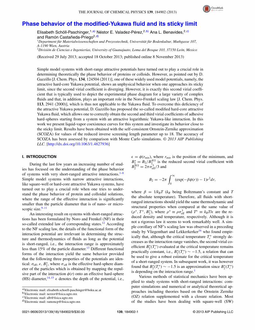
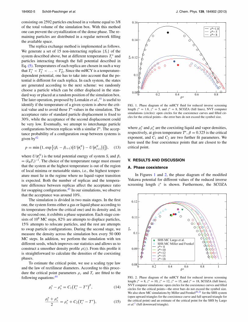
FIG. 1. Phase diagram of the mHCY fluid for reduced inverse screeninglength z∗ = 1.8, z∗ = 5, and z∗ = 8, SCOZA (full lines), NVT computersimulations (circles): open circles for the coexistence curves and filled cir-cles for the critical points—the error bars do not exceed the symbol size.
where ρ∗l and ρ∗
v are the coexisting liquid and vapor densities,respectively, at given temperature T∗, β = 0.325 is the criticalexponent, and C1 and C2 are two further fit parameters. Wehave used the four coexistence points that are closest to thecritical point.
V. RESULTS AND DISCUSSION
A. Phase coexistence
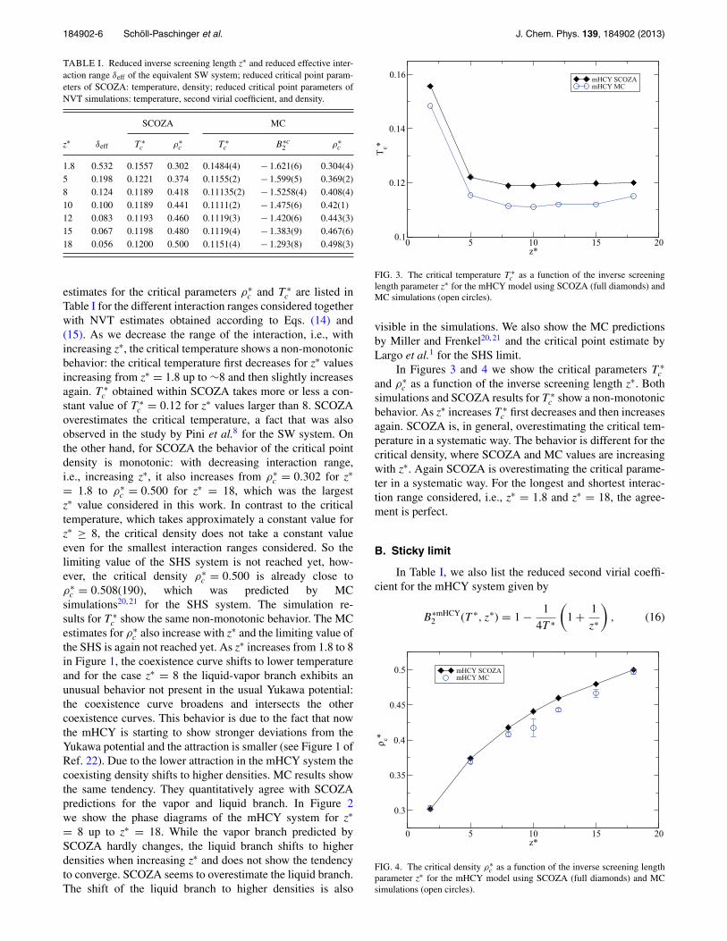
In Figures 1 and 2, the phase diagram of the modifiedYukawa potential for different values of the reduced inversescreening length z∗ is shown. Furthermore, the SCOZA
0 0.2 0.4 0.6 0.8 1ρ∗
0.08
0.09
0.1
0.11
0.12
T*
SHS MC Largo et al.SHS MC Miller and Frenkelz*= 8z*=10z*=12z*=15z*=18
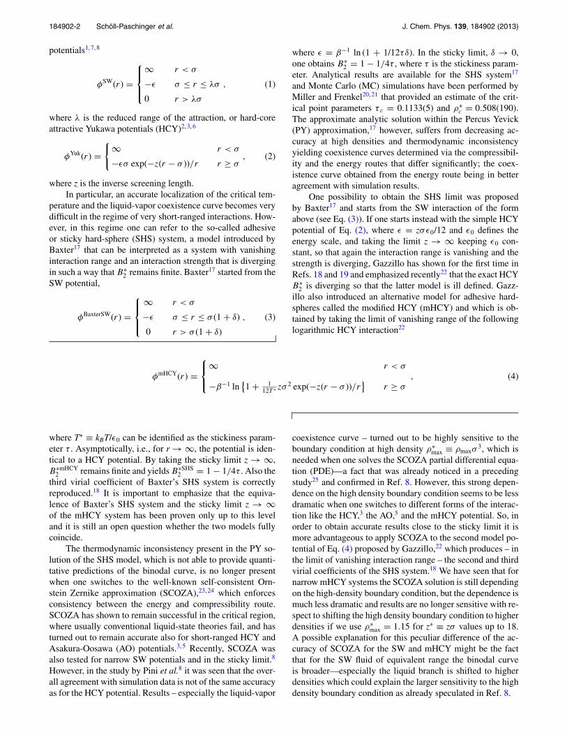
FIG. 2. Phase diagram of the mHCY fluid for reduced inverse screeninglength z∗ = 8, z∗ = 10, z∗ = 12, z∗ = 15, and z∗ = 18, SCOZA (full lines),NVT computer simulations: open circles for the coexistence curves and filledcircles for the critical points—the error bars do not exceed the symbol size.We also show MC simulations by Miller and Frenkel20, 21 for the SHS system(open upward triangles for the coexistence curve and full upward triangle forthe critical point) and an estimate of the critical point for the SHS by Largoet al.1 (full downward triangle).
184902-6 Schöll-Paschinger et al. J. Chem. Phys. 139, 184902 (2013)
TABLE I. Reduced inverse screening length z∗ and reduced effective inter-action range δeff of the equivalent SW system; reduced critical point param-eters of SCOZA: temperature, density; reduced critical point parameters ofNVT simulations: temperature, second virial coefficient, and density.
SCOZA MC
z∗ δeff T ∗c ρ∗
c T ∗c B∗c
2 ρ∗c
1.8 0.532 0.1557 0.302 0.1484(4) − 1.621(6) 0.304(4)5 0.198 0.1221 0.374 0.1155(2) − 1.599(5) 0.369(2)8 0.124 0.1189 0.418 0.11135(2) − 1.5258(4) 0.408(4)10 0.100 0.1189 0.441 0.1111(2) − 1.475(6) 0.42(1)12 0.083 0.1193 0.460 0.1119(3) − 1.420(6) 0.443(3)15 0.067 0.1198 0.480 0.1119(4) − 1.383(9) 0.467(6)18 0.056 0.1200 0.500 0.1151(4) − 1.293(8) 0.498(3)
estimates for the critical parameters ρ∗c and T ∗
c are listed inTable I for the different interaction ranges considered togetherwith NVT estimates obtained according to Eqs. (14) and(15). As we decrease the range of the interaction, i.e., withincreasing z∗, the critical temperature shows a non-monotonicbehavior: the critical temperature first decreases for z∗ valuesincreasing from z∗ = 1.8 up to ∼8 and then slightly increasesagain. T ∗
c obtained within SCOZA takes more or less a con-stant value of T ∗
c = 0.12 for z∗ values larger than 8. SCOZAoverestimates the critical temperature, a fact that was alsoobserved in the study by Pini et al.8 for the SW system. Onthe other hand, for SCOZA the behavior of the critical pointdensity is monotonic: with decreasing interaction range,i.e., increasing z∗, it also increases from ρ∗
c = 0.302 for z∗
= 1.8 to ρ∗c = 0.500 for z∗ = 18, which was the largest
z∗ value considered in this work. In contrast to the criticaltemperature, which takes approximately a constant value forz∗ ≥ 8, the critical density does not take a constant valueeven for the smallest interaction ranges considered. So thelimiting value of the SHS system is not reached yet, how-ever, the critical density ρ∗
c = 0.500 is already close toρ∗
c = 0.508(190), which was predicted by MCsimulations20, 21 for the SHS system. The simulation re-sults for T ∗
c show the same non-monotonic behavior. The MCestimates for ρ∗
c also increase with z∗ and the limiting value ofthe SHS is again not reached yet. As z∗ increases from 1.8 to 8in Figure 1, the coexistence curve shifts to lower temperatureand for the case z∗ = 8 the liquid-vapor branch exhibits anunusual behavior not present in the usual Yukawa potential:the coexistence curve broadens and intersects the othercoexistence curves. This behavior is due to the fact that nowthe mHCY is starting to show stronger deviations from theYukawa potential and the attraction is smaller (see Figure 1 ofRef. 22). Due to the lower attraction in the mHCY system thecoexisting density shifts to higher densities. MC results showthe same tendency. They quantitatively agree with SCOZApredictions for the vapor and liquid branch. In Figure 2we show the phase diagrams of the mHCY system for z∗
= 8 up to z∗ = 18. While the vapor branch predicted bySCOZA hardly changes, the liquid branch shifts to higherdensities when increasing z∗ and does not show the tendencyto converge. SCOZA seems to overestimate the liquid branch.The shift of the liquid branch to higher densities is also
0 5 10 15 20z*
0.1
0.12
0.14
0.16
Tc*
mHCY SCOZAmHCY MC
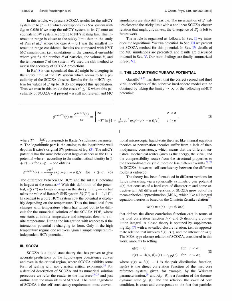
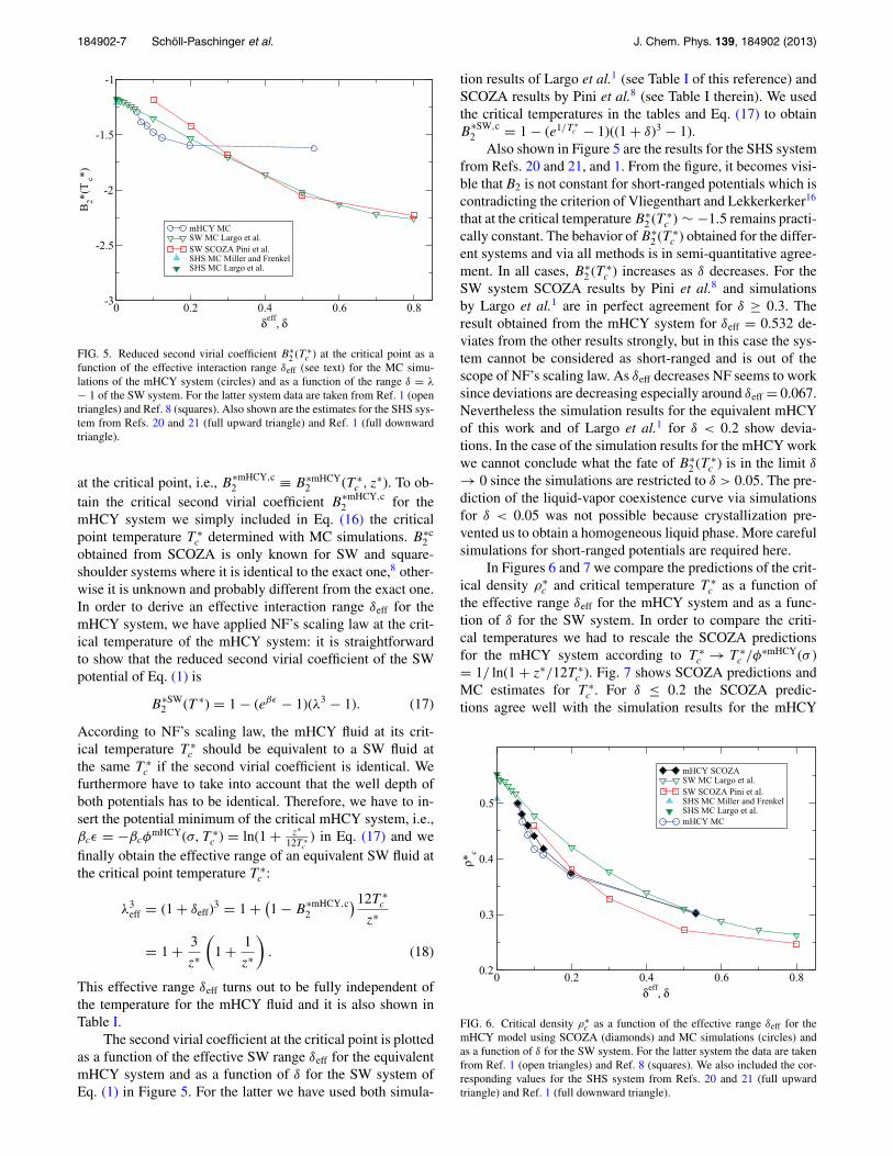
FIG. 3. The critical temperature T ∗c as a function of the inverse screening
length parameter z∗ for the mHCY model using SCOZA (full diamonds) andMC simulations (open circles).
visible in the simulations. We also show the MC predictionsby Miller and Frenkel20, 21 and the critical point estimate byLargo et al.1 for the SHS limit.
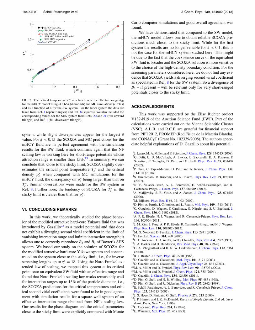
In Figures 3 and 4 we show the critical parameters T ∗c
and ρ∗c as a function of the inverse screening length z∗. Both
simulations and SCOZA results for T ∗c show a non-monotonic
behavior. As z∗ increases T ∗c first decreases and then increases
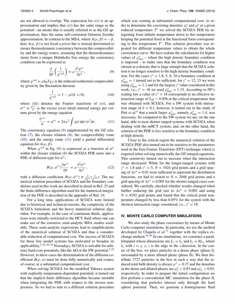
again. SCOZA is, in general, overestimating the critical tem-perature in a systematic way. The behavior is different for thecritical density, where SCOZA and MC values are increasingwith z∗. Again SCOZA is overestimating the critical parame-ter in a systematic way. For the longest and shortest interac-tion range considered, i.e., z∗ = 1.8 and z∗ = 18, the agree-ment is perfect.
B. Sticky limit
In Table I, we also list the reduced second virial coeffi-cient for the mHCY system given by
B∗mHCY2 (T ∗, z∗) = 1 − 1
4T ∗
(1 + 1
z∗
), (16)
0 5 10 15 20z*
0.3
0.35
0.4
0.45
0.5
ρ c*
mHCY SCOZAmHCY MC
FIG. 4. The critical density ρ∗c as a function of the inverse screening length
parameter z∗ for the mHCY model using SCOZA (full diamonds) and MCsimulations (open circles).
184902-7 Schöll-Paschinger et al. J. Chem. Phys. 139, 184902 (2013)
0 0.2 0.4 0.6 0.8δeff
, δ
-3
-2.5
-2
-1.5
-1B
2*(T
c*)
mHCY MCSW MC Largo et al.SW SCOZA Pini et al.SHS MC Miller and FrenkelSHS MC Largo et al.
FIG. 5. Reduced second virial coefficient B∗2 (T ∗
c ) at the critical point as afunction of the effective interaction range δeff (see text) for the MC simu-lations of the mHCY system (circles) and as a function of the range δ = λ
− 1 of the SW system. For the latter system data are taken from Ref. 1 (opentriangles) and Ref. 8 (squares). Also shown are the estimates for the SHS sys-tem from Refs. 20 and 21 (full upward triangle) and Ref. 1 (full downwardtriangle).
at the critical point, i.e., B∗mHCY,c2 ≡ B∗mHCY
2 (T ∗c , z∗). To ob-
tain the critical second virial coefficient B∗mHCY,c2 for the
mHCY system we simply included in Eq. (16) the criticalpoint temperature T ∗
c determined with MC simulations. B∗c2
obtained from SCOZA is only known for SW and square-shoulder systems where it is identical to the exact one,8 other-wise it is unknown and probably different from the exact one.In order to derive an effective interaction range δeff for themHCY system, we have applied NF’s scaling law at the crit-ical temperature of the mHCY system: it is straightforwardto show that the reduced second virial coefficient of the SWpotential of Eq. (1) is
B∗SW2 (T ∗) = 1 − (eβε − 1)(λ3 − 1). (17)
According to NF’s scaling law, the mHCY fluid at its crit-ical temperature T ∗
c should be equivalent to a SW fluid atthe same T ∗
c if the second virial coefficient is identical. Wefurthermore have to take into account that the well depth ofboth potentials has to be identical. Therefore, we have to in-sert the potential minimum of the critical mHCY system, i.e.,βcε = −βcφ
mHCY(σ, T ∗c ) = ln(1 + z∗
12T ∗c
) in Eq. (17) and wefinally obtain the effective range of an equivalent SW fluid atthe critical point temperature T ∗
c :
λ3eff = (1 + δeff)
3 = 1 + (1 − B
∗mHCY,c2
)12T ∗c
z∗
= 1 + 3
z∗
(1 + 1
z∗
). (18)
This effective range δeff turns out to be fully independent ofthe temperature for the mHCY fluid and it is also shown inTable I.
The second virial coefficient at the critical point is plottedas a function of the effective SW range δeff for the equivalentmHCY system and as a function of δ for the SW system ofEq. (1) in Figure 5. For the latter we have used both simula-
tion results of Largo et al.1 (see Table I of this reference) andSCOZA results by Pini et al.8 (see Table I therein). We usedthe critical temperatures in the tables and Eq. (17) to obtainB
∗SW,c2 = 1 − (e1/T ∗
c − 1)((1 + δ)3 − 1).Also shown in Figure 5 are the results for the SHS system
from Refs. 20 and 21, and 1. From the figure, it becomes visi-ble that B2 is not constant for short-ranged potentials which iscontradicting the criterion of Vliegenthart and Lekkerkerker16
that at the critical temperature B∗2 (T ∗
c ) ∼ −1.5 remains practi-cally constant. The behavior of B∗
2 (T ∗c ) obtained for the differ-
ent systems and via all methods is in semi-quantitative agree-ment. In all cases, B∗
2 (T ∗c ) increases as δ decreases. For the
SW system SCOZA results by Pini et al.8 and simulationsby Largo et al.1 are in perfect agreement for δ ≥ 0.3. Theresult obtained from the mHCY system for δeff = 0.532 de-viates from the other results strongly, but in this case the sys-tem cannot be considered as short-ranged and is out of thescope of NF’s scaling law. As δeff decreases NF seems to worksince deviations are decreasing especially around δeff = 0.067.Nevertheless the simulation results for the equivalent mHCYof this work and of Largo et al.1 for δ < 0.2 show devia-tions. In the case of the simulation results for the mHCY workwe cannot conclude what the fate of B∗
2 (T ∗c ) is in the limit δ
→ 0 since the simulations are restricted to δ > 0.05. The pre-diction of the liquid-vapor coexistence curve via simulationsfor δ < 0.05 was not possible because crystallization pre-vented us to obtain a homogeneous liquid phase. More carefulsimulations for short-ranged potentials are required here.
In Figures 6 and 7 we compare the predictions of the crit-ical density ρ∗
c and critical temperature T ∗c as a function of
the effective range δeff for the mHCY system and as a func-tion of δ for the SW system. In order to compare the criti-cal temperatures we had to rescale the SCOZA predictionsfor the mHCY system according to T ∗
c → T ∗c /φ∗mHCY(σ )
= 1/ ln(1 + z∗/12T ∗c ). Fig. 7 shows SCOZA predictions and
MC estimates for T ∗c . For δ ≤ 0.2 the SCOZA predic-
tions agree well with the simulation results for the mHCY
0 0.2 0.4 0.6 0.8δeff
, δ
0.2
0.3
0.4
0.5
ρ*c
mHCY SCOZASW MC Largo et al.SW SCOZA Pini et al.SHS MC Miller and FrenkelSHS MC Largo et al.mHCY MC
FIG. 6. Critical density ρ∗c as a function of the effective range δeff for the
mHCY model using SCOZA (diamonds) and MC simulations (circles) andas a function of δ for the SW system. For the latter system the data are takenfrom Ref. 1 (open triangles) and Ref. 8 (squares). We also included the cor-responding values for the SHS system from Refs. 20 and 21 (full upwardtriangle) and Ref. 1 (full downward triangle).
184902-8 Schöll-Paschinger et al. J. Chem. Phys. 139, 184902 (2013)
0 0.2 0.4 0.6 0.8δ eff
, δ
0
0.5
1
1.5
2T
* cmHCY SCOZASW MC Largo et al.SW SCOZA Pini et al.SHS MC Miller and FrenkelSHS MC Largo et al.mHCY MC
FIG. 7. The critical temperature T ∗c as a function of the effective range δeff
for the mHCY model using SCOZA (diamonds) and MC simulations (circles)and as a function of δ for the SW system. For the latter system the data aretaken from Ref. 1 (open triangles) and Ref. 8 (squares). We also included thecorresponding values for the SHS system from Refs. 20 and 21 (full upwardtriangle) and Ref. 1 (full downward triangle).
system, while slight discrepancies appear for the largest δ
value. For δ < 0.15 the SCOZA and MC predictions for themHCY fluid are in perfect agreement with the simulationresults for the SW fluid, which confirms again that the NFscaling law is working here for short-range potentials whoseattraction range is smaller than 15%.13 In summary, we canconclude that, close to the sticky limit, SCOZA slightly over-estimates the critical point temperature T ∗
c and the criticaldensity ρ∗
c when compared with MC simulations for themHCY fluid, the discrepancy on ρ∗
c being larger than that onT ∗
c . Similar observations were made for the SW system inRef. 8. Furthermore, the tendency of SCOZA for T ∗
c in thesticky limit is clearer than that for ρ∗
c .
VI. CONCLUDING REMARKS
In this work, we theoretically studied the phase behav-ior of the modified attractive hard-core Yukawa fluid that wasintroduced by Gazzillo22 as a model potential and that doesnot exhibit a diverging second virial coefficient in the limit ofvanishing interaction range and infinite interaction strength; itallows one to correctly reproduce B2 and B3 of Baxter’s SHSsystem. We based our study on the solution of SCOZA forthe modified attractive hard-core Yukawa system and concen-trated on the system close to the sticky limit, i.e., for inversescreening lengths up to z∗ = 18. Using the Noro-Frenkel ex-tended law of scaling, we mapped this system at its criticalpoint onto an equivalent SW fluid with an effective range andfound that Noro-Frenkel’s scaling law works remarkably wellfor interaction ranges up to 15% of the particle diameter, i.e.,the SCOZA predictions for the critical temperatures and crit-ical second virial coefficients were found to be in good agree-ment with simulation results for a square-well system of aneffective interaction range obtained from NF’s scaling law.Our results for the phase diagram and the critical parametersclose to the sticky limit were explicitly compared with Monte
Carlo computer simulations and good overall agreement wasfound.
We have demonstrated that compared to the SW model,the mHCY model allows one to obtain reliable SCOZA pre-dictions much closer to the sticky limit. While for the firstsystem the results are no longer reliable for δ < 0.1, this isnot the case for the mHCY system studied here. This mightbe due to the fact that the coexistence curve of the equivalentSW fluid is broader and the SCOZA solution is more sensitiveto the choice of the high-density boundary condition. For thescreening parameters considered here, we do not find any evi-dence that SCOZA yields a diverging second virial coefficientas speculated in Ref. 8 for the SW system. So a divergence ofB2 – if present – will be relevant only for very short-rangedpotentials closer to the sticky limit.
ACKNOWLEDGMENTS
This work was supported by the Elise Richter projectV132-N19 of the Austrian Science Fund (FWF). Part of thecalculations were carried out on the Vienna Scientific Cluster(VSC). A.L.B. and R.C.P. are grateful for financial supportfrom PIFI 2012, PROMEP (Red Física de la Materia Blanda),and CONACyT (Grant No. 102339/2008). The authors appre-ciate helpful explanations of D. Gazzillo about his potential.
1J. Largo, M. A. Miller, and F. Sciortino, J. Chem. Phys. 128, 134513 (2008).2G. Foffi, G. D. McCullagh, A. Lawlor, E. Zaccarelli, K. A. Dawson, F.Sciortino, P. Tartaglia, D. Pini, and G. Stell, Phys. Rev. E 65, 031407(2002).
3P. Orea, C. Tapia-Medina, D. Pini, and A. Reiner, J. Chem. Phys. 132,114108 (2010).
4S. Buzzaccaro, R. Rusconi, and R. Piazza, Phys. Rev. Lett. 99, 098301(2007).
5N. E. Valadez-Pérez, A. L. Benavides, E. Schöll-Paschinger, and R.Castaneda-Priego, J. Chem. Phys. 137, 084905 (2012).
6A. Malijevsky, S. B. Yuste, and A. Santos, J. Chem. Phys. 125, 074507(2006).
7M. Dijkstra, Phys. Rev. E 66, 021402 (2002).8D. Pini, A. Parola, J. Colombo, and L. Reatto, Mol. Phys. 109, 1343 (2011).9C. Gogelein, D. Wagner, F. Cardinaux, G. Nägele, and S. U. Egelhaaf, J.Chem. Phys. 136, 015102 (2012).
10A. P. R. Eberle, N. J. Wagner, and R. Castaneda-Priego, Phys. Rev. Lett.106, 105704 (2011).
11J. M. Kim, J. Fang, A. P. R. Eberle, R. Castaneda-Priego, and N. J. Wagner,Phys. Rev. Lett. 110, 208302 (2013).
12M. G. Noro and D. Frenkel, J. Chem. Phys. 113, 2941 (2000).13D. Frenkel, Science 314, 768 (2006).14H. C. Andersen, J. D. Weeks, and D. Chandler, Phys. Rev. A 4, 1597 (1971).15J. A. Barker and D. Henderson, Rev. Mod. Phys. 48, 587 (1976).16G. A. Vliegenthart and H. N. W. Lekkerkerker, J. Chem. Phys. 112, 5364
(2000).17R. J. Baxter, J. Chem. Phys. 49, 2770 (1968).18D. Gazzillo and A. Giacometti, Mol. Phys. 101, 2171 (2003).19D. Gazzillo and A. Giacometti, J. Appl. Crystallogr. 36, 832 (2003).20M. A. Miller and D. Frenkel, Phys. Rev. Lett. 90, 135702 (2003).21M. A. Miller and D. Frenkel, J. Chem. Phys. 121, 535 (2004).22D. Gazzillo, J. Chem. Phys. 134, 124504 (2011).23D. Pini, G. Stell, and N. B. Wilding, Mol. Phys. 95, 483 (1998).24D. Pini, G. Stell, and R. Dickman, Phys. Rev. E 57, 2862 (1998).25E. Schöll-Paschinger, A. L. Benavides, and R. Castañeda-Priego, J. Chem.
Phys. 123, 234513 (2005).26J. S. Høye, D. Pini, and G. Stell, Physica A 279, 213 (2000).27J. P. Hansen and I. R. McDonald, Theory of Simple Liquids, 2nd ed. (Aca-
demic Press, New York, 1986).28C. Caccamo, Phys. Rep. 274, 1 (1996).29E. Waisman, Mol. Phys. 25, 45 (1973).
184902-9 Schöll-Paschinger et al. J. Chem. Phys. 139, 184902 (2013)
30G. Kahl, E. Schöll-Paschinger, and G. Stell, J. Phys.: Condens. Matter 14,9153 (2002).
31E. Schöll-Paschinger, J. Chem. Phys. 120, 11698 (2004).32D. Costa, G. Pellicane, C. Caccamo, E. Schöll-Paschinger, and G. Kahl,
Phys. Rev. E 68, 021104 (2003).33E. Schöll-Paschinger and G. Kahl, J. Chem. Phys. 123, 134508 (2005).34E. Schöll-Paschinger, D. Levesque, J.-J. Weis, and G. Kahl, J. Chem. Phys.
122, 024507 (2005).35E. Schöll-Paschinger and A. Reiner, J. Chem. Phys. 125, 164503
(2006).36F. F. Betancourt-Cardenas, L. A. Galicia-Luna, A. L. Benavides, J. A.
Ramirez, and E. Schöll-Paschinger, Mol. Phys. 106, 113 (2008).37G. A. Chapela, S. E. Martínez-Casas, and C. Varea, J. Chem. Phys. 86,
5683 (1987).
38R. H. Swendsen and J. S. Wang, Phys. Rev. Lett. 57, 2607 (1986).39C. J. Geyer, in Computing Science and Statistics: Proceedings of the 23rd
Symposium on the Interface (American Statistical Association, New York,1991), p. 156.
40K. Hukushima and K. Nemoto, J. Phys. Soc. Jpn. 65, 1604–1608 (1996).41A. Lomakin, N. Asherie, and G. B. Benedek, J. Chem. Phys. 104, 1646
(1996).42D. J. Earl and M. W. Deem, Phys. Chem. Chem. Phys. 7, 3910–3916
(2005).43N. Rathore, M. Chopra, and J. J. de Pablo, J. Chem. Phys. 122, 024111
(2005).44A. Z. Panagiotopoulos, Observation, Prediction and Simulation of Phase
Transitions in Complex Fluids, NATO ASI Series C Vol. 460 (Kluwer Aca-demic Publishers, Dordrecht, The Netherlands, 1995), pp. 463–501.