peripheral refraction: significance, current limitations and a
TRANSCRIPT
PERIPHERAL REFRACTION: SIGNIFICANCE, CURRENT
LIMITATIONS AND A NEW APPROACH
Cathleen Fedtke, Dipl.‐Ing. (FH)
A thesis submitted in fulfilment of the requirements for the degree of
Doctor of Philosophy
School of Optometry and Vision Science
The University of New South Wales, Sydney, Australia
and
Brien Holden Vision Institute
Sydney, Australia
and
Vision Cooperative Research Centre
Sydney, Australia
April 2011


Certificate of Originality
i
CERTIFICATE OF ORIGINALITY
‘I hereby declare that this submission is my own work and to the best of my knowledge it
contains no materials previously published or written by another person, or substantial
proportions of material which have been accepted for the award of any other degree or
diploma at UNSW or any other educational institution, except where due acknowledgement is
made in the thesis. Any contribution made to the research by others, with whom I have
worked at UNSW or elsewhere, is explicitly acknowledged in the thesis. I also declare that the
intellectual content of this thesis is the product of my own work, except to the extent that
assistance from others in the project's design and conception or in style, presentation and
linguistic expression is acknowledged.’
Cathleen Fedtke
April 2011

Acknowledgements
ii
ACKNOWLEDGEMENTS
First and foremost, I would like to thank my supervisors Brien Holden and Klaus Ehrmann for
giving me the opportunity to pursue this PhD. Thank you for your long‐lasting support and
loyalty throughout. I have been very privileged to work with both of you. Brien, your research,
dedication and enthusiasm to the world of optometry have kept me motivated and
driven. It has truly been an honour and I look forward to working with you and the staff at the
Brien Holden Vision Institute into the future. Klaus, thank you for introducing me to the world
of research and for being my mentor throughout this journey, a journey made possible with
your brilliant ideas and technology expertise. I am very grateful for your continuous incredible
support.
This project would also not have been possible without the financial support from various
sources; an UIPA scholarship funded through the University of New South Wales, a scholarship
funded by the Brien Holden Vision Institute and travel grants for the attendance of
international conferences from the University of New South Wales, the American Academy of
Optometry and the Brien Holden Vision Institute. Thank you.
A special thank you goes to Darrin Falk, who has greatly contributed to the instrumental work
presented in this thesis. Thank you for your incredible help and for reassuring me that there is
a light at the end of the tunnel. Another person that has provided much wealth of expertise to
this project was Arthur Ho. Thank you for sharing your amazing knowledge and for giving me
the opportunities to grow as a researcher.
I would also like to thank many other important helpers of this project. Colm Dolphin for
manufacturing the instrument parts, Thomas Naduvilath and Varghese Thomas for statistical
advice, Judith Flanagan for reading the manuscripts and for providing valuable advice on
scientific writing, Ravi Bakaraju for sharing his valuable knowledge on Zemax and Elsbeth Biβ‐
Harms for helping with analysis of the pupil images. Thank you also to all the participants for
their precious time to take part in my studies.
I am also very grateful for the help provided by staff of many other departments within the
Brien Holden Vision Institute, particularly: Eric Papas and Vivienne Miller for taking care of all
the administrative matters, the Myopia team, including Padmaja Sankaridurg, Percy Lazon de

Acknowledgements
iii
la Jara, Judy Kwan, Les Donovan, Rebecca Weng and Belinda Ford, for being a great clinical
team to work with, the i‐media team for helping me produce great posters and each of my
fellow‐postgraduate students, in particular Maria, Ravi, Fabian, Negar, Krupa, Kalika, Ulli and
Usha, who always provided support and encouragement. I appreciate all your help and
friendship.
I would not have made it through some of the tough times without a few very special people.
Maria, you have given me so much support, not just as an amazing friend on the personal
level, who was there when times were very difficult, but also as a fellow student on the
professional level for helping me with proof‐reading, statistics and critical thinking – thank you,
I have learnt so much from you. Claudia, thank you for your friendship and all the support you
have given me during the last four years. This PhD has been a long‐lasting odyssey with many
ups and downs and I deeply appreciate your friendship through all phases. I would also like to
thank the many other friendships which have formed during this PhD journey. In particular I
would like to thank my friends and colleagues Judy, Beth, Aurelia, Melina, Stephanie and
Elsbeth, who each in their own way made working in the clinic so enjoyable.
Most of all I would like to thank my wonderful family, my Mum & Dad, Loreen, and Manu, who
have been of enormous support to my studies and who have been a constant source of
encouragement. Words cannot describe how much that has meant to me. Thank you so much
for your unconditional support and love.
Abstract
iv
ABSTRACT
Peripheral refractive error has assumed considerable importance with the discovery that
it can influence eye growth. The link between the peripheral state of the eye and myopia
development demands rapid and accurate measurements at individual and population
levels. Currently, the use of conventional refraction techniques requires time‐consuming
sequential re‐alignments.
The aims of this thesis were to identify and assess methodological limitations of current
techniques, test new concepts and develop a method of obtaining more rapid and
accurate peripheral refraction measurements.
At first, the impact of pupil misalignment was investigated using a conventional
autorefractor. As visual field angle increased, tolerance to pupil misalignment decreased
significantly, making peripheral measurements particularly susceptible to this
measurement error. It was also shown that the peripheral entrance pupil shape is not
elliptical as currently assumed, adding further potential for pupil misalignment. Based on
these findings, means to rectify pupil alignment‐related errors when using conventional
instruments were established and validated.
Having ascertained limitations of current peripheral refractometry, a novel instrument
concept was proposed, the EyeMapper. The EyeMapper was designed to perform a rapid
peripheral (and central) refraction scan, from ‐50° to +50°, using 10 stationary deflecting
prisms and a scanning mirror. Like most autorefractors, the operation was based on the
ring‐autorefraction principle. The optical design, consisting of 5 intertwined optical sub‐
systems was developed. Safety aspects and criteria for instrument components were
assessed and the operation principle was verified experimentally. Experimental testing
identified an obstacle relating to the ring‐image analysis and it revealed that peripheral
higher order aberrations have the potential to interfere with the sphero‐cylindrical
refraction readings obtained when applying this ring‐autorefraction principle. A
technique that segregates higher and lower order aberrations was thus deemed more
suitable for measuring peripheral refraction. Hence, the EyeMapper design was updated
to include wavefront measurements. The prototype instrument was then built and
experimentally tested over a range of refractive errors. The EyeMapper uses an array of
beam steering mirrors and a scanning mirror to perform a rapid peripheral refraction
scan in one meridian. Three‐dimensional power maps of the eye can be obtained by
pivoting the instrument around its optical axis.

Table of Contents
v
TABLE OF CONTENTS
CERTIFICATE OF ORIGINALITY ...................................................................................... i
ACKNOWLEDGEMENTS .............................................................................................. ii
ABSTRACT ................................................................................................................ iv
TABLE OF CONTENTS .................................................................................................. v
LIST OF FIGURES ........................................................................................................ x
LIST OF TABLES ...................................................................................................... xvii
GLOSSARY OF ABBREVIATIONS ................................................................................ xix
CHAPTER 1
LITERATURE REVIEW .................................................................................................. 1
1.1 Introduction ......................................................................................................... 1 1.2 Peripheral Vision .................................................................................................. 4
1.2.1 Methods of Testing Peripheral Vision ........................................................ 5 1.3 Peripheral Refractive Error Measurement Techniques .......................................... 6
1.3.1 Subjective Peripheral Refraction ............................................................... 9 1.3.2 Retinoscopy ............................................................................................ 11 1.3.3 Manual Refractometer – Optometer ....................................................... 14 1.3.4 Double‐Pass Technique ........................................................................... 17 1.3.5 Autorefraction ........................................................................................ 20 1.3.6 Photorefraction....................................................................................... 27 1.3.7 Aberrometer ........................................................................................... 30
1.4 Alignment Criteria for Peripheral Refractometry ................................................. 34 1.5 Summary and Conclusion .................................................................................... 38 1.6 Thesis Overview .................................................................................................. 40
1.6.1 Rationale for Research ............................................................................ 40 1.6.2 Hypotheses ............................................................................................. 40 1.6.3 Aims ........................................................................................................ 41
CHAPTER 2
INVESTIGATION OF OPERATOR‐RELATED ALIGNMENT INTRICACIES IN CURRENT PERIPHERAL REFRACTOMETRY ................................................................................. 42
2.1 Overview ............................................................................................................ 42 2.2 Investigation of Pupil Alignment Tolerance ......................................................... 42
2.2.1 Introduction ............................................................................................ 42 2.2.2 Methods ................................................................................................. 44
2.2.2.1 Participants ............................................................................................ 44 2.2.2.2 Instrumentation ..................................................................................... 44 2.2.2.3 Participant Alignment ............................................................................. 45 2.2.2.4 Entrance Pupil Alignment ........................................................................ 46
2.2.3 Results .................................................................................................... 49 2.2.3.1 Central and Peripheral Refraction – Pupil Alignment ............................... 49 2.2.3.2 Pupil Misalignment Threshold of Clinical Significance .............................. 52
Table of Contents
vi
2.2.4 Discussion .............................................................................................. 53 2.2.4.1 Peripheral Refraction and its Tolerance to Lateral Pupil Misalignment .... 53 2.2.4.2 Factors Contributing to Misalignment Errors during Peripheral Refraction
Measurements ....................................................................................... 55 2.2.4.3 Improving Pupil Alignment ...................................................................... 56
2.2.5 Conclusion .............................................................................................. 57 2.3 Three‐Dimensional Model of the Entrance Pupil ................................................ 57
2.3.1 Introduction ........................................................................................... 57 2.3.2 Methods ................................................................................................. 58
2.3.2.1 Model of the Entrance Pupil for Different Viewing Angles ....................... 58 2.3.3 Results .................................................................................................... 60
2.3.3.1 Entrance Pupil Relative to the Actual Pupil.............................................. 60 2.3.3.2 Entrance Pupil Relative to the Viewing Direction ..................................... 60
2.3.4 Discussion .............................................................................................. 67 2.3.4.1 Comparison of the Entrance Pupil Model with in Vivo Pupils ................... 68 2.3.4.2 Implications of the Entrance Pupil Model ................................................ 69 2.3.4.3 The Wide‐Field Eye ................................................................................. 72 2.3.4.4 Recommendations for Future Models ..................................................... 72
2.3.5 Conclusion .............................................................................................. 73 2.4 Summary ............................................................................................................ 73
CHAPTER 3
MEANS TO RECTIFY PUPIL ALIGNMENT ERRORS IN CURRENT PERIPHERAL REFRACTOMERTY .................................................................................................... 75
3.1 Introduction ....................................................................................................... 75 3.2 Methods ............................................................................................................ 76
3.2.1 Phase 1 ................................................................................................... 76 3.2.1.1 Participants ............................................................................................ 76 3.2.1.2 Instrumentation and Alignment Procedure ............................................. 76
3.2.2 Phase 2 ................................................................................................... 78 3.2.2.1 Participants and Instrumentation ............................................................ 78 3.2.2.2 Entrance Pupil: Image Capture and Analysis ............................................ 78
3.3 Results ............................................................................................................... 78 3.3.1 Phase 1 ................................................................................................... 78
3.3.1.1 Establish Correction Models ................................................................... 78 3.3.1.1.1 Refractive Vector Component M ......................................................... 79 3.3.1.1.2 Refractive Vector Component J180 ....................................................... 83 3.3.1.1.3 Refractive Vector Component J45 ......................................................... 85 3.3.1.1.4 Sphero‐Cylindrical Notation ................................................................. 88
3.3.1.2 Investigation of Instrument Binocularity with Pupil Alignment ................ 88 3.3.1.3 Validation of the Correction Algorithm ................................................... 91
3.3.2 Phase 2 ................................................................................................... 93 3.3.2.1 Implementation of the Correction Algorithms ......................................... 93
3.4 Discussion .......................................................................................................... 97 3.4.1 Functions of Pupil Alignment .................................................................. 97
3.4.1.1 Functions of Pupil Alignment for Different Visual Field Angles ................. 97 3.4.1.2 Functions of Pupil Alignment for Different Ocular Parameters ................. 99 3.4.1.3 Functions of Pupil Alignment for Nasal and Temporal Measurements .... 102 3.4.1.4 Instrumentation used to Establish Pupil Alignment Functions ............... 102
3.4.2 Pupil Alignment Correction Models ....................................................... 103 3.4.3 Implementation of Compensation Factor ............................................... 104
3.5 Summary and Conclusion .................................................................................. 105

Table of Contents
vii
CHAPTER 4
OPTICAL DESIGN OF A NOVEL PERIPHERAL REFRACTION CONCEPT: THE EYEMAPPER . 106
4.1 Introduction ..................................................................................................... 106 4.1.1 Design Concept and Operation Principle ............................................... 106 4.1.2 Chapter Overview ................................................................................. 109 4.1.3 Introduction into Optical Designing using ZEMAX .................................. 110
4.2 The EyeMapper’s Reference Model Eye ............................................................ 111 4.2.1 Methods ............................................................................................... 111
4.2.1.1 EyeMapper Reference Model Eye ......................................................... 111 4.2.1.2 Computation of Central and Peripheral Refraction via Ray‐Tracing ........ 113 4.2.1.3 Refractive Error‐Dependent Model Eyes ............................................... 116 4.2.1.4 Accommodation‐Dependent Model Eyes ............................................... 119 4.2.1.5 Computation of Peripheral Refraction for Different Ray‐Trace Modes ... 122
4.2.2 Results .................................................................................................. 125 4.2.2.1 Peripheral Refraction Profiles of Schematic Model Eyes ........................ 125 4.2.2.2 Peripheral Refraction Profiles for Different Ray‐Trace Modes ................ 125
4.2.3 Discussion/Conclusion........................................................................... 127 4.3 The Optical Design of the EyeMapper ............................................................... 128
4.3.1 Autorefraction Paths ............................................................................. 129 4.3.1.1 Deflection System ................................................................................. 129
4.3.1.1.1 Methods ............................................................................................. 129 4.3.1.1.2 Results ................................................................................................ 137
4.3.1.2 Illumination Autorefraction Path .......................................................... 141 4.3.1.2.1 Methods ............................................................................................. 142 4.3.1.2.2 Results ................................................................................................ 144
4.3.1.3 Reflection Autorefraction Path ............................................................. 146 4.3.1.3.1 Methods ............................................................................................. 147 4.3.1.3.2 Results ................................................................................................ 150
4.3.2 Pupil Imaging Path ................................................................................ 153 4.3.2.1 Methods ............................................................................................... 153 4.3.2.2 Results ................................................................................................. 154
4.3.3 Fixation Path ......................................................................................... 156 4.3.3.1 Methods ............................................................................................... 156 4.3.3.2 Results ................................................................................................. 158
4.4 Summary .......................................................................................................... 160 4.5 Conclusion ........................................................................................................ 160
CHAPTER 5
RING‐SCAN‐AUTOREFRACTION PRINCIPLE: COMPONENT CRITERIA, SAFETY ASSESSMENT AND EXPERIMENTAL VALIDATION .......................................................................... 163
5.1 Introduction ..................................................................................................... 163 5.2 On‐ and Off‐Axis Ring Scan Illumination ............................................................ 164
5.2.1 Component Criteria ............................................................................... 164 5.2.1.1 Infrared Light Source – Super Luminescent Diode ................................. 164 5.2.1.2 Dual Axis Galvanometer Scanner ........................................................... 165 5.2.1.3 Single Axis Galvanometer Scanner ........................................................ 165
5.2.2 Safety Assessment ................................................................................ 166 5.2.2.1 Introduction ......................................................................................... 166 5.2.2.2 Methods ............................................................................................... 167
5.2.2.2.1 Single and Repetitive Pulse Exposures ............................................... 167 5.2.2.2.2 Ocular Scanning ................................................................................. 169
Table of Contents
viii
5.2.2.3 Results ................................................................................................. 170 5.2.2.3.1 Retinal Image Size – Visual Angle ....................................................... 170 5.2.2.3.2 Maximum Permissible Exposure as a Function of Exposure Duration172 5.2.2.3.3 Repeated Refraction Measurements ................................................. 175
5.2.2.4 Discussion ............................................................................................ 175 5.2.2.4.1 ANSI Exposure Limits and Ocular Scanning ........................................ 175 5.2.2.4.2 Illumination of Peripheral Retinal Locations ...................................... 177 5.2.2.4.3 Scanner Safety ................................................................................... 179
5.3 Component Criteria for Image Detection ........................................................... 179 5.3.1 Reduction of Interfering Reflections ...................................................... 180 5.3.2 Translation Stage and CCD Sensor ......................................................... 181
5.4 Experimental Validation of the Ring‐Autorefraction Principle ............................ 181 5.4.1 Methods ................................................................................................ 181
5.4.1.1 Experimental Set‐Up and Procedure ..................................................... 181 5.4.1.2 Investigation of Shin‐Nippon Detector and Retinal Images .................... 183
5.4.2 Results ................................................................................................... 185 5.4.2.1 Cross‐Validation of the Autorefraction Principle with optical ZEMAX design
............................................................................................................ 185 5.4.2.2 Cross‐Validation of the Autorefraction Principle with the Shin‐Nippon
Autorefractor ....................................................................................... 186 5.4.3 Discussion ............................................................................................. 187
5.4.3.1 On‐Axis Optical Bench Experiment ........................................................ 187 5.4.3.2 Major Obstacles Encountered During Experimental Testing ................... 188
5.4.3.2.1 Image Analysis for Off‐Axis Ring Images ............................................ 188 5.4.3.2.2 Impact of Higher‐Order Aberrations on Peripheral Ring Images ....... 189
5.5 Future Work ...................................................................................................... 193 5.6 Summary and Conclusion .................................................................................. 194
CHAPTER 6
THE EYEMAPPER ‐ A REAL‐TIME GLOBAL ABERROMETER .......................................... 196
6.1 Introduction ...................................................................................................... 196 6.2 Instrument Design ............................................................................................. 197
6.2.1 Optical Design ....................................................................................... 197 6.2.1.1 Wavefront Sensing Paths ...................................................................... 198
6.2.1.1.1 Deflection System .............................................................................. 198 6.2.1.1.2 Illumination Path................................................................................ 199 6.2.1.1.3 Reflection Path ................................................................................... 199
6.2.1.2 Pupil Imaging Path ................................................................................ 200 6.2.1.3 Fixation Path ........................................................................................ 200
6.2.2 Mechanical Design ................................................................................. 201 6.3 Instrument Construction ................................................................................... 204
6.3.1 Tolerance Analysis ................................................................................. 204 6.3.1.1 Aims ..................................................................................................... 204 6.3.1.2 Methods ............................................................................................... 204
6.3.1.2.1 Sensitivity Analysis and Monte Carlo Simulation ............................... 204 6.3.1.2.2 Tolerance Analysis for the Reflection Path ........................................ 205
6.3.1.3 Results ................................................................................................. 207 6.3.1.3.1 Sensitivity Analysis ............................................................................. 207 6.3.1.3.2 Monte‐Carlo Simulation ..................................................................... 209
6.3.1.4 Discussion ............................................................................................ 210 6.3.2 Instrument Components ........................................................................ 211
6.3.2.1 Deflection System ................................................................................. 211

Table of Contents
ix
6.3.2.2 Illumination Path .................................................................................. 211 6.3.2.3 Reflection Path ..................................................................................... 212 6.3.2.4 Fixation Path ........................................................................................ 213 6.3.2.5 Pupil Imaging Path ................................................................................ 213 6.3.2.6 Other Instrument Parts ......................................................................... 214
6.3.3 The EyeMapper ..................................................................................... 216 6.4 Instrument Validation ....................................................................................... 219
6.4.1 Methods ............................................................................................... 219 6.4.1.1 Peripheral Refraction Model Eye ........................................................... 219 6.4.1.2 Human Eyes .......................................................................................... 221
6.4.1.2.1 Participants ........................................................................................ 221 6.4.1.2.2 Instrumentation, Set‐up and Procedure ............................................ 222
6.4.2 Results .................................................................................................. 223 6.4.2.1 Peripheral Refraction: Model Eye .......................................................... 223 6.4.2.2 Peripheral Refraction: Human Eyes ....................................................... 224
6.4.2.2.1 Peripheral Refraction Profiles ............................................................ 224 6.4.2.2.2 Repeatability ...................................................................................... 229 6.4.2.2.3 Reproducibility ................................................................................... 230 6.4.2.2.4 Refraction Map .................................................................................. 232
6.4.3 Discussion ............................................................................................. 233 6.4.3.1 Accuracy: Model Eye ............................................................................. 233 6.4.3.2 Peripheral Refraction Profiles and Repeatability: Human Eyes ............... 234 6.4.3.3 Reproducibility ..................................................................................... 237
6.5 Discussion......................................................................................................... 237 6.5.1 Peripheral Refraction Instruments ........................................................ 237 6.5.2 Limitations and Suggestions for Future Work ........................................ 240
6.6 Conclusion ........................................................................................................ 241
CHAPTER 7: ........................................................................................................... 243
SUMMARY AND CONCLUSIONS .............................................................................. 243
7.1 Significance of Peripheral Refractometry .......................................................... 243 7.2 Current Limitations ........................................................................................... 243
7.2.1 Participant‐Related Alignment Limitations ............................................ 243 7.2.2 Operator‐Related Alignment Limitations ............................................... 244
7.3 A New Approach ............................................................................................... 245 7.4 Conclusions ...................................................................................................... 246
REFERENCES ...................................................................................................................... 248 APPENDICES APPENDIX A: Patent Application: Determination of Peripheral Refraction .................... 261 APPENDIX B: Pupil Misalignment Correction Algorithms ............................................... 302 APPENDIX C: ZEMAX Macro: Calculation of Peripheral Refraction ................................. 304 APPENDIX D: Publications and Presentations ....................................................................... 305

List of Figures
x
LIST OF FIGURES
Figure 1.1: Emmetropic eye with relative hyperopic defocus in the periphery. ............... 2
Figure 1.2: Scheiner disc principle. ................................................................................ 15
Figure 1.3: Alignment of the peripheral measurement angle with respect to the instrument axis via a) eye turn, b) head turn and c) instrument rotation. .... 35
Figure 1.4: Number of studies and their peripheral refraction techniques used over the last 40 years (left) and the last decade (right). ............................................ 39
Figure 2.1: Modifications to the Shin‐Nippon NVision K5001 autorefractor. .................. 46
Figure 2.2: Right eye pupil alignment matrix. ................................................................ 47
Figure 2.3: The pupil alignment scale. ........................................................................... 48
Figure 2.4: RPRE of the mean refractive components M, J180 and J45 as a function of pupil alignment for each refractive error group and three different visual fields. . 50
Figure 2.5: Optical layout for modelling the entrance pupil. ......................................... 59
Figure 2.6: The three‐dimensional entrance pupil for six and nine (Media file online164) actual pupil sizes (1 mm to 6 mm) at various viewing angles relative to the actual pupil position. ................................................................................... 61
Figure 2.7: The three‐dimensional entrance pupil for six and nine (online media file164) actual pupil sizes at various viewing angles as seen by the observer. .......... 62
Figure 2.8: The tangential profile (side‐projection) of the peripheral entrance pupil from the point‐of‐view of the observer for nine viewing angles. .......................... 63
Figure 2.9: Apparent tilt of the tangential entrance pupil meridian as a function of viewing angle and pupil size. ....................................................................... 63
Figure 2.10: Two‐dimensional (frontal) projection of (a) the actual pupil and (b) the entrance pupil at 60° observation angle showing the shape as seen by the observer. ..................................................................................................... 64
Figure 2.11: Entrance pupil decentration as a function of viewing angle and actual pupil diameter. .................................................................................................... 65

List of Figures
xi
Figure 2.12: Entrance pupil diameter (a) and (c) and magnification (b) and (d) along the tangential (a) and (b) and sagittal (c) and (d) meridians as a function of viewing angle and actual pupil size. ............................................................ 66
Figure 2.13: Comparison of the ratio of tangential (horizontal) to sagittal (vertical) entrance pupil diameter as a function of viewing angle determined by in vivo measurements and the current entrance pupil model for 6 mm and 3 mm actual pupil diameters. ............................................................................... 69
Figure 2.14: Tangential and sagittal spot sizes (in mm) for the horizontal proximal and distal pupil margins as well as the vertical superior pupil margin as a function of viewing angle. ......................................................................................... 71
Figure 3.1 The refractive vector component M (in D) plotted as a function of pupil alignment position (in mm) for the vertical and horizontal pupil meridian (n=40). ........................................................................................................ 80
Figure 3.2 The refractive vector component J180 (in D) plotted as a function of pupil alignment position (in mm) for the vertical and horizontal pupil meridian (n=40). ........................................................................................................ 84
Figure 3.3 The refractive vector component J45 (in D) plotted as a function of pupil alignment position (in mm) for the vertical and horizontal pupil meridian (n=40). ........................................................................................................ 87
Figure 3.4: The sphere, cylinder and axis components plotted as a function of pupil alignment position (in mm) for the vertical and horizontal pupil meridian (n=40). ........................................................................................................ 89
Figure 3.5: Right and left eye refraction data as a function of pupil alignment. ............ 90
Figure 3.6: Three pupil alignment correction models. ................................................... 92
Figure 3.7: Standard deviation (in D) for M, J180 and J45 before and after correction. .... 93
Figure 3.8: Pupil alignment positions as measured during peripheral refraction. .......... 94
Figure 3.9: Measured and corrected M, J180 and J45 as a function of horizontal visual field angle........................................................................................................... 95
Figure 3.10: Spread of the repeats for the measured and corrected M (in D) as a function of peripheral visual field angle of the four participants. .............................. 96
List of Figures
xii
Figure 3.11: Central and peripheral (40°) rays traced into the eye for three different pupil alignment positions, i.e. left: 1.5 mm temporal, middle: central and right: 1.5 mm nasal pupil position. ............................................................................. 98
Figure 3.12: The functions of pupil de‐alignment for the RPRE of M at four visual field angles, i.e. the central visual field and 20°, 30° and 40° nasal visual field, for the Escudero‐Sanz & Navarro model eye (a) and the experimental data (b). ............................................................................................................ 100
Figure 3.13: Functions of pupil de‐alignment for changing ocular parameters. ............. 101
Figure 4.1: A basic diagrammatic plan of the optical layout of the EM. ....................... 108
Figure 4.2: Optical design paths and the respective mode and wavelength used for ray‐trace. ........................................................................................................ 109
Figure 4.3: Shaded layout of the EM reference model eye in IERT mode for two visual field angles (0° and 50°). ........................................................................... 113
Figure 4.4: Pyramid of Zernike Polynomials up to the 5th order. .................................. 113
Figure 4.5: Vitreous chamber depth as a function of central M (LEFT) and y‐radius of the anterior cornea as a function of central J180 (RIGHT). ................................. 118
Figure 4.6: The object sided peripheral angles in IERT mode correspond to the visual field angles (LEFT) and the object sided peripheral angles in OERT mode correspond to the retinal angles (RIGHT). .................................................. 123
Figure 4.7: Comparison of the peripheral refractive vector components M (TOP) and J180 (BOTTOM) as a function of horizontal visual field angle of different schematic model eyes. ............................................................................................... 126
Figure 4.8: Comparison of the refractive power vector components M and J180 as a function of horizontal visual field angle between schematic eyes in IERT (visible) and OERT (visible) mode (TOP) and between schematic eyes in IERT (IR) and OERT (IR) mode (BOTTOM). .......................................................... 127
Figure 4.9: Layout of the optical design of the deflection system. ............................... 137
Figure 4.10: The RPRE of M and J180 as a function of horizontal visual field angle for the eye with and without deflecting components in place. .............................. 141
Figure 4.11: The side layout of the different retinal positions for a range of refractive error eyes. ................................................................................................. 146

List of Figures
xiii
Figure 4.12: Graphical illustration of the design of the deflection system (the prisms and the scanning mirror) and the illumination path (SLD, x‐y scanning mirror and L1). ........................................................................................................... 146
Figure 4.13: Graphical illustration of the design of deflection system (prisms and scanning mirror) and the reflection path (L2, L3, A1, movable CCD). The movement of the CCD camera permits the focussing of the retinal ring images. ............. 152
Figure 4.14: Graphical illustration of the design of deflection system (prisms and scanning mirror) and the reflection path (L2, L3, A1, movable CCD) indicating the system’s image spaced telecentricity. ....................................................... 153
Figure 4.15: Graphical illustration of the pupil imaging path (dotted lines) and the autorefraction paths. ................................................................................ 155
Figure 4.16: The two‐dimensional layout showing the fixation path design with all six fixation target positions for the accommodating eye. ............................... 159
Figure 4.17: Graphical illustration of the fixation path, which has been incorporated into the autorefraction paths and pupil alignment path. .................................. 159
Figure 4.18: Summary of the layout of each optical path designs. ............................... 162
Figure 5.1: LEFT: Dual Axis (x‐y) Galvanometer Scanner, RIGHT: Single Axis Galvanometer Scanner ..................................................................................................... 165
Figure 5.2: ANSI Single Pulse Rule as described by Delori et al.205 ............................... 168
Figure 5.3: Three ANSI Repetitive Pulse Rules as described by Delori et al.205 ............. 168
Figure 5.4: Retinal images and corresponding visual angle for single exposure MPФ calculations............................................................................................... 171
Figure 5.5: Pulsed Line Segment (PLS) definition ........................................................ 172
Figure 5.6: Maximum permissible MPФbeam in mW for all sub‐exposures, i.e. spot (red), circle (pink), line (green), PLS – F 100 Hz (blue – dashed), PLS – F 1000 Hz (turquoise – dashed) and PLS – F 10000 Hz (light blue – dotted). .............. 174
Figure 5.7: Graphical illustration on the use of linearly polarised light for the reduction of interfering reflections. .......................................................................... 181
Figure 5.8: Layout of the optical bench set‐up. ........................................................... 183

List of Figures
xiv
Figure 5.9: A calibration model eye with a known induced refractive error (trial lens) was measured with the Shin‐Nippon NVision K5001. ........................................ 184
Figure 5.10: Detector images for a range of refractive error eyes as computed with ZEMAX (TOP) and as captured on the optical bench set‐up (BOTTOM). ..... 185
Figure 5.11: The number of pixels (± SD) that define the radius of the captured ring image as a function of change in refractive error. ................................................ 186
Figure 5.12: Printed detector images of the Shin‐Nippon NVision K5001 for an emmetropic eye and a +15D hyperopic and ‐15D myopic eye. ................... 186
Figure 5.13: The comparison of the retinal ring image diameters (in mm) as a function of refractive error change (in D) between the Shin‐Nippon NVision K5001 and the illumination path design of the EM. ..................................................... 187
Figure 5.14: Modelling of the retinal ring image as a function of visual field angle. ...... 191
Figure 5.15: The ratio between the tangential retinal ring radii which are distal and proximal to the fovea as a function of visual field angle and refractive error. ................................................................................................................. 192
Figure 6.1: Layout of the EM instrument design. ......................................................... 197
Figure 6.2: Three‐dimensional layout of the deflection system. .................................. 198
Figure 6.3: SolidWorks EM design from above. ........................................................... 201
Figure 6.4: SolidWorks EM design from the side and below. ....................................... 202
Figure 6.5: SolidWorks EM design from the front and above. ...................................... 203
Figure 6.6: Flow chart used for the tolerance analysis of the EM using ZEMAX. .......... 205
Figure 6.7: Reflection path set‐up used for the tolerance analysis. ............................. 206
Figure 6.8: Absolute change in performance with respect to the terms defocus and spherical aberration, for axial lens misalignment of ± 0.5 mm. .................. 207
Figure 6.9: Absolute change in performance for the terms defocus, astigmatism, coma and spherical aberration, when the individual lenses were decentred by ±0.5 mm............................................................................................................ 208
List of Figures
xv
Figure 6.10: Absolute change in performance for the terms of defocus, astigmatism, coma and spherical aberration, when the individual lenses were tilted by 1°. .... 208
Figure 6.11: Pictures taken during the manufacturing process of the EyeMapper. ........ 215
Figure 6.12: The EyeMapper instrument without (A) and with cover (B). ...................... 217
Figure 6.13: The user‐interface of the EyeMapper developed by Darrin Falk. ............... 218
Figure 6.14: Peripheral Refraction Model Eye. .............................................................. 220
Figure 6.15: Custom‐made peripheral fixation device for the COAS. ............................. 223
Figure 6.16: Peripheral refraction profiles of the model eye when measurements were performed with the EyeMapper, the COAS aberrometer and the Shin‐Nippon NVision K5001 autorefractor. .................................................................... 224
Figure 6.17: The refractive vector component M (in D) plotted as a function of visual field angle when measured with the EyeMapper, the COAS aberrometer and the Shin Nippon NVision K5001 autorefractor. ................................................ 225
Figure 6.18: The refractive vector component J180 (in D) plotted as a function of visual field angle when measured with the EyeMapper, the COAS aberrometer and the Shin Nippon NVision K5001 autorefractor. .......................................... 226
Figure 6.19: The refractive vector component J45 (in D) plotted as a function of visual field angle when measured with the EyeMapper, the COAS aberrometer and the Shin Nippon NVision K5001 autorefractor. ................................................ 227
Figure 6.20: Coefficients of repeatability for M, J180 and J45 (in D). ................................ 230
Figure 6.21: The peripheral refraction profile for M measured by two independent operators on two different occasions. ...................................................... 231
Figure 6.22: The relative refraction data measured with the EM and plotted as function of visual field meridian and visual field angle (n=1). ...................................... 232

List of Tables
xvi
LIST OF TABLES
Table 1.1: Summary of all authors with their peripheral refraction technique used. ...... 7
Table 1.2: This table shows all authors and their study set‐ups for the measurement of peripheral subjective refraction. ................................................................... 9
Table 1.3: This table shows all authors and their study set‐ups for the measurement of peripheral retinoscopy. ............................................................................... 12
Table 1.4: This table shows all authors and their study set‐ups for the measurement of peripheral refraction using an optometer. ................................................... 16
Table 1.5: This table shows all authors and their study set‐ups for the measurement of peripheral refraction by use of the double‐pass technique. ......................... 19
Table 1.6: This table shows all authors and their study set‐ups for the measurement of peripheral autorefraction. ........................................................................... 21
Table 1.7: Features of autorefractors used for peripheral refractometry. .................... 23
Table 1.8: This table lists all authors and their study set‐ups for the measurement of peripheral photorefraction. ......................................................................... 28
Table 1.9: This table shows all authors and their study set‐ups used for the measurement of aberrometer‐based peripheral refraction. ........................ 31
Table 1.10: Summary of the findings investigating possible refractive changes between eye and head turn as well as instrument rotation. ....................................... 35
Table 2.1: Absolute M, J180 and J45 (in D) measured at the centred entrance pupil position (0CP) for all three visual field angles. Data are means ± SD. ........... 49
Table 2.2: Pupil misalignment threshold (in mm) of clinical significance (≥0.25D for M and ≥0.125D for J180). .................................................................................. 53
Table 3.1: Study demographics for participants in Phase 1. ......................................... 78
Table 4.1: Lens Data Editor tabulating the set‐up for the EM’s reference model eye in IERT (visible) mode. ................................................................................... 112
Table 4.2: LDE and MFE set‐up prior the optimisation of the eye’s refractive state. ... 117
Table 4.3: LDE and MFE following the optimisation of the eye’s refractive state........ 118
List of Tables
xvii
Table 4.4: Set‐up of the three ZEMAX editors prior the optimisation of the accommodation‐ dependent parameters. .................................................. 120
Table 4.5: The three ZEMAX editors following the optimisation of the accommodation‐ dependent parameters. ............................................................................. 121
Table 4.6: Set‐up of the MCE and MFE prior the optimisation of the retinal angles. ... 124
Table 4.7: The MCE and MFE following the optimisation of the retinal angles. ........... 124
Table 4.8: Field angle settings for ray‐trace in IERT and OERT modes, using either visible (555 nm) or IR (830 nm) wavelengths. ....................................................... 125
Table 4.9: Set‐up of the LDE prior the optimisation of the deflection system. ............ 133
Table 4.10: Set‐up of the MCE prior the optimisation of the deflection system. ........... 134
Table 4.11: Set‐up of the MFE prior the optimisation of the deflection system. ........... 136
Table 4.12: LDE following the optimisation of the deflection system............................ 138
Table 4.13: MCE following the optimisation of the deflection system. .......................... 139
Table 4.14: MFE following the optimisation of the deflection system. ......................... 140
Table 4.15: The total path lengths between the anterior cornea surface and the scanning mirror for all 11 visual field angles in the deflection system. ..................... 140
Table 4.16: LDE and MCE prior the optimisation of the illumination path. ................... 143
Table 4.17: MFE prior the optimisation of the illumination path. ................................. 144
Table 4.18: All three editors following the optimisation of the illumination path. ........ 145
Table 4.19: LDE and MCE prior the optimisation of the reflection path. ....................... 148
Table 4.20: MFE prior the optimisation of the reflection path. ..................................... 150
Table 4.21: LDE and MCE following the optimisation of the reflection path. ................ 151
Table 4.22: MFE following the optimisation of the reflection path. .............................. 152
Table 4.23: LDE and MFE prior the optimisation of the pupil imaging path. ................. 154

List of Tables
xviii
Table 4.24: LDE and MFE following the optimisation of the pupil imaging path. .......... 155
Table 4.25: LDE and MCE prior the optimisation of the fixation path. .......................... 157
Table 4.26: MFE prior the optimisation of the fixation path. ........................................ 157
Table 4.27: All three editors following the optimisation of the fixation path. .............. 158
Table 4.28: Summary of the ray‐trace mode, ray‐trace wavelength, optical components and individual design criteria of each optical path. .................................... 161
Table 5.1: ANSI ocular exposure definitions (α=visual angle subtended by the retinal image to the centre of pupil (mrad)) ......................................................... 167
Table 5.2: MPФ calculation for all single pulse simulations (spot, circle and line) as well as PLS exposure when the measurement of one of the 11 retinal positions takes 0.05 seconds. ................................................................................... 173
Table 5.3: Maximum permissible exposure in mW. .................................................... 175
Table 6.1: Results of the ZEMAX Monte Carlo simulation shown as a change in merit function degradation. ................................................................................ 209
Table 6.2: Maximum permissible exposure limits (mW) for the EyeMapper. .............. 212
Table 6.3: Study demographics .................................................................................. 221
Table 6.4: Summary of the coefficients of reproducibility (in D). ............................... 231
Table 6.5: Features of current peripheral refraction instruments. ............................. 238

Glossary of Abbreviations
xix
GLOSSARY OF ABBREVIATIONS
ANOVA Repeated‐Measures Analysis of Variance
C Cylinder
CAD Computer‐Aided Design
CB Coordinate Break
CCD Charge‐Coupled Device
Conf = Config Configuration
COAS Complete Ophthalmic Analysis System
CP Central Pupil Alignment
CW Continuous Wave
D Dioptres
EM EyeMapper
FC Fibre Channel
I Inferior
IERT Into‐the‐Eye Ray‐Trace
IR Infra‐Red
J45 Oblique astigmatism
J180 With/against the rule astigmatism
L1, L2, L3, L4, L5 Lens 1, 2, 3, 4, 5
LASIK Laser‐Assisted In Situ Keratomileusis
LDE Lens Data Editor
LED Light‐Emitting Diode
LSF Line Spread Function
M Spherical Equivalent
MCE Multi Configuration Editor
MCF Monte Carlo File
MFE Merit Function Editor
MPФ Intrapupillary Radiant Power
N Nasal
NA Numerical Aperture
NP Nasal Pupil De‐Alignment

Glossary of Abbreviations
xx
OD and OS Right and Left Eye
OERT Out‐of‐the‐Eye Ray‐Trace
P Pick‐up solve
PBS Pellicle Beam Splitter
PCBS Polarising Cube Beam Splitter
PLS Pulsed Line Segment
PP Pupil Position
PSF Point Spread Function
RMSE Root Mean Square Error
RP Repetitive Pulse
RPRE Relative Peripheral Refractive Error
S = Sph Sphere
S Superior
SD Standard Deviation
SLD Super Luminescent Diode
SLO Scanning Laser Ophthalmoscope
SP Single Pulse
T Temporal
TDE Tolerance Data Editor
TP Temporal Pupil De‐Alignment
V Variable
ZPL ZEMAX Programming Language
CHAPTER 1: LITERATURE REVIEW
1
CHAPTER 1:
LITERATURE REVIEW*
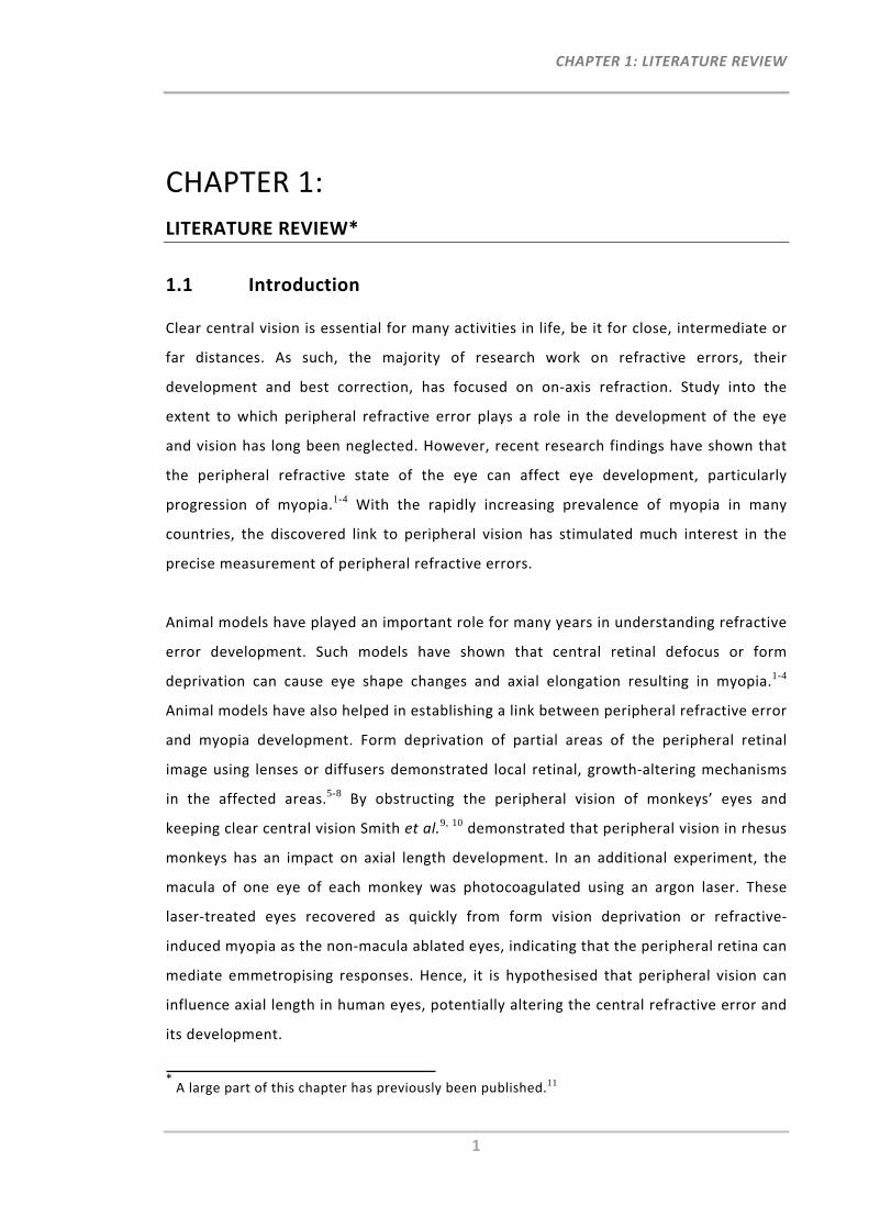
1.1 Introduction
Clear central vision is essential for many activities in life, be it for close, intermediate or
far distances. As such, the majority of research work on refractive errors, their
development and best correction, has focused on on‐axis refraction. Study into the
extent to which peripheral refractive error plays a role in the development of the eye
and vision has long been neglected. However, recent research findings have shown that
the peripheral refractive state of the eye can affect eye development, particularly
progression of myopia.1-4 With the rapidly increasing prevalence of myopia in many
countries, the discovered link to peripheral vision has stimulated much interest in the
precise measurement of peripheral refractive errors.
Animal models have played an important role for many years in understanding refractive
error development. Such models have shown that central retinal defocus or form
deprivation can cause eye shape changes and axial elongation resulting in myopia.1-4
Animal models have also helped in establishing a link between peripheral refractive error
and myopia development. Form deprivation of partial areas of the peripheral retinal
image using lenses or diffusers demonstrated local retinal, growth‐altering mechanisms
in the affected areas.5-8 By obstructing the peripheral vision of monkeys’ eyes and
keeping clear central vision Smith et al.9, 10 demonstrated that peripheral vision in rhesus
monkeys has an impact on axial length development. In an additional experiment, the
macula of one eye of each monkey was photocoagulated using an argon laser. These
laser‐treated eyes recovered as quickly from form vision deprivation or refractive‐
induced myopia as the non‐macula ablated eyes, indicating that the peripheral retina can
mediate emmetropising responses. Hence, it is hypothesised that peripheral vision can
influence axial length in human eyes, potentially altering the central refractive error and
its development.
* A large part of this chapter has previously been published.11
CHAPTER 1: LITERATURE REVIEW
2
In humans, the first link between peripheral refraction and myopia was found in 1971 by
Hoogerheide et al.12 Seventy‐seven percent of young emmetropic pilots with relative
hyperopic shifts in the periphery developed myopia during their training. At that time it
was not acceptable for pilots to have any myopia when commencing their pilot training.
This peripheral refraction test was therefore the first method used in association with
refractive error development to predict the risk of late‐onset myopia for young pilots.
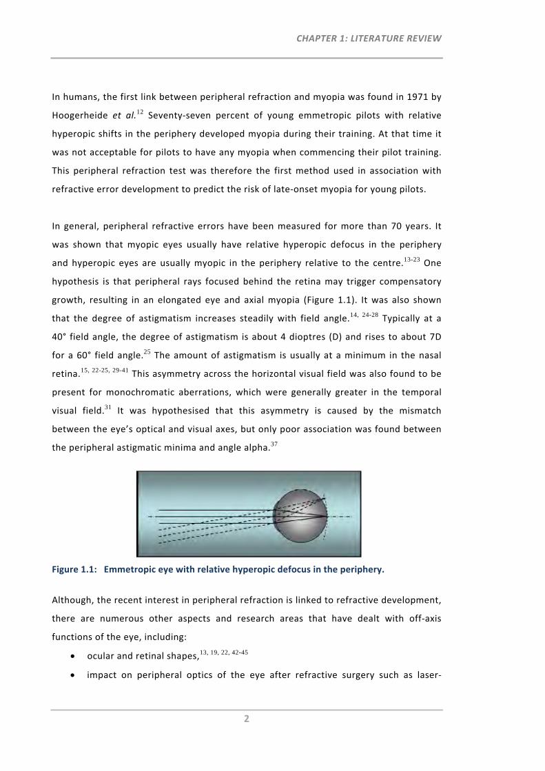
In general, peripheral refractive errors have been measured for more than 70 years. It
was shown that myopic eyes usually have relative hyperopic defocus in the periphery
and hyperopic eyes are usually myopic in the periphery relative to the centre.13-23 One
hypothesis is that peripheral rays focused behind the retina may trigger compensatory
growth, resulting in an elongated eye and axial myopia (Figure 1.1). It was also shown
that the degree of astigmatism increases steadily with field angle.14, 24-28 Typically at a
40° field angle, the degree of astigmatism is about 4 dioptres (D) and rises to about 7D
for a 60° field angle.25 The amount of astigmatism is usually at a minimum in the nasal
retina.15, 22-25, 29-41 This asymmetry across the horizontal visual field was also found to be
present for monochromatic aberrations, which were generally greater in the temporal
visual field.31 It was hypothesised that this asymmetry is caused by the mismatch
between the eye’s optical and visual axes, but only poor association was found between
the peripheral astigmatic minima and angle alpha.37
Figure 1.1: Emmetropic eye with relative hyperopic defocus in the periphery.
Although, the recent interest in peripheral refraction is linked to refractive development,
there are numerous other aspects and research areas that have dealt with off‐axis
functions of the eye, including:
ocular and retinal shapes,13, 19, 22, 42-45
impact on peripheral optics of the eye after refractive surgery such as laser‐

CHAPTER 1: LITERATURE REVIEW
3
assisted in situ keratomileusis (LASIK),46, 47 photorefractive keratectomy,48 or
intraocular lens implantation,47
improvement and better understanding of psychophysical tasks (visual field
perimetry, contrast detection tasks) through correction of the peripheral
refractive errors of the eye,27, 49-53
improvement of off‐axis vision in patients with central visual field loss,54-56
development of theoretical model eyes,57, 58
association between age and peripheral refraction/aberrations,35, 59-62
measurement of peripheral refraction in different ethnicities,63
measurement of angle alpha,37, 58 and angle kappa,54
measurement of refractive changes for different gazes,23, 64-69
measurement of peripheral refractive changes for different accommodation
states,34, 44, 67, 70-75
comparison of peripheral refraction between phakic and with intraocular lens‐
corrected eyes,76
determination of peripheral refraction in keratoconus patients,77
assessment of the risk of onset of myopia,78
impact of orthokeratology lenses on peripheral vision and/or the peripheral
refraction profile 36, 79, 80 and
measurement of peripheral refraction with radial refractive gradient
spectacles,52 soft and rigid contact lenses81 and other custom‐designed spectacle
lenses.82, 83
In general, refraction is a well‐known clinical and optometric procedure used to prescribe
spectacle lenses or contact lenses that deliver clear central vision. Due to its clinical relevance,
numerous objective refraction instruments have been developed over the last years to ease
and streamline clinical vision work. Technological improvements have resulted in many
accurate, reliable methods, such as autorefractors and aberrometers. With the interest in
researchers also wanting to perform peripheral refraction, these commercially available
instruments were generally modified so that they permit the measurement of the peripheral
optics of the eye. As yet no instrument is commercially available which has been designed
with the designated purpose of measuring peripheral refractive errors rapidly and precisely.
CHAPTER 1: LITERATURE REVIEW
4
In this review, previous investigations into peripheral vision of the human eye and methods of
peripheral refractive error measurement will be discussed and obstacles relating to current
measurement techniques ascertained. Information on preference and usefulness of certain
peripheral refraction techniques and suggestions for future technology and research work will
also be given.
1.2 Peripheral Vision
For the measurement of peripheral vision it is important to understand the optical and
physiological factors in the periphery of the eye and to identify stimuli that are most
useful for peripheral vision testing.
Optical factors affecting quality of peripheral vision are refractive error, diffraction,
scatter and aberrations such as high levels of oblique astigmatism, curvature of the field
and horizontal coma. Existence of oblique astigmatism induced by the oblique angle of
the incident light has been known for many years. As early as 1801, Thomas Young
stated that the eye’s “imperfection is partly owing to the unavoidable aberration of
oblique rays, but principally to the insensibility of the retina”.84
Insensitivity of the peripheral retina can be explained by the receptive fields and a
number of neural factors which gradually change from the macula to the periphery,
affecting different aspects of retinal image quality. This includes size, spacing, function,
alignment and distribution of retinal photoreceptors, the rods and cones.85 Whereas the
peripheral retina is dominated by rods, good detectors of motion, the macula area
consists mainly of cones, which are essential for resolution of fine detail, form and
colour detection.
The Troxler effect, discovered in 1804,86, 87 is another factor influencing peripheral vision. This
effect describes an optical cognitive phenomenon whereby a stimulus in the peripheral vision
fades away when a central stimulus is fixated in steady gaze for several seconds. This
phenomenon is due to the adaptation of neurons in the visual system and may form an
obstacle to peripheral vision testing.
CHAPTER 1: LITERATURE REVIEW
5
Physical factors influencing peripheral image quality include peripheral restrictions from
the morphology of eye lids or eye lid abnormalities. The morphology of the eye lids
differs between some ethnic populations, most notably between East Asians and
Caucasians. Studies have shown that a smaller palpebral fissure size, as common in Asian
eye lids, can have an impact on refractive error.88-91
1.2.1 Methods of Testing Peripheral Vision
Central vision is commonly measured by use of a resolution target, such as a logMAR
Bailey‐Lovie chart, in which letters need to be identified. Considering the neural
differences associated with central and peripheral retinal sampling, it has been
suggested to use two different testing procedures for on‐axis and off‐axis vision tests.
Campbell and Gubisch92 showed that resolution in the peripheral visual field is limited
much more by neural factors, due to the reduced density of the retinal ganglion cells
than by optical factors. While detection acuity remains high with increasing eccentricity,
resolution acuity decreases drastically.93-95
There are numerous different peripheral vision tests reported in the research literature,
including motion detection tests such as high‐pass resolution perimetry,54, 96 the
movement of a white square on a black background,97, 98 contrast detection sensitivity
tests using a Gabor stimulus27, 99 or gratings55, 93, 100-103 and resolution tests using the
tumbling‐E letters,21, 100 Landolt C21, 53 or number identification.55 Due to evidence
suggesting peripheral resolution is sampling‐limited, it has been recommended to use
contrast detection sensitivity tests for subjective assessment of peripheral image
quality.27, 101
Several studies have investigated the impact of refractive blur on assessing quality of
peripheral vision using different stimuli.94, 95, 104 Overall, it has been demonstrated that
detection acuity varies strongly with defocus, whereas resolution acuity for high contrast
targets is unaffected by peripheral defocus. The difference between the two acuity
thresholds depends on target properties.101 A decrease in spatial frequencies, as well as
in luminance levels of the stimulus, will reduce detection acuity to a point where it
eventually aligns with resolution acuity, and both will be contrast‐limited.
CHAPTER 1: LITERATURE REVIEW
6
Objective methods such as assessment of point‐spread and line‐spread function using a
double‐pass technique have also been used for evaluation of peripheral image quality.
For larger peripheral angles, the higher order aberrations become more prominent,
impairing the point‐spread or line‐spread function and consequently the peripheral
visual performance.105-107
Correction of peripheral refractive errors is strongly pupil size‐dependent but has shown
to improve image quality and, with that, detection of contrast and movement.38, 54, 55, 93,
97, 108, 109 However, due to the clinical and optometric focus on central refractive error
and only marginal improvement in peripheral resolution acuity, it has often been
discounted, even though peripheral detection acuity can be improved.94 With the current
knowledge that peripheral refraction can influence refractive development, the
assessment of peripheral vision has also become of increased interest to researchers.
Thus, methods and stimuli should be selected carefully when testing peripheral vision.
1.3 Peripheral Refractive Error Measurement Techniques
That visual performance decreases as visual field angle increases has been known for
more than two centuries, when Thomas Young84 indicated that the eye’s “whole extent
of perfect vision is little more than 10 degrees… the imperfections begin within a degree
or two of the visual axis”. First measurements of peripheral refraction were performed
by Ferree and co‐workers in 1931.68
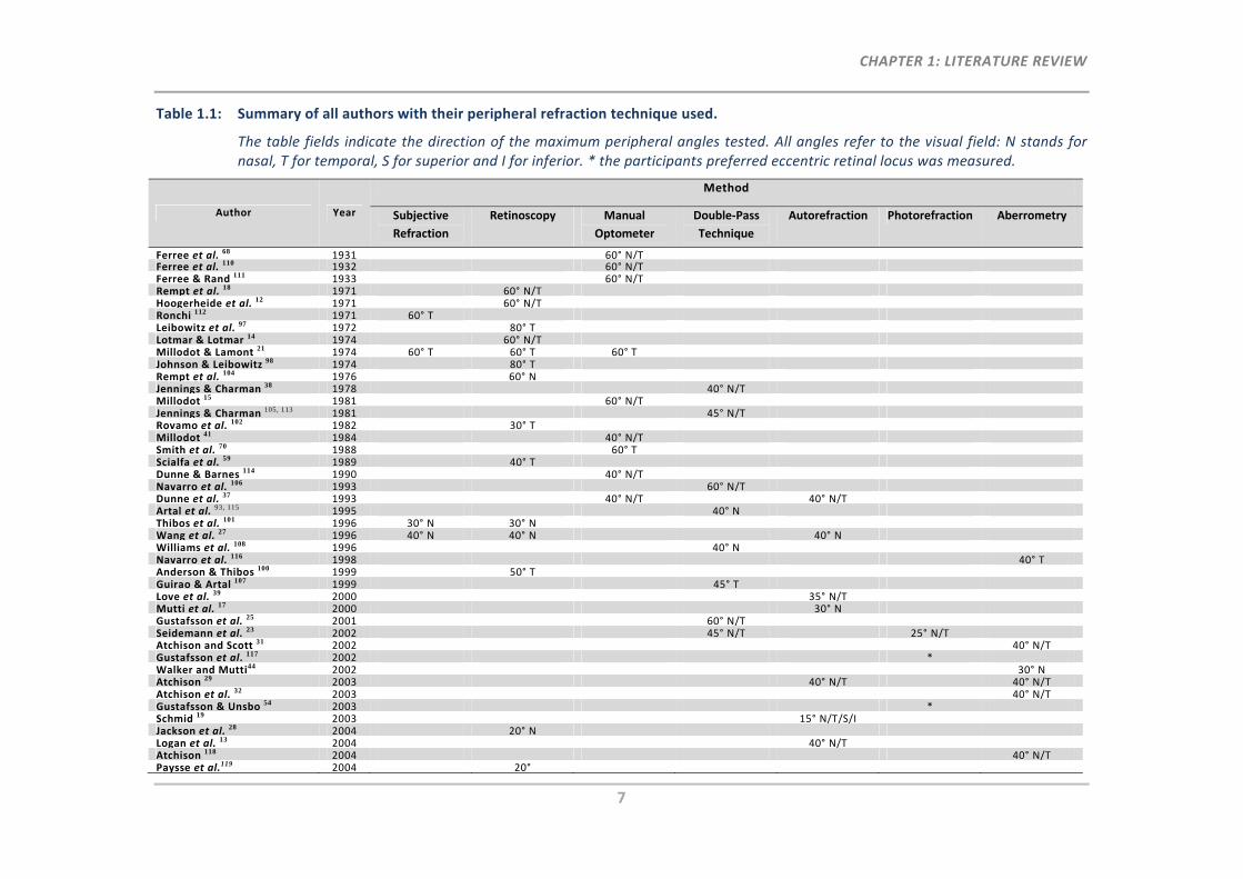
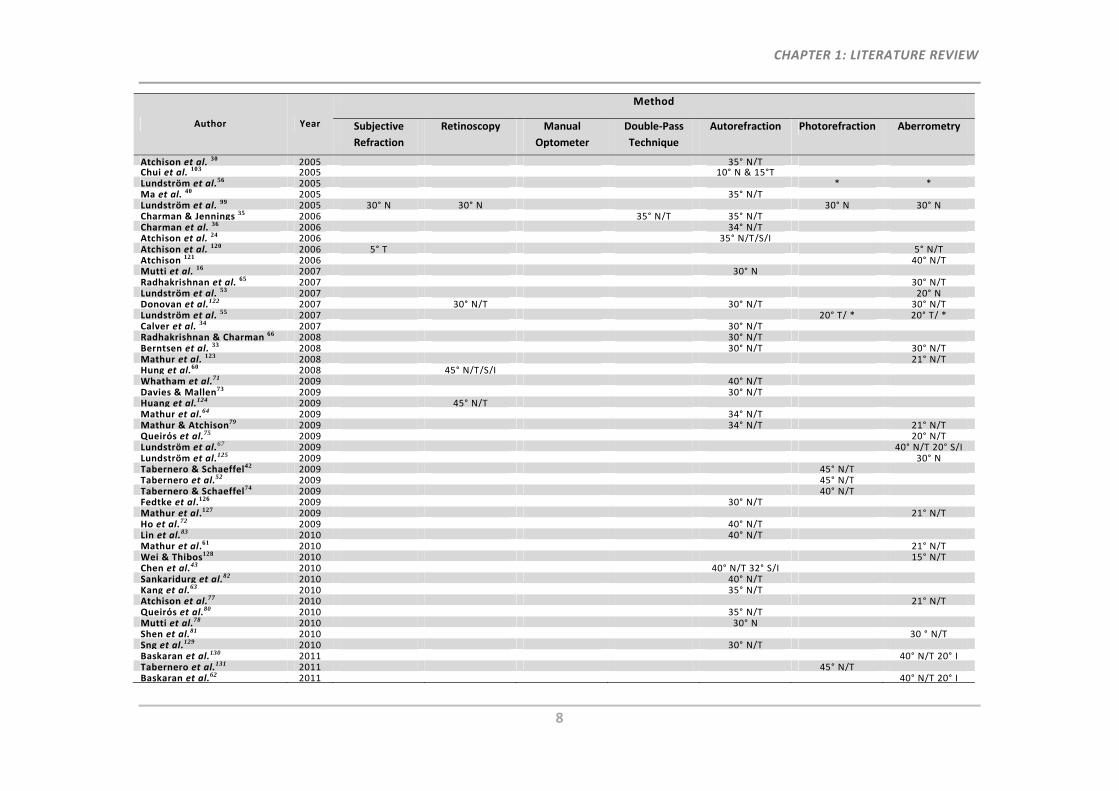
Table 1.1 provides a comprehensive summary on authors and their particular techniques
used for the measurement of peripheral refractive errors. Peripheral refractive errors
were usually measured in steps of 5° or 10°, with techniques such as subjective
refraction, double‐pass technique, manual optometers, retinoscopy, or more common
objective instruments, such as autorefractors, photorefractometers or aberrometers.
Dependent on the instrument modification and study purpose, researchers may either
refer to angles measured with respect to the visual field24, 40, 64 or the retina23, 34, 71 or the
fixation direction.64 The peripheral angles shown in Table 1.1 correspond to the visual
field.
CHAPTER 1: LITERATURE REVIEW
7
Table 1.1: Summary of all authors with their peripheral refraction technique used.
The table fields indicate the direction of the maximum peripheral angles tested. All angles refer to the visual field: N stands for nasal, T for temporal, S for superior and I for inferior. * the participants preferred eccentric retinal locus was measured.
Author Year
Method
Subjective
Refraction
Retinoscopy Manual
Optometer
Double‐Pass
Technique
Autorefraction Photorefraction Aberrometry
Ferree et al. 68 1931 60° N/TFerree et al. 110 1932 60° N/TFerree & Rand 111 1933 60° N/TRempt et al. 18 1971 60° N/THoogerheide et al. 12 1971 60° N/TRonchi 112 1971 60° TLeibowitz et al. 97 1972 80° TLotmar & Lotmar 14 1974 60° N/TMillodot & Lamont 21 1974 60° T 60° T 60° TJohnson & Leibowitz 98 1974 80° TRempt et al. 104 1976 60° NJennings & Charman 38 1978 40° N/TMillodot 15 1981 60° N/TJennings & Charman 105, 113 1981 45° N/TRovamo et al. 102 1982 30° TMillodot 41 1984 40° N/TSmith et al. 70 1988 60° TScialfa et al. 59 1989 40° TDunne & Barnes 114 1990 40° N/TNavarro et al. 106 1993 60° N/TDunne et al. 37 1993 40° N/T 40° N/TArtal et al. 93, 115 1995 40° NThibos et al. 101 1996 30° N 30° NWang et al. 27 1996 40° N 40° N 40° NWilliams et al. 108 1996 40° NNavarro et al. 116 1998 40° TAnderson & Thibos 100 1999 50° TGuirao & Artal 107 1999 45° TLove et al. 39 2000 35° N/TMutti et al. 17 2000 30° NGustafsson et al. 25 2001 60° N/TSeidemann et al. 23 2002 45° N/T 25° N/TAtchison and Scott 31 2002 40° N/TGustafsson et al. 117 2002 *Walker and Mutti44 2002 30° NAtchison 29 2003 40° N/T 40° N/TAtchison et al. 32 2003 40° N/TGustafsson & Unsbo 54 2003 *Schmid 19 2003 15° N/T/S/IJackson et al. 28 2004 20° NLogan et al. 13 2004 40° N/TAtchison 118 2004 40° N/TPaysse et al.119 2004 20°
CHAPTER 1: LITERATURE REVIEW
8
Author Year
Method
Subjective
Refraction
Retinoscopy Manual
Optometer
Double‐Pass
Technique
Autorefraction Photorefraction Aberrometry
Atchison et al. 30 2005 35° N/TChui et al. 103 2005 10° N & 15°TLundström et al.56 2005 * *Ma et al. 40 2005 35° N/TLundström et al. 99 2005 30° N 30° N 30° N 30° NCharman & Jennings 35 2006 35° N/T 35° N/TCharman et al. 36 2006 34° N/TAtchison et al. 24 2006 35° N/T/S/IAtchison et al. 120 2006 5° T 5° N/TAtchison 121 2006 40° N/TMutti et al. 16 2007 30° NRadhakrishnan et al. 65 2007 30° N/TLundström et al. 53 2007 20° NDonovan et al.122 2007 30° N/T 30° N/T 30° N/TLundström et al. 55 2007 20° T/ * 20° T/ *Calver et al. 34 2007 30° N/TRadhakrishnan & Charman 66 2008 30° N/TBerntsen et al. 33 2008 30° N/T 30° N/TMathur et al. 123 2008 21° N/THung et al.60 2008 45° N/T/S/IWhatham et al.71 2009 40° N/TDavies & Mallen73 2009 30° N/THuang et al.124 2009 45° N/TMathur et al.64 2009 34° N/TMathur & Atchison79 2009 34° N/T 21° N/TQueirόs et al.75 2009 20° N/TLundström et al.67 2009 40° N/T 20° S/ILundström et al.125 2009 30° NTabernero & Schaeffel42 2009 45° N/TTabernero et al.52 2009 45° N/TTabernero & Schaeffel74 2009 40° N/TFedtke et al.126 2009 30° N/TMathur et al.127 2009 21° N/THo et al.72 2009 40° N/TLin et al.83 2010 40° N/TMathur et al.61 2010 21° N/TWei & Thibos128 2010 15° N/TChen et al.43 2010 40° N/T 32° S/ISankaridurg et al.82 2010 40° N/TKang et al.63 2010 35° N/TAtchison et al.77 2010 21° N/TQueirόs et al.80 2010 35° N/TMutti et al.78 2010 30° NShen et al.81 2010 30 ° N/TSng et al.129 2010 30° N/TBaskaran et al.130 2011 40° N/T 20° ITabernero et al.131 2011 45° N/TBaskaran et al.62 2011 40° N/T 20° I
CHAPTER 1: LITERATURE REVIEW
9
1.3.1 Subjective Peripheral Refraction
In general, subjective refraction is designated as the “gold standard” for on‐axis
refraction, particularly for the purpose of prescribing optical correction devices. A
literature review by Goss and Grosvenor132 concludes that central subjective refraction
provides reliable refraction measurements within 0.25D to 0.50D and suggests this
technique always be conducted for refinement of objective refraction results.
In general, peripheral refractive errors can be obtained subjectively through
manipulation of the refractive state by introducing trial lenses with different powers into
the peripheral viewing path. The lens that maximises acuity will be determined to
correct the peripheral refractive error of the eye in the appropriate peripheral angle.
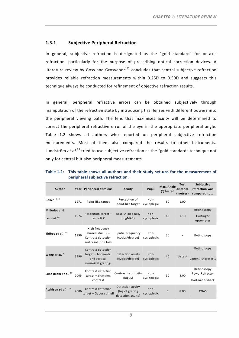
Table 1.2 shows all authors who reported on peripheral subjective refraction
measurements. Most of them also compared the results to other instruments.
Lundström et al.99 tried to use subjective refraction as the “gold standard” technique not
only for central but also peripheral measurements.
Table 1.2: This table shows all authors and their study set‐ups for the measurement of peripheral subjective refraction.
Author Year Peripheral Stimulus Acuity Pupil Max. Angle
(°) tested
Test
distance
(metres)
Subjective
refraction was
compared to …
Ronchi 112 1971 Point‐like target
Perception of
point‐like target
Non‐
cycloplegic60 1.00 ‐
Millodot and
Lamont 26 1974
Resolution target –
Landolt C
Resolution acuity
(logMAR)
Non‐
cycloplegic60 1.10
Retinoscopy
Hartinger
optometer
Thibos et al. 101 1996
High frequency
aliased stimuli –
Contrast detection
and resolution task
Spatial frequency
(cycles/degree)
Non‐
cycloplegic30 ‐ Retinoscopy
Wang et al. 27 1996
Contrast detection
target – horizontal
and vertical
sinusoidal gratings
Detection acuity
(cycles/degree)
Non‐
cycloplegic40 distant
Retinoscopy
Canon Autoref R‐1
Lundström et al. 99
2005
Contrast detection
target – changing
contrast
Contrast sensitivity
(logCS)
Non‐
cycloplegic30 3.00
Retinoscopy
PowerRefractor
Hartmann‐Shack
Atchison et al. 120 2006
Contrast detection
target – Gabor stimuli
Detection acuity
(log of grating
detection acuity)
Non‐
cycloplegic5 8.00 COAS
CHAPTER 1: LITERATURE REVIEW
10
The first peripheral subjective refraction measurements were reported by Ronchi112 in
1971, who studied the relationship between absolute luminance threshold and retinal
eccentricity. The participant, who was experienced in visual experiments, was asked to
view and judge a point‐like peripheral target. Correction of oblique astigmatism up to
60° was achieved using cross‐cylinders.
For four participants, Wang et al.27 and Millodot and Lamont21, 27 compared peripheral
subjective refraction results with two other refraction techniques. They found that with
increasing eccentricity, the agreement of peripheral subjective refraction was closer to
peripheral retinoscopic refraction rather than to results obtained with an optometer or
autorefractor, which revealed highest astigmatism results. Lundström et al.’s 99
peripheral subjective refraction data revealed a larger spread compared with the
Hartmann‐Shack sensor, photorefractor and retinoscopy. Atchison et al.’s120 study
investigated refractive error and aberration variations in the central visual field. They
undertook subjective refraction in the temporal visual field at 2.2° and 5°. Comparison
with refractive errors obtained using the Complete Ophthalmic Analysis System (COAS)
wavefront sensor showed that subjective refraction exhibited a smaller refractive change
(0.37D) between central and 5° measurements than using the wavefront sensing
technique (0.71D).
As mentioned previously, there are several different peripheral vision test targets, which
make a direct comparison or assessment of peripheral refractive error results between
studies difficult. Whereas Wang et al., Lundström et al. and Atchison et al. used contrast
detection stimuli to measure the peripheral refractive state of the eye, Millodot and
Lamont used a resolution target, the Landolt C, while Ronchi relied on the participant’s
shape perception of the peripheral target. Thibos et al.101 highlighted a difference in
peripheral acuity results between spatial resolution and contrast detection tasks, which
reinforces the importance of stimuli choice when assessing peripheral vision or when
measuring peripheral subjective refraction.
Since peripheral subjective refraction requires the participant to pay constant attention
in order to try and detect the target stimulus, it is a difficult and exhausting technique to
CHAPTER 1: LITERATURE REVIEW
11
perform, in particular if there are multiple or large peripheral angles to be tested.99 The
difficulties are mainly due to optical factors such as the increase in peripheral
astigmatism, poor paraxial retinal image quality as well as neural factors, which are
stimuli‐dependent. The previously mentioned Troxler effect can also have an impact on
acuity measurements.86 As a possible result of all these factors, subjective peripheral
refraction measurements have been found to yield highly variable results99 and
measurements are often limited to axis approximations of 90° and 180° when
astigmatism is determined.27 No studies were found reporting on repeatability for
peripheral subjective refraction.
1.3.2 Retinoscopy
Retinoscopy, particularly streak retinoscopy, is a refraction technique that has been used
successfully for the precise measurement of central refraction. The relative movement of
the reflex from the participant’s retina is observed and, with the aid of lenses,
neutralised, providing the eye’s refractive error. The main advantage is its accuracy
when used in pediatric participants and performed by a skilled clinician because it
requires no co‐operation from the participant. Since the participant is not actively
involved in the process retinoscopy is considered an objective technique, however
assessment of the retinoscopic reflex requires an experience‐dependent subjective
decision by the practitioner.
Several studies have used this technique to also measure the peripheral optics of the eye
(Table 1.3).
The first peripheral retinoscopic measurements were conducted by Rempt et al.,18 who
on the basis of their results, introduced the skiagram. This is a peripheral refractometric
diagram used for the categorisation of different peripheral refractive error patterns. For
the large sample sized study they preferred the use of a retinoscope rather than the
optometer technique used by Ferree et al.,68, 110, 111 since this method would have been
“too cumbersome” for the peripheral data to be collected on 442 participants.
Hoogerheide et al.12 and Lotmar and Lotmar14 targeted their investigations in reference
to the refractive error results presented by Rempt et al.18 Hoogerheide and co‐workers’
interests were in finding a characteristic pattern that can predict whether one

CHAPTER 1: LITERATURE REVIEW
12
emmetropic person is more prone to develop myopia than another. Their finding showed
that young emmetropic pilots with hyperopic defocus in the peripheral field were at risk
of developing myopia. Lotmar and Lotmar investigated whether the non‐cycloplegic
peripheral refraction data provided by Rempt et al. fit the theoretical model eye
proposed by Lotmar57 in 1971. Close agreement between the measured and calculated
peripheral astigmatism values was only found up to about 30° eccentricities, thereafter
the theoretical eye model did not fit well with the experimental findings.
Table 1.3: This table shows all authors and their study set‐ups for the measurement of peripheral retinoscopy.
Author Year Pupil Max. Peripheral
angle (°) tested
Test distance to
fixation target
(metres)
Retinoscopy was
compared to …
Rempt et al. 18 1971 cycloplegic 60 3 ‐
Leibowitz et al. 97 1972 ‐ 80 0.787 ‐
Millodot and
Lamont 26 1974 cycloplegic 50 1.1
Subjective refraction
Optometer
Johnson and
Leibowitz 98 1974 non‐cycloplegic 80 0.77 ‐
Rempt et al. 104 1976 cycloplegic 60 3 ‐
Rovamo et al. 102 1982 ‐ 30 ‐ ‐
Scialfa et al. 59 1989 ‐ 40 0.83 ‐
Wang et al. 27 1996 non‐cycloplegic 40 distant Subjective refraction
Autorefraction
Anderson and
Thibos 100 1999 non‐cycloplegic 50 3 ‐
Jackson et al. 28 2004 cycloplegic 20 0.4 ‐
Paysse et al.119 2004 cycloplegic 20 0.4 ‐
Lundström et al. 99 2005 non‐cycloplegic 30 3
Subjective refraction
Photorefraction
Wavefront Sensor
Donovan et al.122 2007 cycloplegic 30 ‐ Autorefraction
Wavefront Sensor
Hung et al.60 2008 cycloplegic 45 0.5 ‐
Huang et al.124 2009 cycloplegic 45 0.5 ‐
Interestingly, two studies conducted by Leibowitz et al.97 and Johnson and Leibowitz98
were able to provide results for measurements of up to 80° in three participants. In
contrast, Millodot and Lamont21 were unable to obtain reliable retinoscopic readings
beyond 50°. Furthermore, Leibowitz et al.97 and Johnson and Leibowitz98 measured
peripheral astigmatism that is far below the values of the majority of published data.
Even though both studies reported measuring far off‐axis refractive errors, no comment
CHAPTER 1: LITERATURE REVIEW
13
was made as to whether it was difficult to perform or whether it can be assumed to be
reliable. However, literature has shown that the majority of studies encountered
difficulties when performing peripheral retinoscopy, in particular for large angles.26, 28, 59
The main issue is that, as measurement angles increase, the pupil appears elliptical to
the examiner and aberrations increase in the periphery. As a result the aberrated reflex
at large angles may be split or behave contradictorily in central and peripheral parts of
the pupil and consequently, it is more complex and difficult to precisely define. This
difficulty was found to be most cumbersome for the task of determining the axis of the
astigmatism.18, 21, 28, 99
Jackson et al.28 and Paysse et al.119 performed peripheral retinoscopy under cycloplegia
in angles up to 20° in order to investigate how much impact slight off‐axis retinoscopy
has in clinical practice. They found a clinically important increase in astigmatism by an
average of 3% per degree of eccentricity. Paysse et al. concluded that “even small
degrees of eccentricity can result in significant errors in refractive error determination.”
Zadnik et al.133 reported that the repeatability of the central retinoscopic measurements
under cycloplegia is poor. The effects of paralysing accommodation through cycloplegia,
which inhibit refraction stability and increase aberrations due to the dilated pupil, would
explain the generally poorer repeatability using cycloplegic retinoscopy. Table 1.3 shows
that half the studies conducted peripheral retinoscopy under cycloplegia, making results
not directly comparable to the refraction results measured under natural pupil
conditions.
Wang et al.27 measured eccentricities of up to 40° (n=3) and Millodot and Lamont26 up to
50° (n=4). They reported that the results were in good agreement with those of
peripheral subjective refraction, the Canon R‐1 autorefractor27 and the manual
optometer (Zeiss Hartinger) respectively.26 Compared to other subjective and objective
techniques, Lundström et al.99 found in a study of 50 participants a significant difference
in cylinder axis when peripheral retinoscopy was performed. They also showed
significant differences (mean difference of ‐0.73 D) in 30° spherical equivalent values
between peripheral retinoscopy and subjective refraction, whereby the retinoscopic
CHAPTER 1: LITERATURE REVIEW
14
values tended towards hyperopia. However, carrying out non‐cycloplegic retinoscopic
refraction reduced the pupil diameter, due to the bright light used, and this was thought
to be the reason for the difference to subjective refraction technique, which was
obtained with normal pupil diameter.
In two recent studies, Hung et al.60 and Huang et al.124 conducted peripheral retinoscopy
in monkeys under cycloplegic conditions. Alignment was achieved with the help of an arc
perimeter and by monitoring the position of the first Purkinje images as a reference.
Good agreement was found between the two examiners that measured the refraction in
the peripheral visual field up to 45°. Furthermore, the mean peripheral refraction result
was very repeatable. There was no mention whether they had any difficulties with
respect to the retinoscopic reflex or the alignment of positions of the monkeys.
Overall, it can be concluded that, similar to peripheral subjective refraction
measurements, peripheral retinoscopy has shown difficulties in determining the axis of
the astigmatism.25, 99 Moreover, if numerous peripheral measurements are required, this
technique also appears to be very protracted and inconvenient, for both participants and
examiners.
1.3.3 Manual Refractometer – Optometer
A different principle for the measurement of refraction of the eye was discovered more
than four centuries ago by Christian Jesuit Scheiner.134 The so‐called Scheiner disc is a
disc with two pinholes that enables identification of the point at which an eye focuses
(Figure 1.2). Having the disc aligned in front of the participant’s visual axis and sending
parallel light rays from a distant object light source through the two apertures into the
eye, generates two small bundles of light. A single focus image is formed on the retina if
the eye is emmetropic (Figure 1.2 a). If an ametropic eye is measured, two light spots
will fall on the retina (Figure 1.2 b and c). To measure the refractive error of the eye, the
position of the object has to be adjusted so that the participant can see one light spot.
This can be done by moving the object mechanically, or by placing a convex lens in the
viewing path, as done in the optometer instrument. Whereas first optometers were
purely subjective instruments, requiring the participant to align the target, later so‐
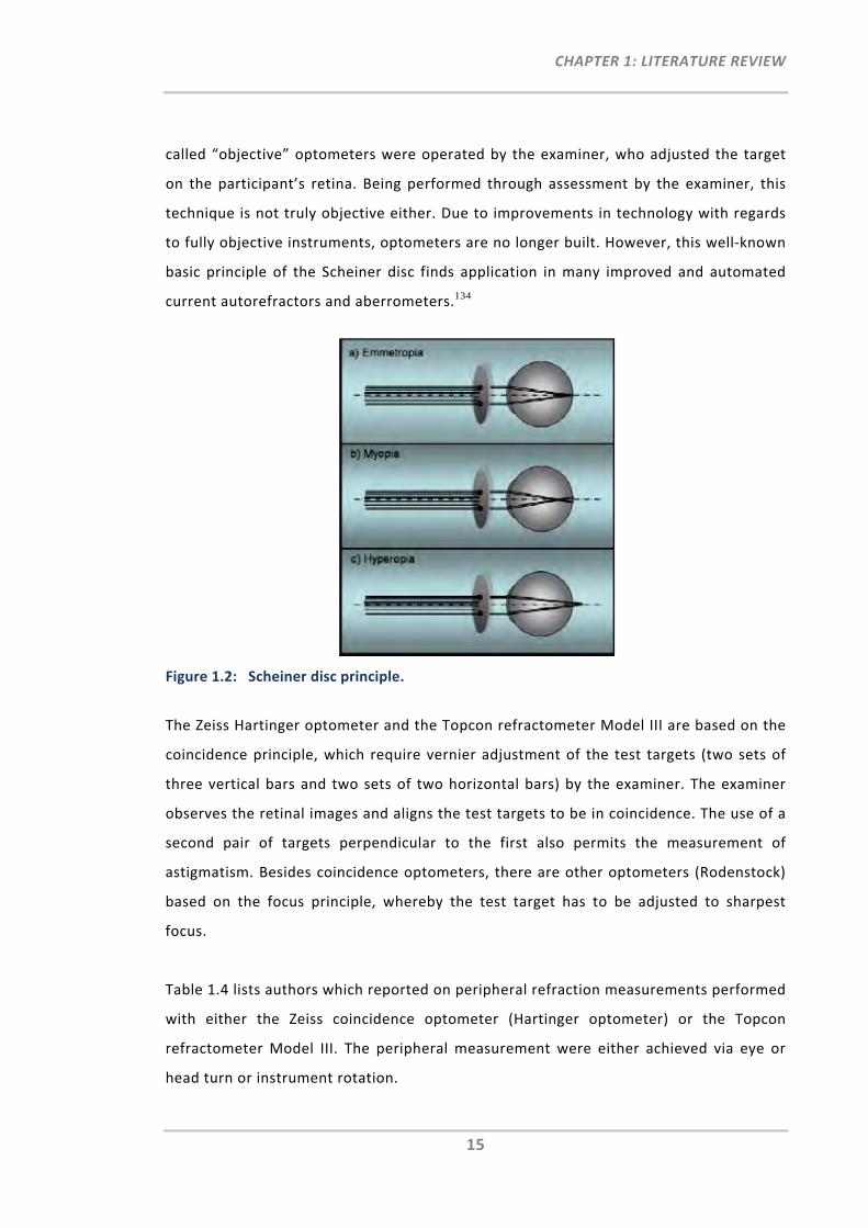
CHAPTER 1: LITERATURE REVIEW
15
called “objective” optometers were operated by the examiner, who adjusted the target
on the participant’s retina. Being performed through assessment by the examiner, this
technique is not truly objective either. Due to improvements in technology with regards
to fully objective instruments, optometers are no longer built. However, this well‐known
basic principle of the Scheiner disc finds application in many improved and automated
current autorefractors and aberrometers.134
Figure 1.2: Scheiner disc principle.
The Zeiss Hartinger optometer and the Topcon refractometer Model III are based on the
coincidence principle, which require vernier adjustment of the test targets (two sets of
three vertical bars and two sets of two horizontal bars) by the examiner. The examiner
observes the retinal images and aligns the test targets to be in coincidence. The use of a
second pair of targets perpendicular to the first also permits the measurement of
astigmatism. Besides coincidence optometers, there are other optometers (Rodenstock)
based on the focus principle, whereby the test target has to be adjusted to sharpest
focus.
Table 1.4 lists authors which reported on peripheral refraction measurements performed
with either the Zeiss coincidence optometer (Hartinger optometer) or the Topcon
refractometer Model III. The peripheral measurement were either achieved via eye or
head turn or instrument rotation.
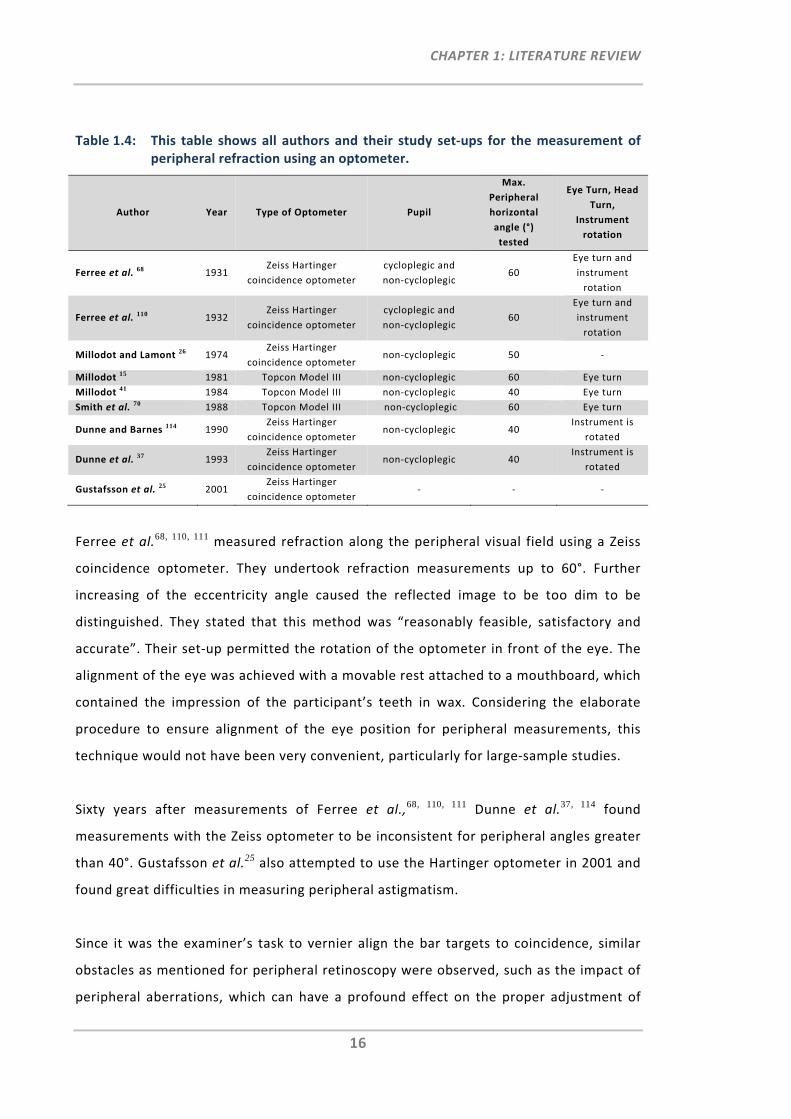
CHAPTER 1: LITERATURE REVIEW
16
Table 1.4: This table shows all authors and their study set‐ups for the measurement of peripheral refraction using an optometer.
Author Year Type of Optometer Pupil
Max.
Peripheral
horizontal
angle (°)
tested
Eye Turn, Head
Turn,
Instrument
rotation
Ferree et al. 68 1931 Zeiss Hartinger
coincidence optometer
cycloplegic and
non‐cycloplegic 60
Eye turn and
instrument
rotation
Ferree et al. 110 1932 Zeiss Hartinger
coincidence optometer
cycloplegic and
non‐cycloplegic 60
Eye turn and
instrument
rotation
Millodot and Lamont 26 1974 Zeiss Hartinger
coincidence optometer non‐cycloplegic 50 ‐
Millodot 15 1981 Topcon Model III non‐cycloplegic 60 Eye turn
Millodot 41 1984 Topcon Model III non‐cycloplegic 40 Eye turn
Smith et al. 70 1988 Topcon Model III non‐cycloplegic 60 Eye turn
Dunne and Barnes 114 1990 Zeiss Hartinger
coincidence optometer non‐cycloplegic 40
Instrument is
rotated
Dunne et al. 37 1993 Zeiss Hartinger
coincidence optometer non‐cycloplegic 40
Instrument is
rotated
Gustafsson et al. 25 2001 Zeiss Hartinger
coincidence optometer ‐ ‐ ‐
Ferree et al.68, 110, 111 measured refraction along the peripheral visual field using a Zeiss
coincidence optometer. They undertook refraction measurements up to 60°. Further
increasing of the eccentricity angle caused the reflected image to be too dim to be
distinguished. They stated that this method was “reasonably feasible, satisfactory and
accurate”. Their set‐up permitted the rotation of the optometer in front of the eye. The
alignment of the eye was achieved with a movable rest attached to a mouthboard, which
contained the impression of the participant’s teeth in wax. Considering the elaborate
procedure to ensure alignment of the eye position for peripheral measurements, this
technique would not have been very convenient, particularly for large‐sample studies.
Sixty years after measurements of Ferree et al.,68, 110, 111 Dunne et al.37, 114 found
measurements with the Zeiss optometer to be inconsistent for peripheral angles greater
than 40°. Gustafsson et al.25 also attempted to use the Hartinger optometer in 2001 and
found great difficulties in measuring peripheral astigmatism.
Since it was the examiner’s task to vernier align the bar targets to coincidence, similar
obstacles as mentioned for peripheral retinoscopy were observed, such as the impact of
peripheral aberrations, which can have a profound effect on the proper adjustment of
CHAPTER 1: LITERATURE REVIEW
17
the optometer targets. Furthermore, the effect of having an elliptical pupil when
measuring through the periphery of the eye reduces the area for the measurement
targets that are focused onto the retina. This finding was mentioned in Smith et al.’s70
study, in which it was noted that for eccentricities larger than 60°, the diameter of the
elliptical pupil is smaller than the outer areas of the target, which are then partially cut‐
off and make adjustment impossible.
1.3.4 Double‐Pass Technique
The double‐pass technique is an ophthalmoscopic method, which was first introduced by
Flamant135 in 1955, enabling the assessment of central retinal image quality. In 1981
Santamaria et al.136 used this method to record double‐pass images of point‐spread
function.
Different experimental set‐ups of the double‐pass techniques were implemented by
different researcher groups.23, 35, 106, 108 The basic principle is that a laser light beam,
usually Helium‐Neon laser, passes first through a neutral density filter to reduce light
intensity and is then spatially filtered by a microscope objective. The beam that expands
from this point source is collimated before entering a small artificial pupil or a slit of a
slit‐lamp that is conjugate with the pupil of the eye. The optical system of the eye then
forms the aberrated image of the point or line source on the retina. The fundus, acting
as a diffuse surface, reflects a small fraction of light and a camera then captures the so‐
called “double‐pass images”. In order to measure the refractive error of the eye, a
focusing lens scans through the double‐pass images and the images corresponding to the
extremes of the Sturm interval are observed. Refraction can be validated by placing the
corrective lens in front of the participant’s eye and the compact image of the least‐
confusion circle will be observable.
Thirteen years after its first on‐axis use, this double‐pass technique has also been
applied for the measurement and evaluation of the peripheral optics of the eye (Table
1.5).
Navarro and Artal106 investigated retinal image quality of point light sources across a
wide visual field, evaluating double‐pass images. Initially, they found paraxial image
CHAPTER 1: LITERATURE REVIEW
18
quality to be much better than previously indicated. They found this to be due to the
loss of paraxial asymmetric aberrations, such as coma and distortion, in the double‐
pass.115 To circumvent this impediment, two alternatives were suggested and
investigated. The first attempt was a modified version of the double‐pass technique,
using different entrance and exit pupil diameters and the second required reconstruction
of the PSF by phase‐retrieval algorithms.107 Both methods provided an estimate of off‐
axis astigmatism and horizontal coma.
Jennings and Charman used the line spread function (LSF) double‐pass technique to
assess image quality across the retina,38 and to correct peripheral refractive errors for
the measurement of the critical fusion frequency113 and to investigate peripheral
refraction changes with age35. For all measurements, they recorded radial and tangential
LSFs in 5° steps up to eccentricities of 45°. Using this double‐pass technique, cylinder
axis determination was limited to 90° or 180°.
Gustafsson et al.25 used a double‐pass technique to measure peripheral astigmatism in
emmetropic eyes in 10° steps up to 60° and found very large individual differences in
oblique astigmatism between 20 eyes. They also repeated the measurements of one
participant on eight different occasions and found a mean standard deviation of the
measured astigmatism over all angles to be 0.60D. The authors also note that the angle
between the sagittal and tangential foci line was different from 90° and that the circle of
least confusion was not in the midpoint of the two foci lines but rather shifted towards
the more hyperopic line.
Seidemann et al.23 used their double‐pass technique for peripheral refraction
measurements up to 45° on 42 participants. Comparison of the photorefraction results
(PowerRefractor) on six participants showed significant correlation. Using a
multimeridional refraction procedure to calculate the average refractive components,
they showed average differences between the spheres of 0.78D and between the
cylinders of 0.85D.

CHAPTER 1: LITERATURE REVIEW
19
Table 1.5: This table shows all authors and their study set‐ups for the measurement of peripheral refraction by use of the double‐pass technique.
Author Year
Double‐Pass Technique
Pupil
Max.
Angle
(°)
tested
Eye or Head
Turn, or
Instrument
Rotation
Double‐pass
technique
was
compared to
…
Apertures Evaluation
Jennings and
Charman 38 1978 Slit
Horizontal and
vertical line
spread function
Non‐
cycloplegic
and
cycloplegic
40 Instrument
is rotated ‐
Jennings and
Charman 105 1981 Slit
Horizontal and
vertical line
spread function
Cycloplegic 45 Instrument
is rotated ‐
Jennings and
Charman 113 1981 Slit
Horizontal and
vertical line
spread function
Cycloplegic 40 Instrument
is rotated ‐
Navarro and
Artal 106 1993
Hole in
perimeter
Modulation
transfer function
Non‐
cycloplegic 60 Head turn ‐
Artal et al. 93 1995
Equal 3 mm
diameter
pupils in
both passes
Focus positions:
sagittal, tangential
foci and circle of
least confusion
Non‐
cycloplegic 40
Instrument
is rotated ‐
Williams et
al.108 1996
Equal 3 mm
diameter
pupils in
both passes
Focus positions:
sagittal, tangential
foci and circle of
least confusion
Cycloplegic 40 Eye turn ‐
Guirao and
Artal 107 1999
Unequal
pupil
diameters
Focus positions:
sagittal, tangential
foci, circle of least
confusion and
coma
Non‐
cycloplegic 45 Eye turn ‐
Gustafsson et
al. 25 2001
Equal 3 mm
diameter
pupils in
both passes
Focus positions:
sagittal, tangential
foci and circle of
least confusion
Non‐
cycloplegic 60
Instrument
is rotated ‐
Seidemann et
al. 23 2002
Equal 1.5
mm
diameter
pupils in
both passes
Focus positions:
sagittal, tangential
foci and circle of
least confusion
Non‐
cycloplegic 45
Instrument
is rotated
Power
Refractor
Jennings and
Charman 35 2006 Slit
Horizontal and
vertical line
spread function
Cycloplegic 35 Instrument
is rotated
Auto‐
refractometer
For most of these peripheral double‐pass techniques, the participants’ head was fixed by
a bite bar and the instrument was rotated in front of the eye. This rotation of the
instrument for each eccentricity angle requires an additional alignment of the second
aperture,93, 108 making it a difficult peripheral refraction procedure to set up. In most
CHAPTER 1: LITERATURE REVIEW
20
studies only few participants were chosen to be measured, which may be due to the
inconvenience of using a bite bar for the alignment.
1.3.5 Autorefraction
Automatic objective refractors (autorefractors, auorefractometers) are fast and easy to
use instruments, which do not require subjective judgments from operators or
participants. For more than two decades they have been used successfully for on‐axis
refraction measurements in ophthalmologic and optometric practices and research
institutions. Most instruments have an integrated function for the measurement of
corneal curvature, which makes them a valuable objective clinical tool.
General problems with some autorefractors can occur due to pseudomyopia caused by
accommodation and inadequate autofogging mechanisms.46, 137-139 Pseudomyopia is
caused by using “closed‐field” autorefractors in which the fixation target is placed at
optical infinity inside the instrument. To avoid instrument‐induced myopia,
autorefraction may be performed under complete cycloplegia. Alternatively, the use of
“open‐view” autorefractors permits fixation and accommodative responses to real‐world
targets external to the instrument.
Only a few autorefractors have been used to measure peripheral refractive errors (Table
1.6). All of them feature a binocular open‐view arrangement through a large beam‐
splitter, avoiding instrument myopia and enabling the fixation of peripheral targets.
These instruments are the Shin‐Nippon NVision K5001, also marketed as the Grand Seiko
WR‐5100K, Shin‐Nippon SRW5000, also marketed as the Grand Seiko WV‐500, the Grand
Seiko WAM‐5500 and the Canon Autoref R‐1. Whereas, the first three instruments
operate on the ring‐autorefraction principle, the Canon Autoref R‐1 operates on the
grating focus principle. Being based on infrared illumination, they all incorporate a
correction factor that adjusts the refraction results to white light. The output refraction
is presented in conventional terms of sphere (S), cylinder (C) and cylinder axis (θ).

CHAPTER 1: LITERATURE REVIEW
21
Table 1.6: This table shows all authors and their study set‐ups for the measurement of peripheral autorefraction.
Author Year Type of Autorefractor Pupil
Max.
peripheralAngle
(°)
Test distance
(metres) Eye or Head Turn
Dunne et al. 371993 Canon Autoref R‐1 Non‐cycloplegic 30 Distant Eye turn
Wang et al. 271996 Canon Autoref R‐1 Non‐cycloplegic 40 Distant ‐
Love et al. 392000 ‐ Cycloplegic 35 Distant ‐
Mutti et al. 172000 Canon Autoref R‐1 Cycloplegic 30 Distant Eye turn
Walker and Mutti44 2002 Canon Autoref R‐1 Non‐cycloplegic 30 Distant Eye turn
Atchison 29 2003
Shin‐Nippon SRW5000 and Canon
Autoref R‐1 Cycloplegic 40 Distant Eye turn
Schmid 192003 Shin‐Nippon NVision K5001 Cycloplegic 15 0.80 ‐
Logan et al. 132004 Canon Autoref R‐1 Cycloplegic 40 0.50 Eye turn
Chui et al.1032005 Shin‐Nippon NVision K5001 Cycloplegic 15 Distant ‐
Atchison et al. 30 2005 Shin‐Nippon SRW5000 Non‐cycloplegic 35 3.30 Eye and head turn
Ma et al. 40
2005 Shin‐Nippon SRW5000 Non‐cycloplegic 35 3.00 Eye turn
Charman and Jennings 35 2006 Shin‐Nippon SRW5000 Non‐cycloplegic 35 6.00 ‐
Charman et al. 36 2006 Shin‐Nippon SRW5000 Non‐cycloplegic 34 3.00 Eye turn
Atchison et al. 24 2006 Shin‐Nippon SRW5000 Non‐cycloplegic 35 3.30 Eye turn
Mutti 16 2007 Canon Autoref R‐1 & the Shin‐Nippon
NVision K5001 Cycloplegic 30 ‐ Eye turn
Calver et al. 342007 Shin‐Nippon Non‐cycloplegic 30 2.50 and 0.40 Eye turn
Donovan et al.122 2007 Shin‐Nippon NVision K5001 cycloplegic 30 2.5 Head turn
Radhakrishnan and Charman 66 2008 Shin‐Nippon SRW5000 Non‐cycloplegic 30 2.00 Eye and head turn
Berntsen et al. 33 2008 Shin‐Nippon NVision K5001 Cycloplegic 30 1.75 Head turn
Queirόs et al.75 2009 Grand Seiko WAM‐5500
Cycloplegic & Non‐
cycloplegic 20 Distant ‐
Whatham et al.71 2009 Shin‐Nippon NVision K5001 Non‐Cycloplegic 40 2.00, 0.40 and 0.30 Head turn
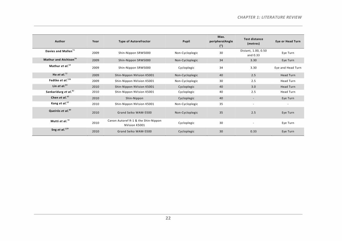
CHAPTER 1: LITERATURE REVIEW
22
Author Year Type of Autorefractor Pupil
Max.
peripheralAngle
(°)
Test distance
(metres) Eye or Head Turn
Davies and Mallen73 2009 Shin‐Nippon SRW5000 Non‐Cycloplegic 30
Distant, 1.00, 0.50
and 0.33 Eye Turn
Mathur and Atchison79 2009 Shin‐Nippon SRW5000 Non‐Cycloplegic 34 3.30 Eye Turn
Mathur et al.64 2009 Shin‐Nippon SRW5000 Cycloplegic 34 3.30 Eye and Head Turn
Ho et al.722009 Shin‐Nippon NVision K5001 Non‐Cycloplegic 40 2.5 Head Turn
Fedtke et al.1262009 Shin‐Nippon NVision K5001 Non‐Cycloplegic 30 2.5 Head Turn
Lin et al.832010 Shin‐Nippon NVision K5001 Cycloplegic 40 3.0 Head Turn
Sankaridurg et al.82 2010 Shin‐Nippon NVision K5001 Cycloplegic 40 2.5 Head Turn
Chen et al.432010 Shin‐Nippon Cycloplegic 40 ‐ Eye Turn
Kang et al.632010 Shin‐Nippon NVision K5001 Non‐Cycloplegic 35 ‐ ‐
Queirόs et al.80 2010 Grand Seiko WAM‐5500 Non‐Cycloplegic 35 2.5 Eye Turn
Mutti et al.78 2010
Canon Autoref R‐1 & the Shin‐Nippon
NVision K5001 Cycloplegic 30 ‐ Eye Turn
Sng et al.1292010 Grand Seiko WAM‐5500 Cycloplegic 30 0.33 Eye Turn
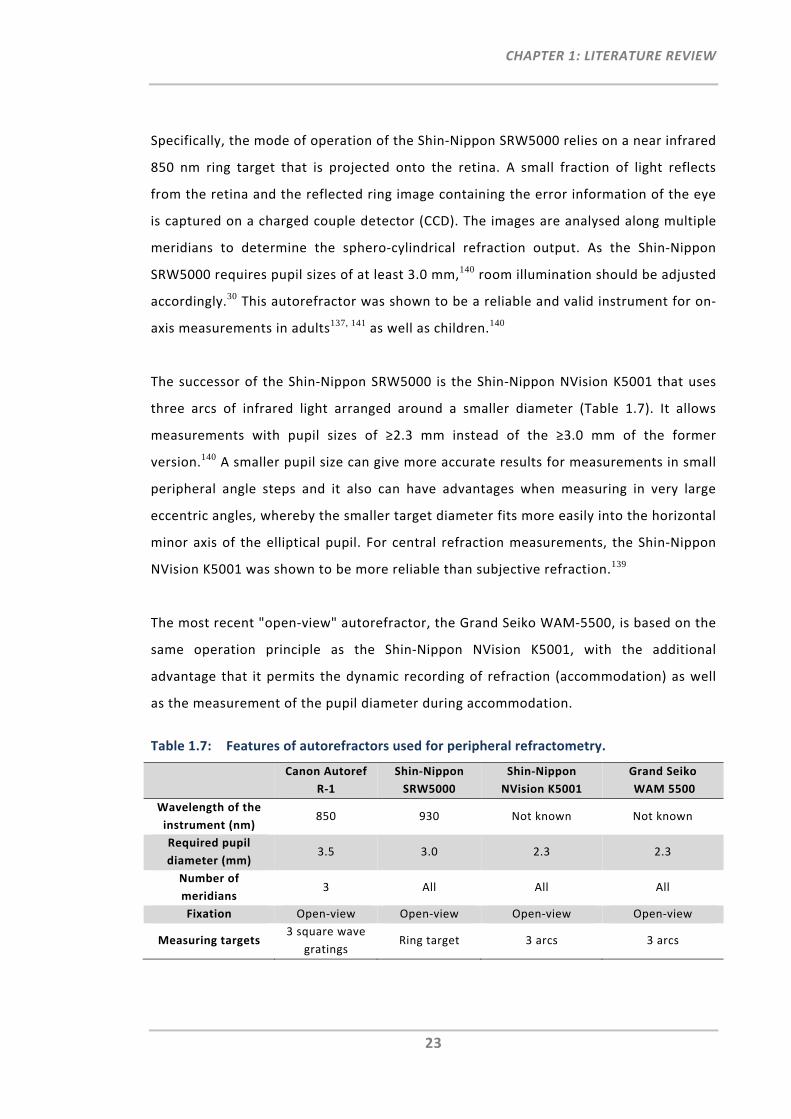
CHAPTER 1: LITERATURE REVIEW
23
Specifically, the mode of operation of the Shin‐Nippon SRW5000 relies on a near infrared
850 nm ring target that is projected onto the retina. A small fraction of light reflects
from the retina and the reflected ring image containing the error information of the eye
is captured on a charged couple detector (CCD). The images are analysed along multiple
meridians to determine the sphero‐cylindrical refraction output. As the Shin‐Nippon
SRW5000 requires pupil sizes of at least 3.0 mm,140 room illumination should be adjusted
accordingly.30 This autorefractor was shown to be a reliable and valid instrument for on‐
axis measurements in adults137, 141 as well as children.140
The successor of the Shin‐Nippon SRW5000 is the Shin‐Nippon NVision K5001 that uses
three arcs of infrared light arranged around a smaller diameter (Table 1.7). It allows
measurements with pupil sizes of ≥2.3 mm instead of the ≥3.0 mm of the former
version.140 A smaller pupil size can give more accurate results for measurements in small
peripheral angle steps and it also can have advantages when measuring in very large
eccentric angles, whereby the smaller target diameter fits more easily into the horizontal
minor axis of the elliptical pupil. For central refraction measurements, the Shin‐Nippon
NVision K5001 was shown to be more reliable than subjective refraction.139
The most recent "open‐view" autorefractor, the Grand Seiko WAM‐5500, is based on the
same operation principle as the Shin‐Nippon NVision K5001, with the additional
advantage that it permits the dynamic recording of refraction (accommodation) as well
as the measurement of the pupil diameter during accommodation.
Table 1.7: Features of autorefractors used for peripheral refractometry.
Canon Autoref
R‐1
Shin‐Nippon
SRW5000
Shin‐Nippon
NVision K5001
Grand Seiko
WAM 5500
Wavelength of the
instrument (nm) 850 930 Not known Not known
Required pupil
diameter (mm) 3.5 3.0 2.3 2.3
Number of
meridians 3 All All All
Fixation Open‐view Open‐view Open‐view Open‐view
Measuring targets 3 square wave
gratings Ring target 3 arcs 3 arcs
CHAPTER 1: LITERATURE REVIEW
24
The Canon Autoref R‐1 is, along with the other three autorefractors, an open‐field
instrument, but of an earlier generation. Its measurement light source emits in the near
infrared wavelength at 930 nm. Even though the Canon R‐1 is no longer commercially
available, it is still in use in some optometric practices. Its widespread past and present
use for research purposes warrants its inclusion in this discussion. The refraction
principle is different to the other three autorefractors; it is based on the grating focus
principle. Three illuminated square wave grating targets arranged in 60° to each other
are adjusted for best output position via a detector system. Although, central refraction
was found to be reliable and relatively valid, accuracy was reduced for the cylinder
component result. It was assumed that the refractive accuracy, in particular for cylinder
and axis values, could be improved by increasing the number of meridians of the
instrument.142 As the Canon R‐1 requires a minimum pupil diameter of at least 3.5 mm,
aberrations such as spherical aberration may have some impact on refraction results.
Compared to central retinoscopy or subjective refraction, the Canon R‐1 showed to be a
reliable refraction instrument for on‐axis measurements.133
Several research groups compared peripheral refraction measurements obtained with
the Canon Autoref R‐1 to other peripheral refraction techniques. Wang et al.27 compared
this instrument to subjective and retinoscopic peripheral refraction. Even though close
agreements were found between objective and subjective methods, considerable
differences were found between peripheral subjective refraction and the Canon R‐1
results measured for the 40° eccentricity angle in the 90° meridian. In addition, Atchison
et al.29 compared peripheral refraction results of the Canon R‐1 with two other
techniques, the Shin‐Nippon SRW5000 and the Hartmann‐Shack wavefront sensor. The
poorest agreements between all instruments were found in conjunction with the Canon
R‐1, suggesting this to be the least comparable instrument. Dunne et al.37 used the Zeiss
Hartinger coincidence optometer and the Canon R‐1 to investigate an association
between peripheral astigmatic errors and angle alpha. Although, there was no significant
difference found between the two refractor results, the graphed results indicate a shift
towards greater astigmatic error measured with the Canon R‐1. They also reported
problems measuring peripheral refraction on the Canon R‐1 for eccentricities greater
than 30° due to the limitations of this instrument on the required pupil size.
CHAPTER 1: LITERATURE REVIEW
25
Whereas most studies with the Shin‐Nippon SRW5000 performed peripheral refraction
measurements along the horizontal visual field meridian, one study by Atchison et al.24
also measured the vertical meridian. By use of beamsplitters and a light emitting diode
(LED), the participant was able to fixate the target in 5° steps upwards or downwards. By
use of this set‐up, only right eyes could be measured, and when gazing downwards, the
upper eye‐lid required holding up to ensure a valid measurement.
Charman and Jennings35 used a double‐pass technique and the Shin‐Nippon SRW5000 to
investigate the factor of peripheral refractive error changes with age. Whereas, the
baseline data were obtained using a double‐pass technique, 26 years later they used the
Shin‐Nippon SRW5000 for the measurement of peripheral refraction. Measurements
revealed a central hyperopic shift over time. However, using two different measurement
techniques, which are based on different operation principles and under different study
protocol conditions such as performing cycloplegic refraction with double‐pass
technique and non‐cycloplegic refraction with the autorefractor, limits a direct
comparison.
Davies and Mallen73 modified the Shin‐Nippon SRW5000 by attaching a rotating +3.00D
Badal system and an axially movable Maltese cross target, to enable both, central and
peripheral refraction measurements at different accommodative states of 0.00D, 1.00D,
2.00D and 3.00D.
Berntsen et al.33 compared peripheral refraction results of the Shin‐Nippon NVision
K5001 with the COAS aberrometer and found equivalent measurements, but having a
more hyperopic spherical equivalent shift with the Shin‐Nippon NVision K5001. Donovan
et al.122 also compared the Shin‐Nippon NVision K5001 autorefractor with the COAS
aberrometer and streak retinoscope Using head turn, peripheral refraction was
measured in 28 participants. They found much lower values in oblique astigmatism
measured with the aberrometer when compared to the two other methods.
Fedtke et al.126 investigated the impact of pupil misalignment on peripheral refraction
measurements when using the Shin‐Nippon NVision K5001. They showed that refraction
CHAPTER 1: LITERATURE REVIEW
26
measurements became more sensitive to pupil misalignment as visual field angle
increased.
Like Davies and Mallen73, Whatham et al.71 and Ho et al.72 also aimed to understand the
impact of accommodation on peripheral refraction profiles. Using the Shin‐Nippon
NVision K5001, they approached the near viewing of targets for peripheral refractometry
differently. An instrument head was mounted on top of the Shin‐Nippon NVision K5001,
which had not only small laser diodes attached to emit visible red light towards the
selected peripheral field positions (up to 40°), but it also had adjustable near viewing
targets at 0.40 and 0.30 m attached to it. In both studies the participants were asked to
turn the head towards the peripheral targets.
With the increased interest in measuring peripheral refraction with open‐view
autorefractors, the latest model, the Grand Seiko WAM‐5500, has now also been
adopted for this purpose.75, 80, 129
Overall, it has been shown that commercially available autorefractors are great objective
tools and they produce similar peripheral refraction results to other techniques.29
Nevertheless, measurement of peripheral refraction with these instruments remains
time‐consuming as they require continuous re‐alignments by the participant towards the
provided peripheral fixation targets as well as continuous re‐alignment of the instrument
axis with the centre of the pupil by the operator. From the four autorefractors used for
peripheral refraction, the Shin‐Nippon NVision K5001 and the Grand Seiko WAM‐5500
are likely to be the most useful instruments for peripheral measurements. This is mainly
due to their smaller pupil size requirement, which is of particular advantage for the
measurement of large peripheral angles. Moreover, the ring‐autorefraction principle
appears to have advantages over the grating focus principle of the Canon Autoref R‐1,
which showed limitations with respect to only using three meridians for the
determination of astigmatism.
Lastly, it should be noted that there are commercially available hand‐held autorefractor
instruments, such as the Retinomax (Nikon Corp.) and the Welch Allyn SureSight Vision
CHAPTER 1: LITERATURE REVIEW
27
Screener, which have proven to be convenient screening tools in schools and nursing
homes.143 Refraction measurements were reported to be in moderate agreement with
each other, though showing large variability in axis measurements.144 Comparison with a
table‐mounted autorefractor and subjective central refraction has shown that these
hand‐held autorefractor instruments overestimate myopia.145, 146 As such, it was
suggested that portable autorefractors should be used as screening tools only, and not
for research purposes.144, 145 Even though these instruments are easy to handle and do
not require off‐axis fixation, no studies were found reporting on the use of these hand‐
held autorefractors for peripheral refraction.
1.3.6 Photorefraction
In photorefractometry, the eye is illuminated by a point light source and the reflected
image in the pupil plane is observed or photographed. The refractive error of the eye can
then be determined by means of distribution analysis of the illumination in the pupil.
The PowerRefractor instrument was developed at the University Eye Hospital Tübingen
and is purchasable through PlusOptix (Erlangen, Germany). It operates on this
photorefraction principle and uses infrared illumination (850 nm). The working distance
is 1 meter. Central refraction with the PowerRefractor has shown to have “major
advantages over current autorefractors in that it is faster, measures both eyes at once,
and gives interpupillary distance, pupil size and information on the alignment of the eyes
at the same time”.147 Choi et al.147 measured central refractive errors in children with the
PowerRefractor and a “closed‐field” autorefractor (Nidek AR800) and found the
PowerRefractor detected smaller amounts of myopia, which could also be attributed to
the pseudomyopia caused by the autorefractor.
As indicated in Table 1.8, this technique has also been used for peripheral
photorefraction measurements. Gustafsson et al.54, 117 tested participants with central
visual field loss and attached concentric rings in 5° steps up to 25° to the PowerRefractor
in order to allow the participant to orientate and to find their normal eccentric gaze. The
purpose of their study was to determine and correct the refractive error of the
participant’s preferred retinal locus. Overall, this technique was found to be very useful
and repeatable.
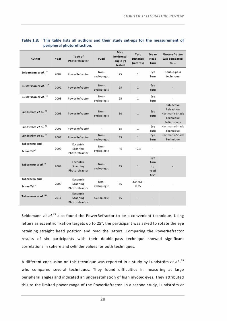
CHAPTER 1: LITERATURE REVIEW
28
Table 1.8: This table lists all authors and their study set‐ups for the measurement of peripheral photorefraction.
Author Year Type of
Photorefractor Pupil
Max.
horizontal
angle (°)
tested
Test
Distance
(metres)
Eye or
Head
Turn
Photorefractor
was compared
to …
Seidemann et al. 23 2002 PowerRefractor
Non‐
cycloplegic 25 1
Eye
Turn
Double‐pass
technique
Gustafsson et al. 117 2002 PowerRefractor
Non‐
cycloplegic 25 1
Eye
Turn ‐
Gustafsson et al. 54 2003 PowerRefractor
Non‐
cycloplegic 25 1
Eye
Turn ‐
Lundström et al. 99 2005 PowerRefractor
Non‐
cycloplegic 30 1
Eye
Turn
Subjective
Refraction
Hartmann‐Shack
Technique
Retinoscopy
Lundström et al. 56 2005 PowerRefractor ‐ 35 1
Eye
Turn
Hartmann‐Shack
Technique
Lundström et al. 55 2007 PowerRefractor
Non‐
cycloplegic 35 1
Eye
Turn
Hartmann‐Shack
Technique
Tabernero and
Schaeffel42 2009
Eccentric
Scanning
Photorefractor
Non‐
cycloplegic 45 ~0.3 ‐ ‐
Tabernero et al.52 2009
Eccentric
Scanning
Photorefractor
Non‐
cycloplegic 45 1
Eye
Turn
to
read
text
‐
Tabernero and
Schaeffel74 2009
Eccentric
Scanning
Photorefractor
Non‐
cycloplegic 45
2.0, 0.5,
0.25 ‐ ‐
Tabernero et al.131 2011
Eccentric
Scanning
Photorefractor
Cycloplegic 45 ‐ ‐ ‐
Seidemann et al.23 also found the PowerRefractor to be a convenient technique. Using
letters as eccentric fixation targets up to 25°, the participant was asked to rotate the eye
retaining straight head position and read the letters. Comparing the PowerRefractor
results of six participants with their double‐pass technique showed significant
correlations in sphere and cylinder values for both techniques.
A different conclusion on this technique was reported in a study by Lundström et al.,99
who compared several techniques. They found difficulties in measuring at large
peripheral angles and indicated an underestimation of high myopic eyes. They attributed
this to the limited power range of the PowerRefractor. In a second study, Lundström et
CHAPTER 1: LITERATURE REVIEW
29
al.55 reported of one case where a very elliptical narrow pupil shape could not be
analysed with the PowerRefractor. Correction of the eccentric peripheral refractive
errors measured with the wavefront sensor showed better improvement of peripheral
visual function in six out of seven participants with central visual field loss, than using
the refractive error corrections measured with the PowerRefractor.
Even though the PowerRefractor was found to be a very useful and easy to use
optometric tool for central refraction, limitations in measuring large peripheral angles
and possible differences with respect to different pupil shapes and analysis may have
some impact on peripheral photorefraction results.
Tabernero and Schaeffel42, 52, 131, 148 have recently introduced the scanning photo‐
refractor, which permits the continuous refraction measurement of the horizontal
meridian up to 45° and thus, allows the faster and more convenient assessment of the
peripheral properties of the eye. With this set‐up, they found that myopic eyes have a
more irregular or “bumpy” retinal shape, than emmetropic eyes. This photoretinoscopic
scanning system is based on a hot mirror, which permits refraction at different angles
through rotational as well as translational movements, while the head and eye remain
stationary. In their first prototype instrument, one main limitation of this continuous
refraction design was the number of required steps (1393 video frames, 19 steps per
mm, 3 steps per video frame) and thus, its long scanning, data acquisition and analysing
duration of approximately 23 seconds. They note that long central fixation could be a
problem when measuring children. They also computed noise of measurement, which
they partly attributed to possible fluctuations of accommodation during fixation, but
mainly due to small fixation errors, which can impact the shift and/or shape of the
peripheral refraction profiles. More measurement noise was found in the nasal side,
which they assume to be due to the partially blocking of the illumination by the
participants nose. Following the first prototype instrument, an upgraded version of the
same instrument was introduced, which reduced measurement time from 23 to 4
seconds. This was achieved with faster mechanics such as a belt‐driven linear translation
stage to speed up the translation of the mirror and a two‐gear belt transmission system
to rapidly rotate the mirror. Although the operation principle of the scanning
CHAPTER 1: LITERATURE REVIEW
30
photorefractor stems from the concept of the PowerRefractor, its main difference and
thus, main disadvantage is that it cannot measure astigmatic errors. Whereas the
PowerRefractor rotates the photoretinoscope to obtain the sphero‐cylindrical refraction
of the eye, the scanning photorefractor only measures the vertical pupil meridian and
thus, provides only spherical errors. The authors mention that a rotational
photoretinoscope principle, such as used in the PowerRefractor, could also been
implemented into the scanning photorefractor, however, this would be complex and
slow down sampling rate and consequently, the peripheral refraction scan would again
require much more time. Instead of using a rotational photoretinoscopic principle, the
authors also suggest to perhaps perform measurements along two pupil meridians, that
is 90 and 180°.131 Despite the many advantages of this peripheral scanning instrument of
having no eye‐ and head‐turn requirements and being a much faster peripheral
refraction technique, being restricted to spherical error measurements limits its use. In
particular, due to the fact that oblique astigmatism is strongly present in the periphery
of the eye and its measurement, assessment and correction has already been shown to
be of relevance to vision scientists.82
1.3.7 Aberrometer
A very simple implementation of the basic principle of aberrometry is the previously
mentioned Scheiner disc. Whereas, the disc of a Scheiner optometer consists of only two
pinholes, Hartmann149 increased the number of pinholes over the entire pupil and traced
the aberrated ray lights accordingly. Shack150 modified this by replacing the disc with an
array of tiny lenses.
Specifically, when using an aberrometer, such as the COAS, a narrow light beam is sent
into the eye projecting a small spot onto the retina. When reflected light from this spot
exits the eye it generates the eye's aberrated wavefront. By use of a set of relay lenses
and the Hartmann‐Shack sensor, which consists of the lenslet array and a detector, the
spots created by the lenslet array are captured by the detector. The relative
displacements of the spots are analysed with respect to their reference spots to provide
the wavefront map of the eye. The wavefront errors or aberration values are provided in
the form of Zernike coefficients, which can then be converted to the conventional
sphero‐cylindrical refraction output.

CHAPTER 1: LITERATURE REVIEW
31
Table 1.9: This table shows all authors and their study set‐ups used for the measurement of aberrometer‐based peripheral refraction.
Author Year Type of
Aberrometer Pupil
Max.
Angle
(°)
tested
Eye or
Head Turn
Aberrometer was
compared to …
Navarro et al. 116 1998 Laser ray‐tracing
method Cycloplegic 40 Eye Turn ‐
Atchison and Scott 31
2002 Hartmann‐Shack Sensor Technique
Cycloplegic 40 Eye Turn ‐
Atchison 29 2003 Hartmann‐Shack Sensor Technique
Cycloplegic 40 Eye Turn Shin‐Nippon SRW5000 Canon Autoref R‐1
Atchison et al. 32 2003 Hartmann‐Shack Sensor Technique
Cycloplegic 40 Eye Turn ‐
Atchison 118 2004 Hartmann‐Shack Sensor Technique
Cycloplegic 40 Eye Turn ‐
Lundström et al. 99 2005 Hartmann‐Shack Sensor Technique
Non‐cycloplegic 30 Eye Turn Subjective Refraction
Photorefraction Retinoscopy
Lundström et al.56 2005 Hartmann‐Shack Sensor Technique
‐ 35 Eye Turn Photorefraction
Atchison et al. 120 2006 COAS Cycloplegic 5 Eye Turn Subjective Refraction
Atchison et al. 121 2006 COAS Cycloplegic 40 Eye Turn ‐
Radhakrishnan and Charman 65
2007 Hartmann‐Shack Sensor Technique
Non‐cycloplegic 30 Eye and
Head Turn ‐
Lundström et al. 53 2007 Hartmann‐Shack Sensor Technique
Non‐cycloplegic 20 Eye Turn ‐
Lundström et al. 55 2007 Hartmann‐Shack Sensor Technique
Non‐cycloplegic 35 Eye Turn Photorefraction
Donovan et al.122 2007 COAS Cycloplegic 30 Eye Turn Shin‐Nippon NVision
K5001 Retinoscopy
Berntsen et al. 33 2008 COAS Cycloplegic 30 Head Turn Shin‐Nippon NVision
K5001
Mathur et al. 123 2008 Hartmann‐Shack Sensor Technique
Non‐cycloplegic 21 Eye Turn ‐
Lundström et al.67 2009 Hartmann‐Shack Sensor Technique
Non‐cycloplegic 40 Eye and
Head Turn ‐
Lundström et al.125 2009 Hartmann‐Shack Sensor Technique
Non‐cycloplegic 30 Eye Turn ‐
Mathur and Atchison79
2009 COAS Non‐cycloplegic 21 Eye Turn Shin‐Nippon SRW5000
Mathur et al.127 2009 COAS Non‐cycloplegic 21 Eye Turn ‐
Mathur et al.61 2010 COAS Non‐cycloplegic 21 Eye Turn ‐
Mathur et al.47 2010 COAS Non‐cycloplegic 21 Eye Turn ‐
Wei and Thibos128 2010 Hartmann‐Shack Sensor Technique
Non‐cycloplegic 15 ‐ ‐
Atchison et al.77 2010 COAS Non‐cycloplegic 21 Eye Turn ‐
Shen et al.81 2010 COAS Non‐cycloplegic 30 Head Turn ‐
Baskaran et al.130 2010 COAS‐HD VR Non‐cycloplegic 40 Eye Turn ‐
Baskaran et al.62 2011 COAS‐HD VR Non‐cycloplegic 40 Eye Turn ‐
CHAPTER 1: LITERATURE REVIEW
32
Whereas the COAS is a commercially available aberrometer, several research groups
have developed their own Hartmann‐Shack wavefront techniques. Table 1.9 shows all
research groups that reported on peripheral measurements obtained with the
Hartmann‐Shack technique.
One such technique used for peripheral measurements has been explained in detail by
Atchison and Scott.31 A beamsplitter and a system of peripheral fixation targets up to 40°
in 5° steps enable measurement of the desired angles in the periphery. For the analysis
of Zernike coefficients obtained at a peripheral angle, the elliptical pupil shape had to be
taken into account and transformations made.29, 32 Detailed information on analysis for
the measurement of their ocular aberrations in the peripheral visual field has been
published.151
A different set‐up for the measurement of peripheral aberrations using the Hartmann‐
Shack technique has been built and applied by Lundström et al.56 This set‐up was
particularly designed for participants with large central visual field loss. The technique
incorporates concentric ring fixation targets, to allow participants alignment with
respect to their preferred retinal locus position. Moreover, it includes an eye tracker as
well as analysing software with unwrapping algorithms that consider elliptical pupil
shapes.
In 2009 Lundström et al.67 used a Hartmann‐Shack wavefront sensor technique that
allows measuring of the periphery of the eye for different accommodative states. This
was achieved by use of a hot mirror, which allowed for an open field of view and hence
binocular fixation to different off‐axis targets at different distances. A bitebar was used
to stabilise the head during the measurements.
Using the COAS aberrometer, five studies by Mathur and Atchison et al.61, 123, 127, 79, 77
mapped higher order aberrations at horizontal visual field locations up to 21° and
vertical visual field locations up to 16° using a beamsplitter for off‐axis target projection.
For this 38 targets were produced onto a projection screen, which the participants had
to view successively.
CHAPTER 1: LITERATURE REVIEW
33
Whereas, the aberrometry‐based peripheral refractions by Berntsen et al.33 obtained
with the COAS were in good agreement to refraction data of the Shin‐Nippon NVision
K5001, Donovan et al.’s122 measurements revealed peripheral astigmatic values which
were almost half in value using the COAS when compared to the Shin‐Nippon NVision
K5001. Compared to the peripheral refraction data obtained with the Shin‐Nippon
SRW5000, Atchison's Hartmann‐Shack wavefront sensor technique showed good
agreement.29 Lundström et al.’s55, 99 comparisons of different peripheral refraction
techniques showed that the Hartmann‐Shack technique was the most useful technique
compared to subjective refraction, retinoscopy and photorefraction. In comparison to
the PowerRefractor, results showed that the Hartmann‐Shack sensor technique by
Lundström et al.56 measured greater astigmatism in the oblique axis and the total
cylinder value obtained was smaller than with the PowerRefractor. Due to
underestimation of oblique off‐axis astigmatism and limitations for large eccentricities
using the PowerRefractor, the Hartmann‐Shack technique has been assumed to be more
accurate for peripheral refraction.
Baskaran et al.62, 130 have used the COAS‐HD VR aberrometer for the measurement of
peripheral refraction measurements. This COAS instrument has an open‐view optical
relay system attached, which permits measurements of up to 40°.
Although all aberrometer techniques were in good agreement with other methods and
considered very useful, a small overestimation of myopia was found for the aberrometry
refractions compared to all the other instruments used in the comparison studies by
Lundström et al.,99 Berntsen et al.33 and Atchison et al.29. This finding was also observed
in validation studies of aberrometers on central measurements in adults152, 153 as well as
children.154 It was suggested this to be due to differences in calibration (wavelength
differences), set‐up (closed‐view versus open‐view) and/or the operation principles
(pupil diameter) between aberrometers and autorefractors.29, 33 As mentioned for
autorefractors, the same participant‐ and operator‐related intricacies (constant re‐
alignment of eye/head and pupil/instrument) remain, which eventually can lead to
prolonged testing times in particular when numerous peripheral angles have to be
measured.
CHAPTER 1: LITERATURE REVIEW
34
Very recently, Wei and Thibos as well as Jaeken and Artal also introduced new scanning
Hartmann‐Shack aberrometers.128, 155 Just like the technique by Tabernero and
Schaeffel,42, 52, 74 both techniques permit the measurement of peripheral optics of the
eye without the need for off‐axis fixation. Wei and Thibos use double‐pass scanning
lenses and a scanning mirror that enable the measurement of the periphery of the eye.
Currently, this technique is limited to visual field measurements up to a mid peripheral
range of ±15°, which takes up to 7 to 8 seconds. The authors note that by combining
both, peripheral fixation and the scanning Hartmann‐Shack aberrometer the
measurement range can be extended beyond the central 30°. Due to strong backward
reflections from the system and the cornea, the current instrument set‐up does not
permit the measurement of on‐axis aberrations and the measurements along the
horizontal meridian. Currently, there is only limited information published on Jaeken and
Artal’s scanning Hartmann‐Shack aberrometer.155 However, first specifications of this
instrument appear promising, indicating that continuous measurements are possible up
to peripheral angles of ±40° and the complete scan takes approximately 2 seconds.
1.4 Alignment Criteria for Peripheral Refractometry
When using conventional refraction techniques for the measurement of the periphery of
the eye, a form of off‐axis fixation or instrument adjustment is required in order to
permit the alignment of a particular peripheral field angle with respect to the instrument
axis. Commonly, the participant is asked to either turn the eye (Figure 1.3 a) or head
(Figure 1.3 b) towards a peripheral fixation target whilst keeping the refraction
instrument in its fixed position. This involves the participant actively taking part in the
measurement procedure, which often can lead to extensive testing times. A third
alternative is the rotation of the measuring device in front of the eye (Figure 1.3 c). This,
however, is often difficult to achieve when using compact instrument designs such as
ready‐made autorefractors or aberrometers.
Whether eye turn measurements can lead to different peripheral refraction results when
compared to straight ahead gaze has previously been investigated by several authors
(Table 1.10).
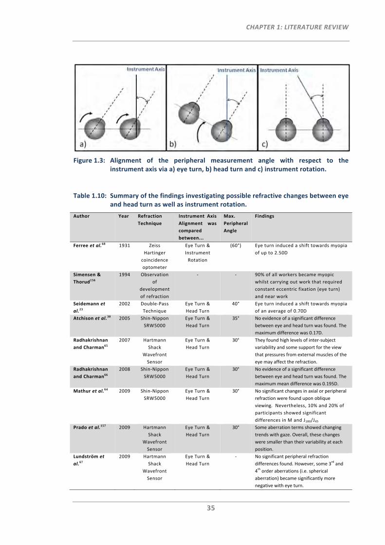
CHAPTER 1: LITERATURE REVIEW
35
Figure 1.3: Alignment of the peripheral measurement angle with respect to the instrument axis via a) eye turn, b) head turn and c) instrument rotation.
Table 1.10: Summary of the findings investigating possible refractive changes between eye and head turn as well as instrument rotation.
Author Year Refraction
Technique
Instrument Axis
Alignment was
compared
between...
Max.
Peripheral
Angle
Findings
Ferree et al.68 1931 Zeiss
Hartinger
coincidence
optometer
Eye Turn &
Instrument
Rotation
(60°) Eye turn induced a shift towards myopia
of up to 2.50D
Simensen &
Thorud156
1994 Observation
of
development
of refraction
‐ ‐ 90% of all workers became myopic
whilst carrying out work that required
constant eccentric fixation (eye turn)
and near work
Seidemann et
al.23
2002 Double‐Pass
Technique
Eye Turn &
Head Turn
40° Eye turn induced a shift towards myopia
of an average of 0.70D
Atchison et al.30 2005 Shin‐Nippon
SRW5000
Eye Turn &
Head Turn
35° No evidence of a significant difference
between eye and head turn was found. The
maximum difference was 0.17D.
Radhakrishnan
and Charman65
2007 Hartmann
Shack
Wavefront
Sensor
Eye Turn &
Head Turn
30° They found high levels of inter‐subject
variability and some support for the view
that pressures from external muscles of the
eye may affect the refraction.
Radhakrishnan
and Charman66
2008 Shin‐Nippon
SRW5000
Eye Turn &
Head Turn
30° No evidence of a significant difference
between eye and head turn was found. The
maximum mean difference was 0.195D.
Mathur et al.64 2009 Shin‐Nippon
SRW5000
Eye Turn &
Head Turn
30° No significant changes in axial or peripheral
refraction were found upon oblique
viewing. Nevertheless, 10% and 20% of
participants showed significant
differences in M and J180/J45
Prado et al.157 2009 Hartmann
Shack
Wavefront
Sensor
Eye Turn &
Head Turn
30° Some aberration terms showed changing
trends with gaze. Overall, these changes
were smaller than their variability at each
position.
Lundström et
al.67
2009 Hartmann
Shack
Wavefront
Sensor
Eye Turn &
Head Turn
‐ No significant peripheral refraction
differences found. However, some 3rd and
4th order aberrations (i.e. spherical
aberration) became significantly more
negative with eye turn.
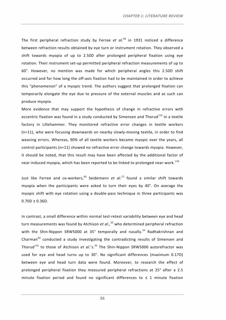
CHAPTER 1: LITERATURE REVIEW
36
The first peripheral refraction study by Ferree et al.68 in 1931 noticed a difference
between refraction results obtained by eye turn or instrument rotation. They observed a
shift towards myopia of up to 2.50D after prolonged peripheral fixation using eye
rotation. Their instrument set‐up permitted peripheral refraction measurements of up to
60°. However, no mention was made for which peripheral angles this 2.50D shift
occurred and for how long the off‐axis fixation had to be maintained in order to achieve
this “phenomenon” of a myopic trend. The authors suggest that prolonged fixation can
temporarily elongate the eye due to pressure of the external muscles and as such can
produce myopia.
More evidence that may support the hypothesis of change in refractive errors with
eccentric fixation was found in a study conducted by Simensen and Thorud156 in a textile
factory in Lillehammer. They monitored refractive error changes in textile workers
(n=11), who were focusing downwards on nearby slowly‐moving textile, in order to find
weaving errors. Whereas, 90% of all textile workers became myopic over the years, all
control participants (n=11) showed no refractive error change towards myopia. However,
it should be noted, that this result may have been affected by the additional factor of
near‐induced myopia, which has been reported to be linked to prolonged near‐work.158
Just like Ferree and co‐workers,68 Seidemann et al.23 found a similar shift towards
myopia when the participants were asked to turn their eyes by 40°. On average the
myopic shift with eye rotation using a double‐pass technique in three participants was
0.70D ± 0.36D.
In contrast, a small difference within normal test‐retest variability between eye and head
turn measurements was found by Atchison et al.,30 who determined peripheral refraction
with the Shin‐Nippon SRW5000 at 35° temporally and nasally.30 Radhakrishnan and
Charman66 conducted a study investigating the contradicting results of Simensen and
Thorud156 to those of Atchison et al.’s.30 The Shin‐Nippon SRW5000 autorefractor was
used for eye and head turns up to 30°. No significant differences (maximum 0.17D)
between eye and head turn data were found. Moreover, to research the effect of
prolonged peripheral fixation they measured peripheral refractions at 25° after a 2.5
minute fixation period and found no significant differences to ≤ 1 minute fixation
CHAPTER 1: LITERATURE REVIEW
37
durations. As retinal eccentricity increased, so did the standard deviations. The authors
explain this to be due to the difficulty for participants to maintain exact eye or head
positions at large eccentricities. In another investigation using the Hartmann‐Shack
technique, the same authors65 found some evidence of eye turn‐induced refractive error
changes of up to 1.00D in hyperopic direction. This finding occurred after 1 to 1.5
minutes viewing at 30° eccentricity. This observation was made in only some individuals
but was not shown for oblique viewing durations of 20 minutes. The same authors65
observed that pupil sizes constricted systematically with increasing oblique viewing
angles. They suggest this pupil constriction to be caused either by stress occurring in the
participant due to the task of maintaining the oblique viewing angle or due to the
mechanical pressures stimulating the ciliary nerves when turning the eye.
Marthur et al.64 measured axial refraction under oblique viewing conditions (30°
temporal and 30° nasal) using the Shin‐Nippon SRW5000 and compared the results to
straight‐ahead viewing. Although they did not find any significant mean effects for the
participant group (n=53), there were at least 10% and 20% of participants that showed
significant differences in the refractive vector components M and J180/J45, respectively. A
similar study was conducted by Prado et al.157 who used a Hartmann Shack wavefront
technique to measure and compare on‐axis aberrations between straight‐ahead and
oblique viewing (30° temporal and 30° nasal). They found that some mean values
showed a trend to change with gaze direction; however these changes were smaller than
the overall variability. Lundström et al.67 showed that some 3rd and 4th order aberrations,
such as spherical aberration, were significantly different between eye and head turn
measurements.
Instead of investigating the impact of eye turn on peripheral refraction results,
Macfadden et al. investigated the impact of eye turn on the peripheral ocular shape and
found a significant shift in retinal profiles when comparing eye rotation and head turn
measurements using the IOLMaster.159
Recently, researchers have also turned their attention to measuring peripheral refraction
when wearing contact lenses81, 160 or spectacle lenses.52, 82 In the latter case, it is
important that the visual axis is perpendicular to the spectacle plane or else peripheral
CHAPTER 1: LITERATURE REVIEW
38
prismatic effects of the spectacle lens can affect the measurement angle. When
measuring peripheral refraction in the contact lens wearing eye, there is a possibility
that eye turn can affect the centration of the contact lens, which potentially can impact
the measured peripheral refractive power. Thus, to avoid peripheral prismatic effects
with spectacle lenses or de‐centration effects of contact lenses, peripheral refraction
measurements should be performed using head turn.
Most of the studies listed in Table 1.10 have shown little or no difference between eye
and head turn measurements. However, these studies have been using somewhat
different study protocols to investigate the impact of eye turn on peripheral refraction
data when compared to head turn or instrument rotation. The use of different
instrumentations, different peripheral angles measured and different durations for
oblique viewing may have had an impact on the different results found. Nevertheless, to
avoid any of the possible effects that may result from eye turn measurements, whether
the eye is measured with or without correction devices, head turn appears to be the
more suitable method for the alignment of the peripheral measurement angle.
1.5 Summary and Conclusion
Clearly, there has been much advancement in refraction instruments over time with
respect to delivering accurate and reliable results for on‐axis measurements but also in
terms of ease of use. These changes in refraction technology are also reflected in their
use for research purposes related to peripheral refractometry. From the current
literature review and Figure 1.4 it is evident that in the last decade, objective techniques
based on autorefraction and aberrometry have become of greatest use for the
measurement of peripheral refraction. The current review suggests that objective
instruments, such as the COAS, the Shin‐Nippon NVision K5001 and the Grand Seiko
WAM‐5500 are the most useful commercially available instruments for peripheral
refraction measurements. Whereas the COAS provides the additional measurement of
higher order aberrations, the Shin‐Nippon NVision K5001 and the Grand Seiko WAM‐
5500 require smallest pupil diameters for autorefractors and they permit binocular
viewing of the external peripheral real‐distance target.
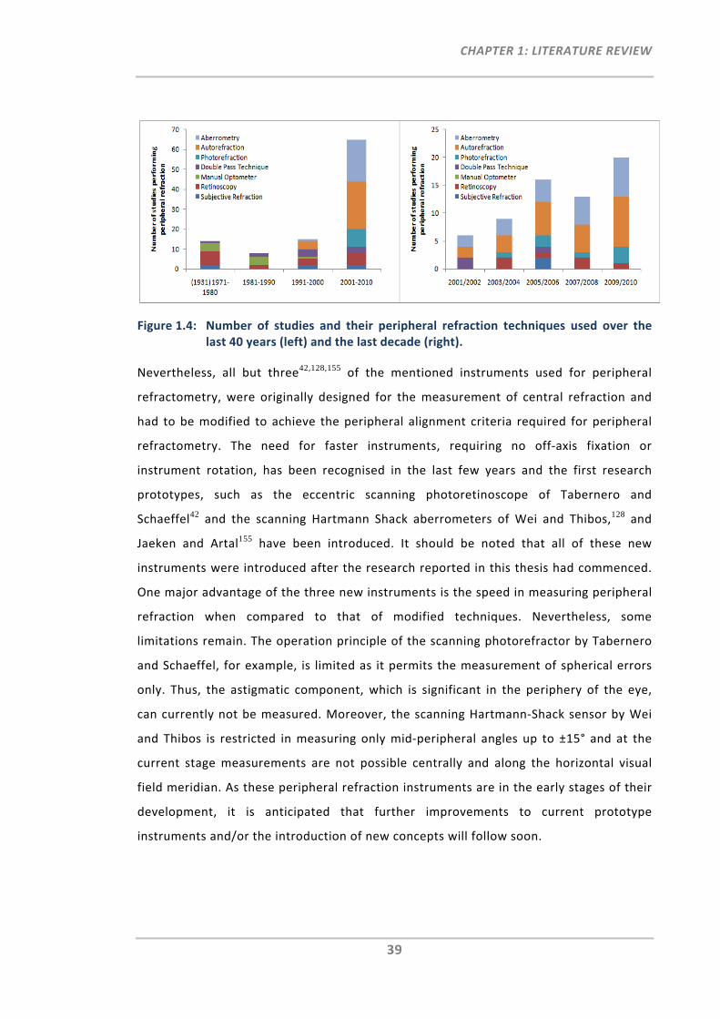
CHAPTER 1: LITERATURE REVIEW
39
Figure 1.4: Number of studies and their peripheral refraction techniques used over the last 40 years (left) and the last decade (right).
Nevertheless, all but three42,128,155 of the mentioned instruments used for peripheral
refractometry, were originally designed for the measurement of central refraction and
had to be modified to achieve the peripheral alignment criteria required for peripheral
refractometry. The need for faster instruments, requiring no off‐axis fixation or
instrument rotation, has been recognised in the last few years and the first research
prototypes, such as the eccentric scanning photoretinoscope of Tabernero and
Schaeffel42 and the scanning Hartmann Shack aberrometers of Wei and Thibos,128 and
Jaeken and Artal155 have been introduced. It should be noted that all of these new
instruments were introduced after the research reported in this thesis had commenced.
One major advantage of the three new instruments is the speed in measuring peripheral
refraction when compared to that of modified techniques. Nevertheless, some
limitations remain. The operation principle of the scanning photorefractor by Tabernero
and Schaeffel, for example, is limited as it permits the measurement of spherical errors
only. Thus, the astigmatic component, which is significant in the periphery of the eye,
can currently not be measured. Moreover, the scanning Hartmann‐Shack sensor by Wei
and Thibos is restricted in measuring only mid‐peripheral angles up to ±15° and at the
current stage measurements are not possible centrally and along the horizontal visual
field meridian. As these peripheral refraction instruments are in the early stages of their
development, it is anticipated that further improvements to current prototype
instruments and/or the introduction of new concepts will follow soon.
CHAPTER 1: LITERATURE REVIEW
40
1.6 Thesis Overview
1.6.1 Rationale for Research
With the discovery that peripheral refractive errors can influence eye growth, their
critical assessment and monitoring has become paramount to current research activities
in the field of myopia. The measurement of rapid and accurate global refraction, that is,
central and peripheral refraction, at individual and population levels has therefore
become of particular demand. Currently, however, time‐consuming sequential re‐
alignments by participants and operators are required when using commercially
available refraction techniques. It has also been shown that when using these
techniques, standard errors commonly increase for larger visual field angles. As there
has been little research conducted to investigate this increase in standard errors,
clarification is still needed to confirm that using these instruments for the measurement
of the peripheral optics of the eye provides accurate results. Preferably, an instrument
dedicated to the rapid and accurate measurement of central and peripheral refraction
would be the ultimate tool for research institutions and clinical practices in the current
quest to understand, monitor and control myopia progression.
Overall, results of this work will help understanding intricacies related to peripheral
refraction measurements when using modified commercially available instruments, will
test new concepts and investigate a new approach of obtaining more rapid and accurate
peripheral refraction measurements.
1.6.2 Hypotheses
The two primary hypotheses of this thesis are:
Refraction measurement accuracy decreases with increasing visual field angle,
due to decreased tolerance to misalignment when using commercially available
refraction instruments for the measurement of peripheral refraction
A new refraction technique, dedicated to measure central and peripheral
refraction rapidly and accurately across the entire visual field, can be developed.
CHAPTER 1: LITERATURE REVIEW
41
1.6.3 Aims
Specifically, the aims for the first part of this thesis are to:
Investigate the impact of pupil (mis‐)alignment on peripheral refraction
measurements when using commercially available instruments (Chapter 2)
Develop and introduce a new method for the correction of pupil alignment errors
when measuring peripheral refraction with commercially available instruments
(Chapter 3).
In an effort to overcome current limitations of peripheral refractometry, the second part
of this thesis aims to introduce and develop a new peripheral refraction instrument that
provides fast and accurate measurements across the visual field. The specific aims are
to:
Develop the optical design of a novel peripheral refraction instrument concept,
the EyeMapper, which has the objective to measure refraction rapidly across the
visual field by use of stationary deflecting components and a scanning mirror,
based on the ring autorefraction principle (Chapter 4)
Assess component and safety criteria for this new instrument concept and to test
and cross‐validate the autorefraction principle with a commercially available
autorefractor (Chapter 5)
Integrate the wavefront sensing principle into the optical and mechanical design
of the EM and build, calibrate and test this new instrument. (Chapter 6).
CHAPTER 2: OPERATOR‐RELATED ALIGNMENT INTRICACIES
42
CHAPTER 2:
INVESTIGATION OF OPERATOR‐RELATED ALIGNMENT INTRICACIES IN CURRENT PERIPHERAL REFRACTOMETRY§
2.1 Overview
Chapter 1 addressed participant‐related alignment intricacies, such as the requirements
for off‐axis fixation and the time‐consuming measurement procedure involved, when
using conventional instruments for the measurement of peripheral refraction. The
objective of Chapter 2 was to investigate also whether operator‐related tasks, such as
the (mis‐)/alignment of the instrument with the centre of the entrance pupil, could
impact the accuracy of instruments adapted for the measurement of peripheral
refraction.
At first, this chapter aimed to investigate the clinical impact of pupil misalignment on the
peripheral refraction results when using the Shin‐Nippon NVision K5001 autorefractor. In
the second part of this chapter, an entrance pupil model was developed and its
geometrical behaviour as a function of peripheral viewing angle was assessed and its
implications on peripheral refraction measurements were discussed.
2.2 Investigation of Pupil Alignment Tolerance
2.2.1 Introduction
Given the recently inferred association of peripheral refraction with myopia
development,10, 124, 161 the relevance and importance of measuring and monitoring
peripheral refraction profiles as accurately as possible has been recognised and
constitutes the basis of many research efforts.
§ Work from this chapter has previously been presented in part by the author and Arthur Ho at the annual meeting of the American Academy of Optometry, Orlando, 2009.126, 162 Based on these presentations, two papers have been published by the author.163, 164 Whereas, most modelling and analysis of the entrance pupil (Section 2.3) was previously carried out by Arthur Ho, the author's additional contribution was the discussion of its implications and the further processing and analysis of the data.
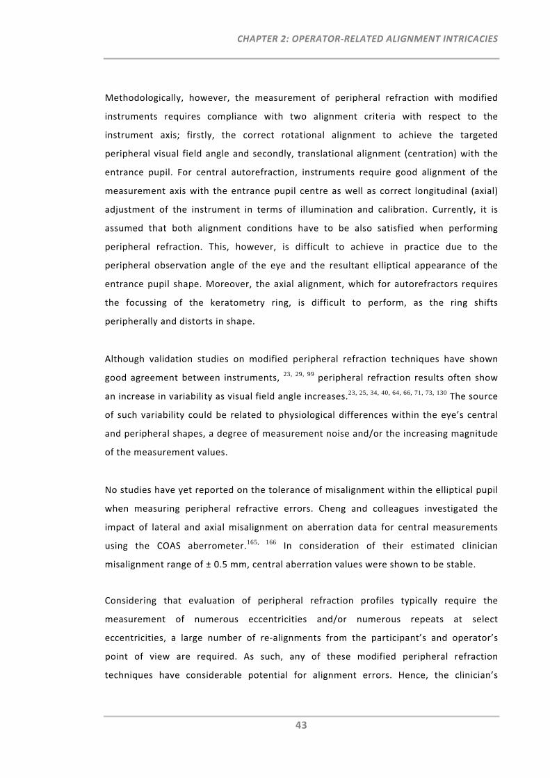
CHAPTER 2: OPERATOR‐RELATED ALIGNMENT INTRICACIES
43
Methodologically, however, the measurement of peripheral refraction with modified
instruments requires compliance with two alignment criteria with respect to the
instrument axis; firstly, the correct rotational alignment to achieve the targeted
peripheral visual field angle and secondly, translational alignment (centration) with the
entrance pupil. For central autorefraction, instruments require good alignment of the
measurement axis with the entrance pupil centre as well as correct longitudinal (axial)
adjustment of the instrument in terms of illumination and calibration. Currently, it is
assumed that both alignment conditions have to be also satisfied when performing
peripheral refraction. This, however, is difficult to achieve in practice due to the
peripheral observation angle of the eye and the resultant elliptical appearance of the
entrance pupil shape. Moreover, the axial alignment, which for autorefractors requires
the focussing of the keratometry ring, is difficult to perform, as the ring shifts
peripherally and distorts in shape.
Although validation studies on modified peripheral refraction techniques have shown
good agreement between instruments, 23, 29, 99 peripheral refraction results often show
an increase in variability as visual field angle increases.23, 25, 34, 40, 64, 66, 71, 73, 130 The source
of such variability could be related to physiological differences within the eye’s central
and peripheral shapes, a degree of measurement noise and/or the increasing magnitude
of the measurement values.
No studies have yet reported on the tolerance of misalignment within the elliptical pupil
when measuring peripheral refractive errors. Cheng and colleagues investigated the
impact of lateral and axial misalignment on aberration data for central measurements
using the COAS aberrometer.165, 166 In consideration of their estimated clinician
misalignment range of ± 0.5 mm, central aberration values were shown to be stable.
Considering that evaluation of peripheral refraction profiles typically require the
measurement of numerous eccentricities and/or numerous repeats at select
eccentricities, a large number of re‐alignments from the participant’s and operator’s
point of view are required. As such, any of these modified peripheral refraction
techniques have considerable potential for alignment errors. Hence, the clinician’s
CHAPTER 2: OPERATOR‐RELATED ALIGNMENT INTRICACIES
44
normal operation range for peripheral refraction is likely to be larger than the previously
estimated central normal misalignment range of ± 0.5 mm when using the COAS
instrument.165, 166
Based on the current technical intricacies in peripheral refractometry, the additional
impact of large oblique astigmatism and the elliptical peripheral entrance pupil, it is
reasonable to assume that sensitivity in measurement error for peripheral refraction
increases with increasing eccentricity. Hence, from the methodological point of view and
with its increasing scientific and clinical relevance, the key objective of this first study
was to investigate how sensitive the peripheral refraction results are with respect to
lateral pupil misalignment in comparison to the sensitivity of central refraction results.
2.2.2 Methods
2.2.2.1 Participants
The study protocol was reviewed and approved by the University of New South Wales
Human Research Ethics Advisory Panel and conformed to the tenets of the Declaration of
Helsinki. Ten emmetropic (central M ≤ |0.50|D) and ten myopic (central M ≤ ‐0.75D)
cooperative adult participants were recruited and successfully enrolled into the study.
All participants were screened for good ocular health and had no history of ocular
anomalies, such as manifest strabismus, non‐orthophoric conditions, or any anterior eye
anomalies. Peripheral refraction was measured for the right uncorrected eye in the
horizontal visual field meridian. Pupils were not dilated for the measurements.
2.2.2.2 Instrumentation
Central and peripheral refraction measurements were performed with the open‐view
autorefractor, the Shin‐Nippon NVision‐K5001 (also known as Grand Seiko WR‐5100K,
Shin‐Nippon, Tokyo, Japan). For this study the autorefractor was modified (Figure 2.1,
left) to allow for easier peripheral refraction measurements. The primary modification
includes the addition of an instrument head, which had been mounted on top of the
autorefractor. The instrument head includes several small red laser diodes that are
aligned to project laser fixation targets into the participant’s visual field, one at a time,
at various angles onto a wall, 2.0 to 2.5 m distant. In the present study, the laser fixation
CHAPTER 2: OPERATOR‐RELATED ALIGNMENT INTRICACIES
45
targets were presented straight ahead from the centre of the autorefractor and 30° in
the nasal and temporal horizontal visual fields. The use of bright laser targets on the
wall, allows even uncorrected ametropic participants to be able to recognise and fixate
on the targets. As explained in Chapter 1, head turn was the preferred method over eye
turn, and the chin‐rest had been modified to allow easy head turn for off‐axis fixation.
Using the method described by Thibos et al.,167 the sphero‐cylindrical refraction output
S/C × θ was converted to the power vectors, M (spherical equivalent), J180 (with‐ and
against‐the‐rule astigmatism) and J45 (oblique astigmatism) as followed:
Equation 2.1 /
Equation 2.2 /
Equation 2.3 /
All data processing (e.g. averaging) and subsequent analyses were performed in terms of
these power vector components.
2.2.2.3 Participant Alignment
Each participant was instructed to turn his/her head toward the presented fixation
target while keeping both eyes stationary, relative to head position, in forward gaze
(Figure 2.1, right). The participant’s cooperation regarding head alignment and accuracy
of fixation was monitored by the operator throughout the measurement procedure.
Nevertheless, it should be noted that, in practice, an additional small compensatory eye
turn may be difficult to perceive and correct. In three participants head misalignment
was measured (five repeats at 30° nasal and 30° temporal visual field angles), which
ranged from ‐6.85° to +5.15° (mean ‐2.13° ± 2.85°). This small compensatory eye turn is
unlikely to have a real impact on the data, particularly because the differences related to
eye and head turn measurements, were, if at all, only found for large peripheral fixation
angles.23, 65 Fixation targets were viewed with both eyes while maintaining normal
blinking. As no participants had manifest strabismus, accurate binocular fixation was
maintained for all measurements at all eccentricities.
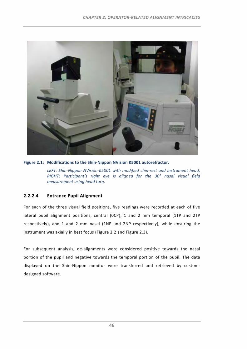
CHAPTER 2: OPERATOR‐RELATED ALIGNMENT INTRICACIES
46
Figure 2.1: Modifications to the Shin‐Nippon NVision K5001 autorefractor.
LEFT: Shin‐Nippon NVision‐K5001 with modified chin‐rest and instrument head; RIGHT: Participant’s right eye is aligned for the 30° nasal visual field measurement using head turn.
2.2.2.4 Entrance Pupil Alignment
For each of the three visual field positions, five readings were recorded at each of five
lateral pupil alignment positions, central (0CP), 1 and 2 mm temporal (1TP and 2TP
respectively), and 1 and 2 mm nasal (1NP and 2NP respectively), while ensuring the
instrument was axially in best focus (Figure 2.2 and Figure 2.3).
For subsequent analysis, de‐alignments were considered positive towards the nasal
portion of the pupil and negative towards the temporal portion of the pupil. The data
displayed on the Shin‐Nippon monitor were transferred and retrieved by custom‐
designed software.
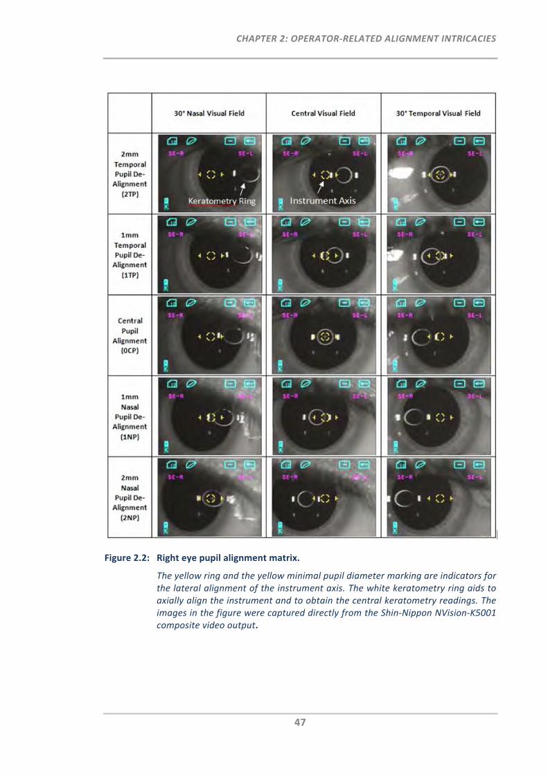
CHAPTER 2: OPERATOR‐RELATED ALIGNMENT INTRICACIES
47
Figure 2.2: Right eye pupil alignment matrix.
The yellow ring and the yellow minimal pupil diameter marking are indicators for the lateral alignment of the instrument axis. The white keratometry ring aids to axially align the instrument and to obtain the central keratometry readings. The images in the figure were captured directly from the Shin‐Nippon NVision‐K5001 composite video output.
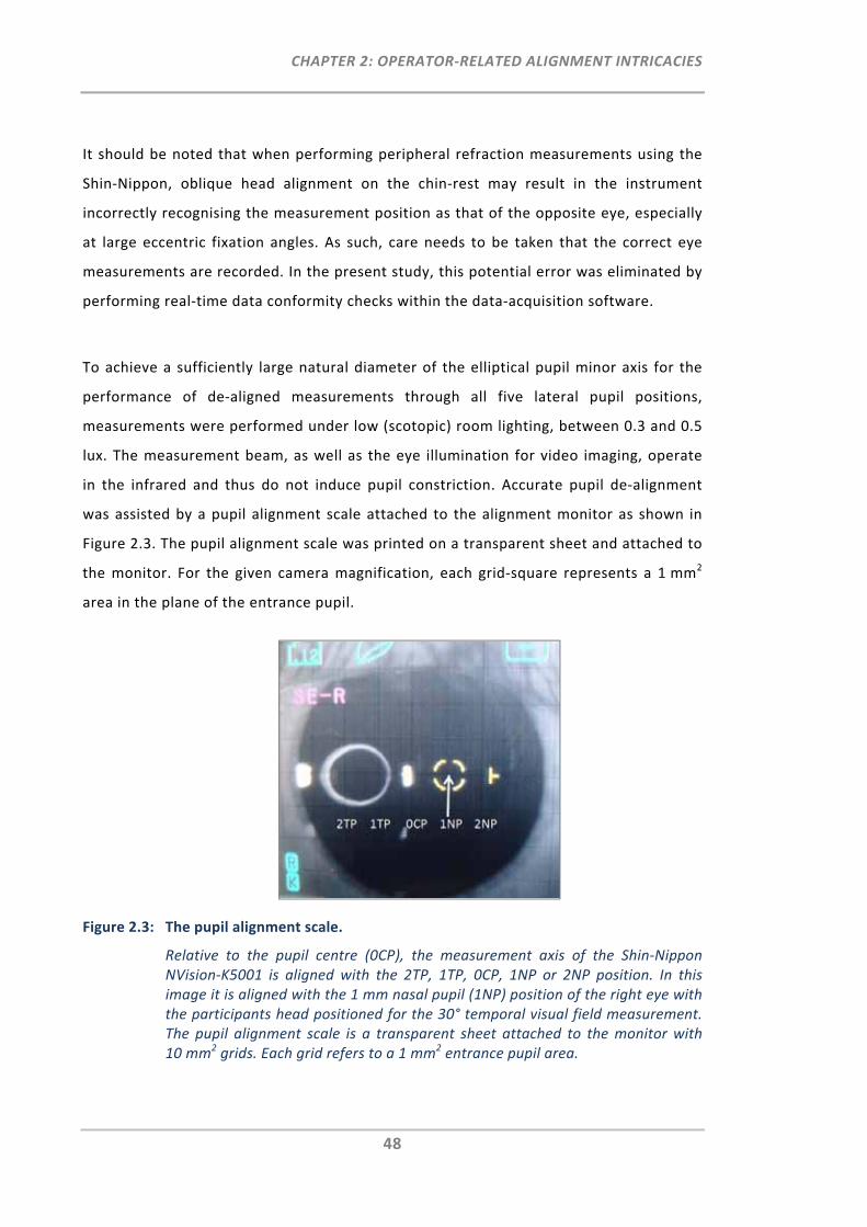
CHAPTER 2: OPERATOR‐RELATED ALIGNMENT INTRICACIES
48
It should be noted that when performing peripheral refraction measurements using the
Shin‐Nippon, oblique head alignment on the chin‐rest may result in the instrument
incorrectly recognising the measurement position as that of the opposite eye, especially
at large eccentric fixation angles. As such, care needs to be taken that the correct eye
measurements are recorded. In the present study, this potential error was eliminated by
performing real‐time data conformity checks within the data‐acquisition software.
To achieve a sufficiently large natural diameter of the elliptical pupil minor axis for the
performance of de‐aligned measurements through all five lateral pupil positions,
measurements were performed under low (scotopic) room lighting, between 0.3 and 0.5
lux. The measurement beam, as well as the eye illumination for video imaging, operate
in the infrared and thus do not induce pupil constriction. Accurate pupil de‐alignment
was assisted by a pupil alignment scale attached to the alignment monitor as shown in
Figure 2.3. The pupil alignment scale was printed on a transparent sheet and attached to
the monitor. For the given camera magnification, each grid‐square represents a 1 mm2
area in the plane of the entrance pupil.
Figure 2.3: The pupil alignment scale.
Relative to the pupil centre (0CP), the measurement axis of the Shin‐Nippon NVision‐K5001 is aligned with the 2TP, 1TP, 0CP, 1NP or 2NP position. In this image it is aligned with the 1 mm nasal pupil (1NP) position of the right eye with the participants head positioned for the 30° temporal visual field measurement. The pupil alignment scale is a transparent sheet attached to the monitor with 10 mm2 grids. Each grid refers to a 1 mm2 entrance pupil area.
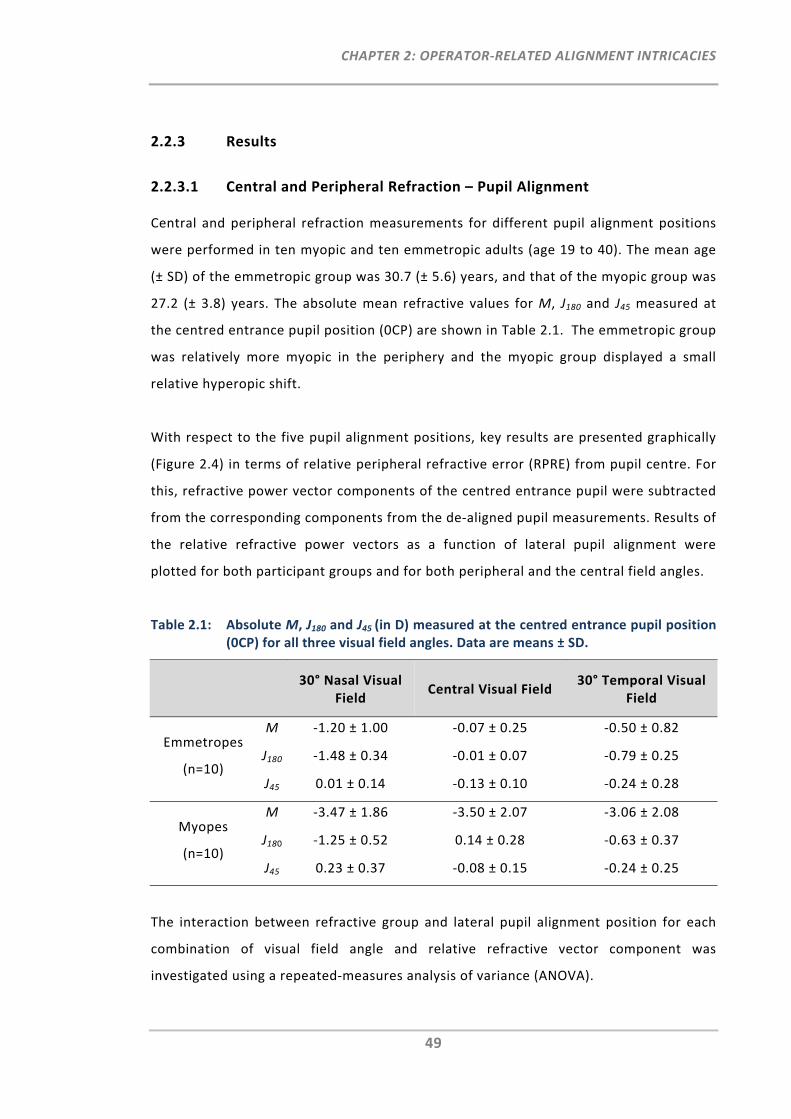
CHAPTER 2: OPERATOR‐RELATED ALIGNMENT INTRICACIES
49
2.2.3 Results
2.2.3.1 Central and Peripheral Refraction – Pupil Alignment
Central and peripheral refraction measurements for different pupil alignment positions
were performed in ten myopic and ten emmetropic adults (age 19 to 40). The mean age
(± SD) of the emmetropic group was 30.7 (± 5.6) years, and that of the myopic group was
27.2 (± 3.8) years. The absolute mean refractive values for M, J180 and J45 measured at
the centred entrance pupil position (0CP) are shown in Table 2.1. The emmetropic group
was relatively more myopic in the periphery and the myopic group displayed a small
relative hyperopic shift.
With respect to the five pupil alignment positions, key results are presented graphically
(Figure 2.4) in terms of relative peripheral refractive error (RPRE) from pupil centre. For
this, refractive power vector components of the centred entrance pupil were subtracted
from the corresponding components from the de‐aligned pupil measurements. Results of
the relative refractive power vectors as a function of lateral pupil alignment were
plotted for both participant groups and for both peripheral and the central field angles.
Table 2.1: Absolute M, J180 and J45 (in D) measured at the centred entrance pupil position (0CP) for all three visual field angles. Data are means ± SD.
30° Nasal Visual
Field Central Visual Field
30° Temporal Visual Field
Emmetropes
(n=10)
M ‐1.20 ± 1.00 ‐0.07 ± 0.25 ‐0.50 ± 0.82
J180 ‐1.48 ± 0.34 ‐0.01 ± 0.07 ‐0.79 ± 0.25
J45 0.01 ± 0.14 ‐0.13 ± 0.10 ‐0.24 ± 0.28
Myopes
(n=10)
M ‐3.47 ± 1.86 ‐3.50 ± 2.07 ‐3.06 ± 2.08
J180 ‐1.25 ± 0.52 0.14 ± 0.28 ‐0.63 ± 0.37
J45 0.23 ± 0.37 ‐0.08 ± 0.15 ‐0.24 ± 0.25
The interaction between refractive group and lateral pupil alignment position for each
combination of visual field angle and relative refractive vector component was
investigated using a repeated‐measures analysis of variance (ANOVA).
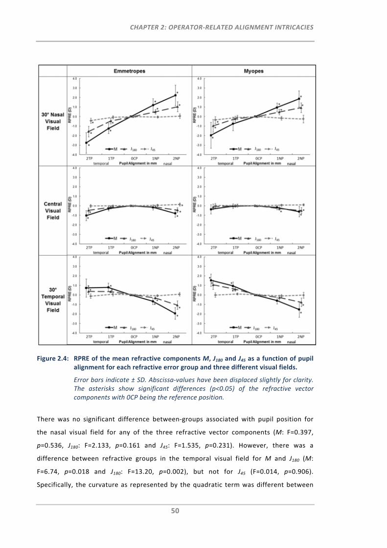
CHAPTER 2: OPERATOR‐RELATED ALIGNMENT INTRICACIES
50
Figure 2.4: RPRE of the mean refractive components M, J180 and J45 as a function of pupil alignment for each refractive error group and three different visual fields.
Error bars indicate ± SD. Abscissa‐values have been displaced slightly for clarity. The asterisks show significant differences (p<0.05) of the refractive vector components with 0CP being the reference position.
There was no significant difference between‐groups associated with pupil position for
the nasal visual field for any of the three refractive vector components (M: F=0.397,
p=0.536, J180: F=2.133, p=0.161 and J45: F=1.535, p=0.231). However, there was a
difference between refractive groups in the temporal visual field for M and J180 (M:
F=6.74, p=0.018 and J180: F=13.20, p=0.002), but not for J45 (F=0.014, p=0.906).
Specifically, the curvature as represented by the quadratic term was different between
CHAPTER 2: OPERATOR‐RELATED ALIGNMENT INTRICACIES
51
the refractive groups for M and J180 (M: F=5.641, p=0.029, J180: F=7.899, p=0.012). This is
also indicated by the more quadratic pupil alignment functions in the emmetropic group
as compared to the myopic group (Figure 2.4). The central visual field measurements
also showed a difference between groups for M (F=5.853, p=0.026), but not for J180
(F=2.036, p=0.171) or J45 (F=0.027, p=0.870).
Repeated‐measures analysis of variance was carried out on the refractive power vectors
M, J180 and J45, to compare the centred with the de‐aligned entrance pupil positions. For
this, a post hoc test for type‐I probability with Bonferroni correction was used. Figure 2.4
indicates statistically significant differences compared to centred entrance pupil
alignment where the critical type‐I probability (statistical significance) is set at 0.05.
For central visual field measurements, the relative refractive vector components M and
J180 decreased quadratically (r≥0.98, p<0.04) with increasing pupil de‐alignment in both
groups. Compared to centred pupil alignment, M and J180 showed significant differences
for all temporal and nasal pupil de‐alignments of 2 mm. The only exceptions in which no
differences were observed were M and J180 for the 2 mm temporal pupil de‐alignment in
the myopic group. A pupil de‐alignment of 1 mm was only significantly different for J180
in the myopic group, when aligned for the 1 mm nasal pupil position. The maximum M
mean difference to centred pupil alignment was ‐1.03D, found at the 2 mm temporal
pupil alignment in the emmetropic group.
For both peripheral visual fields, lateral pupil de‐alignments of 1 and 2 mm resulted in
significant differences for M and J180 when compared to centred pupil alignment (Figure
2.4). The only exceptions were the 1 mm temporal M and J180 for myopes measured at
the 30° nasal visual field and the 1 mm nasal M and J180 for myopes measured at the 30°
temporal visual field. Entrance pupil de‐alignment at the 30° nasal visual field for the
emmetropic group was found to produce the greatest mean difference from centred
pupil alignment for both 2 mm temporal (ΔM=‐2.77D, ΔJ180=‐1.57D) and 2 mm nasal
(ΔM=+2.23D, ΔJ180=+1.04D) pupil de‐alignments. In both refractive groups, M and J180
showed a significant linear (r≥0.94, p<0.02) correlation as de‐alignment progressed from
temporal to nasal for peripheral refraction measurements. To assess whether there is an

CHAPTER 2: OPERATOR‐RELATED ALIGNMENT INTRICACIES
52
asymmetry between the relative pupil alignment slopes of the nasal and temporal visual
fields, the absolute values of the linear slope (D/mm) were determined for M and J180.
Overall, the slopes were greater in the nasal visual field (emmetropic group: slope for
M=1.245, J180=0.618; myopic group: slope for M=0.937, J180=0.455) than in the temporal
visual field (emmetropic group: slope for M=0.684, J180=0.354, myopic group: slope for
M=0.769, J180=0.452). However, paired t‐test analysis showed that this difference in
relative pupil alignment slopes between the nasal and temporal visual field was
significantly different only in the emmetropic (M: p=0.00; J180: p=0.001) and not in the
myopic group (M: p=0.113; J180: p=0.958).
Overall, J45 was least affected by entrance pupil de‐alignment. Compared to centred
pupil alignment, J45 showed only significant differences for central refraction at the 2
mm nasal pupil position in the emmetropic group and for the nasal visual field at the 2
mm temporal pupil position in both groups.
2.2.3.2 Pupil Misalignment Threshold of Clinical Significance
Regression analysis was used to assess the relationship between refractive error
measured for centred and lateral de‐aligned pupil measurements, for the two refractive
groups and the three visual fields.
Data on pupil de‐alignment versus visual fields were fitted with equations to determine
the pupil misalignment threshold of clinical significance (Table 2.2). For this analysis,
first‐order (linear) fits were used for peripheral M and J180, and second‐order (quadratic)
fits were used for on‐axis measurements. A clinically significant difference was defined
as ≥0.25D for M and ≥0.125D for J180 and J45. Positive x refers to nasal pupil misalignment
and negative x refers to temporal pupil misalignment.
For central M and J180 the pupil misalignment threshold of clinical significance ranged
from +0.79 to ‐2.33 mm, while for peripheral M and J180 the range was as small as ±0.20
to ±0.37 mm. Overall, the range was smaller in the emmetropic group when compared to
the myopic group.
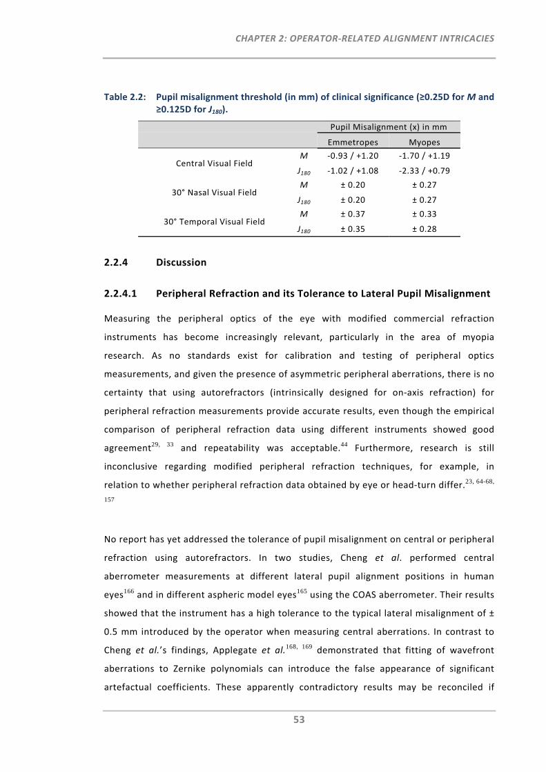
CHAPTER 2: OPERATOR‐RELATED ALIGNMENT INTRICACIES
53
Table 2.2: Pupil misalignment threshold (in mm) of clinical significance (≥0.25D for M and ≥0.125D for J180).
Pupil Misalignment (x) in mm
Emmetropes Myopes
Central Visual Field M ‐0.93 / +1.20 ‐1.70 / +1.19
J180 ‐1.02 / +1.08 ‐2.33 / +0.79
30° Nasal Visual Field M ± 0.20 ± 0.27
J180 ± 0.20 ± 0.27
30° Temporal Visual Field M ± 0.37 ± 0.33
J180 ± 0.35 ± 0.28
2.2.4 Discussion
2.2.4.1 Peripheral Refraction and its Tolerance to Lateral Pupil Misalignment
Measuring the peripheral optics of the eye with modified commercial refraction
instruments has become increasingly relevant, particularly in the area of myopia
research. As no standards exist for calibration and testing of peripheral optics
measurements, and given the presence of asymmetric peripheral aberrations, there is no
certainty that using autorefractors (intrinsically designed for on‐axis refraction) for
peripheral refraction measurements provide accurate results, even though the empirical
comparison of peripheral refraction data using different instruments showed good
agreement29, 33 and repeatability was acceptable.44 Furthermore, research is still
inconclusive regarding modified peripheral refraction techniques, for example, in
relation to whether peripheral refraction data obtained by eye or head‐turn differ.23, 64-68,
157
No report has yet addressed the tolerance of pupil misalignment on central or peripheral
refraction using autorefractors. In two studies, Cheng et al. performed central
aberrometer measurements at different lateral pupil alignment positions in human
eyes166 and in different aspheric model eyes165 using the COAS aberrometer. Their results
showed that the instrument has a high tolerance to the typical lateral misalignment of ±
0.5 mm introduced by the operator when measuring central aberrations. In contrast to
Cheng et al.’s findings, Applegate et al.168, 169 demonstrated that fitting of wavefront
aberrations to Zernike polynomials can introduce the false appearance of significant
artefactual coefficients. These apparently contradictory results may be reconciled if
CHAPTER 2: OPERATOR‐RELATED ALIGNMENT INTRICACIES
54
other errors involved in the measurement of wavefront aberrations are taken into
consideration. Indeed, Cheng et al. suggested that variability of measurements in the
human eyes reflects the changes in the eye’s optics, i.e. caused by fixational eye
movements or microfluctuations in accommodation, rather than instrument noise. In
addition, they showed that asymmetric aberrations occur only to a negligible amount for
lateral pupil de‐alignments when measuring central aberrations.
The present study investigated the impact of pupil de‐alignment on central and
peripheral refraction measurements in emmetropic and myopic eyes. Overall, the pupil
alignment slopes between the emmetropic and myopic group appeared to be similar for
all three visual fields. However, with respect to pupil alignment, differences between
both groups were found for the central and 30° temporal visual field measurements as
well as with respect to nasal‐temporal asymmetry across the visual field. Previous
studies have shown that factors such as corneal curvature170 and the shape of the
eyeball171 differ between emmetropic and myopic eyes. In addition, the nasal‐temporal
asymmetry across the visual field has been noted previously and was shown to decrease
as myopia increases.24 Thus, it is possible that these ocular differences between the
refractive groups may have led to some of the differences found in this study.
With respect to pupil misalignment tolerance, the present study has shown that for
central autorefraction, the pupil misalignment threshold of clinical significance was ≥
0.79 mm. As such, assuming a normal misalignment error of ± 0.5 mm in clinical practice,
central autorefraction can be considered highly tolerant with respect to lateral pupil de‐
alignment. This is in accordance with previous empirical validation studies of
autorefraction instruments for central measurements.138, 139 In contrast to the robust
results in central refraction, even small pupil de‐alignments in peripheral refraction led
to significant errors. Independent of the refractive group, results from this investigation
showed that there is a rapid and linear change in the refractive power vectors M and J180,
when de‐aligning the instrument axis even by only a minimal amount from the pupil
centre during the peripheral refraction measurements. Specifically, a small pupil
alignment error of 0.2 mm caused a significant change when the measurements were
performed in the 30° nasal visual field.
CHAPTER 2: OPERATOR‐RELATED ALIGNMENT INTRICACIES
55
The pupil misalignment threshold for clinical significance in 30° peripheral refraction
measurements was found to be much smaller than for central refraction and thus, can
have a significant impact on the data. It is reasonable to speculate that this may be a
substantial cause of the higher standard errors in peripheral measurement with
increasing eccentricities as seen in previous studies.23, 25, 34, 40, 64, 66, 71, 73 In fact, the
measurement of one eye at visual field angles of 0°, 20°, 30° and 40° confirmed that with
increasing eccentricity, tolerance to pupil misalignment error decreases even further.
The substantial and significant change in M and J180 found for the peripheral refraction
measurements at different pupil positions can mainly be attributed to the different
entrance angles of the peripheral measurement beam at the curved anterior cornea
surface, caused by the combination of peripheral measurement beam and changing
pupil/cornea position. In addition, it is assumed that the elliptical peripheral entrance
pupil can impact on measurements of the peripheral optics of the eye with respect to
pupil misalignment.
2.2.4.2 Factors Contributing to Misalignment Errors during Peripheral
Refraction Measurements
In practice, it is difficult for the operator to maintain consistent and accurate centration
of the peripheral pupil. Unlike in central refraction, this is particularly so when the
measurement of peripheral refraction profiles requires a large number of re‐alignments
and thus, increased participant cooperation, as well as operator attentiveness.
Alignment error in peripheral refractometry is augmented by inherent additional tasks,
i.e. the need for continuous re‐fixation by the participant, the re‐alignment of the
elliptical pupil with respect to the instrument axis, and the retention of a focused
peripherally shifted keratometry ring. Furthermore, time constraints and multiple
independent measurements can affect the accuracy of these tasks.
The aim of this study was to investigate the impact of lateral pupil misalignment on
peripheral refraction measurements. For future work it may also be of interest to
investigate the impact of vertical pupil misalignment on the tolerance values of the
refraction results. It should be noted that the amount of typical alignment error may be
CHAPTER 2: OPERATOR‐RELATED ALIGNMENT INTRICACIES
56
different between the lateral and vertical pupil alignment as lateral pupil alignment, for
example, requires the horizontal movement of the instrument base while the vertical
alignment of the pupil centre is achieved by rotational adjustment using the instrument’s
joy stick.
2.2.4.3 Improving Pupil Alignment
Technology of objective refraction instruments is developing at a rapid pace. The first
autorefractors became commercially available almost four decades ago, and were very
costly.172 Many instruments have been developed since. Especially in terms of
affordability, objective refraction instruments are now a practical consideration for all
practitioners, be they in clinical or research settings. The latest closed‐view
autorefraction models (i.e. CBD/TOMEY RC‐5000, Nidek ARK‐530A) have been equipped
with automated pupil alignment modes, making the instruments even easier to use and
the acquisition of data thereby more reliable and time efficient. In spite of this
advancement, all autorefractors still face limitations with respect to peripheral
refraction, as all are primarily designed for on‐axis refraction while off‐label use and
technical modifications of such instruments potentially compromise some aspects of
their performance.
The results of the present study suggest it would be advantageous to have a fast and
convenient instrument which does not require repeated re‐alignment to the peripheral
entrance pupil for each visual field angle. Until such an instrument becomes generally
available, modifications of current instruments will still be required for peripheral
refractometry. It is suggested that more attention be paid to the issue of pupil alignment
and to provide adequate training for the instrument operator as well as assessment and
validation of intra‐observer and inter‐observer variability prior to the commencement of
any clinical study. A pupil scale attached to the alignment monitor might be a helpful
tool to facilitate more accurate pupil alignment. Finally, given the increased sensitivity in
measurement error it might also be considered to increase the number of repeats for
peripheral refraction measurements, particularly for larger field angles.
CHAPTER 2: OPERATOR‐RELATED ALIGNMENT INTRICACIES
57
2.2.5 Conclusion
This study has demonstrated that accurate lateral alignment of the entrance pupil with
the instrument axis is critical to obtain reliable results when measuring peripheral
refraction with autorefractors. The error sensitivity to misalignment was shown to
increase linearly towards the periphery. At 30° field angle, lateral pupil misalignment
should be kept well below 0.5 mm to ensure clinically relevant accuracy.
2.3 Three‐Dimensional Model of the Entrance Pupil
2.3.1 Introduction
In Section 2.2 it was shown that the requirement for precise pupil alignment is of greater
importance for the measurement of peripheral refraction when compared to central
refraction. As alignment or centration for measurement of peripheral ocular optics is
also related to the change in the shape of the entrance pupil with peripheral viewing, a
more precise understanding of how the geometry of the entrance pupil behaves as a
function of peripheral viewing angle would be of value in understanding the accuracy of
techniques modified for the measurement of the peripheral optics, such as
autorefractors and aberrometer. Not only would information relating to the peripheral
entrance pupil be useful in the current quest to understand the role of peripheral
refraction in myopia progression, but it would also be of value in many aspects of vision
science, such as those requiring knowledge of retinal irradiation (e.g. calculations of
Stiles‐Crawford effect and ocular radiation safety).
The peripheral entrance pupil has been studied previously.173, 174 However, as these were
in vivo human studies, the size and position of the anatomical pupil (aperture stop) of
the eye is unknown. Hence, information such as pupil magnification and the relationship
between entrance pupil and actual pupil centres could not be ascertained. In addition, in
these studies, the axial position and the consequent three‐dimensional shape of the
entrance pupil were not investigated and only a limited number of pupil sizes were
studied (limited to e.g. large versus normal or dilated versus natural).
CHAPTER 2: OPERATOR‐RELATED ALIGNMENT INTRICACIES
58
Thus, the specific aim of this work was to extend the existing work on the peripheral
entrance pupil by modelling and assessing the three‐dimensional entrance pupil
position, shape and centration as a function of viewing angle and pupil size. Moreover,
the implications of this entrance pupil model on current peripheral refraction
measurements are discussed.
2.3.2 Methods
2.3.2.1 Model of the Entrance Pupil for Different Viewing Angles
The anterior segment (i.e. cornea and iris surfaces) of the Navarro schematic model for
the human eye175 was used for the optical modelling of the entrance pupil. The
components of this model were assumed to be circular and co‐axial, and the actual
iris/pupil surface had zero thickness. The entrance pupil of the eye was modelled as a
function of viewing angle and pupil size by ray‐tracing using ZEMAX (ZEMAX
Development Corporation, Bellevue, USA). Nine horizontal viewing angles ranging from
0° to 80° in 10° steps, and six pupil diameters ranging from 1.0 to 6.0 mm in 1.0 mm
steps were analysed.
For the ray‐tracing analysis of one pupil size at one viewing angle, the iris/pupil surface
was set as the object. Viewing angles were modelled as directions in the horizontal
meridian (around a vertical axis). Thus within this model system, the tangential meridian
lies in the horizontal plane while the sagittal meridian lies in a vertical plane. The
iris/pupil diameter was assigned the pupil size to be modelled. Sixteen points on the
iris/pupil surface and lying on the iris/pupil margin were defined, representing points on
sixteen equally spaced semi‐meridians at 22.5° increments. In addition, the point at the
iris/pupil centre was also analysed. Thus a total of seventeen object points were
analysed.
Using the robust, real ray‐aiming options in ZEMAX, from each of these object points, 24
rays consisting of 3 rings by 8 arms of rays (defined using the ZEMAX default merit
function whereby the rings represent ray‐heights of 0.336, 0.707 and 0.942 times the
pupil diameter, and the arms represent ray meridians 0.25π apart starting at 0.125π)
were traced towards the ‘observer’, which is defined as a surface with a 10 mm clear
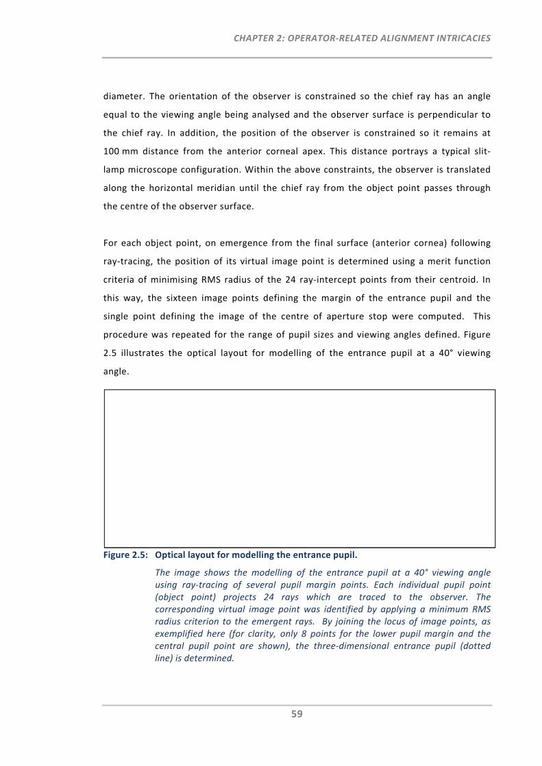
CHAPTER 2: OPERATOR‐RELATED ALIGNMENT INTRICACIES
59
diameter. The orientation of the observer is constrained so the chief ray has an angle
equal to the viewing angle being analysed and the observer surface is perpendicular to
the chief ray. In addition, the position of the observer is constrained so it remains at
100 mm distance from the anterior corneal apex. This distance portrays a typical slit‐
lamp microscope configuration. Within the above constraints, the observer is translated
along the horizontal meridian until the chief ray from the object point passes through
the centre of the observer surface.
For each object point, on emergence from the final surface (anterior cornea) following
ray‐tracing, the position of its virtual image point is determined using a merit function
criteria of minimising RMS radius of the 24 ray‐intercept points from their centroid. In
this way, the sixteen image points defining the margin of the entrance pupil and the
single point defining the image of the centre of aperture stop were computed. This
procedure was repeated for the range of pupil sizes and viewing angles defined. Figure
2.5 illustrates the optical layout for modelling of the entrance pupil at a 40° viewing
angle.
Figure 2.5: Optical layout for modelling the entrance pupil.
The image shows the modelling of the entrance pupil at a 40° viewing angle using ray‐tracing of several pupil margin points. Each individual pupil point (object point) projects 24 rays which are traced to the observer. The corresponding virtual image point was identified by applying a minimum RMS radius criterion to the emergent rays. By joining the locus of image points, as exemplified here (for clarity, only 8 points for the lower pupil margin and the central pupil point are shown), the three‐dimensional entrance pupil (dotted line) is determined.
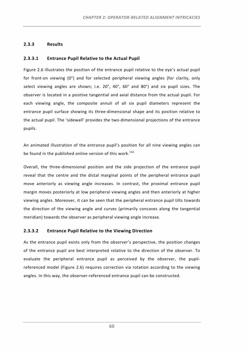
CHAPTER 2: OPERATOR‐RELATED ALIGNMENT INTRICACIES
60
2.3.3 Results
2.3.3.1 Entrance Pupil Relative to the Actual Pupil
Figure 2.6 illustrates the position of the entrance pupil relative to the eye’s actual pupil
for front‐on viewing (0°) and for selected peripheral viewing angles (for clarity, only
select viewing angles are shown; i.e. 20°, 40°, 60° and 80°) and six pupil sizes. The
observer is located in a positive tangential and axial distance from the actual pupil. For
each viewing angle, the composite annuli of all six pupil diameters represent the
entrance pupil surface showing its three‐dimensional shape and its position relative to
the actual pupil. The ‘sidewall’ provides the two‐dimensional projections of the entrance
pupils.
An animated illustration of the entrance pupil’s position for all nine viewing angles can
be found in the published online version of this work.164
Overall, the three‐dimensional position and the side projection of the entrance pupil
reveal that the centre and the distal marginal points of the peripheral entrance pupil
move anteriorly as viewing angle increases. In contrast, the proximal entrance pupil
margin moves posteriorly at low peripheral viewing angles and then anteriorly at higher
viewing angles. Moreover, it can be seen that the peripheral entrance pupil tilts towards
the direction of the viewing angle and curves (primarily concaves along the tangential
meridian) towards the observer as peripheral viewing angle increase.
2.3.3.2 Entrance Pupil Relative to the Viewing Direction
As the entrance pupil exists only from the observer’s perspective, the position changes
of the entrance pupil are best interpreted relative to the direction of the observer. To
evaluate the peripheral entrance pupil as perceived by the observer, the pupil‐
referenced model (Figure 2.6) requires correction via rotation according to the viewing
angles. In this way, the observer‐referenced entrance pupil can be constructed.
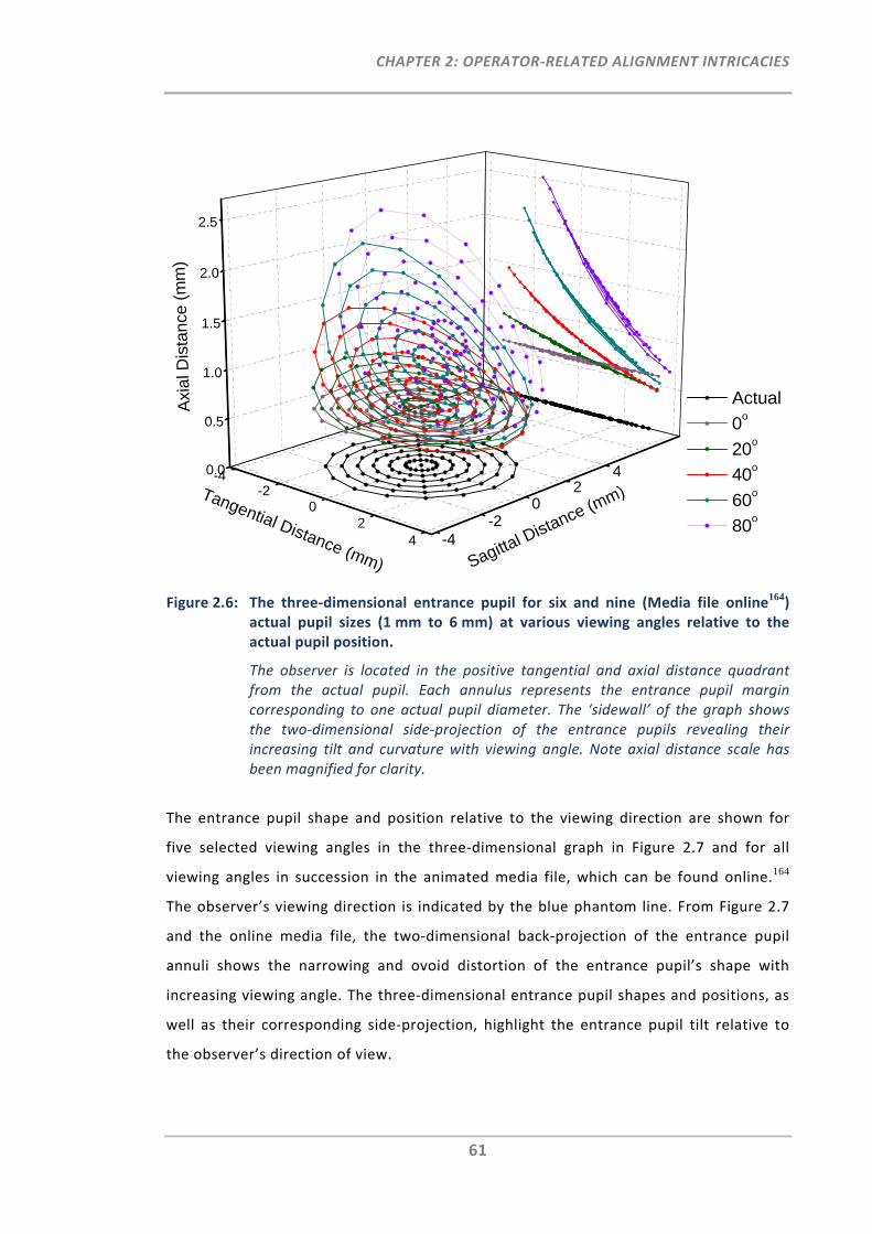
CHAPTER 2: OPERATOR‐RELATED ALIGNMENT INTRICACIES
61
Figure 2.6: The three‐dimensional entrance pupil for six and nine (Media file online164)
actual pupil sizes (1 mm to 6 mm) at various viewing angles relative to the actual pupil position.
The observer is located in the positive tangential and axial distance quadrant from the actual pupil. Each annulus represents the entrance pupil margin corresponding to one actual pupil diameter. The ‘sidewall’ of the graph shows the two‐dimensional side‐projection of the entrance pupils revealing their increasing tilt and curvature with viewing angle. Note axial distance scale has been magnified for clarity.
The entrance pupil shape and position relative to the viewing direction are shown for
five selected viewing angles in the three‐dimensional graph in Figure 2.7 and for all
viewing angles in succession in the animated media file, which can be found online.164
The observer’s viewing direction is indicated by the blue phantom line. From Figure 2.7
and the online media file, the two‐dimensional back‐projection of the entrance pupil
annuli shows the narrowing and ovoid distortion of the entrance pupil’s shape with
increasing viewing angle. The three‐dimensional entrance pupil shapes and positions, as
well as their corresponding side‐projection, highlight the entrance pupil tilt relative to
the observer’s direction of view.
-4-2
02
4 -4-2
02
40.0
0.5
1.0
1.5
2.0
2.5
Actual
0o
20o
40o
60o
80o
Axi
al D
ista
nce
(m
m)
Sagittal Distance (m
m)Tangential Distance (mm)
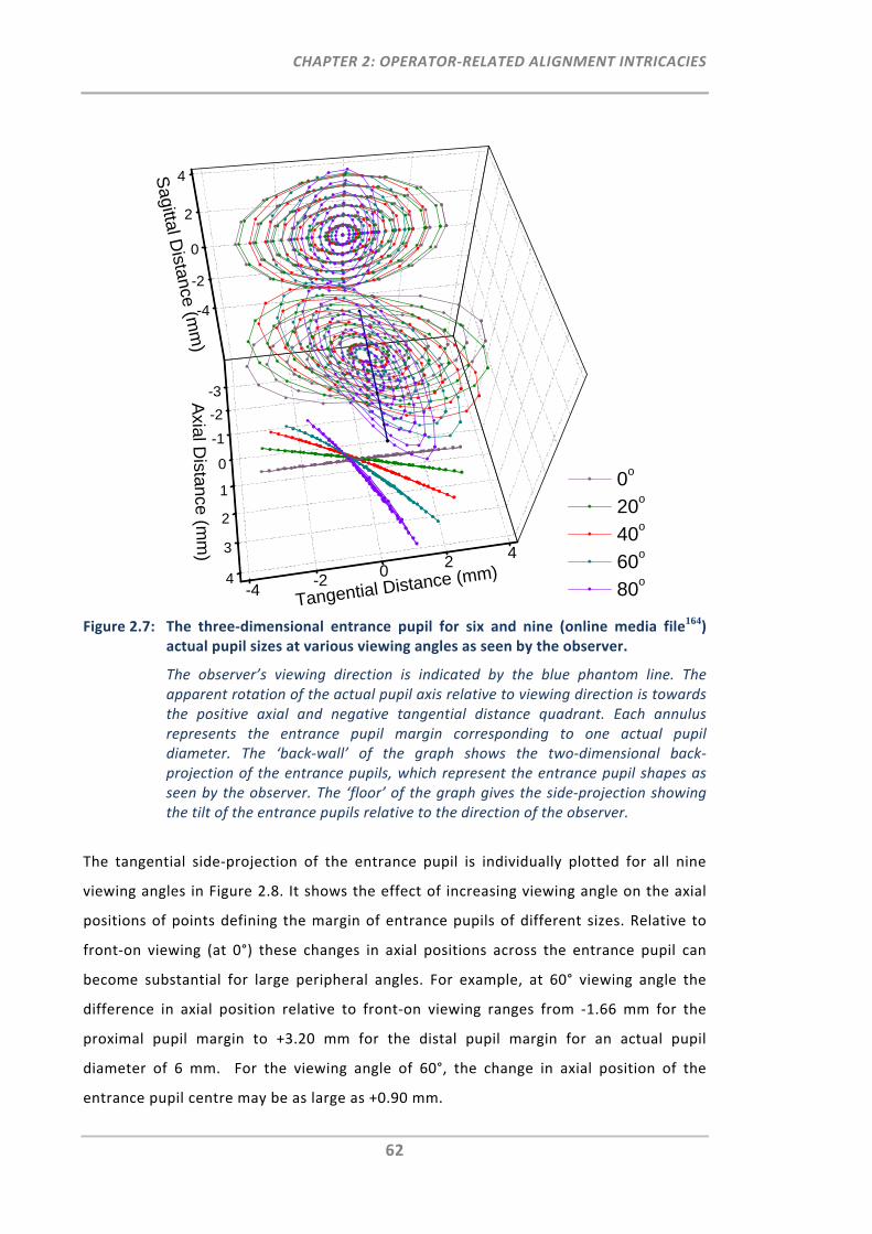
CHAPTER 2: OPERATOR‐RELATED ALIGNMENT INTRICACIES
62
Figure 2.7: The three‐dimensional entrance pupil for six and nine (online media file164)
actual pupil sizes at various viewing angles as seen by the observer.
The observer’s viewing direction is indicated by the blue phantom line. The apparent rotation of the actual pupil axis relative to viewing direction is towards the positive axial and negative tangential distance quadrant. Each annulus represents the entrance pupil margin corresponding to one actual pupil diameter. The ‘back‐wall’ of the graph shows the two‐dimensional back‐projection of the entrance pupils, which represent the entrance pupil shapes as seen by the observer. The ‘floor’ of the graph gives the side‐projection showing the tilt of the entrance pupils relative to the direction of the observer.
The tangential side‐projection of the entrance pupil is individually plotted for all nine
viewing angles in Figure 2.8. It shows the effect of increasing viewing angle on the axial
positions of points defining the margin of entrance pupils of different sizes. Relative to
front‐on viewing (at 0°) these changes in axial positions across the entrance pupil can
become substantial for large peripheral angles. For example, at 60° viewing angle the
difference in axial position relative to front‐on viewing ranges from ‐1.66 mm for the
proximal pupil margin to +3.20 mm for the distal pupil margin for an actual pupil
diameter of 6 mm. For the viewing angle of 60°, the change in axial position of the
entrance pupil centre may be as large as +0.90 mm.
-3
-2
-1
0
1
2
3
4-4
-20
24
-4
-2
0
2
4
0o
20o
40o
60o
80o
Sagittal D
istance (mm
)
Tangential Distance (mm)
Axial D
istance (mm
)
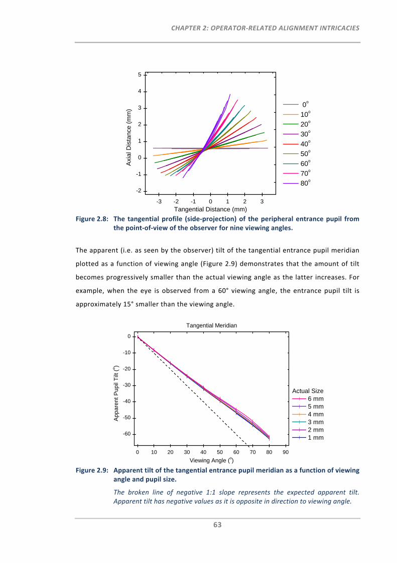
CHAPTER 2: OPERATOR‐RELATED ALIGNMENT INTRICACIES
63
Figure 2.8: The tangential profile (side‐projection) of the peripheral entrance pupil from
the point‐of‐view of the observer for nine viewing angles.
The apparent (i.e. as seen by the observer) tilt of the tangential entrance pupil meridian
plotted as a function of viewing angle (Figure 2.9) demonstrates that the amount of tilt
becomes progressively smaller than the actual viewing angle as the latter increases. For
example, when the eye is observed from a 60° viewing angle, the entrance pupil tilt is
approximately 15° smaller than the viewing angle.
Figure 2.9: Apparent tilt of the tangential entrance pupil meridian as a function of viewing
angle and pupil size.
The broken line of negative 1:1 slope represents the expected apparent tilt. Apparent tilt has negative values as it is opposite in direction to viewing angle.
-3 -2 -1 0 1 2 3
-2
-1
0
1
2
3
4
5
Axi
al D
ista
nce
(mm
)
Tangential Distance (mm)
0o
10o
20o
30o
40o
50o
60o
70o
80o
0 10 20 30 40 50 60 70 80 90
-60
-50
-40
-30
-20
-10
0
App
aren
t P
upil
Tilt
(o)
Viewing Angle (o)
Actual Size 6 mm 5 mm 4 mm 3 mm 2 mm 1 mm
Tangential Meridian
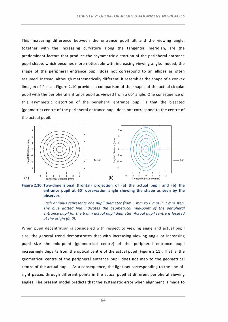
CHAPTER 2: OPERATOR‐RELATED ALIGNMENT INTRICACIES
64
This increasing difference between the entrance pupil tilt and the viewing angle,
together with the increasing curvature along the tangential meridian, are the
predominant factors that produce the asymmetric distortion of the peripheral entrance
pupil shape, which becomes more noticeable with increasing viewing angle. Indeed, the
shape of the peripheral entrance pupil does not correspond to an ellipse as often
assumed. Instead, although mathematically different, it resembles the shape of a convex
limaçon of Pascal. Figure 2.10 provides a comparison of the shapes of the actual circular
pupil with the peripheral entrance pupil as viewed from a 60° angle. One consequence of
this asymmetric distortion of the peripheral entrance pupil is that the bisected
(geometric) centre of the peripheral entrance pupil does not correspond to the centre of
the actual pupil.
Figure 2.10: Two‐dimensional (frontal) projection of (a) the actual pupil and (b) the
entrance pupil at 60° observation angle showing the shape as seen by the observer.
Each annulus represents one pupil diameter from 1 mm to 6 mm in 1 mm step. The blue dotted line indicates the geometrical mid‐point of the peripheral entrance pupil for the 6 mm actual pupil diameter. Actual pupil centre is located at the origin (0, 0).
When pupil decentration is considered with respect to viewing angle and actual pupil
size, the general trend demonstrates that with increasing viewing angle or increasing
pupil size the mid‐point (geometrical centre) of the peripheral entrance pupil
increasingly departs from the optical centre of the actual pupil (Figure 2.11). That is, the
geometrical centre of the peripheral entrance pupil does not map to the geometrical
centre of the actual pupil. As a consequence, the light ray corresponding to the line‐of‐
sight passes through different points in the actual pupil at different peripheral viewing
angles. The present model predicts that the systematic error when alignment is made to
-3 -2 -1 0 1 2 3
-3
-2
-1
0
1
2
3
Sag
ittal
Dis
tanc
e (m
m)
Tangential Distance (mm)
Actual
(a)-3 -2 -1 0 1 2 3
-3
-2
-1
0
1
2
3
Sag
ittal
Dis
tanc
e (m
m)
Tangential Distance (mm)
60o
(b)
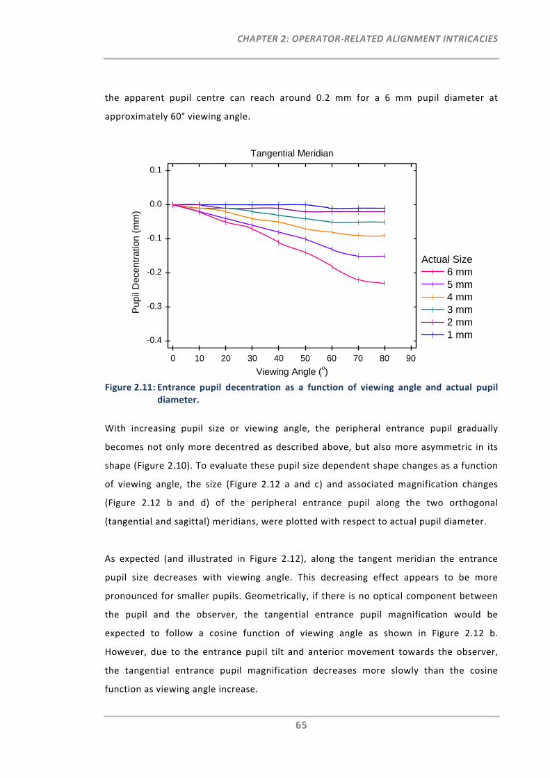
CHAPTER 2: OPERATOR‐RELATED ALIGNMENT INTRICACIES
65
the apparent pupil centre can reach around 0.2 mm for a 6 mm pupil diameter at
approximately 60° viewing angle.
Figure 2.11: Entrance pupil decentration as a function of viewing angle and actual pupil
diameter.
With increasing pupil size or viewing angle, the peripheral entrance pupil gradually
becomes not only more decentred as described above, but also more asymmetric in its
shape (Figure 2.10). To evaluate these pupil size dependent shape changes as a function
of viewing angle, the size (Figure 2.12 a and c) and associated magnification changes
(Figure 2.12 b and d) of the peripheral entrance pupil along the two orthogonal
(tangential and sagittal) meridians, were plotted with respect to actual pupil diameter.
As expected (and illustrated in Figure 2.12), along the tangent meridian the entrance
pupil size decreases with viewing angle. This decreasing effect appears to be more
pronounced for smaller pupils. Geometrically, if there is no optical component between
the pupil and the observer, the tangential entrance pupil magnification would be
expected to follow a cosine function of viewing angle as shown in Figure 2.12 b.
However, due to the entrance pupil tilt and anterior movement towards the observer,
the tangential entrance pupil magnification decreases more slowly than the cosine
function as viewing angle increase.
0 10 20 30 40 50 60 70 80 90
-0.4
-0.3
-0.2
-0.1
0.0
0.1
Pup
il D
ecen
trat
ion
(mm
)
Viewing Angle (o)
Actual Size 6 mm 5 mm 4 mm 3 mm 2 mm 1 mm
Tangential Meridian
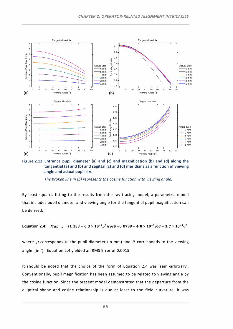
CHAPTER 2: OPERATOR‐RELATED ALIGNMENT INTRICACIES
66
Figure 2.12: Entrance pupil diameter (a) and (c) and magnification (b) and (d) along the tangential (a) and (b) and sagittal (c) and (d) meridians as a function of viewing angle and actual pupil size.
The broken line in (b) represents the cosine function with viewing angle.
By least‐squares fitting to the results from the ray‐tracing model, a parametric model
that includes pupil diameter and viewing angle for the tangential pupil magnification can
be derived:
Equation 2.4: . . . . .
where p corresponds to the pupil diameter (in mm) and corresponds to the viewing
angle (in °). Equation 2.4 yielded an RMS Error of 0.0015.
It should be noted that the choice of the form of Equation 2.4 was ‘semi‐arbitrary’.
Conventionally, pupil magnification has been assumed to be related to viewing angle by
the cosine function. Since the present model demonstrated that the departure from the
elliptical shape and cosine relationship is due at least to the field curvature, it was
0 10 20 30 40 50 60 70 80 90
0
1
2
3
4
5
6
7
8
Ent
ranc
e P
upil
Siz
e (m
m)
Viewing Angle (o)
Actual Size 6 mm 5 mm 4 mm 3 mm 2 mm 1 mm
Tangential Meridian
(a)0 10 20 30 40 50 60 70 80 90
0.4
0.5
0.6
0.7
0.8
0.9
1.0
1.1
Pup
il M
agni
ficat
ion
Viewing Angle (o)
Actual Size 6 mm 5 mm 4 mm 3 mm 2 mm 1 mm
Tangential Meridian
(b)
0 10 20 30 40 50 60 70 80 90
0
1
2
3
4
5
6
7
8
Ent
ranc
e P
upil
Siz
e (m
m)
Viewing Angle (o)
Actual Size 6 mm 5 mm 4 mm 3 mm 2 mm 1 mm
Sagittal Meridian
(c)0 10 20 30 40 50 60 70 80 90
1.10
1.12
1.14
1.16
1.18
1.20
1.22
1.24
Pup
il M
agni
ficat
ion
Viewing Angle (o)
Actual Size 6 mm 5 mm 4 mm 3 mm 2 mm 1 mm
Sagittal Meridian
(d)
CHAPTER 2: OPERATOR‐RELATED ALIGNMENT INTRICACIES
67
decided to employ a modification to the cosine function in which the variable (viewing
angle) has been ‘rescaled’ according to a second‐order function. It is possible that other
forms of function can provide a better fit. But given the excellent resultant RMS, no
further attempts were made to search for a more precise form.
While Equation 2.4 quite precisely predicts tangential pupil magnification, it is somewhat
complex in structure. A simplified equation involving only viewing angle ( in °), still
with good precision (RMS Error = 0.0066 mm), may be obtained:
Equation 2.5: . .
Figure 2.12 also shows that the sagittal entrance pupil size and magnification increases
slightly with increasing viewing angle. This small increase in sagittal pupil size is slightly
greater for smaller pupils. In a similar manner as for tangential pupil magnification, a
parametric equation can be derived to predict sagittal pupil magnification with good
precision (RMS Error = 0.0083 mm) from the viewing angle (in °):
Equation 2.6: . . .
2.3.4 Discussion
Much of what is known about the peripheral entrance pupil was established many
decades ago. Spring & Stiles (1948)174 then later Jay (1962)173 measured the peripheral
entrance pupil shape for in vivo human subjects. They established the change in
diameters along the horizontal and vertical meridians with viewing angle and identified
the departure of the peripheral entrance pupil size from a cosine function with viewing
angle. Jay also noted the departure of the peripheral pupil shape from an ellipse.173
However, these early in vivo studies suffered limitations. For example, without
knowledge of the actual pupil size, the pupil magnification could not be estimated. Also,
no attempt was made to evaluate the changes in the entrance pupil in the axial
dimension.
CHAPTER 2: OPERATOR‐RELATED ALIGNMENT INTRICACIES
68
The present study attempted to extend knowledge of the peripheral entrance pupil. In
particular, the model predicted the pupil magnification for a range of pupil sizes and
viewing angles. The changing shape and its departure from an ellipse of the peripheral
entrance pupil were evaluated with the consequence that the peripheral entrance pupil
centre was found to not correspond to the actual pupil centre. In addition, by
considering the axial dimension, the forward movement, compensatory tilt and
increasing curvature of the peripheral entrance pupil with viewing angle were revealed.
2.3.4.1 Comparison of the Entrance Pupil Model with in Vivo Pupils
There are a number of differences between the peripheral entrance pupil modelled in
the present study and the direct measurement studies above‐mentioned.173, 174 For
simplicity, the entrance pupil model portrays a thin (zero thickness), circular pupil that is
co‐axial with the corneal surfaces. In addition to the temporal viewing angles, Spring &
Stiles measured a nasal viewing angle and were thus able to identify the presence of
nasal‐temporal asymmetry in the peripheral entrance pupil with respect to viewing
angle. Presumably, this is due to the decentration and tilt of the corneal surfaces relative
to the iris.174 Jay suggested that iris thickness may become relevant and would have the
effect of reducing tangential entrance pupil size at high viewing angles.173 Despite these
differences, the entrance pupil model appears to produce predictions of acceptable
precision with respect to the range of in vivo measurement errors. The ratio of
tangential (horizontal) to sagittal (vertical) entrance pupil diameters as a function of
viewing angle for the entrance pupil model of this study, together with in vivo
measurements previously published173, 174 are shown in Fig. 9. In lieu of Spring & Stiles
who refer to large and small pupil diameters and Jay who refers to dilated and natural
pupil diameters, Figure 2.13 plots the values for the actual pupil diameters of 3 and 6
mm. It can be seen that the predictions lie well within the spread of measured results,
particularly of Jay.173 In addition, as the actual pupil size is known in the presented
entrance pupil model, the pupil magnification was also calculable.
The non‐elliptical shape of the entrance pupil at high peripheral angles has been noted
by Jay. The present entrance pupil model has been able to predict and describe this
shape, which appears to be caused by the increasing curvature (primarily concave
towards the observer along the tangential meridian) with viewing angle. As illustrated in
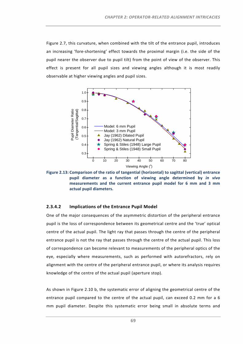
CHAPTER 2: OPERATOR‐RELATED ALIGNMENT INTRICACIES
69
Figure 2.7, this curvature, when combined with the tilt of the entrance pupil, introduces
an increasing ‘fore‐shortening’ effect towards the proximal margin (i.e. the side of the
pupil nearer the observer due to pupil tilt) from the point of view of the observer. This
effect is present for all pupil sizes and viewing angles although it is most readily
observable at higher viewing angles and pupil sizes.
Figure 2.13: Comparison of the ratio of tangential (horizontal) to sagittal (vertical) entrance
pupil diameter as a function of viewing angle determined by in vivo measurements and the current entrance pupil model for 6 mm and 3 mm actual pupil diameters.
2.3.4.2 Implications of the Entrance Pupil Model
One of the major consequences of the asymmetric distortion of the peripheral entrance
pupil is the loss of correspondence between its geometrical centre and the ‘true’ optical
centre of the actual pupil. The light ray that passes through the centre of the peripheral
entrance pupil is not the ray that passes through the centre of the actual pupil. This loss
of correspondence can become relevant to measurements of the peripheral optics of the
eye, especially where measurements, such as performed with autorefractors, rely on
alignment with the centre of the peripheral entrance pupil, or where its analysis requires
knowledge of the centre of the actual pupil (aperture stop).
As shown in Figure 2.10 b, the systematic error of aligning the geometrical centre of the
entrance pupil compared to the centre of the actual pupil, can exceed 0.2 mm for a 6
mm pupil diameter. Despite this systematic error being small in absolute terms and
0 10 20 30 40 50 60 70 80
0.3
0.4
0.5
0.6
0.7
0.8
0.9
1.0
Pup
il D
iam
eter
Rat
io
(Tan
gent
ial/S
agitt
al)
Viewing Angle (o)
Model: 6 mm Pupil Model: 3 mm Pupil Jay (1962) Dilated Pupil Jay (1962) Natural Pupil Spring & Stiles (1948) Large Pupil Spring & Stiles (1948) Small Pupil
CHAPTER 2: OPERATOR‐RELATED ALIGNMENT INTRICACIES
70
falling within normal measurement variability, for some refraction instruments, this
error could impact measurement accuracy, especially at large peripheral angles. In
Section 2.2 it was shown that tolerance to pupil misalignment is much smaller for
peripheral refraction than for central refraction.126 For example, when measuring
peripheral refraction at the 30° nasal visual field using an open‐view autorefractor, the
refractive power vector components M and J180 reached clinical significance for pupil
misalignments as small as 0.2 mm.
In addition, Applegate et al. have demonstrated that misalignment from the pupil centre
during on‐axis wavefront measurements can introduce spurious coefficients into Zernike
polynomial descriptions of the wavefront. This systematic error is not only Zernike
mode‐dependent but also, the larger the misalignment, the more profound its effect.168
Assuming these findings can be extrapolated to peripheral wavefront measurements, it
is reasonable to suggest that a combination of even small pupil misalignment errors, as
well as the systematic error caused by the loss of correspondence of the peripheral
entrance pupil mid‐point with the actual pupil centre, could adversely affect the
accuracy of peripheral ocular measurements.
In many studies of peripheral optics, comparisons are made to the central optics of the
eye. Consideration of the errors in peripheral refractometry or wavefront measurements
due to systematic misalignment, as well as the loss of correspondence between
peripheral and actual pupil centres, suggest that caution needs to be exercised when
making comparisons of peripheral and central measurements.
The axial alignment of most autorefractor and aberrometer instruments requires that
either the cornea or the pupil plane be in focus. This presents no difficulty for on‐axis
measurements, wherein both the cornea mire and the pupil margin appear completely
and symmetrically in focus. According to the entrance pupil model, the axial position
shifts forward for the peripheral entrance pupil but more significantly, the pupil tilt
produces different axial positions for different points on the entrance pupil. From Figure
2.8, for a 60° viewing angle, the axial position range from the distal to the proximal pupil
margin is around 4 mm for a 6 mm pupil. This is the axial focus range of the aberrometer
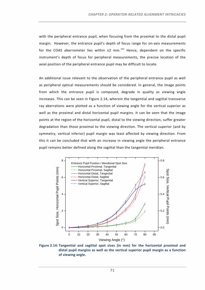
CHAPTER 2: OPERATOR‐RELATED ALIGNMENT INTRICACIES
71
with the peripheral entrance pupil, when focusing from the proximal to the distal pupil
margin. However, the entrance pupil’s depth of focus range for on‐axis measurements
for the COAS aberrometer lies within ±2 mm.165 Hence, dependent on the specific
instrument’s depth of focus for peripheral measurements, the precise location of the
axial position of the peripheral entrance pupil may be difficult to locate.
An additional issue relevant to the observation of the peripheral entrance pupil as well
as peripheral optical measurements should be considered. In general, the image points
from which the entrance pupil is composed, degrade in quality as viewing angle
increases. This can be seen in Figure 2.14, wherein the tangential and sagittal transverse
ray aberrations were plotted as a function of viewing angle for the vertical superior as
well as the proximal and distal horizontal pupil margins. It can be seen that the image
points at the region of the horizontal pupil, distal to the viewing direction, suffer greater
degradation than those proximal to the viewing direction. The vertical superior (and by
symmetry, vertical inferior) pupil margin was least affected by viewing direction. From
this it can be concluded that with an increase in viewing angle the peripheral entrance
pupil remains better defined along the sagittal than the tangential meridian.
Figure 2.14: Tangential and sagittal spot sizes (in mm) for the horizontal proximal and
distal pupil margins as well as the vertical superior pupil margin as a function of viewing angle.
0 10 20 30 40 50 60 70 80 90
0
2
4
6
8Entrance Pupil Position / Meridional Spot Size
Horizontal Proximal, Tangential Horizontal Proximal, Sagittal Horizontal Distal, Tangential Horizontal Distal, Sagittal Vertical Superior, Tangential Vertical Superior, Sagittal
Viewing Angle (°)
Sp
ot S
ize
, Hor
izo
ntal
Pup
il P
oint
s (m
m)
0.0
0.2
0.4
0.6
0.8
Sp
ot Size
, Ve
rtical Pup
il Po
ints (mm
)
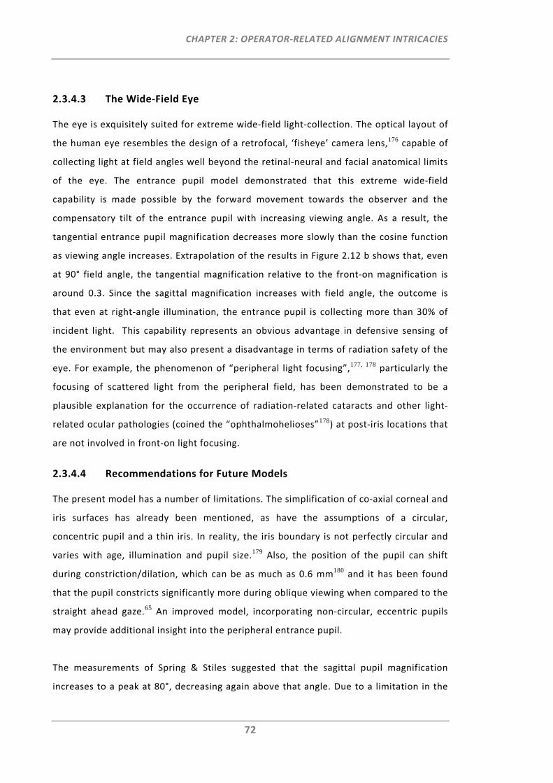
CHAPTER 2: OPERATOR‐RELATED ALIGNMENT INTRICACIES
72
2.3.4.3 The Wide‐Field Eye
The eye is exquisitely suited for extreme wide‐field light‐collection. The optical layout of
the human eye resembles the design of a retrofocal, ‘fisheye’ camera lens,176 capable of
collecting light at field angles well beyond the retinal‐neural and facial anatomical limits
of the eye. The entrance pupil model demonstrated that this extreme wide‐field
capability is made possible by the forward movement towards the observer and the
compensatory tilt of the entrance pupil with increasing viewing angle. As a result, the
tangential entrance pupil magnification decreases more slowly than the cosine function
as viewing angle increases. Extrapolation of the results in Figure 2.12 b shows that, even
at 90° field angle, the tangential magnification relative to the front‐on magnification is
around 0.3. Since the sagittal magnification increases with field angle, the outcome is
that even at right‐angle illumination, the entrance pupil is collecting more than 30% of
incident light. This capability represents an obvious advantage in defensive sensing of
the environment but may also present a disadvantage in terms of radiation safety of the
eye. For example, the phenomenon of “peripheral light focusing”,177, 178 particularly the
focusing of scattered light from the peripheral field, has been demonstrated to be a
plausible explanation for the occurrence of radiation‐related cataracts and other light‐
related ocular pathologies (coined the “ophthalmohelioses”178) at post‐iris locations that
are not involved in front‐on light focusing.
2.3.4.4 Recommendations for Future Models
The present model has a number of limitations. The simplification of co‐axial corneal and
iris surfaces has already been mentioned, as have the assumptions of a circular,
concentric pupil and a thin iris. In reality, the iris boundary is not perfectly circular and
varies with age, illumination and pupil size.179 Also, the position of the pupil can shift
during constriction/dilation, which can be as much as 0.6 mm180 and it has been found
that the pupil constricts significantly more during oblique viewing when compared to the
straight ahead gaze.65 An improved model, incorporating non‐circular, eccentric pupils
may provide additional insight into the peripheral entrance pupil.
The measurements of Spring & Stiles suggested that the sagittal pupil magnification
increases to a peak at 80°, decreasing again above that angle. Due to a limitation in the
CHAPTER 2: OPERATOR‐RELATED ALIGNMENT INTRICACIES
73
optical layout, the entrance pupil model was not able to compute results for viewing
angles at or above 90°. It would be interesting to model and verify this reversal of
sagittal pupil magnification at very high viewing angles.
Finally, for the study of peripheral retinal image quality or other retinal responses, such
as the Stiles‐Crawford Effect, it might be of more value to analyse the exit pupil shape
and size with viewing angle. Such an analysis would need to take into the account the
complex shape181 and gradient refractive index of the crystalline lens.182 Hopefully,
future work can address these aspects of the peripheral optics of the eye.
2.3.5 Conclusion
As the viewing angle increases, the entrance pupil moves forward, exhibits
compensatory tilt and increases in concavity towards the observer. In consequence the
tangential pupil size does not follow a cosine relationship with viewing angle, the shape
of the entrance pupil undergoes asymmetric (non‐elliptical) distortion, and the
geometrical centre of the entrance pupil does not represent precisely the centre of the
actual pupil. Thus, peripheral ocular measurements may be affected adversely,
particularly where alignment to the pupil centre is required. Given the potential adverse
impact misalignment may have on ocular measurements, such as autorefraction, caution
is warranted when comparing such results between peripheral and central viewing
angles. Overall however, it can be concluded that typically, these departures are small
and may only be of significance for peripheral viewing angles larger than 40°.
2.4 Summary
The clinical study on pupil alignment tolerance demonstrated that, independent of the
central refractive error of the eye, even small lateral pupil alignment errors caused by
the operator can lead to significant measurement errors in peripheral refractometry
when using commercially available autorefractors. In addition, the three‐dimensional
entrance pupil model demonstrated that, due to its geometrical behaviour when viewed
from a peripheral angle, the peripheral entrance pupil is not elliptical as assumed and
the mid‐point of the peripheral pupil does not correspond to the centre of the actual
pupil.

CHAPTER 2: OPERATOR‐RELATED ALIGNMENT INTRICACIES
74
From both studies it can be concluded that precise pupil alignment is critical for accurate
measurements of peripheral refraction and that entrance pupil alignment with its mid‐
point, as currently performed in peripheral refractometry, can induce small systematic
lateral errors.
In practice, however, it could be very difficult to circumvent small pupil alignment errors
during peripheral refractometry. Thus, it would be advantageous to have means by
which to correct for such operator‐related errors and to thereby provide more accurate
peripheral refraction measurements.
CHAPTER 3: MEANS TO RECTIFY PUPIL ALIGNMENT ERRORS
75
CHAPTER 3:
MEANS TO RECTIFY PUPIL ALIGNMENT ERRORS IN CURRENT PERIPHERAL REFRACTOMERTY#
3.1 Introduction
Results of Chapter 2 showed that precise pupil alignment is important for accurate
measurements of peripheral refraction. Nevertheless, even for a well‐trained operator,
normal pupil alignment variability is likely to be greater than the precision required for
accurate peripheral refraction measurements. This is due to the fact that measurements
of peripheral refraction profiles require numerous inherent tasks, such as continuous re‐
fixation by the participant and constant re‐alignment of the pupil with respect to the
instrument axis by the operator. The latter is additionally affected by inter‐subject
variability, which is caused by unintended eye or head movements as well as the
anatomy of the eye and eye lid, which can impact the visibility of the pupil area required
to appropriately locate the pupil centre.
The aim of this chapter was to investigate a method that rectifies measurement errors,
which occur during the alignment procedure in peripheral refractometry using modified
commercially available instruments.
In summary, the method requires the following key steps to be taken. Firstly, a
correction algorithm for pupil misalignment is to be established for the instrument to be
used. This can be achieved by using a similar study protocol as explained in Section 2.2,
in which peripheral refraction was measured at pre‐defined pupil positions in order to
determine the functions of pupil alignment.
# Work from this chapter is based on the provisional patent application AU2010901866
(APPENDIX A) and was accepted as poster presentation (ARVO 2011, Fort Lauderdale).
CHAPTER 3: MEANS TO RECTIFY PUPIL ALIGNMENT ERRORS
76
Instead of measuring two selected peripheral visual field angles, measurements at
multiple visual field angles may be collected in order to assess and establish the
relevant viewing‐angle‐ and/or pupil‐position‐dependent correction algorithms. In the
second step, the instrument’s pupil alignment monitor is to be interfaced with a
computer for the purpose of simultaneous capturing of the pupil alignment screen. From
each recorded image, the amount of pupil misalignment is to be determined. The
measured parameters, i.e. the refractive error and the amount of pupil misalignment,
are then fed into the pre‐determined correction algorithms to compensate peripheral
refraction data for their alignment errors.
3.2 Methods
3.2.1 Phase 1
3.2.1.1 Participants
Ethics approval for this study was received from the University of New South Wales
Human Research Ethics Advisory Panel. All participants were recruited and pre‐screened
for good ocular health and were not enrolled if they had any history of ocular anomalies.
There was no exclusion restriction with respect to the refractive error of the
participants’ eyes. In order to establish the pupil misalignment correction algorithm,
central and peripheral refraction measurements were performed in the right eyes of 40
adult participants. To confirm instrument binocularity with respect to peripheral
refraction and pupil alignment, in a subset of 10 participants, central and peripheral
refraction was measured in the left eye as well. All eyes were measured under
uncorrected and non‐cycloplegic conditions. To maintain stable fixation and
accommodation at all angles, the participants’ non‐measured eye was occluded during
the entire peripheral refraction procedure.
3.2.1.2 Instrumentation and Alignment Procedure
For this study, the visual field range of the Shin‐Nippon NVision K5001 was modified to
permit the measurements of central and various peripheral visual field angles, i.e. 20°,
30° and 40° into the temporal and nasal visual fields, as well as 20° and 30° into the
inferior visual fields. For this, laser fixation targets were projected onto the wall, one at
CHAPTER 3: MEANS TO RECTIFY PUPIL ALIGNMENT ERRORS
77
a time and in randomised order. For the refraction procedure, each participant was
requested to turn his/her head towards the presented fixation target. Correct head
alignment was monitored by the operator throughout the measurement procedure.
For each visual field angle measured, the operator’s task was to align the instrument at
several pupil positions relative to the pupil centre. In addition to the horizontal pupil
alignment meridian as measured in the previous study (Chapter 2), this study also aimed
to investigate the impact of vertical pupil de‐alignment. As the minor elliptical entrance
pupil axis for the 40° visual field angle is narrowed further when compared to the
previously measured 30°, the distance between the five pupil de‐alignment positions was
reduced from 1.00 mm to 0.75 mm. As such, the nine pupil alignment positions were the
centred pupil (0mm) and 0.75 mm, 1.50 mm relative from pupil centre towards the
nasal, temporal, inferior and superior pupil. Positive horizontal de‐alignment was
defined as the movement of the instrument axis towards the nasal portion of the pupil
and negative horizontal pupil de‐alignment was defined as the movement of the
instrument axis towards the temporal portion of the pupil. For vertical pupil de‐
alignments, the definition refers to positive de‐alignment being the movement of the
instrument axis towards the superior portion of the pupil while negative pupil de‐
alignment is the movement of the instrument axis towards the inferior portion of the
pupil. For each pupil position, measurements were repeated five times.
All data retrieval and analyses were performed in terms of refractive power vectors, M
(spherical equivalent), J180 (with‐ and against‐the‐rule astigmatism) and J45 (oblique
astigmatism) as well as with respect to the common sphero‐cylindrical notation, i.e.
sphere, cylinder and axis.
By least‐square fitting to the results obtained from this pupil alignment matrix, three
correction models, i.e. a general linear model to be used for the correction of any
measured visual field angle as well as a linear and a quadratic visual field dependent
model, were established and validated.
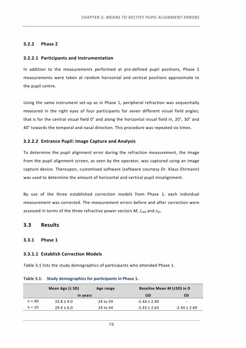
CHAPTER 3: MEANS TO RECTIFY PUPIL ALIGNMENT ERRORS
78
3.2.2 Phase 2
3.2.2.1 Participants and Instrumentation
In addition to the measurements performed at pre‐defined pupil positions, Phase 2
measurements were taken at random horizontal and vertical positions approximate to
the pupil centre.
Using the same instrument set‐up as in Phase 1, peripheral refraction was sequentially
measured in the right eyes of four participants for seven different visual field angles;
that is for the central visual field 0° and along the horizontal visual field in, 20°, 30° and
40° towards the temporal and nasal direction. This procedure was repeated six times.
3.2.2.2 Entrance Pupil: Image Capture and Analysis
To determine the pupil alignment error during the refraction measurement, the image
from the pupil alignment screen, as seen by the operator, was captured using an image
capture device. Thereupon, customised software (software courtesy Dr. Klaus Ehrmann)
was used to determine the amount of horizontal and vertical pupil misalignment.
By use of the three established correction models from Phase 1, each individual
measurement was corrected. The measurement errors before and after correction were
assessed in terms of the three refractive power vectors M, J180 and J45.
3.3 Results
3.3.1 Phase 1
3.3.1.1 Establish Correction Models
Table 3.1 lists the study demographics of participants who attended Phase 1.
Table 3.1: Study demographics for participants in Phase 1.
Mean Age (± SD) Age range Baseline Mean M (±SD) in D
in years OD OS
n = 40 33.8 ± 9.0 24 to 59 ‐2.44 ± 2.90 ‐
n = 10 29.4 ± 6.0 24 to 44 ‐2.43 ± 2.63 ‐2.44 ± 2.69

CHAPTER 3: MEANS TO RECTIFY PUPIL ALIGNMENT ERRORS
79
The refractive vector components M, J180 and J45 as well as the more commonly known
components of the sphero‐cylindrical notation, i.e. sphere, cylinder and axis, were
plotted as a function of pupil alignment position and visual field angle. The data are
provided for central, six horizontal and two inferior visual field angles and for all five
pupil (de‐)alignment positions, i.e. 0 mm. ± 0.75 mm and ± 1.50 mm in the horizontal and
vertical pupil alignment meridian. Key results are presented graphically in terms of
absolute and relative peripheral refractive errors from pupil centre. For all relative
graphs, refractive power vector components of the centred entrance pupil were
subtracted from the corresponding components from the de‐aligned pupil
measurements. In addition to the graphs, regression analysis was performed to indicate
linearity of the individual pupil alignment functions. Parametric equations for the
respective refractive vector components were established by least‐square fitting to
provide the general linear correction algorithm. In addition, for each individual field
angle, linear and quadratic correction models were also determined (APPENDIX B).
3.3.1.1.1 Refractive Vector Component M
Figure 3.1 illustrates the absolute and the relative mean of the refractive vector
component M of the participant group (n = 40) plotted as a function of pupil alignment
and visual field angle.
For measurements of peripheral refraction in the horizontal visual fields, de‐alignment of
the instrument axis in the horizontal pupil meridian showed a good linear correlation in
M across the pupil meridian (r2 > 0.96). This was also found for the measurements of
peripheral refraction in the inferior visual fields, when the pupil was de‐aligned in the
vertical pupil meridian. For both combinations of either horizontal visual field and
horizontal pupil meridian or inferior visual field and vertical pupil meridian, the slope of
the pupil alignment function increased with increasing peripheral visual field angle. The
greatest difference across the pupil meridian was found for the 40° nasal visual field
measurement, where the refractive difference in M was as large as 5.91D between the
1.5 mm nasal and 1.5 mm temporal pupil de‐alignment positions. With reference to the
centred pupil it is shown that with increase in visual field angle, the refractive vector
component M decreased. From this it can be concluded that the participant group had
on average a relative myopic shift in the periphery.
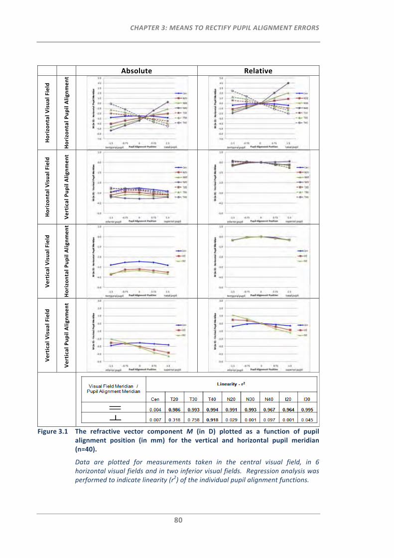
CHAPTER 3: MEANS TO RECTIFY PUPIL ALIGNMENT ERRORS
80
Absolute Relative
Horizontal Visual Field
Horizontal Pupil Alignment
Horizontal Visual Field
Vertical Pupil Alignment
Vertical Visual Field
Horizontal Pupil Alignment
Vertical Visual Field
Vertical Pupil Alignment
Figure 3.1 The refractive vector component M (in D) plotted as a function of pupil alignment position (in mm) for the vertical and horizontal pupil meridian (n=40).
Data are plotted for measurements taken in the central visual field, in 6 horizontal visual fields and in two inferior visual fields. Regression analysis was performed to indicate linearity (r2) of the individual pupil alignment functions.

CHAPTER 3: MEANS TO RECTIFY PUPIL ALIGNMENT ERRORS
81
The graphs also show that the points of intersection, where the nasal and temporal pupil
alignment functions of the same angle meet, e.g. N40 and T40, are displaced nasally
from the pupil centre. This indicates that the nasal visual field measurements showed a
greater relative shift in M than the measurements of the temporal visual field. Similar
asymmetric findings can be made for the inferior visual field measurements and their
vertical pupil de‐alignment functions. Moreover, the relative graph for the combination
of horizontal peripheral refraction and horizontal pupil de‐alignment indicates that the
differences between nasal and central pupil alignment were larger than the differences
between temporal and central alignment.
The graphs for the combination of either horizontal visual field and vertical pupil
meridian or inferior visual field and horizontal pupil meridian demonstrated that in most
cases M decreases slightly towards either pupil de‐alignment direction. This slight
decrease appeared to be consistent for all nasal visual field angles measured. For the
temporal visual fields there was some linearity found, in particular at 40°, where the
difference to central refraction was greatest, i.e. 0.50D at the 1.50 mm inferior pupil
alignment position. Nevertheless, when compared to the graphs where the visual field
meridian was parallel to the pupil alignment meridian, this refractive difference in M was
relatively small.
In summary, pupil de‐alignments perpendicular to the measured visual field meridian
showed a small or no effect on the refractive vector component M, when performing
peripheral refraction. In contrast, pupil de‐alignments parallel to the visual field
meridian had a substantial impact on the refractive vector component M.
For the correction of M for pupil misalignments, three correction models were
established by least‐square fitting. The first model was selected to be a general linear
model, which can be used for the correction of any measured visual field angle. It
provides a symmetric correction for nasal and temporal visual field measurements. To
also account for the slight asymmetry observed between nasal and temporal visual
fields, the second model chosen corrects for each individual visual field angle by using a
linear correction algorithm. Lastly, a quadratic model was chosen for each individual
CHAPTER 3: MEANS TO RECTIFY PUPIL ALIGNMENT ERRORS
82
visual field angle to also correct for the small asymmetry found with respect to nasal and
temporal pupil misalignment.
The linear and quadratic pupil alignment correction algorithms for each individual
peripheral visual field angle can be found in APPENDIX B while the following two
parametric equations provide the general linear correction algorithms for M.
In order to correct the measured refractive vector component Mm (in D) when pupil
misalignment occurs laterally during the measurement of any horizontal visual field
angle (0°<θ<40°), the following equation was derived for calculation of the corrected Mc
(in D):
Equation 3.1: . .
where positive θ is the nasal visual field angle measured (in °), negative θ is the temporal
visual field angle (in °), positive PP is the nasal pupil alignment position (in mm) and
negative PP is the temporal pupil alignment position (in mm).
If vertical pupil misalignment occurs during peripheral refraction measurement in the
inferior visual field (0°<θ<30°), the measured refractive vector component Mm (in D) can
be corrected using the following parametric equation for Mc (in D):
Equation 3.2: . .
where positive θ is the inferior visual field angle measured (in °), positive PP is the
superior pupil alignment position (in mm) and negative PP is the inferior pupil alignment
position (in mm).
Lastly, it should be noted that the standard deviations in Figure 3.1 were omitted for
clarity in order to permit easier comparison of the pupil alignment slopes for each visual
field angle of the group. Standard errors increased with increase in de‐alignment from

CHAPTER 3: MEANS TO RECTIFY PUPIL ALIGNMENT ERRORS
83
pupil centre and with increase in peripheral visual field angle. The RMS errors of all
correction models can be found in APPENDIX B.
3.3.1.1.2 Refractive Vector Component J180
With increase in visual field angle, the same linear increasing trends (r2 > 0.96) as found
for M (Figure 3.1) were observed for J180 (Figure 3.2) for the same combinations of either
horizontal visual field and horizontal pupil meridian, or vertical visual field and vertical
pupil meridian.
With reference to centred pupil alignment, the absolute graphs showed that there is a
substantial shift in J180 with increasing viewing angle. This measured shift was greater for
all the nasal visual field angles when compared to the temporal visual field angles. Also,
the relative graphs for lateral pupil de‐alignment in the horizontal visual field
measurements again demonstrate that the differences in J180 (in D) between nasal and
central pupil alignment were larger than the differences between temporal and central
alignment.
With respect to the results obtained for J180 where pupil de‐alignment was perpendicular
to the measured visual field meridian, it was again apparent that for all visual field
angles J180 changed consistently by relatively small amounts with increasing distance
from the pupil centre when compared to pupil de‐alignment measurements parallel to
the visual field meridian.
The following parametric equations provide the general linear pupil alignment correction
algorithms for J180 for the two relevant combinations of visual field and pupil meridian.
If lateral pupil misalignment occurs during peripheral refraction measurement in the
horizontal visual field (0°<θ<40°), the measured refractive vector component J180m can be
corrected using the following parametric equation for J180c (in D):
Equation 3.3 . .
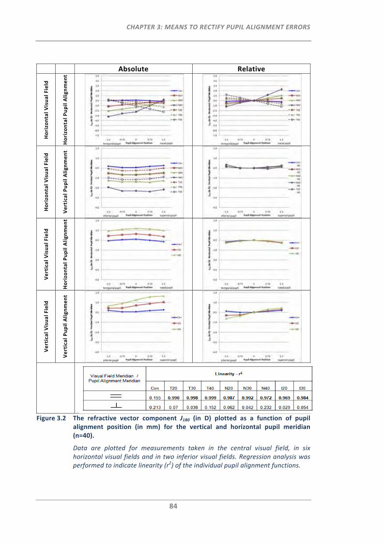
CHAPTER 3: MEANS TO RECTIFY PUPIL ALIGNMENT ERRORS
84
Absolute Relative
Horizontal Visual Field
Horizontal Pupil Alignment
Horizontal Visual Field
Vertical Pupil Alignment
Vertical Visual Field
Horizontal Pupil Alignment
Vertical Visual Field
Vertical Pupil Alignment
Figure 3.2 The refractive vector component J180 (in D) plotted as a function of pupil alignment position (in mm) for the vertical and horizontal pupil meridian (n=40).
Data are plotted for measurements taken in the central visual field, in six horizontal visual fields and in two inferior visual fields. Regression analysis was performed to indicate linearity (r2) of the individual pupil alignment functions.
CHAPTER 3: MEANS TO RECTIFY PUPIL ALIGNMENT ERRORS
85
where positive θ is the nasal visual field angle measured (in °), negative θ is the temporal
visual field angle (in °), positive PP is the nasal pupil alignment position (in mm) and
negative PP is the temporal pupil alignment position (in mm).
Correction of J180m (in D) for vertical pupil alignment errors when measuring the inferior
visual field (0°<θ<30°) can be achieved using the following parametric equation:
Equation 3.4: .
where positive θ is the inferior visual field angle measured (in °), positive PP is the
superior pupil alignment position (in mm) and negative PP is the inferior pupil alignment
position (in mm).
In addition to the general linear parametric equations, the linear and quadratic
correction functions for each individual visual field angle can be found in APPENDIX B.
3.3.1.1.3 Refractive Vector Component J45
Figure 3.3 details the absolute and relative graphs for J45 for all four combinations of
visual field and pupil alignment meridian.
In contrast to the linear correlations found for M and J180 for the combinations where the
visual field meridian was parallel to the pupil alignment meridian, the refractive power
vector J45 did not exhibit any substantial changes with increasing visual field angle.
Instead, J45 showed linear trends for the combinations where the visual field meridians
were perpendicularly directed to the measured pupil alignment meridians (r2 ≥ 0.97). In
these cases, the absolute slope of the pupil alignment function increased with increase
in visual field angle. Again, the greatest refractive difference in J45 across the pupil
meridian was found for the 40° nasal visual field measurement, which in absolute terms
ranged from ‐1.10D to 1.30D. With reference to centred pupil alignment, a small shift in
J45 was observed with increase in peripheral visual field angle. Moreover, the points of
intersection where the pupil alignment functions of the same field angle meet, e.g. N40
CHAPTER 3: MEANS TO RECTIFY PUPIL ALIGNMENT ERRORS
86
and T40, were displaced inferiorly from the pupil centre. Similar asymmetric findings
were made for the inferior visual field measurements and their horizontal pupil de‐
alignment functions.
From the J45 data plotted in Figure 3.3 the linear and quadratic correction functions for
each individual visual field angle (APPENDIX B) as well as the following parametric
equations for the general linear model were determined for the calculation of the
corrected J45c (in D).
If pupil de‐alignment occurs in the vertical pupil meridian when measuring peripheral
refraction in the horizontal visual field (0°<θ<40°) the following equation was derived:
Equation 3.5: . .
where J45m is the measured J45 value (in D), positive θ is the nasal visual field angle
measured (in °), negative θ is the temporal visual field angle (in °), positive PP is the
superior pupil alignment position (in mm) and negative PP is the inferior pupil alignment
position (in mm).
If pupil de‐alignment occurs in the horizontal pupil meridian when measuring peripheral
refraction in the inferior visual field (0°<θ<30°), the measured J45m can be corrected
using the following parametric equation:
Equation 3.6: . .
where positive θ is the inferior visual field angle measured (in °), positive PP is the nasal
pupil alignment position (in mm) and negative PP is the temporal pupil alignment
position (in mm).
It can be concluded that despite the fact that pupil de‐alignment in the meridian parallel
to the measured visual field affected M and J180, pupil de‐alignment along the meridian
perpendicular to the visual field meridian is also of relevance in obtaining accurate
measurements for J45.
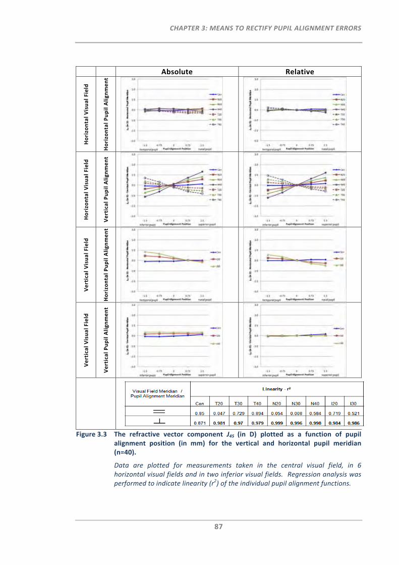
CHAPTER 3: MEANS TO RECTIFY PUPIL ALIGNMENT ERRORS
87
Absolute Relative
Horizontal Visual Field
Horizontal Pupil Alignment
Horizontal Visual Field
Vertical Pupil Alignment
Vertical Visual Field
Horizontal Pupil Alignment
Vertical Visual Field
Vertical Pupil Alignment
Figure 3.3 The refractive vector component J45 (in D) plotted as a function of pupil alignment position (in mm) for the vertical and horizontal pupil meridian (n=40).
Data are plotted for measurements taken in the central visual field, in 6 horizontal visual fields and in two inferior visual fields. Regression analysis was performed to indicate linearity (r2) of the individual pupil alignment functions.

CHAPTER 3: MEANS TO RECTIFY PUPIL ALIGNMENT ERRORS
88
3.3.1.1.4 Sphero‐Cylindrical Notation
In addition to the refractive vector components M, J180 and J45 the more commonly
known sphero‐cylindrical notation, which is described by the three components sphere,
cylinder and axis, was also plotted as a function of pupil de‐alignment and horizontal
visual field angle (Figure 3.4).
Figure 3.4 shows that for horizontal pupil de‐alignments, the sphere component, which
unlike M has no additional astigmatic portion, showed a symmetrical relationship
between nasal and temporal visual field measurements, when referenced to the centred
pupil. Vertical pupil alignment had no substantial impact on the sphere values for either
horizontal visual field angle.
From the plots of the cylinder and axis components as a function of horizontal visual
field angle, the following is apparent: the cylinder component was only affected by
horizontal but not vertical pupil de‐alignment and the axis component showed a good
correlation for vertical but not for horizontal pupil de‐alignment. The cylinder
component showed greater changes as a function of pupil alignment in the nasal visual
field than in the temporal visual field.
3.3.1.2 Investigation of Instrument Binocularity with Pupil Alignment
The top graphs in Figure 3.5 show the relative mean refractive power vectors M, J180 and
J45 as a function of lateral pupil de‐alignment and visual field angle for the right and left
eyes of the selected participant sub‐group (n = 10). Overall, right and left eye slope data
demonstrated very good agreement for M and J180 (paired samples correlation r > 0.726,
p < 0.017) for all peripheral visual field angles. Paired t‐test analysis showed that there
was no difference in M and J180 between the right and left eye slope data for any of the
peripheral visual fields measured (p > 0.069). The only exception was J180 in the 30° nasal
visual field (p = 0.02). Additionally, for each of the five pupil alignment positions and for
each of the seven visual field angles, the relationship between the right eye and left eye
was plotted with respect to each refractive vector component. These plots are shown in
Figure 3.5 bottom, which show the good agreement for M and J180 between right and left
eye data.
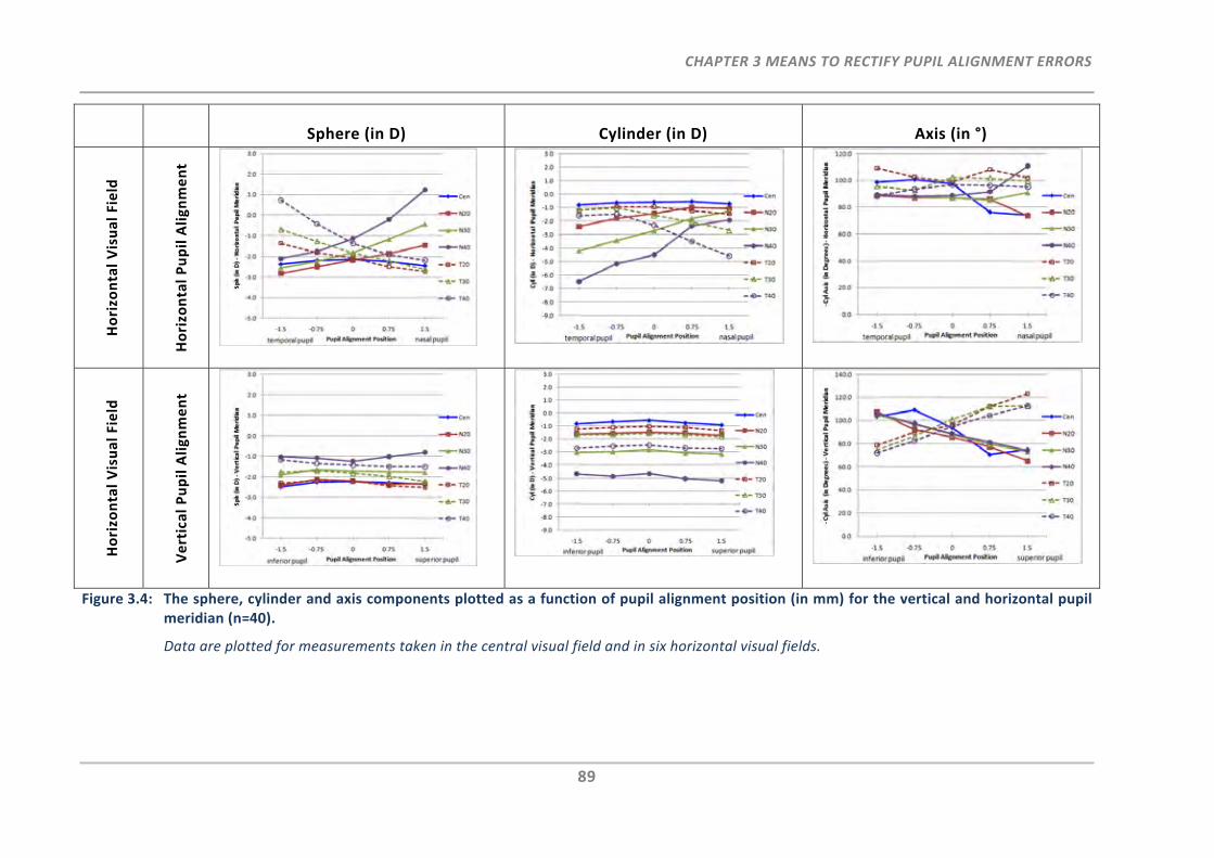
CHAPTER 3 MEANS TO RECTIFY PUPIL ALIGNMENT ERRORS
89
Figure 3.4: The sphere, cylinder and axis components plotted as a function of pupil alignment position (in mm) for the vertical and horizontal pupil meridian (n=40).
Data are plotted for measurements taken in the central visual field and in six horizontal visual fields.
Sphere (in D) Cylinder (in D) Axis (in °)
Horizontal Visual Field
Horizontal Pupil Alignment
Horizontal Visual Field
Vertical Pupil Alignment
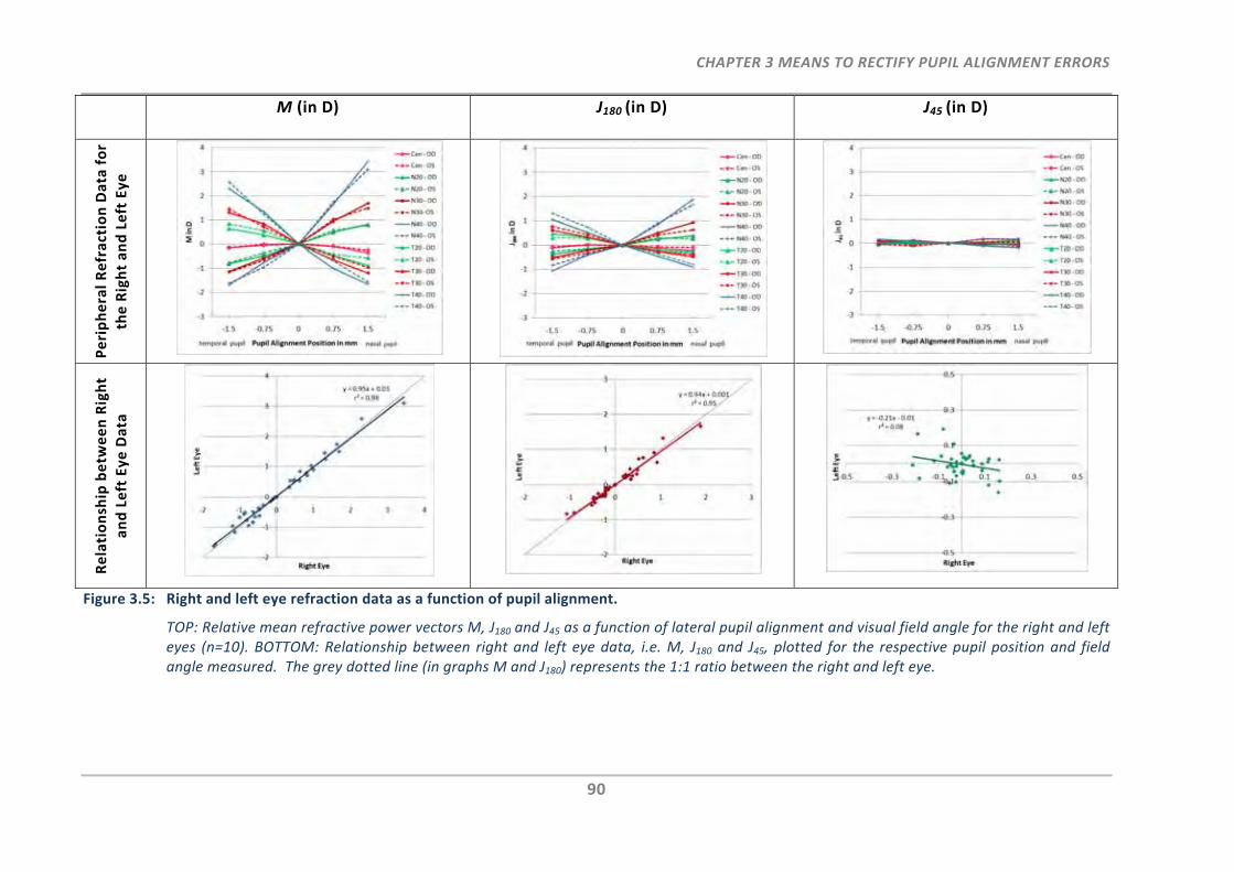
CHAPTER 3 MEANS TO RECTIFY PUPIL ALIGNMENT ERRORS
90
M (in D) J180 (in D) J45 (in D) Peripheral Refraction Data for
the Right and Left Eye
Relationship betw
een Right
and Left Eye Data
Figure 3.5: Right and left eye refraction data as a function of pupil alignment.
TOP: Relative mean refractive power vectors M, J180 and J45 as a function of lateral pupil alignment and visual field angle for the right and left eyes (n=10). BOTTOM: Relationship between right and left eye data, i.e. M, J180 and J45, plotted for the respective pupil position and field angle measured. The grey dotted line (in graphs M and J180) represents the 1:1 ratio between the right and left eye.
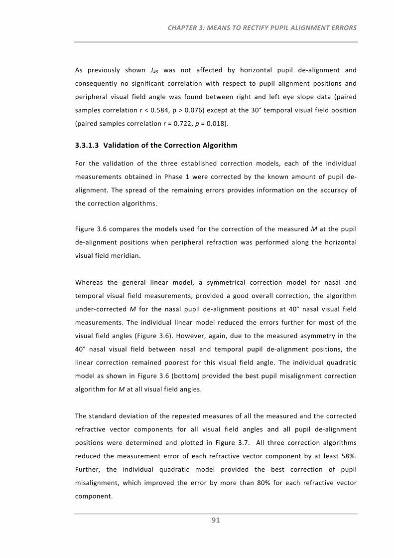
CHAPTER 3: MEANS TO RECTIFY PUPIL ALIGNMENT ERRORS
91
As previously shown J45 was not affected by horizontal pupil de‐alignment and
consequently no significant correlation with respect to pupil alignment positions and
peripheral visual field angle was found between right and left eye slope data (paired
samples correlation r < 0.584, p > 0.076) except at the 30° temporal visual field position
(paired samples correlation r = 0.722, p = 0.018).
3.3.1.3 Validation of the Correction Algorithm
For the validation of the three established correction models, each of the individual
measurements obtained in Phase 1 were corrected by the known amount of pupil de‐
alignment. The spread of the remaining errors provides information on the accuracy of
the correction algorithms.
Figure 3.6 compares the models used for the correction of the measured M at the pupil
de‐alignment positions when peripheral refraction was performed along the horizontal
visual field meridian.
Whereas the general linear model, a symmetrical correction model for nasal and
temporal visual field measurements, provided a good overall correction, the algorithm
under‐corrected M for the nasal pupil de‐alignment positions at 40° nasal visual field
measurements. The individual linear model reduced the errors further for most of the
visual field angles (Figure 3.6). However, again, due to the measured asymmetry in the
40° nasal visual field between nasal and temporal pupil de‐alignment positions, the
linear correction remained poorest for this visual field angle. The individual quadratic
model as shown in Figure 3.6 (bottom) provided the best pupil misalignment correction
algorithm for M at all visual field angles.
The standard deviation of the repeated measures of all the measured and the corrected
refractive vector components for all visual field angles and all pupil de‐alignment
positions were determined and plotted in Figure 3.7. All three correction algorithms
reduced the measurement error of each refractive vector component by at least 58%.
Further, the individual quadratic model provided the best correction of pupil
misalignment, which improved the error by more than 80% for each refractive vector
component.
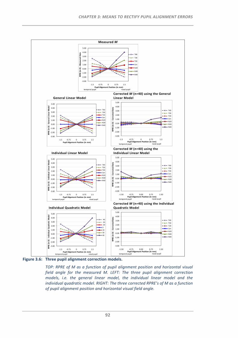
CHAPTER 3: MEANS TO RECTIFY PUPIL ALIGNMENT ERRORS
92
Measured M
General Linear Model Corrected M (n=40) using the General Linear Model
Individual Linear Model Corrected M (n=40) using the Individual Linear Model
Individual Quadratic Model Corrected M (n=40) using the Individual Quadratic Model
Figure 3.6: Three pupil alignment correction models.
TOP: RPRE of M as a function of pupil alignment position and horizontal visual field angle for the measured M. LEFT: The three pupil alignment correction models, i.e. the general linear model, the individual linear model and the individual quadratic model. RIGHT: The three corrected RPRE’s of M as a function of pupil alignment position and horizontal visual field angle.
‐3.00
‐2.00
‐1.00
0.00
1.00
2.00
3.00
4.00
5.00
‐1.5 ‐0.75 0 0.75 1.5
RPRE (in D) ‐Measured Data
Pupil Alignment Position (in mm)
T40
T30
T20
Cen
N20
N30
N40
nasal pupiltemporal pupil
‐3.00
‐2.00
‐1.00
0.00
1.00
2.00
3.00
4.00
5.00
‐1.5 ‐0.75 0 0.75 1.5
RPRE (in D) ‐General Linear M
odel
Pupil Alignment Position (in mm)
T40
T30
T20
Cen
N20
N30
N40
‐3.00
‐2.00
‐1.00
0.00
1.00
2.00
3.00
4.00
5.00
‐1.5 ‐0.75 0 0.75 1.5
RPRE (in D) ‐Corrected Data
Pupil Alignment Position (in mm)
T40
T30
T20
Cen
N20
N30
N40
temporal pupil nasal pupil
‐3.00
‐2.00
‐1.00
0.00
1.00
2.00
3.00
4.00
5.00
‐1.5 ‐0.75 0 0.75 1.5
RPRE (in D) ‐Individual Linear M
odel
Pupil Alignment Position (in mm)
T40
T30
T20
Cen
N20
N30
N40
nasal pupiltemporal pupil
‐3.00
‐2.00
‐1.00
0.00
1.00
2.00
3.00
4.00
5.00
‐1.50 ‐0.75 0.00 0.75 1.50
RPRE (in D) ‐Corrected Data
Pupil Alignment Position (in mm)
T40
T30
T20
Cen
N20
N30
N40
temporal pupil nasal pupil
‐3.00
‐2.00
‐1.00
0.00
1.00
2.00
3.00
4.00
5.00
‐1.5 ‐0.75 0 0.75 1.5
RPRE (in D) ‐Individual Q
uadratic Model
Pupil Alignment Position (in mm)
‐40
‐30
‐20
0
20
30
40
nasal pupiltemporal pupil
‐3.00
‐2.00
‐1.00
0.00
1.00
2.00
3.00
4.00
5.00
‐1.50 ‐0.75 0.00 0.75 1.50
RPRE (in D) ‐Corrected Data
Pupil Alignment Position (in mm)
T40
T30
T20
Cen
N20
N30
N40
temporal pupil nasal pupil
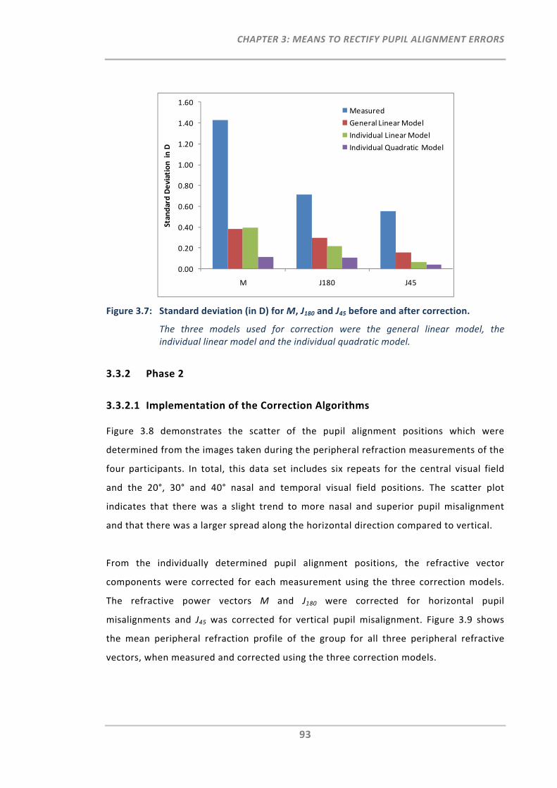
CHAPTER 3: MEANS TO RECTIFY PUPIL ALIGNMENT ERRORS
93
Figure 3.7: Standard deviation (in D) for M, J180 and J45 before and after correction.
The three models used for correction were the general linear model, the individual linear model and the individual quadratic model.
3.3.2 Phase 2
3.3.2.1 Implementation of the Correction Algorithms
Figure 3.8 demonstrates the scatter of the pupil alignment positions which were
determined from the images taken during the peripheral refraction measurements of the
four participants. In total, this data set includes six repeats for the central visual field
and the 20°, 30° and 40° nasal and temporal visual field positions. The scatter plot
indicates that there was a slight trend to more nasal and superior pupil misalignment
and that there was a larger spread along the horizontal direction compared to vertical.
From the individually determined pupil alignment positions, the refractive vector
components were corrected for each measurement using the three correction models.
The refractive power vectors M and J180 were corrected for horizontal pupil
misalignments and J45 was corrected for vertical pupil misalignment. Figure 3.9 shows
the mean peripheral refraction profile of the group for all three peripheral refractive
vectors, when measured and corrected using the three correction models.
0.00
0.20
0.40
0.60
0.80
1.00
1.20
1.40
1.60
M J180 J45
Standard Deviation in D
Measured
General Linear Model
Individual Linear Model
Individual Quadratic Model
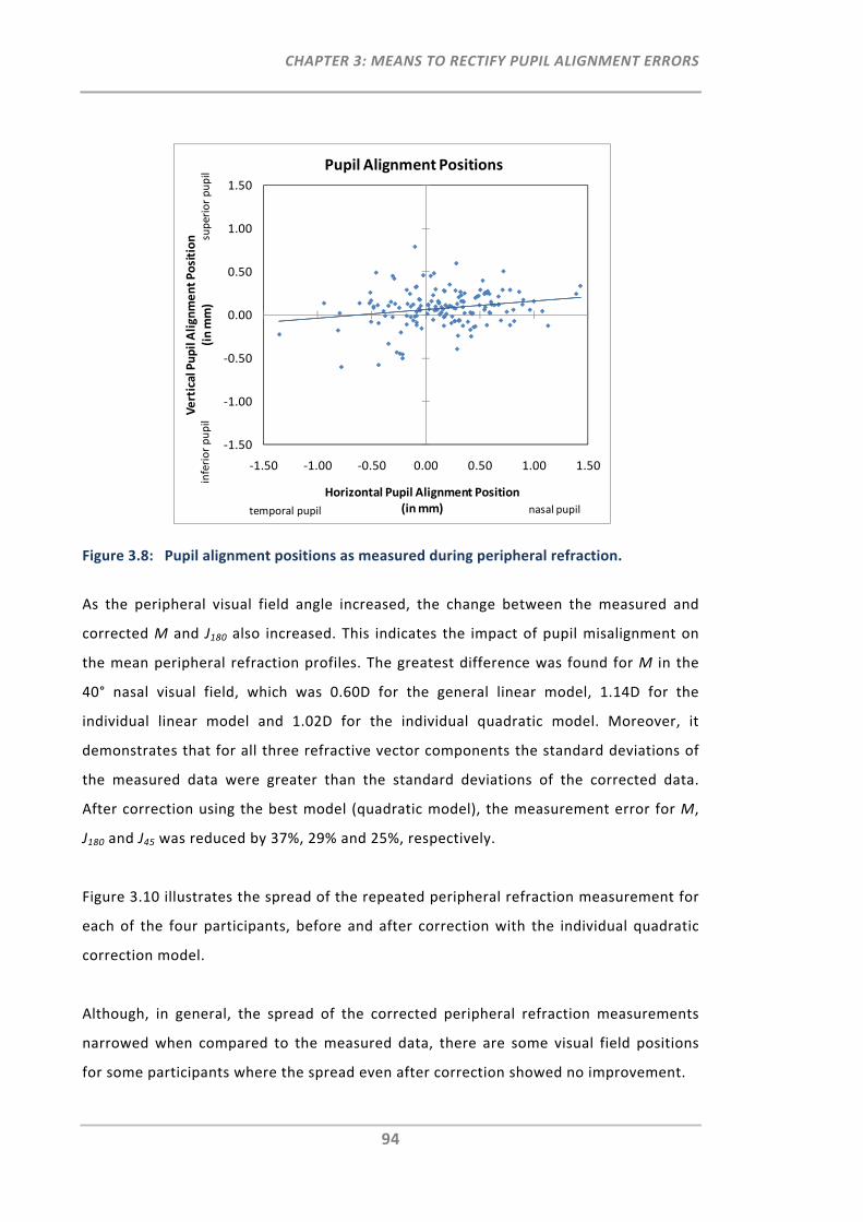
CHAPTER 3: MEANS TO RECTIFY PUPIL ALIGNMENT ERRORS
94
Figure 3.8: Pupil alignment positions as measured during peripheral refraction.
As the peripheral visual field angle increased, the change between the measured and
corrected M and J180 also increased. This indicates the impact of pupil misalignment on
the mean peripheral refraction profiles. The greatest difference was found for M in the
40° nasal visual field, which was 0.60D for the general linear model, 1.14D for the
individual linear model and 1.02D for the individual quadratic model. Moreover, it
demonstrates that for all three refractive vector components the standard deviations of
the measured data were greater than the standard deviations of the corrected data.
After correction using the best model (quadratic model), the measurement error for M,
J180 and J45 was reduced by 37%, 29% and 25%, respectively.
Figure 3.10 illustrates the spread of the repeated peripheral refraction measurement for
each of the four participants, before and after correction with the individual quadratic
correction model.
Although, in general, the spread of the corrected peripheral refraction measurements
narrowed when compared to the measured data, there are some visual field positions
for some participants where the spread even after correction showed no improvement.
‐1.50
‐1.00
‐0.50
0.00
0.50
1.00
1.50
‐1.50 ‐1.00 ‐0.50 0.00 0.50 1.00 1.50
Vertical Pupil Alignment Position
(in mm)
Horizontal Pupil Alignment Position (in mm)
Pupil Alignment Positions
inferior pupil
superior pupil
nasal pupiltemporal pupil
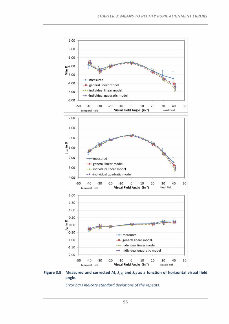
CHAPTER 3: MEANS TO RECTIFY PUPIL ALIGNMENT ERRORS
95
Figure 3.9: Measured and corrected M, J180 and J45 as a function of horizontal visual field angle.
Error bars indicate standard deviations of the repeats.
‐6.00
‐5.00
‐4.00
‐3.00
‐2.00
‐1.00
0.00
1.00
‐50 ‐40 ‐30 ‐20 ‐10 0 10 20 30 40 50
M in D
Visual Field Angle (in °)
measured
general linear model
individual linear model
individual quadratic model
Nasal FieldTemporal Field
‐4.00
‐3.00
‐2.00
‐1.00
0.00
1.00
2.00
‐50 ‐40 ‐30 ‐20 ‐10 0 10 20 30 40 50
J 180 in D
Visual Field Angle (in °)
measured
general linear model
individual linear model
individual quadratic model
Nasal FieldTemporal Field
‐2.00
‐1.50
‐1.00
‐0.50
0.00
0.50
1.00
1.50
2.00
‐50 ‐40 ‐30 ‐20 ‐10 0 10 20 30 40 50
J 45 in D
Visual Field Angle (in °)
measured
general linear model
individual linear model
individual quadratic model
Nasal FieldTemporal Field
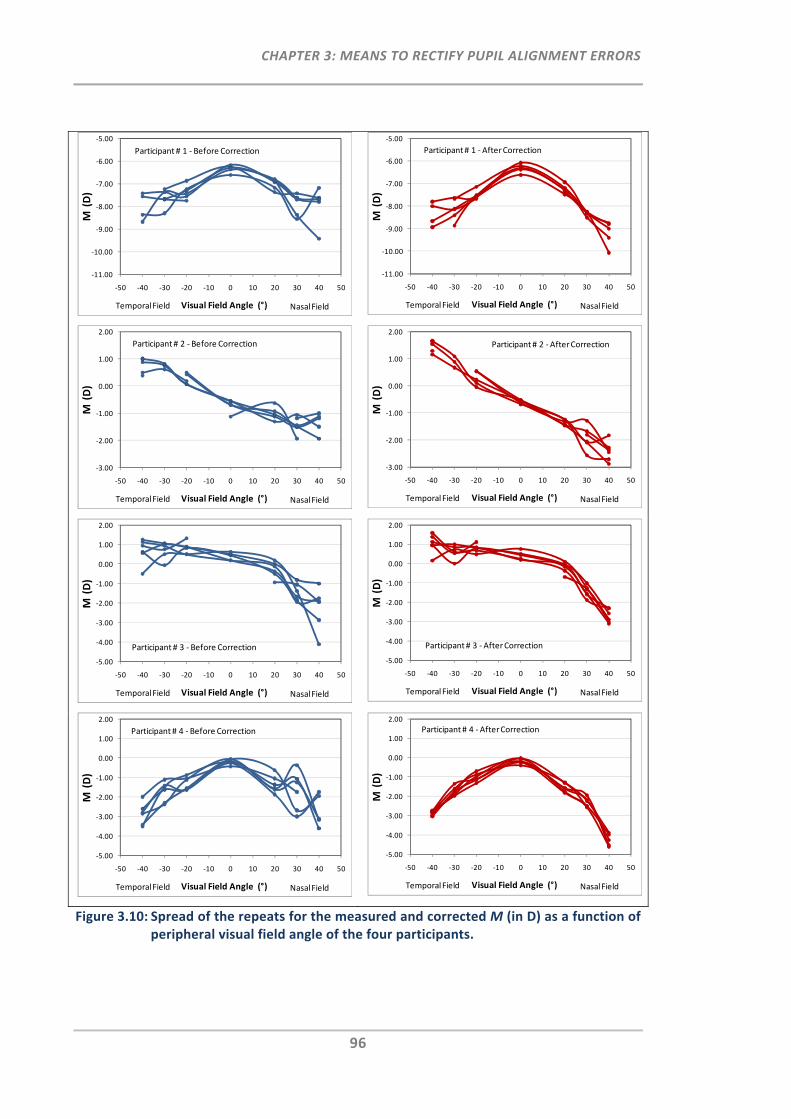
CHAPTER 3: MEANS TO RECTIFY PUPIL ALIGNMENT ERRORS
96
Figure 3.10: Spread of the repeats for the measured and corrected M (in D) as a function of peripheral visual field angle of the four participants.
‐11.00
‐10.00
‐9.00
‐8.00
‐7.00
‐6.00
‐5.00
‐50 ‐40 ‐30 ‐20 ‐10 0 10 20 30 40 50
M(D)
Visual Field Angle (°) Nasal FieldTemporal Field
Participant# 1 ‐ Before Correction
‐11.00
‐10.00
‐9.00
‐8.00
‐7.00
‐6.00
‐5.00
‐50 ‐40 ‐30 ‐20 ‐10 0 10 20 30 40 50
M(D)
Visual Field Angle (°) Nasal FieldTemporal Field
Participant# 1 ‐After Correction
‐3.00
‐2.00
‐1.00
0.00
1.00
2.00
‐50 ‐40 ‐30 ‐20 ‐10 0 10 20 30 40 50
M(D)
Visual Field Angle (°) Nasal FieldTemporal Field
Participant# 2 ‐ Before Correction
‐3.00
‐2.00
‐1.00
0.00
1.00
2.00
‐50 ‐40 ‐30 ‐20 ‐10 0 10 20 30 40 50
M(D)
Visual Field Angle (°) Nasal FieldTemporal Field
Participant # 2 ‐After Correction
‐5.00
‐4.00
‐3.00
‐2.00
‐1.00
0.00
1.00
2.00
‐50 ‐40 ‐30 ‐20 ‐10 0 10 20 30 40 50
M(D)
Visual Field Angle (°) Nasal FieldTemporal Field
Participant# 3 ‐ Before Correction
‐5.00
‐4.00
‐3.00
‐2.00
‐1.00
0.00
1.00
2.00
‐50 ‐40 ‐30 ‐20 ‐10 0 10 20 30 40 50
M(D)
Visual Field Angle (°) Nasal FieldTemporal Field
Participant# 3 ‐After Correction
‐5.00
‐4.00
‐3.00
‐2.00
‐1.00
0.00
1.00
2.00
‐50 ‐40 ‐30 ‐20 ‐10 0 10 20 30 40 50
M(D)
Visual Field Angle (°) Nasal FieldTemporal Field
Participant# 4 ‐ Before Correction
‐5.00
‐4.00
‐3.00
‐2.00
‐1.00
0.00
1.00
2.00
‐50 ‐40 ‐30 ‐20 ‐10 0 10 20 30 40 50
M(D)
Visual Field Angle (°) Nasal FieldTemporal Field
Participant # 4 ‐After Correction
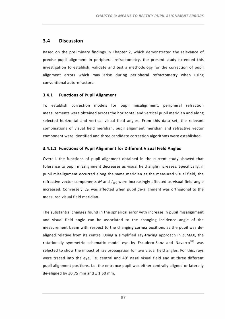
CHAPTER 3: MEANS TO RECTIFY PUPIL ALIGNMENT ERRORS
97
3.4 Discussion
Based on the preliminary findings in Chapter 2, which demonstrated the relevance of
precise pupil alignment in peripheral refractometry, the present study extended this
investigation to establish, validate and test a methodology for the correction of pupil
alignment errors which may arise during peripheral refractometry when using
conventional autorefractors.
3.4.1 Functions of Pupil Alignment
To establish correction models for pupil misalignment, peripheral refraction
measurements were obtained across the horizontal and vertical pupil meridian and along
selected horizontal and vertical visual field angles. From this data set, the relevant
combinations of visual field meridian, pupil alignment meridian and refractive vector
component were identified and three candidate correction algorithms were established.
3.4.1.1 Functions of Pupil Alignment for Different Visual Field Angles
Overall, the functions of pupil alignment obtained in the current study showed that
tolerance to pupil misalignment decreases as visual field angle increases. Specifically, if
pupil misalignment occurred along the same meridian as the measured visual field, the
refractive vector components M and J180 were increasingly affected as visual field angle
increased. Conversely, J45 was affected when pupil de‐alignment was orthogonal to the
measured visual field meridian.
The substantial changes found in the spherical error with increase in pupil misalignment
and visual field angle can be associated to the changing incidence angle of the
measurement beam with respect to the changing cornea positions as the pupil was de‐
aligned relative from its centre. Using a simplified ray‐tracing approach in ZEMAX, the
rotationally symmetric schematic model eye by Escudero‐Sanz and Navarro183 was
selected to show the impact of ray propagation for two visual field angles. For this, rays
were traced into the eye, i.e. central and 40° nasal visual field and at three different
pupil alignment positions, i.e. the entrance pupil was either centrally aligned or laterally
de‐aligned by ±0.75 mm and ± 1.50 mm.
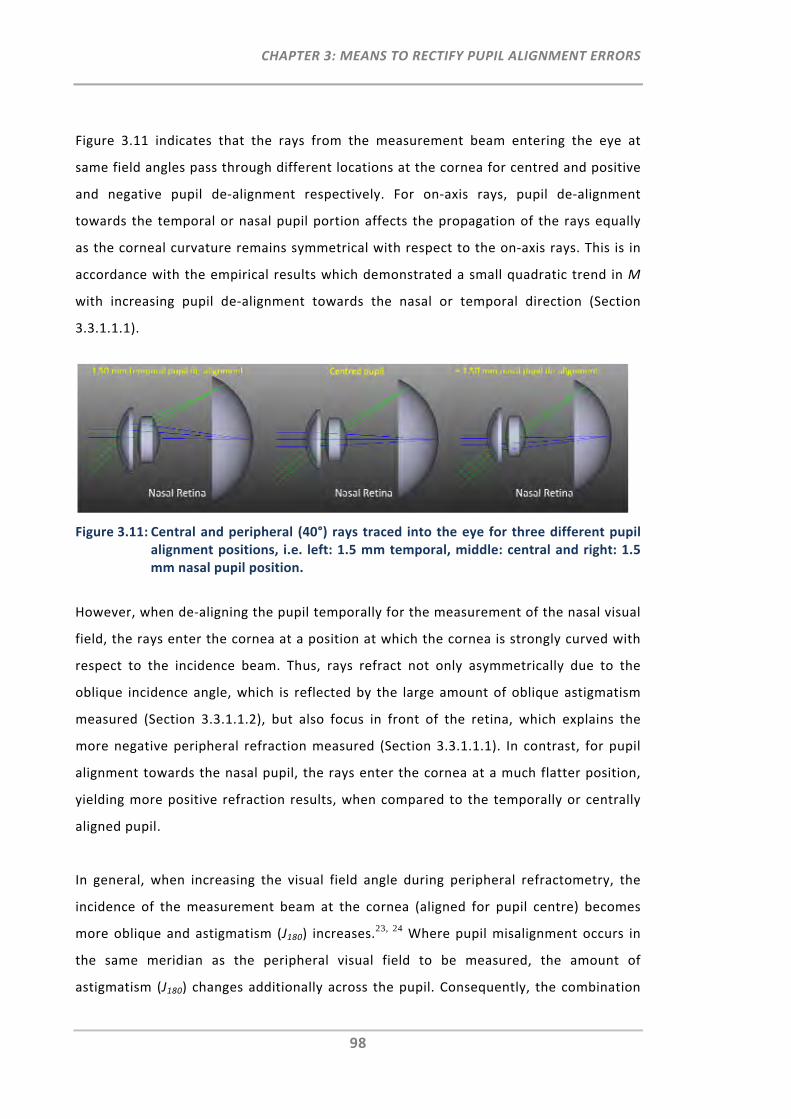
CHAPTER 3: MEANS TO RECTIFY PUPIL ALIGNMENT ERRORS
98
Figure 3.11 indicates that the rays from the measurement beam entering the eye at
same field angles pass through different locations at the cornea for centred and positive
and negative pupil de‐alignment respectively. For on‐axis rays, pupil de‐alignment
towards the temporal or nasal pupil portion affects the propagation of the rays equally
as the corneal curvature remains symmetrical with respect to the on‐axis rays. This is in
accordance with the empirical results which demonstrated a small quadratic trend in M
with increasing pupil de‐alignment towards the nasal or temporal direction (Section
3.3.1.1.1).
Figure 3.11: Central and peripheral (40°) rays traced into the eye for three different pupil alignment positions, i.e. left: 1.5 mm temporal, middle: central and right: 1.5 mm nasal pupil position.
However, when de‐aligning the pupil temporally for the measurement of the nasal visual
field, the rays enter the cornea at a position at which the cornea is strongly curved with
respect to the incidence beam. Thus, rays refract not only asymmetrically due to the
oblique incidence angle, which is reflected by the large amount of oblique astigmatism
measured (Section 3.3.1.1.2), but also focus in front of the retina, which explains the
more negative peripheral refraction measured (Section 3.3.1.1.1). In contrast, for pupil
alignment towards the nasal pupil, the rays enter the cornea at a much flatter position,
yielding more positive refraction results, when compared to the temporally or centrally
aligned pupil.
In general, when increasing the visual field angle during peripheral refractometry, the
incidence of the measurement beam at the cornea (aligned for pupil centre) becomes
more oblique and astigmatism (J180) increases.23, 24 Where pupil misalignment occurs in
the same meridian as the peripheral visual field to be measured, the amount of
astigmatism (J180) changes additionally across the pupil. Consequently, the combination
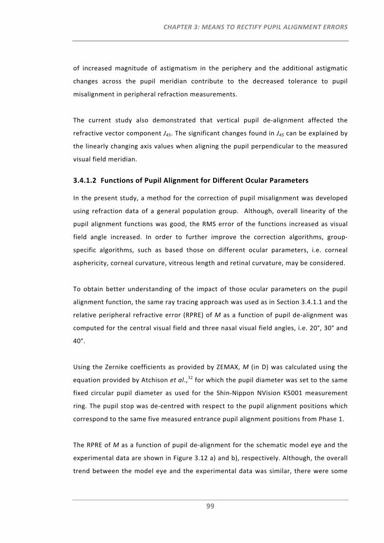
CHAPTER 3: MEANS TO RECTIFY PUPIL ALIGNMENT ERRORS
99
of increased magnitude of astigmatism in the periphery and the additional astigmatic
changes across the pupil meridian contribute to the decreased tolerance to pupil
misalignment in peripheral refraction measurements.
The current study also demonstrated that vertical pupil de‐alignment affected the
refractive vector component J45. The significant changes found in J45 can be explained by
the linearly changing axis values when aligning the pupil perpendicular to the measured
visual field meridian.
3.4.1.2 Functions of Pupil Alignment for Different Ocular Parameters
In the present study, a method for the correction of pupil misalignment was developed
using refraction data of a general population group. Although, overall linearity of the
pupil alignment functions was good, the RMS error of the functions increased as visual
field angle increased. In order to further improve the correction algorithms, group‐
specific algorithms, such as based those on different ocular parameters, i.e. corneal
asphericity, corneal curvature, vitreous length and retinal curvature, may be considered.
To obtain better understanding of the impact of those ocular parameters on the pupil
alignment function, the same ray tracing approach was used as in Section 3.4.1.1 and the
relative peripheral refractive error (RPRE) of M as a function of pupil de‐alignment was
computed for the central visual field and three nasal visual field angles, i.e. 20°, 30° and
40°.
Using the Zernike coefficients as provided by ZEMAX, M (in D) was calculated using the
equation provided by Atchison et al.,32 for which the pupil diameter was set to the same
fixed circular pupil diameter as used for the Shin‐Nippon NVision K5001 measurement
ring. The pupil stop was de‐centred with respect to the pupil alignment positions which
correspond to the same five measured entrance pupil alignment positions from Phase 1.
The RPRE of M as a function of pupil de‐alignment for the schematic model eye and the
experimental data are shown in Figure 3.12 a) and b), respectively. Although, the overall
trend between the model eye and the experimental data was similar, there were some
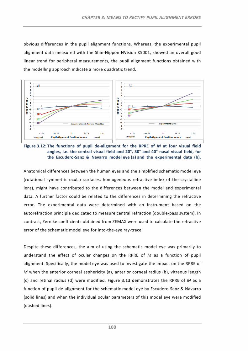
CHAPTER 3: MEANS TO RECTIFY PUPIL ALIGNMENT ERRORS
100
obvious differences in the pupil alignment functions. Whereas, the experimental pupil
alignment data measured with the Shin‐Nippon NVision K5001, showed an overall good
linear trend for peripheral measurements, the pupil alignment functions obtained with
the modelling approach indicate a more quadratic trend.
Figure 3.12: The functions of pupil de‐alignment for the RPRE of M at four visual field angles, i.e. the central visual field and 20°, 30° and 40° nasal visual field, for the Escudero‐Sanz & Navarro model eye (a) and the experimental data (b).
Anatomical differences between the human eyes and the simplified schematic model eye
(rotational symmetric ocular surfaces, homogeneous refractive index of the crystalline
lens), might have contributed to the differences between the model and experimental
data. A further factor could be related to the differences in determining the refractive
error. The experimental data were determined with an instrument based on the
autorefraction principle dedicated to measure central refraction (double‐pass system). In
contrast, Zernike coefficients obtained from ZEMAX were used to calculate the refractive
error of the schematic model eye for into‐the‐eye ray‐trace.
Despite these differences, the aim of using the schematic model eye was primarily to
understand the effect of ocular changes on the RPRE of M as a function of pupil
alignment. Specifically, the model eye was used to investigate the impact on the RPRE of
M when the anterior corneal asphericity (a), anterior corneal radius (b), vitreous length
(c) and retinal radius (d) were modified. Figure 3.13 demonstrates the RPRE of M as a
function of pupil de‐alignment for the schematic model eye by Escudero‐Sanz & Navarro
(solid lines) and when the individual ocular parameters of this model eye were modified
(dashed lines).
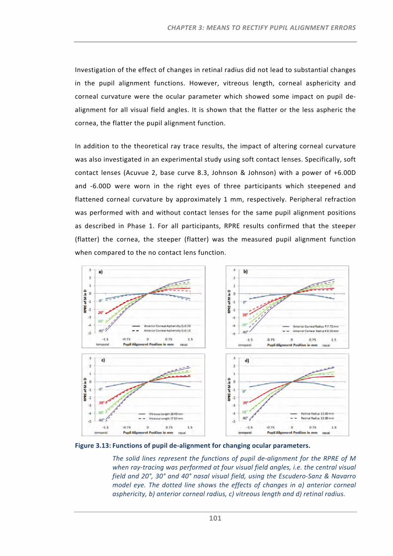
CHAPTER 3: MEANS TO RECTIFY PUPIL ALIGNMENT ERRORS
101
Investigation of the effect of changes in retinal radius did not lead to substantial changes
in the pupil alignment functions. However, vitreous length, corneal asphericity and
corneal curvature were the ocular parameter which showed some impact on pupil de‐
alignment for all visual field angles. It is shown that the flatter or the less aspheric the
cornea, the flatter the pupil alignment function.
In addition to the theoretical ray trace results, the impact of altering corneal curvature
was also investigated in an experimental study using soft contact lenses. Specifically, soft
contact lenses (Acuvue 2, base curve 8.3, Johnson & Johnson) with a power of +6.00D
and ‐6.00D were worn in the right eyes of three participants which steepened and
flattened corneal curvature by approximately 1 mm, respectively. Peripheral refraction
was performed with and without contact lenses for the same pupil alignment positions
as described in Phase 1. For all participants, RPRE results confirmed that the steeper
(flatter) the cornea, the steeper (flatter) was the measured pupil alignment function
when compared to the no contact lens function.
Figure 3.13: Functions of pupil de‐alignment for changing ocular parameters.
The solid lines represent the functions of pupil de‐alignment for the RPRE of M when ray‐tracing was performed at four visual field angles, i.e. the central visual field and 20°, 30° and 40° nasal visual field, using the Escudero‐Sanz & Navarro model eye. The dotted line shows the effects of changes in a) anterior corneal asphericity, b) anterior corneal radius, c) vitreous length and d) retinal radius.

CHAPTER 3: MEANS TO RECTIFY PUPIL ALIGNMENT ERRORS
102
From this modelling approach and the experimental study it can be suggested that the
increased RMS error found for the correction algorithms is likely to be related to the
variations in ocular parameters within the general participant group used in the present
study.
3.4.1.3 Functions of Pupil Alignment for Nasal and Temporal Measurements
From previous studies it is known that peripheral refraction profiles often show a typical
nasal‐temporal asymmetry across the visual field with respect to the astigmatic
component. This asymmetry has been related to a lack of coincidence between the visual
and the optical axis,23, 25, 37, 105 but also a lack of rotational symmetry of the retina.58
Results from this study have also shown some asymmetry with respect to the nasal and
temporal visual field pupil alignment functions for M, J180 and cylinder. With reference to
the centred pupil, the pupil alignment functions of the cylinder component showed that
shifts between the central and nasal visual field were much greater than shifts between
the central and the corresponding temporal visual field shifts. This is in agreement with
the nasal‐temporal astigmatic asymmetry found in previous studies.23, 25, 37, 105 Moreover,
the relative graphs for M and J180 have shown that across the pupil meridian for all
horizontal peripheral visual field angles, the difference between central and nasal pupil
de‐alignment was larger than the difference between central and temporal pupil de‐
alignment. From this, it can be concluded that the indicated asymmetry across the pupil
meridian is associated with the combination of increased magnitude of astigmatism in
the nasal visual field and the additional astigmatic changes when performing refraction
across the pupil meridian.
3.4.1.4 Instrumentation used to Establish Pupil Alignment Functions
Due to potential inter‐instrument variability, it is suggested that data for the
establishment of correction algorithms are to be collected using the same instrument
which is to be used for the measurement of peripheral refraction. The autorefraction
instrument used in this study, the Shin‐Nippon NVision K5001, was originally designed to
measure central refraction only. The summary given on current peripheral refraction
techniques (Chapter 1) indicated that many other instruments/methods have been used
and modified for peripheral refraction measurements which are based on different
CHAPTER 3: MEANS TO RECTIFY PUPIL ALIGNMENT ERRORS
103
operation principles. Unlike the Shin‐Nippon autorefractor, which uses a fixed ring
target, other instruments are based on the principles of aberrometry or photorefraction
to analyse refractive errors across the entire visible pupil, with or without consideration
of the ‘elliptical’ pupil shape. Donovan et al. have compared peripheral refraction
measurements on 28 participants using three instruments which are based on different
operation principles.122 The instruments used were the Shin‐Nippon NVision K5001, the
Complete Ophthalmic Analysis System (COAS aberrometer) and a streak retinoscope.
They found that the output in peripheral J180 of the COAS was almost half the value of
the results obtained with the other two techniques indicating that there may be some
inter‐instrument variability due to different operation principles.
With respect to instrument binocularity, the current study also measured the right as
well as the left eyes of ten participants to confirm the absence of instrument variations
between eye measurements with respect to horizontal pupil de‐alignment in the
horizontal visual field. It was demonstrated that right and left eye data for the pupil
alignment dependent refractive vector components M and J180 correlated very well.
These findings assure that measurements with the Shin‐Nippon NVision K5001 are in
unison for right and left eye measurements, not only with respect to central and
peripheral refraction but also with respect to pupil (mis‐)alignment. Although, it can be
assumed that objective refraction instruments provide consistent binocular central
refraction readings, it is recommended to always verify this assumption for a specific
instrument when measuring peripheral refraction.
3.4.2 Pupil Alignment Correction Models
From the presented data set, three pupil alignment correction models were established
for the correction of the refractive vector components M, J180 and J45 and for the relevant
combinations of visual field meridian and pupil alignment meridian.
Overall there was good linearity, as well as symmetry, between the relative nasal and
temporal pupil alignment functions. Therefore, the first model was selected to be a
general linear model, which has the advantage that it can be applied for the correction
of any measured visual field angle. To also account for the slight asymmetry observed
CHAPTER 3: MEANS TO RECTIFY PUPIL ALIGNMENT ERRORS
104
between nasal and temporal visual fields the second linear model chosen corrects for
each individual visual field angle. Lastly, a quadratic model additionally corrects for the
small asymmetry found with respect to nasal and temporal pupil misalignment.
Nevertheless, it should be noted that the RMS error of each visual‐field dependent
model increases substantially as visual field angle increases. Thus the use of group‐
specific or even a subject‐individual correction model may improve the accuracy of the
current proposed models even further.
3.4.3 Implementation of Compensation Factor
For the validation of the established correction algorithms, each individual measurement
of Phase 1 was corrected by the known amount of pupil de‐alignment. All three models;
the general linear model, the individual linear model and the individual quadratic model,
improved the measurement error by at least 58% when compared to the measured data.
Greatest improvement was achieved with the individual quadratic model. Nevertheless,
it should be noted that correction was done for large and pre‐defined amounts of pupil
de‐alignment, which cannot be directly compared to the peripheral refraction
measurements performed in practice.
Therefore, in Phase 2 peripheral refraction was performed under normal clinical
conditions, whereby misalignments are random and generally smaller. After correction
of the measured data, the variability reduced by at least 25% for all corrected data.† This
reduction was also indicated by the narrowed spread of the repeats of the individual
corrected participant data. However, for some participants and some visual field
positions the variability remained even after correction, which suggests that other
factors contribute to the remaining error when performing repeated measurements on
the same participant.
† In the absence of measurement data for the correctly aligned pupil positions, the pupil mis‐alignment errors and their improvements cannot be determined with certainty, but the reduction in variability after applying the correction algorithm is a good indicator that measurement results had been improved.
CHAPTER 3: MEANS TO RECTIFY PUPIL ALIGNMENT ERRORS
105
In fact one technical obstacle was identified with the current image capture procedure in
Phase 2. It was noticed that there is a small delay (i.e. <0.5 seconds) between the
recording of the refraction reading and the capturing of the image from the pupil
alignment monitor. Any instrument or eye movement or blink within that delay period
would have compromised the error compensation. It is expected that a more reliable
error compensation can be achieved once the simultaneous image capture with the
refraction recording has been assured.
3.5 Summary and Conclusion
The work of this chapter aimed to establish, validate and test a methodology that
rectifies pupil alignment errors that may arise during peripheral refractometry when
using conventional autorefractors.
From the determined pupil alignment matrix in Phase 1, three correction models were
established for the correction of the relevant refractive power vectors. Using the same
data set, the validation of each model exhibited overall improvement in measurement
error of at least 58% for each refractive vector component.
Phase 2 investigated the implementation of the established correction algorithms on
individual data obtained when peripheral refraction was measured with the pupil aligned
approximately to the pupil centre. After correction of pupil misalignment, the variability
for the corrected mean peripheral refraction profile was reduced by at least 25%.
Nevertheless, sample size was small and individual variations remained even after
correction. It is possible that these variations may be related to the observed small delay
in the current image capturing procedure. Moreover, it may be of advantage to increase
precision of the current model by using group‐specific or even subject‐individual
correction models.
Despite the fact that some obstacles and limitations with the current method require
further improvements, the proposed method has shown to reduce the variability caused
by pupil misalignment.
CHAPTER 4: OPTICAL DESIGN OF A NOVEL PERIPHERAL REFRACTION CONCEPT
106
CHAPTER 4:
OPTICAL DESIGN OF A NOVEL PERIPHERAL REFRACTION CONCEPT: THE EYEMAPPER
4.1 Introduction
This chapter introduces a novel peripheral refraction concept that aims to eliminate the
limitations of currently available peripheral refraction techniques. The proposed
instrument, which will henceforth be referred to as the EyeMapper (EM), is based on the
patent application: "Characterising Eye‐Related Optical Systems" as published under the
patent cooperation treaty with the International Publication Number WO 2008/116270
A1. The inventors of this patent application are Klaus Ehrmann, Arthur Ho and Brien
Holden (from the Brien Holden Vision Institute, formerly known as the Institute for Eye
Research Ltd.).184
Initially, this chapter provides a brief overview of the proposed EM concept and its
operation principle. This is followed by a detailed description of the optical design work.
4.1.1 Design Concept and Operation Principle
The EM’s design concept aims to measure the clinically relevant 2nd order aberrations
that are spherical and astigmatic refractive errors of the eye, fast and accurately, across
the visual field. The mode of operation selected for the EM is based on the ring‐
autorefraction principle, which has been used in many commercially available
autorefraction instruments, such as the Shin‐Nippon NVision K5001 (Shin Nippon
Commerce Inc., Tokyo, Japan). Unlike the Shin‐Nippon, which uses a ring‐like mask as
target projection, the EM concept aims to use a near infrared SLD (Super Luminescent
Diode) beam which oscillates by use of a small x‐y scanning mirror to create the
illuminating ring target. Once the ring image is projected onto the retina, the aim is to
capture the reflected ring image in the plane of the detector. A lens relay system moves
rapidly back and forth by a linear translation stage which scans through the focal range
to capture the ring‐like patterns. The spherical and astigmatic refractive errors of the eye
can then be determined by comparing the illumination ring with the reflected captured
CHAPTER 4: OPTICAL DESIGN OF A NOVEL PERIPHERAL REFRACTION CONCEPT
107
ring. Whereas a change in ring size reflects a spherical error, a shape change from ring to
ellipse signifies the astigmatic error.
Unlike conventional autorefractors, which are designed solely to measure central
refraction, the concept of the EM instrument requires numerous additional optical and
mechanical elements to allow for a refraction scan across the visual field, i.e. ranging
from ‐50° to +50° in 10° steps. The distinctive feature of the EM concept is the use of an
array of ten bending prisms and one scanning mirror to rapidly steer the oscillating
illumination beam across the retina. The basic concept for the propagation of the
illumination and reflection beams is shown in Figure 4.1 (a diagrammatic plan taken from
the patent application). Once the 11 illumination beams are back‐scattered from the
retina, 11 sequential reflection beams are generated, which are captured and analysed
to determine the sphero‐cylindrical refraction output.
To avoid the effects of fluctuating fixation and accommodation during the measurement
of the eye, it is aimed to complete the refraction scan in less than one second.
As with any autorefraction instrument, an optical path has to be incorporated to allow
the participant to fix gaze upon an on‐axis target which is commonly placed at optical
infinity. The EM aims to have this target axially adjustable via a second linear translation
stage to enable the measurement of the peripheral refraction profile as a function of
accommodation. An additional optical path is required for the alignment of the pupil
with the instrument axis. In order to enable measurement of any meridian in the visual
field and thus to be able to generate a refractive power map of the eye, the aim of the
mechanical instrument design is to permit the rotation of the instrument towards
selected meridians.
Prior the building and testing of such an instrument, the first key objective was to
develop and assess the optical design of the EM. Specifically, this chapter aimed to
develop the five optical paths of the EM concept: the deflection system, the illumination
path, the reflection path, the pupil imaging path, and the fixation path. For this the
optical system design software ZEMAX (ZEMAX Development Corporation, Bellevue, USA)
was used in its sequential ray‐tracing mode.
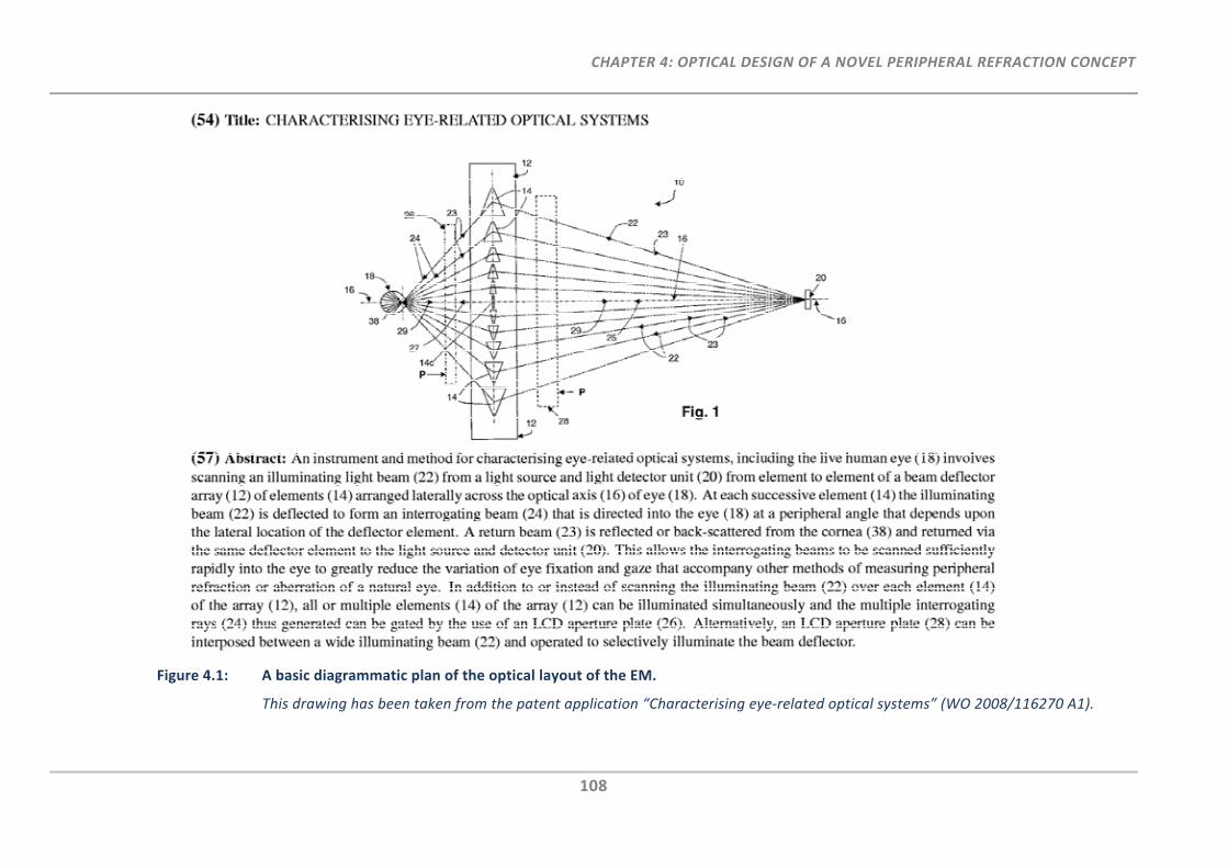
CHAPTER 4: OPTICAL DESIGN OF A NOVEL PERIPHERAL REFRACTION CONCEPT
108
Figure 4.1: A basic diagrammatic plan of the optical layout of the EM.
This drawing has been taken from the patent application “Characterising eye‐related optical systems” (WO 2008/116270 A1).
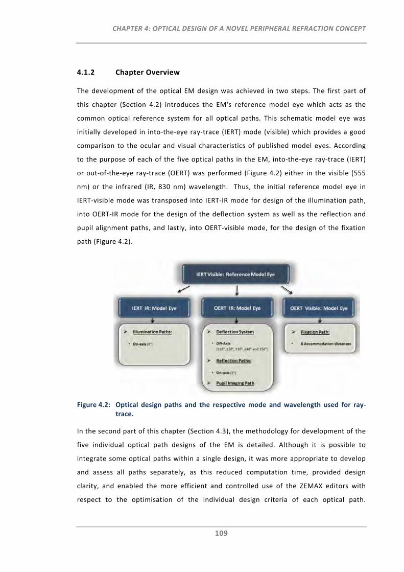
CHAPTER 4: OPTICAL DESIGN OF A NOVEL PERIPHERAL REFRACTION CONCEPT
109
4.1.2 Chapter Overview
The development of the optical EM design was achieved in two steps. The first part of
this chapter (Section 4.2) introduces the EM's reference model eye which acts as the
common optical reference system for all optical paths. This schematic model eye was
initially developed in into‐the‐eye ray‐trace (IERT) mode (visible) which provides a good
comparison to the ocular and visual characteristics of published model eyes. According
to the purpose of each of the five optical paths in the EM, into‐the‐eye ray‐trace (IERT)
or out‐of‐the‐eye ray‐trace (OERT) was performed (Figure 4.2) either in the visible (555
nm) or the infrared (IR, 830 nm) wavelength. Thus, the initial reference model eye in
IERT‐visible mode was transposed into IERT‐IR mode for design of the illumination path,
into OERT‐IR mode for the design of the deflection system as well as the reflection and
pupil alignment paths, and lastly, into OERT‐visible mode, for the design of the fixation
path (Figure 4.2).
Figure 4.2: Optical design paths and the respective mode and wavelength used for ray‐trace.
In the second part of this chapter (Section 4.3), the methodology for development of the
five individual optical path designs of the EM is detailed. Although it is possible to
integrate some optical paths within a single design, it was more appropriate to develop
and assess all paths separately, as this reduced computation time, provided design
clarity, and enabled the more efficient and controlled use of the ZEMAX editors with
respect to the optimisation of the individual design criteria of each optical path.

CHAPTER 4: OPTICAL DESIGN OF A NOVEL PERIPHERAL REFRACTION CONCEPT
110
However, it is important to note that, these paths are intertwined at some point and
thus, some optical components of optical paths needed to overlap and their design and
position needed to match accordingly.
4.1.3 Introduction into Optical Designing using ZEMAX
Primarily, three ZEMAX editors, the Lens Data Editor (LDE), the Multi Configuration
Editor (MCE) and the Merit Function Editor (MFE), were used for the design of the EM
reference model eye as well as each optical EM path. The following six steps provide a
brief overview for the basic set‐up and scope of each ZEMAX editor in order to
accomplish specified optical design goals:
1. Set‐Up of the ZEMAX Lens Data Editor:
The LDE is the primary editor used to enter surfaces and their lens parameters such
as surface curvature, thickness and diameter. Moreover, the LDE is used to define
the basic surfaces of each optical system; the object, image and stop surfaces.
2. Set‐Up of the ZEMAX Multi Configuration Editor:
The MCE is very similar to the LDE in that it stores information on the surface
parameters. Its advantage is that it allows to create and to work with multiple
configurations, which are distinguished by different values for the same parameters
in the LDE. These parameters are specified using Multi Configuration Operands.
3. Definition of Variable Parameters:
As part of the subsequent optimisation, the LDE and MCE are used to specify all
unknown parameters that require optimisation (variable parameters). With respect
to the EM design, unknown parameters can, for example, include the position of
prism surfaces, or the curvatures of lens surfaces.
4. Set‐Up of the ZEMAX Merit Function Editor:
The MFE is used to define and weigh target values of selected Merit Function
Operands that can achieve the specific optical design criteria (merit function)
according to the defined variable parameters.
5. Optimisation:
The optimisation tool in ZEMAX uses a powerful algorithm that aims to find the
“local” minimum of the merit function and thus enables computation of the variable
CHAPTER 4: OPTICAL DESIGN OF A NOVEL PERIPHERAL REFRACTION CONCEPT
111
parameters in the LDE and MCE with respect to the specific design criteria as
defined in the MFE.
6. Review Optical Design Requirements:
The resulting merit function indicates how closely the optimised optical system
meets the specified optical design goals, and thus is used to decide whether the
optical system requires further refinement to achieve the specified optical design
requirements.
4.2 The EyeMapper’s Reference Model Eye
With the advancement of ocular biometric measurements and sophisticated optical
design programs, the modelling of theoretical eyes has become increasingly complex. In
the early development of schematic model eyes, a simple reduced eye consisting of only
a single refracting surface was used. However, gradually, more complex designs, often
rotationally symmetric, with several refracting surfaces, were introduced, such as the
Gullstrand’s No. 1 eye.185 Nowadays, it is possible to work with schematic eye models
having tilted or decentred ocular surfaces and/or having a complex crystalline lens that
consists of different gradient indices.186 Although computerisation makes it possible to
use the most complex and sophisticated eye model, it is not always the most appropriate
schematic model eye with respect to research needs. As such, the aim for the EM’s
reference model eye was not to opt for the most sophisticated of the models previously
published, but to keep it simple, valid and applicable for the design of all the relevant
optical paths of the EM. This section aimed to evaluate the EM reference model eye with
respect to different accommodative and refractive demands and with respect to its
peripheral refraction profile for different ray‐trace modes.
4.2.1 Methods
4.2.1.1 EyeMapper Reference Model Eye
Figure 4.2 shows that the optical paths of the EM instrument require either OERT (visible
and IR) or IERT mode in the IR light. In general, investigations on schematic eye models
are primarily made with respect to eyes in IERT (visible) mode. Having the retina as the
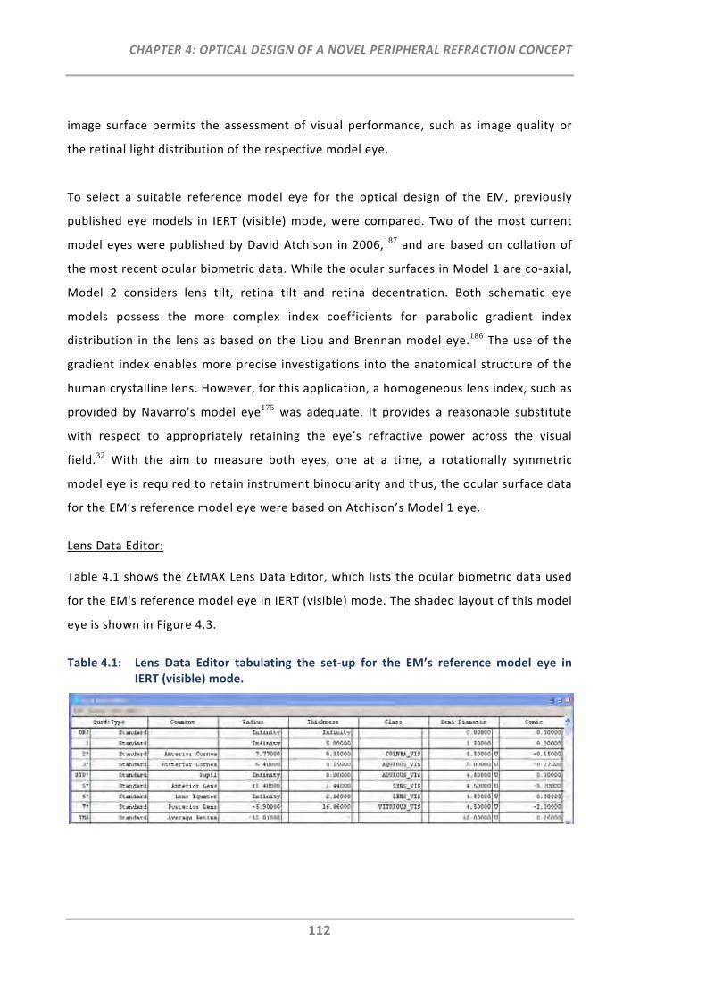
CHAPTER 4: OPTICAL DESIGN OF A NOVEL PERIPHERAL REFRACTION CONCEPT
112
image surface permits the assessment of visual performance, such as image quality or
the retinal light distribution of the respective model eye.
To select a suitable reference model eye for the optical design of the EM, previously
published eye models in IERT (visible) mode, were compared. Two of the most current
model eyes were published by David Atchison in 2006,187 and are based on collation of
the most recent ocular biometric data. While the ocular surfaces in Model 1 are co‐axial,
Model 2 considers lens tilt, retina tilt and retina decentration. Both schematic eye
models possess the more complex index coefficients for parabolic gradient index
distribution in the lens as based on the Liou and Brennan model eye.186 The use of the
gradient index enables more precise investigations into the anatomical structure of the
human crystalline lens. However, for this application, a homogeneous lens index, such as
provided by Navarro's model eye175 was adequate. It provides a reasonable substitute
with respect to appropriately retaining the eye’s refractive power across the visual
field.32 With the aim to measure both eyes, one at a time, a rotationally symmetric
model eye is required to retain instrument binocularity and thus, the ocular surface data
for the EM’s reference model eye were based on Atchison’s Model 1 eye.
Lens Data Editor:
Table 4.1 shows the ZEMAX Lens Data Editor, which lists the ocular biometric data used
for the EM's reference model eye in IERT (visible) mode. The shaded layout of this model
eye is shown in Figure 4.3.
Table 4.1: Lens Data Editor tabulating the set‐up for the EM’s reference model eye in IERT (visible) mode.
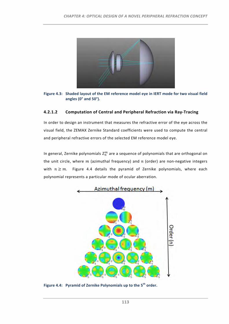
CHAPTER 4: OPTICAL DESIGN OF A NOVEL PERIPHERAL REFRACTION CONCEPT
113
Figure 4.3: Shaded layout of the EM reference model eye in IERT mode for two visual field angles (0° and 50°).
4.2.1.2 Computation of Central and Peripheral Refraction via Ray‐Tracing
In order to design an instrument that measures the refractive error of the eye across the
visual field, the ZEMAX Zernike Standard coefficients were used to compute the central
and peripheral refractive errors of the selected EM reference model eye.
In general, Zernike polynomials are a sequence of polynomials that are orthogonal on
the unit circle, where (azimuthal frequency) and (order) are non‐negative integers
with . Figure 4.4 details the pyramid of Zernike polynomials, where each
polynomial represents a particular mode of ocular aberration.
Figure 4.4: Pyramid of Zernike Polynomials up to the 5th order.
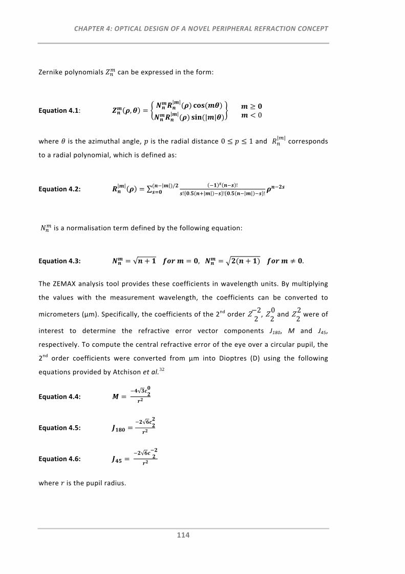
CHAPTER 4: OPTICAL DESIGN OF A NOVEL PERIPHERAL REFRACTION CONCEPT
114
Zernike polynomials can be expressed in the form:
Equation 4.1: ,| |
| | | |
0
where is the azimuthal angle, is the radial distance 0 1 and | | corresponds
to a radial polynomial, which is defined as:
Equation 4.2: | | ∑ !
! . | | ! . | | !
| | /
is a normalisation term defined by the following equation:
Equation 4.3: √ , .
The ZEMAX analysis tool provides these coefficients in wavelength units. By multiplying
the values with the measurement wavelength, the coefficients can be converted to
micrometers (μm). Specifically, the coefficients of the 2nd order Z 22, Z 0
2 and Z 2
2 were of
interest to determine the refractive error vector components J180, M and J45,
respectively. To compute the central refractive error of the eye over a circular pupil, the
2nd order coefficients were converted from μm into Dioptres (D) using the following
equations provided by Atchison et al.32
Equation 4.4: √
Equation 4.5: √
Equation 4.6: √
where is the pupil radius.
CHAPTER 4: OPTICAL DESIGN OF A NOVEL PERIPHERAL REFRACTION CONCEPT
115
For the computation of peripheral refraction and its subsequent comparison with
published data, Atchison et al.’s32 modified equations were used, which stretch the
‘elliptical’ peripheral pupil shape into a circular one. These equations are:
Equation 4.7: √ √
Equation 4.8: √ √
Equation 4.9: √
.
Finally, the refractive vector components for central and peripheral refraction can be
converted into the more common sphero‐cylindrical notation of S/C × θ, where S
corresponds to the sphere, C corresponds to the cylinder and θ corresponds to the axis
component. The conversion can be made using the following equations:
Equation 4.10:
Equation 4.11:
Equation 4.12:
In the case of J180 being 0, the equation of θ is unresolvable and thus, θ has to be defined
upon the value of J45. If J45 < 0, then θ = 135°, and if J45 ≥ 0, θ = 45°. The following
additional equations have to be applied in order to retain θ within the range of the
conventional cylinder axis, i.e. 0 to 180°.
Equation 4.13: If J180 < 0 → θ = θ + 90°
Equation 4.14: If J180 ≥ 0 and J45 ≤ 0 → θ = θ + 180°
The calculations for the refractive power vectors are not built‐in functions of ZEMAX, but
the ZEMAX programming language (ZPL) was used to write Macro 1 (APPENDIX C) in
order to execute these calculations. Moreover, the "Optreturn" command in Macro 1
CHAPTER 4: OPTICAL DESIGN OF A NOVEL PERIPHERAL REFRACTION CONCEPT
116
was used for the optimisation of the refractive vector components in the MFE using the
ZPLM Merit Function Operand. The use of this operand is explained in more detail in the
next section (Section 4.2.1.3).
4.2.1.3 Refractive Error‐Dependent Model Eyes
As the aim of the EM instrument is to measure a range of spherical and astigmatic
refractive errors of the eye, the emmetropic EM reference model eye presented in
Section 4.2.1.1 was not sufficient for the modelling of the optical design requirements of
the EM. In order to theoretically assess the instrument’s refractive error range, the EM
reference model eye required modification. The following section demonstrates the
methodological approach for the modification of the refractive state of the EM reference
model eye in ZEMAX.
Lens Data Editor:
As the reflection path of the optical EM design is the determining path for central and
peripheral refraction, the EM reference model eye in IERT (visible) mode was transposed
to the eye in OERT (IR) mode (Table 4.2, top). As a change in central spherical refractive
error can primarily be attributed to changes in axial length,188 the vitreous chamber
depth was selected so that it could be modified to induce a specified spherical refractive
error (M) of the model eye. Moreover, to induce central astigmatism, the assumption
was made that the eye's astigmatism is solely corneal in nature and thus, the surface
type of the anterior cornea was set to biconic with the y‐meridian of the biconic surface
defined to be modifiable. Nevertheless, it should be noted that in human eyes,
astigmatism is commonly composed of a combination of lenticular and corneal
astigmatism. As the change of the two parameters, vitreous chamber depth and corneal
y‐radius, permit a change in the spherical and astigmatic refractive error respectively,
they were tagged with the letter V (variable) in the LDE (Table 4.2, top) as part of the
subsequent optimisation in the MFE (Table 4.2, bottom).
Merit Function Editor:
As mentioned in Section 4.2.1.2, the optimisation was performed using the “Optreturn”
command in ZEMAX Macro 1 (APPENDIX C), which was linked to the ZPML operand in the
MFE (Table 4.2, bottom). The ZPLM operand with its output data 1 and 3 shows that, as
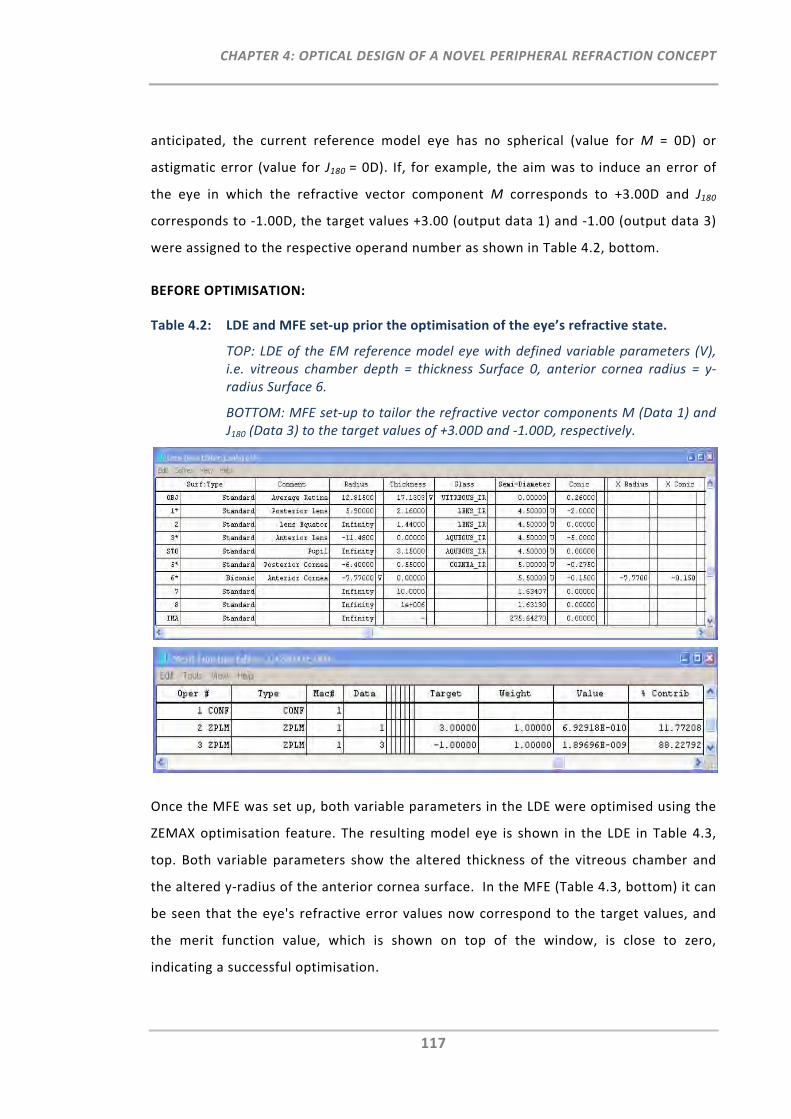
CHAPTER 4: OPTICAL DESIGN OF A NOVEL PERIPHERAL REFRACTION CONCEPT
117
anticipated, the current reference model eye has no spherical (value for M = 0D) or
astigmatic error (value for J180 = 0D). If, for example, the aim was to induce an error of
the eye in which the refractive vector component M corresponds to +3.00D and J180
corresponds to ‐1.00D, the target values +3.00 (output data 1) and ‐1.00 (output data 3)
were assigned to the respective operand number as shown in Table 4.2, bottom.
BEFORE OPTIMISATION:
Table 4.2: LDE and MFE set‐up prior the optimisation of the eye’s refractive state.
TOP: LDE of the EM reference model eye with defined variable parameters (V), i.e. vitreous chamber depth = thickness Surface 0, anterior cornea radius = y‐radius Surface 6.
BOTTOM: MFE set‐up to tailor the refractive vector components M (Data 1) and J180 (Data 3) to the target values of +3.00D and ‐1.00D, respectively.
Once the MFE was set up, both variable parameters in the LDE were optimised using the
ZEMAX optimisation feature. The resulting model eye is shown in the LDE in Table 4.3,
top. Both variable parameters show the altered thickness of the vitreous chamber and
the altered y‐radius of the anterior cornea surface. In the MFE (Table 4.3, bottom) it can
be seen that the eye's refractive error values now correspond to the target values, and
the merit function value, which is shown on top of the window, is close to zero,
indicating a successful optimisation.
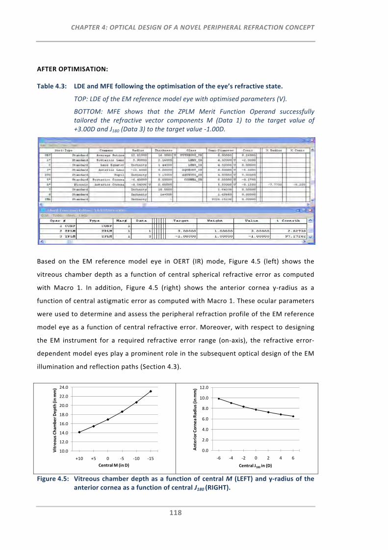
CHAPTER 4: OPTICAL DESIGN OF A NOVEL PERIPHERAL REFRACTION CONCEPT
118
AFTER OPTIMISATION:
Table 4.3: LDE and MFE following the optimisation of the eye’s refractive state.
TOP: LDE of the EM reference model eye with optimised parameters (V).
BOTTOM: MFE shows that the ZPLM Merit Function Operand successfully tailored the refractive vector components M (Data 1) to the target value of +3.00D and J180 (Data 3) to the target value ‐1.00D.
Based on the EM reference model eye in OERT (IR) mode, Figure 4.5 (left) shows the
vitreous chamber depth as a function of central spherical refractive error as computed
with Macro 1. In addition, Figure 4.5 (right) shows the anterior cornea y‐radius as a
function of central astigmatic error as computed with Macro 1. These ocular parameters
were used to determine and assess the peripheral refraction profile of the EM reference
model eye as a function of central refractive error. Moreover, with respect to designing
the EM instrument for a required refractive error range (on‐axis), the refractive error‐
dependent model eyes play a prominent role in the subsequent optical design of the EM
illumination and reflection paths (Section 4.3).
Figure 4.5: Vitreous chamber depth as a function of central M (LEFT) and y‐radius of the anterior cornea as a function of central J180 (RIGHT).
10.0
12.0
14.0
16.0
18.0
20.0
22.0
24.0
+10 +5 0 ‐5 ‐10 ‐15
Vitreous Cham
ber Depth (in mm)
Central M (in D)
0.0
2.0
4.0
6.0
8.0
10.0
12.0
‐6 ‐4 ‐2 0 2 4 6
Anterior Cornea Radius (in mm)
Central J180 in (D)
CHAPTER 4: OPTICAL DESIGN OF A NOVEL PERIPHERAL REFRACTION CONCEPT
119
4.2.1.4 Accommodation‐Dependent Model Eyes
In addition to the refractive error‐dependent model eyes, the EM’s aim is to also
measure peripheral refraction profiles as a function of accommodation. Thus, for the
subsequent optical design of the on‐axis EM fixation path, an accommodation‐
dependent model eye was required.
Popiolek‐Masajada and Kasprzak have investigated the changes of the crystalline lens as
a function of accommodation189 and have provided accommodation‐dependent functions
for relevant lens parameters. For the accommodation‐dependent EM reference model
eye, the linear functions for the posterior lens surface and the lens thickness were
extrapolated using the following equations:
Equation 4.15: . .
Equation 4.16: . .
Again, it should be noted, that the aim for this model eye was not to investigate the
ocular biometric changes of the accommodating eye in detail, but to have a simplified
model which enables modelling of the optical design of the fixation path with respect to
retaining the different accommodative demands.
Set‐Up of ZEMAX Editors:
The LDE shows the EM reference model eye in OERT (visible) mode (Table 4.4, top). As
indicated by Equation 4.16, as accommodation changes, so too does the thickness of the
lens, and to account for this, an additional surface called "additional lens thickness" was
inserted in the LDE. Moreover, the MCE was used to create an eye for various
accommodative states (Table 4.4, middle). The parameters (Multi Configuration
Operands) differentiating the various accommodative states of the eye are; “additional
lens thickness” (THIC 2), posterior lens curvature (CRVT 1), anterior lens curvature (CRVT
4) and accommodation distance (THIC 8). The accommodation distances were pre‐
defined. Lens thickness and posterior lens curvature are the fixed parameters given by
the functions provided in Equation 4.15 and Equation 4.16. Anterior lens curvature is the

CHAPTER 4: OPTICAL DESIGN OF A NOVEL PERIPHERAL REFRACTION CONCEPT
120
BEFORE OPTIMISATION:
Table 4.4: Set‐up of the three ZEMAX editors prior the optimisation of the accommodation‐ dependent parameters.
TOP: The LDE shows the reference model eye in OERT (visible) mode. An additional surface called "additional lens thickness" (surface 2) was inserted.
MIDDLE: The MCE was utilised to create a reference model eye for six different accommodative distances (THIC 8). The parameters (Multi Configuration Operands) differentiating the eye from different accommodative states are lens thickness (THIC 2), posterior lens curvature (CRVT 1), anterior lens curvature (CRVT 4) and accommodation distance (THIC 8). Lens thickness and posterior lens curvature are the parameters given by the functions provided in Equation 4.15 and Equation 4.16. Anterior lens curvature was specified as variable parameter (V).
BOTTOM: Optimisation of the anterior lens curvature was achieved using the MFE operand REAY (real ray y‐coordinate, pupil coordinate Py = 1). This operand aims to tailor the rays to zero for the given accommodation distances (THIC 8).

CHAPTER 4: OPTICAL DESIGN OF A NOVEL PERIPHERAL REFRACTION CONCEPT
121
AFTER OPTIMISATION:
Table 4.5: The three ZEMAX editors following the optimisation of the accommodation‐ dependent parameters.
TOP: The radius of the anterior lens surface optimised for an accommodation demand of 1D (Configuration 2).
MIDDLE: The Multi Configuration Operand CRVT 4 (Anterior lens curvature) optimised for all accommodation distances (THIC 8).
BOTTOM: The Merit Function Operand REAY (real ray y‐coordinate, pupil coordinate Py = 1) successfully tailored to zero for all configurations.
yet unknown parameter and was specified as variable (V). The Merit Function Operand
REAY (real ray y‐coordinate, pupil coordinate Py = 1) was used to target the marginal
rays to reach zero for all configurations in the MFE (Table 4.4, bottom).
Table 4.5 shows the resulting editors following the successful optimisation process. As
anticipated, with increasing accommodation, the lens thickness increases and the
CHAPTER 4: OPTICAL DESIGN OF A NOVEL PERIPHERAL REFRACTION CONCEPT
122
curvatures of both the posterior lens surface, as well as the optimised anterior lens
surface, increase.
This accommodation‐dependent EM reference model eye was then implemented for the
optical design of the EM's fixation path (Section 4.3.3).
4.2.1.5 Computation of Peripheral Refraction for Different Ray‐Trace Modes
With the aim to develop the optical design of the EM, it was of particular importance to
confirm the computation of peripheral refractive errors of the EM reference model eye
with previously published peripheral refraction data of schematic model eyes and to
validate its use for different ray‐trace modes. This validation was performed in three
steps:
Firstly, Macro 1 (APPENDIX C) was used to compute and then compare the peripheral
refraction profiles for the EM reference model eye in IERT mode (visible) with published
model eyes, such as those by Atchison,187 Liou & Brennan,186 Escudero‐Sanz & Navarro183
and Koojiman et al.190 For this, co‐axial ocular surfaces were used for all model eyes. The
refractive power vectors M and J180 were determined for a 3 mm pupil diameter at the
wavelength of 555 nm. Atchison previously compared the peripheral refraction profiles
up to 40° visual field angles of his eye models with the model eyes of other colleagues.
These results were replicated and extended to peripheral refraction profiles up to 50°
and compared with the EM reference model eye (IERT mode, visible).
Secondly, as the reflection path is the refracting path in the subsequent EM design, it is
important to assess whether the peripheral refraction profile obtained in IERT mode is in
agreement with the peripheral refraction profile obtained in OERT mode. In fact,
Atchison and Charman compared on‐axis aberrations of myopic rotational symmetric
model eyes in IERT and OERT mode and found that there are differences, particularly
when refractive error was large.191
Lastly, the difference between ray trace in the visible (555 nm) and IR (830 nm)
wavelengths are compared across the peripheral refraction profile for both, the EM
reference model eye in IERT and in OERT mode.
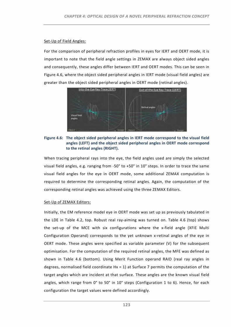
CHAPTER 4: OPTICAL DESIGN OF A NOVEL PERIPHERAL REFRACTION CONCEPT
123
Set‐Up of Field Angles:
For the comparison of peripheral refraction profiles in eyes for IERT and OERT mode, it is
important to note that the field angle settings in ZEMAX are always object sided angles
and consequently, these angles differ between IERT and OERT modes. This can be seen in
Figure 4.6, where the object sided peripheral angles in IERT mode (visual field angles) are
greater than the object sided peripheral angles in OERT mode (retinal angles).
Figure 4.6: The object sided peripheral angles in IERT mode correspond to the visual field angles (LEFT) and the object sided peripheral angles in OERT mode correspond to the retinal angles (RIGHT).
When tracing peripheral rays into the eye, the field angles used are simply the selected
visual field angles, e.g. ranging from ‐50° to +50° in 10° steps. In order to trace the same
visual field angles for the eye in OERT mode, some additional ZEMAX computation is
required to determine the corresponding retinal angles. Again, the computation of the
corresponding retinal angles was achieved using the three ZEMAX Editors.
Set‐Up of ZEMAX Editors:
Initially, the EM reference model eye in OERT mode was set up as previously tabulated in
the LDE in Table 4.2, top. Robust real ray‐aiming was turned on. Table 4.6 (top) shows
the set‐up of the MCE with six configurations where the x‐field angle (XFIE Multi
Configuration Operand) corresponds to the yet unknown x‐retinal angles of the eye in
OERT mode. These angles were specified as variable parameter (V) for the subsequent
optimisation. For the computation of the required retinal angles, the MFE was defined as
shown in Table 4.6 (bottom). Using Merit Function operand RAID (real ray angles in
degrees, normalised field coordinate Hx = 1) at Surface 7 permits the computation of the
target angles which are incident at that surface. These angles are the known visual field
angles, which range from 0° to 50° in 10° steps (Configuration 1 to 6). Hence, for each
configuration the target values were defined accordingly.
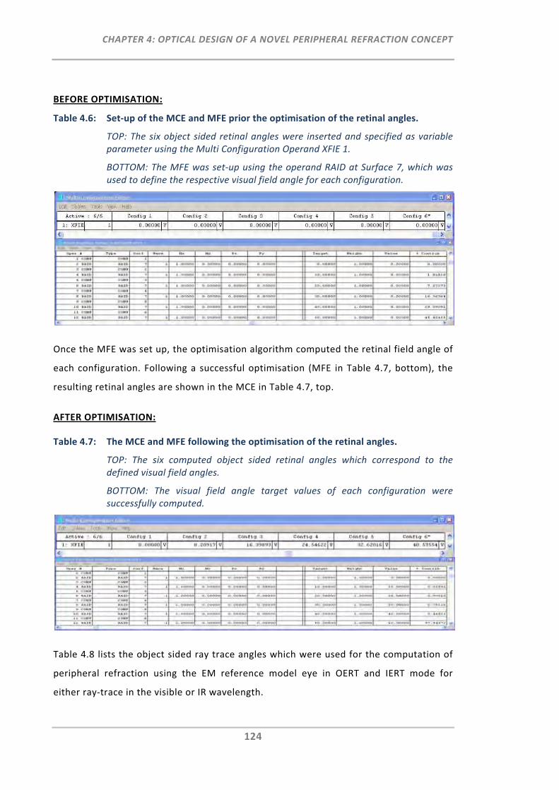
CHAPTER 4: OPTICAL DESIGN OF A NOVEL PERIPHERAL REFRACTION CONCEPT
124
BEFORE OPTIMISATION:
Table 4.6: Set‐up of the MCE and MFE prior the optimisation of the retinal angles.
TOP: The six object sided retinal angles were inserted and specified as variable parameter using the Multi Configuration Operand XFIE 1.
BOTTOM: The MFE was set‐up using the operand RAID at Surface 7, which was used to define the respective visual field angle for each configuration.
Once the MFE was set up, the optimisation algorithm computed the retinal field angle of
each configuration. Following a successful optimisation (MFE in Table 4.7, bottom), the
resulting retinal angles are shown in the MCE in Table 4.7, top.
AFTER OPTIMISATION:
Table 4.7: The MCE and MFE following the optimisation of the retinal angles.
TOP: The six computed object sided retinal angles which correspond to the defined visual field angles.
BOTTOM: The visual field angle target values of each configuration were successfully computed.
Table 4.8 lists the object sided ray trace angles which were used for the computation of
peripheral refraction using the EM reference model eye in OERT and IERT mode for
either ray‐trace in the visible or IR wavelength.
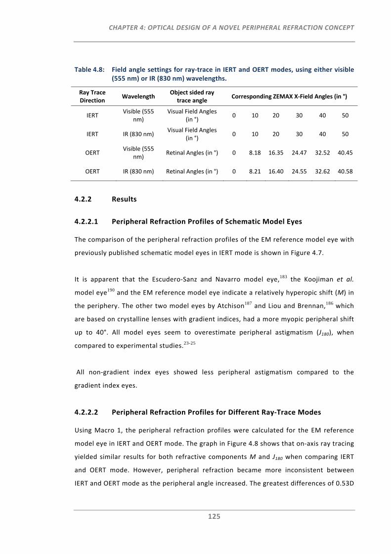
CHAPTER 4: OPTICAL DESIGN OF A NOVEL PERIPHERAL REFRACTION CONCEPT
125
Table 4.8: Field angle settings for ray‐trace in IERT and OERT modes, using either visible (555 nm) or IR (830 nm) wavelengths.
Ray Trace Direction
Wavelength Object sided ray
trace angle Corresponding ZEMAX X‐Field Angles (in °)
IERT Visible (555
nm) Visual Field Angles
(in °) 0 10 20 30 40 50
IERT IR (830 nm) Visual Field Angles
(in °) 0 10 20 30 40 50
OERT Visible (555
nm) Retinal Angles (in °) 0 8.18 16.35 24.47 32.52 40.45
OERT IR (830 nm) Retinal Angles (in °) 0 8.21 16.40 24.55 32.62 40.58
4.2.2 Results
4.2.2.1 Peripheral Refraction Profiles of Schematic Model Eyes
The comparison of the peripheral refraction profiles of the EM reference model eye with
previously published schematic model eyes in IERT mode is shown in Figure 4.7.
It is apparent that the Escudero‐Sanz and Navarro model eye,183 the Koojiman et al.
model eye190 and the EM reference model eye indicate a relatively hyperopic shift (M) in
the periphery. The other two model eyes by Atchison187 and Liou and Brennan,186 which
are based on crystalline lenses with gradient indices, had a more myopic peripheral shift
up to 40°. All model eyes seem to overestimate peripheral astigmatism (J180), when
compared to experimental studies.23-25
All non‐gradient index eyes showed less peripheral astigmatism compared to the
gradient index eyes.
4.2.2.2 Peripheral Refraction Profiles for Different Ray‐Trace Modes
Using Macro 1, the peripheral refraction profiles were calculated for the EM reference
model eye in IERT and OERT mode. The graph in Figure 4.8 shows that on‐axis ray tracing
yielded similar results for both refractive components M and J180 when comparing IERT
and OERT mode. However, peripheral refraction became more inconsistent between
IERT and OERT mode as the peripheral angle increased. The greatest differences of 0.53D
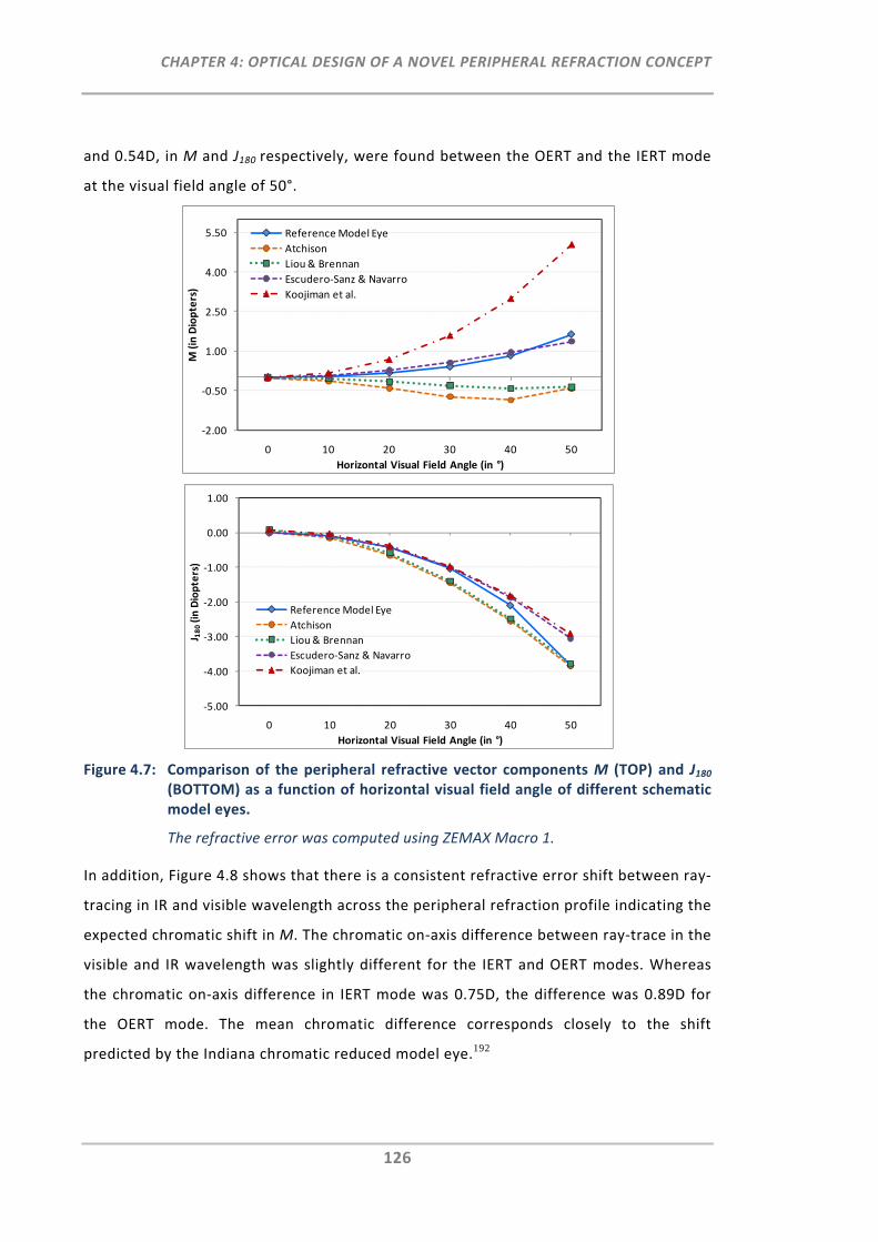
CHAPTER 4: OPTICAL DESIGN OF A NOVEL PERIPHERAL REFRACTION CONCEPT
126
and 0.54D, in M and J180 respectively, were found between the OERT and the IERT mode
at the visual field angle of 50°.
Figure 4.7: Comparison of the peripheral refractive vector components M (TOP) and J180 (BOTTOM) as a function of horizontal visual field angle of different schematic model eyes.
The refractive error was computed using ZEMAX Macro 1.
In addition, Figure 4.8 shows that there is a consistent refractive error shift between ray‐
tracing in IR and visible wavelength across the peripheral refraction profile indicating the
expected chromatic shift in M. The chromatic on‐axis difference between ray‐trace in the
visible and IR wavelength was slightly different for the IERT and OERT modes. Whereas
the chromatic on‐axis difference in IERT mode was 0.75D, the difference was 0.89D for
the OERT mode. The mean chromatic difference corresponds closely to the shift
predicted by the Indiana chromatic reduced model eye.192
‐2.00
‐0.50
1.00
2.50
4.00
5.50
0 10 20 30 40 50
M (in Diopters)
Horizontal Visual Field Angle (in °)
Reference Model Eye
Atchison
Liou & Brennan
Escudero‐Sanz & Navarro
Koojiman et al.
‐5.00
‐4.00
‐3.00
‐2.00
‐1.00
0.00
1.00
0 10 20 30 40 50
J 180(in Diopters)
Horizontal Visual Field Angle (in °)
Reference Model Eye
Atchison
Liou & Brennan
Escudero‐Sanz & Navarro
Koojiman et al.
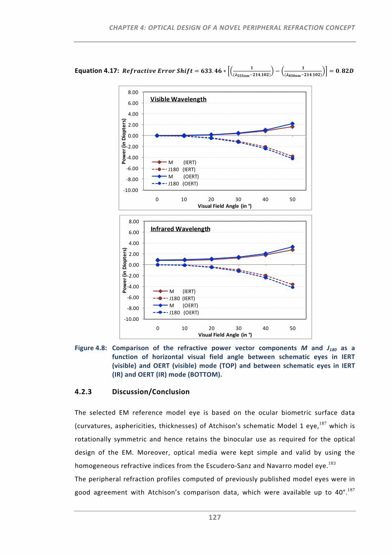
CHAPTER 4: OPTICAL DESIGN OF A NOVEL PERIPHERAL REFRACTION CONCEPT
127
Equation 4.17: .. .
.
Figure 4.8: Comparison of the refractive power vector components M and J180 as a function of horizontal visual field angle between schematic eyes in IERT (visible) and OERT (visible) mode (TOP) and between schematic eyes in IERT (IR) and OERT (IR) mode (BOTTOM).
4.2.3 Discussion/Conclusion
The selected EM reference model eye is based on the ocular biometric surface data
(curvatures, asphericities, thicknesses) of Atchison's schematic Model 1 eye,187 which is
rotationally symmetric and hence retains the binocular use as required for the optical
design of the EM. Moreover, optical media were kept simple and valid by using the
homogeneous refractive indices from the Escudero‐Sanz and Navarro model eye.183
The peripheral refraction profiles computed of previously published model eyes were in
good agreement with Atchison’s comparison data, which were available up to 40°.187
‐10.00
‐8.00
‐6.00
‐4.00
‐2.00
0.00
2.00
4.00
6.00
8.00
0 10 20 30 40 50
Power (in Diopters)
Visual Field Angle (in °)
M (IERT)
J180 (IERT)
M (OERT)
J180 (OERT)
Visible Wavelength
‐10.00
‐8.00
‐6.00
‐4.00
‐2.00
0.00
2.00
4.00
6.00
8.00
0 10 20 30 40 50
Power (in Diopters)
Visual Field Angle (in °)
M (IERT)
J180 (IERT)
M (OERT)
J180 (OERT)
Infrared Wavelength
CHAPTER 4: OPTICAL DESIGN OF A NOVEL PERIPHERAL REFRACTION CONCEPT
128
Neither of the current model eyes, predicted peripheral refraction, in particular J180, well
when compared to in vivo measurements.24 Nevertheless, the aim of this work was not
to study the most accurate wide‐angle schematic model eye with respect to in vivo
peripheral refraction data, but rather to ascertain a model eye that provides a central
and peripheral refraction reference for the subsequent optical design of the EM.
As the optical path designs of the EM instrument require different ray trace modes, it
was important to cross‐validate whether there is a difference in peripheral refraction
profiles between OERT and IERT modes as well as between the visible and IR ray tracing.
Atchison and Charman investigated whether there is a difference between central
aberrations obtained via OERT or IERT mode using Navarro's model eye.191 They showed
that higher levels of ametropia can lead to a considerable change between OERT and
IERT modes. Large refractive errors, as known to be present in the periphery of the eye,
can therefore potentially affect the different ray‐trace modes. The present work has
shown that, as visual field angles increased, the difference between OERT and IERT mode
increased. The difference was as large as 0.54D for J180 at the 50° horizontal visual field
angle. The mean shift for the peripheral refraction profiles obtained at different
wavelengths was in good agreement with the 0.82D shift predicted from the Indiana
chromatic reduced eye model.192
Overall, this model eye was suggested to be an appropriate reference model eye for the
purpose of designing the optical paths of the EM instrument.
4.3 The Optical Design of the EyeMapper
The EM's optical instrument design was developed on the basis of the EM's reference
model eye presented in Section 4.2. In total, the design consists of five optical paths: the
deflection system, the illumination path, the reflection path, the pupil imaging path and
the fixation path. As each path has different optical design requirements, it was
advantageous to develop them as separate designs in ZEMAX. The paths dedicated to
central and peripheral autorefraction are the deflection system, the illumination and
reflection paths. The deflection system comprises the design of the individual prisms and
the determination of the positions of the scanning mirror to allow the ocular scanning of
CHAPTER 4: OPTICAL DESIGN OF A NOVEL PERIPHERAL REFRACTION CONCEPT
129
all 11 visual field angles. The illumination and reflection paths are the paths, which
define the intended refractive error range of the EM instrument. In addition to the three
autorefraction paths, the pupil imaging and the fixation path have to be incorporated, to
enable the viewing/alignment of the pupil by the examiner and the fixation of an on‐axis
target by the participant.
The ZEMAX editors were used to set up the optical paths with respect to the pre‐defined
instrument design requirements (Methods ‐ Before optimisation). Subsequently, the
optical paths were optimised to achieve their individual design goals (Results ‐ After
optimisation).
4.3.1 Autorefraction Paths
4.3.1.1 Deflection System
The prime purpose of the deflection system is to enable the scan of the illumination and
reflection beams across the eye without inducing optical distortions or aberrations.
Based on the proposed design concept (Section 4.1.1) it is aimed to guide the beam
across the visual field via a scanning mirror and ten customised prisms.
4.3.1.1.1 Methods
The methodological approach for the optical design of the deflection system is explained
in the set‐up of the three ZEMAX editors.
Lens Data Editor:
1. LDE Pre‐Settings:
As shown in Table 4.9 the previously implemented EM reference model eye in OERT (IR)
mode was used as reference file for the design of the deflection system. The system pre‐
settings of this model eye were as follows: the surface of the pupil was defined as “Stop”
surface, the ray‐trace wavelength was set to 830 nm, the entrance pupil diameter
corresponded to 3 mm and the robust real ray aiming ZEMAX feature was turned on.
2. Insertion and Definition of Prism and Scanning Mirror Surfaces:
The two prism surfaces, the front and back surface were inserted. The prism material
was chosen to be of high refractive index (N‐BK9, nd=1.69). The rectangular shape and
CHAPTER 4: OPTICAL DESIGN OF A NOVEL PERIPHERAL REFRACTION CONCEPT
130
size of both prism surfaces were defined using the rectangular aperture type settings.
Moreover, the surface for the scanning mirror was inserted and assigned to the glass
type “Mirror” and was also defined as the "Global Coordinate Reference", which was of
importance for the subsequent optimisation.
3. Definition of Reference Distances for On‐Axis System:
With the aim of constructing a compact instrument design, the on‐axis distance between
the eye and the front prism surface and between the prism and the scanning mirror were
defined as being as small as possible (i.e. 55.5 and 200 mm). The distance between the
scanning mirror and the image surface was set to ‐50 mm, which had a negative sign due
to change of the real propagation direction caused by the previous mirror surface.
4. Insertion of Coordinate Breaks:
Coordinate breaks (CB) are dummy surfaces that allow the change of the global
coordinate system to permit the tracing of non‐axial rays. Consequently, CBs were used
for the design of the prisms of the proposed deflection system, where propagating
beams are to be traced for 11 different field angles. In general, CBs are implemented
before and after ray tracing to the selected non‐axial surface. Parameters accounting for
a change in the coordinate system are CB decentres and CB tilts. The sequential order of
decentring and tilting is crucial with respect to the order of CB decentres and tilts. As
shown in Table 4.9, two CBs were placed in front of each prism surface and one CB was
placed after each prism surface. For each prism surface, the first CB decentres the
surface (Translate 1 & 2) as specified in lens units and the second CB tilts the surface
(Rotate 1 & 2) to a certain degree. In order to return to the coordinate system after ray‐
tracing through either of the prism surfaces, the coordinate return feature was applied
at the third CB of each prism surface, which decentres and tilts the coordinate system
back in the correct sequential order.
The prime aim of the scanning mirror is to direct the beam towards 11 different
directions. Using ZEMAX, this scan requirement can be achieved with a CB y‐tilt. Due to
these tilt requirements one CB was placed before and a second CB was placed after the
scanning mirror surface (Table 4.9). Moreover, a CB x‐tilt was used to position the axis
of the scanning mirror in a pre‐defined 15° angle perpendicular to the measurement
meridian.
CHAPTER 4: OPTICAL DESIGN OF A NOVEL PERIPHERAL REFRACTION CONCEPT
131
Multi Configuration Editor:
With the requirement of tracing rays for 11 different field angles, the application of the
MCE was of particular use for the proposed deflection system. The following steps show
the detailed set‐up of the MCE (Table 4.10) including the particular peripheral design
criteria.
1. Definition of Peripheral Angles:
The MCE was utilised to set up the reference model eye, where rays are propagated from
11 different retinal locations (object surface) towards the pupil (STOP surface) by use of
the robust real ray‐aiming feature in ZEMAX. These 11 object sided retinal angles were
defined by the Multi Configuration Operand XFIE 1. The retinal field angles were
specified as previously computed for the schematic model eye in OERT (IR) mode
(Section 0). Negative pick‐up solves (P) were used to mirror the five positive peripheral
retinal angles to the five negative peripheral retinal angles. As pickup solves actively
adjust specific values during the optimisation procedure, they are very useful,
particularly for symmetrical systems with many configurations. Consequently, they were
utilised throughout the MCE set‐up of the deflection system design.
2. Definition of Distances and Aperture Sizes:
To arrange the 10 prisms in an arc shape in front of the eye, the individual distances
between the anterior cornea surface and each of the front prism surfaces (THIC 7) were
pre‐defined for each configuration. Further fixed parameters differentiating the
configurations from each other are related to the different prism sizes which were
defined by prism thickness (THIC 11), minimum rectangular aperture sizes (APMN 10 &
APMN 14) and maximum rectangular aperture sizes (APMX 10 & APMX 14). Due to the
different peripheral ray‐trace angles, the optical path lengths between configurations
differ. Thus, the distance between the second prism surface and the scanning mirror
distance (THIC 15) was as yet, unknown and thus, specified as variable parameter for all
peripheral angles as part of the subsequent optimisation.
3. Definition of CB Parameter:
Parameter 1 of the first CB and Parameter 4 of the second CB, determine respectively,
the different x‐decentrations and y‐tilts of each prism surface relative to the optical axis
in the LDE. The operand PRAM in the MCE is the associated Multi Configuration Operand
CHAPTER 4: OPTICAL DESIGN OF A NOVEL PERIPHERAL REFRACTION CONCEPT
132
that defines CB decentrations and tilts for all individual configurations. As these prism‐
defining parameters were to be computed, they were specified as variable (V) for the
subsequent optimisation.
As for the scanning mirror, the PRAM operand 16/3 represents the x‐tilt of the pre‐
defined 15° angle. Moreover, to determine the amount of y‐tilt that is required for each
configuration, the PRAM operand 16/4 was defined as a variable for the further
optimisation in the MFE.
Merit Function Editor:
As mentioned previously, the Merit Function Editor was used for the optimisation of the
variable parameters specified in the LDE and MCE. Using either an actively damped least
squares or an orthogonal descent algorithm, ZEMAX optimises a merit function which is
composed of target values (Merit Function Operands). The merit function is defined as:
Equation 4.18: ∑
∑
where the subscript ‘i’ indicates the operand number (row number in the MFE
spreadsheet). With a set of 30 variables in the MCE, this optimisation feature is a
powerful tool to assist with the computation of the optical design of the deflection path.
As shown in Table 4.11 the MFE was set up individually for each configuration in the
deflection system. Merit Function Operands were given target values and weights to
achieve certain design goals with respect to the defined variable parameters in the MCE.
The detailed steps for the set‐up of the MFE were as followed:
Listing of Configurations:
Configurations assigned with pickup solves in the MCE were not listed in the MFE as they
are automatically updated. Thus, only configurations for on‐axis ray‐trace (Configuration
1) and peripheral ray‐trace with positive retinal angles (Configurations 2, 4, 6, 8 and 10)
were specified.

CHAPTER 4: OPTICAL DESIGN OF A NOVEL PERIPHERAL REFRACTION CONCEPT
133
Table 4.9: Set‐up of the LDE prior the optimisation of the deflection system.
The LDE for the deflection system was set up using the EM reference model eye in OERT (IR) mode. This is followed by the two prism surfaces which are enclosed by the additional CB surfaces. Whereas the two CBs in front of each prism surface (Translate 1 and Rotate 1) permit their individual decentration and tilt, the CB positioned after each prism surface returns the coordinate system to its global zero location. Similarly, the surface of the scanning mirror was also enclosed by CBs to permit the required x and y‐tilts of the scanning mirror.
R: Return Solves
P: Pickup solves
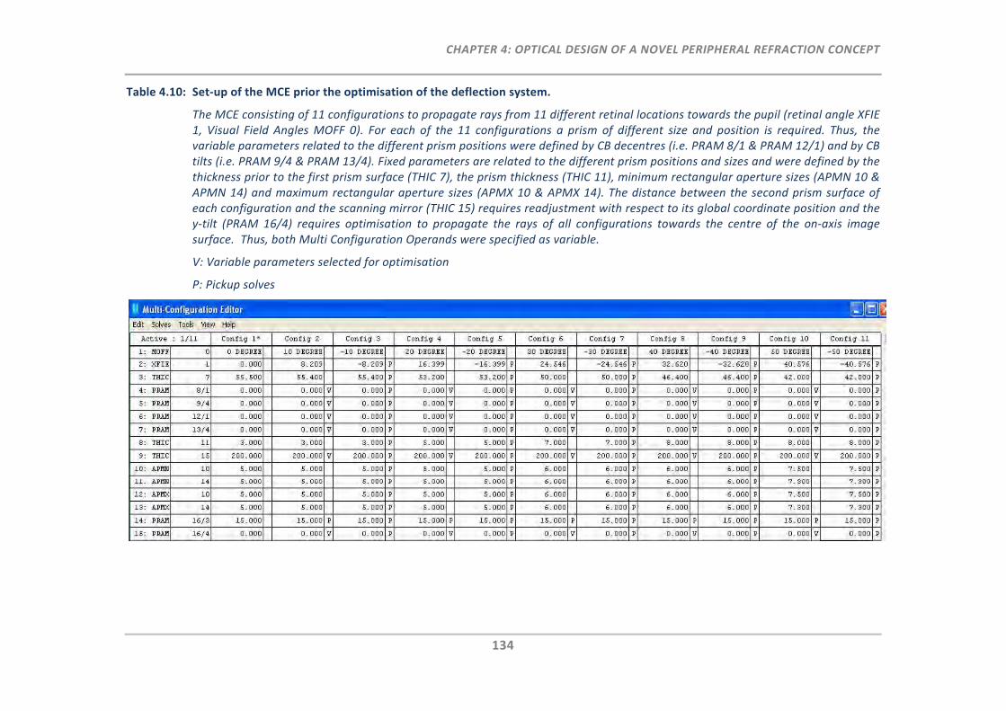
CHAPTER 4: OPTICAL DESIGN OF A NOVEL PERIPHERAL REFRACTION CONCEPT
134
Table 4.10: Set‐up of the MCE prior the optimisation of the deflection system.
The MCE consisting of 11 configurations to propagate rays from 11 different retinal locations towards the pupil (retinal angle XFIE 1, Visual Field Angles MOFF 0). For each of the 11 configurations a prism of different size and position is required. Thus, the variable parameters related to the different prism positions were defined by CB decentres (i.e. PRAM 8/1 & PRAM 12/1) and by CB tilts (i.e. PRAM 9/4 & PRAM 13/4). Fixed parameters are related to the different prism positions and sizes and were defined by the thickness prior to the first prism surface (THIC 7), the prism thickness (THIC 11), minimum rectangular aperture sizes (APMN 10 & APMN 14) and maximum rectangular aperture sizes (APMX 10 & APMX 14). The distance between the second prism surface of each configuration and the scanning mirror (THIC 15) requires readjustment with respect to its global coordinate position and the y‐tilt (PRAM 16/4) requires optimisation to propagate the rays of all configurations towards the centre of the on‐axis image surface. Thus, both Multi Configuration Operands were specified as variable.
V: Variable parameters selected for optimisation
P: Pickup solves
CHAPTER 4: OPTICAL DESIGN OF A NOVEL PERIPHERAL REFRACTION CONCEPT
135
Definition of Chief Ray‐Trace for Each Configuration:
The Merit Function Operand REAX (real X‐coordinate, normalised field coordinate Hx = 1)
was opted to trace the chief rays of each configuration to the centre of the prism front
surface (Surface 10), the centre of the prism back surface (Surface 14) and to the pivot of
the scanning mirror (Surface 20). This was done by defining the target value of this
operand at each of the three surfaces to zero.
Definition of Prism Criteria:
For the design of the individual prisms in the deflection system, the following optical
prism criteria were considered. Aberration is at a minimum only when rays of light pass
through a prism at a minimum deviation angle. The minimum deviation in a prism occurs
when the incidence and emergence angles are identical, leading to a symmetrical
configuration. Therefore, the prisms of each configuration in this instrument were
designed to adhere to these criteria, by targeting the difference (DIFF) between the
angles of the chief ray incident at the first prism surface (RAID 10) to be zero to the
angle of the chief ray exiting the second prism surface (RAED 14).
Maintaining Global Coordinates Identical for All Configurations:
Due to the different peripheral angles, the distances between each prism back surface
and the scanning mirror were the unknown parameters. Using ZEMAX, the computation
of these distances was achieved by ensuring that all configurations in the deflection
system are aligned within the same global coordinate system. The global reference
coordinate was used to define the point of overlap for multiple configurations. This
reference surface was previously pre‐defined to be the scanning mirror surface.
Moreover, the total on‐axis distance between the retina and the scanning mirror (GLCZ
0, Configuration 1) was the pre‐defined reference distance of the deflection system.
Thus, for the computation of the peripheral distances, it was the z‐position (GLCZ 0) of
the peripheral configurations that needed to be targeted to be equal to the z‐position of
the on‐axis configuration.
Definition of the Y‐Tilt of the Scanning Mirror for Each Configuration:
The last requirement for the deflection system was to determine how much y‐tilt of the
scanning mirror is required for each configuration. The Merit Function Operand DIFF was
used to target for the zero difference (DIFF) between the on‐axis chief ray coordinates
and the peripheral chief ray coordinates using the operands REAX (real X‐coordinate,

CHAPTER 4: OPTICAL DESIGN OF A NOVEL PERIPHERAL REFRACTION CONCEPT
136
normalised field coordinate Hx = 1) and REAY (real Y‐coordinate, normalised field
coordinate Hy = 1).
Table 4.11: Set‐up of the MFE prior the optimisation of the deflection system.
For the purpose of clarity, only two configurations are displayed in this Figure, that is Configuration 1 (0° on‐axis, Operands 1 to 18) and Configuration 10 (50° off‐axis, Operands 100 to 119). Note, that configurations assigned with pickup solves were not listed in the MFE as they are automatically updated.
For the computation of the deflection system the MFE was defined using the following Merit Function Operands, which were assigned specific target values. REAX (Surfaces 10, 14 and 20, normalised field coordinates, Hx=1) traces chief rays to the centre of the prism and scanning mirror surfaces. The ray angles defined by the operands RAID (Surface 10) (incident) and RAED 14 (exiting) were aimed to be equal. This was achieved by targeting the difference (DIFF) of the two angles to zero. The angle RAID 8 (Surface 8) was the visual field angle targeted for the computation of the corresponding retinal angles. The difference (DIFF) of the Operand GLCZ 0 (Surface 0, global coordinate z‐position) for Configuration 1 (on‐axis) was targeted to have the same GLCZ 0 position as all the other configurations. Using the DIFF operand, the off‐axis values of REAX and REAY were aimed to have equal intercepts at the image surface as the on‐axis configuration.
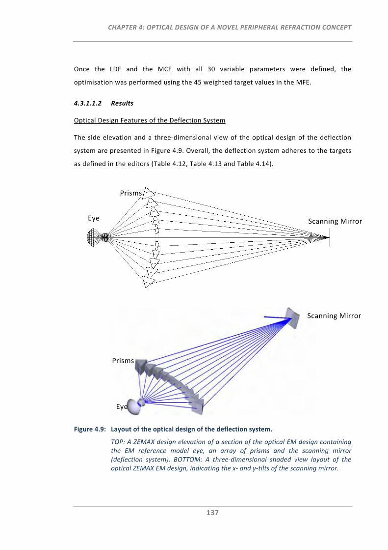
CHAPTER 4: OPTICAL DESIGN OF A NOVEL PERIPHERAL REFRACTION CONCEPT
137
Once the LDE and the MCE with all 30 variable parameters were defined, the
optimisation was performed using the 45 weighted target values in the MFE.
4.3.1.1.2 Results
Optical Design Features of the Deflection System
The side elevation and a three‐dimensional view of the optical design of the deflection
system are presented in Figure 4.9. Overall, the deflection system adheres to the targets
as defined in the editors (Table 4.12, Table 4.13 and Table 4.14).
Figure 4.9: Layout of the optical design of the deflection system.
TOP: A ZEMAX design elevation of a section of the optical EM design containing the EM reference model eye, an array of prisms and the scanning mirror (deflection system). BOTTOM: A three‐dimensional shaded view layout of the optical ZEMAX EM design, indicating the x‐ and y‐tilts of the scanning mirror.
Eye
Prisms
Scanning Mirror
Eye
Prisms
Scanning Mirror

CHAPTER 4: OPTICAL DESIGN OF A NOVEL PERIPHERAL REFRACTION CONCEPT
138
Table 4.12: LDE following the optimisation of the deflection system.
LDE parameters for the prism and scanning mirror surfaces (deflection path) that correspond to the 30° visual field angle of the eye (Configuration 6).
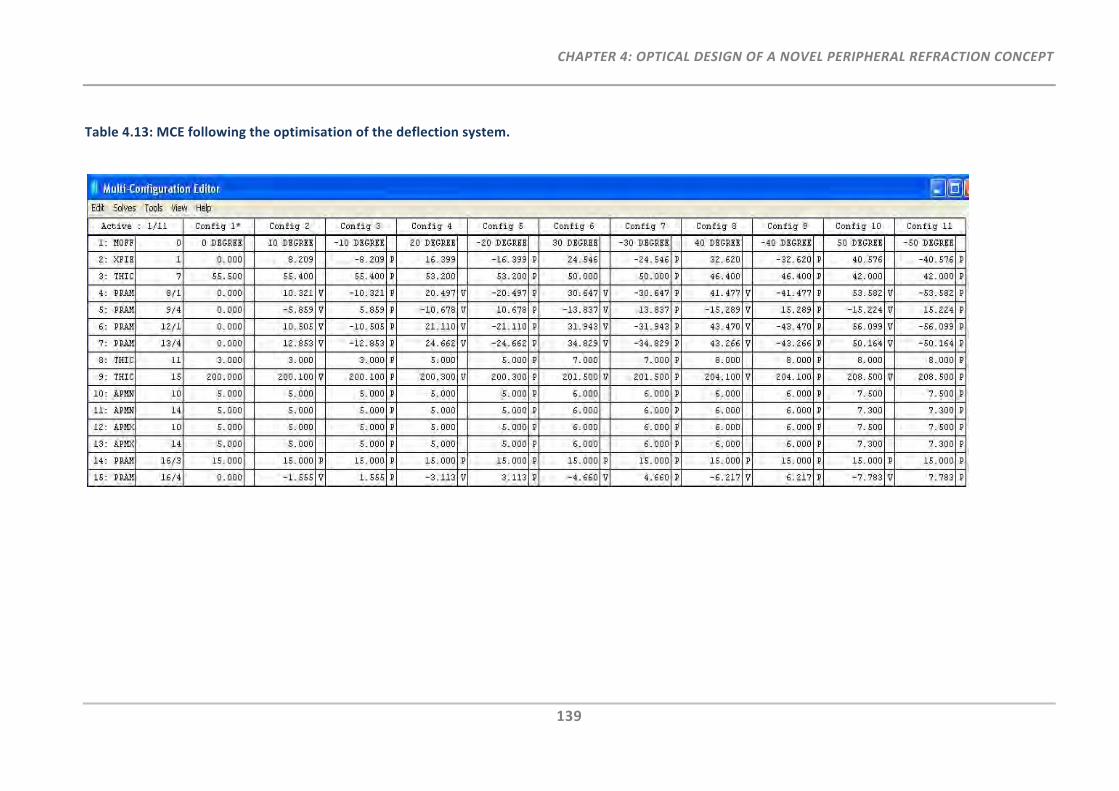
CHAPTER 4: OPTICAL DESIGN OF A NOVEL PERIPHERAL REFRACTION CONCEPT
139
Table 4.13: MCE following the optimisation of the deflection system.
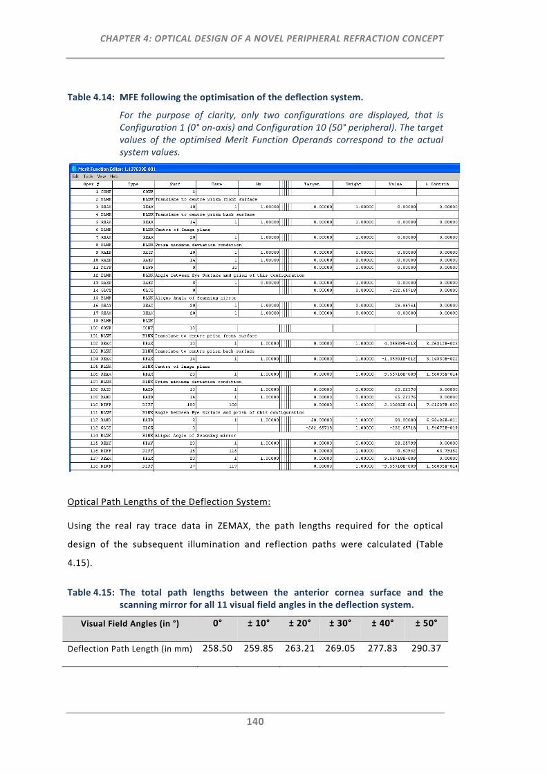
CHAPTER 4: OPTICAL DESIGN OF A NOVEL PERIPHERAL REFRACTION CONCEPT
140
Table 4.14: MFE following the optimisation of the deflection system.
For the purpose of clarity, only two configurations are displayed, that is Configuration 1 (0° on‐axis) and Configuration 10 (50° peripheral). The target values of the optimised Merit Function Operands correspond to the actual system values.
Optical Path Lengths of the Deflection System:
Using the real ray trace data in ZEMAX, the path lengths required for the optical
design of the subsequent illumination and reflection paths were calculated (Table
4.15).
Table 4.15: The total path lengths between the anterior cornea surface and the scanning mirror for all 11 visual field angles in the deflection system.
Visual Field Angles (in °) 0° ± 10° ± 20° ± 30° ± 40° ± 50°
Deflection Path Length (in mm) 258.50 259.85 263.21 269.05 277.83 290.37
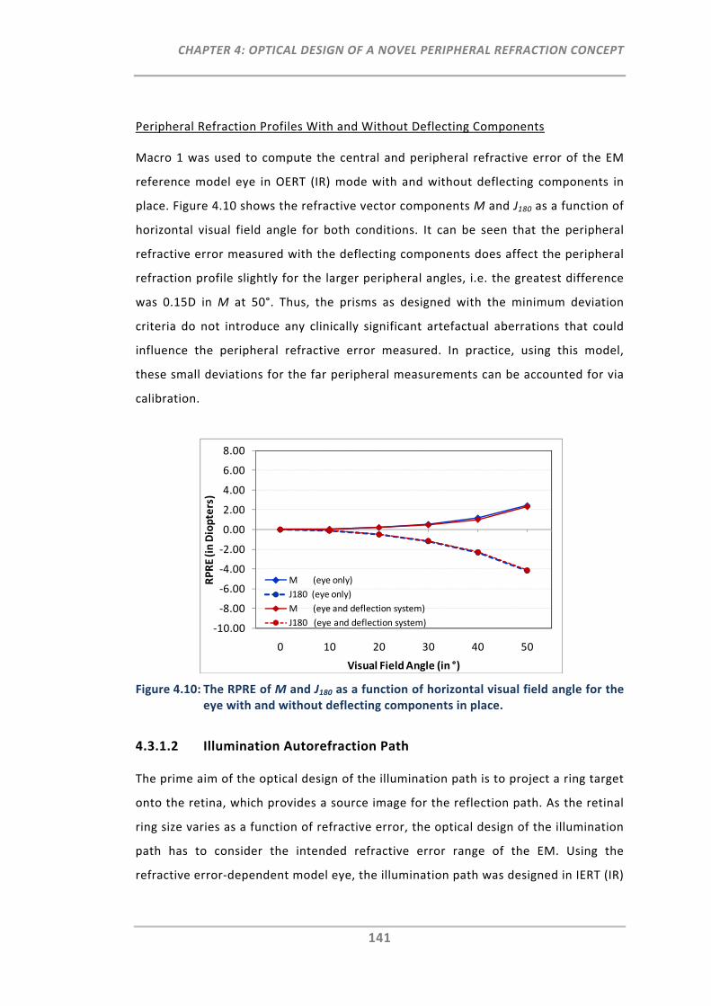
CHAPTER 4: OPTICAL DESIGN OF A NOVEL PERIPHERAL REFRACTION CONCEPT
141
Peripheral Refraction Profiles With and Without Deflecting Components
Macro 1 was used to compute the central and peripheral refractive error of the EM
reference model eye in OERT (IR) mode with and without deflecting components in
place. Figure 4.10 shows the refractive vector components M and J180 as a function of
horizontal visual field angle for both conditions. It can be seen that the peripheral
refractive error measured with the deflecting components does affect the peripheral
refraction profile slightly for the larger peripheral angles, i.e. the greatest difference
was 0.15D in M at 50°. Thus, the prisms as designed with the minimum deviation
criteria do not introduce any clinically significant artefactual aberrations that could
influence the peripheral refractive error measured. In practice, using this model,
these small deviations for the far peripheral measurements can be accounted for via
calibration.
Figure 4.10: The RPRE of M and J180 as a function of horizontal visual field angle for the eye with and without deflecting components in place.
4.3.1.2 Illumination Autorefraction Path
The prime aim of the optical design of the illumination path is to project a ring target
onto the retina, which provides a source image for the reflection path. As the retinal
ring size varies as a function of refractive error, the optical design of the illumination
path has to consider the intended refractive error range of the EM. Using the
refractive error‐dependent model eye, the illumination path was designed in IERT (IR)
‐10.00
‐8.00
‐6.00
‐4.00
‐2.00
0.00
2.00
4.00
6.00
8.00
0 10 20 30 40 50
RPRE (in Diopters)
Visual Field Angle (in °)
M (eye only)
J180 (eye only)
M (eye and deflection system)
J180 (eye and deflection system)

CHAPTER 4: OPTICAL DESIGN OF A NOVEL PERIPHERAL REFRACTION CONCEPT
142
on‐axis mode. Specific aperture and location boundaries from the deflection system
had to be taken into account for the illumination path design.
4.3.1.2.1 Methods
The methodological approach of the optical design of the illumination path under
consideration of the components from the deflection system is shown in the set‐up
of the three ZEMAX editors (Table 4.16 and Table 4.17).
Lens Data Editor:
LDE Pre‐Settings:
For the illumination path design the LDE was set up using the EM reference model
eye in IERT (IR) mode (Table 4.16, top).
Insertion of Additional Surfaces and Pre‐Definition of Distances:
The surfaces of Lens 1 (L1) were entered in the LDE. In order to achieve large and
refractive error sensitive retinal images within the pre‐defined desired refractive
error range (Sphere: +10.0 to ‐15.0D) of the instrument, the position of L1 was
chosen to be as close as possible to the front of the eye (51 mm). The “Stop” surface
was defined at the distance of the prism front surface (as computed in the deflection
system) and was set to 4.5 mm. This diameter subsequently corresponds to the size
of the illuminating ring target at this position. The positions of a pellicle beam splitter
and the x‐y scanning mirror were also pre‐defined.
Definition of Variable Parameter:
The yet unknown parameter of the illumination path design is the power of L1 (i.e.
the front and back surface radii of L1). Assuming L1 is a biconvex lens, the back
surface radius was preset using a negative pick‐up solve linked to the front surface
radius (Table 4.16, top). The front surface radius of L1 was specified as variable
parameter for the subsequent optimisation.
Multi Configuration Editor:
Range Definition for Refractive Error Eyes:
In order to assess and define the retinal image sizes for a range of different refractive
error eyes (central M: +10.0 to ‐15.0D) the MCE was opted to create a selection of
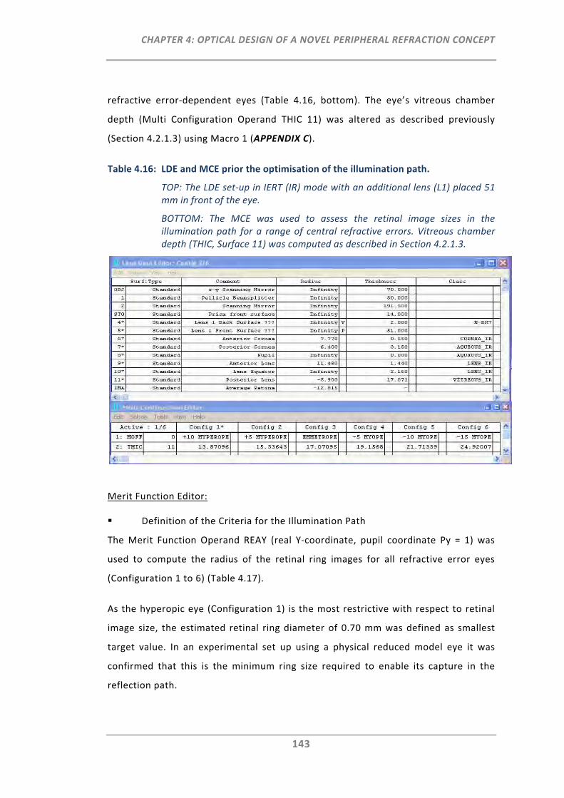
CHAPTER 4: OPTICAL DESIGN OF A NOVEL PERIPHERAL REFRACTION CONCEPT
143
refractive error‐dependent eyes (Table 4.16, bottom). The eye’s vitreous chamber
depth (Multi Configuration Operand THIC 11) was altered as described previously
(Section 4.2.1.3) using Macro 1 (APPENDIX C).
Table 4.16: LDE and MCE prior the optimisation of the illumination path.
TOP: The LDE set‐up in IERT (IR) mode with an additional lens (L1) placed 51 mm in front of the eye.
BOTTOM: The MCE was used to assess the retinal image sizes in the illumination path for a range of central refractive errors. Vitreous chamber depth (THIC, Surface 11) was computed as described in Section 4.2.1.3.
Merit Function Editor:
Definition of the Criteria for the Illumination Path
The Merit Function Operand REAY (real Y‐coordinate, pupil coordinate Py = 1) was
used to compute the radius of the retinal ring images for all refractive error eyes
(Configuration 1 to 6) (Table 4.17).
As the hyperopic eye (Configuration 1) is the most restrictive with respect to retinal
image size, the estimated retinal ring diameter of 0.70 mm was defined as smallest
target value. In an experimental set up using a physical reduced model eye it was
confirmed that this is the minimum ring size required to enable its capture in the
reflection path.
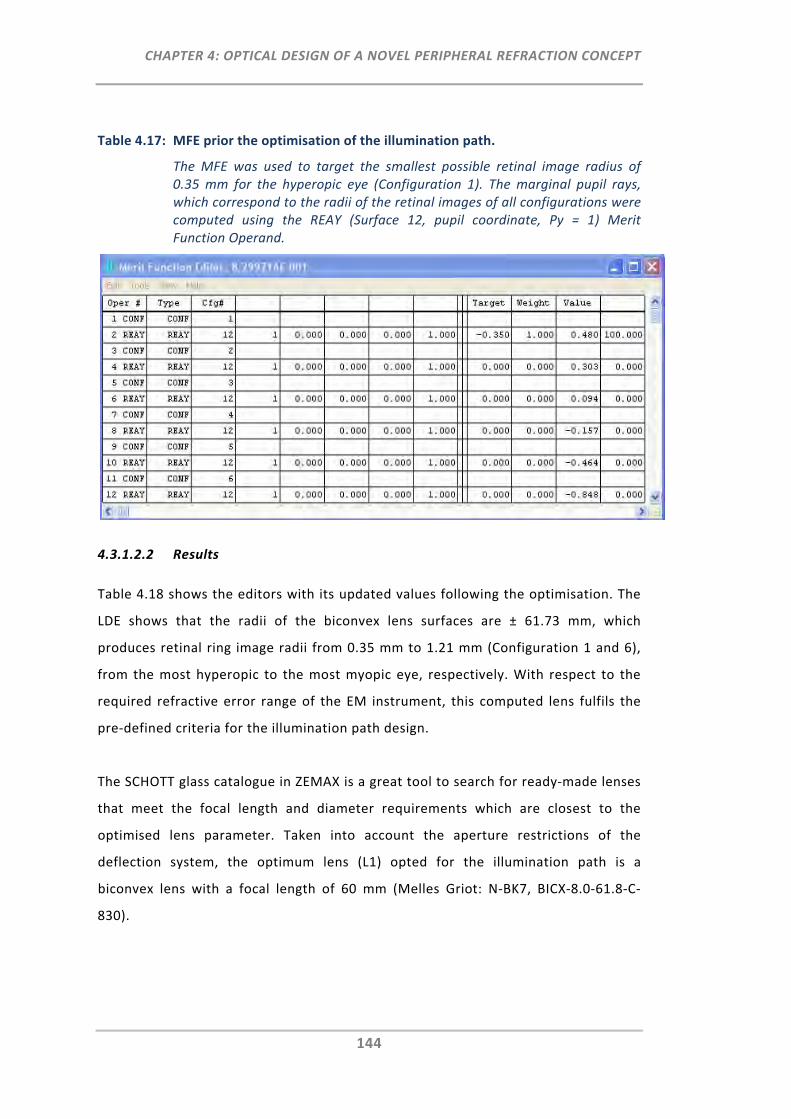
CHAPTER 4: OPTICAL DESIGN OF A NOVEL PERIPHERAL REFRACTION CONCEPT
144
Table 4.17: MFE prior the optimisation of the illumination path.
The MFE was used to target the smallest possible retinal image radius of 0.35 mm for the hyperopic eye (Configuration 1). The marginal pupil rays, which correspond to the radii of the retinal images of all configurations were computed using the REAY (Surface 12, pupil coordinate, Py = 1) Merit Function Operand.
4.3.1.2.2 Results
Table 4.18 shows the editors with its updated values following the optimisation. The
LDE shows that the radii of the biconvex lens surfaces are ± 61.73 mm, which
produces retinal ring image radii from 0.35 mm to 1.21 mm (Configuration 1 and 6),
from the most hyperopic to the most myopic eye, respectively. With respect to the
required refractive error range of the EM instrument, this computed lens fulfils the
pre‐defined criteria for the illumination path design.
The SCHOTT glass catalogue in ZEMAX is a great tool to search for ready‐made lenses
that meet the focal length and diameter requirements which are closest to the
optimised lens parameter. Taken into account the aperture restrictions of the
deflection system, the optimum lens (L1) opted for the illumination path is a
biconvex lens with a focal length of 60 mm (Melles Griot: N‐BK7, BICX‐8.0‐61.8‐C‐
830).
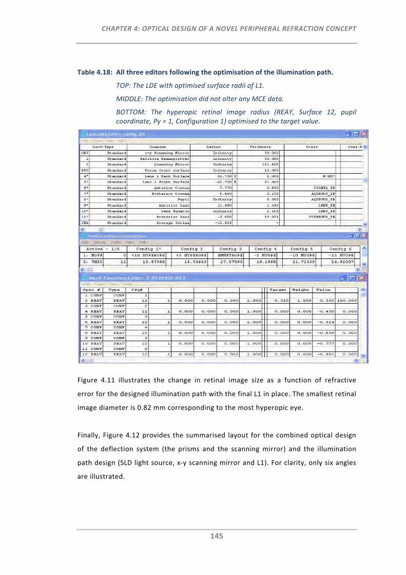
CHAPTER 4: OPTICAL DESIGN OF A NOVEL PERIPHERAL REFRACTION CONCEPT
145
Table 4.18: All three editors following the optimisation of the illumination path.
TOP: The LDE with optimised surface radii of L1.
MIDDLE: The optimisation did not alter any MCE data.
BOTTOM: The hyperopic retinal image radius (REAY, Surface 12, pupil coordinate, Py = 1, Configuration 1) optimised to the target value.
Figure 4.11 illustrates the change in retinal image size as a function of refractive
error for the designed illumination path with the final L1 in place. The smallest retinal
image diameter is 0.82 mm corresponding to the most hyperopic eye.
Finally, Figure 4.12 provides the summarised layout for the combined optical design
of the deflection system (the prisms and the scanning mirror) and the illumination
path design (SLD light source, x‐y scanning mirror and L1). For clarity, only six angles
are illustrated.
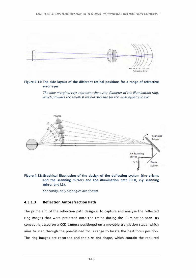
CHAPTER 4: OPTICAL DESIGN OF A NOVEL PERIPHERAL REFRACTION CONCEPT
146
Figure 4.11: The side layout of the different retinal positions for a range of refractive error eyes.
The blue marginal rays represent the outer diameter of the illumination ring, which provides the smallest retinal ring size for the most hyperopic eye.
Figure 4.12: Graphical illustration of the design of the deflection system (the prisms and the scanning mirror) and the illumination path (SLD, x‐y scanning mirror and L1).
For clarity, only six angles are shown.
4.3.1.3 Reflection Autorefraction Path
The prime aim of the reflection path design is to capture and analyse the reflected
ring images that were projected onto the retina during the illumination scan. Its
concept is based on a CCD camera positioned on a movable translation stage, which
aims to scan through the pre‐defined focus range to locate the best focus position.
The ring images are recorded and the size and shape, which contain the required
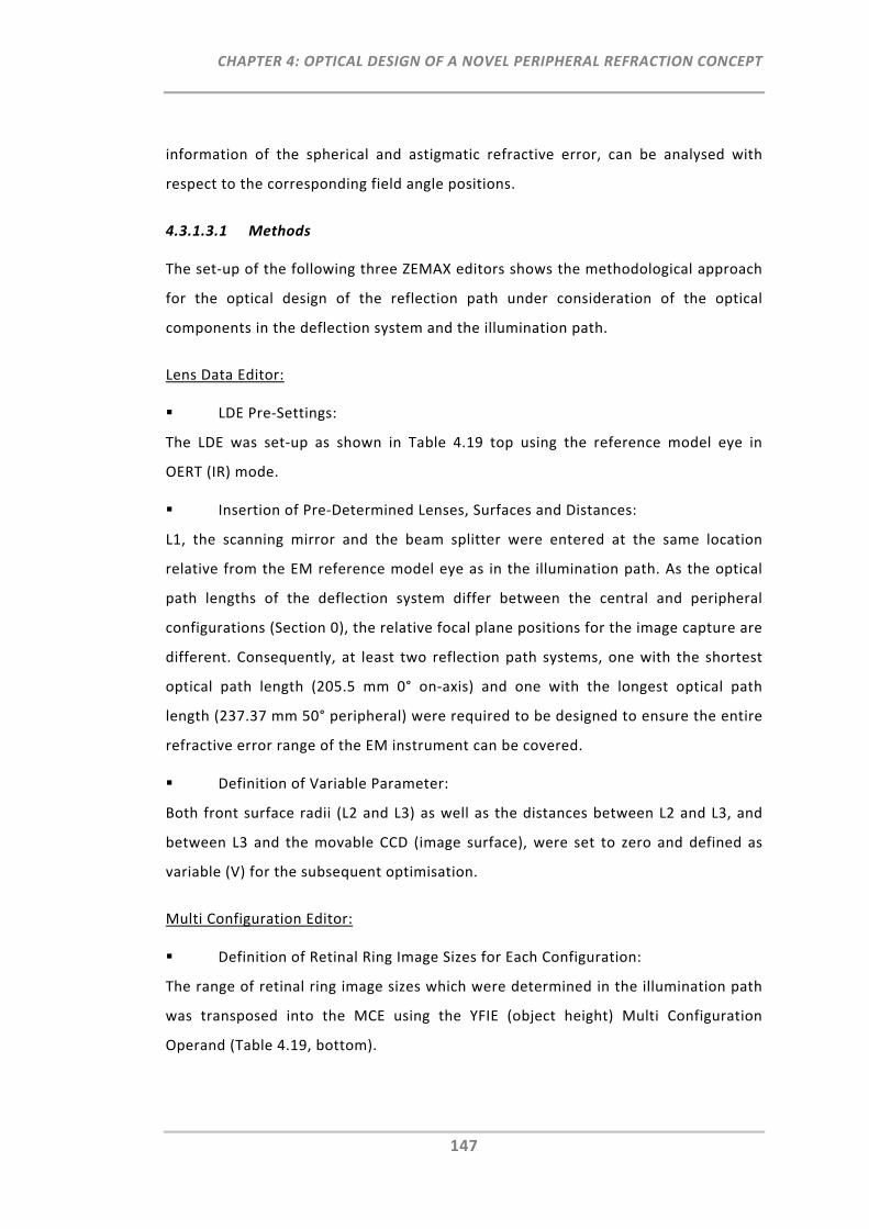
CHAPTER 4: OPTICAL DESIGN OF A NOVEL PERIPHERAL REFRACTION CONCEPT
147
information of the spherical and astigmatic refractive error, can be analysed with
respect to the corresponding field angle positions.
4.3.1.3.1 Methods
The set‐up of the following three ZEMAX editors shows the methodological approach
for the optical design of the reflection path under consideration of the optical
components in the deflection system and the illumination path.
Lens Data Editor:
LDE Pre‐Settings:
The LDE was set‐up as shown in Table 4.19 top using the reference model eye in
OERT (IR) mode.
Insertion of Pre‐Determined Lenses, Surfaces and Distances:
L1, the scanning mirror and the beam splitter were entered at the same location
relative from the EM reference model eye as in the illumination path. As the optical
path lengths of the deflection system differ between the central and peripheral
configurations (Section 0), the relative focal plane positions for the image capture are
different. Consequently, at least two reflection path systems, one with the shortest
optical path length (205.5 mm 0° on‐axis) and one with the longest optical path
length (237.37 mm 50° peripheral) were required to be designed to ensure the entire
refractive error range of the EM instrument can be covered.
Definition of Variable Parameter:
Both front surface radii (L2 and L3) as well as the distances between L2 and L3, and
between L3 and the movable CCD (image surface), were set to zero and defined as
variable (V) for the subsequent optimisation.
Multi Configuration Editor:
Definition of Retinal Ring Image Sizes for Each Configuration:
The range of retinal ring image sizes which were determined in the illumination path
was transposed into the MCE using the YFIE (object height) Multi Configuration
Operand (Table 4.19, bottom).
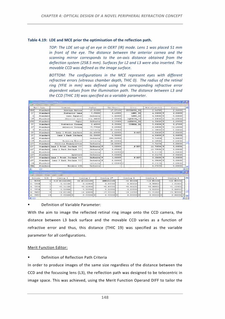
CHAPTER 4: OPTICAL DESIGN OF A NOVEL PERIPHERAL REFRACTION CONCEPT
148
Table 4.19: LDE and MCE prior the optimisation of the reflection path.
TOP: The LDE set‐up of an eye in OERT (IR) mode. Lens 1 was placed 51 mm in front of the eye. The distance between the anterior cornea and the scanning mirror corresponds to the on‐axis distance obtained from the deflection system (258.5 mm). Surfaces for L2 and L3 were also inserted. The movable CCD was defined as the image surface.
BOTTOM: The configurations in the MCE represent eyes with different refractive errors (vitreous chamber depth, THIC 0). The radius of the retinal ring (YFIE in mm) was defined using the corresponding refractive error dependent values from the illumination path. The distance between L3 and the CCD (THIC 19) was specified as a variable parameter.
Definition of Variable Parameter:
With the aim to image the reflected retinal ring image onto the CCD camera, the
distance between L3 back surface and the movable CCD varies as a function of
refractive error and thus, this distance (THIC 19) was specified as the variable
parameter for all configurations.
Merit Function Editor:
Definition of Reflection Path Criteria
In order to produce images of the same size regardless of the distance between the
CCD and the focussing lens (L3), the reflection path was designed to be telecentric in
image space. This was achieved, using the Merit Function Operand DIFF to tailor the
CHAPTER 4: OPTICAL DESIGN OF A NOVEL PERIPHERAL REFRACTION CONCEPT
149
difference in the normalised y‐ray coordinate between the back surface of L3 (REAY
19, Hy = 1) and the image surface (REAY 20, Hy = 1) to zero (Table 4.20). To
determine the focal planes, the marginal pupil y‐ray coordinate (REAY 20, Py = 1) was
set to zero. This set‐up was repeated for all configurations.
Definition of Lens Data Constraints
When there are many variable LDE parameters to be computed it is advantageous for
the subsequent optimisation algorithm to pre‐define some general constraints on
lens data with respect to the instrument needs. For the reflection path design, these
lens data constraints were given by the Merit Function Operands TTGT (thickness
greater than) of Surfaces 15 and 19, and CVLT (curvature less than) of Surface 17.
Moreover, the aperture of the detector surface (image surface) is restricted with
respect to the actual CCD size of the selected camera that is 3.6 mm. Thus, the Merit
Function Operand OPLT 51 of Configuration 6 was targeted to a detector image size
radius (REAY 20, Hy = 1) of less than 1.8 mm. This constraint was solely specified for
Configuration 6, which is the most myopic eye and thus, produces the largest ring
image to be captured.
Insertion of Additional Surfaces and Distances:
Following the beam splitter, the surfaces of Lens 2 (L2) were inserted. An initial
approach of using only one additional focussing lens (L2) for the reflection path
design failed, as optimisation did not provide valid results with respect to the
required reflection path requirements. Hence, the additional surfaces of a third lens
(L3) were inserted. The back surface radii of L2 and L3 were preset by negative pick‐
up solves (P) to aim for biconvex lens designs.
Definition of Translation Stage Range With Respect to Refractive Error Range
A further aim of the reflection path was that the pre‐defined focus range of the EM
instrument had to be covered within the 25 mm distance of the selected translation
stage. As this distance corresponds to the difference between the focal position of
the CCD (TTHI 19) for the most hyperopic eye (Configuration 1) and the most myopic
eye (Configuration 6), this constraint was targeted using the DIFF operand.

CHAPTER 4: OPTICAL DESIGN OF A NOVEL PERIPHERAL REFRACTION CONCEPT
150
Table 4.20: MFE prior the optimisation of the reflection path.
For simplicity, only two configurations are displayed, that is Configuration 1 (+10 Hyperope) and Configuration 6 (‐15 Myope).
For each configuration the value for the normalised field ray coordinate (REAY 20, Hx = 1) was targeted to be zero to render the retina conjugate to the CCD surface. Moreover, to achieve telecentricity in image space, the pupil ray coordinates (Surface 19, REAY, pupil coordinate Px = 1) were targeted to be equal to the pupil coordinates at the detector surface (Surface 20, REAY, pupil coordinate Px = 1). The difference between the focal position of the CCD (Surface 19, TTHI) for the most hyperopic eye (Configuration 1) and the most myopic eye (Configuration 6) was targeted to be zero.
4.3.1.3.2 Results
Under consideration of the previously designed EM deflection system (Section
4.3.1.1) and illumination path (Section 4.3.1.2), the resulting reflection path design
(after optimisation) can be seen in Table 4.21 and Table 4.22.
The LDE shows the computed surface radii of L2 and L3 and their positions for the
emmetropic eye. The MCE shows the change in CCD position (THIC 19) as a function
of refractive error. Due to the longer optical path length at the 50° position, the
positions for the focal planes of the same refractive error eye's shift closer towards
L3. The closest CCD position is 10.59 mm for the most myopic eye at 50°, and the
furthest CCD position is 32.33 mm for the most hyperopic eye at 0°. Thus, this
difference of 21mm covers the refractive error range of the EM instrument with

CHAPTER 4: OPTICAL DESIGN OF A NOVEL PERIPHERAL REFRACTION CONCEPT
151
respect to the given translation stage distance. Moreover, the largest detecor ring
image size (2.54 mm) was covered by the selected CCD size (3.6 mm).
Table 4.21: LDE and MCE following the optimisation of the reflection path.
TOP: The LDE with the optimised surface radii and positions of L2 and L3.
MIDDLE: The MCE with the computed CCD positions (THIC 19) for each configuration of the on‐axis system.
BOTTOM: The MCE with the computed CCD positions (THIC 19) for each configuration of the 50° off‐axis system.
Again, the ZEMAX Schott Glass catalogue was opted to find available lenses that are
close to the computed values (L2: Newport: KPX596 and L3: Melles Griot BXB‐12.7‐
40.7).
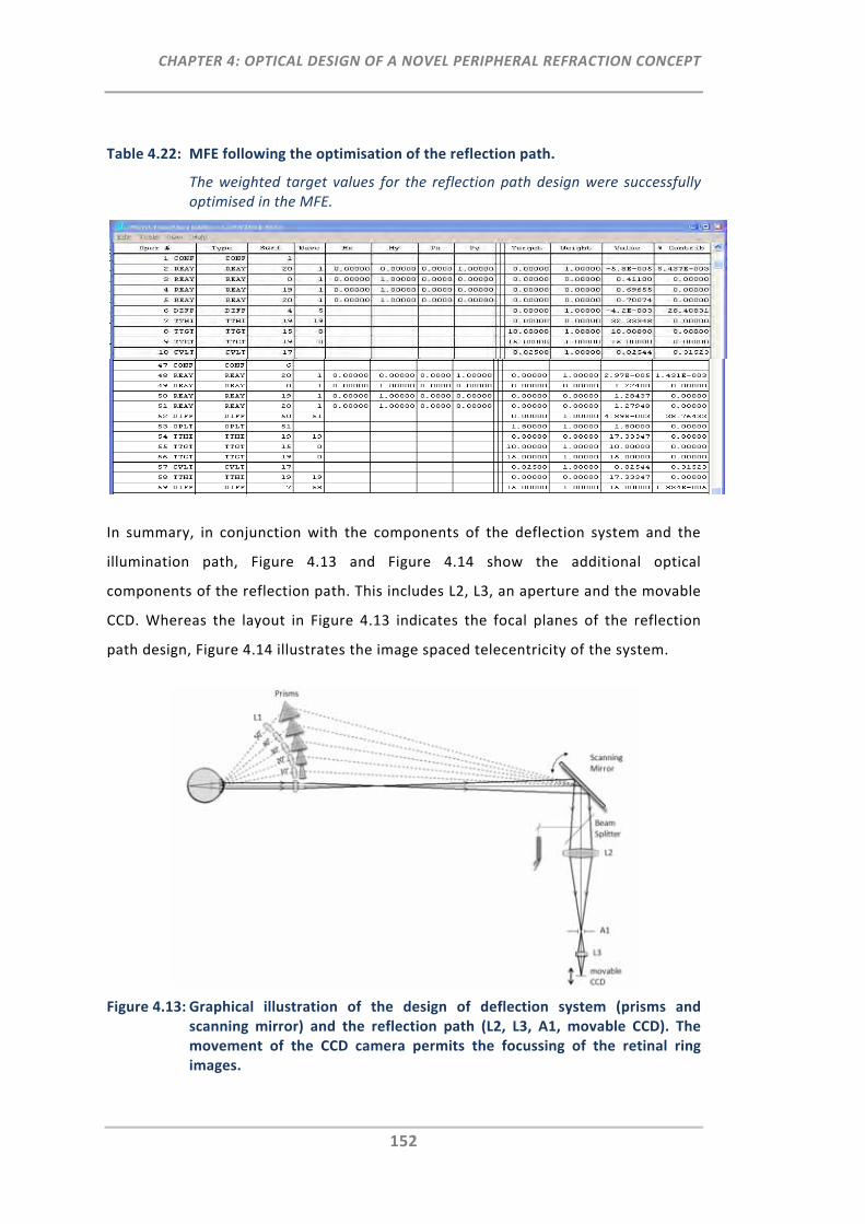
CHAPTER 4: OPTICAL DESIGN OF A NOVEL PERIPHERAL REFRACTION CONCEPT
152
Table 4.22: MFE following the optimisation of the reflection path.
The weighted target values for the reflection path design were successfully optimised in the MFE.
In summary, in conjunction with the components of the deflection system and the
illumination path, Figure 4.13 and Figure 4.14 show the additional optical
components of the reflection path. This includes L2, L3, an aperture and the movable
CCD. Whereas the layout in Figure 4.13 indicates the focal planes of the reflection
path design, Figure 4.14 illustrates the image spaced telecentricity of the system.
Figure 4.13: Graphical illustration of the design of deflection system (prisms and scanning mirror) and the reflection path (L2, L3, A1, movable CCD). The movement of the CCD camera permits the focussing of the retinal ring images.
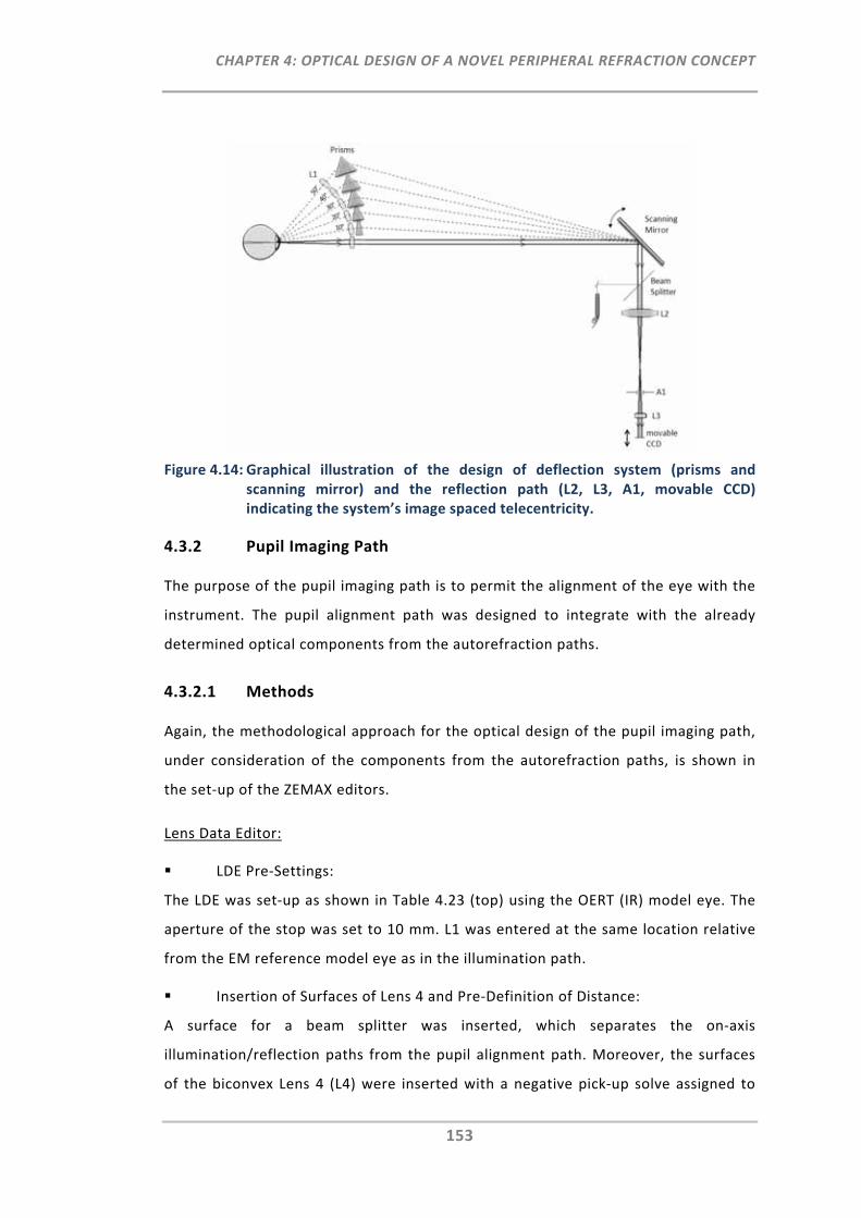
CHAPTER 4: OPTICAL DESIGN OF A NOVEL PERIPHERAL REFRACTION CONCEPT
153
Figure 4.14: Graphical illustration of the design of deflection system (prisms and scanning mirror) and the reflection path (L2, L3, A1, movable CCD) indicating the system’s image spaced telecentricity.
4.3.2 Pupil Imaging Path
The purpose of the pupil imaging path is to permit the alignment of the eye with the
instrument. The pupil alignment path was designed to integrate with the already
determined optical components from the autorefraction paths.
4.3.2.1 Methods
Again, the methodological approach for the optical design of the pupil imaging path,
under consideration of the components from the autorefraction paths, is shown in
the set‐up of the ZEMAX editors.
Lens Data Editor:
LDE Pre‐Settings:
The LDE was set‐up as shown in Table 4.23 (top) using the OERT (IR) model eye. The
aperture of the stop was set to 10 mm. L1 was entered at the same location relative
from the EM reference model eye as in the illumination path.
Insertion of Surfaces of Lens 4 and Pre‐Definition of Distance:
A surface for a beam splitter was inserted, which separates the on‐axis
illumination/reflection paths from the pupil alignment path. Moreover, the surfaces
of the biconvex Lens 4 (L4) were inserted with a negative pick‐up solve assigned to

CHAPTER 4: OPTICAL DESIGN OF A NOVEL PERIPHERAL REFRACTION CONCEPT
154
the back surface radius, and the front surface radius specified as variable for the
subsequent optimisation.
Merit Function Editor:
Definition of Pupil Imaging Path Criteria:
The Merit Function Operand REAY (Surface 15, normalised ray field coordinate, Hy =
1) was targeted to zero to image the pupil area onto the CCD image surface (Table
4.24, bottom). In addition, the use of the merit function operand REAY (Surface 15,
pupil coordinate, Py = 1) permits the computation and optimisation of the image
radius size. Thus, this operand was targeted to be 2 mm, which corresponds to the
size of the selected CCD radius.
Table 4.23: LDE and MFE prior the optimisation of the pupil imaging path.
TOP: The LDE with the reference model eye and L1 in OERT (IR) mode. The surfaces of the beam splitter and the biconvex L4 (P) were added. The front surface radius of L4 as well as the distance to the CCD were specified as variable (V).
BOTTOM: The Merit Function Operand REAY (normalised ray field coordinate, Hy = 1) was used to focus the pupil area onto the pupil camera CCD and REAY (pupil coordinate, Py = 1) was selected to target the pupil camera CCD radius to 2 mm.
4.3.2.2 Results
The resulting pupil alignment path design (after optimisation) can be seen in Table
4.24. The LDE shows the computed surface radii of L4 and the position of the pupil
camera CCD. The MFE shows the correct image radius of 2 mm which corresponds to
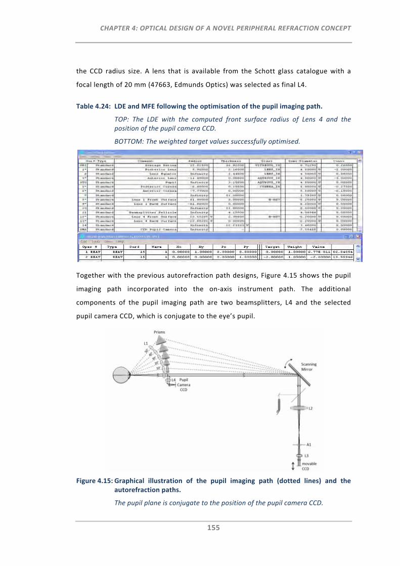
CHAPTER 4: OPTICAL DESIGN OF A NOVEL PERIPHERAL REFRACTION CONCEPT
155
the CCD radius size. A lens that is available from the Schott glass catalogue with a
focal length of 20 mm (47663, Edmunds Optics) was selected as final L4.
Table 4.24: LDE and MFE following the optimisation of the pupil imaging path.
TOP: The LDE with the computed front surface radius of Lens 4 and the position of the pupil camera CCD.
BOTTOM: The weighted target values successfully optimised.
Together with the previous autorefraction path designs, Figure 4.15 shows the pupil
imaging path incorporated into the on‐axis instrument path. The additional
components of the pupil imaging path are two beamsplitters, L4 and the selected
pupil camera CCD, which is conjugate to the eye’s pupil.
Figure 4.15: Graphical illustration of the pupil imaging path (dotted lines) and the autorefraction paths.
The pupil plane is conjugate to the position of the pupil camera CCD.
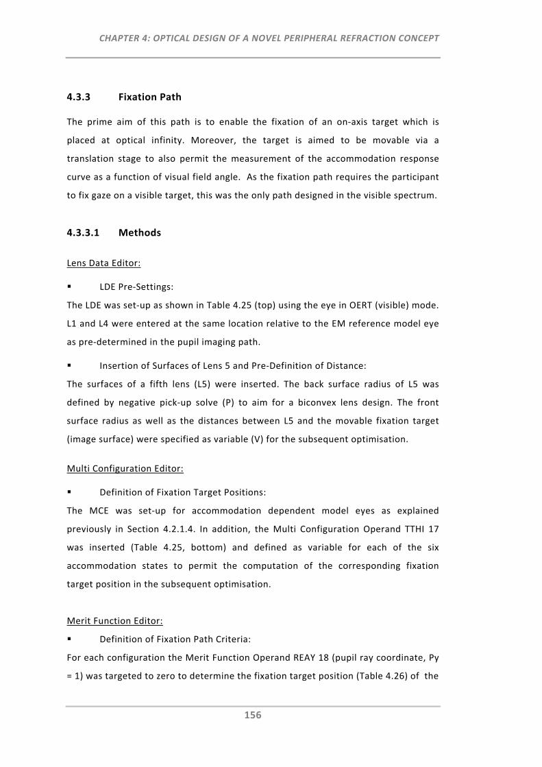
CHAPTER 4: OPTICAL DESIGN OF A NOVEL PERIPHERAL REFRACTION CONCEPT
156
4.3.3 Fixation Path
The prime aim of this path is to enable the fixation of an on‐axis target which is
placed at optical infinity. Moreover, the target is aimed to be movable via a
translation stage to also permit the measurement of the accommodation response
curve as a function of visual field angle. As the fixation path requires the participant
to fix gaze on a visible target, this was the only path designed in the visible spectrum.
4.3.3.1 Methods
Lens Data Editor:
LDE Pre‐Settings:
The LDE was set‐up as shown in Table 4.25 (top) using the eye in OERT (visible) mode.
L1 and L4 were entered at the same location relative to the EM reference model eye
as pre‐determined in the pupil imaging path.
Insertion of Surfaces of Lens 5 and Pre‐Definition of Distance:
The surfaces of a fifth lens (L5) were inserted. The back surface radius of L5 was
defined by negative pick‐up solve (P) to aim for a biconvex lens design. The front
surface radius as well as the distances between L5 and the movable fixation target
(image surface) were specified as variable (V) for the subsequent optimisation.
Multi Configuration Editor:
Definition of Fixation Target Positions:
The MCE was set‐up for accommodation dependent model eyes as explained
previously in Section 4.2.1.4. In addition, the Multi Configuration Operand TTHI 17
was inserted (Table 4.25, bottom) and defined as variable for each of the six
accommodation states to permit the computation of the corresponding fixation
target position in the subsequent optimisation.
Merit Function Editor:
Definition of Fixation Path Criteria:
For each configuration the Merit Function Operand REAY 18 (pupil ray coordinate, Py
= 1) was targeted to zero to determine the fixation target position (Table 4.26) of the

CHAPTER 4: OPTICAL DESIGN OF A NOVEL PERIPHERAL REFRACTION CONCEPT
157
Table 4.25: LDE and MCE prior the optimisation of the fixation path.
TOP: The LDE was set‐up using the eye in OERT (visible) mode. Settings of L1 and L4 were pre‐defined from the illumination and pupil imaging path. Biconvex L5 surfaces were inserted. Front surface radius of L5 was specified as variable.
BOTTOM: The MCE was set up as explained in Section 4.2.1.4. In addition the position of the fixation target (THIC 17) was defined as the variable parameter for all configurations.
Table 4.26: MFE prior the optimisation of the fixation path.
The MFE was set up for all 6 configurations using the operand REAY (Surface 18, pupil coordinate, Py = 1) which determines the respective fixation target positions. The difference (DIFF, Operand 4 ‐ Operand 20) between the position of the fixation target in Configuration 1 (TTHI 17) and the position of the fixation target in Configuration 6 (TTHI 17) was targeted to 20 mm.
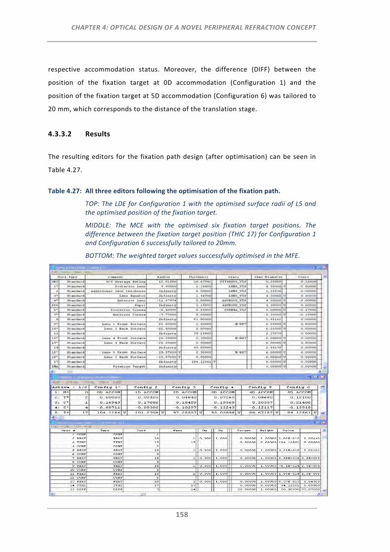
CHAPTER 4: OPTICAL DESIGN OF A NOVEL PERIPHERAL REFRACTION CONCEPT
158
respective accommodation status. Moreover, the difference (DIFF) between the
position of the fixation target at 0D accommodation (Configuration 1) and the
position of the fixation target at 5D accommodation (Configuration 6) was tailored to
20 mm, which corresponds to the distance of the translation stage.
4.3.3.2 Results
The resulting editors for the fixation path design (after optimisation) can be seen in
Table 4.27.
Table 4.27: All three editors following the optimisation of the fixation path.
TOP: The LDE for Configuration 1 with the optimised surface radii of L5 and the optimised position of the fixation target.
MIDDLE: The MCE with the optimised six fixation target positions. The difference between the fixation target position (THIC 17) for Configuration 1 and Configuration 6 successfully tailored to 20mm.
BOTTOM: The weighted target values successfully optimised in the MFE.
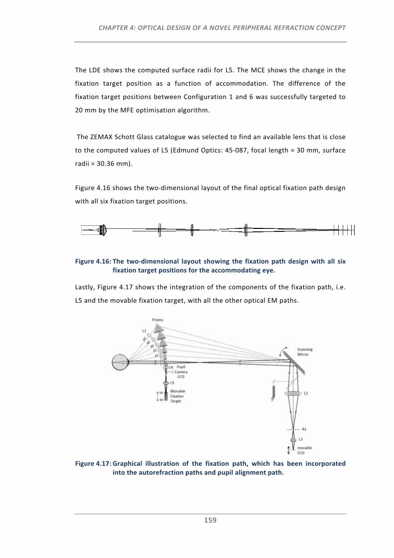
CHAPTER 4: OPTICAL DESIGN OF A NOVEL PERIPHERAL REFRACTION CONCEPT
159
The LDE shows the computed surface radii for L5. The MCE shows the change in the
fixation target position as a function of accommodation. The difference of the
fixation target positions between Configuration 1 and 6 was successfully targeted to
20 mm by the MFE optimisation algorithm.
The ZEMAX Schott Glass catalogue was selected to find an available lens that is close
to the computed values of L5 (Edmund Optics: 45‐087, focal length = 30 mm, surface
radii = 30.36 mm).
Figure 4.16 shows the two‐dimensional layout of the final optical fixation path design
with all six fixation target positions.
Figure 4.16: The two‐dimensional layout showing the fixation path design with all six fixation target positions for the accommodating eye.
Lastly, Figure 4.17 shows the integration of the components of the fixation path, i.e.
L5 and the movable fixation target, with all the other optical EM paths.
Figure 4.17: Graphical illustration of the fixation path, which has been incorporated into the autorefraction paths and pupil alignment path.
CHAPTER 4: OPTICAL DESIGN OF A NOVEL PERIPHERAL REFRACTION CONCEPT
160
4.4 Summary
On the basis of the proposed peripheral refraction concept (patent application WO
2008/116270 A1), the EM reference model eye presented in Section 4.2 was used to
design the five optical paths of the EM instrument with respect to the individual path
criteria (Section 4.3). Table 4.28 shows the summary of all key design requirements
and the respective optical components of each optical path. Moreover, Figure 4.18
provides a summary of all the paths. The prime objectives of each path were
highlighted by the corresponding chief or marginal rays.
4.5 Conclusion
The significance of measuring the peripheral optics of the eye and the current
limitations related to its measurement with commercially available refraction
instruments were addressed in the previous chapters.
The EM concept (patent application WO 2008/116270 A1) proposed in this chapter
aims to overcome peripheral refraction measurement limitations related to both, the
time‐consuming re‐alignment (off‐axis fixation) requirements by participants and the
strict requirements for precise pupil alignment by the operator. The distinctive
feature of this concept is based on a deflection system, which consists of prisms and
a scanning mirror, in order to achieve a fast refraction scan across the visual field.
The ring‐autorefraction principle was the proposed operation principle for the
determination of the eye’s sphero‐cylindrical refraction.
Based on this concept, the optical design work of the EM was developed in this
chapter. For this, a model eye was selected, first, which was used as a reference
point for the subsequent design of the 5 optical paths of the EM; the deflection
system, the illumination path, the reflection path, the pupil imaging path and the
fixation path. Due to the complexity of the optical EM design, particularly the
deflection system, the five paths were designed and assessed individually. For each
optical path, the pre‐defined optical instrument criteria were successfully achieved
with the help of the optical system design software ZEMAX.
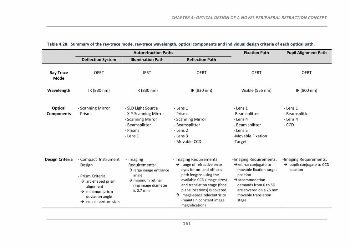
CHAPTER 4: OPTICAL DESIGN OF A NOVEL PERIPHERAL REFRACTION CONCEPT
161
Table 4.28: Summary of the ray‐trace mode, ray‐trace wavelength, optical components and individual design criteria of each optical path.
Autorefraction Paths Fixation Path Pupil Alignment Path
Deflection System Illumination Path Reflection Path
Ray Trace Mode
OERT
IERT
OERT
OERT
OERT
Wavelength IR (830 nm) IR (830 nm) IR (830 nm) Visible (555 nm) IR (800 nm)
Optical Components
‐ Scanning Mirror‐ Prisms
‐ SLD Light Source‐ X‐Y Scanning Mirror ‐ Scanning Mirror ‐ Beamsplitter ‐ Prisms ‐ Lens 1
‐ Lens 1‐ Prisms ‐ Scanning Mirror ‐ Beamsplitter ‐ Lens 2 ‐ Lens 3 ‐ Movable CCD
‐ Lens 1‐Beamsplitter ‐ Lens 4 ‐ Beam splitter ‐ Lens 5 ‐Movable Fixation Target
‐ Lens 1‐ Beamsplitter ‐ Lens 4 ‐ CCD
Design Criteria ‐ Compact Instrument Design
‐ Prism Criteria: arc‐shaped prism
alignment minimum prism
deviation angle equal aperture sizes
‐ Imaging Requirements: large image entrance
angle minimum retinal
ring image diameter is 0.7 mm
‐ Imaging Requirements: range of refractive error
eyes for on‐ and off‐axis path lengths using the available CCD (image sizes) and translation stage (focal plane locations) is covered
image‐space telecentricity (maintain constant image magnification)
‐Imaging Requirements: retina: conjugate to movable fixation target position accommodation demands from 0 to 5D are covered on a 25 mm movable translation stage
‐Imaging Requirements: pupil: conjugate to CCD
location
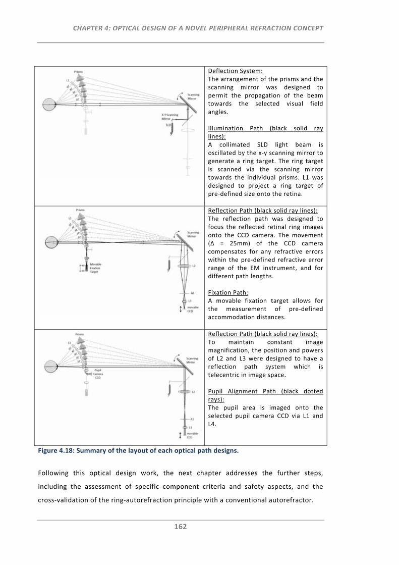
CHAPTER 4: OPTICAL DESIGN OF A NOVEL PERIPHERAL REFRACTION CONCEPT
162
Deflection System:The arrangement of the prisms and the scanning mirror was designed to permit the propagation of the beam towards the selected visual field angles. Illumination Path (black solid ray lines): A collimated SLD light beam is oscillated by the x‐y scanning mirror to generate a ring target. The ring target is scanned via the scanning mirror towards the individual prisms. L1 was designed to project a ring target of pre‐defined size onto the retina.
Reflection Path (black solid ray lines): The reflection path was designed to focus the reflected retinal ring images onto the CCD camera. The movement (∆ = 25mm) of the CCD camera compensates for any refractive errors within the pre‐defined refractive error range of the EM instrument, and for different path lengths. Fixation Path: A movable fixation target allows for the measurement of pre‐defined accommodation distances.
Reflection Path (black solid ray lines): To maintain constant image magnification, the position and powers of L2 and L3 were designed to have a reflection path system which is telecentric in image space. Pupil Alignment Path (black dotted rays): The pupil area is imaged onto the selected pupil camera CCD via L1 and L4.
Figure 4.18: Summary of the layout of each optical path designs.
Following this optical design work, the next chapter addresses the further steps,
including the assessment of specific component criteria and safety aspects, and the
cross‐validation of the ring‐autorefraction principle with a conventional autorefractor.
CHAPTER 5: RING‐SCAN‐AUTOREFRACTION PRINCIPLE
163
CHAPTER 5:
RING‐SCAN‐AUTOREFRACTION PRINCIPLE: COMPONENT CRITERIA, SAFETY ASSESSMENT AND EXPERIMENTAL VALIDATION
5.1 Introduction
In Chapter 4 the optical design of a novel peripheral refraction concept, the EM, was
developed. For this, optical components such as prisms and lenses were selected to
achieve particular optical design goals that permit the measurement of the eye's
refraction profile across the retina, ranging from ‐50° to +50° in 10° steps.
In order to implement and test this optical design, a number of additional functions and
components are required. Moreover, issues such as optical radiation safety limits of the
ring‐ scan illumination, and the speed and precision of the image detection, require
closer examination to ensure the safe and effective operation of the EM.
Thus, the following chapter aimed to:
Evaluate and source the components required to achieve the operational goals of
the proposed EM autorefraction instrument,
Assess the safety requirements of the new illumination principle, that is, ocular
ring scanning and peripheral retinal illumination when using the selected EM
light source,
Set‐up an optical bench experiment, based on the EM’s specific illumination
feature and the critical optical components required to verify the on‐axis ring‐
autorefraction principle and
Cross‐validate the experimental ring images obtained on the optical bench with
the images computed with ZEMAX and those measured with the Shin‐ Nippon
NVision K5001 autorefractor.
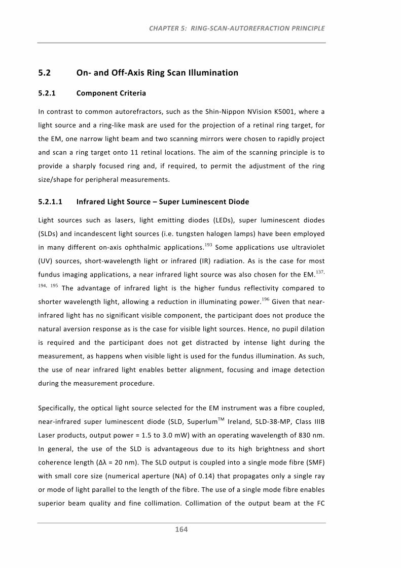
CHAPTER 5: RING‐SCAN‐AUTOREFRACTION PRINCIPLE
164
5.2 On‐ and Off‐Axis Ring Scan Illumination
5.2.1 Component Criteria
In contrast to common autorefractors, such as the Shin‐Nippon NVision K5001, where a
light source and a ring‐like mask are used for the projection of a retinal ring target, for
the EM, one narrow light beam and two scanning mirrors were chosen to rapidly project
and scan a ring target onto 11 retinal locations. The aim of the scanning principle is to
provide a sharply focused ring and, if required, to permit the adjustment of the ring
size/shape for peripheral measurements.
5.2.1.1 Infrared Light Source – Super Luminescent Diode
Light sources such as lasers, light emitting diodes (LEDs), super luminescent diodes
(SLDs) and incandescent light sources (i.e. tungsten halogen lamps) have been employed
in many different on‐axis ophthalmic applications.193 Some applications use ultraviolet
(UV) sources, short‐wavelength light or infrared (IR) radiation. As is the case for most
fundus imaging applications, a near infrared light source was also chosen for the EM.137,
194, 195 The advantage of infrared light is the higher fundus reflectivity compared to
shorter wavelength light, allowing a reduction in illuminating power.196 Given that near‐
infrared light has no significant visible component, the participant does not produce the
natural aversion response as is the case for visible light sources. Hence, no pupil dilation
is required and the participant does not get distracted by intense light during the
measurement, as happens when visible light is used for the fundus illumination. As such,
the use of near infrared light enables better alignment, focusing and image detection
during the measurement procedure.
Specifically, the optical light source selected for the EM instrument was a fibre coupled,
near‐infrared super luminescent diode (SLD, SuperlumTM Ireland, SLD‐38‐MP, Class IIIB
Laser products, output power = 1.5 to 3.0 mW) with an operating wavelength of 830 nm.
In general, the use of the SLD is advantageous due to its high brightness and short
coherence length (∆λ = 20 nm). The SLD output is coupled into a single mode fibre (SMF)
with small core size (numerical aperture (NA) of 0.14) that propagates only a single ray
or mode of light parallel to the length of the fibre. The use of a single mode fibre enables
superior beam quality and fine collimation. Collimation of the output beam at the FC
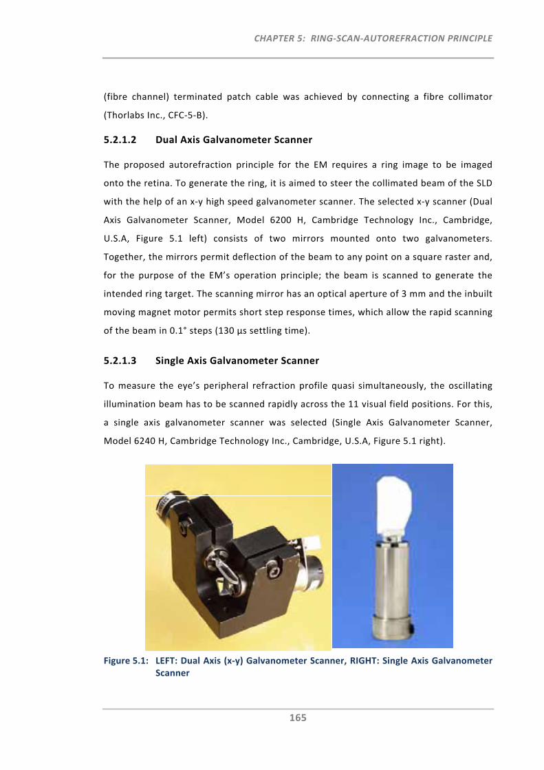
CHAPTER 5: RING‐SCAN‐AUTOREFRACTION PRINCIPLE
165
(fibre channel) terminated patch cable was achieved by connecting a fibre collimator
(Thorlabs Inc., CFC‐5‐B).
5.2.1.2 Dual Axis Galvanometer Scanner
The proposed autorefraction principle for the EM requires a ring image to be imaged
onto the retina. To generate the ring, it is aimed to steer the collimated beam of the SLD
with the help of an x‐y high speed galvanometer scanner. The selected x‐y scanner (Dual
Axis Galvanometer Scanner, Model 6200 H, Cambridge Technology Inc., Cambridge,
U.S.A, Figure 5.1 left) consists of two mirrors mounted onto two galvanometers.
Together, the mirrors permit deflection of the beam to any point on a square raster and,
for the purpose of the EM’s operation principle; the beam is scanned to generate the
intended ring target. The scanning mirror has an optical aperture of 3 mm and the inbuilt
moving magnet motor permits short step response times, which allow the rapid scanning
of the beam in 0.1° steps (130 μs settling time).
5.2.1.3 Single Axis Galvanometer Scanner
To measure the eye’s peripheral refraction profile quasi simultaneously, the oscillating
illumination beam has to be scanned rapidly across the 11 visual field positions. For this,
a single axis galvanometer scanner was selected (Single Axis Galvanometer Scanner,
Model 6240 H, Cambridge Technology Inc., Cambridge, U.S.A, Figure 5.1 right).
Figure 5.1: LEFT: Dual Axis (x‐y) Galvanometer Scanner, RIGHT: Single Axis Galvanometer Scanner
CHAPTER 5: RING‐SCAN‐AUTOREFRACTION PRINCIPLE
166
Unlike the small x‐y scanner, which is positioned closely to the SLD light source for the
oscillation of the beam, this scanner features a large (25 mm) aperture with a ±25°
excursion, to permit on‐ and off‐axis ring scanning of up to ±50°. Due to the larger size of
the mirror, settling time is slower (350 μs) but adequate to meet the EM’s peripheral
refraction scan speed requirements, i.e. to scan 11 positions in less than one second.
5.2.2 Safety Assessment
5.2.2.1 Introduction
Over the last decades, several laser safety standards have carefully been developed to
ensure safe use of lasers.197, 198 With the objective of safe use of both lasers, as well as
optical fibre communication systems utilising laser diodes and light emitting diodes
(LED), the American National Standards Institute (ANSI) standards Z136.1‐2007199 and
Z136.2‐1997200 were introduced for the protection of the human eye from hazardous
light exposures. These standards consider not only accidental ocular exposures to lasers
(i.e. medical or industrial lasers), but also intentional single or repetitive pulse
exposures, as implemented in many ophthalmic applications.201
The EM light source operates in the retinal hazard region, defined as the region including
exposure to wavelengths between 400 and 1400 nm.199 It is therefore critical to consider
the risk of thermal retinal damage that may result following prolonged light exposure
due to resulting protein denaturation of the retinal pigment epithelium.202 However, it
should be noted that near‐infrared light is absorbed much less by the retinal pigment203
than visible wavelengths and thus, the ocular damage threshold is much higher.195
Although the ANSI standards are the most current standards available for the EM light
source application, no consideration is taken with respect to peripheral or ocular
scanning exposures as proposed for the EM instrument. Therefore, the safety standards
of this specific EM light source application were assessed as recommended by de Wit204
and Delori et al.205 For this, the complex scanning system was broken down into a variety
of simulated sub‐exposures, which were assessed on the basis of the ANSI single and
repetitive pulse rules as well as the analysis on ocular scanning by Delori et al.205
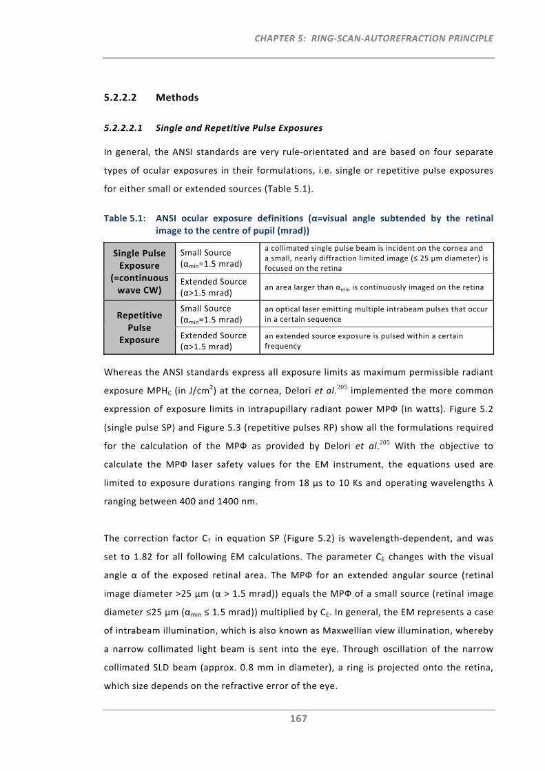
CHAPTER 5: RING‐SCAN‐AUTOREFRACTION PRINCIPLE
167
5.2.2.2 Methods
5.2.2.2.1 Single and Repetitive Pulse Exposures
In general, the ANSI standards are very rule‐orientated and are based on four separate
types of ocular exposures in their formulations, i.e. single or repetitive pulse exposures
for either small or extended sources (Table 5.1).
Table 5.1: ANSI ocular exposure definitions (α=visual angle subtended by the retinal image to the centre of pupil (mrad))
Single Pulse Exposure
(=continuous wave CW)
Small Source (αmin=1.5 mrad)
a collimated single pulse beam is incident on the cornea and a small, nearly diffraction limited image (≤ 25 μm diameter) is focused on the retina
Extended Source (α>1.5 mrad)
an area larger than αmin is continuously imaged on the retina
Repetitive Pulse
Exposure
Small Source (αmin=1.5 mrad)
an optical laser emitting multiple intrabeam pulses that occur in a certain sequence
Extended Source (α>1.5 mrad)
an extended source exposure is pulsed within a certain frequency
Whereas the ANSI standards express all exposure limits as maximum permissible radiant
exposure MPHC (in J/cm2) at the cornea, Delori et al.205 implemented the more common
expression of exposure limits in intrapupillary radiant power MPФ (in watts). Figure 5.2
(single pulse SP) and Figure 5.3 (repetitive pulses RP) show all the formulations required
for the calculation of the MPФ as provided by Delori et al.205 With the objective to
calculate the MPФ laser safety values for the EM instrument, the equations used are
limited to exposure durations ranging from 18 μs to 10 Ks and operating wavelengths λ
ranging between 400 and 1400 nm.
The correction factor CT in equation SP (Figure 5.2) is wavelength‐dependent, and was
set to 1.82 for all following EM calculations. The parameter CE changes with the visual
angle α of the exposed retinal area. The MPФ for an extended angular source (retinal
image diameter >25 μm (α > 1.5 mrad)) equals the MPФ of a small source (retinal image
diameter ≤25 μm (αmin ≤ 1.5 mrad)) multiplied by CE. In general, the EM represents a case
of intrabeam illumination, which is also known as Maxwellian view illumination, whereby
a narrow collimated light beam is sent into the eye. Through oscillation of the narrow
collimated SLD beam (approx. 0.8 mm in diameter), a ring is projected onto the retina,
which size depends on the refractive error of the eye.
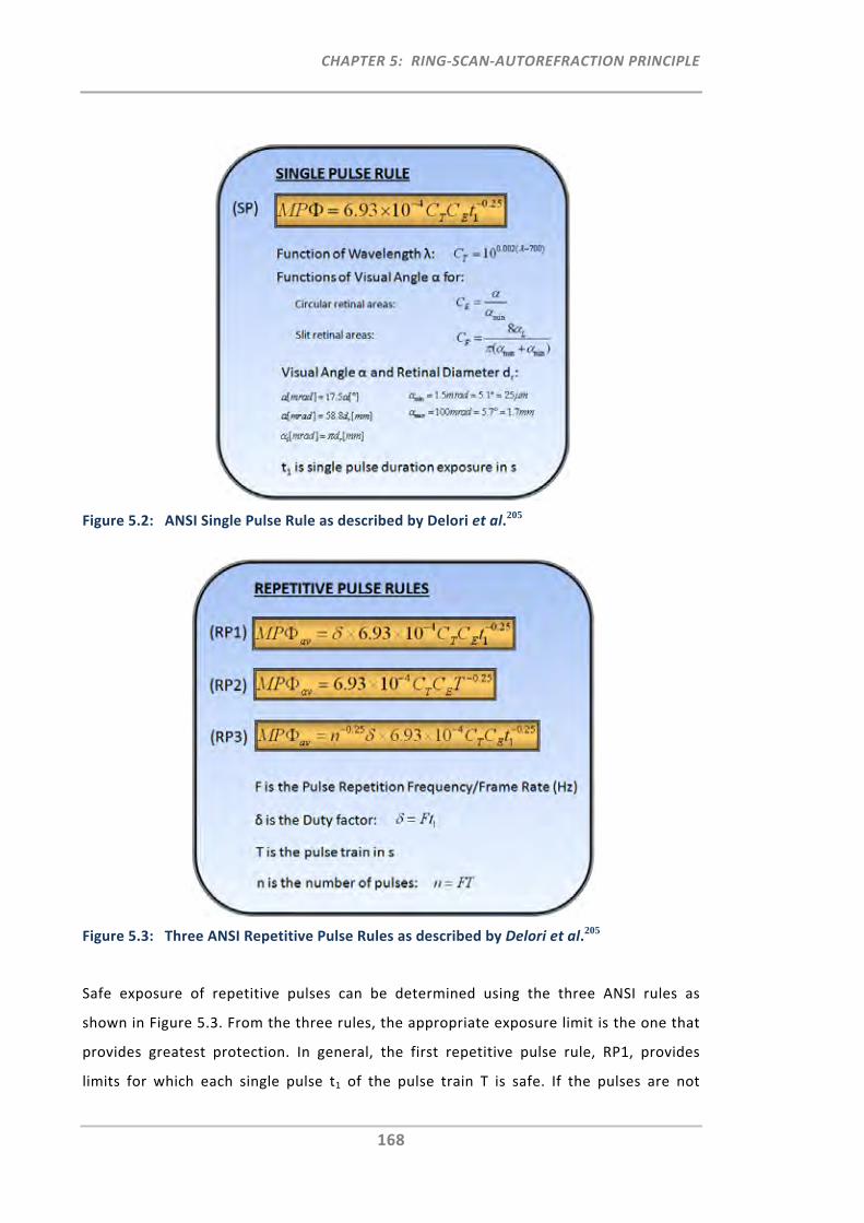
CHAPTER 5: RING‐SCAN‐AUTOREFRACTION PRINCIPLE
168
Figure 5.2: ANSI Single Pulse Rule as described by Delori et al.205
Figure 5.3: Three ANSI Repetitive Pulse Rules as described by Delori et al.205
Safe exposure of repetitive pulses can be determined using the three ANSI rules as
shown in Figure 5.3. From the three rules, the appropriate exposure limit is the one that
provides greatest protection. In general, the first repetitive pulse rule, RP1, provides
limits for which each single pulse t1 of the pulse train T is safe. If the pulses are not
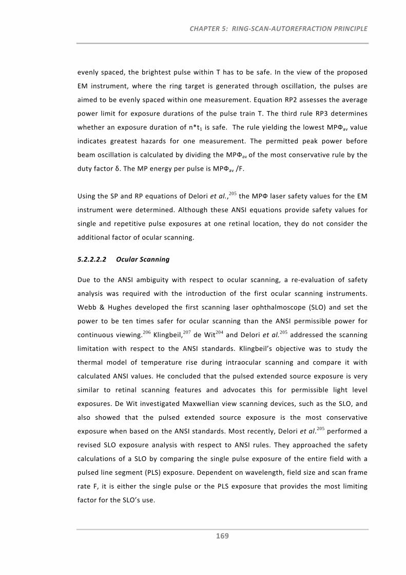
CHAPTER 5: RING‐SCAN‐AUTOREFRACTION PRINCIPLE
169
evenly spaced, the brightest pulse within T has to be safe. In the view of the proposed
EM instrument, where the ring target is generated through oscillation, the pulses are
aimed to be evenly spaced within one measurement. Equation RP2 assesses the average
power limit for exposure durations of the pulse train T. The third rule RP3 determines
whether an exposure duration of n*t1 is safe. The rule yielding the lowest MPФav value
indicates greatest hazards for one measurement. The permitted peak power before
beam oscillation is calculated by dividing the MPФav of the most conservative rule by the
duty factor δ. The MP energy per pulse is MPФav /F.
Using the SP and RP equations of Delori et al.,205 the MPФ laser safety values for the EM
instrument were determined. Although these ANSI equations provide safety values for
single and repetitive pulse exposures at one retinal location, they do not consider the
additional factor of ocular scanning.
5.2.2.2.2 Ocular Scanning
Due to the ANSI ambiguity with respect to ocular scanning, a re‐evaluation of safety
analysis was required with the introduction of the first ocular scanning instruments.
Webb & Hughes developed the first scanning laser ophthalmoscope (SLO) and set the
power to be ten times safer for ocular scanning than the ANSI permissible power for
continuous viewing.206 Klingbeil,207 de Wit204 and Delori et al.205 addressed the scanning
limitation with respect to the ANSI standards. Klingbeil’s objective was to study the
thermal model of temperature rise during intraocular scanning and compare it with
calculated ANSI values. He concluded that the pulsed extended source exposure is very
similar to retinal scanning features and advocates this for permissible light level
exposures. De Wit investigated Maxwellian view scanning devices, such as the SLO, and
also showed that the pulsed extended source exposure is the most conservative
exposure when based on the ANSI standards. Most recently, Delori et al.205 performed a
revised SLO exposure analysis with respect to ANSI rules. They approached the safety
calculations of a SLO by comparing the single pulse exposure of the entire field with a
pulsed line segment (PLS) exposure. Dependent on wavelength, field size and scan frame
rate F, it is either the single pulse or the PLS exposure that provides the most limiting
factor for the SLO’s use.
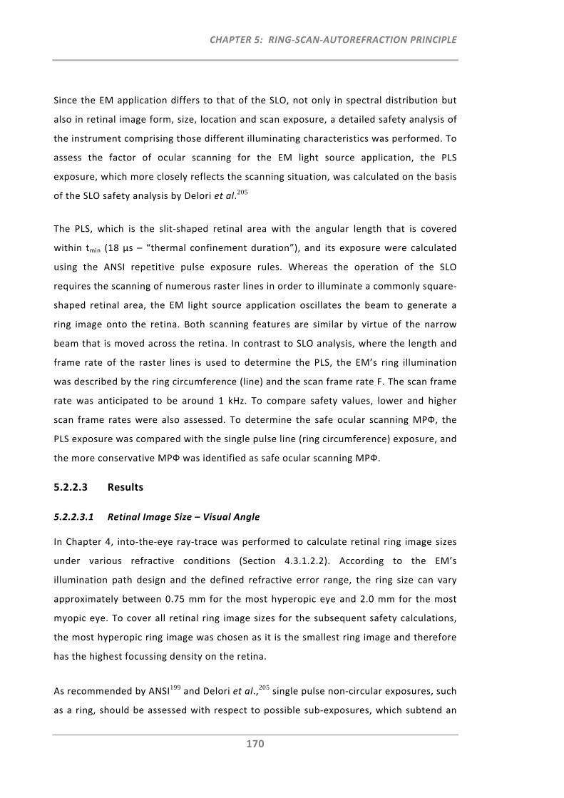
CHAPTER 5: RING‐SCAN‐AUTOREFRACTION PRINCIPLE
170
Since the EM application differs to that of the SLO, not only in spectral distribution but
also in retinal image form, size, location and scan exposure, a detailed safety analysis of
the instrument comprising those different illuminating characteristics was performed. To
assess the factor of ocular scanning for the EM light source application, the PLS
exposure, which more closely reflects the scanning situation, was calculated on the basis
of the SLO safety analysis by Delori et al.205
The PLS, which is the slit‐shaped retinal area with the angular length that is covered
within tmin (18 μs – “thermal confinement duration”), and its exposure were calculated
using the ANSI repetitive pulse exposure rules. Whereas the operation of the SLO
requires the scanning of numerous raster lines in order to illuminate a commonly square‐
shaped retinal area, the EM light source application oscillates the beam to generate a
ring image onto the retina. Both scanning features are similar by virtue of the narrow
beam that is moved across the retina. In contrast to SLO analysis, where the length and
frame rate of the raster lines is used to determine the PLS, the EM’s ring illumination
was described by the ring circumference (line) and the scan frame rate F. The scan frame
rate was anticipated to be around 1 kHz. To compare safety values, lower and higher
scan frame rates were also assessed. To determine the safe ocular scanning MPФ, the
PLS exposure was compared with the single pulse line (ring circumference) exposure, and
the more conservative MPФ was identified as safe ocular scanning MPФ.
5.2.2.3 Results
5.2.2.3.1 Retinal Image Size – Visual Angle
In Chapter 4, into‐the‐eye ray‐trace was performed to calculate retinal ring image sizes
under various refractive conditions (Section 4.3.1.2.2). According to the EM’s
illumination path design and the defined refractive error range, the ring size can vary
approximately between 0.75 mm for the most hyperopic eye and 2.0 mm for the most
myopic eye. To cover all retinal ring image sizes for the subsequent safety calculations,
the most hyperopic ring image was chosen as it is the smallest ring image and therefore
has the highest focussing density on the retina.
As recommended by ANSI199 and Delori et al.,205 single pulse non‐circular exposures, such
as a ring, should be assessed with respect to possible sub‐exposures, which subtend an
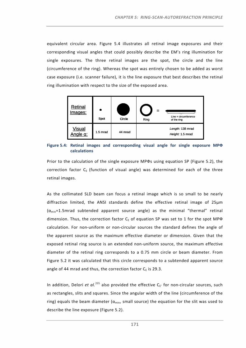
CHAPTER 5: RING‐SCAN‐AUTOREFRACTION PRINCIPLE
171
equivalent circular area. Figure 5.4 illustrates all retinal image exposures and their
corresponding visual angles that could possibly describe the EM’s ring illumination for
single exposures. The three retinal images are the spot, the circle and the line
(circumference of the ring). Whereas the spot was entirely chosen to be added as worst
case exposure (i.e. scanner failure), it is the line exposure that best describes the retinal
ring illumination with respect to the size of the exposed area.
Figure 5.4: Retinal images and corresponding visual angle for single exposure MPФ calculations
Prior to the calculation of the single exposure MPФs using equation SP (Figure 5.2), the
correction factor CE (function of visual angle) was determined for each of the three
retinal images.
As the collimated SLD beam can focus a retinal image which is so small to be nearly
diffraction limited, the ANSI standards define the effective retinal image of 25μm
(αmin=1.5mrad subtended apparent source angle) as the minimal “thermal” retinal
dimension. Thus, the correction factor CE of equation SP was set to 1 for the spot MPФ
calculation. For non‐uniform or non‐circular sources the standard defines the angle of
the apparent source as the maximum effective diameter or dimension. Given that the
exposed retinal ring source is an extended non‐uniform source, the maximum effective
diameter of the retinal ring corresponds to a 0.75 mm circle or beam diameter. From
Figure 5.2 it was calculated that this circle corresponds to a subtended apparent source
angle of 44 mrad and thus, the correction factor CE is 29.3.
In addition, Delori et al.205 also provided the effective CE’ for non‐circular sources, such
as rectangles, slits and squares. Since the angular width of the line (circumference of the
ring) equals the beam diameter (αmin, small source) the equation for the slit was used to
describe the line exposure (Figure 5.2).
Retinal Images:
Visual Angle α:
1.5 mrad 44 mradLength: 138 mrad
Height: 1.5 mrad
Spot Circle Ring
=Line = circumference of the ring
Retinal Images:
Visual Angle α:
1.5 mrad 44 mradLength: 138 mrad
Height: 1.5 mrad
SpotSpot CircleCircle Ring
=Line = circumference of the ring
CHAPTER 5: RING‐SCAN‐AUTOREFRACTION PRINCIPLE
172
To account also for the factor of ocular scanning, the definition from Delori et al.’s205
pulsed line segment (PLS, Figure 5.5) exposure was used. For this, the correction factor
CE’ was determined using the same equation as for the line exposure. The length of the
pulse segment now varies as a function of scan frame rate F.
Figure 5.5: Pulsed Line Segment (PLS) definition
Table 5.2 (top) provides an overview of all four exposures and their retinal image shape
characteristics and the respective formulations, which were used to calculate the visual
angle dependent correction factor CE.
5.2.2.3.2 Maximum Permissible Exposure as a Function of Exposure Duration
Using the correction factor CE or CE’, the MPФ was calculated for all four sub‐exposures,
i.e. spot, circle, line, and PLS. Table 5.2 provides the detailed MPФ calculations for an
exposure duration of 0.05 seconds. This is the approximate intended scan duration to
illuminate each of the 11 retinal locations during the EM peripheral refraction scan. In
addition, Figure 5.6 provides the MPФ as a function of exposure duration for each of the
four retinal image exposures.
Overall, the MPФ analysis showed that the spot exposure was the most limiting sub‐
exposure and the circle exposure was the least restricted. However, with respect to the
exposed area, it is the line and the PLS exposure that come closest to the real retinal ring
scan illumination. When comparing repetitive PLS exposures for different frame rates,
RP3 always provided the most conservative MPФ value out of the three repetitive pulse
exposure rules. When comparing the MPФ values for the single pulse line exposure with
the PLS exposure (RP3 rule), the latter was the limiting factor only if the frame rate was
very high (Table 5.2 and Figure 5.6). For slower frame rates, it was the single pulse line
exposure that provided the more conservative exposure limit. Dependent on the EM’s
final scan frame rate for the ring scan illumination, Figure 5.6 provides an overview and
comparison of the MPФ for all four sub‐exposures as a function of exposure duration.
Ring
=
PLS (Pulsed Line Segment -depends on Frame Frequency F)
Line = circumference of the ring
PLS
tmin=18μs
RingRing
=
PLS (Pulsed Line Segment -depends on Frame Frequency F)
Line = circumference of the ring
PLS (Pulsed Line Segment -depends on Frame Frequency F)
Line = circumference of the ring
PLS
tmin=18μs
PLS
tmin=18μs

CHAPTER 5: RING‐SCAN‐AUTOREFRACTION PRINCIPLE
173
Table 5.2: MPФ calculation for all single pulse simulations (spot, circle and line) as well as PLS exposure when the measurement of one of the 11 retinal positions takes 0.05 seconds.
*For the application of the exposure rules see equations of Figure 5.2 and Figure 5.3.
Frame Rate -
Fframe
Length Width
= Circumference
= π* Retinal Image Diameter
αmin αC αL αW=αmin
1.5 mrad 44 mrad 138 mrad 1.5 mrad0.1° 2.52° 7.91° 0.1°
0.025 0.75 2.35 0.025
Circle Circle
CE
Formula- α/αmin
CE 1 29.33
Single Pulse (SP)
Single Pulse (SP)
Repetitive Rule 1 (RP1)
Repetitive Rule 2 (RP2)
Repetitive Rule 3 (RP3)
Repetitive Rule 1 (RP1)
Repetitive Rule 2 (RP2)
Repetitive Rule 3 (RP3)
Repetitive Rule 1 (RP1)
Repetitive Rule 2 (RP2)
Repetitive Rule 3 (RP3)
t1 (sec) - Single
pulse durationT (sec) - Pulse train duration
tline (sec)
Number of lines in PLS
2.67 78.19 24.64 942 13.86 38.05 144.85 11.97 47.83 18.3 8.51
5.0×10⁻⁵
2
1.8×10⁻⁵
0.05
5.0×10⁻⁴
2
>tmin
Ring = LineLine Scan
Duration (sec)5.0×10⁻³ 5.0×10⁻⁴ 5.0×10⁻⁵
10000 Hz100 Hz 1000 Hz
Length Width
1.5 mrad
Length Width
1/(Frame Rate*Number of lines in PLS)
5 mrad
Length
Slit
CE
=Frame Rate *T*number of segment lines
1000
αW=αmin
1.5 mrad
= Beam Diameter = Beam Diameter = Beam Diameter =t min*a/t line
t line=1/(2*F frame)Retinal Image Characteristics
Pulsed Line Segment = PLS
1/(Frame Rate*Number of lines in PLS) 1/(Frame Rate*Number of lines in PLS)
αPLS
49.7 mrad
= Retinal Image
Diameter
1.8×10⁻⁵
0.05
Retinal Image
Source Shape
Visual Angle α
Spot Circle
= Beam Diameter
ANSI Rules
Exposure Rules*
2.85°0.1°0.1°0.1° 0.29°
0.025 0.025
1.27
Exposure Duration t (sec)
MPbeam (mW)
2.47
Number of pulses
0.05 0.05
100=Frame Rate *T*number of
segment lines
(8*αPLS)/(π*(a max+a min)
=t min*a/t line
t line=1/(2*F frame)
αPLS
1.5 mrad
αW=αmin
Slit
=(8*αPLS)/(π*(a max +a min)
Slit
=(8*αPLS)/(π*(a max +a min)
0.1°
0.085 0.025 0.845 0.025
1.5 mrad
αPLS αW=αmin
Single Pulse (SP)
0.05
Slit
(8*α L)/(π*(a max+a min)
3.46
Width
=t min*a/t line
t line=1/(2*F frame)
1.97
= Beam Diameter
9.23
=Frame Rate *T*number of segment lines
10
1.8×10⁻⁵
0.05
5.0×10⁻³
2
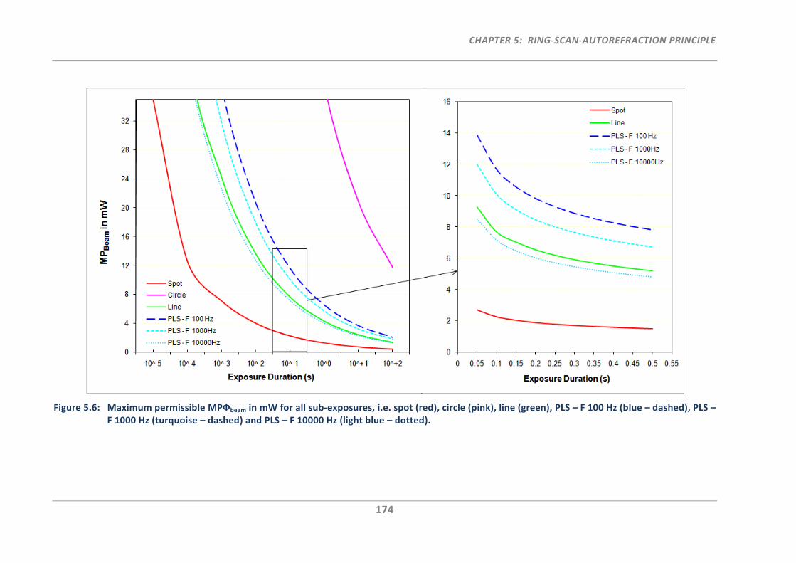
CHAPTER 5: RING‐SCAN‐AUTOREFRACTION PRINCIPLE
174
Figure 5.6: Maximum permissible MPФbeam in mW for all sub‐exposures, i.e. spot (red), circle (pink), line (green), PLS – F 100 Hz (blue – dashed), PLS – F 1000 Hz (turquoise – dashed) and PLS – F 10000 Hz (light blue – dotted).
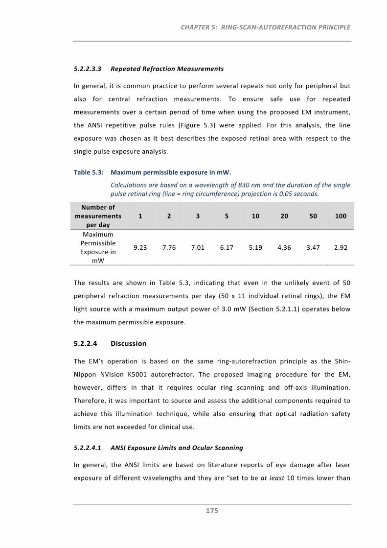
CHAPTER 5: RING‐SCAN‐AUTOREFRACTION PRINCIPLE
175
5.2.2.3.3 Repeated Refraction Measurements
In general, it is common practice to perform several repeats not only for peripheral but
also for central refraction measurements. To ensure safe use for repeated
measurements over a certain period of time when using the proposed EM instrument,
the ANSI repetitive pulse rules (Figure 5.3) were applied. For this analysis, the line
exposure was chosen as it best describes the exposed retinal area with respect to the
single pulse exposure analysis.
Table 5.3: Maximum permissible exposure in mW.
Calculations are based on a wavelength of 830 nm and the duration of the single pulse retinal ring (line = ring circumference) projection is 0.05 seconds.
Number of measurements
per day 1 2 3 5 10 20 50 100
Maximum Permissible Exposure in
mW
9.23 7.76 7.01 6.17 5.19 4.36 3.47 2.92
The results are shown in Table 5.3, indicating that even in the unlikely event of 50
peripheral refraction measurements per day (50 x 11 individual retinal rings), the EM
light source with a maximum output power of 3.0 mW (Section 5.2.1.1) operates below
the maximum permissible exposure.
5.2.2.4 Discussion
The EM’s operation is based on the same ring‐autorefraction principle as the Shin‐
Nippon NVision K5001 autorefractor. The proposed imaging procedure for the EM,
however, differs in that it requires ocular ring scanning and off‐axis illumination.
Therefore, it was important to source and assess the additional components required to
achieve this illumination technique, while also ensuring that optical radiation safety
limits are not exceeded for clinical use.
5.2.2.4.1 ANSI Exposure Limits and Ocular Scanning
In general, the ANSI limits are based on literature reports of eye damage after laser
exposure of different wavelengths and they are “set to be at least 10 times lower than
CHAPTER 5: RING‐SCAN‐AUTOREFRACTION PRINCIPLE
176
the damage threshold, expressed as a 50% probability of a minimum visible lesion”.205
These standards cover either single or repetitive pulse source exposures to the eye, but
they do not consider the specific cases of ocular scanning or off‐axis illumination, as
proposed for the EM instrument. During the ring scanning process, the small spot images
are partially overlapping on the retina and the temperature gradient changes during the
movement within two neighbouring points. With respect to this special ocular ring scan
illumination, a thorough analysis was conducted to assess all possible exposures that
cover this new illumination feature.
Firstly, single pulse exposures were assessed using the ANSI standards and the definition
of Delori et al. on non‐circular exposed retinal areas, which are defined by a visual angle
subtending an equivalent circular area. On the basis of the EM’s ring illumination, the
visual angles for the circle and the line exposure (ring circumference) as well as the spot
exposure (worst case scenario) were therefore assessed with respect to single pulse
exposure. For the same exposure duration of 0.05 s, it was the spot exposure which
proved the most hazardous (MPФ is 2.67 mW), followed by the line exposure (MPФ is
9.23 mW) and lastly, the circle exposure (MPФ is 78.19 mW). To compare similar single
pulse exposures to that of the EM light source application, one example for threshold
determination after a near‐infrared Maxwellian‐view exposure is given by the study by
Roach et al.,208 who compared the effects of 10 s near‐infrared laser irradiation (860 nm,
60 μm retinal spot) on four primate eyes with an implemented standard thermodynamic
model. Experimentally, they performed threshold measurements for the occurrence of
minimum visible lesions on primate retinas, by varying power levels and number of
exposures. They found the minimum visible lesion threshold power to be 27.0 mW after
one hour post‐exposure assessment, which is in very good agreement with their thermal
model damage threshold calculation of 24.12 mW. Their threshold results are 12 times
greater than the MPФ obtained by ANSI exposure limits.
Safety for ocular scanning first became relevant with the introduction of the first SLOs.
Due to the limitations of safety standards in terms of scanned light exposure, Klingbeil207
performed an extensive analysis on retinal temperature rise during intra‐ocular scanning
using a theoretical thermal model in order to find a safe measure. Specifically, he aimed
CHAPTER 5: RING‐SCAN‐AUTOREFRACTION PRINCIPLE
177
to predict more accurate light‐level limits for intrabeam ophthalmic scanning devices
(i.e. SLO) by comparing several ANSI retinal exposure limits to predicted retinal
temperature increase. He found best similarity when comparing thermal effects of
retinal scanning with extended pulsed source illumination. He also concluded that the
calculated ANSI power levels for SLOs at that time were 100‐5000 times less hazardous
than his recommendations based on his theoretical model. De Wit204 also described
safety norms for a laser scanning Maxwellian view system with respect to the SLO
device. By comparing pulsed intrabeam exposure with pulsed extended source exposure,
he also concluded that the latter illumination provided the greatest degree of protection
for SLOs.
The most recent approach on safety assessment for ocular scanning was done by Delori
et al.,205 who suggested a different method to the one used by De Wit204 and Klingbeil.207
Instead of assessing the pulsed extended source exposure with respect to ocular
scanning, Delori et al.205 used the PLS exposure and compared it to the subtended area
single pulse exposure. For their SLO analysis they assessed the MPФ with respect to the
SLO’s operating wavelength range 400‐800 nm and concluded that although a single
pulse exposure over the entire field is the most conservative model for small fields at
short‐wavelengths, for larger wavelengths greater than 700 nm the PLS exposure is to be
selected as safest. The analysis presented here of the EM’s ocular ring scan illumination
showed that when comparing the line and PLS MPФs in Figure 5.6, the PLS calculation
provides the more restrictive exposure when the ring is scanned at a very fast scan frame
rate. For slower scanning the single pulse line exposure provides the more conservative
MPФ.
5.2.2.4.2 Illumination of Peripheral Retinal Locations
The ANSI standards are not only deficient with respect to ocular scanning but also with
respect to the assessment of peripheral retinal imaging as aimed with the proposed EM.
The only ANSI statement made with respect to off‐axis illumination is that “combinations
of sources whose centres are separated by an angle greater than αmax (100 mrad) are
considered as independent”. According to that, the minimum distance where each
retinal spot can be considered as an individual exposure is 1.70 mm (visual angle αmax =
CHAPTER 5: RING‐SCAN‐AUTOREFRACTION PRINCIPLE
178
100 mrad). Using a ray‐tracing approach, the distance between the ring centres of each
of the adjacent illuminated retinal locations was calculated to be approximately 2.9 mm.
Having, no specific off‐axis illumination standards available, studies on the peripheral
retina may provide greater clarification on the impact of exposures on different retinal
locations. As mentioned earlier, thermal retinal damage occurs at threshold levels due to
strong light absorption by melanin of the retinal pigment epithelium.196, 202, 205 Although
attempts were made to measure melanin concentration as a function of retina location,
different results were reported, making a prediction of off‐axis light absorption
inconclusive.196, 209, 210 Polhamus et al.211 developed a model to estimate laser‐induced
threshold damage in the peripheral retina. Their predictions show that with increasing
distance from the macula into the periphery, the threshold for retinal injury rises.
Variation in fundus reflectance with retinal location is of particular interest when the
reflected light requires it to be detected efficiently, for example, for refraction purposes.
Delori and Pflibsen196 compared fundus reflectance on three different retina locations
within a wavelength range of 445 ‐ 805 nm. They showed that fundus reflectance is
affected by the degree of pigment distribution in relation to the retina location
measured. They found that the longer the wavelength and the further into the periphery
it extended, the higher the fundus reflectance.
A review by Berenschot et al.212 lists several studies and modelling investigations into
central and peripheral fundus reflectance. These studies considered not only reflectance
with respect to pigment distribution but investigated the different layers describing the
fundus. One concise fundus reflection model by van de Kraatz et al.213 incorporates the
impact of the Stiles‐Crawford Effect, by including a retinal angle parameter that
describes the directionality of the photoreceptors. This model provides an understanding
of the degree of captured light and the degree of receptor disc reflectance. For the EM,
this may be of relevance considering that the illumination beam for on‐axis
measurements is perpendicular to the retina, but for off‐axis measurements, the
incidence of the illumination beam is oblique on the retina. This impact of oblique light
reflection on the off‐axis fundus was modelled and experimentally determined in a study
CHAPTER 5: RING‐SCAN‐AUTOREFRACTION PRINCIPLE
179
by Bedell and Enoch.214 They investigated the directionality of the retina for central and
eccentric retina locations up to 35° and found that independent of retinal location, all
photoreceptors on the retina align approximately with the centre of the pupil of the eye.
As such, the Stiles‐Crawford Effect exhibits no impediment to the EM application with
respect to amount of fundus reflectance needed.
In summary, with respect to the illumination of peripheral retinal locations as proposed
for the EM instrument, it can be concluded that under consideration of the statement
made within ANSI standards, the retinal damage thresholds found across the retina and
the increased fundus reflectance in the periphery, the above calculation for the ring scan
illumination will provide exposure limits that safely cover both, on‐ as well as off‐axis
ring scan exposures.
5.2.2.4.3 Scanner Safety
In the current safety analysis, a single spot or beam exposure was included. This worst
case scenario can only occur if the scanner were to fail in a position where light is still
directed towards the eye. However, the selected galvanometer scanners are equipped
with the intrinsic safety feature to steer the beam away from the eye as soon as there is
a system shutdown or malfunction and thereby preventing accidental exposure to a non‐
scanned beam. In addition, to the scanners’ in‐built safety features, the ANSI standards
recommend that any “Class 3B laser or laser system should be provided with a
permanently attached beam stop or attenuator.” Hence, a spring loaded mechanical
shutter has been selected to normally block the light beam. A solenoid pulls the shutter
open briefly while the refraction scan can be performed.
5.3 Component Criteria for Image Detection
In addition to the safety and design considerations for the illumination path, the
reflection path also required special optical configuration and component selection,
primarily with respect to minimising interfering reflections and permitting the rapid and
precise capture of the reflected ring images.
CHAPTER 5: RING‐SCAN‐AUTOREFRACTION PRINCIPLE
180
5.3.1 Reduction of Interfering Reflections
Reflections that occur from optical surfaces such as the optical EM components, i.e.
lenses, mirrors and prisms, or the anterior ocular surfaces are disadvantageous, as they
can adversely affect the detection and thus, analysis of the captured retinal ring images.
Possible provisions to overcome the obstacles of unwanted reflections when detecting
EM retinal images have been considered as follows.
Coatings on ocular surfaces control light reflection and transmission through the
mechanisms of optical interference. Particularly, wavelength‐specific anti‐reflection
coatings can reduce reflections to less than 1% on optical surfaces and thus, are widely
used in many optical applications and instruments. Nevertheless, for the EM purposes,
elimination of reflections on optical surfaces alone is not sufficient, as unwanted ocular
reflections from cornea and the crystalline lens surfaces remain.
Figure 5.7 illustrates how the use of linear polarisers and beam splitters can be used to
reduce reflections from the cornea and crystalline lens surfaces and permit detection of
reflections from the retina. Firstly, the non‐polarised beam of the light source (SLD) is
linearly polarised in order to generate s‐polarised light. This light propagates to the
polarising cube beam splitter, which is the optical component that separates the
illumination from the reflection paths. Its polarising properties permit the reflection of
the s‐polarised light, which is directed towards the eye. Whereas, the crystalline lens and
the cornea are highly reflective ocular surfaces which maintain polarisation of the
reflected light, the retina acts as a highly diffuse reflector, reflecting de‐polarised light.
At the polarising beam splitter, only the p‐component of the reflected retinal image can
pass through to the detector and the s‐polarised light from the cornea and crystalline
lens is deflected. The p‐polarised light, as reflected from the retina, can be captured and
analysed.
When using polarising optics, it should be noted that although the state of polarisation
does not affect the measurement output,215 polarising filters and beam splitters result in
loss of light, which may need to be compensated.
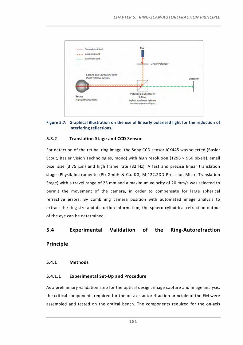
CHAPTER 5: RING‐SCAN‐AUTOREFRACTION PRINCIPLE
181
Figure 5.7: Graphical illustration on the use of linearly polarised light for the reduction of interfering reflections.
5.3.2 Translation Stage and CCD Sensor
For detection of the retinal ring image, the Sony CCD sensor ICX445 was selected (Basler
Scout, Basler Vision Technologies, mono) with high resolution (1296 × 966 pixels), small
pixel size (3.75 μm) and high frame rate (32 Hz). A fast and precise linear translation
stage (Physik Instrumente (PI) GmbH & Co. KG, M‐122.2DD Precision Micro Translation
Stage) with a travel range of 25 mm and a maximum velocity of 20 mm/s was selected to
permit the movement of the camera, in order to compensate for large spherical
refractive errors. By combining camera position with automated image analysis to
extract the ring size and distortion information, the sphero‐cylindrical refraction output
of the eye can be determined.
5.4 Experimental Validation of the Ring‐Autorefraction
Principle
5.4.1 Methods
5.4.1.1 Experimental Set‐Up and Procedure
As a preliminary validation step for the optical design, image capture and image analysis,
the critical components required for the on‐axis autorefraction principle of the EM were
assembled and tested on the optical bench. The components required for the on‐axis
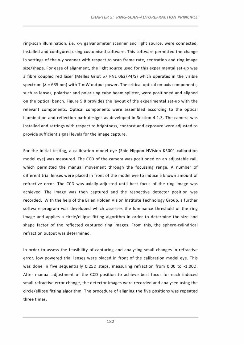
CHAPTER 5: RING‐SCAN‐AUTOREFRACTION PRINCIPLE
182
ring‐scan illumination, i.e. x‐y galvanometer scanner and light source, were connected,
installed and configured using customised software. This software permitted the change
in settings of the x‐y scanner with respect to scan frame rate, centration and ring image
size/shape. For ease of alignment, the light source used for this experimental set‐up was
a fibre coupled red laser (Melles Griot 57 PNL 062/P4/S) which operates in the visible
spectrum (λ = 635 nm) with 7 mW output power. The critical optical on‐axis components,
such as lenses, polariser and polarising cube beam splitter, were positioned and aligned
on the optical bench. Figure 5.8 provides the layout of the experimental set‐up with the
relevant components. Optical components were assembled according to the optical
illumination and reflection path designs as developed in Section 4.1.3. The camera was
installed and settings with respect to brightness, contrast and exposure were adjusted to
provide sufficient signal levels for the image capture.
For the initial testing, a calibration model eye (Shin‐Nippon NVision K5001 calibration
model eye) was measured. The CCD of the camera was positioned on an adjustable rail,
which permitted the manual movement through the focussing range. A number of
different trial lenses were placed in front of the model eye to induce a known amount of
refractive error. The CCD was axially adjusted until best focus of the ring image was
achieved. The image was then captured and the respective detector position was
recorded. With the help of the Brien Holden Vision Institute Technology Group, a further
software program was developed which assesses the luminance threshold of the ring
image and applies a circle/ellipse fitting algorithm in order to determine the size and
shape factor of the reflected captured ring images. From this, the sphero‐cylindrical
refraction output was determined.
In order to assess the feasibility of capturing and analysing small changes in refractive
error, low powered trial lenses were placed in front of the calibration model eye. This
was done in five sequentially 0.25D steps, measuring refraction from 0.00 to ‐1.00D.
After manual adjustment of the CCD position to achieve best focus for each induced
small refractive error change, the detector images were recorded and analysed using the
circle/ellipse fitting algorithm. The procedure of aligning the five positions was repeated
three times.
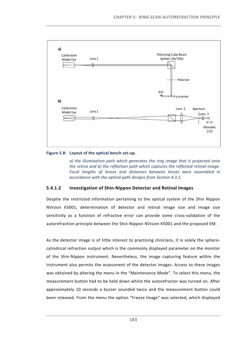
CHAPTER 5: RING‐SCAN‐AUTOREFRACTION PRINCIPLE
183
Figure 5.8: Layout of the optical bench set‐up.
a) the illumination path which generates the ring image that is projected onto the retina and b) the reflection path which captures the reflected retinal image. Focal lengths of lenses and distances between lenses were assembled in accordance with the optical path designs from Section 4.3.1.
5.4.1.2 Investigation of Shin‐Nippon Detector and Retinal Images
Despite the restricted information pertaining to the optical system of the Shin Nippon
NVision K5001, determination of detector and retinal image size and image size
sensitivity as a function of refractive error can provide some cross‐validation of the
autorefraction principle between the Shin‐Nippon NVision K5001 and the proposed EM.
As the detector image is of little interest to practising clinicians, it is solely the sphero‐
cylindrical refraction output which is the commonly displayed parameter on the monitor
of the Shin‐Nippon instrument. Nevertheless, the image capturing feature within the
instrument also permits the assessment of the detector images. Access to these images
was obtained by altering the menu in the “Maintenance Mode”. To select this menu, the
measurement button had to be held down whilst the autorefractor was turned on. After
approximately 10 seconds a buzzer sounded twice and the measurement button could
been released. From the menu the option “Freeze Image” was selected, which displayed
SLD
X‐y scanner
Polarizing Cube Beam Splitter (30/70%)
Polarizer
Lens 1Calibration Model Eye
Lens 1Calibration Model Eye
Lens 2
Lens 3
Movable CCD
a)
b)
Aperture
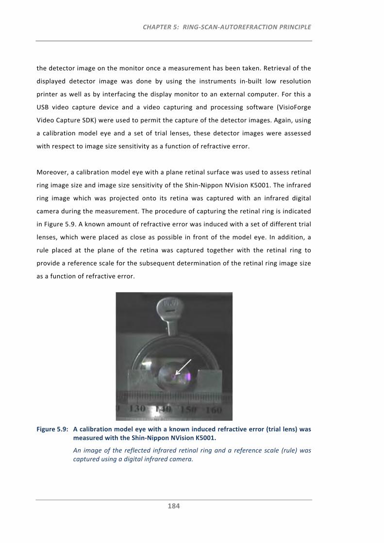
CHAPTER 5: RING‐SCAN‐AUTOREFRACTION PRINCIPLE
184
the detector image on the monitor once a measurement has been taken. Retrieval of the
displayed detector image was done by using the instruments in‐built low resolution
printer as well as by interfacing the display monitor to an external computer. For this a
USB video capture device and a video capturing and processing software (VisioForge
Video Capture SDK) were used to permit the capture of the detector images. Again, using
a calibration model eye and a set of trial lenses, these detector images were assessed
with respect to image size sensitivity as a function of refractive error.
Moreover, a calibration model eye with a plane retinal surface was used to assess retinal
ring image size and image size sensitivity of the Shin‐Nippon NVision K5001. The infrared
ring image which was projected onto its retina was captured with an infrared digital
camera during the measurement. The procedure of capturing the retinal ring is indicated
in Figure 5.9. A known amount of refractive error was induced with a set of different trial
lenses, which were placed as close as possible in front of the model eye. In addition, a
rule placed at the plane of the retina was captured together with the retinal ring to
provide a reference scale for the subsequent determination of the retinal ring image size
as a function of refractive error.
Figure 5.9: A calibration model eye with a known induced refractive error (trial lens) was measured with the Shin‐Nippon NVision K5001.
An image of the reflected infrared retinal ring and a reference scale (rule) was captured using a digital infrared camera.
CHAPTER 5: RING‐SCAN‐AUTOREFRACTION PRINCIPLE
185
5.4.2 Results
5.4.2.1 Cross‐Validation of the Autorefraction Principle with optical ZEMAX
design
Figure 5.10 illustrates the detector images as computed for a range of refractive error
eyes when using the optical design in ZEMAX as well as when the images were recorded
at the position of best focus using the optical bench experiment.
Figure 5.10 shows that the image sizes of the computed and captured images are
comparable. Moreover, it was confirmed that the approximate distance between the
most hyperopic and the most myopic focussed detector position was about 22 mm,
which is in good agreement with the computed distance of the optical reflection path
design.
Figure 5.10: Detector images for a range of refractive error eyes as computed with ZEMAX (TOP) and as captured on the optical bench set‐up (BOTTOM).
Using the circle/ellipse fitting algorithm and pixel‐by‐pixel analysis, small changes in
refractive error were assessed with respect to the captured ring images. Figure 5.11
shows the number of pixels that define the radius of the captured ring image as a
function of change in refractive error. Due to manual focus adjustment on the optical
bench rail, the standard errors for the three repeats were large; however, the mean
slope of three measurements correlated very well (Figure 5.11).
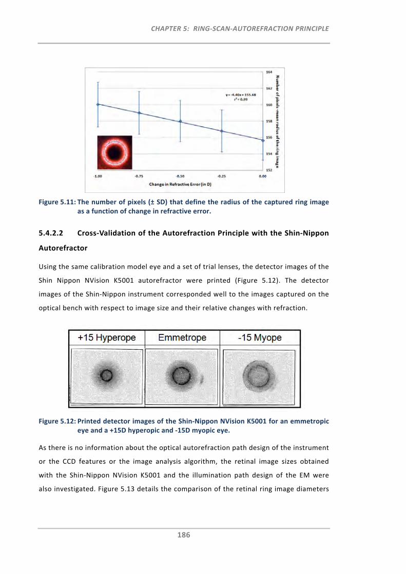
CHAPTER 5: RING‐SCAN‐AUTOREFRACTION PRINCIPLE
186
Figure 5.11: The number of pixels (± SD) that define the radius of the captured ring image as a function of change in refractive error.
5.4.2.2 Cross‐Validation of the Autorefraction Principle with the Shin‐Nippon
Autorefractor
Using the same calibration model eye and a set of trial lenses, the detector images of the
Shin Nippon NVision K5001 autorefractor were printed (Figure 5.12). The detector
images of the Shin‐Nippon instrument corresponded well to the images captured on the
optical bench with respect to image size and their relative changes with refraction.
Figure 5.12: Printed detector images of the Shin‐Nippon NVision K5001 for an emmetropic eye and a +15D hyperopic and ‐15D myopic eye.
As there is no information about the optical autorefraction path design of the instrument
or the CCD features or the image analysis algorithm, the retinal image sizes obtained
with the Shin‐Nippon NVision K5001 and the illumination path design of the EM were
also investigated. Figure 5.13 details the comparison of the retinal ring image diameters
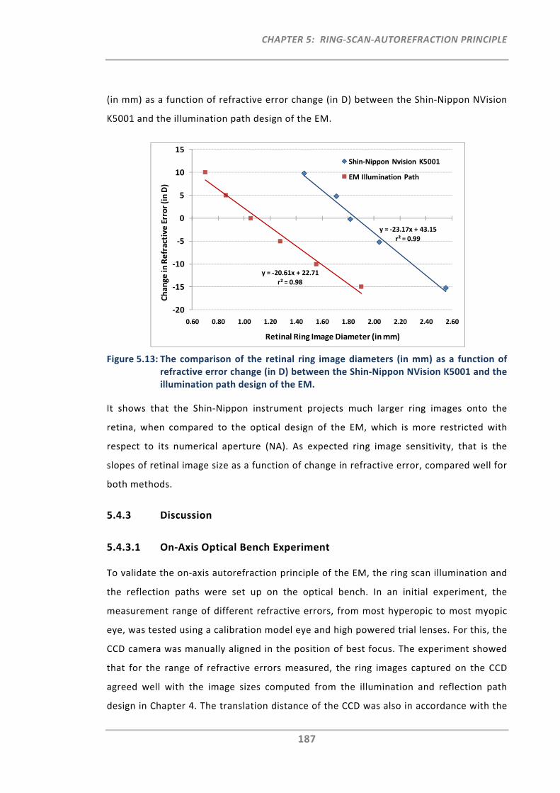
CHAPTER 5: RING‐SCAN‐AUTOREFRACTION PRINCIPLE
187
(in mm) as a function of refractive error change (in D) between the Shin‐Nippon NVision
K5001 and the illumination path design of the EM.
Figure 5.13: The comparison of the retinal ring image diameters (in mm) as a function of refractive error change (in D) between the Shin‐Nippon NVision K5001 and the illumination path design of the EM.
It shows that the Shin‐Nippon instrument projects much larger ring images onto the
retina, when compared to the optical design of the EM, which is more restricted with
respect to its numerical aperture (NA). As expected ring image sensitivity, that is the
slopes of retinal image size as a function of change in refractive error, compared well for
both methods.
5.4.3 Discussion
5.4.3.1 On‐Axis Optical Bench Experiment
To validate the on‐axis autorefraction principle of the EM, the ring scan illumination and
the reflection paths were set up on the optical bench. In an initial experiment, the
measurement range of different refractive errors, from most hyperopic to most myopic
eye, was tested using a calibration model eye and high powered trial lenses. For this, the
CCD camera was manually aligned in the position of best focus. The experiment showed
that for the range of refractive errors measured, the ring images captured on the CCD
agreed well with the image sizes computed from the illumination and reflection path
design in Chapter 4. The translation distance of the CCD was also in accordance with the
y = ‐23.17x + 43.15
r² = 0.99
y = ‐20.61x + 22.71
r² = 0.98
‐20
‐15
‐10
‐5
0
5
10
15
0.60 0.80 1.00 1.20 1.40 1.60 1.80 2.00 2.20 2.40 2.60
Change
in Refractive
Error (in D)
Retinal Ring Image Diameter (in mm)
Shin‐Nippon Nvision K5001
EM Illumination Path
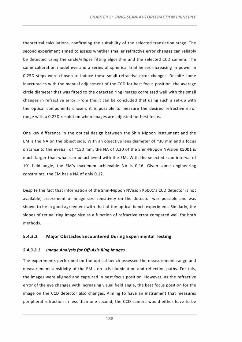
CHAPTER 5: RING‐SCAN‐AUTOREFRACTION PRINCIPLE
188
theoretical calculations, confirming the suitability of the selected translation stage. The
second experiment aimed to assess whether smaller refractive error changes can reliably
be detected using the circle/ellipse fitting algorithm and the selected CCD camera. The
same calibration model eye and a series of spherical trial lenses increasing in power in
0.25D steps were chosen to induce these small refractive error changes. Despite some
inaccuracies with the manual adjustment of the CCD for best focus position, the average
circle diameter that was fitted to the detected ring images correlated well with the small
changes in refractive error. From this it can be concluded that using such a set‐up with
the optical components chosen, it is possible to measure the desired refractive error
range with a 0.25D resolution when images are adjusted for best focus.
One key difference in the optical design between the Shin Nippon instrument and the
EM is the NA on the object side. With an objective lens diameter of ~30 mm and a focus
distance to the eyeball of ~150 mm, the NA of 0.20 of the Shin‐Nippon NVision K5001 is
much larger than what can be achieved with the EM. With the selected scan interval of
10° field angle, the EM’s maximum achievable NA is 0.16. Given some engineering
constraints, the EM has a NA of only 0.12.
Despite the fact that information of the Shin‐Nippon NVision K5001’s CCD detector is not
available, assessment of image size sensitivity on the detector was possible and was
shown to be in good agreement with that of the optical bench experiment. Similarly, the
slopes of retinal ring image size as a function of refractive error compared well for both
methods.
5.4.3.2 Major Obstacles Encountered During Experimental Testing
5.4.3.2.1 Image Analysis for Off‐Axis Ring Images
The experiments performed on the optical bench assessed the measurement range and
measurement sensitivity of the EM’s on‐axis illumination and reflection paths. For this,
the images were aligned and captured in best focus position. However, as the refractive
error of the eye changes with increasing visual field angle, the best focus position for the
image on the CCD detector also changes. Aiming to have an instrument that measures
peripheral refraction in less than one second, the CCD camera would either have to be
CHAPTER 5: RING‐SCAN‐AUTOREFRACTION PRINCIPLE
189
moved very quickly in between the 11 scan positions, or be in a stationary position at the
best averaged focal position and capture images, some of which will be out of focus.
Despite the fact that most of the components permit the fast scanning and translation, it
was found that the camera itself limits the operational goals with respect to
measurement speed if each of the 11 positions had to be aligned for best focus before
being captured. In order to achieve images of high resolution at low light levels, a certain
camera integration time is required per image, which would eventually prolong the
intended peripheral refraction scan duration. With rapid scanning of the peripheral
refraction profile being a key feature and requirement of the EM, the only alternative is
the capturing of all 11 images at one single translation stage position. The best average
CCD position may be determined from an initial alignment scan that computes an
average focal position from three visual field positions, i.e. 0° and ±50°. At this stage,
first attempts to analyse ring images that are well‐out‐of focus were not successful when
using the current circle/ellipse fitting program.
5.4.3.2.2 Impact of Higher‐Order Aberrations on Peripheral Ring Images
As the initial optical bench experiment was not set up for testing in humans, a simple
calibration model eye with plane retinal surface was measured. In addition, experimental
autorefraction measurements with the Shin‐Nippon NVision K5001 were done on both
the calibration model eye and human eyes. When capturing the detector images with the
Shin‐Nippon NVision K5001, a few eyes were also measured during off‐axis fixation. It
was observed that some detector images measured during peripheral refraction
appeared to be slightly asymmetric or distorted in shape and sometimes also in
luminosity. Due to the restrictions in assessment of these low resolution detector images
and due to the unknown image analysis algorithm of the Shin Nippon NVision K5001, an
attempt was made to model the retinal ring image shape as a function of visual field
angle, in order to further investigate these observed distortions of the ring images.
Into‐the eye‐ray trace was performed using the EM reference model eye (Section 4.2.1.1)
and the illumination path design (Section 4.3.1.2). To assess the ring shape in the
periphery, a coordinate break was inserted prior to the surface of the anterior cornea in
the ZEMAX Lens Data Editor. Parameter 3 (PRAM 3, tilt) of this coordinate break was
altered to induce eye turn with respect to the illumination beam of up to 50° in 10°
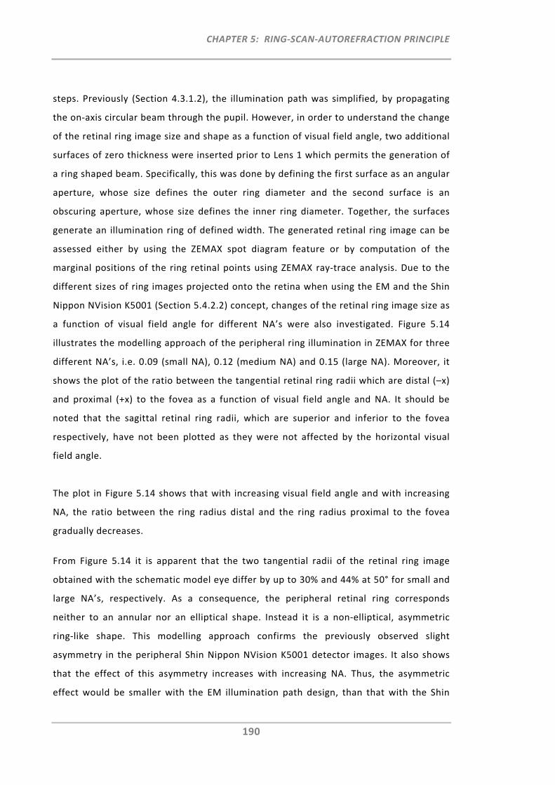
CHAPTER 5: RING‐SCAN‐AUTOREFRACTION PRINCIPLE
190
steps. Previously (Section 4.3.1.2), the illumination path was simplified, by propagating
the on‐axis circular beam through the pupil. However, in order to understand the change
of the retinal ring image size and shape as a function of visual field angle, two additional
surfaces of zero thickness were inserted prior to Lens 1 which permits the generation of
a ring shaped beam. Specifically, this was done by defining the first surface as an angular
aperture, whose size defines the outer ring diameter and the second surface is an
obscuring aperture, whose size defines the inner ring diameter. Together, the surfaces
generate an illumination ring of defined width. The generated retinal ring image can be
assessed either by using the ZEMAX spot diagram feature or by computation of the
marginal positions of the ring retinal points using ZEMAX ray‐trace analysis. Due to the
different sizes of ring images projected onto the retina when using the EM and the Shin
Nippon NVision K5001 (Section 5.4.2.2) concept, changes of the retinal ring image size as
a function of visual field angle for different NA’s were also investigated. Figure 5.14
illustrates the modelling approach of the peripheral ring illumination in ZEMAX for three
different NA’s, i.e. 0.09 (small NA), 0.12 (medium NA) and 0.15 (large NA). Moreover, it
shows the plot of the ratio between the tangential retinal ring radii which are distal (–x)
and proximal (+x) to the fovea as a function of visual field angle and NA. It should be
noted that the sagittal retinal ring radii, which are superior and inferior to the fovea
respectively, have not been plotted as they were not affected by the horizontal visual
field angle.
The plot in Figure 5.14 shows that with increasing visual field angle and with increasing
NA, the ratio between the ring radius distal and the ring radius proximal to the fovea
gradually decreases.
From Figure 5.14 it is apparent that the two tangential radii of the retinal ring image
obtained with the schematic model eye differ by up to 30% and 44% at 50° for small and
large NA’s, respectively. As a consequence, the peripheral retinal ring corresponds
neither to an annular nor an elliptical shape. Instead it is a non‐elliptical, asymmetric
ring‐like shape. This modelling approach confirms the previously observed slight
asymmetry in the peripheral Shin Nippon NVision K5001 detector images. It also shows
that the effect of this asymmetry increases with increasing NA. Thus, the asymmetric
effect would be smaller with the EM illumination path design, than that with the Shin
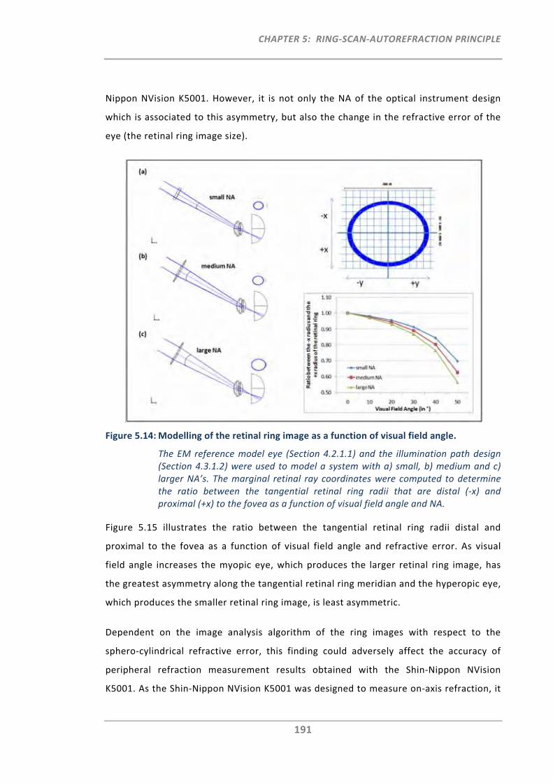
CHAPTER 5: RING‐SCAN‐AUTOREFRACTION PRINCIPLE
191
Nippon NVision K5001. However, it is not only the NA of the optical instrument design
which is associated to this asymmetry, but also the change in the refractive error of the
eye (the retinal ring image size).
Figure 5.14: Modelling of the retinal ring image as a function of visual field angle.
The EM reference model eye (Section 4.2.1.1) and the illumination path design (Section 4.3.1.2) were used to model a system with a) small, b) medium and c) larger NA’s. The marginal retinal ray coordinates were computed to determine the ratio between the tangential retinal ring radii that are distal (‐x) and proximal (+x) to the fovea as a function of visual field angle and NA.
Figure 5.15 illustrates the ratio between the tangential retinal ring radii distal and
proximal to the fovea as a function of visual field angle and refractive error. As visual
field angle increases the myopic eye, which produces the larger retinal ring image, has
the greatest asymmetry along the tangential retinal ring meridian and the hyperopic eye,
which produces the smaller retinal ring image, is least asymmetric.
Dependent on the image analysis algorithm of the ring images with respect to the
sphero‐cylindrical refractive error, this finding could adversely affect the accuracy of
peripheral refraction measurement results obtained with the Shin‐Nippon NVision
K5001. As the Shin‐Nippon NVision K5001 was designed to measure on‐axis refraction, it
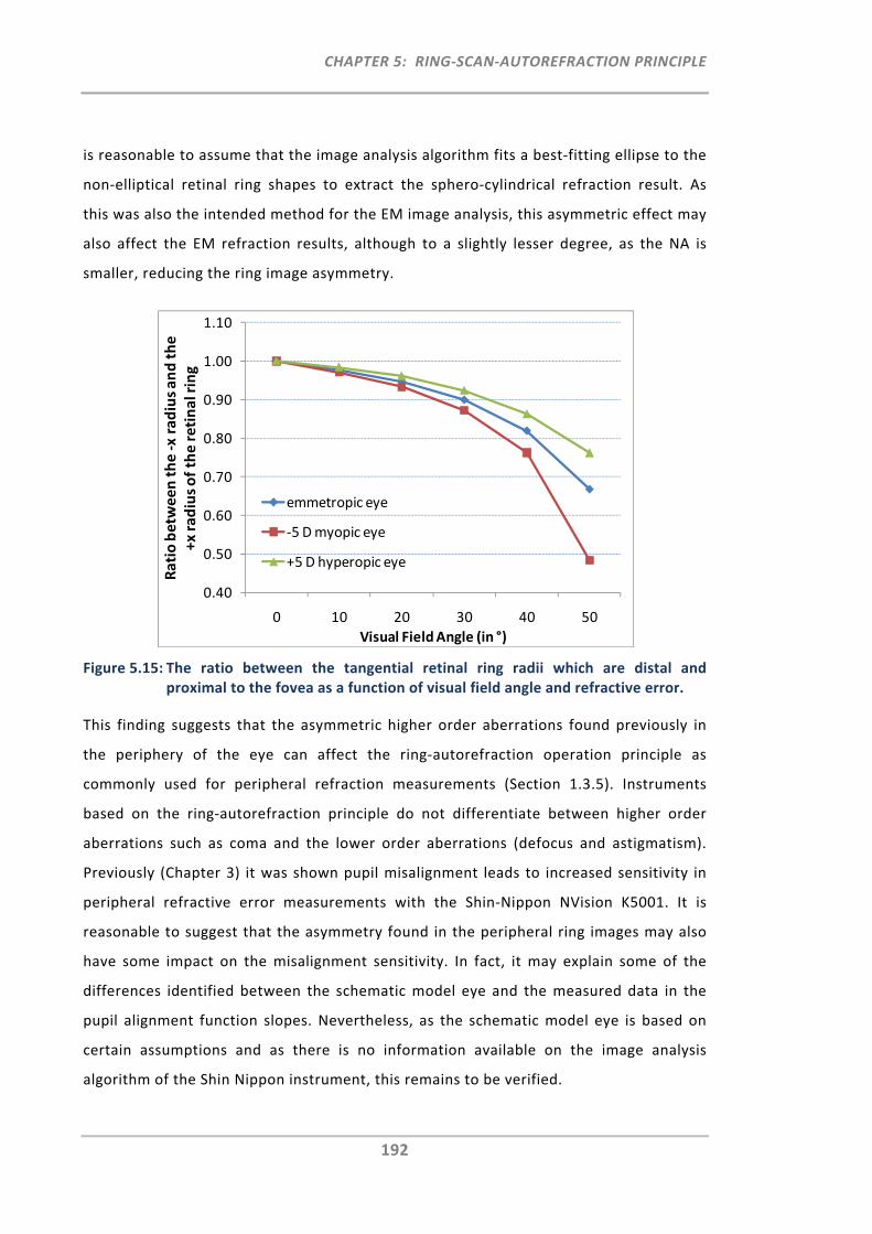
CHAPTER 5: RING‐SCAN‐AUTOREFRACTION PRINCIPLE
192
is reasonable to assume that the image analysis algorithm fits a best‐fitting ellipse to the
non‐elliptical retinal ring shapes to extract the sphero‐cylindrical refraction result. As
this was also the intended method for the EM image analysis, this asymmetric effect may
also affect the EM refraction results, although to a slightly lesser degree, as the NA is
smaller, reducing the ring image asymmetry.
Figure 5.15: The ratio between the tangential retinal ring radii which are distal and proximal to the fovea as a function of visual field angle and refractive error.
This finding suggests that the asymmetric higher order aberrations found previously in
the periphery of the eye can affect the ring‐autorefraction operation principle as
commonly used for peripheral refraction measurements (Section 1.3.5). Instruments
based on the ring‐autorefraction principle do not differentiate between higher order
aberrations such as coma and the lower order aberrations (defocus and astigmatism).
Previously (Chapter 3) it was shown pupil misalignment leads to increased sensitivity in
peripheral refractive error measurements with the Shin‐Nippon NVision K5001. It is
reasonable to suggest that the asymmetry found in the peripheral ring images may also
have some impact on the misalignment sensitivity. In fact, it may explain some of the
differences identified between the schematic model eye and the measured data in the
pupil alignment function slopes. Nevertheless, as the schematic model eye is based on
certain assumptions and as there is no information available on the image analysis
algorithm of the Shin Nippon instrument, this remains to be verified.
0.40
0.50
0.60
0.70
0.80
0.90
1.00
1.10
0 10 20 30 40 50
Ratio betw
een the ‐x radius and the
+x radius of the retinal ring
Visual Field Angle (in °)
emmetropic eye
‐5 D myopic eye
+5 D hyperopic eye
CHAPTER 5: RING‐SCAN‐AUTOREFRACTION PRINCIPLE
193
5.5 Future Work
Despite the fact that the EM’s proposed autorefraction principle was successfully
confirmed in its operation and safety, some of the experimental work discussed in the
present chapter raised considerable concerns with respect to achieving the EM’s
performance goals.
One of the issues is related to the intended rapid measurement of the peripheral
refraction profile. In order to achieve a peripheral refraction scan in less than one
second, the 11 images have to be captured at one CCD position, even if they are out of
focus. Due to the reduced luminosity profile for the captured out of focus ring images,
the current experimental set‐up, as well as the circle/ellipse fitting algorithm, require
further improvement to permit the better capture and analysis of these images.
Of major concern is the identified distortion of the peripheral ring images. With
increasing visual field angle and retinal image size (e.g. myopic eyes), the ring image
becomes increasingly more asymmetric. Previously it was assumed that if alignment with
the pupil centre was ensured, the ring‐autorefraction principle would provide valid
sphero‐cylindrical peripheral refraction measurements. However, it appears that these
peripheral ring images are affected by higher order aberrations, in particular coma, as
they increase with peripheral visual field angle. Even if the sole purpose of the
instrument is to measure the sphero‐cylindrical refraction output, the outcome may
differ depending on the ring image analysis algorithm. The best approach for the
computation of the sphero‐cylindrical refraction output may be to find the average
ellipse that best describes the ring‐like shape and thereby ignores the asymmetric
peripheral ring shape. Nevertheless, if one aims for accurate peripheral refraction
measurements, it would be of value to also account for this asymmetry in the peripheral
ring image. This may be done by fitting a function that best describes this asymmetric
ring shape, perhaps a double‐ellipse function. From this it may be possible to compute
the size and shape by providing not only sphere, cylinder and axis values, but also coma.
Commonly the term coma, however, is provided in unit µm, measured with a wavefront
sensing technique. Thus, extraction of the coma term from the ring image may not be
the most expedient approach.
CHAPTER 5: RING‐SCAN‐AUTOREFRACTION PRINCIPLE
194
The measurement of peripheral higher order aberrations has gained attention most
recently. A study published by Mathur et al.127 measured peripheral aberrations in a
group of emmetropic and myopic young adults. It was found that coma across the visual
field varied significantly between both groups. In fact, coma slopes were two‐fold
greater in the myopic group than in the emmetropic group. The mean slope for coma in
myopic eyes was ‐0.014 μm/degree, whilst in emmetropic eyes the mean slope was ‐
0.006 μm/degree. Using a ray‐tracing approach it was suggested that this difference in
the coma slopes between both groups can be explained by the differences in anterior
corneal radius of curvature, corneal asphericity as well as axial length. Moreover, in a
further study, the impact of age on peripheral aberrations in emmetropic eyes was also
assessed. In older eyes coma increased with visual field angle at a significantly higher
rate (‐0.018 μm/degree) than in younger eyes (‐0.006 μm/degree).61 These findings were
also confirmed in a larger sample sized study by Baskaran et al.62
With the demonstrated differences in peripheral higher order aberrations, such as coma,
between different population groups, it may be of increasing importance for future
research activities to neither ignore nor average these higher order aberration effects
when measuring peripheral refraction. Thus, based on this increased interest and the
other limitations encountered with the ring‐autorefraction principle, a wavefront sensing
technique appears to be the more appropriate operation principle for a dedicated
peripheral refraction instruments.
5.6 Summary and Conclusion
This chapter assessed the safety requirements with respect to the proposed EM’s new
peripheral and ocular ring scan illumination. For this, several exposure cases were
simulated and assessed and the MPФ with the greatest degree of protection was
determined. Under the assumption that a single beam (non‐scanned) exposure is
prevented, the greatest protection was obtained with either the single pulsed line
exposure for slow to medium scan frame rates or the PLS exposure for fast scan frame
rates. Other specific EM characteristics, such as exposure of the peripheral retina and
possible malfunction of the scanners were also addressed with respect to safety
assessment of the proposed EM instrument.
CHAPTER 5: RING‐SCAN‐AUTOREFRACTION PRINCIPLE
195
In addition to the safety requirements, this chapter also assessed the technical
implementation and feasibility of the autorefraction principle for central and peripheral
refractometry. Based on both, the safety and component criteria, the EM on‐axis
autorefraction principle was experimentally verified on the optical bench, and was also
successfully cross‐validated with the Shin Nippon on‐axis autorefraction paths. However,
an obstacle relating to the ring‐image analysis was identified, which would impair one of
the main goals of the EM; the performance of a peripheral refraction scan in less than
one second. Moreover, for the peripheral refraction measurements it was discovered
that higher order aberrations have the potential to interfere with the sphero‐cylindrical
refraction readings. As ray‐tracing and experimental testing have demonstrated,
asymmetric higher order aberrations can distort the symmetry and elliptical shape of the
retinal ring.
This ring asymmetry for peripheral measurements may not only affect the sphero‐
cylindrical peripheral refraction output of current autorefraction instruments but also
that of the proposed EM instrument. With the aim to develop an instrument dedicated
to measure peripheral refraction accurately, it is of importance to account for these
asymmetric changes. The most expedient approach of segregating higher and lower
order aberrations is by measuring the eye’s peripheral wavefront rather than analysing
the asymmetric peripheral ring when using the autorefraction principle. The change of
the EM’s operation principle from the autorefraction ring principle to the wavefront
sensing technique also seems reasonable with respect to the recent and future research
interests in measuring peripheral higher order aberrations. The following chapter
describes the technical implementation of the peripheral wavefront sensing principle in
detail.

CHAPTER 6: THE EYEMAPPER: A REAL‐TIME GLOBAL ABERROMETER
196
CHAPTER 6:
THE EYEMAPPER ‐ A REAL‐TIME GLOBAL ABERROMETER
6.1 Introduction
Initially, the aim of the newly proposed peripheral refraction instrument, the EyeMapper
(EM), was to measure the clinically relevant sphero‐cylindrical refractive errors of the
eye by use of the well‐known ring‐autorefraction operation principle. Findings from
Chapter 5, however, revealed that peripheral higher order aberrations have the potential
to interfere with the autorefraction results. The use of an operation principle based on
the Hartmann‐Shack wavefront sensing principle, which segregates higher and lower
order aberrations, was therefore deemed to be more suitable for an instrument
dedicated to measuring peripheral refraction.
Based on the knowledge gained from the previous chapters, the aims of this chapter
were to:
‐ Update the optical design of the EM to integrate the wavefront sensing principle
(Hartmann‐Shack sensor),
‐ Develop the mechanical design of the clinical EM instrument,∏
‐ Build∏ the EM instrument, and therefore:
o Perform a tolerance analysis,
o Source the additional components required,
o Re‐assess safety requirements on the basis of the new operation
principle,
o Manufacture the instrument parts according to the mechanical design,∏
o Develop the instrument software required,∏
‐ Validate the EM instrument by performing measurements on a model eye and on
ten human eyes.
∏ Aims and tasks labelled with this symbol were achieved with the help of the Brien
Holden Vision Institute Technology Team.
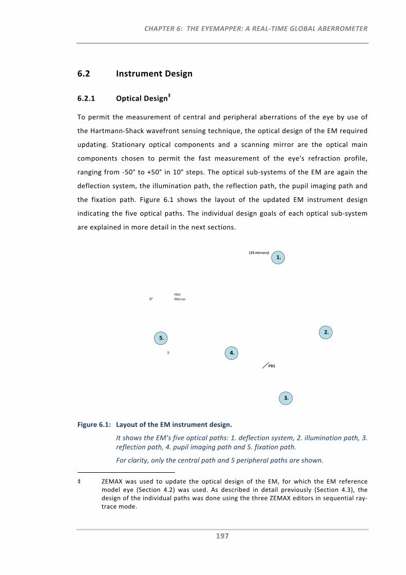
CHAPTER 6: THE EYEMAPPER: A REAL‐TIME GLOBAL ABERROMETER
197
6.2 Instrument Design
6.2.1 Optical Design‡
To permit the measurement of central and peripheral aberrations of the eye by use of
the Hartmann‐Shack wavefront sensing technique, the optical design of the EM required
updating. Stationary optical components and a scanning mirror are the optical main
components chosen to permit the fast measurement of the eye's refraction profile,
ranging from ‐50° to +50° in 10° steps. The optical sub‐systems of the EM are again the
deflection system, the illumination path, the reflection path, the pupil imaging path and
the fixation path. Figure 6.1 shows the layout of the updated EM instrument design
indicating the five optical paths. The individual design goals of each optical sub‐system
are explained in more detail in the next sections.
Figure 6.1: Layout of the EM instrument design.
It shows the EM’s five optical paths: 1. deflection system, 2. illumination path, 3. reflection path, 4. pupil imaging path and 5. fixation path.
For clarity, only the central path and 5 peripheral paths are shown.
‡ ZEMAX was used to update the optical design of the EM, for which the EM reference model eye (Section 4.2) was used. As described in detail previously (Section 4.3), the design of the individual paths was done using the three ZEMAX editors in sequential ray‐trace mode.
2.
3.
5.
4.
0°
(33 mirrors)
5
Hot Mirror
PBS
1.
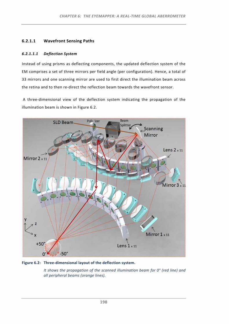
CHAPTER 6: THE EYEMAPPER: A REAL‐TIME GLOBAL ABERROMETER
198
6.2.1.1 Wavefront Sensing Paths
6.2.1.1.1 Deflection System
Instead of using prisms as deflecting components, the updated deflection system of the
EM comprises a set of three mirrors per field angle (per configuration). Hence, a total of
33 mirrors and one scanning mirror are used to first direct the illumination beam across
the retina and to then re‐direct the reflection beam towards the wavefront sensor.
A three‐dimensional view of the deflection system indicating the propagation of the
illumination beam is shown in Figure 6.2.
Figure 6.2: Three‐dimensional layout of the deflection system.
It shows the propagation of the scanned illumination beam for 0° (red line) and all peripheral beams (orange lines).
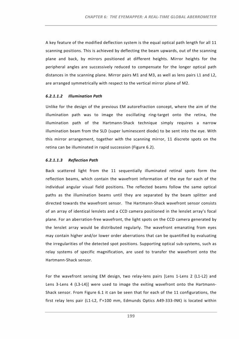
CHAPTER 6: THE EYEMAPPER: A REAL‐TIME GLOBAL ABERROMETER
199
A key feature of the modified deflection system is the equal optical path length for all 11
scanning positions. This is achieved by deflecting the beam upwards, out of the scanning
plane and back, by mirrors positioned at different heights. Mirror heights for the
peripheral angles are successively reduced to compensate for the longer optical path
distances in the scanning plane. Mirror pairs M1 and M3, as well as lens pairs L1 and L2,
are arranged symmetrically with respect to the vertical mirror plane of M2.
6.2.1.1.2 Illumination Path
Unlike for the design of the previous EM autorefraction concept, where the aim of the
illumination path was to image the oscillating ring‐target onto the retina, the
illumination path of the Hartmann‐Shack technique simply requires a narrow
illumination beam from the SLD (super luminescent diode) to be sent into the eye. With
this mirror arrangement, together with the scanning mirror, 11 discrete spots on the
retina can be illuminated in rapid succession (Figure 6.2).
6.2.1.1.3 Reflection Path
Back scattered light from the 11 sequentially illuminated retinal spots form the
reflection beams, which contain the wavefront information of the eye for each of the
individual angular visual field positions. The reflected beams follow the same optical
paths as the illumination beams until they are separated by the beam splitter and
directed towards the wavefront sensor. The Hartmann‐Shack wavefront sensor consists
of an array of identical lenslets and a CCD camera positioned in the lenslet array’s focal
plane. For an aberration‐free wavefront, the light spots on the CCD camera generated by
the lenslet array would be distributed regularly. The wavefront emanating from eyes
may contain higher and/or lower order aberrations that can be quantified by evaluating
the irregularities of the detected spot positions. Supporting optical sub‐systems, such as
relay systems of specific magnification, are used to transfer the wavefront onto the
Hartmann‐Shack sensor.
For the wavefront sensing EM design, two relay‐lens pairs [Lens 1‐Lens 2 (L1‐L2) and
Lens 3‐Lens 4 (L3‐L4)] were used to image the exiting wavefront onto the Hartmann‐
Shack sensor. From Figure 6.1 it can be seen that for each of the 11 configurations, the
first relay lens pair (L1‐L2, f'=100 mm, Edmunds Optics A49‐333‐INK) is located within
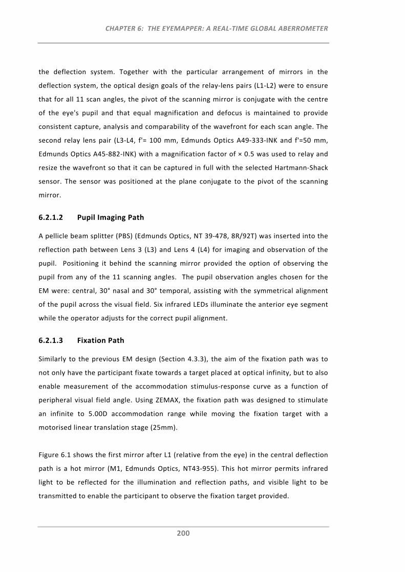
CHAPTER 6: THE EYEMAPPER: A REAL‐TIME GLOBAL ABERROMETER
200
the deflection system. Together with the particular arrangement of mirrors in the
deflection system, the optical design goals of the relay‐lens pairs (L1‐L2) were to ensure
that for all 11 scan angles, the pivot of the scanning mirror is conjugate with the centre
of the eye's pupil and that equal magnification and defocus is maintained to provide
consistent capture, analysis and comparability of the wavefront for each scan angle. The
second relay lens pair (L3‐L4, f'= 100 mm, Edmunds Optics A49‐333‐INK and f'=50 mm,
Edmunds Optics A45‐882‐INK) with a magnification factor of × 0.5 was used to relay and
resize the wavefront so that it can be captured in full with the selected Hartmann‐Shack
sensor. The sensor was positioned at the plane conjugate to the pivot of the scanning
mirror.
6.2.1.2 Pupil Imaging Path
A pellicle beam splitter (PBS) (Edmunds Optics, NT 39‐478, 8R/92T) was inserted into the
reflection path between Lens 3 (L3) and Lens 4 (L4) for imaging and observation of the
pupil. Positioning it behind the scanning mirror provided the option of observing the
pupil from any of the 11 scanning angles. The pupil observation angles chosen for the
EM were: central, 30° nasal and 30° temporal, assisting with the symmetrical alignment
of the pupil across the visual field. Six infrared LEDs illuminate the anterior eye segment
while the operator adjusts for the correct pupil alignment.
6.2.1.3 Fixation Path
Similarly to the previous EM design (Section 4.3.3), the aim of the fixation path was to
not only have the participant fixate towards a target placed at optical infinity, but to also
enable measurement of the accommodation stimulus‐response curve as a function of
peripheral visual field angle. Using ZEMAX, the fixation path was designed to stimulate
an infinite to 5.00D accommodation range while moving the fixation target with a
motorised linear translation stage (25mm).
Figure 6.1 shows the first mirror after L1 (relative from the eye) in the central deflection
path is a hot mirror (M1, Edmunds Optics, NT43‐955). This hot mirror permits infrared
light to be reflected for the illumination and reflection paths, and visible light to be
transmitted to enable the participant to observe the fixation target provided.

CHAPTER 6: THE EYEMAPPER: A REAL‐TIME GLOBAL ABERROMETER
201
6.2.2 Mechanical Design
To develop the intricate three‐dimensional arrangement of numerous components, i.e.
mirrors and lenses, the CAD (Computer‐Aided Design) Software SolidWorks (Dassault
Systèmes SolidWorks Corp.) was used for the EM's mechanical design. This software
proved particularly useful for development of the instrument, as parametric, three‐
dimensional design constraints can be defined to determine the component positioning
and assess and simulate the design prior to building the instrument.
Figure 6.3, Figure 6.4 and Figure 6.5 illustrate the three‐dimensional view of the EM
SolidWorks drawings from three different perspectives. The mechanical instrument
design was developed by Darrin Falk from the Brien Holden Vision Institute Technology
Group.
Figure 6.3: SolidWorks EM design from above.
The red dotted line indicates propagation of the on‐axis reflection beam, from the eye towards the HASO wavefront sensor. The mechanical instrument design was developed by Darrin Falk.
Mirror holding bridge with M2 x 11
Base plate
Eye
L1 x 11
L2 x 11
Mirror mounts with M1 x 11
Shutter PCBS
PBS
HASO
Hot Mirror
Mirror mounts with M3 x 11
L3
L4
Mirror Light Source
Polariser
Pupil Imaging CCD
Scanning Mirror

CHAPTER 6: THE EYEMAPPER: A REAL‐TIME GLOBAL ABERROMETER
202
Figure 6.3 shows the SolidWorks EM design from above, with all the main components
for the deflection system, the illumination and reflection paths positioned above the
base plate. The red dotted line indicates propagation of the on‐axis reflection beam,
from the eye towards the HASO wavefront sensor. The design of the mirror mounts (M1
and M3) was particularly complex, as they had to be spaced tightly and arranged along
an arc shape to fulfil the optical design requirements of the deflection system. All front
surface mirrors were bonded to metal base plates and then attached to the mirror
mounts with four small screws and semi‐flexible O‐rings, which permitted the mirrors to
be finely adjusted for proper alignment. The mirror (M2) holding bridge is the
component that engenders the three‐dimensional structure. Other optical and
mechanical components illustrated in Figure 6.3 are, for example, the mounts for the
lenses, the polarising cube beam splitter (PCBS), the pellicle beam splitter (PBS), and the
light source, as well as the scanning mirror, the shutter and the wavefront sensor
(HASO).
Figure 6.4: SolidWorks EM design from the side and below.
The orange dotted line partially indicates the propagation of the fixation path and the yellow dotted line partially indicates the pupil imaging path. The mechanical instrument design was developed by Darrin Falk.
Base plate
HASO Mirror
MirrorL7
L6
Translation Stage
Galvano Meter
Eye
Bearing Rail for Rotation
Mirror holding bridge with M2 x 11
Mirror
Pupil Imaging CCD
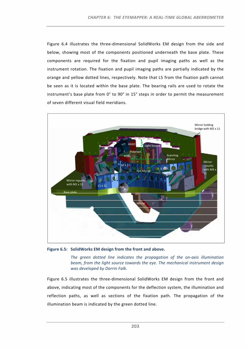
CHAPTER 6: THE EYEMAPPER: A REAL‐TIME GLOBAL ABERROMETER
203
Figure 6.4 illustrates the three‐dimensional SolidWorks EM design from the side and
below, showing most of the components positioned underneath the base plate. These
components are required for the fixation and pupil imaging paths as well as the
instrument rotation. The fixation and pupil imaging paths are partially indicated by the
orange and yellow dotted lines, respectively. Note that L5 from the fixation path cannot
be seen as it is located within the base plate. The bearing rails are used to rotate the
instrument’s base plate from 0° to 90° in 15° steps in order to permit the measurement
of seven different visual field meridians.
Figure 6.5: SolidWorks EM design from the front and above.
The green dotted line indicates the propagation of the on‐axis illumination beam, from the light source towards the eye. The mechanical instrument design was developed by Darrin Falk.
Figure 6.5 illustrates the three‐dimensional SolidWorks EM design from the front and
above, indicating most of the components for the deflection system, the illumination and
reflection paths, as well as sections of the fixation path. The propagation of the
illumination beam is indicated by the green dotted line.
HASO
Polariser
PCBS
L4
Eye
Base plate
Mirror holding bridge with M2 x 11
L1 x 11
L2 x 11
Mirror mounts with M1 x 11
Mirror mounts with M3 x 11
Scanning Mirror
MirrorL6
Hot Mirror
Light Source
L3
CHAPTER 6: THE EYEMAPPER: A REAL‐TIME GLOBAL ABERROMETER
204
6.3 Instrument Construction
Following completion of the optical and mechanical design work, a tolerance analysis
was carried out to determine the required accuracy level of the sourced components and
manufactured mechanical parts. The safety requirements had to be re‐assessed to
comply with the wavefront sensing principle. All mechanical parts were manufactured in
accordance with the required accuracy, after which the instrument was assembled and
aligned. Several calibration tools and methods were developed to ensure that the
instrument performed to the necessary degree of accuracy. Comprehensive software
tools were developed to operate the instrument and to acquire and analyse the data.
6.3.1 Tolerance Analysis
6.3.1.1 Aims
Prior to any instrument manufacture, a tolerance analysis is a helpful method that can
be used to account for the effects of manufacturing and alignment errors. It permits not
only the identification of the individual critical components/elements of the optical
system (sensitivity analysis), but it also assesses the system’s overall performance for a
combination of alignment/manufacturing errors (Monte Carlo simulation).
With the reflection path being the critical optical path for the EM, the aim was to
investigate the impact of manufacturing deficiencies, such as axial position, decentration
and tilts on the individual lenses/elements of the reflection path.
6.3.1.2 Methods
6.3.1.2.1 Sensitivity Analysis and Monte Carlo Simulation
The ZEMAX sensitivity analysis and the Monte Carlo simulation were used for the
computation and analysis of tolerances for the EM. The flow chart in Figure 6.6 provides
an overview of the tolerancing procedure.
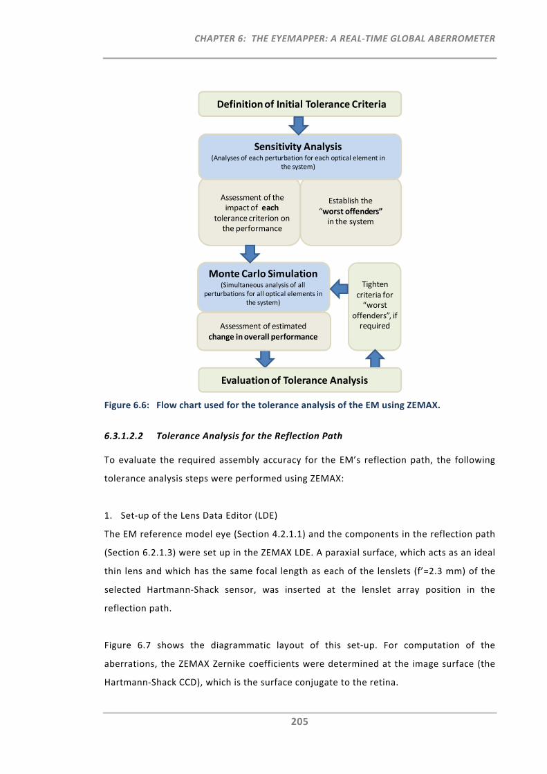
CHAPTER 6: THE EYEMAPPER: A REAL‐TIME GLOBAL ABERROMETER
205
Figure 6.6: Flow chart used for the tolerance analysis of the EM using ZEMAX.
6.3.1.2.2 Tolerance Analysis for the Reflection Path
To evaluate the required assembly accuracy for the EM’s reflection path, the following
tolerance analysis steps were performed using ZEMAX:
1. Set‐up of the Lens Data Editor (LDE)
The EM reference model eye (Section 4.2.1.1) and the components in the reflection path
(Section 6.2.1.3) were set up in the ZEMAX LDE. A paraxial surface, which acts as an ideal
thin lens and which has the same focal length as each of the lenslets (f’=2.3 mm) of the
selected Hartmann‐Shack sensor, was inserted at the lenslet array position in the
reflection path.
Figure 6.7 shows the diagrammatic layout of this set‐up. For computation of the
aberrations, the ZEMAX Zernike coefficients were determined at the image surface (the
Hartmann‐Shack CCD), which is the surface conjugate to the retina.
Definition of Initial Tolerance Criteria
Establish the “worst offenders”in the system
Sensitivity Analysis (Analyses of each perturbation for each optical element in
the system)
Assessment of the impact of each
tolerance criterion on the performance
Tighten criteria for “worst
offenders”, if required
Monte Carlo Simulation (Simultaneous analysis of all
perturbations for all optical elements in the system)
Evaluation of Tolerance Analysis
Assessment of estimated change in overall performance
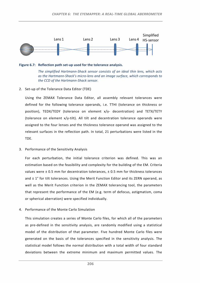
CHAPTER 6: THE EYEMAPPER: A REAL‐TIME GLOBAL ABERROMETER
206
Figure 6.7: Reflection path set‐up used for the tolerance analysis.
The simplified Hartmann‐Shack sensor consists of an ideal thin lens, which acts as the Hartmann‐Shack’s micro‐lens and an image surface, which corresponds to the CCD of the Hartmann‐Shack sensor.
2. Set‐up of the Tolerance Data Editor (TDE)
Using the ZEMAX Tolerance Data Editor, all assembly relevant tolerances were
defined for the following tolerance operands, i.e. TTHI (tolerance on thickness or
position), TEDX/TEDY (tolerance on element x/y‐ decentration) and TETX/TETY
(tolerance on element x/y‐tilt). All tilt and decentration tolerance operands were
assigned to the four lenses and the thickness tolerance operand was assigned to the
relevant surfaces in the reflection path. In total, 21 perturbations were listed in the
TDE.
3. Performance of the Sensitivity Analysis
For each perturbation, the initial tolerance criterion was defined. This was an
estimation based on the feasibility and complexity for the building of the EM. Criteria
values were ± 0.5 mm for decentration tolerances, ± 0.5 mm for thickness tolerances
and ± 1° for tilt tolerances. Using the Merit Function Editor and its ZERN operand, as
well as the Merit Function criterion in the ZEMAX tolerancing tool, the parameters
that represent the performance of the EM (e.g. term of defocus, astigmatism, coma
or spherical aberration) were specified individually.
4. Performance of the Monte Carlo Simulation
This simulation creates a series of Monte Carlo files, for which all of the parameters
as pre‐defined in the sensitivity analysis, are randomly modified using a statistical
model of the distribution of that parameter. Five hundred Monte Carlo files were
generated on the basis of the tolerances specified in the sensitivity analysis. The
statistical model follows the normal distribution with a total width of four standard
deviations between the extreme minimum and maximum permitted values. The
Lens 1 Lens 2 Lens 3 Lens 4Simplified HS‐sensor

CHAPTER 6: THE EYEMAPPER: A REAL‐TIME GLOBAL ABERROMETER
207
model estimates the performance changes (change in criterion) based on the root‐
sum‐square method. From the sensitivity analysis, worst offending tolerances were
re‐evaluated where required.
6.3.1.3 Results
6.3.1.3.1 Sensitivity Analysis
Tolerance analysis results are presented for each optical component (L1, L2, L3 and L4)
and each perturbation (axial misalignment, decentration and tilt) as a function of change
in performance (the change in merit function measurement error). For decentred and
tilted lenses, the change in performance was assessed with respect to the terms defocus,
astigmatism, coma and spherical aberration. Axial misalignment of lenses was assessed
for the terms defocus and spherical aberration only, as astigmatism and coma remain
unaffected by this perturbation.
Axial Misalignment of Optical Components:
Figure 6.8 shows the absolute change in performance for the terms defocus and
spherical aberration, if the axial distance between the individual optical components
would deviate by ± 0.5 mm from its optimum position. It can be seen that the distance
between L1 and L2, as well as the distance between L3 and L4, are the “worst offending
tolerances” with respect to axial misalignment.
Figure 6.8: Absolute change in performance with respect to the terms defocus and spherical aberration, for axial lens misalignment of ± 0.5 mm.
0.000
0.010
0.020
0.030
0.040
0.050
0.060
Eye ‐ L1 L1 ‐ L2 L2 ‐ L3 L3 ‐ L4 L4 ‐ HASO
Change in
microns
Axial Change (in mm)
Defocus Spherical Aberration
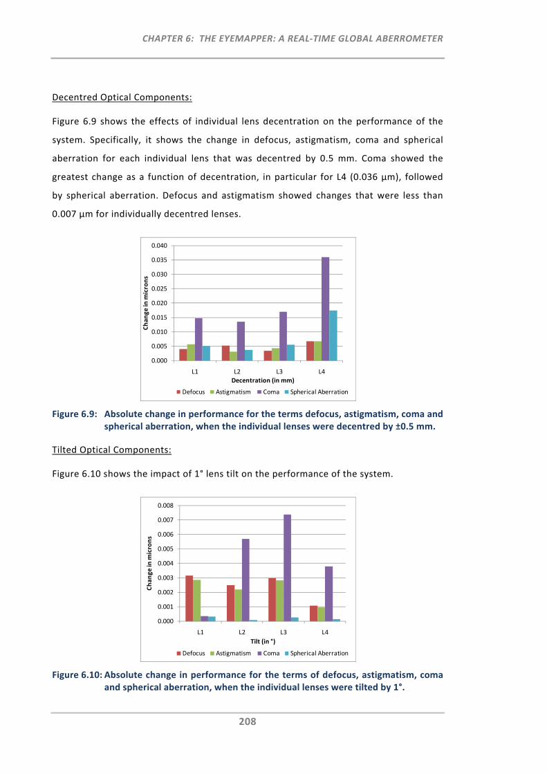
CHAPTER 6: THE EYEMAPPER: A REAL‐TIME GLOBAL ABERROMETER
208
Decentred Optical Components:
Figure 6.9 shows the effects of individual lens decentration on the performance of the
system. Specifically, it shows the change in defocus, astigmatism, coma and spherical
aberration for each individual lens that was decentred by 0.5 mm. Coma showed the
greatest change as a function of decentration, in particular for L4 (0.036 µm), followed
by spherical aberration. Defocus and astigmatism showed changes that were less than
0.007 µm for individually decentred lenses.
Figure 6.9: Absolute change in performance for the terms defocus, astigmatism, coma and spherical aberration, when the individual lenses were decentred by ±0.5 mm.
Tilted Optical Components:
Figure 6.10 shows the impact of 1° lens tilt on the performance of the system.
Figure 6.10: Absolute change in performance for the terms of defocus, astigmatism, coma and spherical aberration, when the individual lenses were tilted by 1°.
0.000
0.005
0.010
0.015
0.020
0.025
0.030
0.035
0.040
L1 L2 L3 L4
Change in
microns
Decentration (in mm)
Defocus Astigmatism Coma Spherical Aberration
0.000
0.001
0.002
0.003
0.004
0.005
0.006
0.007
0.008
L1 L2 L3 L4
Change in microns
Tilt (in °)
Defocus Astigmatism Coma Spherical Aberration
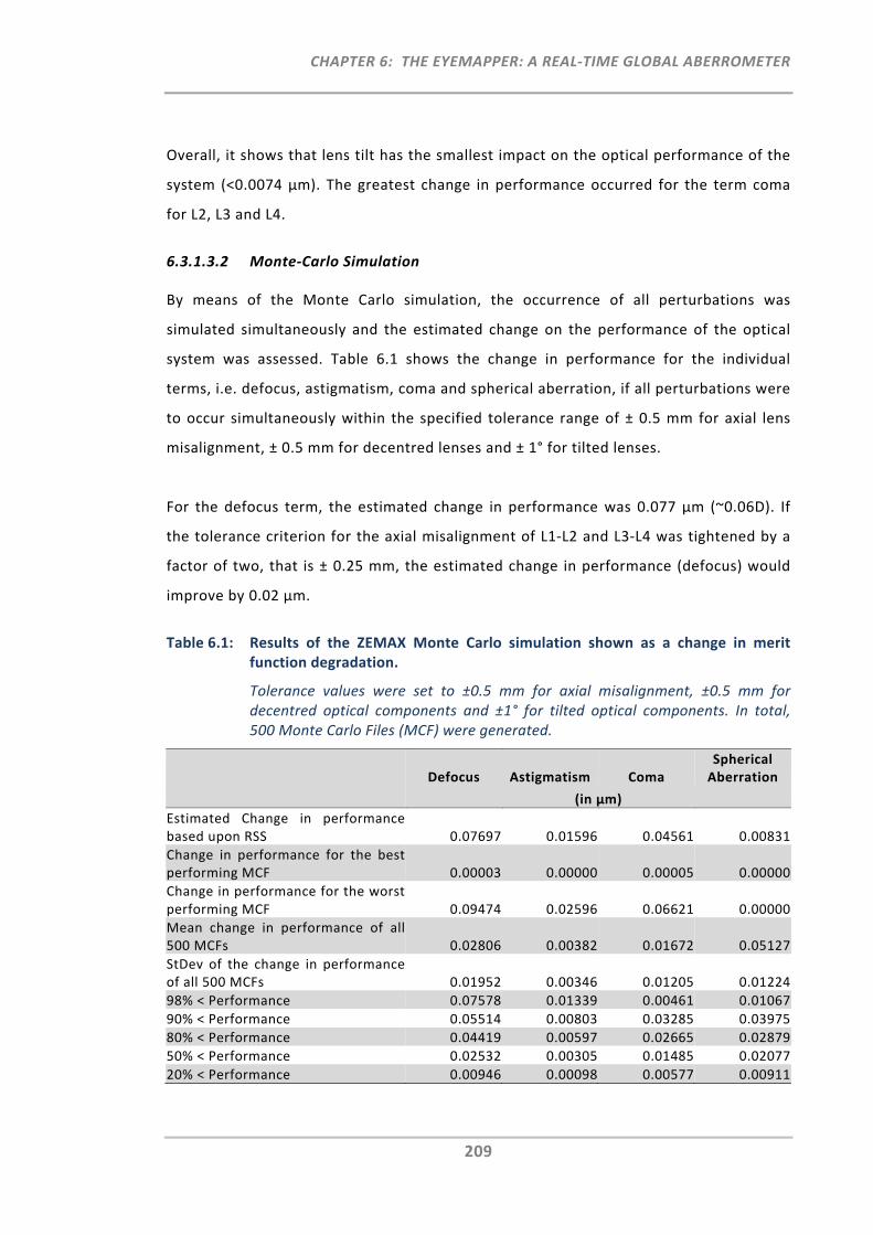
CHAPTER 6: THE EYEMAPPER: A REAL‐TIME GLOBAL ABERROMETER
209
Overall, it shows that lens tilt has the smallest impact on the optical performance of the
system (<0.0074 µm). The greatest change in performance occurred for the term coma
for L2, L3 and L4.
6.3.1.3.2 Monte‐Carlo Simulation
By means of the Monte Carlo simulation, the occurrence of all perturbations was
simulated simultaneously and the estimated change on the performance of the optical
system was assessed. Table 6.1 shows the change in performance for the individual
terms, i.e. defocus, astigmatism, coma and spherical aberration, if all perturbations were
to occur simultaneously within the specified tolerance range of ± 0.5 mm for axial lens
misalignment, ± 0.5 mm for decentred lenses and ± 1° for tilted lenses.
For the defocus term, the estimated change in performance was 0.077 µm (~0.06D). If
the tolerance criterion for the axial misalignment of L1‐L2 and L3‐L4 was tightened by a
factor of two, that is ± 0.25 mm, the estimated change in performance (defocus) would
improve by 0.02 µm.
Table 6.1: Results of the ZEMAX Monte Carlo simulation shown as a change in merit function degradation.
Tolerance values were set to ±0.5 mm for axial misalignment, ±0.5 mm for decentred optical components and ±1° for tilted optical components. In total, 500 Monte Carlo Files (MCF) were generated.
Defocus Astigmatism Coma Spherical Aberration
(in µm)
Estimated Change in performance based upon RSS 0.07697 0.01596 0.04561 0.00831
Change in performance for the best performing MCF 0.00003 0.00000 0.00005 0.00000
Change in performance for the worst performing MCF 0.09474 0.02596 0.06621 0.00000
Mean change in performance of all 500 MCFs 0.02806 0.00382 0.01672 0.05127
StDev of the change in performance of all 500 MCFs 0.01952 0.00346 0.01205 0.01224
98% < Performance 0.07578 0.01339 0.00461 0.01067
90% < Performance 0.05514 0.00803 0.03285 0.03975
80% < Performance 0.04419 0.00597 0.02665 0.02879
50% < Performance 0.02532 0.00305 0.01485 0.02077
20% < Performance 0.00946 0.00098 0.00577 0.00911
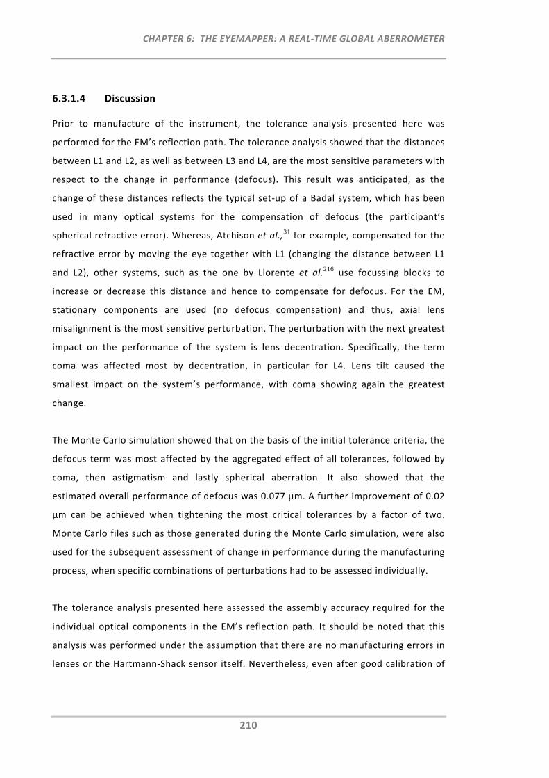
CHAPTER 6: THE EYEMAPPER: A REAL‐TIME GLOBAL ABERROMETER
210
6.3.1.4 Discussion
Prior to manufacture of the instrument, the tolerance analysis presented here was
performed for the EM’s reflection path. The tolerance analysis showed that the distances
between L1 and L2, as well as between L3 and L4, are the most sensitive parameters with
respect to the change in performance (defocus). This result was anticipated, as the
change of these distances reflects the typical set‐up of a Badal system, which has been
used in many optical systems for the compensation of defocus (the participant’s
spherical refractive error). Whereas, Atchison et al.,31 for example, compensated for the
refractive error by moving the eye together with L1 (changing the distance between L1
and L2), other systems, such as the one by Llorente et al.216 use focussing blocks to
increase or decrease this distance and hence to compensate for defocus. For the EM,
stationary components are used (no defocus compensation) and thus, axial lens
misalignment is the most sensitive perturbation. The perturbation with the next greatest
impact on the performance of the system is lens decentration. Specifically, the term
coma was affected most by decentration, in particular for L4. Lens tilt caused the
smallest impact on the system’s performance, with coma showing again the greatest
change.
The Monte Carlo simulation showed that on the basis of the initial tolerance criteria, the
defocus term was most affected by the aggregated effect of all tolerances, followed by
coma, then astigmatism and lastly spherical aberration. It also showed that the
estimated overall performance of defocus was 0.077 µm. A further improvement of 0.02
µm can be achieved when tightening the most critical tolerances by a factor of two.
Monte Carlo files such as those generated during the Monte Carlo simulation, were also
used for the subsequent assessment of change in performance during the manufacturing
process, when specific combinations of perturbations had to be assessed individually.
The tolerance analysis presented here assessed the assembly accuracy required for the
individual optical components in the EM’s reflection path. It should be noted that this
analysis was performed under the assumption that there are no manufacturing errors in
lenses or the Hartmann‐Shack sensor itself. Nevertheless, even after good calibration of
CHAPTER 6: THE EYEMAPPER: A REAL‐TIME GLOBAL ABERROMETER
211
the Hartmann‐Shack sensor, measurement accuracy can be affected by its manufacturing
and alignment tolerances.217, 218
6.3.2 Instrument Components
The following section lists the main instrument components and features chosen for
each optical path in the EM. These components were either sourced from external
suppliers or manufactured in‐house at the Brien Holden Vision Institute by Colm Dolphin.
6.3.2.1 Deflection System
Mirrors
All but two of the mirrors used in the deflection system are aluminium coated, front
surface mirrors with a surface flatness of 1/10 λ accuracy and a reflectance of
approximately 85% at a wavelength of 830 nm. These 32 front surface mirrors are quartz
coated to increase their hardness and to protect the aluminium layer. The majority of
the mirrors had to be custom shaped to fit into the EM’s mechanical design constraints.
The other two mirrors in the deflection system are the central mirror (M1) closest to the
eye, which is the hot mirror (multi‐layer dielectric coating, >95% reflectance, 4 λ
accuracy) used for the insertion of the fixation path, and the scanning mirror (protected
silver coating, >94% reflectance, 1/4 λ accuracy) that is required for the peripheral
refraction scan.
6.3.2.2 Illumination Path
Single Axis Galvanometer Scanner and Light Source
By use of the previously selected single axis galvanometer scanner (Section 5.2.1.3), the
EM scans the narrow SLD beam (wavelength 830nm, Section 5.2.1.1) sequentially and
rapidly across the retina. At each of the 11 retinal locations, the duration of the single
spot exposure is 0.065 seconds. With respect to safe exposure limits, Chapter 5
previously addressed the different sub‐exposures (spot, line, circle and scanning), which
were to be assessed for the on‐and off‐axis ring‐scan illumination. For the updated
wavefront sensing EM, only one relevant exposure had to be assessed; now being a small
spot exposure (Section 5.2.2).
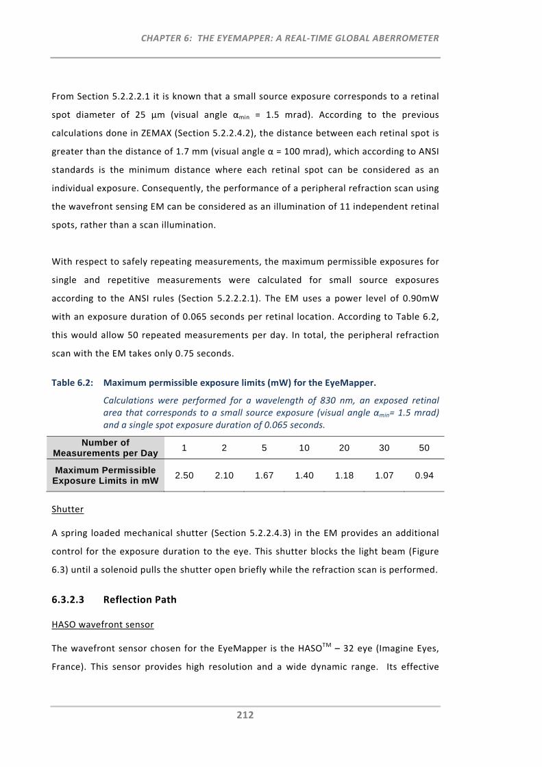
CHAPTER 6: THE EYEMAPPER: A REAL‐TIME GLOBAL ABERROMETER
212
From Section 5.2.2.2.1 it is known that a small source exposure corresponds to a retinal
spot diameter of 25 μm (visual angle αmin = 1.5 mrad). According to the previous
calculations done in ZEMAX (Section 5.2.2.4.2), the distance between each retinal spot is
greater than the distance of 1.7 mm (visual angle α = 100 mrad), which according to ANSI
standards is the minimum distance where each retinal spot can be considered as an
individual exposure. Consequently, the performance of a peripheral refraction scan using
the wavefront sensing EM can be considered as an illumination of 11 independent retinal
spots, rather than a scan illumination.
With respect to safely repeating measurements, the maximum permissible exposures for
single and repetitive measurements were calculated for small source exposures
according to the ANSI rules (Section 5.2.2.2.1). The EM uses a power level of 0.90mW
with an exposure duration of 0.065 seconds per retinal location. According to Table 6.2,
this would allow 50 repeated measurements per day. In total, the peripheral refraction
scan with the EM takes only 0.75 seconds.
Table 6.2: Maximum permissible exposure limits (mW) for the EyeMapper.
Calculations were performed for a wavelength of 830 nm, an exposed retinal area that corresponds to a small source exposure (visual angle αmin= 1.5 mrad) and a single spot exposure duration of 0.065 seconds.
Number of Measurements per Day
1 2 5 10 20 30 50
Maximum Permissible Exposure Limits in mW
2.50 2.10 1.67 1.40 1.18 1.07 0.94
Shutter
A spring loaded mechanical shutter (Section 5.2.2.4.3) in the EM provides an additional
control for the exposure duration to the eye. This shutter blocks the light beam (Figure
6.3) until a solenoid pulls the shutter open briefly while the refraction scan is performed.
6.3.2.3 Reflection Path
HASO wavefront sensor
The wavefront sensor chosen for the EyeMapper is the HASOTM – 32 eye (Imagine Eyes,
France). This sensor provides high resolution and a wide dynamic range. Its effective
CHAPTER 6: THE EYEMAPPER: A REAL‐TIME GLOBAL ABERROMETER
213
pupil diameter is 3.65 mm and 1280 sub‐apertures are located in a monolithic 40 × 32
microlens array. The focal length of each lenslet is 2.30 mm.
Lenses and Polarising Optics
The EM comprises lenses with anti‐reflection coating to permit greatest transmission of
light and to avoid unwanted reflections occurring inside the instrument. Moreover,
polarising optics, such as a polarising cube beam splitter (PCBS) and a polariser were
used to reduce unwanted ocular reflections from cornea and crystalline lens surfaces
(Section 5.3.1).
6.3.2.4 Fixation Path
Fixation Target and Translation Stage
The EM’s distance fixation target features a green illuminated cross on black
background, which similarly to the target used in the COAS aberrometer, promotes
distance viewing. The target is mounted on a fast and precise linear translation stage
(Physik Instrumente (PI) GmbH & Co. KG, M‐122.2DD Precision Micro Translation Stage)
with a travel range of 25 mm and a maximum velocity of 20 mm/s. The 25 mm linear
movement of the fixation target can stimulate accommodation in the range from 0.00D
to 5.00D.
6.3.2.5 Pupil Imaging Path
Pellicle Beam Splitter
The pellicle beam splitter (PBS) selected for the reflection path transmits 92% of light
towards the HASO wavefront sensor and reflects 8% of light, which is used for the pupil
imaging path (Edmunds Optics, NT 39‐478, 8R/92T). The advantage of the pellicle beam
splitter is its thin membrane, which avoids both ghost images from second surface
reflections and changes in optical path lengths.
Pupil Imaging CCD and Single Axis Galvanometer Scanner for Pupil Alignment
The previously selected Sony CCD sensor ICX445 (Section 5.3.2) is the CCD sensor used to
capture the images from the pupil. For the pupil alignment task, the galvanometer
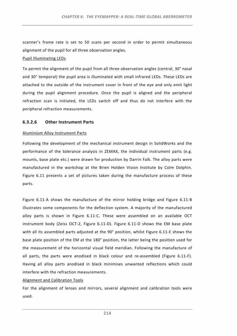
CHAPTER 6: THE EYEMAPPER: A REAL‐TIME GLOBAL ABERROMETER
214
scanner’s frame rate is set to 50 scans per second in order to permit simultaneous
alignment of the pupil for all three observation angles.
Pupil Illuminating LEDs
To permit the alignment of the pupil from all three observation angles (central, 30° nasal
and 30° temporal) the pupil area is illuminated with small infrared LEDs. These LEDs are
attached to the outside of the instrument cover in front of the eye and only emit light
during the pupil alignment procedure. Once the pupil is aligned and the peripheral
refraction scan is initiated, the LEDs switch off and thus do not interfere with the
peripheral refraction measurements.
6.3.2.6 Other Instrument Parts
Aluminium Alloy Instrument Parts
Following the development of the mechanical instrument design in SolidWorks and the
performance of the tolerance analysis in ZEMAX, the individual instrument parts (e.g.
mounts, base plate etc.) were drawn for production by Darrin Falk. The alloy parts were
manufactured in the workshop at the Brien Holden Vision Institute by Colm Dolphin.
Figure 6.11 presents a set of pictures taken during the manufacture process of these
parts.
Figure 6.11‐A shows the manufacture of the mirror holding bridge and Figure 6.11‐B
illustrates some components for the deflection system. A majority of the manufactured
alloy parts is shown in Figure 6.11‐C. These were assembled on an available OCT
instrument body (Zeiss OCT‐2, Figure 6.11‐D). Figure 6.11‐D shows the EM base plate
with all its assembled parts adjusted at the 90° position, whilst Figure 6.11‐E shows the
base plate position of the EM at the 180° position, the latter being the position used for
the measurement of the horizontal visual field meridian. Following the manufacture of
all parts, the parts were anodised in black colour and re‐assembled (Figure 6.11‐F).
Having all alloy parts anodised in black minimises unwanted reflections which could
interfere with the refraction measurements.
Alignment and Calibration Tools
For the alignment of lenses and mirrors, several alignment and calibration tools were
used.
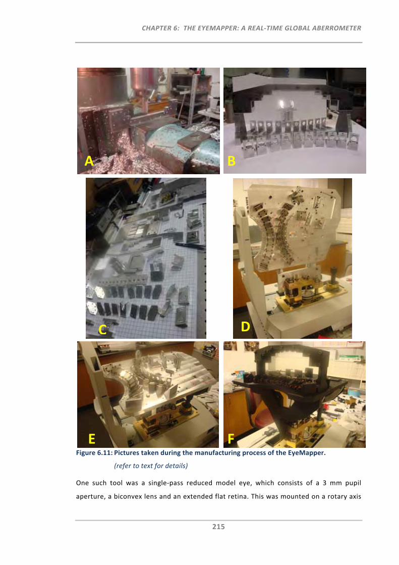
CHAPTER 6: THE EYEMAPPER: A REAL‐TIME GLOBAL ABERROMETER
215
Figure 6.11: Pictures taken during the manufacturing process of the EyeMapper.
(refer to text for details)
One such tool was a single‐pass reduced model eye, which consists of a 3 mm pupil
aperture, a biconvex lens and an extended flat retina. This was mounted on a rotary axis
A B
C D
E F
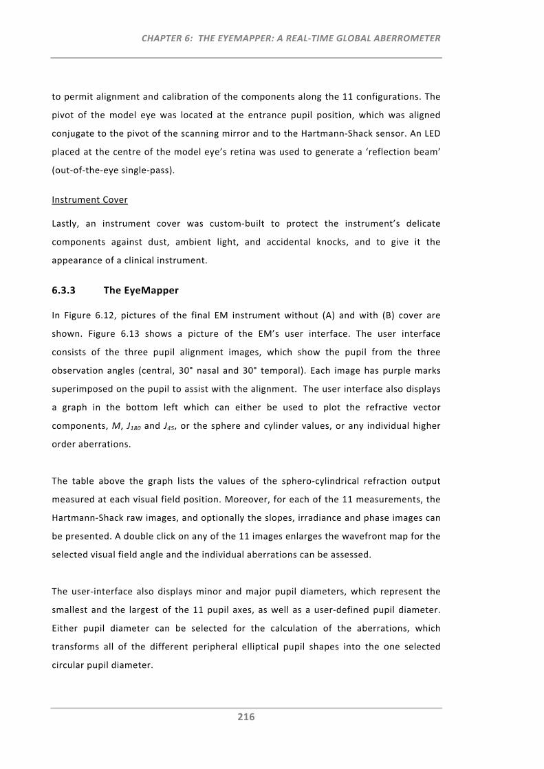
CHAPTER 6: THE EYEMAPPER: A REAL‐TIME GLOBAL ABERROMETER
216
to permit alignment and calibration of the components along the 11 configurations. The
pivot of the model eye was located at the entrance pupil position, which was aligned
conjugate to the pivot of the scanning mirror and to the Hartmann‐Shack sensor. An LED
placed at the centre of the model eye’s retina was used to generate a ‘reflection beam’
(out‐of‐the‐eye single‐pass).
Instrument Cover
Lastly, an instrument cover was custom‐built to protect the instrument’s delicate
components against dust, ambient light, and accidental knocks, and to give it the
appearance of a clinical instrument.
6.3.3 The EyeMapper
In Figure 6.12, pictures of the final EM instrument without (A) and with (B) cover are
shown. Figure 6.13 shows a picture of the EM’s user interface. The user interface
consists of the three pupil alignment images, which show the pupil from the three
observation angles (central, 30° nasal and 30° temporal). Each image has purple marks
superimposed on the pupil to assist with the alignment. The user interface also displays
a graph in the bottom left which can either be used to plot the refractive vector
components, M, J180 and J45, or the sphere and cylinder values, or any individual higher
order aberrations.
The table above the graph lists the values of the sphero‐cylindrical refraction output
measured at each visual field position. Moreover, for each of the 11 measurements, the
Hartmann‐Shack raw images, and optionally the slopes, irradiance and phase images can
be presented. A double click on any of the 11 images enlarges the wavefront map for the
selected visual field angle and the individual aberrations can be assessed.
The user‐interface also displays minor and major pupil diameters, which represent the
smallest and the largest of the 11 pupil axes, as well as a user‐defined pupil diameter.
Either pupil diameter can be selected for the calculation of the aberrations, which
transforms all of the different peripheral elliptical pupil shapes into the one selected
circular pupil diameter.
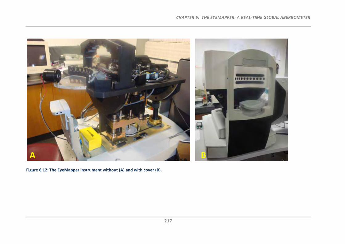
CHAPTER 6: THE EYEMAPPER: A REAL‐TIME GLOBAL ABERROMETER
217
Figure 6.12: The EyeMapper instrument without (A) and with cover (B).
A B
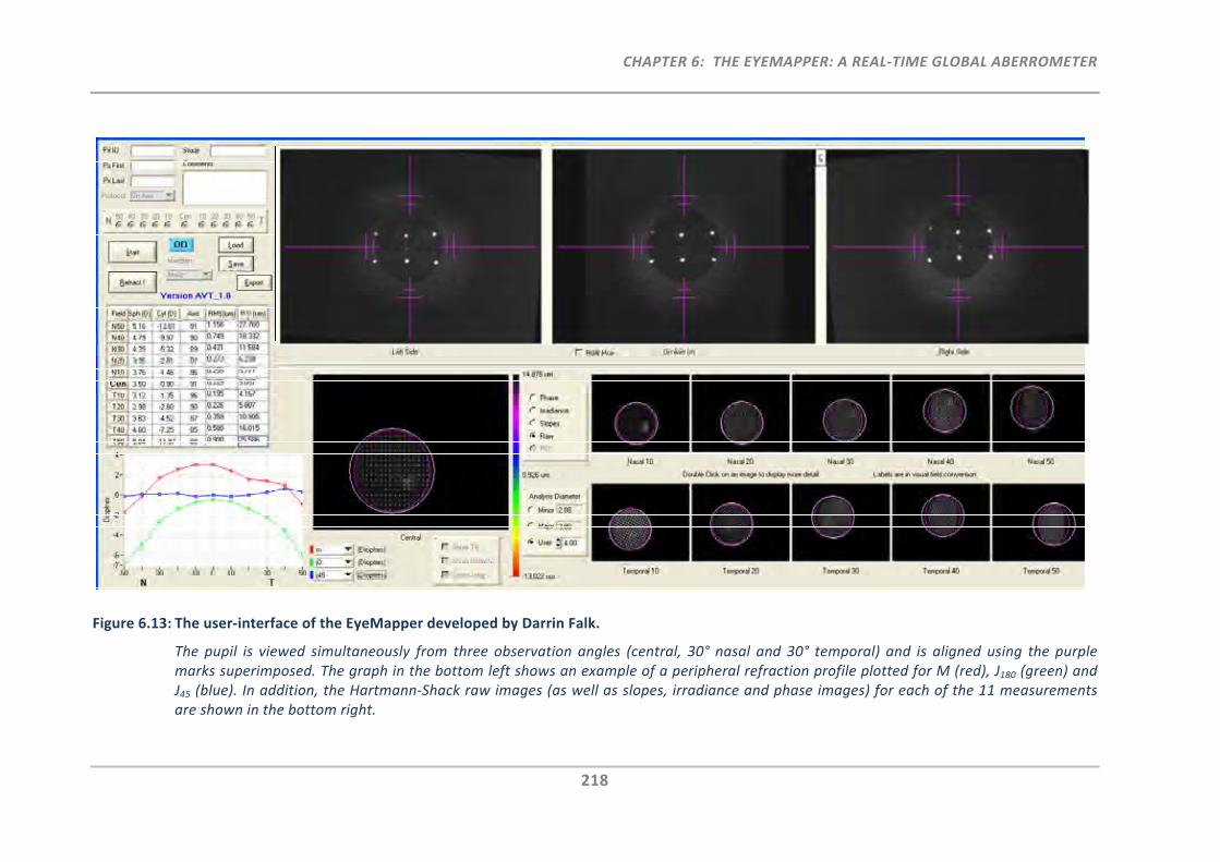
CHAPTER 6: THE EYEMAPPER: A REAL‐TIME GLOBAL ABERROMETER
218
Figure 6.13: The user‐interface of the EyeMapper developed by Darrin Falk.
The pupil is viewed simultaneously from three observation angles (central, 30° nasal and 30° temporal) and is aligned using the purple marks superimposed. The graph in the bottom left shows an example of a peripheral refraction profile plotted for M (red), J180 (green) and J45 (blue). In addition, the Hartmann‐Shack raw images (as well as slopes, irradiance and phase images) for each of the 11 measurements are shown in the bottom right.
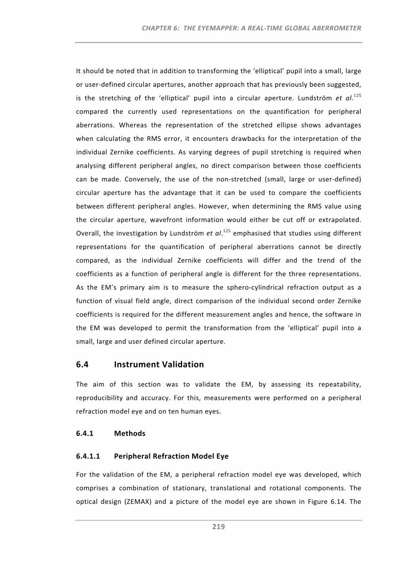
CHAPTER 6: THE EYEMAPPER: A REAL‐TIME GLOBAL ABERROMETER
219
It should be noted that in addition to transforming the ‘elliptical’ pupil into a small, large
or user‐defined circular apertures, another approach that has previously been suggested,
is the stretching of the ‘elliptical’ pupil into a circular aperture. Lundström et al.125
compared the currently used representations on the quantification for peripheral
aberrations. Whereas the representation of the stretched ellipse shows advantages
when calculating the RMS error, it encounters drawbacks for the interpretation of the
individual Zernike coefficients. As varying degrees of pupil stretching is required when
analysing different peripheral angles, no direct comparison between those coefficients
can be made. Conversely, the use of the non‐stretched (small, large or user‐defined)
circular aperture has the advantage that it can be used to compare the coefficients
between different peripheral angles. However, when determining the RMS value using
the circular aperture, wavefront information would either be cut off or extrapolated.
Overall, the investigation by Lundström et al.125 emphasised that studies using different
representations for the quantification of peripheral aberrations cannot be directly
compared, as the individual Zernike coefficients will differ and the trend of the
coefficients as a function of peripheral angle is different for the three representations.
As the EM’s primary aim is to measure the sphero‐cylindrical refraction output as a
function of visual field angle, direct comparison of the individual second order Zernike
coefficients is required for the different measurement angles and hence, the software in
the EM was developed to permit the transformation from the ‘elliptical’ pupil into a
small, large and user defined circular aperture.
6.4 Instrument Validation
The aim of this section was to validate the EM, by assessing its repeatability,
reproducibility and accuracy. For this, measurements were performed on a peripheral
refraction model eye and on ten human eyes.
6.4.1 Methods
6.4.1.1 Peripheral Refraction Model Eye
For the validation of the EM, a peripheral refraction model eye was developed, which
comprises a combination of stationary, translational and rotational components. The
optical design (ZEMAX) and a picture of the model eye are shown in Figure 6.14. The
CHAPTER 6: THE EYEMAPPER: A REAL‐TIME GLOBAL ABERROMETER
220
stationary optical components comprise two lenses (f’=40 mm and f’=60 mm, Edmunds
Optics) and the pupil (5 mm), which in a simplified manner, represent the optics of the
cornea, pupil and crystalline lens. A retinal arm, with a translational retinal surface, is
mounted on a rotary axis with its pivot closely behind L2. While the translational retina
movement permits the adjustment for different refractive states, the rotational
movement permits the alignment for the different peripheral visual field angles. This
model eye permits peripheral refraction measurements up to ±50° and was used to
assess accuracy and to verify the detection of a wide range of spherical and astigmatic
errors as required when measuring the peripheral optics of the eye.
Figure 6.14: Peripheral Refraction Model Eye.
LEFT: Optical design layout of the peripheral refraction model eye; RIGHT: The physical peripheral refraction model eye.
Firstly, the model eye was adjusted for zero defocus . A template on top of the model
eye’s base plate was used to align the retinal arm at angular positions corresponding to
the visual field angles to be measured, i.e. ranging from ‐50° to +50° in 10° steps. The
model eye was then placed in front of the EyeMapper and measurements were taken
sequentially by moving the retinal arm along each of the 11 angular retinal positions.
This procedure was repeated five times. Refraction data were retrieved for a pupil
analysis diameter of 3.5 mm, which enclosed the minor elliptical pupil axis at 50°. To
assess instrument accuracy, a well‐calibrated commercially available aberrometer, the
COAS (Complete Ophthalmic Analysis System COAS, high resolution) was used as control
instrument (pupil analyis diameter was set to 3.5 mm). Moreover, an open‐view
0°
10°
20°
30°
40°
50°Visual Field Angles
L1L2
Pupil
Retina Pivot
CHAPTER 6: THE EYEMAPPER: A REAL‐TIME GLOBAL ABERROMETER
221
autorefractor (the Shin‐Nippon NVision K5001 (Shin Nippon)) was chosen for additional
comparison. When measuring the model eye’s peripheral refraction profile with these
conventional instruments, the model eye required alignment not only for the 11
different retinal positions, but also for the 11 different visual field angles. Measurements
were performed in sequential angular steps by re‐aligning both positions (visual field
angle and retinal angle) and the procedure of measuring the peripheral refraction profile
was repeated five times. Measurements with the autorefractor were limited to visual
field angles of ±10°, ±20° and ±30°. This was due to the fact that large reflections did not
permit on‐axis measurements and that the limited cylinder measurement range provided
results only up to 30°.
6.4.1.2 Human Eyes
6.4.1.2.1 Participants
Besides testing the peripheral refraction model eye for instrument validation, peripheral
refraction measurements were also performed on 10 participants, for which the study
protocol was approved by the institutional research and ethics commitee (VIHEC,
Syndey). To investigate the feasability of measuring eyes of various central refractive
errors and different peripheral refraction profiles, the participants recruited were four
hyperopes (M≥0.50D), four myopes (M≤‐0.50D) and two emmetropes (‐0.50D<M>0.50D).
Study demographics are summarised in Table 6.3.
Table 6.3: Study demographics
Mean Age
(years ± SD)
Mean Spherical Equivalent
(D ± SD)
Emmetropes (n=2) 38.0 ± 18.4 ‐0.08 ± 0.22
Myopes (n=4) 28.5 ± 1.0 ‐4.98 ± 2.57
Hyperopes (n=4) 56.0 ± 7.5 2.48 ± 1.60
In addition to determining the participants baseline peripheral refraction profiles, the
profiles of the same participants’ eyes were measured when wearing commercially
available contact lenses. The lenses selected were two single vision contact lenses
(power ‐3.00D); Acuvue 2 (Johnson Johnson) and Focus Night and Day (FND, CIBA
VISION), which feature opposed power profiles across the optic zone. Whereas the
CHAPTER 6: THE EYEMAPPER: A REAL‐TIME GLOBAL ABERROMETER
222
Acuvue 2 lens exhibits an increase in negative power towards the periphery, the FND
lens increases in positive power.219 The prime aim of including contact lens wear into this
study protocol was to investigate the EM’s capability of being able to differentiate
peripheral refraction profiles with different contact lenses on eye and to assess
measurement repeatability when compared to the baseline measurements. Refraction
measurements were always performed on the participants’ right eyes. The left eyes were
occluded during the measurement procedure in order to maintain stable fixation and
accommodation. To assess instrument reproducibility, the right eye of one participant
was measured on a different occasion by a different operator both with and without
contact lenses.
6.4.1.2.2 Instrumentation, Set‐up and Procedure
Central and peripheral refraction measurements along the horizontal visual field
meridian were performed using three instruments: the EM, the COAS and the Shin
Nippon. Each of these instruments required a slightly different set‐up and alignment
procedure to permit the measurement of the peripheral optics of the eye.
Due to its dedicated purpose and optical design, the set‐up and alignment procedure
with the EM was fastest, as it only required the alignment of the participant's pupil
(simultaneous alignment of the central and two peripheral pupil images) with the
instrument axis. Conversely, peripheral refraction measurements with the Shin‐Nippon
autorefractor and the COAS aberrometer required further modifications and numerous
re‐alignments by both participants and operators. Using the Shin‐Nippon autorefractor,
the same set‐up and alignment procedure as described in detail previously (Section
3.2.1.2) were followed. Refraction measurements were extended to horizontal visual
field angles ranging from ‐40° to +40° in 10° steps. Whilst measurement of this angular
visual field range could be achieved using the autorefractor's open‐view design, this set‐
up was not implementable when using the closed‐view COAS aberrometer. Instead, a
custom‐made peripheral fixation device was developed for the COAS to present
peripheral fixation targets for the 30° nasal and 30° temporal visual field angles (Figure
6.15). To provide targets that are presented at distance, high power focusing lenses were
used in the peripheral fixation device and the targets were mounted on a common block
which could be moved to adjust (de‐)focus.
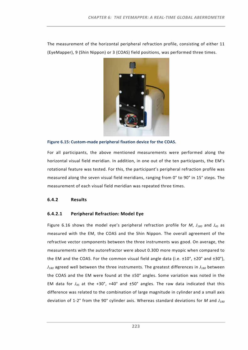
CHAPTER 6: THE EYEMAPPER: A REAL‐TIME GLOBAL ABERROMETER
223
The measurement of the horizontal peripheral refraction profile, consisting of either 11
(EyeMapper), 9 (Shin Nippon) or 3 (COAS) field positions, was performed three times.
Figure 6.15: Custom‐made peripheral fixation device for the COAS.
For all participants, the above mentioned measurements were performed along the
horizontal visual field meridian. In addition, in one out of the ten participants, the EM’s
rotational feature was tested. For this, the participant’s peripheral refraction profile was
measured along the seven visual field meridians, ranging from 0° to 90° in 15° steps. The
measurement of each visual field meridian was repeated three times.
6.4.2 Results
6.4.2.1 Peripheral Refraction: Model Eye
Figure 6.16 shows the model eye’s peripheral refraction profile for M, J180 and J45 as
measured with the EM, the COAS and the Shin Nippon. The overall agreement of the
refractive vector components between the three instruments was good. On average, the
measurements with the autorefractor were about 0.30D more myopic when compared to
the EM and the COAS. For the common visual field angle data (i.e. ±10°, ±20° and ±30°),
J180 agreed well between the three instruments. The greatest differences in J180 between
the COAS and the EM were found at the ±50° angles. Some variation was noted in the
EM data for J45 at the +30°, +40° and ±50° angles. The raw data indicated that this
difference was related to the combination of large magnitude in cylinder and a small axis
deviation of 1‐2° from the 90° cylinder axis. Whereas standard deviations for M and J180
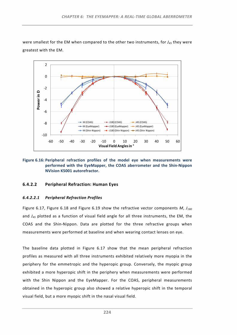
CHAPTER 6: THE EYEMAPPER: A REAL‐TIME GLOBAL ABERROMETER
224
were smallest for the EM when compared to the other two instruments, for J45 they were
greatest with the EM.
Figure 6.16: Peripheral refraction profiles of the model eye when measurements were performed with the EyeMapper, the COAS aberrometer and the Shin‐Nippon NVision K5001 autorefractor.
6.4.2.2 Peripheral Refraction: Human Eyes
6.4.2.2.1 Peripheral Refraction Profiles
Figure 6.17, Figure 6.18 and Figure 6.19 show the refractive vector components M, J180
and J45 plotted as a function of visual field angle for all three instruments, the EM, the
COAS and the Shin‐Nippon. Data are plotted for the three refractive groups when
measurements were performed at baseline and when wearing contact lenses on eye.
The baseline data plotted in Figure 6.17 show that the mean peripheral refraction
profiles as measured with all three instruments exhibited relatively more myopia in the
periphery for the emmetropic and the hyperopic group. Conversely, the myopic group
exhibited a more hyperopic shift in the periphery when measurements were performed
with the Shin Nippon and the EyeMapper. For the COAS, peripheral measurements
obtained in the hyperopic group also showed a relative hyperopic shift in the temporal
visual field, but a more myopic shift in the nasal visual field.
‐10
‐8
‐6
‐4
‐2
0
2
‐60 ‐50 ‐40 ‐30 ‐20 ‐10 0 10 20 30 40 50 60
Power in D
Visual Field Angles in °
M (COAS) J180 (COAS) J45 (COAS)
M (EyeMapper) J180 (EyeMapper) J45 (EyeMapper)
M (Shin‐Nippon) J180 (Shin Nippon) J45 (Shin Nippon)
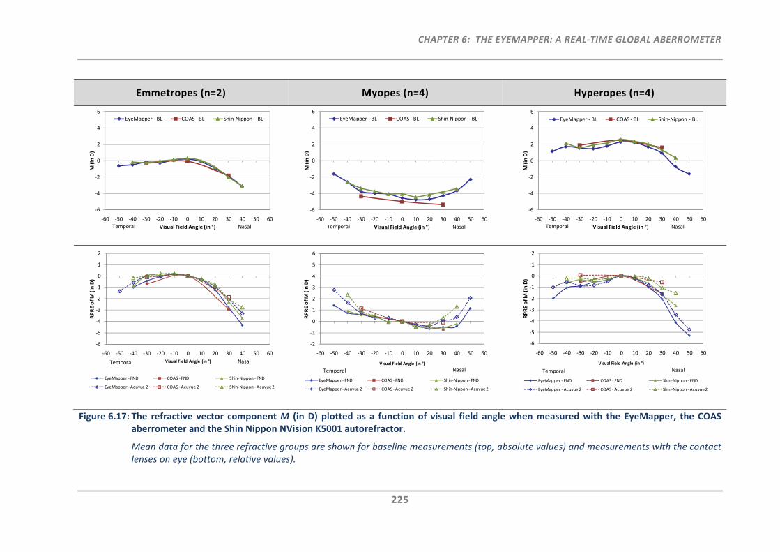
CHAPTER 6: THE EYEMAPPER: A REAL‐TIME GLOBAL ABERROMETER
225
Emmetropes (n=2) Myopes (n=4) Hyperopes (n=4)
Figure 6.17: The refractive vector component M (in D) plotted as a function of visual field angle when measured with the EyeMapper, the COAS aberrometer and the Shin Nippon NVision K5001 autorefractor.
Mean data for the three refractive groups are shown for baseline measurements (top, absolute values) and measurements with the contact lenses on eye (bottom, relative values).
‐6
‐4
‐2
0
2
4
6
‐60 ‐50 ‐40 ‐30 ‐20 ‐10 0 10 20 30 40 50 60
M (in D)
Visual Field Angle (in °)
EyeMapper ‐ BL COAS ‐ BL Shin‐Nippon ‐ BL
Temporal Nasal
‐6
‐4
‐2
0
2
4
6
‐60 ‐50 ‐40 ‐30 ‐20 ‐10 0 10 20 30 40 50 60
M (in D)
Visual Field Angle (in °)
EyeMapper ‐ BL COAS ‐ BL Shin‐Nippon ‐ BL
Temporal Nasal
‐6
‐4
‐2
0
2
4
6
‐60 ‐50 ‐40 ‐30 ‐20 ‐10 0 10 20 30 40 50 60
M (in D)
Visual Field Angle (in °)
EyeMapper ‐ BL COAS ‐ BL Shin‐Nippon ‐ BL
Temporal Nasal
‐6
‐5
‐4
‐3
‐2
‐1
0
1
2
‐60 ‐50 ‐40 ‐30 ‐20 ‐10 0 10 20 30 40 50 60
RPRE of M (in D)
Visual Field Angle (in °)
EyeMapper ‐ FND COAS ‐ FND Shin‐Nippon ‐ FND
EyeMapper ‐Acuvue 2 COAS ‐Acuvue 2 Shin‐Nippon ‐Acuvue 2
Temporal Nasal
‐2
‐1
0
1
2
3
4
5
6
‐60 ‐50 ‐40 ‐30 ‐20 ‐10 0 10 20 30 40 50 60
RPRE of M
(in D)
Visual Field Angle (in °)
EyeMapper ‐ FND COAS ‐ FND Shin‐Nippon ‐ FND
EyeMapper ‐Acuvue 2 COAS ‐Acuvue 2 Shin‐Nippon ‐Acuvue 2
Temporal Nasal
‐6
‐5
‐4
‐3
‐2
‐1
0
1
2
‐60 ‐50 ‐40 ‐30 ‐20 ‐10 0 10 20 30 40 50 60
RPRE of M
(in D)
Visual Field Angle (in °)
EyeMapper ‐ FND COAS ‐ FND Shin‐Nippon ‐ FND
EyeMapper ‐Acuvue 2 COAS ‐Acuvue 2 Shin‐Nippon ‐Acuvue 2
Temporal Nasal
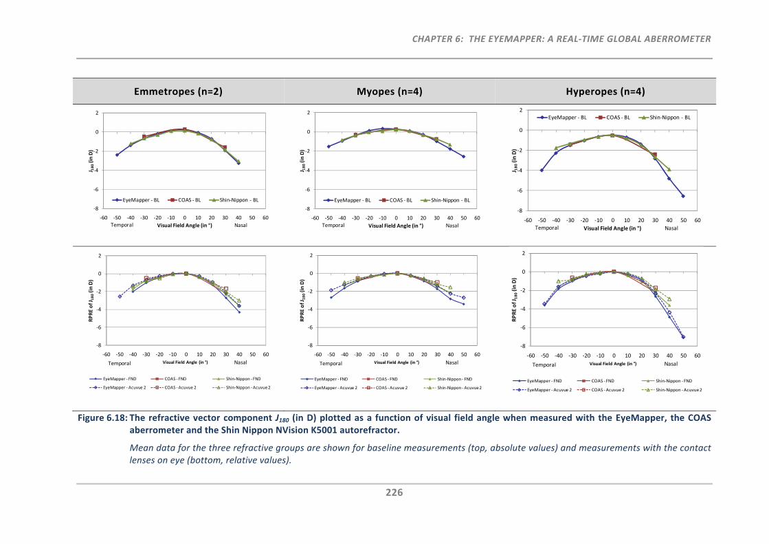
CHAPTER 6: THE EYEMAPPER: A REAL‐TIME GLOBAL ABERROMETER
226
Emmetropes (n=2) Myopes (n=4) Hyperopes (n=4)
Figure 6.18: The refractive vector component J180 (in D) plotted as a function of visual field angle when measured with the EyeMapper, the COAS aberrometer and the Shin Nippon NVision K5001 autorefractor.
Mean data for the three refractive groups are shown for baseline measurements (top, absolute values) and measurements with the contact lenses on eye (bottom, relative values).
‐8
‐6
‐4
‐2
0
2
‐60 ‐50 ‐40 ‐30 ‐20 ‐10 0 10 20 30 40 50 60
J 180(in D)
Visual Field Angle (in °)
EyeMapper ‐ BL COAS ‐ BL Shin‐Nippon ‐ BL
Temporal Nasal
‐8
‐6
‐4
‐2
0
2
‐60 ‐50 ‐40 ‐30 ‐20 ‐10 0 10 20 30 40 50 60
J 180(in D)
Visual Field Angle (in °)
EyeMapper ‐ BL COAS ‐ BL Shin‐Nippon ‐ BL
Temporal Nasal
‐8
‐6
‐4
‐2
0
2
‐60 ‐50 ‐40 ‐30 ‐20 ‐10 0 10 20 30 40 50 60
J 180(in D)
Visual Field Angle (in °)
EyeMapper ‐ BL COAS ‐ BL Shin‐Nippon ‐ BL
Temporal Nasal
‐8
‐6
‐4
‐2
0
2
‐60 ‐50 ‐40 ‐30 ‐20 ‐10 0 10 20 30 40 50 60
RPRE of J 180(in D)
Visual Field Angle (in °)
EyeMapper ‐ FND COAS ‐ FND Shin‐Nippon ‐ FND
EyeMapper ‐Acuvue 2 COAS ‐Acuvue 2 Shin‐Nippon ‐Acuvue 2
Temporal Nasal
‐8
‐6
‐4
‐2
0
2
‐60 ‐50 ‐40 ‐30 ‐20 ‐10 0 10 20 30 40 50 60
RPRE of J 180(in D)
Visual Field Angle (in °)
EyeMapper ‐ FND COAS ‐ FND Shin‐Nippon ‐ FND
EyeMapper ‐Acuvue 2 COAS ‐Acuvue 2 Shin‐Nippon ‐Acuvue 2
Temporal Nasal
‐8
‐6
‐4
‐2
0
2
‐60 ‐50 ‐40 ‐30 ‐20 ‐10 0 10 20 30 40 50 60
RPRE of J 180(in D)
Visual Field Angle (in °)
EyeMapper ‐ FND COAS ‐ FND Shin‐Nippon ‐ FND
EyeMapper ‐Acuvue 2 COAS ‐Acuvue 2 Shin‐Nippon ‐Acuvue 2
Temporal Nasal
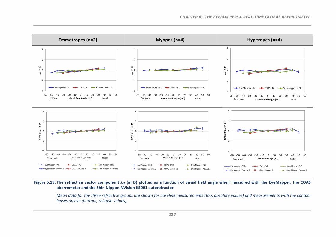
CHAPTER 6: THE EYEMAPPER: A REAL‐TIME GLOBAL ABERROMETER
227
Emmetropes (n=2) Myopes (n=4) Hyperopes (n=4)
Figure 6.19: The refractive vector component J45 (in D) plotted as a function of visual field angle when measured with the EyeMapper, the COAS aberrometer and the Shin Nippon NVision K5001 autorefractor.
Mean data for the three refractive groups are shown for baseline measurements (top, absolute values) and measurements with the contact lenses on eye (bottom, relative values).
‐4
‐2
0
2
4
‐60 ‐50 ‐40 ‐30 ‐20 ‐10 0 10 20 30 40 50 60
J 45(in D)
Visual Field Angle (in °)
EyeMapper ‐ BL COAS ‐ BL Shin‐Nippon ‐ BL
Temporal Nasal
‐4
‐2
0
2
4
‐60 ‐50 ‐40 ‐30 ‐20 ‐10 0 10 20 30 40 50 60
J 45(in D)
Visual Field Angle (in °)
EyeMapper ‐ BL COAS ‐ BL Shin‐Nippon ‐ BL
Temporal Nasal
‐4
‐2
0
2
4
‐60 ‐50 ‐40 ‐30 ‐20 ‐10 0 10 20 30 40 50 60
J 45(in D)
Visual Field Angle (in °)
EyeMapper ‐ BL COAS ‐ BL Shin‐Nippon ‐ BL
Temporal Nasal
‐4
‐2
0
2
4
‐60 ‐50 ‐40 ‐30 ‐20 ‐10 0 10 20 30 40 50 60
RPRE of J
45(in D)
Visual Field Angle (in °)
EyeMapper ‐ FND COAS ‐ FND Shin‐Nippon ‐ FND
EyeMapper ‐Acuvue 2 COAS ‐Acuvue 2 Shin‐Nippon ‐Acuvue 2
Temporal Nasal
‐4
‐2
0
2
4
‐60 ‐50 ‐40 ‐30 ‐20 ‐10 0 10 20 30 40 50 60
RPRE of J
45(in D)
Visual Field Angle (in °)
EyeMapper ‐ FND COAS ‐ FND Shin‐Nippon ‐ FND
EyeMapper ‐Acuvue 2 COAS ‐Acuvue 2 Shin‐Nippon ‐Acuvue 2
Temporal Nasal
‐4
‐2
0
2
4
‐60 ‐50 ‐40 ‐30 ‐20 ‐10 0 10 20 30 40 50 60
RPRE of J
45(in D)
Visual Field Angle (in °)
EyeMapper ‐ FND COAS ‐ FND Shin‐Nippon ‐ FND
EyeMapper ‐Acuvue 2 COAS ‐Acuvue 2 Shin‐Nippon ‐Acuvue 2
Temporal Nasal
CHAPTER 6: THE EYEMAPPER: A REAL‐TIME GLOBAL ABERROMETER
228
For the myopic group, the EM measured more plus (on‐axis 0.41D) when compared to
the COAS and more minus (on‐axis 0.52D) when compared to the Shin Nippon. For on‐
axis measurements, the same trend but with smaller differences was found in the
emmetropic group, where the shift of the COAS was 0.26D more plus and the shift of the
Shin Nippon was 0.13D more minus when compared to the EM. For the hyperopic group,
the EyeMapper measured more minus when compared to the COAS (0.20D) and the Shin
Nippon (0.31D).
In general, the baseline peripheral refraction profiles obtained with the three
instruments were in agreement. However, there were some obvious differences in M at
nasal 30° in the myopic group, where the COAS measured more minus than the other
two instruments (1.09D when compared to the EM, and 1.57D when compared to the
Shin Nippon) and at nasal 40° in the hyperopic group, where the EM measured more
minus (1.09D) when compared to the Shin Nippon.
In addition, Figure 6.17 shows the relative peripheral refraction profiles measured with
the two contact lenses on eye. For all refractive groups and for all three instruments a
difference in peripheral refraction profiles between the two lens types was detected.
Measurements with the FND lens on eye always showed a more myopic shift, when
compared to the measurements with the Acuvue 2 lens one eye. When compared to the
measurements obtained with the EM, the Shin Nippon measured a more hyperopic
peripheral refraction profile.
Figure 6.18 shows the peripheral refraction profiles for the refractive vector component
J180. All three instruments produced similar profiles for the three refractive groups,
which demonstrated the typical nasal‐temporal asymmetry of astigmatism across the
visual field. The hyperopic group showed the greatest peripheral astigmatism, followed
by the emmetropic and then the myopic group. The greatest difference in J180 (0.93D)
was found in the 40° nasal visual field for the hyperopic group between the Shin Nippon
and the EM.
The peripheral refraction profiles obtained with either contact lens type on eye showed
a similar trend for J180 as previously seen in M. Figure 6.18 demonstrates that in the
CHAPTER 6: THE EYEMAPPER: A REAL‐TIME GLOBAL ABERROMETER
229
emmetropic and myopic group, measurements with the FND lens on eye produced
greater peripheral J180 when compared to the measurements with the Acuvue 2 lens on
eye. A smaller difference between the two lens types was found in the hyperopic group
when measurements were performed using the EM. For all refractive groups, with and
without contact lenses on eye, the Shin Nippon measured less peripheral astigmatism
when compared to the EM.
The peripheral refraction profiles for the refractive vector component J45 are shown in
Figure 6.19. Apart from some fluctuations across the visual field, the baseline
measurements obtained from the three instruments compared well with each other.
Greatest fluctuations were found in the hyperopic group, the group which had the
greatest peripheral astigmatism (J180). The difference in relative J45 between the
peripheral refraction profiles obtained with the two contact lens types was small when
measured with all three instruments.
6.4.2.2.2 Repeatability
Figure 6.20 shows the coefficients of repeatability (2.77 × within participant SD, three
repeats) plotted for M, J180 and J45, for all three instruments, for all visual field angles
and for the with‐ and without‐contact lens condition. In general, it can be seen that
independent of the instrument used for the measurements, the coefficients were always
lower when measurements were performed without contact lenses on the eye.
Repeatability generally decreased with increase in peripheral field angle.
For the refractive vector components M and J180, the coefficients of repeatability were
larger for measurements obtained with the Shin Nippon when compared to those
obtained with the EM. This was the case for measurements performed with and without
contact lenses on the eye. For some visual field positions (e.g. for M at temporal and
nasal 40°, without contact lens), the coefficients reached twice those for the Shin Nippon
when compared to the EM. For most, but not all visual field positions, the coefficients of
repeatability for J45 were also larger for the Shin Nippon when compared to the EM.
The coefficients of repeatability for the three visual field positions (0° and ±30°)
measured with the COAS compared to those to the EM, obtained without contact lenses
on eye were very similar. However, in relation to the “with contact lens” measurements,

CHAPTER 6: THE EYEMAPPER: A REAL‐TIME GLOBAL ABERROMETER
230
the coefficients for M were larger for the COAS when compared to the EM and the
coefficients for J180 and J45 were larger for the EM when compared to the COAS.
Without Contact Lens on Eye With Contact Lens on Eye
Coefficient of
Repeatability for M
Coefficient of
Repeatability for J 1
80
Coefficient of
Repeatability for J 4
5
Figure 6.20: Coefficients of repeatability for M, J180 and J45 (in D).
For each visual field angle and each instrument, data were plotted for measurements performed without and with contact lenses on eye.
6.4.2.2.3 Reproducibility
Figure 6.21 shows the peripheral refraction profile for M of one participant as measured
with the EM by two different operators at two different occasions.
The participant’s distinct peripheral refraction profile was noticeable for all conditions,
with and without contact lens wear and when measurements were performed by
operator 1 (visit 1) and operator 2 (visit 2). On average, measurements performed by
0.00
0.50
1.00
1.50
2.00
2.50
3.00
3.50
‐50 ‐40 ‐30 ‐20 ‐10 0 10 20 30 40 50
Visual Field Angle (°)
EyeMapper COAS Shin Nippon
Temporal NasalTemporal NasalTemporal Nasal
0.00
0.50
1.00
1.50
2.00
2.50
3.00
3.50
‐50 ‐40 ‐30 ‐20 ‐10 0 10 20 30 40 50
Visual Field Angle (°)
EyeMapper COAS Shin Nippon
Temporal NasalTemporal NasalTemporal Nasal
0.00
0.20
0.40
0.60
0.80
1.00
1.20
1.40
1.60
‐50 ‐40 ‐30 ‐20 ‐10 0 10 20 30 40 50
Visual Field Angle (°)
EyeMapper COAS Shin Nippon
Temporal NasalTemporal NasalTemporal NasalTemporal Nasal
0.00
0.20
0.40
0.60
0.80
1.00
1.20
1.40
1.60
‐50 ‐40 ‐30 ‐20 ‐10 0 10 20 30 40 50
Visual Field Angle (°)
EyeMapper COAS Shin Nippon
Temporal NasalTemporal NasalTemporal NasalTemporal Nasal
0.00
0.20
0.40
0.60
0.80
1.00
1.20
1.40
1.60
‐50 ‐40 ‐30 ‐20 ‐10 0 10 20 30 40 50
Visual Field Angle (°)
EyeMapper COAS Shin Nippon
Temporal NasalTemporal NasalTemporal NasalTemporal NasalTemporal Nasal
0.00
0.20
0.40
0.60
0.80
1.00
1.20
1.40
1.60
‐50 ‐40 ‐30 ‐20 ‐10 0 10 20 30 40 50
Visual Field Angle (°)
EyeMapper COAS Shin Nippon
Temporal NasalTemporal NasalTemporal NasalTemporal NasalTemporal Nasal

CHAPTER 6: THE EYEMAPPER: A REAL‐TIME GLOBAL ABERROMETER
231
operator 1 were slightly more myopic when compared to measurements performed by
operator 2 (average difference 0.17D at baseline, 0.15D with FND and 0.04D with Acuvue
2) with standard deviations of the repeats being similar for each operator [operator 1:
±0.24D (BL), ±0.24D (FND), ±0.25D (Acuvue 2) and for operator 2: ±0.22D (BL), ±0.24D
(FND), ±0.41D (Acuvue 2)].
Figure 6.21: The peripheral refraction profile for M measured by two independent operators on two different occasions.
Data are shown for one participant (mean of three repeats).
Table 6.4 provides a summary of the coefficients of reproducibility (2.77 × within
operator SD) for M, J180 and J45. Overall, reproducibility for M and J180 was best for
measurements performed with the Acuvue 2 lens, followed by the measurements
performed at baseline, and then the FND lens. Reproducibility for J45 was best at
baseline, followed by the FND lens and then Acuvue 2.
Table 6.4: Summary of the coefficients of reproducibility (in D).
Coefficient of Reproducibility
Baseline
M 1.12
J180 0.73
J45 0.37
Acuvue 2
M 0.86
J180 0.72
J45 0.57
FND
M 1.41
J180 0.73
J45 0.45
‐3
‐2
‐1
0
1
2
3
4
5
6
7
8
‐50 ‐40 ‐30 ‐20 ‐10 0 10 20 30 40 50
M in D
Visual Field Angle
Operator 1 ‐ BL Operator 1 ‐Acuvue 2 Operator 1 ‐Night & Day
Operator 2 ‐ BL Operator 2 ‐Acuvue 2 Operator 2 ‐Night & Day
Temporal Nasal
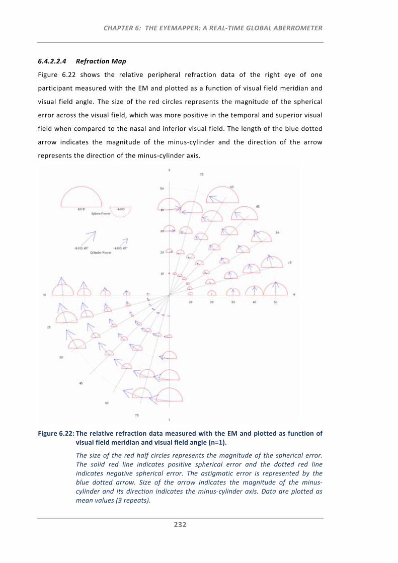
CHAPTER 6: THE EYEMAPPER: A REAL‐TIME GLOBAL ABERROMETER
232
6.4.2.2.4 Refraction Map
Figure 6.22 shows the relative peripheral refraction data of the right eye of one
participant measured with the EM and plotted as a function of visual field meridian and
visual field angle. The size of the red circles represents the magnitude of the spherical
error across the visual field, which was more positive in the temporal and superior visual
field when compared to the nasal and inferior visual field. The length of the blue dotted
arrow indicates the magnitude of the minus‐cylinder and the direction of the arrow
represents the direction of the minus‐cylinder axis.
Figure 6.22: The relative refraction data measured with the EM and plotted as function of visual field meridian and visual field angle (n=1).
The size of the red half circles represents the magnitude of the spherical error. The solid red line indicates positive spherical error and the dotted red line indicates negative spherical error. The astigmatic error is represented by the blue dotted arrow. Size of the arrow indicates the magnitude of the minus‐cylinder and its direction indicates the minus‐cylinder axis. Data are plotted as mean values (3 repeats).
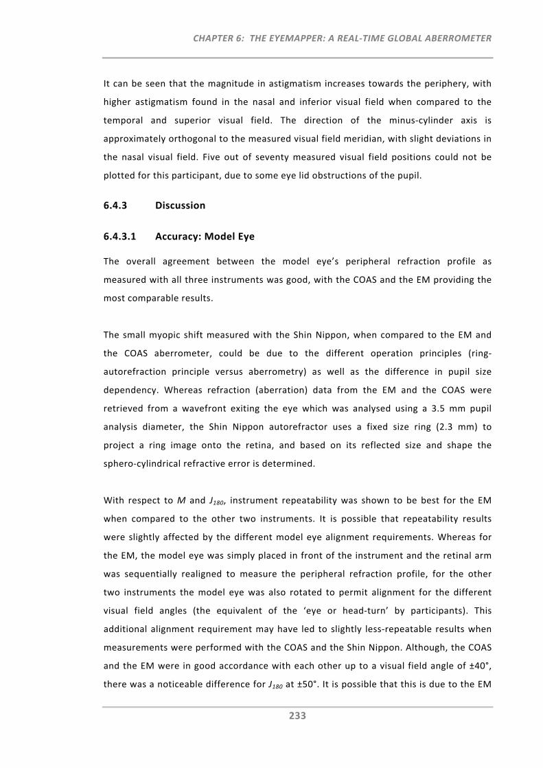
CHAPTER 6: THE EYEMAPPER: A REAL‐TIME GLOBAL ABERROMETER
233
It can be seen that the magnitude in astigmatism increases towards the periphery, with
higher astigmatism found in the nasal and inferior visual field when compared to the
temporal and superior visual field. The direction of the minus‐cylinder axis is
approximately orthogonal to the measured visual field meridian, with slight deviations in
the nasal visual field. Five out of seventy measured visual field positions could not be
plotted for this participant, due to some eye lid obstructions of the pupil.
6.4.3 Discussion
6.4.3.1 Accuracy: Model Eye
The overall agreement between the model eye’s peripheral refraction profile as
measured with all three instruments was good, with the COAS and the EM providing the
most comparable results.
The small myopic shift measured with the Shin Nippon, when compared to the EM and
the COAS aberrometer, could be due to the different operation principles (ring‐
autorefraction principle versus aberrometry) as well as the difference in pupil size
dependency. Whereas refraction (aberration) data from the EM and the COAS were
retrieved from a wavefront exiting the eye which was analysed using a 3.5 mm pupil
analysis diameter, the Shin Nippon autorefractor uses a fixed size ring (2.3 mm) to
project a ring image onto the retina, and based on its reflected size and shape the
sphero‐cylindrical refractive error is determined.
With respect to M and J180, instrument repeatability was shown to be best for the EM
when compared to the other two instruments. It is possible that repeatability results
were slightly affected by the different model eye alignment requirements. Whereas for
the EM, the model eye was simply placed in front of the instrument and the retinal arm
was sequentially realigned to measure the peripheral refraction profile, for the other
two instruments the model eye was also rotated to permit alignment for the different
visual field angles (the equivalent of the ‘eye or head‐turn’ by participants). This
additional alignment requirement may have led to slightly less‐repeatable results when
measurements were performed with the COAS and the Shin Nippon. Although, the COAS
and the EM were in good accordance with each other up to a visual field angle of ±40°,
there was a noticeable difference for J180 at ±50°. It is possible that this is due to the EM
CHAPTER 6: THE EYEMAPPER: A REAL‐TIME GLOBAL ABERROMETER
234
using a more advanced wavefront sensor featuring higher resolution/sampling and wider
dynamic range than the COAS. Although, a ray‐tracing approach was attempted to
calculate the theoretical peripheral refraction profiles for the model eye by use of the
previous equations in ZEMAX (Section 4.2.1.2), the profiles for M and J180 were
increasingly more positive as field angle increased when compared to the profiles
measured with the three instruments. This difference between the results obtained for
the analytical and physical model eyes requires further investigation. The COAS
instrument is generally considered the reference standard for central ocular
aberrometry.165 On the basis that the model eye data obtained from the EM were in
good agreement and showed even better repeatability when compared to the COAS
measurements, it was demonstrated that the EM is an accurate and repeatable
instrument for central and peripheral refraction measurements.
6.4.3.2 Peripheral Refraction Profiles and Repeatability: Human Eyes
As scattering, dispersion and light efficiency differ between human eyes and model eyes,
the second part of this validation study aimed to also perform measurements in human
eyes. It should be noted however, that when measuring human eyes, several other
inherent factors can affect measurements which may be assessed in more detail in
future. These factors include, for example, the impact of: lead and lag of
accommodation, clarity in optical media, the size and location of the blind spot area,
fluctuating fixation, pupil size, eye lid shape etc.
The first aim of the current validation study on human eyes was to assess the
measurements and repeatability of peripheral refraction profiles obtained with and
without contact lenses on eye, for hyperopic, emmetropic and myopic eyes when using
the three instruments, the EM, the COAS and the Shin Nippon.
Due to the COAS and the Shin Nippon being dedicated on‐axis instruments, some
modifications to the set‐up and alignment procedure were required to permit
measurement of the peripheral optics of the eye. Certain instrument boundaries did not
permit the number of visual field angle measurements possible with the EM. While the
COAS could only measure two peripheral positions (±30°), Shin Nippon measurements
were possible up to ±40°. Due to some missing data points for the Shin Nippon and the
COAS, the peripheral refraction profiles as obtained with the EM could not be compared
CHAPTER 6: THE EYEMAPPER: A REAL‐TIME GLOBAL ABERROMETER
235
entirely. Perhaps a different peripheral refraction set‐up for the COAS, such as used by
Mathur et al.123 or by Baskaran et al.130 (COAS HD‐VR) could be used in a future
validation study in order to permit the measurement and comparison of more peripheral
visual field angles.
All peripheral refraction profiles were assessed in terms of refractive power vectors,
which overall showed good agreement between the measurements obtained from the
three instruments. Some on‐axis differences were found for M at baseline for the
different instruments and refractive groups. It was shown that for both the myopic and
the emmetropic group, the COAS measured more minus when compared to the EM, and
the EM measured more minus when compared to the Shin Nippon. This effect was
greater for the younger myopic group when compared to the young emmetropic group,
but this trend was not seen in the older hyperopic group. It is reasonable to suggest that
this difference was caused by the impact of accommodation and instrument myopia in
the younger groups when measurements were performed using the EM and the COAS.
Whereas the Shin Nippon is an open‐view autorefractor, the EM and the COAS are
closed‐view instruments with a working distance of 100 mm and 50 mm, respectively.
This suggests that the COAS, with its smaller working distance may have produced
greater instrument myopia when compared to the EM. That this on‐axis difference is
likely to be due to some accommodation effect is also supported by the results obtained
on the model eye, which showed an opposite shift in M between instruments, with the
Shin Nippon producing a small myopic shift when compared to the EM and the COAS.
When assessing the peripheral refraction profiles with contact lenses on eye, all
instruments indicated the same anticipated trend. The FND lens, which exhibits an
increase in positive power towards the periphery, produced a more myopic peripheral
refraction profile when compared to the Acuvue 2 lens. Conversely, the Acuvue 2 lens,
which exhibits an increase in negative power towards the periphery, produced a more
positive peripheral refraction profile when compared to the Focus Night and Day lens.
With respect to J180, there was a trend for the Shin Nippon measuring less peripheral
astigmatism (J180), when compared to the EM. This was particularly evident for larger
visual field angles and in hyperopic eyes, which exhibited a large degree of peripheral
astigmatism. However, this effect was not observed in the previous measurements
CHAPTER 6: THE EYEMAPPER: A REAL‐TIME GLOBAL ABERROMETER
236
performed on the model eye, which also exhibited large amounts of peripheral
astigmatism. Nevertheless, Shin Nippon measurements performed with the model eye
were only possible for field angles up to ±30°. Moreover, the retina of the model eye
differs to the human retina, as it is plane and not curved in shape. Thus, one reason for
the J180 difference found in human eyes between the Shin Nippon and the EM,
particularly at large peripheral angles, may be explained by the previous modelling
approach for which a schematic model eye with curved retina was used.
It was demonstrated that when using the ring‐autorefraction principle the peripheral
retinal ring images are asymmetrically distorted (Section 5.4.3.2.2) and that this
distortion could potentially interfere with the sphero‐cylindrical refraction output
provided by the autorefractor. For measurements with contact lenses on eye the same
difference was found, with the EM measuring more minus for M and J180 when compared
to the Shin Nippon.
Besides some small fluctuations across the peripheral refraction profile, the overall
profile of J45 was consistent for all three instruments. The greater J45 fluctuations found
in the hyperopic group can be explained by a combination of greater magnitude of
peripheral astigmatism (J180) and a small deviation from the 90° cylinder axis.
With respect to repeatability, the EM produced more repeatable results when compared
to the Shin Nippon. This was particularly so for measurements performed without
contact lenses on eye. There are many factors that could have led to the lower
repeatability when using the Shin Nippon including the decreased tolerance to pupil
misalignment when performing peripheral refraction measurements using the Shin
Nippon (Chapter 2 and 3). Unlike with the EM, where a fast measurement scan is
performed, with the Shin Nippon, measurements were performed sequentially for each
visual field position and thus numerous re‐alignments were required by both participants
and operators. Another reason, as in Chapter 5, could be related to the ring‐
autorefraction principle being not a suitable operation principle, when performing
peripheral refraction measurements.
Although, it was demonstrated that measurements with contact lenses on eye are
possible with the EM, repeatability is still lower when compared to baseline
CHAPTER 6: THE EYEMAPPER: A REAL‐TIME GLOBAL ABERROMETER
237
measurements. One factor could be lens movement on the eye or small amounts of lens
prism, but more work is required to further understand and improve the accuracy of
measuring peripheral refraction profiles with contact lenses on eye.
6.4.3.3 Reproducibility
For one participant, measurements with the EM were repeated on a second occasion by
an independent operator. The measured peripheral refraction profiles were similar
between operators for all conditions, whether measurements were performed with or
without contact lenses on eye. However, there was a small trend for operator 1
measuring more myopic peripheral refraction profiles compared to operator 2
(difference < 0.17D). This may be related to a consistent small difference in pupil
alignment between both operators, which would also explain why the standard
deviations of the repeats were similar for both operators. The small difference in M
measured between operators resulted in the higher coefficients of reproducibility. It
should be noted, however, that due to the small sample size of only one participant, the
current analysis on instrument reproducibility is limited. A larger sample sized study,
where measurements are performed by more than two operators, is therefore
recommended to provide clinically more useful information on the EM’s reproducibility.
6.5 Discussion
6.5.1 Peripheral Refraction Instruments
During the last few years, interest in the measurement of peripheral refractive errors has
increased enormously. For the measurement of peripheral refraction, commercially
available instruments are commonly used (Chapter 1), which when adopted for this
purpose require some form of modification to the instrument set‐up and alignment
procedure. However, alignment requirements, for both, participants (eye/head turn) and
operators (pupil/instrument) can become very time consuming when using such
instruments, and the precise alignment of the pupil was found to be a critical parameter
in peripheral refractometry (Chapter 2). Hence, a new peripheral refraction instrument,
the EyeMapper, was developed with the aim to perform fast and accurate refraction
measurements across a wide visual field.
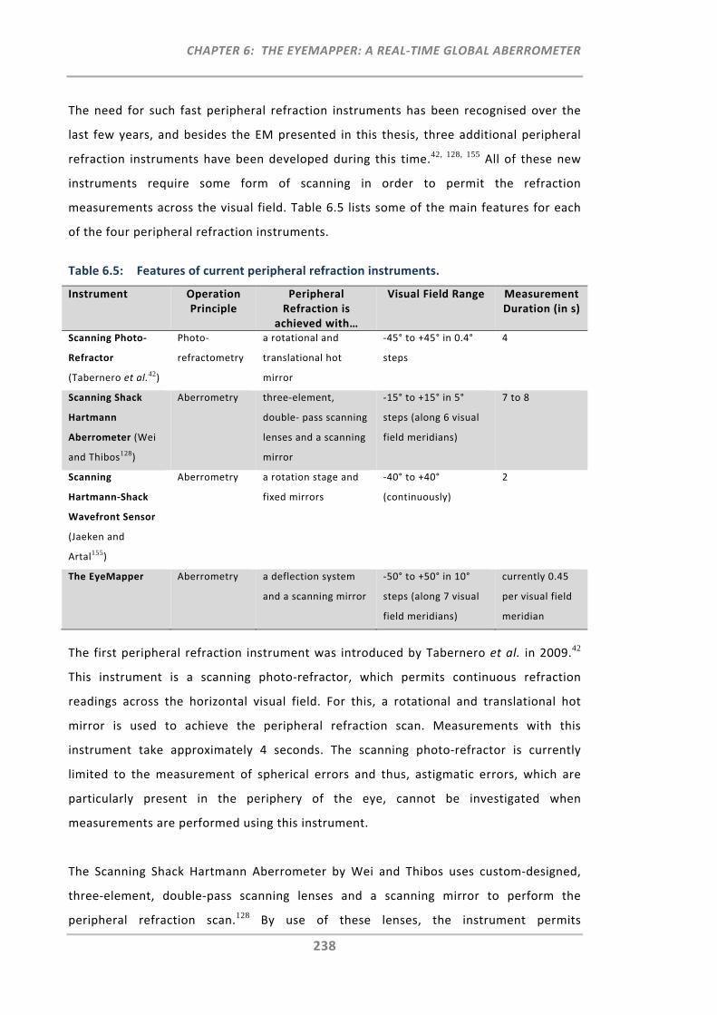
CHAPTER 6: THE EYEMAPPER: A REAL‐TIME GLOBAL ABERROMETER
238
The need for such fast peripheral refraction instruments has been recognised over the
last few years, and besides the EM presented in this thesis, three additional peripheral
refraction instruments have been developed during this time.42, 128, 155 All of these new
instruments require some form of scanning in order to permit the refraction
measurements across the visual field. Table 6.5 lists some of the main features for each
of the four peripheral refraction instruments.
Table 6.5: Features of current peripheral refraction instruments.
Instrument Operation Principle
Peripheral Refraction is
achieved with…
Visual Field Range Measurement Duration (in s)
Scanning Photo‐
Refractor
(Tabernero et al.42)
Photo‐
refractometry
a rotational and
translational hot
mirror
‐45° to +45° in 0.4°
steps
4
Scanning Shack
Hartmann
Aberrometer (Wei
and Thibos128)
Aberrometry three‐element,
double‐ pass scanning
lenses and a scanning
mirror
‐15° to +15° in 5°
steps (along 6 visual
field meridians)
7 to 8
Scanning
Hartmann‐Shack
Wavefront Sensor
(Jaeken and
Artal155)
Aberrometry a rotation stage and
fixed mirrors
‐40° to +40°
(continuously)
2
The EyeMapper Aberrometry a deflection system
and a scanning mirror
‐50° to +50° in 10°
steps (along 7 visual
field meridians)
currently 0.45
per visual field
meridian
The first peripheral refraction instrument was introduced by Tabernero et al. in 2009.42
This instrument is a scanning photo‐refractor, which permits continuous refraction
readings across the horizontal visual field. For this, a rotational and translational hot
mirror is used to achieve the peripheral refraction scan. Measurements with this
instrument take approximately 4 seconds. The scanning photo‐refractor is currently
limited to the measurement of spherical errors and thus, astigmatic errors, which are
particularly present in the periphery of the eye, cannot be investigated when
measurements are performed using this instrument.
The Scanning Shack Hartmann Aberrometer by Wei and Thibos uses custom‐designed,
three‐element, double‐pass scanning lenses and a scanning mirror to perform the
peripheral refraction scan.128 By use of these lenses, the instrument permits
CHAPTER 6: THE EYEMAPPER: A REAL‐TIME GLOBAL ABERROMETER
239
measurements ranging from ‐15° to +15° in 5° steps along 6 visual field meridians. Thus,
a total of 37 refraction measurements can be obtained within 7 to 8 seconds. Currently,
however the central and all peripheral measurements along the horizontal meridian are
not possible as strong backward scattering of light interferes with the measurements.
Like Tabernero et al.’s scanning photo‐refractor, Jaeken and Artal’s open‐view scanning
wavefront sensor measures refraction continuously across the wide horizontal visual
field.155 This instrument comprises a combination of moving (rotation stage, a caging
system and a high speed camera) and fixed components (mirrors). As with the EM, one
design goal of this wavefront sensing technique was to maintain equal path lengths at
each measuring angle. A peripheral refraction scan with this instrument currently takes 2
seconds and further adjustments to the current instrument are required to provide a
clinically more useful version.
The EM uses a deflection system, which comprises numerous stationary mirrors and a
scanning mirror to permit the refraction scan across the visual field. This deflection
system presents some advantages over the other three instruments. Unlike the scanning
aberrometer by Wei and Thibos, where all peripheral measurements are performed via
the same double‐pass scanning lenses, the deflection system of the EM has individual
paths for each peripheral measurement angle and thus, permits measurements up to
±50°. Compared to the instruments by Tabernero et al. and Jaeken and Artal, which
require some moving elements to perform the peripheral refraction scan, the advantage
of the EM’s deflection system is that the scan can be performed very rapidly. In fact
although in the current study the EM’s measurement time was 0.75 seconds, latest
improvements to the instrument have increased the measurement speed even further
and the instrument permits now measurements in only 0.45 seconds. Consequently, the
impact of fluctuating accommodation and/or fluctuating fixation on the refraction
measurements is smallest with the EM compared to the other instruments. On the other
hand, the scanning principles used in the peripheral refraction instruments by Tabernero
et al. and Jaeken and Artal have the advantage that they permit continuous refraction
measurements, which allow the assessment of the complete peripheral refraction
profile. The main advantage of the Scanning Shack Hartmann Aberrometer by Wei and
Thibos is, that during one scan, this instrument permits measurements along 6 (currently
5) visual field meridians. Although the rotational feature of the EM also permits the
CHAPTER 6: THE EYEMAPPER: A REAL‐TIME GLOBAL ABERROMETER
240
measurement of the vertical and five oblique visual field meridians, these measurements
have to be performed independently from each other.
With respect to its size, appearance and user interface, the EM was designed to be used
in clinical practice by a clinician with minimal training. While there is potential for
further refinement of the design to make it a commercial instrument, the EM is closest
to a marketable clinical instrument for routine use.
When comparing the features of the current four peripheral refraction instruments, it is
evident that each instrument has its own advantages and disadvantages. Being in the
early development stages with some limitations still present, it is anticipated that more
refinements are soon to follow for each instrument. Ultimately, these peripheral
refraction instruments have the potential to be used as general myopia monitoring tools
not only in research institutions but also in clinical and optometric practices.
6.5.2 Limitations and Suggestions for Future Work
Being a prototype instrument, the EyeMapper has room for further improvement. The
knowledge gained during the design and development phase, in which many obstacles
had to be overcome, can now assist in the further refinement and testing of the
instrument. The following points list some of the current main limitations of the EM and,
where possible, provide suggestions to address them in either this prototype and/or
future instrument versions:
Peripheral refraction measurements on the model eye have shown that a small
cylinder axis deviation caused some fluctuations in the refractive vector
component J45, particularly at far‐peripheral angles. This is likely to be due to
some small mirror alignment errors in the deflection system which can and need
to be resolved.
The majority of mirrors used in the deflection system are aluminium coated,
front surface mirrors, with a reflectance of approximately 85% at the wavelength
of 830 nm. The use of silver mirrors with higher reflectivity would reduce light
loss, allowing a reduction in the power of the SLD.
CHAPTER 6: THE EYEMAPPER: A REAL‐TIME GLOBAL ABERROMETER
241
The current mechanical beam shutter used in the EM is noisy and a potential
source of vibrations. Replacement by a smoother and less noisy shutter is
suggested.
A slightly larger diameter lens (L1) for the on‐axis alignment would improve
alignment, particularly, when measurements need to be performed for very
large pupils (e.g. under cycloplegia).
The EM is designed with the aim to measure peripheral refraction over wide
angles of view (from ‐50° to +50°). However, in some cases measurements at far
peripheral angles may be not possible due to the participant’s eye lid obstructing
the pupil.
The validation study on the EM has shown that when performing measurements
using closed‐view refraction instruments, adequate autofogging mechanisms
have to be incorporated. With the fixation target being positioned on a movable
translation stage, it would not be difficult to move the target to such a position.
Whether or not a real open‐view set‐up can be incorporated into the EM
instrument, is to be assessed further.
Currently, the EM can measure visual field meridians ranging from 0° to 90° in
15° steps. Perhaps a different rotation method could be implemented in a
future instrument to also permit the measurements of the visual field meridians,
ranging from 0° to 180°.
The EM’s fixation path was designed with the aim to measure the peripheral
refraction profile for different accommodative states. Further work is required to
test this feature and to investigate its implications on visual science.
6.6 Conclusion
A new peripheral refraction instrument, the EyeMapper, was developed at the Brien
Holden Vision Institute, Sydney, Australia. The instrument’s optical design is based on
the wavefront sensing principle, a principle which was deemed to be most suitable for an
instrument dedicated to the measurement of peripheral refraction. By means of a
deflection system and a scanning mirror, this instrument is able to provide global
refraction (aberration) measurements, ranging from ‐50° to +50°, in 10° steps.
Following development of the EM, a peripheral refraction model eye with a rotational
and translational extended plane retina was used to assess instrument accuracy. When
CHAPTER 6: THE EYEMAPPER: A REAL‐TIME GLOBAL ABERROMETER
242
compared to refraction data obtained on a well‐calibrated commercially available
aberrometer, the results obtained with the EM were in good agreement and showed
overall better repeatability. Moreover, in 10 human eyes, measurements were
performed with and without contact lenses on eye, using three instruments; the
EyeMapper and the two commercially available instruments, the Shin Nippon and the
COAS. Overall, the comparability of the peripheral refraction profiles was good between
the instruments; however, the Shin Nippon measured slightly more positive M and J180
values with increasing visual field angle when compared to the EM. Better repeatability
for M and J180 was obtained with the EM, when compared to the Shin Nippon data. In
addition, the peripheral refraction profile of one participant was measured with the EM
by two different operators on two different occasions to demonstrate good
reproducibility.
Compared to other peripheral refraction instruments, the EyeMapper permits the fastest
peripheral refraction scan across the visual field requiring only 0.75 seconds. In addition,
its rotational feature permits the measurements of 7 visual field meridians and its
clinically user‐friendly design, makes it a great myopia monitoring tool for future studies.
CHAPTER 7: SUMMARY AND CONCLUSIONS
243
CHAPTER 7:
SUMMARY AND CONCLUSIONS
7.1 Significance of Peripheral Refractometry
With the rapidly increasing prevalence of myopia in many countries, the discovered link
between myopia development and peripheral refractive error has stimulated great
interest in the critical assessment and monitoring of the peripheral optics of the eye. It
has therefore become paramount for myopia research activities to be able to develop
techniques that measure both central and peripheral refraction, quickly and accurately.
Currently, however, there are several limitations with commercially available refraction
instruments for the measurement of peripheral refraction.
The aims of this thesis were to investigate methodological limitations of current
peripheral refraction techniques, and to introduce and explore new concepts to improve
peripheral refraction.
7.2 Current Limitations
When using conventional instruments for the measurement of peripheral refraction,
modifications and numerous time‐consuming re‐alignments are required, by both
participants and operators.
7.2.1 Participant‐Related Alignment Limitations
To permit the measurement of a particular peripheral visual field angle, the participant is
commonly asked to either turn the eye or the head towards a peripheral fixation target.
The use of two different alignment methods has raised the concern over whether
peripheral refraction measurements obtained through eye and head turn differ (Section
1.4). It was hypothesised that external muscles from the eye may potentially affect eye
turn measurements. Several studies, each based on different study protocols (peripheral
visual field angles, instrumentation, viewing duration, etc.) have sought to answer this
question. Due to the inconclusive results obtained between studies, it was
recommended that, where possible, head turn should be used for peripheral refraction
measurements (Chapter 1). A further limitation associated with participant alignment is
CHAPTER 7: SUMMARY AND CONCLUSIONS
244
the extensive testing time required, particularly when numerous peripheral positions
need to be measured for the determination of the participant’s peripheral refraction
profile. In general, the active and time‐consuming cooperation required by the subject
limits the use of commercially available instruments for the measurement of the
peripheral optics of the eye.
7.2.2 Operator‐Related Alignment Limitations
Besides the participant‐related alignment limitations, one aspect that had not yet been
investigated was whether alignment limitations also exist for the operator when
measuring peripheral refraction. By use of a conventional autorefractor (based on the
ring autorefraction principle) it was demonstrated that, as peripheral visual field angle
increased, tolerance to pupil misalignment by the operator decreased significantly, even
below normal alignment variability, making peripheral refraction measurements more
susceptible to error (Section 2.1). As a result it was concluded that precise pupil
alignment by the operator is critical to obtain accurate peripheral refraction results. In
addition, a three‐dimensional entrance pupil model demonstrated that the peripheral
entrance pupil shape is not elliptical, as currently assumed when aligning the instrument
(Section 2.3). This can lead, potentially, to small systematic alignment errors, particularly
at large peripheral angles.
With precise pupil alignment being such a significant parameter in peripheral
refractometry, a method that aimed to rectify pupil alignment related errors when using
conventional instruments was established, validated and tested (Chapter 3). This method
firstly required the development of a pupil alignment matrix, which was achieved by
measuring refractive error with a conventional autorefractor at pre‐defined pupil de‐
alignment positions for a number of selected visual field angles. In addition, the amount
of pupil misalignment was determined from the pupil alignment screen image, as
captured during the refraction measurement. The relevant correction algorithms for
pupil misalignment were derived from the matrix, and refraction values were corrected
with respect to the amount of pupil misalignment measured. Following correction of
pupil misalignment, the variability for the corrected mean peripheral refraction profile
was reduced by at least 25%. Despite the fact that the developed method was
demonstrated to reduce the variability caused by pupil misalignment, it is anticipated
CHAPTER 7: SUMMARY AND CONCLUSIONS
245
that further reductions can be achieved by refining the correction algorithms and by
eliminating the small image capture delay.
7.3 A New Approach
With the ultimate goal to overcome peripheral refraction measurement limitations
related to both the time‐consuming re‐alignment (off‐axis fixation) requirements by the
participant and the strict requirements for precise pupil alignment by the operator, a
new instrument concept was introduced; the EyeMapper (EM) (Chapter 4). The initial
aim of the EM was to perform a rapid refraction scan, ranging from ‐50° to +50° in 10°
steps, using ten stationary deflecting prisms and one scanning mirror. As with most
autorefractors that are currently adopted for peripheral refractometry, the objective was
to determine the sphero‐cylindrical refraction output by means of the ring‐
autorefraction operation principle. On the basis of the EM reference model eye, the
optical sub‐paths of the proposed EM instrument were designed using the optical system
design software ZEMAX. Specifically, five intertwined optical paths; the deflection
system, the illumination, reflection, pupil imaging and fixation paths, were designed and
evaluated with respect to the individual pre‐defined path criteria.
Prior to testing of this instrument concept, a number of additional functions and
components required sourcing and evaluation to ensure the safe and effective operation
of the proposed EM instrument (Chapter 5). This process included assessment of the on‐
and off‐axis ring scan illumination and its optical radiation safety limits, as well
assessment of the speed and precision of the image detection. As a preliminary
validation step for the optical design, image capture and image analysis, the critical
components required for the EM’s on‐axis ring‐autorefraction principle were assembled
and tested. Although its operation for on‐axis measurements was confirmed and cross‐
validated with a conventional autorefractor, an obstacle relating to the ring‐image
analysis was identified, which would impair one of the main goals of the EM; the
performance of a peripheral refraction scan in less than one second. Additional
experimental testing and modelling also revealed that peripheral higher order
aberrations have the potential to interfere with the sphero‐cylindrical refraction
readings obtained when using this ring‐autorefraction operation principle. A technique
that segregates higher and lower order aberrations was therefore deemed more suitable
for an instrument dedicated to measuring peripheral refraction.
CHAPTER 7: SUMMARY AND CONCLUSIONS
246
Based on the knowledge gained in Chapters 4 and 5, the optical and mechanical EM
design was updated to integrate the wavefront sensing principle. On the basis of the new
design, the first prototype instrument was built at the Brien Holden Vision Institute and
tested experimentally (Chapter 6). The updated EM instrument uses an intricate
arrangement of stationary mirrors and one scanning mirror that together permit global
(central and peripheral) refraction (aberration) measurements, ranging from ‐50° to +50°
in 10° steps. The rotational feature of the EM permits the measurements of seven visual
field meridians ranging from 0° to 90° in 15° steps. An entire peripheral refraction along
one visual field meridian scan can be completed within only 0.75 seconds, making it the
fastest of the four peripheral refraction instruments developed thus far. Finally, the EM
was validated by measuring peripheral refraction on a custom‐designed peripheral
refraction model eye and on 10 human eyes. Peripheral refraction profiles measured on
the custom‐designed model eye were in good agreement with the EM and a well‐
calibrated commercially available aberrometer. Improved repeatability was obtained
using the EM. Improved repeatability was also achieved with the EM when compared to
the Shin Nippon autorefractor for measurements performed on 10 human eyes. This was
true for measurements obtained with and without contact lenses on eye.
In summary, a new clinical instrument, the EyeMapper, was developed which permits
accurate, repeatable and reproducible real‐time global refraction measurements, which
are of particular importance for the monitoring and assessment of myopia progression.
7.4 Conclusions
This thesis comprises a body of work that has contributed to the improved
understanding of methodological limitations of current peripheral refraction techniques.
On the basis of the limitations identified, new methodologies for the advancement of
peripheral refractometry were introduced and explored. All the aims were achieved and
both hypotheses confirmed.
Findings from this thesis have reinforced the fact that when using an instrument for
purposes other than its intended use, it is not certain that the intrinsic application or
operation principle will generate accurate results when used in the modified fashion.
CHAPTER 7: SUMMARY AND CONCLUSIONS
247
This work has implications for numerous research activities; in particular, when the
interpretation of accurate peripheral refraction profiles is required, and where
longitudinal and/or large sample sized studies require a number of repeated
measurements. In the current quest to understand, monitor and control myopia
progression, the clinically robust, fast and accurate EM instrument presented in this
thesis, provides the most advanced tool for the measurement of peripheral refraction
profiles in large population‐based studies, as well as detailed investigations into
peripheral refraction profiles of individuals. It is anticipated that in the near future
applications for peripheral refraction instruments will be found not only in research
institutions but also in general eye care, for example, in assessing retinal image profiles,
in detecting children who are at risk of developing myopia, and in prescribing specific
optical devices with designs to eliminate peripheral hyperopia or myopia. In addition to
refractive error development and control, there are many other research areas related
to the peripheral optics of the eye for which the use of such a fast peripheral refraction
instrument could also be of great benefit, including optimising peripheral visual function
for low vision subjects with absolute central skotoma or in sport and life in general.

REFERENCES
248
REFERENCES
1. Schaeffel F, Glasser A, Howland HC. Accommodation, refractive error and eye growth in chickens. Vision Res 1988;28:639‐57.
2. Zhu X, Park TW, Winawer J, Wallman J. In a matter of minutes, the eye can know which
way to grow. Invest Ophthalmol Vis Sci 2005;46:2238‐41. 3. Stone RA, Pendrak K, Sugimoto R, Lin T, Gill AS, Capehart C, Liu J. Local patterns of image
degradation differentially affect refraction and eye shape in chick. Curr Eye Res 2006;31:91‐105.
4. Smith EL, 3rd, Hung LF, Huang J, Blasdel TL, Humbird TL, Bockhorst KH. Effects of optical
defocus on refractive development in monkeys: evidence for local, regionally selective mechanisms. Invest Ophthalmol Vis Sci 2010;51:3864‐73.
5. Diether S, Schaeffel F. Local changes in eye growth induced by imposed local refractive
error despite active accommodation. Vision Res 1997;37:659‐68. 6. Wallman J, Gottlieb MD, Rajaram V, Fugate‐Wentzek LA. Local retinal regions control
local eye growth and myopia. Science 1987;237:73‐7. 7. Hodos W, Kuenzel WJ. Retinal‐image degradation produces ocular enlargement in chicks.
Invest Ophthalmol Vis Sci 1984;25:652‐9. 8. Smith EL, 3rd, Huang J, Hung LF, Blasdel TL, Humbird TL, Bockhorst KH. Hemiretinal form
deprivation: evidence for local control of eye growth and refractive development in infant monkeys. Invest Ophthalmol Vis Sci 2009;50:5057‐69.
9. Smith EL, 3rd, Hung LF. The role of optical defocus in regulating refractive development
in infant monkeys. Vision Res 1999;39:1415‐35. 10. Smith EL, 3rd, Ramamirtham R, Qiao‐Grider Y, Hung LF, Huang J, Kee CS, Coats D, Paysse
E. Effects of foveal ablation on emmetropization and form‐deprivation myopia. Invest Ophthalmol Vis Sci 2007;48:3914‐22.
11. Fedtke C, Ehrmann K, Holden BA. A review of peripheral refraction techniques. Optom
Vis Sci 2009;86:429‐46. 12. Hoogerheide J, Rempt F, Hoogenboom WP. Acquired myopia in young pilots.
Ophthalmologica 1971;163:209‐15. 13. Logan NS, Gilmartin B, Wildsoet CF, Dunne MC. Posterior retinal contour in adult human
anisomyopia. Invest Ophthalmol Vis Sci 2004;45:2152‐62. 14. Lotmar W, Lotmar T. Peripheral astigmatism in the human eye: experimental data and
theoretical model predictions. J Opt Soc Am 1974;64:510‐3. 15. Millodot M. Effect of ametropia on peripheral refraction. Am J Optom Physiol Opt
1981;58:691‐5.

REFERENCES
249
16. Mutti DO, Hayes JR, Mitchell GL, Jones LA, Moeschberger ML, Cotter SA, Kleinstein RN, Manny RE, Twelker JD, Zadnik K. Refractive error, axial length, and relative peripheral refractive error before and after the onset of myopia. Invest Ophthalmol Vis Sci 2007;48:2510‐9.
17. Mutti DO, Sholtz RI, Friedman NE, Zadnik K. Peripheral refraction and ocular shape in
children. Invest Ophthalmol Vis Sci 2000;41:1022‐30. 18. Rempt F, Hoogerheide J, Hoogenboom WP. Peripheral retinoscopy and the skiagram.
Ophthalmologica 1971;162:1‐10. 19. Schmid GF. Variability of retinal steepness at the posterior pole in children 7‐15 years of
age. Curr Eye Res 2003;27:61‐8. 20. Stone RA, Flitcroft DI. Ocular shape and myopia. Ann Acad Med Singapore 2004;33:7‐15. 21. Millodot M, Lamont, A. Refraction of the periphery of the eye. J Opt Soc Am A
1974;64:110‐11. 22. Atchison DA, Pritchard N, Schmid KL, Scott DH, Jones CE, Pope JM. Shape of the retinal
surface in emmetropia and myopia. Invest Ophthalmol Vis Sci 2005;46:2698‐707. 23. Seidemann A, Schaeffel F, Guirao A, Lopez‐Gil N, Artal P. Peripheral refractive errors in
myopic, emmetropic, and hyperopic young subjects. J Opt Soc Am A Opt Image Sci Vis 2002;19:2363‐73.
24. Atchison DA, Pritchard N, Schmid KL. Peripheral refraction along the horizontal and
vertical visual fields in myopia. Vision Res 2006;46:1450‐8. 25. Gustafsson J, Terenius E, Buchheister J, Unsbo P. Peripheral astigmatism in emmetropic
eyes. Ophthalmic Physiol Opt 2001;21:393‐400. 26. Millodot M, Lamont A. Letter: Refraction of the periphery of the eye. J Opt Soc Am
1974;64:110‐11. 27. Wang YZ, Thibos LN, Lopez N, Salmon T, Bradley A. Subjective refraction of the
peripheral field using contrast detection acuity. J Am Optom Assoc 1996;67:584‐9. 28. Jackson DW, Paysse EA, Wilhelmus KR, Hussein MA, Rosby G, Coats DK. The effect of off‐
the‐visual‐axis retinoscopy on objective refractive measurement. Am J Ophthalmol 2004;137:1101‐4.
29. Atchison DA. Comparison of peripheral refractions determined by different instruments.
Optom Vis Sci 2003;80:655‐60. 30. Atchison DA, Pritchard N, White SD, Griffiths AM. Influence of age on peripheral
refraction. Vision Res 2005;45:715‐20. 31. Atchison DA, Scott DH. Monochromatic aberrations of human eyes in the horizontal
visual field. J Opt Soc Am A Opt Image Sci Vis 2002;19:2180‐4. 32. Atchison DA, Scott DH, Charman WN. Hartmann‐Shack technique and refraction across
the horizontal visual field. J Opt Soc Am A Opt Image Sci Vis 2003;20:965‐73. 33. Berntsen DA, Mutti DO, Zadnik K. Validation of aberrometry‐based relative peripheral
refraction measurements. Ophthalmic Physiol Opt 2008;28:83‐90.

REFERENCES
250
34. Calver R, Radhakrishnan H, Osuobeni E, O'Leary D. Peripheral refraction for distance and near vision in emmetropes and myopes. Ophthalmic Physiol Opt 2007;27:584‐93.
35. Charman WN, Jennings JA. Longitudinal changes in peripheral refraction with age.
Ophthalmic Physiol Opt 2006;26:447‐55. 36. Charman WN, Mountford J, Atchison DA, Markwell EL. Peripheral refraction in
orthokeratology patients. Optom Vis Sci 2006;83:641‐8. 37. Dunne MC, Misson GP, White EK, Barnes DA. Peripheral astigmatic asymmetry and angle
alpha. Ophthalmic Physiol Opt 1993;13:303‐5. 38. Jennings JA, Charman WN. Optical image quality in the peripheral retina. Am J Optom
Physiol Opt 1978;55:582‐90. 39. Love, Gilmartin, Dunne. Relative peripheral refractive error in adult myopia and
emmetropia. Ophthalmol Visual Sci Suppl 41, #1592 (ARVO abstract 2000) 2000. 40. Ma L, Atchison DA, Charman WN. Off‐axis refraction and aberrations following
conventional laser in situ keratomileusis. J Cataract Refract Surg 2005;31:489‐98. 41. Millodot M. Peripheral refraction in aphakic eyes. Am J Optom Physiol Opt 1984;61:586‐
9. 42. Tabernero J, Schaeffel F. More irregular eye shape in low myopia than in emmetropia.
Invest Ophthalmol Vis Sci 2009;50:4516‐22. 43. Chen X, Sankaridurg P, Donovan L, Lin Z, Li L, Martinez A, Holden B, Ge J. Characteristics
of peripheral refractive errors of myopic and non‐myopic Chinese eyes. Vision Res 2010;50:31‐5.
44. Walker TW, Mutti DO. The effect of accommodation on ocular shape. Optom Vis Sci
2002;79:424‐30. 45. Cheng HM, Singh OS, Kwong KK, Xiong J, Woods BT, Brady TJ. Shape of the myopic eye as
seen with high‐resolution magnetic resonance imaging. Optom Vis Sci 1992;69:698‐701. 46. Salchow DJ, Zirm ME, Stieldorf C, Parisi A. Comparison of objective and subjective
refraction before and after laser in situ keratomileusis. J Cataract Refract Surg 1999;25:827‐35.
47. Mathur A, Atchison DA. Influence of spherical intraocular lens implantation and
conventional laser in situ keratomileusis on peripheral ocular aberrations. J Cataract Refract Surg 2010;36:1127‐34.
48. Montes‐Mico R, Charman WN. Image quality and visual performance in the peripheral
visual field following photorefractive keratectomy. J Refract Surg 2002;18:14‐22. 49. Smith G, Atchison DA, Avudainayagam C, Avudainayagam K. Designing lenses to correct
peripheral refractive errors of the eye. J Opt Soc Am A Opt Image Sci Vis 2002;19:10‐8. 50. Smith EL, 3rd, Greeman N, Ho A, Holden B, inventors; Vision CRC Limited, Sydney (AU),
assignee. Methods and apparatuses for altering relative curvature of field and positions of peripheral, off‐axis focal positions. US patent US 7,025,460 B2. 2006 Mar. 17, 2009.
REFERENCES
251
51. Bara S, Navarro R. Wide‐field compensation of monochromatic eye aberrations: expected performance and design trade‐offs. J Opt Soc Am A Opt Image Sci Vis 2003;20:1‐10.
52. Tabernero J, Vazquez D, Seidemann A, Uttenweiler D, Schaeffel F. Effects of myopic
spectacle correction and radial refractive gradient spectacles on peripheral refraction. Vision Res 2009;49:2176‐86.
53. Lundström L, Manzanera S, Prieto PM, Ayala DB, Gorceix N, Gustafsson J, Unsbo P, Artal
P. Effect of optical correction and remaining aberrations on peripheral resolution acuity in the human eye. Opt Express 2007;15:12654‐61.
54. Gustafsson J, Unsbo P. Eccentric correction for off‐axis vision in central visual field loss.
Optom Vis Sci 2003;80:535‐41. 55. Lundström L, Gustafsson J, Unsbo P. Vision evaluation of eccentric refractive correction.
Optom Vis Sci 2007;84:1046‐52. 56. Lundström L, Unsbo P, Gustafsson J. Off‐axis wave front measurements for optical
correction in eccentric viewing. J Biomed Opt 2005;10:034002. 57. Lotmar W. Theoretical Eye Model with Aspherics. Journal of the Optical Society of
America 1971;61:1522. 58. Charman WN, Atchison DA. Decentred optical axes and aberrations along principal visual
field meridians. Vision Res 2009;49:1869‐76. 59. Scialfa CT, Leibowitz HW, Gish KW. Age differences in peripheral refractive error. Psychol
Aging 1989;4:372‐5. 60. Hung LF, Ramamirtham R, Huang J, Qiao‐Grider Y, Smith EL, 3rd. Peripheral refraction in
normal infant rhesus monkeys. Invest Ophthalmol Vis Sci 2008;49:3747‐57. 61. Mathur A, Atchison DA, Charman WN. Effects of age on peripheral ocular aberrations.
Opt Express 2010;18:5840‐53. 62. Baskaran K, Unsbo P, Gustafsson J. Influence of Age on Peripheral Ocular Aberrations.
Optom Vis Sci 2011. 63. Kang P, Gifford P, McNamara P, Wu J, Yeo S, Vong B, Swarbrick H. Peripheral refraction in
different ethnicities. Invest Ophthalmol Vis Sci 2010;51:6059‐65. 64. Mathur A, Atchison DA, Kasthurirangan S, Dietz NA, Luong S, Chin SP, Lin WL, Hoo SW.
The influence of oblique viewing on axial and peripheral refraction for emmetropes and myopes. Ophthalmic Physiol Opt 2009;29:155‐61.
65. Radhakrishnan H, Charman WN. Refractive changes associated with oblique viewing and
reading in myopes and emmetropes. J Vis 2007;7:5. 66. Radhakrishnan H, Charman WN. Peripheral refraction measurement: does it matter if
one turns the eye or the head? Ophthalmic Physiol Opt 2008;28:73‐82. 67. Lundström L, Mira‐Agudelo A, Artal P. Peripheral optical errors and their change with
accommodation differ between emmetropic and myopic eyes. J Vis 2009;9:1‐11. 68. Ferree R, Hardy. Refraction for the peripheral field of vision. Archives of Ophthalmology
1931;5:717‐31.
REFERENCES
252
69. Atchison DA. Third‐Order Theory of Spectacle Lenses Applied to Correction of Peripheral Refractive Errors. Optom Vis Sci 2011;88:E227‐E33.
70. Smith G, Millodot M, McBrien N. The effect of accommodation on oblique astigmatism
and field curvature of the human eye. Clinical & Experimental Optometry 1988;71:119‐25.
71. Whatham A, Zimmermann F, Martinez A, Delgado S, Lazon de la Jara P, Sankaridurg P, Ho
A. Influence of accommodation on off‐axis refractive errors in myopic eyes. J Vis 2009;9:1‐13.
72. Ho A, Zimmermann F, Whatham A, Martinez A, Delgado S, de la Jara P, Sankaridurg P.
Change in Peripheral Refraction and Curvature of Filed of the Human Eye with Accommodation. Proc of SPIE 2009;7163:716318‐1‐5.
73. Davies LN, Mallen EA. Influence of accommodation and refractive status on the
peripheral refractive profile. Br J Ophthalmol 2009;93:1186‐90. 74. Tabernero J, Schaeffel F. Fast scanning photoretinoscope for measuring peripheral
refraction as a function of accommodation. J Opt Soc Am A Opt Image Sci Vis 2009;26:2206‐10.
75. Queiros A, Jorge J, Gonzalez‐Meijome JM. Influence of fogging lenses and cycloplegia on
peripheral refraction. J Optom 2009;2:83‐9. 76. Smith G, Lu CW. Peripheral power errors and astigmatism of eyes corrected with
intraocular lenses. Optom Vis Sci 1991;68:12‐21. 77. Atchison DA, Mathur A, Read SA, Walker MI, Newman AR, Tanos PP, McLennan RT, Tran
AH. Peripheral ocular aberrations in mild and moderate keratoconus. Invest Ophthalmol Vis Sci 2010;51:6850‐7.
78. Mutti DO, Sinnott LT, Mitchell GL, Jones‐Jordan LA, Moeschberger ML, Cotter S,
Kleinstein RN, Manny RE, Twelker D, Zadnik K. Relative peripheral refractive error and the risk of onset and progression of myopia in children. Invest Ophthalmol Vis Sci 2010.
79. Mathur A, Atchison DA. Effect of orthokeratology on peripheral aberrations of the eye.
Optom Vis Sci 2009;86:E476‐84. 80. Queiros A, Gonzalez‐Meijome JM, Jorge J, Villa‐Collar C, Gutierrez AR. Peripheral
refraction in myopic patients after orthokeratology. Optom Vis Sci 2010;87:323‐9. 81. Shen J, Clark CA, Soni PS, Thibos LN. Peripheral refraction with and without contact lens
correction. Optom Vis Sci 2010;87:642‐55. 82. Sankaridurg P, Donovan L, Varnas S, Ho A, Chen X, Martinez A, Fisher S, Lin Z, Smith EL,
3rd, Ge J, Holden B. Spectacle Lenses Designed to Reduce Progression of Myopia: 12‐Month Results. Optom Vis Sci 2010.
83. Lin Z, Martinez A, Chen X, Li L, Sankaridurg P, Holden BA, Ge J. Peripheral defocus with
single‐vision spectacle lenses in myopic children. Optom Vis Sci 2010;87:4‐9. 84. Young T. On the mechanism of the eye. Phils Trans Roy Soc Lond (Biol) 1801;91:23‐88. 85. Choi SS, Garner LF, Enoch JM. The relationship between the Stiles‐Crawford effect of the
first kind (SCE‐I) and myopia. Ophthalmic Physiol Opt 2003;23:465‐72.

REFERENCES
253
86. Clarke FJJ. A study of Troxler's Effect. Journal of Modern Optics 1960;7. 87. Troxler IPV. Über das Verschwinden gegebener Gegenstände innerhalb unseres
Gesichtskreises. Ophthalmologische Bibliothek 1804;2:1‐53. 88. Read SA, Collins MJ, Carney LG. The influence of eyelid morphology on normal corneal
shape. Invest Ophthalmol Vis Sci 2007;48:112‐9. 89. Kame RT, Jue TS, Shigekuni DM. A longitudinal study of corneal astigmatism changes in
Asian eyes. J Am Optom Assoc 1993;64:215‐9. 90. Buehren T, Collins MJ, Carney LG. Near work induced wavefront aberrations in myopia.
Vision Res 2005;45:1297‐312. 91. Read SA, Collins MJ, Carney LG. A review of astigmatism and its possible genesis. Clin Exp
Optom 2007;90:5‐19. 92. Campbell FW, Gubisch RW. Optical quality of the human eye. J Physiol 1966;186:558‐78. 93. Artal P, Derrington AM, Colombo E. Refraction, aliasing, and the absence of motion
reversals in peripheral vision. Vision Res 1995;35:939‐47. 94. Wang YZ, Thibos LN, Bradley A. Effects of refractive error on detection acuity and
resolution acuity in peripheral vision. Invest Ophthalmol Vis Sci 1997;38:2134‐43. 95. Millodot M, Johnson CA, Lamont A, Leibowitz HW. Effect of dioptrics on peripheral visual
acuity. Vision Res 1975;15:1357‐62. 96. Frisen L, Nikolajeff F. Properties of high‐pass resolution perimetry targets. Acta
Ophthalmol (Copenh) 1993;71:320‐6. 97. Leibowitz HW, Johnson CA, Isabelle E. Peripheral motion detection and refractive error.
Science 1972;177:1207‐8. 98. Johnson CA, Leibowitz HW. Practice, refractive error, and feedback as factors influencing
peripheral motion thresholds. Perception & Psychophysics 1974;15:276‐80. 99. Lundström L, Gustafsson J, Svensson I, Unsbo P. Assessment of objective and subjective
eccentric refraction. Optom Vis Sci 2005;82:298‐306. 100. Anderson RS, Thibos LN. Relationship between acuity for gratings and for tumbling‐E
letters in peripheral vision. J Opt Soc Am A Opt Image Sci Vis 1999;16:2321‐33. 101. Thibos LN, Still DL, Bradley A. Characterization of spatial aliasing and contrast sensitivity
in peripheral vision. Vision Res 1996;36:249‐58. 102. Rovamo J, Virsu V, Laurinen P, Hyvarinen L. Resolution of gratings oriented along and
across meridians in peripheral vision. Invest Ophthalmol Vis Sci 1982;23:666‐70. 103. Chui TY, Yap MK, Chan HH, Thibos LN. Retinal stretching limits peripheral visual acuity in
myopia. Vision Res 2005;45:593‐605. 104. Rempt F, Hoogerheide J, Hoogenboom WP. Influence of correction of peripheral
refractive errors on peripheral static vision. Ophthalmologica 1976;173:128‐35.

REFERENCES
254
105. Jennings JA, Charman WN. Off‐axis image quality in the human eye. Vision Res 1981;21:445‐55.
106. Navarro R, Artal P, Williams DR. Modulation transfer of the human eye as a function of
retinal eccentricity. J Opt Soc Am A 1993;10:201‐12. 107. Guirao A, Artal P. Off‐axis monochromatic aberrations estimated from double pass
measurements in the human eye. Vision Res 1999;39:207‐17. 108. Williams DR, Artal P, Navarro R, McMahon MJ, Brainard DH. Off‐axis optical quality and
retinal sampling in the human eye. Vision Res 1996;36:1103‐14. 109. Atchison DA. Effect of defocus on visual field measurement. Ophthalmic Physiol Opt
1987;7:259‐65. 110. Ferree R, Hardy. Refractive asymmetry in the temporal and nasal halves of the visual
field. Am J Ophthalmol 1932;15:513‐22. 111. Ferree R. Interpretation of refractive conditions in the peripheral field of vision. Archives
of Ophthalmology 1933:925‐38. 112. Ronchi L. Absolute threshold before and after correction of oblique‐ray astigmatism. J
Opt Soc Am 1971;61:1705‐9. 113. Jennings JA, Charman WN. The effects of central and peripheral refraction on critical
fusion frequency. Ophthalmic Physiol Opt 1981;1:91‐6. 114. Dunne MC, Barnes DA. Modelling oblique astigmatism in eyes with known peripheral
refraction and optical dimensions. Ophthalmic Physiol Opt 1990;10:46‐8. 115. Artal P, Marcos S, Navarro R, Williams DR. Odd aberrations and double‐pass
measurements of retinal image quality. J Opt Soc Am A Opt Image Sci Vis 1995;12:195‐201.
116. Navarro R, Moreno E, Dorronsoro C. Monochromatic aberrations and point‐spread
functions of the human eye across the visual field. J Opt Soc Am A Opt Image Sci Vis 1998;15:2522‐9.
117. Gustafsson J. The first successful eccentric correction. Visual Impairment Research
2001;3:147‐55. 118. Atchison DA. Anterior corneal and internal contributions to peripheral aberrations of
human eyes. J Opt Soc Am A Opt Image Sci Vis 2004;21:355‐9. 119. Paysse E, Jackson M, Wilhelmus M. Effect of off‐axis retinoscopy on objective refractive
measurement. Transactions 28th Meeting European Strabismological Association, de Faber 2004.
120. Atchison DA, Lucas SD, Ashman R, Huynh MA, Schilt DW, Ngo PQ. Refraction and
aberration across the horizontal central 10 degrees of the visual field. Optom Vis Sci 2006;83:213‐21.
121. Atchison DA. Higher order aberrations across the horizontal visual field. J Biomed Opt
2006;11:34026.
REFERENCES
255
122. Donovan L, Sankaridurg P, Ho A, Hartwig A, Chen X, Holden B. Comparison of central and peripheral refraction determined by infrared autorefraction, Hartmann‐Shack aberrometry and streak retinoscopy. In: AAO. Tampa, Florida; 2007.
123. Mathur A, Atchison DA, Scott DH. Ocular aberrations in the peripheral visual field. Opt
Lett 2008;33:863‐5. 124. Huang J, Hung LF, Ramamirtham R, Blasdel TL, Humbird TL, Bockhorst KH, Smith EL, 3rd.
Effects of form deprivation on peripheral refractions and ocular shape in infant rhesus monkeys (Macaca mulatta). Invest Ophthalmol Vis Sci 2009;50:4033‐44.
125. Lundström L, Gustafsson J, Unsbo P. Population distribution of wavefront aberrations in
the peripheral human eye. J Opt Soc Am A Opt Image Sci Vis 2009;26:2192‐8. 126. Fedtke C, Ehrmann K, Ho A, Holden B. The impact of pupil alignment on peripheral
refraction measurements using the Shin‐Nippon NVision K5001. In: AAO. Orlando; 2009. 127. Mathur A, Atchison DA, Charman WN. Myopia and peripheral ocular aberrations. J Vis
2009;9:15 1‐2. 128. Wei X, Thibos L. Design and Validation of a Scanning Shack Hartmann Aberrometer for
Measurements of the Eye Over a Wide Field of View. Optics Express 2010;18:1134‐43. 129. Sng CC, Lin XY, Gazzard G, Chang B, Dirani M, Chia A, Selveraj P, Ian K, Drobe B, Wong TY,
Saw SM. Peripheral refraction and refractive error in Singapore Chinese children Invest Ophthalmol Vis Sci 2011.
130. Baskaran K, Theagarayan B, Carius S, Gustafsson J. Repeatability of peripheral
aberrations in young emmetropes. Optom Vis Sci 2010;87:751‐9. 131. Tabernero J, Ohlendorf A, Fischer MD, Bruckmann AR, Schiefer U, Schaeffel F. Peripheral
Refraction Profiles in Subjects with Low Foveal Refractive Errors. Optom Vis Sci 2011. 132. Goss DA, Grosvenor T. Reliability of refraction‐a literature review. J Am Optom Assoc
1996;67:619‐30. 133. Zadnik K, Mutti DO, Adams AJ. The repeatability of measurement of the ocular
components. Invest Ophthalmol Vis Sci 1992;33:2325‐33. 134. Scheiner C. Oculus, sive fundamentum opticum Austria: Innspruk 1619. 135. Flamant MF. Etude de la repartition de lumiere dans l'image retinienne d'une fente.
Revue opt theor instrum 1955;34:433‐59. 136. Santamaria J, Artal P, Bescos J. Determination of the point‐spread function of human
eyes using a hybrid optical‐digital method. J Opt Soc Am A 1987;4:1109‐14. 137. Mallen EA, Wolffsohn JS, Gilmartin B, Tsujimura S. Clinical evaluation of the Shin‐Nippon
SRW‐5000 autorefractor in adults. Ophthalmic Physiol Opt 2001;21:101‐7. 138. Bullimore MA, Fusaro RE, Adams CW. The repeatability of automated and clinician
refraction. Optom Vis Sci 1998;75:617‐22. 139. Davies LN, Mallen EA, Wolffsohn JS, Gilmartin B. Clinical evaluation of the Shin‐Nippon
NVision‐K 5001/Grand Seiko WR‐5100K autorefractor. Optom Vis Sci 2003;80:320‐4.
REFERENCES
256
140. Chat SW, Edwards MH. Clinical evaluation of the Shin‐Nippon SRW‐5000 autorefractor in children. Ophthalmic Physiol Opt 2001;21:87‐100.
141. Wolffsohn JS, Gilmartin B, Mallen EA, Tsujimura S. Continuous recording of
accommodation and pupil size using the Shin‐Nippon SRW‐5000 autorefractor. Ophthalmic Physiol Opt 2001;21:108‐13.
142. McBrien NA, Millodot M. Clinical evaluation of the Canon Autoref R‐1. Am J Optom
Physiol Opt 1985;62:786‐92. 143. Cordonnier M, De Maertelaer V. Comparison between two hand‐held autorefractors: the
Sure‐Sight and the Retinomax. Strabismus 2004;12:261‐74. 144. Steele G, Ireland D, Block S. Cycloplegic autorefraction results in pre‐school children
using the Nikon Retinomax Plus and the Welch Allyn SureSight. Optom Vis Sci 2003;80:573‐7.
145. Farook M, Venkatramani J, Gazzard G, Cheng A, Tan D, Saw SM. Comparisons of the
handheld autorefractor, table‐mounted autorefractor, and subjective refraction in Singapore adults. Optom Vis Sci 2005;82:1066‐70.
146. Choong YF, Chen AH, Goh PP. A comparison of autorefraction and subjective refraction
with and without cycloplegia in primary school children. Am J Ophthalmol 2006;142:68‐74.
147. Choi M, Weiss S, Schaeffel F, Seidemann A, Howland HC, Wilhelm B, Wilhelm H.
Laboratory, clinical, and kindergarten test of a new eccentric infrared photorefractor (PowerRefractor). Optom Vis Sci 2000;77:537‐48.
148. Tabernero J, Schaeffel F. Continuous Peripheral Refraction Profiles Measured with a
Scanning Infrared Photoretinoscope in Myopic and Emmetropic Students. In: ARVO. Fort Lauderdale; 2009.
149. Hartmann J. Bemerkungen ueber den Bau und die Justierung von Spektrographen. Z
Instrumentenkunde 1900;20:47. 150. Shack RV, Platt BC. Production and use of a lenticular Hartmann screen. J Opt Soc Am A
1971;61:656. 151. Atchison DA, Scott DH, Charman WN. Measuring ocular aberrations in the peripheral
visual field using Hartmann‐Shack aberrometry. J Opt Soc Am A Opt Image Sci Vis 2007;24:2963‐73.
152. Salmon CTO, van de Pol C. Evaluation of a clinical aberromter for lower‐order accuarcy
and repeatability, higher‐order repeatability, and instrument myopia. Clinical Research 2005;76:461‐72.
153. Salmon TO, West RW, Gasser W, Kenmore T. Measurement of refractive errors in young
myopes using the COAS Shack‐Hartmann aberrometer. Optom Vis Sci 2003;80:6‐14. 154. Martinez AA, Pandian A, Sankaridurg P, Rose K, Huynh SC, Mitchell P. Comparison of
aberrometer and autorefractor measures of refractive error in children. Optom Vis Sci 2006;83:811‐7.
155. Jaeken B, Artal P. Fast Hartmann‐Shack Wavefront Sensor for the Periphery. In: ARVO.
Fort Lauderdale, FL: E‐Abstract: 4303; 2010.
REFERENCES
257
156. Simensen B, Thorud LO. Adult‐onset myopia and occupation. Acta Ophthalmol (Copenh) 1994;72:469‐71.
157. Prado P, Arines J, Bara S, Manzanera S, Mira‐Agudelo A, Artal P. Changes of ocular
aberrations with gaze. Ophthalmic Physiol Opt 2009;29:264‐71. 158. Goss DA. Nearwork and myopia. Lancet 2000;356:1456‐7. 159. Macfadden LA, Gray LS, Strang NC, Seidel D. The effect of eye rotation on measurements
of peripheral retinal shape using the IOLMaster. Invest Ophthalmol Vis Sci 2007;48:E‐abstract 4002.
160. Lazon de la Jara P, Sankaridurg P, Ho A, Martinez A, Donovan L, Smith EL, 3rd, Chen X, Go
J, Holden B. A Silicon Hydrogel Contact Lens Produced Less Myopia Progression Than Single Vision Spectacles in Chinese Children Over a 6 (and 12) Month Period. In: ARVO, Abstract Number: 2198. Fort Lauderdale, Florida; 2010.
161. Smith EL, 3rd, Kee CS, Ramamirtham R, Qiao‐Grider Y, Hung LF. Peripheral vision can
influence eye growth and refractive development in infant monkeys. Invest Ophthalmol Vis Sci 2005;46:3965‐72.
162. Ho A, Fedtke C, Manns F. The peripheral entrance pupil. In: AAO. Orlando: E‐Abstract
90482; 2009. 163. Fedtke C, Ehrmann K, Ho A, Holden BA. Lateral pupil alignment tolerance in peripheral
refractometry. Optom Vis Sci 2011. 164. Fedtke C, Manns F, Ho A. The entrance pupil of the human eye: a three‐dimensional
model as a function of viewing angle. Opt Express 2010;18:22364‐76. 165. Cheng X, Himebaugh NL, Kollbaum PS, Thibos LN, Bradley A. Validation of a clinical
Shack‐Hartmann aberrometer. Optom Vis Sci 2003;80:587‐95. 166. Cheng X, Himebaugh NL, Kollbaum PS, Thibos LN, Bradley A. Test‐retest reliability of
clinical Shack‐Hartmann measurements. Invest Ophthalmol Vis Sci 2004;45:351‐60. 167. Thibos LN, Wheeler W, Horner D. Power vectors: an application of Fourier analysis to the
description and statistical analysis of refractive error. Optom Vis Sci 1997;74:367‐75. 168. Applegate RA, Koenig DE, D. MJ, J. SE, C. NL. Pupil Center Location Uncertainty Is a Major
Source of Instrument Noise in WFE Measurements. In: ARVO; 2009; Fort Lauderdale: E‐Abstract 6160; 2009.
169. Applegate RA, Thibos LN, Twa MD, Sarver EJ. Importance of fixation, pupil center, and
reference axis in ocular wavefront sensing, videokeratography, and retinal image quality. J Cataract Refract Surg 2009;35:139‐52.
170. Scott R, Grosvenor T. Structural model for emmetropic and myopic eyes. Ophthalmic
Physiol Opt 1993;13:41‐7. 171. Atchison DA, Jones CE, Schmid KL, Pritchard N, Pope JM, Strugnell WE, Riley RA. Eye
shape in emmetropia and myopia. Invest Ophthalmol Vis Sci 2004;45:3380‐6. 172. Guyton DL. Automated Refraction. Invest Ophthalmol 1974;13:814‐8.
REFERENCES
258
173. Jay BS. The effective pupillary area at varying perimetric angles. Vision Res 1962;1:418‐24.
174. Spring KH, Stiles WS. Apparent shape and size of the pupil viewed obliquely. Br J
Ophthalmol 1948;32:347‐54. 175. Navarro R, Santamaria J, Bescos J. Accommodation‐dependent model of the human eye
with aspherics. J Opt Soc Am A 1985;2:1273‐81. 176. Ray SF. Applied Photographic Optics, Third Edition ed. Great Britain: Focal Press; 2002. 177. Kwok S, Daszynski D, Kuznetov V, Pham T, Ho A, Coroneo MT. Peripheral light focusing as
a potential mechansim for phakic dysphotopsia and lens phototoxicity. Ophthalmic Physiol Opt 2004;24:119‐29.
178. Coroneo MT, Muller‐Stolzenburg NW, Ho A. Peripheral light focusing by the anterior eye
and the ophthalmohelioses. Ophthalm Surg 1991;22:705. 179. Wyatt HJ. The form of the human pupil. Vision Res 1995;35:2021‐36. 180. Wilson MA, Campbell MC, Simonet P. The Julius F. Neumueller Award in Optics, 1989:
change of pupil centration with change of illumination and pupil size. Optom Vis Sci 1992;69:129‐36.
181. Dubbelman M, Van der Heijde GL, Weeber HA. Change in shape of the aging human
crystalline lens with accommodation. Vision Res 2005;45:117‐32. 182. Moffat BA, Atchison DA, Pope JM. Age‐related changes in refractive index distribution
and power of the human lens as measured by magnetic resonance micro‐imaging in vitro. Vision Res 2002;42:1683‐93.
183. Escudero‐Sanz I, Navarro R. Off‐axis aberrations of a wide‐angle schematic eye model. J
Opt Soc Am A Opt Image Sci Vis 1999;16:1881‐91. 184. Ehrmann K, Ho A, Holden B, inventors; Characterising eye‐related optical systems patent
WO 2008/116270 A1. 2008. 185. Gullstrand A. Appendix II: Procedure of the rays in the eye. Imagery ‐ laws of the first
order. In Helmholtz's Handbuch der Physiologischen Optik, 3rd ed; 1909. 186. Liou HL, Brennan NA. Anatomically accurate, finite model eye for optical modeling. J Opt
Soc Am A Opt Image Sci Vis 1997;14:1684‐95. 187. Atchison DA. Optical models for human myopic eyes. Vision Res 2006;46:2236‐50. 188. Fedtke C, Lazon de la Jara P, Sankaridurg P, Kwan J, Ho A, Holden B. Relationship
between annual refractive error changes and changes in ocular biometric data in Chinese children. In: International Myopia Conference; 2010; Tuebingen, Germany; 2010.
189. Popiolek‐Masajada A, Kasprzak H. Model of the optical system of the human eye during
accommodation. Ophthalmic Physiol Opt 2002;22:201‐8. 190. Kooijman AC. Light distribution on the retina of a wide‐angle theoretical eye. J Opt Soc
Am 1983;73:1544‐50.
REFERENCES
259
191. Atchison DA, Charman WN. Influences of reference plane and direction of measurement on eye aberration measurement. J Opt Soc Am A Opt Image Sci Vis 2005;22:2589‐97.
192. Thibos LN, Ye M, Zhang X, Bradley A. The chromatic eye: a new reduced‐eye model of
ocular chromatic aberrations in humans. Appl Opt 1992;31:3594‐600. 193. Sliney D, Aron‐Rosa D, DeLori F, Fankhauser F, Landry R, Mainster M, Marshall J, Rassow
B, Stuck B, Trokel S, West TM, Wolffe M. Adjustment of guidelines for exposure of the eye to optical radiation from ocular instruments: statement from a task group of the International Commission on Non‐Ionizing Radiation Protection (ICNIRP). Appl Opt 2005;44:2162‐76.
194. Elsner AE, Burns SA, Weiter JJ, Delori FC. Infrared imaging of sub‐retinal structures in the
human ocular fundus. Vision Res 1996;36:191‐205. 195. Zuclich JA, Schuschereba ST, Zwick H, Boppart SA, Fujimoto JG, Cheney FE, Stuck BE. A
comparison of laser‐induced retinal damage from infra‐red wavelengths to that from visible wavelengths. Lasers and Light 1997;8:15‐29.
196. Delori FC, Pflibsen KP. Spectral reflectance of the human ocular fundus. Applied Optics
1989;28:1061‐77. 197. Protection ICoN‐IR. ICNIRP statement on light‐emitting diodes (LEDS) and laser diodes:
implications for hazard assessment. International Commission on Non‐Ionizing Radiation Protection. Health Phys 2000;78:744‐52.
198. EHC23. Lasers and optical radiation. In: 23 E, editor. Environmental health criteria for
lasers and optical radiation. Geneva World health Organization; 1982. 199. ANSI Z136.1‐2007 American National Standard for Safe Use of Lasers. The Laser Institute
of America 2007. 200. ANSI Z136.2‐1997 American National Standard for Safe Use of Optical Fibre
Communication Systems Utilizing Laser Diode and LED Sources. 1997. 201. Stiller H, Rassow B. Light hazards to the patient's retina from ophthalmic instruments.
Appl Opt 1991;30:2187‐96. 202. Sliney DH, Freasier BC. Evaluation of Optical Radiation Hazards. Applied Optics
1973;12:1‐24. 203. Sliney DH, Mellerio J, Gabel VP, Schulmeister K. What is the meaning of threshold in laser
injury experiments? Implications for human exposure limits. Health Phys 2002;82:335‐47.
204. de Wit GC. Safety norms for Maxwellian view laser scanning devices based on the ANSI
standards. Health Phys 1996;71:766‐9. 205. Delori FC, Webb RH, Sliney DH. Maximum permissible exposures for ocular safety (ANSI
2000), with emphasis on ophthalmic devices. J Opt Soc Am A Opt Image Sci Vis 2007;24:1250‐65.
206. Webb RH, Hughes GW. Scanning laser ophthalmoscope. IEEE Trans Biomed Eng
1981;28:488‐92.

REFERENCES
260
207. Klingbeil U. Safety aspects of laser scanning ophthalmoscopes. Health Phys 1986;51:81‐93.
208. Roach W, Thomas R, Buffington G, Polhamus G, Notabartolo J, DiCarlo C, Stockton K,
Stolarski D, Schuster K, Carothers V, Rockwell B, Cain C. Simultaneous exposure using 532 and 860 nm lasers for visible lesion thresholds in the rhesus retina. Health Phys 2006;90:241‐9.
209. Schmidt SY, Peisch RD. Melanin concentration in normal human retinal pigment
epithelium. Regional variation and age‐related reduction. Invest Ophthalmol Vis Sci 1986;27:1063‐7.
210. Weiter JJ, Delori FC, Wing GL, Fitch KA. Retinal Pigment Epithelial Lipofuscin and Melanin
and Choroidal Melanin in Human Eyes. Invest Ophthalmol Vis Sci 1986;27:145‐52. 211. Polhamus G, Thomas R, Hall R, Zuclich J, Zwick H, McLin L. Modeling of laser‐induced
threshold damage in the peripheral retina. Proc SPIE 2002;4617. 212. Berendschot TT, DeLint PJ, van Norren D. Fundus reflectance‐‐historical and present
ideas. Prog Retin Eye Res 2003;22:171‐200. 213. van de Kraats J, Berendschot TT, van Norren D. The pathways of light measured in fundus
reflectometry. Vision Res 1996;36:2229‐47. 214. Bedell HE, Enoch JM. A study of the Stiles‐Crawford (S‐C) function at 35 degrees in the
temporal field and the stability of the foveal S‐C function peak over time. J Opt Soc Am 1979;69:435‐42.
215. Marcos S, Diaz‐Santana L, Llorente L, Dainty C. Ocular aberrations with ray tracing and
Shack‐Hartmann wave‐front sensors: does polarization play a role? J Opt Soc Am A Opt Image Sci Vis 2002;19:1063‐72.
216. Llorente L, Barbero S, Cano D, Dorronsoro C, Marcos S. Myopic versus hyperopic eyes:
axial length, corneal shape and optical aberrations. J Vis 2004;4:288‐98. 217. Pfund J, Lindlein N, Schwider J. Misalignment effects of the Shack‐Hartmann sensor. Appl
Opt 1998;37:22‐7. 218. Curatu C, Curatu G, Rolland J. Tolerance analysis method for Shack‐Hartmann sensors
using a variable phase surface. Optics Express 2005;14:138‐47. 219. Lazon de la Jara P, Ehrmann K, Kwan J, Falk D, Sankaridurg P, Holden B. Contact lens
power profiles and their effect on peripheral refraction. In: AAO. San Francisco: E‐Abstract: 105163; 2010.

Appendix
261
APPENDIX A

Appendix
262

Appendix
263

Appendix
264

Appendix
265

Appendix
266

Appendix
267

Appendix
268

Appendix
269

Appendix
270

Appendix
271

Appendix
272

Appendix
273

Appendix
274

Appendix
275

Appendix
276

Appendix
277

Appendix
278

Appendix
279

Appendix
280

Appendix
281

Appendix
282

Appendix
283

Appendix
284

Appendix
285

Appendix
286

Appendix
287

Appendix
288

Appendix
289

Appendix
290
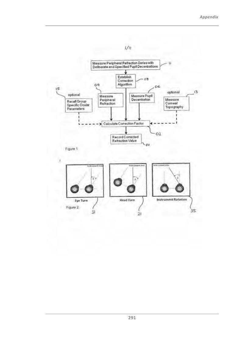
Appendix
291
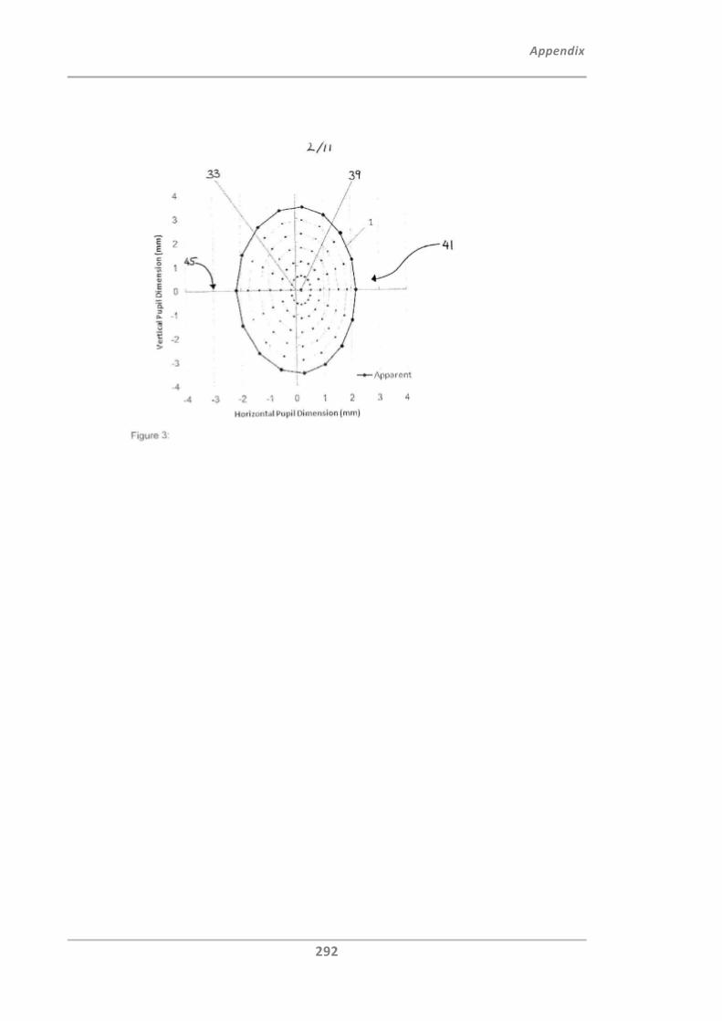
Appendix
292
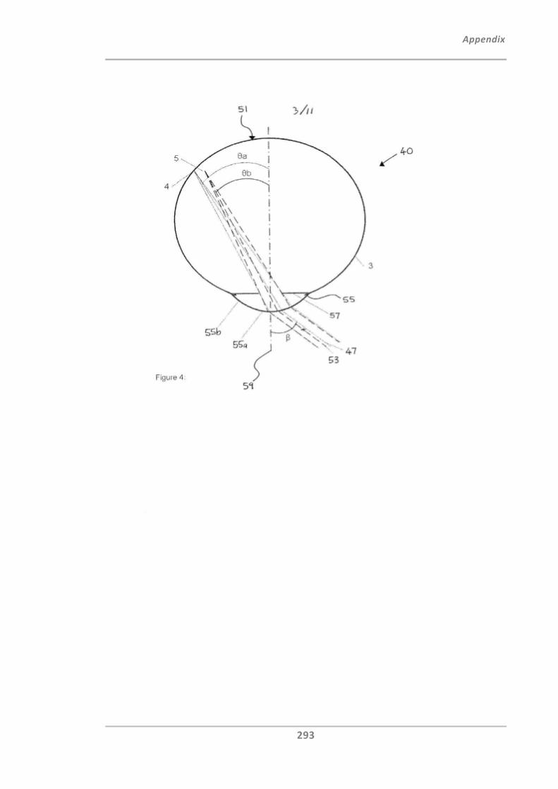
Appendix
293
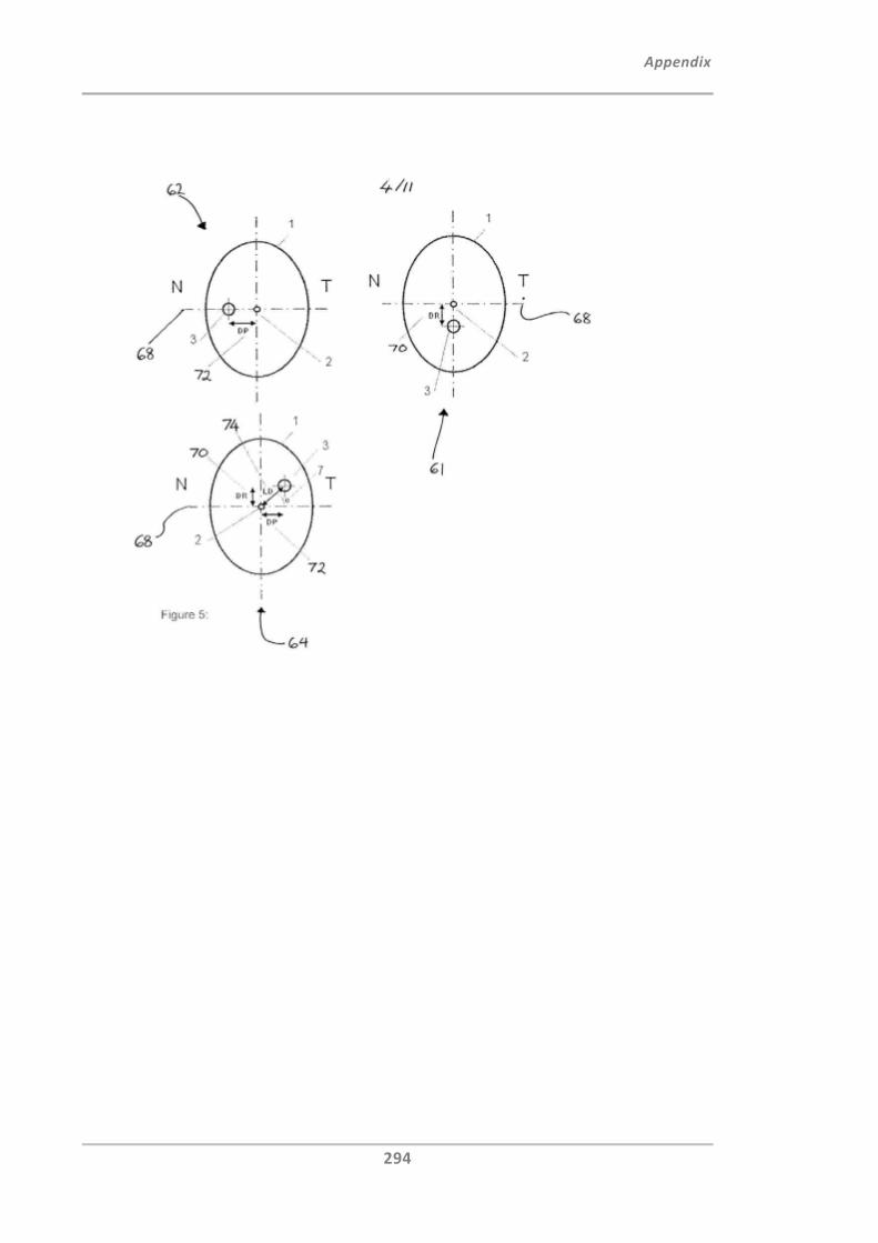
Appendix
294
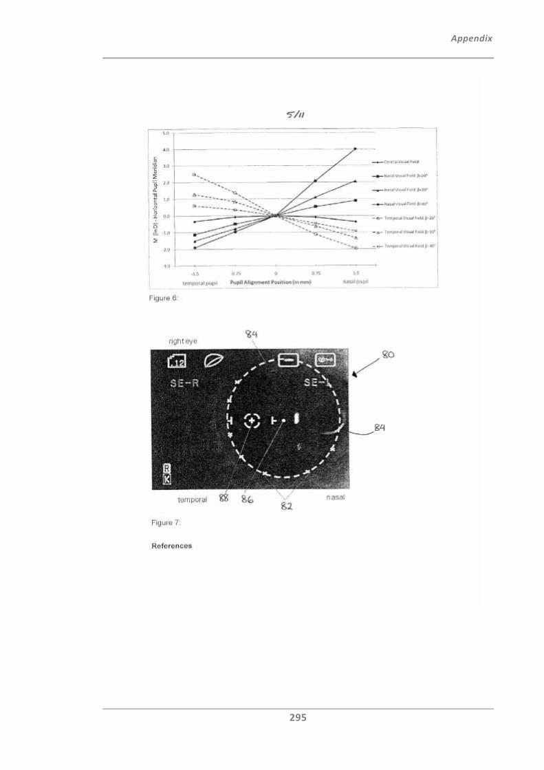
Appendix
295
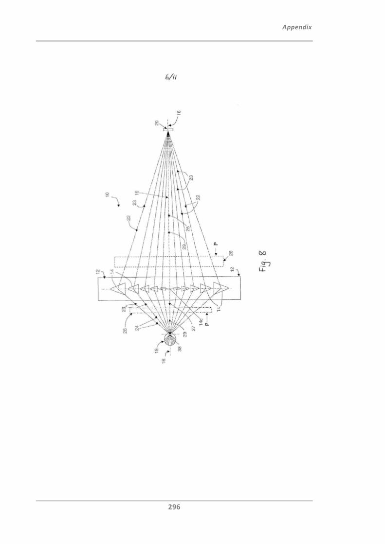
Appendix
296
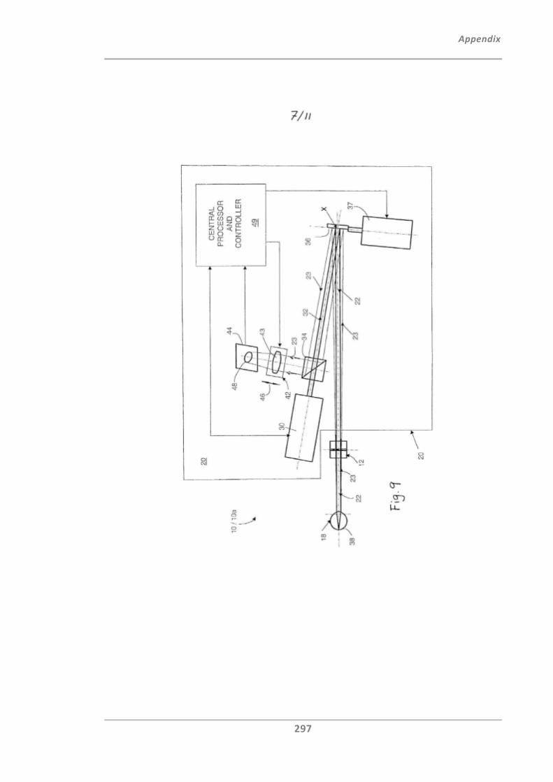
Appendix
297
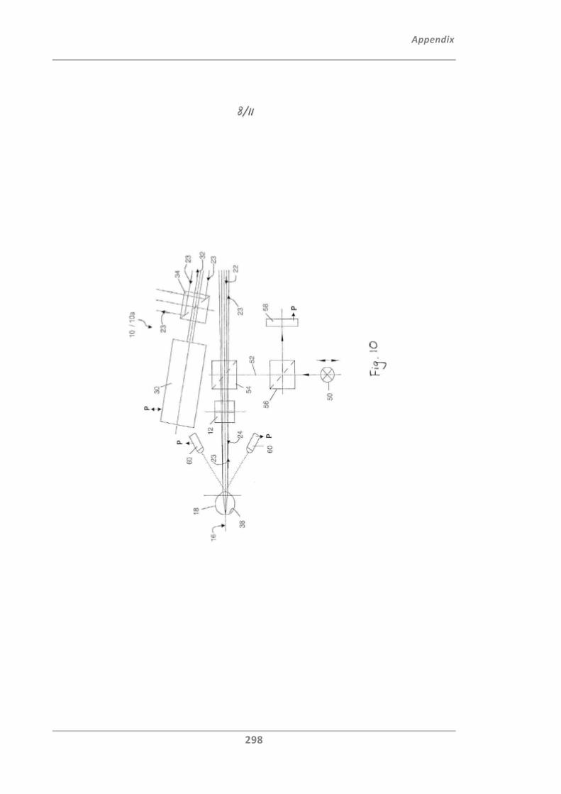
Appendix
298
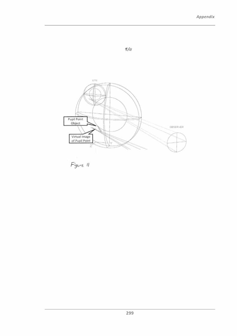
Appendix
299
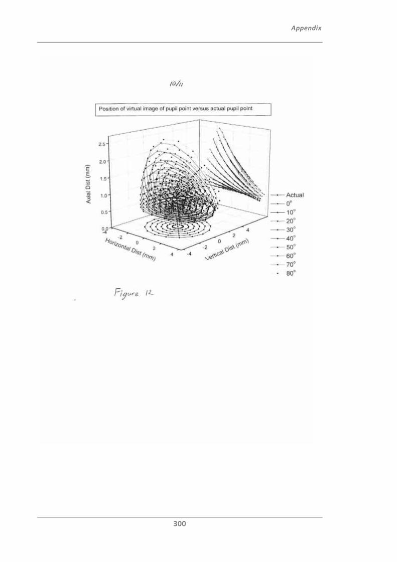
Appendix
300
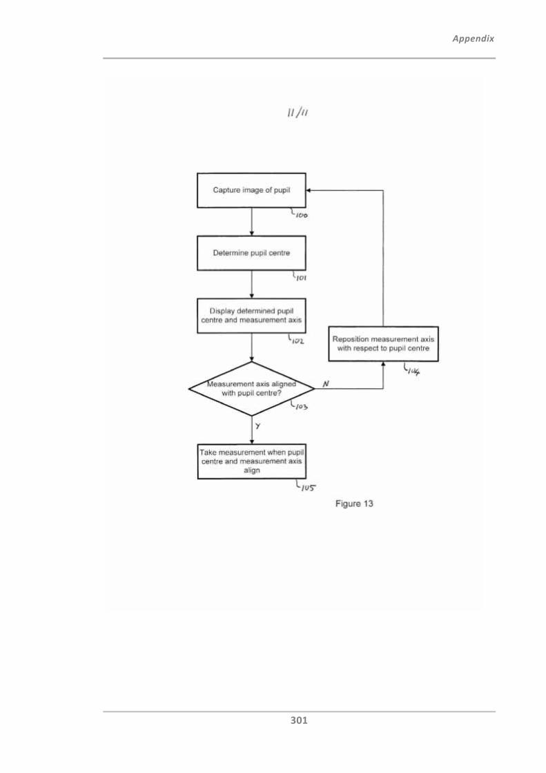
Appendix
301

Appendix
302
APPENDIX B
Visual Field Angle (°) Equations RMSE
Horizontal Pupil
Alignment Meridian
M
nasal 40 1.65 5.50 10 1 1.215
3.66 10 1 2 1.95 2.04 10 1 0.936
nasal 30 1.17 1.77 10 1 0.806
1.05 10 1 2 1.17 5.86 10 2 0.799
nasal 20 6.75 10 1 4.03 10 2 0.534
6.70 10 2 2 6.75 10 1 3.51 10 2 0.530
central 0 1.59 10 1 2 8.39 10 3 1.63 10 3 0.299
temporal ‐205.05 10 1 8.46 10 2 0.533
6.70 10 2 2 5.05 10 1 9.28 10 3 0.529
temporal ‐30 8.65 10 1 3.61 10 2 0.535
3.41 10 2 2 8.65 10 1 7.45 10 2 0.534
temporal ‐40 1.47 1.40 10 1 0.786
7.75 10 2 2 1.47 5.32 10 2 0.783
nasal/temporal θ (‐/+) . . 0.776
J180
nasal 40 180 1.11 3.45 10 1
180 0.615
180 1.89 10 1 2 1.14 1.55 10 1180 0.565
nasal 30 180 5.83 10 1 9.76 10 2
180 0.415
180 5.69 10 2 2 5.83 10 1 3.36 10 2180 0.411
nasal 20180 3.20 10 1 5.12 10 3
180 0.337
180 3.11 10 2 2 3.21 10 1 4.00 10 2180 0.336
central 0 180 8.68 10 2 2 3.34 10 2 1.78 10 2180 0.161
temporal ‐20 180 2.33 10 1 2.85 10 2
180 0.228
180 3.34 10 3 2 2.38 10 1 2.38 10 2180 0.228
temporal ‐30 180 4.21 10 1 2.17 10 2
180 0.281
180 5.79 10 3 2 4.21 10 1 2.82 10 2180 0.281
temporal ‐40 180 7.79 10 1 5.25 10 3
180 0.458
180 2.64 10 3 2 7.78 10 1 8.21 10 3180 0.458
nasal/temporal θ (‐/+) . . 0.445
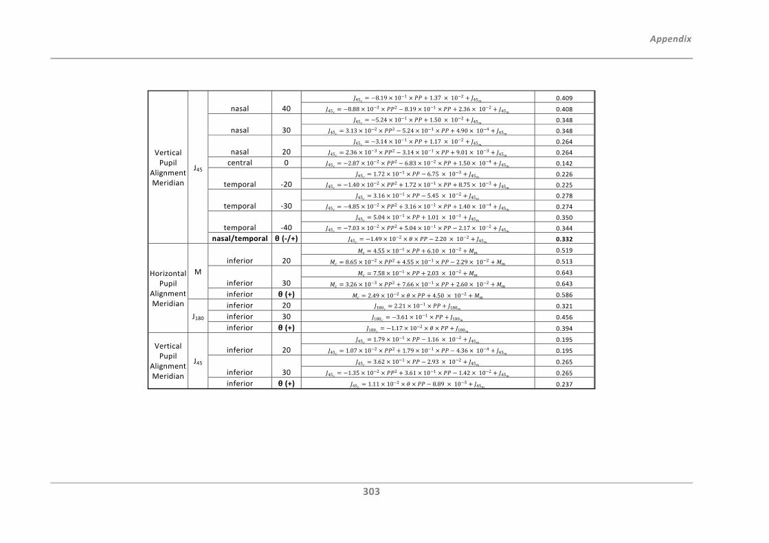
Appendix
303
Vertical Pupil
Alignment Meridian
J45
nasal 40 45 8.19 10 1 1.37 10 2
45 0.409
45 8.88 10 3 2 8.19 10 1 2.36 10 245 0.408
nasal 30 45 5.24 10 1 1.50 10 2
45 0.348
45 3.13 10 2 2 5.24 10 1 4.90 10 445 0.348
nasal 20 45 3.14 10 1 1.17 10 2
45 0.264
45 2.36 10 3 2 3.14 10 1 9.01 10 345 0.264
central 0 45 2.87 10 2 2 6.83 10 2 1.50 10 445 0.142
temporal ‐20 45 1.72 10 1 6.75 10 3
45 0.226
45 1.40 10 2 2 1.72 10 1 8.75 10 345 0.225
temporal ‐30 45 3.16 10 1 5.45 10 2
45 0.278
45 4.85 10 2 2 3.16 10 1 1.40 10 445 0.274
temporal ‐40 45 5.04 10 1 1.01 10 1
45 0.350
45 7.03 10 2 2 5.04 10 1 2.17 10 245 0.344
nasal/temporal θ (‐/+) 45 1.49 10 2 2.20 10 245 0.332
Horizontal Pupil
Alignment Meridian
M
inferior 20
4.55 10 1 6.10 10 2 0.519
8.65 10 2 2 4.55 10 1 2.29 10 2 0.513
inferior 30
7.58 10 1 2.03 10 2 0.643
3.26 10 3 2 7.66 10 1 2.60 10 2 0.643
inferior θ (+) 2.49 10 2 4.50 10 2 0.586
J180
inferior 20 180 2.21 10 1180 0.321
inferior 30 180 3.61 10 1180 0.456
inferior θ (+) 180 1.17 10 2180 0.394
Vertical Pupil
Alignment Meridian
J45
inferior 20 45 1.79 10 1 1.16 10 2
45 0.195
45 1.07 10 2 2 1.79 10 1 4.36 10 445 0.195
inferior 30 45 3.62 10 1 2.93 10 2
45 0.265
45 1.35 10 2 2 3.61 10 1 1.42 10 245 0.265
inferior θ (+) 45 1.11 10 2 8.89 10 345 0.237

Appendix
304
APPENDIX C
Appendix
305
APPENDIX D
Publications and Presentations
Journal Articles
Fedtke C, Ehrmann K, Holden BA. A review of peripheral refraction techniques (2009).
Optom Vis Sci 86:429‐46.
Fedtke C, Manns F, Ho A. The entrance pupil of the human eye: A three‐dimensional
model as a function of viewing angle (2010). Optics Express 18:21:22364‐22376.
Fedtke C, Ehrmann K, Ho A, Holden BA. Lateral pupil alignment tolerance in peripheral
refractometry (2011). Optom Vis Sci 88:4.
Presentations
Fedtke C, Ehrmann K, Ho A, Holden B. The impact of pupil alignment on peripheral
refraction measurements using the Shin‐Nippon NVision K5001. Presented at the
American Academy of Optometry, Orlando, Florida; 2009.
Ho A, Fedtke C, Manns F. The peripheral entrance pupil. Presented at the American
Academy of Optometry, Orlando, US; 2009.
Ho A, Lazon de la Jara P, Martinez A, Kwan J, Fedtke C, Holden BA, Sankaridurg P.
Influence of accommodation on peripheral refraction: Effect of a novel optical design
contact lens for manupulating peripheral defocus. In: Presented at International Myopia
Conference, Tübingen, Germany; 2010. Optom Vis Sci 88:3:441‐42.
Sankaridurg P, Donovan L, Varnas S, Ho A, Kwan J, Fedtke C, Chen X, Ge J, Smith III E,
Holden BA. Impact of spectacle lenses on peripheral refractive errors. Presented at
International Myopia Conference, Tübingen, Germany; 2010. Optom Vis Sci 88:3:443‐44.
Appendix
306
Poster Presentations
Fedtke C, Lazon de la Jara P, Sankaridurg P, Kwan J, Ho A, Holden BA. Relationship
between annual refractive error changes and changes in ocular biometric data in Chinese
children. Presented at International Myopia Conference, Tübingen, Germany; 2010.
Optom Vis Sci 88:3:402
Kwan J, Sankaridurg P, Lazon de la Jara P, Chen X, Fedtke C, Donovan L, Ho A, Ge J,
Holden BA. Association between peripheral refractive error and myopia risk factors.
Presented at International Myopia Conference, Tübingen, Germany; 2010. Optom Vis Sci
88:3:402
Lazon de la Jara P, Sankaridurg P, Martinez A, Kwan J, Fedtke C, Ho A, Holden BA.
Manipulation of the peripheral retinal image using two novel contact lens designs.
Presented at International Myopia Conference, Tübingen, Germany; 2010. Optom Vis Sci
88:3:400
Lazon de la Jara P, Ehrmann K, Kwan J, Fedtke C, Falk D, Sankaridurg P, Holden BA. The
effect of contact lens power profile on peripheral refraction. Presented at the American
Academy of Optometry, San Francisco, US, 2010.
Fedtke C, Ehrmann K, Falk D, Harms‐Biβ E, Ho A, Holden BA. Means to rectify pupil
alignment errors in peripheral refractometry. ARVO. Fort Lauderdale, US, 2011.
Patent Applications
Ehrmann K, Fedtke C, Ho A. Determination of peripheral refraction. Patent Application
Number: AU2010901866