pavement performance measures using android-based smart phone application
TRANSCRIPT

PAVEMENT PERFORMANCE MEASURES USING ANDROID-
BASED SMART PHONE APPLICATION
A Dissertation Work Submitted to Osmania University in Partial Fulfilment of the
Requirements for the Award of Degree of
MASTER OF ENGINEERING
IN
CIVIL ENGINEERING
(With Specialization in Transportation Engineering)
BY
MOHAMMED JUNAID UDDIN
(1603-13-741-410)
Under the Supervision of
Dr. MIR IQBAL FAHEEM
Professor & Head of Civil Engineering Department
Department of Civil Engineering
Deccan College of Engineering and Technology
(Affiliated to Osmania University (A))
Darussalam, Hyderabad, Telangana State-500001
2015

PAVEMENT PERFORMANCE MEASURES USING ANDROID-
BASED SMARTPHONE APPLICATION
A Dissertation Submitted to Osmania University in Partial Fulfillment of the
Requirements for the Award of the Degree of
MASTER OF ENGINEERING
In
CIVIL ENGINEERING
(With Specialization in Transportation Engineering)
By
MOHAMMED JUNAID UDDIN
(Roll No: 1603-13-741-410)
Under the supervision of
Dr. MIR IQBAL FAHEEM
Professor& Head of Civil Engineering Department
Department of Civil Engineering
Deccan College of Engineering & Technology
[Affiliated to Osmania University (A)]
Darussalam, Hyderabad, Telangana State- 500 001
2015

DEPARTMENT OF CIVIL ENGINEERING
UNIVERSITY COLLEGE OF ENGINEERING
OSMANIA UNIVERSITY (A), HYDERABAD
TELANGANA STATE-500007
M. E. DISSERTATION EVALUATION SHEET
Name of the Candidate : MOHAMMED JUNAID UDDIN
Roll No : 1603-13-741-410
Specialization : Transportation Engineering
Date of External Viva voce : ………………………………
Grade : ………………………………
Signature of Chair Person Board
Of Studies in Civil Engineering, OU : ……………………………….
Signature of the External Examiner : ……………………………….
Signature of Supervisor : ……………………………….
Signature of the Head, CED, OU

iii
DEPARTMENT OF CIVIL ENGINEERING
DECCAN COLLEGE OF ENGINEERING AND TECHNOLOGY (Affiliated to Osmania University)
Darussalam, Hyderabad, Telangana State-500001
CERTIFICATE
This is to certify that the dissertation work entitled “Pavement Performance Measures
Using Android-Based Smart Phone Application” submitted by Mohammed Junaid
Uddin bearing Roll No. 1603-13-741-410, in partial fulfillment of the requirements for
the award of the degree of Master of Engineering in Civil Engineering with
specialization in Transportation Engineering submitted to University College of
Engineering (Autonomous), Osmania University, Hyderabad, is a record of bonafide
work carried out by him under my supervision during the academic year 2013-2015.
The results embodied in the work are not submitted to any other university or institute
for the award of any degree or diploma.
Dr. MIR IQBALFAHEEM, M.Tech, Ph.D., FIE, FISCE
Vice Principal, Professor and Head of Civil Engineering Dept.
Department of civil Engineering
Deccan college of Engineering and Technology
Hyderabad, Telangana State – 500001

iv
DECLARATION
I, Mohammed Junaid Uddin (160313741410),student of M.E Civil Engineering,
Transportation Engineering, Deccan college of engineering and Technology, declare
that the project Titled “Pavement Performance Measures Using Android-Based
Smart Phone Application” has been independently carried out under the guidance of
Dr. Mir Iqbal Faheem, Professor & Head of Civil Engineering Department, Deccan
College of Engineering and Technology, Darussalam, Hyderabad, India
No part of the thesis is copied from books/journals/internet and wherever the portion is
taken, the same has been duly referred in the text. The report is based on the project
work done entirely by me and not copied from any other source.
Mohammed Junaid Uddin

v
ACKNOWLEDGEMENTS
I would like to express my sincere thanks to my guide Dr. Mir Iqbal Faheem, Vice
Principal, Professor and Head of Civil Engineering, Deccan College of Engineering and
Technology for his timely and valuable suggestions. I am thankful for his guidance and
active supervision at every stage of the thesis work. He has been constant driving force,
source of inspiration and encouraging me throughout this work. It is his immense
patience and co-operation that has helped for the successful completion of this work.
I am thankful to Prof. M. A. Malik, Director and Principal of Deccan College of
Engineering and Technology for his constant zeal and supervision for the enormous
work he did to make us succeed and management of Dar-us-Salam trust.
I express my sincere thanks to Prof. M. Kumar, Professor and Head of Civil
Engineering, Osmania University, for facilitating the conduct of viva-voce
examination.
I express my sincere thanks to Prof. V Bhikshma, Chairman, Board of Studies, Civil
Engineering Department, Osmania University, for his valuable support and advice for
preparation of this report as per the format and facilitating viva-voce.
I express my sincere thanks to Prof. S Ramachandaram, Principal, University College
of Engineering, Osmania University, Hyderabad for facilitating the conduct of viva-
voce examination.
I express my sincere thanks to Mr. M.A.Kalam, Associate Professor, Civil
Engineering Department, Deccan College of Engineering and Technology, for his
constant support and timely encouragement for the completion of my dissertation work.
I am very much thankful to Mr. Lars Forslöf, Founder and CEO of Roadroid and
whole team for guiding me through the theses work
And indeed special thanks to my seniors especially Mr. Mohd Mihajuddin, Ms.
Tahseen Sultana & Ms. Sumaiya Fatima for their support and making me confident
about my work.
I am very much thankful to my parents, friends and also to my family who have
supported me greatly during the course of this work.
Mohammed Junaid Uddin
vi
ABSTRACT
Goal: The goal of the thesis is to investigate pavement roughness for improving the
performance, using android based smartphone technology.
Design approach: In this thesis research, in order to obtain pavement surface condition
a survey for pavement evaluation is taken with the combination of modern sensor
technology with the help of an Android Smartphone. A road pavement continuously
deteriorates under the combined actions of traffic loading and the environment. The
most common indicators of pavement performance are: fatigue cracking, surface
rutting, riding quality, and skid resistance. The change in the value of these performance
indicators over time is referred to as deterioration. Pavement roughness is a
phenomenon experienced by the passenger and operator of a vehicle. According to the
definition of the American Society of Testing and Materials (ASTM), “roughness is the
deviations of a pavement surface from a true plan a surface with characteristic
dimensions that affect vehicle dynamics, ride quality, dynamic loads, and drainage, for
example, longitudinal profile, transverse profile, and cross slope”. Roughness is an
important indicator of pavement riding comfort and safety. It is a condition indicator
that should be carefully considered when evaluating primary pavements. At the same
time, the use of roughness measurements plays a critical role in the pavement
management system. There are many huge devices used for roughness evaluation.
Findings: It is very essential to evaluate the structural and functional condition of
pavements to determine the present condition of the pavement. The pavement
deterioration studies are important to draw up the most suitable maintenance strategies.
The models predicting pavement performance play an important role in financial
planning and budgeting. The data on performance of in service flexible and rigid
pavements of Hyderabad City were collected. In the study main distresses were
identified from the selected road stretches. Regression models were then developed
using SPSS (Statistical packages for social sciences) package. In the present study two
stretches each of 6km and 20km length were selected. Eleven sets of data were already
available from previous studies and additional one set was collected during this study.
Models were developed for cracking progression, deflection growth, pothole
progression and roughness growth model.

vii
Results: The results obtained for the General Road Network Roughness Surveys where
the roughness of the main road outside the city area, and the roughness within the city.
The device records an IRI roughness measure at a time interval of one second, as
opposed to distance based. The raw (unfiltered) data is presented in which reports a
large variance in IRI along the road length. This detailed low-level data exceeds the
detail necessary of IQL-3/4 data, and therefore the raw unfiltered results from each
direction were manually averaged over a one kilometre length. It can also be seen that
the average IRI across the road length is similar despite the severe runs.
Future scope: This is indeed, a very logical next step in this line of research. For the
modern era, if our local authorities (Government) implement this concept in our
Hyderabad city then the day is not too far for converting worst to best roads in the city.
TABLE OF CONTENTS
TITLE PAGE NO
CERTIFICATE iii
DECLARATION iv
ACKNOWLEDGEMENTS v
ABSTRACT vi
LIST OF TABLES viii
LIST OF FIGURES ix
CHAPTER 1: INTRODUCTION (1-8)
1.1 Introduction 1
1.2 International scenario of Roughness 2
1.3 Indian scenario of Roughness 3
1.4 Factors affecting in evaluation of roughness index 4
1.5 Research motivation 6
1.6 Research gap 7
1.7 Research aim and objective 7
1.8 Research scope 8
1.9 Organization of study 8
CHAPTER 2: LITERATURE REVIEW (9-21)
2.1 Introduction 9
2.2 Critical review 9
2.3 Earlier Studies 11
Summary
CHAPTER 3: DISTRESS METHODS AND MODELS (22-52)
3.1 Introduction 22
3. 2 Types of Distresses 23
3.2.1 Asphalt Pavement Distress 23
3.2.2 Concrete Pavement Distress 31
3.3 Roughness Measuring System 39
3.3.1 Class I System 40
3.3.1.1 Rod and Level 40
3.3.1.2 Dipstick 40
3.3.2 Class II System 41
3.3.2.1 K.J.Law Profilometer 41
3.3.2.2 APL Profilometer 42
3.3.2.3 South Dakota Profiler 43
3.3.3 Class III System 43
3.3.3.1 BPR Roughometer 43
3.3.3.2 Light Weight Profiler 44
3.3.3.3 Laser Profiler 45
3.4 Profiles 47
3.5 Profile Index 48
3.6 Roughness Definition 49
3.7 International Roughness Index (IRI) 49
3.8 Roughness Indices 50
Summary 52
CHAPTER 4: METHODOLOGY AND & COLLECTION (53-83)
4.1 Introduction 53
4.2 Study Area discussion 53
4.3 Research Methodology 56
4.4 Method to Collect Data 57
4.4.1 History 57
4.4.1.1 The First Prototype (2002-06) 60
4.4.1.2 Further Development (2010-11) 62
4.4.1.3 Professional Use (2013-2014) 63
4.5 Quarter Car Model 64
4.6 Calculation of IRI 66
4.7 Understanding Roadroid Use 69
4.8 Data Collection 79
4.9 SPSS Interface 82
Summary 83
CHAPTER 5: ANALYSIS & RESULTS (84-104)
5.1 Introduction 84
5.2 Data Analysis 84
5.2.1 Structural Conditional Data 85
5.2.2 Functional Conditional Data 86

5.2.3 Analysis and Results Using Statistical Techniques 87
5.2.3.1 Modified Structural Number 91
5.2.3.2 Regression Model 92
5.2.3.3 Deflection 93
5.2.3.4 Pothole Progression 93
5.2.3.5 Roughness Progression 93
5.2.4 Profiling of Roads Using Roadroid 94
5.2.5 Information Quality Level 94
5.2.6 Smartphones Applications 95
5.3 Network Roughness Data 96
5.4 Repeatability and Reliability 97
5.5 Practically and Applicability for Roads of Hyderabad 98
5.6 Results 98
5.6.1 General Road Network Roughness Surveys 98
5.6.2 Speed Dependency 99
5.6.3 Vehicle Dependency 103
5.7 Practicalities 103
Summary 104
CHAPTER 6: CONCLUSIONS (105-107)
6.1 Introduction 105
6.2 Conclusions 105
6.3 Recommendations 106
6.4 Model Limitations and Further Research 107
REFERENCES 108

viii
LIST OF TABLES
Table No. Description Page No.
1.1 Riding Comfort Index Values 3
1.2 Strength Coefficient 3
2.1 Critical Review 9
4.1 Detail of Stretches 55
4.2 Application Settings 71
4.3 Roughness data-1 80
4.4 Roughness data-2 81
5.1 Pavement History 84
5.2 Road Parameters 87
5.3 Rout within the city 90
5.4 Rout outside the city 91
5.5 Layers Specifications 92
5.6 Sample Statistics fir Repeatability Exercise 101
5.7 Reliability between Vehicular Speed 101

ix
LIST OF FIGURES
Figure No. Description Page No.
1.1 Factors Influencing Roughness Measurements 6
3.1 Fatigue (Alligator) Cracking 24
3.2 Bleeding 25
3.3 Block Cracking 26
3.4 Pothole 28
3.5 Rod & Level 40
3.6 Dipstick 41
3.7 APL Profilometer 42
3.8 BPR Roughometer 44
3.9 Light Weight Profiler 45
3.10 ICC Laser Profiler 46
3.11 ARAN Laser Profiler 46
4.1 Stretch from Chaderghat, Chanchalguda to Dabeerpura 54
4.2 Stretch from Charminar Rd. – International Airport 54
4.3 Methodology Flow Chart 56
4.4 First Prototype (2002 – 2003) 60
4.5 Second Prototype (2004 – 2006) 60
4.6 Data Collection Using Roadroid 63
4.7 Quarter Car Model 64
4.8 IRI Roughness Scale 67
4.9 Sensitive Wavenumber of IRI 68
4.10 Roadroid Methodology 69
4.11 Basic Principal of Roadroid 69
4.12 Need of the Study 70
4.13 Rehabilitate before it’s too Late 70
4.14 Roadroid Data Processing Process 71
4.15 Gadgets Required for Data Collection 71
4.16 Discretion of the Interface 73
4.17 Data viewed in Server 75

x
Figure No. Description Page No.
4.18 Data Viewed with Snapshots 76
4.19 Data Processing 78
4.20 Data Processing – 2 79
4.21 SPSS Start-up page 82
4.22 Linear regression 83
5.1 Study Area 1 Analysis 85
5.2 Study Area 2 Analysis 85
5.3 Deflection Progression of Hyderabad 86
5.4 Roughness within the city-1 87
5.5 Roughness within the city-2 88
5.6 Roughness within the city-3 88
5.7 Roughness outside the city-1 89
5.8 Roughness outside the city-2 89
5.9 Roughness outside the city-3 89
5.10 Roughness outside the city-4 90
5.11 Information Quality Level (IQL) 95
5.12 Surface Condition of the Roads in Hyderabad 98
5.13 Charminar – Airport Roughness (Raw Unified Data) 100
5.14 Charminar – Airport Avg. data per Kilometer 101
5.15 Runs for the Repeatability exercise of the city Highway 102

1
CHAPTER 1
INTRODUCTION
1.1 Introduction
It is necessary to provide a good road network for the development of any country.
India has a road network of over 4,689,842 kilometres in 2013 the second largest road
network in the world. However, qualitatively India's roads are a mix of modern
highways and narrow, unpaved roads, and are being improved. As of 2011, 54 percent
and about 2.53 million kilometres of Indian roads were paved. India in its past did not
allocate enough resources to build or maintain its road network. This has changed since
1995, with major efforts currently underway to modernize the country's road
infrastructure.
Pavement performance is a function of its relative ability to serve traffic over a period
of time (Highway Research Board). Due to the great complexity of the road
deterioration process, performance models are the best approximate predictors of
expected conditions.
According to 2009 estimates by Goldman Sachs, India will need to invest US$1.7
trillion on infrastructure projects before 2020 to meet its economic needs, a part of
which would be in upgrading India's road network. The Government of India is
attempting to promote foreign investment in road projects. Foreign participation in
Indian road network construction has attracted 45 international contractors and 40
design/engineering consultants, with Malaysia, South Korea, United
Kingdom and United States being the largest players.
Thus there is a great need for the effective and efficient management and maintenance
of the road network. The funding available for periodic maintenance and management
system is limited. In order to determine the most economical strategies, most essential
input is development of deterioration models for structural and functional conditions of
flexible or rigid pavements.

2
1.2 International Scenario of Roughness Evaluation
1. New Zealand Transport Authority (NZTA) has noticed that road users have been
complaining about high levels of ride discomfort despite reports indicating low
levels of roughness. This is mainly due to the fact that NZTA is assessing the
quality of their roads based on a system developed in the 1980’s. Roadroid is a
new roughness measurement application designed to provide cost effective
measurements that also monitor the roughness felt by a road user. The research
aims to determine whether the Roadroid system can represent the roughness felt
by a road user in the Auckland network.
2. The remoteness of the Pacific Island Countries (PICs), similar to parts of Africa,
creates difficulties, both logistically and economically, to undertake detailed in-
country investigations on the road networks. Therefore, rapid assessments of the
condition of the existing road pavements are required to determine the level of
required donor investments to maintain the integrity of the road network. This
explores the use of Roadroid, a simple android application, as a low cost solution
to evaluating road roughness in the Pacific region. It demonstrates the use of the
Roadroid application on the road network in Kiribati, one of the smaller and
debatably the most remote PIC. The results from the study discuss the
performance and practicability of the android application.
3. A test was performed with an autonomous robot which can be used to measure the
International Roughness Index (IRI), a description of pavement ride quality in
terms of its longitudinal profile. A ready-made robot, the Pioneer P3-AT, was
equipped with odometers, a laptop computer, CCD laser, and a SICK laser ranger
finder to autonomously perform the collection of longitudinal profiles. ProVAL
(Profile Viewing and Analysis) software was used to compute the IRI. This work
is an initial step toward autonomous robotic pavement inspections. The authorities
also discuss the future integration of inertial navigation systems and global
positioning systems (INS and GPS) in conjunction with the P3-AT for practical
pavement inspections.

3
1.3 Indian Scenario of Roughness
1. Pavement deterioration is a complex process. It involves not only structural fatigue
but also many functional distresses of pavement. It results from the interaction
between traffic, climate, material and time. Deterioration is the term used to
represent the change in pavement performance overtime. The ability of the road
to satisfy the demands of traffic and environment over its design life is referred to
as performance. Due to the great complexity of the road deterioration process,
performance models are the best approximate predictors of expected conditions.
In this study main distresses were identified from the selected road stretches.
Regression models are then developed using SPSS (Statistical packages for social
sciences) package. T test is used to check the reliability of the model.
2. It is very essential to evaluate the structural and functional condition of pavements
to determine the present condition of the pavement and to predict the service life.
The pavement deterioration studies are important to draw up the most suitable
maintenance strategies. The models predicting pavement performance play an
important role in financial planning and budgeting. The data on performance of in
service flexible highway pavements on National Highway and Major District
Road were collected. In the study main distresses were identified from the selected
road stretches. Regression models were then developed using SPSS (Statistical
packages for social sciences) package. An effort was taken to model the
performance of pavements using fuzzy logic. The fuzzy method that was used is
linguistic fuzzy model. In the present study five stretches each of 1km length were
selected. Eleven sets of data were already available from previous studies and
additional one set was collected during this study. Models were developed for
cracking progression, deflection growth, pothole progression and roughness
growth model. Fuzzy developed models were found to be more suitable than
conventional regression models for selected road stretches.

4
Table 1.1 Riding Comfort Index values
Unevenness Index (mm/km) Riding Comfort Index
<2500 0
2500-3500 1
3500-5000 2
5000-7000 3
7000-10000 4
>10000 5
Table 1.2 Strength Coefficients
Layer/Specification Strength Coefficients
Bituminous Concrete (BC) 40mm 0.3
Bituminous Concrete (BC) 25mm 0.28
Semi Dense Bituminous Concrete (SDBC) 25mm 0.25
Dense Bituminous Macadam(DBM) 0.28
Premix Carpet (PC) 20 mm( only in the case of overlaid
pavements which have PMC as original surfacing)
0.18
Bituminous Macadam(BM) 0.18
Water Bound Macadam(WBM Gr I, II or III) Wet mix
macadam / (Lime cement) stabilized
0.14
1.4 Factors affecting in evaluation of roughness index
The International Roughness Index (IRI) is defined as a mathematical property of a
two-dimensional road profile (a longitudinal slice of the road showing elevation as it
varies with longitudinal distance along a travelled track on the road). As such, it can be
calculated from profiles obtained with any valid measurement method, ranging from
static rod and level surveying equipment to high-speed inertial profiling systems.
IRI is the roughness index most commonly obtained from measured longitudinal road
profiles. It can be calculated using a quarter-car vehicle math model, whose response is
accumulated to yield a roughness index with units of slope (in/mi, m/km, etc.). Since

5
its introduction in 1986. IRI has become the road roughness index most commonly used
worldwide for evaluating and managing road systems.
The measurement of IRI is required for data provided to the United States Federal
Highway Administration, and is covered in several standards from ASTM International:
ASTM E1926 – 08. ASTM E1364 - 95(2005), and others. IRI is also used to evaluate
new pavement construction, to determine penalties or bonus payments based on
smoothness.
The IRI is measured using profilometers, which measure the road profile, or by
correlating the measurements of Response Type Road Roughness Meters (RTRRMS)
to an IRI calculated from a profile. Using World Bank terminology, these are
respectively called Information Quality Level (IQL) 1 and IQL-3 devices, representing
the relative accuracy of the measurements. A common misconception is that the
80 km/h used in the simulation must also be used when physically measuring roughness
with an instrumented vehicle. IQL-1 systems measure the profile direction, independent
of speed, and IQL-3 systems typically have correlation equations for different speeds
to relate the actual measurements to IRI. IQL-1 systems typically report the roughness
at 10–20 m intervals; IQL-3 at 100m+ intervals. The data can be presented using a
moving average to provide a "roughness profile". These IRI profiles are sometimes used
to evaluate new construction to determine bonus/penalty payments for contractors, and
to identify specific locations where repairs or improvements (e.g., grinding) are
recommended. The IRI is also a key determinant of vehicle operating costs which are
used to determine the economic viability of road improvement projects.
The Dipstick Profiler, with a reported accuracy of .01 mm ( 0.0004 inches), is the most
widely used and accepted Class 1 profiler for the purposes of calibrating profilometers
that measure IRI.

6
Figure 1.1 Factors influencing Roughness Measurement
Figure 1.1 shows the list of factors that can affect roughness measurements. These
factors have been categorized to illustrate what influence each factor has on accuracy,
agreement, repeatability and interpretation.
1.5 Research Motivation
In developing countries the development towards the growth in evaluating the
roughness is still going on. Apart from the heavy equipment roughness evaluation
methods in developing countries, a non-equipment evaluation methods using latest
technologies can be brought forward to reduce time, economy, manpower and many
more

7
1.6 Research Gap
The research leading to the development of roughness measuring equipment dates back
more than 60 years. Early profilers were time and labor consuming, required testing at
very slow speeds. With the help of the development of sensors technology and computer
technology, it is no longer the case nowadays. In the thesis research, in order to obtain
useful pavement surface condition data for pavement evaluation, two measuring
systems was developed with the combination of the modern sensors and computer. The
first profile roughness measuring system uses the absolute tilt angle and includes
measuring the profile, filtering the profile to get only those waves of interest, and
mathematically computing all major types of roughness index. The second one uses the
relative angle to measure the profile. The repeatability and correlation analysis between
the two profiles were introduced. They are both Direct Type road roughness evaluation
systems. Knowing these various methods of evaluation may give way to work on many
better evaluation methods where we can reduce money, time, and applicable for remote
areas.
1.7 Research Aim and Objectives
The primary goal in this research is to establish whether Roadroid is a suitable tool to
measure the road roughness felt by a road user. This goal will be validated through the
following objectives:
1. To demonstrate the total Interface of Roadroid.
2. Determine if Roadroid can respond to climatic changes
3. Comparing and analyzing the difference between Roadroid and industry accepted
roughness technology and methods
4. To determine if Roadroid has real world applications and a place in the
transportation Engineering.
The primary objective of these guidelines is to assist road network management
personnel to plan, execute and control the measurement of road roughness (or riding
quality) over a road network. These measurements are typically intended for use in the
network’s Pavement Management System (PMS) to assess the network condition and
prioritize maintenance and rehabilitation actions. Secondary and associated objectives
of these guidelines are to provide a definition and clarification of key concepts and
methodologies.

8
These guidelines are thus primarily concerned with the needs of roads agencies or
managers of road networks. Although some details of measurement procedures are
discussed, the emphasis remains on the needs of the network manager, and not on the
needs of the contractor in charge of the actual roughness measurement. The scope of
the guidelines is also limited to roughness measurement at the network level, and does
not cover applications such as roughness measurement at the project level or for
research purposes.
1.8 Research Scope
This research will focus on developing the Roadroid application and also monitoring
road roughness using this smart phone application ROADROID including the
methodology and specifications. A statistical analysis will be conducted to identify the
results obtained by Roadroid comparing with the standard ones.
1.9 Organization of Study
This dissertation work is presented in six chapters including the introduction chapter
Chapter 2: This chapter contains an overview of the literature on different methods of
roughness evaluation. And it deals with the review of the existing techniques available.
Chapter 3: This chapter explains the basic concepts and a brief review of types of
distresses and the profiling techniques used for evaluating road roughness. Distress
methods and models are also explained briefly.
Chapter 4: This chapter explains the methodology followed in this study which
includes the explanation of methodology followed for Data collection to data
presentation and the use of Roadroid Smartphone application in detail with pictorial
representation.
Chapter 5: This chapter deals with the Data collection using Roadroid and obtaining
results and the method used with the standards of ASTM. And also the analysis of the
data collected using Roadroid with the help of SPSS software to validate the results.
Chapter 6: This final chapter summarizes the work accomplished in this study and
suggests some directions for future research

9
CHAPTER 2
LITRATURE REVIEW
2.1 Introduction
In order to understand the pavement roughness and pavement roughness measurement
problems, current roughness measuring system situation, an overview of the past
studies and the research about different pavement measurement systems are introduced
in this chapter. The significance of related topics and the potential study topics expected
are also presented.
2.2 Critical Review
Many studies where done before the development of the smartphone technology past
in sixties. Then later in the preceding years the development has taken for the
monitoring of the pavement performance. Some of them are:
Table 2.1 Critical Review
S.NO Author(s)/
Organization
Year Evaluation Method Developed Parameters
1 Spangler and Kelley 1960 GMR profilometer pavement profiles
2 HRB 1962 Linear models based
on experimental data
pavement performance
model
3 US Transport federal
agencies
1970 monitoring
pavement conditions
began using profilers
Compromised the
accuracy of profile
measurement.
4 Hodges et al, Parsley
and Robinson
1980 Linear models based
on field data
relationship between
pavement
5 Geipot, Paterson 1982 Riding quality,
longitudinal profiler
Dynamic
characteristics of the
vehicles
6 Gillespie et al, Sayers 1986 riding quality in
terms of IRI
measure of the road
conditions
7 Paterson 1987 vehicle operating
costs (VOC)
economic importance

10
S.NO Author(s)/
Organization
Year Evaluation Method Developed Parameters
8 United States FHWA 1990 Ultrasonic sensors,
laser profiler
Road Roughness
Measuring
9 Kay et al 1993 Pavement Condition
Rating
long-term pavement
performance
10 Queiroz 1983 Linear models mechanistic-empirical
deterioration model
11 Madanat et al 1995 endogeneity bias Maintanance
12 Archilla, Madanat 2001 Statistical analysis,
experimental traffic.
predict pavement
rutting
13 Hao Wang 2006 Road Profiler
Performance
Evaluation And
Accuracy Criteria
Analysis
Different types of
evaluation techniques
14 Jia-Ruey Chang,
Yung-Shuen Su,
Tsun-Cheng Huang,
Shih-Chung Kang
and Shang-Hsien
Hsieh
2009 Measurement Of
The International
Roughness Index
(Iri) Using An
Autonomous Robot
robot (the P3-AT) to
perform roughness
inspections
pavement
management purposes
15 Lars Forslöf
CEO/Inventor
2013 Continuous Road
Condition
Monitoring With
Smart Phones
Method and use of
Roadroid
16 Myles Johnston 2013 Using Cell-Phones
To Monitor Road
Roughness
Relationship between
Roadroid
IRI and Laser IRI
17 Schlotjes, A Visser
& C Bennett
2014 Evaluation Of A
Smartphone
Roughness Meter
Repeatability and
reliability of the
device at various
speed

11
2.3 Earlier Studies
Spangler and Kelley, (1960) developed GMR profilometer at the General Motors
Research Laboratory, the routine analysis of pavement profiles began. NCHRP
sponsored a study of response-type road roughness measuring system such as the BPR
roughometer and vehicles equipped with Mays rider meters in the late 1970s. An
objective of the study was to develop calibration methods for the response type systems.
The best correlation was obtained by using the Golden Car. In the late 1970s, when
many state and federal agencies in charge of monitoring pavement conditions began
using profilers to judge the serviceability of roads, profiling technology found broad
application beyond research in the United States. A major advantage of profilers is that
they are capable of providing a stable and transportable way of measuring roughness.
In other words, roughness values produced by a valid profiler can be compared to values
from prior years and values measured by other valid profilers. Unfortunately,
insufficiencies in profiler design, data processing techniques, and operational practices
have compromised the accuracy of profile measurement.
HRB, (1962) The AASHO Road Test was sponsored by the American Association of
State Highways Officials (AASHO) and was conducted from 1958 through 1960 near
Ottawa, Illinois. The data from this experiment constitutes the most comprehensive and
reliable data set available to date. Unfortunately, some of the original raw data have
been destroyed, and only summary data tables containing average values are available.
The site was chosen because the soil in the area is representative of soils corresponding
to large areas of the Midwestern United States and it was fairly uniform. The climate
was also considered to be representative of many states in the northern part of the
country. The average annual precipitation in the region of the test was 34 inches (864
mm). This precipitation occurred throughout the year without a significant difference
between the dry and wet season. The average temperature during the summer months
was 76 °F (24°C) while the average temperature for the winter months was 27 °F (-3
°C). The soil remained mostly frozen during the winter months with the depth of frost
penetration depending on the length and severity of the cold season. The rate of frost
penetration with time (hereafter referred to as the frost penetration gradient) had an
important impact on the performance of the various pavement sections.

12
Only one subgrade material and one climatic region were evaluated during the AASHO
experiment. The upper part of the embankment was constructed with a selected silty-
clay material with a CBR value between 2 and 4. These values are representative of
large areas in the continental United States. However, although both (climate and
subgrade) conditions are typical of large areas in the United States, the use of the results
outside these conditions should be subjected to detailed assessment to ascertain their
applicability. Estimation of the effects of different subgrade material and environmental
conditions cannot be attained with this data set. For this purpose, new data have to be
obtained.
US Transport federal agencies, (1970) initiated a correlation experiment to establish
correlation and the calibration standard for road roughness measurement and to develop
IRI became an objective of the research program. The main criteria were that IRI is
relevant, transportable and stable with time. The Golden Car simulation was one of the
candidate references considered. After processed the data, a quarter car and a half car
model were found with two vehicle simulations based on Golden car parameters. The
quarter car model was selected because it could be used with all profiling methods that
were in use at that time. Then “Guideline for conducting and calibrating roughness
measurements” was published in 1986. This technical paper presented the instructions
for using various types of equipment to measure profile and get IRI. It also included
computer code for calculating IRI of pavement profile. In 1990, the United States
FHWA required IRI as the standard reference. In the 1990s, the ultrasonic sensors were
used in response type road roughness measuring system. The ultrasonic profiler is a
faster and reliable system. But it has problems with the response type systems: except
that ultrasonic sensors were found to be insufficient for measurement of IRI and RN,
the measurement became erroneous in the presence of water; the system was very
sensitive to the pavement texture and it needs a lot of maintenance. Due to slow
response time of ultrasonic sensors, the test speed of ultrasonic profile was slow.
Through the development and improvement of laser technology, laser sensors were
used in that late 1990s, the measuring speed of the profiler was improved. The
measuring speed could be up to 60 miles per hour. Nowadays, many state department
of transportation in the United States use the laser profiler to measure the pavement
roughness.

13
Hodges et al, Parsley and Robinson, (1980) A study conducted by the Transportation
Road Research Laboratory of the U.K. (TRRL) on in-service road pavements in Kenya.
Provided the additional data needed to update the AASHO models to establish the
relationship between pavement riding quality, pavement strength and actual highway
traffic. The use of in-service pavements made it possible to improve over the original
AASHO models. Some of these improvements are the incorporation of (i) mixed traffic
loading, (ii) different pavement structures over different subgrades, and (iii) a variety
of pavement ages. Furthermore, instead of using serviceability as a measure of riding
quality, actual measurements of roughness in terms of IRI were used. The following
model was developed:
Rt R0 f(SN) Nt
where
Rt : roughness at time t,
RO : initial roughness at time t = 0,
f(SN) : a function of the structural number SN,
SN : structural number developed during the AASHO Road Test
Nt : cumulative number of equivalent 80 kN single axle loads applied
until time t.
Geipot, Paterson, (1982) The models were based on field data from the Brazil-UNDP
Road Cost Study. Which incorporates a very comprehensive set of cross-sectional data
on riding quality, cracking, raveling, rutting, maintenance, traffic and rainfall.
Pavement types and strengths, and traffic volumes were selected according to a
factorially-designed experiment. By designing the experiment, the sample was selected
to minimize the collinearity between time and traffic. The sample comprised heavier
pavements subjected to low and high traffic volumes, as well as light pavement
structures subjected to high and low traffic volumes. One of the estimated deterioration
models predicts roughness increments by accounting for the interaction of various
forms of distress, maintenance activities, pavement strength, traffic loading, age and
environmental factors. The basic principle behind this model was that the various
parameters and mechanisms that were responsible for roughness progression could be

14
grouped into three categories or components. This categorization was done in terms of
the depth of the roughness source within the pavement structure that, in turn, relates to
a specific wavelength band.
Gillespie et al, Sayers, (1986) Some of the most well-known concepts that have been
developed are: the Riding Comfort Index (RCI) (CGRA, 1965), the International
Roughness Index (IRI). To date, the International Roughness Index has enjoyed the
broadest application and has been adopted as a standard for the Federal Highway
Performance Monitoring System (FHWA, 1987). The IRI is a summary statistic of the
surface profile of the road and is computed from the surface elevation. It is defined as
the average rectified slope, which is the ratio of the accumulated suspension motion to
the traveled distance obtained from a mechanical model of a standard quarter car
traveling over the road profile at 80 km/h.
Paterson, (1987) Riding quality also has other economic implications that are as
important as the users’ riding quality considerations. Vehicle operating costs and the
costs of transporting goods increase as the road riding quality deteriorates. These costs
are often one order of magnitude more important than the cost of maintaining the road
to an acceptable level of service. However, while the costs of maintaining the road are
usually incurred by the highway agency, the road users collect the benefits of high
riding quality. While maintenance costs are usually included in a life-cycle cost analysis
to determine the most economic level of service, the incurrence of vehicle operating
costs are often ignored. Previous studies have determined that vehicle operating costs
(VOC) typically increase by 2 to 4 percent for each one m/km of IRI in roughness over
the range of good to poor conditions (Paterson, 1987). The range for typical paved road
pavements is between 2 and 10 m/km IRI. Despite its economic importance, riding
quality is not the most commonly modeled performance indicator for flexible
pavements. The most common pavement deterioration models use surface rutting and
fatigue cracking as performance indicators, and, to a lesser extent skid resistance.
Rutting is very important because of its safety implications. Rutting in the wheel paths
allows water to pond on the surface of the pavement. A vehicle entering this area at
normal highway speed may loose contact between the tire and the pavement surface,
experiencing hydroplaning. This, in turn, may result in the loss of steering control of
the vehicle and result in an accident. Rutting is caused by shear and densification of the
pavement layer materials and subgrade. Cracking, on the other hand, is important from

15
a structural point of view. When cracking of the impervious surface occurs, water may
enter the lower untreated layers of the pavement, weakening them. This results in loss
of support of the surface layer, which accelerates the deterioration process. Cracking
will progress rapidly, causing rutting and potholes to develop. The occurrence of
cracking (crack initiation) is a structural problem that, in general, does not affect riding
quality. However, it may trigger the acceleration of the deterioration process, as
indicated above. The skid resistance performance of the road is important because of
the safety implications. To ensure safe driving conditions, the skid resistance of the
pavement surface should be maintained above a minimum threshold.
United States FHWA, (1990) This technical paper presented the instructions for using
various types of equipment to measure profile and get IRI. It also included computer
code for calculating IRI of pavement profile. In 1990, the United States FHWA required
IRI as the standard reference. In the 1990s, the ultrasonic sensors were used in response
type road roughness measuring system. The ultrasonic profiler is a faster and reliable
system. But it has problems with the response type systems: except that ultrasonic
sensors were found to be insufficient for measurement of IRI and RN, the measurement
became erroneous in the presence of water; the system was very sensitive to the
pavement texture and it needs a lot of maintenance. Due to slow response time of
ultrasonic sensors, the test speed of ultrasonic profile was slow. Through the
development and improvement of laser technology, laser sensors were used in that late
1990s, the measuring speed of the profiler was improved. The measuring speed could
be up to 60 miles per hour. Nowadays, many state department of transportation in the
United States use the laser profiler to measure the pavement roughness.
Kay et al, (1993) The models have the following general form:
PCR 100 1 t β2
Where
PCR : Pavement Condition Rating (scale 0 to 100), and
βl, β2 : regression parameter
Recommended values for the above parameters have been estimated for Western
Washington and are dependent on the type of construction and the surface type. This is
a very simplistic specification. Therefore, it has very limited applicability outside the

16
data set from which it was developed. In this case, only one variable was found to be
statistical significant so the models suffer from serious specification biases. The
parameters are estimated by grouping the data thus resulting in loss of efficiency.
Queiroz, (1983) Linear models based on field data and mechanistic principles.
represent an example of mechanistic-empirical deterioration models. In his work, 63
flexible pavement sections were modeled by means of the multi-layer liner-elastic
theory. The calculated responses used in the development of the models were surface
deflection, horizontal tensile stress, strain and strain energy at the bottom of the surface
asphalt layer, and vertical compressive strain at the top of the subgrade material.
Various models were developed to relate the simulated responses to the observed
pavement conditions in terms of roughness. Regression analysis was then used to
determine the predictive equations. The specified equation for the prediction of
roughness is the following:
log(QIt ) 0 1 t 2 ST 3 D1 4 SEN log Nt
Where
QIt : roughness at time t as measured by the quarter car index in counts/km,
t : pavement age in years,
ST : dummy variable (0 for original surface and 1 for overlaid surfaces),
Dl : thickness of the asphalt layer,
SEN : strain energy at the bottom of the asphalt,
Nt : cumulative equivalent single axle loads up to time t, and
βO-β4 : regression parameters.
This study represents one of the first attempts to incorporate mechanistic principles
into the pavement performance analysis. The strain energy at the bottom of the asphalt
is calculated by applying a model based on multi-layer liner-elastic theory. However,
the study fails to recognize the uncertainty that is introduced into the procedure by
using a multi-layer linear-elastic model to calculate pavement response. This
uncertainty is not incorporated into the final model so the model produces
deterministic estimations.
17
Madanat et al, (1995) Pavements that are expected to carry higher levels of traffic
during their design life are designed to higher standards. The bearing capacity of these
pavements is higher than those designed to withstand lower traffic levels. Thus, any
explanatory variable that is an indicator of a higher bearing capacity, such as the
structural number, will be an endogenous variable that is determined within the model
and cannot be assumed to be exogenous. If such a variable were incorporated into the
model, the estimated parameters would suffer from endogeneity bias.
Archilla and Madanat, (2001) have successfully developed models to predict
pavement rutting by combining two different data sources. Both data sources used in
his dissertation correspond to experimental test sections. Thus, the models are
conditional on the experimental traffic. The next logical step in this line of research is
to investigate the transferability of these models to actual mixed highway traffic. The
problem of multi-collinearity is typical of time-series pavement performance data sets.
Variables such as pavement age and accumulated traffic are usually almost perfectly
collinear. Hence, the estimated models usually fail to identify the effects of both
variables simultaneously. There are no statistical methods to address the problem of
multi- collinearity because it is a problem inherent to the data set. A typical solution
consists of obtaining more data from the original source or to combine various data
sources. The specification of EDF assumes the same exponent of the power law for all
axle configurations. This formulation is consistent with the traditional approach,
especially, when damage is determined in terms of considerations of riding quality.
When other performance indicators are used, different exponents should be considered
for the various configurations. This is especially the case for rutting models, as was
demonstrated by Archilla.
Hao Wang, (2006) A recent profiler round-up compared the performance of 68
profilers on five test sections at Virginia Smart Road. The equipment evaluated
included high-speed, light-weight, and walking-speed profilers, in addition to the
reference device (rod and level). The test sites included two sites with traditional hot-
mix asphalt (HMA) surfaces, one with a coarse-textured HMA surface, one on a
continuously reinforced concrete pavement (CRCP), and one on a jointed plain concrete
pavement (JCP). This investigation used a sample of the data collected during the
experiment to compare the profiles and International Roughness Index (IRI) measured
by each type of equipment with each other and with the reference. These comparisons

18
allowed determination of the accuracy and repeatability capabilities of the existing
equipment, evaluation of the appropriateness of various profiler accuracy criteria, and
recommendations of usage criteria for different applications. The main conclusion of
this investigation is that there are profilers available that can produce the level of
accuracy (repeatability and bias) required for construction quality control and
assurance. However, the analysis also showed that the accuracy varies significantly
even with the same type of device. None of the inertial profilers evaluated met the
current IRI bias standard requirements on all five test sites. On average, the profilers
evaluated produced more accurate results on the conventional smooth pavement than
on the coarse textured pavements. The cross-correlation method appears to have some
advantages over the conventional point-to-point statistics method for comparing the
measured profiles. On the sites investigated, good cross-correlation among the
measured and reference profiles assured acceptable IRI accuracy. Finally, analysis
based on Power Spectral Density and gain method showed that the profiler gain errors
are no uniformly distributed and that errors at different wavelengths have variable
effects on the IRI bias.
Jia-Ruey Chang, Yung-Shuen Su, Tsun-Cheng Huang, Shih-Chung Kang and
Shang-Hsien Hsieh, (2009) In this paper, authorities test whether an autonomous robot
can be used to measure the International Roughness Index (IRI), a description of
pavement ride quality in terms of its longitudinal profile. A ready-made robot, the
Pioneer P3-AT, was equipped with odometers, a laptop computer, CCD laser, and a
SICK laser ranger finder to autonomously perform the collection of longitudinal
profiles. ProVAL (Profile Viewing and AnaLysis) software was used to compute the
IRI. The preliminary test was conducted indoors on an extremely smooth and uniform
50 m length of pavement. The average IRI (1.09 m/km) found using the P3AT is
robustly comparable to that of the commercial ARRB walking profilometer. This work
is an initial step toward autonomous robotic pavement inspections. We also discuss the
future integration of inertial navigation systems and global positioning systems (INS
and GPS) in conjunction with the P3-AT for practical pavement inspections. An
integrated set of vertical displacement sensors (CCD laser), odometers, SICK laser
ranger finder, and control laptop are mounted on the P3-AT, which is manufactured by
MobileRobots Inc (2008). The P3-AT, which can move up to 3 km/h, is capable of
measuring longitudinal profiles using a CCD laser at 15 cm or smaller sampling
19
intervals, from which the IRI can be simultaneously computed using laptop-based
ProVAL software.
Lars Forslöf, (2013) Road condition is an important variable to measure in order to
decrease road and vehicle operating/maintenance costs, but also to increase ride
comfort and traffic safety. By using the built-in vibration sensor in smartphones, it is
possible to collect road roughness data which can be an indicator of road condition up
to a level of class 2 or 3 [1] in a simple and cost efficient way. Since data collection
therefore is possible to be done more frequently one can better monitor roughness
changes over time. The continuous data collection can also give early warnings of
changes and damage, enable new ways to work in the operational road maintenance
management, and can serve as a guide for more accurate surveys for strategic asset
management and pavement planning. Data collection with smartphones will not directly
compete with class 1 precision profiles measurements, but instead complement them in
a powerful way. As class 1 data is very expensive to collect it cannot be done often,
beside this advanced data collection systems also demand complex data analysis and
takes long time to deliver the result. With smartphone based data collection it is possible
to meet both these challenges. A smartphone based system is also an alternative to class
4 – subjective rating, on roads where heavy, complex and expensive equipment is
impossible to use, and for bicycle roads. The technology is objective, highly portable,
and is simple to use. This gives a powerful support to road inventories, inception
reports, tactical planning, program analysis and support maintenance project
evaluation.
The Roadroid smartphone solution has two options for roughness data calculation:
1) estimated IRI (eIRI) - based on a Peak and Root Mean Square (RMS) vibration
analysis – which is correlated to Swedish laser measurements on paved roads. The setup
is fixed but made for three types of cars and is thought to compensate for speed between
20-100 km/h. eIRI is the base for the Roadroid Index (RI) classification of single points
and stretches (road links) of the road. 2) calculated IRI (cIRI) - based on the quarter-
car simulation (QCS) for sampling during a narrow speed range such as 60-80 km/h.
When measuring cIRI, the sensitivity of the device can be calibrated by the operator to
a known reference.

20
Collected data are wirelessly transferred by the operator when needed via a web service
to an internet mapping server with spatial filtering functions. The measured data can be
aggregated in preferred sections (default 100m), as well as exported to other
Geographical Information Systems (GIS) or road management system.
By broadcasting road condition warnings through standards for Intelligent
Transportation Systems (ITS) the information could provide new kinds of dynamic and
valuable input to automotive navigation systems and digital route guides for special
traffic etc.
Myles Johnston, (2013) Over the past decade New Zealand Transport Authority
(NZTA) has noticed that road users have been complaining about high levels of ride
discomfort despite reports indicating low levels of roughness. This is mainly due to the
fact that NZTA is assessing the quality of their roads based on a system developed in
the 1980’s. Roadroid is a new roughness measurement application designed to provide
cost effective measurements that also monitor the roughness felt by a road user. This
research aims to determine whether the Roadroid system can represent the roughness
felt by a road user in the Auckland network. Testing will be conducted by surveying 20
roads of variable characteristics. The results will be compared with industry accepted
measurement systems to determine accuracy and wavelength energy to determine
response. Results show Roadroid has an 81% similarity to Laser data and can represent
the roughness felt by a road user to a ‘good’ level.
Schlotjes, A Visser & C Bennett, (2014) The remoteness of the Pacific Island
Countries (PICs), similar to parts of Africa, creates difficulties, both logistically and
economically, to undertake detailed in-country investigations on the road networks.
Therefore, rapid assessments of the condition of the existing road pavements are
required to determine the level of required donor investments to maintain the integrity
of the road network. This paper explores the use of Roadroid, a simple android
application, as a low cost solution to evaluating road roughness in the Pacific region.
The case study presented in this paper demonstrates the use of the Roadroid application
on the road network in Kiribati, one of the smaller and debatably the most remote PIC.
The results from the study discuss the performance and practicability of the android
application, primarily as an Information Quality Level-3/4 information device, in the
Pacific region. The results from the field surveys supported the delivery of an

21
Information Quality Level3/4 device. The large variation reported in the surveys
between the International Roughness Index collected was attributed to the small
sampling intervals embedded in the device. Post-processing of the data, which averaged
the unfiltered data across one kilometre sub-sections along the main road in South
Tarawa, reduced the variability reported across the road network and provided results
consistent with what experienced evaluators expected. Field surveys were conducted
with the smartphone device and the data was analysed post survey. However, the
statistical reliability of the device was less satisfactory when the roughness
measurements were compared across various speeds. However, within the accuracy
limits of an Information Quality Level-3/4 device, considered to be ±20 % of the
International Roughness Index, the equipment more than satisfied the need. Roadroid
can assist the asset management of road networks by offering a low-cost solution to
monitoring and reporting on the roughness condition of pavements in the Pacific region,
as well as in other developing regions. Although this paper reports on the performance
of the device, further comparison is recommended to confirm the reported International
Roughness Index values accurately reflect the condition of the road pavement. To do
so, it is recommended to comparatively study the results from the Roadroid android
application with those from specialized instrumented vehicles, such as a laser
profilometer.
Summary
In this chapter, various roughness evaluations methods including models. The literature
review in detail for every author has been discussed with their merits and demerits.
These literatures provided a summary of current design practices from established
design guidelines, safety concerns that have been identified. The Major work of most
of the author is pertains to the development of the pavement quality, serviceability and
economical to local authorities. Least work has been done on the Smartphone use in
analyzing road. The main contribution of this study is to evaluate the effect of both the
economical and easier way other than costlier equipped laser profilers.

22
CHAPTER 3
DISTRESS METHODS AND MODELS
3.1 Introduction
Pavement roughness is one of the most important performance measures for pavement
surface performance conditions. Pavement roughness is also an important indicator of
pavement riding comfort and safety. Roughness condition has been used as the criteria
for accepting new construction of pavement (including overlay) and also as the
performance measure to quantify the surface performance of existing pavements in a
pavement management system at both network level and project level. For example,
roughness can be used for dividing the network into uniform sections, establishing
value limits for acceptable pavement condition, and setting maintenance and
rehabilitation (M&R) priorities. Roughness measurements are used to locate areas of
critical roughness and to maintain construction quality control.
The need to measure roughness has brought a wide of instruments on the market,
covering range from rather simple devices to quite complicated systems. In the past
decades, roughness measurement instruments had become the everyday tools for
measuring road roughness. The majority of States now own pavement roughness
measurement systems. A substantial body of knowledge exists for the field of system
design and technology. There are also many proven methods for analyzing and
interpreting data similar to the measurement results obtained from these systems. By
far, the major tools applied in the road roughness quantify is the road profilers. A variety
of devices are available today to measure a road profile. These devices range from the
hand-held Dipstick profilers, high-speed, vehicle-based profilers and ResponseType
Systems. The former devices are based on mathematical modeling of the measured
pavement surface profiles so the result indices are repeatable. However, the latter
systems that were also called as road meters are always a passenger car, a van, a light
truck, or a special trailer. Engineer installed devices to record suspension stroke as a
measure of roughness, normally it is a transducer that accumulates suspension motions
and is known as response-type road roughness measuring system (RTRRMS).
Response-type indices are vehicle dependent and are not repeatable, even when the
same vehicle is used -- due to change in the vehicle's characteristics over time and
driver’s driving behavior. At the same time, difficulties exist in the correlation and

23
transferability of measures from various instruments and the calibration to a common
scale, a situation that is exacerbated through a large number of factors that cause
variations between readings of similar instruments, and even for the same instruments.
The need of correlation and calibration led to the advent of the International Road
Roughness Experiment (IRRE) in Brazil in 1982, which was also led to publish of
International Roughness Index (IRI). The research leading to the development of
roughness measuring equipment dates back more than 60 years. Early profilers were
time and labor consuming, required testing at very slow speeds. With the help of the
development of sensors technology and computer technology, it is no longer the case
nowadays. In this research, in order to obtain useful pavement surface condition data
for pavement evaluation in the State of Florida, an inertial-based road roughness
measurement system was developed with the combination of the modern sensors and
computer. The pavement roughness measuring system uses the vertical acceleration,
laser profile and longitudinal distance sensor to measure the profile, filter the profile to
include only those waves of interest, and mathematically compute all major types of
roughness index.
3.2 Types of Distress
3.2.1 Asphalt Pavement Distress
1. Fatigue (Alligator) Cracking
Fatigue (also called alligator) cracking, which is caused by fatigue damage, is the
principal structural distress which occurs in asphalt pavements with granular and
weakly stabilized bases. Alligator cracking first appears as parallel longitudinal cracks
in the wheel paths, and progresses into a network of interconnecting cracks resembling
chicken wire or the skin of an alligator. Alligator cracking may progress further,
particularly in areas where the support is weakest, to localized failures and potholes.

24
Figure 3.1 Fatigue (Alligator) Cracking
Factors which influence the development of alligator cracking are the number and
magnitude of applied loads, the structural design of the pavement (layer materials and
thicknesses), the quality and uniformity of foundation support, the consistency of the
asphalt cement, the asphalt content, the air voids and aggregate characteristics of the
asphalt concrete mix, and the climate of the site (i.e., the seasonal range and distribution
of temperatures).
Considerable laboratory research into the fatigue life of asphalt concrete mixes has been
conducted. However, attempting to infer from such laboratory tests how asphalt
concrete mix properties influence asphalt pavement fatigue life requires consideration
of the mode of laboratory testing (constant stress or constant strain) and the failure
criterion used. Constant stress testing suggests that any asphalt cement property (e.g.,
lower penetration, higher viscosity) or mix property which increases mix stiffness will
increase fatigue life. Constant-strain testing suggests the opposite: that less brittle mixes
(e.g., higher penetrations, lower viscosities) exhibit longer fatigue lives. The prevailing
recommendations are that low-stiffness (low viscosity) asphalt cements should be used
for thin asphalt concrete layers (i.e., less than 5 inches), and that the fatigue life of such
mixes should be evaluated using constant-strain testing, while high stiffness (high

25
viscosity) asphalt cements should be used for asphalt concrete layers 5 inches and
thicker, and the fatigue life of such mixes should be evaluated using constant-stress
testing. In practice, however, it is not common to modify the mixture stiffness for
different asphalt concrete layer thicknesses.
2. Bleeding
Figure 3.2 Bleeding
Figure 3.2 shows about Bleeding. Bleeding is the accumulation of asphalt cement
material at the pavement surface, beginning as individual drops which eventually
coalesce into a shiny, sticky film. Bleeding is the consequence of a mix deficiency: an
asphalt cement content in excess of that which the air voids in the mix can accommodate
at higher temperatures (when the asphalt cement expands). Bleeding occurs in hot
weather but is not reversed in cold weather, so it results in an accumulation of excess
asphalt cement on the pavement surface. Bleeding reduces surface friction and is
therefore a potential safety hazard.

26
3. Block Cracking and Thermal Cracking
Block cracking is the cracking of an asphalt pavement into rectangular pieces ranging
from about 1 ft to 10 ft on a side. Block cracking occurs over large paved areas such as
parking lots, as well as roadways, primarily in areas not subjected to traffic loads, but
sometimes also in loaded areas. Thermal cracks typically develop transversely across
the traffic lanes of a roadway, sometimes at such regularly spaced intervals that they
may be mistaken for reflection cracks from an underlying concrete pavement or
stabilized base.
Figure 3.3 Block Cracking
Figure 3.3 Block cracking and thermal cracking are both related to the use of an asphalt
cement which is or has become too stiff for the climate. Both types of cracking are
caused by shrinkage of the asphalt concrete in response to low temperatures, and
progress from the surface of the pavement downward. The key to minimizing block and
thermal cracking is using an asphalt cement of sufficiently low stiffness (high
penetration), which is nonetheless not overly temperature-susceptible (i.e., likely to
become extremely stiff at low temperatures regardless of its penetration index at higher
temperatures).

27
4. Bumps, Settlements and Heaves
Bumps, settlements, and heaves in asphalt pavements may be due to frost heave,
swelling or collapsing soil, or localized consolidation (such as that which occurs in
poorly compacted backfill material at culverts and bridge approaches). Frost heave, soil
swelling, and soil collapsing produce longer-wavelength surface distortions than
localized consolidation.
5. Frost heave
Occurs in frost-susceptible soils, when sufficient water is available, in freezing climates
such as the northern half of the United States. Water collects in a pavement´s subgrade
by upward capillary movement from the water table and also by condensation. When
the temperature in the soil drops below freezing, this water freezes and forms ice lenses,
which may be up to 18 inches thick. It is the continued and progressive growth of these
ice lenses as additional water is drawn to the freezing front that produces the dramatic
raising of the road surface known as frost heave. Very fine sands and silts are most
susceptible to frost heave because of their ability to draw water to considerable heights
(e.g., 20 ft) above the water table. Clays also have considerable suction potential and
are also susceptible to frost heave if their plasticity index is less than about 10 to 12.
Lower permeability’s inhibit the formation of ice lenses. Clean sands and gravels and
mixed-grain soils with less than 3 percent material smaller than 0.02 mm are not
susceptible to frost action.
6. Swelling soils
Are those clays and shales which are susceptible to experiencing significant volume
increases when sufficient moisture is available to increase the ratio of voids (air and
water) to solids, especially in the absence of an overburden pressure. Overburden
pressure may be reduced when underlying material is excavated, and replaced by a
pavement. If the moisture content of these soils is normally low (i.e., in a dry climate),
and evaporation of moisture from the soil is hindered by the presence of the pavement,
considerable swelling may result. Swelling soils are responsible for pavement heaving,
poor ride quality, and cracking in many areas of the southern and western United States.

28
7. Collapsing soils
Are those soils which are susceptible to experiencing significant volume decreases
when their moisture content increases significantly, even without an increase in surface
load.6 Soils which are susceptible to collapsing include loessial soils, weakly cemented
sands and silts, and certain residual soils. Such materials typically have a loose, open
structure in which the larger bulky grains are held together by capillary films,
montmorillonite (or other clay materials), or soluble salts.6 Many collapsible soils are
associated with dry or semi-arid climates, while others are commonly found on flood
plains and in alluvial fans as the remains of slope wash and mud flows.
8. Longitudinal Cracking
Nonwheelpath longitudinal cracking in an asphalt pavement may reflect up from the
edges of an underlying old pavement or from edges and cracks in a stabilized base, or
may be due to poor compaction at the edges of longitudinal paving lanes. Longitudinal
cracking may also be produced in the wheelpaths by the application of heavy loads or
high tire pressures. It is important to distinguish between nonwheelpath and wheelpath
longitudinal cracking when conducting condition surveys; only wheelpath longitudinal
cracking should be considered along with alligator cracking in assessing the extent of
load-related damage which has been done to the pavement.
9. Pothole
Figure 3.4 Pothole
Figure 3.3 shows a pothole it is a bowl-shaped hole through one or more layers of the
asphalt pavement structure, between about 6 inches and 3 feet in diameter. Potholes

29
begin to form when fragments of asphalt concrete are displaced by traffic wheels, e.g.,
in alligator-cracked areas. Potholes grow in size and depth as water accumulates in the
hole and penetrates into the base and subgrade, weakening support in the vicinity of the
pothole.
10. Pumping
Pumping is the ejection of water and erodible fines from under a pavement under heavy
wheel loads. On asphalt pavements, pumping is typically evidenced by light-colored
stains on the pavement shoulder near joints and cracks. The major factors which
contribute to pumping are the presence of excess water in the pavement structure,
erodible base or subgrade materials, and high volumes of high-speed, heavy wheel
loads.
11. Ravelling and Weathering
Ravelling and weathering are progressive deterioration of an asphalt concrete surface
as a result of loss of aggregate particles (ravelling) and asphalt binder (weathering) from
the surface downward. Ravelling and weathering occur as a result of loss of bond
between aggregates and the asphalt binder. This may occur due to hardening of the
asphalt cement, dust on the aggregate which interferes with asphalt adhesion, localized
areas of segregation in the asphalt concrete mix where fine aggregate particles are
lacking, or low in-place density of the mix due to inadequate compaction. High air void
contents are associated with more rapid aging and increased likelihood of ravelling.
Increased asphalt film thickness can significantly reduce the rate of aging and offset the
effects of high air voids.2 Surface softening and aggregate dislodging due to oil spillage
are also classified as ravelling. Ravelling and weathering may pose a safety hazard if
deteriorated areas of the surface collect enough water to cause hydroplaning or wheel
spray. Loose debris on the pavement surface which may also be picked up by vehicle
tires is also a potential safety hazard.

30
12. Rutting
Rutting is the formation of longitudinal depression of the wheelpaths, most often due
to consolidation or movement of material in either the base and subgrade or in the
asphalt concrete layer. Another, unrelated, cause of rutting is abrasion due to studded
tires and tire chains. Deformation which occurs in the base and underlying layers is
related to the thickness of the asphalt concrete surface, the thickness and stability of the
base and subbase layers, and the quality and uniformity of subgrade support, as well as
the number and magnitude of applied loads. Deformation which occurs only in the
asphalt concrete later may be the result of either consolidation or plastic flow.
Consolidation is the continued compaction of asphalt concrete by traffic loads applied
after construction. Consolidation may produce significant rutting in asphalt layers
which are very thick and which are compacted during construction to initial air void
contents considerably higher than the long-term air void contents for which the mixes
were designed. Plastic flow is the lateral movement of the mix away from the
wheepaths, most often as a result of excessive asphalt content, exacerbated by the use
of small, rounded aggregates and/or inadequate compaction during construction.
Asphalt cement stiffness is believed to play a relatively minor role in rutting resistance
of asphalt mixes which contain well-graded, angular, rough-textured aggregates.2
Stiffer asphalt cements can increase rutting resistance somewhat, but the tradeoff is that
mixes containing stiffer cements are more prone to cracking in cold weather. Wheelpath
ruts greater than a third to a half an inch in depth are considered by many highway
agencies to pose a safety hazard, due to the potential for hydroplaning, wheel spray,
and vehicle handling difficulties
13. Shoving and Corrugation
Shoving and corrugation are terms which refer to longitudinal displacement of asphalt
concrete in a localized area. Shoving and corrugation are produced by traffic loading,
but are indicative of an unstable liquid asphalt mix (e.g., cutback or emulsion).
14. Slippage Cracking
Slippage cracking occurs as a result of a low-strength asphalt mix in the surface layer
and/or poor bond between the surface layer and underlying layer, in areas where
vehicles brake and turn. Slippage cracking is thus uncommon in highway pavements,
but is common in local roads and streets, particularly at intersections.

31
15. Stripping
Stripping is a loss of bond between aggregates and asphalt binder which typically
progresses upward from the bottom of an asphalt concrete layer. Stripping may be
manifested by several different types of distress, including premature rutting, shoving,
ravelling, and cracking.2 It is often necessary to examine a sample from the asphalt
concrete to determine if stripping is occurring in the layer. Stripping may not be evident
from visual examination of the exterior of an asphalt concrete core, since the
circumference of the core may be damaged by the coring drill. It may be necessary to
split the core apart to examine its interior. If stripping has occurred, partially coated or
uncoated aggregates will be visible. Severe stripping represents a loss of structural
integrity of the asphalt concrete layer, since its effective thickness is reduced as the
stripping progresses. Factors related to the likelihood of stripping include the mineral
and chemical composition of the aggregate, the exposure history of the aggregate
(freshly crushed versus weathered stone), the physical and chemical properties of the
asphalt cement, the presence of moisture, and the construction methods used. The
likelihood of stripping may be reduced by using compatible aggregates and asphalt
cements, drying the aggregate to a minimal water content prior to mixing with asphalt
cement, achieving adequate compaction, providing adequate surface and subsurface
drainage, and using an effective antistripping additive. Several antistripping agents are
available; hydrated lime has been shown effective in research studies.
This are the types of Distresses in Flexible Pavements.
3.2.2 Concrete Pavement Distress
1. Alkali-Aggregate Reaction
Reactive aggregates contain silicates or carbonates which react chemically with alkalies
(i.e., sodium and potassium) in portland cement paste. The product of the reaction is a
gel-like material which absorbs water and swells, causing progressive expansion and
cracking of the concrete. Both coarse and fine aggregate particles can react with cement
paste. The reaction continues until all of the alkali in the cement is consumed, but
deterioration of the concrete can continue even after that time, as the gel product
continues to absorb water and expand into cracks in the concrete. The most significant
factors influencing the occurrence of reactive aggregate distress are the relative
reactivity of the aggregate, the fraction of reactive aggregate in the mix, the particle size

32
of the aggregate, the alkali content of the cement, and the availability of free water.
Reactive aggregate distress may develop rapidly, but more often develops gradually
over a period of many years. In the United States, aggregates containing reactive silica
or siliceous minerals are found predominantly in the West and Southwest, although
some have been found in the Southeast. Aggregates containing reactive carbonates have
been found in the Midwest and Northeast regions of the United States and Canada.
Visible signs of reactive aggregate distress are fine, closely spaced longitudinal or map
cracks emanating from transverse joints and cracks, small joint widths, compressed
joint sealant, and joint spalling, all of which indicate compressive stress buildup in the
pavement. Blowups may also occur in pavements with reactive aggregates. Expansion
of a concrete pavement with reactive aggregates may cause shoving of bridge decks
and cracking of bridge structures. Close inspection of concrete affected by alkali-
aggregate reaction will reveal the presence of the gel product around aggregate particles
and a network of fine cracks throughout the cement matrix.
2. Blowup
A blowup is a shattering or upward buckling of concrete pavement slabs at a joint or
working crack, often occurring in both traffic lanes simultaneously. Blowups occur
when horizontal compressive forces in the slab increase greatly due to expansion of the
slabs, and the joints either become completely closed, or closing of the joints and cracks
is impaired by infiltrated incompressibles. Blowups usually occur in the spring (after
incompressibles have infiltrated during winter months), in the midmorning to midday
(as pavement temperatures rise). A shattering blowup will crumble the concrete for a
few feet on each side of the joint or crack. A buckling blowup will raise the pavement
by several inches on one or both sides of the joint or crack. Both kinds of blowups are
safety hazards which require emergency repair. Spacing of joints and cracks is a
primary factor in blowup potential. JRCP and CRCP are susceptible to blowups, since
their joints and cracks are space far enough apart, and thus open wide enough in cool
periods, to permit substantial infiltration of incompressibles. Blowups rarely occur in
JPCP. Blowups may also occur in one lane of a concrete pavement when full-depth
repairs are being placed in an adjacent lane in hot weather, and the repair area is left
open during the day or is filled with asphalt concrete rather than portland cement
concrete. Therefore, full-depth repairs are often constructed across all lanes under such
conditions, even if only one lane is really in need of repair. For the same reason,

33
pressure relief joints, when needed, should always be placed across all traffic lanes
rather than individual lanes. Concrete pavements which experience expansion due to
reactive aggregates are also very susceptible to blowups. It has also been suggested that
“D” cracking increases blowup potential, by reducing the cross-sectional area of sound
concrete at joints and crack faces to bear the compressive stress which builds up in the
pavement. Poor joint sealant conditions and erodible base materials are also believed to
contribute to blowup potential.
3. Bumps, Settlements and Heaves
Bumps, settlements, and heaves in concrete pavements may be due to frost heave,
swelling or collapsing soils, or localized consolidation. Frost heave, swelling soils, and
collapsing soils were described earlier, in the section of this Appendix on asphalt
pavement distresses. Bumps sometimes develop at bridge approaches not because of
localized consolidation, mentioned earlier, but because of terminal treatments used for
CRCP or JRCP. Terminal treatments fall into two categories: anchorage systems, which
are intended to prevent slab movement, and expansion joints, which are intended to
accommodate slab movement. Lug anchor systems are somewhat effective in
restraining movement at slab ends. Sometimes, however, the slabs can push on the lug
anchors enough to bend them out of position. This causes one or more bumps at the
pavement surface which produce roughness and can also be a safety hazard. Expansion
joints may be interlocking finger-type systems, a section of asphalt no more than a few
feet long, constructed on a sleeper slab, or a wide-flange steel beam with expansion
joint filler material on either side, constructed on a sleeper slab. Good performance has
been reported for the wide-flange beam design. The asphalt concrete expansion joint
design, on the other hand, tends to perform poorly. Movement of the slab ends toward
the bridge compress the asphalt concrete and creates a rough and sometimes unsafe
bump.
4. Corner Break
Corner breaking is a major structural distress in jointed concrete pavements. A corner
break is a diagonal crack that intersects a transverse joint or crack and a longitudinal
joint less than 6 ft from the corner of the slab. A corner break is a vertical crack through
the full thickness of the slab, unlike a corner spall, which runs diagonally downward

34
through only part of the slab thickness. Corner breaks are the result of fatigue damage:
heavy wheel load repetitions at slab corners cause corner deflections and stresses in the
top surface of the slab, resulting in fatigue damage and eventual cracking. Factors which
influence the development of corner breaks include the number and magnitude of
applied loads, the thickness and stiffness of the concrete slab, the stiffness and
uniformity of the base, the degree of load transfer at transverse and longitudinal joints
and cracks, the quality of drainage, and climatic influences (daily and seasonal
temperature and moisture cycles which influence slab curling, joint and crack opening,
and foundation support). Two different situations may lead to corner cracking. In the
first situation, a combination of poor load transfer, poor drainage, and weak base
support permit excessive downward deflection of the slab. As fines are pumped out
from under the leave corner and collect under the approach corner, the leave corner
becomes progressively less supported and experiences progressively higher deflections
and stresses under loads. In this situation, corner breaks tend to occur on the leave side
of the transverse joint before they occur on the approach side, and usually occur along
the outer edge of the slab, where load transfer and moisture conditions are worse. In the
second situation, a combination of poor load transfer, a stiff base layer, and temperature
and/or moisture gradients that make the top of the slab cooler and/or drier than the
bottom of the slab cause the slab corners to curl or warp up out of contact with the base.
When heavy wheel loads are applied to the unsupported corners, they produce high
stresses in the slab and contribute to the fatigue damage which eventually results in
corner breaks. In this situation, corner breaks may occur on either the leave side or the
approach side of the transverse joint. In jointed concrete pavements with perpendicular
joints, corner breaks related to curling will more often occur along the outer edge of the
slab, but in pavements with skewed joints, corner breaks may occur at the acute-angled
corners along both the inner and outer edges of the slab.
5. Curling/Warping Roughness
Upward deformation of slab corners in jointed concrete pavements can contribute to
roughness. Three different temperature and moisture mechanisms, alone or in
combination, may cause upward deformation of slab corners. One is cyclic curling
which occurs due to a negative (nighttime) temperature gradient, i.e., the top of the slab
being cooler and contracting more than the bottom of the slab. The second is permanent
curling, also called construction curling, which occurs when a high positive (daytime)

35
temperature gradient exists in the slab as it hardens. The third is warping due to moisture
gradient in the slab, i.e., the top being drier and contracting more than the bottom of the
slab. Moisture warping may be permanent to some degree and also seasonally cyclic.
6. “D” Cracking
“D” cracking is progressive deterioration of concrete which occurs as a result of freeze-
thaw damage in large aggregates. “D” cracking occurs frequently in concrete
pavements in the northeastern, north central, and south central regions of the United
States. While “D” cracking is not caused by traffic loads, it does diminish the structural
integrity of the concrete, particularly at the outer slab edges, along the centerline, and
in the wheelpaths near joints and cracks. The major factors which influence the
development of “D” cracking are the availability of moisture (including the quality of
base drainage), the occurrence of freeze-thaw cycles,14 the coarse aggregate
composition (sedimentary rocks suck as limestone and dolomite are generally the most
susceptible), the pore size distribution of the coarse aggregate, and the maximum
aggregate size. The fine aggregate does not influence the likelihood of “D” cracking.
The level of air entrainment, likewise, does not influence the likelihood of “D” cracking
(although air entrainment does improve resistance to scaling caused by freeze-thaw
damage in the cement mortar). The composition or brand of cement has little or no
influence on “D” cracking.
7. Faulting
Faulting is a difference in elevation across a joint or crack. Faulting is the result of
pumping under many heavy wheel repetitions, which erodes support beneath the leave
sides of joints or cracks, and builds up fines beneath the approach sides. Faulting is a
major contributor to roughness in JPCP and JRCP, but is not a significant problem for
CRCP. Faulting is also not usually a significant problem for low-volume roads and
streets.
8. Joint Seal Damage
Joint seal damage may take several different forms. Extrusion refers to the joint sealant
being pushed or pulled out of the joint by slab movement or traffic wheels. Infiltration
is the presence of incompressibles and/or vegetation either within the joint sealant
material or between the joint sealant and the joint reservoir walls. Oxidation is

36
hardening of the sealant due to exposure to the elements and ultraviolet radiation.
Adhesive failure is loss of bond between the sealant and the walls of the joint sealant
reservoir. Cohesive failure is splitting within the sealant material due to excessive
tensile strain. Joint seal damage may be caused by the use of an inappropriate sealant
type, improper joint sealant installation, or simply aging of the sealant.
9. Joint Spalling
Joint spalling and joint deterioration are terms which refer to cracking, chipping, or
fraying of concrete slab edges within about 2 ft of transverse joints. Joint spalling may
develop predominantly in the top few inches of the slab, or may develop at a greater
depth below the surface, depending on the environmental conditions at the time of
construction. Joint spalling has several possible causes, including excessively early wet
sawing of transverse joints, infiltration of incompressibles (especially where
delamination has occurred due to inadequate curing), high reinforcing steel, alkali-
aggregate reaction, “D” cracking, misaligned or corroded load transfer devices, weak
concrete in the vicinity of the joint (e.g., honeycombing caused by poor consolidation)
or damage caused by cold milling, grinding, or joint cleaning.
10. Linear Cracking
Concrete pavements exhibit several types of linear cracking. Transverse cracking is the
predominant structural distress in jointed plain concrete highway pavements. Repeated
heavy wheel loads cause fatigue damage in the concrete slab, which eventually results
in slab cracking. Since the greatest stresses are generally produced by wheel loads at
the outer slab edge, midway between the transverse joints, transverse cracking most
commonly results at midslab. Factors which influence the development of transverse
fatigue cracking include the number and magnitude of applied loads, the thickness and
stiffness of the concrete slab, the stiffness and uniformity provided by the base and
foundation, the degree of friction between the slab and base, the degree of load transfer
at transverse and longitudinal joints and cracks, the quality of drainage, and climatic
influences (daily and seasonal temperature and moisture cycles which influence slab
curling, joint and crack opening, and foundation support). In jointed reinforced and
continuously reinforced concrete pavements, midslab transverse cracking develops
early as a result of drying shrinkage. Under repeated heavy wheel load applications, the
reinforcing steel across the shrinkage crack may rupture and the crack will subsequently
37
fault and spall. Thus, transverse crack deterioration in JRCP and CRCP is also a major
structural distress, although its cause differs from that of transverse cracking in JPCP.
Another type of transverse cracking sometimes occurs parallel to and within about 2 ft
of dowelled transverse joints. This type of cracking is caused by either dowel
misalignment or dowel lockup.
11. Longitudinal cracking
Longitudinal cracking occurs in concrete highway and street pavements, but is not
usually due to fatigue damage. The most frequent causes of longitudinal cracking in
highway and street pavements are improper longitudinal joint construction (inadequate
sawcut depth, inadequate joint insert placement depth, or late sawing), foundation
movement (settlements or heaves), or shrinkage (excessive slab width). Longitudinal
cracks may also form to connect existing transverse or diagonal cracks.
12. Diagonal cracking
Diagonal cracking is similar to transverse cracking except that it crosses slabs at an
angle other than perpendicular to the slab edge. Diagonal cracking differs from corner
breaking in that, if it does intersect a transverse joint or crack, it does so at a
considerable distance (more than 6 ft) from the slab corner. A shattered slab is one
which is broken into four or more pieces by transverse, diagonal, and/or longitudinal
cracks.
13. Map Cracking, Crazing, and Scaling
Crazing, also called map cracking, is a network of fine cracks in the top surface of a
concrete slab, usually extending no deeper than a half inch into the concrete. Crazing
or map cracking is usually caused by overfinishing, but may also be indicative of alkali-
aggregate reaction. The latter affects the full thickness of the slab rather than the surface
only, so although the two causes may be difficult to distinguish by visual observation
alone, alkali-aggregate reaction may also be indicated by related distresses (closure,
spalling, longitudinal cracking, and/or blowups at joints and cracks), and by
examination of concrete cores or fragments. Crazing or map cracking is not itself a
serious distress, since it detracts only from a pavement’s appearance and not from its
ride quality, durability, or structural capacity. However, if crazing progresses to scaling,
in which pieces of the concrete surface become loose, the pavement’s ride quality and
38
durability may be reduced. Scaling may also occur as a result of reinforcing steel being
too close to the surface. This type of scaling occurs without crazing and is usually
evidenced by exposed reinforcing steel or reddish brown staining.
14. Polishing
Polishing is the loss of friction of the concrete pavement surface in the wheelpaths, due
to abrasion by tires. Polished wheelpaths look very smooth, even shiny, and feel smooth
to the touch. When the wheelpaths become polished, surface friction is considerably
reduced and the risk of skidding accidents increases.
15. Popouts
Popouts occur when water freezes in coarse aggregate particles near the top surface of
a concrete slab, causing the aggregate to expand and pop out a small piece of concrete
above the aggregate. Popouts are typically about 1 to 4 inches in diameter and about a
half inch to 2 inches deep. Popouts detract from a pavement’s appearance but are not
considered worth repair because they generally do not affect a concrete pavement’s ride
quality, durability, or structural capacity. However, extensive popouts may increase tire
noise, and may possibly aggravate “D” cracking by creating surface cracks through
which water may enter into the slab.
16. Pumping
Pumping is the ejection of water and erodible fines from under a pavement under heavy
wheel loads. As a concrete slab corner is deflected under an approaching heavy wheel
load, water and erodible fines are pumped forward under the adjacent slab corner and
also pumped upward through longitudinal and transverse joints and cracks. When the
wheel crosses the joint or crack and deflects the leave slab corner, water and fines are
forced backward under the approach corner, and up through joints and cracks. Pumped
fines are typically visible as lightcolored stains on the pavement shoulder near joints
and cracks. The major factors which contribute to pumping are the presence of excess
water in the pavement structure, erodible base or subgrade materials, poor deflection
load transfer across joints and cracks, and high volumes of high-speed, heavy wheel
loads. Warping and curling of slab corners due to moisture and temperature gradients
may also contribute to high corner deflections and pumping.

39
17. Punchout
Punchouts are a form of cracking which is unique to continuously reinforced concrete
pavement. A punchout occurs when two closely spaced shrinkage crack lose load
transfer, resulting in high deflections and high stresses under wheel loads in the
“cantilever beam” section of concrete between the cracks. Eventually a short
longitudinal crack forms to connect the two transverse cracks, and the broken piece of
concrete punches down into the base. Punchouts and working transverse cracks are the
two major structural distresses in CRCP. Factors which influence the development of
punchouts are the number and magnitude of applied wheel loads, slab thickness and
stiffness, base stiffness, steel content, drainage conditions, and erosion of support along
the slab edge.
3.3 Roughness Measuring Systems
Pavement profile may be measured in the field and evaluated or summarized by
computer, or it can be processed through a mechanical response type device. The need
to evaluate roughness of pavements was recognized in the 1920s. The concept of the
functional performance of pavements was developed at the AASHO Road Test in the
late 1950s. The most straightforward techniques for measuring the profile of a
pavement is with precision rod and level survey. However, it is time consuming, costly
and limited to the evaluation of short length of pavements. So there are many kinds of
pavement roughness measuring system in the United States. Generally, the roughness
measuring system can be divided into three classes:
1. Class I. Manually operated instruments accurately measure short wavelength
profiles of the pavements. The measurement interval is less than equal to 1 foot,
and the maximum error is 1.5 percent bias, or 19 inches/mile.
2. Class II: Dynamic direct profiling instruments that employ a variety of methods
to produce elevation data. The measurement interval is less than or equal to 2
feet, and the maximum error is 5 percent bias, or 44 inches/mile.
3. Class III: Response Type Road Roughness Measurement System (RTRRMS),
which accumulates suspension deflections from the roadway surfaces. The
maximum error associated with the operation of these instruments is 10
percent, or 32 to 63 inches per mile.

40
Class I and class II include instruments used in the measurement of the shorter
wavelengths contained in the pavement surface profiles. The instruments within these
classifications possess the highest resolution and the smallest acceptable maximum
error. The disadvantages of class I and class II devices are the low operating speed and
the need to close the facility while the measurements are performed.
3.3.1 Class I System
3.3.1.1 Rod and Level
Rod and level shown in Figure 3.5 is called static because the instruments are not
moving when the elevation measures are taken. It is conventional surveying equipment
consisting of a precision rod, a level for establishing the horizontal datum, and a tape
to mark the longitudinal distance for elevation measurement.
Figure 3.5 Rod and level
3.3.1.2 Dipstick
The Dipstick shown in Figure 3.6 is a device developed, patented, and sold by the
Face Company. It is the simplest devices for measuring the profile of the pavement.
It consists of an inclinometer mounted on a frame; a handle and a microcomputer
are mounted on the Dipstick.
The Dipstick is “walked” along the line being profiled. The distance between the
two support feet are 305 mm apart. To get the profile along the ground, the
surveyor leans the device so all of its weight is on the leading foot, then raising the
rear foot slightly off the ground. Then you pivot the device 180 degree about the
leading foot, locating the other foot (formerly behind) in front, along the line being
profiled. The computer monitors the sensor continuously. When it senses the

41
instrument has stabilized, it automatically records the change in elevation and
beeps, signaling that the next step can be taken.
Figure 3.6 Dipstick
The reference elevation is the value calculated for the previous point. The height
relative to reference is deduced by the angle of the device relative to gravity, together
with the spacing between its supports. The longitudinal distance is determined by
multiplying the number of measures made with the known spacing. Data analysis for
IRI computations is computerized and a continuous scaled plot of surface profile can
be printed. However, the Dipstick does not have the capability to generate RN
measurements
3.3.2 Class II System
3.3.2.1 K.J. Law Profilometer
This profiler is a refined version of the original GM-type inertial profiler. The original
GM profiler was developed in the 1960s using inertial reference concept. The original
model consisted of two spring-loaded, road-following wheels mounted on arms beneath
the vehicle. These arms were held in contact with the road by 300-lb spring force. A
linear potentiometer measured the relative displacement between the road surface and
a computed inertial reference. Vehicle frame motion is measured by doubling
integration of the signal from accelerometers, which are mounted on the frame over
each of the rear wheels. These accelerometers sense the vertical motions of the vehicle
body relative to an inertial reference. Frame motion is added to the relative

42
displacement motion. Two profiles result −− one for the right and one for the left wheel
path. Improvements to the original profiler design by K. J. Law Engineers Inc., include
"the conversion to a digital instrumentation system, a non-contacting road sensor, and
a digital, spatial-based processing method for computing the measured profile. The
processing method produces profile measurement that are independent of measuring
speed and changes in speed during measurement." Profiles are measured in real time by
a non-contacting optical displacement measuring system and precision and
accelerometers in the right and left wheel paths. The accelerometers measure vehicle
motion while the optical measuring system measures displacement between the vehicle
body and the paved surface. These two inputs are fed into the system's on-board
microcomputer, which computes the road profile.
3.3.2.2 APL Profilometer
The Longitudinal Profile Analyzer (APL, shown in Figure 3.7) was developed by the
French Road Research Laboratory. It consists of a towed trailer with a combination of
instrumentation and build-in mechanical properties that allow longitudinal profile to be
measured. The profile reference is provided by an inertial pendulum instead of an
accelerometer. This pendulum is centered by a
Figure 3.7 APL Profilometer
Coil spring and amped magnetically. A low voltage displacement transducer is located
between the pendulum and the arm of the road wheel.
As the trailer wheel moves up and down in response to the road roughness, the angle
between pendulum and wheel frame is measured and converted to a vertical distance
measurement, which is recorded at specified distance intervals. Due to the mechanical

43
nature of the device, measurements must be performed at constant speed; the response
is quite sensitive to the speed. Measurement of the profile distortions that are significant
for highway pavements requires operating the APL at approximately 13 mph.
3.3.2.3 South Dakota Profiler
The South Dakota Profiler was developed by the South Dakota Department of
Transportation in 1981. It is typically mounted in a small to mid-sized van and measures
pavement profile and rut depth. Mounted on the front of the initial vehicles are an
accelerometer and ultrasonic sensor for profile measurement in on wheel path and three
ultrasonic sensors for the measurement of the rut depth. Profile elevation measurements
are reported at 1 feet interval and rut depth elevations are measured and reported at 2
feet intervals. Testing speed can range up to 65 mph. Roughness output has been
reported by South Dakota profiling system by a PSI value computed form the measured
profile data. Profile data are processed nearly instantaneously by the system software
using correlations between measured profile values and rating panel values from
surveys conducted in South Dakota. It also has the capability to generate IRI from
measured profile data.
3.3.3 Class III System
There are two basic designs of response-type road roughness measuring systems or
devices: these measuring the displacement between the vehicle body and axle, and those
that use accelerometer to measure the response of the vehicle axle or body. In reality,
these devices measures the response of the vehicle to the roughness of the road; hence,
the term RTRRMS to describe this class of measuring equipment. Due to their low cost,
simple design, and high operating speed, these devices have been widely used by
highway agencies to collect roughness data for pavement management system.
3.3.3.1 BPR Roughometer
The BPR roughometer (shown in Figure 3.8) was first introduced in 1925, and was
recognized as being the best high-speed roughness-measuring device available at that
time. It consisted of a single wheeled trailer that is towed by a car or a light truck at a
speed of 20 mph. The wheel is mounted on leaf springs supported by the trailer frame.
Pavement surface contours cause the sensing wheel to oscillate vertically with respect

44
to the frame. The vertical movement is accumulated using a numerical integrator,
yielding a roughness statistic in terms of in/mile.
Figure 3.8 BPR Roughometer
After some period of use, it was learned that the equipment was highly susceptible to
changes in temperature and to the condition of its bearings and other mechanical
components. In addition, it has a resonant frequency problem that, it excited, produced
erroneous results. Vibrations were commonly noted at high roughness levels. As a
result, its use has gradually declined.
3.3.3.2 Light Weight Profiler
The lightweight non-contact profiler (show in Figure 3.9) has emerged for pavement
quality control and pavement evaluation purposes. It provides the benefit of use
immediately after hot-mix asphalt construction and much sooner than would be possible
with the network level devices on new pavements. However, they have operating speeds
ranging from 8 to 25 miles per hour which makes it impractical for high speed, large
road network data collection. The basic system consists of an accelerometer, a non-
contact sensor distance measuring instrument, a graphic display, a notebook computer,
with a graphics printer. Inputs from the accelerometer and non-contact sensor are fed
to the system's on-board computer, which calculates and stores a user selected
smoothness index, and capable of storing as much as 13,000 miles of data. Pavement
profile data points, taken every inch, are averaged over a running 12-inch interval and
stored as profile points every 6 inches, or every inch if required. The results can be

45
viewed on-screen or output to the printer. The longitudinal measurements are
independent of variations in vehicle weight, speed, extremes in temperature, sunlight,
wind, and pavement color or texture. They can also calculate different smoothness
indices using the same data.
Figure 3.9 Lightweight Profiler
The system also generates a graph plot with defect locations and must grind lines,
which tells the user where the roughness exists and what corrective action to take.
3.3.3.3 Laser Profiler
The Laser Profiler uses an infrared laser and precision accelerometer to obtain an
accurate, precise profile measurement at speeds up to 65 MPH. It uses the measurement
to calculate a profile index (PI), international roughness index (IRI), and ride number
(RN), which is used to rate the surface smoothness. The system also generates a
profilograph-type plot with defect locations and must grind lines, which tells the user
where the roughness exists and what corrective
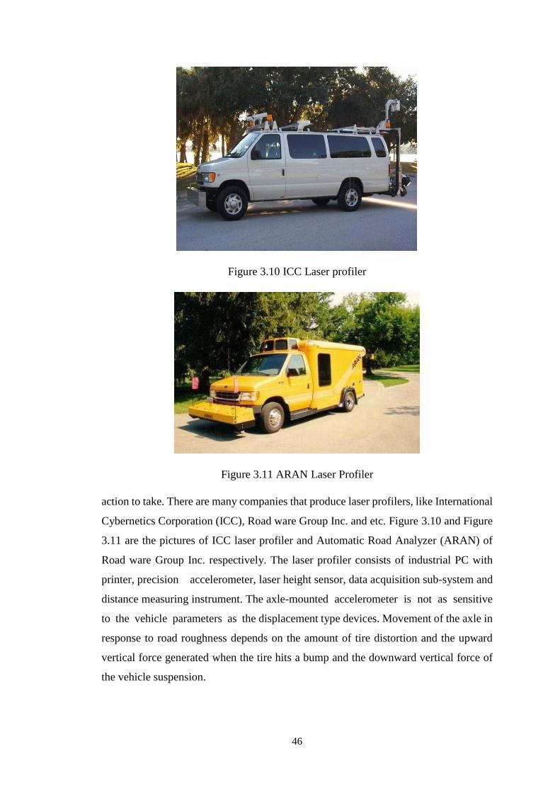
46
Figure 3.10 ICC Laser profiler
Figure 3.11 ARAN Laser Profiler
action to take. There are many companies that produce laser profilers, like International
Cybernetics Corporation (ICC), Road ware Group Inc. and etc. Figure 3.10 and Figure
3.11 are the pictures of ICC laser profiler and Automatic Road Analyzer (ARAN) of
Road ware Group Inc. respectively. The laser profiler consists of industrial PC with
printer, precision accelerometer, laser height sensor, data acquisition sub-system and
distance measuring instrument. The axle-mounted accelerometer is not as sensitive
to the vehicle parameters as the displacement type devices. Movement of the axle in
response to road roughness depends on the amount of tire distortion and the upward
vertical force generated when the tire hits a bump and the downward vertical force of
the vehicle suspension.

47
If the force of the suspension on the axle is greater than the upward force generated by
the bump, then the tire maintains contact with the pavement so the axle provides a
reasonable tracking of the pavement surface. The output of the accelerometer can be
integrated twice to obtain an estimate of the vertical axle movement. However, this
integration process can magnify the effect of undesired noise in the signal. Generally
the axle mounted RTRRMS’s use a measure of the root-mean-square acceleration of
the axle to quantify pavement roughness. The data collected is not affected by vehicle
variation such as speed, weight and suspension. Measurements are not affected by
changes in temperature, pavement color or texture, sunlight, wind and speed.
The Profiler offers many benefits over the conventional method of measurement. It
doesn’t require any set up or break down and operates at speeds up to 65 MPH. This
permits rapid, real-time measurements. This also eliminates the need for lane closures
or traffic control to test existing pavements. When the Profiler is used on an all terrain
vehicle it is so lightweight it can test pavements before they have completely set up.
The Profiler can be provided on any vehicle required by the user. The equipment is
mounted to an all terrain vehicle or can be supplied to mount into any specified vehicle.
The system collects data in real-time as it traverses the pavement’s surface. The raw
data is processed and the results are output in standard or metric units on the flat panel
display or graphics printer and are saved on a hard drive or floppy drive.
The software of Laser profiler includes digital band-pass filters passing wavelengths of
1 feet to 300 feet, digital high-pass filters passing filters passing wavelengths of 2 feet
or less, and statistical models generating the reported roughness statistics root mean
square vertical acceleration (RMSVA), mean absolute slope. The laser profiler provides
surface profile, IRI, Serviceability Index (SI) and Ride Number output.
3.4 Profiles
The evaluation of the entire pavement surface is required to define roughness
completely. However, for most purposes, roughness can be divided into three profile
components of distortion: transverse, longitudinal, and horizontal. Of particular interest
are variations in profile that impart acceleration to the vehicle or occupant and thus
influence comfort and safety. Here, the research will focus on longitudinal profiles.
Distortions of the pavement surface can generate both vertical and lateral acceleration
in the vehicle. Vertical acceleration is the major contributing factor to occupant comfort

48
and derives from longitudinal distortion of the pavement profile. Lateral accelerations
are the result of vehicle roll and yaw. Roll results from rotation about the longitudinal
axis of the vehicle while yaw is the rotation about the vertical axis. The curvature of the
roadway, which contributes to yaw, is normally handled through good geometric
design. Roll results from differential transverse pavement elevations. Under severe
conditions, it can impart an undesirable level of vertical acceleration.
It is possible to take many profiles for a road, each along a different line. However since
approximately 70 percent of vehicles travel in a well-defined wheel path with the right
wheel located 2.5 to 3.5 feet from the pavement edge, the wheel tracks of automobiles
and trucks are approximately 6 and 7 feet apart, respectively. Therefore, line
measurement of the longitudinal profile on the wheel path provides the best sample of
road surface roughness. Furthermore, comparison between the two wheel paths can
provide some measure of the transverse variations that affect roll.
Based on the pavement roughness definition, it is concluded that road roughness
evaluation requires measurement of the longitudinal profile of the pavement in the
vehicle wheel path. The profile of a road, pavement, or ground can be measured along
any continuous imaginary line on the surface and in order to obtain repeatable measures.
It helps to make the line physically by using paint. For engineering interpretation, the
measurements are usually handled with mathematical model that generates a summary
statistics, ranged from power spectrum to some type of roughness index.
3.5 Profile Index
A profile index is a summary number calculated from the data that make up a profile.
The profile index is portable, reproducible and stable with time. Almost all road
profiling system include two summary roughness statistic like, International Roughness
Index (IRI) and the estimate of Mean Panel Rating value Ride Number (RN). Although
there are also some others roughness indices are used, but IRI and RN are the most used
roughness indices because they portable and reproducible and they are stable with time.
So the other roughness indices are not widely available in the form of software and they
correlate so highly with IRI, we will focus on the former two indices

49
3.6 Roughness Definition
From an auto driver’s point of view, pavement roughness is a phenomenon experienced
by the passenger and operator of a vehicle. According to the definition (E867) of the
American Society of Testing and Materials (ASTM), “roughness is the deviations of a
pavement surface from a true planar surface with characteristic dimensions that affect
vehicle dynamics, ride quality, dynamic loads, and drainage, for example, longitudinal
profile, transverse profile, and cross slope”. This definition covers the factors that
contribute to road roughness and it is also very broad. However, it does not provide a
quantitative definition or standard scale for roughness, so it still requires a measurement
and analysis method for quantifying distortions of the pavement surface.
Once the measurement and analysis method is selected, individual agencies can
establish interpretation scale to determine the severity of the roughness level. At the
same time, pavement roughness consists of random multi-frequency waves of many
wavelength and amplitudes. Longitudinal roughness has been defined as "the
longitudinal deviations of a pavement surface from a true planar surface with
characteristic dimensions that affect vehicle dynamics, ride quality and dynamic
pavement load". Pavement profiles, detailed recordings of surface characteristics, are
frequently used to characterize roughness.
There are several causes of pavement roughness: traffic loading, environmental effects,
construction materials and built-in construction irregularities. All pavements have
irregularities built into the surface during construction, so even a new pavement that
has not been opened to traffic can exhibit roughness. The roughness of a pavement
normally increases with exposure to traffic loading and the environment. Short-
wavelength roughness is normally caused by localized pavement distress, that is,
depression and cracking, at the same time the long-wavelength roughness is normally
caused by environmental processes in combination with pavement layer properties.
3.7 International Roughness Index (IRI)
The International Roughness Index (IRI) was established in 1986 by the World Bank
and based on earlier work performed by NCHRP. It was first introduced in the
International Road Roughness Experiment (IRRE) that was held in Brazil. IRI is
calculated from a measured longitudinal road profile by accumulating the output from
a quarter-car model or directly derived from a class 1 or class 2 instruments and divided
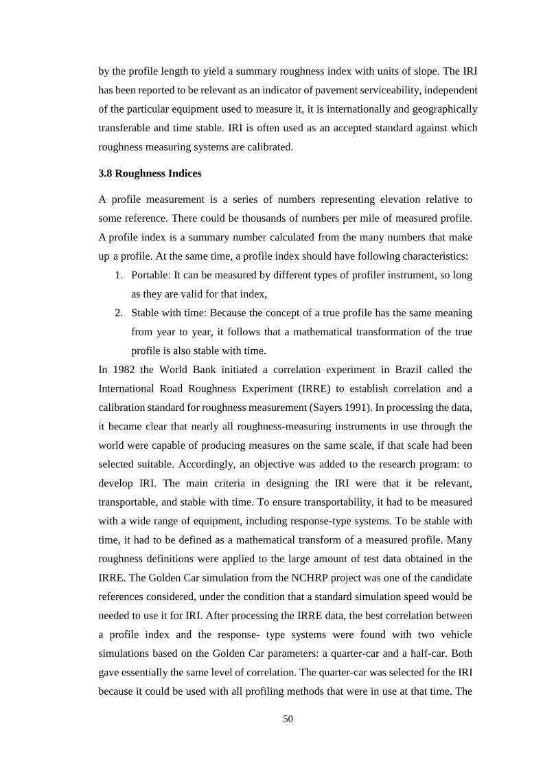
50
by the profile length to yield a summary roughness index with units of slope. The IRI
has been reported to be relevant as an indicator of pavement serviceability, independent
of the particular equipment used to measure it, it is internationally and geographically
transferable and time stable. IRI is often used as an accepted standard against which
roughness measuring systems are calibrated.
3.8 Roughness Indices
A profile measurement is a series of numbers representing elevation relative to
some reference. There could be thousands of numbers per mile of measured profile.
A profile index is a summary number calculated from the many numbers that make
up a profile. At the same time, a profile index should have following characteristics:
1. Portable: It can be measured by different types of profiler instrument, so long
as they are valid for that index,
2. Stable with time: Because the concept of a true profile has the same meaning
from year to year, it follows that a mathematical transformation of the true
profile is also stable with time.
In 1982 the World Bank initiated a correlation experiment in Brazil called the
International Road Roughness Experiment (IRRE) to establish correlation and a
calibration standard for roughness measurement (Sayers 1991). In processing the data,
it became clear that nearly all roughness-measuring instruments in use through the
world were capable of producing measures on the same scale, if that scale had been
selected suitable. Accordingly, an objective was added to the research program: to
develop IRI. The main criteria in designing the IRI were that it be relevant,
transportable, and stable with time. To ensure transportability, it had to be measured
with a wide range of equipment, including response-type systems. To be stable with
time, it had to be defined as a mathematical transform of a measured profile. Many
roughness definitions were applied to the large amount of test data obtained in the
IRRE. The Golden Car simulation from the NCHRP project was one of the candidate
references considered, under the condition that a standard simulation speed would be
needed to use it for IRI. After processing the IRRE data, the best correlation between
a profile index and the response- type systems were found with two vehicle
simulations based on the Golden Car parameters: a quarter-car and a half-car. Both
gave essentially the same level of correlation. The quarter-car was selected for the IRI
because it could be used with all profiling methods that were in use at that time. The

51
consensus of the researchers and participants is that the standard speed should be 80
km/hr (49.7 mph) because at that simulated speed, the IRI is sensitive to the same
profile wavelengths that cause vehicle vibrations in normal highway use. The research
findings were highly encouraging and led the World Bank to publish guidelines for
conducting and calibrating roughness measurements. The researchers (Sayers,
Gillespie, Queiroz and Paterson) prepared instructions for using various types of
equipment to measure IRI. The guidelines also include computer code for calculating
IRI from profile. A companion report described the IRRE, using many analytical
comparisons of algorithms and some sensitivity analyses. In 1990 FHWA required the
IRI as the standard reference for reporting roughness in the Highway Performance
Monitoring System (HPMS).
The IRI is a general pavement condition indicator. It summarizes the roughness
qualities that impact vehicle response, and is most appropriate when a roughness
measure is desired that relates to: overall vehicle operating cost, overall ride quality,
dynamic wheel loads (that is, damage to the road from heavy trucks and braking and
cornering safety limits available to passenger cars), and overall surface condition.
There are following properties of the IRI:
1. It showed maximum correlation with the RTRRMSs in use,
2. It describes profile roughness that causes vehicle vibrations,
3. It is linearly proportional to roughness,
4. It is the first highly portable roughness index that is stable with time
For decades, highway engineers have been interested in estimating the opinion of the
traveling public of the roughness of roads. The PSI scale from the AASHO Road Test
has been of interest to engineers since its introduction in the 1950’s. Ride Number is a
profile index intended to indicate ride-ability on a scale similar to PSI.
Direct collection of subjective opinion of Mean Panel Rating is too expensive and
provides no continuity from year to year. The NCHRP sponsored two research projects
in the 1980’s that investigated the effect of road surface roughness on ride comfort.
During two projects, mean panel ratings were determined experimentally on a 0 to 5
scale for test sites. The researchers investigated a quarter car analysis and found
significantly less correlation between the quarter car index and panel rating than
between a profile index based on short wavelengths.
The profile-based analyses were developed to predict MPR. A method was developed

52
in which PSD functions were calculated for two longitudinal profiles and reduced to
summary statistic called PI (profile index). The PI values for the two profiles were then
combined in a nonlinear transform to obtain an estimate of MPR. There are following
properties for the Ride Number analysis:
1. It uses the 0 to 5 PSI scale,
2. It is a nonlinear transform of a statistic called PI,
3. Ride Number is correlated to IRI but the two are not interchangeable.
Summary
In this chapter, various methods and models are presented in detail. The various
methods available for analysis the roughness are field tests. Different types of
Distresses also empathized in this chapter. And also, various types of profiling
techniques like Laser and many, Model was discussed in this chapter.
53
CHAPTER 4
METHODOLOGY AND DATA COLLECTION
4.1 Introduction
In the thesis report, an inertial-based automatic pavement roughness measuring system
was used. The methods used in the system are described in detail here.
This chapter consists of three sections. The first section will explain the methodology
used to get the pavement profiler from longitudinal distance. Then the quarter car
model, the algorithms of calculated International Roughness Index (cIRI) and Expected
International Roughness Index (eIRI) are described in details. Finally the digital filter
analysis, Data to be collected and will be explained. The discussion of their application
in the pavement measurement system.
4.2 Study Area discussion
The scope of the study was limited to two stretches distributed on two roads one from
Chaderghat, Chanchalguda to Dabeerpura Road and other from Charminar- Rajiv
Gandhi International Airport Road. Study area stretches were selected based on the
category of the road, terrain and traffic conditions, geographical location etc.
Homogenous sections were selected based on the factors like traffic, pavement layer
details, type of surfacing, general surface condition, subgrade soil conditions and
terrain type. Figure 4.1 and Figure 4.2 shows the location of study area. Table 4.1
shows the details of study stretches. The two study areas where within the Hyderabad
city, this are said as Urban City roads.

54
Figure 4.1 Stretch from Chaderghat, Chanchalguda to Dabeerpura Road
Figure 4.2 Stretch from Charminar- Rajiv Gandhi International Airport Road

55
Table 4.1 Details of the Stretches.
SL.NO Name of Road Category No of Homogenous
Sections with chain age
1 Chaderghat,
Chanchalguda to
Dabeerpura
Under City Road
of NH9
HS I - (118-124)
2 Charminar- Rajiv
Gandhi
International
Airport
Via. Srisailam
Highway – 765
City Road
HS II – (180-200)

56
4.3 Research Methodology
The proposed methodology in achieving the objectives is represented in the form of
flow chart as shown in Figure 4.3
Refining & selecting a general topic of wide interest
through various Journals, Thesis and References.
Acquiring the current scenario & information
Assessing the relevance of the
problem
Formulation of Research Objective & Defining Scope of Study
Literature Review
Data Collection
Data
Collecti
on
cIRI
Based on the quarter
car formula for a
narrow speed gap
such as 60-80 km/h
eIRI
Based on a Peak and
Root Mean Square
vibration analysis
Identifying the distresses
Building of Model
Tabulation & Preliminary Analysis of Data
Analysis of Models using SPSS
Analysis of Models using Roadroid
Results
Conclusions from the Model
Scope of further study

57
4.4 Method to Collect Data
By using the built-in vibration sensor in smartphones, it is possible to collect road
roughness data at Class 2 or 3 level in a very simple and cost efficient way. Data
collection can be done continuously and monitor roughness changes over time. The
continuous data collection can also give early warnings of changes and damage, enable
new ways to work in the operational road maintenance management, and can guide
more accurate surveys for strategic asset management and pavement planning. Data
collection with smartphones will not directly compete with Class 1 measurements, but
rather complete them in a powerful way. As Class 1 data is very expensive to collect it
cannot be done often, and advanced data collection systems also demand complex data
analysis and take long time to deliver. Smartphone based data collection can meet both
these challenges.
A smartphone based system is also an alternative to Class 4 – Subjective rating, on
roads where heavy, complex and expensive equipment is impossible to use, and for
bicycle roads. The technology is objective, highly portable and simple to use. This gives
a powerful support to road inventories, inception reports, tactical planning, program
analysis and support maintenance project evaluation.
4.4.1 History
2002-2006 - Research for the Swedish Road Administration using accelerometers and
a PC.
2010 - Technology to measure vibrations was built in to a smartphone.
2011 - First Android app for research of how cars, phones and speed are affecting
values.
2012 - User discovery/development with managers for road maintenance
2013 - First end user projects and piloting in different parts of the world.
The Roadroid smartphone solution has two options for roughness data calculation:

58
1. Estimated IRI (eIRI) - based on a Peak and Root Mean Square vibration analysis
– and correlated to Swedish laser measurements on paved roads. The setup is
fixed but made for three types of cars and is thought to compensate for speed in
20-100 km/h. eIRI is the base for a Roadroid Index (RI) classification of single
points and stretches of road.
Formula developed in correlation with IQL1 measurements (2012).
2. Calculated IRI (cIRI) - based on the quarter car formula for a narrow speed gap
such as 60-80 km/h. cIRI allows the operator to calibrate the sensitivity to a
known reference.
Collected data are digitally transferred to internet maps and can be aggregated in
preferred sections (default 100 m), as well as exported to Geographical Information
Systems (GIS). In addition to optimizing road maintenance, the information could be a
new kind of input to road navigators and digital route guides. Digital bump warnings
can be presented as detected bumps to road navigators through standards for Intelligent
Transportation Systems (ITS).
The International Roughness Index (IRI) is a roughness index commonly obtained from
measured longitudinal road profiles. Since its introduction in 1986, IRI has become
commonly used worldwide for evaluating and managing road systems. Vibrations have
been used since early 1900 for expressing road condition and ride quality.
The traditional techniques for measuring roughness may be categorized as special built
trucks or wagons with laser scanners, bump-wagons, and manually operated rolling
straight edges. Special built equipment is expensive, due to heavy and complex
hardware, low volume of production and need of sophisticated systems and accessories.
Data gathering and analysis are often time consuming. Data collection is typically done
during the summer then analysed and delivered to the maintenance management
systems in late autumn. It is soon then winter and spring where the road faces continual
frost heave/thaw (a very dramatic period in a road´s life with extreme changes in
roughness). The IRI values that were “exact” almost a year ago might now not be the
same any longer. As it is also so expensive to collect and analyse the data, that many
roads are only covered in one lane direction every 3-4 years.
Smartphone based gathering of roughness data, can be done at a low cost and monitor
changes on a daily basis. For frost heave issues it can tell when and where it is

59
happening and if the situation is worse than in previous years. It can be used in the
winter to determine the performance of snow-removal and ice-grading. It may
advantageously be used in performance based contracts or research on road
deterioration, various environmental effects (as heavy rains, flooding).
It should be mentioned that smartphone based systems like Roadroid might challenge
old knowledge, standards, procedures and existing ways to procure:
1. Pavement planners and road engineers know existing inputs;
2. Research organisations, suppliers and buyers have existing ways to work;
3. Organizations have invested time, prestige and huge amounts of money to
develop more and more exact and complex data collection and management
systems.
As described it is necessary to understand the difference between four generic classes
of road roughness measuring methods in use:
Class 1 - Precision profiles
Class 2 - Other profilometric methods
Class 3 - IRI by correlation
Class 4 - Subjective ratings
It is natural that scepticism will appear when a Class 2/3 smartphone is compared with
a multi-million dollar Class 1 vehicle. But a smartphone can deliver up-to-date good
quality roughness data to a web page within 24 hours, in contrast to an expensive
software client with the “exact” Class 1 data from last year.
On the other end of the scale – many road inventories and assessments are actually
made by Class 4 subjective ratings over large areas using pen and paper.
Smartphone data collection fills a gap between the class 1 measurements and class 4
ocular inspections, and we see some early adopters and notice steps of development in
the market.

60
4.4.1.1 The First Prototypes 2002-2006
Figure 4.4 First Prototype (2002-2003)
The Roadroid team has been working with mobile ITS since mid-1990s, particularly
with mobile data gathering, road weather information and road databases.
Figure 4.5 Second Prototype (2004-2016)
During a visit to the Transportation Research Board in Washington in 2001, a Canadian
project was presented that monitored the speed of timber hauling trucks, simply
assuming that where the speed was low the road quality was poor. Our developed idea
was to add vibration measurements.

61
Together with the Royal Institute of Technology, a first pilot scheme was built in 2002-
2003. At that time we used a high-resolution accelerometer at the rear axle of a front
wheel drive vehicle, connected by cable to a portable PC through a signal conditioner.
GPS and GSM were connected through wired serial connections. Two master students
built a first prototype using an industrial software system for signal analysis.
The results were promising and the Swedish National Road Administration financed an
R&D project to further develop and validate the prototype with a focus on gravel roads.
The system was developed into a C++ software for Windows program, and a GIS tool
was implemented for viewing the road quality in different colours.
A validation between ocular inspections and the system´s measurements was performed
and presented at the Transport Forum, Linköping, in 2005. 8 segments of 100 m were
individually assessed according to 4 road condition classes. Module analysis
(experimental analysis of oscillation) was performed on a sample of specific sections
of the 4 road condition classes. Regression analysis was then performed with rules
based on:
1) Amplitude levels for different G,
2) RMS (Root Mean Square),
3) The vehicle speed measured and
4) The length in meters.
The analysis showed that a single test run would classify properly to 70% compared to
an average of subjective ocular inspections, while a single ocular inspection varied
more from the average than that. The method was considered objective with very good
repeatability.
In 2006 the development stalled. The system was considered relatively cheap and
simple to operate at the time (~7000 USD). In retrospect, it had several limitations;
particularly the sensor mounting and cables exposed in the harsh environment under a
car, but also the windows 98 computer and the cable-connected, and a not very accurate,
GPS

62
4.4.1.2 Further Development 2010-2011
In 2010, the ideas from 2002-2006 were reviewed. A major technical development was
now the appearance of mobile smartphones. Literally all peripherals that were
previously connected by cables were now built into a phone and the limitations of
certain components were removed by new advances in technology. We knew the
answers to some of the questions from 2002-2006, e.g. the basis for signal analysis and
the influence of speed. There were however new big questions to solve, such as:
Was it possible to pick up the signals from inside the car?
We knew different car models would give different signals and how could we
handle that?
Would a lower sampling frequency be enough (100 Hz compared to earlier 512
Hz)?
Would the accelerometer sensitivity and the G-scale be sufficient (+/-2G)?
Would different smartphone models return different values (accelerometer
sensitivity).
And authorities developed an Android application and an algorithm using the built-in
accelerometer signal. The choice of Android rather than iPhone was made considering
the open architecture and hardware price/performance relation. We started to sample
data on different roads with different types of vehicles, and over constructed obstacles
in 2011.
The obstacles were passed by different vehicle types 5 times in 6 different speeds: 20,
40, 60, 80, 100 and 120 km/h. Data were sampled with different phones, both with our
algorithm and in raw 100 Hz. During the data analysis, we then discovered a number
of things:
There are differences between different car models, especially at low speeds. In
the 40-80 km/h range, differences are however limited. The tests gave us a
model for how to calculate the speed influence of the signal for the 3 different
type vehicles.
There are big differences between different phones, both for the sampling
frequency and the quality of the accelerometer data. It is of great importance to

63
know these dynamics to achieve comparable data. A phone calibration
procedure is required.
It is of great importance to mount the phone correctly in a good mounting
bracket, preferably in a way that enables the phone´s camera lens to be directed
at the road.
Most importantly: the trials during 2011 showed that usable data could be delivered!
We now had an Android app analysing 100 vibrations per second and saving several of
the essential road condition values with a GPS coordinate!
Figure 4.6 Data Collecting using Roadroid
The road condition data was divided into 4 different levels for visualization: Green for
Good, Yellow for Satisfactory, Red for Unsatisfactory and Black for Poor.
4.4.1.3 Professional Use 2013-2014
Large-scale collection of measurement data in Sweden has been taking place during a
5 month period by the Swedish Automobile Association (Motormännen). The
organization will sample 92,000 km of the Swedish road network to identify and point
out road defects. We will prepare a report to Motormännen when the project is
finished and point out where the worst roads in Sweden are. The project is financed

64
by the Swedish Transport Administration (Trafikverket) which is the Swedish
government agency responsible for the long-term planning of the transport system.
4.5 Quarter Car Model
Figure 4.7 Quarter Car Model
The concept of quarter-car simulation as a method for analysing pavement profile data
was originally an attempt to simulate the output of the BPR roughometer.
Subsequently, vehicle simulation studies at the University of Michigan demonstrated
that full-car and half-car simulation models do not provide an advantage over the
quarter-car simulation and are computationally much complicated. these parameters
include the major dynamic effects that determine how roughness causes vibration in a
road vehicle. The masses, springs, and dampers are defined by the following
parameters: the sprung mass of the vehicle body; the suspension spring and damper
(shock absorber) constants; the Unsprung mass of the suspension, tire, and wheel; and
the spring constant of the tire. Theoretical correctness would require a damper
constant for the tire. However, practical application generally ignores this term.
Mathematically, the behavior of a quarter-car can be described with two-second order
equations:
M S Z S MU ZU Kt (ZU Z ) 0
And

65
M S Z S CS (Z S ZU ) KS (ZS ZU ) 0
Where
Z = road profile elevation,
Zu = elevation of unsprung mass (axle),
Zs = elevation of sprung mass (body)
Kt = tire spring constant,
Ks = suspension spring constant,
Cs = shock absorber constant,
Mu = unsprung mass (axle), and
Ms = sprung mass.
To simplify the equations, the parameters are normalized by the sprung mass, Ms. The
following values for the normalized parameters define the Golden Car data set:
K1 = Kt / Ms = 653,
K2 = Ks / Ms = 63.3
C = Cs / Ms = 6.0
M = Mu / Ms = 0.15
Since RTRRMS devices generally measure the movement between the vehicle axle
and body, simulation requires calculation of the difference in elevation between the
body and axle in response to the road profile and forward motion of the vehicle. This
is accomplished by integrating the difference in the velocities between the sprung and
unsprung mass; producing the quarter-car statistic, QCS:
The terms C represents either the total time required to traverse the section of road or
the length of the section, L. If the time factor is used to normalize the quarter-car
statistic, the calculation results in an average rectified velocity, while a distance base
yields the average rectified slope. There are several acceptable numerical techniques
for the solution of the equation. However, the linear nature of the equations permits
an exact solution with the state transition matrix method. Historically, two sets of

66
vehicle parameters have been used for computing quarter-car statistics for calibration
of RTRRMS devices. A set representing the original BPR Roughometer trailer was
used for several years, until research at the Highway Safety Research Institute
(HRSI) produced an updated set of vehicle parameters. The World Bank recommends
the HSRI vehicle parameters and has termed the quarter-car statistic computed as the
international roughness index, IRI.
4.6 Calculation of IRI
The calculation of the international roughness index (IRI) is accomplished by
computing four variables as functions of the measured profile. (These four variables
simulate the dynamic response of a reference vehicle, shown in Figure 4.6, traveling
over the measured profile.) The equations for the four variables are solved for each
measured elevation point, except for the first point. The average slope over the first
11m (0.5 sec at 80 km/h) is used for initializing the variables by assigning the
following values:
Z1 Z3 (Ya Y1 ) /11
Z2 Z4
a 11/ dx 1
Where Ya is the “a-th” profile elevation point that is a distance of 11m from the start
of the profile, Y1 is the first point, and dx is the sample interval.
The following four-recursive equations are then solved for each elevation point, from
2 to n (n =number of elevation measurement):
Z1 s11Z1 s12 Z 2 s13 Z3 s14 Z 4 P1 Y
Z 2 s21Z1 s22 Z 2 s23 Z3 s24 Z 4 P2 Y
Z3 s31Z1 s32 Z 2 s33 Z3 s34 Z 4 P3 Y ' '
Z 4 s41Z1 s42 Z 2 s43 Z3 s44 Z 4 P4 Y
Where
Y (Yi Yi1 ) / dx slope

67
Sij and Pj are coefficients that are fixed for a given sample interval, dx, thus, the
equations above are solved for each position along the wheel track. After they are
solved for one position, equation above is used to reset the values of Z1', Z2', Z3' and
Z4', for the next position. Also for each position, the rectify slope (RS) of the filtered
profile is computed as:
RSi Z3 Z1
The computed IRI will have units consistent with those used for elevation measures and
for the sample interval. For example, if elevation is measured as millimeters and dx is
expressed in meter, then the IRI will have the preferred units: mm/m=m/km=slope*10.
The coefficients used in the equations are calculated from the equations of motion that
define a quarter-car model. In the general case, they are specific to the vehicle model
parameter values, simulation speed, and the sample interval.
Figure 4.8 IRI Roughness Scale
The IRI summarizes the roughness qualities that impact vehicle response, and is most
appropriate when a roughness measure is desired that relates to: overall vehicle
operating cost, overall ride quality, dynamic wheel loads, and overall surface condition.
Figure 4.8 shows IRI ranges represented by different of road.
IRI is influenced by wavelengths ranged from 1.2 to 30 meters. The wave number
response of the IRI quarter-car filter is shown in Figure 3-5. The amplitude of the output

68
sinusoid is the amplitude of the input, multiplied by the gain shown in Figure 3-5. The
gain shown in the figure is dimensionless.
The IRI filter has maximum sensitivity to slope sinusoids with numbers near 0.065
cycle/m (a wavelength of about 15m) and 0.42 cycle/m (a wavelength of about 2.4m.).
The response is down to 0.5 for 0.03 and 0.8 cycle/m wave numbers that correspond to
wavelengths of 30m and about 1.25m, respectively. However there is still some
response for wavelengths outside this range. An IRI of 0.0 means the profile is perfectly
flat. There is no theoretical upper limit to roughness, although pavements with IRI
values above 8 m/km are nearly impassable except at reduced speeds.
For the specific case of IRI, defined by the NCHRP 228 parameters [Wambold, 1980]
and a standard 80km/hr simulation speed, they depend only on the sample interval.
Complete instructions for measuring IRI are available in Sayers, gillespie, and
Queiroz [Janoff et al, 1990].
Figure 4.9 Sensitive Wave Number of IRI
The instructions include listings of computer programs that solve the equations of
motion and also computer programs that calculate the coefficients.

69
4.7 Understanding Roadroid use
Figure 4.10 Roadroid methodology
Figure 4.11 Basic Principle of Roadroid
Modern smartphones are equipped with a number of sensors including multi-axis
accelerometers, temperature probes, gyroscopes, light intensity sensors, magnetic field
sensors, etc. (Sensors and Cell phones 2013). The Roughness Capture application
collects acceleration in three orthogonal directions, a timestamp, and GPS coordinates
and stores them in an ASCII text file. Data collection rate is specified by the user,
generally in the range of 10 – 100 samples per second, but higher sampling rates are
possible depending upon

70
Figure 4.12 Need of the study
Smartphone hardware. In general, the higher the data collection rate, the better the
accuracy of the estimated pavement profile (with diminishing returns at very high
sampling rates)
Figure 4.13 Rehabilitate before it’s too late

71
Figure 4.14 Roadroid data processing process
Figure 4.15 Gadgets required for data collection
Table 4.2 Application Setting
Car Asphalt Gravel Earth/dirt
Speed 80 km/h 60 km/h 40 km/h
cIRI-sensitivity 1,6 2,2 2,8
cIRI length 40 m 100 m 200 m

72
1. Collect data
First, make sure Roadroid have registered your units IMEI number on the website, and
that your email is filled in Settings->UseEqID, and that the unit is set on the right phone
model and car type.
Mount the phone car rack in the front window.
Make sure the rack is stable
Fit it so it is easy to reach and tap on the display.
Mount the phone as straight as possible, horizontally is often most suitable to
use the GPS-photo function.
Fit the rack so that the camera display the road and Start the cam while fitting
to find a good position!
Start the Roadroid application by tapping the icon (1), press "Ok" to accept settings
(2). Press the yellow “fitting” button (3)

73
While fitting – adjust the phone to X, Y and Z as close to = 0 as possible. The OK
button will turn green when you are within the tolerances. Press the green OK-button.
The interface of the Roadroid looks like this.
Figure 4.16 Description of interface
1. Estimated IRI is collected in speeds between 20-100 km/h – try to keep same speed.
2. Calculated IRI can be adjusted in settings and should be collected in speeds 60-90
km/h.
3. Press “Start/stop sampling” to stop measurement - note date and time to keep track
of your files.
4. Make a good plan of how to collect data, press start/stop in logical intersections of
the road.
2. Upload Data

74
To upload data you need to be connected to a have a stable internet connection.
Preferrably use a WiFi, especially to upload photos. Connect to WiFi through normal
procedure. Test to surf on internet with the phones internet browser. If you can do that
– your phone is connected. If not – you don’t have an internet connection, and will not
be able to upload your data. When you are connected:
1) Tap the Android menu button (down left),
2) Choose “Upload” and then
3) Choose data to upload your collected roughness data (and Media to upload eventual
photos).
Roughness data is saved in maximally 300 kB files (its often smaller). A new file is
saved each time you press Start/stop). Media (photos) can be up to 2 MB!
When the file transfer has started it will continue until finished, stay still during this
process. See the notification in the upper left corner of the display. Click-drag the
notification to view the file transfer progress. Small files uploads in seconds. Larger
files and with poor connection it takes longer time.
When the upload is finished a success message should occur. If there is some problem,
an error message will be seen instead. Advise the user guide to find out more about
possible problems.
When the Data button is pressed:
1. files in the /arq/data folder are compressed and moved to the /arq folder.
2. the Roadroid app transfer function starts, and lastly
3. if the file transfer is successful the zipped files is moved to /arq/backup.
This repeats for every file. If the transfer is incomplete the function will try again next
time an upload is running. The files will stay in the /arq folder until they are successfully
transferred.
1. If the transfer function is not working (see user guide) the files can be moved
manually. Locate the files with the phones file manager in the “/arq” folder on
the unit (or SD-card). When you have found them you can send them by email
(also requires a WiFi connection).

75
2. You can also connect the phone with an USB-cable to your PC, locate the files
with the PC’s file manager and copy/send the files with your PC.
3. If no transfer attempt is done: uncompressed files are located in the "/arq/data”
directory. The data files you may want to transfer is "gps*.txt" and "ueid.txt".
Select and send by email.
4. If a failed transfer was made, zipped files are in the "/arq" folder. Move them
to the "/arq/backup” folder when they are copied or emailed.
The files on the phone are encrypted, and will be decrypted in the web import.
3. View data by the Roadroid web service
When data is successfully uploaded, it will be imported to the web service within an
hour. Surf in to www.roadroid.com and navigate to your geographic area. You will need
a user log-in and password to view details of your data. Depending on if there is a road
network layer available – colored road links will appear on the map. If there are no
colored links, you need to check the “GPS-Points” (5).
Figure 4.17 Data viewed in Server
1. The time filter (3) is used to display and measure point data only within the set
time interval. It can be used to look at changes over time and obtaining
statistics with the report functions.
2. Navigate (4) allow you to drag the map with the mouse. With draw polygon
active, you click on the map to draw a polygon for an area to calculate. Close

76
polygon by double click (turns orange). Click "Calc" to calculate and you
should get the percentage of each 4 road classes Good – Poor and an average
estimated IRI.
3. Map Background: Google Streets is default, but it is changeable to Google
Satellite.
4. The amount of points shown is limited (for server performance reasons).
5. When you zoom in to the map, eIRI – labels will occur at each dot a certain
zoom level.
6. Depending on the road database available, monitoring of the speed profile can
be applied (to see where the road is so bad road that it affects the ability to
maintain speed while driving (Green >70 km/h, Yellow 50-70 km/h, Red 30-
50 km/h, Black <30 km/h).
If photos are uploaded to the Roadroid web they will appear as clickable black spots.
Figure 4.18 Data viewed With Snapshots
4. Download aggregated files
Data is saved in the phone every second between 20-100 km/h - the distance between
the “dots” will vary depending on the speed. To make tables and charts

77
Left: Raw decrypted data in one row per second. Right: Aggregated data in 100 meter
sections.
for studies on a road, or to import data to HDM-4, you need average data in fixed
sections lengths. Through the “import history” you can download the data aggregated
in 100 meter sections as text files.
Log in to www.roadroid.com and click “Import History” (1). You should now see a list
of your uploaded and imported files. Choose “Details” (2), to view the file details:
Filename, Start/stop time etc. Here you have use of your notes (!) from your data
collection. Note start time and some information about location to know what section
you are looking at. The start time is visible be in the filename with your phones IMEI.
There are some functions to zoom into the location, and to “Generate Aggregate file”
(3). This operation will create the 100-meter segment file. Save or open the file to copy
the data to MS Excel.

78
5. Making Charts for Aggregated Files
When you have copied data from your 100-meter .txt file paste it into excel (you can
also open a saved.txt file in excel). This guide is not meant to learning you basic excel
knowledge. A tip is to name the tab with date and time, and possibly name of the actual
section. In the aggregated file you will find following columns: Date Time, Latitude,
Longitude, Distance(m), Speed (km/h), Altitude (m), eIRI and cIRI. (eIRI is an
estimated value and is fixed. cIRI is calculated and is adjustable in the app - see user
guide). When you have pasted/imported your data in excel, you can start making charts.
Figure 4.19 Data Processing

79
The data aggregation length in the web download is 100 meter, a usual import length
in HDM. Speed and vertical profile is interesting for a road engineer to get an overall
view. And the data can preferably be used with images form a GPS-video capture:
4.8 Data Collection
Figure 4.20 Data Processing -2
The collection of data is taken place in three intervals, first at early morning, secondly
afternoon and the third at the mid night. With the help of Roadroid. I myself collected
the data. For the both corridors taken in consideration. Below Table 4.3 shows the
data collected which is within the city and also three runs are made to get the accurate
data. And table 4.4 shows the data of the corridor outside the city limits. Here the data
which is present below is taken with the smartphone application Roadroid the first
columns shows the data and time secondly the latitudes and longitudes to get the exact
location and then the distance covered following with speed and altitude after speed
and altitude, Calculated and Estimated Roughness index is presented through that we
can easily consider the roughness and can take specific measures in getting a better
pavement. Both data collection on both the sites was no more than an hour is being
taken.

80
1. Study Area One
Table 4.3 Roughness data-1
cIRI-sensitivity: 1.5
DateTime Latitude Longitude Distance(m)
Speed
(km/h)
Altitude
(m) eIRI cIRI
6/22/2015 5:51:12 AM 17.37572 78.48831 200 17.46 422.08 6.6 2.51
6/22/2015 5:51:54 AM 17.37738 78.48805 400 19.7 420.47 5.68 3.72
6/22/2015 5:52:34 AM 17.37735 78.48979 600 17.56 419.7 10.63 3.51
6/22/2015 5:53:20 AM 17.37758 78.49152 800 25.98 422.83 5.14 5.53
6/22/2015 5:53:47 AM 17.37926 78.49183 1000 25.26 422.26 4.79 5.23
6/22/2015 5:54:23 AM 17.38102 78.49189 1200 21.65 415.76 6.88 5.34
6/22/2015 5:54:56 AM 17.37976 78.49294 1400 29.49 412.88 6.2 8.45
6/22/2015 5:55:20 AM 17.3781 78.49346 1600 25.47 414.87 11.1 10.13
6/22/2015 5:55:49 AM 17.37716 78.49484 1800 23.77 414.81 12.86 9.94
6/22/2015 5:56:18 AM 17.37629 78.49623 2000 19.68 416.69 12.28 6.7
6/22/2015 5:57:08 AM 17.37614 78.49779 2200 31.82 424.99 11.19 12.33
6/22/2015 5:57:30 AM 17.37542 78.49848 2400 31.78 426.42 10.68 13.51
6/22/2015 5:57:53 AM 17.37361 78.49897 2600 31.87 423.78 8.22 13.68
6/22/2015 5:58:15 AM 17.37205 78.49968 2800 30.54 425.12 10.07 12.82
6/22/2015 5:58:39 AM 17.37048 78.50081 3000 42.91 430.09 7.41 15.34
6/22/2015 5:58:55 AM 17.36911 78.50171 3200 35.18 435.7 7.55 12.89
6/22/2015 5:59:16 AM 17.36722 78.50174 3400 47.71 438.86 7.04 14.69
6/22/2015 5:59:31 AM 17.36543 78.50148 3600 24.36 439.74 11.61 6.46
6/22/2015 6:00:01 AM 17.36379 78.50113 3800 22.65 442.98 7.65 4.33
6/22/2015 6:00:41 AM 17.36431 78.49938 4000 26.49 441.83 5.11 6.63
6/22/2015 6:01:10 AM 17.36545 78.49794 4200 24.18 437.66 6.96 6.35
6/22/2015 6:01:39 AM 17.36611 78.49649 4400 21.91 437.36 7.64 5.35
6/22/2015 6:02:16 AM 17.36649 78.49469 4600 26.61 434.33 6.44 8.28
6/22/2015 6:02:45 AM 17.36693 78.49286 4800 32.27 429.73 4.8 7.94
6/22/2015 6:03:07 AM 17.36692 78.49102 5000 41.32 432.01 10.32 18.18
6/22/2015 6:03:24 AM 17.36694 78.48918 5200 35.7 423.76 8.7 11.62
6/22/2015 6:03:45 AM 17.36739 78.48734 5400 29.09 420.23 8.1 7.87
6/22/2015 6:04:10 AM 17.36787 78.48554 5600 30.08 421.62 8.98 12.36
6/22/2015 6:04:34 AM 17.36842 78.4837 5800 21.17 428.05 8.35 4.73
6/22/2015 6:05:08 AM 17.36908 78.482 6000 19.81 429.28 8.96 6.1
6/22/2015 6:05:48 AM 17.3705 78.48199 6200 18.42 425.87 6.93 3.94
6/22/2015 6:06:39 AM 17.37229 78.48243 6400 21.87 421.95 9.73 6.52
6/22/2015 6:07:12 AM 17.37363 78.48326 6600 29.39 420.47 9.4 10.09
6/22/2015 6:07:35 AM 17.37491 78.48455 6800 34.63 420.6 9.81 14.46
6/22/2015 6:07:56 AM 17.37631 78.48581 7000 29.46 420.38 10.35 12.47
6/22/2015 6:08:21 AM 17.37761 78.48717 7200 24.32 421.13 11.37 9.75

81
2. Study Area Two
Table 4.4 Roughness data-2
cIRI-sensitivity: 1.5
DateTime Latitude Longitude Distance(m)
Speed
(km/h)
Altitude
(m) eIRI cIRI
8/24/2015 2:45:01 PM 17.37563 78.48824 200 5.51 433.49 12.91 0.2
8/24/2015 2:46:02 PM 17.37603 78.48808 400 18.98 425.35 6.66 1.45
8/24/2015 2:46:36 PM 17.37758 78.48833 600 17.53 422.15 6.06 1.06
8/24/2015 2:47:11 PM 17.37744 78.49014 800 9.93 422.46 11.82 0.77
8/24/2015 2:48:14 PM 17.37779 78.49173 1000 7.61 417.83 10.58 0.29
8/24/2015 2:49:45 PM 17.37941 78.49181 1200 17.59 417.28 6.01 0.78
8/24/2015 2:50:26 PM 17.38106 78.49198 1400 8.22 415.51 17.43 0.73
8/24/2015 2:51:51 PM 17.37965 78.49295 1600 41.66 412.88 3.76 2.83
8/24/2015 2:52:08 PM 17.3779 78.49344 1800 30.56 417.19 4.6 2.75
8/24/2015 2:52:31 PM 17.37716 78.49476 2000 29.16 419.67 4.09 2.19
8/24/2015 2:52:56 PM 17.3763 78.49624 2200 29.82 418.37 5.62 2.62
8/24/2015 2:53:19 PM 17.37605 78.49771 2400 34.53 423.52 4.71 3.09
8/24/2015 2:53:40 PM 17.37528 78.49846 2600 42.94 423.56 3.83 3.87
8/24/2015 2:53:57 PM 17.37354 78.49899 2800 20.08 424.64 7.53 1.52
8/24/2015 2:54:33 PM 17.37186 78.49973 3000 32.15 431.24 4.06 2.68
8/24/2015 2:54:56 PM 17.37047 78.50085 3200 34.91 432.26 4.3 2.54
8/24/2015 2:55:15 PM 17.36903 78.50171 3400 37.97 436.37 2.96 2.22
8/24/2015 2:55:34 PM 17.36729 78.50175 3600 52.88 438.21 2.23 2.73
8/24/2015 2:55:48 PM 17.36538 78.50149 3800 17.36 441.18 9.73 0.85
8/24/2015 2:56:30 PM 17.36504 78.5014 4000 1.04 440.96 12.31 0.99
8/24/2015 3:07:40 PM 17.36654 78.50167 4200 26.02 437.8 3.79 1.59
8/24/2015 3:08:08 PM 17.36797 78.50178 4400 38.06 438.1 3.18 1.97
8/24/2015 3:08:26 PM 17.36611 78.50162 4600 48.66 440.08 2.14 2.25
8/24/2015 3:08:41 PM 17.36435 78.50151 4800 23.74 439.13 3.84 1.6
8/24/2015 3:09:12 PM 17.36338 78.50315 5000 8.52 443.09 9.01 0.71
8/24/2015 3:10:35 PM 17.36205 78.50403 5200 16.48 437.83 3.27 0.53
8/24/2015 3:11:18 PM 17.36033 78.50451 5400 16.69 438.63 2.74 0.67
8/24/2015 3:12:00 PM 17.35866 78.50501 5600 20.43 433.8 4.91 0.95
8/24/2015 3:12:35 PM 17.35687 78.50541 5800 22.35 433.44 3.5 1.01
8/24/2015 3:13:07 PM 17.35508 78.50599 6000 29.23 434.87 1.8 1.55
8/24/2015 3:13:32 PM 17.3533 78.50644 6200 8.61 433.28 10.52 0.77
8/24/2015 3:14:56 PM 17.35174 78.50706 6400 23.09 432.49 6.15 2.06
8/24/2015 3:15:26 PM 17.35014 78.50799 6600 28.03 434.97 2.17 1.84
8/24/2015 3:15:52 PM 17.34847 78.50857 6800 27.32 433.2 7.6 1.96
8/24/2015 3:16:17 PM 17.34664 78.50824 7000 45.54 432.89 3.49 2.76
8/24/2015 3:16:32 PM 17.34504 78.50787 7200 8.22 441.19 14.47 0.93
8/24/2015 3:18:06 PM 17.34353 78.50702 7400 21.42 445.83 4.97 1.14
8/24/2015 3:18:38 PM 17.34252 78.50541 7600 49.99 444.68 3.31 3.26
8/24/2015 3:18:52 PM 17.34158 78.50396 7800 41.25 451.2 2.15 1.89

82
8/24/2015 3:19:11 PM 17.34052 78.50237 8000 26.63 450.97 3.97 1.44
8/24/2015 3:19:36 PM 17.33969 78.50086 8200 55.84 449.86 2.13 2.66
8/24/2015 3:19:49 PM 17.33861 78.49917 8400 61.85 448.45 1.76 2.23
8/24/2015 3:20:00 PM 17.33771 78.49773 8600 54.63 452.4 1.7 2.03
8/24/2015 3:20:14 PM 17.33659 78.49617 8800 55.3 449.79 3.09 2.58
8/24/2015 3:20:27 PM 17.33535 78.49457 9000 56.84 446.73 2.21 1.84
8/24/2015 3:20:39 PM 17.33432 78.49329 9200 44.56 444.43 3.07 2.15
8/24/2015 3:20:56 PM 17.3331 78.49184 9400 30.98 443.58 4.74 2.7
8/24/2015 3:21:21 PM 17.33189 78.49037 9600 37.59 442.35 4.84 2.66
8/24/2015 3:21:39 PM 17.33133 78.48867 9800 27.28 441.34 5.11 1.88
8/24/2015 3:22:08 PM 17.33059 78.4869 10000 19.71 446.18 7.08 1.56
8/24/2015 3:22:42 PM 17.32988 78.48529 10200 39.19 449.75 5.6 3.72
8/24/2015 3:23:01 PM 17.32918 78.4834 10400 39.18 450.69 4.26 3.52
8/24/2015 3:23:19 PM 17.32856 78.4818 10600 31.85 452.78 3.3 2.6
8/24/2015 3:23:43 PM 17.32781 78.47996 10800 20.88 451.25 5.72 1.58
8/24/2015 3:24:16 PM 17.32625 78.47981 11000 13.33 453.68 7.12 0.94
8/24/2015 3:25:09 PM 17.32444 78.47995 11200 5.9 462 16.39 0.4
8/24/2015 3:27:10 PM 17.32275 78.48027 11400 23.43 462.24 3.36 1.44
8/24/2015 3:27:39 PM 17.32101 78.48029 11600 31.9 461.79 3.25 1.84
8/24/2015 3:28:01 PM 17.31929 78.47999 11800 20.11 464.39 5.78 1.14
8/24/2015 3:28:38 PM 17.31754 78.47965 12000 15.65 468.1 8.02 0.87
8/24/2015 3:29:26 PM 17.31577 78.47911 12200 19.09 470.5 5.06 1.18
8/24/2015 3:30:04 PM 17.31432 78.47885 12400 7.6 467.27 14.58 0.69
8/24/2015 3:31:30 PM 17.31515 78.47877 12600 34.5 466.39 2.83 2.3
8/24/2015 3:31:51 PM 17.31683 78.47946 12800 21.26 465.76 6.96 1.37
8/24/2015 3:32:25 PM 17.31862 78.47979 13000 33.64 463.57 6.18 2.77
8/24/2015 3:32:46 PM 17.32038 78.48013 13200 28.93 460.35 6.41 2.84
4.9 SPSS Interface
Figure 4.21 SPSS Start-up page

83
The above SPSS screenshot is a start screen load up I had use version 22 for the analysis
of the results.
Figure 4.22 Linear regression
The linear regression technique is being considered. For the analysis and validation
Summary
Measuring roads with smart phones can provide an efficient, scalable, and cost-
effective way for road organizations to deliver road condition data. In this chapter, we
have illustrated this with the use of software bundle—Roadroid. The system which does
not require a network connection during the data collection can geo locate data
(unmatched or matched to existing roads) on a globally level with sufficient accuracy.
We have implemented road condition standards based on previous work as cIRI as well
as our own speed and vehicle independent eIRI standard, which correlate up to 81%
with laser measurement systems

84
CHAPTER 5
ANALYSIS & RESULTS
5.1 Introduction
Pavement surface irregularities (non-planar road profile) lead to vertical accelerations
in moving vehicles. The magnitude of vertical acceleration depends on the severity and
frequency of pavement distresses and other surface irregularities, vehicle suspension
characteristics, and vehicle speed. A 3-axis accelerometer enabled cell phone can be
used to collect vehicle vertical acceleration data, as demonstrated in previous studies,
such as those conducted to identify localized pavement defects. An android-based cell
phone application has been developed in the present study that can capture acceleration
for the purpose of characterizing pavement roughness and individual pavement
distresses. Figure shows vehicle vertical acceleration data collected using Roughness
Capture, an android-based smartphone application developed by Roadroid in Sweden.
5.2 Data Analysis
Data collection was done by taking out two representative sections of (Chaderghat –
Dabeerpura) and (Charminar – Rajiv Gandhi International Airport) each of length 6km
and 20km respectively from the study roads. Eleven sets of data were already available
from previous studies. Additional one set was collected in this study.
Pavement history data collected in this study include pavement layer details, time of
maintenance or strengthening etc. The surface layer details during the first set of data
collection are shown in table
Table 5.1 Data Processing
Study Stretch Pavement Layer details in the year 2015
Chaderghat – Dabeerpura Road 250mm WBM + 50mm BM + 40 mm BC
Charminar – Rajiv Gandhi
International Airport
200mm WBM + 70mm BM + 40mm BC
WBM: Water Bound Macadam, BM: Bituminous Macadam, & BC: Base Course.

85
Figure 5.1 Study Area 1 Analysis
Figure 5.2 Study Area 2 Analysis
5.2.1 Structural condition data
The structural condition data collected for the study include road inventory data, CBR
value and deflection measurement using Benkelman Beam. Vehicle Damage Factor
(VDF) obtained from previous studied were used as a performance parameter.
Road inventory data: In the road inventory data details of pavement type, terrain,
carriage way width, pavement drainage characteristics, land use etc. are taken.
86
California Bearing Ratio: Field investigation and laboratory tests were conducted on
the sub grade soil in order to determine CBR value. Soil samples were taken to
laboratory in sealed containers for moisture content determination and for conducting
CBR tests.
Benkelman Beam Deflection Method: Benkelman beam is a device used to measure the
rebound deflection of pavement. It is the most commonly used instrument and is simple
and cheap. Deflections were measured at 20 points in each kilometre, staggered at 50
meter interval in both directions with truck having rear axle load of 8.17 tonnes and
tyre pressure of 5.6 kg/cm2. The measurements are taken as per the procedure given in
IRC:81-1997. The deflection progressions of two roads are shown in the Figure 5.3
Figure 5.3 Deflection Progression of Hyderabad
5.2.2 Functional condition data
Condition survey: Functional condition data were collected by walk survey associated
with actual measurements. One set of condition data was collected in this study. A
representative section of 1000 m length was selected from each stretch. The different
types of distress observed on these roads included ravelling, cracking, potholes and
fretting. Rutting was absent on these roads. Fretting is not considered as major distress,
therefore it gets eliminated. The distresses were measured in terms of their severity.
The length and width of each were measured with tape. Analysis was carried out by
converting it in to percentages of total carriageway affected. Roughness survey:
Roughness of pavement is an indication of its riding quality and level of service. The
fifth wheel bump integrator was used for the roughness measurement. The vehicle was
driven through the test sections and bumps were measured. With the fifth wheel bump
integrator the value obtained is in mm/km. The data obtained from fifth wheel bump
integrator is converted to standard roughness value (IRI in m/km) using calibration
HS_1
HS-2
HS-3
2 3 4 5 6 7 8 9 10 11

87
equation. The basic statistics of performance parameters are shown in the table. The
performance parameters along with minimum, maximum, mean and standard deviation
of each parameter are listed below.
Table 5.2 Road Parameters
5.2.3 Analysis and Results using Statistical Techniques
Total eleven sets of data were used for the modelling purpose. One set was collected as
part of the present work. Remaining sets were available from previous study. Detailed
structural and functional data collected were analysed. Main distresses were identified
and models were developed for main distresses and deflection.
For the Rout within the city.
Figure 5.4 Roughness within the city-1
y = 0.0045x + 1.363R² = 0.9012
0
2
4
6
8
10
12
14
16
18
200 600 1000 1400 1800 2200 2600 3000
Cal
cula
ted
Ro
ugh
ne
ss
Distance
cIRI
cIRI
Parameter Minimum Maximum Mean Standard
deviation Cracking area(%) 0.000 5.800 0.133 0.790
Deflection (mm) 0.410 1.980 1.114 0.447
Pothole area(%) 0.000 0.976 0.160 0.310
Roughness(m/km) 2.160 5.601 3.077 0.754
Raveling 0 6.097 0.753 1.326
MSN 2.531 5.595 4.279 0.960
VDF 1.292 4.612 2.590 1.250
Age 3 10 5.816 2.293

88
Figure 5.5 Roughness within the city-2
Figure 5.6 Roughness within the city-3
Due to long distance of about 6km. The corridor which was taken within the city from
Chaderghar – Chanclalguda – Darulshifa, the roughness is divided into three parts to
get the clear picture of the calculated roughness, What we are actually getting is the
distance till 3000m (3km) the roughness is ok as per the standards as square of r is
almost one, basically square of r gives the roughness quality with compared to standard
roughness. As we can see at 5.2km the roughness got a peak which means the road at
that site was worst.
For the Rout outside the city
y = -0.0004x + 10.759R² = 0.0077
0
2
4
6
8
10
12
14
16
18
20
3200 3600 4000 4400 4800 5200 5600 6000 6400 6800
Cal
cula
ted
Ro
ugh
ne
ss
Distance
Series1
y = 0.0073x - 39.534R² = 0.5101
0
2
4
6
8
10
12
14
16
6000 6200 6400 6600 6800 7000 7200 7400
Series1

89
Figure 5.7 Roughness outside the city-1
Figure 5.8 Roughness outside the city-2
Figure 5.9 Roughness outside the city-3
y = 0.0009x + 0.2761R² = 0.5456
0
1
2
3
4
5
0 1000 2000 3000 4000Calc
ula
ted
Rou
gh
nes
s
Distance(m)
cIRI
cIRI
y = -0.0005x + 3.7215R² = 0.3608
0
0.5
1
1.5
2
2.5
3
0 2000 4000 6000 8000
Calc
ula
ted
Rou
gh
nes
s
Distance(m)
Series1
y = 0.0002x + 0.7527R² = 0.0818
0
0.5
1
1.5
2
2.5
3
3.5
0 5000 10000 15000
Calc
ula
ted
Rou
gh
nes
s
Distance(m)
Series1

90
Figure 5.10 Roughness outside the city-4
Same for the Roads outside the city area is being considered which is from Charminar
to International Airport rout. Which is srisailam highway. The results are analysed and
validated on SPSS, Statistical Package for Social Sciences.
SPSS Results
Table 5.3 Rout within the city
Model Summary
Model R R Square Adjusted R Square Std. Error of the Estimate
1 .346a .120 .094 3.82178
a. Predictors: (Constant), VAR00001
Coefficientsa
Model
Unstandardized Coefficients Standardized Coefficients
t Sig. B Std. Error Beta
1 (Constant) 3.575 2.547 1.403 .170
VAR00001 .625 .291 .346 2.152 .039
a. Dependent Variable: VAR00002
y = -0.0002x + 4.4283R² = 0.0434
0
0.5
1
1.5
2
2.5
3
3.5
4
0 5000 10000 15000
Cal
cula
ted
Ro
ugh
ne
ss
Distance(m)
Series1
ANOVAa
Model Sum of Squares df Mean Square F Sig.
1 Regression 67.629 1 67.629 4.630 .039b
Residual 496.605 34 14.606
Total 564.235 35
a. Dependent Variable: VAR00002
b. Predictors: (Constant), VAR00001

91
The results for the rout within the city where quite surprising when compared to the
results beyond the city. Which means the road roughness is almost worst in city
compared to the highways, so major preference is to be given to be city roads
relatively to get the smooth drive.
Table 5.4 Rout outside the city
Model Summary
Model R R Square
Adjusted R
Square Std. Error of the Estimate
1 .563a .317 .306 .74276
a. Predictors: (Constant), VAR00001
ANOVAa
Model Sum of Squares df Mean Square F Sig.
1 Regression 16.388 1 16.388 29.705 .000b
Residual 35.308 64 .552
Total 51.696 65
a. Dependent Variable: VAR00002
b. Predictors: (Constant), VAR00001
5.2.3.1 Modified structural number
Pavement strength was expressed in terms of Modified Structural Number (MSN).
The concept of structural number was first introduced as a result of the AASHO Road
test. It is a measure of total thickness of the road pavement weighted according to the
‘strength’ of each layer and calculated as in equation given below.
SN ai di …………………………………………………………… (EQ5.1)
Where
1. i = summation over layers
2. ai = a strength coefficient for each layer
3. di = is the thickness of each layer measured in inches
Coefficientsa
Model
Unstandardized Coefficients
Standardized
Coefficients
t Sig. B Std. Error Beta
1 (Constant) 2.583 .171 15.115 .000
VAR00001 -.137 .025 -.563 -5.450 .000
a. Dependent Variable: VAR00002

92
The strength coefficients suggested for different pavement materials are shown in the
table below. The AASHO Road Test was constructed on a single uniform subgrade
therefore the effect of different subgrades could not be estimated and the structural
number could not include a subgrade contribution. Pavements of a particular structural
number but built on different subgrades will therefore not carry the same traffic to a
given terminal condition. To overcome this problem and to extend the concept to all
subgrades, a subgrade contribution was derived, and a modified structural number
defined as,
MSN = SN + 3.51 log10 (CBRs) - 0.85 (log10 CBRs)2 -1.43 ………(EQ5.2)
Where, CBRs = California Bearing Ratio of the subgrade.
This modification has been used extensively and forms the basis for defining pavement
strength in many pavement performance models.
Table 5.5 Layers Specifications
Layer/Specification Strength
Coefficients
Bituminous Concrete (BC) 40mm 0.3
Bituminous Concrete (BC) 25mm 0.28
Semi Dense Bituminous Concrete (SDBC) 25mm 0.25
Dense Bituminous Macadam(DBM) 0.28
Premix Carpet (PC) 20 mm( only in the case of overlaid pavements
which have PMC as original surfacing)
0.18
Bituminous Macadam(BM) 0.18
Water Bound Macadam(WBM Gr I,II,or III) Wet mix macadam /
(Lime cement) stabilized
0.14
5.2.3.2 Regression models
Regression models are empirical models and were developed using Statistical Packages
for Social Sciences (SPSS). Models were developed for cracking progression: A
common defect in thick bituminous surfaces is formation of cracks. Oxidation of binder
makes the bituminous surface brittle and cause cracking on the surface of the pavement.
Cracks on pavement surface weaken the pavement structure. The various factors
influencing cracking progression were identified as cracking initiation, deflection, VDF
and MSN.

93
Cr 0.985XCri 0.269XDef0.764X (VDF / MSN) 0.186 ……..…… (EQ5.3)
R2 = 0.977
SE = 0.367
5.2.3.3 Deflection
Deflection: Pavement deforms elastically under the wheel load application. Deflection
was not a measure of pavement deterioration, but it has some influence on the rate of
pavement deterioration. Therefore, it is important to predict the deflection value.
Performance and life of the flexible pavements are closely related to rebound deflection
under the wheel loads. The influencing factors selected for deflection prediction
includes VDF, MSN and initial deflection.
Def. 0.358XDefi 0.009XeVDF
0.002Xe MSN
0.653 ………………… (EQ5.4)
R2 = 0.879
SE = 0.107
5.2.3.4 Pothole progression
Pothole progression: Pothole is defined as any localized loss of material or
depression in the surface of a pavement. The performance parameters of pothole
progression are taken as Age, VDF, MSN and pothole initiation.
Pt 1.075XPti 0.013XAge 0.226X (VDF / MSN ) 0.109 …………………………........ (EQ5.5)
R2 = 0.644
SE = 0.381
5.2.3.5 Roughness progression
Roughness progression: Roughness was modeled as a function of roughness initiation,
raveling area, pothole area, VDF, MSN and pavement age.
..(EQ5.6)
R2 = 0.748
SE = 0.725
Where,
1. Age = Pavement age in years
2. Cr = cracking area in percentage at time t
3. Cri = Initial cracking area in percentage
4. Def = Deflection at time t in mm
5. MSN = Modified Structural Number

94
6. Pt = Pothole area in percentage at time t
7. Pti = Initial pothole area in percentage
8. RGi = Initial roughness in m/ km
9. RGt = Roughness at time t in m/ km
10. RV = Raveling area in percentage at time t
11. VDF = Vehicle damage factor
5.2.4 Profiling of Roads using Roadroid
Roadroid is an RTRRMS application that is installed on Android smart phones with the
intention of monitoring road conditions. Roadroid uses the inbuilt accelerometer of a
smart phone to record road roughness and these measurements are stored on a cloud
device that can be accessed within 24 hours of testing. Roadroid can be used with any
variation of vehicle including cars, trucks and heavy commercial vehicles making it
very versatile. The low costs of running this application in relation to laser
measurements make it a cost effective solution to monitor the road network (Forslöf
2012).
Roadroid takes into account three key parameters when measuring a roads roughness
condition. These parameters are current speed, vehicle type and phone model. Roadroid
then outputs data based on four levels of Road Conditions (RC), from green if the
surface is smooth, to black if the surface is rough. A calculation for RC is found every
second, based on an analysis of 100 vibration signals (100 Hz). RC is then stored with
GPS co-ordinates and can be positioned on a map (Forslöf 2012). It is important to
note that Roadroid does not consider itself as a substitute for precise laser
measurements. Roadroid views itself as an indicator to guide maintenance and
pavement plans by providing IRI measurements. Roadroid is a great solution for
generating a quick overview of a provisional network without incurring expensive
equipment costs and the data obtained from Roadroid can be inserted into the Road
Assessment Maintenance Management (RAMM) to plan for future pavement strategies.
5.2.5 Information Quality Level
Road condition data and the information collected through road inspections can be
presented in either simple or detailed terms. The level of information reported in the
data collected in the field is dependent on the variety of effort and level of sophistication
of the collection and processing methods. The amount of detail presented as information
can increase depending on the task and overall situation. For example, at a greater
distance, the outline of an object is identifiable but the features and attributes of the

95
object are undetectable. As one moves closer to the object, the amount of detail
recognized from above increases so the features of the object become clear. The idea
behind this led to the Development of the concept of IQL (Paterson and Scullion, 1990).
Figure 5.11 Information Quality Levels (IQL)
Figure 5.11 shows definitions of each IQL. The detailed data at the base of the pyramid
can be aggregated into fewer individual data items, collectively, to be considered as
higher IQL data. The use of the data determines the IQL of the data collected.
This paper explores the use of the Roadroid android application in the collection of road
roughness data. It is proposed that the collected data will be used in the decision making
process at a network level, opposed to a project level. More specifically, the data will
be used in the evaluation of the road roughness condition across the network. Therefore,
the performance of the device, as an IQL-3/4 device, was assessed.
5.2.6 Smartphone Applications
The introduction of smartphones has opened an industry of smartphone applications
that are accessed daily, for example public transportation timetables, GPS activities,
and weather and news updates. With the availability of wireless internet connections
on all smartphones, location tools within the applications are possible. Offers continual
access to the internet through 3G or 4G networks to their cellphone users. The
developed world is much more advanced with: (i) a larger population and usage of
smartphones within the countries; (ii) faster and more reliable connectivity, particularly

96
accessibility to the internet, provided by the telecommunication providers; and (iii) the
capacity for research and development of smartphone applications. The limited
telecommunications capacity faced by PICs restricts the breadth and diversity of the
applications available to developing countries. Constructively, the Roadroid android
application does not rely on continual cellphone connectivity when in use, instead
utilizes the GPS functions in-built in the smartphone, and therefore the limited
infrastructure capacity in the Pacific is not anticipated to negatively affect the
performance of the device.
Using smartphones to report road condition has been a topic of research studies as early
as the late 2000s. A number of research studies have explored the use of smartphones
in road condition reporting. One study focused on utilizing the accelerometer,
microphone and in-built GPS features in smartphones to detect potholes and bumps in
the roads in developing regions where the urban traffic flow is high. In such cases,
traffic flow patterns are more complex than in developed countries due to the varied
road conditions resulting from the potholed roads and heterogeneous vehicle
composition. Other studies have reported on the success of in-built accelerometers to
detect potholes, specifically, to further inform a real-time alert system and enhance the
response of the Road Controlling Authority and remedial works. The in-built GPS
functions have also been utilized in reporting on real-time traffic congestion.
This paper does not intend to provide a comparison of the existing smartphone
applications nor review the technology architecture and platforms behind the
development of the Roadroid android application. Instead, this paper addresses the
practicability of the device in low income, remote countries with variable road network
conditions. The use of other road roughness applications, android or others, and a
comparison of the applications against industry standard practices for IRI data
collection will be reported in supplementary case studies.
5.3 Network Roughness Data
The data of both the stretches is collected in a similar way as shone, Using the Roadroid
android application, roughness data was collected along a 20 km or 6 km length of the
main road in Hyderabad City, in both lane directions, from the Chaderghat Circle to
round from Malakpet, Chanchalguda, Dabeerpura, Darulshifa, MGBS and Chaderghat,
an whole loop is being made. And another rout from Charminar to Rajiv Gandhi
International Airport, Towards Srisailam Highway. The current condition of the main

97
road inhibited a vehicular speed of greater than 50 km/h, although the speed travelled
across the sample length varied due to (i) Other vehicular traffic influences, (ii)
pedestrian safety, (iii) the number of speed humps on this section of road, and (iv) the
condition of the road surface on some road sections being so bad the vehicle could not
comfortably travel above 20 km/h. The Roadroid android application does not operate
under vehicle speeds of less than 20 km/h and therefore IRI data is not collected when
the speed it too low (Roadroid, 2013). The roughness data was assessed against
subjective roughness estimates from experienced highway engineers. Unfortunately, at
the time of surveys, conventional IRI instruments such as laser profilometers were not
available in Hyderabad for a comparative assessment. This is to be the focus of
subsequent case studies. However, given the extensive testing throughout the
development of the Roadroid android application – albeit on Swedish roads – the
roughness values recorded by the device can be assumed dependable for the intended
purposes of this case study and implementation of an IQl-3/4 device.
5.4 Repeatability and Reliability
A repeatability and reliability exercises were conducted to determine the speed and
vehicle dependency of the Roadroid android application, if any. To do so, the asphalt
airport rout towards Rajiv Gandhi International Airport was repetitively measured at
various speeds. The wheelpaths chosen were on either side of the centreline, typical of
the position of the gears of a vehicle. Photographs depicting the road surface are
presented in Figure. The exercise recorded roughness measurements for three speeds:
30 km/h, 40 km/h, and 50 km/h. Two runs were completed at 30 km/h and 40 km/h,
and three runs at 50 km/h, along the asphalt road near International Airport, where one
run in this exercise was defined as a single trip in either of the vehicle tracks.
The study extended the investigation of the repeatability performance of the Roadroid
android application to consider whether different vehicles have any effect on the
repeatability of the IRI measurements. The roughness data recorded from the operation
of each vehicle was not processed post survey because of a storage bug, which has since
been remedied by the developers.
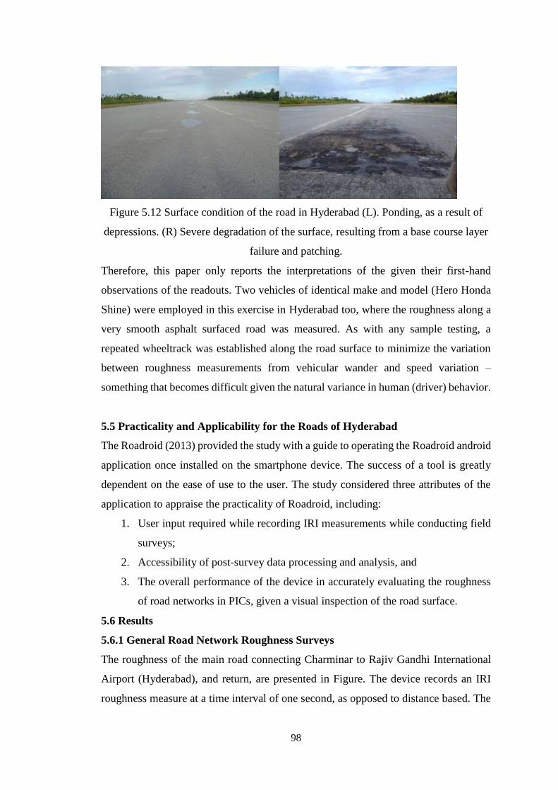
98
Figure 5.12 Surface condition of the road in Hyderabad (L). Ponding, as a result of
depressions. (R) Severe degradation of the surface, resulting from a base course layer
failure and patching.
Therefore, this paper only reports the interpretations of the given their first-hand
observations of the readouts. Two vehicles of identical make and model (Hero Honda
Shine) were employed in this exercise in Hyderabad too, where the roughness along a
very smooth asphalt surfaced road was measured. As with any sample testing, a
repeated wheeltrack was established along the road surface to minimize the variation
between roughness measurements from vehicular wander and speed variation –
something that becomes difficult given the natural variance in human (driver) behavior.
5.5 Practicality and Applicability for the Roads of Hyderabad
The Roadroid (2013) provided the study with a guide to operating the Roadroid android
application once installed on the smartphone device. The success of a tool is greatly
dependent on the ease of use to the user. The study considered three attributes of the
application to appraise the practicality of Roadroid, including:
1. User input required while recording IRI measurements while conducting field
surveys;
2. Accessibility of post-survey data processing and analysis, and
3. The overall performance of the device in accurately evaluating the roughness
of road networks in PICs, given a visual inspection of the road surface.
5.6 Results
5.6.1 General Road Network Roughness Surveys
The roughness of the main road connecting Charminar to Rajiv Gandhi International
Airport (Hyderabad), and return, are presented in Figure. The device records an IRI
roughness measure at a time interval of one second, as opposed to distance based. The

99
raw (unfiltered) data is presented in Figure 4a, which reports a large variance in IRI
along the road length. This detailed low-level data exceeds the detail necessary of IQL-
3/4 data, and therefore the raw unfiltered results from each direction were manually
averaged over a one kilometer length (refer Figure 4b). The developers are updating the
application to include a feature where the user can select their preferred section length
for reporting. It can be seen from Figure 4b that the average IRI across the road length
is similar between the two lanes (10.3 and 10.8), despite the severe deterioration.
While the road is heavily damaged with numerous potholes along its length, the
expected IRI, given the scale presented in Figure 1, was estimated as only up to 12,
while Roadroid indicated that approximately 20 % of the one kilometer lengths
exceeded an IRI of 12 (refer Figure 4b) and individual 1 second readings were about
20 IRI. This, and other testing, suggested that there was an issue with the roughness
filters used by Roadroid and that this was resulting in short wavelength roughness’s
being over-reported. The developers are currently calibrating the system with the results
from a laser profilometer on asphalt surfaced pavements.
5.6.2 Speed Dependency
One of the aims of the repeatability and reliability exercise in city was to determine the
speed dependency of the Roadroid android application, if any. The accuracy of the
reporting of the smartphone application was investigated in other exercises in this case
study. Therefore, for this exercise, the focus remained on the statistical difference
between several runs on the same wheel track, with any outliers removed purposefully,
to prevent skewed distributions, and consideration given to the natural wander of human
driving behavior. International airport road is 2 kilometers long. For consistency across
the exercise, a path of 1650 meters was established. To ensure sufficient data was
available for the statistical analysis, the IRI data recorded at every one second interval
was averaged over 100 meter sub-sections.
Figure 5 depict the correlation between the recorded roughness measurements,
averaged over 100 meter sub-sections, given the various vehicular speeds. The data
reported larger variation across areas of the pavement where defects were present, such
as in Figure 5(R) where the significant deterioration and patching attempts shown in
Figure 3 are located at 900 meters in the Charminar direction.
It was found the Roadroid android application exhibited repeatability over the longer
sampling sections consistent with IQL-3/4 assessments compared to the data recorded

100
at every one second interval. The analysis of the raw unfiltered data showed a high
degree of variation between the recorded measurements, particularly at the higher
speeds investigated in the study (50 km/h). This observation, compared with those
presented in Figure 5.13, suggests the use of small sampling intervals is not statistically
reliable. The significance of the differences between the runs at each speed was
analyzed using paired t-tests. As shown in Table 1, repeatability was observed across 5
of the 6 tests, suggesting that the Roadroid android application consistently measures
roughness at a given speed. Table 5.4 presents the results of the paired t-tests when
comparing the recorded IRI across various vehicle speeds. The results were less
satisfactory and it can be concluded the reliability of the smartphone application is poor
between various speeds. However, as IQL-3/4 data is typically used in a network-level
capacity for the purpose of informing
Figure 5.13 Charminar – Airport road roughness (Raw unified data)
Pavement maintenance works (Bennett and Paterson, 2000), the accuracy of an IQL-
3/4 measurement was considered appropriately for the intended purpose of the device
to be +/- 20 % IRI, and the smartphone device does reflect this type of repeatability.
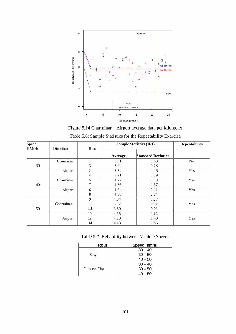
101
Figure 5.14 Charminar – Airport average data per kilometer
Table 5.6: Sample Statistics for the Repeatability Exercise
Speed
KM/Hr
Direction
Run
Sample Statistics (IRI) Repeatability
Average
Standard Deviation
30
Charminar 1 3
3.51 3.09
1.63 0.78
No
Airport 2 4
3.34 3.21
1.16 1.39
Yes
40
Charminar 5 7
4.27 4.36
1.23 1.37
Yes
Airport 6 8
4.64 4.58
2.11 2.24
Yes
Charminar
9 11
13
4.04 1.27 3.97 0.97 Yes
50 3.89 0.91 10 4.38 1.62
Airport 12 4.28 1.43 Yes
14 4.43 1.85
Table 5.7: Reliability between Vehicle Speeds
Rout Speed (km/h)
30 – 40
City 30 – 50
40 – 50
30 – 40
Outside City 30 – 50
40 – 50
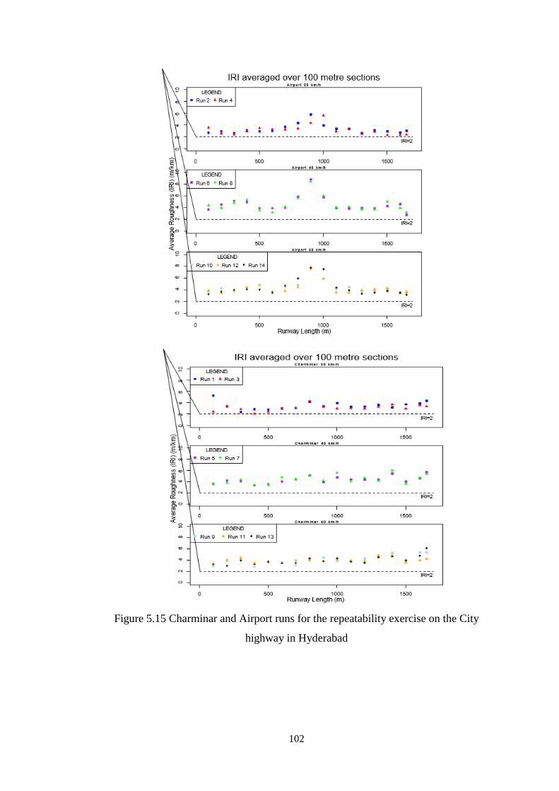
102
Figure 5.15 Charminar and Airport runs for the repeatability exercise on the City
highway in Hyderabad

103
5.6.3 Vehicle Dependency
A second phase to the repeatability and reliability exercise explored the dependency of
the Roadroid android application on the vehicle used to mount the device. Despite the
failure of the instrument to record the data for post-survey analysis, the observations
noted during the exercise, which involved two vehicles of identical make and model,
were:
1. Poor repeatability with data as a result of small sampling lengths across all speeds;
2. A large amount of variation between the raw (unfiltered) IRI measurements, and
3. Inconsistencies in the recorded IRI values between the two vehicles. Although
some variation was anticipated in this exercise due to the variable nature of human
(driver) behaviour, the inconsistencies between the IRI measurements recorded
with the device exceeded those that were expected. Although the vehicles were of
the same make, the tyre pressures were not measured at the time, and because of
the lack of time, the measurements could not be repeated. It was postulated that
the higher tyre pressure caused larger variation in IRI and that it was more prone
to texture effects than the softer tyre. The reported variation in the IRI values could
be attributed to this hypothesis, and will be explored further in succeeding case
studies.
5.7 Practicalities
The operation of Roadroid is simple and requires little input from the user once the
survey commences. Once calibrated, the device easily records the roughness of the road
and stores the information within the device. The information can easily be uploaded to
the developers’ webpage for post-processing, if the user opts for post-processing via
the developers; otherwise manual post-processing is possible. The data upload to
Roadroid server requires a Wi-Fi connection. On upload, raw data is compressed to a
zip-file and transferred to the server by File Transfer Protocol (FTP) or Hypertext
Transfer Protocol (HTTP). After a successful upload, the compressed files are also
stored on the smartphone to prevent accidental loss or deletion of data. These backups
can be manually deleted by the user, which is only possible when the device is
connected to a computer. Alternative data submission is available via email directly
from the smartphone. A promising feature of the Roadroid android application is the
ability to capture GPS photographs of the road surface very easily while conducting the
survey. Along with the survey data, these photographs are processed post-survey and
presented, by location, on a map.

104
During the operation, it was found that an event marker to designate different road
features such as junctions or change of surfacing type would have been useful. The
developers have been updating the Roadroid software to provide this feature. In
addition, on-going development is addressing the concerns expressed in this paper and
to provide a more consistent and reliable device.
Summary
With an enormous roadway network, increasing traffic and loading, and shortfalls in
transportation spending, the timing and prioritization of pavement evaluation and
maintenance has never been more critical. Pavement roughness data is a critical input
for maintenance and rehabilitation planning and overall pavement management, and
has traditionally cost state agencies millions of dollars annually. A smartphone-based
application will not only save millions of tax dollars but also provide ease in data
collection and possibly real time International Roughness Index (IRI) assessment and
localized roughness (i.e., pothole) identification in pavement sections.

105
CHAPTER 6
CONCLUSION
6.1 Introduction
IRI values measured by the smartphone application roughness capture were similar to
those collected with the inertial profiler at two test sites having low to medium
roughness, with very few outliers observed. Even the outliers were in the same ride
category or within one ride category of the reference measurement. These results were
obtained without the need for system calibration.
6.2 Conclusions
The following conclusions are drawn from the present study are:
1. The study shows the relation between the Roadroid International Roughness Index
to Standard International Roughness Index, by comparing with the all previous
techniques used for measuring the road roughness.
2. The case study was taken in the winter to summer season. With the change in
weather condition the results were accurate. Only deformation was due to climatic
change the roads got many potholes, with this the maintenance is more compared
to summer season.
3. This report has presented an analysis of the performance of the Roadroid android
application as a low-cost solution for road condition surveys. With this low cost and
reliable to use any unskilled person can collect the data. The case study investigated
the performance of the Roadroid android application in Hyderabad, a city with
limited resources and capacity to conduct in-field road condition assessments. To
demonstrate the applicability of the device in the southern part of India, the study
determined the effectiveness of the device in the city environment and evaluated
the performance of the IQL-3/4 device in Hyderabad.
4. Given the low cost of the smartphone device compared to specialized instrumented
vehicles in the market, implementing such routine road and pavement condition
surveys of road networks in Telangana state. It allows unskilled technical staff to
collect data, and provides potential donors / funders with objective measures of the
road quality. Such data is a necessary input to an economic evaluation of
investments.

106
5. I would also like to conclude that analysis is being taken place by comparing the
results of SPSS with the results of Roadroid, both shows the pavements are not up
to the mark.
The results from the field surveys supported its use as an IQL-3/4 device but suggest
that there is a filtering issue resulting in an upwards bias for the roughness
measurements. For the network survey, it showed consistent average roughnesses over
long sections. Although roughness is reported at one second intervals, the work
suggests that it would be more appropriate to report them over longer sampling
intervals, such as 100 m.
Repeatability of Roadroid was observed where consistency in IRI recordings at the
same vehicle speeds was noted. The statistical reliability of the device was less
satisfactory when the roughness measurements were compared across various speeds.
However, within the accuracy limits of an IQL-3/4 device of +/- 20 % of the IRI, the
equipment satisfied the need. It would be prudent for those using Roadroid to adopt a
constant survey speed as is used with other IQL-3/4 instruments, such as 50 km/h. The
study suggested variations between two vehicles used to mount the device and
concluded the device is potentially vehicle dependent, but this dependency could be
within the limits of an IQL-3/4 device and thus not be a practical issue.
With improvements to the filtering, and the adoption of larger sampling intervals,
Roadroid has great potential as a low-cost, practical device for measuring road
roughness at IQL-3/4 level. This would assist the asset management of road networks
in developing countries by offering a low-cost solution to monitoring and reporting on
the roughness condition of pavements.
6.3 Recommendations
Further studies of roughness capture will be pursued in follow up studies, particularly
for rough pavement sections, where a higher sampling rate will be investigated.
1. Testing is an underway to assess factors such as vehicle type (varying suspension
characteristics), smartphone type, and vehicle wander on IRI measurement. A
crowd sourcing feasibility study will be the subject of a later investigation. In the
long run, it is hoped that the approach can be used to significantly reduce the cost
of acquiring pavement roughness data for agencies and to reduce user costs for the

107
traveling public by providing more robust feedback regarding route choice and its
effect on estimated vehicle maintenance cost and fuel efficiency, and eventually
perhaps even a measure of safety.
2. From the conclusions drawn in this research there are a number of recommendations
and applications that would be suitable for the Roadroid application. Roadroid can
provide roughness measurements to local council controlled authorities. Who can
use this information to implement decision making and strategize asset maintenance
of their road networks. This allows for effective planning of Hyderabad’s road
networks and can be especially useful in the many pavement rating.
3. We can also use the roughness data obtained by Roadroid to gauge an understanding
of the vehicle operating costs such as fuel consumption, maintenance costs and tire
wear that result from rough roads. This will indicate the road user costs to citizens
and help set a standard of fees to use network roads. The applications are primarily
targeted towards the council however consultants and contractors in the
transportation/construction industry can also benefit from this tool.
6.4 Model Limitations and Future Research
Like any other deterioration model, the model developed in this dissertation is only an
approximation of the actual physical phenomenon of deterioration. There is a prediction
error associated with the model. However, unlike deterministic predictions
characteristic of mechanistic approaches, this error can be estimated to assess the
uncertainty in the predictions. Although the prediction capabilities of the developed
models are superior to most existing models, a number of limitations have been
identified and should be further researched. Some of the limitations are described in the
following paragraphs.
The two data sources used for the joint estimation are from the States of Illinois and
Minnesota. Environmental conditions at these locations are similar, especially in terms
of weather and soil conditions. The developed model is thus conditional on such
conditions, and might produce biased predictions in regions of markedly different
characteristics, e.g. California. A possible approach to overcome this limitation would
consist of obtaining another data source (corresponding to the new regions) and
updating the models by applying joint estimation once again.

108
This is, indeed, a very logical next step in this line of research. The data in the Pavement
Management System of each state could be a reasonable alternative data source. The
data collected as part of the Long-Term Pavement Performance (LTPP) studies of the
Federal Highway Administration could also be ideal for this purpose. By using in-
service pavement data, a large number of new variables could be incorporated into the
deterioration model, and more important potential biases could be determined and
corrected.
An important limitation of this model is that it failed to identify the effect of other
relevant environmental variables, such as stiffness of the asphalt mixture and,
therefore, the strength of the pavement, which in turn determines the deterioration rate.
However, the temperature information available in the data sets used was not precise
enough to characterize this effect.
The model estimation approach assumes that, except for the intercept term, the model
parameters are constant. An alternative approach would be to assume that some of the
parameters of the specification are not constant, but rather randomly distributed across
pavement sections. Under this new assumption, the random coefficients estimation
approach would produce parameter estimates of minimum variance (efficiency). This
could be the case for the layer strength parameters due to construction variability typical
of highway pavements.
Finally, these limitations are a characteristic of the specific model. However, this
dissertation ultimately aimed at showing the feasibility and advantages of using joint
estimation to develop pavement deterioration models rather than the advantages of the
model itself. As indicated above, most of these limitations can be overcome by
repeatedly applying joint estimation to more data sources.

108
REFERENCES
[1] Abaynayaka, S. W., Hide, H., Morosiuk, G., and Robinson, R. (1976). “Tables for
Estimating Vehicle Operating Costs on Rural Roads in Developing Countries.”
Rep. No. 723, Transport and Road Research Laboratory.
[2] ASTM Standard E867 (2012). Standard Terminology Relating to Vehicle-Pavement
Systems. West Conshohocken, PA, 2006, www.astm.org.
[3] Brickman, A. D., Park, W. H., and Wambold, J. C. (1972). “Road Roughness Effects
on Vehicle Performance.” Rep. No. TTSC-2707, Pennsylvania Transportation and
Traffic Safety Center.
[4] Contour. 2014. “Contour—Contour+2.” Contour. Accessed May 30, 2014.
http://contour.com/ collections/cameras/products/contour-2.
[5] Chassiakos, A.P. (2006), A fuzzy-based system for maintenance planning of road
pavements, Proceedings 10th WSEAS International Conference on COMPUTERS,
Vouliagmeni, Athens, Greece.
[6] Dana, H. J., Teller, L. W., Martin, G. E., and Bryant, C. B. 1932. “The Dana
Automatic Recording Roughometer for Measuring Highway Roughness.” In
Proceedings of the 12th Annual Meeting of the Highway Research Board. Accessed
May 30, 2014. http://trid.trb.org/view.aspx?id=105065.
[7] Finn, F. (1998). “Pavement Management Systems — Past, Present, and Future,
Public Roads: 80 Years Old, But the Best Is Yet to Come.” Public Roads, 62(1).
[8] Flintsch, G., and McGhee, K. K. (2009). “Quality Management of Pavement
Condition Data Collection.” National Cooperative Highway Research Program:
Transportation Research Board, NCHRP Synthesis 401.
[9] Gillespie, T. D., and Sayers, M. (1981). “The Role of Road Roughness in Vehicle
Ride.” Transportation Research Record: Journal of the Transportation Research
Board, (836), 15-20.
[10] Gupta A, K. Praveen, and R.Rajat (2012), “A Critical Review of Flexible
Pavement Performance Models Developed for Indian perspective”, Indian
Highways, Indian Road Congress, New Delhi,40(3) pp.41-60.
[11] Islam, T. 2013. “Using Cell-Phones to Monitor Road Roughness.” M.Sc. thesis,
University of Auckland.
[12] Johnston, M. 2013. “Using Cell-Phones to Monitor Road Roughness.” M.Sc.
thesis, University of Auckland.

109
[13] Juang, C.H., and Amirkhanian, S.N. (1992), Unified pavement distress index for
managing flexible pavements, Journal of Transportation Engineering, 118(5), 686-
699.
[14] Klaubert, E. C. (2001). “Highway Effects on Vehicle Performance.” Rep. No.
FHWARD-00-164, Federal Highway Administration, Washington, DC.
[15] McGhee, K. K. (2004). “Automated Pavement Distress Collection
Techniques.” National Cooperative Highway Research Program: Transportation
Research Board, NCHRP Synthesis 334.
[16] MnDOT. (2007) Introduction to the International Roughness Index. Bituminous
Smoothness Training Workshop. Minnesota Department of Transportation. April
11, 2007. Accessed on July 2, 2013.
[17] Motormännen. 2014. “Vägombuden Kontrollerar Svenska Vägars Säkerhet
(Road Inspectors Check Condition ofSwedish Roads.” Motormännen. Accessed
May 30, 2014.
[18] Mathew, B.S., Reshmy, D.S., and Issac, K.P. (2008), Performance Modeling of
rural road pavements using artificial neural network, Indian Highways, Journal of
Indian Roads Congress, 36(1), 31-39.
[19] Muralikrishna, P., and Veeraragavan, A. (2011), Decision support system for
Performance based maintenance management of highway pavements, Journal of
Transportation Research Board, Vol.2205, 155-167.
[20] MORT&H (2004), “Guidelines for Maintenance Management of Primary,
Secondary and Urban Roads”.
[21] Mathew, B.S., Reshmy, D.S. and Issac, K.P. (2008), “Performance Modelling
of Rural Road Pavements Using Artificial Neural Network”, Indian Highways,
Indian Roads Congress, New Delhi, 36(1), pp.31-39.
[22] Muralikrishna P and Veeraragavan.A (2011), “Decision Support System For
Performance Based Maintenance Management Of Highway Pavments”, Journal of
Indian Road Congress, New Delhi, pp.155-167.
[23] OpenLayers. 2014. “OpenLayers Home.” OpenLayers. Accessed May 30,
2014. http://openlayers.org/.
[24] OpenStreetMap. 2014. “OpenStreetMap.” OpenStreetMap. Accessed May 30,
2014. http://www.openstreetmap.org/.

110
[25] Perera, R. W., Kohn, S. D., and Tayabji, S. (2005). “Achieving a High Level of
Smoothness in Concrete Pavements Without Sacrificing Long-Term Performance.”
Rep. No. FHWA-HRT-05-068, Federal Highway Administration (FHWA),
Washington, D.C.
[26] ProVal. 2014. “ProVal: View and Analyze Pavement Profiles.” ProVal.
Accessed May 30, 2014. http://www.roadprofile.com/.
[27] Reddy, B.B, Sharma, R.S., and Veeraragavan, A. (2005), Development of
flexible pavement preservation framework for an integrated Asset management,
Journal of Indian Roads Congress, 66(1), 383-418.
[28] Reddy ,B.B, Sharma,R.S., and Veeraragavan,A.(2005). “Development of
flexible pavement preservation framework for an integrated Asset management.”,
Journal of Indian Roads Congress, Volume 66-1 , April 2005 , 383-418
[29] Reddy,B.B., and Veeraragavan,A. (1998), “Methodology for Sample size
Determination in Pavement Performance Data Collection” , Indian Highways,
Indian Road Congress, New Delhi, 26(11), pp.15-27.
[30] Sreedevi B.G, Salini P. N and Sathish B Nair (2011), “Field performance
indicators for NRMB in A tropical setting”, Indian Highways, January 2011. pp -
47-57.
[31] Sreedevi B.G, Salini P. N, and Nair S.B. (2011), Field performance indicators
for NRMB in A tropical setting, Indian Highways, Journal of Indian Roads, 39(1),
47-57.
[32] Sun, L., and Gu, W. (2012), Pavement Condition Assessment using Fuzzy Logic
Theory and Analytic Hierarchy Process, Journal of Transportation Engineering,
137(9), 648-654.
[33] Sauerwein, P. M., and Smith, B. L. (2011). “Investigation of the Implementation
of a Probe-Vehicle Based Pavement Roughness Estimation System.” Mid-Atlantic
Universities Transportation Center, University Park, PA
[34] Sayers, M. W., Gillespie, T. D., and Paterson, W. D. O. (1986). “International
Road Roughness Experiment: Establishing Correlation and a Calibration Standard
for Measurements: Books.” Rep. No. World Bank Technical Paper No. 45, The
World Bank, Washington, D.C.

111
[35] Sayers, M. W., Gillespie, T. D., and Queiroz, C. A. V. (1986). “The
International Road Roughness Experiment: Establishing Correlation and a
Calibration Standard for Measurements.” World Bank technical paper.
[36] Sayers, M. W., and Karamihas, S. (1996). Interpretation of Road Roughness
Profile Data. Final report of University of Michigan.
[37] Sayers, M. W., Gillespie, T. D., and Paterson, W. D. O. (1986). “Guidelines for
Conducting and Calibrating Road Roughness Measurements.” World Bank
technical paper.
[38] Trafikverket. (2014). “Start Page—NVDB.” Trafikverket. Accessed May 30,
2014. http://www.nvdb.se/.
[39] Tarr, K. E. (2013). “Evaluation of Response Type Application for Measuring
Road Roughness.” M.Sc. thesis, University of Pretoria, South Africa.
[40] U.S. Department of Transportation. (2000). “1999 Status of the Nation’s
Highways, Bridges and Transit: Conditions and Performance.” U.S. Department
of Transportation, Federal Highway Administration, Washington, D.C.
[41] Van Deusen, B. D. (1967). “Analytical Techniques for Designing Riding
Quality into Automotive Vehicles.” 400 Commonwealth Drive, Warrendale, PA
15096-0001, United States.
[42] Woodstrom, J. H. (1990). “Measurements, Specifications, and Achievement of
Smoothness for Pavement Construction.” National Cooperative Highway Research
Program: Transportation Research Board, NCHRP Synthesis 167 4-Washington,
D.C.
[43] Wakeham, K. J., and Rideout, D. G. (2011). “Model Complexity Requirements
in Design of Half Car Active Suspension Controllers.” Presented at ASME
(American Society of Mechanical Engineers) 2011 Dynamic Systems and Control
Conference and Bath/ASME Symposium on Fluid Power and Motion Control,
Virginia.