Research Report KTC-92-1

PAVEMENT DEFLECTION EVALUATIONS

by

R. Clark Graves Research Engineer Associate

David L. Allen Chief Research Engineer

Kentucky Transportation Center College of Engineering University of Kentucky

in cooperation with Transportation Cabinet

Commonwealth of Kentucky

and

Federal Highway Administration U.S. Department of Transportation

The contents of this report reflect the views of the authors who are responsible for the facts and accuracy of the data presented herein. The contents do not necessarily reflect the official views or policies of the University of Kentucky, the Kentucky Transportation Cabinet, nor the Federal Highway Administration. This report does not constitute a standard, specification, or regulation. The inclusion of manufacturer names and trade names are for identification purposes only and are not to be considered as endorsements.

January 1992

Technical Report Documentation Page

1. Report No. 2. Government Accession No, 3. Recipient's Catalog No.

KTC-92-1

4. Title and Subtitle 5. Report Date

January 1992 PAVEMENT DEFLECTION EVALUATIONS

6. Performing Organization Code

7. Author(s) 8 •. Performing Organization Report No.6 C. Graves and D. Allen

KTC-92-1

9. Performing Organization Name and Address tO. Work UnH No. (TRAIS)

KENTUCKY TRANSPORTATION CENTER COLLEGE OF ENGINEERING 11. Contract or Grant No.

UNIVERSITY OF KENTUCKY KYHPR-86-1 09

LEXINGTON, KY 40506-0043 13. Type of Report and Period Covered

12. Sponsoring Agency Name and Address Final Kentucky Transportation Cabinet State Office Building 14. Sponsoring Agency Code

Frankfort, KY 40622

15. Supplementary Notes

Prepared in cooperation with the U.S. Department of Transportation, Federal Highway Administration

16. Abstract

In this study a procedure has been developed to evaluate the structural condition of pavements using Road Rater deflection measurements. These procedures compare actual field deflections with deflections calculated by the Chevron N-Layer linear elastic computer program. The results obtained from these procedures are the layer moduli of the pavement materials. Procedures have been developed for asphaltic concrete pavements and composite pavements, including broken and non-broken concrete layers. This report also contains a comparison of structural overlay determined using the results of the new procedure, with overlays calculated using results from the 2-3 Projected procedure currently used by the Pavement Management branch of the Kentucky Transportation Cabinet. A users manual from the computer programs developed during this study is included in the appendix of the report.

17. Key Words 18. Distribution Statement Pavement Deflection Lagrangian lnterpolatioo

Unlimited with approval of Chevron N-layer Layer Moduli Kentucky Transportation Cabinet Effective Thickness

19. Security Classlf. (of this report) 20. Security Class if. (of this page) 21. No. of Pages 22. Price

Unclassified Unclassified 84

Form DOT 1700.7 (8-72) Reproduction of completed page authorized

DON C. KELLY, P.E.

SECRETARY

AND

COMMISSIONER OF HIGHWAYS

Mr. Paul Toussaint Division Administrator

COMMONWEALTH

TRANSPORTATION CABINET

FRANKFORT, KENTUCKY 40b22

November 9, 1992

Federal Highway Administration 330 West Broadway Frankfort, Kentucky 40602

Subject; IMPLEMENTATION STATEMENT KYHPR-86-109, "Pavement Deflection Evaluations"

Dear Mr. Toussaint:

BRERETON C. JONES

GOVERNOR

The subject research study involved a review and analysis of current procedures for evaluating pavement deflections. Procedures for evaluation of asphaltic concrete and composite pavements containing both broken and non-broken concrete were developed. The procedures developed apply to deflections measured with the Road Rater deflection testing equipment. The general concepts, however, may be used with any type of non-destructive deflection testing equipment.

A database of all pavement deflections collected within the state was also developed. This database contains information on tests conducted by the Transportation Cabinet and the Kentucky Transportation Center. The database includes Road Rater and Falling Weight Deflectometer measurements. The cataloging program was described in Research Report KTC-90-15 "Pavement Deflection Test Database." This database will be updated periodically to provide an up-to-date record of deflection measurements obtained throughout the state.

The major area of implementation for this study is the use of the deflection evaluation procedures. Interactive computer programs were developed for three pavement types - flexible asphaltic concrete pavements, asphaltic concrete over broken and seated concrete, and asphaltic concrete over intact portland cement concrete. The previous evaluation procedure was developed in the early 1980's and has proven to be a good tool in evaluating in-service pavements. This procedure was limited to conventional asphaltic concrete pavement structures. Evaluation

"AN EQUAL OPPORTUNITY EMPLOYER M/F/H"

procedures for composite pavements containing broken or unbroken concrete layers were not available. The current evaluation procedure utilizes the concept of effective

~~ ~~~~~~ ~ ~~~~~~~asph~attt<: <:oncrete thickness:~ The procedure~represents~the~asphaltic~concrete.~.aa.~a··~·· given thickness of reference quality asphaltic concrete. The decrease of this effective thickness provides a measure of the performance of the pavement structure. The new procedure, in addition to providing the effective asphaltic concrete thickness, also provides the in-situ elastic modulus of the asphaltic concrete.

The procedures developed for the other pavement types provide the user with elastic moduli for the subgrade, broken or unbroken concrete, and asphaltic concrete layers. These layer moduli may be used to determine overlay thicknesses for various types of pavements. The overlay designs may utilize limiting strain or other concepts for thickness design. As these procedures are developed, further research may be proposed to optimize these design methods.

The implementation of the procedures developed in this study will provide necessary information for the Cabinet officials to better evaluate the structural condition of pavement structures. This information will allow those officials to optimize the rehabilitation of the highway system.

TABLE OF CONTENTS

List of Figures . . . . . . . . . . . . . . . . . . . . . . . . . . . . . . . . . . . . . . . . . . . . . . . i

List of Tables . . . . . . . . . . . . . . . . . . . . . . . . . . . . . . . . . . . . . . . . . . . . . . . iii

Executive Summary ........................................... iv

Introduction . . . . . . . . . . . . . . . . . . . . . . . . . . . . . . . . . . . . . . . . . . . . . . . . . 1

Background

Historical . . . . . . . . . . . . . . . . . . . . . . . . . . . . . . . . . . . . . . . . . . . . . . 2

Current Deflection Evaluation Techniques . . . . . . . . . . . . . . . . . . . . . 2

Work Plan Objectives . . . . . . . . . . . . . . . . . . . . . . . . . . . . . . . . . . . . . 4

Completed Objectives . . . . . . . . . . . . . . . . . . . . . . . . . . . . . . . . . . . . . 5

Theoretical Background

Theoretical Analysis . . . . . . . . . . . . . . . . . . . . . . . . . . . . . . . . . . . . . . 6

Analysis of Field Deflections . . . . . . . . . . . . . . . . . . . . . . . . . . . . . . . . 8

Effective Thickness Calculation . . . . . . . . . . . . . . . . . . . . . . . . . . . . . . 9

Model Development

Model Definitions . . . . . . . . . . . . . . . . . . . . . . . . . . . . . . . . . . . . . . . 10

Lagrangian Interpolation . . . . . . . . . . . . . . . . . . . . . . . . . . . . . . . . . 12

Program Development

Background . . . . . . . . . . . . . . . . . . . . . . . . . . . . . . . . . . . . . . . . .. . . . 12

Flexible Pavement Model (KTCFLEX) . . . . . . . . . . . . . . . . . . . . . . . . 13

Modulus Calculations . . . . . . . . . . . . . . . . . . . . . . . . . . . . . . . . 13

Effective Thickness . . . . . . . . . . . . . . . . . . . . . . . . . . . . . . . . . . . . . . 19

Broken and Seated Concrete Pavement Model (KTCBREAK) . . . . . . 20

Composite Pavement Model (KTCCOMP) . . . . . . . . . . . . . . . . . . . . . 24

Flexible Pavement Model . . . . . . . . . . . . . . . . . . . . . . . . . . . . . . . . . 24

Theoretical Verification ................. : ............. 24

Field Case Studies Layer Moduli Analysis . . . . . . . . . . . . . . . . . 30

Field Case Studies Effective Thickness Analysis . . . . . . . . . . . . 36

1991 Overlay Comparison ..................... o ••••••• 43

Broken and Seated Concrete Pavement Model ....... o •• o ••••••• 45

Theoretical Verification ......................... 0 ••••• 45

Field Case Studies . . . . . . . . . . . . . . . . . . . .. 0 • • • • ••••• 0 • • • 50

Composite Pavement Model ..................... 0 • 0 0 0 0 ••••• 54

Theoretical Verification .................. 0 ••• 0 0 • 0 0 • 0 •• 54

Field Case Studies . . . . . . . . . . ........... 0 •• 0 • 0 •• 0 0 0 • 0 • 57

Summary and Conclusions . . . . . . . . . . . . . . . . ........ 0 ••• 0 0 0 •• 0 • • • 59

Recommendations .................... 0 • 0 ••••• 0 ••••••• o ••• o • • • 60

References . . . . . . . . . . . . . . . . . . . . . . . . . . . . . . . . ...... 0 •• 0 • 0 • • • • • 62

Appendix o ••• o • • • • • • • • • • • • • • •••••••• 0 ••••••• 0 •••• 0 • • • • • • • • 64

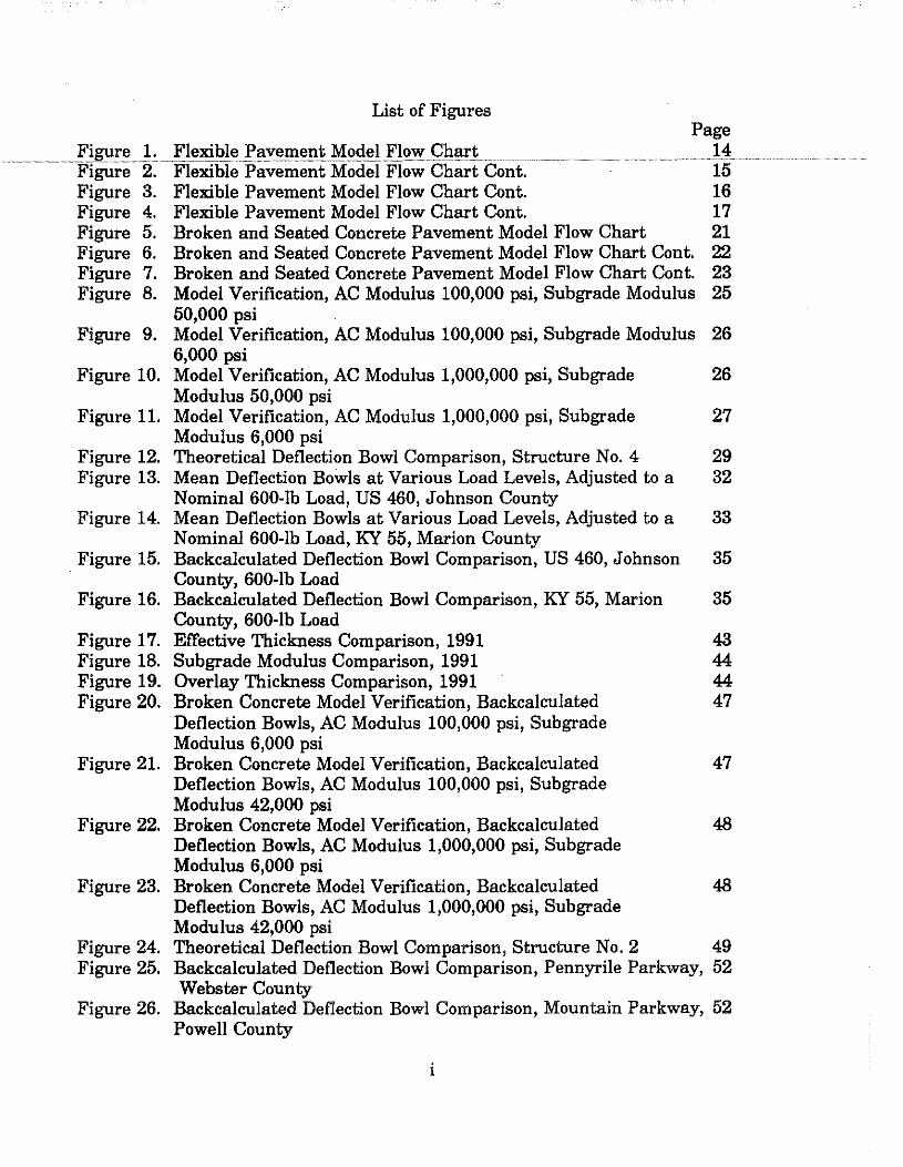
List of Figures

Figure 1. Flexible Pavement Model Flow Chart Page

14 ..... """·-·-·~'"'"'"

···· ······ · Figure 2. F'fe:Kn:Jie PavemeiitM:od.ei.Fio;:chlirt cont. Figure 3. Flexible Pavement Model Flow Chart Cont. Figure 4. Flexible Pavement Model Flow Chart Cont. Figure 5. Broken and Seated Concrete Pavement Model Flow Chart Figure 6. Broken and Seated Concrete Pavement Model Flow Chart Cont. Figure 7. Broken and Seated Concrete Pavement Model Flow Chart Cont. Figure 8. Model Verification, AC Modulus 100,000 psi, Subgrade Modulus

50,000 psi

15 16 17 21 22 23 25

Figure 9. Model Verification, AC Modulus 100,000 psi, Subgrade Modulus 26 6,000 psi

Figure 10. Model Verification, AC Modulus 1,000,000 psi, Subgrade Modulus 50,000 psi

Figure 11. Model Verification, AC Modulus 1,000,000 psi, Subgrade Modulus 6,000 psi

Figure 12. Theoretical Deflection Bowl Comparison, Structure No. 4 Figure 13. Mean Deflection Bowls at Various Load Levels, Adjusted to a

Nominal 600-lb Load, US 460, Johnson County Figure 14. Mean Deflection Bowls at Various Load Levels, Adjusted to a

Nominal 600-lb Load, KY 55, Marion County Figure 15. Backcalculated Deflection Bowl Comparison, US 460, Johnson

County, 600-lb Load Figure 16. Backcalculated Deflection Bowl Comparison, KY 55, Marion

Figure 17. Figure 18. Figure 19. Figure 20.

County, 600-lb Load Effective Thickness Comparison, 1991 Subgrade Modulus Comparison, 1991 Overlay Thickness Comparison, 1991 Broken Concrete Model Verification, Backcalculated Deflection Bowls, AC Modulus 100,000 psi, Subgrade Modulus 6,000 psi

Figure 21. Broken Concrete Model Verification, Backcalculated Deflection Bowls, AC Modulus 100,000 psi, Subgrade Modulus 42,000 psi

Figure 22. Broken Concrete Model Verification, Backcalculated Deflection Bowls, AC Modulus 1,000,000 psi, Subgrade Modulus 6,000 psi

Figure 23. Broken Concrete Model Verification, Backcalculated Deflection Bowls, AC Modulus 1,000,000 psi, Subgrade Modulus 42,000 psi

26

27

29 32

33

35

35

43 44 44 47

47

48

48

Figure 24. Theoretical Deflection Bowl Comparison, Structure No.2 49 Figure 25. Backcalculated Deflection Bowl Comparison, Pennyrile Parkway, 52

Webster County Figure 26. Backcalculated Deflection Bowl Comparison, Mountain Parkway, 52

Powell County

i

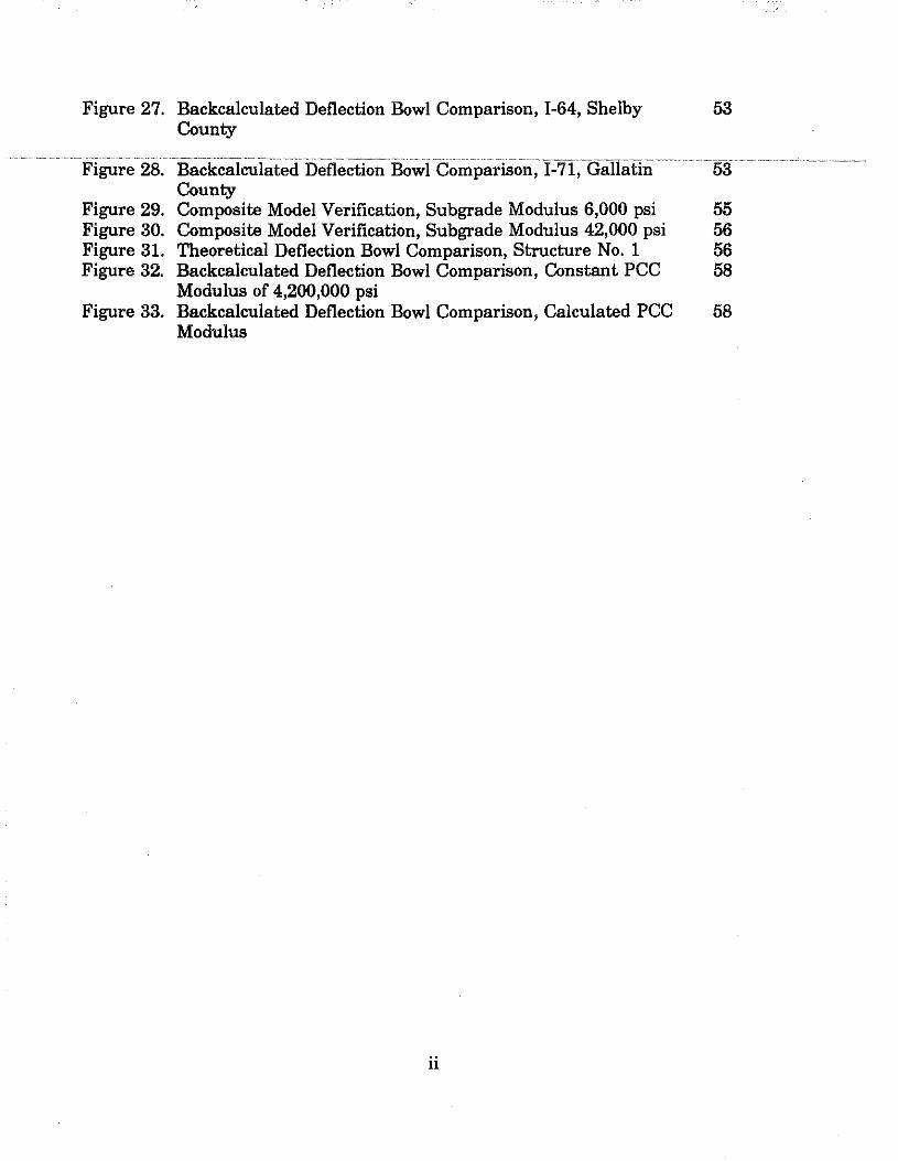
Figure 27. Backcalculated Deflection Bowl Comparison, I-64, Shelby 53 County

· ····· ····~·· Figure28. Backcalc~Ilated Deflection Bowl Comparison, I-71, Gaf1atln 53 County

Figure 29. Composite Model Verification, Subgrade Modulus 6,000 psi 55 Figure 30. Composite Model Verification, Subgrade Modulus 42,000 psi 56 Figure 31. Theoretical Deflection Bowl Comparison, Structure No. 1 56 Figure 32. Backcalculated Deflection Bowl Comparison, Constant PCC 58

Modulus of 4,200,000 psi Figure 33. Backcalculated Deflection Bowl Comparison, Calculated PCC 58

Modulus

11

List of Tables Page

Table 1. Flexible Model Verification 28 .. """ """"" ·-'"""""-'~"~ """""""-'~""~"""""'""""""'~"""~"'~'"'~""""'""""" " -·~'""""'"'"'~"'~'""""'"'"'" " """""""" """""""""""""""""""""""""" ""'"" """""""""""""""""~'"'"'"'"'"'~""" """"""""""""" """""""""""'"""'"'"'"

Table 2. Site Locations for Flexible Model Case Studies 30 Table 3. KTCFLEX Modulus Results 33 Table 4. KTCFLEX Backcalculated Deflections 34 Table 5. Subgrade Modulus Comparison All Data 37 Table 6. Subgrade Modulus Comparison, Data With Eff. > 50 Percent 39

of Design Thickness Table 7. AC Overlay Comparison 41 Table 8. Broken and Seated Concrete Model Verification 46 Table 9. Broken and Seated Concrete Model, Case Studies 51 Table 10. Composite Pavement Model Verification 55

iii

Executive Summary

. .. ··············~··········· .. ~ .. P.avementmanagementtechniques 2ften inc!uc;le yi~:;;:ti~Ls:tiJ:.Ye.Y.f!, ri!l.e <I.11!ility, rt1t measurement and some measure of structural condition. Pavement deflection testing is rapidly becoming an integral part of pavement management practices. Deflection testing provides a rapid and relatively inexpensive method of determining the in-situ condition of existing pavements. Kentucky has been using the Road Rater since the early 1970's for research purposes and pavement evaluations. Currently, the Pavement Management branch of the Kentucky Transportation Cabinet collects Road Rater deflections to assess the structural condition of pavements and to determine overlay thicknesses. Procedures have previously been developed for determining the subgrade strength and effective structural condition of the pavement. These procedures were outlined in Research Report UKTRP-84-9, "Structural Evaluation of Asphaltic Pavements". This procedure is currently utilized by the Pavement Management Branch for structural evaluation of flexible pavements. The procedure is contained in a Fortran program currently utilized on the Transportation Cabinet's mainframe computer.

The evaluation of pavement deflections may be performed in many ways. This report summarizes several of these procedures and outlines the procedure for matching deflection bowls measured in the field with theoretical deflection bowls. The report summarizes the development of procedures for evaluating asphaltic concrete pavements, broken and seated and overlaid pavements, and composite pavements. Interactive computer programs have been developed to evaluate each of these pavement types. This report contains theoretical development and verification along with examples using these programs with actual field collected deflection data.

This report also contains a comparison of the results of the current 2-3 Projected procedure and the new procedure developed for selected projects. The effective thickness and subgrade modulus of each procedure were compared. These results were then input into the current overlay design program. This analysis indicated that the results from the new procedure will reduce the overlay thickness on average 0.64 inch, if all data points are utilized. The Transportation Cabinet also evaluates data points with an effective thickness greater than 50 percent of the design thickness. Using data with an effective thickness greater than 50 percent of the design thickness, the new procedure will reduce the overlay 0.91 inch.

The procedures developed during this study provide a means of determining pavement layer moduli. These layer moduli may be used by Cabinet personnel to determine overlay thicknesses for various types of pavements. These overlays will most probably utilize the concept of limiting strain or other concepts for thickness design. As these procedures are developed, further research may be proposed to optimize these design methods.

This study also recommends that a 2,400-lb dynamic load be utilized during deflection testing using the Road Rater. The use of this load will provide deflections which will be more near the mid range of the testing equipment. In addition this load will more closely simulate the actual field loading conditions.

IV

INTRODUCTION

The major function of a highway agency is to rehabilitate and maintain its ············l:iigJ.lway system: T:YPicaH:Y, ruiiClsareiiofmaa:e a.v:a.naoieto meet rurtlieiieeasortne

highway system. Pavement management concepts have been developed to provide more efficient means to allocate funding, personnel, and other resources in optimum maintenance of the highway system. Kentucky currently has a well developed pavement management system (1), of which structural evaluations are a very important part. However, deflections are not conducted on a network basis as an integral part of the pavement management process. They are primarily performed on a project basis for determining structural condition and design of overlays.

Pavement management techniques often include visual surveys, ride quality, rut measurement, and some measure of structural condition. This measure of structural condition may be obtained by coring the pavement. This invasive method is very costly and could not be performed efficiently on a network level. Pavement deflections are rapidly becoming a more vital part of the pavement management system for non destructive evaluation of pavement condition.

Pavement deflections have been utilized for many years to evaluate the in-situ condition of pavement structures. The method of!oading the pavement has become more sophisticated; therefore, the analysis procedures have become more complex.

This report focuses on procedures which have been developed to evaluate pavement deflections measured with the Road Rater (RR). The methodologies which have been developed could be applied to any type equipment which measures the deflection bowl of the pavement under a given load.

A common method of deflection evaluation is to compare theoretical deflection bowls to field measured deflections bowls. This is a widely utilized concept and computer programs have been developed by various agencies to perform this comparison. Normally these comparisons are made using a linear elastic solution to calculate the theoretical deflections.

Procedures developed under this study for flexible pavements will also provide the subgrade modulus and effective thickness. In addition, the elastic modulus of the asphaltic concrete can be determined. These modulus values and effective thicknesses are determined by comparing the field deflection bowls to theoretical bowls calculated using the Chevron N-Layer computer program (2).

This report details the procedures to match theoretical deflection bowls, obtained using the Chevron N-Layer program, and field deflection bowls. Procedures have been developed for flexible, composite, and broken and seated pavements. These concepts could be modified to evaluate other pavement structures such as aggregate base over subgrade, stabilized base over subgrade, etc. In addition, they could also be modified for use with Falling Weight Deflectometer (FWD) data.

BACKGROUND

Kentucky has been using the Road Rater since the early 1970's for research purposes and pavement evaluations. Currently, the Pavement Management Branch of the Transportation Cabinet collects Road Rater deflections for the purpose of overlay design and ascertaining the conditions of pavements. However, there is no standardized procedure or mechanism for collection of Road Rater deflections by the Pavement Management Branch and the collection of deflection measurements for research evaluations by the Kentucky Transportation Center. There is an immediate need for the establishment of a combined database of deflections.

Procedures have been developed to determine the subgrade strength and effective structural condition of the pavement (3). These procedures have remained relatively the same since the early 1980's. These procedures are currently used by the Pavement Management Branch of the Kentucky Transportation Cabinet to evaluate the condition of selected pavements for analysis of overlay design. The results of these procedures are the elastic modulus of the subgrade and the effective thickness of reference quality asphaltic concrete.

The procedure which is currently used by the Cabinet has been previously outlined in Research Report UKTRP-84-9, "Structural Evaluation of Asphaltic Pavements" (4). The methodology used in that report with respect to the loading of the Road Rater and theoretical determination of deflections remains the same in the new evaluation procedure which is outlined in this report.

The rehabilitation of existing flexible and rigid pavements by overlay is resulting in the construction of composite pavement structures. These composite pavement structures consist of asphaltic concrete over either portland cement concrete or broken and seated portland cement concrete.

The development of procedures for modeling broken and seated concrete pavements is necessary to determine specific thickness design requirements. Current thickness design recommendations for asphaltic concrete overlays over broken and seated concrete pavements assume the broken layer will behave better than a crushed stone aggregate base. By the development of an analysis procedure, more structural credit may be given to the broken concrete layer, therefore possibly requiring a thinner overlay.

Current Deflection Evaluation Techniques

Several techniques have been used to evaluate the pavement deflections obtained using various testing devices. One method involves characterizing the deflection bowl shape, using parameters such as slope, shape factors, basin area, and curvature. These parameters have been related to various material properties. The concepts of deflection

2

basin area and basin shape factors has been documented by Thompson (5). This method uses regression equations to calculate nonlinear resilient layer moduli from deflection

••• m •••••• basin area,~shape. ... factor.s, ... and..centermdeflection .... This..method ... Was ... de.YeJoped.Jor ... :USe .. in ... the absence of expensive computer analysis.

A more recent study, by Hossain and Zaniewski (6) which documented several methods which have been previously utilized in evaluating deflection basins. This study also evaluated the use of an exponential curve, of the form Y = A • e8x, where Y is the deflection, and X is the radial distance from the center of the load. Coefficients A and B are functions of the pavement structure. It was found that the degree of fit of the equation was :useful for judging the ability of the deflection bowl to be evaluated by a deflection matching technique.

Another method which has been widely used is the technique of matching the field measured deflection bowls with theoretically calculated bowls. Extensive research has been conducted in this area since the early 1980's, with the primary emphasis on deflection bowls calculated using a Falling Weight Deflectometer (FWD). An overview of NDT deflection measurements and backcalculation of layer moduli is given by Lytton (7) in ASTM STP 1026.

Several methods have been discussed by Lytton (7), including graphical and empirical solutions to a two layered pavement system, analysis of equivalent layer methods, microcomputer backcalculation, and wave propagation methods.

A microcomputer program has been developed by Hicks and Zhou (8), based on equivalent thickness and Boussinesq theory. This program has the ability to backcalculate layer moduli very quickly and accurately.

Linear elastic theory has also been utilized to backcalculate pavement layer moduli from measured field deflections. There are generally two types of procedures utilized for matching the field deflections with theoretically calculated deflections. One method which is employed by several programs calculates a deflection basin using linear elastic theory based on a set of layer moduli. The program then compares this deflection basin with the field measured basin. The error in the calculated basin is evaluated and the layer moduli are adjusted and a new deflection bowl is determined. This procedure requires that the linear elastic program be executed for each subsequent iteration of layer moduli. Several of these programs are based on a gradient error search method, Lytton (7). Several programs which utilize this procedure have been evaluated by Mahoney, et. al. (9). This study concluded that there was general agreement between the backcalculated layer moduli of each program. Other studies have compared the results of various backcalculation programs, Chou and Lytton (10). Chou and Lytton found that large discrepancies may occur among different analysis methods and different users. They also found that some programs are sensitive to the input parameters, such as subgrade depth and Poissons ratio.

A different technique was utilized by the program MODULUS (11) which was

3

included in the work by Chou and Lytton. MODULUS creates a deflection database, based on linear elastic theory, which covers the range of layer moduli anticipated in the

···········o;trueture~to ~be~evaluated;··.lfhis··program utiHzes~~a ilearch·routine·~an&..Lagrangian·

interpolation to determine a set of layer moduli and theoretical deflections which match the field measured deflections. This routine is faster than other backcalculation programs, in that the database of deflections may be calculated prior to analysis of the test data. The search procedure and interpolation could also be utilized with databases generated by finite element analysis.

In recent years, the increase in personal computer technology has made the analysis of pavement deflection basins more appealing. Faster personal computers have made the programs more accessible and useable to the practicing engineer. Therefore more analysis is being conducted to determine actual material properties from deflection data.

Research has been conducted using dynamic solutions, based on elastodynamic procedures to calculate deflections in layered pavements. Sebaaly, et. a!. (12) compared deflections calculated using both dynamic and static solutions. These solutions were compared to actual field deflections, and it was determined that static analysis resulted in deflections 20 to 40 percent larger than field deflections, while the dynamic analysis resulted in deflections within +/- 15 percent of the field deflections.

Other research conducted by Ong, et. a! (13), describes a dynamic model using finite element analysis to backcalculate layer moduli from dynamic deflections. For the pavement sections studied, the AC layer moduli were not affected by either static or dynamic analysis. However dynamic, analysis produced higher subgrade moduli and lower base moduli than the static analysis. It was also concluded that the depth to rigid layer is also important in the analysis of pavement deflections.

New research is being conducted in the area of dynamic analysis of deflection data, procedures are developing to characterize the pavement structure based on the complete time history obtained with the FWD (14). These procedures have the ability to backcalculate layer moduli, lower layer thickness (base, subgrade, etc.), and for the AC surface, the visco-elastic parameters.

Work Plan Objectives

A. To establish and maintain a statewide deflection database for research and pavement management purposes.

B. To collect deflection measurements for a statewide sample of rigid pavement sections for the purpose of verification and (if necessary) modification of evaluation procedures developed in Kentucky.

C. To search and review available literature relating to the application of deflection measurements for evaluation of rigid, flexible, composite, and other

4

pavement sections.

·································~~~D. ·~~··'I'O···identify~variation&indeflectionbehaviorfor~l'igid~pavements~in..various-~~~ ·····~~~~~ distl'ess conditions.

E. To develop theoretical models fol' simulation of deflection measurements for:

1. composite pavement sections 2. broken and seated portland cement concrete pavements over an

aggregate base over a compacted subgrade, 3. aggregate base over subgrade, and 4. subgrade.

F. To collect and evaluate deflection data for the purpose of verification of theoretical models for simulation of deflection measurements for:

1. composite pavement sections 2. broken and seated portland cement concrete pavements over an

aggregate base over a compacted subgrade, 3. aggregate base over subgrade, and 4. subgrade.

G. To identify and demonstrate potential applications for the use of deflections for constl'uction quality contl'ol.

Completed Objectives

Framework for a pavement deflection database has been established and is outlined in Report KTC-90-14 (15), "Pavement Deflection Test Database. • This report serves as a users guide to the computer program developed to maintain a catalog of deflection measurements. This database contains data obtained from the Kentucky Transportation Center and from the Pavement Management Branch of the Kentucky Transportation Cabinet.

The analysis of rigid pavements is not included in this report. The analysis procedures for rigid pavements have not advanced as fast as those for flexible pavements. There is still considerable discussion about the use of layer moduli or using the "k" term to evaluate the subgrade under rigid pavements.

It was determined that the majority of the current work being done involves the use of falling weight deflectometers, in place of vibratory devices. However, the same concepts of analysis may be applied to vibratory devices.

Three procedures are introduced in this report, for analysis of flexible, broken and seated, and composite pavements. These procedures have been verified both theoretically and with actual field deflections. The theoretical background of Kentucky's current

analysis procedure has been documented and a comparison between the two methods has been conducted.

The procedures for evaluation of aggregate base over subgrade and bare subgrade are not contained in this report. However, the procedure for flexible pavements could be modified to evaluate these types of structures.

The ability of these procedures to evaluate the actual in-situ conditions of the pavement, as determined from laboratory samples, is being conducted in study KYHPR-86-115, "Laboratory and Field Evaluations and Correlations of Properties of Pavement Components."

THEORETICAL BACKGROUND

Theoretical Analysis

The current effective thickness procedure (4, 16) assumes that the thickness of all layers below the asphaltic concrete have remained as constructed. Fatigue and deterioration reduce the effective thickness of the asphaltic concrete to some equivalent thinner thickness of good quality material. In existing pavements, the thickness of the dense graded aggregate (DGA) is assumed to have remained as constructed. The other variables which influence the behavior of the pavement are the effective thickness of the asphaltic concrete and the strength of the subgrade.

Using elastic theory, a relationship relating subgrade modulus and Road Rater deflection may be developed for a given structural section and constant asphaltic concrete modulus and variable DGA modulus. The modulus of the DGA is assumed to vary with the modulus of the layers which confine it. Therefore, for a constant AC modulus and variable subgrade modulus, the DGA modulus must vary as well (17). The equation relating pavement deflection and subgrade modulus may be expressed as follows:

where:

Log(delta) = (K) Log(Esub) + L

delta = Road Rater Deflection (in), K = Slope of the log-log Line, L = Constant, and Esub = Elastic Modulus of the Subgrade (psi),

(1)

Both K and L are dependent upon the asphaltic concrete thickness and DGA thickness, · they may be described by third degree polynomials. The development of this equation

is given in detail in (16).

6

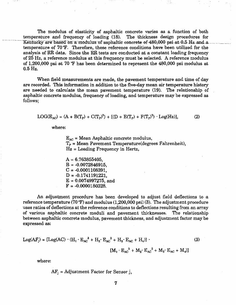
The modulus of elasticity of asphaltic concrete varies as a function of both temperature and frequency of loading (18). The thickness design procedures for

··· ············ !{enrucey·a::re·oa.sed~onlctnodu1us·of~phaltic·concrete...,f.480,000·psiat.0..5~Hz.and~a .......... .... . . temperature of 7o•F. Therefore, these reference conditions have been utilized for the analysis of RR data. Since the RR tests are conducted at a constant loading frequency of 25 Hz, a reference modulus at this frequency must be selected. A reference modulus of 1,200,000 psi at 70 •F has been determined to represent the 480,000 psi modulus at 0.5Hz.

When field measurements are made, the pavement temperature and time of day are recorded. This information in addition to the five-day mean air temperature history are needed to calculate the mean pavement temperature (19). The relationship of asphaltic concrete modulus, frequency of loading, and temperature may be expressed as follows;

where:

EAc = Mean Asphaltic concrete modulus, Tp = Mean Pavement Temperature(degrees Fahrenheit), Hz = Loading Frequency in Hertz,

A = 6. 763855405, B = -0.0072846915, c = -0.0001108391, D = -0.1741191221, E = 0.0074997275, and F = -0.0000180328.

An adjustment procedure has been developed to adjust field deflections to a reference temperature (70 •F) and modulus (1,200,000 psi) (3). The adjustment procedure uses ratios of deflections at the reference conditions to deflections resulting from an array of various asphaltic concrete moduli and pavement thicknesses. The relationship between asphaltic concrete modulus, pavement thickness, and adjustment factor may be expressed as:

Log(AFi) = [Log(AC) · <Ht · EAc3 + H2 • EAc2 + H3 • EAc + H4)] · (3)

[M1 • EAc3 + M2 • EAc

2 + Ms· EAc + M4)]

where:

AFi = Adjustment Factor for Sensor j,

7

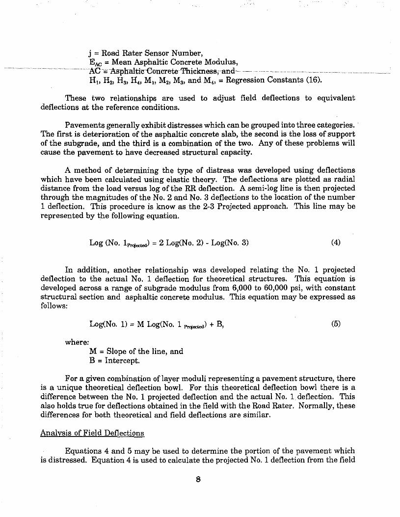
j =Road Rater Sensor Number, EAc = Mean Asphaltic Concrete Modulus,

·AC = :Asphaltic·Concrete·Thickness;and H~o H2, H3, H4, M~o M2, M3, and M4, = Regression Constants (16).

These two relationships are used to adjust field deflections to equivalent deflections at the reference conditions.

Pavements generally exhibit distresses which can be grouped into three categories. The first is deterioration of the asphaltic concrete slab, the second is the loss of support of the subgrade, and the third is a combination of the two. Any of these problems will cause the pavement to have decreased structural capacity.

A method of determining the type of distress was developed using deflections which have been calculated using elastic theory. The deflections are plotted as radial distance from the load versus log of the RR deflection. A semi-log line is then projected through the magnitudes of the No. 2 and No. 3 deflections to the location of the number 1 deflection. This procedure is know as the 2-3 Projected approach. This line may be represented by the following equation.

Log (No. 1rn;ected) = 2 Log{No. 2) - Log(No. 3) (4)

In addition, another relationship was developed relating the No. 1 projected deflection to the actual No. 1 deflection for theoretical structures. This equation is developed across a range of subgrade modulus from 6,000 to 60,000 psi, with constant structural section and asphaltic concrete modulus. This equation may be expressed as follows:

where:

Log{No. 1) = M Log(No. 1 rn;ected) + B,

M = Slope of the line, and B = Intercept.

(5)

For a given combination oflayer moduli representing a pavement structure, there is a unique theoretical deflection bowl. For this theoretical deflection bowl there is a difference between the No. 1 projected deflection and the actual No. 1 deflection. This also holds true for deflections obtained in the field with the Road Rater. Normally, these differences for both theoretical and field deflections are similar.

Analysis of Field Deflections

Equations 4 and 5 may be used to determine the portion of the pavement which is distressed. Equation 4 is used to calculate the projected No. 1 deflection from the field

8

data. This value is then input into Equation 5 to determine the corresponding theoretical No.1 deflection for this structure. A comparison of theoretically calculated No. 1 and

·· ···········~.Pield~No,+is~~indieaterefwhiGh~portionoUhe~pavement.structu.re maybe distr..!)ssed, .......... ·~·~ ~~~

If the theoretically calculated No. 1 deflection is less than the actual measured No. 1 deflection, then the asphaltic concrete is in a weakened condition (Condition 1). If the calculated deflection is greater that the measured No. 1 deflection, then the subgrade or the portion of the structure below the asphaltic concrete is weak (Condition 2).

Two parameters are needed as input into the current overlay design procedure. These parameters are the elastic modulus of the subgrade and the structural worth of the existing asphaltic concrete (effective thickness). The calculation of the effective thickness and in-place subgrade modulus are dependent on the results of the above comparison. The type of distress will determine if actual field No. 1 deflections or theoretical No. 1 deflections, calculated from the projected field No.1 deflection, are used to calculate the effective asphaltic concrete thickness and subgrade modulus.

In Condition 1, the calculated deflection is less than the actual deflection. This indicates a weak AC layer; therefore, the calculated displacement would be the proper deflection had the AC been in good condition. Since the weaker AC causes a bending of the deflection bowl, No. 2 and No. 3 deflections are representative of the subgrade condition. Therefore, the theoretically calculated No. 1 deflection is used in Equation 1 to calculate the test point subgrade modulus. The actual field No. 1 deflection is used to calculate the effective thickness.

In Condition 2, the calculated deflection is greater than the actual No. 1 deflection, therefore the subgrade is in a weakened condition. In this condition, more damage will result in the asphaltic concrete layer and it will deteriorate more quickly. To overcome this weakened condition, a thicker overlay is needed. To accomplish this, the subgrade modulus is calculated using the actual No. 1 deflection and the calculated No. 1 (higher deflection) is used to calculate the effective thickness.

Effective Thickness Calculation

The calculation of effective thickness is achieved using interpolation over a range of deflections calculated from structures of different AC thicknesses. The coefficients of Equation 1 are calculated from a matrix of AC thicknesses ranging from the design thickness down to a minimum thickness. Using Equation 1, solved for the subgrade modulus and the No.1 deflection value chosen by Condition 1 or 2, the subgrade modulus of the test point may be calculated.· This sub grade modulus is used in the matrix of equations, generated for different AC thicknesses, to calculate the corresponding No. 1 sensor deflection. The No. 1 sensor deflection, determined by Condition 1 or 2 for effective thickness calculation is used to interpolate the effective thickness from the matrix of calculated No. 1 deflections. This thickness is the effective thickness of the asphaltic concrete portion of the pavement structure.

9

The Kentucky Transportation Cabinet currently uses the procedure outlined above. The procedure is outlined in Research Report UKTRP-84-9, "Structural Evaluation of

· ·· ········~·Altphaltie.Gonerete~Paveme.nts." . .(4).............. . ........................................................... .

MODEL DEVELOPMENT

Model Definitions

A model has been developed under this study, for each of three different pavement types, they are defined as follows:

Flexible Pavements (Asphaltic Concrete, Dense Graded Aggregate, and Subgrade),

Composite Pavements (Asphaltic Concrete, Concrete Pavement, Dense Graded Aggregate, and Subgrade),

Broken and Seated Pavements (Asphaltic Concrete, Broken Concrete Pavement, Dense Graded Aggregate, and Subgrade).

Each model utilizes the same mathematical concept of matching theoretically calculated deflection bowls with deflection bowls measured in the field. The procedure is an iterative process. Theoretical deflection bowls, calculated from various combinations of layer moduli, are systematically compared to the field deflection bowls. The square root of the sum of the squared differences (least square) between the theoretical and field deflections for all sensors is calculated. The structure which gives the minimum least square is selected as the in-situ structure.

The theoretical deflections are calculated using the Chevron N-Layer linear elastic computer program. The procedure for modeling the load configuration of the Road Rater was reported by Southgate (19). The same load configuration has been utilized in this study.

The theoretical deflections were developed using a matrix of variable material thicknesses and elastic layer moduli. In the flexible pavement model a thickness ratio was utilized instead of requiring a set of DGA thicknesses. This ratio is defined as the asphaltic concrete thickness divided by the total pavement thickness, asphaltic concrete and dense graded aggregate. This is the same ratio which is utilized in Kentucky's pavement design procedure. Ratio's of 1.0 (full depth asphaltic concrete), 0.5, and 0.33 were utilized in this study. As was described earlier, the modulus of the dense graded aggregate is assumed to be a function of the confining layers of asphaltic concrete and subgrade. The matrix of layer moduli and layer thickness for each model are as follows:

10

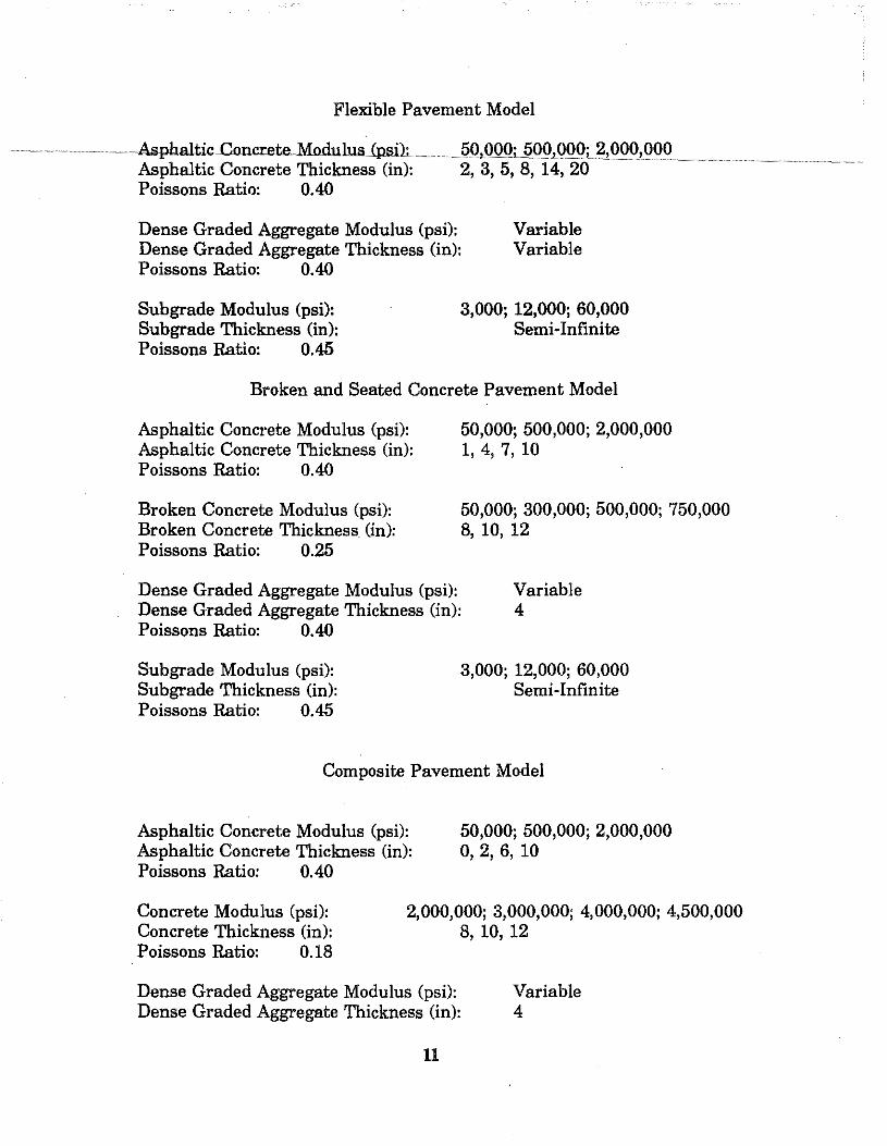
Flexible Pavement Model

···················~ ·······~Asphaltic . .Goncr.ete ... Mo.dulllsipsih...~ .... ~.~ .... .QQ.ill>Qi.QQMOO; ?1QQQ,QQQ ············~··~ Asphaltic Concrete Thickness (in): 2, 3, 5, 8, 14, 20 Poissons Ratio: 0.40

Dense Graded Aggregate Modulus (psi): Dense Graded Aggregate Thickness (in):

Variable Variable

Poissons Ratio: 0.40

Subgrade Modulus (psi): Subgrade Thickness (in): Poissons Ratio: 0.45

3,000; 12,000; 60,000 Semi-Infinite

Broken and Seated Concrete Pavement Model

Asphaltic Concrete Modulus (psi): Asphaltic Concrete Thickness (in): Poissons Ratio: 0.40

Broken Concrete Modulus (psi): Broken Concrete Thickness (in): Poissons Ratio: 0.25

Dense Graded Aggregate Modulus (psi):

50,000; 500,000; 2,000,000 1, 4, 7, 10

50,000; 300,000; 500,000; 750,000 8, 10, 12

Dense Graded Aggregate Thickness (in): Variable 4

Poissons Ratio: 0.40

Subgrade Modulus (psi): Subgrade Thickness (in): Poissons Ratio: 0.45

3,000; 12,000; 60,000 Semi-Infinite

Composite Pavement Model

Asphaltic Concrete Modulus (psi): Asphaltic Concrete Thickness (in): Poissons Ratio: 0.40

50,000; 500,000; 2,000,000 0,2, 6,10

Concrete Modulus (psi): Concrete Thickness (in):

2,000,000; 3,000,000; 4,000,000; 4,500,000 8, 10, 12

Poissons Ratio: 0.18

Dense Graded Aggregate Modulus (psi): Dense Graded Aggregate Thickness (in):

11

Variable 4

Poissons Ratio: 0.40

~ubgr~d~Modulus (psi): .............................. .3,0illl;.l2,illill;.fi0,.0.0.0. ................................................. . Subgrade Thickness (in): Semi-Infinite Poissons Ratio 0.45

All theoretical deflections were calculated using a load of 600 lbf and all deflections are expressed in mils (inches x lO.a).

Lagrangian Interpolation

The matrix of structures previously listed covers a wide range, but not all possibilities. Therefore to calculate deflections which were not included in the database, an interpolation procedure must be used. Lagrangian interpolation (21) was utilized to determine the deflections for structural sections which were not calculated by the database, but are within the ranges of the database. This method of interpolation is valid for an infinite number of data points.

The Lagrangian interpolating formula may be expressed as follows,

(6)

where each L,(x) is expressed as

LJ:x)- (x-x0) ... (x-xi-l)(x -x1• 1) ... (x -xn)

(x1 -x0) ... (x1 -x1_1)(x1 -x,.1) ... (x1 -x)

(7)

The P .(x) is the deflection desired for the value of x, where x may be layer modulus or layer thickness. For interpolation of the database, the Yn would represent the deflections and x. would represent the layer moduli or thicknesses corresponding to the deflections that are being used for interpolation. ·

PROGRAM DEVELOPMENT

Background

A personal computer-based program was written to perform the interpolation across each database. The program was developed using Microsoft QuickBASIC Version 4.5 (22). This program performs all necessary interpolations and least squares

calculations necessary to calculate the matching deflection bowls.

(8)

where:

D10 D2r> D3r, D4r are the field deflections and Dw D2., D3., D41 are the theoretically calculated deflections.

The methodology of these programs is to interpolate across the database for the known parameters and then perform iterative calculations on the remaining variables. Normally, the structural cross section is known; therefore, the database is interpolated for layer thickness directly. The remaining unknowns, elastic moduli, are calculated using an iterative procedure. For simplicity, only the interpolation algorithm will be discussed in this section. The input procedures for the program will be discussed in Appendix A. Each model uses the same methodology; however, the actual interpolation is somewhat different. Each model will be discussed in detail in the following sections.

To provide better relationships for interpolation, the common logarithm of the values have been utilized. The use of a logarithmic relationship provides more accurate interpolation. The specific uses of the logarithmic relationships will be outlined in the following sections.

Flexible Pavement Model (KTCFLEX)

Modulus Calculations

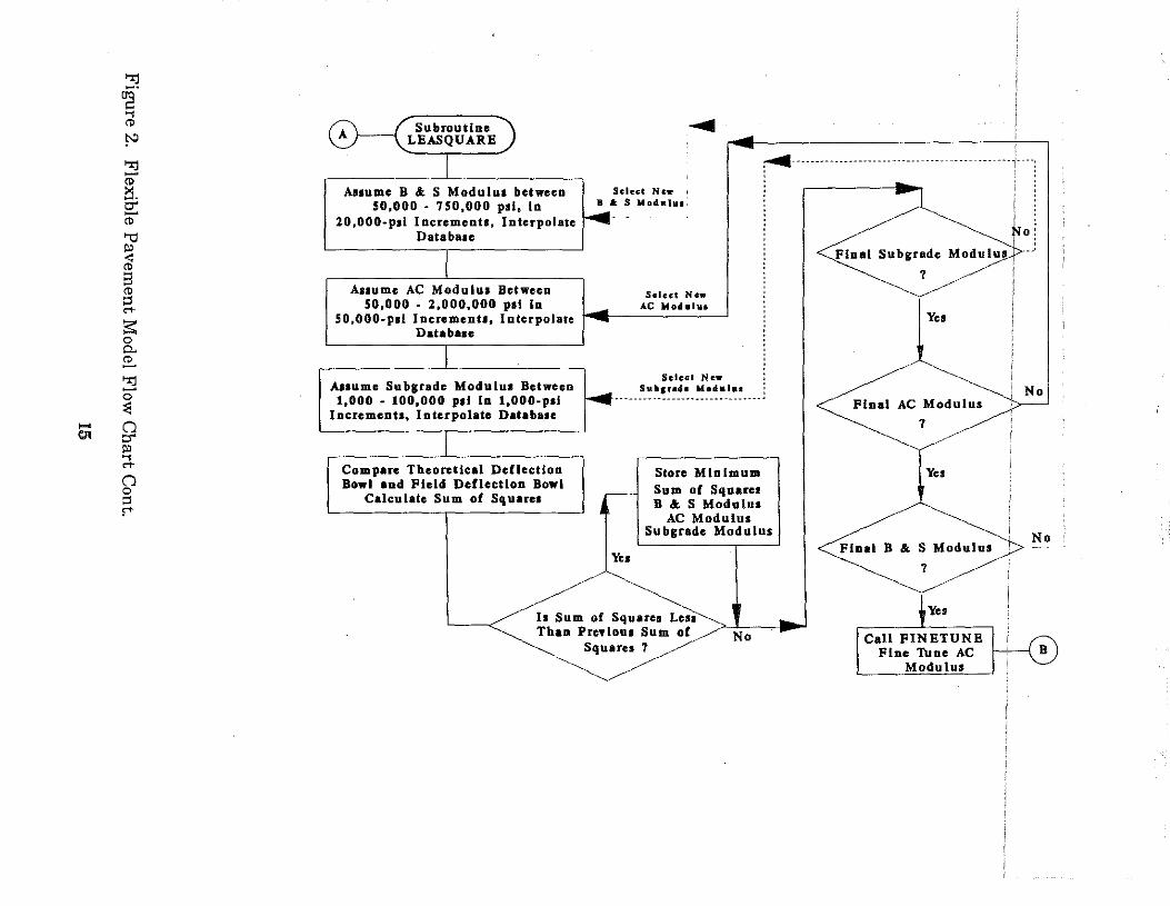
A flow chart of this model is given in Figures 1, 2, 3, and 4. This chart outlines the major steps executed in the program: Each procedure will be discussed in detail in the remainder of this section.

Several pieces of information are required from the user before calculations can begin. The following input information is needed to perform the calculations: layer thicknesses (AC and DGA), field deflections, test date and time of test, and temperature information (surface pavement temperature and 5-day mean air temperature).

Once the structural cross section of the pavement is known, the database may be interpolated for these thicknesses. The database is interpolated first for the thickness ratio (thickness of DGA I total pavement thickness), using subroutine INTRATIO. The relationship of log of the thickness ratio versus deflection is interpolated for the known

13

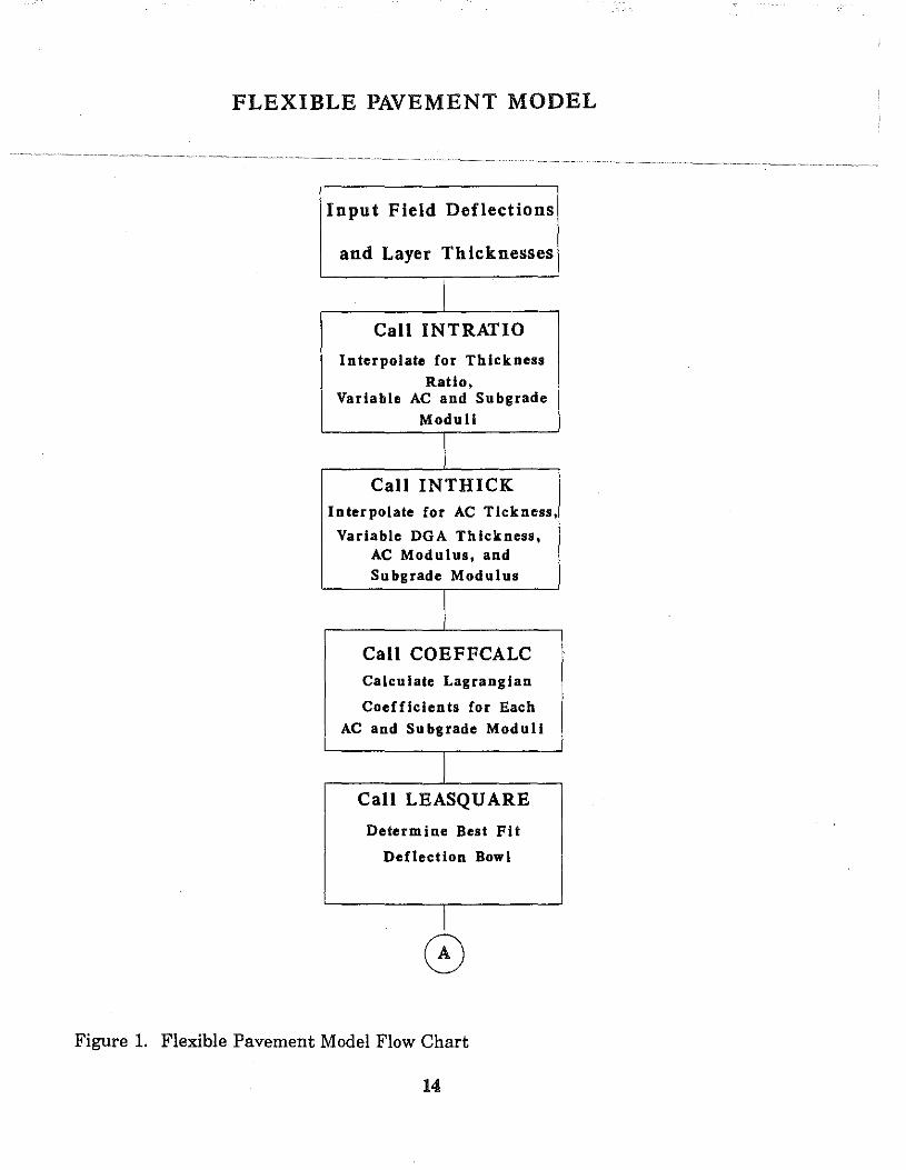
FLEXIBLE PAVEMENT MODEL

Input Field Deflections

and Layer Thicknesses

I Call INTRATIO

Interpolate for Thickness Ratio,

Variable AC and Subgrade

Moduli

I Call INTHICK

Interpolate for AC Tickness,

Variable DGA Thickness, AC Modulus, and Subgrade Modulus

I Call COEFFCALC Calculate Lagrangian

Coefficients for Each AC and Subgrade Moduli

I Call LEASQU ARE

Determine Best Fit

Deflection Bowl

I

0 Figure 1. Flexible Pavement Model Flow Chart

14

'""J ~· .... "' ty

'""J -"' >: -· C" -"' '1::1 ~ "' a "' ::l ~

~ 0 0.. ;E. '""J -0

:6 ..... 0 at C"

I'> .... ~

0 0 ::l ,.

Subroutine LEASQUARE

....... ............................ -----------------

Assume B &. S Modulua between 50,000 • 750,000 psi, in

20,000-pai Increments, Interpolate Data bate

Select New B A S Moduhu

Auume AC Modulua Between select New 50,000 - 2,000,000 psi In AC Moduhu

50,000-pli lncremenu, Interpolate Database

Anume Subarade Modulua Between 1,000 - 100,000 poi in 1,000-poi

Incrementa, Interpolate DatabaJe

Compare Theoretical Deflection Bowl and Field Deflection Bowl

Calculate Sum of Sq uare1

Selccl New Sulloarad• Modulu• ,

. ------------------------------.

Store Minimum Sum of Squarcl B & S Modulus

AC Modulus Subgrade Modulus

h Sum of Squares Lesa Than Prnioua Sum of

Squares 7

Final Subgrade Modulus

7

Final AC Modulus

7

Final B & S Modulus

1

Yes

Call FINETUNE Fine Tune AC

Modulus

' !'•

No

'

Store Minimum Sum of Squares

B Subroutine

F.!N.ET!JJ'! .. !'L.

Assume AC Modulus between 50,000 above and 50,000 below

Value for Minimum Sum of Squares In lO,OOO .. psi Increments, loterpolat

Database

Asaume Subgrade Modulus between

1,000 and 100,000 psi In 1,000-psl

Increments, Interpolate Data Base

Compare Theoretical Deflection Bowl and Field Deflection Bowl

Calulate Sum of Squares

Subgrade Modulus:i-olll--<c (CALSUBMOD)

AC Modulus (CALACMOD)

No Subgrade Modulus•:>------

7

Call EFFTHICK y01 Final AC Modulus No

Tblckneu

Figure 3. Flexible Pavement Model Flow Chart Cont.

16

0

• . ~ • 0

:II • ~ • 0

~ :II ~

~ -~ • ., • • • z • z ~

.: • • . • .. ., .,

Store Minimum Sum of Squares

and Effective Thickness

Call TBMPCALL Calculate Mean

Pavement Temperature

Call ADJDBFL Adjust Deflections to Reference Temperature

Assume AC Modulus 1,200,000 psi

Assum.e Su bgrade Modulus from LBASQUARB, CALSUBMOD,

Interpolate Database

Assume AC Thickness between 1 ln. and the Design Thickness

in O.lS·In. Increments, Interpolate Database

Compare Theoretical Deflection Bowl and Adjusted Field Deflection

Bowl, Calculate Sum of Squares

Yes Is Sum of Squares Less Than Previous Sum of

Squares 7

Yeo BND "---~=---<

Figure 4. Flexible Pavement Model Flow Chart Cont.

17

No

thickness ratio. This creates a new database which contains data only for structures having the same thickness ratio. The new database is then interpolated for the AC

···· ·tbiekness·using·the·relationship of.log{AC.thickness):¥ersusJo.g ... (defle.ction),{subroy.tin,e ........ .. . ......... . INTHICK). This database contains deflections for a matrix of structures for various AC and subgrade moduli, at the field AC and DGA thickness.

The modular ranges for the database calculated are the same as those previously outlined, AC moduli of 50,000; 500,000; and 2,000,000 and subgrade moduli of 3,000, 12,000; and 60,000. For determining the theoretical bowl which will best match the field bowl, deflections at other layer moduli within these ranges must be calculated. The Lagrangian coefficients of L;(x) are calculated for both the AC and subgrade modulus in the subroutine COEFFCALC. Coefficients are calculated for AC moduli on increments of 50,000 psi from 50,000 to 2,000,000 psi. For subgrade moduli, coefficients are calculated on 1,000 psi increments from 1,000 to 100,000 psi.

The process of determining the best fit deflection bowl based on the AC and subgrade modulus is an iterative process. First an AC modulus is assumed, based on a relationship of log (AC modulus) versus log (deflection). The current database is then interpolated for AC modulus. This provides a database which is a function of subgrade modulus and pavement deflection. The deflections are calculated for different subgrade moduli based on the relationship of!og (Subgrade modulus) versus log (Deflection). The subgrade modulus is varied in 1,000 psi increments from 1,000 to 100,000 psi. At each subgrade modulus, the field and theoretical bowls are compared and the least square calculation, Equation 8, is performed in the subroutine LEASQUARE.

If the least square is less than the current minimum least square, then the AC modulus and subgrade modulus are stored as the best fit modular values for the given deflections. This iteration process is carried out for AC modulus increments previously outlined. A total of 4,000 different modular combinations are tested for the best fit theoretical deflection bowl. The combination of layer moduli, representing the smallest least square is assumed to be the best fit layer moduli for the input deflections.

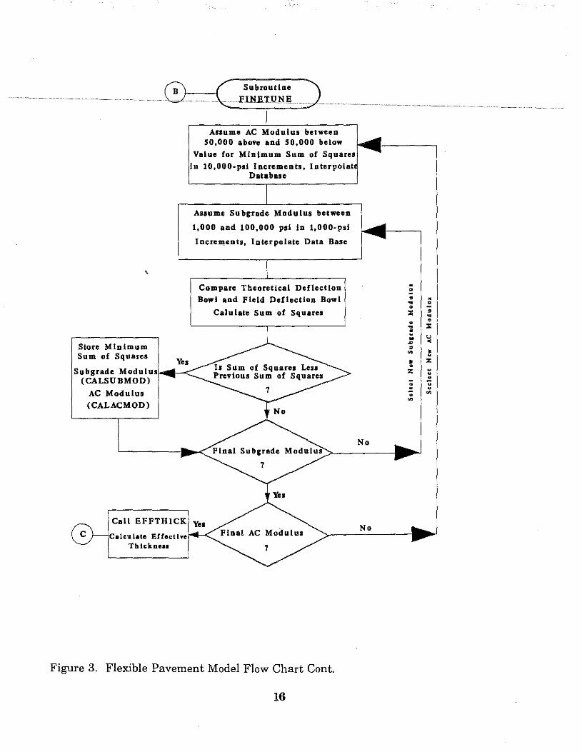
The moduli selected by the previous procedure are utilized to determine another range of moduli with smaller increments. This procedure is carried out in the FINETUNE subroutine. The range for the AC modulus calculations is set as 50,000 psi above the value calculated in the previous step to 50,000 psi below this value. The AC modulus is then varied in 10,000-psi increments. The same iterative procedure is conducted, using the same increments of subgrade modulus, and refined values of AC modulus and subgrade modulus are determined. These values are then selected as the best fit layer moduli, representing the measured field deflections. The deflections have not been adjusted for temperature, therefore these moduli are determined at the prevailing pavement temperature.

18

Effective Thickness

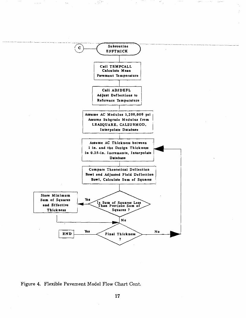
···· ······ ·····~··~·~·~ ~·· ~·-'fil~ calculate~ an ~everlfly~thiekness ~using the~'I'r.anspor~tatien~~Cabinet's~ ... eurrent.. .... procedures, the effective thickness ef the structure is needed. A new method ef calculating effective thickness was developed. Unlike the current effective thickness procedure, the new procedure utilizes all deflections in calculating the effective thickness. In the new procedure, the AC and subgrade moduli are held constant and the asphaltic concrete thickness is varied.

The AC modulus is assumed to be 1,200,000 psi, as was previously discussed. The database which has been interpolated fer thickness ratio is interpolated fer this value ef AC modulus. The new database is then interpolated fer the subgrade modulus which was calculated from the in-situ conditions. This interpolation yields a database calculated fer a constant AC modulus and in-situ subgrade modulus, which varies across AC thickness.

Before the actual effective thickness may be calculated, the field deflections must be adjusted te a reference temperature ef 70 degrees fahrenheit. The method fer adjusting the deflections is the same as is currently utilized in the 2-3 projected procedure, Equation 3.

The mean pavement temperature is calculated based en the pavement surface temperature and the 5-day mean air temperature, prier te the test date. The temperature efthe pavement is calculated in the subroutine TEMPCAL (23). The routine calculates the pavement temperature at a given depth, based en the surface temperature, time ef day, and 5-day mean air temperature. This routine is called twice, te calculate the pavement temperature at the mid height and bottom ef the AC layer. These two temperatures along with the surface temperature are used to calculate the mean pavement temperature.

This mean pavement temperature is then input into the subroutine ADJDEFL. The field deflections are multiplied by the adjustment factor, Equation 3, fer each deflection. The adjusted deflections may then be cern pared to the theoretically calculated deflections.

The database which has been interpolated fer AC and subgrade modulus is new interpolated fer AC thickness en 0.25-inch increments and the resulting deflections are compared te the adjusted field deflections. The least sum ef squares, Equation 8 is calculated fer each deflection bowl, the thickness corresponding te the minimum least sum ef squares is the effective thickness ef the pavement structure. This thickness along with the in-situ subgrade modulus may then be input into the overlay design program.

19

Broken and Seated Concrete Pavement Model CKTCBREAK)

················~··~··'I'he.methodol<>gy~used~in..this.m.odel.is..the.same..as is..used in .. the. flexible model .... with the addition of one layer. Also, no calculation is made for effective thickness in this model. AI; was previously outlined, the modulus of the broken and seated concrete layer is assumed to vary from 50,000 to 750,000 psi. Since this model introduces another layer into the structure, the computational time is greatly increased. All layer moduli calculated using this model are at in-situ conditions, no adjustments have been made for temperature.

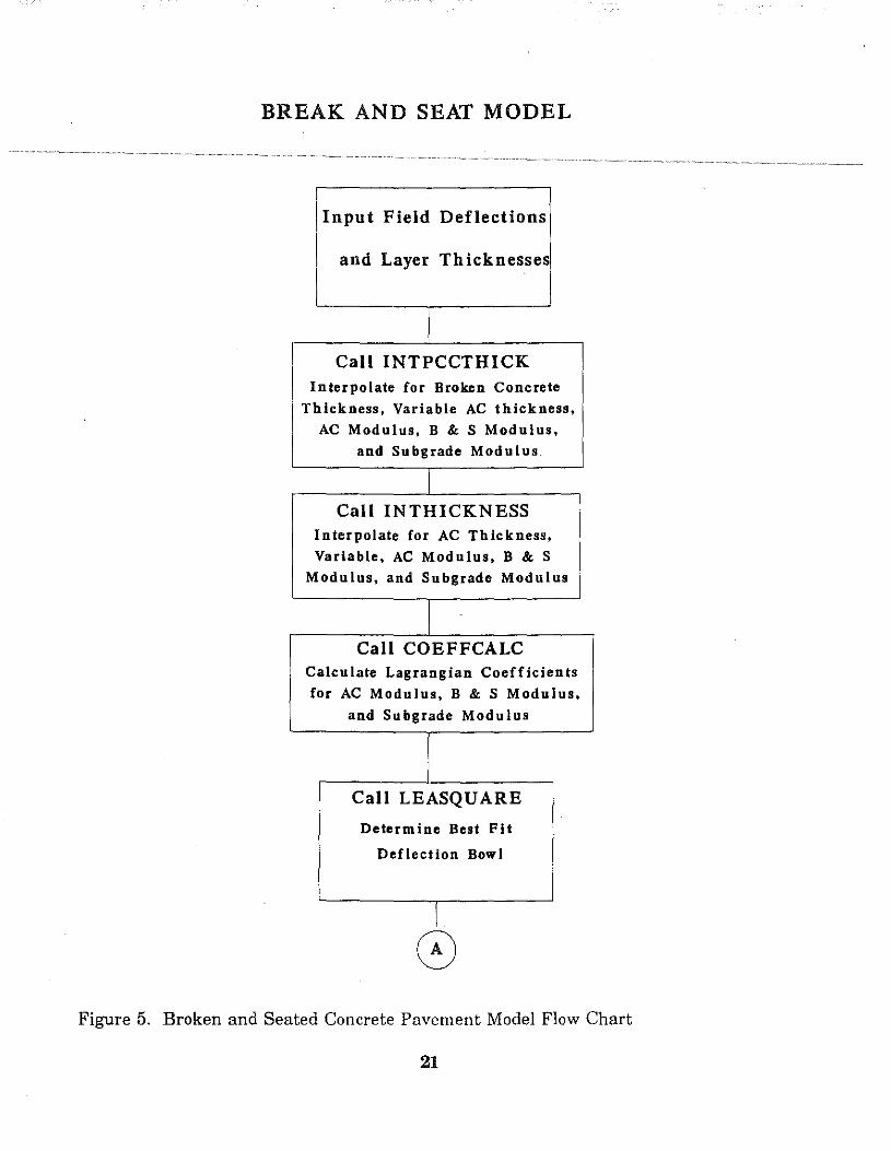
The flow chart for this program is given Figures 4, 5, and 6. The only inputs needed for this program are the structural thickness of the AC overlay and the broken and seated concrete layer. The thickness of dense graded aggregate has been assumed as a constant of 4 inches for all broken and seated concrete pavements.

The subroutine INTPCCTHICK is called to interpolate the database for the thickness of the broken concrete layer. The interpolation is conducted assuming the relationship of log (broken layer thickness) versus log (pavement deflection), with variable AC thickness and modulus, broken concrete modulus, and subgrade modulus. This routine eliminates one thickness variable from the database. The database is now interpolated for AC thickness using the INTHICKNESS subroutine and a log - log relationship between AC thickness and pavement deflection.

The subroutine COEFFCALC is now called to calculate the Lagrangian coefficients, L;(x) for each modulus. Lagrangian coefficients are calculated for AC modulus, in increments of 50,000 psi and 10,000 psi, between 50,000 and 2,000,000 psi. Coefficients for the subgrade modulus are calculated on the same 1,000-psi increments used in KTCFLEX. Coefficients for broken concrete are calculated on increments of 10,000 and 20,000 psi. Coefficients were calculated at two increments for the AC and broken concrete modulus so a fine tuning of these moduli values may be conducted. This fine tuning is performed as was previously described in KTCFLEX.

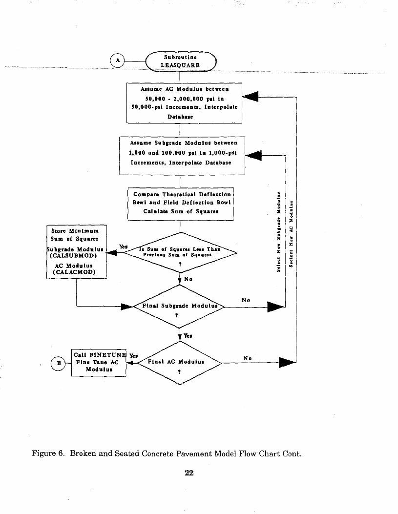
The LEASQUARE subroutine is now called to perform the iteration of each modulus and calculation of the least sum of squares of each bowl. A total of 148,000 different deflection bowls are compared to the field deflection bowl. All relationships between deflection and modulus (subgrade, AC, and broken concrete) are log - log relationships.

The iteration procedure is a three-step process. All combinations for all moduli of three different materials must be evaluated. First, a modulus for the broken concrete is assumed and the database is interpolated, a new database is then created varying across AC modulus and subgrade modulus. This new database is then interpolated for an AC modulus. This database is then interpolated for each subgrade modulus and the resulting deflection bowl is compared to the field deflection bowl.

20

BREAK AND SEAT MODEL

Input Field Deflections

and Layer Thicknesses

Call INTPCCTHICK Interpolate for Broken Concrete

Thickness, Variable AC thickness,

AC Modulus, B & S Modulus,

and Subgrade Modulus

Call INTHICKNESS Interpolate for AC Thickness,

Variable, AC Modulus, B & S

Modulus, and Subgrade Modulus

Call COEFFCALC Calculate Lagrangian Coefficients

for AC Modulus, B & S Modulus,

and Subgrade Modulus

Call LEASQUARE

Determine Best Fit

Deflection Bowl

I

0 Figure 5. Broken and Seated Concrete Pavement Model Flow Chart

21

Store Minimum. Sum of Squares

Subroutine

Assume AC Modulus between

50,000 • 1,000,000 pol In 50,000-psi Increments, Interpolate

Databaoe

Assume Su bgrade Modo lui between

1,000 and 100,000 pol In 1,000-psl

Incrementa, Interpolate Database

Compare Theoretical Deflection Bowl and Field Deflection Bowl

Calulate Sum of Squares

ubgrado Modulu•wiii---<­(CALSUBMOD)

AC Modulus (CALACMOD)

Call FINI!TUN Fine Tune AC

Modulo•

No Subgrade Modulo•>------

No

. • • . .. ! • :II • .. • • .. :II ~

~ • ~ • t .. t "' "' ; ; = • = • • ., .,

Figure 6. Broken and Seated Concrete Pavement Model Flow Chart Cont.

22

"%j

~-.... CD

-.l

to .... 0 I" CD ::l Pl ::l 0. m CD Pl M" CD 0. Q 0 ::l '"' '1 CD M" CD

'"0 Pl

t>:l < ~ CD s

CD ::l M"

s::: 0 0. ~

:31 0

~ Q 0" Pl .... '"'" Q 0 ::l ,...

0-1 Subroutine FINBTUNB

-----~

Assume B & S Modulus between 40,000 above and 40,000 below

Value for Minimum Sum of Squares in 10,000-psi Increments, Interpolate

Database

Assume AC Modulus Between 80,000 above and 80,000 below

Value for Minimum Sum of Squares in 10,000-psi Incremetns, Interpolate

Database

Assume Subgrade Modulus between 1,000 and 100,000 psi in 1,000-psl Increments, Interpolate Database

......

Select New B & S Modo Ius·

Select New AC Modulua

Select New Subsrade Modulua

Store Minimum Sum of Squares B & S Modulus

, ............ .

Compare Theoretical Deflection Bowl and Field Deflection Bowl

Calculate Sum of Squares AC Modulus Subgrade Modulus

Yes

Is Sum of Squares Less Than Previous Sum of

Squares ?

Final Su bgrade Modu his ./

? ~

Yes

Final AC Modulus

?

Yes

Final B & S Modulus[

?

tYes

B

No

No

No

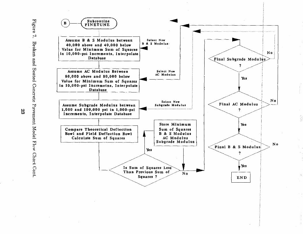
Once this iteration is completed, a fine tuning of the broken concrete modulus and AC modulus is performed. The ranges of interpolation are changed as follows: the AC modulus range is changed to 80,000 psi above and 80,000 psi below the previous value

.................... ~ .. .calculated,..on.~lO,.OO.Ibpsi.incrementsrthe..br.oken..concrete.m.odulus..is~changed.to ... 40.,000 ·········~··~······ psi above the value calculated and 40,000 psi below the previous value, on 10,000-psi increments. The subgrade moduli range remains the same. Using these new ranges, a total of 15,300 structures are compared. The structure corresponding to the minimum sum of least squares best represents the in-situ conditions of the pavement.

Composite Pavement (KTCCOMP)

The procedures used in the composite model are nearly the same as the broken and seated concrete pavement model, with a few exceptions. The composite model contains different layer moduli and Poissons ratio for the concrete layer. This model does not utilize the thickness ratio, instead the thickness of the portland cement concrete layer is varied. In addition, provisions have been made to allow the concrete to be held constant at any modulus value from 2,000,000 to 4,500,000 psi.

MODEL VERIFICATION

The verification process will consist of a theoretical verification and examples of the uses of each model on actual field deflections. The theoretical verification will use deflections which have been calculated using elastic theory as the program inputs. The moduli calculated by the model were compared to the moduli input into the linear elastic program. This verification was conducted for various structural cross-sections.

The output for the flexible pavement model has been compared to the output from the current 2-3 Projected program. These results were also input into the overlay program to compare the calculated overlay from the different backcalculation methods.

Flexible Pavement Model

Theoretical Verification

The structural cross-sections used for the flexible model verifications were as follows:

3" AC, 6" DGA 6" AC, 12" DGA 12" Full Depth AC.

Theoretical deflection bowls were calculated using Chevron, N-Layer for AC moduli of 100,000 and 1,000,000 psi and subgrade moduli of 6,000 and 50,000 psi. Each of these deflection bowls was input into the program KTCFLEX. The program then calculated the corresponding deflection bowl which best fit the theoretical deflection bowl. This deflection bowl is represented by an AC and subgrade modulus.

24

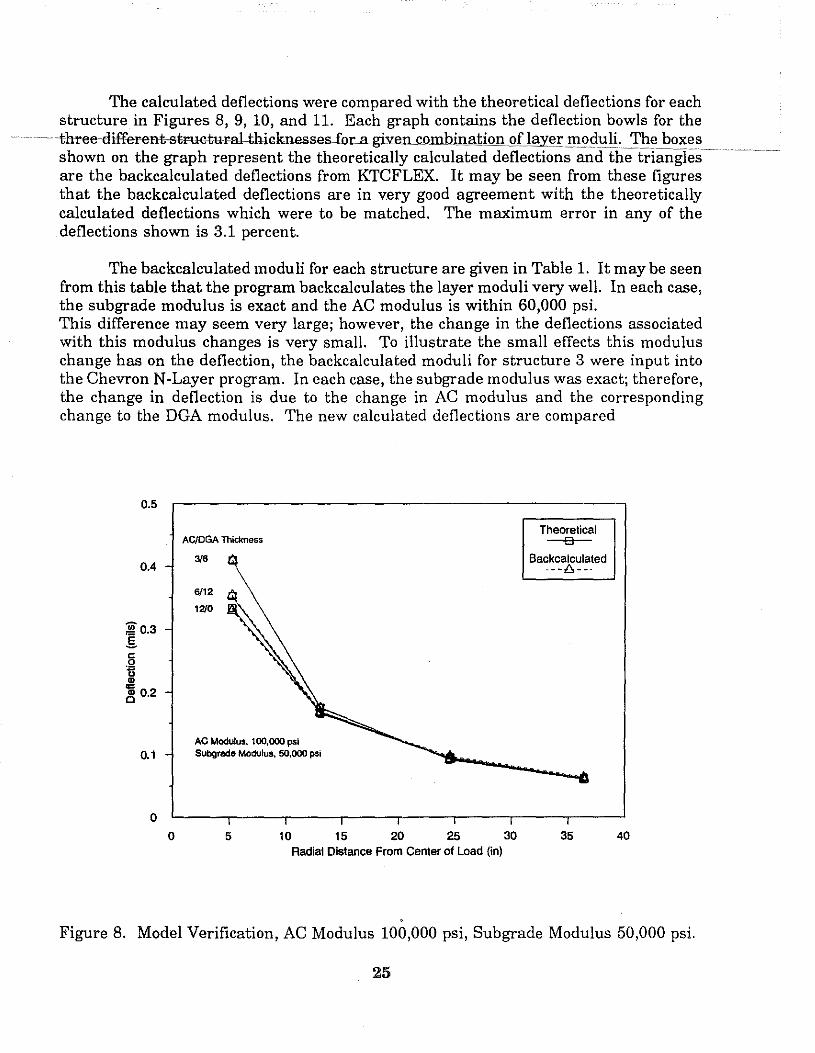
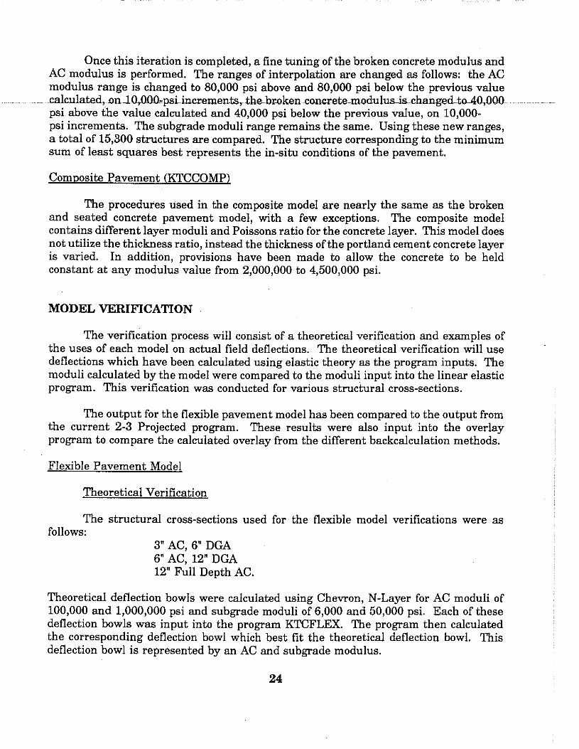
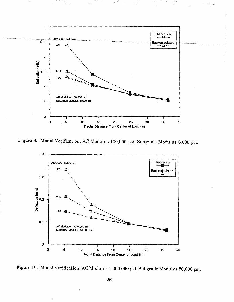
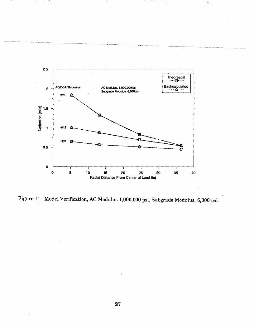
The calculated deflections were compared with the theoretical deflections for each structure in Figures 8, 9, 10, and 11. Each graph contains the deflection bowls for the

··········~·-·three,Jiff~r~ntstruGturaJ..thi.cknesses.i~a.giYen.c.ombination oflay!Jr:.fil()d1lJi,'!'.Jle boxes shown on the graph represent the theoretically calculated deflections and the triangles · · are the backcalculated deflections from KTCFLEX. It may be seen from these figures that the backcalculated deflections are in very good agreement with the theoretically calculated deflections which were to be matched. The maximum error in any of the deflections shown is 3.1 percent.

The backcalculated moduli for each structure are given in Table 1. It may be seen from this table that the program backcalculates the layer moduli very well. In each case, the subgrade modulus is exact and the AC modulus is within 60,000 psi. This difference may seem very large; however, the change in the deflections associated with this modulus changes is very small. To illustrate the small effects this modulus change has on the deflection, the backcalculated moduli for structure 3 were input into the Chevron N-Layer program. In each case, the subgrade modulus was exact; therefore, the change in deflection is due to the change in AC modulus and the corresponding change to the DGA modulus. The new calculated deflections are compared

0.5

0.4

~0.3 .5.

~ ,J!! l!l 0.2

AC/DGA Thickness

3/6

6/12

12/0

AC Modulus, 100,000 psi 0.1 Subgrade Modulus, 50,000 psi

0

0 5 10 15 20 25 Radial Distance From Center of Load (in)

.

30

Theoretical 0

Backcalculated ·--£2.--·

35 40

Figure 8. Model Verification, AC Modulus 100,000 psi, Subgrade Modulus 50,000 psi.

25

3

Theoretical 0

························~-~~·~·~·~·~·~·-··~·······~·~···~··~.2>.<i5 :J-.A.CJDGA.Thit:knes.:L .. ~ .......... ~ ... ~ ........... ~ .... ~ ............. ~ ... ~ ... ~.~·····~···~·~··· .. ···················~·~···················· l~saekealculatedl++························~·················~·~····················~····~·········~·· ·--8--·

2

6/12

12/0

0.5

AC Modulus, 100,000 :I""~. ~§:.:q,--==::::::::~8;.""""""'=----· Subgrada Modulus, 6,000 psi

0

0 5 10 15 20 25 30 35 40 Radial Distance From Center of Load (in)

Figure 9. Model Verification, AC Modulus 100,000 psi, Subgrade Modulus 6,000 psi.

0.4

0.3

Ui 'E c ·~ 0.2

'; 0

0.1

0

0

AC/DGA Thickness

316

5 10 15 20 25 30 Radial Distance From Center of Load (in)

Theoretical 0

Backcalculated ·--8--·

35 40

Figure 10. Model Verification, AC Modulus 1,000,000 psi, Subgrade Modulus 50,000 psi.

26

2.5

Theoretical 0

ACIOGA Thickness AC Modulus, 1,000,000 psi Backcalculated 2

Subgrade Moduluo. fl,OOOpsi ·--/),--·

3/8

~ 1.5 ..5. c: 0

'B ., '5 1 6112 c

12/0 G a 0.5 0

0

0 5 10 15 20 25 30 35 40 Radial Distance From Center of Load (In)

Figure 11. Model Verification, AC Modulus 1,000,000 psi, Subgrade Modulus, 6,000 psi.

27

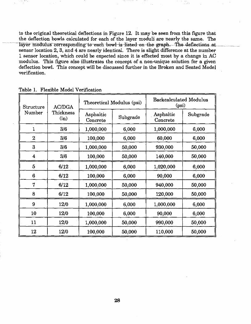
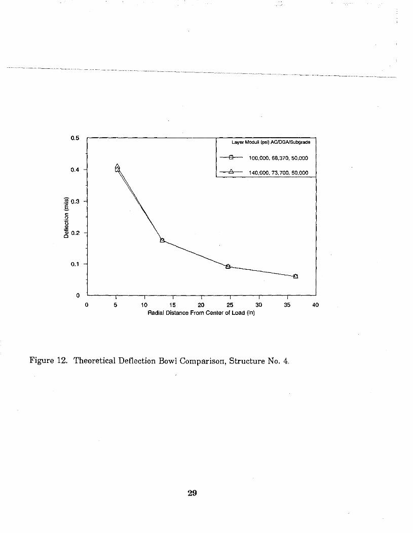
to the original theoretical deflections in Figure 12. It may be seen from this figure that the deflection bowls calculated for each of the layer moduli are nearly the same. The

············~layer moal.il.uscorrestronding~~each howl·~~isted~n~the...gr.aph~'I'he..deflections..aL ............ ·······~··· sensor location 2, 3, and 4 are nearly identical. There is slight difference at the number 1 sensor location, which could be expected since it is effected most by a change in AC modulus. This figure also illustrates the concept of a non-unique solution for a given deflection bowl. This concept will be discussed further in the Broken and Seated Model verification.

Table 1. Flexible Model Verification

Theoretical Modulus (psi) Backcalculated Modulus Structure AC/DGA (psi)

Number Thickness Asphaltic Asphaltic Sub grade (in) Concrete

Sub grade Concrete

1 3/6 1,000,000 6,000 1,000,000 6,000

2 3/6 100,000 6,000 60,000 6,000

3 3/6 1,000,000 50,000 930,000 50,000

4 3/6 100,000 50,000 140,000 50,000

5 6/12 1,000,000 6,000 1,020,000 6,000

6 6/12 100,000 6,000 90,000 6,000

7 6/12 1,000,000 50,000 940,000 50,000

8 6/12 100,000 50,000 120,000 50,000

9 12/0 1,000,000 6,000 1,000,000 6,000

10 12/0 100,000 6,000 90,000 6,000

11 12/0 1,000,000 50,000 990,000 50,000

12 12/0 100,000 50,000 110,000 50,000

0.5

0.4

~0.3 .§.

" 0 ·u ill ~ 0.2

0.1

0

0 5 10

Layer Moduli (psi) AC/DGA/Subgrade

0 100,000, 68,370, 50,000

140,000,73,700,50,000

15 20 25 30 35

Radial Distance From Center of Load (in)

Figure 12. Theoretical Deflection Bowl Comparison, Structure No. 4.

29

40

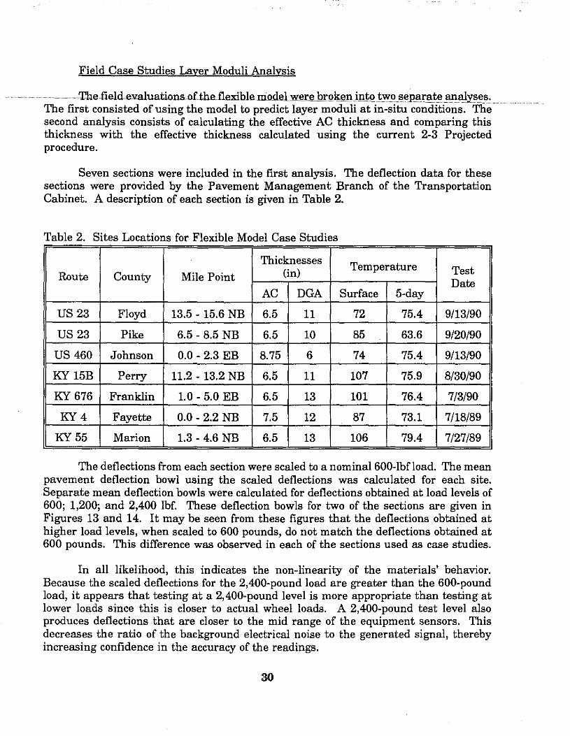
Field Case Studies Layer Moduli Analysis

· ···················· ..... The.field.ev:aluations.ofihaflexiblenio.del.:werebrQ~eni!l t() t..Y<> !;eJ>ar!lte !l!llll.YS~e!!~ . .... . . . The first consisted of using the model to predict layer moduli at in-situ conditions. The second analysis consists of calculating the effectiv:e AC thickness and comparing this thickness :with the effectiv:e thickness calculated using the current 2-3 Projected procedure.

Seven sections :were included in the first analysis. The deflection data for these sections :were provided by the Pavement Management Branch of the Transportation Cabinet. A description of each section is given in Table 2.

Table 2. Sites Locations for Flexible Model Case Studies

Thicknesses Temperature Route County Mile Point (in) Test

Date AC DGA Surface 5-day

us 23 Floyd 13.5 - 15.6 NB 6.5 11 72 75.4 9/13/90

us 23 Pike 6.5-8.5 NB 6.5 10 85 63.6 9/20/90

us 460 Johnson 0.0-2.3 EB 8.75 6 74 75.4 9/13/90

KY 15B Perry 11.2 - 13.2 NB 6.5 11 107 75.9 8/30/90

KY676 Franklin 1.0-5.0 EB 6.5 13 101 76.4 7/3/90

KY4 Fayette 0.0-2.2 NB 7.5 12 87 73.1 7/18/89

KY 55 Marion 1.3-4.6 NB 6.5 13 106 79.4 7/27/89

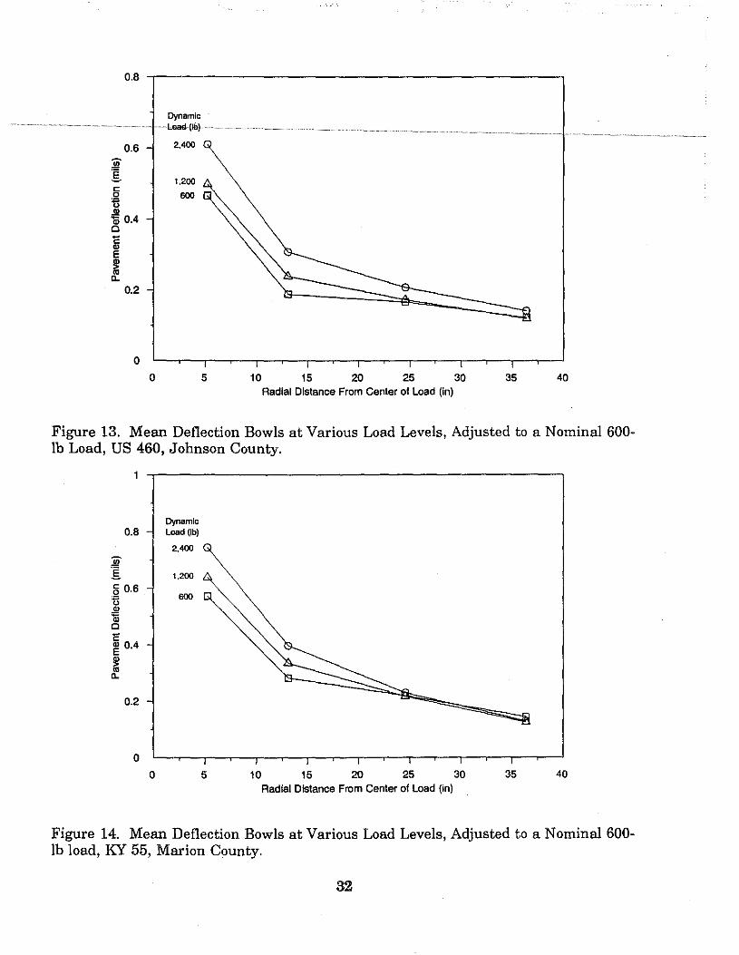
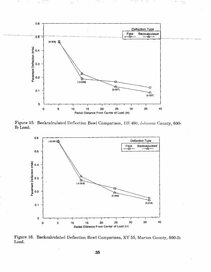
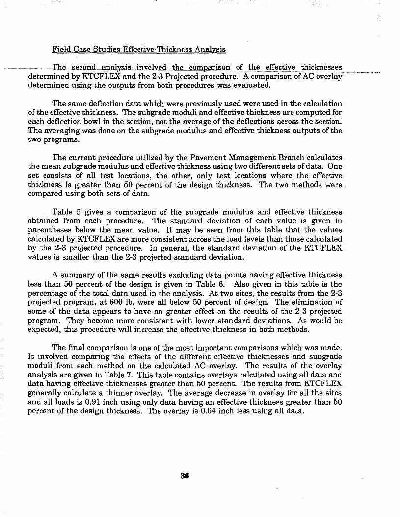
The deflections from each section :were scaled to a nominal600-lbfload. The mean pavement deflection bowl using the scaled deflections :was calculated for each site. Separate mean deflection bowls :were calculated for deflections obtained at load levels of 600; 1,200; and 2,400 lbf. These deflection bowls for t:wo of the sections are given in Figures 13 and 14. It may be seen from these figures that the deflections obtained at higher load levels, :when scaled to 600 pounds, do not match the deflections obtained at 600 pounds. This difference :was observed in each of the sections used as case studies.

In all likelihood, this indicates the non-linearity of the materials' behavior. Because the scaled deflections for the 2,400-pound load are greater than the 600-pound load, it appears that testing at a 2,400-pound level is more appropriate than testing at lower loads since this is closer to actual :wheel loads. A 2,400-pound test level also produces deflections that are closer to the mid range of the equipment sensors. This decreases the ratio of the background electrical noise to the generated signal, thereby increasing confidence in the accuracy of the readings.

30

Each of these mean deflection bowls was input into KTCFLEX with the corresponding structural thicknesses. The layer moduli were then backcalculated. The

·················mfects~oHhe~differenees~indeflection~bowls maybeseen~in'I'able3. Thistablegi:ves~the

layer moduli results from KTCFLEX for deflections obtained at each load level. The backcalculated deflections, corresponding to the layer moduli of 'I'able 3 are given in 'I'able 4. The field deflections are given in parentheses. It may be seen from 'I'able 4 that the difference in the mean deflections for each load level do have an effect on the backcalculated moduli. In most cases, both the AC and subgrade moduli decrease. 'I'able 4 illustrates that the backcalculated deflections are in very good agreement with the field deflections input into KTCFLEX. The field deflection bowls and the backcalculated deflections for two sites are compared in Figures 15 and 16. These figures show that there is very good agreement between the deflection at the number one sensor location. The field deflection bowl appears to be flatter across sensor 2 through 4. This was observed in several of the deflection bowls from other sections.

31

0.8 -,.--------------------------,

:iii" g

0.6

6 ii .!1! Q) 0.4 0

ii E

~ 0.2

0

0

Dynamic

2,400

1,200

600

5 10 15 20 25 30 35 40 Radial Distance From Center of Load (in)

Figure 13. Mean Deflection Bowls at Various Load Levels, Adjusted to a Nominal 600-lb Load, US 460, Johnson County.

Dynamic 0.8 Load (lb)

2,400

1,200

600

0.2

0

0 5 10 15 20 25 30 35 40 Radial Distance From Center of Load (in)

Figure 14. Mean Deflection Bowls at Various Load Levels, Adjusted to a Nominal 600-lb load, KY 55, Marion County.

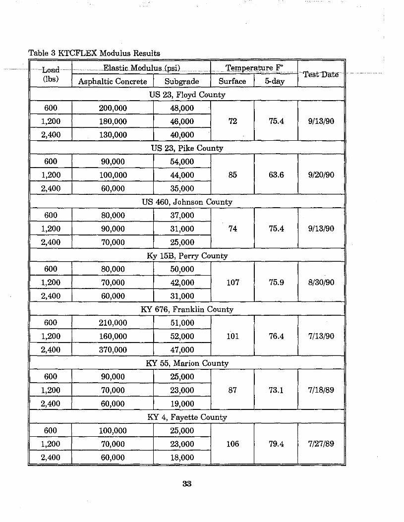
Table 3 KTCFLEX Modulus Results

~ Load ~~ . . ~ ~~ ..... Elastic .. Modulus (psi} T~mp~rat:u,r:e F"' """"" ~ '"""" ~--··--· ...

~TestLlate (lbs) Asphaltic Concrete Sub grade Surface 5-day

US 23, Floyd County

600 200,000 48,000

1,200 180,000 46,000 72 75.4 9/13/90

2,400 130,000 40,000

US 23, Pike County

600 90,000 54,000

1,200 100,000 44,000 85 63.6 9/20/90

2,400 60,000 35,000

US 460, Johnson County

600 80,000 37,000

1,200 90,000 31,000 74 75.4 9/13/90

2,400 70,000 25,000

Ky 15B, Perry County

600 80,000 50,000

1,200 70,000 42,000 107 75.9 8/30/90

2,400 60,000 31,000

KY 676, Franklin County

600 210,000 51,000

1,200 160,000 52,000 101 76.4 7/13/90

2,400 370,000 47,000 .

KY 55, Marion County

600 90,000 25,000

1,200 70,000 23,000 87 73.1 7/18/89

2,400 60,000 19,000

KY 4, Fayette County

600 100,000 25,000

1,200 70,000 23,000 106 79.4 7/27/89

2,400 60,000 18,000

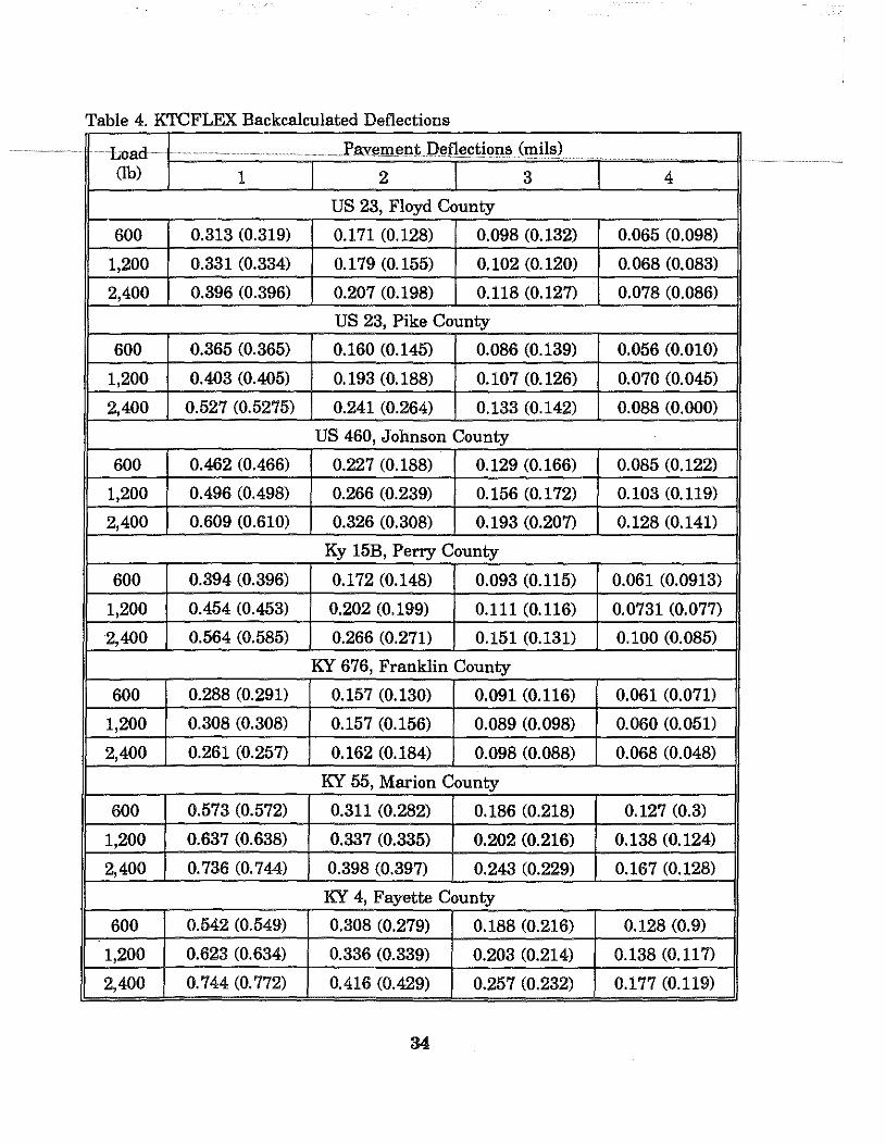
Table 4. KTCFLEX Backcalculated Deflections

~Load .. . . . PaYem ent :Pet1e<:ti()!l~ (lllils) ~"""'"

(!b) 1 2 3 4

US 23, Floyd County

600 0.313 (0.319) 0.171 (0.128) 0.098 (0.132) 0.065 (0.098)

1,200 0.331 (0.334) 0.179 (0.155) 0.102 (0.120) 0.068 (0.083)

2,400 0.396 (0.396) 0.207 (0.198) 0.118 (0.127) O.o78 (0.086)

US 23, Pike County

600 0.365 (0.365) 0.160 (0.145) 0.086 (0.139) 0.056 (0.010)

1,200 0.403 (0.405) 0.193 (0.188) 0.107 (0.126) 0.070 (0.045)

2,400 0.527 (0.5275) 0.241 (0.264) 0.133 (0.142) 0.088 (0.000)

US 460, Johnson County

600 0.462 (0.466) 0.227 (0.188) 0.129 (0.166) 0.085 (0.122)

1,200 0.496 (0.498) 0.266 (0.239) 0.156 (0.172) 0.103 (0.119)

2,400 0.609 (0.610) 0.326 (0.308) 0.193 (0.207) 0.128 (0.141)

Ky 15B, Perry County

600 0.394 (0.396) 0.172 (0.148) 0.093 (0.115) 0.061 (0.0913)

1,200 0.454 (0.453) 0.202 (0.199) 0.111 (0.116) 0.0731 (0.077)

2,400 0.564 (0.585) 0.266 (0.271) 0.151 (0.131) 0.100 (0.085)

KY 676, Franklin County

600 0.288 (0.291) 0.157 (0.130) 0.091 (0.116) 0.061 (0.071)

1,200 0.308 (0.308) 0.157 (0.156) 0.089 (0.098) 0.060 (0.051)

2,400 0.261 (0.257) 0.162 (0.184) 0.098 (0.088) 0.068 (0.048)

KY 55, Marion County

600 0.573 (0.572) 0.311 (0.282) 0.186 (0.218) 0.127 (0.3)

1,200 0.637 (0.638) 0.337 (0.335) 0.202 (0.216) 0.138 (0.124)

2,400 0. 736 (0. 744) 0.398 (0.397) 0.243 (0.229) 0.167 (0.128)

KY 4, Fayette County

600 0.542 (0.549) 0.308 (0.279) 0.188 (0.216) 0.128 (0.9)

1,200 0.623 (0.634) 0.336 (0.339) 0.203 (0.214) 0.138 (0.117)

2,400 0.744 (0.772) 0.416 (0.429) 0.257 (0.232) 0.177 (0.119)

0.6 ~------------------------,

'in '§. 0.4

c: 0 ·g ~ 0.3 Cl

~ ~ ~ 0.2 0..

0.1

0

(0.005)

0 5 10

Deflection T e

Field Backcalculated ~ ::::8:::=.~··········-.CL ....... ~····~

(0.037)

{0.037)

15 20 25 30 35 40 Radial Distance From Center of Load (in)

Figure 15. Backcalculated DeOection Bowl Comparison, US 460, .Johnson County, 600-lb Load.

0.6

0.5

I 0.4 c: 0 ·a ,g) ;; 0.3 Cl 1: " E

" ~ 0.2 0..

0.1

0

(-O.CXll

0

Deflection Type

Field Backcalculated D

(0016)

5 10 15 20 25 30 35 40

Radial Distance From Center of Load (in)

Figure 16. Backcalculated Deflection Bowl Comparison, KY 55, Marion County, 600-lb Load.

35

Field Case Studies Effective Thickness Analysis

.. ~The~second ..... .analysiajnv.olve.d. tlliL~parison <>LthE! !ltl'!l<:tiy!JJI:li~knesses determined by KTCFLEX and the 2-3 Projected procedure. A comparison of AC overlay···-~ determined using the outputs from both procedures was evaluated.

The same deflection data which were previously used were used in the calculation of the effective thickness. The subgrade moduli and effective thickness are computed for each deflection bowl in the section, not the average of the deflections across the section. The averaging was done on the subgrade modulus and effective thickness outputs of the two programs.

The current procedure utilized by the Pavement Management Branch calculates the mean subgrade modulus and effective thickness using two different sets of data. One set consists of all test locations, the other, only test locations where the effective thickness is greater than 50 percent of the design thickness. The two methods were compared using both sets of data.

Table 5 gives a comparison of the subgrade modulus and effective thickness obtained from each procedure. The standard deviation of each value is given in parentheses below the mean value. It may be seen from this table that the values calculated by KTCFLEX are more consistent across the load levels than those calculated by the 2-3 projected procedure. In general, the standard deviation of the KTCFLEX values is smaller than the 2-3 projected standard deviation.

A summary of the same results excluding data points having effective thickness less than 50 percent of the design is given in Table 6. Also given in this table is the percentage of the total data used in the analysis. At two sites, the results from the 2-3 projected program, at 600 lb, were all below 50 percent of design. The elimination of some of the data appears to have an greater effect on the results of the 2-3 projected program. They become more consistent with lower standard deviations. As would be expected, this procedure will increase the effective thickness in both methods.

The final comparison is one of the most important comparisons which was made. It involved comparing the effects of the different effective thicknesses and subgrade moduli from each method on the calculated AC overlay. The results of the overlay analysis are given in Table 7. This table contains overlays calculated using all data and data having effective thicknesses greater than 50 percent. The results from KTCFLEX generally calculate a thinner overlay. The average decrease in overlay for all the sites and all loads is 0.91 inch using only data having an effective thickness greater than 50 percent of the design thickness. The overlay is 0.64 inch less using all data.

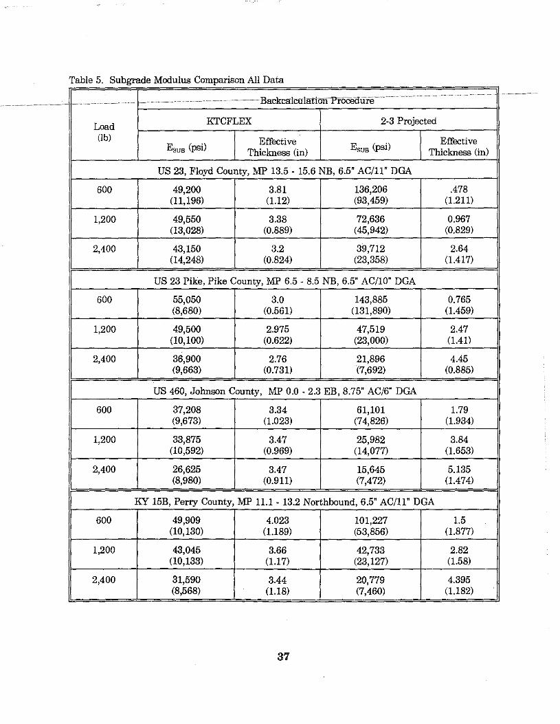
Table 5. Subgrade Modulus Comparison All Data

"

Load KTCFLEX 2-3 Projected

(!b) Effective Effective Esus (psi) Thickness (in) Esus (psi) Thickness (in)

US 23, Floyd County, MP 13.5 . 15.6 NB, 6.5" AC/11" DGA

600 49,200 3.81 136,206 .478 (11,196) (1.12) (93,459) (1.211)

1,200 49,550 3.38 72,636 0.967 (13,028) (0.889) (45,942) (0.829)

2,400 43,150 3.2 39,712 2.64 (14,248) (0.824) (23,358) (1.417)

US 23 Pike, Pike County, MP 6.5 · 8.5 NB, 6.5" AC/10" DGA

600 55,050 3.0 143,885 0.765 (8,680) (0.561) (131,890) (1.459)

1,200 49,500 2.975 47,519 2.47 (10,100) (0.622) (23,000) (1.41)

2,400 36,900 2.76 21,896 4.45 (9,663) (0.731) (7,692) (0.885)

US 460, Johnson County, MP 0.0 . 2.3 EB, 8.75" AC/6" DGA

600 37,208 3.34 61,101 1.79 (9,673) (1.023) (74,826) (1.934)

1,200 33,875 3.47 25,982 3.84 (10,592) (0.969) (14,077) (1.653)

2,400 26,625 3.47 15,645 5.135 (8,980) (0.911) (7,472) (1.474)

KY 15B, Perry County, MP 11.1 - 13.2 Northbound, 6.5" AC/11" DGA

600 49,909 4.023 101,227 1.5 (10,130) (1.189) (53,856) (1.877)

1,200 43,045 3.66 42,733 2.82 (10,133) (1.17) (23,127) (1.58)

2,400 31,590 3.44 20,779 4.395 (8,568) (1.18) (7,460) (1.182)

37

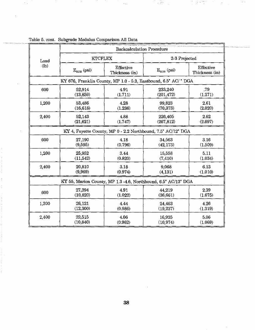
Table 5. cont. Subgrade Modulus Comparison All Data

Backcalculation Procedure

Load KTCFLEX 2-3 Projected

(lb) Effective Effective Esus (psi) Thickness (in) Esus (psi) Thickness (in)

KY 676, Franklin County, MP 1.0 - 5.3, Eastbound, 6.5" AC/' DGA

600 52,914 4.91 233,240 .79 (13,859) (1.711) (201,472) (1.271)

1,200 53,486 4.28 99,823 2.61 (16,618) (1.236) (70,373) (2.020)

2,400 52,143 4.88 226,405 2.62 (21,621) (1.747) (267,812) (2.697)

KY 4, Fayette County, MP 0- 2.2 Northbound, 7.5' AC/12' DGA

600 27,190 4.18 34,563 3.16 (9,595) (0.796) (42,173) (1.509)

1,200 25,952 3.44 15,558 5.11 (11,542) (0.820) (7,410) (1.034)

2,400 20,810 3.18 9,068 6.13 (9,969) (0.974) (4,131) (1.010)

KY 55, Marion County, MP 1.3 -4.6, Northbound, 6.5' AC/13' DGA

600 27,394 4.91 44,219 2.39

(10,820) (1.022) (36,661) (1.675)

1,200 26,121 4.44 24,463 4.26 (12,300) (0.986) (19,237) (1.319)

2,400 22,515 4.06 16,935 5.06 (10,840) (0.962) (10,974) (1.069)

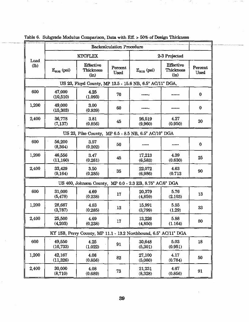
Table 6. Subgrade Modulus Comparison, Data with Eff. > 50% of Design Thickness

Backcalculation •

KTCFLEX 2-3 Projected Load (!b) Effective

Percent Effective Percent

Esua (psi) Thickness Used Esua (psi) Thickness

Used (in) (in)

US 23, Floyd County, MP 13.5. 15.6 NB, 6.5" AC/11" DGA,

600 47,000 4.25 70 0 (10,510) (1.093) ----· ..... _ ... _

1,200 49,000 3.00 60 0 (15,303) (0.939) ----- -----

2,400 36,778 3.81 45

26,519 4.27 30 (7,137) (0.856) (9,960) (0.950)

US 23, Pike County, MP 6.5 • 8.5 NB, 6.5" AC/10" DGA

600 56,200 3.57 50 0 (8,364) (0.202) ---- ___ .,

1,200 46,556 3.47 45

17,213 4.39 25 (11,160) (0.261) (6,583) (0.630)

2,400 33,429 3.50 35 22,072 4.63 90 (9,164) (0.285) (6,986) (0.713

US 460, Johnson County, MP 0.0 • 2.3 EB, 8.75" AC/6" DGA

600 31,000 4.69 17 20,379 5.76 13 (5,478) (0.238) (4,859) (2.103)

1,200 28,667 4.83 13 15,991 5.55

33 (3,787) (0.285) (3,799) (1.29)

2,400 25,500 4.69 17

13,226 5.88 80 (4,203) (0.238) (4,850) (1.164)

KY 15B, Perry County, MP 11.1- 13.2 Northbound, 6.5" AC/11" DGA

600 49,550 4.25 91 30,648 5.03 18 (10,733) (1.022) (5,301) (0.951)

1,200 42,167 4.08 82 27,100 4.17 50 (11,326) (0.856) (5,080) (0.784)

2,400 30,000 4.08 73 21,231 4.67

91 (8,710) (0.689) (8,328) (0.856)

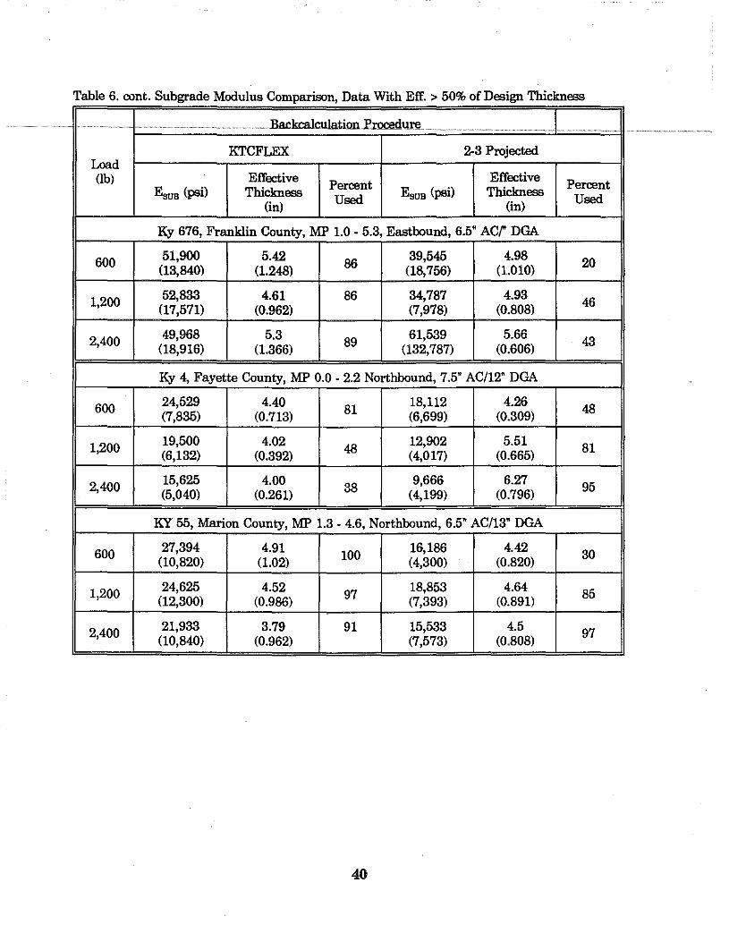
Table 6. cont. Subgrade Modulus Comparison, Data With Eff. > 50% of Design Thickness

~" """ """ "" Backcalculation""I'"l:!l!:edure"""""" '·~··~

KTCFLEX 2-3 I'rojected Load (!b) Effective I'ercent

Effective I'ercent Esus (psi) Thickness

Used Esus (psi) Thickness Used (in) (in)

Ky 676, Franklin County, MI' 1.0 • 5.3, Eastbound, 6.5" ACf DGA

600 51,900 5.42 86

39,545 4.98 20 (13,840) (1.248) (18,756) (1.010)

1,200 52,833 4.61 86 34,787 4.93 46 (17,571) (0.962) (7,978) (0.808)

2,400 49,968 5.3 89

61,539 5.66 43 (18,916) (1.366) (132,787) (0.606)

Ky 4, Fayette County, MI' 0.0. 2.2 Northbound, 7.5' AC/12" DGA

600 24,529 4.40 81

18,112 4.26 48 (7,835) (0.713) (6,699) (0.309)

1,200 19,500 4.02 48

12,902 5.51 81 (6,132) (0.392) (4,017) (0.665)

2,400 15,625 4.00 38

9,666 6.27 95 (5,040) (0.261) (4,199) (0.796)

KY 55, Marion County, MI' 1.3 • 4.6, Northbound, 6.5" AC/13" DGA

600 27,394 4.91 100

16,186 4.42 30 (10,820) (1.02) (4,300) (0.820)

1,200 24,625 4.52 97

18,853 4.64 85 (12,300) (0.986) (7,393) (0.891)

2,400 21,933 3.79 91 15,533 4.5 97 (10,840) (0.962) (7,573) (0.808)

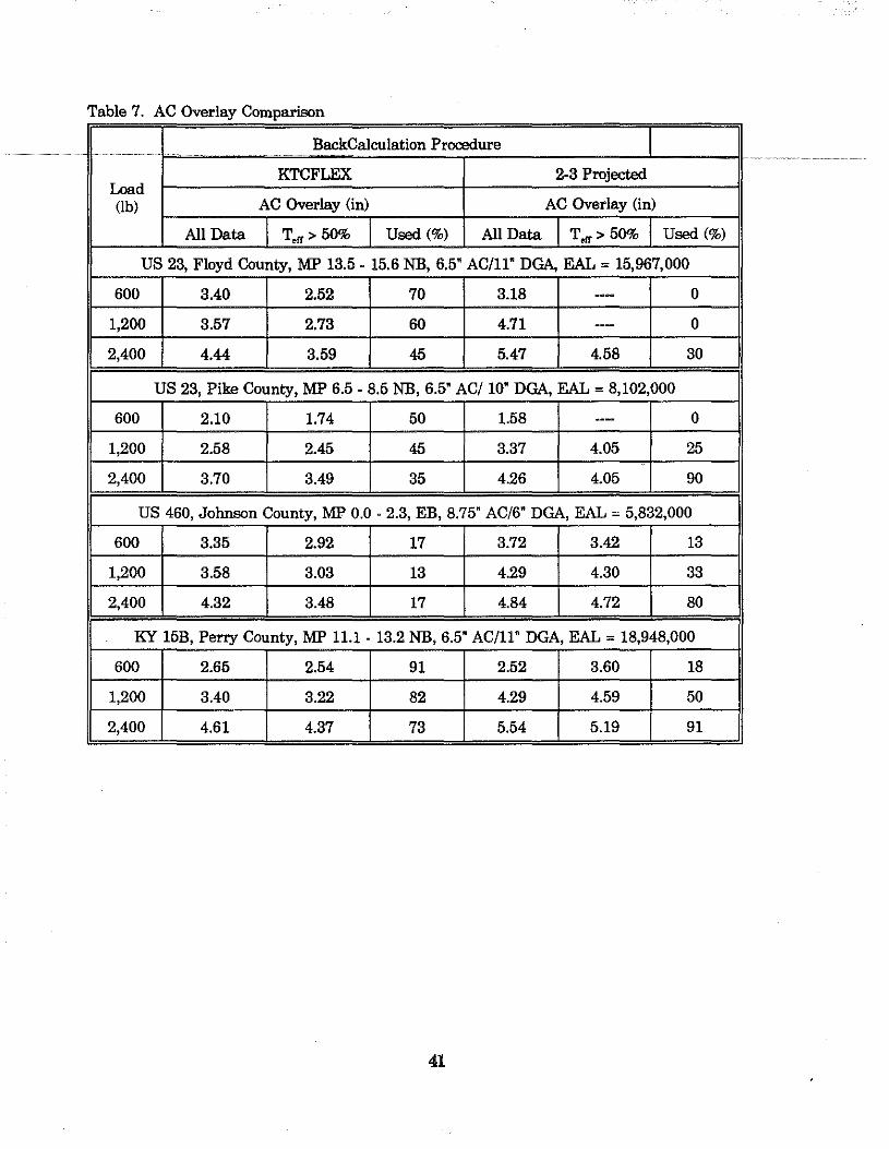
Table 7. AC Overlay Comparison

BackCaiculation Procedure

KTCFLEX 2-3 Projected Load (!b) AC Overlay (in) AC Overlay (in)

All Data T,rr >50% Used(%) All Data T,rr >50% Used(%)

US 23, Floyd County, MP 13.5- 15.6 NB, 6.5" AC/11" DGA, EAL = 15,967,000

600 3.40 2.52 70 3.18 ··- 0

1,200 3.57 2.73 60 4.71 --- 0

2,400 4.44 3.59 45 5.47 4.58 30

US 23, Pike County, MP 6.5- 8.5 NB, 6.5" AC/10" DGA, EAL = 8,102,000

600 2.10 1.74 50 1.58 --- 0

1,200 2.58 2.45 45 3.37 4.05 25

2,400 3.70 3.49 35 4.26 4.05 90

US 460, Johnson County, MP 0.0 - 2.3, EB, 8.75' AC/6' DGA, EAL = 5,832,000

600 3.35 2.92 17 3.72 3.42 13

1,200 3.58 3.03 13 4.29 4.30 33

2,400 4.32 3.48 17 4.84 4.72 80

KY 15B, Perry County, MP 11.1 - 13.2 NB, 6.5" AC/11" DGA, EAL = 18,948,000

600 2.65 2.54 91 2.52 3.60 18

1,200 3.40 3.22 82 4.29 4.59 50

2,400 4.61 4.37 73 5.54 5.19 91

41

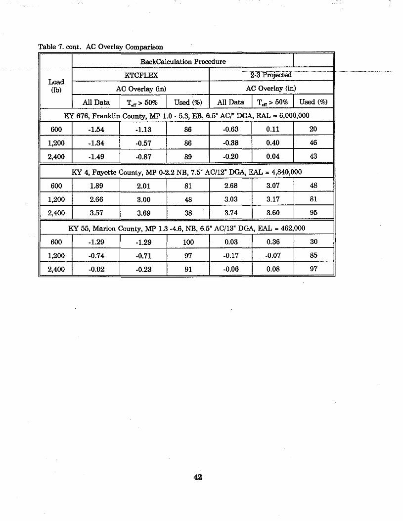
Table 7. cont. AC Overlay Comparison

BackCalculation Procedure

.t\T' ·.F.Y ··············· ········2:a:Pro)ectea. Load (!b) AC Overlay (in) AC Overlay (in)

All Data T,rr >50% Used(%) All Data T,rr >50% Used(%)

KY 676, Franklin County, MP 1.0 - 5.3, EB, 6.5' ACr DGA, EAL = 6,000,000

600 -1.54 -1.13 86 -0.63 0.11 20

1,200 -1.34 -0.57 86 -0.38 0.40 46

2,400 -1.49 -0.87 89 -0.20 0.04 43

KY 4, Fayette County, MP 0-2.2 NB, 7.5" AC/12' DGA, EAL = 4,840,000

600 1.89 2.01 81 2.68 3.07 48

1,200 2.66 3.00 48 3.03 3.17 81

2,400 3.57 3.69 38 3.74 3.60 95

KY 55, Marion County, MP 1.3 -4.6, NB, 6.5' AC/13" DGA, EAL = 462,000

600 -1.29 -1.29 100 0.03 0.36 30

1,200 -0.74 -0.71 97 -0.17 -0.07 85

2,400 -0.02 -0.23 91 -0.06 0.08 97

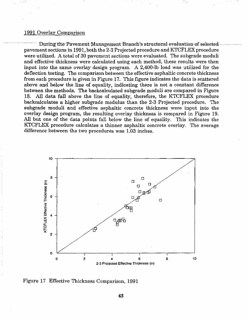
1991 Overlay Comparison

··········----~-- ~urin~th~ePavementManagementBranch'sstructuralevaluati<ln·efselect~d

pavement sections in 1991, both the 2-3 Projected procedure and KTCFLEX procedure were utilized. A total of 30 pavement sections were evaluated. The subgrade moduli and effective thickness were calculated using each method, these results were then input into the same everlay design program. A 2,400-lb load was utilized for the deflection testing. The comparison between the effective asphaltic concrete thickness from each procedure is given in Figure 17. This figure indicates the data is scattered above and belew the line of equality, indicating there is not a constant difference between the methods. The backcalculated subgrade moduli are cempared in Figure 18. All data fall abeve the line of equality, therefore, the KTCFLEX procedure backcalculates a higher subgrade modulus than the 2-3 Projected procedure. The subgrade moduli and effective asphaltic concrete thickness were input into the overlay design program, the resulting overlay thickness is compared in Figure 19. All but one of the data points fall below the line of equality. This indicates the KTCFLEX procedure calculates a thinner asphaltic concrete overlay. The average difference between the two procedures was 1.03 inches.

10 ,-----------------------------------------------~

8 D § D

D D Ill Ill Q) D c: "' 0 6 D :c f- D Q)

.2: [][] 13

~ D

4 ~ off CO --' LL u ~

2

0

0 2 4 6 8 10 2-3 Projec1ed Effec1ive Thickness (in)

Figure 17 Effective Thickness Comparison, 1991

43

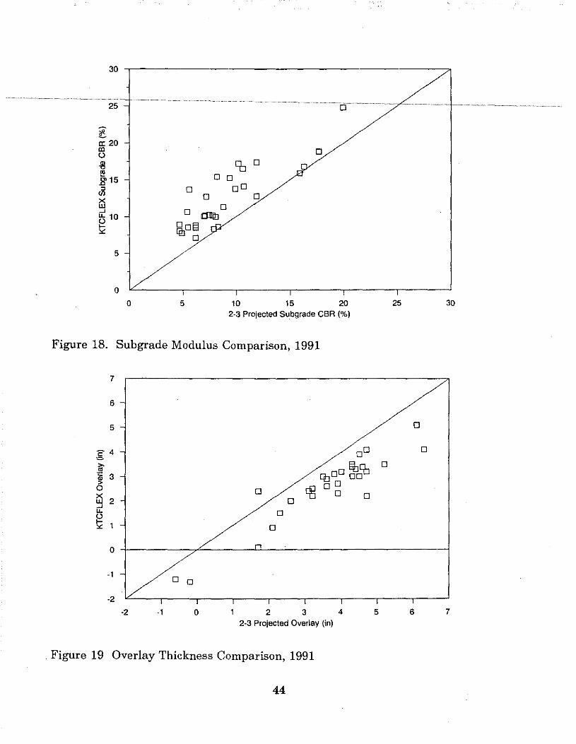
30

25

;fl.

a: 20 m 0 u Q) en 0 ., !!! 0 0 J'l'15

oD :::1 0 (/l 0 0 X w 0

--' 0 llliiD LL 10

~ DoEJ 10 0

5

0

0 5 10 15 20 25 30 2-3 Projected Subgrade CBR (%)

Figure 18. Subgrade Modulus Comparison, 1991

7

6

5 0

24 oo 0 =

l:f:loo ~om 0 ~

~ 3 > cg 0 0 0 0 0 0 ~ 2 0 --' LL 0 u t;:: 1 0

-1 0 0

·2

·2 -1 0 2 3 4 5 6 7 2·3 Projected Overlay (in)

. Figure 19 Overlay Thickness Comparison, 1991

44

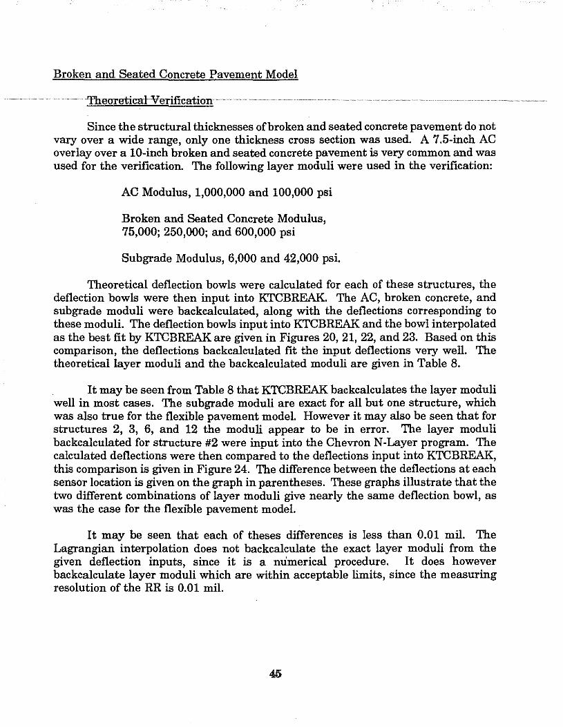
Broken and Seated Concrete Pavement Model

···················· ········ ·1fhmrreticalVerifieation ········· · ·· · · ··· ··· · · ···

Since the structural thicknesses ofbroken and seated concrete pavement do not vary over a wide range, only one thickness cross section was used. A 7.5-inch AC overlay over a 10-inch broken and seated concrete pavement is very common and was used for the verification. 'Th.e following layer moduli were used in the verification:

AC Modulus, 1,000,000 and 100,000 psi

Broken and Seated Concrete Modulus, 75,000; 250,000; and 600,000 psi

Subgrade Modulus, 6,000 and 42,000 psi.

Theoretical deflection bowls were calculated for each of these structures, the deflection bowls were then input into KTCBREAK. 'Th.e AC, broken concrete, and subgrade moduli were backcalculated, along with the deflections corresponding to these moduli. 'Th.e deflection bowls input into KTCBREAK and the bowl interpolated as the best fit by KTCBREAK are given in Figures 20, 21, 22, and 23. Based on this comparison, the deflections backcalculated fit the input deflections very well. 'Th.e theoretical layer moduli and the backcalculated moduli are given in Table 8.

It may be seen from Table 8 that KTCBREAK backcalculates the layer moduli well in most cases. 'Th.e subgrade moduli are exact for all but one structure, which was also true for the flexible pavement model. However it may also be seen that for structures 2, 3, 6, and 12 the moduli appear to be in error. 'Th.e layer moduli backcalculated for structure #2 were input into the Chevron N-Layer program. 'Th.e calculated deflections were then compared to the deflections input into KTCBREAK, this comparison is given in Figure 24. 'Th.e difference between the deflections at each sensor location is given on the graph in parentheses. These graphs illustrate that the two different combinations of layer moduli give nearly the same deflection bowl, as was the case for the flexible pavement model.

It may be seen that each of theses differences is less than 0.01 mil. 'Th.e Lagrangian interpolation does not backcalculate the exact layer moduli from the given deflection inputs, since it is a numerical procedure. It does however backcalculate layer moduli which are within acceptable limits, since the measuring resolution of the RR is 0.01 mil.

Table 8 Broken and Seated Concrete Model Verification

........... AC-Modulus.(psiL Broken Concrete Modulus Subgrade Modulus (psi) . .......... ··········· .......... ·(psi+ Number ·~·· .. .

Theoretical KTCBREAK Theoretical KTCBREAK Theoretical KTCBREAK

1 1,000,000 870,000 75,000 80,000 6,000 6,000

2 1,000,000 480,000 250,000 400,000 6,000 6,000

3 1,000,000 760,000 600,000 740,000 6,000 6,000

4 100,000 120,000 75,000 70,000 6,000 6,000

5 100,000 120,000 250,000 210,000 6,000 6,000

6 100,000 140,000 600,000 400,000 6,000 6,000

7 1,000,000 930,000 75,000 80,000 42,000 42,000

8 1,000,000 920,000 250,000 260,000 42,000 42,000

9 1,000,000 990,000 600,000 620,000 42,000 42,000

10 100,000 100,000 75,000 80,000 42,000 42,000

11 100,000 110,000 250,000 270,000 42,000 41,000

12 100,000 140,000 600,000 450,000 42,000 42,000

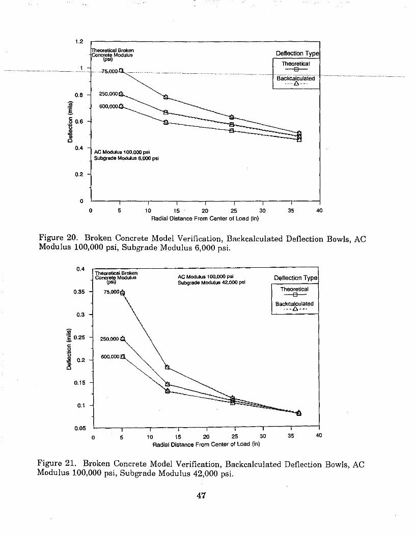
1.2

eoretical Broken Concrete Modulus

(psi) Deflection Type

Theore11cal

···············································~·~·····~·············~·~·~···~· ' =l~ .... ].s .• ooo."""-:::_:~························································~ ........................................................................ -1 6a.Ckci0~iaie•a !~·········~·······································································~ .. .

0.8 250,000

~ §. c ·~ 0.6

~ 0.4

0.2

a a

AC Modulus 100,000 psi Subgrade Modulus 6,000 psi

5 10 15 20 25 Radial Distance From Center of Load (in)

30 35 40

Figure 20. Broken Concrete Model Verification, Backcalculated Deflection Bowls, AC Modulus 100,000 psi, Subgrade Modulus 6,000 psi.

0.4

0.35

0.3

~ 0.25 c: 0 . ., " "' 0.2 ~ c

0.15

0.1

0.05

0

Theoretical Broken Concrete Modulus

(psi)

75,000

250,000

600,000

5

AC Modulus 100,000 psi Subgrade Modulus 42,000 psi

10 15 20 25 30 Radial Distance From Center of Load (in)

Deflection Type

Theoretical 0

Backcalculated ... ~:;, ...

35 40

Figure 21. Broken Concrete Model Verification, Backcalculated Deflection Bowls, AC Modulus 100,000 psi, Subgrade Modulus 42,000 psi.

47

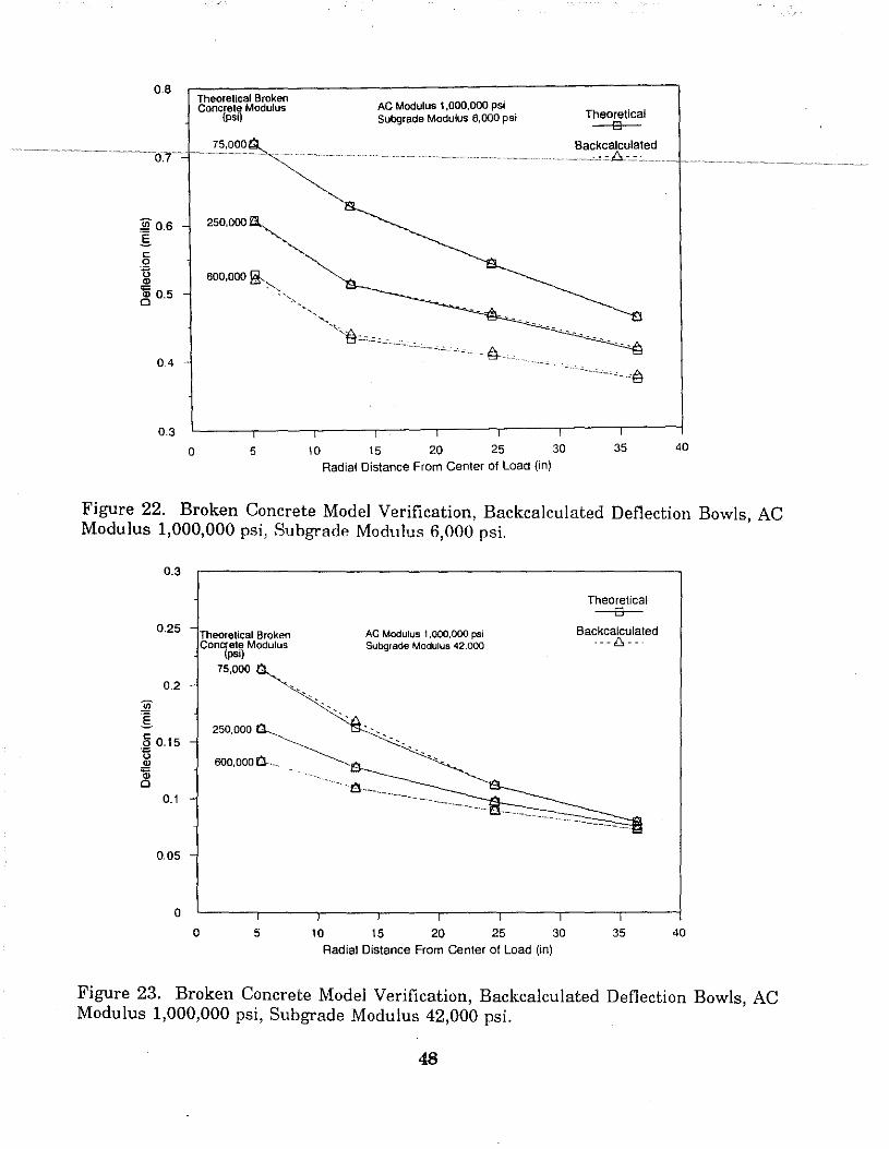
0.8 Theoretical Broken Concrete Modulus

(psi)

75,000

,lg 0.6 250,000 .§. c: 0

~ ~ 0.5

0.4

0.3

0 5

AC Modulus 1 ,000,000 psi Subgrade Modulus 6,000 psi

10 15 20 25 30 Radial Distance From Center of Load (in)

Theoretical 0

35 40

Figure 22. Broken Concrete Model Verification, Backcalculated Deflection Bowls, AC Modulus 1,000,000 psi, Subgrade Modulus 6,000 psi.

:Ef I

0.3

0.25

0.2

5 0.15 ·~

~ 0.1

0.05

0

0

Theoretical Broken Cone~· ate Modulus

(psi)

75,000

250,000 a..__ ---...

600,0000 ... _ ~

AC Modulus 1,000,000 psi Subgrade Modulus 42.000

- . ·-. ·-

5 10 15 20 25 30 Radial Distance From Center of Load (in)

Theoretical 0

Backcalculated ·--!:>--

35 40

Figure 23. Broken Concrete Model Verification, Backcalculated Deflection Bowls, AC Modulus 1,000,000 psi, Subgrade Modulus 42,000 psi.

48

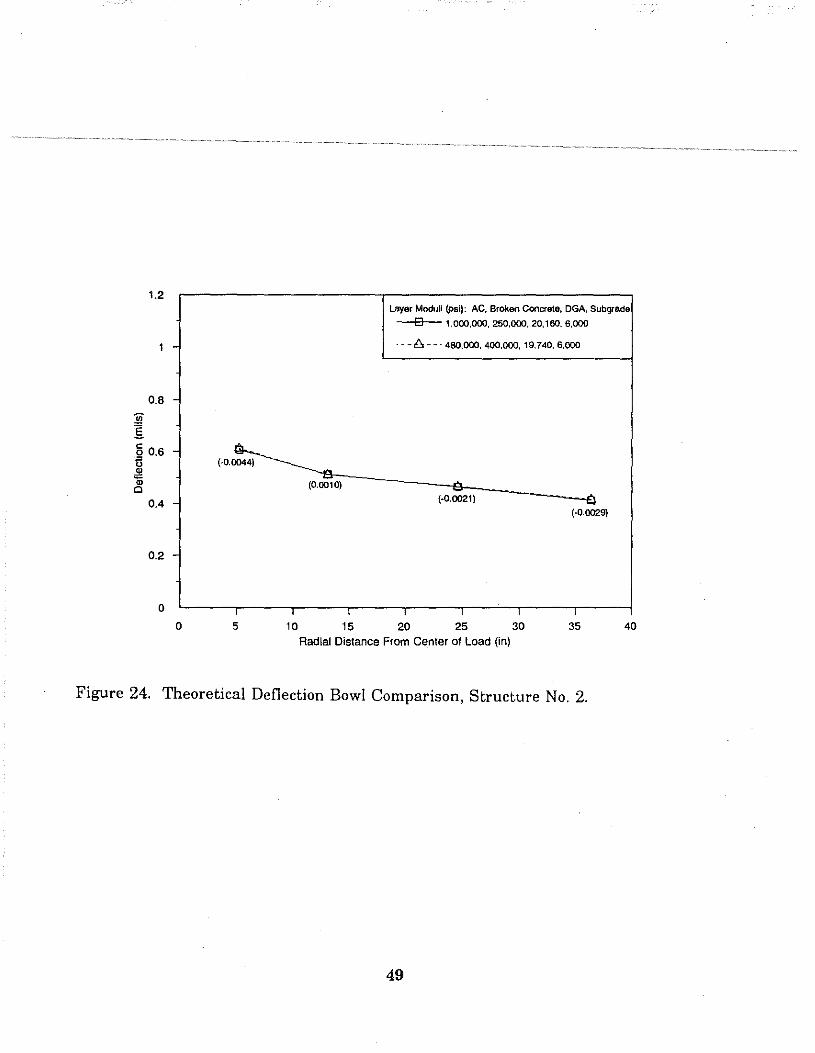
11 I

1.2

0.8 -

§ 0.6 -0

~ 0

0.4 -

0.2 -

0

0

(·0.0044)

I

5

Layer Moduli (psi): AC, Broken Concrete, DGA, Subgrade

0 1,000,000, 250,000,20,160,6,000

. --8.--. 480,000, 400,000, 19,740, 6,000

(0.0010)

(-0.0021)

I I I I I

10 15 20 25 30 Radial Dis1ance From Cen1er of Load (in)

... ~

(·0.0029)

I

35 40

Figure 24. Theoretical Deflection Bowl Comparison, Structure No. 2.

49

Field Case Studies

· ······ ··········· Four·seGtions.have.been.chosen.as.GBSestudies..fur. .. testing.the.br.oken.and.seated. concrete model. Two of the these sections were contained in a previous study on broken and seated concrete pavements (Research Report UKTRP-87-26 (24), "Breaking and Seating of Rigid Pavements"). These sites are I-64, Mile Point 30.8 - 31.8 EB, Shelby county and I-71 Mile Point 60 - 69.4 SB, Gallatin County. The other two sites are currently included in the Transportation Cabinet's Long Term Pavement Performance study. These sites are the Mountain Parkway, MP 30.8 WB, Powell County and Pennyrille Parkway, MP 65 NB, Webster County.

The structural thickness and the average pavement deflections of each section were input into KTCBREAK. The layer moduli results of the program are listed in Table 9, the backcalculated deflections are given in parentheses. It may be seen from this table that the backcalculated deflections match the field deflections very well, the deflection bowl for each section is given in Figures 25, 26, 27, and 28.

The broken concrete modulus does vary over a wide range, from 20,000 to 360,000 psi. This large variation could be due to several reasons, size of broken particles, condition of the concrete before breaking, degree of seating, etc. The actual determination of the best value to be used for design purposes is beyond the scope of this study. These case studies have shown that the model can determine layer moduli which may represent the structure in-situ.

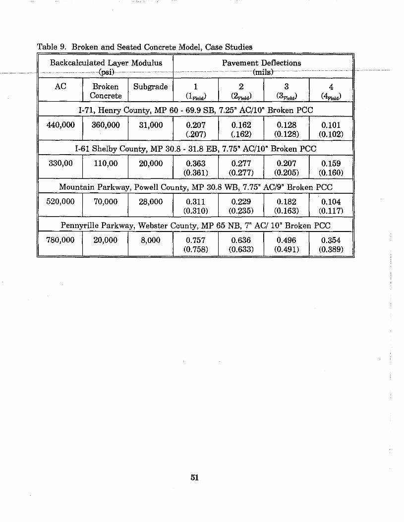
Table 9. Broken and Seated Concrete Model, Case Studies

Backcalculated Layer Modulus Pavement Deflections (, ·"

AC Broken Subgrade 1 2 3 4 Concrete (!Field) (~eld) (3Field) (~eld)

I-71, Henry County, MP 60- 69.9 SB, 7.25" AC/10" Broken PCC

440,000 360,000 31,000 0.207 0.162 0.128 0.101 (.207) (.162) (0.128) (0.102)

I-61 Shelby County, MP 30.8- 31.8 EB, 7.75" AC/10" Broken PCC

330,00 110,00 20,000 0.363 0.277 0.207 0.159 (0.361) (0.277) (0.205) (0.160)

Mountain Parkway, Powell County, MP 30.8 WB,_ 7.75" AC/9" Broken PCC

520,000 70,000 28,000 0.311 0.229 0.182 0.104 (0.310) (0.235) (0.163) (0.117)

Pennyrille Parkway, Webster County, MP 65 NB, 7" AC/ 10" Broken PCC

780,000 20,000 8,000 0.757 0.636 0.496 0.354 (0. 758) (0.633) (0.491) (0.389)

51

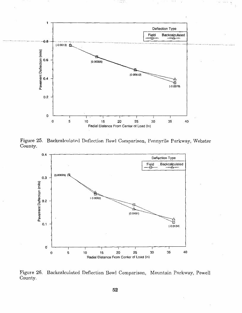
Deflection Type

Field Backcalculated

................................................... o,a ... 1,:~ .. ;;;;;, ;;;··-....................................................................................................................................................... h==:=:§o~===='"'~=~-........................................................................................................ . l 1-0.0013)

!if I 5 0.6 u ~ 0 c: ~ 0..4

~ 0.

0.2

0

0 5

,-0.0379)

10 15 20 25 30 35 40 Radial Distance From Center of Load (in)

Figure 25. Backca]culat.Pd DRf1ection Dow] Comparison, Pcnnyrile Parkway, Webster County.

0.4 ~------------------------,

!if I c: 0 g

0.3

iii 0.2 0 c: Q)

E

~ 0.

0.1

0

(0.00095)

0 5 10

Deflection Type

Field Backcalculated

(-0.0062)

(-0.0134)

15 20 25 30 35 40

Radial Distance From Center of Load (in)

Figure 26. Backcalculated Deflection Bowl Comparison, Mountain Parkway, Powell County.

52

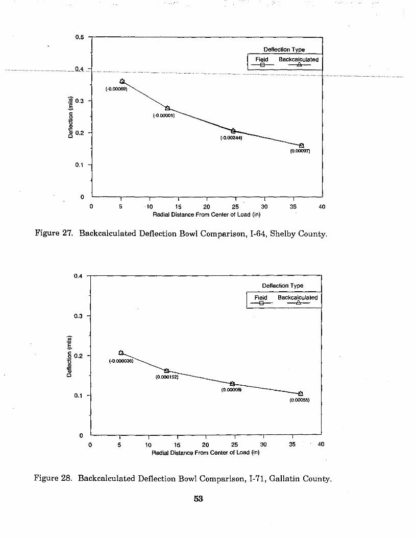
0.5

Deflection Type

Field Backcalculated

J .......................................................................................................................................................... l=:~o~======~===i ..................................................•.............................. . ··································· ..... M!

~0.3 .s

! ~ 0.2

0.1

0

(·0.00069)

0 5 ·10 15 20 25 30 35 40 Radial Distance From Center of Load (in)

Figure 27. Backcalculated Deflection Bowl Comparison, I-64, Shelby County.

0.4

0.3 -

0.1

0

0

(·0.000036)

I

5

Deflection Type

r Field Backcalculated 0 8

(0.000152)

(0.00008)

I I > I ·1

10 15 20 25 30 Radial Distance From Center of Load (in)

-e (0.00055)

I

35 40

Figure 28. Backcalculated Deflection Bowl Comparison, I-71, Gallatin County.

Composite Pavement Model

. ............................ TheoreticaL.:\I"erification .................................. ...... . .......... .. ··~ ~~ ~~ ~·~··············~

The same structural cross section used in the broken concrete model verification of 7.5-inch AC overlay over 10 inches of concrete on 4 inches of DGA is also utilized for the composite pavement model. The following layer moduli were used for the verification:

AC Modulus, 1,000,000 and 100,000 psi Concrete Modulus, 2,500,000 and 4,200,000 psi Subgrade Modulus, 6,000 and 42,000 psi.

Theoretical deflections were calculated for all combinations of the layer moduli listed previously. The theoretical deflections were input into KTCCOMP and the AC, concrete, and subgrade moduli were backcalculated. The deflections corresponding to the backcalculated layer moduli are compared to the deflections input KTCCOMP in Figures 29 and 30. It may be seen from these figures that the model calculates deflections which match the theoretical deflections very well. The backcalculated layer moduli and the theoretical layer moduli are given in Table 10.

It may be seen from this table that the composite model (KTCCOMP) backcalculates the subgrade modulus very well, as was the case with the KTCFLEX and KTCBREAK. However, as was the case with the other models, some backcalculated moduli appear to be in error. Structures 1, 2, and 8 seem to have the largest discrepancies. The backcalculated layer moduli were input into the linear elastic program and the corresponding deflections were calculated. The backcalculated moduli for structure #1 were again input into the Chevron program. The calculated deflections were compared to the deflections input into KTCCOMP, this comparison is given in Figure 31. The differences between the deflections input into KTCCOMP and the deflections corresponding to the backcalculated structure are given in parentheses on the graph. It may be seen that the differences are again less than the measurement resolution of the Road Rater.

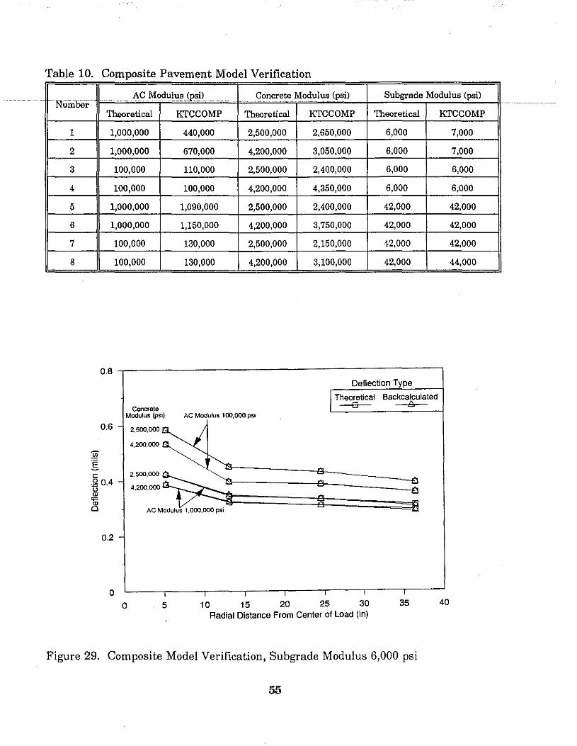
Table 10. Composite Pavement Model Verification

AC Modulus (psi) Concrete Modulus (psi) Subgrade Modulus (psi) .. ~ ... ~· Theoretical KTCCOMP Theoretical KTCCOMP Theoretical KTCCOMP

1 1,000,000 440,000 2,500,000 2,650,000 6,000 7,000

2 1,000,000 670,000 4,200,000 3,050,000 6,000 7,000

3 100,000 110,000 2,500,000 2,400,000 6,000 6,000

4 100,000 100,000 4,200,000 4,350,000 6,000 6,000

5 1,000,000 1,090,000 2,500,000 2,400,000 42,000 42,000

6 1,000,000 1,150,000 4,200,000 3,750,000 42,000 42,000

7 100,000 130,000 2,500,000 2,150,000 42,000 42,000

8 100,000 130,000 4,200,000 3,100,000 42,000 44,000

0.8 -,.-------------------------,

0.6

0.2

0

Concrete Modulus (psi)

2,500,000

4,200,000

2,500,000

4,200,000

AC Modulus 100,000 psi

Deflection Type

Theoretical Backcalculated 0

AC Modulus 1,000,000~p=si~=======~~======~~

0 5 10 15 20 25 30 35 Radial Distance From Center of Load (In)

Figure 29. Composite Model Verification, Subgrade Modulus 6,000 psi

55

40

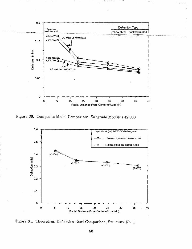
0.2 ..,----------------------,

Deflection Type

0.15 4,200,000

2,500,000 ~~i~~~~~~;~~;;;;;;;;~~~ 4,200,000

AC Modulus 1,000,000 psi

0.05

0

0 5 10 15 20 25 30 35 Radial Distance From Center of Load (in)

Figure 30. Composite Model Comparison, Subgrade Modulus 42,000

0.6

0.5

0.4 (-0.0085)

"' 'E § 0.3 -13

~ 0

0.2 -

0.1 -

0

0 I

5 I

10

(0.0027)

I

15

Layer Moduli (psi) AC/PCC/DGNSubgrade

I

20

0 1,000,000, 2,500.000, 18,600.6,000

A 440,000, 2.sso.ooo. 2o.sao. 1.000

(·0.0003)

' 25

I

30

(0~5)

I

35 Radial Distance From Center of Load (in)

Figure 31. Theoretical Deflection Bowl Comparison, Structure No. 1

40

40

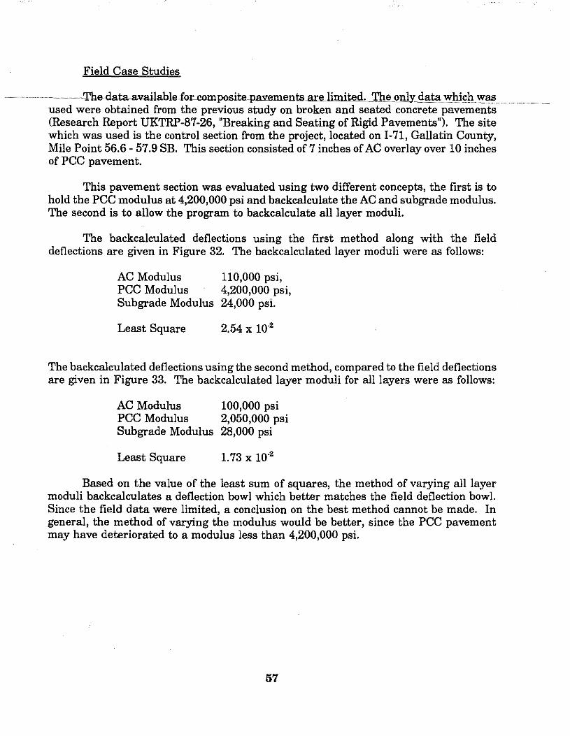
Field Case Studies

········· ············~--~----'I'hedata..a¥ailablefor.composite..pav:ementsar.e.Jimited....'I'he _only data which was used were obtained from the previous study on broken and seated concrete pa¥ements···~~~­(Research Report UKTRP-87-26, "Breaking and Seating of Rigid Pa¥ements"). 'I'he site which was used is the control section from the project, located on 1-71, Gallatin County, Mile Point 56.6- 57.9 SB. This section consisted of 7 inches of AC o¥erlay ov:er 10 inches of PCC pa¥ement.

This pa¥ement section was e¥aluated using two different concepts, the first is to hold the PCC modulus at 4,200,000 psi and backcalculate the AC and subgrade modulus. 'I'he second is to allow the program to backcalculate all layer moduli.

The backcalculated deflections using the first method along with the field deflections are gi¥en in Figure 32. The backcalculated layer moduli were as follows:

AC Modulus PCC Modulus Subgrade Modulus

Least Square

110,000 psi, 4,200,000 psi, 24,000 psi.

2.54 X 10"2

The backcalculated deflections using the second method, compared to the field deflections are gi¥en in Figure 33. The backcalculated layer moduli for all layers were as follows:

AC Modulus PCC Modulus Subgrade Modulus

Least Square

100,000 psi 2,050,000 psi 28,000 psi

1.73 X 10"2

Based on the ¥alue of the least sum of squares, the method of v:arying all layer moduli backcalculates a deflection bowl which better matches the field deflection bowl. Since the field data were limited, a conclusion on the best method cannot be made. In general, the method of v:arying the modulus would be better, since the PCC pa¥ement may ha¥e deteriorated to a modulus less than 4,200,000 psi.

57

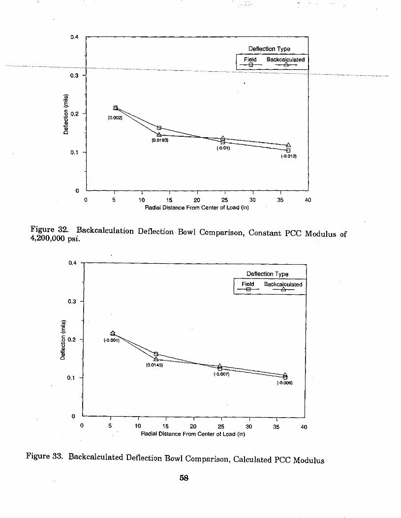
0.4

Deflection Type

Field Backcalculated D 8

0.3

0.1 1·0.013)

(·0.01)

0

0 5 10 15 20 25 30 35 40 Radial Distance From Center of Load (in)

Figure 32. Backcalculation Deflection· Bowl Comparison, Constant PCC Modulus of 4,200,000 psi.

0.4 ..,----------------------,

;w .s

0.3

c: ·~ 0.2

iii 0

0.1

0

0 5 10

Deflection Type

Field Backcalculated 0

1·0.007)

1·0.006)

15 20 25 30 35 40 Radial Distance From Center of Load (In)

Figure 33. Backcalculated Deflection Bowl Comparison, Calculated PCC Modulus

58

SUMMARY AND CONCLUSIONS

................... ··~~Thr.e..e..pavement.models~were.developedjnthis~~?t.Ydy~E!.!!!<h.rllPrlll?ll!Itjng!!,~differgnt type of pavement strucrure. These models represent the majority of the pavement strucrures in place throughout the state. These models were based on linear elastic theory applied to modeling Road Rater dynamic loadings. It has been demonstrated that each model may be used to backcalculate pavement deflections and corresponding layer moduli, which represent the pavement strucrure in the field.

Each model is contained in a separate interactive computer program, which provides input by the user for single data points or reads multiple data sets from computer text files. It has been noted that this procedure is not perfect. These models are based on numerical procedures, both the Lagrangian interpolation and the linear elastic calculations of the database deflections. Deflections interpolated by the programs may not match theoretically calculated deflections perfectly. One of reason for these discrepancies is that one database is used across a large range of layer moduli and strucrural thicknesses. For example, in the interpolation of AC thickness, only 6 points are used to interpolate the database form 2 to 20 inches. If the ranges of interpolation were decreased, and the same number of data points were used, then the accuracy of the backcalculations should increase.

The comparison of the two methods for calculating the effective thickness and corresponding AC overlay has been evaluated. The results using the new procedure are more consistent, as may be noted by the smaller standard deviation of the backcalculated data. More useful data will therefore be obtained which will increase the precision of analysis. The AC overlay calculated from the results of the new procedure is on the average less than the overlay calculated using the 2-3 projected procedure. If all data are used, the decrease in overlay is 0.64 inch. If only data having effective thicknesses greater than 50 percent of the design thickness are used, the decrease is 0.91 inch.

The concept which has been presented could be expanded to include other pavement types and other testing devices. The procedure could be used with any type of deflection calculation program, finite element, nonlinear, etc.

The analysis of broken and seated concrete pavements produced a wide range of values for the broken concrete modulus. The causes of this variability cannot be determined from this limited srudy of broken and seated concrete. Possible causes of this variability could be, broken particle size, subgrade conditions, condition of the concrete prior to breaking, etc.

In the theoretical analysis of the KTCBREAK model, there were several occurrences of non-unique solutions for layer moduli based on the input deflections. It was noted that the differences between the individual deflections were less than the measurement resolution of the Road Rater. More non-unique solutions would be expected in the broken concrete model due to the presence of two relatively stiff layers in the pavement system. In each case, only two solutions were presented; in reality, there may

59

be many more solutions of layer moduli which would produce the same deflection basin.

The flexible pavement model (KTCFLEX)appearstobackcaiC:Uiafe1owasphaltfc concrete moduli. These moduli are calculated using the raw pavement deflections, no corrections were made for temperature. Deflections obtained at higher pavement temperatures would give asphaltic concrete layer moduli lower than moduli obtained at reference conditions. The subgrade modulus appears to be larger than would be expected. This may be attributed to the presence of bedrock very close to the pavement surface or the presence of a crushed rock subgrade. The ability of these procedures to predict the accuracy of the layer moduli to laboratory values is being conducted in another research study, KYHPR-86-115 "Laboratory and Field Evaluations and Correlations of Properties of Pavement Components."

These procedures have several limitations, each program is developed for a specific pavement structure for a fixed number of layers and fixed modular ranges. These programs could be expanded or incorporated into one program which would allow for solutions for multiple layers of varying moduli.

RECOMMENDATIONS

The Kentucky Transportation Center currently has a Falling Weight Deflectometer and the Transportation Cabinet has expressed interest in obtaining one for routine testing. An analysis procedure should be developed to effectively utilize this equipment. The procedure which has been conducted during this research study should be expanded to incorporate deflection measurements obtained using the FWD.

The development of this procedure which backcalculates the individual layer moduli, provides valuable information which may be used in overlay design. Since layer moduli are obtained for each layer for the different pavement types, this provides the information needed to design structural overlays based on a mechanistic procedure. It is recommended that future research be initiated to develop this mechanistic overlay design procedure. Once this procedure has been developed, it could be utilized on any type of pavement for which the layer moduli are known. This procedure would provide more flexibility than the current procedure which is used for flexible pavements.

The current overlay design procedure is only applicable to asphaltic concrete overlays over asphaltic concrete pavements and is based on the design procedure for asphaltic concrete pavements. It is not suitable for determining overlay thicknesses for rehabilitation of pavements containing broken and seated concrete. At the present time, there is no documented method for determining the overlay thickness for composite pavements, asphaltic concrete over broken and seated concrete or asphaltic concrete over portland cement concrete.

00

The procedures developed during this study provide a means of determining pavement layer moduli. These layer moduli may be used by Cabinet personnel to

· ······· 1iet~rmine;>verlay4hielmesses·for-var.jou~types.(}f..pavemmlts . ...Th.ese.overlays ... wi!Lmost ....................... . probably utilize the concept of limiting strain for thickness design. As these procedures are developed, further research may be proposed to optimize these design methods.

It is also recommended that a 2,400-lb dynamic load be utilized during deflection testing using the Road Rater. The.use of this load will provide deflections which will be more near the mid range of the testing equipment. In addition, this load will more closely simulate the actual field loading conditions.

61

REFERENCES

. . ... ·~~ -l~~..AllenTD.L.,~"Re¥ie:wandAnal.ysis~f.Ea=ent.Mlmagement.I'r..a.cti.ceainKeiJ.tl.lcky:;' ~~ ~~ Research Report KTC-90-4, Kentucky Transportation Center, University of Kentucky, Lexington, Kentucky, 1990.

2. Michelo:w, J., "Analyses of Stress end Displacements in N-Layered Elastic System under a Load Uniformly distributed on a Circular Ares," Chevron Oil Research, Richmond, California, September 1963.

3. Sharpe, G.W., Southgate, H.F., and Deen, R.C., "Pavement Evaluation by Using Dy:namic Deflections," Transportation Research Record 700, Washington, DC, 1979.

4. Deen, R.C., Southgate, H.F., and Sharpe, G.W., "Structural Evaluation of Asphaltic Pavements," Research Report UKTRP-84-9, Kentucky Transportation Research Program, University of Kentucky, Lexington, Kentucky, 1984.

5. Thompson, M. and Hoffman, M, "Backcalculating Nonlinear Resilient Moduli from Deflection Data," Transportation Research Record 852, Washington D.C., 1982.

6. Hossain, A.S.M.M., and Zaniewski, J.P., "Characterization of Falling Weight Deflectometer Deflection Basin", Transportation Research Record 852, Washington, D.C., 1982.

7. Lytton, R.L., "Backcalculation of Pavement Layer Properties," Nondestructive Testing of Pavements and Backcalculation of Moduli, ASTM STP 1026, American Society of Testing and Materials, Philadelphia, 1989.

8. Zhou, H, Hicks, R.G., and Bell, C.A., "Bousdef: A Backcalculation Program for Determining Moduli of a Pavement Structure", Transportation Research Record 1060, Washington, D.C., 1990

9. Mahoney, J.P., Coetzee, N.F., Substad, R.N., and Lee, W.L., "A Performance Comparison of Selected Backcalculation Computer Programs," Nondestructive Testing of Pavements and Backcalculation of Moduli, ASTM STP 1026, American Society of Testing and Materials, Philadelphia, 1989.

10. Chou, Y.J. and Lytton, R.L., "Accuracy and Copsistency ofBackcalculated Pavement Layer Moduli," Transportation Research Record 1293, Washington, D.C. 1991.

11. Scullion, T., Uzan, J, and Paredes, M., "MODULUS: A Microcomputer Based Backcalculation System," Research Report 1123-11, Texas Transportation Institute, 1988.

12. Sebaaly, B. E., Mamulouk, M, and Davies, T.G., "Dy:namic Analysis of Falling Weight Deflectometer Data," Transportation Research Record 1070, Washington, D.C. 1986.

13. Ony, L.C., Newcomb, D.E., and Siddharthan, R., "Comparison of Dynamic and Static Backcalculation of Moduli for Three-Layered Pavements, • Transportation Research

...•...•...•... n Recordl293,Washington,l1.C...,.1991L.. mm n n m •• m ••• ····~·~··~·····~ m ~ ~~

14. Magnuson, A.H., Lytton, R.K., and Briggs, R.C., "Comparison of Computer Predictions and Field Data for Dynamic Analysis of Falling Weight Deflectometer Data," Transportation Research Record 1293, Washington, D.C., 1991.

15. Meade, B.W., and Allen, D.L. "Pavement Deflection Test Database, • Research Report KTC-90-14, Kentucky Transportation Center, University of Kentucky, Lexington, Kentucky, 1990.

16. Southgate, H.F., Sharpe, G.W., Deen, R.C., and Havens, H.H., "Structural Capacity of In-Place Asphaltic Concrete Pavements from Dynamic Deflections," Kentucky Transportation Research Program, University of Kentucky, Lexington, Kentucky, August 1981.

17. Southgate, H.F., Deen, R.C., and Havens, J.H., "Development of a Thickness Design System For Bituminous Concrete Pavements," Research Report UKTRP-81-20, Kentucky Transportation Research Program, University of Kentucky, Lexington, Kentucky, 1981.

18. Kallas, B.F., Riley, J.C., "Mechanical Properties of Asphalt Pavement Materials," Proceedings, Second International Conference on the Structural Design of Asphalt Pavements, University of Michigan, Ann Arbor, Michigan, 1967.

19. Southgate, H.F., "An Evaluation of Temperature Distribution Within Asphalt Pavements and Its Relationship to Pavement Deflection, • Research Report, Division of Research, Department of Highways, Commonwealth of Kentucky, 1968

20. Sharpe, G.W., Southgate, H.F.,and Deen, R.C., "Pavement Evaluations using Road Rater Deflections," Research Report 501, Division of Research, Bureau of Highways Department of Transportation, Commonwealth of Kentucky, 1978.

21. Atkinson, K., Elementary Numerical Analysis, John Wiley and Sons, New York, New York, 1985.

22. Microsoft QuickBASIC Computer Program, Microsoft Corporation. 1988.

23. Allen, D.L, Deen, R.C., "A Computerized Analysis of Flexible Pavement Rutting Behavior (PAVRUT)," Research Report UKTRP-85-31, Kentucky Transportation Research Program, University of Kentucky, Lexington, Kentucky, 1985.

24. Sharpe, G.W., Anderson, M., and Deen, R.C., "Breaking and Seating of Rigid Pavements," Research Report UKTRP-87-26, Kentucky Transportation Research Program, University of Kentucky, Lexington, Kentucky, 1987.

APPENDIX A

64

USERS MANUAL KTCFLEX, KTCBREAK, AND KTCCOMP

INTRODUCTION

Three interactive computer programs were developed during this study. These programs are personal computer based and were developed using Microsoft QuickBasic Version 4.5. Input deflections and parameters may be provided to the program by a disk file or by interactive screen inputs. The minimum hardware requirements are as follows:

IBM AT or compatible microcomputer 640 Kb of Ram DOS (Ver. 3.0 or later) operating system Math coprocessor Chip Hard Disk (recommended)

Due to the complex iterative procedures involved in the calculations it is recommended that as a minimum a 80-286 based computer be used. An 80-386 based computer is preferred.

DATA INPUT

Pavement deflections and structural information must be input into the program, by either reading them in from a computer disk file or by providing them manually from the computer keyboard. Temperature information is needed by KTCFLEX if temperature adjustments are to be made and effective asphaltic concrete thickness is determined.

All deflections must be input in mils (inches x lO.a) with dynamic load input in kips. Temperature measurements are to be entered in degrees Fahrenheit along with time in military decimal format.

The input to each program is the same with the following exceptions.

1. No temperature information is input into KTCBREAK and KTCCOMP.

2. The thickness of concrete pavement (broken or intact) replaces the DGA thickness as input for KTCBREAK and KTCCOMP.

R~NGTHEPROGRAM

.. ~~~ .To .... .J:.tlJ! ..... eaclt..P..:r.Qgram ~.th!Lp.:r.Qgi:am name CKTQELEX, KTQBREAK, .. or m mm ·~. KTCCOMP) at the DOS prompt. The screen in Figure A.l will be displayed. This is the introduction screen which asks if you would like to read the deflection data from a file. If your answer is yes (Y), then you will proceed to the data file menu; if your answer in no (N), you will proceed to the single test input section. The input screen for KTCCOMP will also ask the user if they would like to hold the modulus of the concrete layer constant. If the user's answers yes, then the user is asked to input the concrete modulus.

Manual Data Input

If you choose to input the data from the keyboard, the screen in Figure A.2 will be displayed. This screen allows you to scroll through the highlighted fields using the arrow keys on the computer keyboard. Once the data in a field are input, you may move to another field by using the arrow keys, moving to the end of the field, or by pressing <ENTER>. Before you may go to the next input screen, the program will ask if all the data are correct. If your answer is no (N), then it will return you to the top of the input fields. The previous value in each field will be retained, this will allow the user to scroll through the input and make changes.

If you accept the information as being correct and requested no temperature correction, then program execution will begin. If you requested temperature correction, the Temperature Correction Information screen given in Figure A.3 will appear. This screen allows the user to input the time at which the test was made along with the pavement surface temperature and 5-day mean air temperature. The time should be input in military time expressed in decimal hours. The temperature information must be input in degrees Fahrenheit. Movement through the data fields is the same as was discussed for the deflection input fields. The program will again ask if all the information input is correct and allow the user to make changes. Once the user has accepted the information program execution begins. During execution, the screen given in Figure A.4 will be displayed. Once execution has ended, the screen in Figure A.5 will be displayed. This screen contains the results of the analysis. The output screen is very similar for all three programs. However, the results from KTCBREAK and KTCCOMP do not contain effective thickness, but do contain an additional layer moduli for the concrete layer. The user is given the opportunity to print the results displayed on the screen. The user is also given the option to evaluate another pavement section. If the user chooses to evaluate another section, then the program returns to the screen given in Figure A.2. The values which were used in the previous analysis will be displayed.

Disk File Data Input

Each of the programs has the capability to read deflection data from disk files. ················~~TWo~datafile forinats~ mayooreadby~tne-programs; ~Oneforma17is-currently~sed

by the Transportation Cabinet, the other is used by the Kentucky Transportation Center. A typical input data file in the Transportation Cabinet format is given in Figure A.6. These may contain data from different directions or different test locations for the same pavement section. These two test sections must be separated by a line containing the number 9999. This is illustrated in Figure A6 with the 9999 being in bold.

67

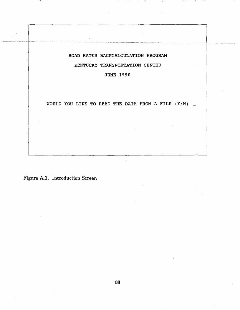
ROAD RATER BACKCALCULATION PROGRAM

KENTUCKY TRANSPORTATION CENTER

JUNE 1990

WOULD YOU LIKE TO READ THE DATA FROM A FILE (Y/N) _

Figure A.l. Introduction Screen

68

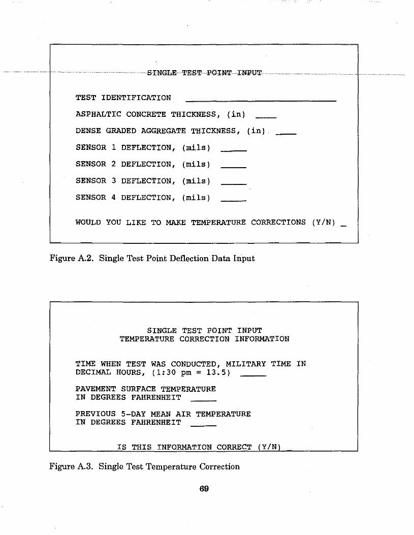
·······························~·~·~··~····~·····~· · · ~·· ·~·~·~·······~. · ·~··· · ~· ~ ~&ING"&E T~E&T P.(liN'I'~~I~NFUT·~·~ ·~~~·~···~·~~·~~~·~~~ ~~.~.~~~~·······~·~·~·~·~·~·~······

TEST IDENTIFICATION

ASPHALTIC CONCRETE THICKNESS, (in)

DENSE GRADED AGGREGATE THICKNESS, (in)

SENSOR 1 DEFLECTION, (mils)

SENSOR 2 DEFLECTION, (mils)

SENSOR 3 DEFLECTION, (mils)

SENSOR 4 DEFLECTION, (mils)

WOULD YOU LIKE TO MAKE TEMPERATURE CORRECTIONS (Y/N) _

Figure A.2. Single Test Point Deflection Data Input

SINGLE TEST POINT INPUT TEMPERATURE CORRECTION INFORMATION

TIME WHEN TEST WAS CONDUCTED, MILITARY TIME IN DECIMAL HOURS, (1:30pm= 13.5)

PAVEMENT SURFACE TEMPERATURE IN DEGREES FAHRENHEIT

PREVIOUS 5-DAY MEAN AIR TEMPERATURE IN DEGREES FAHRENHEIT

IS THIS INFORMATION CORRECT

Figure A.3. Single Test Temperature Correction

69

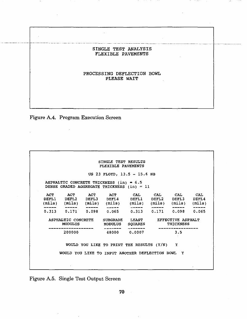
SINGLE TEST ANALYSIS FLEXIBLE PAVEMENTS

PROCESSING DEFLECTION BOWL PLEASE WAIT

Figure A.4. Program Execution Screen

SINGLE TEST RESULTS FLEXIBLE PAVEMENTS

US 23 FLOYD, 13.5 - 15.6 NB

ASPHALTIC CONCRETE THICKNESS (in) = 6.5 DENSE GRADED AGGREGATE THICKNESS (in) = 11

ACT ACT ACT ACT CAL CAL DEFL1 DEFL2 DEFL3 DEFL4 DEFL1 DEFL2 (mils) (mils) (mils) (mils) (mils) (mils)

0.313 0.171 0.098 0.065 0.313 0.171

CAL CAL DEFL3 DEFL4 (mils) (mils)

0. 098 0.065

ASPHALTIC CONCRETE SUBGRADE LEAST EFFECTIVE ASPHALT MODULUS MODULUS SQUARES THICKNESS

------------------ ------- ------- ----------------200000 48000 0.0007 3.5

WOULD YOU LIKE TO PRINT THE RESULTS (Y/N) Y

WOULD YOU LIKE TO INPUT ANOTHER DEFLECTION BOWL Y

Figure A.5. Single Test Output Screen

70

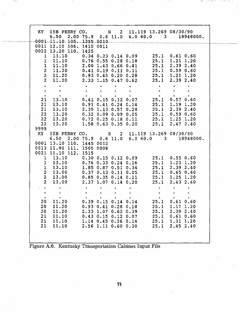
KY 15B PERRY CO. N 2 11.119 13.269 08/30/90 6.50 2.00 75.9 0.6 11.0 6.0 60.0 3 18948000.

~~{){}± ~~11~·~1·0····~·~1·~5·~··~·~·135~ ~0040 ••••~~~.•~•~""" """""""""""" """ _,m_ """"""""""""""" """ """""""""""""""""""" """""""""""'~""

0011 12.10 106. 1410 0011 0022 13.20 110. 1425

1 11.10 0.34 0.23 0.14 0.09 25.1 0.61 0.60 1 11.10 0.76 0.55 0.28 0.18 25.1 1.21 1.20 1 11.10 2.00 1.43 0.66 0.41 25.1 2.39 2.40 2 11.20 0.41 0.19 0.11 0.11 25.1 0.59 0.60 2 11.20 0.93 0.45 0.20 0.28 25.1 1.21 1.20 2 11.20 2.33 1.15 0.47 0.62 25.1 2.39 2.40 . . . . . . . . . . . . . . . • . • . . . . . . . . .

21 13.10 0.41 0.15 0.12 0.07 25.1 0.57 0.60 21 13.10 0. 91 0.41 0.24 0.14 25.1 1.19 1.20 21 13.10 2.35 1.13 0.57 0.28 25.1 2.39 2.40 22 13.20 0.32 0.09 0.09 0.05 25.1 0.59 0.60 22 13.20 o. 72 0.25 0.18 0.11 25.1 1.25 1. 20 22 13.20 1.58 0.63 0.35 0.20 25.1 2.47 2.40

9999 KY 15B PERRY CO. s 2 11.119 13.269 08/30/90

6.50 2.00 75.9 0.6 11.0 6.0 60.0 3 18948000. 0001 13.10 110. 1445 0012 0013 11.90 111. 1505 0008 0021 11.10 112. 1515

1 13.10 0.30 0.15 0.12 0.09 25.1 0.55 0.60 1 13.10 0.76 0.33 0.24 0.16 25.1 1.23 1.20 1 13.10 1. 85 0.87 0.51 0.34 25.1 2.39 2.40 2 13.00 0.37 0.13 0.11 0.05 25.1 0.65 0.60 2 13.00 0.85 0.35 0.14 0.11 25.1 1.25 1.20 2 13.00 2.37 1. 07 0.14 0.20 25.1 2.43 2.40 . . . . . . . . . . . . . . . . . . . . . . . . . . .

20 11.20 0.39 0.15 0.14 0.14 25.1 0.61 0.60 20 11.20 0.93 0.41 0.28 0.18 25.1 1.17 1. 20 20 11.20 2.33 1. 07 0.62 0.39 25.1 2.39 2.40 21 11.10 0.43 0.15 0.12 0.07 25.1 0.61 0.60 21 11.10 1.14 0.45 0.26 0.14 25.1 1. 31 1. 20 21 11.10 2.56 1.11 0.60 0.30 25.1 2.45 2.40

F1gure A.6. Kentucky Transportat10n Cabmet Input F1le

71

The second data file format which may be used is given in Figure A.7. This format is currently used by the Kentucky Transportation Center. This file may also contain deflection measurements for a second direction or test location for the same

··· ········ ~pavement~sect1on;~ A8~1rfthe preVious~data~me~form:at,~the~test~tocations>Il.ust~e~~~~ separated by the number 9999.

Data File Contents

Each data file contains all data which are necessary to process the deflection measurements. Each file must be in ASCII text format. The contents of the file format given in Figure A.6 is as follows:

Line Number 1

Data Type

System (US or KY) Route County Direction Section Number Upper Milepoint Lower Milepoint Test Date

Line Number 2

Data Type

AC Thickness 5-Day Mean Air Temperature DGA Thickness Number of Temperature Measurements

Column Location

1- 3 5-9 10-23 26 30 33-39 40-46 47-54

Column Location

5-9 16- 20 27-30 45-46

Line Number 3, This line is repeated for each Temperature Measurement

Data Type

Beginning Test Number Milepoint Pavement Temperature Time at Temperature Measurement Number of Tests Before Next Temperature Measurement

72

Column Number

1-4 6- 10 12- 15 17- 20 22-23

Line Number 4, This line is repeated for each deflection Measurement

Data Type

Test Number Milepoint Number 1 Deflection Number 2 Deflection Number 3 Deflection Number 4 Deflection Frequency of Loading Actual Test Load Target Test Load

Column Location

1- 4 6- 11 17- 20 22-25 27-30 32-35 41-44 47-50 52-55

The contents of the file format given in Figure A. 7 are as follows:

Line Number 1, Filename

Line Number 2, AC Thickness, DGA Thickness, Time of Temperature Measurement, Pavement Temperature, 5-Day Mean Air Temperature

Line Number 3- 13, Text lines

Line Number 14, This line is repeated for each deflection measurement.

Data Type Column Location

Test Number Test Load Frequency of Loading Number 1 Deflection Number 2 Deflection Number 3 Deflection Number 4 Deflection Stiffness (load/defll)

73

1 - 5 7- 10 9- 12 21- 25 29-33 37- 41 45-49 53-57

If a second set of data is included, the number 9999 must be included at the end of the first set of data. The next line should be the same format as line number 2 .

.... ..................... The.foUo:win.g..line..must.be~one.line .... oftext..describing.the..data :which. are to follow:.. . . The deflection data should be in the same format as the pervious deflection data.

The format of the input data files is the same for all models, KTCFLEX, KTCBREAK, and KTCCOMP. The input data file for KTCBREAK and KTCCOMP must contain the thickness of broken or intact concrete pavement in place of the DGA thickness.

74

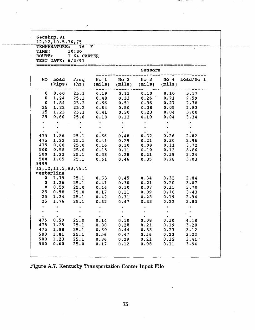
64cshrp.91

~~~~~~~ ~~~~~~~~~~~~~~~~~~~ +~.f1,;2r:, .~1: 2~:i ·~~~1r.~~:r,·~sw. ,7;=_: 6";~ ··~~~7·~~ 6~:-~ ~iF~~~~~~~~~~~~~~~~~~~~~~ ~ ~~~~~~~~~~~~~~ ~~~~~~ ~~~~~ ~~~~ ~ ~~~~~~~ ~ ~ ~~ ~~~~~ ~~~~~~~~~ ~ ~ ~~ ~~~~ ~~~~~~~~~ l~ ~~--~~~-~~-~ TIME: ROUTE: TEST DATE:

10:30 I 64 CARTER 6/3/91

============================================================

No Load Freq (kips) ( hz)

0 0.60 25.1 0 1.24 25.1 0 1. 84 25.2

25 1. 82 25.2 25 1. 23 25.1 25 0.60 25.0

475 1. 86 25.1 475 1. 22 25.1 475 0.60 25.0 500 0.58 25.0 500 1.23 25.1 500 1. 85 25.1

9999 12,12,11.5,83,75.1 centerline

0 1. 79 25.1 0 1. 26 25.1 0 0.59 25.0

25 0.58 25.0 25 1. 24 25.1 25 1. 76 25.1

475 0.59 25.0 475 1.25 25.1 475 1. 88 25.1 500 1. 81 25.1 500 1.23 25.1 500 0.60 25.0

Sensors

No 1 No 2 No 3 No 4 Load/No 1 (mils) (mils) (mils) (mils)

0.19 0.13 0.10 0.10 3.17 0.48 0.33 0.26 0.21 2.59 0.66 0.51 0.36 0.27 2.78 0.64 0.50 0.38 0.05 2.83 0.41 0.30 0.23 0.04 3.00 0.18 0.12 0.10 0.04 3.34

0.66 0.48 0.32 0.26 2.82 0.41 0.29 0.21 0.20 2.96 0.16 0.10 0.08 0.11 3. 72 0.15 0.11 0.10 0.13 3.86 0.38 0.28 0.21 0.19 3.24 0.61 0.46 0.35 0.28 3.03

0.63 0.45 0.34 0.32 2.84 0.41 0.30 0.21 0.20 3.07 0.16 0.10 0.07 0.11 3.70 0.17 0.11 0.09 0.10 3.43 0.42 0.31 0.23 0.19 2.94 0.62 0.47 0.33 0.22 2.83

0.14 0.10 0.08 0.10 4.18 0.38 0.28 0.21 0.19 3.28 0.60 0.44 0.33 0.27 3.12 0.56 0.47 0.36 0.22 3.22 0.36 0.29 0.21 0.15 3.41 0.17 0.12 o.o8 0.11 3.54

Figure A.7. Kentucky Transportation Center Input File

75

Data File Selection

~~~~~~~Dnc~th~choic~haslleen~madetox~d-data.l'rom.~a.ilislcfile,~the~sct:een~giY£mjn ~~~~~~~~~·~·~·~ Figure A8 will be displayed. This screen allows the user to select the file format to be read (KTC or DOT). Once the file form.at has been selected, the user is prompted for the directory containing the data files. The files which will be displayed in the data directory m.ay be chosen by using "*" character to indicate all files or files with all extensions. For example, an input of "A:\*.*" would display all the files in the A drive. An input of "A:\* .dat" would display all files in the A drive which have a file extension of "dat." Once the directory has been selected, the user may proceed by pressing <ENTER>.

The screen in Figure A.9 will be displayed. This is the file selection menu. The user may scroll through the file names using the arrow keys. A maximum of 10 files may be selected for processing. A flle may be selected by pressing <ENTER>, a check mark will appear indicating the file has been selected. A counter is display:ed indicating the number of files currently chosen. If the maximum number of 10 files is reached, the program will not allow any more files to be selected. Once all files to be processed have beim selected, the Esc key is pressed to begin program execution. During execution, the screen given in Figure A.lO will be displayed. Displayed on this screen are the file name being processed, the percentage of that file which is completed and the number of the deflection bowl being processed.

Output Files

Several flles are produced by .the backcalculation programs. The files may be distinguished by the file extension. The following file extensions have been used .

. ETH

. DEF

. OLA

This file contains the effective asphaltic concrete thickness and related information .

This file contains the asphaltic concrete and subgrade modulus along with backcalculated deflections .

Output flle for overlay design program.

All three output flles are produced by KTCFLEX, however only the file containing the elastic moduli and backcalculated deflections is produced by KTCBREAK and KTCCOMP.

76

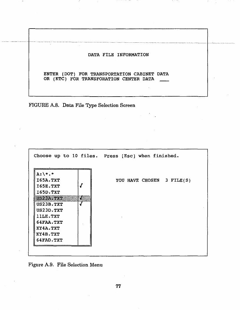
DATA FILE INFORMATION

ENTER (DOT) FOR TRANSPORTATION CABINET DATA OR (KTC) FOR TRANSFORATION CENTER DATA __ _

FIGURE A.S. Data File Type Selection Screen

Choose up to 10 files. Press [Esc] when finished.

A:\* • * I65A.TXT I65E.TXT I65D.TXT

i :-: :·::·.: :··· .· .·.= . ... : =;. : :".

US23B.TXT US23D.TXT llLE.TXT 64FAA.TXT KY4A.TXT KY4B.TXT 64FAD.TXT

l

Figure A.9. File Selection Menu

YOU HAVE CHOSEN 3 FILE(S)

77

.ETH File Contents, KTCFLEX

~~ ~~~ ~~~- ~1\li example~ofth1soutpu~filets given inFigure~A;H.~This~le~containsthe~test~ ~~~~~~ ~~~~~~~~·~·~ section information on Line 2. The following lines preceding the deflection header contain the pavement temperature, time of temperature measurement information, and the 5-day mean air temperature. The remainder of the me contains the results of the backcalculation procedure. The values labeled "SENl RDG through SEN4 RDG" are the actual pavement deflections which have been adjusted to a nominal 600-lb load. The values labeled "ADJ DEFLl through ADJ DEFL4" are deflections which have been adjusted for temperature effects.

The effective asphaltic concrete thickness given is labeled as "ASPH T EFF" and "AC TH". The data labeled "DGA TH" are the actual design DGA thickness plus the lost AC thickness.

The data labeled "SECTION+LOAD" are in a code that represents the section being tested and the target test load. The first number represents the test section while the last two number represent the target load, "06" for 600-lb load, "12" for 1,200 lb load, and "24" for 2,400 lb load.

A statement at the end of the me gives the total number of test points which had an effective thickness less than 50 percent of the design thickness .

. DEF File Contents, KTCFLEX

An example of this data me is given in Figure A.12. This file differs from the .ETH file in that it contains the backcalculated deflections and the elastic modulus for each layer. In addition, this file contains the values of least squares corresponding to the backcalculated deflections.

Data labeled "MOD DEFL2 through MOD DEFL4" are deflections which correspond to the backcalculated subgrade and asphaltic concrete modulus. The data labeled "MOD LS" are the least square corresponding to these deflections.

The deflections used to determine the effective thickness are labeled "EFF DEFLl through EFF DEFL4". The least square associated with these deflections is labeled "EFF LS".

78

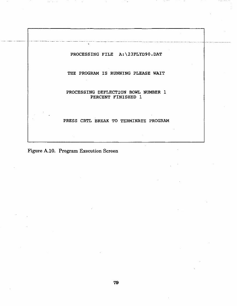
PROCESSING FILE A:\23FLYD90.DAT

THE PROGRAM IS RUNNING PLEASE WAIT

PROCESSING DEFLECTION BOWL NUMBER 1 PERCENT FINISHED 1

PRESS CRTL BREAK TO TERMINATE PROGRAM

Figure A.lO. Program Execution Screen

79

.DEF File Contents, KTCBREAK and KTCCOMP

This file contains the actual pavement deflection adjusted to a nominal 600 lb load along with the backcalculated deflections. The elastic modulus for the asphaltic concrete, broken concrete, and subgrade are also given. These moduli correspond to the backcalculated deflections and least squares value given in the file. An example of this data file is given in Figure A.13 .

. OLA File Contents, KTCFLEX

This file contains the input for the overlay design program used by the Transportation Cabinet, an example is given in Figure A.14. This data file contains the effective asphaltic concrete thickness, DGA thickness, and subgrade modulus, along with the current accumulated ESAL,s for the test section. This file provides the inputs needed for the overlay design program currently used by the Transportation Cabinet.

An example of each input and output data files is included with the analysis software.

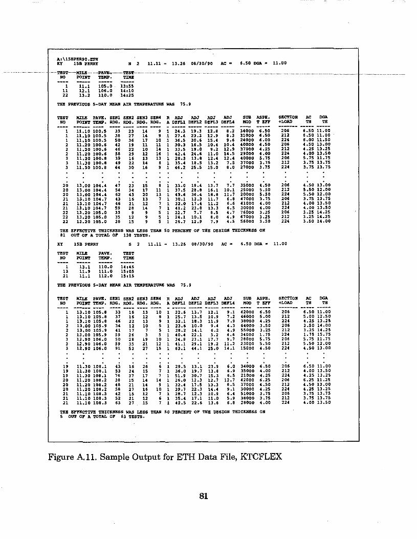
AI \15BPER90 ,E'l'B .. 158 PERRY • 2 11.11 - 13.26 08/30/SIO AC • 6,50 DGA • 11.00

•• ~~~ ~- TIIIB

1 11.1 105.0 13t55 11 12.1 106.0 14110 22 13.2 uo.o 14125

'l'B1!: PRJ!:V'IOUS 5-DAY HEAR AIR 'l'EHPIRA'l'URE WAS 75.9

TEST """" PAVE. SI!:R1 S .. 2 SER3 S!N4 R ADJ ADJ ADJ AOJ SUB ASPB. SECTION AC OGA NO POIRT T!KP , ROO. RDG. RDG, RDG, A D!FL1 DKFL2 D!FL3 DE!'L4 MOD TE1'7 +LOAO "" ""

1 11.10 100.5 33 23 " ' 1 24.3 U.J 12.8 '·' 34000 6.50 200 6.50 11.00 1 11.10 100.5 38 " " ' 1 27.4 23.3 12.9 8.3 31000 6.50 212 6.50 u.oo 1 11.10 100.5 50 " 17 10 1 36.5 30.6 15.4 ••• 24000 6.00 224 6.00 u.so

' 11.20 100.6 " " 11 11 1 30.3 16.5 10.4 10.4 40000 4.50 , .. 4.50 13.00 2 11.20 100.6 .. " 10 .. 1 33.5 u.o '·' 12.9 37000 4.25 212 4.25 13.25 2 11.20 100.6 58 " 12 " 1 42.4 24.6 11.0 u.s 29000 4.00 224 4.00 13.50 3 11,30 100.8 ,.

" " " 1 28.3 13.8 12.4 12.4 40000 5.75 200 5.75 11.75 3 11.30 100.8 .. " " 8 1 35.4 18.5 13.2 7.5 37000 3,75 212 3.75 13.75 3 11.30 100.8 .. 30 " ' 1 46.2 25.5 15.0 8.0 27000 3.75 224 3.75 13.75

20 13.00 104.4 47 23 15 8 1 33.0 lSI .4 13.7 7.7 35000 4.50 206 4.50 13.00 20 13,00 104.4 54 " 17 11 1 37.5 28.8 16.1 10.1 25000 5.50 212 5.50 12.00 20 13.00 104.4 " 43 20 " 1 43.6 36.4 18.8 11.7 20000 5.50 224 5.50 12.00 21 13.10 104.7 " " " 7 1 30.1 13.3 11.7 6.8 47000 3.75 200 3.75 13.75 21 13~10 104.7 .. 21 12 7 1 32.0 17.4 11.2 6.6 41000 4.00 212 4.00 13.50 21 13.10 104.7 " 28 14 7 1 41.2 23.8 13.3 6.S 30000 4.00 224 4,00 13.50 22 13.20 105.0 " ' ' 5 1 22.7 7.7 8 .s 4.7 76000 3.25 206 3.25 14.25

" 13.20 105.0 35 12 ' s 1 24.1 10.1 8 .o ••• 67000 3.25 212 3 .25· 14.25

" 13.20 105.0 38 15 ' 5 1 26.7 12.9 7.' 4.S 56000 3.50 224 3.50 14.00

••• E!"F!CTIV! 'lHIC!Ui!SS WAS LESS TBAll so PERCENT 0!" THE DESIGN 'lHICXH!SS •• 81 OUT OP A TOTAL 0!' 138 TESTS.

KY 158 PERRY s 2 11.11 - 13.26 08/30/90 AC • 6.50 DGA • u.oo

TEST Hl:LE PAVE, TEST NO POIRT ...... TIIIB

1 13.1 110.0 14145

" 11.9 111.0 15t05 21 11.1 112.0 15115

THE PRBV'IOUS 5-DAY HEAR AIR TEMPERATURE WAS 75.9

TEST MILE PAVE. SBR1 SER2 SER3 SI!:N4 R AOJ AOJ AOJ AOJ SUB ASPB. SECTION AC OGA NO POiliT TEMP. ROO. RDG. ROO. RDG. A DBFLl DE!"L2 DBFLJ DIPL4 HOD ..... +LOAD "" TH

1 13.10 105.8 " " " 10 1 22.6 13.7 12.1 '.1 42000 6.50 206 6.50 11.00 1 13.10 1:05.8 37 " 12 8 1 25.7 13.5 10.51 7.2 46000 s.oo 212 5.00 12.50 1 13.10 105.8 .. 22 " ' 1 32.1 18.3 11.9 7.' 38000 4.25 224 4.25 13.25 2 13.00 105.51 " 12 10 5 1 23.6 10.0 9.4 4.3 64000 3.50 206 3.50 14,00 2 13,00 105.9 " 17 7 s 1 28.2 14.1 6.2 4.9 55000 3.25 212 3.25 14.25

' 13.00 105.9 " " 3 5 1 40.4 22.1 3.2 4.6 34000 l. 75 224 1.75 15.75 3 12.90 106.0 so 28 " 10 1 34.9 23.1 17.7 9.7 28000 5.75 206 5.75 11.75 3 12.90 106.0 " 35 21 12 1 41.1 29.1 U.2 11.2 23000 5.50 212 5.50 12.00 3 12.90 106.0 " 53 " 15 1 63.1 44,1 25.0 14.1 15000 4.50 224 4.50 13.00

" 11.30 108.1 " " " 6 1 29.5 13.1 23.9 6.0 34000 6.50 206 6.50 11.00

" 11.30 108.1 53 24 15 7 1 36.0 lSI 0 7 13.8 6.9 35000 4.00 212 4.00 13 .so

" 11.30 108.1 76 37 17 7 1 51.9 30.7 15.3 6.S 21000 4.25 224 4.25 13.25 20 11.20 108.2 38 15 " .. 1 26.0 12.3 12.7 12.7 42000 6.25 206 6.25 11,25 20 11.20 108.2 48 21 " ' 1 32.4 17.5 13.3 a.s 37000 4.50 212 4.50 13.00 20 11.20 108.2 58 27 16 10 1 351.7 22.3 14 ... '.1 30000 4.25 224 4.25 13.25 21 11,10 108.3 42 15 12 7 1 28.7 12.3 10.9 6.4 51000 3.75 206 3,75 13.75 21 11.10 108.3 52 21 12 • 1 35.4 17.1 u.o s •• 38000 3.75 212 3.75 13.75 21 11.10 108.3 " 27 15 7 1 42.5 22.6 13.6 ••• 28000 4.00 224 4.00 13~50

THE EFFECTIVE THICKNESS WAS LESS THAN so PERCENT 0!" THE DESIGN THICKNESS •• 5 OUT OF A TOTAL 0!' 63 TES'l'S.

Figure All. Sample Output for ETH Data File, KTCFLEX

81

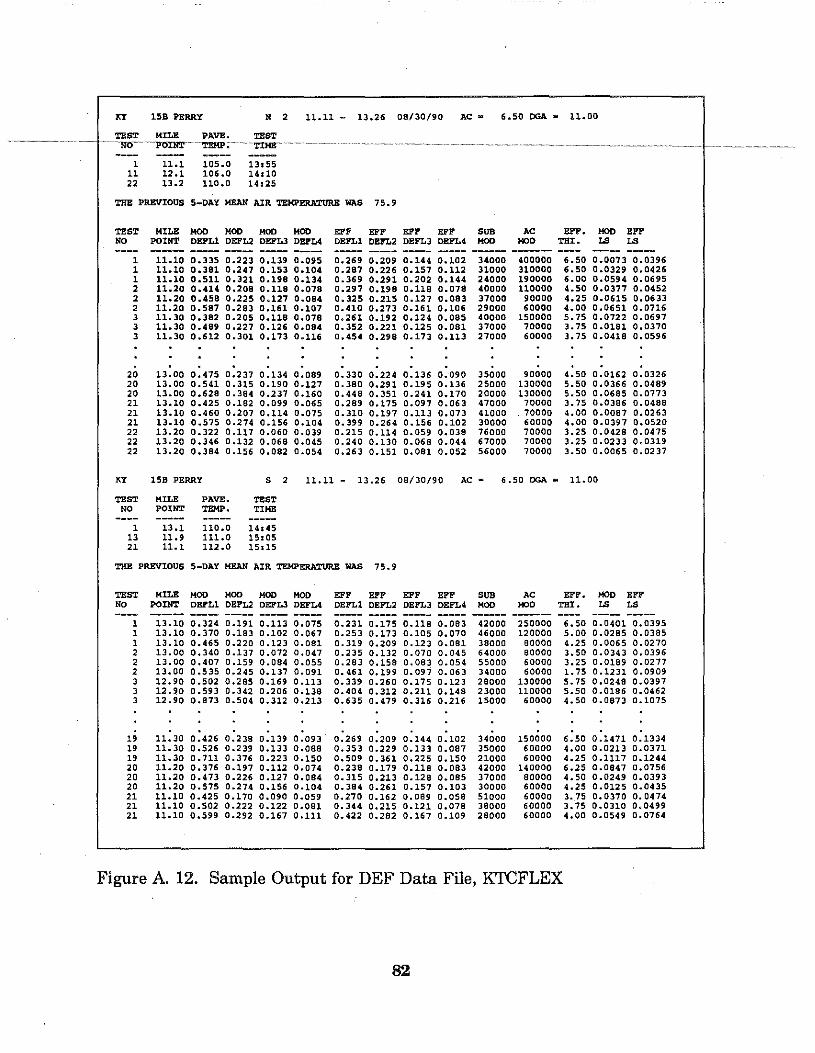
KY 15B PERRY N 2 11.11 - 13.26 08/30/90 AC • 6.50 DGA"" 11.00

TEST MILE PAVE. TEST _:v :v•~ ~--_ .. =

1 11.1 105.0 lJsSS 11 12.1 106 .o 14110 22 13.2 110.0 14z25

THE PREVIOUS 5-DAY MEAN AIR TEMPER.M'URE WAS 75.9

TEST MILE MOO MOD MOO MOO EPP EFP EFP EFP SUB AC EPP. MOD EPP NO POINT DEPLl DEPL2 DEP'LJ DEPL4 DEPLl DEFL2 DEFLJ DEPL4 MOO MOD TBI. r..s LS ------

l 11.10 0.335 0.223 0.139 0.095 0.269 0.209 0.144 0.102 34000 400000 6.50 0.0073 0.0396 1 11.10 0.381 0.247 0.153 0.104 0.287 0.226 0.157 0.112 31000 310000 6.50 0.0329 0.0426 1 11.10 0.511 0.321 0.198 0.134 0.369 0.291 0.202 0.144 24000 190000 6.00 0.0594 0.0695 2 11.20 0.414 0.208 0.118 0.078 0.297 0.198 0.118 0.078 40000 110000 4.50 0.0377 0.0452 2 11.20 0.458 0.225 0.127 0.084 0.325 0.215 0.127 0.083 37000 90000 4.25 0.0615 o. 0633 2 11.20 0.587 0.283 0.161 0.107 0.410 0.273 0.161 0.106 29000 60000 4.00 0.0651 0.0716 3 11.30 0.382 0.205 0.118 0.078 0.261 0.192 0.124 0.085 40000 150000 5.75 0.0722 0.0697 3 11.30 0.489 0.227 0.126 0.084 0.352 0.221 0.125 0.081 37000 70000 3.75 0.0181 0.0370 3 11.30 0.612 0.301 0.173 0.116 0,454 0.298 0.173 0.113 27000 60000 3.75 0.0418 0.0596

20 13.00 0.475 0.237 0.134 0.089 0.330 0.224 0.136 o.·o9o 35000 90000 4.50 0.0162 0,0326 20 13.00 0.541 0.315 0.190 0.127 0.380 0.291 0.195 0.136 25000 130000 5.50 0.0366 0.0489 20 13.00 0.628 0.384 0.237 0.160 0.448 0.351 0.241 0.170 20000 130000 5.50 0.0685 0.0773 21 13.10 0.425 0.182 0.099 0.065 0.289 0.175 0 .. 097 0.063 47000 70000 3.75 0,0386 0.0488 21 13.10 0.460 0.207 0.114 0.075 0.310 0.197 0.113 0.073 41000 . 70000 4. 00 0.0087 0.0263 21 13.10 0.575 0.274 0.156 0.104 0.399 0.264 0.156 0.102 30000 60000 4.00 0.0397 0.0520 22 13.20 0.322 0.117 0.060 0.039 0.215 0.114 0.059 0.038 76000 70000 3.25 0.0429 0,0475 22 13.20 0.346 0.132 0.068 0.045 0.240 0.130 0.069 0.044 67000 70000 3.25 0.0233 0.0319 22 13.20 0.384 0.156 0.082 0.054 0.263 0.151 0.081 0.052 56000 70000 3.50 0.0065 0. 02 37

KY 15B PERRY s 2 11.11 - 13.26 08/30/90 AC - 6.50 OGA"' 11.00

TEST MILE PAVE. TEST NO POINT TEMP. TIME

1 13.1 110.0 14145 13 11.9 111.0 15:05 21 11.1 112 .o 15:15

THE PREVIOUS 5-DAY MEAN AIR TEMPERM:'UR.E WAS 75.9

TEST MILE MOD MOO MOO MOD EPP EPP EPF EPF SUB AC EPP. MOD EPP NO POINT DEPL1 DEPL2 DEFL3 DEFL4 DEFL1 DEPL2 DEFL3 DEFL4 MOD MOD THI. LS LS --- ----

1 13.10 0.324 0.191 0.113 0.075 0.231 0.175 0.118 0.083 42000 250000 6.50 0.0401 0.0395 1 13.10 0.370 0.193 0.102 0.067 0.253 0.173 0.105 0.070 46000 120000 5.00 0,0285 0.0385 1 13.10 0.465 0.220 0.123 0.081 o. 319 0.209 0.123 0.081 38000 80000 4.25 0.0065 0.0270 2 13.00 0.340 0.137 0.072 0.047 0.235 0.132 0.070 0.045 64000 80000 3.50 0.0343 0,0396 2 13.00 0.407 0.159 0.084 0.055 0.283 0.158 0.083 0.054 55000 60000 3.25 0.0189 0.0271 2 13.00 0.535 0.245 0.137 0.091 0.461 0.199 0.097 0.063 34000 60000 1.75 0.1231 0.0909 3 12.90 0.502 0.285 0,169 0.113 0.339 0.260 0.175 0.123 28000 130000 5.75 0.0248 0.0397 3 12.910 0.593 0.342 0.206 0.138 0.404 0.312 0.211 0.148 23000 110000 5.50 0.0186 0.0462 3 12.90 0.873 0.504 0.312 0.213 0.635 0,479 0.316 0.216 15000 60000 4. 50 0.0873 0.1075

19 11.30 0,426 0.238 0.139 0.093 0.269 0.209 0.144 0.102 34000 150000 6.50 0.1471 0.1334 19 11.30 0.526 0.239 0.133 0.088 0.353 0.229 0.133 0,087 35000 60000 4.00 0.0213 0.0371 19 ll.JO a. 711 0.376 0.223 0.150 0,509 0.361 0.225 0.150 21000 60000 4.25 0.1117 0.1244 20 11.20 0.376 0.197 0.112 0.074 0.238 0.179 0.118 0.083 42000 140000 6.25 0.0847 0.0756 20 11.20 0.473 0.226 0.127 0.084 0.315 0.213 0.128 o.o8s 37000 80000 4.50 0.0249 0.0393 20 11.20 0.575 0.274 0 .. 156 0.104 0.384 0.261 0.157 0.103 30000 60000 4.25 0.0125 0.0435 21 11.10 0.425 0.170 0.090 0.059 0.270 0.162 0,089 0.058 51000 60000 3._75 0.0370 0.0474 21 11.10 0.502 0.222 0.122 0.081 0.344 0.215 0.121 0.078 38000 60000 3.75 0.0310 0.0499 21 11.10 0.599 0.292 0.167 0.111 0.422 0.282 0.167 0.109 28000 60000 4.00 0.0549 0.0764

Figure A. 12. Sample Output for DEF Data File, KTCFLEX

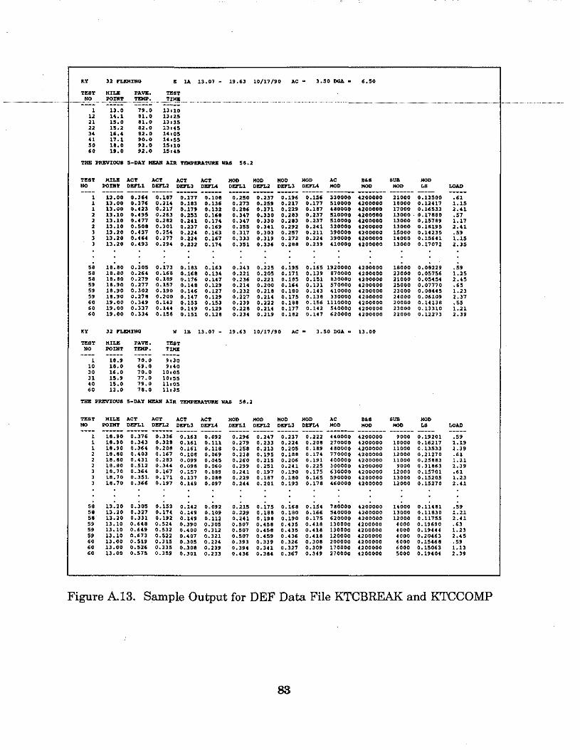
ICY 32 FLJ!:HrH<il • 1A 13.07 - 19.63 10/17/90 AC • 3.50 DGA • 6.50

-r:~'f ~i:T =~ ~X: "i ~i;:o n:O il:io 12 14.1 81.0 13125 21 15.0 81.0 1313.5 22 15.2 82.0 13145

" 16.4 82.0 14105 41 17.1 90.0 Uo55 so 18,0 112.0 15110

" lt.O 92.0 15145

THE PREVIOUS 5-DAY MEAN AIR T!:MPI!:RA'l'UU WAS 58.2 .... HILIC ACT ACT ACT ACT HOD HOD HOD HOD AC ... SUB HOD NO >OINT DEFI.l DEl'L2 DEl'LJ DD'L4 DULl DULl DEl'LJ DEFL< HOD HOD HOD LS LOAD

1 13.00 O.JU 0.187 0.177 0.108 0.250 O.l37 0.1" 0.156 330000 4200000 21000 0.13500 ·" 1 13.00 0.3741i 0.214 0.183 0.136 0.273 0.259 0.217 0.177 510000 4200000 18000 O.UU7 1.15 1 13.00 o.uJ 0.217 0.179 0.132 0.286 0.271 0.229 0.1117 480000 4200000 17000 0.16533 2.U 2 13.10 o.us 0.263 0.253 O.lU O.H7 0.330 0.2U O,l37 510000 4200000 13000 0,17880 .57 2 13.10 0.417 0.282 0.241 0.174 O.H7 0.330 0.283 0.237 510000 4200000 13000 0.15789 1.17 2 13.10 0.508 0.301 0.237 O.lU o. 355 0.341 0.292 0.241 320000 ol200000 13000 0.18195 2.U

' 13.20 O.ol37 o. 25ol 0.22" 0.163 0.317 0.303 0.257 0.211 390000 uooooo 15000 O.U235 ·" ' 13.20 O.ol64 0.277 0.22ol 0.167 o. 333 0.319 0.272 0.22ol 390000 uooooo HOOO 0.15641 1.15

' 13.20 O.ol93 0.29ol 0.232 0.174 0.351 0.336 0.288 0.237 uoooo o1200000 13000 0.17072 2.35

58 18.80 0.305 0.173 0.183 0.163 0.2ol3 0.225 0.195 0.165 1920000 ol200000 18000 0.08229 ·" 58 18.80 0.264 0.168 0.168 0.13ol 0.221 0.205 0.171 0.139 870000 uooooo 23000 0.05756 1.25 58 18.80 0.279 0.189 0.176 O.U7 0.236 0.221 0.185 0.151 830000 uooooo 21000 0.05ol5ol 2.ol5

" 18.90 0.277 0.157 0.148 0.129 0.2U 0.200 0,164 0.131 570000 uooooo 25000 0.07770 ·" " 18.90 0.302 0.190 O.U6 0.127 0,232 0.218 0.180 O.U3 uoooo "200000 23000 0.08U5 1.23

" 18.90 0.271!!1 0.200 0.147 o.1n o.h1 0.2U 0.175 0.138 330000 uooooo loiOOO 0.06109 2.37

" 19.00 0.3U 0.142 0.153 0.153 0.239 0.222 0.181!!1 0.156 1110000 uooooo 20000 O.U1J8 ... " 19.00 0.337 0.1U O.U9 0.129 0.221!!1 0.2U 0.177 O.U2 540000 o1200000 23000 0.13310 1.21

" 19.00 0.33ol 0.158 0.151 0.121!!1 0.23ol 0.219 0.182 O.U7 620000 ollOOOOO 22000 0,12273 2.39

<Y 32 n.EHINQ w lB 13.07 - 19.63 10/17/90 AC • 3.50 DGA"' 13.00

TEST HILIC PAVE. TEST NO >OINT ,...._ TIJ<Z

1 18.9 10.0 9130 10 18.0 69.0 !hoiO 30 16.0 70.0 10105 31 15.9 77.0 10155 ., 15.0 79.0 11105

" 13.0 78.0 11135

THE PREVIOUS 5-DAY MU.R AIR TEKI'EftATURE WAS 58.2

TEST HI I.E ACT ACT ACT ACO HOD HOD HOD HOD AC ... '"" HOD NO >OINT DD'Ll DD'L2 DEl'LJ DD'L( DD'Ll DULl DULJ DD'L< HOD HOD HOD LS LOAD

1 18.90 0.376 0.336 0.163 o.ou 0.296 0.2o11 0.237 0.222 uoooo 4200000 9000 0.19201 ·" 1 18.90 0.343 0.328 0.161 0.111 0.279 o. 233 0.224 0.208 270000 4200000 10000 0.16217 1.19 1 18.90 0.364 0.208 0.161 0.118 0.258 0.213 0.205 0.189 uoooo ollOOOOO 11000 0.13533 2.39 2 18.80 0 .ol03 0.167 0.108 0.069 0.238 0.195 0.188 0.174 770000 4200000 12000 0.21270 ·" 18.1!!10 0.431 0.283 0,099 O.Ool5 0.260 o. 215 0.206 0.191 400000 4200000 11000 0,25883 1.21

18.80 0.512 O.Hol o. 098 0.060 0.299 o. 251 0.2U 0.225 300000 4200000 ~000 0.31863 2.39 18.70 0.3U 0.167 0.157 0.089 0.241 0.197 0.190 0.175 630000 4200000 12000 0.15701 ·" 11!. 70 0.351 0,171 0.137 o. 01!!18 0.229 0.187 0.180 0,165 590000 4200000 13000 0.15205 1.23 18.70 0.366 0.197 0.1U 0.097 0.2U 0.201 0.193 0.178 460000 uooooo 12000 0.15270 2.41

" 13.20 0.305 0.153 0.142 0.092 0.215 0.175 0.168 0.15ol 780000 4200000 uooo 0.11U1 ·" " 13.20 0.327 0.174 0 .1U 0.109 0.229 0.188 0.180 0.166 5ol0000 4200000 13000 0.11830 1.21 58 13.20 0.331 0.192 0.149 0.112 0.2U 0.198 0.190 0.175 620000 4200000 12000 0.11755 2.U

" 13,10 o.u8 0.52.4 0.390 0.305 0.507 o. ol58 0. oilS 0.418 130000 4200000 4000 0.19690 ·" " 13,10 0.6U 0.532 O.oiOO 0.312 0.507 o. ol58 O.ol35 o.U8 130000 4200000 oiOOO 0.19U4 1.23

" 13.10 0.673 0.522 O.ol07 0.321 0.507 O.ol59 O.ol36 0.418 120000 4200000 oiOOO 0.20463 2 ... 5

" 13.00 0.519 0.315 0.305 0.22" 0.393 0.339 0.326 0.308 200000 4200000 6000 0.15oiU ·" " 13.00 0.526 0.335 0.308 0.239 0.394 0.341 0.327 0.309 170000 4200000 6000 0.15063 1.13

" 13,00 0.575 0.359 0.301 0.233 O.ol36 o. 38ol 0.367 0.3U 270000 uooooo 5000 O.l9ol0ol 2.39

Figure A.13. Sample Output for DEF Data File KTCBREAK and KTCCOMP

83

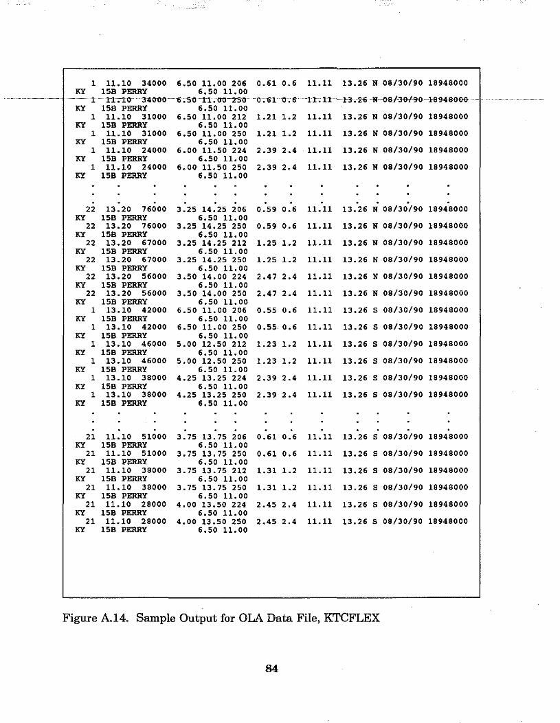
1 11.10 34000 6.50 11.00 206 0.61 0.6 11.11 13.26 N 08/30/90 18948000 KY 158 PERRY 6.50 11.00

~~~~~~~~~~J:,~3"4'01lO ~~6;So"'1.~t~oo-2!!~ct~~~o~,~et ~o"'6 ~~J:t~~u ~1~.~2v N~~oa/3of9o ~u94i!OOO~~~

KY 158 PERRY 6.50 11.00 1 11.10 31000 6.50 11.00 212 1.21 1.2 11.11 13.26 N 08/30/90 18948000

KY 158 PERRY 6.50 11.00 1 11.10 31000 6 .so 11.00 250 1.21 1.2 11.11 13.26 N 08/30/90 18948000

KY 158 PERRY 6.50 11.00 1 11.10 24000 6.00 11.50 224 2.39 2.4 11.11 13.26 N 08/30/90 18948000

KY 158 PERRY 6.50 11.00 1 11.10 24000 6. 00 11.50 250 2.39 2.4 11.11 13.26 N 08/30/90 18948000

KY 158 PERRY 6.50 11.00

. 22 13.20 76000 3.25 14.25 206 0.59 0.6 11.11 13.26 N 08/30/90 18948000

KY 158 PERRY 6.50 11.00 22 13.20 76000 3.25 14.25 250 0.59 0.6 11.11 13.26 N 08/30/90 18948000

KY 158 PERRY 6.50 11.00 22 13.20 67000 3.25 14.25 212 1.25 1.2 11.11 13.26 N 08/30/90 18948000

KY 158 PERRY 6.50 11.00 22 13.20 67000 3.25 14.25 250 1.25 1.2 11.11 13.26 N 08/30/90 18948000

KY 158 PERRY 6.50 11.00 22 13.20 56000 3.50 14.00 224 2.47 2.4 11.11 13.26 N 08/30/90 18948000

KY 158 PERRY 6.50 11.00 22 13.20 56000 3.50 14.00 250 2.47 2.4 11.11 13.26 N 08/30/90 18948000

KY 158 PERRY 6.50 11.00 1 13.10 42000 6 .so 11.00 206 0.55 0.6 11.11 13.26 s 08/30/90 18948000

KY 158 PERRY 6.50 11.00 1 13.10 42000 6 .so 11.00 250 0. 55~ 0.6 11.11 13.26 s 08/30/90 18948000

KY 158 PERRY 6.50 11.00 1 13.10 46000 s.oo 12.50 212 1.23 1.2 11.11 13.26 s 08/30/90 18948000

KY 158 PERRY 6.50 11.00 1 13.10 46000 5.00 12.50 250 1.23 1.2 11.11 13.26 s 08/30/90 18948000

KY 158 PERRY 6.50 11.00 1 13.10 38000 4.25 13.25 224 2.39 2.4 11.11 13.26 s 08/30/90 18948000

KY 158 PERRY 6.50 11.00 1 13.10 38000 4.25 13.25 250 2.39 2.4 11.11 13.26 s 08/30/90 18948000

KY 158 PERRY 6.50 11.00

. 21 11.10 51000 3.75 13.75 206 0.61 0.6 11.11 13.26 s 08/30/90 18948000

KY 158 PERRY 6.50 11.00 21 11.10 51000 3.75 13.75 250 0.61 0.6 11.11 13.26 s 08/30/90 18948000

KY 158 PERRY 6.50 11.00 21 11.10 38000 3.75 13.75 212 1.31 1.2 11.11 13.26 s 08/30/90 18948000

KY 158 PERRY 6.50 11.00 21 11.10 38000 3.75 13.75 250 1.31 1.2 11.11 13.26 s 08/30/90 18948000

KY 158 PERRY 6.50 11.00 21 11.10 28000 4.00 13.50 224 2.45 2.4 11.11 13.26 s 08/30/90 18948000

KY 158 PERRY 6.50 11.00 21 11.10 28000 4.00 13.50 250 2.45 2.4 11.11 13.26 s 08/30/90 18948000

KY 158 PERRY 6.50 11.00

Figure A.l4. Sample Output for OLA Data File, KTCFLEX

84