An efficient scalable time-frequency method for trackingenergy usage of domestic appliances using a two-step

classification algorithm

Paula Meehan

BEng

A Dissertation submitted in fulfilment of the

requirements for the award of

Doctor of Philosophy (PhD)

to the

Dublin City University

Faculty of Engineering and Computing, School of Electronic Engineering

Supervisors: Dr. Stephen Daniels, Dr. Conor McArdle

September 8, 2015

Declaration

I hereby certify that this material, which I now submit for assessment on the

programme of study leading to the award of a PhD is entirely my own work, and

that I have exercised reasonable care to ensure that the work is original, and does

not to the best of my knowledge breach any law of copyright, and has not been

taken from the work of others save and to the extent that such work has been cited

and acknowledged within the text of my work.

Signed: (Candidate)

Student ID: 56412521

Date: September 8, 2015

Acknowledgements

I would like to thank all the people in Dublin City University and the Energy De-

sign Lab, past and present, who helped me along my PhD journey. This work would

not have been possible without the financial support of the School of Engineering,

to whom I am grateful. I’d like to thank my supervisors, Dr. Stephen Daniels and

Dr. Conor McArdle, for their support and guidance.

A special thanks to Shane and Jie, who made the Energy Lab a place I wanted

to work. I would especially like to thank all those friends who’ve spent time with

me and provided me with much needed chocolate (and wine!). Thanks to JP and

his special brand of motivation, to Jean, Kelly and Jackie for the nights out and to

Ruaidhri and Oisin who were always ready for a cup of tea and a chat.

To Scott, who probably ended up learning more about my PhD than he ever cared

to know, thank you for putting up with me, cheering me up when things were tough

and being there to listen to my discoveries.

To my family, particularly my parents Sheila and Paul, thank you for your love,

support, and unwavering (and maybe sometimes deluded) belief in me. There is no

doubt in my mind that this PhD would not have been possible without the support

from both my family and friends.

III

Contributions

List of peer reviewed contributions

• P. Meehan, C. McArdle and S. Daniels. An efficient scalable time-frequency

method for tracking energy usage of domestic appliances using a two-step

classification algorithm. Energies, 7041-7066, 2014, doi:10.3390/en7117041.

• P. Meehan, S. Phelan, C. McArdle and S. Daniels. Temporal and frequency

analysis of power signatures for common household appliances. Symposium

on ICT and Energy Efficiency and Workshop on Information Theory and

Security (CIICT 2012), pages 2227, Stevenage, UK, July 2012, doi:10.1049

/cp.2012.1856. Institution of Engineering and Technology.

• S. Phelan, P. Meehan, and S. Daniels. Using Atmospheric Pressure Tendency

to Optimise Battery Charging in Off-Grid Hybrid Wind-Diesel Systems for

Telecoms. Energies, 3052-3071, 2013, doi:10.3390/en6063052.

• S. Phelan, P. Meehan, S. Krishnamurthy and S. Daniels. Smart energy man-

agement for off-grid hybrid sites in telecoms. Symposium on ICT and Energy

Efficiency and Workshop on Information Theory and Security (CIICT 2012),

pages 1521, Stevenage, UK, July 2012, doi:10.1049/cp.2012.1855. Institu-

tion of Engineering and Technology.

• J. Yang, S. Phelan, P. Meehan, and S. Daniels. A distributed real time sensor

network for enhancing energy efficiency through ICT. Symposium on ICT and

Energy Efficiency and Workshop on Information Theory and Security (CIICT

IV

2012), pages 814, Stevenage, UK, July 2012, doi:10.1049/cp.2012.1854. In-

stitution of Engineering and Technology.

V

List of other contributions

• Paula Meehan and Stephen Daniels. Identification of Domestic Appliances

using NILM. Presentation of work at RINCE Research Day, January 2013.

• Paula Meehan and Stephen Daniels. Temporal and Frequency Analysis of

Power Signatures for Common Household Appliances. Presentation of work

at Faculty of DCU Engineering Research Day, August 2012

• Paula Meehan and Stephen Daniels. Temporal and Frequency Analysis of

Power Signatures for Common Household Appliances. Poster presentation

at Symposium on ICT and Energy Efficiency and Workshop on Information

Theory and Security (CIICT 2012), July 2012.

• Paula Meehan and Stephen Daniels. Monitoring Appliance Power Usage

from a Single Point of Measurement. Presentation of work at RINCE Re-

search Day, January 2012

• Paula Meehan and Stephen Daniels. Efficiency of Energy Systems. Poster

presentation at Faculty of DCU Engineering Research Day, May 2011. (Best

poster award).

VI

Contents

Acknowledgements III

Contributions IV

List of Figures XII

List of Tables XVIII

Abstract XXI

1 Introduction 1

1.1 Research objectives . . . . . . . . . . . . . . . . . . . . . . . . . . 4

1.2 Solution and contributions . . . . . . . . . . . . . . . . . . . . . . 5

1.3 Organisation of thesis document . . . . . . . . . . . . . . . . . . . 7

2 Literature review of domestic appliance identification 9

2.1 Introduction . . . . . . . . . . . . . . . . . . . . . . . . . . . . . . 9

2.2 An overview of load identification . . . . . . . . . . . . . . . . . . 10

2.3 Applications of load identification . . . . . . . . . . . . . . . . . . 10

2.4 Load identification signal acquisition techniques . . . . . . . . . . . 13

VII

2.5 Appliance characterisation signature types . . . . . . . . . . . . . . 15

2.5.1 Steady state signatures . . . . . . . . . . . . . . . . . . . . 15

2.5.2 Transient signatures . . . . . . . . . . . . . . . . . . . . . 22

2.5.3 Ambient signatures . . . . . . . . . . . . . . . . . . . . . . 25

2.6 Appliance classification algorithms and performance metrics . . . . 27

2.6.1 Performance metrics: accuracy . . . . . . . . . . . . . . . . 33

2.6.2 Performance metrics: complexity . . . . . . . . . . . . . . 36

2.6.3 Performance metrics: efficiency . . . . . . . . . . . . . . . 37

2.7 Summary table of state of the art . . . . . . . . . . . . . . . . . . . 37

2.8 Conclusion . . . . . . . . . . . . . . . . . . . . . . . . . . . . . . 40

3 Measurement tools and techniques 41

3.1 Introduction . . . . . . . . . . . . . . . . . . . . . . . . . . . . . . 41

3.2 Measurement sensors . . . . . . . . . . . . . . . . . . . . . . . . . 42

3.2.1 Current sensor . . . . . . . . . . . . . . . . . . . . . . . . 43

3.2.2 Voltage sensor . . . . . . . . . . . . . . . . . . . . . . . . 45

3.2.3 Temperature sensor . . . . . . . . . . . . . . . . . . . . . . 46

3.3 Data acquisition device . . . . . . . . . . . . . . . . . . . . . . . . 46

3.4 Calibration of the measurement system . . . . . . . . . . . . . . . . 47

3.5 Conclusion . . . . . . . . . . . . . . . . . . . . . . . . . . . . . . 49

4 An analysis of the electrical system 51

4.1 Introduction . . . . . . . . . . . . . . . . . . . . . . . . . . . . . . 51

4.2 Voltage source . . . . . . . . . . . . . . . . . . . . . . . . . . . . . 52

4.3 Domestic appliances as electrical loads . . . . . . . . . . . . . . . . 56

4.3.1 Appliances and operation modes . . . . . . . . . . . . . . . 56

VIII

4.3.2 Typical appliances found in a household . . . . . . . . . . . 61

4.3.3 Appliance test set . . . . . . . . . . . . . . . . . . . . . . . 62

4.3.4 Appliance current variation during operation . . . . . . . . 70

4.4 Conclusion . . . . . . . . . . . . . . . . . . . . . . . . . . . . . . 72

5 Identifying appliances using signatures based on FFT harmonics and a

naive Bayes classifier 73

5.1 Introduction . . . . . . . . . . . . . . . . . . . . . . . . . . . . . . 73

5.2 Methodology . . . . . . . . . . . . . . . . . . . . . . . . . . . . . 74

5.3 Algorithm . . . . . . . . . . . . . . . . . . . . . . . . . . . . . . . 76

5.3.1 Signature library . . . . . . . . . . . . . . . . . . . . . . . 78

5.3.2 Naive Bayes classifier . . . . . . . . . . . . . . . . . . . . 80

5.4 Experimental procedure . . . . . . . . . . . . . . . . . . . . . . . . 82

5.5 Results and Analysis . . . . . . . . . . . . . . . . . . . . . . . . . 84

5.5.1 Using the steady state FFT to identify appliances in isolation 85

5.5.2 Identifying appliance combinations and comparing using a

virtual signature library versus a real measured signature

library . . . . . . . . . . . . . . . . . . . . . . . . . . . . . 87

5.6 Conclusion . . . . . . . . . . . . . . . . . . . . . . . . . . . . . . 90

6 A two step classification method that uses a time frequency signature 92

6.1 Introduction . . . . . . . . . . . . . . . . . . . . . . . . . . . . . . 92

6.2 Methodology . . . . . . . . . . . . . . . . . . . . . . . . . . . . . 93

6.3 Algorithm . . . . . . . . . . . . . . . . . . . . . . . . . . . . . . . 98

6.3.1 Event detection and the extraction of the FFT signature of

an event . . . . . . . . . . . . . . . . . . . . . . . . . . . . 100

IX

6.3.2 Signature library . . . . . . . . . . . . . . . . . . . . . . . 102

6.3.3 Step I: classify load TYPE using the transient signal . . . . 104

6.3.4 Step II: classifying appliance using steady state signal and

naive Bayes classifier . . . . . . . . . . . . . . . . . . . . . 107

6.4 Experimental procedure . . . . . . . . . . . . . . . . . . . . . . . . 108

6.5 Results and Analysis . . . . . . . . . . . . . . . . . . . . . . . . . 111

6.5.1 Accuracy of event detection . . . . . . . . . . . . . . . . . 111

6.5.2 Accuracy of TYPE classification . . . . . . . . . . . . . . . 112

6.5.3 Differences between TYPE I and II appliance steady state

signatures with respect to voltage . . . . . . . . . . . . . . 114

6.5.4 Accuracy of appliance identification . . . . . . . . . . . . . 115

6.5.4.1 Effect of background appliances . . . . . . . . . 118

6.5.4.2 Effect of number of harmonics in signature . . . . 119

6.5.5 Applying TYPE classification at OFF events . . . . . . . . 120

6.6 Conclusion . . . . . . . . . . . . . . . . . . . . . . . . . . . . . . 123

7 Conclusion 125

7.1 Summary . . . . . . . . . . . . . . . . . . . . . . . . . . . . . . . 125

7.2 Contributions of this work . . . . . . . . . . . . . . . . . . . . . . 128

7.3 Future Work . . . . . . . . . . . . . . . . . . . . . . . . . . . . . . 129

8 Appendices 133

8.1 Measurement box schematic . . . . . . . . . . . . . . . . . . . . . 133

8.2 Voltage and harmonics measured in different environments . . . . . 136

8.3 Appliance harmonic distributions . . . . . . . . . . . . . . . . . . . 141

8.4 Transient signal profile and rate of change plots for all appliances . . 142

X

8.5 Code . . . . . . . . . . . . . . . . . . . . . . . . . . . . . . . . . . 146

8.5.1 LabVIEWTM code for acquiring signals using the LabJack . 146

Bibliography 149

XI

List of Figures

1.1 Core components of an appliance load monitoring system . . . . . . 2

2.1 The signal choices for a load monitoring system . . . . . . . . . . . 14

2.2 PQ signature space for different appliances [1] . . . . . . . . . . . . 17

2.3 First sixteen current harmonic signatures for four different appli-

ances (monitor, CPU, lamp, television) [2] . . . . . . . . . . . . . . 20

2.4 Four of the seven signatures (normalised FFT, IPW, admittance,

eigenvalues) for a water boiler, air conditioner, TV and induction

cooker, [3] . . . . . . . . . . . . . . . . . . . . . . . . . . . . . . 22

2.5 Using ‘v sections’ derived from the instantaneous power at start up

as a signature [4] . . . . . . . . . . . . . . . . . . . . . . . . . . . 23

2.6 Using the transient EMI noise on the voltage line as a signature to

identify different appliances [5] . . . . . . . . . . . . . . . . . . . . 25

2.7 Supplementary sensor information for a microwave appliance, this

figure shows the current draw and the corresponding sound, tem-

perature and vibration signals measured when the microwave is in

operation [6] . . . . . . . . . . . . . . . . . . . . . . . . . . . . . . 26

2.8 An example of a ROC curve [7] . . . . . . . . . . . . . . . . . . . 35

XII

2.9 Comparison of complexity for different load identification algo-

rithms, n, n+ n2 and 2n . . . . . . . . . . . . . . . . . . . . . . . 36

3.1 Experimental set-up . . . . . . . . . . . . . . . . . . . . . . . . . . 42

3.2 Measurement box which measures both current (using a Hall Effect

Sensor) and voltage passively . . . . . . . . . . . . . . . . . . . . . 43

3.3 Allegro Hall Effect ACS712 (current sensor in measurement box)

input output signal relationship [8] . . . . . . . . . . . . . . . . . . 45

3.4 Voltage sensing circuit which consists of a potential divider circuit,

inverting amplifier circuit and an optocoupler circuit . . . . . . . . . 46

3.5 Comparison of current acquired for the fridge using the PM3000a

and the measurement box (which contains an Allegro Hall Effect

Sensor for current measurement) . . . . . . . . . . . . . . . . . . . 49

4.1 The voltage variation measured over one day and the corresponding

national power demand [9] . . . . . . . . . . . . . . . . . . . . . . 53

4.2 Measured amplitudes of the first five odd voltage harmonics from

the test environment over a 24 hour period (01/05/12). . . . . . . . . 54

4.3 Relationship of higher voltage harmonics to fundamental over a 24

hour period (01/15/2012). These are the same voltages as shown in

Figure 4.2. . . . . . . . . . . . . . . . . . . . . . . . . . . . . . . . 55

4.4 Radiator current draw cycles with respect to temperature of radiator 57

4.5 Current and temperature of refrigerator over an eight hour period at

setting 2 . . . . . . . . . . . . . . . . . . . . . . . . . . . . . . . . 59

4.6 The current draw for each microwave oven setting . . . . . . . . . . 60

4.7 PC current draw at different CPU usages . . . . . . . . . . . . . . . 61

XIII

4.8 Steady state temporal waveforms for each of the test appliances (1/2) 64

4.9 Steady state temporal waveforms for each of the test appliances (2/2) 65

4.10 First five odd current harmonic amplitudes of each of the test appli-

ances in steady state (1/2) . . . . . . . . . . . . . . . . . . . . . . . 67

4.11 First five odd current harmonic amplitudes of each of the test appli-

ances in steady state (2/2) . . . . . . . . . . . . . . . . . . . . . . . 68

4.12 Transient temporal waveforms for each of the test appliances (with

the transient highlighted) (1/2) . . . . . . . . . . . . . . . . . . . . 69

4.13 Transient temporal waveforms for each of the test appliances (with

the transient highlighted) (2/2) . . . . . . . . . . . . . . . . . . . . 70

4.14 Variation of current during appliances’ operation . . . . . . . . . . 71

5.1 Flow diagram representing the load identification algorithm which

runs every second. . . . . . . . . . . . . . . . . . . . . . . . . . . . 77

5.2 The effect of changing the number of harmonics used in the signa-

ture to identify each individual appliance with two days unseen test

data. . . . . . . . . . . . . . . . . . . . . . . . . . . . . . . . . . . 86

5.3 Accuracy of predicting individual appliances from combinations

using virtual signatures compared to those of measured signatures . 89

6.1 The transient current signal for four different loads in the temporal

domain, a panel radiator and grill (TYPE I) and a microwave oven

and a blender (TYPE II). . . . . . . . . . . . . . . . . . . . . . . . 98

6.2 Algorithm flow diagram representing the load identification algo-

rithm. . . . . . . . . . . . . . . . . . . . . . . . . . . . . . . . . . 99

XIV

6.3 This plot is an example of an event being detected at time τ and the

requirements this event must fulfil in order to be labelled an event.

Each point along the line represents the RMS current calculated

from a one second array of current signal (as denoted by a window). 101

6.4 This plot shows the data used to calculate ∆FFT from an event that

occurred at time τ , used to classify the appliance. . . . . . . . . . . 102

6.5 An example of a TYPE I and II transient signal (kettle and refrig-

erator respectively) where the signal, profile and derivative of the

envelope can be seen. . . . . . . . . . . . . . . . . . . . . . . . . . 105

6.6 Breakdown of switching and background appliances used in each test.110

6.7 RMS current of the LCD TV when it turns ON and a possible non

off event detection (highlighted). . . . . . . . . . . . . . . . . . . . 112

6.8 The transient current for the panel radiator and vacuum cleaner il-

lustrating the potential poor performance of their TYPE classification.114

6.9 Identification accuracy for specific appliances as more appliances

are added to operate in the background. . . . . . . . . . . . . . . . 119

8.1 The schematic for the measurement box used to measure current

and voltage in the experiment (1/2). . . . . . . . . . . . . . . . . . 134

8.2 The schematic for the measurement box used to measure current

and voltage in the experiment (2/2). . . . . . . . . . . . . . . . . . 135

8.3 The voltage measured in a domestic environment and the relation-

ship of higher voltage harmonics to fundamental over a 24 hour

period on a weekend day. . . . . . . . . . . . . . . . . . . . . . . . 137

XV

8.4 The voltage measured in a lab environment and the relationship of

higher voltage harmonics to fundamental over a 24 hour period on

a weekend day. . . . . . . . . . . . . . . . . . . . . . . . . . . . . 138

8.5 The voltage measured in a lab environment and the relationship of

higher voltage harmonics to fundamental over a 24 hour period on

a weekday. . . . . . . . . . . . . . . . . . . . . . . . . . . . . . . . 139

8.6 The voltage measured in a lab environment and the relationship of

higher voltage harmonics to fundamental over a 24 hour period on

a weekday. . . . . . . . . . . . . . . . . . . . . . . . . . . . . . . . 140

8.7 A histogram and corresponding Gaussian distribution for the each

of the first five odd current harmonic amplitudes of the fridge . . . . 141

8.8 Positive profile of the transient temporal waveforms for each of the

TYPE I test appliances . . . . . . . . . . . . . . . . . . . . . . . . 142

8.9 Positive profile of the transient temporal waveforms for each of the

TYPE II test appliances . . . . . . . . . . . . . . . . . . . . . . . . 143

8.10 Derivative of the positive profile of the transient temporal wave-

forms for each of the TYPE I test appliances . . . . . . . . . . . . . 144

8.11 Derivative of the positive profile of the transient temporal wave-

forms for each of the TYPE II test appliances . . . . . . . . . . . . 145

8.12 The front panels used for viewing the signals acquired in real time

by the measurement system, the first panel is the total power con-

sumption, the second panel is the temporal and frequency of the

current signal and the third panel is the same for the voltage. The

power consumption of a PC is being measured in this panel. . . . . 146

XVI

8.13 The VI shows the extraction of the various mathematical features

from each signal. The input to this VI is a 1 second array contain-

ing the temporal signal. The maximum and minimum amplitudes,

wavelength, frequency, RMS and FFT of the signal are acquired in

this VI and passed to the next stage. . . . . . . . . . . . . . . . . . 147

8.14 This is the front panel of the LabVIEWTM VI which identifies the

appliance(s) consuming power using the naive Bayes classifier. A

green light indicates the on appliances. . . . . . . . . . . . . . . . . 148

8.15 The VI shows the identification of which appliance is consuming

power using the naive Bayes classifier. The input to the VI is the

FFT of the current signal. The VI contains a signature library for

the individual appliances. The output of the VI is the most likely

appliance(s) that are consuming power. . . . . . . . . . . . . . . . . 149

XVII

List of Tables

2.1 Description of true negative, false negative, false positive, true positive 34

2.2 Confusion matrix description . . . . . . . . . . . . . . . . . . . . . 35

2.3 Comparison of complete load identification techniques. . . . . . . . 39

4.1 Voltage statistics measured in the test environment (30/04/12 to

09/05/12) . . . . . . . . . . . . . . . . . . . . . . . . . . . . . . . 52

4.2 EN50160 standard limits for harmonic amplitudes on voltage supply 54

4.3 Measured variation range of harmonic amplitudes on the voltage

supply (30/04/12 to 09/05/12) . . . . . . . . . . . . . . . . . . . . 55

4.4 Difference between refrigerator power settings for Thor TH251 fridge

(with no contents) . . . . . . . . . . . . . . . . . . . . . . . . . . . 58

4.5 Relative consumption in a household by load type [10] . . . . . . . 62

4.6 Details of the appliances used in the tests, including their rated

power (based on manufacturer’s details) and their power factor mea-

sured by the Allegro PM3000a Universal Power Analyser at 50 Hz. . 63

XVIII

4.7 EN61000-3-2 current harmonic limits for two classes of household

appliances, Class A appliances are household appliances up to 16 A

and Class D appliances are electronic appliances that are rated less

than 600 W. . . . . . . . . . . . . . . . . . . . . . . . . . . . . . . 66

5.1 Signatures of the individual appliances calculated from training data,

the mean and standard deviation measured for each appliance har-

monic amplitude (where the 1st harmonic is at 50 Hz). . . . . . . . 79

5.2 List of the appliances used in the test and their rated power . . . . . 83

5.3 Number of test combinations collected for each of the nine appliances 84

5.4 Accuracy for identifying each individual appliance using the five

odd current harmonics as a signature and with two days of unseen

test data. . . . . . . . . . . . . . . . . . . . . . . . . . . . . . . . . 87

5.5 Accuracy of method when comparing measured signatures with vir-

tual signatures . . . . . . . . . . . . . . . . . . . . . . . . . . . . . 88

6.1 Properties of the set of test appliances, as measured by the Allegro

PM3000a Universal Power Analyser at 50 Hz. . . . . . . . . . . . . 94

6.2 The mean of the amplitude of the current harmonics for each appli-

ance used in this experiment. . . . . . . . . . . . . . . . . . . . . . 96

6.3 An example entry in the signature library for two appliances (one

of each type). . . . . . . . . . . . . . . . . . . . . . . . . . . . . . 103

6.4 The library values representing the rate of change of the transient

signal. . . . . . . . . . . . . . . . . . . . . . . . . . . . . . . . . . 104

6.5 Number of test ON and OFF events for each appliance divided by

type . . . . . . . . . . . . . . . . . . . . . . . . . . . . . . . . . . 109

XIX

6.6 Accuracy of the event detection algorithm. . . . . . . . . . . . . . . 111

6.7 Area under the curve (AUC) values for classifying the correct type

to an appliance based on features from the ON transient signal (Eqn.

2.4, Chapter 2). . . . . . . . . . . . . . . . . . . . . . . . . . . . . 113

6.8 Amplitude and phase of voltage and current for two types of appli-

ances, the panel radiator (TYPE I) and microwave (TYPE II) . . . . 115

6.9 Accuracy for identifying an appliance when using two different fea-

ture sets and a naive Bayes classifier (Eqn. 2.4, Chapter 2). . . . . . 116

6.10 AUC calculated for identifying an appliance turning ON and OFF

when classifying the type based on the transient signal and then

using a select set of current harmonics as features based on the type

(Eqn. 2.4, Chapter 2). . . . . . . . . . . . . . . . . . . . . . . . . . 117

6.11 Number of harmonics in signature versus sum of the squared error. . 120

6.12 Accuracy of classifying the TYPE of appliance OFF using a the set

of current harmonics as features (Eqn. 2.4, Chapter 2). . . . . . . . 122

6.13 Comparison between accuracy of identifying appliances at OFF

when using three odd current harmonics to identify appliance and

when using a two step classification method which classifies the

appliance TYPE first and then reclassifies the appliance using the

specific number of harmonics to that appliance TYPE (Eqn. 2.4,

Chapter 2). . . . . . . . . . . . . . . . . . . . . . . . . . . . . . . 123

XX

Abstract

Load identification is the practice of measuring electrical signals in a domestic

environment in order to identify which electrical appliances are consuming power.

One reason for developing a load identification system is to reduce power con-

sumption by increasing consumers’ awareness of which appliances consume most

energy. The thesis outlines the development of a load disaggregation method that

measures the aggregate electrical signals of a domestic environment and extracts

features to identify each power consuming appliance. A single sensor is deployed

at the main incoming power point, to sample the aggregate current signal. The

method senses when an appliance switches ON or OFF and uses a two-step clas-

sification algorithm to identify which appliance has caused the event. Parameters

from the current in the temporal and frequency domains are used as features to de-

fine each appliance. These parameters are the steady state current harmonics and

the rate of change of the transient signal. Each appliance’s electrical characteristics

are distinguishable using these parameters. There are three types of loads that an

appliance can fall into, linear nonreactive, linear reactive or nonlinear reactive. It

has been found that by identifying the load type first, and then using a second clas-

sifier to identify individual appliances within these types, the overall accuracy of

the identification algorithm is improved.

Chapter 1

Introduction

The growing concern of climate change has motivated research in the reduc-

tion of energy consumption. In Europe, households account for 25.9% of energy

consumption, which is equivalent to approximately 250 million tonnes of oil per

annum [13]. The average U.S. household consumed 11 MWh of electricity in 2009,

approximately 66% of which is consumed by household electrical appliances [14].

Studies have shown that making users aware of how much power they are consum-

ing can encourage reductions in power consumption by approximately 15% [15].

Load monitoring is one technique enabling the reduction of energy consumption.

The ability to identify the appliances that are consuming power, and how much

power specific appliances consume, will give a more detailed indication to users of

where energy savings can be made, allowing usage behaviour to be modified and

so optimising energy savings.

Load monitoring involves disaggregating the total power consumption of a do-

mestic household into the appliances which are consuming power at that moment

in time. The process involves analysing changes in the aggregate electrical signals

1

of a household, for example power or current signals, and identifying what appli-

ances are running. This allows one to know each individual appliance’s power con-

sumption. Figure 1.1 shows the core components of an appliance load monitoring

system. The complete system consists of the appliances that are being monitored,

the electrical network to which they are connected and the monitoring system. A

mix of disparate appliance types and the non-ideal nature of the electrical supply

both contribute to the challenge of designing an effective and efficient method that

accurately determines the state of the system.

Current

Measurement Box

Data Acquisition

Data Analysis

Data Acquisition and Computation

Electrical Power Source (Mains)

Electrical Loads

Figure 1.1: Core components of an appliance load monitoring system

Before an efficient load monitoring method is developed, there is a need to

understand the power system in more detail. The power source and the electrical

load are complex components of the electrical environment. The voltage source

2

provided by the electrical supplier should ideally be a single-frequency sine wave,

undistorted and with no harmonic content. Due to nonlinear loads operating on the

grid this is not the case. There are multiple voltage harmonics evident in the source,

the amplitudes of these vary daily. This varying voltage can have an effect on the

current of the electrical loads on the system.

An appliance in its most simple form has two states - it can be either ON or

OFF. However, this is not indicative of the behaviour of the majority of electrical

appliances. Typically, when switched on, an appliance goes through a transitional

state before it reaches its operational steady state. This can be caused by an initial

spike in electrical current, or by the appliance needing time to reach its operating

temperature etc. Appliances with multiple operating states add an extra dimension

of complexity. Some appliances (for example a fan heater with multiple settings)

have multiple discrete states while others (for example a hand drill) have continu-

ously varying states. Appliance behaviour can also be subject to user interaction.

Finding a single, or small number, of meaningful electrical features that that can be

used to identify all appliances is one of the challenges of load monitoring.

Studies have shown that up to 42 unique appliances contribute to the average

household’s electric load, although typically 80% of its total power consumption

can be attributed to eight appliances [16]. In a household of N appliances, there

are 2N − 1 possible different combinations of these appliances consuming power at

the same time, assuming ‘binary’ appliances. This large number of possible com-

binations means the load monitoring system should classify each appliance with an

easily identifiable unique signature. It should be possible to identify a single appli-

ance if it is operating alongside one or more other appliances. The cost of adding

sensors and additional equipment may be hard to justify in a domestic setting, so a

3

single point of measurement is preferable.

An effective load monitoring method should have a number of capabilities along-

side having an acceptable degree of accuracy of identification. The computational

methods used for appliance identification should have low complexity and be effi-

cient and so be capable of operating in a system with large numbers of appliances.

Each type of domestic appliance should be catered for, including simple resistive

loads and more complex nonlinear appliances. The method should be developed

with a view to being deployed on a system that uses a single cost-effective sensor

and simple data processing engine that can be deployed remotely and should be

feasible to deploy in a real environment. The signature for each appliance should

be sufficiently detailed to distinguish appliances with a high degree of accuracy

without being overly complex or have numerous parameters. The method should

not rely on large amounts of training data and should be able to cope with ran-

dom variations in the environment, and not be sensitive to voltage and temperature

variations.

This thesis outlines an investigation into load monitoring techniques and the

environment in which a load monitoring system is to be deployed.

1.1 Research objectives

This work is carried out with the aim to achieve the following criteria:

• To identify a method of identifying what appliances are consuming power

using a single point of measurement. This method should be an efficient

method that can operate in a system with large numbers of appliances and

has good scalability, has an acceptable degree of accuracy and works for all

4

types of domestic loads.

• The method should be developed with a view to being deployed on a system

that uses a single cost effective sensor and simple data processing engine that

can be deployed remotely. The method should be feasible to deploy in a real

environment.

There are also a number of subset objectives that will be addressed when achiev-

ing the main research aims.

• The signature for each appliance should be sufficiently detailed to distinguish

appliances with a high degree of accuracy without being overly complex or

have numerous parameters.

• The signature for each appliance shouldn’t need large amounts of training

data to create.

• Each type of domestic appliance should be catered for with this method, in-

cluding simple resistive loads and more complex nonlinear appliances.

• The method should be able to cope with random variations in the environ-

ment, and not be sensitive to voltage and temperature variations.

1.2 Solution and contributions

This work presents a load monitoring system that identifies what appliances are

consuming power using a single electrical signal measured at a single point of mea-

surement. The method uses a two-step classification algorithm and the aggregate

5

current signal to identify each appliance. The method waits for an event to occur,

where an event is an appliance switching on or off. Information from the current

signal in both the temporal and frequency domains is used to identify what appli-

ance is responsible for the event. The signature for each appliance is derived from

the rate of change of the current in the temporal domain when an appliance turns

on, and from the amplitudes of specific steady state current harmonics. The method

has been optimised to work for both simple restive appliances and more complex

nonlinear loads.

The proposed system has been designed, implemented and tested in a deploy-

ment of domestic environment in a laboratory. A prototype load monitoring system

has been deployed and real measurements from multiple appliances have been used

in order to both verify and validate the system’s performance. The appliances used

in the tests encompass a wide variety of load types that are commonly found in

domestic households, including resistive heating loads, lighting loads, motor loads

and electronic loads. The tests are carried out in an environment which is uncon-

trolled and subject to varying voltages and temperatures.

The contributions of the load monitoring system described in this thesis and the

work carried out in its development are highlighted as the following:

• The design and development of an efficient, scalable, accurate load identifi-

cation method that identifies what appliances are consuming power using a

single point of measurement.

• A method that will work for all types of appliances commonly found in a

domestic environment, including simple linear loads and more complex non-

6

linear loads. The method will work in an efficient way using robust charac-

teristics that are not overly complex and will give a unique signature to each

appliance.

• A method designed for practical implementation in a domestic environment,

that will be efficient and have low computational complexity and is cost-

effective.

1.3 Organisation of thesis document

The rest of this thesis is laid out as follows; Chapter 2 outlines a literature review

of the state of the art research. It details the different methods currently employed

for domestic load identification. The various measurement techniques, identifica-

tion signatures and classification methods are described. This chapter also details

the various ways in which load identification can be utilised. The chapter is ended

with a comparison of the complete load monitoring techniques which have a signa-

ture library and algorithm and have been deployed and tested for several appliances.

Chapter 3 describes the measurement and experimental set-up in detail. It out-

lines how the electrical signals and other measurements were obtained and the cal-

ibration process used to ensure these measurements were correct.

Chapter 4 outlines a thorough investigation of the environment in which the load

monitoring system is to be deployed. It details the complex environment including

the voltage supply in the test environment and its variation. It also contains an

analysis on the different appliances’ behaviour, including start up and steady state

7

power usage profiles for different appliances. The chapter outlines a breakdown

of a common household’s power consumption and lists the appliances used in the

test and the reasons why these appliances were chosen. An initial introduction of

the transient and steady state signals for each of these appliances is shown. The

work presented in this chapter is new as it hasn’t been covered in such detail in the

literature to date.

Chapter 5 outlines an approach to identifying appliances consuming power. The

method uses signatures for each appliance based on the harmonics in the current

signal. Each individual appliance in the set is measured in isolation and a virtual

combination library is created. The signature library is used with a naive Bayes

classifier to identify what appliance(s) are consuming power.

Chapter 6 develops the method in Chapter 5 further and improves on any of the

shortcomings from it. The method proposed in this chapter uses features from the

temporal and frequency current signals and a two step classification algorithm to

identify what appliance has caused a change in the system. A thorough analysis of

this method is carried out including justification for using a two step classification

algorithm. The results of the method are presented and conclusions are made.

The thesis is concluded in Chapter 7 where there is a summary of the work that

has been done and also suggestions for future work.

8

Chapter 2

Literature review of domestic

appliance identification

2.1 Introduction

This chapter introduces load identification, discusses the state of the art and the

applications of load monitoring. It details the various methods that are currently

undergoing research to identify appliances. It describes the different processes in-

volved in creating a total load monitoring and identification method, namely the

measurement process, appliance characterisation method and decision algorithm.

The load identification methods are then assessed on their confidence and complex-

ity.

9

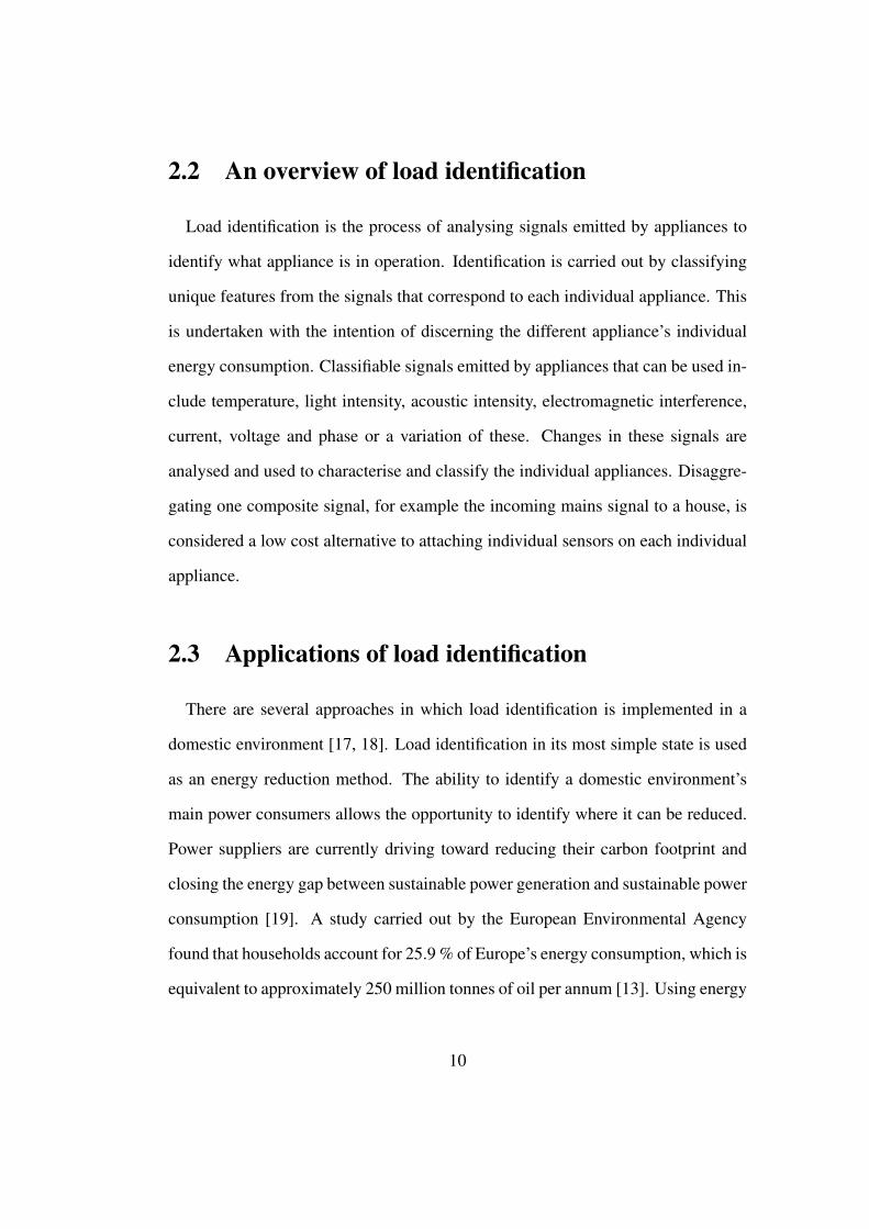
2.2 An overview of load identification

Load identification is the process of analysing signals emitted by appliances to

identify what appliance is in operation. Identification is carried out by classifying

unique features from the signals that correspond to each individual appliance. This

is undertaken with the intention of discerning the different appliance’s individual

energy consumption. Classifiable signals emitted by appliances that can be used in-

clude temperature, light intensity, acoustic intensity, electromagnetic interference,

current, voltage and phase or a variation of these. Changes in these signals are

analysed and used to characterise and classify the individual appliances. Disaggre-

gating one composite signal, for example the incoming mains signal to a house, is

considered a low cost alternative to attaching individual sensors on each individual

appliance.

2.3 Applications of load identification

There are several approaches in which load identification is implemented in a

domestic environment [17, 18]. Load identification in its most simple state is used

as an energy reduction method. The ability to identify a domestic environment’s

main power consumers allows the opportunity to identify where it can be reduced.

Power suppliers are currently driving toward reducing their carbon footprint and

closing the energy gap between sustainable power generation and sustainable power

consumption [19]. A study carried out by the European Environmental Agency

found that households account for 25.9 % of Europe’s energy consumption, which is

equivalent to approximately 250 million tonnes of oil per annum [13]. Using energy

10

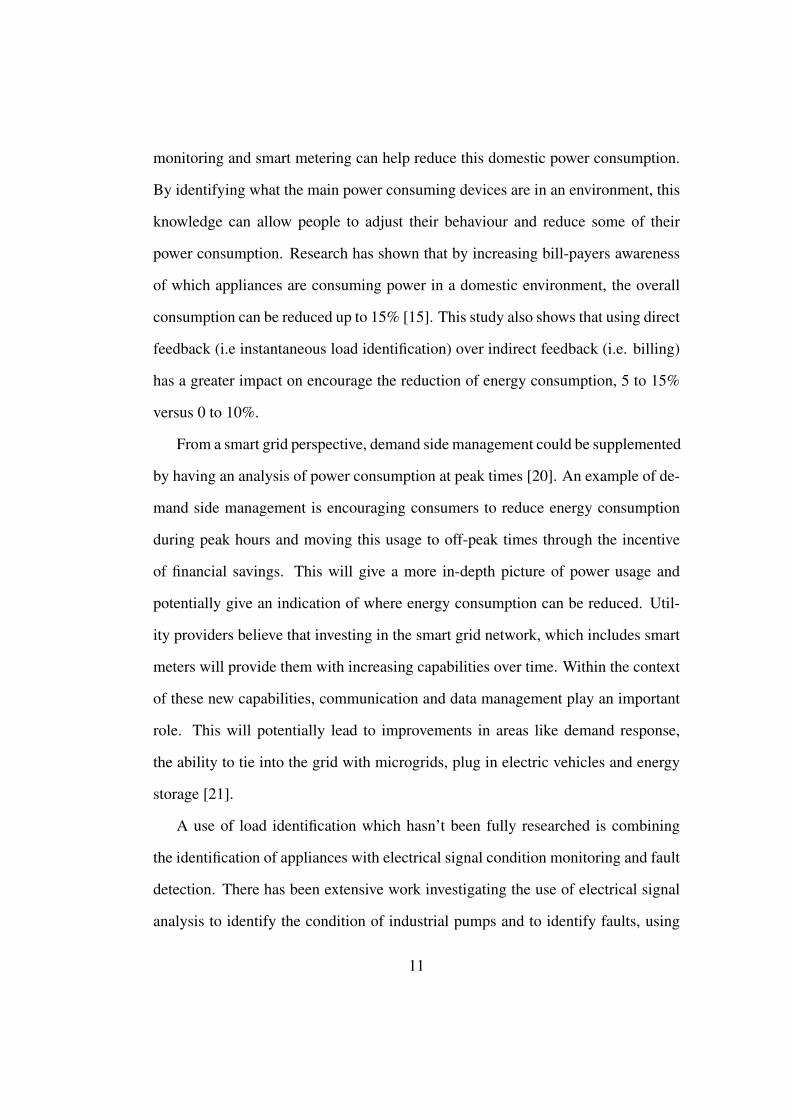
monitoring and smart metering can help reduce this domestic power consumption.

By identifying what the main power consuming devices are in an environment, this

knowledge can allow people to adjust their behaviour and reduce some of their

power consumption. Research has shown that by increasing bill-payers awareness

of which appliances are consuming power in a domestic environment, the overall

consumption can be reduced up to 15% [15]. This study also shows that using direct

feedback (i.e instantaneous load identification) over indirect feedback (i.e. billing)

has a greater impact on encourage the reduction of energy consumption, 5 to 15%

versus 0 to 10%.

From a smart grid perspective, demand side management could be supplemented

by having an analysis of power consumption at peak times [20]. An example of de-

mand side management is encouraging consumers to reduce energy consumption

during peak hours and moving this usage to off-peak times through the incentive

of financial savings. This will give a more in-depth picture of power usage and

potentially give an indication of where energy consumption can be reduced. Util-

ity providers believe that investing in the smart grid network, which includes smart

meters will provide them with increasing capabilities over time. Within the context

of these new capabilities, communication and data management play an important

role. This will potentially lead to improvements in areas like demand response,

the ability to tie into the grid with microgrids, plug in electric vehicles and energy

storage [21].

A use of load identification which hasn’t been fully researched is combining

the identification of appliances with electrical signal condition monitoring and fault

detection. There has been extensive work investigating the use of electrical signal

analysis to identify the condition of industrial pumps and to identify faults, using

11

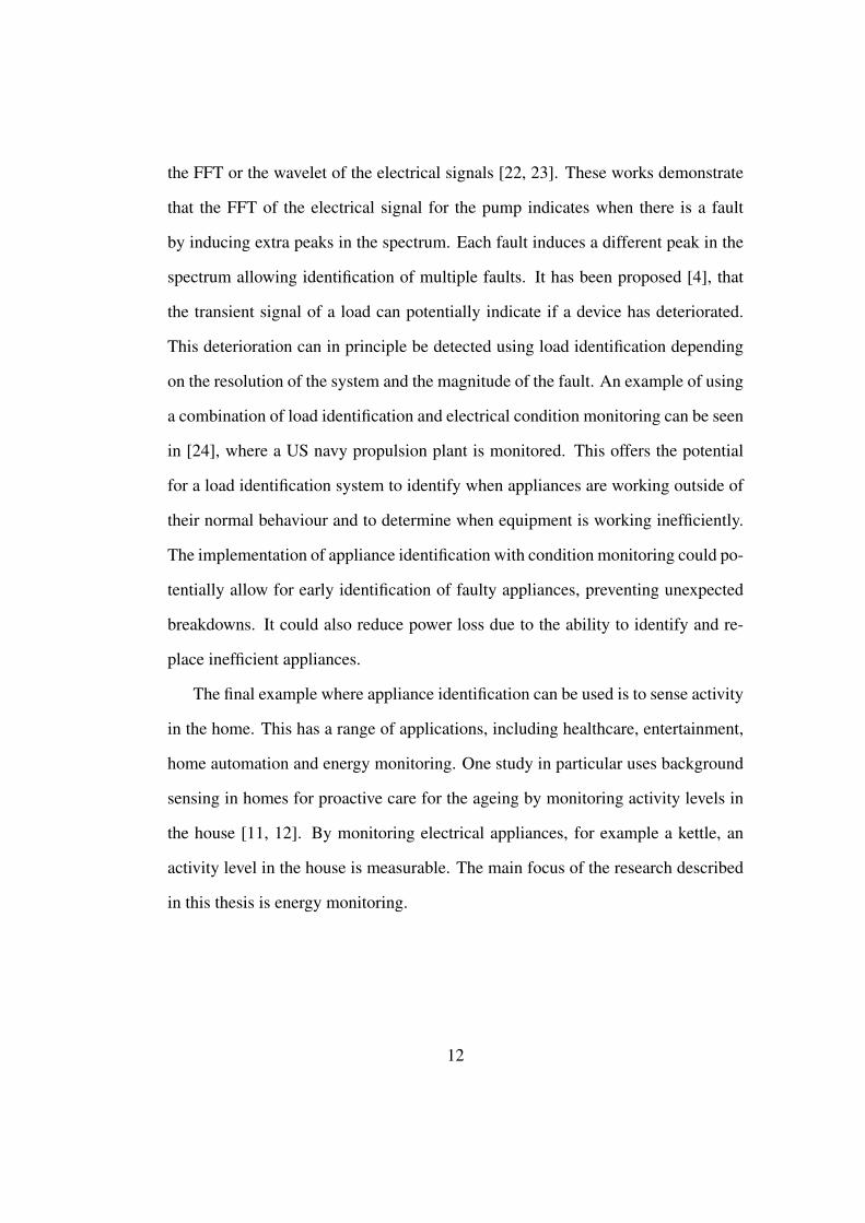
the FFT or the wavelet of the electrical signals [22, 23]. These works demonstrate

that the FFT of the electrical signal for the pump indicates when there is a fault

by inducing extra peaks in the spectrum. Each fault induces a different peak in the

spectrum allowing identification of multiple faults. It has been proposed [4], that

the transient signal of a load can potentially indicate if a device has deteriorated.

This deterioration can in principle be detected using load identification depending

on the resolution of the system and the magnitude of the fault. An example of using

a combination of load identification and electrical condition monitoring can be seen

in [24], where a US navy propulsion plant is monitored. This offers the potential

for a load identification system to identify when appliances are working outside of

their normal behaviour and to determine when equipment is working inefficiently.

The implementation of appliance identification with condition monitoring could po-

tentially allow for early identification of faulty appliances, preventing unexpected

breakdowns. It could also reduce power loss due to the ability to identify and re-

place inefficient appliances.

The final example where appliance identification can be used is to sense activity

in the home. This has a range of applications, including healthcare, entertainment,

home automation and energy monitoring. One study in particular uses background

sensing in homes for proactive care for the ageing by monitoring activity levels in

the house [11, 12]. By monitoring electrical appliances, for example a kettle, an

activity level in the house is measurable. The main focus of the research described

in this thesis is energy monitoring.

12

2.4 Load identification signal acquisition techniques

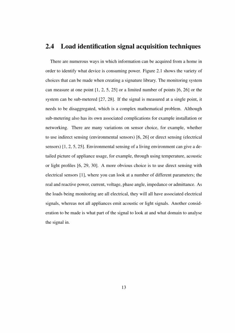
There are numerous ways in which information can be acquired from a home in

order to identify what device is consuming power. Figure 2.1 shows the variety of

choices that can be made when creating a signature library. The monitoring system

can measure at one point [1, 2, 5, 25] or a limited number of points [6, 26] or the

system can be sub-metered [27, 28]. If the signal is measured at a single point, it

needs to be disaggregated, which is a complex mathematical problem. Although

sub-metering also has its own associated complications for example installation or

networking. There are many variations on sensor choice, for example, whether

to use indirect sensing (environmental sensors) [6, 26] or direct sensing (electrical

sensors) [1, 2, 5, 25]. Environmental sensing of a living environment can give a de-

tailed picture of appliance usage, for example, through using temperature, acoustic

or light profiles [6, 29, 30]. A more obvious choice is to use direct sensing with

electrical sensors [1], where you can look at a number of different parameters; the

real and reactive power, current, voltage, phase angle, impedance or admittance. As

the loads being monitoring are all electrical, they will all have associated electrical

signals, whereas not all appliances emit acoustic or light signals. Another consid-

eration to be made is what part of the signal to look at and what domain to analyse

the signal in.

13

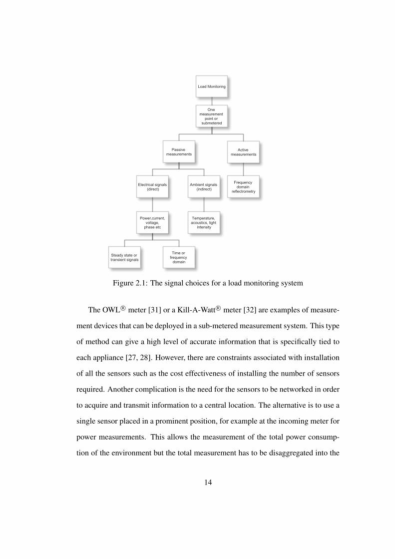
Figure 2.1: The signal choices for a load monitoring system

The OWL R© meter [31] or a Kill-A-Watt R© meter [32] are examples of measure-

ment devices that can be deployed in a sub-metered measurement system. This type

of method can give a high level of accurate information that is specifically tied to

each appliance [27, 28]. However, there are constraints associated with installation

of all the sensors such as the cost effectiveness of installing the number of sensors

required. Another complication is the need for the sensors to be networked in order

to acquire and transmit information to a central location. The alternative is to use a

single sensor placed in a prominent position, for example at the incoming meter for

power measurements. This allows the measurement of the total power consump-

tion of the environment but the total measurement has to be disaggregated into the

14

contributing appliances.

The sampling frequency at which the measurements are taken is an important

consideration. Low frequency measurements are taken at a sampling rate of ap-

proximately 1 Hz and the higher frequency measurements are taken at rates ranging

from 105 Hz (which is derived from the Nyquist-Shannon sampling theorem and is

a minimum of two times the fundamental frequency) to 500 kHz. Low frequency

measurements tend to depend on using features such as time of use or operation

duration. Higher frequency measurements allow an in-depth snapshot of events -

particularly transient events when devices turn on, off or to different states.

Generally the physical measurement system is designed with a specific mea-

surement signal in mind. The system is optimised for the type of signal being

analysed, whether it is a transient or steady state signal and in the time or frequency

domain.

2.5 Appliance characterisation signature types

This section outlines the different types of signature libraries used in a appliance

load identification system. These methods are based either on the transient elec-

trical signal, the steady state electrical signal or an ambient environmental signal.

Some of these signatures are analysed in the frequency domain, while others in the

temporal domain.

2.5.1 Steady state signatures

Signatures based on steady state signals are one of the more popular load iden-

tification methods [1, 2, 33, 34, 35]. Transients tend to last for less than five sec-

15

onds and have been found to be less repeatable than steady state signals by some

researchers [36]. The steady state signal lasts for the duration of an appliance’s

operation, which, depending on the appliance can last for several minutes or more,

for example typically a kettle runs for three minutes, a fridge for twenty minutes

and a TV could be run for an hour upwards. The following section details the four

most significant ways in which a steady state signature has been used to identify

appliances. The first method is one of the most popular methods and it uses the real

and reactive power to identify appliances with a simple matching algorithm; the

second method uses the real power with a more complex decision algorithm; the

third method is based on the frequency spectrum of the appliance; and the fourth

method uses a combination of multiple signature types.

Using signatures from the temporal domain is also one of the more popular

methods being used to identify appliances [3, 4, 37, 38, 39]. One of the first papers

which used this approach was Hart [1], where high frequency measurements of

real (P) and reactive (Q) power are categorised into a PQ signature space (Figure

2.2). As can be seen in the figure, loads that are far from each other in the PQ

signature space are easy to identify. However this method also leads to overlapping

devices which lie in the same area of the signature space when appliances consume

approximately the same real and reactive power. An algorithm which matches equal

turn on and turn off power changes is used to detect appliances. The matching

algorithm assumes that the positive change of power (start on) matches the negative

change of power (turn off). This method can easily detect and track the on-off

appliances, but has problems in detecting multi-state and variable-load appliances.

Another problem with this method is due to appliances changing their resistance

after they turn on, from the heating of components. Appliances can be mismatched

16

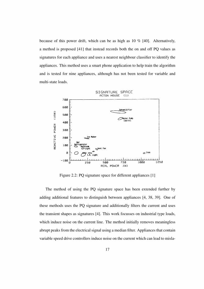
because of this power drift, which can be as high as 10 % [40]. Alternatively,

a method is proposed [41] that instead records both the on and off PQ values as

signatures for each appliance and uses a nearest neighbour classifier to identify the

appliances. This method uses a smart phone application to help train the algorithm

and is tested for nine appliances, although has not been tested for variable and

multi-state loads.

Figure 2.2: PQ signature space for different appliances [1]

The method of using the PQ signature space has been extended further by

adding additional features to distinguish between appliances [4, 38, 39]. One of

these methods uses the PQ signature and additionally filters the current and uses

the transient shapes as signatures [4]. This work focusses on industrial type loads,

which induce noise on the current line. The method initially removes meaningless

abrupt peaks from the electrical signal using a median filter. Appliances that contain

variable speed drive controllers induce noise on the current which can lead to misla-

17

belling appliances. This approach considers the shapes of the transient events (their

power profile in time) as an additional feature. This method is discussed in further

detail in the transient section below. An alternative additional feature proposed was

to use edge detection of appliances from powering on and off or changing between

states, and the slopes of the appliance’s current during operation [38, 39]. This

method was developed exclusively for appliances with significant power draw, for

example a washing machine or refrigerator and was tested for identifying up to six

appliances successfully.

The second steady state signature method uses a simple signature based on the

real power and a complex algorithm [40, 33, 34]. This method has a high accuracy

(90%) in identifying large household appliances (for example white goods appli-

ances) with distinguishable power features. These methods tend to train appliance

models based on usage patterns. Generic models of appliance are tuned to specific

appliance instances using aggregate data, for example fridges have typical charac-

teristics like the shape of their current draw over time. A generic model is created

based on this shape and then tuned to the specific values for the actual instance of

this appliance. These models are used to disaggregate the energy consumption of

individual appliances from a household’s aggregate load. To combat the problem of

distinguishing between appliances with similar power consumption, the algorithm

uses rules about appliance behaviour, for example time of use or length of usage

[40]. Another example of one of these types of methods is based on modelling the

appliances using hidden Markov models (HMMs) [33, 34]. The appliances models

are disaggregated using an extension of the Viterbi algorithm, before being sub-

tracted from the aggregate load. This method is evaluated using real data from

multiple households and it is shown that it is possible to generalise between similar

18

appliances in different households. The tests involve disaggregating specific large

appliances (for example a refrigerator and electric shower) from household data

using sub-metered training data and total current draw at mains as test data. The

method is not tested on all appliances in the household and does not work for small

loads.

The third steady state signature method analyses the steady state signals in the

frequency domain and uses the spectrum as a signature for each appliance. This

method of using the steady state signal in the frequency domain has been explored

in various ways. The first suggestion of using the power spectrum as a characteristic

can be found in papers by Hart and Sultanem [1, 35] but they deferred to using

the PQ signature space as their main techniques. Using harmonic content as a

signature was not implemented until 2000 when a method for identifying ten loads

in a three phase environment was developed by measuring a variation of the (1st,

2nd, 3rd, 4th, 5th, 7th and 9th) current harmonics of each load [36]. They found

that the steady state measurement had a lower standard deviation than the transient

measurement and was more repeatable. Using the harmonic spectrum was also

suggested as a method for identifying variable speed loads [42]. Variable-speed

drives (VSDs) are industrially important variable-demand loads that are difficult to

track non-intrusively. VSDs can also be found in domestic appliances, for example

a vacuum cleaner. The method uses the correlation between the fundamental power

harmonic and selected harmonics as an identifier for the motor. The correlations

are strong they can be modelled by a function [42]. The reason for this correlation

is unknown and therefore could make this method unstable.

The most complete method using the spectrum of the steady state signal as a sig-

nature was developed by Srinivasan [2], who proposed using the first fifteen FFT

19

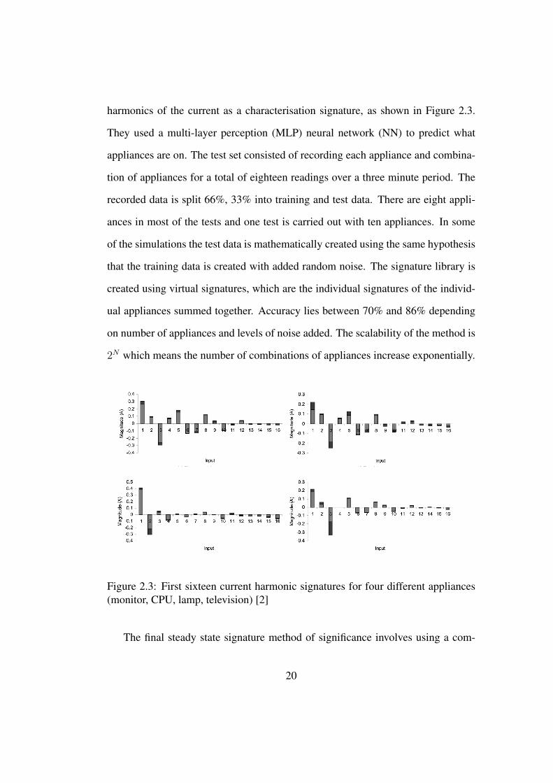
harmonics of the current as a characterisation signature, as shown in Figure 2.3.

They used a multi-layer perception (MLP) neural network (NN) to predict what

appliances are on. The test set consisted of recording each appliance and combina-

tion of appliances for a total of eighteen readings over a three minute period. The

recorded data is split 66%, 33% into training and test data. There are eight appli-

ances in most of the tests and one test is carried out with ten appliances. In some

of the simulations the test data is mathematically created using the same hypothesis

that the training data is created with added random noise. The signature library is

created using virtual signatures, which are the individual signatures of the individ-

ual appliances summed together. Accuracy lies between 70% and 86% depending

on number of appliances and levels of noise added. The scalability of the method is

2N which means the number of combinations of appliances increase exponentially.

Figure 2.3: First sixteen current harmonic signatures for four different appliances(monitor, CPU, lamp, television) [2]

The final steady state signature method of significance involves using a com-

20

bination of multiple signatures. The CLP Research Institute [3, 37] uses seven

different load signatures to identify their appliances. The seven signatures are PQ,

the current waveform, the eigenvalues, the instantaneous admittance waveform, the

FFT harmonics of the current, the length of the switching transient waveform and

the instantaneous power waveform. The appliance library consists of twenty-seven

different appliances. The test data is created based on the individual measure-

ments, where events and combinations of appliances are mathematically created

using Monte Carlo methods and noise was added. There are three simulations sce-

narios tested, the first are normally distributed switching events, the second are

evenly distributed switching events and the third are behaviourally based switching

events. The algorithm detects an event as a change in power of 100 W and the dif-

ference between two time periods, one before and one after the event, is found. The

seven unknown signatures are derived from this event. These unknown signatures

are each classified using a least residue method and a NN and provide a candidate

pool of possible predictions. A committee decision is made using this candidate

pool to decide what appliance(s) have just turned on or off. The three committee

decision types used are most common appliance (MCO) predicted, least unified

residue (LUR) (i.e. the smallest difference between the event signature and the pre-

dicted signatures) and a maximum likelihood estimate (MLE), which is based on a

simulated a priori knowledge estimation of the probability reflecting the accuracy

of the combination. The MLE is the most computationally intensive method and

involves a large amount of a priori simulation for the appliances. There are several

results from the method, the accuracy of the method (with both ACs on) is 90% for

MLE, 85% for the LUR and 83% for the MCO. The accuracy decreases with the

number of appliances operating simultaneously, it decreases by about 10% when

21

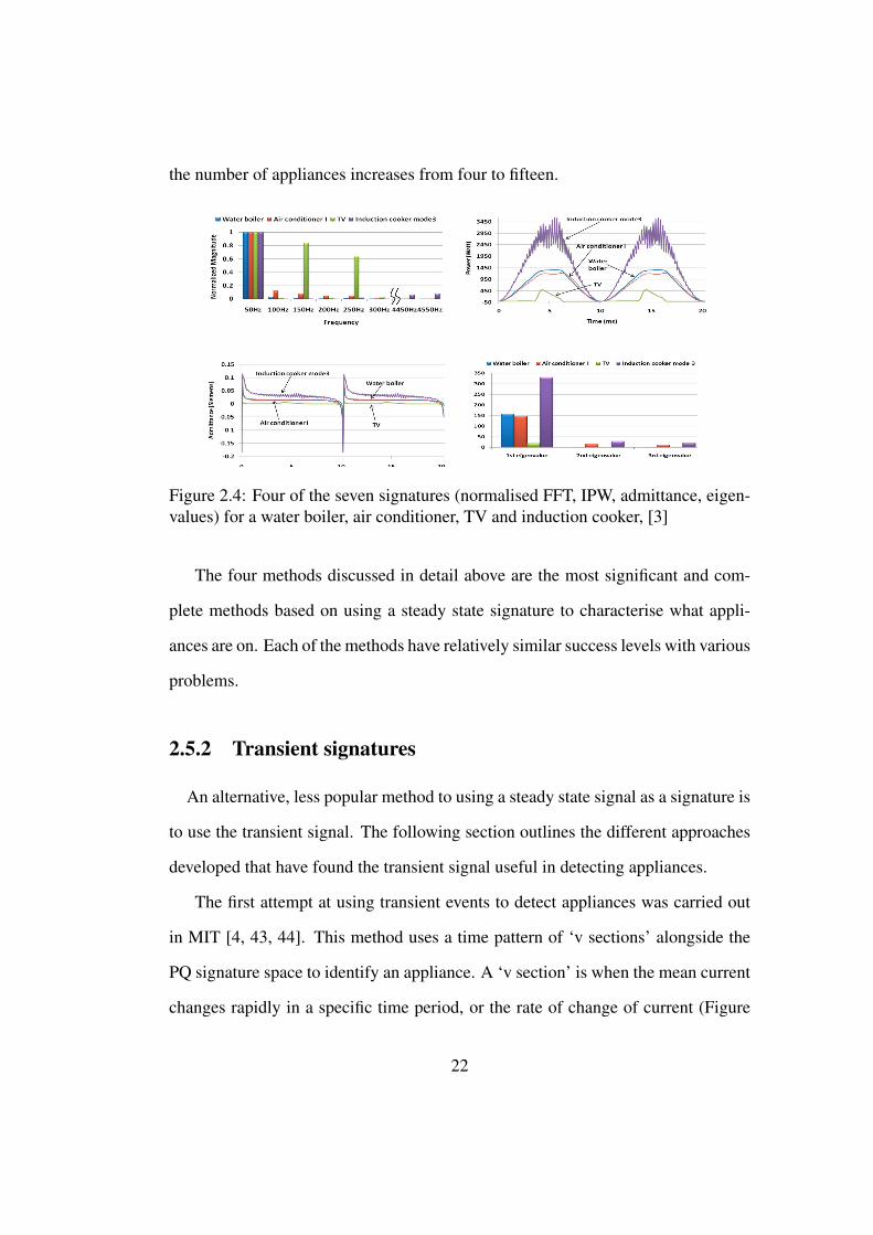
the number of appliances increases from four to fifteen.

Figure 2.4: Four of the seven signatures (normalised FFT, IPW, admittance, eigen-values) for a water boiler, air conditioner, TV and induction cooker, [3]

The four methods discussed in detail above are the most significant and com-

plete methods based on using a steady state signature to characterise what appli-

ances are on. Each of the methods have relatively similar success levels with various

problems.

2.5.2 Transient signatures

An alternative, less popular method to using a steady state signal as a signature is

to use the transient signal. The following section outlines the different approaches

developed that have found the transient signal useful in detecting appliances.

The first attempt at using transient events to detect appliances was carried out

in MIT [4, 43, 44]. This method uses a time pattern of ‘v sections’ alongside the

PQ signature space to identify an appliance. A ‘v section’ is when the mean current

changes rapidly in a specific time period, or the rate of change of current (Figure

22

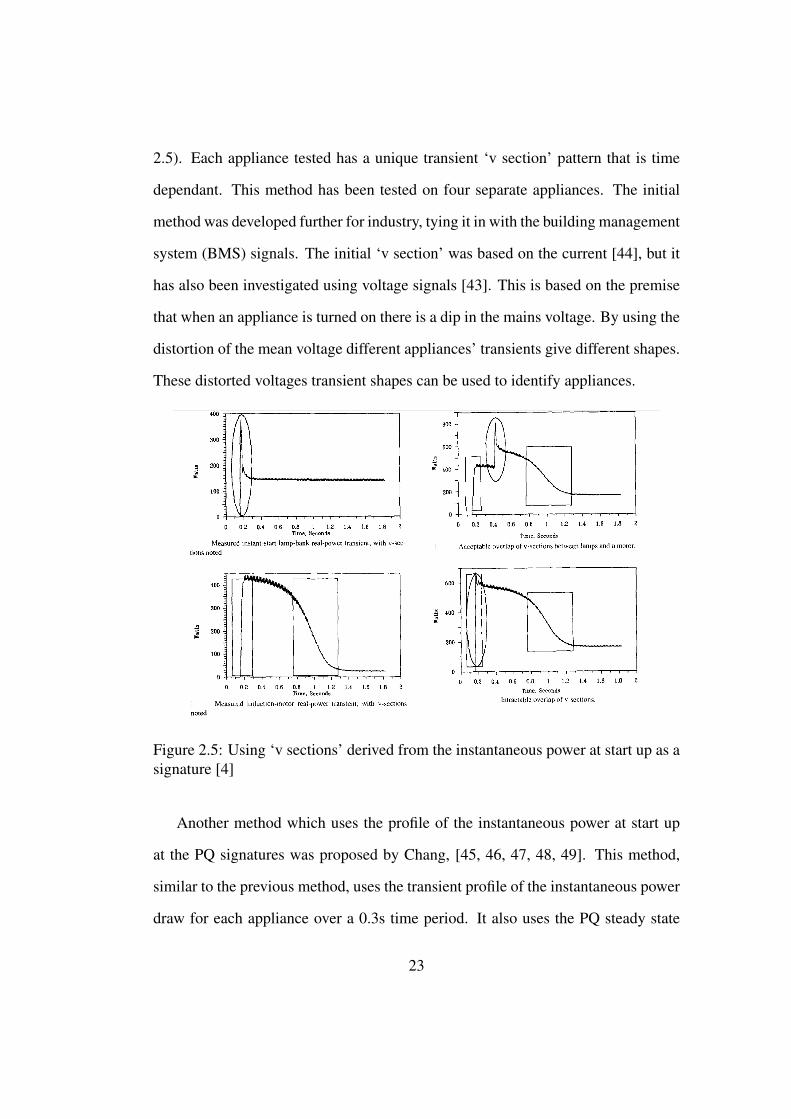
2.5). Each appliance tested has a unique transient ‘v section’ pattern that is time

dependant. This method has been tested on four separate appliances. The initial

method was developed further for industry, tying it in with the building management

system (BMS) signals. The initial ‘v section’ was based on the current [44], but it

has also been investigated using voltage signals [43]. This is based on the premise

that when an appliance is turned on there is a dip in the mains voltage. By using the

distortion of the mean voltage different appliances’ transients give different shapes.

These distorted voltages transient shapes can be used to identify appliances.

Figure 2.5: Using ‘v sections’ derived from the instantaneous power at start up as asignature [4]

Another method which uses the profile of the instantaneous power at start up

at the PQ signatures was proposed by Chang, [45, 46, 47, 48, 49]. This method,

similar to the previous method, uses the transient profile of the instantaneous power

draw for each appliance over a 0.3s time period. It also uses the PQ steady state

23

signals and a multi layer feed forward (MLFF) neural network. The system is tested

for three appliances which have similar PQ signatures and the transient signature is

used to distinguish between the appliances further. Each of the transient signatures

are recorded for four seconds at 30kHz, there are 78 events recorded in total. Half

of the data is used for training and and half for testing. The average accuracy of the

method is 87%. This method is tested for a total of five different appliances, it is

found that the accuracy of the method increases from approximately 60% to 90 %

when the PQ signature is supplemented with the transient signature. The scalability

of this method with the addition of more appliances is (N +N2).

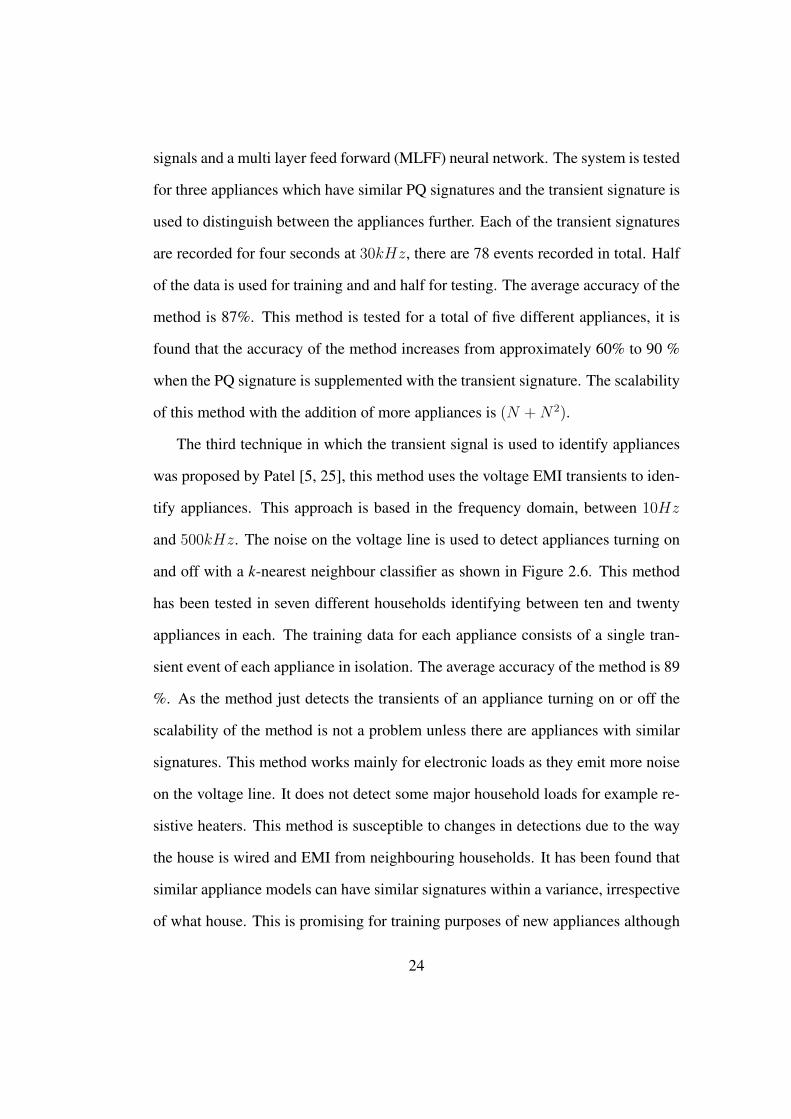
The third technique in which the transient signal is used to identify appliances

was proposed by Patel [5, 25], this method uses the voltage EMI transients to iden-

tify appliances. This approach is based in the frequency domain, between 10Hz

and 500kHz. The noise on the voltage line is used to detect appliances turning on

and off with a k-nearest neighbour classifier as shown in Figure 2.6. This method

has been tested in seven different households identifying between ten and twenty

appliances in each. The training data for each appliance consists of a single tran-

sient event of each appliance in isolation. The average accuracy of the method is 89

%. As the method just detects the transients of an appliance turning on or off the

scalability of the method is not a problem unless there are appliances with similar

signatures. This method works mainly for electronic loads as they emit more noise

on the voltage line. It does not detect some major household loads for example re-

sistive heaters. This method is susceptible to changes in detections due to the way

the house is wired and EMI from neighbouring households. It has been found that

similar appliance models can have similar signatures within a variance, irrespective

of what house. This is promising for training purposes of new appliances although

24

this can also cause a problem when there are similar appliances in different rooms

which can be mislabelled as one another

Figure 2.6: Using the transient EMI noise on the voltage line as a signature toidentify different appliances [5]

The three methods listed above are the significant methods which use transient

information to identify appliances. Again none of these methods are a complete

solution and still have problems associated with them that need to be addressed

before a complete load monitoring system can be defined.

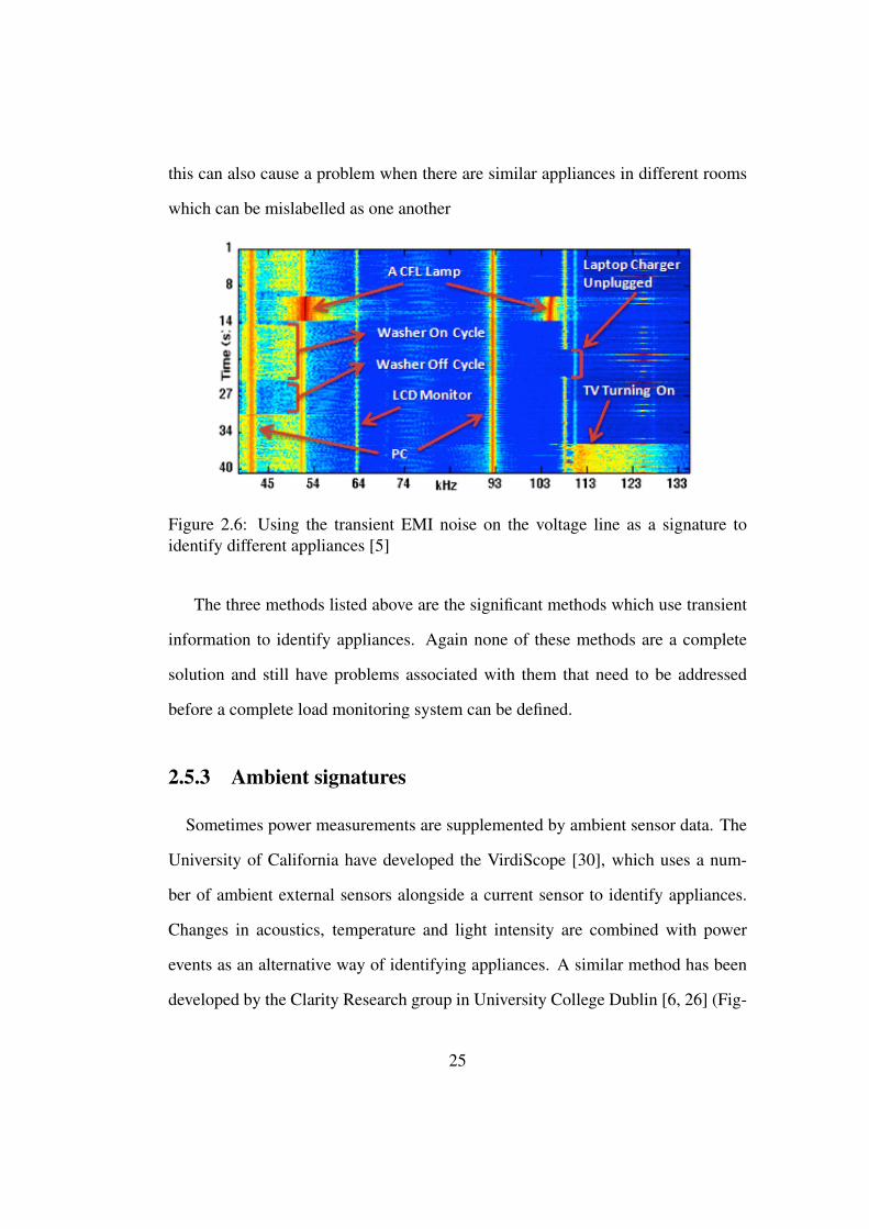
2.5.3 Ambient signatures

Sometimes power measurements are supplemented by ambient sensor data. The

University of California have developed the VirdiScope [30], which uses a num-

ber of ambient external sensors alongside a current sensor to identify appliances.

Changes in acoustics, temperature and light intensity are combined with power

events as an alternative way of identifying appliances. A similar method has been

developed by the Clarity Research group in University College Dublin [6, 26] (Fig-

25

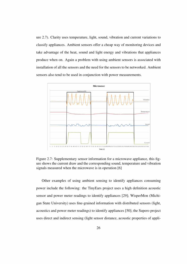
ure 2.7). Clarity uses temperature, light, sound, vibration and current variations to

classify appliances. Ambient sensors offer a cheap way of monitoring devices and

take advantage of the heat, sound and light energy and vibrations that appliances

produce when on. Again a problem with using ambient sensors is associated with

installation of all the sensors and the need for the sensors to be networked. Ambient

sensors also tend to be used in conjunction with power measurements.

Figure 2.7: Supplementary sensor information for a microwave appliance, this fig-ure shows the current draw and the corresponding sound, temperature and vibrationsignals measured when the microwave is in operation [6]

Other examples of using ambient sensing to identify appliances consuming

power include the following: the TinyEars project uses a high definition acoustic

sensor and power meter readings to identify appliances [29]; WisperMon (Michi-

gan State University) uses fine-grained information with distributed sensors (light,

acoustics and power meter readings) to identify appliances [50]; the Supero project

uses direct and indirect sensing (light sensor distance, acoustic properties of appli-

26

ances, and appliances rated powers) to identify appliances [51]. A method of using

ambient light sensors was proposed by Jazizadeh, from the University of Southern

California [52]. Baranski proposed using an optical sensor that reads the revolu-

tions of a houses’ power meter to monitor power usage [53]. Alahmad suggested

alongside using power feature analysis to use time domain reflectrometry (TDR)

and frequency domain reflectrometry (FDR) to find the location of the appliances

[54]. These methods represent alternative approaches to monitoring and identify-

ing when appliances are consuming power. Using environmental sensors alongside

power sensors to identify appliances is a way of increasing the accuracy of a load

identification system.

2.6 Appliance classification algorithms and performance

metrics

The main research effort in appliance load identification has been focused on

signature exploration rather than algorithm development. Each of the power moni-

toring methods described above use a classification algorithm to decide which ap-

pliance is consuming power. Classification is the problem of identifying to which

of a set of classes a new observation belongs, on the basis of a training set of data

containing observations whose class membership is known. In machine learning,

classifiers are associated with supervised learning. Supervised learning is the task

of creating a function based on labelled training data.

Support vector machines (SVMs) have been used in several different load iden-

tification methods. Patel [25] uses high frequency transient current information and

27

a SVM to identify appliances. They are also used in [55] with features extracted

from the real and reactive power signals. A SVM is one of the most robust clas-

sification algorithms [56]. A SVM only requires a small number of training data

samples and is insensitive to the number of dimensions each class may have. The

classification is performed geometrically, which means that each class occupies a

space derived from the training data. The best classification function is found by

maximizing the margin between the classes. An initial drawback of SVMs is their

computational inefficiency when the number of classes increases to thousands, al-

though this is not really a problem with load identification algorithms, where the

maximum number of appliances tend to be around forty [57]. In order to work for

a problem with such a large number of classes the approach is to break the larger

optimization problem into a series of carefully chosen smaller variables.

Hidden Markov models (HMMs) [33, 58, 59, 60] are a classifier typically used

with low frequency measurements in load identification, where the maximum sam-

pling time is every one second. The data tends to be real power or real current and

contains less information than higher frequency measurements. HMMs are widely

used to model stochastic processes and are suited to modelling the combination of

independent processes [61]. HMMs are a popular algorithm choice as the mod-

els are mathematically rich and when applied properly, they work well in practice.

There are four main components in a HMM; the states, or the labels that are to

be assigned; the emission probabilities, each state has its own emission probabil-

ity which are based on the parameters of each class; the transition probabilities,

which is the probability of moving from one state to another; and the final compo-

nent is the output probability [62]. An HMM generates a sequence, when one state

is visited, there is a residue from the states emission probability distribution. The

28

next state to visit is chosen according to the state’s transition probability distribu-

tion. The model thus generates two strings of information. One is the underlying

state path, as the model transitions from state to state. The other is the observed

sequence, each residue being emitted from one state in the state path. HMMs do

not deal well with correlations between residues as they assume that each residue

depends only on one underlying state.

Each appliance is modelled as a single HMM trained using a number of obser-

vations. An example of an observation used could be the initial probability of an

appliance state, the number of possible states an appliance may have or the prob-

ability of the appliance being on at a particular point in time. The system uses an

observation to infer what state has changed. The task is to identify, given the pa-

rameters of the model, the probability of a particular output sequence. One of the

difficulties with using HMMs is determining how a given observation sequence is

derived. The observation sequence is used to adjust the model parameters during

the training sequence. The training problem is the crucial one for most applications

of HMMs, since it allows the model parameters to be adapted under observed train-

ing. There is no known way to analytically solve for the model which maximizes

the probability of the observation sequence.

Finite state machines (FSMs) are another example of an algorithm which has

been implemented in load identification, for example Hart [1] uses the PQ signature

space and a FSM to identify appliances. FSMs are widely used to model systems

in diverse areas [63]. A FSM is an abstract machine that can be in one of a finite

number of states. The machine is in only one state at a time; the state it is in at

any given time is called the current state. It can change from one state to another

when initiated by a triggering event or condition; this is called a transition. A

29

particular FSM is defined by a list of its states, and the triggering condition for

each transition. Optimizing an FSM means finding the machine with the minimum

number of states that performs the same function. FSM are not known for scaling

particularly well. Another example of a load identification method using FSM is

[64] where the real power measurements sampled every second and a FSM is used

to decide what appliances are on.

Another relatively common classification method used are artificial neural net-

works (ANNs). An ANN is a computational mathematical model based on the

neural networks found in the brain [65]. An ANN works by using a weighted sum

of the inputs which represent ‘neurons’ to predict an output. The weights in an

ANN are adaptive and are tuned by a learning algorithm. The functionality of the

network is determined by the strengths of the connections between neurons. In a

supervised ANN the training data, i, is used to create an attribute vector Xi, and an

target vector Yi. Xi is processed through the neural network to produce an output yi,

the parameters or weights w of the network are modified to optimise the search and

minimised the total squared error. Non-linear functions are easily approximated us-

ing ANNs. ANNs are a black box method, so it is not obvious how it carries out its

decisions and can be difficult to interpret. ANNs can also be sensitive to the initial

choice of network parameters, such as the input weights.

An example of ANN being used for load identification can be seen in [46, 48,

49], where they are used in conjunction with a number of different signatures in-

cluding the real and reactive power, transient events and wavelets to improve ac-

curacy. The fifteen first real and imaginary current harmonics are used by [2] with

an ANN to identify appliances. Another method developed uses neural networks

in combination with a selection of features, namely the current waveform, active

30

and reactive power, harmonics, instantaneous admittance waveform, instantaneous

power waveform and eigenvalues and switching transient waveform to identify ap-

pliances [3]. An unusual method of using time domain reflectrometry along power

lines and the real time power in conjunction with an ANN [54, 66] uses turn on tran-

sients and the PQ space with neural networks. ANNs are one of the more popular

classification algorithms used in load identification.

A k-nearest neighbour (kNN) classifier has been used by [5] to classify appli-

ances using high frequency voltage information. The kNN classifier finds a group

of k objects in the training set that are closest to the test object and bases the assign-

ment of the label based on the neighbourhood [56]. This approach is based on a set

of labelled objects, a similarity measure to compute the distance between objects

and a value for k, the number of nearest neighbours to be considered.

There are a number of parameters that need to be decided before implementing

the kNN classifier, for example the choice of k. Another parameter to be chosen

is the size of the neighbourhood, which can affect the sensitivity of the classifier.

The choice in counting the labels in the neighbourhood, and whether to base it

on the majority number of the neighbours or the labels of the closest neighbours

is another parameter. How to measure the distance between objects, whether to

chose euclidean or cosine can also affect the results. This distance can depend on

the dimensionality of the data and whether the attributes need to be scaled, or if

one attribute will dominate the decision. A kNN classifier is a computationally

inexpensive model to build, but classifying unknown objects is relatively expensive

due to the need to compute the distance of the k nearest neighbours to each new

sample, which can be expensive for a large training data set. The kNN classifier

is a classifier that can perform well, despite its simplicity and is well suited for

31

multi-model classes.

The naive Bayes classifier is another classifier that has been as a classification

algorithm for a load identification method [67, 68]. It is an algorithm that can be

rapidly deployed within a system [69]. It is an appealing classifier because of its

simplicity, robustness and surprising effectiveness [56]. The classifier can be read-

ily applied to large data sets and the results are easy to interpret. An advantage of the

naive Bayes is that it only requires a small amount of training data to estimate the

parameters necessary for classification. The classifier is based on Bayes’ theorem

and assumes independence between the individual features and because indepen-

dent variables are assumed, only the variances of the features for each class need

to be calculated [56, 69]. Although the classifier assumes independence between

the individual features, it has been shown that the naive Bayes classifier may still

be optimal even when there are strong dependencies present between the attributes

[69, 70].

Some work has been carried out in the literature to compare different algorithms

for load identification. Marchiori et al [67] compared a maximum likelihood classi-

fier with a naive Bayes classifier using the PQ signature space. They found that the

naive Bayes classifier performed better. Reinhardt compares a total of nine differ-

ent classification methods including a Bayesian network, a naive Bayes, a random

forest and random committee method [68]. They find the Bayesian network the

most favourable method for their signature, with the naive Bayes classifier as a very

close second (0.03% difference in accuracy). It is clear that there is no one specific

classification method that is currently being used for load identification.

ANNs have been used in a number of load identification algorithms [2, 46, 48,

49] mainly due to their ability to recognize nonlinear functions, the ability to adapt

32

to different environments, and their high noise tolerance. In general neural net-

works have won popularity in time series analysis research, under which appliance

identification falls. However, current research in other fields, for example in the pre-

diction of packet-switched traffic, shows that in some cases traditional linear mod-

els can succeed over neural networks with less resources and less time-consuming

methods [71, 72]. Therefore although ANNs appear to be one of the more pop-

ular algorithms used in load identification methods, the naive Bayes classifier has

been chosen as the classifier in this work. Of the work that has been carried out

to compare between different classification methods [67, 68] it has been found that

the naive Bayes classifier performs very well. Also, the results from a naive Bayes

classifier are easy to interpret, whereas an ANN is a black box method so it can be

difficult to interpret the decision process.

2.6.1 Performance metrics: accuracy

To ensure that the identification system and classification algorithm being used

is effective the accuracy is calculated to assess its performance. This is done by

comparing the output results of the classifier with the expected targets. In statistical

analysis there are two types of error that can occur, a type I error which is a false

positive and a type II error which is a false negative. For the purpose of this work,

and as mentioned in [17], a receiver operating characteristic (ROC) curve is used to

test effectiveness of the algorithm. The ROC curve [73] illustrates the performance

of a binary classifier system by identifying the true positives, true negatives, false

positives and false negatives. An example of a true negative (TN), false negative

(FN), false positive (FP) and true positive (TP) can be seen in Table 2.1.

33

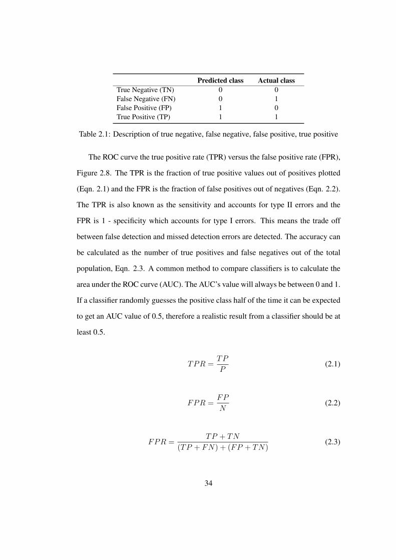
Predicted class Actual classTrue Negative (TN) 0 0False Negative (FN) 0 1False Positive (FP) 1 0True Positive (TP) 1 1

Table 2.1: Description of true negative, false negative, false positive, true positive

The ROC curve the true positive rate (TPR) versus the false positive rate (FPR),

Figure 2.8. The TPR is the fraction of true positive values out of positives plotted

(Eqn. 2.1) and the FPR is the fraction of false positives out of negatives (Eqn. 2.2).

The TPR is also known as the sensitivity and accounts for type II errors and the

FPR is 1 - specificity which accounts for type I errors. This means the trade off

between false detection and missed detection errors are detected. The accuracy can

be calculated as the number of true positives and false negatives out of the total

population, Eqn. 2.3. A common method to compare classifiers is to calculate the

area under the ROC curve (AUC). The AUC’s value will always be between 0 and 1.

If a classifier randomly guesses the positive class half of the time it can be expected

to get an AUC value of 0.5, therefore a realistic result from a classifier should be at

least 0.5.

TPR =TP

P(2.1)

FPR =FP

N(2.2)

FPR =TP + TN

(TP + FN) + (FP + TN)(2.3)

34

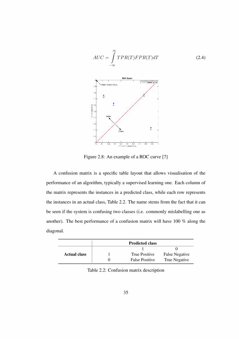
AUC =

∞∫−∞

TPR(T )FPR(T )dT (2.4)

Figure 2.8: An example of a ROC curve [7]

A confusion matrix is a specific table layout that allows visualisation of the

performance of an algorithm, typically a supervised learning one. Each column of

the matrix represents the instances in a predicted class, while each row represents

the instances in an actual class, Table 2.2. The name stems from the fact that it can

be seen if the system is confusing two classes (i.e. commonly mislabelling one as

another). The best performance of a confusion matrix will have 100 % along the

diagonal.

Predicted class

Actual class1 0

1 True Positive False Negative0 False Positive True Negative

Table 2.2: Confusion matrix description

35

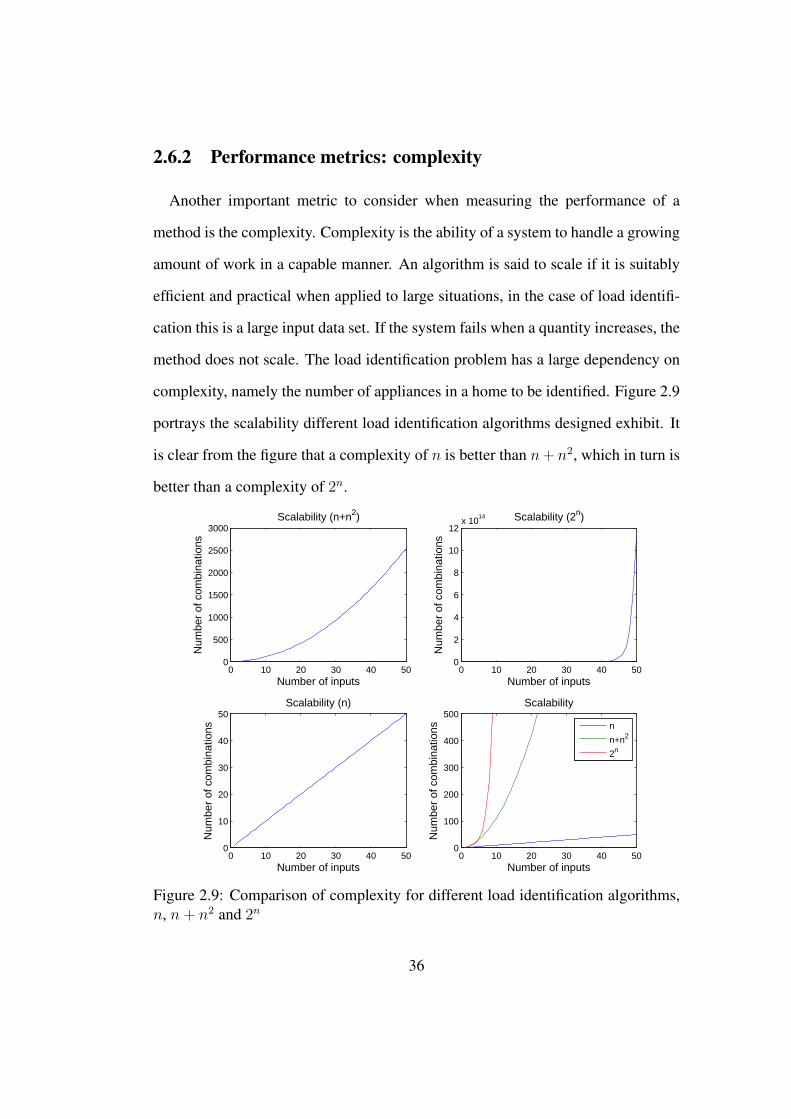
2.6.2 Performance metrics: complexity

Another important metric to consider when measuring the performance of a

method is the complexity. Complexity is the ability of a system to handle a growing

amount of work in a capable manner. An algorithm is said to scale if it is suitably

efficient and practical when applied to large situations, in the case of load identifi-

cation this is a large input data set. If the system fails when a quantity increases, the

method does not scale. The load identification problem has a large dependency on

complexity, namely the number of appliances in a home to be identified. Figure 2.9

portrays the scalability different load identification algorithms designed exhibit. It

is clear from the figure that a complexity of n is better than n+ n2, which in turn is

better than a complexity of 2n.

0 10 20 30 40 500

500

1000

1500

2000

2500

3000Scalability (n+n2)

Num

ber

of c

ombi

natio

ns

Number of inputs0 10 20 30 40 50

0

2

4

6

8

10

12x 10

14 Scalability (2n)

Num

ber

of c

ombi

natio

ns

Number of inputs

0 10 20 30 40 500

10

20

30

40

50Scalability (n)

Num

ber

of c

ombi

natio

ns

Number of inputs0 10 20 30 40 50

0

100

200

300

400

500Scalability

Num

ber

of c

ombi

natio

ns

Number of inputs

n

n+n2

2n

Figure 2.9: Comparison of complexity for different load identification algorithms,n, n+ n2 and 2n

36

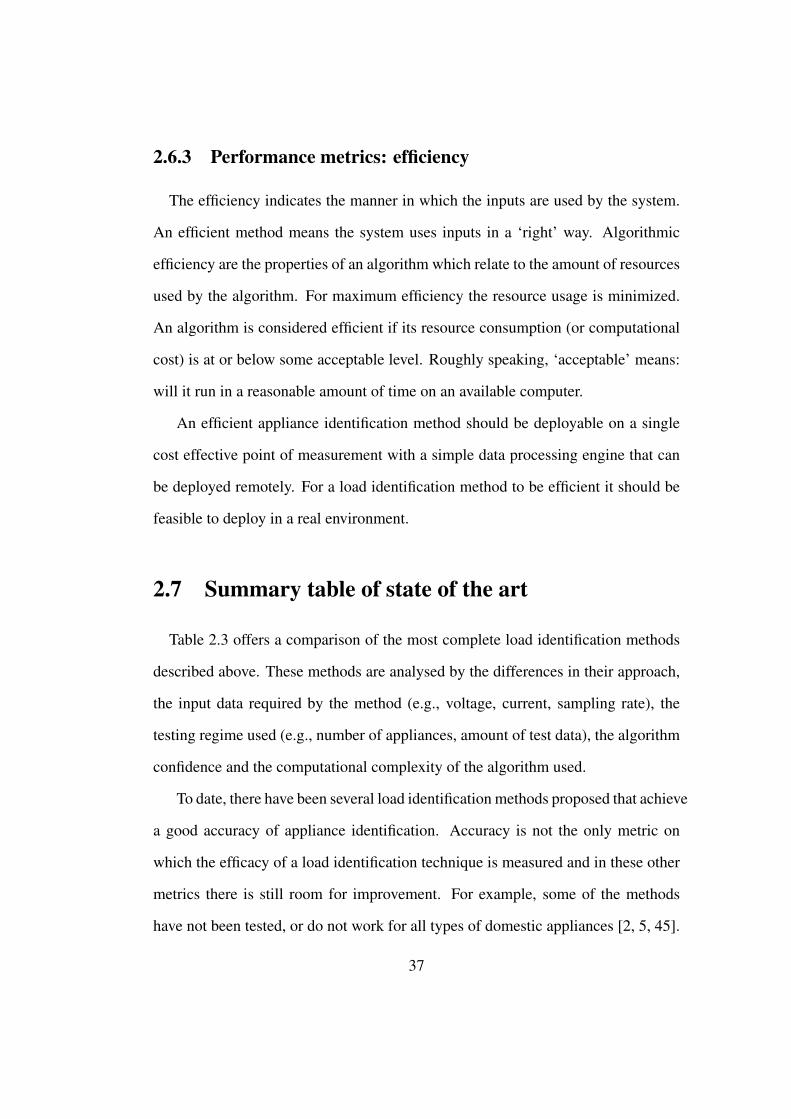
2.6.3 Performance metrics: efficiency

The efficiency indicates the manner in which the inputs are used by the system.

An efficient method means the system uses inputs in a ‘right’ way. Algorithmic

efficiency are the properties of an algorithm which relate to the amount of resources

used by the algorithm. For maximum efficiency the resource usage is minimized.

An algorithm is considered efficient if its resource consumption (or computational

cost) is at or below some acceptable level. Roughly speaking, ‘acceptable’ means:

will it run in a reasonable amount of time on an available computer.

An efficient appliance identification method should be deployable on a single

cost effective point of measurement with a simple data processing engine that can

be deployed remotely. For a load identification method to be efficient it should be

feasible to deploy in a real environment.

2.7 Summary table of state of the art

Table 2.3 offers a comparison of the most complete load identification methods

described above. These methods are analysed by the differences in their approach,

the input data required by the method (e.g., voltage, current, sampling rate), the

testing regime used (e.g., number of appliances, amount of test data), the algorithm

confidence and the computational complexity of the algorithm used.

To date, there have been several load identification methods proposed that achieve

a good accuracy of appliance identification. Accuracy is not the only metric on

which the efficacy of a load identification technique is measured and in these other

metrics there is still room for improvement. For example, some of the methods

have not been tested, or do not work for all types of domestic appliances [2, 5, 45].

37

These methods focus mainly on electronic and motor loads (which overall can ac-

count for approximately 45% of a domestic environment’s load consumption [10])

and they ignore resistive heating loads (which account for approximately 25% of a

domestic load). Some of the methods proposed do not use real measurements to test

their hypothesis, but simulate the test data [3, 37]. This is not a robust enough test.

One of the methods proposed is quite computationally complex and has numerous

signatures in the signature library, but does not show the efficacy of having seven

signatures over a smaller set [3, 37].

The current state of the art leads us to develop a method with the main goal

of being efficient with a low complexity algorithm that can scale to many appli-

ances has good accuracy in differentiating appliances, particularly between resistive

loads. The method needs to be tested in a proper test regime with a realistic number

of appliances (and a reasonable distribution of appliance types) and a reasonable

amount of test data. This research aims to provide a solution that addresses all of

the criteria for an effective load identification solution.

38

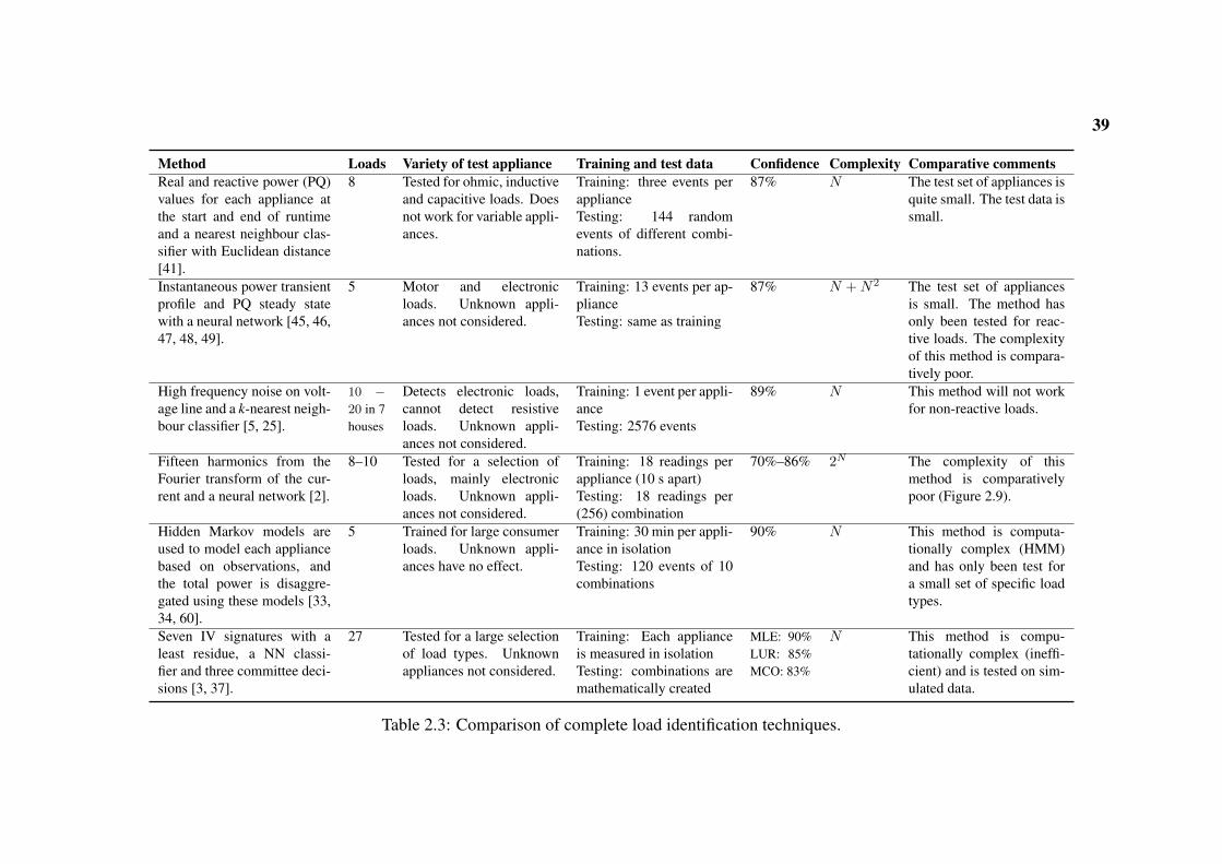
39

Method Loads Variety of test appliance Training and test data Confidence Complexity Comparative commentsReal and reactive power (PQ)values for each appliance atthe start and end of runtimeand a nearest neighbour clas-sifier with Euclidean distance[41].

8 Tested for ohmic, inductiveand capacitive loads. Doesnot work for variable appli-ances.

Training: three events perapplianceTesting: 144 randomevents of different combi-nations.

87% N The test set of appliances isquite small. The test data issmall.

Instantaneous power transientprofile and PQ steady statewith a neural network [45, 46,47, 48, 49].

5 Motor and electronicloads. Unknown appli-ances not considered.

Training: 13 events per ap-plianceTesting: same as training

87% N +N2 The test set of appliancesis small. The method hasonly been tested for reac-tive loads. The complexityof this method is compara-tively poor.

High frequency noise on volt-age line and a k-nearest neigh-bour classifier [5, 25].

10 −20 in 7houses

Detects electronic loads,cannot detect resistiveloads. Unknown appli-ances not considered.

Training: 1 event per appli-anceTesting: 2576 events

89% N This method will not workfor non-reactive loads.

Fifteen harmonics from theFourier transform of the cur-rent and a neural network [2].

8–10 Tested for a selection ofloads, mainly electronicloads. Unknown appli-ances not considered.

Training: 18 readings perappliance (10 s apart)Testing: 18 readings per(256) combination

70%–86% 2N The complexity of thismethod is comparativelypoor (Figure 2.9).

Hidden Markov models areused to model each appliancebased on observations, andthe total power is disaggre-gated using these models [33,34, 60].

5 Trained for large consumerloads. Unknown appli-ances have no effect.

Training: 30 min per appli-ance in isolationTesting: 120 events of 10combinations

90% N This method is computa-tionally complex (HMM)and has only been test fora small set of specific loadtypes.

Seven IV signatures with aleast residue, a NN classi-fier and three committee deci-sions [3, 37].

27 Tested for a large selectionof load types. Unknownappliances not considered.

Training: Each applianceis measured in isolationTesting: combinations aremathematically created

MLE: 90%LUR: 85%MCO: 83%

N This method is compu-tationally complex (ineffi-cient) and is tested on sim-ulated data.

Table 2.3: Comparison of complete load identification techniques.

2.8 Conclusion

This chapter outlines the state of the art research into load identification, it de-

scribes the processes involved in developing a load identification system, namely

data measurement and acquisition techniques, characterisation methods and classi-

fication algorithms. It also discusses how to assess the performance of a load iden-

tification method. The chapter also outlines the uses of a load identification system,

including those outside of generic power monitoring. This chapter also highlights

the capabilities the proposed load identification must have in order to be an effective

method. The method must have an acceptable degree of accuracy, the algorithm’s

computational complexity should be low and efficient and be capable of working

for a large number of appliances. The load disaggregation method should be able

to identify the different varieties of loads found in a domestic environment. The

method must be tested with real measurements to ensure the validity of the results

and to accurately measure the method’s effectiveness. The next chapter outlines

the monitoring system developed in order to acquire the signals used in the load

identification technique developed and the initial analysis of the signals acquired.

40

Chapter 3

Measurement tools and techniques

3.1 Introduction

This section outlines the methods in which the appliance data are recorded. It will

describe the equipment and sensors used to measure signals and their limitations.

The measurement system must be designed with considerations of cost, accuracy

and safety with regards to electrical isolation. The experimental set-up comprised

of a simulated domestic environment in a laboratory which contained commonly

found household appliances. This lab setting allows an in-depth analysis for each

of the appliances, where the temperature and electrical signals of a device are mea-

sured simultaneously. This analysis can inform us about the appliance’s behaviour,

for example the fridge, and the temperature at which the compressor turns on and

off and the effect on the current draw. It also offers the ability to measure appli-

ances at different voltage levels (using a variable AC transformer) to see the effect

of this on the current. The measurement system used to carry out the experiments

comprises a PC connected to a data acquisition (DAQ) device and a current sensor

41

and voltage sensor which measure the load’s electrical characteristics (Figure 3.1).

This system is tested on a 230 V 50 Hz electrical power grid, but it can easily be

adapted to work on a 60 Hz system. The experiments are carried out in a simulated

domestic environment in a university lab setting.

Figure 3.1: Experimental set-up

3.2 Measurement sensors

With the problem of load monitoring in mind there are a number of considera-

tions to be taken into account: the measurements signals must be safe and isolated

from the electrical mains; the cost of the system must be affordable; the accuracy of

the system must be acceptable; and the feasibility of deployment in a real domestic

42

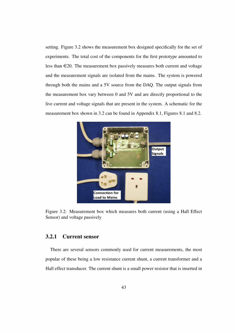
setting. Figure 3.2 shows the measurement box designed specifically for the set of

experiments. The total cost of the components for the first prototype amounted to

less than e20. The measurement box passively measures both current and voltage

and the measurement signals are isolated from the mains. The system is powered

through both the mains and a 5V source from the DAQ. The output signals from

the measurement box vary between 0 and 5V and are directly proportional to the

live current and voltage signals that are present in the system. A schematic for the

measurement box shown in 3.2 can be found in Appendix 8.1, Figures 8.1 and 8.2.

Figure 3.2: Measurement box which measures both current (using a Hall EffectSensor) and voltage passively

3.2.1 Current sensor

There are several sensors commonly used for current measurements, the most

popular of these being a low resistance current shunt, a current transformer and a

Hall effect transducer. The current shunt is a small power resistor that is inserted in

43

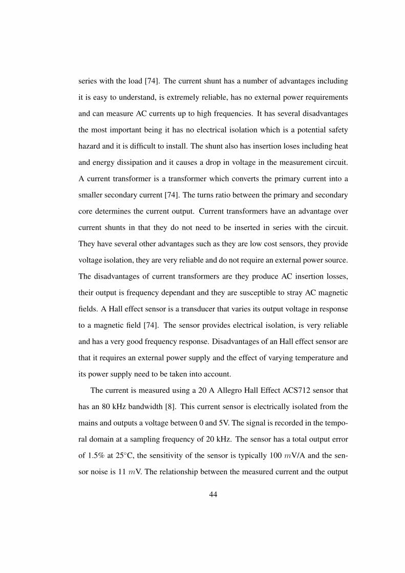
series with the load [74]. The current shunt has a number of advantages including

it is easy to understand, is extremely reliable, has no external power requirements

and can measure AC currents up to high frequencies. It has several disadvantages

the most important being it has no electrical isolation which is a potential safety

hazard and it is difficult to install. The shunt also has insertion loses including heat

and energy dissipation and it causes a drop in voltage in the measurement circuit.

A current transformer is a transformer which converts the primary current into a

smaller secondary current [74]. The turns ratio between the primary and secondary

core determines the current output. Current transformers have an advantage over

current shunts in that they do not need to be inserted in series with the circuit.

They have several other advantages such as they are low cost sensors, they provide

voltage isolation, they are very reliable and do not require an external power source.

The disadvantages of current transformers are they produce AC insertion losses,

their output is frequency dependant and they are susceptible to stray AC magnetic

fields. A Hall effect sensor is a transducer that varies its output voltage in response

to a magnetic field [74]. The sensor provides electrical isolation, is very reliable

and has a very good frequency response. Disadvantages of an Hall effect sensor are

that it requires an external power supply and the effect of varying temperature and

its power supply need to be taken into account.

The current is measured using a 20 A Allegro Hall Effect ACS712 sensor that

has an 80 kHz bandwidth [8]. This current sensor is electrically isolated from the

mains and outputs a voltage between 0 and 5V. The signal is recorded in the tempo-

ral domain at a sampling frequency of 20 kHz. The sensor has a total output error

of 1.5% at 25C, the sensitivity of the sensor is typically 100 mV/A and the sen-

sor noise is 11 mV. The relationship between the measured current and the output

44

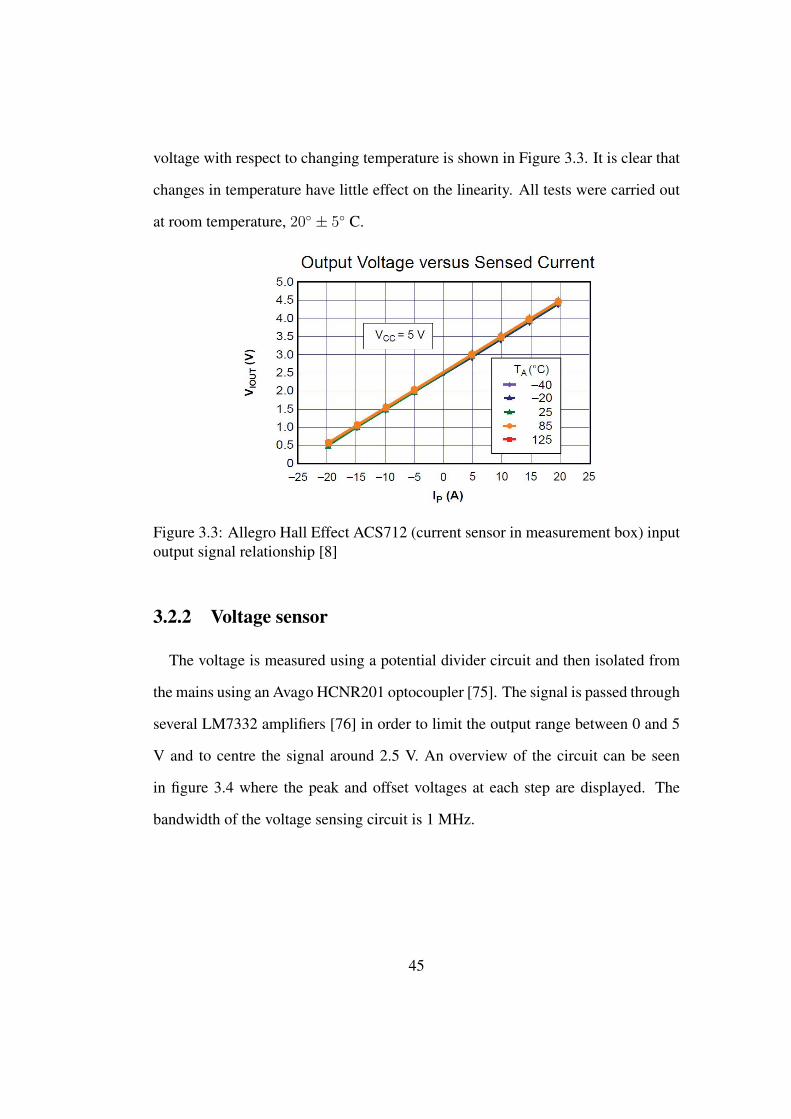
voltage with respect to changing temperature is shown in Figure 3.3. It is clear that

changes in temperature have little effect on the linearity. All tests were carried out

at room temperature, 20 ± 5 C.

Figure 3.3: Allegro Hall Effect ACS712 (current sensor in measurement box) inputoutput signal relationship [8]

3.2.2 Voltage sensor

The voltage is measured using a potential divider circuit and then isolated from

the mains using an Avago HCNR201 optocoupler [75]. The signal is passed through

several LM7332 amplifiers [76] in order to limit the output range between 0 and 5

V and to centre the signal around 2.5 V. An overview of the circuit can be seen

in figure 3.4 where the peak and offset voltages at each step are displayed. The

bandwidth of the voltage sensing circuit is 1 MHz.

45

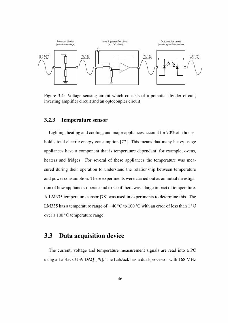
Figure 3.4: Voltage sensing circuit which consists of a potential divider circuit,inverting amplifier circuit and an optocoupler circuit

3.2.3 Temperature sensor

Lighting, heating and cooling, and major appliances account for 70% of a house-

hold’s total electric energy consumption [77]. This means that many heavy usage

appliances have a component that is temperature dependant, for example, ovens,

heaters and fridges. For several of these appliances the temperature was mea-

sured during their operation to understand the relationship between temperature

and power consumption. These experiments were carried out as an initial investiga-

tion of how appliances operate and to see if there was a large impact of temperature.

A LM335 temperature sensor [78] was used in experiments to determine this. The

LM335 has a temperature range of−40 C to 100 C with an error of less than 1 C

over a 100 C temperature range.

3.3 Data acquisition device

The current, voltage and temperature measurement signals are read into a PC

using a LabJack UE9 DAQ [79]. The LabJack has a dual-processor with 168 MHz

46

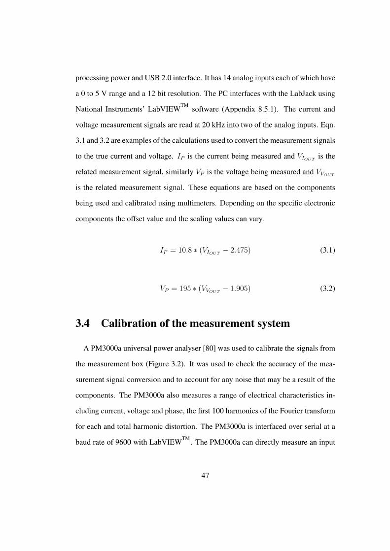
processing power and USB 2.0 interface. It has 14 analog inputs each of which have

a 0 to 5 V range and a 12 bit resolution. The PC interfaces with the LabJack using

National Instruments’ LabVIEWTM software (Appendix 8.5.1). The current and

voltage measurement signals are read at 20 kHz into two of the analog inputs. Eqn.

3.1 and 3.2 are examples of the calculations used to convert the measurement signals

to the true current and voltage. IP is the current being measured and VIOUTis the

related measurement signal, similarly VP is the voltage being measured and VVOUT

is the related measurement signal. These equations are based on the components

being used and calibrated using multimeters. Depending on the specific electronic

components the offset value and the scaling values can vary.

IP = 10.8 ∗ (VIOUT− 2.475) (3.1)

VP = 195 ∗ (VVOUT− 1.905) (3.2)

3.4 Calibration of the measurement system

A PM3000a universal power analyser [80] was used to calibrate the signals from

the measurement box (Figure 3.2). It was used to check the accuracy of the mea-

surement signal conversion and to account for any noise that may be a result of the

components. The PM3000a also measures a range of electrical characteristics in-

cluding current, voltage and phase, the first 100 harmonics of the Fourier transform

for each and total harmonic distortion. The PM3000a is interfaced over serial at a

baud rate of 9600 with LabVIEWTM . The PM3000a can directly measure an input

47

of 30ARMS and 1400VRMS with an accuracy of 0.5%. A comparison was carried

out between the measurement box current sensor and the PM3000a for a test load,

in this case the fridge. Figure 3.5 graphs the output from both sensors for the first,

third, fifth, seventh and ninth current harmonics. There is more noise apparent for

the signals acquired with the current sensor than the PM3000a, but the current sen-

sor is an inexpensive sensor whereas the PM3000a is an industrial multimeter with

high accuracy so this is to be expected. The magnitude of the current measured

by each sensor is within a very close range (less than 5% for the first three har-

monics and less than 10% for the last two) and the Hall Effect sensor was deemed

acceptable for future tests.

48

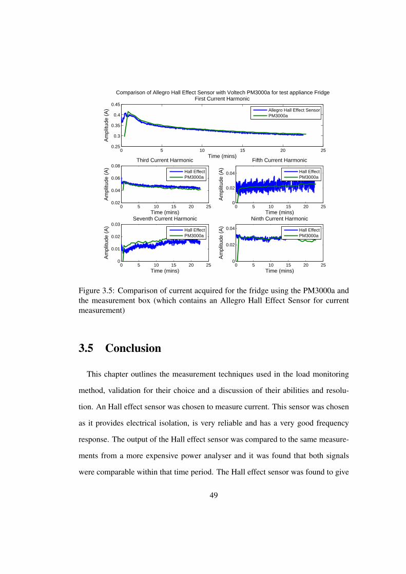
0 5 10 15 20 250.25

0.3

0.35

0.4

0.45

Time (mins)

Am

plitu

de (

A)

Comparison of Allegro Hall Effect Sensor with Voltech PM3000a for test appliance FridgeFirst Current Harmonic

Allegro Hall Effect SensorPM3000a

0 5 10 15 20 250.02

0.04

0.06

0.08

Time (mins)

Am

plitu

de (

A)

Third Current Harmonic

Hall EffectPM3000a

0 5 10 15 20 250

0.02

0.04

Fifth Current Harmonic

Time (mins)A

mpl

itude

(A

)

Hall EffectPM3000a

0 5 10 15 20 250

0.01

0.02

0.03Seventh Current Harmonic

Time (mins)

Am

plitu

de (

A)

Hall EffectPM3000a

0 5 10 15 20 250

0.02

0.04

Ninth Current Harmonic

Time (mins)

Am

plitu

de (

A)

Hall EffectPM3000a

Figure 3.5: Comparison of current acquired for the fridge using the PM3000a andthe measurement box (which contains an Allegro Hall Effect Sensor for currentmeasurement)

3.5 Conclusion

This chapter outlines the measurement techniques used in the load monitoring

method, validation for their choice and a discussion of their abilities and resolu-

tion. An Hall effect sensor was chosen to measure current. This sensor was chosen

as it provides electrical isolation, is very reliable and has a very good frequency

response. The output of the Hall effect sensor was compared to the same measure-

ments from a more expensive power analyser and it was found that both signals

were comparable within that time period. The Hall effect sensor was found to give

49

an accurate measurement of the current while keeping within acceptable cost con-

straints. The next chapter analyses the environment in which the tests will be carried

out and typical electrical loads found in a domestic environment.

50

Chapter 4

An analysis of the electrical system

4.1 Introduction

This chapter discusses the electrical environment in which a load monitoring

system will be deployed. In order to develop an efficient algorithm for identifying

appliances, there is a need to understand the problem in more detail. The power

source and the electrical load are complex components of the electrical system. This

section discusses the environment in which the appliances are interacting and the

appliances themselves. The voltage is supplied by the Irish Electrical Supply Board.

Ideally there shouldn’t be any harmonics on the line but there are due to nonlinear

loads. In the electrical system all loads are in parallel, therefore theoretically the

total current consumed in the system is the sum of the individual currents. The

measurements used to explain the electrical system were taken with the equipment

described in Chapter 3.

51

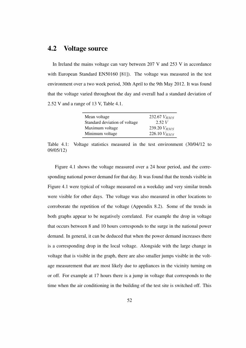
4.2 Voltage source

In Ireland the mains voltage can vary between 207 V and 253 V in accordance

with European Standard EN50160 [81]). The voltage was measured in the test

environment over a two week period, 30th April to the 9th May 2012. It was found

that the voltage varied throughout the day and overall had a standard deviation of

2.52 V and a range of 13 V, Table 4.1.

Mean voltage 232.67 VRMS

Standard deviation of voltage 2.52 VMaximum voltage 239.20 VRMS

Minimum voltage 226.10 VRMS

Table 4.1: Voltage statistics measured in the test environment (30/04/12 to09/05/12)

Figure 4.1 shows the voltage measured over a 24 hour period, and the corre-

sponding national power demand for that day. It was found that the trends visible in

Figure 4.1 were typical of voltage measured on a weekday and very similar trends

were visible for other days. The voltage was also measured in other locations to

corroborate the repetition of the voltage (Appendix 8.2). Some of the trends in

both graphs appear to be negatively correlated. For example the drop in voltage

that occurs between 8 and 10 hours corresponds to the surge in the national power

demand. In general, it can be deduced that when the power demand increases there

is a corresponding drop in the local voltage. Alongside with the large change in

voltage that is visible in the graph, there are also smaller jumps visible in the volt-

age measurement that are most likely due to appliances in the vicinity turning on

or off. For example at 17 hours there is a jump in voltage that corresponds to the

time when the air conditioning in the building of the test site is switched off. This

52

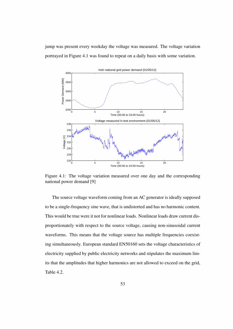
jump was present every weekday the voltage was measured. The voltage variation

portrayed in Figure 4.1 was found to repeat on a daily basis with some variation.

0 5 10 15 202000

2500

3000

3500

4000

Pow

er D

eman

d (M

W)

Time (00:00 to 24:00 hours)

Irish national grid power demand (01/05/12)

0 5 10 15 20226

228

230

232

234

236

238

Vol

tage

(V

)

Time (00:00 to 24:00 hours)

Voltage measured in test environment (01/05/12)

Figure 4.1: The voltage variation measured over one day and the correspondingnational power demand [9]

The source voltage waveform coming from an AC generator is ideally supposed

to be a single-frequency sine wave, that is undistorted and has no harmonic content.

This would be true were it not for nonlinear loads. Nonlinear loads draw current dis-

proportionately with respect to the source voltage, causing non-sinusoidal current

waveforms. This means that the voltage source has multiple frequencies coexist-

ing simultaneously. European standard EN50160 sets the voltage characteristics of

electricity supplied by public electricity networks and stipulates the maximum lim-

its that the amplitudes that higher harmonics are not allowed to exceed on the grid,

Table 4.2.

53

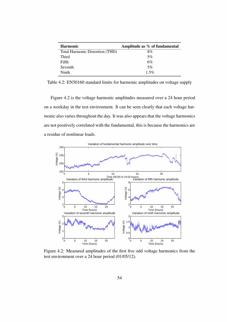
Harmonic Amplitude as % of fundamentalTotal Harmonic Distortion (THD) 8%Third 5%Fifth 6%Seventh 5%Ninth 1.5%

Table 4.2: EN50160 standard limits for harmonic amplitudes on voltage supply

Figure 4.2 is the voltage harmonic amplitudes measured over a 24 hour period

on a weekday in the test environment. It can be seen clearly that each voltage har-

monic also varies throughout the day. It was also appears that the voltage harmonics

are not positively correlated with the fundamental, this is because the harmonics are

a residue of nonlinear loads.

0 5 10 15 20225

230

235

240

Vol

tage

(V

)

Time (00:00 to 24:00 hours)

Variation of fundamental harmonic amplitude over time

0 5 10 15 202

3

4

5

Vol

tage

(V

)

Time (hours)

Variation of third harmonic amplitude

0 5 10 15 202

4

6

8

Vol

tage

(V

)

Time (hours)

Variation of fifth harmonic amplitude

0 5 10 15 200

1

2

3

Vol

tage

(V

)

Time (hours)

Variation of seventh harmonic amplitude

0 5 10 15 200

0.5

1

1.5

2

Vol

tage

(V

)

Time (hours)

Variation of ninth harmonic amplitude

Figure 4.2: Measured amplitudes of the first five odd voltage harmonics from thetest environment over a 24 hour period (01/05/12).

54

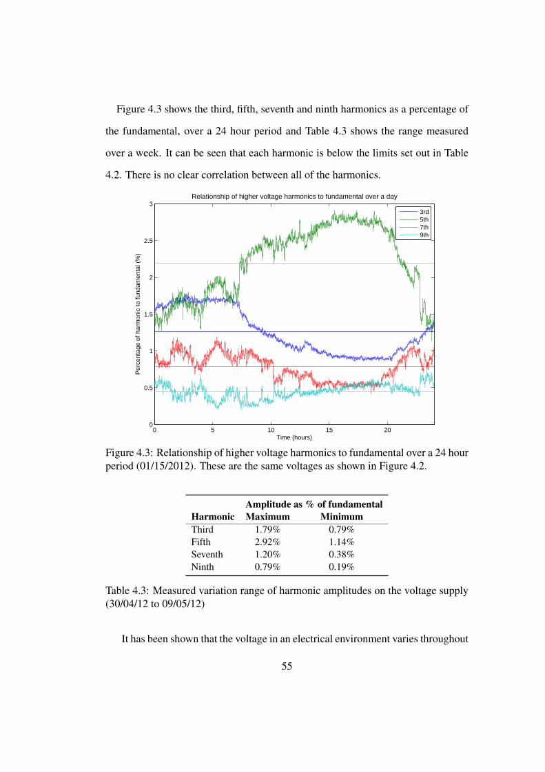
Figure 4.3 shows the third, fifth, seventh and ninth harmonics as a percentage of

the fundamental, over a 24 hour period and Table 4.3 shows the range measured

over a week. It can be seen that each harmonic is below the limits set out in Table

4.2. There is no clear correlation between all of the harmonics.

0 5 10 15 200

0.5

1

1.5

2

2.5

3

Time (hours)

Per

cent

age

of h

arm

onic

to fu

ndam

enta

l (%

)

Relationship of higher voltage harmonics to fundamental over a day

3rd5th7th9th

Figure 4.3: Relationship of higher voltage harmonics to fundamental over a 24 hourperiod (01/15/2012). These are the same voltages as shown in Figure 4.2.

Amplitude as % of fundamentalHarmonic Maximum MinimumThird 1.79% 0.79%Fifth 2.92% 1.14%Seventh 1.20% 0.38%Ninth 0.79% 0.19%

Table 4.3: Measured variation range of harmonic amplitudes on the voltage supply(30/04/12 to 09/05/12)

It has been shown that the voltage in an electrical environment varies throughout

55

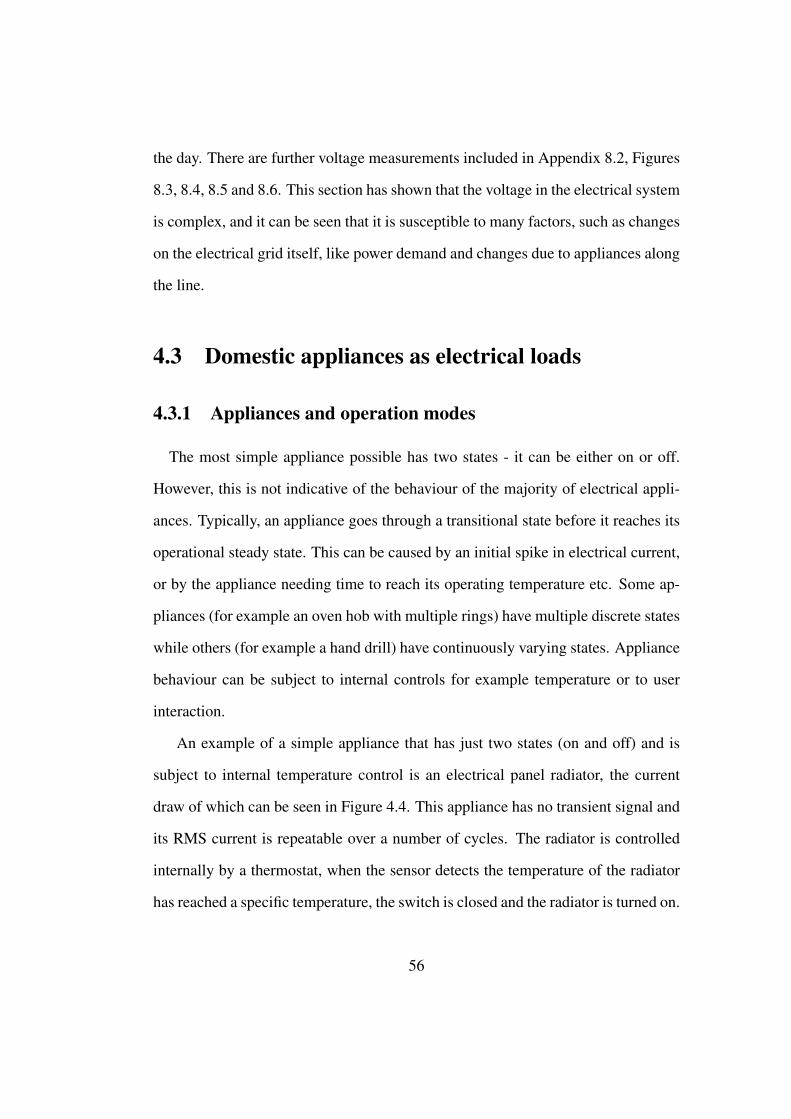
the day. There are further voltage measurements included in Appendix 8.2, Figures

8.3, 8.4, 8.5 and 8.6. This section has shown that the voltage in the electrical system

is complex, and it can be seen that it is susceptible to many factors, such as changes

on the electrical grid itself, like power demand and changes due to appliances along

the line.

4.3 Domestic appliances as electrical loads

4.3.1 Appliances and operation modes

The most simple appliance possible has two states - it can be either on or off.

However, this is not indicative of the behaviour of the majority of electrical appli-

ances. Typically, an appliance goes through a transitional state before it reaches its

operational steady state. This can be caused by an initial spike in electrical current,

or by the appliance needing time to reach its operating temperature etc. Some ap-

pliances (for example an oven hob with multiple rings) have multiple discrete states

while others (for example a hand drill) have continuously varying states. Appliance

behaviour can be subject to internal controls for example temperature or to user

interaction.

An example of a simple appliance that has just two states (on and off) and is

subject to internal temperature control is an electrical panel radiator, the current

draw of which can be seen in Figure 4.4. This appliance has no transient signal and

its RMS current is repeatable over a number of cycles. The radiator is controlled

internally by a thermostat, when the sensor detects the temperature of the radiator

has reached a specific temperature, the switch is closed and the radiator is turned on.

56

The case is the same for the radiator turning off. The running time of the appliance

will change based on the temperature of the environment in which the appliance is

operating, but the general operation of the appliance will not.

0

5

10

15

20

25

30

35

40

45

0

0.1

0.2

0.3

0.4

0.5

0.6

0.7

0.8

0.9

1

14:30:00 14:44:24 14:58:48 15:13:12 15:27:36 15:42:00 15:56:24

Cu

rre

nt

(A)

Time

RadiatorCurrent

RadiatorTemperature

Tem

pe

rature

(°C)

Figure 4.4: Radiator current draw cycles with respect to temperature of radiator

An example of an appliance with two states (on and off), is subject to internal

temperature control and has a transitional state is the refrigerator (Figure 4.5). The

refrigerator is one of the most common appliances found in a domestic setting and

is one of the top ten contributors to power consumption in a domestic environment

[58]. The refrigerator used in our tests has five settings, each setting corresponds to

the thermostat of the refrigerator operating for a different temperature. This means

the refrigerator will run for different lengths of time at each setting (Table 4.4).

Figure 4.5 shows nine cycles of the fridge operating at setting 2. Each cycle lasts

for approximately the same duration and the time between cycles is also similar.

The temperature and RMS current cycles of the fridge are plotted. The temperature

varies between 8 C and 9 C turning on and off the compressor. It is noteworthy

57

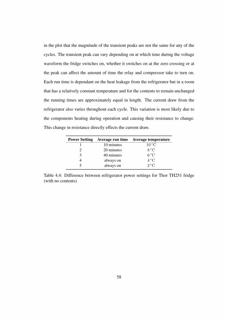
in the plot that the magnitude of the transient peaks are not the same for any of the

cycles. The transient peak can vary depending on at which time during the voltage

waveform the fridge switches on, whether it switches on at the zero crossing or at

the peak can affect the amount of time the relay and compressor take to turn on.

Each run time is dependant on the heat leakage from the refrigerator but in a room

that has a relatively constant temperature and for the contents to remain unchanged

the running times are approximately equal in length. The current draw from the

refrigerator also varies throughout each cycle. This variation is most likely due to

the components heating during operation and causing their resistance to change.

This change in resistance directly effects the current draw.

Power Setting Average run time Average temperature1 10 minutes 10 C2 20 minutes 8 C3 40 minutes 6 C4 always on 4 C5 always on 2 C

Table 4.4: Difference between refrigerator power settings for Thor TH251 fridge(with no contents)

58

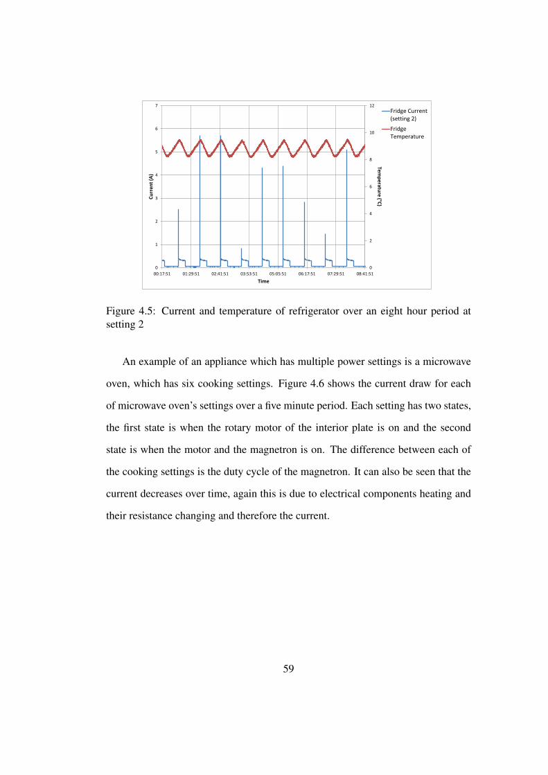
0

2

4

6

8

10

12

0

1

2

3

4

5

6

7

00:17:51 01:29:51 02:41:51 03:53:51 05:05:51 06:17:51 07:29:51 08:41:51

Cu

rre

nt

(A)

Time

Fridge Current(setting 2)

FridgeTemperature

Tem

pe

rature

(°C)

Figure 4.5: Current and temperature of refrigerator over an eight hour period atsetting 2

An example of an appliance which has multiple power settings is a microwave

oven, which has six cooking settings. Figure 4.6 shows the current draw for each

of microwave oven’s settings over a five minute period. Each setting has two states,

the first state is when the rotary motor of the interior plate is on and the second

state is when the motor and the magnetron is on. The difference between each of

the cooking settings is the duty cycle of the magnetron. It can also be seen that the

current decreases over time, again this is due to electrical components heating and

their resistance changing and therefore the current.

59

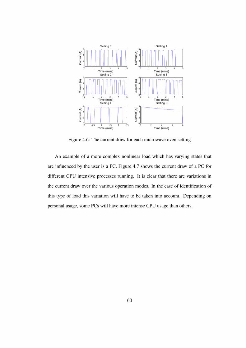
0 1 2 3 4 50

2

4

6Setting 0

Time (mins)

Cur

rent

(A

)

0 1 2 3 4 50

2

4

6Setting 1

Time (mins)

Cur

rent

(A

)

0 1 2 3 4 50

2

4

6Setting 2

Time (mins)

Cur

rent

(A

)

0 1 2 3 4 50

2

4

6Setting 3

Time (mins)

Cur

rent

(A

)

0 0.5 1 1.5 2 2.50

2

4

6Setting 4

Time (mins)

Cur

rent

(A

)

0 2 4 6 80

2

4

6Setting 5

Time (mins)

Cur

rent

(A

)

Figure 4.6: The current draw for each microwave oven setting

An example of a more complex nonlinear load which has varying states that

are influenced by the user is a PC. Figure 4.7 shows the current draw of a PC for

different CPU intensive processes running. It is clear that there are variations in

the current draw over the various operation modes. In the case of identification of

this type of load this variation will have to be taken into account. Depending on

personal usage, some PCs will have more intense CPU usage than others.

60

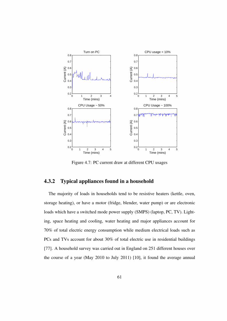
0 1 2 3 40.2

0.3

0.4

0.5

0.6

0.7

0.8Turn on PC

Cur

rent

(A

)

Time (mins)0 1 2 3 4 5

0.2

0.3

0.4

0.5

0.6

0.7

0.8CPU usage < 10%

Cur

rent

(A

)

Time (mins)

0 1 2 3 4 50.2

0.3

0.4

0.5

0.6

0.7

0.8CPU Usage ~ 50%

Cur

rent

(A

)

Time (mins)0 1 2 3 4 5

0.2

0.3

0.4

0.5

0.6

0.7

0.8CPU Usage ~ 100%

Cur

rent

(A

)

Time (mins)

Figure 4.7: PC current draw at different CPU usages

4.3.2 Typical appliances found in a household

The majority of loads in households tend to be resistive heaters (kettle, oven,

storage heating), or have a motor (fridge, blender, water pump) or are electronic

loads which have a switched mode power supply (SMPS) (laptop, PC, TV). Light-

ing, space heating and cooling, water heating and major appliances account for

70% of total electric energy consumption while medium electrical loads such as

PCs and TVs account for about 30% of total electric use in residential buildings

[77]. A household survey was carried out in England on 251 different houses over

the course of a year (May 2010 to July 2011) [10], it found the average annual

61

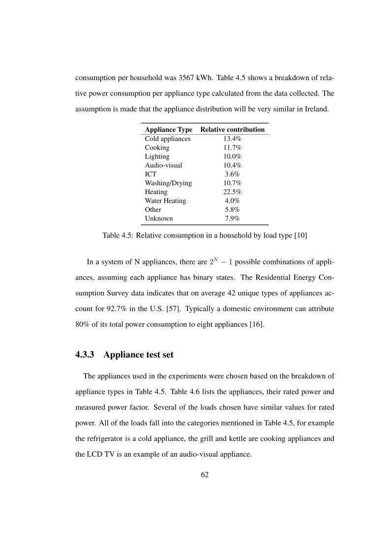
consumption per household was 3567 kWh. Table 4.5 shows a breakdown of rela-

tive power consumption per appliance type calculated from the data collected. The

assumption is made that the appliance distribution will be very similar in Ireland.

Appliance Type Relative contributionCold appliances 13.4%Cooking 11.7%Lighting 10.0%Audio-visual 10.4%ICT 3.6%Washing/Drying 10.7%Heating 22.5%Water Heating 4.0%Other 5.8%Unknown 7.9%

Table 4.5: Relative consumption in a household by load type [10]

In a system of N appliances, there are 2N − 1 possible combinations of appli-

ances, assuming each appliance has binary states. The Residential Energy Con-

sumption Survey data indicates that on average 42 unique types of appliances ac-

count for 92.7% in the U.S. [57]. Typically a domestic environment can attribute

80% of its total power consumption to eight appliances [16].

4.3.3 Appliance test set

The appliances used in the experiments were chosen based on the breakdown of

appliance types in Table 4.5. Table 4.6 lists the appliances, their rated power and

measured power factor. Several of the loads chosen have similar values for rated

power. All of the loads fall into the categories mentioned in Table 4.5, for example

the refrigerator is a cold appliance, the grill and kettle are cooking appliances and

the LCD TV is an example of an audio-visual appliance.

62

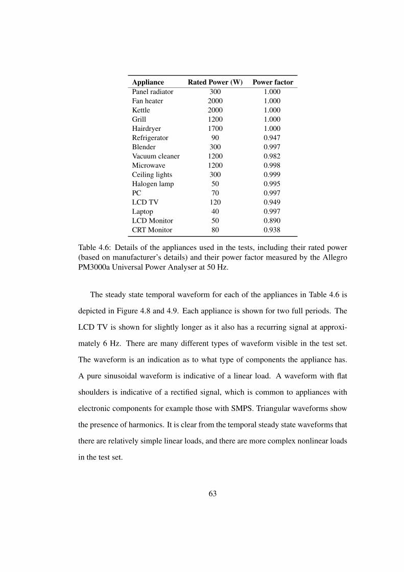
Appliance Rated Power (W) Power factorPanel radiator 300 1.000Fan heater 2000 1.000Kettle 2000 1.000Grill 1200 1.000Hairdryer 1700 1.000Refrigerator 90 0.947Blender 300 0.997Vacuum cleaner 1200 0.982Microwave 1200 0.998Ceiling lights 300 0.999Halogen lamp 50 0.995PC 70 0.997LCD TV 120 0.949Laptop 40 0.997LCD Monitor 50 0.890CRT Monitor 80 0.938

Table 4.6: Details of the appliances used in the tests, including their rated power(based on manufacturer’s details) and their power factor measured by the AllegroPM3000a Universal Power Analyser at 50 Hz.

The steady state temporal waveform for each of the appliances in Table 4.6 is

depicted in Figure 4.8 and 4.9. Each appliance is shown for two full periods. The

LCD TV is shown for slightly longer as it also has a recurring signal at approxi-

mately 6 Hz. There are many different types of waveform visible in the test set.

The waveform is an indication as to what type of components the appliance has.

A pure sinusoidal waveform is indicative of a linear load. A waveform with flat

shoulders is indicative of a rectified signal, which is common to appliances with

electronic components for example those with SMPS. Triangular waveforms show

the presence of harmonics. It is clear from the temporal steady state waveforms that

there are relatively simple linear loads, and there are more complex nonlinear loads

in the test set.

63

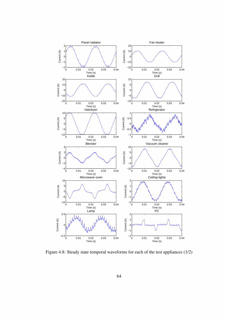
0 0.01 0.02 0.03 0.04−2

−1

0

1

2Panel radiator

Time (s)

Cur

rent

(A

)

0 0.01 0.02 0.03 0.04−20

−10

0

10

20Fan heater

Time (s)

Cur

rent

(A

)

0 0.01 0.02 0.03 0.04−20

−10

0

10

20Kettle

Time (s)

Cur

rent

(A

)

0 0.01 0.02 0.03 0.04−10

−5

0

5

10Grill

Time (s)

Cur

rent

(A

)

0 0.01 0.02 0.03 0.04−10

−5

0

5

10Hairdryer

Time (s)

Cur

rent

(A

)

0 0.01 0.02 0.03 0.04−1

−0.5

0

0.5

1Refrigerator

Time (s)

Cur

rent

(A

)

0 0.01 0.02 0.03 0.04−4

−2

0

2

4Blender

Time (s)

Cur

rent

(A

)

0 0.01 0.02 0.03 0.04−10

−5

0

5

10Vacuum cleaner

Time (s)

Cur

rent

(A

)

0 0.01 0.02 0.03 0.04−10

−5

0

5

10Microwave oven

Time (s)

Cur

rent

(A

)

0 0.01 0.02 0.03 0.04−2

−1

0

1

2Ceiling lights

Time (s)

Cur

rent

(A

)

0 0.01 0.02 0.03 0.04−0.5

0

0.5Lamp

Time (s)

Cur

rent

(A

)

0 0.01 0.02 0.03 0.04−2

−1

0

1

2PC

Time (s)

Cur

rent

(A

)

Figure 4.8: Steady state temporal waveforms for each of the test appliances (1/2)

64

0 0.02 0.04 0.06 0.08 0.1−1

−0.5

0

0.5

1LCD TV

Time (s)

Cur

rent

(A

)

0 0.01 0.02 0.03 0.04−2

−1

0

1

2CRT Monitor

Time (s)

Cur

rent

(A

)

0 0.01 0.02 0.03 0.04−2

−1

0

1

2Laptop

Time (s)

Cur

rent

(A

)

0 0.01 0.02 0.03 0.04

−0.5

0

0.5

LCD Monitor

Time (s)

Cur

rent

(A

)

Figure 4.9: Steady state temporal waveforms for each of the test appliances (2/2)

Many of the test appliances have non-sinusoidal steady state signals that sug-

gest the presence of harmonics in the signal. The international standard EN61000-

3-2 for electromagnetic compatibility sets limits for harmonic current emitted by

electric equipment supplied from the mains network at 230 V, Table 4.7. Class

A appliances are most household appliances for example cooking appliances, cold

appliances and lighting and Class D are electronic appliances with power less than

600 W. The even harmonic limits are lower than the odd harmonic limits and as the

harmonic order increases the limit of the harmonic amplitude decreases.

65

Current Limit (A)Harmonic Order Class A Class D

2nd 1.08 -3rd 2.30 2.304th 0.43 -5th 1.14 1.146th 0.30 -7th 0.77 0.778th 0.23 -9th 0.40 0.4010th 0.18 -11th 0.33 0.33

.. .. ..

n th 0.15

(15

n

)0.15

(15

n

)

Table 4.7: EN61000-3-2 current harmonic limits for two classes of household ap-pliances, Class A appliances are household appliances up to 16 A and Class Dappliances are electronic appliances that are rated less than 600 W.

The first five odd current harmonic amplitudes for each of the appliances are

shown in Figures 4.10 and 4.11. The first five odd current harmonics were cho-

sen based on the EN61000-3-2 standard, Table 4.7. The electronic loads such as

the PC, laptop and LCD TV have harmonics that are highly visible. Appliances

that have motors such as the refrigerator, blender and vacuum cleaner have a sig-

nificant third harmonic. Resistive heating loads such as the panel radiator, kettle

and grill all appear to have very low harmonic content, but do have some content

visible nonetheless. Similarly powered loads for example the vacuum cleaner and

microwave which are both rated at 1200 W have different levels at each of the har-

monics.

66

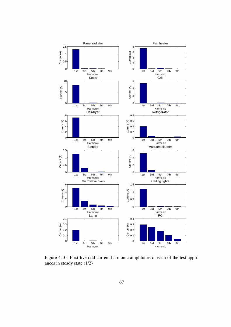
1st 3rd 5th 7th 9th0

0.5

1

1.5Panel radiator

Harmonic

Cur

rent

(A

)

1st 3rd 5th 7th 9th0

2

4

6

8Fan heater

Harmonic

Cur

rent

(A

)

1st 3rd 5th 7th 9th0

5

10Kettle

Harmonic

Cur

rent

(A

)

1st 3rd 5th 7th 9th0

2

4

6Grill

Harmonic

Cur

rent

(A

)

1st 3rd 5th 7th 9th0

2

4

6

8Hairdryer

Harmonic

Cur

rent

(A

)

1st 3rd 5th 7th 9th0

0.2

0.4

0.6

0.8Refrigerator

Harmonic

Cur

rent

(A

)

1st 3rd 5th 7th 9th0

0.5

1

1.5Blender

Harmonic

Cur

rent

(A

)

1st 3rd 5th 7th 9th0

2

4

6Vacuum cleaner

Harmonic

Cur

rent

(A

)

1st 3rd 5th 7th 9th0

2

4

6Microwave oven

Harmonic

Cur

rent

(A

)

1st 3rd 5th 7th 9th0

0.5

1

1.5Ceiling lights

Harmonic

Cur

rent

(A

)

1st 3rd 5th 7th 9th0

0.1

0.2

0.3

0.4Lamp

Harmonic

Cur

rent

(A

)

1st 3rd 5th 7th 9th0

0.1

0.2

0.3

0.4PC

Harmonic

Cur

rent

(A

)

Figure 4.10: First five odd current harmonic amplitudes of each of the test appli-ances in steady state (1/2)

67

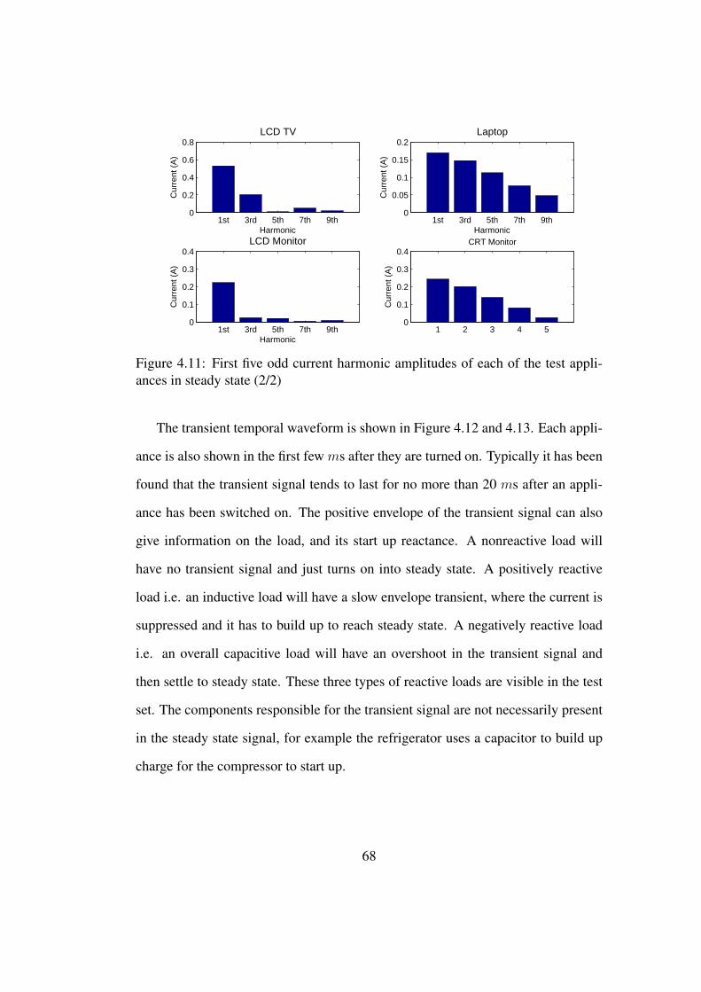
1st 3rd 5th 7th 9th0

0.2

0.4

0.6

0.8LCD TV

Harmonic

Cur

rent

(A

)

1st 3rd 5th 7th 9th0

0.05

0.1

0.15

0.2Laptop

Harmonic

Cur

rent

(A

)

1st 3rd 5th 7th 9th0

0.1

0.2

0.3

0.4LCD Monitor

Harmonic

Cur

rent

(A

)

1 2 3 4 50

0.1

0.2

0.3

0.4CRT Monitor

Cur

rent

(A

)

Figure 4.11: First five odd current harmonic amplitudes of each of the test appli-ances in steady state (2/2)

The transient temporal waveform is shown in Figure 4.12 and 4.13. Each appli-

ance is also shown in the first few ms after they are turned on. Typically it has been

found that the transient signal tends to last for no more than 20 ms after an appli-

ance has been switched on. The positive envelope of the transient signal can also

give information on the load, and its start up reactance. A nonreactive load will

have no transient signal and just turns on into steady state. A positively reactive

load i.e. an inductive load will have a slow envelope transient, where the current is

suppressed and it has to build up to reach steady state. A negatively reactive load

i.e. an overall capacitive load will have an overshoot in the transient signal and

then settle to steady state. These three types of reactive loads are visible in the test

set. The components responsible for the transient signal are not necessarily present

in the steady state signal, for example the refrigerator uses a capacitor to build up

charge for the compressor to start up.

68

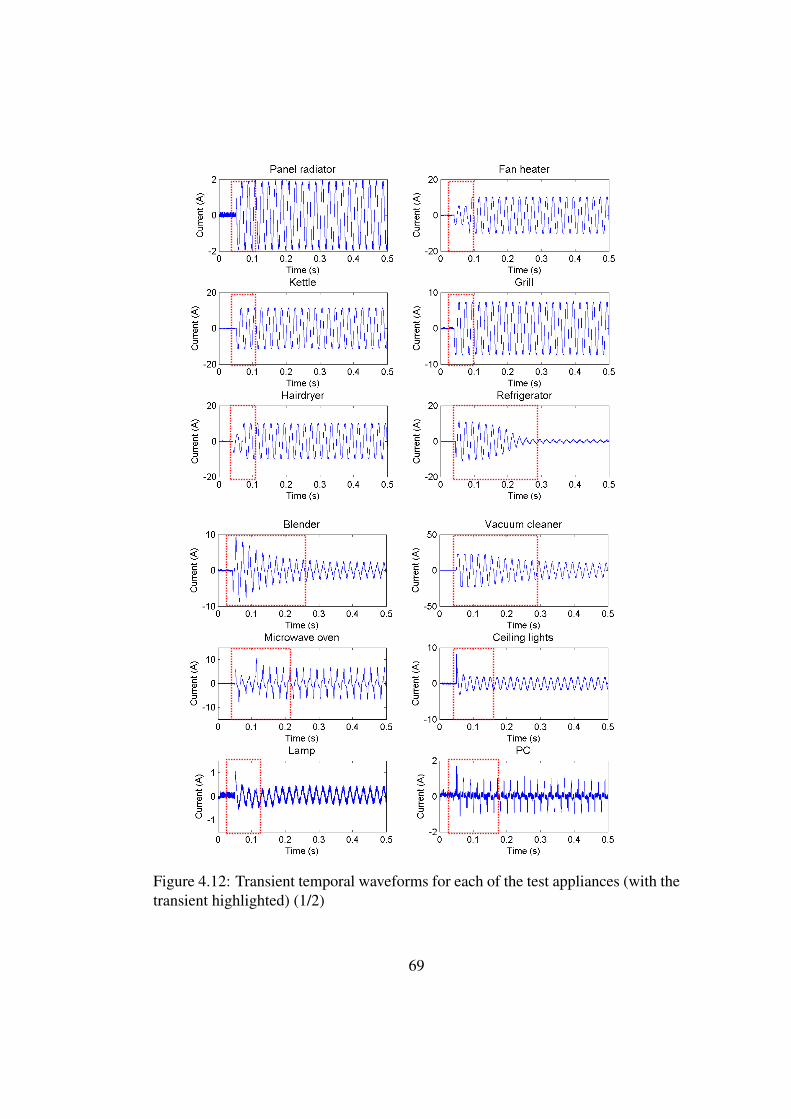
Figure 4.12: Transient temporal waveforms for each of the test appliances (with thetransient highlighted) (1/2)

69

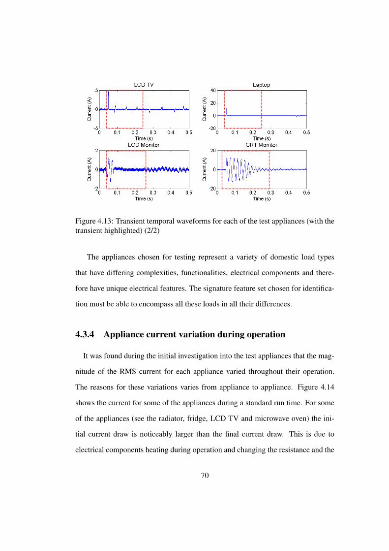
Figure 4.13: Transient temporal waveforms for each of the test appliances (with thetransient highlighted) (2/2)

The appliances chosen for testing represent a variety of domestic load types

that have differing complexities, functionalities, electrical components and there-

fore have unique electrical features. The signature feature set chosen for identifica-

tion must be able to encompass all these loads in all their differences.

4.3.4 Appliance current variation during operation

It was found during the initial investigation into the test appliances that the mag-

nitude of the RMS current for each appliance varied throughout their operation.

The reasons for these variations varies from appliance to appliance. Figure 4.14

shows the current for some of the appliances during a standard run time. For some

of the appliances (see the radiator, fridge, LCD TV and microwave oven) the ini-

tial current draw is noticeably larger than the final current draw. This is due to

electrical components heating during operation and changing the resistance and the

70

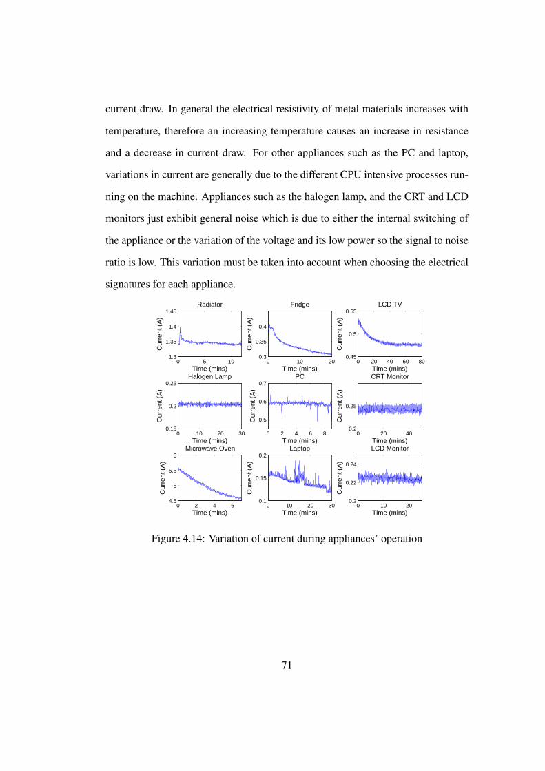
current draw. In general the electrical resistivity of metal materials increases with

temperature, therefore an increasing temperature causes an increase in resistance

and a decrease in current draw. For other appliances such as the PC and laptop,

variations in current are generally due to the different CPU intensive processes run-

ning on the machine. Appliances such as the halogen lamp, and the CRT and LCD

monitors just exhibit general noise which is due to either the internal switching of

the appliance or the variation of the voltage and its low power so the signal to noise

ratio is low. This variation must be taken into account when choosing the electrical

signatures for each appliance.

0 5 101.3

1.35

1.4

1.45Radiator

Cur

rent

(A

)

Time (mins)0 10 20

0.3

0.35

0.4

Fridge

Cur

rent

(A

)

Time (mins)0 20 40 60 80

0.45

0.5

0.55LCD TV

Cur

rent

(A

)

Time (mins)

0 10 20 300.15

0.2

0.25Halogen Lamp

Cur

rent

(A

)

Time (mins)0 2 4 6 8

0.5

0.6

0.7PC

Cur

rent

(A

)

Time (mins)0 20 40

0.2

0.25

CRT Monitor

Cur

rent

(A

)

Time (mins)

0 2 4 64.5

5

5.5

6Microwave Oven

Cur

rent

(A

)

Time (mins)0 10 20 30

0.1

0.15

0.2Laptop

Cur

rent

(A

)

Time (mins)0 10 20

0.2

0.22

0.24

LCD Monitor

Cur

rent

(A

)

Time (mins)

Figure 4.14: Variation of current during appliances’ operation

71

4.4 Conclusion

This chapter details some initial experiments carried out on the various appli-

ances which builds the foundation for the next two chapters make some of their as-

sumptions. The operation of some of the appliances has been analysed in detail and

an understanding of why these appliances consume power and the way they do has

been found. It has been found that there are harmonics present on the voltage line,

and these vary throughout the day. It is evident from the analysis of the measure-

ments that the electrical system is subjected to complex appliance behaviour and a

complex voltage source. This makes the problem of load monitoring and disaggre-

gating appliances challenging. The next chapter presents a preliminary method for

disaggregating the appliances contributing to the total power consumption based on

the findings of this chapter.

72

Chapter 5

Identifying appliances using

signatures based on FFT harmonics

and a naive Bayes classifier

5.1 Introduction

Load monitoring involves disaggregating the total power consumption of the en-

vironment into the appliances which are consuming power. The changing incoming

electrical signals are analysed and from these it can be deduced what appliances are

running and thereby allow one to know each individual appliance’s power consump-

tion. Chapter 4 describes the complexities of the electrical system and analyses the

different type of load variations. With this information in mind this chapter out-

lines an approach to using the electrical signals from an appliance to identify what

appliances are in operation.

This chapter presents a method that measures individual signatures for each

73

appliance and from this creates a virtual signature library of all the possible combi-

nations of appliances. Each individual appliance is measured operating in isolation

and a signature is extracted from the signal. The signature in this method is specific

harmonic selected from the Fourier transform of the steady state current signal. A

virtual library is created by additively combining the individual signatures. A naive

Bayes classifier is used to identify what the most probable appliance(s) are oper-

ating allowing the identification of multiple appliances operating at the same time.

The merits and limitations of this method are discussed and recommendations for

an improved scheme are presented.

5.2 Methodology

In most countries, household power is single-phase electric power, with two or

three wired contacts at each outlet. In Europe, 230 VRMS are supplied at 50 Hz

to each household’s main incoming power point where each domestic load is then

connected in parallel. Kirchoff’s current law states that at any node in an electrical

circuit, the sum of currents flowing into that node is equal to the sum of currents

flowing out of that node. It is assumed that the electrical system in a domestic

setting is linear and therefore all individual currents can be summed together to

give the aggregate current.

The method of load monitoring developed measures the aggregate current sig-

nal and identifies the contributing appliances. In order to identify each appliance

when it turns on, an appliance signature library, derived from the electrical power

signal of each appliance, is created. The signature library should uniquely identify

each appliance. The Fourier transform of a signal transforms the waveform from

74

the time domain into a sequence of values at different frequencies in the frequency

domain. Figures 4.10 and 4.11 (Chapter 4) show each appliance’s unique FFT spec-

trum. These current spectra are different for each appliance and each appliance has

harmonic content present in the signal. The first five odd harmonics of the spectrum

give a sufficient approximation of the signal. These harmonics were chosen based

on the harmonic limits presented by EN61000-3-2, Table 4.7. If these limits are met

by appliance manufacturers, there should be very little harmonic content in the even

current harmonics. As the frequency spectrum increases the amplitudes of the odd

current harmonics also should decrease. For these reasons the first five odd current

harmonic amplitudes are chosen as a signature for each appliance.

This chapter carries out a number of experiments in order to test the effective-

ness of using the odd current harmonic amplitudes and a naive Bayes classifier to

identify appliances. First the hypothesis that the current harmonic amplitudes and

a naive Bayes classifier are accurate in identifying each individual appliance in iso-

lation is tested. This will test both the effectiveness of the harmonic amplitudes as

a signature for distinguishing between appliances and the naive Bayes as a classi-

fier, which has been chosen as due to its simplicity and robustness. The method

will then be extended to work for combinations of multiple appliance, first by us-

ing measured signatures for each of the different combinations and then by creating

a virtual library from the individual signatures. A comparison of the accuracy of

using a measured signature library for each appliance combination versus a virtual

signature library for each appliance combination is carried out. This will ultimately

show whether creating a virtual library for multiple appliances is a suitable method.

75

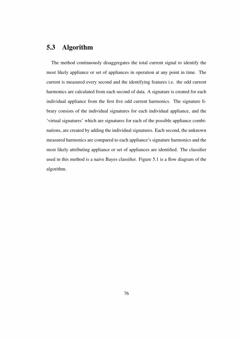
5.3 Algorithm

The method continuously disaggregates the total current signal to identify the

most likely appliance or set of appliances in operation at any point in time. The

current is measured every second and the identifying features i.e. the odd current

harmonics are calculated from each second of data. A signature is created for each

individual appliance from the first five odd current harmonics. The signature li-

brary consists of the individual signatures for each individual appliance, and the

‘virtual signatures’ which are signatures for each of the possible appliance combi-

nations, are created by adding the individual signatures. Each second, the unknown

measured harmonics are compared to each appliance’s signature harmonics and the

most likely attributing appliance or set of appliances are identified. The classifier

used in this method is a naive Bayes classifier. Figure 5.1 is a flow diagram of the

algorithm.

76

Classify set of appliances using naïve Bayes and

SSFFT

Signature Library

Retrieve current signal harmonics

Measured steady state FFT (SSFFT) Steady state signatures (SSFFTs)

The amplitudes of the first five odd current harmonics measured from the live current.

The library consists of a signature for each appliance and each combination of appliances. This is derived from the first five amplitudes of the FFT.

Measured Input

Identify probable appliance set

SSFFT

SSFFTs

Figure 5.1: Flow diagram representing the load identification algorithm which runsevery second.

The naive Bayes classifier was chosen due to reasons outlined in Chapter 2. The

classifier uses the training data to create a distribution for each class i.e. appliance.

The training data consists of the steady state samples of each of the five odd current

harmonic amplitudes for each appliance. The most likely appliance that is consum-

ing power is calculated using the library of signature distributions and Bayesian

probabilities. The probability is calculated for each appliance that the unknown

measurement belongs to that appliance (or set of appliances). The maximum prob-

ability from all the possible calculated appliance probabilities indicates the most

likely appliance to be consuming power.

77

5.3.1 Signature library

There are two steps or parts to creating the signature library. The first step is to

use real measured data to describe the individual appliances. This data is used to

create a signature for each appliance, that is sampled from the training data. The

second part of the library is the virtual library. The virtual library is created to

account for all the possible combinations of appliances that can occur. The vir-

tual library is created by adding the individual signatures to create the appliance

combinations’ signatures.

Each individual appliance’s signature is generated from that appliance operating

in isolation in steady state. The first five odd harmonics are sampled for a training

time, and the mean µ and standard deviation σ of each are calculated and are used as

the signature parameters, Table 5.1. It can be seen that similarly powered appliances

are separated through using multiple harmonic amplitudes, for example the CRT

monitor and the fridge which are both approximately 80 W the signature parameters

are completely different, Table 5.1.

78

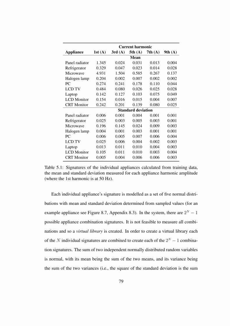
Current harmonicAppliance 1st (A) 3rd (A) 5th (A) 7th (A) 9th (A)

MeanPanel radiator 1.345 0.024 0.031 0.013 0.004Refrigerator 0.329 0.047 0.023 0.014 0.028Microwave 4.931 1.504 0.585 0.267 0.137Halogen lamp 0.204 0.002 0.007 0.002 0.002PC 0.274 0.241 0.178 0.110 0.044LCD TV 0.484 0.080 0.026 0.025 0.028Laptop 0.142 0.127 0.103 0.075 0.049LCD Monitor 0.154 0.016 0.015 0.004 0.007CRT Monitor 0.242 0.201 0.139 0.080 0.025

Standard deviationPanel radiator 0.006 0.001 0.004 0.001 0.001Refrigerator 0.025 0.003 0.005 0.003 0.001Microwave 0.196 0.145 0.024 0.009 0.003Halogen lamp 0.004 0.001 0.003 0.001 0.001PC 0.006 0.005 0.007 0.006 0.004LCD TV 0.025 0.006 0.004 0.002 0.003Laptop 0.013 0.011 0.010 0.004 0.003LCD Monitor 0.105 0.011 0.010 0.003 0.004CRT Monitor 0.005 0.004 0.006 0.006 0.003

Table 5.1: Signatures of the individual appliances calculated from training data,the mean and standard deviation measured for each appliance harmonic amplitude(where the 1st harmonic is at 50 Hz).

Each individual appliance’s signature is modelled as a set of five normal distri-

butions with mean and standard deviation determined from sampled values (for an

example appliance see Figure 8.7, Appendix 8.3). In the system, there are 2N − 1

possible appliance combination signatures. It is not feasible to measure all combi-

nations and so a virtual library is created. In order to create a virtual library each

of the N individual signatures are combined to create each of the 2N − 1 combina-

tion signatures. The sum of two independent normally distributed random variables

is normal, with its mean being the sum of the two means, and its variance being

the sum of the two variances (i.e., the square of the standard deviation is the sum

79

of the squares of the standard deviations). For example, if X and Y are indepen-

dent random variables that are normally distributed, then their sum is also normally

distributed. i.e., if X ∼ N(µX , σX) and Y ∼ N(µY , σY ) then Z = X + Y there-

fore Z ∼ N(µX + µY ,√σ2X + σ2

Y ). The virtual signature library is built using this

premise, where X is the signature for one appliance operating, Y is the signature for

a second appliance and Z is the signature of both appliances operating concurrently.

5.3.2 Naive Bayes classifier

Classification is the problem of identifying which class a new observation be-

longs to. Each class is described by its features. In this case, an individual ap-

pliance is the class and the features are the amplitudes of the first five odd current

harmonics. The prior probability is the probability before any evidence is taken into

account. It is assumed that each appliance Aj is equally likely to be switched on at

any time, so the prior probability is the same for all appliances, Eqn. 5.1, where N

is the number of appliances and j is the appliance 1:N.

P (Aj) =1

N(5.1)

Each appliance Aj , is represented in the library by five harmonics, and each

harmonic is a normal distribution Hi ∼ N(µi, σi), where i is one of the five cur-

rent harmonics. The mean, µi, and standard deviation, σi for each distribution are

calculated from training data. The algorithm is fed a test sample x, where the val-

ues for each of the harmonic amplitudes are known, but the appliance is unknown.

The sample x is a vector which contains five values, each representing a current

harmonic amplitude at a point in time. The probability that x belongs to appliance

80

Aj is calculated, using the harmonics from x and the distributions for Aj from the

signature library. The probability is calculated for each of the harmonics from test

sample x to belong to a specific harmonic distribution using Eqn. 5.2.

p(xi|Hi) =1√

2πσ2i

exp

(−(xi − µi)2

2σ2i

)(5.2)

It is assumed that for each appliance, the harmonics are independent. The prod-

uct of the harmonic probabilities for each appliance is calculated, Eqn. 5.3. This

probability is known as the likelihood, which is the probability of the sample x

belonging to Aj .

p(x|Aj)=5∏

n=1

p(xi|Hi) (5.3)

The algorithm calculates the posterior probability that x belongs to each of the

appliances Aj (for example the refrigerator, radiator etc.). The adjusted probability

(posterior) is p(x|Aj), which is the probability that the sample x belongs to Aj ,

given the features of the class Aj . The posterior probability is calculated in Eqn.

5.4 and 5.5, where the prior is the probability of a specific appliance switching on.

The likelihood is the probability that the features of x belong toAj . The evidence is

a summation of the likelihoods of the sample x belonging to any of the appliances.

The evidence is then used as a scaling factor so that the posteriors lie between 0 and

1.

posterior =prior × likelihood

evidence(5.4)

81

posterior(Aj) = p(Aj|x) =P (Aj)× p(x|Aj)∑Nn=1 P (Ak)× p(x|Ak)

(5.5)

The posterior probability is calculated for all of the appliances in the library.

The maximum calculated posterior from all the appliance posteriors is then iden-

tified as the most likely appliance to be consuming power. The algorithm is then

expanded to account for all the combinations of appliances. There are 2N − 1 pos-

sible combinations, so the prior probability will become1

2N − 1. In the equations

above Aj will represent each probable appliance combination.

5.4 Experimental procedure

Each signature is derived from a full running cycle of their operation, so for

the case of the fridge the amount of the data used for training is twenty minutes

and for the PC it is one hour. The training data amount varies depending on each

appliance, but in all cases it does not exceed ninety minutes. Each appliance is

isolated from other appliances and measured directly at the electrical mains. The

mean and standard deviation were calculated for each harmonic and can be seen in

Table 5.1. As the transient part of the signal generally only lasts for approximately

one or two seconds it is disregarded from the signature definition. This decision

has been made on the premise that, for example, a fridge can have a run time of

ten minutes (or even thirty minutes), and the transient part of the signal is trivial in

comparison.

To carry out the test, nine appliances were chosen from the appliances listed in

Table 4.6, Chapter 4. Nine appliances were chosen, similar to work presented in [2],

82

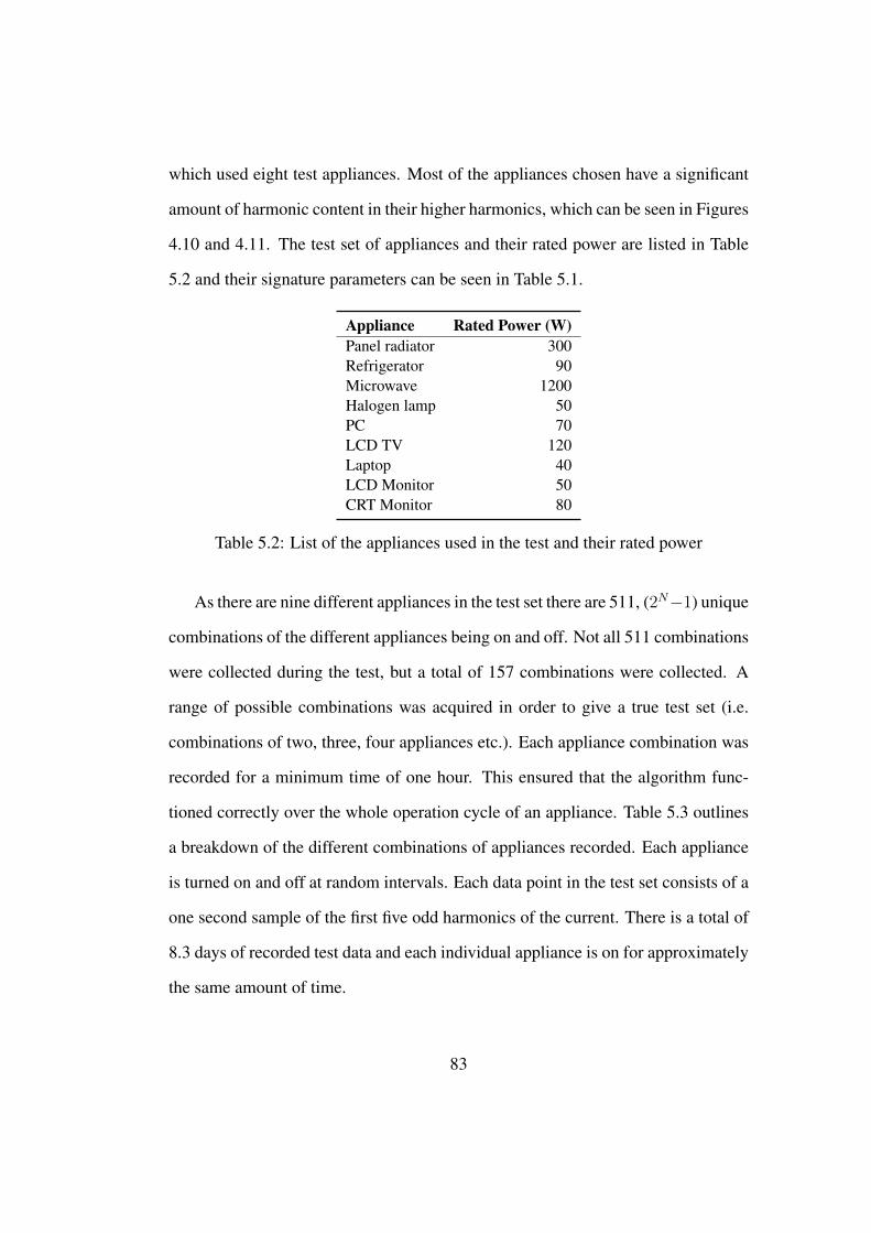
which used eight test appliances. Most of the appliances chosen have a significant

amount of harmonic content in their higher harmonics, which can be seen in Figures

4.10 and 4.11. The test set of appliances and their rated power are listed in Table

5.2 and their signature parameters can be seen in Table 5.1.

Appliance Rated Power (W)Panel radiator 300Refrigerator 90Microwave 1200Halogen lamp 50PC 70LCD TV 120Laptop 40LCD Monitor 50CRT Monitor 80

Table 5.2: List of the appliances used in the test and their rated power

As there are nine different appliances in the test set there are 511, (2N−1) unique

combinations of the different appliances being on and off. Not all 511 combinations

were collected during the test, but a total of 157 combinations were collected. A

range of possible combinations was acquired in order to give a true test set (i.e.

combinations of two, three, four appliances etc.). Each appliance combination was

recorded for a minimum time of one hour. This ensured that the algorithm func-

tioned correctly over the whole operation cycle of an appliance. Table 5.3 outlines

a breakdown of the different combinations of appliances recorded. Each appliance

is turned on and off at random intervals. Each data point in the test set consists of a

one second sample of the first five odd harmonics of the current. There is a total of

8.3 days of recorded test data and each individual appliance is on for approximately

the same amount of time.

83

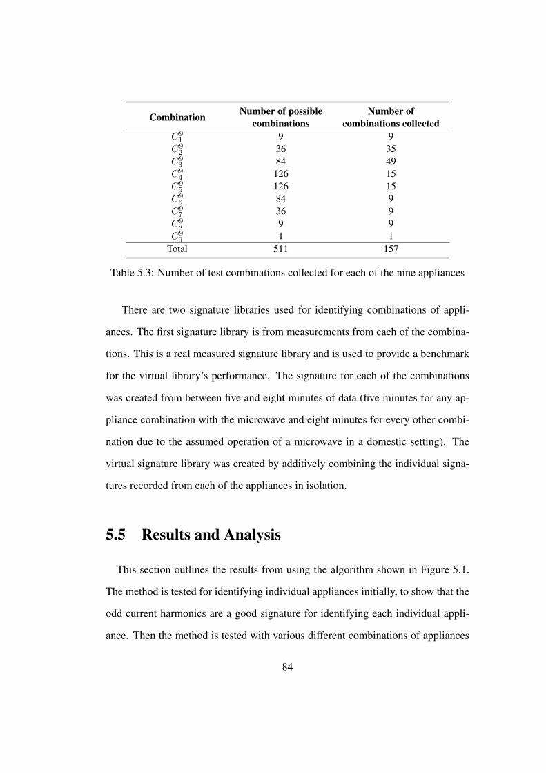
Combination Number of possiblecombinations

Number ofcombinations collected

C91 9 9

C92 36 35

C93 84 49

C94 126 15

C95 126 15

C96 84 9

C97 36 9

C98 9 9

C99 1 1

Total 511 157

Table 5.3: Number of test combinations collected for each of the nine appliances

There are two signature libraries used for identifying combinations of appli-

ances. The first signature library is from measurements from each of the combina-

tions. This is a real measured signature library and is used to provide a benchmark

for the virtual library’s performance. The signature for each of the combinations

was created from between five and eight minutes of data (five minutes for any ap-

pliance combination with the microwave and eight minutes for every other combi-

nation due to the assumed operation of a microwave in a domestic setting). The

virtual signature library was created by additively combining the individual signa-

tures recorded from each of the appliances in isolation.

5.5 Results and Analysis

This section outlines the results from using the algorithm shown in Figure 5.1.

The method is tested for identifying individual appliances initially, to show that the

odd current harmonics are a good signature for identifying each individual appli-

ance. Then the method is tested with various different combinations of appliances

84

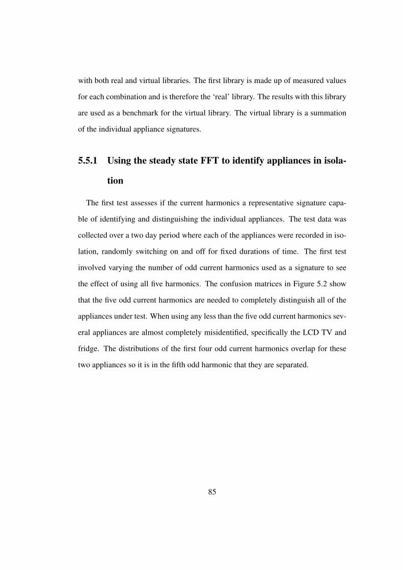
with both real and virtual libraries. The first library is made up of measured values

for each combination and is therefore the ‘real’ library. The results with this library

are used as a benchmark for the virtual library. The virtual library is a summation

of the individual appliance signatures.

5.5.1 Using the steady state FFT to identify appliances in isola-

tion

The first test assesses if the current harmonics a representative signature capa-

ble of identifying and distinguishing the individual appliances. The test data was

collected over a two day period where each of the appliances were recorded in iso-

lation, randomly switching on and off for fixed durations of time. The first test

involved varying the number of odd current harmonics used as a signature to see

the effect of using all five harmonics. The confusion matrices in Figure 5.2 show

that the five odd current harmonics are needed to completely distinguish all of the

appliances under test. When using any less than the five odd current harmonics sev-

eral appliances are almost completely misidentified, specifically the LCD TV and

fridge. The distributions of the first four odd current harmonics overlap for these

two appliances so it is in the fifth odd harmonic that they are separated.

85

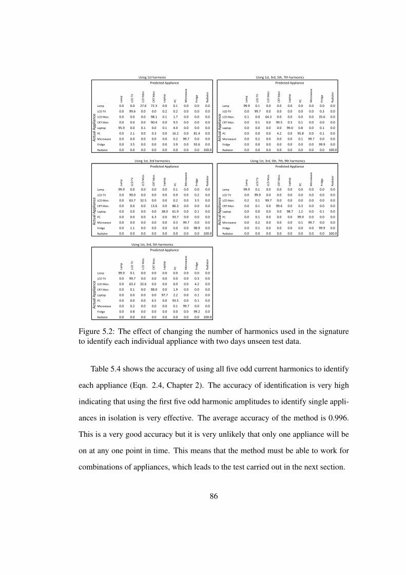
Lam

p

LCD

TV

LCD

Mo

n.

CR

T M

on

.

Lap

top

PC

Mic

row

ave

Frid

ge

Rad

iato

r

Lam

p

LCD

TV

LCD

Mo

n.

CR

T M

on

.

Lap

top

PC

Mic

row

ave

Frid

ge

Rad

iato

r

Lamp 0.0 0.0 27.6 72.3 0.0 0.1 0.0 0.0 0.0 Lamp 99.9 0.1 0.0 0.0 0.0 0.0 0.0 0.0 0.0

LCD TV 0.0 99.6 0.0 0.0 0.2 0.2 0.0 0.0 0.0 LCD TV 0.0 99.7 0.0 0.0 0.0 0.0 0.0 0.3 0.0

LCD Mon. 0.0 0.0 0.0 98.1 0.1 1.7 0.0 0.0 0.0 LCD Mon. 0.1 0.0 64.3 0.0 0.0 0.0 0.0 35.6 0.0

CRT Mon. 0.0 0.0 0.0 90.4 0.0 9.5 0.0 0.0 0.0 CRT Mon. 0.0 0.1 0.0 99.5 0.3 0.1 0.0 0.0 0.0

Laptop 95.9 0.0 0.1 0.0 0.1 4.0 0.0 0.0 0.0 Laptop 0.0 0.0 0.0 0.0 99.0 0.8 0.0 0.1 0.0

PC 0.0 2.1 0.0 0.3 0.0 16.2 0.0 81.4 0.0 PC 0.0 0.0 0.0 4.2 0.0 95.8 0.0 0.1 0.0

Microwave 0.0 0.0 0.0 0.0 0.0 0.2 99.7 0.0 0.0 Microwave 0.0 0.2 0.0 0.0 0.0 0.1 99.7 0.0 0.0

Fridge 0.0 3.5 0.0 0.0 0.0 3.9 0.0 92.6 0.0 Fridge 0.0 0.0 0.0 0.0 0.0 0.0 0.0 99.9 0.0

Radiator 0.0 0.0 0.0 0.0 0.0 0.0 0.0 0.0 100.0 Radiator 0.0 0.0 0.0 0.0 0.0 0.0 0.0 0.0 100.0

Lam

p

LCD

TV

LCD

Mo

n.

CR

T M

on

.

Lap

top

PC

Mic

row

ave

Frid

ge

Rad

iato

r

Lam

p

LCD

TV

LCD

Mo

n.

CR

T M

on

.

Lap

top

PC

Mic

row

ave

Frid

ge

Rad

iato

r

Lamp 99.9 0.0 0.0 0.0 0.0 0.1 0.0 0.0 0.0 Lamp 99.9 0.1 0.0 0.0 0.0 0.0 0.0 0.0 0.0

LCD TV 0.0 99.0 0.0 0.0 0.0 0.9 0.0 0.2 0.0 LCD TV 0.0 99.9 0.0 0.0 0.0 0.0 0.0 0.0 0.0

LCD Mon. 0.0 63.7 32.5 0.0 0.0 0.2 0.0 3.5 0.0 LCD Mon. 0.2 0.1 99.7 0.0 0.0 0.0 0.0 0.0 0.0

CRT Mon. 0.0 0.0 0.0 13.6 0.0 86.3 0.0 0.0 0.0 CRT Mon. 0.0 0.1 0.0 99.6 0.0 0.3 0.0 0.0 0.0

Laptop 0.0 0.0 0.0 0.0 38.0 61.9 0.0 0.1 0.0 Laptop 0.0 0.0 0.0 0.0 98.7 1.2 0.0 0.1 0.0

PC 0.0 0.0 0.0 6.3 0.0 93.7 0.0 0.0 0.0 PC 0.0 0.1 0.0 0.0 0.0 99.9 0.0 0.0 0.0

Microwave 0.0 0.0 0.0 0.0 0.0 0.3 99.7 0.0 0.0 Microwave 0.0 0.2 0.0 0.0 0.0 0.1 99.7 0.0 0.0

Fridge 0.0 1.1 0.0 0.0 0.0 0.0 0.0 98.9 0.0 Fridge 0.0 0.1 0.0 0.0 0.0 0.0 0.0 99.9 0.0

Radiator 0.0 0.0 0.0 0.0 0.0 0.0 0.0 0.0 100.0 Radiator 0.0 0.0 0.0 0.0 0.0 0.0 0.0 0.0 100.0

Lam

p

LCD

TV

LCD

Mo

n.

CR

T M

on

.

Lap

top

PC

Mic

row

ave

Frid

ge

Rad

iato

r

Lamp 99.9 0.1 0.0 0.0 0.0 0.0 0.0 0.0 0.0

LCD TV 0.0 99.7 0.0 0.0 0.0 0.0 0.0 0.3 0.0

LCD Mon. 0.0 63.2 32.6 0.0 0.0 0.0 0.0 4.2 0.0

CRT Mon. 0.0 0.1 0.0 98.0 0.0 1.9 0.0 0.0 0.0

Laptop 0.0 0.0 0.0 0.0 97.7 2.2 0.0 0.1 0.0

PC 0.0 0.0 0.0 6.5 0.0 93.5 0.0 0.1 0.0

Microwave 0.0 0.2 0.0 0.0 0.0 0.1 99.7 0.0 0.0

Fridge 0.0 0.8 0.0 0.0 0.0 0.0 0.0 99.2 0.0

Radiator 0.0 0.0 0.0 0.0 0.0 0.0 0.0 0.0 100.0

Using 1st, 3rd harmonics Using 1st, 3rd, 5th, 7th, 9th harmonics

Using 1st, 3rd, 5th harmonics

Predicted Appliance

Act

ual

Ap

plia

nce

Act

ual

Ap

plia

nce

Act

ual

Ap

plia

nce

Predicted Appliance

Predicted Appliance Predicted Appliance

Using 1st, 3rd, 5th, 7th harmonics

Act

ual

Ap

plia

nce

Predicted Appliance

Using 1st harmonic

Act

ual

Ap

plia

nce

Figure 5.2: The effect of changing the number of harmonics used in the signatureto identify each individual appliance with two days unseen test data.

Table 5.4 shows the accuracy of using all five odd current harmonics to identify

each appliance (Eqn. 2.4, Chapter 2). The accuracy of identification is very high

indicating that using the first five odd harmonic amplitudes to identify single appli-

ances in isolation is very effective. The average accuracy of the method is 0.996.

This is a very good accuracy but it is very unlikely that only one appliance will be

on at any one point in time. This means that the method must be able to work for

combinations of appliances, which leads to the test carried out in the next section.

86

Appliance AUCPanel radiator 0.999Refrigerator 0.999Microwave 0.999Halogen lamp 0.999PC 0.983LCD TV 0.998Laptop 0.994LCD Monitor 0.999CRT Monitor 0.998

Table 5.4: Accuracy for identifying each individual appliance using the five oddcurrent harmonics as a signature and with two days of unseen test data.

5.5.2 Identifying appliance combinations and comparing using

a virtual signature library versus a real measured signa-

ture library

The method was extended and tested for combinations of multiple appliances.

Table 5.5 and Figure 5.3 show the accuracy values for the prediction of each ap-

pliance from the test combination set (Table 5.3) . The accuracy is the ratio of

the number of correctly predicted occurrences of an appliance to the total number

of occurrences of that appliance (Eqn. 2.4, Chapter 2). Real (measured) signatures

have been used as a benchmark to compare how accurate a representation the virtual

library is. As is expected the accuracy of using a real measured signature library is

better than a virtual signature library.

87

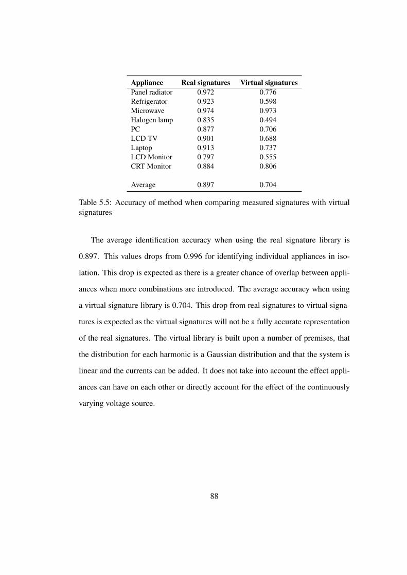
Appliance Real signatures Virtual signaturesPanel radiator 0.972 0.776Refrigerator 0.923 0.598Microwave 0.974 0.973Halogen lamp 0.835 0.494PC 0.877 0.706LCD TV 0.901 0.688Laptop 0.913 0.737LCD Monitor 0.797 0.555CRT Monitor 0.884 0.806

Average 0.897 0.704

Table 5.5: Accuracy of method when comparing measured signatures with virtualsignatures

The average identification accuracy when using the real signature library is

0.897. This values drops from 0.996 for identifying individual appliances in iso-

lation. This drop is expected as there is a greater chance of overlap between appli-

ances when more combinations are introduced. The average accuracy when using

a virtual signature library is 0.704. This drop from real signatures to virtual signa-

tures is expected as the virtual signatures will not be a fully accurate representation

of the real signatures. The virtual library is built upon a number of premises, that

the distribution for each harmonic is a Gaussian distribution and that the system is

linear and the currents can be added. It does not take into account the effect appli-

ances can have on each other or directly account for the effect of the continuously

varying voltage source.

88

Rad. Fridge Micro. PC Laptop CRT LCD TV Lamp0

0.5

1Accuracy

Acc

urac

y

MeasuredsignaturesVirtualsignatures

Figure 5.3: Accuracy of predicting individual appliances from combinations usingvirtual signatures compared to those of measured signatures

The classification accuracy values aren’t the same for all appliances. For some

appliances it is much higher than for others, for example the microwave has the

highest accuracy. The microwave is also the largest load, (Table 5.2) so its signal

to noise ratio (SNR) would be much larger than that of the halogen lamp, which

is the smallest load and also has one of the lowest identification accuracies. The

LCD monitor and the halogen lamp have the lowest accuracy in this test and are

also two of the smallest loads at 60 W and 50 W respectively, Table 5.2. Another

note is that the appliances with lower harmonic content (relative to the amplitude

their fundamental harmonics) have the worst accuracy. Appliances that appear to

have lower harmonic content (halogen bulb) are ‘lost’ within combined signals.

A study was carried out to investigate the impact of the interaction between ap-

pliances due to a shared source impedance [82]. It found that using arithmetic sums

of harmonic current magnitudes can overestimate the cumulative harmonic currents

produced by distributed single-phase power electronic loads. This work found that,

for an adjustable speed drive appliance, that as the power increased there was an

attenuation effect on harmonic current magnitudes and an impact on phase angles,

especially for higher order harmonics. These variations are also visible in the sys-

89

tem impedance magnitude. This implied that there is an attenuation effect when a

number of similar load types are operated on a shared system impedance. From this

they found that there is an attenuation affect on harmonics when similar load types

operate on the same system, and if the aggregate current is calculated using super-

position, there can be an overestimation. This is a very likely reason that the virtual

library is not a fully accurate representation of the appliance combinations. As

more appliances are added to the system the virtual harmonic amplitudes increas-

ingly overestimate the cumulative harmonic currents produced by the appliances

and the signatures are not representative of the actual system.

5.6 Conclusion

This chapter outlines a method for continuously identifying appliances consum-

ing power using the current FFT as a signature for each appliance and a naive Bayes

classifier to identify when each appliance is on. The work in this chapter does not

present a feasible fully deployable method for identifying appliances consuming

power. There are a number of problems with the final method including the average

accuracy of the method not being as good as the literature (70% versus 80%, Table

2.3, Chapter 2) not being good enough, the complexity of the method (2N−1) being

quite high and other concerns, such as a lengthy training time. The overall accuracy

of the method is 70% when all the combinations of the appliances are taken into

account, which is not competitive with other methods. The virtual library is not

a fully accurate representation for the appliance combinations, and the sum of the

harmonic current amplitudes may overestimate the total actual current. This work

shows that the first five odd current harmonics alongside the naive Bayes classifier

90

is an effective method at distinguishing between individual appliances (Table 5.4).

With these findings in mind the next chapter presents a further developed method

where both the scalability and the accuracy are improved. The training time is de-

creased to a more acceptable time for a real time deployment and the method is

optimised to work for all types of appliances including lower powered appliances

and appliances with smaller amounts of higher harmonic content.

91

Chapter 6

A two step classification method that

uses a time frequency signature

6.1 Introduction

The previous chapter outlines a method that uses the steady state current harmon-

ics to identify which appliances are consuming power continuously. This method

shows that the odd current harmonics and the naive Bayes classifier are accurate at

identifying individual appliances, but the method is limited when combinations of

appliances are included. The complexity of the method is 2N − 1 which is not ideal

and the training time for each individual signature is longer than feasible (greater

than five minutes). The average confidence is 70% and when compared with other

methods it falls short. This chapter presents a method which builds on this work

with the goal of improving on performance in these areas.

The method presented in this chapter is event based, and uses time and fre-

quency features from the current signal to identify what appliance has turned ON or

92

OFF. An event is when an appliance turns on or off. The method utilizes a two-step

classification algorithm and looks at the differences before and after the event and

extracts features for classification. By changing the algorithm to an event based

method the scalability of the method is instantly improved to a complexity of N , as

only one appliance at a time has to be identified.

6.2 Methodology

There are several key points that need to be achieved when developing an efficient

load identification method. Table 2.3, Chapter 2 outlines the current state of the art

and highlights the specific research areas that need to be maintained or improved

on when developing an efficient method. A good load monitoring method will be

efficient and not overly complex, it will have an accuracy of identification above

80%, an algorithm complexity of N and will identify all types of appliances.

The method presented in Chapter 5 has several shortcomings and this chapter

aims to improve on these shortcomings. The method in this chapter monitors the

continuous aggregate current signal and waits for an appliance to turn on or off.

When an appliance switches state, the current signal changes and this is identified

as an event. The algorithm uses the change in the current signal from before and

after the event to identify what appliance has caused it. By changing the method

from continuous identification to event based identification this will also improve

the complexity of the method. If the algorithm only identifies an appliance at an

event, it will only need to be able to identify one appliance at an time (assuming

only one appliance changes at any time). Therefore the complexity of the system

will be N. Using an event based method introduces the possibility of using transient

93

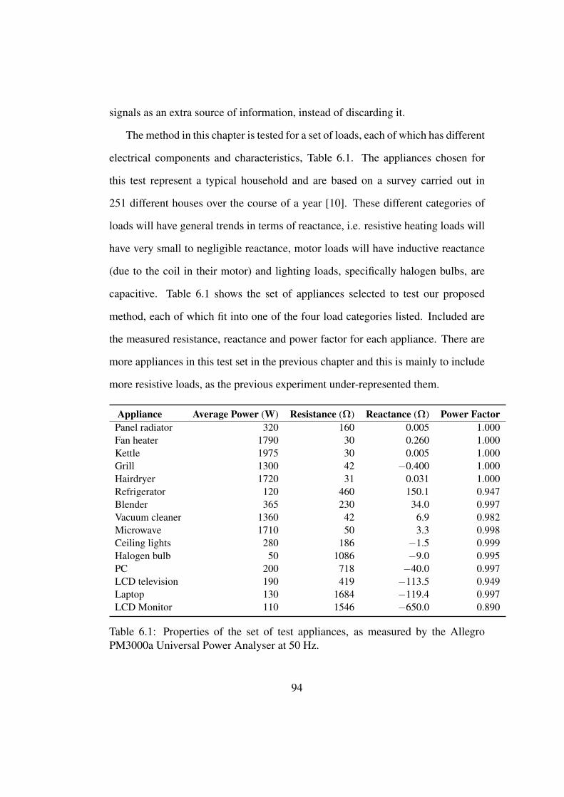
signals as an extra source of information, instead of discarding it.

The method in this chapter is tested for a set of loads, each of which has different

electrical components and characteristics, Table 6.1. The appliances chosen for

this test represent a typical household and are based on a survey carried out in

251 different houses over the course of a year [10]. These different categories of

loads will have general trends in terms of reactance, i.e. resistive heating loads will

have very small to negligible reactance, motor loads will have inductive reactance

(due to the coil in their motor) and lighting loads, specifically halogen bulbs, are

capacitive. Table 6.1 shows the set of appliances selected to test our proposed

method, each of which fit into one of the four load categories listed. Included are

the measured resistance, reactance and power factor for each appliance. There are

more appliances in this test set in the previous chapter and this is mainly to include

more resistive loads, as the previous experiment under-represented them.

Appliance Average Power (W) Resistance (Ω) Reactance (Ω) Power FactorPanel radiator 320 160 0.005 1.000Fan heater 1790 30 0.260 1.000Kettle 1975 30 0.005 1.000Grill 1300 42 −0.400 1.000Hairdryer 1720 31 0.031 1.000Refrigerator 120 460 150.1 0.947Blender 365 230 34.0 0.997Vacuum cleaner 1360 42 6.9 0.982Microwave 1710 50 3.3 0.998Ceiling lights 280 186 −1.5 0.999Halogen bulb 50 1086 −9.0 0.995PC 200 718 −40.0 0.997LCD television 190 419 −113.5 0.949Laptop 130 1684 −119.4 0.997LCD Monitor 110 1546 −650.0 0.890

Table 6.1: Properties of the set of test appliances, as measured by the AllegroPM3000a Universal Power Analyser at 50 Hz.

94

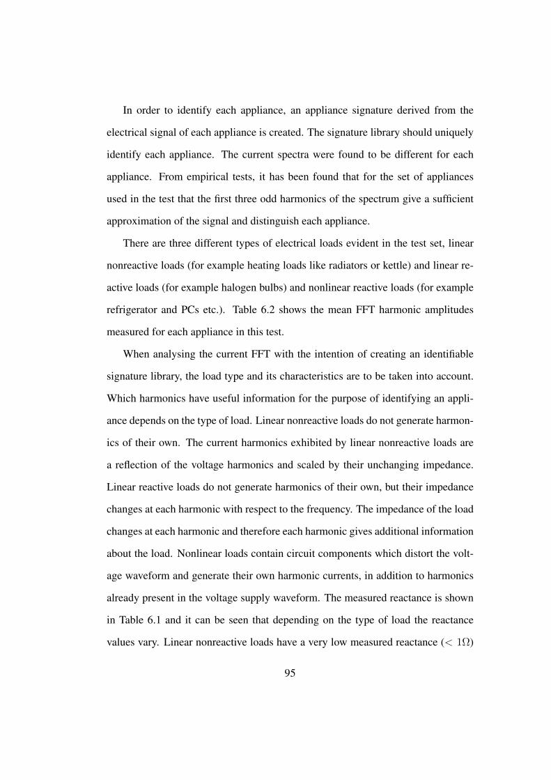
In order to identify each appliance, an appliance signature derived from the

electrical signal of each appliance is created. The signature library should uniquely

identify each appliance. The current spectra were found to be different for each

appliance. From empirical tests, it has been found that for the set of appliances

used in the test that the first three odd harmonics of the spectrum give a sufficient

approximation of the signal and distinguish each appliance.

There are three different types of electrical loads evident in the test set, linear

nonreactive loads (for example heating loads like radiators or kettle) and linear re-

active loads (for example halogen bulbs) and nonlinear reactive loads (for example

refrigerator and PCs etc.). Table 6.2 shows the mean FFT harmonic amplitudes

measured for each appliance in this test.

When analysing the current FFT with the intention of creating an identifiable

signature library, the load type and its characteristics are to be taken into account.

Which harmonics have useful information for the purpose of identifying an appli-

ance depends on the type of load. Linear nonreactive loads do not generate harmon-

ics of their own. The current harmonics exhibited by linear nonreactive loads are

a reflection of the voltage harmonics and scaled by their unchanging impedance.

Linear reactive loads do not generate harmonics of their own, but their impedance

changes at each harmonic with respect to the frequency. The impedance of the load

changes at each harmonic and therefore each harmonic gives additional information

about the load. Nonlinear loads contain circuit components which distort the volt-

age waveform and generate their own harmonic currents, in addition to harmonics

already present in the voltage supply waveform. The measured reactance is shown

in Table 6.1 and it can be seen that depending on the type of load the reactance

values vary. Linear nonreactive loads have a very low measured reactance (< 1Ω)

95

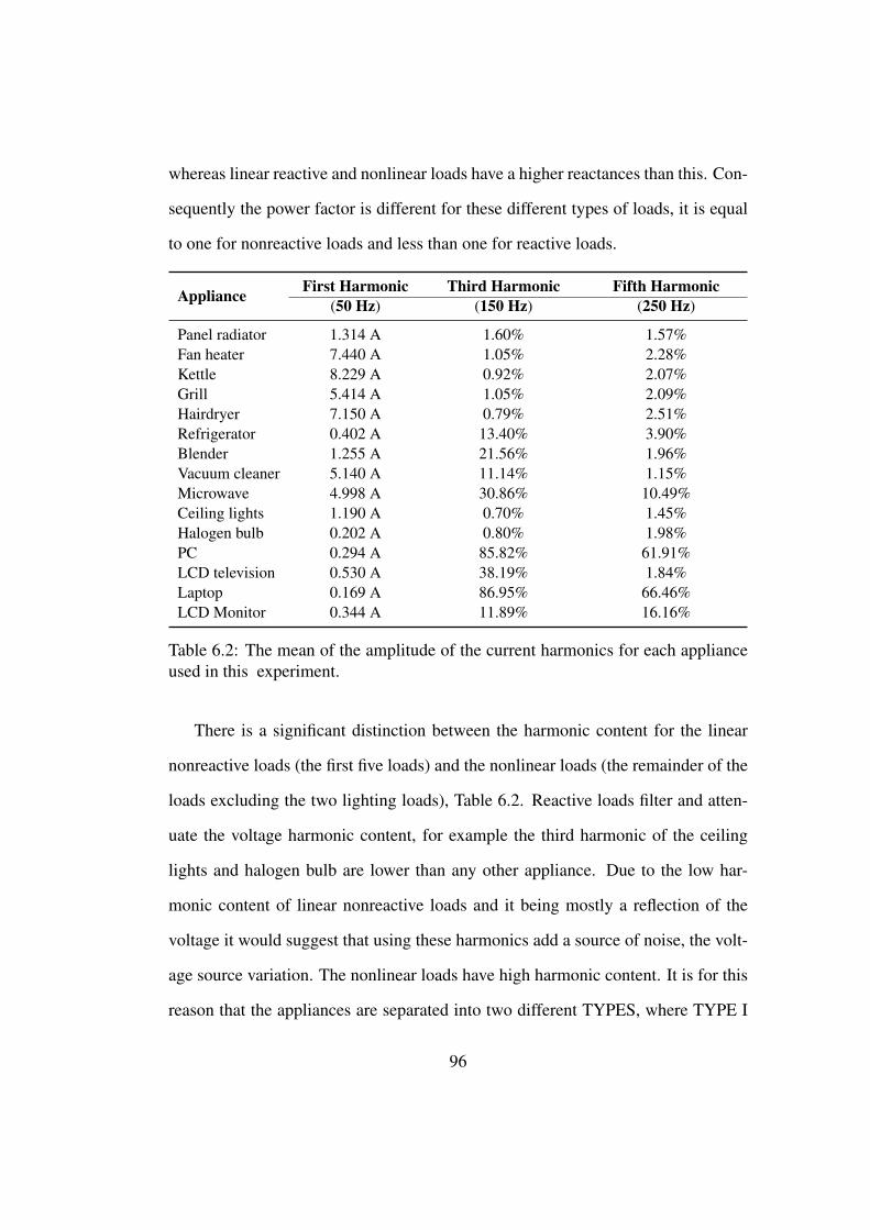
whereas linear reactive and nonlinear loads have a higher reactances than this. Con-

sequently the power factor is different for these different types of loads, it is equal

to one for nonreactive loads and less than one for reactive loads.

Appliance First Harmonic Third Harmonic Fifth Harmonic(50 Hz) (150 Hz) (250 Hz)

Panel radiator 1.314 A 1.60% 1.57%Fan heater 7.440 A 1.05% 2.28%Kettle 8.229 A 0.92% 2.07%Grill 5.414 A 1.05% 2.09%Hairdryer 7.150 A 0.79% 2.51%Refrigerator 0.402 A 13.40% 3.90%Blender 1.255 A 21.56% 1.96%Vacuum cleaner 5.140 A 11.14% 1.15%Microwave 4.998 A 30.86% 10.49%Ceiling lights 1.190 A 0.70% 1.45%Halogen bulb 0.202 A 0.80% 1.98%PC 0.294 A 85.82% 61.91%LCD television 0.530 A 38.19% 1.84%Laptop 0.169 A 86.95% 66.46%LCD Monitor 0.344 A 11.89% 16.16%

Table 6.2: The mean of the amplitude of the current harmonics for each applianceused in this experiment.

There is a significant distinction between the harmonic content for the linear

nonreactive loads (the first five loads) and the nonlinear loads (the remainder of the

loads excluding the two lighting loads), Table 6.2. Reactive loads filter and atten-

uate the voltage harmonic content, for example the third harmonic of the ceiling

lights and halogen bulb are lower than any other appliance. Due to the low har-

monic content of linear nonreactive loads and it being mostly a reflection of the

voltage it would suggest that using these harmonics add a source of noise, the volt-

age source variation. The nonlinear loads have high harmonic content. It is for this

reason that the appliances are separated into two different TYPES, where TYPE I

96

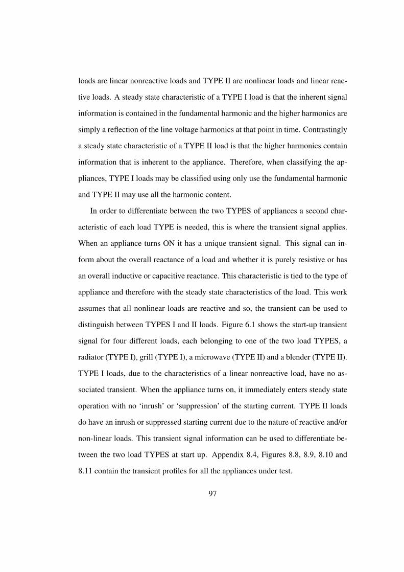
loads are linear nonreactive loads and TYPE II are nonlinear loads and linear reac-

tive loads. A steady state characteristic of a TYPE I load is that the inherent signal

information is contained in the fundamental harmonic and the higher harmonics are

simply a reflection of the line voltage harmonics at that point in time. Contrastingly

a steady state characteristic of a TYPE II load is that the higher harmonics contain

information that is inherent to the appliance. Therefore, when classifying the ap-

pliances, TYPE I loads may be classified using only use the fundamental harmonic

and TYPE II may use all the harmonic content.

In order to differentiate between the two TYPES of appliances a second char-

acteristic of each load TYPE is needed, this is where the transient signal applies.

When an appliance turns ON it has a unique transient signal. This signal can in-

form about the overall reactance of a load and whether it is purely resistive or has

an overall inductive or capacitive reactance. This characteristic is tied to the type of

appliance and therefore with the steady state characteristics of the load. This work

assumes that all nonlinear loads are reactive and so, the transient can be used to

distinguish between TYPES I and II loads. Figure 6.1 shows the start-up transient

signal for four different loads, each belonging to one of the two load TYPES, a

radiator (TYPE I), grill (TYPE I), a microwave (TYPE II) and a blender (TYPE II).

TYPE I loads, due to the characteristics of a linear nonreactive load, have no as-

sociated transient. When the appliance turns on, it immediately enters steady state

operation with no ‘inrush’ or ‘suppression’ of the starting current. TYPE II loads

do have an inrush or suppressed starting current due to the nature of reactive and/or

non-linear loads. This transient signal information can be used to differentiate be-

tween the two load TYPES at start up. Appendix 8.4, Figures 8.8, 8.9, 8.10 and

8.11 contain the transient profiles for all the appliances under test.

97

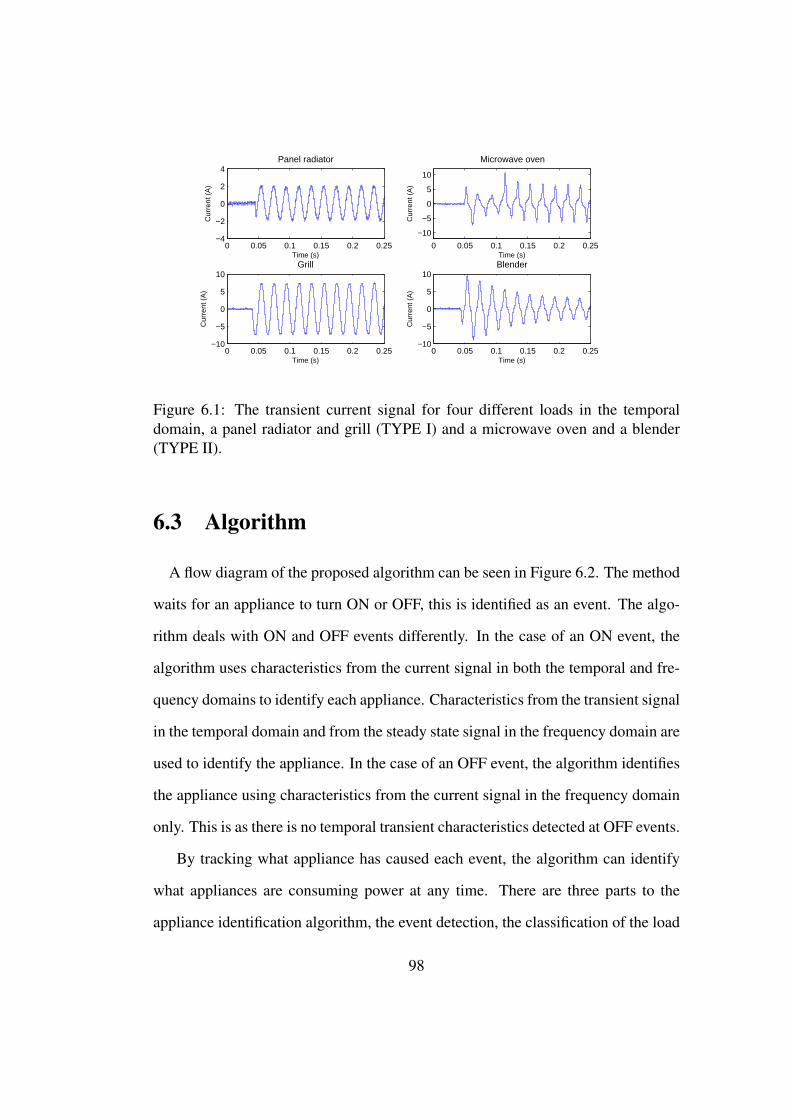
0 0.05 0.1 0.15 0.2 0.25−4

−2

0

2

4Panel radiator

Time (s)

Cur

rent

(A

)

0 0.05 0.1 0.15 0.2 0.25

−10

−5

0

5

10

Microwave oven

Time (s)

Cur

rent

(A

)

0 0.05 0.1 0.15 0.2 0.25−10

−5

0

5

10Grill

Time (s)

Cur

rent

(A

)

0 0.05 0.1 0.15 0.2 0.25−10

−5

0

5

10Blender

Time (s)

Cur

rent

(A

)Figure 6.1: The transient current signal for four different loads in the temporaldomain, a panel radiator and grill (TYPE I) and a microwave oven and a blender(TYPE II).

6.3 Algorithm

A flow diagram of the proposed algorithm can be seen in Figure 6.2. The method

waits for an appliance to turn ON or OFF, this is identified as an event. The algo-

rithm deals with ON and OFF events differently. In the case of an ON event, the

algorithm uses characteristics from the current signal in both the temporal and fre-

quency domains to identify each appliance. Characteristics from the transient signal

in the temporal domain and from the steady state signal in the frequency domain are

used to identify the appliance. In the case of an OFF event, the algorithm identifies

the appliance using characteristics from the current signal in the frequency domain

only. This is as there is no temporal transient characteristics detected at OFF events.

By tracking what appliance has caused each event, the algorithm can identify

what appliances are consuming power at any time. There are three parts to the

appliance identification algorithm, the event detection, the classification of the load

98

TYPE and the specific appliance identification.

Wait for change in IRMS --> EVENT

Classify using ΔFFT and naïve Bayes classifier

Is EVENT ON?

YES NO

Classify using naïve Bayes and specific ΔFFT harmonics

based on load TYPE

Classify load TYPE using TS

Measured Inputs Signature Library

IRMS Transient Signal (TS) ΔFFT Transient Signal (TS) Steady state (SSFFT)

The RMS current measured every second.

The positive peaks and negative peaks from the derivative of current transient temporal envelope.

The difference in the steady state current harmonic amplitudes before and after an event.

The positive peaks and negative peaks from the derivative of current transient temporal envelope.

Odd current harmonic amplitudes of each appliance.

Identify probable appliance

Measured Input

IRMS

TS

ΔFFT

Signature Library

SSFFT

TS

Figure 6.2: Algorithm flow diagram representing the load identification algorithm.

99

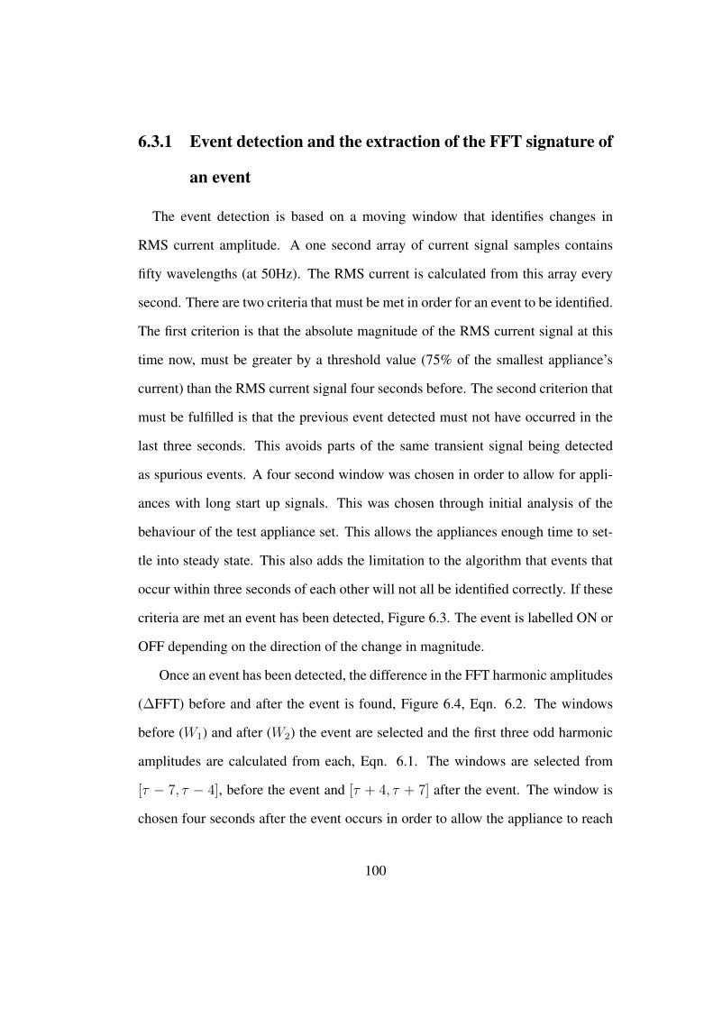
6.3.1 Event detection and the extraction of the FFT signature of

an event

The event detection is based on a moving window that identifies changes in

RMS current amplitude. A one second array of current signal samples contains

fifty wavelengths (at 50Hz). The RMS current is calculated from this array every

second. There are two criteria that must be met in order for an event to be identified.

The first criterion is that the absolute magnitude of the RMS current signal at this

time now, must be greater by a threshold value (75% of the smallest appliance’s

current) than the RMS current signal four seconds before. The second criterion that

must be fulfilled is that the previous event detected must not have occurred in the

last three seconds. This avoids parts of the same transient signal being detected

as spurious events. A four second window was chosen in order to allow for appli-

ances with long start up signals. This was chosen through initial analysis of the

behaviour of the test appliance set. This allows the appliances enough time to set-

tle into steady state. This also adds the limitation to the algorithm that events that

occur within three seconds of each other will not all be identified correctly. If these

criteria are met an event has been detected, Figure 6.3. The event is labelled ON or

OFF depending on the direction of the change in magnitude.

Once an event has been detected, the difference in the FFT harmonic amplitudes

(∆FFT) before and after the event is found, Figure 6.4, Eqn. 6.2. The windows

before (W1) and after (W2) the event are selected and the first three odd harmonic

amplitudes are calculated from each, Eqn. 6.1. The windows are selected from

[τ − 7, τ − 4], before the event and [τ + 4, τ + 7] after the event. The window is

chosen four seconds after the event occurs in order to allow the appliance to reach

100

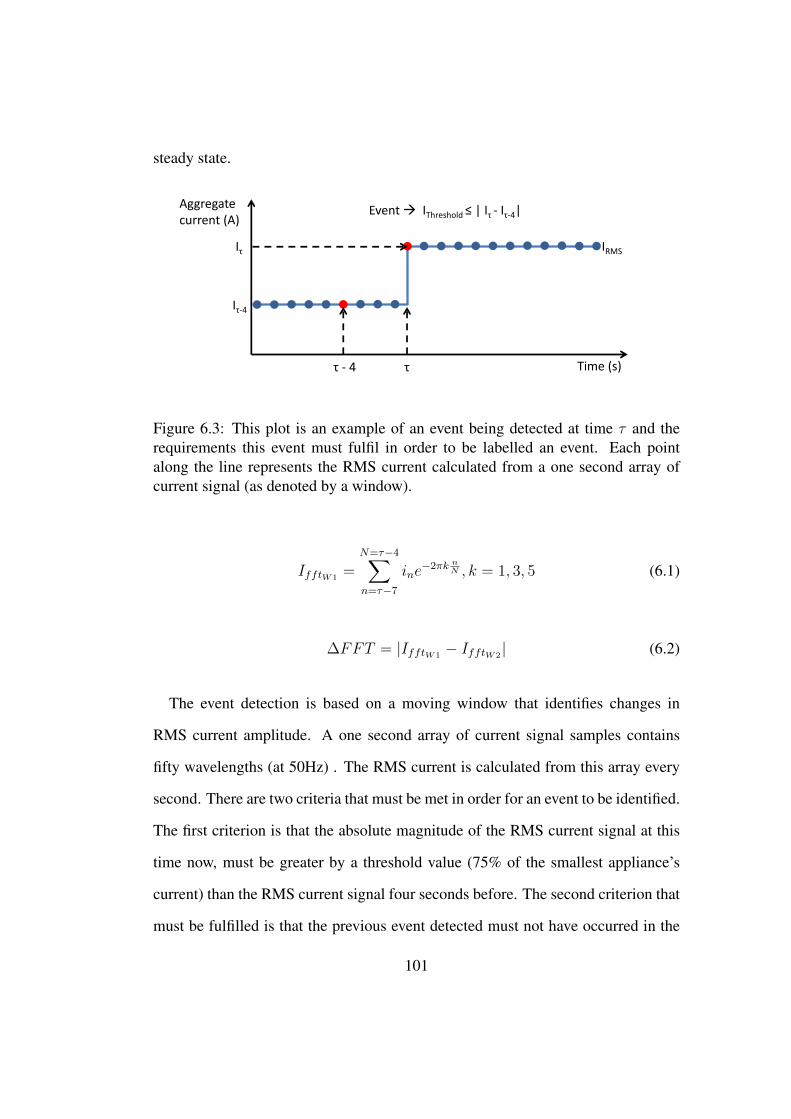
steady state.

Aggregate current (A)

Time (s) τ

Iτ

τ - 4

Iτ-4

IRMS

Event IThreshold ≤ | Iτ - Iτ-4|

Figure 6.3: This plot is an example of an event being detected at time τ and therequirements this event must fulfil in order to be labelled an event. Each pointalong the line represents the RMS current calculated from a one second array ofcurrent signal (as denoted by a window).

IfftW1=

N=τ−4∑n=τ−7

ine−2πk n

N , k = 1, 3, 5 (6.1)

∆FFT = |IfftW1− IfftW2

| (6.2)

The event detection is based on a moving window that identifies changes in

RMS current amplitude. A one second array of current signal samples contains

fifty wavelengths (at 50Hz) . The RMS current is calculated from this array every

second. There are two criteria that must be met in order for an event to be identified.

The first criterion is that the absolute magnitude of the RMS current signal at this

time now, must be greater by a threshold value (75% of the smallest appliance’s

current) than the RMS current signal four seconds before. The second criterion that

must be fulfilled is that the previous event detected must not have occurred in the

101

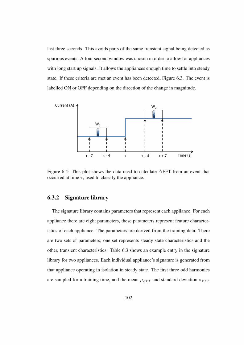
last three seconds. This avoids parts of the same transient signal being detected as

spurious events. A four second window was chosen in order to allow for appliances

with long start up signals. It allows the appliances enough time to settle into steady

state. If these criteria are met an event has been detected, Figure 6.3. The event is

labelled ON or OFF depending on the direction of the change in magnitude.

Current (A)

Time (s) τ τ - 4 τ - 7 τ + 7 τ + 4

W1

W2

Figure 6.4: This plot shows the data used to calculate ∆FFT from an event thatoccurred at time τ , used to classify the appliance.

6.3.2 Signature library

The signature library contains parameters that represent each appliance. For each

appliance there are eight parameters, these parameters represent feature character-

istics of each appliance. The parameters are derived from the training data. There

are two sets of parameters; one set represents steady state characteristics and the

other, transient characteristics. Table 6.3 shows an example entry in the signature

library for two appliances. Each individual appliance’s signature is generated from

that appliance operating in isolation in steady state. The first three odd harmonics

are sampled for a training time, and the mean µFFT and standard deviation σFFT

102

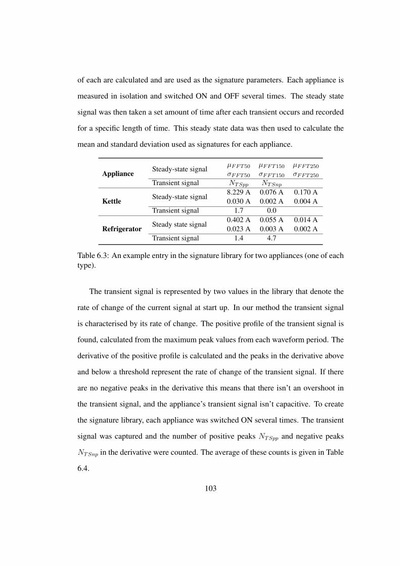
of each are calculated and are used as the signature parameters. Each appliance is

measured in isolation and switched ON and OFF several times. The steady state

signal was then taken a set amount of time after each transient occurs and recorded

for a specific length of time. This steady state data was then used to calculate the

mean and standard deviation used as signatures for each appliance.

Appliance Steady-state signalµFFT50 µFFT150 µFFT250σFFT50 σFFT150 σFFT250

Transient signal NTSpp NTSnp

Kettle Steady-state signal8.229 A 0.076 A 0.170 A0.030 A 0.002 A 0.004 A

Transient signal 1.7 0.0

Refrigerator Steady state signal0.402 A 0.055 A 0.014 A0.023 A 0.003 A 0.002 A

Transient signal 1.4 4.7

Table 6.3: An example entry in the signature library for two appliances (one of eachtype).

The transient signal is represented by two values in the library that denote the

rate of change of the current signal at start up. In our method the transient signal

is characterised by its rate of change. The positive profile of the transient signal is

found, calculated from the maximum peak values from each waveform period. The

derivative of the positive profile is calculated and the peaks in the derivative above

and below a threshold represent the rate of change of the transient signal. If there

are no negative peaks in the derivative this means that there isn’t an overshoot in

the transient signal, and the appliance’s transient signal isn’t capacitive. To create

the signature library, each appliance was switched ON several times. The transient

signal was captured and the number of positive peaks NTSpp and negative peaks

NTSnp in the derivative were counted. The average of these counts is given in Table

6.4.

103

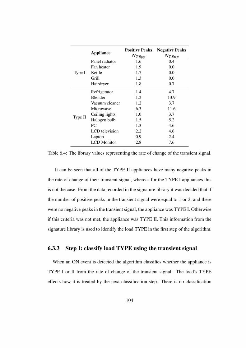
Appliance Positive Peaks Negative PeaksNTSpp NTSnp

Type I

Panel radiator 1.6 0.4Fan heater 1.9 0.0Kettle 1.7 0.0Grill 1.3 0.0Hairdryer 1.8 0.7

Type II

Refrigerator 1.4 4.7Blender 1.2 13.9Vacuum cleaner 1.2 3.7Microwave 6.3 11.6Ceiling lights 1.0 3.7Halogen bulb 1.5 5.2PC 1.3 4.6LCD television 2.2 4.6Laptop 0.9 2.4LCD Monitor 2.8 7.6

Table 6.4: The library values representing the rate of change of the transient signal.

It can be seen that all of the TYPE II appliances have many negative peaks in

the rate of change of their transient signal, whereas for the TYPE I appliances this

is not the case. From the data recorded in the signature library it was decided that if

the number of positive peaks in the transient signal were equal to 1 or 2, and there

were no negative peaks in the transient signal, the appliance was TYPE I. Otherwise

if this criteria was not met, the appliance was TYPE II. This information from the

signature library is used to identify the load TYPE in the first step of the algorithm.

6.3.3 Step I: classify load TYPE using the transient signal

When an ON event is detected the algorithm classifies whether the appliance is

TYPE I or II from the rate of change of the transient signal. The load’s TYPE

effects how it is treated by the next classification step. There is no classification

104

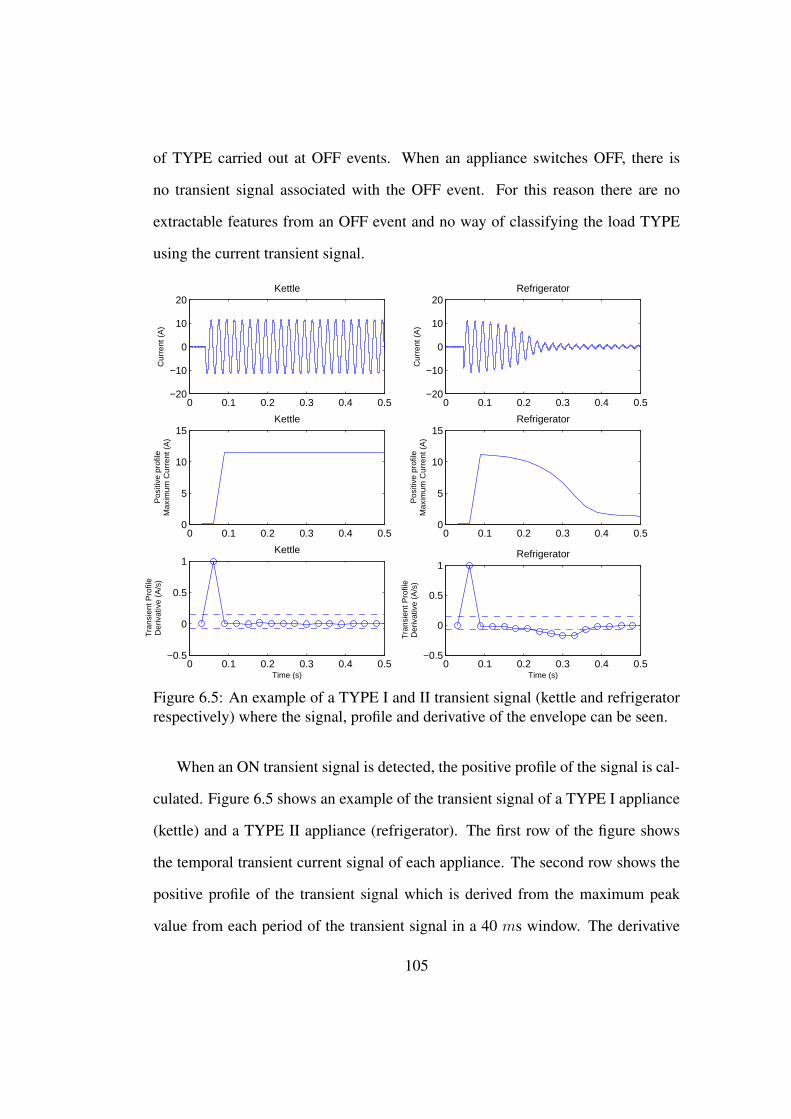
of TYPE carried out at OFF events. When an appliance switches OFF, there is

no transient signal associated with the OFF event. For this reason there are no

extractable features from an OFF event and no way of classifying the load TYPE

using the current transient signal.

0 0.1 0.2 0.3 0.4 0.5−20

−10

0

10

20Kettle

Cur

rent

(A

)

0 0.1 0.2 0.3 0.4 0.5−20

−10

0

10

20Refrigerator

Cur

rent

(A

)

0 0.1 0.2 0.3 0.4 0.50

5

10

15Kettle

Pos

itive

pro

file

Max

imum

Cur

rent

(A

)

0 0.1 0.2 0.3 0.4 0.50

5

10

15Refrigerator

Pos

itive

pro

file

Max

imum

Cur

rent

(A

)

0 0.1 0.2 0.3 0.4 0.5−0.5

0

0.5

1Kettle

Time (s)

Tra

nsie

nt P

rofil

eD

eriv

ativ

e (A

/s)

0 0.1 0.2 0.3 0.4 0.5−0.5

0

0.5

1Refrigerator

Time (s)

Tra

nsie

nt P

rofil

eD

eriv

ativ

e (A

/s)

Figure 6.5: An example of a TYPE I and II transient signal (kettle and refrigeratorrespectively) where the signal, profile and derivative of the envelope can be seen.

When an ON transient signal is detected, the positive profile of the signal is cal-

culated. Figure 6.5 shows an example of the transient signal of a TYPE I appliance

(kettle) and a TYPE II appliance (refrigerator). The first row of the figure shows

the temporal transient current signal of each appliance. The second row shows the

positive profile of the transient signal which is derived from the maximum peak

value from each period of the transient signal in a 40 ms window. The derivative

105

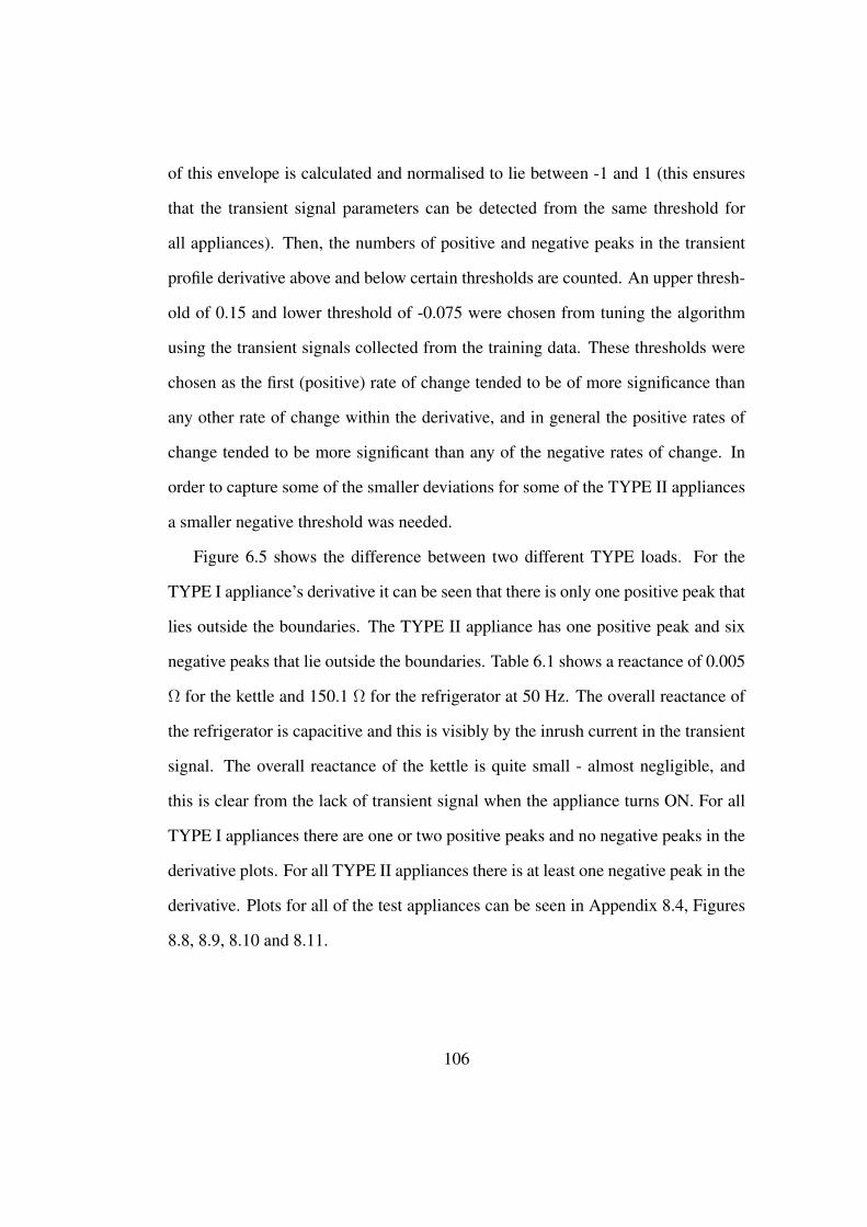
of this envelope is calculated and normalised to lie between -1 and 1 (this ensures

that the transient signal parameters can be detected from the same threshold for

all appliances). Then, the numbers of positive and negative peaks in the transient

profile derivative above and below certain thresholds are counted. An upper thresh-

old of 0.15 and lower threshold of -0.075 were chosen from tuning the algorithm

using the transient signals collected from the training data. These thresholds were

chosen as the first (positive) rate of change tended to be of more significance than

any other rate of change within the derivative, and in general the positive rates of

change tended to be more significant than any of the negative rates of change. In

order to capture some of the smaller deviations for some of the TYPE II appliances

a smaller negative threshold was needed.

Figure 6.5 shows the difference between two different TYPE loads. For the

TYPE I appliance’s derivative it can be seen that there is only one positive peak that

lies outside the boundaries. The TYPE II appliance has one positive peak and six

negative peaks that lie outside the boundaries. Table 6.1 shows a reactance of 0.005

Ω for the kettle and 150.1 Ω for the refrigerator at 50 Hz. The overall reactance of

the refrigerator is capacitive and this is visibly by the inrush current in the transient

signal. The overall reactance of the kettle is quite small - almost negligible, and

this is clear from the lack of transient signal when the appliance turns ON. For all

TYPE I appliances there are one or two positive peaks and no negative peaks in the

derivative plots. For all TYPE II appliances there is at least one negative peak in the

derivative. Plots for all of the test appliances can be seen in Appendix 8.4, Figures

8.8, 8.9, 8.10 and 8.11.

106

6.3.4 Step II: classifying appliance using steady state signal and

naive Bayes classifier

This step uses the same algorithm outlined in Section 5.3.2 with a few amend-

ments. The classifier used is a naive Bayes classifier which uses training data to

calculate signature distributions for each appliance. The naive Bayes classifier uses

training data to calculate signature distributions for each appliance. The signatures

for each appliance are the amplitudes of the first three odd current harmonics. The

calculated difference in the harmonic amplitudes (∆FFT, Figure 6.4) from before

and after an event are input into the classifier, and the probability of that value be-

longing to each individual appliance is calculated. The appliance with the highest

probability is chosen as the most likely appliance to have caused that event.

When an event occurs, the appliance TYPE is classified. Depending on the

appliance TYPE, the specific harmonics used to identify the appliance are varied.

If an appliance is classified as TYPE I, the fundamental harmonic is used by the

naive Bayes classifier. If the appliance is classified as TYPE II, the first five odd

harmonics are used by the naive Bayes classifier.

In the appliance test set there are five TYPE I appliances and ten TYPE II appli-

ances. If the appliance has been classified as a TYPE I load the fundamental FFT

amplitude, and the fundamental harmonic signatures of the five TYPE I appliances

are input to the naive Bayes classifier. Similarly if the appliance is identified as

TYPE II the five FFT amplitudes are input to the naive Bayes classifier alongside

the ten TYPE II appliance signatures. The most likely appliance is identified from

the appliance with the highest probability from the classifier.

When the event is OFF there are not transient features associated with the signal

107

and there is no classification of TYPE step. In this case the difference before and

after the event are found for all three FFT harmonics of the measurement signal and

with all fifteen appliance signatures are input into the naive Bayes classifier. The

most likely appliance to have caused the event is identified.

6.4 Experimental procedure

In order to assume a realistic training time for a real environment deployment it

was attempted to keep the training time for each appliance to a minimum. Each

appliance was measured in isolation. The appliance under test was switched ON

ten times to record the transient signal. The steady state signal was measured from

five seconds after each transient and recorded for a further ten seconds. For each

appliance there was a total of 100 seconds of steady state data to create the steady

state signatures and ten transient events from which to derive the transient signa-

tures. All of the training data for all of the appliances was recorded over a three

hour period. The experiment was carried out in a simulated domestic environment,

described in Chapter 4.

There are fifteen different test appliances, which means there are over 32,000

(2N − 1) unique combinations of the different appliances being power cycled. It is

not possible to record all these combinations. In order to attempt to have a strin-

gent robust test each appliance was switched ON and OFF a number of times under

different conditions. Initially each appliance is tested individually and then tested

while other appliances are operating in steady state. The appliance under test was

switched ON and OFF while combinations of up to nine other appliances were

operating in steady state. A breakdown of the number of events recorded per ap-

108

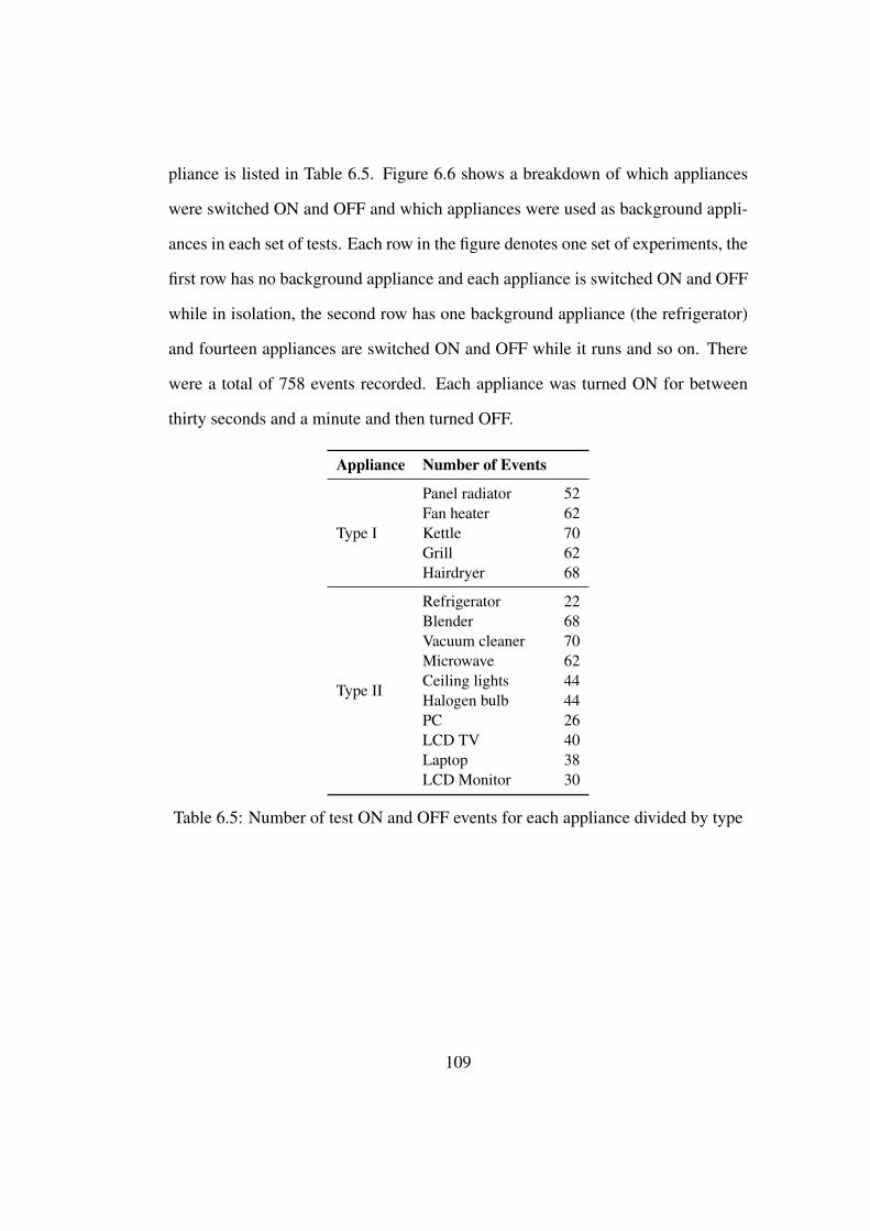
pliance is listed in Table 6.5. Figure 6.6 shows a breakdown of which appliances

were switched ON and OFF and which appliances were used as background appli-

ances in each set of tests. Each row in the figure denotes one set of experiments, the

first row has no background appliance and each appliance is switched ON and OFF

while in isolation, the second row has one background appliance (the refrigerator)

and fourteen appliances are switched ON and OFF while it runs and so on. There

were a total of 758 events recorded. Each appliance was turned ON for between

thirty seconds and a minute and then turned OFF.

Appliance Number of Events

Type I

Panel radiator 52Fan heater 62Kettle 70Grill 62Hairdryer 68

Type II

Refrigerator 22Blender 68Vacuum cleaner 70Microwave 62Ceiling lights 44Halogen bulb 44PC 26LCD TV 40Laptop 38LCD Monitor 30

Table 6.5: Number of test ON and OFF events for each appliance divided by type

109

Pan

el r

adia

tor

Fan

hea

ter

Ke

ttle

Gri

ll

Hai

rdry

er

Ref

rige

rato

r

Ble

nd

er

Vac

uu

m c

lean

er

Mic

row

ave

Cei

ling

ligh

ts

Hal

oge

n b

ulb

PC

LCD

TV

Lap

top

LCD

Mo

nit

or

SW SW SW SW SW SW SW SW SW SW SW SW SW SW SW

SW SW SW SW SW B SW SW SW SW SW SW SW SW SW SW Switching appliance

SW SW SW SW SW SW SW SW SW SW SW SW SW B B B Background appliance

SW B SW SW SW SW SW SW SW SW B B SW SW SW

SW SW SW SW B B SW SW SW SW SW B SW B SW

SW SW SW SW B B SW SW SW SW SW B B SW B

B SW SW B SW B SW SW SW SW SW B B SW B

SW SW SW SW B B SW SW SW SW B B B B B

B SW SW SW B B SW SW SW SW B B B B B

B SW SW SW B B SW SW B SW B B B B B

Type I Type II

Key

Figure 6.6: Breakdown of switching and background appliances used in each test.

The test data was recorded over a period of twelve hours over the space of a

weekend day. The test scenario was constructed to test the robustness of both the

transient and steady state features for each appliance when subjected to the variation

in the voltage source over the course of the day and to possible interference from

other appliances. To ensure sufficient data was collected to test the algorithm fully,

different appliances were used as background appliances while others were tested as

switching appliances. In general the appliances chosen as background appliances

for each test tend to be those that would be found operating over longer periods

of time as background appliances in a household, for example the PC, LCD TV

or the refrigerator. The switching appliances chosen in this test also tend to be

appliances that are switched on for shorter periods of time, while other appliances

are operating, for example the kettle or the blender.

110

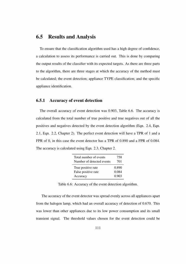
6.5 Results and Analysis

To ensure that the classification algorithm used has a high degree of confidence,

a calculation to assess its performance is carried out. This is done by comparing

the output results of the classifier with its expected targets. As there are three parts

to the algorithm, there are three stages at which the accuracy of the method must

be calculated; the event detection; appliance TYPE classification; and the specific

appliance identification.

6.5.1 Accuracy of event detection

The overall accuracy of event detection was 0.903, Table 6.6. The accuracy is

calculated from the total number of true positive and true negatives out of all the

positives and negatives detected by the event detection algorithm (Eqn. 2.4, Eqn.

2.1, Eqn. 2.2, Chapter 2). The perfect event detection will have a TPR of 1 and a

FPR of 0, in this case the event detector has a TPR of 0.890 and a FPR of 0.084.

The accuracy is calculated using Eqn. 2.3, Chapter 2.

Total number of events 758Number of detected events 701

True positive rate 0.890False positive rate 0.084Accuracy 0.903

Table 6.6: Accuracy of the event detection algorithm.

The accuracy of the event detector was spread evenly across all appliances apart

from the halogen lamp, which had an overall accuracy of detection of 0.670. This

was lower than other appliances due to its low power consumption and its small

transient signal. The threshold values chosen for the event detection could be

111

changed to improve the halogen lamp’s accuracy. It was found that changing this

had an effect on other appliances, specifically the TV, where extra non-events would

be captured. Figure 6.7 shows the RMS current of the TV when it turns on. It can be

seen that it has an initial state that lasts for thirty seconds and then a drop in current,

which would be identified as an OFF event if the threshold values were changed. It

was for this reason the poor accuracy of the halogen lamp’s events was accepted.

Figure 6.7: RMS current of the LCD TV when it turns ON and a possible non offevent detection (highlighted).

6.5.2 Accuracy of TYPE classification

The average AUC calculated for the classification of the appliance TYPE using

the transient signal is 0.936 which is shown per appliance in Table 6.7 (Eqn. 2.4,

Chapter 2). The threshold values chosen in the algorithm were optimised to work

across all appliances.

112

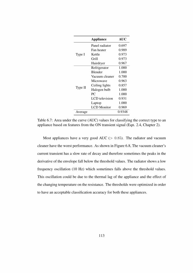
Appliance AUC

Type I

Panel radiator 0.697Fan heater 0.989Kettle 0.973Grill 0.973Hairdryer 0.967

Type II

Refrigerator 1.000Blender 1.000Vacuum cleaner 0.700Microwave 0.963Ceiling lights 0.857Halogen bulb 1.000PC 1.000LCD television 0.931Laptop 1.000LCD Monitor 0.969

Average 0.9348

Table 6.7: Area under the curve (AUC) values for classifying the correct type to anappliance based on features from the ON transient signal (Eqn. 2.4, Chapter 2).

Most appliances have a very good AUC (> 0.85). The radiator and vacuum

cleaner have the worst performance. As shown in Figure 6.8, The vacuum cleaner’s

current transient has a slow rate of decay and therefore sometimes the peaks in the

derivative of the envelope fall below the threshold values. The radiator shows a low

frequency oscillation (10 Hz) which sometimes falls above the threshold values.

This oscillation could be due to the thermal lag of the appliance and the effect of

the changing temperature on the resistance. The thresholds were optimized in order

to have an acceptable classification accuracy for both these appliances.

113

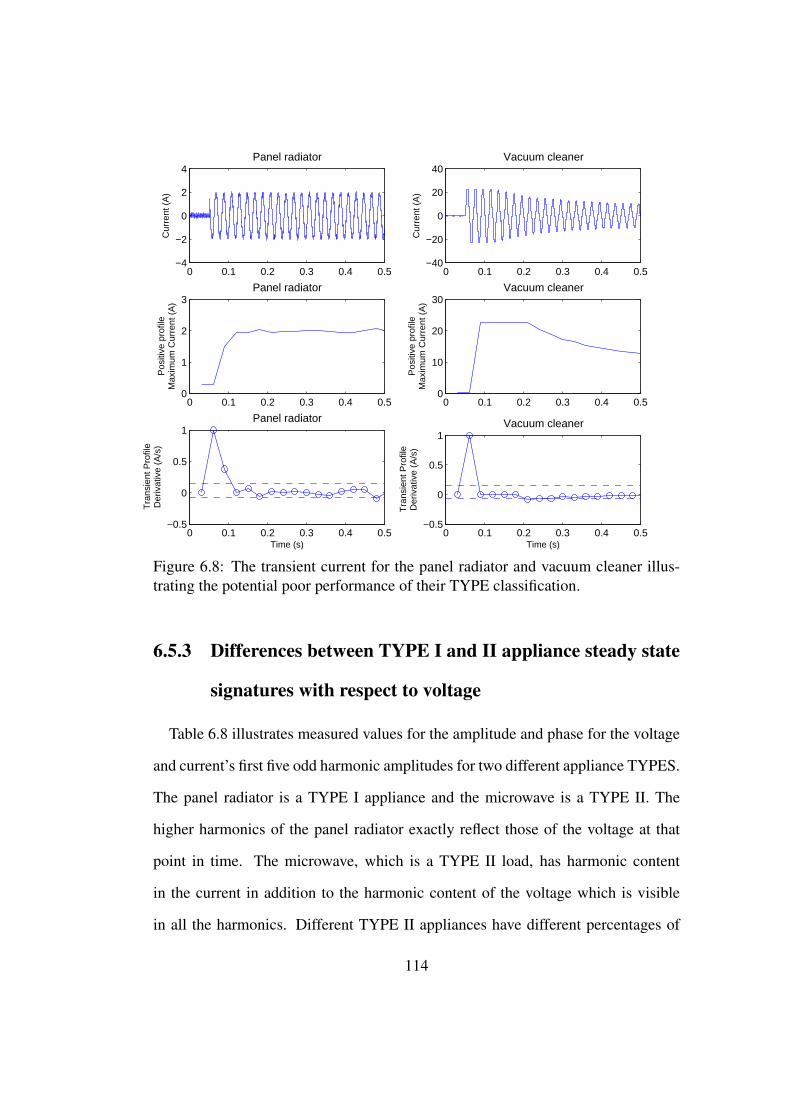
0 0.1 0.2 0.3 0.4 0.5−4

−2

0

2

4Panel radiator

Cur

rent

(A

)

0 0.1 0.2 0.3 0.4 0.5−40

−20

0

20

40Vacuum cleaner

Cur

rent

(A

)0 0.1 0.2 0.3 0.4 0.5

0

1

2

3Panel radiator

Pos

itive

pro

file

Max

imum

Cur

rent

(A

)

0 0.1 0.2 0.3 0.4 0.50

10

20

30Vacuum cleaner

Pos

itive

pro

file

Max

imum

Cur

rent

(A

)

0 0.1 0.2 0.3 0.4 0.5−0.5

0

0.5

1Panel radiator

Time (s)

Tra

nsie

nt P

rofil

eD

eriv

ativ

e (A

/s)

0 0.1 0.2 0.3 0.4 0.5−0.5

0

0.5

1Vacuum cleaner

Time (s)

Tra

nsie

nt P

rofil

eD

eriv

ativ

e (A

/s)

Figure 6.8: The transient current for the panel radiator and vacuum cleaner illus-trating the potential poor performance of their TYPE classification.

6.5.3 Differences between TYPE I and II appliance steady state

signatures with respect to voltage

Table 6.8 illustrates measured values for the amplitude and phase for the voltage

and current’s first five odd harmonic amplitudes for two different appliance TYPES.

The panel radiator is a TYPE I appliance and the microwave is a TYPE II. The

higher harmonics of the panel radiator exactly reflect those of the voltage at that

point in time. The microwave, which is a TYPE II load, has harmonic content

in the current in addition to the harmonic content of the voltage which is visible

in all the harmonics. Different TYPE II appliances have different percentages of

114

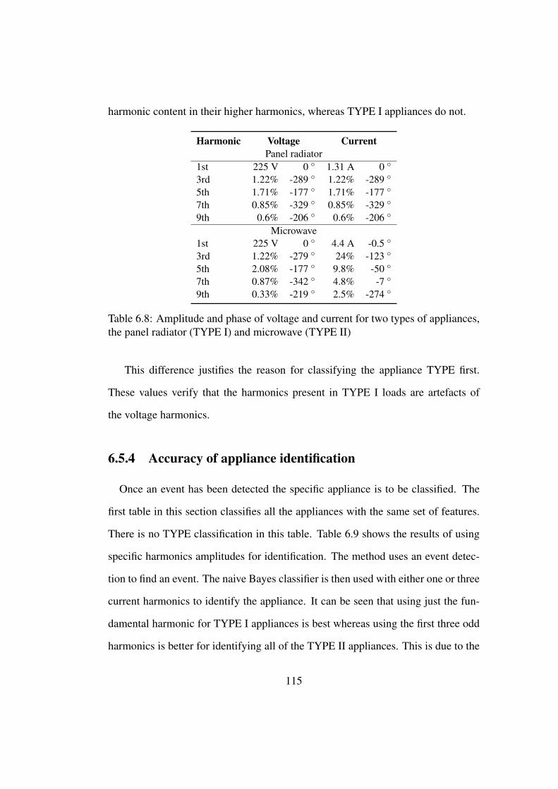
harmonic content in their higher harmonics, whereas TYPE I appliances do not.

Harmonic Voltage CurrentPanel radiator

1st 225 V 0 1.31 A 0

3rd 1.22% -289 1.22% -289

5th 1.71% -177 1.71% -177

7th 0.85% -329 0.85% -329

9th 0.6% -206 0.6% -206

Microwave1st 225 V 0 4.4 A -0.5

3rd 1.22% -279 24% -123

5th 2.08% -177 9.8% -50

7th 0.87% -342 4.8% -7

9th 0.33% -219 2.5% -274

Table 6.8: Amplitude and phase of voltage and current for two types of appliances,the panel radiator (TYPE I) and microwave (TYPE II)

This difference justifies the reason for classifying the appliance TYPE first.

These values verify that the harmonics present in TYPE I loads are artefacts of

the voltage harmonics.

6.5.4 Accuracy of appliance identification

Once an event has been detected the specific appliance is to be classified. The

first table in this section classifies all the appliances with the same set of features.

There is no TYPE classification in this table. Table 6.9 shows the results of using

specific harmonics amplitudes for identification. The method uses an event detec-

tion to find an event. The naive Bayes classifier is then used with either one or three

current harmonics to identify the appliance. It can be seen that using just the fun-

damental harmonic for TYPE I appliances is best whereas using the first three odd

harmonics is better for identifying all of the TYPE II appliances. This is due to the

115

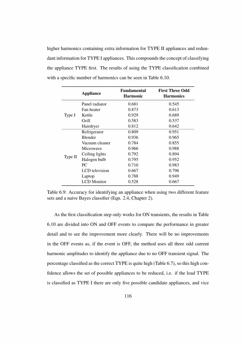
higher harmonics containing extra information for TYPE II appliances and redun-

dant information for TYPE I appliances. This compounds the concept of classifying

the appliance TYPE first. The results of using the TYPE classification combined

with a specific number of harmonics can be seen in Table 6.10.

Appliance FundamentalHarmonic

First Three OddHarmonics

Type I

Panel radiator 0.681 0.545Fan heater 0.873 0.613Kettle 0.929 0.689Grill 0.583 0.537Hairdryer 0.812 0.642

Type II

Refrigerator 0.809 0.951Blender 0.936 0.965Vacuum cleaner 0.784 0.855Microwave 0.966 0.988Ceiling lights 0.792 0.894Halogen bulb 0.795 0.952PC 0.710 0.983LCD television 0.667 0.796Laptop 0.788 0.949LCD Monitor 0.528 0.667

Table 6.9: Accuracy for identifying an appliance when using two different featuresets and a naive Bayes classifier (Eqn. 2.4, Chapter 2).

As the first classification step only works for ON transients, the results in Table

6.10 are divided into ON and OFF events to compare the performance in greater

detail and to see the improvement more clearly. There will be no improvements

in the OFF events as, if the event is OFF, the method uses all three odd current

harmonic amplitudes to identify the appliance due to no OFF transient signal. The

percentage classified as the correct TYPE is quite high (Table 6.7), so this high con-

fidence allows the set of possible appliances to be reduced, i.e. if the load TYPE

is classified as TYPE I there are only five possible candidate appliances, and vice

116

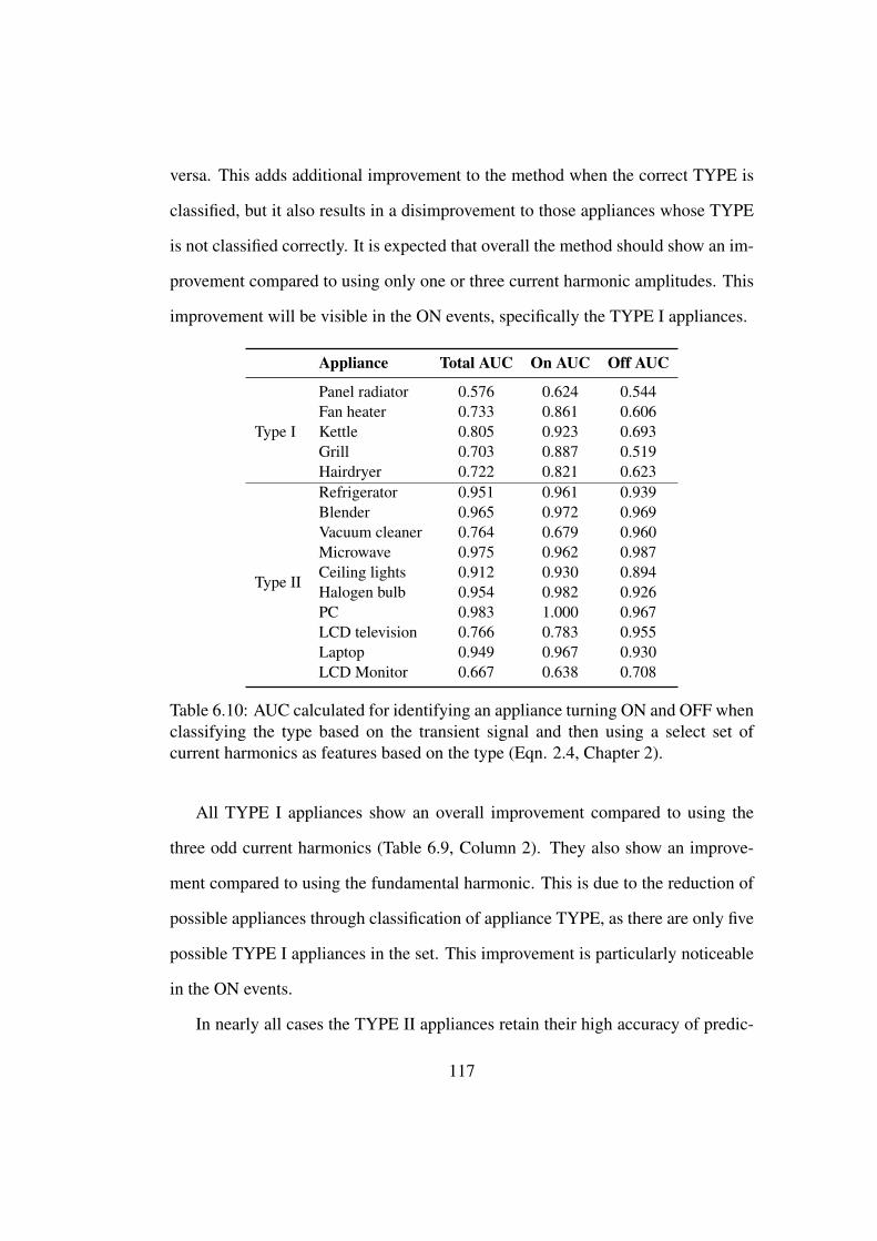
versa. This adds additional improvement to the method when the correct TYPE is

classified, but it also results in a disimprovement to those appliances whose TYPE

is not classified correctly. It is expected that overall the method should show an im-

provement compared to using only one or three current harmonic amplitudes. This

improvement will be visible in the ON events, specifically the TYPE I appliances.

Appliance Total AUC On AUC Off AUC

Type I

Panel radiator 0.576 0.624 0.544Fan heater 0.733 0.861 0.606Kettle 0.805 0.923 0.693Grill 0.703 0.887 0.519Hairdryer 0.722 0.821 0.623

Type II

Refrigerator 0.951 0.961 0.939Blender 0.965 0.972 0.969Vacuum cleaner 0.764 0.679 0.960Microwave 0.975 0.962 0.987Ceiling lights 0.912 0.930 0.894Halogen bulb 0.954 0.982 0.926PC 0.983 1.000 0.967LCD television 0.766 0.783 0.955Laptop 0.949 0.967 0.930LCD Monitor 0.667 0.638 0.708

Table 6.10: AUC calculated for identifying an appliance turning ON and OFF whenclassifying the type based on the transient signal and then using a select set ofcurrent harmonics as features based on the type (Eqn. 2.4, Chapter 2).

All TYPE I appliances show an overall improvement compared to using the

three odd current harmonics (Table 6.9, Column 2). They also show an improve-

ment compared to using the fundamental harmonic. This is due to the reduction of

possible appliances through classification of appliance TYPE, as there are only five

possible TYPE I appliances in the set. This improvement is particularly noticeable

in the ON events.

In nearly all cases the TYPE II appliances retain their high accuracy of predic-

117

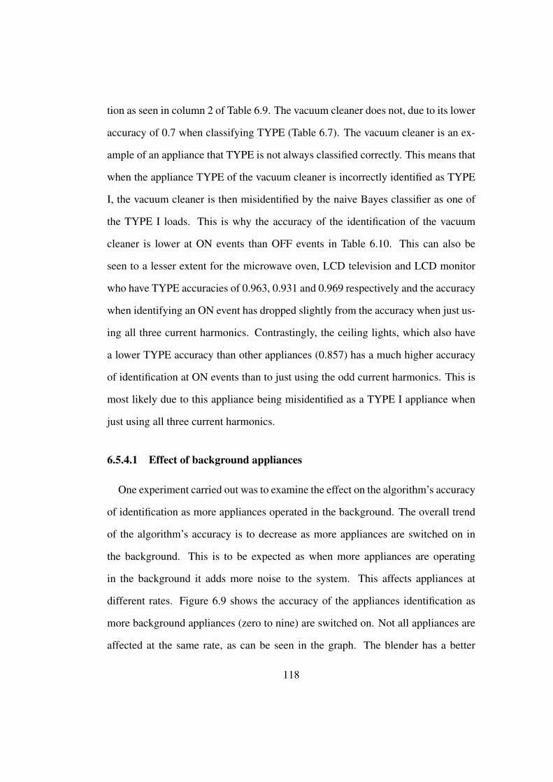
tion as seen in column 2 of Table 6.9. The vacuum cleaner does not, due to its lower

accuracy of 0.7 when classifying TYPE (Table 6.7). The vacuum cleaner is an ex-

ample of an appliance that TYPE is not always classified correctly. This means that

when the appliance TYPE of the vacuum cleaner is incorrectly identified as TYPE

I, the vacuum cleaner is then misidentified by the naive Bayes classifier as one of

the TYPE I loads. This is why the accuracy of the identification of the vacuum

cleaner is lower at ON events than OFF events in Table 6.10. This can also be

seen to a lesser extent for the microwave oven, LCD television and LCD monitor

who have TYPE accuracies of 0.963, 0.931 and 0.969 respectively and the accuracy

when identifying an ON event has dropped slightly from the accuracy when just us-

ing all three current harmonics. Contrastingly, the ceiling lights, which also have

a lower TYPE accuracy than other appliances (0.857) has a much higher accuracy

of identification at ON events than to just using the odd current harmonics. This is

most likely due to this appliance being misidentified as a TYPE I appliance when

just using all three current harmonics.

6.5.4.1 Effect of background appliances

One experiment carried out was to examine the effect on the algorithm’s accuracy

of identification as more appliances operated in the background. The overall trend

of the algorithm’s accuracy is to decrease as more appliances are switched on in

the background. This is to be expected as when more appliances are operating

in the background it adds more noise to the system. This affects appliances at

different rates. Figure 6.9 shows the accuracy of the appliances identification as

more background appliances (zero to nine) are switched on. Not all appliances are

affected at the same rate, as can be seen in the graph. The blender has a better

118

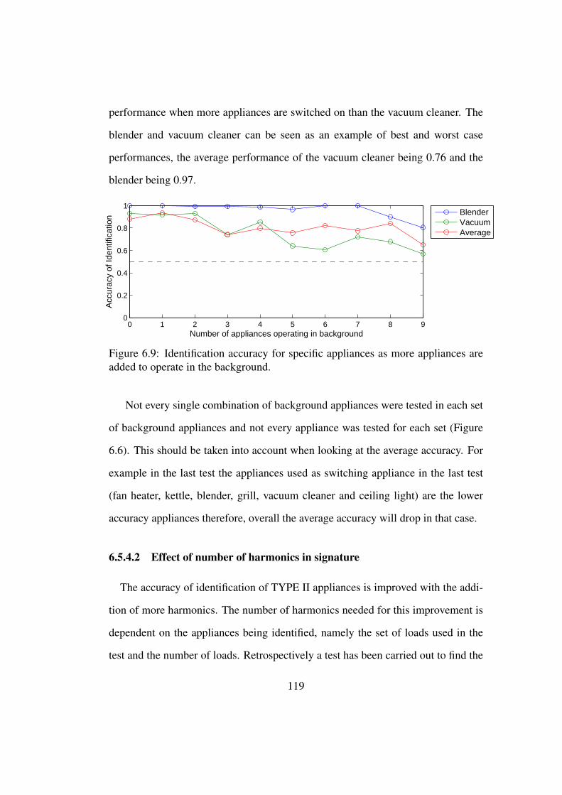
performance when more appliances are switched on than the vacuum cleaner. The

blender and vacuum cleaner can be seen as an example of best and worst case

performances, the average performance of the vacuum cleaner being 0.76 and the

blender being 0.97.

0 1 2 3 4 5 6 7 8 90

0.2

0.4

0.6

0.8

1

Number of appliances operating in background

Acc

urac

y of

Iden

tific

atio

n

BlenderVacuumAverage

Figure 6.9: Identification accuracy for specific appliances as more appliances areadded to operate in the background.

Not every single combination of background appliances were tested in each set

of background appliances and not every appliance was tested for each set (Figure

6.6). This should be taken into account when looking at the average accuracy. For

example in the last test the appliances used as switching appliance in the last test

(fan heater, kettle, blender, grill, vacuum cleaner and ceiling light) are the lower

accuracy appliances therefore, overall the average accuracy will drop in that case.

6.5.4.2 Effect of number of harmonics in signature

The accuracy of identification of TYPE II appliances is improved with the addi-

tion of more harmonics. The number of harmonics needed for this improvement is

dependent on the appliances being identified, namely the set of loads used in the

test and the number of loads. Retrospectively a test has been carried out to find the

119

optimal number of harmonics to identify each appliance for this set of appliances.

It has been found that there is no significant improvement in the overall accuracy

of the method beyond three harmonics, Table 6.11. Therefore this method has been

presented for three harmonics. The sum of the squared error for each method has

been found to be best for three harmonics.

Signature harmonics Sum of the squared error1st 0.23281st, 3rd 0.00901st, 3rd, 5th 0.00601st, 3rd, 5th, 7th 0.00651st, 3rd, 5th, 7th, 9th 0.0073

Table 6.11: Number of harmonics in signature versus sum of the squared error.

6.5.5 Applying TYPE classification at OFF events

The method proposed shows an improvement in the accuracy of identification by

classifying the load TYPE and then classifying the appliance using this information

at ON events. Although there is an improvement of identification overall, there is

still some room left to improve at OFF events. Table 6.12 shows the accuracy of

using the three current harmonics to classify the appliance TYPE for OFF events.

This method uses a two step classification method where the first step uses the

naive Bayes classifier and the three odd current harmonic amplitudes to identify the

appliance TYPE. The second step of the classifier then decides that if the appliance

is identified as a TYPE I load, the naive Bayes classifier is rerun with just the fun-

damental harmonic and the five possible TYPE I appliances, otherwise the previous

appliance identification is accepted. As there is no detectable transient information

from an OFF event, the steady state signature must be used to identify the appli-

120

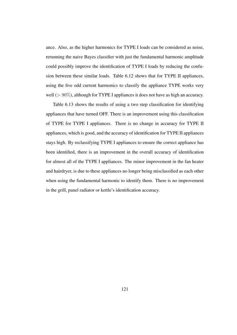
ance. Also, as the higher harmonics for TYPE I loads can be considered as noise,

rerunning the naive Bayes classifier with just the fundamental harmonic amplitude

could possibly improve the identification of TYPE I loads by reducing the confu-

sion between these similar loads. Table 6.12 shows that for TYPE II appliances,

using the five odd current harmonics to classify the appliance TYPE works very

well (> 90%), although for TYPE I appliances it does not have as high an accuracy.

Table 6.13 shows the results of using a two step classification for identifying

appliances that have turned OFF. There is an improvement using this classification

of TYPE for TYPE I appliances. There is no change in accuracy for TYPE II

appliances, which is good, and the accuracy of identification for TYPE II appliances

stays high. By reclassifying TYPE I appliances to ensure the correct appliance has

been identified, there is an improvement in the overall accuracy of identification

for almost all of the TYPE I appliances. The minor improvement in the fan heater

and hairdryer, is due to these appliances no longer being misclassified as each other

when using the fundamental harmonic to identify them. There is no improvement

in the grill, panel radiator or kettle’s identification accuracy.

121

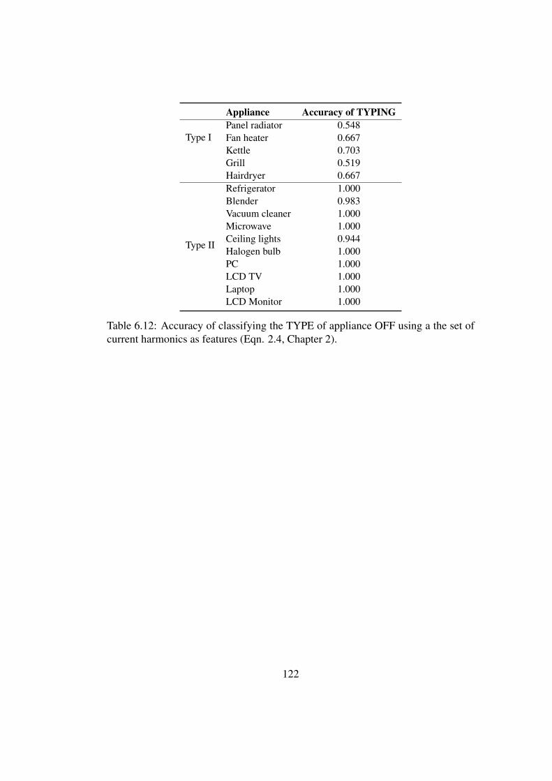
Type I

Appliance Accuracy of TYPINGPanel radiator 0.548Fan heater 0.667Kettle 0.703Grill 0.519Hairdryer 0.667

Type II

Refrigerator 1.000Blender 0.983Vacuum cleaner 1.000Microwave 1.000Ceiling lights 0.944Halogen bulb 1.000PC 1.000LCD TV 1.000Laptop 1.000LCD Monitor 1.000

Table 6.12: Accuracy of classifying the TYPE of appliance OFF using a the set ofcurrent harmonics as features (Eqn. 2.4, Chapter 2).

122

Type I

Appliance OFF Accuracy(NO TYPING)

OFF Accuracy(WITH TYPING)

Panel radiator 0.544 0.544Fan heater 0.606 0.665Kettle 0.693 0.693Grill 0.519 0.519Hairdryer 0.623 0.667

Type II

Refrigerator 0.939 0.939Blender 0.969 0.969Vacuum cleaner 0.860 0.860Microwave 0.987 0.987Ceiling lights 0.894 0.894Halogen bulb 0.926 0.926PC 0.967 0.967LCD TV 0.755 0.755Laptop 0.930 0.930LCD Monitor 0.708 0.708

Table 6.13: Comparison between accuracy of identifying appliances at OFF whenusing three odd current harmonics to identify appliance and when using a two stepclassification method which classifies the appliance TYPE first and then reclassifiesthe appliance using the specific number of harmonics to that appliance TYPE (Eqn.2.4, Chapter 2).

6.6 Conclusion

This chapter presents a method that identifies appliances that are consuming

power with a high degree of accuracy. The method is event based, and uses time

and frequency signals from the current to identify what appliance has turned ON or

OFF. The system uses a rule based algorithm and a naive Bayes classifier as a two

step classification method. The algorithm is event based and the scalability of the

method is N . The problems presented in the previous chapter have been addressed

and several conclusions can be made about the system from this work.

It is clear that the current harmonics and a naive Bayes classifier are a good

123

combination for identifying and distinguishing individual appliances. Utilising the

knowledge of what appliances emit harmonics due to their internal components and

what appliances do not when choosing an identification signature improves the ac-

curacy of the method. There are general characteristics that can be associated with

each type which allows different appliances to be categorised into typesets. Linear

nonreactive loads have no harmonic content of their own, and have no transient sig-

nal. Nonlinear loads and reactive loads do have harmonic content, and also have a

transient signal.

The method presented in this chapter is capable of identifying what appliances

are consuming power using a single point of measurement. It is an efficient method

that can operate in a system with large numbers of appliances and still has an ac-

ceptable degree of accuracy. The method presented has been tested for real world

measurements taken from an environment where appliances are actively operating.

Some of the methods presented in Chapter 2 do not work for all types of domestic

appliances. These methods focus mainly on electronic and motor loads and they do

not account for resistive heating loads. The method presented in this chapter is ca-

pable of identifying electronic, motor and resistive heating loads that are common

to domestic environments.

124

Chapter 7

Conclusion

This chapter concludes the thesis and the work carried out in developing a load

monitoring method. The chapter first summaries the work described throughout

the thesis. A series of overall conclusions are then made from the work and the

contributions of this work are listed. The end of this chapter proposes future work

for the load monitoring method described.

7.1 Summary

This thesis outlines the development of a load monitoring method that identifies

what appliances are consuming power using a single point of measurement. The

aggregate current signal is measured at the incoming point and the appliances that

are consuming power are derived from this signal. Chapter 1 introduces load mon-

itoring and presents the motivations for load monitoring and this work. It outlines

the research objectives and the criteria which the method should meet. The method

developed must be efficient with good scalability, accuracy and work for all types

125

of domestic loads.

Chapter 2 documents the state of the art research in this area. It outlines the

various methods developed for load monitoring. It describes the processes involved

in developing a load monitoring system, namely data measurement and acquisition

techniques, characterisation methods and classification algorithms. It also discusses

how to assess the performance of a load monitoring method. The chapter also

outlines the applications of a load monitoring system, including those outside of

power monitoring for energy reduction. The chapter finishes with a comparison

of the six most complete load monitoring methods and draws the conclusion that

presently there are no load monitoring approaches which fulfil all the requirements

of an effective load monitoring method.

Chapter 3 describes the measurement techniques used in this work and provides

a justification for the sensor choice. An Hall effect sensor was chosen to measure

current. This sensor was chosen as it provides electrical isolation, is very reliable

and has a very good frequency response. The current is sampled with a DAQ at a

relatively low sampling frequency (20 kHz).

Chapter 4 details the initial experiments carried out to investigate the complex

environment in which a load monitoring system is to operate. The findings from this

chapter provide the foundation on which the chapters following make their assump-

tions. The voltage source in the test environment was measured and analysed and

it was found that there are multiple varying harmonics present on the voltage line.

This can potentially have an effect on the appliances on this network. The different

variants of appliances were outlined and how this can also affect the method. An

appliance can differ in a number of ways, specifically by the number of operating

states and by the electrical composition of the load. The operation of some appli-

126

ances have been analysed in detail and an understanding of the way these appliances

consume power is shown. The different variants of an appliance’s electrical compo-

nents and the resulting current signals are shown. These variations and complexities

of the load monitoring environment make disaggregating appliances challenging.

Chapter 5 outlines a method for continuously identifying appliances consuming

power using the current FFT as a signature for each appliance and a naive Bayes

classifier to identify when each appliance is on. The current signal of each appli-

ance is measured in isolation and a signature is derived from this. The signature for

each appliance is the first five odd current harmonic amplitudes. A virtual signature

library is created by adding the individual signatures together in different combina-

tions to create a library of all the possible combinations. The library is built upon

the premise that in a domestic household’s electrical network, the system is linear

and all the appliances are in parallel. The method investigated is not a feasible fully

deployable method but there are a number of conclusions drawn from the work. It is

shown that the first five odd current harmonics alongside the naive Bayes classifier

is an effective method at distinguishing individual appliances (Table 5.4). There are

a number of problems with the final method including the overall accuracy per ap-

pliance not being good enough when compared to the literature, the complexity of

the method (2N −1) being quite poor and other concerns, such as a lengthy training

time.

Chapter 6 builds on the findings from the previous chapters and presents a

method that identifies appliances that are consuming power with a higher degree

of accuracy. The method is event based, and uses time and frequency signals from

the current to identify each appliance. An event occurs when an appliance turns

ON or OFF. The system uses a rule based algorithm and a naive Bayes classifier in

127

a two step classification method. The problems presented in the previous chapter

have been addressed and several conclusions can be made about the system from

this work. The new method divides the appliances into two categories, or TYPES,

which are treated differently by the classifier based on their characteristics. TYPE I

loads are linear nonreactive have no harmonic content of their own, and the transient

signal is flat with no inrush. TYPE II loads are nonlinear appliances and reactive

appliances, which do have harmonic content, and a reactive transient signal. This

work shows that if the method utilises the TYPE of appliance and therefore the

amount of harmonic content that is inherent to that appliance, the system is im-

proved. Utilising these characteristics for identifying the appliances can greatly

improve the method. The final method presented has an overall accuracy of 83%

and a complexity of N, with a greatly reduced training time from before.

This chapter concludes the work and presents the contributions from this work.

The chapter also offers some areas for future work in which the load monitoring

method can be advanced further.

7.2 Contributions of this work

• This thesis presents an efficient, scalable, accurate load identification method

that identifies what appliances are consuming power using a single point of

measurement.

– The method has a complexity of N and can operate in a system with

large numbers of appliances.

– The overall accuracy of the method is 83%.

128

– The method works for all types of appliances including simple linear

nonreactive loads and more complex nonlinear reactive loads.

– The method works in an efficient way using robust signatures that are

not overly complex and give a unique identity to each appliance.

– The method designed has low computational complexity and is practical

to implement in cost-effective hardware.

• This work shows that using a two step classification method, that uses a sig-

nature set optimised for an appliance based on its general characteristics, can

improve the overall accuracy of identifying appliances. The algorithm in

this method treats different types of appliances by optimising their signature

based on their electrical properties. This allows the method to work for a

wider range of appliances.

• This work shows that by combining time and frequency domain information

derived from the aggregate electrical current signal, the accuracy of appliance

identification (over a wide range of appliance types) can be improved.

7.3 Future Work

The next step to this work is to deploy the load monitoring system in a real setting

and track the appliance changes. There are different scenarios where the system can

be deployed, as an in-home appliance monitoring method for either personal en-

ergy monitoring or as a health/activity monitor, in conjunction with smart metering,

or in an office or industrial environment. In order for the system to be deployed

there are a number of areas which the system needs to be tuned. The physical mea-

129

surement and monitoring system needs to be adapted for remote monitoring and

communication; the algorithm method needs to be adapted to track appliances and

to extend the set of appliances it can work for; and a user interface for training

appliances and generating reports needs to be developed, with perhaps with some

alert system.

In order to deploy the system in a real environment the system would need to

be slightly adapted for easy installation and for remote communication. The mea-

surement sensor should be feasible to deploy in a domestic environment, it should

be easy to install, inexpensive and not require a large power supply. The method

presented in this thesis has been tested using an inexpensive current sensor. The

sensor can be easily adapted to be used in a smart meter and this would not impact

the accuracy of the method. The identification algorithm that has been developed

has an acceptable accuracy and is not overly complex and therefore should not be

difficult to deploy on an inexpensive chipset. The algorithm calculated the FFT and

the rate of change of the current signal, both of which can be easily carried out

using microprocessors. The decision process the algorithm uses itself is not overly

complex and should not take too much effort to deploy on a microprocessor.

An application needs to be developed that will have some user interface and a

procedure for training appliances. The method has been tested with a short training

period for each appliance (less than five minutes). This is the area in which the

method will have to be developed further in order to deploy the method in a real en-

vironment. Ideally the system could just be placed in the system and training should

not be cumbersome to the consumer. Training multiple appliances can be time con-

suming and it is unrealistic to assume that all consumers would be willing to take

the time to do this. Another area for future work is to investigate the feasibility of

130

adapting the method for office and industry environments. Some of the appliances

tested in the method would be similar to those found in these environments so that

would suggest that it would work well in such a setting. There would be a lot of

similar appliances so this may add some difficulty to the problem.

Depending on the function of the deployment, there needs to be a reporting

functionality that will track the actual appliance usage and build a summary report.

If this method were to be used in conjunction with an energy tracking method the

reporting function should ideally build weekly reports and track energy usage per

appliance and then compare the weekly usage with historical data to ensure power

usage is not rising. The future method could identify areas of power reduction for

specific appliances. Alternatively, if this method were to be used as a health moni-

toring method it could monitor for specific events throughout the day, for example

turning the kettle on at 9 a.m. and if these events do not occur send out an alert.

The system algorithm at the minute does not tracking appliances as they turn on

or off. This could be implemented as a standalone tracking system that tracks appli-

ance state and does not feed into the decision algorithm or it could be used to help

the current appliance identification algorithm make a more informed decision based

on the current state of the system. A benefit of implementing tracking appliances

into the algorithm, is a reduced set of appliances that can cause a possible event and

therefore possibly an increase probability of identifying the correct appliance. One

of the pitfalls of using a tracking algorithm that reduces the possible appliance that

could have caused an event is that if an appliance is incorrectly labelled as switching

on or off and then actually switches on or off this can affect the overall accuracy.

To combat this the method could use a limited memory to overcome accumulating

state error in the system.

131

Future work would include extending the capability of the method to identify

more signatures for example those of multi-state appliances or faulty appliances.

The identification of multi state appliances can be achieved by adding a subset of

appliances to TYPE II appliances where, when a multi-state appliance is detected

switching on, the algorithm will expect one of the following events to be a change

in state of this appliance.

The current method could also be expanded to include some fault detection. For

example using historical data it could potentially alert for when appliances start be-

having abnormally, for example longer run times on the refrigerator or increased

current draw for a specific appliance. Alternatively the method could be expanded

to incorporate electrical fault detection, for example electrical arcing. An electri-

cal arc is an unconstrained transfer of energy between the exposed conductor and

another conductor or ground [83]. As electrical devices and cables age they are

subjected to physical damage. This may result in part of a conductor becoming

exposed causing current to ‘arc’ across conductors. Sometimes when an arc fault

occurs in an electrical circuit, it can go unnoticed by conventional protection de-

vices. A load monitoring method could have an extra layer of monitoring where if

the characteristics of an arc are detected an alarm is flagged.

132

Chapter 8

Appendices

8.1 Measurement box schematic

Figure 8.1 and 8.2 show the circuit schematic for the measurement box used in

the experiment set-up. The measurement box measures current using a Hall Effect

sensor and measures voltage using a voltage divider circuit optically isolated from

the mains. The output of the circuit is two 0-5V signals that are linear to the live

current and voltage.

133

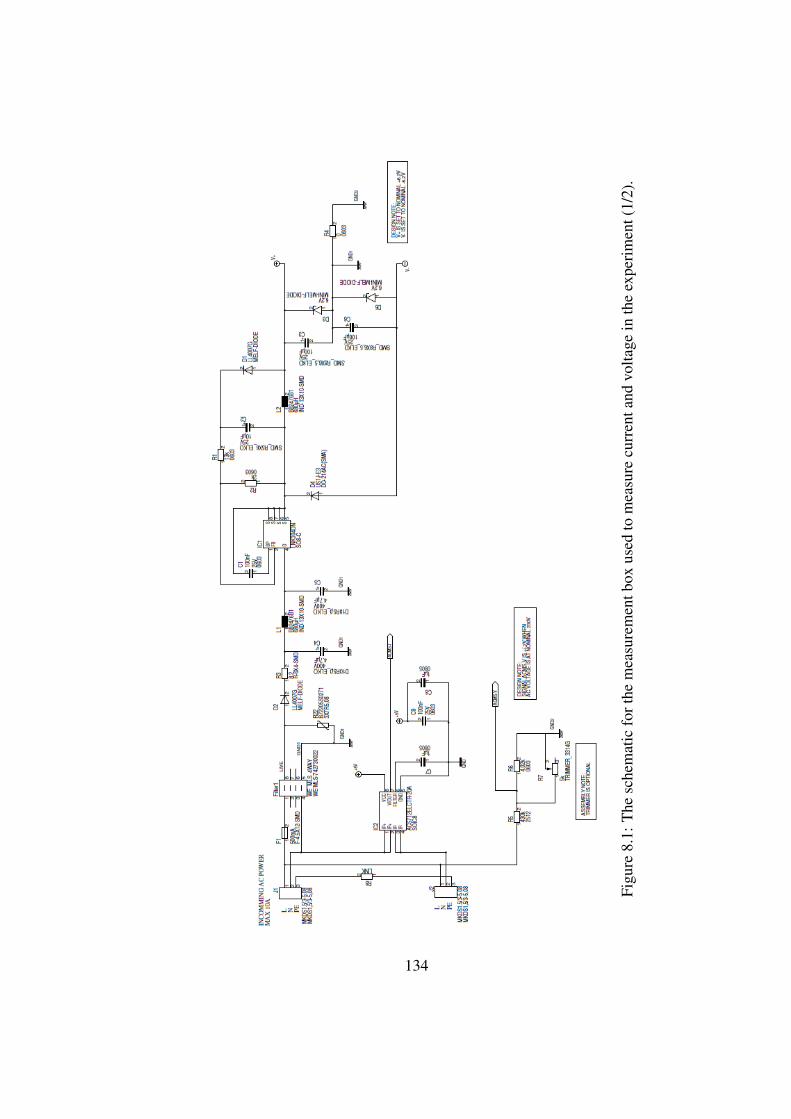
Figu

re8.

1:T

hesc

hem

atic

fort

hem

easu

rem

entb

oxus

edto

mea

sure

curr

enta

ndvo

ltage

inth

eex

peri

men

t(1/

2).

134

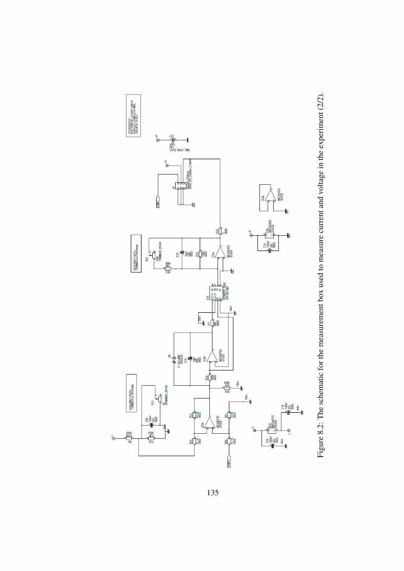
Figu

re8.

2:T

hesc

hem

atic

fort

hem

easu

rem

entb

oxus

edto

mea

sure

curr

enta

ndvo

ltage

inth

eex

peri

men

t(2/

2).

135

8.2 Voltage and harmonics measured in different en-

vironments

It was found that the voltage varied in the environment where the tests took

places. The voltage was measured in two additional environments to assess whether

the variation of the voltage was an artefact of the building the experiments were be-

ing carried out in, or if the voltage variation was common in all environments. It

can be seen that the variation of the voltage and the voltage harmonics is differ-

ent in different environments. It can also be seen that the voltage and the voltage

harmonics vary in many different environments.

136

0 5 10 15 20254

256

258

260

262

264

266Voltage in a domestic environment (apartment)

Fun

dam

enta

l har

mon

ic a

mpl

itude

(V

)

Saturday 09/08/14 − 12am to 12am (hours)

0 5 10 15 200

0.2

0.4

0.6

0.8

1

1.2

1.4Voltage harmonics in a domestic environment (apartment)

Har

mon

ics

as %

of f

unda

men

tal (

%)

Saturday 09/08/14 − 12am to 12am (hours)

ThirdFifthSeventhNinth

Figure 8.3: The voltage measured in a domestic environment and the relationshipof higher voltage harmonics to fundamental over a 24 hour period on a weekendday.

137

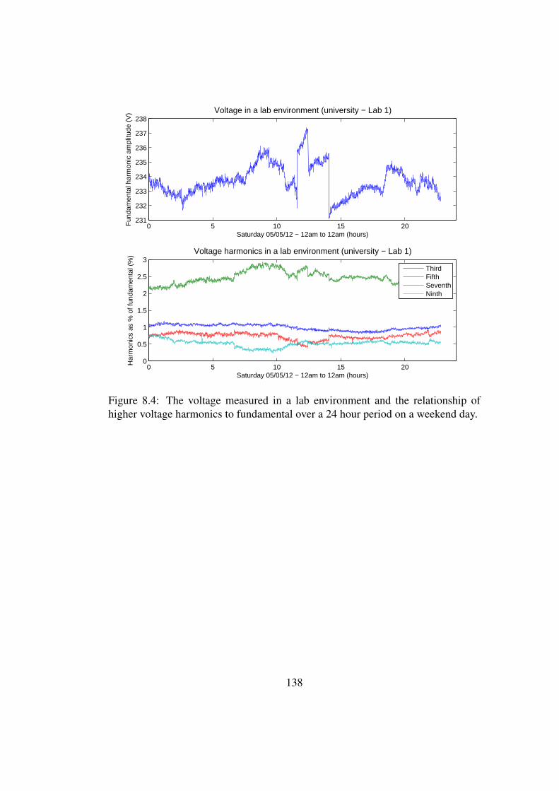
0 5 10 15 20231

232

233

234

235

236

237

238Voltage in a lab environment (university − Lab 1)

Fun

dam

enta

l har

mon

ic a

mpl

itude

(V

)

Saturday 05/05/12 − 12am to 12am (hours)

0 5 10 15 200

0.5

1

1.5

2

2.5

3Voltage harmonics in a lab environment (university − Lab 1)

Har

mon

ics

as %

of f

unda

men

tal (

%)

Saturday 05/05/12 − 12am to 12am (hours)

ThirdFifthSeventhNinth

Figure 8.4: The voltage measured in a lab environment and the relationship ofhigher voltage harmonics to fundamental over a 24 hour period on a weekend day.

138

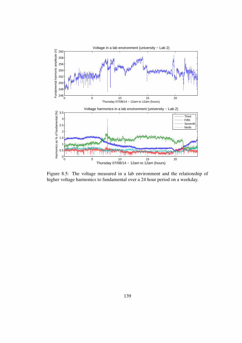
0 5 10 15 20246

248

250

252

254

256

258

260Voltage in a lab environment (university − Lab 2)

Fun

dam

enta

l har

mon

ic a

mpl

itude

(V

)

Thursday 07/08/14 − 12am to 12am (hours)

0 5 10 15 200

0.5

1

1.5

2

2.5

3

3.5Voltage harmonics in a lab environment (university − Lab 2)

Har

mon

ics

as %

of f

unda

men

tal (

%)

Thursday 07/08/14 − 12am to 12am (hours)

ThirdFifthSeventhNinth

Figure 8.5: The voltage measured in a lab environment and the relationship ofhigher voltage harmonics to fundamental over a 24 hour period on a weekday.

139

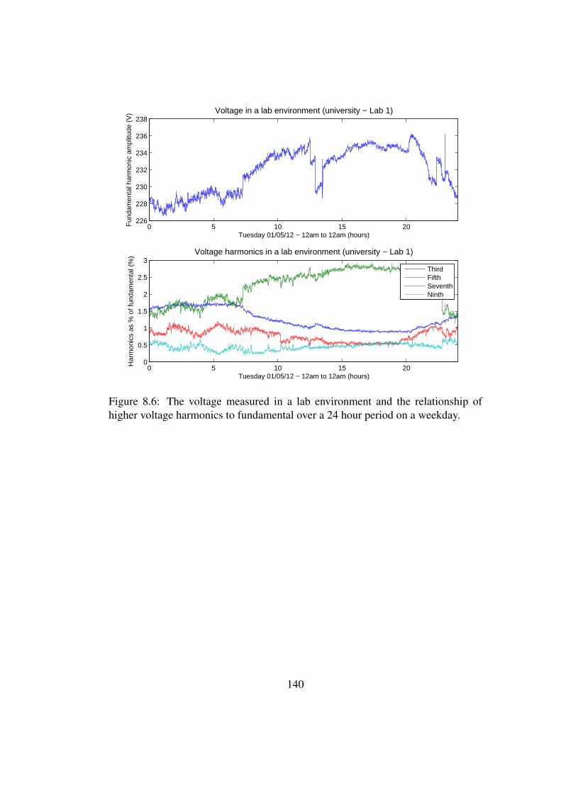
0 5 10 15 20226

228

230

232

234

236

238Voltage in a lab environment (university − Lab 1)

Fun

dam

enta

l har

mon

ic a

mpl

itude

(V

)

Tuesday 01/05/12 − 12am to 12am (hours)

0 5 10 15 200

0.5

1

1.5

2

2.5

3Voltage harmonics in a lab environment (university − Lab 1)

Har

mon

ics

as %

of f

unda

men

tal (

%)

Tuesday 01/05/12 − 12am to 12am (hours)

ThirdFifthSeventhNinth

Figure 8.6: The voltage measured in a lab environment and the relationship ofhigher voltage harmonics to fundamental over a 24 hour period on a weekday.

140

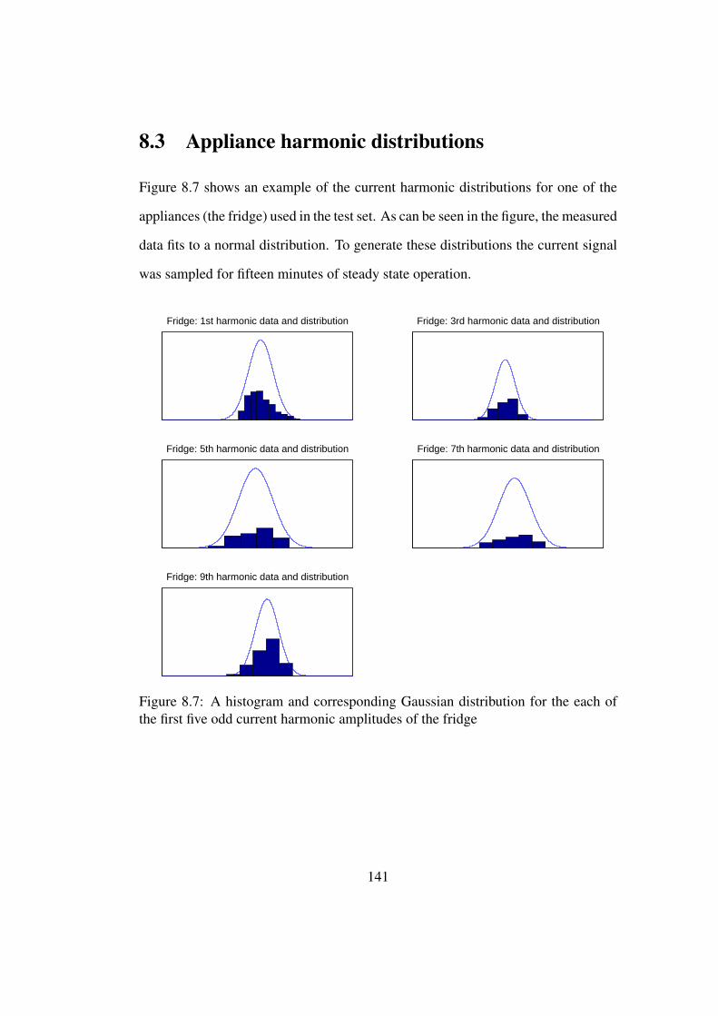
8.3 Appliance harmonic distributions

Figure 8.7 shows an example of the current harmonic distributions for one of the

appliances (the fridge) used in the test set. As can be seen in the figure, the measured

data fits to a normal distribution. To generate these distributions the current signal

was sampled for fifteen minutes of steady state operation.

Fridge: 1st harmonic data and distribution Fridge: 3rd harmonic data and distribution

Fridge: 5th harmonic data and distribution Fridge: 7th harmonic data and distribution

Fridge: 9th harmonic data and distribution

Figure 8.7: A histogram and corresponding Gaussian distribution for the each ofthe first five odd current harmonic amplitudes of the fridge

141

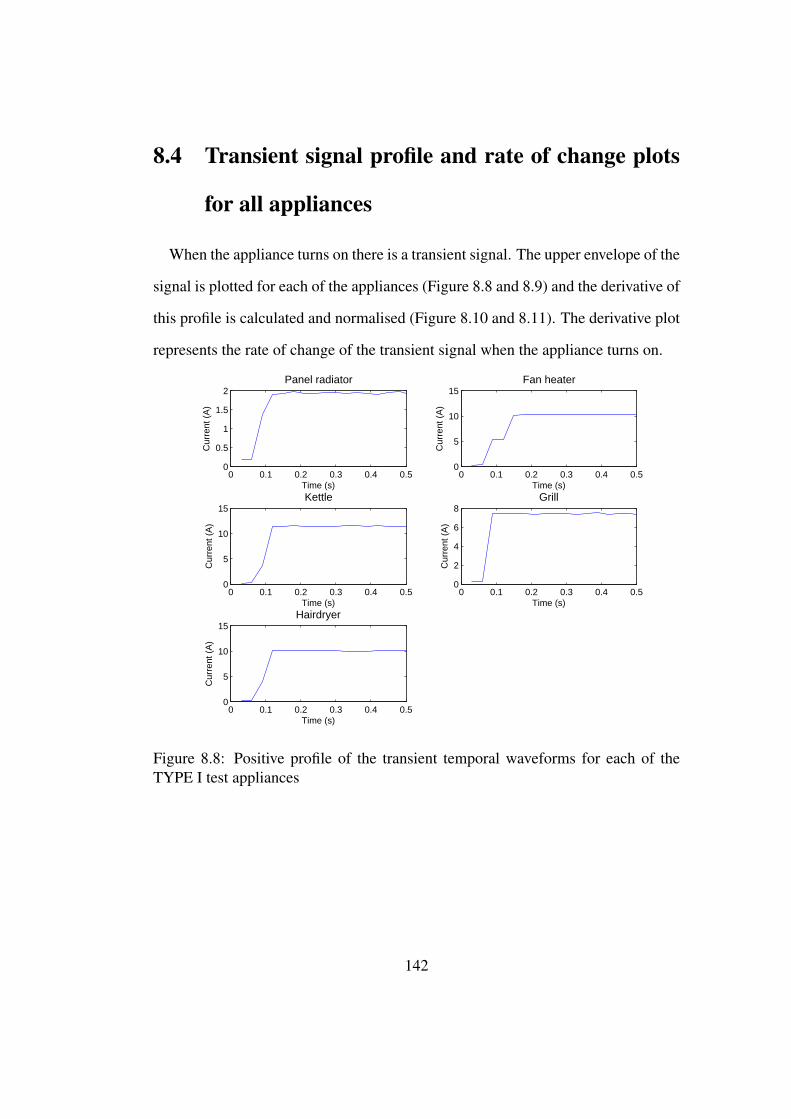
8.4 Transient signal profile and rate of change plots

for all appliances

When the appliance turns on there is a transient signal. The upper envelope of the

signal is plotted for each of the appliances (Figure 8.8 and 8.9) and the derivative of

this profile is calculated and normalised (Figure 8.10 and 8.11). The derivative plot

represents the rate of change of the transient signal when the appliance turns on.

0 0.1 0.2 0.3 0.4 0.50

0.5

1

1.5

2Panel radiator

Time (s)

Cur

rent

(A

)

0 0.1 0.2 0.3 0.4 0.50

5

10

15Fan heater

Time (s)

Cur

rent

(A

)

0 0.1 0.2 0.3 0.4 0.50

5

10

15Kettle

Time (s)

Cur

rent

(A

)

0 0.1 0.2 0.3 0.4 0.50

2

4

6

8Grill

Time (s)

Cur

rent

(A

)

0 0.1 0.2 0.3 0.4 0.50

5

10

15Hairdryer

Time (s)

Cur

rent

(A

)

Figure 8.8: Positive profile of the transient temporal waveforms for each of theTYPE I test appliances

142

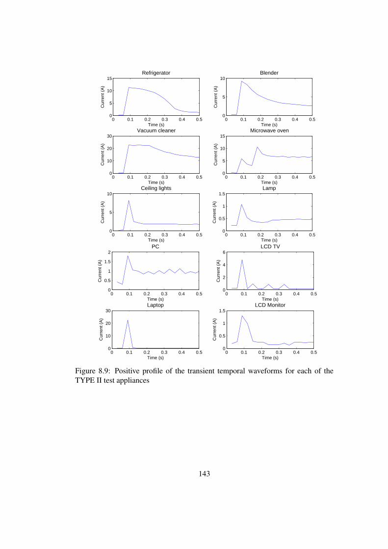
0 0.1 0.2 0.3 0.4 0.50

5

10

15Refrigerator

Time (s)

Cur

rent

(A

)

0 0.1 0.2 0.3 0.4 0.50

5

10Blender

Time (s)

Cur

rent

(A

)

0 0.1 0.2 0.3 0.4 0.50

10

20

30Vacuum cleaner

Time (s)

Cur

rent

(A

)

0 0.1 0.2 0.3 0.4 0.50

5

10

15Microwave oven

Time (s)

Cur

rent

(A

)

0 0.1 0.2 0.3 0.4 0.50

5

10Ceiling lights

Time (s)

Cur

rent

(A

)

0 0.1 0.2 0.3 0.4 0.50

0.5

1

1.5Lamp

Time (s)

Cur

rent

(A

)

0 0.1 0.2 0.3 0.4 0.50

0.5

1

1.5

2PC

Time (s)

Cur

rent

(A

)

0 0.1 0.2 0.3 0.4 0.50

2

4

6LCD TV

Time (s)

Cur

rent

(A

)

0 0.1 0.2 0.3 0.4 0.50

10

20

30Laptop

Time (s)

Cur

rent

(A

)

0 0.1 0.2 0.3 0.4 0.50

0.5

1

1.5LCD Monitor

Time (s)

Cur

rent

(A

)

Figure 8.9: Positive profile of the transient temporal waveforms for each of theTYPE II test appliances

143

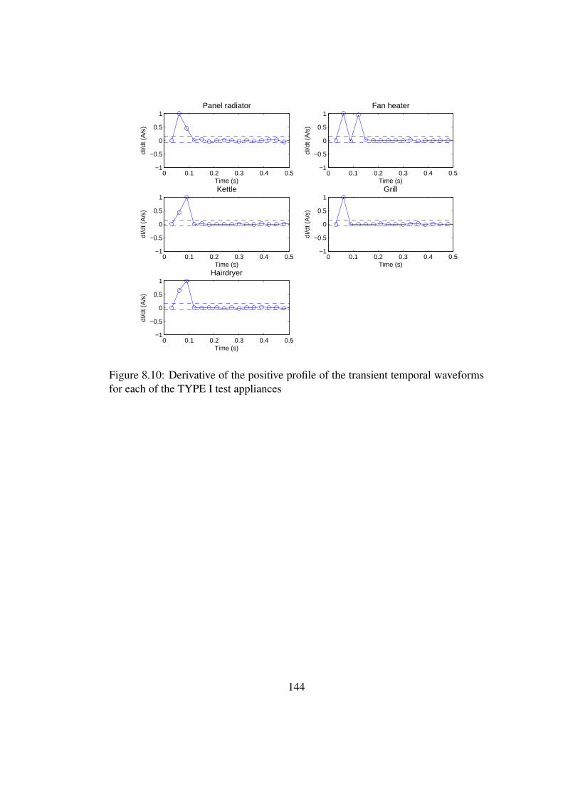
0 0.1 0.2 0.3 0.4 0.5−1

−0.5

0

0.5

1Panel radiator

Time (s)

dI/d

t (A

/s)

0 0.1 0.2 0.3 0.4 0.5−1

−0.5

0

0.5

1Fan heater

Time (s)

dI/d

t (A

/s)

0 0.1 0.2 0.3 0.4 0.5−1

−0.5

0

0.5

1Kettle

Time (s)

dI/d

t (A

/s)

0 0.1 0.2 0.3 0.4 0.5−1

−0.5

0

0.5

1Grill

Time (s)

dI/d

t (A

/s)

0 0.1 0.2 0.3 0.4 0.5−1

−0.5

0

0.5

1Hairdryer

Time (s)

dI/d

t (A

/s)

Figure 8.10: Derivative of the positive profile of the transient temporal waveformsfor each of the TYPE I test appliances

144

0 0.1 0.2 0.3 0.4 0.5−1

−0.5

0

0.5

1Refrigerator

Time (s)

dI/d

t (A

/s)

0 0.1 0.2 0.3 0.4 0.5−1

−0.5

0

0.5

1Blender

Time (s)

dI/d

t (A

/s)

0 0.1 0.2 0.3 0.4 0.5−1

−0.5

0

0.5

1Vacuum cleaner

Time (s)

dI/d

t (A

/s)

0 0.1 0.2 0.3 0.4 0.5−1

−0.5

0

0.5

1Microwave oven

Time (s)

dI/d

t (A

/s)

0 0.1 0.2 0.3 0.4 0.5−1

−0.5

0

0.5

1Ceiling lights

Time (s)

dI/d

t (A

/s)

0 0.1 0.2 0.3 0.4 0.5−1

−0.5

0

0.5

1Lamp

Time (s)

dI/d

t (A

/s)

0 0.1 0.2 0.3 0.4 0.5−1

−0.5

0

0.5

1PC

Time (s)

dI/d

t (A

/s)

0 0.1 0.2 0.3 0.4 0.5−1

−0.5

0

0.5

1LCD TV

Time (s)

dI/d

t (A

/s)

0 0.1 0.2 0.3 0.4 0.5−1

−0.5

0

0.5

1Laptop

Time (s)

dI/d

t (A

/s)

0 0.1 0.2 0.3 0.4 0.5−1

−0.5

0

0.5

1LCD Monitor

Time (s)

dI/d

t (A

/s)

Figure 8.11: Derivative of the positive profile of the transient temporal waveformsfor each of the TYPE II test appliances

145

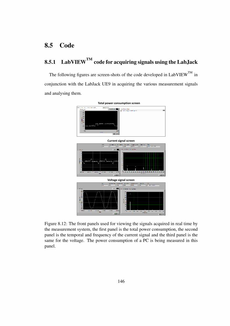
8.5 Code

8.5.1 LabVIEWTM code for acquiring signals using the LabJack

The following figures are screen-shots of the code developed in LabVIEWTM in

conjunction with the LabJack UE9 in acquiring the various measurement signals

and analysing them.

Total power consumption screen

Current signal screen

Voltage signal screen

Figure 8.12: The front panels used for viewing the signals acquired in real time bythe measurement system, the first panel is the total power consumption, the secondpanel is the temporal and frequency of the current signal and the third panel is thesame for the voltage. The power consumption of a PC is being measured in thispanel.

146

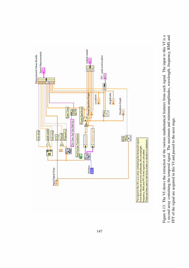
Figu

re8.

13:

The

VI

show

sth

eex

trac

tion

ofth

eva

riou

sm

athe

mat

ical

feat

ures

from

each

sign

al.

The

inpu

tto

this

VI

isa

1se

cond

arra

yco

ntai

ning

the

tem

pora

lsig

nal.

The

max

imum

and

min

imum

ampl

itude

s,w

avel

engt

h,fr

eque

ncy,

RM

San

dFF

Tof

the

sign

alar

eac

quir

edin

this

VIa

ndpa

ssed

toth

ene

xtst

age.

147

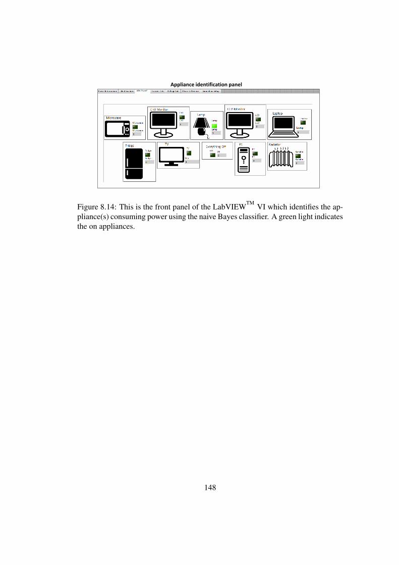
Appliance identification panel

Figure 8.14: This is the front panel of the LabVIEWTM VI which identifies the ap-pliance(s) consuming power using the naive Bayes classifier. A green light indicatesthe on appliances.

148

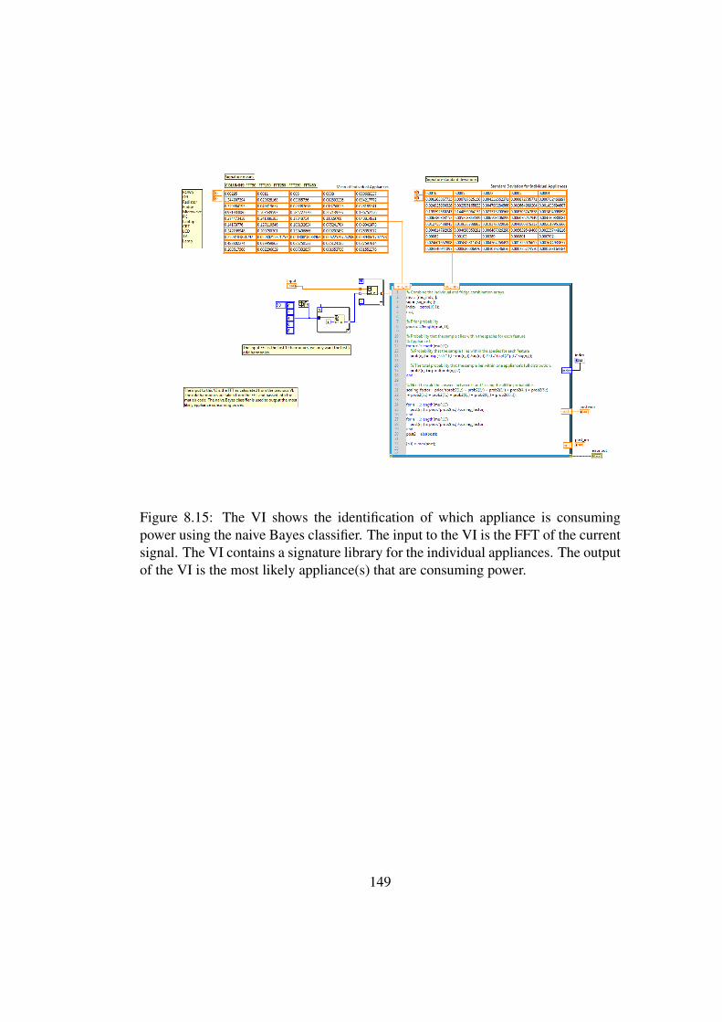
Figure 8.15: The VI shows the identification of which appliance is consumingpower using the naive Bayes classifier. The input to the VI is the FFT of the currentsignal. The VI contains a signature library for the individual appliances. The outputof the VI is the most likely appliance(s) that are consuming power.

149

Bibliography

[1] G. Hart, “Nonintrusive appliance load monitoring,” Proceedings of the IEEE,

vol. 80, no. 12, pp. 1870–1891, 1992.

[2] D. Srinivasan, W. Ng, and A. Liew, “Neural-network-based signature recogni-

tion for harmonic source identification,” Power Delivery, IEEE Transactions

on, vol. 21, no. 1, pp. 398–405, 2006.

[3] J. Liang, S. Ng, G. Kendall, and J. Cheng, “Load signature study part I: Basic

concept, structure, and methodology,” Power Delivery, IEEE Transactions on,

vol. 25, no. 2, pp. 551–560, 2010.

[4] L. Norford and S. Leeb, “Non-intrusive electrical load monitoring in commer-

cial buildings based on steady-state and transient load-detection algorithms,”

Energy and Buildings, vol. 24, no. 1, pp. 51–64, 1996.

[5] S. Gupta, M. Reynolds, and S. Patel, “Electrisense: single-point sensing using

EMI for electrical event detection and classification in the home,” in Proceed-

ings of the international conference on Ubiquitous computing. ACM, 2010,

pp. 139–148.

150

[6] A. Schoofs, A. Guerrieri, D. Delaney, G. O’Hare, and A. Ruzzelli, “Annot:

Automated electricity data annotation using wireless sensor networks,” in Sen-

sor Mesh and Ad Hoc Communications and Networks (SECON), 2010 7th

Annual IEEE Communications Society Conference on. IEEE, 2010, pp. 1–9.

[7] Wikipedia, “The ROC space and plots of four prediction types,”

https://en.wikipedia.org/wiki/Receiver operating characteristic#/media/File:

ROC space-2.png, accessed on 05 July 2015.

[8] Allegro MicroSystems, LLC, “ACS712: Fully integrated, hall-effect-

based linear current sensor IC with 2.1 kVRMS voltage isolation and a

low-resistance current conductor,” http://www.allegromicro.com/Products/

Current-Sensor-ICs/Zero-To-Fifty-Amp-Integrated-Conductor-Sensor-ICs/

ACS712.aspx, accessed on 15 October 2013.

[9] Eirgrid Operations, Ireland, “Irish national grid system demand,” http://www.

eirgrid.com/operations/systemperformancedata/systemdemand/, accessed on

03 September 2013.

[10] Intertek Testing and Certification Ltd, Milton Keyes, “R66141 final report

issue 4 household electricity survey: A study of domestic electrical prod-

uct usage,” http://savethebulb.org/wordpress/wp-content/uploads/2012/07/

10043 R66141HouseholdElectricitySurveyFinalReportissue41.pdf, accessed

on 09 August 2014.

[11] E. D. Mynatt, J. Rowan, S. Craighill, and A. Jacobs, “Digital family portraits:

supporting peace of mind for extended family members,” in Proceedings of the

151

SIGCHI conference on Human factors in computing systems. ACM, 2001,

pp. 333–340.

[12] E. M. Tapia, S. S. Intille, and K. Larson, Activity recognition in the home using

simple and ubiquitous sensors. Springer, 2004.

[13] European Environmental Agency, “Final energy consumption by sector

in the EU-27, 1990-2006,” http://www.eea.europa.eu/data-and-maps/figures/

final-energy-consumption-by-sector-in-the-eu-27-1990-2006, accessed on

12 December 2012.

[14] U.S Energy Information Administration, “Residential energy consump-

tion survey,” http://www.eia.gov/todayinenergy/detail.cfm?id=10271&src=

%E2%80%B9%20Consumption%20%20%20%20%20%20Residential%

20Energy%20Consumption%20Survey%20(RECS)-b1, accessed on 02

August 2014.

[15] S. Darby, “The effectiveness of feedback on energy consumption,” A Review

for DEFRA of the Literature on Metering, Billing and Direct Displays, vol.

486, 2006.

[16] D. R. Carlson, M. Berges, and H. S. Matthews, “How many appliances does it

take to??” in 1st International Workshop on Non-Intrusive Load Monitoring,

2012.

[17] M. Zeifman and K. Roth, “Nonintrusive appliance load monitoring: Review

and outlook,” Consumer Electronics, IEEE Transactions on, vol. 57, no. 1, pp.

76–84, 2011.

152

[18] Y. Du, L. Du, B. Lu, R. Harley, and T. Habetler, “A review of identification

and monitoring methods for electric loads in commercial and residential build-

ings,” in Energy Conversion Congress and Exposition (ECCE), IEEE. IEEE,

2010, pp. 4527–4533.

[19] Electrical Supply Board Ireland, “Sustainability report 2012,” http://www.esb.

ie/main/downloads/sustainability/sustainability report 2012.pdf, accessed on

14 February 2014.

[20] Electrical Supply Board, Ireland, “Sustainable networks and smart meter-

ing,” http://www.esb.ie/main/sustainability/smart-meters.jsp, accessed on 30

August 2013.

[21] H. Farhangi, “The path of the smart grid,” Power and Energy Magazine, IEEE,

vol. 8, no. 1, pp. 18–28, 2010.

[22] S. Nandi, H. Toliyat, and X. Li, “Condition monitoring and fault diagnosis

of electrical motors-a review,” Energy Conversion, IEEE Transactions on,

vol. 20, no. 4, pp. 719–729, 2005.

[23] N. Mehala, “Condition monitoring and fault diagnosis of induction motor us-

ing motor current signature analysis,” 2010.

[24] W. C. Greene, “Evaluation of non-intrusive monitoring for condition based

maintenance applications on US Navy propulsion plants,” 2005.

[25] S. Patel, T. Robertson, J. Kientz, M. Reynolds, and G. Abowd, “At the flick of

a switch: Detecting and classifying unique electrical events on the residential

153

power line,” in Proceedings of the international conference on Ubiquitous

computing. Springer-Verlag, 2007, pp. 271–288.

[26] A. Ruzzelli, C. Nicolas, A. Schoofs, and G. O’Hare, “Real-time recognition

and profiling of appliances through a single electricity sensor,” in Sensor Mesh

and Ad Hoc Communications and Networks (SECON), 2010 7th Annual IEEE

Communications Society Conference on. IEEE, 2010, pp. 1–9.

[27] S. Park, H. Kim, H. Moon, J. Heo, and S. Yoon, “Concurrent simulation plat-

form for energy-aware smart metering systems,” Consumer Electronics, IEEE

Transactions on, vol. 56, no. 3, pp. 1918–1926, 2010.

[28] M. Berges, E. Goldman, H. S. Matthews, and L. Soibelman, “Training load

monitoring algorithms on highly sub-metered home electricity consumption

data,” Tsinghua Science & Technology, vol. 13, pp. 406–411, 2008.

[29] Z. Taysi, M. Guvensan, and T. Melodia, “Tinyears: spying on house appli-

ances with audio sensor nodes,” in Proceedings of the ACM Workshop on Em-

bedded Sensing Systems for Energy-Efficiency in Buildings. ACM, 2010, pp.

31–36.

[30] Y. Kim, T. Schmid, Z. Charbiwala, and M. Srivastava, “Viridiscope: design

and implementation of a fine grained power monitoring system for homes,” in

Proceedings of the international conference on Ubiquitous computing. ACM,

2009, pp. 245–254.

[31] OWL, “The owl wireless electricity monitor,” http://www.theowl.com/, ac-

cessed on 7th January 2014.

154

[32] P3International, “The Kill-A-Watt energy meter,” http://www.p3international.

com/, accessed on 7th January 2014.

[33] O. Parson, S. Ghosh, M. Weal, and A. Rogers, “Using hidden markov models

for iterative non-intrusive appliance monitoring,” 2011.

[34] Parson, Ghosh, Weal, and Rogers, “Non-intrusive load monitoring using prior

models of general appliance types,” AAAI, 2012.

[35] F. Sultanem, “Using appliance signatures for monitoring residential loads at

meter panel level,” Power Delivery, IEEE Transactions on, vol. 6, no. 4, pp.

1380–1385, 1991.

[36] A. Cole and A. Albicki, “Nonintrusive identification of electrical loads in a

three-phase environment based on harmonic content,” in Instrumentation and

Measurement Technology Conference, IMTC. Proceedings of the IEEE, vol. 1.

IEEE, 2000, pp. 24–29.

[37] J. Liang, S. Ng, G. Kendall, and J. Cheng, “Load signature study-part II: Dis-

aggregation framework, simulation, and applications,” Power Delivery, IEEE

Transactions on, vol. 25, no. 2, pp. 561–569, 2010.

[38] A. Cole and A. Albicki, “Data extraction for effective non-intrusive identifica-

tion of residential power loads,” Instrumentation and Measurement Technol-

ogy Conference, IMTC. Proceedings of the IEEE, vol. 2, pp. 812–815, 1998.

[39] Cole and Albicki, “Algorithm for nonintrusive identification of residential ap-

pliances,” Circuits and Systems, 1998. ISCAS’98. Proceedings of the 1998

IEEE International Symposium on, vol. 3, pp. 338–341, 1998.

155

[40] J. Powers, B. Margossian, and B. Smith, “Using a rule-based algorithm to

disaggregate end-use load profiles from premise-level data,” Computer Appli-

cations in Power, IEEE, vol. 4, no. 2, pp. 42–47, 1991.

[41] M. Weiss, A. Helfenstein, F. Mattern, and T. Staake, “Leveraging smart meter

data to recognize home appliances,” in Pervasive Computing and Communi-

cations (PerCom), 2012 IEEE International Conference on. IEEE, 2012, pp.

190–197.

[42] K. Lee, S. Leeb, L. Norford, P. Armstrong, J. Holloway, and S. Shaw, “Esti-

mation of variable-speed-drive power consumption from harmonic content,”

Energy Conversion, IEEE Transactions on, vol. 20, no. 3, pp. 566–574, 2005.

[43] R. Cox, S. Leeb, S. Shaw, and L. Norford, “Transient event detection for non-

intrusive load monitoring and demand side management using voltage distor-

tion,” in Applied Power Electronics Conference and Exposition, APEC, IEEE.

IEEE, 2006, pp. 7–pp.

[44] S. B. Leeb, S. R. Shaw, and J. L. Kirtley Jr, “Transient event detection in

spectral envelope estimates for nonintrusive load monitoring,” Power Deliv-

ery, IEEE Transactions on, vol. 10, no. 3, pp. 1200–1210, 1995.

[45] K.-L. Chen, H.-H. Chang, and N. Chen, “A new transient feature extraction

method of power signatures for nonintrusive load monitoring systems,” in

Applied Measurements for Power Systems (AMPS), 2013 IEEE International

Workshop on. IEEE, 2013, pp. 79–84.

156

[46] H.-H. Chang, “Non-intrusive demand monitoring and load identification for

energy management systems based on transient feature analyses,” Energies,

vol. 5, no. 11, pp. 4569–4589, 2012.

[47] H.-H. Chang, K.-L. Chen, Y.-P. Tsai, and W.-J. Lee, “A new measurement

method for power signatures of nonintrusive demand monitoring and load

identification,” Industry Applications, IEEE Transactions on, vol. 48, no. 2,

pp. 764–771, 2012.

[48] H.-H. Chang, C.-L. Lin, and J.-K. Lee, “Load identification in nonintrusive

load monitoring using steady-state and turn-on transient energy algorithms,”

in Computer Supported Cooperative Work in Design (CSCWD), 2010 14th

International Conference on. IEEE, 2010, pp. 27–32.

[49] H.-H. Chang, H.-T. Yang, and C.-L. Lin, “Load identification in neural net-

works for a non-intrusive monitoring of industrial electrical loads,” in Com-

puter Supported Cooperative Work in Design IV. Springer, 2008, pp. 664–

674.

[50] (2012) Wispermon: Residential power usage monitoring in the dark. [Online].

Available: http://www.cse.msu.edu/glxing/docs/power.pdf

[51] D. Phillips, R. Tan, M. Moazzami, G. Xing, and J. Chen, “Superflo: A sensor

system for unsupervised residential power usage monitoring.”

[52] F. Jazizadeh and B. Becerik-Gerber, “A novel method for non intrusive load

monitoring of lighting systems in commercial buildings,” Bridges, vol. 10, pp.

9 780 784 412 343–0066, 2014.

157

[53] M. Baranski and J. Voss, “Nonintrusive appliance load monitoring based on an

optical sensor,” in Power Tech Conference Proceedings, 2003 IEEE Bologna,

vol. 4. Ieee, 2003, pp. 8–pp.

[54] M. Alahmad, H. Hasna, and E. Sordiashie, “Non-intrusive electrical load mon-

itoring and profiling methods for applications in energy management sys-

tems,” in Systems, Applications and Technology Conference (LISAT), 2011

IEEE Long Island. IEEE, 2011, pp. 1–6.

[55] M. Berges, E. Goldman, H. Matthews, and L. Soibelman, “Enhancing electric-

ity audits in residential buildings with nonintrusive load monitoring,” Journal

of Industrial Ecology, vol. 14, no. 5, pp. 844–858, 2010.

[56] X. Wu, V. Kumar, J. R. Quinlan, J. Ghosh, Q. Yang, H. Motoda, G. J. McLach-

lan, A. Ng, B. Liu, S. Y. Philip et al., “Top 10 algorithms in data mining,”

Knowledge and Information Systems, vol. 14, no. 1, pp. 1–37, 2008.

[57] Energy Information Administration, “Residential energy consumption survey

(RECS) end-use consumption of electricity,” 2001.

[58] J. Kolter and M. Johnson, “Redd: A public data set for energy disaggrega-

tion research,” in Workshop on Data Mining Applications in Sustainability

(SIGKDD), San Diego, CA, 2011.

[59] Y. Wang, X. Hao, L. Song, C. Wu, Y. Wang, C. Hu, and L. Yu, “Tracking

states of massive electrical appliances by lightweight metering and sequence

decoding,” in Proceedings of the Sixth International Workshop on Knowledge

Discovery from Sensor Data. ACM, 2012, pp. 34–42.

158

[60] A. Zoha, A. Gluhak, M. Nati, and M. A. Imran, “Low-power appliance moni-

toring using factorial hidden markov models,” pp. 527–532, 2013.

[61] L. R. Rabiner, “A tutorial on hidden markov models and selected applications

in speech recognition,” Proceedings of the IEEE, vol. 77, no. 2, pp. 257–286,

1989.

[62] S. R. Eddy, “What is a hidden markov model?” Nat Biotech, vol. 22, no. 10,

2004.

[63] D. Lee and M. Yannakakis, “Principles and methods of testing finite state

machines-a survey,” Proceedings of the IEEE, vol. 84, no. 8, pp. 1090–1123,

1996.

[64] D. Bergman, D. Jin, J. Juen, N. Tanaka, C. Gunter, and A. Wright, “Dis-

tributed non-intrusive load monitoring,” in Innovative Smart Grid Technolo-

gies (ISGT), IEEE PES International Conference and Exhibition on. IEEE,

2011, pp. 1–8.

[65] D. Michie, D. J. Spiegelhalter, and C. C. Taylor, “Machine learning, neural

and statistical classification, ch. 6 p85-86,” 1994.

[66] H. Chang, K. Chen, Y. Tsai, and W. Lee, “A new measurement method for

power signatures of non-intrusive demand monitoring and load identification,”

in Industry Applications Society Annual Meeting (IAS), IEEE. IEEE, 2011,

pp. 1–7.

159

[67] A. Marchiori, D. Hakkarinen, Q. Han, and L. Earle, “Circuit-level load

monitoring for household energy management,” Pervasive Computing, IEEE,

vol. 10, no. 1, pp. 40–48, 2011.

[68] A. Reinhardt, D. Burkhardt, M. Zaheer, and R. Steinmetz, “Electric appliance

classification based on distributed high resolution current sensing,” in Local

Computer Networks Workshops (LCN Workshops), 2012 IEEE 37th Confer-

ence on. IEEE, 2012, pp. 999–1005.

[69] “The optimality of naive Bayes, author=Zhang, Harry, journal=A A, vol-

ume=1, number=2, pages=3, year=2004.”

[70] P. Domingos and M. Pazzani, “Beyond independence: Conditions for the op-

timality of the simple Bayesian classifier,” in Proc. 13th Intl. Conf. Machine

Learning, 1996, pp. 105–112.

[71] I. Klevecka, “Forecasting network traffic: A comparison of neural networks

and linear models,” in Proceedings of the 9th International Conference Relia-

bility and Statistics in Transportation and Communication, RelStat, 2009, pp.

21–24.

[72] D. Xhemali, C. J. Hinde, and R. G. Stone, “Naive bayes vs. decision trees vs.

neural networks in the classification of training web pages,” 2009.

[73] T. Fawcett, “An introduction to ROC analysis,” Pattern recognition letters,

vol. 27, no. 8, pp. 861–874, 2006.

[74] B. Drafts, “Methods of current measurement,” http://fwbell.com/downloads/

files/Methods Current Measurement.pdf, accessed on 21 August 2014.

160

[75] Avago Technologies, “HCNR201 high-linearity analog optocou-

plers,” http://www.avagotech.com/pages/en/optocouplers plastic/

plastic high linearity analog optocoupler/hcnr201/, accessed on 15 Oc-

tober 2013.

[76] Texas Instruments, “LM7332 dual rail-to-rail input/output, 30V, wide voltage

range, high output operational amplifier,” http://www.ti.com/product/lm7332,

accessed on 15 October 2013.

[77] Y. Yi-xin, L. Peng, and Z. Chun-liu, “Non-intrusive method for on-line power

load decomposition,” in Electricity Distribution, 2008. CICED 2008. China

International Conference on. IEEE, 2008, pp. 1–8.

[78] Texas Instruments, “LM335 precision temperature sensor,” http://www.ti.

com/product/lm335, accessed on 16 October 2013.

[79] LabJack Corporation, “Labjack UE9 data acquisition device,” http://labjack.

com/ue9, accessed on 16 October 2013.

[80] Voltech, “PM3000a three-phase power analyzer,” http://www.voltech.com/

products/poweranalyzers/PM3000.aspx, accessed on 29 July 2013.

[81] ESB Networks Ireland, “Domestic voltage range in Ireland,” http://www.

esb.ie/esbnetworks/en/domestic-customers/voltage problems.jsp, accessed on

8 August 2013.

[82] A. Mansoor, W. Grady, A. Chowdhury, and M. Samotyi, “An investigation

of harmonics attenuation and diversity among distributed single-phase power

161

electronic loads,” in Transmission and Distribution Conference, 1994., Pro-

ceedings of the 1994 IEEE Power Engineering Society. IEEE, 1994, pp.

110–116.

[83] D. Sweeting and A. Stokes, “Energy transfers within arcing faults in electrical

equipment,” in Electric Fuses and their Applications, 2007. ICEFA 2007. 8th

International Conference on. IEEE, 2007, pp. 169–178.

162