arX

iv:0

811.

2723

v1 [

cond

-mat

.mtr

l-sc

i] 1

7 N

ov 2

008

Pattern formation during diffusion limited transformations in solids

M. Fleck,1 C. Huter,1 D. Pilipenko,1 R. Spatschek,2, 1 and E. A. Brener1

1Institut fur Festkorperforschung, Forschungszentrum Julich, D-52425 Julich, Germany2Interdisciplinary Centre for Advanced Materials Simulation (ICAMS), Ruhr-Universitat Bochum, Germany

(Dated: November 17, 2008)

We develop a description of diffusion limited growth in solid-solid transformations, which arestrongly influenced by elastic effects. Density differences and structural transformations provokestresses at interfaces, which affect the phase equilibrium conditions. We formulate equations forthe interface kinetics similar to dendritic growth and study the growth of a stable phase from ametastable solid in both a channel geometry and in free space. We perform sharp interface calcu-lations based on Green’s function methods and phase field simulations, supplemented by analyticalinvestigations. For pure dilatational transformations we find a single growing finger with symmetrybreaking at higher driving forces, whereas for shear transformations the emergence of twin struc-tures can be favorable. We predict the steady state shapes and propagation velocities, which canbe higher than in conventional dendritic growth.

I. INTRODUCTION

Transformations between different solid states of a material are essential for many technological and scientific appli-cations, and understanding their kinetics is therefore not only interesting because of the scientific variety and beauty,but also important for tailoring of new materials with specific properties. Often, these processes are accompaniedby elastic deformations, which can be e.g. due to density differences or structural changes, which provoke stressesat interfaces between adjacent phases. The influence on the thermodynamics of the transitions between differentphases has been thoroughly discussed in the literature [1, 2], whereas the kinetics of these processes are still far lessunderstood.

Facing this lack of understanding, we would like to mention that very fruitful concepts have been developed todescribe the dynamics of solidification or melting processes as moving boundary problems. It means that the evolutionof the different phases is described on the very detailed level of the motion of the interfaces between them, for whichsuitable equations of motion have to be posed. A particular application is the famous example of dendritic growth,where heat or component diffusion is the rate limiting process. At the interface between the solid and melt phase thetemperature or concentration is close to its phase equilibrium value. The concentration jump or the release of latentheat due to partitioning leads to a jump in the corresponding fluxes at the interfaces, and the magnitude of this jumpis directly related to the local interface velocity. Altogether, this provides a closed description for the motion of eachinterface point, and many efforts have been done towards analytical and numerical solutions of this problem.

It turns out that the questions concerning existence, shape and growth velocity of steady state patterns in solid-ification crucially depend on selection mechanisms. In this spirit the influence of many different physical effects onsolidification or melting processes has been studied throughout the years [3, 4]. For example, the effect of isotropicsurface tension was proven not to serve as a selection mechanism for a solution, whereas anisotropic surface tensionleads to a unique solution. Also, the appearance of triple junctions can provide a selection mechanism, and cantherefore lead to a solution of the free boundary problem [5].

Of course, the situation considering solid-solid transformation kinetics differs significantly from the solidification ormelting problem, where elastic effects often play only a minor role. Still, we follow here the same successful conceptsto formulate a free boundary description for the transformation kinetics in solids, now including the important effectof elasticity. In real systems many other effects apart from elastic effects come into play – like inhomogeneouscompositions, the Mullins-Sekerka instability, crystal anisotropies, polycrystalline structures, etc. – and also quitesuccessful attempts have been made to model this complex behavior (see for example in [6] and references therein).Here, in contrast, we focus on gaining a fundamental understanding of the elastic influence on pattern formationprocesses, and we restrict our investigations therefore to simple and “clean” model systems. Correspondingly, weconsider only a single diffusion field, namely the thermal diffusion in pure materials.

The formulation of such a model system requires to write down explicit expressions for the boundary conditionsand suitable equations of motion at the propagating interfaces, which therefore have to be tracked during the entiredynamical process. Finally, it provides a detailed description of the microstructure evolution on the level of individualgrains in a polycrystalline structure. As for the dendritic growth, we focus here on the regime of diffusion limitedgrowth. Then, propagation of a front generates or consumes latent heat, which has to diffuse through the system,and we assume that this is the rate-limiting process. This is in contrast to isothermal solid-solid transformations thatwere discussed in [7], which are driven by local interface kinetics, therefore allowing fast front propagation also on

2

the scale of the sound speed. Many important properties result from the influence of elastic effects due to structuraltransformations and density differences.

Apart from sharp interface methods, that are based on Green’s function techniques, we also use phase field de-scriptions, which are nowadays widely used. More importantly, however, is that we supplement these numericalinvestigations by analytical calculations which allow to understand these processes and the relevant parameters on adeeper basis.

II. FORMULATION OF THE PROBLEM

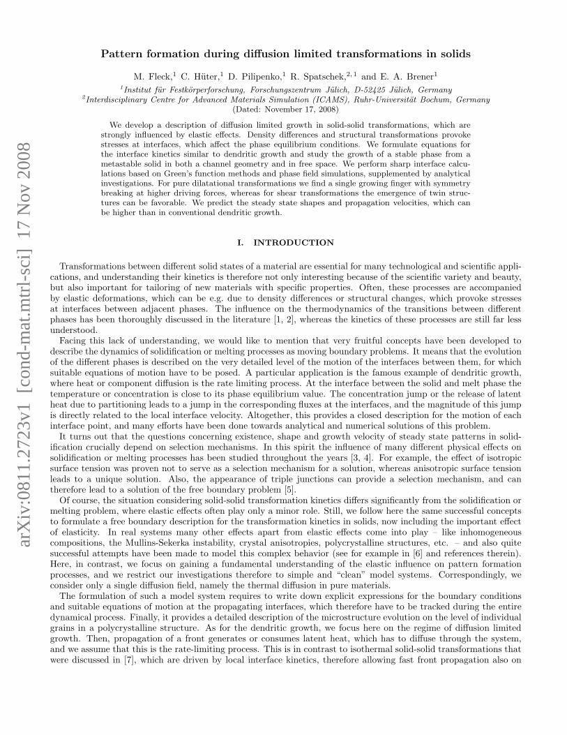
Specifically, we consider the growth of an equilibrium solid phase β from another metastable solid phase α, asdepicted in Fig. 1. At a temperature Teq, both stress-free phases are in bulk equilibrium with each other, whereasbelow this value the new β phase is thermodynamically favorable. Far ahead of the propagating front, the system istherefore exposed to a lower temperature T∞, and we define a dimensionless temperature w = C(T − T∞)/L, whereL denotes the latent heat of the transition and C the heat capacity. Within the solid phases the evolution of thetemperature field obeys a diffusion equation,

D∇2w =∂w

∂t, (1)

where D is the thermal diffusivity, which we assume to be equal in both phases, as well as the heat capacity (sym-metrical model).

The motion of the interfaces follows from energy conservation principles, which account here for the net heat fluxand the generation or absorption of latent heat due to the local motion of the interface with normal velocity vn,

vn =Dn · (∇w[β]int −∇w

[α]int), (2)

where n is the interface normal and the superscripts denote the phases.Elastic effects enter into the problem via a modification of the local phase equilibrium condition at the moving

interfaces. In contrast to previous investigations [8, 9], we now assume the phases to be coherently connected, i.e. weneglect the appearance of any slips, detachments or defect formation at the interfaces, which is reasonable for smallmisfits. It is important to mention here, that with the assumption of coherency we formulate a completely differentmodel being capable to describe qualitatively different types of elastic effects. For example the well-known effect ofelastic hysteresis [1, 2], which was proven to disappear without coherency [8], is now included in the model.

In a Lagrangian description of linear elasticity, the displacement field is denoted by u, and the coherency conditionreads, u[α] = u[β] at the interface. The strain field is then given by the symmetrical spatial derivative, ǫik =(∂ui/∂xk + ∂uk/∂xi) /2. This implies that tangential and shear strains ǫττ , ǫsτ , ǫss are continuous at the interfacewith τ, s being the two tangential directions. Force balance demands the continuity of the normal and shear stresses,σnn, σnτ , σns, where n is the normal direction. Here, the stresses are defined as the derivative of the free energy withrespect to the strains, σik = ∂F/∂ǫik.

The interface temperature for a planar, stress free interface is given by w = ∆, with ∆ = C(Teq −T∞)/L. Capillarycorrections induce a curvature dependent term, and for simplicity we discuss only the case of isotropic surface tensionγ. Finally, elastic deformations lead to an additional change of the interface temperature. Altogether, this leads tothe local equilibrium boundary condition [10]

wint = ∆ − d0κ +TeqC

L2δFel, (3)

with d0 = γTeqC/L2 being the capillary length and κ the local curvature of the interface, counted positive for aconvex phase β (see Fig. 1); Notice that due to the coherency constraint [11, 12], the elastic shift of the equilibrium

temperature is proportional to the difference of a new potential δFel = F[α]el − F

[β]el , which is related to the elastic free

energy Fel via the Legendre transformation Fel = Fel − σniǫni. Here, we use the sum convention for repeated indicesfor the sake of brevity.

From now on, we restrict our considerations to linear isotropic elasticity. Taking the relaxed state of the α phaseas reference, the elastic contribution to the free energy there reads

F[α]el =

E

2(1 + ν)

(

ν

1 − 2νǫ2ii + ǫ2ik

)

, (4)

3

FIG. 1: Schematic figure of the steady state growth, with constant velocity v, of a thermodynamically favored phase β intoa metastable phase α, which is initially at temperature T∞. The motion of the interface is locally described by the interface-normal velocity vn, which is given by the local heat conservation Eq. (2). The dashed lines at the two side borders indicatethat we will discuss two different types of outer boundary conditions: Free growth, where the strains decay for x, y → ∞, andchannel growth, with fixed displacements and thermal insulation at the walls. In the growth direction y the system is assumedto be infinite in both cases.

where E and ν are Young’s elastic modulus and Poisson ratio, respectively. In contrast, the elastic contribution tothe free energy density of the new phase β reads

F[β]el =

E

2(1 + ν)

(

ν

1 − 2ν

(

ǫii − ǫ0ii)2

+(

ǫik − ǫ0ik)2

)

, (5)

which has an other state of zero elastic energy due to the lattice strain ǫ0ik assigned to the phase transformation (seefor example (author?) [1, 2]). In the following we will call ǫ0ik the eigenstrain of the transformation. Particular casesof eigenstrains and their interpretation will be discussed in the next section.

The mechanical equilibrium and coherency conditions provide expressions for the discontinuous jumps of the strainsat the interface

ǫ[β]nn − ǫ[α]

nn =ǫ0nn +ν

1 − ν(ǫ0ss + ǫ0ττ ), (6)

ǫ[β]nτ − ǫ[α]

nτ =ǫ0nτ , ǫ[β]ns − ǫ[α]

ns = ǫ0ns, (7)

which are only related to the imposed eigenstrain. Defining an eigenstress tensor via Hooke’s law

σ0ik =

E

1 + ν

(

ǫ0ik +ν

1 − 2νδikǫ0ll

)

, (8)

we obtain after a few straightforward algebraic manipulations for the elastic contribution to the local equilibriumcondition Eq. (3)

δFel =σ0ikǫ

[α]ik − E

2(1 − ν2)

(

(ǫ0ττ )2 + (ǫ0ss)2 + 2νǫ0ττǫ0ss + 2(1 − ν)(ǫ0τs)

2)

. (9)

Apparently, this expression depends on the strain state of the α phase at the interface.As already implicitly assumed above, the elastic degrees of freedom relax fast on diffusive timescales, and therefore

the application of static elasticity is legitimate. Therefore, Newton’s second law becomes

∂σik

∂xk= 0. (10)

4

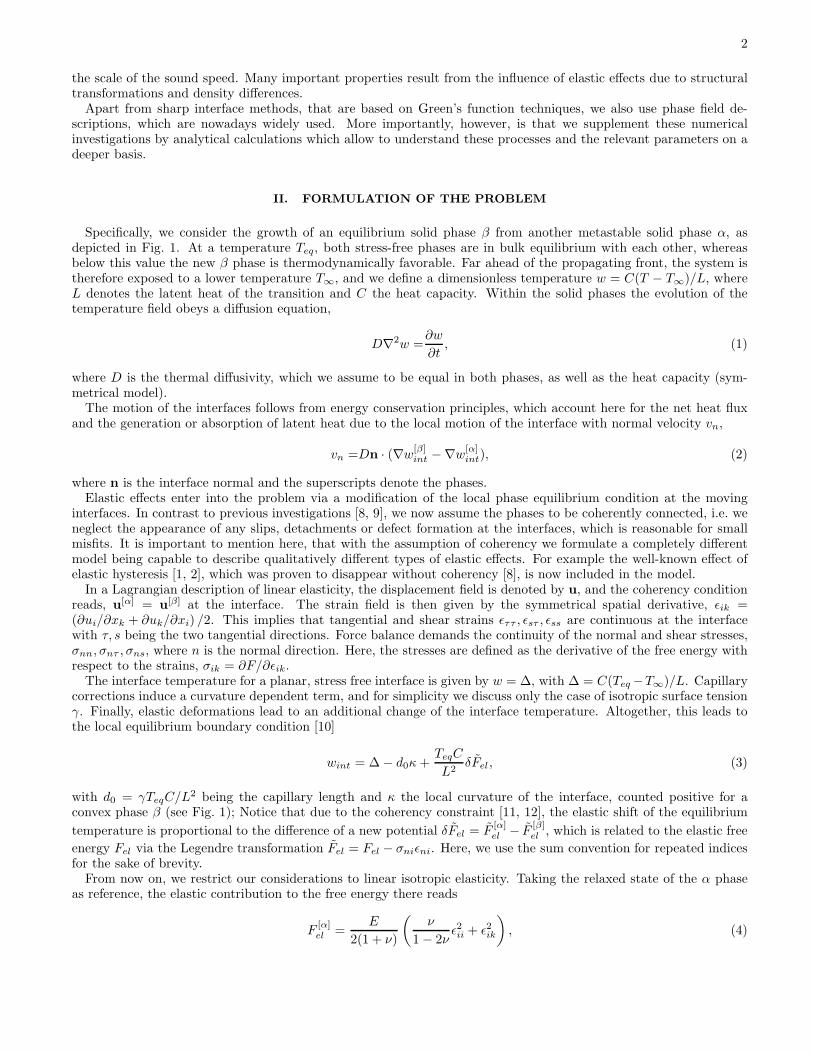
FIG. 2: Visualisation of the hexagonal to orthorhombic transformation. From the symmetry its obvious, that the orientationangle ϑ of the new orthorhombic phase can have only the three different values 0,±2π/3.

The above set of equations now has to be supplemented by boundary conditions at the external system boundaries,and we will discuss different scenarios below. They complete the self-sonsistent description of the moving boundaryproblem, which require the simultaneous solution of the elastic and diffusion equations, coupled via the boundaryconditions at the propagating interfaces, leading to a complicated nonlinear and nonlocal problem.

We note that we will later also discuss more complicated situations with more than one growing phase. Then, alsosimilar boundary conditions and equations have to be set up for the interfaces between them. Typically, then alsotriple junctions will appear, where the contact angles are given by Young’s law.

III. MODELS OF STRUCTURAL TRANSITIONS

The simplest case of a characteristic lattice strain is to assume the bond length of the new phase β to be uniformlylonger or shorter in all directions in comparison to the reference phase, i.e. ǫ0ik = ǫd

ik = ǫδik, which implies a densitychange. Notice, that this kind of transformations, to which we will refer to as dilatational eigenstrain, only changesthe volume of an elementary cell, and not its relative dimensions or its scaled shape.

The opposite case are transformations, where the volume of the unit cell is conserved and only the shape is changed.These shear transformations are characterized by a traceless eigenstrain tensor. A particular transition involving shearstrain can occur e.g. in hexagonal crystals, where the transition leads to a lowering of the symmetry from C6 to C2.This is the case for example in hexagonal-orthorombic transitions in ferroelastics (see [13] and references therein).Let the principal axis C6 be oriented in z direction. For simplicity we neglect all other possible strains with higher(axial) symmetry. By proper choice of the crystal orientation around the main axis in the initial phase, we obtain thenew phase in three possible states in the xy plane due to the original hexagonal symmetry (See Fig. 2). Then thenonvanishing components of the eigenstrain tensor ǫ0ik = ǫs

ik are ǫsyy = −ǫs

xx = ǫ cos 2ϑ and ǫsxy = ǫ sin 2ϑ, where the

orientation angle ϑ is either ϑ = 0 or ϑ = ±2π/3.We also consider a more generic mixed mode case, where the self-strain of the transformation is a linear combination

of the above two different transformations. We will discuss the following two mixing cases

ǫ0ik = ǫ±ik(η) = ηǫdik ± (1 − η)ǫs

ik (11)

and refer to them as positive or negative mixing.It is important to mention that switching from positive to negative mixing corresponds to a rotation of the eigenstrain

tensor by an angle π/2. Since our model is isotropic in all respects except the choice of the eigenstrain tensor, theonly predefined direction is given by the growth velocity. Therefore, we can interpret the negative mixing case torepresent physically the same system as the positive mixing case but with a growth direction perpendicular to it.

5

IV. FREE GROWTH

As a first application, we discuss the growth of the stable β phase from the metastable α phase in an infinitely largesystem, which is exposed to the temperature T∞ far away from the interface. For simplicity, we discuss an effectivelytwo-dimensional infinite system, assuming translational invariance in z direction. In particular, we assume a planestrain situation from point of view of elasticity. Also, we choose the elastic boundary conditions such that all stressesdecay far away from the interface.

Seeking for steady state solutions in free space, we use Green’s function methods for solving both the elastic andthe diffusional problem, to finally obtain self-consistently the shape and the velocity of the growing front. While thederivation of the integral representation of the thermal field is well-known, see e.g. [14], we present the calculation of

δFel in more detail [10]. To this end, we express the elastic problem using the eigenstrain-independent stress tensor

σik; for the α phase it is the same as the nomimal stress, σ[α]ik = σ

[α]ik , whereas in the β phase it is σ

[β]ik = σ

[β]ik + σ0

ik.In terms of the new stress tensor σik, the mechanical equilibrium equation ∂σik/∂xk = fi introduces a force densitywhich is localized on the interface and vanishes in the bulk,

fi = σ[β]in − σ

[α]in = σ0

in. (12)

This means that the problem of two coherently connected solids with different reference state is equivalent to a mono-lithic material with a distribution of point forces along the interface. We can therefore use an integral representationof the displacement field,

ui =

∫

ds′Gik(r − r′)fk(r′), (13)

where the integration is performed along the interface, and the free-space Green’s tensor Gik(r − r′) of the elasticproblem is given by [15]

Gik(r) =1 + ν

4π(1 − ν)E

(xixk

r2− (3 − 4ν)δik ln r

)

. (14)

This function is the displacement response at r to a point force located in the origin. As a result, the mismatchprovokes long-ranged elastic deformations, and therefore induces a nonlocal character to the problem. The aboveexpressions can then be used to calculate the elastic influence on the interface temperature wint.

Far behind the tip the interface profile becomes parabolic and is described by the asymptotic Ivantsov parabola[16]. In this region, the elastic strains have decayed, and only the constant local contribution to δFel (second term in

Eq. 9) remains. Consequently, the effective driving force ∆ consists not only of the thermal undercooling ∆, which iscontrolled by the applied temperature T∞, but also a contribution ∆el from the elasticity,

∆el =CTeqE[(ǫ0yy)

2 + (ǫ0zz)2 + 2νǫ0yyǫ

0zz]

2(1 − ν2)L2. (15)

We can consider ∆el as a parameter quantifying the strength of the elastic effects. The elastic effects therefore inducea shift of the equilibrium temperature, and the effective undercooling ∆ is lower than the actually applied thermaldriving force,

∆ = ∆ − ∆el, (16)

which reflects the elastic hysteresis [1, 2].By elimination of the thermal field [14] we can derive the steady state equation for the shape of the solid-solid

interface in a closed dimensionless representation, which reads in the co-moving frame of reference [10],

∆ − d0κ

R+

TeqCδFel

L2=

p

π

∫ ∞

−∞

dx′ exp[−p(y(x) − y(x′))]K0(pµ(x, x′)). (17)

Here, p = vR/2D denotes the Peclet number (v is the steady state velocity), and it is related to the driving force

by the implicit relation ∆ =√

πp ep erfc(p). Furthermore, K0 is the modified Bessel function of third kind in zeroth

order, and µ(x, x′) = [(x − x′)2 + (y(x) − y(x′))2]1/2. In the above expression we rescaled all lengths by the radius ofcurvature R of the asymptotic Ivantsov parabola.

Consequently, the central equation (17), together with the expression for the elastic contribution (9), where thestrains are expressed via the integral representation (13) results in a complicated integro-differential equation for

6

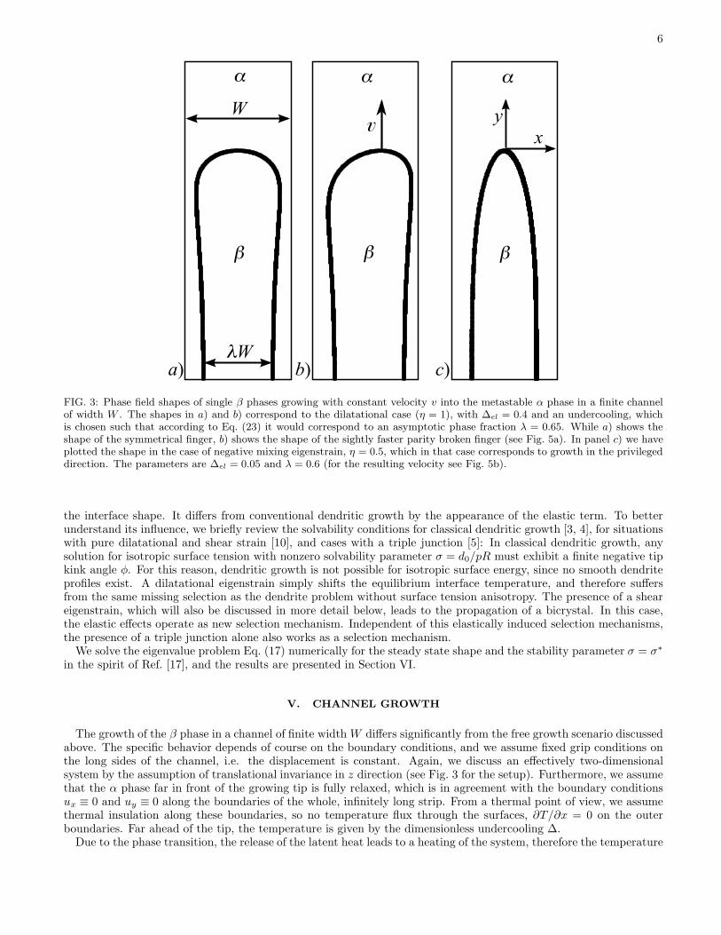
FIG. 3: Phase field shapes of single β phases growing with constant velocity v into the metastable α phase in a finite channelof width W . The shapes in a) and b) correspond to the dilatational case (η = 1), with ∆el = 0.4 and an undercooling, whichis chosen such that according to Eq. (23) it would correspond to an asymptotic phase fraction λ = 0.65. While a) shows theshape of the symmetrical finger, b) shows the shape of the sightly faster parity broken finger (see Fig. 5a). In panel c) we haveplotted the shape in the case of negative mixing eigenstrain, η = 0.5, which in that case corresponds to growth in the privilegeddirection. The parameters are ∆el = 0.05 and λ = 0.6 (for the resulting velocity see Fig. 5b).

the interface shape. It differs from conventional dendritic growth by the appearance of the elastic term. To betterunderstand its influence, we briefly review the solvability conditions for classical dendritic growth [3, 4], for situationswith pure dilatational and shear strain [10], and cases with a triple junction [5]: In classical dendritic growth, anysolution for isotropic surface tension with nonzero solvability parameter σ = d0/pR must exhibit a finite negative tipkink angle φ. For this reason, dendritic growth is not possible for isotropic surface energy, since no smooth dendriteprofiles exist. A dilatational eigenstrain simply shifts the equilibrium interface temperature, and therefore suffersfrom the same missing selection as the dendrite problem without surface tension anisotropy. The presence of a sheareigenstrain, which will also be discussed in more detail below, leads to the propagation of a bicrystal. In this case,the elastic effects operate as new selection mechanism. Independent of this elastically induced selection mechanisms,the presence of a triple junction alone also works as a selection mechanism.

We solve the eigenvalue problem Eq. (17) numerically for the steady state shape and the stability parameter σ = σ∗

in the spirit of Ref. [17], and the results are presented in Section VI.

V. CHANNEL GROWTH

The growth of the β phase in a channel of finite width W differs significantly from the free growth scenario discussedabove. The specific behavior depends of course on the boundary conditions, and we assume fixed grip conditions onthe long sides of the channel, i.e. the displacement is constant. Again, we discuss an effectively two-dimensionalsystem by the assumption of translational invariance in z direction (see Fig. 3 for the setup). Furthermore, we assumethat the α phase far in front of the growing tip is fully relaxed, which is in agreement with the boundary conditionsux ≡ 0 and uy ≡ 0 along the boundaries of the whole, infinitely long strip. From a thermal point of view, we assumethermal insulation along these boundaries, so no temperature flux through the surfaces, ∂T/∂x = 0 on the outerboundaries. Far ahead of the tip, the temperature is given by the dimensionless undercooling ∆.

Due to the phase transition, the release of the latent heat leads to a heating of the system, therefore the temperature

7

far behind the tip T−∞ is higher than in front. Under the given circumstances it is quite obvious that in this tailregion a homogeneous state is reached. In particular, since the interfaces do not move there, the temperature becomesindeed constant.

For simplicity, we discuss here only the specific case of a purely diagonal eigenstrain, i.e. ǫij = 0 for i 6= j, todemonstrate the analytical procedure. In contrast, in the case of an eigenstrain tensor with nonzero off-diagonalelements, bicrystal patterns emerge, and we will briefly discuss this situation below; it is quite obvious that theanalysis can be performed in an analogous way.

Due to the confinement of the system, phase coexistence is possible in a finite range of undercoolings, and we cancalculate the asymptotic volume fraction λ of the new phase (see Fig. 3). Notice, that in contrast to the isothermalsituation discussed in [7], the temperature in the tail region is not a control parameter but has to be found self-consistently, due to the thermally insulating boundaries. In terms of the asymptotic phase fraction λ, the width ofthe β phase in the tail region is written as λW . Mechanical compatibility requires

(1 − λ)ǫ[α]xx + λǫ[β]

xx = 0, (18)

since the average lateral strain must vanish due to the boundary conditions for the displacement. Together withthe mechanical equilibrium condition of force balance, we can then calculate the elastic fields in the tail region, andconsequently the elastic energy. Then, we calculate the energy excess δF , due to the appearance of a finite fractionof the new phase λ. It is defined as the difference between the energy for λ = 0 without any phase β and the energywith an arbitrary but finite fraction,

δF = − W(

λF[β]el + (1 − λ)F

[α]el

)

− 2γ + W

λ∫

0

(

L(Teq − T (λ′))

Teq

)

dλ′. (19)

Initially, there is only the elastically relaxed but metastable phase α at the constant temperature ∆. As soon as wehave a finite phase fraction λ, the energy increases by elastic and capillary contributions. Finally, the integral appearsdue to thermal insulation, since an increase of the amount of the phase β by phase transformation processes generateslatent heat, and therefore causes an increase of the temperature. Using the heat conservation condition we find therelation between this temperature and the phase fraction to be

T (λ) = T∞ + λL

C. (20)

Therefore, we obtain for the energy excess as a function of the asymptotic phase fraction λ

δF(λ) =WL2

CTeq

(

(∆ − ∆el)λ − 1

2(1 + ael∆el)λ2 − 2d0

W

)

, (21)

where the parameter ∆el, as already introduced above in Eq. (15), defines the strength of elastic effects, and

ael =CTeq(1 + ν)(1 − 2ν)

L2(1 − ν)E

(

σ0yy

)2

∆el(22)

is a parameter depending on the type of eigenstrain. The maximum of this energy excess, ∂∆F (λ)/∂λ = 0, providesthe equilibrium fraction, which expresses the thermodynamic balance between elastic deformation and free energyrelease due to the phase transition,

λeq =1

1 + ael∆el(∆ − ∆el) . (23)

If the fraction λeq is in the range 0 < λeq < 1, we obtain phase coexistence in the asymptotic regime far behindthe tip. We would like to point out that one can derive this equation also by using the phase equilibrium conditionEq. (3).

Then growth of the β phase demands that the energy excess (21) for the equilibrium fraction (23) has to be positive,

δF(λ) =WL2

CTeq

(

1

2(1 + ael∆el)λ2 − 2d0

W

)

> 0. (24)

This is equivalent to the condition λ > λcrit, where λcrit is given by

λ2crit =

4d0

W

1

1 + ael∆el. (25)

8

We note that for the shear transformations discussed above, the most favorable process is the growth of a bicrystal,where two twinned phases β and β′ with ϑ = ±2π/3 grow together, because this is energetically most favorable [7].For the bicrystal configuration, the analysis can be performed in a similar way, and then also the β/β′ grain boundaryenergy appears in the energy balance analogous to Eq. (19).

Considering the channel geometry, we use a phase field formulation to solve the full free boundary problem numer-ically. This method is very versatile and allows to study even more complicated scenarios, e.g. the full dynamicalevolution and not only the steady state regime, three-dimensionsal situations with full anisotropy of elasticity andsurface tension or simulations beyond the symmetrical model, where the two phases have different diffusion constants.Nevertheless, for brevity of presentation, we confine our investigations to the simple, isotropic, two-dimensional andthermally symmetric case that we also used for the Green’s function approach in the free space geometry and theabove analytical calculations.

The phase field method introduces an additional numerical lengthscale ξ, the width of the transition region betweenthe different solid phases. This means that an order parameter, which discriminates between the different phases, hasa profile φ = [1+ tanh(n/ξ)]/2 in normal direction through an interface. We operate here in the sharp interface limit,which means that this lengthscale is significantly smaller than all other physical lengthscales present in the problem.Then the description recovers the desired sharp interface equations that were proposed above.

Hence, we introduce the phase field φ having a value φ = 1 in the metastable initial phase, and a value φ = 0 inthe new phase. We start from a free energy functional

F [φ, w, ui] =

∫

V

(fs + fdw + f) dV, (26)

where fs(∇φ) = 3γξ(∇φ)2/2 is the gradient energy density and fdw(φ) = 6γφ2(1−φ)2/ξ is the double well potential,guaranteeing that the free energy functional has two local minima at φ = 0 and φ = 1 corresponding to the twodistinct phases of the system. The form of the double well potential and the gradient energy density are chosen suchthat the phase field parameter ξ defines the interface width and the parameter γ corresponds to the interface energyof the sharp interface description [18]. The free energy density f(φ, w, ui) of our phase field description is chosen tobe an interpolation between the two distinct free energies of the model,

f(φ, ui, w) =F[α]el h(φ) + F

[β]el (1 − h(φ)) + L

T − Teq

Teq(1 − h(φ)), (27)

where we choose the interpolation function h to be h(φ) = φ2(3 − 2φ). It is the simplest polynom satisfying thenecessary interpolation conditions h(0) = 0 and h(1) = 1, and having a vanishing slope at φ = 0 and φ = 1, in ordernot to shift the bulk states.

The evolution equation of the phase field is given by the variational expression

∂φ

∂t= − M

3γξ

(

δF

δφ

)

ui,w

. (28)

For large values of the mobility M we recover the desired case of diffusion limited growth. The elastodynamic equationsread

ρui = −(

δF

δui

)

φ,w

=∂σik

∂xk, (29)

which recover static elasticity for slowly propagating interfaces in comparison to the sound speed vs ∼ (E/ρ)1/2, withρ being the mass density.

For the temperature field we have the usual thermal diffusion equation with the motion of the phase field or interfacebeing a source of latent heat,

∂w

∂t= D∇2w + h′(φ)

∂φ

∂t, (30)

where the prime denotes the derivative with respect to φ. The phase field model presented here is very similar to themodel in [19]. However, there only the very special case of melting or crystallization of a confined sphere with elasticeffects was discussed.

For the simulations we typically use parameters W/d0 = 100 and W/ξ = 80.

9

0

1

2

3

4

5

6

7

10.50

σ*

η

0

2

4

6

8

10

0 0.5 1 1.5 2

σ*

∆el/p

η=0.3η=0.5

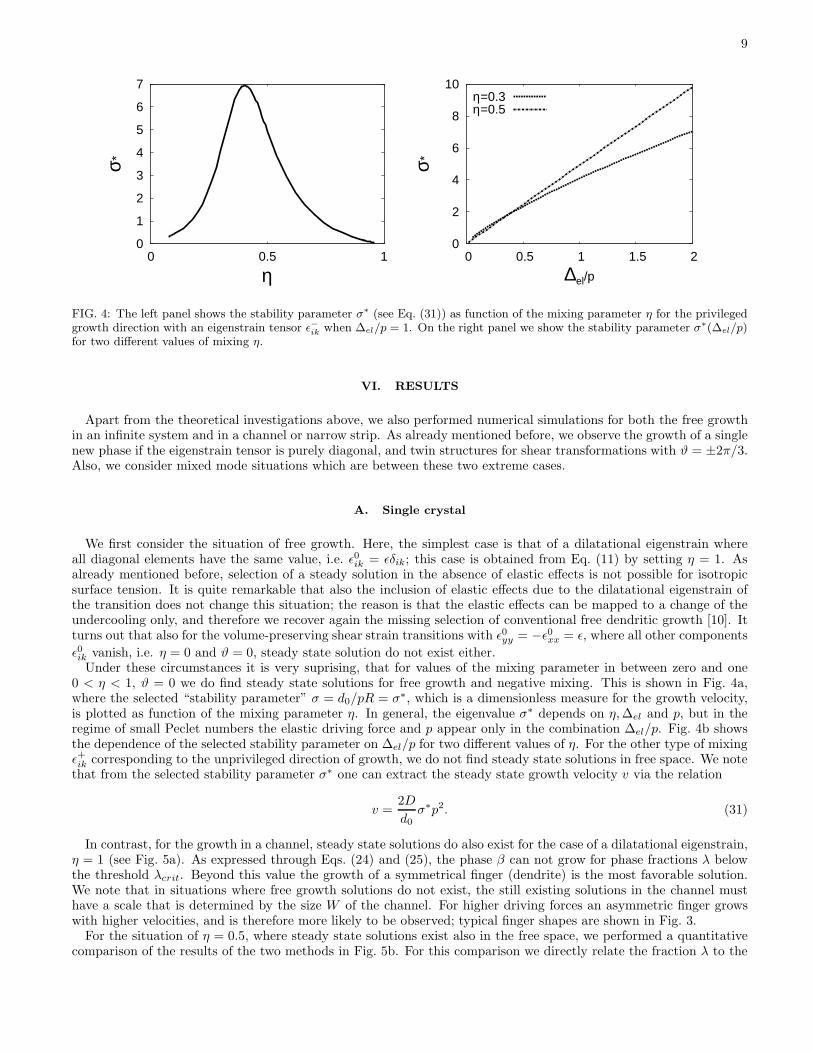
FIG. 4: The left panel shows the stability parameter σ∗ (see Eq. (31)) as function of the mixing parameter η for the privilegedgrowth direction with an eigenstrain tensor ǫ−

ikwhen ∆el/p = 1. On the right panel we show the stability parameter σ∗(∆el/p)

for two different values of mixing η.

VI. RESULTS

Apart from the theoretical investigations above, we also performed numerical simulations for both the free growthin an infinite system and in a channel or narrow strip. As already mentioned before, we observe the growth of a singlenew phase if the eigenstrain tensor is purely diagonal, and twin structures for shear transformations with ϑ = ±2π/3.Also, we consider mixed mode situations which are between these two extreme cases.

A. Single crystal

We first consider the situation of free growth. Here, the simplest case is that of a dilatational eigenstrain whereall diagonal elements have the same value, i.e. ǫ0ik = ǫδik; this case is obtained from Eq. (11) by setting η = 1. Asalready mentioned before, selection of a steady solution in the absence of elastic effects is not possible for isotropicsurface tension. It is quite remarkable that also the inclusion of elastic effects due to the dilatational eigenstrain ofthe transition does not change this situation; the reason is that the elastic effects can be mapped to a change of theundercooling only, and therefore we recover again the missing selection of conventional free dendritic growth [10]. Itturns out that also for the volume-preserving shear strain transitions with ǫ0yy = −ǫ0xx = ǫ, where all other components

ǫ0ik vanish, i.e. η = 0 and ϑ = 0, steady state solution do not exist either.Under these circumstances it is very suprising, that for values of the mixing parameter in between zero and one

0 < η < 1, ϑ = 0 we do find steady state solutions for free growth and negative mixing. This is shown in Fig. 4a,where the selected “stability parameter” σ = d0/pR = σ∗, which is a dimensionless measure for the growth velocity,is plotted as function of the mixing parameter η. In general, the eigenvalue σ∗ depends on η, ∆el and p, but in theregime of small Peclet numbers the elastic driving force and p appear only in the combination ∆el/p. Fig. 4b showsthe dependence of the selected stability parameter on ∆el/p for two different values of η. For the other type of mixingǫ+ik corresponding to the unprivileged direction of growth, we do not find steady state solutions in free space. We notethat from the selected stability parameter σ∗ one can extract the steady state growth velocity v via the relation

v =2D

d0σ∗p2. (31)

In contrast, for the growth in a channel, steady state solutions do also exist for the case of a dilatational eigenstrain,η = 1 (see Fig. 5a). As expressed through Eqs. (24) and (25), the phase β can not grow for phase fractions λ belowthe threshold λcrit. Beyond this value the growth of a symmetrical finger (dendrite) is the most favorable solution.We note that in situations where free growth solutions do not exist, the still existing solutions in the channel musthave a scale that is determined by the size W of the channel. For higher driving forces an asymmetric finger growswith higher velocities, and is therefore more likely to be observed; typical finger shapes are shown in Fig. 3.

For the situation of η = 0.5, where steady state solutions exist also in the free space, we performed a quantitativecomparison of the results of the two methods in Fig. 5b. For this comparison we directly relate the fraction λ to the

10

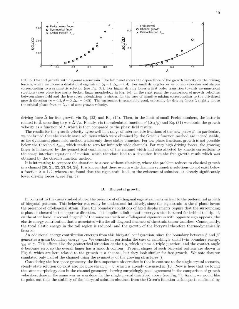
0 0.2 0.4 0.6 0.8

λ0

0.02

0.04

0.06

υd0/2

D

Parity broken fingerSymmetrical fingerCritical fraction λ

crit

0 0.2 0.4 0.6

λ0

0.1

0.2

υd0/2

D

Free growthChannel growthCritical fraction λ

crit

FIG. 5: Channel growth with diagonal eigenstrain. The left panel shows the dependence of the growth velocity on the drivingforce λ, where we choose a dilatational eigenstrain (η = 1, ∆el = 0.4). For small driving forces we obtain velocities and shapescorresponding to a symmetric solution (see Fig. 3a). For higher driving forces a first order transition towards asymmetricalsolutions takes place (see parity broken finger morphology in Fig. 3b). In the right panel the comparison of growth velocitiesbetween phase field and the free space calculations is shown, for the case of negative mixing corresponding to the privilegedgrowth direction (η = 0.5, ϑ = 0, ∆el = 0.05). The agreement is reasonably good, especially for driving forces λ slightly abovethe critical phase fraction λcrit of zero growth velocity.

driving force ∆ for free growth via Eq. (23) and Eq. (16). Then, in the limit of small Peclet numbers, the latter is

related to ∆ according to p ≈ ∆2/π. Finally, via the calculated function σ∗(∆el/p) and Eq. (31) we obtain the growthvelocity as a function of λ, which is then compared to the phase field results.

The results for the growth velocity agree well in a range of intermediate fractions of the new phase β. In particular,we confirmed that the steady state solutions which were obtained by the Green’s function method are indeed stable,as the dynamical phase field method tracks only these stable branches. For low phase fractions, growth is not possiblebelow the threshold λcrit, which tends to zero for infinitely wide channels. For very high driving forces, the growingfinger is influenced by the geometrical confinement of the channel width and also affected by kinetic corrections tothe sharp interface equations of motion, which therefore lead to a deviation from the free growth result which wasobtained by the Green’s function method.

It is interesting to compare the situation to a case without elasticity, where the problem reduces to classical growthin a channel [20, 21, 22, 23, 24, 25]. It is known that there even in wide channels symmetric solutions do not exist belowa fraction λ = 1/2, whereas we found that the eigenstrain leads to the existence of solutions at already significantlylower driving forces λ, see Fig. 5a.

B. Bicrystal growth

In contrast to the cases studied above, the presence of off-diagonal eigenstrain entries lead to the preferential growthof bicrystal patterns. This behavior can easily be understood intuitively, since the eigenstrain in the β phase favorsthe presence of off-diagonal strain. Then the boundary conditions of fixed displacements require that the surroundingα phase is sheared in the opposite direction. This implies a finite elastic energy which is stored far behind the tip. If,on the other hand, a second finger β′ of the same size with an off-diagonal eigenstrain with opposite sign appears, theelastic energy contribution that is associated with the off-diagonal elements of the strain tensor vanishes. Consequently,the total elastic energy in the tail region is reduced, and the growth of the bicrystal therefore thermodynamicallyfavored.

An additional energy contribution emerges from this bicrystal configuration, since the boundary between β and β′

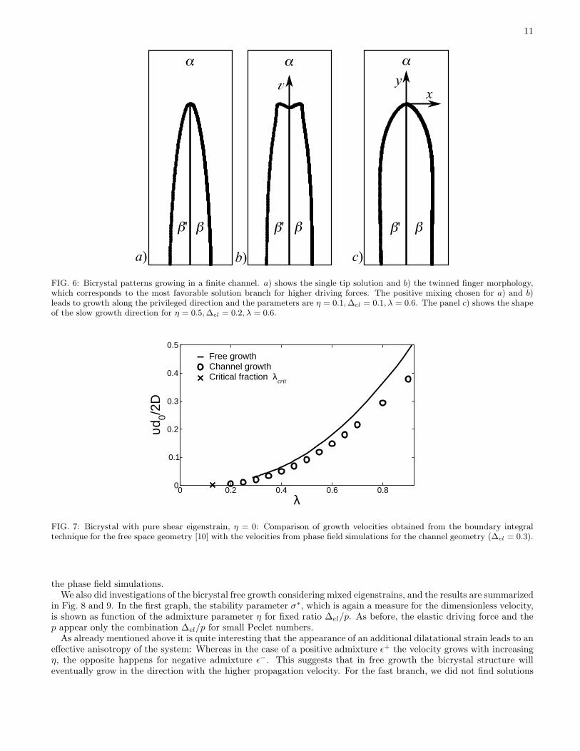
generates a grain boundary energy γgb. We consider in particular the case of vanishingly small twin boundary energy,γgb ≪ γ. This affects also the geometrical situation at the tip, which is now a triple junction, and the contact angleφ becomes zero, so the overall finger has a smooth contour. Typical shapes of such bicrystal pattern are shown inFig. 6, which are here related to the growth in a channel, but they look similar for free growth. We note that wesimulated only half of the channel using the symmetry of the growing structures [7].

Considering the free space geometry, the first important observation is that in contrast to the single crystal scenario,steady state solution do exist also for pure shear, η = 0, which is already discussed in [10]. New is here that we foundthe same morphology also in the channel geometry, showing surprisingly good agreement in the comparison of growthvelocities, done in the same way as was done for the single crystal described above (see Fig. 7). Again, we would liketo point out that the stability of the bicrystal solution obtained from the Green’s function technique is confirmed by

11

FIG. 6: Bicrystal patterns growing in a finite channel. a) shows the single tip solution and b) the twinned finger morphology,which corresponds to the most favorable solution branch for higher driving forces. The positive mixing chosen for a) and b)leads to growth along the privileged direction and the parameters are η = 0.1, ∆el = 0.1, λ = 0.6. The panel c) shows the shapeof the slow growth direction for η = 0.5, ∆el = 0.2, λ = 0.6.

0 0.2 0.4 0.6 0.8λ

0

0.1

0.2

0.3

0.4

0.5

υd0/2

D

Free growthChannel growthCritical fraction λ

crit

FIG. 7: Bicrystal with pure shear eigenstrain, η = 0: Comparison of growth velocities obtained from the boundary integraltechnique for the free space geometry [10] with the velocities from phase field simulations for the channel geometry (∆el = 0.3).

the phase field simulations.We also did investigations of the bicrystal free growth considering mixed eigenstrains, and the results are summarized

in Fig. 8 and 9. In the first graph, the stability parameter σ∗, which is again a measure for the dimensionless velocity,is shown as function of the admixture parameter η for fixed ratio ∆el/p. As before, the elastic driving force and thep appear only the combination ∆el/p for small Peclet numbers.

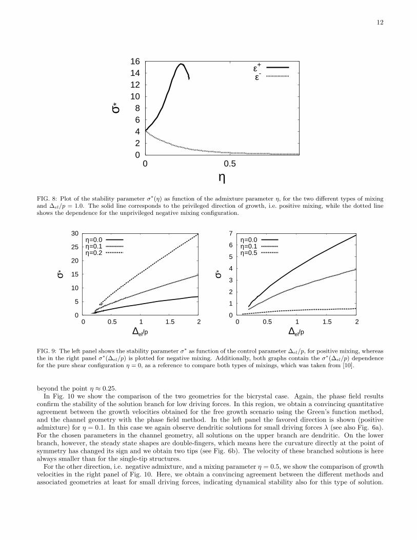
As already mentioned above it is quite interesting that the appearance of an additional dilatational strain leads to aneffective anisotropy of the system: Whereas in the case of a positive admixture ǫ+ the velocity grows with increasingη, the opposite happens for negative admixture ǫ−. This suggests that in free growth the bicrystal structure willeventually grow in the direction with the higher propagation velocity. For the fast branch, we did not find solutions

12

0 2 4 6 8

10 12 14 16

0.50

σ*

η

ε+

ε-

FIG. 8: Plot of the stability parameter σ∗(η) as function of the admixture parameter η, for the two different types of mixingand ∆el/p = 1.0. The solid line corresponds to the privileged direction of growth, i.e. positive mixing, while the dotted lineshows the dependence for the unprivileged negative mixing configuration.

0

5

10

15

20

25

30

0 0.5 1 1.5 2

σ*

∆el/p

η=0.0η=0.1η=0.2

0

1

2

3

4

5

6

7

0 0.5 1 1.5 2

σ*

∆el/p

η=0.0η=0.1η=0.5

FIG. 9: The left panel shows the stability parameter σ∗ as function of the control parameter ∆el/p, for positive mixing, whereasthe in the right panel σ∗(∆el/p) is plotted for negative mixing. Additionally, both graphs contain the σ∗(∆el/p) dependencefor the pure shear configuration η = 0, as a reference to compare both types of mixings, which was taken from [10].

beyond the point η ≈ 0.25.In Fig. 10 we show the comparison of the two geometries for the bicrystal case. Again, the phase field results

confirm the stability of the solution branch for low driving forces. In this region, we obtain a convincing quantitativeagreement between the growth velocities obtained for the free growth scenario using the Green’s function method,and the channel geometry with the phase field method. In the left panel the favored direction is shown (positiveadmixture) for η = 0.1. In this case we again observe dendritic solutions for small driving forces λ (see also Fig. 6a).For the chosen parameters in the channel geometry, all solutions on the upper branch are dendritic. On the lowerbranch, however, the steady state shapes are double-fingers, which means here the curvature directly at the point ofsymmetry has changed its sign and we obtain two tips (see Fig. 6b). The velocity of these branched solutions is herealways smaller than for the single-tip structures.

For the other direction, i.e. negative admixture, and a mixing parameter η = 0.5, we show the comparison of growthvelocities in the right panel of Fig. 10. Here, we obtain a convincing agreement between the different methods andassociated geometries at least for small driving forces, indicating dynamical stability also for this type of solution.

13

0 0.2 0.4 0.6 0.8

λ0

0.1

0.2

0.3

0.4

υd0/2

DFree growthTwinned fingerSingle-tip fingerCritical fraction λ

crit

0 0.1 0.2 0.3 0.4 0.5 0.6

λ0

0.02

0.04

υd0/2

D

Free growthChannel GrowthCritical fraction λ

crit

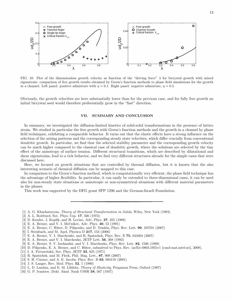
FIG. 10: Plot of the dimensionless growth velocity as function of the “driving force” λ for bicrystal growth with mixedeigenstrain: comparison of free growth results obtained by Green’s function methods to phase field simulations for the growthin a channel. Left panel: positive admixture with η = 0.1. Right panel: negative admixture, η = 0.5.

Obviously, the growth velocities are here substantially lower than for the previous case, and for fully free growth aninitial bicrystal seed would therefore preferentially grow in the “fast” direction.

VII. SUMMARY AND CONCLUSION

In summary, we investigated the diffusion-limited kinetics of solid-solid transformations in the presence of latticestrain. We studied in particular the free growth with Green’s function methods and the growth in a channel by phasefield techniques, exhibiting a comparable behavior. It turns out that the elastic effects have a strong influence on theselection of the arising patterns and the corresponding steady state velocities, which differ crucially from conventionaldendritic growth. In particular, we find that the selected stability parameter and the corresponding growth velocitycan be much higher compared to the classical case of dendritic growth, where the solutions are selected by the tinyeffect of the anisotropy of surface tension. Different structural transitions, which are described by dilatational andshear eigenstrains, lead to a rich behavior, and we find very different structures already for the simple cases that werediscussed here.

Here, we focused on growth situations that are controlled by thermal diffusion, but it is known that the alsointeresting scenario of chemical diffusion can be mapped to this case.

In comparison to the Green’s function method, which is computationally very efficient, the phase field technique hasthe advantage of higher flexibility. In particular, it can easily be extended to three-dimensional cases, it can be usedalso for non-steady state situations or anisotropic or non-symmetrical situations with different material parametersin the phases.

This work was supported by the DFG grant SPP 1296 and the German-Israeli Foundation.

[1] A. G. Khachaturyan, Theory of Structural Transformation in Solids, Wiley, New York (1983)[2] A. L. Roitburd, Sov. Phys. Usp. 17, 326 (1974)[3] D. Kessler, J. Koplik, and H. Levine, Adv. Phys. 37, 255 (1988)[4] E. A. Brener, and V. I. Mel’nikov, Adv. Phys. 40, 53 (1991)[5] E. A. Brener, C. Huter, D. Pilipenko, and D. Temkin, Phys. Rev. Lett. 99, 105701 (2007)[6] I. Steinbach, and M. Apel, Physica D 217, 153 (2006)[7] E. A. Brener, V. I. Marchenko, and R. Spatschek, Phys. Rev. E 75, 041604 (2007)[8] E. A. Brener, and V. I. Marchenko, JETP Lett. 56, 368 (1992)[9] E. A. Brener, S. V. Iordanskii, and V. I. Marchenko, Phys. Rev. Lett. 82, 1506 (1999)

[10] D. Pilipenko, E. A. Brener, and C. Huter, submitted to Phys. Rev. (arXiv:0803.1955v1 [cond-mat.mtrl-sci], 2008).[11] I. A. Privorotskii, Sov. Phys. JETP 33, 825 (1971)[12] R. Spatschek, and M. Fleck, Phil. Mag. Lett., 87, 909 (2007)[13] S. H. Curnoe, and A. E. Jacobs, Phys. Rev. B 63, 094110 (2001)[14] J. S. Langer, Rev. Mod. Phys. 52, 1 (1980)[15] L. D. Landau, and E. M. Lifshitz, Theory of Elasticity, Pergamon Press, Oxford (1987)[16] G. P. Ivantsov, Dokl. Akad. Nauk USSR 58, 567 (1947)

14

[17] D. I. Meiron, Phys. Rev. A 33, 2704 (1986)[18] C. Gugenberger, R. Spatschek, and K. Kassner, Phys. Rev. E 78, 016703 (2008)[19] J. Slutsker and K. Thornton, A. L. Roytburd, J. A. Warren, and G. B. McFadden, Phys. Rev. B 74, 914103 (2006)[20] D. Kessler, J. Koplik, and H. Levine, Phys. Rev. A 34, 4980 (1986)[21] E.A. Brener, M. Geilikman, and D.E. Temkin, Sov. Phys. JETP 67, 1002 (1988).[22] E. A. Brener, H. Muller-Krumbhaar, Y. Saito, and D. Temkin, Phys. Rev. E 47, 1151 (1993)[23] R. Kupferman, D. A. Kessler, and E. Ben-Jacob, Physica (Amsterdam) 231A, 451 (1995)[24] M. Ben Amar, and E. A. Brener, Phys. Rev. Lett. 75, 561 (1995)[25] M. Ben Amar, E. A. Brener, Physica D, 98, 128 (1996).