Aloke Paul · Tomi LaurilaVesa Vuorinen · Sergiy V. Divinski

Thermodynamics, Diffusion and the Kirkendall Effect in Solids

Thermodynamics, Diffusion and the KirkendallEffect in Solids

Aloke Paul • Tomi LaurilaVesa Vuorinen • Sergiy V. Divinski

Thermodynamics, Diffusionand the Kirkendall Effectin Solids

123

Aloke PaulDepartment of Materials EngineeringIndian Institute of ScienceBangaloreIndia

Tomi LaurilaVesa VuorinenDepartment of Electrical Engineering

and AutomationSchool of Electrical EngineeringAalto UniversityAaltoFinland

Sergiy V. DivinskiInstitute for Materials PhysicsUniversity of MünsterMünsterGermany

ISBN 978-3-319-07460-3 ISBN 978-3-319-07461-0 (eBook)DOI 10.1007/978-3-319-07461-0Springer Cham Heidelberg New York Dordrecht London

Library of Congress Control Number: 2014940711

� Springer International Publishing Switzerland 2014This work is subject to copyright. All rights are reserved by the Publisher, whether the whole or part ofthe material is concerned, specifically the rights of translation, reprinting, reuse of illustrations,recitation, broadcasting, reproduction on microfilms or in any other physical way, and transmission orinformation storage and retrieval, electronic adaptation, computer software, or by similar or dissimilarmethodology now known or hereafter developed. Exempted from this legal reservation are briefexcerpts in connection with reviews or scholarly analysis or material supplied specifically for thepurpose of being entered and executed on a computer system, for exclusive use by the purchaser of thework. Duplication of this publication or parts thereof is permitted only under the provisions ofthe Copyright Law of the Publisher’s location, in its current version, and permission for use mustalways be obtained from Springer. Permissions for use may be obtained through RightsLink at theCopyright Clearance Center. Violations are liable to prosecution under the respective Copyright Law.The use of general descriptive names, registered names, trademarks, service marks, etc. in thispublication does not imply, even in the absence of a specific statement, that such names are exemptfrom the relevant protective laws and regulations and therefore free for general use.While the advice and information in this book are believed to be true and accurate at the date ofpublication, neither the authors nor the editors nor the publisher can accept any legal responsibility forany errors or omissions that may be made. The publisher makes no warranty, express or implied, withrespect to the material contained herein.

Printed on acid-free paper

Springer is part of Springer Science+Business Media (www.springer.com)

Aloke Paul dedicates this book to his Ph.D.guide

Prof. Frans J. J. van Loo, The Netherlands

Prof. Frans J. J. van Loo

Preface

Diffusion in solids plays an important role in many processes in Material Scienceand is the basis for numerous technological applications. In the nineteenth century,diffusion in a solid material was hard to imagine because of densely packedstructure. In fact, the first systematic diffusion study in solid state was carried outonly in the late nineteenth century.

Before the work of Ernst O. Kirkendall and Fredrick Seitz in the 1940s, it was acommon belief that all the components diffuse at the same rate in solid materials.Based on this assumption, direct exchange and ring mechanisms were wronglysuggested to explain the diffusion of the components in crystalline solids.(Surprisingly, the ring mechanism was rediscovered in molecular dynamic simu-lation of grain boundary diffusion!) Kirkendall’s work played an important role informulating the basis of the theory of defect, i.e. vacancy-dependent diffusionmechanism. Following this thought-provoking concept many outstanding paperswere published to further establish the relations to estimate the different diffusionparameters from experiments. In the mean time, based on Georg Karl vonHevesy’s work, radiotracer technique to study diffusion was developed whichsheds light on the fundamental aspect of the atomic nature of diffusion. In factSeitz, based on the available tracer diffusion study on pure Cu and Kirkendall’sexperiment, proved beyond doubt that diffusion of substitutional atoms occurs byvacancy mechanism.

Looking back to the many books published on this subject by other researchers,it is evident that there exists no book with a special emphasis on interdiffusion andon the Kirkendall effect. Further, as thermodynamics plays an important role ininterdiffusion, without a proper understanding of the subject, many fundamentalaspects of interdiffusion may remain unclear. Therefore, we introduce theimportant aspects of thermodynamics from the solid-state diffusion perspectiveand then discuss the phenomenological process of interdiffusion extensively.Moreover, the understanding of the interdiffusion process is not complete withoutunderstanding the atomic mechanism of diffusion and different types of diffusion,such as lattice and grain boundary diffusion. Therefore, these topics are discussedin detail. Still, we are limiting the present consideration by metallic systems withuncharged defects.

Chapter 1 starts with very basic concepts of thermodynamics. The laws ofthermodynamics are introduced and different extensive and intensive properties

vii

and variables are briefly discussed. The chapter is focused on a short and concisedescription of the approaches to represent and utilize the thermodynamic data in amanner suitable for interdiffusion studies. Therefore, many different ways torepresent the thermodynamic data of a given system graphically are introduced.Special emphasis is given to Gibbs energy diagrams, phase diagrams and differenttypes of potential diagrams. Many of the relations developed and diagramsintroduced in this chapter will be frequently used in subsequent chapters.

Chapter 2 introduces different aspects of the hierarchical structure of solids:atomic structure, unit cells, grain structure, defects, microstructure, etc., which arevery essential for understanding of the material systems. Some aspects related tothe defect structures in intermediate compounds, including the effect of atomicorder, are also discussed.

Chapter 3 starts with the Fick’s laws of diffusion. The second law is derivedfrom the first law. Subsequently, several solutions for diffusion problems withdifferent kinds of initial and boundary conditions are given. Limitations of thesolutions obtained are discussed, too. This chapter is written in such a way thatnew students in the field or undergraduate students can understand the very basicsof Fick’s laws and their solutions, so that the formalism could directly be appliedfor processing of the experimental data.

Chapter 4 relates thermodynamics with interdiffusion of components. Differentkinds of microstructures, which are expected to grow in the interdiffusion zone,depending on the given phase diagram and composition of the end members of thediffusion couples are explained in detail.

Chapter 5 discusses the atomic mechanisms of diffusion in detail. The maindifference between the interstitial and substitutional diffusion mechanisms is dis-cussed. Anisotropy of diffusion, effect of temperature, and the fundamental con-cept of a correlation factor are introduced in detail. The analytical and numericalapproaches for calculation of the correlation factors are introduced. Diffusion inordered phases is also disussed with a highlight on specific atomistic mechanismsand correlation effects.

Chapter 6 concentrates on interdiffusion in systems with a wide compositionrange. First, the limitations of the error function analysis are discussed based onthe topics introduced in Chap. 3 After that, different approaches that are used toestimate the diffusion data are explained. The Kirkendall effect and the concept ofintrinsic diffusion coefficients are introduced. The estimation of the tracer diffusioncoefficients indirectly from a diffusion couple is also explained.

Chapter 7 discusses the estimation of the diffusion parameters in line com-pounds and phases with a narrow homogeneity range. Few practical examples areintroduced to explain the steps needed for quantitative analysis.

Chapter 8 concentrates in the very recent developments in understanding theKirkendall effect and the physicochemical approach. By using this approach, onecan not only estimate the diffusion parameters, but also achieve more profoundunderstanding of the microstructural evolution of an interdiffusion zone.

Chapter 9 concentrates on diffusion in multicomponent systems. The mathe-matical and experimental difficulties in estimating the diffusion parameters in

viii Preface

ternary or higher order systems are discussed. A pseudo-binary approach, whichsimplifies the conditions for the estimation of the diffusion parameter with muchbetter efficiency, is introduced. The usefulness of the diffusion couple techniquefor the determination of phase diagrams is also discussed.

Chapter 10 concentrates mainly on short-circuit diffusion. Microstructures witha hierarchy of short-circuit paths are explained and the kinetic regimes of diffusionin such structures are introduced and discussed. Many practical examples are givenin order to explain the practical estimation of the diffusion parameters. Finally, theeffect of grain boundary diffusion on interdiffusion and Kirkendall effects arebriefly discussed.

Chapter 11 introduces the complications arising from the growth of the phasesas thin films. The roles of nucleation barriers, interfacial energies and elasticstrains in reactive diffusion are discussed. Further, nucleation issues in solid-stateamorphization are also discussed. Finally, it is shown that there is no fundamentaldifference between thin film and bulk diffusion couples and the complications inthe former arise mainly from the structural features of thin films.

It should be noted that this book is biased towards experimental techniques.Important developments are going on simulation, which are not covered here.Three different groups have joined together to write on few important aspects suchas thermodynamics, interdiffusion, atomic mechanism and short-circuit diffusion.In this also, few aspects are not covered extensively, which are beyond therequirements for the students or available in other books.

As usual, we don’t expect it to be complete error-free. We would appreciate ifyou write us with your comments and feedback so that we can take care in the nextedition.

Preface ix

Acknowledgment

Although four authors have written this book, the important contributions ondifferent topics have come from several researchers over many decades. As one ofthe authors, I (Aloke Paul) dedicate this book to one of such researchers and myPh.D. guide Prof. Frans J. J. van Loo, Eindhoven University of Technology, TheNetherlands, for seminal contribution during his illustrious research career. Atmany places, especially in Chaps. 6–8, relations are derived based on his andcoworker’s work. He should have been the author of the book, which I expressedto him many times during my Ph.D. However, he was very clear that after mythesis, he would like to spend his retired life differently.

Dr. Alexander Kodentsov (Sasha) is another very important person influencingmy research career. He taught me most of the experimental techniques and tricksleading to many successes. However, it was my inability that I could not improvemy writing skill beyond a certain limit which is far behind his! He was alwaysthere, whenever I needed from personal to professional needs.

I am grateful to other co-workers, Dr. Mark van Dal, Dr. Csaba Cserháti, Dr.Pascal Oberndorff and Prof. Andrei Gusak for explaining many issues during myearly stage of the career.

I am lucky to get very good research students and learnt many new aspects ofdiffusion through their work, questions and discussions. Additionally, they havedone the most painful job of reading carefully, finding mistakes or drawing manyfigures. This book would be very difficult to complete without the help in the end,especially from Sangeeta Santra, Varun Baheti and Soumitra Roy on finalizing thechapters. I also thank my colleagues for their help during my difficult days.

I would like to acknowledge the financial support from Humboldt Foundationfor my stay at Muenster University, Germany during which many chapters werewritten.

In the end, I thank two most important ladies in my life, wife Bhavna anddaughter Pihu to make me get going through thick and thin.

We (Tomi Laurila and Vesa Vuorinen) would like to acknowledge our Ph.D.supervisor Professor (emeritus) Jorma Kivilahti for his contributions on the subjectof thermodynamics. Many aspects of Chap. 1 are indebt to the textbook, whichprofessor Kivilahti wrote in Finnish in the early 1980s. I (Tomi Laurila) wouldalso like to pay my tribute to late Dr. Francois d’Heurle who I had the pleasure toknow. He introduced to me the interesting fields of silicides and thin film reactions.

xi

Also Dr. Kejun Zeng, Dr. Jyrki Molarius and Dr. Ilkka Suni are acknowledged fortheir contributions to the field of thermodynamic modelling and reactive phaseformation in thin film diffusion couples as well as collaborating with me during myPh.D. work. Finally, I want to thank the most important group of people in my life,my family, which consist of my wife Milla and our three children Miro, Mirellaand Miko. Thanks for being there!

I (Vesa Vuorinen) would also like to express my gratitude to my family—myparents, my wife Maija and my children Viivi, Ville and Vili—for their love andsupport.

I (SergiyDivinski) acknowledge two outstanding persons who influence largelymy scientific life—Prof. Leonid Nikandrovich Larikov, Institute of Metals Phys-ics, National Academy of Science, Kiev, Ukraine, who was my Ph.D. supervisor,introduced me to the diffusion-based phenomena and whom I cannot overpay mylate tribute, and Prof. Christian Herzig, Institute of Materials Physics, Universityof Münster, Germany, friendly and intensive collaboration and countless discus-sions with whom determined my current specialization. And, of course, myfamily—my wife Sveta and my daughters, Veronika and Alisa, they all togetherwere and are on my side and not only support the viewpoint that ‘‘there is a lifebeyond science’’, but prove that this is the most important part of our life!

xii Acknowledgment

Contents

1 Thermodynamics, Phases, and Phase Diagrams . . . . . . . . . . . . . . 11.1 Thermodynamics System and Its State . . . . . . . . . . . . . . . . . 21.2 The Laws of Thermodynamics . . . . . . . . . . . . . . . . . . . . . . . 31.3 Heterogeneous Systems . . . . . . . . . . . . . . . . . . . . . . . . . . . . 51.4 Commonly Used Terms and First Glance

at Phase Diagrams . . . . . . . . . . . . . . . . . . . . . . . . . . . . . . . 71.5 Spontaneous Change . . . . . . . . . . . . . . . . . . . . . . . . . . . . . . 121.6 Free Energy and Phase Stabilityof Single-Component

System . . . . . . . . . . . . . . . . . . . . . . . . . . . . . . . . . . . . . . . 191.7 Pressure Effect of Single-Component Phase Diagram . . . . . . . 241.8 Free Energy and Stability of Phases in a Binary System . . . . . 26

1.8.1 Change in Free Energy in an Ideal System . . . . . . . . 271.8.2 Change in Free Energy in a System with

Exothermic Transformation . . . . . . . . . . . . . . . . . . . 301.8.3 Change in Free Energy in a System with

Endothermic Transformation . . . . . . . . . . . . . . . . . . 301.9 Thermodynamics of Solutions and Phase Diagrams . . . . . . . . 32

1.9.1 The Chemical Potential and Activity in a BinarySolid Solution . . . . . . . . . . . . . . . . . . . . . . . . . . . . 32

1.9.2 Free Energy of Solutions . . . . . . . . . . . . . . . . . . . . . 331.10 Lever Rule and the Common Tangent Construction . . . . . . . . 401.11 The Gibbs Phase Rule. . . . . . . . . . . . . . . . . . . . . . . . . . . . . 431.12 Correlation of Free Energy and Phase Diagram

in Binary Systems . . . . . . . . . . . . . . . . . . . . . . . . . . . . . . . 451.13 Ternary Phase Diagrams . . . . . . . . . . . . . . . . . . . . . . . . . . . 531.14 Stability Diagrams (Activity Diagrams, etc.) . . . . . . . . . . . . . 611.15 The Use of Gibbs Energy Diagrams . . . . . . . . . . . . . . . . . . . 64

1.15.1 Effect of Pressure on the Phase Equilibrium . . . . . . . 731.15.2 Ternary Molar Gibbs Energy Diagrams. . . . . . . . . . . 77

1.16 Interdependence of Chemical Potentials: Gibbs–DuhemEquation . . . . . . . . . . . . . . . . . . . . . . . . . . . . . . . . . . . . . . 80

xiii

1.17 Molar Volume of a Phase and Partial Molar Volumesof the Species . . . . . . . . . . . . . . . . . . . . . . . . . . . . . . . . . . 82

1.18 Few Standard Thermodynamic Relations . . . . . . . . . . . . . . . . 84References . . . . . . . . . . . . . . . . . . . . . . . . . . . . . . . . . . . . . . . . . 86

2 Structure of Materials . . . . . . . . . . . . . . . . . . . . . . . . . . . . . . . . 872.1 Hierarchical Structure of Materials . . . . . . . . . . . . . . . . . . . . 872.2 Atomic Bonding . . . . . . . . . . . . . . . . . . . . . . . . . . . . . . . . . 872.3 Crystal Lattice . . . . . . . . . . . . . . . . . . . . . . . . . . . . . . . . . . 892.4 Grain Structure. . . . . . . . . . . . . . . . . . . . . . . . . . . . . . . . . . 912.5 Defects . . . . . . . . . . . . . . . . . . . . . . . . . . . . . . . . . . . . . . . 93

2.5.1 Point Defects . . . . . . . . . . . . . . . . . . . . . . . . . . . . . 932.5.2 Linear Defects . . . . . . . . . . . . . . . . . . . . . . . . . . . . 1012.5.3 Two-Dimensional Defects . . . . . . . . . . . . . . . . . . . . 1022.5.4 Volume Defects . . . . . . . . . . . . . . . . . . . . . . . . . . . 103

2.6 Some Examples of Intermediate Phases and TheirCrystal Structure. . . . . . . . . . . . . . . . . . . . . . . . . . . . . . . . . 1032.6.1 Defects in Intermediate Phases . . . . . . . . . . . . . . . . . 1052.6.2 Crystal Structures and Point Defects in Ordered

Binary Intermetallics on an Example of Ni-, Ti-,and Fe-Aluminides . . . . . . . . . . . . . . . . . . . . . . . . . 107

2.6.3 Calculation of Point Defect Formation Energies . . . . . 1082.7 Microstructure and Phase Structure. . . . . . . . . . . . . . . . . . . . 113References . . . . . . . . . . . . . . . . . . . . . . . . . . . . . . . . . . . . . . . . . 114

3 Fick’s Laws of Diffusion . . . . . . . . . . . . . . . . . . . . . . . . . . . . . . . 1153.1 Fick’s First and Second Laws of Diffusion . . . . . . . . . . . . . . 1153.2 Solution of Fick’s Second Law to Estimate

the Diffusion Coefficient . . . . . . . . . . . . . . . . . . . . . . . . . . . 1193.2.1 Solution for a Thin-Film Condition. . . . . . . . . . . . . . 1193.2.2 Solution for Homogenization (Separation

of Variables) . . . . . . . . . . . . . . . . . . . . . . . . . . . . . 135References . . . . . . . . . . . . . . . . . . . . . . . . . . . . . . . . . . . . . . . . . 139

4 Development of Interdiffusion Zone in Different Systems . . . . . . . 1414.1 Chemical Potential as the Driving Force for Diffusion

and Phase Layer Growth in an Interdiffusion Zone. . . . . . . . . 1414.2 Few Practical Examples . . . . . . . . . . . . . . . . . . . . . . . . . . . 1494.3 Making Products by a Diffusion Process . . . . . . . . . . . . . . . . 160References . . . . . . . . . . . . . . . . . . . . . . . . . . . . . . . . . . . . . . . . . 165

5 Atomic Mechanism of Diffusion . . . . . . . . . . . . . . . . . . . . . . . . . 1675.1 Different Types of Diffusion . . . . . . . . . . . . . . . . . . . . . . . . 1675.2 Interstitial Atomic Mechanism of Diffusion . . . . . . . . . . . . . . 173

xiv Contents

5.2.1 Relation Between Jump Frequency andthe Diffusion Coefficient . . . . . . . . . . . . . . . . . . . . . 173

5.2.2 Random Walk of Atoms . . . . . . . . . . . . . . . . . . . . . 1815.2.3 Effect of Temperature on the Interstitial Diffusion

Coefficient. . . . . . . . . . . . . . . . . . . . . . . . . . . . . . . 1845.2.4 Tracer Method of Measuring the Interstitial

Diffusion Coefficient . . . . . . . . . . . . . . . . . . . . . . . 1875.2.5 Orientation Dependence of Interstitial Diffusion

Coefficient. . . . . . . . . . . . . . . . . . . . . . . . . . . . . . . 1885.3 Diffusion in Substitutional Alloys. . . . . . . . . . . . . . . . . . . . . 191

5.3.1 Measurement of Tracer Diffusion Coefficient . . . . . . 1925.3.2 Concept of the Correlation Factor. . . . . . . . . . . . . . . 1935.3.3 Calculation of the Correlation Factor . . . . . . . . . . . . 1965.3.4 The Relation Between the Jump Frequency and the

Diffusion Coefficient in Substitutional Diffusion . . . . 1985.3.5 Effect of Temperature on Substitutional Diffusion . . . 2015.3.6 Orientation Dependence in Substitutional

Diffusion . . . . . . . . . . . . . . . . . . . . . . . . . . . . . . . . 2065.3.7 Effect of Phase Transitions on Substitutional

Diffusion . . . . . . . . . . . . . . . . . . . . . . . . . . . . . . . . 2135.4 Diffusion Mechanisms in Intermetallics. . . . . . . . . . . . . . . . . 213

5.4.1 Diffusion in Disordered Intermetallic Compounds . . . 2145.4.2 Diffusion Mechanisms in Ordered Intermetallic

Compounds . . . . . . . . . . . . . . . . . . . . . . . . . . . . . . 2165.4.3 Six-Jump Cycle Mechanism. . . . . . . . . . . . . . . . . . . 2165.4.4 Sublattice Diffusion Mechanism . . . . . . . . . . . . . . . . 2215.4.5 Triple-Defect Diffusion Mechanism . . . . . . . . . . . . . 2235.4.6 Antistructure Bridge Mechanism . . . . . . . . . . . . . . . 2255.4.7 Interstitial Diffusion Mechanism. . . . . . . . . . . . . . . . 2265.4.8 Other Diffusion Mechanisms . . . . . . . . . . . . . . . . . . 227

5.5 Correlation Factors of Diffusion in IntermetallicCompounds . . . . . . . . . . . . . . . . . . . . . . . . . . . . . . . . . . . . 2285.5.1 Calculation of the Probabilities P . . . . . . . . . . . . . . . 2305.5.2 The Monte Carlo Calculation Scheme. . . . . . . . . . . . 233

References . . . . . . . . . . . . . . . . . . . . . . . . . . . . . . . . . . . . . . . . . 237

6 Interdiffusion and the Kirkendall Effect in Binary Systems . . . . . 2396.1 Matano–Boltzmann Analysis . . . . . . . . . . . . . . . . . . . . . . . . 2406.2 Limitation of the Matano–Boltzmann Analysis. . . . . . . . . . . . 2486.3 Den Broeder Approach to Determine the Interdiffusion

Coefficient. . . . . . . . . . . . . . . . . . . . . . . . . . . . . . . . . . . . . 2496.4 Wagner’s Approach to the Calculation of the Interdiffusion

Coefficient. . . . . . . . . . . . . . . . . . . . . . . . . . . . . . . . . . . . . 2526.5 Change in Total Volume of the Diffusion Couple. . . . . . . . . . 257

Contents xv

6.6 The Kirkendall Effect . . . . . . . . . . . . . . . . . . . . . . . . . . . . . 2666.7 Darken Analysis: Relation Between Interdiffusion

and Intrinsic Diffusion Coefficients . . . . . . . . . . . . . . . . . . . 2726.8 Relations for the Estimation of the Intrinsic Diffusion

Coefficients . . . . . . . . . . . . . . . . . . . . . . . . . . . . . . . . . . . . 2756.8.1 Heumann’s Method. . . . . . . . . . . . . . . . . . . . . . . . . 2766.8.2 Relations Developed with the Help of Wagner’s

Treatment . . . . . . . . . . . . . . . . . . . . . . . . . . . . . . . 2796.8.3 Multifoil Technique to Estimate the Intrinsic

Diffusion Coefficients . . . . . . . . . . . . . . . . . . . . . . . 2816.9 Different Ways to Detect the Kirkendall Marker Plane . . . . . . 2866.10 Phenomenological Equations: Darken’s Analysis

for the Relations Between the Interdiffusion, Intrinsic,and Tracer Diffusion Coefficients . . . . . . . . . . . . . . . . . . . . . 288

6.11 Limitations of the Relations Developed by Darkenand Manning’s Correction for the Vacancy Wind Effect . . . . . 291

References . . . . . . . . . . . . . . . . . . . . . . . . . . . . . . . . . . . . . . . . . 297

7 Growth of Phases with Narrow Homogeneity Rangeand Line Compounds by Interdiffusion . . . . . . . . . . . . . . . . . . . . 2997.1 Time-Dependent Growth of the Phase Layer . . . . . . . . . . . . . 2997.2 Calculation of the Diffusion Parameters in Line Compounds

or the Phases with Narrow Homogeneity Range: Conceptof the Integrated Diffusion Coefficient . . . . . . . . . . . . . . . . . 307

7.3 Calculation of the Average Interdiffusion Coefficient . . . . . . . 3127.4 Comments on the Relations Between the Parabolic

Growth Constants, Integrated and Average InterdiffusionCoefficients . . . . . . . . . . . . . . . . . . . . . . . . . . . . . . . . . . . . 315

7.5 Calculation of the Ratio of the Intrinsic DiffusionCoefficients . . . . . . . . . . . . . . . . . . . . . . . . . . . . . . . . . . . . 320

7.6 Calculation of the Tracer Diffusion Coefficients. . . . . . . . . . . 3237.7 The Kirkendall Marker Velocity in a Line Compound . . . . . . 3257.8 Case Studies . . . . . . . . . . . . . . . . . . . . . . . . . . . . . . . . . . . 328

7.8.1 Calculation of the Integratedand the Ratio of the Tracer Diffusion Coefficients . . . 328

7.8.2 Calculation of the Absolute Values of the TracerDiffusion Coefficients . . . . . . . . . . . . . . . . . . . . . . . 330

7.8.3 Diffusion Studies in the Ti-Si System and theSignificance of the Parabolic Growth Constant . . . . . 333

References . . . . . . . . . . . . . . . . . . . . . . . . . . . . . . . . . . . . . . . . . 336

8 Microstructural Evolution of the Interdiffusion Zone . . . . . . . . . . 3378.1 Stable, Unstable, and Multiple Kirkendall Marker Planes . . . . 338

xvi Contents

8.2 A Physicochemical Approach to Explain the MorphologicalEvolution in an Interdiffusion Zone . . . . . . . . . . . . . . . . . . . 348

8.3 The Application of the Physicochemical Approachin an Incremental Diffusion Couple with a SingleProduct Phase . . . . . . . . . . . . . . . . . . . . . . . . . . . . . . . . . . 360

8.4 The Application of the Physicochemical Approachto Explain the Multiphase Growth . . . . . . . . . . . . . . . . . . . . 366

8.5 Effect of Electrical Current on the MicrostructuralEvolution of the Diffusion Zone. . . . . . . . . . . . . . . . . . . . . . 377

References . . . . . . . . . . . . . . . . . . . . . . . . . . . . . . . . . . . . . . . . . 384

9 Interdiffusion in Multicomponent Systems . . . . . . . . . . . . . . . . . . 3879.1 Interdiffusion and Intrinsic Diffusion Coefficients

in Multicomponent Systems . . . . . . . . . . . . . . . . . . . . . . . . . 3879.2 Average Effective and Integrated Diffusion Coefficients

in Multicomponent System . . . . . . . . . . . . . . . . . . . . . . . . . 3999.3 A Pseudobinary Approach . . . . . . . . . . . . . . . . . . . . . . . . . . 405

9.3.1 Estimation of Diffusion Parametersin a Binary System . . . . . . . . . . . . . . . . . . . . . . . . . 406

9.3.2 A Pseudobinary Approach in a Ternary System . . . . . 4099.3.3 A Pseudobinary Approach in a Multicomponent

System . . . . . . . . . . . . . . . . . . . . . . . . . . . . . . . . . 4139.3.4 Estimation of Diffusion Parameters in Line

Compounds Following the PseudobinaryApproach. . . . . . . . . . . . . . . . . . . . . . . . . . . . . . . . 414

9.4 Estimation of Tracer Diffusion Coefficients in aTernary System . . . . . . . . . . . . . . . . . . . . . . . . . . . . . . . . . 417

9.5 Determination of Phase Diagram FollowingDiffusion Couple Technique . . . . . . . . . . . . . . . . . . . . . . . . 420

References . . . . . . . . . . . . . . . . . . . . . . . . . . . . . . . . . . . . . . . . . 426

10 Short-Circuit Diffusion . . . . . . . . . . . . . . . . . . . . . . . . . . . . . . . . 42910.1 Fisher Model of GB Diffusion . . . . . . . . . . . . . . . . . . . . . . . 431

10.1.1 Approximate Solution of the Fisher Model . . . . . . . . 43410.1.2 Exact Solutions of the Fisher Model . . . . . . . . . . . . . 43810.1.3 Comparison of the Solutions of GB

Diffusion Problem . . . . . . . . . . . . . . . . . . . . . . . . . 44210.2 Kinetic Regimes of GB Diffusion. . . . . . . . . . . . . . . . . . . . . 443

10.2.1 C Regime of GB Diffusion . . . . . . . . . . . . . . . . . . . 44610.2.2 B Regime of GB Diffusion . . . . . . . . . . . . . . . . . . . 44710.2.3 A Regime of GB Diffusion . . . . . . . . . . . . . . . . . . . 44810.2.4 BC Transition Regime of GB Diffusion . . . . . . . . . . 45010.2.5 AB Transition Regime of GB Diffusion . . . . . . . . . . 452

10.3 Determination of the Segregation Factor s . . . . . . . . . . . . . . . 459

Contents xvii

10.4 Nonlinear GB Segregation and GB Diffusion. . . . . . . . . . . . . 46410.5 Microstructures with Hierarchy of Short-Circuit

Diffusion Paths. . . . . . . . . . . . . . . . . . . . . . . . . . . . . . . . . . 46710.5.1 Kinetic Regimes of GB Diffusion in a Material

with a Hierarchic Microstructure . . . . . . . . . . . . . . . 46710.5.2 Temperature Dependence of Interface Diffusion

in Material with a Hierarchic Microstructure . . . . . . . 48010.6 Dependence of GB Diffusion on GB Parameters . . . . . . . 483

10.7 Effect of Purity on GB Diffusion . . . . . . . . . . . . . . . . . . . . . 48410.8 Grain Boundary Interdiffusion . . . . . . . . . . . . . . . . . . . . . . . 485

10.8.1 Coupling of Diffusion and Strain for GBInterdiffusion . . . . . . . . . . . . . . . . . . . . . . . . . . . . . 485

10.8.2 Kirkendall Effect in GB Interdiffusion . . . . . . . . . . . 48710.8.3 Morphology of Growing Phases Affected

by GB Diffusion. . . . . . . . . . . . . . . . . . . . . . . . . . . 489References . . . . . . . . . . . . . . . . . . . . . . . . . . . . . . . . . . . . . . . . . 490

11 Reactive Phase Formation in Thin Films . . . . . . . . . . . . . . . . . . . 49311.1 Role of Nucleation . . . . . . . . . . . . . . . . . . . . . . . . . . . . . . . 493

11.1.1 Activation Energy Dg* . . . . . . . . . . . . . . . . . . . . . . 49711.1.2 Interfacial Free Energy r. . . . . . . . . . . . . . . . . . . . . 49711.1.3 (Elastic) Strain Energy Dhd . . . . . . . . . . . . . . . . . . . 49811.1.4 The Chemical Driving Force . . . . . . . . . . . . . . . . . . 49811.1.5 Nucleation Issues in Solid-State Amorphization . . . . . 500

11.2 Metastable Structures and Nucleation onConcentration Gradient . . . . . . . . . . . . . . . . . . . . . . . . . . . . 503

11.3 Role of the Interfaces . . . . . . . . . . . . . . . . . . . . . . . . . . . . . 51011.4 The Role of Grain Boundaries . . . . . . . . . . . . . . . . . . . . . . . 51111.5 Role of the Impurities . . . . . . . . . . . . . . . . . . . . . . . . . . . . . 51311.6 Phase Formation in Thin-Film Structures. . . . . . . . . . . . . . . . 514

11.6.1 Linear-Parabolic Treatment . . . . . . . . . . . . . . . . . . . 51411.6.2 Interfacial Reaction Barrier Approach . . . . . . . . . . . . 52111.6.3 Similarities Between the Growth Models. . . . . . . . . . 525

References . . . . . . . . . . . . . . . . . . . . . . . . . . . . . . . . . . . . . . . . . 526

Author Biography . . . . . . . . . . . . . . . . . . . . . . . . . . . . . . . . . . . . . . . 529

xviii Contents

Chapter 1Thermodynamics, Phases, and PhaseDiagrams

In this chapter, we will briefly go through the basics of chemical thermodynamics.It is assumed that the reader is somewhat familiar with the fundamental concepts,and therefore, they are not discussed in great detail. The emphasis of the chapter isto build a thermodynamic foundation that can be utilized in the later chapters fordiffusion kinetic analyses. We will put special emphasis on the use of differenttypes of diagrams to represent thermodynamic data. Therefore, we introduce phasediagrams, potential diagrams, and Gibbs free energy diagrams in considerabledetail. These ‘‘tools’’ are then used extensively in diffusion kinetic analysis later onin the book. We will conclude the chapter by introducing some commonly usedthermodynamic conventions.

Classical thermodynamics is a phenomenological theory which deals with thephysical properties of macroscopic systems under equilibrium conditions and therelations between them. The great importance of classical thermodynamics lies inits exactness as well as in its generality. It does not make any assumptions con-cerning the atomic structure of the system nor the interactions between the atoms.Even though this can be regarded as being beneficial in many applications, this canalso be regarded as a weakness, especially in the case of solids and their solutionsand compounds. Statistical thermodynamics, on the other hand, strives to obtainthermodynamic relationships based on the molecular behavior of matter. It pro-vides additional information that cannot be achieved with classical thermody-namics. Firstly, statistical thermodynamics shows that the laws of thermodynamicsare a direct consequence of the principles of quantum theory combined with onevery general statistical postulate. Secondly, statistical thermodynamics providesgeneral relations that cannot be derived from the laws of thermodynamics. Mostimportantly, by utilizing statistical thermodynamics, it is possible to obtain aphysical understanding of the properties of solutions and about the reasons fortheir behavior. Thus, it is beneficial to utilize both of the approaches describedabove to obtain a more fundamental understanding of the behavior of differentmaterial combinations. The subject of thermodynamics is vast, and there are alarge number of excellent books available [1–5]. The following seeks to sum-marize those parts of thermodynamics that are considered essential for a basicunderstanding of energetics in materials science. Further, the topics in Chap. 1 are

A. Paul et al., Thermodynamics, Diffusion and the Kirkendall Effect in Solids,DOI: 10.1007/978-3-319-07461-0_1, � Springer International Publishing Switzerland 2014

1

chosen in such a way to be closely correlated to the use of thermodynamics in thediffusion calculations from subsequent chapters. The treatment utilized in Chap. 1partly follows the approach presented in the comprehensive textbook written byKivilahti [6].

1.1 Thermodynamics System and Its State

The system is a clearly defined part of a macroscopic space, distinguished from therest of the space by a physical boundary. The rest of the space (taking only the partthat can be regarded to interact with the system) is defined as the environment. Thesystem can be isolated, closed, or open depending on its interactions with theenvironment. An isolated system cannot exchange energy or matter, a closedsystem can exchange energy, but not matter, and an open system can exchangeboth energy and matter with the environment. A system can be homogeneous, thusthoroughly uniform, or heterogeneous. A homogeneous system is defined as aphase, which can be either a pure component (element or chemical compound) or asolution phase. A heterogeneous system, on the other hand, is a phase mixture.Thermodynamics aims to determine the state of the system under investigation.From experiment, it is known that when a certain number of macroscopic variablesof the system have been fixed, the values of all other variables are also fixed andthe state of the system becomes fully determined. In thermodynamics, the vari-ables can be extensive, intensive, and partial. Extensive properties depend on thesize of the system, whereas the intensive properties do not. Partial properties arethe molar properties of a component. Those variables which are chosen to rep-resent the system are called independent variables. A macrostate of the system ischaracterized, for example, by its temperature (T), pressure (p), and composition(ni) or temperature (T), volume (V), and composition (ni). A macrostate does notchange over time if its observable properties do not change. The system can,however, go through changes in its state for a number of different reasons. Thesechanges can be reversible or irreversible. A reversible change is a change that canbe reversed by an infinitesimal modification of a variable, whereas irreversibleprocesses have a definite direction which cannot be reversed. In a system, theenergy of that system is constantly being redistributed among the particles of thatsystem. The particles in liquids and gases are constantly redistributing in locationas well as changing in quanta value (the individual amount of energy that eachmolecule has). Every specific arrangement of the energy of each molecule in thewhole system at one instant is called a microstate. The nature of every microstateimplicitly contains the important concept of fluctuations in it. It is evident that agiven macrostate can be represented by number of different microstates.

2 1 Thermodynamics, Phases, and Phase Diagrams

1.2 The Laws of Thermodynamics

Thermodynamics is based on a few empirical generalizations, which are stated inthe form of the following laws.

The zeroth law defines temperature such that if two systems are independentlyin equilibrium with a third system, they must also be in equilibrium with eachother. Then, they have a common state variable—temperature.

The first law states the principle of conservation of energy such that themacrostate of a system can be characterized with an extensive variable, calledinternal energy E, which is constant in an isolated system. When the systeminteracts with the environment and transfers from one macrostate to another, theinfinitesimal change in the internal energy can be stated as

E ¼ dqþ dw ð1:1Þ

where dq and dw are the heat and work transferred into the system during thechange. When the system receives heat from the environment, dq [ 0, and whenthe system gives up heat, dq \ 0. The same is, of course, true for the worktransferred. If the system does work, dw\0, and if work is done on the system,dw [ 0.If the external pressure acting on the systems’ straight interface is p, thendw ¼ �pdV , if the expansion work is the only form of work. The internal energyof the system is a state function. This means that dE is an exact differential. Duringa change, its value is, therefore, independent of the path between the initial and thefinal states. It is to be noted that dq and dw are not exact differentials, but infin-itesimal quantities of heat and work, and thus, they are path functions. Their value,when integrated, depends on the path between the initial and final states.

The second law gives the criteria for the spontaneous change in nature thatallows the macrostate in equilibrium to be characterized by a variable S, theentropy, which has the following properties

(i) Entropy, which is defined as

S ¼ dq

T

� �rev

ð1:2Þ

is a state function. In Eq. 1.2, the subscript rev refers to a reversible process.Entropy can be expressed as a function of the independent state variables of thesystem as S ¼ S E;Vi; nið Þ. The infinitesimal entropy change of a closed system inan arbitrary reversible process can be thus written as

dS ¼ oS

oE

� �dE þ oS

oV

� �dV ð1:3Þ

1.2 The Laws of Thermodynamics 3

By utilizing the first law dEð ÞV ;ni¼ dq and Eq. 1.2, we obtain

oS

oE

� �V ;n

¼ 1T

ð1:4Þ

where T is the absolute temperature.

(ii) The entropy of the system is an extensive property.(iii) The entropy of the system can change for one of two reasons, either as a

result of the transfer of entropy between the system and the environment orby the creation of entropy within the system. The entropy change can bewritten as

dS ¼ deSþ diS ð1:5Þ

where diS is the entropy created within the system. From the experiment, it isknown that this quantity is always positive. During a totally reversible change, theentropy change can be zero. When the system is isolated, its entropy can never bedecreased

dS ¼ dSð ÞE;V¼ diS� 0 ð1:6Þ

Hence, in real irreversible processes, the entropy of an isolated system alwaysincreases and reaches its maximum at the equilibrium state.

The third law states that the entropy of the system has a property that S! So

when T ! 0, where So is a constant independent of the structure of the system. Atabsolute zero, the entropy of pure, defect-free, crystalline elements has the samevalue, So, which has been chosen to be zero.

Thus, the thermodynamics of closed and isolated systems is based on the fol-lowing equations

dE ¼ dqþ dw for all changesð Þ

dS ¼ dq

Tfor reversible changesð Þ

dS� 0 for changes in isolated systemsð Þ

These equations can be combined to give the fundamental equation for a closedhomogeneous system

dE ¼ TdSþ dw or

dE ¼ TdS� pdVð1:7Þ

if only expansion work is considered.

4 1 Thermodynamics, Phases, and Phase Diagrams

Note The concept of entropy is highly ambiguous. Several interpretationshave been given to entropy. The entropy law is a consequence of the fact thatmatter is composed of interacting particles that are in motion and whichconstantly show a tendency to muddle up and thereby to mix both matter andenergy. Thus, it has been proposed that entropy is the measure of the systemsmixed-upness (Gibbs), or the degree of disorder (Planck). According toGuggenheim, entropy is the measure of the spread of energy and matter.Shannon, on the other hand, has defined entropy as the lack of information ordata [6].

The above equations are valid for closed systems with fixed composition. Inorder to extend the treatment to open heterogeneous systems, we need to choose athird variable, one that describes the composition and quantity of the system. Thisis the ni being the number of moles of component i.

1.3 Heterogeneous Systems

A heterogeneous system is composed of several homogeneous subsystems,meaning phases which each have their own energy E/, entropy S/, and compo-sition ni

/ (i = 1, 2, … k). Consequently, the energy, the entropy, and the number ofmoles of substance of the phase mixture are

E ¼X

/

E/ ð1:8Þ

S ¼X

/

S/ ð1:9Þ

n ¼X

/

n/ ¼X

/

Xi

n/i ð1:10Þ

To exactly determine the state of the phase mixture requires that each phase thatit contains must be described accurately. If we choose the variables (S, V, and ni) todescribe the state of a given phase, all other properties are then necessarilyfunctions of the chosen variables. This means that especially the internal energy ofa phase can be expressed as E/(S/, V/, ni

/). Its exact differential for an arbitrarychange can be written as

1.2 The Laws of Thermodynamics 5

dE ¼ oE

oS

� �dSþ oE

oV

� �dV þ

Xi

oE

oni

� �dni ð1:11Þ

When the composition of the phase does not change, Eq. 1.7 is valid and thefirst two partial derivatives in Eq. 1.11 are temperature of the phase (T) and itspressure (p). The last term is defined as the chemical potential of a component i.The chemical potential is defined formally in the following [1]: ‘‘If to anyhomogeneous mass we suppose an infinitesimal quantity of any substance to beadded and its entropy and volume remaining unchanged, the increase of the energyof the mass divided by the quantity of the substance added is the (chemical)potential for that substance in the mass considered.’’

Consequently, we obtain an equation for the change in the phase internal energy

dE/ ¼ T/dS/ � p/dV/ þX

i

l/i dn/

i ð1:12Þ

This equation is the fundamental equation for the independent variables S, V,and ni. The internal energy E is their characteristic function, the thermodynamicpotential of the phase. In a thermodynamic system, each phase has such apotential.

Next, a new thermodynamic function is defined with the help of internal energyand entropy

F ¼ E � TS ð1:13Þ

By differentiating the function and by substituting Eq. 1.13 into the differentialform of 1.12, we obtain

dF/ ¼ �S/dT/ � p/dV/ þX

i

l/i dn/

i ð1:14Þ

This equation defines the Helmholtz free energy F, which is a function of theindependent variables T, V, and ni. The properties of this free energy function shallbe discussed in more detail in Sect. 1.5.

Let us further examine the function E/ with independent variables (S/, V/, andni

/). Because T, p, and li are intensive variables, they are not dependent on theamount of phase /. From this, it follows that as the intensive variables remainconstant, Eq. 1.12 can be integrated. This gives the thermodynamic potential ofphase / as

E/ ¼ TS/ � pV/ þX

i

l/i n/

i ð1:15Þ

Next, we define two new functions, the enthalpy (H) and the Gibbs free energy (G)

6 1 Thermodynamics, Phases, and Phase Diagrams

H � E þ pV ð1:16Þ

G � H � TS ð1:17Þ

By recalling the definition of Helmholtz free energy (1.13), Eq. 1.15 (togetherwith 1.16 and 1.17) yields a function

G/ ¼X

i

l/i n/

i ð1:18Þ

This function (Gibbs free energy) is also a thermodynamic potential of a phase,and it is an extensive variable. Therefore, the Gibbs free energy of a phase mixtureis given as

G ¼X

/

Xi

l/i n/

i ð1:19Þ

When the Gibbs free energy function for a phase is known, all other thermo-dynamic properties of a given phase can be expressed with the help of thispotential and its derivatives. The properties of the Gibbs free energy function arediscussed in more detail in Sect. 1.5.

1.4 Commonly Used Terms and First Glance at PhaseDiagrams

Thermodynamics is an exact discipline. Therefore, it is of great importance todefine a few more key terms which will be frequently encountered later on in thetext. A component refers to independent species in the system under investigation,giving the minimum number of substances which must be available in the labo-ratory in order to make up any chosen equilibrium mixture of the system inquestion. A phase is a region of uniformity in a system under investigation, asalready stated. It is a region of uniform chemical composition and uniformphysical properties. A phase is also distinguished from other dissimilar regions byan interface.

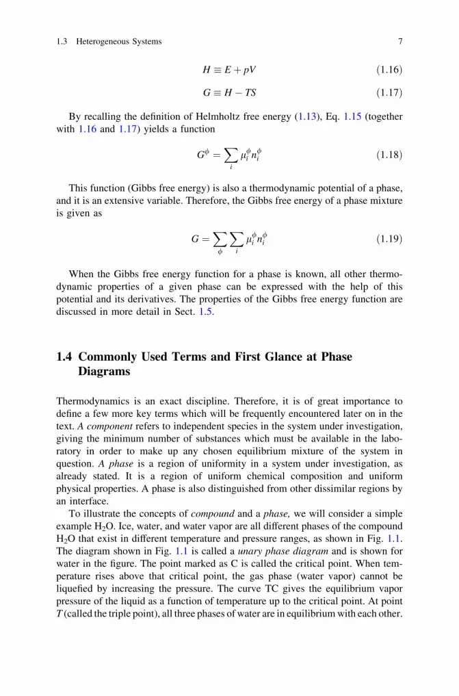
To illustrate the concepts of compound and a phase, we will consider a simpleexample H2O. Ice, water, and water vapor are all different phases of the compoundH2O that exist in different temperature and pressure ranges, as shown in Fig. 1.1.The diagram shown in Fig. 1.1 is called a unary phase diagram and is shown forwater in the figure. The point marked as C is called the critical point. When tem-perature rises above that critical point, the gas phase (water vapor) cannot beliquefied by increasing the pressure. The curve TC gives the equilibrium vaporpressure of the liquid as a function of temperature up to the critical point. At pointT (called the triple point), all three phases of water are in equilibrium with each other.

1.3 Heterogeneous Systems 7

Based on the Gibbs phase rule (derived later on) at this point, the number of degreesof freedom is zero. The equilibrium can therefore be attained only at a specifictemperature and pressure. The curve ST gives the equilibrium vapor pressure of thesolid (ice) as a function of temperature. The curve TM gives the change in themelting point of ice as a function of pressure. It is to be noted here that the curve TMfor the system H2O is highly unusual as the TM curve here is descending, whereas inmost of the systems, it is ascending. This is a result of the fact that the molar volumeof solid water (ice) is larger than that of liquid water (in Sect. 1.7 is introduced theClausius–Clapeyron equation that can be used to calculate this). In most systems,however, the opposite is true. Another unary system exhibiting this type of behavior(i.e., larger volume in solid than in liquid) is bismuth (Bi).

Different pure elements, for example, Cu or Ni, also have three different phases:solid, liquid, and gas. Similarly, two allotropic forms, solid gray tin and white tin,which have a different crystal structure and properties, are considered as distinctphases. To show the example of phases with two different components, we con-sider the Ag–Cu binary phase diagram, which is shown in Fig. 1.2. All phases aremade of the two components, Ag and Cu. The different phases a, b, and liquid arestable within a certain temperature and composition (expressed here as weightpercentage) range. Note that the phase diagram shown in Fig. 1.2 is determined atconstant pressure. The a-phase is basically a solid solution Ag(Cu), that is, Ag(with its face-centered cubic (FCC) structure) with a limited amount of dissolvedCu, whereas the b-phase is a solid solution Cu(Ag), that is, Cu (with FCC struc-ture) with a limited amount of dissolved Ag. Different notations (a and b) are usedto differentiate solid solutions from pure elements. The solvus curve separates thesingle solid-phase region a from the solid two-phase region a + b. Similarly,another solvus curve separates the one-phase solid region b from that of the solidtwo-phase region a + b. The solidus curve separates the solid one-phase a-regionfrom the two-phase region where the solid a and the liquid are in equilibrium.Similarly, another solidus curve separates the solid one-phase region b from thetwo-phase region b + liquid. The liquidus curve, on the other hand, separates thetwo-phase a + liquid and b + liquid areas from the liquid one-phase area L. In

Fig. 1.1 The pressure–temperature diagram of H2O

8 1 Thermodynamics, Phases, and Phase Diagrams

Fig. 1.2, there is a horizontal line of specific importance. It represents the so-calledeutectic reaction, where liquid L reacts to form two new solid phases a and b. Atthe line, there are three phases L, a, and b which are in equilibrium with eachother. According to the Gibbs phase rule (note that here the pressure is constant),such an equilibrium in a binary system can exist only at a specific temperature andonly with specific compositions of the three phases participating in the equilib-rium. It is common practice to show the stability of phases in a single-componentsystem in different temperature and pressure ranges as shown in Fig. 1.1. In abinary system case, the stability of the phases is shown in a different temperatureand composition range under constant pressure. Unless mentioned, a binary phasediagram (shown in Fig. 1.2) is commonly determined at atmospheric pressure.Note that at different pressure, the binary temperature–composition phase diagramwill be different since the equilibrium transition temperature between differentphases changes with pressure. It is also to be noted that typically, especially in thecase of metals, the vapor region is not shown in the binary phase diagram as ittypically exists at relatively high temperatures under atmospheric pressure.Finally, it is important to realize that one cannot obtain any information aboutkinetics or the morphology of the phase mixture from the phase diagram. Thediagram only gives information about the phases that can be in equilibrium undercertain composition–temperature combinations. Although there are three differentspecies present in a system, there are times when the phase diagram is presented asa binary phase diagram. For example, as Fig. 1.3 shows, the MgO–Al2O3 phasediagram is presented as a binary phase diagram, where MgO and Al2O3 areconsidered as the components. The reason for this is clear. Even though there arethree species (Mg, O, and Al) in the system, there are only two components (MgOand Al2O3). Only the amounts of these components can be changed independently.This is called a pseudobinary phase diagram.

Fig. 1.2 Binary phasediagram of Ag–Cu

1.4 Commonly Used Terms and First Glance at Phase Diagrams 9

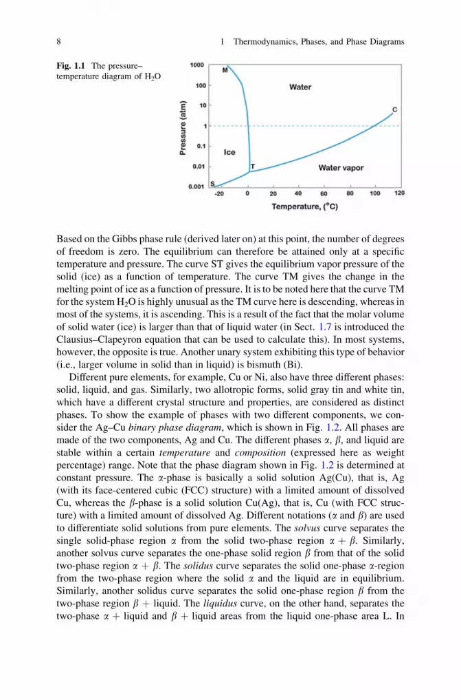
In a ternary system (Fig. 1.4), where three elements are mixed, the phasediagrams take the standard form of a prism which combines an equilateral trian-gular base (ABC) with three binary system ‘‘walls’’ (A–B, B–C, and C–A). Thisthree-dimensional form allows the three independent variables to be specified(two-component concentrations and temperature). In practice, determining dif-ferent sections of the diagram from these kinds of graphical models is difficult and,therefore, horizontal (isothermal) sections through the prism are used (Fig. 1.4b).The isothermal section is a triangle at a given temperature, where each cornerrepresents the pure element, each side represents relevant binary systems, andareas of different phases can be determined inside the triangle. In addition to theisothermal section, also vertical sections (isopleths) can be taken from a spacediagram of a given ternary system. We will return to these diagrams and their usesin Sects. 1.12 and 1.13.

Another commonly used term, as already mentioned, is composition. Compo-sition can be expressed in terms of mole fraction, atomic fraction or atomic per-centage, and weight fraction or weight percentage. It should be pointed out that in abinary (not pseudobinary) or multicomponent system, the mole fraction is equal tothe atomic fraction. This can be shown very easily for a system of total 1 mol,where XA and XB are mole fractions of A and B, respectively. This can be written as

XA þ XB ¼ 1 ð1:21Þ

If nA and nB are the total number of atoms of A and B, respectively, we canwrite

XA ¼ nA=No and XB ¼ nB=No ð1:22Þ

where No (=6.022 9 1023 atoms/mole) is the Avogadro number.

Fig. 1.3 Pseudobinary phasediagram of MgO and Al2O

10 1 Thermodynamics, Phases, and Phase Diagrams

This means that the atomic fraction of A ðNAÞ and B ðNBÞ, with the help ofEq. 1.21, can be expressed as

NA ¼nA

nA þ nB

¼ XANo

XANo þ XBNo¼ XA

XA þ XB

¼ XA ð1:23aÞ

NB ¼nB

nA þ nB

¼ XBNo

XANo þ XBNo¼ XB

XA þ XB

¼ XB ð1:23bÞ

Although in the previous example, we considered the one-mole system (whichwill be useful in the proceeding section), it can be shown that the mole fraction isalways equal to the atom fraction, even if the system has a total more or less thanone mole of atoms. For example, we consider the system of total x mole, where themole of A and B are xA and xB, respectively. This can be written as

xA þ xB ¼ x ð1:24Þ

The mole fraction of A, XA, can be expressed as

XA ¼xA

x¼ xA

xA þ xB

ð1:25Þ

Consequently, the atomic fraction of A, NA, can be expressed as

NA ¼nA

nA þ nB

¼ xANo

xANo þ xBNo¼ xA

xA þ xB

¼ xA ð1:26Þ

A similar expression can be derived for B.

Fig. 1.4 a Ternary system, and b isothermal section at T = x �C

1.4 Commonly Used Terms and First Glance at Phase Diagrams 11

Concentration can be expressed as molal concentration, that is, ci = number ofmoles (g-atoms, g-ions, etc.) of the solute i per 1,000 g of solution, or as volumeconcentration, that is, the number of moles per cubic meter (m3). It is to be notedthat the latter definition is valid only at constant temperature. When describing thecomposition of the liquid solution, for example, it is expedient to use as the twoother independent variables (in addition to composition regardless of how it isexpressed) temperature and pressure, so that differentiation with respect to tem-perature implies constant pressure. Thus, we have

oC

oT

� �¼ �aCS

where a is the thermal expansivity and Cs is the concentration of the species ofinterest. The relation above shows that if Cs is chosen as a variable, it will not bean independent variable [2]. Further, when we consider the solid state, it becomesevident that in order to use volume concentrations, we should have knowledgeabout the molar volume as a function of composition of the phase under investi-gation. This is why volume concentrations are not always convenient variablesand, for this reason, will not typically be used later on in the text.

1.5 Spontaneous Change

Entropy is the basic fundamental concept when the direction of natural change isconsidered as discussed in Sect. 1.2. Unfortunately, the use of entropy as thecriteria for spontaneous change requires that changes in both the system andthe environment are investigated. As the environment is not always easily defined,the entropy criterion is not convenient to use in many practical cases. However, ifwe concentrate on the system, we may lose some generality but gain a lot in thesense that the environment no longer needs to be considered. Next, we will look ingreater detail how this can be achieved. Consider a system in thermal equilibriumwith its surroundings at a temperature T. When a change in the system occurs, thesecond law of thermodynamics states (the Clausius inequality)

dS� dq

T� 0 ð1:27Þ

Depending on the conditions under which the process occurs, this inequalitycan be developed in two ways.

(i) Heat transfer at constant volume

In the absence of non-expansive work, it is possible to write dqV ¼ dE. This isbecause as volume is kept constant and only expansion work is considered, thework done by or to the system must be zero. Thus, we can write

12 1 Thermodynamics, Phases, and Phase Diagrams

dE ¼ dq

and utilizing Eq. 1.27, the following is obtained

dS� dE

T� 0 ð1:28Þ

It is to be noted that here the criteria of spontaneity is expressed in terms ofstate functions only. Equation 1.28 can be rearranged as

TdS� dE V constant; no additional workð Þ ð1:29Þ

At either constant internal energy (dE = 0) or constant entropy (dS = 0),Eq. 1.29 can be expressed as

dSE;V � 0 or dES;V � 0

The first inequality states that entropy increases in a spontaneous change in asystem with constant volume and constant internal energy. The second inequalitystates that given the constant entropy and volume of a system, its internal energydecreases during spontaneous change. This is, in fact, a statement about entropysince it states that if the entropy of the system remains unchanged in the trans-formation, there must be an increase in the entropy of the environment caused bythe outflow of heat from the system.

(ii) Heat transfer at constant pressure

Again, in the absence of non-expansive work, we may write dqp ¼ dH andobtain

TdS� dH p constant; no additional workð Þ ð1:30Þ

At constant enthalpy or entropy, the following inequalities are obtained

dSH;p� 0 or dHS;p� 0

which can be interpreted in a similar fashion as inequalities concerning heattransfer at constant V.

Unfortunately, transformations where E and V, H and p, S and V, or S and p areconstant are rare. Far more frequently, transformations take place under conditionswhere V and T, or even more typically, p and T, are constant.

Equations 1.29 and 1.30 can be written as

dE � TdS� 0 and dH � TdS� 0 ð1:31Þ

The Helmholtz and Gibbs free energy functions were defined as follows(Sect. 1.3)

1.5 Spontaneous Change 13

F ¼ E � TS and G ¼ H � TS ð1:32Þ

At constant temperature, the differentials of the functions F and G are

dFð ÞT ;V¼ dE � TdS ð1:33Þ

dGð ÞT ;p¼ dH � TdS ð1:34Þ

where the entropies of the phases have been replaced by the temperature of thesystem. We get two new inequalities for a spontaneous change with frequentlyobserved variables

dFð ÞT ;V � 0 ð1:35Þ

dGð ÞT ;p� 0 ð1:36Þ

(iii) Expansion work is not the only form of work

How shall the above-derived conditions for spontaneity change if the expansionwork is no longer the only form of work? The second law of thermodynamicsstates that dE ¼ dqþ dwtot, where dwtot ¼ dw0 � pdV is the total work and dw0

takes into account all other forms of work except expansion work. By solving dq,we get

dq¼ dE � dw0 þ pdV ð1:37Þ

and utilizing the fact that dq� TdS� 0, we obtain

dE � TdS� dw0 þ pdV � 0 ð1:38Þ

By utilizing the definition of the Helmholtz free energy, we obtain

dFð ÞT � dw0 � pdV ¼ dwtot ð1:39Þ

Thus, at constant T, change occurs spontaneously when the change in Helm-holtz energy is smaller than the total amount of work. If the volume is constantdV = 0, then

dFð ÞT ;V � dw0 ð1:40Þ

which is equal to Eq. 1.39 when the expansion work is the only form of work.

14 1 Thermodynamics, Phases, and Phase Diagrams

From the definition of enthalpy (H = E + pV) and from dE ¼ dqþ dw0 � pdVunder constant pressure, it follows that

dHð Þp¼ dE þ pdV ¼ dqþ dw0 � pdV þ pdV ð1:41Þ

which gives

dqp ¼ dHð Þp�dw0 ð1:42Þ

Combining this with Eq. 1.31 results in

dH � TdS� dw0 � 0 constant pressureð Þ ð1:43Þ

and finally,

dGð ÞT ;p� dw0 ð1:44Þ

At constants T and p, the change is spontaneous if the change in Gibbs energy isless than the additional work done. Equations 1.44 and 1.40 can be stated also as�DGis the maximum amount of work (other than expansion work) that the systemcan release during spontaneous change at constant temperature and pressure. Thevalue �DFis the maximum amount of total work that the system can release duringspontaneous change at constant temperature.

Given that G = G(T, P, n1, n2,…) in an open system, with ni being the numberof moles of component i, the derivative of the Gibbs energy function yields

dG ¼ �SdT þ VdpþX

i

lidni ð1:45Þ

where li is the chemical potential of component i. At a constant value of theindependent variables P, T, and nj(j 6¼ i), the chemical potential equals the partialmolar Gibbs free energy, (qG/qni)P,T,j 6¼i. The chemical potential (partial Gibbsenergy) has an important function analogous to temperature and pressure.A temperature difference determines the tendency of heat to flow from one bodyinto another, while a pressure difference, on the other hand, determines the ten-dency toward a bodily movement. A chemical potential can be regarded as thecause of a chemical reaction or the tendency of a substance to diffuse from onephase to another.

As shown before in Eq. 1.17, the Gibbs free energy can be expressed as

G ¼ H � TS

1.5 Spontaneous Change 15

where H (J/mole) is the enthalpy, T (Kelvin, K) is the absolute temperature, andS (J/mole K) is the entropy of the system. Further, H, the total heat content or totalenergy of the system, was defined in Eq. 1.16 as

H ¼ E þ pV

where E is the internal energy, P is the pressure, and V is the volume of the system.In general, the contribution of PV in Eq. 1.16 is very small in the solid and

liquid states if the pressure is not exceptionally high. Therefore, while workingwith condensed phases (solid and liquid), the PV term can, in most cases, beneglected. Hence, the change in internal energy of the system can be approximatedto be equal to its enthalpy

H ¼ E ð1:46Þ

The internal energy of the system consists of the potential and kinetic energiesof the atoms within the system. The kinetic energy of solids and liquids is causedby the vibration of atoms at their position. In liquids and gases, the translationaland rotational movement of the atoms (or molecules), within the system, providesan additional contribution to the kinetic energy. Every atom vibrates with differentenergy at its position with degrees of freedom in x, y, and z directions with veryhigh frequency that is temperature dependent. The frequency spectrum starts from0 and goes up to a maximum value of mD, which is called the Debye frequency. Byutilizing the vibration frequencies, it is possible to calculate the heat capacity of agiven solid. Above a certain temperature (hD, the Debye temperature), all atomsare essentially vibrating with their corresponding maximum Debye frequency. Formetals at room temperature, they are typically above their Debye temperature,which makes it possible to use single (maximum) frequency values when con-sidering the diffusion of atoms, for instance. The average total energy (=3NkTwhere k is the Boltzmann constant and N is the number of atoms in a crystal) ofatoms is fixed with respect to a particular temperature. Moreover, the vibration ofany atom depends on the vibration of neighboring atoms because of inter-atomicbonding. This coupling produces an elastic wave with quantized energy. Thequantum of energy in an elastic wave is called a phonon. For example, soundwaves and thermal vibrations in crystals are phonons. The other part of internalenergy in solids, the potential energy, depends on the inter-atomic bondingbetween the atoms. In a single-component system, the potential energy depends onone type of bonding, but, in a binary or multicomponent system, the potentialenergy depends on the type, number, and magnitude of the different bonds betweenthe atoms within the system. This is explored further in Sect. 1.9 for binary sys-tems cases. The entropy of a crystal is composed of two terms: thermal entropyand the configurational entropy. The first part is concerned with the distribution ofenergy over the available energy states in the crystal (system) and the latter partwith the distribution of atoms or particles within the crystal (system).

16 1 Thermodynamics, Phases, and Phase Diagrams

Note By utilizing the Gibbs free energy, all forms of work (excludingexpansion work) can be taken into account 2(DG)p,T C w0 = Rlini +cA + zFU + ���, where the first term is the chemical part, the second is thesurface energy contribution, the third is the electrical component, etc. Thus,Gibbs energy gives the amount of maximum additional (non-expansion)work that the system can perform. For all spontaneous processes, the changein Gibbs energy must be negative. It should also be noted that the temper-ature and pressure of the system do not have to be constant during the wholeprocess. It is adequate that they are the same at the initial and final stages. Anexample is an exothermic reaction taking place at temperature T, where thereaction heat is transferred to the environment at the end of the reaction, thusmaking Tinitial equal to Tfinal. This is, of course, a consequence of the fact thatthe Gibbs energy is a state function and its value is only dependent on theinitial and final states, not the path between them.The Helmholtz free energy of a closed system, on the other hand, is afunction of temperature and volume. Helmholtz free energy (F) is maximumfree energy, which can be used to do work at constant volume and tem-perature and can be expressed as

F ¼ E � TS

where E is the internal energy. The main difference between Gibbs freeenergy (i.e., the change in energy at constant pressure and temperature) andHelmholtz free energy (i.e., the change in energy at constant volume andtemperature) is ‘‘PV’’. This comes from the fact that there is need for extrawork to accommodate the volume change. Thus, the Helmholtz free energyis the maximum amount of any kind of work the system can do and is,therefore, sometimes called the maximum work function. The change inHelmholtz free energy must also always be negative for a spontaneouschange.

With the help of the Gibbs free energy function derived above, the equilibriumstate of the system can be investigated. There is the relation between the chemicalpotential of components and the total Gibbs energy of the system, as expressed inEq. 1.19 (Sect. 1.3) through

Gtot ¼X

/

Xi

l/i n/

i

ffi �

The Gibbs energy function can be utilized from the component level to thesystem level and back again. Hence, Eq. 1.19 provides the very important con-nection between component and system level properties.

1.5 Spontaneous Change 17

Three stable equilibrium states to be considered here are (i) complete or globalthermodynamic equilibrium, (ii) local thermodynamic equilibrium, and (iii) partialthermodynamic equilibrium. When the system is at complete equilibrium, itsGibbs free energy (G) function has reached its minimum value

dG ¼ 0 or lai ¼ lb

i ¼ � � � ¼ l/i ; i ¼ A;B;C; . . .ð Þ ð1:47Þ

and then, the system is in mechanical, thermal, and chemical equilibrium with itssurroundings. Consequently, there are no gradients inside the individual phasesand no changes in the macroscopic properties of the system are to be expected.

Local equilibrium, on the other hand, is defined in such a way that the equilibriumexists only at the interfaces between the different phases present in the system. Thismeans that the thermodynamic functions are continuous across the interface and thecompositions of the phases right at the interface are very close to those indicated bythe equilibrium phase diagram. This also indicates that there are activity gradients inthe adjoining phases. These gradients, together with the diffusivities, determine thediffusion of components in the various phases of a joint region.

Partial equilibrium means that the system is in equilibrium only with respect tocertain components. It is generally found that some processes taking place in thesystem can be rapid, while others are relatively slow. If the rapid ones occurquickly enough to fulfill the requirements for stable equilibrium (within the limitof error) and the slow ones are slow enough that they can be ignored, then it isquite proper to treat the system as being in equilibrium with respect to the rapidprocesses alone [7].

It is also possible that the global energy minimum of the system is not acces-sible owing to different restrictions. In such cases, we are dealing with metastableequilibrium, which can be defined as a local minimum of the total Gibbs energy ofthe system. In order to obtain global stable equilibrium, some forms of activation(e.g., thermal energy) must be brought into the system. It is to be noted thatmetastable equilibrium can also be complete, local, or partial; the local metastableequilibrium concept, in any case, will be used frequently in the following sections.Very often, one or more interfacial compounds, which should be thermodynami-cally stable at a particular temperature, are not observed between two materialsand, then, these interfaces are in local metastable equilibrium. Another situationcommonly encountered occurs in solid/liquid reaction couples, where during thefew first seconds, the solid material is in local metastable equilibrium with theliquid containing the dissolved atoms, before the intermetallic compound(s) isformed at the interface. In fact, a principle commonly known as Ostwald’s rulestates that, when a system undergoing reaction proceeds from a less stable state,the most stable state is not formed directly but rather the next more stable state isformed, and so on, step by step until (if ever) the most stable is formed. It is a factthat most materials used in everyday life have not been able to reach their absoluteminimum energy state and are, therefore, in metastable equilibrium. It should benoted that a system at metastable equilibrium has thermodynamic properties,which are exactly determined, just as a system at stable equilibrium.

18 1 Thermodynamics, Phases, and Phase Diagrams

1.6 Free Energy and Phase Stabilityof Single-Component System

Different phases of a single element can be stable at a different temperature rangeunder a particular pressure (we consider atmospheric pressure). For example,below the melting point, a solid phase is stable, whereas above the melting point, aliquid phase is stable. In general, at a particular temperature, the phase with thelowest Gibbs free energy will be the stable one. If at a particular temperature, thefree energy of two phases is the same, then both phases are stable at that tem-perature. This takes place, for example, at the melting point where the solid andthe liquid phases exist together. This also means that the system is in equilibriumand there is no driving force for change. To explain the stability of phases atdifferent temperatures, we need to know the change in their free energies as afunction of temperature. Consequently, (following Eq. 1.18) in order to determinefree energy at a particular temperature, it is necessary to determine the enthalpyand the entropy at that particular temperature. Both properties can be determinedfrom the knowledge of specific heat at constant pressure, CP. The specific heat orspecific heat capacity CP (J/mole K) is defined as the amount of heat required toincrease the temperature of a system by one Kelvin under constant pressure.

The absorption or release of heat, dq, in a reversible process, at constantpressure from the system to the surrounding area is equal to the enthalpy change,dH, of the system. We can write

dq ¼ dH ð1:48Þ

Further, from the definition of Cp, the equation can be written

Cp ¼dq

dTð1:49Þ

From Eqs. 1.48 and 1.49, follows

dH ¼ CpdT ð1:50Þ

By integrating Eq. 1.50, it can be expressed as

ZH

o

dH ¼ZT

o

CPdT

HT ¼ Ho þZT

o

CPdT

ð1:51Þ

where HT and Ho are enthalpy at temperature T and 0 K, respectively.

1.6 Free Energy and Phase Stability of Single-Component System 19

The enthalpy at room temperature 298 K is often known, and Eq. 1.51 can bewritten as

HT ¼ H298 þZT

298

CPdT ð1:52Þ

Further, from the definition of entropy for a reversible process, we know

dS ¼ dq

T¼ CPdT

Tð1:53Þ

By integrating Eq. 1.53, we get

ST ¼ So þZT

o

CP

TdT ¼

ZT

o

Cp

TdT ð1:54Þ

where So is the entropy at 0 K. However at 0 K, the entropy of a defect-free pureelement is, by definition, zero (according to the third law of thermodynamics).Moreover, if the entropy at 298 K is known, then Eq. 1.54 can be written as

ST ¼ S298 þZT

298

CP

TdT ð1:55Þ

Note We have considered above a pure element with a defect-free structure.However, it is to be emphasized that it is impossible to obtain a defect-freestructure at temperatures above 0 K. There will always be a certain amountof point defects, such as vacancies and impurities present in the structureunder the equilibrium condition. The free energy of a phase including thecontribution from defects can be expressed as

Gm ¼ Gþ DGd

Gm is the free energy of a single-component material with point defects; G isthe free energy of the defect-free material, and DGd is the free energy changebecause of the presence of defects. As will be shown later on, vacancies, forinstance, are always present with a certain equilibrium concentration above0 K. However, since the concentration of defects, in general, is smallcompared to the number of atoms, we can in many cases neglect the con-tribution from DGd.

20 1 Thermodynamics, Phases, and Phase Diagrams

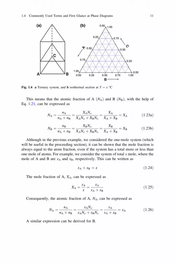
In general, the CP values for different phases can be experimentally determinedand are available in the literature. The way that CP typically varies with temper-ature is shown in Fig. 1.5a. From the knowledge of CP, it is possible to calculateH and S at a particular temperature T and consequently determine the variation offree energy G as a function of temperature. If there are phase transformationswithin the temperature range of interest, the enthalpies and entropies of the cor-responding transformation must be added, at the appropriate T, and the integrationmust continue with the Cp value of the new phase, to obtain the correct H and S atthe required temperature. The enthalpy of the formation of all pure elements underatmospheric pressure and with their most stable form at room temperature (298 K)has been defined to be zero at all temperatures. These are called the standardenthalpies of formation. And from these, the enthalpy change as a function of

temperature can be determined as HT ¼RT

298CPdT. The typical change in enthalpy,

entropy, and free energy is shown in Fig. 1.5b. There are a few important pointsthat should be noted here. It is clear from Eq. 1.50 that the slope of the enthalpycurve dH/dT is equal to CP. Since the value of CP always increases with tem-perature, the slope of the enthalpy curve will also increase continuously with risingtemperature. Further, from standard thermodynamic relation, we know thatdG = Vdp - SdT. Since transformations at constant pressure are under consid-eration, we can write dG = - SdT. Hence, the slope of the free energy curve dG/dT is equal to -S. Since entropy always increases with temperature, the slope ofthe free energy, G, should always decrease with rising temperature.

Now, let us consider the stability of the solid and liquid phases of a metal. Todo this, we will first need to determine the change in free energy with temperaturefor both solid and liquid phases separately. From Eqs. 1.17, 1.50, and 1.55, we canwrite the expressions for free energy for solid and liquid phases as

GS ¼ HS0 þ

ZT

0

CSPdT � T

ZT

0

CSP

TdT ð1:56aÞ

GL ¼ HL0 þ

ZT

0

CLPdT � T

ZT

0

CLP

TdT ð1:56bÞ

The superscripts ‘‘S’’ and ‘‘L’’ are denoted for solid and liquid phases,respectively. In general, the CP of the liquid phase at a particular temperature ishigher than that of the solid phase. The typical variation of CP for solid and liquidphases is shown in Fig. 1.6a. The corresponding changes in enthalpy and freeenergy as a function of temperature of the phases are shown in Fig. 1.6b.

As already discussed, the pV term for both solid and liquid phases is very smalland the enthalpy can be taken to be practically equal to E. Therefore, the Gibbsenergy function can be written as G = E - TS, making the free energy low for a

1.6 Free Energy and Phase Stability of Single-Component System 21

phase with a low internal energy E and/or high entropy S. It is also apparent that atlow temperature, the E term will dominate, whereas at higher temperature, theterm becomes more and more significant. In general, the solid phases have higherbonding energies compared to those of liquid phases. So the internal energy, i.e.,enthalpy, of the solid phase is lower than the liquid phase. Further, the entropies ofliquids are typically larger than those of solids. Thus, at higher temperatures, theliquid phase becomes stable. From Fig. 1.6b, it can be seen, for instance, thatbelow the melting point the solid phase is stable, whereas above the melting pointthe liquid phase is stable. At the melting point, their Gibbs energies are the same,as discussed in the beginning of this section.

Now, let us turn to consider solid-state transformation between gray tin to whitetin. Gray tin has a diamond crystal structure which is very brittle. White tin, on theother hand, which is commercially available with a metallic luster has a BCT(body-centered tetragonal) structure. The Gibbs energy curves for both structuresare shown in Fig. 1.7.

In Fig. 1.7, the molar Gibbs energy of the BCT-Sn has been set at zero for alltemperatures. Thus, the BCT-Sn is the reference state. The Gibbs energies ofdifferent forms of Sn are then compared against this self-chosen reference value.As can be seen from Fig. 1.7, BCT-Sn should be stable between 13 and 232 �C.Below 13 �C, Sn with a diamond structure is the most stable form of tin, and above232 �C, the liquid Sn is the most stable form of tin. It is to be noted that eventhough the transition temperature between the diamond and body-centeredtetragonal structures is 13 �C, in practice the transformation requires undercoolingto about -30 �C. This is because at 13 �C, the two crystal structures are inequilibrium and their Gibbs energies are the same. Thus, the driving force for thetransformation is zero. As temperature decreases, the driving force for the trans-formation increases and the kinetics becomes slower. Thus, the optimum condi-tions for the transformation are found at -30 �C. This occurrence of the low

Fig. 1.5 a Typical change of CP with temperature. b Arbitrary values of H, S, and G withtemperature. Note that in many metals, the enthalpy is zero at room temperature, 298 K

22 1 Thermodynamics, Phases, and Phase Diagrams

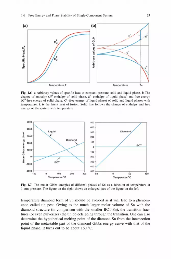
temperature diamond form of Sn should be avoided as it will lead to a phenom-enon called tin pest. Owing to the much larger molar volume of Sn with thediamond structure (in comparison with the smaller BCT-Sn), the transition frac-tures (or even pulverizes) the tin objects going through the transition. One can alsodetermine the hypothetical melting point of the diamond Sn from the intersectionpoint of the metastable part of the diamond Gibbs energy curve with that of theliquid phase. It turns out to be about 160 �C.

Fig. 1.6 a Arbitrary values of specific heat at constant pressure solid and liquid phase. b Thechange of enthalpy (HS-enthalpy of solid phase, HL-enthalpy of liquid phase) and free energy(GS-free energy of solid phase, GL-free energy of liquid phase) of solid and liquid phases withtemperature. L is the latent heat of fusion. Solid line follows the change of enthalpy and freeenergy of the system with temperature

Fig. 1.7 The molar Gibbs energies of different phases of Sn as a function of temperature at1 atm pressure. The figure on the right shows an enlarged part of the figure on the left

1.6 Free Energy and Phase Stability of Single-Component System 23

The increasing importance of the entropy term (-TS) is the reason why inmany metals, we find the phase with a relatively closely packed structure is stableat a lower temperature, whereas a relatively loosely packed structure is stable athigher temperature. The reason for this lies in a more loosely packed structurewhere there is a higher degree of vibrational freedom. For instance, a-Ti with anHCP structure is stable at low temperature, whereas b-Ti with a BCC structure isstable at high temperature.

1.7 Pressure Effect of Single-Component Phase Diagram

Until now, as mentioned earlier, it has been assumed that all transformations occurunder constant, typically atmospheric, pressure. If we consider the Gibbs freeenergy at constant temperature but under different pressure, for example, at higherpressure, then the freedom for vibration of atoms will be decreased in comparisonwith the normal pressure. This will result in an increase in free energy, as shown inFig. 1.8. We know from the standard thermodynamic relation dG = Vdp - SdTthat the slope of the free energy versus pressure curve is equal to volume V, atconstant temperature. Since the volume of matter generally decreases withincreasing pressure, the slope of the free energy versus pressure curve will bepositive, but it will decrease continuously with increasing pressure. Consequently,the equilibrium transition temperature from one phase to another will be differentunder different pressures and depending on the conditions, the transition temper-ature with increasing pressure might increase or decrease. This can be understoodas being based on the Clausius–Clapeyron relation, which can be derived byconsidering the equilibrium transition temperature between the a- and c-phases inan iron system. By using a standard thermodynamic relation, it is possible to writefor the molar Gibbs energy

Fig. 1.8 The variation ofmolar Gibbs free energy gwith increase in pressure

24 1 Thermodynamics, Phases, and Phase Diagrams

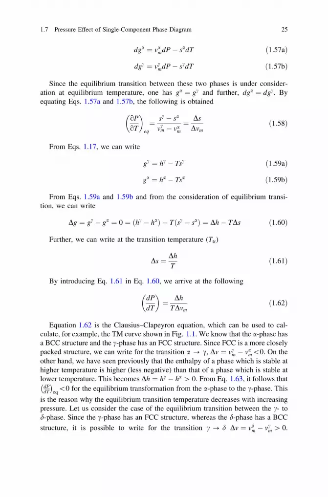
dga ¼ vamdP� sadT ð1:57aÞ

dgc ¼ vcmdP� scdT ð1:57bÞ

Since the equilibrium transition between these two phases is under consider-ation at equilibrium temperature, one has ga ¼ gc and further, dga ¼ dgc. Byequating Eqs. 1.57a and 1.57b, the following is obtained

oP

oT

� �eq

¼ sc � sa

vcm � va

m

¼ Ds

Dvmð1:58Þ

From Eqs. 1.17, we can write

gc ¼ hc � Tsc ð1:59aÞ

ga ¼ ha � Tsa ð1:59bÞ

From Eqs. 1.59a and 1.59b and from the consideration of equilibrium transi-tion, we can write

Dg ¼ gc � ga ¼ 0 ¼ ðhc � haÞ � Tðsc � saÞ ¼ Dh� TDs ð1:60Þ

Further, we can write at the transition temperature (Ttr)

Ds ¼ Dh

Tð1:61Þ

By introducing Eq. 1.61 in Eq. 1.60, we arrive at the following

dP

dT

� �¼ Dh

TDvmð1:62Þ

Equation 1.62 is the Clausius–Clapeyron equation, which can be used to cal-culate, for example, the TM curve shown in Fig. 1.1. We know that the a-phase hasa BCC structure and the c-phase has an FCC structure. Since FCC is a more closelypacked structure, we can write for the transition a ? c, Dv ¼ vc

m � vam\0. On the

other hand, we have seen previously that the enthalpy of a phase which is stable athigher temperature is higher (less negative) than that of a phase which is stable atlower temperature. This becomes Dh ¼ hc � ha [ 0. From Eq. 1.63, it follows that

dPdT

� �eq

\0 for the equilibrium transformation from the a-phase to the c-phase. This

is the reason why the equilibrium transition temperature decreases with increasingpressure. Let us consider the case of the equilibrium transition between the c- tod-phase. Since the c-phase has an FCC structure, whereas the d-phase has a BCC

structure, it is possible to write for the transition c ? d Dv ¼ vdm � vc

m [ 0.

1.7 Pressure Effect of Single-Component Phase Diagram 25

Further, from our previous explanation, we can write Dh ¼ hd � hc [ 0. SodPdT

� �eq

[ 0 for this transition and equilibrium transition temperature increases with

increasing pressure.

1.8 Free Energy and Stability of Phases in a Binary System

In the previous sections, we have considered mainly single-component systems(i.e., pure elements). It is common knowledge that most materials in nature consistof several phases and that these phases themselves are never pure elements. In fact,based on the second law of thermodynamics, a pure substance exists only in ourminds and represents a limiting state, which we may asymptotically approach butnever actually obtain. Thus, the thermodynamic description of multicomponentsystems is of great importance from the theoretical as well as from the practicalpoint of view. In the treatment of multicomponent open systems, the most commonprocess considered in defining the thermodynamic functions for a solution is calledthe mixing process, which Guggenheim defines as [2]:

The mixing process is the change in state experienced by the system when appropriateamounts of the ‘pure’ components in their reference states are mixed together forming ahomogeneous solution brought to the same temperature and pressure as the initial state.

It is to be noted that although the mixing process is strongly influenced byinteraction forces between atoms and molecules (i.e., Dh), the fundamental causebehind mixing is the entropy (Ds) change of the system.

For our analysis, we shall consider a system with a total of one mole of atoms,where XA is the mole fraction of element A and XB is the mole fraction of elementB. This translates into

XA þ XB ¼ 1 ð1:63Þ

We define the free energies of pure elements A as GA and that of B as GB at aparticular temperature. The total molar free energy g0 of a purely mechanicalmixture can be written as

g0 ¼ XAgA þ XBgB ð1:64Þ

Now, if we allow interdiffusion to taken place between the elements A and B,there will be change in the free energy because of mixing, gmix. Consequently, thetotal free energy of the system after mixing can be written as

g ¼ g0 þ Dgmix ð1:65Þ

26 1 Thermodynamics, Phases, and Phase Diagrams

From Eqs. 1.17 and 1.65, we find the expression for the free energy changebecause of mixing as

DGmix ¼ g� g0 ¼ h� Ts� h0 þ Ts0 ¼ ðh� h0Þ � Tðs� s0ÞDgmix ¼ Dhmix � TDsmix

ð1:66Þ

where ho and h are the total enthalpy of the system before and after mixing. Thevalues so and s are the entropies of the system before and after mixing. The valueDhmix ¼ ðh� h0Þ is the change in enthalpy, and Dsmix ¼ ðs� s0Þ is the change inentropy due to mixing. The enthalpy of mixing can be zero, negative, or positivedepending on the system; the entropy of mixing, on the other hand, is alwayspositive. We shall first briefly discuss the mixing process in general and then looka little closer at where the different terms in Eq. 1.66 arise.

1.8.1 Change in Free Energy in an Ideal System

Note that in the case of an ideal solution, Dhmix ¼ 0 and the free energy of thesystem can be written as

g ¼ g0 þ Dgmix ¼ g0 � TDsmix ð1:67Þ

The change in free energy with composition is shown in Fig. 1.9a at oneparticular temperature T. The straight dotted line represents the total free energyðg0 ¼ XAgA þ XBgBÞ of the elements A and B before any mixing (i.e., a purelymechanical mixture of A and B). The solid curved line represents the free energyof the system after mixing ðg ¼ g0 � TDsmixÞ. Further, the change in free energywith composition at higher temperature, T1, is shown in Fig. 1.9b. The change infree energy caused by mixing in an ideal solution Dgmix ¼ �TDsmix is naturallylarger at the higher temperature.

Entropy of mixing (Dsmix)The entropy of mixing originates from two different contributions, thermal and

configurational. If we consider that there are no volume and enthalpy changescaused by mixing, then the only contribution to the entropy will configurational.Configurational entropy comes from the possibility of arranging the atoms A and Bin different ways for a particular macrostate. Following statistical thermodynam-ics, the configurational entropy can be expressed as

S ¼ k ln w ð1:68Þ

where w is a thermodynamic probability, a kind of measure of randomness. Thismeans that the molar entropy of mixing can be written as

1.8 Free Energy and Stability of Phases in a Binary System 27

Dsmix ¼ s� s0 ¼ k ln w� k ln 1 ¼ k ln w ð1:69Þ

where, as explained before, s0 is the entropy before mixing and s is the entropyafter mixing. Since in the case of a pure element, there is only one way by whichatoms can be arranged (if vacancies are neglected), we can write w = 1. If weconsider the random solid solution, then the number of different ways by whichatoms A and B can be arranged is

w ¼ ðnA þ nBÞ!nA!nB!

ð1:70Þ

where nA and nB are the total number of atoms of A and B, respectively.According to Stirling’s approximation,

ln N! ¼ N ln N � N ð1:71Þ

Following Stirling’s approximation, Eq. 1.69 can be written as

DSmix ¼ k ln w

¼ ½ðnA þ nBÞ lnðnA þ nBÞ � ðnA þ nBÞ� � ½nA ln nA � nA� � ½nB ln nB � nB�ð1:72Þ

Fig. 1.9 Free energy versuscomposition diagram in anideal case at a lowtemperature, T, and b hightemperature, T1

28 1 Thermodynamics, Phases, and Phase Diagrams

From the definition of the mole fraction, we can write

nA ¼ XAN0; nB ¼ XBN0; XA þ XB ¼ 1 ð1:73Þ

Substituting Eq. 1.73 in Eq. 1.72, we get

Dsmix ¼ �kN0½XA ln XA þ XB ln XB�¼ �R½XA ln XA þ XB ln XB�

ð1:74Þ

It is, therefore, clearly apparent from Eq. 1.74 that the entropy of mixing isalways positive and will vary, as shown in Fig. 1.10. It can also be seen that theentropy of mixing reaches its maximum at XB = 0.5. To find the slope at differentcompositions, we can differentiate Eq. 1.74 (note that XA + XB = 1).

dDsmix

dXB

¼ �R � lnð1� XBÞ � ð1� XBÞ1

ð1� XBÞþ ln XB þ XB

1XB

�

¼ �R lnXB

ð1� XBÞ

ð1:75Þ

So the slope at XB = 0.5 is equal to zero, whereas the slope at XB = 0 or 1 isinfinity. Thus, it is evident from the above discussion why a pure substance is just alimit which we can approach but never achieve—as stated at the beginning of thissection. As the slope goes to infinity at XB = 0, it states that in order to remove thelast B impurity from A, an infinite amount of energy must be used.

Fig. 1.10 The change inentropy of mixing with thechange in composition

1.8 Free Energy and Stability of Phases in a Binary System 29

1.8.2 Change in Free Energy in a System with ExothermicTransformation

As discussed above, the enthalpy of mixing in an exothermic transformation isnegative. The free energy of mixing for such a case at different compositions at aparticular temperature T is shown in Fig. 1.11a. The free energy curves at highertemperature T1 are shown in Fig. 1.11b. At higher temperature, the TDsmix termwill be higher, making Dgmix higher after mixing. In consequence, the total freeenergy of the system will change far more drastically with composition comparedto at lower temperature.

1.8.3 Change in Free Energy in a System with EndothermicTransformation

In endothermic transformation, the enthalpy of mixing Dhmix [ 0. So, if thetemperature under consideration is reasonably low, the negative contribution to theGibbs energy of mixing from TDsmix may be smaller than the positive contributionfrom the enthalpy of mixing Dhmix within a certain composition range. In that case,

Fig. 1.11 Free energy versuscomposition diagram for asystem with exothermictransformation at a lowtemperature, T, and b hightemperature, T1

30 1 Thermodynamics, Phases, and Phase Diagrams

the free energy of mixing will be positive at a certain composition range and thetotal free energy change can vary, for example, as shown in Fig. 1.12 resulting in aformation of a miscibility gap. However, at higher temperature, T1 at all compo-sitions Dhmix will be smaller than TDsmix and the free energy of mixing is alwaysnegative, as can be seen in Fig. 1.12b. The next section considers the origin of theenthalpy of mixing.

Note We have considered a very simplified model to establish the relation offree energy after mixing in a binary system. We have not considered theelastic strain that could play an important role. In some systems, where thesize of the atoms is very similar, this factor can be disregarded. However, insome systems because of a large difference in atomic size, the elastic strainmight play a significant role. Calculations, however, become extremelycomplicated if we are to consider the effect of elastic strain and so it is leftoutside the scope of this book. It must, nevertheless, be remembered that theelastic energy (as other forms of work) can be incorporated into the Gibbsfree energy of the system.

Fig. 1.12 Free energy versuscomposition diagram in asystem with endothermictransformation at a lowtemperature, T, and b hightemperature, T1

1.8 Free Energy and Stability of Phases in a Binary System 31

1.9 Thermodynamics of Solutions and Phase Diagrams

In the following section, the thermodynamic background necessary for under-standing the phase diagrams introduced briefly in Sect. 1.4 is discussed. After thatthe binary and ternary phase diagrams are discussed in greater detail.

1.9.1 The Chemical Potential and Activity in a Binary SolidSolution

For any heterogeneous system at equilibrium, the chemical potential of a com-ponent i has the same value in all phases of the system, where the component hasaccessibility. A general problem for dealing with solutions thermodynamically canbe regarded as one of properly determining the chemical potentials of the com-ponents. Usually, the treatment utilizes the activity function introduced by Lewisand Randall [8]. The value of the treatment lies in its close relation to composition;with appropriate choice of reference state, the activity approaches the mole frac-tion as the mole fraction approaches unity. Most commonly in the thermodynamicsof solutions, it is not the activity which is used, but rather the activity coefficientwhich is defined as the ratio of the activity ai to the mole fraction Xi

ci ¼ai

Xið1:76Þ

In terms of the chemical potential, the activity can be expressed

l ji � lo

i ¼ RT ln a ji ¼ RT ln X j

i þ RT ln c ji ð1:77Þ

where loi is the chemical potential of pure i in the reference or standard state, l j

i

the chemical potential of i in phase j, a ji the activity of component i in phase j,

R the gas constant, T the temperature, and (i = A, B,…; j = a, b,…). In thelimiting case of ideal solutions, where the enthalpy (Dh = 0) and volume change(Dm = 0) of mixing are zero and the only contribution to Gibbs free energy ofmixing arises from the configurational entropy term

Dsm ¼Xi¼A

Xi ln Xi ð1:78Þ

the activity coefficient in Eq. 1.77 is unity and the activity of the component equalsits mole fraction (i.e., Raoultian behavior, see discussion below). If the equality isvalid for all compositions, the solution is called perfect. Thus, the activity coef-ficient represents deviation of the real solutions from this limiting behavior. Theuse of activity coefficient instead of activity in Eq. 1.77 clearly indicates the

32 1 Thermodynamics, Phases, and Phase Diagrams

excess energy term RT ln l ji to be responsible for the non-ideal behavior. This

issue is addressed in more detail in the next section.As only relative values of thermodynamic functions can be determined, an

agreed reference state has to be established for each element or species in order tomake thermodynamic treatment quantitative (see Fig. 1.7 and related discussion).In principle, the choice of the reference state is arbitrary as long as the chosen stateis used consequently throughout the analysis. The chosen state is then defined to bezero and all other possible states of the element are compared against the referencestate to obtain their relative stabilities. It should be noted that there are someuncertainties related to the usage of reference states in the literature.

1.9.2 Free Energy of Solutions

In Sect. 1.9, we briefly discussed the so-called mixing process as well as the binarysolution phases. In the beginning of this section, we also introduced the concept ofactivity, which describes the deviation of the behavior of a solution from idealbehavior. A statistical approach can be used to provide more insight into theproperties of the phases. The simplest model is one in which the total energy of thesolution is given by a summation of interactions between the nearest neighboratoms. If we have a binary system with two types of atoms (A and B), there will bethree interaction energy terms. These are the energy of the A–A pairs, that of theB–B pairs, and that of the A–B pairs. Here, we assume that the total energy of thesolution arises from the interactions between the nearest neighbors. The bindingenergy may be defined by considering that the change in energy as the distancebetween a pair of atoms is decreased from infinity to an equilibrium separation.The change in energy during this process is the binding energy, which for a pair ofA atoms is given as -2eAA, for B atoms as -2eBB, and so forth. Thus, the bondenergies are negative quantities.

The simplest model for real solution phases based on the above-defined nearestneighbor interaction approach is the so-called regular solution model. It is basedon the following assumptions: (i) Mixing among accessible lattice spaces iscompletely random pi ¼ Ni

N ¼ Xi, (ii) atoms interact only with their nearestneighbors, (iii) the bond energy between dissimilar atoms eij is independent ofcomposition and temperature, and (iv) there is no change in volume upon mixing.

Let us examine a solution which is formed by two metals (A and B) with anidentical crystal structure. Let us further assume that the system as defined above isin equilibrium with its surroundings. We will presume that metal A has NA atomsand metal B has NB atoms and that eAA and eBB are the bond energies of the AAand BB atom pairs according to the assumptions (ii) and (iii). Then, the config-uration energies of pure metals, with the coordination number z, are E0

A ¼zN0

AeAA=2 and E0B ¼ zN0

BeBB=2, when the atoms are at rest at their equilibriumlattice points. The number two in the nominator in the above equations is

1.9 Thermodynamics of Solutions and Phase Diagrams 33

introduced in order to prevent calculating the A–A and B–B interactions twice.The formation of the solution phase starts by removing one atom from each metaland transferring them to an infinite distance from the metal (and each other). Thework associated with this process is -z(eAA + eBB). By returning an atom A tometal B and an atom B to metal A, the pure metals are transformed into solutionswith infinite dilution. The total number of A–B bonds with bond energy eAB inthese solutions is 2z. The energy associated with this mixing process (per inter-change) can be described as

dE ¼ 2z eAB �12ðeAA þ eBBÞ

� ¼ �2zIAB ð1:79Þ

where IAB (per bond) is the interchange energy.As the energy change associated with the formation of a mixture with a number

of NAB bonds is DE ¼ NABIAB, the internal energy of the solution phase is

E ¼ z

2

ffi �NAðeAAÞ þ

z

2

ffi �NBðeBBÞ þ NABIAB ð1:80Þ

The next step is to identify what the most probable number of AB bonds (NAB)is with the nominal composition of Xo

B. This problem can be resolved by utilizingthe first assumption of the regular solution model, i.e., that the mixing among thelattice sites is completely random. This means that the probability that an atom Ais in position 1 equals pA(1) = (NA/N) and that atom B is in position 2 equalspB(2) = (NB/N). However, since pA(1)pB(2) = (NANB/N2) and becausepA(1)pB(2) = pA(2)pB(1), we get

pð1;2ÞAB ¼2NANB

N2ð1:81Þ

In the solution phase, we have total of 0.5zN adjacent lattice site pairs andtherefore,

�pAB ¼ pð1;2ÞAB ¼2NANB

N2

zN

2

� �¼ z

NANB

NA þ NB

� �ð1:82Þ

Thus, the internal energy of the solution phase can be written as

E ¼ z

2

ffi �NAðeAAÞ þ

z

2

ffi �NBðeBBÞ þ z

NANB

NA þ NB

� �IAB ð1:83Þ

By assuming that the chemical potentials of pure metals A and B can beapproximated as l0

A ffi 12 Z eAAð Þ and l0

B ffi 12 Z eBBð Þ and utilizing the definition of

the chemical potential, the Gibbs energy of the regular solution phase becomes

34 1 Thermodynamics, Phases, and Phase Diagrams

G ¼ NAloA þ NBlo

B þ kTX

i

Ni lnNi

NA þ NB

� �þ z

NANB

NA þ NB

� �IAB ð1:84Þ

from which the molar Gibbs energy is obtained as

g ¼ XoAlA þ Xo

BlB þ RTX

i

Xi ln Xi þ LABXAXB ð1:85Þ

where LAB (=zNIAB) is the molar interaction energy, i.e., the interactionparameter.

The relationship between activity and the interaction parameter can be writtenas

ai ¼ ciXi ¼ Xi expLijð1� XiÞ2

RT

" #ð1:86Þ

Consequently, the sign of the interaction parameter determines whether theformation of mixture is favored or hindered. When |eAA + eBB| \ |2eAB| and theinteraction parameter is negative (remember that the bonding energies are nega-tive), the solution will have a larger than random probability of bonds betweenunlike atoms, and thus, mixing or compound formation is favored, as in Fig. 1.13.The converse is true when the interaction parameter is positive (|eAA + eB-

B| [ |2eAB|) since atoms then prefer to be neighbors to their own kind and formclusters. From Eq. 1.86, it is also seen how the activity coefficient depends on boththe sign and magnitude of the interaction parameter. Activity is eventuallydetermined by the interactions between different types of atoms in the solutionphase. It is also helpful to notice that the excess term in Eq. 1.86 LABXAXB can beidentified with the enthalpy of mixing in Eq. 1.66.

Justification of Eq. 1.86Deviations from ideal behavior are commonly expressed in the form of excessfunctions. The excess Gibbs energy of mixing can be expressed asDgxs

mix ¼ Dhxsmix � TDsxs

mix. This is the extra energy of mixing resulting fromthe formation of a real instead of an ideal solution. In a regular solution model,the entropy of mixing is defined to be the same as that of an ideal solution.

Fig. 1.13 Schematicpresentation of the effect ofthe sign of the enthalpy ofmixing and that of theinteraction parameter on theformation of a solution phase

1.9 Thermodynamics of Solutions and Phase Diagrams 35

Thus, the excess entropy of mixing Dsxsmix is zero and Dgxs

mix ¼ Dhxsmix in the

case of regular solutions. Therefore, the expression LABXAXB in Eq. 1.86 canbe equated to the excess enthalpy of mixing. It is to be noted that theexpression LABXAXB is also the simplest possible expression for the excessenergy of mixing, as it is required that the excess energy of mixing goes tozero when XA = 0 or XA = 1. There is a standard relation between the partialmolar properties of a component and the total properties of a phase that can beexpressed for the excess enthalpy of mixing and the partial excess enthalpy ofthe mixing of component B as

DhxsB;mix ¼ Dhxs

mix þ XA

dDhxsmix

dXB

We have the above-defined Dhxsmix ¼ LABXAXB ¼ LABð1� XBÞXB ¼

LABðXB � X2BÞ

Thus, dDhxsmix

dXB

¼ LABð1� 2XBÞ

and we obtain

DhxsB;mix ¼ LABXAXB þ XALABð1� 2XBÞ

¼ XALABðXB þ 1� 2XBÞ ¼ XALABð1� XBÞ ¼ LABX2A

The excess enthalpy of the mixing of component B can also be equated (inthe case of regular solution model) to RT ln cB as discussed above.Thus, we can write as follows:

RT ln cB ¼ LABX2A

cB ¼ expLABð1� XBÞ2

RT

" #

As aB ¼ XBcB, we finally obtain

aB ¼ XBcB ¼ XB expLABð1� XBÞ2

RT

" #

36 1 Thermodynamics, Phases, and Phase Diagrams

In Fig. 1.14, the effect of the sign and magnitude of the interaction parameteron the formation of a solution phase is shown [9]. When there is no preferredinteraction between the atoms in the system, the interaction parameter LAB = 0(eAA + eBB = 2eAB), the integral heat of mixing is zero, and the free energy ofmixing is given by curve I. As the interaction parameter is made more positive, itcan be seen how the enthalpy of mixing becomes more positive and the free energyof mixing becomes less negative. When a certain magnitude of positive interactionis reached, it can be seen that the system is about to enter the state where thesolution phase becomes unstable. When LAB is increased to even more positivevalues, one can see how the Gibbs energy curve changes its sign of curvature at themiddle region and the so-called miscibility gap is formed. This is associated withthe formation of two separate phase regions—one rich in A and another rich in B.

Fig. 1.14 The effect of interaction parameter on the stability of a solution phase [9]

1.9 Thermodynamics of Solutions and Phase Diagrams 37

It was shown that one may find a situation where the interaction parameter iszero and there is no net interaction between A and B (i.e., eAA + eBB = 2eAB).This type of behavior is associated with the above-defined ideal systems and isdescribed by Raoult’s law. The Raoultian solution was shown above to be the onewhere the activity coefficient (Eq. 1.76) is unity and the activity of the componentequals its mole fraction. Such behavior is shown in Fig. 1.15. If Raoult’s law isobeyed by the solution phase through the whole composition range, the solution iscalled perfect. This type of solution does not exist in reality, but it does provide aconvenient reference state to which the behavior of real solutions can be com-pared. In Fig. 1.15, another limiting law (Henry’s law) is also shown. This limitinglaw can be understood by utilizing the regular solution model and Eq. 1.86. Whenone approaches the limit where Xi ? 0, i.e., the solution becomes dilute, it can beseen from Eq. 1.87 that the activity coefficient becomes concentration independentas

1ci ¼ expLij

RT

� ð1:87Þ

This defines the Henry’s law line seen in Fig. 1.15. The limiting laws shown inFig. 1.15 provide the reference states to which real solutions can be compared. Aswe approach pure substance (Xi ? 1), the solution behavior necessarily approa-ches Raoultian behavior no matter how ‘‘non-ideally’’ it otherwise behaves. This istrue also for Henry’s law, as all solutions approach it as the solution becomesdilute enough. It is also to be noted that if the solute follows Henry’s law, then thesolvent necessarily follows Raoult’s law. Furthermore, whereas perfect solutionsdo not exist, ideal solution behavior is commonly encountered in practice withinrestricted composition limits.

Fig. 1.15 Raoult’s and Henry’s laws in a binary solution

38 1 Thermodynamics, Phases, and Phase Diagrams

Historically, activity measurements have been carried out mainly by measuringthe changes in the partial pressure of a given substance upon alloying with respectto the values of the pure component. As this type of approach also gives an easilyaccessible alternative route to derive the above-defined limiting laws, we shallbriefly consider Raoult’s and Henry’s laws from this point of view. Consider apure liquid A in a closed vessel (initially evacuated) at temperature T. It willspontaneously evaporate until the pressure in the vessel is equal to the saturatedvapor pressure of liquid A (po

A) at temperature T. At this point, the rate of evap-oration reðAÞ and the rate of condensation rcðAÞ are equal. In order for an atom toescape the surface of the liquid and enter the gas phase, it must overcome theattractive forces exerted on it by its neighbors (i.e., overcome the activation energyE barrier). The magnitude of E determines the intrinsic evaporation rate. Thecondensation rate is proportional to the number of A atoms in the vapor phase,which strike (and stick) the liquid surface in unit time. For a fixed temperature, thecondensation rate is proportional to the pressure of the vapor rcðAÞ ¼ kpo

A which isequal to reðAÞ at equilibrium. A similar situation holds for a liquid B. If we now adda small amount of liquid B to liquid A, what happens? If the mole fraction of A inthe resulting binary mixture is XA and assuming that the atomic diameters of A andB are comparable and there is no surface excess, the fraction of the surface areaoccupied by A atoms is XA. It is a natural assumption that atom A can evaporateonly from a site where it is present and, therefore, reðAÞ is decreased by a factor ofXA and the equilibrium pressure exerted by A is decreased from po

A to pA

reðAÞXA ¼ kpA ð1:88Þ

and by utilizing the above-defined equality between evaporation rate and equi-librium pressure, we obtain

pA ¼ XApoA ð1:89Þ

which is Raoult’s law. A similar equation holds for component B. The law statesthat the vapor pressure exerted by a component i in a solution is equal to theproduct of the mole fraction of i in the solution and the vapor pressure of i at thetemperature of the solution.

While deriving Raoult’s law, it was assumed that there is no change in theintrinsic evaporation rates. This requires that the magnitudes of the A–A, B–B, andA–B interactions are balanced so that the depth of the potential energy well of anatom at the surface site is independent of the types of atoms surrounding it (seediscussion below). If we take that the A–B interaction is much stronger than thatbetween identical atoms and consider a solution of A in B which is sufficientlydilute in such a way that every A atom is surrounded only by B atoms, in this case,the activation energy for an A atom to evaporate from the surface is higher thanwithout B and thus, the intrinsic evaporation rate will be smaller ðr0eðAÞ\reðAÞÞ and

equilibrium occurs when

1.9 Thermodynamics of Solutions and Phase Diagrams 39

r0eðAÞXA ¼ kpA ð1:90Þ

which results in

pA ¼r0eðAÞreðAÞ

XApoA ð1:91Þ

and as ðr0eðAÞ\reðAÞÞ, pA is a smaller quantity than that in Eqs. 1.88, 1.91 can be

written as

pA ¼ k0AXA ð1:92Þ

If the XA of the solution is increased, it becomes more probable that not all ofthe A atoms at the surface are surrounded only by the B atoms. This will have aneffect on the activation energy (depth of the potential energy well), and thus, aftera certain critical value of XA, the intrinsic evaporation rate becomes compositiondependent and Eq. 1.93 no longer holds. Equation 1.93 is, of course, Henry’s law(a similar equation holds for B atoms also). Note also that Raoultian and Henrianactivity coefficients have different reference states. More information about the useof these standard states as well as changing between them can be found, forexample, from Refs. [10, 11].

1.10 Lever Rule and the Common Tangent Construction

When two materials, especially metals, are mixed together, they either form ahomogeneous solution or separate into a mixture of phases, as already discussed.Let us consider an alloy X in Fig. 1.16 in the binary system A–B to separate into amixture of two phases a and b (under a particular temperature and pressure).

We shall assume that there are N atoms of alloy X and that the fraction of atomsin the a-phase is (1-x) and in the b-phase is x. The number of B atoms in alloy X isnX

B, the number of B atoms in the a-phase is naB, and the number of B atoms in the

b-phase is nbB. We can change these to atomic fractions by dividing by the total

number of atoms N to get

XB ¼nx

B

N

XaB ¼

naB

Nð1� xÞ

XbB ¼

nbB

Nx

ð1:93Þ

40 1 Thermodynamics, Phases, and Phase Diagrams

Since nXB ¼ na

B þ nbB, then

NXB ¼ NXaBð1� xÞ þ NXb

Bx ð1:94Þ

where

x ¼ XB � XaB

XbB � Xa

B

¼ m

mþ nð1:95Þ

and

1� x ¼ XbB � XB

XbB � Xa

B

¼ n

mþ nð1:96Þ

and

x

1� x¼ m

nð1:97Þ

Equation 1.97 is called the lever rule, which enables us to calculate the relativeamounts of phases in a phase mixture in terms of the alloy composition and thephases into which it separates. The free energy of a phase mixture can also bedetermined by using the lever rule. If alloy X separates into phases a and b, the freeenergy of an alloy will be unchanged by the separation. The free energy of alloyX is, therefore, equal to the sum of the free energies of the a- and b-phases. Since

alloy X consists of an amount of the a-phase equal toXb

B�XB

XbB�Xa

B

� �and similarly

XB�XaB

XbB�Xa

B

� �of the b-phase, the molar free energy of alloy X will be

g ¼ aXb

B � XB

XbB � Xa

B

!þ b

XB � XaB

XbB � Xa

B

!ð1:98Þ

Fig. 1.16 The lever rule

1.10 Lever Rule and the Common Tangent Construction 41

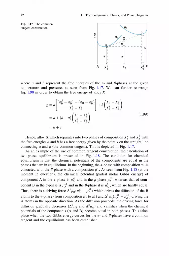
where a and b represent the free energies of the a- and b-phases at the giventemperature and pressure, as seen from Fig. 1.17. We can further rearrangeEq. 1.98 in order to obtain the free energy of alloy X

g ¼ aðXb

B � XaBÞ � ðXB � Xa

BÞXb

B � XaB

" #þ b

XB � XaB

XbB � Xa

B

!

¼ aþ ðb� aÞ XB � XaB

XbB � Xa

B

!

¼ aþ c

ð1:99Þ

Hence, alloy X which separates into two phases of composition XaB and Xb

B withthe free energies a and b has a free energy given by the point x on the straight lineconnecting a and b (the common tangent). This is depicted in Fig. 1.17.

As an example of the use of common tangent construction, the calculation oftwo-phase equilibrium is presented in Fig. 1.18. The condition for chemicalequilibrium is that the chemical potentials of the components are equal in thephases that are in equilibrium. In the beginning, the a-phase with composition a1 iscontacted with the b-phase with a composition b1. As seen from Fig. 1.18 (at themoment in question), the chemical potential (partial molar Gibbs energy) of

component A in the a-phase is la1A and in the b-phase lb1

A , whereas that of com-

ponent B in the a-phase is la1A and in the b-phase it is lb1

A , which are hardly equal.

Thus, there is a driving force D1lBðla1B � lb1

B Þ which drives the diffusion of the B

atoms to the a-phase (from composition b1 to a1) and D1lAðlb1A � la1

A Þ driving theA atoms in the opposite direction. As the diffusion proceeds, the driving force fordiffusion gradually decreases (D2lB and D2lA) and vanishes when the chemicalpotentials of the components (A and B) become equal in both phases. This takesplace when the two Gibbs energy curves for the a- and b-phases have a commontangent and the equilibrium has been established.

Fig. 1.17 The commontangent construction

42 1 Thermodynamics, Phases, and Phase Diagrams

1.11 The Gibbs Phase Rule

The Gibbs phase rule explains the number of phases that will be present in asystem in equilibrium and is expressed as

F þ P ¼ C þ N ð1:100Þ

where F is the number of degrees of freedom (always C 0), P is the number ofphases (liquid phase, a-phase, b-phase), C is the number of components, andN corresponds to the non-compositional variable. In our case, there are two non-compositional variables present, temperature and pressure. This means thatEq. 1.100 can be written as

F þ P ¼ C þ 2 ð1:101Þ

Now for the purpose of explaining the stability of the phases in equilibrium, asingle-component system that is presented in Fig. 1.19a is considered. First, let usexamine the single-phase, solid, liquid or gas phase, region which can be written inthis region C = 1, P = 1. Also from Eq. 1.101, we can write F = 2. This meansthat in this region, there are two degrees of freedom, temperature and pressure.Accordingly, temperature and pressure can be varied independently within theregion. Consequently, to determine the state of the phase in a single-phase region,

Fig. 1.18 Use of the common tangent construction to determine the phase equilibria

1.11 The Gibbs Phase Rule 43

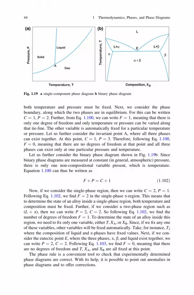
Fig. 1.19 a single-component phase diagram b binary phase diagram

both temperature and pressure must be fixed. Next, we consider the phaseboundary, along which the two phases are in equilibrium. For this can be writtenC = 1, P = 2. Further, from Eq. 1.100, we can write F = 1, meaning that there isonly one degree of freedom and only temperature or pressure can be varied alongthat tie-line. The other variable is automatically fixed for a particular temperatureor pressure. Let us further consider the invariant point A, where all three phasescan exist together. At this point, C = 1, P = 3. Therefore, following Eq. 1.100,F = 0, meaning that there are no degrees of freedom at that point and all threephases can exist only at one particular pressure and temperature.

Let us further consider the binary phase diagram shown in Fig. 1.19b. Sincebinary phase diagrams are measured at constant (in general, atmospheric) pressure,there is only one non-compositional variable present, which is temperature.Equation 1.100 can thus be written as

F þ P ¼ C þ 1 ð1:102Þ

Now, if we consider the single-phase region, then we can write C = 2, P = 1.Following Eq. 1.102, we find F = 2 in the single-phase a-region. This means thatto determine the state of an alloy inside a single-phase region, both temperature andcomposition must be fixed. Further, if we consider a two-phase region such as(L + a), then we can write P = 2, C = 2. So following Eq. 1.102, we find thenumber of degrees of freedom F = 1. To determine the state of an alloy inside thisregion, we need to fix only one variable, either T, XA, or XB. Since, if we fix any oneof these variables, other variables will be fixed automatically. Take, for instance, T2

where the composition of liquid and a-phases have fixed values. Next, if we con-sider the eutectic point E, where the three phases, a, b, and liquid exist together, wecan write P = 2, C = 2. Following Eq. 1.103, we find F = 0, meaning that thereare no degrees of freedom and T, XA, and XB are all fixed at this point.

The phase rule is a convenient tool to check that experimentally determinedphase diagrams are correct. With its help, it is possible to point out anomalies inphase diagrams and to offer corrections.

44 1 Thermodynamics, Phases, and Phase Diagrams

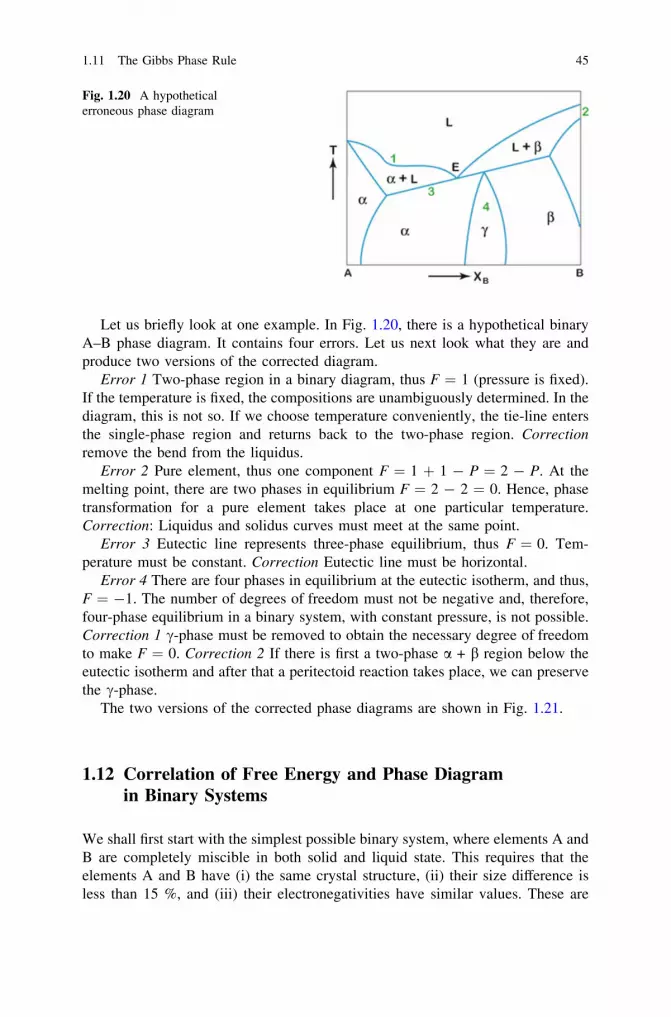
Let us briefly look at one example. In Fig. 1.20, there is a hypothetical binaryA–B phase diagram. It contains four errors. Let us next look what they are andproduce two versions of the corrected diagram.

Error 1 Two-phase region in a binary diagram, thus F = 1 (pressure is fixed).If the temperature is fixed, the compositions are unambiguously determined. In thediagram, this is not so. If we choose temperature conveniently, the tie-line entersthe single-phase region and returns back to the two-phase region. Correctionremove the bend from the liquidus.

Error 2 Pure element, thus one component F = 1 + 1 - P = 2 - P. At themelting point, there are two phases in equilibrium F = 2 - 2 = 0. Hence, phasetransformation for a pure element takes place at one particular temperature.Correction: Liquidus and solidus curves must meet at the same point.

Error 3 Eutectic line represents three-phase equilibrium, thus F = 0. Tem-perature must be constant. Correction Eutectic line must be horizontal.

Error 4 There are four phases in equilibrium at the eutectic isotherm, and thus,F = -1. The number of degrees of freedom must not be negative and, therefore,four-phase equilibrium in a binary system, with constant pressure, is not possible.Correction 1 c-phase must be removed to obtain the necessary degree of freedomto make F = 0. Correction 2 If there is first a two-phase a + b region below theeutectic isotherm and after that a peritectoid reaction takes place, we can preservethe c-phase.

The two versions of the corrected phase diagrams are shown in Fig. 1.21.

1.12 Correlation of Free Energy and Phase Diagramin Binary Systems

We shall first start with the simplest possible binary system, where elements A andB are completely miscible in both solid and liquid state. This requires that theelements A and B have (i) the same crystal structure, (ii) their size difference isless than 15 %, and (iii) their electronegativities have similar values. These are

Fig. 1.20 A hypotheticalerroneous phase diagram

1.11 The Gibbs Phase Rule 45

known as the Hume-Rothery rules. An example of such a system is Cu–Ni above355 �C (i.e., above the solid state, miscibility gap caused at least partly by theferromagnetism of Ni). Thus, the A–B system shown in Fig. 1.22 exhibits idealbehavior and atoms will not have any preference to select neighboring atoms. Togive a mental picture of what complete miscibility in solid state means, we cantrace the following line of thought. If one begins with pure A, with its own crystalstructure, and starts to replace A atoms with B atoms, then, in the case of completesolubility, one can eventually replace all A atoms with B atoms without anychange in crystal structure or formation of new phases and reach pure element B,with its own crystal structure (which has to be, by definition, the same as A’s). Toillustrate this behavior, we have to consider the change in free energy withcomposition for two different phases, solid (gs) and liquid (gL), to find the stabilityof the phases at different temperatures and compositions. Here, we assume that the

melting point of element A (TAm ) is higher than the melting point of element B

(TBm). First, if we consider a relatively high temperature, as shown in Fig. 1.22a, we

know from our previous discussion that the liquid phase will be stable because of ahigh contribution of entropy. Now, if we start to decrease the temperature to acertain extent, two factors shall be mainly noticed, which shall change in the freeenergy diagram. We have seen before that the free energy of a liquid phasedecreases faster than that of a solid phase. So with the decrease in temperature, thedifference in free energy of both liquid and solid phases will decrease. Further,because of the decrease in temperature, the contribution of Dgmix �TDsmix willdecrease, which means that the curvature of both curves will recede. If wedecrease the temperature up to the melting point of element A (TA

m), then we shallfind, as shown in Fig. 1.22b, that gL and gS will intersect at XB = 0. If the tem-perature is decreased further, then the curves are found to intersect somewhere inthe middle, as shown in Fig. 1.22c. The diagram can be separated into threedifferent composition range of 0� XS

B

� �, XS

B � XLB

� �, and XL

B � 1� �

. Here, espe-

cially the composition range of XSB � XL

B

� �draws attention for further discussion.

Fig. 1.21 The two correct versions of the diagram shown in Fig. 1.20

46 1 Thermodynamics, Phases, and Phase Diagrams

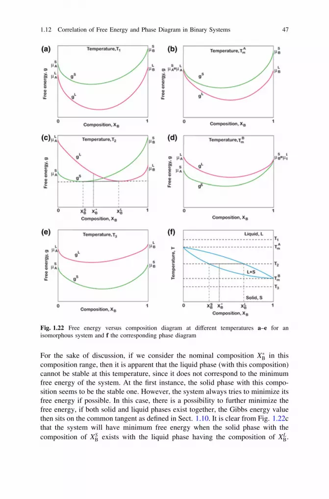
For the sake of discussion, if we consider the nominal composition XB in thiscomposition range, then it is apparent that the liquid phase (with this composition)cannot be stable at this temperature, since it does not correspond to the minimumfree energy of the system. At the first instance, the solid phase with this compo-sition seems to be the stable one. However, the system always tries to minimize itsfree energy if possible. In this case, there is a possibility to further minimize thefree energy, if both solid and liquid phases exist together, the Gibbs energy valuethen sits on the common tangent as defined in Sect. 1.10. It is clear from Fig. 1.22cthat the system will have minimum free energy when the solid phase with thecomposition of XS

B exists with the liquid phase having the composition of XLB.

Fig. 1.22 Free energy versus composition diagram at different temperatures a–e for anisomorphous system and f the corresponding phase diagram

1.12 Correlation of Free Energy and Phase Diagram in Binary Systems 47

Since XB is the average composition of the alloy, the mole fraction of the solidphase, following the lever rule (defined in Sect. 1.8), will be ðXL

B � XBÞ=ðXLB � XS

BÞand the mole fraction of the liquid phase will be ðXB � XS

BÞ=ðXLB � XS

BÞ. It shouldbe noted that with the change in average composition within the range ofðXL

B � XSBÞ, the composition of the solid and liquid phases will not change, but, only

the relative amount of the phases will change. It can also be understood fromFig. 1.22c that in this range, the liquid and solid phases with the composition XS

B

and XLB will exist together, since the chemical potential or activity of elements A

and B in both the phases must be the same (lSA ¼ lL

A and lSB ¼ lL

B). In other words,once solid and liquid phases reach their stable composition, there is no furtherdriving force for change. It is also clear that in the composition range of 0� XS

B

� �,

the solid phase will be stable since it has minimum free energy in that compositionrange, whereas in the composition range of XL

B � 1� �

, only the liquid phase will bestable since it has minimum free energy in that composition range. If we decreasethe temperature to TB

m , the free energy curves of the phases, as depicted inFig. 1.22d, will intersect at XB = 1. If we decrease the free energy of the systemeven further, the free energy of the solid phase, as shown in Fig. 1.22e, will belower than the free energy of the liquid phase in all compositions and the solidphase will be stable. The corresponding phase diagram can be seen from Fig. 1.22f.

Next, let us consider a solution with a positive heat of mixing (endothermicbehavior), which means that there is a miscibility gap in the system. Further, it isassumed that the miscibility gap occurs only in the solid state but not in the liquidphase. Thus, at low temperatures, the free energy of the mixing of the solid phase willbe positive because of the positive heat of mixing. At higher temperature, however,the free energy of mixing becomes negative, because of the growing importance ofthe entropy term ð�TDsmixÞ. At a reasonably high temperature, the free energy of thesolid and liquid phases might vary with composition, as shown in Fig. 1.23a.

With a further decrease in temperature to TAm , the free energy curves of solid

(gS) and liquid (gL) phases will intersect, as is presented in Fig. 1.23b. Any furtherdecrease in temperature down to T2, because of the difference in curvature, gL

intersects gS at two points, so there are five-phase regions stable at a differentcomposition range, as given in Fig. 1.23c. With a further decrease in temperatureto T3, we shall find that gS is lower than gL at all compositions so that only the solidphase is stable at this temperature, as shown in Fig. 1.23d. It also should be notedthat because of the endothermic nature of transformation, with the decrease intemperature, the curvature of gS is decreased very rapidly and with the furtherdecrease in temperature to T4, the free energy of mixing becomes positive and thecurvature of the free energy curve will become positive in a certain compositionrange in the middle.

This is the reason why in this composition range, the solid cannot be present as asingle stable phase but will spontaneously dissociate into two different phases withcompositions a1 and a2, as can be seen from Fig. 1.23e. The area between compo-sitions a1 and a2 in Fig. 1.23e is called the spinodal region. It is to be noted that

48 1 Thermodynamics, Phases, and Phase Diagrams

decomposition of the phase inside the spinodal does not require nucleation. Only afterreaching the inflection points of the Gibbs energy curve, must nucleation precede theformation of a new phase. Figure 1.23f presents the corresponding phase diagram.

There are systems in which the enthalpy of mixing is positive and of such a highmagnitude that the free energy curve will have positive curvature within a certaincomposition range up to a reasonably high temperature. In such cases, the freeenergy curves of the phases will change as a function of temperature in a wayshown in Fig. 1.24a–e. The corresponding phase diagram is presented in Fig. 1.24f.Here, the main difference will be that at temperature TE and at a particular

Fig. 1.23 Free energy versus composition diagram of a system which goes through endothermictransformation because of mixing and corresponding phase diagram

1.12 Correlation of Free Energy and Phase Diagram in Binary Systems 49

composition XE, the three phases, a, b, and L, can all exist together. Point E, plottedin Fig. 1.24f, corresponds to eutectic transformation. At the eutectic isotherm, thenumber of degrees of freedom is zero and thus, the equilibrium can occur only at aspecific temperature and with fixed compositions of a, b, and L.

In all the above cases, we have considered systems where the crystal structureof elements A and B were similar and thus, there has been only one free energycurve for the solid phase. However, in a system where the elements have differentcrystal structure, we need to consider different free energy curves for differentelements, as shown in Fig. 1.25. Let us designate, A(B), i.e., element A with aparticular crystal structure, alloyed with some B as the a-phase. Similarly, B(A) is

Fig. 1.24 Free energy versus composition diagram of a system which goes through endothermictransformation with very high enthalpy of mixing and corresponding phase diagram

50 1 Thermodynamics, Phases, and Phase Diagrams

designated as the b-phase. Note in Fig. 1.25a that element A with the crystalstructure of element B (ga

B) will have a much higher free energy than its stable freeenergy (ga

A); thus, it is a metastable crystal structure of A. Similarly, gaB is much

higher than gaB. This system, under our consideration, also has an eutectic trans-

formation as in the previous example.Let us next consider the case, where the formation of the c-phase in the system

is associated with strong exothermic transformation, as can be noted fromFig. 1.26a. This implies that there is considerable difference in the electroneg-ativities of the elements A and B. Note also that with only a slight change in

Fig. 1.25 Free energy versus composition diagram of a system where elements have differentcrystal structures and corresponding phase diagram

1.12 Correlation of Free Energy and Phase Diagram in Binary Systems 51

composition, the free energy of this phase increases very rapidly. Thus, thecomposition limits of the stability region of this phase are strictly limited. Thecorresponding phase diagram at a particular temperature T is given in Fig. 1.26b.As will be discussed in Sect. 2.6, different atoms in the ordered phase try tooccupy particular lattice positions in the crystal to maximize the number of A–Bbonds depending on the average composition of the phase. These ordered phasesare known as intermetallic compound or intermediate phases, and in general, thesephases have a different crystal structure than the crystal structure of the pureelement. In the example shown in Fig. 1.26, it is to be observed that the c-phasehas a very narrow homogeneity range. However, in some cases, as presented inFig. 1.27, the ordered phase can, in fact, have a wide homogeneity range, wherethe change in free energy (because of the small change in composition) is not verystriking, unlike as in the previous example. These phases can deviate from theirstoichiometric composition because of the presence of defects, as discussed inSect. 1.11.

Fig. 1.26 Free energy versus composition diagram and the corresponding phase diagram wherethe phase (ordered c-phase) goes through strong exothermic transformation

Fig. 1.27 Free energy versus composition diagram and the corresponding phase diagram wherethe ordered c-phase has a wide homogeneity range

52 1 Thermodynamics, Phases, and Phase Diagrams

1.13 Ternary Phase Diagrams

According to the Gibbs phase rule, the number of degrees of freedom in ahomogeneous ternary phase under constant pressure is three. Thus, we need tospecify three independent variables (two-component mole fractions and temper-ature) in order to fix an equilibrium in a ternary solution phase. This leads to athree dimensional (T, XA, XB) presentation. As already discussed, it is of commonpractice to utilize an equilateral triangular (the Gibbs triangle) base (ABC) withthree binary system ‘‘walls’’ (A–B, B–C, C–A) and temperature as the verticalaxis. Next, we will briefly discuss ternary space diagrams as well as the isothermaland vertical sections taken from those diagrams.

Figure 1.28 shows the simplest possible ternary system, where there is com-plete solid and liquid solubility in the system (ABC). This ternary space model isvery simple and easy to interpret, but as the systems become more complex, thespace model becomes harder and harder to use. Therefore, it is common practice toutilize different sections and projections from the space model to yield more easilyaccessible information. As an example, the liquidus and solidus projections fromthe ABC system are shown in Fig. 1.29.

These types of projections are typically made with constant temperatureintervals and can therefore be interpreted similarly as the contour lines in a map.Accordingly, the closer the spacing of the projection lines, the steeper is theprojected surface. Isothermal sections are the most commonly used types of pre-sentation of ternary equilibria. Figure 1.30 shows the isothermal section at tem-perature T3 from the ABC system given in Fig. 1.28.

The plane intersects the liquidus surface at T3 along the curve l1l2 and thesolidus surface along the curve s1s2. On the left-hand side of the curve l1l2, there is

Fig. 1.28 Ternary spacediagram with complete solidand liquid solubilities in allthree binary systems

1.13 Ternary Phase Diagrams 53

a single-phase liquid region and on the right-hand side of the curve s1s2, there is asingle-phase solid region. Between these two curves, there is a two-phase liquidand a solid region. The compositions of the phases in two-phase equilibrium areobtained at the end points of the tie-line and the amounts by the lever rule, as inbinary phase diagrams. The directions of the tie-lines lying within the figure varyfan-like, so that there is a gradual transition from the direction of one bounding tie-line to that of the other. No two tie-lines at the same temperature may ever cross.This is a direct result of the Gibbs phase rule. Beyond these considerations,nothing can be said about the direction of tie-lines, except that they must run fromliquidus to solidus. Other than those tie-lines on the edges of the diagram, none ofthem point toward a corner of the diagram unless by mere coincidence or due to acomplete lack of solubility with the element at the given corner. Therefore, it isnecessary to determine the position and direction of the tie-lines experimentally. Itshould be noted that the activity of a given component has the same value at eachend of a tie-line.

Vertical sections (isopleths) from ternary space diagrams can also be taken.Figure 1.31 presents some ways in which this can be achieved. Afterward, theseisopleths are shown in Fig. 1.32.

Even though the isopleths appear quite like binary phase diagrams, they mustnot be confused with them. In general, tie-lines cannot be used with isopleths andthey only show the temperature composition regions of the different phases.

Fig. 1.29 Solidus andliquidus projections from thespace diagram in Fig. 1.28

Fig. 1.30 Isothermal sectionat temperature T from thediagram seen in Fig. 1.28

54 1 Thermodynamics, Phases, and Phase Diagrams

When there are three phases in equilibrium in a ternary system under constantpressure, there is still one degree of freedom left. Thus, three-phase equilibrium in aternary system exists within a certain temperature range and not at a single tem-perature as in binary systems under constant pressure. Three-phase equilibrium in aternary phase diagram is represented by a tie-triangle and as the temperaturechanges these tie-triangles form a ‘‘stack’’ of tie-triangles (Fig. 1.33). The com-position of phases participating in the three-phase equilibrium can be found fromthe corners of the tie-triangle and the amount by applying the lever rule three times.

In this hypothetical ternary system in AC, there is complete solid and liquidsolubility, whereas AB and BC are eutectic systems. Point M is the eutectic pointof system AB, which is at a higher temperature than N, which is the eutectic pointof the system BC. Thus, in both binary systems (AB and BC), an eutectic reactionl,a + b takes place. In Fig. 1.34, the surfaces AMNC ja MNB are the liquidus

Fig. 1.31 Different ways onecan take an isopleth

Fig. 1.32 Two isoplethstaken along the lines ab andAc

Fig. 1.33 Stack of tie-traingles

1.13 Ternary Phase Diagrams 55

surfaces and thus determine the solubilities of a and b to liquid. These surfacesmeet at the eutectic valley MN. DG and EF are curves joining the points repre-senting the respective compositions of the a and b phases formed in the eutecticreactions in the binary systems. DME and GNF are horizontal lines that representthese eutectic reactions. The surfaces ADGC and BEF are the solidus surfaces. Thethree curves MN, DG, and EF do not lie in the same plane. The curve MN liesabove the surface DEFG, in such a way that there are three curved surfacesDMNG, MEFN, and DEFG, which enclose a three-phase space where a, b, and theliquid are in equilibrium. Each of these surfaces is made up of tie-lines repre-senting l + a, l + b, and a + b equilibria. The surfaces DMNG, MEFN, andDEFG separate the three-phase space from the liquid + a, liquid + b , and a + bregions, respectively. Where the three-phase region terminates in the binary sys-tems AB and BC, it shrinks to the binary eutectic lines. In a ternary system, theeutectic reaction l ? a + b occurs over a range of temperature. If we have analloy with nominal composition of X, as in Fig. 1.34, the solidification takes placeas follows. During the solidification, the first solid phase to form is primary b,when the liquidus surface is first met. The composition of the liquid then changesalong a path on the liquidus surface and that of the solid b along a path on thesolidus surface as the temperature decreases. Then, at a certain temperature T1,before solidification is completed, the liquid composition reaches a point on thecurve MN and solid composition a point on the curve EF. The situation at T1 isgiven in Fig. 1.35a where a tie-triangle is drawn. At this temperature, the nominalcomposition is seen to lie on the lb tie-line. When the temperature is decreased toT2, the three-phase equilibrium is established, as the nominal composition now liesinside the tie-triangle Fig. 1.35b. The compositions of the liquid, a, and b aregiven by the points l2, a2, and b2, and their respective amounts can be obtained byapplying the lever rule three times

Fig. 1.34 ABC ternarysystem, where binary systemAC has complete solidsolubility and binary systemsAB and BC are eutectic ones

56 1 Thermodynamics, Phases, and Phase Diagrams

% liquidðl2Þ ¼Xl02l2l02� 100; % b2 ¼

Xb02b2b

02

� 100 and % a2 ¼Xa02a2a02

� 100

Solidification ends at T3 when the a3b3 tie-line is encountered.As the ternary systems become more complicated, the analysis shown above

becomes increasingly difficult. Thus, it is of common practice to utilize differentsections taken from the space model to provide information in a more accessibleform. Next, we shall consider isothermal sections a little more, as they, in general,provide the most useful information on the ternary system. When working with theisothermal section and naming the phase regions, it is helpful to remember that thesides of the three-phase triangles must always face the two-phase regions, and atthe corners of the tie-triangle, single-phase regions exist. These rules are based onthe more general Palatnik-Landau theorem. Figure 1.36 contains an example of theAuPbSn system at 200 �C with all the phase regions clearly marked in the figure. Itis to be noted that in the case of systems with stoichiometric compounds, the two-phase regions between three-phase regions may be reduced to just a single tie-line.

As an example of utilization of isothermal sections, we shall consider the fol-lowing case. An interesting behavior has been observed in the Cu/SnBi eutecticsystem during soldering at temperatures above 200 �C. In particular, when thesolder volume is small, reactions can result in drastic changes to the microstructurewhen soldering times are increased. Since bismuth does not react with Cu, only tin isconsumed during the reactions. This will eventually lead to a shift in the liquid soldercomposition toward the Bi-rich corner. When the isothermal section of the SnBiCuequilibrium phase diagram is investigated, it is to be noted that when the enrichmentof liquid with bismuth increases and the composition of the solder is around60 at-% bismuth, the local equilibrium condition changes, as shown in Fig. 1.37.

Fig. 1.35 The process of solidification of an alloy with nominal composition X in the systemshown in Fig. 1.34 is exemplified in this figure as a function of temperature. a Temperature atwhich liquid composition reaches a point on the curve MN and solid composition a point on thecurve EF, b temperature where three-phase equilibrium is established, and c temperature whensolidification ends

1.13 Ternary Phase Diagrams 57

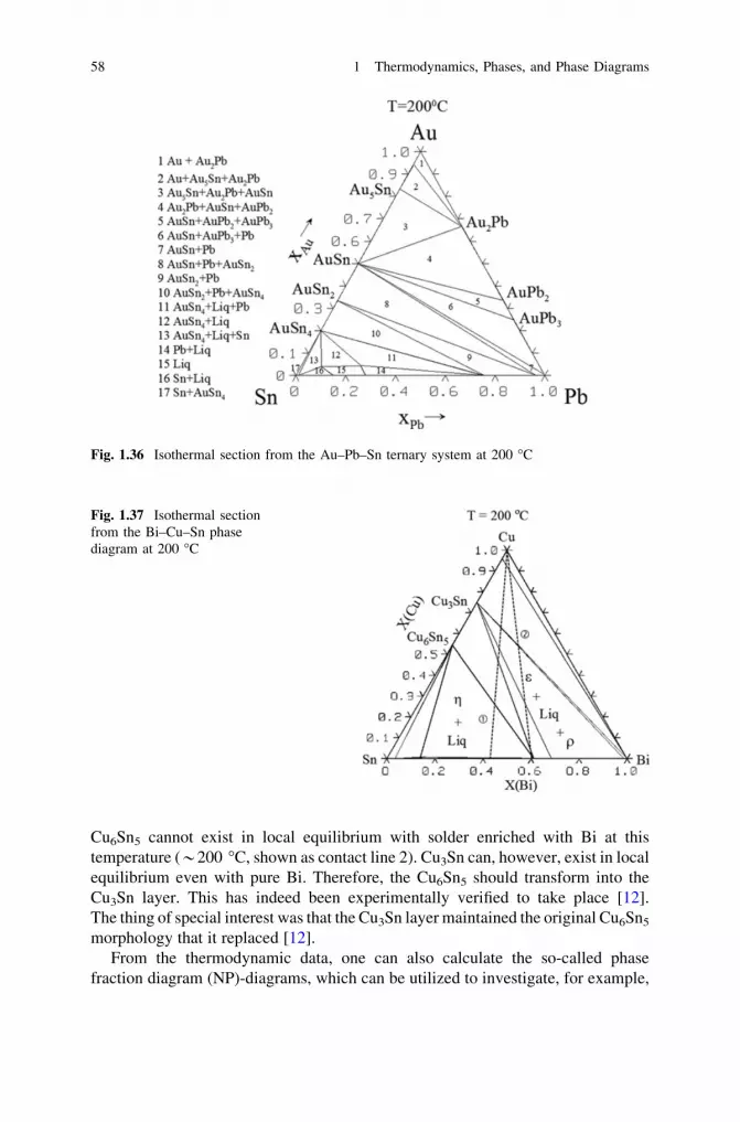
Cu6Sn5 cannot exist in local equilibrium with solder enriched with Bi at thistemperature (*200 �C, shown as contact line 2). Cu3Sn can, however, exist in localequilibrium even with pure Bi. Therefore, the Cu6Sn5 should transform into theCu3Sn layer. This has indeed been experimentally verified to take place [12].The thing of special interest was that the Cu3Sn layer maintained the original Cu6Sn5

morphology that it replaced [12].From the thermodynamic data, one can also calculate the so-called phase

fraction diagram (NP)-diagrams, which can be utilized to investigate, for example,

Fig. 1.36 Isothermal section from the Au–Pb–Sn ternary system at 200 �C

Fig. 1.37 Isothermal sectionfrom the Bi–Cu–Sn phasediagram at 200 �C

58 1 Thermodynamics, Phases, and Phase Diagrams

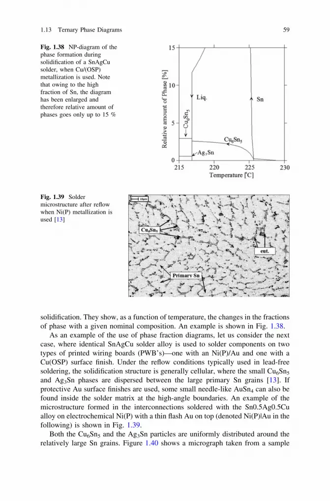
solidification. They show, as a function of temperature, the changes in the fractionsof phase with a given nominal composition. An example is shown in Fig. 1.38.

As an example of the use of phase fraction diagrams, let us consider the nextcase, where identical SnAgCu solder alloy is used to solder components on twotypes of printed wiring boards (PWB’s)—one with an Ni(P)/Au and one with aCu(OSP) surface finish. Under the reflow conditions typically used in lead-freesoldering, the solidification structure is generally cellular, where the small Cu6Sn5

and Ag3Sn phases are dispersed between the large primary Sn grains [13]. Ifprotective Au surface finishes are used, some small needle-like AuSn4 can also befound inside the solder matrix at the high-angle boundaries. An example of themicrostructure formed in the interconnections soldered with the Sn0.5Ag0.5Cualloy on electrochemical Ni(P) with a thin flash Au on top (denoted Ni(P)|Au in thefollowing) is shown in Fig. 1.39.

Both the Cu6Sn5 and the Ag3Sn particles are uniformly distributed around therelatively large Sn grains. Figure 1.40 shows a micrograph taken from a sample

Fig. 1.38 NP-diagram of thephase formation duringsolidification of a SnAgCusolder, when Cu/(OSP)metallization is used. Notethat owing to the highfraction of Sn, the diagramhas been enlarged andtherefore relative amount ofphases goes only up to 15 %

Fig. 1.39 Soldermicrostructure after reflowwhen Ni(P) metallization isused [13]

1.13 Ternary Phase Diagrams 59

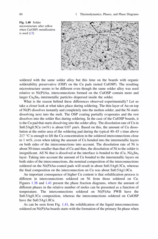
soldered with the same solder alloy but this time on the boards with organicsolderability preservative (OSP) on the Cu pads (noted Cu|OSP). The resultingmicrostructure seems to be different even though the same solder alloy was usedrelative to Ni(P)|Au, interconnections formed on the Cu|OSP contain more andlarger Cu6Sn5 intermetallic particles dispersed inside the solder.

What is the reason behind these differences observed experimentally? Let ustake a closer look at what takes place during soldering. The thin layer of Au on topof Ni(P) dissolves instantly and completely into the molten solder, and the Ni startsdissolving next into the melt. The OSP coating partially evaporates and the restdissolves into the solder flux during soldering. In the case of the Cu|OSP boards, itis the Cu pad that starts dissolving into the solder alloy. The dissolution rate of Cu inSn0.5Ag0.5Cu (wt%) is about 0.07 lm/s. Based on this, the amount of Cu disso-lution at the entire area of the soldering pad during the typical 40–45 s time above217 �C is enough to lift the Cu concentration in the soldered interconnections closeto 1 wt%, even when taking the amount of Cu bonded into the intermetallic layerson both sides of the interconnections into account. The dissolution rate of Ni isabout 50 times smaller than that of Cu and thus, the dissolution of Ni to the solder isinsignificant. All Ni that is dissolved at the interface is bonded to the (Cu, Ni)6Sn5

layer. Taking into account the amount of Cu bonded to the intermetallic layers onboth sides of the interconnections, the nominal composition of the interconnectionssoldered on the Ni(P)|Au-coated pads will result in about Sn0.5Ag0.3Cu, whereasthe final composition on the interconnection on Cu was about Sn0.5Ag1.0Cu.

An important consequence of higher Cu content is that solidification process isdifferent in interconnections soldered on Ni from those soldered on Cu.Figures 1.38 and 1.41 present the phase fraction diagrams, where the amount ofdifferent phases in the relative number of moles can be presented as a function oftemperature. The interconnections soldered on Ni(P)|Au PWB have theSn0.5Ag0.3Cu composition, whereas the interconnections soldered on Cu|OSPhave the Sn0.5Ag1.0Cu.

As can be seen from Fig. 1.41, the solidification of the liquid interconnectionssoldered on Ni(P)|Au boards starts with the formation of the primary Sn phase when

Fig. 1.40 Soldermicrostructure after reflowwhen Cu(OSP) metallizationis used [13]

60 1 Thermodynamics, Phases, and Phase Diagrams

the interconnections are cooled down from the peak reflow temperature to belowthe liquidus temperature of 229 �C. The Cu6Sn5 phase does not nucleate until below222 �C, where the composition of the liquid reaches the eutectic valley. Figure 1.38presents the phase fraction diagram of the liquid interconnections soldered onCu|OSP boards. In this case, the solidification begins with the formation of primaryCu6Sn5 below 229 �C. However, the nominal composition of the liquid soon meetsthe curve of two-fold saturation, after which the solidification of the interconnec-tions proceeds by the binary eutectic reaction L ? (Sn)eut + (Cu6Sn5)eut. Belowthe four-phase invariant temperature, there is more than three times as much Cu6Sn5

in the Cu|OSP interconnections as in those on the Ni(P)|Au substrate. It is to benoted that the above analysis of solidification has been carried out by consideringthat the system is in complete equilibrium. As this is not typically the case inpractical applications, the above-presented discussion must be taken to representthe ideal situation where kinetics plays no role in the process.

1.14 Stability Diagrams (Activity Diagrams, etc.)

The activity diagram shown in the right-hand side of Fig. 1.42 is one form of manydifferent types of stability diagrams. In such a diagram, the thermodynamicpotential of one of the components is plotted as a function of the relative atomicfractions of the other two components. The activity values which are needed in theconstruction of such a diagram can be calculated from the assessed thermodynamicdata. When calculating the activities of the components, the activities of thestoichiometric compounds at equilibrium are regarded to be one. It should be notedthat the precision of the calculations is very much dependent on the accuracy and

Fig. 1.41 NP-diagram of thephase formation duringsolidification when Ni(P)/Aumetallization is used [13]

1.13 Ternary Phase Diagrams 61

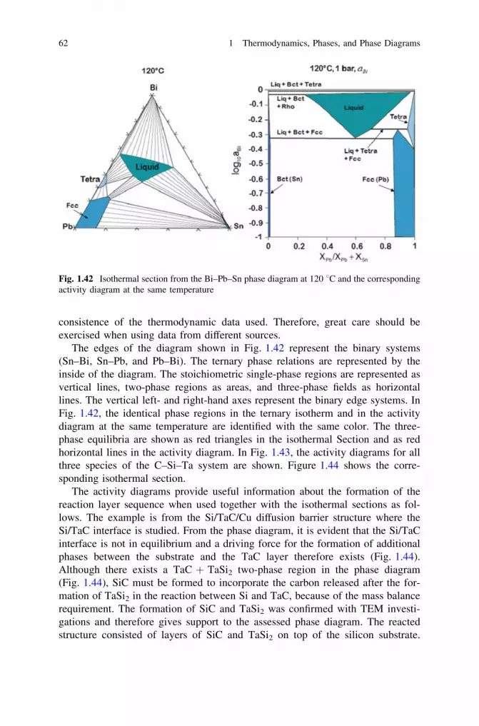
consistence of the thermodynamic data used. Therefore, great care should beexercised when using data from different sources.

The edges of the diagram shown in Fig. 1.42 represent the binary systems(Sn–Bi, Sn–Pb, and Pb–Bi). The ternary phase relations are represented by theinside of the diagram. The stoichiometric single-phase regions are represented asvertical lines, two-phase regions as areas, and three-phase fields as horizontallines. The vertical left- and right-hand axes represent the binary edge systems. InFig. 1.42, the identical phase regions in the ternary isotherm and in the activitydiagram at the same temperature are identified with the same color. The three-phase equilibria are shown as red triangles in the isothermal Section and as redhorizontal lines in the activity diagram. In Fig. 1.43, the activity diagrams for allthree species of the C–Si–Ta system are shown. Figure 1.44 shows the corre-sponding isothermal section.

The activity diagrams provide useful information about the formation of thereaction layer sequence when used together with the isothermal sections as fol-lows. The example is from the Si/TaC/Cu diffusion barrier structure where theSi/TaC interface is studied. From the phase diagram, it is evident that the Si/TaCinterface is not in equilibrium and a driving force for the formation of additionalphases between the substrate and the TaC layer therefore exists (Fig. 1.44).Although there exists a TaC + TaSi2 two-phase region in the phase diagram(Fig. 1.44), SiC must be formed to incorporate the carbon released after the for-mation of TaSi2 in the reaction between Si and TaC, because of the mass balancerequirement. The formation of SiC and TaSi2 was confirmed with TEM investi-gations and therefore gives support to the assessed phase diagram. The reactedstructure consisted of layers of SiC and TaSi2 on top of the silicon substrate.

Fig. 1.42 Isothermal section from the Bi–Pb–Sn phase diagram at 120 8C and the correspondingactivity diagram at the same temperature

62 1 Thermodynamics, Phases, and Phase Diagrams

The original TaC was completely consumed during the reaction, since no traces ofit could be found at 800 �C. The reaction sequence seemed to be Si/SiC/TaSi2/TaC, in which the TaC was used completely to yield the final structure Si/SiC/TaSi2. Silicon is expected to be the first species moving at this interface owing tothe following reasons. Firstly, Si has been found to be the mobile species duringthe formation of TaSi2 that occurs around 650 �C in the binary Ta–Si system by Siin diffusion, whereas the movement of Ta has not been observed under similarconditions. Secondly, chemical bonding between Ta and C in the TaC compoundis expected to be strong, and breaking of these bonds, which is required for therelease and subsequent diffusion of Ta, would require large amounts of energy.Owing to the facts stated above, the diffusion of tantalum or carbon in this systemis not considered to be highly probable. Consequently, Si is anticipated to be themain diffusing species at the Si/TaC interface around 800 �C.

Fig. 1.43 Activity diagrams for C, Si, and Ta at 800 �C [14]

1.14 Stability Diagrams (Activity Diagrams, etc.) 63

Whether the above-presented phase formation sequence is thermodynamicallypossible can be investigated with the help of Fig. 1.43. As can be seen from thecalculated activity diagram, Si can move along its lowering activity in the proposedreaction sequence and therefore, diffusion of Si in this particular reaction sequence isallowed on thermodynamic grounds. The examination of the calculated activitydiagrams for carbon and tantalum does not restrict the diffusion of these elements inthe suggested reaction sequence either (Fig. 1.43). However, as already discussed,carbon and tantalum are strongly bonded to each other in the TaC compound and arenot expected to move easily. Therefore, the reaction most likely starts by Si indiffusion into TaC (most probably via grain boundaries). This is followed by theformation of TaSi2, which then leads to the accompanied dissociation of TaC. Thereleased carbon is then available for the formation of SiC in the reaction with Si. Thismechanism will finally yield the experimentally observed structure Si/SiC/TaSi2.

1.15 The Use of Gibbs Energy Diagrams

In the following examples, the use of Gibbs energy diagrams is presented. Thediscussion follows largely that presented in the classical treatments of the subjectby Hillert [10, 15].

In Fig. 1.45, a typical molar property diagram at a given temperature T0 isshown. The diagram shows some of the basic properties of a molar property dia-gram. From Fig. 1.45, one can see, for example, how a Gibbs energy of a phase isdefined (ga ¼ Xa

AlaA þ Xa

BlaB) with the help of chemical potentials, how the

Fig. 1.44 Isothermal sectionat 800 �C from the C–Si–Tasystem [14]

64 1 Thermodynamics, Phases, and Phase Diagrams

chemical potentials for a species in a given phase are defined (from the end points ofthe tangent), that the slope of a tangent equals the chemical potential difference of B

and A in the alpha phase dga

dXB¼ la

B � laA

ffi �, and so on. These simple geometrical

features of the molar diagrams can be used for a wide variety of applications [15].The positive curvature of the Gibbs energy curve makes the phase stable against

fluctuations in composition. The same feature of the curve also provides thedriving force for the elimination of differences in composition within the phase(Fig. 1.46). Thus, this is the driving force for diffusion. Let us consider the situ-ation where B atoms diffuse from a region of high concentration (more preciselyactivity) to a region of low concentration. Each individual region may be regardedas a reservoir of B with its own value of gB, and the difference in gB is identical tothe decrease in Gibbs free energy when one mole of B is transferred. We make anassumption that the rate of transfer is proportional to the decrease in Gibbs freeenergy and the number of B atoms per volume XB

vmand inversely proportional to the

transport distance Dy. With these assumptions, the expression for the flux of Batoms may be written as

JB ¼ �MBXB

vm

DgB

vm¼ �MB

vmXB

dgB

dXB

DXB

Dyð1:103Þ

Fig. 1.45 Typical molarproperty diagram

Fig. 1.46 Determination ofthe driving force for diffusionwithin a solution phase

1.15 The Use of Gibbs Energy Diagrams 65

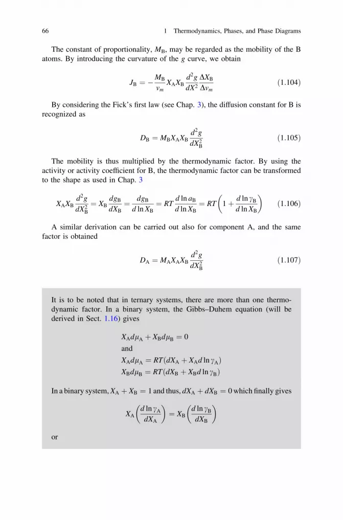
The constant of proportionality, MB, may be regarded as the mobility of the Batoms. By introducing the curvature of the g curve, we obtain

JB ¼ �MB

vmXAXB

d2g

dX2

DXB

Dvmð1:104Þ

By considering the Fick’s first law (see Chap. 3), the diffusion constant for B isrecognized as

DB ¼ MBXAXB

d2g

dX2B

ð1:105Þ

The mobility is thus multiplied by the thermodynamic factor. By using theactivity or activity coefficient for B, the thermodynamic factor can be transformedto the shape as used in Chap. 3

XAXB

d2g

dX2B

¼ XB

dgB

dXB

¼ dgB

d ln XB

¼ RTd ln aB

d ln XB

¼ RT 1þ d ln cB

d ln XB

� �ð1:106Þ

A similar derivation can be carried out also for component A, and the samefactor is obtained

DA ¼ MAXAXB

d2g

dX2B

ð1:107Þ

It is to be noted that in ternary systems, there are more than one thermo-dynamic factor. In a binary system, the Gibbs–Duhem equation (will bederived in Sect. 1.16) gives

XAdlA þ XBdlB ¼ 0

and

XAdlA ¼ RT dXA þ XAd ln cAð ÞXBdlB ¼ RT dXB þ XBd ln cBð Þ

In a binary system, XA þ XB ¼ 1 and thus, dXA þ dXB ¼ 0 which finally gives

XA

d ln cA

dXA

� �¼ XB

d ln cB

dXB

� �

or

66 1 Thermodynamics, Phases, and Phase Diagrams

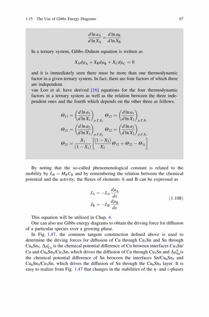
d ln aA

d ln XA

¼ d ln aB

d ln XB

In a ternary system, Gibbs–Duhem equation is written as

XAdlA þ XBdlB þ XCdlC ¼ 0

and it is immediately seen there must be more than one thermodynamicfactor in a given ternary system. In fact, there are four factors of which threeare independent.van Loo et al. have derived [16] equations for the four thermodynamicfactors in a ternary system as well as the relation between the three inde-pendent ones and the fourth which depends on the other three as follows.

H11 ¼d ln a1

d ln X1

� �p;T ;X2

H12 ¼d ln a1

d ln X2

� �p;T ;X1

H21 ¼d ln a2

d ln X1

� �p;T ;X2

H22 ¼d ln a2

d ln X2

� �p;T ;X1

H21 ¼X1

1� X1ð Þ1� X2ð Þ

X2H12 þH22 �H11

�

By noting that the so-called phenomenological constant is related to themobility by LB ¼ MBCB and by remembering the relation between the chemicalpotential and the activity, the fluxes of elements A and B can be expressed as

JA ¼ �LA

dlA

dx

JB ¼ �LB

dlB

dx

ð1:108Þ

This equation will be utilized in Chap. 4.One can also use Gibbs energy diagrams to obtain the driving force for diffusion

of a particular species over a growing phase.In Fig. 1.47, the common tangent construction defined above is used to

determine the driving forces for diffusion of Cu through Cu3Sn and Sn throughCu6Sn5. Dle

Cu is the chemical potential difference of Cu between interfaces Cu3Sn/Cu and Cu6Sn5/Cu3Sn, which drives the diffusion of Cu through Cu3Sn and Dlg

Snisthe chemical potential difference of Sn between the interfaces Sn/Cu6Sn5 andCu6Sn5/Cu3Sn, which drives the diffusion of Sn through the Cu6Sn5 layer. It iseasy to realize from Fig. 1.47 that changes in the stabilities of the g- and e-phases

1.15 The Use of Gibbs Energy Diagrams 67

(in their Gibbs free energy) will change the values of DlgSn and Dle

Cu and thusincrease or decrease the driving forces for diffusion of components in the system.

From Fig. 1.47, other important features can also be extracted. For instance, thecommon tangent between the curves gL

bin and gg gives the equilibrium solubility ofCu to a liquid solder (L), which is given as eXL

Cu. The equilibrium solubility is theamount of Cu that can be dissolved infinitely slowly to liquid solder before the g-phase comes into equilibrium with the liquid. The formation of the g-phase doesnot, however, occur with this composition, as the driving force is zero at this point(no supersaturation). In real cases, the dissolution of Cu does not take placeinfinitely slow and, therefore, the equilibrium solubility is generally exceeded. Thesolubility of Cu does not increase infinitely, but there is an upper limit for its valueand this can also be determined from Fig. 1.47. When more and more Cu dissolvesinto liquid, eventually, a situation is faced where the dissolution of more Cu wouldlead to the precipitation of pure metallic Cu out of the supersaturated solder. Thiscorresponds to the common tangent construction between the solder and pure Cu.The tangent point in the liquid curve at this metastable equilibrium gives the uppervalue of Cu that can be dissolved into liquid solder at any rate, i.e., the metastablesolubility mXL

Cu. When this value has been reached, also the driving force for theformation of the g-phase has reached its maximum (shown in the diagram asDgL!g in Fig. 1.47). Since the metastable solubility is directly related to the dis-solution rate of a given metal to a solder in question, it provides importantinformation about the formation of intermetallic compounds between differentmetals and solders. In many cases, its value is about 2–3 times larger than theequilibrium solubility [17–19].

Fig. 1.47 Gibbs energydiagram from the Cu–Snsystem at 235 �C

68 1 Thermodynamics, Phases, and Phase Diagrams

To get an idea about the relation between the above discussion and the actualphase formation in reaction couple where solid Cu is in contact with liquid Sn, it ishelpful to consider the schematic presentation of the situation in Fig. 1.48. As Cucomes into contact with liquid Sn, it starts to dissolve rapidly. The equilibriumsolubility of Cu6Sn5 to liquid Sn (eXCu

L ) is achieved quickly (in fractions of sec-ond). Owing to the reasons explained above, the dissolution does not stop at thisvalue but the dissolution of Cu continues until the ultimate limit, the metastablesolubility (mXCu

L ), is reached. At this point, the equilibrium between pure Cu andsupersaturated liquid is achieved (equal chemical potential of Cu in both phases).This means that the dissolution of Cu must stop as there is no driving force for thatanymore. At the same point, the maximum driving force for the formation ofCu6Sn5 is established (see Fig. 1.47). The composition profile of Cu is duringthese initial stages are shown by the hatched area in Fig. 1.49. As can be seen,

Fig. 1.48 Schematicpresentation of the solidCu/liquid Sn reaction coupleafter about 1 s (upper figure)and after several minutes(lower figure)

1.15 The Use of Gibbs Energy Diagrams 69

there is a certain amount of Cu, the double hatched area, which exceeds theequilibrium solubility of Cu6Sn5 to liquid Sn. This is the extra amount of Cu thatcan be used to form Cu6Sn5 isothermally. It is evident from Fig. 1.49 that at theinterface between Cu6Sn5 and the liquid Sn, the equilibrium solubility is estab-lished (where the second vertical dashed line from the left crosses the compositioncurve in Fig. 1.49).

The driving force for the precipitation can also be evaluated from the Gibbsphase diagram (Fig. 1.50). In Fig. 1.50, an alloy, a1, which is inside the two-phaseregion a + b is shown. The Gibbs free energy of the system would decrease byprecipitation of b, and the total driving force for the complete reaction in one moleof the alloy is given by the short arrow Dg The driving force for the formation of avery small quantity of b from a large quantity of a1 is obtained by considering thetangent representing the supersaturated a-phase. The magnitude of the drivingforce (in nucleation stage) is given by the separation of the points at the twotangents as

Fig. 1.49 Enlarged part ofthe solubility curves of theupper figure in Fig. 1.48

Fig. 1.50 Determination of adriving force for thenucleation of a new phasefrom supersaturated solidsolution

70 1 Thermodynamics, Phases, and Phase Diagrams

Dg ¼ XbAla1

A þ XbBla1

B � gb

gb ¼ XbAlae

A þ XbBlae

B

Dg ¼ XbAðla1

A � laeA Þ þ Xb

Bðla1B � lae

B Þð1:109Þ

For low supersaturations, one can introduce the curvature of the ga curve. Bycomparing the triangles in Fig. 1.50, one obtains

Dg

XbB � Xa

B

¼ ðlB � lAÞ1

ð1:110Þ

This can be further modified to obtain

Dg ¼ XbB � Xa

B

ffi �DðlB � lAÞ ¼ Xb

B � XaB

ffi �D

dga

dXB

� �ð1:111Þ

Dg ¼ d2ga

dX2B

XbB � Xa

B

ffi �DXa

B ð1:112Þ

The last expression contains a factor xbB � xa

B

ffi �which is the difference in

composition between the two phases. At the start of the precipitation, a new phasemay be favored (higher driving force) if it differs much in composition even whenit cannot be in stable equilibrium with the matrix phase. Thus, formation of ametastable phase (here e) is favored (Fig. 1.51) according to the Ostwald rule.

One can also obtain quantitative numerical data about energy changes in agiven system, by utilizing the simple geometric constructions shown abovetogether with some simplified assumptions. Let us take one example from theimportant Cu–Sn system (Fig. 1.52). Consider the nucleation and growth of theg-phase, with Xg

Cu ¼ a and XgSn ¼ b (a + b = 1), out of supersaturated solder

mXLCu ¼ c. The driving force for the nucleation of the g-phase is given by Dgg ¼

gLtg � gL

tg (per mole of g). The two terms can be expanded as

Fig. 1.51 Formation of ametastable phase

1.15 The Use of Gibbs Energy Diagrams 71

gLtg ¼ Xg

CumlL

Cu þ ð1� XgCuÞ

mlLSn ð1:113Þ

and

gLtg ¼ Xg

CuelL

Cu þ ð1� XgCuÞ

elLSn ð1:114Þ

which gives

) Dgg ¼ XgCu

mlLCu þ 1� Xg

Cu

� �mlL

Sn � XgCu

elLCu þ 1� Xg

Cu

� �elL

Sn

�ð1:115Þ

and by using the definition of the chemical potential of a component, this gives

¼ RT XgCu ln

maLCu

eaLCu

� �þ Xg

Sn lnmaL

SneaL

Sn

� �� ð1:115Þ

If we simplify the treatment by assuming that the liquid behaves as a perfectsolution, the activity values can be replaced by compositions, which give

ffi RT XgCu ln

mXLCu

eXLCu

� �þ ð1� Xg

CuÞ ln1� mXL

Cu

1� eXLCu

� ��

ffi 8:3145 J/Kmol � 508 K 0:545 ln0:06

0:018

� �þ ð1� 0:545Þ ln 1� 0:06

1� 0:018

� ��

¼ 2687:5 J/mol

ð1:116Þ

Fig. 1.52 Gibbs energydiagram from the Cu–Snsystem at 235 �C

72 1 Thermodynamics, Phases, and Phase Diagrams

Similarly, the change in Gibbs energy of the system owing to the precipitationof Cu6Sn5 can be expressed as

Dgtot ¼ gLtg � egL

tgð¼ DgL!LþgÞ ð1:117Þ

This can be written as

¼ RT mXLCu ln

maLCu

eaLCu

� �þ mXL

Sn lnmaL

SneaL

Sn

� �� ð1:118Þ

and by again assuming perfect behavior

ffi RT mXLCu ln

mXLCu

eXLCu

� �þ 1� mXL

Cu

� �ln

1� mXLCu

1� eXLCu

� ��

ffi 8:3145 J/Kmol � 508 K 0:06 ln0:06

0:018

� �þ ð1� 0:06Þ ln 1� 0:06

1� 0:018

� ��

¼ 131:6 J/mol

ð1:119Þ

Hence, it can be concluded that these simple molar diagrams (Gibbs free energydiagrams) give an extensive amount of important information in an easily visu-alized form.

1.15.1 Effect of Pressure on the Phase Equilibrium

Related to the effects of pressure on the phase equilibrium, we shall consider twoequations, the Laplace and the Kelvin equations. If a fluid interface is curvedbetween two phases, then it turns out that the pressures on either side must bedifferent. When the system is in equilibrium, every part of the surface must be inmechanical equilibrium (also in thermal and chemical). For a curved surface, theforces of surface tension are exactly balanced by the difference in pressure on thetwo sides of the interface. This is expressed by the Laplace equation

pa � pb ¼ c1r0þ 1

r00

� �ð1:120Þ

where P stands for the pressure, c is the surface tension, and r0 and r00 are the radiiof curvatures. By convention, positive values are assigned for the radii of curvatureif they lie in phase a (see Fig. 1.53).

An important consequence of the Laplace equation concerns the effect of sur-face curvature on the vapor pressure of a liquid. This relationship is known as theKelvin equation

1.15 The Use of Gibbs Energy Diagrams 73

lnpc

p1

� �¼ cvL

m

RT

� �2rm

� �ð1:121Þ

where pc and p? are the vapor pressures over the curved surface of mean curvaturermð 1

rm¼ 1

21r0 þ 1

r00

� �and a flat surface (r = ?) and vL

m is the molar volume of the

liquid. There is a convention to assign a positive sign to rm when it lies in theliquid phase and a negative sign when it lies in the vapor phase. Equation 1.121can be used, for example, to rationalize capillary condensation or in the treatmentof nucleation (Chap. 11). Condensation occurs when the actual vapor pressureexceeds the equilibrium vapor pressure. If the surface is curved, the Kelvin Eq. 1.121 shows that the actual pressure can be significantly lower than equilibriumpressure and thus, condensation in pores in the solid (if the liquid wets the solid) orbetween closed spaced solid particles may occur.

The effect pressure on the phase equilibrium can be investigated with Gibbsenergy diagrams. According to the definition, the Gibbs free energy of a phasedepends upon the pressure according to g ¼ gð0Þ þ pvm where 0 denotes theatmospheric pressure. As discussed above, for condensed phases, the pvm term canoften be neglected if the pressure is not exceptionally high. However, it plays animportant role if the two phases in equilibrium are under different pressures. Thisoccurs, as shown above, when the interface is curved and is caused by the surfacetension (or energy) of the curved interfaces. Next, we shall briefly discuss how theequilibrium between two phases is changed by the introduction of increasedpressure. The two g curves are displaced upward by the amounts pava

m and pavbm,

respectively. This takes place even with phase compositions so well defined thatthey will not change (Fig. 1.54a). The change in gB, for instance, can be evaluatedas follows. By comparing the triangles in Fig. 1.54b, one obtains

gB � pbvbm

gB � pavam

¼ XbA

XaA

ð1:122Þ

where DGB equals gB(pa, pb) - gB(0). The above equation can be rearranged togive

Fig. 1.53 Pressuredifference across a curvedsurface

74 1 Thermodynamics, Phases, and Phase Diagrams

gBðpa; pbÞ � gBð0Þ ¼Xa

Apbvbm � Xb

Apavam

XaA � Xb

A

ð1:123Þ

A similar equation can be derived also for gA. When considering a spherical bparticle in an a matrix, it is usually assumed that the matrix is under atmosphericpressure and one can therefore use pa ¼ 0. One then obtains a diagram shown inFig. 1.55. The compositional change, DXa

B (for small values), can be written as

DXaB ¼

pbvbm

d2ga�dX2

B� Xb

B � XaB

ffi � ð1:124Þ

By inserting pb ¼ 2cr and utilizing the regular solution model, one obtains

DXaB ¼

2cvbmXa

AXaB

r RT � 2LaABXa

AXaB

� �Xb

B � XaB

ffi � ð1:125Þ

Fig. 1.55 Nucleation of bphase from a-matrix

Fig. 1.54 Effect of pressure on phase equilibrium between two stoichiometric phases

1.15 The Use of Gibbs Energy Diagrams 75

If both phases can vary in composition, the calculations become much morecomplicated.

It is also possible to use Gibbs energy diagrams to investigate the segregation ofa given impurity to grain boundaries (Fig. 1.56). This involves a so-called constantvolume condition. If we assume that the interface can be approximated as a thinlayer of a homogeneous phase with constant thickness and its own Gibbs energyfunction as well as that the partial molar volumes of all the phases (including theinterfacial phase) are independent of composition, we can use parallel tangentconstruction to find the interfacial composition. In this case, we consider exchangeof atoms (A and B) between the interface and the bulk. The number of atoms at theinterface is considered to be constant. Thus, if atom A leaves the interface andenters the bulk and atom B moves into opposite direction at the same time, theGibbs free energy should not change

laA � lb

A ¼ laB � lb

B ð1:127Þ

where a refers to the bulk phase and b to interface. This can be rewritten as

lbB � lb

A ¼ laB � la

A ð1:128Þ

which gives the slopes for the interfacial phase and for the bulk phase

dgb

XB

¼ dga

XB

ð1:129Þ

For interphase segregation, where the volume is not necessarily fixed otherapproaches, like that of Gibbs surface excess model, must be utilized. Any change ofc due to an appreciable addition of B can be obtained directly from the molar Gibbsenergy diagram. For instance, if one wants to estimate the maximum segregation to agrain boundary (which can possibly occur), the construction shown in Fig. 1.57 canbe used. This is based on the fact that the maximum amount to segregate mustcertainly be less than the segregation needed in order to make the surface tension

Fig. 1.56 Parallel tangentconstruction to investigatesegregation

76 1 Thermodynamics, Phases, and Phase Diagrams

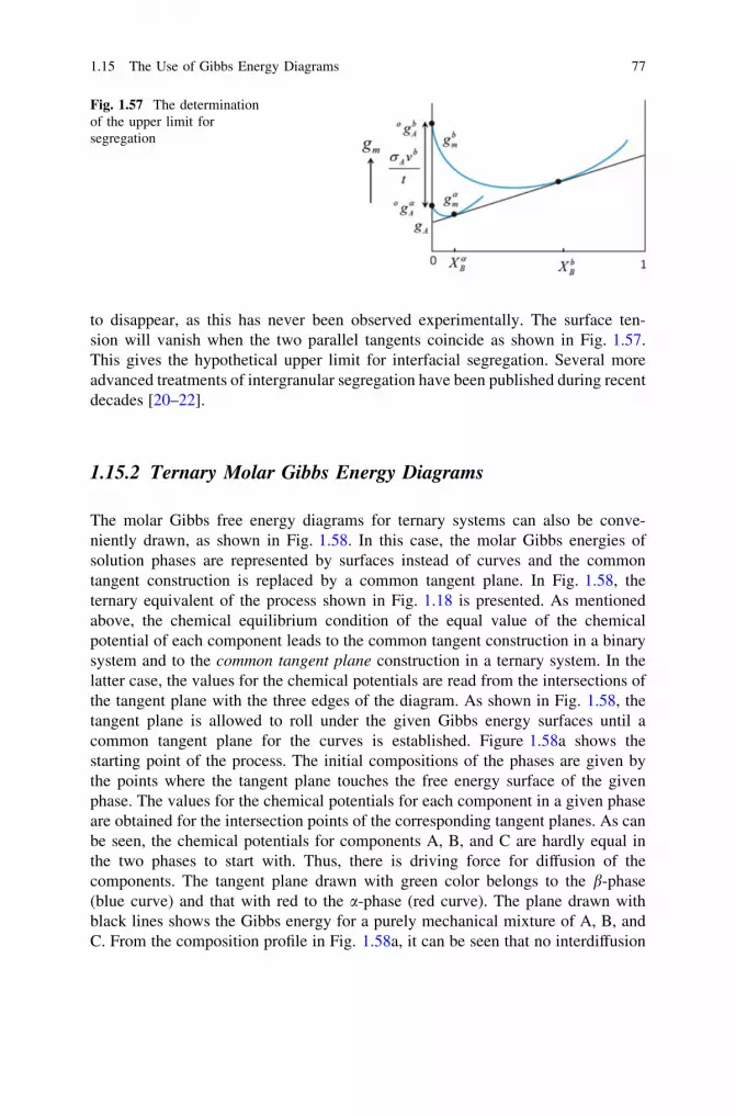
to disappear, as this has never been observed experimentally. The surface ten-sion will vanish when the two parallel tangents coincide as shown in Fig. 1.57.This gives the hypothetical upper limit for interfacial segregation. Several moreadvanced treatments of intergranular segregation have been published during recentdecades [20–22].

1.15.2 Ternary Molar Gibbs Energy Diagrams

The molar Gibbs free energy diagrams for ternary systems can also be conve-niently drawn, as shown in Fig. 1.58. In this case, the molar Gibbs energies ofsolution phases are represented by surfaces instead of curves and the commontangent construction is replaced by a common tangent plane. In Fig. 1.58, theternary equivalent of the process shown in Fig. 1.18 is presented. As mentionedabove, the chemical equilibrium condition of the equal value of the chemicalpotential of each component leads to the common tangent construction in a binarysystem and to the common tangent plane construction in a ternary system. In thelatter case, the values for the chemical potentials are read from the intersections ofthe tangent plane with the three edges of the diagram. As shown in Fig. 1.58, thetangent plane is allowed to roll under the given Gibbs energy surfaces until acommon tangent plane for the curves is established. Figure 1.58a shows thestarting point of the process. The initial compositions of the phases are given bythe points where the tangent plane touches the free energy surface of the givenphase. The values for the chemical potentials for each component in a given phaseare obtained for the intersection points of the corresponding tangent planes. As canbe seen, the chemical potentials for components A, B, and C are hardly equal inthe two phases to start with. Thus, there is driving force for diffusion of thecomponents. The tangent plane drawn with green color belongs to the b-phase(blue curve) and that with red to the a-phase (red curve). The plane drawn withblack lines shows the Gibbs energy for a purely mechanical mixture of A, B, andC. From the composition profile in Fig. 1.58a, it can be seen that no interdiffusion

Fig. 1.57 The determinationof the upper limit forsegregation

1.15 The Use of Gibbs Energy Diagrams 77

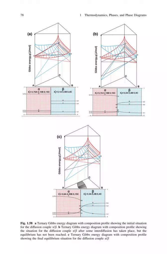
Fig. 1.58 a Ternary Gibbs energy diagram with composition profile showing the initial situationfor the diffusion couple a/b. b Ternary Gibbs energy diagram with composition profile showingthe situation for the diffusion couple a/b after some interdiffusion has taken place, but theequilibrium has not been reached. c Ternary Gibbs energy diagram with composition profileshowing the final equilibrium situation for the diffusion couple a/b

78 1 Thermodynamics, Phases, and Phase Diagrams

has taken place. As can be seen from Fig. 1.58b, the tangent planes start to rollunder the Gibbs free energy surfaces and, consequently, the chemical potentials ofthe components start to change. It is evident that Fig. 1.58b represents an inter-mediate stage in the process as the chemical potentials for components A, B, and Care not yet equal in both phases. From the composition profile of the a/b-diffusioncouple in Fig. 1.58b, it can be seen that the compositions at the interface have beenchanged. Further, it is noticed that only components A and B diffuses in this caseand component C is immobile. The end-member compositions are unaffected bythe diffusion process as required (See Chap. 3 for further discussion). The finalequilibrium situation is given in Fig. 1.58c, in which the common tangent plane isshown. As can be seen, the chemical potentials for the components are now equalat each phase and thus, the chemical equilibrium condition is fulfilled.

Another example from a ternary Gibbs energy diagram is shown in Fig. 1.59which represents the stability of phases in the BiCuSn system at 235 �C. There aretwo intermetallic compounds, (Cu6Sn5 (g) and Cu3Sn (e)), which enter the stableequilibrium at this temperature. A vertical section (SnBieut?Cu) through thisdiagram is shown in Fig. 1.60. As can be seen, the section resembles the Gibbsenergy diagram of the binary Cu-Sn system, but it is not exactly the same. The‘‘tangent lines’’ drawn in the diagram (Fig. 1.60) are not identical to the tangentlines in Fig. 1.52, but are 2D sections through the corresponding tangent planes.

Fig. 1.59 Ternary molarGibbs energy diagram fromthe BiCuSn system at 235 �C[17]

1.15 The Use of Gibbs Energy Diagrams 79

1.16 Interdependence of Chemical Potentials:Gibbs–Duhem Equation

In this section, we shall derive the Gibbs–Duhem relation, which will be useful inproceeding chapters to find the relation between diffusion under chemical potentialgradient with the diffusion in the absence chemical potential gradient as thedriving force. From our point of view, the application of Gibbs–Duhem equation toobtain the change in the chemical potential because of the change in compositionof an alloy is the most important use of the general relation. For the sake ofexplanation, let us consider the free energy versus composition diagram, as shownin Fig. 1.61. First, we consider the point P and from the slope at that we candetermine the chemical potential of elements A and B at that point as lP

A and lPB,

respectively. Now suppose we make a small change in the composition and moveto the point Q. Again from the slope of the free energy at that point, we can find the

chemical potential of elements as lQA and lQ

B . So it is apparent that the change inchemical potential of elements, A and B, because of the change in composition is

�dlA ¼ lQA � lP

A

� �and �dlB ¼ ðlQ

B � lPBÞ, respectively. Further, from any point

P or Q, it can be written that

� dlA

XB

¼ dlB

XA

¼ dðlB � lAÞ1

ð1:130Þ

Fig. 1.60 A vertical sectionthrough the Gibbs energydiagram shown in Fig. 1.59[17]

80 1 Thermodynamics, Phases, and Phase Diagrams

Further, from the slope, we can write

dg

dXB

¼ lB � lA

1ð1:131Þ

Combining Eqs. 1.130 and 1.131 and multiplying XAXB, the expressionbecomes

�XAdlA ¼ XBdlB ¼ XAXB

d2g

dX2B

dXB ð1:132Þ

Further, it can be shown that

d2g

dX2B

¼ d2g

dX2A

ð1:133Þ

It follows that

XAdlA þ XBdlB ¼ 0 ð1:134Þ

Equation 1.134 is known as Gibbs Duhem equation. It illustrates clearly thatchemical potentials, or any other partial thermodynamic properties [5], cannot bechanged independently. On the contrary, for example, in a binary system con-sidered here, when the one chemical potential is changed, the other one mustchange also. This is evident also in ternary systems as shown in Fig. 1.58a–c.Further, we can derive one another useful relation from Eq. 1.134. FromEqs. 1.132 and 1.133 follows

�XA

dlA

dXB

¼ XB

dlB

dXB

¼ XAXB

d2g

dX2B

¼ XAXB

d2g

dX2A

ð1:135Þ

Fig. 1.61 The change inchemical potential because ofthe change in composition isshown to derive the Gibbs–Duhem equation

1.16 Interdependence of Chemical Potentials: Gibbs–Duhem Equation 81

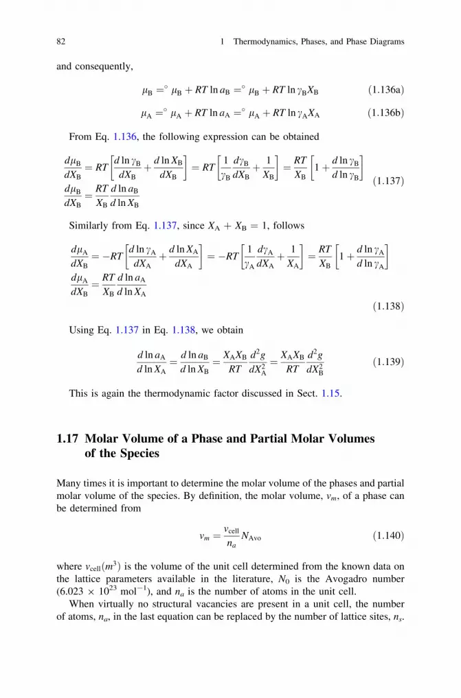
and consequently,

lB ¼� lB þ RT ln aB ¼� lB þ RT ln cBXB ð1:136aÞ

lA ¼� lA þ RT ln aA ¼� lA þ RT ln cAXA ð1:136bÞ

From Eq. 1.136, the following expression can be obtained

dlB

dXB

¼ RTd ln cB

dXB

þ d ln XB

dXB

� ¼ RT

1cB

dcB

dXB

þ 1XB

� ¼ RT

XB

1þ d ln cB

d ln cB

�

dlB

dXB

¼ RT

XB

d ln aB

d ln XB

ð1:137Þ

Similarly from Eq. 1.137, since XA + XB = 1, follows

dlA

dXB

¼ �RTd ln cA

dXA

þ d ln XA

dXA

� ¼ �RT

1cA

dcA

dXA

þ 1XA

� ¼ RT

XB

1þ d ln cA

d ln cA

�

dlA

dXB

¼ RT

XB

d ln aA

d ln XA

ð1:138Þ

Using Eq. 1.137 in Eq. 1.138, we obtain

d ln aA

d ln XA

¼ d ln aB

d ln XB

¼ XAXB

RT

d2g

dX2A

¼ XAXB

RT

d2g

dX2B

ð1:139Þ

This is again the thermodynamic factor discussed in Sect. 1.15.

1.17 Molar Volume of a Phase and Partial Molar Volumesof the Species

Many times it is important to determine the molar volume of the phases and partialmolar volume of the species. By definition, the molar volume, vm, of a phase canbe determined from

vm ¼vcell

naNAvo ð1:140Þ

where vcellðm3Þ is the volume of the unit cell determined from the known data onthe lattice parameters available in the literature, N0 is the Avogadro number(6.023 9 1023 mol-1), and na is the number of atoms in the unit cell.

When virtually no structural vacancies are present in a unit cell, the numberof atoms, na, in the last equation can be replaced by the number of lattice sites, ns.

82 1 Thermodynamics, Phases, and Phase Diagrams

We can neglect the amount of thermal vacancies, since this number is very small.On the other hand, when constitutional vacancies are created in the structure and ifthe number is appreciable, we should consider this for the calculation of molarvolumes. In this case, we can write na ¼ ns � nV , with nV being the number ofvacancies present in the unit cell.

So, when there are no structural vacancies present in the structure, the calculationof molar volume is rather straightforward. However, for further clarification, welike to extend our discussion to the calculation which contains structural vacancies.For this purpose, we consider the B2 NiAl phase in an Ni–Al system. The homo-geneity range of the B2 phase is shown in Fig. 1.62. It can be seen that there is awide homogeneity range on both sides of the stoichiometry. As will be discussed inChap. 2, deviation from the homogeneity in the Ni-rich side is achieved by theNi-antisite defects (NiAl that is Ni atom occupying the sublattice belongs to Alatom), whereas deviation in the Al-rich side is achieved by the presence of tripledefect (2VNi þ NiAl composed of two vacancies in sublattice belonging to Niatoms and one Ni atom occupying a site in a sublattice belonging to Al atoms).

Fig. 1.62 The change in a lattice parameter and b vacancy concentration of NiAl phase andc molar volume of the phase (a and b are from [23])

1.17 Molar Volume of a Phase and Partial Molar Volumes of the Species 83

So to calculate the molar volume in the Ni-rich side is straightforward and thenumber of lattice positions can be used to count the number of atoms. However, inthe Al-rich side, we need to consider the number of antisites for the calculation ofmolar volume. The molar volume of the phase at different compositions can becalculated from the available data on the lattice parameter and vacancy concen-tration, as shown in Fig. 1.62a and b, respectively. The calculated molar volume ofthe phase is shown in Fig. 1.62c.

The partial molar volume of the species can be defined as the change in molarvolume because of the addition of a very small amount of the species. The partialmolar volume of the species Að�vAÞ and Bð�vBÞ is related with the molar volume of aphase, or an alloy (vm) is related by

vm ¼ XA�vA þ XB�vB ð1:141Þ

Thus, the partial molar volume of the species at a particular composition, XB, canbe calculated by taking slope at v from the molar volume versus compositiondiagram, as shown in Fig. 1.63. The values �vA and �vB are the partial molar volumesof the species A and B, respectively, at XB. This is a property diagram similar to thatwhich was extensively used in Sect. 1.15 (the molar Gibbs energy diagram).

1.18 Few Standard Thermodynamic Relations

Derivations for a few relations can be found in [24]. We have previously shownthat the mole fraction and the atomic fraction are the same in the systems we haveconsidered. We commonly present the diffusion data with respect to atomicfraction or atomic percentage, and we shall use them for further derivations.

NA þ NB ¼ 1 ð1:142Þ

Fig. 1.63 The determinationof partial molar volume of thespecies, A and B in a binarysystem is shown

84 1 Thermodynamics, Phases, and Phase Diagrams

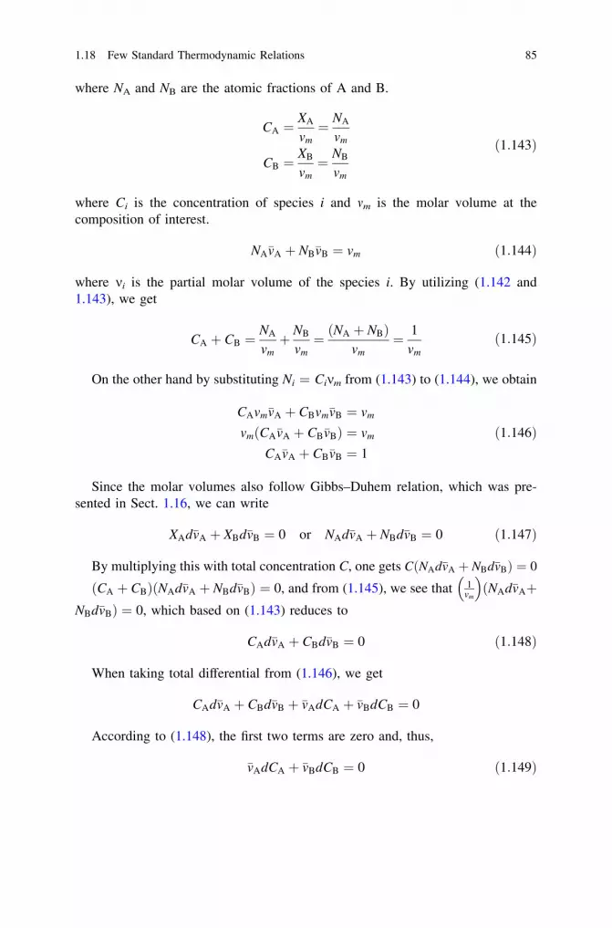
where NA and NB are the atomic fractions of A and B.

CA ¼XA

vm¼ NA

vm

CB ¼XB

vm¼ NB

vm

ð1:143Þ

where Ci is the concentration of species i and mm is the molar volume at thecomposition of interest.

NA�vA þ NB�vB ¼ vm ð1:144Þ

where mi is the partial molar volume of the species i. By utilizing (1.142 and1.143), we get

CA þ CB ¼NA

vmþ NB

vm¼ NA þ NBð Þ

vm¼ 1

vmð1:145Þ

On the other hand by substituting Ni = Cimm from (1.143) to (1.144), we obtain

CAvm�vA þ CBvm�vB ¼ vm

vm CA�vA þ CB�vBð Þ ¼ vm

CA�vA þ CB�vB ¼ 1

ð1:146Þ

Since the molar volumes also follow Gibbs–Duhem relation, which was pre-sented in Sect. 1.16, we can write

XAd�vA þ XBd�vB ¼ 0 or NAd�vA þ NBd�vB ¼ 0 ð1:147Þ

By multiplying this with total concentration C, one gets CðNAd�vA þ NBd�vBÞ ¼ 0

ðCA þ CBÞðNAd�vA þ NBd�vBÞ ¼ 0, and from (1.145), we see that 1vm

ffi �NAd�vAþð

NBd�vBÞ ¼ 0, which based on (1.143) reduces to

CAd�vA þ CBd�vB ¼ 0 ð1:148Þ

When taking total differential from (1.146), we get

CAd�vA þ CBd�vB þ �vAdCA þ �vBdCB ¼ 0

According to (1.148), the first two terms are zero and, thus,

�vAdCA þ �vBdCB ¼ 0 ð1:149Þ

1.18 Few Standard Thermodynamic Relations 85

When we consider that molar volume is not constant

dCA ¼�vB

v2m

� �dNA

dCB ¼�vA

v2m

� �dNB

ð1:150Þ

References

1. K. Denbigh, The Principles of chemical equilibrium, 3rd ed., Cambridge University Press,Cambridge, U.K, 1978.

2. E.A. Guggenheim, Thermodynamics, Elsevier Science, The Netherlands, 1967.3. D. Kondepudi and I. Prigogine, Modern Thermodynamics From Heat Engines to Dissipative

Structures, Wiley, 1998.4. P. Atkins and J. DePaula, Physical Chemistry, Macmillan Higher Education, 2009.5. N. A. Gokcen, Thermodynamics, Techscience incorporated, 1975.6. J.K. Kivilahti, Theory of metallic solutions, Otakustantamo, 1982, (in Finnish).7. L. Darken and R. Gurry, Physical Chemistry of Metals, McGraw-Hill, (1953).8. G.N. Lewis and M. Randall, Thermodynamics, revised by K. Pitzer and L. Brewer, McGraw-

Hill, 1961.9. D. Gaskell, Introduction to Metallurgical Thermodynamics, McGraw-Hill, Tokyo, 1973.

10. M. Hillert, Phase Equilibria, Phase Diagrams and Phase Transformations: TheirThermodynamic Basis, Cambridge Univ. Press, 1998.

11. H. Lukas, S. Fries, and B. Sundman (2007) Computational Thermodynamics- The CalphadMethod, Cambridge University Press (2007).

12. Rönkä K., van Loo F.J.J. and. Kivilahti J.K, Metal. Mater. Trans. A, 29A (1998) 2951.13. T. Mattila, V. Vuorinen and J.K. Kivilahti, J. of Mater. Res. 19 (2004) 3214.14. Laurila T., Zeng K., Molarius J., Suni I., and Kivilahti J.K., Journal of Applied Physics 91

(2002) 5391.15. Hillert M., ‘‘The Uses of Gibbs Free Energy-Composition Diagrams’’, in Lectures on the

Theory of Phase Transformations, (Ed. H.I. Aaronson, The Metallurgical Society of theAIME, (1975)).

16. C. Cserhati, U. Ugaste, M. van Dal, N. Lousberg, A. Kodentsov, and F.J.J. van Loo, Defectand Diffusion Forum 194-199 (2001) 189.

17. T. Laurila, V. Vuorinen and J.K Kivilahti, Materials Science and Engineering – R, R49, (1-2),pp. 1-60, (2005).

18. Laurila T, Vuorinen V. and Paulasto-Kröckel M, Materials Science and Engineering – R, R68(2010) 1-38.

19. R. Wang and Y. Kim, Metall Trans 5 (1974) 1973.20. E. Hondros and M. Seah, Metall. Trans. A, 8A (1977) 1363.21. M. Guttmann, Metall. Trans. A 8A (1977) 1383.22. E. Guggenheim, Trans. Faraday Soc, 36 (1940) 397.23. Y.A. Chang and J.P. Neumann, Prog. Solid State Chem. 14 (1982) 221.24. L. Trimble, D. Finn and A. Cosgarea, Acta Metallurgica 13 (1965) 501.

86 1 Thermodynamics, Phases, and Phase Diagrams

Chapter 2Structure of Materials

In this chapter, we will briefly go through the hierarchical structure of materials.First, the atomic bonding and crystal structures are covered briefly. Then, theemphasis is placed on the presence of different types of defects and imperfections.Since point defects provide the fundamental basis for understanding the atomicmechanisms of diffusion, they are discussed in detail. In addition, the crystalstructures including also the defect structures of intermediate phases and orderedbinary intermetallics are quantitatively presented.

2.1 Hierarchical Structure of Materials

Most properties are actually highly structure sensitive. Therefore, it is of utmostimportance to understand the basis for the structure of materials to be able tocontrol the properties and reliability of engineering materials. Microstructure is ageneral term used to cover a wide range of structural features, ranging from thosevisible to the naked eye (for instance, macrostructure) to those correspondingto the inter-atomic distances in the crystal lattice (for instance, nanostructure).In other words, the size scale of the structural features ranges about 10 orders ofmagnitude. Therefore, in order to observe the structural features at these differentscales, as shown in Fig. 2.1 [1], adequate resolving power is required.

Frequently, a large variety of structural features on different levels is note-worthy. Therefore, in the following chapters, the hierarchical structure of materialsis presented.

2.2 Atomic Bonding

An atom can exist in different energy states according to the kind of interaction it haswith neighboring atoms. The nature of this interaction is defined by the type ofatomic bonding. The bonds can be categorized into two classes according to thebond energy. The primary bonds ([100 kJ/mol) are ionic, covalent, and metallic.

A. Paul et al., Thermodynamics, Diffusion and the Kirkendall Effect in Solids,DOI: 10.1007/978-3-319-07461-0_2, � Springer International Publishing Switzerland 2014

87

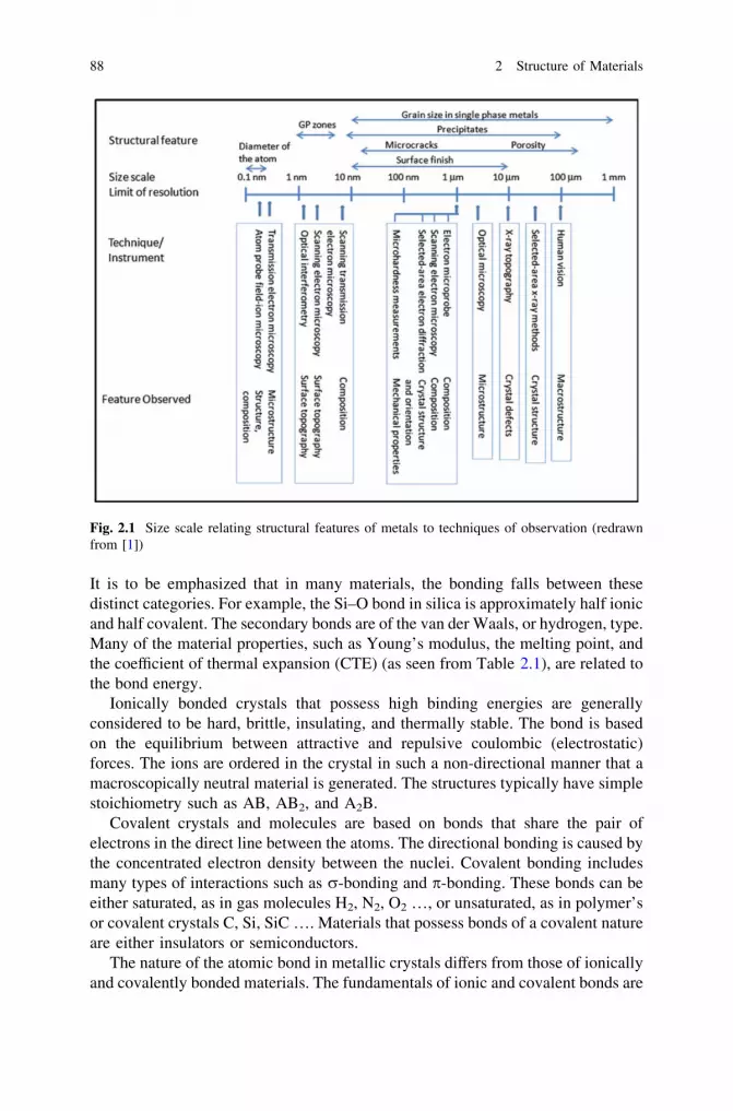
It is to be emphasized that in many materials, the bonding falls between thesedistinct categories. For example, the Si–O bond in silica is approximately half ionicand half covalent. The secondary bonds are of the van der Waals, or hydrogen, type.Many of the material properties, such as Young’s modulus, the melting point, andthe coefficient of thermal expansion (CTE) (as seen from Table 2.1), are related tothe bond energy.

Ionically bonded crystals that possess high binding energies are generallyconsidered to be hard, brittle, insulating, and thermally stable. The bond is basedon the equilibrium between attractive and repulsive coulombic (electrostatic)forces. The ions are ordered in the crystal in such a non-directional manner that amacroscopically neutral material is generated. The structures typically have simplestoichiometry such as AB, AB2, and A2B.

Covalent crystals and molecules are based on bonds that share the pair ofelectrons in the direct line between the atoms. The directional bonding is caused bythe concentrated electron density between the nuclei. Covalent bonding includesmany types of interactions such as r-bonding and p-bonding. These bonds can beeither saturated, as in gas molecules H2, N2, O2 …, or unsaturated, as in polymer’sor covalent crystals C, Si, SiC …. Materials that possess bonds of a covalent natureare either insulators or semiconductors.

The nature of the atomic bond in metallic crystals differs from those of ionicallyand covalently bonded materials. The fundamentals of ionic and covalent bonds are

Fig. 2.1 Size scale relating structural features of metals to techniques of observation (redrawnfrom [1])

88 2 Structure of Materials

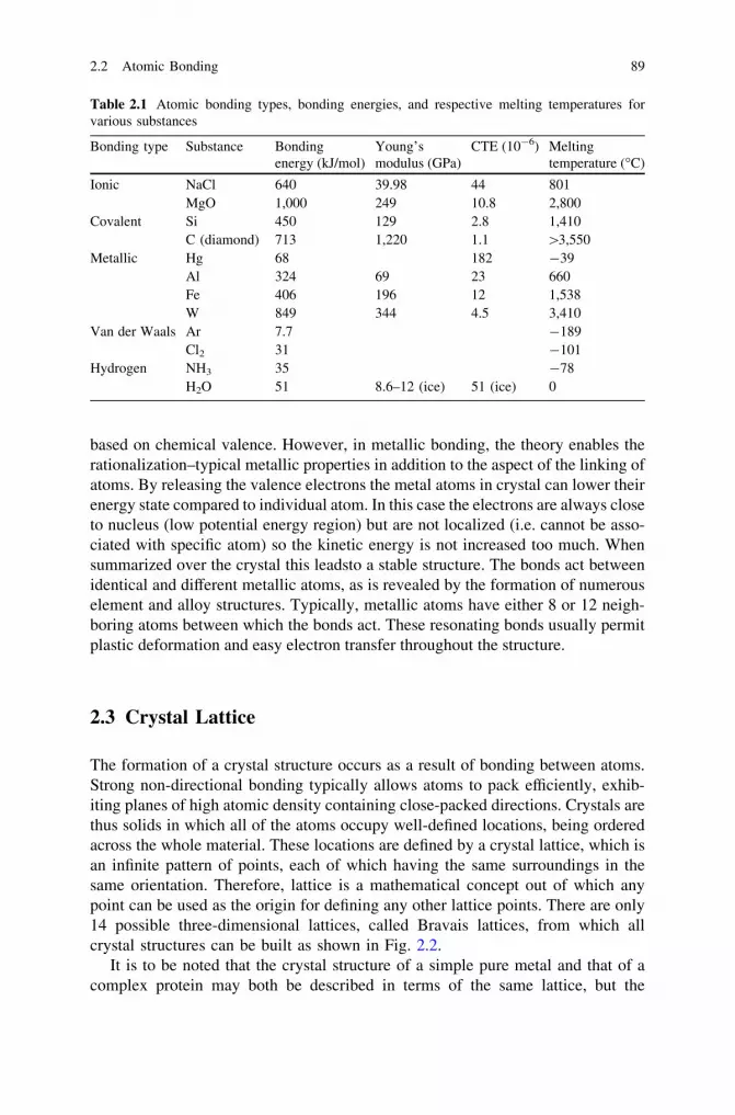
based on chemical valence. However, in metallic bonding, the theory enables therationalization–typical metallic properties in addition to the aspect of the linking ofatoms. By releasing the valence electrons the metal atoms in crystal can lower theirenergy state compared to individual atom. In this case the electrons are always closeto nucleus (low potential energy region) but are not localized (i.e. cannot be asso-ciated with specific atom) so the kinetic energy is not increased too much. Whensummarized over the crystal this leadsto a stable structure. The bonds act betweenidentical and different metallic atoms, as is revealed by the formation of numerouselement and alloy structures. Typically, metallic atoms have either 8 or 12 neigh-boring atoms between which the bonds act. These resonating bonds usually permitplastic deformation and easy electron transfer throughout the structure.

2.3 Crystal Lattice

The formation of a crystal structure occurs as a result of bonding between atoms.Strong non-directional bonding typically allows atoms to pack efficiently, exhib-iting planes of high atomic density containing close-packed directions. Crystals arethus solids in which all of the atoms occupy well-defined locations, being orderedacross the whole material. These locations are defined by a crystal lattice, which isan infinite pattern of points, each of which having the same surroundings in thesame orientation. Therefore, lattice is a mathematical concept out of which anypoint can be used as the origin for defining any other lattice points. There are only14 possible three-dimensional lattices, called Bravais lattices, from which allcrystal structures can be built as shown in Fig. 2.2.

It is to be noted that the crystal structure of a simple pure metal and that of acomplex protein may both be described in terms of the same lattice, but the

Table 2.1 Atomic bonding types, bonding energies, and respective melting temperatures forvarious substances

Bonding type Substance Bondingenergy (kJ/mol)

Young’smodulus (GPa)

CTE (10-6) Meltingtemperature (�C)

Ionic NaCl 640 39.98 44 801MgO 1,000 249 10.8 2,800

Covalent Si 450 129 2.8 1,410C (diamond) 713 1,220 1.1 [3,550

Metallic Hg 68 182 -39Al 324 69 23 660Fe 406 196 12 1,538W 849 344 4.5 3,410

Van der Waals Ar 7.7 -189Cl2 31 -101

Hydrogen NH3 35 -78H2O 51 8.6–12 (ice) 51 (ice) 0

2.2 Atomic Bonding 89

number of atoms allocated to each lattice point (i.e., motifs) can vary from one tofew thousands. Thus, a crystal structure is composed of a lattice plus a motif. Theunit cells can be either simply primitive, body centered, face centered, or basecentered. A primitive unit cell contains only a single lattice point, whereas a base-centered and body-centered cell contains two lattice points and a face-centered cellcontains four lattice points.

The fundamentals of the crystal symmetry, planes, and directions as well astheir indexing and nomenclature can be found from many excellent textbooks, forinstance [2, 3]. Therefore, only the most common crystal types for pure metals andalloys, i.e., the close-packed face-centered cubic (FCC), body-centered cubic(BCC), and hexagonal close-packed (HCP) crystals, are presented in brief here.The atomic arrangement of the FCC and HCP crystals are shown in Fig. 2.3, wherethe location of the atom in the third layer defines whether the structure becomeshexagonal close packed (left, ABAB… arrangement) or FCC (right, ABCABC…arrangement). BCC crystals are not closely packed, and therefore, they containmore empty spaces (tetrahedral and octahedral interstitial sites) as can be seenfrom Fig. 2.4 and Table 2.2.

Fig. 2.2 Bravais lattices

90 2 Structure of Materials

2.4 Grain Structure

Grain structure is composed of small crystals that form a three-dimensionalaggregate. The main characteristics are grain size, shape, and grain shape anisot-ropy. An impingement grain structure forms when grains grow until they meet orimpinge, for example, during secondary recrystallization, producing characteristicragged interfaces. A columnar grain structure is produced by unidirectional growth

Fig. 2.3 Close-packed arrangements

Fig. 2.4 Octahedral (O) and tetrahedral (T) interstitial sites in FCC-, HCP-, and BCC-typemetals

2.4 Grain Structure 91

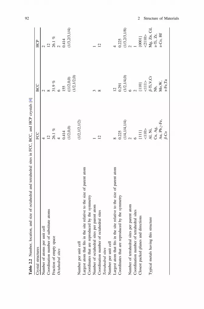
Tab

le2.

2N

umbe

r,lo

cati

on,

and

size

ofoc

tahe

dral

and

tetr

ahed

ral

site

sin

FC

C,

BC

C,

and

HC

Pcr

ysta

ls[4

]

Cry

stal

stru

ctur

esF

CC

BC

CH

CP

Num

ber

ofat

oms

per

unit

cell

42

2C

oord

inat

ion

num

ber

ofsu

bsti

tute

atom

s12

812

Fra

ctio

nof

empt

ysp

ace

26.1

%31

.9%

26.1

%O

ctah

edra

lsi

tes

46

20.

414

155

0.41

4(1

/2,0

,0)

((1/

2,0,

0)(1

/3,2

/3,1

/4)

(1/2

,1/2

,0)

(1/2

,1/2

,1/2

)N

umbe

rpe

run

itce

llL

arge

stat

omth

atfi

tsin

the

site

rela

tive

toth

esi

zeof

pare

ntat

omC

oord

inat

esth

atar

ere

prod

uced

byth

esy

mm

etry

Num

ber

ofoc

tahe

dral

site

spe

rpa

rent

atom

13

1C

oord

inat

ion

num

ber

ofoc

tahe

dral

site

s12

812

Tet

rahe

dral

site

sN

umbe

rpe

run

itce

llL

arge

stat

omth

atfi

tsin

the

site

rela

tive

toth

esi

zeof

pare

ntat

om8

124

Coo

rdin

ates

that

are

repr

oduc

edby

the

sym

met

ry0.

225

0.29

10.

225

(1/4

,1/4

,1/4

)(1

/2,1

/4,0

)(1

/3,2

/3,1

/8)

Num

ber

ofte

trah

edra

lsi

tes

per

pare

ntat

om2

62

Coo

rdin

atio

nnu

mbe

rof

tetr

ahed

ral

site

s6

21

Clo

sest

pack

edpl

anes

and

dire

ctio

ns{1

11}

{110

}{0

001}

\11

0[\

111[

\21

10[

Typ

ical

met

als

havi

ngth

isst

ruct

ure

Al,

Ni,

b-T

i,V,C

rM

g,Z

n,C

d,C

u,A

g,N

b,a-

Ti,

Zr,

Au,

Pb,

c-F

e,M

o,W

,a-

Co,

Hf

b-C

oa-

Fe,

Ta

92 2 Structure of Materials

such as in solidification or electrochemical plating (See Fig. 2.5a). Equiaxed grainscan be formed by several processes such as recrystallization (See Fig. 2.5b) orsolidification.

2.5 Defects

Many physical (especially mechanical) properties of solid materials are primarilybased on the presence of different types of defects and imperfections. In otherwords, often specific material characteristics are deliberately fashioned by intro-ducing a controlled amount of particular defect. The classification of crystallineimperfections is generally made according to either the geometry or dimension-ality of the defect. Thus, the defects are typically divided into (i) point defects,which are related to a single or a few atomic positions, (ii) linear (or one-dimensional) defects, (iii) two-dimensional defects such as surfaces, interfaces,and different types of boundaries, and (iv) volume defects including inclusions,cracks, voids, and pores.

2.5.1 Point Defects

Point defects are central to gain an understanding of the atomic mechanisms ofdiffusion, and therefore, they are discussed in detail. There can be a few types ofpoint defects present in the structure in an equilibrium condition (e.g., vacancies,impurities, and antistructure). Typically, in ‘‘pure’’ elements, vacancies andimpurities are present in the structure. First, let us discuss the defects present in thepure elements and then turn to consider the defects present in the ordered phases.

Fig. 2.5 Cross-polarized optical images from a columnar electrochemically plated Sn crystalsbetween Cu equiaxed SnBi alloy and b recrystallized SAC solder interconnection after 3,000cycles during a -40 �C () +125 �C thermal cycling test

2.4 Grain Structure 93

2.5.1.1 Equilibrium Vacancy Concentration in Pure Elements

The presence of vacancies in a pure element can be estimated using the same kindof treatment as was followed to find the free energy in a binary system, asexplained previously in Sect. 1.8. The formation of vacancies can be explained, asshown in Fig. 2.6, where one atom diffuses from the interior of the crystal to thesurface leaving a vacant site (the Schottky defect). There is another type of pointdefect, called the Frenkel defect, which is formed when an atom from a lattice sitemoves into an interstitial site thus leaving an empty space (vacancy) behind. Forthe sake of analysis, the presence of vacancies (V) in the element A can bevisualized as a binary system of A and V. Now, the creation of vacancies isassociated with the increase in internal energy because of broken bonds around thevacancies. In general, the equilibrium number of vacancies is so small that we canneglect the interaction between them. Thus, if we consider that the number ofvacancies to be very small, then the increase in enthalpy resulting from the for-mation of vacancies can be written as

Dh � XvDhv ð2:1Þ

Here, DXv is the mole fraction of the vacancy and Dhv is the increase inenthalpy caused by one mole of vacancies.

Factors contributing to Dhv in metals are as follows:

1. Change in the volume. When an atom is removed from the center of the latticeand is placed at the surface, there is no change in the surface area, but rather anincrease in the volume. This decreases the average energy of the electrons,giving a negative change in energy.

2. The removal of an atom leaves behind one atomic volume devoid of charge.Free electrons around the site tend to flow into this vacancy. Since there in nopositive charge in the vacant site, the electrostatic energy is increased. Tominimize this effect, there will be a sharp change in the electron density, whichimposes in the end a higher kinetic energy for the electrons and an increase inthe energy of the lattice.

3. When an atom is removed, the surrounding ions will relax into the vacancydecreasing slightly the energy of the final lattice.

Fig. 2.6 Movement of atoms to create a vacancy at the interior

94 2 Structure of Materials

If we now consider the total effect of all the above-mentioned three contribu-tions, it is to be found that the sum is positive Dhv; thus, it costs energy to form avacancy.

The entropy can be divided into two parts, namely thermal entropy and config-urational entropy (Sect. 1.5). Now, if we consider the change in entropy resultingfrom the mixing of vacancies with the pure element, there will be two types ofcontributions. First, there will be the change in the vibration pattern of the atomsnext to vacancies because of extra free space. The increase in entropy caused by theextra freedom of vibration can be written as XvDsv. Here, Dsv is the increase inentropy for one mole of vacancies. Furthermore, there will be a change in con-figurational entropy considering the mixing of A and V and this can be expressedas (Note that we are considering XA þ Xv ¼ 1)

Dsmix ¼ �R Xv ln Xv þ 1� Xvð Þ ln 1� Xvð Þ½ � ð2:2Þ

So the total change in entropy can be written as

Ds ¼ DsvXv � R Xv ln Xv þ 1� Xvð Þ ln 1� Xvð Þ½ � ð2:3Þ

Thus, the total free energy of the system containing vacancies can be written as

G ¼ GA þ DG ð2:4Þ

where GA is the free energy of the defect free system of pure element A. DG is thechange in free energy and can be expressed as (Sect. 1.3)

DG ¼ DH � TDS ð2:5Þ

From Eqs. 2.2 to 2.5, the total free energy of the system can be written as

G ¼ GA þ XvDHv � T DSv � R Xv ln Xv þ 1� Xvð Þ ln 1� Xvð Þ½ �f g ð2:6Þ

The change in enthalpy, entropy, and free energy due to an increasing numberof vacancies can be seen in Fig. 2.7. It is apparent that DH increases linearly withthe increase in vacancies, whereas �TDS decreases very rapidly in the beginning,but the rate of change decreases drastically. So it should be clear that in thebeginning, the total free energy of the system will decrease with the creation ofvacancies, but after a certain range, the free energy will start to increase becauseDH will start dominating. The system will therefore go through a minimum. Wehave seen before in Sect. 1.2 that a system will stay in equilibrium when it hasminimum free energy. So we can state that the system will remain in equilibriumwith free energy Ge. Further, we know that in the equilibrium condition,

2.5 Defects 95

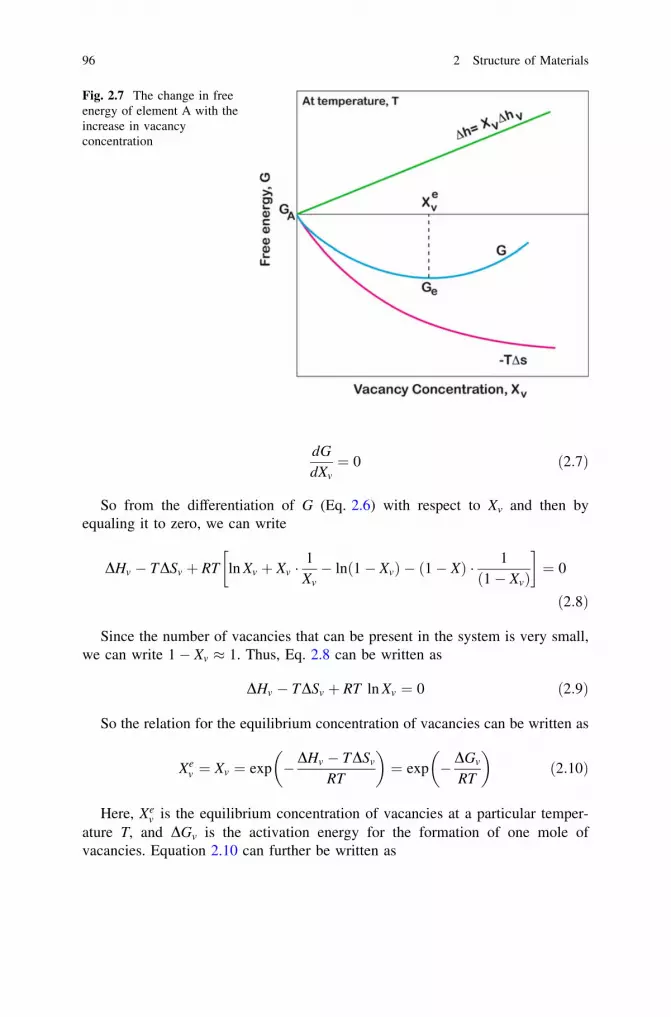
dG

dXv¼ 0 ð2:7Þ

So from the differentiation of G (Eq. 2.6) with respect to Xv and then byequaling it to zero, we can write

DHv � TDSv þ RT ln Xv þ Xv �1Xv� ln 1� Xvð Þ � 1� Xð Þ � 1

1� Xvð Þ

� �¼ 0

ð2:8Þ

Since the number of vacancies that can be present in the system is very small,we can write 1� Xv � 1. Thus, Eq. 2.8 can be written as

DHv � TDSv þ RT ln Xv ¼ 0 ð2:9Þ

So the relation for the equilibrium concentration of vacancies can be written as

Xev ¼ Xv ¼ exp �DHv � TDSv

RT

� �¼ exp �DGv

RT

� �ð2:10Þ

Here, Xev is the equilibrium concentration of vacancies at a particular temper-

ature T, and DGv is the activation energy for the formation of one mole ofvacancies. Equation 2.10 can further be written as

Fig. 2.7 The change in freeenergy of element A with theincrease in vacancyconcentration

96 2 Structure of Materials

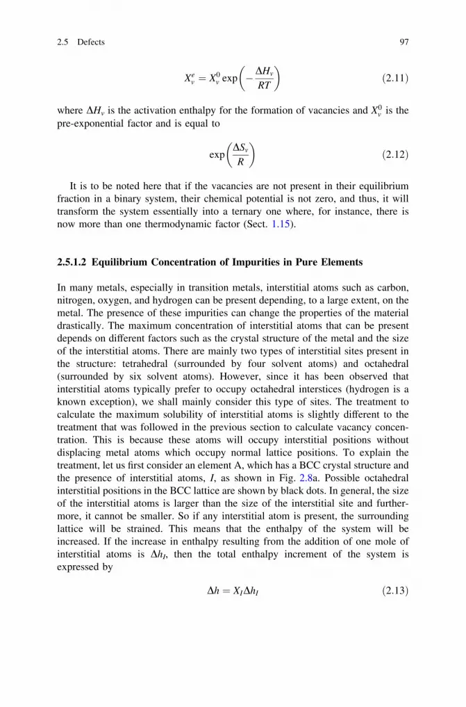
Xev ¼ X0

v exp �DHv

RT

� �ð2:11Þ

where DHv is the activation enthalpy for the formation of vacancies and X0v is the

pre-exponential factor and is equal to

expDSv

R

� �ð2:12Þ

It is to be noted here that if the vacancies are not present in their equilibriumfraction in a binary system, their chemical potential is not zero, and thus, it willtransform the system essentially into a ternary one where, for instance, there isnow more than one thermodynamic factor (Sect. 1.15).

2.5.1.2 Equilibrium Concentration of Impurities in Pure Elements

In many metals, especially in transition metals, interstitial atoms such as carbon,nitrogen, oxygen, and hydrogen can be present depending, to a large extent, on themetal. The presence of these impurities can change the properties of the materialdrastically. The maximum concentration of interstitial atoms that can be presentdepends on different factors such as the crystal structure of the metal and the sizeof the interstitial atoms. There are mainly two types of interstitial sites present inthe structure: tetrahedral (surrounded by four solvent atoms) and octahedral(surrounded by six solvent atoms). However, since it has been observed thatinterstitial atoms typically prefer to occupy octahedral interstices (hydrogen is aknown exception), we shall mainly consider this type of sites. The treatment tocalculate the maximum solubility of interstitial atoms is slightly different to thetreatment that was followed in the previous section to calculate vacancy concen-tration. This is because these atoms will occupy interstitial positions withoutdisplacing metal atoms which occupy normal lattice positions. To explain thetreatment, let us first consider an element A, which has a BCC crystal structure andthe presence of interstitial atoms, I, as shown in Fig. 2.8a. Possible octahedralinterstitial positions in the BCC lattice are shown by black dots. In general, the sizeof the interstitial atoms is larger than the size of the interstitial site and further-more, it cannot be smaller. So if any interstitial atom is present, the surroundinglattice will be strained. This means that the enthalpy of the system will beincreased. If the increase in enthalpy resulting from the addition of one mole ofinterstitial atoms is DhI, then the total enthalpy increment of the system isexpressed by

Dh ¼ XIDhI ð2:13Þ

2.5 Defects 97

where XI ¼ nIN0

is the mole fraction of the interstitial atoms present in the system

and nI is the total number of interstitial atoms. Again, there will be two differenttypes of contribution to entropy. The first contribution comes from the fact thatthe vibration of atoms A next to the interstitial atoms will change from a normalmode of vibration and will be more random and irregular because of the dis-tortion of the lattice. If we consider that the change of the entropy due to thechange of vibration pattern is DSI for one mole of interstitial atoms, then for XI

mole of interstitial atoms the change in entropy will be XIDSI. Further, there willalso be an increase in entropy because of the mixing of the solvent and interstitialatoms. Now, from the crystal structure, as shown in Fig. 2.8a for two solventatoms, there are six sites for interstitial atoms. Additionally, we can write that foreach A atom, there are three sites for interstitial atoms. So if we consider thatthere are N0 numbers of A atoms, then there will be 3N0 numbers of sitesavailable for interstitial atoms. In another sense, we can say that nI atoms willrandomly occupy nI sites from 3N0 sites. Following statistical thermodynamics,the entropy of mixing can be written as

DSmix ¼ S� S0 ¼ k ln w� k ln 1 ¼ k ln w ð2:14Þ

where w is roughly the measure of randomness, S0 is the entropy before mixing,and S is the entropy after mixing. Since in the case of a pure element, there is onlyone way by which atoms can be arranged, we can write w = 1. If we consider thatinterstitial atoms will choose their sites completely randomly, then we can write

w ¼ 3N0!

nI! 3N0 � nIð Þ! ð2:15Þ

Fig. 2.8 Octahedral interstitial positions are shown by black dots in a BCC unit cell and b FCCunit cell

98 2 Structure of Materials

According to Stirling’s approximation,

ln N! ¼ N ln N � N

Following Stirling’s approximation, Eq. 2.15 can be derived as

DSmix ¼ k 3N0 ln 3N0 � nI ln nI � 3N0 � nIð Þ ln 3N0 � nIð Þ½ � ð2:16Þ

Furthermore, Eq. 2.16 can be written as

DSmix ¼ R 3 ln 3N0 �nI

N0ln nI �

3N0 � nI

N0ln 3N0 � nIð Þ

� �

DSmix ¼ R 3 ln3N0

3N0 � nI

� nI

N0ln

nI

3N0 � nI

� � ð2:17Þ

Further, replacing XI ¼ nI=N0, Eq. 2.17 can be written as

DSmix ¼ R 3 ln3

3� XI

� XI lnXI

3� XI

� �ð2:18Þ

So the total free entropy change can be written as

DS ¼ XIDSI þ R 3 ln3

3� XI

� XI lnXI

3� XI

� �ð2:19Þ

Moreover, the total free energy of the system after the addition of interstitialatoms can be written as

G ¼ GA þ DG ¼ GA þ DH � TDSI

G ¼ GA þ XIDHI � TXIDSI � RT 3 ln3

3� XI

� XI lnXI

3� XI

� � ð2:20Þ

As we have seen in the previous section that the equilibrium concentration of

interstitial atoms can be found from dGdXI¼ 0. Thus,

DHI � TDSI � RT � 33� XI

� XI

XI

� ln XI þ ln 3� XIð Þ � XI

3� XI

� �¼ 0

DHI � TDSI þ RT lnXI

3� XI

¼ 0

ð2:21Þ

Further, the activation energy for the interstitial atom additions can be writtenas DgI ¼ DHI � TDSI. Since we have considered that the concentration of impu-rities is much less, we can write 3� XI � 3. So Eq. 2.21 can be written as

2.5 Defects 99

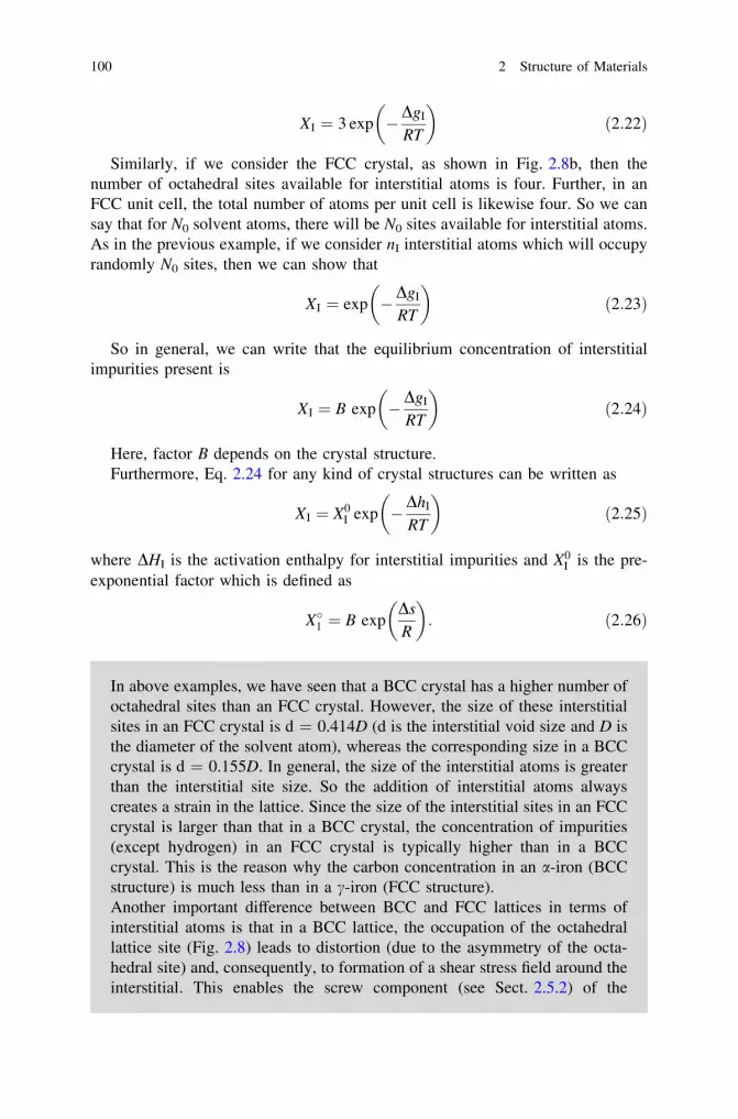
XI ¼ 3 exp �DgI

RT

� �ð2:22Þ

Similarly, if we consider the FCC crystal, as shown in Fig. 2.8b, then thenumber of octahedral sites available for interstitial atoms is four. Further, in anFCC unit cell, the total number of atoms per unit cell is likewise four. So we cansay that for N0 solvent atoms, there will be N0 sites available for interstitial atoms.As in the previous example, if we consider nI interstitial atoms which will occupyrandomly N0 sites, then we can show that

XI ¼ exp �DgI

RT

� �ð2:23Þ

So in general, we can write that the equilibrium concentration of interstitialimpurities present is

XI ¼ B exp �DgI

RT

� �ð2:24Þ

Here, factor B depends on the crystal structure.Furthermore, Eq. 2.24 for any kind of crystal structures can be written as

XI ¼ X0I exp �DhI

RT

� �ð2:25Þ

where DHI is the activation enthalpy for interstitial impurities and X0I is the pre-

exponential factor which is defined as

X�1 ¼ B expDs

R

� �: ð2:26Þ

In above examples, we have seen that a BCC crystal has a higher number ofoctahedral sites than an FCC crystal. However, the size of these interstitialsites in an FCC crystal is d = 0.414D (d is the interstitial void size and D isthe diameter of the solvent atom), whereas the corresponding size in a BCCcrystal is d = 0.155D. In general, the size of the interstitial atoms is greaterthan the interstitial site size. So the addition of interstitial atoms alwayscreates a strain in the lattice. Since the size of the interstitial sites in an FCCcrystal is larger than that in a BCC crystal, the concentration of impurities(except hydrogen) in an FCC crystal is typically higher than in a BCCcrystal. This is the reason why the carbon concentration in an a-iron (BCCstructure) is much less than in a c-iron (FCC structure).Another important difference between BCC and FCC lattices in terms ofinterstitial atoms is that in a BCC lattice, the occupation of the octahedrallattice site (Fig. 2.8) leads to distortion (due to the asymmetry of the octa-hedral site) and, consequently, to formation of a shear stress field around theinterstitial. This enables the screw component (see Sect. 2.5.2) of the

100 2 Structure of Materials

dislocations (which possesses only the shear stress component) to interactwith the stress field created. As in iron, for instance, at low temperatures, themajority of dislocations are of the screw type (or have the majority of thescrew component), and this leads to differences in the mechanical propertiesof the BCC and FCC forms of iron.

2.5.2 Linear Defects

Dislocations, which are the most typical linear (or one-dimensional) defects, andtheir ability to move define the ductility (plasticity) of metals and explain why thestrength of a metal crystal is far less than the theoretical strength calculated on thebasis of the bond strength between the metal atoms. During typical plastic defor-mation, dislocations are formed by the Frank-Read source with the rate of *106/s.Due to the force (stress), the dislocations glide along the close-packed crystal planes.When the dislocation density of a material is increased, also the internal energy isincreased more than the entropy. Therefore, the dislocations are not stable and tend toannihilate or escape from the crystal. The decrease in ductility and increase instrength are related to the interactions between the dislocations as well as betweenthe dislocations and other obstacles to movement such as precipitations or grainboundaries. At high homologous temperatures (T[0.45 Tm), dislocations can alsoclimb, which increases the degrees of freedom of movement, leading to lowerstrength and higher ductility. In addition, many different types of crystals react atincreased rates at the points where dislocations intersect the surface.

Even though the plastic deformation occurring via dislocation movement isqualitatively fully comprehended in macro- and microcrystalline materials, thequantitative analyses still remain incomplete [5]. This is due to the difficulties inaveraging the interactions between dislocations and the other mechanisms con-tributing to the plastic flow on the plastic flow on the nanoscale, such as grainrotation, twinning, etc. [5]. It is also to be noted that, from an atomistic point ofview, the length of dislocation becomes increasingly important as the grain size ofthe material approaches the nanoscale.

Although there are many different types of dislocations, they all can be con-sidered as combinations of the two fundamental types (i.e., the edge dislocationsand screw dislocations shown in Fig. 2.9).

Summary of dislocations:

1. Dislocations are formed during deformation.2. Dislocations glide due to a stress (force) along close-packed planes

running in a close-packed direction.

2.5 Defects 101

3. As dislocation density increases, the internal energy of the materialincreases more than its entropy. Therefore, dislocations are not stable andtry to annihilate.

4. Dislocations interact with each other, and thus, gliding becomes moredifficult. This, in turn, increases the strength of the material, yet theductility is decreased. Other obstacles, such as grain boundaries andprecipitates, have a similar effect.

5. At increased temperatures (T [ 0.45 Tm), dislocations can climb, whichincreases the degrees of freedom for their movement. This causesdecrease in strength and increase in ductility.

2.5.3 Two-Dimensional Defects

The two-dimensional defects (i.e., planar defects, especially surfaces and inter-faces) have a significant effect not only on the mechanical properties of materialsbut also on their chemical reactivity. For example, the reaction rates during cor-rosion are typically determined by the amount of exposed surface area. In addition,these defects, such as grain boundaries between crystallites in a polycrystallinealloy, provide lower activation energy short circuit paths for atomic diffusion andimpurities tend to segregate there. Since the surface and interfacial diffusion can beorders of magnitude faster than that of bulk diffusion, see Fig. 10.2 in Chap. 10

Fig. 2.9 Edge dislocation and screw dislocation

102 2 Structure of Materials

these short circuit paths may have significant technological impacts, for example,in the electromigration reliability of electronic circuits, as can be seen fromTable 2.3. In addition, the two-dimensional defects interact with other defects,such as dislocations, as discussed in Sect. 2.5.2.

It is also to be noted that these defects have their own energy, surface energy,which quantifies the disruption of intermolecular bonds that occur when a surfaceis created. The minimization of surface energy provides a driving force for manyimportant phenomena such as sintering, wetting, and grain coarsening. Other typesof planar defects are low- and high-angle grain boundaries, in which adjacentgrains can be distinguished depending on the misalignments of atomic planes, twinboundaries, and antiphase boundaries.

2.5.4 Volume Defects

Volume defects (bulk defects, 3D defects) like precipitates, inclusions, cracks, voids,and pores also have important effects on the mechanical, thermal, electronic, andoptical properties of solids. These defects are typically introduced into the materialduring manufacturing and fabrication steps. Furthermore, these defects are capableof increasing mechanical stress locally and are thus especially deleterious to themechanical reliability of the metal. However, in dispersion hardening, foreign par-ticles or additional elements that form precipitates are added to strengthen the parentmaterial by forming obstacles to movement of dislocations facilitating plasticdeformation. The good high-temperature strength of many super-alloys is due to thesecond-phase particles. Nonetheless, pores, cracks, and voids that act as stressconcentration sites are typically detrimental for mechanical strength.

2.6 Some Examples of Intermediate Phasesand Their Crystal Structure

There are numerous different kinds of ordered phases that are present with manydiffering crystal structures varying from being relatively simple to extremelycomplicated. There are basically two types that intermediate phases can form,

Table 2.3 Lattice, grain boundary, and surface interdiffusion coefficients of Cu, Al, and(SnPb)eut at 100 �C [6]

Material Temp. ratio 373/Tm Diffusivities at 100 �C (m2/s)

Cu 0.275 Lattice Dl = 7 9 10-24

Grain Dgb = 3 9 10-11

Surface Ds = 10-8

Al 0.4 Dl = 1.5 9 10-15 Dgb = 6 9 10-7

(SnPb)eut 0.82 Dl = 2 9 10-5 to -6

2.5 Defects 103

being interstitial and substitutional compounds. The precise type of phase that willform depends on the relative atomic size, valency, and electronegativity as wasdiscussed earlier (Sect. 1.12). When one type of atom is much smaller thananother, then the smaller atoms are able to occupy the interstitial positions in thecrystal of the other atom. For example, different kinds of metal carbides are inter-stitial intermetallic compounds. Some of the examples are shown in Fig. 2.10. Whenatom sizes differ by a factor of 1.1–1.6, Laves phase might form (see Fig. 2.11). Theother type are substitutional compounds where one type of atom occupies oneparticular sublattice and another type of atom occupies the other sublattice.

The main difference with these kinds of substitutional alloys and the case ofrandom alloys is that there is an equal probability for both atoms to occupy a par-ticular position. A few different examples of these kinds of compounds are shown inFig. 2.10. Note that we have shown relatively simple examples which will be con-sidered for discussion in forthcoming chapters. Some systems, for example, Cu3Au,CuAu, and CuZn, transform to disordered phases at high temperature, because of thedominating role of entropy compared to enthalpy in these systems.

Fig. 2.10 Crystal structure of substitutional ordered phases: a B2 (AB)-NiAl, CoAl, CuZn,AuZn; b L12 (A3B)-Ni3Al, Ni3Ga, Ni3Ge; c L1o (AB) -CuAu, CoPt, FePt; d A15 (A3B)- Nb3Sn,Nb3Ge, V3Si

104 2 Structure of Materials

2.6.1 Defects in Intermediate Phases

The composition range of the intermediate phases in binary systems can vary froma very narrow homogeneity range, as shown in Fig. 1.26, to a reasonably widehomogeneity range, as shown in Fig. 1.27. There is no ordered phase presentwhich is a perfect line compound that is with stoichiometric composition withoutany deviation. The deviation from stoichiometric composition is achieved by thepresence of constitutional defects in the structure. Mainly two types of defects arefound in these structures. One type is structural vacancies. Note that structuralvacancies found because of deviation from the stoichiometric composition aredifferent from the thermal vacancies which are always present at a specific tem-perature with a certain equilibrium concentration. Another type of defect which istypically found is an antisite (or an antistructure) defect that is created when anatom occupies a position belonging to the other type of atom.

To clarify what has been stated above, let us consider one of the most studiedordered structures, the B2 phase. Let us see the crystal structure a little differently, asshown in Fig. 2.12a. The lattice positions can be divided into two types, the a- and b-sublattices. If A atoms, in a binary A–B alloy, occupy the a-sublattice ([0,0,0]positions), then the B atoms will occupy the b-sublattice ( 1

2;12;

12½ � positions). It can be

seen that two simple cubes of the a-sublattice and the b-sublattice interpenetrate eachother forming the B2 structure. At stoichiometric composition and in a perfectcrystal, we expect this condition to occur. However, when composition deviates fromthe stoichiometric composition, defects will be present in the structure and thenumber of defects depends on the extent of deviation in the composition.

There can be two types of B2 intermediate phases. One type is in the A-rich sidewhere antisite defects are present, whereas in the B-rich side, triple defects arepresent, as shown in Fig. 2.12. A triple defect is so named because it comprises a total

Fig. 2.11 C15 Laves phaseA2B type

2.6 Some Examples of Intermediate Phases and Their Crystal Structure 105

of three defects, namely two vacancies in the a-sublattice and one antisite defect inthe b-sublattice. It is important to keep in mind that the triple defects are not nec-essary bounded defects, i.e. the vacancies and antisite do not necessary occupynearest neighboring positions. The triple defect disorder refers the total defectconcentrations when there are two vacancies for each antisite atom, see Sect. 2.6.3 formore details. These kinds of defects are found, for example, in the B2 NiAl, CoAl,NiGa, and CoGa phases. There is another kind of B2 phase, where in both sides of thestoichiometry, only antisite defects are present, as shown in Fig. 2.12c. This kind ofdefect is found in the B2 AuZn, CuZn, AgZn, and AgMg phases, for instance.

Fig. 2.12 Defect structure in B2 phases. a Perfect crystal. b Phases where on one side of thestoichiometric composition, there is the presence of triple defects, whereas on the other side,antisite defects are present. c Phases where on both sides of the stoichiometric compositions,antisite defects are present

106 2 Structure of Materials

However, it should be pointed out that a triple defect is not a common defect inphases other than the B2 structure. Instead, simple vacancies are typically present.Moreover, in most of the ordered phases in both sides of the stoichiometry, onlyantistructure defects are present. We have seen earlier that at above 0 K, there willalways be some vacancies present (their number depending on the temperature)due to the fact that they are thermodynamic equilibrium defects. Similarly, inordered phases, even at stoichiometric composition vacancies and antistructure,defects will be present and the number of defects increases with increasing tem-perature. However, calculation of point defects in ordered phases is not verystraightforward as shown next.

2.6.2 Crystal Structures and Point Defects in Ordered BinaryIntermetallics on an Example of Ni-, Ti-,and Fe-Aluminides

The ordered Ni-, Ti-, and Fe-aluminides reveal different crystalline structures. Themost important are the following: B2 (NiAl and FeAl, see Fig. 2.10a), L12 (Ni3Al,see Fig. 2.10b), L10 (TiAl, see Fig. 2.10c), D019 (Ti3Al, see Fig. 2.13a), and D03

(Fe3Al, see Fig. 2.13b). Here, the ideally ordered crystalline structures of Ni-, Ti-,and Fe-aluminides are schematically presented, i.e., the structures at zero tem-perature and at perfect stoichiometric compositions. As the temperature increasesand/or the composition deviates from stoichiometry, substitutional point defectsare inevitably generated. Four types of substitutional point defects can generally beintroduced in a two-atomic intermetallic compound AB, namely the vacancies onboth sublattices, VA and VB, and the atoms on the differing sublattices, AB and BA

(the antistructure or antisite atoms). One may differentiate between structural(constitutional) and thermal point defects which could be created in an off-stoi-chiometric intermetallic compound. In a strict definition, the structural defects arethose defects which remaining thermal equilibrium in the intermetallic compoundeven at T = 0 in its maximally ordered state in order to accommodate the devi-ation from the stoichiometric composition. The difference between the real con-centration of defects at T 6¼ 0 and the concentration of the structural defectspresents the concentration of the thermal defects.

In a strict sense, nature does not ‘‘mark’’ the defects as constitutional or thermalones. Such subdivision is helpful only from an educational point of view in orderto refer to different sources of defects in a given compound. In such a definition,the concentration of thermal defects can even be negative. The Al-rich phase NiAlseems to present such an example. A further difference between the structural andthermal defects stems from the fact that one type of structural point defects isgenerally sufficient to accommodate the deviation from the stoichiometry, whereasat least two types of thermal point defects have to be simultaneously created tosatisfy the mass-balance conditions (to preserve the given composition, i.e., thegiven ratio between the constitutional elements).

2.6 Some Examples of Intermediate Phases and Their Crystal Structure 107

Moreover, the point defects have not to be uniformly distributed over thedifferent sublattices in an ordered intermetallic compound.

In Fig. 2.14, the concentrations of different defects in the intermetallic com-pounds under consideration are compared at T = 0.75Tm. This temperature cor-responds to T = 1,252 K for Ni3Al, 1,434 K for NiAl, 1,457 K for Ti3Al, 1,294 Kfor TiAl, and 1,195 K for FeAl. Tm is the melting temperature of the stoichiometriccomposition of the given compound. The defect concentrations on differentsublattices can be calculated according to the chemical reaction approachdescribed below. Since in an intermetallic compound, point defects are created in acorrelated manner in order to preserve the given composition, the concentration ofpoint defects depends on the formation energies of all four types of defect. Theliterature data were here used for numerical estimates. It is important to note thatthe formation entropy effects were neglected.

The chemical reaction approach is outlined below for the example of NiAl. Thevibrational energy contribution is neglected.

2.6.3 Calculation of Point Defect Formation Energies

The calculation of defect energies in pure metals is quite straightforward and waspresented in Sect. 2.5 in detail. In the case of intermetallic compounds, however,the defect energies have to be calculated in a modified way. The energy differencebetween a block of perfect unit cells and that containing a given defect yields thevalues which may be called the ‘‘raw’’ formation energy of the defect. The ‘‘raw’’values of single defects together with the cohesive energy per atom, e0, used in thepresented estimates, are listed in Table 2.4. The B2 NiAl phase is exemplified hereas a binary AB compound (A = Ni and B = Al). Since introduction of a singledefect generally violates the composition of the compound, these ‘‘raw’’ values bythemselves cannot represent the thermodynamical quantities. The effective for-mation energies, which correspond to the Arrhenius approximations of the tem-perature dependence of the defect concentrations, can be used with this aim.

Fig. 2.13 Lattice structures of Ti3Al a and Fe3Al b aluminides. The Ti and Al atoms arerepresented by black and gray spheres. Fe has two sublattices indicated by FeI and FeII

108 2 Structure of Materials

Fig. 2.14 Concentrations of vacancy and antistructure atoms on transition metal and aluminumsublattices in NiAl, Ni3Al, TiAl, Ti3Al, and FeAl as a function of composition at T = 0.75 Tm

(Tm is the melting point of the compound)

2.6 Some Examples of Intermediate Phases and Their Crystal Structure 109

The equilibrium defect concentrations in an intermetallic compound can be cal-culated using either canonical or grand canonical ensemble formalism. Of course,both methods will give the same result, so the choice of approach is a matter ofconvenience. Alternatively, the point defects can be treated as individual species anddifferent point defect reactions can be considered as chemical reactions in a multi-component lattice gas [7]. This approach is sketched here and, of course, it gives thesame results as the previous two, yet in a slightly more elegant way.

Till the end of this section, we will use a special notation for the defect con-centrations in view of a specific structure of an ordered compound. We willintroducing the occupation probabilities of a defect P on a given sublattice denotedas YP instead of concentration variables, which are determined in mole fractions.This approach simplifies significantly the analysis for ordered compounds.

The point defect concentrations are assumed to be small, so that the defectinteractions are neglected. Formally, each type P of point defects is described by achemical potential

lP ¼ eP þ kT ln YP ð2:27Þ

Here, eP is the ‘‘raw’’ formation energy of a single defect and YP is the occu-pation probability of the defect P per unit site in its own sublattice. The commonlyused defect concentrations, XP, see Sect. 2.5, expressed as the site fractions of thenumber of defects are related to YP by the obvious relation for the B2 structures:2XP = YP.

The four unknown equilibrium point defect concentrations {YP} in a B2compound, i.e., the vacancy concentrations on the two sublattices and the con-centrations of the two types of antisite atoms, can be determined from the kineticequilibrium conditions with respect to the three point defect reactions, supple-mented by the conservation law for a fixed alloy composition. The latter can bewritten in the form

n 1� 2YVA� 2YVB

ð Þ ¼ 14

YVB� YVA

ð Þ þ 12

YAB� YBA

ð Þ ð2:28Þ

where

n ¼ XA �12

ð2:29Þ

is the deviation of the alloy composition (mole fraction of A, XA) from the idealstoichiometric composition (XA = 0.5). Neglecting the terms such as n2 in

Table 2.4 The ‘‘raw’’ formation energies of single point defects in NiAl where V is the vacancy,the bottom subscript denotes the sublattice, and e0 is the cohesive energy of the alloy

eVNi eVAl eNi_Al eAl_Ni e0

‘‘Raw’’ formation energy, eV/atom 5.978 5.471 -0.920 3.457 -4.494

110 2 Structure of Materials

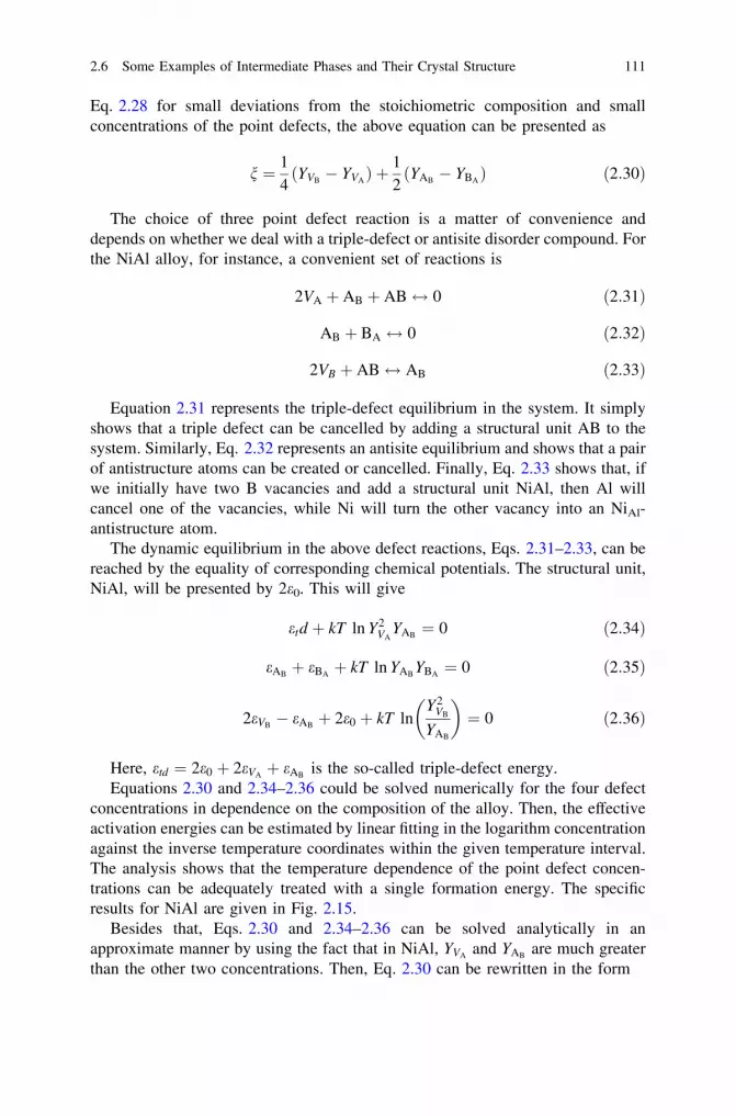
Eq. 2.28 for small deviations from the stoichiometric composition and smallconcentrations of the point defects, the above equation can be presented as

n ¼ 14

YVB� YVA

ð Þ þ 12

YAB� YBA

ð Þ ð2:30Þ

The choice of three point defect reaction is a matter of convenience anddepends on whether we deal with a triple-defect or antisite disorder compound. Forthe NiAl alloy, for instance, a convenient set of reactions is

2VA þ AB þ AB$ 0 ð2:31Þ

AB þ BA $ 0 ð2:32Þ

2VB þ AB$ AB ð2:33Þ

Equation 2.31 represents the triple-defect equilibrium in the system. It simplyshows that a triple defect can be cancelled by adding a structural unit AB to thesystem. Similarly, Eq. 2.32 represents an antisite equilibrium and shows that a pairof antistructure atoms can be created or cancelled. Finally, Eq. 2.33 shows that, ifwe initially have two B vacancies and add a structural unit NiAl, then Al willcancel one of the vacancies, while Ni will turn the other vacancy into an NiAl-antistructure atom.

The dynamic equilibrium in the above defect reactions, Eqs. 2.31–2.33, can bereached by the equality of corresponding chemical potentials. The structural unit,NiAl, will be presented by 2e0. This will give

etd þ kT ln Y2VA

YAB¼ 0 ð2:34Þ

eABþ eBA

þ kT ln YABYBA¼ 0 ð2:35Þ

2eVB� eAB

þ 2e0 þ kT lnY2

VB

YAB

� �¼ 0 ð2:36Þ

Here, etd ¼ 2e0 þ 2eVAþ eAB

is the so-called triple-defect energy.Equations 2.30 and 2.34–2.36 could be solved numerically for the four defect

concentrations in dependence on the composition of the alloy. Then, the effectiveactivation energies can be estimated by linear fitting in the logarithm concentrationagainst the inverse temperature coordinates within the given temperature interval.The analysis shows that the temperature dependence of the point defect concen-trations can be adequately treated with a single formation energy. The specificresults for NiAl are given in Fig. 2.15.

Besides that, Eqs. 2.30 and 2.34–2.36 can be solved analytically in anapproximate manner by using the fact that in NiAl, YVA

and YABare much greater

than the other two concentrations. Then, Eq. 2.30 can be rewritten in the form

2.6 Some Examples of Intermediate Phases and Their Crystal Structure 111

n ¼ 12

YAB� 1

4YVA

ð2:37Þ

From Eq. 2.37, we have YVA¼ 2YAB

for the stoichiometric composition, n = 0.For the A-rich compositions n[0, the A antistructure atoms are the main defectsðYVA

� YABÞ and Eq. 2.37 transforms into YAB

¼ 2n. On the other hand, for theB-rich compositions n\ 0, the A vacancies are mainly formed ðYVA

ffi YABÞ and

Eq. 1.174 will be read as YVA¼ �4n. These relations make it possible to solve

analytically the system of Eqs. 2.34–2.36 and to find the concentrations of all fourpoint defects under the given approximations. The analytical expressions for theeffective formation energies are given in Table 2.5. The comparison with Fig. 2.15suggests that these results correspond well to the numerical data at the stoichi-ometric composition and far from the stoichiometry.

The calculations suggest that the Ni vacancies and the Ni antistructure atomsare the main defects in NiAl and the concentration of Al vacancies is by a feworders of magnitude lower than the concentration of Ni vacancies in accordancewith the experimental observations.

A similar form of analytic solution can be used for other compounds, andthe results are presented in Fig. 2.14. Figure 2.14a–e demonstrate a fewimportant features of defect behavior. It is obvious that both the Ti-aluminides(Fig. 2.14c, d) and Ni3Al (Fig. 2.14b) belong to the antistructure defect type ofintermetallic compounds, since antistructure atoms are predominantly generatedto accommodate the deviation from the stoichiometry. In contrast, NiAl revealsa triple-defect type of point defect disorder and constitutional Ni vacancies existin NiAl on the Al-rich side, as in Fig. 2.14a. Moreover, the Ni vacancy con-centration is very large also on the Ni-rich side, for example, XVA

10�4 atT = 0.75Tm. In the other intermetallics under consideration, the vacancies arealso mainly concentrated on the transition metal sublattice and their concen-tration amounts to about 10-6 to 10-5 at T = 0.75Tm. These are also the typicalvacancy concentrations in close-packed pure metals at the same reduced tem-perature. The vacancy concentration on the Al sublattice is remarkably smaller,especially in B2–FeAl, see Fig. 2.14e.

Fig. 2.15 Effectiveformation energies Ef of thepoint defects as function ofcomposition cNi

112 2 Structure of Materials

B2–FeAl is neither a compound with a pure antisite disorder nor a compoundwith a pure triple-defect disorder. FeAl demonstrates a hybrid behavior in whichthe relation between the Fe vacancy concentration and that of the antistructureatoms depends crucially on temperature.

The concentration of the Ti antistructure atoms in the Ti-aluminides is generallylarger than that of the Ni antistructure atoms in the Ni-aluminides of the samecomposition, as in Fig. 2.14. This fact corresponds to a higher degree of thermaldisorder inherent in Ti-aluminides at similar reduced temperatures. These featuresplay a decisive role in the analysis of the respective self-diffusion behavior.

An important question now arises as to how the particular crystal structure ofthe given intermetallic compound can affect the self-diffusion properties. It isgenerally accepted that self-diffusion in close-packed structures occurs via nearest-neighbor jumps of vacancies. Since random vacancy jumps between differentsublattices would generally produce disorder (and since there is a strong tendencyto accomplish the reverse), ordering jump after a given disordering jump, thecorrelated jumps of vacancies will clearly play a decisive role in the long-rangediffusion process. These problems will be considered in Chap. 5.

2.7 Microstructure and Phase Structure

The structural details at different levels that create the microstructure of agiven material are shown in Fig. 2.16. On the other hand, microstructures can bedivided, based on the formation mechanism, into three major types namely solidi-fication structures, solid-state transformation structures, and annealing structures.Figure 2.17 shows, as an example, an eutectic solidification structure of AuSn-alloyand the same material after annealing at 150 �C for 6,600 h. A profound discussionon different types of microstructures can be found, for example, from the ASMhandbook, and therefore, it is not included here [1] (Fig. 2.16).

Table 2.5 Analytical expressions of the effective formation energies QfP of the point defects P,

P = VNi, VAl, NiAl, and AlNi (in eV/Atom) in NiAl in dependence on composition n = XNi–�

n\ 0 n = 0 n[ 0

QfVNi

0 etd=3 etd=20 0.683 1.024

QfVAl

2e0 þ eVAl þ eVNi 4e0 þ 3eVAl þ eVNi � eNiAlð Þ=3 e0 þ eVAl � 12 eNiAl

2.461 1.778 1.437

QfNiAl

etd etd=3 02.048 0.683 0

QfAlNi

eAlNi � 2e0 � 2eVNi �2e0 � 2eVNi þ 3eAlNi þ 2eNiAlð Þ=3 eAlNi þ eNiAl

0.489 1.854 2.537

2.6 Some Examples of Intermediate Phases and Their Crystal Structure 113

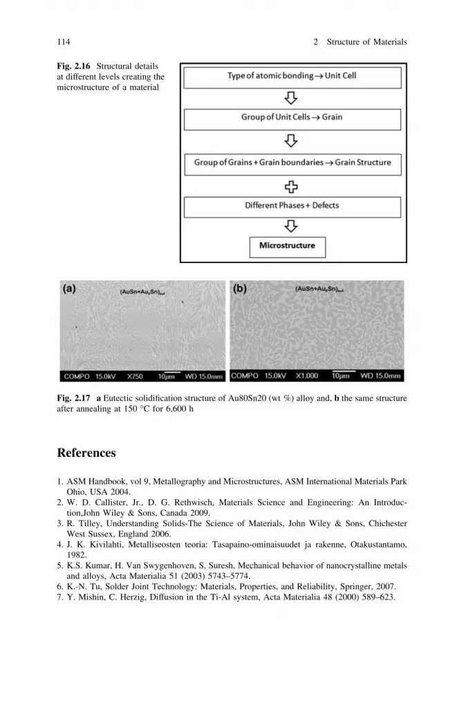
References

1. ASM Handbook, vol 9, Metallography and Microstructures, ASM International Materials ParkOhio, USA 2004.

2. W. D. Callister, Jr., D. G. Rethwisch, Materials Science and Engineering: An Introduc-tion,John Wiley & Sons, Canada 2009.

3. R. Tilley, Understanding Solids-The Science of Materials, John Wiley & Sons, ChichesterWest Sussex, England 2006.

4. J. K. Kivilahti, Metalliseosten teoria: Tasapaino-ominaisuudet ja rakenne, Otakustantamo,1982.

5. K.S. Kumar, H. Van Swygenhoven, S. Suresh, Mechanical behavior of nanocrystalline metalsand alloys, Acta Materialia 51 (2003) 5743–5774.

6. K.-N. Tu, Solder Joint Technology: Materials, Properties, and Reliability, Springer, 2007.7. Y. Mishin, C. Herzig, Diffusion in the Ti-Al system, Acta Materialia 48 (2000) 589–623.

Fig. 2.16 Structural detailsat different levels creating themicrostructure of a material

Fig. 2.17 a Eutectic solidification structure of Au80Sn20 (wt %) alloy and, b the same structureafter annealing at 150 �C for 6,600 h

114 2 Structure of Materials

Chapter 3Fick’s Laws of Diffusion

In this chapter, Fick’s laws of diffusion are introduced. The second law is derivedusing the first law and the mass conservation. Solutions for the second law con-sidering a constant diffusion coefficient for different conditions are given. Fewexamples are also introduced to show the estimation procedure.

3.1 Fick’s First and Second Laws of Diffusion

Adolf Fick [1] was the first man to propose the phenomenological relation fordiffusion. His reasoning being the following: when considering the flux of particles(atoms, molecules, ions etc.) in a one-dimensional system caused by a concen-tration gradient, the flux can be expressed as

J ¼ dm

dtA¼ �D

oC

oxð3:1aÞ

where J (mol/m2 s) is the flux, dm (mol) is the change in the amount of matter insmall time dt (seconds), A (m2) is the area, D (m2/s) is the diffusion coefficient,C (mol/m3) is the concentration of the particles, and x (m) is the positionparameter. The negative sign stems from the fact that diffusion occurs in thedirection opposite to the increasing concentration gradient.

It should be noted immediately that the Fick’s first law can be directly appliedonly in a steady-state condition, as shown in Fig. 3.1, where the composition doesnot change with time. In addition, there should not be any external driving forcespresent other than the concentration gradient. Let us consider a square pipe of ironand pass carburizing gas inside and decarburizing gas outside of the pipe. If the wallis reasonably thin, a steady state might prevail in the system. Suppose further thatthe concentrations at the inner and the outer surfaces are Ci and Co, respectively.Then, the concentration gradient can be written as dC

dx ¼Co�Cixo�xi

¼ � Ci�Coxo�xi

¼ � Ci�Cod .

Here, d is the wall thickness. The diffusion coefficient, D in this system, can be

A. Paul et al., Thermodynamics, Diffusion and the Kirkendall Effect in Solids,DOI: 10.1007/978-3-319-07461-0_3, � Springer International Publishing Switzerland 2014

115

estimated from what we know about the flux in the system. The flux can be esti-mated from the transferred material per unit time, that is, dm

dt (mol/s) = DmDt divided

by the area. If the pipe is cylindrical with an average radius of r and length of l, thenthe concentration gradient is dC

dr and material transferred in mol/s through the area

A = 2prl is DmDt . Therefore, we can write

J ¼ Dm

Dt 2prlð Þ ¼ �DoC

or

Dm

Dt¼ �D 2p lð Þ oC

o ln r

ð3:1bÞ

Fig. 3.1 Steady-statediffusion and the compositionprofile

116 3 Fick’s Laws of Diffusion

Note here that if a steady state prevails, then concentration profile, which is oCox

or oCo ln r, will not change with time. However, under most experimental conditions,

the concentration at a particular position changes with time at any location. Forexample, consider two blocks of alloys A–B with average concentrations of CB

1

and CB2 which are coupled and annealed at an increased temperature. The change

in the concentration with the annealing time is shown in Fig. 3.2a. Similarly, wecan consider the diffusion of element B in a block of material A, as shown inFig. 3.2b. Any possible changes in the composition profiles with time are shown.In this condition, Fick’s first law cannot be used to estimate the diffusion coeffi-cient of the components because of the absence of a time parameter. What isneeded, therefore, is a relation which is able to explain the non-steady-state dif-fusion process, that is, the change in concentration at a particular position withincreasing annealing time.

For this purpose, Fick’s second law is derived from the consideration of massconservation and Fick’s first law. For the sake of explanation, let us consider avery thin slab Dx ¼ x2 � x1ð Þ in the diffused block of A from the example, asshown in Fig. 3.2b. The flux of element B in this thin slab, as shown in Fig. 3.3.The block with a unit cross-sectional area is the one under consideration. If the fluxcoming in through the plane x1 is J1

B, then the total amount of element B comingthrough this plane in a short time d t can be written as J1

Bd t. Similarly, the totalamount of material out through the plane x2 can be written as J2

Bd t. If we considerJ1

B [ J2B, the increase in concentration of B in the small thickness of Dx can be

written as

Fig. 3.2 Change in non-steady-state composition profile with time (a) in a diffusion couple of C1B

and C2B (b) for diffusion of B in A

3.1 Fick’s First and Second Laws of Diffusion 117

dCB ¼ðJ1

B � J2BÞd t

Dxð3:2Þ

Furthermore, since only a very small thickness Dx is being considered, thevariation of flux in this region can be considered linear so that

oJB

ox¼ J2

B � J1B

Dx¼ � J1

B � J2B

Dxð3:3Þ

Using Eq. 3.2 in Eq. 3.3 and considering very small time, we can write

oCB

ot¼ � oJB

oxð3:4Þ

Following Fick’s first law, shown above in Eqs. 3.1a, 3.4 can be written as

oCB

o t¼ o

oxDB

oCB

ox

� �ð3:5aÞ

For a constant diffusion coefficient, we can write

oCB

o t¼ DB

o2CB

ox2ð3:5bÞ

Equation 3.5a is better known as Fick’s second law. One important point,however, should be noted here that it is not possible to use Fick’s first law toestimate the distribution of components over the whole interaction zone in a

Fig. 3.3 Change in flux withdistance in a very thin slab

118 3 Fick’s Laws of Diffusion

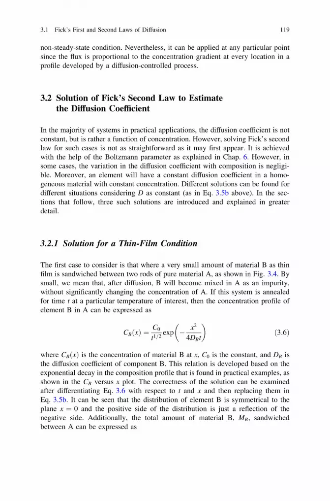
non-steady-state condition. Nevertheless, it can be applied at any particular pointsince the flux is proportional to the concentration gradient at every location in aprofile developed by a diffusion-controlled process.

3.2 Solution of Fick’s Second Law to Estimatethe Diffusion Coefficient

In the majority of systems in practical applications, the diffusion coefficient is notconstant, but is rather a function of concentration. However, solving Fick’s secondlaw for such cases is not as straightforward as it may first appear. It is achievedwith the help of the Boltzmann parameter as explained in Chap. 6. However, insome cases, the variation in the diffusion coefficient with composition is negligi-ble. Moreover, an element will have a constant diffusion coefficient in a homo-geneous material with constant concentration. Different solutions can be found fordifferent situations considering D as constant (as in Eq. 3.5b above). In the sec-tions that follow, three such solutions are introduced and explained in greaterdetail.

3.2.1 Solution for a Thin-Film Condition

The first case to consider is that where a very small amount of material B as thinfilm is sandwiched between two rods of pure material A, as shown in Fig. 3.4. Bysmall, we mean that, after diffusion, B will become mixed in A as an impurity,without significantly changing the concentration of A. If this system is annealedfor time t at a particular temperature of interest, then the concentration profile ofelement B in A can be expressed as

CB xð Þ ¼ C0

t1=2exp � x2

4DBt

� �ð3:6Þ

where CB xð Þ is the concentration of material B at x, C0 is the constant, and DB isthe diffusion coefficient of component B. This relation is developed based on theexponential decay in the composition profile that is found in practical examples, asshown in the CB versus x plot. The correctness of the solution can be examinedafter differentiating Eq. 3.6 with respect to t and x and then replacing them inEq. 3.5b. It can be seen that the distribution of element B is symmetrical to theplane x = 0 and the positive side of the distribution is just a reflection of thenegative side. Additionally, the total amount of material B, MB, sandwichedbetween A can be expressed as

3.1 Fick’s First and Second Laws of Diffusion 119

MB ¼Zþ1

�1

CBdx ð3:7Þ

Thus, MB can be found by replacing Eq. 3.6 in Eq. 3.7 as

MB ¼Zþ1

�1

C0

t1=2exp � x2

4DB t

� �dx ð3:8Þ

We consider k ¼ x2ffiffiffiffiffiffiDBtp so that dx ¼ 2

ffiffiffiffiffiffiffiffiDBtp� �

dk. Since C0 is a constant term,

we can write

MB ¼ 2C0ffiffiffiffiffiffiDB

p Zþ1

�1

exp �k2� �dk ¼ 2C0

ffiffiffiffiffiffiffiffiffipDB

pð3:9Þ

Fig. 3.4 Material B issandwiched between blocksof material A. The change in

CB, dCBdx , and d2CB

dx2 with x isshown after annealing fortime, t

120 3 Fick’s Laws of Diffusion

SinceRþ1�1

exp �k2� �dk ¼

ffiffiffiffipp

For a particular annealing time, t is constant and using Eq. 3.9 in Eq. 3.6, wecan write

CB xð Þ ¼ MB

2ffiffiffiffiffiffiffiffiffiffiffipDBtp exp � x2

4DB t

� �ð3:10Þ

From the CB versus x plot, one can find dCBdx versus x as shown in Fig. 3.4. Since

the constant diffusion coefficient is under consideration, dCdx versus x reflects the

flux at different planes after a certain annealing time t that can be understood fromthe Fick’s first law. It is apparent from the profile that there is no diffusion atx = 0, þ1, and �1. The infinite distance represents the ends of the sample,which are not affected by the diffusion of components. Moreover, the fact that theflux is zero at x = 0 demonstrates that both positive and negative sides of thesystem do not influence each other. In another sense, it seems as if the two

different parts are joined together at x = 0. Further, the d2Cdx2 versus x profile gives

an overall idea about the region where the system is losing the diffusing element

(i.e., where o2CBox2

� �\0) and in which part it is gaining (i.e., where o2CB

ox2

� �[ 0).

However, it should be noted that the region where the system is losing or gainingflux changes with time, since the concentration profile changes with time, asshown in Fig. 3.5.

As already mentioned, the system considered for the above discussion acts as iftwo different parts are joined together. If material B is joined or deposited on thesurface of material A, as shown in Fig. 3.6, then Eq. 3.10 must be written as

Fig. 3.5 Change inconcentration with time in athin-film sandwiched couple

3.2 Solution of Fick’s Second Law to Estimate the Diffusion Coefficient 121

CB ¼MBffiffiffiffiffiffiffiffiffiffiffipDB tp exp � x2

4DBt

� �ð3:11Þ

Note here that the factor 2 from the denominator in Eq. 3.10 is removed sincethe material diffuses in one direction only. Equation 3.11 can be written as

ln CB ¼ lnMBffiffiffiffiffiffiffiffiffiffiffipDB tp � x2

4DB tð3:12Þ

As shown in Fig. 3.6, the diffusion coefficient DB can be estimated from the

slope ¼ � 14DBt

� �of the ln CB versus x2 plot.

3.2.1.1 Solution for a Semi-infinite Diffusion Couple (Error FunctionAnalysis)

When two blocks with different concentrations are joined and annealed at anincreased temperature for diffusion, this is called a diffusion couple. A diffusioncouple is one of the important techniques to study diffusion with an addedadvantage that often it resembles the actual reaction layer structure in manyapplications. The treatment to estimate the diffusion parameters is similar when apiece of material is exposed to the gaseous medium, for example, as in carburi-zation of steel having a situation as shown in Fig. 3.2b. With the change in time, thepenetration length and the concentration at a particular position will be changed. Asemi-infinite system is one where the ends of the couple are not affected by the

Fig. 3.6 Determination ofthe diffusion coefficient isshown from the slope of theln CB versus x2 plot

122 3 Fick’s Laws of Diffusion

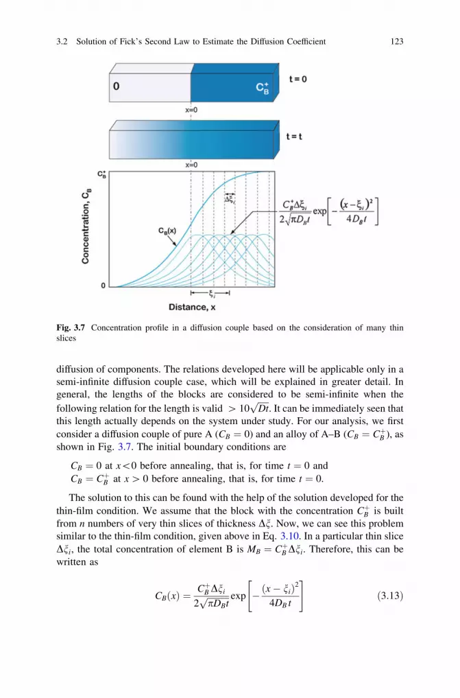
diffusion of components. The relations developed here will be applicable only in asemi-infinite diffusion couple case, which will be explained in greater detail. Ingeneral, the lengths of the blocks are considered to be semi-infinite when thefollowing relation for the length is valid [ 10

ffiffiffiffiffiDtp

. It can be immediately seen thatthis length actually depends on the system under study. For our analysis, we firstconsider a diffusion couple of pure A (CB ¼ 0) and an alloy of A–B (CB ¼ CþB ), asshown in Fig. 3.7. The initial boundary conditions are

CB ¼ 0 at x\0 before annealing, that is, for time t ¼ 0 andCB ¼ CþB at x [ 0 before annealing, that is, for time t ¼ 0.

The solution to this can be found with the help of the solution developed for thethin-film condition. We assume that the block with the concentration CþB is builtfrom n numbers of very thin slices of thickness Dn. Now, we can see this problemsimilar to the thin-film condition, given above in Eq. 3.10. In a particular thin sliceDni, the total concentration of element B is MB ¼ CþB Dni. Therefore, this can bewritten as

CB xð Þ ¼ CþB Dni

2ffiffiffiffiffiffiffiffiffiffipDBtp exp � x� nið Þ2

4DB t

" #ð3:13Þ

Fig. 3.7 Concentration profile in a diffusion couple based on the consideration of many thinslices

3.2 Solution of Fick’s Second Law to Estimate the Diffusion Coefficient 123

Here, x is replaced by x� nið Þ, since the slice Dni is located at a distance ni

from the initial contact plane, x = 0. Similarly, we consider all other thin slicesand from the assumption that different slices do not affect each other, the con-centration at any position x after superposition can be written as

CB xð Þ ¼ CþB2ffiffiffiffiffiffiffiffiffiffipDBtp

Xn

i¼1

exp � x� nið Þ2

4DB t

" #Dni ð3:14Þ

The first slice Dn1 is at the distance of n1 ¼ 0 and the nth slice Dnn is at thedistance of nn ¼ þ1 from the initial contact plane, x ¼ 0. The concentration atany position x, following Eq. 3.14, can be written in the integral form as

CB xð Þ ¼ CþB2ffiffiffiffiffiffiffiffiffiffipDBtp

Z1

0

exp � x� nð Þ2

4DB t

" #dn ð3:15Þ

Let us consider

g ¼ x� n

2ffiffiffiffiffiffiffiffiDB tp ð3:16Þ

Differentiating Eq. 3.16,

dg ¼ � dn

2ffiffiffiffiffiffiffiffiDB tp ð3:17Þ

For n ¼ 0, g ¼ x2ffiffiffiffiffiffiDBtp , and for n ¼ 1, g ¼ �1. So Eq. 3.15 can be written as

CB xð Þ ¼ � CþBffiffiffipp

Z�1

x= 2ffiffiffiffiffiffiDBtpð Þ

exp �g2� �

dg ¼ CþBffiffiffipp

Zx= 2ffiffiffiffiffiffiDBtpð Þ

�1

exp �g2� �

dg ð3:18Þ

The value of the integral in Eq. 3.18 is not straightforward to estimate. So forthe sake of convenience, Eq. 3.18 is converted in terms of error function. The errorfunction of z, which is basically the value of the integral from 0 to z, expressed as

erf zð Þ ¼ 2ffiffiffippZz

0

exp �g2� �

dg ð3:19Þ

In general, the values of erf(z) as a function of z is available in the literature andthe positive values of z are listed in Table 3.1. The variation is shown in Fig. 3.8for both positive and negative values of z. From Eq. 3.18,

124 3 Fick’s Laws of Diffusion

Tab

le3.

1er

f(z)

valu

esar

eli

sted

for

z,w

hich

can

beob

tain

edfr

omer

fzðÞ¼

2 ffiffi ppP 1 n¼

0�

1ðÞn

z2nþ

1

n!2nþ

1ð

Þ¼

2 ffiffi pp

z�

z3

1!�

3þ

z5

2!�

5�

z7

3!�

7..

....

....

..�

�

Sec

ond

digi

taf

ter

deci

mal

ofz

z0

12

34

56

78

9

0.0

0.00

000

0.01

128

0.02

256

0.03

384

0.04

511

0.05

637

0.06

762

0.07

886

0.09

008

0.10

128

0.1

0.11

246

0.12

362

0.13

476

0.14

587

0.15

695

0.16

800

0.17

901

0.18

999

0.20

094

0.21

184

0.2

0.22

270

0.23

352

0.24

430

0.25

502

0.26

570

0.27

633

0.28

690

0.29

742

0.30

788

0.31

828

0.3

0.32

863

0.33

891

0.34

913

0.35

928

0.36

936

0.37

938

0.38

933

0.39

921

0.40

901

0.41

874

0.4

0.42

839

0.43

797

0.44

747

0.45

689

0.46

623

0.47

548

0.48

466

0.49

375

0.50

275

0.51

167

0.5

0.52

050

0.52

924

0.53

790

0.54

646

0.55

494

0.56

332

0.57

162

0.57

982

0.58

792

0.59

594

0.6

0.60

386

0.61

168

0.61

941

0.62

705

0.63

459

0.64

203

0.64

938

0.65

663

0.66

378

0.67

084

0.7

0.67

780

0.68

467

0.69

143

0.69

810

0.70

468

0.71

116

0.71

754

0.72

382

0.73

001

0.73

610

0.8

0.74

210

0.74

800

0.75

381

0.75

952

0.76

514

0.77

067

0.77

610

0.78

144

0.78

669

0.79

184

0.9

0.79

691

0.80

188

0.80

677

0.81

156

0.81

627

0.82

089

0.82

542

0.82

987

0.83

423

0.83

851

1.0

0.84

270

0.84

681

0.85

084

0.85

478

0.85

865

0.86

244

0.86

614

0.86

977

0.87

333

0.87

680

1.1

0.88

021

0.88

353

0.88

679

0.88

997

0.89

308

0.89

612

0.89

910

0.90

200

0.90

484

0.90

761

1.2

0.91

031

0.91

296

0.91

553

0.91

805

0.92

051

0.92

290

0.92

524

0.92

751

0.92

973

0.93

190

1.3

0.93

401

0.93

606

0.93

807

0.94

002

0.94

191

0.94

376

0.94

556

0.94

731

0.94

902

0.95

067

1.4

0.95

229

0.95

385

0.95

538

0.95

686

0.95

830

0.95

970

0.96

105

0.96

237

0.96

365

0.96

490

1.5

0.96

611

0.96

728

0.96

841

0.96

952

0.97

059

0.97

162

0.97

263

0.97

360

0.97

455

0.97

546

1.6

0.97

635

0.97

721

0.97

804

0.97

884

0.97

962

0.98

038

0.98

110

0.98

181

0.98

249

0.98

315

1.7

0.98

379

0.98

441

0.98

500

0.98

558

0.98

613

0.98

667

0.98

719

0.98

769

0.98

817

0.98

864

1.8

0.98

909

0.98

952

0.98

994

0.99

035

0.99

074

0.99

111

0.99

147

0.99

182

0.99

216

0.99

248

1.9

0.99

279

0.99

309

0.99

338

0.99

366

0.99

392

0.99

418

0.99

443

0.99

466

0.99

489

0.99

511

(con

tinu

ed)

3.2 Solution of Fick’s Second Law to Estimate the Diffusion Coefficient 125

Tab

le3.

1(c

onti

nued

)

Sec

ond

digi

taf

ter

deci

mal

ofz

z0

12

34

56

78

9

2.0

0.99

532

0.99

552

0.99

572

0.99

591

0.99

609

0.99

626

0.99

642

0.99

658

0.99

673

0.99

688

2.1

0.99

702

0.99

715

0.99

728

0.99

741

0.99

753

0.99

764

0.99

775

0.99

785

0.99

795

0.99

805

2.2

0.99

814

0.99

822

0.99

831

0.99

839

0.99

846

0.99

854

0.99

861

0.99

867

0.99

874

0.99

880

2.3

0.99

886

0.99

891

0.99

897

0.99

902

0.99

906

0.99

911

0.99

915

0.99

920

0.99

924

0.99

928

2.4

0.99

931

0.99

935

0.99

938

0.99

941

0.99

944

0.99

947

0.99

950

0.99

952

0.99

955

0.99

957

2.5

0.99

959

0.99

961

0.99

963

0.99

965

0.99

967

0.99

969

0.99

971

0.99

972

0.99

974

0.99

975

2.6

0.99

976

0.99

978

0.99

979

0.99

980

0.99

981

0.99

982

0.99

983

0.99

984

0.99

985

0.99

986

2.7

0.99

987

0.99

987

0.99

988

0.99

989

0.99

989

0.99

990

0.99

991

0.99

991

0.99

992

0.99

992

2.8

0.99

992

0.99

993

0.99

993

0.99

994

0.99

994

0.99

994

0.99

995

0.99

995

0.99

995

0.99

996

2.9

0.99

996

0.99

996

0.99

996

0.99

997

0.99

997

0.99

997

0.99

997

0.99

997

0.99

997

0.99

998

3.0

0.99

998

0.99

998

0.99

998

0.99

998

0.99

998

0.99

998

0.99

998

0.99

999

0.99

999

0.99

999

3.1

0.99

999

0.99

999

0.99

999

0.99

999

0.99

999

0.99

999

0.99

999

0.99

999

0.99

999

0.99

999

3.2

0.99

999

0.99

999

0.99

999

1.00

000

1.00

000

1.00

000

1.00

000

1.00

000

1.00

000

1.00

000

126 3 Fick’s Laws of Diffusion

CB xð Þ ¼ CþBffiffiffipp

Z0

�1

exp �g2� �

dgþZx= 2ffiffiffiffiffiffiDBtpð Þ

0

exp �g2� �

dg

2664

3775

CB xð Þ ¼ CþBffiffiffipp �

Z�1

0

exp �g2� �

dgþZx= 2ffiffiffiffiffiffiDBtpð Þ

0

exp �g2� �

dg

2664

3775

CB xð Þ ¼ CþB2�erf �1ð Þ þ erf

x

2ffiffiffiffiffiffiffiffiDBtp

� �

ð3:20Þ

It can be seen from Fig. 3.8 that

erf �zð Þ ¼ �erf zð Þ; erf �1ð Þ ¼ �1 ð3:21Þ

Therefore, Eq. 3.20 can be written as

CB xð Þ ¼ CþB2

1þ erfx

2ffiffiffiffiffiffiffiffiDBtp

� � ð3:22aÞ

CB xð ÞCþB

¼ 12

1þ erfx

2ffiffiffiffiffiffiffiffiDBtp

� � ð3:22bÞ

It should be noted here that position x is the distance from x = 0. For thenegative side, the sign inside the bracket will be negative. Thus, it is mandatory tofind the location of x = 0 after measuring the concentration profile for the cal-

culation of the diffusion coefficient. For x = 0, CB xð Þ ¼ CþB2 1þ 0½ � ¼ CþB

2 . There-

fore, the location of the initial contact plane isCþB2 that is exactly at the middle of

the concentration profile. This is to be expected, since we are considering here aconstant diffusion coefficient at all possible concentrations.

Fig. 3.8 Variation oferf(z) with z

3.2 Solution of Fick’s Second Law to Estimate the Diffusion Coefficient 127

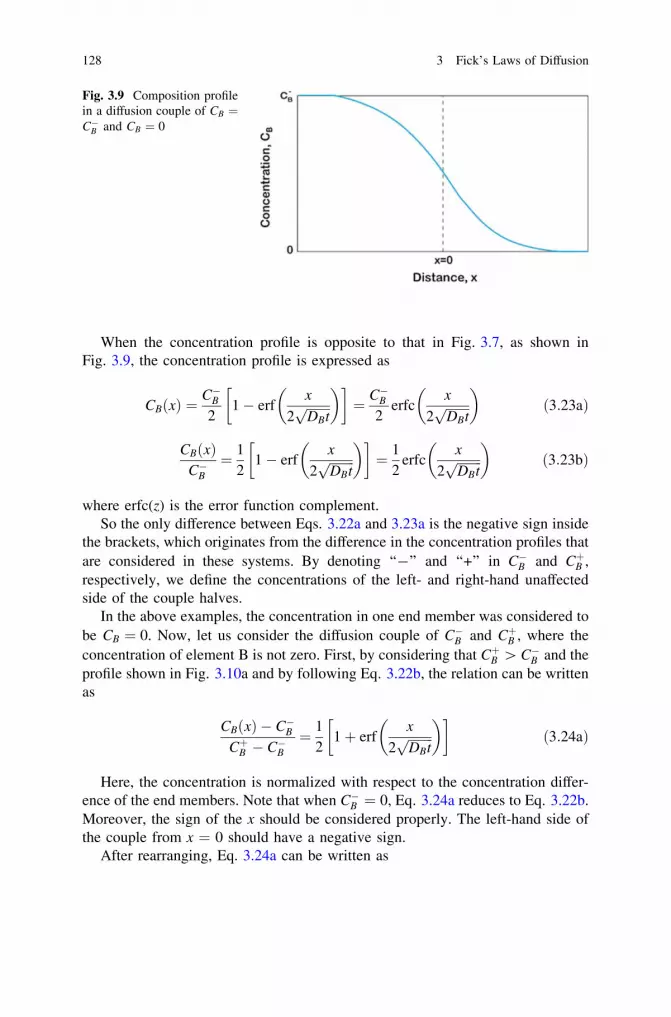
When the concentration profile is opposite to that in Fig. 3.7, as shown inFig. 3.9, the concentration profile is expressed as

CB xð Þ ¼ C�B2

1� erfx

2ffiffiffiffiffiffiffiffiDBtp

� � ¼ C�B

2erfc

x

2ffiffiffiffiffiffiffiffiDBtp

� �ð3:23aÞ

CB xð ÞC�B

¼ 12

1� erfx

2ffiffiffiffiffiffiffiffiDBtp

� � ¼ 1

2erfc

x

2ffiffiffiffiffiffiffiffiDBtp

� �ð3:23bÞ

where erfc(z) is the error function complement.So the only difference between Eqs. 3.22a and 3.23a is the negative sign inside

the brackets, which originates from the difference in the concentration profiles thatare considered in these systems. By denoting ‘‘-’’ and ‘‘+’’ in C�B and CþB ,respectively, we define the concentrations of the left- and right-hand unaffectedside of the couple halves.

In the above examples, the concentration in one end member was considered tobe CB ¼ 0. Now, let us consider the diffusion couple of C�B and CþB , where theconcentration of element B is not zero. First, by considering that CþB [ C�B and theprofile shown in Fig. 3.10a and by following Eq. 3.22b, the relation can be writtenas

CB xð Þ � C�BCþB � C�B

¼ 12

1þ erfx

2ffiffiffiffiffiffiffiffiDBtp

� � ð3:24aÞ

Here, the concentration is normalized with respect to the concentration differ-ence of the end members. Note that when C�B ¼ 0, Eq. 3.24a reduces to Eq. 3.22b.Moreover, the sign of the x should be considered properly. The left-hand side ofthe couple from x = 0 should have a negative sign.

After rearranging, Eq. 3.24a can be written as

Fig. 3.9 Composition profilein a diffusion couple of CB ¼C�B and CB ¼ 0

128 3 Fick’s Laws of Diffusion

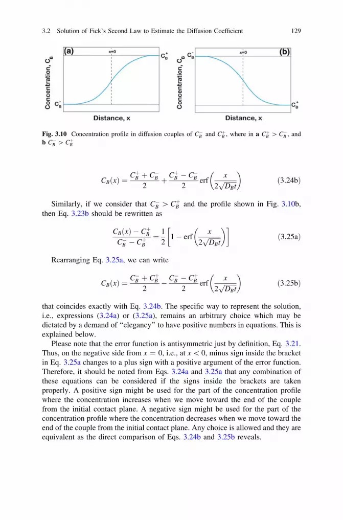
CB xð Þ ¼ CþB þ C�B2

þ CþB � C�B2

erfx

2ffiffiffiffiffiffiffiffiDBtp

� �ð3:24bÞ

Similarly, if we consider that C�B [ CþB and the profile shown in Fig. 3.10b,then Eq. 3.23b should be rewritten as

CB xð Þ � CþBC�B � CþB

¼ 12

1� erfx

2ffiffiffiffiffiffiffiffiDBtp

� � ð3:25aÞ

Rearranging Eq. 3.25a, we can write

CB xð Þ ¼ C�B þ CþB2

� C�B � CþB2

erfx

2ffiffiffiffiffiffiffiffiDBtp

� �ð3:25bÞ

that coincides exactly with Eq. 3.24b. The specific way to represent the solution,i.e., expressions (3.24a) or (3.25a), remains an arbitrary choice which may bedictated by a demand of ‘‘elegancy’’ to have positive numbers in equations. This isexplained below.

Please note that the error function is antisymmetric just by definition, Eq. 3.21.Thus, on the negative side from x = 0, i.e., at x \ 0, minus sign inside the bracketin Eq. 3.25a changes to a plus sign with a positive argument of the error function.Therefore, it should be noted from Eqs. 3.24a and 3.25a that any combination ofthese equations can be considered if the signs inside the brackets are takenproperly. A positive sign might be used for the part of the concentration profilewhere the concentration increases when we move toward the end of the couplefrom the initial contact plane. A negative sign might be used for the part of theconcentration profile where the concentration decreases when we move toward theend of the couple from the initial contact plane. Any choice is allowed and they areequivalent as the direct comparison of Eqs. 3.24b and 3.25b reveals.

Fig. 3.10 Concentration profile in diffusion couples of C�B and CþB , where in a CþB [ C�B , andb C�B [ CþB

3.2 Solution of Fick’s Second Law to Estimate the Diffusion Coefficient 129

Note that here it is also necessary to find the location of the initial contact plane(x = 0) for the calculation of the diffusion coefficient from the concentrationprofile. For x = 0, Eq. 3.24b or 3.25b will reduce to

CB x ¼ 0ð Þ ¼ C�B þ CþB2

ð3:26Þ

This suggests that the average concentration will indicate the location of theinitial contact plane.

Now, let us turn to consider the carburization of steel, where the carbon con-centration of steel from the surface is increased by diffusion. In this process, steelis kept in a gas mixture of CH4 and CO at the temperature of interest. Dependingon the ratio of the gases supplied, the carbon concentration at the surface is keptconstant by a constant supply of gases. Thus, with the increase in annealing time,the concentration profile of the carbon changes, as shown in Fig. 3.11a. If weconsider that the initial carbon concentration of the steel is Co and the carbonconcentration at the surface is Cs, following Eq. 3.25a (since C diffuses from leftto right), the concentration of C, C(x), comparing Fig. 3.10b can be written as

C xð Þ � Co

CS � Co¼ 1� erf

x

2ffiffiffiffiffiDtp

� �ð3:27aÞ

Furthermore, Eq. 3.27a can be rearranged as

C xð Þ ¼ CS � CS � C0ð Þ erfx

2ffiffiffiffiffiDtp

� �ð3:27bÞ

Fig. 3.11 Change in concentration profile with annealing time during carburization of steel inwhich a C diffuse from left to right, and b C diffuse from right to left

130 3 Fick’s Laws of Diffusion

Here, the main difference between Eqs. 3.25a and 3.27a is that the numericalfactor � is missing. The numerical factor is removed since here we have only oneside of the profile from x = 0 compared to the two sides in the previous diffusioncouple example. It is also important to note that if we consider that the carbon isdiffusing in the opposite direction, as shown in Fig. 3.11b, we shall find the samerelation as in Eq. 3.27a. In this case, as C is diffusing from right to left, Eq. 3.24ashould be written comparing Fig. 3.10a as

C xð Þ � Co

CS � Co¼ 1þ erf � x

2ffiffiffiffiffiDtp

� �¼ 1� erf

x

2ffiffiffiffiffiDtp

� �¼ erfc

x

2ffiffiffiffiffiDtp

� �ð3:28Þ

If we consider the carburization treatment of a material with no carbon presentbefore the carburization treatment, that is, Co ¼ 0, the above relation will reduceto

C xð Þ ¼ CS 1� erfx

2ffiffiffiffiffiDtp

� � ¼ CS erfc

x

2ffiffiffiffiffiDtp

� �ð3:29Þ

When considering decarburization, as shown in Fig. 3.12 where the carbonconcentration at the surface Cs = 0 for the whole time, then from Eq. 3.28, therelation for decarburization can be written

C xð Þ ¼ C0 erfx

2ffiffiffiffiffiDtp

� �ð3:30Þ

Fig. 3.12 Concentrationprofile for a decarburizationtreatment

3.2 Solution of Fick’s Second Law to Estimate the Diffusion Coefficient 131

Yet another important relation can be obtained from the above discussion. Letus consider the carburization experiment once again. We know that the diffusioncoefficient depends on temperature; it is considered to be D1 at T1 and D2 at T2.Suppose we wish to know what is the time difference needed to achieve a par-ticular concentration, let us say C xð Þ ¼ C1 at a particular distance, x1 at two

different temperatures. We can write C xð Þ�Co

CS�Co¼ C1�Co

CS�Coin Eq. 3.28 and

x21

D1t1¼ x2

1

D2t2ð3:31Þ

Next follows a discussion of the calculation of the diffusion coefficient in adiffusion couple. Suppose that under consideration, we have a diffusion couple oftwo different blocks with composition C�B ¼ C1

B and CþB ¼ C2B such that C2

B [ C1B.

Therefore, the concentration profile shown in Fig. 3.10a can be expected and it canbe expressed as

CB xð Þ ¼ C2B þ C1

B

2

� �þ C2

B � C1B

2

� �erf

x

2ffiffiffiffiffiDtp

� �ð3:32Þ

If the system has a constant molar volume, Eq. 3.32 reduces to

NBðxÞ ¼N2

B þ N1B

2þ N2

B � N1B

2

� �erf

x

2ffiffiffiffiffiDtp

� �ð3:33Þ

since CB ¼ NBVm¼ XB

Vm, where NB is the atomic fraction, XB is the mole fraction of

element B, and Vm is the molar volume. Suppose these compositions are N1B ¼ 0:3

and N2B ¼ 0:7, as shown in Fig. 3.13. This couple is annealed for 25 h. A com-

position profile might built up such that the atomic fraction of B at the distance of2.5 lm from x = 0 would be NB ¼ 0:6. Using the relation in Eq. 3.33, it is possibleto estimate the diffusion coefficient in this system. From the description above, weknow that NB ¼ 0:6, N1

B ¼ 0:3, N2B ¼ 0:7, t ¼ 25 h ¼ 25� 60� 60 = 90,000 s,

and x ¼ 2:5 lm ¼ 2:5� 10�6 m. Substituting these values in Eq. 3.33, we get

erf2:5� 10�6

2ffiffiffiffiffiffiffiffiffiffiffiffiffiffiffiffiffiffiffiffiffiffiffiD� 90;000p

� �¼ 0:5 ð3:34Þ

From the values listed in Table 3.1, we see that there is no value exactly forerf(z) = 0.5. We have the values erf(z) = 0.49375 for z = 0.47 and erf(z) = 0.50275for z = 0.48. Since these values are very close, we can consider linear variation andfind the value of z for erf(z) = 0.5 following

132 3 Fick’s Laws of Diffusion

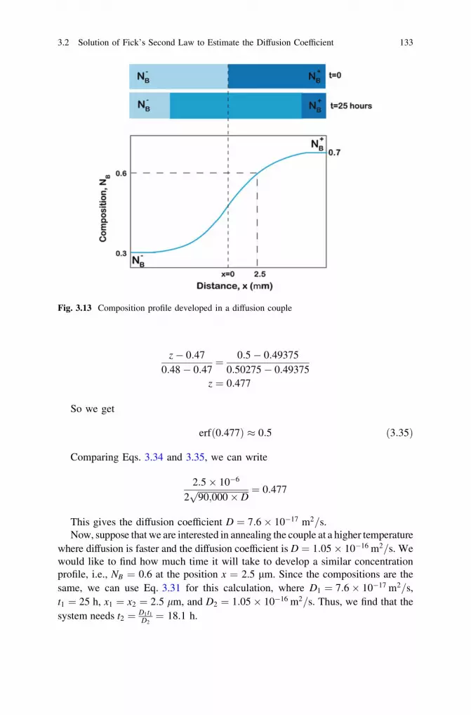
z� 0:470:48� 0:47

¼ 0:5� 0:493750:50275 � 0:49375

z ¼ 0:477

So we get

erf 0:477ð Þ � 0:5 ð3:35Þ

Comparing Eqs. 3.34 and 3.35, we can write

2:5� 10�6

2ffiffiffiffiffiffiffiffiffiffiffiffiffiffiffiffiffiffiffiffiffiffiffi90;000� Dp ¼ 0:477

This gives the diffusion coefficient D ¼ 7:6� 10�17 m2=s.Now, suppose that we are interested in annealing the couple at a higher temperature

where diffusion is faster and the diffusion coefficient is D ¼ 1:05� 10�16 m2=s. Wewould like to find how much time it will take to develop a similar concentrationprofile, i.e., NB = 0.6 at the position x = 2.5 lm. Since the compositions are thesame, we can use Eq. 3.31 for this calculation, where D1 ¼ 7:6� 10�17 m2=s,t1 ¼ 25 h, x1 ¼ x2 ¼ 2:5 lm, and D2 ¼ 1:05� 10�16 m2=s. Thus, we find that thesystem needs t2 ¼ D1t1

D2¼ 18.1 h.

Fig. 3.13 Composition profile developed in a diffusion couple

3.2 Solution of Fick’s Second Law to Estimate the Diffusion Coefficient 133

The relations used above are strictly applicable only in the case of semi-infinite diffusion couples. This means that annealing time must be shortenough such that the end parts of the material are not affected by the dif-fusion of components. We have stated previously that the length of eachblock in a couple should be greater than 10

ffiffiffiffiffiDtp

. However, in practice, evenif one atomic layer in the end is found to be unaffected, the couple can beconsidered as semi-infinite. It must be apparent that the values for the lengthof the blocks can be considered as semi-infinite depend on diffusion coef-ficient, temperature, and desired annealing time. If the system is not semi-infinite, the analysis will lead to an inaccurate results.

Let us consider a situation shown in Fig. 3.14. At time t = 0, that is, the timebefore annealing, the concentration in the position ranges from -h to h is C ¼ Co.Outside this range, the concentration is C ¼ 0. Therefore, this can be seen as ablock/film with the thickness of 2 h having concentration of Co sandwichedbetween the materials with the concentration of zero. The initial profile at t = 0 isindicated by the dotted line. The concentration profile, after time t = t, is indicatedby the solid curve. It should be noted here that this condition is different from thecondition discussed in Sect. 3.2.1, where the diffusing element from a very thinlayer mixes in the impurity level without significantly altering the concentration ofthe bulk material into which the component is diffusing. In this example, weconsider a relatively thick film or block with a finite thickness such that thediffusing components from this relatively thick film/block will change the overallconcentration of the material in between which this layer is sandwiched. In the

Fig. 3.14 Diffusion profiledeveloped from a thick film

134 3 Fick’s Laws of Diffusion

thin-film solution as shown Sect. 3.2.1, we considered the concentration of thediffusing element only. In this example, however, we consider the concentrationprofile of an alloy.

Following a procedure similar to that used to develop the error function anal-ysis, the diffusion profile can be expressed as

CðxÞ ¼ 12

Co erfh� x

2ffiffiffiffiffiDtp þ erf

hþ x

2ffiffiffiffiffiDtp

ð3:36Þ

It can be seen that the diffusion profile has a reflection at x = 0. The bookwritten by J. Crank can be consulted for a more detailed treatment on this [2].

3.2.2 Solution for Homogenization (Separation of Variables)

Now, let us consider a system that ultimately reaches homogenization, meaningthat we must turn to consider relatively long annealing times. In any system, theconcentration varies with respect to two variables time t and position x. Hence, wecan write

C x; tð Þ ¼ XðxÞTðtÞ ð3:37Þ

Partial differentiation with respect to x and t gives

dC

dt¼ X

dT

dtð3:38aÞ

d2C

dx2¼ T

d2X

dx2ð3:38bÞ

Replacing Eqs. 3.38a and 3.38b in Fick’s second law expressed in Eq. 3.5b, weobtain

XdT

dt¼ DT

d2X

dx2ð3:39aÞ

1DT

dT

dt¼ 1

X

d2X

dx2ð3:39bÞ

From Eq. 3.39a, it can be observed that the relation is divided with respect tot and x. Both sides should be equal to the same constant value. For the sake ofconvenience, let us consider the constant as �k2. There is an advantage in con-sidering the constant like this, which will become clearer to the reader during thederivation that follows. We can write

3.2 Solution of Fick’s Second Law to Estimate the Diffusion Coefficient 135

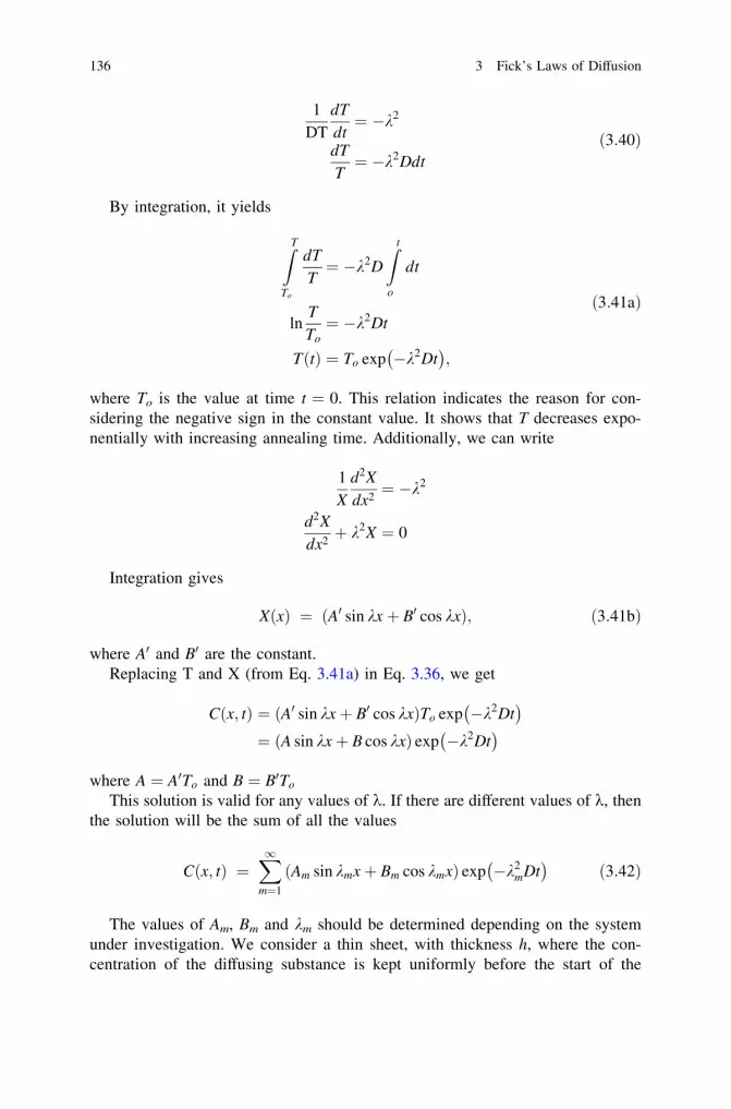
1DT

dT

dt¼ �k2

dT

T¼ �k2Ddt

ð3:40Þ

By integration, it yields

ZT

To

dT

T¼ �k2D

Z t

o

dt

lnT

To¼ �k2Dt

T tð Þ ¼ To exp �k2Dt� �

;

ð3:41aÞ

where To is the value at time t = 0. This relation indicates the reason for con-sidering the negative sign in the constant value. It shows that T decreases expo-nentially with increasing annealing time. Additionally, we can write

1X

d2X

dx2¼ �k2

d2X

dx2þ k2X ¼ 0

Integration gives

XðxÞ ¼ A0 sin kxþ B0 cos kxð Þ; ð3:41bÞ

where A0 and B0 are the constant.Replacing T and X (from Eq. 3.41a) in Eq. 3.36, we get

Cðx; tÞ ¼ A0 sin kxþ B0 cos kxð ÞTo exp �k2Dt� �

¼ A sin kxþ B cos kxð Þ exp �k2Dt� �

where A ¼ A0To and B ¼ B0To

This solution is valid for any values of k. If there are different values of k, thenthe solution will be the sum of all the values

Cðx; tÞ ¼X1m¼1

Am sin kmxþ Bm cos kmxð Þ exp �k2mDt

� �ð3:42Þ

The values of Am, Bm and km should be determined depending on the systemunder investigation. We consider a thin sheet, with thickness h, where the con-centration of the diffusing substance is kept uniformly before the start of the

136 3 Fick’s Laws of Diffusion

diffusion process. Further, the concentration at the surfaces of the sheet is alwayskept at zero. Thus, the boundary conditions can be written as

C ¼ Co; for 0\x\h; at t ¼ 0

C ¼ 0; for x ¼ 0 and x ¼ h; at t [ 0

From the second boundary condition, C is zero at x = 0 at any time only ifBm = 0. Moreover, C is zero at x = h at any time only if km = mp/h, where m is apositive integer. Replacing these values in Eq. 3.42, we get

Cðx; tÞ ¼X1m¼1

Am sinmph

x� �

exp �m2p2

h2Dt

� �ð3:43Þ

From the first boundary condition for t = 0, we get

Co ¼X1m¼1

Am sinmph

x� �

ð3:44Þ

Now, we need to find the value of Am. We multiply both sides by sin nph xdx and

integrate in the range of 0 to h.

Zh

o

Co sinnph

x� �

dx ¼X1m¼1

Am

Zh

o

sinnph

x sinmph

xdx

0@

1A ð3:45Þ

On the right-hand side, all integrals will be zero except for only one valuen = m. When n = m, the value of the integral is h/2. So we can write

Am ¼2h

Zh

o

Co sinmph

x� �

dx ð3:46Þ

Integration of this shows the value of 0 for even values of m and 4Co/mp for anyodd values of m. The summation of the integer values can be changed so that wecan use this relation for every integer, with the result that it will give odd m valuesfor every integer. This can be written as

Am ¼4Co

mp¼ Aj ¼

4C

2jþ 1ð Þp j ¼ 0; 1; 2. . .. . .. . .

So Eq. 3.43 can be written as

Cðx; tÞ ¼ 4Co

p

X1j¼0

12jþ 1

sin2jþ 1ð Þpx

hexp � 2jþ 1ð Þ2p2

h2Dt

!ð3:47Þ

3.2 Solution of Fick’s Second Law to Estimate the Diffusion Coefficient 137

This solution is the summation of all the terms for j equal from zero to infinity.However, it must be clear from the relation that the value for every successivej decreases exponentially (note the negative sign inside the exponent). It should,therefore, be possible to represent the concentration with the first few values ofj. Let us estimate the value for j = 0 and 1 after time t.

Cj¼0ðx; tÞ ¼4Co

psin

px

hexp � p2

h2Dt

� �for j ¼ 0:

Cj¼1ðx; tÞ ¼4Co

p13

sin3px

hexp � 9p2

h2Dt

� �for j ¼ 1:

Taking ratio of these two values, we get

Cj¼0ðx; tÞCj¼1ðx; tÞ

¼ 3 exp8p2

h2Dt

� �

As explained earlier, this solution can be used where the thickness of the systemis relatively small so that it can reach homogeneity in a reasonable time frame.This thickness again depends on the diffusion coefficient at that particular tem-perature of interest. Let us consider h ¼ 4

ffiffiffiffiffiDtp

, where the ratio given above is 419.This means that if we neglect even the second term, the error is only 0.2 %. On theother hand, if we have h ¼ 10

ffiffiffiffiffiDtp

, the ratio is 6.6. If we neglect the second term,an error of around 15 % is to be expected. Thus, the number of terms that shouldbe considered depends on the system and the temperature, since D varies differ-ently in different systems at a particular temperature.

Note There is widespread confusion as to the usefulness or the applicabilityof Fick’s fist law. Many even think that this law cannot be used in anyrealistic situation. It should be noted here that there is no fundamentalproblem in Fick’s first law. It is true that it cannot be used directly to studythe time-dependent mass distribution in a non-steady case. However, at oneparticular composition after a fixed annealing time, Fick’s first law is stillapplicable to relate the flux and the concentration gradient at any particularconcentration. This will be shown in Chap. 6 in which the relations for thecalculation of different diffusion parameters are developed.It is also stated many times that the chemical potential gradient is the realdriving force for the diffusion process and not the concentration gradient. Aswill be discussed in Chap. 4, it is correct that the chemical potential gradientalways indicates the direction of diffusing components correctly, sincecomponents always diffuse down the chemical potential gradient. It is rathercommon to find the diffusion of components also down the concentrationgradient in the majority of systems. However, there are also several exam-ples of uphill diffusion (especially in multicomponent systems), where thedirection of the diffusing components is against the concentration gradient

138 3 Fick’s Laws of Diffusion

because of a favorable chemical potential gradient. In this case also, Fick’slaws are applicable and the uphill diffusion is indicated by a negative sign inthe diffusion coefficient compared to a positive sign for the downhill diffu-sion. For further clarification, see Chap. 9 on multicomponent diffusionanalysis.

References

1. A. Fick, Annalen der Physik 170 (1855) 592. J. Crank, The Mathematics of Diffusion, Oxford University Press, New York, 1956

3.2 Solution of Fick’s Second Law to Estimate the Diffusion Coefficient 139

Chapter 4Development of Interdiffusion Zonein Different Systems

In this chapter, the microstructural evolution in the interdiffusion zone in adiffusion couple is explained based on thermodynamics. A two-phase mixturecannot develop in a binary system, whereas this is possible to find in a ternarysystem. Condition for finding an uphill diffusion is explained.

As discussed in the previous chapter, when two different blocks are joined fordiffusion, it is called a diffusion couple. For example, two alloys of A-B binarysystem are coupled, as shown in Fig. 4.1. The concentration (or composition) ofthe left-hand side of the couple is CB

- (or NB-) and the concentration (or compo-

sition) of the right-hand side of the couple is CB+ (or NB

+). We consider CB- \ CB

+

(or NB- \ NB

+). In general (meaning not in uphill diffusion), as will be discussedlater in this chapter, A will diffuse from left to right and B will diffuse from right toleft. In uphill diffusion, the direction of diffusing component is just the opposite.As the atoms interdiffuse with each other, the overall process is known as inter-diffusion. The definition and details of the diffusion parameters are discussed atgreater length in Chaps. 5–8. In this chapter, the discussion is on the growth of thephases in an interdiffusion zone in different systems.

4.1 Chemical Potential as the Driving Force for Diffusionand Phase Layer Growth in an Interdiffusion Zone

In most practical examples, diffusion occurs under the presence of driving forces.A chemical driving force that is the diffusion caused by differences in the chemicalpotential or activity of the components is common to the majority of systems.Additionally, a few other types of forces might influence the diffusion process. Forexample, in the electronic industry, the flow of electrons also drives the diffusionprocess because of the presence of current. The presence of driving forces makesthe jump rate of atoms higher in one particular direction. Let us consider theisomorphous phase diagram that is presented in Fig. 4.2a. The free energy curveof the solid solution phase at temperature, T, is shown in Fig. 4.2b. At any

A. Paul et al., Thermodynamics, Diffusion and the Kirkendall Effect in Solids,DOI: 10.1007/978-3-319-07461-0_4, � Springer International Publishing Switzerland 2014

141

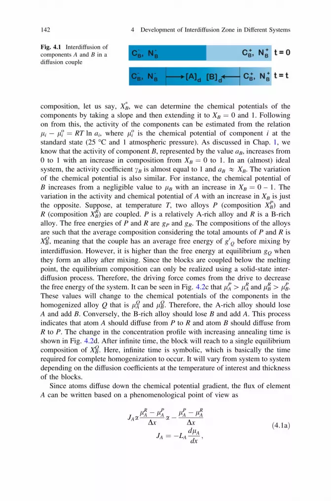
composition, let us say, XB*, we can determine the chemical potentials of the

components by taking a slope and then extending it to XB = 0 and 1. Followingon from this, the activity of the components can be estimated from the relationli - li

o = RT ln ai, where lio is the chemical potential of component i at the

standard state (25 �C and 1 atmospheric pressure). As discussed in Chap. 1, weknow that the activity of component B, represented by the value aB, increases from0 to 1 with an increase in composition from XB = 0 to 1. In an (almost) idealsystem, the activity coefficient cB is almost equal to 1 and aB & XB. The variationof the chemical potential is also similar. For instance, the chemical potential ofB increases from a negligible value to lB with an increase in XB = 0 – 1. Thevariation in the activity and chemical potential of A with an increase in XB is justthe opposite. Suppose, at temperature T, two alloys P (composition XB

P) andR (composition XB

R) are coupled. P is a relatively A-rich alloy and R is a B-richalloy. The free energies of P and R are gP and gR. The compositions of the alloysare such that the average composition considering the total amounts of P and R isXB

Q, meaning that the couple has an average free energy of g0Q before mixing byinterdiffusion. However, it is higher than the free energy at equilibrium gQ whenthey form an alloy after mixing. Since the blocks are coupled below the meltingpoint, the equilibrium composition can only be realized using a solid-state inter-diffusion process. Therefore, the driving force comes from the drive to decreasethe free energy of the system. It can be seen in Fig. 4.2c that lA

P [ lAR and lB

R [ lBP.

These values will change to the chemical potentials of the components in thehomogenized alloy Q that is lA

Q and lBQ. Therefore, the A-rich alloy should lose

A and add B. Conversely, the B-rich alloy should lose B and add A. This processindicates that atom A should diffuse from P to R and atom B should diffuse fromR to P. The change in the concentration profile with increasing annealing time isshown in Fig. 4.2d. After infinite time, the block will reach to a single equilibriumcomposition of XB

Q. Here, infinite time is symbolic, which is basically the timerequired for complete homogenization to occur. It will vary from system to systemdepending on the diffusion coefficients at the temperature of interest and thicknessof the blocks.

Since atoms diffuse down the chemical potential gradient, the flux of elementA can be written based on a phenomenological point of view as

JAalR

A � lPA

Dxa� lP

A � lRA

Dx

JA ¼ �LAdlA

dx;

ð4:1aÞ

Fig. 4.1 Interdiffusion ofcomponents A and B in adiffusion couple

142 4 Development of Interdiffusion Zone in Different Systems

where the proportionality constant LA is called the phenomenological constant ofcomponent A.

Similarly for component B, it can be written as

JBalP

B � lRB

Dxa� lR

B � lPB

Dx

JB ¼ �LBdlB

dx;

ð4:1bÞ

where LB is the phenomenological constant for element B. These relations weredeveloped previously in Chap. 1 (Sect. 1.15).

Fig. 4.2 Interdiffusion in a complete solid solution is explained in a phase diagram, bg versuscomposition diagram, c chemical potentials of components, and d the diffusion couple andcomposition profiles

4.1 Chemical Potential as the Driving Force for Diffusion 143

In terms of the concentration gradient, we can write

JAaCR

A � CPA

Dxa� CP

A � CRA

Dx

JA ¼ �DAdCA

dx

ð4:1cÞ

Similarly, we can write

JBaCP

B � CRB

Dxa� CR

B � CPB

Dx

JB ¼ �DBdCB

dx

ð4:1dÞ

DA and DB are the intrinsic diffusion coefficients, i.e., the diffusion coefficients ofthe components A and B.

Therefore, it can be seen in this system that the components diffuse down thechemical potential and concentration gradient. This is indeed the case for mostsystems. However, in uphill diffusion, it is different—as will be explained at theend of this section. Since composition changes with time at one particular location,driving force and flux of components also change accordingly. It is a fact that thediffusion coefficient depends on a few other factors such as crystal structure anddefects, which will be covered in the next few chapters. For now, we consider ahypothetical phase diagram, the one shown in Fig. 4.3a. A diffusion couple ismade of the pure components A and B, at temperature T, as presented in Fig. 4.3a.At this temperature of interest, there are three regions between A and B: thephase mixture of A and b, the single-phase b, and the phase mixture of b andB. Following the Gibbs phase rule, F = C – P + 2, where F is the degrees offreedom, C is the number of the components, and P is the number of the phases. Asthe experiments are conducted at constant temperature and pressure, this relationcan be written as F = C – P. In a binary system (C = 2), it becomes F + P = 2.Therefore, in binary diffusion couple, the total number of phases and the degrees offreedom can be two. Since composition is one of the degrees of freedom alreadypresent, only one phase can be present in the interdiffusion zone. This furtherindicates that at any position to the diffusion direction, a phase mixture cannotgrow in a binary system. Therefore, only the b phase will grow in the interdiffusionzone. We can observe from Figs. 4.3b and c that at the interface I, A and b are inequilibrium, and at the interface II, b and B are in equilibrium. Although localequilibrium exists at these interfaces, the diffusion of the components will occursince there is a difference in the chemical potential of the components betweeninterfaces I and II. We witness a continuous change in the chemical potentialacross the interdiffusion zone. For example, it changes from lA

I to lAII for the

element A. In fact, this is true in any interdiffusion zone, where there will be acontinuous variation in chemical potential during the entire interdiffusion process.In this particular case, since the phase has a very narrow homogeneity range, thechemical potential changes very sharply.

144 4 Development of Interdiffusion Zone in Different Systems

From the above discussion, it must be clear that if we couple the alloys P and Q,as shown in Fig. 4.3a, there will be no interdiffusion because there is no differencein the chemical potential of the components even though a composition differenceexists. This indicates that the composition or concentration differences between thecouples do not explain the interdiffusion of the components. It is necessary toexamine the interdiffusion process based on the difference in the chemicalpotentials. What we are actually saying is that there will be no interdiffusionbetween the alloys P and Q. Self-diffusion of the components in the respectivealloys still can occur. All these are covered to in greater detail in the next chapteras a part of the discussion on the atomic mechanism of diffusion. Even the size ofthe phases increases in the alloys to minimize the interfacial energy since these aretwo-phase mixtures.

Let us consider another phase diagram, as shown in Fig. 4.4a. At the temper-ature of our interest T, we have a solid solution a, an intermetallic compound b,and a solid solution c. The free energy diagram is shown in Fig. 4.4b and the

Fig. 4.3 Growth of a phase with narrow composition range is explained in a the hypotheticalphase diagram, b free energy versus composition diagram, c the variation of the chemicalpotential of components, and d the interdiffusion zone and composition profile

4.1 Chemical Potential as the Driving Force for Diffusion 145

change in the chemical potential of element B is shown in Fig. 4.4c. Following theexplanations above, it can be understood that the a, b, and c phases will grow inthe interdiffusion zone and the likely composition profile is shown in Fig. 4.4d.It can be seen that the two-phase mixture, where the chemical potentials of thecomponents are constant, will not develop in the interdiffusion zone. Therefore, asexpected, the continuous change in the chemical potential is present in the inter-diffusion zone.

Now we turn to consider a phase diagram, shown in Fig. 4.5a, which has acomplete solid solution in the high temperature range and a miscibility gap in thelow temperature range. Therefore, when A and B are coupled in these temperatureranges, different composition profiles will develop in the interdiffusion zone. Asshown in Fig. 4.5b, interdiffusion zone will show continuous change in thecomposition profile at T1, whereas at T2, it will exhibit a composition jump.

The whole diffusion process is completely different, if we couple two alloysP and Q inside the miscibility gap, as presented in Fig. 4.6a. The process isexplained with respect to the chemical potential of the components, as can be

Fig. 4.4 Interdiffusion in a system where the solid solution phases are present along with anintermetallic compound with a wide homogeneity range is explained. a Hypothetical phasediagram, bg versus XB diagram, c the change in chemical potential with composition, and d thediffusion couple and composition profile

146 4 Development of Interdiffusion Zone in Different Systems

Fig. 4.5 Interdiffusion attwo different temperatures isexplained in a system wherethere is a miscibility gap atthe lower temperature.a Hypothetical phasediagram, b compositionprofile at higher temperature,where it has a complete solidsolution, and c compositionprofile at lower temperature,where it has a miscibility gap

4.1 Chemical Potential as the Driving Force for Diffusion 147

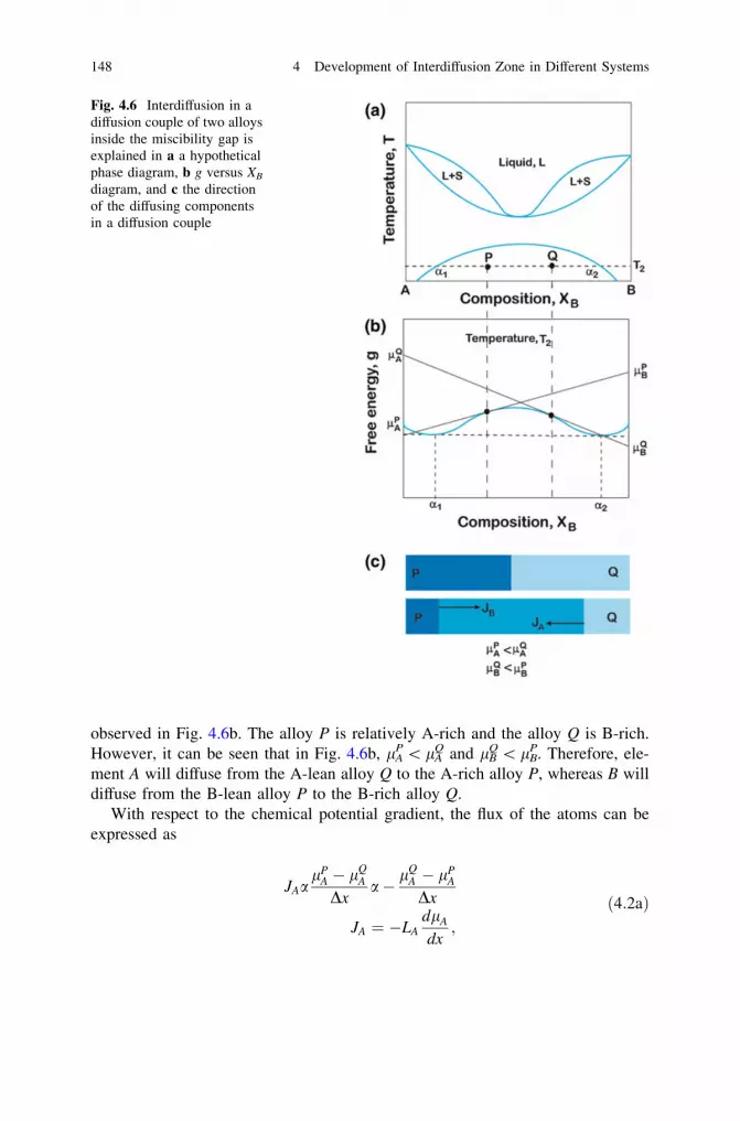
observed in Fig. 4.6b. The alloy P is relatively A-rich and the alloy Q is B-rich.However, it can be seen that in Fig. 4.6b, lA

P \lAQ and lB

Q \ lBP. Therefore, ele-

ment A will diffuse from the A-lean alloy Q to the A-rich alloy P, whereas B willdiffuse from the B-lean alloy P to the B-rich alloy Q.

With respect to the chemical potential gradient, the flux of the atoms can beexpressed as

JAalP

A � lQA

Dxa� lQ

A � lPA

Dx

JA ¼ �LAdlA

dx;

ð4:2aÞ

Fig. 4.6 Interdiffusion in adiffusion couple of two alloysinside the miscibility gap isexplained in a a hypotheticalphase diagram, b g versus XB

diagram, and c the directionof the diffusing componentsin a diffusion couple

148 4 Development of Interdiffusion Zone in Different Systems

Similarly,

JBalQ

B � lPB

Dxa� lP

B � lQB

Dx

JB ¼ �LBdlB

dx;

ð4:2bÞ

In terms of concentration gradient, we can write

JAaCP

A � CQA

Dx

JA ¼ DAdCA

dx:

ð4:2cÞ

Similarly,

JB ¼ DBCQ

B � CPB

Dx¼ DB

dCB

dx: ð4:2dÞ

Therefore, the minus sign of Fick’s first law is not there in the relationsexpressed in Eqs. 4.2c and 4.2d. This would suggest that the components diffuseup the concentration gradient rather than down the concentration gradient and, forthis simple reason, it is called uphill diffusion. It should be noted here that therelations for the calculation of the diffusion coefficients from the compositionprofiles are derived considering the minus sign in Fick’s first law. The samerelations can be used to determine the diffusion coefficients even if the system goesthrough uphill diffusion. Nonetheless, the diffusion coefficient will have a negativesign.

4.2 Few Practical Examples

In this section, we shall provide a few examples that are based upon real workingsystems. From Fig. 4.7a [1], it can be seen that in the high temperature range, theAu–Cu system has a complete solid solution. Thus, after coupling Au and Cu at850 �C for 9 h [1], a continuous change in the composition is to be found, asdepicted in Fig. 4.7b. It needs to be pointed out here that, below 410 �C, a con-tinuous change in the composition profile will not develop because of the presenceof the intermediate phases, as was discussed above based on the hypotheticaldiffusion couples in Figs. 4.3 and 4.4.

It can be seen in the Au–Sb phase diagram in Fig. 4.8a [2], that below 633 K,there is only one compound AuSb2 that is present. The solubility of Sb in Au isvery low and the solubility of Au in Sb is negligible. In the diffusion couple of Auand Sb at 607 K (330 �C) annealed for 225 h, it is mainly the AuSb2 phase that is

4.1 Chemical Potential as the Driving Force for Diffusion 149

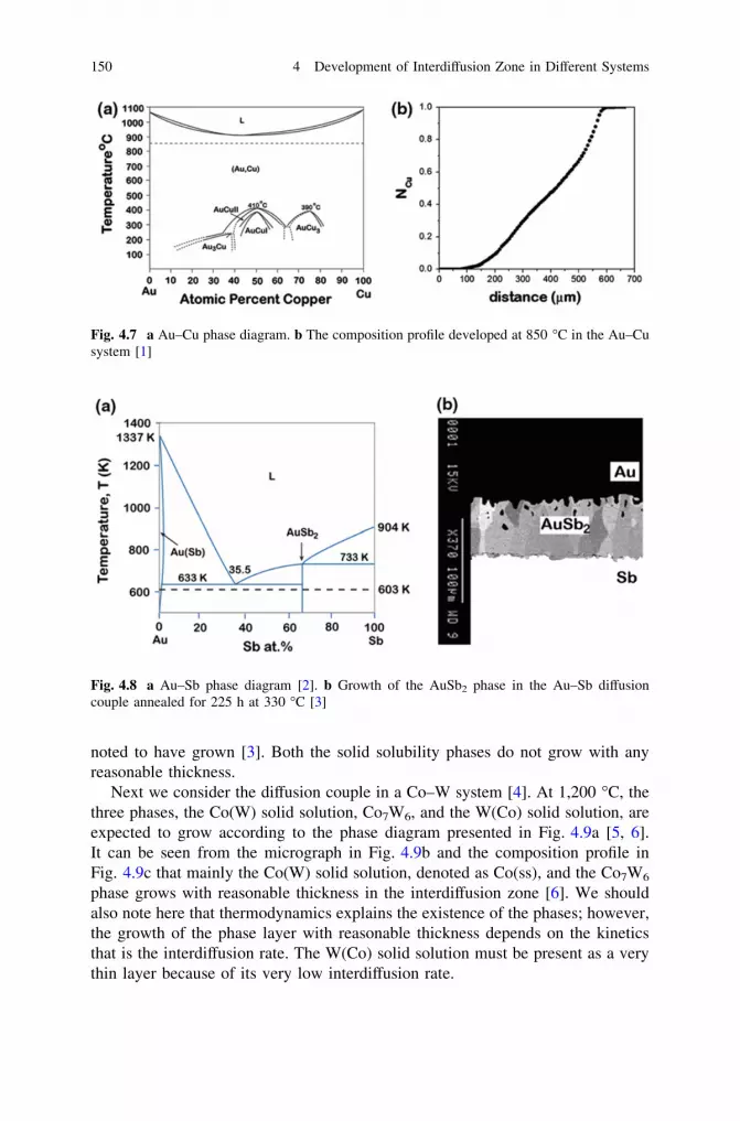
noted to have grown [3]. Both the solid solubility phases do not grow with anyreasonable thickness.

Next we consider the diffusion couple in a Co–W system [4]. At 1,200 �C, thethree phases, the Co(W) solid solution, Co7W6, and the W(Co) solid solution, areexpected to grow according to the phase diagram presented in Fig. 4.9a [5, 6].It can be seen from the micrograph in Fig. 4.9b and the composition profile inFig. 4.9c that mainly the Co(W) solid solution, denoted as Co(ss), and the Co7W6

phase grows with reasonable thickness in the interdiffusion zone [6]. We shouldalso note here that thermodynamics explains the existence of the phases; however,the growth of the phase layer with reasonable thickness depends on the kineticsthat is the interdiffusion rate. The W(Co) solid solution must be present as a verythin layer because of its very low interdiffusion rate.

Fig. 4.7 a Au–Cu phase diagram. b The composition profile developed at 850 �C in the Au–Cusystem [1]

Fig. 4.8 a Au–Sb phase diagram [2]. b Growth of the AuSb2 phase in the Au–Sb diffusioncouple annealed for 225 h at 330 �C [3]

150 4 Development of Interdiffusion Zone in Different Systems

Fig. 4.9 a Co–W phase diagram [4], b diffusion couple of Co/W annealed at 1,200 �C for 25 h[6], and c the measured composition profile [6]

4.2 Few Practical Examples 151

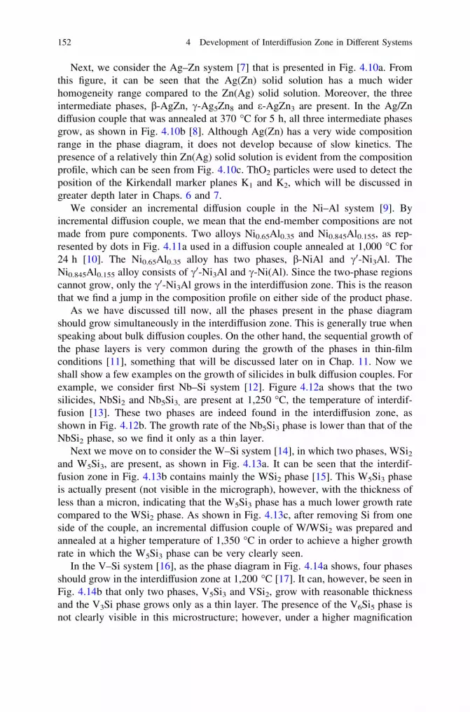
Next, we consider the Ag–Zn system [7] that is presented in Fig. 4.10a. Fromthis figure, it can be seen that the Ag(Zn) solid solution has a much widerhomogeneity range compared to the Zn(Ag) solid solution. Moreover, the threeintermediate phases, b-AgZn, c-Ag5Zn8 and e-AgZn3 are present. In the Ag/Zndiffusion couple that was annealed at 370 �C for 5 h, all three intermediate phasesgrow, as shown in Fig. 4.10b [8]. Although Ag(Zn) has a very wide compositionrange in the phase diagram, it does not develop because of slow kinetics. Thepresence of a relatively thin Zn(Ag) solid solution is evident from the compositionprofile, which can be seen from Fig. 4.10c. ThO2 particles were used to detect theposition of the Kirkendall marker planes K1 and K2, which will be discussed ingreater depth later in Chaps. 6 and 7.

We consider an incremental diffusion couple in the Ni–Al system [9]. Byincremental diffusion couple, we mean that the end-member compositions are notmade from pure components. Two alloys Ni0.65Al0.35 and Ni0.845Al0.155, as rep-resented by dots in Fig. 4.11a used in a diffusion couple annealed at 1,000 �C for24 h [10]. The Ni0.65Al0.35 alloy has two phases, b-NiAl and c0-Ni3Al. TheNi0.845Al0.155 alloy consists of c0-Ni3Al and c-Ni(Al). Since the two-phase regionscannot grow, only the c0-Ni3Al grows in the interdiffusion zone. This is the reasonthat we find a jump in the composition profile on either side of the product phase.

As we have discussed till now, all the phases present in the phase diagramshould grow simultaneously in the interdiffusion zone. This is generally true whenspeaking about bulk diffusion couples. On the other hand, the sequential growth ofthe phase layers is very common during the growth of the phases in thin-filmconditions [11], something that will be discussed later on in Chap. 11. Now weshall show a few examples on the growth of silicides in bulk diffusion couples. Forexample, we consider first Nb–Si system [12]. Figure 4.12a shows that the twosilicides, NbSi2 and Nb5Si3, are present at 1,250 �C, the temperature of interdif-fusion [13]. These two phases are indeed found in the interdiffusion zone, asshown in Fig. 4.12b. The growth rate of the Nb5Si3 phase is lower than that of theNbSi2 phase, so we find it only as a thin layer.

Next we move on to consider the W–Si system [14], in which two phases, WSi2and W5Si3, are present, as shown in Fig. 4.13a. It can be seen that the interdif-fusion zone in Fig. 4.13b contains mainly the WSi2 phase [15]. This W5Si3 phaseis actually present (not visible in the micrograph), however, with the thickness ofless than a micron, indicating that the W5Si3 phase has a much lower growth ratecompared to the WSi2 phase. As shown in Fig. 4.13c, after removing Si from oneside of the couple, an incremental diffusion couple of W/WSi2 was prepared andannealed at a higher temperature of 1,350 �C in order to achieve a higher growthrate in which the W5Si3 phase can be very clearly seen.

In the V–Si system [16], as the phase diagram in Fig. 4.14a shows, four phasesshould grow in the interdiffusion zone at 1,200 �C [17]. It can, however, be seen inFig. 4.14b that only two phases, V5Si3 and VSi2, grow with reasonable thicknessand the V3Si phase grows only as a thin layer. The presence of the V6Si5 phase isnot clearly visible in this microstructure; however, under a higher magnification

152 4 Development of Interdiffusion Zone in Different Systems

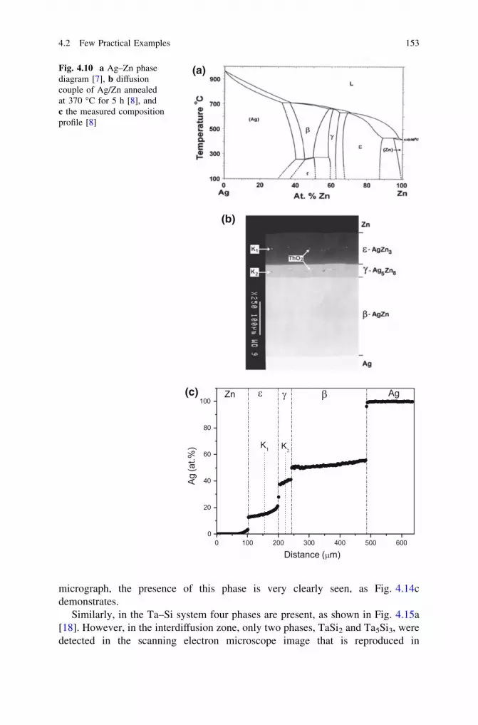
micrograph, the presence of this phase is very clearly seen, as Fig. 4.14cdemonstrates.

Similarly, in the Ta–Si system four phases are present, as shown in Fig. 4.15a[18]. However, in the interdiffusion zone, only two phases, TaSi2 and Ta5Si3, weredetected in the scanning electron microscope image that is reproduced in

(a)

(b)

(c)

Fig. 4.10 a Ag–Zn phasediagram [7], b diffusioncouple of Ag/Zn annealedat 370 �C for 5 h [8], andc the measured compositionprofile [8]

4.2 Few Practical Examples 153

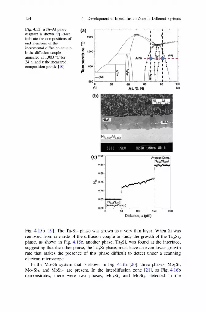
Fig. 4.15b [19]. The Ta5Si3 phase was grown as a very thin layer. When Si wasremoved from one side of the diffusion couple to study the growth of the Ta5Si3phase, as shown in Fig. 4.15c, another phase, Ta2Si, was found at the interface,suggesting that the other phase, the Ta3Si phase, must have an even lower growthrate that makes the presence of this phase difficult to detect under a scanningelectron microscope.

In the Mo–Si system that is shown in Fig. 4.16a [20], three phases, Mo3Si,Mo5Si3, and MoSi2, are present. In the interdiffusion zone [21], as Fig. 4.16bdemonstrates, there were two phases, Mo5Si3 and MoSi2, detected in the

Fig. 4.11 a Ni–Al phasediagram is shown [9]. Dotsindicate the compositions ofend members of theincremental diffusion couple.b the diffusion coupleannealed at 1,000 �C for24 h, and c the measuredcomposition profile [10]

154 4 Development of Interdiffusion Zone in Different Systems

Fig. 4.12 a Nb–Si phase diagram [12] and b the interdiffusion zone developed in between thediffusion couple of Nb/Si annealed at 1,250 �C for 24 h [13]

Fig. 4.13 a W–Si phase diagram [14], b the interdiffusion zone of the W/Si diffusion coupleannealed at 1,225 �C for 9 h, and c the interdiffusion zone of the incremental diffusion couple W/WSi2 annealed at 1,350 �C for 16 h [15]

4.2 Few Practical Examples 155

interdiffusion zone. The transmission electron microscope image [22] shows thepresence of the Mo3Si phase, which was not possible to detect under the scanningelectron microscope. This would strongly suggest that the growth rate of the Mo3Siphase is much lower compared to the other phases. In fact, in the Ti/Al diffusioncouple, only the TiAl3 phase was found in the interdiffusion zone [23]. All theother phases present in the phase diagram, the TiAl2, TiAl, and Ti3Al phases, werenot to be found. These three phases appeared in an incremental couple of TiAl3/Ti,which is suggestive of a much lower growth rate compared to that of TiAl3 in theTi/Al diffusion couple.

Sometimes, changing annealing temperature or time plays an important role onfinding the phases differently in the interdiffusion zone. In the Co–Ta system, aspresented in Fig. 4.17 [24], we found that only the Co2Ta phase grows in theinterdiffusion zone at 1,050 �C. However, when the couple is annealed at1,150 �C, the other two phases, CoTa2 and CoTa, which were not visible (but mustbe present as very thin layer) at 1,050 �C, were found to form. This indicates thatthe growth rate of these two phases increased at 1,150 �C making it possible to

Fig. 4.14 a V–Si phase diagram [16], b interdiffusion zone of the V/Si diffusion couple annealedat 1,200 �C for16 h, and c V-rich phases of the same diffusion couple [17]

156 4 Development of Interdiffusion Zone in Different Systems

find them along with the Co2Ta phase. In the Pd-Sn phase diagram [25], eightintermetallic compounds are present. When the Pd/Sn diffusion couple wasannealed at 175 �C for 9 h, only the PdSn4 phase layer was found with higherthickness, as Fig. 4.18a makes clear of its presence [26]. However, upon closerexamination—at the PdSn4/Pd interface as the location is marked by (b) inFig. 4.18a and shown in Fig. 4.18b—another two phases, PdSn3 and PdSn2, weredetected. Similar behavior was noticed at 150 �C for the same annealing time of9 h at 150 �C. However, when the couple was annealed for a longer period of36 h, the other two phases were also to be found with higher thickness, as shown inFig. 4.18c. All these further indicate that the growth rate of the other missingphases must be even lower.

Therefore, as expected, all the phases might grow simultaneously especially inbulk diffusion couples. Yet all the phases might not grow with a reasonablethickness to be detectable by the scanning electron microscope. A much higherresolution image from a transmission electron microscope might show the

Fig. 4.15 a Ta–Si phase diagram [18], b interdiffusion zone of the Ta/Si diffusion coupleannealed at 1,250 �C for 9 h, and c incremental diffusion couple of Ta/TaSi2 annealed at1,350 �C for 9 h [19]

4.2 Few Practical Examples 157

Fig. 4.16 a Mo–Si phase diagram [20], b interdiffusion zone of the Mo/Si diffusion coupleannealed at 1,300 �C for 16 h [21], and c interdiffusion zone of the Mo/MoSi2 couple showing thepresence of the Mo3Si phase [22]

Fig. 4.17 Interdiffusion zone of the Ta/Co diffusion couple annealed at a 1,050 �C for 16 h andb 1,150 �C for 16 h [24]

158 4 Development of Interdiffusion Zone in Different Systems

presence of these phase layers as very thin layers. However, it might not be alwaystrue. In the Cu–Sn diffusion couple [27], it is suspected that the Cu3Sn phase doesnot grow in the beginning along with the Cu6Sn5 phase. As will be discussed muchlater in Chap. 11, sequential growth is rather commonplace in thin-film conditions.

Sometimes, the phases developed in the interdiffusion zone suggest that theproblem lies in the phase diagram. As the Ti–Si phase diagram in Fig. 4.19ashows, the Ti3Si phase does not exist at above 1,170 �C [28]. However, when theexperiment was conducted at 1,200 �C, this phase was found along with the otherphases as shown in Fig. 4.19b. The same was to be found at 1,225 �C; however, itwas not found at 1,250 �C, as shown in Fig. 4.19c and d, hinting strongly that thisphase exists up to the temperature somewhere between the temperatures1,225–1,250 �C [29]. Similarly, the diffusion couple experiments were used todetect problems in a few other phase diagrams [10, 24, 30].

In a ternary system, unlike in a binary system, a phase mixture can evolve in theinterdiffusion zone. This could be understood with the help of the Gibbs phaserule, F = C – P + 2. Again, since the experiments are conducted at constant

Fig. 4.18 a Interdiffusion zone of the Pd/Sn diffusion couple annealed at 175 �C for 9 h, b Pd-rich phases in the same diffusion couple, and c interdiffusion zone of the Pd/Sn diffusion coupleannealed at 150 �C for 36 h [26]

4.2 Few Practical Examples 159

temperature and pressure, this relation can be written as F = C – P. In a ternarysystem (C = 3), it becomes F = 3 - P. Therefore, in the ternary diffusion couple,the total of number of phases and the degrees of freedom can be three. Since thecomposition is one of the degrees of freedom, a mixture of the two phases coulddevelop in the interdiffusion zone. It can, for instance, be seen in the Au(20Cu)/Sndiffusion couple presented in Fig. 4.20a [31] that two layers with phase mixtureshave developed: one layer with (Au,Cu)Sn4 and (Au,Cu)Sn and another layer with(Au,Cu)Sn2 and (Au,Cu)Sn. This does not necessarily mean that layers always willgrow with the phase mixture in a ternary system, as found in the Co(50Ni)/Modiffusion couple, which can be seen in Fig. 4.20b. This will be discussed further inChap. 9 (Sect. 9.5).

4.3 Making Products by a Diffusion Process

The study of diffusion is important to gain a full understanding on many physicaland mechanical properties of materials. Most of the phase transformations in thesolid state occur by some kind of a diffusion-controlled process. It is a commonassumption that the study of diffusion is important in order to generate data forfurther understanding of the related processes. However, there are many products

Fig. 4.19 a Ti–Si phase diagram [28], b Ti/Si couple annealed at 1,200 �C for 16 h, and c andd Ti-rich phases in the interdiffusion zone annealed at 1,225 and 1,250 �C annealed for 16 h [29],respectively

160 4 Development of Interdiffusion Zone in Different Systems

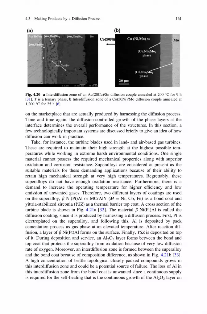
on the marketplace that are actually produced by harnessing the diffusion process.Time and time again, the diffusion-controlled growth of the phase layers at theinterface determines the overall performance of the structures. In this section, afew technologically important systems are discussed briefly to give an idea of howdiffusion can work in practice.

Take, for instance, the turbine blades used in land- and air-based gas turbines.These are required to maintain their high strength at the highest possible tem-peratures while working in extreme harsh environmental conditions. One singlematerial cannot possess the required mechanical properties along with superioroxidation and corrosion resistance. Superalloys are considered at present as thesuitable materials for these demanding applications because of their ability toretain high mechanical strength at very high temperatures. Regrettably, thesesuperalloys do not have enough oxidation resistance. Furthermore, there is ademand to increase the operating temperature for higher efficiency and lowemission of unwanted gases. Therefore, two different layers of coatings are usedon the superalloy, b Ni(Pt)Al or MCrAlY (M = Ni, Co, Fe) as a bond coat andyittria-stabilized zirconia (YSZ) as a thermal barrier top coat. A cross section of theturbine blade is shown in Fig. 4.21a [32]. The material b Ni(Pt)Al is called thediffusion coating, since it is produced by harnessing a diffusion process. First, Pt iselectroplated on the superalloy, and following this, Al is deposited by packcementation process as gas phase at an elevated temperature. After reaction dif-fusion, a layer of b Ni(Pt)Al forms on the surface. Finally, YSZ is deposited on topof it. During deposition and service, an Al2O3 layer forms between the bond andtop coat that protects the superalloy from oxidation because of very low diffusionrate of oxygen. Moreover, an interdiffusion zone is formed between the superalloyand the bond coat because of composition difference, as shown in Fig. 4.21b [33].A high concentration of brittle topological closely packed compounds grows inthis interdiffusion zone and could be a potential source of failure. The loss of Al inthis interdiffusion zone from the bond coat is unwanted since a continuous supplyis required for the self-healing that is the continuous growth of the Al2O3 layer on

Fig. 4.20 a Interdiffusion zone of an Au(20Cu)/Sn diffusion couple annealed at 200 �C for 9 h[31]. T is a ternary phase, b Interdiffusion zone of a Co(50Ni)/Mo diffusion couple annealed at1,200 �C for 25 h [6]

4.3 Making Products by a Diffusion Process 161

top of the bond coat, i.e., in the middle of bond coat and top coat. Self-healing isimportant to cover the surface where spallation of Al2O3 occurs. Since Al diffusesout from the bond coat, it is important to study the role of different factors thatdetermine the diffusion of components [34–36]. One of the beneficial roles of Pt inthe bond coat is an increase in the Al diffusion rate [37]. This ensures that theservice life of a turbine blade is increased threefold. Another type of bond coat,MCrAlY, is called an overlay coating since it is deposited directly on the super-alloy—unlike the b Ni(Pt)Al coating. Again, similar studies are important tounderstand or enhance the performance. Studies not only on the bond coat, but alsoextensive diffusion studies in the superalloys, themselves conducted to understandmany properties such as homogenization and creep.

Nb3Sn is one of the A15 intermetallic superconductors used in many applica-tions where the need is beyond the ability of NbTi (greater than a magnetic field of8 T). Since this is a brittle intermetallic compound, it cannot be drawn as wire.Different manufacturing techniques are used to circumvent this problem, such asthe bronze technique, the internal tin process, the powder-in-tube process, the jellyroll process, as well as infiltration, to name but a few. Diffusion plays an importantrole in the vast majority of production processes. To make our point, we shall nowdiscuss only the bronze technique, which is one of the most favored routes. In thistechnique, Nb rods are inserted into Cu(Sn) bronze alloys. Next, this block isdrawn as wire. The cross-sectional view is given in Fig. 4.22a [38]. Following this,the composite wire is annealed in the temperature range of 700–850 �C such thatNb3Sn grows at the Nb/Cu(Sn) interface, as shown in Fig. 4.22b, which wasannealed at 850 �C for 4 h. It has already been shown that the growth rate of theintermetallic compound changes drastically because of a small change in Sncontent in the Cu(Sn) bronze alloy, which changes the Sn diffusion rate throughthe product phase [39, 40]. Even the addition of small amounts of differentcomponents such as Ti, Zr, or Hf also increases the growth rate [41]. Similarly, themanufacturing procedure of V3Ga is being researched, a process which mayreplace Nb3Sn because of better properties.

Fig. 4.21 a Cross section of a turbine blade [32] b Diffusion couple of CMX 4 superalloy withNi(15Pt)Al bond coat at 1,200 �C, annealed for 25 h [33]

162 4 Development of Interdiffusion Zone in Different Systems

Flip-chip and wire bonding are the two techniques to join chip–chip and chip–substrate. As shown in the schematic diagram presented in Fig. 4.23a, differentunderbump metallizations (UBM) are used for different purposes to make thebonding by using an Sn-based solder alloy in flip-chip bonding. Cu is used forgood bonding, Ni is used as a barrier layer, and Au is used for corrosion protection.During soldering, Sn-based intermetallic compounds form by reaction betweenthe UBM layers in the solid state and the solder in the liquid state. Further, duringthe service, these compounds grow by a solid-state diffusion-controlled process.As already explained, the chemical potential difference acts as the driving force forthe growth of the phases. Additionally, an electrical current with a very highdensity due to the small dimensions also plays an important role in the growth ofthe phases. The growth of the phase layers in the Cu–Sn system is explained inFig. 4.24b [42]. In the absence of any current, the two-phase layers, Cu3Sn and

Fig. 4.22 a Cross-sectional view of Nb/Cu(Sn) composite wire and b growth of Nb3Sn at800 �C, annealed for 4 h [38]

Fig. 4.23 Schematic diagram of cross-sectional view where a flip-chip and b wire bonds areshown

4.3 Making Products by a Diffusion Process 163

Fig. 4.24 a The IRF6716MPbF component package and the test board. b The growth of thephase layers of the three interconnections investigated is shown for no current (NC) drain andsource. Phase layers are grown in the middle of printed wire board (PWB) Cu and SnAgCu (SAC)solder [42]

164 4 Development of Interdiffusion Zone in Different Systems

Cu6Sn5, grow in the interdiffusion zone. It must be clear that Cu diffuses from theCu end member toward the solder, whereas Sn diffuses from the solder alloytoward the Cu. Depending on the direction of the electron flow, the diffusion ofthese components is affected. When there is no current, the thickness of the Cu3Snphase is less than the thickness of the Cu6Sn5 phase. The thicknesses of theselayers become comparable when the electrons flow in the direction of the solder tothe Cu. On the other hand, the thickness of Cu6Sn5 increases without changing thethickness of Cu3Sn, when the electrons flow from the Cu to the solder. Thisphenomenological process is discussed in further detail in Chap. 8.

Similarly in wire bonding, as shown in Fig. 4.23b, Au wires are connected withAl pad. During service, several phases grow at the interface, being affected bychemical and electrical driving forces.

Often, in order to achieve a property balance, dissimilar materials such asmetal–metal, metal–ceramic and ceramic–ceramic are joined by a solid-statediffusion bonding process. This process is being exploited to produce a seamlessbond between two different types of superalloys. Metal–metal bondings are pro-duced by this method when these are difficult to join properly by welding. In manyapplications, however, ceramics are preferred as the top layer and a metal or alloyas the substrate. In this case, the materials are bonded directly or joined using aninter-layer. Even two different ceramic layers are also bonded using a metal inter-layer. Multilayer laminate structures are also produced following a similar method.To achieve this, alternate layers are deposited using various techniques or rolledafter stacking before annealing to create a good bond by a diffusion-controlledprocess.

References

1. R. Ravi and A. Paul, Journal of Materials Science: Materials in Electronics, 23 (2012) 21522. H. Okamoto, Journal of Phase Equilibria 17 (1996) 783. A. Paul, A.A. Kodentsov, G. de With, F.J.J. van Loo, Intermetallics 11 (2003) 11954. H. Okamoto, Journal of Phase Equilibria and Diffusion 29 (2008) 1195. R. Ravi and A. Paul, Intermetallics 19 (2011) 4266. V.D. Divya, U. Ramamurty and A. Paul, Metallurgical and Materials Transactions 43 (2012)

15647. B. Predel, Landolt-Börnstein, Group IV Physical Chemistry 12A (2006) 18. A.A. Kodentsov, Aloke Paul, Frans J.J. van Loo, Zeitschrift für Metallkunde 95 (2004) 2589. K.J. Lee, P. Nash, Journal of Phase Equilibria 12 (1991) 551

10. C. Cserháti, A. Paul, A.A. Kodentsov, M.J.H. van Dal, F.J.J. van Loo, Intermetallics 11(2003) 291

11. U. Gösele and K. N. Tu, Journal of Applied Physics 53 (1982) 325212. M.E. Schlesinger, H. Okamoto, A.B. Gokhale and R. Abbaschian, Journal of Phase Equilibria

14(1993) 50213. S. Prasad and A. Paul, Acta Materialia 59 (2011) 157714. Z. Guo, W. Yuan, Y. Sun, Z. Cai and Z. Qiao, Journal of Phase Equilibria and Diffusion 30

(2009) 56415. S. Roy and A. Paul, Intermetallics 37 (2013) 83

4.3 Making Products by a Diffusion Process 165

16. J. F. Smith, Bulletin of Alloy Phase Diagrams 6 (1985) 26617. S. Prasad and A. Paul, Journal of Phase Equilibria and Diffusion 32 (2011) 21218. M.E. Schlesinger Journal of Phase Equilibria 15 (1994) 9019. S. Roy and A. Paul, Philosophical Magazine, 92 (2012) 421520. A.B. Gokhale and G.J. Abbaschian, Journal of Phase Equilibria 12 (1991) 49321. S. Prasad and A. Paul, Intermetallics 19 (2011) 119122. J.K. Yoon, J.Y. Byun, G.H. Kim, J.S. Kim, C.S. Choi, Thin Solid Films 405 (2002) 17023. F.J.J van Loo and G.D Rieck, Acta Metallurgica 21 (1971) 6124. V. Baheti, S. Roy, R. Ravi and A. Paul, Intermetallics, 33 (2013) 8725. H. Okamoto, Journal of Phase Equilibria and Diffusion 33 (2012) 25326. R. Ravi and A. Paul, Journal of Materials Science: Materials in Electronics,23 (2012) 230627. A. Paul, C. Ghosh and W.J. Boettinger, Metallurgical and Materials Transactions A 42A

(2011) 95228. H.J. Seifert, H.L. Lukas and G. Petzow, Zeitschrift für Metallkunde 87 (1996) 229. S. Roy, S. Divinski and A. Paul, Philosophical Magazine 94 (2014) 68330. V.D. Divya, U. Ramamurty and A. Paul, Intermetallics 18 (2010) 25931. S. Santra, S. Islam, R. Ravi, V. Vuorinen, T. Laurila and A. Paul, Phase evolutions in

AuCu/Sn system by solid state reactive diffusion. Journal of Electronic Materials (2014).doi:10.1007/s11664-014-3241-z

32. Nitin P. Padture, Maurice Gell, Eric H. Jordan, Science 296 (2002) 28033. P. Kiruthika and A. Paul, Private communication.34. A. Paul, A.A. Kodentsov and F.J.J. van Loo, Acta Materialia 52 (2004) 40435. A. Paul, A.A. Kodentsov and F.J.J. van Loo, Journal of Alloys and Compounds 403 (2005) 14736. V.D. Divya, U. Ramamurty and A. Paul, Philosophical Magazine 92 (2012) 218737. Kristen A. Marino, Berit Hinnemann, and Emily A. Carter, Proceedings of the National

Academy of the Sciences of the United States of America 5 (2011) 548038. S. Santra and A. Paul, Private communication39. A.K. Kumar and A. Paul, Journal of Electronic Materials, 38 (2009) 70040. T. Laurila, V. Vuorinen A.K. Kumar and A. Paul, Applied Physics Letters, 96 (2010)

231910141. M. Suenaga, D.O. Welch, R.L. Sabatini, O.F. Kammere and S. Okuda, Journal of Applied

Physics 59 (1986) 84042. T. Laurila, J. Karppinen, V.Vuorinen, A. Paul and M. Paulasto-Kröckel, Journal of Electronic

Materials 40 (2011) 1517

166 4 Development of Interdiffusion Zone in Different Systems

Chapter 5Atomic Mechanism of Diffusion

In this chapter, we analyze the diffusion mechanisms in metals from an atomisticpoint of view. It is shown that the defects of crystalline structure, mainly vacanciesand interstitial atoms, mediate diffusion. The fundamental difference between self-diffusion and tracer (self- or impurity) diffusion is introduced, and the basicconcept of correlation factors is discussed. Further, the temperature and orientationdependence of diffusion according to both substitutional and interstitial mecha-nisms are examined. The complications related to specific structure of compounds,including the effect of ordering, are introduced.

In the previous chapter, we discussed diffusion without considering the atom-istic mechanisms of diffusion. For example, we considered a diffusion couplewhere two different materials are fixed together. In another example, we consid-ered a thin film sandwiched between different materials. Further, diffusion duringcarburization and decarburization was discussed. It is important to note here thatdifferent atomistic mechanisms of diffusion are involved in these different cases.

5.1 Different Types of Diffusion

On atomistic scale, diffusion of atoms is mediated by defects of the crystallinestate. In this respect, the diffusion mechanisms can mainly be divided into twocategories: substitutional and interstitial. Interstitialcy diffusion (of importance inthe case of semiconductors), which is not so common, is not considered for dis-cussion here. As shown in Fig. 5.1a, host atoms exchange positions with vacanciesin substitutional diffusion. Therefore, the presence of vacancies is the primaryrequirement for substitutional diffusion and an atom can jump on the condition thatvacancy is present at the nearest neighbor position. Impurities such as C, H, N, andO occupy the interstitial sites, as shown in Fig. 5.1b. When these atoms jump toanother vacant interstitial position, it is called interstitial diffusion. We have seenin Chap. 2 that the equilibrium concentrations of vacancies or impurities are verysmall. Therefore, the jump of atom in substitutional diffusion is restricted, whichdepends on the availability of a vacancy. On the other hand, since concentration of

A. Paul et al., Thermodynamics, Diffusion and the Kirkendall Effect in Solids,DOI: 10.1007/978-3-319-07461-0_5, � Springer International Publishing Switzerland 2014

167

impurities is typically very low, most of the nearest neighbor interstitial positionsare free for the atom to jump. This is one of the reasons to find much higher rate ofinterstitial diffusion compared to that of substitutional diffusion. As it will bediscussed later in this chapter, substitutional diffusion is even more complicated inan ordered phase compared to a solid solution phase.

As discussed in Chap. 2, in a polycrystalline material, different kinds of defectsmight be present. When diffusion occurs through the lattice inside a grain by pointdefects, it is called lattice diffusion or volume diffusion. It is denoted as Dl or Dv.Edge dislocations are one of the line defects present in the structure. When dif-fusion occurs via these dislocations, it is called pipe diffusion, since it resembleslike flow of atoms through a pipe, as shown in Fig. 5.2. In polycrystalline mate-rials, grain boundaries are always present, as shown by arrows in Fig. 5.3. Ingeneral, these are more open (compared to the lattice inside the grain). Therefore,atoms can diffuse at much faster rate and it is called the grain boundary diffusion.As it will be discussed in Chap. 10, grain boundary diffusion coefficient, Dgb,depends on the type of the particular interface, mainly on the misorientation of thegrains and the interface inclination. Generally, diffusion along low-angle grain

Fig. 5.1 a Substitutional diffusion is explained based on atomic arrangement on (111) plane in aFCC crystal. ‘‘v’’ denotes a vacancy. b Interstitial diffusion is explained in a FCC crystal. Filledblack dot is the impurity atom, and open small circles indicate the free interstitial positions

168 5 Atomic Mechanism of Diffusion

boundaries (with the misorientation angle h taken conventionally to be less than15�) is slower with respect to that along the high-angle grain boundaries (i.e., withh[ 15�). For further details, the reader is referred to Chap. 10. When diffusionoccurs over the surface, as shown in Fig. 5.4, it is called surface diffusion. Thistype of diffusion is also found through the cracks or pores in the material.

As already discussed, in substitutional lattice diffusion, first condition is thatvacancy is available at the next neighbor position where an atom could jump. Wehave seen in Chap. 2 that it has its own activation energy barrier for the formationof vacancies. Moreover, the jumping atom has to displace the neighboring atoms

Fig. 5.2 Diffusion through an edge dislocation is explained

Fig. 5.3 Grain boundaries ina polycrystalline material

5.1 Different Types of Diffusion 169

from their equilibrium positions temporarily to create enough space to exchange theposition with vacancies. Energy is required to spend for this elastic deformation,which is called the activation energy for migration. Therefore, as it will be seenduring the derivation for Arrhenius equation, the activation energy for substitu-tional lattice diffusion comes from activation energy for vacancy formation andmigration. In the case of pipe and grain boundary diffusion, the activation energyfor migration is less (compared to the lattice diffusion) because of extra free spaceavailable. This is the reason that with the increase in misorientation of grains, grainboundary diffusion rate generally increases (still this diffusion enhancement canremain relatively small for ‘‘compact’’ interfaces such as a coherent twin bound-ary). In surface diffusion, the activation energy barrier is even less since atoms aremissing above the jumping atom. Further, the activation energy barrier for inter-stitial diffusion is less than the substitutional diffusion since vacancies are notrequired. Even the activation energy for migration is also less because of smallersize of diffusing atom. With the decrease in the size of the interstitial atoms, theactivation energy is expected to decrease in a particular material.

A diffusion couple of alloys C�B and CþB in the A–B system is shown in Fig. 5.5.The interdiffusion zone is grown because of diffusion of elements A and B. Thediffusion of these elements is called intrinsic diffusion, and diffusion coefficientsare called the intrinsic diffusion coefficients, denoted by DA and DB. Since, overall,the atoms interdiffuse to each other, it is called interdiffusion and the diffusioncoefficient is called the interdiffusion coefficient, ~D. It should be noted here that theinterdiffusion coefficient is a kind of average of the intrinsic diffusion coefficientsand expressed as ~D ¼ CAVADB þ CBVBDA. Vi is the partial molar volume ofelement i. When the variation of the molar volume with composition in theinterdiffusion zone can be neglected, it is expressed as ~D ¼ NADB þ NBDA.Therefore, it is not a direct average of the intrinsic diffusion coefficients. It shouldbe noted here that following the error function analysis as discussed in Chap. 3, wecalculate the interdiffusion coefficient. More accurate approaches to calculate theinterdiffusion coefficients and the intrinsic diffusion coefficients will be discussedin Chap. 6.

In the example above, we discussed interdiffusion that occurs in the presence ofchemical driving force. Electric current could also be present in some systems usedespecially in the electronics industry. In fact, diffusion also occurs in the absence

Fig. 5.4 Surface diffusion isexplained

170 5 Atomic Mechanism of Diffusion

of any external driving forces, as shown in the example in Fig. 5.6. If radioisotopeof element A (A*) is deposited on the surface of the same element A, by measuringthe intensity of isotope decays, we know that A* diffuses inside A. Note that thedifference between A* and A is only in the atomic mass and there is no differencein chemical potential. So except the very little gain in configurational entropy inthis particular example, there is no other driving force present. Radioisotopes areactually used to trace the diffusion of elements. It indicates that in a piece of pureelement A, jump, that is, the diffusion of atoms, is always happening just becauseof thermal vibration.

Let us consider the defects which mediate diffusion, i.e., vacancies or interstitialatoms. The corresponding diffusion coefficients (of vacancies, Dv, or interstitials,Di) are defined as the self-diffusion coefficient DS (to be not mixed with the tracerself-diffusion coefficient, D*, see below). Since self-diffusion of elements cannot betraced or measured, if it proceeds via vacancies since there is no marker for avacancy. On the other hand, (radio) tracer atoms are used to monitor movements ofatoms and to measure the diffusion coefficient. The corresponding phenomenon iscalled tracer diffusion (or tracer self-diffusion), and tracer self-diffusion coefficientis denoted as D*. Note that although radioisotopes are used to trace the diffusion,the tracer self-diffusion coefficient is not necessarily equal to DS. These are relatedby D� ¼ fDS, where f is the correlation factor and it is less than one in substitutionaldiffusion. In the case of diffusion via vacancy mechanism, the above relationship iswritten as D* = fDv and f is a just geometric factor specific to the given lattice inthe case of tracer self-diffusion.

Fig. 5.5 Interdiffusion ofelements A and B in adiffusion couple

Fig. 5.6 Tracer diffusion ofelement A is shown

5.1 Different Types of Diffusion 171

In the interstitial diffusion, the correlation factor is just unity, f = 1, whichmeans D* = DS. This will be explained in detail in this chapter. Note here thatthin-film solution of the Fick’s second law, as explained in Chap. 3 (Sect. 3.2), isused to determine the tracer diffusion coefficients. Then, from the calculated/known value of f, one can estimate the self-diffusion coefficient. Note that theso-called perturbed angular correlation method [54] might provide Dv directly.

If the diffusion rate of element B using the radioisotope (B*) is measured inelement A, it is called impurity (or solute) tracer diffusion of B in A and the diffusioncoefficient is expressed as D�BðAÞ. This is shown in Fig. 5.7. Note here that the amount

of B* should be so small that it can mix in A in the impurity level without forming asolid solution or a compound. Otherwise, the relation, developed based on thin-filmsolution, cannot be used to determine the diffusion coefficient. If the concentration ishigh, interdiffusion coefficient should be calculated following the relation developedby error function analysis or the relations developed in Chaps. 6 and 7.

In previous chapters, we have discussed diffusion in general and the develop-ment of concentration profiles. There are two approaches to study diffusion insolids, namely a continuum approach and a consideration of the atomic mecha-nism. Following the continuum approach, we study the development of concen-tration profiles and calculate diffusion parameters without going into the details ofthe atomic level of diffusion. That means we deal with mainly the kinetics ofdiffusion. This is followed in previous two chapters. On the other hand, the atomicmechanism of diffusion is important to understand the diffusion mechanism.Depending on the types of diffusion and the phase or materials, diffusion mech-anism could be very different in different systems.

We know from our discussion in the first chapter that atoms vibrate with the Debyefrequency of about 1013 s-1 and the average energy of 3kT (k is the Boltzmannconstant and T is the absolute temperature). With increasing temperature, the averageenergy of atoms increases without changing much in the frequency. In general, thesize of atoms is higher than the size of the voids or the passage through which theatom should jump. Therefore, sufficient energy is required to displace the neigh-boring atoms elastically or temporarily from their equilibrium positions. The actualbarrier in three dimensions will be explained later. The energy required for thismigration is called the activation energy for migration. This is the same as theactivation energy for diffusion in the case of interstitial diffusion. However, insubstitutional diffusion, as explained earlier, the presence of a vacancy is must for asuccessful jump. We have explained in Chap. 2 that there is always equilibrium

Fig. 5.7 Measurement ofimpurity diffusion coefficientis shown

172 5 Atomic Mechanism of Diffusion

concentration of vacancies present. However, the system has to spend energy tocreate vacancies, which is called the activation energy for the formation of vacancies.These will be discussed in detail in the following sections. Therefore, the activationenergy for substitution diffusion is the sum of activation energy for migration and theactivation energy for vacancy formation. On the other hand, activation energy forinterstitial diffusion is equal to the energy required for migration.

It should be noted here that we do not have any technique to see how really theatoms jump. The diffusion mechanism also could be very complicated because ofvarious factors involved. However, it is possible to visualize diffusion based onvery simplified theories, as explained for interstitial and substitutional diffusionseparately.

5.2 Interstitial Atomic Mechanism of Diffusion

5.2.1 Relation Between Jump Frequency and the DiffusionCoefficient

As already mentioned, atoms vibrate at their equilibrium positions and might gainsufficient energy to jump to another position. This jump is possible just because ofthermal vibration even if there are no other internal (chemical potential difference)or external (flow of electrons) forces present. Diffusion of atoms increases to aparticular direction because of the presence of driving forces. Otherwise, the jumpis truly random. It means that the successive jump does not depend on the previousjump and it has equal probability to jump to all the neighboring free sites available.That means it might go back to its previous position.

In the beginning, we shall discuss the random jump of atoms. The jump rate orfrequency of atoms can be related to the diffusion coefficient following verysimplified discussion. We consider a FCC unit cell, as shown in Fig. 5.8.Depending on equilibrium concentration, there could be one interstitial atom at thecenter of the unit cell. The equilibrium concentration of impurities, in general, isso small that we neglect the presence of another interstitial atom very close to it.Three adjacent planes, denoted by P, Q, and R, are shown. Out of these threeplanes, let us consider first the exchange of atoms between planes Q and R.Following, we shall discuss it considering jump to any directions in threedimensions. Suppose the number of interstitial atoms on plane Q is nQ per unit areaand plane R is nR per unit area. For the sake of discussion, we assume thatnQ [ nR. If we consider the jump frequency, that is, the number of jumps of atomsper unit time from plane Q, as CQ, then the flux of atoms can be written as

JQ ¼12

nQCQ ð5:1aÞ

5.1 Different Types of Diffusion 173

Factor � comes from the fact that there is an equal probability that atoms willjump from plane Q to P or R. Note here that the unit of flux is number/(unitarea 9 unit time). If number is converted to moles, unit area in m2 and time in s,the unit for flux will be mol/m2 � s, which is considered in Chap. 3 for thediscussion of Fick’s laws of diffusion. If the jump frequency of atoms from plane Ris CR, then the flux of atoms from R to Q can be written as

JR ¼12

nRCR ð5:1bÞ

Fig. 5.8 Diffusion of interstitial atoms between different planes is shown

174 5 Atomic Mechanism of Diffusion

Since nQ [ nR, the net flux of atoms from R to Q can be written as

J ¼ JQ � JR ¼12

nQCQ � nRCRð Þ ð5:2Þ

Note here that we have considered random jump of atoms in the absence of anydriving forces. In an isotropic or cubic system (as explained in Sect. 5.2.5),

CQ ¼ CR ¼ C ð5:3Þ

It indicates that the resultant flux is because of the difference in number of atoms indifferent planes only.

Therefore, Eq. 5.2 can be written as

J ¼ 12

nQ � nRð ÞC ð5:4Þ

We consider the distance between planes Q and R is very small and equal toDx. So the concentration of interstitial atoms on plane Q is CQ ¼ nQ=Dx and thatof plane R is CR ¼ nR=Dx. Note here that the number of atoms is divided by alength parameter to get the unit of number/unit volume for concentration.

Therefore, Eq. 5.4 can be written as

J ¼ 12

CQ � CRð ÞDxC ð5:5Þ

Further, since we have considered very small inter-planar spacing, the concen-tration gradient can be written as

CR � CQð ÞDx

¼ � CQ � CRð ÞDx

¼ � dC

dxð5:6Þ

We could assume the linear change in the concentration profile, since Dx is verysmall.

By replacing Eq. 5.6 in Eq. 5.5, we get

J ¼ � 12Dx2C

dC

dxð5:7Þ

After comparing with Fick’s first law J ¼ �D dCdx

� �, the diffusion coefficient can be

expressed as

D ¼ 12

CDx2 ð5:8Þ

5.2 Interstitial Atomic Mechanism of Diffusion 175

Note here that Dx is related to the lattice parameter. For a known crystalstructure, the average jump frequency can be calculated from the measured dif-fusion coefficients. One important fact here should be noted here that the factor �comes from our consideration of jumps between two planes. Jump to forward orbackward direction is considered for easy explanation. However, in actual case, ina crystal in three dimensions, every atom can jump to any of the Z positions. Z isthe coordination number, that is, the number of nearest neighbors.

Therefore, the diffusion coefficient is related to the jump frequency by

D ¼ 1Z

C Dxð Þ2 ð5:9Þ

Similarly, if we consider the jump of an atom to a particular position i only,Eq. 5.9 can be written as

D ¼ Ci Dxið Þ2 ð5:10Þ

Here, Ci is the jump frequency to a particular position. Therefore, the overall jumpfrequency, C, can be related to Ci by

C ¼ ZCi ð5:11Þ

Atoms are free to jump to any of the nearest neighbor positions. That meansatom can jump to any of the interstitial sites numbered as 1–12 in a FCC crystal, asshown in Fig. 5.8. We have considered nQ atoms on plane Q. Different atoms onthat plane could jump randomly to any of the positions. If the structure is notisotropic, as discussed in Sect. 5.2.5, jump frequency could be different to differentpositions. Since we calculate the diffusion coefficient from the average of jumps ofmany atoms, we can write

D ¼ 1Z

XZ

i¼0

CiDx2i ð5:12Þ

In an isotropic FCC crystal, the average diffusion coefficient with equal jumpfrequency to all the positions can be written as

D ¼ 112

Xi¼12

i¼0

CDx2i ð5:13Þ

Let us determine the diffusion coefficient in x direction in a FCC lattice, as shownin Fig. 5.8. The effective jump lengths to positions 1, 2, 3, and 4 are Dx ¼ � a

2, topositions 5, 6, 7, and 8 are Dx ¼ 0, and to positions 9, 10, 11, and 12 are Dx ¼ a

2.Further jump frequencies to any of the sites are the same, since it is an isotropicsystem and there should not be any difference in the activation energy formigration. Following Eq. 5.13, we can write

176 5 Atomic Mechanism of Diffusion

D ¼ 112

X4

i¼1

CDx2i þ

X8

i¼5

CDx2iþX12

i¼9

CDx2i

!

¼ 112

4C Dxð Þ2þ4C 0ð Þ þ 4C Dxð Þ2h i

¼ 23CDx2 ¼ 1

6Ca2

ð5:14Þ

The possibilities of different jump frequencies and anisotropy of diffusion arediscussed in Sect. 5.2.5. The main difference in the relation derived in Eqs. 5.8 and5.14 for the diffusion coefficient calculated from the same crystal structure stemsfrom the fact that in the latter case, we have considered the jump of atoms to bothnegative and positive directions along the x-axis. So it is apparent that thenumerical factor depends on our consideration and also on the crystal structure. Ina broader sense, diffusion coefficient in any system can be written as

D / Ca2 ¼ g Ca2 ð5:15Þ

Here, the proportionality constant, g, in some literatures is called geometricconstant.

Fick’s first law is the center relation in physics of diffusion. How far does itremain to be valid if one goes to the atomistic scale and do consider gra-dients between successive atomistic layers? Very recently, Adda et al. [1]have demonstrated by an atomistic study that Fick’s first law is valid also fora ‘‘strongest possible’’ concentration gradient. The authors used numericalsimulations as a tool to check the linearity between the flux and the con-centration gradient for vacancy-mediated diffusion of atoms in a solid andfor atom diffusion in a model liquid. It was proven that Fick’s law is valid inboth systems even in the presence of the strongest possible tracer concen-tration gradients, provided that the diffusion time is enough for tracer jumpsover several nearest neighbor distances.

From the relations derived above, we find an interesting fact. From the measuredvalues, we know that the diffusion coefficient of carbon in c-iron with FCC structureat 1,100 �C is in the order of 10-10 m2/s. The jump distance can approximately beconsidered as Dx & 1 Å = 10-10 m. This gives the jump frequency C in the orderof 1010 s-1. This means that atoms change their position in the order of 1010 timesper second at 1,100 �C! This number looks very large. However, it should be notedthat atoms make successful jump one out of 103 only, since Debye vibration fre-quency is in the order of 1013 s-1. Now, just for the sake of discussion, we considerthat one particular atom moves only in one direction following the straight line.Then, it would cover a distance of 1010 (m) 9 10-10 (s-1) 9 3,600 (s) =

5.2 Interstitial Atomic Mechanism of Diffusion 177

3,600 m = 3.6 km in 1 h! However, measured composition profiles in an experi-ment indicate that the actual penetration length is less than a millimeter. That meansatoms do not follow a straight path. In fact, in the absence of any driving forces,atoms move completely randomly, which is explained in the next section.

5.2.1.1 Jumps in the Presence of External Force

If an external force is applied, the effective energy barriers for atom jumps will bemodified. Correspondingly, the jump frequencies depend on the external force thatin turn modifies the resulting flux of atoms.

Let us consider an external force F caused by an external potential field,F ¼ �rVðxÞ, as shown in Fig. 5.9. If the potential field V(x) is applied, the energylandscape for atom jumps is modified as shown in Fig. 5.9—while withoutexternal field all sites were equivalent and all barriers are considered to be equal toe, the energy barriers of jumps along and opposite to the direction of potentialgradient become to be different. This difference is designated by D in Fig. 5.9.

Let n1 and n2 be the numbers of interstitial atoms at planes 1 and 2, respec-tively. The planes are considered to be located at x - a/2 and x + a/2, and a is thedistance between the planes. Let the jump frequencies of atoms from site 1 to site 2be C12, and C21 is the frequency of a reverse jump. The number of atoms in thelayer at the middle of the planes 1 and 2 is n(x) and n(x) = a � C(x), respectively,where C(x) is the atomic concentration at the position x. Then, considering theplanes 1 and 2 as atomic positions with a very small distance in between andassuming that the atom concentration practically does not vary on such distances,we can write

n1 ¼ nðxÞ � a

2on

oxð5:16aÞ

and

n2 ¼ nðxÞ þ a

2on

ox: ð5:16bÞ

Then, the flux of atoms between the planes 1 and 2 is

J ¼ n1C12 � n2C21; ð5:17Þ

and substituting Eqs. 5.16a and 5.17, we arrive at

J ¼ �aC12 þ C21

2on

oxþ n C12 � C21ð Þ

¼ �a2 C12 þ C21

2oC

oxþ aC C12 � C21ð Þ:

ð5:18Þ

178 5 Atomic Mechanism of Diffusion

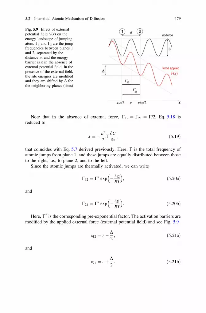
Note that in the absence of external force, C12 = C21 = C/2, Eq. 5.18 isreduced to

J ¼ � a2

2C

oC

ox; ð5:19Þ

that coincides with Eq. 5.7 derived previously. Here, C is the total frequency ofatomic jumps from plane 1, and these jumps are equally distributed between thoseto the right, i.e., to plane 2, and to the left.

Since the atomic jumps are thermally activated, we can write

C12 ¼ C� exp � e12

RT

ffi �; ð5:20aÞ

and

C21 ¼ C� exp � e21

RT

ffi �: ð5:20bÞ

Here, C* is the corresponding pre-exponential factor. The activation barriers aremodified by the applied external force (external potential field) and see Fig. 5.9

e12 ¼ e� D2; ð5:21aÞ

and

e21 ¼ eþ D2: ð5:21bÞ

Fig. 5.9 Effect of externalpotential field V(x) on theenergy landscape of jumpingatom. C1 and C2 are the jumpfrequencies between planes 1and 2, separated by thedistance a, and the energybarrier is e in the absence ofexternal potential field. In thepresence of the external field,the site energies are modifiedand they are shifted by D forthe neighboring planes (sites)

5.2 Interstitial Atomic Mechanism of Diffusion 179

As it was stated above, the case D/2 � e is considered. Then,

C12 ¼ C� exp � e� D=2RT

� �¼ C� exp � e

RT

ffi �exp

D2RT

� �� 1

2C 1þ D

2RT

� �;

ð5:22aÞ

and

C12 ¼ C� exp � eþ D=2RT

� �¼ C� exp � e

RT

ffi �exp � D

2RT

� �� 1

2C 1� D

2RT

� �:

ð5:22bÞ

Now, substituting these equations into relation (5.18), the flux of atomsbetween planes 1 and 2 is

J ¼ � a2

2C

oC

oxþ aDC

2RTC ¼ �D

oC

oxþ vC: ð5:23Þ

Here, the diffusion coefficient defined by Eq. 5.8 is used (Dx = a is the presentcase), and an additional term to Fick’s first law, vc, is appeared in the presence ofthe driving force. We see that if an external potential field is applied, the net flux ofatoms is determined by a sum of two terms, diffusional one, �D oc

ox, and convectiveone, vc. The convection velocity, v, is given by

v ¼ aDC2RT

¼ a2

2C

D=a

RT¼ D

D=a

RT¼ D

RTF; ð5:24Þ

which is the well-known Nernst–Einstein equation. We used an obvious relation,F ¼ � oV

ox ¼ Da, and see Fig. 5.9. Within the given approximation, i.e., linear terms,

the convection velocity is proportional to the external force F and mobility M isdetermined by the diffusion coefficient D, M = D/RT.

The effect of other driving force (e.g., temperature gradient or electric force)can be treated quite similarly. The driving force F induces inequality of the jumpfrequencies C12 and C21, and to the first-order expansion, we may write

C12 ¼12

C 1þ nð Þ ð5:25aÞ

and

C12 ¼12

C 1� nð Þ: ð5:25bÞ

180 5 Atomic Mechanism of Diffusion

These equations can be considered as a definition of the term n. Substitutingthese expressions to Eq. 5.18, we arrive to Eq. 5.23 with the following expressionfor the convection velocity,

v ¼ an C: ð5:26Þ

The thermal energy RT per net jump of one mole of interstitial atoms in thedirection of the applied force is equal to the work done by the force over the jumpdistance a,

RTC12 � C21

C=2¼ Fa; ð5:27Þ

and using expressions (5.25a) and (5.25b),

n ¼ a

2F

RT: ð5:28Þ

Thus, the convection velocity is

v ¼ a2C0

2F

RT¼ D

RTF: ð5:29Þ

Again, we arrived to the Nernst–Einstein equation, expression (5.24), which isvalid if the driving force is small when the expansions (5.25a) and (5.25b) can beused (Fig. 5.9).

5.2.2 Random Walk of Atoms

As explained already, atoms vibrate at their equilibrium position and might gainsufficient energy to jump to any of the neighboring available positions. Further,after making a successful jump, it might jump again to any of the sites. Twosuccessive jumps are not related. If the atom does not come back to the previousposition, then we can say that the atom is diffused. For the sake of explanation, letus consider a two-dimensional array of solvent atoms as shown in Fig. 5.10. Fol-lowing, the jump in a three-dimensional lattice will be considered. Suppose initiallyone interstitial atom is located at position P. After many jumps, this atom reaches,let say, to Q. Now question is that how many jumps it will make to reach Q.

One can easily count that there are few short routes available, as shown by greendotted arrows, which need 14 jumps to reach Q from P. However, chance of takingany of the short routes by making all necessary jump is least expected. It might takea torturous route as shown by black solid arrows. Note that the steps in the middleare not shown. At first glance, it seems impossible to make any prediction on theaverage number of jumps or time necessary for considering random walk of atoms.

5.2 Interstitial Atomic Mechanism of Diffusion 181

However, following a simplified approach, we can roughly estimate it. We assumethat the atom makes n jumps to reach from P to Q. The jump vector Ln connectingthe points P and Q can be written as

Ln ¼ l1 þ l2 þ l3 þ � � � þ ln ¼Xn

i¼1

li; ð5:30Þ

where li is the jump vector of the ith jump. To calculate the magnitude, we need totake dot product.

Ln � Ln ¼ L2n ¼ l1 � l1 þ l1 � l2 þ l1 � l3 þ � � � þ l1 � ln

þ l2 � l1 þ l2 � l2 þ l2 � l3 þ � � � þ l2 � lnþ l3 � l1 þ l3 � l2 þ l3 � l3 þ � � � þ l3 � ln. . .

. . .

þ ln � l1 þ ln � l2 þ ln � l3 þ � � � þ ln � ln

ð5:31Þ

Equation 5.31 can be arranged as

L2n ¼

Xn

i¼1

li � li þ 2Xn�1

i¼1

li � liþ1 þ 2Xn�2

i¼1

li � liþ2. . . ð5:32Þ

The first sum includes all diagonal terms li� li, the second sum consists all li� li+1

and li+1 � li terms (according to dot product of vectors, these are the same), thethird sum consists all li � li+2 and li+2 � li terms, and so on. Equation 5.32 can berewritten as

Fig. 5.10 Jump of aninterstitial atom throughdifferent routes from theposition P to the position Q

182 5 Atomic Mechanism of Diffusion

L2n ¼

Xn

i¼1

li � li þ 2Xn�1

j¼1

Xn�j

i¼1

li � liþj

¼Xn

i¼1

l2i þ 2

Xn�1

j¼1

Xn�j

i¼1

lij j liþj

�� �� cos hi;iþj

ð5:33Þ

Here, cos hi;iþj is the angle between jump vectors li and li+j.Note that we are considering diffusion in crystalline solids. If we consider the

diffusion in cubic system, magnitude of the jump vectors are equal since direct jump ispossible only to the nearest neighbor positions. Therefore, Eq. 5.33 can be written as

L2n ¼ nl2 þ 2l2

Xn�1

j¼1

Xn�j

i¼1

cos hi;iþj ð5:34Þ

Till now, we have considered jumps of one particular atom only. However, to findthe average jump distance, we should consider many atoms together and takeaverage of jumps of all the atoms. The first term in Eq. 5.34, that is, nl2, will be thesame for all the atoms. The differences in total jump distance because of choosingdifferent path by different atoms are counted in the second term. Therefore,Eq. 5.34 can be written, after taking average from many atoms, as

�L2n ¼ nl2 1þ 2

n

Xn�1

j¼1

Xn�j

i¼1

cos hi;iþj

0@

1A ð5:35Þ

Further, since we have considered the random walk of many atoms together, forevery positive value of cos hi;iþj from an atom, there will be an equal chance of anegative value from the jump of another atom. It is explained with the help ofinterstitial atoms sitting in an octahedral void in a FCC crystal, as shown inFig. 5.11. There are 12 jump vectors l1 to l12. It must be clear that for every jumpvector, there is an equal but negative jump vector; for example, l2 = -l12. Further

Fig. 5.11 Jump vectors of aninterstitial atom are shown

5.2 Interstitial Atomic Mechanism of Diffusion 183

because of random nature of jump, atoms have equal probability to jump to any ofthe locations. If one atom has jump sequence of l1 � l2, then there is an equalprobability that another atom has jump sequence of l1 � l12. So we can write, forexample, li � l2 � li � l12 ¼ 0. This will lead the double summation of Eq. 5.35 to

zero. Therefore, it is safe to write thatPn�1

j¼1

Pn�ji¼1 cos hi;iþj

ffi �¼ 0 in a cubic

isotropic crystal, and Eq. 5.35 can then be rewritten as

�L2n ¼ nl2 ð5:36Þ

Therefore, the average magnitude of jumps of many atoms after n number ofjumps can be written as

�Ln ¼ffiffiffiffiffi�L2

n

q¼

ffiffiffinp

l ð5:37Þ

Note that we are considering the average taken from many atoms. There can behuge difference in the distance that different atoms will travel after a particulardiffusion time. Equation 5.37 indicates that atoms will make an average(14)2 = 386 jumps to reach from P to Q, where 14 jumps are required followingthe shorter routes. We reconsider the example what we have discussed already inthe previous section. With average jump frequency of 1010 s-1 of carbon at1,100 �C in C-iron, the average effective jump length in 1 h is �Ln ¼

ffiffiffinp

l ¼ffiffiffiffiffiffiffiffiffiffiffiffiffiffiffiffiffiffiffiffiffiffiffiffiffiffi1010 � 3;600

p� 10�10 m ¼ 0:6 mm ¼ 600 lm. Further, note here that this is an

average from many atoms. Different atoms will actually jump different distancesand the difference in jump length could be very large.

This concept of random walk is actually developed based on Einstein’smathematical analysis of Brownian motion. He developed the relation fordiffusivity as D ¼ h�L2

ni=6t, considering the jump of atoms in threedimensions.

5.2.3 Effect of Temperature on the Interstitial DiffusionCoefficient

We have already discussed that atoms vibrate at their positions with an averageenergy of 3kT. With the increase in temperature, thermal energy of the systemincreases so that atoms vibrate even more violently. That means the jump fre-quency will increase with increasing temperature. However, the atoms cannotjump freely, since the void between the host atoms, through which atoms shouldjump, is smaller than the size of the atom. Therefore, the host atoms should be

184 5 Atomic Mechanism of Diffusion

moved elastically as explained in Fig. 5.12. The change in local free energy withthe movement of the atom is shown. In the beginning, the atoms are at theirequilibrium positions and the energy at this ground state is gg per mol of atoms.The free energy is the highest in the middle, where it needs maximum energy tomove the host atoms elastically. This is called an activated state, and the freeenergy is ga per mol of atoms. Following, atoms reach to another ground state. Soan extra energy of Dga ¼ ga � gg per mole of atoms is required to cross the barrier.This is the activation energy for interstitial diffusion and is equal to the energyrequired for the migration Dgm. Atoms jump with Debye frequency, v, and theprobability of the successful jump to a new position is exp �Dgm=RTð Þ. Therefore,the jump frequency to a particular position can be written as

Ci ¼ m exp �Dga

RT

� �ð5:38Þ

From Eq. 5.10, Eq. 5.38 can be written as

D ¼ mDx2 exp �Dga

RT

� �¼ D00 exp �Dga

RT

� �; ð5:39Þ

where D00 is the temperature-independent pre-exponential factor. This temperature-dependent relation for the diffusion coefficient relation is the Arrhenius equation.

Fig. 5.12 a The jump ofatom from one equilibriumposition to anotherequilibrium position. b Themovement of interstitial atomand the neighboring solventatoms is shown. For the sakeof explanation, we haverotated the atomic structureby 45o. c The associated freeenergy change with themovement of the interstitialatom is shown

5.2 Interstitial Atomic Mechanism of Diffusion 185

Further, Dga ¼ Dha � TDsa. With the help of this relation, many times Eq. 5.39 isexpressed as

D ¼ mDx2 expDsa

R

� �exp �Dha

RT

� �¼ D0 exp �Dha

RT

� �ð5:40Þ

In this equation, D0 ¼ m Dx2 exp Dsa

R

ffi �¼ D00 exp Dsa

RT

� �is the pre-exponential

factor and Dha is the activation enthalpy for diffusion. Note here that at a particulartemperature, the change in entropy because of migration is more or less fixed in asystem. This accounts for the change in entropy because of the change in vibrationpattern of neighboring atoms where the elastic displacement of the host atoms isgreatest.

Equation 5.40 can be written as

ln D ¼ ln D0 �Q

RTð5:41aÞ

log D ¼ log D0 �Q

2:3RTð5:41bÞ

Therefore, the activation energy and the pre-exponential factor can be deter-mined from the plots shown in Fig. 5.13.

It must be clear from the discussion above that the pre-exponential factor andthe activation energy depend on a number of factors, such as size of the interstitialatoms, elastic modulus of the material, lattice parameter and the crystal structure.Because of this size factor, e.g., the diffusion rates of small elements in Fe have todecrease generally in the order of H, O, N, and C. Some available data are listed inTable 5.1. It is clearly seen that solely the size factor has a limited applicability,though it is very useful in the analysis of the diffusion trends. One has to mentionthat the atomic radii depend strongly on the environment and the charge state andany tabulated data have to be used with cautions.

Fig. 5.13 a ln D versus 1/T plot and b log D versus 1/T plot to calculate the activation energyand the pre-exponential factor

186 5 Atomic Mechanism of Diffusion

Similar dependencies for these small elements were found for their diffusion ina-Ti with the HCP lattice, too. However, one recognizes immediately that theelectronic effects are also important in explaining the atomic diffusion rates. Mostprominent example is the diffusion of transition metal atoms, such as Co, Fe, andNi, in a-Ti, see below in the chapter—they are even faster than C or N!

5.2.4 Tracer Method of Measuring the InterstitialDiffusion Coefficient

Since the concentration of the diffusing impurity element is very small, tracermethod is followed to calculate the impurity diffusion coefficient utilizing radio-isotopes, which are easy to detect. This is explained in Fig. 5.14. Radioisotopes ofimpurity element A are deposited on the substrate B, in which the impurity dif-fusion coefficient would be measured. At the temperature of the experiment,radioisotope impurity elements diffuse inside the substrate. Different atoms diffusedifferent lengths because of random walk of atoms. With the increase in annealingtime, the penetration distance increases. After the experiment for certain time at adesired temperature, the specimen is sliced at different known distances along thex direction and the concentration of the radioisotopes is measured by measuringintensities of the emitted rays. Following the solution for thin film from Fick’ssecond law, we can write

IRðxÞ ¼1ffiffiffiffiffiffiffiffiffiffiffipD�At

p exp � x2

4D�At

� �ð5:42Þ

ln IR ¼ ln1ffiffiffiffiffiffiffiffiffiffiffipD�At

p !

� x2

4D�Atð5:43Þ

where IR is the specific or relative intensity measured and D�A is the impuritydiffusion coefficient of element A.

Table 5.1 The tracer impurity diffusion coefficients, D* (m2/s), and the corresponding activationenthalpies, Q (kJ/mol), for diffusion of small atoms in FCC and BCC iron [2–8]

Impurity Atomicradius(pm)

BCC Fe FCC Fe

Q (kJ/mol) D* at 300K (m2/s)

References Q (kJ/mol) D* at 1,400K (m2/s)

References

H 25 6 7 9 10-9 [2] 43 2 9 10-8 [3]O 60 92 4 9 10-23 [4] 166 9 9 10-11 [5]N 65 73 2 9 10-20 [6] 169 5 9 10-11 [7]C 70 84 5 9 10-21 [6] 148 7 9 10-11 [8]

The atomic radii after [9] are listed. For comparison, the atomic radius of Fe is 140 pm

5.2 Interstitial Atomic Mechanism of Diffusion 187

From the slope � 14D�

At of ln IR versus x2 plot, as shown in Fig. 5.14, D�A can be

calculated using the known annealing time.

5.2.5 Orientation Dependence of Interstitial DiffusionCoefficient

In Sect. 5.2.2, we considered a cubic crystal to simplify the derivation for averagejump length calculation during random walk in which the magnitudes of all jumpvectors are equal. Following, we were able to derive a simple relation to explainthe random walk of atoms. However, in some structures such as hexagonal,tetragonal, or orthorhombic, the jump vectors in different directions could bedifferent. Even the void size through which the atoms jump could also be differentto find different jump frequencies and the activation energy for diffusion.

For comparison, we consider face-centered cubic and orthorhombic structures,as shown in Fig. 5.15. We consider again the presence of an interstitial atom in anoctahedral site in the middle. Other octahedral sites are shown by open dottedcircle to which the interstitial atom could jump. We have discussed earlier thatdiffusion coefficient is calculated from the average jumps of many atoms. In a FCCcrystal, the diffusion coefficient can be written as

D ¼ 112

X12

i¼0

CiDx2i ð5:44Þ

Fig. 5.14 Tracer method to determine impurity tracer diffusion coefficient is shown

188 5 Atomic Mechanism of Diffusion

In a cubic crystal because of symmetry, as shown in Fig. 5.15a, there is equalprobability of jump frequency to any of the positions and Eq. 5.44 can be writtenas

D ¼ 112

CX12

i¼0

Dx2i ð5:45Þ

We consider the diffusion along the x-axis. All the nearest neighbor interstitialsites have equal distances. Considering positive and negative sides on the x-axis,the effective jump length for the positions 1, 2, 3 and 4 is -a/2, where a is thelattice parameter. This is zero for positions 5, 6, 7 and 8. Although atoms jump tothese positions, the effective length is zero considering the jump along the x-axis.This is a/2 for positions 9, 10, 11 and 12. Therefore, the diffusion coefficient alongthe x-axis can be written as

Dx ¼1

12C 4 � a

2

ffi �2þ4 0ð Þ þ 4

a

2

ffi �2 �

¼ 16Ca2 ð5:46Þ

We consider the diffusion along the y-axis. The effective jump length to thepositions 2, 6, 7, and 10 is equal to -a/2. This is zero for positions 1, 3, 9, and 11and a/2 for positions 4, 5, 8, and 12. Therefore, the diffusion coefficient along they-axis can be written as

Fig. 5.15 Interstitial sites are shown in a face-centered cubic and b orthorhombic face-centeredcubic crystal structures to explain the anisotropy in diffusion

5.2 Interstitial Atomic Mechanism of Diffusion 189

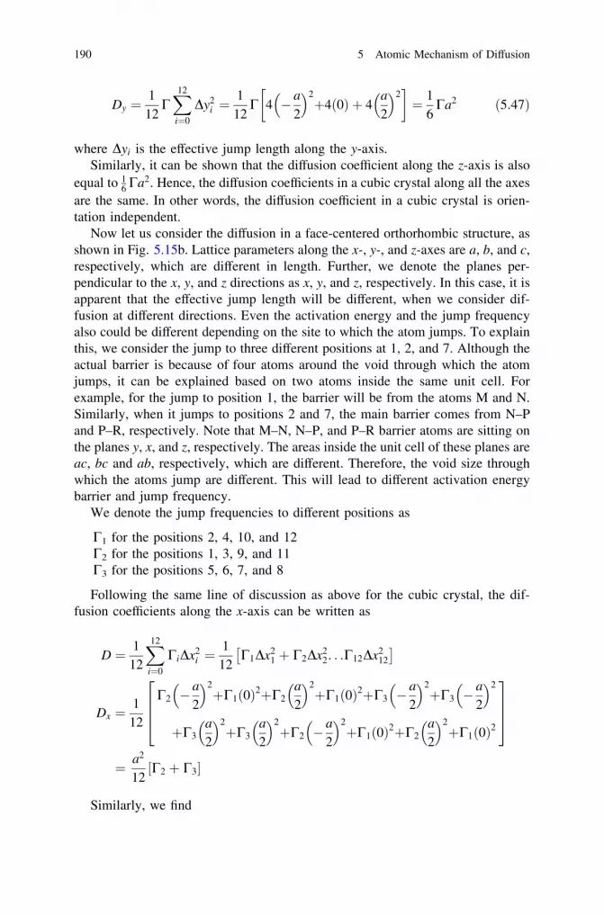
Dy ¼1

12CX12

i¼0

Dy2i ¼

112

C 4 � a

2

ffi �2þ4 0ð Þ þ 4

a

2

ffi �2 �

¼ 16Ca2 ð5:47Þ

where Dyi is the effective jump length along the y-axis.Similarly, it can be shown that the diffusion coefficient along the z-axis is also

equal to 16 Ca2. Hence, the diffusion coefficients in a cubic crystal along all the axes

are the same. In other words, the diffusion coefficient in a cubic crystal is orien-tation independent.

Now let us consider the diffusion in a face-centered orthorhombic structure, asshown in Fig. 5.15b. Lattice parameters along the x-, y-, and z-axes are a, b, and c,respectively, which are different in length. Further, we denote the planes per-pendicular to the x, y, and z directions as x, y, and z, respectively. In this case, it isapparent that the effective jump length will be different, when we consider dif-fusion at different directions. Even the activation energy and the jump frequencyalso could be different depending on the site to which the atom jumps. To explainthis, we consider the jump to three different positions at 1, 2, and 7. Although theactual barrier is because of four atoms around the void through which the atomjumps, it can be explained based on two atoms inside the same unit cell. Forexample, for the jump to position 1, the barrier will be from the atoms M and N.Similarly, when it jumps to positions 2 and 7, the main barrier comes from N–Pand P–R, respectively. Note that M–N, N–P, and P–R barrier atoms are sitting onthe planes y, x, and z, respectively. The areas inside the unit cell of these planes areac, bc and ab, respectively, which are different. Therefore, the void size throughwhich the atoms jump are different. This will lead to different activation energybarrier and jump frequency.

We denote the jump frequencies to different positions as

C1 for the positions 2, 4, 10, and 12C2 for the positions 1, 3, 9, and 11C3 for the positions 5, 6, 7, and 8

Following the same line of discussion as above for the cubic crystal, the dif-fusion coefficients along the x-axis can be written as

D ¼ 112

X12

i¼0

CiDx2i ¼

112

C1Dx21 þ C2Dx2

2. . .C12Dx212

�

Dx ¼1

12

C2 �a

2

ffi �2þC1 0ð Þ2þC2

a

2

ffi �2þC1 0ð Þ2þC3 �

a

2

ffi �2þC3 �

a

2

ffi �2

þC3a

2

ffi �2þC3

a

2

ffi �2þC2 �

a

2

ffi �2þC1 0ð Þ2þC2

a

2

ffi �2þC1 0ð Þ2

2664

3775

¼ a2

12C2 þ C3½ ffi

Similarly, we find

190 5 Atomic Mechanism of Diffusion

Dy ¼b2

12C1 þ C3½ ffi

Dz ¼c2

12C1 þ C2½ ffi

Therefore, we get Dx 6¼ Dy 6¼ Dz. From the above discussion, we can say that iftracer diffusion experiments with impurity elements are conducted on a cubiccrystal, the diffusion coefficient will be the same irrespective of the orientation ofthe substrate. On the other hand, the diffusion coefficient in a substrate withorthorhombic structure will be different in different directions. This can be foundfrom experiments by selecting a single crystal substrate with different orientationsand then by doing tracer diffusion experiments, as explained in the previoussection. It can be easily understood that even if the jump frequency is the same andthere is a difference in lattice parameters in a non-cubic crystal structure, such thatthe total jump length for atoms will be different in different directions to finddifferent diffusion coefficients.

There exist experimental evidences on the anisotropic nature of the interstitialdiffusion. Typically, this kind of diffusion anisotropy is not as large as that foundin some cases of substitutional diffusion. What is a reason for such behavior? Inorder to answer this non-trivial question, at least semiqualitatively, one has toconsider these diffusion mechanisms in details. We will limit us to the case ofmetallic system in which one should not deal with the charge state of the pointdefects. The key point is the magnitude of the corresponding energy barriers. Themigration barriers are typically smaller in the case of interstitial diffusion, whichare typically of the order of 0.2–0.5 eV, and they are larger for substitutionaldiffusion (1 eV and more). Correspondingly, the differences in the barriers for thediffusion jumps in different directions are typically larger for substitutional dif-fusion in comparison with those for interstitial one. Therefore, the diffusionanisotropy is more prominent. The effect is still moderate for pure metals, e.g., inHCP a-Ti or Zn, in which the diffusion anisotropy for self-diffusion is within afactor of 2 or 3 (Fig. 5.16), but it can reach the orders of magnitude in intermetalliccompounds due to the anisotropy of sublattices (see the discussion in Sect. 5.3.6).

5.3 Diffusion in Substitutional Alloys

In the second chapter, we have discussed the formation of equilibrium concen-tration of vacancies. This concentration is, in general, in the order of 10-3–10-4

near the melting point. That means one vacancy is present in a cube of 10–14atoms in each direction. Because of this low concentration, we can neglect thevacancy–vacancy interactions. Although vacancy is just a vacant lattice site, it isconsidered as one of the entities to mediate discussion. Therefore, exchanging

5.2 Interstitial Atomic Mechanism of Diffusion 191

position of a vacancy with an atom can be seen as diffusion of atom, as well as thediffusion of the vacancy. One interesting fact should be noted here that if we arelooking at one particular atom, the diffusion of that atom will depend on theavailability of a vacancy to its neighboring position. On the other hand, for avacancy, this restriction is not there and it can exchange position with any of theatoms. In other words, one particular atom cannot go through a random jumpprocess; however, a vacancy can go through it. This is the reason that in substi-tutional diffusion, tracer and self-diffusion coefficients are different, althoughradioisotopes are used to study the self-diffusion of elements. These two arerelated by a correlation factor. To explain this in detail, first we need to explain thetracer diffusion method in substitutional diffusion.

5.3.1 Measurement of Tracer Diffusion Coefficient

As stated earlier, even in a pure material, diffusion of atoms is always happeningjust because of thermal vibration. Since there is no driving force present, atoms gothrough a random jump. The diffusion rate depends on the homologous temper-ature, that is, the temperature relative to its melting point. Since the atoms are verysmall and at relatively high temperature these might change place too many timesper second, we cannot study the diffusion directly. For this sake, the tracer tech-nique is developed, in which the diffusion of radioisotopes is quantified from themeasurement of intensities of emitted rays at different depths after certainannealing time. This is similar to the procedure already explained for the calcu-lation of impurity diffusion coefficient in Sect. 5.2.4. To study the self-diffusioncoefficient of element B, radioisotopes of B* are deposited as very thin layer on ablock of material B, as shown in Fig. 5.17. After certain annealing time, the

Fig. 5.16 Self-diffusion insingle crystals of Zn, In, andSn parallel (solid lines) andperpendicular (dashed lines)to the c-axis of the HCPstructure. The data from thecollection [11] are used

192 5 Atomic Mechanism of Diffusion

specific intensity of the emitted ray is measured at different depths after serialsectioning. In this case, Eq. 5.44 can be rewritten as

ln IR ¼ ln1ffiffiffiffiffiffiffiffiffiffiffipD�Bt

p !

� x2

4D�Btð5:48Þ

Following the tracer diffusion coefficient, D�B could be calculated from theslope, � 1

4D�B

t, of the plot ln IR versus x2. However, as mentioned earlier, the

measured tracer diffusion coefficient is not exactly the same as the self-diffusioncoefficient. They are related by a correlation factor, f. Sometimes, the tracer self-diffusion coefficient is stated as the same as self-diffusion coefficient, which is notreally correct. In the next section, we have explained the concept of the correlationfactor.

5.3.2 Concept of the Correlation Factor

For the sake of discussion, we consider the tracer diffusion experiment asexplained above in a FCC metal structure with [111] orientation. Atomicarrangement on the (111) plane is shown in Fig. 5.18. For the ease of explanation,we consider two-dimensional arrangements, although the argument is valid inthree dimensions also. Suppose we have a situation that a vacancy, V, is sur-rounded by five B and one B*, as shown in Fig. 5.18a. Now suppose B* and Vexchange their position and come to the situation, as shown in Fig. 5.18b. Since

Fig. 5.17 Tracer method to determine tracer diffusion coefficient is shown

5.3 Diffusion in Substitutional Alloys 193

the fraction of vacancies present in the structure is rather small, there is noguarantee that the tracer atom will find another vacancy to exchange its positionimmediately again to move forward. As explained before, there could be onevacancy present in a cube of 10 to 14 atoms each side only at melting point. Atlower temperatures the vacancy concentration is significantly smaller and theimaginary size of the corresponding cube is considerably larger. So the nextprobable jump of B* is back to the previous position after exchanging position withthe vacancy. Then, there will be no diffusion. However, from the previous example,we have seen that the tracer atoms indeed move forward. Therefore, if this moveforwards, the next probable jump is to position 1 or 5, on the condition that vacancyalready exchanged position with the atoms located at these positions. To move evenfurther, the next probability of jump of the tracer atom is to any of the positions 8 or6. However, the probability is even lower than that of the previous jump, since aftertwo successive jumps, vacancy has to reach to these positions of interest before thetracer atom could exchange position. Note that in the middle of these two successivejumps, also vacancy might deviate to other direction because of random nature. Theprobability of tracer atom to reach to the position 7 is the least, since before thisexchange; the vacancy first has to reach to that position after making few successfuljumps. Therefore, vacancy can go through a completely random jump process.However, the jump of the tracer atom is related to other jumps.

From the arguments developed in Sect. 5.2.2, we can write

�L2v ¼ nl2 ð5:49Þ

Since tracer atoms go through correlated jumps, the second term in Eq. 5.43,that is, double summation, is not zero and can be expressed as

�L2t ¼ nl2 1þ 2

n

Xn�1

j¼1

Xn�j

i¼1

cos hi;iþj

0@

1A ð5:50Þ

where �L2t is the square of average jump distance of tracer atoms after n jumps.

Fig. 5.18 Exchanging position between radioisotope B* and vacancy is shown

194 5 Atomic Mechanism of Diffusion

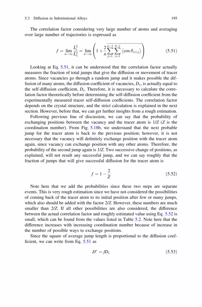
The correlation factor considering very large number of atoms and averagingover large number of trajectories is expressed as

f ¼ limn!1

�L2t

�L2v

¼ limn!1

1þ 2n

Xn�1

j¼1

Xn�j

i¼1

cos hi;iþj

� �0@

1A ð5:51Þ

Looking at Eq. 5.51, it can be understood that the correlation factor actuallymeasures the fraction of total jumps that give the diffusion or movement of traceratoms. Since vacancies go through a random jump and it makes possible the dif-fusion of many atoms, the diffusion coefficient of vacancies, Dv, is actually equal tothe self-diffusion coefficient, Ds. Therefore, it is necessary to calculate the corre-lation factor theoretically before determining the self-diffusion coefficient from theexperimentally measured tracer self-diffusion coefficients. The correlation factordepends on the crystal structure, and the strict calculation is explained in the nextsection. However, before that, we can get further insights from a rough estimation.

Following previous line of discussion, we can say that the probability ofexchanging positions between the vacancy and the tracer atom is 1/Z (Z is thecoordination number). From Fig. 5.18b, we understand that the next probablejump for the tracer atom is back to the previous position; however, it is notnecessary that the vacancy will definitely exchange position with the tracer atomagain, since vacancy can exchange position with any other atoms. Therefore, theprobability of the second jump again is 1/Z. Two successive change of positions, asexplained, will not result any successful jump, and we can say roughly that thefraction of jumps that will give successful diffusion for the tracer atom is

f ¼ 1� 2Z

ð5:52Þ

Note here that we add the probabilities since these two steps are separateevents. This is very rough estimation since we have not considered the possibilitiesof coming back of the tracer atom to its initial position after few or many jumps,which also should be added with the factor 2/Z. However, these numbers are muchsmaller than 2/Z. If all other possibilities are also considered, the differencebetween the actual correlation factor and roughly estimated value using Eq. 5.52 issmall, which can be found from the values listed in Table 5.2. Note here that thedifference increases with increasing coordination number because of increase inthe number of possible ways to exchange positions.

Since the square of average jump length is proportional to the diffusion coef-ficient, we can write from Eq. 5.51 as

D� ¼ fDs ð5:53Þ

5.3 Diffusion in Substitutional Alloys 195

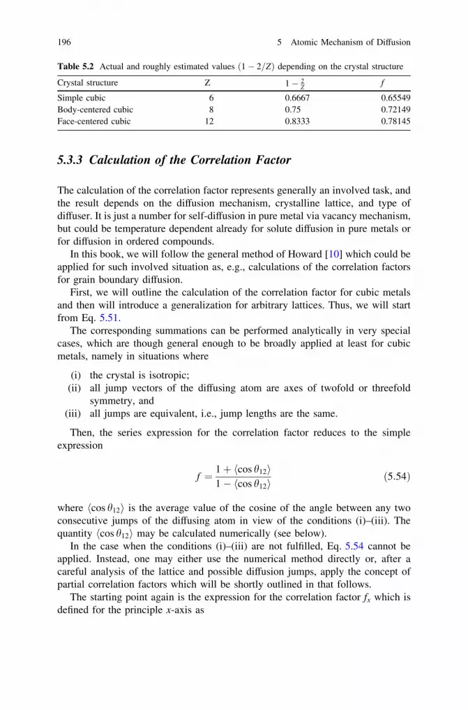
5.3.3 Calculation of the Correlation Factor

The calculation of the correlation factor represents generally an involved task, andthe result depends on the diffusion mechanism, crystalline lattice, and type ofdiffuser. It is just a number for self-diffusion in pure metal via vacancy mechanism,but could be temperature dependent already for solute diffusion in pure metals orfor diffusion in ordered compounds.

In this book, we will follow the general method of Howard [10] which could beapplied for such involved situation as, e.g., calculations of the correlation factorsfor grain boundary diffusion.

First, we will outline the calculation of the correlation factor for cubic metalsand then will introduce a generalization for arbitrary lattices. Thus, we will startfrom Eq. 5.51.

The corresponding summations can be performed analytically in very specialcases, which are though general enough to be broadly applied at least for cubicmetals, namely in situations where

(i) the crystal is isotropic;(ii) all jump vectors of the diffusing atom are axes of twofold or threefold

symmetry, and(iii) all jumps are equivalent, i.e., jump lengths are the same.

Then, the series expression for the correlation factor reduces to the simpleexpression

f ¼ 1þ cos h12h i1� cos h12h i ð5:54Þ

where cos h12h i is the average value of the cosine of the angle between any twoconsecutive jumps of the diffusing atom in view of the conditions (i)–(iii). Thequantity cos h12h i may be calculated numerically (see below).

In the case when the conditions (i)–(iii) are not fulfilled, Eq. 5.54 cannot beapplied. Instead, one may either use the numerical method directly or, after acareful analysis of the lattice and possible diffusion jumps, apply the concept ofpartial correlation factors which will be shortly outlined in that follows.

The starting point again is the expression for the correlation factor fx which isdefined for the principle x-axis as

Table 5.2 Actual and roughly estimated values ð1� 2=ZÞ depending on the crystal structure

Crystal structure Z 1� 2Z

f

Simple cubic 6 0.6667 0.65549Body-centered cubic 8 0.75 0.72149Face-centered cubic 12 0.8333 0.78145

196 5 Atomic Mechanism of Diffusion

fx ¼ 1þ 2

P1i¼1

P1j¼1 xixiþj

� �P1

i¼1 x2ih i

ð5:55Þ

Here, xi is the x projection of the ith jump, which could be now different fordifferent jumps. It is clear that the summation has to be done over the jumps withnonzero x component. Only such jumps will be considered and counted in thesummations. The consideration is general with no limitations on jump lengths andsymmetry. Thus, it is applicable for short-circuit diffusion, too, or in the case ofdiffusion in non-cubic lattices.

The critical point is the classification of all jumps in different types. Since thelattice is periodic, the number of all types N is finite and let the subscript a labelthese types as a = 1, 2, 3, …N. The types are defined such as for all xi of the sametype, the sum

P1j¼1 xixiþj

� �could be rewritten as

X1j¼1

xixiþj

� �¼X1j¼1

xaxa;j� �

ð5:56Þ

and it does not depend on i. Here, the subscript a, j refers to the jth jump after ajump of the type a. Then, one can show that Eq. 5.55 could be written in matrixnotation as

fx ¼ c � f ð5:57Þ

where c = (c1,…,cN) is the vector with components ca which represent the fractionof jumps of the type a in any very long sequence of atom jumps and f = (f1,…,fN)is the vector of the partial correlation factors representing the contributions of thegiven types of jumps. The latter is defined by the expression

f ¼ Iþ 2Z � TðE� TÞ�1 � d: ð5:58Þ

Here, I is the N-component unit column vector, E is the N 9 N unit matrix,d = (|z1|,…, |zN|) is the column vector of the jump distances of type a jumps, Z isthe N 9 N matrix which diagonal elements are equal to z�1

a

�� ��, a = 1,…, N, andT is a N 9 N matrix with the elements

tab ¼ Pþab � P�ab; a; b ¼ 1; . . .;N:

Here, Pþab P�ab

ffi �is the probability that a tracer jump of type a is immediately

followed by a tracer jump of type b in the same (+) or opposite (-) direction. Themain point is the determination of these probabilities which may be evaluatedusing numerical methods. The advantage is a low cost of the numerical calcula-tions in which the jump history of a given tracer is enough to follow over 106

individual jumps. If the numerical method will be applied directly to Eq. 5.54, the

5.3 Diffusion in Substitutional Alloys 197

atom jumps have to be followed up to 109 individual jumps to have a reasonableaccuracy in sophisticated cases of non-cubic crystals. The application of theconcept will be demonstrated for the case of diffusion in MoSi2 below.

Generally, the correlation factors can directly be calculated using numericalmethods. The starting point is the determination of all jump frequencies which areinvolved in diffusion of a tracer atom over the lattice. Having calculated thetransition probabilities for all possible vacancy jumps, the correlation factor can becalculated by the Monte Carlo approach. In simulations, a box of the size of, let ussay, 100 9 100 9 100 with the given structure is first generated. A vacancy iscreated at the center of the block, and the vacancy is allowed to perform the giventypes of jumps. The probabilities pi of these jumps can be calculated according tothe transition frequencies mi estimated before:

pi ¼miPzj¼1 mj

; ð5:59Þ

where z is the coordination number of the given lattice. The time-residencealgorithm is typically applied. Each jump of the vacancy is successful, and thetime variable is increased by

s ¼ 1Pzj¼1 mj

: ð5:60Þ

The atomic correlation factors for species k, several species belong to the latticeunder consideration, are calculated from the equation:

fk ¼Pnk

i¼1 R2i

mka2k

; ð5:61Þ

where Ri is the net displacement of the ith atom of type k, nk is the total number ofatoms of type k, mk is the total number of vacancy exchanges with atoms of type k,and ak is the elementary jump length.

5.3.4 The Relation Between the Jump Frequencyand the Diffusion Coefficient in SubstitutionalDiffusion

For the sake of explanation, let us consider (111) planes of a pure element B withFCC crystal, as shown in Fig. 5.19. We consider that there is a radioisotope, B*,present on the plane Q which is surrounded by six B, numbered as 4–9, respec-tively. Based on the crystal structure, we can say that if three nearest neighborsites, numbered as 1–3, respectively, are actually on the plane P below Q, then

198 5 Atomic Mechanism of Diffusion

other three nearest neighbor sites, numbered as 10–12, respectively, are on theplane R above the plane P. Since we are considering random jump process, we cansay that the tracer atom can jump to any of these 12 positions, on the condition thatvacancy is present on that site. To derive the relation, as we did in the case ofinterstitial diffusion, we first consider the jump of atoms between planes Q and R.Following, we shall develop the general relation that can be used without anyrestrictions.

Now, we follow the previous line of discussion as considered to relate the jumpfrequency with the diffusion coefficient in Sect. 5.2.1. We consider the exchangeof vacancies and the tracer atom between planes Q and R. B* can jump to any ofthe sites 10–12, on the condition that vacancy is available at the site of interest.Therefore, the flux of the tracer atom can be expressed as

~J�Q ¼3

12nQf pVCQ ¼

14

nQf pVCQ ð5:62Þ

The numerical factor comes from the fact that a tracer atom exchanges positionwith vacancy in one of the 3 sites (10–12) on the plane R out of total 12 nearestneighbors. nQ is the total number of tracer atoms present on the plane Q. pV is theprobability to find a vacancy, f is the correlation factor, and CQ is the jump

Fig. 5.19 The jump of the radiotracer B* between (111) planes of B with FCC crystal structure isdiscussed

5.3 Diffusion in Substitutional Alloys 199

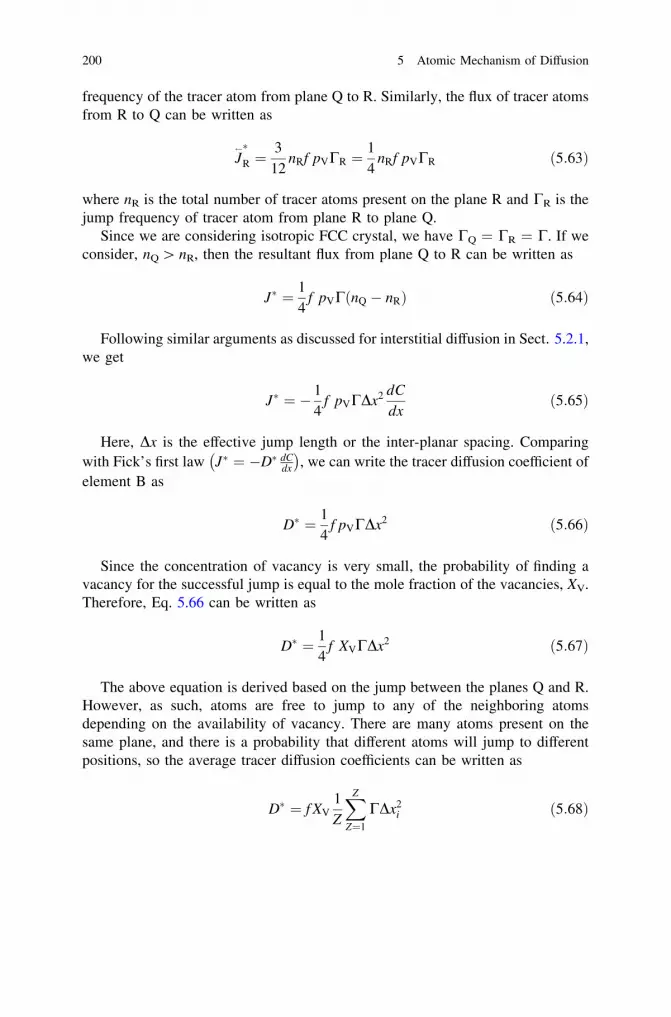
frequency of the tracer atom from plane Q to R. Similarly, the flux of tracer atomsfrom R to Q can be written as

J �

R ¼3

12nRf pVCR ¼

14

nRf pVCR ð5:63Þ

where nR is the total number of tracer atoms present on the plane R and CR is thejump frequency of tracer atom from plane R to plane Q.

Since we are considering isotropic FCC crystal, we have CQ = CR = C. If weconsider, nQ [ nR, then the resultant flux from plane Q to R can be written as

J� ¼ 14

f pVC nQ � nRð Þ ð5:64Þ

Following similar arguments as discussed for interstitial diffusion in Sect. 5.2.1,we get

J� ¼ � 14

f pVCDx2 dC

dxð5:65Þ

Here, Dx is the effective jump length or the inter-planar spacing. Comparingwith Fick’s first law J� ¼ �D� dC

dx

� �, we can write the tracer diffusion coefficient of

element B as

D� ¼ 14

f pVCDx2 ð5:66Þ

Since the concentration of vacancy is very small, the probability of finding avacancy for the successful jump is equal to the mole fraction of the vacancies, XV.Therefore, Eq. 5.66 can be written as

D� ¼ 14

f XVCDx2 ð5:67Þ

The above equation is derived based on the jump between the planes Q and R.However, as such, atoms are free to jump to any of the neighboring atomsdepending on the availability of vacancy. There are many atoms present on thesame plane, and there is a probability that different atoms will jump to differentpositions, so the average tracer diffusion coefficients can be written as

D� ¼ f XV

1Z

XZ

Z¼1

CDx2i ð5:68Þ

200 5 Atomic Mechanism of Diffusion

The tracer diffusion to a particular position i can be expressed as

D�i ¼ f XVCiDx2i ð5:69Þ

where C ¼ ZCi.If the crystal is not isotropic and the jump frequency is different to different

positions, then the tracer diffusion coefficient from the average of different kinds ofjumps can be written as

D� ¼ f XV

1Z

XZ

Z¼1

CiDx2i ð5:70Þ

From the relation between the tracer self-diffusion and self-diffusion coeffi-cients (Eq. 5.53), the self-diffusion coefficient, that is, the vacancy diffusioncoefficient, can be expressed as

Ds ¼ XV

1Z

XZ

Z¼1

CiDx2i ð5:71Þ

5.3.5 Effect of Temperature on Substitutional Diffusion

As it is discussed, in substitutional diffusion, atoms exchange position with thevacancies. However, the atom has to move the neighboring atoms elastically for asuccessful jump, as shown in Fig. 5.20. Just for the sake of explanation, two-dimensional atomic arrangements are shown instead of actual three dimensions.The probability with which atoms will make a successful jump at a particular

temperature T is expressed as exp � Dgm

RT

ffi �. Here, Dgm is the activation energy for

migration per mol of atoms. Since atoms make m (Debye frequency) attempts per

second, the jump frequency can be written as Ci ¼ m exp � Dgm

RT

ffi �and the self-

diffusion coefficient can be expressed as

D ¼ mXV Dx2 exp �Dgm

RT

� �ð5:72Þ

Therefore, the only difference in the relation between temperature-dependentself-diffusion coefficient and the interstitial diffusion coefficient (Eq. 5.39) is theextra term XV. From the discussion in Chap. 2, we know that the equilibriumvacancy concentration at a particular temperature, T, is expressed as

5.3 Diffusion in Substitutional Alloys 201

XV ¼ exp �DgV

RT

� �ð5:73Þ

By replacing Eq. 5.73 in Eq. 5.72, we get

D ¼ mDx2 exp �Dgm þ DgV

RT

� �¼ D0 exp �Dga

RT

� �ð5:74Þ

D0 is the temperature-independent pre-exponential factor. The activationenergy barrier for the self-diffusion comes from two different contributions, onefrom the activation energy for the formation of vacancies and another is from theactivation energy barrier for migration. So it must be apparent that the interstitialdiffusion in general is much easier than substitutional diffusion. Sometimes,anomalies are found, as shown in Fig. 5.21. Further, Eq. 5.74 can be written as

ln D ¼ ln D0 �Q

RT

log D ¼ log D0 �Q

2:3RT

So it is apparent that one can determine the activation energy for diffusionfrom the plot of ln D versus 1

T or log D versus 1T, where the slope is equal to -Q/R or

-Q/2.3R, respectively.Interstitial diffusion and substitutional diffusion of C and Fe are compared for

the case of Fe in Sect. 5.3.7. The hexagonal lattices of a-Ti, a-Zr, and a-Hfrepresent other interesting cases featuring fast diffusion rates of small nonmetallicatoms, such as C or O, and even ‘‘ultrafast’’ diffusion rates of transition metals—Fe, Ni, Co, and Mn (see Fig. 5.21). The corresponding diffusion rates are fasterthan those of self-diffusion by five (C in a-Ti) or seven (Ni in a-Ti) orders of

Fig. 5.20 Activation energybarrier for substitutionaldiffusion is explained withthe a atomic movement andb change in free energyduring movement

202 5 Atomic Mechanism of Diffusion

magnitude! The diffusion enhancement of, e.g., Ni in a-Zr approaches 10 orders ofmagnitude at 1,000 K. These ultrafast diffusion rates are explained by interstitialdiffusion mechanism of the transition metal atoms and are related to the specificelectronic effects owing to their unfilled d-states. Only, hydrogen reveals evenfaster diffusion rates in these hexagonal structures.

Note that the diffusion rates of transition metal atoms become ‘‘normal’’ in bccbeta phases, i.e., b-Ti, b-Zr, or b-Hf, and in fact, these atoms diffuse via a commonvacancy mechanism. As an example, diffusion of small nonmetallic atoms, tran-sition metals, and Ti is shown in Fig. 5.22. At first glance, the diffusion behaviorof Fe and Ni at the a ? b transition in Ti does not follow common rules (seeSect. 5.3.7 for the a ? c transition in Fe)—although the bcc lattice (b-Ti) is moreopen, the diffusion rates of Ni and Fe either continue to follow the low-temperatureArrhenius line established in the more dense phase (Ni) or even drop withincreasing temperature (Fe). The reason is the basic change of the underlyingdiffusion mechanism—from interstitial one for Ni and Fe in a-Ti to substitutionalone in b-Ti.

Figure 5.22 features several important issues on self- and solute diffusion incrystalline solids:

Fig. 5.21 Ultrafast diffusion of transition metal atoms (Fe and Ni) and fast diffusion ofnonmetallic solutes (C, O, and N) in a-Ti (left) and a-Zr (right) in comparison with self-diffusion(thick solid lines). Only the diffusivities perpendicular to the c-axis are presented. The data for a-Ti are from (Ti) [12], (Fe) [13], (Ni) [14], (C) [15], (O) [16], and (N) [17], and for a-Zr, they aretaken from (Zr) [18], (Fe) [19], (Ni) [20], (C) [21], (O) [22], and (N) [23]

5.3 Diffusion in Substitutional Alloys 203

• Diffusion mechanism (interstitial vs. vacancy mediated) has a strong effect ondiffusion rates, and small nonmetallic atoms diffuse typically much faster inmetals in comparison with the self-diffusion rates.

• The diffusion rate depends strongly on the type of lattice. In fact, self-diffusionof Ti is significantly enhanced in more open bcc structure of b-Ti comparing tothat of very dense hcp structure of a-Ti. This is true for vacancy-mediateddiffusion hopping mechanism, and the enhancement is less pronounced forspecies diffusing via interstitial mechanism.

• Strongly curved temperature dependences in the Arrhenius coordinates couldbe measured, e.g., for Ti self- or Fe solute diffusion in b-Ti, as shown inFig. 5.22.

The latter point required a special consideration. Generally, two differentmechanisms can be suggested to explain the observed behavior:

(a) A change of basic properties of the lattice with approaching the criticaltemperature, as phonon softening in b-Ti near melting point [28] or adecrease of magnetization in ferromagnetic Fe at the ferro-para-magnetictransition temperature;

(b) Existence of two different diffusion mechanisms with different activationenergies.

The existence of fast diffusing solutes with strong binding to vacancies or(potentially) a tendency to form a solute—self-interstitial pairs could significantly

Fig. 5.22 Comparisonbetween the diffusion rates ofsmall nonmetallic atoms (C,O, and N) and transitionmetals (Ni and Fe) in the a-and b-phases of Ti. The dataare taken from Refs. [15, 24](C), [16, 25] (O), [17, 26](N), [14, 27] (Ni), [13, 27](Fe), and [12, 28] (Ti) for a-and b-phases, respectively

204 5 Atomic Mechanism of Diffusion

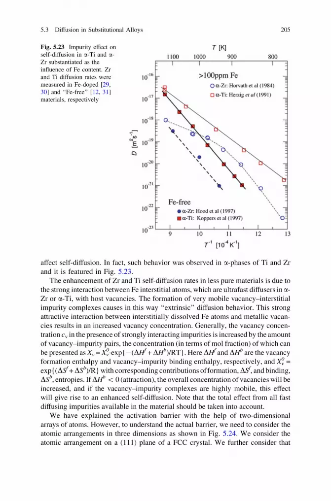
affect self-diffusion. In fact, such behavior was observed in a-phases of Ti and Zrand it is featured in Fig. 5.23.

The enhancement of Zr and Ti self-diffusion rates in less pure materials is due tothe strong interaction between Fe interstitial atoms, which are ultrafast diffusers in a-Zr or a-Ti, with host vacancies. The formation of very mobile vacancy–interstitialimpurity complexes causes in this way ‘‘extrinsic’’ diffusion behavior. This strongattractive interaction between interstitially dissolved Fe atoms and metallic vacan-cies results in an increased vacancy concentration. Generally, the vacancy concen-tration cv in the presence of strongly interacting impurities is increased by the amountof vacancy–impurity pairs, the concentration (in terms of mol fraction) of which canbe presented as Xv = Xv

0�exp{-(DHf + DHb)/RT}. Here DHf and DHb are the vacancyformation enthalpy and vacancy–impurity binding enthalpy, respectively, and Xv

0 =exp{(DSf + DSb)/R} with corresponding contributions offormation, DSf, and binding,DSb, entropies. If DHb \ 0 (attraction), the overall concentration of vacancies will beincreased, and if the vacancy–impurity complexes are highly mobile, this effectwill give rise to an enhanced self-diffusion. Note that the total effect from all fastdiffusing impurities available in the material should be taken into account.

We have explained the activation barrier with the help of two-dimensionalarrays of atoms. However, to understand the actual barrier, we need to consider theatomic arrangements in three dimensions as shown in Fig. 5.24. We consider theatomic arrangement on a (111) plane of a FCC crystal. We further consider that

Fig. 5.23 Impurity effect onself-diffusion in a-Ti and a-Zr substantiated as theinfluence of Fe content. Zrand Ti diffusion rates weremeasured in Fe-doped [29,30] and ‘‘Fe-free’’ [12, 31]materials, respectively

5.3 Diffusion in Substitutional Alloys 205

atom 2 jumps to vacancy at 6. Therefore, the jumping atom has to displace atoms 1and 4 on the same plane and 7 below and 8 above this plane, respectively.Therefore, the actual barrier plane has atoms 1, 8, 4, and 7.

Now, we consider a material with BCC structure, as shown in Fig. 5.25. Two-dimensional atomic arrangement is shown for (110) plane. The activation barrier isnot clear, when, for example, atom 2 jumps to a vacant lattice site at the center. Ifwe consider just one unit cell, it seems that the activation barrier is mainly becauseof the atoms 1, 7, and 6. However, to understand the actual barrier, we need toconsider another unit cell, keeping atom 2 at the body center position. It must beapparent that actually, the atom has to cross another barrier plane also with atoms9, 10, and 11. That means it has to cross two barrier planes in total to make asuccessful jump. This is the reason that the free energy versus distance curve inBCC crystal may have two humps.

In Fig. 5.26, the results of real calculations are presented for a-Fe and b-Zr.Although such shallow minima are sometimes observed in other cases, too, onehas to be careful with corresponding interpretation in view of approximate natureof the used inter-atomic potentials.

5.3.6 Orientation Dependence in Substitutional Diffusion

We start our discussion with a BCC lattice, which has coordination number Z = 8.For the ease of explanation, we consider the presence of a vacancy at the bodycenter position, as shown in Fig. 5.27.

This is an isotropic system. That means all the jump lengths are equal. Even theactivation energy for all the jumps also should be the same to consider Ci ¼ C. Weconsider diffusion along the x-axis (h100i direction). Suppose atoms 1, 2, 5, and 6are on one plane, V is on the next plane, and atoms 3, 4, 7, and 8 are on anotherplane. So vacancy has equal probability to exchange position with any of the

Fig. 5.24 Activation barrier plane is shown in a FCC structure

206 5 Atomic Mechanism of Diffusion

atoms. Further, different vacancies will exchange position with different atoms.Therefore, the diffusion coefficient from Eq. 5.71 can be written as

Dxs ¼ Dh100i

s ¼ Xv

1Z

XZ

Z¼1

CiDx2i ¼ XvC

18

4 � a

2

ffi �2þ4

a

2

ffi �2 �

¼ 14

XvCa2 ð5:75Þ

Fig. 5.25 Activation barrierplanes are shown in a BCCstructure

Fig. 5.26 Energy barrier as afunction of the position of thejumping atom normalized tothe jump distance for a-Feand b-Zr after Chirkov andNazarov [32]. Two humps inthe energy landscape areclearly seen

5.3 Diffusion in Substitutional Alloys 207

where ± a/2 are the effective jump lengths.

Similarly, we can show that Dys ¼ Dh010i

s ¼ 14 XvCa2 and Dz

s ¼ Dh001is ¼ 1

4 XvCa2.Now, we consider diffusion along the h110i direction that is perpendicular to

the plane (110). The effective jump length is equal to the inter-planar spacinga=

ffiffiffi2p

. It can be seen easily that atoms 2, 4, 6, and 8 are located on the sameplane (110) with the vacancy. So the exchange of the vacancy with these atomswill not contribute to diffusion distance along the h110i direction. The exchangeof vacancy to any of the atoms 1, 5, 3, and 7 will only contribute to the diffusion.So the diffusion coefficient in this direction can be written as

Dsh110i ¼ XvC

18

4ð0Þ þ 4 affiffiffi2p

� �2" #

¼ 14

XvCa2 ð5:76Þ

From the above discussions, we can see that the diffusion coefficient is insen-sitive to the direction in a BCC structure.

Let us now consider a FCC structure, as shown in Fig. 5.28a. Again, we canconsider Ci ¼ C, since it is an isotropic system. It has a coordination number of 12.That means different vacancies on the same plane will exchange position with anyof the 12 atoms with an equal probability. When we consider the diffusion alongthe x-axis, the effective jump length is Dx ¼ �a=2 for the exchange with atoms 5,6, 7, and 8 and a/2 for the exchange with atoms 10, 11, 12, and 13. On the otherhand, the effective jump length is zero for the exchange with atoms 1, 2, 3, and 4.So the diffusion coefficient along the x-axis can be written as

Dxs ¼ XvC

112

4 � a

2

ffi �2þ4ð0Þ þ 4

a

2

ffi �2 �

¼ 16

XvCa2 ð5:77Þ

The same value will be found, when we consider diffusion along the y- orz-axis.

Fig. 5.27 BCC unit cell is shown with the presence of a vacancy at the center

208 5 Atomic Mechanism of Diffusion

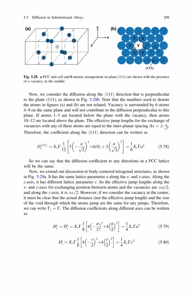
Now, we consider the diffusion along the h111i direction that is perpendicularto the plane (111), as shown in Fig. 5.28b. Note that the numbers used to denotethe atoms in figures (a) and (b) are not related. Vacancy is surrounded by 6 atoms4–9 on the same plane and will not contribute to the diffusion perpendicular to thisplane. If atoms 1–3 are located below the plane with the vacancy, then atoms10–12 are located above the plane. The effective jump lengths for the exchange ofvacancies with any of these atoms are equal to the inter-planar spacing Dx ¼ affiffi

3p .

Therefore, the coefficient along the h111i direction can be written as

Dh111is ¼ XvC

112

3 � affiffiffi3p

� �2

þ6ð0Þ þ 3affiffiffi3p� �2

" #¼ 1

6XvCa2 ð5:78Þ

So we can say that the diffusion coefficient to any directions in a FCC latticewill be the same.

Now, we extend our discussion to body-centered tetragonal structures, as shownin Fig. 5.29a. It has the same lattice parameter a along the x- and y-axes. Along thez-axis, it has different lattice parameter c. So the effective jump lengths along thex- and y-axes for exchanging position between atoms and the vacancies are a=2,and along the z-axis, it is c=2. However, if we consider the vacancy at the center,it must be clear that the actual distance (not the effective jump length) and the sizeof the void through which the atoms jump are the same for any jumps. Therefore,we can write Ci ¼ C. The diffusion coefficients along different axes can be writtenas

Dxs ¼ Dy

s ¼ XvC18

4 � a

2

ffi �2þ4

a

2

ffi �2 �

¼ 14

XvCa2 ð5:79Þ

Dsz ¼ XvC

18

4 � c

2

ffi �2þ4

c

2

ffi �2 �

¼ 14

XvCc2 ð5:80Þ

Fig. 5.28 a FCC unit cell and b atomic arrangement on plane (111) are shown with the presenceof a vacancy in the middle

5.3 Diffusion in Substitutional Alloys 209

Further, we consider the face-centered orthorhombic structure with latticeparameters a, b, and c along the x-, y-, and z-axes, respectively, as shown inFig. 5.29b. Note here that (similar to the discussion on interstitial diffusion in thesame crystal structure in Sect. 5.2.5) atoms 1, 2, 3, and 4 are on the x plane withthe area of bc, atoms 5, 7, 9, and 11 are on the y plane with the area of ac, andatoms 6, 8, 10, and 12 are on the z plane with the area of ab. So the jumpfrequencies will be different when vacancies exchange position with the atoms ondifferent planes. These are denoted as C1, C2, and C3 for the atoms on x, y, andz planes, respectively. Further, the effective jump lengths along the x, y, andz directions are a=2; b=2 and c=2. Therefore, the diffusion coefficients can beexpressed as

Ds ¼1

12XV

X12

i¼0

CiDx2i ¼

112

C1Dx21 þ C2Dx2

2 � � � þ C12Dx212

�

Dxs ¼ Xv

112

C1 0ð Þ2þC1 0ð Þ2þC1 0ð Þ2þC1 0ð Þ2þC2 �a=2ð Þ2þC3 �a=2ð Þ2

þ C2 �a=2ð Þ2þC3 �a=2ð Þ2þC2 a=2ð Þ2þC3 a=2ð Þ2þC2 a=2ð Þ2þC3 a=2ð Þ2

" #

¼ 112 Xv C2 þ C3ð Þa2 ð5:81aÞ

Dys ¼ Xv

112

C1 �b=2ð Þ2þC1 b=2ð Þ2þC1 b=2ð Þ2þC1 �b=2ð Þ2þC2 0ð Þ2þC3 b=2ð Þ2

þ C2 0ð Þ2þC3 �b=2ð Þ2þC2 0ð Þ2þC3 b=2ð Þ2þC2 0ð Þ2þC3 �b=2ð Þ2

24

35

¼ 112

Xv C1 þ C3ð Þb2 ð5:81bÞ

Fig. 5.29 a Body-centered tetragonal and b face-centered orthorhombic structures are shownwith the presence of a vacancy in the middle

210 5 Atomic Mechanism of Diffusion

Dzs ¼ Xv

112

C1 c=2ð Þ2þC1 �c=2ð Þ2þC1 c=2ð Þ2þC1 �c=2ð Þ2þC2 c=2ð Þ2þC3 0ð Þ2

þC2 �c=2ð Þ2þC3 0ð Þ2þC2 c=2ð Þ2þC3 0ð Þ2þC2 �c=2ð Þ2þC3 0ð Þ2

24

35

¼ 112

Xv C1 þ C2ð Þc2

ð5:81cÞ

Therefore, from Eqs. 3.58a, 3.58b, and 3.58c, we can write in an orthorhombicstructure

Dsx 6¼ Ds

y 6¼ Dsz ð5:82Þ

Now, we discuss hexagonal close packed structure. Lattice parameters are a andc, as shown in Fig. 5.30. If we consider the presence of a vacancy in the middle ofthe basal plane, we can see that it is surrounded by total 12 atoms. There are sixatoms on the basal plane, numbered as 1–6, respectively. Three atoms are atdistance þ c

2 along the z-axis, numbered as 7–9, respectively, and three atoms are atdistance � c

2, numbered as 10–12, respectively. We need to consider two jumpfrequencies: C1 for exchanging position with atoms 1–6 and C2 for exchangingposition with atoms 7–12. So the diffusion along the x- and z-axes can be written as

Ds ¼1

12XV

X12

i¼0

CiDx2i ¼

112

C1Dx21 þ C2Dx2

2 � � � þ C12Dx212

�

Dsx ¼ XV

112

C1 �að Þ2þC1 �a=2ð Þ2þC1 a=2ð Þ2þC1 að Þ2þC1 a=2ð Þ2þC1 �a=2ð Þ2

þC2 �a=2ð Þ2þC2 0ð Þ2þC2 a=2ð Þ2þC2 �a=2ð Þ2þC2 0ð Þ2þC2 a=2ð Þ2

24

35

¼ 112

XVa2 3C1 þ C2ð Þ

ð5:83aÞ

Dsz ¼ XV

112

C1 0ð Þ2þC1 0ð Þ2þC1 0ð Þ2þC1 0ð Þ2þC1 0ð Þ2þC1 0ð Þ2

þC2 c=2ð Þ2þC2 c=2ð Þ2þC2 c=2ð Þ2þC2 �c=2ð Þ2þC2 �c=2ð Þ2þC2 �c=2ð Þ2

24

35

¼ 18C2XVc2

ð5:83bÞ

One interesting point should be noted here. In the case of an ideal HCP

structure, we know that ca ¼

ffiffi83

qand C1 ¼ C2 (note that it has similarities in

packing with a FCC structure). So it becomes Dx ¼ DZ . However, this is not truein most of the hexagonal structures, since in general, the ratio of lattice parametersdeviates from the ideality. This will result in different jump frequencies also in

5.3 Diffusion in Substitutional Alloys 211

different directions, and certain diffusion anisotropy is measured accordingly (seethe experimental examples in Fig. 5.16).

In Sect. 5.2.5, the diffusion anisotropy for interstitial diffusion was documented.As it was stated, the ratio of diffusivities of interstitial atoms in different directionsis generally not too large, within a factor of 2–3. On the other hand, the diffusionanisotropy for substitutional atoms can be very pronounced, especially if weconsider intermetallic phases. For example, the diffusion anisotropy approachesthree to four orders of magnitude for Mo diffusion in MoSi2 and is about an orderof magnitude for Si diffusion in MoSi2 (Fig. 5.31). A pronounced anisotropy of Ti

Fig. 5.30 Atomicarrangement and differentjump frequencies are shownto explain anisotropy indiffusion in a hexagonalclosed packed crystalstructure

Fig. 5.31 Arrhenius plots ofthe diffusion coefficients ofMo (black) and Si (blue) inMoSi2 perpendicular (dashedlines) and parallel (solidlines) to the tetragonal axis,after [33, 34]

212 5 Atomic Mechanism of Diffusion

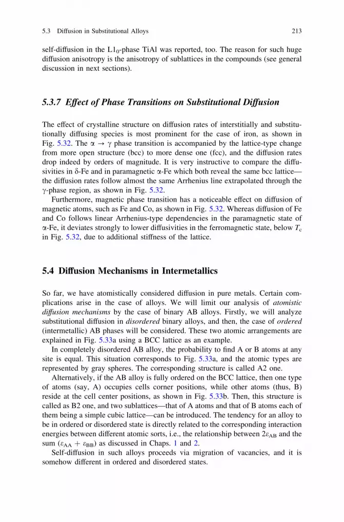
self-diffusion in the L10-phase TiAl was reported, too. The reason for such hugediffusion anisotropy is the anisotropy of sublattices in the compounds (see generaldiscussion in next sections).

5.3.7 Effect of Phase Transitions on Substitutional Diffusion

The effect of crystalline structure on diffusion rates of interstitially and substitu-tionally diffusing species is most prominent for the case of iron, as shown inFig. 5.32. The a ? c phase transition is accompanied by the lattice-type changefrom more open structure (bcc) to more dense one (fcc), and the diffusion ratesdrop indeed by orders of magnitude. It is very instructive to compare the diffu-sivities in d-Fe and in paramagnetic a-Fe which both reveal the same bcc lattice—the diffusion rates follow almost the same Arrhenius line extrapolated through thec-phase region, as shown in Fig. 5.32.

Furthermore, magnetic phase transition has a noticeable effect on diffusion ofmagnetic atoms, such as Fe and Co, as shown in Fig. 5.32. Whereas diffusion of Feand Co follows linear Arrhenius-type dependencies in the paramagnetic state ofa-Fe, it deviates strongly to lower diffusivities in the ferromagnetic state, below Tc

in Fig. 5.32, due to additional stiffness of the lattice.

5.4 Diffusion Mechanisms in Intermetallics

So far, we have atomistically considered diffusion in pure metals. Certain com-plications arise in the case of alloys. We will limit our analysis of atomisticdiffusion mechanisms by the case of binary AB alloys. Firstly, we will analyzesubstitutional diffusion in disordered binary alloys, and then, the case of ordered(intermetallic) AB phases will be considered. These two atomic arrangements areexplained in Fig. 5.33a using a BCC lattice as an example.

In completely disordered AB alloy, the probability to find A or B atoms at anysite is equal. This situation corresponds to Fig. 5.33a, and the atomic types arerepresented by gray spheres. The corresponding structure is called A2 one.

Alternatively, if the AB alloy is fully ordered on the BCC lattice, then one typeof atoms (say, A) occupies cells corner positions, while other atoms (thus, B)reside at the cell center positions, as shown in Fig. 5.33b. Then, this structure iscalled as B2 one, and two sublattices—that of A atoms and that of B atoms each ofthem being a simple cubic lattice—can be introduced. The tendency for an alloy tobe in ordered or disordered state is directly related to the corresponding interactionenergies between different atomic sorts, i.e., the relationship between 2eAB and thesum (eAA + eBB) as discussed in Chaps. 1 and 2.

Self-diffusion in such alloys proceeds via migration of vacancies, and it issomehow different in ordered and disordered states.

5.3 Diffusion in Substitutional Alloys 213

5.4.1 Diffusion in Disordered Intermetallic Compounds

In this case, diffusion is mediated by jumps of vacancies, though the particularenergy barriers depend on the kind of jumping atom and local environment of it. Ina mean field approach, the effect of local environment can be neglected and onehas to introduce just two jump frequencies for a vacancy: xA and xB.

Fig. 5.33 Examples of atomic arrangements in binary AB alloy with disordered A2 (a) and orderedB2 (b) structures. The A and B atoms are sketched as black and white spheres. The gray spheres inthe first figure represent site at which the probabilities to find either A or B atom are equal

Fig. 5.32 Effect of crystalline structure and magnetic transition on diffusion rates of interstitiallydiffusing (C and N) and substitutionally diffusing (Fe and Co) species on the example of diffusionin iron

214 5 Atomic Mechanism of Diffusion

A very useful (and exact as mean field approximation) approach was derived byManning [35]. His treatment will be sketched here for a binary AB random alloy.The vacancy correlation factor, fv, is represented as

fvnv ¼ f Av nA þ f B

v nB ð5:84Þ

where f Av and f B

v are the partial vacancy correlation factors, nA and nB are thenumber of vacancy jumps performed as exchange with the atoms of the sorts A andB, respectively, and nv is the total number of vacancy jumps for the given timet. The key point of the Manning approach is the introduction of the escape fre-quency H defined as

H ¼ fvM0xv ð5:85Þ

Here, xv is the average vacancy jump frequency, and M0 is the function of thegeometrical tracer correlation factor f0 for the given lattice occupied by one sort ofatoms,

M0 ¼ 2f0 1� f0ð Þ ð5:86Þ

The tracer correlation factors of atoms A and B, fA and fB, respectively, one canuse an expression, which is almost analogous to Eq. 5.54,

fA ¼1þ tA1� tA

and fB ¼1þ tB1� tB

with tA ¼ pþA � p�A and tB ¼ pþB � p�B , where pþA (pþB ) is the probability for A (B)atom to make the second jump in the same direction as that of the first jump and,correspondingly, p�A (p�B ) is the probability for A (B) atom to make the secondjump opposite to the direction of the first jump. Using the escape frequency H andthe vacancy–atom exchange frequencies xA and xB introduced above, the tracercorrelation factors can be represented as

fA ¼H

2xA þ Hand fB ¼

H

2xB þ H

Within Manning’s theory, the tracer correlation factors are related to the partialvacancy correlation factors by the following expressions:

fA ¼ f0f Av and fB ¼ f0f B

v

In the mean field approximation, the average vacancy exchange frequency is

xv ¼ cAxA þ cBxB ¼ cAxA þ ð1� cAÞxB ð5:87Þ

Here, the vacancy concentration is considered to be negligibly low.

5.4 Diffusion Mechanisms in Intermetallics 215

5.4.2 Diffusion Mechanisms in Ordered IntermetallicCompounds

In this case, A and B atoms are not randomly distributed on the same crystallinelattice, as shown in Fig. 5.33b. As it was explained in Chap. 2, generally 4 types ofbasic substitutional defects can be introduced in ordered AB compound. We willillustrate this point for the B2 binary AB compound, as shown in Fig. 5.33b. Wecan introduce two sublattices, A and B sublattices, for the perfectly orderedstoichiometric compound, which would exclusively be occupied by A and Batoms, respectively. Since the chemical nature of A and B is considered to bedifferent, it costs different energy to produce vacancy on A or B sublattice andthese defects have to be differentiated, as shown in Fig. 5.34a and b.

Two further defects are the antisite or antistructure atoms when atoms of onesort occupy sites on the wrong sublattice, as shown in Fig. 5.34c, d. As detailedanalysis in Chap. 2 has substantiated, the formation energies (as well as formationentropies and formation volumes) of all defects have not necessarily the same, andas a rule, they substantially deviate.

The ordered structure of intermetallic compounds imposes certain limitationson geometrically possible vacancy-mediated diffusion mechanisms. Below, themost important diffusion mechanisms are discussed.

5.4.3 Six-Jump Cycle Mechanism

Originally, this mechanism was proposed for B2 compounds [36], but later it waselaborated for others ordered structures, too. A scheme of this mechanism with a[110] net displacement of the vacancy is shown in Fig. 5.35. One starts with avacancy on the A sublattice, and after 6 successive jumps, the vacancy exchangesits position with A atom along the face diagonal of the unit cell. During this cyclicmovement, disorder in the phase AB increases first—from VA to VB + BA (jump1), then to VA + BA + AB (jump 2), and finally to VB + 2BA + AB (jump 3)—and then, it is restored to the initial one, i.e., with the only A vacancy—fromVB + 2BA + AB to VA + BA + AB (jump 4), then to VB + BA (jump 5), andfinally to VA (jump 6).

Thus, as a result of 6 jumps, a vacancy accomplishes one and a half cycle andeffectively jumps along the diagonal of the face, as shown in Fig. 5.35. It is clearthat first jumps are related to an increase of the energy of the crystal since defects(antisite atoms) are produced. The situation after the 3rd jump represents a mostdisordered state: one vacancy and three antisite atoms left behind as a result of thefirst cycle. Following jumps will restore the order in the lattice, and exactly thesame ordered state (single vacancy on the initial sublattice) is retained.

216 5 Atomic Mechanism of Diffusion

Fig. 5.35 The scheme of the six-jump cycle mechanism with a net [110] displacement of thevacancy VA

Fig. 5.34 Four types of substitutional defects in ordered AB compound with A and B atomsshown as black and white spheres and vacancy as a cube: vacancy on the a A and b B sublattices,c A atom on the B sublattice, and d B atom on the A sublattice

5.4 Diffusion Mechanisms in Intermetallics 217

One has to pay attention that two further types of cycles are possible in the B2lattice, as shown in Fig. 5.36, corresponding to the [001] net displacement of theinitial vacancy—the so-called bent (Fig. 5.36a) and flat (Fig. 5.36b) cycles.

It is important that the atoms do not necessarily move along the vectors drawnin Figs. 5.35 and 5.36, and the exact trajectories have to be determined viaappropriate atomistic simulations. The vectors, as in each case of such schematic

Fig. 5.36 Two variants of the six-jump cycle mechanism with the net [001] displacement of thevacancy—a bent and b flat cycles. As a result, the vacancy on A sublattice and A atom exchangetheir positions along the edge of the unit cell

218 5 Atomic Mechanism of Diffusion

representation, just connect the initial and final positions of the vacancy for aparticular jump during accomplishing the whole cycle motion.

The energy barriers are not necessarily the same for all types of the cycles. Anexample of atomistic calculations (allowing relaxation after each jump) is pre-sented in Fig. 5.37 for the case of B2-ordered NiAl (in Figs. 5.35, 5.36, the Niatoms are A and Al atoms are B). One recognize, e.g., that the 110 cycles are mostprobable in this structure for NiAl. Further, the atomistic simulation with reliableinter-atomic potentials reveals that the first disordering jump of the vacancyinvolves typically the highest energy barrier. Subsequent jumps, requiring thougha thermal activation, could bring system even to a configuration with a lower totalenergy with respect to the neighboring configurations, as shown in Fig. 5.37. Ofcourse, the energy of the system is completely restored after the vacancy hasaccomplished the full sequence of six jumps.

A very important note is due here. Could the temperature dependence of diffusionaccording to such sophisticated jump sequence be described by a single Arrhenius-type dependence like Eq. 5.74? If yes, how is the activation barrier defined? Is thisthe highest barrier in the sequence? The numerical simulations give very importanthints and predict that diffusion by such highly correlated jump sequence (in par-ticular, for the six-jump cycles) can reasonably be described by an Arrhenius law,Eq. 5.74, and the migration energy can conveniently be represented by a sum of twocontributions—the height of the first barrier and the activation energy correspondingto the correlation effects. This can qualitatively be exemplified in Fig. 5.37.According to such viewpoint, the energy barriers for all types of the six-jump cyclesare exactly the same and correspond to the height of the first barrier. Still the [001]-type cycles involve very high barriers for the 3rd jumps, as shown in Fig. 5.37, sothat the probability of a reverse jump in those sequences is significantly larger andthe whole jump sequence will hardly be accomplished, especially at lower tem-peratures. As the temperature increases, the importance of the difference in thebarrier heights decreases, since it is proportional to exp(-Q/kT), and such sequences

Fig. 5.37 The energybarriers corresponding todifferent six-jump cycles inthe B2 structure of NiAl. Thejump sequences were definedin Figs. 5.35 and 5.36, andthe abscissa axis representsthe distance along jumpvectors defined for the wholecycle

5.4 Diffusion Mechanisms in Intermetallics 219

may occur. This strong temperature dependence of the probability of the accom-plishment of the cycles corresponds to a large contribution to the effective activationenergy. This conclusion is of general importance for diffusion mechanisms whichinclude more than one jump of a defect. The present consideration highlights theimportance of careful determination of the correlation effects for the diffusionmechanisms in ordered alloys.

The correlated jumps of the atomic species during accomplishing the cyclesimpose certain limitations on the quantities which can be measured in a diffusionexperiment. Firstly, in a highly ordered state near the stoichiometric composition,the ratio of tracer diffusivities of both components, DA/DB, can adopt only thevalues within the interval

1q DA

DB

q ð5:88Þ

where q was calculated to be 2 [37] and was later corrected to q & 2.034 byincluding the correlation effects [38]. The ratio of diffusivities of Ag and Mg inb-AgMg, Zn and Au in b0-AuZn, and Cd and Au in b-AuCd falls into these limits,and this is typically considered as a strong support of the six-jump cycle mech-anism in these compounds.

Diffusion by the six-jump cycles is a highly correlated process, as we havealready seen. Thus, the correlation factor is supposed to be rather small. However,one should generally distinguish two types of correlations which characterize thesix-jump cycles. Considering the individual cycles as effective vacancy jumpevents occurring with the given frequency, one can calculate the resulting corre-lation factors ~fA and ~fB [38]. For B2 NiAl, Monte Carlo calculations resulted in~fNi � 0:782 and ~fAl � 0:860. In contrast, the tracer correlation factors for Ni andAl atoms in that case were calculated to be fNi � 0:445 and fAl � 0:022, respec-tively. We note that fNi is not as small as it was usually anticipated for the six-jumpcycle mechanism. This fact should be taken into account when interpreting theresults of, e.g., Mössbauer effect experiments, which allowed establishing thegeometry of individual atomic jumps and, by comparing the local jump rates withthe long-range diffusion data, estimating the corresponding correlation factor.

In [39], the isotope effect was measured for both Au and Zn in the B2-orderedb0-AuZn alloys, with EAu (and correspondingly fAu) being considerably larger thanEZn (fZn) in Zn-rich alloys (e.g., EAu = 0.35 and EZn = 0.05 in the Au-51.85 at.%Zn alloy). This fact resembles the relation between fNi and fAl in B2-NiAl for thesix-jump cycle mechanism [40] and can be explained by the predominant vacancyconcentration in the Au sublattice and an increased probability of a reverse jumpof a Zn atom which has initiated a six-jump cycle. One may argue that since bothatom types in the B2 AB alloy participate in the same cycle, the pertinent cor-relation factors fA and fB have to be similar. However, this is generally not true, asthe simulations of correlation effects during diffusion according to the six-jumpcycle mechanism in NiAl have shown, and very different correlation factors for the

220 5 Atomic Mechanism of Diffusion

two components can be obtained. Thus, the large difference between fA and fB inan AB compound cannot be considered as an argument against the six-jump cyclemechanism.

The six-jump cycles are to be considered as a subset of a general n-jump cyclemechanism, since, e.g., 3-jump cycles were considered in the L10 structure of TiAland 10-jump cycles were introduced to explain diffusion in quasicrystallinecompounds. Moreover, higher n cycles can be introduced in the B2 structure, too(with n = 10, for example), by a simple inspection of the lattice. In this regard, thesix-jump cycles represent simply the n-cycle mechanism with the lowest possiblein the given structure number of n successive jumps of a single vacancy inotherwise perfect lattice (thus, n = 3 for L10, n = 6 for B2, n = 6 for L12, andn = 10 for Mackay icosahedrons, respectively, as basic tilling units of icosahedralquasicrystals, etc.).

There is one important point here. The six-jump cycle mechanism was con-sidered for a perfectly ordered lattice containing one vacancy on a given sublattice.In this sense, it was analyzed for the stoichiometric composition of the AB alloy.However, there are basically no objections against the existence of such highlycorrelated jump sequences in off-stoichiometric AB compounds. As the compo-sition of a given compound deviates from the stoichiometric one, a large amount of(constitutional) defects appear and mutual interaction between different defects hasto be considered. If a vacancy performing a six-jump cycle meets an antistructureatom on a particular lattice, the limits in the previous equation are changed [41].It was shown that q may become significantly larger that unity [41]. Thus, in a lessordered state, experimental values of DA/DB being larger than 2 can no longer beconsidered as an indication that the six-jump cycle mechanism does not operate.One may easily see that such six-jump cycle will be transformed to four-cyclemechanism in the B2 structure if vacancy and antisite atoms reside in differentsublattices, as shown in Fig. 5.38. Further subtypes of the general n-jump cyclemechanism could formally be introduced. The sequences differ by activationenergies, and the level of correlation of individual jumps and thus with differentprobabilities could be found by inspection of the results of real simulations usingmolecular dynamics.

5.4.4 Sublattice Diffusion Mechanism

When one of the components forms a lattice structure which enables the nearestneighbor jumps through the respective sublattice, random jumps of a vacancy onthis sublattice will not affect the order in the compound. As an example, thismechanism is schematically presented in Fig. 5.39 for the L12 structure. It isimportant that this mechanism can dominate diffusion not only of the majoritycomponent, but also of the minority component. In such a case, a minority atomjumps into the ‘‘wrong’’ sublattice and continues its migration through this sub-lattice. The sublattice diffusion mechanism was extensively analyzed in [42, 43].

5.4 Diffusion Mechanisms in Intermetallics 221

It is obvious that the diffusivities of both components are not coupled by arelation similar to Eq. 5.88, if the sublattice diffusion mechanism operates.

The correlation factors for the sublattice diffusion mechanism in the L12

structure of Ni3Al are different for diffusion of the majority (i.e., Ni) and minority(i.e., Al) components. The calculations as outlined above provide that fNi = 0.689.The determination of fAl is more intricate, and e.g., a five-frequency model has tobe invoked (see Fig. 5.40).

Fig. 5.38 A scheme of 4-jump cycles for the B2 structure. The flat (1–2–3–4) and bent (10–20–3–4) cycles are shown. These jump sequences are flowed starting from a vacancy on Ni sublattice(square) as a nearest neighbor of a Ni antisite atom, NiAl (the shaded circle). The vacancy firstcan exchange its position with Al atom occupying the next nearest neighbor position to NiAl (thejump of type 10) or Al atom from 4th coordination shell of NiAl (the jump of type 1). The jumps 20

or 2 correspond to the most disordered states with two NiAl and one AlNi (and a Ni vacancy, ofcourse). The jumps 3 and 4 restore the initial order in the compound

Fig. 5.39 A scheme of sublattice diffusion mechanism for the case of A3B compound. Here, Aand B atoms are represented by dark and bright spheres, respectively. Eight possible directions ofnearest neighbor jumps of a B vacancy are shown by dashed lines

222 5 Atomic Mechanism of Diffusion

The somewhat lengthy calculations demonstrate that the Al correlation factorcan be expressed in a usual way via the vacancy—Al atom exchange frequency x2

and the vacancy escape frequency H:

fAl ¼H

x2 þ Hand H ¼ 10x3Fz 2x1 þ 5x3Fxð Þ

2x1 þ 5x3 Fz þ Fxð Þ

Here, Fx and Fz are functions of x4/x0, and they are changed in the range of0.2–1, if x4/x0 increases from 0 to ?.

5.4.5 Triple-Defect Diffusion Mechanism

This mechanism was originally proposed by Bakker and Stolwijk for the B2compound CoGa [44]. It specifies the migration of a triple defect, which representsa bounded entity composed of two transition metal vacancies and one transitionmetal atom in an antistructural position. The triple-defect mechanism in CoGa wasdescribed to correspond to the two nearest neighbor jumps of a Co atom and onenext nearest neighbor jump of a Ga atom. In Fig. 5.41, the triple-defect mechanismis shown for the case of the B2-NiAl compound. As a result of the indicatedsequence of jumps, the triple defect moves leaving the order in the compoundunchanged.

Since a correlated sequence of atomic jumps is involved, the diffusivities ofboth components in the perfectly ordered state are coupled by Eq. 5.88 withq = 13.3.

The correlation factors are supposed to be small for the triple-defect diffusionmechanism. They were calculated for B2-NiAl and fNi & 0.05 at T = 1,300 K inRef. [45] using a Monte Carlo method (Fig. 5.42). fNi depends remarkably ontemperature, and the contribution of this temperature dependence to the overall

Fig. 5.40 The jump frequencies for a Ni vacancy (cube) neighboring an Al antisite atom (redsphere). The five frequencies x0–x4 for a vacancy on the Ni sublattice are indicated: x0 is thefrequency of Ni vacancy jumps away from the Al antisite atom; x1 is the frequency of directexchange with the Al antisite; x2 is the jump frequency between neighboring positions of the Alantisite; x3 is the frequency of vacancy jump from first neighbor position of the Al antisite to amore distant neighbor; and x4 is the frequency of the reverse jump to x3

5.4 Diffusion Mechanisms in Intermetallics 223

activation enthalpy of Ni diffusion by the triple-defect mechanism amounts to17 kJ/mol. This fact has to be taken into account in interpreting activation enthalpyof diffusion in ordered compounds.

Fig. 5.41 A scheme of the triple-defect mechanism as it can occur in the B2 compound NiAl—either via a sequence of a three or b four atomic jumps. In the first case, atoms of one kinds, mostprobably of Al, perform a next nearest neighbor jump within own sublattice to temporary Alvacancy, the jump 2 in (a)

224 5 Atomic Mechanism of Diffusion

5.4.6 Antistructure Bridge Mechanism

This mechanism was originally proposed by Kao and Chang [46] for the B2structure and was later extended also to L12 structures [47]. The antistructurebridge (ASB) mechanism is schematically presented in Fig. 5.43a. As a result ofthe two indicated jumps, the vacancy and the antistructure atom effectivelyexchange their positions. Since the vacancy can in fact jump up to the 4th or 5thcoordination shell from its initial position (depending on the lattice structure), theresulting large geometrical factor of the ASB mechanism increases its contributionto the diffusivity.

It is important to note that the contribution of this mechanism has a percolationnature in the sense that long-range diffusion by the ASB mechanism will occuronly if the concentration of the antistructure atoms will be sufficiently high. Arelatively high critical concentration for a B2 structure was initially estimated frompurely geometrical arguments. The Monte Carlo simulation of this processresulted, however, in a smaller value of the percolation threshold, about 5 %. Suchan antistructure atom concentration can indeed exist in intermetallics, and the ASBmechanism becomes important for explaining the observed diffusion behavior inNi aluminides [45, 48].

In the L10 structure of the phase TiAl, other types of the ASB mechanism are ofprime importance. One of such variant is presented in Fig. 5.43b. After the indi-cated two jumps (1 + 2), the A vacancy moved perpendicular to the A atom layersusing an antistructure A atom as a ‘‘bridge.’’ If a further antistructure atom in asuitable nearest neighbor position is available for the vacancy after its secondjump, the next ASB sequence may start, as it is indicated in Fig. 5.43b. The MonteCarlo calculation of the percolation threshold for the long-range diffusion by thisvariant of the ASB mechanism yields about 11 % of the antistructure atoms as thecritical concentration.

Fig. 5.42 Temperaturedependence of correlationfactors of Ni diffusion in theB2-phase NiAl determinedfor triple-defect anddivacancy diffusionmechanisms. The divacancymechanism here is referred toa mechanism of diffusion viaa pair of Ni vacancies

5.4 Diffusion Mechanisms in Intermetallics 225

During the ASB sequence of jumps, only one sort of atoms moves (seeFig. 5.43). Therefore, the diffusivities of the two components are not coupled.

In a strict sense, the genuine ASB mechanism operates only after the perco-lation threshold is reached. However, in combination with another mechanism(usually the sublattice diffusion mechanism), the ASB mechanism (e.g., jumpsequence 1 ? 2 in Fig. 5.8b) can substantially contribute already to long-rangediffusion without any percolation threshold. One can therefore use the term ‘‘ASBmechanism’’ also in such cases, referring to the specific sequence presented inFig. 5.43a, b.

5.4.7 Interstitial Diffusion Mechanism

Small metallic atoms could diffuse interstitially in a matrix of a given intermetalliccompound. In Fig. 5.44, the solute diffusion of Fe and Ni in pure a-Ti, a2-Ti3Al,and in c-TiAl is presented in comparison with Ti self-diffusion in these materialsas a function of the reduced temperature Tm/T. Here, Tm is the melting point ofpure Ti or the intermetallic alloys of the stoichiometric composition. Figure 5.44substantiates that both Fe and Ni are fast diffusers in a-Ti or in a2-Ti3Al, [49, 50],while they are ‘‘normal’’ diffusers in c-TiAl.

Fig. 5.43 The antistructure bridge mechanism as it can be found in B2 (a) and L10

(b) compounds

226 5 Atomic Mechanism of Diffusion

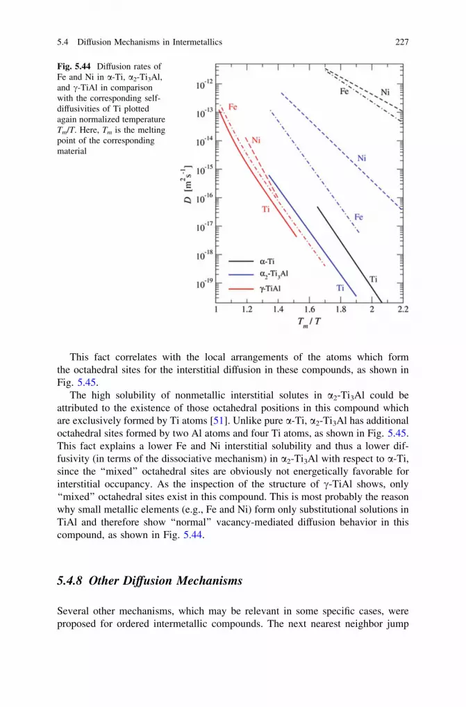
This fact correlates with the local arrangements of the atoms which formthe octahedral sites for the interstitial diffusion in these compounds, as shown inFig. 5.45.

The high solubility of nonmetallic interstitial solutes in a2-Ti3Al could beattributed to the existence of those octahedral positions in this compound whichare exclusively formed by Ti atoms [51]. Unlike pure a-Ti, a2-Ti3Al has additionaloctahedral sites formed by two Al atoms and four Ti atoms, as shown in Fig. 5.45.This fact explains a lower Fe and Ni interstitial solubility and thus a lower dif-fusivity (in terms of the dissociative mechanism) in a2-Ti3Al with respect to a-Ti,since the ‘‘mixed’’ octahedral sites are obviously not energetically favorable forinterstitial occupancy. As the inspection of the structure of c-TiAl shows, only‘‘mixed’’ octahedral sites exist in this compound. This is most probably the reasonwhy small metallic elements (e.g., Fe and Ni) form only substitutional solutions inTiAl and therefore show ‘‘normal’’ vacancy-mediated diffusion behavior in thiscompound, as shown in Fig. 5.44.

5.4.8 Other Diffusion Mechanisms

Several other mechanisms, which may be relevant in some specific cases, wereproposed for ordered intermetallic compounds. The next nearest neighbor jump

Fig. 5.44 Diffusion rates ofFe and Ni in a-Ti, a2-Ti3Al,and c-TiAl in comparisonwith the corresponding self-diffusivities of Ti plottedagain normalized temperatureTm/T. Here, Tm is the meltingpoint of the correspondingmaterial

5.4 Diffusion Mechanisms in Intermetallics 227

mechanism may correspond to the lowest activation energy of single Ni vacancymigration in Al-rich NiAl. Also, a divacancy mechanism, with both vacanciesbelonging to the same sublattice in NiAl, may be suggested. After the givensequence of four atomic jumps, the initial order is completely restored and thedivacancy has moved by one step.

5.5 Correlation Factors of Diffusion in IntermetallicCompounds

The calculation of the correlation factors for simple lattices was outlines in Sect.5.3.3. In ordered intermetallic compounds, the procedure is somehow modified,since the geometry of sublattices and specific diffusion mechanisms have to betaken into account, and it will be presented in this subchapter using MoSi2 as anexample. We will limit us for Si diffusion in MoSi2, for which the diffusionmechanism is considered as well established [52]. We will follow the analysisconsidered in detail in [53].

Generally, diffusion is described by a symmetric diffusivity tensor of rank 2.For a tetragonal crystal like MoSi2, this tensor has two principal components.Diffusion is fully described by the diffusivities along the tetragonal axis, D||, andperpendicular to it, D\. Denoting the frequencies of type-1 and type-2 jumps as x1

and x2, respectively (see Fig. 5.46), the tracer diffusivities can be written as

Djj ¼12

c

3

ffi �2x1f1jj þ x2f2jj

ffi �Ceq

V ¼12

c

3

ffi �2x1 þ x2ð ÞfjjCeq

V ð5:89Þ

and

Fig. 5.45 Local atomic environments of octahedral interstitial sites in a-Ti, a2-Ti3Al, and c-TiAl

228 5 Atomic Mechanism of Diffusion

D? ¼12

a2x1f1?CeqV ð5:90Þ

Here, CeqV is the vacancy concentration on the Si sublattice in thermal equi-

librium. f1? is the partial correlation factor for diffusion perpendicular to thetetragonal axis. Since type-2 jumps do not contribute to diffusion perpendicular tothe tetragonal axis, the partial correlation factor coincides with the total correlationfactor in this direction, i.e., f1? ¼ f? � f1jj and f2jj are the partial correlation factorsfor diffusion parallel to the tetragonal axis related to the jump types 1 and 2,respectively. fjj is the total correlation factor related to diffusion in this direction.It can be expressed in terms of the partial correlation factors as

fjj ¼x1f1jj þ x2f2jj

x1 þ x2¼

f1jj þ x2x1

f2jj

1þ x2x1

ð5:91Þ

Partial and total correlation factors are functions of the frequency ratio x2/x1.The anisotropy ratio of diffusion

D?Djj¼ a2x1f1?

c3

� �2x1f1jj þ x2f2jj

ffi � ¼ a2f1?

c3

� �2f1jj þ x2

x1f2jj

ffi � ð5:92Þ

is fully described by the correlation factors and is a function of the frequency ratioas well. The strong anisotropy of both Mo and Si diffusion in MoSi2 is documentedin Fig. 5.30.

In order to calculate the partial correlation factors fi, one cannot take advantageof the inversion symmetry, because the Si sublattice sites are not inversion centers,as shown in Fig. 5.46. Moreover, there is no twofold or threefold symmetry around

Fig. 5.46 a Lattice structure of MoSi2 and b the structure of the Si sublattice. The two types ofSi vacancy jumps are shown

5.5 Correlation Factors of Diffusion in Intermetallic Compounds 229

the direction of the type-1 jumps. We suggest combining Howard’s matrix method[10] and a Monte Carlo approach to calculate the correlation factors, as it wasdescribed above.

Both types of jumps contribute to diffusion parallel to the tetragonal axis, asshown in Fig. 5.46. Hence, the relevant partial correlation factors can be deter-mined as

f jj ¼ Iþ 2Z � TðE� TÞ�1 � d ð5:93Þ

where f jj ¼ ðf1jj ; f2jj Þ is the column vector of the partial correlation factors, I the2-component unit column vector, E the 2 9 2 unit matrix, d = (|z1|, |z2|) thecolumn vector of the jump distances |z1| = c/6 and |z2| = c/3 of type-1 and type-2

jumps, Z ¼ z�11

�� �� 00 z�1

2

�� ������

����, respectively. T is a 2 9 2 matrix with the elements

tij ¼ Pþij � P�ij ; i; j ¼ 1; 2: ð5:94Þ

Here, Pij is the probability that a tracer jump of type i is immediately followedby a tracer jump of type j in the same (+) or opposite (-) direction along thetetragonal axis.

Since only type-1 jumps contribute to diffusion perpendicular to the tetragonalaxis (Fig. 5.46), Eq. 5.44 can be simplified, and the relevant correlation factor f\can be written as

f? ¼1þ t

1� tð5:95Þ

with

t ¼ Pþ � P� ð5:96Þ

Here, P± is the probability that a type-1 jump is immediately followed by atype-1 tracer jump with the same (+) or opposite (-) displacement perpendicularto the tetragonal axis.

5.5.1 Calculation of the Probabilities P

The probabilities Pij and P± introduced above have to be determined in order tocalculate the correlation factors. Let us start with diffusion along the tetragonalaxis. Diffusion perpendicular to the axis is simpler and will be consideredafterward.

230 5 Atomic Mechanism of Diffusion

Figure 5.46b shows the situation immediately after a tracer atom jump of thetype 1. The tracer atom is at the site O, whereas the vacancy occupies theneighboring site A after this jump. It is obvious that if the next jump of the tracer isa type-2 jump, the sign of its displacement with respect to the tetragonal axis willbe the same as that of the first jump (both jumps displace the tracer atom in thenegative direction of the z-axis). Alternatively, if the next jump of the tracer is atype-1 jump (leading to one of the lattice points A, B, C, or D in Fig. 5.46b), thesign of its z component will definitely be opposite to the sign of the z component ofthe first jump. Therefore, the probabilities are Pþ11 ¼ 0; P�11 6¼ 0; Pþ12 6¼ 0, andP�12 ¼ 0, and the corresponding matrix elements reduce to t11 ¼ �P�11 andt12 ¼ Pþ12. Considering the situation prevailing just after a tracer jump of type 2,we arrive at the relationships Pþ21 6¼ 0; P�21 ¼ 0; Pþ22 ¼ 0, and P�22 6¼ 0, and thust21 ¼ Pþ21 and t22 ¼ �P�22.

Let us suppose that the tracer atom has just performed a jump of type 1. Weneed to know the probabilities P�11 and Pþ12 that the next jump of the tracer atomwill be of type 1 or 2, respectively. These two sequential tracer jumps can gen-erally be mediated by the same vacancy or by two different vacancies. As a usualapproximation in the encounter model, the vacancy concentration is considered asvery small, and thus, a tracer encounter with a next vacancy occurs only after thefirst encounter has totally been completed (e.g., when the first vacancy has escapedfrom the tracer atom). Therefore, the individual encounters are well separated intime, and a new vacancy does not disturb the correlations induced by a previousvacancy. In this case, the correlation factors do not depend on the vacancyconcentration.

If taking into account that the two successive tracer jumps can generally beinduced by the same or by different vacancies, two different contributions to thetotal probabilities Pij are expected: firstly, a contribution from the encounter withthe same vacancy and secondly, a contribution from sequential encounters with theold and the new vacancy. In the latter case, the tracer jump of type i has occurredas a last event of the encounter with the old vacancy (and the vacancy has thenescaped from the tracer atom), and the next tracer jump of type j has been inducedby a new vacancy through its first exchange with the tracer atom. The secondcontribution to Pij is important for the MoSi2 structure. This is in contrast to latticestructures with inversion symmetry, where the fresh vacancies equally contributeto both Pþij and P�ij . Hence, they do not affect the resulting correlation factors,

which depend only on the differences tij ¼ Pþij � P�ij . However, in the case of alattice structure, in which the site positions are not inversion centers (this is thecase of the Si sublattice of MoSi2), the fresh vacancies may give different con-tributions to Pþij and P�ij . To illustrate this problem, let us consider the followingsituation: Suppose a first vacancy has induced a tracer jump of type 1 and has beenescaped. After some time, a fresh vacancy will approach the tracer atom from atotally random direction and will induce the next tracer jump. If this next tracerjump is of type 1, it will definitely be in the opposite direction to the first jump of

5.5 Correlation Factors of Diffusion in Intermetallic Compounds 231

type 1 with respect to the tetragonal axis. This fact increases the total probabilityP�11, but, by no means, it changes the value of Pþ11, which remains zero. Therefore,the total probability P�11 must be known to calculate t11 and finally to compute thecorrelation factors.

At first, let us consider the contribution of an encounter of the tracer atom withthe same vacancy to P1j, j = 1, 2. Since the vacancy performs a random walk, itcan either induce tracer jumps of type 1 or 2, or escape without inducing anyfurther jump of the tracer atom. Let us denote the probability for the latter event byPe1 , the escape probability after a type-1 jump. Furthermore, we denote theprobabilities that the same vacancy induces a type-1 or type-2 jump during itsrandom walk, which follows the initial site exchange with the tracer atom, by ~P�11

and ~Pþ12, respectively. The sum of all probabilities for the path of a particularvacancy equals unity:

~P�11 þ ~Pþ12 þ Pe1 ¼ 1 ð5:97Þ

A similar relationship holds for the vacancy random walk when the first siteexchange resulted in a type-2 jump:

~Pþ21 þ ~P�22 þ Pe2 ¼ 1 ð5:98Þ

The quantities ~Pij describe the probabilities of sequential jumps of types i and

j of a tracer atom caused by the same vacancy. In contrast, the Pij denotes the total

probabilities of sequential jumps of types i and j of the tracer atoms, irrespective ofwhich vacancy has induced these jumps. As explained above, in order to calculatePij , we have to add to ~Pij the probability that a ‘‘fresh’’ vacancy induces the jumpj at its first site exchange with the tracer atom, provided that the ‘‘old’’ vacancy hasescaped from the system (remember that this ‘‘old’’ vacancy has previouslyinduced the jump i), i.e.,

Pij ¼ ~Pij þ Pei~Pj ð5:99Þ

Here, ~Pj is the probability that a vacancy arriving from an arbitrary latticeposition of the Si sublattice at a nearest neighbor position of site O induces thejump j of the tracer atom at its very first site exchange. We have ~P1 þ ~P2 ¼ 1,because the ‘‘fresh’’ vacancy can induce either a type-1 or type-2 jump of thetracer atom.

In the absence of driving forces, the flux of fresh vacancies, which induce thejump j at the first site exchange with the tracer atom, is the same as the reverse fluxof vacancies escaping after an inverse jump -j without inducing any further jumpof the tracer atom, namely xjPe�j CV. On the Si sublattice, a vacancy can inducefour jumps of type 1 and one jump of type 2. In view of the lattice symmetry, theescape probabilities for jumps j and -j are equal (j = 1, 2). Furthermore, in

232 5 Atomic Mechanism of Diffusion

thermal equilibrium, the probability to find a vacancy on any site of the Si sub-lattice is the same. Therefore,

~P1 ¼4x1Pe1

4x1Pe1 þ x2Pe2

ð5:100Þ

and

~P2 ¼x2Pe2

4x1Pe1 þ x2Pe2

ð5:101Þ

Combining the above equations, the final expression for Pij becomes

Pij ¼ ~Pij þ Pej

njxjPej

4x1Pe1 þ x2Pe2

; i; j ¼ 1; 2: ð5:102Þ

Here, n1 = 4 and n2 = 1 are the numbers of jumps of the corresponding type.In the case of diffusion perpendicular to the tetragonal axis, only type-1 jumps

must be taken into account. Then, one can simply calculate P as

P ¼ ~P ð5:103Þ

Here, ~P is the probability that during a random walk of the given vacancy, thesecond jump of the tracer atom will occur in the same (+) or opposite (-) directionwith respect to the first jump. Due to the symmetry of the structure in the planeperpendicular to the tetragonal axis and in contrast to the previous case of diffusionalong the tetragonal axis, the fresh vacancies give equal contributions to both P+

and P-. Thus, Eq. 5.95 is not affected by such vacancies, since only the differencet = P+ - P- is important in the calculation of the correlation factor f\.

5.5.2 The Monte Carlo Calculation Scheme

A Monte Carlo approach can be applied to calculate ~Pij and Pei , and the structureof Eq. 5.101 suggests the calculation scheme. At first, a tracer atom and a vacancyare placed at the positions O and A on the Si sublattice (Fig. 5.46b). This corre-sponds to the atomic configuration after a type-1 jump. Then, the random walk ofthe vacancy is initiated and followed in the computer until the vacancy eitherescapes (see below) or induces a jump of type j of the tracer atom (j = 1, 2). Byperforming the Monte Carlo runs many times, the probabilities ~P�11;

~Pþ12, and Pe1

are thus determined. Similarly, by simulating the atomic configuration after a type-2 jump and following the random walk of the vacancy, the probabilities ~P�21; ~Pþ22,and Pe2 are determined. From Eq. 5.101, the probabilities Pij are then calculated

5.5 Correlation Factors of Diffusion in Intermetallic Compounds 233

using the probabilities ~Pij and Pei (i, j = 1, 2) obtained from the Monte Carlosimulation.

The probabilities ~P are calculated in a similar manner: An atomic configu-ration after the tracer jump of type 1 is modeled, and the following random walk ofthe vacancy is considered until it either induces a tracer jump or escapes from thetracer atom. The events resulting in the type-1 jump (with a nonzero displacementperpendicular to the tetragonal axis) are counted, and their probability is deter-mined by appropriate averaging. In view of Eq. 5.102, neither is it necessary todetermine the probability that the vacancy escapes nor that it induces a jump oftype 2 (with zero displacement perpendicular to the tetragonal axis). The proba-bilities ~P can be inserted in Eq. 5.93 instead of the total probabilities P±, and therelevant correlation factor f\ can be determined.

In the simulation, the initial vacancy and a tracer atom were introduced into thecenter of the simulation block. If the vacancy reaches the external boundary of thesimulation block in the course of its random walk, we consider it as escaped fromthe tracer atom. The particular values of Pij and Pei turned out to depend on thesize of the simulation block. However, their combination in Eq. 5.101 approachesa constant value when the size of the simulation block is increased.

The random walk of a vacancy is simulated in a standard manner. On any latticesite, the vacancy can perform either one out of 4 possible jumps of type 1 or onejump of type 2. The corresponding probabilities are x1/(4x1 + x2) and x2/(4x1 + x2), respectively. Since the absolute diffusivities are not addressed here,the frequency ratio x2/x1 is the only crucial parameter.

All probabilities depend only on this ratio. By using an appropriate randomnumber generator, for each Monte Carlo step, the direction of the vacancy jump ischosen in agreement with the above-mentioned probabilities for the given value ofthe ratio x2/x1. The position of the vacancy is then updated, and the next jumpdirection is selected. Thus, in each Monte Carlo step, the vacancy definitelyperforms one jump onto a neighbor site, and the probability of the given jumpdepends on the frequency ratio x2/x1. The frequency ratio x2/x1 was changed inthe simulations in the wide range from 10-5 to 105.

In the particular calculations, a simulation block of 80 9 80 9 80 unit cellswas found to give satisfactory results (the unit cell for the MoSi2 structure isshown in Fig. 5.46a). The random walk of a vacancy was followed until either thevacancy induces a jump of type j of the tracer atom or the vacancy reaches theouter surface of the simulation block. This procedure was repeated for 105 to 107

times, and the probabilities ~Pij and Pei were estimated from suitable averages ofthe individual Monte Carlo runs. Then, the partial correlation factors were cal-culated for the chosen ratios of the frequencies x2/x1.

One comment about the calculation of the probabilities P± may be added.Diffusion perpendicular to the tetragonal axis is mediated exclusively by type-1jumps. Consideration of type-1 jumps solely would correspond to a two-dimen-sional random walk within a Si bilayer of the MoSi2 structure. The escapeprobability in a random walk on a two-dimensional lattice is exactly zero.

234 5 Atomic Mechanism of Diffusion

However, since in the Si sublattice, type-2 jumps also occur with a probabilitydepending on the ratio x2/x1, the vacancy can still escape from the tracer atom andrandomize. If the ratio x2/x1 is very small, the vacancy will very rarely jump toanother Si bilayer in the MoSi2 structure during the simulation run. However, aftera sufficiently large number of jumps, the vacancy will almost have lost its‘‘memory’’ of the position of the tracer atom and can be considered as‘‘randomized.’’

The calculated partial and total correlation factors are presented in Fig. 5.47 asfunctions of the frequency ratio x2/x1. For practical purposes and for convenientreference, it is useful to express the numerically calculated correlation factors bysuitable analytical formula. Appropriate fits can be obtained ratios of polynomialfunctions:

f ¼a0 þ a1

x2x1

ffi �þ a2

x2x1

ffi �2

b0 þ b1x2x1

ffi �þ b2

x2x1

ffi �2þb3

x2x1

ffi �3 ð5:104Þ

with appropriate values of the constants ai and bi. The curves in Fig. 5.47 aredrawn using such expressions. Note that the rational form of the fitting functionhas no direct physical background. However, the crystal lattice could be linked to

Fig. 5.47 The correlationfactors of Si diffusion on theSi sublattice of MoSi2 as afunction of the frequencyratio x2/x1. The error barsrepresent the standarddeviations from the meanvalues. The solid linescorrespond to Eq. 5.104

5.5 Correlation Factors of Diffusion in Intermetallic Compounds 235

an electrical network and the correlation factors may be expressed in terms of theresistivity of such a network. It seems reasonable that the resistivity of a networkwith parallel and series connections is likely expressed by a rational function. Eachpartial correlation factor is calculated by own set of parameters.

The correlation factor f\ for diffusion perpendicular to the tetragonal axischanges monotonically from 0.466 ± 0.002 to 0.748 ± 0.002 when x2/x1

increases from 10-4 to 103 (Fig. 5.47, squares), respectively. For x2/x1 = 0,diffusion is confined to a Si bilayer and can be considered to be two-dimensional.Then, Si diffusion perpendicular to the tetragonal axis can still occur without type-2 jumps (Fig. 5.46b), and the pertaining correlation factor f\ is finite. No long-range diffusion along the tetragonal axis occurs in such a case: A jump witha +z component is immediately followed by a jump with a -z component and viceversa. For x2/x1 = 0, the Si sublattice can be considered as a square lattice. Theexact correlation factor of vacancy diffusion on a square lattice is known to be0.4669 which is well reproduced by the Monte Carlo technique.

The partial correlation factor f1jj increases monotonically from almost zero to0.80 ± 0.02 when x2/x1 increases in the same range (Fig. 5.47, triangles up).Somehow unexpected is the behavior of f2jj , which approaches a value of 1.5 whenx2/x1 ? 0 (Fig. 5.47, triangles down). As x2/x1 increases, f2jj drops gradually tozero. The total correlation factor of Si diffusion along the tetragonal axis, fjj,remains smaller than unity (Fig. 5.47, circles), although the partial correlationfactor f2jj is larger than unity at small values of x2/x1.

The case of f2jj is very interesting. Forward correlation produced by the specificstructure of the Si sublattice in MoSi2 results in f2jj[ 1 for x2/x1 ? 0. Let usanalyze this limiting case analytically.

Suppose that a tracer atom has just performed a type-1 jump. Since x2 & 0, thevacancy performs an almost two-dimensional random walk in the Si bilayer inwhich the tracer atom is located. Since the escape probability on a two-dimen-sional lattice is zero, the vacancy will definitely return to the tracer atom and atsometime induces a type-1 jump. The probability for the vacancy to jump into theneighboring Si bilayers and to induce a type-2 jump is practically zero. Thus, forx2/x1 ? 0, we have P�11 ? 1 and Pþ12 ? 0. Now consider a random walk of thevacancy just after a type-2 jump of the tracer atom has occurred. The vacancy andthe tracer atom are in different Si bilayers, and the probability that the vacancyimmediately induces the type-2 backward jump of the tracer atom is almost zero,i.e., P�22 & 0. However, occasionally, the vacancy will interchange somewherebetween the Si bilayers; it can then appear in the same Si bilayer where the traceratom is located. The probability that the vacancy will jump exactly toward thetracer atom position is negligibly small. Then, after a random walk within the Sibilayer where the tracer atom is located, the vacancy will induce a type-1 jump ofthe tracer atom. Thus, it is reasonable to suppose that Pþ21 ? 1 if x2 ? 0.Introducing these values of Pij Eq. 5.102 and taking into account that the escapeprobabilities are zero, the T matrix for x2/x1 ? 0 becomes

236 5 Atomic Mechanism of Diffusion

T ¼ �1 01 0

�������� ð5:105Þ

Then, the partial correlation factors turn out to be

f1jj ¼ 1þ 2 � � 12

� �¼ 0 ð5:106Þ

and

f2jj ¼ 1þ 2 � 12

� �c=6c=3¼ 1:5 ð5:107Þ

These estimates for the limiting case x2/x1 ? 0 perfectly agree with the MonteCarlo results of Fig. 5.47.

This example teaches us that though the correlation factors do not exceedunity just by definition, the partial correlation factors could be larger thanunity, if a forward correlation of jumps is involved. Diffusion of Si atoms inMoSi2 represents a textbook example where one of partial correlation factorscan be as large as 1.5!

References

1. Y. Adda, J. Philibert and V. Pontikis, Physical Review B 85 (2012) p. 144121-1.2. K. Kiuchi and R.B. McLlan, Acta Metallurgica 34 (1983) 961.3. H. Bester and K.W. Lange, Arch Eisenhütttenswes. 43 (1972) 283.4. J. Takadi, S. Yamamoto and M. Adachi, Z Metallkd 77 (1986) 6.5. J. Takadi, S. Yamamoto, S. Kikuchi and M. Adachi, Metallurgical Transactions A 17 (1986)

221.6. J. R. G. da Silva and R. B. McLellan, Materials Science and Engineering 26 (1976) 83.7. P. Grieveson and E. T. Turkdogan, Trans Metall Soc AIME 230 (1964) 407.8. J. Agren, Scripta Materialia 20 (1986) 1507.9. J. C. Slater, Journal of Chemical Physics 41 (1964) 3199.

10. R. E. Howard, Physical Review 144 (1966) 650.11. Mehrer H. (ed), Diffusion in Solid Metals and Alloys, Landolt-Börnstein, Group II: Crystal

and Solid State Physics, Vol 26 (1990) Springer-Verlag, Berlin, pp. 58-62.12. M. Köppers, Chr. Herzig, M. Friesel, and Y. Mishin, Acta Materialia 45 (1997) 4181.13. H. Nakajima, M. Koiwa, and S. Ono, Scripta Materialia 17 (1983) 1431.14. H. Nakajima and M. Koiwa, Titanium Science and Technology Proc. 5th Int. Conf. on Ti,

(1985) p. 1759.15. C. Minkwitz and Chr. Herzig, Defects and Diffusion Forum 143-147 (1997) 61.

5.5 Correlation Factors of Diffusion in Intermetallic Compounds 237

16. D. David, G. Beranger, and E.A. Garcia, Journal of the Electrochemical Society 130 (1983)423.

17. A. Anttila, J. Räisänen, and J. Keinonen, Applied Physics Letters 42 (1983) 498.18. G.M. Hood, H. Zou, R.J. Schultz, N. Matsuura, J.A. Roy, and J.A. Jackman, Defects and

Diffusion Forum 143-147 (1997) 49.19. H. Nakajima, G.M. Hood, and R.J. Schultz, Philosophical Magazine B 58 (1988) 319.20. G.M. Hood and R.J. Schultz, Materials Science Forum 15-18 (1987) 475.21. R.P. Agarwala and A.R. Paul, Journal of Nuclear Materials 58 (1975) 25.22. I.G. Ritchie and A. Atrens, Journal of Nuclear Materials 67 (1977) 254.23. A. Anttila, J. Räisänen, and J. Keinonen, Journal of Less Common Metals 96 (1984) 257.24. I. I. Kovenski, Diffusion in BCC metals, ASM (1965) page 283.25. D. V. Ignatov, M. S. Model, L. F. Sokirianskii, A. Y. Shinaev, Titanium Sci Techn IV (1973)

2535.26. R. S. Wasiliewski and G. L. Kehl, Journal of the Institute of Metals 83 (1954) 94.27. G. B. Gibbs, D.Graham and D. H. Tomlin, Philosophical Magazine 8 (1963) 1269.28. U. Köhler and Chr. Herzig, Physica Status Solidi B 144 (1987) 243.29. J. Horvath, F. Dyment, and H. Mehrer, Journal of Nuclear Materials 126 (1984) 206.30. Chr. Herzig, R. Willecke, and K. Vierrege, Philosophical Magazine A 63 (1991) 949.31. G.M. Hood, H. Zou, R.J. Schultz, N. Matsuura, J.A. Roy, and J.A. Jackman, Defects and

Diffusion Forum 143-147 (1997) 49.32. A. Chirkov and A. Nazarov, Diffusion Fundamentals 3 (2005) 1.33. M. Salamon and H. Mehrer, Defect Diffusion Forum, 216-217 (2002) 161.34. M. Salamon, PhD Thesis, Münster University, Münster, Germany (2003).35. JR Manning, Diffusion Kinetics for Atoms in Crystals (Princeton, New Jersey: Van Nostrand,

1968).36. E.W. Elcock and C.W. McCombie, Physical Reiew B 109 (1958) 605.37. H.A. Domian and H.I. Aaronson, Diffusion in Body-Centered Cubic Metals, editor, American

Society for Metals (1965) page 209.38. M. Arita, M. Koiwa and S. Ishioka, Acta Materialia 37 (1989) 1363.39. R. Hilgedieck and Chr. Herzig, Z. Metallkd. 74 (1983) 38.40. S.V. Divinski and Chr. Herzig, Intermetallics 8 (2000) 1357.41. I.V. Belova and G.E. Murch, Philosophical Magazine A 82 (2002) 269.42. H. Wever, Defects and Diffusion Forum 83 (1992) 55.43. H. Numakura, T. Ikeda, M. Koiwa and A. Almazouzi, Philosophical Magazine A 77 (1998)

887.44. N.A. Stolwijk, M. van Gend and H. Bakker, Philosophical Magazine A 42 (1980) 783.45. St. Frank, S.V. Divinski, U. Södervall and Chr. Herzig, Acta Materialia 49 (2001) 1399.46. C.R. Kao and Y.A. Chang, Intermetallics 1 (1993) 237.47. S.V. Divinski and L.N. Larikov, Journal of Physics: Condensed Matter 9 (1997) 7873.48. S.V. Divinski, St. Frank, U. Södervall and Chr. Herzig, Acta Materialia 46 (1998) 4369.49. Chr. Herzig, T. Przeorski and Y. Mishin, Intermetallics 7 (1999) 389.50. Yu. Mishin and Chr. Herzig, Acta Materialia 48 (2000) 589.51. Chr. Herzig, T. Przeorski, M. Friesel, F. Hisker and S.V. Divinski, Intermetallics 9 (2001)

461.52. M. Salamon, A.Strohm, T. Voss, P. Laitinen, I. Riihimaki, S. Divinski, W. Frank, J.

Raisanen, H. Mehrer, Philosophical Magazine 84 (2004) 737.53. S. Divinski, M. Salamon, H. Mehrer, Philosophical Magazine 84 (2004) p. 757.54. M. O. Zacate, A. Favrot, G. S. Collins, Atom Movement in In3La Studied via Nuclear

Quadrupole Relaxation, Phys. Rev. Lett. 92 (2004) 225901.

238 5 Atomic Mechanism of Diffusion

Chapter 6Interdiffusion and the Kirkendall Effectin Binary Systems

This chapter deals with diffusion in the phases with wide homogeneity range.Different approaches, which could be used to estimate the variation of interdif-fusion coefficients with composition, are described. Following the Kirkendalleffect is introduced along with the estimation of the intrinsic diffusion coefficients.The estimation of the tracer diffusion coefficients from a diffusion couple is alsoexplained.

This chapter considers the continuum approach of diffusion, where the diffusionof components is treated in a continuous medium without going into the details ofthe atomic mechanism of diffusion. The advantage of this approach is that we cananalyze and predict the micro- and/or macroscopic physicochemical changes inapplications without going into a complicated atomistic model. In 1896, SirW. C. Roberts reported for the first time the systematic study of the diffusion ofgold in solid lead [1]. From the experiments in the early twentieth century, it wasevident that the diffusion coefficient in the solid state is not a constant, but is rathera function of composition and temperature. Earlier in Chap. 3, we introduced thesolutions for Fick’s second law of diffusion considering the constant diffusioncoefficient, which are not usually the case in practical examples. In many systems,diffusion coefficients might vary in the range of a few orders of magnitude. It is notpossible to solve the relation considering the variation in the diffusion coefficientwith composition, since a particular composition changes location with time inthe interdiffusion zone. To clarify, considering the variation of interdiffusioncoefficient with composition, Fick’s second law can be written as

oC

ot¼ o

oxeD oC

ox

� �

¼ oeDox

oC

oxþ eD o2C

ox2

ð6:1Þ

The term oeD=ox makes the equation inhomogeneous, and the solution in theclosed form is not possible.

A. Paul et al., Thermodynamics, Diffusion and the Kirkendall Effect in Solids,DOI: 10.1007/978-3-319-07461-0_6, � Springer International Publishing Switzerland 2014

239

However, instead of finding a solution for C(x, t) as done in Chap. 3, it is

possible to find the solution for eD ¼ eD Cð Þ; that is, the variation in the interdif-fusion coefficient with concentration using the Boltzmann parameter.

6.1 Matano–Boltzmann Analysis

Matano [2] with the help of the Boltzmann parameter [3] solved Fick’s second lawso that we are able to estimate the variation in the interdiffusion coefficients withcomposition. Frequently, researchers use the Matano–Boltzmann analysis toestimate the interdiffusion coefficients at desired compositions from a measuredcomposition profile. However, the limitation of this method is that it can be usedstrictly where the partial molar volumes of the components are constant; that is, thetotal volume does not change with reaction and mixing. This is explained ingreater detail later in this chapter in Sect. 6.5. At this point, we are interested toderive the Matano–Boltzmann relation. Consider the case, when two alloys ofinitial concentrations C�B and CþB are coupled and annealed for a reasonably shorttime t such that after annealing, some parts of the end members still remainunaffected by interdiffusion as shown in Fig. 6.1. The boundary conditions can bewritten as

CB ¼ C�B for x\ 0 at t ¼ 0

CB ¼ CþB for x [ 0 at t ¼ 0ð6:2Þ

where ‘‘-’’ and ‘‘+’’ represent the left- and right-hand ends of the diffusion couple.Boltzmann [3] introduced the variable

k ¼ k CBð Þ ¼ x� xoð Þ=t1=2 ¼ x=t1=2 ð6:3Þ

where xo = 0 is the location of the initial contact plane (bonding interface beforeannealing) and x is the location with respect to this plane. The initial contact planeis also known as the Matano plane in most of the literature on this subject.Equation 6.3 suggests that every concentration, for example, C�B, will move fromthe initial contact plane such that k� ¼ k C�B

ffi �¼ x�=t1=2 will have a fixed value. To

clarify further, we consider Fig. 6.1. Suppose at the location x1, the concentrationof the plane is C�B after an annealing time of t1. At another annealing time, let ussuppose after t2, the same concentration is to be found at the location of x2.According to the Boltzmann parameter, the plane corresponding to C�B will movesuch that

k� ¼ k C�Bffi �

¼ x1=t1=21 ¼ x2=t1=2

2 ¼ constant

240 6 Interdiffusion and the Kirkendall Effect in Binary Systems

It further indicates that in a diffusion-controlled process (parabolic growth ofthe phase layer), every concentration in the interdiffusion zone will have a fixed kvalue. This means that we can verify the diffusion-controlled process by plotting kversus x=t1=2 after conducting the experiments for different annealing times. Thevariation of k estimated at different concentrations with respect to x=t1=2 will bethe same irrespective of different annealing times. However, note that k at oneparticular concentration will depend on the end-member concentrations in thediffusion couple and will have a different value in another diffusion couple withdifferent end members.

Using the Boltzmann parameter given in Eq. 6.3, we obtain

oCB

ot¼ oCB

okokot¼ � 1

2x

t3=2

oCB

okoCB

ox¼ oCB

okokox¼ 1

t1=2

oCB

ok

ð6:4Þ

And replacing Eq. 6.4 in Fick’s second law (Eq. 6.1) results in

Fig. 6.1 Significance of theBoltzmann parameter isexplained with the help ofa Diffusion couple and b itsconcentration profile

6.1 Matano–Boltzmann Analysis 241

oCB

ot¼ o

oxeD oC

ox

� �� x

2t32

oCB

ok

¼ o

ox

eDt

12

oCB

ok

!¼ o

t12ox

eD oCB

ok

� � ð6:5Þ

since the concentration profiles under consideration are after a fixed annealingtime t. From Eq. 6.3, it is possible to write ok ¼ ox=t1=2. By introducing it inEq. 6.5, we get

� x

2t3=2

oCB

ok¼ 1

t

o

okeD oCB

ok

� �

Again by replacing with the Boltzmann parameter, k, it can be written withrespect to variable k as

� k2

dCB

dk¼ d

dkeD dCB

dk

� �ð6:6Þ

Multiplying both the sides by dk, we get

� 12kdCB ¼ d eD dCB

dk

� �ð6:7Þ

The initial conditions of Eq. 6.2 at time t = 0 can be rewritten as

C ¼ C�B at k ¼ �1C ¼ CþB at k ¼ þ1

ð6:8Þ

Integrating Eq. 6.7 from the initial concentration C�B to the concentration of

interest, C�B to measure the interdiffusion coefficient, eD, results in

� 12

ZC�BC�B

kdCB ¼ eDdCB

dk

����C�B

C�B

ð6:9Þ

The data are always measured at some fixed time so that t is constant. Replacingthe Boltzmann parameter, we arrive at

� 12

ZC�BC�B

xdCB ¼ eDtdCB

dx

����C�B

C�B

¼ eDtdCB

dx

� �C�B

� eDtdCB

dx

� �C�B

¼ eDtdCB

dx

� �C�B

ð6:10Þ

242 6 Interdiffusion and the Kirkendall Effect in Binary Systems

since dCBdx

ffi �C�B¼ 0 at the unaffected part of the diffusion couple, where it has a

concentration of C�B (see Fig. 6.2). Equation 6.10 can thus be rewritten as

eD C�Bffi �

¼ � 12t

dx

dCB

� �C�B

ZC�BC�B

xdCB

264

375 ð6:11Þ

So the interdiffusion coefficient at the concentration of interest C�B can bedetermined using Eq. 6.11. This is explained considering the composition profiledeveloped in a binary A–B system, as presented in Fig. 6.2c. In general, it is easier

Fig. 6.2 Calculation of thediffusion parameter followingMatano–Boltzmannparameter. a Diffusioncouple, b finding the locationof the initial contact plane byequalizing the areas P and Q,and c estimation of theinterdiffusion coefficient isexplained

6.1 Matano–Boltzmann Analysis 243

to integrate with respect to x in order to estimate the area under the integral. Afterintegrating by parts, the following is obtained

eD C�Bffi �

¼ � 12t

dx

dCB

� �C�B

x� C�B � C�Bffi �

�Zx�

x�1

CB � C�Bffi �

dx

24

35 ð6:12Þ

since x� ¼ x� � xo. The value x�1 is the location at the unaffected end member ofthe diffusion couple on the left. Note here that the location parameter is measuredwith respect to xo and the concentration is considered from one unaffected part ofthe diffusion couple (left-hand side in the present case). From Fig. 6.2c, theinterdiffusion coefficient can be expressed in terms of the areas as

eD C�Bffi �

¼ 12t

dx

dCB

� �C�B

Sþ R½ � ð6:13Þ

Note here the missing minus sign, since the values of R and S are actuallypositive and negative, respectively, in this particular case. To estimate the inter-diffusion coefficients using Eq. 6.13, it is necessary to use the absolute values ofthe areas R and S. However, we should be careful before choosing Eq. 6.13 ratherthan Eq. 6.12. This is because Eq. 6.13 cannot be used directly if the concentrationof interest is on the other side of the initial contact plane. It is nevertheless alwayssafe to refer to Eq. 6.12. This is explained with an example at the end of thissection.

It must be clear that we need to determine the location of the initial contactplane (as explained in Fig. 6.2b) for the determination of the interdiffusion coef-ficients. From the mass balance, we can write

ZCþBC�B

xdCB ¼ 0

ZCoB

C�B

xdCB þZCþBCo

B

xdCB ¼ 0 ð6:14aÞ

Zxo

x�1

CB � C�Bffi �

dx ¼Zxþ1

xo

CþB � CB

ffi �dx ð6:14bÞ

where CoB is the concentration of the component B at xo after interdiffusion. Note

here that the other parts in both the sides after integration by parts are equal to zerosince xo = 0. The value xþ1 is the location at the unaffected end member of the

244 6 Interdiffusion and the Kirkendall Effect in Binary Systems

diffusion couple on the right. Equations 6.14a and 6.14b suggests that the locationof xo can be found by equalizing the areas denoted by P and Q, as shown inFig. 6.2b.

To clarify the estimation methodology, we consider an imaginary diffusioncouple in a hypothetical binary system, the one portrayed in Fig. 6.3. For instance,suppose a diffusion couple was made between two alloys of A0.85B0.15 andA0.15B0.85. Following the explanations given in Chap. 4, only the b phase willgrow with a wide homogeneity range of NB = 0.4 to NB = 0.6. For the sake of

easy explanation and estimation of eD without the use of any software, we considerthat the composition profile inside the product phase in the diffusion couple has afixed slope. Furthermore, we assume that the molar volume is constant overthe whole composition range. Since CB ¼ NB=vm, where mm is the molar volume,Eq. 6.12 can be rewritten as

eD N�Bffi �

¼ � 12t

dx

dNB

� �N�B

x� N�B � N�Bffi �

�Zx�

x�1

NB � N�Bffi �

dx

24

35 ð6:15Þ

Note here that it is actually possible to consider the molar volume of thedifferent phases for the calculation in real systems. The methodology explainedhere based on the NB versus x profile is similar to the calculation from CB versusx profile using Eq. 6.12. Suppose the diffusion couple was annealed for 100 h andthe measured composition profile shows the thickness of the product phase layer asbeing 200 lm. The composition profile is measured along the dotted line shown onthe diffusion couple in Fig. 6.3. The hypothetical composition profile is shown inFig. 6.4a.

As explained above, the prerequisite of the calculation is finding the location ofthe initial contact plane. By equalizing the areas P and Q, we find this plane to belocated at 150 lm, as can be noted from Fig. 6.4b. Therefore, this location shouldbe set to zero, as shown in Fig. 6.4c. Now suppose, we wish to estimate theinterdiffusion coefficient at NB = 0.45, which is located at -50 lm. It will,therefore, be necessary to first estimate the slope. Since it has a fixed slope over thewhole product phase, it can be estimated as

dNB

dx¼ 0:6� 0:4

100� ð�100Þ½ � � 10�6¼ 0:2

200� 10�6¼ 103=m

Further, the areas that are shown in Fig. 6.4c can be written as

S ¼ x� N�B � N�Bffi �

¼ x� � xoð Þ N�B � N�Bffi �

¼ �50� 10�6 0:45� 0:15ð Þ ¼ �15� 10�6 m

6.1 Matano–Boltzmann Analysis 245

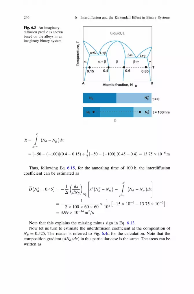
R ¼Zx�

x�1

NB � N�Bffi �

dx

¼ �50� ð�100Þ½ � 0:4� 0:15ð Þ þ 12�50� ð�100Þ½ � 0:45� 0:4ð Þ ¼ 13:75� 10�6 m

Thus, following Eq. 6.15, for the annealing time of 100 h, the interdiffusioncoefficient can be estimated as

eD N�B ¼ 0:45ffi �

¼ � 12t

dx

dNB

� �N�B

x� N�B � N�Bffi �

�Zx�

x�1

NB � N�Bffi �

dx

24

35

¼ � 12� 100� 60� 60

� 1103�15� 10�6 � 13:75� 10�6� �

¼ 3:99� 10�14 m2=s

Note that this explains the missing minus sign in Eq. 6.13.Now let us turn to estimate the interdiffusion coefficient at the composition of

NB = 0.525. The reader is referred to Fig. 6.4d for the calculation. Note that thecomposition gradient dNB=dxð Þ in this particular case is the same. The areas can bewritten as

Fig. 6.3 An imaginarydiffusion profile is shownbased on the alloys in animaginary binary system

246 6 Interdiffusion and the Kirkendall Effect in Binary Systems

N ¼ x� N�B � N�Bffi �

¼ x� � xoð Þ N�B � N�Bffi �

¼ 25� 10�6 0:525� 0:15ð Þ ¼ 9:375� 10�6 m

M ¼Zx�

x�1

NB � N�Bffi �

dx

¼ 25� ð�100Þ½ � 0:4� 0:15ð Þ þ 12

25� ð�100Þ½ � 0:525� 0:4ð Þ ¼ 39:06� 10�6 m

As a result, the interdiffusion coefficient can be estimated as

(a) (b)

(c) (d)

Fig. 6.4 Calculation procedure of the interdiffusion coefficient at the composition of interest.a Composition profile, b locating the initial contact plane, c estimating the interdiffusioncoefficient at the composition of interest in the left-hand side of the initial contact plane, andd estimating the interdiffusion coefficient at the composition of interest in the right-hand side ofthe initial contact plane

6.1 Matano–Boltzmann Analysis 247

eD N�B ¼ 0:525ffi �

¼ � 12t

dx

dNB

� �N�B

x� N�B � N�Bffi �

�Zx�

x�1

NB � N�Bffi �

dx

24

35

¼ � 12� 100� 60� 60

� 1103

9:375� 10�6 � 39:06� 10�6� �

¼ 4:12� 10�14 m2=s

6.2 Limitation of the Matano–Boltzmann Analysis

We have shown previously that the location of the initial contact plane or theMatano plane can be found from the concentration profile, i.e., CB versus x using

the relationR xo

x�1 CB � C�Bffi �

dx ¼R xþ1

xoCþB � CBð Þdx. Ideally, it should also be

possible to find this plane from CA versus x using the relationR xo

x�1 C�A � CA

ffi �dx ¼

R xþ1

xoCA � CþAffi �

dx. Note here that NA + NB = 1, N�Aþ N�

B¼ 1. Therefore

CB vs. x increases from left to right ðC�B \CþB Þ, CA vs. x decreases in the samedirection ðC�A [ CþA Þ. Since there is a unique initial contact plane, we should beable to find the same location by following any of the profiles. However, this is notalways the case. As explained in Fig. 6.5, there can be three different situationsdepending on the variation of the molar volume with composition. It is almostimpossible to find a practical system, in which molar volume varies ideally fol-lowing Vegard’s law with the composition as shown in Fig. 6.5a. However, thereare a few systems, where the deviation of the molar volume from the straight lineconnecting the molar volumes of the pure components vA

m and vBm is marginal.

Consequently, there will be almost no change in the total volume of the diffusioncouple after interdiffusion. In this case, the initial contact planes located from theprofiles CB versus x and CA versus x will be more or less the same. In fact, if themolar volume varies ideally following Vegard’s law ðvm ¼ NAvA

m þ NBvBmÞ, then

the location of this plane found from any of the profiles will be exactly the same.In most of the systems, the molar volume deviates from the ideality. There can bepositive deviation, as presented in Fig. 6.5b. Since the compositions that developin the interdiffusion zone have a higher molar volume than the ideal value, therewill be expansion in the diffusion couple, resulting in an increase in the total lengthof the diffusion couple. Note here that the diffusion profile in the diffusion coupleis one dimensional. In this case, two different locations of the initial contact planeare found (as explained later in Sect. 6.5). In fact, both are actually incorrect andwe are unable to find the exact location of the initial contact plane. In a system,where the molar volume has a negative deviation from the ideality, the diffusioncouple will shrink after interdiffusion, as depicted in Fig. 6.5c. In this case also,

248 6 Interdiffusion and the Kirkendall Effect in Binary Systems

two different values will be found when the initial contact plane is determinedfrom CA versus x and CB versus x.

As explained in the previous section, it is necessary to find the location of theinitial contact plane for the calculation of the interdiffusion coefficient using theMatano–Boltzmann relation. In most of the systems, the molar volume deviatesfrom ideality. Therefore, we are unable to locate the position of the initial contactplane exactly. This leads to an error in the calculation of the diffusion parameters.

To circumvent this problem, relations to estimate eD were developed such thatthere is no need to find the initial contact plane. Ballufi [4] first derived thesolution for the interdiffusion coefficient for systems where the molar volume doesnot change ideally. Sometime later, Sauer and Freise [5] generalized the Matano–Boltzmann analysis for the same conditions. Wagner [6] then came to a similarrelation but by using a simpler and easy-to-understand method. Next came DenBroeder [7] who developed the relation based on a much simpler graphicalinterpretation. Here, the Den Broeder approach is first explained, as it is fairly easyto follow. After that, we present the Wagner approach, which is very useful toderive the equations to be used for the estimation of few other important diffusionparameters along with the interdiffusion coefficients.

6.3 Den Broeder Approach to Determinethe Interdiffusion Coefficient

Den Broeder [7] followed an easy-to-understand graphical approach. The con-centration-normalizing variable YC is introduced such that

YC ¼CB � C�BCþB � C�B

ð6:16Þ

Fig. 6.5 Effect of deviation of molar volume in the diffusion couples is shown for a ideal case,b positive deviation, and c negative deviation

6.2 Limitation of the Matano–Boltzmann Analysis 249

This leads to

dYC ¼dCB

CþB � C�Bð6:17Þ

Replacing Eqs. 6.16 and 6.17 in Eq. 6.12 results in

eD Y�Cffi �

¼ � 12t

dx

dYC

� �Y�C

x�Y�c �Zx�

x�1

YCdx

24

35 ð6:18Þ

To determine the interdiffusion coefficients using the relation expressed inEq. 6.18, it is necessary to convert the concentration profile (Fig. 6.6b) to YC

versus x, as shown in Fig. 6.6c. Note here that Y�C ¼ 0 and YþC ¼ 1. In terms of theareas shown in Fig. 6.6c, Eq. 6.18 can be expressed as

Fig. 6.6 Calculation of the interdiffusion coefficients is shown following Den Broeder’s approach.a Diffusion couple, b concentration profile, c derivation of the Den Broeder’s approach, and d slopeat the concentration of interest

250 6 Interdiffusion and the Kirkendall Effect in Binary Systems

eD Y�Cffi �

¼ 12t

dx

dYC

� �Y�C

Sþ R½ � ð6:19Þ

The minus sign is missing in Eq. 6.19 (similar to Eq. 6.13) since the value ofS is negative and the value of R is positive. With respect to the position of theinitial contact plane xo we can write

Rþ SþM ¼ P ð6:20Þ

By adding N to both sides, we get

Rþ SþM þ N ¼ Pþ N

SþM þ N ¼ Pþ N � Rð6:21Þ

We can further write that

SþM þ N ¼ x� � xoð ÞYþC ¼ x� ð6:22aÞ

Since YþC ¼ 1.

Pþ N ¼Zxþ1

x�

1� YCð Þdx ð6:22bÞ

R ¼Zx�

x�1

YCdx ð6:22cÞ

Replacing 6.22a, 6.22b and 6.22c in 6.21, we get

x� ¼Zxþ1

x�

1� YCð Þdx�Zx�

x�1

YCdx ð6:23Þ

Therefore, the following is obtained

S ¼ x�Y�C ¼ Y�C

Zxþ1

x�

1� YCð Þdx� Y�C

Zx�

x�1

YCdx ð6:24Þ

6.3 Den Broeder Approach to Determine the Interdiffusion Coefficient 251

Sþ R ¼ Y�C

Zxþ1

x�

1� YCð Þdx� Y�C

Zx�

x�1

YCdxþZx�

x�1

YCdx

¼ 1� Y�Cffi � Zx�

x�1

YCdxþ Y�C

Zxþ1

x�

1� YCð Þdx

ð6:25Þ

Replacing Eq. 6.25 in Eq. 6.19 gives

eD Y�Cffi �

¼ 12t

dx

dYC

� �Y�C

1� Y�Cffi � Zx�

x�1

YCdxþ Y�C

Zxþ1

x�

1� YCð Þdx

24

35 ð6:26Þ

Following Fig. 6.6d, we can express Eq. 6.26 as

eD Y�Cffi �

¼ 12t

dx

dYC

� �Y�C

1� Y�Cffi �

Rþ Y�CQ� �

ð6:27Þ

This means that it is no longer necessary to locate the initial contact plane. Wemeasure the composition profile, i.e., NB versus x, by using the composition-measuring techniques. NB is the atomic fraction of the component B. Dividing theatomic fractions by the respective molar volumes, the concentration profile canthen be estimated. The concentration profile is converted into the concentration-normalizing variable YC versus x. Next, the interdiffusion coefficients can beestimated by determining the gradient at the point of interest and by estimating theareas R and Q, as shown in Fig. 6.6d, considering the known annealing time t. Thatmeans we do not have to consider an ideal variation or a fixed molar volume asrequired for the calculation using the Matano–Boltzmann analysis. Note here thatSauer-Freise [5] derived the same relation but differently.

6.4 Wagner’s Approach to the Calculationof the Interdiffusion Coefficient

From Fick’s first law and the relations expressed in Sect. 1.18 (Eq. 1.150), thefollowing is obtained

eJB ¼ �eD oCB

ox¼ �eD �vA

v2m

oNB

oxð6:28aÞ

Similarly, the interdiffusion flux with respect to the component A can beexpressed as

252 6 Interdiffusion and the Kirkendall Effect in Binary Systems

eJA ¼ �eD oCA

ox¼ �eD �vB

v2m

oNA

ox¼ eD �vB

v2m

oNB

ox¼ �vB

�vA

eD �vA

v2m

oNB

oxð6:28bÞ

Since NA + NB = 1From Eqs. 6.28a and 6.28b, we can write

�vAeJA þ �vBeJB ¼ 0 ð6:29Þ

So it must be apparent that the interdiffusion fluxes are different when estimatedusing the concentration profiles of different components. However, the interdif-fusion coefficient is a material constant and the value is the same, whetherdetermined with respect to either of the component A or component B.

Using the relations presented in Eq. 1.144 (Sect. 1.18), Eq. 6.28a can berewritten as

eJBNB�vB þ NA�vAð Þ

vm¼ �eD �vA

v2m

oNB

ox

eD ¼ � vm NB�vBeJB þ NA�vAeJB

ffi ��vA oNB=oxð Þ

Using Eq. 6.29, we can write

eD ¼ � vm �NB�vAeJA þ NA�vAeJB

ffi ��vA oNB=dxð Þ

eD ¼ vm NBeJA � NAeJB

ffi �oNB=ox

ð6:30Þ

From Fick’s second law, as expressed in Eq. 3.4, we can write

o

ot

NB

vm

� �¼ oCB

ot¼ � oeJB

oxð6:31aÞ

o

ot

NA

vm

� �¼ oCA

ot¼ � oeJA

oxð6:31bÞ

We introduce a composition-normalized variable as

YB ¼NB � N�BNþB � N�B

ð6:32Þ

This can be rewritten as

NB ¼ NþB YB þ N�B 1� YBð Þ ð6:33aÞ

6.4 Wagner’s Approach to the Calculation of the Interdiffusion Coefficient 253

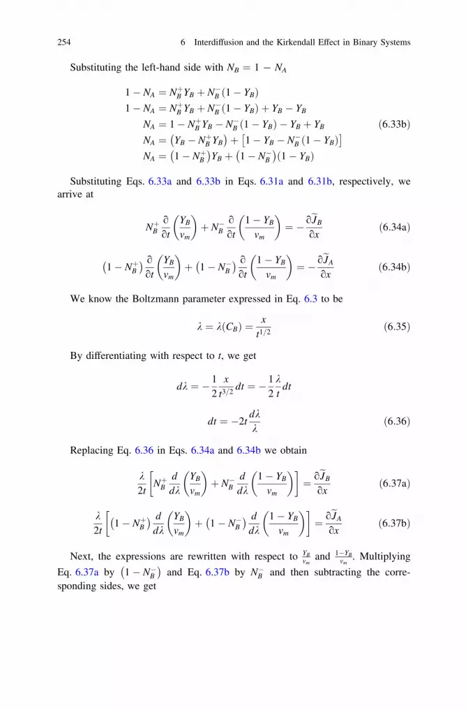
Substituting the left-hand side with NB = 1 - NA

1� NA ¼ NþB YB þ N�B 1� YBð Þ1� NA ¼ NþB YB þ N�B 1� YBð Þ þ YB � YB

NA ¼ 1� NþB YB � N�B 1� YBð Þ � YB þ YB

NA ¼ YB � NþB YB

ffi �þ 1� YB � N�B 1� YBð Þ� �

NA ¼ 1� NþBffi �

YB þ 1� N�Bffi �

1� YBð Þ

ð6:33bÞ

Substituting Eqs. 6.33a and 6.33b in Eqs. 6.31a and 6.31b, respectively, wearrive at

NþBo

ot

YB

vm

� �þ N�B

o

ot

1� YB

vm

� �¼ � oeJB

oxð6:34aÞ

1� NþBffi � o

ot

YB

vm

� �þ 1� N�Bffi � o

ot

1� YB

vm

� �¼ � oeJA

oxð6:34bÞ

We know the Boltzmann parameter expressed in Eq. 6.3 to be

k ¼ k CBð Þ ¼ x

t1=2ð6:35Þ

By differentiating with respect to t, we get

dk ¼ � 12

x

t3=2dt ¼ � 1

2kt

dt

dt ¼ �2tdkk

ð6:36Þ

Replacing Eq. 6.36 in Eqs. 6.34a and 6.34b we obtain

k2t

NþBd

dkYB

vm

� �þ N�B

d

dk1� YB

vm

� � ¼ oeJB

oxð6:37aÞ

k2t

1� NþBffi � d

dkYB

vm

� �þ 1� N�Bffi � d

dk1� YB

vm

� � ¼ oeJA

oxð6:37bÞ

Next, the expressions are rewritten with respect to YBvm

and 1�YBvm

. Multiplying

Eq. 6.37a by 1� N�Bffi �

and Eq. 6.37b by N�B and then subtracting the corre-sponding sides, we get

254 6 Interdiffusion and the Kirkendall Effect in Binary Systems

� k2t

NþB � N�Bffi � d

dkYB

vm

� �¼ N�B

oeJA

ox� 1� N�Bffi � oeJB

oxð6:38aÞ

In the same way, multiplying Eq. 6.37a by 1� NþBð Þ and Eq. 6.37b by NþB andthen subtracting the corresponding sides leads to

k2t

NþB � N�Bffi � d

dk1� YB

vm

� �¼ NþB

oeJA

ox� 1� NþBffi � oeJB

oxð6:38bÞ

By differentiating the Boltzmann parameter with respect to x, we get

dk ¼ dx

t1=2

Next, we multiply dk to the left-hand side and dx/t1/2 to the right-hand side ofEq. 6.38a so that

� k2t

NþB � N�Bffi �

dYB

vm

� �¼ 1

t1=2N�B deJA � 1� N�B

ffi �deJB

� �

From the Boltzmann parameter, we can write x ¼ x�1; k ¼ k�1 andx ¼ x�; k ¼ k�.

Integrating for a fixed annealing time t from k ¼ k�1 to a particular position ofinterest k ¼ k� (corresponds to the mole fraction N�B), we get

� 12t

NþB � N�Bffi � Zk�

k�1

kdYB

vm

� �¼ 1

t1=2N�B

ZeJ �Ao

deJA � 1� N�Bffi � ZeJ �B

o

deJB

2664

3775

Note that the interdiffusion flux at the unaffected part x ¼ x�1 or k ¼ k�1 iszero.

Following integration by parts on the left-hand side, we get

� 12t

NþB � N�Bffi � k�Y�B

v�m�Zk�

k�1

YB

vmdk

24

35 ¼ 1

t1=2N�B eJ�A � 1� N�B

ffi �eJ�B� �

12t

NþB � N�Bffi �

� k�Y�Bv�mþZk�

k�1

YB

vmdk

24

35 ¼ 1

t1=2N�B eJ�A � 1� N�B

ffi �eJ�B� �ð6:39aÞ

In the same way, we multiply Eq. 6.38b by dk on the left-hand side and by dx/t1/2 on the right-hand side. Following integration from k ¼ k� to k ¼ kþ1 and thenby doing integration by parts on the left-hand side of the equation, we get

6.4 Wagner’s Approach to the Calculation of the Interdiffusion Coefficient 255

12t

NþB � N�Bffi � k� 1� Y�B

ffi �v�m

þZkþ1

k�

1� YBð Þvm

dk

264

375 ¼ 1

t1=2NþB eJ�A � 1� NþB

ffi �eJ�B� �

Note here the sign because of (1 - YB).

12t

NþB � N�Bffi �

�k� 1� Y�Bffi �

v�m�Zkþ1

k�

1� YBð Þvm

dk

264

375 ¼ 1

t1=2�NþB eJ�A þ 1� NþB

ffi �eJ�B� �

ð6:39bÞ

J�A and J�B are the fluxes at k ¼ k�. Multiplying Eq. 6.39a by 1� Y�Bffi �

andEq. 6.39b by Y�B and subtracting the corresponding sides, we obtain

12t

NþB � N�Bffi �

1� Y�Bffi � Zk�

k�1

YB

vmdkþ Y�B

Zkþ1

k�

1� YBð Þvm

dk

24

35

¼ 1

t1=2N�BeJ�A � 1� N�B

ffi �eJ�B� �ð6:40Þ

Note here that the right-hand side of the relation can be found by replacing

Y�B ¼N�B�N�BNþB �N�B

and 1� Y�B ¼NþB �N�BNþB �N�B

.

Since dk ¼ dxt1=2, Eq. 6.40 can be written as

12t

NþB � N�Bffi �

1� Y�Bffi � Zk�

k�1

YB

vmdxþ Y�B

Zkþ1

k�

1� YBð Þvm

dx

264

375

¼ N�BeJ�A � 1� N�Bffi � eJ�B� �

ð6:41Þ

Previously, we have derived the interdiffusion coefficient with respect to the

interdiffusion fluxes eJA and eJB in Eq. 6.30. At a particular composition of interest

NB ¼ N�B, for the fluxes of eJ �A and eJ�B, it can be written as

eD N�Bffi �

¼v�m N�BeJ�A � N�AeJ�Bffi �

dNB=dxð Þx�ð6:42Þ

Substituting Eq. 6.41 in Eq. 6.42 results in

eD N�Bffi �

¼NþB � N�Bffi �

v�m2t dNB=dxð Þx�

1� Y�Bffi � Zx�

x�1

YB

vmdxþ Y�B

Zx�1

x�

1� YBð Þvm

dx

24

35 ð6:43Þ

256 6 Interdiffusion and the Kirkendall Effect in Binary Systems

From Eq. 6.32, we can write

dYB ¼dNB

NþB � N�Bð6:44Þ

And replacing Eq. 6.44 in Eq. 6.43, we get

eD Y�Bffi �

¼ v�m2t dYB=dxð Þx�

1� Y�Bffi � Zx�

x�1

YB

vmdxþ Y�B

Zxþ1

x�

1� YBð Þvm

dx

24

35 ð6:45Þ

The calculation procedure is explained in Fig. 6.7. After measuring the com-position profile in atomic fraction, presented in Fig. 6.7b, the normalized profileshould be plotted, as shown in Fig. 6.7c. Moreover, from the knowledge of thevariation of the molar volume with composition, YB

vmand 1�YB

vmversus x should be

plotted as shown in Fig. 6.7d and e, respectively. If we wish to estimate theinterdiffusion coefficient at the composition, N�B, which is located at x� in thediffusion couple, we need to estimate how the gradient dYB

dx at Y�B corresponds to N�B.

Afterward, the areas R ¼R x�

x�1YBvm

dx and S ¼R xþ1

x�1�YBð Þ

vmdx should be determined to

estimate the interdiffusion coefficients using the relation expressed in Eq. 6.45.Further, the difference between the Den Broeder [7] or Sauer-Freise [5] treat-

ment with Wagner’s approach [7] should be noted. This should lead to somedifference in the diffusion data estimated, especially if the molar volume deviatesfrom the ideality. In fact, for a constant molar volume, these relations are the same.

It should be noted here that when interdiffusion coefficients are estimated over awide composition range, the impurity diffusion coefficients could be estimated byextending the data to 0 and 100 atomic percent of an element. At 0 at.% B, wehave the impurity diffusion coefficient of B in pure A, and at 100 at.% B, we havethe impurity diffusion coefficient of A in pure B. This is commonly practiced inmany systems.

6.5 Change in Total Volume of the Diffusion Couple

In Sect. 6.2, we have already discussed that there could be a change in the totalvolume of the diffusion couple depending on the deviation of the molar volumefrom the ideality. In these couples, we are unable to locate the initial contact planexo exactly [8, 9]. In fact, the change in volume is related to the difference (in termsof distance) between the locations found using the profiles CA versus x and CB

versus x. In this section, we shall show the relation between the changes in totalvolume with the location of the initial contact planes estimated following aquantitative analysis based on a hypothetical diffusion couple.

6.4 Wagner’s Approach to the Calculation of the Interdiffusion Coefficient 257

As shown in Fig. 6.8, suppose we couple two alloys N�B (or N�A , expressed withrespect to the element A) and NþB ðNþA Þ. Note here that N�B is a B-lean alloy and NþBis a B-rich alloy, such that NþB [ N�B . Following the same argument, we can writeNþA \N�A . As explained previously, the location of the initial contact plane shouldbe estimated with respect to CA versus x and CB versus x. Similarly, it can bedetermined using the composition-normalized variable, introduced during thederivation of Wagner’s relation, from the YB=vm versus x and YA=vm versus x plots,

as can be seen from Fig. 6.9. Note that YB ¼ NB�N�BNþB �N�B

and YA ¼NA�NþAN�A �NþA

. Further, we

can write

1� YB ¼ 1� NB � N�BNþB � N�B

¼ NþB � NB

NþB � N�B¼ 1� NþA � 1þ NA

1� NþA � 1þ N�A¼ NA � NþA

N�A � NþA¼ YA

ð6:46Þ

Fig. 6.7 Explanation of the calculation procedure of the interdiffusion coefficient followingWagner’s approach. a An imaginary diffusion couple, b NB versus x, c YB versus x profile,d YB=Vm versus x profile, and e 1� YBð Þ=Vm versus x profile

258 6 Interdiffusion and the Kirkendall Effect in Binary Systems

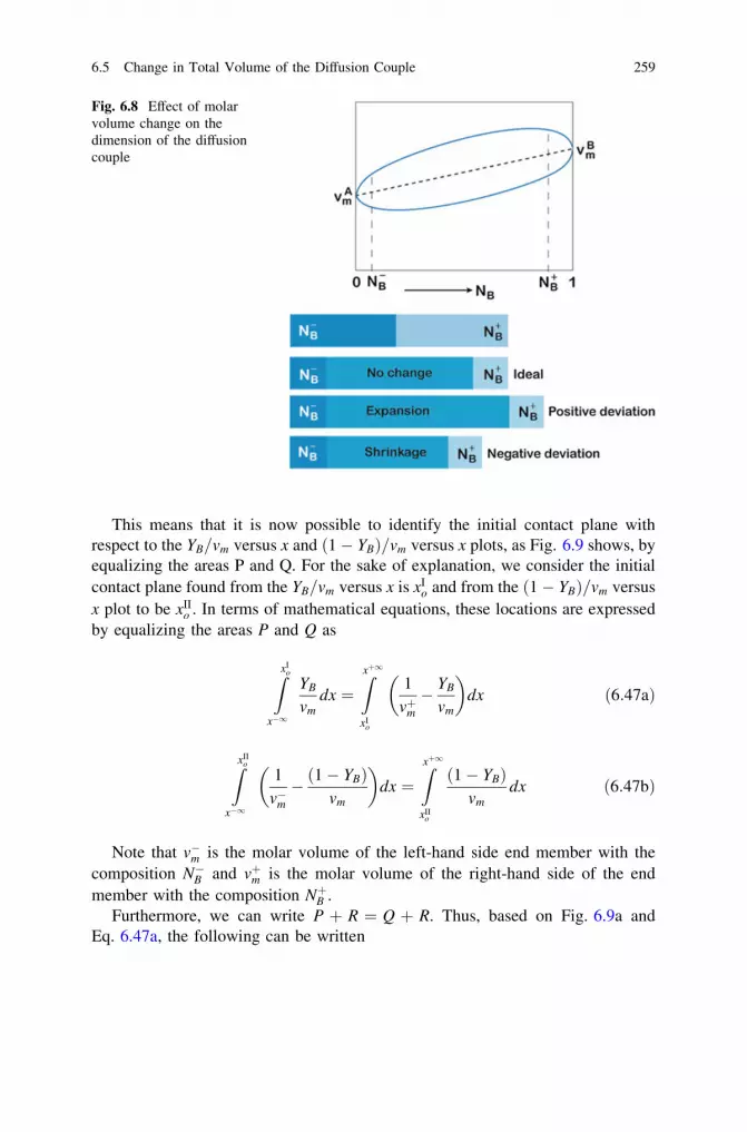
This means that it is now possible to identify the initial contact plane withrespect to the YB=vm versus x and 1� YBð Þ=vm versus x plots, as Fig. 6.9 shows, byequalizing the areas P and Q. For the sake of explanation, we consider the initialcontact plane found from the YB=vm versus x is xI

o and from the 1� YBð Þ=vm versusx plot to be xII

o . In terms of mathematical equations, these locations are expressedby equalizing the areas P and Q as

ZxIo

x�1

YB

vmdx ¼

Zxþ1

xIo

1vþm� YB

vm

� �dx ð6:47aÞ

ZxIIo

x�1

1v�m� 1� YBð Þ

vm

� �dx ¼

Zxþ1

xIIo

1� YBð Þvm

dx ð6:47bÞ

Note that v�m is the molar volume of the left-hand side end member with thecomposition N�B and vþm is the molar volume of the right-hand side of the endmember with the composition NþB .

Furthermore, we can write P + R = Q + R. Thus, based on Fig. 6.9a andEq. 6.47a, the following can be written

Fig. 6.8 Effect of molarvolume change on thedimension of the diffusioncouple

6.5 Change in Total Volume of the Diffusion Couple 259

ZxIo

x�1

YB

vmdxþ

Zxþ1

xIo

YB

vmdx¼

Zxþ1

xIo

1vþm� YB

vm

� �dxþ

Zxþ1

xIo

YB

vmdx

Zxþ1

x�1

YB

vmdx¼ 1

vþm

Zxþ1

xIo

dx

xþ1 � xIo

vþm¼Zxþ1

x�1

YB

vmdx

xþ1 � xIo ¼ vþm

Zxþ1

x�1

YB

vmdx

ð6:48aÞ

Similarly, with the help of Fig. 6.9b and Eq. 6.47b, we can write

ZxIIo

x�1o

1� YBð Þvm

dxþZxII

o

x�1

1v�m� 1� YBð Þ

vm

� �dx¼

ZxIIo

x�1o

1� YBð Þvm

dxþZxþ1

xIIo

1� YBð Þvm

dx

1v�m

ZxIIo

x�1

dx¼Zxþ1

x�1

1� YBð Þvm

dx

xIIo � x�1

v�m¼Zxþ1

x�1

1� YBð Þvm

dx

xIIo � x�1 ¼ v�m

Zxþ1

x�1

1� YBð Þvm

dx ð6:48bÞ

Fig. 6.9 Profiles used for the derivation of the molar volume effect on the total volume of thediffusion couple. a YB=vm versus x and b 1� YBð Þ=vm versus x plots

260 6 Interdiffusion and the Kirkendall Effect in Binary Systems

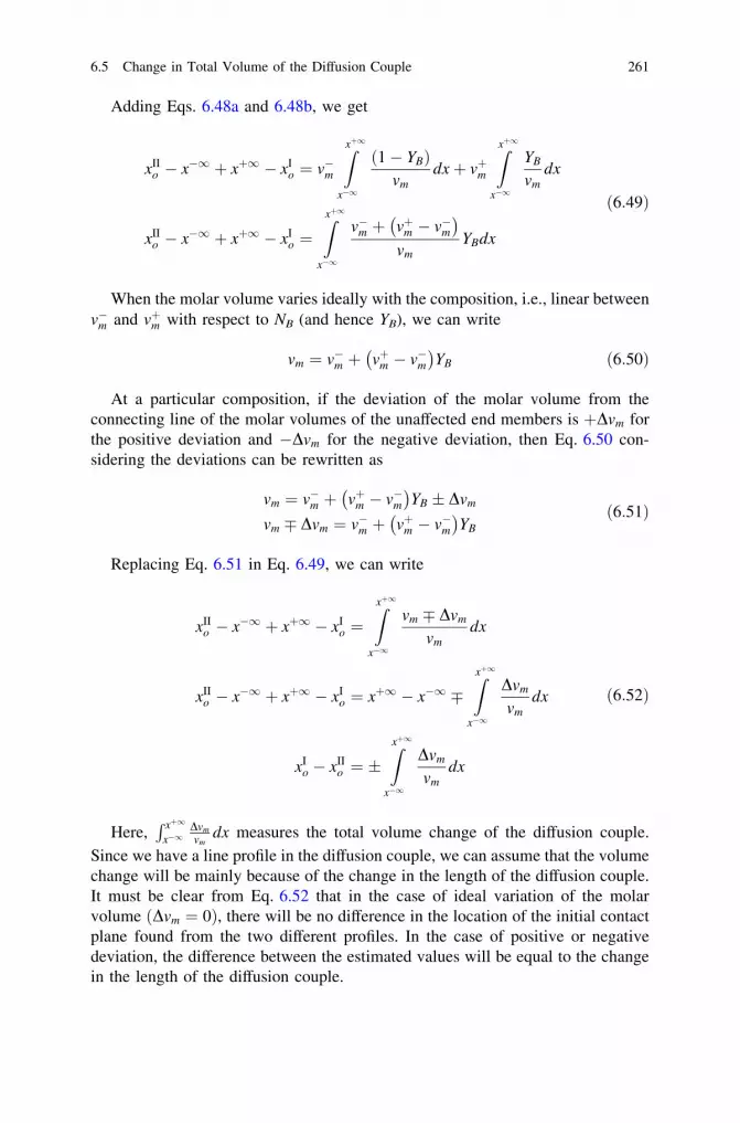
Adding Eqs. 6.48a and 6.48b, we get

xIIo � x�1 þ xþ1 � xI

o ¼ v�m

Zxþ1

x�1

1� YBð Þvm

dxþ vþm

Zxþ1

x�1

YB

vmdx

xIIo � x�1 þ xþ1 � xI

o ¼Zxþ1

x�1

v�m þ vþm � v�mffi �vm

YBdx

ð6:49Þ

When the molar volume varies ideally with the composition, i.e., linear betweenv�m and vþm with respect to NB (and hence YB), we can write

vm ¼ v�m þ vþm � v�mffi �

YB ð6:50Þ

At a particular composition, if the deviation of the molar volume from theconnecting line of the molar volumes of the unaffected end members is þDvm forthe positive deviation and �Dvm for the negative deviation, then Eq. 6.50 con-sidering the deviations can be rewritten as

vm ¼ v�m þ vþm � v�mffi �

YB � Dvm

vm � Dvm ¼ v�m þ vþm � v�mffi �

YBð6:51Þ

Replacing Eq. 6.51 in Eq. 6.49, we can write

xIIo � x�1 þ xþ1 � xI

o ¼Zxþ1

x�1

vm � Dvm

vmdx

xIIo � x�1 þ xþ1 � xI

o ¼ xþ1 � x�1 �Zxþ1

x�1

Dvm

vmdx

xIo � xII

o ¼ �Zxþ1

x�1

Dvm

vmdx

ð6:52Þ

Here,R xþ1

x�1Dvmvm

dx measures the total volume change of the diffusion couple.

Since we have a line profile in the diffusion couple, we can assume that the volumechange will be mainly because of the change in the length of the diffusion couple.It must be clear from Eq. 6.52 that in the case of ideal variation of the molarvolume ðDvm ¼ 0Þ, there will be no difference in the location of the initial contactplane found from the two different profiles. In the case of positive or negativedeviation, the difference between the estimated values will be equal to the changein the length of the diffusion couple.

6.5 Change in Total Volume of the Diffusion Couple 261

To explain the effect of the change in the total volume on the estimated valuesof the initial contact plane, a very simple hypothetical diffusion couple is con-sidered in Fig. 6.10. In the hypothetical phase diagram, as shown in Fig. 6.10a,there are three compounds with narrow homogeneity range a, b, and c which arepresent. The average composition of these phases with respect to the element B, NB

are 0.25 (A0.75B0.25), 0.6 (A0.4B0.6), and 0.75 (A0.25B0.75). As discussed in Chap. 4,if we couple a and c, the b phase will grow in the interdiffusion zone, as Fig. 6.10cshows. If the molar volume varies ideally, as is the case in this system, then if themolar volume of a is 1 unit and c is 2 units, the molar volume of b will be 1.7 units(see Fig. 6.10b). Additionally, suppose that 0.6 mol of a and 1.4 mol of c getconsumed to produce 2 mol of b. In terms of the reaction equation, we can write

0:6A0:75B0:25 að Þ þ 1:4A0:25B0:75 cð Þ ! 2A0:4B0:6 bð Þ ð6:53Þ

Since the diffusion couple has a line profile, we can consider the unit cross-sectional area. Consequently, the units consumed or produced can be directlyexpressed in length units, such that

0:6� 1 að Þ þ 1:4� 2 cð Þ ! 2� 1:7 bð Þ ¼ 3:4 units ð6:54Þ

This further means that 0.6 units of a and 2.8 units of c get consumed toproduce 3.4 units of b. The composition profile developed is shown in Fig. 6.11b.

Fig. 6.10 a Imaginary phase diagram showing, b the positive deviation of the molar volume andc its effect on the dimension of the diffusion couple

262 6 Interdiffusion and the Kirkendall Effect in Binary Systems

Following on from this, the YB=vm versus x and 1� YBð Þ=vm versus x plots areshown in Fig. 6.11c, d. The values used in Fig. 6.11c, d are estimated as follows

a phase: NaB ¼ N�B ¼ 0:25,

YaB ¼ Y�B ¼

NB � N�BNþB � N�B

¼ NaB � Na

B

NcB � Na

B

¼ 0:25� 0:250:75� 0:25

¼ 0;

YaB

vam

¼ 01¼ 0;

1� YaB

vam

¼ 11¼ 1

b phase: NbB ¼ NB ¼ 0:6,

YbB ¼ YB ¼

NB � N�BNþB � N�B

¼ NbB � Na

B

NcB � Na

B

¼ 0:6� 0:250:75� 0:25

¼ 0:7;

YbB

vbm

¼ 0:71:7¼ 0:412;

1� YbB

vbm

¼ 0:31:7¼ 0:1765

x

NB

0.25

0.60

0.75

3.4 units−∞x +∞x

0

0.412

0.5

3.4 μm

m

B

v

Y

PQ

x

−∞x +∞x

1

0.1765

0

3.4 μm

R

S

x

+∞x−∞x

m

B

v

Y−1

(a)

(b)

(c) (d)

Iox

IIox

Fig. 6.11 Estimation of the initial contact plane is explained when molar volume varies ideally.a Diffusion couple, b composition profile, c YB=vm versus x plot showing the location of xI

o, andd 1� YBð Þ=vm versus x plot showing the location of xII

o

6.5 Change in Total Volume of the Diffusion Couple 263

c phase: NcB ¼ NþB ¼ 0:75,

YcB ¼ YþB ¼

NB � N�BNþB � N�B

¼ NcB � Na

B

NcB � Na

B

¼ 0:75� 0:250:75� 0:25

¼ 1;

YcB

vcm¼ 1

2¼ 0:5;

1� YcB

vcm¼ 0

2¼ 0

From Eq. 6.54, we know that the actual location of the initial contact plane is0.6 units from the a/b interface. Now, let us examine whether it is possible tolocate this initial contact plane. By equating the areas P and Q in the YB=vm versusx plot—as seen from Fig. 6.11c—we get the location xI

o as

0:412� 0ð ÞxIo ¼ 0:5� 0:412ð Þ 3:4� xI

o

ffi �xI

o ¼ 0:6

Similarly, we find the location of the initial contact plane xIIo from the

1� YBð Þ=vm versus x plot given in Fig. 6.11d by equating the areas R and S as

1� 0:1765ð ÞxIIo ¼ 0:1765 3:4� xII

o

ffi �xII

o ¼ 0:6

This means we are able to locate the exact position of the initial contact planefrom any of the profiles when molar volume varies ideally with composition.

Now let us consider the positive deviation of the molar volume for the b phaseas 1.85 units, as shown in Fig. 6.10b. Similar to the previous example, we considerthe growth of 2 mol of the product phase by consuming 0.6 mol of a and 1.4 molof c. The reaction equation is therefore the same, as expressed in Eq. 6.53.However, the units consumed or produced can be directly expressed in lengthunits, such that

0:6� 1 að Þ þ 1:4� 2 cð Þ ! 2� 1:85 bð Þ ¼ 3:7 units ð6:55Þ

This means that 0.6 units of a and 2.8 units of c get consumed to produce 3.7units of b, resulting in an expansion of (3.7 - 3.4 =) 0.3 units. There is expansionon both sides of the initial contact plane inside the b phase. Now, let us see whatwe find from the YB=vm versus x and 1� YBð Þ=vm versus x plots. The plots areshown in Fig. 6.12.

a phase: NaB ¼ N�B ¼ 0:25,

YaB ¼ Y�B ¼

NB � N�BNþB � N�B

¼ NaB � Na

B

NcB � Na

B

¼ 0:25� 0:250:75� 0:25

¼ 0;

YaB

vam

¼ 01¼ 0;

1� YaB

vam

¼ 11¼ 1

264 6 Interdiffusion and the Kirkendall Effect in Binary Systems

b phase: NbB ¼ NB ¼ 0:6,

YbB ¼ YB ¼

NB � N�BNþB � N�B

¼ NbB � Na

B

NcB � Na

B

¼ 0:6� 0:250:75� 0:25

¼ 0:7;

YbB

vbm

¼ 0:71:85

¼ 0:378;1� Yb

B

vbm

¼ 0:31:85

¼ 0:162

c phase: NcB ¼ NþB ¼ 0:75,

YcB ¼ YþB ¼

NB � N�BNþB � N�B

¼ NcB � Na

B

NcB � Na

B

¼ 0:75� 0:250:75� 0:25

¼ 1;

YcB

vcm¼ 1

2¼ 0:5;

1� YcB

vcm¼ 0

2¼ 0

x

NB

0.25

0.60

0.75

3.7 units−∞x +∞x

0

0.378

0.5

3.7 μm

v

YB

PQ

x

−∞x +∞x

1

0.162

0

3.7 μm

R

S

x

+∞x−∞x

v

YB−1

(a)

(b)

(c) (d)

Iox

IIox

Fig. 6.12 Estimation of the initial contact plane is explained when molar volume deviatespositively. a Diffusion couple, b composition profile, c YB=vm versus x plot showing the locationof xI

o, and d 1� YBð Þ=vm versus x plot showing the location of xIIo

6.5 Change in Total Volume of the Diffusion Couple 265

By equating the areas P and Q in the YB=vm versus x plot as shown inFig. 6.12c, we obtain the location xI

o as

0:378� 0ð ÞxIo ¼ 0:5� 0:378ð Þ 3:7� xI

o

ffi �xI

o ¼ 0:9

Similarly, we find the location of the initial contact plane xIIo from the

1� YBð Þ=v versus x plot, as shown in Fig. 6.12d by equating the areas R and S as

1� 0:162ð ÞxIIo ¼ 0:162 3:7� xII

o

ffi �xII

o ¼ 0:6

Thus, we find the two different locations from two different plots. These distancesfrom the a/b interface are 0.6 and 0.9. Actual, initial plane must be located betweenthese two, which we are unable to find. In this case, we have considered just one linecompound with a fixed composition. Therefore, when considering homogeneousexpansion, we can still locate the exact location of this plane, which should be at0:6þ 0:6� 0:3

3:4 ¼ 0:653 units from the a/b interface. This is estimated based on theexpansion for the length of 0.6 units consumed from the a phase, that is, the lengthfrom the a/b interface in the case of ideal variation of the molar volume. However, inmost practical examples, the expansion or the shrinkage of the interdiffusion zonewill not be homogeneous and it is almost impossible to locate the exact position ofthis plane. The Wagner and Den Broeder methods, as discussed in the previoussections, are useful to estimate the interdiffusion coefficients without locating theexact position of the initial contact plane. However, as we shall discuss later inChap. 8, there is still a need to locate this position for the rationalization of thepossibilities of multiple Kirkendall marker planes. We shall discuss how it is possibleto still find this location indirectly with a small error (see Sect. 8.4).

6.6 The Kirkendall Effect

Till now, the estimation procedure of the interdiffusion coefficients has beendiscussed, which is a kind of average of the intrinsic diffusion coefficients ofcomponents. In fact, for long, it was a commonly held belief that the diffusivitiesof the components are the same. Based on this belief, the atomic mechanisms ofdiffusion were developed. However, on many occasions, scientists researching thisfield noted a strange behavior. For example, in 1929, Pfeil [10] reported onepeculiar phenomenon while studying the oxidation of iron and steel:

It had frequently been noticed that small particles of foreign matter (such as pieces ofmuffle) falling on the surface of oxidising iron were gradually buried. The scale grew upround these particles until they finally disappeared beneath the surface, but they couldafterwards be found by breaking up the layer of scale.

266 6 Interdiffusion and the Kirkendall Effect in Binary Systems

This is explained with the aid of a schematic diagram in Fig. 6.13. The foreignmatter, i.e., the muffle pieces, acted as an inert material and did not take any part inthe reaction and the diffusion process. This was an indication that Fe had a higherdiffusion rate compared to that of oxygen. After diffusing through the oxide layer,Fe reacted with O2 to produce the oxide layer. Since the product phase grew at theoxide/air interface, the oxide layer covered the muffle pieces.

As indicated in the book written by Darken and Gurry [11], Hartley [12] wasthe first to deliberately use foreign inert particles, titanium dioxide, in an organicacetone/cellulose–acetate system, to study the inequality of the diffusing compo-nents. Immediately after that, Smigelkas and Kirkendall [13] reported a similartechnique to study the inequality of the diffusivities of the components in theCu–Zn binary system. Instead, they used molybdenum wires as inert markers.Hartley’s work went unnoticed in the community working on the metallic systems,and the work published by Kirkendall changed the viewpoints on the atomicmechanism of diffusion. The movement of the inert markers caused by the dif-ference in the diffusion coefficients of the components in an interdiffusion zone isknown as the Kirkendall effect.

The experiment followed by Smigelkas and Kirkendall [13] is explained withthe help of the schematic diagram represented in Fig. 6.14. A rectangular bar(18 9 1.9 cm2) of 70–30 wrought brass (70 wt% Cu–30 wt% Zn) was first pre-pared. After the standard metallographic preparation of grinding and polishing,130 lm Mo wires were placed on opposite sides of the surfaces. Next, a 2,500 lmthick electroplated copper layer was deposited. The diffusion couple was thensubjected to annealing at 785 �C. At different intervals, a small piece was cross-sectioned and the rest of the block was annealed further. This way, it was possibleto examine the movement of the markers at different annealing times. With theincrease in annealing time, the thickness of the product phase a brass increased andthe distance between the markers decreased. The movement of the markers wasestimated after rectifying the volume change in the interdiffusion zone and foundto be parabolic with time. It should be noted here that the Mo markers neither took

Fig. 6.13 Schematicdiagram explaining themovement of debris insidethe oxide layer on steel

6.6 The Kirkendall Effect 267

part in the diffusion process nor did they react with the diffusing components. Theequal diffusivities would have resulted in no movement of the markers because ofthe transfer of equal amount of material on either side of the Kirkendall plane. Themovement of the markers, on the other hand, indicated the unequal diffusion ratesof the components in the a brass, Cu(Zn) solid solution. In the manuscript, theyreported [13]:

The movement of the insoluble molybdenum wire was conclusive evidence that the alphabrass was being forced back as a whole (or attracted back) as a result of the diffusing out ofthe zinc atoms individually.

From this study, two conclusions were drawn which had enormous impact atthat time on solid-state diffusion [13]:

1. The rate of diffusion of zinc is much greater than that of copper in alpha brass, and2. When zinc diffuses more rapidly than copper in alpha brass, the interface shifts to

compensate at least partially for the diffusion rate.

Fig. 6.14 Schematic illustration of the Kirkendall’s experiment

268 6 Interdiffusion and the Kirkendall Effect in Binary Systems

The results reported by Kirkendall not only showed that the diffusion rates ofthe components in a solid are different, it also helped to establish the vacancymechanism for substitutional diffusion.

At first, this work was highly criticized mainly by the renowned scientistR. F. Mehl, who was the reviewer of the article and did not accept it immediatelyfor the publication. He felt that this could be an experimental artifact and otherfactors such as the transport of Zn vapor could have a significant effect. Ultimately,he accepted the article for publication and the manuscript was published alongwith the comments from many scientists. The impact of the work can be realizedfrom R. F. Mehl’s [14] comment:

If verified, this ‘‘Kirkendall effect’’ would greatly modify not only the treatment of dif-fusion data but also the theory of mechanism of diffusion. It would, for example, be nolonger possible to represent diffusion data in a substitutional solid solution by one coef-ficient, applying to both metal atoms since the separate coefficients are not equal, but onewould have to show two coefficients, one each for each of the two metal atoms.

The historical development of this discussion can be traced by reading thearticle by Nakajima [15]. Immediately after the publication, R. F. Mehl along withhis student da Silva conducted many rigorous studies in many Cu-based solidsolutions with different types of markers [16]. Simultaneously, many other groupsalso worked on this topic. Ultimately, everybody agreed with the results publishedby Kirkendall, and this phenomenon thereafter was known as the Kirkendall effect.

In the mean time, which might not be known by many, in 1942, Huntington andSeitz also established that substitutional diffusion in metals occurs by a vacancymechanism [17]. It should be noted here that the second manuscript [18] of Kir-kendall’s career in which he mentioned for the first time the difference in diffusioncoefficients of components was published in the same year (before validating thefact with a detailed experimental work in his third manuscript [13] in 1947).However, because of ongoing Second World War, Huntington and Seitz’s paperwas overlooked. In fact, before all these developments, Zener [20] proposed adirect interchange mechanism, where, as shown in Fig. 6.15a, two atoms exchangetheir position directly. If this is true, then there should be no difference in thediffusion rates of components. In their landmark article, Huntington and Seitz [17]

V

(a) (b)Fig. 6.15 Atomic diffusionmechanisms: a directinterchange mechanism andb vacancy mechanism

6.6 The Kirkendall Effect 269

estimated the activation energy for Cu self-diffusion for (i) a direct exchangemechanism, (ii) an interstitial mechanism, and (iii) the vacancy mechanism. Theyused the experimentally determined activation energy for the tracer diffusioncoefficient of Cu for comparison, which varied in the range of 2.1–2.5 eV(202.6–241.2 kJ/mol). Based on their rudimentary calculations, they found thetheoretically calculated values to be 17.2 eV (1,659.6 kJ/mol) for the directinterchange mechanism and 10 eV (964.9 kJ/mol) for the interstitial diffusionmechanism. On the other hand, they got a value of about 2.8 eV (270.2 kJ/mol) forthe vacancy mechanism in which around 1.8 eV (173.7 kJ/mol) is required forvacancy formation and 1 eV (96.5 kJ/mol) for migration. Therefore, the theoret-ically estimated activation energy is very close to the value estimated by experi-ments if the vacancy mechanism of diffusion is considered. They stated that [17]:

The results of these computations…seem to show beyond a reasonable doubt that thevacancy mechanism of diffusion is greatly preferred over the other two considered here forcopper.

In a private communication, Zener criticized this rudimentary calculation.Following this, Huntington and Seitz [19] refined their calculation and found thatthe true value of the activation energy for the interchange mechanism is close to10.3 eV (993.8 kJ/mol). They also assumed that the activation energy for inter-stitial diffusion must be somewhat smaller than the value that they initially esti-mated. Therefore, they felt that these two mechanisms are dubious for the diffusionof components. Theoretically calculated values are much higher compared to theexperimentally estimated values of activation energy.

Zener still believed in a defect-free diffusion mechanism although he did notshow any proof against the vacancy mechanism. In 1949, he proposed a new ringmechanism, as explained in Fig. 6.16 [20], where the movement of atoms willproduce a ring to exchange positions. He estimated the activation energy requiredwould be 4 eV/atom (386 kJ/mol), which is not as high as the direct interchangemechanism. In the meantime, in 1947, Smigelkas and Kirkendall reported themovement of a fiducial marker in a Cu(Zn) alloy. From the Cu(Zn) alloy, whenzinc diffuses away, all the sites are not occupied by the flow of Cu from theopposite direction with the result that vacant sites are left unoccupied. In anothersense, there should be a flow of vacancies opposite to the faster diffusingcomponents (here Zn) to compensate for the difference between the Zn and Cufluxes. Ultimately, this leads to shrinking on the brass side and swelling on thecopper side so that the markers move toward the brass side. In many systems,Kirkendall pores form in the interdiffusion zone, which will be discussed in thenext section.

After Zener’s ring mechanism [20] proposal, Seitz [21] discussed differentaspects to defend the vacancy mechanism of diffusion. The main difficulty inaccepting the validity of the vacancy mechanism was because of doubts thatlingered concerning existence of vacancies. However, he used the Kirkendallmarker experiments as a proof of the vacancy mechanism. As already mentioned,

270 6 Interdiffusion and the Kirkendall Effect in Binary Systems

R. F. Mehl’s group experimented on many systems to validate Kirkendall markerexperiment. On request, Mehl wrote a letter stating the outcome of the experimentsto Seitz as [21]:

(1) We have repeated this experiment some thirty times, in five metallic systems and atvarious temperatures. We are able to attain a very satisfactory degree of precision in allmeasurements, greater than that which Kirkendall attained.(2) We were able to demonstrate that the Matano boundary does coincide with the initialboundary in all cases, when correction is made for change of lattice parameter. This, to besure, is, as you say, merely the law of conservation of mass, with the sole qualification thatit demonstrates also that changing percentages of vacancies in the couples are not greatenough to affect the experiment, as might be expected.(3) The fiducial markers move in all systems studied and at all temperatures by an amountwhich varies markedly from system to system.(4) For a time we entertained the thought that vapor pressure might be the controllingfactor, arguing that transport by vapor along the interface between the wire and the alloymight give the movement of the wires observed. We have now investigated all types ofmarkers including various wires, powders and foils. All of them move and by the sameamount; even those which are wetted and which actually dissolve partially show the sameamount of movement.

Fig. 6.16 Exchange of atoms by ring mechanism a two-, b three-, c four-ring in FCC lattice, andd four-ring in BCC lattice

6.6 The Kirkendall Effect 271

Based on these points, Seitz mentioned that [21]:

It is clear from the start that the Kirkendall experiment cannot be explained naturally interms of the diffusion mechanism if this is assumed to be exclusively of the interchangetype, that is, if one of the possible mechanisms studied by Zener is assumed to predom-inate completely. For in this case an atom which shifts its position would always do so bymoving from one normal position to another and would always be replaced at once byanother atom. As a result the lattice array would be maintained completely intact, exceptfor the local expansion or contraction that arises from the variation of the average size ofthe unit cell with composition, which does not appear to be sufficient to explain theKirkendall effect.

6.7 Darken Analysis: Relation Between Interdiffusionand Intrinsic Diffusion Coefficients

From Kirkendall’s experiment, it was apparent that the diffusion process in solidsolutions could not be explained by a single diffusion coefficient. Rather, it isnecessary to consider the diffusion rates of all the components. This was firsttreated mathematically in 1948 by Darken [22]. Almost at the same time, Hartleyand Crank [23] studied the same subject and they named the diffusivities of thecomponents as intrinsic diffusion coefficients. Seitz [24] and Bardeen [25]described the diffusion process more extensively. Before discussing the assump-tions or the limitations of the Darken analysis, it is pertinent to first explain theconcepts introduced by Darken. In Sect. 6.11, we have described different factsand limitations of this analysis.

Let us consider a hypothetical binary diffusion couple of components A andB of the compositions N�B (A-rich) and NþB (B-rich), as shown in Fig. 6.17. Beforeannealing, fiducial (inert) markers are applied at the interface and annealed at anelevated temperature so that interdiffusion takes place. When interdiffusion starts,the markers are trapped at a certain fixed composition and cannot escape at a laterstage. Thus, the movement of the markers actually indicates the movement of aparticular composition. If the intrinsic diffusivity of DB is higher than that of DA atthat marker plane (called the Kirkendall plane), then the marker plane will move tothe right-hand side from the initial contact interface xo. The intrinsic flux and theintrinsic diffusion coefficient of the components can be estimated at the Kirkendallmarker plane, which are related following Fick’s first law as

JA ¼ �DAoCA

ox

� �K

ð6:56aÞ

JB ¼ �DBoCB

ox

� �K

ð6:56bÞ

272 6 Interdiffusion and the Kirkendall Effect in Binary Systems

This Kirkendall reference plane xK (denoted by K) is not fixed but movesrelative to the laboratory frame of reference, that is, the initial contact plane xo asshown in Fig. 6.17. Suppose the velocity of the Kirkendall marker plane is mK.Darken [22] explained the relation between the interdiffusion fluxes at the

Kirkendall marker planes eJA and eJB measured with respect to xo and the intrinsicdiffusion fluxes JA and JB measured with respect to xK as

eJA ¼ JA þ vKCA ð6:57aÞ

eJB ¼ JB þ vKCB ð6:57bÞ

From Eq. 6.29, in an infinite diffusion couple, the following can be derived

�vAeJA þ �vBeJB ¼ eJvolA þ eJvol

B ¼ 0 ð6:58Þ

where eJvolA and eJvol

B are the volume fluxes (volume flux = partial molar volume ofcomponent, �vi 9 molar flux) with respect to elements A and B, respectively. FromEq. 6.58, we arrive at

JvolA ¼ �vAeJA ¼ �vAJA þ vK�vACA ð6:59aÞ

JvolB ¼ �vBeJB ¼ �vBJB þ vK�vBCB ð6:59bÞ

Substituting Eqs. 6.59a and 6.59b in Eq. 6.58 and then using the relationsexpressed in Eqs. 6.56a and 6.56b, we obtain

Kx

x

x

Kx

ox

ox

−BN +

BN

−BN +

BN

−BN +

BN

0=t

1tt =

2tt =

Fig. 6.17 Movement of theinert markers with theincrease in annealing time,where t2 [ t1 [ t = 0

6.7 Darken Analysis 273

� �vADAoCA

ox

� �K

þ�vACAvK � �vBDBoCB

ox

� �K

þ�vBCBvK ¼ 0

�vACA þ �vBCB

ffi �vK ¼ �vADA

oCA

ox

� �K

þ�vBDBoCB

ox

� �K

ð6:60Þ

By using the standard thermodynamic relations expressed in Eqs. 1.146 and1.149, the following can be derived

vK ¼ �ð�vBJB þ �vAJAÞ ¼ �vB DB � DAð Þ oCB

ox

� �K

ð6:61aÞ

Similarly, with respect to the concentration profile of the component A, we canderive

vK ¼ �vA DA � DBð Þ oCA

ox

� �K

ð6:61bÞ

Further from Eq. 1.150

vK ¼�vA�vB

v2m

DB � DAð Þ oNB

ox

� �K

ð6:62Þ

If the molar volume is constant in a phase, then Eq. 6.62 can be written as

vK ¼ DB � DAð Þ oNB

ox

� �K

ð6:63Þ

The marker velocity can also be estimated directly from the known locations ofthe initial contact plane xo and the Kirkendall marker plane xK. The relation can bederived using the Boltzmann parameter, as expressed above in Eq. 6.3.

kK ¼ k CKð Þ ¼ xK � xo

t1=2¼ xK

t1=2

vK ¼dxK

dt¼

d kKt1=2ffi �

dt¼ kK

2t1=2¼ xK � xo

2t¼ xK

2t

ð6:64Þ

Therefore, if it is possible to estimate the location of the initial contact planecorrectly, we can therefore estimate the Kirkendall marker velocity using Eq. 6.64.

From Eqs. 6.57b and 6.61a, we can write

�eD oCB

ox¼ �DB

oCB

oxþ CBvK

�eD oCB

ox

� �K

¼ �DBoCB

ox

� �K

þCB�vB DB � DAð Þ oCB

ox

� �K

274 6 Interdiffusion and the Kirkendall Effect in Binary Systems

Utilizing the standard thermodynamic relations that were presented earlier inSect. 1.18 (Eq. 1.146), this turns into

�eD oCB

ox

� �K

¼ � 1� CB�vBð ÞDBoCB

ox

� �K

� CB�vBDAoCB

ox

� �K

�eD oCB

ox

� �K

¼ � CA�vADB þ CB�vBDAð Þ oCB

ox

� �KeD ¼ �vACADB þ �vBCBDA

ð6:65Þ

In a rare case, if the molar volume is constant such that vm ¼ �vA ¼ �vB, Eq. 6.65reduces to

eD ¼ NADB þ NBDA ð6:66Þ

Equation 6.66 is known as the Darken equation.Note here that the interdiffusion coefficients can be measured at any position in a

concentration profile; however, the intrinsic diffusivities can only be measured atcompositions indicated by the inert markers. Therefore, Eq. 6.66 can be used only at themarker plane to estimate all the parameters such as interdiffusion and intrinsic diffusioncoefficients. At other compositions, only the interdiffusion coefficient can be estimated.

The basic conditions of the previous equations are that the system is underisothermal and isobaric conditions, that no high external force is present (whichmight cause plastic deformation of the sample or, possibly, pressure-dependentdiffusion coefficients), and time-dependent effects are absent such as the recrys-tallization process. This might cause a gradual transition from the grain boundarydiffusion to the much slower bulk (lattice) diffusion.

6.8 Relations for the Estimation of the IntrinsicDiffusion Coefficients

As mentioned previously, the intrinsic diffusivities can be measured only at theKirkendall plane position, xK. Heumann [26] and van Loo [27] derived relationsfollowing which the intrinsic diffusion coefficients can be estimated from thecomposition profile. Wagner [6] did not derive these relations; however, on thesimilar line of treatment, we can derive the same relations. In this section, differentways to estimate the intrinsic diffusion coefficients will be discussed [8]. We shallfirst explain the Heumann approach. Next, the relations for the calculation of theintrinsic diffusion coefficients will be developed using the approach followed byWagner for the calculation of the interdiffusion coefficients. These were deriveddifferently by van Loo [27]. In the end, the multifoil technique will be describedfollowing which these parameters can be estimated over the whole interdiffusionzone at different compositions in a single diffusion couple instead of at one par-ticular composition by following the previous two methods.

6.7 Darken Analysis 275

6.8.1 Heumann’s Method

As already explained, the markers are trapped in a plane with a particular com-position in a diffusion couple and move depending on the relative mobilities of thecomponents. Since the diffusion parameters are fixed for a particular compositionat a particular temperature, we can integrate the intrinsic flux of the elementB crossing the Kirkendall marker plane over the annealing time t as

XB ¼ �Z t

0

JKB dt ¼ DB

Z t

0

dCB

dx

� �K

dt ð6:67Þ

Note here that since the element B diffuses from right to left, the intrinsic fluxshould be taken as negative.

dCB

dx

� �K

¼ dCB

dk

� �K

dkdx

ð6:68aÞ

where k ¼ kðCÞ ¼ xt1=2 is the Boltzmann parameter explained above in Eq. 6.3.

Therefore, Eq. 6.68a can be written as

dCB

dx

� �K

¼ 1

t1=2

dCB

dk

� �K

ð6:68bÞ

As explained previously that every k corresponds to one particular concentra-tion in a diffusion couple, we can write Eq. 6.67 as

XB ¼ DBdCB

dk

� �K

Z t

0

dt

t1=2¼ 2DBt1=2 dCB

dk

� �K

ð6:69Þ

Replacing Eq. 6.68b in Eq. 6.69, we get (using the standard thermodynamicrelations given in Sect. 1.18)

XB ¼ 2DBtdCB

dx

� �K

¼ 2DBt�vA

v2m

dNB

dx

� �K

ð6:70aÞ

According to Fig. 6.18, since the direction of the diffusion of the componentA is opposite to that of B—that is, from left to right—the sign for the intrinsic fluxshould be taken positive for component A, and we can write

XA ¼Z t

0

JKA dt ¼� 2DAt

dCA

dx

� �K

¼ �2DAt�vB

v2m

dNA

dx

� �K

¼ 2DAt�vB

v2m

dNB

dx

� �K

ð6:70bÞ

276 6 Interdiffusion and the Kirkendall Effect in Binary Systems

From Eqs. 6.70a and 6.70b, we can write the ratio of the intrinsic diffusioncoefficients as

DB

DA¼ �vB

�vA

XB

XAð6:71Þ

The cumulative intrinsic fluxes X that cross the Kirkendall marker plane areshown graphically in Fig. 6.18, which are estimated by taking the differences ofthe area under the concentration profile at time t = 0 and t = t, as shown inFig. 6.18b, c.

In the A-rich side (that is, in the left-hand side), in which the component B hasdiffused from the right-hand side:

For t = 0, the area is X. For t = t, the area is B + P. Therefore, the difference is

XB ¼ Bþ P� X ¼ Bþ P� Pþ Qð Þ ¼ B� Q ¼ Bþ xK1

v�m� C�A

� �, since xK is

negative in this example.In the B-rich side, that is, in the right-hand side, in which the component A has

diffused from the left-hand side:For t = 0, the area is Y. For t = t, the area is A + R + S. Consequently, the

difference is XA ¼ Aþ R note S ¼ Yð Þ ¼ A� xKCþA . Therefore,

DB

DA¼ �vB

�vA

Bþ xK1

v�m� C�A

� �A� xKCþA

¼ �vB

�vA

Bþ xK1

v�m� N�A

v�m

� �

A� xKNþAvþm

DB

DA¼ �vB

�vA

R xK

x�1ðC�A � CAÞdxþ xK1

v�m� N�A

v�m

� �R xþ1

xKðCA � CþA Þdx� xK

NþAvþm

ð6:72aÞ

Note that for a constant molar volume, ðvm ¼ �vA ¼ �vBÞ, and Eqs. 6.72a and6.72b, following similar analysis using Fig. 6.17d, e, reduces to

DB

DA¼

B1 þ xK 1� N�Affi �

A1 � xKNþADB

DA¼R xK

x�1ðN�A � NAÞdxþ xK 1� N�Affi �

R xþ1

xKðNA � NþA Þdx� xKNþA

ð6:72bÞ

Note here that the need for locating the initial contact plane (i.e., the Matanoplane), for the calculation of the intrinsic diffusion coefficients, is similar to itsneed for the calculation of the interdiffusion coefficient using the Matano–Boltz-mann analysis, as explained previously in Sect. 6.1. It is not necessary only in thecase of diffusion couples with pure components as the end members, since N�A ¼ 1

6.8 Relations for the Estimation of the Intrinsic Diffusion Coefficients 277

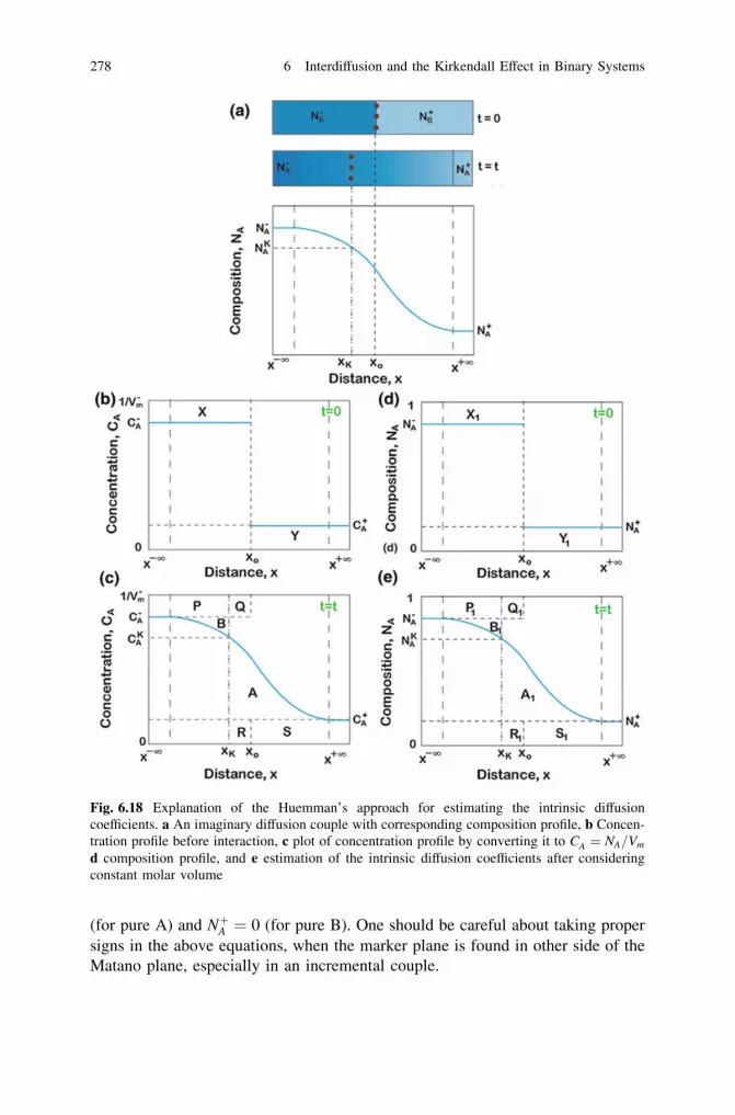
(for pure A) and NþA ¼ 0 (for pure B). One should be careful about taking propersigns in the above equations, when the marker plane is found in other side of theMatano plane, especially in an incremental couple.

Fig. 6.18 Explanation of the Huemman’s approach for estimating the intrinsic diffusioncoefficients. a An imaginary diffusion couple with corresponding composition profile, b Concen-tration profile before interaction, c plot of concentration profile by converting it to CA ¼ NA=Vm

d composition profile, and e estimation of the intrinsic diffusion coefficients after consideringconstant molar volume

278 6 Interdiffusion and the Kirkendall Effect in Binary Systems

6.8.2 Relations Developed with the Help of Wagner’sTreatment

Equation 6.39a and 6.39b at the Kirkendall marker plane can be written as

12t

NþB � N�Bffi �

� kKYKB

vKm

þZkK

k�1

YB

vmdk

264

375 ¼ 1

t12

N�B eJKA � 1� N�B

ffi �eJKB

� �ð6:73aÞ

12t

NþB � N�Bffi �

�kK 1� YK

B

ffi �vK

m

�Zkþ1

kK

1� YBð Þvm

dk

264

375 ¼ 1

t12

�NþB eJKA þ 1� NþB

ffi �eJKB

� �

ð6:73bÞ

To write a relation with respect to eJKB only, we multiply Eq. 6.73a by NþB and

Eq. 6.73b by N�B . Subsequently, we add them and after rearranging, we get [8]

12t

NþB � N�Bffi �

�kK YKB

vKm

NþB þ1� YK

B

ffi �vK

m

N�B

�þ NþB

ZkK

k�1

YB

vmdk� N�B

Zkþ1

kK

1� YBð Þvm

dk

8><>:

9>=>;

264

375

¼ 1

t12

�NþB 1� N�Bffi �eJK

B þ N�B 1� NþBffi �eJK

B

� �

Replacing YKB ¼

NKB�N�B

NþB �N�Band 1� YK

B ¼NþB �NK

B

NþB �N�B

12t

NþB � N�Bffi �

�kK NKB

vKm

þ NþB

ZkK

k�1

YB

vmdk� N�B

Zkþ1

kK

1� YBð Þvm

dk

8><>:

9>=>;

264

375 ¼ 1

t1=2� NþB � N�Bffi � eJK

B

� �

eJKB ¼

t1=2

2tkK NK

B

vKm

� NþB

ZkK

k�1

YB

vmdkþ N�B

Zkþ1

kK

1� YBð Þvm

dk

264

375

eJKB ¼

t1=2

2tkK NK

B

vKm

� t1=2

2tNþB

ZkK

k�1

YB

vmdk� N�B

Zkþ1

kK

1� YBð Þvm

dk

264

375

By replacing the Boltzmann parameter kK ¼ xK

t1=2 and then using the relation ofthe velocity of the marker plane vK ¼ xK

2t , as expressed in Eq. 6.64, we arrive at

6.8 Relations for the Estimation of the Intrinsic Diffusion Coefficients 279

eJKB ¼ vKCK

B �t1=2

2tNþB

ZkK

k�1

YB

vmdk� N�B

Zkþ1

kK

1� YBð Þvm

dk

264

375

Note that the concentration of the marker plane is CKB ¼

NKB

vKm

From the Boltzmann parameter, we know that dk ¼ dxt1=2 and we can write

eJKB ¼ vKCK

B �12t

NþB

ZxK

x�1

YB

vmdx� N�B

Zxþ1

xK

1� YBð Þvm

dx

24

35

Compared to Eq. 6.57b, the intrinsic flux of the element B at the Kirkendallmarker plane can be written as

JKB ¼ �

12t

NþB

ZxK

x�1

YB

vmdx� N�B

Zxþ1

xK

1� YBð Þvm

dx

24

35

From Fick’s first law, it follows that

DB ¼12t

ox

oCB

� �K

NþB

ZxK

x�1

YB

vmdx� N�B

Zxþ1

xK

1� YBð Þvm

dx

24

35 ð6:74Þ

Further, using the standard thermodynamic relations given in Eq. 1.150

DB ¼12t

v2m

�vA

ox

oNB

� �K

NþB

ZxK

x�1

YB

vmdx� N�B

Zxþ1

xK

1� YBð Þvm

dx

24

35 ð6:75Þ

Equation 6.75 can be used if we wish to determine the intrinsic diffusion coef-ficients using the profiles NB versus x, YB=vm versus x, and 1� YBð Þ=vm versus x.

The equation for the interdiffusion flux eJA can be written in the same way.Multiplying Eq. 6.73a by 1� NþBð Þ and Eq. 6.73b by 1� N�B

ffi �and following the

similar procedure, the intrinsic diffusivity for the component A can be derived as

DA ¼12t

ox

oCA

� �K

NþA

ZxK

x�1

YB

vmdx� N�A

Zxþ1

xK

1� YBð Þvm

dx

24

35 ð6:76Þ

280 6 Interdiffusion and the Kirkendall Effect in Binary Systems

By once again utilizing the Eq. 1.150, the following is obtained

DA ¼12t

v2m

�vB

ox

oNA

� �K

NþA

ZxK

x�1

YB

vmdx� N�A

Zxþ1

xK

1� YBð Þvm

dx

24

35 ð6:77Þ

From Eqs. 6.75 and 6.77, we can write

DB

DA¼ �vB

�vA

NþBR xK

x�1YBvm

dx� N�BR xþ1

xK

1�YBð Þvm

dx

�NþAR xK

x�1YBvm

dxþ N�AR xþ1

xK

1�YBð Þvm

dx

" #¼ �vB

�vA

NþB R� N�B S

�NþA R� N�A S

ð6:78Þ

The calculation procedure is shown in Fig. 6.19. R and S are the areas as shownin the figure. Note here that, unlike the Heumann method, there is no need to locatethe initial contact position, a task which is not easily accomplished.

In general, instead of estimating the intrinsic diffusion coefficients usingEqs. 6.75 and 6.77 directly, one can estimate the interdiffusion coefficient usingEq. 6.45 and the ratio of diffusivities using Eq. 6.78. Afterward, the intrinsicdiffusion coefficients can be estimated using Eqs. 6.65 or 6.66. Note that it is just amatter of choice.

6.8.3 Multifoil Technique to Estimate the IntrinsicDiffusion Coefficients

In the example above, we have seen that the intrinsic diffusion coefficients couldbe estimated only at the Kirkendall marker plane only, since this is the onlymarked plane that moved from the beginning depending on the relative mobilitiesof the components. Therefore, many diffusion couples with different end-membercompositions need to be prepared (leading to marker planes at different compo-sitions), if we want to determine the intrinsic diffusion coefficients at differentcompositions. This was done in the b phase of the Ni–Al system [28], which couldbe a tedious task depending on the system. The multifoil technique is developed insuch a way that we are able to estimate these parameters over the whole com-position range of interest from only a single experiment. This is explained with thehelp of experimental results in the Ni–Pt system [29]. In this technique, many foilsof two dissimilar materials are stacked together. Therefore, it is relatively easy tofollow this technique if the foils could be made. Fortunately, this is relativelystraightforward in the case of metals. The number of foils used for these experi-ments is decided based on the thickness of the interdiffusion zone developed in thebulk diffusion couple experiments. After the interdiffusion process, accordingto the boundary condition of the equations, some unaffected parts should be leftat the ends of the diffusion couple. The back scattered electron image of the

6.8 Relations for the Estimation of the Intrinsic Diffusion Coefficients 281

interdiffusion zone developed is shown in Fig. 6.20a. The velocity v of the markersat different planes can be determined by the relation developed by Levasseur andPhilibert [30], Cornet [31] and van Loo et al. [32]

v ¼ 12t

y� xody

dxo

� �ð6:79Þ

Here, xo is the initial position of markers before interdiffusion and x is the newposition after the interdiffusion, such that y = (x - xo) is the net displacement. Itcan be seen that for x0 = 0 (i.e., the Kirkendall plane), according to Eq. 6.79,v = y/2t, which is the Kirkendall marker displacement similar to Eq. 6.64.

The composition profile of the Pt/Ni diffusion couple is shown in Fig. 6.20b.The displacement of the markers is measured using the backscattered electron

Fig. 6.19 Explanation of van Loo’s approach for the estimation of the intrinsic diffusioncoefficients. a Diffusion couple with corresponding composition profile, b YB=vm versus x plot,and c 1� YBð Þ=vm versus x plot

282 6 Interdiffusion and the Kirkendall Effect in Binary Systems

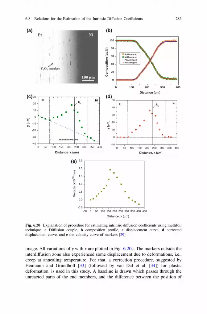
image. All variations of y with x are plotted in Fig. 6.20c. The markers outside theinterdiffusion zone also experienced some displacement due to deformations, i.e.,creep at annealing temperature. For that, a correction procedure, suggested byHeumann and Grundhoff [33] (followed by van Dal et al. [34]) for plasticdeformation, is used in this study. A baseline is drawn which passes through theunreacted parts of the end members, and the difference between the position of

(e)

(a) (b)

(c) (d)

Fig. 6.20 Explanation of procedure for estimating intrinsic diffusion coefficients using multifoiltechnique. a Diffusion couple, b composition profile, c displacement curve, d correcteddisplacement curve, and e the velocity curve of markers [29]

6.8 Relations for the Estimation of the Intrinsic Diffusion Coefficients 283

markers and this baseline gives the actual displacement of the markers, which isshown in Fig. 6.20d. Thus, we assume the deformation rate of the end members ofthe couple to be equal and constant. The difference between the marker dis-placement measured in the diffusion couple and the value corresponding to thebaseline—i.e., the dashed line in Fig. 6.20c giving the actual marker shift (plottedin Fig. 6.20d)—was constructed. It should be noted that the maximum displace-ment need not to be necessarily at the Kirkendall marker plane only, as is found inthis system.

The displacement is then plotted versus x0 (= x - y) to determine dy=dxo.Following on from this, the velocities of the different marker planes are estimatedfrom Eq. 6.79 as plotted in Fig. 6.20e. Furthermore, we can derive

DB

DA¼ �vBDB

�vBDA

DB

DA¼ �vB �vBCB þ �vACAð ÞDB

�vB �vBCB þ �vACAð ÞDA

Since, as shown previously in Eq. 1.146, �vBCB þ �vACA ¼ 1

DB

DA¼ �vB �vACADB þ �vBCBDBð Þ

�vB�vACADA þ �vB�vBCBDA

DB

DA¼ �vB �vACADB þ �vBCBDAð Þ þ �vBCB DB � DAð Þ½ �

�vB �vACADB þ �vBCBDAð Þ � �vA�vBCA DB � DAð Þ

Since according to Eq. 6.65 eD ¼ �vACADB þ �vBCBDA, we can write

DB

DA¼

�vB eD þ �vBCB DB � DAð Þ� �

�vB eD � �vA�vBCA DB � DAð ÞDB

DA¼eD þ �vBCB DB � DAð ÞeD � �vA�vB

�vBCA DB � DAð Þ

DB

DA¼

eD oCBox

ffi �þ �vB DB � DAð Þ oCB

ox

ffi �CBeD oCB

ox

ffi �� �vB DB � DAð Þ oCB

ox

ffi ��vA�vB

CA

Since according to Eqs. 6.61a and 6.61b v ¼ �vB DB � DAð Þ oCBox

ffi �, we can write

DB

DA¼

eDðoCB=oxÞ þ vCBeDðoCB=oxÞ � v �vA�vB

CA

DB

DA¼

1þ veDðoCB=oxÞCB

1� veDðoCB=oxÞCA

�vA�vB

284 6 Interdiffusion and the Kirkendall Effect in Binary Systems

DB

DA¼ 1þ f CB

1� f CAð�vA=�vBÞwhere f ¼ v

eDðoCB=oxÞð6:80Þ

Therefore, from the values of v, as shown in Fig. 6.20e, it is possible to estimate

DB=DA. After estimating eD following previously explained approaches, we can theestimate intrinsic diffusion coefficients using Eq. 6.65. The interdiffusion coeffi-cients estimated in a bulk diffusion couple must be compared with the estimatedvalues from a multifoil experiment in order to validate the results. It can be seen inFig. 6.21a that the interdiffusion coefficients are more or less the same. This helpsto understand if stacking of foils created any problem in the diffusion couple. The

0 20 40 60 80 10010-16

10-15

10-14

10-13

Bulk diffusion couple Multifoil experiment

(a)

at. % Pt

~ D (m

2/s

)

1200oC

0 20 40 60 80 1006.5

7.0

7.5

8.0

8.5

9.0

9.5(b)

mo

lar

volu

me

(x10

-6 m3 /m

ole

)

at. % Pt

0 20 40 60 80 10010-15

10-14

10-13(c)

at.% Pt

dif

fusi

on

co

effi

cien

t (m

2 /s)

DPt

DNi

Fig. 6.21 Estimation ofdiffusion parametersfollowing multifoil techniqueas discussed in previousfigure: a interdiffusioncoefficients, b molar volume,and c the intrinsic diffusioncoefficients in the Ni–Ptsystem [29]

6.8 Relations for the Estimation of the Intrinsic Diffusion Coefficients 285

variation of the molar volume is shown in Fig. 6.21b. The intrinsic diffusioncoefficients that were subsequently estimated by multifoil technique are given inFig. 6.21c.

6.9 Different Ways to Detect the KirkendallMarker Plane

As already explained, it is important to use inert markers at the mating interface ofa diffusion couple and anneal it to detect the Kirkendall marker plane afterinterdiffusion. Following, these inert particles are found under a scanning electronmicroscope (SEM) by image analysis or by detecting the X-ray peak originatedfrom the material used as marker in an energy dispersive spectrometer (EDS) orwavelength dispersive spectrometer (WDS) detectors. Depending on the system inwhich they are used, different materials are used as markers, and these materialscan be used in wire or powder form. Powders are used more often because of easeof use. It is important to note that the markers selected do not react with thediffusing components, which will otherwise not move ideally depending on theirrelative mobilities. Markers are made from should be impervious to the diffusingcomponents, and there should be enough space between them to not hinder themovement of the diffusing components. Marker size should be much smaller thanthe total interdiffusion zone thickness. On the other hand, the markers should notbe so small that they are dragged along by the grain boundaries, a phenomenon wehave often witnessed, especially when we have used the particles in powder formand the particle size was less than 0.1 lm. As already mentioned, Kirkendall andmany others preferred to use Mo or W wires as inert markers. Due to the diffi-culties in placing the wires, powders are used more commonly these days. Theseare dispersed in acetone, and a small drop is placed on a metallographicallyprepared smooth surface of one of the couple halves. The acetone evaporatesleaving the particles distributed evenly on the surface. Distribution could bechecked in an optical microscope. In general, we prefer, on average around20–30 lm spacing between the particles for average particle size of 1–2 lm.However, strictly speaking, it is difficult to achieve very good control over thedistribution of the particles and the desired distribution pattern might not beachieved in first attempt. This process is repeated after cleaning the surface withacetone until we have an acceptable distribution pattern. It is not possible toachieve a perfectly even distribution; however, having too many particles clumpedtogether in many locations should be avoided. Once satisfied, another couple halfis placed above and clamped in a fixture to place it in the calibrated furnace forannealing. According to our experience, a marker size of 1–5 lm works welldepending on the system and the thickness of the interdiffusion zone. Differentrefractory metal and oxide powders such as W, Mo, ThO2, TiO2, and Y2O3 areused in metallic systems. Similarly, Au and Pt particles are used in oxides. ThO2

acts as the best marker in most of the metallic systems, since this is one of the

286 6 Interdiffusion and the Kirkendall Effect in Binary Systems

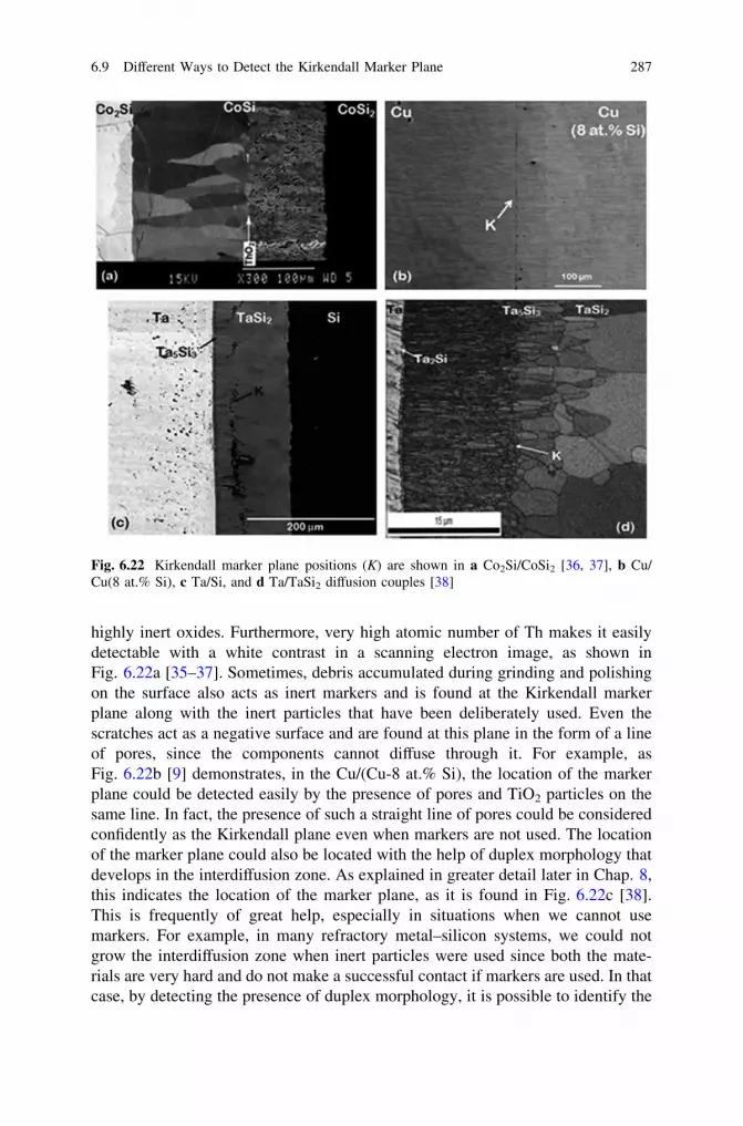
highly inert oxides. Furthermore, very high atomic number of Th makes it easilydetectable with a white contrast in a scanning electron image, as shown inFig. 6.22a [35–37]. Sometimes, debris accumulated during grinding and polishingon the surface also acts as inert markers and is found at the Kirkendall markerplane along with the inert particles that have been deliberately used. Even thescratches act as a negative surface and are found at this plane in the form of a lineof pores, since the components cannot diffuse through it. For example, asFig. 6.22b [9] demonstrates, in the Cu/(Cu-8 at.% Si), the location of the markerplane could be detected easily by the presence of pores and TiO2 particles on thesame line. In fact, the presence of such a straight line of pores could be consideredconfidently as the Kirkendall plane even when markers are not used. The locationof the marker plane could also be located with the help of duplex morphology thatdevelops in the interdiffusion zone. As explained in greater detail later in Chap. 8,this indicates the location of the marker plane, as it is found in Fig. 6.22c [38].This is frequently of great help, especially in situations when we cannot usemarkers. For example, in many refractory metal–silicon systems, we could notgrow the interdiffusion zone when inert particles were used since both the mate-rials are very hard and do not make a successful contact if markers are used. In thatcase, by detecting the presence of duplex morphology, it is possible to identify the

Fig. 6.22 Kirkendall marker plane positions (K) are shown in a Co2Si/CoSi2 [36, 37], b Cu/Cu(8 at.% Si), c Ta/Si, and d Ta/TaSi2 diffusion couples [38]

6.9 Different Ways to Detect the Kirkendall Marker Plane 287

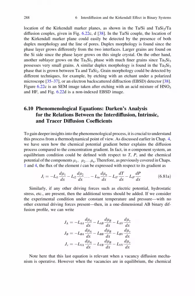
location of the Kirkendall marker planes, as shown in the Ta/Si and TaSi2/Tadiffusion couples, given in Fig. 6.22c, d [38]. In the Ta/Si couple, the location ofthe Kirkendall marker plane could easily be detected by the presence of bothduplex morphology and the line of pores. Duplex morphology is found since thephase layer grows differently from the two interfaces. Larger grains are found onthe Si side since the phase layer grows on this single crystal. On the other hand,another sublayer grows on the Ta5Si3 phase with much finer grains since Ta5Si3possesses very small grains. A similar duplex morphology is found in the Ta5Si3phase that is grown between Ta and TaSi2. Grain morphology could be detected bydifferent techniques, for example, by etching with an etchant under a polarizedmicroscope [35–37], or an electron backscattered diffraction (EBSD) detector [38].Figure 6.22c is an SEM image taken after etching with an acid mixture of HNO3

and HF, and Fig. 6.22d is a non-indexed EBSD image.

6.10 Phenomenological Equations: Darken’s Analysisfor the Relations Between the Interdiffusion, Intrinsic,and Tracer Diffusion Coefficients

To gain deeper insights into the phenomenological process, it is crucial to understandthis process from a thermodynamical point of view. As discussed earlier in Chap. 4,we have seen how the chemical potential gradient better explains the diffusionprocess compared to the concentration gradient. In fact, in n component system, anequilibrium condition could be defined with respect to T, P, and the chemicalpotential of the components l1; l2. . .ln. Therefore, as previously covered in Chaps.1 and 4, the flux of the element i can be expressed with respect to its gradient as

Ji ¼ �Li1dl1

dx� Li2

dl2

dx. . .� Lin

dln

dx� LiT

dT

dx� LiP

dP

dxð6:81aÞ

Similarly, if any other driving forces such as electric potential, hydrostaticstress, etc., are present, then the additional terms should be added. If we considerthe experimental condition under constant temperature and pressure—with noother external driving forces present—then, in a one-dimensional AB binary dif-fusion profile, we can write

JA ¼ �LAAdlA

dx� LAB

dlB

dx� LAV

dlv

dx

JB ¼ �LBAdlA

dx� LBB

dlB

dx� LBV

dlv

dx

Jv ¼ �LVAdlA

dx� LVB

dlB

dx� LVV

dlv

dx

Note here that this last equation is relevant when a vacancy diffusion mecha-nism is operative. However when the vacancies are in equilibrium, the chemical

288 6 Interdiffusion and the Kirkendall Effect in Binary Systems

potential of the vacancy should, therefore, be considered to be zero. As mentionedearlier, we have not discussed the assumptions of Darken analysis. Nonetheless, ittakes mainly two assumptions: (i) vacancies remain in equilibrium at every con-centration of the interdiffusion zone and (ii) the off-diagonal phenomenological

constants are zero. Therefore, we have lv ffi 0; dlvdx ffi 0; LAB ¼ 0 and LBA ¼ 0,

meaning that the flux of the components can be written as

JA ¼ �LAAdlA

dxð6:81bÞ

JB ¼ �LBBdlB

dxð6:81cÞ

If F is the force due to the chemical potential an dmB is the velocity of thecomponent B, then the mobility of B can be written as MB ¼ vB F. Therefore, theflux of element B can be written as

JB ¼ CBvB ¼ MBFCB ð6:82Þ

Since the force is equal to the chemical potential gradient where the atoms

diffuse down the gradient, we can write F ¼ � dlBdx . Consequently, Eq. 6.82 can be

written as

JB ¼ �MBCBdlB

dxð6:83Þ

In comparison with Eq. 6.81c, the phenomenological constant can be written asLB ¼ MBCB. When comparing it with Fick’s first law, we can write

DB ¼ MBCBdlB

dCB¼ MB

NB

vm

dlB

dCBð6:84Þ

Further using the standard thermodynamic relation in Eq. 1.150

DB ¼vm

�vAMBNB

dlB

dNB¼ vm

�vAMB

dlB

d ln NBð6:85Þ

Furthermore,

lB ¼ loB þ RT ln aB ¼ lo

B þ RT ln NB þ ln cBð Þ ð6:86Þ

Substituting Eq. 6.86 in Eq. 6.85

DB ¼vm

�vAMBRT

d ln aB

d ln NB¼ vm

�vAMBRT 1þ d ln cB

d ln NB

� �ð6:87Þ

6.10 Phenomenological Equations 289

In the measurement of the tracer diffusion coefficient, as explained previouslyin Chap. 5, there is no driving force for diffusion. Moreover, since this is ameasurement in a single-composition alloy, the volume terms are unnecessary.Thus, it is possible to write the tracer diffusion coefficient with respect to themobility term from Eq. 6.87 as

D�B ¼ M�BRT ð6:88Þ

The above relation is known as the Nernst–Einstein relation.Substituting Eq. 6.88 in Eq. 6.87, we get

DB ¼ D�Bvm

�vA

d ln aB

d ln NB¼ D�B

vm

�vA1þ d ln cB

d ln NB

� �ð6:89aÞ

In the same way, for the component A

DA ¼ D�Avm

�vB

d ln aA

d ln NA¼ D�A

vm

�vB1þ d ln cA

d ln NA

� �ð6:89bÞ

According to the Gibbs–Duhem relation derived much earlier in Chap. 1(Eqs. 1.134 and 1.139), we know that d ln aA

d ln NA¼ d ln aB

d ln NB. Substituting Eqs. 6.89a and

6.89b in Eq. 6.65, we arrive at

eD ¼ NAD�B þ NBD�Affi � d ln aB

d ln NB

� �ð6:90Þ

This relation was first proposed by Darken [22].The ratio of intrinsic diffusivities in terms of tracer diffusivities can be

expressed by

DB

DA¼ �vB

�vA

D�BD�A

ð6:91Þ

Comparing Eqs. 6.78 and 6.91

D�BD�A¼

NþBR xK

x�1YBvm

dx� N�BR xþ1

xK

1�YBð Þvm

dx

�NþAR xK

x�1YBvm

dxþ N�AR xþ1

xK

1�YBð Þvm

dx

" #ð6:92Þ

Using this relation, it is possible to estimate the ratio of tracer diffusion coef-ficients at the Kirkendall marker plane using the composition profile. The velocityof the Kirkendall marker plane from Eqs. 6.61a, 6.89a and 6.89b can be written as

290 6 Interdiffusion and the Kirkendall Effect in Binary Systems

vK ¼ �vB D�Bvm

�vA� D�A

vm

�vB

� �H

oCB

ox

� �K

ð6:93Þ

where H ¼ d ln aAd ln NA

¼ d ln aBd ln NB

is known as the thermodynamic factor.

6.11 Limitations of the Relations Developed by Darkenand Manning’s Correction for the Vacancy WindEffect

After the above analysis by Darken, Bardeen [25] made a thorough analysis andexplained that the relations developed by Darken can be derived by consideringenough sources and sinks for vacancies to maintain this equilibrium ðdlv=dx ffi 0Þover the interdiffusion zone. Subsequently, Seitz [39] showed further that every-where inside the interdiffusion zone vacancies should be at equilibrium ðlv ffi 0Þ.He further explained that Darken’s relations (Eq. 6.66) could be used in bothsubstitutional and interstitial diffusion. Bardeen and Herring [40] argued (based onthe experimental results available in the 1950s) that Darken’s relations are fulfilledin most of the diffusion couples. Therefore, a volume of vacancies should becreated on one side of the couple and absorbed on the other side. This volume isequivalent to the volume shift by the Kirkendall marker plane, that is, the shiftdistance xK ¼ xK � xo multiplied by the cross-sectional area of the couple. Thispoint is clarified in Fig. 6.23. In this example, the component A has a higherdiffusion rate compared to B. Therefore, the vacancies flow in the same directionof the component B, which has the lower diffusion rate of the two. FollowingEqs. 1.149 and 6.61a, we can write [41]

vK ¼ vmJV ¼ �ð�vBJB þ �vAJAÞ ð6:94Þ

The dJV=dx versus x plot gives the idea in which part vacancies are created(positive) and absorbed (negative). Analysis indicates that grain boundaries, pores,cracks [39], and interfaces [41] act as a source and sink for vacancies. Doo andBalluffi [42] presented the proof on the role of edge dislocations related to theKirkendall marker shift. Its role as sink and source is explained more clearly inFig. 6.24 with the aid of a schematic illustration of the lattice planes and dislo-cations. The vacancies are flowing from right to left since there is a net flux ofatoms from left to right. On the left, the dislocations act as sinks, where the atomsare replaced by vacancies from the extra plane. On the right, they act as sources,where the atoms are added to the extra planes [43]; that is, the vacancies arecreated and move to neighboring positions.

6.10 Phenomenological Equations 291

One interesting feature noticed in many diffusion couples is that pores are foundon the side of the diffusion couple toward which the marker plane moves. In thebeginning, the reason for the formation of voids was not clear and was believedthat this might be incidental in a few diffusion couples [44]. However, over time, itbecame clear that this must be related to the Kirkendall effect. Branes [45] foundthat the volume of these pores is considerable and influences the Kirkendall planeshift. In the absence of any voids, the marker plane movement would be more [35].Therefore, these two can be considered as competitive phenomena. In somecouples, as can be seen in Fig. 6.22a, the content of pores is very high. In general,the lack of sinks is considered to be a valid explanation for finding these pores,especially if one component has a much higher diffusion rate compared to theother, as is the case in the CoSi phase. The diffusion rate of Si is around 30 times

Fig. 6.23 Flow of vacanciesdepending on the intrinsicfluxes is explaineda composition profile, b fluxof components, and c creationand annihilation of vacancies

292 6 Interdiffusion and the Kirkendall Effect in Binary Systems

higher than that of Co in this phase [36]. Similar behavior was found in the Nb5Si3phase, as shown in Fig. 6.25a, in which one side of the Kirkendall marker plane iscovered by pores [46]. The diffusion rate of Si is approximately 100 times higherthan that of Nb in this phase. The area fraction of the pores in the Cu3Sn phase isfound to be noticeably less, as seen from the Cu/Sn system shown in Fig. 6.25b[8]. It is believed that the distribution of the pores is affected by the impuritiespresent in the end members. Note here that the diffusion rate of Cu is almost30 times higher than that of Sn in this phase [47]. The differences in pore volumevary from system to system, and these differences may be due to the difference inthe availability of sinks, the relative mobilities of the components, or the presenceof impurities or inclusions, for instance. When the pore volume is substantial, thisfactor should be considered in the calculation of the diffusion parameters, as wasdone in the Co–Si system [36].

Along with the formation of pores, the development of stress in the diffusioncouple and the deformation of the diffusion couple are also associated with theKirkendall effect. Previously, the Kirkendall effect has been discussed based on themovement of the markers and the shrinkage on one side with the correspondingswelling on the other side of the couple based on a one-dimensional diffusion (i.e.,composition) profile. With the accumulation of vacancies and/or pore formation,tensile stress develops on one side of the couple and compressive stress developson the other side where an extra amount of atoms are accommodated. This mayresult in a three-dimensional change in the diffusion couple, as shown in Fig. 6.26[48]. After annealing for time t, Fig. 6.26b shows one-dimensional deformation,whereas Fig. 6.26c presents the volume deformation. In this case, there will beequal deformation in all directions, which is one-third of the total deformation inone-dimensional deformation case. The dots on the figure represent the markersshowing the deformation areas. For further reading on deformation and bending,the reader is referred to the manuscripts by Boettinger et al. [49] and Daruka et al.

Fig. 6.24 Edge dislocations as sink and source of vacancies are explained

6.11 Limitations of the Relations Developed by Darken and Manning’s Correction 293

Fig. 6.25 Evolution of theKirkendall voids in differentsystems is explained in thea Nb5Si3 [46] and b Cu3Snphases [8]

Fig. 6.26 a Deformation ofdiffusion couple anddistribution of inert particlesare shown before theexperiments and whendeformation is b onedimensional and c threedimensional. Dots indicatethe markers at differentplanes

294 6 Interdiffusion and the Kirkendall Effect in Binary Systems

[50]. It should be noted here that the deformation or bending of the sample couldbe significant in a thin-film diffusion couple.

Darken’s treatment correlates the interdiffusion, intrinsic, and tracer diffusioncoefficients of the components with the aid of the thermodynamic factor. Asexplained, in a binary system, the intrinsic diffusivities of the components aredifferent. When diffusion is controlled by a vacancy mechanism, the net flow ofmatter in one direction will be balanced by a flow of vacancies in the oppositedirection. Manning explained that the net flux of vacancies creates a vacancywind effect during interdiffusion [51, 52]. According to this theory, the flow ofvacancies will make a jump of some extra vacancies. The jump of extravacancies means an increase in the diffusion rate of the faster diffusing com-ponents and a decrease in the diffusion rate of the slower diffusing componentthan what is expected when adopting the relations developed by Darken. Toaccommodate this effect, he incorporated a correction factor into the equationsdeveloped by Darken. Naturally, these modified equations are known as theDarken–Manning equations.

Assuming there is no supersaturation, binding of vacancies, and no clusteringin the alloy, Manning modified Eqs. 6.89a and 6.89b using a random alloy modelas

DA ¼vm

�vBD�AH 1þWAð Þ ð6:95aÞ

DB ¼vm

�vAD�BH 1�WBð Þ ð6:95bÞ

where the vacancy wind factor Wi ¼2Ni D�A�D�Bð Þ

Mo NAD�AþNBD�Bð Þ ; Mo is a constant, which

depends on the crystal structure of the system, Ni is the mole fraction of com-ponent i, and H is the thermodynamic factor d ln aA=d ln NA ¼ d ln aB=d ln NB.Replacing Eqs. 6.95a and 6.95b in Eq. 6.65 and after some simple arithmetic, wearrive at

eD ¼ NAD�B þ NBD�Affi �

H WAB ð6:96Þ

where WAB ¼ 1þ 2NANB D�A�D�Bð Þ2Mo NAD�BþNBD�Að Þ NAD�AþNBD�Bð Þ

In the same way, the Kirkendall marker velocity was modified to

vK ¼ �vBvm

�vAD�B �

vm

�vBD�A

� �a H

oCB

ox¼ 1

vm�vBD�B � �vAD�Affi �

a HoNB

oxð6:97Þ

where a ¼ 1=f and f is the correlation factor for self-diffusion. Last equation canbe written after modifying the relation using equations in Sect. 1.18.

6.11 Limitations of the Relations Developed by Darken and Manning’s Correction 295

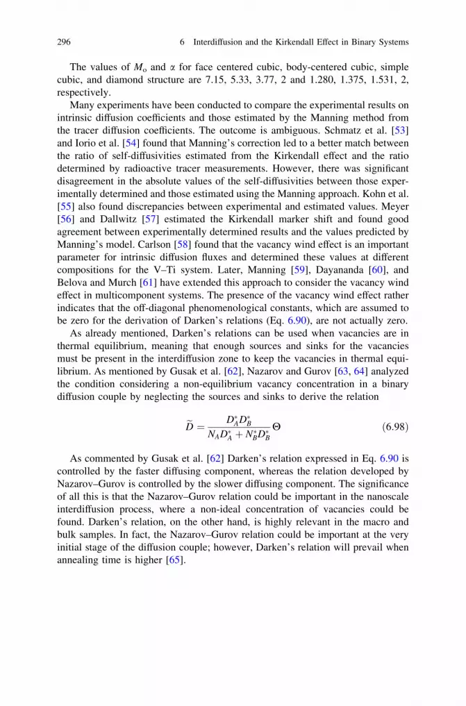
The values of Mo and a for face centered cubic, body-centered cubic, simplecubic, and diamond structure are 7.15, 5.33, 3.77, 2 and 1.280, 1.375, 1.531, 2,respectively.

Many experiments have been conducted to compare the experimental results onintrinsic diffusion coefficients and those estimated by the Manning method fromthe tracer diffusion coefficients. The outcome is ambiguous. Schmatz et al. [53]and Iorio et al. [54] found that Manning’s correction led to a better match betweenthe ratio of self-diffusivities estimated from the Kirkendall effect and the ratiodetermined by radioactive tracer measurements. However, there was significantdisagreement in the absolute values of the self-diffusivities between those exper-imentally determined and those estimated using the Manning approach. Kohn et al.[55] also found discrepancies between experimental and estimated values. Meyer[56] and Dallwitz [57] estimated the Kirkendall marker shift and found goodagreement between experimentally determined results and the values predicted byManning’s model. Carlson [58] found that the vacancy wind effect is an importantparameter for intrinsic diffusion fluxes and determined these values at differentcompositions for the V–Ti system. Later, Manning [59], Dayananda [60], andBelova and Murch [61] have extended this approach to consider the vacancy windeffect in multicomponent systems. The presence of the vacancy wind effect ratherindicates that the off-diagonal phenomenological constants, which are assumed tobe zero for the derivation of Darken’s relations (Eq. 6.90), are not actually zero.

As already mentioned, Darken’s relations can be used when vacancies are inthermal equilibrium, meaning that enough sources and sinks for the vacanciesmust be present in the interdiffusion zone to keep the vacancies in thermal equi-librium. As mentioned by Gusak et al. [62], Nazarov and Gurov [63, 64] analyzedthe condition considering a non-equilibrium vacancy concentration in a binarydiffusion couple by neglecting the sources and sinks to derive the relation

eD ¼ D�AD�BNAD�A þ N�BD�B

H ð6:98Þ

As commented by Gusak et al. [62] Darken’s relation expressed in Eq. 6.90 iscontrolled by the faster diffusing component, whereas the relation developed byNazarov–Gurov is controlled by the slower diffusing component. The significanceof all this is that the Nazarov–Gurov relation could be important in the nanoscaleinterdiffusion process, where a non-ideal concentration of vacancies could befound. Darken’s relation, on the other hand, is highly relevant in the macro andbulk samples. In fact, the Nazarov–Gurov relation could be important at the veryinitial stage of the diffusion couple; however, Darken’s relation will prevail whenannealing time is higher [65].

296 6 Interdiffusion and the Kirkendall Effect in Binary Systems

References

1. W.C. Roberts-Austen, Phil. Trans. Roy. Soc. A187 (1896) 3832. C. Matano, Jap. J. Phys. 8 (1933) 1093. L. Boltzmann, Ann. Physik. 53 (1894) 9594. R.W. Ballufi, Acta Met. 8 (1960) 8715. F. Sauer and V. Freise, Z. Electrochem. 66 (1962) 3536. C. Wagner, Acta Met. 17 (1969) 997. F.J.A. den Broeder, Scripta Met. 3 (1969) 3218. A. Paul, The Kirkendall effect in solid state diffusion. PhD Thesis, Technische Universiteit

Eindhoven, The Netherlands, 20049. S. Santra, H. Dong, T. Laurila, A. Paul, Proceedings of the Royal Society A 470 (2013)

20130464.10. L.B. Pfeil, J. Iron Steel 119 (1929) 50111. L.S. Darken and R.W. Gurry, Physical chemistry of metals, McGraw Hill Book Company,

Columbus, OH 43218, USA, 1953.12. G.S. Hartley, Trans. Faraday Soc. 46 (1946) 613. A.D. Smigelkas and E.O. Kirkendall, Trans. AIME 171 (1947) 13014. R.F. Mehl, Trans. AIME 171 (1947) 13515. H. Nakajima, JOM 49 (1997) 1516. L.C.C. da Silva and R.F. Mehl, Trans. AIME 191 (1951) 15517. H.B. Huntington and F. Seitz, Phys. Rev. 61 (1942) 31518. E.O. Kirkendall, Trans. AIME, 147 (1942) 10419. H.B. Huntington and F. Seitz, Phys. Rev. 76 (1949) 172820. C. Zener, Acta Cryst. 3 (1950) 34621. F. Sietz, Acta Cryst. 3 (1950) 35522. L.S. Darken, Trans. Met. Soc. AIME 175 (1948) 18423. G.S. Hartley and J. Crank, Trans. Faraday Soc. 45 (1949) 80124. F. Seitz, Phys. Rev. 74 (1948) 151325. J. Bardeen, Phys. Rev. 1 (1949) 140326. T. Heumann, Z. Phys. Chem. 201 (1952)16827. F.J.J. van Loo, Acta Met. 18 (1970) 110728. A Paul, AA Kodentsov, FJJ Van Loo, Journal of alloys and compounds 403 (2005) 14729. VD Divya, U Ramamurty, A Paul, Journal of Materials Research 26 (2011) 238430. J. Levasseur and J. Philibert: J. Phys. Stat. Sol. B, 21 (1967) K131. J.F. Cornet: J. Phys. Chem. Solids 35, (1974) 124732. F.J.J. van Loo, G.F. Bastin and G.D. Rieck, Science of Sintering, 11 (1979) 933. T. Heumann, and K. J. Grundhoff. Z. Metallkd. 63 (1972) 17334. M.J.H. van Dal, M.C.L.P. Pleumeeres, A.A. Kodenstov and F.J.J. van Loo, Acta Met. 48,

(2000) 38535. MJH Van Dal, D Huibers, AA Kodentsov, FJJ Van Loo, Intermetallics 9 (2001) 40936. MJH Van Dal, AA Kodentsov, FJJ Van Loo, Intermetallics 9 (2001) 45137. A Paul, MJH Van Dal, AA Kodentsov, FJJ Van Loo, Acta Materialia 52 (2004) 62338. S.Roy and A. Paul, Philosophical Magazine 92 (2012) 421539. F. Seitz, Acta Metall. 1 (1953) 35540. J. Bardeen and C. Herring, Imperfections in nearly Perfect crystals, Wiley, New York, 1952.41. F.J.J. van Loo, Prog. Solid State Chem. 20 (1990) 4742. V.Y. Doo and R.W. Balluffi, Acta Met. 6(1958) 42843. Y. Adda and J. Philibert, Atom movements and mass transport in solids, Les Éditions de

Physique, Les Ulis, 1991.44. L.C. Correa Da Silva and R.F. Mehl, Trans. Amer. Inst. Min. Met. Eng. 191 (1951) 15545. R.S. Branes, Effects associated with the Flow of Vacancies in Intermetallic Diffusion, Proc.

Phys. Soc. 65B (1952) 512

References 297

46. S Prasad, A Paul, Acta Materialia 59 (2011) 157747. A Paul, C Ghosh, WJ Boettinger, Metallurgical and Materials Transactions A 42 (2011) 95248. J. Schlipf, Acta Metall. 21 (1973) 43549. W.J. Boettinger, G.B. McFadden, S.R. Coriell, R.F. Sekerka, J.A. Warren, Acta Mat. 53

(2005) 199550. I. Daruka, I.A. Szabó, D.L. Beke, C. Cserháti, A. Kodentsov, F.J.J. Van Loo, 44 (1996) 498151. J.R. Manning, Phys. Rev. 124 (1961) 47052. J.R. Manning, Acta Met. 15 (1967) 81753. D.J. Schmatz, H.A. Domain and H.I. Aaronson, J. Appl. Phys. 37 (1966) 174154. N.R. Iorio, M.A. Dayananda and R.E. Grace, Met. Trans. 4 (1973) 133955. A. Kohn, J. Levasseur, J. Philibert and M. Wanin, Acta Met. 18 (1970) 16356. R.O. Meyer, Phys. Rev. 181 (1969) 108657. M.J. Dallwitz, Acta Met. 20 (1972) 122958. P.T. Carlson, Met. Trans. A 7A (1975) 199-20859. J.R. Manning, Metallurgical and Materials Transactions B, 1 (1970) 49960. M.A. Dayananda, Met. Trans. 2 (1971) 33461. I.V. Belova, G.E. Murch, Act Mat. Volume 55 (2007) Pages 62762. A.M.Gusak , S.V. Kornienko, G.V.Lutsenko, Defect and Diffusion Forum, 264 (2007) 10963. A.V.Nazarov and K.P.Gurov: Phys. Metal. Metallogr. Vol. 37 (1974), 49664. A.V.Nazarov and K.P.Gurov: Phys. Metal. Metallogr. Vol. 38 (1974) 48665. H. Mehrer, Diffusion in solids: fundamentals, methods, materials, diffusion-controlled

processes, Springer-Verlag GmbH, Berlin Germany, 2007

298 6 Interdiffusion and the Kirkendall Effect in Binary Systems

Chapter 7Growth of Phases with NarrowHomogeneity Range and Line Compoundsby Interdiffusion

In this chapter, the growth of the line compounds and the phases with narrowhomogeneity range by reactive diffusion is discussed. The concept of the inte-grated diffusion coefficient is introduced. In the end, few case studies are given toexplain the estimation procedure of the diffusion coefficients.

7.1 Time-Dependent Growth of the Phase Layer

In the previous chapter, we covered how interdiffusion works in a solid solutionor—to put it another way—how the interdiffusion process affects the growth ofphases with a wide composition range. In this present chapter, the growth of thephases with a narrow homogeneity range and the line compounds will be pre-sented. Earlier, we showed that it is possible to validate the assumption thatdiffusion controls the process under investigation by using the Boltzmannparameter. However, in the case of line compounds, this must be verified byexamining the parabolic nature of the growth. To simplify the discussion, let usconsider an interdiffusion zone, where only a single-phase layer grows. In a dif-fusion-controlled process, the rate of increase in layer thickness is inversely pro-portional to the layer thickness itself. This arises from the fact that the amount ofdiffusing flux decreases with the increase in layer thickness, because the atomshave to diffuse a longer distance. Therefore, the following can be written

dx

dt/ 1

xð7:1aÞ

dx

dt¼ k

1x

ð7:1bÞ

where x is the layer thickness, t is the time, and k is a constant. Integrating Eq. 7.1bfrom zero layer thickness at time zero to the layer thickness of Dx after theannealing time of t, we get

A. Paul et al., Thermodynamics, Diffusion and the Kirkendall Effect in Solids,DOI: 10.1007/978-3-319-07461-0_7, � Springer International Publishing Switzerland 2014

299

Dx2 ¼ 2kpt ð7:2Þ

where kp is the parabolic growth constant. Thus, the parabolic nature of the growthis checked by plotting Dx versus t or Dx2 versus t, as discussed in Figs. 7.1, 7.3,7.4, 7.5 and 7.6. Sometimes, instead plotting, Dx versus t1=2 plot Dx2 versus t isfound from which the parabolic growth constant can be estimated from the slope¼ 2kp

� �, as presented in Fig. 7.1b. In fact, it is also a common practice to plot

Dx versus t to verify the parabolic nature of the growth, as shown in Fig. 7.1a.The activation energy for the growth of a phase can be determined by con-

ducting diffusion experiments at different temperatures. According to the Arrhe-nius equation,

kp ¼ kop exp � Qg

RT

ffi �ð7:3Þ

where kpo is the pre-exponential factor, R is the gas constant, and Qg is the

activation energy for growth. The activation energy can be estimated from theslope �Qg=R

� �of the ln kp versus 1=T plot, as can be seen from Fig. 7.2. Rather

the zero thickness at zero annealing time should not be added to the experimentallymeasured data points.

Under ideal conditions, the layer thickness at the beginning of the experiment iszero. However, for a number of reasons, different kinds of situation can beencountered. The thickness of the phase layer is always measured after a certainannealing time. When the line is extrapolated to t = 0, sometimes, it may intersectthe y-axis (axis for thickness) at some positive value of Dxi. This can be realizedfrom Fig. 7.3. One of the reasons to find this kind of behavior is because of thegrowth during the heating and cooling cycles at the time of the heat treatment.Most of the experiments are conducted in vacuum or under flowing inter-gases. In

Δx

t

Δx

t

2

(a) (b)

0 0

Fig. 7.1 Plots of the growth of a phase layer during diffusion-controlled process a Dx versust and b Dx2 versus t

300 7 Growth of Phases with Narrow Homogeneity Range and Line Compounds

these cases, the sample has to be placed in the furnace first and only then heated tothe desired temperature. After the completion of annealing at a specific temper-ature, the growth of the phase layer during the cooling down period could beavoided by quenching the sample immediately. However, if the interface isweak—for example, in a metal/silicon diffusion couples—or if we like to avoidoxidation, furnace cooling is preferred. In the calculations, only the isothermalannealing time at the desired temperature is taken into account. Therefore, Dxi

indicates the growth of layer thickness during the heating and cooling cycles. If theactivation energy for growth is low, this contribution can be significant. Thecontribution will be smaller, however, when the activation energy is high. This canbe understood from the fact that the activation energy indicates the difference in

kp

1/T

high Q

low Qg

g

Fig. 7.2 Arrhenius plot explaining the activation energies

Δx

t

Δx

t

2

Δx Δxi i2

(a) (b)

0 0

Growth during heating and cooling Growth during heating and cooling

Growth during isothermal annealing Growth during isothermal annealing

Fig. 7.3 Parabolic growth plots showing the effect of growth during heating and cooling cyclesin the furnace

7.1 Time-Dependent Growth of the Phase Layer 301

growth rate at different temperatures, as shown in Fig. 7.2. Keeping the sample atthe desired annealing temperature for a relatively long time, we can minimize thiscontribution to the overall growth.

It is not very straightforward to understand whether the positive value of Dxi

indicates only the growth of the phase layer during the heating and cooling cycles.In interdiffusion, both lattice and grain boundary diffusion might play a significantrole. In the beginning, when the size of the grains is very small (representing ahigh grain boundary area), the growth of the phase might happen mainly due to theflux diffused via the grain boundaries. However, with an increase in annealingtime, grains also grow along with the layer thickness. Therefore, after a certainannealing time, the diffusion process could be controlled by the lattice diffusion. Inthis case, if Dx2 is plotted with respect to t for short annealing times, the transitionwill be clear from the curve, as shown in Fig. 7.4b. In most of the cases, however,this will be difficult to find because of very small transition time. Therefore, if theexperiments are conducted by choosing the annealing times in the later stagewhere the lattice diffusion-controlled growth process has already started after theinitial grain boundary diffusion-controlled process, Dxi will be positive. Then, itwill be difficult to understand whether this is because of the heating and coolingcycles or because of the initial grain boundary diffusion. It should be noted herethat this is not a problem to determine the parabolic growth constant, since it canbe estimated from the slope directly. In terms of an equation, it can be written as

Dx2 � Dx2i ¼ 2kpt ð7:4Þ

However, if we wish to examine the reason for finding the positive Dxi value,one experiment should be conducted by heating to the desired temperature andthen cooling without holding it for isothermal annealing.

Many times immediately after the start of annealing, the layer cannot startgrowing. This can be realized from Fig. 7.5. This phenomenon is generally foundwhen the surface layer is covered by a thin oxide layer—something which is verycommonly found in couples with Al, as was found in the Ti/Al diffusion couple [1,2]. It might have an incubation period of many hours during which the growth ofthe phase was reaction controlled. Once the oxide layer is completely broken, thediffusion-controlled parabolic growth of the phase is found. Sometimes, the smallbroken pieces of oxide are found in the product phase itself [1]. The parabolicgrowth constant in this case is estimated from

Dx2 ¼ 2kp t � toð Þ ð7:5Þ

Many times, [2–4], a carbon or phosphorous segregated layer could be presentat one of the material surfaces. A very small concentration, even in the range of afew parts per million, is enough to create problem at the initial stage of the growthprocess. This might even lead to a different diffusion process in the beginning andeven might become a reaction-controlled process because of the limited amount ofimpurities.

302 7 Growth of Phases with Narrow Homogeneity Range and Line Compounds

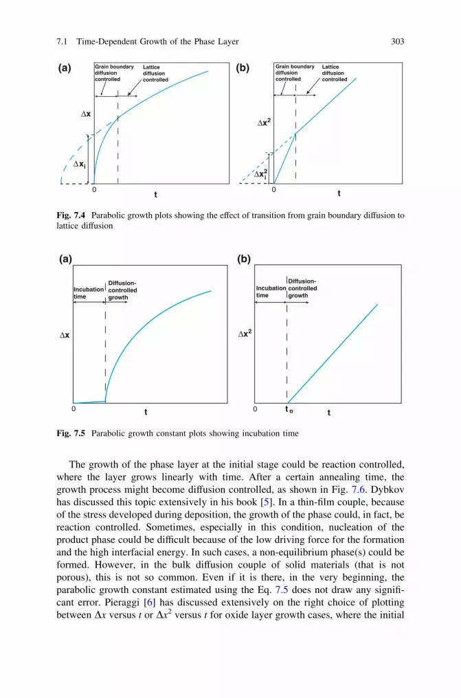
The growth of the phase layer at the initial stage could be reaction controlled,where the layer grows linearly with time. After a certain annealing time, thegrowth process might become diffusion controlled, as shown in Fig. 7.6. Dybkovhas discussed this topic extensively in his book [5]. In a thin-film couple, becauseof the stress developed during deposition, the growth of the phase could, in fact, bereaction controlled. Sometimes, especially in this condition, nucleation of theproduct phase could be difficult because of the low driving force for the formationand the high interfacial energy. In such cases, a non-equilibrium phase(s) could beformed. However, in the bulk diffusion couple of solid materials (that is notporous), this is not so common. Even if it is there, in the very beginning, theparabolic growth constant estimated using the Eq. 7.5 does not draw any signifi-cant error. Pieraggi [6] has discussed extensively on the right choice of plottingbetween Dx versus t or Dx2 versus t for oxide layer growth cases, where the initial

Δx

t

Δx

t

2

(a) (b)

00

Δx2i

Δxi

Grain boundarydiffusion controlled

Latticediffusion controlled

Grain boundarydiffusion controlled

Latticediffusion controlled

Fig. 7.4 Parabolic growth plots showing the effect of transition from grain boundary diffusion tolattice diffusion

Δx

t

Δx

t

2

(a) (b)

00

Incubationtime

Diffusion-controlledgrowth

t o

Incubationtime

Diffusion-controlledgrowth

Fig. 7.5 Parabolic growth constant plots showing incubation time

7.1 Time-Dependent Growth of the Phase Layer 303

fast growth rate does not contribute to the steady-state growth at the later stage.However, oxide systems are beyond the scope of discussion in this book. Inter-ested readers are referred to the manuscript by Pieraggi [6] or to the summary ofthe outcome by van Loo [2].

If the aim is to ultimately conduct the experiments to determine the activationenergy for growth, then time-dependent experiments ideally should be conductedat every temperature, in the case that Dxi is positive or there is an incubation time.On the other hand, it can be neglected, if these are small. It is also possible toconsider similar deviation, if the temperature range of a particular study is not veryhigh. This value might not be very different at differing temperatures within a shorttemperature range. It is easy to appreciate the need to conduct time-dependentexperiments at every temperature based on the results plotted with respect to theArrhenius equation for the calculation of the activation energy, as shown inFig. 7.2. If the data points fall more or less on the line, this indicates that thedeviation in the temperature range of interest will be similar. It should be notedhere that sometimes data are fit by considering zero thickness at zero annealingtime, as shown in Fig. 7.7b in the Mg/Ni diffusion couple [7]. When experimentaldata points are extrapolated to zero time, these will never lead to zero thicknessexactly because of error associated with the experiments even if there are no issuesat the initial stages as discussed above. However, there is nothing wrong to showthe graph, as presented in Fig. 7.7c, which is drawn after extracting the data pointsfrom Fig. 7.7b. With such a small error, one can conveniently consider that thesystem is not affected by the factors discussed above at the initial stage.

If local equilibrium is achieved in an interdiffusion zone, as shown by Wagner[8], Gurov et al. [9], and Kidson [10], all the phase layers contained in the phasediagram should be present in the interdiffusion zone. Local equilibrium is, ingeneral, found in the bulk diffusion couple, and it is expected that all phase layers

Δx

t

Δx

t

2

(a) (b)

0 0

Reaction controlled

DiffusioncontrolledReaction

controlledDiffusioncontrolled

Fig. 7.6 Parabolic growth plots showing transition from reaction-controlled to diffusion-controlled growth

304 7 Growth of Phases with Narrow Homogeneity Range and Line Compounds

start growing together. However, it is also true that the growth rates of one or morephases are much lower compared to the growth rate of other phases. In such cases,the phases with slower growth rates might actually be present in the interdiffusionzone, but proper analysis, for example, under a transmission electron microscope(TEM) is required to detect the phase. In the Mo–Si system [11], three phases,MoSi2, Mo5Si3, and Mo3Si, should be present in the interdiffusion zone of the Mo/Si diffusion couple. However, the interdiffusion zone was mainly covered by theMoSi2 phase with a very thin layer of the Mo5Si3 phase [12]. Mo3Si phase was notdetected at all. Our calculation showed that the thickness of Mo3Si in this couple isin the nanometer range, which is not possible to detect under a scanning electronmicroscope. TEM analysis by Yoon et al. [13] showed the presence of this phase.The same phase was grown with reasonable thickness in Mo/Mo5Si3 incrementalcouple [14]. In the Au/Sn diffusion couple, the Au5Sn phase was not found;however, it was revealed after etching the sample [15]. Even in the bulk diffusioncouples, sometimes, a sequential rather than a simultaneous phase growth issometimes suspected [16]. However, the initial time for the sequential growthcould be so small that validating this fact experimentally is difficult. In the

(a) (b)

(c)

Fig. 7.7 a Mg/Ni diffusion couple annealed at 480 �C for 45 h. Growth of the product phaseswith respect to square root time are shown for b considering zero thickness at zero time andc without considering it in the data fit [7]

7.1 Time-Dependent Growth of the Phase Layer 305

thin-film couple, instead of simultaneous growth, sequential growth is verycommon and the phases may not grow parabolically with time [17]. Nucleationproblem is also encountered frequently especially in the thin-film couples [18–21].

In multiphase growth, if all the phases grow parabolically with time, the growthof the total interdiffusion zone will also be parabolic with time. Quite often, thephase(s) grow with more or less straight interface, and it is relatively easy to checkthe parabolic nature of the growth, as can be seen in the Mg–Ni system which isreproduced in Fig. 7.7 [7]. However, many times [22], as found in the Au/Sndiffusion couple, one or more phase layers could be very wavy, and this leads to ahigh standard deviation in the calculation of the parabolic growth constant, asshown in Fig. 7.8 [23].

In the end, it should be noted that the parabolic growth constant is not a materialconstant since the thickness of a particular phase layer changes with the change incomposition of the end members. It is therefore not straightforward to discuss thediffusion behavior based on the parabolic growth constant calculations. In a par-ticular condition, the activation energy for growth could be the same as the acti-vation energy for the diffusion coefficient (single-phase growth of a line compoundin the interdiffusion zone). In most conditions (multiphase growth), however, theseare actually different. Therefore, incorrect conclusions may be drawn if the dif-fusion behavior is discussed solely based on the calculation of the parabolicgrowth constant. It is always safe to consider the diffusion coefficients, since thediffusion coefficient is a material constant. In fact, as will be discussed, thethickness of a particular phase layer is grown differently in different couples withdifferent end members such that the diffusion coefficients of the phases remainconstant.

(a) (b)

Fig. 7.8 a Au/Sn diffusion couple at 180 �C for 36 h [15]. b Growth of the phase layers withrespect to time at 180 �C [23]

306 7 Growth of Phases with Narrow Homogeneity Range and Line Compounds

7.2 Calculation of the Diffusion Parameters in LineCompounds or the Phases with Narrow HomogeneityRange: Concept of the Integrated Diffusion Coefficient

The relations derived in Chap. 6 cannot be used to estimate the diffusion coeffi-cients for compounds with a narrow homogeneity range. To explain this, weconsider an imaginary phase diagram as shown in Fig. 7.9a. An alloy in the aphase (NB

�) is coupled with an alloy in the c phase (NBþ). Following the argu-

ments discussed in Chap. 4, the a, b, and c phases with a composition profileshown in Fig. 7.9b could grow in the interdiffusion zone. In the b phase, thecomposition profile will have a negligible gradient since this phase has a verynarrow composition range. Previously in Chap. 6, the relation for the interdiffusioncoefficient (Eq. 6.45) was derived as

~D YB�ð Þ ¼ vm

�

2t dYB=dxð ÞYB�

1� YB�ð ÞZx�

x�1

YB

vmdxþ YB

�Zxþ1

x�

1� YBð Þvm

dx

24

35 ð7:6Þ

To determine the interdiffusion coefficient, it is necessary to calculate thegradient dYB

dx ¼ 1NþB �N�B

dNBdx , which is almost impossible to determine in the b phase.

To overcome this problem, Wagner [8] introduced the concept of the integrateddiffusion coefficient ~Dint—which is the interdiffusion coefficient ~D integrated over

the unknown composition range, let us say DNbB ¼ Nb 2

B � Nb 1B . In mathematical

terms, it is expressed as

~Dbint ¼

ZNb 2B

Nb 1

B

~DdNB ð7:7Þ

The interdiffusion coefficient may not vary significantly in the narrow com-position range, and hence, Eq. 7.7 can be written as

~Dbint ¼ ~D Nb2

B � Nb1B

� �¼ ~DDNb

B ð7:8Þ

Frequently, the phase might grow with only a small composition range (notvery narrow). It remains, however, difficult to calculate the composition gradientwith minimum error. Often, a phase might have a reasonably wide compositionrange, yet the gradient changes very sharply near the interface, or it does not growwith the complete measureable composition range. If the actual composition rangeis known, the average interdiffusion diffusion coefficient is estimated from theintegrated diffusion coefficient using the relation

7.2 Calculation of the Diffusion Parameters in Line Compounds 307

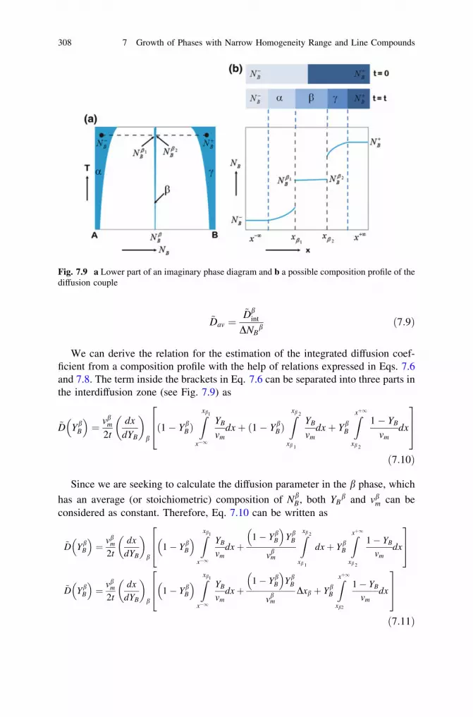
~Dav ¼~Db

int

DNBb ð7:9Þ

We can derive the relation for the estimation of the integrated diffusion coef-ficient from a composition profile with the help of relations expressed in Eqs. 7.6and 7.8. The term inside the brackets in Eq. 7.6 can be separated into three parts inthe interdiffusion zone (see Fig. 7.9) as

~D YbB

� �¼ vb

m

2t

dx

dYB

ffi �b

ð1� YbBÞZxb1

x�1

YB

vmdxþ ð1� Yb

BÞZxb 2

xb 1

YB

vmdxþ Yb

B

Zxþ1

xb 2

1� YB

vmdx

264

375

ð7:10Þ

Since we are seeking to calculate the diffusion parameter in the b phase, which

has an average (or stoichiometric) composition of NbB, both YB

b and vbm can be

considered as constant. Therefore, Eq. 7.10 can be written as

~D YbB

� �¼ vb

m

2t

dx

dYB

ffi �b

1� YbB

� � Zxb1

x�1

YB

vmdxþ

1� YbB

� �Yb

B

vbm

Zxb 2

xb 1

dxþ YbB

Zxþ1

xb 2

1� YB

vmdx

264

375

~D YbB

� �¼ vb

m

2t

dx

dYB

ffi �b

1� YbB

� � Zxb1

x�1

YB

vmdxþ

1� YbB

� �Yb

B

vbm

Dxb þ YbB

Zxþ1

xb2

1� YB

vmdx

264

375

ð7:11Þ

Fig. 7.9 a Lower part of an imaginary phase diagram and b a possible composition profile of thediffusion couple

308 7 Growth of Phases with Narrow Homogeneity Range and Line Compounds

The thickness of the b phase is Dxb ¼ xb 2 � xb 1 . Further, we can write

dx

dYB

ffi �b

¼ NþB � N�B� � dx

dNB

ffi �b

¼ NþB � N�B� � Dxb

DNbð7:12Þ

Replacing Eq. 7.12 in Eq. 7.11, we arrive at

~Dbint ¼ ~DDNb ¼

vbm

2tDxb NþB � N�B� �

� 1� YbB

� � Zxb1

x�1

YB

vmdxþ

1� YbB

� �Yb

B

vbm

Dxb þ YbB

Zxþ1

xb2

1� YB

vmdx

264

375

Since YB ¼ NB�N�BNþB �N�B

; YbB ¼

NbB�N�B

NþB �N�B; the above relation can be written as

~Dbint ¼

NBb � NB

�� �NBþ � NB

b� �

NBþ � NB

�Dxb� �2

2t

þ vmb

2tNBþ � NB

�ð Þ Dxb 1� YBb

� � Zxb1

x�1

YB

vmdxþ YB

bZxþ1

xb2

1� YB

vmdx

264

375

~Dbint ¼

NbB � N�B

� �NþB � Nb

B

� �NþB � N�B

Dxb

� �2

2t

þ Dxb

2t

NþB � NbB

NþB � N�B�Zxb1

x�1

vbm

vmNB � N�B� �

dxþ NbB � N�B

NþB � N�B�Zxþ1

xb2

vbm

vmNþB � NB

� �dx

264

375

ð7:13aÞ

Note here that the first term that is the term outside the bracket accounts for theprofile of the phase of interest (b) to calculate the integrated diffusion coefficient.The first term inside the bracket accounts for the composition profile of the phaseson the left-hand side, whereas the second term accounts for the phases present onthe right-hand side of the phase of interest b. Numerous cases contain many linecompounds or the phases with a narrow homogeneity in the interdiffusion zone.The composition profile in the solid solution in the ends of the couple might benegligible compared to the thickness of the phases with a narrow homogeneityrange. In that case, Eq. 7.13a can therefore be written as

7.2 Calculation of the Diffusion Parameters in Line Compounds 309

~Dbint ¼

NbB � N�B

� �NþB � Nb

B

� �NþB � N�B

Dxb� �2

2t

þ Dxb

2t

1NþB � N�B

NþB � NbB

� �Xb�1

i¼2

vbm

vim

Ni

B � N�B

� �Dxi þ Nb

B � N�B

� � Xn�1

i¼bþ1

vbm

vim

NþB � NiB

� �Dxi

" #

ð7:13bÞ

~Dbint ¼

NbB � N�B

� �NþB � Nb

B

� �NþB � N�B

kbp

þ Dxb

2t

1NþB � N�B

NþB � NbB

� �Xb�1

i¼2

vbm

vim

Ni

B � N�B

� �Dxi þ Nb

B � N�B

� � Xn�1

i¼bþ1

vbm

vim

NþB � NiB

� �Dxi

" #

ð7:13cÞ

since kbp ¼

Dxbð Þ22t . Note here that the end members are numbered as 1 and n. (n - 2)

phases––i.e., from 2 to (n - 1)—grow in the interdiffusion zone. As shownin Fig. 7.10, suppose three phases, a, b, and c grow and we wish to calculate theintegrated diffusion coefficient of the b phase. Equation 7.13b can then be expressedas

~Dbint ¼

a� b

aþ b

Dxb

� �2

2tþ Dxb

2t

1aþ b

bvb

m

vam

P

ffi �þ a

vbm

vcm

Q

ffi �� ð7:14aÞ

where a ¼ NBb � NB

�, b ¼ NþB � NbB, P ¼ DxaðNB

a � NB�Þ, and Q ¼ DxcðNþB � Nc

BÞ.The integrated diffusion coefficients for the a and the c phases can be estimated,

following Fig. 7.11 from

~Dinta ¼ c� d

cþ d

Dxa

� �2

2tþ Dxa

2t

1cþ d

d 0ð Þ þ cva

m

vmb

M þ vma

vmc

N

ffi �� ð7:14bÞ

where c ¼ NaB � N�B , d ¼ NB

þ � NBa,M ¼ DxbðNþB � Nb

BÞ, and N ¼ DxcðNþB � NcBÞ.

It should be noted here that the first term inside the bracket becomes zero as nophase(s) are present on the left-hand side of the phase of interest.

~Dcint ¼

e� f

eþ f

Dxc

� �2

2tþ Dxc

2t

1eþ f

fvc

m

vam

Rþ vcm

vbm

S

ffi �þ e 0ð Þ

� ð7:14cÞ

310 7 Growth of Phases with Narrow Homogeneity Range and Line Compounds

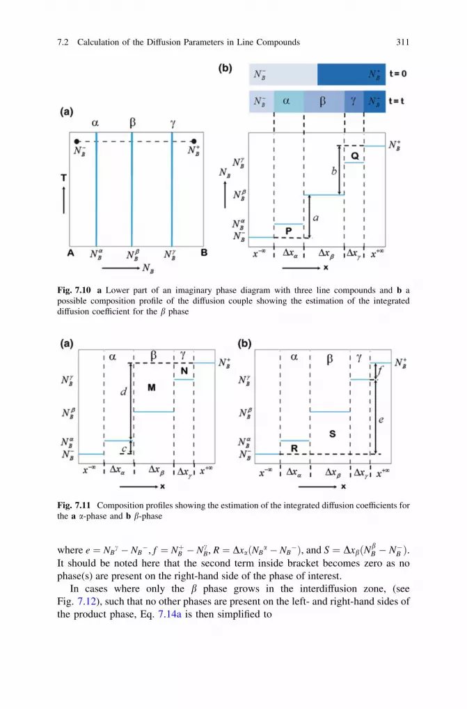
where e ¼ NBc � NB

�, f ¼ NþB � NcB, R ¼ DxaðNB

a � NB�Þ, and S ¼ DxbðNb

B � N�B Þ.It should be noted here that the second term inside bracket becomes zero as nophase(s) are present on the right-hand side of the phase of interest.

In cases where only the b phase grows in the interdiffusion zone, (seeFig. 7.12), such that no other phases are present on the left- and right-hand sides ofthe product phase, Eq. 7.14a is then simplified to

Fig. 7.10 a Lower part of an imaginary phase diagram with three line compounds and b apossible composition profile of the diffusion couple showing the estimation of the integrateddiffusion coefficient for the b phase

Fig. 7.11 Composition profiles showing the estimation of the integrated diffusion coefficients forthe a a-phase and b b-phase

7.2 Calculation of the Diffusion Parameters in Line Compounds 311

~Dbint ¼

a� b

aþ b

Dxb

� �2

2t¼ a� b

aþ bkb

p ð7:15Þ

where kpb is the parabolic growth constant of the b phase.

7.3 Calculation of the Average Interdiffusion Coefficient

Often, a phase grows in the interdiffusion zone, which has a composition range ofonly a few percent. Nevertheless, it still may not be possible to estimate thecomposition gradient with the minimum of error. For example, when Ni and Mowere coupled at 1,150 �C for 9 h, the interdiffusion zone developed with theNi(Mo) solid solution and the r phase following the phase diagram, as shown inFig. 7.13 [24]. After plotting the average smoothened composition profile on the

Fig. 7.12 Estimation of the integrated diffusion coefficient in an incremental diffusion couple isexplained for a a diffusion couple with two phase mixtures as the end members and b singlephases as the end members

312 7 Growth of Phases with Narrow Homogeneity Range and Line Compounds

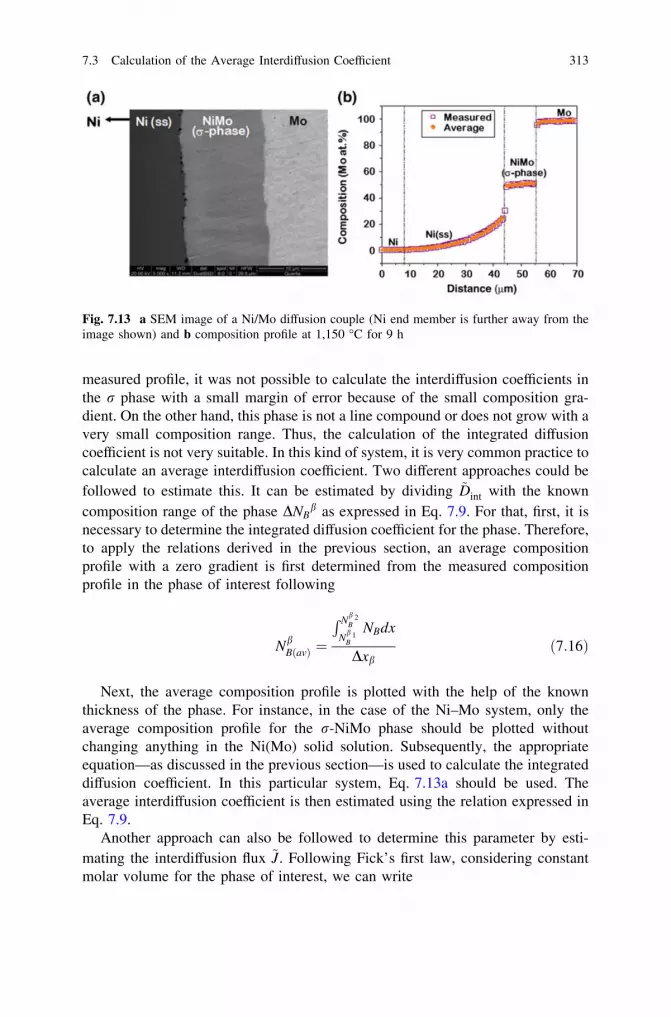
measured profile, it was not possible to calculate the interdiffusion coefficients inthe r phase with a small margin of error because of the small composition gra-dient. On the other hand, this phase is not a line compound or does not grow with avery small composition range. Thus, the calculation of the integrated diffusioncoefficient is not very suitable. In this kind of system, it is very common practice tocalculate an average interdiffusion coefficient. Two different approaches could befollowed to estimate this. It can be estimated by dividing ~Dint with the knowncomposition range of the phase DNB

b as expressed in Eq. 7.9. For that, first, it isnecessary to determine the integrated diffusion coefficient for the phase. Therefore,to apply the relations derived in the previous section, an average compositionprofile with a zero gradient is first determined from the measured compositionprofile in the phase of interest following

NbBðavÞ ¼

R Nb 2B

Nb 1B

NBdx

Dxbð7:16Þ

Next, the average composition profile is plotted with the help of the knownthickness of the phase. For instance, in the case of the Ni–Mo system, only theaverage composition profile for the r-NiMo phase should be plotted withoutchanging anything in the Ni(Mo) solid solution. Subsequently, the appropriateequation—as discussed in the previous section—is used to calculate the integrateddiffusion coefficient. In this particular system, Eq. 7.13a should be used. Theaverage interdiffusion coefficient is then estimated using the relation expressed inEq. 7.9.

Another approach can also be followed to determine this parameter by esti-mating the interdiffusion flux ~J. Following Fick’s first law, considering constantmolar volume for the phase of interest, we can write

Fig. 7.13 a SEM image of a Ni/Mo diffusion couple (Ni end member is further away from theimage shown) and b composition profile at 1,150 �C for 9 h

7.3 Calculation of the Average Interdiffusion Coefficient 313

~J ¼ �~DdC

dx¼ �~D

1

vbm

dNB

dxð7:17Þ

Generally, in a phase with a small composition range, the variation of the latticeparameters with composition is not known. Therefore, an average constant molarvolume is considered, which is estimated based on the lattice parameter data ofstoichiometric composition. Replacing Eqs. 7.17 and 7.7, we get

~Dbint ¼

ZNb 2B

Nb 1

B

~DdNB ¼� vbm

Zxb 2

xb 1

~Jdx ð7:18Þ

Therefore, ~Dbint can be estimated after calculating the variation of ~J with

composition and then integrating it over the length of the phase of interest. Thevalue ~J can be estimated using the relation developed by Den Broeder for theinterdiffusion coefficient (Eq. 6.26) expressed as

~D Y�C� �

¼ 12t

dx

dYC

ffi �Y�C

1� Y�C� � Zx�

x�1

YCdxþ Y�C

Zxþ1

x�

1� YCð Þdx

24

35

Since according to Eq. 6.16, the concentration-normalized variable is expressed

as YC ¼ CB�C�BCþB�C�B

~D Y�C� � dCB

dx¼

CþB � C�B� �

2t1� Y�C� � Zx�

x�1

YCdxþ Y�C

Zxþ1

x�

1� YCð Þdx

24

35

Therefore, using Fick’s first law, we can write

~J Y�C� �

¼ �CþB � C�B� �

2t1� Y�C� � Zx�

x�1

YCdxþ Y�C

Zxþ1

x�

1� YCð Þdx

24

35 ð7:19aÞ

After calculating the flux in the composition range of the phase of interest, theintegrated diffusion coefficient can be estimated by integrating the flux over thephase layer thickness in accordance with Eq. 7.18. This can also be estimatedusing the expression of the composition-normalized variable used by Wagner [8]to develop the relation for the interdiffusion coefficient, expressed by (Eq. 6.45)

314 7 Growth of Phases with Narrow Homogeneity Range and Line Compounds

~D Y�B� �

¼ v�m2t dYB=dxð ÞY�B

1� Y�B� � Zx�

x�1

YB

vmdxþ Y�B

Zxþ1

x�

1� YBð Þvm

dx

24

35

~DdNB

dx¼

v�m NþB � N�B� �

2t1� Y�B� � Zx�

x�1

YB

vmdxþ Y�B

Zxþ1

x�

1� YBð Þvm

dx

24

35

where YB ¼ NB�NB�

NBþ�NB

�. Fick’s first law, with the help of Eq. 1.150, can be written as

~J ¼ �~DdCB

dx¼ �~D

�vA

v2m

ffi �dNB

dx

Replacing this in the previous equation, we get

~J ¼ � �v�Av�m

NþB � N�B� �

2t1� Y�B� � Zx�

x�1

YB

vmdxþ Y�B

Zxþ1

x�

1� YBð Þvm

dx

24

35 ð7:19bÞ

If we consider a constant molar volume in the phase of interest, we can writev�m ¼ v�A. Therefore, the relation for the interdiffusion flux can be written as

~J ¼ �NþB � N�B� �

2tvm1� Y�B� � Zx�

x�1

YBdxþ Y�B

Zxþ1

x�

1� YBð Þdx

24

35 ð7:19cÞ

Note that for constant molar volume, Eq. 7.19a will be the same as Eq. 7.19c.We have noticed in many cases that the last approach that is the determination ofthe average interdiffusion coefficient by integrating the interdiffusion flux givessmaller error than averaging the composition profile following Eq. 7.16

7.4 Comments on the Relations Between the ParabolicGrowth Constants, Integrated and AverageInterdiffusion Coefficients

One important fact can be explained with the help of Eq. 7.15 and Fig. 7.12.Previously, we stated that the parabolic growth constant is not a material constant.In fact, the integrated diffusion coefficient is a material constant and it has a fixedvalue at a particular stoichiometric composition of the compound and the tem-perature. Moreover, this means that at a particular temperature, the integrateddiffusion coefficient is constant irrespective of the end-member composition.However, the parabolic growth constant or the thickness of the phase layer actually

7.3 Calculation of the Average Interdiffusion Coefficient 315

depends on the composition of the end members. It is explained in Fig. 7.12. Whenthe compositions of the end members are closer to the product phase, it will growwith a higher thickness compared to the one having a larger difference in the end-member composition. For example, we consider that the composition of theproduct phase b is NB

b ¼ 0:5. Suppose, in Fig. 7.12a, the end-member composi-tions are N�B ¼ 0:45 and NB

þ ¼ 0:55. Therefore, from Eq. 7.15, the parabolicgrowth constant in this case would be

kbpðaÞ ¼

0:100:05� 0:05

� ~Dbint ð7:20aÞ

In the second case, as shown in Fig. 7.12b, suppose the end-member compo-sitions are N�B ¼ Na

B ¼ 0:35 and NþB ¼ NcB ¼ 0:65. We can write

kbpðbÞ ¼

0:300:15� 0:15

� ~Dbint ð7:20bÞ

Therefore, for the same annealing time, we can write

kbpðaÞ

kbpðbÞ

¼ 0:100:30� 0:15� 0:15

0:05� 0:05¼ 3 ð7:20cÞ

This now means that the parabolic growth constant in the first case will be 3times higher. If the annealing time is the same, the ratio of the layer thickness willbe (since Dx2 ¼ 2kpt)

DxbðaÞDxbðbÞ

¼ffiffiffi3p¼ 1:73 ð7:20dÞ

This indicates that in the first diffusion couple, the layer thickness will be 1.73times higher than the second diffusion couple. A physical explanation for this canbe easily understood. In the first case (Fig. 7.12a), the end members have a phasemixture of (a + b) and (b + c) between which the b phase grows. The componentA dissociates from the a phase at one interface and then diffuses through the b phaseto reach to the other interface and reacts with the c phase to produce the b phase.Similarly, B dissociates from the c phase and then diffuses to other phase and reactswith the a phase to produce the b phase. In this way, dissociation and reaction of thea and c phases produces the b phase. Moreover, the b phase that already exists in theend members directly adds to the b product phase in the interdiffusion zone. On theother hand, in the second case (Fig. 7.12b), the b phase is not present in the endmembers. The product b phase grows by dissociation and reaction only. Therefore,the growth rate in the first case is higher, which is shown by the derivations above.Read Chap. 8 for a better understanding of such mechanisms.

Furthermore, it also should be noted that, in an incremental diffusion couple (ifonly one phase grows), the thickness of the phase layer is always higher than the

316 7 Growth of Phases with Narrow Homogeneity Range and Line Compounds

thickness of the same phase grown in a multiphase interdiffusion zone. In fact,many times, we are not able to calculate the diffusion parameter of a phase in amultiphase interdiffusion since it does not grow with reasonable thickness. Todetermine the diffusion parameter with a smaller error in that phase, an incrementaldiffusion couple is conducted such that the phase of interest grows with a higherthickness [25–27]. This can be understood from Eq. 7.13c. In an incrementalcouple, only the first part of the equation is relevant, whereas in multiphase growth,the first part is related to the phase of interest and the second part is relevant for theother phases. In an incremental couple, the components can dissociate at theinterfaces and diffuse through the phase of interest only for the growth of this phase.On the other hand, in a couple with multiphase growth, the components have todiffuse through all the phases, which grow together but at different rates. Moreover,simultaneous growth and consumption process at the interfaces make the diffusionprocess very complicated, which will be discussed in detail in Chap. 8. In fact,Wagner [8] named the parabolic growth constant estimated in a diffusion couple ofend members with pure components as the parabolic growth constant of the firstkind, kI

P. When the parabolic growth constant is estimated in an incremental dif-fusion couple with a single phase in the interdiffusion zone, it is referred to as theparabolic growth constant of the second kind, kII

P .Here, two important facts should be noted. In two different incremental diffu-

sion couples with different end-member compositions, when the same phase growsin an interdiffusion zone, the parabolic growth constant values will be different.After measuring the growth rate at different temperatures, when the parabolicgrowth constants are plotted following the Arrhenius equation, as expressed inEq. 7.3, the difference will be in the pre-exponential factor only. The activationenergy for the parabolic growth will be same in both the cases. However, when thegrowth of a particular phase is compared between an incremental couple and thecouple with the end members where other phase(s) also grow (multiphase growth),the key values—i.e., the parabolic growth constants, the pre-exponential factors,and the activation energies—will all be different. This is the reason why theparabolic growth constant is not a material constant but rather depends on thecomposition of the end members. On the other hand, the integrated diffusioncoefficient is a material constant and it is the same for a particular phase, irre-spective of the end-member composition. In fact, a phase under different condi-tions grows such that the integrated diffusion coefficient is the same.

To continue with the discussion on the activation energy for the parabolicgrowth constant and the integrated diffusion coefficient, another important factshould be noted. Replacing Eq. 7.3 in Eq. 7.15, we obtain

~Dint ¼a� b

aþ b� ko

p exp � Qg

RT

ffi �ð7:21aÞ

Similarly, the Arrhenius equation for the integrated interdiffusion coefficientcould be written as

7.4 Comments on the Relations 317

~Dint ¼ ~Doint exp �QD

RT

ffi �ð7:21bÞ

By comparing the relations above, it can be easily understood that when in anincremental diffusion couple a single phase grows in the interdiffusion zone, theactivation energy for both—the parabolic growth constant and the integrateddiffusion coefficient—is the same. The difference is in the pre-exponential termsonly. However, it is not true for the phase when it grows with other phases in theinterdiffusion zone. In multiphase growth, the parabolic growth constant of a phaseis nonetheless estimated directly from the measured thickness of that phase only.However, for the calculation of the integrated diffusion coefficient, the thicknessand the composition of the other phases are also used, as explained in Eq. 7.13a. Inmultiphase growth, when one particular phase grows with a much higher thicknessthan that of the other thin phases, we have seen that the difference between theactivation energies of the parabolic growth constants and the integrated diffusioncoefficients is much less for the thick phase. However, it could be significantlydifferent in the case of a phase with much lower thickness. The comments aboveare also true when the activation energy for the parabolic growth constants and theaverage interdiffusion coefficients are compared. These are shown in the Fe–Nbsystem, as presented in Fig. 7.14 for the NbFe2 and NbFe phases. The NbFe2 phasegrows with a much higher thickness, and there is not much difference in theactivation energy for the parabolic growth constant and the average interdiffusioncoefficient. On the other hand, the NbFe phase grows with a small thickness andthere is a high difference in the activation energies [28].

In many cases, for example, during the interaction of Cu with Sn-based solder,as shown in Fig. 7.15 [29], where two phases Cu3Sn and Cu6Sn5 grow in theinterdiffusion zone, we cannot estimate the diffusion parameters. Although thesolder is a multicomponent alloy, only Sn from the solder along with the Cu fromthe Cu printed wiring board takes part in the interdiffusion process. We may feeloptimistic that it is possible to estimate the diffusion parameters by considering itas a binary Cu/Sn system. However, we cannot do so. It should be noted here thatthe condition for the use of the relations derived for the calculation of the diffusionparameters is valid only when we are able to measure the concentration profile upto the unaffected zone in the couple. It is not possible to estimate exactly howmuch length is affected in the solder alloy, and it is even almost impossible to findthe average composition profile because of presence of a phase mixture.

When only one phase layer grows in the interdiffusion zone, in such couples, itis common practice to calculate the interdiffusion coefficient using the relation

Dx ¼ 2ffiffiffiffiffi~Dtp

. This relation is written based on the error function analysis explainedpreviously in Chap. 3, with the consideration that the interdiffusion coefficient isconstant. However, sometimes, this relation is used even when more than onephase layer grows at the interface. This is incorrect, since in this calculation, thediffusion parameter for the phase of interest is incorrectly estimated withoutconsidering the growth of the other phases. Sometimes, one interdiffusion

318 7 Growth of Phases with Narrow Homogeneity Range and Line Compounds

coefficient is estimated taking the thickness of all the phases together. Note thatthis is also not correct, since different phases have different compositions and theywill have different diffusion coefficients and perhaps different diffusion mecha-nisms. We commented previously, that when all the phases grow parabolicallywith time, the total thickness of the interdiffusion zone would also be parabolicwith time. By considering this fact, sometimes, the activation energy for growth is

(a) (b)

(d)(c)

(e) (f)

Fig. 7.14 a Fe/Nb diffusion couple annealed at 1,150 �C for 25 h, b measured compositionprofile, Arrhenius plots of the parabolic growth constants for c NbFe2 and d NbFe phases,Arrhenius plots of the average interdiffusion coefficients for e NbFe2 and f NbFe phases

7.4 Comments on the Relations 319

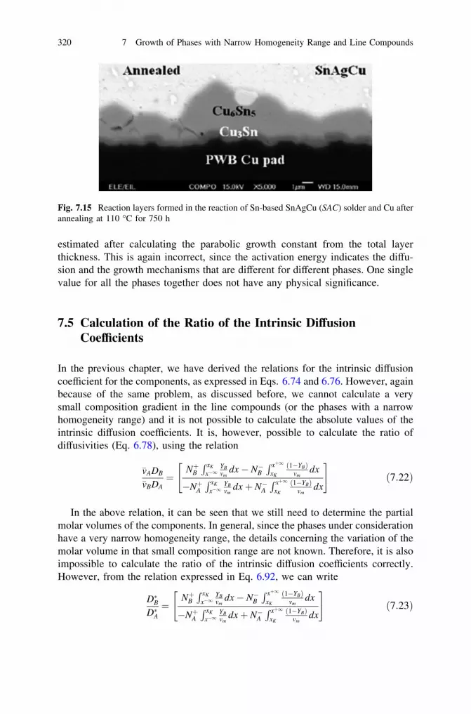
estimated after calculating the parabolic growth constant from the total layerthickness. This is again incorrect, since the activation energy indicates the diffu-sion and the growth mechanisms that are different for different phases. One singlevalue for all the phases together does not have any physical significance.

7.5 Calculation of the Ratio of the Intrinsic DiffusionCoefficients

In the previous chapter, we have derived the relations for the intrinsic diffusioncoefficient for the components, as expressed in Eqs. 6.74 and 6.76. However, againbecause of the same problem, as discussed before, we cannot calculate a verysmall composition gradient in the line compounds (or the phases with a narrowhomogeneity range) and it is not possible to calculate the absolute values of theintrinsic diffusion coefficients. It is, however, possible to calculate the ratio ofdiffusivities (Eq. 6.78), using the relation

�vADB

�vBDA¼

NþBR xK

x�1YBvm

dx� N�BR xþ1

xK

1�YBð Þvm

dx

�NþAR xK

x�1YBvm

dxþ N�AR xþ1

xK

1�YBð Þvm

dx

" #ð7:22Þ

In the above relation, it can be seen that we still need to determine the partialmolar volumes of the components. In general, since the phases under considerationhave a very narrow homogeneity range, the details concerning the variation of themolar volume in that small composition range are not known. Therefore, it is alsoimpossible to calculate the ratio of the intrinsic diffusion coefficients correctly.However, from the relation expressed in Eq. 6.92, we can write

D�BD�A¼

NþBR xK

x�1YBvm

dx� N�BR xþ1

xK

1�YBð Þvm

dx

�NþAR xK

x�1YBvm

dxþ N�AR xþ1

xK

1�YBð Þvm

dx

" #ð7:23Þ

Fig. 7.15 Reaction layers formed in the reaction of Sn-based SnAgCu (SAC) solder and Cu afterannealing at 110 �C for 750 h

320 7 Growth of Phases with Narrow Homogeneity Range and Line Compounds

Thus, at the location of the Kirkendall marker plane, we can calculate directlythe ratio of the tracer diffusion coefficients. However, again, in Eq. 7.23, we havedisregarded the contribution from the vacancy wind effect. Considering thevacancy wind effect, Eq. 7.23 can be written correctly as

D�B 1�WBð ÞD�A 1þWAð Þ ¼

NþBR xK

x�1YBvm

dx� N�BR xþ1

xK

1�YBð Þvm

dx

�NþAR xK

x�1YBvm

dxþ N�AR xþ1

xK

1�YBð Þvm

dx

" #ð7:24Þ

where Wi ¼ 2NiðD�A�D�BÞMoðNAD�AþNBD�BÞ

.

For most intermetallic compounds that have a complicated crystal structure, thevalue of the structure factor Mo is not readily available. For this reason, wecalculate the ratio of the tracer diffusion coefficients using the relation expressed inEq. 7.23, i.e., by neglecting the role of the vacancy wind effect. Because of thisassumption, we cannot estimate the ratio of the tracer diffusion coefficients cor-rectly; however, it is still very useful, to understand the atomic mechanism ofdiffusion. In many cases, this does not greatly affect the estimated values and errorfalls within the limit of experimental error that one typically expects from theexperimental procedure.

The calculation procedures to determine the ratio of the tracer diffusion coef-ficients are explained in Fig. 7.16. Note here that we need to calculate the integrals

U ¼R xK

x�1YBvm

dx and W ¼R xþ1

xK

1�YBð Þvm

dx on the either side of the Kirkendall marker

plane, located at xK , and indicated by the white dotted markers on the schematicdiffusion couple. When we calculate the ratio of the tracer diffusion coefficients ina line compound by neglecting the contribution of the vacancy wind effect,Eq. 7.23 can be rewritten as

D�BD�A¼ NþB U� N�B W�NþA Uþ N�A W

� ð7:25Þ

In few cases, such as that presented in Fig. 7.16a, there could be a phase ofinterest with narrow composition range in which the marker plane is located. Onboth sides of this phase, composition varies continuously. In this case, the valuesof U and W are

U ¼Zxb 1

x�1

NB � N�B� �

vmdxþ

NbB � N�B

� �

vbm

Dxb1

0@

1A ¼

Zxb 1

x�1

NB � N�B� �

vmdxþ R1

vbm

0@

1A

ð7:26aÞ

W ¼Zxþ1

xb 2

NþB � NBð Þvm

dxþNþB � Nb

B

� �

vbm

Dxb2

0B@

1CA ¼

Zxþ1

xb 2

NþB � NBð Þvm

dxþ S 1

vbm

0B@

1CA ð7:26bÞ

7.5 Calculation of the Ratio of the Intrinsic Diffusion Coefficients 321

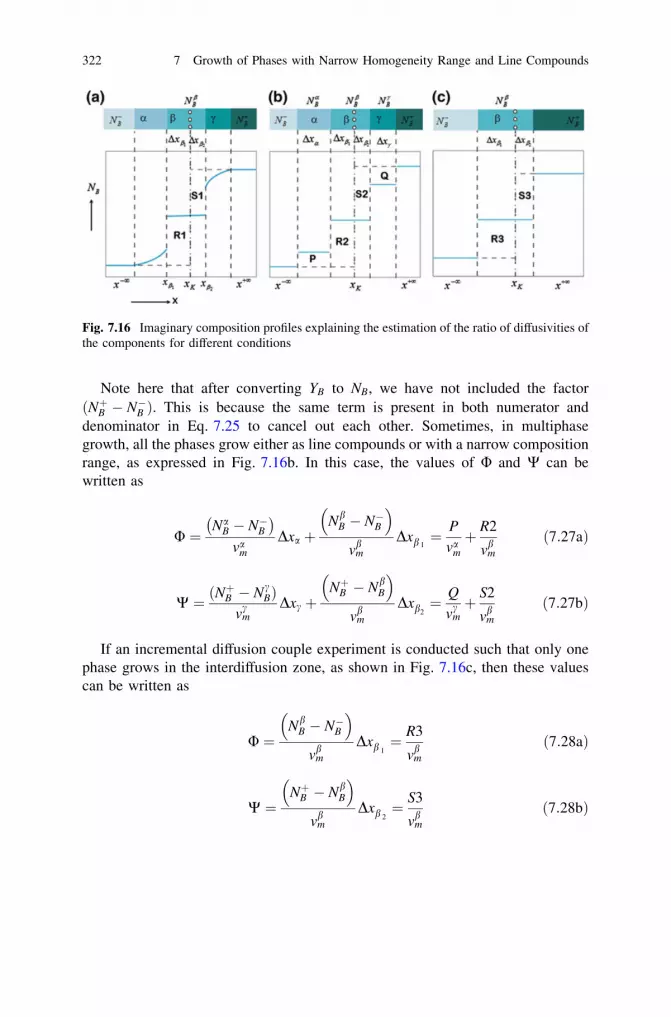
Note here that after converting YB to NB, we have not included the factorðNþB � N�B Þ. This is because the same term is present in both numerator anddenominator in Eq. 7.25 to cancel out each other. Sometimes, in multiphasegrowth, all the phases grow either as line compounds or with a narrow compositionrange, as expressed in Fig. 7.16b. In this case, the values of U and W can bewritten as

U ¼Na

B � N�B� �

vam

Dxa þNb

B � N�B

� �

vbm

Dxb 1¼ P

vam

þ R2

vbm

ð7:27aÞ

W ¼ NþB � NcBð Þ

vcm

Dxc þNþB � Nb

B

� �

vbm

Dxb2¼ Q

vcmþ S2

vbm

ð7:27bÞ

If an incremental diffusion couple experiment is conducted such that only onephase grows in the interdiffusion zone, as shown in Fig. 7.16c, then these valuescan be written as

U ¼Nb

B � N�B

� �

vbm

Dxb 1¼ R3

vbm

ð7:28aÞ

W ¼NþB � Nb

B

� �

vbm

Dxb 2¼ S3

vbm

ð7:28bÞ

Fig. 7.16 Imaginary composition profiles explaining the estimation of the ratio of diffusivities ofthe components for different conditions

322 7 Growth of Phases with Narrow Homogeneity Range and Line Compounds

7.6 Calculation of the Tracer Diffusion Coefficients

The previous chapter contained an explanation of the procedure for estimating thetracer diffusion coefficients in a diffusion couple indirectly by using the interdif-fusion coefficients, the ratio of the intrinsic diffusion coefficients, and the ther-modynamic factor. It can also be estimated directly (without calculating theinterdiffusion coefficient) by using the absolute values of the intrinsic diffusioncoefficients and the thermodynamic factor. As explained in the previous section,we can estimate only the ratio of the tracer diffusion coefficients in the phases witha narrow homogeneity range. Consequently, we need to relate the integrated dif-fusion coefficients with the ratio of the tracer diffusion coefficients and thermo-dynamic parameters (driving forces) to estimate the absolute values of the tracerdiffusion coefficients. We consider a hypothetical incremental diffusion couple of aand c, as shown in Fig. 7.17, where only a single b phase grows at the interface.Further, a is A-rich phase and c is B-rich phase. This means that A dissociates froma at the interface I and then diffuses to the interface II. At this interface, A reactswith c to produce the b phase. Concurrently, B dissociates from c and then diffusesto the interface I. At this interface, it reacts with a to produce the b phase. From thechemical potential point of view (see Chaps. 1 and 4), A diffuses from the inter-faces I to II because lI

A [ lIIA . Simultaneously, B diffuses from the interface II to I

because lIIB [ lI

B, as explained in Fig. 7.17. Replacing the relation between theinterdiffusion coefficient and the tracer diffusion coefficient as expressed in Eq. 6.90(see Chap. 6) in Eq. 7.7, we get

~Dint ¼ZNb 2

B

Nb 1B

NbAD�B þ Nb

BD�A

� � d ln aB

d ln NB

ffi �dNB

~Dint ¼ZaII

B

aIB

NbAD�B þ Nb

BD�A

� �Nb

Bd ln aB

ð7:29Þ

where aBI and aII

B are the activities of the component B at the interfaces I and II,respectively. Since we are considering an average composition of the phase with avery narrow homogeneity range and at that composition, it will have the fixedtracer diffusion coefficient of the components. This can therefore be written as

~Dint ¼ZaII

B

aIB

NbAD�B þ Nb

BD�A

� �Nb

Bd ln aB ¼ NbAD�B þ Nb

BD�A

� �Nb

B ln aIIB � ln aI

B

� �

ð7:30Þ

7.6 Calculation of the Tracer Diffusion Coefficients 323

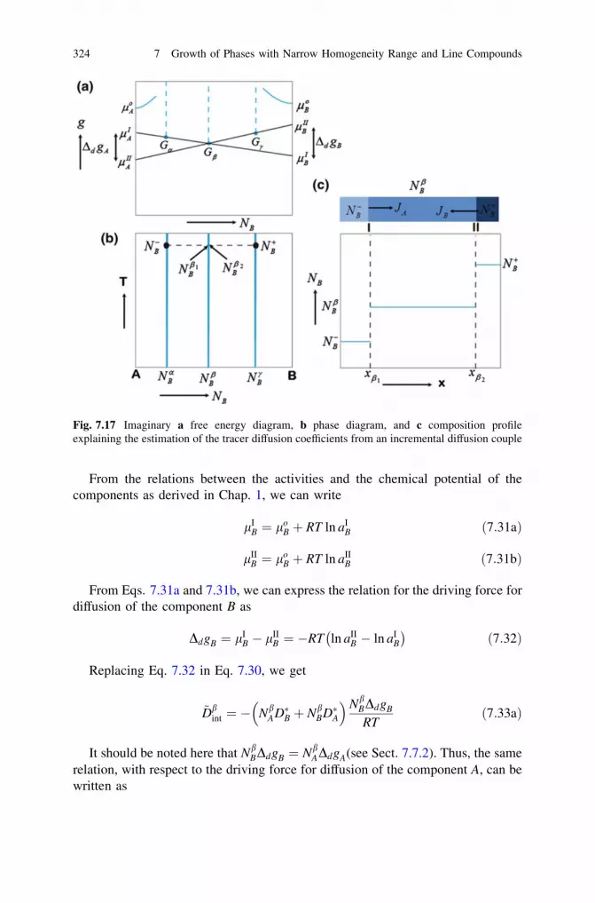
From the relations between the activities and the chemical potential of thecomponents as derived in Chap. 1, we can write

lIB ¼ lo

B þ RT ln aIB ð7:31aÞ

lIIB ¼ lo

B þ RT ln aIIB ð7:31bÞ

From Eqs. 7.31a and 7.31b, we can express the relation for the driving force fordiffusion of the component B as

DdgB ¼ lIB � lII

B ¼ �RT ln aIIB � ln aI

B

� �ð7:32Þ

Replacing Eq. 7.32 in Eq. 7.30, we get

~Dbint ¼ � Nb

AD�B þ NbBD�A

� �NbBDdgB

RTð7:33aÞ

It should be noted here that NbBDdgB ¼ Nb

ADdgA(see Sect. 7.7.2). Thus, the samerelation, with respect to the driving force for diffusion of the component A, can bewritten as

Fig. 7.17 Imaginary a free energy diagram, b phase diagram, and c composition profileexplaining the estimation of the tracer diffusion coefficients from an incremental diffusion couple

324 7 Growth of Phases with Narrow Homogeneity Range and Line Compounds

~Dbint ¼ � Nb

AD�B þ NbBD�A

� �NbADdgA

RTð7:33bÞ

If the product phase b grows between the pure end members A and B such thatno other phases are present in the phase diagram, it is possible to write Eq. 7.33aas

~Dbint ¼ � Nb

AD�B þ NbBD�A

� �Df gb

RTð7:34Þ

whereDf gb is the free energy for the formation of the b phase. Therefore, byestimating the ratio of the tracer diffusion coefficients, the integrated diffusioncoefficients, and the driving force for diffusion of the components, the absolutevalues of the tracer diffusion coefficients can be estimated.

One important fact should be noted here that the integrated diffusion coeffi-cients and the ratio of the tracer diffusion coefficients could be estimated from anytype of diffusion couple—whether an incremental diffusion couple or a couplewith pure end members. However, the driving force for diffusion should be esti-mated considering the growth of the product phase in an incremental couple fromthe adjacent phases in the phase diagram. Similarly, even if the diffusion param-eters in the product b phase are estimated in an incremental couple with phasemixtures of a + b and b + c as the end members (for, e.g., see Fig. 7.12a), thedriving force for diffusion should be estimated as if the layer is grown between thepure a and c phases as the end members. Note here that the diffusion coefficientsare the material constants and would have the same values irrespective of thedifferent end members.

7.7 The Kirkendall Marker Velocity in a Line Compound

In the previous chapter, we have derived the relation for the velocity of the markerplane (Eq. 6.61) as

vK ¼ �vB DB � DAð Þ oCB

ox

ffi �K

ð7:35Þ

Since we cannot determine the absolute values of the intrinsic diffusion coef-ficients in the line compound, the relation must be derived differently. Usingstandard thermodynamic relations (Eq. 1.150) together with Eq. 7.35, the fol-lowing can be written

7.6 Calculation of the Tracer Diffusion Coefficients 325

vK ¼�vA�vB

v2m

DB � DAð Þ oNB

ox

ffi �K

ð7:36Þ

Integrating Eq. 7.36 over the composition range from NBb 1 to Nb 2

B and theposition range (that is the thickness) from xb 1 to xb 2 ,

Zxb 2

xb 1

vKdx ¼ZNb 2

B

Nb 1B

�vA�vB

v2m

DB � DAð ÞdNB ð7:37Þ

Further, we know from Eq. 6.65 that

~Dvm ¼ NA�vADB þ NB�vBDA ð7:38Þ

Using Eq. 7.38 in Eq. 7.37, we arrive at

vKDxb ¼�vA�vB

v2m

DB � DAð ÞZNb2

B

Nb1B

~Dvm

NA�vADB þ NB�vBDAdNB

Here, we are considering the phase with a narrow homogeneity range or a linecompound with an almost fixed or an average composition. Consequently, it ispossible to consider the intrinsic diffusion coefficients and molar volume of the bphase as more or less constant. It will, therefore, almost have a fixed velocity.Thus, we can write

vKDxb ¼�vA�vB

vm

DB � DA

NA�vADB þ NB�vBDA

ZNb2B

Nb1B

~DdNB ð7:39Þ

From the definition of the integrated diffusion coefficient (Eq. 7.7) and dividingboth numerator and denominator by �vBDA in Eq. 7.39, the velocity can be writtenas [30]

vK ¼�vA

vm

DBDA� 1

�vADB�vBDA

� �NA þ NB

~Dint

Dxbð7:40Þ

Again, it is almost impossible to calculate the partial molar volumes of thephase and the exact velocity is thus impossible to calculate. Mostly, we considervm ¼ �vA ¼ �vB and calculate the velocity of the marker plane in a line compound. Itcan be seen that to calculate the velocity of the marker plane, it is first necessary to

326 7 Growth of Phases with Narrow Homogeneity Range and Line Compounds

calculate the intrinsic (or the ratio of the intrinsic) diffusion coefficient from thecomposition profile. We can derive a simpler relation to estimate this valuedirectly from the composition profile. We denote / ¼

Rx�1

xK Yvm

dx and

w ¼R xþ1

xK

1�Yvm

dx. Therefore, the relation for the intrinsic diffusion coefficients, as

expressed in Eqs. 6.75 and 6.77, can be written as

DB ¼12t

v2m

�vA

ox

oNB

ffi �K

NþB /� N�B w� �

ð7:41aÞ

DA ¼12t

v2m

�vB

ox

oNA

ffi �K

NþA /� N�A w� �

ð7:41bÞ

Replacing Eq. 7.41a, b in Eq. 7.36, we get

vK ¼�vA�vB

v2m

12t

v2m

�vA

ox

oNB

ffi �K

NþB /� N�B w� �

� 12t

v2m

�vB

ox

oNA

ffi �K

NþA /� N�A w� ��

oNB

ox

ffi �K

Since NA þ NB ¼ 1 that is dNA þ dNB ¼ 0, we can write

vK ¼12t

�vB NþB /� N�B w� �

þ �vA NþA /� N�A w� �� �

vK ¼12t

�vBNþB þ �vANþA� �

/� �vBN�B þ �vAN�A� �

w� � ð7:42aÞ

In a diffusion couple with pure components as end members, N�B ¼ 0, NA� ¼ 1,

NþB ¼ 1, and NþA ¼ 0. Therefore, Eq. 7.42a reduces to [26]

vK ¼12t

�vB/� �vAw½ � ð7:42bÞ

The advantage of using Eq. 7.42a is that this makes it possible to determine thevelocity of the marker plane directly from the Y/vm versus x plot. Furthermore, thisrelation can be used in any phase with wide homogeneity range or a line com-pound. In order to calculate the partial molar volumes in a line compound or in aphase where the variation of the molar volume with composition is not known, theapproximate velocity of the marker plane can be estimated by considering�vB ¼ �vA ¼ vm.

It should be noted here that we have composition jumps between the endmembers and the product phases in multiphase growth. Mathematically, wecannot differentiate the composition profile anywhere if it is not continuousat some points. Therefore, we actually assume a sharp, but continuouschange in composition at those points. On the other hand, we highlight that

7.7 The Kirkendall Marker Velocity in a Line Compound 327

all important relations, i.e., those for the estimation of the integrated diffu-sion coefficient using Eq. 7.13a, the interdiffusion flux using Eq. 7.19a, andthe ratio of diffusivities by Eqs. 7.22 and 7.23, were derived without anydifferentiation of the composition profile, and thus, the obtained formulas aremathematically correct.

7.8 Case Studies

7.8.1 Calculation of the Integrated and the Ratioof the Tracer Diffusion Coefficients

We consider a diffusion couple of Nb/Si annealed at 1,250 �C for 24 h [27].According to the phase diagram shown in Fig. 7.18a, two phase layers Nb5Si3 andNbSi2 are expected to grow at the interface, as can be seen in Fig. 7.18b.According to the composition analysis, the composition profile in the Nb(Si) andSi(Nb) was negligible and can be neglected. Since the phases are actually linecompounds, the composition profile can be drawn after measuring the thickness ofthe phase layers, as shown in Fig. 7.19a. ‘‘K’’ denotes the location of the Kir-kendall marker plane. Therefore, we can calculate the integrated diffusion coef-ficients for both the phases and the ratio of the tracer diffusion coefficients inthe NbSi2 phase. The thicknesses of the phase layers are mentioned in the profile.The calculated molar volumes of the phases are vNb5Si3

m ¼ 9:6� 10�6 andvm

NbSi2 ¼ 8:7� 10�6 m3=mol.The integrated diffusion coefficients can be estimated as (see Fig. 7.19b, c)

~DNb5Si3int ¼ a� b

aþ b

Dx2Nb5Si3

2tþ DxNb5Si3

2t

b 0ð Þ þ a vNb5Si3m

vNbSi2m

P� �

aþ b

24

35 ¼ 4:4� 10�16 m2=s

where a ¼ 38� 0 ¼ 3

8, b ¼ 1� 38 ¼ 5

8, DxNb5Si3 ¼ 4:7� 10�6 m, 2t ¼ 2� 24� 60�60 ¼ 172; 800 s, and P ¼ 1� 2

3

� �� 110:2� 10�6 m.

~DNbSi2int ¼ c� d

cþ d

Dx2NbSi2

2tþ DxNbSi2

2t

d vNbSi2m

vNb5Si3m

Q� �

þ c 0ð Þcþ d

264

375 ¼ 1:6� 10�14 m2=s

where c ¼ 23� 0 ¼ 2

3, d ¼ 1� 23 ¼ 1

3, DxNb5Si3 ¼ 110:2� 10�6 m, 2t ¼ 2�24�60�60 ¼ 172; 800 s, and Q ¼ 1� 3

8

� �� 4:7� 10�6 m.

328 7 Growth of Phases with Narrow Homogeneity Range and Line Compounds

Fig. 7.18 a Nb–Si phase diagram [31] and b Nb/Si diffusion couple annealed at 1,250 �C for24 h [27]

Fig. 7.19 Estimation of the diffusion parameters from the composition profile in the Nb–Sisystem is explained. a Composition profile, estimation of the integrated diffusion coefficient forb Nb5Si3, c NbSi2, and d estimation of the ratio of diffusivities in the NbSi2 phase

7.8 Case Studies 329

The ratio of the diffusivities can be estimated as (see Fig. 7.19d)

D�Si

D�Nb

¼ NþSiU� N�SiW�NþNbUþ N�NbW

� ¼ 4:62

where U ¼ Mv

Nb5Si3m

þ Nv

NbSi2m

, W ¼ Rv

NbSi2m

, M ¼ 38� 0� �

� 4:7� 10�6 m, N ¼ 23� 0� �

�76:2� 10�6 m, R ¼ 1� 2

3

� �� 34� 10�6 m, N�Si ¼ 0, NSi

þ ¼ 1, N�Nb ¼ 1, andNNb

þ ¼ 0.

7.8.2 Calculation of the Absolute Values of the TracerDiffusion Coefficients

Let us consider the incremental diffusion couple between Co0.48Si0.52 and Si [25,30]. From the Co–Si phase diagram shown in Fig. 7.20a [31], it can be seen thatthe Co0.48Si0.52 alloy consists of two phases, CoSi and CoSi2. Therefore, in thediffusion couple, as expected, only the CoSi2 phase is grown, as shown inFig. 7.20b. The couple was annealed at 1,186 �C for 100 h. ThO2 particles wereused to detect the location of the Kirkendall marker plane. The length of the phaselayer on either side of the marker plane is shown. With the aim of calculating theabsolute values at the Kirkendall marker plane, we should first determine theintegrated diffusion coefficients and the ratio of the tracer diffusion coefficients.These are

~DCoSi2int ¼ ab

aþ b

Dx2CoSi2

2t

¼ ð2=3� 0:52Þð1� 2=3Þ1� 0:52

154:4� 10�6� �2

2� 100� 60� 60¼ 3:3� 10�15 m2=s

vCo

vSi

DSi

DCo

¼ D�Si

D�Co

¼ NþSiR� N�SiS

�NþCoRþ N�CoS

�

¼ 1� ð2=3� 0:52Þ � 102:2� 0:52� 1� 2=3ð Þ � 52:2�0� 2=3� 0:52ð Þ � 102:2þ 0:48� ð1� 2=3Þ � 52:2

� ¼ 0:7

Now, we need to calculate the driving force for diffusion of the componentsthrough the CoSi2 phase. As mentioned earlier, we need to consider as if theproduct phase is grown between the pure CoSi and Si end members. Since thediffusion parameters are the material constants, the values estimated above wouldbe the same. The free energy of the phases at 1,186 �C is estimated using thethermodynamic parameters, as listed in Table 7.1. First, the enthalpy and theentropy at the temperature of interest are estimated using the relations

330 7 Growth of Phases with Narrow Homogeneity Range and Line Compounds

hT ¼ h298 þZT

298

CPdT ð7:43aÞ

sT ¼ s298 þZT

298

CP

TdT ð7:43bÞ

where Cp ¼ Aþ BT � CT2

Fig. 7.20 a Co–Si phase diagram, b Co0.48Si0.52/Si diffusion couple annealed at 1,186 �C for100 h, c composition profile, and d the estimation of the driving forces [25, 30]

Table 7.1 Thermodynamic parameters in Co–Si system are tabulated

Details of Cp values

CoSi CoSi2 Si

A 49.16 70.86 23.698B 9 10-3 12.1 I8.66 3.305C 9 105 7.54 9.93 4.351S298 43.2 J/mol.K 64.2 J/mol.K 18.81 J/mol.Kh298 -94,600 J (mole of CoSi) -98,700 J (mole of CoSi2) 0

7.8 Case Studies 331

After this, the free energies of the phases are estimated using the relationg = h - Ts. The values are estimated as g(CoSi) = -218,714.9 J/mole ofCoSi, g(CoSi2) = -281,727.8 J/mol of CoSi2, and g(Si) = -54,814.57 J/moleof atom. To estimate the driving forces from a free energy diagram—which isdrawn with respect to per mol of atom—it is necessary to divide the values ofg estimated for CoSi and CoSi2 by the number of atoms in the compound that is2 and 3, respectively. This leads to g(CoSi) = -109,357.45 J/mole of atom andg(CoSi2) =-93,909.27 J/mole of atom. We can use the estimated value of the Sifree energy as it is. After plotting the values, as shown in Fig. 7.20d, we getDdgSi = -8,199 J/mol of Si atom and DdgCo = -16,398 J/mol of Co atom.Previously, we stated that NSiDdgSi ¼ NCoDdgCo. It can be seen that this is truesince NSi ¼ 2=3 and NCo ¼ 1=3. Next, the absolute values of the tracer diffusioncoefficients are determined using the relations

~Dint ¼ 3:3� 10�15 m2=s ¼ � NCoD�Si þ NSiD�Co

� �NSiDdgSi

RTD�Si

D�Co

¼ 0:7

The values are estimated as D�Co ¼ 8:25� 10�15 m2=s; D�Si ¼ 5:77�10�15 m2=s.

The estimated values of the driving forces demonstrate that NSiDdgSi ¼NCoDdgCo. We can demonstrate that this is true in a different way with respect tothe reaction/diffusion at the interfaces. This is explained with the help of Fig. 7.21.It can be seen that Si diffuses to the interface I and reacts with CoSi to produce theCoSi2 phase. Co dissociates at the same interface from CoSi to produce theproduct phase at the same interface. The dissociated Co diffuses through the CoSi2product phase and reacts with Si at the interface II to produce the CoSi2 productphase. In terms of a reaction at the interfaces, we can write

Interface I

2CoSi ¼ Co½ �dþCoSi2 ð7:44aÞ

CoSi þ Si½ �d¼ CoSi2 ð7:44bÞ

Interface II

2Si þ Co½ �d¼ CoSi2 ð7:44cÞ

Note here that the above interface reactions do not control the growth of thephase. Rather, the diffusion of the components through the product phase controlsthe growth process. From Eq. 7.44b, we can write the energy change per mol ofmoving Si atom as

332 7 Growth of Phases with Narrow Homogeneity Range and Line Compounds

DdgSi ¼ g CoSi2ð Þ � g CoSið Þ � g Sið Þ ð7:45aÞ

Since the same Co atoms are involved in producing the product phase at bothinterfaces, by adding Eqs. 7.44a and 7.44c, we can write

2CoSi þ 2Si ¼ 2CoSi2

Therefore, the energy change per mol of a moving Co atom can be written as

DdgCo ¼ 2g CoSi2ð Þ � 2g CoSið Þ � 2g Sið Þ ð7:45bÞ

Comparing Eqs. 7.45a and 7.45b, we can write

DdgCoSi2Co ¼ 2DdgCoSi2

Si

13

DdgCoSi2Co ¼ 2

3DdgCoSi2

Si

NCoSi2Co DdgCoSi2

Co ¼ NCoSi2Si DdgCoSi2

Si

7.8.3 Diffusion Studies in the Ti-Si Systemand the Significance of the Parabolic Growth Constant

Ti–Si is one of the important refractory metal–silicon systems used extensively inthe very large-scale integrated (VLSI) industry. The C54 phase TiSi2 is used as acontact because of its low resistivity and excellent thermal stability. This materialis grown by depositing a thin film of Ti on Si. Later, self-aligned silicide (salicide)is grown at the interface by a diffusion-controlled process. Therefore, extensivestudies have been conducted in this system in order to understand the growth of thephases mainly in the thin-film condition because of the relevance of such studies.Time-dependent experiments were conducted, and the growth of the phase wasfound to follow the parabolic growth law (that is, diffusion-controlled growth)[32]. However, studies in the thin-film condition might not be suitable to develop abasic understanding of both the phase growth mechanism and the atomic mech-anism of diffusion, which is explained in more detail later in Chap. 11.

Interdiffusion in the bulk solid-state condition is ideal for fundamental studies.As shown in Fig. 7.22a, the TiSi2, TiSi, and Ti5Si4 phases are grown with a higher

Fig. 7.21 A schematicrepresentation of the CoSi/Sidiffusion couple

7.8 Case Studies 333

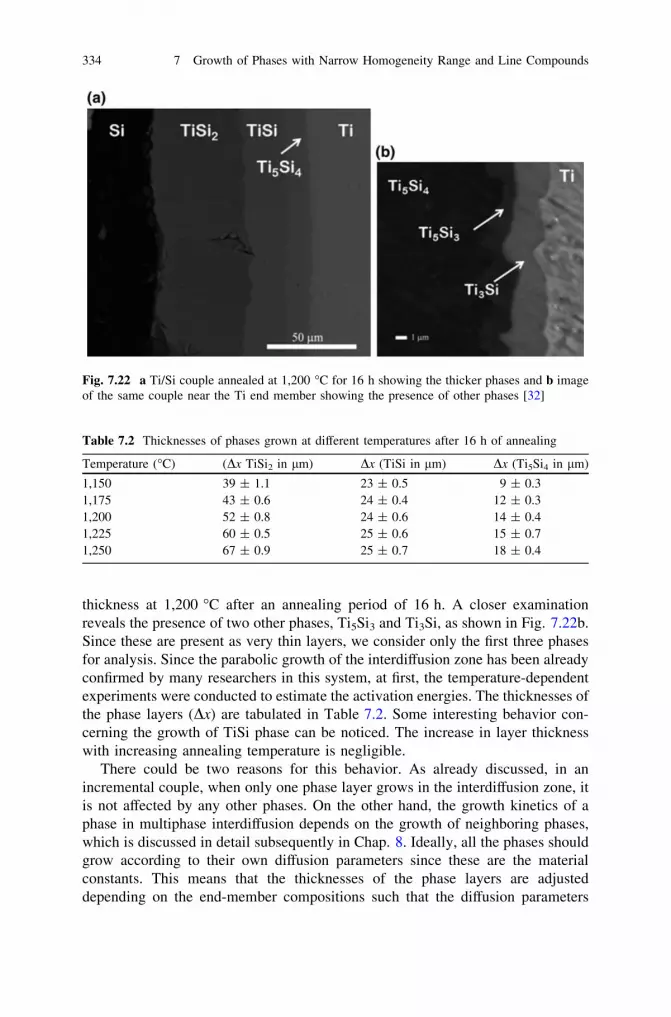
thickness at 1,200 �C after an annealing period of 16 h. A closer examinationreveals the presence of two other phases, Ti5Si3 and Ti3Si, as shown in Fig. 7.22b.Since these are present as very thin layers, we consider only the first three phasesfor analysis. Since the parabolic growth of the interdiffusion zone has been alreadyconfirmed by many researchers in this system, at first, the temperature-dependentexperiments were conducted to estimate the activation energies. The thicknesses ofthe phase layers (Dx) are tabulated in Table 7.2. Some interesting behavior con-cerning the growth of TiSi phase can be noticed. The increase in layer thicknesswith increasing annealing temperature is negligible.

There could be two reasons for this behavior. As already discussed, in anincremental couple, when only one phase layer grows in the interdiffusion zone, itis not affected by any other phases. On the other hand, the growth kinetics of aphase in multiphase interdiffusion depends on the growth of neighboring phases,which is discussed in detail subsequently in Chap. 8. Ideally, all the phases shouldgrow according to their own diffusion parameters since these are the materialconstants. This means that the thicknesses of the phase layers are adjusteddepending on the end-member compositions such that the diffusion parameters

Fig. 7.22 a Ti/Si couple annealed at 1,200 �C for 16 h showing the thicker phases and b imageof the same couple near the Ti end member showing the presence of other phases [32]

Table 7.2 Thicknesses of phases grown at different temperatures after 16 h of annealing

Temperature (�C) (Dx TiSi2 in lm) Dx (TiSi in lm) Dx (Ti5Si4 in lm)

1,150 39 ± 1.1 23 ± 0.5 9 ± 0.31,175 43 ± 0.6 24 ± 0.4 12 ± 0.31,200 52 ± 0.8 24 ± 0.6 14 ± 0.41,225 60 ± 0.5 25 ± 0.6 15 ± 0.71,250 67 ± 0.9 25 ± 0.7 18 ± 0.4

334 7 Growth of Phases with Narrow Homogeneity Range and Line Compounds

remain the same. There is, therefore, a possibility that the growth rate of the otherphase changed with temperature in such a way that the growth rate of TiSi phasedid not vary significantly with temperature. This also means that the activationenergy for the growth of this phase is relatively low compared to the other phases.Secondly, it is possible that this phase could not grow ideally—that is, paraboli-cally with time—in a multiphase interdiffusion zone, as was found, for instance, inthe Ti–Al system [1]. To investigate this, time-dependent experiments were con-ducted at 1,200 �C. As can be seen clearly from Fig. 7.23a–c, all three phasesgrow by a diffusion-controlled process since a linear dependence of the phasethickness squares Dx2 versus time 2t is found. This fact indicates that the activationenergy for the interdiffusion of TiSi phase must be low compared to the otherphases, as discussed above, which is clear from Fig. 7.23d. Another importantpoint should be noted here: We might ask whether time-dependent experimentsshould be conducted at every temperature, especially when Dx 6¼ 0 at t = 0, as itis found in this particular system. This can be decided based on the tempera-ture-dependent experiments. If the growth of the phase layer is affected differentlyat different temperatures, data points will not fall on a line in the Arrhenius plot.Figure 7.23d shows that these points do actually fall on a line for all the phases in

Fig. 7.23 Time-dependent experiments at 1,200 �C for 4, 9, 16, 25, and 36 h are shown by Dx2

versus 2t plots for a TiSi2, b TiSi, c Ti5Si4, and d the integrated diffusion coefficients for TiSi2,TiSi, and Ti5Si4 plotted following the Arrhenius equation [32]

7.8 Case Studies 335

this system, this indicates that the phases are affected similarly at the initial stagein the temperature range of our interest. This is true for most of the systems, ifexperiments are conducted relatively within a small temperature range.

References

1. F. J. J. van Loo and G.D. Rieck, Acta Metallurg. 21 (1973) 61–712. F. J. J. van Loo, Prog. Solid State Chem. 20 (1990) 47–993. C.P. Heijwegen and G.D. Rieck, Metall. Trans. 4 (1973) 2159–21674. G.M. Becht, F.J.J. van Loo and R. Metselaar, Reactivity of Solids 6 (1988) 45–59.5. V.I. Dybkov, Solid state reaction kinetics, IPMS Publications, Kyiv, 2013.6. B. Pieraggi, Oxidation of Metals 27 (1987) 177–1857. M.Y. Tsai, M.H. Chou, C.R. Kao, J. Alloys Comp. 471 (2009) 90–928. C. Wagner, Acta Metall. 17 (1969) 99–1079. K.P. Gurov, V.N. Pimenov and Y.E. Ugaste, Fiz. metal, metalloved. 32 (1971) 103

10. G.V. Kidson, J. Nucl. Mater. 3 (1961) 21–2911. A. B Gokhale, G. J Abbaschian, J. Phase Equilibria 12 (1991) 493–49812. S. Prasad and A. Paul, Intermetallics 19 (2011) 1191–120013. J.K. Yoon, J.Y. Byun, G.H. Kim, J.S. Kim, C.S Choi. Thin Solid Films 405 (2002) 170–17814. J.K. Yoon, J.K. Lee, K.H. Lee, J.Y. Byun, G.H. Kim, K.T. Hong, Intermetallics 11 (2003)

687–69615. A. Paul, A.A. Kodentsov, F.J.J. van Loo, Z. Metallkunde 95 (2004) 913–92016. A. Paul, C. Ghosh and W.J. Boettinger, Metall. Mater. Trans. A 42A (2011) 952–96317. K. N. Tu, G. Ottaviani, U. Gösele and H. Föll, J. Appl. Phys. 54 (1983) 758–76318. V.I. Dybkov, J. Mater. Sic. 21 (1986) 3078–308419. F.M. d’Heurle, J. Mater.Res. 3 (1988) 167–19520. D.S. Williams, R.A. Rapp and J.P. Hirth, Thin Solid Films 142 (1986) 47–6421. U. Gösele and K.N. Tu, J. Appl. Phys. 66 (1989) 2619–262622. A. Paul, M.J.H. van Dal, A.A. Kodentsov and F.J.J. van Loo, Acta Mater. 52 (2004) 623–63023. A. Paul, A.A. Kodentsov, F.J.J. van Loo, unpublished research24. V.D. Divya, S.S.K. Balam, U. Ramamurty and A. Paul, Scripta Materialia 62 (2010) 621–62425. M.J.H van Dal, A.A Kodentsov, F.J.J van Loo, Intermetallics, 9 (2001) 451–45626. A. Paul, The Kirkendall effect in solid state diffusion, PhD Thesis, Technische Universiteit

Eindhoven, Eindhoven, The Netherlands, 200427. S. Prasad and A. Paul, Acta Materialia 59 (2011) 1577–158528. S.S.K. Balam, and A. Paul, Metall. Mater. Trans. 41A (2010) 2175–2179.29. T. Laurila, J. Karppinen, V.Vuorinen, A. Paul and M. Paulasto-Kröckel, Journal of Electronic

Materials 40 (2011) 151730. M.J.H. van Dal, Microstructural stability of the Kirkendall plane, PhD thesis, Technische

Universiteit Eindhoven, The Netherlands, 200131. M.E. Schlesinger, H. Okamoto, A.B. Gokhale and R. Abbaschian, Journal of Phase Equilibria

14(1993) 50232. S. Roy, S. Divinski and A. Paul, Philosophical Magazine 94 (2014) 683.

336 7 Growth of Phases with Narrow Homogeneity Range and Line Compounds

Chapter 8Microstructural Evolutionof the Interdiffusion Zone

In this chapter, previously unknown behavior of marker plane is shown. In most ofthe cases, we find the markers along one particular plane; however, in certaincondition, these might spread. Sometimes, markers split into more than one planes.A characteristic microstructural feature is found to develop depending on thenumber and location of the marker planes. This led to development of a physico-chemical approach explaining the microstructural evolution in the interdiffusionzone.

As already discussed in Chap. 6, the discovery of the Kirkendall effect [1, 2] isone of the most important developments in the area of solid-state diffusion. Thishelped to validate the vacancy-mediated substitutional diffusion. For long, it wasknown that the markers accumulate at a single plane with a fixed composition.However, sometimes, an unusual behavior of the marker plane has been reported inthe literature on this subject. Bastin and Rieck [3] placed W wire at the interface ofa Ni/Ti diffusion couple before annealing it at 800 �C for 72 h. Three phases, Ti2Ni,TiNi, and TiNi3, were grown in the interdiffusion zone. Surprisingly, the authorsfound pieces of broken W wire in different phases, as if these markers tried to moveto different planes simultaneously. Much later, in 1993, Shimozaki et al. [4]reported another unusual behavior in the b0-AuZn phase grown by interdiffusion inthe Au/Au0.36Zn0.64 diffusion couple. As discussed in Chap. 6, the position of themarker plane could be detected by the presence of a line of pores that developedbecause of the negative surface (such as scratches or by the presence of debris lefton the metallographically prepared bonding surfaces). In general, the markers usedto detect the Kirkendall plane are also found along with these on the same plane.Shimozaki et al. used 5-lm-diameter W wire as an inert marker. To their surprise,they found the wires at one plane and the traces (pores caused by scratches ordebris) of the original interface at another plane. In both cases, the actual reason forsuch behavior was not known. In the meantime, following theoretical analysis,Cornet and Calais [5] and van Loo et al. [6] described the possibility of finding morethan one Kirkendall marker plane in an interdiffusion zone. In their analysis, theyconsidered a diffusion couple of a and b with a single interface between them. First,they showed that depending on the initial composition of the end members, thesame interface can act as both a source and a sink for vacancies when one particular

A. Paul et al., Thermodynamics, Diffusion and the Kirkendall Effect in Solids,DOI: 10.1007/978-3-319-07461-0_8, � Springer International Publishing Switzerland 2014

337

component diffuses at a faster rate in both the phases. If DA=DB [ 1 in one phaseand DA=DB\1 in the other phase, depending on the initial end-member compo-sitions, there could be two Kirkendall planes present in the interdiffusion zone. Inthat case, the inert markers placed at the initial contact plane have to split and willaccumulate at two different planes: one in the a phase and the other in the b phase.In fact, we should consider a marker plane in each phase. Depending on theend-member compositions, the intrinsic diffusion coefficients and the interdiffusioncoefficients, it is possible to actually find one or more than one marker planes. Afterthe manuscript published by Shimozaki et al. extensive studies were conducted inseveral systems including the Ni–Ti and the Au–Zn systems in order to demonstratethe previously unknown behavior of the marker planes [7–13]. Now, we know thatthe inert markers could be stable to be found in one plane. Under certain circum-stances, we might notice some unstable behavior, in which, instead of accumulationin one plane, the markers might spread over a wider area. Depending on theend-member compositions and diffusivities, more than one plane also could befound in a single phase or in different phases. Based on which, a physico-chemicalapproach is developed to explain the morphologies in a multiphase interdiffusionzone depending on the presence of a single or multiple Kirkendall planes.

8.1 Stable, Unstable, and Multiple Kirkendall MarkerPlanes

In Chap. 6, we have seen that the intrinsic diffusion coefficients can be estimatedover the composition range using an incremental diffusion couple by makingseveral diffusion couples with different end members or from a single diffusioncouple by making a multifoil diffusion couple. Once the intrinsic diffusion coef-ficients (DA and DB) are calculated, the velocity at a different composition in aparticular diffusion couple can be determined from the knowledge of these dif-fusion parameters at different compositions and the concentration gradient mea-sured at those compositions following the relation as expressed in Eq. 6.61

vK ¼ �vB DB � DAð Þ oCB

ox

� �K

ð8:1Þ

The velocity of the Kirkendall plane (or the composition of the Kirkendall markerplane) can also be determined directly by locating the initial contact plane xo andthe Kirkendall marker plane xK from the relation as expressed in Eq. 6.64

vK ¼xK � xo

2t¼ xK

2tð8:2Þ

Therefore, at the intersection point of these two lies the location of the Kirkendallmarker plane, since both have the same velocity at this plane [7, 8]. To explain

338 8 Microstructural Evolution of the Interdiffusion Zone

further in a simplified system, let us consider, the constant molar volume of asystem, such that vA ¼ vB ¼ vm and a constant interdiffusion coefficient ~D over thewhole concentration range. Therefore, Fick’s second law reduces to

oNB

o t¼ ~D

o2NB

ox2ð8:3Þ

The solution of Eq. 8.3 with respect to error function can be written as [7, 8, 10]

NB ¼12

erfcx

2ffiffiffiffiffi~Dtp

� �ð8:4Þ

For a constant molar volume, Eq. 8.1 can be written as

v ¼ DB � DAð Þ oNB

oxð8:5Þ

Further, the Darken relation (Eq. 6.65) can be expressed as

~D ¼ NADB þ NBDA ð8:6Þ

If we would like to consider a constant ratio of diffusivities, Eq. 8.5, with the helpof Eq. 8.6 can be written as

v ¼ ~DDB

DA� 1

NADB

DAþ NB

!oNB

oxð8:7Þ

With the help of Eq. 8.4, Eq. 8.7 can be written as

v ¼ ~DDB

DA� 1

NADB

DAþ NB

!�1ffiffiffi

pp 1

2ffiffiffiffiffi~Dtp

� �exp � x

2ffiffiffiffiffi~Dtp

� �2" #

ð8:8Þ

After plotting v versus x using Eq. 8.8, the location of the Kirkendall plane can berationalized by the intersection of the straight line—expressed by Eq. 8.2—that goesthrough x = 0. The velocity diagram, as shown in Fig. 8.1, is estimated for~D ¼ 10�14 m2=s; DA=DB ¼ 3; t ¼ 106 s and for the constant molar volume [7, 10].

Note that in an actual case, the ratios of the diffusivities are not constant overthe whole composition range and even the molar volume might change drastically.In that case, Eqs. 8.1 and 8.2 should be used to construct the velocity curve. Cornetand Calais [5] explained the possibility of finding multiple Kirkendall markerplanes in a theoretical analysis. Much later, the group of van Loo [7–13] conductedextensive experimental studies to show the different possibilities of the markerplanes and explained these behaviors with the help of theoretical analysis that hasbeen developed based on the work by Cornet and Calais [5]. Now, we know that a

8.1 Stable, Unstable, and Multiple Kirkendall Marker Planes 339

stable marker plane can be present in a system such that all the inert markersaccumulate along a single composition indicating the position of the Kirkendallmarker plane. On the other hand, markers can be unstable such that they spreadover a composition or region in the interdiffusion zone. In a few special cases,markers have been known to bifurcate or trifurcate. There is a possibility ofbifurcation in a single phase or in two different phases.

Before showing the experimental results, it is necessary to understand thecondition in which different kinds of behavior could be found [7, 8]. We consider asystem where in the A-rich side A has a higher diffusion rate compared to B and inthe B-rich side B has a higher diffusion rate compared to A. In such a case,according to Eq. 8.1, as shown in Fig. 8.2, the velocity will have a negative valuein the A-rich side and positive values in the B-rich side. We have considered theleft-hand side of the diffusion couple as being A-rich and the right-hand side of thecouple as being B-rich. Following, the number and nature of the marker plane willdepend on the location of the intersection on the velocity curve by the straight linedetermined by Eq. 8.2. Depending on the end-member compositions, the inter-diffusion coefficients and the intrinsic diffusion coefficients, the straight lineestimated from the position of the marker plane might intersect the velocity curveat a point, where it has a negative gradient dv=dx\0. This point is shown inFig. 8.2a. In this case, it will have a stable marker plane such that all the markerswill accumulate at this Kirkendall marker plane located at xK. At the very initialstage, if for any reason, the markers move ahead of this plane, they will slow downdue to lower velocity and come back to the stable plane. On the other hand, if themarkers are left behind this plane, they will move faster because of the highervelocity and drift to the marker plane. Therefore, the marker plane acts as theattractor for the markers to accumulate the inert particles from the nearbypositions.

As shown in Fig. 8.2b, by changing the end-member compositions in the samesystem, the position of the initial contact plane xo = 0 might move such that thestraight line intersects the velocity curve at a point where it has a positive gradient

Fig. 8.1 Velocity diagramshowing the location of theKirkendall marker plane [7]

340 8 Microstructural Evolution of the Interdiffusion Zone

Fig. 8.2 Imaginary velocity diagrams showing the possibility of finding a a stable marker plane,b an unstable marker plane, and c bifurcation of the marker plane in the same system [7]

8.1 Stable, Unstable, and Multiple Kirkendall Marker Planes 341

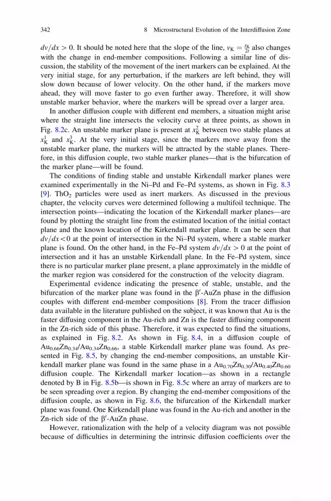
dv=dx [ 0. It should be noted here that the slope of the line, vK ¼ xK

2t also changeswith the change in end-member compositions. Following a similar line of dis-cussion, the stability of the movement of the inert markers can be explained. At thevery initial stage, for any perturbation, if the markers are left behind, they willslow down because of lower velocity. On the other hand, if the markers moveahead, they will move faster to go even further away. Therefore, it will showunstable marker behavior, where the markers will be spread over a larger area.

In another diffusion couple with different end members, a situation might arisewhere the straight line intersects the velocity curve at three points, as shown inFig. 8.2c. An unstable marker plane is present at x2

K between two stable planes atx1

K and x3K. At the very initial stage, since the markers move away from the

unstable marker plane, the markers will be attracted by the stable planes. There-fore, in this diffusion couple, two stable marker planes—that is the bifurcation ofthe marker plane—will be found.

The conditions of finding stable and unstable Kirkendall marker planes wereexamined experimentally in the Ni–Pd and Fe–Pd systems, as shown in Fig. 8.3[9]. ThO2 particles were used as inert markers. As discussed in the previouschapter, the velocity curves were determined following a multifoil technique. Theintersection points—indicating the location of the Kirkendall marker planes—arefound by plotting the straight line from the estimated location of the initial contactplane and the known location of the Kirkendall marker plane. It can be seen thatdv=dx\0 at the point of intersection in the Ni–Pd system, where a stable markerplane is found. On the other hand, in the Fe–Pd system dv=dx [ 0 at the point ofintersection and it has an unstable Kirkendall plane. In the Fe–Pd system, sincethere is no particular marker plane present, a plane approximately in the middle ofthe marker region was considered for the construction of the velocity diagram.

Experimental evidence indicating the presence of stable, unstable, and thebifurcation of the marker plane was found in the b0-AuZn phase in the diffusioncouples with different end-member compositions [8]. From the tracer diffusiondata available in the literature published on the subject, it was known that Au is thefaster diffusing component in the Au-rich and Zn is the faster diffusing componentin the Zn-rich side of this phase. Therefore, it was expected to find the situations,as explained in Fig. 8.2. As shown in Fig. 8.4, in a diffusion couple ofAu0.66Zn0.34/Au0.34Zn0.66, a stable Kirkendall marker plane was found. As pre-sented in Fig. 8.5, by changing the end-member compositions, an unstable Kir-kendall marker plane was found in the same phase in a Au0.70Zn0.30/Au0.40Zn0.60

diffusion couple. The Kirkendall marker location—as shown in a rectangledenoted by B in Fig. 8.5b—is shown in Fig. 8.5c where an array of markers are tobe seen spreading over a region. By changing the end-member compositions of thediffusion couple, as shown in Fig. 8.6, the bifurcation of the Kirkendall markerplane was found. One Kirkendall plane was found in the Au-rich and another in theZn-rich side of the b0-AuZn phase.

However, rationalization with the help of a velocity diagram was not possiblebecause of difficulties in determining the intrinsic diffusion coefficients over the

342 8 Microstructural Evolution of the Interdiffusion Zone

whole composition range in the b0-AuZn phase. Absence of the data on latticeparameter variation and Zn evaporation during melting complicated the analysis.Similar bifurcation of the Kirkendall marker plane was found in the b-NiAl phase,as shown in Fig. 8.7 in a diffusion couple of Ni41.7Al58.3/Ni72.24Al27.76 at 1,000 �C.The optical micrograph in Fig. 8.7b presents the whole interdiffusion zone, and theback scattered electron image in Fig. 8.7c exhibits the position of the two markerplanes shown by the presence of ThO2 particles. One marker plane was found inthe Ni-rich and another in the Al-rich side of the b-NiAl phase [11]. To estimatethe intrinsic diffusion coefficients over the homogeneity range in this phase, manyincremental diffusion couple experiments were conducted such that marker posi-tions are found at different compositions. The composition of the diffusion couplesand the annealing times are listed in Table 8.1 along with the couple in whichbifurcation of the marker plane was found.

The estimated interdiffusion coefficients and the ratio of the intrinsic diffusioncoefficients are shown in Fig. 8.8a and b. From the average of these values, theintrinsic diffusion coefficients are estimated using Eq. 6.66, as shown in Fig. 8.8c.The velocity curve was determined with the help of the concentration gradient

Fig. 8.3 a Velocity diagram constructed experimentally in the Ni–Pd system and b experimen-tally found a stable marker plane. c Velocity diagram constructed experimentally in the Fe–Pdsystem and d experimentally found unstable marker plane [9]

8.1 Stable, Unstable, and Multiple Kirkendall Marker Planes 343

obtained from the measured composition profile in the diffusion couple showingbifurcation of the marker plane, as shown in Fig. 8.9a. Afterward, the straight linedetermined from vK ¼ xK � xoð Þ=2t ¼ xK=2t is drawn by calculating the initialcontact plane and from knowledge of the known location of the marker plane. In

Fig. 8.4 a Compositions for a diffusion couple indicating on the Au–Zn phase diagram in whichb a single marker plane is found [8]

344 8 Microstructural Evolution of the Interdiffusion Zone

Fig. 8.5 a Compositions for a diffusion couple indicating on the Au–Zn phase diagram in whichb unstable marker plane is found, c shows the marker region [8]

8.1 Stable, Unstable, and Multiple Kirkendall Marker Planes 345

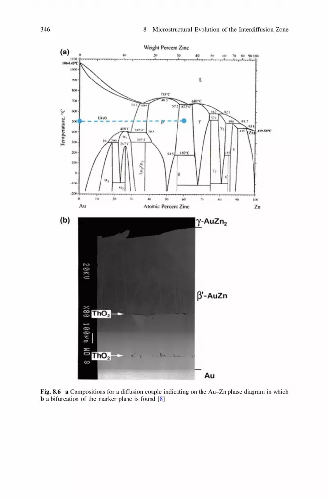
Fig. 8.6 a Compositions for a diffusion couple indicating on the Au–Zn phase diagram in whichb a bifurcation of the marker plane is found [8]

346 8 Microstructural Evolution of the Interdiffusion Zone

Fig. 8.7 a Compositions for a diffusion couple indicating on the Ni–Al phase diagram in whichb a bifurcation of the marker plane is found in the b-NiAl phase (polarized light microscopeimage), c back scattered electron image clearly shows the location of the marker planes [11]

8.1 Stable, Unstable, and Multiple Kirkendall Marker Planes 347

the velocity diagram given in Fig. 8.9b, we see that this straight line intersects thevelocity curve at two points where it has a negative gradient. There is a jump in themiddle of the velocity curve since the composition profile does not grow with anymeasurable thickness near the stoichiometric composition because of the lowinterdiffusion coefficients.

The bifurcation of the Kirkendall marker plane shown in the previous examples isfound in a single phase. Bifurcation in different phases is found more often than thatin a single phase such as in Ag–Zn, Co–Si, Ni–Ti, and Au–Sn systems. Theexamples for Ag–Zn [12], Co–Si [14, 15], and Ni–Ti [10] systems are shown inFig. 8.10. In fact, the study on the Ni–Ti system was conducted since this is one ofthe first systems indicating the likelihood of more than one Kirkendall marker plane.Trifurcation of the Kirkendall marker plane is very rare and it was found in the Ti–Al system [16], which was in fact predicted from the data reported on diffusionparameters before the experimental proof. Theoretically, these behaviors of themarker planes were studied by Höglund and Ågren [17] and Boettinger et al. [18].

8.2 A Physicochemical Approach to Explainthe Morphological Evolution in an Interdiffusion Zone

It has been seen in many examples that a characteristic morphology develops inthe product phase when grown by reactive diffusion. For example, three incre-mental diffusion couples in different systems are shown in Fig. 8.11 [14, 15, 19,20]. It can be seen that a duplex morphology is present whenever there is aKirkendall marker plane present. In Fig. 8.10a, the bifurcation of the marker planeis shown in the Ag–Zn system [12]. The grain morphologies in different phases areshown in Fig. 8.12. In the e-AgZn3 and c-Ag5Zn8 phases, the marker planes are

Table 8.1 Details of the incremental diffusion couple experiments conducted at 1,000 �C arelisted

Couple no. Diffusion couple Time (h)

1 Ni49.8Al50.2/Ni72.24Al27.76 1002 Ni49.8Al50.2/Ni66.24Al33.76 243 Ni46Al54/Ni72.24Al27.76 244 Ni46Al54/Ni66.24Al33.76 245 Ni46Al54/Ni57.5Al42.5 1006 Ni46Al54/Ni57.5Al42.5 247 Ni46Al54/Ni49.8Al50.2 1008 Ni49.8Al50.2/Ni57.5Al42.5 1009 Ni46Al54/Ni52.2Al47.8 10010 Ni46Al54/Ni52.2Al47.8 2411 Ni41.7Al58.3/Ni72.24Al27.76 2412 Ni46Al54/Ni54Al46 24

348 8 Microstructural Evolution of the Interdiffusion Zone

Fig. 8.8 a The interdiffusioncoefficients, b the ratio of theintrinsic diffusion coefficientsand c the estimated intrinsicdiffusion coefficients atdifferent compositions in theb-NiAl phase at1,000 �C [11]

8.2 A Physicochemical Approach to Explain the Morphological Evolution 349

present and the duplex morphology is also evident. On the other hand, there is nomarker plane present in the b-AgZn phase, where uniform and continuous grainmorphology is present.

The experimental results shown above indicate that the phase layer growsdifferently at different interface interphases. In reactive diffusion, the productphase layers are grown because of the reaction/dissociation of the diffusingcomponent from the interfaces. Although the phases are grown by the reactionsand/or dissociation at the interface interphases, growth of the phases are notcontrolled by these processes. We are considering the systems, in which diffusionof components through the phase layers takes longer time to control the growthprocess. There are many examples, especially in thin-film conditions, where thegrowth of the phase is reaction controlled, which are not considered here. Beforeestimating the diffusion parameters with the help of a physicochemical approach,

Fig. 8.9 a Composition profile and b the velocity diagram rationalization of the bifurcation ofthe marker plane [11]

350 8 Microstructural Evolution of the Interdiffusion Zone

Fig. 8.10 Experimentalevidences of bifurcations ina Ag–Zn [12], b Co–Si [14,15], and c Ni–Ti [10] systems

8.2 A Physicochemical Approach to Explain the Morphological Evolution 351

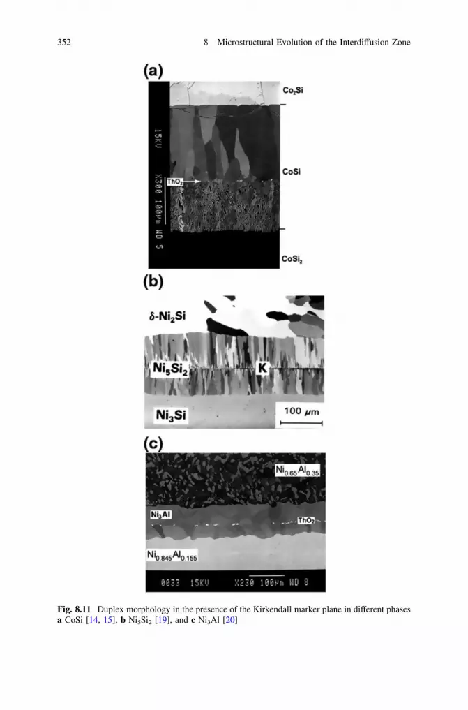
Fig. 8.11 Duplex morphology in the presence of the Kirkendall marker plane in different phasesa CoSi [14, 15], b Ni5Si2 [19], and c Ni3Al [20]

352 8 Microstructural Evolution of the Interdiffusion Zone

which is developed considering the reactions and dissociations at the interfaces inreal systems along with the diffusion of the component through the phase layer, weshall first show that this approach is equivalent to the relations developed in theprevious chapters.

Fig. 8.12 Duplex morphology in the presence of the Kirkendall marker plane in a e-phase,b c-phase and c a uniform grain morphology in the b-phase because of the absence of any markerplane [12]

8.2 A Physicochemical Approach to Explain the Morphological Evolution 353

For the sake of simplicity, let us consider a diffusion couple of a and c phases inwhich a line compound b grows in an interdiffusion zone, as shown in Fig. 8.13[21]. The stoichiometric compositions of the a, b, and c phases are A1-mBm, A1-

nBn, and A1-pBp, respectively. Suppose a is an A-rich and b is a B-rich phase.Therefore, as shown in the figure, A dissociates from the a phase at the interface Ito produce the product b phase. The dissociated A then diffuses to the interface IIand reacts with the c phase to produce the b phase. At the same time, B dissociatesfrom the c phase at the interface II to produce the b phase. The dissociated Bdiffuses to the interface I to produce the b phase. Therefore, at both interfaces, theproduct phase b is grown by the dissociation and reaction of the components.Suppose, [du]A mol/m2 is the flux of the component A crossing the Kirkendallmarker plane in the short period of time dt. Similarly, the flux of the component Bthat crosses the marker plane in that short period of time is [dv]B mol/m2. Thelocation of the marker plane in the interdiffusion zone is shown by filled circles,and the location is denoted as xK. It is evident that the thickness of the productphase that is grown in the left-hand side of the marker plane is due to the reactionand dissociation at the interface I. On the other hand, the right-hand side of theproduct phase from the Kirkendall marker plane is grown because of the reactionand dissociation at the interface II. Therefore, we should write the reaction anddissociation equations at the two different interfaces.

Reaction dissociation equations at the interface I:

n

n� mduA1�mBm a phaseð Þ ! du ½A�d þ

m

n� mduA1�nBn b phaseð Þ

Fig. 8.13 A schematicdiagram explaining thephysicochemical approach

354 8 Microstructural Evolution of the Interdiffusion Zone

dissociation of A

1� n

n� mdvA1�mBm a phaseð Þ þ dv ½B�d !

1� m

n� mdvA1�nBn b phaseð Þ

reaction of B.Reaction dissociation equations at the interface II:

n

p� nduA1�pBp c phaseð Þ þ du ½A�d !

p

p� nduA1�nBn b phaseð Þ

reaction of A

1� n

p� ndvA1�pBP c phaseð Þ ! dv ½B�d þ

1� p

p� ndvA1�nBn b phaseð Þ

dissociation of A.The amount of the b phase produced at the interface I is 1

n�m mduþ 1� mð Þdv½ �mol/m2 and at the interface II is 1

p�n pduþ 1� pð Þdv½ � mol/m2. Suppose, the molar

volume of the product b phase is vm, which will be written as vbm at latter stage.

Suppose, the thicknesses of the phase layer grown from the interfaces I and II in thisshort period of time dt is dxI=K and dxK=II, respectively. Therefore, we can write

1n� m

mduþ ð1� mÞdv½ � vm ¼ dxI=K ð8:9aÞ

1p� n

pduþ ð1� pÞdv½ � vm ¼ dxK=II ð8:9bÞ

Furthermore, we can write both the left- and right-hand sides of the end members,as well as the composition of the product phases as m ¼ N�B ; p ¼ NþB and n ¼ NB.Therefore, Eqs. 8.9a and 8.9b can be rewritten as

N�B duþ ð1� N�B Þdv ¼ NB � N�Bvm

dxI=K ð8:10aÞ

NþB duþ ð1� NþB Þ dv ¼ NþB � NB

vmdxK=II ð8:10bÞ

If the fluxes of the diffusing components A and B are 0 at time t = 0 and becomeu and v after the annealing time t, we can write Eqs. 8.10a and 8.10b by integratingas

8.2 A Physicochemical Approach to Explain the Morphological Evolution 355

N�B

Zu

o

duþ ð1� N�B ÞZv

o

dv ¼ZxK

x�1

NB � N�Bvm

dx

N�B uþ ð1� N�B Þv ¼ZxK

x�1

NB � N�Bvm

dx

NþB

Zu

o

duþ ð1� NþB ÞZv

o

dv ¼Zxþ1

xK

NB � N�Bvm

dx

ð8:11aÞ

NþB uþ ð1� NþB Þv ¼Zxþ1

xK

NþB � NB

vmdx ð8:11bÞ

Now, we would like to write the expressions separately for u and v. MultiplyingEq. 8.11a by 1� NþBð Þ and Eq. 8.11b by 1� N�B

� �and then by subtracting, we get

N�B ð1� NþB Þu� NþB ð1� N�B Þu ¼ ð1� NþB ÞZxK

x�1

NB � N�Bvm

dx

� ð1� N�B ÞZxþ1

xK

NþB � NB

vmdx

u ¼ � ð1� NþB ÞZxK

x�1

NB � N�BNþB � N�B

1vm

dx� ð1� N�B ÞZxþ1

xK

NþB � NB

NþB � N�B

1vm

dx

24

35

Introducing the composition normalizing variable YB ¼ NB�N�BNþ

B�N�

B

such that

1� YB ¼ NþB�NB

NþB�N�

B

, we can write

u ¼ � ð1� NþB ÞZxK

x�1

YB

vmdx� ð1� N�B Þ

Zxþ1

xK

1� YB

vmdx

24

35

u ¼ � NþA

ZxK

x�1

YB

vmdx� N�A

Zxþ1

xK

1� YB

vmdx

24

35

ð8:12aÞ

Multiplying Eq. 8.11a by N�B and Eq. 8.11b by NþB and then by subtracting, we get

356 8 Microstructural Evolution of the Interdiffusion Zone

NþB ð1� N�B Þv � N�B ð1� NþB Þv ¼ NþB

ZxK

x�1

NB � N�Bvm

dx� N�B

Zxþ1

xK

NþB � NB

vmdx

v ¼ NþB

ZxK

x�1

NB � N�BNþB � N�B

1vm

dx� N�B

Zxþ1

xK

NþB � NB

NþB � N�B

1vm

dx

v ¼ NþB

ZxK

x�1

YB

vmdx� N�B

Zxþ1

xK

1� YB

vmdx

ð8:12bÞ

The intrinsic flux of A that is JA and the intrinsic flux of B that is JB can be relatedto u and v. It is a fact that the intrinsic fluxes are inversely proportional to t1=2.Moreover, the sign of the flux of A should be taken as positive since it diffusesfrom left to right and the flux of B should be taken as negative since it diffusesfrom right to left. Therefore, we can write

u ¼Zu

0

du ¼Z t

0

JA dt ¼Z t

0

k

t1=2dt ¼ kt1=2

1=2¼ 2tJA ¼ �2tDA

oCA

oxð8:13aÞ

v ¼Zv

0

dv ¼�Z t

0

JB dt ¼ �Z t

0

k

t1=2dt ¼ �2tJB ¼ 2tDB

oCB

oxð8:13bÞ

where k is the proportionality constant. Note here that Ji ¼ �DioCiox . From

Eqs. 8.12 and 8.13a, we can write

DA ¼12t

ox

oCA

� �NþA

ZxK

x�1

Y

vmdx� N�A

Zxþ1

xK

1� Y

vmdx

24

35 ð8:14aÞ

DB ¼12t

ox

oCB

� �NþB

ZxK

x�1

Y

vmdx� N�B

Zxþ1

xK

1� Y

vmdx

24

35 ð8:14bÞ

Note that these are the relations developed by van Loo [22] and are those that wederived earlier in Chap. 6 following the approach by Wagner [13]. From thestandard thermodynamic relations oCA ¼ �vB=v2

m

� �oNA; oCB ¼ �vA=v2

m

� �oNB (Eq.

1.150), we can write the ratio of the intrinsic diffusion coefficients as

8.2 A Physicochemical Approach to Explain the Morphological Evolution 357

�vADB

�vBDA

¼ JB

JA

¼ v

uð8:15aÞ

Following Eq. 6.91, we can write this with respect to the ratio of the tracer dif-fusion coefficients as

D�BD�A¼ �vADB

�vBDA

¼ JB

JA

¼ v

uð8:15bÞ

Therefore, since the partial molar volumes are not known in a phase with a narrowhomogeneity range, we actually measure the ratio of the tracer diffusion coeffi-cients after neglecting the role of the vacancy wind effect, as explained in Chap. 6.

Previously in Chap. 6, we derived the relation between the interdiffusioncoefficients and the intrinsic diffusion coefficients as

~D ¼ CA�vADB þ CB�vBDA ð8:16Þ

since NB þ NA ¼ 1; Ci ¼ Nivm

, we can write the interdiffusion coefficients with

respect to u and v with the help of Eqs. 8.13a and 8.13b as [21]

~D ¼ vm

2t

ox

oNB

NBuþ NAv½ � ð8:17Þ

In the case of a compound with a very narrow homogeneity range, since wecannot measure the composition profile, the integrated diffusion coefficient ismeasured. With respect to u and v, we can express this as [23]

~Dbint ¼

ZNIIB

NIB

~D dNB ¼ZxII

b

xIb

vm

2tNBuþ NAv½ � dx ¼ vb

m

2tNb

Buþ NbAv

h iDxb ð8:18Þ

As explained in Chap. 6, here the unknown composition range of the b phase isNII

B � NIB, the thickness of the phase layer is Dxb ¼ xII

b � xIb. The average molar

volume of the phase vbm and the composition Nb

B can be considered as constant andduring a fixed annealing time of t fixed amount of fluxes, u and v transfer throughthe Kirkendall marker plane. The values of u and v can be estimated from thecomposition profile using the relations expressed in Eqs. 8.12a and 8.12b. It shouldbe noted here that by replacing these relations in Eqs. 8.17 and 8.18, we can derivethe same relations for the interdiffusion coefficient and the integrated diffusioncoefficient as derived by Wagner, which are described in Chaps. 6 and 7.

The velocity of the marker plane following Eq. 6.62 can be estimated by

358 8 Microstructural Evolution of the Interdiffusion Zone

vK ¼ �ð�vAJA þ �vBJBÞ

Replacing Eq. 8.13a in the above equation, we get

vK ¼ � �vA

u

2t� �vB

v

2t

� �¼ 1

2t�vBv� �vAuð Þ ð8:19aÞ

If the values of the partial molar volumes are not known—for instance, in aphase with a narrow homogeneity range—we consider vm ¼ �vA ¼ �vB, where vm isthe molar volume of the product phase. Therefore, we can write

xK ¼ 2tvK ¼ vm v� uð Þ ð8:19bÞ

It can be understood from the above discussion that the phase layer growsdifferently from the two different interfaces and we should expect a duplex mor-phology separated by a Kirkendall marker plane as shown in Fig. 8.11. Therefore,one expects the same values of diffusion coefficients when derived followingdifferent approaches explained in Chaps. 6 and 7 or this chapter. The physico-chemical approach has an additional benefit that it sheds light on the morpho-logical evolutions in the interdiffusion zone.

Fig. 8.14 Interdiffusion zoneof the CoSi phase in adiffusion couple of Co2Si/CoSi2 annealed at 1,000 �Cfor 49 h and use of thephysicochemical approachfor the estimation of thediffusion parameter [14]

8.2 A Physicochemical Approach to Explain the Morphological Evolution 359

8.3 The Application of the Physicochemical Approachin an Incremental Diffusion Couple with a SingleProduct Phase

Let us now apply this physicochemical approach to estimate the integrated dif-fusion coefficient and the ratio of the tracer diffusion coefficients in real systems.We consider the growth of CoSi in a diffusion couple of Co2Si and CoSi2 annealedat 1,100 �C for 49 h, as shown in Fig. 8.11a. The description of the analysis ispresented in Fig. 8.14 [16, 21]. It is to be anticipated that Co will dissociate fromthe Co-rich phase Co2Si at the interface I to produce the CoSi product phase. Cowill then diffuse to the interface II to react with the CoSi2 phase and produce theCoSi phase. Similarly, Si dissociates from the Si-rich phase (the CoSi2 phase at theinterface II) to produce the CoSi phase. The dissociated Si diffuses to the interfaceI to react with the Co2Si phase and produce the CoSi phase.

In terms of chemical reaction equations:

At the interface I (Co2Si/CoSi)

3uCo2=3Si1=3 ! u½ �Coþ2uCo1=2Si1=2

3vCo2=3Si1=3 þ v½ �Si! 4vCo1=2Si1=2

At the interface II (CoSi/CoSi2)

3uCo1=3Si2=3 þ u½ �Co! 4uCo1=2Si1=2

3vCo1=3Si2=3 ! v½ �Siþ2vCo1=2Si1=2

The parameters [u]Co and [v]Si are the number of moles of Co and Si atoms,respectively, transferred per unit area of the reaction layer during the total diffu-sion time. Following on from this, we can write

2uþ 4vð ÞvCoSim ¼ DxI

CoSi ð8:20aÞ

4uþ 2vð ÞvCoSim ¼ DxII

CoSi ð8:20bÞ

Note that the same relations can be obtained directly from Eq. 8.11.

N�Siuþ 1� N�Si

� �v ¼

ZxK

x�1

NSi � N�Si

vCoSim

dx ¼ NSi � N�Si

vCoSim

ZxK

x�1

dx ¼ NSi � N�Si

vCoSim

DxICoSi

NþSiuþ 1� NþSi

� �v ¼

Zxþ1

xK

NþSi � NSi

vCoSim

dx ¼ NþSi � NSi

vCoSim

Zxþ1

xK

dx ¼ NþSi � NSi

vCoSim

DxIICoSi

360 8 Microstructural Evolution of the Interdiffusion Zone

In this example, N�Si ¼ 1=3; 1� N�Si ¼ 2=3; NþSi ¼ 2=3; 1� NþSi ¼ 1=3; NSi ¼1=2 and 1� NSi ¼ 1=2. We are considering a phase with a narrow compositionrange that is an average composition and the constant molar volume of the phase.It can be seen that from the composition values written above, we get the samerelations in Eq. 8.20.

The thicknesses of the sublayers measured from the microstructure shown inFig. 8.14 are DxI

CoSi ¼ 162 lm. Note here that the actual length of DxIICoSi is

measured as 107 lm (approximately 23 %); however, the length of DxIICoSi ¼

82:4 lm is considered for the calculation because of the presence of pores in thissublayer [14, 15]. The molar volume of the CoSi phase is vCoSi

m ¼ 6:6�10�6 m3=mol: Using these values, we find u = 0.07 and v = 6.1 mol/m2.Therefore, the integrated diffusion coefficient and the ratio of the tracer diffusioncoefficients can be estimated using the relations expressed in Eqs. 7.15b and 7.18as (for an annealing time of 49 h)

D�Si

D�Co

¼ v

u¼ 87

~DCoSiint ¼

vCoSim

2tNCoSi

Si uþ NCoSiCo v

Dxb

¼ 6:60� 10�6

2� 49� 60� 6012� 0:07þ 1

2� 6:1

� �162þ 82:4ð Þ � 10�6

¼ 1:41� 10�14 m2=s

Once again, it was possible to calculate the same values using the relationsshown in Chap. 7 (Eq. 7.15).

~DCoSiint ¼

NCoSiSi � NCo2Si

Si

� �NCoSi2

Si � NCoSiSi

� �NCoSi2

Si � NCo2SiSi

� � Dx2CoSi

2t

¼ 1=6� 1=61=3

� 162þ 82:4ð Þ � 10�6

2� 49� 60� 60

¼ 1:41� 10�14 m2=s

Now, let us consider an incremental couple in which a single product phasegrows from the end members with two phase alloys, as shown in Fig. 8.15 [23].One of the end members has a composition of Co0.81Si0.19. It can be observed fromthe phase diagram and the alloy in the end member that it is a phase mixture of e-Co—that is, e-Co(Si) solid solution with a composition of Co0.83Si0.17 at 1,100 �C.Another alloy used as an end member has an average composition of Co0.52Si0.48,meaning that it is a phase mixture of Co2Si and CoSi phases. The volume fractionof the phases can be estimated by the lever rule, as explained in Chap. 1.

Before proceeding to the reaction equations, it is necessary to understand themechanism by which the product phase grows at the interdiffusion zone. Note that

8.3 The Application of the Physicochemical Approach 361

only the e-Co(Si) phase from the left-hand side end member and the CoSi phasefrom the right-hand side end member will take part in the reaction or the disso-ciation process. The Co2Si phase that is already present in the alloy will directlyadd to the product phase. This is the reason, as explained in Chap. 7 (Sect. 7.4), thegrowth rate of a product phase is different depending on the end-member com-positions. If we select alloys having a composition closer to the product phase, thegrowth kinetics of the phase will be higher since the amount of this phase—whichcan be directly added to the product phase—is higher. The reaction dissociationequations at the interfaces can be written as [23].

At the interface I (Co0.81Si0.19/Co2Si)

2:04uCo0:83Si0:17 eð Þ ! u½ �Coþ1:04uCo2=3Si1=3

4:06vCo0:83Si0:17 eð Þ þ v½ �Si! 5:06vCo2=3Si1=3

At the interface II (CoSi/CoSi2)

2uCo1=2Si1=2 þ u½ �Co! 3uCo2=3Si1=3

4vCo1=2Si1=2 ! v½ �Siþ3vCo2=3Si1=3

The parameters [u]Co and [v]Si are the number of moles of Co and Si atoms,respectively, transferred per unit area of the reaction layer during the total diffu-sion time. Therefore, (1.04u + 5.06v) moles of the Co2Si phase are produced atthe interface I caused by the dissociation and reaction processes. Moreover, asalready discussed for the (2.04u + 4.06v) moles of the e-Co(Si) phase that isconsumed at the interface I, a portion of the Co2Si phase will be directly added tothe product phase. Following the lever rule, we know that in an alloy with anaverage composition of Co0.81Si0.19, the ratio of the mole fractions of the Co2Si

Fig. 8.15 a Co–Si phase diagram and b use of the physicochemical approach in the Co2Si phasegrown at 1,100 �C after annealing for 100 h [23]

362 8 Microstructural Evolution of the Interdiffusion Zone

phase to the e-Co(Si) phase with a composition of Co0.83Si0.17 is 0:19�0:171=3�0:19 ¼ 0:14.

For the consumption of (2.04u + 4.06v) moles of the e-Co(Si) phase at thisinterface, 0.14(2.04u + 4.06v) moles of the Co2Si phase will be directly added tothe product phase. Therefore, the growth of the Co2Si phase from the interface Ican be written as

1:04uþ 5:06vð Þ þ 0:14ð2:04uþ 4:06vÞ½ �vCo2Sim ¼ DxI

Co2Si

1:3uþ 5:6vð ÞvCo2Sim ¼ DxI

Co2Si

ð8:21aÞ

Similarly, at the interface II, (3u + 3v) moles of the Co2Si phase are produced bythe reaction and dissociation processes. Since (2u + 4v) moles of CoSi are con-sumed at this interface, a portion of the Co2Si phase will be directly added to theproduct phase. Following the lever rule, the ratio of moles of the Co2Si phase tothe CoSi phase in an alloy with an average composition of a Co0.52Si0.48 alloy is0:5�0:480:48�1=3 ¼ 0:136. For the consumption of (2u + 4v) moles of CoSi, 0.136(2u + 4v)

moles of the Co2Si phase will be directly added to the product phase. Therefore,the growth of the Co2Si phase from the interface II can be written as

3uþ 3vð Þ þ 0:136ð2uþ 4vÞ½ �vCo2Sim ¼ DxII

Co2Si

3:3uþ 3:5vð ÞvCo2Sim ¼ DxII

Co2Si

ð8:21bÞ

The same relations can be obtained directly from Eq. 8.11.

N�Siuþ ð1� N�SiÞv ¼ZxK

x�1

NSi � N�Si

vCo2Sim

dx ¼ NSi � N�Si

vCo2Sim

ZxK

x�1

dx ¼ NSi � N�Si

vCo2Sim

DxICo2Si

NþSiuþ ð1� NþSiÞv ¼Zxþ1

xK

NþSi � NSi

vCo2Sim

dx ¼ NþSi � NSi

vCo2Sim

Zxþ1

xK

dx ¼ NþSi � NSi

vCo2Sim

DxIICo2Si

In this example, N�Si ¼ 0:19; 1� N�Si ¼ 0:81; NþSi ¼ 0:48; 1� NþSi ¼ 0:52; NSi ¼1=3 and 1� NSi ¼ 2=3. It can be seen that from the composition values writtenabove, we arrive at the same relations as those in Eq. 8.21.

The thicknesses of the sublayers measured from the microstructure shown inFig. 8.15 are DxI

Co2Si ¼ 147 lm and DxIICo2Si ¼ 309 lm. The molar volume of the

Co2Si phase is vCo2Sim ¼ 6:56� 10�6 m3=mol. Using these values, we find

u = 13.55 and v = 0.78. Therefore, the integrated diffusion coefficient and theratio of the tracer diffusion coefficients can be estimated using the relationsexpressed in Eqs. 8.15b and 8.18 as (for an annealing time of 100 h)

8.3 The Application of the Physicochemical Approach 363

D�Si

D�Co

¼ v

u¼ 0:06

~DCo2Siint ¼ vCo2Si

m

2tNCo2Si

Si uþ NCo2SiCo v

DxCo2Si

¼ 6:56� 10�6

2� 100� 60� 6013� 13:55þ 2

3� 0:78

� �147þ 309ð Þ � 10�6

¼ 2:1� 10�14 m2=s

It should be pointed out here that the relations developed in this chapter could alsobe used to calculate the diffusion parameters at the Kirkendall marker plane wherethe composition varies in the interdiffusion zone. For example, as shown inFig. 8.16 in a Ni0.65Al0.35/Ni0.845Al0.155 diffusion couple, the c0 phase grows in theinterdiffusion zone [21]. It can be understood from the Ni–Al phase diagram inFig. 4.11a [24] that Ni0.65Al0.35 is a phase mixture of the b-NiAl phase with thecomposition of the Ni0.625Al0.375 (dark matrix) and the c0-Ni3Al phase (grayprecipitates) having the composition of Ni0.72Al0.28. The other end member with acomposition of Ni0.845Al0.155 is a c-Ni(Al) solid-solution phase [20]. Unlike theprevious examples, in this case, there will be composition redistribution after the c0

phase gets added to the product phase from the end member.The composition profile of the interdiffusion zone is shown in Fig. 8.17a. We

consider that u and v in mol/m2 are the fluxes of Al and Ni crossing the Kirkendallmarker plane for the total annealing time of 196 h. The relations expressed inEq. 8.11 for this diffusion couple can be written as

0:65uþ 0:35v ¼ZxK

x�1

NNi � 0:65vm

dx ð8:22aÞ

0:845uþ 0:155v ¼Zxþ1

xK

0:845� NNi

vmdx ð8:22bÞ

Fig. 8.16 Use of thephysicochemical approach inNi3Al phase grown in adiffusion couple at 1,000 �Cannealed for 196 h [20]

364 8 Microstructural Evolution of the Interdiffusion Zone

Fig. 8.17 Explanation ofestimation of the diffusionparameters byphysicochemical approach inNi3Al [21]

8.3 The Application of the Physicochemical Approach 365

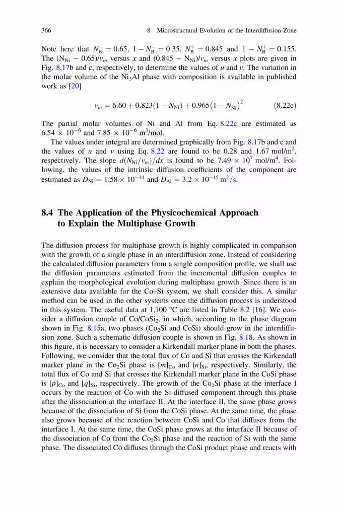
Note here that N�B ¼ 0:65; 1� N�B ¼ 0:35; NþB ¼ 0:845 and 1 - NþB ¼ 0:155.The (NNi - 0.65)/vm versus x and (0.845 - NNi)/vm versus x plots are given inFig. 8.17b and c, respectively, to determine the values of u and v. The variation inthe molar volume of the Ni3Al phase with composition is available in publishedwork as [20]

vm ¼ 6:60þ 0:823 1� NNið Þ þ 0:965 1� NNi

� �2 ð8:22cÞ

The partial molar volumes of Ni and Al from Eq. 8.22c are estimated as6.54 9 10-6 and 7.85 9 10-6 m3/mol.

The values under integral are determined graphically from Fig. 8.17b and c andthe values of u and v using Eq. 8.22 are found to be 0.28 and 1.67 mol/m2,respectively. The slope d NNi=vmð Þ=dx is found to be 7.49 9 107 mol/m4. Fol-lowing, the values of the intrinsic diffusion coefficients of the component areestimated as DNi ¼ 1:58� 10�14 and DAl ¼ 3:2� 10�15 m2=s.

8.4 The Application of the Physicochemical Approachto Explain the Multiphase Growth

The diffusion process for multiphase growth is highly complicated in comparisonwith the growth of a single phase in an interdiffusion zone. Instead of consideringthe calculated diffusion parameters from a single composition profile, we shall usethe diffusion parameters estimated from the incremental diffusion couples toexplain the morphological evolution during multiphase growth. Since there is anextensive data available for the Co–Si system, we shall consider this. A similarmethod can be used in the other systems once the diffusion process is understoodin this system. The useful data at 1,100 �C are listed in Table 8.2 [16]. We con-sider a diffusion couple of Co/CoSi2, in which, according to the phase diagramshown in Fig. 8.15a, two phases (Co2Si and CoSi) should grow in the interdiffu-sion zone. Such a schematic diffusion couple is shown in Fig. 8.18. As shown inthis figure, it is necessary to consider a Kirkendall marker plane in both the phases.Following, we consider that the total flux of Co and Si that crosses the Kirkendallmarker plane in the Co2Si phase is [m]Co and [n]Si, respectively. Similarly, thetotal flux of Co and Si that crosses the Kirkendall marker plane in the CoSi phaseis [p]Co and [q]Si, respectively. The growth of the Co2Si phase at the interface Ioccurs by the reaction of Co with the Si-diffused component through this phaseafter the dissociation at the interface II. At the interface II, the same phase growsbecause of the dissociation of Si from the CoSi phase. At the same time, the phasealso grows because of the reaction between CoSi and Co that diffuses from theinterface I. At the same time, the CoSi phase grows at the interface II because ofthe dissociation of Co from the Co2Si phase and the reaction of Si with the samephase. The dissociated Co diffuses through the CoSi product phase and reacts with

366 8 Microstructural Evolution of the Interdiffusion Zone

the CoSi2 phase to produce CoSi. Si that reacts with the Co2Si phase at theinterface II is actually produced by the dissociation from the CoSi2 phase at theinterface III to produce the CoSi product phase. Therefore, it must be clear thatthe Co2Si and CoSi phases at the interfaces grow by consuming the neighboringphase(s) and at the same time become consumed because of the growth of theneighboring phase(s).

In terms of reaction equations, these can be written as:

At the interface I (Co/Co2Si on the Co2Si side)

2nCoþ n Si½ �d! 3nCo2=3Si1=3

At the interface II (Co2Si/CoSi on the Co2Si side)

4nCo1=2Si1=2 ! n Si½ �dþ3nCo2=3Si1=3

2mCo1=2Si1=2 þ m ½Co�d ! 3mCo2=3Si1=3

At the interface II (Co2Si/CoSi on the CoSi side)

Table 8.2 The integrated diffusion coefficients ~Dint

� �, molar volumes of the Co-silicides (vm),

and the ratio of tracer diffusivities of Si and Co �vCoDSi

�vSiDCo

� �at 1,100 �C in different phases are listed

Phases

Co2Si CoSi

~Dint m2=sð Þ (1.5 ± 0.5) 9 10-14 (4.6 ± 0.3) 9 10-14

D�Si

D�Co

¼ �vCoDSi

�vSiDCo

� �0.06 ± 0.025 35 ± 15

vm (m3 mol-1) 6.56 9 10-6 6.60 9 10-6

These are the average values obtained from many different diffusion couples. Therefore, the dataconsidered for Co2Si in this table are different from the data obtained in a particular diffusioncouple, as discussed in the previous example

Fig. 8.18 A schematic diagram explaining the physicochemical approach in a Co/CoSi2diffusion couple

8.4 The Application of the Physicochemical to Explain 367

3pCo2=3Si1=3 ! p Co½ �dþ2pCo1=2Si1=2

3qCo2=3Si1=3 þ q Si½ �d! 4qCo1=2Si1=2

At the interface III (CoSi/CoSi2 on the CoSi side)

3pCo1=3Si2=3 þ p Co½ �d! 4pCo1=2Si1=2

3qCo1=3Si2=3 ! q Si½ �dþ2qCo1=2Si1=2

Therefore, 3n moles of the Co2Si phase are produced at the interface I. At theinterface II, (3m + 3n) moles of Co2Si are produced and at the same time(3p + 3q) moles get consumed. At the same interface, on the other side, (2p + 4q)moles of CoSi are produced; however, (4n + 2 m) moles get consumed. At theinterface III, (4p + 2q) moles of CoSi are produced.

vCo2=3Si1=3m � 3n ¼ DxI

Co2Si

vCo2=3Si1=3m � 3mþ 3n� 3p� 3qð Þ ¼ DxII

Co2Si

vCo1

2Si1

2m � 2pþ 4q� 4n� 2mð Þ

vCo1

2Si1

2m � 4pþ 2qð Þ

ð8:23aÞ

The integrated diffusion coefficients can be written as

~DCo2Siint ¼ vCo2Si

m

2tNCo2Si

Si mþ NCo2SiCo n

DxI

Co2Si þ DxIICo2Si

� �

~DCoSiint ¼

vCoSim

2tNCoSi

Si pþ NCo2SiCo q

DxII

CoSi þ DxIIICoSi

� � ð8:23bÞ

The ratio of the diffusivities can be written as

D�Si

D�Co

Co2Si

¼ �vCoDSi

�vSiDCo

Co2Si

¼ n

m

D�Si

D�Co

CoSi

¼ �vCoDSi

�vSiDCo

CoSi

¼ q

p

ð8:23cÞ

Using the molar volume values, the integrated diffusion coefficients and the ratioof the intrinsic (or tracer diffusion coefficients), as listed in Table 8.2, we find thevalues for 100 hrs as

DxICo2Si ¼ 32 lm, DxII

Co2Si ¼ 133 lm; DxIICoSi ¼ 168:5 lm, DxII

CoSi ¼ 294:5 lm,

m ¼ 26:8; n ¼ 1:6; p ¼ 0:6 and q ¼ 21:0 mol=m2:

368 8 Microstructural Evolution of the Interdiffusion Zone

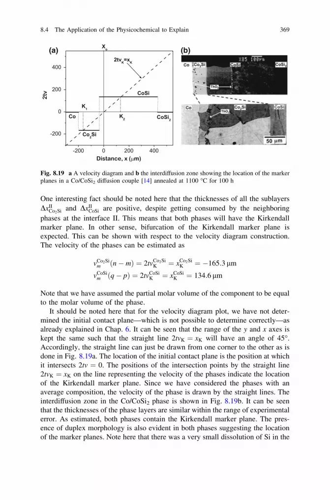
One interesting fact should be noted here that the thicknesses of all the sublayersDxII

Co2Si and DxIICoSi are positive, despite getting consumed by the neighboring

phases at the interface II. This means that both phases will have the Kirkendallmarker plane. In other sense, bifurcation of the Kirkendall marker plane isexpected. This can be shown with respect to the velocity diagram construction.The velocity of the phases can be estimated as

vCo2Sim n� mð Þ ¼ 2tvCo2Si

K ¼ xCo2SiK ¼ �165:3 lm

vCoSim q� pð Þ ¼ 2tvCoSi

K ¼ xCoSiK ¼ 134:6 lm

Note that we have assumed the partial molar volume of the component to be equalto the molar volume of the phase.

It should be noted here that for the velocity diagram plot, we have not deter-mined the initial contact plane—which is not possible to determine correctly—asalready explained in Chap. 6. It can be seen that the range of the y and x axes iskept the same such that the straight line 2tvK ¼ xK will have an angle of 45�.Accordingly, the straight line can just be drawn from one corner to the other as isdone in Fig. 8.19a. The location of the initial contact plane is the position at whichit intersects 2tv = 0. The positions of the intersection points by the straight line2tvK ¼ xK on the line representing the velocity of the phases indicate the locationof the Kirkendall marker plane. Since we have considered the phases with anaverage composition, the velocity of the phase is drawn by the straight lines. Theinterdiffusion zone in the Co/CoSi2 phase is shown in Fig. 8.19b. It can be seenthat the thicknesses of the phase layers are similar within the range of experimentalerror. As estimated, both phases contain the Kirkendall marker plane. The pres-ence of duplex morphology is also evident in both phases suggesting the locationof the marker planes. Note here that there was a very small dissolution of Si in the

(a) (b)

Fig. 8.19 a A velocity diagram and b the interdiffusion zone showing the location of the markerplanes in a Co/CoSi2 diffusion couple [14] annealed at 1100 �C for 100 h

8.4 The Application of the Physicochemical to Explain 369

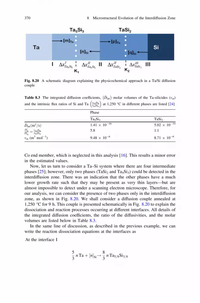
Co end member, which is neglected in this analysis [16]. This results a minor errorin the estimated values.

Now, let us turn to consider a Ta–Si system where there are four intermediatephases [25]; however, only two phases (TaSi2 and Ta5Si3) could be detected in theinterdiffusion zone. There was an indication that the other phases have a muchlower growth rate such that they may be present as very thin layers—but arealmost impossible to detect under a scanning electron microscope. Therefore, forour analysis, we can consider the presence of two phases only in the interdiffusionzone, as shown in Fig. 8.20. We shall consider a diffusion couple annealed at1,250 �C for 9 h. This couple is presented schematically in Fig. 8.20 to explain thedissociation and reaction processes occurring at different interfaces. All details ofthe integrated diffusion coefficients, the ratio of the diffusivities, and the molarvolumes are listed below in Table 8.3.

In the same line of discussion, as described in the previous example, we canwrite the reaction dissociation equations at the interfaces as

At the interface I

53

n Taþ n½ �Si!83

n Ta5=8Si3=8

Fig. 8.20 A schematic diagram explaining the physicochemical approach in a Ta/Si diffusioncouple

Table 8.3 The integrated diffusion coefficients, ~Dint

� �molar volumes of the Ta-silicides (vm)

and the intrinsic flux ratios of Si and Ta �vTaDSi

�vSiDTa

� �at 1,250 �C in different phases are listed [24]

Phase

Ta5Si3 TaSi2~Dint m2=sð Þ 1.41 9 10-16 5.02 9 10-14

D�Si

D�Ta¼ �vTaDSi

�vSiDTa

5.8 1.1

vm (m3 mol-1) 9.48 9 10-6 8.71 9 10-6

370 8 Microstructural Evolution of the Interdiffusion Zone

At the interface II (Ta5Si3 side)

97

m Ta1=3Si2=3 þ m½ �Ta!167

m Ta5=8Si3=8

157

n Ta1=3Si2=3 ! n½ �Siþ87

n Ta5=8Si3=8

Interface II (TaSi2 side)

87

q Ta5=8Si3=8 þ q½ �Si!157

q Ta1=3Si2=3

167

p Ta5=8Si3=8 ! p½ �Taþ97

p Ta1=3Si2=3

Interface III

2 p Siþ ½ p �Ta ! 3 p Ta1=3Si2=3

Accordingly, the thicknesses of the sublayers can be related to the mole of theproduct phases formed at the different interfaces can be written as

83

n � vTa5Si3m ¼ DxI

Ta5Si3

167

m þ 87

n

� �� 16

7pþ 8

7q

� �� �� vTa5Si3

m ¼ DxIITa5Si3

157

q þ 97

p

� �� 15

7n þ 9

7m

� �� �� vTaSi2

m ¼ DxIITaSi2

3p� vTaSi2m ¼ DxIII

TaSi2

ð8:24aÞ

Following, the integrated diffusion coefficients and the ratio of the diffusivities ofthe components can be written as

~DTa5Si3int ¼ vTa5Si3

m

2tNTa5Si3

Ta nþ NTa5Si3Si m

DxI

Ta5Si3þ DxII

Ta5Si3

� �

~DTaSi2int ¼ vTaSi2

m

2tNTaSi2

Ta qþ NTaSi2Si p

DxII

TaSi2þ DxIII

TaSi2

� � ð8:24bÞ

D�Si

D�Ta

Ta5Si3

¼ n

m

D�Si

D�Ta

TaSi2

¼ q

p

ð8:24cÞ

8.4 The Application of the Physicochemical to Explain 371

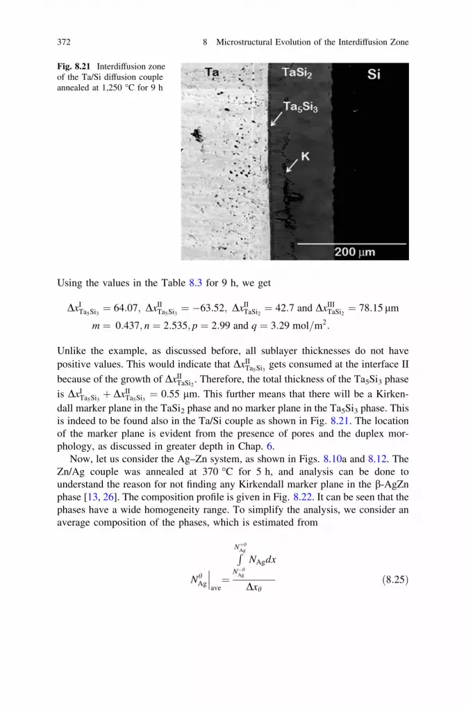
Using the values in the Table 8.3 for 9 h, we get

DxITa5Si3

¼ 64:07; DxIITa5Si3

¼ �63:52; DxIITaSi2¼ 42:7 and DxIII

TaSi2¼ 78:15 lm

m ¼ 0:437; n ¼ 2:535; p ¼ 2:99 and q ¼ 3:29 mol=m2:

Unlike the example, as discussed before, all sublayer thicknesses do not havepositive values. This would indicate that DxII

Ta5Si3gets consumed at the interface II

because of the growth of DxIITaSi2

. Therefore, the total thickness of the Ta5Si3 phase

is DxITa5Si3

þ DxIITa5Si3

= 0.55 lm. This further means that there will be a Kirken-dall marker plane in the TaSi2 phase and no marker plane in the Ta5Si3 phase. Thisis indeed to be found also in the Ta/Si couple as shown in Fig. 8.21. The locationof the marker plane is evident from the presence of pores and the duplex mor-phology, as discussed in greater depth in Chap. 6.

Now, let us consider the Ag–Zn system, as shown in Figs. 8.10a and 8.12. TheZn/Ag couple was annealed at 370 �C for 5 h, and analysis can be done tounderstand the reason for not finding any Kirkendall marker plane in the b-AgZnphase [13, 26]. The composition profile is given in Fig. 8.22. It can be seen that thephases have a wide homogeneity range. To simplify the analysis, we consider anaverage composition of the phases, which is estimated from

NhAg

ave¼

RNþhAg

N�hAg

NAgdx

Dxhð8:25Þ

Fig. 8.21 Interdiffusion zoneof the Ta/Si diffusion coupleannealed at 1,250 �C for 9 h

372 8 Microstructural Evolution of the Interdiffusion Zone

where h is the phase of interest, N�hAg and Nþh

Ag are the phase boundary composi-tions, and Dxh is the thickness of the interested phase. The estimated averagecompositions of the e, c and b phases are Ag0.154Zn0.846, Ag0.394Zn0.606, andAg0.521Zn0.479, respectively. For our analysis without complication, we ignore thedissolution of Ag in Zn and Zn in Ag, since the composition profiles developed inthese solid solutions are small.

The schematic diffusion couple is presented above in Fig. 8.23. Based on theaverage compositions of the phases, the reaction/dissociation equations at differentinterfaces can be written as

Interface I—Zn/AgZn3 (AgZn3 side)

5:49nZn þ ½n�Ag ! 6:49nAg0:154Zn0:846 eð Þ

Reaction of Ag with Zn

Interface II—AgZn3/Ag5Zn8 (AgZn3 side)

0:64mAg0:394Zn0:606 cð Þ þ ½m�Zn ! 1:64mAg0:154Zn0:846 eð Þ

Reaction of Zn with Ag5Zn8

3:53nAg0:394Zn0:606 cð Þ ! ½n�Ag þ 2:53nAg0:154Zn0:846 eð Þ

Dissociation of Ag from Ag5Zn8

Interface II—AgZn3/Ag5Zn8 (Ag5Zn8 side)

Fig. 8.22 Compositionprofile of the Ag/Zn diffusioncouple annealed at 370 �C for5 h

8.4 The Application of the Physicochemical to Explain 373

1:64pAg0:154Zn0:846 eð Þ ! ½p�Zn þ 0:64pAg0:394Zn0:606 cð Þ

Dissociation of Zn from AgZn3

2:53qAg0:154Zn0:846 eð Þ þ ½q�Ag ! 3:53qAg0:394Zn0:606 cð Þ

Reaction of Ag with AgZn3

Interface III—Ag5Zn8/AgZn (Ag5Zn8 side)

3:10pAg0:521Zn0:479 bð Þ þ ½p�Zn ! 4:10pAg0:394Zn0:606 cð Þ

Reaction of Zn with AgZn

4:77qAg0:521Zn0:479 bð Þ ! ½q�Ag þ 3:77qAg0:394Zn0:606 cð Þ

Dissociation of Ag from AgZn

Interface III—Ag5Zn8/AgZn (AgZn side)

4:10rAg0:394Zn0:606 cð Þ ! ½r�Zn þ 3:10rAg0:521Zn0:479 bð Þ

Dissociation of Zn from Ag5Zn8

3:77sAg0:394Zn0:606 cð Þ þ ½s�Ag ! 4:77sAg0:521Zn0:479 bð Þ

Reaction of Ag with Ag5Zn8

Interface IV—AgZn/Ag (AgZn side)

Fig. 8.23 A schematic diagram explaining the physicochemical approach in the Ag/Zn diffusioncouple

374 8 Microstructural Evolution of the Interdiffusion Zone

1:09rAgþ ½r�Zn ! 2:09rAg0:521Zn0:479 bð Þ

Reaction of Zn with Ag.

Here, m, n, p, q, r, and s are the fluxes (moles/m2) of the components as shown inFig. 8.23. The product phases produced at different interfaces can be related to thethicknesses of the sublayers as

vem 6:49nð Þ ¼ DxI

e

vem 1:64mþ 2:53n� 1:64p� 2:53qð Þ ¼ DxII

e

vcm 0:64pþ 3:53q� 0:64m� 3:53nð Þ ¼ DxII

c

vcm 4:10pþ 3:77q� 4:10r � 3:77sð Þ ¼ DxIII

c

vbm 3:10r þ 4:77s� 3:10p� 4:77qð Þ ¼ DxIII

b

vbm 2:09rð Þ ¼ DxIV

b

The molar volumes of the e, c and b phases are 9.20 9 10-6, 9.44 9 10-6 and9.46 9 10-6 m3/mol. The sublayer thicknesses in the e and c phases measureddirectly from the Ag–Zn diffusion couple as shown in Fig. 8.24 are DxI

e ¼48:6; DxII

e ¼ 50:2; DxIIc ¼ 16:65; DxIII

c ¼ 24:45 and DxIIIb þ DxIV

b

� �¼ 244 lm.

The ratio of the diffusivities in the b-AgZn phase was estimated using an incre-

mental couple as rs ¼

VAgDZn

VZnDAg¼ 6:5. From these, the rest of the parameters are

estimated as m = 19.62, n = 0.81, p = 13.88, q = 2.37, r = 13.52,s = 2.08 mol/m2, and DxIII

b ¼ �23:72 and DxIVb ¼ 267:72 mm. Therefore, the

negative value of DxIIIb is suggestive of the consumption of the sublayer by the

neighboring phase and the absence of the Kirkendall marker plane in the b phase.Now, let us consider different locations of the marker planes and the kind of

morphology to be expected in the interdiffusion zone. Our discussion shall bebased upon only two product phases in the interdiffusion zone; the description is,however, the same when a different number of phases are formed. Typically, weexpect to find one of the three examples given in Fig. 8.24.

Suppose, two phases (A2B and AB2) are grown in the interdiffusion zone of ahypothetical A/B diffusion couple. There is a possibility that the marker planes arepresent in both the phases, as shown in Fig. 8.24a, meaning that the thicknesses ofall the sublayers are positive and duplex morphology should be expected in boththe phases. It should be noted here that finding more than one Kirkendall plane inan interdiffusion zone is not very common—with very few rare examples beingfound till date [27]. In most cases, a single marker plane is present in one of thephases—as shown in Fig. 8.24b—which signifies that the thicknesses of thesublayers DxI

A2B and DxIIA2B are positive in the A2B phase. DxII

AB2is negative, which

8.4 The Application of the Physicochemical to Explain 375

means that this part is consumed because of the growth of the DxIIA2B. However,

DxIIIAB2

is positive. This suggests that duplex morphology is to be expected in theA2B phase and a uniform morphology is expected in the AB2 phase. There couldbe many examples where the marker plane is present at one of the interfaces of theend-member/product phase, as shown in Fig. 8.24c. Very frequently, it is con-cluded (based on the similar location of the marker plane) that one of the com-ponents has a much higher diffusion rate compared to the other in both phases.This is not correct. For example, if the marker plane is present at the A/A2Binterface, it is true that A has a much higher diffusion rate compared to B in theA2B phase. However, it is not indicative of the relative mobilities of the com-ponents in the AB2 phase. There could be a comparable diffusion rate of both thecomponents in this phase. Due to the significantly higher diffusion rate of A andnegligible diffusion rate of B in the A2B phase, DxI

AB2will be negligible and DxII

AB2

will be almost equal to the total thickness of the A2B phase. Moreover, due to thevery high flux of A through this phase, the growth rate of this product phase is veryhigh at the interface II and might consume the whole of DxII

AB2and a part of DxIII

AB2

such that DxIIAB2

will have a negative value. Therefore, both the phases will have auniform morphology. It should be noted here that, sometimes, even if the possi-bility of bifurcation of the marker plane is expected in an interdiffusion zone, themarkers in both the phases might not be found. This was seen in the Cu–Sn system,where the Cu3Sn and Cu6Sn5 phases are seen to be growing at the interdiffusionzone [28]. The marker plane was found only in the Cu6Sn5 phase; however,according to the analysis based on the diffusion parameters in the phases, the

Fig. 8.24 Schematic representation of the diffusion couple explaining the situation for findinga bifurcation of the marker plane b a single Kirkendall marker plane in the A2B phase and c asingle marker plane at A/A2B phase

376 8 Microstructural Evolution of the Interdiffusion Zone

marker plane should be present in both the phases. To find the marker planes inboth the phases, it is important that both phases should start growing together fromthe beginning to trap the markers. This is, in general, found in bulk diffusioncouples, as discussed till now. In thin films, on the other hand, sequential phasegrowth is very frequently reported. The presence of the marker plane only in theCu6Sn5 phase, however, indicates the sequential growth of the phases, where theCu3Sn phase, most probably, started growing after some incubation period. If thisis true, once all the markers get trapped in the Kirkendall marker plane in theCu6Sn5 phase, no markers will be left in the Cu3Sn phase after it starts growing.

8.5 Effect of Electrical Current on the MicrostructuralEvolution of the Diffusion Zone

The physicochemical approach can also be utilized to rationalize the effect ofadditional driving forces, such as electric field, on the growth of interfacial phases.Figure 8.25 shows a cross section of the component with the directions of thecurrent and electron flux. The electron flux enters the component from the sourcecontact and leaves from the drain contact. In the forthcoming analysis of the effectof the electron flow on the IMC, growth only the on the printed wiring board(PWB) side is considered. This is because, at the component side, the presence ofAg finish will make the analysis less quantitative.

Figure 8.26 shows the interfacial microstructures from solder—PWB interfacesfrom the samples that have been annealed at 110 �C for 750 h and both the drainas well as source contacts after 750 h of constant current stressing.

Due to the relatively complex geometry of the interconnections and the differ-ences in cross-sectional areas, the current crowding effects and thus the differencesin current densities cannot be easily addressed. However, even if only the directionof the electron flux is taken into consideration, the marked differences in the totalIMC growth kinetics as well as the relative thicknesses of the Cu6Sn5 and Cu3Snintermetallic compounds can be observed when these differences are comparedwith the results obtained using the diffusion couple experiments [29, 30]. Closerexamination of Table 8.4 and Fig. 8.26 reveals that when the flow of electrons istoward the PWB, the g and e phase layers are almost of the same thickness, whereasin the opposite situation, the thickness of Cu3Sn is drastically reduced.

The thickness ratio of Cu6Sn5 to Cu3Sn is unusually high in the case of theannealed samples (Table 8.4) when compared to the earlier results from the Cu/Sn(X) diffusion couples [31–35]. It is known that impurity and alloying compo-nents can drastically change the growth kinetics of the IMC compounds [32].Hence, it is not surprising that the IMC ratio differs from that observed with highpurity materials. Based on our previous experiments, it is known that alloyingcomponents (like Ni) in copper increase the Sn flux through Cu6Sn5 but have nomeasurable effect on the intrinsic fluxes inside Cu3Sn. This, in turn, results in a

8.4 The Application of the Physicochemical to Explain 377

lower growth rate of Cu3Sn than in the case of a pure Cu/Sn diffusion couple. Thedecrease in the growth rate of Cu3Sn can be understood when it is noticed that thegrowth of the reaction layers in multiphase diffusion couples is dependent on eachother. Thus, when the formation rate of Cu6Sn5 at the Cu3Sn/Cu6Sn5 interfaceincreases, more and more Cu3Sn is consumed by the growing g layer. As the fluxesof either Sn or Cu inside Cu3Sn are not significantly altered, this results in theobserved growth behavior. A similar (but slightly different) effect using theelectron flux can be observed here as discussed below. Regarding the annealed

Fig. 8.25 SEM micrographof the structure of thecomponent used in theelectromigration study

Fig. 8.26 SEM micrographshowing the interfacialreaction layer structuredepending on the direction ofthe electron flux [29]

378 8 Microstructural Evolution of the Interdiffusion Zone

samples, it is to be noted that in this case, the Cu–Sn IMCs are growing betweenthe Cu and SnAgCu solder instead of between Cu and pure Sn. Based on theexperimental results [34], it is known that the thickness of Cu3Sn is smaller whengrowth takes place in the Cu/SnAgCu diffusion couple than in the Sn/Cu diffusioncouple at the same temperature. This can be understood when considering how thepresence of Ag and Cu in solder affects the activities of the diffusing components.The presence of Cu in the solder decreases the driving force for diffusion of Cufrom the Cu-substrate to the solder as the activity difference decreases. Likewise,the lowering of the activity of Sn in the solder (because of the presence of Ag)reduces the driving force for diffusion of Sn toward the Cu-substrate, thus reducingthe Sn flux. These two effects combine to produce the observed difference betweenthe Cu/Sn and Cu/SnAgCu reaction couples. Finally, it is emphasized that also theslightly lower temperature used here (110 �C instead of 125 �C which is used inthe reference cases [34, 35]) will itself contribute to the observed smaller thicknessratio of Cu3Sn to Cu6Sn5.

From the results of the steady current experiments, it can be seen that in thedrain contact, the electron flux comes from the solder side to the interface. Thus,the PWB pad is acting as the anode, meaning that the Sn flux toward the PWB isincreased in both IMC layers whereas the flux of Cu from the PWB is decreased,which, based on the experimental results, seems to favor the growth of Cu3Sn. Thiscan be analyzed in more detail with the help of Fig. 8.27 and the followingreaction equations.’

The reaction scheme

The reactions occurring at different interfaces of the reaction couple, as shown inFig. 8.27, can be expressed as follows

Interface I:

3qCuþ q½Sn�d ! 4qCu3=4Sn1=4

Interface II Cu3Sn side:

Table 8.4 Thickness data of the intermetallic compounds grown at the interface

Cu3Sn Cu6Sn5 Cu6Sn5 to Cu3Snratio

No current 0.8 lm 3 lm 3.80.093 mol/m2 0.283 mol/

m2

Constant current from PWB 2.1 lm 2.3 lm 1.10.244 mol/m2 0.217 mol/

m2

Constant current fromsolder

0.9 lm (*no change)0.1 mol

3.8 lm 4.20.36 mol/m2

8.5 Effect of Electrical Current on the Microstructural Evolution 379

119

pCu6=11Sn5=11 þ p Cu½ �d!209

pCu3=4Sn1=4

113

qCu6=11Sn5=11 ! q Sn½ �dþ83

qCu3=4Sn1=4

Interface II Cu6Sn5 side:

209

rCu3=4Sn1=4 ! r Cu½ �dþ119

rCu6=11Sn5=11

83

sCu3=4Sn1=4 þ s Sn½ �d!113

sCu6=11Sn5=11

Interface III:

56

rSnþ r Cu½ �d!116

rCu6=11Sn5=11

Fig. 8.27 Schematic presentation of the interfacial reactions occurring in the reaction couple

380 8 Microstructural Evolution of the Interdiffusion Zone

Here, p and q are the moles of Cu and Sn, respectively, transferred per unit areathrough the Cu3Sn phase during the total diffusion time t. Similarly, r and s are thenumber of moles of Cu and Sn transported during interaction per unit area throughthe Cu6Sn5-phase layer. From the equations written above, it is clear that at theinterface II, not only 20

9 pþ 83 q

� �moles of Cu3Sn grow, but also 20

9 r þ 83 s

� �moles

get consumed because of the growth of the Cu6Sn5 phase. Similarly, 119 r þ 11

3 s� �

moles of Cu6Sn5 grow at the same interface, but 119 pþ 11

3 q� �

moles get consumedby the Cu3Sn phase.

The thickness of the parts of the product phase layers resulting from theinterfacial reactions given above can be expressed as

4q� vCu3Snm ¼ DxCu3Sn

I

209

pþ 83

q� 209

r � 83

s

� �� vCu3Sn

m ¼ DxCu3SnII

119

r þ 113

s� 119

p� 113

q

� �� vCu6Sn5

m ¼ DxCu6Sn5II

116

r � vCu6Sn5m ¼ DxCu6Sn5

III

where DxCu3SnI and DxCu3Sn

II are the thicknesses of the sublayers in the Cu3Sn phase.

DxCu6Sn5II and DxCu6Sn5

III are the thicknesses of sublayers in the Cu6Sn5 phase. Thesesublayers are separated by the Kirkendall marker planes in these phases. InTable 8.5, the experimental results about the effect of the electron flow on thegrowth of the IMCs are presented in a different way. In addition to thickness, theamount of each phase has been tabulated in terms of mole/m2 for the sake ofdiscussion.

PWB as the anode

Table 8.5 Summary of theexperimental results

Cu6Sn5 (lm) Cu3Sn (lm) IMC tot (lm)

After solderingNo current 1 0.1 1.1Drain 1 0.1 1.1Source 1 0.1 1.11,500 CyclesNo current 1.8 1.4 3.2Drain 2.4 1.2 3.6Source 3.6 0.3 3.93,000 CyclesNo current 1.9 1.9 3.8Drain 2.7 1.5 4.2Source 4.4 0.5 4.9

8.5 Effect of Electrical Current on the Microstructural Evolution 381

Let us first consider that there is an equal increase in the flux of Sn and an equaldecrease in the flux of Cu in both the phases. First, the two cases will be addressedseparately and then the combined effect of the changes in the Cu and Sn fluxes isaddressed.

(i) Increase in the Sn flux through the phases:

Owing to the diffusion of Sn, 4 parts (in terms of moles) of the Cu3Sn productphase will grow at the interface I plus a further 8/3 parts at the interface II byconsuming the Cu6Sn5 phase. On the other hand, 8/3 parts will get consumedbecause of the growth of the Cu6Sn5 phase at the interface II. So, in total, there willbe a net gain of 4 parts of the Cu3Sn phase in this case.

Similarly, 11/3 parts of the Cu6Sn5 phase will grow at the interface II and thesame amount will get consumed because of the growth of the Cu3Sn phase at thatinterface. So, there should be no net change in the layer thickness of the Cu6Sn5

phase.

(ii) Decrease in the Cu flux through the phases:

If the flow of Cu decreases at the same rate through both the phases, there willbe 20/9 parts (in terms of moles) less production of Cu3Sn at the interface II.Further, because of the decreased diffusion rate of Cu through the Cu6Sn5 phase,there will be 20/9 less consumption of the Cu3Sn phase at the interface II. So, thereshould be no net change in the layer thickness of the Cu3Sn phase because of theflow of electrons from solder to the PWB.

On the other hand, as a result of the lower production of the Cu3Sn phase at theinterface II, there will be 11/9 parts less consumption of the Cu6Sn5 phase at thatinterface. At the same time (because of the decreased flow rate of Cu through theCu6Sn5 phase), there will 11/9 parts less production of the Cu6Sn5 phase due to thedissociation of the Cu3Sn phase at the interface II. Finally, there will be lowerproduction of 11/6 parts of the Cu6Sn5 phase at the interface III. So, there shouldbe a net loss in the thickness of the Cu6Sn5 phase compared to the situation whenthere is no flow of electrons.

(iii) Combined effect of Sn and Cu fluxes

Thus, if the Cu and Sn fluxes are affected similarly in both the phases, then forevery 4 parts of Cu3Sn phase increase there will be a corresponding 11/6 partsdecrease in the layer thickness of the Cu6Sn5 phase. This means that for a one-partincrease in the thickness of the Cu3Sn phase, there will be a corresponding 0.46parts decrease in the thickness of the Cu6Sn5 phase. In our experimental results, weactually get for a 0.151 parts (mol/m2) increase in the thickness of the Cu3Sn phasea corresponding decrease of 0.066 parts in the Cu6Sn5 phase. This can be put inanother way: for a 1-part Cu3Sn phase increase, we get 0.44 parts of decrease inthe Cu6Sn5 phase. This is very close to the analysis presented above and can thus

382 8 Microstructural Evolution of the Interdiffusion Zone

be taken to indicate that the components (Sn and Cu) are indeed affected in asimilar fashion by the electron flow. To conclude, it is now self-evident that it istime to reexamine the assumption that Sn should be strongly affected by theelectron flux owing to its higher effective valence (Z*).

PWB as the cathode

Again, we consider there to be an equal decrease of Sn flux and an increase ofCu in both the phases. The good match between the analysis results based on thisassumption with the experimental results, shown above, gives us further confi-dence that this approach is justified.

(i) Increase in Cu flux through the phases:

When the amount of Cu3Sn increases by 20/9 parts (in moles) by consuming theCu6Sn5 phase at the interface II because of the increase of Cu flux, 20/9 parts ofthe same phase will get consumed because of the growth of the Cu6Sn5 phase atthe same interface. So, there will be no net gain or loss in the thickness of theCu3Sn phase because of the increase in the diffusion rate of Cu. Owing to theincrease in the flow of Cu through the Cu3Sn phase, the increased consumption of11/9 of the Cu6Sn5 phase will occur at the interface II. However, at the same time,11/9 parts of the same phase will grow by dissociation of the Cu3Sn phase, becauseof the increase in flow of Cu through this phase. A further increase of 11/6 parts ofthe Cu6Sn5 phase will occur due to the increase in the flow of Cu through the gphase. So, there should be no net gain in the thickness of the Cu3Sn phase, but anet gain of 11/6 parts in the thickness of the Cu6Sn5 phase.

(ii) Decrease in Sn flux through the phases:

Owing to the decreased diffusion rate of Sn through the Cu3Sn phase, there willbe a corresponding 4 parts decrease in the layer thickness. Similarly, there will be8/3 parts less produced at the interface II caused by the dissociation of the Cu6Sn5

phase. Furthermore, because of the decreased diffusion rate of Sn through theCu6Sn5 phase, the consumption of the same phase will be 8/3 parts less at the sameinterface. So, the net loss for the Cu3Sn should be 4 parts.

Because of the decrease of Sn flux through the Cu6Sn5 phase, there will be 11/3parts less production of the phase at the interface II by consuming the Cu3Snphase. At the same time, there will be 11/3 parts less consumption of the samephase because of the low diffusion rate of Sn through the Cu3Sn phase. So, thereshould be no net gain in the Cu6Sn5 phase layer thickness because of low flux ofSn through both the phases.

(iii) Combined effect of Sn and Cu fluxes

When we consider the increase in the flow of Cu and the correspondingdecrease in the flow of Sn to occur equally through both the phases, there will be anet gain of 11/6 parts in the thickness of Cu6Sn5 and a net decrease of 4 parts in thethickness of the Cu3Sn phase. However, the diffusion rate of Sn is known to be

8.5 Effect of Electrical Current on the Microstructural Evolution 383

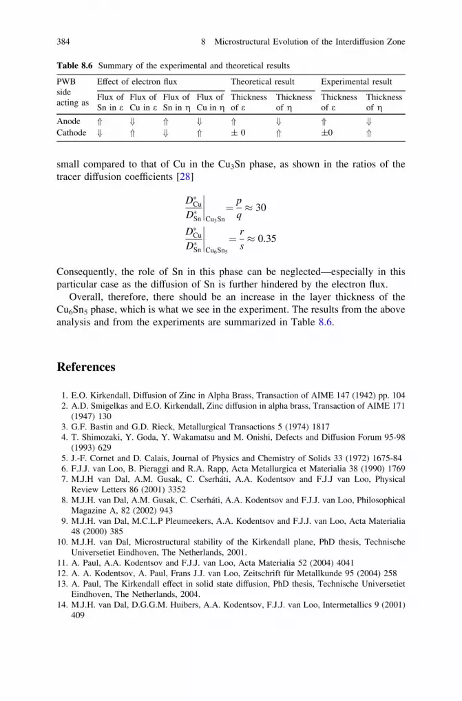
small compared to that of Cu in the Cu3Sn phase, as shown in the ratios of thetracer diffusion coefficients [28]

D�Cu

D�Sn

Cu3Sn

¼ p

q� 30

D�Cu

D�Sn

Cu6Sn5

¼ r

s� 0:35

Consequently, the role of Sn in this phase can be neglected—especially in thisparticular case as the diffusion of Sn is further hindered by the electron flux.

Overall, therefore, there should be an increase in the layer thickness of theCu6Sn5 phase, which is what we see in the experiment. The results from the aboveanalysis and from the experiments are summarized in Table 8.6.

References

1. E.O. Kirkendall, Diffusion of Zinc in Alpha Brass, Transaction of AIME 147 (1942) pp. 1042. A.D. Smigelkas and E.O. Kirkendall, Zinc diffusion in alpha brass, Transaction of AIME 171

(1947) 1303. G.F. Bastin and G.D. Rieck, Metallurgical Transactions 5 (1974) 18174. T. Shimozaki, Y. Goda, Y. Wakamatsu and M. Onishi, Defects and Diffusion Forum 95-98

(1993) 6295. J.-F. Cornet and D. Calais, Journal of Physics and Chemistry of Solids 33 (1972) 1675-846. F.J.J. van Loo, B. Pieraggi and R.A. Rapp, Acta Metallurgica et Materialia 38 (1990) 17697. M.J.H van Dal, A.M. Gusak, C. Cserháti, A.A. Kodentsov and F.J.J van Loo, Physical

Review Letters 86 (2001) 33528. M.J.H. van Dal, A.M. Gusak, C. Cserháti, A.A. Kodentsov and F.J.J. van Loo, Philosophical

Magazine A, 82 (2002) 9439. M.J.H. van Dal, M.C.L.P Pleumeekers, A.A. Kodentsov and F.J.J. van Loo, Acta Materialia

48 (2000) 38510. M.J.H. van Dal, Microstructural stability of the Kirkendall plane, PhD thesis, Technische

Universetiet Eindhoven, The Netherlands, 2001.11. A. Paul, A.A. Kodentsov and F.J.J. van Loo, Acta Materialia 52 (2004) 404112. A. A. Kodentsov, A. Paul, Frans J.J. van Loo, Zeitschrift für Metallkunde 95 (2004) 25813. A. Paul, The Kirkendall effect in solid state diffusion, PhD thesis, Technische Universetiet

Eindhoven, The Netherlands, 2004.14. M.J.H. van Dal, D.G.G.M. Huibers, A.A. Kodentsov, F.J.J. van Loo, Intermetallics 9 (2001)

409

Table 8.6 Summary of the experimental and theoretical results

PWBsideacting as

Effect of electron flux Theoretical result Experimental result

Flux ofSn in e

Flux ofCu in e

Flux ofSn in g

Flux ofCu in g

Thicknessof e

Thicknessof g

Thicknessof e

Thicknessof g

Anode * + * + * + * +Cathode + * + * ± 0 * ±0 *

384 8 Microstructural Evolution of the Interdiffusion Zone

15. M.J.H. van Dal, A.A. Kodentsov and F.J.J. van Loo, Intermetallics 9 (2001) 45116. A. Paul, M.J.H. van Dal, A.A. Kodentsov and F.J.J. van Loo, Acta Materialia 52 (2004) 623-17. L. Höglund, & J. Ågren, Acta Materialia 49 (2001) 131118. W.J. Boettinger, J.E. Guyer, C.E. Campbell and G.B. McFadden, Proceeding of the Royal

Society London A 463 (2007) 334719. J.H. Gülpen, A.A. Kodentsov, F.J.J. van Loo, Zeitschrift für Metallkunde 86 (1995) 530.20. C. Cserháti, A. Paul, A.A. Kodentsov, M.J.H. van Dal, F.J.J. van Loo, Intermetallics 11

(2003) 291-297.21. C. Ghosh and A. Paul, Acta Materialia 55 (2007) 192722. F.J.J. van Loo, Acta Metallurgica 18 (1970) 110723. A. Paul, A.A. Kodentsov and F.J.J. van Loo, Intermetallics, 14 (2006) 142824. H. Okamoto, Journal of Phase Equilibria and diffusion 25 (2004) 39425. S. Roy and A. Paul, Philosophical Magazine, 92 (2012) 421526. A.A. Kodentsov, A. Paul, and F.J.J. van Loo, Defects and Diffusion Forum 258-260 (2006)

18227. A. Paul, Journal of Materials Science: Materials in Electronics 22 (2011) 83328. A. Paul, C. Ghosh and W.J. Boettinger, Metallurgical and Materials Transactions A 42A

(2011) 95229. T. Laurila, J. Karppinen, V.Vuorinen, A. Paul and M. Paulasto-Kröckel, Journal of Electronic

Materials 40 (2011) 151730. T. Laurila, J. Karppinen, V. Vuorinen, J. Li, A.Paul and M. Paulasto-Kröckel, Journal of

Electronic Materials 41 (2012)31. J. Dekker, A. Lodder and J. van Ek, Physical Review B 56 (1997) 12167-1217732. T. Laurila, V. Vuorinen, and M. Paulasto-Kröckel, Materials Science and Engineering Reprts,

R68, (2010) 133. V. Vuorinen, T. Laurila, T. Mattila, E. Heikinheimo, J. Kivilahti, Journal of Electronic

Materials 36 (2007) 135534. J. Hurtig, Master’s Thesis, Helsinki University of Technology, (2006).35. T. Laurila, J. Hurtig, V. Vuorinen, and J.K. Kivilahti, Microelectronics Reliability 49 (2009)

242

References 385

Chapter 9Interdiffusion in Multicomponent Systems

In this Chapter, estimation of the diffusion parameters in the multicomponentsystem is explained. A pseudobinary approach simplifying the mathematicalconditions is also described. Finally the use of diffusion couple establishing thephase diagram is presented.

In the previous chapters, we have explained the diffusion analysis in binarysystems. In fact, it is relatively easy to study interdiffusion when only two com-ponents take part in the diffusion process. This is the reason that the majority ofsystems studied are binary systems. With an increase in the number of compo-nents, the study of interdiffusion either becomes (at best) rather difficult or (atworst) close to impossible. Even, the physical meaning of some of the parametersinvolved are not very easy to understand [1]. Research is going on to develop aneasier approach for the study of multicomponent systems. In this chapter, we shallintroduce the concept very briefly without going into too much complexity—something that could be difficult for new students of the diffusion process tounderstand. A book written by Kirkaldy and Young [2] will shed further light onthis topic. A comprehensive review written by Dayananda in Ref. [3] could be veryuseful to understand the details on the evolution of the composition in ternary andquaternary systems. The main difference between binary and multicomponentsystems is that in binary systems, we neglect the cross-terms. On the other hand,these are important to consider in multicomponent systems, which might havestrong influence. This fact as well as the influence of vacancies on diffusion inbinary alloys in general will be clear after the discussion below and from the notein the end of the Sect. 9.4.

9.1 Interdiffusion and Intrinsic Diffusion Coefficientsin Multicomponent Systems

The interdiffusion flux of an i-th component in a multicomponent system based onOnsager’s formulism [4, 5] can be written as

A. Paul et al., Thermodynamics, Diffusion and the Kirkendall Effect in Solids,DOI: 10.1007/978-3-319-07461-0_9, � Springer International Publishing Switzerland 2014

387

~Ju ¼ �Xn�1

v¼1

~Dnuv

oCv

oxð9:1aÞ

The interdiffusion fluxes estimated from the composition profiles of differentcomponents are related by (following the same line of discussion in Chap. 6 forbinary systems)

Xn

u¼1

�vu~Ju ¼ �v1~J1 þ �v2~J2 þ � � � � � � þ �vn~Jn ¼ 0 ð9:1bÞ

where ~Ju is the interdiffusion flux of the component u, ~D is the interdiffusioncoefficient, C is the concentration, x is the position parameter, �vu is the partialmolar volume, and n is the dependent variable. From Eq. 9.1b, it can be under-stood that we need to estimate the interdiffusion fluxes for (n-1) components. Theflux for the n-th component can be determined from these values. Compositions ofdifferent components are related by N1 þ N2 þ � � � � � � þ Nn ¼ 1. Therefore, if weconsider the n-th component as the dependent variable, the interdiffusion fluxescan be expressed with (n-1) components. This means that the total (n-1)2

interdiffusion coefficients are required to express the interdiffusion fluxes of all the(n-1) independent components.

Following Eq. 9.1a, in a ternary system (n = 3), ~J1 and ~J2 can be expressed as

~J1 ¼ �~D311

oC1

ox� ~D3

12oC2

ox¼ �~D3

111

vm

oN1

ox� ~D3

121

vm

oN2

oxð9:2aÞ

~J2 ¼ �~D321

oC1

ox� ~D3

22oC2

ox¼ �~D3

211

vm

oN1

ox� ~D3

221

vm

oN2

oxð9:2bÞ

The second part of the relations above is true for a constant molar volume, vm. Inmost ternary systems, the change in lattice parameters with composition is notknown and an average molar volume is considered for the estimations. FollowingEq. 9.1b, ~J3 can be related by (for the constant molar volume and constant partialmolar volumes of the components)

~J1 þ ~J2 þ ~J3 ¼ 0 ð9:3Þ

The average molar volume can be estimated by taking the weighted fraction ofthe molar volumes of the pure components that is vm avð Þ ¼ 1

n

Pni¼1 vi

m, where vim is

the molar volume of the pure component i. In Eqs. 9.2a and 9.2b, ~D311 and ~D3

22 arethe main (or direct) interdiffusion coefficients, which represent the influence of theconcentration gradient of one component on the diffusion rate of the same com-ponent. ~D3

12 and ~D321 are the cross- or indirect interdiffusion coefficients, which

represent the influence of the concentration gradient of one component on the

388 9 Interdiffusion in Multicomponent Systems

diffusion rate of the other component. The third component is considered as thedependent variable. Therefore, the values of ~D3

11;~D3

12;~D3

21, and ~D322 are required

to relate or to calculate the interdiffusion fluxes in a ternary system.The estimation of these parameters, however, is not as straightforward as in a

binary system. These parameters can only be determined at the point of inter-section of the composition profiles from two different diffusion couples. Forexample, in a Ni–Co–Pt system, the diffusion couples were made with differentcompositions and annealed at 1,200 �C for 25 h. [6]. It can be seen in Fig. 9.1athat the two composition profiles are found to intersect at a composition shown bya red circle. In each diffusion couple, the interdiffusion flux of the two componentscan be determined from the measured composition profile. The composition profileof Co(25Pt)/Ni is shown in Fig. 9.1b. Kirkaldy [7] explained that it is possible touse the Matano–Boltzmann analysis to determine the interdiffusion flux. A fewyears later, the same was discussed by Philibert and Guy [8]. Therefore, theinterdiffusion flux of each component i can be determined using the relation [fromEq. 7.19a]

~Ji YCi

� �¼ �

Cþi � C�iffi �

2t1� YCi

� � Zx�

x�1

YCi dxþ YCi

Zxþ1

x�

1� YCið Þ dx

24

35 ð9:4aÞ

where YCi¼ Ci�C�i

Cþi �C�i. Since, we generally consider a constant molar volume caused

by an unknown variation of the molar volume in a ternary system, we can write

~Ji Yið Þ ¼ �Nþi � N�iffi �

2tvm1� Yið Þ

Zx�

x�1

Yidxþ Yi

Zxþ1

x�

1� Yið Þ dx

24

35 ð9:4bÞ

where Yi ¼ Ni�N�iNþi �N�i

. Note that the same relation can be written, when the flux is

estimated using Wagner’s relation considering the constant molar volume, as canbe seen in Eq. 7.19c. The variation of the interdiffusion flux estimated from thecomposition profile in Fig. 9.1b is shown in Fig. 9.1c. The correctness of theestimation can be checked by examining whether the summation of the interdif-fusion fluxes that is ~JNi þ ~JCo þ ~JPt ¼ 0 because of the consideration of the con-stant molar volume. Note that depending on the direction of the diffusingcomponent, if the interdiffusion fluxes for Co and Pt are positive, the interdiffusionflux of Ni should be negative. By considering Ni as a dependent variable, wecalculate the interdiffusion fluxes of the independent variables Co and Pt at thecomposition of the intersection point. Accordingly, we can write

~JCo couple 1ð Þ ¼ �~DNiCoCo

1vm

oNCo

ox

� �Couple 1

�~DNiCoPt

1vm

oNPt

ox

� �Couple 1

ð9:5aÞ

9.1 Interdiffusion and Intrinsic Diffusion 389

Fig. 9.1 Compositionprofiles of diffusion couplesin Ni–Co–Pt system annealedat 1,200 �C for 25 h areshown on a Ni–Co–Pt Gibb’striangle. b Composition-distance profile of theCo(25Pt)/Ni diffusion coupleand c estimated variation ofinterdiffusion fluxes ofcomponents [6]

390 9 Interdiffusion in Multicomponent Systems

~JPt couple 1ð Þ ¼ �~DNiPtCo

1vm

oNCo

ox

� �Couple 1

�~DNiPtPt

1vm

oNPt

ox

� �Couple 1

ð9:5bÞ

Similarly, at the same intersection point, we can calculate the interdiffusion fluxesof these two components from the composition profile that is developed in thesecond diffusion couple (Ni25Pt)/Co. These fluxes are related to the interdiffusioncoefficients as

~JCo couple 2ð Þ ¼ �~DNiCoCo

1vm

oNCo

ox

� �Couple 2

�~DNiCoPt

1vm

oNPt

ox

� �Couple 2

ð9:5cÞ

~JPt couple 2ð Þ ¼ �~DNiPtCo

1vm

oNCo

ox

� �Couple 2

�~DNiPtPt

1vm

oNPt

ox

� �Couple 2

ð9:5dÞ

The interdiffusion coefficients are the material constants, and these should be thesame at that particular composition. Therefore, solving the above equations, fourinterdiffusion coefficients can be estimated at the point of intersection from twoseparate diffusion profiles.

The interdiffusion coefficients in a ternary system were first time estimated byZeibold and Ogilvie [9] in the Cu–Au–Ag system. It must be apparent that manydiffusion couples should be prepared to calculate the variation of the interdiffusioncoefficients with composition over the whole composition range in a ternarysystem. The diffusion couples prepared in the Ni–Co–Pt system, which wereannealed at 1,200 �C for 25 h, are shown in Fig. 9.2 [6]. The interdiffusioncoefficients can be estimated at all the compositions where the diffusion profileshave intersected. Variation of the data are shown in Fig. 9.3.

Fig. 9.2 Compositionprofiles developed in differentdiffusion couples of Co–Ni–Pt system annealed at1,200 �C for 25 h are shownin the Gibbs triangle. Profileswith dotted lines indicate thepresence of uphill diffusion.Compositions at which threeprofiles intersect are shownby circles [6]

9.1 Interdiffusion and Intrinsic Diffusion 391

A relatively high rate of error is expected in the estimation of these ternary-system parameters (compared to any binary system) because of the requirementsof two diffusion profiles. This can be explained with the estimated data in the Ni–Co–Pt system. As circled in Fig. 9.2, there are two compositions, at which threedifferent composition profiles have intersected. We should, therefore, be able toestimate the interdiffusion coefficients by considering any of the two diffusioncouples at the same intersection points. The estimated values are listed inTable 9.1. The data of three rows at both compositions are estimated, consideringthree different combinations. It can be seen that there is no change in the sign ofthe diffusion coefficients; however, there was a relatively high difference betweenthe diffusion parameters estimated.

Another important question is which component should be considered as adependent component. As explained by Kirkaldy and Young [2], the dependentvariable should be chosen such that the conditions written below are fulfilled—conditions that are derived based on the thermodynamic requirements and stabilityof the solutions

~D311 þ ~D3

22 [ 0 ð9:6aÞ

ð~D311 þ ~D3

22Þ2� 4ð~D3

11~D3

22 � ~D312

~D321Þ ð9:6bÞ

ð~D311

~D322 � ~D3

12~D3

21Þ� 0 ð9:6cÞ

In general, when the diffusion experiments are conducted in a small section, it is acommon practice to consider the solvent component (that is, the major component)as the dependent variable. Of course, it is still wise to check whether the aboveconditions written in Eqs. 9.6a, 9.6b and 9.6c are met. When the experiments arecovered in the whole composition range, after estimation of the data, it is neces-sary to check for which component the conditions for the dependent variable isfulfilled at all compositions. Repeatedly—as it was in the case of the Ni–Co–Ptsystem—the conditions are met when we consider any of the components as thedependent variable. It should be noted at this point that presenting data with

Table 9.1 The main and cross-interdiffusion coefficients estimated at the composition wherethree intersecting diffusion profiles in the Co–Ni–Pt are listed [6]

Composition at. % ~DNiCoCo

(10-14 m2/s)

~DNiCoPt

(10-15 m2/s)

~DNiPtCo

(10-15 m2/s)

~DNiPtPt

(10-14 m2/s)

Ni = 19.8, Co = 22.7and Pt = 57.5

0.8 -5 -6.2 1.10.3 -1.7 -6.9 1.21.2 -1.9 -7.1 1.2

Ni = 43, Co = 40and Pt = 17

1.7 -7.1 -0.9 0.41.5 -2.5 -1.2 1.30.9 -3 -0.2 0.8

392 9 Interdiffusion in Multicomponent Systems

respect to one dependent variable is sufficient, since the interdiffusion coefficientsconsidering different components as dependent variables are related by [10]

~D211 ¼ ~D3

11 � ~D312 ð9:7aÞ

~D213 ¼ �~D3

12 ð9:7bÞ

~D231 ¼ ~D3

22 þ ~D312 � ~D3

11 � ~D321 ð9:7cÞ

~D233 ¼ ~D3

22 þ ~D312 ð9:7dÞ

~D122 ¼ ~D3

22 � ~D321 ð9:7eÞ

~D123 ¼ �~D3

21 ð9:7fÞ

~D132 ¼ ~D3

11 þ ~D321 � ~D3

22 � ~D312 ð9:7gÞ

~D133 ¼ ~D3

11 þ ~D321 ð9:7hÞ

The variation of the interdiffusion coefficients estimated in the Ni–Co–Pt system isshown in Fig. 9.3.

The interdiffusion fluxes that are estimated based on the composition profile ofa particular component are related to the intrinsic fluxes of the components by [3]

~Ju ¼ Ju � Nu

Xn

k¼1

Jk ð9:8aÞ

In a ternary system, these can be written as

~J1 ¼ 1� N1ð ÞJ1 � N1 J2 þ J3ð Þ ¼ N2 þ N3ð ÞJ1 � N1 J2 þ J3ð Þ ð9:8bÞ

~J2 ¼ 1� N2ð ÞJ2 � N2 J1 þ J3ð Þ ¼ N1 þ N3ð ÞJ2 � N2 J1 þ J3ð Þ ð9:8cÞ

~J3 ¼ 1� N3ð ÞJ3 � N3 J1 þ J2ð Þ ¼ N1 þ N2ð ÞJ3 � N3 J1 þ J2ð Þ ð9:8dÞ

where Ju is the intrinsic flux of the component u. Furthermore, the intrinsic flux isrelated to the intrinsic diffusion coefficients by [3]

Ju ¼ �Xn�1

v¼1

Dnuv

oCv

oxð9:9aÞ

In a ternary system, we can write

9.1 Interdiffusion and Intrinsic Diffusion 393

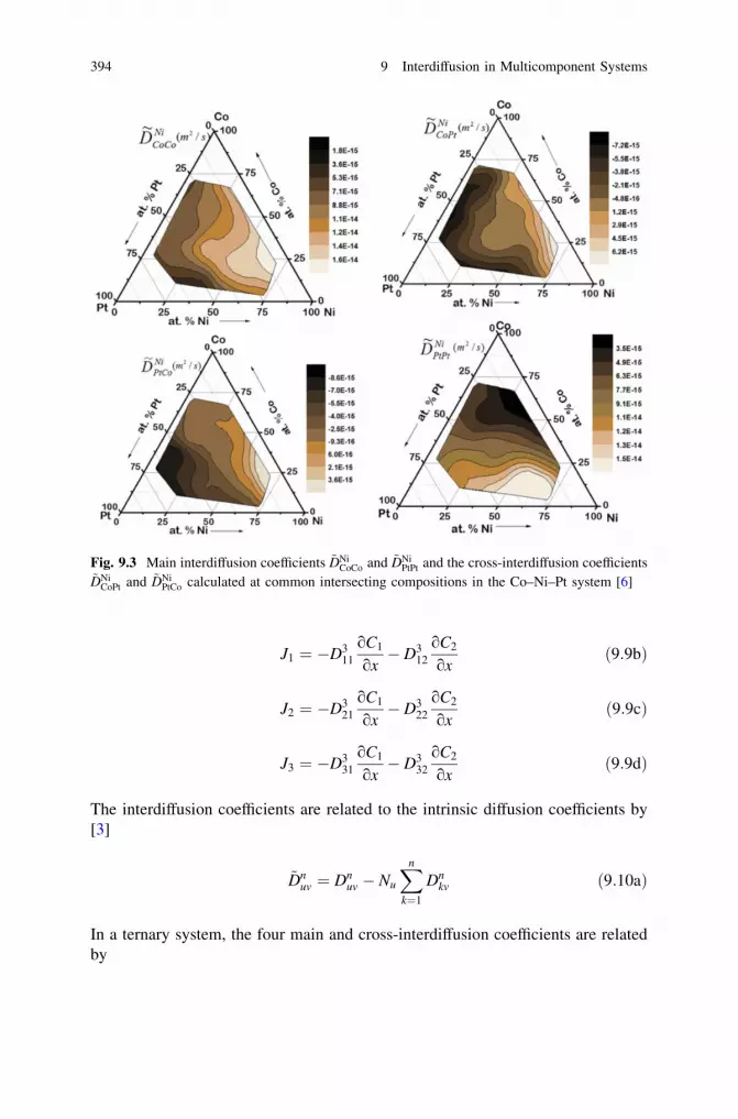
J1 ¼ �D311

oC1

ox� D3

12oC2

oxð9:9bÞ

J2 ¼ �D321

oC1

ox� D3

22oC2

oxð9:9cÞ

J3 ¼ �D331

oC1

ox� D3

32oC2

oxð9:9dÞ

The interdiffusion coefficients are related to the intrinsic diffusion coefficients by[3]

~Dnuv ¼ Dn

uv � Nu

Xn

k¼1

Dnkv ð9:10aÞ

In a ternary system, the four main and cross-interdiffusion coefficients are relatedby

Fig. 9.3 Main interdiffusion coefficients ~DNiCoCo and ~DNi

PtPt and the cross-interdiffusion coefficients~DNi

CoPt and ~DNiPtCo calculated at common intersecting compositions in the Co–Ni–Pt system [6]

394 9 Interdiffusion in Multicomponent Systems

~Dn11 ¼ Dn

11 � N1 Dn11 þ Dn

21 þ Dn31

ffi �ð9:10bÞ

~Dn12 ¼ Dn

12 � N1 Dn12 þ Dn

22 þ Dn32

ffi �ð9:10cÞ

~Dn21 ¼ Dn

21 � N2 Dn11 þ Dn

21 þ Dn31

ffi �ð9:10dÞ

~Dn22 ¼ Dn

22 � N2 Dn12 þ Dn

22 þ Dn32

ffi �ð9:10eÞ

Lane and Kirkaldy [11] described the requirements of these six intrinsic diffusioncoefficients to describe the intrinsic or interdiffusion fluxes and the interdiffusioncoefficients. From the relations above, it must be clear that these can be estimatedat the composition of the intersection from the two diffusion couples with anadditional condition that the inert particles used as markers (indicating the positionof the Kirkendall plane) are also located at that composition. Six intrinsic fluxescan be estimated at this composition using the method developed by Heumann asexplained previously in Sect. 6.11a, [12, 13] or the relation developed in Sect.6.8b, which is expressed as

JKi ¼ �

12t

Nþi

ZxK

x�1

Yi

vmdx� N�i

Zxþ1

xK

1� Yið Þvm

dx

24

35 ð9:11aÞ

For constant molar volume, it can be written as

JKi ¼ �

12tvm

Nþi

ZxK

x�1

Yidx� N�i

Zxþ1

xK

1� Yið Þdx

24

35 ð9:11bÞ

Since there is very little chance of getting the markers at the point of intersection,which is very difficult to predict, it is very rare for anyone to estimate the intrinsicdiffusion coefficients following this method. For example, Sohn and Dayananda[14] estimated these six intrinsic diffusion coefficients at one composition in theFe–Ni–Al system. Dayananda [15] developed an approach in which the intrinsicdiffusion coefficients can be estimated from a single vapor/solid diffusion couple.Therefore, this method is restricted to systems, where the components are able toreact in the vapor phase (such as Zn and Mg) with solid alloys. This approach wasapplied in the Cu–Zn–Mn [16] and Ag–Zn–Cd [17] systems.

The existence of the zero flux plane (ZFP) in the interdiffusion zone of differentmulticomponent systems is shown by Dayananda et al. in many systems [14, 18,19]. This is associated with the uphill diffusion of a component in a particular partof the interdiffusion zone and the downhill diffusion in the other part. This can beexplained with the help of the CoPt/Ni diffusion couples in the Ni–Co–Pt system,with varying compositions of CoPt alloys, as shown in Fig. 9.2. The compositionprofiles and the estimated interdiffusion fluxes are presented in Fig. 9.4, where it

9.1 Interdiffusion and Intrinsic Diffusion 395

can be seen that in the Co(25Pt)/Ni couple, all the components diffuse down theconcentration gradient. Therefore, if the interdiffusion fluxes of Co and Pt areexpressed with a positive sign, the interdiffusion flux of Ni will be expressed witha negative sign. In the Co(50Pt)/Ni couple, very minor uphill diffusion is to beobserved, and in the Co(75Pt)/Ni couple, clear uphill diffusion of Co is to be seen.The Co profile in the Co(75Pt)/Ni interdiffusion zone increases first to a highercomposition than the composition used (25 at.%) in the Co(75Pt) end member andthen decreases in the other part of the interdiffusion zone. For this reason, theestimated interdiffusion flux of Co has a negative sign in the beginning and thenchanges to a positive sign. During the transition from negative to positive values, itgoes through a zero value and the plane corresponding to this composition is called

(a) (b)

(c) (d)

(e) (f)

Fig. 9.4 Composition profiles developed in a Co(25Pt)/Ni, c Co(50Pt)/Ni, e Co(75Pt)/Nidiffusion couples and the corresponding calculated flux profiles are shown in b, d, and f [6]

396 9 Interdiffusion in Multicomponent Systems

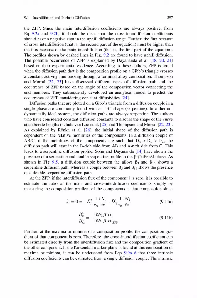
the ZFP. Since the main interdiffusion coefficients are always positive, fromEq. 9.2a and 9.2b, it should be clear that the cross-interdiffusion coefficientsshould have a negative sign in the uphill diffusion range. Further, the flux becauseof cross-interdiffusion (that is, the second part of the equation) must be higher thanthe flux because of the main interdiffusion (that is, the first part of the equation).The profiles shown by dashed lines in Fig. 9.2 are found to have uphill diffusion.The possible occurrence of ZFP is explained by Dayananda et al. [18, 20, 21]based on their experimental evidence. According to these authors, ZFP is foundwhen the diffusion path that is the composition profile on a Gibb’s triangle crossesa constant activity line passing through a terminal alloy composition. Thompsonand Morral [22, 23] have discussed different types of diffusion path and theoccurrence of ZFP based on the angle of the composition vector connecting theend members. They subsequently developed an analytical model to predict theoccurrence of ZFP considering constant diffusivities [24].

Diffusion paths that are plotted on a Gibb’s triangle from a diffusion couple in asingle phase are commonly found with an ‘‘S’’ shape (serpentine). In a thermo-dynamically ideal system, the diffusion paths are always serpentine. The authorswho have considered constant diffusion constants to discuss the shape of the curveat elaborate lengths include van Loo et al. [25] and Thompson and Morral [22, 23].As explained by Rönka et al. [26], the initial shape of the diffusion path isdependent on the relative mobilities of the components. In a diffusion couple ofAB/C, if the mobilities of the components are such that DA [ DB [ DC, thediffusion path will start in the B-rich side from AB and A-rich side from C. Thisleads to a serpentine diffusion profile. Sohn and Dayananda [14] have shown thepresence of a serpentine and double serpentine profile in the b-(NiFe)Al phase. Asshown in Fig. 9.5, a diffusion couple between the alloys b3 and b15 shows aserpentine diffusion path, whereas a couple between b5 and b17 shows the presenceof a double serpentine diffusion path.

At the ZFP, if the interdiffusion flux of the component i is zero, it is possible toestimate the ratio of the main and cross-interdiffusion coefficients simply bymeasuring the composition gradient of the components at that composition since

~Ji ¼ 0 ¼ �~D3i1

1vm

oN1

ox� ~D3

i21

vm

oN2

oxð9:11aÞ

~D3i1

~D3i2

¼ � oN2=oxð ÞoN1=oxð Þ

����ZFP

ð9:11bÞ

Further, at the maxima or minima of a composition profile, the composition gra-dient of that component is zero. Therefore, the cross-interdiffusion coefficient canbe estimated directly from the interdiffusion flux and the composition gradient ofthe other component. If the Kirkendall marker plane is found at this composition ofmaxima or minima, it can be understood from Eqs. 9.9a–d that three intrinsicdiffusion coefficients can be estimated from a single diffusion couple. The intrinsic

9.1 Interdiffusion and Intrinsic Diffusion 397

diffusion coefficients were estimated in this fashion by Sohn and Dayananda [14]in the Fe–Ni–Al system.

By extrapolating the interdiffusion coefficients to binary axes, we can extract thebinary diffusion coefficients and the impurity diffusion coefficients [14]. Forexample, when the ~D2

11 and ~D222 values are extended to zero composition of 3, these

values are equal to the interdiffusion coefficients in the binary 1–2 system. Whenthe composition of component 1 approaches zero, ~D2

11 and ~D311 are equal to the

impurity diffusion coefficient of 1, which is D1 ð2; 3Þ in the binary 2–3 system [9].In a quaternary system, the requirements for the estimation of the interdiffusion

coefficients are even more stringent. For example, following Eq. 9.1a, the inter-diffusion fluxes of the components, considering a constant molar volume, can beexpressed as

~J1 ¼ �~D411

1vm

oN1

ox� ~D4

121

vm

oN2

ox� ~D4

13

1vm

oN3

oxð9:12aÞ

~J2 ¼ �~D421

1vm

oN1

ox� ~D4

22

1vm

oN2

ox� ~D4

23

1vm

oN3

oxð9:12bÞ

~J3 ¼ �~D431

1vm

oN1

ox� ~D4

321

vm

oN2

ox� ~D4

33

1vm

oN3

oxð9:12cÞ

~J1 þ ~J2 þ ~J3 þ ~J4 ¼ 0 ð9:12dÞ

Therefore, there are nine interdiffusion coefficients to determine and for that weneed three composition profiles to intersect at one particular composition. It isalmost impossible to design experiments in such a way that three diffusion couples

Fig. 9.5 Diffusion profiles in the Fe–Ni–Al system showing serpentine (b15/b3) and doubleserpentine diffusion (b5/b17) paths [14]

398 9 Interdiffusion in Multicomponent Systems

are able to intersect at a common point in a three-dimensional composition space[1]. This is the simple reason why there have been no previous experimentsconducted to determine these nine interdiffusion coefficients in a quaternary sys-tem. Experimental studies are available in Cu–Ni–Zn–Mn [20] and Ni–Cr–Co–Mo[21] quaternary systems—the interdiffusion coefficients, however, were not esti-mated from three intersecting diffusion couples. In the Cu–Ni–Zn–Mn system, theinterdiffusion fluxes were estimated, which can be done directly from the com-position profiles measured using the relation in Eqs. 9.4a and 9.4b. In the Ni–Cr–Co–Mo system, only the major interdiffusion coefficients were estimated in asingle diffusion couple in which two components did not develop the diffusionprofile such that the cross-interdiffusion coefficients could be considered as zero.

There is always a special interest to develop an experimental approach for the(easy) determination of diffusion parameters in systems with three or more compo-nents. Krishtal et al. [27] first developed a treatment to estimate the diffusionparameters in a multicomponent system, considering the constant diffusion coeffi-cients. In the following decade, Thompson and Morral [23] developed a square rootdiffusivity approach, again by considering the constant diffusion coefficients. Thismeans that these treatments can be used when the composition differences of thediffusion couples are reasonably small such that the diffusion coefficients do not varysignificantly over that composition range. The approach developed by Thompson andMorral was used to estimate the diffusion parameters in a few quaternary systems,keeping the composition difference of the diffusion couple end members very smallsuch as 5 at.% [28–30]. Stalker et al. [28] have shown that in such a small compositionrange, they could estimate back the interdiffusion flux with a very minor error.

9.2 Average Effective and Integrated Diffusion Coefficientsin Multicomponent System

As it is discussed above, in a ternary system, it is necessary to determine fourinterdiffusion coefficients at the point of intersection from two different diffusioncouples. To circumvent this problem, Dayananda and Sohn [31] introduced theconcept of the average effective interdiffusion coefficient so that this parametercould be estimated from a composition profile in a single diffusion couple. FromEq. 9.2a, we can write

~Ji ¼ �~D3i1

oC1

ox� ~D3

i2oC2

oxð9:13Þ

In terms of the effective interdiffusion coefficient

~Ji ¼ �~Deffi

oCi

oxð9:14Þ

9.1 Interdiffusion and Intrinsic Diffusion 399

Comparing Eqs. 9.13 and 9.14, we can write

~Deffi ¼ ~D3

i1oC1

oCi� ~D3

i2oC2

oCið9:15Þ

Therefore, the effective interdiffusion coefficients are a kind of average of the mainand cross-interdiffusion coefficients and do not shed any light on the individualvalues. To estimate this parameter, one needs to follow the step discussed below.Suppose we are interested to estimate these parameters on either side of the initialcontact plane. Integrating Eq. 9.14 from the unaffected left-hand side of the endmember to the initial contact plane that is the Matano plane, we get

Zxo

x�1

~Jidx¼ �ZCo

i

C�i

~Deffi dCi ¼� �~D

eff

i;L

ZCoi

C�i

dCi ¼ �~Deff

i;L C�i � Coi

ffi �

�~Deff

i;L ¼

Rxo

x�1~Jidx

C�i � Coi

¼ P

C�i � Coi

ð9:16aÞ

where Coi is the composition at the Matano plane that is the initial contact plane.

�~Deff

i;L is the average effective diffusion coefficient on the left-hand side of theMatano plane. P is the area, as shown in Fig. 9.6a.

Integrating Eq. 9.14 from the Matano plane to the unaffected right-hand side ofthe diffusion couple, we get

Zxþ1

xo

~Jidx ¼ �ZCþiCo

i

~Deffi dCi ¼ ��~D

eff

i;R

ZCþiCo

i

dCi ¼ �~Deff

i;R Coi � Cþi

ffi �

�~Deff

i;R ¼

Rxþ1xo

~Jidx

Coi � Cþi

¼ Q

Coi � Cþi

ð9:16bÞ

�~Deff

i;R is the average effective diffusion coefficient on the right-hand side of the

Matano plane. Q is the area as shown in Fig. 9.6a. The value of ~Ji can be estimatedusing the relation expressed in Eqs. 9.4a and 9.4b. Note here that for the com-position profile considered in this figure, both the numerator and denominator ofEqs. 9.16a and 9.16b are negative in order to give positive values for the averageeffective interdiffusion coefficients.

Dayananda and Sohn [31] used this procedure to estimate the average effectiveinterdiffusion coefficients on either side of the Matano plane and then estimatedback the concentration profile from these estimated values to show that this is anefficient estimation procedure.

400 9 Interdiffusion in Multicomponent Systems

Dayananda and Sohn [32] developed another model, following which—instead ofestimating one average effective diffusion coefficient—the average values of the mainand cross-interdiffusion coefficients can be estimated from only a single diffusioncouple. Integrating Eq. 9.13 over the composition range of interest, we can write

Zx2

x1

~Jidx ¼ �ZC1 x2ð Þ

C1 x1ð Þ

~D3i1dC1 �

ZC2 x2ð Þ

C2 x1ð Þ

~D3i2dC2

Zx2

x1

~Jidx ¼ ��~D3i1

ZC1 x2ð Þ

C1 x1ð Þ

dC1 � �~D3i2

ZC2 x2ð Þ

C2 x1ð Þ

dC2

Zx2

x1

~Jidx ¼ ��~D3i1 C1 x2ð Þ � C1 x1ð Þ½ � � �~D

3i2 C2 x2ð Þ � C2 x1ð Þ½ � ð9:17aÞ

where, �~D3i1 and �~D

3i2 are the average interdiffusion coefficients estimated over the

composition range of interest. Now, multiplying Eq. 9.13 by x� xoð Þ on both sidesand then integrating over the same composition range of interest, we get

Fig. 9.6 Explanation of the a average effective diffusion coefficients and b average main andcross-interdiffusion coefficients from a single diffusion profile in a ternary system

9.2 Average Effective and Integrated Diffusion Coefficients 401

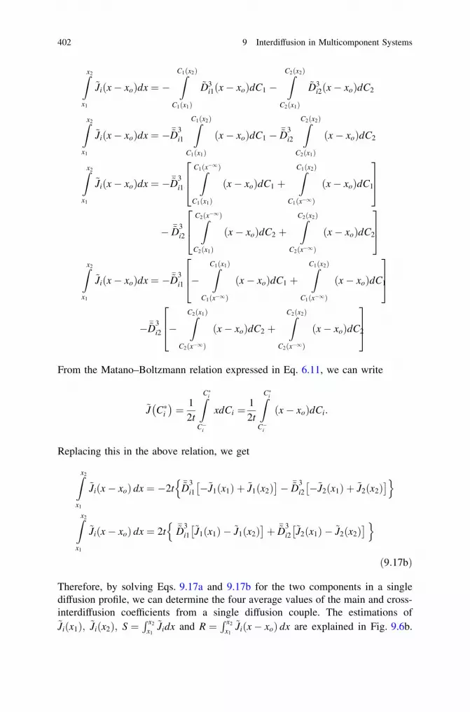
Zx2

x1

~Ji x� xoð Þdx ¼ �ZC1 x2ð Þ

C1 x1ð Þ

~D3i1 x� xoð ÞdC1 �

ZC2 x2ð Þ

C2 x1ð Þ

~D3i2 x� xoð ÞdC2

Zx2

x1

~Ji x� xoð Þdx ¼ ��~D3i1

ZC1 x2ð Þ

C1 x1ð Þ

x� xoð ÞdC1 � �~D3i2

ZC2 x2ð Þ

C2 x1ð Þ

x� xoð ÞdC2

Zx2

x1

~Ji x� xoð Þdx ¼ ��~D3i1

ZC1 x�1ð Þ

C1 x1ð Þ

x� xoð ÞdC1 þZC1 x2ð Þ

C1 x�1ð Þ

x� xoð ÞdC1

264

375

� �~D3i2

ZC2 x�1ð Þ

C2 x1ð Þ

x� xoð ÞdC2 þZC2 x2ð Þ

C2 x�1ð Þ

x� xoð ÞdC2

264

375

Zx2

x1

~Ji x� xoð Þdx ¼ ��~D3i1 �

ZC1 x1ð Þ

C1 x�1ð Þ

x� xoð ÞdC1 þZC1 x2ð Þ

C1 x�1ð Þ

x� xoð ÞdC1

264

375

��~D3i2 �

ZC2 x1ð Þ

C2 x�1ð Þ

x� xoð ÞdC2 þZC2 x2ð Þ

C2 x�1ð Þ

x� xoð ÞdC2

264

375

From the Matano–Boltzmann relation expressed in Eq. 6.11, we can write

~J C�iffi �

¼ 12t

ZC�iC�i

xdCi ¼12t

ZC�iC�i

x� xoð ÞdCi:

Replacing this in the above relation, we get

Zx2

x1

~Ji x� xoð Þ dx ¼ �2t �~D3i1 �~J1 x1ð Þ þ ~J1 x2ð Þ

� �~D3i2 �~J2 x1ð Þ þ ~J2 x2ð Þ n o

Zx2

x1

~Ji x� xoð Þ dx ¼ 2t �~D3i1

~J1 x1ð Þ � ~J1 x2ð Þ

þ �~D3i2

~J2 x1ð Þ � ~J2 x2ð Þ n o

ð9:17bÞ

Therefore, by solving Eqs. 9.17a and 9.17b for the two components in a singlediffusion profile, we can determine the four average values of the main and cross-interdiffusion coefficients from a single diffusion couple. The estimations of~Ji x1ð Þ; ~Ji x2ð Þ; S ¼

R x2

x1~Jidx and R ¼

R x2

x1~Ji x� xoð Þ dx are explained in Fig. 9.6b.

402 9 Interdiffusion in Multicomponent Systems

Dayananda and Sohn [32] used this method to calculate the diffusion parameters inthe Cu–Ni–Zn, Fe–Ni–Al, and Ni–Cr–Al systems. From the estimated diffusionparameters, they estimated back the composition profiles and found that the dif-ference between the actual profiles from which these parameters were estimatedand then estimated profiles is negligible.

The advantage of these two methods developed by Dayananda et al. is that it isnow possible to estimate the diffusion parameters from only a single diffusioncouple—compared to a need for two intersecting diffusion profiles in the con-ventional method previously explained in Sect. 9.1. However, the disadvantage isthat we calculate a kind of average value over the composition range, where thediffusion coefficients might vary significantly. If the first method is followed, theaverage effective diffusion coefficients should be estimated for all the componentsfrom their composition profiles. On the other hand, in the estimation of the averagemain and cross-interdiffusion coefficients (explained in the second method), thecompositions profiles of two components are required. Additionally, in the secondcase, after estimating the average main and cross-interdiffusion coefficients, thestability of the solution should be checked by validating the conditions given inEq. (9.6a, 9.6b and 9.6c). Cermak and Rothova [33] argued that by making theinterval (between x1 and x2) very small, the values can be estimated close to that ofthe actual values that were estimated at the point of intersection from the twodifferent diffusion couples. However, much recently, Cheng et al. [34] have shownthat this cannot be used to determine the composition-dependent diffusion coef-ficients as demanded by Cermak and Rothova.

Many times, as seen from the binary system case discussed in Chap. 6, internary systems, layers also grow in the interdiffusion zone with the line com-pounds or the phases with a narrow homogeneity range. Because of the very smallcomposition range, it is not possible to design experiments such that compositionprofiles from two different diffusion couples intersect at a common compositioninside the phase. Further, it is also not possible to determine the concentrationgradient. Therefore, the integrated diffusion coefficients should be estimated fordifferent components using the relation (based on Eqs. 7. 17 and 7. 19a

~Dbint;i ¼

ZNb 2B

Nb 1

B

~Deffi dNB ¼ � vb

m

Zxb 2

xb 1

~Jidx ð9:18aÞ

~J Y�C;i

� �¼ �

Cþi � C�iffi �

2t1� Y�C;i

� � Zx�

x�1

YC;idxþ Y�C;i

Zxþ1

x�

1� YC;i

ffi �dx

24

35

ð9:18bÞ

where YC;i ¼Ci�C�iCþi �C�i

.

9.2 Average Effective and Integrated Diffusion Coefficients 403

Similarly, using the relations developed by Wagner [35] following Eq. 7. 19c, itcan be expressed for constant molar volume as

~J ¼ �NþB � N�Bffi �

2t1� Y�Bffi � Zx�

x�1

YB

vmdxþ Y�B

Zxþ1

x�

1� YBð Þvm

dx

24

35 ð9:18cÞ

Note here that for the constant molar volume, Eq. 9.18b will be the same asEq. 9.4b.

Therefore, as explained above in Chap. 7, in a ternary system also, the inte-grated diffusion coefficients of different components can be estimated by inte-grating the interdiffusion flux (determined from a composition or concentrationprofile) using Eq. 9.18b, 9.18c or Eq. 9.4 over the thickness Dxb ¼ xb2

� xb1

ffi �of

the phase layer of interest b. One important fact should be noted here that, in abinary case, there is only one integrated diffusion coefficient, which is the samewhen estimated from the composition profile of any of the components. However,in a ternary system, each component will have an integrated diffusion coefficient ifthese develop a diffusion profile in the interdiffusion zone.

If the composition range of the phase is narrow but known, then the averageeffective interdiffusion coefficient can be estimated by dividing the integrateddiffusion coefficient with the composition range

~Deffi ¼

~Dbint

DNbB

ð9:19Þ

It should be noted here that the average effective interdiffusion coefficient in Eqs. 7.9and 9.19 is the same. Further, this is called the average interdiffusion coefficient in abinary system, which is the average of the interdiffusion coefficients. In a ternarysystem, it is called the average effective interdiffusion coefficients—which is a kindof average of the main and cross-interdiffusion coefficients in a phase. The estimationof the average effective interdiffusion coefficient in a ternary system is the onlyoption and very useful in many systems. For example, the diffusion paths developedin different diffusion couples in the Ni–Co–W are shown in Fig. 9.7a. It can be seenthat in a few diffusion couples, l-(Co,Ni)7W6 grows with a small composition range.The composition profile of the Co(25Ni)/W diffusion couple is shown in Fig. 9.7b[36]. It must be clear that it is not easy to design experiments such that the compo-sition profiles from two different diffusion couples intersect in the range of phasecomposition. It is also difficult to calculate the concentration gradient inside the lphase, since it does not vary enough with composition to measure with a minimumerror. Therefore, the average effective diffusion coefficients were estimated tounderstand the interdiffusion process in this system.

404 9 Interdiffusion in Multicomponent Systems

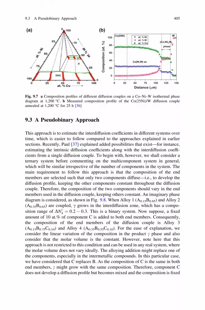
9.3 A Pseudobinary Approach

This approach is to estimate the interdiffusion coefficients in different systems overtime, which is easier to follow compared to the approaches explained in earliersections. Recently, Paul [37] explained added possibilities that exist—for instance,estimating the intrinsic diffusion coefficients along with the interdiffusion coeffi-cients from a single diffusion couple. To begin with, however, we shall consider aternary system before commenting on the multicomponent system in general,which will be similar irrespective of the number of components in the system. Themain requirement to follow this approach is that the composition of the endmembers are selected such that only two components diffuse—i.e., to develop thediffusion profile, keeping the other components constant throughout the diffusioncouple. Therefore, the composition of the two components should vary in the endmembers used in the diffusion couple, keeping others constant. An imaginary phasediagram is considered, as shown in Fig. 9.8. When Alloy 1 (A0.15B0.85) and Alloy 2(A0.35B0.65) are coupled, c grows in the interdiffusion zone, which has a compo-sition range of DNc

A ¼ 0:2� 0:3: This is a binary system. Now suppose, a fixedamount of 10 at.% of component C is added to both end members. Consequently,the composition of the end members of the diffusion couple is Alloy 3(A0.15B0.75C0.10) and Alloy 4 (A0.35B0.55C0.10). For the ease of explanation, weconsider the linear variation of the composition in the product c phase and alsoconsider that the molar volume is the constant. However, note here that thisapproach is not restricted to this condition and can be used in any real system, wherethe molar volume does not vary ideally. The alloying addition might replace one ofthe components, especially in the intermetallic compounds. In this particular case,we have considered that C replaces B. As the composition of C is the same in bothend members, c might grow with the same composition. Therefore, component Cdoes not develop a diffusion profile but becomes mixed and the composition is fixed

(a) (b)

Fig. 9.7 a Composition profiles of different diffusion couples on a Co–Ni–W isothermal phasediagram at 1,200 �C. b Measured composition profile of the Co(25Ni)/W diffusion coupleannealed at 1,200 �C for 25 h [36]

9.3 A Pseudobinary Approach 405

throughout the diffusion couple. Therefore, from Eqs. 9.2a, 9.2b and 9.8a–9.8d, forN2 as fixed composition it is clear that the diffusion in this ternary system should beconsidered as a pseudobinary system. For example, if we consider that the com-position of component 2 is fixed, from the intrinsic flux (J2 = 0) the interdiffusionflux (~J2 ¼ 0) and the concentration gradient (dC2=dx ¼ 0), the relations are reducedto the relations in a binary system. Therefore, the estimation procedure is rathersimilar. To explain the steps, we first consider the couple in the binary system andthen explain it for the ternary (pseudobinary) system.

9.3.1 Estimation of Diffusion Parameters in a Binary System

A diffusion couple of two blocks with compositions of, let us say, Alloy 1(A0.15B0.85) and Alloy 2 (A0.35B0.65) as presented in Fig. 9.9a. Suppose in themiddle, a single phase c grows with a composition range of DNc

A ¼ 0:2�0:3. Tosimplify the explanation, we consider a linear change in the composition in theinterdiffusion zone, as shown in composition profiles of A and B in Figs. 9.9b and c.Further, we consider that there is no change in the molar volume with the change incomposition. These assumptions are taken such that it will be easier for the readersto calculate the diffusion parameters without the help of any software. As men-tioned already, this method is applicable in any real system, where the compositionprofile is not linear and the molar volume deviates from ideality. For the calculationof the intrinsic diffusion coefficients, we consider the presence of the marker planein the interdiffusion zone. Although the variation of the interdiffusion coefficientswith composition can be estimated, the interdiffusion and intrinsic diffusion coef-ficients at the marker plane only are estimated at present so that we can validate the

Fig. 9.8 Compositions of thealloys chosen for diffusioncouples [37]

406 9 Interdiffusion in Multicomponent Systems

results. The interdiffusion flux of a component i in a binary or multicomponentsystem can be estimated by Eq. 7.19c

~Ji ¼ �DNi

2tvcm

1� Yið ÞZx�

x�1

Yidxþ Yi

Zxþ1

x�

1� Yið Þdx

24

35

¼ � DNi

2tvcm

1� Yið ÞZxK

x�1

Yidxþ Yi

Zxþ1

xK

1� Yið Þdx

24

35

ð9:20aÞ

We can calculate the interdiffusion flux of A by

~JA ¼ �DNA

2tvcm

1� YAð ÞZxK

x�1

YAdxþ YA

Zxþ1

xK

1� YAð Þdx

24

35: ð9:20bÞ

A minus sign is there since the component A diffuses from right to left and theinterdiffusion flux is negative. For the interdiffusion flux of B, a minus sign willnot be there since it diffuses from left to right. The composition range of thediffusion couple is DNA ¼ NþA � N�A , where NþA and N�A are the composition of theinitial and unaffected parts of the left- and right-hand sides of the end members, x*

is the position of interest, YA is the composition normalized variable and is equal toNA�N�ANþA �N�A

. From Fick’s first law for constant molar volume, we can write

~JA ¼ �~DdCA

dx¼ �~D

1vc

m

dNA

dxð9:20cÞ

From Eqs. 9.20b and 9.20c, we can write the relation for the interdiffusion coef-ficient at the marker plane (denoted by K) as

~D ¼ 12t

dx

dNA=DNA

� �K

1� YKA

ffi � ZxK

x�1

YAdxþ YKA

Zxþ1

xK

1� YAð Þdx

24

35

¼ 12t

dx

dYA

� �K

1� YKA

ffi � ZxK

x�1

YAdxþ YKA

Zxþ1

xK

1� YAð Þdx

24

35

ð9:20dÞ

It should be noted here that the data estimated will be the same if estimated withrespect to the composition profile of B instead of A. Let us consider that themarkers used at the interface before annealing are shifted to 0.24 atomic fraction A(0.76 atomic fraction B) located at 40 lm from the Alloy 1/c phase interface. Thetotal thickness of the product c phase grown in the interdiffusion zone is 100 lmafter 25 h of annealing at one particular temperature T. The interdiffusion coeffi-cients can be estimated at any of compositions; however, we calculate it at the

9.3 A Pseudobinary Approach 407

marker plane to validate our results. With the help of Eq. 9.20d and from the YA

versus x plot, as shown in Fig. 9.9d, the interdiffusion coefficient is estimated as2.05 9 10-14 m2/s.

The intrinsic diffusion coefficients of components A and B can be estimatedfrom Eqs. 6.74 and 6.76

DA ¼12t

dx

dCA

� �K

NþA

ZxK

x�1

YA

vmdx� N�A

Zxþ1

xK

1� YA

vm

� �dx

24

35

¼ 12t

dx

dNA

� �K

NþA

ZxK

x�1

YAdx� N �A

Zxþ1

xK

1� YAð Þdx

24

35

ð9:21aÞ

DB ¼12t

dx

dCB

� �K

NþB

ZxK

x�1

YA

vmdx� N�B

Zxþ1

xK

1� YA

vm

� �dx

24

35

¼ � 12t

dx

dNANþB

ZxK

x�1

YAdx� N �B

Zxþ1

xK

1� YAð Þdx

24

35

ð9:21bÞ

since we are considering a constant molar volume in the phase of our interest andin a binary system NA þ NB ¼ 1.

Therefore, using Fick’s first law, the intrinsic fluxes can be expressed as

JA ¼ �1

2tvcm

NþA

ZxK

x�1

YAdx� N�A

Zxþ1

xK

1� YAð Þdx

24

35 ð9:21cÞ

JB ¼1

2tvcm

NþB

ZxK

x�1

YAdx� N�B

Zxþ1

xK

1� YAð Þdx

24

35 ð9:21dÞ

Since A diffuses from right to left, JA ¼ �DAdCAdx and B diffuses from left to right,

JB ¼ DBdCBdx . The intrinsic diffusion coefficients are estimated at the Kirkendall

marker plane as DKA ¼ 0:72� 10�14 and DK

B ¼ 6:27� 10�14m2=s. The accuracy ofthe estimations can be checked from the relation between the interdiffusion andintrinsic diffusion coefficients (Eq. 6.65)

~DK ¼ NKA DK

B þ NKB DK

A ð9:22Þ

408 9 Interdiffusion in Multicomponent Systems

Fig. 9.9 a Diffusion couple of Alloys 1 and 2, b composition profile with respect to elementA c composition profile with respect to element B and d composition normalized variable YA

versus x plot [37]

9.3.2 A Pseudobinary Approach in a Ternary System

Now, consider a ternary diffusion couple of Alloy 3 and Alloy 4, as shown in Fig. 9.8.For the sake of explanation, we first consider that the homogeneity range of the cphase does not change because of the addition of C. Furthermore, the component Creplaces the component B. Now, we need to select the end-member compositions,

9.3 A Pseudobinary Approach 409

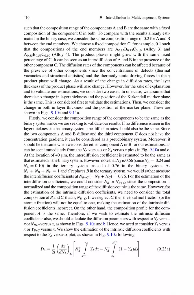
such that the composition range of the components A and B are the same with a fixedcomposition of the component C in both. To compare with the results already esti-mated in the binary case, we consider the same composition range of 0.2 for A and Bbetween the end members. We choose a fixed composition C, for example, 0.1 suchthat the compositions of the end members are A0.15B0.75C0.10 (Alloy 3) andA0.35B0.55C0.10 (Alloy 4). The product phases might grow with the same fixedpercentage of C. It can be seen as an interdiffusion of A and B in the presence of theother component C. The diffusion rates of the components can be affected because ofthe presence of other components since the concentrations of defects (thermalvacancies and structural antisites) and the thermodynamic driving forces in the cproduct phase will change. As a result of the change in diffusion rates, the layerthickness of the product phase will also change. However, for the sake of explanationand to validate our estimations, we consider two cases. In one case, we assume thatthere is no change in layer thickness and the position of the Kirkendall marker planeis the same. This is considered first to validate the estimations. Then, we consider thechange in both in layer thickness and the position of the marker plane. These areshown in Figs. 9.10a and 9.11a.

Firstly, we consider the composition range of the components to be the same as thebinary system since we are seeking to validate our results. If no difference is seen in thelayer thickness in the ternary system, the diffusion rates should also be the same. Sincethe two components A and B diffuse and the third component C does not have theconcentration gradient, it can be considered as a pseudobinary system. Moreover, itshould be the same when we consider either component A or B for our estimations, ascan be seen immediately from the NA versus x or YA versus x plots in Fig. 9.10a and c.At the location of 40 lm, the interdiffusion coefficient is estimated to be the same asthat estimated in the binary system. However, note that NB is 0.66 (since NA = 0.24 andNC = 0.10) in the ternary system instead of 0.76 in the binary system. AsNA + NB + NC = 1 and C replaces B in the ternary system, we would rather measurethe interdiffusion coefficients at NB+C (= NB + NC) = 0.76. For the estimation of theinterdiffusion coefficients, we could consider NB or NB+C, since the composition isnormalized and the composition range of the diffusion couple is the same. However, forthe estimation of the intrinsic diffusion coefficients, we need to consider the totalcomposition of B and C, that is, NB+C. If we neglect C, then the total mol fraction (or theatomic fraction) will not be equal to one, making the estimation of the intrinsic dif-fusion coefficients incorrect. On the other hand, the composition profile for the com-ponent A is the same. Therefore, if we wish to estimate the intrinsic diffusioncoefficients also, we should calculate the diffusion parameters with respect to NA versusx or NB+C versus x, as shown in Figs. 9.10a and b. Hence, we need to consider YA versusx or YB+C versus x. We show the estimation of the intrinsic diffusion coefficients withrespect to the YA versus x plot, as shown in Fig. 9.10c following

DA ¼12t

dx

dNA

� �K

NþA

ZxK

x�1

YAdx� N�A

Zxþ1

xK

1� YAð Þdx

24

35 ð9:23aÞ

410 9 Interdiffusion in Multicomponent Systems

Fig. 9.10 Composition profiles of a diffusion couple in a ternary A–B–C system a compositionprofile of element A b composition profile of elements (B + C), c composition normalizedvariable YA versus x plot [37]

9.3 A Pseudobinary Approach 411

Fig. 9.11 Composition profiles of a diffusion couple in a ternary A–B–C system, where layerthickness is affected because of addition of C with A and B a composition profile of element Ab composition profile of elements (B + C), c composition normalized variable YA versus x plot [37]

412 9 Interdiffusion in Multicomponent Systems

DB ¼ �12t

dx

dNA

� �K

NþBþC

ZxK

x�1

YAdx� N �BþC

Zxþ1

xK

1� YAð Þdx

24

35 ð9:23bÞ

We considered exactly the same location of the marker plane and we obtain thesame values of DA and DB as estimated in the binary system.

To validate the results, we considered the same layer thickness. However, asalready mentioned, the layer thickness—and even the location of the markerplane—actually change due to the addition of another component, since it influ-ences both defect concentrations and the thermodynamic driving force. It couldincrease or decrease the growth rate depending on the particular system underconsideration. Let us consider that the growth rate in the presence of C is lowerand the layer thickness after annealing for 25 h is 90 lm. There is also a change inthe location of the marker plane, which is to be found at 0.245 of NA, at thelocation of 40.5 lm from the Alloy 3/c phase interface, as shown in Fig. 9.11a.The YA versus x plot is presented in Fig. 9.11c. The interdiffusion and intrinsicdiffusion coefficients are estimated at the marker plane as ~D ¼ 1:68� 10�14,DA = 1.13 9 10-14 and DB = 3.38 9 10-14 m2/s.

Therefore, we have seen that if the experiments are conducted in a particularway, the ternary system can be treated as a pseudobinary system and the samerelations developed for the binary system can be used. We have shown the esti-mations at one particular composition only, however, just as in a binary system, itis possible to estimate the variation of the interdiffusion coefficients with thecompositions. Any error in estimation of the data caused by the deviation in theaverage composition of the end member is discussed in detail [37], which indicatesthat we could estimate the data without much error when the average compositiondeviates within ±1 at.%, a task which is not very difficult to achieve.

9.3.3 A Pseudobinary Approach in a Multicomponent System

As already explained, alloy compositions are chosen such that the composition of onecomponent is the same and then a third component is added at the cost of the secondcomponent. Similarly, we can add many components, which will replace the com-ponent B and then the estimation procedure will be the same. The interdiffusioncoefficients can be estimated with respect to the composition profile of A or B.However, for the estimation of the intrinsic diffusion coefficients, we should considerthe composition profile of A or the total of the other components (B + X). Thisapproach is useful when studying the diffusion of intermetallic compounds, where, ingeneral, one alloying component replaces another particular component. If we areinterested to study interdiffusion in random solid solutions and calculate the interdif-fusion at the equiatomic compositions (let us say, a five-component system), then onlytwo components, for instance, A and B could vary in the range of 0.15–0.25. Following,0.2 atomic fractions of all other components should be added to both the alloys that are

9.3 A Pseudobinary Approach 413

Fig. 9.12 Compositionprofile of multicomponentdiffusion couple in randomsolid solution [37]

to be bonded, as shown in Fig. 9.12. Moreover, the interdiffusion coefficients can beestimated at 0.2 atomic fractions from any of the composition profiles (A or B).However, the main difficulty in this system is for the estimation of the intrinsic dif-fusion coefficients, since we cannot decide how to add the composition of the othercomponents with A and B. Further, analysis is required to tackle this issue. A similarproblem will be faced if one particular component replaces both of the components. Insuch cases, also the interdiffusion coefficient can only be estimated.

9.3.4 Estimation of Diffusion Parameters in LineCompounds Following the Pseudobinary Approach

As already explained, the integrated diffusion coefficients ~Dint should be estimated whenphases grow with a narrow homogeneity range. This is basically the interdiffusioncoefficient integrated over the unknown small composition range of, for example, thephase b. This can be expressed with the help of Eq. 9.18a, 9.18b and 9.18c as

eDbint ¼

ZN 00A

N 0A

~DdNA

~Dbint ¼ �

ZxII

xI

~JVbmdx ¼ �~Jvb

mDxb

From Eq. 9.4b

~J ¼ �NþA � N�Affi �

2tvbm

1� Y�Affi � Zx�

x�1

YAdxþ Y�A

Zxþ1

x�

1� YAð Þdx

24

35

Therefore,

~Dbint ¼

NþA � N�Affi �

Dxb

2t1� YAð Þ

Zx�

x�1

YAdxþ YA

Zxþ1

x�

1� YAð Þdx

24

35

ð9:24Þ

414 9 Interdiffusion in Multicomponent Systems

As already explained in Chap. 7 [from Eq. 7.18], we can estimate the ratio of thediffusivities for a constant molar volume by

DA

DB¼

NþARxK

x�1YAdx� N �A

Rxþ1xK

1� YAð Þdx

" #

�NþBþC

RxK

x�1YAdxþ N �BþC

Rxþ1xK

1� YAð Þdx

" # ð9:25Þ

Let us consider a diffusion couple between Alloy 7 (A0.15B0.75C0.1) and Alloy 8(A0.35B0.55C0.1) where one line compound grows with the compositionA0.25B0.65C0.1, as shown in Fig. 9.13. Suppose the marker plane is located at adistance of 40.5 lm from the Alloy 5/b phase interface. The values are estimatedas ~Dint ¼ 2:25� 10�14 m2=s and DB

DA¼ 2:33.

The examples given above are discussed mainly based on the ternary systems;however, the same method can be followed in systems that consider more thanthree components as long as only two components diffuse. There are a fewadvantages in following this pseudobinary approach compared to the othermethods explained before. For example, from a single diffusion couple, we canestimate the variation of the interdiffusion coefficients over the whole compositionrange in the interdiffusion zone as well as the intrinsic diffusion coefficients at theKirkendall marker plane. This is otherwise very difficult in a ternary system andalmost impossible in a quaternary system. The possibility of conducting pseud-obinary experiments to examine the role of alloying additions in a more systematicapproach could be understood from Fig. 9.14. Suppose, we would like to study theeffect of Pt on the diffusion rate of Ni and Pt in the b-Ni(Pt)Al phase, which is usedin jet engines as a bond coat for protection from oxidation. The diffusion rates ofNi and Al are very important for a proper understanding of the performance andthe life of the product. To estimate the diffusion of the component and predict thedefects present on different sublattices, it is necessary to conduct experimentssystematically such that the data estimated at different compositions can be

Fig. 9.13 Compositionprofile of element A in amulticomponent system,where a line compound growsin the interdiffusion zone [37]

9.3 A Pseudobinary Approach 415

compared. Since we can estimate the diffusion parameters at the point of inter-section by following the conventional method, we need to prepare two couples, forexample, a couple of Alloy 1/Alloy 2 and Alloy 3/Alloy 4, as shown in Fig. 9.14a.In general, diffusion profiles are S-shaped, as already discussed, and it is almostimpossible to predict beforehand the point of intersection. With the aim of gettingthe point of intersection with the same ratio of Ni and Al (but with an increasingcontent of Pt), suppose another set of diffusion profiles are prepared from Alloy 5/Alloy 6 and Alloy 7/Alloy 8. In these alloys, the Pt content is increased whilekeeping the Ni/Al ratio the same, with the expectation of finding the point ofintersection at the same Ni/Al ratio—yet with increased Pt compared to the pre-vious case. However, these will not necessarily intersect at the desired compositionand may even intersect at a different Ni/Al composition, as shown in Fig. 9.14. Weare unable to compare the results from different sets of couples, which is some-thing very commonly encountered. Therefore, the estimation in the ternary sys-tems is mostly restricted to the data generation, without any further understandingon the complex process of diffusion. Moreover, there is rarely any chance that themarkers will also be at the point of intersection to estimate the intrinsic diffusioncoefficients. In this regard, pseudo-binary approach rather should be followed.

Fig. 9.14 Advantage of a pseudobinary approach explained a diffusion couples followingconventional technique, b diffusion couples in a pseudobinary approach, c diffusion couple ofNi(9.5Pt)50Al/Ni(9.5Pt)40Al annealed at 1,100 �C for 25 h, and d its composition profile

416 9 Interdiffusion in Multicomponent Systems

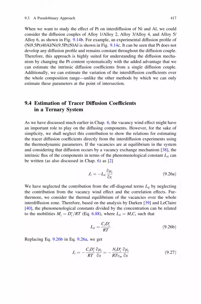
When we want to study the effect of Pt on interdiffusion of Ni and Al, we couldconsider the diffusion couples of Alloy 1/Alloy 2, Alloy 3/Alloy 4, and Alloy 5/Alloy 6, as shown in Fig. 9.14b. For example, an experimental diffusion profile of(Ni9.5Pt)40Al/Ni(9.5Pt)50Al is shown in Fig. 9.14c. It can be seen that Pt does notdevelop any diffusion profile and remains constant throughout the diffusion couple.Therefore, this approach is highly suited for understanding the diffusion mecha-nism by changing the Pt content systematically with the added advantage that wecan estimate the intrinsic diffusion coefficients from a single diffusion couple.Additionally, we can estimate the variation of the interdiffusion coefficients overthe whole composition range—unlike the other methods by which we can onlyestimate these parameters at the point of intersection.

9.4 Estimation of Tracer Diffusion Coefficientsin a Ternary System

As we have discussed much earlier in Chap. 6, the vacancy wind effect might havean important role to play on the diffusing components. However, for the sake ofsimplicity, we shall neglect this contribution to show the relations for estimatingthe tracer diffusion coefficients directly from the interdiffusion experiments usingthe thermodynamic parameters. If the vacancies are at equilibrium in the systemand considering that diffusion occurs by a vacancy exchange mechanism [38], theintrinsic flux of the components in terms of the phenomenological constant Lii canbe written (as also discussed in Chap. 6) as [2]

Ji ¼ �Liioli

oxð9:26aÞ

We have neglected the contribution from the off-diagonal terms Lij by neglectingthe contribution from the vacancy wind effect and the correlation effects. Fur-thermore, we consider the thermal equilibrium of the vacancies over the wholeinterdiffusion zone. Therefore, based on the analysis by Darken [39] and LeClaire[40], the phenomenological constants divided by the concentration can be relatedto the mobilities Mi ¼ D�i =RT (Eq. 6.88), where Lii ¼ MiCi such that

Lii ¼CiD�iRT

ð9:26bÞ

Replacing Eq. 9.26b in Eq. 9.26a, we get

Ji ¼ �CiD�iRT

oli

ox¼ � NiD�i

RTvm

oli

oxð9:27Þ

9.3 A Pseudobinary Approach 417

Since li ¼ loi þ RT ln ai and ai ¼ ciNi, as discussed in Chap. 1, Eq. 9.27 can be

written as

Ji ¼ �NiD�ivmai

oai

ox¼ � D�i

vmci

oai

oxð9:28Þ

From Eqs. 9.8a, 9.27 and 9.28 considering a constant molar volume in a ternarysystem, we can write

eJ1 ¼ �N1D�1RTvm

ol1

oxþ N1

N1D�1RTvm

ol1

oxþ N2D�2

RTvm

ol2

oxþ N3D�3

RTvm

ol3

ox

� �

¼ � D�1c1vm

oai

oxþ N1

D�1c1vm

oa1

oxþ D�2

c2vm

oa2

oxþ D�3

c3vm

oa3

ox

� � ð9:29aÞ

eJ2 ¼ �N2D�2RTvm

ol2

oxþ N2

N1D�1RTvm

ol1

oxþ N2D�2

RTvm

ol2

oxþ N3D�3

RTvm

ol3

ox

� �

¼ � D�2c2vm

oa2

oxþ N2

D�1c1vm

oa1

oxþ D�2

c2vm

oa2

oxþ D�3

c3vm

oa3

ox

� � ð9:29bÞ

~J3 ¼ �~J1 � ~J2 ð9:29cÞ

If the thermodynamic data in a ternary system are known, using the composition ina diffusion couple, the interdiffusion fluxes are estimated at the point of interestusing the relation in Eq. 9.4a. Further, from the known activities (or chemicalpotentials) of the components at a different composition, the composition profilecan be converted to the activity or the chemical potential profile for all thecomponents. From these profiles, the thermodynamic parameters required inEq. 9.29a, 9.29b and 9.29c can be estimated. Subsequently, the tracer diffusioncoefficients of the components can be estimated at the point of interest. Rönkaet al. [26] estimated the interdiffusion and the tracer diffusion coefficients at thepoint of intersection from two diffusion couples in a Cu–Fe–Ni system, finding thatthe estimated tracer diffusion coefficients are consistent with the data available inliterature in the Cu–Ni and Fe–Ni systems.

The intrinsic fluxes in the system considering the constant molar volume can bewritten as [26]

Jv ¼ �Xn

i¼1

Ji ð9:30aÞ

In a ternary system, it is reduced to

Jv ¼ � J1 þ J2 þ J3ð Þ ð9:30bÞ

418 9 Interdiffusion in Multicomponent Systems

Replacing Eq. 9.27 in Eq. 9.30b, we get

Jv ¼N1D�1RTvm

ol1

oxþ N2D�2

RTvm

ol2

oxþ N3D�3

RTvm

ol3

oxð9:30cÞ

Therefore, the position of the Kirkendall marker plane can be found from therelation above, since (as discussed in Chap. 6)

vmJv ¼xK

2tð9:31Þ

By comparing the shift in the diffusion couple (and estimating the shift with thehelp of the estimated diffusion coefficients using the relations above), it is possibleto examine the reliability of the estimation procedure.

In the above analysis, the vacancy wind effect could be neglected since weneglected the off-diagonal terms Lij. In an actual case, however, these might not benegligible. As mentioned by Belova et al. [41], in some rare cases, these off-diagonal terms could dominate to change the direction of the atomic flux. Manning[42, 43] developed the relations including the vacancy wind effect. Dayananda[44] extended this theory for the determination of the vacancy wind effectexperimentally in a multicomponent system, considering the non-diagonal phe-nomenological constants. Moleko et al. [45] also developed a model, consideringthe vacancy wind effect. Belova et al. [41] have reported an interesting outcome intheir analysis based on the experimental data compiled by Divinski et al. [46] inthe Cu–Ni–Fe system. They have shown the procedure to determine the jumpfrequencies, correlation factors, and the vacancy wind effects following the theorydeveloped by Manning [43] and Dayananda [44] from the available tracer diffu-sion coefficients. In the process, they have shown that Darken formulism (ignoringthe off-diagonal term) is reliable to express the diagonal phenomenological con-stants in terms of the tracer diffusion coefficients. They have also demonstrated theprocedure to calculate the tracer diffusion coefficients and the vacancy wind effectfrom the interdiffusion coefficients following the theory developed by Darken [39],Manning [43], and Dayananda [44]

Holly and Danielewski [47] have developed an extended Darken quantitativemodel to describe the multicomponent interdiffusion process based on the con-sideration of local mass conservation and by using the expressions for drift anddiffusional flux—the momentum conservation equations where the diffusivities ofcomponents vary with composition. Filipek et al. [48] used this analysis in the Fe–Co–Ni system and found good agreement between theoretically estimated andexperimentally determined composition profiles developed in the diffusion cou-ples. Divinski et al. [46] applied this model in the Cu–Fe–Ni system to show goodagreement between the estimated and experimental interdiffusion concentration,

9.4 Estimation of Tracer Diffusion Coefficients in a Ternary System 419

which validates the assumptions made by Holly and Danielewski in their model forthe description of interdiffusion in a non-ideal system.

An important note is due here. The vacancies in a binary alloy can beconsidered as third component and thus, generally, even binary alloys haveto be treated as multicomponent systems. Then, the off-diagonal termscannot be neglected that results in a vacancy wind effect for the binarycompositions. However, in typical situation, the vacancy concentrations aresmall and the resulting correction on the vacancy wind effect is about unity.In most binary couples, the corresponding contribution can safely beneglected, especially in view of the experimental uncertainties. Neverthe-less, it is important to keep this fact in mind.

9.5 Determination of Phase Diagram Following DiffusionCouple Technique

Knowledge of phase diagrams is very important for developing any new material orfor gaining a full understanding of the physical and mechanical behavior ofmaterials. However, the determination of a phase diagram is a very tedious pro-cedure. The level of complexity increases drastically in ternary system compared tosimpler binary systems. Numerous samples must be prepared in order to establish aternary phase diagram. Added complications come from the fact that the phaseequilibria existing at the solid state might not be achieved by a melt route—especially if there is a peritectic reaction present. On the other hand, a diffusioncouple along with the melting of selective alloys could be very handy to decreasethe number of experiments (or alloys) required to establish a phase diagram. Formore comprehensive treatment on this area, the readers are referred to an excellentreview written by Kodentsov et al. [49] and the book on methods for phase diagramdetermination [50]. The use of the diffusion couple for the development of the phasediagram was, in fact, first proposed by Kirkaldy [51]. Kirkaldy and Brown [52]formulated the number of rules, which were then compiled by Clark [53] based on ahypothetical diffusion couple. Most recently, Morral [54] has compiled a few morerules developed at a later stage. At this point, we shall discuss mainly the rulesdescribed by Clark and explain the advantages and limitations of using a diffusioncouple for the determination of phase diagrams.

It should be pointed out here that, unlike in a binary diffusion couple, in a ternarycouple a two-phase mixture can develop when the experiment is conducted at aconstant temperature. This can be understood from the Gibb’s phase rule F = C –P + 2. At constant temperature and pressure, we can write F = C – P. In a ternarysystem, C = 3. Therefore, F + P = 3 and the two phases (that is P = 2) are

420 9 Interdiffusion in Multicomponent Systems

allowed, keeping the variation of the concentration as one degree of freedom.Previously in Chap. 4, we have seen that in a binary system, two phase mixturecannot grow in the middle of a diffusion couple since it is not allowed to develop aregion of equilibrium before the whole diffusion couple reaches to an equilibriumstate. Similarly, three phase mixture cannot grow in a ternary diffusion couple. Atwo phase mixture can grow only when the diffusion path (i.e. the compositionprofile) goes from one phase area to two phase area, cuts the tie-lines at a givenangle and returns to one phase area. If the one phase area is named a and the twophase are is a + b, then under these circumstances the a phase contains precipitatesof the b phase and thus a two phase mixture has been formed. The rules aredescribed based on the diffusion path (that is the plot of composition profile of adiffusion couple on a Gibb’s triangle) in a ternary diffusion couple between A andZ on a hypothetical phase diagram, as shown in Fig. 9.15a [49].

Note that there are many phases, such as a, b, d, r, p, k, l, and c that arepresent. The two-phase equilibrium regions are shown by connected tie lines, andthe three-phase regions are kept blank. When the composition profile is examinedfrom alloy Z, the variation in the composition inside the d phase should be shownby a diffusion path drawn with a solid line ab. Since the phases d and r areseparated by a wavy interface, the solid-line diffusion path should intersect the tielines as shown by bc. Then, the diffusion path goes through the r phase as shownby cd. Following, the precipitates of the p phase appear inside this phase and againafter that the r phase is present as a single phase. This means that the diffusionpath should enter the two-phase equilibrium region as shown by def and thenreturns again to the r phase to continue up to fg. Phases r and p are separated by astraight interface. Therefore, the diffusion path should run parallel to the tie linesas shown by gh and it should be drawn by a dotted line. ij shows the three-phaseequilibrium region starting from phase p toward two-phase region k and l. jkshows the phase mixture of k and l. The location of the line in the two-phaseequilibrium region depends on the relative amounts of the phases. kl shows thetransition from one three-phase equilibrium to another three-phase equilibrium. lmshows the path from two-phase equilibrium k–c to the c phase. Following, thediffusion path goes through the c phase, as shown by mn. One important factshould be noted here, as denoted by the blue dotted line in Fig. 9.15b, the diffusionpath should intersect the line connecting Z and A at least once. For any deviation inthe composition profile, the diffusion path moves away from the straight line;however, because of the mass balance, it has to go in the opposite direction afterintersecting the connecting line. Moreover, a two-phase mixture develops onlywhen the diffusion path passes through a three-phase equilibrium. Let us consideranother hypothetical phase diagram and the diffusion couple as explained byKodentsov et al. [49], as shown in Fig. 9.16. Suppose two alloys R and S arecoupled, so that a ternary phase develops at the interface. Therefore, the diffusionpath first cuts through the tie lines between the a and the l phases, the position ofthe line depending on the relative phase fractions of the phases. At the interface I,three phases, a, l, and T are in equilibrium at specific points of contact, which isrepresented by a dotted line on the phase diagram. After the phase mixture, only

9.5 Determination of Phase Diagram Following Diffusion Couple Technique 421

Fig. 9.15 a Hypothetical phase diagram showing a diffusion path in a diffusion couple betweenA and Z and b mass balance (blue dotted) line showing intersection with diffusion path [49]

422 9 Interdiffusion in Multicomponent Systems

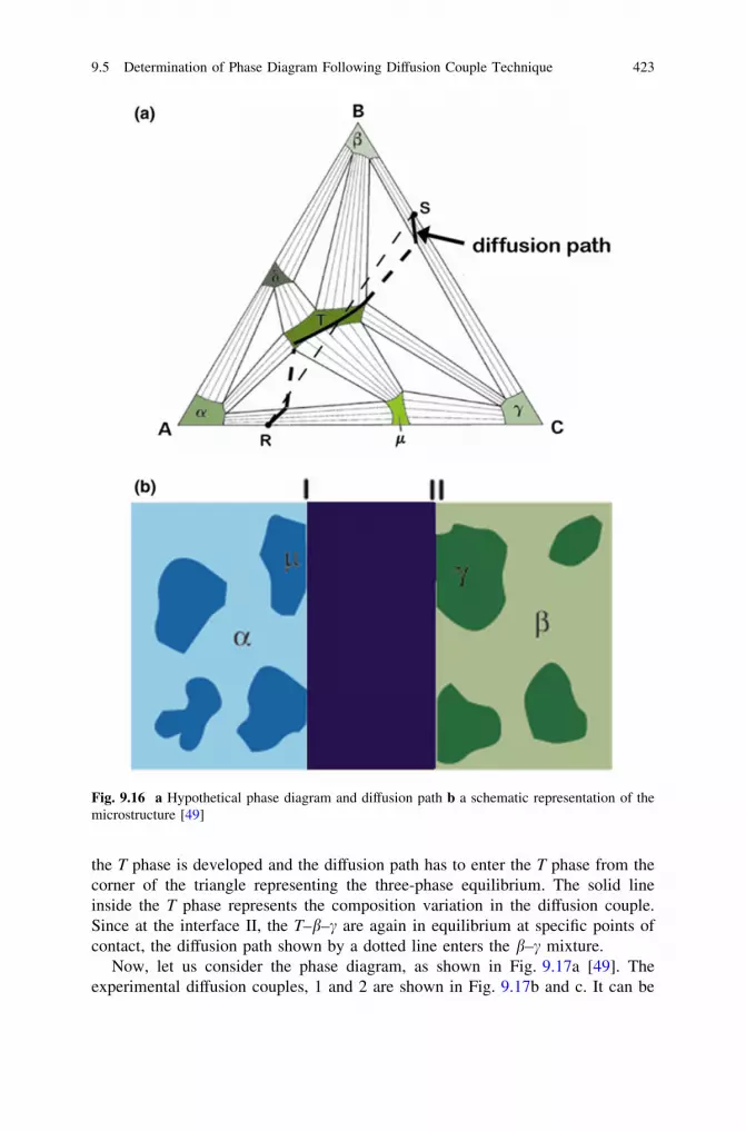
the T phase is developed and the diffusion path has to enter the T phase from thecorner of the triangle representing the three-phase equilibrium. The solid lineinside the T phase represents the composition variation in the diffusion couple.Since at the interface II, the T–b–c are again in equilibrium at specific points ofcontact, the diffusion path shown by a dotted line enters the b–c mixture.

Now, let us consider the phase diagram, as shown in Fig. 9.17a [49]. Theexperimental diffusion couples, 1 and 2 are shown in Fig. 9.17b and c. It can be

Fig. 9.16 a Hypothetical phase diagram and diffusion path b a schematic representation of themicrostructure [49]

9.5 Determination of Phase Diagram Following Diffusion Couple Technique 423

seen that since Ag is in equilibrium with the Fess solid solution and Fe2Ti, nothingdevelops at the interdiffusion zone of the Ag/Fe80Ti20 diffusion couple. On theother hand, the diffusion couple Ag/Fe30Ti70 goes through two three-phase

Fig. 9.17 a Diffusion couplecomposition on an isothermalAg–Fe–Ti phase diagram,interdiffusion zone betweenb Ag/Fe80Ti20 and c Ag/Fe30Ti70 developed afterannealing at 850 �C for 100 h[55]

424 9 Interdiffusion in Multicomponent Systems

Fig. 9.18 a Isothermal crosssection of the Ni–Cr–V phasediagram at 1,150 �C.b Interdiffusion zonesdeveloped after (b) 16 andc 49 h [49]

9.5 Determination of Phase Diagram Following Diffusion Couple Technique 425

equilibriums. Therefore, at the interface I, it has the three-phase equilibrium ofAg–FeTi–TiAg. At the interface II, it has another three-phase equilibrium, that ofFeTi–TiAg–b(Ti). In the interdiffusion zone, it grows as a phase mixture of FeTiand TiAg.

At times, by making a single diffusion couple, the information on the wholephase diagram can be developed by examining the interdiffusion zone of a dif-fusion couple at different times [49, 55], as shown in Fig. 9.18. For example, avery thin layer of Ni was sandwiched between two thick foils of Cr and V at1,150 �C. The interdiffusion zone was examined at different time intervals for theidentification of the phases evolved and measurement of the composition profiles.Using this information and with the additional help of few melted alloys as shownby dots on the phase diagram, one can define the phase boundaries much better.Many times, the diffusion couple experiments alone are not enough to establish thephase diagram. We assume local equilibrium at the interfaces in a diffusion couple,meaning that the chemical potential varies continuously over the interdiffusionzone. In a bulk diffusion couple, all the phases on a diffusion path are expected togrow. However, one or more phases might grow with a very small thickness and itcould be very difficult to detect or measure the composition. Furthermore, time andtime again, it is difficult to measure the exact phase boundary composition—especially if the composition varies sharply near the interface. When the com-position is measured by an electron probe microanalyzer, depending on the gun(tungsten filament or field emission), the composition should be measured at least1–3 lm inside from the edge of the phase boundary depending on the components.In the case of a sharp change in composition, the measured value could be sig-nificantly different from the actual phase boundary composition. If the compositiondoes not change sharply, this difference could be low. Therefore, by combining themeasurement of a few equilibrated alloys along with the diffusion couple exper-iments, we can establish a reasonably accurate phase diagram.

Often, the composition profiles measured from the diffusion couples indicatethe need for further studies to establish the phase diagram correctly. For example,the composition range of the l phase measured in the Ni–Co–W system, as shownin Fig. 9.7a, is higher than the range published in the previous phase diagrams.Similarly, issues were also found in the Co–Ta system, which was corrected by thediffusion couple experiments [58].

References

1. R.T. DeHoff and N. Kulkarni, Materials Research 5 (2002) 2092. J.S. Kirkaldy and D.J. Young, Diffusion in the condensed state, The Institute of Metals,

London 1987.3. Diffusion in Solids: Recent Developments, Edited by M.A. Dayananda, G.E. Murch,

Metallurgical Society of AIME, Warrendale, PA, 1985.4. L. Onsager, Physical Review 37(1931) 405 and 38 (1932) 22655. L. Onsager, Annals of the New York Academy of Sciences 46 (1965) 241

426 9 Interdiffusion in Multicomponent Systems

6. V.D. Divya, U. Ramamurty and A. Paul, Philosophical Magazine 93 (2013) 21907. J.S. Kirkaldy, Canadian Journal of Physics 35 (1957) 4358. J. Philibert and A.G. Guy, Comptes Rendus 257 (1963) 22819. T.O. Zeibold and R.E. Ogilvie, Trans TMS-AIME 239 (1967) 942-53

10. Y.H. Sohn and M.A. Dayananda, Metallurgical and Materials Transaction A 33 (2002) 337511. J.E. Lane and J.S. Kirkaldy, Canadian Journal of Physics 42 (1964) 164312. T. Heumann, Zeitschrift für Physikalische Chemie 201 (1952) 16813. A.G. Guy and J. Philibert, Zeitschrift für Metallkunde, 50 (1965) 84114. Y.H. Sohn and M.A. Dayananda, Acta Materialia 48 (2000) 142715. M.A. Dayananda, Trans TMS AIME 242 (1968) 136916. J.D. Whittenberger and M.A. Dayananda, Metallurgical Transactions 1 (1970) 330117. P.T. Carlson, M.A. Dayananda and R.E. Grace, Metallurgical Transactions A 6 (1975) 124518. C.W. Kim and M.A. Dayananda, Metallurgical Transactions A 14 (1983) 85719. C.W. Kim and M.A. Dayananda, Metallurgical Transactions A 15 (1984) 64920. K.E. Kansky and M.A. Dayananda, Metallurgical Transactions A 16 (1985) 112321. J.A. Heaney and M.A. Dayananda, Metallurgical Transactions A 17 (1986) 98322. M.S. Thompson and J. E. Morral, Acta Metallurgica 34 (1986) 339.23. M.S. Thompson and J.E. Morral, Acta Metallurgica 34 (1986) 220124. M.S. Thompson and J.E. Morral, Metallurgical Transactions A 28 (1987) 156525. F.J.J. van Loo, G.F. Bastin and J.W.G.A Vrolijk, Metallurgical Transactions A 18 (1987) 80126. K.J. Rönka, A.A. Kodentsov, P.J.J. van Loon, J.K. Kivilahti and F.J.J. van Loo, Metallurgical

and Materials Transactions A 27 (1996) 222927. S. Krishtal, A.P. Mokrov, A.V. Akimov, and P.N. Zakharov, Fiz Metal Metalloved 35 (1973)

123428. M.K. Stalker, J.E. Morral and A.D. Romig, Metallurgical Transactions A 23 (1992) 324529. Y. Minamino, Y. Koizumi, T. Tsuji, Y. Yamada and T. Takahashi, Materials Transactions 44

(2003) 6330. T. Takahashi, K. Hisayuki, T. Yamane, Y. Minamino and T. Hino, Materials Transactions 44

(2003) 225231. M.A. Dayananda and Y.H. Sohn, Scripta Materialia 35 (1996) 68332. M.A. Dayananda and Y.H. Sohn, Metallurgical and Materials Transactions A 30 (1999) 53533. J. Cermak and V. Rothova, Acta Materialia 51 (2003) 441134. K. Cheng, W. Chen, D. Liu, L. Zhang Y. Du, Scripta Materialia 76 (2014) 5.35. C. Wagner, Acta Metallurgica 17 (1969) 9936. V. D. Divya, U. Ramamurty and A. Paul, Metallurgical and Materials Transactions A

(2012) 156437. A. Paul, Philosophical Magazine 93 (2013) 229738. J. Bardeen and C. Herring: Atom Movements, Ed: J.H. Hollomon, ASM, Cleveland, OH,

1951 pp. 87-11139. L.S. Darken, Atom Movements, Ed: J.H. Hollomon, ASM, Cleveland, OH, 1951 pp. 1-1740. A.D. LeClaire: Progress in Metal Physics, Ed. B Chalmers, Pergamon, London, 4(1953) 265-

33241. I.V. Belova, G.E. Murch, R. Filipek and M. Danielewski, Acta Materialia, 53 (2005)

4613–4622.42. J. R. Manning, Metallurgical Transactions 1970, vol. I, pp. 49943. J.R. Manning. Physical Review B 4 (197) 111144. M.A. Dayananda, Metallurgical Transactions 2 (1971) 33445. L.K. Moleko, A.R. Allnatt, E.L. Allnatt. Philosophical Magazine A 59 (1989) 14146. S.V. Divinski, F. Hisker, Chr. Herzig, R. Filipek, M. Danielewski, Defects and Diffusion

Forum 237-240 (2005) 5047. K. Holly and M. Danielewski: Physical Review B 50 (1994) 1333648. R. Filipek, M. Danielewski and R. Bachorczyk, Defect and Diffusion Forum 237-240 (2005)

408

References 427

49. AA. Kodentsov, G.F. Bastin and F.J.J. van Loo, Journal of alloys and compounds 320 (2001)207

50. J.C. Zhao (Ed.), Methods of Phase diagram Determination, Elsevier, Oxford, UK, 200751. J.S. Kirkaldy, Canadian Journal of Physics 36 (1958) 91752. J.S. Kirkaldy, L.C. Brown, Canadian Metallurgical Quaterly 2 (1963) 125053. J.B. Clark, Transactions of Metallurgical Society AIME 227 (1963) 125054. J.E. Morral, Metallurgical and Materials Transactions 43A (2012) 346255. J.A. van Beek, A.A. Kodentsov, F.J.J. van Loo, Journal of Alloys and Compounds 221 (1995)

10856. A. Davydov, UR Kattner, Journal of Phase Equilibria 24 (2003) 20957. H. Okamoto Journal of Phase Equilibria 28 (2007) 30058. V. Baheti, S. Roy, R. Ravi and A. Paul, Intermetallics, 33 (2013) 87

428 9 Interdiffusion in Multicomponent Systems

Chapter 10Short-Circuit Diffusion

In this chapter, we describe the basics of diffusion along short circuits in materials,especially along grain boundaries. The fundamental model of Fisher is representedand discussed in detail. Its approximate solution, which is important from adidactic point of view, is given at first. Then, the exact solutions for instantaneousand constant sources are sketched and a general approach for the analysis ofexperimental data is formulated. The concept of kinetic regimes of diffusion inmaterials with a hierarchy of short-circuit paths is introduced and discussed usingoriginal experimental data on nanocrystalline alloys. The effect of grain boundarydiffusion on interdiffusion phenomena is evaluated.

Short-circuit diffusion paths in metals and alloys have attracted continuousattention because of their technological importance. Alloying, sintering, and oxi-dation—these are the phenomena, which demand consideration of interface- ordislocation-enhanced diffusion, just to name a couple of them. The importance ofthe kinetic and thermodynamic properties of interfaces grows considerably whenconsidering the miniaturization of whole devices or the length scale of their typicalstructure features. The interface structure, its kinetics, stability, and possiblestructure transformations are strongly affected by solute segregation, both of thealloying components and residual impurities.

Typically one- and two-dimensional defects are considered as short circuits inmaterials, such as dislocation lines, dislocation walls, grain boundaries (i.e.,interfaces between differently oriented grains), and phase boundaries (i.e., inter-faces between different phases which could even be equally oriented). Further-more, such defects are triple lines or triple junctions, i.e., lines along which threedifferently oriented grains meet in a polycrystalline material, and free surfaces, seeFig. 10.1, where possible short-circuit paths are sketched.

The short-circuit defects, such as dislocations and grain boundaries, could havea strong impact on the process of interdiffusion, especially since the diffusion ratesof atoms are typically enhanced along these defects.

A compilation of diffusion rates in a crystalline bulk and along typical short-circuit paths in a metal is presented in Fig. 10.2 using pure silver as an example.As a rule of thumb, the reader can memorize that self-diffusion is fastest along afree surface where the activation energy Qs constitutes 0.1–0.3 of the activation

A. Paul et al., Thermodynamics, Diffusion and the Kirkendall Effect in Solids,DOI: 10.1007/978-3-319-07461-0_10, � Springer International Publishing Switzerland 2014

429

energy of the bulk diffusion Qv. Diffusion rates along high-angle grain boundariesare slower with the activation energy Qgb, which amounts typically to (0.4–0.6)Qv.Low-angle grain boundaries and dislocation walls reveal typically slower diffusionrates, although these are scarcely studied. Again, as a rule of thumb, one may writethat Dlb & Dd and typically these values amount to (0.01 7 0.1) Dgb; that is, thecorresponding diffusion coefficients do not typically exceed 10 % of the valueswhich correspond to the diffusivities of high-angle grain boundaries Dgb. Here, Dlb

and Dd are the diffusion coefficients of the low-angle grain boundary and ofindividual dislocations, respectively.

Grain boundary (GB) diffusion measurements are very sensitive to the struc-tural state of GBs. Small changes in atomic positions can result in correspondingchanges of energy barriers for diffusion jumps. Since the diffusion rate dependsexponentially on the energy barriers, a significant change in the GB diffusivities,both for solute and matrix atoms, can be expected.

Fig. 10.2 Comparison ofexperimental data ondiffusion rates in pure Ag inbulk, Dv [41], alongdislocations, Dd [42], alonggrain boundaries, Dgb [42],and on surface in vacuum, Ds

[43]. For generality, thetemperature scale isnormalized on the meltingpoint of Ag, Tm = 1,235 K

Fig. 10.1 Schematicrepresentation of defectswhich may act as short-circuitpaths in a polycrystallinematerial: dislocation line q;grain boundaries, e.g., ABCDone; triple lines as AD one;and phase boundaries as theinterface between phasesa and b

430 10 Short-Circuit Diffusion

The current GB diffusion measurements almost exclusively rely on the modelwhich was suggested by Fisher in 1951 [1]. This is especially true for self-diffusion.Bokstein et al. [2] and later Gibbs [3] recognized that the GB diffusion problem hasto be specially treated in solute diffusion cases, namely the solute segregation atgrain boundaries has to be taken into account. Subsequent development of the GBdiffusion theory is most completely represented by the famous handbook on thefundamentals of grain and interphase boundary diffusion [4].

10.1 Fisher Model of GB Diffusion

The commonly accepted Fisher model [1] is a model of the fast GB diffusion inwhich a leakage of diffusing atoms to the bulk is normal to GB (Fig. 10.3). Thesolid is considered as a two-dimensional (xy) object which is characterized by aunique (isotropic) diffusion coefficient Dv. The grain boundary is characterized bya (typically) enhanced diffusion coefficient Dgb (Dgb � Dv) and represents a slabof the thickness d, oriented perpendicularly to the outer surface (y = 0).

The diffusion transport of atoms in material occurs then via the fast diffusion oftracer atoms from the outer surface along the grain boundaries with subsequentleakage into the crystalline bulk and further diffusion with typically a lower dif-fusion rate.

The diffusion problem will be formulated in the following way

ocgb

ot¼ Dgb

o2cgb

ox2þ o2cgb

oy2

� �when xj j\d=2 ð10:1aÞ

ocv

ot¼ Dv

o2cv

ox2þ o2cv

oy2

� �when xj j[ d=2 ð10:1bÞ

The boundary condition

scv �d=2; y; tffi �

¼ cgbð�d=2; y; tÞ ð10:2Þ

takes into account the GB segregation in the linear form (the so-called Henryisotherm), where s is the segregation coefficient (Fig. 10.3). The definition of s isgiven by Eq. 10.2 itself, i.e.,

s ¼ cgbð�d=2; y; tÞcv �d=2; y; tffi � ¼ cgbð�d=2Þ

cv �d=2

ffi � ð10:2aÞ

and is considered as a constant in the GB diffusion experiment which does notdepend on the position, time, and the solute concentrations, even though the latter

10 Short-Circuit Diffusion 431

is not a necessary condition and one can go beyond the linear segregationapproximation.

Additionally, we have to take into account the equality of diffusion fluxes

perpendicularly to the GB at �d=2; yffi �

Dv

ocv

ox

����xj j¼d=2

¼ Dgb

ocgb

ox

����xj j¼d=2

ð10:3Þ

Now, we may use the conditions that the GB width d is small, several atomicdistances, and Dgb � Dv. Then, on the same scale, the change of cgb is signifi-cantly smaller than that of cv. Thus, expanding cgb(x, y, t) in a Taylor series aroundx = 0, we have

cgbðx; y; tÞ ¼ cgbð0; y; tÞ þx2

2o2cgbðx; y; tÞ

ox2

����x¼0

þ � � � : ð10:4Þ

Here, we neglected the higher-order terms and used the symmetry of the

problem with respect to x = 0, i.e., ocgbðx;y;tÞox

���x¼0¼ 0. Denoting cgb(0) = cgb(0, y, t)

and c00gbð0Þ ¼o2cgbðx;y;tÞ

ox2

���x¼0

and substituting Eq. 10.4 into Eq. 10.1a, we arrive at

ð xj j\d=2Þ

Fig. 10.3 Schematic illustration of Fisher model of GB diffusion updated including probableeffect of GB segregation. The distribution of tracer atoms in the GB of the width d and diffusioncoefficient Dgb is sketched. Far from the outer surface (y = 0), the tracer atoms enter thecrystallite bulk by leakage from the grain boundary and they diffuse further with the diffusioncoefficient Dv

432 10 Short-Circuit Diffusion

o

otcgbð0Þ þ

x2

2c00gbð0Þ

� �

¼ Dgb

o2

ox2cgbð0Þ þ

x2

2c00gbð0Þ

� �þ o2

oy2cgbð0Þ þ

x2

2c00gbð0Þ

� �� � ð10:5Þ

Since both cgb(0) and c00gbð0Þ are functions of y and t and do not depend on x bydefinition and limiting us by the terms linear in d, we have

ocgbð0Þot

¼ Dgb c00gbð0Þ þo2cgbð0Þ

oy2

� �ð10:6Þ

Now, we will substitute the expansion (Eq. 10.4) into the boundary conditions(Eqs. 10.2 and 10.3), and again neglecting the term of the order of d2 and higher,we will arrive at

sc �d=2; y; tffi �

¼ cgbð0Þ ð10:7Þ

and

Dv

ocv

ox

����xj j¼d=2

¼ Dgb

o

oxcgbð0Þ þ

x2

2c00gbð0Þ

� � ����xj j¼d=2

¼ Dgb

d2

c00gbð0Þ ð10:8Þ

Equation 10.8 may be rewritten as

Dgbc00gbð0Þ ¼2d

Dv

ocv

ox

����xj j¼d=2

ð10:9Þ

After substitution of this expression into Eq. 10.6, we arrive at a final system ofdiffusion equations for the GB diffusion problem

ocgb

ot¼ Dgb

o2cgb

oy2þ 2Dv

docv

ox

����xj j¼d=2

; when xj j\d=2 ð10:10Þ

and Eq. 10.1b for diffusion in the crystalline bulk, xj j[ d=2. Here,cgb : cgb(0) : cgb(y, t), since the GB concentration does not depend on thecoordinate x under the approximations used, i.e., the small value of d and thesignificant diffusion enhancement in the GB slab.

There is a straightforward interpretation of Eq. 10.10, i.e., the concentration oftracer atoms in a GB is changed due to diffusion along the GB, the first term on theon the right-hand side of the equation, and due to tracer leakage into the crystallinebulk, the rate of which is controlled by the gradient of the bulk concentration near

10.1 Fisher Model of GB Diffusion 433

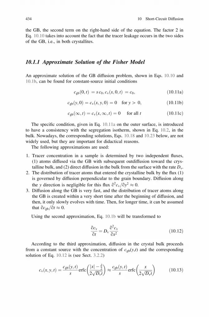
the GB, the second term on the right-hand side of the equation. The factor 2 inEq. 10.10 takes into account the fact that the tracer leakage occurs in the two sidesof the GB, i.e., in both crystallites.

10.1.1 Approximate Solution of the Fisher Model

An approximate solution of the GB diffusion problem, shown in Eqs. 10.10 and10.1b, can be found for constant-source initial conditions

cgb 0; tð Þ ¼ s c0; cv x; 0; tð Þ ¼ c0; ð10:11aÞ

cgb y; 0ð Þ ¼ cv x; y; 0ð Þ ¼ 0 for y [ 0; ð10:11bÞ

cgbð1; tÞ ¼ cvðx;1; tÞ ¼ 0 for all t ð10:11cÞ

The specific condition, given in Eq. 10.11a on the outer surface, is introducedto have a consistency with the segregation isotherm, shown in Eq. 10.2, in thebulk. Nowadays, the corresponding solutions, Eqs. 10.18 and 10.23 below, are notwidely used, but they are important for didactical reasons.

The following approximations are used:

1. Tracer concentration in a sample is determined by two independent fluxes,(1) atoms diffused via the GB with subsequent outdiffusion toward the crys-talline bulk, and (2) direct diffusion in the bulk from the surface with the rate Dv.

2. The distribution of tracer atoms that entered the crystalline bulk by the flux (1)is governed by diffusion perpendicular to the grain boundary. Diffusion alongthe y direction is negligible for this flux o2cv=oy2 � 0.

3. Diffusion along the GB is very fast, and the distribution of tracer atoms alongthe GB is created within a very short time after the beginning of diffusion, andthen, it only slowly evolves with time. Then, for longer time, it can be assumedthat ocgb=ot � 0.

Using the second approximation, Eq. 10.1b will be transformed to

ocv

ot¼ Dv

o2cv

ox2ð10:12Þ

According to the third approximation, diffusion in the crystal bulk proceedsfrom a constant source with the concentration of cgb(y,t) and the correspondingsolution of Eq. 10.12 is (see Sect. 3.2.2)

cvðx; y; tÞ ¼cgbðy; tÞ

serfc

xj j � d2

2ffiffiffiffiffiffiffiDvtp

� �� cgbðy; tÞ

serfc

x

2ffiffiffiffiffiffiffiDvtp

� �ð10:13Þ

434 10 Short-Circuit Diffusion

at xj j[ d=2. Here erfc(u) is the complimentary error function defined as

erfc uð Þ ¼ 1� erf ðuÞ ¼ 2ffiffiffippZ1

u

expð�z2Þdz

Under the third approximation, Eq. 10.10 transforms to

o2cgb

oy2¼ � 2Dv

dDgb

ocv

ox

����xj j¼d=2

ð10:14Þ

Since cv as a function of x for the given y and t is known (Eq. 10.13), we haveto evaluate its x derivative at xj j ¼ d=2 and substitute the resulting expression intoEq. 10.15. As a result, we have

o2cgb

oy2¼ 2

ffiffiffiffiffiffiffiffiffiffiffiffiDv=pt

psdDgb

cgb ð10:15Þ

This is the second-order differential equation, the solution of which in the quasi-stationary case under consideration is

cgbðy; tÞ ¼ sc0 exp � y

L

ffi �ð10:16Þ

where the reduced penetration depth L is defined by

L2 ¼ sdDgb

ffiffiffiffiffiffiffiffit

4Dv

r ffiffiffipp¼ P

ffiffiffiffiffiffiffiffit

4Dv

r ffiffiffipp

ð10:17Þ

Here, the so-called triple product of GB diffusion P, P = sdDgb, is introduced.The resulting distribution of tracer atoms in the crystalline bulk around a grain

boundary ð xj j[ d=2Þ is then defined as

cvðx; y; tÞ ¼ cIv þ cII

v

¼ c0erfcy

2ffiffiffiffiffiffiffiDvtp

� �þ c0 exp � 4Dv

pt

� �1=4 yffiffiffiPp

" #erfc

xj j � d2

2ffiffiffiffiffiffiffiDvtp

� � ð10:18Þ

Here, the first term cIv corresponds to the direct diffusion of tracer atoms from

the sample surface into the crystalline bulk via bulk diffusion (see Chap. 3) and thesecond term cII

v is the Fisher solution for the GB diffusion problem and it representsthe concentration of tracer atoms in the crystalline bulk which appeared there viafast GB diffusion and subsequent outdiffusion from the GB. In the GB slabð xj j\d=2Þ, the tracer concentration follows Eq. 10.16.

10.1 Fisher Model of GB Diffusion 435

In a typical GB diffusion experiment, one determines the so-called layer con-centration of the tracer atoms (or a value which is proportional to it as in the caseof radioactive isotopes), cðy; tÞ, as a function of the penetration depth y for thegiven diffusion time t.

Let us represent our sample as a polycrystalline material with a grain sized being much larger than the diffusion length in the crystalline bulk, d �

ffiffiffiffiffiffiffiDvtp

(the exact conditions for diffusion in polycrystalline material will be consideredbelow), so that the diffusion fluxes from neighboring grain boundaries do notoverlap. Following the Fisher model, the GBs are still represented as parallel slabsof the thickness d which are perpendicular to the outer surface. Then, the tracerconcentration in a thin layer perpendicular to the y-axis is determined as

cðy; tÞ ¼ 2d

Zd=2

0

cgbðy; tÞdxþZd=2

d=2

cIvðy; tÞ þ cII

v ðx; y; tÞ�

dx

264

375 ð10:19Þ

Here, we have used the symmetry of the GB diffusion problem and integratedonly over a half of a grain and the grain boundary, i.e., from x = 0 to x = d/2.Since d � d and cgb and cI

v do not depend on x, the first two integrals are trivial

cðy; tÞ ¼ 2d

d2

cgbðy; tÞ þd

2cI

vðy; tÞ þZd=2

d=2

cIIv ðx; y; tÞdx

264

375

¼ dd

cgbðy; tÞ þ cIvðy; tÞ þ

2d

Zd=2

d=2

cIIv ðx; y; tÞdx

ð10:20Þ

Now, we will use the condition d �ffiffiffiffiffiffiffiDvtp

that allows us to extend the upperintegration bond to infinity. Performing integration (using the standard formulaR1u

erfc vð Þdv ¼ exp �u2ð Þ=ffiffiffipp� u erfc uð Þ which is derived via integration by

parts), we obtain

cðy; tÞ ¼ sdc0

dexp � y

L

ffi �þ c0erfc

y

2ffiffiffiffiffiffiffiDvtp

� �þ 4c0 exp � y

L

ffi � ffiffiffiffiffiffiffiffiDvt

pd2

rð10:21Þ

Or regrouping the terms

cðy; tÞ ¼ c0erfcy

2ffiffiffiffiffiffiffiDvtp

� �þ c0

sdd

1þ 2ffiffiffipp 2

ffiffiffiffiffiffiffiDvtp

sd

� �exp � y

L

ffi �ð10:22Þ

Thus, in the case of GB diffusion from a constant source, the distribution oftracer atoms in a polycrystalline material is represented by a sum of two terms, as

436 10 Short-Circuit Diffusion

given in Eq. 10.22, the first term is the result of direct diffusion via the crystallinebulk and follows a complimentary error function solution (see Chap. 2) and thesecond term is now a signature of the presence of GBs in the material and rep-resents an exponential function of the depth y (for this approximate solution).

Since the complimentary error function is nearly c0 exp � y2

4Dvt

ffi �at large depths

and decreases rapidly, the penetration profiles have their specific shape—rapiddecrease of the tracer concentration in the near-surface region and a shallow tailwhich corresponds to the GB diffusion contribution. Thus, at large depths, typi-cally, y [ 5

ffiffiffiffiffiffiffiDvtp

cðy; tÞ ffi c0sdd

1þ 2ffiffiffipp 2

ffiffiffiffiffiffiffiDvtp

sd

� �exp � y

L

ffi �ð10:23Þ

The term in square brackets is very important and can be written as 1þ 2ffiffipp a�1,

where a is the GB diffusion parameter

a ¼ sd

2ffiffiffiffiffiffiffiDvtp ð10:24Þ

which is the ratio of the effective GB diffusion width sd and the diffusion length inthe crystalline bulk 2

ffiffiffiffiffiffiffiDvtp

. Equation 10.24 is simplified if a ffi 1, and at largedepths,

cðy; tÞ ffi c04ffiffiffiffiffiffiffiffiffiffiffiffiDvt=p

pd

exp � y

L

ffi �ð10:25Þ

This solution of the GB diffusion problem (the Fisher solution) corresponds tothe case when the amount of tracer atoms residing at the GB—the first term in thesquare brackets in Eq. 10.23—is negligible with respect to that in the crystallinebulk—the second term.

Equation 10.25 suggests how the GB diffusion parameter, the triple productP = sdDgb, can be determined from a GB diffusion experiment. One has to plot thelogarithm of the tracer concentration as a function of the depth, and havingdetermined the slope of the curve L-1, the triple product will be determined as

P ¼ sdDgb ¼ 2

ffiffiffiffiffiffiDv

pt

rL2 ¼ 2

ffiffiffiffiffiffiDv

pt

r� o ln c

oy

� ��2

ð10:26Þ

There exists also another way to determine the triple product experimentally.We will directly start from Eq. 10.18 and look on the isoconcentration contours fora cv(x, y, t) distribution around a GB after the given diffusion time t at large depthswhen the GB diffusion-related flux dominates (the second term in Eq. 10.18). Thex and y derivatives of cv(x, y, t) at the GB, xj j ¼ d=2, are (only one sign of x has to

10.1 Fisher Model of GB Diffusion 437

be analyzed in view of the symmetry conditions, we will consider the positivex direction)

ocvðx; y; tÞox

¼ c0 exp � y

L

h i 2ffiffiffipp exp �

x� d2

� 2

4Dvt

!1

2ffiffiffiffiffiffiffiDvtp ¼ c0ffiffiffiffiffiffiffiffiffiffi

pDvtp exp � y

L

h i

ð10:27Þ

and

ocvðx; y; tÞoy

¼ � c0

Lexp � y

L

h ierfc

x� d2

2ffiffiffiffiffiffiffiDvtp

� �¼ � c0

Lexp � y

L

h ið10:28Þ

The ratio of the two derivatives is equal to the cotangent of the angle w at whichthe isoconcentration line meets the GB

cot w ¼ocvðx;y;tÞ

oxocvðx;y;tÞ

oy

¼ LffiffiffiffiffiffiffiffiffiffipDvtp ¼ p�1=4 P

2Dv

ffiffiffiffiffiffiffiDvtp

� �1=2

¼ p�1=4 sdDgb

2Dv

ffiffiffiffiffiffiffiDvtp

� �1=2

ð10:29Þ

Thus, having measured the tracer distribution around the GB after GB diffusionand having determined the angle w, we can determine the triple product P as

P ¼ sdDgb ¼ 2ffiffiffiffiffiptp

D3=2v cot2 w ð10:30Þ

In the case of self-diffusion, the segregation effects are absent and s = 1. Then,the triple product P is reduced to the double product P = dDgb. Thus, in a typicalGB diffusion experiment, it is not the GB diffusion coefficient Dgb itself, but thetriple product sdDgb or double product dDgb which can be determined accordingly.The way of determination of s, d, and Dgb individually will be described below.

10.1.2 Exact Solutions of the Fisher Model

Exact solutions of the GB diffusion problem were derived by Whipple [5] andSuzuoka [6] for constant and instantaneous source conditions and generalized byLe Claire [7]. For further details, the reader is referred to the original papers or tothe textbook [4]. Here, we will present the final results.

First, the following dimensionless parameters are introduced

n ¼ x� d=2ffiffiffiffiffiffiffiDvtp ð10:31Þ

438 10 Short-Circuit Diffusion

g ¼ yffiffiffiffiffiffiffiDvtp ð10:32Þ

b ¼ D� 1ð Þa ¼ D� 1ð Þ sd

2ffiffiffiffiffiffiffiDvtp � sdDgb

2Dv

ffiffiffiffiffiffiffiDvtp ð10:33Þ

Here, D is the ratio of the GB and bulk diffusion coefficients

D ¼ Dgb

Dv

ð10:34Þ

In the case of a constant source, the tracer distribution in the crystalline bulk is

cvðn; g; bÞ ¼ cIv þ cII

v

¼ c0erfc gð Þ þ c0g2ffiffiffippZD

1

exp �g2=4r½ r3=2

erfc12

D� 1D� r

� �1=2

nþ r� 1b

� �" #dr

ð10:35ÞIn the case of an instantaneous source, when the amount M of tracer atoms has

been applied to the outer surface of the sample, the exact solution of the GBdiffusion problem appears as

cvðn; g; bÞ ¼ cIv þ cII

v ¼MffiffiffiffiffiffiffiffiffiffipDvtp exp � g2

4

� �

þ MffiffiffiffiffiffiffiffiffiffipDvtp

ZD

1

g2

4r� 1

2

� �exp �g2=4r½

r3=2erfc

12

D� 1D� r

� �1=2

nþ r� 1b

� �" #dr

ð10:36ÞIn the case of the radiotracer diffusion experiment, when the layer concentration

cðyÞ is determined, its distribution is governed by Eq. 10.20 with cIv and cII

v

determined by either Eq. 10.35 or 10.36. In order to derive the correspondingexpressions, we again will consider only the GB diffusion-related term cII

v andneglect the amount of tracer atoms within the GB; that is, a ffi 1 is assumed (theseconditions will be further classified by the B regime of GB diffusion; see below).Then, the layer tracer concentration is determined by

(instantaneous source conditions)

cðg; bÞ ffi M

dffiffiffippZD

1

g2

r� 2

� �exp �g2=4r½

r3=2

D� rD� 1

� �1=2exp �Y2ð Þffiffiffi

pp � Yerfc Yð Þ

� �dr

ð10:37aÞ

10.1 Fisher Model of GB Diffusion 439

and (constant-source conditions)

cðg; bÞ ffi 2c0gffiffiffiffiffiffiffiDvtp

dffiffiffipp

ZD

1

g2

r� 2

� �exp �g2=4r½

r3=2

D� rD� 1

� �1=2exp �Y2ð Þffiffiffi

pp � Y erfc Yð Þ

� �dr

ð10:37bÞ

Here,

Y ¼ r� 12b

D� 1D� r

� �1=2

For the specified geometry, the grain size d has to be considered as the spacingbetween opposite GBs or the size of sample if a bicrystal with a single GB isconsidered.

Although Eq. 10.37a or 10.37b could be readily incorporated in a numericalanalysis for the fitting of the experimentally determined concentration profile, LeClaire [7] has derived simplified expressions which are easy to handle, and theyare commonly used in GB data processing. In this case, the GB diffusion-relatedtails of the penetration profiles are fitted by the following exponential function

cðyÞ ¼ c exp � y

K

ffi �6=5� �

ð10:38Þ

Here, the effective reduced penetration depth K was found to be a function ofthe GB diffusion parameters

K2 ¼ P

ffiffiffiffiffiffiffiffit

4Dv

rqb�p ð10:39Þ

with q and p (generally small) being numerical constants. The specific values ofthese constants depend on the value of b and the type of initial conditions. The fullset of specific constants in dependence on the value of b is given in the textbook[4]. Here, we will list the most important expressions rewriting Eq. 10.39 for thevalue of the triple (double) product P.

In the case of the instantaneous source, the diffusivity value P is determined by(b[ 10)

P ¼ 1:322

ffiffiffiffiffiffiDv

t

r� o ln c

oy6=5

� ��5=3

ð10:40Þ

and in the case of the constant source, the corresponding expression is (b[ 104)

440 10 Short-Circuit Diffusion

P ¼ 1:308

ffiffiffiffiffiffiDv

t

r� o ln c

oy6=5

� ��5=3

ð10:41Þ

The main feature of GB diffusion is the linear dependence of the logarithm ofthe tracer concentration on the depth to the power of 1.2 = 6/5. One has to keep inmind that the power 6/5 is only a numerical approximation of the exact solution. Ageneral expression for the triple product P is given by the formula

P ¼ qDp

v

tr� o ln c

oy6=5

� ��m

ð10:42Þ

Here, q, p, r, and m are numerical constants which depend on the type of initialconditions and the value of the parameter b, as seen from Table 10.1.

These solutions are valid for the case when the GBs are perpendicular to theouter surface of the sample. This situation is fulfilled in the case of diffusion in abicrystal.

In the case of GB diffusion in a polycrystalline material with the grain size d,Levine and MacCallum have analyzed a situation [8] when the diffusion fluxesfrom different grains do not overlap, but the GB diffusion length K is significantlylarger than the grain size

sd� d � K ð10:43Þ

Then, one has to take into account that the local positions of the GBs aretypically inclined with respect to the penetration depth y that modifies the tracerdistribution. In the case of instantaneous source conditions, the layer tracer con-centration was shown [8] to follow Eq. 10.38 and the triple product of GB dif-fusion can be determined by Eq. 10.42 with the following values

q ¼ 1:946; p ¼ r ¼ 0:5; m ¼ 5=3 ifffiffiffiffiffiffiffiDvtp

� 0:025d ð10:44Þ

and

q ¼ 1:889; p ¼ r ¼ 0:5; m ¼ 5=3 ifffiffiffiffiffiffiffiDvtp

¼ 0:079d ð10:45Þ

As a result, compared to the Le Claire approximation of the Whipple exactsolution (the first row in Table 10.1), one recognizes that the same slope of thepenetration profile in a polycrystalline material corresponds to the triple productP increased by a factor 1.47 with that corresponding to the bicrystalline diffusionexperiment. Alternatively, we can deduce that the random orientation of GBs in apolycrystalline material reduces the effective penetration depth and this has to betaken into account in the analysis of the penetration profiles.

10.1 Fisher Model of GB Diffusion 441

10.1.3 Comparison of the Solutions of GB Diffusion Problem

How sensitive is the result of the processing of experimental profiles to the methodused? How large an error could be introduced via improper analysis? Thesequestions will be analyzed below.

Below, the results of the radiotracer experiments on the diffusion of a 110mAgradioisotope in Cu bicrystals will be presented and different methods of analysisare compared. The Cu bicrystal was grown from two single crystalline seedsmisoriented one with respect to the other by rotation around a common [001] axison 36.3�. Correspondingly, almost each fifth atom of one crystal occupies the samepositions which would correspond to the (imaginary) atomic positions of the othercrystal, if it would be extended to infinity. The resulting grain boundary is termedas nearly R5(310)[001] where R5 is the inverse number of equivalent atomicpositions in both crystals, (310) is the GB plane, and [001] is the rotation axis. Theatomic positions near the corresponding grain boundary are shown in Fig. 10.2 asthey were obtained by atomistic simulation using molecular dynamics. Such astructure indicates that the diffusion rates along the GB could be higher than thosein the crystalline bulk—first of all in view of a more open structure.

For the general description of GB structures, types, and properties, the reader isreferred to a number of well-known textbooks [9–12].

Diffusion of Ag along the [001] axis of the GB, the atomistic structure of which ispresented in Fig. 10.4, was measured using precise parallel sectioning, and theobtained concentration profiles are plotted in Fig. 10.5. The triple product P wasdetermined using the Fisher approximate solution plotting the profile against thedepth y (Fig. 10.5a) and using Wipple (Fig. 10.5b) and Suzuoka (Fig. 10.5c) exactsolutions, i.e., by plotting the tracer concentrations against the depth to the 6/5 power.

Figure 10.5 demonstrates some important points about different methods ofprofile processing. First, the usage of the sectioning method for measurements ofGB diffusion has a great advantage in that the exact type of initial conditions is notreally important—in this particular case, the difference between the application ofWipple’s and Suzuoka’s solutions is marginal and below 1 %—far below thetypical experimental uncertainty, which amounts in total to about 10–15 % for ahigh-quality GB diffusion experiment. The approximate Fisher solution underes-timates the diffusivity—in this particular case, the triple product is determined tobe lower by about 50 % with respect to that which follows from the exact

Table 10.1 Values of the numerical parameters in Eq. 10.42 depending on the type of initialconditions and the value of the GB diffusion parameter b

Type of initialconditions

b q p r m

Instantaneous [10 1.322 0.5 0.5 5/3 = 1.66710 \b\ 100 1.084 0.469 0.531 1.718

Constant 102 \b\ 104 1.206 0.492 0.508 1.681b[ 104 1.308 0.5 0.5 5/3

442 10 Short-Circuit Diffusion

solutions. However, it can be shown that the ratio of the deduced triple (double)products using approximate and exact solutions, PFisher/PWhipple, is almost constantif b[ 10 [7]. Thus, if GB diffusion is measured at different temperatures and usesthe Fisher model for data analysis, we would underestimate the triple products ateach temperature, but almost a correct value of the activation enthalpy will bedetermined for the temperature dependence of the deduced diffusivity.

It is hardly possible to prove the correctness of the exact solution with respect tothe approximate one by the shape of the experimental profile itself—good-qualityfits are obtained using both ln c versus y and ln c versus y6/5 dependencies, asdepicted in Fig. 10.5. However, if one can measure the GB diffusion-related part ofthe penetration profile over three or even more decades in decrease of the tracerconcentration, it becomes clear that the tracer distribution does follow the ln c ver-sus y6/5 dependence, given in Fig. 10.6. Such a textbook example has been measuredfor Fe diffusion in a nanocrystalline c-FeNi alloy with the grain size of 100 nm [13].This example demonstrates the advantage of the serial sectioning method indetermination of the GB diffusion parameters, if the penetration profiles were pro-cessed to the depths that a significant (over several orders of magnitude) decrease ofthe tracer concentration related to the GB diffusion contribution was followed.

10.2 Kinetic Regimes of GB Diffusion

In our derivation of the approximate and exact solutions of the GB diffusionproblem in Fisher’s formulation, several critical assumptions were used:

• The amount of tracer atoms within the GB itself was neglected; see for instanceEqs. 10.23 and 10.25;

Fig. 10.4 Atomic positionscorresponding toR5(310)[001] grain boundaryas obtained by moleculardynamic simulation. Atomsare color coded with respectto the crystallographicsymmetry of theneighborhood from blue(perfect FCC lattice) to white(random lattice)

10.1 Fisher Model of GB Diffusion 443

• The diffusion fluxes from different GBs were considered as independent andnot interfering with one another, as in Eq. 10.13, for instance; and

• Linear (Henry-type) segregation at the GB was assumed, as in Eq. 10.2a.

Below, we will formulate the strict conditions of the application of derivedformalism (i.e., approximate Fisher or exact Whipple and Suzuoka solutions) tothe GB diffusion problem and will discuss the situations when the basicassumptions above cannot be used. First, we will follow the classification of Har-rison [14] who introduced the kinetic regimes of GB diffusion in a polycrystallinematerial with one type of short-circuit diffusion paths (i.e., the grain boundariesfeaturing the same kinetic, thermodynamic, and structural parameters—the GBdiffusion coefficient, segregation factor, and GB width). Then, we will extend thiscommon classification to real materials in which several distinct short-circuitdiffusion paths may act simultaneously. The reader can easily imagine a poly-crystalline material with a not negligible dislocation density in which diffusion can

Fig. 10.5 Penetration profiles (i.e., plots of relative specific activity vs. the penetration depth y)for Ag diffusion in Cu near R5(310)[100] grain boundary when processed according to Fisher’sapproximate solution (a) and to the Whipple (b) and Suzuoka (c) exact solutions

444 10 Short-Circuit Diffusion

occur along the grain boundaries, dislocations, and in the crystalline bulk withfundamentally different rates.

We are starting with a parallel slab model (i.e., Fisher’s model) in which threebasic kinetic regimes can be distinguished, the C, B, and A regimes, as shown inFig. 10.7.

Fig. 10.6 Diffusion of Fe in c-FeNi nanocrystalline alloy at 852 K and 751 K as analyzed usingapproximate Fisher solution (open symbols, upper abscise axis) and exact Suzuoka solution (filledsymbols, bottom abscise axis). Perfect linearity of the profiles in the coordinates of ln c versus y6/5

and their systematic curvature in the coordinates of ln c versus y are clearly seen

δ d

(a) (b) (c)

Fig. 10.7 Schematic classification of GB diffusion regimes after Harrison [16]: the C (a), B (b),and A (c) kinetics. The tracer distribution after a given diffusion anneal is sketched (gray regions).The grain boundaries are considered as homogeneous slabs of width d and diffusivity Dgb. Thegrain size d is indicated

10.2 Kinetic Regimes of GB Diffusion 445

10.2.1 C Regime of GB Diffusion

At low temperatures (short times of diffusion annealing treatment), the bulk dif-fusion length,

ffiffiffiffiffiffiffiDvtp

, is small with respect to the effective GB width s�d and thetracer atoms concentrate exclusively in the GBs (Fig. 10.7a).

Using the GB diffusion parameter a, given in Eq. 10.24—the Le Claireparameter—the mathematical condition for this regime corresponds to the relation

a � sd

2ffiffiffiffiffiffiffiDvtp [ 1 ð10:46Þ

As an example, the penetration profiles measured for Ni GB diffusion inpolycrystalline Cu (grain size of 400 lm) are shown in Fig. 10.8a.

If the bulk diffusion flux can be neglected, tracer atoms localize within the GBsand their distribution follows standard solutions for diffusion in homogeneousmedia, which is characterized by the diffusion coefficient Dgb.

An instantaneous source solution

c ¼ dM

dffiffiffiffiffiffiffiffiffiffiffiffipDgbt

p exp � y2

4Dgbt

� �ð10:47Þ

and a constant source solution

c ¼ dc0

derfc

y

2ffiffiffiffiffiffiffiffiffiDgbt

p !

ð10:48Þ

Assuming the Gaussian-type solution for GB tracer diffusion, the correspondingGB diffusion coefficient can be determined as

Dgb ¼14t� o ln c

oy2

� ��1

ð10:49Þ

Plotting the penetration profiles in the coordinates of the logarithm of con-centration against depth squared, one recognizes that the corresponding tails of theprofiles do follow the Gaussian-type solution and the slopes of the fit lines allowdetermination of the GB diffusion coefficients directly.

The main problem of the GB diffusion measurement in the C kinetic regime isrelated to the extremely low signal which has to be detected from the tiny amountof tracer atoms localized in (a few) grain boundaries of a polycrystalline solid—note the factor d/d in Eqs. 10.47 and 10.48.

However, using high-end detectors and optimizing counting facilities, it ispossible to conduct reliable C-type GB diffusion measurements even for bicrystalswith a single grain boundary [15]. It is not possible to overestimate the

446 10 Short-Circuit Diffusion

fundamental importance of such measurements, since they would provide directinformation on the GB diffusion coefficient as a function of all crystallographicparameters of the specific interface under investigation. As an example, the pen-etration profiles for Ag diffusion in Cu R5(310)[001] bicrystal are presented inFig. 10.8b. The atomic structure of the R5(310)[001] grain boundary, shown inFig. 10.4, suggests an anisotropy of GB diffusion and, indeed, faster diffusionalong the tilt axis (perpendicular to the image plane) was measured comparing tothat perpendicular to the tilt axis (within the image plane in Fig. 10.4 along theinterface).

10.2.2 B Regime of GB Diffusion

With increasing temperature, the bulk diffusion length becomes much larger thanthe GB width d (for self-diffusion) or the effective GB width sd (in the case ofsolute diffusion) and diffusion out of the GB into the bulk cannot be neglected. Ifthe bulk diffusion fluxes from different GBs do not overlap (Fig. 10.7b), such

Fig. 10.8 Penetration profiles measured in the C-type kinetic regime for Ni diffusion inpolycrystalline Cu [44] (a) and for Ag diffusion in Cu R5(310)[001] bicrystals [15] (b). In b, theprofiles measured for Ni diffusion along (filled symbols) and perpendicular (open symbols) to the[001] tilt axis are shown

10.2 Kinetic Regimes of GB Diffusion 447

conditions correspond to the B kinetics. Formally, the following conditions have tobe fulfilled

a � sd

2ffiffiffiffiffiffiffiDvtp \0:1 ð10:50Þ

and

K � dffiffiffiffiffiffiffiDvtp [ 3 ð10:51Þ

As it is seen from its definition, K* is the ratio of the grain size to the bulkdiffusion length.

This is the regime in which the above-derived expressions, Eqs. 10.25, 10.37a,and 10.38, are valid. As the analysis has shown, the only parameter which can bedetermined from such a GB diffusion experiment is the triple product P of thesegregation factor s, the GB width d, and the GB diffusivity Dgb, P = s�d�Dgb, aspresented in Eqs. 10.26 and 10.42.

Examples of the B-type penetration profiles are presented in Fig. 10.9 for Nidiffusion in polycrystalline Cu (Fig. 10.9a) and for Ag diffusion in CuR5(310)[001] bicrystals (Fig. 10.9b).

The near-surface parts of the penetration profiles are caused by bulk diffusionfrom the outer surface, the term c1

v in Eq. 10.20, and they are omitted from thecorresponding fit procedure. A good linearity of the GB diffusion-related parts ofthe profiles in the coordinates of the logarithm of the concentration against thedepth to the power 6/5 is clearly to be seen.

10.2.3 A Regime of GB Diffusion

At even higher temperatures (very long diffusion times), the bulk diffusion fluxesfrom different GBs overlap, as in Fig. 10.7c, and diffusion proceeds in an effec-tively homogeneous medium. In the parallel slab model of a polycrystal, thediffusion rate is characterized by an effective diffusion coefficient, Deff [16]

Deff ¼ gDgb þ ð1� gÞDv ð10:52Þ

Here, g is the time spent by the diffused atoms within a GB,

g ¼ sf

1� f þ sfð10:53Þ

with f being the fraction of GBs in the polycrystal [4].

448 10 Short-Circuit Diffusion

In the case of a fine-grained polycrystalline material, the Maxwell–Garnet-typerelation [17, 18]

Deff ¼ Dv

2ð1� f ÞDv þ ð1þ 2f ÞDgb

ð2þ f ÞDv þ ð1� f ÞDgb

ð10:54Þ

can be more appropriate. Note that Eq. 10.54 is written for the case of self-diffusion, s = 1.

Thus, the following solutions are applicable

c ¼ dM

dffiffiffiffiffiffiffiffiffiffiffiffipDeff tp exp � y2

4Deff t

� �ð10:55Þ

in the case of instantaneous source and

c ¼ dc0

derfc

y

2ffiffiffiffiffiffiffiffiffiffiDeff tp

� �ð10:56Þ

in the case of a constant source.

Fig. 10.9 Penetration profiles measured in the B-type kinetic regime a for Ni diffusion inpolycrystalline Cu and b for Ag diffusion in Cu R5(310)[001] bicrystals. In b, the profilesmeasured for Ni diffusion along (filled symbols) and perpendicular (open symbols) to the [001] tiltaxis are shown

10.2 Kinetic Regimes of GB Diffusion 449

An example of penetration profile measured in the A-type kinetic regime willbe presented below.

Table 10.2 gives a general overview of the GB diffusion regimes with relevantparameters and the quantities which can be measured in the case of self-diffusion(s = 1).

In Table 10.2, two transition regimes B–C and A–B are listed, and they will bediscussed shortly below.

10.2.4 BC Transition Regime of GB Diffusion

Often, GB diffusion measurements in a coarse-grained material cannot be per-formed under strict C or B kinetic regime conditions and they fall into transitionkinetics from the C to B regime. This is especially true for solute diffusion whenthe exact value of the segregation factor is not known a priori. An example of apenetration profile measured in the transition BC regime for Ni diffusion in Cu ispresented in Fig. 10.10a.

Self-consistent determination of the segregation factor s for Ni in Cu allowedunambiguous analysis of the profile which was measured for the value ofa = 0.66. According to Table 10.2, this value corresponds to the transition BCregime. Figure 10.10a suggests that such a profile reveals a systematic deviationfrom the anticipated behavior when analyzed according to both B and C kineticconditions.

In Fig. 10.10b, the determined GB diffusion coefficients Dgb are plotted as afunction of inverse temperature and a very important feature of data processing isimmediately seen. The filled symbols in Fig. 10.10b represent the data pointsmeasured in the true C-type conditions and determined applying Eq. 10.49, whilethe open square corresponds to the profile represented in Fig. 10.10a and analyzedas hypothetically measured in the C regime. Such improper processing of the GBdiffusion profiles results in an underestimation of the true diffusion coefficient, inthe particular case, by a factor of three.

In order to prove the diffusion regime, the diffusion experiment at 635 K wasrepeated with a significantly shorter diffusion time, by a factor of 20. A simpleinspection of Eq. 10.46 indicates immediately that the values of a will be larger

Table 10.2 Limits of GB diffusion kinetic regimes, shape of the concentration profiles, and thevalues which can be determined in the parallel slab model

Regime C TransitionBC

B Transition AB A

GB diffusionparameters

a[ 1 0.1 \ a\ 1 a\ 0.1 a\ 0.1 a\ 0.1– – b[ 10 b[ 2– – K* [ 3 0.4 \K* \ 3 K* \ 0.4

Profile shape c exp �qy2ð Þ – c exp �qy6=5�

c exp �qy3=2�

c exp �qy2ð ÞDgb Dgb and P P Dgb Deff

450 10 Short-Circuit Diffusion

and the C-type kinetic regime will be promoted with a = 13. Indeed, the newlydetermined diffusion coefficient fits perfectly the Arrhenius line, denoted by thefilled symbols in Fig. 10.10b.

Still, there is a possibility to process the penetration profiles measured in thetransition regime introducing correction factors for the determined diffusioncoefficient Dgb (analysis according to the C kinetics) or the triple product P (Bkinetics). As a most appropriate method, one can use a modification of the approachof Szabo with co-workers [19]. The following flowchart is proposed in such cases:

1. The penetration profiles are first replotted as a function of the reduced depthaw4/5, where w is determined by

w ¼ yffiffiffiPp 4Dv

t

� �1=4

¼ yffiffiffiffiffiffiffiffiffiffiffiffisdDgb

p 4Dv

t

� �1=4

ð10:57Þ

and a is given by Eq. 10.24. The determination of a and w requiresknowledge of s, d, and Dgb. The self-consistent approach for determinationof these parameters will be described below in more detail. Here, in orderto have a first approximation of w, the profile is recommended to beanalyzed as measured in the B regime, if a\ 0.5, and as measured in the Cregime at a[ 0.5. In this case, the values of P or Dgb will be determinedfrom the corresponding profile slope and the reduced depths w andaccordingly the product aw4/5 will be estimated.

Fig. 10.10 An example of a penetration profile measured at T = 635 K for Ni diffusion inpolycrystalline Cu and plotted according to the a B regime (bottom abscise axis) or C regime(upper abscise axis) of GB diffusion and b the Arrhenius plot for the determined Dgb values

10.2 Kinetic Regimes of GB Diffusion 451

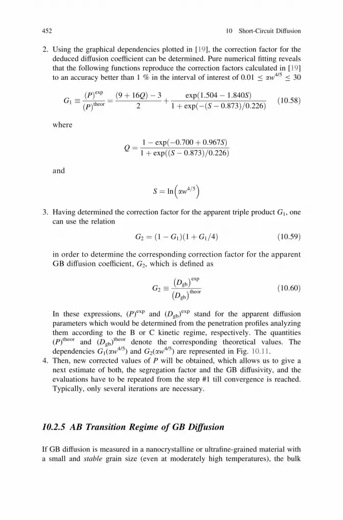
2. Using the graphical dependencies plotted in [19], the correction factor for thededuced diffusion coefficient can be determined. Pure numerical fitting revealsthat the following functions reproduce the correction factors calculated in [19]to an accuracy better than 1 % in the interval of interest of 0.01 B aw4/5 B 30

G1 �Pð Þexp

Pð Þtheor¼ 9þ 16Qð Þ � 3

2þ exp 1:504� 1:840Sð Þ

1þ exp �ðS� 0:873ð Þ=0:226Þ ð10:58Þ

where

Q ¼ 1� exp �0:700þ 0:967Sð Þ1þ exp ðS� 0:873Þ=0:226ð Þ

and

S ¼ ln aw4=5ffi �

3. Having determined the correction factor for the apparent triple product G1, onecan use the relation

G2 ¼ 1� G1ð Þ 1þ G1=4ð Þ ð10:59Þ

in order to determine the corresponding correction factor for the apparentGB diffusion coefficient, G2, which is defined as

G2 �Dgb

� exp

Dgb

� theorð10:60Þ

In these expressions, (P)exp and (Dgb)exp stand for the apparent diffusionparameters which would be determined from the penetration profiles analyzingthem according to the B or C kinetic regime, respectively. The quantities(P)theor and (Dgb)theor denote the corresponding theoretical values. Thedependencies G1(aw4/5) and G2(aw4/5) are represented in Fig. 10.11.

4. Then, new corrected values of P will be obtained, which allows us to give anext estimate of both, the segregation factor and the GB diffusivity, and theevaluations have to be repeated from the step #1 till convergence is reached.Typically, only several iterations are necessary.

10.2.5 AB Transition Regime of GB Diffusion

If GB diffusion is measured in a nanocrystalline or ultrafine-grained material witha small and stable grain size (even at moderately high temperatures), the bulk

452 10 Short-Circuit Diffusion

diffusion length may become comparable to the grain size and the parameter K*,taken from Eq. 10.51, would be about unity. In such a case, the penetration profilesneither follow a Gaussian solution, ln c y2 (the A kinetics), nor a Suzuoka’ssolution, ln c y6=5 (the B kinetics). In Fig. 10.12, a set of model penetrationprofiles are presented which are calculated with the following set of parameters:Dv = 10-14 m2/s, t = 100 s, Dgb = 10-9 m2/s, d = 10-8 m, a = 0.005, andb = 500 for grain size d = 10-7 m, 10-6 m, and 10-5 m, thus by varying theparameter K* from 10 to 1 and finally to 0.1, respectively.

Fig. 10.11 Dependencies of the corrections factors G1 and G2 on the reduced depth aw4/5 asdetermined by approximate Eqs. 10.58 and 10.59

Fig. 10.12 Simulated penetration profiles at Dv = 10-14 m2/s, t = 100 s, Dgb = 10-9 m2/s,d = 10-8 m, a = 0.005, and b = 500 for grain size d = 10-7 m, 10-6 m, and 10-5 m. Theprofiles are represented according to the A (a), AB (b), and B (c) kinetic regime conditions. Thevalue of the parameter K* is indicated. The parameter k is a scaling factor

10.2 Kinetic Regimes of GB Diffusion 453

Figure 10.12 suggests clearly (compare with Table 10.2) that if a\ 0.1 andb[ 10, the conditions of the B kinetics are fulfilled at K* = 0.1 and those of the Akinetics hold at K* = 10 and the profiles are strictly linear when plotted against y6/5

in the former case and against y2 in the latter. However, if K* = 1, unusual curvatureof the profiles for both presentations is obvious, as seen from Fig. 10.12a, c.

This case of K* & 1 has to be analyzed further. In the derivation, we will limitourselves to the case of self-diffusion (s = 1).

Let us consider a general polyhedral polycrystalline body with an averagedgrain size hdi and effective GB thickness d. Since d may be comparable with d (asin the case of nanocrystals), we will introduce a parameter l, l % hdi + d, asshown in Fig. 10.13. This will allow us to use common geometric theorems for apolycrystalline body with an arbitrary grain size 0 B d B ?. Then, the volumefraction e of the GB material will be determined by e = 2d/l % 2/(1 + \ d [/d).

Let cgb be the concentration of the diffusant in the grain boundary materials.Considering a one-dimensional problem and assuming that cgb = cgb(y, t) dependsonly on the depth y and time t, the master equation for the GB diffusion in apolycrystalline body will be

eocgbðy; tÞ

ot¼ 2e 1þ e=2ð Þ

3Dgb

o2cgbðy; tÞo2y

� rF ð10:61Þ

The following boundary conditions are valid for a constant source

cgb 0; tð Þ ¼ 1; cgbð1; tÞ ¼ 0; cgb y; 0ð Þ ¼ 0; y [ 0 ð10:61aÞ

Fig. 10.13 Definition ofgeometric parameters for ananocrystalline material. Anarbitrary section through thebody perpendicular to thediffusion direction is shown

454 10 Short-Circuit Diffusion

and for an instantaneous source

cgbð1; tÞ ¼ 0; cgb y; 0ð Þ ¼ Md yð Þ; ocgb

oy y¼0

����� ¼MdðtÞDgb

ð10:61bÞ

Here, r is the total GB surface area per unit volume, which may be estimated asr = 2e(1 - e)2, F is the effective flux of the tracer atoms into the grain volumefrom GBs, M is the amount of the tracer material for the instantaneous source, andd(y) is the standard delta function.

The flux F = F(y, t) into the grain interior is

Fðy; tÞ ¼Z t

0

ocgbðy; sÞos

Gðt � sÞds ð10:62Þ

where G(t) is the flux into an averaged grain with the diffusivity Dv at zero initialdiffusant concentration on its boundaries. The true form of G depends on the grainshapes. It is possible to derive their analytical formula for simple geometric forms.However, only approximate expressions can be obtained in a general case. Havingintroduced the reduced time s = (4Dv/d2)t, an empirical function may be used,

GðtÞ ¼ GðsÞ ¼ 2Dv

dffiffiffiffiffipsp exp �e2s

� �ð10:63Þ

Let us introduce also a reduced penetration depth

g ¼ 1d

ffiffiffiffiffiffiffiffiffiffiffiffiffiffiffiffiffi6Dv

Dgb 1þe=2ð Þ

qh iy ¼ 1

d

ffiffiffiffiffiffiffiffiffiffiffiffiffiffi6

D 1þe=2ð Þ

qh iy. Here, D = Dgb/Dv. Then, Eq. 10.61 can be

rewritten as

ocgb

os¼ o2cgb

o2g� d 1� eð Þ2

2Dv

Gðg; sÞ ð10:64Þ

The total concentration of the diffusant c averaged over a section of thepolycrystalline body will be

cðg; sÞ ¼ ecgbðg; sÞ þ rZs

0

cvðg; mÞGðs� mÞdm ð10:65Þ

where cv is the concentration inside the grains. It is convenient to use the Laplacetransformation to solve Eqs. 10.61–10.64. By applying the Laplace transformationto Eq. 10.64, the general solution may be presented as (boundary conditions for aconstant source being taken into account)

10.2 Kinetic Regimes of GB Diffusion 455

cðg; sÞ ¼ e2pi

Z10þi1

10�i1

~Cðg; s; pÞdp

¼ e2pi

Z10þi1

10�i1

eps � 1ð Þ 1p

1þ ð1� eÞ2ffiffiffiffiffiffiffiffiffiffiffiffipþ e2

p" #

exp �g p 1þ ð1� eÞ2ffiffiffiffiffiffiffiffiffiffiffiffipþ e2

p !" #1=2

8<:

9=;dp

ð10:66Þ

where the path of integration is to the right side of all singularities of the integrand~C. Since the initial concentration is zero, the term eps may be replaced by (eps - 1).We have two singularity points in the complex plane, p = 0 and -e2 (seeFig. 10.14). Since the integrand has no singularities inside the region R, the integralalong the contour L must be zero. The integrals on CR and Cq0 approach zero at

R ? ? and q0 ? 0, respectively, and e2pi

RCq

~Cdp! eþ ð1� eÞ2 at q ? 0. This

finite value is self-extracted in the final form of the integral in Eq. 10.66. Thus, thecomplex integral along the line f0 ± i? can be transformed to a sum of theintegrals along four line segments (Fig. 10.13)

cðg; sÞ ¼ ep

Ze2

0

1� e�1sð ÞU1

sin gffiffiffiffiffiffi1U

pffi �d1

þ ep

Z1

e2

1� e�1sð Þexp �g

ffiffiffi1p

A sin u2

� �1

ð1� eÞ2ffiffiffiffiffiffiffiffiffiffiffiffi1� e2

p cos Bþ sin B

" #d1

ð10:67Þ

Here, U ¼ 1þ ð1�eÞ2ffiffiffiffiffiffiffiffie2�gp ; A ¼ 1þ ð1�eÞ4

g�e2

h i1=4; B ¼ g

ffiffiffi1p

A cos u2; cosu ¼ 1þ ð1�eÞ4

g�e2

h i�1:

This form of solution allows performing a transition to e ? 1 (d ? 0) limit,and the general solution for GB diffusion in a pure grain boundary material from aconstant source will be obtained

Cðg; sÞ ¼ 1� 1p

Z1

0

e�1s sin gffiffiffi1p�

1d1 ð10:68Þ

In an opposite case, a Fisher-like solution will be derived. Indeed, let us make atransition to e ? 0 limit in Eq. 10.67. The first term in Eq. 10.67 gives therewith acontribution with the magnitude of only about e2 and can be neglected. Thus, it

remains to evaluate the last term. Since A�!e!0

gþ1g

ffi �14, we may write

456 10 Short-Circuit Diffusion

c ¼ ep

Z1

0

1� e�1sð Þexp �g 1

4ð1þ1Þ

ffi �1=4

1

� sin g1ð1þ 21Þ2

4ð1þ gÞ

!1=40@

1Aþ 1ffiffiffi

gp cos g

1ð1þ 21Þ2

4ð1þ gÞ

!1=40@

1A

24

35d1

ð10:69Þ

Let us evaluate the coefficient c ¼ �d ln Cdg

���g¼0¼ � 1

C1d

6D

� 1=2dCdy

���y¼0

representing

the slope of the relevant curve. After simple algebraic transformations, one mayfind that at e! 0 C y ¼ 0ð Þ ¼ 2e

ffiffisp

pand

dC

dg

���� g¼0e!0

¼ e

pffiffiffi2pZ1

0

1� e�1s

15=4 1þ 1ð Þ1=4

ffiffiffiffiffiffiffiffiffiffiffiffiffiffiffi1þ 212

p� 1

h id1 ffi 2

ffiffiffi6p

p1=4

ffiffiffiffiffiffiffiffiffiffiDv

dDgb

s1

pDvtð Þ1=4

Z1

0

ffiffiffimp

exp �m2�

dm

ð10:70Þ

The estimate of the integral in Eq. 10.70 suggests the slope c in the presentsolution differs and distinguishes from Fisher’s result only by a factor of 1.59. Aboutthe same factor (*1.57) was derived by Levine and McCallum for GB diffusion in apolycrystalline material [8]. The numerical analysis shows that the concentration

distribution is characterized by the product g � s�1=4 ¼ g0 � b�1=2 32þe

ffi �1=2where

g0 ¼ y=ffiffiffiffiffiffiffiDvtp

and b are conventional dimensionless parameters. Thus, Eq. 10.67allows us to examine the GB diffusivity in the whole range of grain sizes.

In a similar way, one can derive the solution for the instantaneous source,

Fig. 10.14 Singularitypoints and the integrationcontour L in calculation of theintegral Eq. 10.66

10.2 Kinetic Regimes of GB Diffusion 457

cðg; sÞ ffiZe2

0

e�1s U3=2ffiffiffi1p cos g

ffiffiffiffiffiffi1U

pffi �d1

�Z1

e2

e�1sA exp �g

ffiffiffi1p

A sin /2

ffi �ffiffiffi1p sin

/2þ 1� eð Þ2ffiffiffiffiffiffiffiffiffiffiffiffi

1� e2p cos

/2

!sin Bþ 1� eð Þ2ffiffiffiffiffiffiffiffiffiffiffiffi

1� e2p sin

/2� cos

/2

!cos B

" #d1

ð10:71Þ

Substituting e = 1, it is possible to obtain the standard Gaussian solution fordiffusion in a homogeneous media from an instantaneous source,

cðg; sÞ ¼ MffiffiffiffiffiffiffiffiffiffiffiffipDgbt

p exp � g2

4Dgbt

� �ð10:72Þ

Equations 10.67 and 10.69 cannot be further simplified and require a numericalevaluation. A detailed analysis in terms of stretched exponential functions such asln c ym demonstrates that in the case of small values of e2s 4Dvt

l2 and s 4Dvtd2

(that corresponds to the C type of diffusion kinetics), the power m = 2. In the caseof the B regime (large values of s and small values of e2s), m = 6/5. The diffusionbehavior in the transition regime (large values of s and e2s & 1) is the mostinteresting and unusual power dependence with m = 3/2 being observed. InFig. 10.12b, the simulated penetration profiles are plotted as a function of y3/2.Almost perfect linearity of the profile with K* = 4(e2s)-1 = 1 is clearly to beseen.

We have shown that the tracer distribution in the case of the C regime of GBdiffusion allows determination of the value of Dgb, while the double product dDgb

(or the triple product sdDgb for solute diffusion) is determined in the case of the Bkinetic regime. Effective penetration in the B regime is described by the reduceddepth w = g � s-1/4. On the other hand, the effective penetration in the transitionAB regime is determined by the value

w ¼ gs�0:45 ¼ 1d

ffiffiffiffiffiffiffiffiffiffiffiffiffiffiffiffiffiffiffiffiffiffiffiffiffiffi6Dv

Dgb 1þ e=2ð Þ

s4Dv

d2

� ��0:45" #

yt�0:45 ð10:73Þ

This quantity is related to the standard reduced depth w via the following

expression: w ¼ w � s�0:2 32þe

ffi �1=2¼ w D

b

ffi ��0:13

2þe

ffi �1=2. The corresponding slopes,

S ¼ �d ln c=dw3=2, are a weak function of e2s and S % 1.128 at e2s % 1. This factsuggests the following expression for the determination of the GB diffusioncoefficient in this regime

Dgb ffi54

4Dvt

d2

� �0:091t

S

S0exp

!1:33

¼ 54

s0:09

t

S

S0exp

!1:33

ð10:74Þ

458 10 Short-Circuit Diffusion

Here, S0exp ¼ �d ln c=dy3=2 is to be determined by fitting of the experimentalprofile. Inserting the numerical factors, this expression is written as

Dgb ¼16:65

1þ d=d

D0:1v

d0:2t0:9� o ln c

oy3=2

� ��4=3

ð10:75Þ

The value of the GB width d enters explicitly Eq. 10.75 and has to be deter-mined separately. However, the final result only slightly depends on the value of ddue to the power of 0.2.

Experimentally measured profiles belonging to the transition AB kinetic regimeare shown in Fig. 10.15. They represent the case of Fe diffusion in a nanocrys-talline (grain size of 100 nm) c-FeNi alloy [13]. It is seen that the linearity of theprofiles in the given coordinates is followed over three orders of magnitude indecrease of the tracer concentration!

10.3 Determination of the Segregation Factor s

The majority of GB diffusion experiments are performed under the B kineticregime. The defined effective activation enthalpy of GB diffusion in this case

Fig. 10.15 Examples ofpenetration profiles measuredin the AB transition regimefor Fe diffusion innanocrystalline c-FeNialloy [13]

10.2 Kinetic Regimes of GB Diffusion 459

P ¼ P0 exp �Qgb

RT

� �ð10:76Þ

contains the real enthalpy of GB diffusion DHgb and the enthalpy of segregationHseg \ 0

Qgb ¼ DHgb þ Hseg ð10:77Þ

Theoretically, the GB width can depend on temperature and contribute toEq. 10.77. However, the available data are consistent with the approximationd = const, which is to be seen below. The analysis of Table 10.2 suggests a wayfor separate determination of GB diffusion parameters in systematic measurementson the same polycrystalline material. A combination of the B- and C-typeexperiments is crucial, since the GB diffusion coefficient Dgb is measured in the Ckinetics (typically at lower temperatures), while the triple product P, P = sdDgb, isdetermined at higher temperatures in the B kinetics for solute diffusion. These datacan be combined, and the product sd will be estimated

sd ¼ Pð ÞB�kinetics

Dgb

� C�kinetics¼

sdDgb

� B�kinetics

Dgb

� C�kineticsð10:78Þ

This approach is outlined in Fig. 10.16 for selected solutes.Figure 10.16 suggests that the values of the triple product P, being extrapolated

to lower temperatures of the C-type measurements, are systematically smaller thanthe corresponding diffusion coefficients Dgb and the difference reaches orders ofmagnitude. This difference is exactly the product sd.

A comment is due here. The subdivision of the measured data in B and Ckinetics is strongly based on the values of the segregation factor s which is typ-ically unknown in advance. Moreover, the value of d has also to be known. Aspecial procedure is suggested to analyze the GB diffusion data in a self-consistentand reliable way.

The value of the GB diffusional width d can be determined similarly toEq. 10.78 if one performs a similar series of self-diffusion measurements in both Band C kinetics. Then, the corresponding segregation factor is simply unity and

d ¼ Pð ÞB�kinetics

Dgb

� C�kinetics¼

dDgb

� B�kinetics

Dgb

� C�kineticsð10:79Þ

As an example, the GB diffusion data on high-purity polycrystalline Ni mea-sured both in the B and C kinetic regimes are presented in Fig. 10.17.

Figure 10.17 suggests that there is a huge gap between the directly measuredvalues of Dgb and the extrapolated high-temperature data for P = dDgb. This isexactly the (diffusional) GB width d. Table 10.3 lists the values reported so far

460 10 Short-Circuit Diffusion

Fig. 10.16 Compilation ofresults on Ag [19], Ge [45],Ni [44], and Bi [46] GBdiffusion in 5N8 high-purityCu measured in both, theB-type (solid symbols) andC-type (open symbols)kinetics. The determinationof the product sd for Ni issketched. The grain boundaryself-diffusion of Cu [47] isplotted by thick dashed (theB kinetics) and solid(the C kinetics) lines

Fig. 10.17 Compilation ofGB self-diffusionmeasurements in Ni in both,B (squares) and C (circles)kinetic regimes [30]. Opensymbols represent the datadetermined in the transitionBC regime. The way ofdetermination of the GBwidth d is sketched

10.3 Determination of the Segregation Factor s 461

based on the GB self-diffusion measurements. As one can see, d = 0.5 nm is avery good estimate for the GB width for the GB diffusion of matrix atoms.

The knowledge of the GB width d allows a consistent analysis of solute GBdiffusion and determination of the segregation properties. The flowchart of suchanalysis is as follows:

1. One starts assuming d = 0.5 nm and uses a reasonable estimate of the segre-gation factor s. According to the empirical relation of Hondros and Seah [20],the segregation factor s is inversely proportional to the bulk solubility of thesolute cv0

s ¼ kH

cv0

ð10:80Þ

where the Hondros’ constant is within the range kH = 1 to 10 [20]. Thisestimate can be recommended as a good initial guess. Otherwise, one mayuse s = 1.

2. Knowing the product sd enables us to analyze all profiles according to thegiven GB diffusion kinetics, as given in Table 10.2.

3. Having determined the triple products P, one should approximate them by anArrhenius temperature dependence, P ¼ P0 expð�Qgb=RTÞ. Extrapolating thenthe P values to lower temperatures of the Dgb measurements, the product sdwill be determined.

4. Again, fitting the sd data by an Arrhenius line, sd ¼ s0d expð�DHs=RTÞ, thevalues of sd can be determined for all temperatures in question. This gives newestimates of the GB diffusion parameters, (a and b) and one should repeat theloop starting from step #2.

Typically, after several iterations, a convergence is reached.

Table 10.3 Compilation of published results on the diffusional GB width d

Material Tracer d (nm) Reference

NiO 63Ni 0.7 [48]Ag 110mAg 0.43 ± 0.27b [42]Ag 110mAg 0.5a [49]c-FeNi 59Fe 0.5a [13, 22]c-FeNi 63Ni 0.55 ± 0.43 [50]a-Fe 59Fe 0.5a [51]Ni (99.999 wt%) 63Ni 0.54 ± 0.1 [30]Ni (99.99 wt%) 63Ni 0.6 ± 0.2 [31]a-Ti 44Ti, 57Co 0.5a [52]

a The assumption d = 0.5 nm allowed to treat the results consistentlyb Our estimate of the GB width from the data given by Sommer and Herzig [42]. The authorsstated originally that assuming d = 0.5 nm, the B and C kinetic data will produce consistentresults

462 10 Short-Circuit Diffusion

As an example of systematic measurements of GB diffusion in the same, high-purity polycrystalline Cu, the data on different solutes are collected in Table 10.4and shown in Fig. 10.18.

The described approach is based on the following main approximations:

• Constant and isotropic GB width d is assumed;• Arrhenius-type dependencies are assumed to hold for both Dgb and P, i.e.,

Db ¼ Dgb0 expð�DHgb=RTÞ and P ¼ P0 expð�Qgb=RTÞ, respectively;• Linear segregation of the solute (the Henry isotherm) is supposed; that is, the

segregation coefficient is not changed along the boundary, s = const for thegiven temperature T;

• The limits of the GB diffusion regimes are strictly defined.

Table 10.4 Compilation of available GB diffusion and segregation data on different solutes inthe same high-purity (99.9998 wt.%) Cu

Tracer P0 (m3/s) Qgb

(kJ/mol)Dgb0 (m2/s) DHgb

(kJ/mol)s0d (m) -Hs

(kJ/mol)s0 Refs.

Cu 3.9 9 10-16 72.5 7.8 9 10-7 72.5 – – – [47]Ag 1.4 9 10-15 69.1 1.7 9 10-4 108.6 8.0 9 10-12 39.5 0.016 [19]Ge 4.0 9 10-16 58.6 2.8 9 10-6 84.8 1.45 9 10-10 26.2 0.29 [45]Bi 6.6 9 10-12 102.8 2.4 9 10-1 156.2 2.7 9 10-11 53.4 0.054 [46]Ni 1.9 9 10-16 73.8 6.9 9 10-7 90.4 3.0 9 10-10 16.6 0.60 [44]

Fig. 10.18 Solutesegregation in high-puritycopper as determined by GBdiffusion measurement. TheArrhenius parameters arelisted in Table 10.4

10.3 Determination of the Segregation Factor s 463

The next (very important) approximation is that the GB widths for self-diffusiondsd and that for solute diffusion dsolute are equal: dsd = dsolute. Generally speaking,this may not be the case. One may imagine that dsolute [ dsd (even dsolute � dsd)and Dsolute

gb which enters the triple product P will correspond to an effective value.In such a case, the application of Eq. 10.78 would be incorrect.

There are, however, strong arguments that this is not the case, at least for suchsolutes as Ag and Bi in Cu in the case of true dilute solution. The segregationenthalpies derived from the application of Eq. 10.78 agree well with the inde-pendently measured data produced by Auger spectroscopy.

Several features can be highlighted:

• Fast (slow) diffusants in a bulk tend to remain identical in GB;• Strong GB segregation tends to reduce the GB diffusivity; the stronger a

segregation, the greater the retardation effect.

10.4 Nonlinear GB Segregation and GB Diffusion

The described theory of GB diffusion, contained in Eqs. 10.1–10.43, predicts linearpenetration profiles in the coordinates of the logarithm of concentration againstdepth to the 6/5 power if GB diffusion occurs in the B kinetic regime. The solutionsare derived considering (1) the constant and isotropic GB width d, (2) the constantand isotropic GB diffusion coefficient Dgb � Dv, and (3) the constant value of thesegregation factor s, given in Eq. 10.2. However, segregation could stronglydepend on the solute concentration in the bulk that is known as nonlinear segre-gation [21]. In such cases, nonlinear (strongly curved) penetration profiles areexpected for GB solute diffusion [4]. An example is given in Fig. 10.19a, while aperfect B-type penetration profile is measured for Ag diffusion in Cu bicrystal if alow amount of tracer material is used (0.3 kBq of radioactive 110mAg is initiallydeposited); strongly and characteristically curved penetration profiles are obvious ifthe tracer concentration is significantly increased (12 or even 120 kBq of 110mAg).The above analysis clearly demonstrates that this is not the type of boundaryconditions—instantaneous versus constant source—that could introduce such acurvature of the profiles.

Using the penetration profiles presented in Fig. 10.19a, it is possible to deter-mine the pertinent segregation isotherm, i.e., cgb as a function of cv, cgb(cv). Thekey moment is that using radiotracer material with a known specific activity andby applying the Fisher solution, it is possible to determine the absolute bulk soluteconcentration just near the GB cv0 (in mole fractions) as a function of the pene-tration depth y. According to the Fisher solution for the B regime, the layerconcentration of the tracer cðyÞ at the given depth y is fully determined by out-diffusion from the GB considered as a constant source with the concentration cv0,

and is described by Eq. 10.13. Integrating over x, we derive

464 10 Short-Circuit Diffusion

cv0ðyÞ ¼d

4p

Dvt

� �cðyÞ ð10:81Þ

In this case, d is the diameter of the bicrystals used in the experiments presentedin Fig. 10.19a.

At large depths (low tracer concentrations), a linear (Henry) segregation iso-therm is valid and cgb(y) can be determined using the value of the correspondingsegregation factor sH, which was found in an independent series of B- and C-typeGB diffusion measurements, as shown in Table 10.4.

Let us introduce y0 as the critic depth below which the Henry segregation isvalid. Then, regrouping the term in Eq. 10.25, we have at y [ y0

d

4p

Dvt

� �cðyÞ � cv0ðyÞ ¼ c0 exp � y

L

ffi �¼ c0 exp � y

LffiffiffiffiffisHp

� �ð10:82Þ

and

cgbðyÞ ¼ sHcv0 ¼ sHc0 exp � y

LffiffiffiffiffisHp

� �ð10:83Þ

Here, the reduced penetration depth L, seen from Eq. 10.17, is written as L ¼

LffiffiffiffiffisHp

where L* is now L ¼ffiffiffiffiffiffiffiffiffiffidDgb

ppt

4Dv

ffi �1=4

Generally, at arbitrary depth, the bulk and GB concentrations may be decom-posed as

Fig. 10.19 Penetration profiles measured for Ag diffusion in Cu R5 bicrystal at a differentamounts of the tracer material applied and b the determined segregation isotherms

10.4 Nonlinear GB Segregation and GB Diffusion 465

cv0ðyÞ ¼ DvðyÞ þ c0 exp � y

LffiffiffiffiffisHp

� �ð10:84Þ

and

cgbðyÞ ¼ DgbðyÞ þ sHc0 exp � y

LffiffiffiffiffisHp

� �ð10:85Þ

The terms Dv(y) and Dgb(y) represent the deviations of the measured tracerconcentrations at the depth y from the Fisher solution of the GB diffusion problemin the presence of only linear segregation with s = sH. The total tracer distributionobeys the standard equation of GB diffusion, Eq. 10.15, which can be presented as

o2cgb

oy2¼ L�2cv0 ð10:86Þ

with the boundary condition cv0 ? 0 and cgb ? 0 as y ? ?. CombiningEqs. 10.84–10.86, the following relation is obtained

o2Dgb

oy2¼ L�2Dv ð10:87Þ

with a more appropriate boundary condition Dv = Dgb = 0 as y C y0. This is asimple second-order differential equation which can be solved by double inte-gration. As a result, the GB solute concentration will be found as a function of thepenetration depth y

cgbðyÞ ¼ sHc0 exp � y

LffiffiffiffiffisHp

� �þ L�2

Zy

y0

dsZs

y0

DvðuÞdu ð10:88Þ

Since cv0 is measured as a function of the penetration depth y, as given inEq. 10.81, the relation given in Eq. 10.88 implicitly determines the segregationisotherm cgb(cv0).

This method is applied to the two curved penetration profiles measured for GBdiffusion of Ag in Cu bicrystal, as shown in Fig. 10.19a. The results, i.e., cgb asfunction of cv0, are presented in Fig. 10.19b. The resulting segregation isothermsderived from the two independent GB diffusion experiments are consistent. Onerealizes that using very sensitive radiotracer GB diffusion measurements with asuitable tracer on bicrystals, it is possible to reliably determine the segregationisotherm already starting from very small GB concentrations. Regarding thisfeature, the presented radiotracer method is superior to other experimental tech-niques so far applied for treating the segregation phenomena.

466 10 Short-Circuit Diffusion

10.5 Microstructures with Hierarchy of Short-CircuitDiffusion Paths

Microstructure in technologically relevant materials is far more complicated as itis captured by a simple bicrystal-like model, as depicted in Fig. 10.3. Often, ahierarchic microstructure is revealed in a material as, for example, was the case ofa sintered nanocrystalline c-FeNi alloy [13, 22]—the nanocrystalline grains (withthe grain size of d * 100 nm) turned out to be clustered in agglomerates with anaverage size da of 30–50 lm. This microstructure is shown in Fig. 10.20 and issketched in Fig. 10.21a. In Fig. 10.20, the results of optical and atomic forcemicroscopy (AFM) techniques are combined since they examine the microstruc-ture on different scales. Individual nanograins are perfectly resolved by the AFMtechnique, whereas micrometer-large agglomerates are clearly seen by opticalmicroscopy after suitable surface preparation (polishing and etching).

Thus, at least two different types of internal interfaces existed in such material—the interfaces between the nanograins and the interfaces between agglomerates (orclusters) of these grains. These interfaces are deliberately drawn as thin and thickboundaries in Fig. 10.21a since very different diffusion properties may be expected(as is the case).

On the other hand, the hierarchy of short-circuit diffusion paths in a typicalpolycrystalline material can be represented by the following contributions(grouped according to the corresponding diffusion rates):

• Triple junctions, i.e., line defects representing the lines along which threegrains and correspondingly three GBs meet (however, so far, no direct tracerdata for the dilute (Henry) limit exist, which would unambiguously confirmthat the diffusion along the triple junctions is faster than along the corre-sponding grain boundaries, since the available data correspond to the results ofmicroprobe analysis [23] or 3D atom-probe tomography [24], which may sufferfrom contaminate chemical effects);

• General (random) high-angle GBs;• Low-angle GBs, dislocation walls, and individual dislocations.

For the effect of dislocations on GB diffusion and rigorous analysis of thecorresponding kinetic regimes, the reader is referred to original papers [25, 26].The corresponding analytical formulation (as well as the case of triple junctiondiffusion) are very similar to that presented below.

10.5.1 Kinetic Regimes of GB Diffusion in a Materialwith a Hierarchic Microstructure

In the case of a hierarchy of the microstructure (Fig. 10.21a), three potentialdiffusion paths should simultaneously be taken into account:

10.5 Microstructures with Hierarchy of Short-Circuit Diffusion Paths 467

1. Short-circuit diffusion along the inter-agglomerate boundaries. Each of suchinterfaces is assumed to be represented by a homogeneous slab of the width da

and the diffusivity Da;2. Short-circuit diffusion along nanocrystalline GBs which are considered as

homogeneous slabs of the width d and the diffusivity Dgb;3. Bulk diffusion with the diffusion coefficient Dv.

It is reasonable to assume (and this was experimentally verified) that in thetemperature interval of typical diffusion measurements

Fig. 10.20 Microstructure of nanocrystalline c-FeNi alloy [25] as revealed by optic microscopyand atomic force microscopy (insert)—individual nanograins are clustered in micrometer-largeagglomerates

Fig. 10.21 a Schematic microstructure of the nanocrystalline c-FeNi alloy with a hierarchicmicrostructure. Small nanograins (of the size d) are clustered in agglomerates of the size da. d andda are the widths of nano-GBs and inter-agglomerate boundaries, respectively; Dv, Dgb, and Da

are the bulk, nano-GB, and inter-agglomerate boundary diffusivities, respectively. In b, theconcentrations, which are relevant to the definitions of the segregation factors s and sa, areindicated

468 10 Short-Circuit Diffusion

Da � Dgb � Dv ð10:89Þ

Taking this relation into account, three different diffusion fluxes can generallybe introduced:

1. Direct volume diffusion from the sample surface into the nanograins, diffusionrate Dv;

2. GB diffusion along nanocrystalline boundaries Dgb with subsequent outdiffu-sion into the grain interior, Dv; and

3. Diffusion along the inter-agglomerate boundaries Da with subsequent outdif-fusion to the nanoboundaries Dgb and then into the grain bulk Dv.

Thus, the regimes of interface diffusion for the processes (1) and (3) have to bespecified separately in order to describe the overall diffusion kinetic. Taking this inmind, a two-letter designation was suggested [13], such as C–B. Each letter cor-responds to the given Harrison kinetic regime, introduced above in Sect. 10.2,which is satisfied for the particular interface type. We first specify the regime fornano-GBs and then for inter-agglomerate boundary diffusion. Therefore, the C–Bregime describes the case when the C regime of diffusion along the nanocrystallineGBs (no outdiffusion into bulk) is satisfied and when simultaneously the (quasi) Bregime of diffusion along the inter-agglomerate boundaries (fast diffusion alongthe inter-agglomerate boundaries with subsequent outdiffusion into the adjacentnano-GBs) is fulfilled. The word ‘‘quasi’’ is necessary to indicate that the regime issimilar to that of B, but due to the different outdiffusion kinetics (tracer leakageoccurs only at places where nanocrystalline GBs cross the inter-agglomerateboundaries), the triple product is modified, see Sect. 10.5.1.2. And it does notfollow it, as will be shown below.

In the case of solute diffusion, the segregation of the solute to both types ofinternal interfaces has to be taken into account. More than one segregation coef-ficient have to be introduced. The solute atoms can generally be in excess in thefollowing (see Fig. 10.21b):

(a) Nanocrystalline GBs with respect to the adjacent bulk;(b) Inter-agglomerate interfaces with respect to the adjacent bulk; and(c) Inter-agglomerate interfaces with respect to the adjacent positions in the

nano-GBs which intersect this inter-agglomerate interface.

In view of relation in Eq. 10.89, two segregation factors are required to describethe diffusion problem under consideration: s, which characterizes the solute excessin a nano-GB with respect to an adjacent bulk plane, and sa, which corresponds toan excess of the solute in the inter-agglomerate boundary with respect to theadjacent position in the nanocrystalline GB

s ¼ cgb

cvð0Þð10:90Þ

10.5 Microstructures with Hierarchy of Short-Circuit Diffusion Paths 469

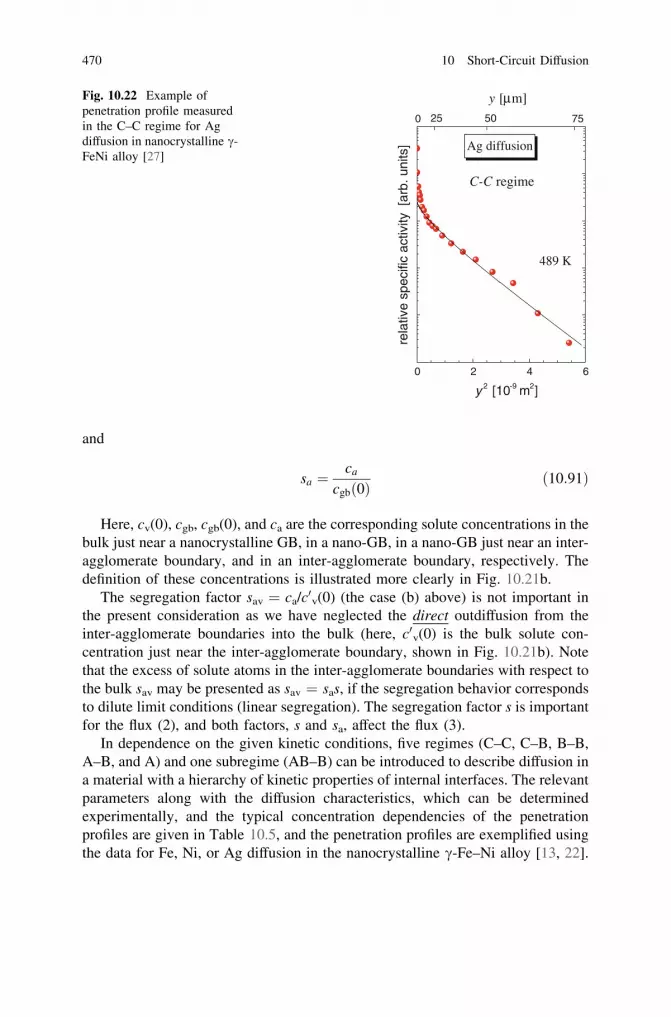
and

sa ¼ca

cgbð0Þð10:91Þ

Here, cv(0), cgb, cgb(0), and ca are the corresponding solute concentrations in thebulk just near a nanocrystalline GB, in a nano-GB, in a nano-GB just near an inter-agglomerate boundary, and in an inter-agglomerate boundary, respectively. Thedefinition of these concentrations is illustrated more clearly in Fig. 10.21b.

The segregation factor sav = ca/c0v(0) (the case (b) above) is not important inthe present consideration as we have neglected the direct outdiffusion from theinter-agglomerate boundaries into the bulk (here, c0v(0) is the bulk solute con-centration just near the inter-agglomerate boundary, shown in Fig. 10.21b). Notethat the excess of solute atoms in the inter-agglomerate boundaries with respect tothe bulk sav may be presented as sav = sas, if the segregation behavior correspondsto dilute limit conditions (linear segregation). The segregation factor s is importantfor the flux (2), and both factors, s and sa, affect the flux (3).

In dependence on the given kinetic conditions, five regimes (C–C, C–B, B–B,A–B, and A) and one subregime (AB–B) can be introduced to describe diffusion ina material with a hierarchy of kinetic properties of internal interfaces. The relevantparameters along with the diffusion characteristics, which can be determinedexperimentally, and the typical concentration dependencies of the penetrationprofiles are given in Table 10.5, and the penetration profiles are exemplified usingthe data for Fe, Ni, or Ag diffusion in the nanocrystalline c-Fe–Ni alloy [13, 22].

0 2 4 6

C-C regime

Ag diffusion

75500 25

489 K

y [μm]

rela

tive

spec

ific

activ

ity [

arb.

uni

ts]

y 2 [10-9 m2]

Fig. 10.22 Example ofpenetration profile measuredin the C–C regime for Agdiffusion in nanocrystalline c-FeNi alloy [27]

470 10 Short-Circuit Diffusion

Tab

le10

.5P

aram

eter

sof

kine

tic

regi

mes

ofG

Bdi

ffus

ion

ina

nano

crys

tall

ine

mat

eria

lw

ith

ahi

erar

chic

alm

icro

stru

ctur

e

Reg

ime

Con

diti

ons

Mea

sure

dpa

ram

eter

sT

ypic

alco

ncen

trat

ion

depe

nden

ce

C–C

a¼

sd2ffiffiffiffiffi D

vt

p[

1;a a¼

s ad a

2kffiffiffiffiffiffiffi D

gbt

p[

1D

a¼

1 4tq�

12

c/

expð�

q 2y2Þ(

Fig

.10

.22)

C–B

a[

1;a

a\

0.1,

b a¼

Pa

2Dgb

ffiffiffiffiffiffiffiffiffi

Dgbt

p�

2;

ffiffiffiffiffiffiffiffiffi

Dgbt

p\

d a=

4

Dgb¼

1 4tq�

11

Pa¼

s ad a

Da

k¼

1:31

ffiffiffiffiffiffiffiffi

Dgb t

rq�

5=3

2

c/

expð�

q 1y2Þþ

expð�

q 2y6=

5Þ

(Fig

.10

.23)

B–B

a\0.

1,b�

2,ffiffiffiffiffiffiffi D

vtp

\d=

4;

a0 a\

0:1;

b0 a�

2;ffiffiffi Pp

pt

4Dv

ffi� 1=

4\

d a=

2P¼

sdD

gb¼

1:31

ffiffiffiffiffiffi Dv t

rq�

5=3

1

Pa¼

s ad a

Da

k¼

1:80

ffiffiffiffiffiffiffiffi

Dgb

sd

rD

v t�� 1=

4

q�2

2

c/

expð�

q 1y6=

5Þþ

expð�

q 2yÞ

(Fig

.10

.24)

AB

–Bd=

4\ffiffiffiffiffiffiffi D

vtp

\3d

;a00 a\

0:1;

b00 a�

2;ffiffiffiffiffiffiffiffiffiffi

Da ef

ftp

\d a=4

sDgb¼

16:4

8D

0:1

v

d0:2t0:

9q�

4=3

1

P0 a¼

s ad a

Da¼

1:31

ffiffiffiffiffiffiffiffi

Da ef

f

t

rq�

5=3

2

c/

expð�

q 1y3=

2Þþ

expð�

q 2y6=

5Þ(

Fig

.10

.25)

A–B

ffiffiffiffiffiffiffi Dvt

p[

3d;

ffiffiffiffiffiffiffiffiffiffi

Da ef

ftp

\d a=4;

a00 a\

0:1;

b00 a�

2D

a effffi

1 2sf

gb

1þ

sfgb

Dgb¼

1 4tq�

11

P0 a¼

s ad a

Da¼

1:31

ffiffiffiffiffiffiffiffi

Da ef

f

t

rq�

5=3

2

c/

expð�

q 1y2Þþ

expð�

q 2y6=

5Þ

(Fig

.10

.26)

Affiffiffiffiffiffiffiffiffiffi

Da ef

ftp

[3d

aD

M effffi

sfg

b=2

1þsf

gbD

gbþ

ssaf a=

21þ

ssaf a

Da¼

14t

q 2c/

expð�

q 2y2Þ(

Fig

.10

.27)

The

valu

ec

isth

ela

yer

conc

entr

atio

n,y

isth

epe

netr

atio

nde

pth,

q 1an

dq 2

are

the

num

eric

alfa

ctor

s,an

dk

=2d

/dis

the

dens

ity

ofna

no-G

Bs

inte

rsec

ting

anin

ter-

aggl

omer

ate

boun

dary

.O

ther

para

met

ers

are

defi

ned

inth

ete

xt

10.5 Microstructures with Hierarchy of Short-Circuit Diffusion Paths 471

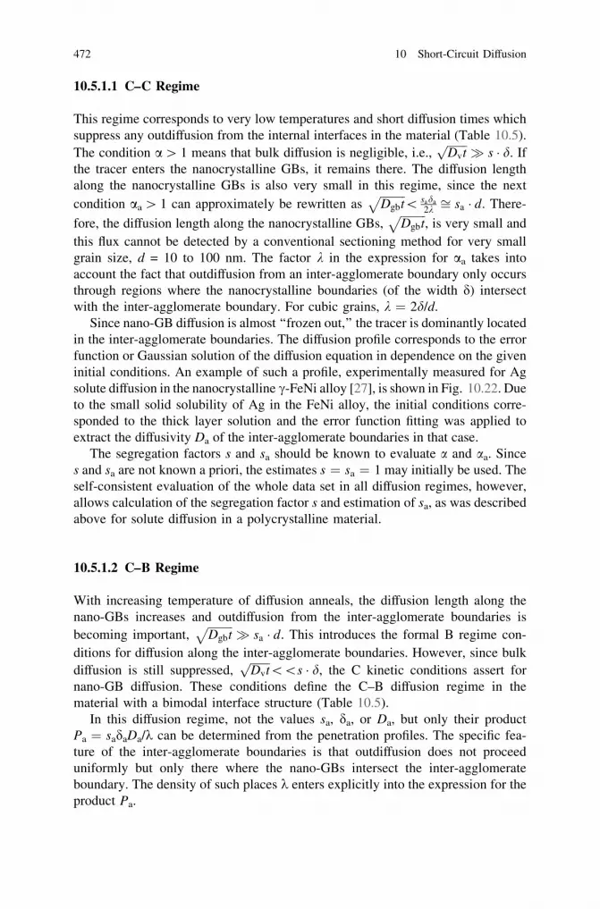
10.5.1.1 C–C Regime

This regime corresponds to very low temperatures and short diffusion times whichsuppress any outdiffusion from the internal interfaces in the material (Table 10.5).The condition a[ 1 means that bulk diffusion is negligible, i.e.,

ffiffiffiffiffiffiffiDvtp

� s � d. Ifthe tracer enters the nanocrystalline GBs, it remains there. The diffusion lengthalong the nanocrystalline GBs is also very small in this regime, since the nextcondition aa [ 1 can approximately be rewritten as

ffiffiffiffiffiffiffiffiffiDgbt

p\ sada

2k ffi sa � d. There-

fore, the diffusion length along the nanocrystalline GBs,ffiffiffiffiffiffiffiffiffiDgbt

p, is very small and

this flux cannot be detected by a conventional sectioning method for very smallgrain size, d = 10 to 100 nm. The factor k in the expression for aa takes intoaccount the fact that outdiffusion from an inter-agglomerate boundary only occursthrough regions where the nanocrystalline boundaries (of the width d) intersectwith the inter-agglomerate boundary. For cubic grains, k = 2d/d.

Since nano-GB diffusion is almost ‘‘frozen out,’’ the tracer is dominantly locatedin the inter-agglomerate boundaries. The diffusion profile corresponds to the errorfunction or Gaussian solution of the diffusion equation in dependence on the giveninitial conditions. An example of such a profile, experimentally measured for Agsolute diffusion in the nanocrystalline c-FeNi alloy [27], is shown in Fig. 10.22. Dueto the small solid solubility of Ag in the FeNi alloy, the initial conditions corre-sponded to the thick layer solution and the error function fitting was applied toextract the diffusivity Da of the inter-agglomerate boundaries in that case.

The segregation factors s and sa should be known to evaluate a and aa. Sinces and sa are not known a priori, the estimates s = sa = 1 may initially be used. Theself-consistent evaluation of the whole data set in all diffusion regimes, however,allows calculation of the segregation factor s and estimation of sa, as was describedabove for solute diffusion in a polycrystalline material.

10.5.1.2 C–B Regime

With increasing temperature of diffusion anneals, the diffusion length along thenano-GBs increases and outdiffusion from the inter-agglomerate boundaries isbecoming important,

ffiffiffiffiffiffiffiffiffiDgbt

p� sa � d. This introduces the formal B regime con-

ditions for diffusion along the inter-agglomerate boundaries. However, since bulkdiffusion is still suppressed,

ffiffiffiffiffiffiffiDvtp

\\s � d, the C kinetic conditions assert fornano-GB diffusion. These conditions define the C–B diffusion regime in thematerial with a bimodal interface structure (Table 10.5).

In this diffusion regime, not the values sa, da, or Da, but only their productPa = sadaDa/k can be determined from the penetration profiles. The specific fea-ture of the inter-agglomerate boundaries is that outdiffusion does not proceeduniformly but only there where the nano-GBs intersect the inter-agglomerateboundary. The density of such places k enters explicitly into the expression for theproduct Pa.

472 10 Short-Circuit Diffusion

The diffusion length for diffusion along the nanocrystalline GBs,ffiffiffiffiffiffiffiffiffiDgbt

p, should

be smaller than the size da of the agglomerates in this regime. Otherwise, the dif-fusion fluxes from different inter-agglomerate boundaries will overlap and the for-mal A kinetic regime might become important. In the C–B diffusion regime, theparameter a is larger than unity and the tracer does not penetrate into the bulk. Thediffusion process is thus confined to nano-GBs and inter-agglomerate boundariesonly. The tracer is mainly located in the nano-GBs.

An example of such a penetration profile measured for Fe diffusion in nano-c-FeNi [22] is presented in Fig. 10.23. A two-stage shape of the penetration profile isclearly seen. The first part, which is characterized by the ln c y2 depth depen-dence of the concentration profile, corresponds to the nano-GB diffusion in the Cregime. As a result, the nano-GB diffusivity Dgb can directly be determined fromthis part (Table 10.5).

The second part of the penetration profile in Fig. 10.23 corresponds to the fasterdiffusion mode from the surface into the inter-agglomerate boundaries with sub-sequent outdiffusion into adjacent nanocrystalline GBs. Since formal B-typeconditions are fulfilled in this diffusion mode, the Suzuoka solution, given inEqs. 10.37a–10.38, of the interface diffusion problem has to be applied, as inTable 10.5. The solid line in Fig. 10.23 represents the relevant fit.

10.5.1.3 B–B Regime

If temperature and/or time of diffusion anneal increases further, the bulk diffusionflux becomes more significant and cannot be neglected. Then, the diffusion processwill be dominated by two fluxes:

0.0 0.5 1.0

C-B regime

Fe diffusion

500 25

669 K

y [μm]

rela

tive

spec

ific

activ

ity [

arb.

uni

ts]

y 6/5 [10-5 m6/5]

Fig. 10.23 Example ofpenetration profile measuredin the C–B regime for Fediffusion in nanocrystallinec-FeNi alloy [22]

10.5 Microstructures with Hierarchy of Short-Circuit Diffusion Paths 473

1. GB diffusion along the nanocrystalline GBs with subsequent outdiffusion intothe grain interior and

2. Faster diffusion along inter-agglomerate boundaries with subsequent outdiffu-sion to nanoboundaries and then into the grains.

Since the bulk diffusion lengthffiffiffiffiffiffiffiDvtp

has to be smaller than the grain size tosatisfy the conditions of this B–B regime (Table 10.5), the total contribution ofdirect volume diffusion from the sample surface into the nanograins can beneglected. Correspondingly, two-stage penetration profiles should be observed. Anexample of such a profile, which was measured for Ni diffusion in nano-c-FeNi[28], is shown in Fig. 10.24.

The B regime conditions are satisfied for the flux (1). Therefore, the Suzuokasolution to the GB diffusion problem is applied to analyze this term. As a result, thefirst part of the penetration profile should be linear in the coordinates of lnc versus y6/5

and only the triple product P = sdDgb can be determined, but not the nano-GBdiffusivity Dgb itself (see Table 10.5). The parameter b ¼ P=2Dv

ffiffiffiffiffiffiffiDvtp

has to belarge enough in order to observe a distinct GB diffusion-related tail. It was shown thatb C 2 can be used as a lower limit of the B regime [22].

The diffusion flux (2) represents a fundamentally new situation. In order todescribe an analytic expression for the layer tracer concentration c that entered thesample this way, we will reformulate the Fisher model for inter-agglomerateboundary diffusion from a constant source. The tracer concentrations cv(x, y, t) inthe bulk, the cgb(x, y, t) in nanocrystalline grain boundaries, and the ca(x, y, t) ininter-agglomerate boundaries are to be considered. To derive an analytical solu-tion, the following approximations are made (see Fig. 10.21b):

0 1 2 3 4 5

B-B regime

Ni diffusion

2000 100

881 K

y [μm]

rela

tive

spec

ific

activ

ity [

arb.

uni

ts]

y 6/5 [10-5 m6/5 ]

Fig. 10.24 Example ofpenetration profile measuredin the B–B regime for Nidiffusion in nanocrystallinec-FeNi alloy [28]

474 10 Short-Circuit Diffusion

1. Diffusion in the nanocrystalline grains (bulk diffusion) occurs primarily normal tothe local position of the GB, i.e., in the y direction in Fig. 10.21b, cv(x, y, t) =cv(y, t). The direct bulk diffusion from the surface into the grain is assumed to benegligible.

2. The relationship given in Eq. 10.89 is supposed to be valid. Thus, the traceratoms enter the GB slabs only by leaving the inter-agglomerate boundary alongthe x direction, while direct GB diffusion along the nanocrystalline GBs fromthe surface is neglected. Thus, cgb(x, y, t) = cgb(x, t). Moreover, the conditionocgbðx; tÞ=ot � 0 is assumed when describing bulk diffusion. The latter meansthat outdiffusion from the nanocrystalline GBs into the bulk occurs in nearlyconstant-source conditions as in the original formulation of Fisher’s model.

3. With respect to GB diffusion, the tracer distribution within the inter-agglom-erate boundaries is established within a very short period of time s and therelations ca(x, y, t) = ca(y, t) and ocaðy; tÞ=otjt [ s� 0 are assumed.

Considering the interfaces as homogeneous slabs with given diffusivities, thefollowing equations can be written for the concentrations ca, cgb, and cv

ocaðy; tÞot

¼ Da

o2caðy; tÞoy2

þ k2da

Jgb

��xj j¼da=2

þ 2da

Jvj xj j¼da=2; xj j\da=2 ð10:92Þ

ocgbðx; tÞot

¼ Dgb

o2cgbðx; tÞox2

þ 2Dv

docvðy; tÞ

oy

����yj j¼d=2

; xj j[ da=2; yj j\d=2

ð10:93Þ

ocvðx; y; tÞot

¼ Dv

o2cvðx; y; tÞox2

þ o2cvðx; y; tÞoy2

� �; xj j[ da=2; yj j[ d=2

ð10:94Þ

Here, Jgb and Jv are the fluxes of tracer atoms leaving the inter-agglomerateboundary through adjacent nanocrystalline GBs and the bulk, respectively; kdetermines the density of outdiffusion paths from the inter-agglomerate boundary,as can be observed from Table 10.5.

In the present analysis, we will also neglect the amount of tracer which leavesthe inter-agglomerate boundary by direct outdiffusion into the bulk, given by thelast term in Eq. 10.92. Thus, Jvj xj j¼da=2¼ 0 and this condition decouples the con-

centrations ca and cv. Then, the tracer distribution ~cv in the volume after diffusionalong an inter-agglomerate boundary and then along a given nanocrystalline GB isgiven by (see Eq. 10.18)

~cv ¼ caerfcy

2ffiffiffiffiffiffiffiDvtp

� �exp � 4Dv

pt

� �1=4 xffiffiffiPp

" #ð10:95Þ

10.5 Microstructures with Hierarchy of Short-Circuit Diffusion Paths 475

Then, the total amount Mgb of tracer atoms entering the bulk this way is givenby

Mgb ¼ 2ca

Z1

0

erfcy

2ffiffiffiffiffiffiffiDvtp

� �dy

Z1

0

exp � 4Dv

pt

� �1=4 xffiffiffiPp

" #dx

¼ 2ffiffiffi2p

ca

p3=4D1=4

v t3=4ffiffiffiPp

ð10:96Þ

Note that according to the exact solution of the GB diffusion problem with aconstant source [4]

Mgb ¼ ca

ffiffiffiffiffiffi2Pp

Cð7=4ÞD1=4v t3=4 ð10:97Þ

where C is the Euler gamma function. We see that Eqs. 10.96 and 10.97 differ bythe numerical factors only (about 1.199 and 1.539, respectively). However, in viewof the approximate character of the original system of Eqs. 10.92–10.94, we willuse Eq. 10.96 in the following.

The flux Jgb can easily be calculated as Jgb ¼ 1d

oMgb

ot . Substituting the obtainedexpression for Jgb into Eq. 10.92 and by applying the conditionocaðy; tÞ=otjt [ s� 0, the final equation for ca is

o2caðy; tÞoy2

¼ 1:798ffiffiffiffiffiffiffiffiffiffiffiffiDgb=d

pdaDa=k

Dv=tð Þ1=4ca ð10:98Þ

This equation has the following solution under the boundary condition ofca ? 0 at y ? ?

ca ¼ c0 exp � 1:798daDa=k

ffiffiffiffiffiffiffiffiDgb

d

rDv

t

� �1=4 !1=2

y

8<:

9=; ð10:99Þ

Thus, the plot of ln c against y yields a straight line and its slope determines theproduct Pa = daDa/k for inter-agglomerate boundary diffusion in the B–B kineticregime

Pa ¼daDa

k¼ 1:798

ffiffiffiffiffiffiffiffiDgb

d

rDv

t

� �1=4

� o ln c

oy

� ��2

ð10:100Þ

It was shown [28] that the approximate solution for Pa, as given in Eq. 10.100,is precise enough to be applied in a diffusion experiment. The parameters a0a andb0a, which determine the conditions of the B–B regime (Table 10.5), are defined asfollows:

476 10 Short-Circuit Diffusion

a0a ¼sada

kffiffiffiffiffiffiffiffiffiffiffiffisdDgb

p 4Dv

pt

� �1=4

ð10:101Þ

and

b0a ¼Pa

Dgb

ffiffiffiffiffiffiffiffiffiffiffiffisdDgb

p 4Dv

pt

� �1=4

ð10:102Þ

The fit in Fig. 10.24 describes the experimental points quite well over almostfour decades of decrease in concentration, supplying reliable data on both nano-GB and inter-agglomerate boundary diffusion.

10.5.1.4 AB–B Regime

As it was shown, the temperature interval of the B–B regime has an upper limit bythe condition that an overlap of the bulk diffusion fluxes from different nanocrys-talline GBs must be avoided. With increasing temperature, this condition will beviolated. For interface diffusion in a unimodal structure, it is known that the con-ditions of the A kinetic regime are fulfilled if the bulk diffusion length is muchlarger than the grain size d. In between, the transition AB regime exists, atd=4\

ffiffiffiffiffiffiffiDvtp

\3d. The key feature of this subregime is the unusual depth depen-dence of the concentration profile: lnc * y3/2, see Sect. 10.2.5. Such profiles wereindeed measured in the experiments on Fe diffusion in nano-c-FeNi [13], observedfrom Fig. 10.15. The measured decrease of the logarithm of concentration with thepenetration depth over more than three decades definitely allowed ruling out the B(lnc * y6/5) or A (lnc * y2) kinetics in the relevant cases.

In the case of a nanomaterial with a bimodal distribution of the interfacecharacteristics, the subregime AB–B can be introduced. Examples of such profiles,which were measured for Ni diffusion in nano-c-FeNi, are shown inFig. 10.25. The first part of the two-stage profile measured at T = 1,002 K islinear in the coordinates of lnc versus y3/2 (nano-GB diffusion), and the second oneis linear in the coordinates of lnc versus y6/5 (inter-agglomerate boundary diffu-sion). The solid line, which represents the relevant fit in Fig. 10.25, nicelyreproduces the experimental data over about five orders of magnitude in con-centration. The profile, which was measured at T = 1013 K (Fig. 10.25), revealsonly a part related to nano-GB diffusion and is almost perfectly linear over threedecades in the coordinates of lnc versus y3/2. The product sDgb can be determinedfrom the first part of the profile (see Table 10.5), whereas the triple product P00a ¼sadaDa can be evaluated from the deeper part of the concentration profile. Theinter-agglomerate boundary diffusion problem in such conditions is still not solvedexactly. The tracer leakage from inter-agglomerate boundaries into agglomeratescan approximately be described by an effective diffusivity Da

eff as in Eq. 10.52,

10.5 Microstructures with Hierarchy of Short-Circuit Diffusion Paths 477

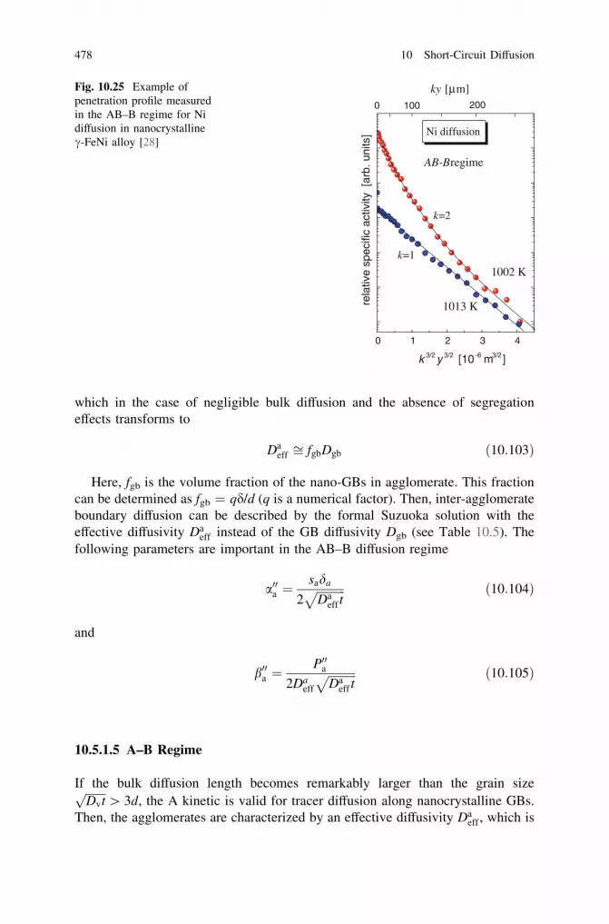
which in the case of negligible bulk diffusion and the absence of segregationeffects transforms to

Daeff ffi fgbDgb ð10:103Þ

Here, fgb is the volume fraction of the nano-GBs in agglomerate. This fractioncan be determined as fgb = qd/d (q is a numerical factor). Then, inter-agglomerateboundary diffusion can be described by the formal Suzuoka solution with theeffective diffusivity Da

eff instead of the GB diffusivity Dgb (see Table 10.5). Thefollowing parameters are important in the AB–B diffusion regime

a00a ¼sada

2ffiffiffiffiffiffiffiffiffiffiDa

eff tp ð10:104Þ

and

b00a ¼P00a

2Daeff

ffiffiffiffiffiffiffiffiffiffiDa

eff tp ð10:105Þ

10.5.1.5 A–B Regime

If the bulk diffusion length becomes remarkably larger than the grain sizeffiffiffiffiffiffiffiDvtp

[ 3d, the A kinetic is valid for tracer diffusion along nanocrystalline GBs.Then, the agglomerates are characterized by an effective diffusivity Da

eff , which is

0 1 2 3 4

k=1

k=2

1013 K

1002 K

AB-B regime

Ni diffusion

2000 100

ky [μm]

rela

tive

spec

ific

activ

ity [

arb.

uni

ts]

k 3/2y 3/2 [10-6 m3/2]

Fig. 10.25 Example ofpenetration profile measuredin the AB–B regime for Nidiffusion in nanocrystallinec-FeNi alloy [28]

478 10 Short-Circuit Diffusion

described by a modified Hart–Mottlock or Maxwell–Garnet equation in the case ofsolute diffusion, as shown in Eqs. 10.52 and 10.54.

Since typically Dv ffi Dgb and fgb ffi 1, only the nano-GB diffusion contribu-tion becomes important (see Table 10.5).

If the resulting diffusion length inside of the agglomeratesffiffiffiffiffiffiffiffiffiffiDa

eff tp

is smaller than

the agglomerate sizeffiffiffiffiffiffiffiffiffiffiDa

eff tp

\da=4, the fluxes from different inter-agglomerateboundaries do not overlap and diffusion occurs in the A–B kinetic regime in thebimodal interface microstructure under consideration. The penetration profilesgenerally should be composed of two parts. The first part corresponds to bulkdiffusion in a homogeneous material (inner part of agglomerates) characterized byan effective diffusion coefficient Da

eff . An example of such a penetration profile ispresented in Fig. 10.26 for the case of Fe diffusion in nano-c-FeNi [13]. The pen-etration profile turns out to be slightly curved at large depths, as seen in Fig. 10.26.However, the number of relevant experimental points is too small to be able toextract reliably the inter-agglomerate boundary diffusivity. The deviation from thelinearity in this profile could only be detected due to the extremely high sensitivity ofthe applied radionuclide-counting facilities, which allowed an accurate detection ofthe penetration profile over five decades in the decrease of concentration.

10.5.1.6 A Regime

With increasing temperature, the effective diffusivity of the agglomerates Daeff in

Eq. 10.94 becomes larger and the relevant diffusion length can be remarkablylarger than the agglomerate size

ffiffiffiffiffiffiffiffiffiffiDa

eff tp

[ 3da. Then, the A kinetic is valid fortracer diffusion in this material. The nanocrystalline alloy as a whole can be

0 2 4 6 8 10 12

A-B regime

Fe diffusion

300200100

1013 K

y [μm]

rela

tive

spec

ific

activ

ity [

arb.

uni

ts]

y 2 [10-8 m2]

Fig. 10.26 Example ofpenetration profile measuredin the A–B regime for Fediffusion in nanocrystallinec-FeNi alloy [13]

10.5 Microstructures with Hierarchy of Short-Circuit Diffusion Paths 479

considered as a homogeneous material with the effective diffusivity DMeff . The

penetration profile should follow the thin-layer solution of the diffusion equation,and the inclination of the fitting line in the coordinates of lnc versus y2 gives theeffective diffusivity DM

eff .An example of such a profile measured for Ag diffusion in nanocrystalline FeNi

alloy at T = 1,200 K [27] is shown in Fig. 10.27. The contribution of the inter-agglomerate boundary diffusivity Da to the effective diffusivity DM

eff was found tobe less than 10 %, and the relevant relation in Table 10.1 allows a consistentdetermination of the nano-GB diffusivity Dgb. The knowledge of the segregationfactor s is imperative for such calculations, and it was determined by an iterativeapproach (see below).

10.5.2 Temperature Dependence of Interface Diffusionin Material with a Hierarchic Microstructure

Diffusion of Fe, Ni, and Ag in a nanocrystalline c-FeNi alloy was intensivelymeasured in the extended temperature interval from about 500 to 1,200 K. Thepenetration profiles were analyzed according to the strict mathematical conditionsof the appearance of the given kinetic regime, and consistent data in the wholetemperature interval were derived. For the analysis of Fe and Ni diffusion, therelevant segregation factors sFe and sNi are close to unity. Fe and Ni show completemutual miscibility in the c-phase, and one may expect only slight (if any) seg-regation of both Fe and Ni to internal interfaces in the c-FeNi alloy. On the other

0 5 10

A regime

Ag diffusion

300200100

1200 K

y [μm]

rela

tive

spec

ific

activ

ity [

arb.

uni

ts]

y 2 [10-8 m2]

Fig. 10.27 Example ofpenetration profile measuredin the A regime for Agdiffusion in nanocrystallinec-FeNi alloy [27]

480 10 Short-Circuit Diffusion

hand, Ag reveals very small solubility in FeNi and a strong Ag segregation tointernal interfaces is expected.

Ag diffusion in the nanocrystalline c-FeNi was measured in various diffusionregimes, and the succession of the kinetics C–C, C–B, AB–B, and A was observed,and the diffusivities of both nano-GBs and inter-agglomerate boundaries weredetermined, as presented in Fig. 10.28.

The diffusivity Dgb of the nanocrystalline GBs was directly determined in theC–B kinetics. In order to establish the limits of relevant kinetic regimes and toanalyze the experimental data, the knowledge of the segregation factor s isimperative. As it was shown above, the segregation factor s can be determined by acombination of the C- and B-type GB diffusion measurements. Whereas the B–Bkinetics was observed for both Fe and Ni diffusion, it cannot be realized for Agdiffusion in the nanocrystalline FeNi alloy for formal reasons. In the case of self-diffusion, s = 1 and the conditions a ¼ d=2

ffiffiffiffiffiffiffiDvtp

\0:1 and 2ffiffiffiffiffiffiffiDvtp

\d=2 cansimultaneously be satisfied in the given temperature interval even for such a smallgrain size d as d = 100 nm. This is no longer the case for diffusion of such astrongly segregating solute as Ag. The above-mentioned inequalities can berewritten as

ffiffiffiffiffiffiffiffiffiffiffiffiffiffiffiffiffiffiffiffiDvt [ 5sdp

andffiffiffiffiffiffiffiDvtp

\d=4, respectively. Taking into account that

6 8 10 12 14 16 18 2010

-27

10-26

10-25

1x10-24

1x10-23

10-22

1x10-21

1x10-20

1x10-19

10-18

10-17

δDa/λ

Pa

P=sδDgb

δDgb

s

500

Ag diffusion

6008001200

Kinetics:

T [K]

C-C, C-B

AB-B A-B

P=s

δ Dgb

, δD

gb, P

a [m

3 /s]

T -1 [104 K -1]

Fig. 10.28 Arrhenius diagram for Ag diffusion in nanocrystalline c-FeNi alloy [27]. Filledsymbols represent the diffusivity of nanocrystalline GBs, and open symbols correspond to inter-agglomerate boundary diffusion. The conditions d = 0.5 nm and da = 1 nm were used torecalculate the measured Pa and P values for the relevant diffusivities Da and Dgb. The tripleproduct P for Ag diffusion in coarse-grained FeNi alloy is also shown (diamonds). The method ofcalculation of the segregation factor s for Ag in FeNi is illustrated

10.5 Microstructures with Hierarchy of Short-Circuit Diffusion Paths 481

d = 100 nm and d % 0.5 nm, it becomes evident that these relations cannotsimultaneously be satisfied if s [ 10. As the temperature increases, the C–Bkinetic regime ð

ffiffiffiffiffiffiffiDvtp

\sd=2Þ changes to the A–B kinetics withffiffiffiffiffiffiffiDvtp

[ 3d.This fundamental difficulty can be overcome by the B-type GB diffusion

measurements in coarse-grained material (with a remarkably larger value of thegrain size d). The key point is that the close similarity between Ni self-diffusion inthe coarse-grained and nanocrystalline c-FeNi alloy [28] suggests similar GBstructures in these materials. The measurements of Ag diffusion in the coarse-grained c-Fe–Ni alloy yielded the triple product P = sdDgb as a function oftemperature (diamonds in Fig. 10.28). The data on P for Ag diffusion (determinedfor the coarse-grained material) can thus be combined with the direct data on Dgb

(determined for the nanocrystalline material). As a result, the temperaturedependence of the segregation factor s can be derived (Fig. 10.28).

Ag segregates strongly at GBs in the c-FeNi alloy, for example, s = 1,000 atT = 700 K. Here, an iterative procedure was applied to calculate s. Havingdetermined several values of Dgb (supposing that the low-temperature measure-ments were performed in the C kinetics), a crude estimate of s can be determinedby combination of these Dgb values and the P values for coarse-grained material.This estimate of s allows a more precise calculation of the parameter a and thus abetter evaluation of the limits of the C–B regime. This in turn allows a morejustified calculation of Dgb until self-consistency is reached.

Having determined the segregation factor s, an Ag GB diffusion experiment inthe nanocrystalline material has been designed, which satisfies the conditions ofthe AB–B kinetics (the B–B kinetics cannot be fulfilled for formal reasons). Forthis purpose, the time and temperature of the diffusion anneal have to be chosenvery carefully using Table 10.5. The value determined for sDgb is multiplied bythe GB width d and is plotted in Fig. 10.28 (triangle up). Almost perfect agreementwith the independent data of P = sdDgb measured in coarse-grained material(diamonds) is obtained, as depicted in Fig. 10.28. This fact supports the conclusionthat the diffusivities of the nanocrystalline (d * 100 nm) and coarse-grained(d * 0.5 mm) materials are very similar.

Ag diffusion along the inter-agglomerate boundaries proceeds much faster thanalong the nano-GBs, as portrayed in Fig. 10.28 (open symbols). Having deter-mined Pa = sadaDa/k and Da separately in the C–B and C–C regimes, respectively,the factor sada/k can be estimated. Taking k as k = 2d/d with d = 0.5 nm andd = 100 nm, an upper estimate of the product sada is obtained, sada * 1 nm.Since the inter-agglomerate boundaries present a more open structure with respectto the nano-GBs, the value of da & 1 nm seems to be a good estimate. Thus, thesegregation factor sa for Ag seems to be about unity. This means that there ispractically no excess of Ag atoms in the inter-agglomerate boundaries with respectto the nanocrystalline GBs, as shown in Eq. 10.91, and the segregation behavior ofthese two internal interfaces with respect to the bulk is similar. In Fig. 10.28, thevalue of Da measured in the C–C regime is multiplied by the factor da/k (using theestimates da = 1 nm and k = 0.01) for comparison with the Pa values measured in

482 10 Short-Circuit Diffusion

the C–B regime (open star and circles, respectively). Assuming sa = 1, the tem-perature dependence of Pa can be presented by the linear Arrhenius relationship(dotted line in Fig. 10.28).

10.6 Dependence of GB Diffusion on GB Parameters

The grain boundary represents an interface between two crystals. Therefore, eachGB can be characterized by the following macroscopic and microscopic param-eters: matrix of rotation between the two crystalline coordinate systems, forinstance, the axis x! and angle h of rotation (3 parameters); the inclination of theGB plane with respect to a chosen direction n! (2 parameters); and the matrix of

atomic translation t!¼ ðtx; ty; tzÞ. The set of parameters ðx!; h; n!Þ can be chosenon demand during bicrystal preparation by setting the misorientations of thecrystals and properly choosing the required position of the interface. The param-

eters t! cannot be influenced, and thus, they are known as microscopic.In dependence on the given set of the parameters ðx!; h; n!Þ, it is possible for us

to distinguish the following:

• Low-angle grain boundary with h B 15�;• High-angle GBs with h[ 15�;• Special (low sigma) GBs with special values of ðx!; hÞ so that the value of the

inverse density of equivalent (coinciding) positions of the two lattices is small,for example, R5, R7, etc. The values of R1 and R3 correspond to the low-angleand twin boundaries, respectively;

• Pure tilt GBs with x!? n!, i.e., the misorientation axis lies in the GB plane;• Pure twist GBs with x! k n!, i.e., the misorientation axis is perpendicular to the

GB plane;• GB of a mixed type;• Symmetric and asymmetric GBs.

Generally, GB diffusion and segregation depends on all these parameters.The production and characterization of oriented bicrystals is an extremely

difficult task. The desired misorientation has to be uniform along the GB with ahigh accuracy showing only small fluctuations of the GB plane orientation. Evennowadays, the production of top-quality-oriented bicrystals looks more like artthan a technology. The state of the art in such measurements is represented by theworks of Herzig with co-workers [29]. They demonstrated that the precise spec-ification of all three misorientation angles to the accuracy of ±0.1� (including thenon-avoidable twist component) is required to rationalize the orientation depen-dence and to observe cusps in diffusivities at low-R misorientations.

In Fig. 10.29, GB diffusion of Au in Cu near R5 GBs [29] is presented as afunction of the misorientation angle h. The observed increase of the GB diffusivitywith approaching the perfect R5 misorientation from large tilt angles h[ 36.9� is

10.5 Microstructures with Hierarchy of Short-Circuit Diffusion Paths 483

caused by an increase in the accompanying twist component. This effect ‘‘masks’’partially the deep cusp in the GB diffusivity occurring at the perfect R5misorientation.

10.7 Effect of Purity on GB Diffusion

The purity and segregation of solutes can both strongly affect the GB diffusion. InFig. 10.30, Ni GB self-diffusion measured in coarse-grained polycrystalline Ni ofdifferent purity levels [30, 31] is compared. The GB diffusion has been measured

Fig. 10.29 GB diffusion of195Au in Cu R5(310)[001]bicrystals as a function of thetilt angle h measured at twotemperatures 661 K and780 K after [29]. Themisorientation anglecorresponding to the exactR5(310)[001] interface isshown by dotted line. Thedashed lines are drawn asguidance for eyes

Fig. 10.30 Ni GB self-diffusion measured in 99.6[30], 99.99 [31], and99.999 wt.% [30] purepolycrystalline Ni materials

484 10 Short-Circuit Diffusion

by the same technique and using the same equipment. As a general trend, it is seenthat the higher the purity of a material, the higher the grain boundary diffusivityP = d � Dgb and the lower the effective activation energy for grain boundarydiffusion. One has to mention that different ‘‘critical’’ impurities, which stronglysegregate at GBs and which could affect dramatically the grain boundary diffusion,might be present in different materials.

Figure 10.30 suggests a strongly non-monotonous dependence of Dgb on thepurity of Ni, D99:999

gb � D99:99gb � D99:6

gb , especially at low temperatures. The prob-

lem of the effect of impurities on GB diffusion has been analyzed in [31].

10.8 Grain Boundary Interdiffusion

So far, tracer diffusion along GBs was considered. However, as in the case of bulkdiffusion, one can consider the case of chemical grain boundary diffusion just likethe diffusion of A atoms along GBs of B or that of A atoms along GBs of AB, etc.,occurring in corresponding couples. The predominance of GB diffusion corre-sponds typically to low temperatures and is especially important for thin-film ormicroelectronic applications. Unfortunately, this subject is even not completelyunderstood from the theoretical point of view because of the inherent requirementsto consider coupled diffusion–elasticity or diffusion–plasticity problems, just for-getting a rather small number of dedicated and well-posed experimentalmeasurements.

Here, we will shortly consider several issues, including diffusion–strain cou-pling in GB interdiffusion, the manifestation of the Kirkendall effect, and mor-phology development under GB interdiffusion.

10.8.1 Coupling of Diffusion and Strain for GBInterdiffusion

Herring [32] has analyzed the chemical potential of atoms in a GB underassumption that the GB is a perfect sink or source of vacancies and has shown thatby neglecting the higher-order contributions of the stress tensor components, thechemical potential is modified by the value of Dl

Dl ¼ �rX ð10:106Þ

where r is the normal tensile traction at the GB and X is the atomic volume.Let us analyze a simplified GB interdiffusion problem considering a stressed

bicrystal. We will follow the formulation of Klinger and Rabkin [33, 34], as seenfrom Fig. 10.31.

10.7 Effect of Purity on GB Diffusion 485

The atomic fluxes of the components along the GB, JA, and JB can be repre-sented as the sums of two contributions associated with the gradient of concen-tration and the gradient of normal stress

JA ¼ �dDAgb

ocAgb

oyþ

dDAgbX

kTcA

gb

oroy

ð10:107aÞ

JB ¼ �dDBgb

ocBgb

oyþ

dDBgbX

kTcB

gb

oroy

ð10:107bÞ

Here, d is the GB width (assumed to be the same for both components),DA

gbðDBgbÞ is the diffusion coefficient of A (B) atoms along the GB, and cA

gbðcBgbÞ is

the GB concentration of A (B) atoms (in at/m3). The atomic volume X is alsosupposed to be the same for both components, and thus,

cAgb þ cB

gb ¼1X

ð10:108Þ

As a result of GB diffusion of A in B, the new material is plated as a wedge ofthe thickness w, as shown in Fig. 10.31. The conditions of mass conservation of Aand B atoms are written as (for the case where the wedge is growing, ow=ot [ 0)

docA

gb

ot¼ d

o

oyDA

gb

ocAgb

oy

!� dX

kT

o

oyDA

gbcAgb

oroy

� �� cA

gb

ow

otð10:109aÞ

Fig. 10.31 A sample of material B, considered as a bicrystals with a single GB perpendicular toits surface, with the layer of material A deposited on its surface. The GB fluxes of A and B atomsare indicated, and an imbalance of JA and JA leads to formation of a wedge of extra material atthe GB. The wedge thickness, 2w(x,y), is indicated

486 10 Short-Circuit Diffusion

docB

gb

ot¼ d

o

oyDB

gb

ocBgb

oy

!� dX

kT

o

oyDB

gbcBgb

oroy

� �� cB

gb

ow

otð10:109aÞ

In [33] the case of the same and constant GB diffusion coefficients was considered,DA

gb ¼ DBgb ¼ Dgb ¼ const, that Eq. 10.108 corresponds to a simplified equation

owðy; tÞot

¼ � dXDgb

kT

o2rðy; tÞoy2

ð10:110Þ

The plated out material can be represented as a mass of edge dislocations withthe Burgers vector density of ow=oy [33]. Then, the diffusion of A and thickeningof the wedge correspond to the climb of these dislocations toward B. The normalstresses can be written as [35]

rðy; tÞ ¼ r0 � EZ1

0

Kðy; zÞ owðz; tÞoz

dz ð10:111Þ

Here, E* = E/4p(1 - m2) is the equivalent elastic modulus and

Kðy; zÞ ¼ 1y� z

þ 1yþ z

� 6y

yþ zð Þ2þ 4y2

yþ zð Þ3

The solution of the system of Eqs. 10.109 and 10.111 (or a simplified solutionof Eqs. 10.110 and 10.111) represents the evolution of GB concentration andnormal stresses in the case of GB interdiffusion.

10.8.2 Kirkendall Effect in GB Interdiffusion

GB interdiffusion of A in B was extensively analyzed by Rabkin and Klinger [34],and we will follow their analysis. The diffusion problem is sketched in Fig. 10.31.The inequality of GB diffusion fluxes leads to plating out of additional material atthe GB in the form of a wedge, as seen from Fig. 10.29. In this case, the GBconcentration profiles are influenced by the normal GB stresses developing in thecourse of GB interdiffusion. It is important that the effective GB diffusion coef-ficients are weak functions of the relative difference of intrinsic GB diffusivities.

Klinger and Rabkin have shown that if DA [ DB, i.e., if the solute diffusesfaster than the matrix atoms, compressive GB stresses are developed in the near-surface zone, while at larger depths, the stresses are tensile. In the opposite caseDA \ DB, which is most probable in view of the experimental data, for instance,

10.8 Grain Boundary Interdiffusion 487

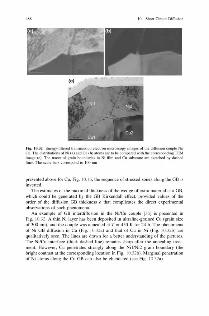
presented above for Cu, Fig. 10.16, the sequence of stressed zones along the GB isinverted.

The estimates of the maximal thickness of the wedge of extra material at a GB,which could be generated by the GB Kirkendall effect, provided values of theorder of the diffusion GB thickness d that complicates the direct experimentalobservations of such phenomena.

An example of GB interdiffusion in the Ni/Cu couple [36] is presented inFig. 10.32. A thin Ni layer has been deposited in ultrafine-grained Cu (grain sizeof 300 nm), and the couple was annealed at T = 450 K for 24 h. The phenomenaof Ni GB diffusion in Cu (Fig. 10.32a) and that of Cu in Ni (Fig. 10.32b) arequalitatively seen. The lines are drawn for a better understanding of the pictures.The Ni/Cu interface (thick dashed line) remains sharp after the annealing treat-ment. However, Cu penetrates strongly along the Ni1/Ni2 grain boundary (thebright contrast at the corresponding location in Fig. 10.32b). Marginal penetrationof Ni atoms along the Cu GB can also be elucidated (see Fig. 10.32a).

Fig. 10.32 Energy-filtered transmission electron microscopy images of the diffusion couple Ni/Cu. The distributions of Ni (a) and Cu (b) atoms are to be compared with the corresponding TEMimage (c). The tracer of grain boundaries in Ni film and Cu substrate are sketched by dashedlines. The scale bars correspond to 100 nm

488 10 Short-Circuit Diffusion

10.8.3 Morphology of Growing Phases Affectedby GB Diffusion

The GB interdiffusion can strongly affect the morphology of growing phases in aninterdiffusion couple. The present analysis follows generally the analysis of vanLoo [37]. Typical structures having been observed in different experiments areshown in Fig. 10.33.

The presence of grain boundaries in the end members can change the mor-phology of the reaction layer at low temperatures due to dominant GB diffusion,presented in Fig. 10.33a, b. Such cases correspond qualitatively to the model ofKlinger and Rabkin considered above and given in Fig. 10.31. Experimentally, theappearance of the GB wedges was observed by Bastin [38] during the formation ofb-Ti via GB diffusion of Ni into a-Ti. Tracers of iron in a-Ti were shown to playthe key role in the corresponding experiments since addition of Fe stabilizes the b-Ti phase. Similar experiments on iron-free a-Ti stopped this kind of GB inter-diffusion [38]. Bastin argued that the formation of a particular type of morphology,i.e., (a) or (b) in Fig. 10.33, has to depend on the position of the relevant interfacewith respect to the Matano plane.

If the rate of GB interdiffusion dominates over that through the crystalline bulk,morphology as in Fig. 10.33c may be formed. Such a kind of reaction layer growthhas been observed for Ni3A1 grown in the Ni/NiA1 diffusion couples [39].

At even lower temperatures, when bulk diffusion can be considered as frozen,thin needle-like crystals can often be formed, as shown in Fig. 10.33d. This casecorresponds, for example, to the Cu3Si formation in the Cu–Si couples [40].Simultaneously, straight interphase boundaries are found. One may argue thatinterphase boundary diffusion is responsible for the flattering of the interface andGB interdiffusion for plating out material around grain boundaries.

Fig. 10.33 Possible morphologies appearing in interdiffusion couples in the presence of GBdiffusion: a formation of GB wedges toward reaction layer, b GB wedges toward end memberswith formation of solid solutions, c predominant growth of GB wedges due to enhanced GBdiffusion, and d needle-like morphology of reaction layer due to the dominance of GB diffusion

10.8 Grain Boundary Interdiffusion 489

References

1. J. C. Fisher, Journal of Applied Physics 22 (1951) 74.2. B. S. Bokstein, I. A. Magidson, and I. L. Svetlov, The Physics of Metals and Metallography 6

(1958) 1040.3. J. B. Gibbs, Physica Status Solidi 16 (1966) K27.4. I. Kaur, Y. Mishin and W. Gust, Fundamentals of Grain and Interphase Boundary Diffusion

(Chichester, John Wiley 1995).5. R. T. P. Whipple, Philosophical Magazine 45 (1954) 1225.6. T. J. Suzuoka, Journal of the Physical Society of Japan 19 (1964) 839.7. A. D. Le Claire, British Journal of Applied Physics 14 (1963) 351.8. H. S. Levine and McCallum, Journal of Appllied Physics 31 (1960) 595.9. H. Gleiter, Microstructure, in: Physical Metallurgy, R.W. Cahn, P. Haasen (Eds.), North-

Holland Physics Publishing, 1983, 649.10. R. W. Balluffi, Grain-Boundary Diffusion Mechanisms in Metals, in: Diffusion in Crystalline

Solids, G.E. Murch, A.S. Nowick (Eds.), Academic Press, Inc. (1984) 320.11. D. Wolf and S. Yip, Materials Interfaces – Atomic-level Structure and Properties, Chapman

and Hall (1992).12. A. P. Sutton and R.W. Balluffi, Interfaces in Crystalline Materials, Clarendon Press, Oxford

(1995).13. S.V. Divinski, F. Hisker, Y.-S. Kang, J.-S. Lee and Chr. Herzig, Zeitschrift für Metallkunde

93 (2002) 256.14. L. G. Harrison, Transactions of the Faraday Society 57 (1961) 597.15. S.V. Divinski, H. Edelhoff and S. Prokofjev, Physical Review B 85 (2012) 144104.16. E.W. Hart, Acta Materialia 5 (1957) 597.17. J. C. Maxwell, A treatise on elasticity and magnetism, 3rd Ed. Clarendon press, 1892 page

435.18. J. C. Maxwell-Garnett, Philosophical Transactions of the Royal Society A: Mathematical,

Physical and Engineering Sciences 203 (1904) 385.19. S.V. Divinski, M. Lohmann and Chr. Herzig, Acta Materialia 49 (2001) 249.20. E. D. Hondros and M. P. Seah, Metallurgical Transactions A 8 (1977) 1363.21. D. McLean, Grain Boundaries in Metals, Clarendon Press, Oxford (1957).22. S.V. Divinski, F. Hisker, Y.-S. Kang, J.-S. Lee and Chr. Herzig, Zeitschrift für Metallkunde

93 (2002) 265.23. B. Bokstein, V. Ivanov, O. Oreshina, A. Peteline and S. Peteline, Materials Science and

Engineering A, 302 (2001) 151.24. M. Reda Chellali, Z. Balogh and G. Schmitz, Ultramicroscopy 132 (2013) 164.25. L. Klinger and E. Rabkin, Acta Materialia 47 (1999) 725.26. S.V. Divinski, J. Geise, E. Rabkin and Chr. Herzig, Zeitschrift für Metallkunde 95 (2004) 1.27. S.V. Divinski, Y.S. Kang, J.S. Lee and Chr. Herzig, Acta Materialia 52 (2004) 631.28. S.V. Divinski, Y.S. Kang, J.S. Lee, F. Hisker and Chr. Herzig, Interface Science, 11 (2003)

67.29. E. Budke, T. Surholt, S. Prokofjev, L. Shvindlerman and Chr. Herzig, Acta Materialia 47

(1999) 385.30. S.V. Divinski, G. Reglitz and G. Wilde, Acta Materialia 58 (2010) 386.31. D. Prokoshkina, V. Esin, G. Wilde and S.V. Divinski, Acta Materialia 61 (2013) 5188.32. C.J. Herring, Journal of Applied Physics 21 (1950) 437.33. L. Klinger and E. Rabkin, Acta Materialia 55 (2007) 4689.34. L. Klinger and E. Rabkin, Acta Materialia 59 (2011) 1389.35. H. Gao, L. Zhang, W.D. Nix, C.V. Thompson and E. Arzt, Acta Materialia 47 (1999) 2865.36. J. Ribbe, G. Schmitz and S. V. Divinski, unpublished work (2007).37. F. J. J. van Loo, Progress in Solid State Chemistry 21 (1990) 47.38. G.F. Bastin and G.D. Rieck, Metallurgical Transactions 5 (1974) 1817.

490 10 Short-Circuit Diffusion

39. M. M. P. Janssen and G. D. Rieck, Transactions of the Metallurgical Society of the AmericanInstitute of Mining, Metallurgical and Petroleum Engineers 239 (1967) 1372.

40. J. G. M. Becht, F. J. J. van Loo and G. Metselaar, Reactivity of Solids 6 (1988) 45.41. S. J. Rothman, N. L. Peterson, and J. T. Robinson, Physica Status Solidi 3b (1970) 635.42. J. Sommer and Chr. Herzig, Journal of Applied Physics 72 (1992) 2758.43. Ya. E. Geguzin and G. N. Kovalev, Fizika Tverdogo Tela 5 (1963) 1687.44. S.V. Divinski, J. Ribbe, G. Schmitz and Chr. Herzig, Acta Materialia 55 (2007) 3337.45. M. Lohmann, S.V. Divinski and Chr. Herzig, Z Metallkd 94 (2003) 249.46. S.V. Divinski, M. Lohmann and Chr. Herzig, Acta Materialia 53 (2004) 1249.47. T. Surholt and Chr. Herzig, Acta Materialia 45 (1997) p. 3817.48. A. Atkinson and R.I. Taylor, Philosophical Magazine A 43 (1981) 979.49. P. Gas, D. L. Beke and J. Bernardini, Philosophical Magazine Letters 65 (1992) 133.50. S.V. Divinski, F. Hisker, Y.-S. Kang, J.-S. Lee and Chr. Herzig, Interface Science 11 (2003) 67.51. A. Inoue, H. Nitta and Y. Iijima. Acta Materialia 55 (2007) 5910.52. J. Fiebig, H. Rösner, Y. Estrin and G. Wilde, Journal of Applied Physics 110 (2011) 083514.

References 491

Chapter 11Reactive Phase Formation in Thin Films

In this chapter, we will discuss some aspects related to reactive phase formation inthin films. We try to utilize as much as possible the information accumulatedduring the earlier chapters and built on that. We will first have a brief look onnucleation issues, especially in solid state, before moving into effect of micro-structure and impurities on the reactive phase formation. Finally, we will introducesome of the models for phase growth that have been introduced in the past andthen discuss in detail about their pros and cons.

The formation of crystalline phases starts by nucleation (which is actuallypreceded by interdiffusion to create a driving force for the process). The nucleationstage and factors influencing it are discussed in Sect. 11.1. If the stable crystallinephases cannot form directly, metastable structures will form first, as discussedpreviously in Chap. 1. The formation of amorphous metastable structures is dis-cussed in Sect. 11.2. The kinetics of phase formation is influenced by numerousfactors such as impurities, interfaces, and stresses—all these are briefly discussedin Sects. 11.3, 11.4 and 11.5. Finally, growth models developed to describereactive phase formation in thin films are critically evaluated in Sect. 11.6.

11.1 Role of Nucleation

When a new phase AB is formed at an interface between two elements A and B,the driving force for the reaction is the Gibbs energy of formation of AB from pureA and B. However, the formation of AB involves creation of two new interfaces A/AB and AB/B instead of the old A/B interface. This in general leads into increasein surface energy Dr of the system (Fig. 11.1). The classical theory of nucleationmandates that the competition between the gain in free energy DG and the energyloss Dr should give rise to nucleation mechanisms with an activation energy DG*

proportional to Dr3/DG2 (Fig. 11.2). There has been much criticism of the clas-sical theory of nucleation. Nevertheless, it illustrates quite simply the major factorsinvolved in the nucleation process.

A. Paul et al., Thermodynamics, Diffusion and the Kirkendall Effect in Solids,DOI: 10.1007/978-3-319-07461-0_11, � Springer International Publishing Switzerland 2014

493

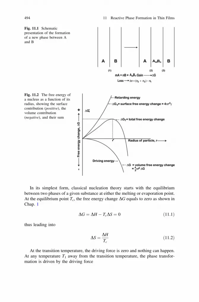
In its simplest form, classical nucleation theory starts with the equilibriumbetween two phases of a given substance at either the melting or evaporation point.At the equilibrium point Tc, the free energy change DG equals to zero as shown inChap. 1

DG ¼ DH � TcDS ¼ 0 ð11:1Þ

thus leading into

DS ¼ DH

Tcð11:2Þ

At the transition temperature, the driving force is zero and nothing can happen.At any temperature T1 away from the transition temperature, the phase transfor-mation is driven by the driving force

Fig. 11.1 Schematicpresentation of the formationof a new phase between Aand B

Fig. 11.2 The free energy ofa nucleus as a function of itsradius, showing the surfacecontribution (positive), thevolume contribution(negative), and their sum

494 11 Reactive Phase Formation in Thin Films

DG ¼ DH 1� T1

Tc

� �ð11:3Þ

as long as T1 is not too far from Tc. This transformation is opposed by the surfaceenergy contribution.

The total free energy of a nucleus with average radius r and free energy DG1

(calculated per unit volume) is expressed generally as

DG ¼ br2r� ar3DG1 ð11:4Þ

where a and b are geometrical terms taking into account the fact that if the nucleusis crystalline, it will generally not be spherical, because of the anisotropic char-acteristics of crystalline elements, but tries to adopt some definite shape withminimum surface energy. This can be determined with Wulff construction ifsufficient data on surface energies of various crystal planes are available. Therelation between the free energy of a nucleus and its radius is shown in Fig. 11.2.As seen, DG passes through a maxim that corresponds to the critical size r* of thenucleus. The population of nuclei smaller than r* will exist in some form of quasi-equilibrium distribution (e.g., they constantly appear and disappear maintainingsome kind of ‘‘equilibrium’’ distribution), whereas nuclei larger than r* will tend togrow. The value of the critical nucleus can be obtained by derivation of (11.4)

r� ¼ 2br3a

DG1 ð11:5Þ

Furthermore, the free energy of the critical nuclei becomes (at any temperature T)[see, Eqs. 11.3–11.5]

DG� ¼ 4b3r3T2c =27a2DH2ðT � TcÞ2 ð11:6Þ

At that temperature, the rate of nucleation q* will be proportional to the concen-tration of critical nuclei and to the rate at which such nuclei can form, generally somediffusion term of the type exp(-Q/kT), so that (with a proportionality factor K)

q� ¼ K expð�DG�=kTÞ expð�Q=kTÞ ð11:7Þ

Proportionality factor can be explained briefly as follows. Under the dynamicconditions that prevail during nucleation, one expects the number of nuclei ofcritical size to be less than predicted by thermodynamic equilibrium. This is due tothe fact that during nucleation the equilibrium population of critical nuclei isconstantly being depleted by the nuclei that grow. The proportionality factor isusually estimated to be about two. It contains also the so-called the Zeldovichfactor that is a measure of the probability that fluctuations will cause nuclei, even asize above the critical limit, to dissolve as long as their free energy remains within

11.1 Role of Nucleation 495

kT of DG. Thus, every microcluster passing the critical size will not grow. Thismeans also that there is a flat region with a width of d in the free energy versusradius plot. The Zeldovich factor is the reciprocal of this width. It may assumevalues of the order of 10-2.

In general in the formation of phases from the end elements, DG’s are large andthus activation energy (DG*) is small and the nucleation is quite easy. However,after the first phase in the formation of subsequent phases, nucleation may play adecisive role. It should be noted that DG* is actually formed from two parts DG*1

and DG*2, DG* = DG*1 + DG*2, where DG*1 is related to the density of thecrystalline nucleus and DG*2 to their growth, e.g., diffusion kinetics.

When a nucleus of a new phase is formed, this generally causes a volumechange to take place. In solid–solid nucleation, this is accompanied by deforma-tion energy DHd (elastic energy, plus the possible plastic energy). The activationenergy for nucleation becomes proportional to Dr3/(DGc-DHd)2, where DGc isthe ‘‘chemical’’ free energy of bulk phases and the energy associated withdeformation is subtracted from that value. One can derive this by first including theterm for strain energy into Eq. 11.4. It is also a bit more convenient to consider thefree energy per atom of the nucleus rather than the free energy per volume of thenucleus as in Eq. 11.4. The free energy associated with the formation of a nucleusof n atoms, Dg, may be written as

Dg ¼ nDgC þ gn23cþ nhd ð11:8Þ

wheren number of atoms in nucleusDgC bulk (chemical) free energy change per atom in nucleusg shape factor such that gn2/3 = surface areac surface tension & surface free energy (exactly for liquids, but only

approximately with solids, because in solids there is also another factor (thesurface stress) which contributes to surface energy)

hd strain energy per atom in nucleus

One may regroup this equation as

Dg ¼ nðDgC þ hdÞ þ gn23c ð11:9Þ

The term DgC will be negative below the transformation temperature, whereas hd

and c are both positive. Hence, if jDgCj[ hd, then the first term is negative. Thefree energy required (Dg*) to form the critical size nucleus (n*) is found bydifferentiating Eq. 11.9 and assuming DgC, hd, g, and c as constants.

Dg� ¼ 427

g3c3

DgC þ hdð Þ2ð11:10Þ

496 11 Reactive Phase Formation in Thin Films

A large strain energy hd reduces the denominator and makes Dg* large. Thismeans that nucleation is more difficult since the critical size nucleus has a higherenergy of formation. This strain energy must be compensated by the lattice and canbe done, for example, in silicides, mainly by the diffusive motion of atoms or inmetals by dislocation motion. Large strains may change the energetic status of thesystem and lead to formation of metastable structures (e.g., amorphous phases) aswill be discussed later on. It is to be noted that the strain energy is essentiallyirrelevant to incoherent nucleation. In the case of strained incoherent microcluster,diffusion of thermal vacancies to or from the disordered interface may completelyeliminate the strain energy of the system [1]. It is the cases of coherent andsemicoherent precipitates where the strain energy becomes relevant. It may beargued that all nuclei are coherent at the very first stages of nucleation. However,at the same time, it should be realized that these phenomena may be inaccessible toexperimental methods in many occasions.

The most important parameters determining the phase selection during nucle-ation are the activation energy of nucleation, Dg*, the interface energies r and, thechemical driving force DgC, and the elastic strain energy Dhd—although this lastparameter is not relevant to incoherent precipitate cases. In order to evaluate apossible phase selection, reasonable estimates of these parameters must beobtained.

11.1.1 Activation Energy Dg*

This term can be approximated by the activation energy of diffusion, since theformation of a critical nucleus is mainly determined by diffusional jumps. If this isnot available, it can be also approximated with the activation energy of growth ofthe formed phase in the planar growth regime. From investigations on the laterstage of growth, it has been concluded that the precipitates formed in the A/Binterface first grow to coalescence within the A/B interface [2]. These resultsindicate that growth of the nucleus is preferred in the direction of the interfaceemphasizing the importance of atomic mobility of the A/B interface. Therefore, itis reasonable to assume that the activation energy of volume diffusion is only anupper estimate for the activation energy of growth.

11.1.2 Interfacial Free Energy r

The interface free energies of crystalline phases consist of two contributions: thechemical contribution related to (chemical) atomic interaction energy, and thestructural contribution that originates from the free energy of structural defectsassociated with semicoherent and incoherent interfaces [3]. The interface freeenergy terms are hardly known, and even if they are known they are usually bulk

11.1 Role of Nucleation 497

values, and therefore, their use in early stages of phase formation is highlyquestionable. The interfacial free energies in the solid state are likely to varybetween values approaching zero for epitaxial interfaces to maximum values of theorder of few J/cm2 for random interfaces [4]. It should be emphasized that surfacefree energies of crystalline solids are very much dependent on the history of thespecimen, crystal orientation, defect density, impurities etc., and they may dependon the size of the microcluster. Hence, the values of surface free energies for solidsare not material constants, but are specific for the sample in question.

11.1.3 (Elastic) Strain Energy Dhd

Elastic strain energy affects the nucleation, particularly in the case of coherent orsemicoherent precipitates, as can be seen from the Eq. 11.10. Here, one willconsider only elastic energy, yet the deformations involved can reach proportionsbeyond the usual elastic limits of the materials. A complete analysis of theseeffects should take into account the energy stored in plastic deformation as well.The elastic energy resulting from the formation of a third phase will depend on theelastic characteristics of all three phases. In the simplified case where all threephases have the same elastic constants, the energy is given by the followingrelation [1, 5]

Dgel ¼ 2s 1þ mð Þ=9 1� mð Þ½ �e2 ð11:11Þ

where s, the shear modulus of elasticity, is also called the modulus of rigidity, m isthe Poisson ratio, and e, the strain, is the ratio between the excess volume (underzero stress) and the volume of the hole (here the volume of the reactants) [4].Ignoring the problems of anisotropy, the following relations from the theory ofelasticity can be utilized. Young’s modulus E is equal to s times 2(1 + m); sometables also give the compression or bulk modulus, which is equal to E, divided by3(1-2m). The problems of interest here do not concern isotropic materials butthree different materials at once. As a zeroth approximation, one may consider thatthe strain energy is given by an average of the different elastic constants.

11.1.4 The Chemical Driving Force

In order to calculate the chemical driving force for the nucleation of a new phase atthe A/B interface, the free energy curves of the solid solution phases and of theformed compounds must be known. These can be determined by applying theCALPHAD method [6–10]. If there exists no information about lattice stabilitiesand so on in the system, these quantities can be evaluated by ab initio methods. Insystems with large negative heat of compound formation, the driving force for the

498 11 Reactive Phase Formation in Thin Films

nucleation of a new phase from the pure elements (with no or negligible terminalsolid solubility) is large and approaches to the free energy of compound formationin the reaction temperature. However, in all systems, interdiffusion must occur firstto create the necessary driving force for nucleation. Thus, as this may in somecases substantially decrease the initially available driving force for compoundformation, this issue must be taken into account [11].

In Thompsons [11] treatment, it is shown that interdiffusion must precedenucleation of new phases and that only after some interdiffusion has occurred therecan be a driving force for nucleation (see also Sect. 1.15 for more details). Thisrequirement imposes a kinetic constraint to the first-phase formation. Thus, rela-tive mobilities of diffusing components in competing phases will determine whichphase will form first.

In Fig. 11.3, the Gibbs energy curves of the AB system at a given temperatureare shown, where A and B have different crystal structures a and b, respectively,and they can form a stable intermediate phase g and a metastable phase M. Byassuming that A diffuses into b much faster than B into a, we simplify the case sothat only diffusion of A into b needs to be considered. According to the thermo-dynamic principle of phase equilibrium (see Sect. 1.15), as diffusion proceeds, thefirst phase to nucleate should be g in b when a sufficient volume of b has reachedits equilibrium composition Xeq with g (see the tangent line between b and g inFig. 11.3). Here, it should be remembered from the earlier discussion (Sect. 1.15)that even though g becomes stable at this point, it will not form, since there is nosupersaturation, which would provide the necessary driving force for nucleation. Ifg cannot nucleate, it will become possible for the metastable phase M to nucleatein b when a sufficient volume of b has reached its equilibrium composition Xm

with M, provided that the interdiffusion continues. Similar arguments about therequired supersaturation as presented above naturally also apply here. Theappearance of the metastable phase M would therefore indicate that the timerequired for nucleation of g is longer than the time required for interdiffusion tothe point at which M can nucleate. If neither g nor M can nucleate when thecomposition of b passes through Xeq and Xm sequentially, b will polymorphicallytransform into M when its composition reaches X0. This analysis leads to a con-clusion that the phase selection depends on the interdiffusion rate in the parentphases as well as the nucleation rates of the product phases.

While the relative rates of nucleation are (ultimately) controlling the phaseselection, which phase can nucleate (and grow) is controlled by interdiffusion.Hence, the first-phase formation depends exclusively on the kinetics. It is to benoted, however, that thermodynamics of the system influences the magnitude of thediffusion coefficients via the interaction parameters (see Chap. 1). The nucleationrates are controlled not only by the barriers to nucleation, and hence, the volumeGibbs energy DGv and the energies of the interfaces r involved, but also by thediffusion required to form critically sized clusters of the product phases. Thompson[11] further suggested that if one component diffused rapidly into the other andself-diffusion of the host was slow, polymorphic phase transitions were favored, sothat phases with broad compositional ranges of stability and phases that were rich in

11.1 Role of Nucleation 499

the slowly moving component were preferred, and such phases with low energyinterfaces with the host phase(s) would be especially favored. This points towardamorphous phase formation as will be discussed below.

It should also be emphasized that the free energies of compound formationcalculated by the CALPHAD method typically refer to bulk materials. In a smallnucleus, the chemical long-range order may not be fully developed due to theinterfacial constraints, thus increasing its free energy with respect to the bulkvalue. In addition, despite the surface energy terms are important in small scalesencountered during nucleation, they are typically disregarded in traditionalCALPHAD calculations. Further, strain energy may also be important if inco-herent interface has not yet been created between the forming nuclei and thematrix. Therefore, the free energy of an ordered chemical compound (as derivedfrom the CALPHAD method) should be viewed as the lower limit for the freeenergy of the compound nucleus. Thus, the driving force for the formation of acertain compound may be considerably smaller than calculated by using bulkvalues.

11.1.5 Nucleation Issues in Solid-State Amorphization

The term solid-state amorphization (SSA) is used to describe manufacture ofamorphous alloys by solid-state reaction of the crystalline elements. There are twoimportant nucleation-related problems in solid-state amorphization. One is tounderstand how an amorphous phase forms at an interface between two crystallineelements, the other is to explain how nucleation and growth of a crystalline ele-ment is suppressed until an amorphous layer has attained a temperature- andsystem-dependent critical thickness. The first problem is dealt below and thesecond in subsequent sections.

Fig. 11.3 Schematicillustration of the free energyversus composition of asystem AB, where elementsA and B have differentequilibrium crystal structuresa and b, respectively, andthey can form a crystallineintermetallic phase g and ametastable intermetallicphase M [11]

500 11 Reactive Phase Formation in Thin Films

The most studied amorphizating system is probably Ni–Zr [12, 13]. It is pos-sible to form amorphous layer between Ni and Zr by annealing in the solid state.Once formed, the layer continues to grow until it has reached a temperature-dependent critical thickness. At this critical thickness the amorphization is ter-minated by nucleation of the crystalline Ni–Zr compound at the interface betweenthe amorphous alloy and crystalline Zr. Recent experimental investigations haverevealed that there is a barrier to nucleation of alloy phases at a Ni/Zr interface andthat some Zr grain boundaries are sufficiently potent heterogeneous sites that theyreduce this obstacle and allow reaction at a temperature sufficiently low foramorphization to be possible [14–16]. However, calculation based on classicalnucleation theory suggests that no such barrier exists [17, 18]. The experimentalevidence suggests that either the estimates of the volume and surface terms in thework of Johnson [17] and of Clemens [18] are incorrect or that some additionaleffects, not included in the classical nucleation analysis, are at work.

As has been discussed above, classical nucleation theory assumes that there isno obstacle for creating small clusters of a new phase within an existing phase.Some of these then acquire critical size and start to grow. Kelton and Greer [19]made a quantitative test based on numerical modeling of the cluster evolution formultistep annealing treatments in lithium disilicate glass. They found the classicaltheory of nucleation to be valid provided that the critical size was greater than 16or 20 molecular formula units. The classical approach might not deal adequatelywith a situation in which the predicted critical size is of molecular dimensions orsmaller for two reasons. First, the key parameters in classical theory are thevolume free energy and the interfacial free energy as seen above. They may bothbe functions of cluster size as was discussed earlier. A second, more fundamentalproblem is that it may be wrong to base nucleation calculations upon clusters ofthe critical size while neglecting the obstacle to reaction which is presented bycreating initial very small clusters of a new phase. This is related to the abovetreatment of Thompson showing that significant interdiffusion is required beforethe formation of clusters is possible in systems exhibiting extensive solidsolubility.

If classical theory of nucleation is inadequate in circumstances where thepredicted critical radius is small, other means of analyzing the initial reaction at,for example, Ni/Zr interface. In particular, one might examine processes, whichprecedes the formation of clusters of an alloy phase and which could provide abarrier to nucleation, which is larger than the one predicted by classical theory.One could examine first an unmixed interface and then calculate the likelihood ofpair’s exchanges. As an effect of such exchanges, two solid solutions would form,one of Ni in Zr and one of Zr in Ni. These solid solutions could act as precursors tothe glassy phase. The thermodynamic quantities associated with exchange processare assumed to be the molar strain free energy gs, the molar enthalpy of mixing hm

and the molar configurational entropy sc [20]. If an interface contains N pairs ofatoms, of which a fraction of n have exchanged, the configurational entropy is (asshown in Chap. 1)

11.1 Role of Nucleation 501

sc ¼ �Nk n lnðnÞ þ ð1� nÞ lnð1� nÞ½ � ð11:12Þ

assuming that the use of Stirling’s approximation is justified. Minimizing the freeenergy of the interface with respect to n gives

n ¼ 1þ exphþ gs

kT

� �ffi �ð11:13Þ

This expression predicts a barrier to reaction if (h + gs) is positive.It is necessary to estimate the magnitudes of hm and gs as was done previously

in the case of classical approach. Christian [21] suggests that the strain energy thatresults from dissolving an atom of element B in matrix of element A is

gs ¼2sAKBðvA � vBÞ2

vBð3KB þ 4sAÞð11:14Þ

Here, sA and vA are the shear modulus and atomic volume of element A, respec-tively, while KB and vB are the bulk modulus and atomic volume of element B.Substitution of atomic volumes from Barret and Massalski [22] and elastic modulefrom Brandes [23] into Eq. 11.14 gives a free energy increase of 1.6 9 10-19 J/atom on dissolving Zr in Ni, and 2.6 9 10-19 on dissolving Ni in Zr. Thus, gs is128 kJ/g atom. It must be emphasized that the Eq. 11.14 is only approximate andfurthermore, the Ni and Zr lattices will not strain independently of each other, andNi is likely to dissolve in Zr also interstitially. The large value predicted byEq. 11.14 is intrinsic to systems with propensities to form glasses by solid-stateamorphization (SSA). It has been noticed that disparity between the atomic sizesof species is required in order that an amorphous phase can grow and in order tosuppress the nucleation of a crystalline phase(s) as Eq. 11.14 suggests.

An attempt to estimate the enthalpy change h on exchanging a pair of atoms ismore complicated because atoms at the unmixed interface already have nearestneighbors, which are not similar. For this reason, only part of the full enthalpy ofmixing is available to contribute to h. It is noticeable that even the full enthalpy ofmixing -43 kJ/g atom at the equiatomic composition [24] is much less than theevaluated gs. From these values, it seems that (h + gs) may be positive and theremight be a barrier to exchange atoms at the Ni/Zr interface.

Christian [21] suggests that while single dislocations cannot readily reducestresses developed in small volumes, larger defects, such as grain boundaries, maybe able to. This could explain why grain boundaries at Ni/Zr interfaces are able toact as heterogeneous sites. It does not, however, indicate why Zr, rather than Nigrain boundaries are needed. One reason might be that the free energies associatedwith certain Zr grain boundaries are greater than the free energies of Ni grainboundaries. A second possibility is that the strain energy associated with dissolvingNi atom in Zr is greater than that caused by dissolving Zr atom in Ni. A thirdpossibility is that the diffusional asymmetry in Ni–Zr makes the slow-diffusing Zrthe ‘‘matrix’’ element for SSA, and the reaction must begin in the Zr lattice.

502 11 Reactive Phase Formation in Thin Films

It will be thermodynamically favorable for the precursor solid solutions totransform into an amorphous phase, since the interfacial energy increase associ-ated with the formation of two amorphous/polycrystalline interfaces is probablyless than the free energy penalty attributable to strains in the solid solutions. Itshould be remembered that the incoherent interface can act as a source or sink forthermal vacancies, thus enabling the relief of strains in the system. It is alsopossible that the stresses developed in the system may change the energetic sit-uation in such a way that amorphous phase becomes more stable than the crys-talline ones. The amorphous phase can dissolve solute atoms more easily and isalso expected to be able to relax stresses more effectively than crystalline phase.The effect of stresses can be integrated into the Gibbs energy equation of a phasein question. The stress term may lift the Gibbs energy curve of the crystallinephase/phases to such high level that amorphous phase becomes the stable one (seeSect. 1.15).

11.2 Metastable Structures and Nucleationon Concentration Gradient

The types of metastability in alloys have been classified by Turnbull [25] ascompositional, structural, and morphological. The degree of metastability ischaracterized by the free energy excess of the system over that of the equilibriumstate. Turnbull [25] expressed this energy per mole as a fraction of R�Tm, where R isthe gas constant and �Tm is the average of the elemental melting points. Compo-sitional metastability is where an equilibrium phase exists outside its normalcomposition range, and it is associated with large excess energies of up to about1:0 R�Tm. Structural metastability is where a phase has a non-equilibrium structure,typically with excess energies of about 0:5 R�Tm. Morphological metastability hasthe lowest excess energy, about 0:1 R�Tm, but is perhaps the most widespread, andgenerally useful, type of metastability. Its excess energy arises from the abnor-mally large area of grain boundaries and interphase interfaces.

A system in true metastable equilibrium would not have access to any state oflower free energy by means of a continuous structural change [26]. A goodexample of such is a fully relaxed amorphous phase, in which any transformationto a lower free energy microstructure can commence only with a discrete nucle-ation stage which has an energy barrier as discussed. On the other hand, mostmorphologically metastable microstructures are not in metastable equilibrium butcan evolve continuously on annealing. In this case, the energy barrier is notnucleation, but the activation energy of atoms making diffusional jumps. Such asystem is thermodynamically unstable but is configurationally frozen [26]. Indeedvirtually all so-called metastable microstructures, whether in fact metastable orunstable, have technologically useful lifetimes because they are at sufficientlylow temperatures to be configurationally frozen. One interesting example of

11.1 Role of Nucleation 503

morphological metastability is the room temperature annealing of either sputter orelectrochemically deposited copper in IC fabrication [27–29]. After deposition, thegrain size of the films increases after few hours in room temperature. The drivingforce is provided by the systems tendency to decrease its surface area and therebyits surface energy.

The formation of metastable structures has been observed also in many silicideforming systems [30–34]. The occurrence of these metastable structures is relatedto the specific features of the thin films. Among these are the very fast atomictransport and very steep concentration gradients often observed in thin-filmstructures. Since, amorphous films are always metastable, there always exists acrystalline phase or mixture of several crystalline phases, which are thermody-namically more stable than the amorphous phase. In other words, amorphousphases exist only due to some kind of barrier(s), which prevents the formation ofequilibrium phases.

In all the above-mentioned silicide systems where the solid-state amorphous(SSA) phase formation has been observed to take place, it has been observed thatin the formation temperature range only the smaller atoms are mobile (e.g., Ni inSi and Si in Ta). This can explain the absence of crystalline compound nucleationduring the growth of a glassy interlayer [35]. The relative immobility of the largeratom must act as a kinetic constraint to the formation of crystalline compoundnuclei. Such nucleation apparently requires the collective motion of both atomicspecies. Thus, glass growth seems to require diffusional asymmetry in binarydiffusion couples. In higher temperatures, the formation of crystalline phasesbecomes possible due to the enhanced atomic transport.

The absence of compounds in SSA leads to equilibria involving much highersolute contents in the elemental solid solutions that in full equilibrium. Theequilibria are also at much lower temperatures than are usual for the phasesinvolved. Figure 11.4 shows the equilibrium phase diagram for Au–Si. This sys-tem, in which glass formation by rapid liquid quenching was first found byKlement et al. [36], is a simple eutectic. In binary eutectic systems, the chemicalinteraction between the elements is repulsive. As the attractive interaction betweenthe elements is increased, compounds will start to appear in a binary system.

A good example of this is Ni–Zr (Fig. 11.5), which exhibits SSA and is indeedone of the most widely investigated systems exhibiting SSA as stated earlier. Sincethe compounds do not enter into the SSA reaction, the relevant metastable phasediagram is shown by the bold curves in Fig. 11.5. The curves show actually theextended liquiduses. This kind of metastable phase diagrams can be calculatedwith the help of CALPHAD method as already discussed. Under normal condi-tions of SSA in Ni–Zr system (composition of the a phase is about Ni60Zr40

annealed at 300 �C) [37], it is clear from the metastable phase diagram that thereshould be eutectic melting of a mixture of the elemental solid solutions. Theliquid-like amorphous phase is favored with respect to the solid solutions, and itcan therefore be formed by annealing, rather than by rapid quenching as in systemlike Au–Si. However, the SSA reaction is exothermic and not endothermic asmight be expected for melting. This is because the enthalpy of mixing the two

504 11 Reactive Phase Formation in Thin Films

elements in the liquid-state amorphous phase is highly negative and outweighs theaverage enthalpy of fusion. Such a negative enthalpy of mixing arises whenthe liquid alloy has a specific heat significantly higher than the solid state of the

Fig. 11.4 The equilibriumphase diagram of Au–Si, asystem showing glassformation by melt quenching,but not by SSA

Fig. 11.5 The equilibriumphase diagram of Ni–Zr, asystem exhibiting SSA. Apossible metastable phasediagram in the absence ofcompounds is shown by boldcurves [26]

11.2 Metastable Structures and Nucleation on Concentration Gradient 505

system. In fact, substantial excess specific heats have been measured directly ingood glass-forming alloys, for example, Pd40Ni40P20 [38]. They are associatedwith ordering in the liquid state. If there were to be a eutectic melting temperaturefor Ni–Zr (involving only elemental phases and the liquid), the entropy of meltingwould have to be positive. Combined with the negative enthalpy of melting, thiswould imply a negative equilibrium temperature [26]. The conclusion is that forNi–Zr, the eutectic equilibrium does not exist above absolute zero. Provided thatthe intermetallic compounds can be avoided, the amorphous phase in the middle ofthe composition range is stable down to absolute zero. The phase equilibria insystems such as Au–Si and Ni–Zr are related to each other, and an evolution fromone type of eutectic system to the other is found as the ordering tendency in theliquid alloy is increased.

One example of impurity-induced amorphous phase formation can be foundfrom the ternary Ta–C–O system. The high-resolution micrograph displayed inFig. 11.6 reveals the presence of an amorphous layer at the TaC/Cu interface. Thecomposition of the layer was determined to be Ta with marked amounts of oxygenand carbon from the very thin foil (tens of nanometers thick) with the X-ray energy-dispersive spectrometry (EDS) in the analytical TEM. Equally high amounts ofoxygen and carbon were not detected from either side of the amorphous layer. Thelayer is most probably Ta[O, C]x (i.e., metastable oxide) containing some carbonreleased from the partly dissociated TaC layer. The formation of the amorphouslayer was most likely caused by the presence of oxygen in the films and alsobecause of the diffusion of extra oxygen to the films from the annealing environ-ment. The structure of the Cu overlayer is strongly columnar, thus providingsuitable short-circuit paths for oxygen diffusion from the atmosphere duringannealing. The overall oxygen content of the as-deposited films is expected to be1–2 at.%. In particular, the upper part of the TaC layer (i.e., near the TaC/Cuinterface) should contain even higher amounts of oxygen. This is owing to thesputtering system, which is equipped with turbodrag pumps to guarantee oil-freedeposition, and therefore, the pumping of water vapor from the chamber is not veryefficient, although system has load lock. In the case of the Si/Ta/Cu metallizationsystem, secondary ion mass spectrometry (SIMS) analyses revealed an amorphousoxygen-rich layer to be present already in the as-deposited films. Even though thismay be the case also in this system, the major part of the incorporated oxygen ismost likely present at the grain boundaries of the as-deposited TaC layer.

The isothermal section of the metastable Ta–C–O phase diagram at 600 �C isdisplayed in Fig. 11.7. The oxygen partial pressure used in the calculations was0.2 9 10-4 Pa. Since no thermodynamic data for the metastable Ta oxides areavailable, the data for stable Ta2O5 phase are used [39–43]. It is evident that themetastable amorphous Ta[O, C]x will eventually transform into the stable phases(i.e., Ta2O5 and graphite). In fact, according to the XRD results, the formation ofTa2O5 took place at 725 �C (Fig. 11.8). When the formation of Ta2O5 takes place,TaC and graphite must also be present, since they form a three-phase field in thediagram (Fig. 11.7). TaC phase is expected to come into local equilibrium withmetastable Ta[O, C]x before the formation of stable Ta2C is possible. Therefore,

506 11 Reactive Phase Formation in Thin Films

the formation of Ta2C has been suppressed in the calculations to obtain the con-ditions of the actual metallization structure. The initial state of the system, wherethe TaC is in equilibrium with the entrapped oxygen, is marked with the contactline (C.L.) in the isothermal section, showing that the situation is highly unstable.The initial composition is located on the contact line and inside the three-phasefield (TaC + Ta2O5 + graphite) in the isothermal section. Since the overalloxygen content is relatively low (*1–2 at.%), the composition lies close to the

Fig. 11.6 HREMmicrograph from theamorphous Ta[O, C]x phasefrom the sample annealed at600 �C for 30 min

Fig. 11.7 Isothermal sectionfrom the evaluated metastableternary Ta–C–O phasediagram at 600 �C under theexternal oxygen pressure ofabout 0.2 9 10-4 Pa. Thetie-lines in the TaC–Ta2O5

two-phase region are shownin the diagram. The contactline (C.L.) between the TaCfilm and oxygen indicatingthe initial unstableequilibrium as well as theapproximate composition ofthe TaC[O] are also shown

11.2 Metastable Structures and Nucleation on Concentration Gradient 507

Ta–C binary system (the anticipated composition being depicted in Fig. 11.7).When the TaC[O]gb films are annealed at elevated temperatures, oxygen dissolvesinto the TaC matrix, resulting ultimately in the formation of the stable Ta2O5 andgraphite. However, owing to the kinetic constraints, the direct formation of thestable tantalum oxide is not possible and the formation of the amorphousTa[O, C]x layer takes place. Considering the thickness of the amorphous layer at600 �C, it is evident that some oxygen has to be incorporated into the films alsofrom the annealing atmosphere. Only after the temperature raises above 700 �C,the relaxation of the kinetic constraints enables the formation of the stable three-phase structure (TaC + Ta2O5 + graphite).

The reason for the existence of the Ta[O, C]x layer in amorphous form atrelatively high temperatures is not known. However, what is known, is that met-alloids, such as B, C, N, Si, and P, can stabilize amorphous structure in transitionmetals [44]. It is expected that in this system carbon, which is released from thepartially decomposed TaC layer and incorporated into the growing amorphousTa[O, C]x layer, stabilizes the amorphous structure. The carbon inhibits thecrystallization of the amorphous Ta[O, C]x up to 725 �C, where the formation ofTa2O5 is observed (Fig. 11.8). The reason for the absence of graphite after thecrystallization of Ta oxide is the very difficult nucleation of graphite, as observedelsewhere [14]. The stabilizing effect of carbon enables the growth of the amor-phous layer to about half the thickness of the original TaC layer at the temperatureof crystallization.

The phenomena of SSA have lead to increased interest in interfacial reactionsoccurring in composition gradients. In fact, as it was stated in the beginning in thinfilm couples, there often occur very steep concentration gradients. Desré andYavari attributed the formation of amorphous phase in a thin-film system to a greatcomposition gradient [45, 46]. By using simple thermodynamic arguments, theyshowed that sharp composition gradients increased the stability of an amorphousphase layer by eliminating or reducing the driving force Dga?c for nucleation ofcrystalline intermetallic phases in an amorphous layer. This effect increases withincreasingly negative Dhmix and free energy of alloying Dg. As diffusive mixingproceeds further during growth of the amorphous layer, the composition gradientflattened out and the driving force for crystalline phase formation is gradually

Fig. 11.8 XRD spectra fromthe Si/TaC(70 nm)/Cu(400 nm) sample annealedat 725 �C for 30 min

508 11 Reactive Phase Formation in Thin Films

restored. The energy barrier for their nucleation also diminishes toward the valueof the classic theory

The existence of a composition gradient in the interfacial region has beenexperimentally observed in the Ni–Si system, and the width of the interfacialregion was estimated to be B2 9 10-3 lm [47]. This region can be an amorphousphase or a crystalline solution phase. Figure 11.9b shows the Gibbs energy curveof such an amorphous region (Gam) at the A/B interface.

According to the classic theory of homogeneous nucleation, in order for acrystalline stoichiometric phase b - AC*B1-C* to nucleate in the amorphousregion, the nucleus with radius r in Fig. 11.9a must attain a critical radius r* andequilibrium exists at the interface between the amorphous phase and b. Whencomposition gradient in the amorphous phase is represented by line C(X) as shownin Fig. 11.9a, since the tangents of Gam both at C(-r) and C(+r) are in touch withthe Gibbs energy curve of the b phase, Gb, the nucleus can grow further, whichmeans that the radius r has reached the critical size (r = r*). If the compositiongradient in the amorphous phase is greater as represented by C0(X), however, thenucleus will not attain the critical size because the tangents both from C0(-r) andC0(+r) miss the tip of Gb. Therefore, there exists a critical composition gradientrCc for b to nucleate. As long as the composition gradient in the amorphous phaseis greater than rCc, the crystalline phase will not form. Note also that the ori-entation and shape of the nuclei with respect to composition gradient are alsoimportant as it will change the value of radius.

Following the thermodynamic approach of Cahn and Hilliard for a non-uniformsystem [48], the Gibbs free energy of a volume v of an amorphous layer can bewritten as

ga vð Þ ¼ qZv

½g0ðCÞ þ NAvðrCÞ2�dv ð11:15Þ

where q is the number of moles of atoms per unit volume, g0(C) is the Gibbs freeenergy per atom of an amorphous phase with uniform composition C, NA isAvogadro’s number, and v is a constant. From this can be calculated the Gibbs freeenergy of formation of a nucleus for the compound AC*B1-C* which includes theclassic interfacial term

DgN ¼ 24rpcr2 þ 8q½Dgpc C�ð Þ � NAvðrCÞ2�r3 þ 4=3qaðrCÞ2r5 ð11:16Þ

where rpc is the interfacial energy at the polymorphous crystallization front,Dgpc(C*) is the Gibbs free energy of polymorphous crystallization at C*, a =q2Dg/qC2 is assumed to be constant in the range C* - rrC \ C \ C* + rrC.

As it can be seen from the Eq. 11.16, the concentration gradient leads to a termto the fifth power of the embryo size. As the coefficient of the r5 is positive, thisterm will contribute to increase in DGN.

11.2 Metastable Structures and Nucleation on Concentration Gradient 509

For the typical composition gradients which occur during the solid-state

amorphous reaction (rC B 10+6/cm), the energy factor NAv rCð Þ2 in Eq. 11.16 isnegligible. After some algebra, an analytical expression for the critical gradientrCc, at which DgN is both minimum and equal to zero, is obtained as

rCc ¼q

9 rpc

ð2jDgpcjÞ3=2

a1=2ð11:17Þ

Above this critical gradient, there is no driving force for compound nucleation.

11.3 Role of the Interfaces

The intrinsic diffusion coefficients of A and B in a given phase are generallydifferent, thus leading into a flux of point defects equal to JA - JB. This fluxchanges stepwise at each interface, so that point defects must be created or anni-hilated at these places. If the interface is unable to perform this task, it leads to theinjection of point defects into the substrate [49] (Fig. 11.10). If this injection ofpoint defects into substrate is observed, it is always a signal of some departure fromequilibrium, because then the interface is not a perfect sink for point defects as itshould be in equilibrium situation. This can lead to the supersaturation or under-saturation of point defects close to interface. Hence, this means that the compound

Fig. 11.9 Gibbs energytangent constructions forcompositions at the tips of thecritical nucleus ofintermetallic phase in anamorphous layer subject tothe concentration gradientrC [45]

510 11 Reactive Phase Formation in Thin Films

will not have the expected composition (non-stoichiometry). It is to be noted that inthe Darken treatment of diffusion (see from Sect. 6.7 forward) equilibrium numberof point defects are assumed to be present. This means that there should be enoughsources and sinks for the point defect to maintain number of vacancies at theirequilibrium concentrations. This is typically the case when macroscopic diffusionphenomena are considered. However, when the nanoscale diffusion phenomena aresurveyed, the distribution of vacancy sources and sinks may become an issue andthe Darken analysis is not valid anymore. Then other type of analyses must beutilized, such as Nazarov-Gurov type approach (see Chap. 5 for more details).

It should also be emphasized that the ‘‘chemical constants’’ (see subsequentsections on the growth models), i.e., reactivity depends on the state of the inter-faces and may be changed due to point defect saturation. Interfaces also offerfavorable heterogeneous nucleation sites for new phases as they reduce the size ofthe critical nuclei (see above Sect. 11.1).

11.4 The Role of Grain Boundaries

Thin films possess usually high density of grain boundaries (Fig. 11.11), whichcan have effect on the growth kinetics. This is because of the enhanced atomtransport via the short-circuit paths. A simple situation readily occurs in thin-filmexperiments: columnar grains, with their long axis along the direction of thediffusion flux. This situation can be modeled by dividing the film into two differentparts: one with diffusion coefficient Dvol (lattice) and the other with diffusioncoefficient Dgb (grain boundary). The number of atoms transported per unit areaand unit time is given by:

MðtÞ ¼ ðAlJl þ AgbJgbÞ ¼ ðAlDvol þ AgbDgbÞdc

dxð11:18Þ

Fig. 11.10 Injection of pointdefects at the interfaces

11.3 Role of the Interfaces 511

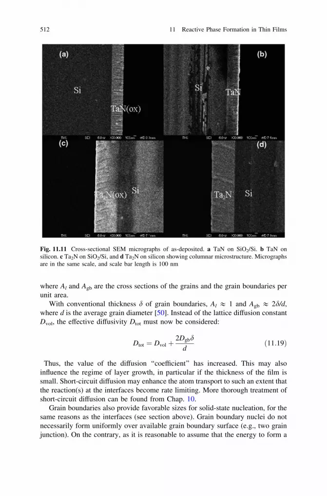
where Al and Agb are the cross sections of the grains and the grain boundaries perunit area.

With conventional thickness d of grain boundaries, Al & 1 and Agb & 2d/d,where d is the average grain diameter [50]. Instead of the lattice diffusion constantDvol, the effective diffusivity Dtot must now be considered:

Dtot ¼ Dvol þ2Dgbd

dð11:19Þ

Thus, the value of the diffusion ‘‘coefficient’’ has increased. This may alsoinfluence the regime of layer growth, in particular if the thickness of the film issmall. Short-circuit diffusion may enhance the atom transport to such an extent thatthe reaction(s) at the interfaces become rate limiting. More thorough treatment ofshort-circuit diffusion can be found from Chap. 10.

Grain boundaries also provide favorable sizes for solid-state nucleation, for thesame reasons as the interfaces (see section above). Grain boundary nuclei do notnecessarily form uniformly over available grain boundary surface (e.g., two grainjunction). On the contrary, as it is reasonable to assume that the energy to form a

Fig. 11.11 Cross-sectional SEM micrographs of as-deposited. a TaN on SiO2/Si. b TaN onsilicon. c Ta2N on SiO2/Si, and d Ta2N on silicon showing columnar microstructure. Micrographsare in the same scale, and scale bar length is 100 nm

512 11 Reactive Phase Formation in Thin Films

nucleus of critical size is smaller at grain edges and grain corners (three and fourgrain junctions, respectively). These sites with lowest critical free energy forformation of nucleus do not necessarily contribute most to the overall nucleationrate. This is because the number of atoms which can participate in the nucleationprocess also decreases with the dimensionality of the site. Cahn [51] has shownthat the opposing effects of lower energy barriers and fewer atoms participating inthe nucleation process as the dimensionality of the site can be used to map outdifferent nucleation conditions under which the greatest initial contribution to thenucleation rate is made by the sites of various types.

11.5 Role of the Impurities

Impurities have important effects on the formation of phases in thin film and bulkcouples. Presence of some impurity may enhance the formation of a particularphase at the expense of another (see Sect. 11.2 for the case of impurity-inducedamorphous phase formation). Impurities may increase or decrease reaction tem-peratures or influence the kinetics of a phase transformation. Impurities are alsofrequently responsible for the absence of phases in diffusion couples as comparedto the corresponding phase diagram. One example of the increased reactiontemperature is the formation of TaSi2, in the reaction between thin Ta film and Sisubstrate, which occurs at 923 K [52]. However, if there is oxygen at the Si/Tainterface, the temperature of formation will rise well above 1,023 K [53]. Anotherexample of bulk samples is the catalyzing effect of phosphorous on the formationof Cu3Si in the reaction between bulk copper foil and Si substrate [54]. The effectof impurities on diffusional transport should also be considered. Impurities maysegregate preferably to grain boundaries and interfaces. When they segregate tograin boundaries, they may reduce the effect of the short-circuit diffusion paths,thus affecting the mass transport in the system (see Chap. 10 for details).

The driving force for the equilibrium segregation of solute or impurity atoms tograin boundaries is systems tendency to lower its total free energy. In addition tokinetic constraints, the extent of intergranular segregation depends on impuritiesinfluence on the grain boundary energy as well as on the factors controlling theirsolubility, i.e., size factor and chemical interactions between dissimilar atoms.Since both the kinetics and the solubility depend on temperature, the segregationof impurities decreases with increasing temperature. By gathering large amountsof experimental data on grain boundary segregation, Hondros and Seah [55]showed that the smaller the solubility of an impurity in the solvent the higher is itssegregation potential. This ‘‘rule of thumb’’ is frequently used when consideringthe segregation tendency of a given impurity.

The classical free surface adsorption models have often been used for evalu-ating grain boundary segregation because of the analogies between intergranularsegregation and adsorption at free surfaces [56]. This approach is valid if it takesinto account the specific features, which differentiate the grain interface from

11.4 The Role of Grain Boundaries 513

surfaces. Thus, even the most dilute grain boundary can be regarded as a two-dimensional phase with the same components as in the bulk [57]. These compli-cations imply, among other things, that one has to utilize the extended phase ruleinstead of the classical phase rule when evaluating the degrees of freedom for thesystem. A generalized phase rule has been derived for system including surfacesand interfaces by Defay and Prigogine [58]. If c is the number of components, p isthe number of 3D phases, u number of 2D surface phases, and number of degreesof freedom f can be expressed as follows:

f þ p ¼ cþ 2� pð Þ�ðu� sÞ ¼ v� ðu� sÞ ð11:20Þ

where v is the classical (Gibbs) degrees of freedom (ignoring surfaces) and s is thenumber of ‘‘surface species.’’ Two surfaces are of different species if they separatedifferent couples of bulk phases. For instance, in the case of a grain boundaryprecipitate b in a matrix a, the interfaces a/a and a/b are of different species ands = 2. Also surfaces of different orientations should be considered as differentspecies. It is to be noted that the equilibrium condition, i.e., that the chemicalpotential of a component i has the same value in all phases of the system, is validalso for grain boundaries and surfaces as shown in Sect. 1.15. Several treatments ofintergranular segregation have been published during the past decades. Extensivereviews of the models can be found from Refs. [59, 60].

11.6 Phase Formation in Thin-Film Structures

There has been a view that phase formation in thin-film couples is sequential incomparison to simultaneous phase formation in bulk couples. In many worksdealing with formation of silicides, only one or two silicide layers have beenreported to grow [52, 59–69]. There have been several different approaches toexplain this phenomenon [70–78], which will be summarized briefly next. It is tobe noted that the method of evaluating microstructural evolution in diffusioncouples introduced in Chap. 8 can be used in thin-film couples and is used as abenchmark when other treatments are discussed. As these phenomena have beenthoroughly discussed in that chapter, the treatment is not repeated here for the caseof thin-film couples.

11.6.1 Linear-Parabolic Treatment

This treatment has been used by many authors to describe reactive phase forma-tion, including d’Heurle, Gas, and Philibert [49, 68, 69, 74]. The treatment wasfirst used to describe the formation of silicon dioxide [74].

514 11 Reactive Phase Formation in Thin Films

11.6.1.1 Growth of One Phase Between Pure A and B

One assumes that a compound AB grows between the pure elements A and B bythe diffusion of A atoms (Fig. 11.12). If one starts from the ‘‘pure’’ diffusionalgrowth, one obtains the following equation:

JA ¼ CA �MA �dlA

dLð11:21Þ

where the mobility is MA ¼ DAkT

If one assumes that the intrinsic diffusion coefficient DA is not a function ofconcentration one obtains

JA ¼ CA �DA

kT� DgA

Lð11:22Þ

where DgA is the Gibbs energy per A atom of the reaction A + B = AB. Morespecifically, it is the required energy to move one mole of A atoms from the A/ABinterface across the AB layer to the AB/B interface, i.e., the driving force for diffusionDlA. This value can again be obtained from the molar Gibbs energy plot of the systemin question using common tangent construction if one has the assessed thermody-namic data of the system available as shown in Sect. 1.15 and in [79, 80]. Since

dL

dt¼ JA � vA ð11:23Þ

cA ¼1vA

ð11:24Þ

then

dL

dt¼ DA �

DgA

kT� 1

Lð11:25Þ

Fig. 11.12 Schematicpresentation of the ABgrowth between the pureelements A and B

11.6 Phase Formation in Thin-Film Structures 515

If one integrates the Eq. 11.25, one obtains the familiar parabolic growth law:

L2 ¼ Kt ð11:26Þ

If Eq. 11.26 is considered at very small layer thickness, one encounters a seriousproblem, since if the L & 0, then

dL

dt� 1 ð11:27Þ

This means that pure parabolic kinetics seems impossible. Therefore, d’Heurleet al. [49, 68, 69] introduced the concept of linear-parabolic kinetics.

The starting point is again the Eq. 11.25, where one introduces a ‘‘kineticparameter’’ to take into account reactions at the interfaces

dL

dt¼ DA �

DgA

kT� 1

Lþ K 00ð11:28Þ

As the thickness of the layer approaches zero L ? 0, then the Eq. 11.28 reachesthe form

dL

dt� DA �

DgA

kT� 1

K 00ð11:29Þ

If one integrates this equation, one obtains:

L2 þ K 0L ¼ Kðt þ t0Þ ð11:30Þ

where K0 = 2 K00

When layer thickness grow large and reaction time becomes long (as usually inbulk couples), one obtains the ‘‘normal’’ parabolic growth equation

L!1) L2 � Kt ð11:31Þ

11.6.1.2 Multiphase Growth Between Pure A and B

If, instead of one phase, several phases grow between A and B, the situation isslightly different, since the growth of a specific phase depends not only its owngrowth kinetics but also from the growth kinetics of the adjacent phases(Fig. 11.13).Thus, the rate equations are coupled (see Chap. 8 for details). FromFig. 11.13, the following equations can be derived (A is still the only diffusingspecies)

516 11 Reactive Phase Formation in Thin Films

dL1

dt! J1 � J2 ð11:32Þ

dL2

dt! 2J2 � J1 ð11:33Þ

where the coefficient 2 in the Eq. 11.33 comes from the stoichiometry.In layer 1, A atoms diffuse through the A2B layer to react with the AB layer

according to the equation:

1: Aþ AB ¼ A2B

Dg1 ¼ DgfA2B � Dgf

AB

In the other layer 2, the growth of AB takes place at two interfaces:

2a: A2B� A ¼ AB2b: Aþ B ¼ ABtotal A2Bþ B ¼ 2AB

Dg2 ¼ 2DgfAB � Dgf

A2B

It follows that:

dL1

dt¼ 2

a1

L1� X1

X2

a2

L2

a1 ¼ D1Dg1

kTand a2 ¼ D2

Dg2

kT

ð11:34Þ

X1

X2¼ vA2B

vAB! x ð11:35Þ

Fig. 11.13 Schematicpresentation of multiphasegrowth between pureelements A and B

11.6 Phase Formation in Thin-Film Structures 517

dL2

dt¼ 2

a2

L2� 2

1x

a1

L1ð11:36Þ

The layer thicknesses L1, L2 and the total thickness L1 + L2 are functions offfiffitp

.If one investigates the growth of different layers:L1 grows if the inequality

2a1

L1[ x

a2

L2ð11:37Þ

is fulfilled.Similarly L2 grows if

a2

L2[

1x

a1

L1; and 2a1L2 [ xa2L1 [ a1L2; ð11:38Þ

which leads approximately to the equation:

2D1

D2[

L1

L2[

D1

D2ð11:39Þ

The ratio L1L2

can be solved from the following equation:

L1

L2¼

2x a1 � xa2 þ

ffiffiffiffiffiffiffiffiffiffiffiffiffiffiffiffiffiffiffiffiffiffiffiffiffiffiffiffiffiffiffiffiffiffiffiffiffiffiffiffiffiffiffi2x a1 � xa2� �2þ8a1a2

q4a2

ð11:40Þ

This ratio L1/L2 produces to the following diagram where there are three regimesof growth (Fig. 11.14).

At the region M, L1 grows and L2 shrinks, within the region O, L2 grows and L1

shrinks and at the region N, both phases can grow simultaneously. As the timeincreases and if it is assumed that end elements in reaction couple are not con-sumed, the reaction couple eventually reaches the N region and both phases cangrow simultaneously.

11.6.1.3 ‘‘Pure’’ Diffusional Approach to Multiphase Growth

From the ‘‘pure’’ diffusional point of view regarding the growth of A2B and ABlayers between pure A and B, the following conclusions can be drawn:

(a) All phases grow simultaneously. This contradicts experimental results fromthin-film experiments where sequential phase formation has been observed

(b) Growth rate is parabolic, e.g., L ?ffiffitp

518 11 Reactive Phase Formation in Thin Films

(c) Phases cannot disappear in reaction couple. This is as a result of the fact thatas the layer thickness goes to zero the growth rate should approach infinity:L ? 0 then dL

dt / 1(d) However, even for the pure diffusional growth of the phases, their thickness

ratio is proportional to the ratio of the diffusion coefficients in the layersL1L2! D1

D2

For example, if the ratio of the diffusion coefficients is 104, which is of reasonablemagnitude for real experiments, and for example, if the layer thickness of the layer1 is L1 = 103 Å, then the thickness of the layer 2 would be L2 = 10-1 Å. In thiscase, the layer 2 cannot be said to really exist. This shows how within the ‘‘pure’’diffusional theory, without any further assumptions, one already gets into troublewith layer thicknesses that are readily used in the common thin-film technology.However, this has also been used to defend the traditional ‘‘pure’’ diffusionapproach, since it has been stated that all the phases are present in the reactioncouple as required, but the thicknesses may be so small that they are impossible todetect.

(e) One can conclude that with small layer thicknesses with ‘‘pure’’ diffusionaltheory, mathematics of the theory, and the actual physics are contradictory

11.6.1.4 Linear-Parabolic Approach to Multiphase Growth

As we noticed, serious problems are encountered with thin-film structures if oneuses the traditional ‘‘pure’’ diffusion control approach. On the other hand, ifone examines the problem with the help of linear-parabolic growth kinetics the

Fig. 11.14 Presentation ofthe different growth regionsin the A/A2B/AB/B reactioncouple under diffusioncontrol [71]

11.6 Phase Formation in Thin-Film Structures 519

above-mentioned issues can be avoided. The equations describing the growth ofthe layers are the following:

dL1

dt¼ 2

a1

L1 þ K 001� x

a2

L2 þ K 002ð11:41Þ

dL2

dt¼ 2

a2

L2 þ K 002� 2

xa1

L1 þ K 001ð11:42Þ

If one assumes that the layer formation is sequential as experimentally observedin thin-film experiments, it means that L2 = 0 at the beginning. The driving forcefor the formation of AB does, however, exist, e.g., dL2

dt [ 0, and therefore, thegrowth rate of AB is positive. Then, one obtains the following inequality:

a2

K 002[

1x

a1

L1c þ K 001ð11:43Þ

which leads to the concept of ‘‘critical thickness’’:

L1c [1x

a1

a2K 002 � K 001 ð11:44Þ

This means that the AB phase will not start to grow until the thickness of theA2B layer has reached a minimal thickness, despite the fact that the driving forcefor the formation of AB exists! Also if the other end element is depleted (A or B)before the A2B has reached the critical thickness, the AB phase will not occur.Furthermore, if the AB layer is present initially, it will start to shrink as the A2Blayer grows at its expense—if A2B layer has not yet reached the critical thicknessthat would enable the simultaneous growth of both phases. If one plots thethickness of the phases similar to the plot as seen in Fig. 11.14, one obtains thesame kind of plot—just the nodal lines are translated (Fig. 11.15). The slope of thelines remain unchanged, they are simply translated vertically by the quantity givenby the ‘‘reaction’’ factor. There is, however, an additional important feature thatcan be seen from Fig. 11.15. If the conditions of the growth process lie inside thearea marked as R in the figure, the phase 2 (L2) would disappear under theseconditions.

The ‘‘simultaneous’’ phase growth found in the bulk diffusion couples can beexplained on the basis of the same critical thickness. In bulk couples, the annealingtimes are long and the layer thickness are large and therefore the phases ‘‘easily’’reach the required critical thickness, thus enabling the observation of severalphases. It should, however, be emphasized that in the bulk couples also, there areoccasions where all the predicted phases are not observed.

Basically, we end up with three rules for the linear-parabolic treatment of two-phase growth

520 11 Reactive Phase Formation in Thin Films

1. The criterion for the first-phase formation is a kinetic one: It is determined bythe value of diffusitivity

2. The first phase grows alone until a critical thickness, which depends on thesame parameters, at this point the second phase appears

3. After some transient, the both phases grow simultaneously with proportionalthickness increments.

11.6.2 Interfacial Reaction Barrier Approach

The approach was introduced by Gösele and Tu [72, 77] in order to investigate thedifference between thin film and bulk reaction couples. It was basically anextension of earlier work by other authors [73–75]. Interfacial reaction barrier wasused to describe the energy barrier associated with changes in atomic arrangementsor effects due to volume changes at the interface due to the formation of newinterface at the expense of the old. In that way, it is somewhat related to interfacialenergy.

They used a model system to consider the effect of the interfacial reactionbarriers to multiphase growth in a reaction couple where the AbB and AcB growbetween the saturated AaB and AdB phases (a[b[ c[ d). It was also assumed

Fig. 11.15 Presentation ofthe different growth regionsin the A/A2B/AB/B reactioncouple according to linear-parabolic kinetics (see textfor details) [71]

11.6 Phase Formation in Thin-Film Structures 521

that the AbB and AcB phases are already present at the beginning with giventhickness xb and xc. This assumption was introduced in order to avoid the problemsarising from nucleation of the phases. Intention was especially to check whetherone of the layers would shrink away completely under various kinetic conditions.

Their model was characterized by the interdiffusion coefficients ~Db and ~Dc.These coefficients are related to the intrinsic diffusion coefficients by the Darkenequation

~Db ¼ NBDAb þ NADB

b ð11:45Þ

The volume of the formed compound X0 per A or B atom is assumed to beconstant. They also introduced b which is the ratio of A atoms to B atom in theAbB compound. The shift of the interfaces can be calculated from the equations

dxb

dt¼ GbJA

b � GbcJAc ð11:46Þ

dxc

dt¼ GcJ

Ac � GcbJA

b ð11:47Þ

with the (positive) diffusion fluxes of A atoms in the AbB and AcB layer

JAb ¼ DCeq

b keffb =ð1þ xbj

effb =~DbÞ ð11:48Þ

JAc ¼ DCeq

c jeffc =ð1þ xcj

effc =~DcÞ ð11:49Þ

where

DCeqb ¼ Ceq

ba � Ceqbc ð11:50Þ

and

1

jeffb

¼ 1jbaþ 1

jbcð11:51Þ

The various quantities with the subscript c have analogous meaning for the AcBlayer.

The quantities Gb, Gbc, Gc, and Gcb take into account the change in compo-sition at the interfaces

Gb ¼ X0ð1þ b2Þ 1a� b

þ 1b� c

� �ð11:52Þ

Gc ¼ X0ð1þ b2Þ 1b� c

þ 1c� d

� �ð11:53Þ

522 11 Reactive Phase Formation in Thin Films

Gbc ¼ Gcb ¼ X0ð1þ bÞð1þ cÞ=ðb� cÞ ð11:54Þ

The fluxes described above are assumed to be independent of each other. Theschematic presentation of the situation is shown in Fig. 11.16. In the figure, thedifferent parameters are depicted only for the AbB layer, but they are analogous forthe other interfaces and layers.

The assumption that the fluxes are independent leads into equations:

JbA ¼ jbcðCbc � Ceq

bcÞ; at the AbB interface ð11:55Þ

and

JAc ¼ jcbðCeq

cb � CcbÞ; at the AcB interface ð11:56Þ

The quantity jbc describes the reaction barrier against the growth of AbB layer atthe expense of the AcB layer, and jcb characterizes the reaction barrier against thegrowth of the AcB layer at the expense of the AbB layer. The basic differencebetween this approach and the ‘‘traditional’’ diffusional approach is the occurrenceof the interfacial reaction barriers. If the reactions at the interfaces are fast, thereaction barriers tend to approach infinity. Hence, for fast reactions, the growthrates are as described in the ‘‘pure’’ diffusion theory.

The condition for growth of the AbB layer dxb

dt [ 0 may be expressed in terms ofthe ratio r of the diffusion fluxes

Fig. 11.16 Schematicpresentation of theconcentration profile of Aatoms in the AaB/AbB/AcB/AdB diffusion couple

11.6 Phase Formation in Thin-Film Structures 523

r ¼JAb

JAc

ð11:57Þ

as

r [Gc

Gcb¼ r1 ð11:58Þ

The analogous condition for the growth of the AcB layer is

r\Gc

Gcb¼ r2 ð11:59Þ

with

r1 ¼ ð1þ cÞða� bÞ=ð1þ bÞða� cÞ ð11:60Þ

and

r2 ¼ ð1þ cÞðb� dÞ=ð1þ bÞðc� dÞ ð11:61Þ

where r2 [ r1, holds, since (a - b) \ (a - c) and (b - d) [ (c - d)When the parameters xb; xc;Di

b;Dic; j

effb ;and jeff

c have such a values that the flux

ratio r is between r1 and r2 both layers can grow simultaneously. However, if theflux ratio is not between them, one layer will shrink and the other will grow.Hence, situation is similar as shown already in the Fig. 11.14. This similarity alsoimplies that there should be a critical thickness as in the other two previoustreatments. It can be found also within this theory, and it is expressed as follows:

xcritc ¼

r1DCeqc Dc

�

DCeqb jeff

b

ð11:62Þ

where the growth of AbB is reaction controlled and the growth of AcB diffusioncontrolled, thus simulating sequential phase formation. It states that the AbB layercannot coexist with the AcB layer as long as the thickness of the AcB layer isbelow the xcrit

c . This means that even without any nucleation difficulties the AbBcannot form with the AcB layer in the AaB/AbB/AcB/AdB diffusion couple whenthe thickness of the xc is not large enough. This again predicts sequential phasegrowth.

524 11 Reactive Phase Formation in Thin Films

11.6.3 Similarities Between the Growth Models

It is very interesting to compare the results obtained above and those derived inChap. 8. Despite the differences between the approaches, all the models lead tosimilar results. It is also common to both approaches that they neglect thenucleation difficulties in order to avoid complications. In fact, it has been shown byd’Heurle [4] that in most cases nucleation plays a role in the very early stage of thecompound formation that is at the present time beyond experimental reach.Nevertheless, nucleation still plays a decisive role with some silicides, especiallyafter the first-phase formation.

In the above two models, reactions at the interface are taken into account withthe help of a ‘‘chemical constant.’’ This concept is common to both the abovemodels despite the slightly different names that are used. The ‘‘chemical constant’’is, however, a slightly obscure entity, because it is not clear what are its contents.In Göseles approach [72, 77], it was related to the arrangement of atoms in theinterface and the volume changes due to formation of a new interface. Thus, itshould contain some ‘‘nucleation’’ contribution also. In the other approach, themeaning of the ‘‘chemical constants’’ was somewhat similar. On the contrary, inthe physicochemical approach outlined in Chap. 8 there is no need for ad hocchemical constants as reaction related issues arise naturally from the stoichiom-etric considerations.

The prediction power of the two models above is quite poor, due to the natureof the ‘‘chemical constants.’’ There is no theoretical method at the present tocalculate these constants a priori. Hence, they can be determined only by exper-iments. Also the lack of availability to use measured or estimated thermodynamicand kinetic (diffusion constants) values reduce the use of these approaches. Again,in the physicochemical approach one can readily utilize experimental and theo-retical thermodynamic and kinetic data, which makes the approach derived indetail in Chap. 8 a very strong and feasible tool to understand interfacial reactionlayer growth in thin film as well as in bulk couples.

From a certain point of view, both of the above models are a posteriori in theirnature, as they can explain afterward the phase formation sequence but cannotpredict it. Moreover, the ‘‘chemical constants’’ used in all the models are verymuch case dependent, since they are basically depended on the conditions of theinterfaces and are therefore very sensitive to impurities, additional films etc.Furthermore, these constants are not achievable by experimental methods. Theapproaches, however, fade away the somewhat ‘‘traditional’’ distinction betweenthin film and bulk couples, since fundamentally the behavior is more or less thesame. Nevertheless, in practical situations, the contributions due to the grainboundaries, impurities etc. mentioned above (Sect. 11.5 onwards) must be takeninto account in thin films. This does not change the underlying theoretical fact thateven in bulk reaction couples phase formation is basically sequential.

If one compares the above treatments to the physicochemical model extensivelydiscussed in Chap. 8, the benefits of the latter over the two approaches are

11.6 Phase Formation in Thin-Film Structures 525

obvious. As discussed above, the physicochemical model contains only measur-able quantities, and it has also predictive power. Thus, it is the opinion of theauthors that the physicochemical model should be used whenever the morpho-logical evolution of a binary diffusion zone is rationalized.

References

1. Russel, K.C. Colloid Interface Sci., 13, 205, 1980.2. Coffey K.R., Clevenger L.A., Barmak K., Rudman D.A., and Thompson C.V., Appl. Phys.

Lett., 55, 852, 1989.3. Bormann R., Mat. Res. Soc. Symp. Proc., 343, 169, 1994.4. d’ Heurle F.M., J. Mater. Res., 3, 167, 1988.5. Eshelby J.D., Proc. R. Soc. A London Ser. A., 241, 376, 1957.6. Saunders N. and. Miodownik A.P, CALPHAD, Calculation of Phase Diagrams, Pergammon

Materials Series, Elsevier Science, 1998.7. Kaufman L. and Bernstein H., Computer Calculation of Phase Diagrams, Academic Press,

New York, 1970.8. Ansara I., Pure Appl. Chem., 62, 71, 1990.9. Lukas H.L., Weiss J., and Henig E.T., CALPHAD, 6, 229, 1982.

10. Bormann R. and Zöltzer K., phys. stat. sol.(a), 131, 691, 1992.11. Thompson C.V., J. Mater. Res., 7, 367, 1992.12. Newcomb S.B. and Tu K.N., Appl. Phys. Lett., 48, 1436, 1986.13. Cotts E. J., Meng W.J., and Johnson W.L., Phys. Rev. Lett., 57, 2295, 1986.14. Vredenberg A. M, Westendorp J.F.M., Saris F.W., van den Pers N.M., and de Keijser Th. H.,

J. Mater. Res., 1, 774, 1986.15. Meng W.J., Nieh C.W., Ma E., Fultz B., and Johnson W.L., Mater. Sci. Eng., 97, 87, 1988.16. Erhart P., Averback R., Hahn H., Yadavalli S., and Flynn C.P., J. Mater. Res., 3, 1276, 1988.17. Johnson W.L., Dolgin B., and van Rossum M., in Glass:Current Issues, NATO ASI Series,

eds. A.F. Wright and L. Dopuy, (Dordrecht:Martinus Nijhoff), 172, 1985.18. Clemens B.M., J. Appl. Phys., 61, 4525, 1987.19. Kelton K.F. and Greer A.L., J. Phys. Rev. B, 38, 10089, 1988.20. Highmore R.J., Phil. Mag. B, 61, 455, 1990.21. Christian J.W., The Theory of Transformations in Metals and Alloys, Part 1, (Oxford,

Pergamon), 1975.22. Barret C. and Massalski T.B., The Structure of Metals, (McGraw-Hill), 1966.23. Brandes E. editor, Smithelss Metals Reference Book, 6th edition (London, Butterworths),

1983.24. Saunders N. and Miodownik A.P., J. Mater. Res., 1, 38, 1986.25. Turnbull D., Metall. Trans. A, 12, 695, 1981.26. Greer A.L., Phil. Mag. B, 61, 525, 1990.27. Barmak K., Gungor A., Cabral C., Jr., and Harper J. M. E., J. Appl. Phys., 94, 1605, 2003.28. Harper J. M. E., Cabral C., Jr., Andricacos P. C., Gignac L., Noyan I. C., Rodbell K. P., and

Hu C. K., J. Appl. Phys. 86, 2516, 1999.29. Detavernier C., Deduytsche D., Van Meirhaeghe R. L., De Baerdemaeker J., and Dauwe C.,

Appl. Phys. Lett. 82, 1863, 2003.30. Herd S., Tu K.N., and Ahn K.Y., Appl. Phys. Lett., 42, 597, 1983.31. d’Heurle F.M., Petersson C.S., Baglin J.E.E., La Placa S.J., and Wong C.Y., J. Appl. Phys.,

55, 4208, 1984.32. Vanderwalker D.M., Appl. Phys. Lett., 48, 707, 1986.33. Holloway K. and Sinclair R., J. Appl. Phys., 61, 1359, 1987.

526 11 Reactive Phase Formation in Thin Films

34. Meyerheim H.L., Lengeler B., and Göbel H.E., J. Appl. Phys., 68, 2694, 1990.35. W.L. Johnson, Prog. Mater. Sci., 30, 1986, 81.36. W. Klement, R.H. Willens, and P. Duwez, Nature, 187, 1960, 869.37. Clemens B.M., Johnson W.L., and Schwarz R.B., J. Non-Crystal. Solids, 61-62, 817, 1984.38. Evans P.V., Garcia-Escorial A., Donovan P.E., and Greer A.L., MRS Symposium

Proceedings, 57, 234, 1987.39. E. Gebhardt and H. D. Sehezzi, Z. Metallkd., 50, 521, (1952).40. H. Jehn and E. Olzi, J. Less-Common Met., 27, 297, (1972).41. S. Stecura, Metall. Trans., 5, 1337, (1974).42. R. Lauf and C. Altstetter, Scr. Metall., 11, 938, (1977).43. G. Boreau and P. Gerdanian, J. Phys. Chem. Solids, 42, 749, (1981).44. M.A. Nicolet, in: Diffusion in Amorphous Materials, eds. H. Jain and D. Gupta, (TMS

Warrendale, 1994), pp. 225-234.45. Desre P.J. and Yavari A.R., Phys. Rev. Lett., 64, 1533, 1990.46. Desre P.J., Acta Metall. Mater., 39, 2309, 1991.47. Grunthaner P. J., Grunthaner F. J., and Mayer J. W., J. Vac. Sci. Technol, 17, 924, 1980.48. Cahn W. and Hilliard J. E., J. Chem. Phys, 28, 258, 1958.49. Philibert J., Appl. Surf. Sci., 53, 74, 1991.50. Kaur I. and Gust W., Fundamentals of Grain and Interphase Boundary Diffusion, Ziegler

Press, 1989.51. Cahn J.W., Acta Metall., 4, 449, (1956).52. Ottaviani G., Thin Solid Films, 140, 3, 1986.53. Christou A. and Day H.M., J. Electr. Mater., 5, 1, 1976.54. Becht J.G.M., ‘‘The Influence of Phosphorous on the Solid State Reaction Between Copper

and Silicon or Germanium’’, Doctoral Thesis, Tech. University of Eindhoven Netherlands,1987.

55. Hondros E. and Seah M., Int. Met. Rev, 22, 262, 1977.56. Hondros E. and Seah M., Metall. Trans. A, 8A, 1363, 1977.57. Guttmann M., Metall. Trans. A, 8A, 1383, 1977.58. Poate J.M. and Tisone T.S., Appl. Phys. Lett., 24, 391, 1974.59. Lau S.S., Mayer J.W., and Tu K.N., J. Appl. Phys., 49, 4005, 1978.60. van Gurp G.J., van der Weg W.F., and Sigurd D., J. Appl. Phys., 49, 4011, 1978.61. Scott D.M. and Nicolet M.-A., Phys. Stat. Solidi., 66, 773, 1981.62. Tsaur B.Y., Lau S.S., Mayer J.W., and Nicolet M.-A., Appl. Phys. Lett., 38, 922, 1981.63. Eizenberg M. and Tu K.N., J. Appl. Phys., 53, 6885, 1982.64. Petersson C.S., Baglin J.E.E., Dempsey J.J., d’Heurle F.M. and La Place S.S., J. Appl. Phys.,

53, 4866, 1982.65. Canali C., Catellani F., Ottaviani G. and Prudenziati M., Appl. Phys. Lett., 33, 187, 1978.66. Coulman B. and Chen H., J. Appl. Phys., 59, 3467, 1986.67. Lien C.-D., Nicolet M.-A., and Lau S.S., Thin Solid Films, 143, 63, 1986.68. d’Heurle F.M. and Petersson C.S., Thin Solid Films, 128, 283, 1985.69. Gas P. and d’Heurle F.M., App. Surf. Sci.,73, 153, 1993.70. Philibert J., Materials Science Forum, 155-156, 15, 1994.71. d’ Heurle F.M., ‘‘The Kinetics of Reactive Phase Formation: Silicides’’, in Silicides:

Fundamentals and Applications, (Eds. L. Miglio and F. d’Heurle), World Scientific, pp. 169-186, 2001.

72. Gösele U. and Tu, K. N. J. Appl. Phys., 66, 2619, 1989.73. Geguzin Ye Ya, Kaganovskiy Yu.S, Paritskaya L.M., and., Solunskiy V.I, Phys. Met.

Metallogr., 47, 127, 1980.74. Deal E. and Grove A.S., J. Appl. Phys., 36, 3770, 1965.75. Farrel P., Gilmer G.H., and Suenaga M., Thin Solid Films, 25, 253, 1975.76. Taguchi O., Iijima Y., and Hirano K., J. Japan Inst. Metals., 51, 4, 292, 1987.

References 527

77. Gösele U. and Tu K.N., J. Appl. Phys., 53, 3252, 1982.78. Wagner C., Acta Metall., 17, 99, 1969.79. Gulpen J., ‘‘Reactive Phase Formation in the Ni-Si System’’, Doctoral Thesis, Technical

University of Eindhoven, The Netherlands, 1995.80. Rönkä K., ‘‘Time-Dependent Microstructural and Compositional Changes at the Interfaces

between Materials in Electronics’’, Doctoral Thesis, Helsinki University of Technology,Finland, 2001.

528 11 Reactive Phase Formation in Thin Films

Author Biography

Professor Aloke Paul is currently running anactive search group working on diffusion-relatedproblems in the Department of MaterialsEngineering, Indian Institute of Science,Bangalore, India. Major areas of researchinclude development of new phenomenologicalmodels in solid-state diffusion, materials inelectronic packaging, bond coat in jet engineapplications, growth of A15 intermetallicsuperconductors, etc. He teaches a postgraduatelevel course on Diffusion in solids. He hasguided several Ph.D. and M.E. students. At

present, he has co-authored more than 80 articles in various international journals.

Professor Tomi Laurila received the D.Sc.degree (with honors) from the Helsinki Universityof Technology in 2001. At the moment, he isAssociate Professor in the field of Microsystemtechnology and holds an adjunct professorship onElectronics Reliability and Manufacturing. Hisresearch involves the study of interfacial reactionsbetween dissimilar materials used inmicrosystems, biocompatibility issues related todifferent types of materials and electrochemicalmeasurements of neurotransmitters from thebrain. He has published extensively (about 70scientific papers, including also book chapters

and a text book) on the thermodynamic–kinetic analysis of interfacial reactions,electrochemical detection of biomolecules and issues related to reliability testing ofelectronic devices. Prof. Laurila is also responsible for the teaching of materialscience, electronics reliability, and bioadaptive technology to under- and postgraduateas well as postdoctoral students.

A. Paul et al., Thermodynamics, Diffusion and the Kirkendall Effect in Solids,DOI: 10.1007/978-3-319-07461-0, � Springer International Publishing Switzerland 2014

529

Dr. Vesa Vuorinen received his M.Sc. degree in1995 in Materials Science and Engineering andD.Sc. degree in 2006 in the Department ofElectronics from the former Helsinki Universityof Technology, currently Aalto University.Currently, he is working as Senior UniversityLecturer as well as Project Manager in the researchgroup of Electronics Integration and Reliability.His research has been focused on the interfacialreactions encountered in lead-free electronics andreliability of high-density electronics assemblieswith emphasis on soldering metallurgy on physicsof failure viewpoint.

Dr. Sergiy Divinski is a Privat-Docent at theInstitute of Materials Physics, University ofMünster, Germany, where he leads theradiotracer laboratory which represents one ofthe most reputed and internationally recognizeddiffusion schools. He teaches graduate andpostgraduate courses on Diffusion in Solids,Numerical methods in Material Science anddifferent aspects of Materials Science. He hasco-authored more than 150 articles in variousinternational journals and several book chaptersin the field of Diffusion in Solids.

530 Author Biography