Policy Research Working Paper 9562

Pathways out of Extreme Poverty

Tackling Psychosocial and Capital Constraints with a Multi-faceted Social Protection Program in Niger

Thomas BossuroyMarkus Goldstein

Dean KarlanHarounan Kazianga

William Parienté Patrick Premand

Catherine ThomasChristopher Udry

Julia Vaillant Kelsey Wright

Social Protection and Jobs Global PracticeDevelopment Impact Evaluation Group &Africa Gender Innovation LabMarch 2021

Pub

lic D

iscl

osur

e A

utho

rized

Pub

lic D

iscl

osur

e A

utho

rized

Pub

lic D

iscl

osur

e A

utho

rized

Pub

lic D

iscl

osur

e A

utho

rized

Produced by the Research Support Team

Abstract

The Policy Research Working Paper Series disseminates the findings of work in progress to encourage the exchange of ideas about development issues. An objective of the series is to get the findings out quickly, even if the presentations are less than fully polished. The papers carry the names of the authors and should be cited accordingly. The findings, interpretations, and conclusions expressed in this paper are entirely those of the authors. They do not necessarily represent the views of the International Bank for Reconstruction and Development/World Bank and its affiliated organizations, or those of the Executive Directors of the World Bank or the governments they represent.

Policy Research Working Paper 9562

This paper analyzes a four-arm randomized evaluation of a multi-faceted economic inclusion intervention deliv-ered by the Government of Niger to female beneficiaries of a national cash transfer program. All three treatment arms include a core package of group savings promotion, coaching, and entrepreneurship training, in addition to the regular cash transfers from the national program. The first variant also includes a lump-sum cash grant and is similar to a traditional graduation intervention (“capital” package). The second variant substitutes the cash grant with psycho-social interventions (“psychosocial” package). The third variant includes the cash grant and the psychosocial inter-ventions (“full” package). The control group only receives the regular cash transfers from the national program. All

three treatments generate large impacts on consumption and food security six and 18 months post-intervention. They increase participation and profits in women-led off-farm business and livestock activities, as well as improve various dimensions of psychosocial well-being. The impacts tend to be larger in the full treatment, followed by the cap-ital and psychosocial treatments. Consumption impacts up to 18 months after the intervention already exceed costs in the psychosocial package (the benefit-cost ratio for the psy-chosocial package is 126 percent; full package, 95 percent; and capital package, 58 percent). These results highlight the value of addressing psychosocial constraints as well as capital constraints in government-implemented poverty reduction programs.

This paper is a joint product of the Social Protection and Jobs Global Practice, the Development Impact Evaluation Group, and Africa Gender Innovation Lav. It is part of a larger effort by the World Bank to provide open access to its research and make a contribution to development policy discussions around the world. Policy Research Working Papers are also posted on the Web at http://www.worldbank.org/prwp. The authors may be contacted at ppremand@worldbank.org.

Pathways out of Extreme Poverty: Tackling Psychosocial and Capital Constraints with a Multi-faceted Social Protection Program in Niger

Thomas Bossuroy -- Markus Goldstein -- Dean Karlan -- Harounan Kazianga -- William Parienté --

Patrick Premand -- Catherine Thomas -- Christopher Udry -- Julia Vaillant -- Kelsey Wright

March 20211

Keywords: poverty, livelihoods, graduation, economic inclusion, psychosocial, cash grant, field

experiment

JEL Codes: D12, D13, D14, O12, O13, O17

1 This paper is based on a collaboration between the Government of Niger, the World Bank Sahel Adaptive Social Protection program, Africa

Gender Innovation Lab, DIME and Innovations for Poverty Action. The study was supported by the Sahel Adaptive Social Protection Program at

the World Bank, the Wellspring Philanthropic Fund, as well as the Niger Adaptive Safety Nets Project, managed by the Cellule Filets Sociaux

(CFS) in the Prime Minister’s office of the Government of Niger. We are grateful to Ali Mory Maidoka, Moussa Bouda, Bassirou

Karimou, Kadi Aboubacar, Moumouni Moussa, and the whole CFS staff, as well as Carlo del Ninno, Mahamane Maliki Amadou and the World

Bank Sahel Adaptive Social Protection Program team for a fruitful collaboration. CFS led the intervention implementation, with technical

assistance from the World Bank (led by Thomas Bossuroy and Patrick Premand), Trickle Up (led by Jo Sanson and Yerefolo Malle), CESAM (led

by Dissou Zomahoun), Robin Audy, Soumaila Abdoulaye Sambo and Damel Dieng. Sahel Consulting (led by Adamou Hamadou) collected the

study data, with support from Achille Mignondo Tchibozo at IPA, Karim Paré, Moumouni Moussa, Moustapha Labo Saley and Almoustapha

Yatta Theodore. Yazen Kashlan at IPA and GPRL (Northwestern University) provided outstanding research assistance. We are grateful for inputs

and comments at various parts of the study from Christian Bodewig, Carlo del Ninno, Nathanael Goldberg, Margaret Grosh, Arianna

Legovini, John Loeser, Hazel Rose Markus, Richard Sedlmayr, Gregory Walton as well as seminar participants at IPA and the World Bank. The

computational reproducibility of the results has been verified by DIME analytics. The study was pre-registered in the AEA RCT registry: https://

www.socialscienceregistry.org/trials/2544. The findings, interpretations, and conclusions expressed in this paper are entirely those of the

authors. They do not necessarily represent the views of the World Bank and its affiliated organizations; those of the Executive Directors of

the World Bank or the governments they represent. Corresponding author: Patrick Premand, ppremand@worldbank.org.

2

1. Introduction

In the past 20 years, governments worldwide have scaled targeted high-frequency cash transfer

programs to low-income households. These programs have had well-documented positive impacts on

welfare and investments. Yet the extreme poor may face multiple market failures that limit the ability of

cash transfers alone to generate a sustained exit from poverty. “Cash plus programs”, which add

interventions such as savings, training or information to cash transfers, hold promise for generating

more sustained long-run impacts. Indeed, a set of multi-faceted “graduation” programs, typically

implemented by nonprofit organizations, test a version of this approach with five additional

components, and find large impacts on welfare, income-generating activities and earnings in both the

short and medium run.2 Governments are increasingly interested to scale these approaches through

national social protection systems,3 though important questions remain about feasibility and

effectiveness.

We analyze the effects of a multi-faceted economic inclusion intervention implemented by the

Government of Niger to address a range of constraints among very poor households, including capital

and psychosocial constraints. We use a four-arm (three treatment and one control) randomized

controlled trial (RCT) conducted in a sample of women already receiving monthly poverty-targeted cash

transfers from a national program.4 All three treatment variants (but not the control) include a core set

of components: village savings groups, coaching and entrepreneurship training. The first variant

(“capital”) adds a lump-sum cash grant to the core components and is close to the traditional graduation

program studied in the literature.5 The second variant (“psychosocial”) adds a life skills training and

community sensitization on aspirations and social norms to the core components. The third variant

(“full”) adds both the lump-sum cash grant and the psychosocial interventions to the core components.

Note that there is no variant of just the monthly cash transfers plus the core components (i.e., without

the capital or psychosocial components); we discuss this in the design section.

2 See for instance Banerjee et al. 2015b; Banerjee et al, 2016; Bandiera et al., 2017; Bedoya et al., 2019; Banerjee et al, 2020a; Balboni et al., 2020. 3 Beegle et al., 2018; Andrews et al., 2021. 4 The study is part of a multi-country RCT embedded in the Sahel Adaptive Social Protection program that also includes Burkina Faso, Mauritania, and Senegal. Niger was first to implement the intervention; as of the writing of this paper, follow-up survey data have not yet been collected in other sites. 5 For instance, Banerjee et al., 2015b or Bandiera et al., 2017. One difference is that the Niger intervention provides a lump-sum cash grant instead of in-kind assets.

3

Our results show a strong impact from each of the three variants on the primary outcomes of

consumption and food security at both six and 18 months post-intervention. Each variant also strongly

increases investments, women-led off-farm business activities and revenues, livestock holdings and

revenues, and household income diversification. We find positive impacts on several dimensions of

psychological and social well-being, as well as women’s empowerment.

Comparing impacts on primary outcomes across treatment arms, the full package tends to perform best,

with the capital package second-best and psychosocial package third. However, the differences in

impacts across arms are small relative to their differences in costs. Both the psychosocial and full

packages have benefit-cost ratios significantly higher than the capital package. In fact, the psychosocial

package already reaches its break-even point after 18 months based on observed consumption impacts

alone (benefit-cost ratio for the psychosocial package=126%; full package=95%; capital package=58%).

These benefit-cost ratios are lower bounds since they only include consumption impacts up to 18

months post-intervention as benefits (hence not accounting for impacts on assets, investments, or

psychosocial well-being). We find considerably higher benefit-cost ratios than prior graduation studies

(such as Banerjee et al., 2015b or Bedoya et al., 2019) when we make similar assumptions about the

sustainability of impacts.

We contribute to five related literatures. First and second, we test the importance of relaxing capital

constraints and psychosocial constraints in opening pathways out of extreme poverty. For capital

constraints, the strongest existing evidence comes from programs that merely provide capital. This falls

into three categories: lump-sum cash grants;6 small, regular transfers (often provided by government

cash transfer programs),7 and microcredit.8 While some studies do examine the impact of the transfer

interacted with, or built on top of, some other program, few test this on top of a complex multi-faceted

program as we do here.

Similarly, psychosocial components have been tested mostly on their own as stand-alone programs

(albeit less frequently, and heterogeneity in program design renders comparison more difficult) rather

than as part of a larger set of interventions. Psychological and economic research suggests diverse

constraints (e.g., strong gender norms, high stress, strained cognitive bandwidth) to low-income

women’s capacity to aspire, to build socio-emotional skills, and, ultimately, to pursue economic

6 de Mel et al., 2012; Macours et al., 2012; Karlan et al., 2015; Haushofer and Shapiro, 2016. 7 Alderman and Yemtsov, 2014; Bastagli et al., 2019; Davis et al., 2016; Fiszbein et al., 2009; Ralston et al., 2017. 8 Angelucci et al., 2015; Attanasio et al., 2015; Banerjee et al., 2015a; Banerjee et al., 2015c; Breza and Kinnan, 2018; Crépon et al., 2015; Tarozzi et al., 2015; Karlan and Zinman, 2010; Karlan and Zinman, 2011; Meager, 2019.

4

opportunities.9 Psychology based interventions that focus on shifting social norms or teaching relevant

interpersonal and intrapersonal skills can support women in setting and pursuing their goals.10 For

instance, media-based interventions that use relatable role models to shift community-wide social

norms and aspirations have been shown to boost future-oriented financial investments and promote

women’s empowerment.11 Psychological interventions (e.g., goal-setting, growth mindset and initiative,

self-affirmation, cognitive behavioral therapy) have also led to improvements in economic well-being,

small business outcomes, and women’s empowerment in developing countries.12 As evidenced in these

literatures, many psychosocial programs target either individual-level or community-level factors;

however, the psychosocial components we study were designed to simultaneously build women’s

individual skills and aspirations while shifting community-level social norms.13

Third, speaking directly to the budding literature on multi-faceted programs, a frequent question

surrounds the choice of components. This has both theoretical implications on the assumption of the

underlying binding constraints causing extreme poverty, as well as practical relevance for the selection

of the most cost-effective components to achieve policy objectives. For instance, Blattman et al. (2016)

estimate the value of providing supervision and follow-up support in addition to a grant and training

intervention. Sedlmayr et al. (2020) isolate the impact of training and savings group formation, and test

light behavioral components. Banerjee et al. (2020b) identify the contribution of savings accounts as

well as lump-sum asset transfers as stand-alone components. Marguerie and Premand (2021) compare

cash grants that address capital constraints and savings groups that address savings constraints.

Fourth, we contribute to the evolving literature on the impact of graduation programs on women’s

empowerment. Early work focused on women’s decision making power and found weak or no impacts.14

However, more recent work uses a wider set of proxies for women’s empowerment and finds significant

impacts on women’s participation in decisions on their own body, time and political involvement, as well

as social capital in Afghanistan (Bedoya et al., 2019).15

9 Ajayi, et al., forthcoming; Appadurai, 2004; Bernhardt et al., 2018; Dalton et al., 2016; Field et al., 2019; Genicot and Ray, 2017; Haushofer and Fehr, 2014; Jayachandran, 2020; Macours and Vakis, 2014; Mullainathan and Shafir, 2013. 10 Ashraf et al., 2020; Baranov et al., 2019; Bursztyn et al., 2020; Paluck and Ball, 2010. 11 Bernard et al., 2015; Bernard et al., 2019; La Ferrara, 2016; Orkin et al., 2020; Paluck and Ball, 2010; Riley, 2017. 12 Blattman et al., 2017; Campos et al., 2017 ; Ghosal et al., 2020 ; Haushofer et al., 2020; Orkin et al., 2020; Saraf et al., 2019. 13 This builds on recent literature that highlights the importance of multi-level approaches to affect social change (Hamedani and Markus, 2019). 14 Banerjee et al., 2015b; Bandiera et al., 2017. 15 Laszlo (2019) reviews other studies, including qualitative work, that add a more nuanced understanding of how graduation programs may affect women’s empowerment.

5

Fifth, the academic literature on multi-faceted social protection programs is typically generated by

partnerships between researchers and nonprofit organizations. Yet they are designed to then inform

government social protection policies. Results on the effectiveness of large-scale government-led

programs may differ from efficacy of smaller-scale NGO programs (Muralidharan and Niehaus, 2017). A

pilot managed by a nongovernmental organization may not scale seamlessly via government-led

programs (Bold et al., 2018), which are then also important to test. Multi-faceted social protection

programs typically build on top of systems created for national cash transfer programs, which have risen

considerably in popularity around the world to provide consumption support to very poor households.

Indeed, an increasing number of countries are layering livelihood support interventions on their national

cash transfer programs. Our setting in Niger is exactly that. National safety net program’s staff oversee

the delivery of the intervention, actively leading the implementation of key components and supervising

providers contracted to deliver more specialized trainings. The intervention is low cost ($ 263 PPP for

the psychosocial package, $ 482 PPP for the capital package and $ 584 PPP for the full package) and led

by a government agency in one of the poorest countries in the world.16

2. Interventions

2.1. The Niger national cash transfer program

Niger is one of the poorest countries in the world with a rural poverty rate of 51.4 percent (World Bank,

2017) and ranks last in human development indicators (UNDP, 2018). Landlocked in the Sahel and

located on the edge of the Sahara Desert, Niger is highly exposed to climatic shocks, and its population

faces high food insecurity and frequent droughts. After repeatedly relying on emergency humanitarian

response, the Government of Niger set up a more permanent system to address chronic poverty and

food insecurity. Its cornerstone is a national cash transfer program17 that provides monthly payments of

10,000 XOF for two years ($15.95, $38.95 PPP), which represents approximately 11% of yearly

household consumption for targeted poor rural households. The program was rolled-out in 3 main

phases and reached 100,000 beneficiary households between 2012 and 2019. We are studying the 3rd

16 Monetary amounts expressed in US dollar terms are set at 2016 prices and deflated using CPI published by the World Bank. In 2016, 1 US dollar = 242.553 XOF PPP. In nominal terms, in 2016, 1 US dollar = 592.445 XOF. We consider the costs to be incurred in 2018, with an inflation rate of 5.85%. Hence 10,000 XOF in 2018 = 10000 / (592.4 * 1.0585) = $15.95 in 2016. 17 The program was put in place through an Adaptive Social Safety Net Project managed by the Safety Net Unit (Cellule Filets Sociaux, CFS) in the Office of the Prime Minister, with support from the World Bank.

6

phase of the program, implemented from 2016 to 2019, which reached approximately 20,000

households. The cash transfers are unconditional but are delivered with behavioral change promotion

activities that encourage investments in young children’s human capital.18

The national cash transfer program applies geographical targeting before using household-level poverty

targeting to select beneficiaries. The program reaches all 8 regions in the country. Within each region,

the communes with highest poverty are selected. In practice, most selected communes are rural. Within

communes, all villages are eligible and public lotteries are organized to select beneficiary villages.19

Poverty targeting methods are applied to determine the beneficiary households.20 Within selected

households, a woman over 20 is the recipient of the cash transfers.

2.2. The economic inclusion packages

The multi-faceted economic inclusion program aims to improve participation in income-generating

activities, raise earnings and facilitate economic diversification. It can be described as a combination of

three main sets of activities delivered on top of the regular cash transfer program.21 The “core”

components address potential constraints to income-generating activities such as financial inclusion,

basic micro-entrepreneurship skills and access to markets. A second package further addresses capital

constraints by providing a lump-sum cash grant for productive purposes in addition to the core

components. A third package replaces the lump-sum cash grant with psychosocial components aiming

to strengthen aspirations, interpersonal and intrapersonal skills , as well as to address gender and social

18 In the phase of the program we analyze, all beneficiaries of the cash transfer program receive the behavioral change promotion activities. Premand and Barry (2020) disentangle the effects of this behavioral change promotion from cash transfers as part of a RCT embedded in an earlier phase of the program between 2012 and 2014. 19 The public lotteries are used to select villages for transparency due to the lack of disaggregated data on poverty within communes and the impossibility to cover all villages due to budget constraints. Premand and Barry (2020) discuss the process to select beneficiary villages through lotteries in more detail for an earlier phase of the program. We do not focus on this aspect as our experiment contains cash transfer beneficiary villages only. 20 Three alternative targeting methods were tested and randomized at the village level in the sample used for this study, including proxy means testing, community-based targeting and a formula to proxy temporary food insecurity. Premand and Schnitzer (2020) analyze the relative performance of these targeting methods. The targeting resulted in the selection of approximately 40% of households per village to participate in the program. The program generally provides transfers to the first wife of the household head, though in the context of the study the individual recipient varied among adult women within the households. This will be studied in future research analyzing intra-household dynamics in more detail. 21 The intervention packages were designed to address constraints to productive employment faced by safety net beneficiaries that were identified through diagnostic studies (Bossuroy et al., 2020). The main constraints were considered to be a lack of access to capital, a lack of access to agricultural inputs and markets, a lack of management skills and financial education, challenges in managing climate-related and other environmental risks to production, as well as social norms limiting women’s engagement in income-generating activities.

7

norms. A fourth package includes the core, capital and psycho-social components. The program was

delivered to the adult woman in the household who receives the regular cash transfers.

The core components (included in all three treatment variants)

Coaching: The coaching component is a core feature that facilitates the delivery of the various

interventions and ties them together in the eyes of the beneficiaries. Beneficiaries form groups of 15 to

25 members and select a coach to mentor them throughout the program. Coaches are men or women

from the same village, generally selected for their capacity to advise on income-generating activities and

be the face of the group for service providers and market agents.22 These community coaches have a

few years of education and limited technical skills but are chosen by the community for their

trustworthiness and knowledge about local economic opportunities. They typically have basic literacy

skills, and in many cases are younger men who have completed primary school and do not have stable

employment. Coaches facilitate the implementation of group-based program activities, including

promoting attendance of beneficiaries at meetings and coordinating with service providers. They carry

out group-level coaching sessions, during which challenges and opportunities for income-generating

activities are discussed. The group-level coaching sessions take place during weekly savings group

meetings (see below). Coaches also provide some individualized follow-up to beneficiaries according to

their specific needs.

Saving groups: The groups of beneficiaries form a Village Savings and Loans Association (“VSLA”), with

initial training from the coach. At the beginning of the program, the group receives a VSLA kit (a lockbox,

individual booklets, rubber stamps), elects members to various positions (president, secretary,

accountant) and collectively decides on the rules governing the association. Key decisions include the

cost of a saving “share”, the maximum amount of and applicable conditions for taking out a loan, the

interest rate, and the duration of a full savings cycle. Group members also define other parameters such

as a mandatory contribution to an emergency fund or the penalties for rule infractions. At weekly

meetings throughout the program, members save through the purchase of between one and five shares

in the savings fund, contribute a fixed amount to the emergency fund, and may take out a short-term

loan from the savings fund. A full savings cycle lasts between 9 and 12 months, at which point the

22Coaches are not cash transfer beneficiaries. They are selected by the community in an open assembly. They receive 10,000 XOF per month (11% of consumption for beneficiary household, less for coaches’ households), plus small contributions from beneficiaries. This is considered a stipend and not a salary.

8

accumulated savings and other earnings (interest, penalty fees) are shared among members in

proportion to the amount of savings shares owned by each member.

Micro-entrepreneurship training: A week-long micro-entrepreneurship training is delivered to those

same groups. The curriculum is adapted from ILO’s Start and Improve Your Business (“SIYB”) Level 1

training, which is tailored to non-literate participants. It covers fundamental cross-cutting micro-

entrepreneurship skills, including basic accounting and management principles, market research,

planning and scheduling, saving, and investing. In addition, the training focuses on the choice of

livelihood activities and the preparation of a basic business plan for the chosen activity, with support

from the trainer and coach. It does not include any technical training in specific activities. The training is

delivered by private trainers contracted by the government through small firms.

Access to markets: Coaches are trained to deliver information sessions on market access. Depending on

the time in the production cycle, they hold group sessions to discuss where to buy inputs for agricultural

activities, how to choose suppliers, where to sell products. Some coaches have reportedly acted as

market agents for the group, facilitating group purchases and sales in exchange for a small payment

from group members.

The capital component

Lump-sum cash grant: A lump-sum cash grant of 80,000 XOF ($127, or $311 in 2016 PPP) is provided to

promote investments in income generating activities. The cash grant is delivered through the cash

transfer program payment system, which relies on a network of micro-finance institutions that deliver

cash in person. Payments are not conditional on participation in other program activities, though in

practice compliance and participation are very high (discussed below in section 3.2).

The psychosocial components

The psychosocial components include community-level programming—community sensitization on

social norms and aspirations—and individual-level programming—life skill training for the beneficiaries.

While they are relatively light, they aim to trigger four main mechanisms: (i) address social norms and

build stronger community and peer-support for beneficiaries to engage in income-generating activities,

particularly through tying women’s engagement in economic activity to local values; (ii) address gender

norms to foster intra-household support for women’s income generating activities and intra-household

dialogue and conflict resolution; (iii) expand community- and individual-level aspirations; and (iv)

promote women’s behavioral skills related to interpersonal communication, problem-solving,

9

leadership, and goal setting as well as supportive self-beliefs such as self-efficacy and self-worth.

Appendix A provides a detailed description of the psychosocial components.

Community sensitization on aspirations and social norms: The full community, including elders,

economic and traditional leaders, as well as program beneficiaries and their husbands (or other family

members), are invited to attend a video screening and a community discussion. Program staff project a

short video, filmed in local languages, that depicts the story of a couple that overcomes household and

personal constraints and develops economic activities, with support from family and the larger

community. As a result, they become more economically resilient. After the screening, trained

facilitators guide a public discussion on social norms, aspirations, and community values.23 Together,

these components apply multiple approaches to shift social norms and aspirations, including the use of

role models in the video, peer effects in the audience construction, goal setting and social consensus

techniques in the discussion, and values alignment in both the video and discussion.24

Life skills training: A week-long life-skills training is organized for groups of beneficiaries. Grounded in

participatory problem-centered learning, the training incorporates exercises such as role plays, games,

and case studies. The nine modules of the curriculum focus on building skills for effective decision-

making, problem-solving, goal setting, interpersonal communication, and women’s leadership while

simultaneously building self-worth, self-efficacy, and aspirations. In addition, discussions prompted

participants to relate their economic goals to broader values and spousal, gender and generational

roles.25 The training is delivered by private trainers contracted by the government through small firms.

2.3. Government-led implementation

The multi-faceted economic inclusion intervention was designed for implementation across the Sahel.

The system to deliver the intervention varies across countries, ranging from a fully government-

implemented program to a fully NGO-implemented program (Archibald et al., 2020). The Niger

intervention stands out as being closely integrated with a government-led national cash transfer

23 In particular, the questions prompted the community to relate the film’s storyline and characters to their lives; to relate adaptation to traditional communal values and practices, including filial piety, security for future generations, and reciprocity; and to collectively set aspirations and identify practices for economic advancement. 24 See Bernard et al., 2015; Tankard and Paluck, 2016; Thomas, et al., 2020; Walton and Wilson, 2018. 25 It was adapted from the Life Skills Workshops (Ateliers Compétences de Vie) developed in Benin by a local training firm.

10

program.26 This makes it particularly informative about the potential for effective scale-up of multi-

faceted interventions through government systems.

National, regional and local staff from the Niger national cash transfer program are responsible for key

aspects of implementation, actively leading the delivery of the savings groups, coaching, access to

market and cash grant components. Field agents lead the selection, training and supervision of

community coaches. Field agents are also in charge of coordinating and supervising the delivery of

trainings contracted out to private providers. The role of private providers is limited to the hiring of

short-term qualified personnel, which are trained by the program to deliver the training content and

curriculum.

The productive inclusion intervention is designed to be low-cost and scalable. Costs are kept low by

layering the intervention on existing delivery systems of the cash transfer program, leveraging pre-

existing targeting efforts, beneficiary registries, or monitoring and information tools. Field

implementation is facilitated by working with an existing structure of staff at the local, regional and

national levels. The delivery model is designed to ensure feasibility of implementation at scale. A key

parameter is the number of program staff per beneficiary.27 In the context of the government-led

program, there is 1 program staff per 8.8 villages (covering 596 beneficiaries, or 25 beneficiary groups).

This is a much lower ratio of staff per beneficiary than for standard NGO programs. In contrast, the

model relies much more heavily on community coaches. There are on average 1.2 coaches per village

(large villages had 2). Each coach is responsible for an average of 56 beneficiaries or 2.4 groups. While

the reliance on lower-level agents may reduce quality of implementation, it lowers cost and is a more

realistic model for implementation at a large scale.28 Lastly, the lump-sum cash grant is delivered

26 The institutional anchoring of the program in a high-level government structure is also noteworthy. The national cash transfer program is led by a safety nets unit in the Office of the Prime Minster. From a political economy standpoint, governments in Sub-Saharan Africa (including Niger) find the “productive” dimension of social protection programs particularly valuable. As such, the intervention’s goal to strengthen productive impacts among rural populations is closely aligned with higher-level policy objectives. 27 Program staff (field agents) were hired by the national safety nets unit for the cash transfer program (which started in 2011). They do assignments of 2 years (the duration of a cash transfer cycle), typically before rotating to a new area. They are based in the mayor’s office in each commune. In communes where the productive interventions were implemented, there were around 30 field agents. Nationally, the total number of field agents working in the cash transfer program is around 100. Field agents are supervised by regional safety net offices (of which there are 8), with dedicated staff. Regional offices then report to the central safety net unit in the prime minister’s office. 28 In the case of the Niger cash transfer program, the approach is a routine way of delivering services and has also been used to implement accompanying measures to promote child development at large scale (Premand and Barry, 2020).

11

through the existing cash transfer program payment system. This was considered easier to implement

than the in-kind asset transfers provided by many traditional graduation programs.29

In light of these implementation modalities, the results can be interpreted as those obtained when

delivering a well-designed and highly scalable intervention through a relatively high-performing

government implementing agency in a very poor country.

3. RCT Design and Data

3.1 Experimental design

The Niger cash transfer program has relatively large geographical scope, which contributes to external

validity of the study findings. In total, approximately 100,000 households have participated in the Niger

cash transfer program since 2012.30 The study focuses on the 3rd wave of the program, which reached

22,507 beneficiary households in 329 villages in 17 communes (counties) of the five most populous of

Niger’s eight regions (Dosso, Maradi, Tahoua, Tillaberi and Zinder, see figure 2 for a map of study

communes). All of the villages receiving cash transfers in the 17 communes are included in our sample.

After combining small neighboring villages with under 8 beneficiaries for ease of program operations,

322 villages entered the randomization.

The study is a cluster-randomized controlled trial in which villages with existing cash transfer

beneficiaries were randomly allocated to one of the four arms – one control group and three treatment

arms with variants of the intervention package. Within village there was no additional randomization,

thus all eligible households within village receive the same treatment. Figure 1 summarizes the design.

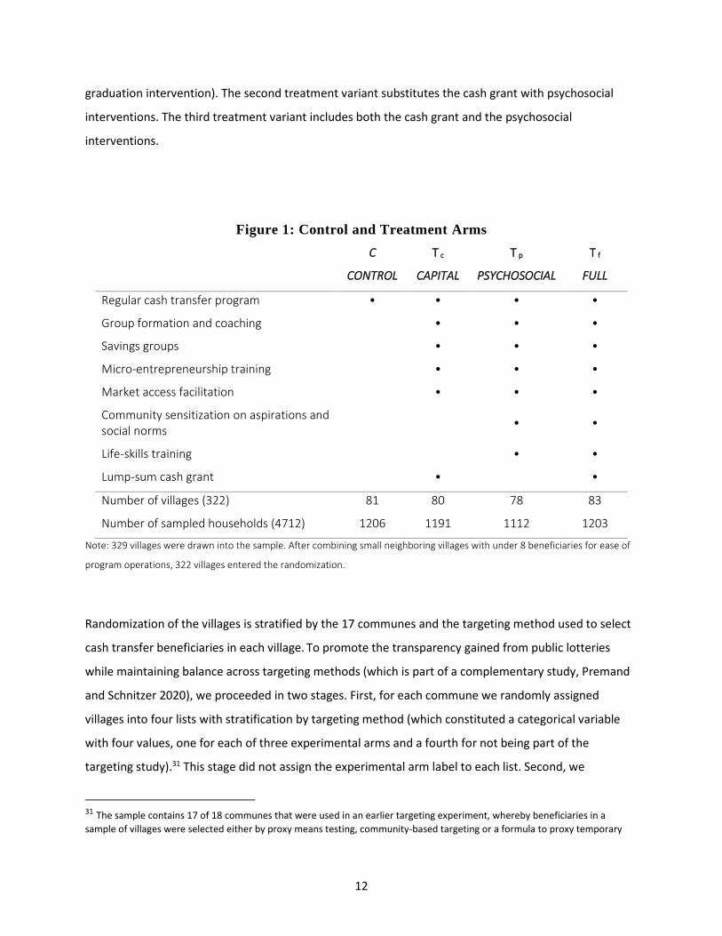
As is evident from Figure 1, all three treatment variants share a core set of interventions: group

formation and coaching, savings groups, entrepreneurship training, and market access facilitation. The

first treatment variant also includes a lump-sum cash grant (similar to the asset transfer in a traditional

29 While the program is largely government-led and government-implemented, it was funded by the World Bank. This made it possible to use streamlined financial management procedures and hire program staff on term contracts. Although the program staff had a profile similar to other government technical agents, they likely had stronger performance incentives. The World Bank and international NGOs provided technical support for the design and monitoring of the intervention, but the government agency was fully responsible for delivery and implementation. 30 The program reached 1 million individuals out of a rural population in poverty of 7 million (see World Bank, 2017). Note that,

as discussed further below, the program eligibility threshold is below the poverty line, and can be considered closer to an

extreme poverty line. About 80 percent of households are below the poverty line in program areas, but approximately the

poorest half of them is covered by the program.

12

graduation intervention). The second treatment variant substitutes the cash grant with psychosocial

interventions. The third treatment variant includes both the cash grant and the psychosocial

interventions.

Figure 1: Control and Treatment Arms

C T c T p T f

CONTROL CAPITAL PSYCHOSOCIAL FULL

Regular cash transfer program • • • •

Group formation and coaching • • •

Savings groups • • •

Micro-entrepreneurship training • • •

Market access facilitation • • •

Community sensitization on aspirations and social norms

• •

Life-skills training • •

Lump-sum cash grant • •

Number of villages (322) 81 80 78 83

Number of sampled households (4712) 1206 1191 1112 1203

Note: 329 villages were drawn into the sample. After combining small neighboring villages with under 8 beneficiaries for ease of

program operations, 322 villages entered the randomization.

Randomization of the villages is stratified by the 17 communes and the targeting method used to select

cash transfer beneficiaries in each village. To promote the transparency gained from public lotteries

while maintaining balance across targeting methods (which is part of a complementary study, Premand

and Schnitzer 2020), we proceeded in two stages. First, for each commune we randomly assigned

villages into four lists with stratification by targeting method (which constituted a categorical variable

with four values, one for each of three experimental arms and a fourth for not being part of the

targeting study).31 This stage did not assign the experimental arm label to each list. Second, we

31 The sample contains 17 of 18 communes that were used in an earlier targeting experiment, whereby beneficiaries in a

sample of villages were selected either by proxy means testing, community-based targeting or a formula to proxy temporary

13

organized a public lottery in each of the 17 communes to randomly assign each list to one of the four

experimental arms (three treatment or control). The lottery was organized by the cash transfer program

government team and held in the capital of the commune in presence of village chiefs or elders.

One limitation of this design is that we could not include a fourth treatment arm with “core components

only.” This implies that, while we can test the importance of including capital on top of the core and

psychosocial components (by comparing the “Full” arm to the “Psychosocial” arm), if the psychosocial

components change the marginal value of the capital, then we would not estimate the effect of

providing capital as part of a program without those psychosocial components. Likewise, we are testing

the importance of including psychosocial components on top of a design that includes the lump-sum

capital transfer (by comparing the “Full” arm to the “Capital” arm). Had there been a treatment arm

with just the “core” components (village savings groups, coaching, and entrepreneurship training), then

we could have estimated the marginal value of the psychosocial components to that treatment arm,

thus providing an estimate of the psychosocial components with and without accompanying lump-sum

capital transfers (and likewise for capital, with and without the psychosocial components).32

3.2 Sampling, Timeline and Data

Out of the 22,507 cash transfer beneficiaries that were assigned to the 4 treatment variants, 4,712

households from 329 villages were drawn into a sample for data collection. In each village, up to 15

households were sampled.33 Twenty-eight villages had fewer than 15 beneficiary households, resulting

in an average of 14 sampled households per village.

Figure 3 summarizes the study timeline. Baseline data collection took place between April and June

2017. The public lotteries took place after data collection in June 2017. The intervention was delivered

food insecurity, as detailed in Premand and Schnitzer (2020). Some villages were not sampled for the targeting study, thus the stratification had four strata, three for the different targeting methods and one for not being in the targeting study (in which case proxy means testing was employed for targeting). 32 Premand and Stoeffler (2020) study the effects of cash transfers through a RCT embedded in an earlier phase of the Niger program. They find that cash transfers increase consumption, savings and resilience to shocks, but on average have no effects on income-generating activities related to agriculture or household enterprises. Stoeffler et al. (2020) use a quasi-experimental design to study the impacts of cash transfers combined only with savings facilitation in a pilot that preceded the Niger cash transfer program. They find impacts on asset accumulation 18 months after program termination, but no effects on earnings or diversification in off-farm business activities. 33 All beneficiary households for which data were collected as part of the prior targeting study (Premand and Schnitzer, 2020) were included. Beneficiaries are those who were scheduled for at least one cash transfer payment on or before November 15, 2016. The remaining village quota was randomly selected among all the remaining cash transfer beneficiaries who were not sampled as part of the previous study.

14

between September 2017 and January 2019.34 Two follow-up surveys were collected. The first follow-up

took place in February and March 2019, a median of 6 months (3 to 9 months) post-intervention (after

the delivery of the lump-sum grant in treatment arms with the capital component). The second follow-

up survey occurred a year later in February and March 2020, a median of 18 months post-intervention

(after the delivery of the cash grants in treatment arms with the capital component).

The baseline survey covers the following topics: household structure, productive activities, off-farm

businesses, finance, housing, food security, cash transfers, gender attitudes, program preferences,

psychosocial well-being (discussed below and detailed in appendix B), food consumption and spending,

agriculture, livestock, fishing, assets, education and health spending, non-food spending, social

programs, transfers and shocks.35 The follow-up surveys include all of the baseline modules. In addition,

the modules on finance, cash transfers, gender, psychosocial well-being and livestock were expanded.

New sections were added on business practices, beneficiary health, business practices, and height and

weight for children 6-59 months old.36 The cash transfer beneficiary, generally a woman in the

household, is the primary survey respondent across all survey rounds. The head of household could

respond to questions on consumption, agriculture, assets, social programs, transfers and shocks.37

Table A.1 reports descriptive baseline statistics and balance tests across the experimental arms for a set

of pre-specified variables. Of beneficiaries, 99% are female and they are 38 years old on average. Among

the beneficiaries, 90% live in male-headed households, and about a quarter are in a polygamous union

with a household head. Less than 8% are literate and they have on average less than 0.5 year of

schooling. On average, the villages are 23 km from the capital of the commune, and beneficiaries take

34 The saving groups were set up in September 2017, community sensitization on social norms was carried out between January and April 2018, coaching started in May 2018, life and business skills training were completed in July 2018, and cash grants were disbursed between July 2018 and January 2019. Implementation was randomized in two phases. Each activity was implemented first in an ‘early’ group before being implemented in a ‘late’ group. Specifically, cash grants were disbursed in July-August 2018 for the early group, and in November-January 2019 for the late group. The randomization to the ‘early’ and ‘late’ groups confounds duration of exposure and seasonality, so that we do not consider it in the analysis. 35 A Living Standard Measurement Survey collected in 2014 by the National Statistics Institute of Niger served as a basis for the included consumption items, assets, and crop types. The questionnaire was developed in French. The psychosocial questions and hunger scales were translated in local languages. For the other modules, surveyors did on-the-spot translations to local languages after extensive training to coordinate translations. At baseline, 65% of surveys were conducted in Hausa, and 34% of surveys were conducted in Zarma. 36 At baseline, due to time constraints, some questions on agricultural plots and off-farm income generating activities were only

asked for those owned or managed by the beneficiary or head of household. The follow-up surveys collected information on all

plots and off-farm activities in the household. 37 In practice, the majority of beneficiaries responded to the entire survey, since heads of household were often traveling during the survey period.

15

about 70 minutes (via their usual mode of transportation) to get to the nearest market. On the whole,

the experiment is well-balanced.

The baseline response rate was 97.8% of sample households. In the 1st and 2nd follow-ups, 95.0% and

91.3% of sample households were successfully interviewed, respectively.38 Attrition at follow-up is

balanced across the treatment arms (Table A.1, bottom panel).

To complement the survey data, monitoring data were collected through the project administrative

information systems.39 Cost data were collected from financial systems. Information on implementation

quality was also collected through field visits and a qualitative process evaluation.

Table A.2 documents compliance with treatment assignment based on administrative data. Overall, the

share of treated households receiving intended benefits is very high. Across all treatment arms, the

participation rate in VSLA meetings was 92%, and the attendance rate in the micro-entrepreneurship

training was 95%. There was more variation in the delivery of individual coaching visits, with on average

52% of beneficiaries receiving coaching visits each month. Participation in other intervention elements

was also high. Across the psychosocial and full treatment groups, 94% of beneficiaries attended life skills

training and 89% the community sensitizations. Across the capital and full treatment groups, 99.9% of

beneficiaries received the cash grants.

3.3 Estimation Strategy

By comparing each treatment arm to the control group, the design allows us to identify the impact and

cost-effectiveness of the capital package, the psychosocial package, and the full package. In addition, we

identify the added value or marginal impacts of key elements of the interventions. By comparing the full

package to the psychosocial (respectively capital) package, we identify the added value (marginal

impact) of the cash grant (respectively psychosocial components) - net of potential complementarities

with elements of the core intervention component.

38 Of those consenting households interviewed at the baseline, 95.3% were successfully re-interviewed in the 1st follow-up and 91.3% in the 2nd follow-up. Due to the Covid-19 outbreak, the 2nd follow-up survey was suspended at the end of March 2020 without implementing a planned tracking phase. 39 Some information was collected at the individual level (e.g. participation in trainings, delivery of cash grant), and other information at a more aggregate level (number of beneficiaries per group or village participating in community sensitization, receiving individual coaching visits, etc.).

16

We estimate separate intent-to-treat treatment effects for each arm (treatment package) for pre-

specified outcomes based on the following specification:

𝑌𝑖,𝑡 = 𝛽𝑝,𝑡𝑇𝑝𝑠𝑦𝑐ℎ𝑜𝑠𝑜𝑐𝑖𝑎𝑙 + 𝛽𝑐,𝑡𝑇𝑐𝑎𝑝𝑖𝑡𝑎𝑙 + 𝛽𝑓,𝑡𝑇𝑓𝑢𝑙𝑙 + 𝑌0,𝑖 + 𝛾 + 𝜀𝑖 (1)

where Yi,t is the outcome of interest for household or individual i in the 1st or 2nd follow-up (t = 1 or t =2);

Tpsychosocial, Tcapital and Tfull are indicators for village assignment to the psychosocial, capital, or full

treatment package; γ is a vector of randomization strata fixed effects. We estimate this specification

separately for each follow-up. Standard errors are clustered at the village level, the unit of

randomization. To increase precision, we include a control for the outcome at baseline (Y0,i) when

available. When not available for a subset of households, we set the baseline control to the mean

outcome in the randomization strata and include a dummy for a missing measurement at baseline. ßp,t,

ßc,t and ßf,t are the main parameters of interest. They capture the impact of each treatment package for

cash transfer beneficiary households.40

To estimate the added value of the cash grant and psychosocial components net of complementarities

with the core package, we report three additional tests for each data collection round:

First, we test the added value of the cash grant with H0: 𝛽𝑓 -𝛽𝑝 = 0.

Second, we test the added value of the psychosocial interventions (the community sensitization

intervention and life skills training) with H0: 𝛽𝑓 -𝛽𝑐 = 0.

Third, we test for equality of treatment effects between the capital and psychosocial packages with: H0:

𝛽𝑐 -𝛽𝑝 = 0.

Finally, we test for equality of treatment effects between data collection rounds to uncover any

temporal effects (for each treatment arm separately). We focus the discussion mostly on results from

the 2nd follow-up.

The outcomes were pre-specified in a pre-analysis plan.41 We specified two primary outcomes:

consumption per adult equivalent and the (reverse of) FAO’s Food Insecurity Experience Scale (FIES, see

Ballard et al., 2013; Nord et al., 2016). In addition, we also report the Food Consumption Score (FCS, see

40 We had pre-specified that if a joint test across the two primary outcome variables failed to reject equality of the full and

capital packages, we would pool the full and capital arms in an additional specification. Psychosocial would remain a separate

treatment arm. In practice, we do not fail to reject equality and do not present this additional specification. 41 See https://www.socialscienceregistry.org/versions/52534/docs/version/document

17

WFP, 2008).42 We pre-specified a range of intermediary outcomes, discussed in Section 4, which capture

the pathways through which the interventions were expected to affect the primary welfare outcomes.

Tables A.3 and Table A.4 provide more details on variable construction. Appendix B also provides more

information on the psychosocial outcomes.

To account for multiple hypotheses, we calculate p-values adjusted within each treatment arm within

predetermined families of variables and report corrections in Table A.5. Following our pre-analysis plan,

we correct p-values controlling for both the false discovery rate (FDR) and the family-wise error rate

(FWER). The FDR is the expected proportion of rejected null hypotheses that are actually true, whereas

the FWER is the probability of incorrectly rejecting at least one true null hypothesis among all those

tested. The FWER is our preferred correction. Results are robust to corrections.

4. Results

4.1 Main welfare outcomes: Consumption and food security (Table 1)

We find statistically significant treatment effects on household consumption and food security for all

three packages at both follow-ups (Table 1, column 1). Impacts on per capita consumption per day are

between $0.09-$0.25 in the 1st follow-up (5%-13% relative to control). Impacts are larger for the full

package than the capital and psychosocial packages; and we cannot reject equality between the

psychosocial and capital packages. Impacts on consumption are sustained in the 2nd follow-up and

statistically significant at the 1% level for the three treatment arms ($0.12-$0.25, or 7%-15% relative to

control). Impacts for the full package are larger than the capital package in the 2nd follow-up, but we do

not reject equality between the full package and the psychosocial package (p=0.146). The point estimate

for the psychosocial package doubles between the 1st and 2nd follow-up, but we marginally cannot reject

equality between the two surveys (p=0.12). The difference between rounds is not statistically significant

for the full and capital packages either.

Results also show statistically significant and robust impacts of all three treatment packages on food

security in both follow-ups. Household food security (column 2), the (inverse of FIES with 12-month

recall), improves by 0.21-0.66, a 6%-20% change relative to control, corresponding to a decrease in 0.2-

42 Although it was pre-specified as a secondary outcome, the food consumption score provides another measure of food security that captures the eligible women’s dietary diversity. For this reason, we report it along with FIES in the main outcome table.

18

0.66 types of food insecurity situations over the past 12 months (out of eight possible types of food

insecurity situations). The eligible women’s dietary diversity (FCS, column 3) improves by 2.71-6.01

points over the 7 days prior to the survey (a 10%-22% improvement relative to control). Treatment

effects are sustained in the 2nd follow-up, with impacts of 0.47-0.63 on household food security (13%-

18% relative to control) and 2.78-6.11 on dietary diversity (9%-19% relative to control). Estimated

treatment effects of the psychosocial package are consistently smaller than the full and capital packages

in the 1st follow-up, but we cannot reject equality between the capital and psychosocial packages in the

2nd follow-up. These patterns are similar to those found for consumption and show that households

assigned to the psychosocial package catch up over time with households assigned to the capital

package.43

4.2 Eligible women’s revenues and labor supply (Tables 2 and 3)

One of the main objectives of the intervention was to improve household welfare by promoting

economic diversification and raising earnings in income-generating activities. Table 2 presents impacts

on individual-level productive revenues for the eligible woman. We focus on the eligible woman because

she is the main beneficiary, and turn to household-level effects in the next section. Revenues are

measured for 4 main types of activities: off-farm businesses (column 1), agriculture (harvest value,

column 2), wage earnings (column 3) and livestock (column 4). Overall, Table 2 shows large impacts on

revenues from off-farm household businesses, and (especially in the 2nd follow-up) livestock and

agriculture.

The intervention is particularly effective in increasing eligible women’s earnings from off-farm self-

employment activities. Strong positive impacts on business revenues are found for all three treatments

at both follow-ups (column 1). In the 1st follow-up, business revenues increase by $17-$36 per eligible

woman per month, which constitutes a very large increase of 76%-160% relative to control. Consistent

with the magnitude of welfare impacts between treatment arms, impacts on business revenues tend to

be larger for the full package, and smaller for the psychosocial package (although we cannot reject

equality between the full and capital packages). Results from the 2nd follow-up reveal similar patterns,

with impacts of $10-$21, or 49%-102% relative to control. We can reject equality of impacts between

43 Point estimates for the psychosocial package tend to be larger in the 2nd follow-up than in the 1st, and significantly so for the food security experience scale (p=0.067), though not the food consumption score (p=0.937).

19

rounds; estimates are relatively smaller in the 2nd compared to the 1st follow-up, but they remain of

large magnitude.

Impacts on eligible women’s livestock revenues are only statistically significant in the 1st follow-up for

the psychosocial package, while impacts in the 2nd follow-up are statistically significant for the capital

and full packages (column 4). We cannot reject equality of treatment effects between packages or

between rounds, however.

Substantial impacts are found on eligible women’s revenues from agriculture (as proxied by harvest

value) in the 2nd follow-up for the psychosocial and full packages (column 2). We can reject equality of

treatment effects between follow-ups for the psychosocial and full packages, with larger effects in the

2nd than in the 1st follow-up. The limited effects in the 1st follow-up are not surprising given the

intervention lasted until after the planting season. Interestingly, impacts from the capital package are

not significant and we can reject equality with the psychosocial and full packages in the 2nd follow-up,

suggesting that the cash grants are not the main drivers of impacts on agricultural revenues.

Lastly, wage employment is rare in the study sample, and treatment effects are limited (column 3). In

the 2nd follow-up, statistically significant treatment effects are found for the full package, though not for

the psychosocial or capital packages.44 Impacts on wage earnings are small in magnitude in absolute

terms. An increase in wage earnings was not necessarily expected because wage employment was not

directly promoted by the program. However, it is consistent with finding impacts on the use of paid

labor in agriculture and the intervention promoting social ties, as further discussed below.

Table 3 presents impacts on eligible women’s labor participation (days worked per month) for the same

break-down of economic activities as in Table 2. The number of days worked by eligible women in

income-generating activities increases substantially relative to control, especially in off-farm businesses

and livestock. As such, findings are generally consistent with results on revenues from income-

generating activities.

The time worked by eligible women in household businesses increase strongly by 2.2 – 3.7 days per

month in the 2nd follow-up (or 36%-61% relative to control) (Table 3, column 1).45 These impacts are

larger for the full package than the psychosocial package, but we cannot reject equality between the

44 Statistically significant treatment effects are found in the 1st follow-up for the capital and full packages, but we cannot reject equality between the three packages. 45 Effects for the 1st follow-up are significantly larger than in the 2nd follow-up, with increases of 3.6 – 4.9 days per month (or 58%-78% relative to the control group).

20

capital and full packages, or between the capital and psychosocial packages. Time worked by eligible

women on livestock activities also increases by 1.62-3.16 days per month in the 2nd follow-up (11%-21%

relative to the control group) (column 4). No significant change in time spent in agriculture is found in

any treatment arm, though this indicator has high variance (column 2). Point estimates for days spent in

salaried employment are small, positive, and mostly not significant (column 3).

Consistent with large increases in household welfare and food security, beneficiaries show large and

meaningful improvements in revenues and labor supply. We now present effects on intermediate

outcomes at the household level.

4.3 Household economic diversification and income-generating activities (Table 4)

Table 4 documents impacts on household income diversification. It contains an index of the number of

income sources (column 1), the number of crop types (column 2), off-farm business types (column 3),

livestock types (column 4) and wage job types46 (column 5). (See Table A.3 for details on variable

constructions). Results on economic diversification at the household level are highly consistent with

results from section 4.2 on eligible women’s revenues and labor supply. Large impacts are found on

household economic diversification (column 1): the number of income sources significantly increases for

all three treatment arms and both follow-up surveys. Impacts range from 0.34-0.49 additional income

sources in the 1st follow-up (7%- 10% relative to control), and 0.19-0.38 additional income sources in the

2nd follow-up (4%-8% relative to control). We cannot reject equality between the two follow-ups,

despite smaller point estimates in the 2nd follow-up. Impacts are larger for the full package than the

psychosocial package at both follow-ups, but differences between other packages are not significant. As

for eligible women, impacts on diversification are associated with increases in the number of off-farm

household business types (column 2) as well as the number of livestock types (column 5). Effects on

diversification in agriculture (column 3) or wage jobs (column 4) are small and mostly not statistically

significant.

These results are consistent with increased diversification in off-farm activities, which the intervention

promoted. We now discuss in more detail impacts on income-generating activities, and we distinguish

46 The survey only asked about wage jobs for the eligible woman and the household head.

21

effects along the extensive and intensive margins. We start with off-farm household businesses, before

discussing agricultural and livestock activities.

4.3.1 Off-farm household businesses (Table 5)

Table 5 documents large impacts on participation and earnings in off-farm businesses for all treatment

arms at both follow-up surveys. Impacts tend to be larger for the full package, and we can reject

equality with the psychosocial and capital packages for several variables. Impacts are sustained in the

2nd follow-up survey, although point estimates tend to be smaller than in the 1st follow-up survey, with

statistically significant differences between rounds.

The three intervention packages lead to substantial impacts on participation in off-farm business

activities along the extensive and intensive margins. The share of households operating an off-farm

business activity increases by 8-10 percentage points in the 2nd follow-up (from a mean of 71 percent in

the control group) (Table 5, column 1), driven by an increase in small businesses processing agricultural

products and commerce. The share of households reporting that these businesses are their main activity

also increases by 6-12 percentage points in the 2nd follow-up (from a mean of 0.26 in the control group)

(column 2). The number of businesses increases by 0.25-0.35 in the 2nd follow-up (from a mean of 1.10

in the control group) (column 3). Impacts on participation in household businesses are highly significant

for the three treatment arms. We cannot reject equality of treatment effects between the capital and

psychosocial packages. Treatment effects tend to be larger for the full package. The magnitude of the

impacts is substantial in both follow-ups, but tend to be smaller in the 2nd follow-up.

Consistent with the observed increase in participation, the interventions lead to large increases in

investments in off-farm businesses (column 4). Investments measured in the 1st follow-up capture the

intervention period. Investments in household businesses increase by $19-$39. Investments are

significantly larger for the full package ($39) than the capital package ($28), which itself is significantly

larger than the psychosocial package ($19). Treatment effects on investments in off-farm businesses are

of substantial magnitude, representing between 80% and 162% of investments in the control group. At

the same time, these investments represent a small share of the cash grants (less than 15%).

Interestingly, impacts on investments in the 2nd follow-up remain positive, even though it is beyond the

intervention period ($8 in the psychosocial arm, $14 in the psychosocial arm, and $15 in the full arm),

22

indicating sustained investments over time. The estimated effects are smallest in the psychosocial arm,

but we cannot reject equality between the capital and full treatment arms.

The intervention induces very large impacts on revenues and profits from off-farm businesses (columns

5 and 6). Monthly revenues increase by $36-$62 in the 1st follow-up, representing 50%-84% of revenues

in the control group. This leads to increases in profits by $11-$20 in the 1st follow-up, again a very large

magnitude. These impacts on profits are about a third of impacts on revenues, and 39%-70% of profits in

the control group. They also represent $136-$244 per year per household in the 1st follow-up. These are

large impacts relative to impacts on consumption, which are $131 (psychosocial package), $228 (capital

package) and $373 (full package) per household per year. As such, increases in business profits explain

all of the observed consumption impacts for the psychosocial package ($136/131), respectively 74%

($169/228) for the capital package and 65% ($244/373) for the full package. Impacts are largest for the

full package, though we cannot reject equality of impacts between the psychosocial and capital

packages. Results are very robust for the 2nd follow-up survey. We can reject equality of impacts

between rounds for the capital group only, and point estimates are smaller in the 2nd follow-up survey,

but remain of large magnitude.

Lastly, the interventions lead to improvements in business practices, but the effects are relatively small

(column 7). An index shows that treated households increase their use of healthy business practice by

0.16-0.25 standard deviation in the 2nd follow-up.47 Impacts are robust across treatments, but

significantly higher in the full package than in the psychosocial package.48 Overall, note that the use of

these practices remains low. Also note that these results might in part be driven by an increase in the

share of households reporting off-farm business activities as their primary activities in the treatment

group. Even though beneficiaries of all packages receive the same micro-entrepreneurship training and

coaching, this could partly explain differences across arms.

47 This reflects the use of an additional 0.7 to 0.9 more healthy business practices in their primary activity (from a mean of 2 business practices in the control group). 48 Similar results are found in the 1st follow-up survey. We can reject equality of coefficients between the two rounds, with estimates of slightly larger magnitude in the 1st follow-up. The impact on the index of healthy business practices is driven by robust impacts across its elements: knowing production costs, knowing profitability, setting sale targets, changing suppliers, negotiating prices of supplies, studying suppliers, studying competitors, studying customers, etc.

23

4.3.2. Agriculture (Table 6)

Table 6 presents estimated treatment effects on a set of outcomes related to agriculture, encompassing

production, input usage and crop sales.49

Recall that the productive interventions lasted until after the planting season, and results on production

are unsurprisingly mixed in the 1st follow-up: the psychosocial and full packages have a modest impact

on area cultivated but no statistically significant impact on production.50 All three packages raise input

usage, participation in the output market, and crop sales, however.51

The interventions have substantial effects on production in the 2nd follow-up. The psychosocial and full

packages increase harvest value by $90 and $79, respectively (Table 6, column 3). The point estimates

correspond to increases of 28% and 25% relative to the control group. Interestingly, the capital package

does not induce any detectable impact on harvest value, suggesting that the cash grants are not the

main drivers of impacts on agricultural revenues. Note that total production decreases on average from

$539 in the 1st follow-up to $315 in the 2nd follow-up. Such a large decline cannot be explained by the

changes in inputs nor by self-reported shocks shown in column 4. We cannot rule out, however,

weather-related shocks that could have affected production negatively.

There is no detectable effect on area cultivated in the 2nd follow-up, but we find positive and significant

effects on input usage. The capital and the full packages increase chemical fertilizer usage by 5-6

percentage points, or 30%-33% relative to control (columns 5-8). We reject equality of impacts between

the full and the psychosocial arms, and between the capital and the psychosocial arms. Households

assigned to the full package increase their use of phytosanitary products and hired labor, too.

The interventions increase participation in the output market (columns 9-11). In the 2nd follow-up, sale

value increases by $10 for the psychosocial package and by $7 for the full package (column 10). While

these points estimates are large relative to the control mean ($30), they are lower than estimates from

the 1st follow-up. Because average production declines, households may reduce their crop sales,

49 The interventions do not alter household’s likelihood to be involved in agriculture. The point estimates in column 1 are all small, similar in both follow-ups, and none is statistically significant. We do not see impacts on crop choice either. 50 The psychosocial and full packages both increase area cultivated by around 0.30 hectares in the 1st follow-up, an 8.5% increase relative to the control mean. While the point estimate for the capital package is not statistically significant, we cannot reject equality with other packages. These modest changes in area cultivated do not translate into a significant increase in production (column 3). 51 The capital and the full packages increase the use of chemical fertilizers by about 5 percentage points and all packages increase the use of paid labor. Crop sales (column 10) increase by approximately 30% for all three packages. The estimated effects on sales are corroborated by increases in the probability of selling at least one crop (column 9) and the percentage of production value commercialized (column 11).

24

especially if they have access to other sources of revenues such as those provided by the capital and full

packages.

4.3.3 Livestock (Table 7)

Table 7 shows estimated treatment effects on livestock, including outcomes measuring the current stock

(columns 1-2), the flow of livestock over time (columns 3-4) and the revenues derived from livestock

activities (column 5).

All three treatments have positive and significant impacts on herd size (column 1), and livestock asset

value (column 2). In the 2nd follow-up, livestock count, measured in tropical livestock units,52 increases

by 0.31 units for the psychosocial package, 0.52 units for the capital package, and 0.80 units for the full

package. Because these estimates are similar between rounds, it is noteworthy that a time bound

program can generate large impacts on livestock accumulation that are sustained over time.

Results indicate that households that receive the cash grant (by being assigned to the capital or the full

package) increase the value of livestock by an amount approximately equivalent to the grant, and that

this effect persists over time. In the 2nd follow-up, livestock asset value increases by $260 for the capital

arm and by $330 for the full package. The magnitudes of those effects are large compared to a grant

amount of $325. We cannot reject equality between follow-ups. The psychosocial package, which did

not include a cash grant, exhibits a smaller increase in livestock value (of $112) that is statistically

significant in the 2nd follow-up. The capital and full packages have significantly higher livestock values

than the psychosocial package at both follow-ups, suggesting that the cash grant contributes to livestock

investments.

The three treatments impact flow outcomes (columns 3-4) in the 1st follow-up,53 but these effects

mostly vanish by the 2nd follow-up. Annual changes in tropical livestock units (column 3) are negative,

relatively small and not statistically significant. Similarly, the impacts on livestock purchases are smaller

in magnitude in the 2nd follow-up for the three treatment arms, and statistically significant for the full

package only. This suggests that beneficiaries do not keep accumulating livestock after the end of the

52 See Table A.3 for a detailed definition. The index gives different weights to small and large animals. 53 The capital and full arms lead to an annual increase (in TLU) of 0.35 and 0.23. The capital and full packages increase livestock purchases by $98 and $107. These figures represent approximately 30% of the cash grant.

25

intervention. It also contrasts with results on household off-farm businesses, where sustained

investments are observed after the intervention.

Household livestock revenues increase across all three arms in the 2nd follow-up.54 Revenues increase by

$37 for the psychosocial package. The capital and the full packages increase revenues by $69 and $71.

Relative to the control group, these estimates correspond to a 28%-54% increase.55

The results provide some insights on how households invest in livestock. The estimates in columns 1-2

(stocks) are essentially the same in the two follow-ups. There are some initial changes or adjustments in

flows (columns 3 and 4) in the 1st follow-up which have almost vanished by the 2nd follow-up. One

possible interpretation is that some households purchase livestock in the 1st period and sell it in the 2nd

period. This is consistent with the effects on livestock revenues that are mostly detectable in the 2nd

period.

4.4 Assets and savings (Tables 8 and 9)

We first investigate the effects of the interventions on the value of assets owned by the eligible women

and their households. The full and capital packages include a cash grant that could have a direct impact

on the purchase of new assets, while all packages could also induce the purchase of assets through the

positive impacts on revenues shown in section 4.2. Table 8 presents results for agricultural assets, non-

agricultural assets and household assets.

The interventions only induce a modest increase (10% relative to control) on agricultural asset values

(which include items such as plows and pumps) that is marginally significant for the full package in the

2nd follow-up only (Table 8, column 1).

We find evidence that all packages increase the value of business assets (column 2) in the 2nd follow-up

(while the effect is statistically significant only for the full package in the 1st follow-up). The effects are

relatively large compared to the control mean (for example, an increase of 32% for the full package).

However, reported business asset values are low across all arms, representing 3% of productive asset

54 The revenues include proceeds from animal sales but exclude sales of secondary livestock products such as milk or eggs. 55 Only the full treatment raises livestock revenues substantially in the 1st follow-up. The point estimate in column 5 implies an increase of revenues by $46 (33% increase relative to the control mean). The estimate is not statistically different from that of the psychosocial arm, however.

26

values in the control group, and even less in the treatment arms.56 Earlier results show that the three

packages have a large effect on off-farm business income (Table 2) and investments (Table 5).

Contrasting those results with the more modest effects on business assets illustrate that off-farm

businesses supported by the program – generally petty trade and food transformation activities – are

not very intensive in fixed capital.

We also find that the psychosocial and full packages affect the number of household non-productive

assets (measured with an asset index), such as beds or pots (column 3). At both follow-ups, we reject

equality of impacts between the full and the capital packages, but not between the full and psychosocial

packages.

We now turn our attention to the results on several outcomes related to households’ financial

engagement (Table 9). Saving behavior is an important outcome in the theory of change of the program.

The VSLA component, which is part of all treatment arms, aims to facilitate the creation of savings

groups and to provide technical support to their management. We first test whether the treatment arms

change households’ participation to savings group either in a VSLA, which is the type of savings group

promoted by the program, or in a tontine (which are informal ROSCAs common in the Sahel region).

Results in columns 1 and 2 show estimated treatment effects on the probability to be part of a savings

group, respectively the total amounts deposited over the last three months. Due to issues in the

measurement of those outcomes in the 1st follow-up, we focus on results in the 2nd follow-up.57 We find

that all treatments have large effects on participation in savings groups (27, 31 and 33 percentage points

56 This measure is potentially noisy, as the survey asked for total asset values for each of their businesses, not disaggregated by each asset. 57 For completeness, we present results for both follow-ups in Table 9, though there are some inconsistencies in results for the

1st follow-up. Although we find positive effects on the probability to be part in a VSLA/tontine (column 1) for all packages in

both follow-ups, the effects are much larger in the 2nd follow-up. Similarly, the three treatment arms increase the amount of

deposits (column 2) in the 2nd follow-up, but have no effect in the 1st follow-up. We believe that this difference is driven by a

measurement issue in the 1st follow-up survey. Our data shows (column 1) that most of the respondents in the control group

(93 %) declare participating in a VSLA/tontine in the 1st follow-up, compared to only 53% in the 2nd follow-up. Disaggregating

the participation in saving groups by tontine and VSLA (Table A.6, columns 3 and 4) shows that 84% of the control declare

participating in a VSLA and 23% in a tontine in the 1st follow-up. This level of participation in a VSLA in the control at 1st follow-

up appears very unlikely. It may come from the way the question was phrased in the 1st follow-up. For instance, it is possible

that respondents included in this response their participation in beneficiary groups established for the child development

promotion activities as part of the cash transfer program (see Premand and Barry, 2020). These activities were implemented

consistently across all treatment and control villages in the sample we analyze in this paper. As part of these groups,

beneficiaries met to discuss topics related to child nutrition and development. The activities did not cover savings or productive

activities, although beneficiaries sometimes made small contributions for cooking demonstrations. The difference in results

between the 1st and 2nd follow-up survey may also have been influenced by the recall period, which was 24 months in the 1st

follow-up but 12 months in the 2nd follow-up, or some misunderstanding on the question during the training of surveyors,

although results remain unchanged when we control for surveyor fixed effects (Table A.6, column 2).

27

for the psychosocial, capital and full arms respectively). The full package has a greater impact than the

psychosocial one, but we do not reject equality between the capital and psychosocial arms or the full

and capital arms. Consequently, we find similar patterns in the effects on the level of deposits made

over the three months before the survey (column 2), ranging from a 92% (psychosocial arm) to a 159%

(full arm) increase compared to the control. The interventions also increase deposits in other savings

instruments outside the household (column 3), although saving in instruments other than groups is

uncommon. Effects are concentrated in the full and capital arms in the 2nd follow-up.

Most of the cash transfer beneficiaries do not report borrowing (only $9 yearly in the control) and only

the full package changes the average outstanding loan amount in the 2nd follow-up (column

4). However, the (full and capital) packages that include a cash grant increase the amount beneficiaries

lend to others outside the household in the 1st follow-up, although the effects are small and are not

sustained in the 2nd follow-up.

Finally, the program does not have much effect on transfers into (column 6) the households, though it

does increase transfers out (column 7). Households in the control receive a large amount ($176) of

transfers yearly (these transfers may come from anyone who is not part of the household, but do not

include government transfers such as the safety net program) and only the capital arm at the 2nd follow-

up reduces this amount (by $28). The transfers made to other households are much more limited ($9.5

per year in the control). The three treatments increase yearly transfers out by $5-$8, which are large

relative effects (57-85% relative to control), but remain small in absolute terms.

4.5 Psychological and social well-being (Tables 10 and 11)

Tables 10 and 11 report the impacts on psychological and social well-being among eligible women,

respectively. We measure psychological well-being through a series of indices: a mental health index

(capturing elements such as depression and life satisfaction), a social worth index (including self-efficacy

and social standing), and a future expectations index (covering social status, life satisfaction and child

status).58

58 Appendix B and Table A.4 detail the content and construction of each index. Results from components of each index are provided in Table A.7 (mental health index components), Table A.8 (social worth index components) and Table A.9 (future expectation index components).

28

We find that all three packages have a positive, statistically significant impact on the mental health,

social worth and future expectations of eligible women, and that these impacts are sustained over time

(Table 10). The full package has significantly higher impacts than the other two packages in the first

follow-up, with coefficients approximately double the magnitude of those of the capital and

psychosocial packages. Yet in the 2nd follow-up, we cannot reject equality between the full and

psychosocial packages. The capital treatment has the smallest point estimate of the three packages

(though we cannot reject equality between the capital and psychosocial packages in most cases).

Impacts on mental health grow from 0.1 to 0.21 standard deviation between the 1st and 2nd follow-up

for beneficiaries of the psychosocial package (column 1). These results are driven by improvements in

depression and disability. In contrast, the impacts on social worth and future expectations are

somewhat reduced over time, but that reduction is statistically significant only for the full package

which has the highest point estimates in both follow-ups (columns 2 and 3). For social worth, the

reduction seems to be driven by some attenuation in the social standing, while self-efficacy on the other

hand appears fairly stable.

Table 11 displays results related to dimensions of social well-being. The first two columns examine

impacts on a social support index (containing role models as well as people beneficiaries could go to for

advice on economic activities and conflict) and a financial support index (whether beneficiaries can raise

funds from others around them).59 Results show that all three packages have positive impacts on these

indices at both follow-ups, with the full package showing the greatest impacts on financial support.

Notably, for the financial support index, only the psychosocial and full packages increase the

beneficiary’s number of financial supporters, i.e., those they could go to for financial help, at both

follow-ups. While these positive impacts on financial and social support persist over time, they

significantly weaken between the 1st and 2nd follow-up for all packages, except for social support in the

psychosocial package. For the social support index, the observed decline is spread across most of the

component variables, with the notable exception of the number of market intermediaries which, if

anything, increases over time.

Column 3 summarizes intra-household dynamics, which include variables related to the quality of the

relationship with the respondent’s partner as well as with the respondent’s household. None of the

59 Appendix B and Table A.4 detail the content and construction of each index. Results from components of each index are

provided in Table A.10 (social support index), Table A.11 (financial support index), Table A.12 (future expectation index), Table

A.13 (social cohesion and closeness to community) and Table A.14 (collective action index).

29

packages statistically significantly improves overall intra-household dynamics at 18 months post-

intervention, although the psychosocial package has a small positive effect on overall intra-household

dynamics in the 1st follow-up.60

Column 4 presents impacts on a social cohesion and community closeness index (including elements

such as trust within the village and community inclusiveness). In the 1st follow-up, the psychosocial and

full packages have equivalent, significant impacts on social cohesion, and these are greater than the null

effects of the capital package. In the 2nd follow-up, however, all three packages show positive impacts

on this social cohesion index, with no significant difference across the packages. The main variable that

seems to be driving this result is trust in other women in the village.

Finally, column 5 shows a collective action index that captures engagement in associations as well as

donations and volunteer work. The collective action index significantly increases for all packages with

impacts sustained over time and with positive movement across almost all elements of the index. Here

again, the full package has a stronger effect than the capital package 18 months post-intervention.

Consistent with other measures of social well-being, the effects weaken slightly between the 1st and the

2nd follow-up, even though they stay strongly statistically significant.

Overall, these results document widespread improvements across dimensions of psychological and

social well-being as well as community engagement and collective action, particularly for the

psychosocial and full packages. These results indicate significant impacts on dimensions of women’s

social empowerment. Overall, the findings are highly consistent with the observed improvements in

economic welfare and participation in income-generating activities.

4.6 Women’s control over decisions and resources (Table 12)

Table 12 summarizes treatment effects on women’s decision-making power and productive agency

using two indices. The first index covers her decision-making and control over her earnings and

productive activities, and the second index summarizes her decision-making and control over household

resources and household decisions such as family planning and children’s education.61

60 It also significantly improves the partner dynamics index in the 2nd follow up (Table A.12). 61 Results from components of each index can be found in Tables A.15 (control over earnings and productive agency) and Table A.16 (control over household resources).

30

We find that the interventions have a positive and significant impact on the beneficiary’s control over

her earnings and productive agency. This is true for all three packages and sustained over time. The full

package has significantly larger impacts than either the psychosocial or capital package in the 1st follow-

up. Over time, the full package has slightly weaker impact. The positive effects on this index are driven

mainly by the off-farm business and livestock domains, which is consistent with patterns documented in

sections 4.1 and 4.2. For example, beneficiaries receiving the full package are 22 percentage points more

likely to own an off-farm business and 16 percentage points more likely to own livestock (Table A15,

columns 9 and 10). Effects are also significant for the psychosocial and capital packages, albeit smaller

for the package without the grant. This translates into increased decision-making and control over these

activities. All packages significantly increase the influence the beneficiary has on decisions concerning

the household’s off-farm businesses, and the full and capital packages increase her influence on

decisions related to livestock and her control over livestock revenues.

Conversely, we see no impact on the decision-making power of beneficiaries over household resources

and related domains, whether six or 18 months post-intervention. A closer look at the income gains may

provide some explanation for this. Looking at the main sources of revenues, Table 2 shows significant

gains for the beneficiary. However, a comparison with Tables 5, 6, and 7 shows that the increase in

beneficiary revenues is not over fifty percent of the increase in total household revenues. To illustrate,

take the case of the full package in the 2nd follow-up. The beneficiary increase in business revenues is 44

percent of the total household gain in this realm, with the corresponding figures for harvest and

livestock revenues at 17 and 23 percent respectively.62 These numbers suggest significant spillovers

within households. They also indicate that the beneficiary woman’s share of household income is not

increasing. This might hence explain why we do not see increased bargaining power leading to control

over household decisions.

Taking these results together with the results in section 4.5, we see significant improvements in a

number of dimensions of women’s empowerment – their engagement in the community, their collective

action and their control over their own economic activities. This is consistent with the impacts of

graduation programs found when using a broad range of indicators (as in Bedoya et al., 2019), in

contrast with more limited results from the original graduation studies based on narrower measures

(Banerjee et al., 2015b). However, as the household head’s income rises as well, we do not see

62 These figures are obtained by comparing estimated impacts on the beneficiary’s revenues in Table 2, with corresponding estimates of impacts on household revenues (respectively in Table 5, column 5; Table 6, column 3 and Table 7, column 5).

31

significant gains in intrahousehold interactions or decision making, which likely depend on her relative

position in the household rather than absolute income gains.

4.7 Children’s outcomes (Table 13)

Table 13 documents impacts on children, specifically school attendance (column 1), an index of child

labor capturing participation in income-generating activities (column 2), an index of participation in

household chores (column 3), and an anthropometric measure capturing the weight for height z score

(used to proxy wasting, column 4). The point estimate for school attendance is positive and statistically

significant for the capital package (6 percentage points, or 14% relative to control). However, it is not

significant in other treatments. We find an increase in labor and chores for children, potentially due to

the increase in income-generating activities in the household. This is consistent with the increases in

eligible women’s participation in economic activities. There is no difference between packages in the 2nd

follow-up, though effects are larger in the full and capital package in the 1st follow-up. Children’s

participation in housework (such as cleaning) also increases in the 1st follow-up, but the effects are not

statistically significant in the 2nd follow-up.63 This change over time could be due to pressure on eligible

women’s time during the intervention, which may have induced a temporary shift of household chores

toward children. Lastly, no statistically significant effect on anthropometrics is found (although the point

estimates are negative).64 This shows that large increases in welfare, food security and revenues from

income-generating activities do not necessarily translate into improvements of children’s

anthropometrics.65

5. Cost-Benefit Analysis (Table 14)

Table 14 presents cost-benefit calculations. Panel 1 details program costs based on the administrative

data, per beneficiary of each intervention package.66 In 2016 PPP US dollars, total costs are $263 for the

63 The effect on children’s participation in housework is driven by girls, with no effect for boys. 64 No statistically significant effects are found on other anthropometric variables, such as weight for age or height for age z-scores. 65As such, the results are consistent with earlier findings on the Niger cash transfer program showing that improvements of household welfare or food security do not induce improvements in children’s outcomes (Premand and Barry, 2020). Muted impacts of cash transfers on anthropometrics were also observed in Burkina Faso (Akresh et al., 2013). 66 We do not account for cash transfer program costs and the cost of the underlying social protection systems (targeting, payment,…) since these are incurred for the control group as well.

32

psychosocial package, $482 for the capital package and $584 for the full package. The lump-sum cash

grant ($321) is clearly the main cost driver.67 In comparison, the psychosocial interventions (community

sensitization and life skills) are much cheaper ($102). This is key for the relative cost-effectiveness of the

capital and psychosocial packages.

Panel 2 summarizes estimated benefits. The calculations are conservative as they only consider welfare

impacts on consumption, without accounting for impacts on assets or psychosocial well-being.68 We

consider various scenarios regarding the sustainability of impacts after the 2nd follow-up survey. First,

we consider zero impacts after the 2nd follow-up survey (scenario A). We then consider various yearly

rates of dissipation of impacts, including 75% (scenario B1), 50% (scenario B2) and 25% (scenario B3).

Lastly, we assume impacts are sustained in perpetuity (scenario C).69 We use a 5% discount rate.

Panel 3 presents the benefit-cost ratios. Importantly, row 9 shows that the benefit-cost ratios are above

1 for the psychosocial package, and almost equal to 1 for the full package, even considering benefits end

after 18 months. The results are remarkable as the psychosocial package is cost-effective even when

assuming that no program impact is sustained after the 2nd follow-up. Benefit-cost ratios are slightly

lower for the full package, though the orders of magnitude are close and the full package nearly reaches

its break-even point based on consumption impacts observed up to 18 months post-intervention. We

cannot reject equality of the benefit-cost ratios for the psychosocial and full package (p= 0.34). On the

other hand, the capital package has a lower benefit-cost ratio, due to the relatively large cost of the cash

grants and the limited additional consumption impacts they generate. We can reject equality of the

benefit-cost ratio between the psychosocial and capital package (p= 0.030), as well as between the full

and capital package (p= 0.026). Note, however, that impacts on assets are at times larger in the capital

and full package, and not accounted for in cost-benefit analysis based on consumption alone. These

results are robust under alternative discount rates of 5%, 7% and 10%. Row 10 presents results under

alternative rates of dissipation. Results again show large benefit-cost ratios for the psychosocial and full

67 Panel 1 in table 14 lists cash grant costs that are slightly higher than the cash grant value of 80,000 XOF ($127, or $311 in 2016 PPP) because it also accounts for operational and payment costs. 68 Cumulated consumption impacts are calculated as half the impacts on yearly consumption in the 1st follow-up plus impacts on yearly consumption in the 2nd follow-up. Estimated consumption impacts amount to $131 (psychosocial package), $228 (capital package) and $373 (full package) per household per year in the 1st follow-up, and $298 (psychosocial package), $196 (capital package) and $425 (full package) terms per household per year at 2nd follow-up. 69 While this is the least conservative scenario, it is the benchmark case used by Banerjee et al. (2015b), which facilitates comparisons, see conclusion.

33

packages. The capital package becomes cost-effective when assuming a rate of dissipation of 45% per

year after the 2nd follow-up.70

The high cost-effectiveness of the intervention is further illustrated by internal rates of return (IRR) that

are positive and high across most assumptions. IRR are 13% for the psychosocial package without

assuming any sustained impacts after the 2nd follow-up. With a dissipation of impacts of 50% per year

after the 2nd follow-up, IRR are 39% for the psychosocial package and 21% for the full package, while the

capital package almost reaches break-even point (IRR=-2%). IRR reach 70% (psychosocial package), 33%

(capital package) and 53% (full package) when assuming sustained impacts.

6. Conclusion

We document strong impacts of three variants of a multi-faceted social protection program on

consumption and food security six and 18 months post-intervention. These welfare improvements are

consistent with large observed increases in earnings from women-led income-generating activities, in

particular off-farm self-employment and livestock. Savings and asset accumulation also increase. We

find substantial impacts across several dimensions of psychological and social well-being. The

interventions increase women’s social empowerment and control over their income-generating

activities and earnings, although this does not carry through to a stronger say in household decision-

making.

In general, results are very robust between treatment arms. The full package tends to have the largest

impacts on welfare, food security and income-generating activities. Only small differences in impacts on

intermediate outcomes emerge over time between the capital and psychosocial packages. For instance,

the psychosocial treatment catches up with the capital treatment in some dimensions of welfare and

food security by the 2nd follow-up survey. The psychosocial treatment induces larger effects on

70 The full package is nearly cost-effective in the 2nd follow-up, and would be cost-effective assuming a 92% yearly dissipation rate. In panel 3, impacts are assumed constant 1-6 months post-intervention (equal to half the yearly impacts estimated in the 1st follow-up), as well as 7-18 months post-intervention (equal to yearly impacts estimated in the 2nd follow-up). Table A.17 provides results assuming linear growth between the end of the intervention (assuming zero impact at that point) and the 1st follow-up, as well as between the 1st and 2nd follow-ups. Results again show the largest ratio for the psychosocial package, followed by the full and capital packages. These estimations are more conservative. We can reject equality between the full and capital package (p= 0.055), but not between the psychosocial and capital package (borderline, with p= 0.129) and between the full and capital package (p= 0.677). The full package is cost-effective if impacts dissipate at a rate of 77% per year post-intervention, the psychosocial package, 92% per year post-intervention, and the capital package, 44% per year post-intervention.

34

agricultural revenues than the capital treatment, while the capital treatment induces larger effects on

livestock and asset accumulation than the psychosocial treatment. Improvements across dimensions of

psychological and social well-being as well as community engagement and collective action are

widespread but particularly strong for the psychosocial and full packages.

The magnitude of impacts on welfare is large across packages, but the psychosocial components are

cheaper than the lump-sum cash grant. In fact, cumulated impacts on consumption 18 months after the

end of the intervention already exceed the cost of the psychosocial package and nearly reach the break-

even point for the full package. Overall, the psychosocial package is cost-effective based on

consumption impacts alone. The full and capital package are cost-effective under weak assumptions

about the sustainability of impacts beyond the 2nd follow-up, even without considering other observed

benefits such as asset accumulation or improvements in psychological well-being. As such, these results

show the potential value of addressing psychosocial constraints as well as capital constraints in multi-

faceted social protection interventions.

The results also illustrate the value of delivering multi-faced interventions through government-led

national cash transfer programs. The program costs ($ 263 PPP for the psychosocial package, $ 482 PPP

for the capital package and $ 584 PPP for the full package) are substantially lower than similar

graduation programs implemented in other contexts: $ 1,475 PPP in India, $ 4,215 PPP in Ethiopia, $

5,483 PPP in Ghana, $ 6,044 PPP in Pakistan (Banerjee et al., 2015b), or $6,183 PPP in Afghanistan

(Bedoya et al., 2019).71 The Niger intervention was specifically designed in a cost-conscious way, to

ensure it could be scaled-up through government systems. Assuming impacts last for perpetuity (as in

the benchmark case in Banerjee et al., 2015b), the benefits in Niger are 20.9 times larger than costs for

the psychosocial package, 13.5 times larger for the full package, and 7.6 times larger for the capital

package. As such, and strikingly, the benefit-cost ratios estimated in Niger are 2-5 times larger than

those in Banerjee et al. (2015b) for India (433%), 3-8 times larger than those found for Ethiopia (260%),

as well as 1.5-4 times larger than those for Afghanistan (Bedoya et al., 2019). It is noteworthy that the

government-led Niger intervention is highly cost-effective even compared to traditional graduation

programs implemented by NGOs elsewhere. As such, the results highlight models to scale up multi-

faceted economic inclusion interventions for extreme poor households through government systems.

This paper is the first of a multi-country RCT that also includes Burkina Faso, Mauritania and Senegal.

The promising results from the Niger site will need to be confirmed following data collection in other

71 We express costs in 2016 PPP for comparison.

35

sites. In line with the pre-analysis plan for this research program, future work will include a pooled

analysis across the four countries, a finer assessment of heterogeneity and mechanisms, as well as

research of the role of the multi-faceted programs in fostering resilience and helping households

mitigate the effects of exogenous shocks. Additional research in Niger will also deepen the analysis of

intra-household dynamics and psychosocial mechanisms.

References Ajayi, Kehinde, Smita Das, Léa Rouanet, and Clara Delavallade. Forthcoming. “Gender Differences in Socio-

Emotional Skills in Sub-Saharan Africa.” Mimeo. Akresh, Richard, Damien De Walque, and Harounan Kazianga. 2013. “Cash Transfers and Child Schooling:

Evidence from a Randomized Evaluation of the Role of Conditionality.” World Bank Policy Research Working Paper Series, no. 6340. https://www.doi.org/10.1596/1813-9450-6340.

Alderman, Harold, and Ruslan Yemtsov. 2014. “How Can Safety Nets Contribute to Economic Growth?” World Bank Economic Review 28 (1): 1–20. https://doi.org/10.1093/wber/lht011.

Andrews, Colin, Aude de Montesquiou, Inés Arévalo Sánchez, Puja Vasudeva Dutta, Boban Varghese Paul, Sadna Samaranayake, Janet Heisey, Timothy Clay, and Sarang Chaudhary. 2021. “The Potential to Scale: Economic Inclusion for the Poorest. The State of Economic Inclusion Report.” Washington, DC: World Bank. https://www.peiglobal.org/resources/preview-state-economic-inclusion-report-2021

Angelucci, Manuela, Dean Karlan, and Jonathan Zinman. 2015. “Microcredit Impacts: Evidence from a Randomized Microcredit Program Placement Experiment by Compartamos Banco.” American Economic Journal: Applied Economics 7 (1): 151–82. https://doi.org/10.1257/app.20130537.

Appadurai, Arjun. 2004. “The Capacity to Aspire: Culture and the Terms of Recognition.” In Culture and Public Action, edited by Vijayendra Rao and Michael Walton. Stanford University Press.

Archibald, Edward, Thomas Bossuroy, and Patrick Premand. 2020. “Productive Inclusion Measures and Adaptive Social Protection in the Sahel: A Case Study.” Washington, DC: The World Bank. http://documents1.worldbank.org/curated/en/945281604463808844/pdf/A-Case-Study.pdf.

Ashraf, Nava, Natalie Bau, Corinne Low, and Kathleen McGinn. 2020. "Negotiating a Better Future: How Interpersonal Skills Facilitate Intergenerational Investment." The Quarterly Journal of Economics 135 (2):1095-1151. https://10.1093/qje/qjz039.

Attanasio, Orazio, Britta Augsburg, Ralph De Haas, Emla Fitzsimons, and Heike Harmgart. 2015. “The Impacts of Microfinance: Evidence from Joint-Liability Lending in Mongolia.” American Economic Journal: Applied Economics 7 (1): 90–122. https://doi.org/10.1257/app.20130489.

Balboni, Clare, Oriana Bandiera, Robin Burgess, Maitreesh Ghatak, and Anton Heil. 2020. “Why Do People Stay Poor?” STICERD - Economic Organisation and Public Policy Discussion Papers Series. Suntory and Toyota International Centres for Economics and Related Disciplines, LSE. https://econpapers.repec.org/paper/cepstieop/067.htm.

Ballard, Terri J, Anne W Kepple, and Carlo Cafiero (2013). “The food insecurity experience scale: development of a global standard for monitoring hunger worldwide". FAO, Rome. http://www.fao.org/fileadmin/templates/ess/voh/FIES_Technical_Paper_v1.1.pdf

36

Bandiera, Oriana, Robin Burgess, Narayan Das, Selim Gulesci, Imran Rasul, and Munshi Sulaiman. 2017. “Labor Markets and Poverty in Village Economies.” The Quarterly Journal of Economics 132 (2): 811–70. https://doi.org/10.1093/qje/qjx003

Banerjee, A., E. Duflo, R. Chattopadhyay, and J. Shapiro. 2016. “The Long Term Impacts of a ‘Graduation ’ Program : Evidence from West Bengal.” Mimeo. https://economics.mit.edu/files/12031

Banerjee, Abhijit, Esther Duflo, Rachel Glennerster, and Cynthia Kinnan. 2015a. “The Miracle of Microfinance? Evidence from a Randomized Evaluation.” American Economic Journal: Applied Economics 7 (1): 22–53. https://doi.org/10.1257/app.20130533.

Banerjee, Abhijit, Esther Duflo, Nathanael Goldberg, Dean Karlan, Robert Osei, William Parienté, Jeremy Shapiro, Bram Thuysbaert, and Christopher Udry. 2015b. “A Multifaceted Program Causes Lasting Progress for the Very Poor: Evidence from Six Countries.” Science 348 (6236). https://doi.org/10.1126/science.1260799.

Banerjee, Abhijit, Esther Duflo, and Garima Sharma. 2020a. “Long-Term Effects of the Targeting the Ultra Poor Program.” NBER Working Papers, no. 28074 (November). https://www.nber.org/system/files/working_papers/w28074/w28074.pdf.

Banerjee, Abhijit, Karlan, Dean, Robert Osei, Hannah Trachtman, and Udry Christopher. 2020b. “Unpacking a Multi-Faceted Program to Build Sustainable Income for the Very Poor.” Mimeo. https://www.poverty-action.org/sites/default/files/publications/Unpacking%20Manuscript.pdf.

Banerjee, Abhijit, Dean Karlan, and Jonathan Zinman. 2015c. “Six Randomized Evaluations of Microcredit: Introduction and Further Steps.” American Economic Journal: Applied Economics 7 (1): 1–21. https://doi.org/10.1257/app.20140287.

Baranov, Victoria, Johannes Haushofer, and Chaning Jang. 2019. “Can Positive Psychology Improve Psychological Well-Being and Economic Decision-Making? Experimental Evidence from Kenya.” Economic Development and Cultural Change 68 (4): 1345–76. https://doi.org/10.1086/702860.

Bastagli, Francesca, Jessica Hagen-Zanker, Luke Harman, Valentina Barca, Georgina Sturge, and Tanja Schmidt. 2019. “The Impact of Cash Transfers: A Review of the Evidence from Low- and Middle-Income Countries.” Journal of Social Policy 48 (3): 569–94. https://doi.org/10.1017/S0047279418000715.

Bedoya, Guadalupe, Aidan Coville, Johannes Haushofer, Mohammad Isaqzadeh, and Jeremy P. Shapiro. 2019. “No Household Left Behind: Afghanistan Targeting the Ultra Poor Impact Evaluation,” NBER Working Papers, no. 25981 (June). https://doi.org/10.3386/w25981.

Beegle, Kathleen, Maddalena Honorati, and Emma Monsalve. 2018. “Reaching the Poor and Vulnerable in Africa Through Social Safety Nets.” In Realizing the Full Potential of Social Safety Nets in Africa, 49–86. Washington, D.C.: The World Bank. https://doi.org/10.1596/978-1-4648-1164-7_ch1.

Bernard, Tanguy, Stefan Dercon, Kate Orkin, and Alemayehu Seyoum Taffesse. 2015. “Will Video Kill the Radio Star? Assessing the Potential of Targeted Exposure to Role Models through Video.” The World Bank Economic Review 29 (suppl_1): S226–37. https://doi.org/10.1093/wber/lhv014.

Bernard, Tanguy, Stefan Dercon, Kate Orkin, and Alemayehu Seyoum Taffesse. 2019. “Parental Aspirations for Children’s Education: Is There a ‘Girl Effect’? Experimental Evidence from Rural Ethiopia.” AEA Papers and Proceedings 109 (May): 127–32. https://doi.org/10.1257/pandp.20191072.

Bernhardt, Arielle, Erica Field, Rohini Pande, Natalia Rigol, Simone Schaner, and Charity Troyer-Moore. 2018. "Male Social Status and Women's Work." AEA Papers and Proceedings 108:363-67. https://doi.org/10.1257/pandp.20181086.

Blattman, Christopher, Eric P. Green, Julian Jamison, M. Christian Lehmann, and Jeannie Annan. 2016. “The Returns to Microenterprise Support among the Ultrapoor: A Field Experiment in Postwar Uganda.” American Economic Journal: Applied Economics 8 (2): 35–64. https://doi.org/10.1257/app.20150023.

Blattman, Christopher, Julian C. Jamison, and Margaret Sheridan. 2017. “Reducing Crime and Violence: Experimental Evidence from Cognitive Behavioral Therapy in Liberia.” American Economic Review 107 (4): 1165–1206. https://doi.org/10.1257/aer.20150503.

37

Bold, Tessa, Mwangi Kimenyi, Germano Mwabu, Alice Ng’ang’a, and Justin Sandefur. 2018. “Experimental Evidence on Scaling up Education Reforms in Kenya.” Journal of Public Economics 168 (December): 1–20. https://doi.org/10.1016/j.jpubeco.2018.08.007.

Bossuroy, Thomas, Estelle Koussobe, and Patrick Premand. 2020. “Constraints to Productive Employment Faced by Safety Nets Beneficiaries in the Sahel : Results of a Multi-Country Qualitative Assessment.” Washington, DC: The World Bank. https://openknowledge.worldbank.org/handle/10986/33552.

Breza, Emily, and Cynthia Kinnan. 2018. “Measuring the Equilibrium Impacts of Credit: Evidence from the Indian Microfinance Crisis,” NBER Working Papers, no. 24329 (February). https://ideas.repec.org/p/nbr/nberwo/24329.html.

Bursztyn, Leonardo, Alessandra L. González, and David Yanagizawa-Drott. 2020. “Misperceived Social Norms: Women Working Outside the Home in Saudi Arabia.” American Economic Review 110 (10): 2997–3029. https://doi.org/10.1257/aer.20180975.

Campos, Francisco, Michael Frese, Markus Goldstein, Leonardo Iacovone, Hillary C. Johnson, David McKenzie, and Mona Mensmann. 2017. “Teaching Personal Initiative Beats Traditional Training in Boosting Small Business in West Africa.” Science 357 (6357): 1287–90. https://doi.org/10.1126/science.aan5329.

Crépon, Bruno, Florencia Devoto, Esther Duflo, and William Parienté. 2015. “Estimating the Impact of Microcredit on Those Who Take It Up: Evidence from a Randomized Experiment in Morocco.” American Economic Journal: Applied Economics 7 (1): 123–50. https://doi.org/10.1257/app.20130535.

Dalton, Patricio S., Sayantan Ghosal, and Anandi Mani. 2016. “Poverty and Aspirations Failure.” The Economic Journal 126 (590): 165–88. https://doi.org/10.1111/ecoj.12210.

Davis, Benjamin, Sudhanshu Handa, Nicola Hypher, Natalia Winder Rossi, Paul Winters, and Jennifer Yablonski. 2016. From Evidence to Action: The Story of Cash Transfers and Impact Evaluation in Sub-Saharan Africa. FAO, UNICEF and Oxford University Press.

Field, Erica M., Rohini Pande, Natalia Rigol, Simone G. Schaner, and Charity Troyer Moore. 2019. "On Her Own Account: How Strengthening Women's Financial Control Affects Labor Supply and Gender Norms." National Bureau of Economic Research Working Paper Series No. 26294. https://doi.org/10.3386/w26294.

de Mel, Suresh, David McKenzie, and Christopher Woodruff. 2012. “One-Time Transfers of Cash or Capital Have Long-Lasting Effects on Microenterprises in Sri Lanka.” Science 335 (6071): 962–66. https://doi.org/10.1126/science.1212973.

Fiszbein, Ariel, Norbert Schady, Francisco Ferreira, Margaret Grosh, Niall Keleher, Pedro Olinto, and Emmanuel Skoufias. 2009. “Conditional Cash Transfers: Reducing Present and Future Poverty.” World Bank Policy Research Report. Washington, DC: The World Bank. https://openknowledge.worldbank.org/bitstream/handle/10986/2597/476030PUB0Cond101Official0Use0Only1.pdf?sequence=1.

Genicot, Garance, and Debraj Ray. 2017. “Aspirations and Inequality.” Econometrica 85 (2): 489–519. https://doi.org/10.3982/ECTA13865.

Ghosal, Sayantan, Smarajit Jana, Anandi Mani, Sandip Mitra, and Sanchari Roy. 2020. "Sex Workers, Stigma and Self-Image: Evidence from Kolkata Brothels." The Review of Economics and Statistics 0 (ja):1-45. https://doi.org/10.1162/rest_a_01013 .

Hamedani, Mar Yam G., and Hazel Rose Markus. 2019. "Understanding Culture Clashes and Catalyzing Change: Culture Cycle Approach." Frontiers in Psychology 10 (700). https://doi.org/10.3389/fpsyg.2019.00700

Haushofer, Johannes, and Ernst Fehr. "On the Psychology of Poverty." Science 344, no. 6186 (2014): 862-867. https://doi.org/10.1126/science.1232491.

Haushofer, Johannes, and Jeremy Shapiro. 2016. “The Short-Term Impact of Unconditional Cash Transfers to the Poor: Experimental Evidence from Kenya.” The Quarterly Journal of Economics 131 (4): 1973–2042. https://doi.org/10.1093/qje/qjw025.

38

Haushofer, Johannes, Robert Mudida, and Jeremy P. Shapiro. 2020. “The Comparative Impact of Cash Transfers and a Psychotherapy Program on Psychological and Economic Well-Being,” NBER Working Papers, no. 28106 (November). https://www.nber.org/system/files/working_papers/w28106/w28106.pdf.

Jayachandran, Seema. 2020. “Social Norms as a Barrier to Women’s Employment In Developing Countries.” Mimeo, September. https://faculty.wcas.northwestern.edu/~sjv340/social_norms_flfp.pdf.

Karlan, Dean, Ryan Knight, and Christopher Udry. 2015. “Consulting and Capital Experiments with Microenterprise Tailors in Ghana.” Journal of Economic Behavior & Organization 118 (C): 281–302. https://doi.org/10.1016/j.jebo.2015.04.005.

Karlan, Dean, and Jonathan Zinman. 2010. “Expanding Credit Access: Using Randomized Supply Decisions to Estimate the Impacts.” The Review of Financial Studies 23 (1): 433–64. https://doi.org/10.1093/rfs/hhp092.

Karlan, Dean, and Jonathan Zinman. 2011. “Microcredit in Theory and Practice: Using Randomized Credit Scoring for Impact Evaluation.” Science 332 (6035): 1278–84. https://doi.org/10.1126/science.1200138.

La Ferrara, Eliana. 2016. “Mass Media and Social Change: Can We Use Television to Fight Poverty?” Journal of the European Economic Association 14 (4): 791–827. https://doi.org/10.1111/jeea.12181

Laszlo, Sonia. 2019. “The Gender Transformative Potential of Graduation Programs.” Institute for the Study of International Development, GWP-2019-25 – Research Contribution Paper, Accessed November 25, 2020. http://grow.research.mcgill.ca/publications/working-papers/gwp-2019-25.pdf.

Macours, Karen, Patrick Premand, and Renos Vakis. 2012. “Transfers, Diversification and Household Risk Strategies: Experimental Evidence with Lessons for Climate Change Adaptation.” World Bank Policy Research Working Paper, no. 6053 (April). https://openknowledge.worldbank.org/bitstream/handle/10986/6055/WPS6053.pdf

Macours, Karen, and Renos Vakis. 2014. “Changing Households’ Investment Behaviour through Social Interactions with Local Leaders: Evidence from a Randomised Transfer Programme.” The Economic Journal 124 (576): 607–33. https://doi.org/10.1111/ecoj.12145.

Marguerie, Alicia, and Patrick Premand. 2021. “Savings and Capital Support in a Livelihood Package for the Poor: Micro-Entrepreneurship, Social Outcomes and Local Spill-Overs in Post-Conflict Côte d’Ivoire.” Mimeo.

Meager, Rachael. 2019. “Understanding the Average Impact of Microcredit Expansions: A Bayesian Hierarchical Analysis of Seven Randomized Experiments.” American Economic Journal: Applied Economics 11 (1): 57–91. https://doi.org/10.1257/app.20170299.

Mullainathan, Sendhil, and Eldar Shafir. 2013. Scarcity: Why Having Too Little Means so Much. New York: Times Books, Henry Holt and Company.

Muralidharan, Karthik, and Paul Niehaus. 2017. “Experimentation at Scale.” Journal of Economic Perspectives 31 (4): 103–24. https://doi.org/10.1257/jep.31.4.103.

Nord, Mark, Carlo Cafiero, and Sara Viviani. 2016. "Methods for estimating comparable prevalence rates of food insecurity experienced by adults in 147 countries and areas." Journal of Physics: Conference Series https://doi.org/10.1088/1742-6596/772/1/012060.

Orkin, Kate, Robert Garlick, Mahreen Mahmud, Richard Sedlmayr, Johannes Haushofer and Stefan Dercon. 2020. “Aspirations, Assets, and Anti-Poverty Policies”. Mimeo.

Paluck, Elizabeth Levy, and Laurie Ball. 2010. “Social Norms Marketing Aimed at Gender Based Violence: A Literature Review.” International Rescue Committee. https://www.eldis.org/document/A62687.

Premand, Patrick, and Oumar Barry. 2020. “Behavioral Change Promotion, Cash Transfers and Early Childhood Development: Experimental Evidence from a Government Program in a Low-Income Setting.” Policy Research Working Paper No. 9368. World Bank, Washington, DC. https://openknowledge.worldbank.org/handle/10986/34385.

39

Premand, Patrick, and Pascale Schnitzer. 2020. “Efficiency, Legitimacy, and Impacts of Targeting Methods: Evidence from an Experiment in Niger.” The World Bank Economic Review, September. https://doi.org/10.1093/wber/lhaa019.

Premand, Patrick, and Quentin Stoeffler. 2020. “Do Cash Transfers Foster Resilience? Evidence from Rural Niger.” Policy Research Working Paper No. 9473. World Bank, Washington, DC. https://openknowledge.worldbank.org/handle/10986/34774.

Ralston, Laura R., Colin Andrews, and Allan Jer-Yu Hsiao. 2017. “The Impacts of Safety Nets in Africa : What Are We Learning ?,” World Bank Policy Research Working Paper Series, no. 8255 (November). https://ideas.repec.org/p/wbk/wbrwps/8255.html.

Riley, Emma. 2017. "Role models in movies: the impact of Queen of Katwe on students’ educational attainment," CSAE Working Paper Series 2017-13, Centre for the Study of African Economies, University of Oxford. http://www.csae.ox.ac.uk/materials/papers/csae-wps-2017-13.pdf

Saraf, Priyam, Tasmia Rahman, and Julian Jamison. 2019. “Group‐Based Cognitive Behavioral Therapy (CBT) Training Improves Mental Health of SME Entrepreneurs: Experimental Evidence from Conflict‐Affected Areas of Pakistan.” World Bank Policy Research Working Paper Series no. 8872 (June). http://documents1.worldbank.org/curated/en/339861559669899428/pdf/Group-Based-Cognitive-Behavioral-Therapy-CBT-Training-Improves-Mental-Health-of-SME-Entrepreneurs-Experimental-Evidence-from-Conflict-Affected-Areas-of-Pakistan.pdf.

Sedlmayr, Richard, Anuj Shah, and Munshi Sulaiman. 2020. “Cash-plus: Poverty Impacts of Alternative Transfer-Based Approaches.” Journal of Development Economics 144 (May): 102418. https://doi.org/10.1016/j.jdeveco.2019.102418.

Stoeffler, Quentin, Bradford Mills, and Patrick Premand. 2020. “Poor Households’ Productive Investments of Cash Transfers: Quasi-Experimental Evidence from Niger.” Journal of African Economies 29 (1): 63–89. https://doi.org/10.1093/jae/ejz017.

Tankard, Margaret E., and Elizabeth Levy Paluck. 2016. “Norm Perception as a Vehicle for Social Change.” Social Issues and Policy Review 10 (1): 181–211. https://doi.org/10.1111/sipr.12022.

Tarozzi, Alessandro, Jaikishan Desai, and Kristin Johnson. 2015. “The Impacts of Microcredit: Evidence from Ethiopia.” American Economic Journal: Applied Economics 7 (1): 54–89. https://doi.org/10.1257/app.20130475.

Thomas, Catherine C., Nicholas G. Otis, Justin R. Abraham, Hazel Rose Markus, and Gregory M. Walton. 2020. "Toward a science of delivering aid with dignity: Experimental evidence and local forecasts from Kenya." Proceedings of the National Academy of Sciences 117 (27):15546. https://doi.org/10.1073/pnas.1917046117.

UNDP. 2018. “Human Development Report, 2018 Statistical Update”, UNDP, New York http://hdr.undp.org/en/2018-update

Walton, Gregory, and Timothy Wilson. 2018. “Wise Interventions: Psychological Remedies for Social and Personal Problems.” Psychological Review 125 (October): 617–55. https://doi.org/10.1037/rev0000115.

World Bank. 2017. Republic of Niger Priorities for Ending Poverty and Boosting Shared Prosperity : Systematic Country Diagnostic. World Bank, Washington, DC. https://openknowledge.worldbank.org/handle/10986/28994https://openknowledge.worldbank.org/bitstream/handle/10986/28994/NIGER-SCD-12012017.pdf

WFP (World Food Programme). 2008. ”Food Consumption Analysis: Calculation and Use of the Food Consumption Score in Food Consumption and Food Security Analysis.” Technical Guidance Sheet, Rome. https://documents.wfp.org/stellent/groups/public/documents/manual_guide_proced/wfp197216.pdf.

8 Figures

Figure 2: Communes in the sample

40

Context

Surveys & Interventions

Jan DecApr Jul Oct Jan Apr Jul Oct Jan Apr Jul Oct Jan Apr Jul Oct Jan Apr Jul Oct

RegistrationMar

Cash transfers beginJun

TargetingJan

Productive interventions

Lean season

Ramadan

Surveys

Group formation and coaching

Facilitation of community savings and loan groups

Community sensitization on aspirations and social norms

Life-skills training

Micro-entrepreneurship training

Cash grants

Study Timeline (2016 - 2020)

20162017 2018 2019 2020

Legend

Figure 3: Study Timeline

9 Main Tables

Table 1: Primary Outcomes

(1) (2) (3)

Gross

consumption

(daily, USD/adult eq.)

Food

security

(raw sum)

Food

consumption

score

Followup 1 (6 months after cash grants)

Capital 0.15∗∗∗ 0.52∗∗∗ 4.17∗∗∗

(0.05) (0.12) (0.84)

Psychosocial 0.09∗ 0.21∗ 2.71∗∗∗

(0.05) (0.11) (0.86)

Full 0.25∗∗∗ 0.66∗∗∗ 6.01∗∗∗

(0.06) (0.11) (0.93)

Observations 4405 4476 4476

Control mean 1.95 3.26 27.76

Control SD 1.12 2.49 16.59

p (Capital = Psychosocial) 0.179 0.013 0.097

p (Capital = Full) 0.069 0.268 0.043

p (Psychosocial = Full) 0.003 0.000 0.001

Followup 2 (18 months after cash grants)

Capital 0.12∗∗∗ 0.50∗∗∗ 3.69∗∗∗

(0.04) (0.12) (1.05)

Psychosocial 0.18∗∗∗ 0.47∗∗∗ 2.78∗∗∗

(0.05) (0.12) (1.06)

Full 0.25∗∗∗ 0.63∗∗∗ 6.11∗∗∗

(0.05) (0.13) (1.13)

Observations 4238 4303 4303

Control mean 1.67 3.59 31.62

Control SD 0.99 2.48 16.91

p (Capital = Psychosocial) 0.204 0.787 0.357

p (Capital = Full) 0.003 0.285 0.018

p (Psychosocial = Full) 0.146 0.203 0.002

p (Followup 1 = Followup 2 for Capital) 0.493 0.845 0.597

p (Followup 1 = Followup 2 for Psychosocial) 0.120 0.067 0.937

p (Followup 1 = Followup 2 for Full) 0.995 0.783 0.923

Notes: Results presented are OLS estimates that include controls for randomization strata and, where possible,baseline outcomes. We assign baseline strata means to households surveyed at followup but not at baseline andwe control for such missing values with an indicator. Robust standard errors are shown in parentheses, clusteredat the village level. *** p < 0.01, ** p < 0.05, * p < 0.1. All monetary amounts are PPP-adjusted USD terms,set at 2016 prices and deflated using CPI published by the World Bank. In 2016, 1 USD = 242.553 XOF PPP.All continuous variables are winsorized at the 98th and 2th percentiles at the most disaggregated level feasible.See Table A.3 for details on variable construction.

42

Table 2: Beneficiary Revenues

(1) (2) (3) (4)

Business

revenue

(monthly, USD)

Harvest

value

(yearly, USD)

Wage

earnings

(yearly, USD)

Livestock

revenue

(yearly, USD)

Followup 1 (6 months after cash grants)

Capital 28.63∗∗∗ -18.01 5.15∗∗ 5.18

(4.64) (16.11) (2.31) (4.44)

Psychosocial 17.05∗∗∗ -14.18 2.61 10.46∗∗

(3.97) (15.01) (1.81) (4.78)

Full 35.79∗∗∗ -13.52 4.62∗∗ 6.13

(5.04) (15.21) (1.81) (4.38)

Observations 4476 4476 4476 4476

Control mean 22.36 59.39 3.78 27.13

Control SD 69.50 552.22 29.04 123.80

p (Capital = Psychosocial) 0.016 0.598 0.310 0.274

p (Capital = Full) 0.188 0.499 0.825 0.828

p (Psychosocial = Full) 0.000 0.923 0.296 0.336

Followup 2 (18 months after cash grants)

Capital 19.62∗∗∗ 4.85 2.17 14.79∗∗∗

(3.81) (3.76) (1.61) (5.43)

Psychosocial 9.92∗∗∗ 14.32∗∗∗ 0.21 8.46

(3.43) (4.87) (1.69) (5.90)

Full 20.62∗∗∗ 13.35∗∗∗ 3.51∗ 16.75∗∗∗

(4.11) (4.18) (1.79) (5.87)

Observations 4252 4252 4252 4252

Control mean 20.25 18.69 2.91 29.82

Control SD 62.37 63.62 23.47 108.03

p (Capital = Psychosocial) 0.012 0.057 0.290 0.308

p (Capital = Full) 0.822 0.040 0.503 0.742

p (Psychosocial = Full) 0.010 0.853 0.067 0.176

p (Followup 1 = Followup 2 for Capital) 0.025 0.155 0.254 0.132

p (Followup 1 = Followup 2 for Psychosocial) 0.069 0.060 0.336 0.767

p (Followup 1 = Followup 2 for Full) 0.000 0.081 0.660 0.112

Notes: Results presented are OLS estimates that include controls for randomization strata and, where possible, baselineoutcomes. We assign baseline strata means to households surveyed at followup but not at baseline and we control for suchmissing values with an indicator. Robust standard errors are shown in parentheses, clustered at the village level. *** p <0.01, ** p < 0.05, * p < 0.1. All monetary amounts are PPP-adjusted USD terms, set at 2016 prices and deflated using CPIpublished by the World Bank. In 2016, 1 USD = 242.553 XOF PPP. All continuous variables are winsorized at the 98th and2th percentiles at the most disaggregated level feasible. See Table A.3 for details on variable construction.

43

Table 3: Beneficiary Labor Participation

(1) (2) (3) (4)

Days spent

in off-farm

business

Days spent

in

agriculture

Days spent

in salaried

employment

Days spent

raising

livestock

Followup 1 (6 months after cash grants)

Capital 4.00∗∗∗ -1.34 0.21 3.13∗∗∗

(0.53) (1.58) (0.15) (0.53)

Psychosocial 3.56∗∗∗ 1.27 0.17 1.68∗∗∗

(0.52) (1.79) (0.13) (0.61)

Full 4.85∗∗∗ -0.37 0.31∗∗ 3.48∗∗∗

(0.55) (1.74) (0.15) (0.56)

Observations 4476 4476 4476 4476

Control mean 6.19 30.72 0.77 16.94

Control SD 10.72 38.84 3.09 14.07

p (Capital = Psychosocial) 0.461 0.123 0.823 0.013

p (Capital = Full) 0.150 0.542 0.521 0.481

p (Psychosocial = Full) 0.030 0.365 0.368 0.003

Followup 2 (18 months after cash grants)

Capital 2.97∗∗∗ -1.65 -0.02 3.16∗∗∗

(0.51) (1.86) (0.17) (0.57)

Psychosocial 2.19∗∗∗ -1.02 -0.23 1.62∗∗

(0.51) (1.90) (0.17) (0.63)

Full 3.68∗∗∗ 0.72 -0.09 2.85∗∗∗

(0.55) (1.75) (0.18) (0.57)

Observations 4252 4252 4252 4252

Control mean 6.05 28.62 1.03 14.76

Control SD 10.21 37.67 4.58 14.21

p (Capital = Psychosocial) 0.175 0.745 0.197 0.015

p (Capital = Full) 0.229 0.175 0.684 0.578

p (Psychosocial = Full) 0.013 0.333 0.426 0.046

p (Followup 1 = Followup 2 for Capital) 0.057 0.890 0.266 0.957

p (Followup 1 = Followup 2 for Psychosocial) 0.014 0.308 0.054 0.944

p (Followup 1 = Followup 2 for Full) 0.014 0.608 0.079 0.338

Notes: Results presented are OLS estimates that include controls for randomization strata and, where possible, baselineoutcomes. We assign baseline strata means to households surveyed at followup but not at baseline and we control for suchmissing values with an indicator. Robust standard errors are shown in parentheses, clustered at the village level. *** p <0.01, ** p < 0.05, * p < 0.1. We measure the number of days the beneficiary spent any time working on an activity, not thenumber of full days worked in the activity. Since beneficiaries can spend time on multiple activities in any given day, the sumbetween categories is not a proxy for total time worked. See Table A.3 for details on variable construction.

44

Table 4: Income Diversification (Household)

(1) (2) (3) (4) (5)

No. of

income

sources

Off-farm

business

types

Crop

types

Wage

types

Livestock

types

Followup 1 (6 months after cash grants)

Capital 0.39∗∗∗ 0.10∗∗∗ 0.02 0.01 0.26∗∗∗

(0.07) (0.03) (0.03) (0.02) (0.05)

Psychosocial 0.34∗∗∗ 0.12∗∗∗ 0.01 0.04∗ 0.19∗∗∗

(0.08) (0.03) (0.03) (0.02) (0.05)

Full 0.50∗∗∗ 0.12∗∗∗ 0.01 0.04∗ 0.33∗∗∗

(0.07) (0.03) (0.03) (0.02) (0.05)

Observations 4476 4476 4476 4476 4476

Control mean 4.68 0.72 2.07 0.15 1.74

Control SD 1.75 0.63 0.65 0.45 1.19

p (Capital = Psychosocial) 0.513 0.583 0.671 0.127 0.193

p (Capital = Full) 0.158 0.647 0.889 0.116 0.133

p (Psychosocial = Full) 0.049 0.898 0.758 0.854 0.006

Followup 2 (18 months after cash grants)

Capital 0.28∗∗∗ 0.07∗∗ -0.01 -0.01 0.23∗∗∗

(0.07) (0.03) (0.03) (0.02) (0.05)

Psychosocial 0.19∗∗∗ 0.07∗∗ 0.03 -0.03 0.14∗∗∗

(0.07) (0.03) (0.03) (0.02) (0.05)

Full 0.38∗∗∗ 0.08∗∗∗ 0.06∗ -0.01 0.26∗∗∗

(0.07) (0.03) (0.03) (0.02) (0.05)

Observations 4303 4303 4303 4303 4303

Control mean 4.75 0.73 2.01 0.17 1.85

Control SD 1.69 0.63 0.63 0.46 1.21

p (Capital = Psychosocial) 0.226 0.998 0.252 0.410 0.100

p (Capital = Full) 0.151 0.587 0.033 0.922 0.681

p (Psychosocial = Full) 0.016 0.576 0.381 0.385 0.046

p (Followup 1 = Followup 2 for Capital) 0.172 0.248 0.465 0.500 0.561

p (Followup 1 = Followup 2 for Psychosocial) 0.122 0.111 0.522 0.029 0.375

p (Followup 1 = Followup 2 for Full) 0.184 0.332 0.218 0.117 0.130

Notes: Results presented are OLS estimates that include controls for randomization strata and, where possible, baselineoutcomes. We assign baseline strata means to households surveyed at followup but not at baseline and we control for suchmissing values with an indicator. Robust standard errors are shown in parentheses, clustered at the village level. *** p <0.01, ** p < 0.05, * p < 0.1. See Table A.3 for details on variable construction.

45

Table 5: Off-Farm Activities (Household)

(1) (2) (3) (4) (5) (6) (7)

Household

has a

business {0,1}

Beneficiary’s

main activity

is off-farm {0,1}

No. of

household

businesses

Beneficiary’s

investments

(yearly, USD)

Business

revenue

(monthly, USD)

Business

profits

(monthly, USD)

Beneficiary’s

healthy business

practices index

Followup 1 (6 months after cash grants)

Capital 0.10∗∗∗ 0.12∗∗∗ 0.28∗∗∗ 27.99∗∗∗ 49.90∗∗∗ 14.10∗∗∗ 0.44∗∗∗

(0.02) (0.02) (0.05) (4.17) (8.31) (2.75) (0.06)

Psychosocial 0.11∗∗∗ 0.12∗∗∗ 0.28∗∗∗ 19.22∗∗∗ 36.40∗∗∗ 11.35∗∗∗ 0.31∗∗∗

(0.02) (0.02) (0.05) (4.11) (7.38) (2.63) (0.05)

Full 0.11∗∗∗ 0.16∗∗∗ 0.41∗∗∗ 38.72∗∗∗ 61.66∗∗∗ 20.34∗∗∗ 0.46∗∗∗

(0.02) (0.02) (0.05) (4.82) (9.47) (3.44) (0.06)

Observations 4476 4476 4476 4476 4476 4476 4283

Control mean 0.68 0.26 1.08 23.94 73.44 29.15 0.00

Control SD 0.47 0.44 1.04 68.25 153.94 57.70 1.00

p (Capital = Psychosocial) 0.431 0.875 0.905 0.055 0.121 0.363 0.028

p (Capital = Full) 0.334 0.021 0.013 0.035 0.248 0.084 0.706

p (Psychosocial = Full) 0.878 0.040 0.014 0.000 0.009 0.011 0.006

Followup 2 (18 months after cash grants)

Capital 0.09∗∗∗ 0.08∗∗∗ 0.24∗∗∗ 13.59∗∗∗ 27.60∗∗∗ 8.61∗∗∗ 0.22∗∗∗

(0.02) (0.02) (0.05) (2.75) (8.35) (2.85) (0.04)

Psychosocial 0.08∗∗∗ 0.06∗∗∗ 0.25∗∗∗ 8.06∗∗∗ 23.32∗∗∗ 8.49∗∗∗ 0.16∗∗∗

(0.02) (0.02) (0.05) (2.38) (8.01) (2.83) (0.05)

Full 0.10∗∗∗ 0.12∗∗∗ 0.35∗∗∗ 14.96∗∗∗ 46.88∗∗∗ 15.46∗∗∗ 0.25∗∗∗

(0.02) (0.02) (0.05) (2.93) (8.75) (3.12) (0.04)

Observations 4303 4303 4303 4252 4303 4303 4134

Control mean 0.71 0.26 1.10 19.54 73.69 27.53 0.00

Control SD 0.45 0.44 0.99 44.89 187.51 59.33 1.00

p (Capital = Psychosocial) 0.622 0.344 0.884 0.046 0.611 0.969 0.192

p (Capital = Full) 0.559 0.072 0.037 0.666 0.029 0.027 0.538

p (Psychosocial = Full) 0.254 0.006 0.065 0.016 0.007 0.027 0.063

p (Followup 1 = Followup 2 for Capital) 0.789 0.142 0.513 0.000 0.008 0.097 0.000

p (Followup 1 = Followup 2 for Psychosocial) 0.162 0.021 0.523 0.002 0.154 0.400 0.016

p (Followup 1 = Followup 2 for Full) 0.578 0.059 0.252 0.000 0.117 0.173 0.000

Notes: Results presented are OLS estimates that include controls for randomization strata and, where possible, baseline outcomes. We assign baseline stratameans to households surveyed at followup but not at baseline and we control for such missing values with an indicator. Robust standard errors are shown inparentheses, clustered at the village level. *** p < 0.01, ** p < 0.05, * p < 0.1. All monetary amounts are PPP-adjusted USD terms, set at 2016 prices anddeflated using CPI published by the World Bank. In 2016, 1 USD = 242.553 XOF PPP. All continuous variables are winsorized at the 98th and 2th percentilesat the most disaggregated level feasible. The dependent variables in columns 2, 4, and 7 in this table originate from survey questions that were only asked ofthe beneficiary while the other variables capture the entire household. See Table A.3 for details on variable construction.

46

Table 6: Agriculture (Household)

(1) (2) (3) (4) (5) (6) (7) (8) (9) (10) (11)

Cultivated

any crop

{0,1}

Area of

cultivated

crops (ha)

Harvest

value

(yearly, USD)

Lost

annual

crop {0,1}Purchased

seeds {0,1}

Used

chemical

fertilizer {0,1}

Used

pytosanitary

products {0,1}

Used

paid

labor {0,1}

Sold

annual

crop {0,1}

Sale

value

(yearly, USD)

Commercial-

ization %

(10)/(3)=(11)

Followup 1 (6 months after cash grants)

Capital 0.00 0.17 -29.94 0.00 0.02 0.05∗∗ 0.03∗∗ 0.04∗∗∗ 0.02 17.61∗∗ 0.02∗∗

(0.01) (0.13) (51.71) (0.01) (0.02) (0.02) (0.01) (0.01) (0.02) (7.47) (0.01)

Psychosocial 0.00 0.30∗∗ -22.01 0.01 0.01 0.02 0.01 0.03∗ 0.06∗∗∗ 18.32∗∗∗ 0.03∗∗∗

(0.01) (0.12) (46.52) (0.01) (0.02) (0.02) (0.01) (0.02) (0.02) (6.32) (0.01)

Full -0.00 0.28∗∗ 17.45 -0.01 0.02 0.05∗∗∗ 0.03∗∗∗ 0.08∗∗∗ 0.04∗ 16.67∗∗∗ 0.02∗

(0.01) (0.12) (53.05) (0.01) (0.02) (0.02) (0.01) (0.02) (0.02) (6.01) (0.01)

Observations 4476 4476 4476 4476 4476 4476 4476 4476 4476 4476 3701

Control mean 0.96 3.56 538.74 0.10 0.54 0.14 0.09 0.14 0.45 61.65 0.12

Control SD 0.19 2.86 1,617.94 0.30 0.50 0.35 0.28 0.35 0.50 125.47 0.18

p (Capital = Psychosocial) 0.974 0.382 0.783 0.879 0.584 0.139 0.090 0.365 0.045 0.930 0.204

p (Capital = Full) 0.697 0.416 0.175 0.274 0.992 0.986 0.711 0.060 0.298 0.901 0.767

p (Psychosocial = Full) 0.717 0.895 0.244 0.271 0.620 0.066 0.033 0.007 0.272 0.802 0.114

Followup 2 (18 months after cash grants)

Capital -0.01 -0.04 31.09 0.01 -0.04∗ 0.05∗∗∗ 0.02 0.03 -0.00 2.75 0.00

(0.01) (0.13) (21.28) (0.02) (0.02) (0.02) (0.01) (0.02) (0.02) (3.46) (0.01)

Psychosocial -0.00 0.15 89.71∗∗∗ -0.02 -0.04∗ 0.01 0.01 0.02 0.02 9.72∗∗ 0.01

(0.01) (0.14) (22.65) (0.02) (0.02) (0.02) (0.01) (0.02) (0.02) (3.85) (0.01)

Full -0.00 0.12 78.75∗∗∗ -0.02 -0.03 0.06∗∗∗ 0.05∗∗∗ 0.09∗∗∗ 0.01 7.27∗ -0.00

(0.01) (0.15) (21.25) (0.02) (0.02) (0.02) (0.01) (0.02) (0.02) (4.04) (0.01)

Observations 4303 4303 4303 4303 4303 4303 4303 4303 4303 4303 3530

Control mean 0.98 3.65 315.24 0.18 0.48 0.15 0.07 0.13 0.35 29.61 0.09

Control SD 0.14 2.75 347.81 0.39 0.50 0.35 0.25 0.34 0.48 68.49 0.17

p (Capital = Psychosocial) 0.796 0.138 0.016 0.088 0.955 0.046 0.757 0.609 0.243 0.078 0.562

p (Capital = Full) 0.389 0.231 0.031 0.024 0.647 0.590 0.016 0.001 0.429 0.252 0.620

p (Psychosocial = Full) 0.592 0.848 0.655 0.624 0.680 0.014 0.010 0.000 0.680 0.563 0.241

p (Followup 1 = Followup 2 for Capital) 0.256 0.126 0.273 0.672 0.009 0.963 0.557 0.327 0.376 0.038 0.114

p (Followup 1 = Followup 2 for Psychosocial) 0.386 0.335 0.026 0.272 0.046 0.841 0.557 0.514 0.076 0.181 0.017

p (Followup 1 = Followup 2 for Full) 0.988 0.300 0.277 0.405 0.037 0.620 0.391 0.565 0.274 0.148 0.078

Notes: Results presented are OLS estimates that include controls for randomization strata and, where possible, baseline outcomes. We assign baseline stratameans to households surveyed at followup but not at baseline and we control for such missing values with an indicator. Robust standard errors are shown inparentheses, clustered at the village level. *** p < 0.01, ** p < 0.05, * p < 0.1. All monetary amounts are PPP-adjusted USD terms, set at 2016 prices anddeflated using CPI published by the World Bank. In 2016, 1 USD = 242.553 XOF PPP. All continuous variables are winsorized at the 98th and 2th percentilesat the most disaggregated level feasible. See Table A.3 for details on variable construction.

47

Table 7: Livestock (Household)

(1) (2) (3) (4) (5)

Livestock

count (TLU)

Livestock

asset

value (USD)

Change

in livestock

count (yearly, TLU)

Livestock

purchase

value (USD)

Livestock

revenue

(yearly, USD)

Followup 1 (6 months after cash grants)

Capital 0.74∗∗∗ 268.77∗∗∗ 0.35∗∗∗ 98.45∗∗∗ 7.92

(0.14) (76.89) (0.09) (10.49) (18.46)

Psychosocial 0.39∗∗∗ 98.48 0.09 5.31 22.57

(0.15) (67.45) (0.10) (8.97) (17.23)

Full 0.90∗∗∗ 305.51∗∗∗ 0.23∗∗ 107.35∗∗∗ 46.32∗∗

(0.16) (75.82) (0.10) (10.07) (18.08)

Observations 4476 4418 4476 4476 4476

Control mean 1.58 705.09 -0.28 67.24 138.82

Control SD 2.43 1,353.59 3.22 214.81 382.79

p (Capital = Psychosocial) 0.035 0.030 0.001 0.000 0.439

p (Capital = Full) 0.323 0.660 0.085 0.440 0.048

p (Psychosocial = Full) 0.004 0.006 0.086 0.000 0.192

Followup 2 (18 months after cash grants)

Capital 0.52∗∗∗ 259.62∗∗∗ -0.04 8.84 69.34∗∗∗

(0.16) (80.47) (0.09) (7.48) (17.28)

Psychosocial 0.31∗∗ 111.59∗ -0.08 1.34 36.88∗∗

(0.13) (66.91) (0.09) (7.61) (17.48)

Full 0.80∗∗∗ 329.12∗∗∗ -0.10 19.62∗∗ 71.49∗∗∗

(0.14) (71.06) (0.09) (8.17) (17.93)

Observations 4303 4263 4303 4303 4303

Control mean 1.41 641.69 -0.41 47.98 133.24

Control SD 2.32 1,260.90 1.83 187.24 305.75

p (Capital = Psychosocial) 0.233 0.096 0.652 0.317 0.090

p (Capital = Full) 0.104 0.448 0.485 0.178 0.910

p (Psychosocial = Full) 0.002 0.010 0.861 0.029 0.074

p (Followup 1 = Followup 2 for Capital) 0.110 0.910 0.001 0.000 0.002

p (Followup 1 = Followup 2 for Psychosocial) 0.519 0.845 0.203 0.728 0.500

p (Followup 1 = Followup 2 for Full) 0.442 0.710 0.009 0.000 0.250

Notes: Results presented are OLS estimates that include controls for randomization strata and, where possible, baseline outcomes.We assign baseline strata means to households surveyed at followup but not at baseline and we control for such missing values withan indicator. Robust standard errors are shown in parentheses, clustered at the village level. *** p < 0.01, ** p < 0.05, * p < 0.1.All monetary amounts are PPP-adjusted USD terms, set at 2016 prices and deflated using CPI published by the World Bank. In2016, 1 USD = 242.553 XOF PPP. All continuous variables are winsorized at the 98th and 2th percentiles at the most disaggregatedlevel feasible. TLU represents Tropical Livestock Units. See Table A.3 for details on variable construction.

48

Table 8: Assets (Household)

(1) (2) (3)

Agricultural

asset

value (USD)

Business

asset

value (USD)

Household

asset

index

Followup 1 (6 months after cash grants)

Capital 0.88 5.43 0.06

(10.96) (4.18) (0.06)

Psychosocial -8.26 4.45 0.13∗∗

(10.35) (3.89) (0.06)

Full 0.38 14.44∗∗∗ 0.18∗∗∗

(10.27) (3.90) (0.06)

Observations 4476 4476 4476

Control mean 187.09 32.33 -0.07

Control SD 244.65 86.33 1.31

p (Capital = Psychosocial) 0.404 0.829 0.279

p (Capital = Full) 0.962 0.046 0.050

p (Psychosocial = Full) 0.395 0.020 0.380

Followup 2 (18 months after cash grants)

Capital 14.90 7.84∗∗ 0.04

(11.10) (3.38) (0.06)

Psychosocial 0.92 6.56∗ 0.13∗∗

(10.72) (3.74) (0.06)

Full 17.33∗ 9.48∗∗∗ 0.15∗∗∗

(10.38) (3.65) (0.06)

Observations 4303 4303 4303

Control mean 176.99 29.87 -0.07

Control SD 220.70 76.69 1.28

p (Capital = Psychosocial) 0.209 0.751 0.097

p (Capital = Full) 0.816 0.659 0.040

p (Psychosocial = Full) 0.122 0.481 0.731

p (Followup 1 = Followup 2 for Capital) 0.202 0.560 0.696

p (Followup 1 = Followup 2 for Psychosocial) 0.350 0.618 0.892

p (Followup 1 = Followup 2 for Full) 0.099 0.235 0.614

Notes: Results presented are OLS estimates that include controls for randomization strata and, where possible, baselineoutcomes. We assign baseline strata means to households surveyed at followup but not at baseline and we control for suchmissing values with an indicator. Robust standard errors are shown in parentheses, clustered at the village level. *** p <0.01, ** p < 0.05, * p < 0.1. All monetary amounts are PPP-adjusted USD terms, set at 2016 prices and deflated using CPIpublished by the World Bank. In 2016, 1 USD = 242.553 XOF PPP. All continuous variables are winsorized at the 98th and2th percentiles at the most disaggregated level feasible. See Table A.3 for details on variable construction.

49

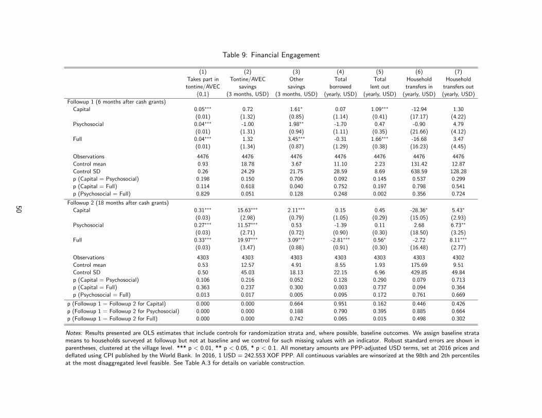
Table 9: Financial Engagement

(1) (2) (3) (4) (5) (6) (7)

Takes part in

tontine/AVEC

{0,1}

Tontine/AVEC

savings

(3 months, USD)

Other

savings

(3 months, USD)

Total

borrowed

(yearly, USD)

Total

lent out

(yearly, USD)

Household

transfers in

(yearly, USD)

Household

transfers out

(yearly, USD)

Followup 1 (6 months after cash grants)

Capital 0.05∗∗∗ 0.72 1.61∗ 0.07 1.09∗∗∗ -12.94 1.30

(0.01) (1.32) (0.85) (1.14) (0.41) (17.17) (4.22)

Psychosocial 0.04∗∗∗ -1.00 1.98∗∗ -1.70 0.47 -0.90 4.79

(0.01) (1.31) (0.94) (1.11) (0.35) (21.66) (4.12)

Full 0.04∗∗∗ 1.32 3.45∗∗∗ -0.31 1.66∗∗∗ -16.68 3.47

(0.01) (1.34) (0.87) (1.29) (0.38) (16.23) (4.45)

Observations 4476 4476 4476 4476 4476 4476 4476

Control mean 0.93 18.78 3.67 11.10 2.23 131.42 12.87

Control SD 0.26 24.29 21.75 28.59 8.69 638.59 128.28

p (Capital = Psychosocial) 0.198 0.150 0.706 0.092 0.145 0.537 0.299

p (Capital = Full) 0.114 0.618 0.040 0.752 0.197 0.798 0.541

p (Psychosocial = Full) 0.829 0.051 0.128 0.248 0.002 0.356 0.724

Followup 2 (18 months after cash grants)

Capital 0.31∗∗∗ 15.63∗∗∗ 2.11∗∗∗ 0.15 0.45 -28.36∗ 5.43∗

(0.03) (2.98) (0.79) (1.05) (0.29) (15.05) (2.93)

Psychosocial 0.27∗∗∗ 11.57∗∗∗ 0.53 -1.39 0.11 2.68 6.73∗∗

(0.03) (2.71) (0.72) (0.90) (0.30) (18.50) (3.25)

Full 0.33∗∗∗ 19.97∗∗∗ 3.09∗∗∗ -2.81∗∗∗ 0.56∗ -2.72 8.11∗∗∗

(0.03) (3.47) (0.88) (0.91) (0.30) (16.48) (2.77)

Observations 4303 4303 4303 4303 4303 4303 4302

Control mean 0.53 12.57 4.91 8.55 1.93 175.69 9.51

Control SD 0.50 45.03 18.13 22.15 6.96 429.85 49.84

p (Capital = Psychosocial) 0.106 0.216 0.052 0.128 0.290 0.079 0.713

p (Capital = Full) 0.363 0.237 0.300 0.003 0.737 0.094 0.364

p (Psychosocial = Full) 0.013 0.017 0.005 0.095 0.172 0.761 0.669

p (Followup 1 = Followup 2 for Capital) 0.000 0.000 0.664 0.951 0.162 0.446 0.426

p (Followup 1 = Followup 2 for Psychosocial) 0.000 0.000 0.188 0.790 0.395 0.885 0.664

p (Followup 1 = Followup 2 for Full) 0.000 0.000 0.742 0.065 0.015 0.498 0.302

Notes: Results presented are OLS estimates that include controls for randomization strata and, where possible, baseline outcomes. We assign baseline stratameans to households surveyed at followup but not at baseline and we control for such missing values with an indicator. Robust standard errors are shown inparentheses, clustered at the village level. *** p < 0.01, ** p < 0.05, * p < 0.1. All monetary amounts are PPP-adjusted USD terms, set at 2016 prices anddeflated using CPI published by the World Bank. In 2016, 1 USD = 242.553 XOF PPP. All continuous variables are winsorized at the 98th and 2th percentilesat the most disaggregated level feasible. See Table A.3 for details on variable construction.

50

Table 10: Psychological Well-Being Indices

(1) (2) (3)

Mental

health

index

Social

worth

index

Future

expectations

index

Followup 1 (6 months after cash grants)

Capital 0.13∗∗∗ 0.16∗∗∗ 0.12∗∗∗

(0.04) (0.04) (0.04)

Psychosocial 0.10∗∗ 0.22∗∗∗ 0.15∗∗∗

(0.04) (0.04) (0.04)

Full 0.23∗∗∗ 0.36∗∗∗ 0.28∗∗∗

(0.04) (0.04) (0.03)

Observations 4476 4476 4476

Control mean 0.00 -0.00 -0.00

Control SD 1.00 1.00 1.00

p (Capital = Psychosocial) 0.560 0.228 0.437

p (Capital = Full) 0.012 0.000 0.000

p (Psychosocial = Full) 0.002 0.000 0.001

Followup 2 (18 months after cash grants)

Capital 0.15∗∗∗ 0.12∗∗∗ 0.11∗∗

(0.04) (0.04) (0.04)

Psychosocial 0.21∗∗∗ 0.20∗∗∗ 0.15∗∗∗

(0.04) (0.04) (0.05)

Full 0.26∗∗∗ 0.26∗∗∗ 0.20∗∗∗

(0.04) (0.04) (0.04)

Observations 4175 4175 4175

Control mean 0.00 -0.00 0.00

Control SD 1.00 1.00 1.00

p (Capital = Psychosocial) 0.149 0.075 0.505

p (Capital = Full) 0.007 0.001 0.047

p (Psychosocial = Full) 0.247 0.174 0.222

p (Followup 1 = Followup 2 for Capital) 0.625 0.368 0.948

p (Followup 1 = Followup 2 for Psychosocial) 0.022 0.814 0.920

p (Followup 1 = Followup 2 for Full) 0.569 0.043 0.087

Notes: Results presented are OLS estimates that include controls for randomization strata and, where possible, baselineoutcomes. We assign baseline strata means to households surveyed at followup but not at baseline and we control for suchmissing values with an indicator. Robust standard errors are shown in parentheses, clustered at the village level. *** p <0.01, ** p < 0.05, * p < 0.1. All indices are standardized with respect to the control group in that same time period. SeeTable A.4 for details on variable construction. Results from components of each index are provided in Table A.7 (mentalhealth index components), Table A.8 (social worth index components) and Table A.9 (future expectation index components).

51

Table 11: Social Well-Being Indices

(1) (2) (3) (4) (5)

Social

support

index

Financial

support

index

Intra-household

dynamics

index

Social cohesion and

community closeness

index

Collective

action

index

Followup 1 (6 months after cash grants)

Capital 0.27∗∗∗ 0.29∗∗∗ 0.07 0.03 0.30∗∗∗

(0.06) (0.05) (0.04) (0.05) (0.05)

Psychosocial 0.24∗∗∗ 0.35∗∗∗ 0.07∗ 0.12∗∗∗ 0.34∗∗∗

(0.04) (0.05) (0.04) (0.05) (0.05)

Full 0.32∗∗∗ 0.48∗∗∗ 0.06 0.12∗∗∗ 0.42∗∗∗

(0.05) (0.05) (0.04) (0.04) (0.05)

Observations 4476 4476 4476 4476 4476

Control mean 0.00 0.00 -0.00 0.00 -0.00

Control SD 1.00 1.00 1.00 1.00 1.00

p (Capital = Psychosocial) 0.569 0.252 0.961 0.063 0.347

p (Capital = Full) 0.417 0.000 0.946 0.047 0.018

p (Psychosocial = Full) 0.075 0.012 0.982 0.929 0.119

Followup 2 (18 months after cash grants)

Capital 0.13∗∗∗ 0.19∗∗∗ 0.02 0.08∗ 0.27∗∗∗

(0.04) (0.04) (0.04) (0.05) (0.05)

Psychosocial 0.18∗∗∗ 0.21∗∗∗ 0.04 0.13∗∗∗ 0.27∗∗∗

(0.05) (0.04) (0.04) (0.04) (0.05)

Full 0.18∗∗∗ 0.35∗∗∗ -0.01 0.09∗∗ 0.35∗∗∗

(0.04) (0.05) (0.04) (0.05) (0.05)

Observations 4160 4252 4160 4160 4160

Control mean 0.00 -0.00 0.00 -0.00 0.00

Control SD 1.00 1.00 1.00 1.00 1.00

p (Capital = Psychosocial) 0.284 0.607 0.642 0.244 0.997

p (Capital = Full) 0.217 0.000 0.466 0.782 0.105

p (Psychosocial = Full) 0.968 0.004 0.210 0.341 0.092

p (Followup 1 = Followup 2 for Capital) 0.025 0.084 0.403 0.393 0.568

p (Followup 1 = Followup 2 for Psychosocial) 0.288 0.012 0.629 0.840 0.202

p (Followup 1 = Followup 2 for Full) 0.016 0.014 0.188 0.590 0.253

Notes: Results presented are OLS estimates that include controls for randomization strata and, where possible, baseline outcomes.We assign baseline strata means to households surveyed at followup but not at baseline and we control for such missing values withan indicator. Robust standard errors are shown in parentheses, clustered at the village level. *** p < 0.01, ** p < 0.05, * p <0.1. All indices are standardized with respect to the control group in that same time period. See Table A.4 for details on variableconstruction. Results from components of each index are provided in Table A.10 (social support index), Table A.11 (financial supportindex), Table A.12 (future expectation index), Table A.13 (social cohesion and closeness to community) and Table A.14 (collectiveaction index).

52

Table 12: Decision-Making and Productive Agency Indices

(1) (2)

Controls

earnings

index

Controls

HH resources

index

Followup 1 (6 months after cash grants)

Capital 0.27∗∗∗ 0.03

(0.04) (0.04)

Psychosocial 0.22∗∗∗ 0.05

(0.04) (0.04)

Full 0.34∗∗∗ 0.06

(0.04) (0.04)

Observations 4476 4161

Control mean 0.00 -0.00

Control SD 1.00 1.00

p (Capital = Psychosocial) 0.333 0.522

p (Capital = Full) 0.050 0.386

p (Psychosocial = Full) 0.005 0.777

Followup 2 (18 months after cash grants)

Capital 0.25∗∗∗ -0.01

(0.05) (0.05)

Psychosocial 0.16∗∗∗ 0.06

(0.05) (0.05)

Full 0.25∗∗∗ 0.04

(0.04) (0.05)

Observations 4252 4055

Control mean 0.00 -0.00

Control SD 1.00 1.00

p (Capital = Psychosocial) 0.075 0.110

p (Capital = Full) 0.891 0.218

p (Psychosocial = Full) 0.045 0.664

p (Followup 1 = Followup 2 for Capital) 0.735 0.493

p (Followup 1 = Followup 2 for Psychosocial) 0.210 0.937

p (Followup 1 = Followup 2 for Full) 0.077 0.676

Notes: Results presented are OLS estimates that include controls for randomization strata and, where possible, baselineoutcomes. We assign baseline strata means to households surveyed at followup but not at baseline and we control for suchmissing values with an indicator. Robust standard errors are shown in parentheses, clustered at the village level. *** p <0.01, ** p < 0.05, * p < 0.1. All indices are standardized with respect to the control group in that same time period. SeeTable A.4 for details on variable construction. Results from components of each index can be found in Table A.15 (controlover earnings and productive agency) and Table A.16 (control over household resources).

53

Table 13: Children’s Outcomes

(1) (2) (3) (4)

Child

attended

school {0,1}

Child

labor

index

Child

chores

index

Weight/

height

z-score

Followup 1 (6 months after cash grants)

Capital 0.05∗ 0.06∗ 0.07∗∗ 0.01

(0.03) (0.03) (0.03) (0.05)

Psychosocial 0.00 0.12∗∗∗ 0.08∗∗∗ -0.03

(0.03) (0.03) (0.03) (0.05)

Full 0.01 0.17∗∗∗ 0.04 -0.07

(0.03) (0.04) (0.03) (0.05)

Observations 13145 13145 13145 5017

Control mean 0.41 0.00 0.00 -0.77

Control SD 0.49 1.00 1.00 1.09

p (Capital = Psychosocial) 0.153 0.085 0.694 0.486

p (Capital = Full) 0.220 0.005 0.207 0.107

p (Psychosocial = Full) 0.742 0.287 0.102 0.396

Followup 2 (18 months after cash grants)

Capital 0.06∗∗ 0.11∗∗∗ 0.03 -0.02

(0.03) (0.03) (0.03) (0.05)

Psychosocial 0.03 0.12∗∗∗ 0.04 -0.01

(0.03) (0.03) (0.03) (0.05)

Full 0.03 0.14∗∗∗ -0.02 -0.03

(0.03) (0.03) (0.03) (0.05)

Observations 13939 13939 13939 5663

Control mean 0.42 -0.00 -0.00 -0.62

Control SD 0.49 1.00 1.00 1.20

p (Capital = Psychosocial) 0.332 0.757 0.927 0.976

p (Capital = Full) 0.273 0.343 0.054 0.813

p (Psychosocial = Full) 0.982 0.535 0.057 0.790

p (Followup 1 = Followup 2 for Capital) 0.259 0.260 0.280 0.685

p (Followup 1 = Followup 2 for Psychosocial) 0.101 0.895 0.205 0.767

p (Followup 1 = Followup 2 for Full) 0.271 0.574 0.130 0.403

Notes: Results presented are OLS estimates that include controls for randomization strata and, where possible, baselineoutcomes. We assign baseline strata means to households surveyed at followup but not at baseline and we control for suchmissing values with an indicator. Robust standard errors are shown in parentheses, clustered at the village level. *** p <0.01, ** p < 0.05, * p < 0.1. The weight/height index is not standardized with respect to the control group. See Table A.4for details on variable construction.

54

Capital Psychosocial FullPanel 1: Program costs per beneficiary, USD PPP 2016

Program administration 78 78 78 Identification, Communication 3 3 3 Measure 0. Group formation 1 1 1 Measure 1. Coaching 9 9 9 Measure 2. Community sensitization on aspirations and social norms 0 38 38 Measure 3. Facilitation of community savings and loan groups 2 2 2 Measure 4. Life-skills training 0 64 64 Measure 5. Micro-entrepreneurship training 65 65 65 Measure 6. Cash grants 321 0 321 Measure 7. Facilitation of market and information access 4 4 4Total costs, calculated as if all incurred immediately at beginning of year 0 482 263 584

(1) Total costs, inflated to year 2 at 5% annual discount rate 531 290 644

Panel 2: Benefits per Household, USD PPP 2016, All Values Inflated to Year 2 at 5% annual social discount rateA

(2) Year 1 Gross Consumption Treatment Effect, using 5% discount rate 228 131 373(3) Year 2 Gross Consumption Treatment Effect 196 298 425(4) B1: Year 3 Onward Gross Consumption Treatment Effect, assuming dissipation of 75% 61 93 133

B2: Year 3 Onward Gross Consumption Treatment Effect, assuming dissipation of 50% 178 271 386B3: Year 3 Onward Gross Consumption Treatment Effect, assuming dissipation of 25% 491 745 1062

(5) C: Year 3 Onward Gross Consumption Treatment Effect, assuming year 2 gains persist in perpetuity 3739 5679 8088

(6) A: Total Benefits: 0.5*(2) + (3) = (6) using 5%, no impact after year 2 310 364 611(7) B1: Total Benefits: 0.5*(2) + (3) + (4) = (7) 5% discount rate, 75% annual dissipation 372 457 744

B2: Total Benefits using 5% discount rate, 50% annual dissipation 489 635 997B3: Total Benefits using 5% discount rate, 25% annual dissipation 801 1109 1673

(8)C: Total Benefits: 0.5*(2) + (3) + (5) = (8) using 5% discount rate, assuming year 2 gains persist in perpetuity 4049 6043 8699

Panel 3: Benefit/Cost RatiosA

(9) A: Total Benefits/Total Costs Ratio: (6) / (1) = (9) at 5% discount rate 58% 126% 95%A: Benefit/Cost Ratio, at discount rate of 7% 57% 121% 92%A: Benefit/Cost Ratio, at discount rate of 10% 54% 115% 88%

(10) B1: Total Benefits/Total Costs: (7) / (1) = (10), 5% discount, 75% annual dissipation 70% 158% 116%B2: Benefit/Cost Ratio using 5% discount rate, 50% annual dissipation 92% 219% 155%B3: Benefit/Cost Ratio using 5% discount rate, 25% annual dissipation 151% 383% 260%

(11)C: Total Benefits/Total Costs Ratio: (8) / (1) = (11) using 5% discount rate, assuming year 2 gains persist in perpetuity 762% 2087% 1352%

(12) Real Internal Rate of Return (IRR) A: assuming dissipation of 100% after year 2, at 5% discount rate -28% 13% -3% B1: assuming annual dissipation of 75% -16% 25% 8% B2: assuming annual dissipation of 50% -2% 39% 21% B3: assuming annual dissipation of 25% 15% 54% 36% C: assuming effects are sustained in perpetuity 33% 70% 53%

Notes: We use 98% winsorized consumption estimates in our benefits calculation. Note that in rows 6, 7, and 8 we halve consumption benefits in year 1 since we measure these benefits 6 months after the intervention on average. All monetary amounts are PPP-adjusted USD terms, set at 2016 prices and deflated using CPI published by the World Bank. In 2016, 1 USD = 242.553 XOF PPP. We assume yearly impacts post-intervention.

Table 14: Cost-benefit Analysis

Appendix A. Additional information on the psychosocial components

The psychosocial components included a community-wide sensitization and a life skills training. Thesewere designed to simultaneously address multiple psychosocial constraints to beneficiaries’ economicengagement, from individual- to community-level factors, and to do so in culturally responsive ways.

These design choices build on two foundational ideas in social and cultural psychology. First, beyondindividual motivation, behavior is influenced by what the social context permits (Markus and Kitayama,2010; Lewin, 1952). Accordingly, individual-level behavior change strategies, like life skills trainings, areexpected to have greater and more sustained effects when, for instance, social norms are alsosupportive of the new behaviors (Walton and Yeager, 2020). Second, cultures across the world displaydifferent levels of collectivism and social norm enforcement, which shape individual behaviors (Gelfandet al., 2011; Hofstede, 2001; Leung and Cohen, 2011; Markus and Conner, 2014). Hausa and Zarmaethnic groups in Niger are predominantly Muslim, highly collectivistic, and gender roles are guided bystrong social norms and religious practices.1 In such normatively tight and interdependent socioculturalcontexts, coordinating individuals’ behavior and goals with those of their community and aligning theinterventions with commonly-held values was expected to lead to greater individual motivation andsocial support (Markus, 2016; Riemer et al., 2014).

1. Community sensitization on aspirations and social norms

The sensitization aimed to introduce the productive interventions’ objectives to the community and topromote social norms and aspirations supportive of women’s economic activities.

Content of the intervention. The sensitization was an evening program in which beneficiaries andother family and community members were invited to gather to view a film projected on a large screen,followed by a guided group discussion. The activity lasted approximately 1.5 hours in total.

The 20-minute film showed an aspirational story that combined local stories collected during qualitativepiloting with social and behavior change principles. It was recorded in Hausa and Zarma.2 The filmportrayed the story of a Muslim woman named Amina pursuing a new business (processing and sellinghibiscus or “bissap” juice) after a drought affected her millet crop. Amina is shown using the supportof her family and community to adapt her economic activities, including consulting her mother-in-lawon adaptation and change, her cousin on making bissap juice, and her husband on their financialoptions. She and her husband overcome a conflict on her plan to save with her women’s group, withthe father-in-law being the mediator. In the end, she and her husband are shown selling bissap juice,food, and solar-based charging in their new shop as their children return from school. In the finalscene, Amina shares what she has learned with other women in the village.

Immediately after the film, the audience was led through a group discussion of approximately 40-60minutes. There were five discussion topics: summarizing the film’s main themes; relating the film tothe audience’s experiences; sharing family and community stories about ‘traditions of adaption’;identifying best practices for more secure future; and creating consensus around solidarity toward thisfuture. Facilitators were encouraged to pick respondents from across the audience to elicit widespreadparticipation and to elevate women’s responses.

Aligning desired behaviors with communal values. Given strong social and religious norms in ruralNiger, in certain areas women’s economic engagement can lead to social censure, particularly if womenare seen to be self-interested and ambitious. Some interventions in the international literature activelyteach self-focus and personal initiative skills to improve outcomes of income-generating activities(Campos et al., 2017). However, the approach here considers a more interdependent model that

1For instance, see Hofstede Insights Country Comparison (www.hofstede-insights.com/country-comparison).2See links to full video in Zarma and Hausa with French subtitles, and 4-minute clip with English subtitles.

56

recognizes the motivational power of matching a group’s values and cultural ways of being, as opposedto overlooking or overriding them. The community sensitization thus sought to frame the goals of theeconomic inclusion interventions and women’s economic activity as being aligned with binding,communal values, such as solidarity, filial piety, loyalty, and respect for authority (Feinberg and Willer,2015; Leung and Cohen, 2011; Stephens et al., 2012; Thomas and Markus, forthcoming; Thomaset al., 2020). For instance, in the film Amina demonstrates her interdependent goals to help herchildren, her husband, and her community through her economic activities, beyond her ownadvancement, and she shows solidarity and loyalty to her peers by sharing her new knowledge withthem. Amina shows filial piety and respect for authority by seeking out advice and mediation from herelders, who provide supportive advice based on their own experience adapting to changingcircumstances in the past. Relatedly, the discussion asked the community to reflect on ‘traditions ofadaptation’ from their ancestors so that upcoming changes in economic practices could be understoodto represent, rather than defy, tradition and filial piety.

Community participation and social norms. Particularly in this more interdependent andnormatively tight sociocultural study context, watching the film with close others was expected tobetter shift social norms around typical and appropriate economic behaviors for women and to generatemore sustained social support (Bandura, 2001; Paluck, 2009). Accordingly, beneficiaries wereencouraged to invite their husbands, family members, and friends. Given the importance of hierarchyand of local leaders in norm setting and enforcement (Paluck and Shepherd, 2012; San Martin et al.,2018), traditional leaders were engaged in conducting the event and, along with other elders, religiousleaders, and economic leaders, were invited to attend. Leveraging group-based decision-making forsocial change (Lewin, 1952), the discussion prompted the audience to build consensus aroundpracticing norms of mutual support and solidarity, particularly of the beneficiaries, that could advancecommunity development.

Role models, aspirations, and goal setting. A goal of role modeling women’s economicengagement through film was to build self-efficacy and promote aspirations for economic mobility bothamong beneficiaries and their community. According to social cognitive theory, the use of role modelscan encourage uptake of new behaviors via observational learning of social exemplars; it can also buildself-efficacy through vicarious experience, which can in turn boost aspirations, motivation, andresilience to setbacks (Bandura, 2001). Because similarity and relatability of characters are central tonarrative persuasion, the video involved local actors and the discussion prompted the audience toconnect the film’s story to their own lives (Slater and Rouner, 2002). The film also featured traditionalmusic and proverbs in Hausa and Zarma.

Building on an evidence-based motivational strategy of WOOP, or Wish Outcome Obstacle Plan(Oettingen, 2014), the discussion further prompted participants to project themselves into the future,to consider the goal of creating a more secure future for the next generation in particular, and then toidentify adaptation strategies that could advance this goal as well as difficulties that could stand in theway. The discussion leader closed by expressing positive expectations of a strong future for thecommunity.

2. Life Skills Training

The life skills training was delivered over 7 half-days. It was supported by emerging research on thebenefits of non-cognitive or soft skills trainings. Teaching soft skills such as self-worth, interpersonalcommunication, and sense of control have been shown to promote a range of positive life outcomes,including improved productivity, earnings, health, and educational outcomes (Acevedo et al., 2017;Adhvaryu, Kala, and Nyshadham, 2018; Blattman, Jamison, and Sheridan, 2017; Ashraf et al., 2020;Heckman, Stixrud, and Urzua, 2006). Several studies have found soft skills trainings to be as or more

57

effective in boosting employment and entrepreneurial outcomes compared to hard skills or technicaltrainings (Campos et al., 2017; Barrera-Osorio, Kugler, and Silliman, 2020).

The training was grounded in ‘andragogy,’ an approach to adult education that prioritizes self-directed,experiential, problem-centered, participatory, and personalized learning (Knowles, 1984). The trainingthus incorporated individual- and group-based exercises, including collective brainstorming sessions,case studies, role plays, games, open discussions, and illustrations.

The training included 9 modules:

1. Overview of the life skills curriculum, key competencies, and their utility for achieving one’saspirations and realizing one’s values.

2. Our values and perspectives: Identification of one’s three top communal and individual values(e.g., honor, dignity, generosity, loyalty, piety, education, family); understanding how one canexercise these values through their work.

3. Self-affirmation and self-worth: Identifying one’s strengths, value to one’s family and others, androle in society; linking self-worth to personal initiative and self-expression as well as to opennessto feedback and change; understanding differences between self-worth and selfishness,aggressiveness, or passiveness.

4. Decision-making and problem solving: How to identify a problem; analyze relevant information;gather different perspectives; identify multiple solutions; anticipate consequences; make informeddecisions that meet one’s values, vision, and the interests of concerned persons; act on thedecision; and reflect on the outcomes.

5. Second viewing of the sensitization film: Reinforcement of key themes and competenciesdisplayed in Amina’s story, including her values and decision-making, creativity in the face ofshocks, leading by example, and contributions to her community’s development.

6. Interpersonal communication and using one’s voice: Understanding the significance of goodcommunication, common obstacles, and key principles of good communication and self-expression(e.g., using a message clear and simple, credible information, productive circumstances andchannels of communication, an approach tailored to the relationship and status of the otherperson, maintained eye contact, audible and slow speech, amicable and open verbal andnon-verbal communication).

7. Financial education: Setting and prioritizing top financial goals and charting out intermediatesteps; mental contrasting with future savings, building a culture of saving, defining one’s capacityto save, and seeing savings as a source of resilience; budgeting across seasons and across expensetypes.

8. Leadership and gender: Identifying female leaders and role models and qualities of leaders (e.g.,having strong networks; taking responsibility; mediating conflicts; being forward-looking, inspiring,calm, and courageous); discussing ways women can contribute to community decision-making andsupport their communities and families; and brainstorming ideas for actions that participantscould take in their communities.

9. Third viewing of the sensitization film and summary: Analysis of the film in relation to thecompetencies displayed by different actors; summary of the session including an exchange ofparticipants’ experiences and lessons learned.

58

Appendix B. Additional information on the psychosocial outcomes

Process of measure selection, adaptation, and development

Through piloting, the research team selected and adapted items from existing scales as well as developedoriginal measures with face validity, or subjective construct accuracy in the local context. We additionallyincluded culturally meaningful indicators of psychological and social well-being (e.g., inner peace, enemyship).In the selection and development of psychosocial measures, careful attention was paid to cultural relevanceand comprehensibility. All items, and their references where relevant, are described in Table A.4.

Psychological well-being indices

The psychological well-being outcomes assessed mental health and psychosocial assets, including self-efficacy,subjective social status, and future expectations. Broadly, mental health and psychosocial assets predict arange of positive economic, health, and empowerment outcomes (Operario, Adler, and Williams, 2004;Wuepper and Lybbert, 2017). In particular, poor mental health, self-efficacy, and hope have been posited tocontribute to poverty through their effects on motivation and future-oriented decision-making (Dalton, Ghosal,and Mani, 2016; Duflo, 2012; Ridley et al., 2020; Wuepper and Lybbert, 2017).

Mental health included CESD-R-10, a depression screener designed for community samples; functionaldisability items from SRQ-20; life satisfaction using an adapted Cantril ladder; sense of inner peace; andself-assessed mental health. Disability items, assessing somatic symptoms and role functioning, andself-assessed mental health item were included to capture cultural differences in mental illness symptoms (e.g.,somatization) and functional impairments (Thomas et al., 2016; Ali, Ryan, and De Silva, 2016). Inner peacewas considered a culturally specific indicator of well-being, according to qualitative piloting and West Africanstudies (Osei-Tutu et al., 2020).

Social worth assessed self-efficacy and social standing. Capturing judgments of one’s capabilities, perceivedself-efficacy is a motivational keystone, particularly of goal setting and pursuit, in Western psychologicalresearch (Bandura, 1997). Social standing assessed the MacArthur socioeconomic status ladder and threecontext-specific ladders of community standing: being respected, having one’s opinion followed, and showingmoral behavior. Such self-assessments of one’s social position have been found to predict health, well-being,and feelings of financial security, above and beyond income (Operario, Adler, and Williams, 2004).

Future expectations gauged expectations for personal and intergenerational socioeconomic status as well aslife satisfaction in the future, through adapted MacArthur ladders. Notably, hope, or positive expectations forthe future, has been posited to contribute to graduation programs’ effects on poverty reduction (Duflo, 2012).Additionally, Delavande et al. (2011) find that subjective expectations often accurately predict futurebehaviors and outcomes and, in this case, capture expected trajectories of mobility.

Social well-being indices

The social well-being outcomes were seen as potential determinants of women’s economic outcomes in the lowliteracy, low resource, and normatively tight study setting where women’s opportunities often come throughtheir relationships and where reciprocal networks of support can be critical to cope with shocks (Woolcock andNarayan, 2000; Akyeampong et al., 2014). Moreover, social well-being is often integral to individual happinessand wellbeing among interdependent groups (Hitokoto and Uchida, 2015; Osei-Tutu et al., 2020).

Social support and financial support assessed women’s level of social capital, both bonding and bridging(Woolcock and Narayan, 2000). Social support assessed the extent of one’s instrumental support network,based on the number of relationships one has for acquiring information, advice, and opportunities. Financialsupport assessed the extent of one’s financial support network, based on perceived ability to receive financialhelp in times of need and number of financial supporters. Together, these questions capture whetherbeneficiaries are able to develop informal systems of support for economic resilience and opportunity.

59

Social cohesion and closeness to community assessed expectations of social support, feelings of trust andcloseness, experienced tension (reversed), and number of enemies (reversed). Of note, the idea of personalenemies, or people who wish to sabotage your success, is prevalent in West Africa where socialinterdependence can be high (Adams, 2005). Enemies can arise from envy and resentment that can, forinstance, accompany inequality in new opportunities or resources. Number of enemies was included as alocally relevant indicator of social cohesion, in addition to feelings and experiences of cohesion.

Groups and collective action assessed community engagement and support through the number of groupsbelonged to, the number of leadership positions held, monetary and volunteer contributions to communityprojects, and self-reported collective initiative. This measure assessed whether the interventions may haveindirect benefits to communities beyond direct benefits to beneficiaries.

Intrahousehold dynamics assessed perceived quality of intrahousehold relationships, including feelings of trust,closeness, and support as well as experienced conflicts (reversed). Given that many economic and behavioraldecisions are made at the household level in the study setting, this measure gauged the extent to whichbeneficiaries felt aligned with and supported by members of their household in decision-making or experiencedtensions (reversed). It also assessed the Inclusion of Other in Self visual scale and sense of trust as indicatorsof intrahousehold closeness and positive relationality (Aron, Aron, and Smollan, 1992).

60

Appendix C. Additional Tables

Table A.1: Balance and Attrition

Control Capital Psychosocial Full T-test Joint F-test Pooled F-testMean/SE Mean/SE Mean/SE Mean/SE p-value p-value p-value

Variable (1) (2) (3) (4) (1)-(2) (1)-(3) (1)-(4) (2)-(3) (2)-(4) (3)-(4) (5) (6)

Beneficiary is HH head 0.104(0.011)

0.109(0.012)

0.111(0.010)

0.102(0.011)

0.423 0.282 0.843 0.714 0.381 0.232 0.660 0.606

Beneficiary is handicapped 0.013(0.003)

0.021(0.004)

0.015(0.004)

0.018(0.004)

0.174 0.632 0.133 0.179 0.569 0.740 0.653 0.178

Female (HH head) 0.102(0.011)

0.116(0.013)

0.114(0.012)

0.113(0.012)

0.135 0.163 0.310 0.977 0.541 0.491 0.883 0.181

Female (beneficiary) 0.986(0.003)

0.990(0.003)

0.987(0.004)

0.988(0.003)

0.326 0.821 0.860 0.514 0.751 0.760 0.839 0.417

Polygamy (HH head) 0.285(0.018)

0.263(0.015)

0.266(0.015)

0.300(0.018)

0.498 0.292 0.300 0.968 0.077* 0.106 0.154 0.918

Polygamy (beneficiary) 0.266(0.017)

0.252(0.015)

0.255(0.014)

0.284(0.017)

0.810 0.508 0.213 0.929 0.117 0.106 0.213 0.772

Age (HH head) 47.607(0.478)

47.201(0.433)

47.240(0.509)

46.562(0.478)

0.496 0.188 0.106 0.853 0.307 0.152 0.468 0.155

Age (beneficiary) 37.818(0.436)

37.971(0.423)

37.821(0.478)

37.095(0.464)

0.412 0.679 0.348 0.314 0.037** 0.106 0.195 0.655

Education (years, HH head) 0.537(0.072)

0.646(0.084)

0.574(0.079)

0.505(0.070)

0.161 0.377 0.931 0.937 0.381 0.655 0.531 0.341

Education (years, beneficiary) 0.306(0.042)

0.406(0.053)

0.284(0.044)

0.350(0.052)

0.100 0.799 0.400 0.086* 0.933 0.252 0.271 0.290

Primary education (0/1, HH head) 0.025(0.005)

0.027(0.006)

0.030(0.006)

0.024(0.005)

0.743 0.120 0.658 0.146 0.771 0.528 0.653 0.349

Primary education (0/1, beneficiary) 0.015(0.004)

0.015(0.004)

0.010(0.003)

0.012(0.003)

0.786 0.201 0.416 0.484 0.899 0.869 0.777 0.468

Literate (HH head) 0.264(0.017)

0.277(0.016)

0.285(0.017)

0.263(0.017)

0.224 0.174 0.894 0.626 0.312 0.381 0.638 0.287

Literate (beneficiary) 0.071(0.007)

0.082(0.010)

0.071(0.009)

0.075(0.010)

0.156 0.963 0.454 0.379 0.814 0.767 0.619 0.431

Health index (HH head) 0.000(0.030)

0.027(0.035)

0.031(0.031)

0.034(0.034)

0.515 0.498 0.329 0.941 0.638 0.761 0.951 0.371

Health index (beneficiary) -0.000(0.036)

0.035(0.035)

0.002(0.036)

0.044(0.033)

0.348 0.947 0.351 0.293 0.953 0.483 0.657 0.535

Continued on next page

61

Table A.1: Balance and Attrition – continued from previous page

Control Capital Psychosocial Full T-test Joint F-test Pooled F-testMean/SE Mean/SE Mean/SE Mean/SE p-value p-value p-value

Variable (1) (2) (3) (4) (1)-(2) (1)-(3) (1)-(4) (2)-(3) (2)-(4) (3)-(4) (5) (6)

No. of rooms in house 2.497(0.076)

2.422(0.064)

2.490(0.076)

2.629(0.071)

0.577 0.898 0.037** 0.471 0.004*** 0.064* 0.019** 0.538

Minutes to heatlh center 47.079(2.707)

46.827(3.579)

50.488(3.448)

51.100(2.733)

0.460 0.400 0.477 0.371 0.447 0.938 0.617 0.702

Minutes to market 73.008(3.523)

68.875(4.124)

76.453(3.686)

72.459(3.487)

0.237 0.416 0.454 0.068* 0.748 0.250 0.271 0.616

Minutes to water source 12.143(1.144)

12.413(1.089)

12.586(1.227)

12.652(0.930)

0.882 0.948 0.494 0.252 0.876 0.387 0.914 0.768

Distance to capital of commune (km) 23.402(1.200)

22.122(1.102)

23.793(1.294)

22.128(1.140)

0.285 0.856 0.077* 0.574 0.975 0.397 0.525 0.415

N 1188 1165 1084 1171Clusters 81 80 78 83

Response rate in actual baseline sample

Follow-up 1 0.957(0.007)

0.953(0.008)

0.950(0.008)

0.950(0.009)

0.420 0.455 0.267 0.991 0.801 0.946 0.991 0.306

Follow-up 2 0.910(0.015)

0.927(0.010)

0.929(0.009)

0.907(0.015)

0.522 0.107 0.445 0.809 0.230 0.148 0.341 0.610

N 1188 1165 1084 1171Clusters 81 80 78 83

Response rate in pre-baseline sampleBaseline 0.985

(0.004)0.978

(0.004)0.975

(0.005)0.973

(0.005)0.060* 0.064* 0.020** 0.985 0.296 0.516 0.627 0.008***

Follow-up 1 0.955(0.007)

0.950(0.008)

0.949(0.008)

0.945(0.009)

0.356 0.486 0.214 0.874 0.620 0.796 0.919 0.247

Follow-up 2 0.906(0.015)

0.922(0.010)

0.925(0.009)

0.899(0.016)

0.588 0.106 0.357 0.803 0.160 0.123 0.249 0.667

N 1206 1191 1112 1203Clusters 81 80 78 83

Notes: The values displayed for the t-tests are based on the differences in the means across the groups. Standard errors for all tests are clustered at the village level. Fixed effects usingrandomization strata are included in all estimation regressions. The joint F-test in column 5 shows the p-value from a test of equality of treatment arms. while the pooled F-test in column6 shows the p-value from a test of pooled treatment (i.e., a regression with a dummy for any treatment arm). The health index variable is a z-score index standardized against the controlgroup and generated using three physical activity variables: the reported difficulty of (1) lifting a 10 kg sac, (2) walking 4 hours, and (3) working all day in the field. These three componentsrange from 1 to 4. In calculating the distance-to-commune variable, we assign commune centroids to households located more than 30 km away from this centroid (measured as the averagelocation of non-outlying households in the commune). *** p < 0.01, ** p < 0.05, * p < 0.1.

62

Table A.2: Compliance Based on Administrative Data

Treatment Arm

Pooled Capital Psychosocial Full

1. Percentage of targeted beneficiaries who received individual coaching each month 52.2% 51.9% 50.5% 54.1%

2. Attendance rates of beneficiaries at community savings and loan groups 92.0% 92.8% 91.7% 91.5%

3. Attendance rates of beneficiaries at community sensitization on aspirations and social norms 89.3% - 89.0% 89.8%

4. Attendance rates of beneficiaries at micro-entrepreneurship training 95.0% 96.4% 94.9% 93.6%

5. Attendance rates of beneficiaries at life skills training 93.8% - 94.0% 93.5%

6. Percentage of targeted beneficiaries who received their cash grant 99.9% 99.7% - 100%

Notes: We show compliance data collected by the program’s administrators. The cash grant provision and participation in training (rows 4-6) aremeasured at the individual level. Participation in coaching sessions and savings groups (rows 1 and 2) is measured at the group level. And participationin the community sensitization session (video screening, row 3) is measured at the village level.

63

Table A.3: Variable Definitions and Construction

Variable Definition

Table 1 Primary Outcomes

Gross consumption (daily,

USD/adult eq.)

Total daily consumption per adult equivalent is the sum of daily household food and non-food consumption as well as

expenditures on education, healthcare, household repairs, and celebrations, divided by the number of adult equivalents

per household.

For food consumption, we ask about household consumption of a variety of food products in the last week. To get food

expenditure, we multiply amounts consumed by prices. For food products that are both purchased and consumed, we use

reported purchase prices. For food products that are consumed but not purchased, we use median purchase prices. We

winsorize consumed values within each food product and we divide weekly household totals by 7.

For non-food consumption, we ask about monthly and yearly expenses on a wide variety of goods and services that are

typically consumed on a monthly (yearly) basis. For education expenditures, we ask about spending in the last academic

year on transportation and various school-related items such as tuition fees and accommodation. For health

expenditures, we ask about monthly and yearly expenses such as doctor’s consultations and vaccination costs. For

celebrations, we ask about food, non-food, drink, and clothing expenditures made over the last year during events such

as marriages or religious ceremonies. For household repair expenditures, we ask about costs incurred over the last year

improving or repairing household features such as roofs, walls, or animal pens. For each of these expenditures, we

winsorize values at the finest level possible and re-scale to daily values.

Food security scale Using the FIES scale, we ask eight yes/no questions about a household’s food security over the last year where 0 = “yes”

and 1 = “no” and we present a raw sum. The questions are “have you or other members of your household 1) been

worried about not having enough food, 2) been unable to eat nutritious and healthy foods, 3) had to eat a smaller

variety of foods, 4) had to skip a meal, 5) eaten less than they thought they should, 6) run out of food, 7) been hungry

but did not eat, and 8) gone an entire day without eating?” (Nord, Cafiero, and Viviani, 2016; Ballard, Kepple, and

Cafiero, 2013)

Food consumption score We ask beneficiaries about the number of days in the last week that the they consumed items in 8 different food groups,

and we compute a linear combination of these items: (WFP, 2008)

2·cereals + 2·tubers + 3·pulses + vegetables + fruit + 4·meat/fish/eggs + 4·milk + 0.5·oil + 0.5·sugar

Table 2 Beneficiary Revenues

Business revenue (monthly,

USD)

For each business within the household, we ask directly about revenues generated over the last 30 days or in the last

month that the business was in operation. We winsorize revenues at the business-level at the 98th percentile. We

exclude businesses that are both owned and managed by someone outside the household and we divide revenues by the

number of co-owners to get the beneficiary’s share. Lastly, we only sum across beneficiary-owned/managed businesses.

Continued on next page

64

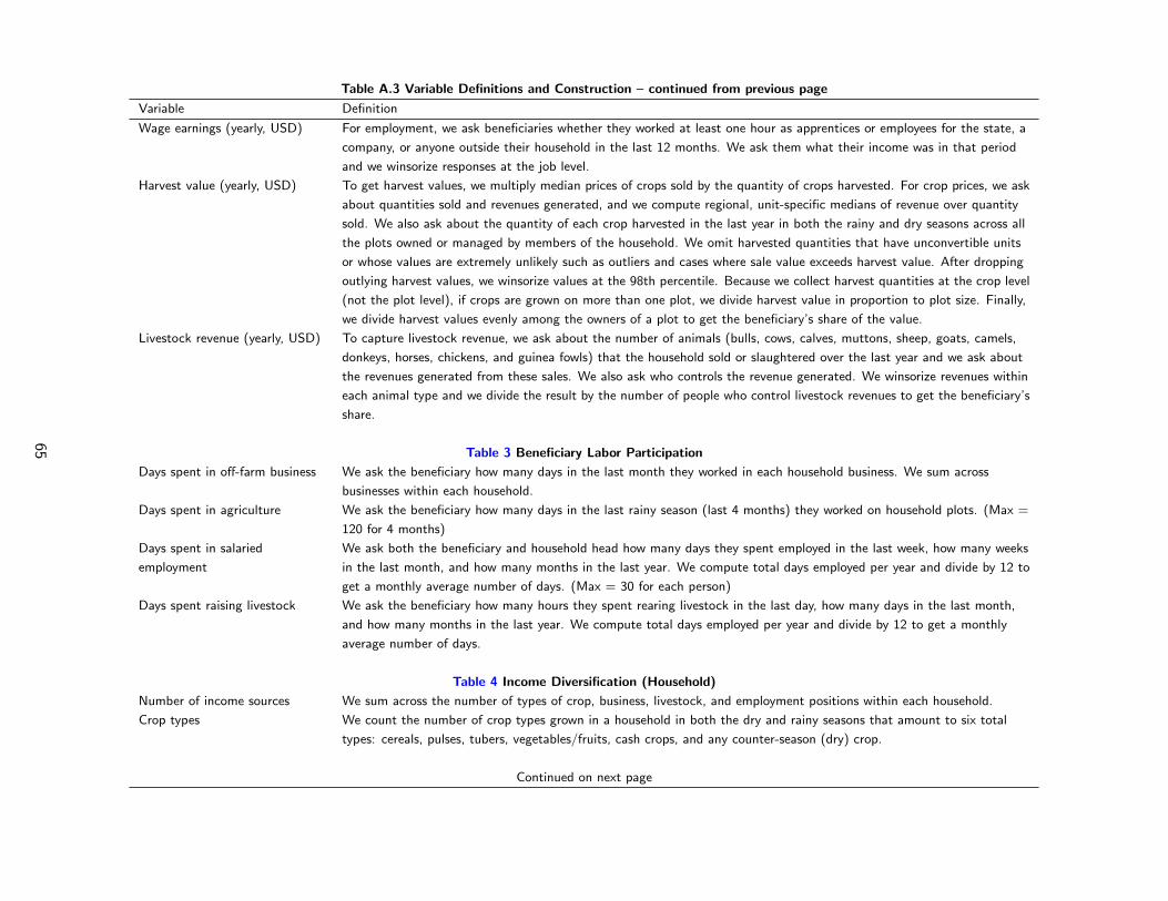
Table A.3 Variable Definitions and Construction – continued from previous page

Variable Definition

Wage earnings (yearly, USD) For employment, we ask beneficiaries whether they worked at least one hour as apprentices or employees for the state, a

company, or anyone outside their household in the last 12 months. We ask them what their income was in that period

and we winsorize responses at the job level.

Harvest value (yearly, USD) To get harvest values, we multiply median prices of crops sold by the quantity of crops harvested. For crop prices, we ask

about quantities sold and revenues generated, and we compute regional, unit-specific medians of revenue over quantity

sold. We also ask about the quantity of each crop harvested in the last year in both the rainy and dry seasons across all

the plots owned or managed by members of the household. We omit harvested quantities that have unconvertible units

or whose values are extremely unlikely such as outliers and cases where sale value exceeds harvest value. After dropping

outlying harvest values, we winsorize values at the 98th percentile. Because we collect harvest quantities at the crop level

(not the plot level), if crops are grown on more than one plot, we divide harvest value in proportion to plot size. Finally,

we divide harvest values evenly among the owners of a plot to get the beneficiary’s share of the value.

Livestock revenue (yearly, USD) To capture livestock revenue, we ask about the number of animals (bulls, cows, calves, muttons, sheep, goats, camels,

donkeys, horses, chickens, and guinea fowls) that the household sold or slaughtered over the last year and we ask about

the revenues generated from these sales. We also ask who controls the revenue generated. We winsorize revenues within

each animal type and we divide the result by the number of people who control livestock revenues to get the beneficiary’s

share.

Table 3 Beneficiary Labor Participation

Days spent in off-farm business We ask the beneficiary how many days in the last month they worked in each household business. We sum across

businesses within each household.

Days spent in agriculture We ask the beneficiary how many days in the last rainy season (last 4 months) they worked on household plots. (Max =

120 for 4 months)

Days spent in salaried

employment

We ask both the beneficiary and household head how many days they spent employed in the last week, how many weeks

in the last month, and how many months in the last year. We compute total days employed per year and divide by 12 to

get a monthly average number of days. (Max = 30 for each person)

Days spent raising livestock We ask the beneficiary how many hours they spent rearing livestock in the last day, how many days in the last month,

and how many months in the last year. We compute total days employed per year and divide by 12 to get a monthly

average number of days.

Table 4 Income Diversification (Household)

Number of income sources We sum across the number of types of crop, business, livestock, and employment positions within each household.

Crop types We count the number of crop types grown in a household in both the dry and rainy seasons that amount to six total

types: cereals, pulses, tubers, vegetables/fruits, cash crops, and any counter-season (dry) crop.

Continued on next page

65

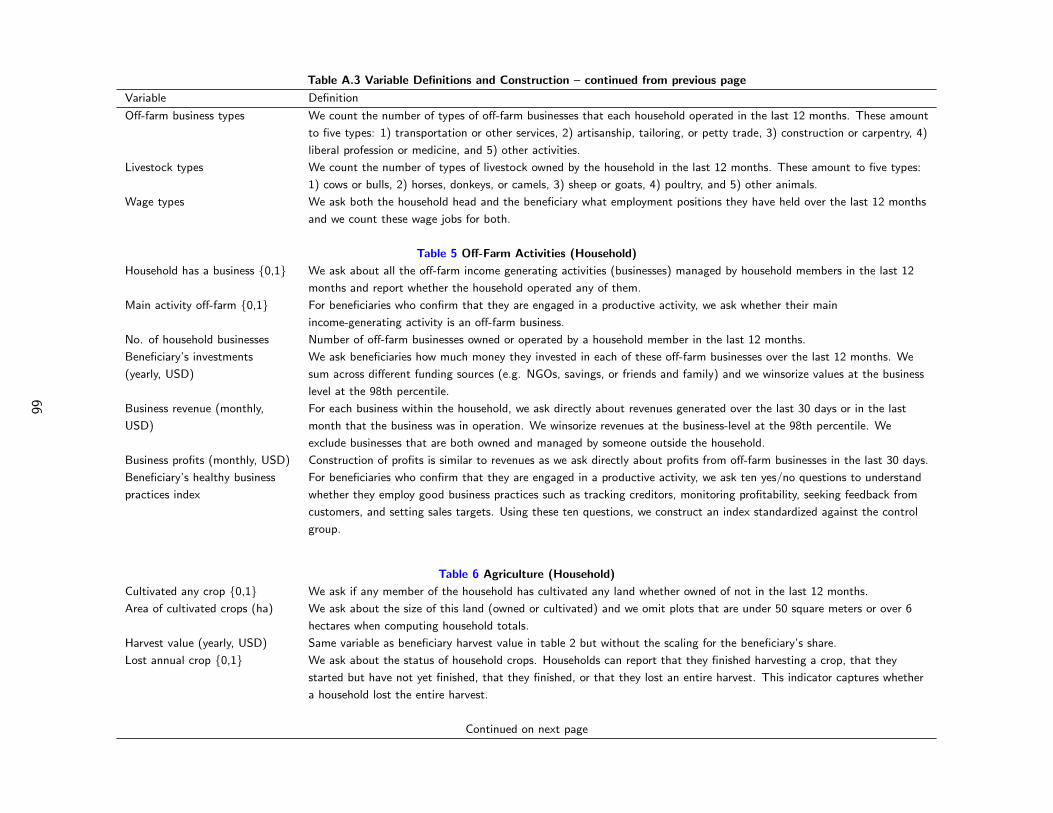
Table A.3 Variable Definitions and Construction – continued from previous page

Variable Definition

Off-farm business types We count the number of types of off-farm businesses that each household operated in the last 12 months. These amount

to five types: 1) transportation or other services, 2) artisanship, tailoring, or petty trade, 3) construction or carpentry, 4)

liberal profession or medicine, and 5) other activities.

Livestock types We count the number of types of livestock owned by the household in the last 12 months. These amount to five types:

1) cows or bulls, 2) horses, donkeys, or camels, 3) sheep or goats, 4) poultry, and 5) other animals.

Wage types We ask both the household head and the beneficiary what employment positions they have held over the last 12 months

and we count these wage jobs for both.

Table 5 Off-Farm Activities (Household)

Household has a business {0,1} We ask about all the off-farm income generating activities (businesses) managed by household members in the last 12

months and report whether the household operated any of them.

Main activity off-farm {0,1} For beneficiaries who confirm that they are engaged in a productive activity, we ask whether their main

income-generating activity is an off-farm business.

No. of household businesses Number of off-farm businesses owned or operated by a household member in the last 12 months.

Beneficiary’s investments

(yearly, USD)

We ask beneficiaries how much money they invested in each of these off-farm businesses over the last 12 months. We

sum across different funding sources (e.g. NGOs, savings, or friends and family) and we winsorize values at the business

level at the 98th percentile.

Business revenue (monthly,

USD)

For each business within the household, we ask directly about revenues generated over the last 30 days or in the last

month that the business was in operation. We winsorize revenues at the business-level at the 98th percentile. We

exclude businesses that are both owned and managed by someone outside the household.

Business profits (monthly, USD) Construction of profits is similar to revenues as we ask directly about profits from off-farm businesses in the last 30 days.

Beneficiary’s healthy business

practices index

For beneficiaries who confirm that they are engaged in a productive activity, we ask ten yes/no questions to understand

whether they employ good business practices such as tracking creditors, monitoring profitability, seeking feedback from

customers, and setting sales targets. Using these ten questions, we construct an index standardized against the control

group.

Table 6 Agriculture (Household)

Cultivated any crop {0,1} We ask if any member of the household has cultivated any land whether owned of not in the last 12 months.

Area of cultivated crops (ha) We ask about the size of this land (owned or cultivated) and we omit plots that are under 50 square meters or over 6

hectares when computing household totals.

Harvest value (yearly, USD) Same variable as beneficiary harvest value in table 2 but without the scaling for the beneficiary’s share.

Lost annual crop {0,1} We ask about the status of household crops. Households can report that they finished harvesting a crop, that they

started but have not yet finished, that they finished, or that they lost an entire harvest. This indicator captures whether

a household lost the entire harvest.

Continued on next page

66

Table A.3 Variable Definitions and Construction – continued from previous page

Variable Definition

Purchased seeds {0,1} Indicator for whether a household bought some of the seeds it used on any plot during the rainy season.

Used chemical fertilizer {0,1} Indicator for whether a household used inorganic or chemical fertilizer on any plot during the rainy season.

Used phytosanitary products

{0,1}Indicator for whether a household used phytosanitary products on any plot during the rainy season.

Used paid labor {0,1} Indicator for whether a household used paid labor (in cash or in kind) on any plot during the rainy season.

Sold annual crop {0,1} For crops that have been completely or partially harvested, we ask whether any portion has been sold.

Sale value (yearly, USD) For sale values, we multiply regional, unit-specific median selling prices by quantities sold. As we did for harvest values,

we omit sale quantities that have unconvertible units or whose values are extremely unlikely such as outliers and cases

where sale value exceeds harvest value. After dropping outlying sales values, we winsorize values at the 98th percentile.

Commercialization % Commercialization percent of crops (sale value ÷ harvest value)

Table 7 Livestock (Household)

Livestock count (TLU) If a household reports that any of its members owned or raised livestock in the last 12 months, we ask for the number of

animals that currently belong to the household itself. We report these numbers using Tropical Livestock Units where

conversion factors are as follows (Njuki et al., 2011):

Camels = 1.1 Horses, mares, or donkeys = 0.8 Cows and calves = 0.70 Bulls = 0.5

Pigs = 0.20 Sheep, goats, and mutton = 0.10 Guinea Fowl = 0.03 Chicken = 0.01

Livestock types See table 4

Livestock asset value (USD) We ask each household about the quantity and expected sale value of different types of livestock they currently own. We

compute and winsorize unit values at the livestock level.

Change in livestock count

(yearly, TLU)

We also ask how many animals any household members owned 12 months ago to compute the change in livestock

ownership. We present this change in Tropical Livestock Units as we do for livestock count above.

Livestock purchase value (USD) If households purchased livestock in the last 12 months, we ask them about the value of their purchases. Like animal sale

values, we winsorize purchase values at the animal level at the 98th percentile.

Livestock revenue (yearly, USD) Same as beneficiary livestock revenue in table 2 but not reduced to beneficiary’s share.

Table 8 Assets (Household)

Agricultural asset value (USD) We ask about agricultural equipment such as rakes, plows, and pickaxes currently owned by the household. We divide

reported values by quantities to get unit values and we winsorize unit values within each asset type.

Business asset value (USD) We ask about the value of equipment and materials the household currently owns and employs in its off-farm business

activities.

Household asset index We compute a PCA index using the reported current ownership of household assets such as televisions, cellphones, beds,

and tables.

Table 9 Financial Engagement

Continued on next page

67

Table A.3 Variable Definitions and Construction – continued from previous page

Variable Definition

Takes part in tontine/AVEC

{0,1}We ask beneficiaries whether they take part in a savings group where savings groups are either tontines such that one

contributor receives a payout every meeting or VSLAs where payouts are shared among the contributors at the end of

every cycle.

Tontine/AVEC savings (3

months, USD)

We report beneficiaries’ savings over the last 3 months by multiplying the size of contributions by their frequency and the

number of months in the last 3 months that the beneficiary contributed. We then winsorize these monthly contributions

and compute totals regardless of the type of savings group.

Other savings (3 months, USD) We also ask beneficiaries if they deposited any savings in the last 3 months (1) formally with a bank, savings bank, or

other institution, (2) informally in the form of credit with traders or suppliers, agricultural cooperatives, or mobile money

or (3) as cash with friends, neighbors, or family members outside the household, or at home in a box or bag, or in the

form of jewelry. We winsorize these values at the deposit level at the 98th percentile and we report totals across deposit

locations.

Total borrowed (yearly, USD) We ask whether beneficiaries have taken out personal loans in the last 12 months from savings groups (excluding

tontines), microfinance institutions, friends or neighbors, family members outside the household, lenders, traders, or any

other party. We report the amount of outstanding debt (principal and interest), winsorized at the 98th percentile.

Total lent out (yearly, USD) We ask beneficiaries how much money other household members still owe them today and we winsorize responses at the

98th percentile.

Household transfers in (yearly,

USD)

We ask the household head about the size and frequency of any transfer (money, products, or goods) that the household

has received over the last 12 months from any person (family or otherwise) who is not currently a member of the

household. We winsorize yearly totals at the 98th percentile.

Household transfers out (yearly,

USD)

We ask the household head about the size and frequency of any transfer (money, products, or goods) that the household

sent out over the last 12 months to any person (family or otherwise) who is not currently a member of the household.

We winsorize yearly totals at the 98th percentile.

Notes: All continuous variables are winsorized at the 98th and 2th percentiles at the most disaggregated level feasible.

68

Table A.4: Index Definitions and Construction

Variable Components Sub-components (if any) Possible answers

Table 10 Psychological Well-Being Indices

Mental health index Less depression: Sum of 10 questions

from CESD-R-10 (Radloff, 1977)

No. of days felt the details of life bothered you

more than usual

0 - 7 days

No. of days felt you had trouble concentrating on

what you were doing

0 - 7 days

No. of days felt sad 0 - 7 days

No. of days felt that what you were doing took all

your energy

0 - 7 days

No. of days felt you were confident in the future

(reversed)

0 - 7 days

No. of days felt nervous, tense, or worried 0 - 7 days

No. of days felt you had trouble sleeping peacefully 0 - 7 days

No. of days felt happy (reversed) 0 - 7 days

No. of days felt alone 0 - 7 days

No. of days felt so tired that you could do nothing 0 - 7 days

Less disability: Sum of 4 questions

from SRQ-20 (Harding et al., 1980)

No. of days you have had a headache 0 - 7 days

No. of days your digestion was bad 0 - 7 days

No. of days you had difficulty fulfilling your family

responsibilities

0 - 7 days

No. of days you had difficulties in your daily work 0 - 7 days

Life satisfaction today (MacArthur Scale) (Operario, Adler, and Williams, 2004) † 1 lower - 10 higher

Inner Peace (MacArthur Scale) 1 lower - 10 higher

Self-reported mental health:

standardized mental health assessment

In general, would you say that your mental health is

excellent, very good, good, fair or poor?

1 bad - 5 excellent

Social worth index Self-efficacy: Sum of 7 questions from

GSE-10 (Schwarzer, Jerusalem, et al.,

1995) and 1 from Rosenberg

Self-Esteem (Rosenberg, 2015)

GSE 1: You can successfully solve problems if you

put in enough effort.

1 not at all - 4 yes,

absolutely

Continued on next page

69

Table A.4 Index Definitions and Construction – continued from previous page

Variable Components Sub-components (if any) Possible answers

GSE 2: If someone doesn’t want you to do

something, you can find a way to do whatever you

want to do anyway.

1 not at all - 4 yes,

absolutely

GSE 3: It is easy for you to stay on the path you

have set out for yourself and achieve your goals in

life.

1 not at all - 4 yes,

absolutely

GSE 4: You are confident that you are able to cope

well with unexpected events.

1 not at all - 4 yes,

absolutely

GSE 7: You can stay calm when you are faced with

difficulties because you have the ability to adapt.

1 not at all - 4 yes,

absolutely

GSE 8: When you have to solve a problem, you can

usually find more than one solution.

1 not at all - 4 yes,

absolutely

GSE 9: If you find yourself in a difficult situation,

you can usually find a solution.

1 not at all - 4 yes,

absolutely

Rosenberg self-esteem: You are able to do things as

well as most people.

1 not at all - 4 yes,

absolutely

Social Standing: Sum of 4 MacArthur

Scale questions †There are people who are not good people and who

do not have good behavior (point down). But there

are also people who have a lot of good qualities and

who have a good behavior (point up)

1 lower - 10 higher

At the top of the ladder there are the most

respected people, such as the village chief and

religious leaders, and at the bottom there are the

least respected people, such as the excluded

1 lower - 10 higher

At the top of the ladder there are the people whose

opinion is followed the most in the community, and

at the bottom there are the people whose opinion is

the least followed

1 lower - 10 higher

At the top of the stairs are the people with the

most resources, the most education, and the most

respected jobs. At the bottom are the lowest-status

people who have the least money, the least

education, and the least respected or unemployed

jobs

1 lower - 10 higher

Continued on next page

70

Table A.4 Index Definitions and Construction – continued from previous page

Variable Components Sub-components (if any) Possible answers

Future expectations index Expected social status (MacArthur Scale) 1 lower - 10 higher

Expected life satisfaction two years from now (MacArthur Scale) 1 lower - 10 higher

Expected social position of child at age 30 (MacArthur Scale) 1 lower - 10 higher

Table 11 Social Well-Being Indices

Social support index How many people do you know who have personally succeeded in life? Integer

How many people can you go to for advice on income-generating activities? Integer

How many people come to you for advice on income-generating activities? Integer

How many people can you go to for advice on arguments or disputes? Integer

How many people come to you for advice on arguments or disputes? Integer

How many people can you trust to sell your products in other markets? Integer

Financial support index Respondent can count on village community to help them in case of financial difficulties 1 not at all - 4 yes,

absolutely

Number of people whom respondent

could ask for money

No. of siblings that you can ask for money Integer

No. of family members that you can ask for money Integer

No. of friends that you can ask for money Integer

No. of other people that you can ask for money Integer

What is the probability that you will be able to raise 30,000 XOF over the next month 1 not at all likely - 4

very likely

Intra-household dynamics

index

Partner dynamics When you disagree with your spouse, you feel

comfortable telling him so

1 never - 4 most of

the time

Do you think your spouse will always do the things

that are best for you?

1 never - 4 most of

the time

How close you feel to your partner? (hand gesture)

‡1 independent - 4

integrated

Household dynamics Your household has NOT prevented you from

visiting friends or family in the last 12 months

0 no - 1 yes

In the last 6 months, have you had tensions with

other members of your household? (reversed)

1 yes, a lot - 4 not at

all

How close you feel to your household? (hand

gesture) ‡1 independent - 4

integrated

Social cohesion and

closeness to community

index

You can count on the help of the women of your village when you have difficulties. Do you agree? 1 not at all - 4 yes,

absolutely

Continued on next page

71

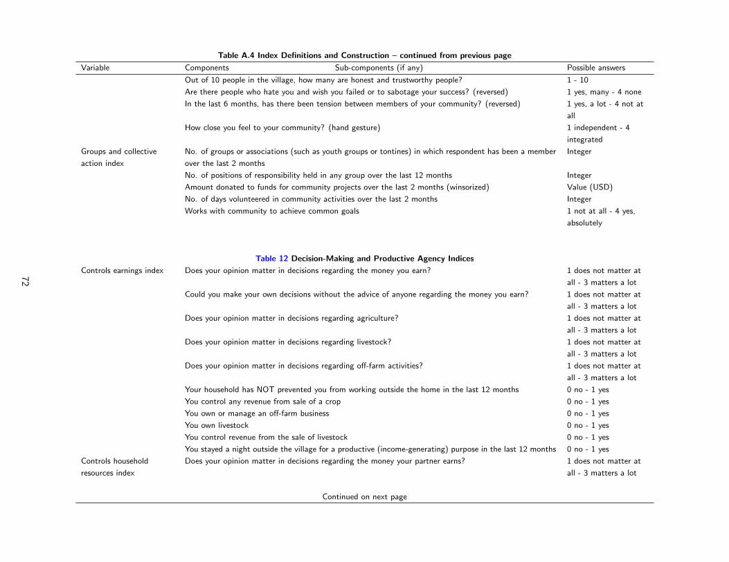
Table A.4 Index Definitions and Construction – continued from previous page

Variable Components Sub-components (if any) Possible answers

Out of 10 people in the village, how many are honest and trustworthy people? 1 - 10

Are there people who hate you and wish you failed or to sabotage your success? (reversed) 1 yes, many - 4 none

In the last 6 months, has there been tension between members of your community? (reversed) 1 yes, a lot - 4 not at

all

How close you feel to your community? (hand gesture) 1 independent - 4

integrated

Groups and collective

action index

No. of groups or associations (such as youth groups or tontines) in which respondent has been a member

over the last 2 months

Integer

No. of positions of responsibility held in any group over the last 12 months Integer

Amount donated to funds for community projects over the last 2 months (winsorized) Value (USD)

No. of days volunteered in community activities over the last 2 months Integer

Works with community to achieve common goals 1 not at all - 4 yes,

absolutely

Table 12 Decision-Making and Productive Agency Indices

Controls earnings index Does your opinion matter in decisions regarding the money you earn? 1 does not matter at

all - 3 matters a lot

Could you make your own decisions without the advice of anyone regarding the money you earn? 1 does not matter at

all - 3 matters a lot

Does your opinion matter in decisions regarding agriculture? 1 does not matter at

all - 3 matters a lot

Does your opinion matter in decisions regarding livestock? 1 does not matter at

all - 3 matters a lot

Does your opinion matter in decisions regarding off-farm activities? 1 does not matter at

all - 3 matters a lot

Your household has NOT prevented you from working outside the home in the last 12 months 0 no - 1 yes

You control any revenue from sale of a crop 0 no - 1 yes

You own or manage an off-farm business 0 no - 1 yes

You own livestock 0 no - 1 yes

You control revenue from the sale of livestock 0 no - 1 yes

You stayed a night outside the village for a productive (income-generating) purpose in the last 12 months 0 no - 1 yes

Controls household

resources index

Does your opinion matter in decisions regarding the money your partner earns? 1 does not matter at

all - 3 matters a lot

Continued on next page

72

Table A.4 Index Definitions and Construction – continued from previous page

Variable Components Sub-components (if any) Possible answers

Does your opinion matter in decisions regarding current household expenses? 1 does not matter at

all - 3 matters a lot

Does your opinion matter in decisions regarding major household purchases? 1 does not matter at

all - 3 matters a lot

Does your opinion matter in decisions regarding family planning? 1 does not matter at

all - 3 matters a lot

Does your opinion matter in decisions regarding your own healthcare? 1 does not matter at

all - 3 matters a lot

Does your opinion matter in decisions regarding your children’s education? 1 does not matter at

all - 3 matters a lot

Could you make your own decisions without the advice of anyone regarding current household expenses? 1 does not matter at

all - 3 matters a lot

Could you make your own decisions without the advice of anyone regarding household purchases? 1 does not matter at

all - 3 matters a lot

Could you make your own decisions without the advice of anyone regarding family planning? 1 does not matter at

all - 3 matters a lot

Could you make your own decisions without the advice of anyone regarding your own healthcare? 1 does not matter at

all - 3 matters a lot

Table 13 Children’s Outcomes

Child attended school Child (age 6 - 14) attended school in the last 12 months 0 no - 1 yes

Child labor index Number of days that a child (age 6 - 14) in the household was involved in an off-farm activity Integer

Number of days that a child (age 6 - 14) in the household was involved in agricultural labor Integer

Number of days that a child (age 6 - 14) in the household was involved in tending livestock Integer

Child chores index Indicator for whether a child (age 6 - 14) in the household contributed to collecting firewood or water 0 no - 1 yes

Indicator for whether a child (age 6 - 14) in the household helped in doing laundry 0 no - 1 yes

Indicator for whether a child (age 6 - 14) in the household helped in shopping 0 no - 1 yes

Weight/height z-score Child wasting index following WHO definition, based on the weight/height z-score for children ages 6-59

months

Notes: The variable listed in the first column is a z-score index of the components listed in the second column (except for ”child attended school” in

table 13). Some components are made up of sub-components, which are shown to the right of the components. All indices are standardized against

the control group.

†MacArthur Scale questions are phrased as follows using life satisfaction as an example: “please imagine a ladder, with steps numbered from 0 at the

bottom to 10 at the top. The top of the ladder represents the best possible life for you and the bottom of the ladder represents the worst possible life

for you. On which step of the ladder would you say you personally feel you stand at this time?”

‡Hand gestures for social closeness: surveyors spread their hands wider than their shoulders to signal independence and they join their hands to signal

integration.

73

Table A.5: Multiple Hypothesis Test Corrections

6 months post-intervention 18 months post-intervention

MHT family Capital Arm Psychosocial Arm Full Arm Capital Arm Psychosocial Arm Full Arm

Variable Actual FDR† FWER‡ Actual FDR FWER Actual FDR FWER Actual FDR FWER Actual FDR FWER Actual FDR FWER

Table 1 Primary Outcomes

Gross consumption (daily, USD/adult

eq.)

0.002 0.002 0.007 0.083 0.083 0.117 0 0 0 0.007 0.007 0.016 0.001 0.001 0.003 0 0 0

Food security (raw sum) 0 0 0 0.058 0.083 0.153 0 0 0 0 0 0 0 0.001 0.004 0 0 0

Food consumption score 0 0 0 0.002 0.005 0.016 0 0 0 0 0.001 0.002 0.009 0.009 0.019 0 0 0

Table 2 Beneficiary Revenues

Business revenue (monthly, USD) 0 0 0 0 0 0 0 0 0 0 0 0 0.004 0.008 0.031 0 0 0

Harvest value (yearly, USD) 0.264 0.264 0.375 0.345 0.345 0.455 0.375 0.375 0.477 0.198 0.213 0.380 0.004 0.008 0.044 0.002 0.003 0.007

Wage earnings (yearly, USD) 0.036 0.073 0.169 0.094 0.126 0.234 0.006 0.012 0.042 0.213 0.213 0.281 0.465 0.465 0.517 0.101 0.101 0.141

Livestock revenue (yearly, USD) 0.244 0.264 0.494 0.029 0.059 0.161 0.162 0.216 0.377 0.007 0.014 0.028 0.152 0.203 0.356 0.005 0.006 0.020

Table 3 Beneficiary Labor Participation

Days spent in off-farm business 0 0 0 0 0 0 0 0 0 0 0 0 0 0 0 0 0 0

Days spent in agriculture 0.398 0.398 0.442 0.479 0.479 0.536 0.833 0.833 0.847 0.377 0.503 0.651 0.593 0.593 0.616 0.682 0.682 0.698

Days spent in salaried employment 0.132 0.176 0.301 0.210 0.280 0.432 0.061 0.081 0.168 0.931 0.931 0.937 0.207 0.276 0.441 0.616 0.682 0.877

Days spent raising livestock 0 0 0 0.006 0.012 0.034 0 0 0 0 0 0 0.010 0.020 0.067 0 0 0

Table 4 Income Diversification (Household)

No. of income sources 0 0 0 0 0 0 0 0 0 0 0 0 0.007 0.017 0.061 0 0 0

Crop types 0.534 0.646 0.813 0.848 0.848 0.863 0.607 0.607 0.636 0.786 0.786 0.808 0.329 0.329 0.390 0.052 0.065 0.141

Off-farm business types 0 0 0 0 0 0 0 0 0 0.013 0.021 0.064 0.010 0.017 0.059 0.001 0.002 0.013

Livestock types 0 0 0 0 0 0.001 0 0 0 0 0 0 0.004 0.017 0.051 0 0 0

Wage types 0.646 0.646 0.671 0.064 0.080 0.189 0.103 0.128 0.249 0.539 0.674 0.807 0.224 0.280 0.485 0.566 0.566 0.611

Table 5 Off-Farm Activities (Household)

Household has a business {0,1} 0 0 0 0 0 0 0 0 0 0 0 0 0 0 0.002 0 0 0

Beneficiary’s main activity is off-farm

{0,1}0 0 0 0 0 0 0 0 0 0 0 0.003 0.001 0.001 0.009 0 0 0

No. of household businesses 0 0 0 0 0 0 0 0 0 0 0 0 0 0 0 0 0 0

Beneficiary’s investments (yearly,

USD)

0 0 0 0 0 0 0 0 0 0 0 0 0.001 0.001 0.005 0 0 0

Business revenue (monthly, USD) 0 0 0 0 0 0 0 0 0 0.001 0.001 0.008 0.004 0.004 0.007 0 0 0

Business profits (monthly, USD) 0 0 0 0 0 0 0 0 0 0.003 0.003 0.009 0.003 0.003 0.008 0 0 0

Beneficiary’s healthy business

practices index

0 0 0 0 0 0 0 0 0 0 0 0 0 0.001 0.005 0 0 0

Table 6 Agriculture (Household)

Cultivated any crop {0,1} 0.843 0.843 0.855 0.858 0.858 0.850 0.845 0.845 0.877 0.293 0.538 0.918 0.412 0.462 0.496 0.819 0.819 0.846

Area of cultivated crops (ha) 0.186 0.341 0.752 0.015 0.042 0.197 0.018 0.039 0.195 0.746 0.884 0.972 0.270 0.422 0.901 0.410 0.564 0.882

Harvest value (method 2) 0.563 0.688 0.938 0.636 0.747 0.968 0.742 0.817 0.950 0.145 0.319 0.669 0 0.001 0.007 0 0.001 0.009

Lost annual crop {0,1} 0.705 0.775 0.928 0.629 0.747 0.987 0.496 0.607 0.888 0.433 0.596 0.888 0.292 0.422 0.853 0.125 0.228 0.573

Purchased seeds {0,1} 0.221 0.347 0.763 0.523 0.747 0.985 0.261 0.358 0.764 0.055 0.302 0.491 0.055 0.203 0.482 0.155 0.243 0.612

Continued on next page

74

Table A.5: Multiple Hypothesis Test Corrections – continued from previous page

6 months post-intervention 18 months post-intervention

MHT family Capital Arm Psychosocial Arm Full Arm Capital Arm Psychosocial Arm Full Arm

Variable Actual FDR† FWER‡ Actual FDR FWER Actual FDR FWER Actual FDR FWER Actual FDR FWER Actual FDR FWER

Used chemical fertilizer {0,1} 0.014 0.070 0.203 0.287 0.526 0.883 0.003 0.017 0.063 0.006 0.063 0.100 0.462 0.462 0.741 0.001 0.003 0.023

Used pytosanitary products {0,1} 0.026 0.071 0.237 0.679 0.747 0.911 0.008 0.021 0.118 0.118 0.319 0.697 0.232 0.422 0.911 0 0.001 0

Used paid labor {0,1} 0.003 0.035 0.074 0.064 0.141 0.435 0 0 0 0.116 0.319 0.679 0.293 0.422 0.893 0 0 0

Sold annual crop {0,1} 0.419 0.576 0.903 0.003 0.015 0.068 0.052 0.095 0.347 0.851 0.884 0.966 0.307 0.422 0.795 0.547 0.669 0.898

Sale value (yearly, USD) 0.019 0.070 0.193 0.004 0.015 0.072 0.006 0.021 0.061 0.428 0.596 0.924 0.012 0.067 0.219 0.073 0.161 0.451

Commercial- ization % (10)/(3)=(11) 0.037 0.080 0.290 0 0.004 0.011 0.087 0.136 0.409 0.884 0.884 0.892 0.445 0.462 0.870 0.726 0.798 0.938

Table 7 Livestock (Household)

Livestock count (TLU) 0 0 0 0.007 0.036 0.048 0 0 0 0.001 0.002 0.013 0.019 0.089 0.129 0 0 0

Livestock asset value (USD) 0.001 0.001 0 0.145 0.319 0.492 0 0 0 0.001 0.002 0.018 0.096 0.161 0.326 0 0 0

Change in livestock count (yearly,

TLU)

0 0 0.004 0.403 0.504 0.722 0.018 0.018 0.061 0.666 0.666 0.689 0.396 0.495 0.666 0.277 0.277 0.304

Livestock purchase value (USD) 0 0 0 0.554 0.554 0.580 0 0 0 0.238 0.298 0.501 0.860 0.860 0.884 0.017 0.021 0.046

Livestock revenue (yearly, USD) 0.668 0.668 0.709 0.191 0.319 0.521 0.011 0.014 0.042 0 0 0 0.036 0.089 0.186 0 0 0.001

Table 8 Assets (Household)

Agricultural asset value (USD) 0.936 0.936 0.942 0.426 0.426 0.445 0.970 0.970 0.974 0.180 0.271 0.414 0.931 0.931 0.937 0.096 0.096 0.118

Business asset value (USD) 0.195 0.419 0.524 0.253 0.380 0.484 0 0.001 0.005 0.021 0.063 0.098 0.080 0.120 0.207 0.010 0.015 0.050

Household asset index 0.280 0.419 0.533 0.027 0.080 0.135 0.002 0.003 0.013 0.478 0.478 0.504 0.020 0.060 0.088 0.007 0.015 0.035

Table 9 Financial Engagement

Takes part in tontine/AVEC {0,1} 0 0 0.016 0.001 0.005 0.098 0.001 0.003 0.055 0 0 0 0 0 0 0 0 0

Tontine/AVEC savings (3 months,

USD)

0.583 0.816 0.941 0.444 0.518 0.717 0.326 0.456 0.832 0 0 0 0 0 0 0 0 0

Other savings (3 months, USD) 0.060 0.140 0.362 0.036 0.124 0.254 0 0 0 0.008 0.018 0.069 0.457 0.640 0.858 0.001 0.001 0.007

Total borrowed (yearly, USD) 0.953 0.953 0.957 0.127 0.297 0.552 0.810 0.810 0.819 0.890 0.890 0.898 0.121 0.211 0.478 0.002 0.004 0.022

Total lent out (yearly, USD) 0.008 0.028 0.109 0.182 0.318 0.620 0 0 0 0.121 0.141 0.271 0.720 0.840 0.929 0.067 0.078 0.190

Household transfers in (yearly, USD) 0.452 0.790 0.937 0.967 0.967 0.970 0.305 0.456 0.745 0.060 0.091 0.270 0.885 0.885 0.897 0.869 0.869 0.883

Household transfers out (yearly, USD) 0.757 0.884 0.957 0.245 0.343 0.676 0.436 0.508 0.757 0.065 0.091 0.314 0.039 0.092 0.369 0.004 0.005 0.030

Table 10 Psychological Well-Being Indices

Mental health index 0.003 0.003 0.009 0.016 0.016 0.025 0 0 0 0 0 0 0 0 0 0 0 0

Social worth index 0 0 0 0 0 0 0 0 0 0.006 0.009 0.022 0 0 0 0 0 0

Future expectations index 0.002 0.003 0.009 0 0 0 0 0 0 0.011 0.011 0.021 0.002 0.002 0.006 0 0 0

Table 11 Social Well-Being Indices

Social support index 0 0 0.001 0 0 0 0 0 0 0.004 0.006 0.017 0 0 0 0 0 0

Financial support index 0 0 0 0 0 0 0 0 0 0 0 0 0 0 0 0 0 0

Intra-household dynamics index 0.114 0.143 0.269 0.094 0.094 0.126 0.108 0.108 0.147 0.634 0.634 0.671 0.323 0.323 0.367 0.787 0.787 0.791

Social cohesion and community

closeness index

0.451 0.451 0.472 0.009 0.012 0.034 0.006 0.008 0.025 0.094 0.118 0.234 0.003 0.003 0.012 0.043 0.054 0.114

Collective action index 0 0 0 0 0 0 0 0 0 0 0 0 0 0 0 0 0 0

Table 12 Decision-Making and Productive Agency Indices

Controls earnings index 0 0 0 0 0 0 0 0 0 0 0 0 0 0.001 0 0 0 0

Controls HH resources index 0.496 0.496 0.532 0.167 0.167 0.198 0.142 0.142 0.172 0.776 0.776 0.784 0.234 0.234 0.264 0.419 0.419 0.456

Table 13 Children’s Outcomes

Child attended school {0,1} 0.076 0.120 0.265 0.894 0.894 0.900 0.604 0.604 0.648 0.026 0.051 0.112 0.263 0.350 0.525 0.237 0.474 0.624

Continued on next page

75

Table A.5: Multiple Hypothesis Test Corrections – continued from previous page

6 months post-intervention 18 months post-intervention

MHT family Capital Arm Psychosocial Arm Full Arm Capital Arm Psychosocial Arm Full Arm

Variable Actual FDR† FWER‡ Actual FDR FWER Actual FDR FWER Actual FDR FWER Actual FDR FWER Actual FDR FWER

Child labor index 0.090 0.120 0.244 0.001 0.002 0.015 0 0 0 0.002 0.007 0.021 0.001 0.002 0.006 0 0 0.003

Child chores index 0.011 0.045 0.101 0.004 0.009 0.032 0.223 0.297 0.459 0.239 0.318 0.482 0.243 0.350 0.637 0.480 0.590 0.761

Weight/height z-score 0.888 0.888 0.902 0.540 0.720 0.806 0.120 0.240 0.419 0.756 0.756 0.787 0.781 0.781 0.802 0.590 0.590 0.622

Notes: At each survey phase and within each treatment arm, we correct p-values for multiple hypothesis testing within each family of variables. Columns labeled actual show the p-values used in the main tables. Italics: p < 0.1. Bold: p

< 0.05. Bold and underlined: p < 0.01.

†: Columns labeled FDR show False Discovery Rate-adjusted q-values following the step-up approach of (Benjamini and Hochberg, 1995) which assumes that the p-values within a family are positively correlated.

‡: Columns labeled FWER show Family-Wise Error Rate-corrected p-values following the procedure outlined in (Barsbai et al., 2020), capturing the existing correlation between p-values by exploiting treatment randomization and runing a

bootstrap resampling procedure.

76

Table A.6: Financial Engagement (Extensive Margins)

(1) (2) (3) (4)

Takes part in

tontine/AVEC

{0,1}

Takes part in

tontine/AVEC

(enumerator F.E.)

Savings group:

tontine

{0,1}

Savings group:

AVEC

{0,1}Followup 1 (6 months after cash grants)

Capital 0.05∗∗∗ 0.05∗∗∗ -0.03∗ 0.10∗∗∗

(0.01) (0.01) (0.02) (0.02)

Psychosocial 0.04∗∗∗ 0.04∗∗∗ -0.04∗∗ 0.08∗∗∗

(0.01) (0.01) (0.02) (0.02)

Full 0.04∗∗∗ 0.04∗∗∗ -0.02 0.08∗∗∗

(0.01) (0.01) (0.02) (0.02)

Observations 4476 4476 4476 4476

Control mean 0.93 0.93 0.23 0.84

Control SD 0.26 0.26 0.42 0.37

p (Capital = Psychosocial) 0.198 0.083 0.817 0.177

p (Capital = Full) 0.114 0.105 0.585 0.113

p (Psychosocial = Full) 0.829 0.806 0.405 0.921

Followup 2 (18 months after cash grants)

Capital 0.31∗∗∗ 0.31∗∗∗ -0.00 0.34∗∗∗

(0.03) (0.03) (0.01) (0.03)

Psychosocial 0.27∗∗∗ 0.27∗∗∗ -0.01 0.30∗∗∗

(0.03) (0.03) (0.01) (0.03)

Full 0.33∗∗∗ 0.33∗∗∗ 0.00 0.35∗∗∗

(0.03) (0.03) (0.01) (0.03)

Observations 4303 4303 4303 4303

Control mean 0.53 0.53 0.07 0.49

Control SD 0.50 0.50 0.26 0.50

p (Capital = Psychosocial) 0.106 0.068 0.439 0.086

p (Capital = Full) 0.363 0.425 0.586 0.477

p (Psychosocial = Full) 0.013 0.011 0.180 0.018

p (Followup 1 = Followup 2 for Capital) 0.000 0.000 0.200 0.000

p (Followup 1 = Followup 2 for Psychosocial) 0.000 0.000 0.303 0.000

p (Followup 1 = Followup 2 for Full) 0.000 0.000 0.243 0.000

Notes: Results presented are OLS estimates that include controls for randomization strata and, where possible, baseline outcomes.We assign baseline strata means to households surveyed at followup but not at baseline and we control for such missing values withan indicator. Robust standard errors are shown in parentheses, clustered at the village level. *** p < 0.01, ** p < 0.05, * p < 0.1.All monetary amounts are PPP-adjusted USD terms, set at 2016 prices and deflated using CPI published by the World Bank. In2016, 1 USD = 242.553 XOF PPP. All continuous variables are winsorized at the 98th and 2th percentiles at the most disaggregatedlevel feasible. See Table A.3 for details on variable construction.

77

Table A.7: Mental Health Index Components

(1) (2) (3) (4) (5) (6)

Mental

health

index

Less

depression

{0-70}

Less

disability

{0-28}

Life

satisfaction

{1-10}

Inner

peace

{1-10}

Self-reported

mental

health

Followup 1 (6 months after cash grants)

Capital 0.13∗∗∗ 0.60 0.24 0.40∗∗∗ 0.23∗∗ -0.02

(0.04) (0.47) (0.24) (0.09) (0.09) (0.04)

Psychosocial 0.10∗∗ 0.60 0.15 0.29∗∗∗ 0.22∗∗ -0.02

(0.04) (0.47) (0.23) (0.09) (0.09) (0.04)

Full 0.23∗∗∗ 1.22∗∗∗ 0.56∗∗ 0.62∗∗∗ 0.32∗∗∗ 0.01

(0.04) (0.47) (0.22) (0.09) (0.09) (0.04)

Observations 4476 4476 4476 4476 4476 4476

Control mean 0.00 46.72 21.27 5.16 6.74 0.01

Control SD 1.00 11.53 5.47 2.07 2.04 1.01

p (Capital = Psychosocial) 0.560 0.994 0.671 0.260 0.835 0.985

p (Capital = Full) 0.012 0.194 0.128 0.010 0.302 0.427

p (Psychosocial = Full) 0.002 0.208 0.041 0.001 0.221 0.425

Followup 2 (18 months after cash grants)

Capital 0.15∗∗∗ 1.48∗∗∗ 0.62∗∗∗ 0.20∗∗ 0.22∗∗∗ -0.01

(0.04) (0.42) (0.21) (0.09) (0.07) (0.04)

Psychosocial 0.21∗∗∗ 1.69∗∗∗ 0.84∗∗∗ 0.28∗∗∗ 0.26∗∗∗ 0.04

(0.04) (0.43) (0.21) (0.09) (0.07) (0.04)

Full 0.26∗∗∗ 2.06∗∗∗ 0.77∗∗∗ 0.45∗∗∗ 0.34∗∗∗ 0.01

(0.04) (0.45) (0.19) (0.09) (0.07) (0.04)

Observations 4175 4175 4175 4175 4175 4175

Control mean 0.00 45.24 20.81 5.40 6.81 -0.01

Control SD 1.00 11.35 5.16 1.90 1.91 1.01

p (Capital = Psychosocial) 0.149 0.636 0.306 0.407 0.604 0.245

p (Capital = Full) 0.007 0.178 0.422 0.003 0.092 0.563

p (Psychosocial = Full) 0.247 0.408 0.731 0.039 0.230 0.485

p (Followup 1 = Followup 2 for Capital) 0.625 0.141 0.183 0.089 0.881 0.926

p (Followup 1 = Followup 2 for Psychosocial) 0.022 0.063 0.013 0.881 0.689 0.332

p (Followup 1 = Followup 2 for Full) 0.569 0.167 0.411 0.156 0.833 0.924

Notes: Results presented are OLS estimates that include controls for randomization strata and, where possible, baseline outcomes.We assign baseline strata means to households surveyed at followup but not at baseline and we control for such missing values withan indicator. Robust standard errors are shown in parentheses, clustered at the village level. *** p < 0.01, ** p < 0.05, * p < 0.1.See Table A.4 for details on variable construction.

78

Table A.8: Social Worth Index Components

(1) (2) (3)

Social

worth

index

Self

efficacy

{7-32}

Social

standing

{4-40}Followup 1 (6 months after cash grants)

Capital 0.16∗∗∗ 0.47∗∗∗ 0.87∗∗∗

(0.04) (0.16) (0.25)

Psychosocial 0.22∗∗∗ 0.62∗∗∗ 1.11∗∗∗

(0.04) (0.15) (0.24)

Full 0.36∗∗∗ 1.11∗∗∗ 1.73∗∗∗

(0.04) (0.16) (0.24)

Observations 4476 4476 4476

Control mean -0.00 22.99 23.23

Control SD 1.00 3.86 6.19

p (Capital = Psychosocial) 0.228 0.310 0.350

p (Capital = Full) 0.000 0.000 0.001

p (Psychosocial = Full) 0.000 0.001 0.015

Followup 2 (18 months after cash grants)

Capital 0.12∗∗∗ 0.40∗∗ 0.47∗

(0.04) (0.17) (0.27)

Psychosocial 0.20∗∗∗ 0.72∗∗∗ 0.75∗∗∗

(0.04) (0.17) (0.27)

Full 0.26∗∗∗ 0.89∗∗∗ 1.02∗∗∗

(0.04) (0.16) (0.24)

Observations 4175 4175 4175

Control mean -0.00 22.75 24.10

Control SD 1.00 3.93 5.98

p (Capital = Psychosocial) 0.075 0.089 0.279

p (Capital = Full) 0.001 0.004 0.021

p (Psychosocial = Full) 0.174 0.297 0.260

p (Followup 1 = Followup 2 for Capital) 0.368 0.770 0.225

p (Followup 1 = Followup 2 for Psychosocial) 0.814 0.648 0.289

p (Followup 1 = Followup 2 for Full) 0.043 0.273 0.025

Notes: Results presented are OLS estimates that include controls for randomization strata and, where possible, baselineoutcomes. We assign baseline strata means to households surveyed at followup but not at baseline and we control for suchmissing values with an indicator. Robust standard errors are shown in parentheses, clustered at the village level. *** p <0.01, ** p < 0.05, * p < 0.1. See Table A.4 for details on variable construction.

79

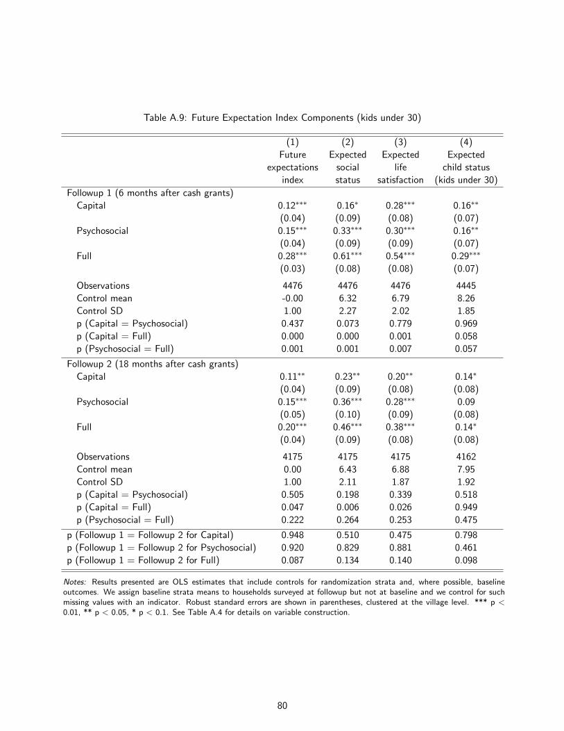
Table A.9: Future Expectation Index Components (kids under 30)

(1) (2) (3) (4)

Future

expectations

index

Expected

social

status

Expected

life

satisfaction

Expected

child status

(kids under 30)

Followup 1 (6 months after cash grants)

Capital 0.12∗∗∗ 0.16∗ 0.28∗∗∗ 0.16∗∗

(0.04) (0.09) (0.08) (0.07)

Psychosocial 0.15∗∗∗ 0.33∗∗∗ 0.30∗∗∗ 0.16∗∗

(0.04) (0.09) (0.09) (0.07)

Full 0.28∗∗∗ 0.61∗∗∗ 0.54∗∗∗ 0.29∗∗∗

(0.03) (0.08) (0.08) (0.07)

Observations 4476 4476 4476 4445

Control mean -0.00 6.32 6.79 8.26

Control SD 1.00 2.27 2.02 1.85

p (Capital = Psychosocial) 0.437 0.073 0.779 0.969

p (Capital = Full) 0.000 0.000 0.001 0.058

p (Psychosocial = Full) 0.001 0.001 0.007 0.057

Followup 2 (18 months after cash grants)

Capital 0.11∗∗ 0.23∗∗ 0.20∗∗ 0.14∗

(0.04) (0.09) (0.08) (0.08)

Psychosocial 0.15∗∗∗ 0.36∗∗∗ 0.28∗∗∗ 0.09

(0.05) (0.10) (0.09) (0.08)

Full 0.20∗∗∗ 0.46∗∗∗ 0.38∗∗∗ 0.14∗

(0.04) (0.09) (0.08) (0.08)

Observations 4175 4175 4175 4162

Control mean 0.00 6.43 6.88 7.95

Control SD 1.00 2.11 1.87 1.92

p (Capital = Psychosocial) 0.505 0.198 0.339 0.518

p (Capital = Full) 0.047 0.006 0.026 0.949

p (Psychosocial = Full) 0.222 0.264 0.253 0.475

p (Followup 1 = Followup 2 for Capital) 0.948 0.510 0.475 0.798

p (Followup 1 = Followup 2 for Psychosocial) 0.920 0.829 0.881 0.461

p (Followup 1 = Followup 2 for Full) 0.087 0.134 0.140 0.098

Notes: Results presented are OLS estimates that include controls for randomization strata and, where possible, baselineoutcomes. We assign baseline strata means to households surveyed at followup but not at baseline and we control for suchmissing values with an indicator. Robust standard errors are shown in parentheses, clustered at the village level. *** p <0.01, ** p < 0.05, * p < 0.1. See Table A.4 for details on variable construction.

80

Table A.10: Social Support Index Components

(1) (2) (3) (4) (5) (6) (7)

Social

support

index

No. of

role

models

No. of

activity

advisors

No. of

activity

mentees

No. of

conflict

advisors

No. of

conflit

mentees

No. of

market

intermediaries

Followup 1 (6 months after cash grants)

Capital 0.27∗∗∗ 0.70∗∗∗ 0.31∗∗∗ 0.57∗∗∗ 0.35∗ 0.15∗ 0.05

(0.06) (0.22) (0.12) (0.09) (0.19) (0.08) (0.07)

Psychosocial 0.24∗∗∗ 0.47∗∗∗ 0.34∗∗∗ 0.54∗∗∗ 0.16∗ 0.18∗∗ 0.14∗

(0.04) (0.15) (0.09) (0.09) (0.08) (0.08) (0.07)

Full 0.32∗∗∗ 0.59∗∗∗ 0.47∗∗∗ 0.68∗∗∗ 0.31∗∗∗ 0.21∗∗ 0.18∗∗

(0.05) (0.16) (0.08) (0.09) (0.09) (0.09) (0.08)

Observations 4476 4476 4476 4476 4476 4476 4476

Control mean 0.00 3.45 2.22 1.30 2.48 1.72 1.54

Control SD 1.00 2.79 2.08 1.82 1.90 2.08 1.72

p (Capital = Psychosocial) 0.569 0.284 0.792 0.778 0.336 0.742 0.205

p (Capital = Full) 0.417 0.630 0.158 0.260 0.861 0.550 0.070

p (Psychosocial = Full) 0.075 0.415 0.175 0.170 0.112 0.768 0.523

Followup 2 (18 months after cash grants)

Capital 0.13∗∗∗ 0.26 0.10 0.32∗∗∗ 0.15∗ 0.03 0.16∗∗

(0.04) (0.18) (0.09) (0.09) (0.09) (0.09) (0.07)

Psychosocial 0.18∗∗∗ 0.19 0.31∗∗ 0.39∗∗∗ 0.15∗ 0.22∗∗ 0.17∗∗

(0.05) (0.17) (0.12) (0.09) (0.08) (0.09) (0.08)

Full 0.18∗∗∗ 0.48∗∗ 0.28∗∗∗ 0.44∗∗∗ 0.06 0.12 0.22∗∗∗

(0.04) (0.21) (0.10) (0.10) (0.08) (0.08) (0.07)

Observations 4160 4160 4160 4160 4160 4160 4160

Control mean 0.00 3.36 2.37 1.55 2.54 1.79 1.68

Control SD 1.00 4.24 2.33 1.90 1.77 2.05 1.60

p (Capital = Psychosocial) 0.284 0.695 0.100 0.478 0.964 0.024 0.862

p (Capital = Full) 0.217 0.287 0.055 0.284 0.296 0.281 0.381

p (Psychosocial = Full) 0.968 0.141 0.820 0.685 0.286 0.192 0.573

p (Followup 1 = Followup 2 for Capital) 0.025 0.095 0.135 0.024 0.334 0.322 0.270

p (Followup 1 = Followup 2 for Psychosocial) 0.288 0.165 0.813 0.206 0.903 0.731 0.711

p (Followup 1 = Followup 2 for Full) 0.016 0.636 0.129 0.034 0.040 0.444 0.692

Notes: Results presented are OLS estimates that include controls for randomization strata and, where possible, baseline outcomes.We assign baseline strata means to households surveyed at followup but not at baseline and we control for such missing values withan indicator. Robust standard errors are shown in parentheses, clustered at the village level. *** p < 0.01, ** p < 0.05, * p < 0.1.See Table A.4 for details on variable construction.

81

Table A.11: Financial Support Index Components

(1) (2) (3) (4)

Financial

support

index

Village

financial

support {1-4}

No. of

financial

supporters

Fundraising

probability

{1-4}Followup 1 (6 months after cash grants)

Capital 0.29∗∗∗ 0.10∗∗∗ 0.27 0.32∗∗∗

(0.05) (0.04) (0.24) (0.04)

Psychosocial 0.35∗∗∗ 0.17∗∗∗ 0.84∗∗∗ 0.27∗∗∗

(0.05) (0.04) (0.25) (0.04)

Full 0.48∗∗∗ 0.18∗∗∗ 0.97∗∗∗ 0.45∗∗∗

(0.05) (0.03) (0.23) (0.05)

Observations 4476 4476 4476 4476

Control mean 0.00 2.60 6.30 1.49

Control SD 1.00 0.87 5.93 0.82

p (Capital = Psychosocial) 0.252 0.095 0.031 0.291

p (Capital = Full) 0.000 0.021 0.003 0.010

p (Psychosocial = Full) 0.012 0.745 0.604 0.000

Followup 2 (18 months after cash grants)

Capital 0.19∗∗∗ 0.05 0.08 0.24∗∗∗

(0.04) (0.04) (0.22) (0.04)

Psychosocial 0.21∗∗∗ 0.07∗ 0.40∗ 0.21∗∗∗

(0.04) (0.04) (0.24) (0.04)

Full 0.35∗∗∗ 0.13∗∗∗ 0.46∗∗ 0.36∗∗∗

(0.05) (0.04) (0.23) (0.04)

Observations 4252 4160 4252 4252

Control mean -0.00 2.63 6.49 1.43

Control SD 1.00 0.87 5.64 0.78

p (Capital = Psychosocial) 0.607 0.670 0.156 0.553

p (Capital = Full) 0.000 0.041 0.078 0.005

p (Psychosocial = Full) 0.004 0.106 0.798 0.001

p (Followup 1 = Followup 2 for Capital) 0.084 0.357 0.532 0.060

p (Followup 1 = Followup 2 for Psychosocial) 0.012 0.039 0.130 0.204

p (Followup 1 = Followup 2 for Full) 0.014 0.270 0.105 0.099

Notes: Results presented are OLS estimates that include controls for randomization strata and, where possible, baselineoutcomes. We assign baseline strata means to households surveyed at followup but not at baseline and we control for suchmissing values with an indicator. Robust standard errors are shown in parentheses, clustered at the village level. *** p <0.01, ** p < 0.05, * p < 0.1. See Table A.4 for details on variable construction.

82

Table A.12: Intra-Household Dynamics Index Components

(1) (2) (3) (4) (5) (6) (7) (8) (9)

Intra-household

dynamics

index

Partner

dynamics

index

Disagrees

with partner

{1-4}

Trusts

partner

{1-4}

Partner

inclusiveness

{1-4}

Household

dynamics

index

Household allows

family visits

{0,1}

Household

tensions

infrequent {1-4}

Household

inclusiveness

{1-4}Followup 1 (6 months after cash grants)

Capital 0.07 0.09∗ 0.06 -0.02 0.06∗∗ 0.04 0.01 -0.01 0.04

(0.04) (0.04) (0.05) (0.03) (0.02) (0.04) (0.01) (0.02) (0.03)

Psychosocial 0.07∗ 0.08∗ 0.06 0.05∗ 0.02 0.02 -0.01 0.00 0.05∗

(0.04) (0.04) (0.05) (0.03) (0.02) (0.04) (0.01) (0.02) (0.03)

Full 0.06 0.03 -0.05 0.07∗∗ 0.02 0.06 0.00 0.00 0.06∗∗

(0.04) (0.04) (0.06) (0.03) (0.02) (0.04) (0.01) (0.02) (0.03)

Observations 4476 3880 3765 3768 3826 4476 4476 4476 4476

Control mean -0.00 0.02 2.60 3.64 3.71 -0.00 0.93 3.82 3.38

Control SD 1.00 0.99 1.14 0.64 0.55 1.00 0.25 0.53 0.72

p (Capital = Psychosocial) 0.961 0.793 0.995 0.025 0.066 0.603 0.097 0.690 0.812

p (Capital = Full) 0.946 0.193 0.059 0.003 0.099 0.703 0.549 0.583 0.527

p (Psychosocial = Full) 0.982 0.242 0.040 0.514 0.778 0.346 0.282 0.878 0.675

Followup 2 (18 months after cash grants)

Capital 0.02 0.01 0.09 -0.02 -0.01 0.02 -0.00 -0.00 0.04

(0.04) (0.05) (0.06) (0.03) (0.02) (0.04) (0.01) (0.02) (0.03)

Psychosocial 0.04 0.12∗∗∗ 0.12∗∗ 0.03 0.04∗ -0.04 -0.03∗∗ -0.01 0.02

(0.04) (0.04) (0.06) (0.03) (0.02) (0.04) (0.01) (0.03) (0.03)

Full -0.01 0.02 0.06 -0.01 0.00 -0.03 -0.01 0.00 -0.03

(0.04) (0.04) (0.05) (0.03) (0.02) (0.04) (0.01) (0.02) (0.03)

Observations 4160 3557 3493 3490 3498 4160 4160 4160 4160

Control mean 0.00 0.00 2.73 3.69 3.78 -0.00 0.91 3.76 3.30

Control SD 1.00 0.99 1.17 0.60 0.50 1.00 0.29 0.58 0.75

p (Capital = Psychosocial) 0.642 0.024 0.596 0.097 0.035 0.151 0.051 0.802 0.497

p (Capital = Full) 0.466 0.966 0.514 0.810 0.687 0.230 0.666 0.864 0.026

p (Psychosocial = Full) 0.210 0.017 0.237 0.147 0.084 0.798 0.145 0.672 0.109

p (Followup 1 = Followup 2 for Capital) 0.403 0.222 0.676 0.952 0.027 0.608 0.378 0.847 0.840

p (Followup 1 = Followup 2 for Psychosocial) 0.629 0.448 0.429 0.611 0.449 0.218 0.210 0.767 0.401

p (Followup 1 = Followup 2 for Full) 0.188 0.811 0.160 0.038 0.499 0.098 0.436 0.950 0.026

Notes: Results presented are OLS estimates that include controls for randomization strata and, where possible, baseline outcomes. We assign baseline stratameans to households surveyed at followup but not at baseline and we control for such missing values with an indicator. Robust standard errors are shown inparentheses, clustered at the village level. *** p < 0.01, ** p < 0.05, * p < 0.1. See Table A.4 for details on variable construction.

83

Table A.13: Social Cohesion and Closeness to Community

(1) (2) (3) (4) (5) (6)

Social cohesion and

community closeness

index

Trusts

village

women {1-4}

No. of

trusted

villagers {1-10}

Don’t

have

enemies {1-4}

Community

tensions

infrequent {1-4}

Community

inclusiveness

{1-4}Followup 1 (6 months after cash grants)

Capital 0.03 0.09∗∗ 0.04 -0.03 -0.05 0.06

(0.05) (0.04) (0.08) (0.04) (0.03) (0.04)

Psychosocial 0.12∗∗∗ 0.16∗∗∗ 0.01 -0.03 0.00 0.15∗∗∗

(0.05) (0.04) (0.09) (0.04) (0.04) (0.04)

Full 0.12∗∗∗ 0.15∗∗∗ -0.01 0.03 -0.01 0.11∗∗∗

(0.04) (0.03) (0.08) (0.04) (0.04) (0.04)

Observations 4476 4476 4476 4476 4476 4476

Control mean 0.00 2.79 4.95 2.87 3.63 2.54

Control SD 1.00 0.87 2.00 0.99 0.74 0.87

p (Capital = Psychosocial) 0.063 0.044 0.783 0.952 0.162 0.015

p (Capital = Full) 0.047 0.043 0.544 0.144 0.270 0.120

p (Psychosocial = Full) 0.929 0.737 0.796 0.111 0.727 0.292

Followup 2 (18 months after cash grants)

Capital 0.08∗ 0.08∗∗ 0.03 0.02 0.03 0.02

(0.05) (0.03) (0.07) (0.04) (0.04) (0.04)

Psychosocial 0.13∗∗∗ 0.10∗∗∗ 0.08 0.09∗ 0.02 0.08∗∗

(0.04) (0.03) (0.07) (0.05) (0.04) (0.04)

Full 0.09∗∗ 0.11∗∗∗ 0.10 -0.02 0.01 0.05

(0.05) (0.03) (0.08) (0.05) (0.04) (0.04)

Observations 4160 4160 4160 4160 4160 4160

Control mean -0.00 2.82 4.90 2.86 3.50 2.48

Control SD 1.00 0.82 1.96 1.02 0.83 0.85

p (Capital = Psychosocial) 0.244 0.690 0.530 0.158 0.680 0.125

p (Capital = Full) 0.782 0.348 0.385 0.373 0.577 0.512

p (Psychosocial = Full) 0.341 0.620 0.782 0.029 0.888 0.413

p (Followup 1 = Followup 2 for Capital) 0.393 0.864 0.957 0.323 0.098 0.485

p (Followup 1 = Followup 2 for Psychosocial) 0.840 0.126 0.501 0.016 0.791 0.146

p (Followup 1 = Followup 2 for Full) 0.590 0.392 0.276 0.291 0.659 0.164

Notes: Results presented are OLS estimates that include controls for randomization strata and, where possible, baseline outcomes. We assign baseline stratameans to households surveyed at followup but not at baseline and we control for such missing values with an indicator. Robust standard errors are shown inparentheses, clustered at the village level. *** p < 0.01, ** p < 0.05, * p < 0.1. See Table A.4 for details on variable construction.

84

Table A.14: Collective Action Index Components

(1) (2) (3) (4) (5) (6)

Collective

action

index

No. of

associations

where member

No. of

association

responsibilities

Community

project

donations (USD)

Volunteering

days

Works with

community

{1-4}Followup 1 (6 months after cash grants)

Capital 0.30∗∗∗ 0.35∗∗∗ 0.06∗∗∗ 0.32∗∗ 0.19 0.09∗∗∗

(0.05) (0.05) (0.02) (0.14) (0.14) (0.03)

Psychosocial 0.34∗∗∗ 0.34∗∗∗ 0.10∗∗∗ 0.21 0.36∗∗∗ 0.13∗∗∗

(0.05) (0.05) (0.03) (0.13) (0.14) (0.03)

Full 0.42∗∗∗ 0.37∗∗∗ 0.11∗∗∗ 0.70∗∗∗ 0.26∗ 0.12∗∗∗

(0.05) (0.05) (0.03) (0.15) (0.14) (0.03)

Observations 4476 4476 4476 4476 4476 4476

Control mean -0.00 0.74 0.17 0.77 1.13 2.99

Control SD 1.00 0.90 0.55 2.73 3.64 0.74

p (Capital = Psychosocial) 0.347 0.890 0.231 0.371 0.232 0.163

p (Capital = Full) 0.018 0.560 0.113 0.008 0.604 0.242

p (Psychosocial = Full) 0.119 0.496 0.692 0.000 0.492 0.748

Followup 2 (18 months after cash grants)

Capital 0.27∗∗∗ 0.31∗∗∗ 0.08∗∗∗ 0.10∗∗ 0.06 0.09∗∗∗

(0.05) (0.07) (0.02) (0.05) (0.10) (0.03)

Psychosocial 0.27∗∗∗ 0.29∗∗∗ 0.07∗∗∗ 0.14∗∗∗ 0.06 0.07∗∗

(0.05) (0.07) (0.02) (0.05) (0.11) (0.03)

Full 0.35∗∗∗ 0.42∗∗∗ 0.10∗∗∗ 0.16∗∗∗ 0.11 0.08∗∗∗

(0.05) (0.07) (0.02) (0.05) (0.12) (0.03)

Observations 4160 4160 4160 4160 4160 4160

Control mean 0.00 0.51 0.11 0.19 0.65 3.02

Control SD 1.00 1.30 0.46 1.03 2.45 0.69

p (Capital = Psychosocial) 0.997 0.786 0.852 0.453 0.992 0.730

p (Capital = Full) 0.105 0.116 0.320 0.256 0.614 0.857

p (Psychosocial = Full) 0.092 0.084 0.226 0.651 0.652 0.853

p (Followup 1 = Followup 2 for Capital) 0.568 0.613 0.708 0.129 0.422 0.998

p (Followup 1 = Followup 2 for Psychosocial) 0.202 0.545 0.452 0.614 0.077 0.206

p (Followup 1 = Followup 2 for Full) 0.253 0.581 0.696 0.001 0.400 0.309

Notes: Results presented are OLS estimates that include controls for randomization strata and, where possible, baseline outcomes. We assign baseline stratameans to households surveyed at followup but not at baseline and we control for such missing values with an indicator. Robust standard errors are shown inparentheses, clustered at the village level. *** p < 0.01, ** p < 0.05, * p < 0.1. All monetary amounts are PPP-adjusted USD terms, set at 2016 prices anddeflated using CPI published by the World Bank. In 2016, 1 USD = 242.553 XOF PPP. All continuous variables are winsorized at the 98th and 2th percentilesat the most disaggregated level feasible. See Table A.4 for details on variable construction.

85

Table A.15: Control Over Earnings and Productive Agency Index Components

(1) (2) (3) (4) (5) (6) (7) (8) (9) (10) (11) (12)

Controls

earnings

index

Own

earnings

influence {1-3}

Own

earnings

unil. power {1-3}Agriculture

influence {1-3}Livestock

influence {1-3}

Off-farm

business

influence {1-3}

Benef. free

to work

{0,1}

Benef. controls

crop

revenue {0,1}

Beneficiary

has a

business {0,1}

Benef. owns

livestock

{0,1}

Benef. controls

livestock

revenue {0,1}

Benef. traveled

for work

{0,1}Followup 1 (6 months after cash grants)

Capital 0.27∗∗∗ 0.08∗∗∗ 0.00 0.01 0.10∗∗∗ 0.17∗∗∗ 0.01 0.01 0.18∗∗∗ 0.16∗∗∗ 0.02 -0.01

(0.04) (0.02) (0.04) (0.03) (0.03) (0.03) (0.01) (0.02) (0.02) (0.02) (0.02) (0.01)

Psychosocial 0.22∗∗∗ 0.03 0.04 0.04 0.08∗∗∗ 0.15∗∗∗ -0.00 0.02 0.19∗∗∗ 0.06∗∗ 0.04∗∗ -0.00

(0.04) (0.02) (0.04) (0.03) (0.03) (0.04) (0.01) (0.02) (0.02) (0.02) (0.02) (0.01)

Full 0.34∗∗∗ 0.09∗∗∗ 0.05 0.06∗ 0.12∗∗∗ 0.21∗∗∗ 0.01 0.01 0.22∗∗∗ 0.16∗∗∗ 0.02 -0.00

(0.04) (0.02) (0.04) (0.03) (0.03) (0.04) (0.01) (0.01) (0.02) (0.02) (0.02) (0.01)

Observations 4476 4042 4068 3944 3421 3230 4476 4476 4476 4476 4476 4476

Control mean 0.00 2.70 2.15 2.42 2.67 2.48 0.88 0.16 0.44 0.59 0.19 0.06

Control SD 1.00 0.60 0.92 0.73 0.63 0.76 0.33 0.37 0.50 0.49 0.39 0.23

p (Capital = Psychosocial) 0.333 0.024 0.361 0.497 0.344 0.665 0.195 0.807 0.995 0.000 0.127 0.254

p (Capital = Full) 0.050 0.610 0.249 0.125 0.553 0.157 0.999 0.872 0.118 0.961 0.849 0.354

p (Psychosocial = Full) 0.005 0.007 0.850 0.446 0.105 0.102 0.210 0.650 0.152 0.000 0.142 0.886

Followup 2 (18 months after cash grants)

Capital 0.25∗∗∗ 0.01 0.09∗∗ 0.02 0.06∗∗ 0.12∗∗∗ 0.00 -0.00 0.14∗∗∗ 0.13∗∗∗ 0.07∗∗∗ -0.00

(0.05) (0.02) (0.04) (0.03) (0.02) (0.04) (0.01) (0.01) (0.02) (0.02) (0.02) (0.01)

Psychosocial 0.16∗∗∗ 0.02 0.03 0.01 0.04 0.12∗∗∗ -0.01 0.01 0.12∗∗∗ 0.06∗∗ 0.03 -0.00

(0.05) (0.02) (0.04) (0.03) (0.03) (0.03) (0.01) (0.01) (0.02) (0.02) (0.02) (0.01)

Full 0.25∗∗∗ 0.05∗∗ 0.06 -0.01 0.08∗∗∗ 0.15∗∗∗ -0.01 -0.02 0.17∗∗∗ 0.14∗∗∗ 0.07∗∗∗ -0.01∗∗

(0.04) (0.02) (0.04) (0.03) (0.03) (0.03) (0.01) (0.01) (0.02) (0.02) (0.02) (0.00)

Observations 4252 3928 3945 3862 3305 3113 4160 4252 4252 4252 4252 4252

Control mean 0.00 2.78 2.36 2.61 2.74 2.57 0.89 0.13 0.51 0.57 0.21 0.02

Control SD 1.00 0.53 0.85 0.65 0.54 0.73 0.31 0.33 0.50 0.49 0.41 0.13

p (Capital = Psychosocial) 0.075 0.546 0.132 0.838 0.553 0.876 0.420 0.640 0.390 0.003 0.029 0.864

p (Capital = Full) 0.891 0.098 0.420 0.363 0.337 0.311 0.316 0.262 0.283 0.377 0.998 0.033

p (Psychosocial = Full) 0.045 0.278 0.414 0.450 0.139 0.219 0.914 0.097 0.054 0.000 0.027 0.018

p (Followup 1 = Followup 2 for Capital) 0.735 0.041 0.098 0.922 0.174 0.361 0.636 0.446 0.068 0.130 0.020 0.286

p (Followup 1 = Followup 2 for Psychosocial) 0.210 0.932 0.836 0.523 0.259 0.432 0.894 0.583 0.006 0.966 0.437 0.881

p (Followup 1 = Followup 2 for Full) 0.077 0.274 0.829 0.099 0.234 0.245 0.239 0.111 0.019 0.511 0.032 0.354

Notes: Results presented are OLS estimates that include controls for randomization strata and, where possible, baseline outcomes. We assign baseline strata means to householdssurveyed at followup but not at baseline and we control for such missing values with an indicator. Robust standard errors are shown in parentheses, clustered at the village level.*** p < 0.01, ** p < 0.05, * p < 0.1. See Table A.4 for details on variable construction.

86

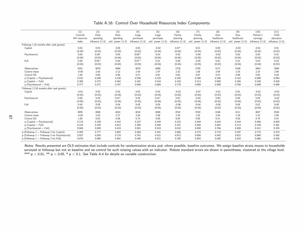
Table A.16: Control Over Household Resources Index Components

(1) (2) (3) (4) (5) (6) (7) (8) (9) (10) (11)

Controls

HH resources

index

Daily

spending

influence {1-3}

Daily

spending

unil. power {1-3}

Large

purchases

influence {1-3}

Large

purchases

unil. power {1-3}

Family

planning

influence {1-3}

Family

planning

unil. power {1-3}

Own

healthcare

influence {1-3}

Own

healthcare

unil. power {1-3}

Partner’s

earnings

influence {1-3}

Child

education

influence {1-3}Followup 1 (6 months after cash grants)

Capital 0.03 0.03 0.00 0.05 -0.02 0.07∗ 0.01 0.00 -0.03 -0.01 0.01

(0.04) (0.02) (0.03) (0.03) (0.04) (0.04) (0.04) (0.02) (0.04) (0.03) (0.02)

Psychosocial 0.05 0.04∗ 0.05 0.06∗∗ 0.03 0.02 -0.04 -0.02 0.02 0.05 0.01

(0.04) (0.02) (0.04) (0.03) (0.04) (0.04) (0.05) (0.02) (0.04) (0.03) (0.02)

Full 0.06 0.05∗∗ 0.04 0.07∗∗ 0.01 0.00 -0.05 0.01 0.01 0.03 0.03

(0.04) (0.02) (0.04) (0.03) (0.04) (0.04) (0.05) (0.02) (0.04) (0.04) (0.02)

Observations 4161 4078 4094 4079 4090 2730 2740 4171 4198 3843 3596

Control mean -0.00 2.63 2.12 2.50 1.97 2.32 1.68 2.84 2.25 2.25 2.80

Control SD 1.00 0.60 0.90 0.71 0.91 0.82 0.87 0.43 0.90 0.82 0.49

p (Capital = Psychosocial) 0.522 0.589 0.230 0.558 0.220 0.202 0.280 0.204 0.152 0.099 0.983

p (Capital = Full) 0.386 0.273 0.402 0.301 0.410 0.103 0.213 0.600 0.240 0.249 0.428

p (Psychosocial = Full) 0.777 0.571 0.747 0.656 0.684 0.770 0.889 0.088 0.794 0.648 0.469

Followup 2 (18 months after cash grants)

Capital -0.01 0.02 0.03 0.02 0.03 -0.03 -0.07 -0.01 0.01 -0.02 -0.02

(0.05) (0.03) (0.04) (0.03) (0.04) (0.05) (0.05) (0.02) (0.03) (0.03) (0.02)

Psychosocial 0.06 0.04 0.07∗ 0.05 0.07∗ 0.02 -0.04 0.00 0.05 0.04 -0.02

(0.05) (0.03) (0.04) (0.03) (0.04) (0.05) (0.04) (0.02) (0.04) (0.03) (0.02)

Full 0.04 0.05 0.04 0.05 0.05 -0.08 -0.04 -0.00 0.05 0.01 0.00

(0.05) (0.03) (0.03) (0.03) (0.04) (0.05) (0.04) (0.02) (0.03) (0.04) (0.02)

Observations 4055 4006 4016 4010 4006 2510 2539 4106 4111 3627 3520

Control mean -0.00 2.63 2.27 2.50 2.08 2.28 1.82 2.84 2.34 2.32 2.86

Control SD 1.00 0.63 0.86 0.73 0.90 0.84 0.90 0.41 0.85 0.76 0.41

p (Capital = Psychosocial) 0.110 0.328 0.342 0.327 0.245 0.232 0.459 0.624 0.244 0.066 0.920

p (Capital = Full) 0.218 0.244 0.811 0.394 0.540 0.341 0.484 0.802 0.113 0.339 0.381

p (Psychosocial = Full) 0.664 0.859 0.419 0.901 0.519 0.032 0.950 0.766 0.836 0.412 0.335

p (Followup 1 = Followup 2 for Capital) 0.493 0.777 0.602 0.564 0.341 0.085 0.175 0.719 0.397 0.770 0.374

p (Followup 1 = Followup 2 for Psychosocial) 0.937 0.926 0.710 0.761 0.421 0.912 0.956 0.402 0.622 0.860 0.363

p (Followup 1 = Followup 2 for Full) 0.676 0.894 0.961 0.495 0.521 0.185 0.903 0.605 0.424 0.666 0.456

Notes: Results presented are OLS estimates that include controls for randomization strata and, where possible, baseline outcomes. We assign baseline strata means to householdssurveyed at followup but not at baseline and we control for such missing values with an indicator. Robust standard errors are shown in parentheses, clustered at the village level.*** p < 0.01, ** p < 0.05, * p < 0.1. See Table A.4 for details on variable construction.

87

Capital Psychosocial FullPanel 1: Program costs per beneficiary, USD PPP 2016

Program administration 78 78 78 Identification, Communication 3 3 3 Measure 0. Group formation 1 1 1 Measure 1. Coaching 9 9 9 Measure 2. Community sensitization on aspirations and social norms 0 38 38 Measure 3. Facilitation of community savings and loan groups 2 2 2 Measure 4. Life-skills training 0 64 64 Measure 5. Micro-entrepreneurship training 65 65 65 Measure 6. Cash grants 321 0 321 Measure 7. Facilitation of market and information access 4 4 4Total costs, calculated as if all incurred immediately at beginning of year 0 482 263 584

(1) Total costs, inflated to year 2 at 5% annual discount rate 531 290 644

Panel 2: Benefits per Household, USD PPP 2016, All Values Inflated to Year 2 at 5% annual social discount rateA

(2) Year 1 Gross Consumption Treatment Effect (linear growth for months 1-6) 69 39 112(3) Year 2 Gross Consumption Treatment Effect (linear growth for months 7-18) 215 228 411(4) B1: Year 3 Onward Gross Consumption Treatment Effect, assumed dissipation of 75% 67 71 128

B2: Year 3 Onward Gross Consumption Treatment Effect, assumed dissipation of 50% 196 207 374B3: Year 3 Onward Gross Consumption Treatment Effect, assumed dissipation of 25% 539 571 1027

(5)C: Year 3 Onward Gross Consumption Treatment Effect, assuming year 2 gains persist in perpetuity 4104 4348 7826

(6) A: Total Benefits: (2) + (3) = (6) using 5%, no impact after year 2 284 268 523(7) B1: Total Benefits: (2) + (3) + (4) = (7) 5% discount rate, 75% annual dissipation 351 339 651

B2: Total Benefits using 5% discount rate, 50% annual dissipation 480 475 897B3: Total Benefits using 5% discount rate, 25% annual dissipation 823 838 1550

(8)C: Total Benefits: (2) + (3) + (5) = (8) using 5% discount rate, assuming year 2 gains persist in perpetuity 4388 4615 8349

Panel 3: Benefit/Cost Ratios

(9) A: Total Benefits/Total Costs Ratio: (6) / (1) = (9) at 5% discount rate 53% 92% 81%A: Benefit/Cost Ratio, at discount rate of 7% 53% 91% 80%A: Benefit/Cost Ratio, at discount rate of 10% 51% 88% 78%

(10) B1: Total Benefits/Total Costs: (7) / (1) = (10), 5% discount, 75% annual dissipation 66% 117% 101%B2: Benefit/Cost Ratio using 5% discount rate, 50% annual dissipation 90% 164% 139%B3: Benefit/Cost Ratio using 5% discount rate, 25% annual dissipation 155% 289% 241%

(11)C: Total Benefits/Total Costs Ratio: (8) / (1) = (11) using 5% discount rate, assuming year 2 gains persist in perpetuity 826% 1594% 1297%

(12) Real Internal Rate of Return (IRR) A: assuming dissipation of 100% after year 2, at 5% discount rate -30% -4% -11% B1: assuming annual dissipation of 75% -17% 8% 1% B2: assuming annual dissipation of 50% -2% 22% 15% B3: assuming annual dissipation of 25% 15% 38% 31% C: assuming effects are sustained in perpetuity 34% 56% 49%

Notes: We use 98% winsorized consumption estimates in our benefits calculation. Note that we measure benefits 6 months after the intervention on average in year 1 and 18 months on average in year 2. All monetary amounts are PPP-adjusted USD terms, set at 2016 prices and deflated using CPI published by the World Bank. In 2016, 1 USD = 242.553 XOF PPP. We assume linear growth of impacts by month post-intervention.

Table A17: Cost-benefit analysis (assuming linear growth of impacts post-intervention)

Appendix References

Acevedo, Paloma, Guillermo Cruces, Paul Gertler, and Sebastian Martinez. 2017. “Living Up to Expectations:How Job Training Made Women Better Off and Men Worse Off”. NBER Working Paper No. 23264.

Adams, Glenn. 2005. “The Cultural Grounding of Personal Relationship: Enemyship in North American andWest African Worlds.” Publisher: American Psychological Association, Journal of personality and socialpsychology 88 (6): 948.

Adhvaryu, Achyuta, Namrata Kala, and Anant Nyshadham. 2018. “The Skills to Pay the Bills: Returns to On-the-job Soft Skills Training”. NBER Working Paper No. 24313. http://www.nber.org/papers/w24313.pdf.

Akyeampong, Emmanuel, Robert H. Bates, Nathan Nunn, and James Robinson. 2014. Africa’s Development inHistorical Perspective. Cambridge University Press.

Ali, Gemma-Claire, Grace Ryan, and Mary J. De Silva. 2016. “Validated Screening Tools for Common MentalDisorders in Low and Middle Income Countries: A Systematic Review”. PLOS ONE 11 (6): e0156939.https://dx.plos.org/10.1371/journal.pone.0156939.

Aron, Arthur, Elaine N. Aron, and Danny Smollan. 1992. “Inclusion of Other in the Self Scale and the Structureof Interpersonal Closeness.” Journal of Personality and Social Psychology 63 (4): 596–612. http://doi.apa.org/getdoi.cfm?doi=10.1037/0022-3514.63.4.596.

Ashraf, Nava, Natalie Bau, Corinne Low, and Kathleen McGinn. 2020. “Negotiating a Better Future: HowInterpersonal Skills Facilitate Intergenerational Investment”. The Quarterly Journal of Economics 135 (2):1095–1151. https://academic.oup.com/qje/article/135/2/1095/5698825.

Ballard, Terri J, Anne W Kepple, and Carlo Cafiero. 2013. “The Food Insecurity Experience Scale: Developmentof a Global Standard for Monitoring Hunger Worldwide”. FAO, Rome. http://www.fao.org/fileadmin/templates/ess/voh/FIES_Technical_Paper_v1.1.pdf.

Bandura, Albert. 1997. Self-Efficacy: The Exercise of Control. New York: W.H. Freeman.

— . 2001. “Social Cognitive Theory of Mass Communication”. Media Psychology 3 (3): 265–299. http:

//www.tandfonline.com/doi/abs/10.1207/S1532785XMEP0303_03.

Barrera-Osorio, Felipe, Adriana Kugler, and Mikko Silliman. 2020. “Hard and Soft Skills in Vocational Training:Experimental Evidence from Colombia”. NBER Working Paper No. 27548.

Barsbai, Toman, Victoria Licuanan, Andreas Steinmayr, Erwin Tiongson, and Dean Yang. 2020. “Informationand the Acquisition of Social Network Connections”. NBER Working Paper No. 27346.

Benjamini, Yoav, and Yosef Hochberg. 1995. “Controlling the False Discovery Rate: A Practical and PowerfulApproach to Multiple Testing”. Journal of the Royal statistical society: series B (Methodological) 57 (1):289–300.

Blattman, Christopher, Julian C Jamison, and Margaret Sheridan. 2017. “Reducing Crime and Violence: Ex-perimental Evidence From Cognitive Behavioral Therapy in Liberia”. American Economic Review 107 (4):1165–1206.

Campos, Francisco, Michael Frese, Markus Goldstein, Leonardo Iacovone, Hillary C Johnson, David McKen-zie, and Mona Mensmann. 2017. “Teaching personal initiative beats traditional training in boosting smallbusiness in West Africa”. Science 357 (6357): 1287–1290.

Dalton, Patricio S, Sayantan Ghosal, and Anandi Mani. 2016. “Poverty and Aspirations Failure”. The EconomicJournal 126 (590): 165–188.

Delavande, Adeline, Xavier Gine, and David McKenzie. 2011. “Measuring Subjective Expectations in DevelopingCountries: A Critical Review and New Evidence”. Journal of development economics 94 (2): 151–163.

Duflo, Esther. 2012. “Human Values and the Design of the Fight Against Poverty”. Tanner Lectures, HarvardUniversity.

89

Feinberg, Matthew, and Robb Willer. 2015. “From Gulf to Bridge: When Do Moral Arguments Facilitate PoliticalInfluence?” Personality and Social Psychology Bulletin 41 (12): 1665–1681. http://journals.sagepub.com/doi/10.1177/0146167215607842.

Gelfand, Michele J., Jana L. Raver, Lisa Nishii, Lisa M. Leslie, Janetta Lun, Beng Chong Lim, Lili Duan, AssafAlmaliach, Soon Ang, and Jakobina Arnadottir. 2011. “Differences between Tight and Loose Cultures: A33-Nation Study”. Science 332 (6033): 1100–1104.

Harding, Timothy W, V De Arango, J Baltazar, CE Climent, HHA Ibrahim, L Ladrido-Ignacio, and NN Wig. 1980.“Mental Disorders in Primary Health Care: A Study of Their Frequency and Diagnosis in Four DevelopingCountries”. Psychological medicine 10 (2): 231–241.

Heckman, James, Jora Stixrud, and Sergio Urzua. 2006. “The Effects of Cognitive and Noncognitive Abilitieson Labor Market Outcomes and Social Behavior”. NBER Working Paper No. 12006. http://www.nber.org/papers/w12006.pdf.

Hitokoto, Hidehumi, and Yukiko Uchida. 2015. “Interdependent Happiness: Theoretical Importance and Mea-surement Validity”. Journal of Happiness Studies 16 (1): 211–239. https://doi.org/10.1007/s10902-014-9505-8.

Hofstede, Geert. 2001. Culture’s Consequences: Comparing Values, Behaviors, Institutions, and Organizationsacross Nations. Thousand Oaks, Calif.; London: Sage. http://www.vlebooks.com/vleweb/product/openreader?id=none&isbn=9781452207933.

Knowles, Malcolm Shepherd. 1984. Andragogy in Action: Applying Modern Principles of Adult Learning. SanFrancisco, CA: Jossey Bass.

Leung, Angela K.-Y., and Dov Cohen. 2011. “Within-and between-Culture Variation: Individual Differences andthe Cultural Logics of Honor, Face, and Dignity Cultures.” Publisher: American Psychological Association,Journal of personality and social psychology 100 (3): 507.

Lewin, K. 1952. “Group Decision and Social Change”. In Readings in social psychology, 459–473.

Markus, Hazel Rose. 2016. “What Moves People to Action? Culture and Motivation”. Current Opinion in Psy-chology, Culture, 8:161–166. http://www.sciencedirect.com/science/article/pii/S2352250X15003048.

Markus, Hazel Rose, and Alana Conner. 2014. Clash!: How to Thrive in a Multicultural World. Penguin.

Markus, Hazel Rose, and Shinobu Kitayama. 2010. “Cultures and Selves: A Cycle of Mutual Constitution”.Publisher: Sage Publications Sage CA: Los Angeles, CA, Perspectives on psychological science 5 (4): 420–430.

Njuki, Jemimah, Elizabeth J Poole, J Johnson, Isabelle Baltenweck, Pamela N Pali, Zaibet Lokman, and SamuelMburu. 2011. Gender, livestock and livelihood indicators.

Nord, Mark, Carlo Cafiero, and Sara Viviani. 2016. “Methods for Estimating Comparable Prevalence Rates ofFood Insecurity Experienced by Adults in 147 Countries and Areas”. Journal of Physics: Conference Series.https://doi.org/10.1088/1742-6596/772/1/012060.

Oettingen, Gabriele. 2014. Rethinking Positive Thinking: Inside the New Science of Motivation. New York, NY:Current.

Operario, Don, Nancy E Adler, and David R Williams. 2004. “Subjective Social Status: Reliability and PredictiveUtility for Global Health”. Psychology & health 19 (2): 237–246.

Osei-Tutu, Annabella, Vivian A. Dzokoto, Adjeiwa Akosua Affram, Glenn Adams, Joakim Norberg, and BertjanDoosje. 2020. “Cultural Models of Well-Being Implicit in Four Ghanaian Languages”. Frontiers in Psychology11:1798. https://www.frontiersin.org/article/10.3389/fpsyg.2020.01798/full.

Paluck, Elizabeth Levy. 2009. “What’s in a Norm? Sources and Processes of Norm Change.” Journal of Personal-ity and Social Psychology 96 (3): 594–600. http://doi.apa.org/getdoi.cfm?doi=10.1037/a0014688.

90

Paluck, Elizabeth Levy, and Hana Shepherd. 2012. “The Salience of Social Referents: A Field Experiment onCollective Norms and Harassment Behavior in a School Social Network.” Journal of Personality and SocialPsychology 103 (6): 899–915. http://doi.apa.org/getdoi.cfm?doi=10.1037/a0030015.

Radloff, Lenore Sawyer. 1977. “The Ces-D Scale: A Self-Report Depression Scale for Research in the GeneralPopulation”. Applied psychological measurement 1 (3): 385–401.

Ridley, Matthew, Gautam Rao, Frank Schilbach, and Vikram Patel. 2020. “Poverty, Depression, and Anxiety:Causal Evidence and Mechanisms”. Science 370 (6522). https://www.sciencemag.org/lookup/doi/10.1126/science.aay0214.

Riemer, Hila, Sharon Shavitt, Minkyung Koo, and Hazel Rose Markus. 2014. “Preferences Don’t Have to BePersonal: Expanding Attitude Theorizing With a Cross-Cultural Perspective.” Psychological review 121 (4):619.

Rosenberg, Morris. 2015. Society and the Adolescent Self-Image. Princeton University Press.

San Martin, Alvaro, Marwan Sinaceur, Amer Madi, Steve Tompson, William W. Maddux, and Shinobu Kitayama.2018. “Self-Assertive Interdependence in Arab Culture”. Publisher: Nature Publishing Group, Nature HumanBehaviour 2 (11): 830–837.

Schwarzer, Ralf, Matthias Jerusalem, et al. 1995. “Generalized Self-Efficacy Scale”. Measures in health psychol-ogy: A user’s portfolio. Causal and control beliefs 1 (1): 35–37.

Slater, Michael D., and Donna Rouner. 2002. “Entertainment—Education and Elaboration Likelihood: Un-derstanding the Processing of Narrative Persuasion”. Communication Theory 12 (2): 173–191. http :

//onlinelibrary.wiley.com/doi/abs/10.1111/j.1468-2885.2002.tb00265.x.

Stephens, Nicole M., Stephanie A. Fryberg, Hazel Rose Markus, Camille S. Johnson, and Rebecca Covarrubias.2012. “Unseen Disadvantage: How American Universities’ Focus on Independence Undermines the AcademicPerformance of First-Generation College Students.” Publisher: American Psychological Association, Journalof Personality and Social Psychology 102 (6): 1178.

Thomas, Catherine C., and Hazel Rose Markus. Forthcoming. “Enculturating Development Science: Beyond theWEIRD Independent Paradigm”. Mimeo.

Thomas, Catherine C., Nicholas G. Otis, Justin R. Abraham, Hazel Rose Markus, and Gregory M. Walton.2020. “Toward a Science of Delivering Aid with Dignity: Experimental Evidence and Local Forecasts fromKenya”. Proceedings of the National Academy of Sciences 117 (27): 15546–15553. http://www.pnas.org/lookup/doi/10.1073/pnas.1917046117.

Thomas, Catherine C., S.D. Rathod, M.J. De Silva, H.A. Weiss, and V. Patel. 2016. “The 12-Item WHO Dis-ability Assessment Schedule II as an Outcome Measure for Treatment of Common Mental Disorders”. GlobalMental Health 3:e14. https://www.cambridge.org/core/product/identifier/S2054425116000078/type/journal_article.

Walton, Gregory M., and David S. Yeager. 2020. “Seed and Soil: Psychological Affordances in Contexts Helpto Explain Where Wise Interventions Succeed or Fail”. Current Directions in Psychological Science 29 (3):219–226.

WFP. 2008. Food Consumption Analysis: Calculation and Use of the Food Consumption Score in Food SecurityAnalysis.

Woolcock, M., and D. Narayan. 2000. “Social Capital: Implications for Development Theory, Research, andPolicy”. The World Bank Research Observer 15 (2): 225–249. https://academic.oup.com/wbro/

article-lookup/doi/10.1093/wbro/15.2.225.

Wuepper, David, and Travis J. Lybbert. 2017. “Perceived Self-Efficacy, Poverty, and Economic Development”.Annual Review of Resource Economics 9 (1): 383–404. http://www.annualreviews.org/doi/10.1146/annurev-resource-100516-053709.

91