participatory prospective analysis: exploring and anticipating challenges with stakeholders
TRANSCRIPT


UNESCAP-CAPSA The Centre for Alleviation of Poverty through Secondary Crops’ Development in Asia and the Pacific (CAPSA) is a subsidiary body of UNESCAP. It was established as the Regional Co-ordination Centre for Research and Development of Coarse Grains, Pulses, Roots and Tuber Crops in the Humid Tropics of Asia and the Pacific (CGPRT Centre) in 1981 and was renamed CAPSA in 2004. Objectives CAPSA promotes a more supportive policy environment in member countries to enhance the living conditions of rural poor populations in disadvantaged areas, particularly those who rely on secondary crop agriculture for their livelihood, through socio-economic and policy research, training and dissemination of information. In its activities, the Centre aims to serve the needs of its primary target group, high level research managers and policy analyst/planners, concerned with the role of agriculture in poverty alleviation. Programmes 1. Co-ordination of socio-economic and policy research on secondary crops, networking and
partnership with other international organizations and key stakeholders, conduction of research and analysis of trends and opportunities with regard to improving the economic status of rural populations.
2. Production, packaging and dissemination of information and successful practices on poverty
reduction, and the dissemination of information and good practices on poverty reduction measures. 3. Training of national personnel, particularly national scientists and policy analysts and provision of
advisory services. UNESCAP-CAPSA Monographs currently available: CGPRT No. 45 Domestic Supply and Consumption Patterns of Coarse Grains, Pulses, Roots and
Tuber Crops in Asia and the Pacific Edited by Robin Bourgeois and Yannick Balerin CGPRT No. 44 Reconciling Actors’ Preferences in Agricultural Policy - Towards a New Management
of Public Decisions Edited by Franck Jésus and Robin Bourgeois CGPRT No. 43 Coping against El Nino for Stabilizing Rainfed Agriculture: Lessons from Asia and the Pacific: Proceedings of a Joint Workshop Held in Cebu, the Philippines, September17-19, 2002 Edited by Shigeki Yokoyama and Rogelio N. Concepcion CGPRT No. 42 The CGPRT Feed Crops Supply/Demand and Potential/Constraints for their
Expansion in South Asia: Proceedings of a Workshop Held in Bogor, Indonesia, September 3-4, 2002 Edited by Budiman Hutabarat CGPRT No. 41 P.A.C.T. A Pro-Active Conciliation Tool: Analysing Stakeholders’ Inter-Relations Edited by Franck Jésus CGPRT No. 40 Food Security in Southwest Pacific Island Countries: Proceedings of a Workshop Held in Sydney, Australia, December 12-13, 2000 Edited by Pantjar Simatupang and D.R. Stoltz (Continued on inside back cover)

Participatory Prospective Analysis
Exploring and Anticipating Challenges with Stakeholders
“UNESCAP-CAPSA: Centre for Alleviation of Poverty through Secondary Crops’ Development in Asia and the Pacific”

The designations employed and the presentation of material in this publication do not imply the expression of any opinion whatsoever on the part of the Secretariat of the United Nations concerning the legal status of any country, territory, city or area of its authorities, or concerning the delimitation of its frontiers or boundaries. The opinions expressed in signed articles are those of the authors and do not necessarily represent the opinion of the United Nations.

CAPSA NO. 46
Participatory Prospective Analysis
Exploring and Anticipating Challenges with Stakeholders
Robin Bourgeois Franck Jésus
UNESCAP-CAPSA Centre for Alleviation of Poverty through Secondary Crops’ Development in Asia and the Pacific
CIRAD French Agricultural Research Centre for International Development

v
Table of Contents
Page
List of Tables ......................................................................................................................... vii List of Figures ....................................................................................................................... ix List of Boxes ......................................................................................................................... xi Foreword ........................................................................................................................... xiii Acknowledgements ............................................................................................................... xv Abstract ........................................................................................................................... xvii Executive Summary ............................................................................................................... xix Introduction ......................................................................................................................... 1 Part I The Participatory Prospective Analysis (PPA) Method
The philosophy of the PPA method ........................................................................ 5 Methodological components ................................................................................... 7
Presentation of the method ............................................................................... 7 Definition of the system’s limits ...................................................................... 8 Identification of variables ................................................................................ 8 Selection and definition of key variables ......................................................... 9 Mutual influence analysis ................................................................................ 10 Interpretation of influence/dependence links ................................................... 14 Definition of the states of variables ................................................................. 20 Building scenarios ............................................................................................ 21 Using scenarios ................................................................................................ 22
Implementing the PPA ............................................................................................ 23 Equipment and resources ................................................................................. 24 Organizing group work .................................................................................... 26 The question of experts and expertise .............................................................. 27
Part II The PPA Method at Work: The Case of Secondary Crop Research and Development Prospects in Asia and the Pacific
Context .................................................................................................................... 31 Organization of the PPA ......................................................................................... 32
System identification ........................................................................................ 32 Creation of a working group and workshop organization ................................ 33

vi
Process and results .................................................................................................. 34 Identification of key variables .......................................................................... 34 Influence/dependence analysis ......................................................................... 36 Building scenarios ............................................................................................ 44 Analysis of implications ................................................................................... 46
Conclusion ............................................................................................................... 52 Final Remarks .......................................................................................................................... 55 References ................................................................................................................................ 57 Acronyms ................................................................................................................................. 61 Annexes
Annex 1. The Delphi Method .................................................................................. 65 Annex 2. About Scenarios ....................................................................................... 67 Annex 3. The RAINAPOL Approach ..................................................................... 69 Annex 4. Indirect Influence and Matricial Calculation ........................................... 73 Annex 5. Formula for Calculation of I/D Tables and Graphs ................................. 77 Annex 6. Glossary of Selected Terms Related to the PPA Method ........................ 81 Annex 7. Programme for a 5-Day PPA Workshop ................................................. 85 Annex 8. Variables’ Influence/Dependence and Strength ...................................... 89

vii
List of Tables
Page
Table 1. The methodology of PPA ................................................................................. 8 Table 2. Architecture of the software package ............................................................... 14 Table 3. Possible interpretations of the variables’ position in the visualization graph .. 17 Table 4. Display of variables, states and incompatibilities ............................................ 21 Table 5. Representation of a scenario ............................................................................ 21 Table 6. Typology of attitude’s towards scenario building and discussion ................... 23 Table 7. List and qualifications of stakeholders/experts ................................................ 33 Table 8. The direct I/D matrix ........................................................................................ 37 Table 9. Results of direct influence analysis .................................................................. 39 Table 10. Results of indirect influence analysis ............................................................... 42 Table 11. Driving variables, states and incompatibilities ................................................. 45 Table 12. Final list of scenarios and assessment of plausibility ....................................... 46 Table 13. Synthesis of the application of the PPA method to secondary crop research and development prospects ..................................................................................... 53

v
List of Figures
Page
Figure 1. Prospective is not prediction ............................................................................ 4 Figure 2. The key principles of the PPA method ............................................................ 7 Figure 3. Matrix displayed in “Variables’ influence” worksheet and automatic links ..... 11 Figure 4. Filling the influence/dependence matrix .......................................................... 12 Figure 5. Organization and utilization of a discussion board .......................................... 13 Figure 6. Location of the functional worksheets ............................................................. 14 Figure 7. Direct dependence and influence tables ........................................................... 15 Figure 8. Variables’ strength tables based on direct influence ........................................ 16 Figure 9. Signification of variables according to their place in the I/D graph ................ 16 Figure 10a. Relatively unstable system................................................................................ 17 Figure 10b. Stable system (illustrative case) ....................................................................... 17 Figure 11. Changes in variables’ position according to direct or indirect influence ......... 19 Figure 12. Visualization of total I/D graph and total weighted strength ........................... 19 Figure 13. Room layout for expert meeting workshop ...................................................... 25 Figure 14. Visualization graph for direct influence ........................................................... 40 Figure 15. Visualization graph for indirect influence ........................................................ 41 Figure 16. Comparison of direct and indirect strength ranking ......................................... 43
vi

x

xi
List of Boxes
Page
Box 1. Some rules for identifying variables ................................................................ 9 Box 2. Relevance of variables and identifiable states .................................................. 9 Box 3. How many variables to keep? .......................................................................... 10 Box 4. The PPA workshop in brief .............................................................................. 24 Box 5. The driving variables ....................................................................................... 44 Box 6. The stakes ......................................................................................................... 44 Box 7. Scenario 13 ....................................................................................................... 47 Box 8. Scenario 10 ....................................................................................................... 49 Box 9. Scenario 8 ......................................................................................................... 51

xii

xiii
Foreword
Prospective techniques are progressively becoming indispensable tools for policy decisions, particularly in the area of research for sustainable agriculture and sustainable development.
As a matter of fact, there are many cases where today’s behaviour makes long-term
prints on ecosystems and societies. For example, the Green Revolution’s successes all over Asia could perfectly satisfy those who look only at the past and present situation. For those who look forward, the Green Revolution will have to deal with number of severe constraints and economic problems that could reduce drastically its success.
“Business as usual” prospective scenarios elicit the following vital problems: extension
of salinization of soils, extension of water logging, water table depletion, water pollution, reduction of farm revenues and stagnating yields. This could lead us to backtrack towards food insecurity and rural poverty.
In such contexts, the role of research is to anticipate and provide solutions before
problems have the chance to grow and become more difficult to resolve, especially if we leave their evolution flow toward extreme situations. But trying to foresee is a difficult task. Without good methodology, it could lead to the expression of useless phantasmagorical views or manipulation by lobbies. Therefore, rigorous frames and techniques are needed in order to identify the key mechanisms of economic, social and environmental evolutions, and explore the scope of possible future situations they could generate.
Of course, nobody can predict what the future will be, but that is not the purpose of a
prospective study. But putting together the experience and the expertise of well informed specialists, and using tools allowing the expression of coherent options, one becomes more forearmed and equipped to take today’s decisions for tomorrow’s welfare. It is from this perspective that this document is very beneficial. Thanks to the authors and UNESCAP CAPSA.
Michel Griffon Advisor to the Director General
Sustainable Development CIRAD

xiv

xv
Acknowledgements
The authors wish to express their deep gratitude to Philippe Guizol at CIFOR in Bogor, Jean-François Lecoq at CIRAD TERA Montpellier, and Yannick Balerin from AFD in Cambodia, for reviewing the early draft of this book and providing useful comments and suggestions to improve its scientific, technical and practical content. We are indebted to Michel Griffon, Advisor for sustainable development at CIRAD who not only reviewed this book but also accepted to write the Foreword.
We also wish to express our thanks to all our colleagues in Asia and the Pacific who have directly and indirectly contributed to this publication through their active participation in the prospective work conducted by CIRAD and CAPSA in the region.
Matthew Burrows, Agustina Mardyanti, Francisca Wijaya and Fetty Prihastini from CAPSA made their usual invisible but much needed contributions to this publication, thanks to their skills in editing, page making, designing and error-tracking.
CAPSA and CIRAD are thankful to the Indonesian Government who provided resources for the publication of this book, and to the Japanese Government for providing partial financial support to the prospective workshop on secondary crops’ research and development in Asia and the Pacific
Finally, we would like to acknowledge the influence of the work of Michel Godet and the French prospectivists on our own work. We hope that this book will in turn contribute to enlarge its recognition and usefulness.

xvi
xvii
Abstract
This book presents the Participatory Prospective Analysis method, an applied foresighting approach developed by CIRAD and CAPSA for strengthening the capacity of stakeholders to become more active in making decisions related to their future. It is a tool designed to explore and anticipate changes with the participation of experts, including stakeholders, to provide rapid results and to offer interaction between participants. It fits to situations where multiple stakeholders interact within complex systems and is particularly appropriate for exploring policy options at local or sectorial levels such as for local regional development or commodity-based development.
This approach combines participatory learning as a capacity-building tool with the sharing of information in order to level the playing field among stakeholders through the reduction of information asymmetry. The illustrative case study about the prospects of secondary crop research and development in Asia and the Pacific shows that the information stakeholders individually possess can be shared and organized to produce foreknowledge and can help them to better understand their environment and be better prepared to act.

xviii

xix
Executive Summary
Introduction
1. The rural sector in developing countries has experienced tremendous modifications during the last century, marked by the effects of long trends, of unforeseen events, and of ruptures and the response of the societies to them. Who, at the beginning of the 20th century, could have said that rural Asia would and could feed more than three billion human beings yet remain the largest reservoir of extremely poor people? And who can imagine how it will look in twenty years?
2. The purpose of this book is to present the conceptual basis, the content and an application of the Participatory Prospective Analysis (PPA), an approach that can be considered as a specific type of foresight. The methods of prospective analysis were formalized and developed in France in the 1990s. They explore implications from alternative assumptions and aim to provide a range of choices and ends for decision makers. PPA can therefore be used to prepare strategic actions or to discover whether changes are necessary today.
3. An introduction to futures study methods precedes Part I where a detailed presentation of the method can be found. Part II shows the application of PPA to the prospects of secondary crop research and development in Asia and the Pacific. Part I
4. The original feature of PPA is its comprehensive and quickly operational framework designed to fulfil the demand for a well-structured effort of anticipation and exploration, that also focuses on interactions and consensus building. The philosophy attached to this method relies on several principles: relevance, consistency, plausibility, transparency, effectiveness, participation, capacity-building and reproducibility. 5. The method facilitates the anticipation of changes in unstable environments. It helps stakeholders to prepare to face highly versatile evolutions and to better argue strategic choices. It is also a capacity-building tool, conceived to produce and share efficiently useful information for decision-making.
Presentation of the method 6. The method proposed in this book is a component of a wider approach, the RAINAPOL approach developed by CIRAD and CAPSA and can be considered as an adaptation of the generic method of scenarios into an eight-step process as indicated below. It is supported by software developed in Excel and available at the following address for free download: http://www.uncapsa.org.
7. Definition of the system’s limits. The definition of the issue to which this method intends to provide foreknowledge is used to define the limits of the exercise. The issue can be regarded as a system whose nature can be characterized (spatial dimension and timeframe).

xx
8. Identification of variables. This process relies on the structural analysis method and brainstorming. It starts with the listing of the variables that have an influence on the constitution and evolution of the system, from retrospective, present and future points of view.
9. Definition of key variables. The relevance of the variables is then discussed. Variables for which it is impossible to define different states are irrelevant. A final list of variables is established and a clear and consensual definition is given to each one. All selected variables are entered in the computer in the cells of the corresponding matrix.
10. Mutual influence analysis. The analysis of direct influence/dependence (I/D) links among variables is based on a consensual valuation approach. Values are discussed and immediately entered in the I/D matrix. Through a chain of automatic links all other matrices, tables and graphs are instantly filled and updated. The graphs provide an immediate view of the variables role in the system according to their position, and the tables display composite indexes for the ranking of the variables. 11. Interpretation of influence/dependence links. Tables and graph analyses are combined to identify the different types of variables: “drivers”, “stakes”, “marginal” and “output” variables. The results consist of the selection of a limited number of variables.
12. Definition of the states of variables. A state is a description of the variable in the future. Sometimes called morphological analysis, its objective is to browse the domain of possible futures, to reduce it and to explore consistent, relevant and plausible alternatives. It focuses on contrasted and mutually exclusive states. This procedure helps introduce ruptures in the future, a critical aspect that is not incorporated in most forecasting works. The variables and their states are then listed in a table that becomes the base for the elaboration of the scenarios.
13. Building scenarios. A scenario is a combination of variables in different states. Scenarios are produced through brainstorming and clustering following an identical process as for the identification of variables: elimination of redundant scenarios, grouping of scenarios and discussion of results. The decision about which scenarios to keep for further analysis is based on likeliness, plausibility and contrast.
14. Strategic implications and anticipated actions. Each selected scenario is characterized using a common framework that includes: the description of the scenario (combination of states), the implication on the main stake and output variables, the strategic elements and the possible actions. Two types of possible actions can be generated: (i) reduction of the impact of negative scenarios and taking advantage of the effects of positive scenarios, and (ii) promoting the occurrence of desirable scenarios. The first one enables stakeholders to prepare for a range of possible situations that could be encountered in the future (be pre-active). The second relates to the modification of the present so that a more desirable future can be expected (be pro-active). Through the identification of contrasted scenarios and the related factors of change, one becomes able to select a desirable, yet plausible, vision of the future and to identify a path leading to this vision.

xxi
Implementing the PPA 15. Equipment and resources. The implementation of expert-meeting workshops needs the careful preparation of materials, equipment and organization of work. An isolated meeting-room is needed with space for displaying information and allowing convivial interaction among participants. The room must be equipped with two computers, one LCD projector and a screen, a printer, and a nearby photocopy facility. Visualization materials must be readied in advance. These include: coloured cards, markers, supports for card display, pinning and fixation tools. As facilitation is a key issue, a team of four people, two facilitators, one computer operator and one secretary, is the ideal set-up.
16. Organizing group work. Expert meetings using a working group approach give different people with different backgrounds and knowledge the possibility to meet and interact in order to produce a collective vision. This vision is considered as an operational representation of the situation under analysis. A key point is the identification and selection of the participating experts. These are individuals known for their familiarity with the subject at hand. They are selected on an individual basis and their capacity to confront and exchange multiple points of view. The stakeholders directly concerned with the issues at hand are among the experts invited to a PPA workshop. This contributes to strengthen the relevance of the work and the commitment of the participants. Sessions are conducted under the guidance of a neutral facilitator who is not a stakeholder. Facilitators must have practised this method before conducting such workshops.
17. The question of experts and expertise. Experts bring the possibility to incorporate non-recorded and/or qualitative data into the whole process and to take advantage of an often-unsuspected wealth of information. As stakeholders, invited experts can also directly apply the results or produce changes. However, there are some potential problems due to the recourse on experts’ knowledge. The first problem is the aggregation of individual opinions into a common representation. The second problem relates to the fact that nobody is omniscient, and experts are bound by their understanding of the problem, their own interest and other factors. Biases may thus be introduced in the process. These can nevertheless be kept to a low level. Agreement on the collective decision-making procedure and the use of structured frameworks combined with brainstorming techniques allow the experts to go through a common mental process, facilitating the aggregation of their preferences. The quantitative valuation methods are also supported by transparent computerized methods.
Part II
Context 18. The scientific exploration of futures is rather new in Asia and the Pacific with the exception of Japan. The establishment of the APEC Technology Foresight Centre in Thailand in 1998 gave a strong boost to this approach in several countries. However, few exercises related to the agricultural sector have been implemented in the region. The work undertaken by CAPSA has a very modest dimension compared to APEC’s and can be considered as a pioneer effort to introduce alternative approaches in the exploration of futures.
19. CAPSA’s decision to explore possible evolutions that may affect research and development on secondary crops in Asia and the Pacific up to the horizon 2015 was taken as a joint initiative

xxii
in the framework of two projects, ELNINO and MAPSuD. The prospective workshop helped the ELNINO project to refine its policy recommendations and enabled the MAPSuD project to highlight key issues in the preparation of CAPSA’s strategy.
20. Expected products included:
Key factors influencing the future of secondary crops in Asia and the Pacific, Contrasted images of possible futures and their consequences, Possible actions to mitigate negative implications and promote positive changes.
Organization of the PPA 21. The case was developed during a four-day workshop organized at CAPSA in Bogor, preceded by two weeks of preparation and two weeks of finalization. The issue was identified as: what are the variables affecting the future research and development of secondary crops (i.e. food crops grown by farmers excluding rice and wheat) by the horizon 2015 in Asia and the Pacific? It covers 26 Asian and Pacific countries. Initially nine participants were invited from Cambodia, China, India, Indonesia, Korea, Malaysia, Thailand, the Philippines, and Viet Nam. Finally, a total of eight people attended this workshop on a permanent basis displaying a wide range of qualifications.
Process and results 22. Identification of key variables. A total of 31 variables were identified. They were grouped by categories using a two-level classification. The first distinction was made between endogenous and exogenous variables. Then a cluster-type grouping helped categorized the variables according to specific domains: environment and natural resources, socio-economic variables, policy variables, supply and demand.
23. Influence/dependence analysis. The discussion on direct influence between variables took a full day. Filling the matrix necessitated to discuss a total number of 930 interactions for a total of five hours of work.
24. Selection of key variables. A two-step approach was used to sort variables, eliminating first variables with a dependence level above one and then those with an influence or strength level below one. Eight variables were finally selected: “Urbanization”, “Income change”, “Availability of suitable land”, “Population growth”, “Water availability”, “Climate variation”, “LMO regulation” and “Climate pattern”. A further set of “stake” variables was identified as follows: “Level of priority from government to CGPRT crops”, “CGPRT trade policies within the region”, “Production technology development”, “Government intervention in input supply”, “Rural infrastructure”, “Technology transfer”, “Socio-economic characteristics of CGPRT crop growers”, and “Level of priority from government to CGPRT crops”. 25. Scenarios. Thirteen scenarios were identified by the participants. Three contrasted scenarios were selected as indicated below. The first two scenarios are adverse scenarios for the research and development of secondary crops; the third one still poses some threats to the future development of these crops, the farmers who grow them and the related research and development organizations.

xxiii
“Faint chances to endure”. Feeding a growing urban population under climatic stress. While climatic conditions worsen and the population growth rate remains unchanged, urban areas develop at a high rate attracting the rural population. Income disparity increases while no specific regulation controls the development of LMO. Under such circumstances, land and water resources become less available for secondary crops. “Change or suffer”. Resource scarcity and strong regulation. While climatic conditions remain unchanged, land and water availability for secondary crops decreases in a context were LMO regulation becomes stringent. Population growth remains as high as today. Urban areas still attract the rural population. At the same time, income disparity keeps increasing. “Adapt to survive”. Favourable social and natural conditions for agricultural development. This scenario is more favourable. Population growth and urbanization slow down. Climatic conditions remain unchanged, while land and water for secondary crops are available. Disparity of income decreases and the LMO regulation becomes stringent.
26. Analysis of implications. The participants could only discuss the first scenario in length. The two other scenarios were developed by CAPSA staff and further discussed through the exchange of electronic mail with the participants. Scenario discussion followed a common pattern including a brief narrative based on the states taken by the driving variables, the related states of the stake variables, implications for research organizations and institutions, and possibilities to fight for a better scenario through a review of actions for preventing the key variables to take the states that induce negative effects. 27. The table below synthesizes these results, showing for each scenario, the implications of the anticipated situation for organizations involved in secondary crop research and in developing weather sensitive strategies, and strategic elements to modify the likeliness of occurrence of these scenarios.

xxiv
Scenario Implications Strategic elements
Faint chances to
endure
Polarization of the agricultural sector. Decreasing government’ funds for research, extension services and rural infrastructure, but high intervention in input supply. Development of biotechnological breakthroughs and the private sector for research.
Population control. Reduce rural migration. Redistribution policies to reduce income disparities. Ratification of the Kyoto and Cartagena protocols. Regional approach for climatic risk management strategies.
Change or suffer
Competitiveness of other more adaptable/valuable crops. Research funds maintained but focus on yield improvement and adaptability. Maintaining technology transfer. Still some investment in rural infrastructures.
Population and migration control. Redistribution policies to reduce income disparities. Ratification of the Kyoto and Cartagena protocols.
Adapt to survive
New consumption patterns reducing CGPRT crop needs with the exception of feed/industrial industries. Research work focuses on new priorities (matching needs of agro-industries). Risk of decreasing biodiversity.
Establish network for maintaining secondary crop biodiversity. Explore potential of secondary crops for new agro-industrial uses.
Final remarks
28. This book presents an applied approach for strengthening the capacity of stakeholders to become more active in making decisions related to their future. It is a tool designed to provide rapid results and to offer interaction between various stakeholders. It fits to situations where multiple stakeholders interact within complex systems and is particularly appropriate for exploring policy options at local or sectorial levels such as for local regional development or commodity development. 29. This approach combines participatory learning as a capacity-building tool with the sharing of information in order to level the playing field among stakeholders through the reduction of information asymmetry. Therefore, careful attention should be paid to the process of selecting participants. The illustrative case study shows that the information stakeholders individually possess can be shared and organized to produce foreknowledge to help the same stakeholders to better understand their environment.

1
Introduction From Prevision to Anticipation, the Future in Perspective
Who, at the beginning of the 20th century, could have said that rural Asia would and could feed more than three billion human beings and at the same time constitute the largest reservoir of extremely poor people? Who could have said in the mid-eighties when Indonesia reached rice self-sufficiency that twenty years later it would become the largest rice importer in the world? And, today, who could imagine how the rural sector in Asia and the Pacific will look in twenty or fifty years? The rural sector in developing countries in Asia and the Pacific, and worldwide, has experienced tremendous modifications over the last century.
Its evolution is marked by the combined effect of (i) long trends such as population growth, rural-urban migration, globalization of trade, (ii) unforeseen events such as climatic and biological hazards, economic or political crises, conflicts, or ruptures such as technological breakthroughs (the Green Revolution, Biotechnology development) or socio-economic events (the 1997 financial crisis in Asia), and (iii) the response of the societies to these changes.
The question of the future is, today, a key issue that goes beyond merely reacting to changes. It is a central question that humanity attempts to tackle with various instruments, ranging from mysticism and rule of thumb to econometrics, general equilibrium models and foresighting. Even in our post-industrial scientific societies, the simplest methods such as the mere extrapolation of past trends co-exist with highly sophisticated tools, the most rigorous with the most casual.
The purpose of this introduction is to briefly discuss the conceptual basis and relevance of foreknowledge generation as a tool for action. In the first section, we will present different concepts and discuss their interest. Then we will develop the rationale and need for a specific tool, the Participatory Prospective Analysis (PPA) enabling the generation of foreknowledge in a context of multiple stakeholders interacting on complex issues. This tool will be presented in Part I. Its application to the case of secondary crops’ research and development in Asia and the Pacific will be detailed in Part II as a comprehensive example of the use of PPA.
Dealing with uncertainty
Since there is ample recognition that the future cannot be known, that uncertainties are too big, the immediate question to answer is what can we know about the future? Typically, two rather different answers can be given to this simple but far-reaching question. One is brought by the forecasting approach, the other by foresighting. The purpose of this section is to discuss and clarify the key differences between “prevision” and “forethought” as these words crystallize two different types of expectation with regards to applying scientific tools and methods to explore the future. The following discussion intends to clarify the key patterns of both approaches and make understandable why, as far as CAPSA is concerned, and when questions about rural development are at stake, a prospective analysis approach is more suitable, and the reason why the PPA methodology was developed.

2 Introduction
Forecasting Forecasting is prevision and is usually employed to estimate what would happen to a given
issue over time (time-series forecasting), or to make predictions about differences among people, firms, or other objects (cross-sectional data). The methods traditionally used in forecasting include qualitative studies and application of judgment as well as quantitative (statistical) methods (Armstrong, 2001). The major judgemental forecasting procedure is the Delphi method (Joppe, 2004) see Annex 1. Judgemental procedures are useful when data is missing or not reliable. Quantitative methods rely essentially on econometric models using trend analysis such as the IMPACT model used for the establishment by IFPRI of a baseline 2020 vision on the global food situation (Rosegrant et al., 2001).
Besides the well-known use of forecasting in meteorology for instance, it is employed by private companies for commercial strategy development. In short, as Skumanich and Silbernagel (1997) explain, forecasting is an effort to assess future conditions based on current conditions and trends but with a “connotation of predictability”.
Foresighting One key characteristic of foresighting is the consideration of alternative futures and the
design of related actions to achieve a desired goal (de Jouvenel, 1993; Georghiou, 2001). Generally speaking, foresighting is a process by which one comes to a fuller understanding of the forces shaping the long-term future, based on monitoring clues and indicators of evolving trends and developments; it covers a wide range of analyses, from short-term thematic analyses on a specific sector to long-term broad assessments of future changes (Skumanich and Silbernagel, 1997). There is for instance a long tradition of national foresight exercises realized by European countries in relation with questions about the future of science and technology (Barré, 2002; Eerola et al., 2004).
In addition, foresighting is almost always associated with a joint process (Kuhlman et al., 1999) where different people work together either in the production of the outcome (participatory action) or in the discussion of the results (participatory reaction).
The shift from forecasting to foresighting dates back to the 1980s. According to Georghiou (2001) three generations of foresighting approaches can be observed, each one evolving into a more comprehensive and complex one. At the beginning approaches were of limited scope and narrow vision, very comparable to forecasting, and performed by a few technology experts. It expanded during the second phase to the academic world and industry and, finally, dealt with social stakeholders and incorporated societal concern, becoming a socio-economic problem solving approach that Georghiou (2001) calls “Third-generation foresight”. An example of this third-generation foresighting is the UNIDO Regional Initiatives on Technology Foresight for Central and Eastern Europe, Newly Independent States and Latin America1.
This evolutionary look at foresighting helps understand where it stems from, and why, still, authors consider forecasting as having a similar purpose as foresigthing2. Therefore, the distinction between foresight and forecast is not always clear. For instance, Delphi is a forecasting method that is sometimes used as a foresight methodology (Blind, 2001; Kuhlman, 2002; Popper and Korte, 2004). Furthermore, in discussing foresight, authors may put a strong emphasis on detailed timeframes and the identification of the most likely scenario, an approach that edges to forecasting3.
1 See UNIDO website at http://www.unido.org/doc/12120. 2 See for instance Gordon (1994) using the generic name of forecasting for discussing all possible methods related to the
generation of knowledge about the future, including scenarios. 3 For a more detailed discussion on the use of scenario in foresighting, refer to Annex 2.

From Prevision to Anticipation, the Future in Perspective 3
Therefore, in order to avoid any confusion and misunderstanding, we will preferably use in this document the words “prospective analysis”, rather than foresight4.
Prospective analysis: the generation of foreknowledge
A definition from Saur (1991) states that prospective analysis is “A method applied to the problems of systems where specialists can join with decision makers in order to regroup in a concerted way different available approaches”. Hatem, Cazes and Roubelat (1993, p. 18) give another simple and understandable definition: …“a look at the future to enlighten present action”. The methods of prospective analysis (La Prospective) were formalized and developed in France in the 1990s by various authors and practitioners (Lesourne, 1989; Godet, 1991; de Jouvenel, 1993; Hatem, Cazes and Roubelat, 1993; Godet, 1996). In the agricultural sector, the French National Institute for Agricultural Research (INRA) established a Prospective Unit in 1993 and has since developed a specific method for prospective analysis, the SYSPAHMM method (Sebillotte and Sebillotte, 2003).
Because it is generally employed in ill-structured, large problems within an environment of external factors that are usually very complex, it explicitly works under uncertainty through exploring implications from alternative assumptions rather than detailing the implications of a narrow set of hypotheses.
As such, prospective analysis does not usually focus on the optimization of solutions but on the provision of a range of choices and ends for the decision makers and helps design a range of alternatives rather than select the best alternative within a pre-defined set.
Prospective analysis is thus a tool used to generate a new kind of knowledge. This is not ascertained knowledge about what the future will be (Figure 1), about what will be true and certain. As indicated in the comprehensive presentation of foresight by the European Foundation for the Improvement of Living and Working Conditions, “Knowledge is not equivalent to truth and certainty” (Eurofound, 2003, p.113).
In this sense we consider here this type of knowledge as foreknowledge. Foreknowledge is about how and why the future may take various aspects, and about what these aspects are. Foreknowledge plays two roles: it can be used to prepare strategic actions (What should I be prepared to do if this or that happens?) or it can be used to discover whether changes are necessary today (What consequences would this or that evolution have on me and what can I do to improve them?). Thus, prospective analysis can be used either as an exploratory tool, anticipating changes through scenarios or as a normative tool as an action-oriented approach starting from a selected vision of the future and determining the path to reach it (Business Digest, 2002). An example of its use as normative tool can be found in the Co-View process developed by CIFOR (2003) for participatory learning in forest management.
4 Note that the word “prospective” is derived from the French as a substitute for “foresighting”. Donnelly uses the words
“prospective analysis”, for example, in reference to Michel Godet’s work.

4 Introduction
Figure 1. Prospective is not prediction
Present situation Possible future 1
Possible future 2
Possible future 4
Possible future 3
Present situation
Future situation
Prospective is
Prospective is not

5
Part I The Participatory Prospective Analysis (PPA) Method
Undertaking the development of a prospective analysis exercise is a heavy task. As Godet (1991) argues, the time and resources involved may be huge. The author cites examples of prospective work lasting several years and still unable to be concluded. The UNIDO Technology Foresight in Hungary took three years and involved thousands of people. The shortest exercises usually last several months up to one year. As a result, many organizations are reluctant to embark on such time consuming efforts with uncertain results. Still, however, one can argue that it should be possible to devote some reasonable amount of time to this type of work and to reach rather satisfying results, i.e. results that improve one’s strategic preparation for the future. A modest but well-structured effort of anticipation and exploration, given a specific question and timeframe will always be better than blindly reacting to unexpected events.
The philosophy of the PPA method
The approach proposed in this handbook is designed to fulfil this specific type of demand. It consists of an adaptation of various methods combined into a comprehensive and rapidly operational framework. Its cognitive nature can be characterized as a “focus on interactions and consensus building”, according to Barré (2002, p. 140) typology. Its originality does not rely on the methods used, since most of them are well known and have been developed by prospectivists (Godet, 1991; Hatem, Cazes and Roubelat, 1993; Godet, 1996) but on the deliberate decision to promote the interest for the generation of foreknowledge through an attractive procedure that allows for rather rapid results1. The application of this method to different situations and context, its wide acceptance by the participants and interest from users convinced us that it was worth the effort of publishing this practical handbook2. Our ambition is not to impose a new way or paradigm for the generation of foreknowledge but to contribute to improving decision-making tools through the design of this specific alternative approach.
The philosophy attached to the proposed method relies on several principles: relevance, consistency, plausibility, transparency, efficiency, participation, and reproducibility. These are classified into three categories, briefly discussed below and represented in Figure 2.
Principles related to the objectives of the method Effectiveness. The whole exercise is designed to be implemented in a limited timeframe. The total effective-workday requirement for the implementation of the method ranges from twenty to forty. Several organizational options are possible, but usually the two main options are either a five-day workshop with two weeks for preparation and one or two weeks for the finalization of the results, or a two-to-three-month process divided into milestone activities. 1 See for instance the LIPSOR website at http://www.3ie.org/lipsor/lipsor_uk/index_uk.htm. 2 This method has been used by CIRAD Ecopol (“Economics, Markets and Policies” Programme) for various topics
such as: prospects of tree crop smallholder development in Indonesia; rural Development prospects in Cambodia, prospects of pig and rice in the Red River Delta in Viet Nam, the future of CIRAD scientific cooperation in Indonesia…

6 Part I
Participation. The method seeks for the integration of stakeholders’ knowledge into a comprehensive framework for the exploration of the future. It seeks to grant enough time for the participants to interact. In addition, electronic communication media enables the participants from different countries to maintain a link with the facilitator and among themselves in the preparation and ensuing phases of commenting on results and critical review.
Principles related to the features of the method Consistency. This refers to the internal coherence of the results. The visions of futures produced must be convincing and should not verse into pure fantasy. This is ensured through the use of a rigorous sequence of steps, each one leading to the generation of results that in turn become input for the next step. Reproducibility. The method used and the implementation process are neither specific to the issue nor to the country and can therefore be used for comparative results. It can be reproduced in any country, as well as at regular intervals to monitor or anticipate new evolutions. Transparency. There is no “black box” or manipulation in the implementation of the method, such as hidden hypothesis or modelling formula. All steps are clearly documented as they are implemented and all results are made available to all participants. Relying on brainstorming techniques targeting equal participation opportunity, the method enables all members to express their ideas and to see them taken into consideration.
Principles related with finalities of the method Capacity building. The PPA method provides an opportunity for stakeholders of different origins and backgrounds to elaborate together and share an understanding of possible changes that could deeply affect their future and related visions. Therefore, it contributes to capacity building through a learning-by-doing process by (i) enabling people to realize that while their social status’ may differ, they all possess useful and relevant knowledge to be inputted in a common process, (ii) providing them with information, and (iii) enabling them to identify room for manoeuvre. Plausibility. Using scenarios, the PPA method must ensure a high level of plausibility within the results. It promotes creativity within a set of rules that bounds imagination with common sense. Relevance. This refers to the production of results that can be used for action. The PPA method is an applied method that intends to provide the user with an added value, a direct benefit from its implementation. This benefit must be directly linked with the expectation of the user.

The Participatory Prospective Analysis (PPA) Method 7
Figure 2. The key principles of the PPA method
In summary, this Participatory Prospective Analysis method consists of a staggered
framework aiming at anticipating changes in unstable environments with stakeholders’ input. It helps stakeholders to be prepared to face highly versatile evolutions and to better argue strategic choices. It is also a capacity building tool, conceived to produce and share efficiently useful information for decision-making.
Methodological components
Presentation of the method The method proposed in this book is a component of a wider approach, the RAINAPOL
approach developed by CIRAD and CAPSA (Jésus and Bourgeois, 2003) designed to facilitate the process of integrating multiple stakeholders’ preferences in public policy decision (see Annex 3). Within this larger framework, the PPA method specifically targets the generation of foreknowledge and can be considered as an adaptation of the generic method of scenarios (Godet, 1991; Godet, 1996) into an eight-step process. Each step is characterized by its purpose and is associated to some specific methods as indicated in Table 1. These steps will be detailed in the following sections of this Part. A simple software package using Microsoft Excel has also been developed to support this work. Its utilization will be explained in this Part and illustrated with a case study presented in Part II.
Rapid visible results
Reiteration
Standard procedure
Learning by doing and information
Co-construction
Direct interactions
Built-in logics
Consistency
Plausibility
Effectiveness Participation
Capacity building
Reproducibility
Transparency
Relevance
Objectives
Finalities
Features
8 Part I
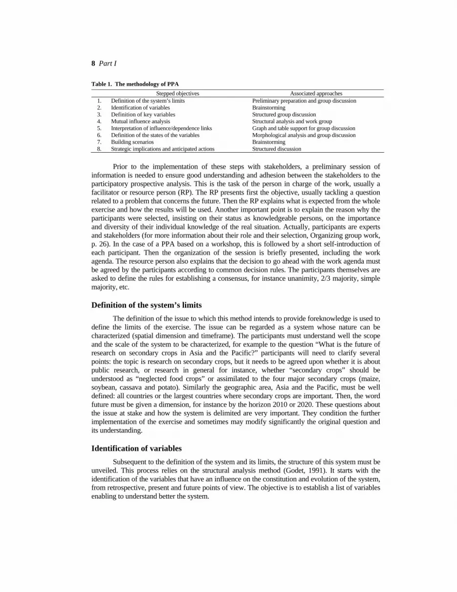
Table 1. The methodology of PPA Stepped objectives Associated approaches
1. Definition of the system’s limits Preliminary preparation and group discussion 2. Identification of variables Brainstorming 3. Definition of key variables Structured group discussion 4. Mutual influence analysis Structural analysis and work group 5. Interpretation of influence/dependence links Graph and table support for group discussion 6. Definition of the states of the variables Morphological analysis and group discussion 7. Building scenarios Brainstorming 8. Strategic implications and anticipated actions Structured discussion
Prior to the implementation of these steps with stakeholders, a preliminary session of
information is needed to ensure good understanding and adhesion between the stakeholders to the participatory prospective analysis. This is the task of the person in charge of the work, usually a facilitator or resource person (RP). The RP presents first the objective, usually tackling a question related to a problem that concerns the future. Then the RP explains what is expected from the whole exercise and how the results will be used. Another important point is to explain the reason why the participants were selected, insisting on their status as knowledgeable persons, on the importance and diversity of their individual knowledge of the real situation. Actually, participants are experts and stakeholders (for more information about their role and their selection, Organizing group work, p. 26). In the case of a PPA based on a workshop, this is followed by a short self-introduction of each participant. Then the organization of the session is briefly presented, including the work agenda. The resource person also explains that the decision to go ahead with the work agenda must be agreed by the participants according to common decision rules. The participants themselves are asked to define the rules for establishing a consensus, for instance unanimity, 2/3 majority, simple majority, etc.
Definition of the system’s limits The definition of the issue to which this method intends to provide foreknowledge is used to
define the limits of the exercise. The issue can be regarded as a system whose nature can be characterized (spatial dimension and timeframe). The participants must understand well the scope and the scale of the system to be characterized, for example to the question “What is the future of research on secondary crops in Asia and the Pacific?” participants will need to clarify several points: the topic is research on secondary crops, but it needs to be agreed upon whether it is about public research, or research in general for instance, whether “secondary crops” should be understood as “neglected food crops” or assimilated to the four major secondary crops (maize, soybean, cassava and potato). Similarly the geographic area, Asia and the Pacific, must be well defined: all countries or the largest countries where secondary crops are important. Then, the word future must be given a dimension, for instance by the horizon 2010 or 2020. These questions about the issue at stake and how the system is delimited are very important. They condition the further implementation of the exercise and sometimes may modify significantly the original question and its understanding.
Identification of variables Subsequent to the definition of the system and its limits, the structure of this system must be
unveiled. This process relies on the structural analysis method (Godet, 1991). It starts with the identification of the variables that have an influence on the constitution and evolution of the system, from retrospective, present and future points of view. The objective is to establish a list of variables enabling to understand better the system.

The Participatory Prospective Analysis (PPA) Method 9
In order to ensure equal participation among the participants, the process of variable identification is based on the free expression of individual opinions, either through visualization techniques in the case of a workshop (coloured cards) or through direct submission of ideas through electronic means in the case of virtual workshops. In the first case, the participants write the variables they consider important on coloured cards, one variable per card. Cards are then collected and displayed on a wall or board. Redundant cards that present exactly the same meaning are immediately removed. Then cards/variables are first grouped together by broad categories enabling to discuss similarities and then similar cards that have different wordings are progressively removed. In this process careful attention is paid to reaching a consensus between the participants on the elimination or retention of each card, asking, when necessary, the author to explain what was meant. The same process is conducted in the case of electronic consultation of experts, the resource person playing the role of synthesizing and dispatching information. At this stage there is no discussion on the relevance of variables yet.
Selection and definition of key variables After consensus has been reached about which variables to keep for discussion, the next step
is to discuss the relevance of these variables. Simple rules are useful to discuss whether the content of a proposition by a participant is a variable or not as indicated in Box 1 below. Often participants request clarification of the notion of “variable” and examples. Ideally, examples should be given with reference to a case unrelated to the issue at stake to avoid influencing the participants.
Box 1.
Some rules for identifying variables
Rule 1: A sentence is not a variable (for example: “Fertilizers are expensive”). Rule 2: Negative forms are not variables (For example: “No good weather”). Rule 3: Physical expressions are usually not variables (For example: “Money”). The corresponding variables for the examples in parenthesis could be “Cost of fertilizers”, “Climatic conditions”, “Availability of funds”.
Variables for which it is impossible to define different states should be considered as
irrelevant (Box 2). Usually, a state is described using qualifying words, such as adjectives, while variables are substantives.
Box 2.
Relevance of variables and identifiable states
For instance, “Bad relations between farmers and traders” is not a variable; the variable is “Relationship between farmers and traders”. This variable can take different states in the same system such as “distrust” or “mutual trust”; similarly “Farmers’ psychology” will be irrelevant if nobody is able to describe what the different states it can take are. The question “Is it a variable or a state?” is important here. The difference between variables and states is that a state pictures a situation in which the system or part of it can be found. “High prices” or “fluctuating prices” are states, “Prices” is a variable.

10 Part I
A final list of variables is then established and a clear and consensual definition is given to each variable and kept for further reference3. As indicated in Box 3, the establishment of the final list of variables must be carefully monitored since it will condition the further implementation of the method and the quality of results.
Box 3.
How many variables to keep?
Two opposite trends may appear: the trend to add more and more specific and narrow variables and the trend to reduce the number of variables by grouping them under more generic names. The risk associated with the first trend is that too many variables make further discussions very long and tedious due to the rather repetitive process used. Our experience shows that often the additional variables end up becoming marginal variables that have almost no influence in the system. The risk associated with the second trend is an oversimplification of the system leading to a very limited capacity of exploration and anticipation. As a result all variables are equally influent and the building of scenarios is difficult. A way to mitigate this trend is to regroup the variables under more generic headers that are not considered themselves as variables. While there is no rule for defining the appropriate number of variables, indicatively, variable identification based on this brainstorming and discussion process leads generally to an average of thirty to forty variables.
At this stage, all selected variables are represented by nicknames and these are entered by
the resource person in the computer in the corresponding cells of the first left hand column of the matrix located in the “Variables’ influence” worksheet of the Microsoft Excel software package used for this phase of the work4. The nicknames can be typed one by one or pasted from another Excel table. When variables are entered, all tables in the related worksheets are automatically updated and display the variables in all header columns and header rows. Entering variable names requires therefore, only one step as indicated in Figure 3 5.
Mutual influence analysis Experts are then invited to analyze the direct influence/dependence (I/D) links of each
variable on the others, using a consensual valuation approach. Actually, the interest we develop for the variables, in a system perspective, is not only related to the nature of the variables but also to their interactions with other variables in the system. The structural analysis method relies on direct influence assessment as a way to classify variables. Practically, influence assessment consists of a valuation of the direct influence of each variable on the others using a scale from “0 = no influence” to “3 = very strong influence”6. Values are discussed among participants and, once agreed upon, they are immediately entered in the Influence/Dependence (I/D) matrix in the worksheet “Variables’ influence” already mentioned above and as indicated in Figure 4.
3 Although the process of reaching a consensus for the definition of each variable may seem long, it actually helps to
save a lot of time and discussion in subsequent steps. 4 The ready-to-use packaged software is available for free download at UNESCAP-CAPSA website:
http://www.uncapsa.org. People who wish to download and use this software are only requested to register their names and data and to sign a user agreement. The basic package includes a 50x50 matrix.
5 For a comprehensive view of the software architecture, refer to Figure 6 and Table 2, p. 14. 6 Other scales were tested such as a simple 0-1 scale and 0-5 scale. The addition of more values in the scale does not
significantly modify the results but makes them much longer to obtain compared to the 0-3 scale. The 0-1 scale is simpler but results are less contrasted since the power of a variable on another is assessed in a binary way. Our preference goes therefore for the 0-3 scale as the best compromise.

The Participatory Prospective Analysis (PPA) Method 11
Figure 3. Matrix displayed in “Variables’ influence” worksheet and automatic links
This step is the most time consuming part of the workshop and is directly dependent on the
number of variables. For instance, a list of thirty-five variables will lead to 35x34=1,190 relationships to be discussed and an equivalent number of cells to be filled in the matrix. Godet (1991) reports exercises with more than seventy variables and 5,000 to 10,000 relations to analyze, requiring up to three months. However, as participants become more used to the discussion process, their capacity to deal with variables increases and the process gains in speed.
Legend: 0 means no influence3 strong influence2 mild influence1 little influence
OF ON Nickname 1 Nickname 2 Nickname 3 Nickname 4 Nickname 5 Nickname 61 Nickname 12 Nickname 23 Nickname 34 Nickname 45 Nickname 56 Nickname 6
Influence of variables on one another
Nickname 1 - Nickname 1 -Nickname 2 - Nickname 2 -Nickname 3 - Nickname 3 -Nickname 4 - Nickname 4 -Nickname 5 - Nickname 5 -Nickname 6 - Nickname 6 -- - - -
Global influence Global dependence
Nickname 1 - Nickname 1 -Nickname 2 - Nickname 2 -Nickname 3 - Nickname 3 -Nickname 4 - Nickname 4 -Nickname 5 - Nickname 5 -Nickname 6 - Nickname 6 -- - - -
Global indirect influence Global indirect dependence
… and tables.
OF ON Nickname 1 Nickname 2 Nickname 3 Nickname 4 Nickname 5 Nickname 6Nickname 1 - - - - - -Nickname 2 - - - - - -Nickname 3 - - - - - -Nickname 4 - - - - - -Nickname 5 - - - - - -Nickname 6 - - - - - -- - - - - -
Variables' indirect influence on one another
OF ON Nickname 1 Nickname 2 Nickname 3 Nickname 4 Nickname 5 Nickname 6Nickname 1 - - - - - -Nickname 2 - - - - - -Nickname 3 - - - - - -Nickname 4 - - - - - -Nickname 5 - - - - - -Nickname 6 - - - - -- - - - - - -
Variables' total influence on one another
Entering variables’ names here automatically updates variables’ name there and in all other worksheets...

12 Part I
The data entry process needs to be carried out only once for each variable, entering the influence values on other variables from left to right, column-by-column and then descending to the next row. Through a chain of automatic links, all related matrices, tables and graphs are filled and updated. The I/D matrix and the related tables and graphs permit to almost immediately obtain and visualize the results from the I/D discussion.
Figure 4. Filling the influence/dependence matrix
Influence of variables on one another Legend: 0 means no influence 3 strong influence 2 mild influence 1 little influence OF ON Nickname 1 Nickname 2 Nickname 3 Nickname 4 Nickname 5 Nickname 6
1 Nickname 1 2 3 1 2 Nickname 2 2 1 3 Nickname 3 1 1 4 Nickname 4 2 1 1 5 Nickname 5 3 3 6 Nickname 6 1
In order to accelerate the valuation process, a discussion board can be used. With this board
such as the one presented in Figure 5, the resource person facilitates the discussion of the variables’ influence values. For each variable, the process of valuation starts by identifying the 0-influence relations, that is, all variables that according to the experts are independent from any direct influence from the variable discussed. Then, one proceeds to ask for the variables that are extremely (strongly) dependent on the discussed variable. The low or mild influences on the remaining variables (values 1 or 2) are discussed last. Decisions are made by consensus allowing experts to express their arguments7.
An important point is to ensure that only direct influence is taken into consideration at this stage. Actually, indirect influences are automatically computed in a separate table, through matricial calculation (see Annex 4). However, ascertaining the direct nature of the relationship is not always evident. Experience shows at least three potential sources of errors.
7 This process helps obtain contrasted values for the assessment of the variables. Alternative methods used earlier that
do not concentrate on identifying first the zero influence are less relevant and often give unclear results. In particular, the establishment of the values cannot be based on the average from expert opinion. If at least one expert considers that a variable has a small influence on another, using an average value, however small but different from 0, will have an important impact on the final architecture of the variables due to the special properties of the numeral 0.
Values of each variable’s influence on the others are entered from left to right in the matrix, starting with the first row corresponding to “Nickname 1” and filling the intersection cells with the other variables. When the first row is complete, the same process applies to the row corresponding to “Nickname 2”, etc. In the above example, “Nickname 5” has no influence on “Nickname 1”, “Nickname 3” and “Nickname 6” and is strongly influent on “Nickname 2” and “Nickname 4”. The total influence of “Nickname 5” is 6. “Nickname 5” is only little influenced by “Nickname 2” and “Nickname 4”. Its dependence is 2.
Influence
Dependence

The Participatory Prospective Analysis (PPA) Method 13
1. Confusion in the causality relation: someone believes that A influences B but it is actually the opposite. This happens frequently at the beginning of the I/D analysis but the participants themselves usually rapidly correct it. However, it may also happen that two variables mutually and directly influence each other, with different or similar strengths.
2. Transitivity: A influences B and B influences C, therefore A influences C. This is a case of indirect influence and should not be included for the reason indicated earlier. When there is a causal indirect relationship between two variables, it is usually possible to identify the intermediate variable that links them. If this variable is part of the system (already listed), it is a case of transitivity. However, if the variable is not included, the question of the inclusion of this new variable must be discussed. If experts agree to include it, the list is modified accordingly and the I/D analysis is undertaken with this additional variable. If experts consider the variable as unrelated to the system, then it is recommended to consider the interaction between the two variables as direct.
3. Co-variation: intuitively someone thinks that two variables are linked because they evolve similarly, but this can be explained by other causes such as a similar factor influencing both variables: A is influenced by D and B is influenced by D, but A and B are not directly linked.
The role of the resource person is therefore crucial in helping the experts to only consider
causal direct relations. While the process seems to be very time consuming in the beginning, with more practice the experts become extremely expeditious in this exercise.
Figure 5. Organization and utilization of a discussion board
Preparation: the name of the variable is displayed in the upper part of the board 1st step: all variables on which it has no influence are pinned in the “0” column 2nd step: all variables on which it has a strong influence are pinned in the “3” column 3rd step: remaining variables are dispatched to columns “1” and “2”.
1st step 2nd step 3rd step
Influence of is Nickname 1
Nickname 4
Nickname 5
0 on
Nickname 3
3 on
Nickname 2
2 on
Nickname 6
1 on

14 Part I
Interpretation of influence/dependence links The software where Influence/Dependence data is stored is a multiple worksheets file with
built-in links8. The structure and function of this file and these worksheets is indicated in Figure 6 and Table 2. As indicated earlier data is entered only into the first worksheet.
Figure 6. Location of the functional worksheets
Table 2. Architecture of the software package Worksheets name Content Utility “Variables’ influence”
− The matrix where variables’ names and direct I/D values are entered
− Four tables located below the matrix and displaying: the direct influence, the direct dependence, the direct strength and the weighted direct strength of each variable
Basic storage of the direct I/D values and inputs for other matrices Assess the direct role of each variable with three indicators: how much they affect the system, how much they are affected by the system and a ranking of their relative power
“Variables’ dir. strength graph”
− A graph that displays the position of each variable along two axes according to their weighted direct influence and direct dependence
Enables to visualize the position of the variables and determines their current role according to their location in this four-quadrant graph
“Variables’ total influ”
− A matrix called “Variables’ indirect influence on one another” where indirect I/D values are automatically computed
− Four tables located below this matrix and displaying: the indirect influence, the indirect dependence, the indirect strength and the weighted indirect strength of each variable
Calculates the result of the multiplication of the first matrix automatically Assess the indirect role of each variable through three indicators: how much they affect the system, how much they are affected by it and a ranking of their power
Continued…
8 Note that the file is presented in a ready-to-use format, where most of the intermediary calculations, results and
formula are hidden. For more details on the location of this additional data and an explanation about the formula content and rationale, please refer to Annex 5.

The Participatory Prospective Analysis (PPA) Method 15
Table 2. Architecture of the software package (continued) Worksheets name Content Utility “Variables’ total influ”
− A matrix called “Variables’ total influence on one another” located below these tables where direct and indirect values are summed
− Four tables located below the matrix and displaying: the global influence, the global dependence, the global strength and the weighted global strength of each variable
Produces total I/D values through summing direct and indirect values Assess the total role of each variable through three indicators: how much they affect the system, how much they are affected by it and a ranking of their power
“Variables’ indir. strength graph”
− A graph that displays the position of each variable along two axes according to their weighted indirect influence and indirect dependence
Enables to visualize the position of the variables and determines their future or potential role according to their location in this four-quadrant graph
“Variables’ total strength graph”
− A graph that displays the position of each variable along two axes according to their weighted total influence and total dependence
Enables to visualize the position of the variables and determines their role according to their location in this four-quadrant graph.
“Feuill1” − A matrix to be filled manually (optional) Used for indirect influence/dependence analysis of higher levels
Interpretation of the tables. The tables (direct or global, indirect and total) provide
information on three aspects of each variable: its influence, its dependence and its strength. The influence value of each variable that is displayed in the first (influence) table corresponds to the sum of the values entered in the row related to that variable in the above matrix. The variable with the highest score is the most influent. Similarly, the influence value of each variable that is displayed in the next (dependence) table corresponds to the sum of the values entered in the column related to that variable in the matrix (Figure 7). The higher the value, the more dependent the variable.
Figure 7. Direct dependence and influence tables
Global influence Global dependence Nickname 1 6 Nickname 1 3 Nickname 2 3 Nickname 2 7 Nickname 3 2 Nickname 3 5 Nickname 4 4 Nickname 4 3 Nickname 5 6 Nickname 5 2 Nickname 6 1 Nickname 6 2 - - - -
In the left table, the values represent the sum by row of the numbers entered in the matrix displayed in Figure 5. It shows that two variables have the highest total influence of 6. The right table displays the sum by column of the values entered in the matrix. It shows for instance that “Nickname 2” is the variable most influenced by the others (value is 7) and therefore the most dependent.
The (direct or global, indirect, total) strength and weighted strength tables (Figure 8) correspond to a combined indicator developed to establish a ranking of the variables. It combines in a single formula the influence and the dependence of the variable. The formula is detailed in Annex 5. It is based on the idea that two variables with similar influence but different dependence values are not equally powerful in the system. The formula is set up so that the variable with the highest influence and the lowest dependence is the strongest. The difference between strength and weighted (ponderated) strength is an additional calculation made to centre the distribution of the variables on one as the average value. Weighted strength is the value used for ranking of variables and comparison between direct and indirect influences for instance.

16 Part I
Figure 8. Variables’ strength tables based on direct influence
Global strength Ponderated global strength Nickname 1 0.18 Nickname 1 1.91 Nickname 2 0.04 Nickname 2 0.43 Nickname 3 0.03 Nickname 3 0.27 Nickname 4 0.10 Nickname 4 1.09 Nickname 5 0.20 Nickname 5 2.14 Nickname 6 0.02 Nickname 6 0.16
In the left table, the values represent a composite indicator combining the influence and dependence of each variable. In the right column, this value is adjusted so that the distribution of variables is centred on 1. “Nickname 5” appears to be the strongest variable while “Nickname 6” is the weakest.
Interpretation of the graphs. The (direct, indirect, total) influence graphs display how the variables are scattered in a four-quadrant space delimited by two axes. It is based on the weighted I/D values of each variable calculated from the influence and dependence table. Interpretation of results includes: interpreting the position of the variable; discussing the shape of the distribution and interpreting direct and indirect results.
The position of the variable. Each quadrant in the graph corresponds to specific characteristics of the variables as indicated in Figure 9. The upper-left quadrant (1) is the area of the driving variables where most of the strongest variables are present. The upper-right quadrant (2) corresponds to leverage variables, both influent and dependent. Some of them can be considered also as strong variables. The lower-right quadrant (3) corresponds to the output variables, very dependent and little influent. In the lower-left quadrant (4) one will find the marginal variables. Little influent and little dependent, these variables behave rather independently from the system. Usually, they either represent long and independent trends or very specific issues that are not relevant. Therefore they are usually excluded from further analysis. Godet (1991) identifies also a grey area, along the axes that separate quadrant 4 from the others, where a “bunch” of variables can be found, whose role in the system is not clearly identified.
Figure 9. Signification of variables according to their place in the I/D graph
Overview of the importance of the different variables
0 0,2 0,4 0,6 0,8
1 1,2 1,4 1,6 1,8
2
0 0,2 0,4 0,6 0,8 1 1,2 1,4 1,6 1,8 2 Dependence
Influ
ence
Bunch variables
Driving variables (1) Leverage variables (2)
Marginal variables
(4)
Output variables
(3)

The Participatory Prospective Analysis (PPA) Method 17
A more comprehensive table for reading the variables is also given by Godet (1991) citing the work of Ténière-Buchot. Table 3 below is adapted from his work.
Table 3. Possible interpretations of the variables’ position in the visualization graph Graph position Possible lexical domains and associated meanings Systemic Communication Power Time Interaction Upper left Driving variables Hypothesis Strength Past Legitimacy Upper right Leverage variables Stakes Threats/opportunities Present Action Lower right Output variables Results Weakness Future Judgement Lower left Marginal variables Discourse False problem Instant Communication Grey area Bunch variables unclear unclear unclear unclear
In our experience, this table provides meaningful entries for interpretation of variables. We
have noted for instance that some variables lengthily discussed during the brainstorming and definition processes end up in the lower-left quadrant. This table helps to understand why. Some of these variables are erroneously presented and as they constitute a false problem or relate to common discourse, they generate an instantaneous process of communication, which generally does not lead to the elimination of the variable. The I/D analysis clearly sets the variable in the marginal area.
Conversely, there is usually almost no conflicting discussion about the variables that apparently drive the system today. These variables are frequently proposed by several experts. They are “obvious” in the sense that everybody accepts the hypothesis of their strength, based on past experience. As such, the legitimacy of these variables is unquestionable for everybody.
These interpretations should be conducted, however, with caution as the nature of the variable itself and the type of problem represented through this systemic analysis greatly influence the extent to which a detailed interpretation can be given to the position of one or another variable. Nevertheless, the phase of discussion of the results with the group of experts is necessary and improves greatly the efficiency of the subsequent steps.
The shape of the distribution. Godet also proposes an interpretation of the global shape of the variables’ distribution in the graph. As indicated in Figure 10a, when variables are spread along a diagonal line extending from quadrant 4 to quadrant 2, the system is rather unstable. This is due to the fact that most of the variables are marginal or leverage variables and only the latter influence the evolution of the system. A change will affect these variables and is likely to be amplified by the multiple interactions among them, making it difficult to explore what the future configurations of the system may be. Conversely, a roughly crescent-like shape such as the one displayed in Figure 10b (illustrative case) represents a rather stable system made of some driving variables (Nickname 5 and 1) strongly commanding the output variables (Nickname 2 and 3), while Nickname 4 is a bunch variable and Nickname 6 a marginal variable.
Figure 10a. Relatively unstable system Figure 10b. Stable system (illustrative case) Overview of the importance of the different variables
0
0,2
0,4
0,6
0,8
1
1,2
1,4
1,6
1,8
2
0 0,2 0,4 0,6 0,8 1 1,2 1,4 1,6 1,8 2
Dependence
Influ
ence
Overview of the importance of the different variables (direct influences)
------ ------
Nickname 3
Nickname 2
Nickname 5
Nickname 4
Nickname 1
Nickname 6-
--- -----------------------------
0.20 0.40 0.60 0.80 1.00 1.20 1.40 1.60 1.80 2.00
- 0.50 1.00 1.50 2.00
Dependence
Influ
ence
Author and copyright: Franck Jésus Cirad Amis Ecopol -

18 Part I
Interpretation of direct versus indirect influence. The third component of the interpretation of the structural analysis relates to the variations observed between direct and indirect I/D results. While the meaning of the direct results is clear, that is representing the factors currently influencing the system, the meaning of the indirect results and how to interpret them need to be well understood.
We have shown (see Annex 4) that the multiplication of the direct I/D matrix by itself is equivalent to calculating the indirect influence between variables. Reiteration of the self-multiplication of the resulting matrix enables accordingly to calculate several levels of indirect influences. The changes in the relative strength (ranking through global ponderated strength table), or in their relative position in the graph, provide useful indications. The comparison between direct- and indirect-influence graphs is therefore a useful tool for identifying indirectly strong variables. Our interpretation is that variables that progressively gain strength with indirect influence calculation, that is, if their relative global strength and/or ranking increase, or they tend to move towards the upper part of the graph, are variables whose effects are revealed over a longer period. They should be considered as variables having an important position in the future of the system. In particular, variables located in the upper-right part of the graph that glide progressively towards the upper-left may constitute future driving forces. Since the variables located in the upper-right quadrant are also considered as “stakes”, control over these variables becomes a key issue.
In the illustrative case of the “Nickname” variables (Figure 11) two variables switch position as driving variables in the system, while the others remain in the same place. The positions of these variables have also changed in the graphs as indicated in Figure 11: “Nickname 4” goes upward and to the left shifting from the bunch area to the driving variable area, while “Nickname 1” follows a reverse trend becoming more a bunch area variable.
The crescent-like shape of the variables’ distribution is reinforced in the indirect influence graph.
Selection of the variables. The process of interpreting the results of the structural analysis leads to the selection of a limited number of variables, resulting from the discussion of direct and indirect influences. Scenarios are then constructed based on a combination of future possible states of the selected variables. Therefore, the participants are confronted with a difficult decision about how many and which variables to select. The trade-off is that more variables will make more difficult and complex the construction of scenarios; fewer variables will lead to an oversimplification and a very narrow capacity for exploration of the futures. In this field, there is no absolute rule but some principles of common sense: 1) more than eight variables is rapidly unmanageable, less than three does not justify the time and effort spent on the preceding steps; 2) the number of variables can be adjusted according to the varieties and number of states (next step), if several variables present only limited possible states (for instance one or two), more variables can be added and vice versa9; 3) a gap in the range of values of the variables’ strengths can be used as an indicative limit (for instance if there is one very strong variable and a cluster of three other variables that is well separated from the other variables, the selection could be limited to only these four variables).
9 See for instance the case study in Part II where eight variables were selected and then recombined into six.

The Participatory Prospective Analysis (PPA) Method 19
Figure 11. Changes in variables’ position according to direct or indirect influence
In the case of the Nickname variables, the combination of direct and indirect influence
analysis would lead to decide to use three variables in order to further explore the evolution of the system, as indicated in Figure 12. These variables appear clearly both on the visualization graph and on the weighted total (direct+indirect) strength table as the driving forces.
Figure 12. Visualization of total I/D graph and total weighted strength
Three variables are selected for building scenarios.
Ponderated global direct strength Ponderated global indirect strengthNickname 5 2.14 Nickname 5 2.17 Nickname 1 1.91 Nickname 4 1.79 Nickname 4 1.09 Nickname 1 1.05 Nickname 2 0.43 Nickname 2 0.54 Nickname 3 0.27 Nickname 3 0.29 Nickname 6 0.16 Nickname 6 0.17
Overview of the importance of the different variables (direct influences)
------ ------
Nickname 3
Nickname 2
Nickname 5
Nickname 4
Nickname 1
Nickname 6-
--- -----------------------------
0.20 0.40 0.60 0.80 1.00 1.20 1.40 1.60 1.80 2.00
- 0.50 1.00 1.50 2.00
Dependence
Influ
ence
Author and copyright: Franck Jésus Cirad Amis Ecopol -
Overview of the importance of the different variables (indirect influences)
------ ------
Nickname 3Nickname 2
Nickname 5
Nickname 4
Nickname 1
Nickname 6-
--- -----------------------------
0.20 0.40 0.60 0.80 1.00 1.20 1.40 1.60 1.80 2.00
- 0.50 1.00 1.50 2.00
Dependence
Influ
ence
Author and copyright: Franck Jésus Cirad Amis Ecopol -
Overview of the importance of the different variables (direct and indirect influences)
------ ------
Nickname 3Nickname 2
Nickname 5
Nickname 4Nickname 1
Nickname 6-
--- -----------------------------
0.20 0.40 0.60 0.80 1.00 1.20 1.40 1.60 1.80 2.00
- 0.50 1.00 1.50 2.00
Dependence
Influ
ence
Author and copyright: Franck Jésus Cirad Amis Ecopol -
Ponderated total strength Nicknam e 5 2.17 Nicknam e 1 1.48 Nicknam e 4 1.43 Nicknam e 2 0.47 Nicknam e 3 0.28 Nicknam e 6 0.16

20 Part I
Definition of the states of variables This step is sometimes called morphological analysis (Godet, 1991 and 1996; The Futures
Group, 1994)10. Its objective is to browse the domain of possible futures, to reduce it and to explore consistent, relevant and plausible alternatives. For each selected variable experts are requested to identify some states these variables can possibly take in the future, focusing on contrasted and mutually exclusive alternatives. A state is a description of the variable in the future; it is not a measure of a variable. For example, the variable “International Aid for Developing Countries” can take the following states: “Strong support from the international community to all developing countries”, or “Selected support for countries showing progress in growth and democratic indicators”, or “Support for Africa only” or “no more support for developing countries”. This example shows that the states of a variable should not necessarily be limited to “good” and “bad” nor “high”, “medium” and “low”. By this procedure, one expects also the experts to introduce ruptures in the future, a critical aspect that is not incorporated in most forecasting works.
The discussion of the states follows also a participatory process, variable per variable, through brainstorming and the elaboration of a consensus on the accepted states. States that seem to be “unlikely” to happen must not be included, but one has to be very careful with statements about likeliness. For example, a prospective analysis of the economic situation of most Asian countries made in early 1997 may have discarded a state like “Sudden economic, financial and political breakdown” for a variable such as “Economic environment”, except if one of the few experts, who had drawn the attention on this possibility before, had been invited to participate in the exercise.
The variables and their respective states are then listed in a table similar to Table 4. This table represents the base for the combinatory work leading to the elaboration of the scenarios. In principle, the number of possible combinations is the direct product of the number of variables by the number of states for each variable. For instance, with 6 variables having respectively, two, four, three, two, four and two states, the total number of combinations is 2x4x3x2x4x2= 384. Adding one variable with four states would give 1,536 combinations…
One way to reduce the dimension of the universe of possible futures is to proceed to a consistency analysis based on the identification of mutual incompatibility between states. For this purpose experts are invited to list the states that cannot or are very unlikely to coexist11. To facilitate this process, each variable is given a reference (for instance a capital letter) and each state a number. Experts have then just to write down the paired combination of incompatibility. These are then discussed and represented in the table. Table 4 shows the representation of a situation related to the “Nickname” case, where 6 variables and their states can give a total of 384 combinations and where experts had stated that the following combinations were mutually incompatible: A1-E3; A2-E4; B4-E4; C3-F2; C1-F1; E1-F1; E3-F2; C1-E3. Combinations including states that are linked by the black lines would have to be discarded. This effectively reduces the morphological space.
10 See also the Glossary of selected terms related to foresight and prospective in Annex 6. 11 Note that here the word unlikely does not relate to some probabilistic occurrence, but to logical thinking. See for
instance the incompatibilities identified in Table 11, p. 45.

The Participatory Prospective Analysis (PPA) Method 21
Table 4. Display of variables, states and incompatibilities Variables States
A. Nickname 1
1
2
B. Nickname 2
1
2
3
4
C. Nickname 3
1
2
3
D. Nickname 4
1
2
E. Nickname 5
1
2
3
4
F. Nickname 6
1
2
Building scenarios A scenario is a combination of variables in different states. As indicated above the number
of scenarios is not just a product of multiplying the number of states with the mutual incompatibility of some states reducing the total number of scenarios. After identifying these incompatibilities, the participants are given time to produce a certain number of scenarios. Visualization cards can be used, each one describing the combination of variables and states (for example A2-B3-C1-D2-E4-F2) or using reproduction of tables where lines are drawn linking the states of the different variables as indicated in Table 5.
The number of scenarios proposed by the experts is usually limited to five. It seems to be a good compromise enabling the experts to be creative in building scenarios and ensuring plausibility. Different exercises have shown that when experts are given only three possible scenarios, they rather automatically think in terms of “good/positive/desirable”, “current/neutral/trend” and “bad/negative/adverse’. Five scenarios give room at least for two alternative visions per expert. However, it still ensures a certain level of plausibility and consistency in the conception of the scenario.
Table 5. Representation of a scenario Variables Scenario
A. Nickname 1 1 2
B. Nickname 2 1 2 3 4
C. Nickname 3 1 2 3
D. Nickname 4 1 2
E. Nickname 5 1 2 3 4
F. Nickname 6 1 2

22 Part I
As each scenario can be identified through a combination of variables and states, the suggestions made by the experts are regrouped so that similar scenarios can be clustered through an identical process as used for the identification of variables: elimination of redundant scenarios, grouping of scenarios and discussion of results.
The grouping of scenarios leads to reduce their total number, but it is not usually sufficient and decisions must be made on which scenarios to keep for further analysis. The number of cards or the number of times a similar scenario is proposed by the experts gives a first indication. This usually tends to highlight the most likely or plausible scenarios, but does not help to identify which ones among the others also have some plausibility that deserves to be taken into consideration, even if they are considered somehow less likely due to important ruptures for example.
The word plausibility refers here more to the notion of conceivability/credibility than to possibility/probability, though the latter is also included. A way to identify plausible scenarios is to give the experts a certain number of stars to allocate to the scenarios. For instance, in a list of 15 scenarios, 12 experts allocate freely 10 green stars among all scenarios according to the criterion of probability. This establishes a ranking of scenarios according to some kind of likeliness of occurrence. This idea of probability is not a measure that can be confidently considered as how likely the scenario will happen. It reflects only the fact that the experts think that the combination of the states that constitute the scenario is “more realistic”. Often, this relates to scenarios that are very close to the trend or average scenario formed by the continuation of the current states. The identification of the most contrasted scenarios in the list and a discussion of their internal consistency is a complementary and recommended approach for the selection of scenarios12. It is advisable at this stage to keep a number of scenarios that exceeds three to avoid the trap of the “bad/good/average” scheme, and to focus on contrasted scenarios.
Using scenarios Each selected scenario feeds a structured discussion using a common framework that
includes the description of the scenario (combination of states), the implication on other key variables of the system (the control/leverage and output/results variables), the strategic elements (those that influence the evolutions of the system) and the possible actions. Two types of possible actions can be generated: (i) reduction of the impact of negative scenarios and taking advantage of the effects of positive scenarios, and (ii) promoting the occurrence of desirable scenarios. The resulting information becomes therefore a kind of roadmap for the stakeholders and the organizations that are concerned with the treated problem.
The first action enables stakeholders to be prepared for a range of possible situations to be encountered in the future (be pre-active). The exploration of the futures helps guard against “any” eventuality, reacting by anticipation. The second action relates to the modification of the present so that a more desirable future can be expected (be pro-active). Through the identification of contrasted scenarios and the related factors of change, one becomes able to select a desirable, yet plausible, vision of the future and to identify a path leading to this vision; in other words to some extent become able to “master” the fate.
As we indicated in the introduction of this book, the result is the generation of foreknowledge. This is not knowledge about what the future will be but about what it may look like according to how some key variables evolve. The strategic elements identified in the scenario can become indicators for monitoring the evolution of the real world and give early indication on its possible evolution. Stakeholders are therefore better prepared to face changes since they have already, at least partly, explored how these changes may affect the future.
12 See for instance the case developed in Part II.

The Participatory Prospective Analysis (PPA) Method 23
However, the usefulness of the building and discussion of scenarios is above all a question of stakeholders’ attitude as indicated in the table below. Passive/reactive behaviours will not take advantage of this generation of foreknowledge. Pre-active and pro-active behaviours on the other hand will use this information, though in different ways corresponding to the distinction between exploratory and normative approaches.
Table 6. Typology of attitude’s towards scenario building and discussion Attitude Use of scenarios Implications Activity Strategy Passive No use Accept to be led by
external forces Nothing specific Let it be
Reactive No use Adjust to changes when they arise
Nothing specific Wait and see
Pre-active Explore the future Anticipate changes to adjust early the
responses
Monitor the states of key variables
Guarded against any eventuality
Pro-active Influence the futures Identify and promote desirable changes
Modify the states of key variables
Master your fate
In conclusion, the type of prospective analysis proposed in the PPA method goes beyond
the elaboration of scenarios. It is a full process where expert participants who are at the same time stakeholders are led to view their environment from a very different perspective. It gives them the opportunity to understand it better, to get more insight about the forces at work and the stakes. They become aware that there is always room for manoeuvre not only to prepare for future changes, but also to have a say in these changes even on a limited scale. As such, it is a tool for people empowerment through the generation and sharing of information, and through the sharing of ideas and knowledge.
It is therefore not surprising that the selection of the expert participants is a key issue in the success and impact of this approach. This issue will be further developed in the following section concerning the organization and practical implementation of the PPA method.
Implementing the PPA
While the preceding section focused on the content of the PPA method, describing step by step the methodology, the concepts and results in a logical sequence, this section details the practical arrangements needed in order to properly conduct this work. Readers who are interested with the result of a direct application of the method to secondary crops research and development in Asia and the Pacific may skip this section and go directly to Part II, p. 31. However, this section provides practical knowledge and useful hints for the implementation of the PPA method, including a discussion about expert and expertise.
The option presented here is the workshop-supported PPA. The other option is the PPA conducted through distance communication and periodic meetings. It will not be developed here, although it basically follows the same organizational principles in terms of group work and the selection of experts.
The rationale for using workshops as one of the key supports for a scenario-based approach is well known:
“There are also benefits from involving members of an organization or community in futures’ exercises or more specifically in a foresight process. Scenario workshops can help participants gain ‘ownership’ of scenarios as well as deeper understanding of issues. (… ) Thus the participants should understand the logic underlying the choice

24 Part I
and the contents of scenarios much better than they would if presented with the material in a standard report. They should be better informed as to the key issues at stake, and better equipped to use the scenarios in decision-making and to explain them to the outside world. Scenarios produced in this way should also possess greater legitimacy than those produced by a smaller expert group or visionary guru” (Eurofound, 2003, p. 89).
The main aspects of the implementation of a PPA workshop are presented in Box 4.
Detailed management and organizational issues are discussed thereafter. They include discussion about equipment and resources, the organization of group work and special attention to the role of the experts/stakeholders in the whole process13.
Box 4.
The PPA workshop in brief
Characteristics Requirements Group (team) work (8-15 people) Participant agreement/commitment Balanced selection of participants Resources for organization cost Neutral, trained resource person Materials (boards, flip charts, colored cards, Consensus seeking approach markers, tape, magnets, etc.) Clear and shared objective Meeting and working space Common agreed-upon rules Secretarial help
Equipment and resources The implementation of an expert-meeting workshop needs preparation of materials and
equipment as indicated below.
Facilities. An isolated meeting-room is needed with ample space for displaying information on the walls or on supports located along the walls. The size of the room must fit, or be arranged to fit, with the number of participants, so that they can both easily interact and see the results. Tables and chairs should be arranged in a U-shape, the most effective form for both purposes as indicated in Figure 13. Amenities should include a place for coffee breaks provided by the organizers.
Equipment. As the PPA method is a computer-supported approach, minimum requirements include two PCs (or laptops), one LCD projector and a screen (or a wall if appropriate), a printer, and a nearby photocopy facility. One computer is connected to the LCD projector and is used as support for implementation of the methodological steps. One computer is connected to the printer for quick production of results, photocopy and immediate distribution to the participants
Materials. As visualization techniques are widely used, related materials are needed and must be readied in advance. These include:
Coloured cards: minimum size 20x10 cms used in landscape orientation. Consider minimum 4 x 150 cards for one workshop (four colours).
Markers: at least one per participant plus some spare. Support for card display: these supports are either the walls of the meeting room, flip charts, whiteboards, or Styrofoam boards. Flip charts are the least useful support because of the rather large space required for displaying cards and keeping results visible during the workshop that usually exceeds the size of flip charts. It is advisable to use either the walls
13 See also Jésus and Bourgeois, 2003.
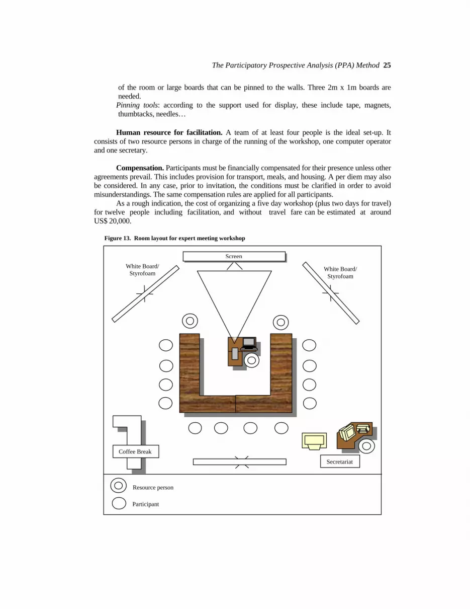
The Participatory Prospective Analysis (PPA) Method 25
of the room or large boards that can be pinned to the walls. Three 2m x 1m boards are needed.
Pinning tools: according to the support used for display, these include tape, magnets, thumbtacks, needles…
Human resource for facilitation. A team of at least four people is the ideal set-up. It
consists of two resource persons in charge of the running of the workshop, one computer operator and one secretary.
Compensation. Participants must be financially compensated for their presence unless other
agreements prevail. This includes provision for transport, meals, and housing. A per diem may also be considered. In any case, prior to invitation, the conditions must be clarified in order to avoid misunderstandings. The same compensation rules are applied for all participants.
As a rough indication, the cost of organizing a five day workshop (plus two days for travel) for twelve people including facilitation, and without travel fare can be estimated at around US$ 20,000.
Figure 13. Room layout for expert meeting workshop
Resource person
Participant
Coffee Break
Secretariat
White Board/ Styrofoam
White Board/ Styrofoam
Screen

26 Part I
Organizing group work The PPA workshop is a typical expert meeting (Jésus and Bourgeois, 2003) using a working
group approach. It is based on the recognition that “participation calls for collective analysis” (Pretty, 1995). The idea is to make possible for different people from different backgrounds and knowledge to meet and interact so that from the interaction process a common vision can emerge with sufficient clarity. This common vision is considered as an operational representation of the situation under analysis.
A key point is the identification and selection of the group of experts. We use here the definition of an expert given by Skumanich and Silbernagel (1997, citing Millet (1991)) that considers experts as individuals who have extraordinary familiarity with the subject at hand. The choice of this definition is not neutral. It implies that experts are above all recognized for their expertise, that is, for their specific knowledge. Therefore, invited experts are selected on an individual basis and not on their belonging to a specific organization, though the latter may be a criterion for finding people with a specific field of expertise14. Furthermore, this knowledge is not necessarily academic or scientific knowledge. It is the knowledge about the subject at hand, which means that for instance if the subject at hand is about fixing tyres, a qualified engineer of a tyre producing company or a well-known specialist of rubber chemistry research will have less expertise than the neighbourhood garage mechanic. What matters is the subject at hand.
As far as the PPA method is concerned, the subjects at hand are complex and multi-faceted. They cannot be covered by one type of expert. Confrontation and exchange of multiple points of view is needed in order to build a reliable representation of the systems and questions that are analyzed and explored. Lessons from fifty years of expert-based foresight activities show that not only “technical” experts who are producers of knowledge, but also the users of this knowledge, that is all stakeholders, must be involved (Jewell, Uchupalanan and Sripaipan, 2001). Actually, experts invited to the PPA workshop are the stakeholders directly concerned with the issues at hand. This not only ensures matching participants knowledge with the scope of the work, it also contributes to strengthen the relevance of the work and the commitment of the participants. Furthermore, it increases the likeliness to see the results used in pre-active and pro-active ways.
Various methods can be used to select experts. Loveridge (2002, p. 15), for example, identifies methods such as “Asking around individual people”, or “Consulting appropriate professional institutions and their membership lists”. Co-nomination based on bibliometrics and mapping clusters of researchers to select a group of people representative of the larger group from which one thinks the opinion as experts is also proposed. From this group one asks each member about a certain number of other representative experts (snowball sampling).
These methods have inconvenient aspects: “asking around” may introduce disciplinary or thematic biases in the final selection of experts due to limitation to a specific field of expertise. Consulting professional institutions may induce the selection of a vested interest group, which is not representing the position (and expertise) of all stakeholders and not compatible with our definition of experts. The co-nomination process reflects the fact that foresight has been basically developed for science and technology questions. When applied to local development questions for instance the method is more difficult to implement since written references proving the expertise are unlikely.
However, the concept of defining a representative group of the wider groups of stakeholders is extremely appropriate and is the leading principle for the expert selection in our method. Indeed, experts have to be carefully identified. They are expected to bring practical and real knowledge concerning the various aspects of the system. Thus, criteria for selecting these participants includes geographic coverage, subject matter knowledge, institutional affiliation, and socio-economic 14 This is a common source of difficulties in the organization of PPA workshops as the organizing committee or people
in charge tend to look at institutionalized expertise and not at individualized expertise. One should be very firm on the point that experts are individuals and not representatives of formal organizations.
The Participatory Prospective Analysis (PPA) Method 27
characteristics. The process of expert selection is a combination of “asking around” and “co-nomination based on expert opinion” balanced by individual checking. A preliminary consultation of the possible participants about who else could be consulted and invited is a useful approach, since it helps select people on the basis of multiple opinions, increasing the likeliness of developing good relations during the workshop.
In the selection of participants, one must pay attention to their number. Too many participants would make the method unworkable or less interactive; too few would hamper the attainment of the objectives or introduce biases. A total of 8-15 people, with an optimum of around 12 usually provides a good representation and workable conditions.
It is advisable to prepare replacement lists to compensate for the unavailability of some pre-selected participants. Replacement experts come from the same selection process as second-best candidates. The failing experts should not propose replacements since there is no guarantee about the expertise of the substitute. In the selection process, careful attention should also be given to individual participants’ profiles. They must be selected for their openness to discussion and acceptance of other opinions. Narrow-minded, ill-tempered people must be excluded, even if they have good knowledge, since they are likely to either block the group work or bias it15. Besides, no segregation shall be applied based on education or literacy criteria such as the capacity to read, speak or write a specific language. Otherwise there will be the risk that no participant would be aware of the situation of some specific aspects of the system. Special support must be provided for participants who need it for reading, writing or speaking the language used during the work in order to have them fully involved in the discussion process. This includes having someone to write down their ideas on cards or to read loudly the information sets that are discussed if needed16.
Workshop sessions are conducted under the guidance of a neutral resource person who is not a stakeholder in the system. Resource people must have already practised this method in “simulated real case” exercises. These consist of applying the method with a group of volunteer people (colleagues, other trainees) so that the process of handling a full session is known and mastered before starting a real case.
The resource persons play a crucial role. They must act as facilitators having extensive knowledge of the method to conduct the sessions step by step without interfering in the content, making sure that all participants are given an equal opportunity to intervene, and that the basic steps and rules agreed upon are understood and followed. Consensus seeking is the basic approach for this work to be achieved properly. It means that the move from each step to the next one should only occur after an agreement has been reached among all group members. The resource person must also ensure that records are kept from each step with the help of the computer operator and that results are quickly distributed to the participants with the help of the secretary.
The question of experts and expertise Expert-based methods all face similar constraints and present similar advantages. In this
section we will briefly summarize them and provide some hints in order to make the best use of this approach.
Strengths. In addition to the obvious value of their own expertise, experts bring the possibility to incorporate non-recorded and or qualitative data into the whole process. This is a way
15 The ideas of such people can be collected before the workshop and discussed with other participants during the
workshop. The workshop results are then discussed with the people interviewed. 16 Prospective analysis workshops were organized in Cambodia with resource persons not familiar with the Khmer
language. A team of translators and the participants themselves facilitated the conduction of this analysis in English and Khmer. It is a matter of organization that requires more time for the implementation of the different steps of the method.

28 Part I
to take advantage of an often-unsuspected wealth of information. Besides, through the presence of autonomous individuals there is room for the introduction of imagination and creativity, two key elements with regards to the objective of the method.
One of the pre-eminent reasons why this PPA relies on the expert meeting method is that experts are also stakeholders. As such, the quality of the foreknowledge they generate may increase significantly because they do not only know about the situation but can also contribute directly to make it change or to influence it (Donnelly, citing the work of Pool).
Weaknesses. However, one must be aware about some potential problems due to the tendency to base this method on experts’ knowledge.
The first weakness is the aggregation of opinion for at least two reasons: idiosyncrasy and aggregation rules. Firstly, idiosyncrasy makes it difficult to understand how each expert produces an opinion, and therefore how to aggregate them (Skumanich and Silbernagel, 1997). Secondly, when dealing with complex problems or specific local issues, the number of experts can be either very large or very limited. A small number of experts limits the use of what Loveridge (2002) calls the rules of “the frequentist tradition”. But even with many experts, this rule cannot be decisive since 1) experts belong to a paradigmatic world that has its (often-implicit) perception of the future and 2) the perceptions of experts may reflect the public perception and the related systems of action. Aggregation through consensus is often presented as an alternative but nevertheless it is not flawless. When, expert-based methods (interviews, questionnaires or group dynamics) seek to produce a consensus representing expert opinions, it actually introduces a bias toward the centre/majority opinion and extremes or divergences are forgone (Skumanich and Silbernagel, 1997). Thus, in expert-based methods the aggregation occults the problem of distribution of opinion. It is assumed that distribution is unimodal while it may well be bi- or pluri-modal, a dimension that is absent from most foresighting approaches (Loveridge, 2002).
The second weakness is related to Simon’s “Bounded Rationality” concept that makes experts unable to assess the “entire set of possible states of the world … and also the consequences that are implied by that choice for each of the possible states…” (Loveridge, 2002, p. 10). As a result, the preferences expressed by experts are not a reflection of omniscience but are bound by their understanding of the problem, its own interest and even sometimes simple mental exhaustion due to the lengthy process: “experts are not omniscient, but they have their own agendas, predilections and prejudices that become embedded in their opinions” (Loveridge, 2002). This problem surges also from “bias versus cost” trade-offs. Cost and time consideration may lead to reduce the number of experts, however the lower their number the more likely the bias (Skumanich and Silbernagel, 1997; Loveridge, 2002). In addition, several problems that are inherent to the partial knowledge of the experts such as failure to identify randomness, inconsistency in judgements across time, limited human computational capability or inability to bring order out of chaos (Loveridge, 2002) must not be ignored.
Abating weaknesses and building upon strengths. Because of the potential weaknesses of
expert-based methods, we endeavoured to at least partially solve or reduce the aggregation problem in the conception of the PPA. First, decision-making rules do not rely on median opinions or any other related statistical measurement since the number of experts usually invited does not allow for such often-criticized aggregation techniques. Second, expert opinion is organized with the means of two structured frameworks, the structural analysis and the morphological analysis. Combined with brainstorming techniques they allow the experts to produce their opinions through a similar and common mental process, facilitating therefore the aggregation17. As Godet (1996, p. 65) states
17 Brainstorming is today considered as a quite compulsory method for expert meetings and participatory approaches
(Popper and Korte, 2004).

The Participatory Prospective Analysis (PPA) Method 29
about structural analysis: “The ambition of this tool is precisely to enable the structuring of collective thinking by reducing unavoidable biases”18. Third, with the acceptance of common decision rules and the discussion of the results, the aggregation process becomes more transparent. Thus, even if it is not fully satisfying, at least points of disagreement and related decisions are clear and can always be further discussed. Fourth, the recourse to quantitative valuations is to a large extent limited and, whenever needed, supported by transparent computerized methods (such as the I/D matrix, tables and graphs) for further discussion.
Any representation of the reality is by definition biased since it cannot reflect its entirety. Therefore, the bias problem is neither specific to the PPA method nor to the choice of collecting information from experts. Still, reducing biases is needed to ensure the relevance and plausibility of the results. Bias reduction in PPA results from the combination of several measures. The first measure relates to the process of selecting experts (“Organizing group work”, p. 26).
Another source of possible bias is the strong influence some individuals may exert on the other experts during the workshop discussions. The adoption of decision rules by the group members and the supervision of the group dynamics by a trained resource person is usually sufficient to reduce this bias to an acceptable level.
Finally, the word “expert” should not lure us into an artificial feeling that it is possible to know all about a topic by just inviting the right person. Biases due to incompleteness of knowledge must not be under-estimated. These can be seriously reduced by careful identification of the various fields where expertise is needed and inviting corresponding experts. In addition, the use of computerized tools, for analyzing the relationships between variables for instance, is another way to counterbalance some of the inherent limits of the experts, such as the identification of randomness (represented by variables belonging to the quadrant 4 of the I/D graph), reducing inconsistencies (through systematic checking of relations between variables), increasing computational ability (through matrix calculation formula), and helping to see emerging order (indirect influence calculation and visualization graphs).
However, many points remain to be improved, such as the process for ascertaining the existence of direct influence links among variables; the use of numeric scales to assess the strength of these links, the choice of the future states of the variables.
In conclusion, the organization of the expert-based PPA workshop involving stakeholders is inseparable from its content. Preparation of the materials and equipment, selection of participants, meeting room arrangements, quality of the resource persons and their command of the method, decision-making rules, time allocation, all these elements contribute to the success of the method. None of these should be overlooked for being allegedly less important than the content of the workshop.
18 Author’s own translation.

31
Part II The PPA Method at Work: The Case of Secondary Crop Research and Development Prospects in Asia and the Pacific
Context
Works related with the exploration of futures are rather new in Asia and the Pacific with the exception of Japan, a pioneer country in Technology Foresight. In 1994, a workshop on Future Visions for Southeast Asia was held in Malaysia, developing visions based on scenarios (Inayatullah, 1995). But it is with the establishment of the APEC Technology Foresight Centre in Thailand in 1998, that a strong boost was given to this approach in several countries, focusing for instance on water supply and management, technologies for learning and culture, and mega-cities development issues such as sustainable transport and health (Jewell, Uchupalanan and Sripaipan, 2001). All these approaches are based on scenario analysis, Delphi method and consultations (Tegart, 2001). However, so far, few exercises related to the agricultural sector have been implemented in the region, while in France prospective analysis was institutionalized at INRA in 1993 (Sebillotte, 1993). Noticeable cases of futures’ research include however, the Technology Foresight Study for Thailand’s Agricultural Development concluded in 1999 (Suwana-adth, 2001), and the application of foresight in Viet Nam for the food processing sector and the tea industry (Tien and Quan, 2003).
The work undertaken by CAPSA has a very modest dimension compared to these regional or national activities and can be considered as a pioneer effort to introduce alternative approaches in the exploration of futures. So far, the PPA method has been used in Indonesia (Prospect of secondary crop research and development in Asia and the Pacific), in Cambodia (Challenges for rural development) and in Viet Nam (Development of the pig agrifood system). In all cases these exercises can be characterized as a sectorial prospective with strategic components when compared to the classification used by Barré (2002) for technology foresight. The Indonesian case is further detailed thereafter.
The decision to explore possible evolutions that may affect research and development on secondary crops in Asia and the Pacific up to the horizon 2015 was taken as a joint initiative in the framework of two CAPSA projects1. One project, called ELNINO mainly focused on collecting and analyzing data related to ELNINO abnormal weather conditions affecting upland agriculture in selected Asian and Pacific countries2. As climatic conditions and climatic change are key factors affecting the development of upland agriculture, where secondary crop production is concentrated, the objective was to acquire a better understanding of the occurrence, risks and impacts of these abnormal weather conditions on production and rural economies, in order to elaborate strategic proposals for upland agriculture technologies and farm management, as well as corresponding policies. The exploratory assessment of the relative importance of climatic conditions and how they influence other factors in relation with the development of secondary crops was thought to be important information for this project. The prospective analysis workshop made possible for the
1 Formerly named UNESCAP CGPRT Centre. 2 For more details on this project, refer to Yokoyama and Concepcion, 2003.

32 Part II
ELNINO project to refine its policies and strategic proposals by confronting them with the broader picture given by possible evolutions of scenarios.
At the same time, this workshop was an opportunity to use the PPA method elaborated within the framework of the MAPSuD project to further develop the analysis of the current situation of secondary crops in Asia and the Pacific through projections toward the future3. The project focused on strengthening the research and development capacity for socio-economic and policy analysis of the development of secondary crops in Asia and the Pacific and its contribution to sustainable development. It intended to gather information on current activities and key actors in this field and proposed to elaborate programs for regional training that fit with the needs of the participants. The prospective workshop helped the MAPSuD project to anticipate changes and therefore prepare for supporting the regional research and development capacity in addressing key issues in the future development of secondary crops.
This workshop was therefore intended to explore possible evolutions that may affect the development of secondary crops in Asia and the Pacific up to the horizon 2015 and to generate:
- An understanding of the key factors that may affect the development of these crops. - A vision of secondary crops for the horizon 2015 based on scenarios. - An appreciation of the prospective analysis method as a tool for action. - Identification of issues for CAPSA’s future projects and related activities.
Expected products included thus: Key factors influencing the future of secondary crops in Asia and the Pacific. Contrasted images of possible futures and their consequences. Possible actions to mitigate negative implications and promote positive changes.
Organization of the PPA
The decision to conduct this exploratory work and to base it on the PPA method supported by expert meeting did not emanate from the participating countries but from the two above-mentioned projects of CAPSA, whose mandate is to perform such activities in order to strengthen the capacity of R&D centres in Asia and the Pacific and promote interaction among them.
Since expected participants lived in distant places within the ESCAP region, the decision was taken to implement such an exercise using the expert meeting workshop approach. The first step, preliminary to the selection of the experts was to identify the limits of the system.
System identification The system was identified as follows:
The question: What are the variables affecting the future of secondary crop research and development by the horizon 2015 in Asia and the Pacific?
Geographic area: Twenty-six Asian and Pacific countries limited west by Pakistan, east by Japan and Fiji, north by Mongolia and China, and south by Australia.
Thematic focus: Research and Development of secondary crops. Secondary crops are defined as annual food crops grown by farmers excluding rice and wheat.
3 MAPSuD stands for Management of Agricultural Policy for Sustainable Development, a CIRAD/AMIS-Ecopol and
UNESCAP-CAPSA collaborative project.

The PPA Method at Work 33
Creation of a working group and workshop organization Expert participants were selected based on their involvement in secondary crop research and
development in some of the key countries in Asia and the Pacific where these crops play an important role. The group was initially built up from CAPSA correspondents who answered our surveys and/or participants of the ELNINO project. Participants were not expected to talk as representative or spokespeople of their government or citizens, but to express their understanding of the future of R&D in relation to secondary crops as experts/stakeholders in this domain. Initially all nine invited participants from Cambodia, China, India, Indonesia, Korea, Malaysia, Thailand, the Philippines, and Viet Nam confirmed their attendance. However, late cancellations, which made it impossible to organize substitutions, reduced the number of experts to seven from five countries (Cambodia, India, Indonesia, Malaysia and the Philippines)4. In addition, an expert from Japan (ELNINO Project Leader) participated to the workshop. A total of nine people participated to this workshop on a permanent basis displaying a wide range of qualifications as indicated in Table 7.
Table 7. List and qualifications of stakeholders/experts
Expertise Invited and participating experts Country
Crops Thematic
CARDI - Deputy Director Cambodia General Research management/Farming
System research
CAPSA – R&D Programme Leader CAPSA Secondary crops Socio-economic research
IARI - Division of Agricultural Economics - Director India Pulses, Maize
Soybean Socio Economic, opportunity and constraints of crop development
AIAT - East Java Socio-Economic Research Division - Head Indonesia Maize
Soybean Agriculture farming system
ICFORD - Policy Analysis of Food Crops - Head Indonesia Food crops Policies
ICASERD - Senior Researcher Indonesia Secondary crops Socio-economic research
CAPSA – ELNINO Project Leader Japan Secondary crops ELNINO project
MARDI - Economic and Technology Management Research Centre –
Deputy Director Malaysia CGPRT crops Technology and production.
ELNINO project
PCARRD - Socio-Economics Research Division - Director Philippines
Maize, Groundnut,
Sweet PotatoTrade, Socio Economic
Continued…
4 Three experts cancelled their participation (Korea, China and Thailand) being called to attend last minute national or
international consulting or executive committees. The expertise of these participants was the same reason why they were selected for this exercise and why they were also requested to attend these meetings.

34 Part II
Table 7. List and qualifications of stakeholders/experts (continued)
Expertise Invited non-attending experts Country
Crops Thematic
CCAP - Head of Household Food Security Programme China Maize Breeding
KREI - Department of Agricultural Marketing and Commodities – Senior
Research Fellow Korea
Maize, potato soybean,
sweet potato
Economy, trade, Food security
OAE – Expert Agricultural Economics and Policy Thailand
Maize Soybean Cassava
Trade, evaluation of market potentiality
El Niño risks
NIAPP – Agro-economic Zoning Division Viet Nam Soybean Groundnut
Socio Economy policy for crops development
The exercise took place in 2002 during four days at CAPSA in Bogor, Indonesia, from
November 25 to 28. The workshop agenda followed the PPA methodology as indicated in Annex 7. This annex also shows the time allocation for each step of the process. According to the participants, one additional day would have been needed to complete with more details the last step of elaboration of scenarios5.
Protocol and opening speeches were given limited importance to provide more time allocation for the technical content of the workshop.
Process and results
This section reviews, step by step, the process and outputs of the PPA method applied to the case of secondary crop research and development prospects in Asia and the Pacific. It is intended not only to provide an example of the application of the method but also to present visions of the futures for secondary crop research and development. These two objectives are combined through an iterative process explaining how the results are obtained and how they are used to process the implementation of the method.
Identification of key variables The brainstorming session helped to freely list all variables that, according to the experts,
have influenced, are influencing or could influence the role and importance of secondary crops in the economies of Asia and the Pacific. Then the proposed variables were discussed until a consensus was reached about which variables to keep, to eliminate, or to modify. Each variable was also reviewed to make sure that all participants understood them uniformly. This step took altogether near to five hours of work.
A total of 31 variables were identified. They were grouped by categories using a two-level classification. The first level relates to the position of the variable in relation to the system, i.e. an exogenous (external) variable or an endogenous (internal) variable. The rationale for this classification can be found for example in Godet (1991). It corresponds to the idea of variables that affect the system from outside and others that affect it from inside. It is related also to the capacity of control people within the system may exert on these variables, this capacity being nil for exogenous variables. An additional distinction was made on a geographic basis between variables having a worldwide dimension and variables more specifically related to Asia and the Pacific.
5 Based on our experience, we now propose the organization of five-day workshops.

The PPA Method at Work 35
The second level of classification is more a cluster-type grouping, where variables are regrouped according to common domains. We identified, for example, variables related to environment and natural resources, socio-economic variables, policy variables, supply and demand variables. However, this grouping does not modify the list of variables established by experts. For a better understanding and in order to avoid lengthy discussions in the next steps, the experts agreed upon a specific definition for each variable, as indicated below.
Exogenous international variables Environment Climate variation: How the climate is changing from one year to another (related to El Niño). Climate pattern: The prevailing general weather conditions (long trends). Socio-economy CGPRT trade policies of other countries: Policies of countries outside of the geographic
limits of the system concerning various aspects of secondary crop trade such as tariffs, subsidies…
Demand for CGPRT crops from non-ESCAP countries: Self-explanatory. World wheat production: Self- explanatory. World rice production: Self- explanatory.
Rules and regulations LMO regulation: International regulations on living modified organisms (LMO) determining
how permissively these regulations allow for the circulation of these organisms. Role of WTO: Existence and level of enforceable regulations on international trade. International regulation on environment: Existence and level of enforceable regulations on
environment.
Exogenous regional variables Socio-economy Population growth: Increase in people’s numbers. Urbanization: Development of urban area attracting rural populations. Income change: Modification of income distribution in the populations of Asia and the
Pacific. Food preferences: The constitutive elements of the diet of populations in Asia and the Pacific. Social stability: Social conditions of the countries favourable or not for the development of
agriculture/secondary crops. Natural resources and environment Availability of suitable land: The amount of land that can be used for secondary crops. Water availability: The amount of water available for secondary crops. Pest and disease: Outbreaks of pests and diseases on secondary crops.
Endogenous variables Supply Production technology development: Technology available to improve the production of
secondary crops. Technology transfer: Capacity to transfer technology from research centres to users. Production: Quantity of secondary crops produced by countries in Asia and the Pacific.

36 Part II
Socio-economic characteristics of CGPRT crop growers: Characteristics of households and farming systems.
Production cost: Costs of inputs and labour involved in the production of secondary crops. Farm gate price: Price of secondary crops received by the farmer at the farm.
Demand Development of animal husbandry: Development of animal production that consumes
secondary crops (including fisheries). CGPRT trade policies within the region: Policies related to the circulation of secondary crop
products in the region (includes import/export aspects). Development of food industry: Development of secondary crop based products by the food
industry. Development of feed industry: Development of secondary crop based products by the feed
industry. Development of other industries: Development of secondary crop based products by non-feed
and non-food industries.
Policy Government intervention in input supply: Measures taken by the government to facilitate the
procurement of inputs for the cultivation of secondary crops. Rural infrastructure: Includes storage, transportation, market and facilities in order to move
the crops from the production area to the consumption area. Level of priority from government to CGPRT crops: Specific policies to encourage (or not)
secondary crop development.
Influence/dependence analysis The discussion on direct influence between variables took a full day. It was necessary to
explain first the concept of direct influence as discussed in Part I. Then variables were entered in the first matrix forming a 31x31 table. To fill the matrix it was necessary to discuss a total number of 930 interactions for a total of five hours of work. This represents an average of 20 seconds per case. In fact the discussion of the first three variables and their interactions with the others took more time than for the rest of the variables. This is a normal process of learning-by-doing, where experts become more and more familiar with the method and very quickly can easily identify and agree about the cases where no direct influence exist and were very strong direct influence is evident.
Direct influence of each variable on all the others was discussed and rated with the participants with consensus-based rules of decision. In case of disagreement, the experts opted for a simple majority decision based on a hand-raised vote after the presentation of opposite arguments.
The filling rate of the resulting matrix is 46 per cent (Table 8). This rate is above the 25 per cent limit considered by Godet (1991) as a good result. However, we consider it reasonably acceptable given the lower number of variables (31) against the number of variables used in Godet’s examples (70 to 100). The hypothesis is that if the representation of a system is obtained through a less number of variables it is likely that the “scope” of each variable is somehow bigger and therefore more variables may entertain direct links with the others.

The PPA Method at Work 37
Table 8. The direct I/D matrix
1 2 3 4 5 6 7 8 9 10 11 12 13 14 15 16 17 18 19 20 21 22 23 24 25 26 27 28 29 30 31Population growth 3 3 2 2 1 3 2 1 3 1 1 1 2 2 1 1 1 Climate variation 3 2 3 3 1 3 2 2 1 2 3 1 2 Climate pattern 3 2 3 1 2 1 3 1 1 1 - 1 1 1 2 1 1
Urbanization 1 1 3 3 3 2 1 2 2 3 1 2 1 1 2 3 2 3 1 2 2 2 Income change 2 3 3 1 2 3 3 3 2 1 1 2 3 2 3 1 2 1 3 Food preference 1 3 2 2 1 2 3 2 1 2 3 2 LMO regulation 1 3 3 1 1 1 2 2 2 2 2 2 1 - 2 1 Avail of suitable Land 1 1 3 2 2 1 2 1 3 3 1 2 2 2 1 1 2 3 Water availability 1 1 3 2 3 1 1 1 3 3 2 1 1 1 2 3 Prod technology devpt 2 2 2 2 3 3 1 3 1 1 2 1 1 2 2 2 1 2 1 Technology transfer 2 2 1 3 1 3 1 2 2 1 1 1 1 1
Production 1 1 1 1 2 1 1 2 2 3 3 3 2 2 2 2 2 2 2 Dev of animal husb 2 1 1 1 1 2 1 1 1 1 1 2 2 3 2 2Pest and disease 1 3 2 1 1 1 3 1 2 1 1 2 2 2 Social stability 1 1 1 1 2 3 3 2 1 1 2 1 1 1 Soc-ec char of farmers 1 1 1 2 3 2 2 3 3 2 2 2 1 1 1 1 Production cost 2 3 1 2 3 2 2 2 1 1 2 Trade pol oth countries 2 1 2 1 3 1 1 1 2 2 1 1 1 2 3 Trade pol in region 1 1 1 2 1 3 1 2 2 3 1 2 1 1 2 1 3 3
Role of WTO 1 1 1 2 3 3 2 1 1 1 2 2 2 2 Govt interv input suply 2 2 3 2 2 1 3 3 2 1 1 1 1 Rural infrastructure 1 1 2 2 1 2 2 3 3 3 3 3 Demand from oth coun 1 2 2 3 1 2 3 2 1 1 1 1 1 1 3 Devpt of food industry 1 1 1 3 2 3 2 1 1 1 1 1 1 2 2 3 Devpt of feed industry 3 3 3 2 1 1 1 2 1 3 Devpt of oth industries 1 2 2 1 1 3 2 1 2 World wheat prod 1 1 2 1 2 1 2 2 1 World rice prod 1 2 1 1 2 1 2 1 Govt priority CGPRT 1 2 3 3 3 1 3 2 2 1 3 3 2 1 1 3 Int regulation on envt 3 1 1 2 1 1 2 1 2 1 1 1 1 1 2 1 1 Farm gate price 1 1 1 2 1 2 2 2 3 1 1 3 3 1 2

38 Part II
Results and interpretation of the automatic computation of variable direct influence According to the ranking of the variables based on their direct influence, there are five
variables that are stronger than the others (Table 9). All these variables belong to the category of exogenous variables. This result is not surprising and indeed confirms the consistency of the I/D analysis conducted by the experts. “Income change” and “Urbanization” constitute a first group of determining factors affecting the future of secondary crop development in Asia and the Pacific. They correspond to very strong and significant changes in the region where most countries will see their urban population exceeding the rural population within twenty years, and were the purchasing power of the populations has drastically increased in many countries.
These two variables are followed by a group of three variables related to demography and climate whose strength is mainly due to their very limited dependence on the others.
On the other extreme of the ranking, variables such as “Production” or “Farm gate price” are the most dependent, an intuitive result that confirms also the consistency of the analysis. More surprisingly, variables related to competing products such as world rice or maize production are considered marginal in terms of direct influence.
These observations are confirmed by the position of these variables in the direct I/D visualization graph displayed in Figure 14. Outside of the bunch variables symbolized by the area in light grey overwriting, “Urbanization”, “Income change” and “Population growth” are located in the driving variables quadrant, while rice and world wheat production variables are in the marginal variables quadrant. Among the most important leverage variables it is worth mentioning the policies related to secondary crop development, regional trade policies and production technology development.
The general shape of the variable distribution follows roughly a characteristic shape of a rather stable system, represented by a red dotted line, with a few variables more strongly influential than others, and a majority of variables playing an unclear role (the “bunch”). However, a few leverage variables introduce some instability (upper-right quadrant).
Results and interpretation of the automatic computation of variable indirect influence Calculation of indirect influences and the related tables and graph (Figure 15 and Table 10)
as well as the representation of their evolution as indicated in Figure 16 show some interesting changes in the relative strength of the variables. In the upper part of the ranking, the first group of five variables remain globally unchanged, but “urbanization” and “income changes” receive lower values. This signifies that these variables are perceived today as the driving forces but a more detailed analysis of their links within the studied system shows that they are also rather indirectly dependent from other variables and thus over a longer term period their strength decreases. Meanwhile, climatic conditions and demography are shown as variables having the strongest indirect effects in the system. The demand for secondary crops from non-ESCAP countries remains stable as a variable of importance. In the next group of nine variables, two important changes modify the composition of the group. The variable “Role of WTO” becomes suddenly negligible (drop from 10th position to last) while “Development of feed industry” rises from 28th to 13th position. Similarly, in the last group “Development of food industry” and “Development of other industries” move up in the ranking scale. This indicates that although these variables are influenced by other factors they play an important role in the future of the system due to their indirect influence6. On the other hand, “CGPRT trade policies of other countries” sees its strength decrease in terms of indirect influence. Along with the position of the WTO variable and the world rice and wheat production variables, this indicates that variables related with international trade seem to be
6 This result was used for further programming of CAPSA activities (Bourgeois, 2004), and is confirmed by the ever-
increasing potential uses of secondary crops, as witnessed in CAPSA monthly Bulletin “CGPRT Flash”.

The PPA Method at Work 39
less influential over a longer term then variables related to the regional development of the demand for secondary crops.
Table 9. Results of direct influence analysis
Global
influence Global
dependence Ponderated
global strength
Income change 41 9 2.30
Urbanization 43 13 2.26
Population growth 30 3 1.87
Climate variation 28 3 1.73
Climate pattern 25 4 1.48
Demand for CGPRT crops from non-ESCAP countries 25 7 1.34
Availability of suitable land 33 25 1.29
International regulation on environment 23 6 1.25
Water availability 29 22 1.13
Role of WTO 24 11 1.13
LMO regulation 26 16 1.10
Food preference 24 12 1.10
Level of priority from government to CGPRT crops 34 40 1.07
CGPRT trade policies within the region 31 33 1.03
Production technology development 34 47 0.98
CGPRT trade policies of other countries 24 19 0.92
Pest and disease 23 18 0.88
Production 35 68 0.81
Rural infrastructure 26 31 0.81
Development of animal husbandry 24 31 0.72
Socio-economic characteristics of CGPRT crop growers 28 48 0.71
Technology transfer 22 26 0.69
Development of food industry 26 45 0.65
Government intervention in input supply 24 38 0.64
Farm gate price 26 58 0.55
Social stability 21 35 0.54
Production cost 21 41 0.49
Development of feed industry 20 41 0.45
World wheat production 13 13 0.45
Development of other industries 15 24 0.40
World rice production 11 22 0.25

40 Part II
Figure 14. Visualization graph for direct influence
Overview of the importance of the different variables
(direct influences)
- -
Development of feed industry
Demand for CGPRT crop from non ESCAP countries
Rural infrastructureGovernment intervention in input
supplyRole of WTO
CGPRT trade policies within the region
CGPRT trade policies of other countries
Production cost
Socio-economic characteristics of CGPRT crop growers
Climate pattern
Climate variation
Income changeUrbanization
Population growth
Food preference
LMO regulation
Availability of suitable land
Water availability
Production technology development
Technology transfer Development of animal husbandry
Pest and disease Social stability
-
Development of other industriesWorld wheat production
World rice production
Level of priority from government to CGPRT crops
International regulation on environment
- - - - - - - - - - - - - - - - -
0,20
0,40
0,60
0,80
1,00
1,20
1,40
1,60
1,80
2,00
- 0,20 0,40 0,60 0,80 1,00 1,20 1,40 1,60 1,80 2,00 Dependence Author and copyright: Franck Jésus Cirad Amis Ecopol -2001
Influ
ence
Development of food industry

The PPA Method at Work 41
Figure 15. Visualization graph for indirect influence
Overview of the importance of the different variables
(indirect influences)
- -
Development of feed industryDevelopment of food industryDemand for CGPRT crop from non
ESCAP countriesRural infrastructureGovernment intervention in input
supply Role of WTO
CGPRT trade policies within the region
CGPRT trade policies of other countries
Production cost Socio-economic characteristics of CGPRT crop growers
Climate pattern Climate variation Income change
Urbanization Population growth
Food preference
LMO regulationAvailability of suitable Land Water availability Production technology development
Technology transfer
Production
Development of animal husbandryPest and disease Social stability
-
Development of other industries
World wheat production World rice production
Level of priority from government to CGPRT crops
International regulation on environment
Farm gate price
- - - - - - - - - - - - - - - - -
0,20
0,40
0,60
0,80
1,00
1,20
1,40
1,60
1,80
2,00
- 0,20 0,40 0,60 0,80 1,00 1,20 1,40 1,60 1,80 2,00 Dependence
Influ
ence
Author and copyright: Franck Jésus Cirad Amis Ecopol -2001

42 Part II
Table 10. Results of indirect influence analysis
Global
influence Global
dependence Ponderated
global strength
Climate variation 64 4 2,11
Population growth 65 9 1,99
Climate pattern 58 7 1,80
Urbanization 65 31 1,54
Income change 68 43 1,46
Demand for CGPRT crop from non-ESCAP countries 54 25 1,29
Food preference 56 37 1,18
Water availability 58 51 1,06
Level of priority from government to CGPRT crops 62 66 1,06
International regulation on environment 44 21 1,04
LMO regulation 54 44 1,04
Availability of suitable land 57 53 1,03
Development of feed industry 57 64 0,94
CGPRT trade policies within the region 60 77 0,91
Production technology development 60 77 0,90
Development of food industry 58 73 0,89
Government intervention in input supply 52 63 0,83
Rural infrastructure 53 70 0,79
Farm gate price 55 79 0,79
Pest and disease 49 65 0,72
Development of other industries 47 61 0,72
Development of animal husbandry 47 60 0,72
Technology transfer 50 70 0,72
Social stability 50 72 0,71
Production cost 50 74 0,71
Production 53 89 0,70 Socio-economic characteristics of CGPRT crop growers 50 77 0,68
World wheat production 32 21 0,68
CGPRT trade policies of other countries 50 77 0,68
World rice production 36 32 0,66
Role of WTO 47 70 0,66

The PPA Method at Work 43
Figure 16. Comparison of direct and indirect strength ranking
Climate variationPopulation growthClimate patternUrbanization Income changeDemand for CGPRT crop from non-ESCAP countriesFood preferenceWater availabilityLevel of priority from government to CGPRT cropsInternational regulation on environmentLMO regulationAvailability of suitable landDevelopment of feed industryCGPRT trade policies within the regionProduction technology developmentDevelopment of food industryGovernment intervention in input supplyRural infrastructureFarm gate pricePest and diseaseDevelopment of other industriesDevelopment of animal husbandryTechnology transferSocial stabilityProduction costProduction Socio-economic characteristics of CGPRT crop growersWorld wheat productionCGPRT trade policies of other countriesWorld rice productionRole of WTO
Indirect Strength ranking
Income change Urbanization Population growth Climate variation Climate pattern Demand for CGPRT crops from non-ESCAP countriesAvailability of suitable land International regulation on environmentWater availability Role of WTO LMO regulation Food preference Level of priority from government to CGPRT cropsCGPRT trade policies within the regionProduction technology development CGPRT trade policies of other countriesPest and disease Production Rural infrastructure Development of animal husbandry Socio-economic characteristics of CGPRT crop growersTechnology transfer Development of food industry Government intervention in input supplyFarm gate price Social stability Production cost Development of feed industry World wheat production Development of other industries World rice production
Direct Strength ranking

44 Part II
Building scenarios The selection of key variables to be used for the building of scenarios was based on a two-
step approach where first, variables were sorted according to their dependence level. Only variables with a dependence level below one were further sorted according first to their influence and then their global strength. As a result, eight variables as indicated in Box 5 appear as key variables determining the evolution of the system (direct and total influence above one, dependence below one)7. They form a combination of exogenous environmental variables and socio-economic regional variables.
Box 5.
The driving variables
Urbanization Income change Availability of suitable land Population growth Water availability Climate variation LMO regulation Climate pattern
A further three variables were identified for their relative importance as variables indirectly
affecting the system. These are: Demand for CGPRT crops from non-ESCAP countries Food preference Level of priority from government to CGPRT crops
Although these variables are not particularly dominant now, they may bear some weight in
the future evolution of the system. One variable is exogenous and therefore needs only to be monitored (the demand from other countries). One relates to the region’s food habits and is a macro social and economic variable that can be monitored while the last one is clearly a management/policy variable, a key stake for the future of secondary crops in the region. This last variable belongs with some others found in the right part of the graph, close to the average line of influence, to a set of seven management variables that are endogenous to the region.
As shown in Box 6 these were identified as “stakes”, that is, variables that can be at least partially controlled or regulated by some actors within the system. In this case, the focus was given to variables that could be managed either by government authorities, research and development organizations and/or farmers. The stake variables are mainly policy and production variables as indicated in Box 6 below.
Box 6.
The stakes
Level of priority from government to CGPRT crops CGPRT trade policies within the region Production technology development Government intervention in input supply Rural infrastructure Technology transfer Socio-economic characteristics of CGPRT crop growers
These variables will be used later for a more detailed description of the scenarios built from
the key variables they depend upon.
7 This box is a summary of the table displayed in Annex 8.

The PPA Method at Work 45
For establishing the future states of the key variables, a brainstorming session was organized, also using visualization cards. For each key variable, possible states by the horizon 2015 were identified, discussed and placed in a table similar to Table 11. They refer to possible contrasted situations in the future. Incompatibilities of states were also discussed and symbolized in the table with black lines indicating unlikely combinations of states.
Table 11. Driving variables, states and incompatibilities
STATE
1. Population growth Lower Same
2. Climate variation Increasing Same Unpredictable
3. Climate pattern Worsening Same
4. Urbanization Low High
5. Income change Reducing disparity Increasing disparity
6. LMO regulation Stringent Lenient
7. Availability of suitable land Less Same More
8. Water availability Less Same More
Proposed scenarios resulted from the discussion of plausible combinations of states that
were proposed by the experts after the identification of states and mutual incompatibilities. Each corresponding scenario was put on a separate card, allowing each participant to propose four scenarios with four cards. These were grouped and discussed until consensus was reached about the final list of scenarios.
Fifteen scenarios were proposed. Their plausibility was assessed through the comparison of experts’ opinion using the allocation of “stars” representing the possibility for a scenario to occur. Each expert was given 13 stars, a number equal to the number of scenarios, since scenarios 14 and 11 were not included in this process due to their similarity to scenarios 13 and 9. Each participant was free to allocate as many of these 13 stars as they wished to the scenarios according to how plausible they looked from his/her expert viewpoint. The results of this allocation were translated into a percentage of stars attributed to each scenario. This obviously does not reflect in any sense the likeliness of occurrence, nor any probability for a scenario to occur. It is a way of indicating where the attention should focus in the further exploration of the futures of the system. According to the participants, two scenarios, S13 and S10, emerged with a higher plausibility. Scenarios S4 and S3 were considered as not far enough contrasted from S13 and S10 to justify their deeper analysis. An additional highly contrasted scenario, S8, was selected as participants felt that it represented a vision of the future that needed to be discussed in more details.
Given the combination of states presented in the scenarios, the participants felt that for the next step, the two climatic variables could be grouped into one, in terms of future states considering that the state “worsening” in climate patterns included the state “increasing” for the climate variation variable, the combination of these two variables giving finally only two states “unchanged” and “worsening”. Similarly, the multiple mutual incompatibilities between states for the two variables “availability of suitable land” and “water availability” resulted in the combination

46 Part II
of these variables into land and water availability with three states “less” (when at least one state is less), “same” (when both states are “same”), and more (when at least one state is “more”).
Table 12 displays the final 13 scenarios, the related states of the variables and the results of the plausibility discussion.
Table 12. Final list of scenarios and assessment of plausibility
States
Climate Population growth Urbanization Income change LMO
regulation
Land and water
availability
Scenario plausibility
S13 Worsening Unchanged High Increasing disparity Lenient Less 20
S10 Unchanged Unchanged High Increasing disparity Stringent Less 17
S8 Unchanged Lower Low Decreasing disparity Stringent Improved 3
S12 Worsening Unchanged Low Increasing disparity Lenient Unchanged 3
S9 Unchanged Unchanged Low Increasing disparity Lenient Less 4
S15 Unchanged Unchanged Low Increasing disparity Stringent Improved 1
S3 Unchanged Lower High Decreasing disparity Stringent Less 10
S1 Unchanged Lower High Increasing disparity Stringent Unchanged 7
S2 Unchanged Lower High Increasing disparity Lenient Less 8
S4 Worsening Lower High Increasing disparity Lenient Less 11
S6 Unchanged Lower Low Decreasing disparity Stringent Less 4
S7 Unchanged Lower Low Increasing disparity Stringent Unchanged 2
S5 Worsening Lower Low Increasing disparity Stringent Less 8
Analysis of implications
Discussion process During the workshop, the participants could only discuss the scenario with the highest
plausibility (S13) 8. The two other scenarios were developed by the MAPSuD and ELNINO staff and further discussed through the exchange of electronic mail with the participants. The three of them are presented extensively below.
The process of discussing scenarios follows a common pattern. First the three scenarios were tentatively given a descriptive title. Scenario 13 became: “Feeding a growing population under climatic stress”, scenario 10 became “Resources scarcity and strong regulation” while scenario 8 was called “Favourable social and natural conditions for agricultural development”.
Each scenario was briefly summarized by a narrative based on the states taken by the driving variables. Then under each scenario, the characteristics of key internal variables and the related state of the system were discussed, as indicated earlier. Subsequently, main stakes or implications for research organizations and institutions concerned with weather sensitive strategies were discussed, and scenarios had to be eventually renamed according to the perspective brought. Finally, possibilities to fight for a better scenario were explored since besides helping to prepare for responding to the anticipated changes should a scenario materialize, prospective analysis also helps to identify possible domains of actions that could be implemented to reduce the likeliness of
8 The discussion of the three scenarios could not be fully completed within the workshop timeframe. This four-day
workshop was actually just one day short for completing the task through to the end. This further justifies the current format recommended for the implementation of the PPA method through expert-meetings approach as a five-day event.

The PPA Method at Work 47
“negative” scenarios to occur. It consisted mainly of assessing what actions could prevent the key variables to take the states that induce this negative situation.
The scenarios
Box 7.
Scenario 13 Feeding a growing urban population under climatic stress While climatic conditions worsen and the population growth rate remains unchanged, urban areas develop at a high rate, attracting the rural population. Income disparity increases while no specific regulation controls the development of LMO. Under such circumstances, land and water resources become less available for secondary crops.
Influence on key internal variables and states of the system > Socio-economic characteristics of the CGPRT crop growers. Some farmers seize the opportunity in a permissive regulatory environment enabling them to use Living Modified Organisms to grow crops that generate the highest value added with low labour requirement (maize/India, potato/India-China and soybean) in order to respond to the lower availability of land and the growing urban demand for food. Others farmers in more marginal areas rely on low input crops in order to maintain minimum food security at the household level (cassava, sweet potato). This leads to a growing polarization of the agricultural sector. > Level of priority from government to CGPRT crops. The governments in the region become increasingly concerned with feeding the growing urban population, because increasing income disparity places more and more people in a vulnerable situation. Thus, sustaining food and nutrition security for a growing urban population becomes the priority of politicians who want to keep their position. As a consequence, state resources are allocated in priority to emergency measures to procure cheap food (imports, emergency aid). Even if the urban and industrial sectors develop, this does not necessarily mean that the government budget increases. Thus, fewer resources are allocated to agricultural research and development. > CGPRT crop trade policies within the region. The countries seek to mitigate the food problem through massive imports as long as their budgets permit. They liberalize trade and deregulate imports to facilitate the inflow of cheap food. This policy further affects the viability of local agriculture and more and more farmers abandon the agricultural sector, alimenting the reduction of land use to grow crops. A framework of more liberal trade policies within the ESCAP countries appears and is completed by bilateral barter trade agreements enabling countries to supply their needs even if they are short of liquidity. > Production technology development. Agricultural research is expected to produce more technological breakthroughs with fewer resources. Furthermore, it is put to the forefront of public opinion for its lack of solutions to the rampant food shortages. Research organizations abandon many programs and concentrate on a few domains and commodities to respond to shortages of resources. The key scientists and programs are those who can quickly provide the expected breakthroughs. These are likely to happen though the uncontrolled use of biotechnology and genetic engineering. Scientists who are able to provide techniques to reclaim marginal lands and increase production are praised. > Technology transfer. Pressures on the technology transfer system to deliver the expected technological breakthroughs increase. However, since the agricultural population is getting older,

48 Part II
and less educated compared to other populations due to the rural migrations, it is less open to changes, making the work of extension services more difficult. Governments’ food procurement expenditures affect their capacity to repay their debts and put state budgets in the red. International financing institutions impose the privatization of large sectors, in particular the “inefficient” state technology transfer apparatus. > Government intervention in input supply. Governments’ intervention works mostly through the reduction of constraints or regulations in order to allow the easy procurement of cheap agricultural inputs. New genetically modified varieties are widely used without control and the occurrence of related hazards increases, affecting parts of the rural area, in particular those still suitable for high commercial value farming, which usually represent the more fertile and resource-endowed areas. As a result, production does not increase as expected in spite of the application of technological breakthroughs. > Rural infrastructure. The state budget situation does not allow for infrastructure investment, which thus receives low priority, except for some selected areas (irrigated areas, commercial farming). This reinforces the polarization of agriculture.
Main stakes or implications for research organizations Given the implications of this scenario for research centres in the region, the scenario was
finally named: “Faint chances to endure”. In order to face the implication of this scenario and ensure their survival under such
circumstances, national research organizations have to prepare early and set up a coherent strategy. This strategy includes the following points:
− Promote contractual research agreements with the private sector and international donors so that the reduction of government funds does not put in jeopardy the whole research system.
− Strengthen their capacity for “breakthrough” research as identified for the future. Depending on the country and the crops, those breakthroughs may not only concern biotechnology but also the management of natural resources.
− Pay special attention to the research capacity in remote areas (collaborative work, training) to develop technologies for more vulnerable environment. No other organization will have this mandate since private sector investment will concentrate on wealthier, well-equipped areas with direct connections to the demand markets.
− Highlight for decision makers the (social and economic) importance of secondary crops and the benefits to be expected from related research in order to prevent a too drastic reduction of their resources.
− Monitor the changes that affect the future of secondary crops to prepare for actively responding to these changes.
Main stakes or implications for institutions concerned with weather sensitive strategies This scenario displays dramatic negative changes partly related to worsening weather
conditions. In order to mitigate the effects of the worsening climate, institutions dealing with weather sensitive strategies have to prepare in advance through the following actions:
− Refine predicting capability of climate abnormalities. − Propose risk management strategies – agricultural diversification to reduce the
sensitivity of agricultural output to adverse weather; increase and improve food storage capacity to reduce the direct impact of shortages on the local economy; promote the development of abiotic stress resistant crops (drought, salinity, flood, etc.); promote watershed management, water saving technologies, incorporation of organic matter.

The PPA Method at Work 49
− Consider the relevance of a scheme to ensure minimum protection against the impact of abnormal weather conditions on production (solidarity funds, crop insurance, emergency funds).
− Promote a regional approach for coordinating the exchange of basic food commodities in the case of adverse weather conditions.
Fighting for a better scenario In this scenario, actions that could prevent the “key variables” to take the states that induce
this negative situation include: − The ratification of the Kyoto and Cartagena protocols. − Population control. − Reduce the rural migration, and create more employment in rural areas through
“territory management” i.e. defining a management scheme incorporating interconnected rural and urban areas in their ecological, social and economic dimensions.
− Redistribution policies to reduce the income disparities (fiscal policies).
Box 8.
Scenario 10
Resource scarcity and strong regulation
While climatic conditions remain unchanged, land and water availability for secondary crops decreases in a context were LMO regulations become stringent. The population growth remains as high as today. Urban areas still attract the rural population. At the same time, income disparity continues to increase.
Influence on key internal variables and the state of the system > Socio-economic characteristics of CGPRT crop growers. Secondary crop farmers face a difficult time due to decreasing water availability and suitable land for secondary crops. At the same time, the availability and the access to new secondary crop high-potential varieties, which could provide higher yield and/or higher adaptability to small, favourable agro-ecological systems, is limited as LMO regulations become stringent. Consequently, as a response, land and water shortages as well as little improvement in the yield/adaptability potential of the crops, farmers in more favourable areas grow more yielding and valuable crops, and among secondary crops, maize, soybean and potato are favoured. In the other areas, subsidence crops are preferred. Production of subsistence secondary crops is stabilizing and/or slowly decreasing. The biodiversity of secondary crops is threatened. > Level of priority from government to CGPRT crops. The governments become increasingly concerned with feeding growing urban populations, since income disparity places more and more people in a vulnerable situation. However, as the weather conditions remain unchanged, with alternatively better and worse conditions, governments are not always on emergency standby, and are able to take short/middle term measures to limit the food supply crisis. Funds for research and development target yield increases and more efficient uses of land resources and water. > CGPRT trade policies within the region. Occasionally, governments of the ESCAP countries solve food security problems with massive imports. In order to maintain a minimum local production, countries set import tariffs. Exports are regulated in relation with national stocks. > Production technology development. The amount of money for national research is maintained at a significant level, especially because of the needs for feeding the urban population, and the
50 Part II
stringent LMO regulation. Mainly breakthroughs from traditional ways to improve varieties (breeding) can be expected to be shared with farmers. Research programs focus on yield improvement and adaptability to face land and water constraints, with limited genetic engineering. > Technology transfer. Public technology transfers are maintained in order to limit the impact of land and water scarcity in remote areas. More favourable areas see the limited development of private sector extension services. > Government intervention in input supply. Government intervention operates mostly through the reduction of the constraints or regulations in order to allow for easy procurement of cheap agricultural inputs. Limited use of genetically modified varieties, due to stringent regulations, further strengthens the importance of other inputs such as fertilizers, organic manure and pesticides. For cost reasons, attention is given to more integrated approaches such as Integrated Pest Management in remote areas. > Rural infrastructure. Facing the need to increase, store and transport production to consumers some investment is made to develop rural infrastructure, in particular, roads and silos.
Main stakes or implications for research organizations Given these implications for research centres in the region, the scenario was finally named:
“Change or suffer”. In order to face the implication of this scenario and ensure the continuation of their activities
under such circumstances, national research organizations have to prepare early and set up a coherent strategy. This strategy includes the following points:
− Develop cooperation among national research centres in the region in order to share scientific knowledge from diverse agro-climatic conditions and to strengthen the capacity to produce breakthroughs in breeding for yield improvement and drought resistance.
− Concentrate research on the reduction of production costs and the development of integrated approaches for natural resources management, especially in less favoured areas.
− Advocate for and contribute to maintaining the biodiversity of secondary crops.
Main stakes or implications for institutions concerned with weather sensitive strategies This scenario displays negative changes partly related to worsening weather conditions. In
order to mitigate the effects of the worsening climate, institutions concerned with weather sensitive strategies have to prepare in advance through the following actions:
− Refine predicting capability of climate abnormalities. − Propose risk management strategies: increase and improve food storage capacity to
reduce the direct impact of shortages on the local economy; promote the development of abiotic stress resistant crops (drought, salinity, flood, etc.), promote watershed management, water saving technologies, incorporation of organic matter.
Fighting for a better scenario Actions that could be implemented to reduce the likeliness of this negative scenario to occur
include: − The ratification of the Kyoto protocol. − Population control. − Reducing rural migration, and creating more employment in rural areas through
“integrated land use planning” i.e. defining a management scheme incorporating

The PPA Method at Work 51
interconnected rural and urban areas in their ecological, social and economic dimensions.
− Redistribution policies to reduce the income disparities (fiscal policies).
Box 9. Scenario 8
Favourable social and natural conditions for agricultural development Population growth and urbanization slow down. Climatic conditions remain unchanged, while land and water for secondary crops are available. Disparity of income decreases and the LMO regulations become stringent.
Influence on key internal variables and state of the system > Socio-economic characteristics of the CGPRT crop growers: As climatic conditions do not worsen, and only periodically threaten the agricultural sector with a rather predictable pattern, farmers are likely to invest in more risky but more profitable crops. Land and water availability further reduces risks. Farmers’ preference is for tree crops, vegetables and animal products; all products whose demand is boosted by the reduction in income disparity which means that an urban and rural middle-class develops. This induces a new consumption pattern with a more diverse diet including a higher share of meat, vegetables and fruits. Therefore, secondary crops in general are less likely to be grown with the exception of some crops that are in high demand by the developing processing industries. These are in particular: potato and soybean for the food industry, maize and cassava for the feed industry and cassava for other industrial uses.
This situation also induces a risk that more resilient, adverse-condition-resistant varieties or crops are abandoned, threatening the natural genetic diversity of these crops. > Level of priority from government to CGPRT crops. Good conditions in the agricultural sector lead to reduced government intervention in this sector, in particular for the secondary crops whose development becomes increasingly driven by the industrial demand for food, feed or others. The market rules farmers’ production decisions. Governments become concerned when seasonal variations occasionally threaten agricultural outputs. This marginally affects secondary crops since these are the most resilient to limited adverse weather conditions. > CGPRT trade policies within the region. Exports are encouraged to provide foreign currencies or limit imports. However, intervention is not based on subsidies. > Production technology development. Government funds for research are maintained at a significant level, especially since with stringent LMO regulation mainstream research relies on well-known ways (breeding) to improve varieties. Research programs still focus on yield improvement, but need to address two new priorities: variety research to meet product demand from agro-industry and other industries (specific properties such as size, taste, specific contents, quality), and biodiversity conservation. Industrial firms develop their own research and contracted research, and agreements between the private sector and public institutions expand. > Technology transfer. Public technology transfer systems do not focus on secondary crops since farmers become increasingly linked with private industries and traders. Private sector input providers develop extension to ensure regular demand for their products, while processing industries advise farmers on production technologies to ensure a regular supply of products with the expected industrial qualities. > Government intervention in input supply. No special regulation, strict application of stringent LMO regulation.
52 Part II
> Rural infrastructure. Since governments pay little attention to the agricultural sector, investment in infrastructure is only limited to the most productive areas.
Main stakes or implications for research organizations Given these implications for research centres in the region, the scenario was finally named:
“Adapt to survive”. In order to face the implication of this scenario and ensure their development under such
circumstances, national research organizations have to prepare early and set up a coherent strategy. This strategy includes the following points:
- Secure contracts with the private sector in order to ensure funding, anticipate and respond to the specific demands of the industrial sector with suitable secondary crops.
- Develop partnerships with other international or national organizations to maintain national biodiversity as a resource to mitigate the effect of possible future hazards.
Main stakes or implications for institutions concerned with weather sensitive strategies This scenario displays a rather favourable climatic set of conditions. Institutions concerned
with weather sensitive strategies would have to concentrate mainly on: - Mitigation of periodic negative impacts of weather variation (water, temperature)
through a better predicting capacity and early-warning campaigns directed at farmers.
Fighting for a better scenario This is a rather “favourable” scenario in terms of climatic, and socio-economic general
evolution. However, it does not mean that secondary crops’ research and development automatically benefits from such circumstances. In particular, this scenario threatens the biodiversity of secondary crops through a stronger focus on commercial crops as requested by agro-industries.
In order to anticipate the negative impacts of this situation, it is needed to promote the following actions:
- Establish a network for maintaining secondary crop biodiversity within the region. - Explore the potential of secondary crops for new agro-industrial uses in particular in
the non-food, non-feed sector.
Conclusion
Table 13 synthesizes the results of the application of the PPA method to conduct a collective exploratory reflection about the futures of secondary crop research and development in Asia and the Pacific. The table summarizes for each scenario (first column), the implications of the anticipated situation for organizations involved in secondary crop research and in developing weather sensitive strategies, as well as strategic elements that are of particular importance to modify the likeliness of occurrence of these scenarios. Within the thirteen scenarios initially identified, only three, the main contrasted ones, are indicated in Table 13. Other scenarios mainly represent gradual or minor variations. It is interesting to note that even though these three scenarios are contrasted, they do not represent a good, bad and trend/average situation. The first two scenarios are adverse scenarios for secondary crop R&D, while the third one still poses some threat to the future development of these crops, the farmers who grow them and the related research.

The PPA Method at Work 53
Table 13. Synthesis of the application of the PPA method to secondary crop research and development prospects Scenario Implications Strategic elements
Faint chances to endure
Polarization of the agricultural sector. Decreasing government’ funds for research, extension services and rural infrastructure, but high intervention in input supply. Development of biotechnological breakthroughs and private sector for research.
Population control. Reduce rural migration. Redistribution policies to reduce income disparities. Ratification of the Kyoto and Cartagena protocols. Regional approach for climatic risk management strategies.
Change or suffer
Competitiveness of other more adaptable/valuable crops. Research funds maintained but focus on yield improvement and adaptability. Maintaining technology transfer. Still some investment in rural infrastructures.
Population and migration control. Redistribution policies to reduce income disparities. Ratification of the Kyoto and Cartagena protocols.
Adapt to survive
New consumption pattern reducing CGPRT crop needs, with the exception of feed/industrial industries. Research work focuses on new priorities (matching needs of agro-industries). Risk of decreasing of biodiversity.
Establish network for maintaining secondary crop biodiversity. Explore potential of secondary crops for new agro-industrial uses.
The current situation in Asia and the Pacific is a combination of the first two scenarios. The
analysis of these scenarios and their implications reveal that a series of specific measures or decisions need to be taken whatever the future configuration, in order to:
i. Reduce the likelihood of negative scenarios. ii. Ensure resilience of secondary crop research through anticipation. iii. Define resilient weather sensitive strategies to be implemented.

57
References
Armstrong S.J. (ed.), 2001. A Handbook for Researchers and Practioners, Boston: Kluwer Academic Publishers.
Baltes, et al., 2002. Computer-mediated communication and group decision making: A meta-analysis. Organizational Behavior and Human Decision Processes 87(1):156-179.
Barré, R., 2002. Foresights and their themes, analysis, typology and perspectives. In IPTS-JRC (ed.). The Role of Foresight in the Selection of Research Policy Priorities, Conference Proceedings, European Commission, Seville, July 2002.
Blind, K., 2001. Delphi as a Technology Foresight Methodology : Experiences from Germany. Paper presented at the Regional Conference on Technology Foresight for Central and Eastern Europe and the Newly Independent States, 4-5 April 2001, Vienna, Austria. (http://www.unido.org/file-storage/download/?file_id=12279).
Business Digest, 2002. La prospective art ou discipline? Collection Les Etats de l’Art supplement No. 117 (Mars 2002).
Bourgeois, R., 2004. Prioritization of Research and Development Themes in the Context of Poverty Reduction and Rural Development in the Region. Workshop Report, Bogor, Indonesia: UNESCAP-CAPSA.
CIFOR, 2003. Collaborative Learning. Donnelly, D. Forecasting Assessment Literature. Media Futures Archives – Forecasting, Web
Document. (http://www.hfac.uh.edu/MediaFutures/Assesment.html). Eerola, et al., 2004. Nordic H2 Energy Foresight - Complementary Contribution of Expert
Views and Formal Analyses. Paper presented at the EU-US Seminar on New Technology Foresight, Forecasting and Assessment Methods, Seville, 13-14 May 2004.
Eurofound, 2003. Handbook of Knowledge Society Foresight. European Foundation for the Improvement of Living and Working Conditions. Only available on-line at: (http://www.eurofound.eu.int).
European Commission, 2002. The Role of Foresight in the Selection of Research Policy Priorities, IPTS-JRC (ed.). Conference Proceedings, Seville, July 2002.
The Futures Group, 1994. Relevance Tree and Morphological Analysis. AC/UNU Millenium Project. Futures Research Methodology.
Georghiou, L., 2001. Third generation foresight – integrating the socio-economic dimension. In The Proceeding of International Conference on Technology Foresight - The Approach to and the Potential for New Technology Foresight, March 2001. Science and Technology Foresight Center, National Institute of Science and Technology Policy, Japan. (http://www.nistep.go.jp/achiev/ftx/mat077e/html/mat077oe.html).
Godet, M., 1991. De L’anticipation à L’action. Manuel de Prospective et de Stratégie, Dunod, Paris.
Godet, M., 1996. La Boite à Outils de Prospective Stratégique. Cahiers du LIPS No. 5. CNAM, Paris.
Gonod, P.F., 1997. Problématique et Praxéologie de la Prospective. Séminaire de Formation à la Prospective, (Février 1997). INRA.
Gordon, T.J., 1994. Integration of Forecasting Methods and the Frontiers of Futures Research. AC/UNU Millenium Project. Futures Research Methodology.

58 References
Hatem, F., Cazes, B. and Roubelat, F., 1993. La Prospective – Pratiques et Méthodes. Economica.
Inayatullah, S., 1995. Futures visions for South-east Asia: some early warning signals. Futures 27(6).
Jésus, F., Bourgeois, R., 2003. Reconciling Actors’ Preferences in Agricultural Policy – Towards a New Management of Public Decisions. CGPRT Centre Monograph No. 44, Bogor, Indonesia: CGPRT Centre.
Jewell, T. Uchupalanan, K. and Sripaipan, C., 2001. Authority, legitimacy and credibility of technology foresight studies. In The Proceeding of International Conference on Technology Foresight - The Approach to and the Potential for New Technology Foresight, March 2001. Science and Technology Foresight Center, National Institute of Science and Technology Policy, Japan.
Joppe, M., 2004. The Delphi Method. Website Document, Toronto: Ryerson University. (http://www.ryerson.ca/~mjoppe/researchProcess/841TheDelphiMethod.htm).
Jouvenel, H. (de), 1993. La prospective: concepts et démarche. Futuribles (179):51-71 (septembre 1993).
Kuhlman, S., 2002. Foresight and technology assessment as complementing evaluation tools. In W. Polt, J. Rojo, K. Zinöcker, G. Fahrenkrog, A. Tübke (eds.). RTD Evaluation Tool Box - Assessing the Socio-Economic Impact of RTD-Policies Brussels/Luxembourg: EUROPEAN COMMISSION, Joint Research Centre, Institute for Prospective Technological Studies, CSC-EEC-EAEC. IPTS Technical Report Series, EUR 20382 EN: 171-176.
Kuhlmann, S., et al., 1999. Improving Distributed Intelligence in Complex Innovation Systems. Final report of the Advanced Science & Technology Policy Planning Network (ASTPP), a Thematic Network of the European Targeted Socio-Economic Research Programme (TSER), Brussels/Luxembourg. (www.isi.fhg.de/ti/Final.pdf)
Legay, J.M., 1997. L’expérience et le modèle. Un discours sur la méthode. Sciences en Questions, Paris: INRA.
Lesourne, J., 1989. Plaidoyer pour une recherche en prospective. In Futuribles. No. 137 (Novembre).
Linstone, H.A. and Turoff, M. (eds.), 1976. The Delphi Method, Techniques and Applications, Addison-Wesley, Reading.
Loveridge, D., 2002. Experts and Foresight: Review and Experience. PREST Discussion paper Series 02-09, Manchester: The University of Manchester.
Mermet, L., 1993. Une méthode de prospective: les exercices de simulation de politiques. In Natures-Sciences-Sociétés, 1(1).
Meunier, F., 1994. L’analyse structurelle du système, in Kayser, Brun, Cavailhès , Lacombe: Pour une ruralité choisie. DATAR, Editions de l’Aube.
NRLO, 2004. Foresight by the National Council for Agricultural Research. Den Haag: Web Document. (http://www.agro.nl/nrlo/english/method.htm).
Popper, R. and Korte, W.B., 2004. Xtreme Euforia: Combining Foresight Methods. Paper presented at the EU-US Seminar on New Technology Foresight, Forecasting and Assessment Methods, Seville, 13-14 May 2004.
Pretty, J.N., 1995. Participatory Learning for Sustainable Agriculture. World Development 23(8): 1247-1263.
Rosegrant, M.W., Paisner M.S., Meijer, S. and Witcover, J., 2001. 2020 Global Food Outlook: Trends, Alternatives and Choices. Food Policy Report. Washington, D.C.: IFPRI.
Saur, K.S., 1991. The Encyclopedia of World Problems and Human Potential, 4th edition, Vol 2, München.
Sebillotte, M., 1993. Avenir de L'agriculture et Futur de l'INRA, Paris: INRA.

References 59
Sebillotte, M., and Sebillotte, C., 2002. Recherche finalise, organization et prospective: la méthode prospective SYSPAHMM. OCL 9(5):329-345 (October 2002).
Skumanich, M., Silbernagel, M., 1997. Foresighting around the World: A Review of Seven Best-In-Kind Programs, Seattle: Battelle Seattle Research Center. (http://www.seattle.battelle.org/Services/ E&S/foresite).
Suwana-adth, M., 2001. Lessons learned in technology foresight from developing country perspectives. In The Proceeding of International Conference on Technology Foresight - The Approach to and the Potential for New Technology Foresight, March 2001. Science and Technology Foresight Center, National Institute of Science and Technology Policy, Japan. (http://www.nistep.go.jp/achiev/ftx/mat077e/html/mat077le.html)
Tegart, G., 2001. Multi-economy foresight, experience of the APEC Center for technology foresight. In The Proceeding of International Conference on Technology Foresight - The Approach to and the Potential for New Technology Foresight, March 2001. Science and Technology Foresight Center, National Institute of Science and Technology Policy, Japan. (http://www.nistep.go.jp/achiev/ftx/mat077e/html/mat077fe.html)
Tien, L.D. and Quan, N.M., 2003. The application of foresight in Vietnam: initial results and orientations for coming years. In Second International Conference on Technology Foresight, February 2003, Tokyo, Japan. (http://www.nistep.go.jp/IC/ic030227/pdf/p5-4.pdf).
Yokoyama, S. and Concepcion, R.N., 2003. Coping against El Nino for Stabilizing Rainfed Agriculture: Lessons from Asia and the Pacific. CGPRT Centre Monograph No 43, Bogor, Indonesia: CGPRT Centre.

60 References

61
Acronyms
AIAT Assessment Institute for Agricultural Technology (Indonesia) APEC Asia-Pacific Economic Cooperation CARDI Cambodian Agricultural Research and Development Institute CCAP Centre for Chinese Agricultural Policy CAPSA Centre for Alleviation of Poverty through Secondary Crops’
Development in Asia and the Pacific CGPRT Coarse Grains, Pulses, Roots and Tubers CIFOR Centre for International Forestry Research CIRAD - AMIS Centre de Co-opération Internationale en Recherche Agronomique pour
le Développement (France) – Département « Appui Méthodologique à l’Innovation Scientifique »
ECOPOL Economics, Policies and Markets (a CIRAD AMIS Programme) I/D Influence/Dependence IARI Indian Agricultural Research Institute ICASERD Indonesian Center for Socio Economic Research and Development ICFORD Indonesian Center for Food Crop Research and Development INRA Institut National de la Recherche Agronomique (France) KREI Korea Rural Economic Institute LCD Liquid Crystal Display LIPSOR Laboratory for Investigation in Prospective Strategy and Organization LMO Living Modified Organisms MAPSuD Management of Agricultural Policies for Sustainable Development MARDI Malaysian Agricultural Research and Development Institute NIAPP National Institute of Agricultural Planning and Production (Viet Nam) OAE Office of Agricultural Economics (Thailand) PC Personal Computer PCARRD Philippines Council for Agriculture, Forestry and Natural Resources
Research and Development PPA Participatory Prospective Analysis R&D Research and Development SYSPAHMM System - Process - Aggregates of Hypotheses - Microscenarios -
Macroscenarios UN ESCAP United Nations Economic and Social Commission for Asia and
the Pacific UNIDO United Nations Industrial Development Organization WTO World Trade Organization

62

Annexes


65
Annex 1. The Delphi Method (Extracts from Eurofound “The Handbook of Knowledge Foresight Society”)
Extract 1. What is the Delphi method? (p. 44)
“Delphi involves a survey of opinion. In principle this should be expert opinion. But it is a survey that is designed to feed information back to its respondents, not just to provide material for processing by data analysts. What makes Delphi different from other opinion surveys is the way in which this is accomplished. Delphi does not just involve a one-off posing of questions (though sometimes conventional opinion surveys are mistakenly described as Delphis). The survey is circulated to the same set of respondents at least twice. […] Together with the same set of questions, the respondents in later rounds receive feedback on the structure of responses at previous rounds. […] The purpose, then, of providing this feedback, and offering the chance for respondents to modify their judgements in its light, is to promote exchange of views and information and, in the case of Delphi forecasting, to allow people to see how far their forecasts and expectations correspond to those of a wider pool of respondents. The anonymity of the survey is, furthermore, intended to reduce the dominance of discussions and the exercise of influence by the loudest or most senior figures.”
Extract 2. How can Delphi methods be used? (p. 45)
“The most common application of Delphi has been to investigate when particular developments might happen, requesting judgements usually about the most likely time period in which a particular development might occur. […] An alternative application, that has been used less often but that may be more useful for some purposes, is to enquire about how far a development might have occurred by a particular point in time. For example, what proportion of the population might be living in single person households by the year 2020?
Often, alongside these forecasting questions, there will be other survey questions about possible driving, constraining and facilitating factors, or about the economic or social implications, of particular trends. […] Many other types of Delphi are possible: the method can be applied to eliciting and interrogating judgements about practically any issue. […] For instance, it is quite possible to seek opinions about the extent to which various policies might contribute to a solution of a social problem, or even about what priority should be given to different social and economic objectives. […]
Another important aspect of Delphis that is often neglected is the stress that is usually put, by default, on consensus. It is very common for the majority view to be taken to be the Delphi forecasts, […] Delphi studies provide impressive results when well conducted. It must be stressed that this will require careful and laborious choice of participants, preparation of questions, and provision of feedback. Some so-called Delphis do not reiterate the survey or provide adequate feedback to respondents, and their value is thus compromised. Delphi surveys are fairly time-consuming and labour intensive. Drop out rates among respondents may be high, and persuading them to fill in successive questionnaires is troublesome (which is one reason why few iterations has become the norm).


67
Annex 2. About Scenarios
Scenarios are often assimilated with future analysis, be it foresighting or prospective analysis. However these methods should not be reduced to scenarios. The following discussion aims at clarifying key issues related with the use of scenarios as instruments in the prospective analysis.
What are scenarios?
A scenario is an outline of a possible future based on schematic descriptions of some key variables and the development of a logical flow of causes and effects (Skumanich and Silbernagel, 1997; Loveridge, 2002). Scenarios characterize therefore, a variety of possible futures or future states of a beforehand-defined system, according to the way variables are seen to influence each other. A scenario includes the representation of the starting point, a selection of hypotheses, a path, and a final representation of the system with possibly some intermediate representations (Godet, 1991; Gonod, 1997). Authors sometimes even agree that scenarios are not made for prediction but for provocation (Business Digest, 2002). This means that one should be clear that predictability is not the objective. In prospective analysis, scenarios can be discussed in terms of possibility but not from a strictly quantitative perspective as if to measure some probability or level of occurrence. They should be looked at from a qualitative angle as to develop an understanding of the states key factors or variables that shape the system. As Sebillote points out, the scenarios are used to structure the possible future (Sebillotte, 2003).
According to the purpose of prospective analysis, scenarios can be exploratory or normative (Godet, 1991; de Jouvenel, 1993 and Godet, 1996). Exploratory scenarios are elaborated through the research of possible states for key variables elaborated from the current knowledge of past and present conditions and judgment on possible evolutions and ruptures. Normative scenarios, sometimes also called strategic scenarios or relevance trees are elaborated through a reverse approach, when a final future state (usually desirable) is “known” or selected, from which the path leading to this state is back-tracked to identify the key variables and conditions leading to this possible future1. The selection of scenarios can be based not on the content of the scenario but on the preference concerning the consequences of the scenario (Loveridge, 2002)
Simulations are game-like methods where various combinations of variables are developed until their implications are displayed over a given period of time (Mermet, 1993; Skumanich and Silbernagel, 1997). A good example of simulation applied to the world food sector can be found in the “2020 Vision” produced by IFPRI (Rosegrant et al., 2001).
The advantages of using scenarios
Scenarios offer the possibility to integrate several variables related to different dimensions of a same system, in particular qualitative variables. They are therefore particularly well-suited to apprehend the multi-dimensional aspects of complex systems characterised by technical, social, economic and cultural variables as for instance when addressing rural development policy issues. They are used in various ways. The policy simulation exercises developed by Mermet (1993) for 1 The word “known” should not be understood as definitive knowledge but as a choice made among alternatives
generated by foreknowledge.

68 Annex 2
instance expose a panel of high level decision makers to a situation where they have to make decisions in a virtual context defined by a scenario and some rules of interaction.
In addition, using scenarios avoids the question of predictability performance assessment, a recurrent problem in forecasting. Since several outcomes are contemplated (Skumanich and Silbernagel, 1997) this question is unsound. Actually, in prospective analysis, as previously stated, predictability does not matter.2
Furthermore, scenarios help to think about ruptures and they challenge status quo thinking (Godet, 1991; Skumanich and Silbernagel, 1997). As such, with a perspective of action, these are useful tools being more oriented at changing mindsets (Skumanich and Silbernagel, 1997).
The limits of scenarios
However, as Godet (1991) clearly warns, scenarios are not a panacea. They should be carefully used, and not misused for what they are not. A scenario is not any type of fantasy projected in the future. Unless rigorous methods for scenario building are used, the risk of producing useless results is large. In addition, one should not underestimate the limitations in the construction of scenarios whatever the method used. When scenarios are based on expert opinion, they can be biased by the experts’ selection procedure or by experts’ power in expressing their opinion (section on The question of experts and expertise, p. 27); when elaborated through computerized techniques they are limited to the model specification and biased by model hypotheses.
2 However, probability is often implicitly associated with scenarios. In the case of forecasting, one may consider that
there is only one scenario with a probability of occurrence set at 1. When considering many future states in foresighting exercises, the question of the likeliness of occurrence of these states raises concerns. Errors are usually related to either overestimation of the future impact of current dominant trends and underestimation of very likely events, overestimation of the likelihood of low probability events and distortion due to beguiling or impressive events (Skumanich and Silbernagel, 1997). In prospective analysis, this is not relevant.

69
Annex 3. The RAINAPOL Approach
In more and more countries, existing decision-making mechanisms for public intervention are increasingly questioned due to pressure for market liberalization, decentralization processes and the increasing role of the civil society. However, while the classical role of government is challenged, few methods have been proposed to enable the design of viable alternatives. In a attempt to overcome this deficiency, the RAINAPOL approach proposes a method to design efficient public decision management processes1.
It aims at enhancing the success of policies by making it possible for all stakeholders to be involved in the definition and implementation processes, thus contributing to making these policies become collaborative and coordinated public decisions. As displayed below, it consists of a combination of tools and methods for the identification of policy objectives, concerned stakeholders and issues at stake, and for the definition and implementation of concrete actions and provides means and guidance to foster progressive actors’ participation and involvement in decision-making and policy implementation processes. Methods & Tools Objective Consultative definition of policy objectives: Ensure the topic to be tackled is
important and considered as thus by stakeholders.
The PACT institutional analysis method : Analyze actors’ inter-relations and facilitate conciliation and collaborative decision-making processes.
Participatory Rapid ACtor Typology method: Identify and characterize all stakeholders.
The CADIAC Commodity chain analysis: Develop consensus among stakeholders for the improvement of a food supply chain based on its integral analysis.
Expert meeting techniques: Provide information, involve stakeholders in the information generation process and help sharing and broadcasting it.
Validation meetings: Enable to validate, share and broadcast important information with stakeholders.
Policy arena workshops: Allow stakeholders to collectively design processes of change.
Prospective analysis workshops: Build a common vision of future stakes and derive collective decisions on what decisions should be taken and how.
Related simulation tools: MATA models Means to foster discussions among Simulation within the CADIAC method stakeholders on the feasibility and Multi-agent systems models efficiency of options of change.
1 Reconciling Actors’ preferences in Agricultural Policy.

70 Annex 3
RAINAPOL is a staggered approach combining formal stages with participatory phases as summarized below. The rationales behind the design of the approach is to (1) allow a comprehensive and gradual understanding of a situation or a given problem, (2) enable the gradual involvement of the different stakeholders, and (3) gradually make possible for stakeholders to work together and achieve collaborative and coordinated public decisions.
Tools and methods enhancing stakeholders’ participation and involvement
Policy arena workshops
Prospective workshops
Consultations, interviews
Expert meetings.
Validation meetings
Interactive simulations with stakeholders
Formal stages of the approach
Technico-economic stakes identification and characterization
Definition of a policy objective
Socio-institutional stakes identification and characterization
Exploration of futures through scenario building
Appraisal of future options through
simulations
Stakeholders identification

The RAINAPOL Approach 71
The RAINAPOL approach is not an all-purpose and all situation approach. Its specificities bring about some important implications for those who decide to engage in the process. The persons who implement it cannot maintain a position of detached observer. From one stage to another, they build close relations with the stakeholders. They gradually involve themselves in a process of change, not as decision makers but as facilitators helping stakeholders to design and implement the change in a collaborative way. In a similar manner, the decision makers who request or support the use of the approach do not simply ask for a report to be ready on their desk, they involve themselves in a process of discussion and co-decision with other stakeholders to make things change.

73
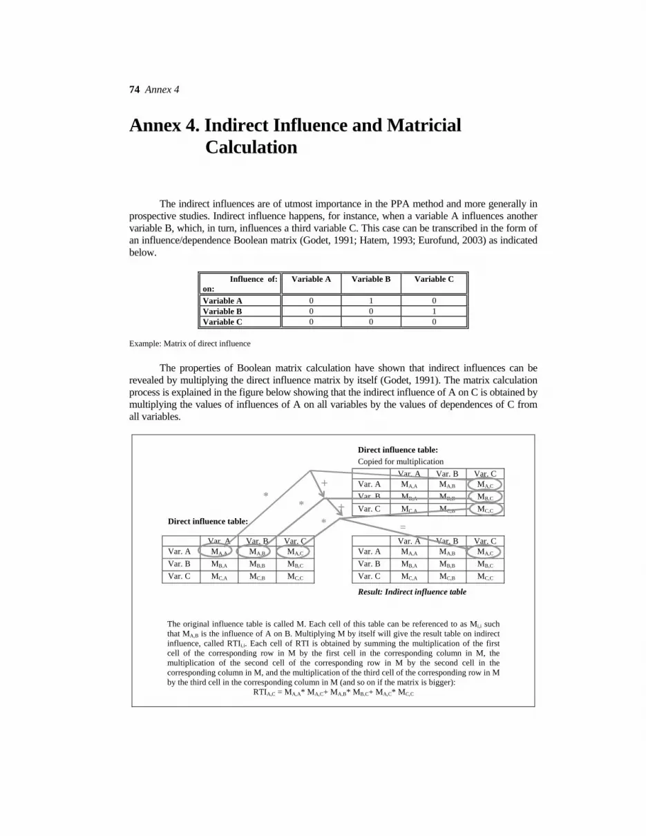
74 Annex 4
Annex 4. Indirect Influence and Matricial Calculation
The indirect influences are of utmost importance in the PPA method and more generally in prospective studies. Indirect influence happens, for instance, when a variable A influences another variable B, which, in turn, influences a third variable C. This case can be transcribed in the form of an influence/dependence Boolean matrix (Godet, 1991; Hatem, 1993; Eurofund, 2003) as indicated below.
Influence of:on:
Variable A Variable B Variable C
Variable A 0 1 0 Variable B 0 0 1 Variable C 0 0 0
Example: Matrix of direct influence
The properties of Boolean matrix calculation have shown that indirect influences can be revealed by multiplying the direct influence matrix by itself (Godet, 1991). The matrix calculation process is explained in the figure below showing that the indirect influence of A on C is obtained by multiplying the values of influences of A on all variables by the values of dependences of C from all variables.
Direct influence table: Copied for multiplication Var. A Var. B Var. C Var. A MA,A MA,B MA,C Var. B MB,A MB,B MB,C Var. C MC,A MC,B MC,C Direct influence table: Var. A Var. B Var. C Var. A Var. B Var. C Var. A MA,A MA,B MA,C Var. A MA,A MA,B MA,C Var. B MB,A MB,B MB,C Var. B MB,A MB,B MB,C Var. C MC,A MC,B MC,C Var. C MC,A MC,B MC,C Result: Indirect influence table
The original influence table is called M. Each cell of this table can be referenced to as Mi,i such that MA,B is the influence of A on B. Multiplying M by itself will give the result table on indirect influence, called RTIi,i. Each cell of RTI is obtained by summing the multiplication of the first cell of the corresponding row in M by the first cell in the corresponding column in M, the multiplication of the second cell of the corresponding row in M by the second cell in the corresponding column in M, and the multiplication of the third cell of the corresponding row in M by the third cell in the corresponding column in M (and so on if the matrix is bigger):
RTIA,C = MA,A* MA,C+ MA,B* MB,C+ MA,C* MC,C
* =
+ *
+ *

Indirect Influence and Matricial Calculation 75
Applying this process to the example above, one obtains the following indirect influence matrix. There, one sees that, as expected, A has an indirect influence on C (through B).
Indirect Influence of:on:
Variable A Variable B Variable C
Variable A 0 0 1 Variable B 0 0 0 Variable C 0 0 0
The comparison between direct and indirect influences seems easy when one uses simple 0-
1 binary values to express influence levels: multiplication of influence levels can not exceed the 0-1 binary scale. But this is not the case when one uses influence values ranging from 1 to 3 or more. Besides, indirect influences can use multiple paths on the same case. If four variables are considered: A, B, C and D, there can be a situation where A indirectly influence C through B and through D (Table below). There, even with a simple 0-1 scale for direct influence, matrix calculation can come out with values exceeding 1.
Direct influence of:on:
Var. A Var. B Var. C Var. D
Var. A 0 1 0 1 Var. B 0 0 1 0 Var. C 0 0 0 0 Var. D 0 0 1 0
Indirect influence of:
on: Var. A Var. B Var. C Var. D
Var. A 0 0 2 0 Var. B 0 0 0 0 Var. C 0 0 0 0 Var. D 0 0 0 0
To allow comparison between direct and indirect influence, a convention regarding
influence “transmission” is used to come off with a scale ranging from 0 to 3 in both cases. We will illustrate this convention by a set of simple examples. Let’s consider again a variable A influencing a variable B, which in turn influences a variable C. If the influence of B on C is strong (with a value of 3), we consider that A’s influence on B can be fully transmitted to C through B, while, if the influence of B on C is weaker, we consider that there will be some loss in the transmission of influence. To take account of this transmission convention, the results of direct influence multiplication are simply divided by 3, the highest influence value.

76 Annex 4
The second convention used concerns multiple-path influences, such as in the cases of the four variables A, B, C and D presented above. Here we consider that if, for instance, A has a strong influence on B (value of 3), which also has a strong influence on C (value of 3 as well), then A has the strongest possible influence on C through B (value of 3). Since this is the strongest possible influence, no additional influence can modify it (as in the case of A also influencing C through D). In a similar way, if the indirect influence of A on C through B is small while the indirect influence of A on C through D is strong, then the latter will prevail and the former won’t weaken or increase it. The convention, then, is to keep the strongest of all the multiple path indirect influences.
These two conventions are explicit choices made by the authors. They seem justified but are open to discussion and modification. With these two conventions, it is finally possible to come up with values of indirect influence ranging from 0 to 3 that can be compared to the values of direct influence. The resulting formula, for the case of four variables would then be the following1:
RTIA,C = Max (MA,A* MA,C ; MA,B* MB,C ; MA,C* MC,C ; MA,D* MD,C)/3
1 The actual formula written in the Excel tables is slightly different: it uses a maximum of maximums. This is to by-pass
the limitation on the authorized number of arguments in the Max function in Excel worksheets. It does not change the results.
3
3
3 3
A
B D
1
C
2
3
1 3
A
B D
2
C
Indirect influence
Direct influence
3
3 3 A B C
1
3 1A B C
Cases of full transmission of A’s influence through B
1/3
1 1A B C
Indirect influence
Direct influence
1
1 3 A B C
Cases with a loss in the transmission of A’s influence through B

Indirect Influence and Matricial Calculation 77

77
Annex 5. Formula for Calculation of I/D Tables and Graphs
The software supporting the matrix, tables and graphs includes, but is hides, all the necessary formula for the automatic calculation of the values after completing the first matrix. The purpose of this annex is to explain where these formula are located and to make clear their formulation so that all users, and in particular stakeholders, can receive clear answers about how the results were obtained.
Formula for the calculation of the global I/D tables
All I/D tables including the word “global” in their Header are made of cells containing the following formula: “=+[Cell Number]”. This means that the value of the cell is equal to the value of the referred Cell Number. However, the reference cells are hidden in the version presented to the participants as one can notice by looking for instance at the extreme right side of the first matrix in the “Variables influence” worksheet. In this worksheet, column BA is not visible. However, it is possible to unhide it by clicking with the mouse on the AZ column head, dragging the mouse to highlight also the BB header. The two columns are highlighted. Then by clicking on the right button of the mouse, the option “Unhide” appears. After clicking “Unhide” the hidden column BA appears with a heading “Global Influence” at the level of the table row header. Below this cell, each cell contains a formula such as =SUM (C11:AZ11) for instance, which means that the value of the cell is equal to the sum value of all the cells in the matrix row located to its left.
The same process can be repeated to reveal the formula and values of the cells hidden in row 61 (you will see that the “Variables influence” worksheet does not display row 61). In this case the generic label of the row is “General Dependence” and the cell displays the sum value of all the cells in the matrix column that are located above them.
In order to restore the setting with the hidden formula, just click on the “Undo” icon.
In addition, some hidden formulas are located next to these tables: • Cells D115 and G115 of the “Variables’ influence” worksheet display the sum value of all
values given to each variable, respectively the total influence and the total dependence. These cells are used as intermediary result for other formulas.
• The cells to the right of these tables (E65:E114) and (H65:H114) display values calculated with the following formula type:
(Cell value) =+D65/($D$115/(50-NB.SI(D$65:D$114;0)))
This formula helps to calculate the value of the “x” coordinate that will be displayed on the visualization graph located in the “Variables' dir. strength graph” worksheet. The formula makes the calculation of the value of the variable’s influence (D65) divided by the average influence value D115/(number of variables). The formulation (50-NB.SI(D$65:D$114;0)) takes into account the fact that in this 50x50 matrix less than 50 variables are usually entered and therefore the average value has to be calculated by dividing D115 by the real number of variables.
Similarly, the formula in array (H65:H114) calculates the value of the “y” coordinate of the corresponding variable displayed in the “Variables’ dir. strength graph” worksheet.

78 Annex 5
A simple way to make the formula appear is to position the cursor of the mouse on one cell of the array and look at the display of fx in the upper menu on the screen. To make the values appear in the cells, select the cell or the array and then change the font color to black. To revert to the default set up, click “Undo”.
These formula can be found also in similar locations and with similar functions in the “Variables' total influ” worksheet corresponding to “Variables' indir. strength graph” and “Variables' total strength graph”.
Formula for the calculation of the global strength and ponderated strength tables
The values displayed in the global strength tables in “Variables influence” and “Variables' total influ” worksheets are obtained with the following formula:
=IF(ESTNUM((D65/D$115)*(D65/(D65+G65)));(D65/D$115)*(D65/(D65+G65));0)
This formula corresponds to a calculation of the global strength based on the following process: first the influence of the variable is divided by the total influence of all variables, and then this result is multiplied by the quotient of the variable’s influence by the sum of its influence and dependence. This process helps to take into consideration in the assessment of a variable’s strength both its influence and its dependence.
For instance let’s take the case of three variables (A, B and C) of respectively 20, 20 and 10 for their influence value and 10, 20 and 20 for their dependence value. The total influence of the variables is 50. Apparently based on their influence A and B have the same strength, but it is logical to consider that A is stronger since it is less dependent than B (10 instead of 20). Similarly, although B and C have the same dependence, B should be stronger since it is more influent. Using the formula we obtain the resulting respective strength:
A strength = 20/50*20/(20+10) = 0.2666 B strength = 20/50*20/(20+20) = 0.2000 C strength = 10/50*20/(20+20) = 0.1000
The formula establishes an appropriate assessment of the global strength of a variable based
on both its influence and dependence. The IF(ESTNUM…) formulation is used to avoid the problem of a division by 0 which would result in a non numeric value (error message: #DIV/0!) that would impede any further calculation. If this occurs, this function automatically replaces the non-numeric value by 0.
At the bottom of these tables two cells (for instance cells D168 and D169 in the “Variables influence” worksheet) are used for intermediary calculation of the average strength of the variables displayed in the next table as indicated below.
The ponderated strength tables display the strength of the variables centered around the average value of 1 for easier interpretation. Each cell in this table contains a formula such as: =+D118/D$168. It corresponds to the division of the variable’s strength by the average strength of the variables in the system. Variables with values above 1 are stronger than the average variable and reciprocally. These values are used for the ranking of the variables according to their strength.

Formula for Calculation of I/D Tables and Graphs 79
Formula for the values displayed in the indirect I/D matrix
The values automatically displayed in the variables’ indirect influence matrix located on the top of the “Variables’ total influ” worksheet are obtained by the following formula (for the case of the cell C6): (C6 Value) ='Variables'' influence'!BE11 which means that the value of the cell is equivalent of the value found in cell BE11 in the “Variables influence” worksheet.
This cell and the others related to the indirect values of influence are hidden in the “Variables’ influence” worksheet. They contain formula of matricial calculation corresponding to the multiplication of the direct influence matrix by itself. For more information about the relation between indirect influence and matricial calculation and the details of the formula, please refer to Annex 4.
To unhide them proceed as for unhiding the values of column BA in section I of this Annex.
Formula for the values displayed in the total I/D matrix
The table where total influence values are stored is located in the lower part of the “Variables' total influ” worksheet, starting from cell A168. The values are obtained with the following formula (example of cell C168):
(C168 value) =C6+'Variables'' influence'!D11
This formula indicates that the total influence results from directly summing the direct and indirect influences of the variable obtained from the corresponding cells in the direct and indirect influence matrices.
Worksheet protection and data entry control
All worksheets and cells are protected against mishandling using the protection mode offered in Excel, except for the direct I/D matrix where data must be inputted. A password is used to ensure that the decision to unprotect and modify some tables or cells is not taken. The default password is “PPAFJRB”. In order to unprotect any protected cell, select a cell with the mouse and enter a value. Then follow the instructions that appear on the screen.
In addition to cell and worksheet protection, the cells in the direct I/D have been formatted to accept only four values: 0, 1,2 and 3. This limits data entry error such as typing 20 in one cell instead of 2 and 0 in two consecutive cells, or typing a wrong number that is not authorized.

80 Annex 5

81
Annex 6. Glossary of Selected Terms Related to the PPA Method
(source: http://www.audiencedialogue.org/gloss-fut.html) Actor Any person, organization or (sometimes) impersonal force affecting the future of the system being studied. Very similar meaning to stakeholder. However, all actors are stakeholders, but not all stakeholders need be actors. Alternative futures The idea that there is not a single future, but a range of futures, all of which might occur at the same time. Now the accepted view among futurists. Anticipation If you can’t predict the future correctly, what’s the use of futures studies? Answer: even if you don’t know what’s going to happen, or when it’s going to happen, you can at least anticipate a range of possibilities, and prepare for them. Backcasting Working backwards from a possible future state to determine how it might unfold. Delphi method A way of estimating future measures by asking a group of experts to make estimates, recirculating the estimates back to the group, and repeating the process till the numbers converge. Often used for estimating when an event might occur - e.g. “In what year will the majority of households in OECD countries have broadband internet access?” Developed in the 1950s by Harold Linstone and Murray Turoff, and widely used, especially in Japan. Endogenous Caused from within. For example, if a manufacturer decides to stop making one product and make another instead, the change is endogenous if the decision is a completely internal one. But if they decide to change because the market for the old product was disappearing, the decision might be endogenous, but the influence would be exogenous (the opposite). Exogenous Caused externally. For example, when an industry, or an area changes due to pressures from outside the industry, that’s an exogenous change. The opposite of endogenous. Forecasting Predicting that an event will happen, to a defined extent, and sometimes with a defined probability. For example “there’s a 50-50 chance that at least 1 millimetre of rain will fall in this area tomorrow” is a forecast. Forecasts are usually applied to short-term futures - no more than a few years ahead. A forecast is considered to be less certain than prediction, but more certain than conjecture or anticipation.

82 Annex 6
Foresight A broad term covering all methods of envisaging the future, but with an emphasis on the alternative futures concept. However, forecasting is not normally included as a part of foresight. Compare with future studies. Future This common word is mentioned here because it actually has two meanings, which could be called future-as-time and future-as-image. If you ask “when is the future?” the answer is that it’s some time ahead, but probably not this year. But if you ask “where is the future?” the present tense gives it away: it’s inside people’s heads, and as such it’s here right now. These two different meanings can cause confusion. Future(s) studies The study of the ways in which futures could happen. Note the plural: this makes it clear that futures are not predetermined. Unfortunately, use of the plural “futures” causes confusion with trading of commodity futures - perhaps a reason for the increasing acceptance of the word foresight to describe the study of the future(s). Holistic Considering a system as a whole, not as a collection of parts. (That would be considered atomistic.) Atomistic views of you include your separate roles as (perhaps) employee, consumer, mother ... - or as head, arms, torso ... - or as skin, bone, blood ... - and so on. Though there are many kinds of atomistic view, there is only one holistic view: of you as an entire person. Image A mental picture of the future - similar to vision. Judgemental forecasting Making a numerical forecast using expert judgement or intuition, not only mathematical formulas. (But of course the assumptions inherent in those formulas also make them judgemental.) Much the same as subjective forecasting or qualitative forecasting. Modelling Creating a model of what might happen in the future, given a set of equations that relate inputs to outputs. This is usually a mathematical model that runs on a computer. Special software is available for creating these models - or you can simply use a spreadsheet, setting up a series of formulas in cells that reference one another. The difficulty lies in verifying the assumptions embodied in the equations - often not a mathematical process at all. Morphological analysis A way of looking at the future, by dividing it into logically exclusive possibilities. First developed by the astronomer Fritz Zwicky. A trivial example: what will the weather be at midday tomorrow? Looking at all possible combinations of sun, cloud, rain, and wind, not all of these are possible, and some conditional predictions can safely be made: e.g. there will not be both sun and rain in the same spot unless it is windy.

Glossary of Selected Terms Related ro the PPA Method 83
Normative A normative scenario is one that describes a preferred future. (That’s the futurists’ use of the word; it has a different meaning when describing psychological testing, where it refers to comparing individuals.) Paradigm A way of thinking that’s so widespread in a particular society that people hardly notice they think that way. A paradigm shift is a change in a paradigm - often not noticed till it’s well under way. Paradigm shifts take years to happen. Prediction A specific statement that something will happen in the future. “It will rain tomorrow” is a prediction, and so is “If the wind is westerly and I sleep till after 8am, it will rain tomorrow” - but “it may rain tomorrow” is not a prediction. Probability The likelihood that an event will occur, on a scale ranging from 0 (no chance at all) to 1 (or 100 per cent - totally predictable). Prognosis A set of expectations for a future that seems very likely to happen - e.g. if world interest rates decline this year, the prognosis is that share prices will increase. A prognosis could be considered less certain than a prediction but more certain than a forecast. Projection A term used in forecasting, similar to extrapolation. For example, if the population of a city was 90,000 last year and 100,000 this year, the simplest projection would be for a population of 110,000 next year. These days, forecasts often produce multiple projections, depending on various assumptions. For example, an assumption of high economic growth for the city might lead to a projection of 115,000, while low economic growth might give a projected population of 105,000. Prospective A French term, developed by futurist Michel Godet, for a class of methods he has developed for examining the future. Scenario Normally (in futures studies) this refers to brief description of a possible future. This is known as a snapshot scenario, because it’s like a snapshot or photo of the future. Another sense of scenario, also used in futures studies, is that a scenario is a description of the route from now to a possible future. This is known as a chain scenario. Unlike a forecast, which predicts future values of a few specific variables, a scenario is more descriptive than numerical. Simulation Modelling with an element of time, using either a computer program or a game with human players. A series of events is simulated, to find out what’s likely to happen next.

84 Annex 6
Strategic planning and scenario planning The differences between strategic planning and scenario planning: Strategic planning is about one organization; scenario planning usually has a broader scope, e.g. an industry or a geographical area. Strategic planning implies that the organization can set and achieve its targets regardless of its environment; scenario planning takes a broader range of factors into account. Finally, scenario planning is often done as an input to strategic planning. System Anything that has boundaries, receives inputs and processes them to produce outputs. For example, you: the boundary is your skin, you receive sensory and food inputs, and your outputs are whatever you do. There are also computer systems, energy systems, geophysical systems, mechanical systems, business systems, etc. Trend A measure that has been changing steadily. “The trend over the last 20 years has been for more and more people to go to university.” Some people use “trend” to mean “fashion” - not quite the same as the standard meaning. Vision A vision is a clear view of the future, usually one that an organization is working toward achieving for itself. Note that a vision is usually singular: an organizations with a unified vision statement is not considering alternative futures.
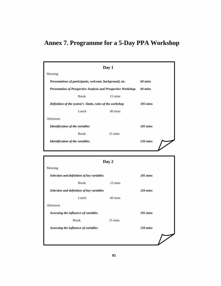
85
Annex 7. Programme for a 5-Day PPA Workshop
Day 1 Morning
Presentations of participants, welcome, background, etc. 60 mins Presentation of Prospective Analysis and Prospective Workshop 60 mins
Break 15 mins Definition of the system’s limits, rules of the workshop 105 mins
Lunch 60 mins
Afternoon
Identification of the variables 105 mins
Break 15 mins
Identification of the variables 120 mins
Day 2 Morning
Selection and definition of key variables 105 mins
Break 15 mins
Selection and definition of key variables 120 mins
Lunch 60 mins Afternoon
Assessing the influence of variables 105 mins
Break 15 mins
Assessing the influence of variables 120 mins

86 Annex 7
Day 3 Morning
Assessing the influence of variables, computation 105 mins
Break 15 mins Assessing the influence of variables, discussion 120 mins
Lunch 60 mins Designing contrasted scenarios, selection of key variables 90 mins
Afternoon
Designing contrasted scenarios, definition of states 105 mins
Break 15 mins
Designing contrasted scenarios, combining states 105 mins
Day 4 Morning
Selection of contrasted scenarios 105 mins
Break 15 mins
Selection of contrasted scenarios 120 mins
Lunch 60 mins Afternoon
Analysis of scenarios implication 105 mins
Break 15 mins
Analysis of scenarios implication 120 mins
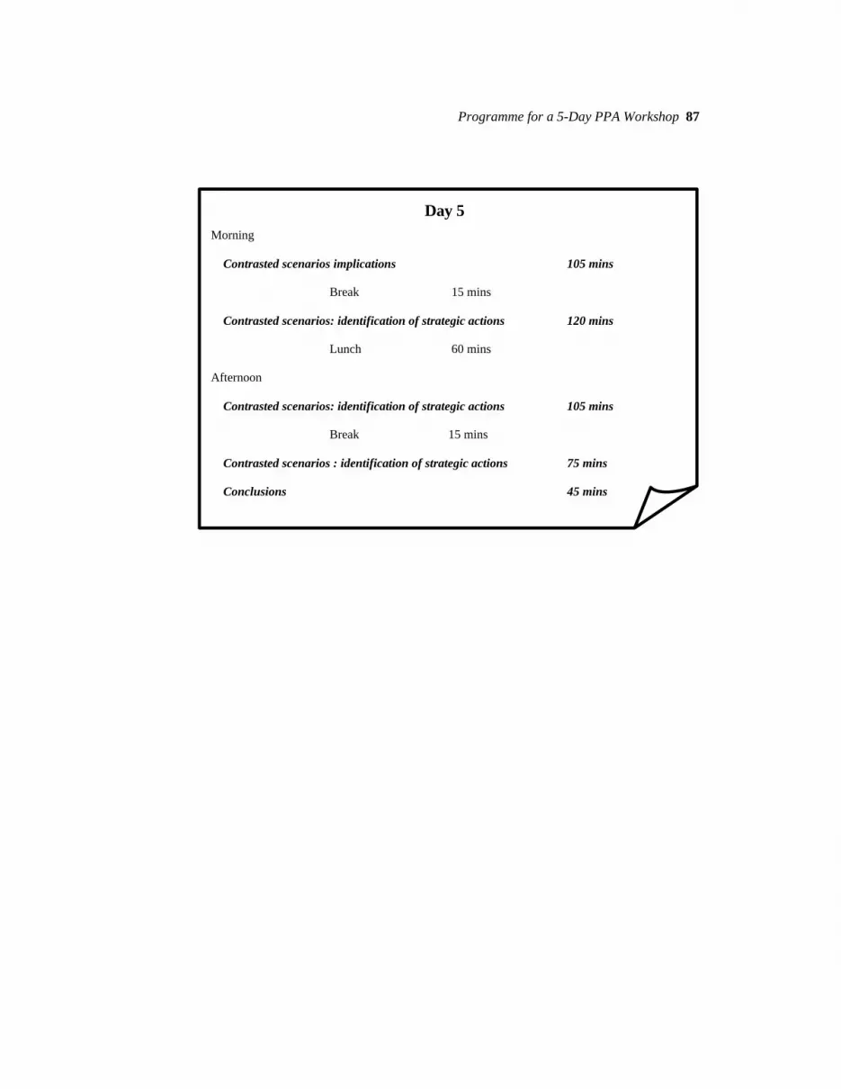
Programme for a 5-Day PPA Workshop 87
Day 5 Morning
Contrasted scenarios implications 105 mins
Break 15 mins Contrasted scenarios: identification of strategic actions 120 mins
Lunch 60 mins
Afternoon
Contrasted scenarios: identification of strategic actions 105 mins
Break 15 mins
Contrasted scenarios : identification of strategic actions 75 mins Conclusions 45 mins

88 Annex 7

Annex 8. Variables’ Influence/Dependence and Strength
Variables Direct influence
Direct dependence
Direct strength
Indirect influence
Indirect dependence
Indirect strength
Total influence
Total dependence
Total strength
Urbanization 1,65 0,5 2,26 1,22 0,58 1,54 1,36 0,56 1,79 Income change 1,57 0,34 2,3 1,27 0,80 1,46 1,37 0,65 1,73
Availability of suitable land 1,26 0,96 1,29 1,07 0,99 1,03 1,13 0,98 1,12 Population growth 1,15 0,11 1,87 1,22 0,17 1,99 1,20 0,15 1,96 Water availability 1,11 0,84 1,13 1,07 0,96 1,06 1,09 0,92 1,09 Climate variation 1,07 0,11 1,73 1,20 0,07 2,11 1,16 0,09 1,99 LMO regulation 1 0,61 1,1 1,01 0,82 1,04 1,00 0,75 1,06 Climate pattern 0,96 0,15 1,48 1,09 0,14 1,80 1,04 0,14 1,71
Demand for CGPRT crops from non ESCAP countries 0,96 0,27 1,34 1,01 0,47 1,29 0,99 0,41 1,31
Role of WTO 0,92 0,42 1,13 0,88 1,30 0,66 0,89 1,01 0,77 Food preference 0,92 0,46 1,1 1,05 0,69 1,18 1,01 0,61 1,16
CGPRT trade policies of other countries 0,92 0,73 0,92 0,93 1,44 0,68 0,92 1,21 0,74
International regulation on environment 0,88 0,23 1,25 0,82 0,39 1,04 0,84 0,34 1,11
Pest and disease 0,88 0,69 0,88 0,91 1,22 0,72 0,59 0,68 0,51 Development of other industries 0,57 0,92 0,4 0,88 1,13 0,72 0,78 1,06 0,61
World wheat production 0,5 0,5 0,45 0,60 0,39 0,68 0,57 0,43 0,60 World rice production 0,42 0,84 0,25 0,67 0,60 0,66 0,90 1,04 0,77 Technology transfer 0,84 1 0,69 0,93 1,31 0,72 0,90 1,21 0,71 Rural infrastructure 1 1,19 0,81 0,99 1,31 0,79 0,99 1,27 0,80
Development of animal husbandry 0,92 1,19 0,72 0,88 1,11 0,72 0,89 1,14 0,72 CGPRT trade policies within the
region 1,19 1,26 1,03 1,11 1,43 0,91 1,14 1,38 0,95 Social stability 0,8 1,34 0,54 0,93 1,34 0,71 0,89 1,34 0,66
Government intervention in input supply 0,92 1,46 0,64 0,98 1,17 0,83 0,96 1,26 0,77
Continued…
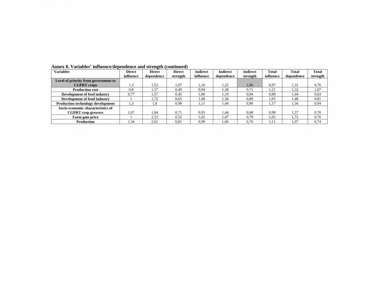
Annex 8. Variables’ influence/dependence and strength (continued)
Variables Direct influence
Direct dependence
Direct strength
Indirect influence
Indirect dependence
Indirect strength
Total influence
Total dependence
Total strength
Level of priority from government to CGPRT crops 1,3 1,53 1,07 1,16 1,22 1,06 0,97 1,31 0,76
Production cost 0,8 1,57 0,49 0,94 1,38 0,71 1,21 1,32 1,07 Development of feed industry 0,77 1,57 0,45 1,06 1,19 0,94 0,89 1,44 0,63 Development of food industry 1 1,72 0,65 1,08 1,36 0,89 1,05 1,48 0,81
Production technology development 1,3 1,8 0,98 1,11 1,44 0,90 1,17 1,56 0,94 Socio-economic characteristics of
CGPRT crop growers 1,07 1,84 0,71 0,93 1,44 0,68 0,98 1,57 0,70 Farm gate price 1 2,22 0,55 1,02 1,47 0,79 1,02 1,72 0,70
Production 1,34 2,61 0,81 0,99 1,66 0,70 1,11 1,97 0,74