strategies anticipating a difference in search depth using opponent-model search
TRANSCRIPT

Theoretical Computer Science 252 (2001) 83–104www.elsevier.com/locate/tcs
Strategies anticipating a di�erence in search depth usingopponent-model search
Xinbo Gaoa, Hiroyuki Iidab ;∗, Jos W.H.M. Uiterwijkc,H. Jaap van den Herikc
aSchool of Electronic Engineering, Xidian University, Xi’an 710071, ChinabDepartment of Computer Science, Shizuoka University, 3-5-1 Juhoku, Hamamatsu 432-8011, JapancDepartment of Computer Science, Universiteit Maastricht, P.O. Box 616, 6200 MD Maastricht,
Netherlands
Abstract
In this contribution we propose a class of strategies which focus on the game as well as onthe opponent. Preference is given to the thoughts of the opponent, so that the strategy underinvestigation might be speculative. We describe a generalization of OM search, called (D; d)-OMsearch, where D stands for the depth of search by the player and d for the opponent’s depth ofsearch. A known di�erence in search depth can be exploited by purposely choosing a suboptimalvariation with the aim to gain a larger advantage than when playing the objectively best move.The di�erence in search depth may have the result that the opponent does not see the variationin su�ciently deep detail. We then give a pruning alternative for (D; d)-OM search, denoted by�-�2 pruning. A best-case analysis shows that �-�2 prunes very e�ciently, comparable to thee�ciency of �-� with regard to minimax. The e�ectiveness of the proposed strategy is con�rmedby simulations using a game-tree model including an opponent model and by experiments in thedomain of Othello. c© 2001 Elsevier Science B.V. All rights reserved.
Keywords: Opponent modelling; Speculative play; �-�2 pruning; Othello
1. Introduction
The minimax method and all its sophisticated variants have as implicit assumptionthat the player and the opponent use the same search strategy. Basically this means:(1) the leaves are evaluated by an evaluation function and (2) the values are backed upvia a minimax-like procedure. The evaluation function may contain all kind of specialfeatures but in essence it evaluates the position (including the use of quiescence search)
∗ Corresponding author.E-mail addresses: [email protected] (X. Gao), [email protected] (H. Iida), uiterwijk@cs.
unimaas.nl (J.W.H.M. Uiterwijk), [email protected] (H.J. van den Herik).
0304-3975/01/$ - see front matter c© 2001 Elsevier Science B.V. All rights reserved.PII: S0304 -3975(00)00077 -3

84 X. Gao et al. / Theoretical Computer Science 252 (2001) 83–104
according to a set of preset criteria. For instance, a chess program will never change thevalue of a Knight in the evaluation function, not even when it is informed by outsideknowledge that the opponent is quite threatening in the endgame when operating withtwo Knights. The program’s evaluation function is �xed and not speculative. After aleaf has been evaluated, the minimax back-up procedure is applied. It is as logicaland practical as one can think. Other ideas on the backing up of a value are sparse(cf. [11]). In the past, some ideas not suitable for practical application are put forwardby Rivest [19]. The only exception implemented in tournament programs lies at thevery beginning of the back-up procedure. For instance, if a draw is foreseen as theoutcome of the game (e.g., by repetition of positions) and the opponent is considered tobe weak, a contempt factor may indicate that playing the second-best move is preferred.This is the most elementary step of opponent modelling. It shows a slight deviationfrom the two above-mentioned steps of a minimax-like strategy, although one can arguethat the deviation is within the evaluation function.An extension of the idea has been developed in opponent-model search. A grand-
master attempting to understand the intention behind the opponent’s previous movesmay employ some form of speculative play, anticipating the opponent’s weak reply [7].Iida et al. [5, 6] modelled such thinking processes based on possible mistakes by theopponent, and proposed OM search (short for opponent-model search) as a generalizedgame-tree search model. In OM search perfect knowledge of the opponent’s evaluationfunction is assumed. This knowledge may lead to the conclusion that the opponent isexpected to make a mistake in a given position. As a consequence the mistake maybe exploited to the advantage of the player possessing the knowledge. In such an OM-search model, it is implicitly assumed that both players search to the same depth inthe game tree.In actual game playing as seen in Shogi tournaments, we have observed [6] that the
two opponents may not only have di�erent evaluation functions, but may also reachdi�erent search depths. These observations have led us to propose a generalization ofOM search, called (D; d)-OM search, in which the di�erence of depth is incorporated.The di�erence in depth is in the name: D stands for the depth of search of the �rstplayer, and d for the opponent’s.In Section 2 we characterize (D; d)-OM search by de�nition. Three assumptions are
given explicitly and the (D; d)-OM-search algorithm is described in detail. Then, inSection 3, the characteristics of (D; d)-OM search are elaborated upon, and the rela-tionship between (D; d)-OM search, OM search, and minimax is discussed. Section 4describes a variant of the �-� algorithm that prunes branches within (D; d)-OM search,denoted by �-�2 pruning. Section 5 illustrates the performance of a given specula-tive strategy with random-tree simulations as well as with experiments in the domainof Othello. How to apply this strategy e�ciently to actual game-playing positions isdiscussed in Section 6. Finally, the main conclusions and some limitations of thisspeculative strategy are given in Section 7.

X. Gao et al. / Theoretical Computer Science 252 (2001) 83–104 85
2. (D; d)-OM Search
This section provides the relevant de�nitions and assumptions for (D; d)-OM search.In addition, an example is presented showing how a value at any position in a searchtree is computed using (D; d)-OM search. By convention and for clarity of understand-ing, the two players are distinguished as the max player and the min player. Below,we discuss (D; d)-OM search from the viewpoint of the max player.
2.1. De�nitions and assumptions
For (D; d)-OM search we use the following de�nitions and assumptions.
De�nition 1 (Playing strategy). A playing strategy is a three-tuple 〈D; EV; SS〉, whereD is the player’s search depth, EV is his static evaluation function and SS denotes thesearch strategy, i.e., the way to back up values from the leaves to the root in a searchtree.
De�nition 2 (Player model). A player model is the assumed playing strategy of aplayer. For any player X with search depth DX , static evaluation function EVX andsearch strategy SSX , we de�ne a player model as MX = 〈DX ; EVX ; SSX 〉.
(D; d)-OM search is discussed under three assumptions. Here OM stands for OMsearch, and MM for minimax strategy. P is a given position in which the max playeris to move.
Assumption 3 (The opponent’s strategy). The min player’s playing strategy is Mmin =〈d; EVmin ; MM 〉; which means that the min player will perform some minimax strategyat any successor of P and will evaluate the leaf positions at depth (d+ 1) in the maxplayer’s game tree using static evaluation function EVmin.
Assumption 4 (Knowledge about the opponent). The max player knows the strategyof the min player, Mmin = 〈d; EVmin ; MM 〉; i.e.; his min player’s model coincides withthe min player’s strategy.
Assumption 5 (Exploiting the knowledge). The max player employs 〈D; EVmax;(D; d)-OM 〉 as playing strategy; which means that he evaluates the leaf positions atdepth D using his static evaluation function EVmax and backs up the values by (D; d)-OM search.
Like OM search, (D; d)-OM search stems from speculative play as practicedby grandmasters. In a game, a grandmaster acquires and uses the model of the op-ponent to spot a potential mistake, and then obtains an advantage by anticipating thismistake.

86 X. Gao et al. / Theoretical Computer Science 252 (2001) 83–104
2.2. The algorithm of (D; d)-OM search
In (D; d)-OM search, a pair of values is computed for the positions at and abovedepth (d+1). One value comes from the opponent model and one from the max player’smodel. Below depth (d+1), the max player no longer uses the opponent model. Thereonly one value is computed for each position; it is backed up by minimax search.Let i; j from now on range over all immediate successor positions of a node in
question. Let a node be termed a max node if the max player is to move, a minnode otherwise. According to the assumptions, D is the search depth of the max playerand d is the search depth of the min player as predicted by the max player. Thenthe function V (P;OM (D; d)) and V (P;MM (d)) are de�ned for relevant nodes, whereV (P;OM (D; d)) is the value considered by the max player and V (P;MM (d)) is thevalue for the min player, predicted by the max player:
V (P;OM (D; d))
=
maxiV (Pi; OM (D − 1; d− 1)) if P is an interior max node;
V (Pj; OM (D − 1; d− 1)) with jsuch that V (Pj;MM (d− 1))= min
iV (Pi;MM (d− 1)) if P is an interior
min node and d¿0;
miniV (Pi; OM (D − 1; d− 1)) if P is an interior min node
and d ¡ 0;
EVmax(P) if D = 0 (P is a leaf node);
(1)
V (P;MM (d)) =
maxiV (Pi;MM (d− 1)) if P is an interior max node;
miniV (Pi;MM (d− 1)) if P is an interior min node;
EVmin(P) if d = −1 (P is a “leaf ” node):(2)
The algorithm of (D; d)-OM search is given in pseudocode in Fig. 1.An example of (D; d)-OM search is shown in Fig. 2. In this search tree two di�erent
root values are obtained due to the di�erent models of the players. Using (3; 1)-OMsearch yields a value of 11 and using minimax a value of 9. In this example, the maxplayer may thus achieve a better result by (3; 1)-OM search than by minimax; he willselect the left branch. For clarity, we reiterate that d denotes the search depth for theopponent, i.e., the �nal depth will be reached at depth d + 1 in the search tree ofthe �rst player. In the example, the nodes at depth 2 thus will be evaluated for bothplayers, while those at depth 3 will only be evaluated for the �rst player.Moreover, it is assumed that the player using (D; d)-OM search always searches
deeper than the opponent, i.e., that D¿d. Cases such as the opponent being modelledby a deep search using a very fast but simplistic evaluation function, and the �rst

X. Gao et al. / Theoretical Computer Science 252 (2001) 83–104 87
procedure (D; d)-OM(P,depth):=* Iterative deepening at root P *==* Two values are returned, according to equations (2) and (1) *=if depth=d + 1 then begin=* Evaluate the min-player’s leaf nodes *=
V MM[P] ← Evaluate(P,min)V OM[P] ← Minimax(P,depth)return (V MM[P],V OM[P])
end
{Pi | i=1; : : : ; n}← Generate(P)=* Expand P to generate all its successors Pi *=for each Pi do begin(V MM[Pi],V OM[Pi])← (D; d)-OM(Pi ,depth+1)
end
=* Back up the evaluated values *=if P is a max node then begin=* At a max node both the max player and the min player back up the maximum *=V MM[P]← max
16i6nV MM[Pi]
V OM[P]← max16i6n
V OM[Pi]
endelse begin =* P is a min node *==* At a min node, the min player backs up the minimum and the max player backs upthe value of the node selected by the min player *=V MM[P]← V MM[Pj] = min
16i6nV MM[Pi]
V OM[P]← V OM[Pj]endreturn (V MM[P],V OM[P])
procedure Minimax(P,depth):=* Iterative deepening below depth d + 1 *==* Returns the minimax value according to the max player *=
if depth=D then begin=* Evaluate the max player’s leaf nodes *=
V MM[P]← Evaluate(P,max)return (V MM[P])
end
{Pi | i=1; : : : ; n}← Generate(P)=* Expand P to generate all its successors Pi *=for each Pi do beginV MM[Pi]← Minimax(Pi ,depth+1)
end
=* Back up the evaluated values *=if P is a max node then beginV MM[P]← max
16i6nV MM[Pi]
endelse begin =* P is a min node *=V MM[P]← min
16i6nV MM[Pi]
endreturn (V MM[P])
Fig. 1. The algorithm of (D; d)-OM search in pseudocode.

88 X. Gao et al. / Theoretical Computer Science 252 (2001) 83–104
Fig. 2. (D; d)-OM search and minimax compared, with D=3 and d=1. The numbers beside the circles=boxes represent the back-up values by (3; 1)-OM search (upper) and minimax from the min player’s point ofview (lower), respectively. The numbers inside the circles=boxes represent the back-up values by minimaxfrom the max player’s point of view. Depths 3 and 2 contain the leaf positions for the max player and themin player, respectively, i.e., these values (in italics) are evaluated statically using the max player’s or themin player’s evaluation function.
player relying on a shallower search but with a very sophisticated evaluation function,are not treated in the above formulation. The incorporation of such cases will not bedi�cult in practice, but it would make the formal de�nitions needless complex. Hencewe do not consider it in this article.
3. Characteristics of (D; d)-OM search
In this section, some characteristics of (D; d)-OM search are described and comparedwith those of the minimax strategy. The relation among (D; d)-OM search, OM searchand minimax is discussed. It results in two remarks and a theorem relating the rootvalues as produced by (D; d)-OM search and minimax.
3.1. Relations among (D; d)-OM search, OM search and minimax
The algorithm of (D; d)-OM search given in Section 2 shows that the max playerperforms a minimax search when backing up the static-evaluation-function values fromdepths D to (d + 1), while from depths (d + 1) to 1 the max player performs pureOM search. So from the viewpoint of search algorithms, (D; d)-OM search can beconsidered as a combination of pure OM search and minimax search.A di�erent view is also possible: all the moves determined by minimax, OM search
and (D; d)-OM search take some opponent model into account, i.e., each choice isbased on the player’s own model and some opponent model. Accordingly, all the threestrategies can be considered as opponent-model-based search strategies. The di�erenceamong them lies in the speci�cation of the opponent model.

X. Gao et al. / Theoretical Computer Science 252 (2001) 83–104 89
Table 1The opponent models used in minimax, OM search and (D; d)-OM search
Algorithm The opponent model
Minimax 〈D − 1; EVmax ;MM〉OM search 〈D − 1; EVmin ;MM〉(D; d)-OM search 〈d; EVmin ;MM〉
The opponent models used by the max player in minimax, OM search and (D; d)-OM search are listed in Table 1. We assume that the max player moves �rst withsearch depth D and evaluation function EVmax, i.e., in a game tree the root is a maxposition.Table 1 shows that OM search is a generalization of minimax (in which the oppo-
nent does not necessarily use the same evaluation function as the max player), and(D; d)-OM search is a generalization of OM search (in which the opponent does notnecessarily search to the same depth as the max player). This is more precisely for-mulated by the following two remarks.
Remark 6. (D; d)-OM search is identical to OM search when d=D − 1.
Remark 7. (D; d)-OM search is identical to minimax when d=D − 1 and EVmin =EVmax.
From the opponent models used in the three search strategies, the one in (D; d)-OMsearch has the highest exibility due to the smallest limitation of the opponent’s choiceabout search depth and evaluation function. So, (D; d)-OM search is the most universalmechanism of the three, and has in principle the largest potential for practical use.
3.2. A theorem on root values
Based on the di�erent back-up procedures of the evaluation-function values, thefollowing characteristic can be derived.
Theorem 8. For the root position R in a game tree we have the following relation:
V (R;OM (D; d))¿V (R;MM (D)); (3)
where V (R;OM (D; d)) denotes the value at root R by (D; d)-OM search andV (R;MM (D)) the one by minimax with search depth D. The theorem is proven byinduction on the level in the game tree.
The above theorem implies that if the max player has a perfect opponent model,(D; d)-OM search based on such a model can enable the max player to reach a positionthat may be better, but will never be worse than the one yielded by the minimax

90 X. Gao et al. / Theoretical Computer Science 252 (2001) 83–104
strategy. In this we follow the commonly-accepted assumption that the deeper thesearch, the higher the playing strength.
4. �-�2 Pruning (D; d)-OM search
In this section, we introduce an e�cient variant of (D; d)-OM search, which we call�-�2 pruning (D; d)-OM search.
4.1. �-�2 Pruning
In games, such as Shogi, chess and Othello, the number of nodes visited by asearch algorithm increases exponentially with the search depth. This obviously limitsthe scope of the search, especially since game-playing programs have to meet externaltime constraints. Ever since minimax was introduced to game-playing, many techniqueshave been proposed to speed up the search process. We only mention the general�-� pruning [13], the null-move procedure for chess [1, 2] and ProbCut for Othello[3]. On the basis of �-� pruning, Iida et al. proposed �-pruning as an enhancement forOM search [5].(D; d)-OM search backs up the static-evaluation-function values from depths D to
(d+ 1) with minimax, and from depths (d+ 1) to the root with OM search. So it ispossible to split (D; d)-OM search into two parts, and then speed them up separately.To guarantee generality, we select �-� pruning to speed up the minimax part and�-pruning for the OM-search part. The whole algorithm is named �-�2 pruning.For details about �-� and � pruning, we refer to [13] and [5] respectively. Pseu-
docode for the �-�2 algorithm is given in Fig. 3.
4.2. Analysis of the �-�2 pruning’s best case
Below we perform a quantitative study of the savings of the �-�2 pruning algorithm.Otherwise stated, we focus on the question: how many nodes of a tree need to beexamined on the average?We start considering the question on how many game-tree nodes must be examined
in the best case. The search costs are assumed to depend mainly on the evaluation (thebuilding of the search tree and the backing-up procedure are assumed to have negligiblecosts). Therefore, in the discussion below the e�ciency is examined by focussing onthe counting of statically evaluated positions. Moreover, we assume that the cost ofan evaluation, either by a min player or by a max player, has a constant cost of1 unit. Furthermore, the game tree is assumed to be uniform with w successors at anynon-leaf position and to have depth D.Considering the ‘pure’ (D; d)-OM search algorithm without any improved e�ciency
(see Fig. 1), the max player has to evaluate wD + wd+1 positions.Below, we distinguish three types of max nodes. First, type-1 max nodes are de�ned
recursively: the root node of the search tree is a type-1 node; further, every left-most

X. Gao et al. / Theoretical Computer Science 252 (2001) 83–104 91
procedure �-�2(P; �; �,depth):=* Iterative deepening at root P *==* Two values are returned, according to equations (2) and (1) *=if depth= d + 1 then begin=* Evaluate the min-player’s leaf nodes *=
V MM[P]←Evaluate(P,min)V OM[P]← �-�(P; �; �; d + 1)return (V MM[P],V OM[P])
end
{Pi|i=1; : : : ; n}←Generate(P)=* Expand P to generate all its successors Pi *=
for each Pi do begin(V MM[Pi],V OM[Pi])← �-�2(Pi; �,V MM[Pi],depth+1)if P is a max node then begin=* �-pruning at the max node *=if V MM[Pi]¿ � then beginreturn (V MM[P],V OM[P])
endendend
=* Back up the evaluated values *=if P is a max node then begin=* At a max node both the max player and the min player back upthe maximum *=
V MM[P]← max16i6n
V MM[Pi]
V OM[P]← max16i6n
V OM[Pi]
end
else begin =* P is a min node *==* At a min node, the min player backs up the minimum and themax player backs up the value of the node selected by the min player*=
V MM[P]←V MM[Pj] = min16i6n
V MM[Pi]
V OM[P]←V OM[Pj]end=* Update the the value of � *=�←V MM[P]return (V MM[P],V OM[P])
Fig. 3. The algorithm of �-�2 in pseudocode.
successor of every child of a type-1 node is a type-1 node. Second, every brother nodeof a type-1 node is a type-2 node. Third, all other max nodes in the search tree aretype-3 nodes.We investigate the search tree at level d+1, called the evaluation level. Here the min-
player evaluations are performed. The max-player evaluations may be also performedon this level (D=d + 1) or are backed-up from larger depths. We distinguish twocases: (1) the evaluation level is a max level (d is odd) or (2) a min level (d iseven).

92 X. Gao et al. / Theoretical Computer Science 252 (2001) 83–104
Fig. 4. An example of �-�2 (2,1)-OM search. Values outside the nodes are as in Fig. 2. A ‘−’ means thatthe evaluation concerned can be omitted. The relevant max-node types are indicated within the nodes.
Fig. 5. An example of �-�2 (3,1)-OM search. See Fig. 4 for legends.
4.2.1. d is oddThe number of type-1 nodes at the evaluation level equals w(d+1)=2. At every such
node one min-player evaluation has to be performed. The number of max-player eval-uations depends on the remaining depth (D − d − 1) beneath the evaluation level.Since only max-player evaluations are involved, the remaining trees can be searchedup to depth D using �-�. The number of max-player evaluations is thus given byN��(D − d− 1; w), i.e., the costs for an examination by the �-� algorithm in the bestcase for the speci�ed depth and width and is given [13] by
N��(d; w) = wbd=2c + wdd=2e − 1:
The total costs for type-1 nodes at the evaluation level thus are given by
w(d+1)=2(1 + N��(D − d− 1; w)):
As the simplest example, a best-case search tree for (2,1)-OM search and width 2 isgiven in Fig. 4 with 4 evaluations for the type-1 leaf nodes. An example where themax player looks deeper in the tree than the min player is given in Fig. 5 (a best-caseexample for (3,1)-OM search and width 2) with a total of 6 evaluations for the type-1nodes at the evaluation level.

X. Gao et al. / Theoretical Computer Science 252 (2001) 83–104 93
Fig. 6. An example of �-�2 (4,3)-OM search. See Fig. 4 for legends.
For every type-2 node at the evaluation level, only one min-player evaluation hasto be performed. No max-player evaluations are needed, since in best case they areirrelevant for the back-up values of the parent nodes (see Figs. 4 and 5). Since thetotal number of type-2 nodes at the evaluation level equals (w − 1) times the numberof type-1 nodes, the total costs for the type-2 nodes are given by (w − 1)w(d+1)=2.For each type-3 node at the evaluation level we have again one min-player evaluation
and no max-player evaluations. Since type-3 nodes have ancestors at which �-pruninghas been performed (see Fig. 6), we have to count the number of type-3 nodes at theevaluation level. By discrete summation we �nd that this number equals
(w − 1)(d−1)=2∑k=1
wkN��(d− 2k; w);
where d¿3. When d=1 the number of type-3 nodes is w(w − 1).Taking together all costs, we obtain, for the case with d odd,
w(d+1)=2(1 + N��(D − d− 1; w)) + (w − 1)w(d+1)=2
+ (w − 1)(d−1)=2∑k=1
wkN��(d− 2k; w)
= w(d+1)=2(w + N��(D − d− 1; w)) when d¿3;
+(w − 1)(d−1)=2∑k=1
wkN��(d− 2k; w)
w(d+1)=2(1 + N��(D − d− 1; w)) + (w − 1)w(d+1)=2 + w(w − 1) when d = 1:
94 X. Gao et al. / Theoretical Computer Science 252 (2001) 83–104
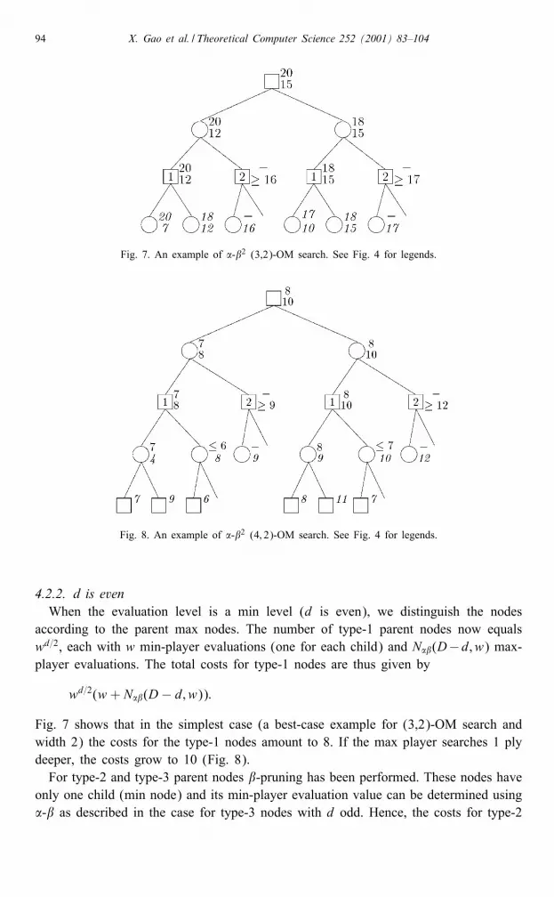
Fig. 7. An example of �-�2 (3,2)-OM search. See Fig. 4 for legends.
Fig. 8. An example of �-�2 (4; 2)-OM search. See Fig. 4 for legends.
4.2.2. d is evenWhen the evaluation level is a min level (d is even), we distinguish the nodes
according to the parent max nodes. The number of type-1 parent nodes now equalswd=2, each with w min-player evaluations (one for each child) and N��(D−d; w) max-player evaluations. The total costs for type-1 nodes are thus given by
wd=2(w + N��(D − d; w)):
Fig. 7 shows that in the simplest case (a best-case example for (3,2)-OM search andwidth 2) the costs for the type-1 nodes amount to 8. If the max player searches 1 plydeeper, the costs grow to 10 (Fig. 8).For type-2 and type-3 parent nodes �-pruning has been performed. These nodes have
only one child (min node) and its min-player evaluation value can be determined using�-� as described in the case for type-3 nodes with d odd. Hence, the costs for type-2

X. Gao et al. / Theoretical Computer Science 252 (2001) 83–104 95
Table 2The best-case costs by four di�erent search algorithms for various search depths and widths. The ratio is anindication of the e�ciency of the pruning algorithm
D d w Minimax �-� Ratio (%) (D; d)-OM �-�2 Ratio (%)
5 2 2 32 11 34.4 40 16 40.05 3 2 48 20 41.75 4 2 64 18 28.110 7 2 1024 63 6.2 1280 138 10.810 8 2 1536 162 10.510 9 2 2048 226 11.05 2 10 100,000 1099 1.1 101,000 1280 1.35 3 10 110,000 2900 2.65 4 10 200,000 3710 1.910 7 10 1010 19,999 0.002 1:01× 1010 577,010 0.00610 8 10 1:1× 10¹⁰ 730,010 0.00710 9 10 2.0 ×10¹⁰ 4,960,010 0.0255 2 35 52,500,000 44,099 0.084 52,564,750 46,480 0.0885 3 35 54,022,500 127,400 0.2365 4 35 105,043,750 167,860 0.16010 7 35 2:76× 1015 1:05× 108 3:80× 10−6 2:76× 1015 312,001,410 1:1× 10−510 8 35 2:86× 1015 460,691,910 1:6× 10−510 9 35 5:52× 1015 9,185,325,660 1:7× 10⁻⁴
and type-3 nodes together are given by
(w − 1)d=2−1∑k=1
wkN��(d− 2k; w);
where d¿4. When d=2 the costs for type-2 and type-3 nodes are w(w − 1).Taking together all costs, we obtain, for the case with d even,
wd=2(w + N��(D − d; w)) + w(w − 1) when d = 2
wd=2(w + N��(D − d; w)) + (w − 1)d=2−1∑k=1
wkN��(d− 2k; w) when d¿4:
Table 2 presents the costs for several best-case search trees, using four di�erent searchalgorithms. In this table we include data for the cases w=2 (like our example trees),w=10 (typical for games like Othello) and w=35 (typical for chess-like games).We can see from Table 2 that �-�2 (D; d)-OM search is a signi�cant improvement
over pure (D; d)-OM search. For relatively small d, it appears that �-�2 is almost ase�cient as �-�. For larger d; �-� outperforms �-�2.We note that in the M∗ algorithm, the multi-model-based search strategy developed
by Carmel and Markovitch [4], a similar pruning mechanism was described as our�-�2-pruning. However, due to their recursive application of opponent modelling theirpruning is not guaranteed to yield always the same result as the non-pruning ana-logue. Only when the evaluation functions for both players obey certain conditions, in

96 X. Gao et al. / Theoretical Computer Science 252 (2001) 83–104
particular when they do not di�er too much, the correctness of their ��∗ algorithm isproven.
5. Experimental results of (D; d)-OM search
In this section, we describe two experiments on the performance of (D; d)-OMsearch, one with a game-tree model including an opponent model and the other inthe domain of Othello. The main purpose of these experiments is to con�rm the e�ec-tiveness of the proposed speculative strategy when a player has perfect knowledge ofthe opponent model.
5.1. Experiments with random trees
In order to investigate the performance of a search algorithm, a number of game-treemodels have commonly been used [14, 15]. However, for OM-like algorithms we needa model including an opponent model. Iida et al. have proposed a game-tree modelto measure the performance of OM search and tutoring-search algorithms [8]. On thebasis of this model, we built another game-tree model including the opponent model toestimate the performance of (D; d)-OM search. As a measure of performance, we usethe H value of an algorithm like we did for OM search. With this game-tree modeland the H values, the performance of (D; d)-OM search is studied.
5.1.1. Game-tree modelThe game-tree model we propose for this experiment is a uniform tree. A random
score is assigned for each node in the game tree and the scores at leaf nodes arecomputed as the sum of numbers on the path from the root to the leaf node. Thisincremental model was also proposed by Newborn [16] and goes back to a schemeproposed by Knuth and Moore [13]. The max player’s score for a leaf position at depthD (say PD) is calculated as follows:
EVmax(PD) =D∑k=0
r(Pk); (4)
the min player’s score for a leaf position at depth (d+ 1) (say Pd+1) is calculated asfollows:
EVmin(Pd+1) =d+1∑k=0
r(Pk); (5)
where −R6r(·)6R, and r(·) has a uniform random distribution and R is an adjustableparameter. The resulting random numbers at leaf nodes have a normal distribution.Note that the min player uses the same random score r(·) as the max player. It isimplied that EVmax =EVmin when D=d+1. In this case, (D; d)-OM search is identicalto the minimax strategy according to Remark 2.

X. Gao et al. / Theoretical Computer Science 252 (2001) 83–104 97
This game-tree model comes closer to approximating the parent=child behaviour inreal game trees and re ects a game tree including models for both players, in whichdi�erent opponent models are simulated by various search depths d. For this game-treemodel, we recognize that the strength of the min player is equal to that of the maxplayer when d=D − 1 and that the min player has less information from the searchtree about a given position when d¡D − 1. Note that we only investigate situationswith d6D−1, since otherwise (D; d)-OM search is unreliable and should not be used.
5.1.2. H valueIn order to estimate the performance of (D; d)-OM search, like OM search, we de�ne
the so-called H value (Heuristic performance value) for the root R by
H (R) =V (R;OM (D; d))− Vmin(R;D)Vmax(R;D)− Vmin(R;D) × 100: (6)
Here, V (R;OM (D; d)) represents the value at R by (D; d)-OM search and Vmin(R;D)is given by
Vmin(P;D) = miniEVmax(Pi); Pi ∈ all the leaf nodes at depth D: (7)
Vmax(P;D) is similarly given by
Vmax(P;D) = maxiEVmax(Pi); Pi ∈ all the leaf nodes at depth D: (8)
The strategy indicated by (7) obtains the minimum value of the root R by lookingahead D plies and the strategy indicated by (8) analogously the maximum value. H (R)then represents the normalized performance of (D; d)-OM search and can be thoughtof as a characteristic of the strategy. Although the value of this performance measureremains to be proven, we have con�dence in it, since we feel that the scaling applied byusing the minimum and maximum values of the leaves sets the resulting performancein appropriate perspective.
5.1.3. Preliminary results on the performance of (D; d)-OM searchTo get a feeling for the performance of (D; d)-OM search, several preliminary ex-
periments were performed using the game-tree model proposed above.As a �rst experiment, we observe the performance of (D; d)-OM search for various
values of d. In this experiment, D is �xed at 6 and 7, and d ranges from 0 to D−1. Acomparison of (6; d)-OM search and minimax is presented in Fig. 9, while (7; d)-OMsearch and minimax are compared in Fig. 10, all strategies with a �xed branching factorof 5. All curves shown in Figs. 9 and 10 are average results over 100 experiments.Figs. 9 and 10 show that
• the results support Theorem 8 and Remark 2. In particular,◦ d=0 means that the opponent does not perform any search at all. The max playertherefore has to rely on minimax.
◦ when d=5 in Fig. 9 and d=6 in Fig. 10, i.e., d=D − 1, the min player looksahead to the same depth in the search tree as the max player. In this case, the

98 X. Gao et al. / Theoretical Computer Science 252 (2001) 83–104
Fig. 9. (6; d)-OM search and minimax compared.
Fig. 10. (7; d)-OM search and minimax compared.
max player actually performs pure OM search. Since EVmax(P)=EVmin(P) in ourexperiments, the conditions laid down in Remark 7 are ful�lled, and (D; d)-OMsearch is identical to minimax.
• the uctuation in H values of (D; d)-OM search for depths d from 1 to D−1 hardlyseems dependent on the value of d. This is explained by the fact that the ratio ofmistakes of OM search does not depend on the depth of search, but only on thebranching factor [7]. The results may suggest that the uctuation in H values of(D; d)-OM search has a maximum at d= bD=2c.
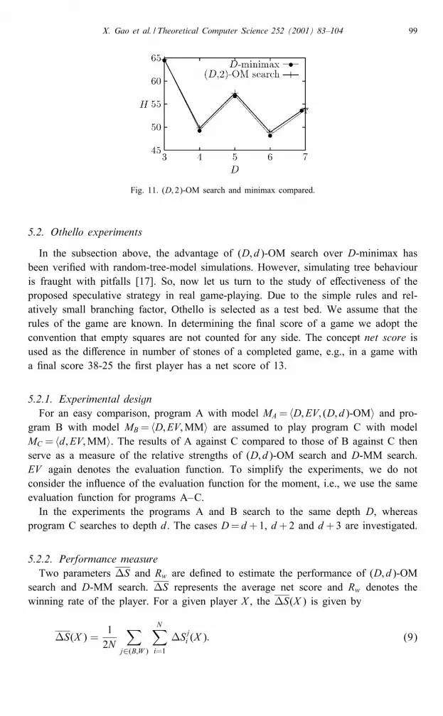
In a second experiment, we have investigated the performance of (D; d)-OM searchfor various values of D. In this experiment, d is �xed at 2 and D ranges from 3 to7. The results are shown in Fig. 11, which is an average result over 100 experiments,again using a branching factor of 5.Fig. 11 tells us that the H value of (D; d)-OM search is greater than that of
D-minimax. Of course, the gain of (D; d)-OM search over D-minimax is very small,since d is �xed at 2, which means that OM search is only performed in the upper2 plies, whereas in the remainder of the search tree minimax is performed. In ad-dition, (D; d)-OM search and D-minimax show the same uctuation in H values, aconsequence of both using the same evaluation function.
X. Gao et al. / Theoretical Computer Science 252 (2001) 83–104 99
Fig. 11. (D; 2)-OM search and minimax compared.
5.2. Othello experiments
In the subsection above, the advantage of (D; d)-OM search over D-minimax hasbeen veri�ed with random-tree-model simulations. However, simulating tree behaviouris fraught with pitfalls [17]. So, now let us turn to the study of e�ectiveness of theproposed speculative strategy in real game-playing. Due to the simple rules and rel-atively small branching factor, Othello is selected as a test bed. We assume that therules of the game are known. In determining the �nal score of a game we adopt theconvention that empty squares are not counted for any side. The concept net score isused as the di�erence in number of stones of a completed game, e.g., in a game witha �nal score 38-25 the �rst player has a net score of 13.
5.2.1. Experimental designFor an easy comparison, program A with model MA= 〈D; EV; (D; d)-OM〉 and pro-
gram B with model MB= 〈D; EV;MM〉 are assumed to play program C with modelMC = 〈d; EV;MM〉. The results of A against C compared to those of B against C thenserve as a measure of the relative strengths of (D; d)-OM search and D-MM search.EV again denotes the evaluation function. To simplify the experiments, we do notconsider the in uence of the evaluation function for the moment, i.e., we use the sameevaluation function for programs A–C.In the experiments the programs A and B search to the same depth D, whereas
program C searches to depth d. The cases D=d+1, d+2 and d+3 are investigated.
5.2.2. Performance measureTwo parameters �S and Rw are de�ned to estimate the performance of (D; d)-OM
search and D-MM search. �S represents the average net score and Rw denotes thewinning rate of the player. For a given player X , the �S(X ) is given by
�S(X ) =12N
∑j∈(B;W )
N∑i=1
�Sji (X ): (9)

100 X. Gao et al. / Theoretical Computer Science 252 (2001) 83–104
Table 3The results of programs A and B vs. program C, for D= d + 1
Programs Performance dmeasure 1 2 3 4
Scores 37:4=26:6 35:8=28:2 38:8=25:0 39:2=24:8A vs. C �S(A) 10.8 7.6 13.8 14.4
Rw(A) 66% 65% 69.5% 73.5%
Scores 37:4=26:6 35:8=28:2 38:8=25:0 39:2=24:8B vs. C �S(B) 10.8 7.6 13.8 14.4
Rw(B) 66% 65% 69.5% 73.5%
In this formula, �SBi (X ) denotes the net score obtained by player X when he playswith Black. Similarly, �SWi (X ) is the analogous number for playing White, and 2Nrepresents the total number of games, equally divided over games starting with Blackand with White. Therefore, this performance measure o�sets the in uence caused byhaving the initiative, which in general is widely believed to be a decisive advantagein White’s favour.The winning rate of player X; Rw(X ) is de�ned as
Rw(X ) =n+ m2N
× 100%; (10)
where n denotes the number of won games when X plays with White, and m is thatwhen X plays with Black.In our experiments, we let N =50, i.e., a total of 100 games are played for each case.
5.2.3. Preliminary resultsTable 3 shows the results for the case D=d+ 1, where the average scores by 100
games are given in the format x=y, with x the number of stones obtained by the �rstplayer and y by the opponent.From Table 3 we see that programs A and B obtain identical scores against pro-
gram C, in accordance with Remark 7, i.e., that in the case D=d+1 (D; d)-OM searchis identical to D-MM search. In addition, the results indicate that deepening search canconfer some advantage. When D=d + 1, the average winning rate is approximately68.5%.Table 4 lists the results for the case D=d + 2, showing that the performance of
(D; d)-OM search then always is signi�cantly better than that of D-MM search by asmall margin.We speculate that the edge of (D; d)-OM search over D-MM search will increase
with a better evaluation function (the present one mainly just counting disks). This isan area for future research.Table 5 gives the results for the case D=d + 3. Again it is clear that (D; d)-OM
search is stronger than D-MM search. However, when d=3, although the winningrate of (D; d)-OM search is greater than that of D-MM search, the average net gain

X. Gao et al. / Theoretical Computer Science 252 (2001) 83–104 101
Table 4The results of programs A and B vs. program C, for D= d + 2
Programs Performance dmeasure 1 2 3 4
Scores 39:9=24:1 41:7=22:3 41:2=22:8 40:2=23:8A vs. C �S(A) 15.8 19.4 18.4 16.4
Rw(A) 75.5% 78.5% 79% 76.5%
Scores 37:8=26:2 39:7=24:3 40:8=22:9 39:9=24:1B vs. C �S(B) 11.4 15.4 17.9 15.8
Rw(B) 68.5% 76% 78% 74.5%
Table 5The results of programs A and B vs. program C, for D= d + 3
Programs Performance dmeasure 1 2 3
Scores 43:9=20 45:4=18:6 42:1=21:9A vs. C �S(A) 23.9 26.8 20.2
Rw(A) 88% 88.5% 94%
Scores 41:8=22:1 43:7=20:3 44:4=19:5B vs. C �S(B) 19.7 23.4 24.9
Rw(B) 85% 86.5% 90%
of (D; d)-OM search is surprisingly lower. We believe that this also is a result ofthe use of a simpli�ed evaluation function. Comparing Tables 3–5 we also notice thatthe bene�t of (D; d)-OM search over D-MM search grows with larger di�erence insearch depth between the opponents. Obviously, OM search is suited to pro�t as muchas possible from defects in the evaluation function, which is precisely the reason why(D; d)-OM search was proposed. Moreover, although the margins are small we see fromTables 3–5 that (D; d)-OM search always is as good as (when D=d + 1) or better(when D¿d+1) than minimax. We feel that the signi�cance of this observation alsodepends on the evaluation function in use. This will be subject of future research.
6. Applications of (D; d)-OM search
Since (D; d)-OM search stems from grandmaster’s experience, it is implied that theplayer using this strategy has a higher playing strength. Even then, a grandmasteremploys only in some special cases (D; d)-OM search to get some advantage. Theseinclude the case that the opponent is really weak, and the case that the grandmasterreaches a bad position. Regarding the former, (D; d)-OM search can help the playerwin in fewer moves or by more stones. With respect to the latter, the grandmaster has

102 X. Gao et al. / Theoretical Computer Science 252 (2001) 83–104
to wait for mistakes by his opponent, in which case (D; d)-OM search can help himto enhance the position.
6.1. The requirements for applying (D; d)-OM search
So far, we assumed that the max player’s static evaluation function EVmax is possiblydi�erent from the min player’s one EVmin. However, it is very di�cult to have reliableknowledge of the opponent’s evaluation function to perform (D; d)-OM search. Knowl-edge of the opponent’s search depth (especially when the opponent is a machine) maybe more reliable. We therefore restrict ourselves in this section to potential applicationsof (D; d)-OM search for the case EVmax =EVmin.Under this assumption the requirements for applying the proposed (D; d)-OM search
can be given by the following lemma.
Lemma 9. Let � be the search depth di�erence between the max player and themin player in game playing; i.e.; �=D − d. If �¿2; then (D; d)-OM search can beapplied.
This means that the condition �¿2 gives the minimum depth di�erence at whichit is bene�cial to use (D; d)-OM search over minimax in order to anticipate on theopponent’s mistakes resulting from its limited search depth.The detailed proof for the above lemma can be found in [6]. Furthermore, we can
estimate in how many ways (D; d)-OM search can be applied. Each way of applying(D; d)-OM search is completely de�ned by the players’ search depths D and d, where,for de�niteness, D¿d + 2 (from Lemma 9 and De�nition 2). By simple discretesummation, we �nd for the number of ways, considering that the min player may,from instance to instance, choose any model with depth at most equal to d and sincethe max player may respond by choosing his D to match, that
N (D; d) =d∑i=1
(D − i − 1) = D × d− 12d(d+ 3);
where N (D; d) denotes the number of ways of applying (D; d)-OM search.
6.2. Possible applications
Since (D; d)-OM search is a speculative strategy, the reliability depends on the cor-rectness of the opponent model. We admit that it may seem unlikely that such a strategywill be of much practical use in game-playing. However, there are several situationswhere such a strategy can be of signi�cant support.One such possible application is in building a tutoring strategy for game playing [8].
In comparison with the pupil, the tutor can be considered a grandmaster. For tutoring tobe successful, the tutor should have a clear representation of his pupil. This statementis paramount when classifying tutoring strategies into the wider context of methodspossessing a clear picture of their opponents. Tutoring strategies therefore are a special

X. Gao et al. / Theoretical Computer Science 252 (2001) 83–104 103
case of models possessing an opponent model. The balance in tutoring strategies isdelicate: on the one hand it is essential that the tutor has a good model of his pupil.On the other hand, the give-away move should not be so obvious as to be noticeableby the person being tutored. Thereby, with the help of (D; d)-OM search, the gameis manipulated in the direction of an interesting position from which the novice may�nd a good or excellent move “by accident”; the novice’s interest in the game mayincrease, stimulating his progress on the way towards becoming a strong player.Another possible application is devising a cooperative strategy for multi-agent games,
such as soccer [12], 4-player variants of chess [18] and so on. In such games, (D; d)-OM search can be used by the stronger player to construct a cooperative strategywith his partner(s). Here, compared to the weaker partner(s), the stronger one is agrandmaster, who can apply (D; d)-OM search in order to model his partner(s) play[10]. One large advantage of such cooperative strategies is that it is much easier toobtain a reliable partner model than an opponent model.
7. Conclusions and limitations
In this paper, a speculative strategy for game-playing, called (D; d)-OM search, isproposed using a model of the opponent, in which di�erence in search depths is ex-plicitly taken into account. The algorithm and characteristics of this search strategy areintroduced. A more e�cient variant, named �-�2, is also proposed and its e�ciencyis analyzed. The e�ectiveness is con�rmed by experimental results from random-treesimulations and from the Othello domain.Although the opponent model used by (D; d)-OM search is more exible than that
by pure OM search, it is di�cult to have a reliable estimate of the search depthand evaluation function of the opponent. Mostly, the max player will only have atentative model of the opponent, and as a consequence this will lead to a risk ifthe model is not in accordance with the real opponent’s thinking process. Whereaspreliminary experiments indicated that the applicability of OM search is greater forweaker opponents [9], more work will be needed to investigate whether this holds alsofor (D; d)-OM search.Another point for future research is the recursive application of (D; d)-OM search,
analogous to Carmel and Markovitch’ [4] M∗ algorithm. Assume we use (4; 1)-OMsearch. In the present implementation the algorithm uses 2-MM search to determinethe max player’s values at depth 2. A better exploitation of the opponent’s weaknesswould be to use (2; 1)-OM search. The computational costs for this extension shouldcarefully be weighed against the bene�ts.
Acknowledgements
This work was supported in part by the Japanese Ministry of Education Grant-in-Aid for Scienti�c Research on Priority Area 732. The authors are grateful to the

104 X. Gao et al. / Theoretical Computer Science 252 (2001) 83–104
anonymous referees whose comments have resulted in numerous improvements of aprevious version of this article.
References
[1] G.M. Adelson-Velskiy, V.L. Arlazarov, M.V. Donskoy, Some methods of controlling the tree search inchess programs, Arti�cial Intelligence 6 (4) (1975) 361–371.
[2] D.F. Beal, A generalized quiescence search algorithm, Arti�cial Intelligence 43 (1) (1990) 85–98.[3] M. Buro, ProbCut: an e�ective selective extension of the alpha-beta algorithm, ICCA J. 18 (2) (1995)
71–76.[4] D. Carmel, S. Markovitch, Pruning algorithms for multi-model adversary search, Arti�cial Intelligence
99 (2) (1998) 325–355.[5] H. Iida, J.W.H.M. Uiterwijk, H.J. van den Herik, Opponent-model search, Technical Report #CS 93-03,
Department of Computer Science, Universiteit Maastricht, Maastricht, The Netherlands, 1993.[6] H. Iida, J.W.H.M. Uiterwijk, H.J. van den Herik, I.S. Herschberg, Potential applications of
opponent-model search; Part 1: the domain of applicablity, ICCA J. 16 (4) (1993) 201–208.[7] H. Iida, Heuristic theories on game-tree search, Ph.D. Thesis, Tokyo University of Agriculture and
Technology, Tokyo, Japan, 1994.[8] H. Iida, K. Handa, J.W.H.M. Uiterwijk, Tutoring strategies in game-tree search, ICCA J. 18 (4) (1995)
191–204.[9] H. Iida, I. Kotani, J.W.H.M. Uiterwijk, H.J. van den Herik, Gains and risks of OM search, in: H.J.
van den Herik, J.W.H.M. Uiterwijk (Eds.), Advances in Computer Chess 8, Universiteit Maastricht,Maastricht, The Netherlands, 1997, pp. 153–165.
[10] H. Iida, J.W.H.M. Uiterwijk, H.J. van den Herik, Cooperative strategies for pair playing, in: H. Iida,(Ed.), IJCAI-97 Workshop Proc. Using Games as an Experimental Testbed for AI Research, IJCAI,Nagoya, Japan, 1997, pp. 85–90.
[11] A. Junghanns, Are there practical alternatives to alpha-beta?, ICCA J. 21 (1) (1998) 14–32.[12] H. Kitano, M. Asada, Y. Kuniyoahi, I. Noda, E. Osawa, Robocup: the robot world cup initiative, in:
H. Kitano, J. Bates, B. Hayes-Roth (Eds.), Proc. IJCAI-95 Workshop on Entertainment and AI=Life,IJCAI, Montreal, Qu�ebec, 1995, pp. 19–24.
[13] D.E. Knuth, R.W. Moore, An analysis of alpha-beta pruning, Arti�cial Intelligence 6 (1975) 293–326.[14] T.A. Marsland, Relative e�ciency of alpha-beta implementations, Proc. Eighth Internat. Joint Conf. on
Arti�cial Intelligence, IJCAI, 1983, pp. 763–766.[15] A. Muszycka, R. Shinghal, An empirical comparison of pruning strategies in game trees, IEEE Trans.
SMC-15 (3) (1985) 389–399.[16] M.M. Newborn, The e�ciency of the alpha-beta search on trees with branch-dependent terminal node
scores, Arti�cial Intelligence 8 (1977) 137–153.[17] A. Plaat, J. Schae�er, W. Pijls, A. de Bruin, Best-�rst �xed-depth minimax algorithms, Arti�cial
Intelligence 87 (1–2) (1996) 255–293.[18] D.B. Pritchard, The Encyclopedia of Chess Variants, Games & Puzzles Publications, Godalming, Surrey,
UK, 1994.[19] R.L. Rivest, Game tree searching by min=max approximation, Arti�cial Intelligence 34 (1) (1988)
77–96.