Preprint version of article published in Perception and Psychophysics, 61: 636–660 (1999)

Parsing silhouettes: The short-cut ruleManish Singh Gregory D. Seyranian Donald D. Hoffman

Department of Cognitive SciencesUniversity of California, Irvine

Many researchers have proposed that, for the purpose of recognition, human vision parsesshapes into component parts. Precisely how is not yet known. The minima rule for silhouettes(Hoffman & Richards, 1984) defines boundary points at which to parse, but does not tell howto use these points to cut silhouettes, and therefore does not tell what the parts are. In thispaper, we propose the short-cut rule, which states that, other things being equal, human visionprefers to use the shortest possible cuts to parse silhouettes. We motivate this rule, and thewell-known Petters rule for modal completion, by the principle of transversality. We presentfive psychophysical experiments that test the short-cut rule, show that it successfully predictspart cuts which connect boundary points given by the minima rule, and show that it can alsocreate new boundary points.

Introduction

The ease with which we recognize visual objects is decep-tive: chess programs can now compete with chess masters,but no computer-vision system can compete with the visionof a toddler. Object recognition is complex and computation-ally demanding, and typically uses cues such as shape, color,texture, motion, and context. However, the ease with whichwe can, in many cases, recognize an object without any cuesbut shape suggests that shape is a key aspect of recognition.This raises the question: How does human vision representshape for the purpose of recognition?

One proposal is that human vision uses parts combinedinto structural representations (Biederman, 1987; 1990; Bie-derman & Cooper, 1991; Hoffman & Richards, 1984; Marr& Nishihara, 1978; Palmer, 1977). It represents a shape interms of (i) the shapes of its component parts and (ii) thespatial relationships between these parts.

On this approach, representing a shape involves parsingit into sub-units—not unlike parsing a sentence in naturallanguage—and describing the relationships between these

Manish Singh is now at the Department of Brain and CognitiveSciences, Perceptual Science Group, E10-120, Massachusetts Insti-tute of Technology, Cambridge, MA 02139.

For discussions and suggestions we thank Marc Albert, BruceBennett, Myron Braunstein, Mike D’Zmura, Ki-Ho Jeon, Jin Kim,Jeff Liter, Scott Richman, Asad Saidpour, and Jessica Turner. Forassistance in running the experiments we thank My Bui, RizwanaMela, Elizabeth Sullivan, and Michelle Young. And we thankStephen E. Palmer, Steven Yantis, and two anonymous reviewersfor helpful comments on previous versions of the paper. This re-search was supported by National Science Foundation Grant DIR-9014278.

Correspondence concerning this article can be addressed toManish Singh at manish@psyche.mit.edu, Greg Seyranian atgregs@aris.ss.uci.edu, or Donald D. Hoffman at ddhoff@uci.edu.

(a) (b)Figure 1. Part cut on a silhouette. The silhouette in (a) is unam-biguously parsed in (b) with a part cut (depicted by a dashed line).

(b) (c)(a)Figure 2. A silhouette with more than one parse. The silhouette in(a) is naturally parsed as in (b) or in (c).

subunits—again, not unlike the syntactical structure of a sen-tence. And, just as some sentences admit multiple parses,so too do some shapes. For example, compare the shape inFigure 1a (which is nicely parsed by the part cut, indicatedby a dashed line, in Figure 1b) with the one in Figure 2a(which can be parsed either by the part cuts shown in Figure2b, or by the part cuts shown in Figure 2c). The parsing of

1

2 MANISH SINGH GREGORY D. SEYRANIAN DONALD D. HOFFMAN

shapes, when it occurs, is quick and effortless—perhaps evenpreattentive (Baylis & Driver, 1994; 1995a; 1995a; Driver &Baylis, 1995; Hoffman & Singh, 1997).

Part-based representations have been studied extensivelyby psychologists1 and computer scientists.2 Parts, unliketemplate and Fourier approaches, can deal effectively withocclusion, self-occlusion, and certain types of non-rigidityin which rigid parts move relative to each other (Hoffman& Richards, 1984; Pinker, 1985). They can explain theclassic visual phenomenon, first noted by Mach, that sym-metry is easier to detect than repetition (Baylis & Driver,1995b; Driver & Baylis, 1995; Mach, 1885/1959), and thephenomenon discovered by Attneave that a piece of curvelooks different depending on which side is taken to be “fig-ure” (Attneave, 1971; Hoffman & Richards, 1984; see Figure5). They can also alter the perception of transparency (Singh& Hoffman, in press). However, parts may be less importantin the visual recognition of faces (Farah, 1996; Tanaka &Farah, 1993; Turk & Pentland, 1991; Yuille, 1991).

A natural question arises: How does human vision parseshapes into parts? Some theorists postulate that there is a setof basic shapes, or primitives, which human vision searchesfor in images—primitives such as generalized cones (Bin-ford, 1971; Marr, 1977) or geons (Biederman, 1987). Ac-cording to these theories, human vision parses a shape byfinding these primitives in the shape. Hence the primitivesare responsible for (i) finding parts, and (ii) describing them.

Other theorists postulate that there are rules, based on ge-ometric properties alone, by which human vision computesthe boundaries between parts for any given shape. The min-ima rule (Hoffman & Richards, 1984) is a step in that direc-tion. For a 2D silhouette, the minima rule provides bound-ary points on the silhouette outline, through which part cutsmust pass (see Figure 3a). And for 3D shapes, the minimarule provides boundary curves on the surface of the shapethrough which part cuts must pass (see Figure 3b). However,the minima rule does not define the part cuts themselves—itonly constrains them by requiring them to pass through theboundary points it provides.

We deal here only with the parsing of silhouettes, not of3D shapes. The relationship between 3D shapes and silhou-ettes is complex, and beyond the scope of this paper (but see,e.g., Richards, Koenderink, & Hoffman, 1987). However,human subjects do see parts in silhouettes—so the parsing ofsilhouettes is of psychological interest.

In this paper, we propose that human vision parses silhou-ettes according to the short-cut rule.

Short-cut rule: Divide silhouettes into parts using the short-est possible cuts.

In other words, if boundary points can be joined in morethan one way to parse a silhouette, human vision prefers thatparsing which uses the shortest cuts. For the shape in Figure2a, for instance, the short cut rule gives the cuts shown inFigure 2b rather than the cuts shown in Figure 2c. In this pa-per a cut is (1) a straight line which (2) crosses an axis of lo-cal symmetry (see section entitled Short Cuts), (3) joins twopoints on the outline of a silhouette, such that (4) at least one

Figure 3. Minima rule gives part boundaries which are (a) pointson 2D shapes, and (b) curves on 3D shapes.

of the two points has negative curvature. For some shapessuch as elbows, the short-cut rule can create boundary pointsthat are not negative minima of curvature.

We begin by reviewing the minima rule and related re-search on shape partitioning. We then motivate the short-cutrule by the geometry of transversal intersections, and relate itto Petter’s rule for modal completion (Petter, 1956; Kanizsa,1979, p. 40). Finally, we present five experiments that test,and support, the short-cut rule.

A few caveats and disclaimers. There is much to theparsing of visual shapes that we cannot explore here. First,top-down factors can influence visual parsing (e.g., Schyns,Goldstone, & Thibaut, 1998; Schyns & Murphy, 1994;Schyns & Rodet, 1997; Singh & Landau, 1998). These areno less important than the short-cut rule that we examine.But to keep this work to manageable size, we focus hereon the short-cut rule. Once geometric factors like the short-cut rule are understood we have a better chance to integratethem with the top-down. Second, as mentioned earlier, manyfactors besides parts influence visual recognition. Motion,texture, color, and surface characteristics can also be impor-tant (Biederman, Glass, & Stacy, 1973; Bruce & Humphreys,1994). These cannot be ignored. Ultimately we want to knowhow these interact with geometric factors in visual parsingand object recognition. Third, parts appear at many spatialscales. Smaller parts nest within larger ones to form hierar-chies. Information at multiple scales affects the cutting ofparts. The issue of scale and how it affects part cuts is com-plex and important. But here we assume that some scale ofresolution, and some piecewise continuous approximation ofthe shapes, has been fixed.

1 A partial list includes Baylis & Driver (1994; 1995a; 1995b),Bennett and Hoffman (1987), Beusmans, Hoffman, and Bennett(1987), Biederman (1987), Biederman and Cooper (1991), Braun-stein, Hoffman, and Saidpour (1989), Driver & Baylis (1995), Hoff-man ((1983a); (1983b)), Hoffman and Richards (1984), Hoffmanand Singh (1997), Marr ((1977); (1982)), Marr & Nishihara, 1978),Palmer, 1977), Pentland, 1986), Stevens & Brookes, 1988), Ter-zopoulos, Witkin, & Kass (1987),Todd, Koenderink, van Doorn,and Kappers (1995), Tversky and Hemenway (1984).

2 A partial list includes Binford (1971, December), Brooks(1981), Dickinson, Pentland, & Rosenfeld (1992), Guzman (1971),Siddiqi and Kimia (1995), Winston (1975).

PARSING SILHOUETTES: THE SHORT-CUT RULE 3

The Minima Rule

Our starting point is the minima rule (Hoffman &Richards, 1984). In this section we briefly review the min-ima rule, its philosophy, strengths, and motivations. We thendiscuss its limitations. These limitations are the point of de-parture for our work here.

The minima rule embodies a fundamental shift in philoso-phy toward the problem of object parts. As noted earlier, thedominant philosophy of most researchers has been to spec-ify the shapes that parts may take, and then to look for theseshapes in images. We call this the shape primitives approach.Among the part shapes that have been proposed are polyhe-dra (Roberts, 1965; Waltz, 1975; Winston, 1975), general-ized cylinders and cones (Binford, 1971; Marr & Nishihara,1978), geons (Biederman, 1987), and superquadrics (Pent-land, 1986). Each such proposal works well on a specialclass of objects. None comes close to capturing the vari-ety and complexity of object parts in general. And each, ifviewed as a general theory of the human perception of parts,is clearly ad hoc.

The minima rule separates the issue of finding parts fromthe issue of describing them. In the shape primitives ap-proach, finding and describing parts is done in a single pro-cess: trying to fit primitives to a given image. This entails,however, that parts whose shapes are not in the predefinedset of primitives cannot be found. Hoffman & Richards(1984) have argued, instead, that the mechanisms which findparts are more basic, and operate regardless of the shapesof the parts. The minima rule thus has different strengthsand limitations. Rather than defining part shapes it definespart boundaries. And rather than looking for part shapesin images, it looks for part boundaries.3 One advantage isthat its definition of part boundaries is expressed solely inthe language of differential geometry and therefore appliesto any shape defined by a piecewise differentiable function.In other words, it applies quite generally. We will discuss itslimitations shortly.

But first we examine the rule, its motivations, and itsstrengths. The minima rule comes in two versions, one forpartitioning 3D shapes and one for partitioning 2D silhou-ettes. Here we need only the version for silhouettes, sinceour task is to define part cuts on silhouettes. We need notdiscuss the 3D version, which can be found elsewhere (Hoff-man, 1983; Hoffman & Richards, 1984; Bennett & Hoffman,1987; Beusmans et al., 1987; Hoffman & Singh, 1997) andwhich requires prior discussion of the differential geometryof surfaces. The version for silhouettes is as follows.

Minima Rule for Silhouettes: Cut each silhouette into partsusing concave cusps and negative minima of curvature of itsbounding contour.

Figure 4 illustrates this rule. Figure 4a shows a silhou-ette, with regions of positive curvature and negative curva-ture marked. (The shaded side is “figure,” and the white is“ground.”) Note that positive regions are convex and neg-ative regions concave. This figure also has two cusps on it,one concave and labeled A, one convex and labeled B. Figure

+

+

-

-

-B

A

(a) (b)

+

+

-

-

BA

(c) (d)Figure 4. Geometry related to the minima rule. In (a) is shown asilhouette with ”figure” indicated by stippling. Regions of positiveand negative curvature are indicated by + and − respectively. Thecusp labeled A is concave, i.e., pointing into the figure. The cusplabeled B is convex, i.e., pointing into the ground. In (b) the neg-ative minima of curvature are indicated by dots. These are the partboundary points according to the minima rule. In (c) is shown thesame silhouette as in (a), but with figure and ground reversed. Notethe change in signs of curvature. Now the cusp labeled A is convexwhereas B is concave. In (d) the new negative minima of curvatureare indicated by dots. A reversal of figure and ground changes thepart boundaries.

(a) (b)Figure 5. A demonstration of the minima rule. The two wiggleson the right look different even though they are identical. Why?According to the minima rule you break them into parts differently.

4b shows the boundary points, as defined by the minima rule,between parts. If figure and ground reverse, as in Figure 4c,then regions of negative curvature become positive and viceversa. Moreover concave cusps become convex, and viceversa. This entails, according to the minima rule, that thereare now different boundary points, as shown in Figure 4d.

This shift of boundary points, when figure and ground re-

3 This is what makes the minima rule a “boundary-based” ap-proach. The “boundaries” in question are boundaries betweenparts—regions where one part ends and another begins. They arenot the bounding contours that define 2D silhouettes—an easy mis-interpretation (see Siddiqi & Kimia, 1995, p. 239–240).

4 MANISH SINGH GREGORY D. SEYRANIAN DONALD D. HOFFMAN

(a) (b) (c)Figure 6. The minima rule does not say to form part cuts by con-necting consecutive negative minima of curvature. It is clear thatdoing so can produce very strange parts, as in (a), (b). Sometimes,this does not even give legitimate part cuts, as in (c).

verse, can explain some interesting perceptual effects. One,discussed by Attneave (1971), is shown in Figure 5. Onthe left is a disk with a wiggle through it. On the right thetwo halves are pulled apart at the wiggle. By constructioneach half has an identical wiggle. But notice that the twowiggles look quite different—a fact easily confirmed by ex-periment (Hoffman, 1983a). The reason, according to theminima rule, is this: The two halves induce opposite assign-ments of figure and ground on the two wiggles. Thereforeregions of positive curvature for one wiggle have negativecurvature for the other, and vice versa. And therefore theparts, whose boundaries are (by the minima rule) at nega-tive minima of curvature, must be different for the two wig-gles. Thus the reason the wiggles look different is that youdivide them differently into parts. A similar account can begiven for the well-known face-goblet illusion, and for some3D illusions as well (Hoffman & Richards, 1984; Hoffman& Singh, 1997). The minima rule has also fared well in sev-eral psychophysical tests of its implications for the percep-tion of shape similarity (Hoffman, 1983a), short-term mem-ory for shapes (Braunstein et al., 1989), naming pictures withdeleted contours (Biederman & Cooper, 1991), the detectionof symmetry and repetition (Baylis & Driver, 1994, 1995a;1995b; Driver & Baylis, 1995), structure from motion (Said-pour, 1983a), figure-ground perception in 2D and 3D (Hoff-man & Singh, 1997), the perception of transparency (Singh& Hoffman, in press), and preattentive popout (Wolfe & Ben-nett, 1997).

It is clear from the above treatment that we are using cur-vature as a signed quantity. This differs, for example, fromAttneave’s (1954) treatment in which curvature is taken tomean magnitude of curvature—and is therefore a positivequantity. Attneave’s observation that information along acontour is concentrated at points of ’maxima of curvature’is a statement, in our framework, about the visual impor-tance of both negative minima and positive maxima of cur-vature. Within the context of parsing, however, the minimarule makes a distinction between these two kinds of curvatureextrema, assigning a special status to the negative minima.

The minima rule is distinct from the theory of codons(Richards & Hoffman, 1985; Richards, Dawson, & Whitting-ton, 1986). The domain of codons is plane curves, whereas

Figure 7. Transversality and concave creases. On the left aretwo generic surfaces. On the right they interpenetrate genericallyto form a composite object. By transversality, their surfaces formconcave creases (depicted by dashed curves) at almost every pointwhere they intersect.

the domain of the minima rule is, as we have seen, silhou-ettes and three-dimensional shapes. The theory of codonsuses minima of curvature, both positive and negative, toparse plane curves. The minima rule, by contrast, uses onlynegative minima of curvature as boundary points on silhou-ettes. The theory of codons parses any given plane curve into‘codons’, and then represents that curve using a classificationscheme for codons. The minima rule for silhouettes, by con-trast, only provides boundary points through which part-cutsmust pass. It does not define the cuts—and hence the parts—themselves. In particular, it does not join consecutive minimato form parts. Indeed, doing so can give strange parts (Figure6a, b) or no parts at all (Figure 6c).

The minima rule is based on a principle from the field ofdifferential topology called transversality (Guillemin & Pol-lack, 1974; Hoffman & Richards, 1984). The relevant caseof transversality is shown in Figure 7. On the left are twoarbitrary shapes in 3D, labeled S1 and S2. On the right S1and S2 interpenetrate to form a single composite object. S1and S2 are distinct elements of the (sparse) visual scene onthe left, and would be natural candidates for parts of the com-posite object on the right, if only we could distinguish them.Transversality says that we can—if S1 and S2 are genericshapes and if they interpenetrate at random. In this genericcase, at almost every point where the surface of S1 intersectsthat of S2 the tangent planes to the two surfaces have differ-ent orientations in space. Therefore the two surfaces meet,at each such point, in a concave crease. These points areindicated by the dashed curve on the composite object. Thiscrease is concave because it points into the object (i.e., intothe “figure”). By contrast, the edges of a cube are convexcreases, because they point out of the cube (i.e., out of the“figure”). Another way to understand it is this: If S1 andS2 each have smooth surfaces, then the dashed contour indi-cates the only points on the surface of the composite objectthat are not smooth. Thus transversality directly motivatesa strategy for dividing 3D shapes into parts along concavecreases. Combining this with processes of smoothing givesthe minima rule for 3D shapes, and combining it further withprojection onto an image plane leads to the minima rule for

PARSING SILHOUETTES: THE SHORT-CUT RULE 5

(a) (b)

(c) (d)Figure 8. A limitation of the minima rule. The two crosses in (a)and (b) have the same number of negative minima, and at roughlythe same locations. However, their natural partitionings, as given in(c) and (d), are very different. Clearly, some property other than thepresence of negative minima of curvature is required to explain thedifference in partitionings of these crosses.

silhouettes (Hoffman & Richards, 1984).

Transversality, however, is not an account of part genesis.As we have seen, it applies when two separate objects arejoined to form a new object. But it applies equally well, insmoothed form, when an object protrudes from another, aswhen a branch grows out of a stem. Transversality is an ab-stract principle of mathematics and so applies regardless ofthe genesis of the part.

The minima rule explains some aspects of our perceptionsof parts. But it has notable limitations. As we mentionedearlier, for a silhouette the minima rule gives precise bound-ary points at which to cut. But, as noted by Beusmans etal. (1987), the minima rule does not tell how to pair theseboundary points to define part cuts. Consider, for instance,the two shapes in Figures 8a and 8b—versions of which ap-pear in Rom and Medioni (1993), Siddiqi & Kimia (1995),and Kimia, Tannenbaum, and Zucker (1991; 1995). Theshape in Figure 8b can be seen as the result of pulling theshape in Figure 8a outwards and to each side. Clearly, such atransformation has little effect on the negative minima of theshape: There are still four negative minima and at roughlythe same locations. And in both cases, the minima rule sim-ply provides these four negative minima as boundary points,and is silent about how to connect them to form part cuts.4However, the natural perceptual organizations of these twoshapes are different—see Figures 8c and 8d. The shape in 8ais most naturally perceived as a small central core surroundedby four small parts, whereas the shape in 8b is most naturallyperceived as a large vertical body with two small parts pro-truding on the sides. Hence the minima rule, in itself, is un-able to account for the difference in perceptual organizationsof the two shapes.5 There are two reasons. First, the minima

Figure 9. Another limitation of the minima rule: Some part bound-aries are not negative minima of curvature.

rule uses only properties of the contour that outlines the sil-houette. And second, the minima rule uses only differentialproperties of the contour (namely, the presence of negativeminima of curvature). To define part cuts, we must add tothe minima rule (i) properties of the region enclosed by thecontour, and (ii) properties that are more global to the shape.

Another limitation of the minima rule is that it does notindicate which points in addition to negative minima of cur-vature are good part boundaries, even though there are surelysuch points (Hoffman & Richards, 1984, p. 72). Figure 9,for instance, shows an elbow which can be naturally cut asindicated by the dotted line. This line terminates at one endin a negative minimum of curvature, and at the other in apoint with zero curvature.

The short-cut rule, as we shall see, augments the minimarule in a way that repairs some of these limitations. But thereis relevant prior work on parts and part cuts by Marr (1977),Biederman (1987, 1990), and by Siddiqi & Kimia (1995), towhich we now turn.

Generalized ConesA silhouette can convey a rich sense of shape in three di-

mensions. To explain this, Marr (1977) suggested that humanvision interprets silhouettes as being the images of general-ized cones (first defined by Binford, 1971). A generalizedcone is the three-dimensional surface “swept out by movinga simple smooth cross-section along some axis, at the sametime magnifying or contracting it in a smoothly varying way”(Marr, 1977, p. 447)—see Figure 10. Marr showed that gen-eralized cones are a powerful tool for interpreting simple sil-houettes. Marr further suggested that human vision interpretscomplex silhouettes as the composition of two or more gen-eralized cones. To do so it must cut the silhouette into parts,each of which corresponds to a single generalized cone, andthen analyze each cone.

These cuts, Marr proposed, are straight lines that lie en-tirely within the silhouette and divide it into regions. Eachsuch region has a qualitative symmetry whose axis is the im-age of the axis of the corresponding generalized cone. Theendpoints of each cut are at curvature inflections, and some-times in concave or convex regions. The precise position of

4 Considerations of genericity, however, allow us to rule out partcuts that cross each other—see Beusmans et al. (1987).

5 It is important to note, however, that since the minima rule doesnot make cuts, it cannot, a fortiori, make unnatural ones (cf. Kimiaet al., 1995, p. 212).

6 MANISH SINGH GREGORY D. SEYRANIAN DONALD D. HOFFMAN

Figure 10. The definition of a generalized cone.

(a) (b)Figure 11. (a) Some geons, and (b) some objects made by com-bining geons. Adapted from Biederman (1987).

the endpoints is chosen to minimize the portion of the silhou-ette’s contour left unmatched by the qualitative symmetries.

Marr’s analysis is elegant. But as he was well aware theassumptions it requires are restrictive: The silhouette mustbe the image of generalized cones whose axes are coplanar,and the viewing direction must not significantly foreshortenthe axes of the generalized cones. A more general account isneeded.

Geons

To explain the speed and accuracy with which human vi-sion recognizes objects at the entry-level—for example, as atable, a horse, or a car—Biederman (1987, 1990) proposed atheory called recognition-by-components or RBC. RBC pos-tulates 24 primitive volumetric shapes, called geons6 (seeFigure 11a for some examples), and claims that any visualobject can be represented as an arrangement of these geonsin specific spatial relationships (see Figure 11b). Further-more, the geon representations are, by construction, stableover changes in viewpoint, so that the same representation isactivated from almost any viewing direction.

RBC faces the same difficulties that primitive-basedschemes typically face, viz., limited generality. However,it has the advantage that geons derive from the principle of“nonaccidental properties” (Lowe, 1985; Witkin & Tenen-baum, 1983), whereas polyhedra, superquadrics, and gener-alized cones make no appeal to a first principle. Nonacciden-tal properties are properties of 3D shape which, generically,survive projection onto an image plane. An example is thedistinction between straight and curved: a curved edge in3D will, generically, project to a curved edge in the imageplane. It takes a special viewpoint to make a curved edgein 3D project to a straight edge in an image—and if such aspecial viewpoint happens to occur, human vision often mis-interprets the resulting image because it interprets the im-age as arising from a generic, rather than special, viewpoint

(a)

(c)

(b)

(d)Figure 12. The four nonaccidental properties used in derivingthe set of geons: (a) curved versus straight cross section; (b) con-stant versus expanding only versus expanding and then contractingcross-section; (c) symmetrical versus asymmetrical cross-section;(d) curved versus straight axis.

(a) (b) (c)Figure 13. Geons have (a) pointed tips, or (b) truncated tips, butnot (c) rounded tips, even though the difference pointed, truncated,and rounded tips is one which survives projection, and is thereforea nonaccidental property.

(Freeman, 1994). Figure 12 shows the four nonaccidentalproperties used to generate the set of geons.

Although geons appeal to the principle of nonaccidentalproperties, they are not the complete set of shape primitivesthat follow from this principle. As an example, geons endeither in pointed tips (as in Figure 13a) or in truncations (asin Figure 13b); there are no geons with rounded tips (Fig-ure 13c). But clearly the distinction between rounded tips,truncated tips, and pointed tips is one that generically sur-vives projection—and is therefore a nonaccidental property.Indeed it is required for the proper recognition of toes, fin-gers, peeled bananas, and aircraft fuselages, which cannot beapproximated by geons (i.e., with truncated or pointed tips).One might say this problem is easy to fix: Just add to the listof geons a couple more shapes with rounded tips. And nodoubt this is easy to do. But there are many other nonacci-dental properties that have been omitted from the list as well.Why are some nonaccidental properties used to define geonsand others not? No principle has been given for choosingsome nonaccidental properties and not others.

6 The 1987 version of RBC had 36 geons, but the 1990 versionhas 24.

PARSING SILHOUETTES: THE SHORT-CUT RULE 7

(a) (b) (c)Figure 14. Siddiqi & Kimia’s (1995) definition of limb. In (a) thelimb is depicted by the dashed curve. The cocircular tangents aredepicted by arrows. In (b) and (c) are examples where the definitionof limb fails, since the tangents are not cocircular. This failure ofcocircularity is generic.

Limbs and Necks

Siddiqi and Kimia (1995), building on the work of Kimiaet al. (1991; 1995), recognized the limits of the minima rule,and proposed that silhouettes are parsed in two ways: limbsand necks. Siddiqi & Kimia (1995) define a limb as follows:“A limb is a part-line going through a pair of negative curva-ture minima with co-circular boundary tangents on (at least)one side of the part-line” (p. 243). A “part-line” is a partcut. Two tangent vectors are “co-circular” if both are tangentto one circle (Parent & Zucker, 1989, p. 829). Figure 14aillustrates their definition of limb, with the part cut depictedby a dashed line, and co-circular tangents depicted by ar-rows. This definition almost never applies to real parts sinceits requirement of co-circular tangents almost surely7 neverholds. Figures 14b and c, for instance, show examples inwhich tangents at negative minima of curvature are not co-circular. It is easy to concoct such examples since the failureof co-circularity is generic.8 This means that allowing tol-erance in the computation of co-circularity, which is usefulin other contexts (e.g., Parent & Zucker, 1989), cannot fixthe problem here: limbs would just go from measure zero tohighly unlikely.

The definition of limb, furthermore, has a counterintuitiveimplication: many part cuts that one normally calls limbs,e.g., cuts for the arms and legs of the human body (Figure15), fail both the co-circularity condition and the conditionof passing through two negative minima of curvature, andthus fail to be limbs according to the above definition. Thedefinition of limb, therefore, is much too restrictive. The cutsit defines are almost surely never found on any real shape.

Siddiqi & Kimia (1995) define a neck as follows: “A neckis a part-line which is also a local minimum of the diame-ter of an inscribed circle” (p. 243). Figure 16a illustratesthis definition, as does the central cut in Figure 16b and thetwo cuts in Figure 16c. Unfortunately the definition of neckgiven by Siddiqi & Kimia fails for a large class of shapes thatshould be classified as necks. In Figure 16d, for example, thedashed line indicates a natural cut, and should be made. Butit is not captured by the definition of a neck. The problem isthat the circle cannot be inscribed: the cut is the diameter ofthe circle, but the circle is too big to be inscribed. Thus thedefinition of neck is too restrictive.

Figure 15. Siddiqi & Kimia’s (1995) definition of limb excludeshuman (and animal) limbs; such limbs are not cocircular, and manydo not contain two negative minima.

Short Cuts

The situation seems to be this. Negative minima of curva-ture are powerful geometric determinants of perceived partboundaries on 2D silhouettes. But they are not the only suchdeterminants. And a comprehensive (bottom-up) account ofpart perception must describe all geometric factors and theirinteractions in determining not just boundary points, but en-tire part cuts. Here, we propose an important such factor: cutlength.

Consider the elbow depicted in Figure 17a. Which cutseems most natural—cut xy or cut xz? Casual inspectionsuggests that xy is by far more natural. (This is also, as wewill see shortly in our experiments, the verdict of subjects inexperiments with similar figures.)

Why is xy the preferred cut? Even in a shape as simpleas this elbow, several factors are at play. We have designedthis elbow, however, to minimize the effects of most factorsother than cut length. For example, the two lengths labeled Lin Figure 17a are identical, so that this length is not a factor.The points y and z both have identical curvature (viz., zero),so that this also is not a factor. One difference is the areaof the two parts defined by the two cuts, but this difference

7 Something is said to be true “almost surely” if it is true “every-where except possibly on sets of measure zero.” See, for example,Guillemin & Pollack (1974) and Halmos (1950).

8 A simple proof of this is the following: Pick at random twopoints in the plane. Pick at random a line passing through the firstpoint. Draw the circle passing through both points and tangent tothis line (this circle is defined uniquely). Then, of the countlesslines through the second point, just one will be tangent to this cir-cle. Thus cocircularity obtains with measure zero, and limbs almostsurely don’t occur.

8 MANISH SINGH GREGORY D. SEYRANIAN DONALD D. HOFFMAN

(a) (b)

(d)(c)Figure 16. Siddiqi & Kimia’s (1995) definition of neck. In (a) theneck is depicted by the dashed curve. In (b) the middle dashed lineis a neck. In (c) both dashed lines are necks (Siddiqi et al., 1996).In (d) is an example where the definition of neck fails, since thedashed line is not the diameter of an inscribed circle.

(a) (b)

x L

L

A

Az

y

xz

y

Figure 17. The distance factor. In both (a) and (b) the cut xy ispreferred to the cut xz because xy is shorter.

is eliminated in Figure 17b, and still the cut xy is preferred.This suggests that a key factor here is that the Euclidean dis-tance from x to y is shorter than that from x to z.

Therefore it appears that the goodness of a cut joining twopoints x and y involves the Euclidean distance dx,y = |x− y|.We say the goodness “involves the distance” rather than “isthe distance.” There is more to this factor. In some casescloser is not better, as shown in Figure 18. Points x and win this figure are certainly close to each other, but we are nottempted to cut the figure from x to w.

Why? Figure 18 suggests that the answer lies in the geom-etry of the silhouette between x and w. In this figure it seemsthat points x and z could have a cut between them, but pointsx and w could not, even though the distance between x and wis smaller than that between x and z. So Euclidean distancealone is not the key to determine how close two points mustbe before a cut between should be impossible. One consider-ation, of course, is that the cut xz involves two negative min-ima, whereas cut xw involves only one. But there is anotherfactor at play here. To state it, we need the notion of localsymmetry. Local symmetry is a weak form of symmetry that

xz w

Figure 18. Closer is not always better: A part cut must also crossan axis of local symmetry.

(b)(a)Figure 19. The axes of local symmetry for two shapes.

allows for the axes of symmetry to be curved, and also foraxes that span only local subshapes of an entire shape. Whatthe axes of local symmetry provide, in effect, is the skeletalaxial structure of any given 2D shape. Figure 19 displays theaxes of symmetry for two silhouettes. Various schemes havebeen proposed to compute the axes of local symmetry (Blum& Nagel, 1978; Brady & Asada, 1984; Leyton, 1992). Wewill use Brady & Asada’s (1984) definition.

What seems to be key in Figure 18, then, is that thestraight-line cut between x and z passes through an axis oflocal symmetry of the silhouette, whereas the straight cut be-tween x and w does not. A cut that fails to cross a local-symmetry axis simply does not chop off a region naturalenough to be considered for parthood. In other words, aslong as a cut crosses a local symmetry axis, shorter cuts are(other things being equal) better. If a cut does not cross anaxis of local symmetry, it is simply no good. This is nota differential-geometric property of the contour of the sil-houette, but rather a more global geometric property of theregion enclosed by it.

Why should cut length be such an important factor in de-termining part cuts on a silhouette? The answer lies in thegeometry of transversal intersections. Consider a generic in-tersection, in 3D space, of two cylinders such that the radiusof cross section of one cylinder is larger than that of the other(see Figure 20). Only two kinds of transversal intersectionsare possible that will produce ambiguities in parsing the pro-jected silhouette: a complete intersection, as shown in Fig-ure 20a, and a partial intersection, as shown in Figure 20b.A complete intersection can be characterized by the propertythat it leads to two contours of intersection, whereas a partialintersection leads to a single contour of intersection.

Let us consider the relative probability of obtaining these

PARSING SILHOUETTES: THE SHORT-CUT RULE 9

Figure 20. The two kinds of transversal intersections for two cylin-ders with unequal radii of cross section: (a) complete intersection,and (b) partial intersection.

Figure 21. The two kinds of transversal intersections for two cylin-ders with equal radii of cross section: (a) complete intersection, and(b) partial intersection.

two kinds of intersections, as a function of the ratio of theradii of the two cylinders (larger to smaller). As this ratiogets larger (say, as we keep the radius of the thicker cylinderfixed, and gradually decrease the radius of the thinner one),the probability of obtaining a partial intersection graduallydecreases to 0, and the probability of obtaining a completeintersection increases to 1. (The limiting case, of course, isachieved when the thin cylinder is just a line piercing throughthe thicker cylinder.) On the other hand, as this ratio getssmaller and approaches 1 (say, as we keep the radius of thethicker cylinder fixed, and gradually increase the radius ofthe thinner one), the probability of obtaining a partial inter-section gradually increases to 1, and the probability of ob-taining a complete intersection decreases to 0. In the limitingcase, where both cylinders have the same radius (see Figure21), the probability of obtaining a complete intersection is,in fact, 0. In other words, the set of relative orientations andtranslations that give rise to a complete intersection (shownin Figure 21a) has measure zero in the set of all possible ori-entations and translations that yield an intersection.9

Consider now the shape of the concave creases producedin each of the two intersection types. In the case of a com-plete intersection, so long as the two cylinders have unequalradii, the concave creases always encircle the thinner cylin-der, and never the thicker one (see Figure 20a). In the caseof a partial intersection, the concave crease encircles neitherof the two cylinders (see Figure 20b)—so in this case the

parsing of the projected image is left ambiguous.The outcome of this analysis, then, is as follows: As the

ratio of the radii of the two cylinders (larger to smaller) in-creases, the probability that the two cylinders will meet in acomplete intersection gets closer to 1. Therefore, the proba-bility that the concave crease of the intersection goes aroundthe thinner cylinder gets closer to 1. Hence, a projected sil-houette of this intersection should be naturally parsed usingthe shorter cuts (which correspond to the projections of theconcave creases produced by the intersection). On the otherhand, as the ratio of the radii of the cylinders approaches 1,there is a high probability that the cylinders will meet in apartial intersection—therefore, the parsing of the projectedsilhouette is ambiguous.

Given any silhouette, whether cylindrical or not, whosecorresponding 3D geometry is unknown, the principle ofgenericity (in the form used by Freeman, 1994) dictates thatthe silhouette should be interpreted as deriving from a 3Dshape that is roughly as deep as it is wide in the image.Therefore, as we saw with the cylinders above, the concavecrease will generically go around the part with the thinnersilhouette. For this reason, we hypothesize that:

1. given a silhouette in which the part boundaries can bepaired in more than one way to yield cuts, human vi-sion will prefer to make the shorter cuts, and

2. the probability of making the shorter cuts will increaseas the ratio of the longer to the shorter cut gets moreextreme.

The short-cut rule differs from necks (Siddiqi & Kimia,1995) in that the short-cut rule, unlike necks, does not re-quire the use of an inscribed circle, a requirement that wenoted earlier is quite restrictive. Therefore the short cut ruleis not restricted to measuring distances only along diametersof inscribed circles, but instead takes into account distancesbetween all pairs of points on the contour of the silhouettewhich are separated by an axis of local symmetry. For exam-ple, in Figure 17a and b the short-cut rule can explain whysubjects prefer the cut xy over the cut xz; however neithercut is a limb or a neck (Siddiqi & Kimia, 1995), so limbs andnecks cannot explain this preference.

This ecological motivation for the short-cut rule also mo-tivates the well-known Petter’s rule (Petter, 1956; Kanizsa,1979, p. 40) for modal completion of contours, which statesthat human vision prefers to make modal completions asshort as possible. For instance, for the cross in Figure 23b(which is rendered in a homogenous color), human visionprefers to make a modal completion along contour y ratherthan contour x, so that the vertical bar is seen as occluding thehorizontal one. This rule has been motivated by the heuristicthat, due to perspective projection, closer objects tend, ce-teris paribus, to have larger retinal images (Shipley & Kell-man, 1992b; Stoner & Albright, 1993). But this motivationis admittedly very rough (Tommasi, Bressan, & Vallortigara,

9 Recall that our current discussion includes only those intersec-tions that produce ambiguities in parsing the projected silhouette.

10 MANISH SINGH GREGORY D. SEYRANIAN DONALD D. HOFFMAN

(a) (b)

a b

c d

(c)

e

fi

j g

h

Figure 22. Some simple figures used in our experiments.

1995). However, the ecological motivation we have alreadygiven for the short-cut rule can be applied to Petter’s rule asfollows. When human vision is presented with a stimulus,like Figure 23b, of homogeneous color, it finds the negativeminima of curvature and pairs them using the short-cut rule.Because the color is homogeneous, it is initially ambiguouswhether these pairings should be taken to be part cuts ormodal contours (since it is not known whether the silhouettearises from a single object with parts, or from two differentobjects separated in depth). Further processing, possibly go-ing on in parallel with the pairing process, is required to makethis decision. Once this decision is made, the pairing decidedon by the short-cut rule is then taken to be either a part cut ora modal contour. In this way, Petter’s rule for modal contoursinherits the ecological motivation for the short-cut rule.

The Experiments

We chose two classes of shapes for the experiments:crosses (see Figure 22a) and elbows (see Figures 22b and22c). These are natural candidates because, as we have seen,they are simple, they display key limitations of the minimarule, and they allow a clean test of the short-cut rule.

The crosses have four negative minima of curvature.While the minima rule states that these are part boundaries,it does not specify how they should be joined. The short-cut rule predicts that subjects will join these part bound-aries so as to make the shortest cuts possible. Because thesefigures have straight lines and 90o angles, they are easilyparametrized and thus allow us to test a truly representativesample of crosses, not just those that might favor the short-cut rule. The elbows have but one negative minimum. Theminima rule states that this point must be a part boundarybut does not indicate what the other part boundary should be.The short-cut rule predicts that subjects will choose that partboundary which will create the shortest possible cut. Thesefigures, like the crosses, are easily parametrized and thus al-low us to test a representative sample of elbows.

Experiments 1 and 3 required subjects to hand draw cutson shapes, and contained fewer trials, whereas Experiments2, 4, and 5 involved a 3AFC task on a computer, and con-tained many more trials. These experiments do not testwhether the subjects would spontaneously parse such shapesif not asked to do so: Our task required subjects either to

xy

z

w

(a) (b)Figure 23. (a) The parameters of the cross-shaped figures used inExperiments 1 and 2. The stimuli were drawn with black outlinesand gray interiors in order to suppress the perception of illusorycontours, which are quite striking in (b), for example. We wantedsubjects to perceive a single object with parts, and not two object-sone partially occluding the other.

draw a fixed number of cuts, or to choose among a fewgiven cuts. However, as we note in the Introduction, there isprior empirical work which suggests that human vision doesparse shapes spontaneously (Biederman, 1987; Biederman& Cooper, 1991; Braunstein et al., 1989; Hoffman, 1983a;1983b; Hoffman & Singh, 1997), and perhaps even preat-tentively (Baylis & Driver, 1995a; 1995b). What our cur-rent experiments investigate is how the preferred cuts changewith various parameters of the shapes. The ‘Crosses’ Exper-iments The crosses were symmetric about the vertical andhorizontal axes. This allows them to be parametrized by four(orthogonal) parameters x, y, z, and w (see Figure 23a). Thespace of such crosses thus has four parameters. However,since we assume, for now, that the parsing of shapes is scaleinvariant, we do not wish to distinguish between a cross andscaled versions of it. Therefore, we can factor out scaling,so that the space of such (scale-invariant) crosses has threeparameters—for example, the three (orthogonal) parametersxy , z

y , and wy .

The independent variables we chose to parametrize thespace of crosses were:

1. distance ratio,d =

length of horizontal cutlength of vertical cut = x

y ;

2. area ratio,A =

area of part produced by horizontal cutarea of part produced by vertical cut = xz

wy ;

3. horizontal protrusion,10

h =length of horizontal partwidth of horizontal part = w

y .

Note that the area ratio, xzwy , is orthogonal to the two other

variables and is scale invariant. We chose this variable, in-stead of z

y , for its more intuitive and geometric interpretation.For example, it allows us to test whether the area of a partcreated by a given cut influences parsing.

10 We are using the term “protrusion” somewhat loosely. SeeHoffman & Singh (1997) for a precise definition that applies gener-ally.

PARSING SILHOUETTES: THE SHORT-CUT RULE 11

(a) (b) (c)Figure 24. Three types of cuts on a cross: (a) horizontal, (b) ver-tical, and (c) multiple.

Based on the minima rule, the short-cut rule, the principleof genericity (e.g., Beusmans et al., 1987), and considera-tions of symmetry, we expected three ways of parsing a crossto be most natural. We called these horizontal cuts (Figure24a: two horizontal cuts, both passing through negative min-ima), vertical cuts (Figure 24b: two vertical cuts, both pass-ing through negative minima), and multiple cuts (Figure 24c:both horizontal and vertical cuts are present).

We predicted that subjects would make the shortest cutsbetween parse points. As an example, for the cross in Figure23a, the vertical cuts are shortest and seem most natural.

The stimuli were drawn with a black outline and gray in-terior, as illustrated in Figure 23a. This was done to suppressthe perception of illusory contours—which are quite strik-ing, for example, when the figures are filled uniformly withblack, as in Figure 23b (see, for example, Kanizsa, 1979, andShipley & Kellman, 1992, for work on self-splitting figures).We wanted subjects to perceive a single object, and not tworectangular objects—one partially occluding the other.

Experiment 1

As discussed above, we expected the crosses to be parsedwith vertical cuts, horizontal cuts, or a combination of these.To check this, the first experiment tested whether subjectswould use any other cuts to parse the crosses, in a free-drawing task.Method

Subjects. Forty-five undergraduate students at the Uni-versity of California, Irvine, volunteered to participate forcourse credit. Data from two subjects were excluded fromanalysis because they failed to follow instructions.

Materials. The stimulus set consisted of a packet of 113sheets of paper (27 different stimuli, each repeated 4 times,plus 5 practice trials.) Each sheet had a cross-shaped figureprinted on it, that was symmetric about both of its axes. Toavoid any vertical or horizontal biasing effects, half of thefigures were presented with a tilt of 15 degrees to the left ofvertical, and the other half with a tilt of 15 degrees to theright of vertical. The first five sheets were practice.

Design. This experiment was a 3× 3× 3 within-subjectsfactorial design. The three independent variables were: (i)The distance ratio, d, (ii) the area ratio, A, and (iii) the hori-zontal protrusion, h. Each of the three independent variableshad three levels: 1/2 , 1, and 2. Figure 25 illustrates all thestimuli used for the experiment. The dependent measure wasthe percentage of vertical cuts. (“Multiple cuts” was not an

Pro

trusi

on =

1/2

Distance Ratio1/2 1 2

Are

a R

atio

1/2

1

2

Are

a R

atio

1/2

1

2A

rea

Rat

io

1/2

1

2

Pro

trusi

on =

1P

rotru

sion

= 2

Figure 25. All figures used in Experiments 1 and 2 organized bydistance ratio, area ratio, and horizontal protrusion.

option in this experiment.) The short cut rule predicts thatas d increases the percentage of vertical cuts increases, be-cause as d increases the vertical cuts become shorter than thehorizontal.

Procedure. The experiment was run in six separate ses-sions. Each subject was seated at a desk, in a separate cubicleroom. On the desk was the stimulus set packet (placed facedown), a pencil, and a ruler. The subjects were instructedto (a) pick up the top sheet from the packet, (b) turn it faceup, (c) decide how they would cut the figure most naturallyinto three parts, and (d) draw two straight-line cuts, with theruler and pencil provided, to achieve this partitioning. (Welimited subjects to two cuts because this is the simplest taskthat adequately tests our theoretical expectations.) After theywere done with a figure, they were to place that sheet face-down, in a separate stack. It was stressed that they should

12 MANISH SINGH GREGORY D. SEYRANIAN DONALD D. HOFFMAN

0.0

0.2

0.4

0.6

0.8

1.0d = 2

d = 1

d = 1/2

211/2

Pro

porti

on o

f Ver

tical

Cut

s

Area Ratio

Distance Ratio

Figure 26. The proportion of vertical cuts made by subjects inExperiment 1, as a function of distance ratio and area ratio.

not look forward or backward in the two stacks. The first fivesheets were practice trials. The ordering of the experimentaltrials was randomized for each subject. The subjects weremonitored continuously to make sure they were followinginstructions. Subjects were debriefed and thanked for theirparticipation.Results and Discussion

Each response was classified as a vertical cut, horizontalcut, or other. A response was classified as vertical if bothcuts made were vertical, and passed within 5 mm of the neg-ative minima. It was classified as horizontal if both cuts madewere horizontal, and passed within 5 mm of the negative min-ima (see Figure 24). It was classified as other if it was nei-ther horizontal, nor vertical. Out of all responses from the 43subjects whose data were included in the analysis, less than0.1% were other. These were excluded from the analysis.

An alpha level of .05 was used for all statistical tests. Athree-way analysis of variance (ANOVA) showed a main ef-fect of the distance ratio, F(2,84) = 44.743, p < .0001, butno main effect of the area ratio, F(2,84) = 1.839,ns, and nomain effect of the horizontal protrusion, F(2,84) = 0.933,ns.There was a significant interaction between the distance ratioand the area ratio, F(4,168) = .381, p < .05. Post-hoc com-parisons revealed that the area ratio had an effect only whenthe distance ratio was 1—and for these stimuli, subjects pre-ferred to cut parts with larger areas. (See Figure 26 for agraphed summary of the results.) These results suggest thatin these stimuli the distance ratio is the dominant geomet-ric factor used by human vision for parsing. As predicted,shorter cuts are much preferred to longer.

These results also indicate that in forced-choice experi-ments on crosses it is legitimate to restrict the alternatives tohorizontal cuts, vertical cuts, or a combination of these.

Experiment 2

Because of the tedious task in Experiment 1, each stimuluswas presented only 4 times to each subject. This precludedreliable modeling of individual subjects’ data, or comparingof trends across subjects. However the second experiment

used a forced-choice task on a computer, allowing manymore trials, and allowing us to model each subject’s data in-dividually.Method

Subjects. Ten graduate students at the University of Cal-ifornia, Irvine, volunteered to participate. Subjects were notpaid and received no course credit.

Materials. The experiment was run on a MacintoshQuadra 840AV, using the program SuperLab. The stimuliused were the same 27 cross-shaped figures as in Experiment1 (see Figure 25), but each was presented 24 times.

Design. This experiment had the same 3× 3× 3 within-subjects factorial design as Experiment 1: the independentvariables were d, A, and h, and each had the levels 1/2, 1, and2. Each stimulus figure was repeated in 24 trials, resulting ina total of 648 (+ 5 practice) trials. There were two dependentmeasures: the percentage of vertical cuts responses, and thepercentage of multiple cuts responses.

Procedure. The subjects were seated at a desk, 0.6 me-ters from a computer screen. The computer displayed theinstructions for the experiment. The subjects pushed a keyto indicate that they were done with the instructions. Eachtrial that followed was structured as follows: First there ap-peared on the screen, for 2 seconds, a cross-shaped figure,presented either with a tilt of 15 degrees to the left of vertical,or 15 degrees to the right of vertical. During this time, thesubjects were to decide how they would partition the shapemost naturally into parts. There followed a blank screen for500 ms, and then a screen with the initial cross-shaped figure(in its original location) along with three possible partition-ings of that figure presented, in small, at the bottom of thescreen, and numbered 1, 2, and 3. The subjects indicated, bypressing the corresponding number key, which of the threechoices corresponded to their partitioning. The three choiceswere vertical cuts, horizontal cuts, and multiple cuts (see Fig-ure 24). The numbering of the three different partitioningchoices was counterbalanced across trials. The subject’s re-sponse terminated the trial.

The first 5 trials were practice. The experimental trialswere divided into 4 blocks, each consisting of 27 x 6 = 162trials, for a total of 648 trials.Results and Discussion

Subjects’ data were initially analyzed for internal consis-tency. Data for the first 12 instances of each figure were cor-related to data for the last 12. Prior to the experiment wechose to reject all data from any subject whose correlationwas less than 0.5. No data were eliminated. Subjects’ datawere analyzed individually. First the multiple cuts responseswere analyzed. In general, subjects made few multiple cuts(mean = 4.23%), and did so primarily when the distanceratio and area ratio were both 1. Five of the ten subjectsmade virtually no multiple cuts (mean = 1.48%). The re-maining five subjects made multiple cuts only when both dand A were 1 (mean = 6.98%). Because of the low overalloccurrence of the multiple cuts responses, the percentage ofvertical cuts responses was taken as the primary dependentmeasure.Linear Regression. For vertical cuts responses, each subject’s

PARSING SILHOUETTES: THE SHORT-CUT RULE 13

data was fitted to a number of linear regression models. Thepercentage of vertical cuts, cv, was transformed to a newvariable, c′v, using an arc sine function (Kendall & Stuart,1963) to improve the normality of its distribution. The pre-cise transform was

c′v = 2 Sin−1√cv (1)

The terms corresponding to the distance ratio d, and the arearatio A, were taken to be, respectively, log(d), and log(A),(instead of simply d and, A).11

From some preliminary modeling, it was clear that thedistance ratio was doing most of the work. The modelswe tested, therefore, all included the distance ratio—alongwith all possible combinations of the other two independentvariables. In these models, the horizontal protrusion, h, ex-plained almost none of the variability in the data. (This re-mained true, also, when we replaced h with log(h).)

Therefore, we needed to consider only those models thatinvolved the variables log(d), and log(A). Also, in almostevery case, adding log(A) to the model containing only thedistance ratio did significantly improve the model’s fit.

For these reasons, our conclusion was that the linear re-gression equation,

c′v = β0 +β1log(d)+β2log(A),

provided the best model for our data. Figure 27 shows thesummary of this model, with the β1 and β2 parameters plot-ted along the x-axis and y-axis, respectively, with 95% con-fidence intervals for the estimates of these parameters, andwith r2-values of the model’s fit to each individual’s data.

In sum, distance was again the strongest factor, with sub-jects preferring shorter, rather than longer, cuts as predicted.Although area was also used by individual subjects (out of10 subjects, 8 had a coefficient for A that was significantlydifferent from zero), it was used differently by different sub-jects: 7 our of the 10 subjects cut off parts with the small-est area, while 3 cut off parts with the largest area. Overall,however, there was no main effect of area.

The ‘Elbows’ Experiments

Experiment 3Unlike the crosses from Experiments 1 and 2, the elbow inFigure 22b has but one negative minimum of curvature, la-beled g. The minima rule states that this point is one end of apart cut, but does not state which point is the other end. Sev-eral cuts seem plausible. Joining at point i seems reasonableas this is the only other extremum of curvature in the fig-ure, albeit a positive maximum (we call this a diagonal cut).However, joining at either j or h also seems reasonable asthese are the locally shortest cuts possible that pass throughthe figure’s axis of symmetry (we call these horizontal cutand vertical cut, respectively). The short-cut rule makes aclear prediction: subjects will choose the shortest part cut,i.e., the cut gh. Experiment 3, like Experiment 1, studies thecuts subjects make in a free-hand task. Experiment 4, like

-0.6 -0.3-0.9

-0.4

-0.6

-0.2

0.0

0.0 0.3 0.6 0.9

0.2

0.4

c' = β + β log(d) + β log(A) 1 20v

β1

β2

.77

.81

.93

.91.88

.89

.84.55

.71

.61

Figure 27. A plot of the coefficients b 1 and b 2 for the finallinear model c′v = β0 +β1log(d)+β2log(A) in Experiment 2. Eachpoint represents a different subject. Also shown are 95% confidenceintervals, and r2-values for the model.

Experiment 2, studies cuts in more detail. As in Experiments1 and 2, three factors are systematically varied: the distanceratio, d, the area ratio, A, and the horizontal protrusion, h (seeFigure 28). Experiment 5 investigates whether smoothing the

11 The reason for this is as follows: When a cross-shaped figurewith distance ratio d0, and area ratio A0, is rotated through an angleof 90o, the distance and area ratios of the resulting cross become,respectively, 1

d0, and 1

A0. At the same time, by our very conven-

tion, vertical cuts on the original cross become horizontal cuts onthe rotated cross, and vice versa. Also (ignoring multiple cuts), wehave,

cv = 1− ch,

where cv is percent vertical cuts, and ch is percent horizontalcuts. Now, if our model were, for example, c′v = β0 + β1log(d)+β2log(A), (i.e., without the log’s), the equation above would giveus, β0 +β1d0 +β2A0 = 1−(β0 +β1

1d0

+β21

A0), which cannot hold,

except in the degenerate case where d0 = A0 = 1. On the otherhand, if d and A, are replaced by log(d) and log(A) respectively,this problem is solved:

β0 +β1log(d0)+β2log(A0) = 1− (β0 +β11

log(d0)+β2

1log(A0)

),

In fact, this equation now tells us that for a perfect equality, we musthave b0 = 0.5. (This argument, however, is clearly not applicableto the horizontal protrusion, h.)

The assumption behind this argument (cv = 1 − ch) holds forabout half of the subjects. For the others, the transform can bethought of as a simple fitting technique.

14 MANISH SINGH GREGORY D. SEYRANIAN DONALD D. HOFFMAN

x

y

w

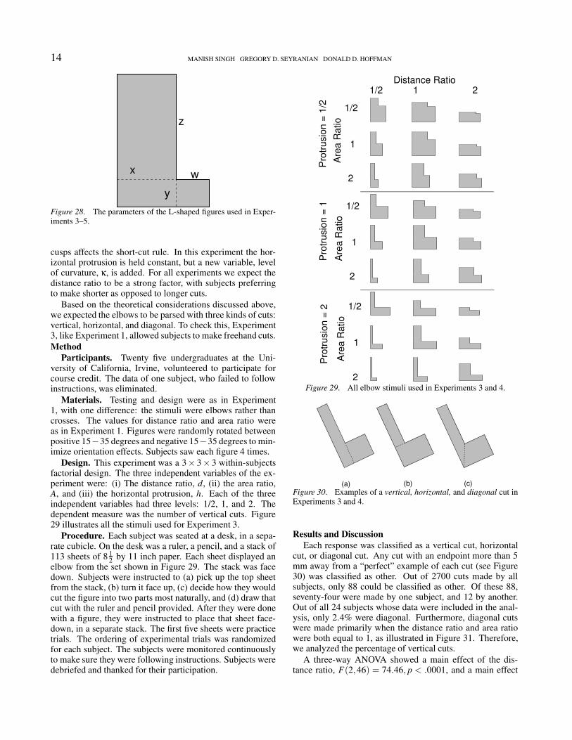
z

Figure 28. The parameters of the L-shaped figures used in Exper-iments 3–5.

cusps affects the short-cut rule. In this experiment the hor-izontal protrusion is held constant, but a new variable, levelof curvature, κ, is added. For all experiments we expect thedistance ratio to be a strong factor, with subjects preferringto make shorter as opposed to longer cuts.

Based on the theoretical considerations discussed above,we expected the elbows to be parsed with three kinds of cuts:vertical, horizontal, and diagonal. To check this, Experiment3, like Experiment 1, allowed subjects to make freehand cuts.Method

Participants. Twenty five undergraduates at the Uni-versity of California, Irvine, volunteered to participate forcourse credit. The data of one subject, who failed to followinstructions, was eliminated.

Materials. Testing and design were as in Experiment1, with one difference: the stimuli were elbows rather thancrosses. The values for distance ratio and area ratio wereas in Experiment 1. Figures were randomly rotated betweenpositive 15−35 degrees and negative 15−35 degrees to min-imize orientation effects. Subjects saw each figure 4 times.

Design. This experiment was a 3× 3× 3 within-subjectsfactorial design. The three independent variables of the ex-periment were: (i) The distance ratio, d, (ii) the area ratio,A, and (iii) the horizontal protrusion, h. Each of the threeindependent variables had three levels: 1/2, 1, and 2. Thedependent measure was the number of vertical cuts. Figure29 illustrates all the stimuli used for Experiment 3.

Procedure. Each subject was seated at a desk, in a sepa-rate cubicle. On the desk was a ruler, a pencil, and a stack of113 sheets of 8 1

2 by 11 inch paper. Each sheet displayed anelbow from the set shown in Figure 29. The stack was facedown. Subjects were instructed to (a) pick up the top sheetfrom the stack, (b) turn it face up, (c) decide how they wouldcut the figure into two parts most naturally, and (d) draw thatcut with the ruler and pencil provided. After they were donewith a figure, they were instructed to place that sheet face-down, in a separate stack. The first five sheets were practicetrials. The ordering of experimental trials was randomizedfor each subject. The subjects were monitored continuouslyto make sure they were following instructions. Subjects weredebriefed and thanked for their participation.

Pro

trusi

on =

1/2

Distance Ratio1/2 1 2

Are

a R

atio

1/2

1

2

Are

a R

atio

1/2

1

2

Are

a R

atio

1/2

1

2

Pro

trusi

on =

1P

rotru

sion

= 2

Figure 29. All elbow stimuli used in Experiments 3 and 4.

(a) (b) (c)Figure 30. Examples of a vertical, horizontal, and diagonal cut inExperiments 3 and 4.

Results and DiscussionEach response was classified as a vertical cut, horizontal

cut, or diagonal cut. Any cut with an endpoint more than 5mm away from a “perfect” example of each cut (see Figure30) was classified as other. Out of 2700 cuts made by allsubjects, only 88 could be classified as other. Of these 88,seventy-four were made by one subject, and 12 by another.Out of all 24 subjects whose data were included in the anal-ysis, only 2.4% were diagonal. Furthermore, diagonal cutswere made primarily when the distance ratio and area ratiowere both equal to 1, as illustrated in Figure 31. Therefore,we analyzed the percentage of vertical cuts.

A three-way ANOVA showed a main effect of the dis-tance ratio, F(2,46) = 74.46, p < .0001, and a main effect

PARSING SILHOUETTES: THE SHORT-CUT RULE 15

0.0

0.1

0.2

0.3d = 2

d = 1

d = 1/2

211/2

Pro

porti

on o

f Dia

gona

l Cut

s

Area Ratio

Distance Ratio

Figure 31. The proportion of diagonal cuts made by subjects inExperiment 3, as a function of distance ratio and area ratio.

0.0

0.2

0.4

0.6

0.8

1.0d = 2

d = 1

d = 1/2

211/2

Pro

porti

on o

f Ver

tical

Cut

s

Area Ratio

Distance Ratio

Figure 32. The proportion of vertical cuts made by subjects inExperiment 3, as a function of distance ratio and area ratio.

of the area ratio, F(2,46) = 5.65, p < .01, but no main ef-fect of the horizontal protrusion, F(2,46) = 0.06,ns. Post-hoc comparisons with a Tukey’s HSD revealed that, as pre-dicted by the short-cut rule, subjects made significantly morevertical cuts when the distance ratio was 2 than when 1, or1/2. The number of vertical cuts made at a distance ratioof 1 was significantly greater than at a distance ratio of 1/2.Furthermore, subjects made significantly more vertical cutswhen the area ratio was 1/2 than when 1 or 2. There wasan interaction between the distance ratio and the area ratio,F(4,92) = 4.50, p < .01. (See Figure 32 for a graphed sum-mary of the results.) As in Experiment 1, post-hoc analysisrevealed that the area ratio had an effect only when the dis-tance ratio was 1; for these stimuli, subjects preferred to cutparts with larger areas. As predicted, subjects preferred tomake shorter cuts for these figures.

Experiment 4

Experiment 3, as in Experiment 1, had only 4 repetitionsper stimulus per subject. This meant that we could not re-liably model individual subjects’ data, or compare trends

across subjects. However, in Experiment 4, as in Experi-ment 2, we used a 3AFC design presented by computer. Wetherefore had many more trials.Method

Participants. Twelve graduate students volunteered toparticipate. Subjects were not paid and received no coursecredit.

Design and Procedure. Testing and design were as inExperiment 2. Stimuli were the same as those used in Exper-iment 3. Values for the distance ratio, area ratio, and hori-zontal protrusion were the same as those used in Experiment3. Figures were randomly rotated between positive 15− 35degrees and negative 15−35 degrees to minimize orientationeffects. Figures were presented mirrored about the verticalaxis to control for left/right bias. The display of horizon-tal, vertical and diagonal choices in the key were counterbal-anced for each figure. We presented subjects with each ofthe 27 figures 24 times, 12 mirrored and 12 non-mirrored,for a total of 648 trials. The procedure was identical to thatin Experiment 2. On each trial subjects saw one large figure.Subjects were instructed to cut the figure into two parts mostnaturally, as quickly and carefully as possible. A key thenappeared below the figure. Subjects were to select the optionthat best represented their choice. We limited the choices tothese three cuts based on our findings in Experiment 3. Theinstructions were designed to encourage subjects to decidehow they would parse the figure before the key appeared.Results and Discussion

Subjects’ individual data were first analyzed for internalconsistency. Responses to the first 12 instances of each figurewere correlated to those for the last 12. Prior to the experi-ment we chose to reject data from any subject whose corre-lation was less than 0.5. One subject’s data was eliminated.The diagonal cut responses were analyzed first. As in Experi-ment 3, subjects made few diagonal cuts and did so primarilywhen the distance ratio and area ratio were both 1. Again, wechose to analyze only the percentage of vertical cuts.Linear Regression Analysis. Each subjects’ data was fittedto several linear models as in Experiment 2. We performeda log transform of each factor (distance ratio, area ratio andhorizontal protrusion) for the same reason as in Experiment2 (see footnote 11). The percentage of vertical cuts, cv, wastransformed to a new variable, c′v, using the arc sine functionin Equation 1 to improve the normality of its distribution.Model comparisons revealed that the horizontal protrusionwas a significant factor for only 2 of the 12 subjects. There-fore, the final model used was:

c′v = β0 +β1log(d)+β2log(A).

Figure 33 summarizes the individual fits to the first model byplotting the coefficients for the distance and area ratios. Co-efficients for the distance ratios are plotted on the abscissa,and coefficients for the area ratio are plotted on the ordinate.Error bars are given for 95% confidence intervals. Factorswhose confidence intervals include 0 are not significant. Ther2 for the model is also given near each plot point. As can beseen, the models are quite predictive for almost all subjects.

16 MANISH SINGH GREGORY D. SEYRANIAN DONALD D. HOFFMAN

3210-1

-1

0

1

β1

β2

c' = β + β log(d) + β log(A) 1 20v

.75

.86

.88

.95.87

.89

.83

.86

.78

.20

.63

Figure 33. Plot of the coefficients b1 and b2 for the linear model,c′v = β0 + β1log(d)+ β2log(A) in Experiment 4. Each point repre-sents a different subject. Also shown are 95% confidence intervals,and r2-values for the model.

wyx

z

Figure 34. An example of a smoothed elbow used in Experi-ment 5. The elbows were created by two hyperbolic functionsy1 = ε

x and y2 = εx+β +λ.

Average r2 for the distance and area ratio model was 0.772,SD= 0.199. This includes one outlying r2 of 0.197. Withoutthis score, the average rises to 0.829.

The distance ratio was by far the most important factor,with significant coefficients ranging from 0.4 to 2.2. Thecoefficients are all positive, indicating that subjects prefershorter cuts as predicted.

Experiment 5

In Experiment 5 we sought to determine if the short-cutrule still holds when part-boundaries are smooth (not cuspsas in all our previous experiments). We smoothed the el-bows of Experiments 3 and 4 by using two hyperbolic func-tions with identical curvature, as illustrated in Figure 34.12

The distance and area ratios can therefore be precisely com-puted.13 Smoothing the elbows has an interesting effect: thepositive maximum becomes the unique point locally sym-metric to the negative minimum (see Figure 22c). By con-trast, in the cusp case (see Figure 22b), the negative min-imum, g, is locally symmetric to all points between h andj. We chose to study smoothing on elbows rather than oncrosses because smoothing crosses does not change the localsymmetry relationships between the part boundaries. Hori-zontal protrusion remained the same, w

y . However, becausethis variable proved insignificant in Experiments 1, 2, 3 and4, we chose to hold this variable constant at a value of 2.This allowed for a larger factorial design with the remainingvariables. In addition to the distance ratio and area ratio, weincluded a variable for level of curvature, κ, with the valuesof ‘high’, ‘low’, and ‘cusp’ (or infinite).Method

Participants. Ten graduate students volunteered to partic-ipate. Subjects were not paid and received no course credit.Four of these subjects had previously participated in eitherExperiment 4 or Experiment 2, but had not been debriefed.

Design and Procedure. Testing and design were as in Ex-periment 4. This experiment was a 3×3×3 within-subjectsfactorial design. The three independent variables of the ex-periment were as follows: (i) The distance ratio, d, (ii) thearea ratio, A, and (iii) the level of curvature, κ. Distanceand area ratios were the same as in Experiments 3 and 4,viz., levels of 1

2 , 1, and2. The horizontal protrusion was heldconstant at 2, a value previously used in Experiments 3 and4. Figure 35 illustrates all the stimuli that were used for Ex-periment 5. The forced choices for cut types remained the

12 The functions were as follows:

y1 =εx

and y2 =ε

x +β+λ.

In these figures the negative minimum occurs at point:

a = (√

ε +β,√

ε+λ),

and the positive maximum at:

b = (√

ε,√

ε).

13 The functions were:

Distance Ratio =

√ε+β√ε+λ

, and

Area Ratio =

R z√ε+λ

ε√ε+y +λ+ ε√

ε+y+β dyR w√

ε+βε√ε+x +β+ ε√

ε+x+λ dx.

PARSING SILHOUETTES: THE SHORT-CUT RULE 17Lo

w C

urva

ture

Hig

h C

urva

ture

Cus

pDistance Ratio

1/2 1 2A

rea

Rat

io

1/2

1

2

Are

a R

atio

1/2

1

2

Are

a R

atio

1/2

1

2Figure 35. All elbow stimuli used in Experiment 5.

same as in Experiments 3 and 4: horizontal, vertical, and di-agonal. Each cut originated at the negative minimum of cur-vature. Diagonal cuts were joined to the positive maximum,horizontal cuts were drawn parallel to the horizontal axis (ofthe picture plane), and vertical cuts were drawn parallel tothe vertical axis. Figures were then randomly rotated be-tween positive 15−35 degrees and negative 15−35 degreesto minimize orientation effects. Figures were also presentedmirrored about the vertical axis to control for left/right bias.The display of horizontal, vertical and diagonal choices inthe key were counterbalanced across the presentation of eachfigure. We presented subjects with each figure 24 times, 12mirrored and 12 non-mirrored for a total of 648 trials. Fig-ures were displayed on a Macintosh Quadra 840 AV runningSuperLab for Macintosh.Results and Discussion

Subjects’ data were initially analyzed for internal consis-tency. Data for the first 12 instances of each figure were cor-related to data for the last 12. Prior to the experiment wechose to reject all data from any subject whose correlation

3210-1

-1

0

1

2

β1

β2

c' = β + β log(d) + β log(A) 1 20v

.84

.88

.84.90

.93.82

.82

.70

.76

.31

Figure 36. Plot of the coefficients b1 and b2 for the linear model,c′v = β0 + β1log(d)+ β2log(A) in Experiment 5. Each point repre-sents a different subject. Also shown are 95% confidence intervals,and r2-values for the model.

was less than 0.5. No data were eliminated.The diagonal cut responses were analyzed first. Only 2 of

10 subjects made more than 3% diagonal cuts. As in Exper-iments 3 and 4, diagonal cuts were made primarily when thedistance ratio and area ratio were both 1.

Linear Regression Analysis. Subjects’ data were fitted tothe following model:

c′v = β0 +β1log(d)+β2log(A).

The term for curvature was not found to be significant forany subject and was therefore not included in the final. Asin previous modeling, an arc sine transform was performedon the percentage of vertical cuts. Figure 36 summarizesthe individual fits to the vertical cuts model by plotting thecoefficients for the distance-ratio and area-ratio terms. Co-efficients for the distance ratio are plotted on the abscissa,and coefficients for the area ratio are plotted on the ordinate.Error bars are plotted for 95% confidence intervals. Factorswhose confidence intervals include 0 are not significant. Ther2 for the model is also given near each plot point. This graphdemonstrates that, even for the smoothed elbows, subjectspreferred to make shorter cuts.

Concluding Remarks

Human vision constructs visual objects, including theirshapes and surface properties (Hoffman, in press; Singh &Hoffman, 1997). Decomposing these shapes into parts facil-itates the recognition and manipulation of objects. To date

18 MANISH SINGH GREGORY D. SEYRANIAN DONALD D. HOFFMAN

there is no comprehensive theory of shape parsing. The min-ima rule, for instance, gives precise boundary points at whichto parse, but does not state how to join these points to formpart cuts. In this paper, we examine a geometric rule for de-termining part cuts: the short-cut rule. This rule follows fromthe geometry of transversal intersections in three dimensions,and is supported by our experiments. In experiments withcrosses, subjects prefer to join negative minima of curvatureso as to produce the shortest cuts possible. In experimentswith elbows, subjects prefer the shortest cut passing throughthe single negative minimum of curvature; thus the short-cut rule not only joins existing boundary points given by theminima rule, but it also creates new boundary points that arenot negative minima of curvature. Indeed, as shown in Figure37a, the short-cut rule can dictate a natural cut which termi-nates at neither end in a negative minimum of curvature (Sid-diqi & Kimia, 1995); the short-cut rule pulls the boundarypoints of the cut slightly away from negative minima of cur-vature that have low salience. Sharp negative minima of cur-vature are stronger attractors of part cuts than weak negativeminima (Hoffman & Singh, 1997). So while the short-cutrule might pull the boundary points of a part cut away fromweak negative minima, as in Figure 37a, it might not whenthe negative minima are sharp, as in Figure 37b. The inter-action between the short-cut rule and the salience of negativeminima is an interesting topic for further research. Anotherexample of this interaction can be seen in the dumbbell ofFigure 16b, which has a neck in the middle of the shape. Thecenter region of the dumbbell is composed of concave arcsof circles. Since each concave arc of a circle is a region ofnegative minima of curvature,14 the minima rule does not, byitself, pick out a unique point of the arc as a part boundary.Moreover, the magnitude of (normalized) curvature in thesearcs is low, so that they have low salience as part boundaries.At the ends of each arc are sharp negative minima of curva-ture, which have high salience. Thus salience would dictatethat part cuts should join these sharp points (cutting off theends of the dumbbell), whereas the short-cut rule would dic-tate a part cut in the middle of the dumbbell. In this competi-tion the short-cut rule loses (see, e.g., Braunstein et al., 1989,figure 6); subjects prefer to cut at the salient sharp points. Inother competitions, salience might lose to the short-cut rule.Salience and the short-cut rule can also agree, rather thancompete, as in Figure 16c. Here the part cut indicated at thetop of the shape is longer and connects negative minima withweaker salience, whereas the part cut indicated at the bottomis shorter and connects negative minima of higher (normal-ized) curvature and therefore higher salience. As a result,subjects prefer the bottom cut (Siddiqi, Tresness, & Kimia,1996).

Our motivation for the short-cut rule can also motivatePetter’s (1956) rule. Recall that the short-cut rule can berelated to Petter’s rule because, given a chromatically ho-mogeneous silhouette, it is initially ambiguous whether thesilhouette arises from a single 3D object with parts, or fromtwo different 3D objects separated in space. Hence, givensuch a silhouette, human vision finds the negative minimaof curvature and pairs them using the short-cut rule. De-

(a) (b)Figure 37. (a) An example of a part cut in which neither end isa negative minimum of curvature (Siddiqi & Kimia, 1995). Thisexample shows that the short-cut rule can sometimes pull the end-points of a part cut slightly away from negative minima of curva-ture that have low salience (Hoffman & Singh, 1997). However, asshown in (b), the short-cut rule might fail to pull the endpoints ofpart cuts away from negative minima of curvature that have highsalience.

pending on further processing, these pairings may becomeeither part cuts or modal completions. Under this assump-tion, the results of our experiments suggest that the “largermeans closer” heuristic (Shipley & Kellman, 1992; Stoner &Albright, 1993) fails to provide an adequate motivation forPetter’s rule: Recall that with the crosses, the distance ra-tio consistently predicted subjects’ preferred choices of cuts,whereas the area ratio failed to do so. However, further workis required to confirm this result for modal completions.

The short-cut rule and the salience of negative minima ofcurvature together determine many part cuts on silhouettes;but there are undoubtedly other factors as well. Part bound-aries that are locally symmetric to each other might be bettercandidates for part cuts. Cuts that have “good continuation”with tangents at part boundaries might be preferred to thosethat do not (Kellman & Shipley, 1991; Siddiqi et al., 1996;Singh & Hoffman, in press). The orientation of a silhouettemight affect part cuts. One set of cuts might be preferred be-cause it yields fewer parts, or parts with no negative minimaon their contours, or just simpler descriptions. And for someshapes, subjects might see no part cuts at all. Future work onpart cuts will need to address these issues.

References

Attneave, F. (1954). Some informational aspects of visual percep-tion. Psychological Review, 61, 183–193.

Attneave, F. (1971). Multistability in perception. Scientific Ameri-can, 225, 63–71.

Baylis, G. C., & Driver, J. (1994). Parallel computation of symme-try but not repetition in single visual objects. Visual Cognition,1, 377–400.

Baylis, G. C., & Driver, J. (1995a). Obligatory edge assignmentin vision – the role of figure and part segmentation in symmetry

14 Circular concavities are nongeneric: Almost any infinitesimalperturbation of such a concavity induces in it a locally unique neg-ative minimum of curvature. So examples like Figure 16b almostsurely never appear in nature. Hence, it is not surprising that humantreats circular concavities no differently than negative minima ofcurvature.

PARSING SILHOUETTES: THE SHORT-CUT RULE 19

detection. Journal of Experimental Psychology: Human Percep-tion and Performance, 21, 1323–1342.

Bennett, B. M., & Hoffman, D. D. (1987). Shape decompositionsfor visual shape recognition: The role of transversality. In W. A.Richards & S. Ullman (Eds.), Image understanding (pp. 215–256). Norwood, New Jersey: Ablex.

Beusmans, J., Hoffman, D. D., & Bennett, B. M. (1987). Descrip-tion of solid shape and its inference from occluding contours.Journal of the Optical Society of America, A, 4, 1155–1167.

Biederman, I. (1987). Recognition-by-components: A theory ofhuman image understanding. Psychological Review, 94, 115–147.

Biederman, I. (1990). Higher-level vision. In D. N. Osherson& J. M. Kosslyn, S. M. amd Hollerbach (Eds.), Visual cognitionand action: An invitation to cognitive science, vol.2 (pp. 41–72).Cambridge, MA: MIT Press.

Biederman, I., & Cooper, E. E. (1991). Priming contour-deleted im-ages: evidence for intermediate representations in visual objectrecognition. Cognitive Psychology, 23, 393–419.

Biederman, I., Glass, A. L., & Stacy, J., E. W. (1973). Scanning forobjects in real-world scenes. Journal of Experimental Psychol-ogy, 97, 22–27.

Binford, T. O. (1971, December). Visual perception by computer.IEEE Systems Science and Cybernetics Conference, Miami, FL.

Blum, H., & Nagel, R. N. (1978). Shape description using weightedsymmetric axis features. Pattern Recognition, 10, 167–180.

Brady, M., & Asada, H. (1984). Smoothed local symmetries andtheir implementation. The International Journal of Robotics Re-search, 3, 36–61.

Braunstein, M. L., Hoffman, D. D., & Saidpour, A. (1989). Partsof visual objects: an experimental test of the minima rule. Per-ception, 18, 817–826.

Bruce, V., & Humphreys, G. W. (1994). Recognizing objects andfaces. In V. Bruce & G. W. Humphreys (Eds.), Object and facerecognition (pp. 141–180). East Sussex: Lawrence Erlbaum As-sociates Ltd.

Driver, J., & Baylis, G. C. (1995). One-sided edge assignment invision. 2. part decomposition, shape description, and attentionto objects. Current Directions in Psychological Science, 4, 201–206.

Farah, M. (1996). Is face recognition ‘special’? evidence fromneuropsychology. Behavioral Brain Research, 368, 542–545.

Freeman, W. T. (1994). The generic viewpoint assumption in aframework for visual perception. Nature, 76, 181–189.

Guillemin, V., & Pollack, A. (1974). Differential topology. Engle-wood Cliffs, NJ: Prentice-Hall.

Guzman, A. (1971). Analysis of curved line drawings using contextand global information. In Machine intelligence, 6,. Edinburgh:Edinburgh University Press.

Halmos, P. R. (1950). Measure theory. New York: Van Nostrand.Hoffman, D. D. (1983a). Representing shapes for visual recogni-

tion. Doctoral dissertation, Massachusetts Institute of Technol-ogy, Cambridge, MA, USA.

Hoffman, D. D. (1983b). The interpretation of visual illusions.Scientific American, 249, 154–162.

Hoffman, D. D. (in press). Visual intelligence. New York: Norton.Hoffman, D. D., & Richards, W. A. (1984). Parts of recognition.

Cognition, 18, 65–96.Hoffman, D. D., & Singh, M. (1997). Salience of visual parts.

Cognition, 63, 29–78.

Kanizsa, G. (1979). Organization in vision: essays on gestalt per-ception. New York: Praeger.

Kendall, M. G., & Stuart, A. (1963). The advanced theory of statis-tics. New York: Hafner Publishing Company.

Kimia, B. B., Tannenbaum, A. R., & Zucker, S. W. (1991). Entropyscale-space. In (pp. 333–344). New York: Plenum Press.

Leyton, M. (1992). Symmetry, causality, mind. Cambridge, MA:MIT Press.

Lowe, D. (1985). Perceptual organization and visual recognition.Amsterdam: Kluwer.

Mach, E. (1885/1959). The analysis of sensations, and the relationof the physical to the psychical. New York: Dover.

Marr, D. (1977). Analysis of occluding contour. Proceedings of theRoyal Society of London, B, 197, 441–475.

Marr, D. (1982). Vision. San Francisco: Freeman Press.Marr, D., & Nishihara, H. K. (1978). Representation and recog-

nition of three-dimensional shapes. Proceedings of the RoyalSociety of London, B, 200, 269–294.

Palmer, S. E. (1977). Hierarchical structure in perceptual represen-tation. Cognitive Psychology, 9, 441–474.

Parent, P., & Zucker, S. W. (1989). Trace inference, curvatureconsistency and curve detection. IEEE Transactions on PatternAnalysis and Machine Intelligence, 11, 823–839.

Pentland, A. P. (1986). Perceptual organization and the representa-tion of natural form. Artificial Intelligence, 28, 293–331.

Petter, G. (1956). Nuove ricerche sperimentali sulla totalizzazionepercettiva. Rivisita di Psicologia, 50, 213–217.

Pinker, S. (1985). Visual cognition: An introduction. In S. Pinker(Ed.), Visual cognition (pp. 1–63). Cambridge, MA: MIT Press.

Richards, W. A., Dawson, B., & Whittington, D. (1986). Encod-ing contour shape by curvature extrema. Journal of the OpticalSociety of America, A, 3, 1483–1489.

Richards, W. A., & Hoffman, D. D. (1985). Codon constraintson closed 2d shapes. Computer Vision, Graphics, and ImageProcessing, 31, 156–177.

Richards, W. A., Koenderink, J., & Hoffman, D. D. (1987). In-ferring three-dimensional shapes from two-dimensional silhou-ettes. Journal of the Optical Society of America, A, 4, 1168–1175.

Roberts, L. (1965). Machine perception of three-dimensionalsolids. In J. T. Tippett et al. (Eds.), Optical and electroopticalinformation processing (pp. 125–143). Cambridge, MA: MITPress.

Rom, H., & Medioni, G. (1993). Hierarchical decomposition andaxial shape description. IEEE Transactions on PAMI, 11, 823–839.

Saidpour, A. (1983a). The salience of part boundaries in objectdecomposition. Doctoral dissertation, University of California,Irvine, Irvine, CA, USA.

Schyns, P. G., Goldstone, R. L., & Thibaut, J. P. (1998). The de-velopment of features in object concepts. Behavioral and BrainSciences, 21, 1–54.

Schyns, P. G., & Murphy, G. L. (1994). The ontogeny of partrepresentation in object concepts. In D. L. Medin (Ed.), Thepsychology of learning and motivation: Advances in researchand theory, 31 (pp. 305–349). San Diego, CA: Academic Press,Inc.

Schyns, P. G., & Rodet, L. (1997). Categorization creates func-tional features. Journal of Experimental Psychology: Learning,Memory, and Cognition, 23, 681–696.

20 MANISH SINGH GREGORY D. SEYRANIAN DONALD D. HOFFMAN

Shipley, T. F., & Kellman, P. J. (1992b). Perception of partly oc-cluded objects and illusory figures: Evidence for an identity hy-pothesis. Journal of Experimental Psychology: Human Percep-tion and Performance, 10, 106–120.

Siddiqi, K., & Kimia, B. B. (1995). Parts of visual form: com-putational aspects. IEEE Transactions on Pattern Analysis andMachine Intelligence, 17, 239–251.

Siddiqi, K., Tresness, K. J., & Kimia, B. B. (1996). Parts of visualform: psychophysical aspects. Perception, 25, 399–424.

Singh, M., & Hoffman, D. D. (1997). Constructing and representingvisual objects. Trends in Cognitive Sciences, 1, 98–102.

Singh, M., & Hoffman, D. D. (in press). Part boundaries alter theperception of transparency. Psychological Science.

Singh, M., & Landau, B. (1998). Parts of visual shape as primitivesfor categorization. Behavioral and Brain Sciences, 21, 36–37.

Stevens, K. A., & Brookes, A. (1988). The concave cusp as adeterminer of figure-ground. Perception, 17, 35–42.

Stoner, G. R., & Albright, T. D. (1993). Image segmentation cuesin motion processing: Implications for modularity in vision. .Journal of Cognitive Neuroscience, 5, 129–149.

Tanaka, J. W., & Farah, M. J. (1993). Parts and wholes in facerecognition. Quarterly Journal of Experimental Psychology, 46,225–245.

Tommasi, L., Bressan, P., & Vallortigara, G. (1995). Solving oc-clusion indeterminacy in chromatically homogeneous patterns.Perception, 24, 391–403.

Turk, M., & Pentland, A. (1991). Eigenfaces for recognition. Jour-nal of Cognitive Neuroscience, 3, 71-86.

Tversky, B., & Hemenway, K. (1984). Objects, parts, and cat-egories. Journal of Experimental Psychology: General, 113,169–193.

Waltz, D. (1975). Generating semantic descriptions from drawingsof scenes with shadows. In P. Winston (Ed.), The psychology ofcomputer vision (pp. 19–91). New York: McGraw-Hill.

Winston, P. A. (1975). Learning structural descriptions from ex-amples. In P. Winston (Ed.), The psychology of computer vision(pp. 157–209). New York: McGraw-Hill.

Witkin, A. P., & Tenenbaum, J. M. (1983). On the role of structurein vision. In J. Beck, B. Hope, & A. Rosenfeld (Eds.), Humanand machine vision (pp. 481–543). New York: Academic Press.

Wolfe, J. M., & Bennett, S. C. (1997). Preattentive object files:shapeless bundles of basic features. Vision Research, 37, 25–43.

Yuille, A. L. (1991). Deformable templates for face recognition.Journal of Cognitive Neuroscience, 3, 59–70.