Parametric models for spatially correlated survival data forindividuals with multiple cancers

Ulysses Diva1, Dipak K. Dey2, and Sudipto Banerjee3,*,†,‡1 Global Biometric Sciences, Bristol-Myers Squibb Company, Wallingford, CT, U.S.A2 Department of Statistics, University of Connecticut, Storrs, CT, U.S.A3 Department of Biostatistics, University of Minnesota, Minneapolis, MN, U.S.A

SUMMARYIncorporating spatial variation could potentially enhance information coming from survival data. Inaddition, simultaneous (joint) modeling of time-to-event data from different diseases, such as cancers,from the same patient could provide useful insights as to how these diseases behave together. Thispaper proposes Bayesian hierarchical survival models for capturing spatial correlations within theproportional hazards (PH) and proportional odds (PO) frameworks. Parametric (Weibull for the PHand log-logistic for the PO) models were used for the baseline distribution while spatial correlationis introduced in the form of county–cancer-level frailties. We illustrate with data from theSurveillance Epidemiology and End Results database of the National Cancer Institute on patients inIowa diagnosed with multiple gastrointestinal cancers. Model checking and comparison amongcompeting models were performed and some implementation issues were presented. We recommendthe use of the spatial PH model for this data set.

KeywordsBayesian hierarchical models; frailty models; Markov chain Monte Carlo (MCMC); proportionalhazards; proportional odds; spatial association; survival modeling

1. INTRODUCTIONThe importance of accounting for underlying spatial correlation in modeling data withgeographic information has been recognized in several areas (see, e.g. [1–4]). Accounting forspatial correlation could provide insights that would have been overlooked otherwise. On theother hand, the failure to include such information could potentially lead to spurious ormisleading results.

In biostatistics and epidemiology, there has been a growing interest in modeling survival dataaccounting for spatial associations. Li and Ryan [5] and Banerjee et al. [6] addressed thisproblem under a proportional hazards (PH) framework from classical and Bayesianperspectives, respectively. Semi-parametric approaches were proposed by Banerjee and Dey[7] using a proportional odds (PO) structure on the survival times, and by Li and Lin [8] usingnormal transformations of the survival times that marginally follow the PH model.

*Correspondence to: Sudipto Banerjee, School of Public Health, University of Minnesota, A460 Mayo Building, MMC 303, 420 DelawareStreet, SE, Minneapolis, MN 55455, U.S.A.†E-mail: sudiptob@biostat.umn.edu‡Associate Professor of Biostatistics.

NIH Public AccessAuthor ManuscriptStat Med. Author manuscript; available in PMC 2009 July 14.

Published in final edited form as:Stat Med. 2008 May 30; 27(12): 2127–2144. doi:10.1002/sim.3141.

NIH

-PA Author Manuscript

NIH

-PA Author Manuscript

NIH

-PA Author Manuscript

As opposed to modeling disease incidence and mortality, survival modeling provides a slightlydifferent perspective with regard to the nature of the disease. It focuses upon how many areexpected to survive after a certain period of time, how fast is the rate of failure, and what drivesshortened or prolonged survival; all of these may be influenced by several factors such asgender, race, age, type of cancer, treatment obtained, and access to healthcare facilities.

Among the widely investigated diseases are the different types of cancers. The SEER(Surveillance Epidemiology and End Results) database of the National Cancer Instituteprovides a rich amount of data on patients from different registries possibly suffering frommultiple types of cancers. Consequently, survival models for multiple cancers are sought forpractical reasons, such as to assess survival from multiple primary cancers simultaneously andto adjust the survival rates from a specific primary cancer in the presence of other primarycancers (see, e.g. [9,10]). Recently, Carlin and Banerjee [11] implemented spatial survivalmodels, where each patient developed possibly several cancers. They based their modelingupon the first primary cancer incorporating the effects of subsequent cancers (if any) on thatindividual as binary regressors indicating the presence or absence, but ignored the time-to-event information available for any subsequent primary cancers.

On the other hand, Diva et al. [12] (henceforth, DBD) proposed semi-parametric PH modelsthat directly incorporated information on survival times from subsequent primary cancers. Formodeling the spatial associations, both studies employed multivariate conditionally auto-regressive (MCAR) model, which is, in fact, a multi-layered Markov random field (MRF) (see,e.g. [13,14]). In this approach, each type of cancer is given its own spatial distribution over anunderlying map, but are also spatially correlated among themselves, so that the cancer effectsnested within space have a joint distribution that follows a multi-layered MRF or, morespecifically, an MCAR distribution. While we adopt the multivariate approach employed byDBD to handle survival data from multiple cancers, here we consider parametric specificationsof the PH and PO models. In general, parametric specifications are simpler to implement andfaster to execute, can produce better model performance when the specified parametric formis close to the observed pattern, and can provide a better framework to distinguish betweenmodels. Although the nature of the data sets used in DBD and this paper is similar, here weactually used different search criteria, which correspond to a different target population andlead to slightly different model interpretations. For purposes of comparing the performance ofthe parametric and semi-parametric implementations, we also applied our model to the DBDdata although the results are not presented in detail.

We present our modeling approach in Section 2. Technical and numerical aspects of theBayesian implementation of the models are described in Section 3. We illustrate and evaluateour proposed models in Section 4 with data on cancers of six (6) gastrointestinal (GI) organs.Finally, Section 5 concludes the paper with a summary and some recommendations.

2. PARAMETRIC MODELS FOR MULTIPLE CANCERS2.1. Data on patients with multiple cancers

Let us consider a relatively simple version of the SEER data, where we extracted survivalinformation on patients suffering from multiple cancers. Along with survival information,patient-specific and patient–cancer combination-specific covariates are also available. Patient-specific information includes gender, race, marital status, number of primary cancersdiagnosed, and their county of residence. Patient–cancer-specific information relates to age atdiagnosis, the stage of the cancer (in situ, local, distant or regional), the type (radiation and/orsurgery) of treatment that each patient underwent for each type of the cancer, and so on. As anexample, consider a patient, say with ID 00171, who first contracted cancer of the smallintestine (the first primary cancer) in 1986, developed colon cancer in 1991, pancreatic cancer

Diva et al. Page 2

Stat Med. Author manuscript; available in PMC 2009 July 14.

NIH

-PA Author Manuscript

NIH

-PA Author Manuscript

NIH

-PA Author Manuscript

in 1995, and eventually died in 1998. We present the data for this particular patient in Table I,incorporating information about the disease progression. We extract information about thispatient from the SEER database, where each entry corresponding to the patient would list thetype of cancer, the age at diagnosis, the stage of the cancer, the status at end point (dead oralive), and the survival time (or censorship time) in months. Note that the status is labeled as‘Dead’ for all entries, as it corresponds to the status at the end point.

The succeeding subsections describe approaches in modeling survival time with the data setupdescribed above. While there are other viable approaches that may be used we decided toconcentrate on the parametric PH and PO models for various reasons. Firstly, it should be notedthat the two models can be considered direct opposites in the assumptions that they employ[15]. Secondly, it is straightforward to incorporate spatial and non-spatial correlations in thecorresponding regression models. Although the use of a parametric specification in the baselinedistributions could greatly limit the flexibility of the resulting models, it lends ease ofinterpretation for the model parameters and reduces the computational burden considerably.Finally, and perhaps most importantly, exploratory data analysis techniques described inSection 4 suggest that the parametric models may be appropriate. The Bayesian modelingframework will be used for its flexibility and facility in handling complex hierarchical models.

2.2. PH modelThe PH model [16] is one of the most commonly used survival models that incorporatescovariate effects. It is given by

(1)

where h(t) denotes the hazard function, x are the covariates, and β is the corresponding vectorof regression coefficients. Also, h0(t) denotes a baseline hazard function, which is oftenmodeled semi-parametrically (see, e.g. [12,17–19]). However, in this paper we specified aWeibull(λ1, λ2) baseline hazard function, which gives h0(t) = λ1λ2tλ1−1. The parametric setupis equivalent to specifying a Weibull regression model for the logarithm of the survival time[20]. That is

(2)

with μ= −(1/λ1) log(λ2), γ = 1/λ1, β* = −(1/λ1)β, and Y follows the extreme value distributionwith density fY (y) = exp(y −ey),−∞ < y <∞. This gives a natural interpretation of λ1 and λ2 tobe the scale and intercept parameters, respectively. The above setup also has an acceleratedfailure-time interpretation, with acceleration factor given by exTβ*

The term exTβ in (1) is interpreted as the multiplicative change in the hazard function frombaseline due to the covariates. As with any regression setting care must be given in setting upthe covariates so that the value x= 0 is meaningful. The PH model assumes that the hazard ratio(relative risk) between two levels of a covariate, X, is constant over time, i.e. h(t | X)/h(t |X*) = e(X−X*)Tβ, while the odds ratio approaches either 0 or +∞.

2.3. PO modelAnother model that could be used for multiple cancer data incorporating covariate effects isthe PO model, popularized by Bennett [21]. The model is given by

Diva et al. Page 3

Stat Med. Author manuscript; available in PMC 2009 July 14.

NIH

-PA Author Manuscript

NIH

-PA Author Manuscript

NIH

-PA Author Manuscript

(3)

where S(t | x) is the survival function evaluated at t conditional on the observed covariates, x,and β is the corresponding vector of regression coefficients. The baseline survival function,S0(t), is oftentimes modeled semi-parametrically (see, e.g. [7,22]). However, in this paper, wemodeled the baseline distribution as log-logistic(λ1, λ2) so that S0(t) = 1/(1+λ2tλ1). Similar tothe PH model with Weibull baseline, this formulation of the PO model has a correspondinglinear regression model in log-time given by

(4)

with μ= −(1/λ1)log(λ2), γ =1/λ1, β* = −(1/λ1)β, Ỹ follows the logistic distribution with anddensity fỸ (y) =e−y/[1+e−y]2, −∞ < y <∞ [20].

The PO model may be considered to be on the opposite end of the spectrum as the PH modelsince it assumes that the hazard ratio approaches unity over time, i.e. that the covariate effectson the hazards disappear over time. In addition, although the estimates of the parameters maybe similar between the two models, the interpretation of the regression component significantlydiffers. The term exTβ in the PO model is interpreted as the change in the odds of survival (orfailure, depending on the parametrization), given the observed covariates or risk factors.

2.4. Capturing correlation using frailtiesSuppose that there are I counties and in the ith county we observe ni patients suffering from at

least two of K cancer types of interest. We uniquely identify each of the patientsthrough the ordered pair (i, j), as the jth patient (j = 1,2,…,ni) from the ith county. Let tijk denotethe survival time, the time to death, or end of study (censoring) for the (i, j)th patient fromdiagnosis with the kth type of cancer. Since not all patients develop all the K types of cancer,we list the possible cancers as {1,2,…, K} and form the subset C(i, j) ⊆ {1,2,…, K} as theindices of the cancers developed by the (i, j)th patient. Thus, if patient 00171 in our exampleabove is the 10th patient from the seventh county and if small intestine, colon, and pancreasare cancer types 2,3, and 6, respectively, in {1,2,…, K} then C(7,10) = {2,3,6}. Hence, whenreferring to ti jk, k ∈ C(i, j) unless otherwise noted. Clearly, these survival times will be correlatedfor similar county–patient–cancer combinations. We capture these correlations by introducingappropriate frailties.

Let u(i, j) denote the frailty for the (i, j)th patient, νk be the frailty for the kth cancer type, andφik be the frailty for the kth cancer type, nested within the ith county. For purposes of discussion,let us assume the patient frailties to be independent and normally distributed (zero-centered)

with county-specific variances, i.e. . However, in the implementation of themodels, we did not include the patient frailties for this particular data set as convergenceproblems were encountered, probably due to the scarcity and imbalance of information at thepatient–county level. Let us then collect the K cancer frailties into a vector ν and assume a jointzero-centered normal distribution with unknown covariance matrix Λ That is, ν= (ν1,…,νK)T

~ N(0,Λ), where Λ is a K × K covariance matrix.

Diva et al. Page 4

Stat Med. Author manuscript; available in PMC 2009 July 14.

NIH

-PA Author Manuscript

NIH

-PA Author Manuscript

NIH

-PA Author Manuscript

The spatial frailties, {φik}, are assigned an MCAR(α,Λ) distribution by first forming the I K

×1 vector , where each Φi=(φi1,…,φik)T is the K ×1 vector of the spatial frailtiesfor the K cancers within the ith county, and assigning a joint zero-centered normal distributionwith a covariance matrix that accounts for the spatial structure of the region. That is, by {φik}~ MCAR(α,Λ), we mean

where ΣW(α)= (Diag(mi) − α W)−1, mi is the number of neighbors of the ith county, and W isthe adjacency matrix of the graph representing our region. It should be noted that only α, thespatial smoothness parameter, is random in ΣW(α). Carlin and Banerjee [11] have shown thatas long as α ∈ (0,1), we have a proper MCAR distribution. In this setup, we are essentiallyusing the same covariance matrix for the cancer main effects and the spatial frailties within aparticular county. This is accomplished by using a Kronecker product of spatial structure and‘cancer dispersion’, an approach for modeling interactions that has been suggested earlier innon-spatial contexts by Clayton [23]. Several generalizations may be used to further enrich themodels, such as using a different cancer covariance matrix ϒ resulting in MCAR(α,ϒ), usingdifferent spatial smoothness parameters for each cancer type resulting in MCAR((α1,…, αK),Λ) [11,14], and having νi ~ N(0,Λi) (not identically distributed) where each county has its owncancer–covariance pattern. However, the above generalizations of the MCAR(α,Λ) requiresubstantial information on multiple cancer patients, which, unfortunately, is rare in practice.For instance, in the SEER database there is considerable imbalance of information at thecounty–cancer level, with some counties having more cases of a particular cancer and noobserved case of the other cancers, rendering many of the more general models unidentifiable.Therefore, we restrict our subsequent attention to the MCAR(α,Λ) specification and comparewith non-spatial models. For more information about MCAR models and possiblegeneralizations the reader is referred to [11,13,14,24].

3. NUMERICAL IMPLEMENTATION3.1. PH model

Considering the kind of data described in Section 2.1, a parametric PH model with Weibull(λ1, λ2) baseline distribution incorporating covariate effects, main effects for patients andcancers and nested effects for cancers within counties, may be expressed as

(5)

for i = 1,2,…, I, j = 1,2,…,ni, and k = 1,2,…, K. Using the above specification and lettingδ(i, j) be a death indicator (status at end point) for the (i, j)th patient, we obtain the likelihood

(6)

Diva et al. Page 5

Stat Med. Author manuscript; available in PMC 2009 July 14.

NIH

-PA Author Manuscript

NIH

-PA Author Manuscript

NIH

-PA Author Manuscript

where is the survival functionevaluated at ti jk conditional on the parameters and observed covariates.

To complete the Bayesian specification of the PH model, we need to assign prior distributionsfor the parameters. We assign vague normal, say β~ N(0,105 p× p), or improper flat prior, f(β) ∝ 1, for the regression coefficients, a Gamma(s0, s1) prior for the Weibull scale parameterλ1, and a log-normal(μ0, τ2) for the Weibull shape parameter λ2, where s0, s1, μ0, and τ2 arehyper-parameters specified to obtain vague prior distributions. We also need to specify priorsfor the parameters of the frailty distributions presented in Section 2.4. We assign inverted-Gamma, IG(ai, bi), priors for the ’s, an inverted-Wishart prior, IW(r0, Λ0), for the covariancematrix λ, and U(0, 1) or a Beta prior for the spatial smoothness parameter α, where the hyper-parameters are chosen to obtain vague prior distributions.

The parameters of the baseline hazard function, λ1 and λ2, and the regression parameters, β(with either flat or vague Gaussian priors), all have full conditional distributions that are log-concave and can be updated using the adaptive rejection sampling (ARS) algorithm [25] or aMetropolis step. The same applies to the patient frailties {u(i, j)}, the cancer frailties {νk}, andthe spatial frailties {φik}. The full conditional distributions for the ’s, are conjugate inverted-Gamma distributions that are directly updated. The cancer covariance parameter, λ, has aconjugate inverted-Wishart distribution, following from a lemma proved in DBD and statedin the Appendix. Finally, the spatial smoothness parameter, α, is updated using a slicesampler [26,27], which amounts to a rejection sampler from the prior of α.

Comparing with a non-spatial PH model with φik = 0,i = 1,…, I and k = 1,…, K, we obtainessentially the same likelihood but without the spatial components {φik} and α. Consequently,the full conditional distribution of Λ now excludes the contribution from the spatial frailties.The full conditional distributions are presented in the Appendix.

3.2. PO modelAnalogous to the PH model presented in the previous subsection, a parametric PO model withlog-logistic(λ1, λ2) baseline distribution incorporating covariate effects, main effects forpatients and cancers and nested effects for cancers within counties, may be expressed as

(7)

for i = 1,2,…, I, j = 1,2,…,ni, and k = 1,2,…, K. Using the above specification with δ(i, j) as inSection 3.2, the likelihood contribution of the (i, j)th patient is given by

(8)

with the parameters defined in previous sections.

We next assign prior distributions to complete the hierarchical specification. As in the PHsetting we assign vague multivariate normal or improper flat prior for the regressioncoefficients, a Gamma(s0, s1) prior for the scale parameter λ1 and a log-normal(μ0, τ2) for the

Diva et al. Page 6

Stat Med. Author manuscript; available in PMC 2009 July 14.

NIH

-PA Author Manuscript

NIH

-PA Author Manuscript

NIH

-PA Author Manuscript

shape parameter λ2 of the log-logistic baseline distribution, inverted-Gamma, IG(ai, bi), priorsfor the ’s, an inverted-Wishart prior, IW(r0, Λ0), for the covariance matrix Λ, and U(0, 1)or a Beta prior for the spatial smoothness parameter α, where the hyper-parameters are chosento obtain vague prior distributions.

Although the likelihoods arising from PH differ from PO, their full conditional distributionsbehave very similarly in terms of functional characteristics (i.e. log-concavity, conjugacy, etc.)and hence were updated using the same approaches described in Section 3.1. The detailsregarding the full conditional distributions are presented in the Appendix.

4. ILLUSTRATIONData were obtained from the 1973–2001 SEER Public Use Incidence Database [28] on patientsfrom the state of Iowa diagnosed with at least two of the following GI cancers: stomach, smallintestine, colon, rectum, gall bladder, and pancreas. The above sites were identified in the SEERdatabase by the variable site recode. We have collected a total of 7740 cases (stomach: 196cases; small intestine: 144 cases; colon: 5702 cases; rectum: 1435 cases; gall bladder: 52 cases;and pancreas: 211 cases) from 3666 patients representing all 99 counties in the state. Survivaltime in months (from diagnosis to end of study or death) and the status at endpoint wererecorded. For purposes of this investigation, death was defined based on all-cause mortalityfor lack of a more definitive source of information. All autopsy (diagnosed after death) caseswere discarded as they do not contribute any information to either the hazard rate or the survivalodds but would only complicate the numerical implementation. In addition to the survivalinformation, we also looked at the gender, number of primaries (nprimes dichotomized as ‘=2(Mode)’ or ‘>2’), radiation and/or surgery received for each site (0 for neither, 1 otherwise),age at diagnosis in years, and the stage of the cancer (in situ and unstaged (Stage I), local (StageII), regional (Stage III), distant (Stage IV)). In this data set we have 49.6 per cent of the patientsto be females and 31.6 per cent having more than two primary cancers. Of the total number ofcases, 43.9,33, and 10.5 per cent were Stages II, III, and IV, respectively, and only 19.6 percent received site-specific radiation and/or surgery.

Graphical approaches were used to evaluate the appropriateness of the modeling frameworkwe are proposing [20]. The Kaplan–Meier estimates of the survival function for each cancersite are plotted in Figure 1, while appropriate functions of the estimated cumulative hazards(log(H) for Weibull and log(exp(H)−1) for log-logistic distributions) are plotted against thenatural logarithm of time in Figure 2. Both plots suggest that the survival distributions of thedifferent cancers may be coming from the same family, differing only in some specificparameters. In particular, the survival distributions of the different cancers may be differentonly in terms of the shape parameters under either Weibull or log-logistic distributions. Theparallel lines in Figure 2(a) suggest that the Weibull distribution may be appropriate formodeling the survival distribution of the different cancers. A similar observation could be madefor the log-logistic distribution, Figure 2(b), but some curvature is notable at larger survivaltimes indicating that this model may not fit as well as the Weibull model.

We then fitted the MCAR(α,Λ) and the non-spatial PH and PO models to the data. As mentionedin Section 2.4, the models were implemented without the patient-specific frailties due toconvergence issues. Henceforth, we adopt the naming convention presented in Table II.Appropriate Gibbs samplers were set up to obtain samples from the posterior distributions.Metropolis–Hastings algorithms with normal candidates were used to update the posteriordistributions of the regression parameters, the frailties, and the parameters of the baselinedistribution. The cancer variance–covariance matrix Λ was updated using direct draws fromthe appropriate inverted-Wishart distribution. The results of the model-fitting exercise with 10

Diva et al. Page 7

Stat Med. Author manuscript; available in PMC 2009 July 14.

NIH

-PA Author Manuscript

NIH

-PA Author Manuscript

NIH

-PA Author Manuscript

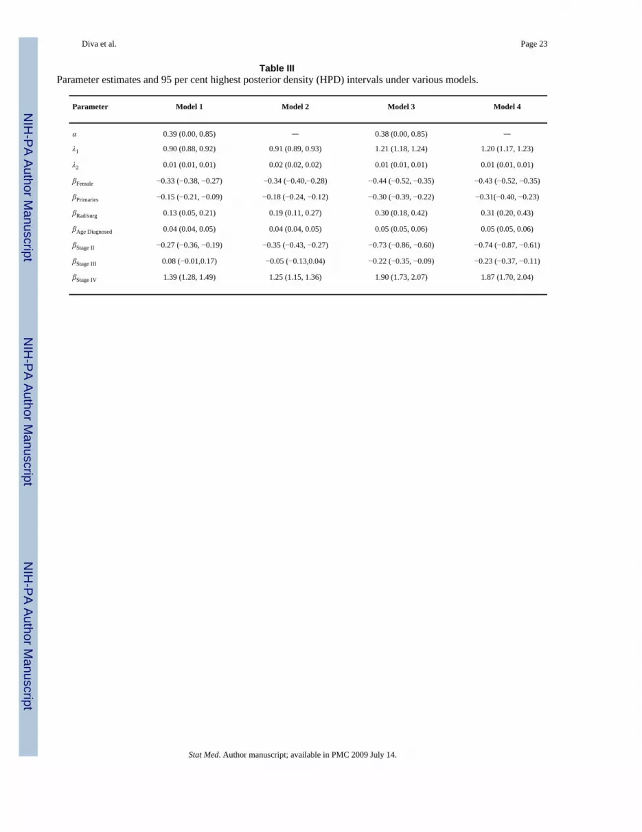
000 post-burnin samples were summarized using the Bayesian output analysis program [29]and are presented in Table III.

It can be observed from Table III that the parameter estimates are consistent across the differentmodels, which should give additional support to the modeling framework. For the PH models,the regression terms contribute to the increase or decrease in the hazard rate. The negativecoefficients for gender suggest that the relative risk of dying is significantly lower in womenthan in men. This finding is consistent with the estimated mortality rates presented in the SEERcancer statistics review [30] as well as in the results of DBD. The number of primary cancershas a significant negative coefficient, which indicates a lowering of hazard rate as more primarycancers are observed. The same phenomenon has been observed in DBD, where they notedthat this variable is post hoc in the sense that one does not know how many primaries the patientwill develop in the beginning, hence could not be taken as a prognostic factor. An interestingfinding is the increased risk for those who received site-specific radiation and/or surgery(positive regression coefficient). Upon further investigation we found out that more advancedstage (Stages III and IV) cancer cases tend to receive radiation and/or surgery (21.07 per cent,s.e.= 0.01 per cent) compared with early stage (Stages I and II) cancer cases (18.44 per cent,s.e.= 0.01 per cent). In addition, for early-stage cancer cases the risk of dying given a site-specific radiation/surgery was performed is 37.10 per cent (s.e.= 0.02 per cent) compared with56.48 per cent (s.e.= 0.02 per cent) for cases in the advanced stages. This suggests that thosereceiving radiation and/or surgery already have a higher risk of dying to start with. It is alsoworth mentioning that the relative risk of failure increases with age as indicated by the positiveregression coefficient.

For the PO model, similar interpretations of the regression parameter estimates can be madealthough the regression terms now affect the odds of failure. From Model 3, for instance, the−0.44 coefficient for gender suggests that the odds of failure at any time is significantly lowerfor females than males by a factor of 0.64 (= failure odds ratio). A similar finding is observedfor a number of primary cancers with a failure odds ratio (>2 νs = 2) of 0.74. An increase inodds of failure is noted for cases who underwent site-specific radiation/surgery compared withthose who did not. An increase in the odds of failure with older age (1.05 times for each unitincrease in age) is observed. Note that the estimate does not depend on the unit of age whilein the PH model a unit change results in the re-scaling of the estimate.

We employed two approaches to evaluate the performance of the proposed models, the first ofwhich is the conditional predictive ordinate (CPO) with the average log-marginal pseudo-likelihood (ALMPL). Roughly speaking, the CPO statistic is a Bayesian criterion that is usedto evaluate how well the model predicts a particular observation given the rest of the data.Following Gelfand and Dey [31], the CPO statistic for the (i jk)th case is given by

(9)

where Di jk=(i jk)th observation, xi jk is the corresponding covariate vector, D(−i jk) is the datawithout the (i jk)th observation, D is the complete data, and Θ is the collection of parameters.The four models under consideration have very similar expressions for the CPO statistic, exceptfor the presence of additional terms in the MCAR(α,Λ) models and the actual expressions ofthe likelihood contribution. The CPO expression for each model is as follows:

Diva et al. Page 8

Stat Med. Author manuscript; available in PMC 2009 July 14.

NIH

-PA Author Manuscript

NIH

-PA Author Manuscript

NIH

-PA Author Manuscript

where Di jk = {ti jk, δi j; k ∈ Cii, j)}, f (Di jk|xi jk, Zm, Θm) is the corresponding likelihoodcontribution, g(Zm|D,Θm) is the full conditional distribution of the frailties, and π(Θm|D) is theposterior distribution of the parameters. For the MCAR(α,Λ) models (m = 1,3), Zm = {νk, φik;k ∈ C(i, j)} and Θm = (β,λ1, λ2, Λ, α). For the non-spatial models (m = 2,4), Zm = {νk; k ∈C(i, j)} and Θm = (β,λ1, λ2, Λ). The integrals given above cannot be obtained in closed formand hence were evaluated using Monte Carlo integration. For each model, the ALMPL (overthe total number of cases) was used as an overall measure of model fit and was calculated as

where n is the total number of cases. Larger values of ALMPL indicate better model fit. Thecalculated ALMPL values are notably close for the four models (−3.99, − 3.88, − 3.92, and −3.90 for Model 1, Model 2, Model 3, and Model 4, respectively). A similar finding could benoted from the boxplots of the {log(CPOi jk)} (Figure 3). The boxplots are exhibiting verysimilar distributions except for a couple of extreme values in Model 1. It appears that the CPOstatistic was not capable of distinguishing between the proposed parametric models, whichleads us to consider another method for evaluating the fit of the model.

One of the classical approaches in evaluating the goodness of fit of a parametric survival modelis using the Cox–Snell residuals. The Cox–Snell residuals are essentially the cumulative hazardrates based on the fitted model and are expected to follow a standard exponential distributionif the model is adequate [20]. However, in this particular application, we need to take intoaccount the presence of the frailty terms. Hence, we define conditional (on the realized frailties)Cox–Snell residuals as

where H is the cumulative hazard function evaluated at ti jk given the covariates, frailties, andthe model parameters. It can be argued that the observed frailty terms, Zm, merely contributeconstant terms to the shape parameter and hence we would expect the same properties as theclassical Cox–Snell residuals. The quantile plots of the conditional Cox–Snell residuals againstthe unit exponential distribution (not shown) suggest that of the four models, the PH modelwith the MCAR(α,Λ) spatial frailties is the most adequate. The other three models havedistributions with much lighter tails than the unit exponential indicating a lack of fit. However,since some of the survival times are censored, there is potential censoring of the Cox–Snellresiduals as well. A more appropriate presentation is the plot of the distribution functions basedon the Cox–Snell residuals vs the distribution function of a standard exponential distribution(Figure 4). The residuals from the four models appear to have lighter left tails than that of theexponential. Further investigation shows that a higher percentage of the residuals from cancertypes with sparse data (stomach, small intestine, gall bladder, and pancreas) fall on the left tailsof the distribution functions than colon and rectal cancers. In addition to having lighter lefttails, models based on the log-logistic distribution (Models 3 and 4) also have lighter right tails.This suggests that the PH models (Models 1 and 2) might be more appropriate.

On the basis of the results of the model evaluation and comparison techniques, we suggest theuse of Model 1, the parametric PH model with the MCAR(α,Λ) spatial frailties, to be the finalmodel. The spatial frailties for this model are summarized in the choropleth maps (Plate 1).We could observe from the map that there is a clustering effect among adjacent counties. It

Diva et al. Page 9

Stat Med. Author manuscript; available in PMC 2009 July 14.

NIH

-PA Author Manuscript

NIH

-PA Author Manuscript

NIH

-PA Author Manuscript

should also be noted that the frailty values are not to be interpreted in absolute terms as theysimply correspond to either a decrease or an increase in relative risks in a particular countycompared with the rest. This is due to the zero-mean constraint imposed for identifiability. Thespatial frailties together with some additional data, such as hospital/healthcare facility locationsand general socioeconomic status at the county level, could augment the information availableto policymakers and researchers in assessing which factors not available in the SEER databasepotentially contribute to elevating/lowering of hazard rates.

The a priori cancer correlation matrix for the recommended model is presented in Table IV.The coefficients range from insignificant to moderate strength. The strongest correlation isbetween colon and stomach cancers (0.38) while small intestine is weakly correlated with allthe other cancers except colon. Negative correlation with the other cancers is generallyobserved for pancreatic cancer. Positive coefficients between two cancers indicate that theirhazard rates go up or down together while negative coefficients point to opposing trends in thehazard rates.

5. SUMMARY AND FUTURE WORKThis paper proposed parametric models for spatially correlated multivariate cancer survivaldata. Using data on 6 GI cancers in the state of Iowa collected from the SEER database, weillustrated that there are significant correlations between the hazard rates among the cancers.There is also evidence of spatial association across the different counties. We also note thatfor this particular data set, females have relatively lower risks of dying compared with malesand that more primary cancers result in lower hazard rate for a specific cancer. Higher (older)age at diagnosis increases the risk of failure, which may be attributed to the use of all-causemortality as endpoint. We also found that cases who received site-specific radiation and/orsurgery had higher risks compared with those who did not. This could be attributed to the factthat most of the radiation/surgery cases were already at elevated risk by being in more advancedstages.

For this particular data set, the use of parametric models is both practical and appropriate. Theproposed parametric models lend themselves to straightforward implementation and ease ofinterpretation of the parameters. Semi-parametric approaches could also be used for modelingthe baseline distributions as in DBD. Preliminary investigations comparing parametric andsemi-parametric implementations of the PH model with the MCAR(α,Λ) structure wereconducted using the colon and rectal cancer data set and recommended hazard model presentedin DBD. Although results are not presented here, we have found that the parametric modelperformed better (ALMPL= −4.03) than its semi-parametric counterpart (ALMPL= −6.03).However, a more extensive evaluation is necessary to determine under which circumstancesit would be more appropriate to use the parametric or semi-parametric implementation.

As mentioned in Section 2.4, the MCAR(α,Λ) structure may be generalized in several ways:accounting for different spatial and non-spatial cancer variance–covariance matrices, MCAR(α,ϒ); accounting for different spatial smoothness parameters for each type of cancer, MCAR((α1,…, αK), Λ); and accounting for different cancer variance–covariance patterns for eachcounty, MCAR(α,(Λ1,…, ΛI)). These extensions of the MCAR(α,Λ) model were notimplemented as they would require a more robust data set as a result of complexity. It is alsoworth mentioning that convergence problems were encountered when introducing patient-specific frailties. This is likely due to the fact that most patients in the data set were diagnosedwith only two of the 6 GI cancers studied.

A potential issue with the multivariate modeling approach presented is the identifiability ofthe dependence structure (not the model) due to the different cancers censoring each other’s

Diva et al. Page 10

Stat Med. Author manuscript; available in PMC 2009 July 14.

NIH

-PA Author Manuscript

NIH

-PA Author Manuscript

NIH

-PA Author Manuscript

survival times. A suggested remedy is to use age at diagnosis as the endpoint instead of survivaltimes. However, while both endpoints are time to event in nature and are clinically relevant,the resulting models would have very different interpretations. The question of which endpointis more appropriate and relevant is beyond the scope of this paper. Finally, while the MCARstructure provides a useful framework for modeling the dependencies, it is possible that usinga different dependence structure could give different results and model interpretation. Wetherefore recommend that caution be taken when interpreting the observed correlations.

References1. Turechek WW, Madden LV. A generalized linear modeling approach for characterizing disease

incidence in spatial hierarchy. Phytopathology 2002;93:458–466. [PubMed: 18944361]2. Ramsay T, Burnett R, Krewski D. Exploring bias in a generalized additive model for spatial air pollution

data. Environmental Health Perspectives 2003;111:1283–1288. [PubMed: 12896847]3. Lichstein JW, Simons TR, Shriner SA, Franzreb KE. Spatial autocorrelation and autoregressive models

in ecology. Ecological Monographs 2002;72(3):445–463.4. Biggeri A, Marchi M, Lagazio C, Martuzzi M, Böhning D. Nonparametric maximum likelihood

estimators for disease mapping. Statistics in Medicine 2000;19:2539–2554. [PubMed: 10960870]5. Li Y, Ryan L. Modeling spatial survival data using semiparametric frailty models. Biometrics

2002;58:287–297. [PubMed: 12071401]6. Banerjee S, Wall M, Carlin BP. Frailty modelling for spatially correlated survival data with application

to infant mortality in Minnesota. Biostatistics 2003;4:123–142. [PubMed: 12925334]7. Banerjee S, Dey DK. Semiparametric proportional odds model for spatially correlated survival data.

Lifetime Data Analysis 2005;11:175–191. [PubMed: 15938545]8. Li Y, Lin X. Semiparametric normal transformation models for spatially correlated survival data.

Journal of the American Statistical Association 2006;101:591–603.9. Heinavaara, S. PhD Thesis, University of Helsinki, Statistical Research Reports, No. 18. The Finnish

Statistical Society; 2003. Modelling survival of patients with multiple cancers.10. Sankila R, Hakulinen T. Survival of patients with colorectal carcinoma: effect of prior breast cancer.

Journal of the National Cancer Institute 1998;90:6365.11. Carlin, BP.; Banerjee, S. Hierarchical multivariate car models for spatio-temporally correlated

survival data. In: Bernardo, JM.; Bayarri, MJ.; Berger, JO.; Dawid, AP.; Heckerman, D.; Smith, AF.;West, M., editors. Bayesian Statistics. Vol. 7. Oxford University Press; Oxford: 2003. p. 45-64.

12. Diva UA, Banerjee S, Dey DK. Modeling spatially correlated survival data for individuals withmultiple cancers. Statistical Modeling 2007;7(2):1–23.

13. Mardia KV. Multidimensional multivariate Gaussian Markov random fields with application to imageprocessing. Journal of Multivariate Analysis 1998;24:45–64.

14. Gelfand AE, Vounatsou P. Proper multivariate conditional autoregressive models for spatial dataanalysis. Biostatistics 2002;4:11–25. [PubMed: 12925327]

15. Zucker DM, Yang S. Inference for a family of survival models encompassing the proportional hazardsand proportional odds model. Statistics in Medicine 2005;25:995–1014. [PubMed: 16220492]

16. Cox DR. Regression models with life tables. Journal of the Royal Statistical Society 1972;34:187–220.

17. Gelfand AE, Ghosh SK, Christiansen C, Soumerai SB, McLaughlin TJ. Proportional hazards models:a latent competing risk approach. Applied Statistics 2000;49:385–397.

18. Goetghebeur E, Ryan L. Semiparametric regression analysis of interval-censored data. Biometrics2000;56:1139–1144. [PubMed: 11129472]

19. Sinha D, Chen MH, Ghosh SK. Bayesian analysis and model selection for interval-censored survivaldata. Biometrics 1999;55:585–590. [PubMed: 11318218]

20. Klein, JP.; Moeschberger, ML. Survival Analysis: Techniques for Censored and Truncated Data.Springer; New York: 1997. p. 373-400.

21. Bennett S. Analysis of survival data by the proportional odds model. Statistics in Medicine1983;2:273–277. [PubMed: 6648142]

Diva et al. Page 11

Stat Med. Author manuscript; available in PMC 2009 July 14.

NIH

-PA Author Manuscript

NIH

-PA Author Manuscript

NIH

-PA Author Manuscript

22. Yang S, Prentice RL. Semiparametric inference in the proportional odds regression model. Journalof the American Statistical Association 1999;94:125–136.

23. Clayton DG. Some approaches to the analysis of recurrent event data. Statistics in Medical Research1995;3:244–262.

24. Jin X, Carlin BP, Banerjee S. Generalized hierarchical multivariate car models for areal data.Biometrics 2005;61:950–961. [PubMed: 16401268]

25. Gilks WR, Wild P. Adaptive rejection sampling for Gibbs sampling. Journal of the Royal StatisticalSociety, Series C 1992;41:337–348.

26. Agarwal D, Gelfand AE. Slice Gibbs sampling for simulation based fitting of spatial models. Statisticsand Computing 2005;15:61–69.

27. Neal R. Slice sampling. Annals of Statistics 2003;31(3):705–767.28. Surveillance, Epidemiology, and End Results (SEER) Program (www.seer.cancer.gov) SEER*Stat

Database: Incidence—SEER 11 Regs + AK Public-use, November 2003 Sub (1973–2001 varying).National Cancer Institute, DCCPS, Surveillance Research Program, Cancer Statistics Branch,released April 2004, based on the November 2003 submission.

29. Smith, BA. Bayesian Output Analysis Program (BOA) Version 1.1 User’s Manual. [08 August 2005].http://www.public-health.uiowa.edu/boa/

30. Ries, LAG.; Eisner, MP.; Kosary, CL.; Hankey, BF.; Miller, BA.; Clegg, L.; Mariotto, A.; Feuer, EJ.;Edwards, BK. SEER Cancer Statistics Review. National Cancer Institute; Bethesda, MD: 1975–2002.Available from: http://seer.cancer.gov/csr/19752002/ based on November 2004 SEER datasubmission, posted to the SEER Web site 2005

31. Gelfand AE, Dey DK. Bayesian model choice: asymptotics and exact calculations. Journal of RoyalStatistical Society, Series B 1994;56:501–514.

Appendix

APPENDIX

1. LemmaLet A and B be I × I and K × K matrices and let x be any vector of length I K. Then, there exista K × K matrix C and an I × I matrix D such that xT(A ⊗ B)x= tr(C B)= tr(D A).

ProofSee DBD.

2. Full conditional distributions for the PH modelsIn the succeeding expressions we let H(ti jk; xi jk, Θ) be the cumulative hazard function withparameters Θ= {λ1, λ2, β, ν, u, Φ} and D = {ti jk, δ(i, j), xi jk} be the observed data. For notational

convenience, let Σi, j,k denote and Πi, j,k denote unlessotherwise specified.

a. For λ1 with Gamma(s0, s1) prior, the full conditional distribution is given by

which can be updated using an ARS or a Metropolis step.

b. For λ2 with log-normal(μ0, ) prior, the full conditional distribution is given by

Diva et al. Page 12

Stat Med. Author manuscript; available in PMC 2009 July 14.

NIH

-PA Author Manuscript

NIH

-PA Author Manuscript

NIH

-PA Author Manuscript

which is updated using an ARS or a Metropolis step.

c. For β with prior, the full conditional distribution is given by

which is updated using an ARS or a Metropolis step.

d. For u(i, j) with independent prior, the full conditional distribution is given by

which is updated using an ARS or a Metropolis step.

e. For with IG(ai, bi) prior, the full conditional distribution is given by

where ni is the number of patients in the ith county and . This is updatedusing direct draws from its density.

f. For ν with MVN(0,Λ) prior, the full conditional distribution is given by

which is updated using an ARS or a Metropolis step.

g. For Φ with MCAR(α,Λ) prior, the full conditional distribution is given by

which is updated using an ARS or a Metropolis step.

h. For Λ with IW(r0, Λ0) prior, the full conditional distribution follows from the lemmaabove and is given by

Diva et al. Page 13

Stat Med. Author manuscript; available in PMC 2009 July 14.

NIH

-PA Author Manuscript

NIH

-PA Author Manuscript

NIH

-PA Author Manuscript

with which is updated using directdraws from its density. The derivations are omitted for brevity and the reader isreferred to DBD for details.

i. For α with U(0,1) prior, the full conditional distribution is given by

which is updated using a slice sampler outlined below:

i. Within the current state of the Gibbs sampler, let

ii. Generate U ~ U(0, f (Φ; α,Λ)).

iii. Generate α* ~ f (α).

iv. If U > f (Φ; α*,Λ) set α= α*. Otherwise, repeat Step (i).

This procedure is equivalent to a rejection sampling from the prior of α.

j. For the non-spatial PH model, the {φik}’s and α will disappear and we would need tomake the following modification to the full conditional distribution of Λ:

with which is updated using direct draws from its density.

3. Full conditional distributions for the PO models

In the succeeding expressions we let with parameters Θ= {λ1, λ2, β, ν, u, Φ} and the observed data D = {ti jk, δ(i, j), xi jk}. For notational convenience,

let Σ i, j,k denote and Πi,j,k denote unless otherwisespecified. The same expressions for the full conditional distributions were obtained for Λ andα as in the PH model and hence were omitted.

a. For λ1 with Gamma(s0, s1) prior, the full conditional distribution is given by

which can be updated using a Metropolis step.

Diva et al. Page 14

Stat Med. Author manuscript; available in PMC 2009 July 14.

NIH

-PA Author Manuscript

NIH

-PA Author Manuscript

NIH

-PA Author Manuscript

b. For λ2 with log-normal(μ0, ) prior, the full conditional distribution is given by

which is updated using a Metropolis step.

c. For &beta; with prior, the full conditional distribution is given by

which is updated using a Metropolis step.

d. For u(i, j) with independent prior, the full conditional distribution is given by

which is updated using a Metropolis step.

e. For with I G(ai, bi) prior, the full conditional distribution is given by

where ni is the number of patients in the ith county and . This is updatedusing direct draws from its density.

f. For ν with MVN(0,Λ) prior, the full conditional distribution is given by

which is updated using a Metropolis step.

g. For Φ with MCAR(αΛ) prior, the full conditional distribution is given by

which is updated using a Metropolis step.

Diva et al. Page 15

Stat Med. Author manuscript; available in PMC 2009 July 14.

NIH

-PA Author Manuscript

NIH

-PA Author Manuscript

NIH

-PA Author Manuscript

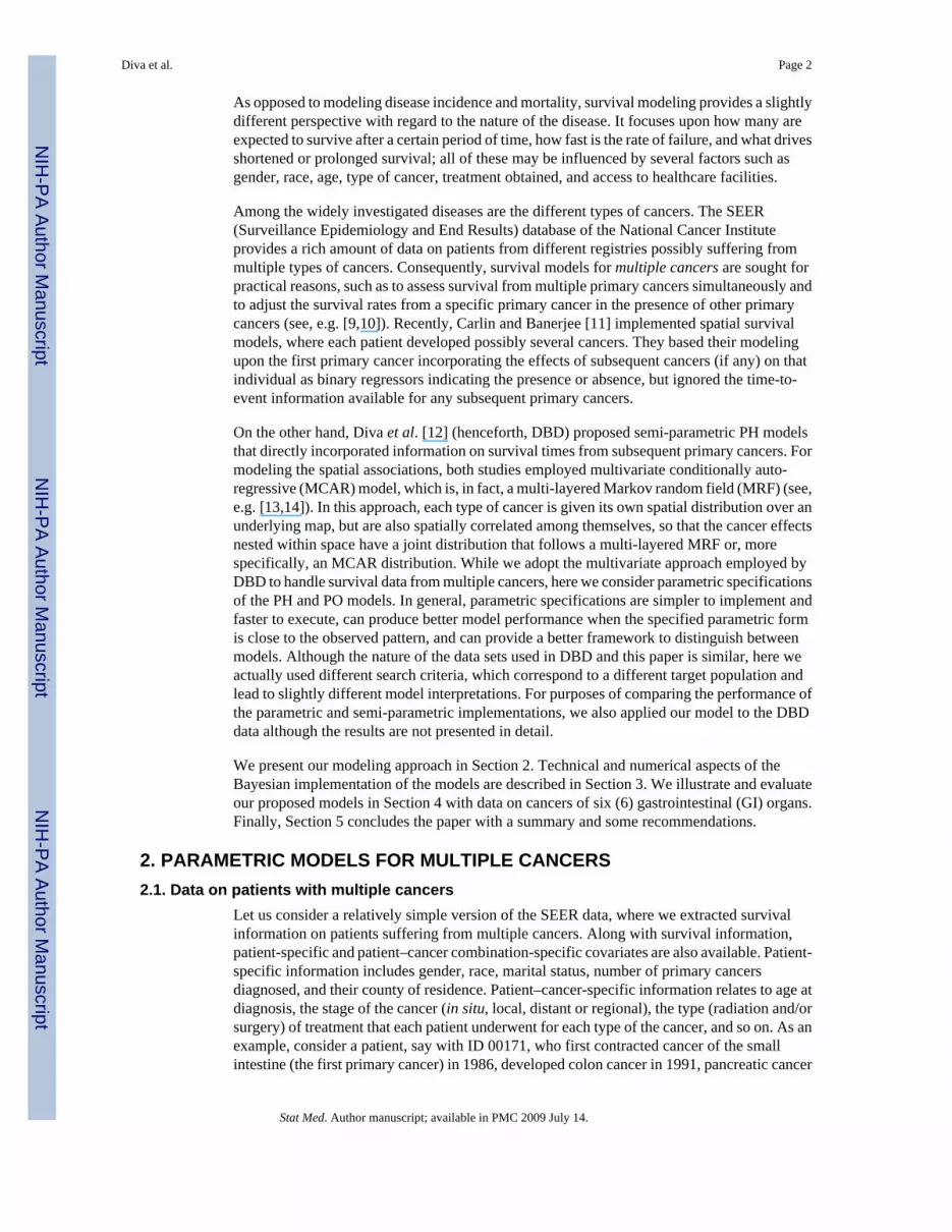
Figure 1.Kaplan–Meier plots of the survival times for the six GI cancers studied in the state of Iowa.

Diva et al. Page 16

Stat Med. Author manuscript; available in PMC 2009 July 14.

NIH

-PA Author Manuscript

NIH

-PA Author Manuscript

NIH

-PA Author Manuscript

Figure 2.Exploratory data analysis plots to check appropriateness of the Weibull (log(H)) and log-logistic (log(exp(H)−1)) distributions based on Kaplan–Meier estimates of the cumulativehazard function. The x-axes for both graphs represent the natural logarithm of the survival time.Linear trends provide support to the use of the specified distribution: (a) Weibull distribution;and (b) Log-logistic distribution.

Diva et al. Page 17

Stat Med. Author manuscript; available in PMC 2009 July 14.

NIH

-PA Author Manuscript

NIH

-PA Author Manuscript

NIH

-PA Author Manuscript

Figure 3.Boxplots of the log(CPO) for each model. Larger values of the log(CPO) indicate more supportfor the model.

Diva et al. Page 18

Stat Med. Author manuscript; available in PMC 2009 July 14.

NIH

-PA Author Manuscript

NIH

-PA Author Manuscript

NIH

-PA Author Manuscript

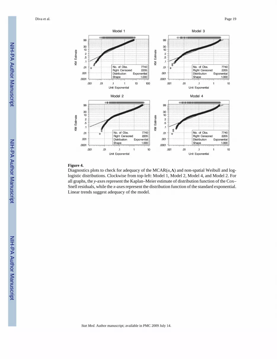
Figure 4.Diagnostics plots to check for adequacy of the MCAR(α,Λ) and non-spatial Weibull and log-logistic distributions. Clockwise from top-left: Model 1, Model 2, Model 4, and Model 2. Forall graphs, the y-axes represent the Kaplan–Meier estimate of distribution function of the Cox–Snell residuals, while the x-axes represent the distribution function of the standard exponential.Linear trends suggest adequacy of the model.

Diva et al. Page 19

Stat Med. Author manuscript; available in PMC 2009 July 14.

NIH

-PA Author Manuscript

NIH

-PA Author Manuscript

NIH

-PA Author Manuscript

Plate 1.Plots of the spatial frailties for each type of GI cancer studied based on the proportional hazardsmodel with Weibull(λ1, λ2) baseline distribution (Model 1). color change from blue to redindicates an increase from negative (lower risk) to positive frailties (higher risk). The samecutoff points were used to facilitate comparison between cancer types.

Diva et al. Page 20

Stat Med. Author manuscript; available in PMC 2009 July 14.

NIH

-PA Author Manuscript

NIH

-PA Author Manuscript

NIH

-PA Author Manuscript

NIH

-PA Author Manuscript

NIH

-PA Author Manuscript

NIH

-PA Author Manuscript

Diva et al. Page 21Ta

ble

IIll

ustra

tive

exam

ple

of d

ata

for a

pat

ient

with

mul

tiple

can

cers

.

Cou

nty

Patie

nt ID

Gen

der

No.

of p

rim

arie

sC

ance

r ty

peSt

age

Age

at d

iagn

osis

Rad

iatio

n/su

rger

ySu

rviv

al ti

me*

Stat

us

700

171

Fem

ale

3Sm

all i

ntes

tine

Dis

tant

57N

o14

3D

ead

700

171

Fem

ale

3C

olon

Loca

l63

No

78D

ead

700

171

Fem

ale

3Pa

ncre

asD

ista

nt67

Yes

25D

ead

* Surv

ival

tim

e is

giv

en in

mon

ths a

fter d

iagn

osis

.

Stat Med. Author manuscript; available in PMC 2009 July 14.

NIH

-PA Author Manuscript

NIH

-PA Author Manuscript

NIH

-PA Author Manuscript

Diva et al. Page 22

Table IIDescriptions of the four parametric models considered.

Model Model description

Model 1 Proportional hazards model with MCAR(α,Λ)

Model 2 Non-spatial proportional hazards model

Model 3 Proportional odds model with MCAR(α,Λ)

Model 4 Non-spatial proportional odds model

Stat Med. Author manuscript; available in PMC 2009 July 14.

NIH

-PA Author Manuscript

NIH

-PA Author Manuscript

NIH

-PA Author Manuscript

Diva et al. Page 23

Table IIIParameter estimates and 95 per cent highest posterior density (HPD) intervals under various models.

Parameter Model 1 Model 2 Model 3 Model 4

α 0.39 (0.00, 0.85) — 0.38 (0.00, 0.85) —

λ1 0.90 (0.88, 0.92) 0.91 (0.89, 0.93) 1.21 (1.18, 1.24) 1.20 (1.17, 1.23)

λ2 0.01 (0.01, 0.01) 0.02 (0.02, 0.02) 0.01 (0.01, 0.01) 0.01 (0.01, 0.01)

βFemale −0.33 (−0.38, −0.27) −0.34 (−0.40,−0.28) −0.44 (−0.52, −0.35) −0.43 (−0.52, −0.35)

βPrimaries −0.15 (−0.21, −0.09) −0.18 (−0.24, −0.12) −0.30 (−0.39, −0.22) −0.31(−0.40, −0.23)

βRad/surg 0.13 (0.05, 0.21) 0.19 (0.11, 0.27) 0.30 (0.18, 0.42) 0.31 (0.20, 0.43)

βAge Diagnosed 0.04 (0.04, 0.05) 0.04 (0.04, 0.05) 0.05 (0.05, 0.06) 0.05 (0.05, 0.06)

βStage II −0.27 (−0.36, −0.19) −0.35 (−0.43, −0.27) −0.73 (−0.86, −0.60) −0.74 (−0.87, −0.61)

βStage III 0.08 (−0.01,0.17) −0.05 (−0.13,0.04) −0.22 (−0.35, −0.09) −0.23 (−0.37, −0.11)

βStage IV 1.39 (1.28, 1.49) 1.25 (1.15, 1.36) 1.90 (1.73, 2.07) 1.87 (1.70, 2.04)

Stat Med. Author manuscript; available in PMC 2009 July 14.

NIH

-PA Author Manuscript

NIH

-PA Author Manuscript

NIH

-PA Author Manuscript

Diva et al. Page 24Ta

ble

IVC

orre

latio

n co

effic

ient

s (95

per

cen

t hig

hest

pos

terio

r den

sity

(HPD

) int

erva

ls) o

f the

can

cer f

railt

ies b

ased

on

the

prop

ortio

nal h

azar

dsm

odel

with

Wei

bull(λ 1

, λ2)

bas

elin

e di

strib

utio

n (M

odel

1).

Typ

eSt

omac

hSm

all i

ntes

tine

Col

onR

ectu

mG

all b

ladd

er

Smal

l int

estin

e0.

17 (0

.11,

0.24

)—

——

—

Col

on0.

38 (0

.26,

0.5

0)−0

.02

(−0.

08,0

.04)

——

—

Rec

tum

−0.0

1 (−

0.03

,0.0

1)0.

15 (0

.09,

0.2

2)−0

.01

(−0.

04,0

.02)

——

Gal

l bla

dder

−0.0

9 (−

0.13

, −0.

05)

0.19

(0.1

1, 0

.27)

−0.1

2 (−

0.17

, −0.

07)

0.00

(−0.

03,0

.05)

—

Panc

reas

−0.1

6 (−

0.22

, −0.

10)

−0.2

2 (−

0.29

, −0.

14)

−0.0

4 (−

0.08

,0.0

1)−0

.13

(−0.

17, −

0.08

)−0

.11

(−0.

16, −

0.06

)

Stat Med. Author manuscript; available in PMC 2009 July 14.