VarianceAnalysis of Linear SIMOModelswithSpatially

CorrelatedNoise ?

Niklas Everitt a, Giulio Bottegal a, Cristian R. Rojas a, Hakan Hjalmarsson a

aACCESS Linnaeus Center, School of Electrical Engineering, KTH - Royal Institute of Technology, Sweden

Abstract

Substantial improvement in accuracy of identified linear time-invariant single-input multi-output (SIMO) dynamical models ispossible when the disturbances affecting the output measurements are spatially correlated. Using an orthogonal representationfor the modules composing the SIMO structure, in this paper we show that the variance of a parameter estimate of a moduleis dependent on the model structure of the other modules, and the correlation structure of the disturbances. In addition, wequantify the variance-error for the parameter estimates for finite model orders, where the effect of noise correlation structure,model structure and signal spectra are visible. From these results, we derive the noise correlation structure under which thementioned model parameterization gives the lowest variance, when one module is identified using less parameters than theother modules.

Key words: System identification, Asymptotic variance, Linear SIMO models, Least-squares.

1 Introduction

Recently, system identification in dynamic networks hasgained popularity, see e.g., Van den Hof et al. (2013);Dankers et al. (2013b,a, 2014); Ali et al. (2011); Mat-erassi et al. (2011); Torres et al. (2014); Haber and Ver-haegen (2014); Gunes et al. (2014); Chiuso and Pil-lonetto (2012). In this framework, signals are modeledas nodes in a graph and edges model transfer functions.To estimate a transfer function in the network, a largenumber of methods have been proposed. Some have beenshown to give consistent estimates, provided that a cer-tain subset of signals is included in the identification pro-cess (Dankers et al., 2013b,a). In these methods, the userhas the freedom to include additional signals. However,little is known on how these signals should be chosen,and how large the potential is for variance reduction.From a theoretical point of view there are only a few re-sults regarding specific network structures e.g., Hagg etal. (2011); Ramazi et al. (2014); Wahlberg et al. (2009).To get a better understanding of the potential of adding

? This work was partially supported by the Swedish Re-search Council under contract 621-2009-4017, and by the Eu-ropean Research Council under the advanced grant LEARN,contract 267381.

Email addresses: everitt@kth.se (Niklas Everitt),bottegal@kth.se (Giulio Bottegal), crro@kth.se (CristianR. Rojas), hjalmars@kth.se (Hakan Hjalmarsson).

available information to the identification process, weask the fundamental questions: will, and how much, anadded sensor improve the accuracy of an estimate of acertain target transfer function in the network? We shallattempt to give some answers by focusing on a specialcase of dynamic networks, namely single-input multi-output (SIMO) systems, and in a wider context, dynamicnetworks.

SIMO models are interesting in themselves. They findapplications in various disciplines, such as signal pro-cessing and speech enhancement (Benesty et al., 2005),(Doclo and Moonen, 2002), communications (Bertauxet al., 1999), (Schmidt, 1986), (Trudnowski et al., 1998),biomedical sciences (McCombie et al., 2005) and struc-tural engineering (Ulusoy et al., 2011). Some of these ap-plications are concerned with spatio-temporal models,in the sense that the measured output can be strictly re-lated to the location at which the sensor is placed (Sto-ica et al., 1994), (Viberg et al., 1997), (Viberg and Ot-tersten, 1991). In these cases, it is reasonable to expectthat measurements collected at locations close to eachother are affected by disturbances of the same nature. Inother words, noise on the outputs can be correlated; un-derstanding how this noise correlation affects the accu-racy of the estimated model is a key issue in data-drivenmodeling of SIMO systems.

For SIMO systems, our aim in this contribution is to

Preprint submitted to Automatica 26 January 2015

arX

iv:1

501.

0307

7v1

[cs

.SY

] 1

3 Ja

n 20

15

quantify the model error induced by stochastic distur-bances and noise in prediction error identification. Weconsider the situation where the true system can accu-rately be described by the model, i.e., the true systemlies within the set of models used, and thus the bias(systematic) error is zero. Then, the model error mainlyconsists of the variance-error, which is caused by distur-bances and noise when the model is estimated using afinite number of input-output samples. In particular, weshall quantify the variance error in terms of the noisecovariance matrix, input spectrum and model structure.These quantities are also crucial in answering the ques-tions we have posed above, namely, when and how much,adding a sensor pays off in terms of accuracy of the es-timated target transfer function.

There are expressions for the model error, in terms ofthe asymptotic (in sample size) (co-) variance of theestimated parameters, for a variety of identificationmethods for multi-output systems (Ljung, 1999),(Ljungand Caines, 1980). Even though these expressions cor-respond to the Cramer-Rao lower bound, they are typi-cally rather opaque, in that it is difficult to discern howthe model accuracy is influenced by the aforementionedquantities. There is a well-known expression for the vari-ance of an estimated frequency response function thatlends itself to the kind of analysis we wish to facilitate(Ljung, 1985; Yuan and Ljung, 1984; Zhu, 1989). Thisformula is given in its SIMO version by (see e.g., Zhu(2001))

CovG(ejω) ≈ n

NΦu(ω)−1Φv(ω), (1)

where Φu is the input spectrum and Φv is the spectrumof the noise affecting the outputs. Notice that the ex-pression is valid for large number of samples N andlarge model order n. For finite model order there aremainly results for SISO models (Hjalmarsson and Nin-ness, 2006; Ninness and Hjalmarsson, 2004, 2005a,b)and recently, multi-input-single-output (MISO) models.For MISO models, the concept of connectedness (Gev-ers et al., 2006) gives conditions on when one input canhelp reduce the variance of an identified transfer func-tion. These results were refined in Martensson (2007).For white inputs, it was recently shown in Ramazi etal. (2014) that an increment in the model order of onetransfer function leads to an increment in the variance ofanother estimated transfer function only up to a point,after which the variance levels off. It was also quan-tified how correlation between the inputs may reducethe accuracy. The results presented here are similarin nature to those in Ramazi et al. (2014), while theyregard another special type of multi-variable models,namely multi-input single-output (MISO) models. Notethat variance expressions for the special case of SIMOcascade structures are found in Wahlberg et al. (2009),Everitt et al. (2013).

1.1 Contribution of this paper

As a motivation, let us first introduce the following twooutput example. Consider the model:

y1(t) = θ1,1u(t− 1) + e1(t),

y2(t) = θ2,2u(t− 2) + e2(t),

where the input u(t) is white noise and ek, k = 1, 2 ismeasurement noise. We consider two different types ofmeasurement noise (uncorrelated with the input). In thefirst case, the noise is perfectly correlated, let us for sim-plicity assume that e1(t) = e2(t). For the second case,e1(t) and e2(t) are independent. It turns out that in thefirst case we can perfectly recover the parameters θ1,1and θ2,2, while, in the second case we do not improve theaccuracy of the estimate of θ1,1 by also using the mea-surement y2(t). The reason for this difference is that, inthe first case, we can construct the noise free equation

y1(t)− y2(t) = θ1,1u(t− 1)− θ2,2u(t− 2)

and we can perfectly recover θ1,1 and θ2,2, while in thesecond case neither y2(t) nor e2(t) contain informationabout e1(t).

Also the model structure plays an important role for thebenefit of the second sensor. To this end, we considera third case, where again e1(t) = e2(t). This time, themodel structure is slightly different:

y1(t) = θ1,1u(t− 1) + e1(t),

y2(t) = θ2,1u(t− 1) + e2(t).

In this case, we can construct the noise free equation

y1(t)− y2(t) = (θ1,1 − θ2,2)u(t− 1).

The fundamental difference is that now only the differ-ence (θ1,1 − θ2,1) can be recovered exactly, but not theparameters θ1,1 and θ2,1 themselves. They can be identi-fied from y1(t) and y2(t) separately, as long as y1 and y2are measured. A similar consideration is made in Ljunget al. (2011), where SIMO cascade systems are consid-ered.

This paper will generalize these observations in the fol-lowing contributions:

• We provide novel expressions for the variance-errorof an estimated frequency response function of aSIMO linear model in orthonormal basis form, orequivalently, in fixed denominator form (Ninness etal., 1999). The expression reveals how the noise cor-relation structure, model orders and input varianceaffect the variance-error of the estimated frequencyresponse function.

2

• For a non-white input spectrum, we show where inthe frequency spectrum the benefit of the correla-tion structure is focused.

• When one module, i.e., the relationship between theinput and one of the outputs, is identified using lessparameters, we derive the noise correlation struc-ture under which the mentioned model parameter-ization gives the lowest total variance.

The paper is organized as follows: in Section 2 we definethe SIMO model structure under study and provide anexpression for the covariance matrix of the parameterestimates. Section 3 contains the main results, namelya novel variance expression for LTI SIMO orthonormalbasis function models. The connection with MISO mod-els is explored in Section 4. In Section 5, the main resultsare applied to a non–white input spectrum. In section 6we derive the correlation structure that gives the mini-mum total variance, when one block has less parametersthan the other blocks. Numerical experiments illustrat-ing the application of the derived results are presented inSection 7. A final discussion ends the paper in Section 8.

2 Problem Statement

G1(q) Σ

e1(t) y1(t)

...u(t)

Gk(q) Σ

ek(t) yk(t)

...

Gm(q) Σ

em(t) ym(t)

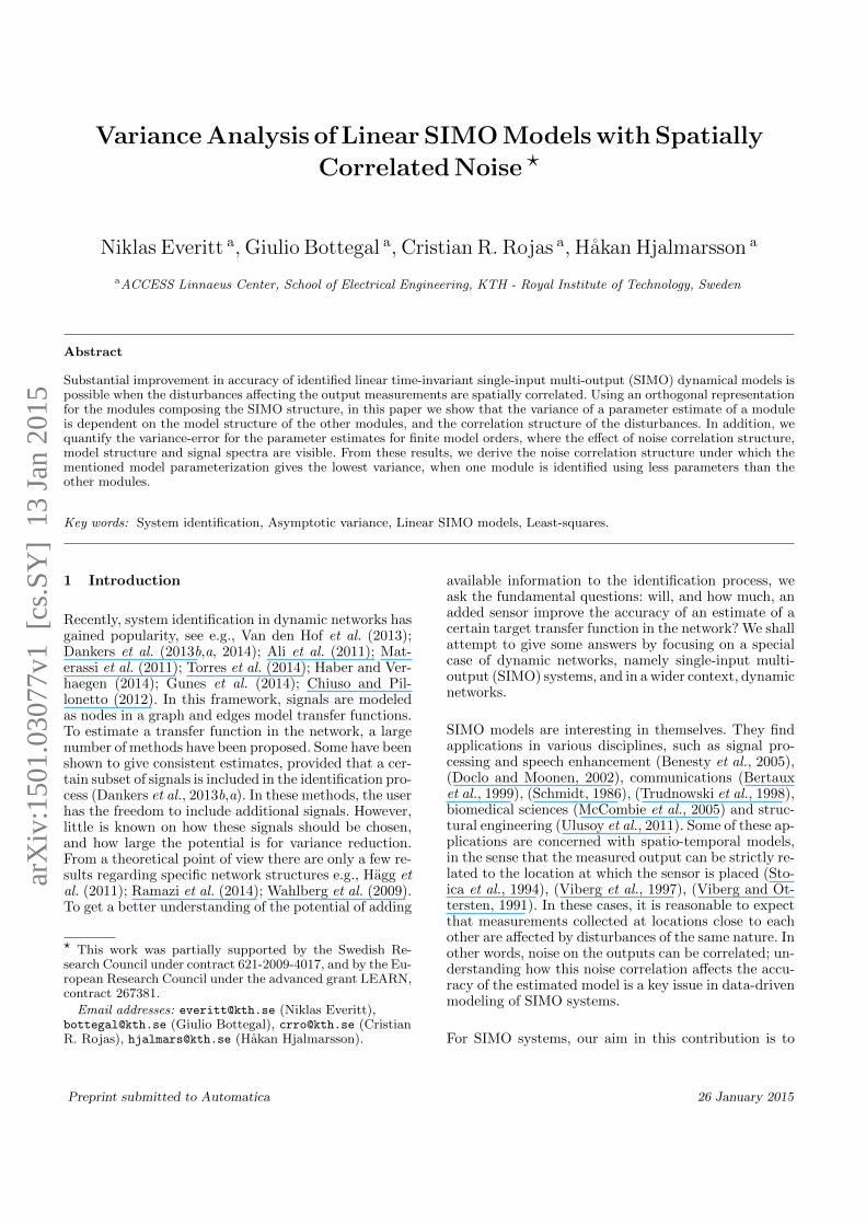
Fig. 1. Block scheme of the linear SIMO system.

We consider linear time-invariant dynamic systems withone input and m outputs (see Fig. 1). The model is de-scribed as follows:

y1(t)

y2(t)...

ym(t)

=

G1(q)

G2(q)...

Gm(q)

u(t) +

e1(t)

e2(t)...

em(t)

, (2)

where q denotes the forward shift operator, i.e., qu(t) =u(t+1) and the Gi(q) are causal stable rational transferfunctions. The Gi are modeled as

Gi(q, θi) = Γi(q)θi, θi ∈ Rni, i = 1, . . . ,m, (3)

where n1 ≤ . . . ≤ nm and Γi(q) =[B1(q), . . . ,Bni

(q)],

for some orthonormal basis functions {Bk(q)}nm

k=1. Or-thonormal with respect to the scalar product defined forcomplex functions f(z), g(z) : C → C1×m as 〈f, g〉 :=12π

∫ π−πf(eiω)g∗(eiω) dω. Let us introduce the vector no-

tation

y(t) :=

y1(t)

y2(t)...

ym(t)

, e(t) :=

e1(t)

e2(t)...

em(t)

.

The noise sequence {e(t)} is zero mean and temporallywhite, but may be correlated in the spatial domain:

E [e(t)] = 0

E[e(t)e(s)T

]= δt−sΛ (4)

for some positive definite matrix covariance matrix Λ,and where E [·] is the expected value operator. We ex-press Λ in terms of its Cholesky factorization

Λ = ΛCHΛTCH , (5)

where ΛCH ∈ Rm×m is lower triangular, i.e.,

ΛCH =

γ11 0 . . . 0

γ21 γ22 . . . 0... . . .

. . . 0

γm1 γm2 . . . γmm

(6)

for some {γij}. Also notice that since Λ > 0,

Λ−1 = Λ−TCHΛ−1CH . (7)

We summarize the assumptions on input, noise andmodel as follows:

Assumption 1 The input {u(t)} is zero mean station-ary white noise with finite moments of all orders, andvariance σ2 > 0. The noise {e(t)} is zero mean and tem-porally white, i.e, (4) holds with Λ > 0, a positive def-inite matrix. It is assumed that E

[|e(t)|4+ρ

]< ∞ for

some ρ > 0. The data is generated in open loop, that is,the input {u(t)} is independent of the noise {e(t)}. Thetrue input-output behavior of the data generating systemcan be captured by our model, i.e the true system can bedescribed by (2) and (3) for some parameters θoi ∈ Rni ,i = 1, . . . ,m, where n1 ≤ . . . ≤ nm. The orthonormalbasis functions {Bk(q)} are assumed stable. 2

Remark 2 Generalization of the model structure:

3

• The assumption that the modules have the same or-thogonal parameterization in (3) is less restrictivethan it might appear at first glance, and made forclarity and ease of presentation. A model consist-ing of non-orthonormal basis functions can be trans-formed into this format by a linear transformation,which can be computed by the Gram-Schmidt proce-dure (Trefethen and Bau, 1997). Notice that fixeddenominator models, with the same denominator inall transfer functions, also fit this framework (Nin-ness et al., 1999). However, it is essential for ouranalysis that the modules share poles.

• It is not necessary to restrict the input to bewhite noise. A colored input introduces a weight-ing by its spectrum Φu, which means that thebasis functions need to be orthogonal with re-spect to the inner product 〈f, g〉Φu

:= 〈fΦu, g〉.If Φu(z) = σ2R(z)R∗(z), where R(z) is a monicstable minimum phase spectral factor; the trans-formation Γi(q) = σ−1R(q)−1Γi(q) is a procedurethat gives a set of orthogonal basis functions in theweighted space. If we use this parameterization, allthe main results of the paper carry over naturally.However, in general, the new parameterization doesnot contain the same set of models as the originalparameterization. Another way is to use the Gram-Schmidt method, which maintains the same modelset and the main results are still valid. If we wouldlike to keep the original parameterization, we may,in some cases, proceed as in Section 5 where theinput signal is generated by an AR-spectrum.

• Note that the assumption that n1 ≤ . . . ≤ nm is notrestrictive as it only represents an ordering of themodules in the system.

2.1 Weighted least-squares estimate

By introducing θ =[θT1 , . . . , θ

Tm

]T∈ Rn, n :=

∑mi=1 ni

and the n×m transfer function matrix

Ψ(q) =

Γ1 0 0

0. . . 0

0 0 Γm

,we can write the model (2) as a linear regression model

y(t) = ϕT (t)θ + e(t), (8)

where

ϕT (t) = Ψ(q)Tu(t).

An unbiased and consistent estimate of the parametervector θ can be obtained from weighted least-squares,with optimal weighting matrix Λ−1 (see, e.g., Ljung

(1999); Soderstrom and Stoica (1989)). Λ is assumedknown, however, this assumption is not restrictive sinceΛ can be estimated from data. The estimate of θ is givenby

θN =

(N∑t=1

ϕ(t)Λ−1ϕT (t)

)−1 N∑t=1

ϕ(t)Λ−1y(t). (9)

Inserting (8) in (9) gives

θN = θ +

(N∑t=1

ϕ(t)Λ−1ϕT (t)

)−1 N∑t=1

ϕ(t)Λ−1e(t).

Under Assumption 1, the noise sequence is zero mean,hence θN is unbiased. It can be noted that this is thesame estimate as the one obtained by the prediction er-ror method and, if the noise is Gaussian, by the max-imum likelihood method (Ljung, 1999). It also followsthat the asymptotic covariance matrix of the parameterestimates is given by

AsCov θN =(E[ϕ(t)Λ−1ϕT (t)

])−1. (10)

Here AsCov θN is the asymptotic covariance matrixof the parameter estimates, in the sense that theasymptotic covariance matrix of a stochastic sequence{fN}∞N=1, fN ∈ C1×q is defined as 1

AsCov fN := limN→∞

N · E [(fN − E [fN ])∗(fN − E [fN ])].

In the problem we consider, using Parseval’s formulaand (7), the asymptotic covariance matrix, (10), can bewritten as 2

AsCov θN =

[1

2π

∫ π

−πΨ(ejω)Ψ∗(ejω) dω

]−1= 〈Ψ, Ψ〉−1, (11)

where

Ψ(q) =1

σΨ(q)Λ−TCH . (12)

Note that Ψ(q) is block upper triangular since Ψ(q) is

block diagonal and Λ−TCH is upper triangular.

1 This definition is slightly non-standard in that the secondterm is usually conjugated. For the standard definition, ingeneral, all results have to be transposed, however, all resultsin this paper are symmetric.2 Non-singularity of 〈Ψ, Ψ〉 usually requires parameter iden-tifiability and persistence of excitation (Ljung, 1999).

4

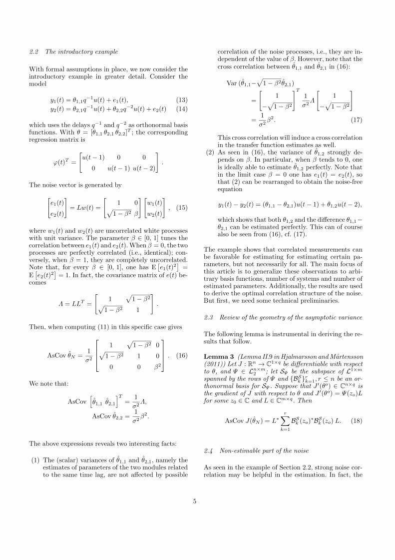
2.2 The introductory example

With formal assumptions in place, we now consider theintroductory example in greater detail. Consider themodel

y1(t) = θ1,1q−1u(t) + e1(t), (13)

y2(t) = θ2,1q−1u(t) + θ2,2q

−2u(t) + e2(t) (14)

which uses the delays q−1 and q−2 as orthonormal basisfunctions. With θ = [θ1,1 θ2,1 θ2,2]T ; the correspondingregression matrix is

ϕ(t)T =

[u(t− 1) 0 0

0 u(t− 1) u(t− 2)

].

The noise vector is generated by[e1(t)

e2(t)

]= Lw(t) =

[1 0√

1− β2 β

][w1(t)

w2(t)

], (15)

where w1(t) and w2(t) are uncorrelated white processeswith unit variance. The parameter β ∈ [0, 1] tunes thecorrelation between e1(t) and e2(t). When β = 0, the twoprocesses are perfectly correlated (i.e., identical); con-versely, when β = 1, they are completely uncorrelated.Note that, for every β ∈ [0, 1], one has E

[e1(t)2

]=

E[e2(t)2

]= 1. In fact, the covariance matrix of e(t) be-

comes

Λ = LLT =

[1

√1− β2√

1− β2 1

].

Then, when computing (11) in this specific case gives

AsCov θN =1

σ2

1

√1− β2 0√

1− β2 1 0

0 0 β2

. (16)

We note that:

AsCov[θ1,1 θ2,1

]T=

1

σ2Λ,

AsCov θ2,2 =1

σ2β2.

The above expressions reveals two interesting facts:

(1) The (scalar) variances of θ1,1 and θ2,1, namely theestimates of parameters of the two modules relatedto the same time lag, are not affected by possible

correlation of the noise processes, i.e., they are in-dependent of the value of β. However, note that thecross correlation between θ1,1 and θ2,1 in (16):

Var (θ1,1−√

1− β2θ2,1)

=

[1

−√

1− β2

]T1

σ2Λ

[1

−√

1− β2

]=

1

σ2β2. (17)

This cross correlation will induce a cross correlationin the transfer function estimates as well.

(2) As seen in (16), the variance of θ1,2 strongly de-pends on β. In particular, when β tends to 0, oneis ideally able to estimate θ1,2 perfectly. Note thatin the limit case β = 0 one has e1(t) = e2(t), sothat (2) can be rearranged to obtain the noise-freeequation

y1(t)− y2(t) = (θ1,1 − θ2,1)u(t− 1) + θ1,2u(t− 2),

which shows that both θ1,2 and the difference θ1,1−θ2,1 can be estimated perfectly. This can of coursealso be seen from (16), cf. (17).

The example shows that correlated measurements canbe favorable for estimating for estimating certain pa-rameters, but not necessarily for all. The main focus ofthis article is to generalize these observations to arbi-trary basis functions, number of systems and number ofestimated parameters. Additionally, the results are usedto derive the optimal correlation structure of the noise.But first, we need some technical preliminaries.

2.3 Review of the geometry of the asymptotic variance

The following lemma is instrumental in deriving the re-sults that follow.

Lemma 3 (Lemma II.9 in Hjalmarsson and Martensson(2011)) Let J : Rn → C1×q be differentiable with respectto θ, and Ψ ∈ Ln×m2 ; let SΨ be the subspace of L1×m

spanned by the rows of Ψ and {BSk }rk=1, r ≤ n be an or-thonormal basis for SΨ . Suppose that J ′(θo) ∈ Cn×q isthe gradient of J with respect to θ and J ′(θo) = Ψ(zo)Lfor some z0 ∈ C and L ∈ Cm×q. Then

AsCov J(θN ) = L∗r∑

k=1

BSk (zo)∗BSk (zo) L. (18)

2.4 Non-estimable part of the noise

As seen in the example of Section 2.2, strong noise cor-relation may be helpful in the estimation. In fact, the

5

variance error will depend on the non-estimable part ofthe noise, i.e., the part that cannot be linearly estimatedfrom other noise sources. To be more specific, define thesignal vector ej\i(t) to include the noise sources frommodule 1 to module j, with the one from module i ex-cluded, i.e.,

ej\i(t) :=

[e1(t), . . . , ej(t)

]Tj < i,[

e1(t), . . . , ei−1(t)]T

j = i,[e1(t), . . . , ei−1(t), ei+1(t), . . . , ej(t)

]Tj > i.

Now, the linear minimum variance estimate of ei givenej\i(t), is given by

ei|j(t) := %Tijej\i(t). (19)

Introduce the notation

λi|j := Var [ei(t)− ei|j(t)], (20)

with the convention that λi|0 := λi. The vector %ij in(19) is given by

%ij =[Cov ej\i(t)

]−1E[ej\i(t)ei(t)

].

We call

ei(t)− ei|j(t)

the non-estimable part of ei(t) given ej\i(t).

Definition 4 When ei|j(t) does not depend on ek(t),where 1 ≤ k ≤ j, k 6= i, we say that ei(t) is orthogonalto ek(t) conditionally to ej\i(t).

The variance of the non-estimable part of the noise isclosely related to the Cholesky factor of the covariancematrix Λ. We have the following lemma.

Lemma 5 Let e(t) ∈ Rm have zero mean and covari-ance matrix Λ > 0. Let ΛCH be the lower triangularCholesky factor of Λ, i.e., ΛCH satisfies (5), with {γik}as its entries as defined by (6). Then for j < i,

λi|j =

i∑k=j+1

γ2ik.

Furthermore, γij = 0 is equivalent to that ei(t) is orthog-onal to ej(t) conditionally to ej\i(t).

PROOF. See Appendix A. �

Similar to the above, for i ≤ m, we also define

ei:m(t) :=[ei(t) . . . em(t)

]T,

and for j < i we define ei:m|j(t) as the linear minimumvariance estimate of ei:m(t) based on the other signalsej\i(t), and

Λi:m|j := Cov [ei:m(t)− ei:m|j(t)].

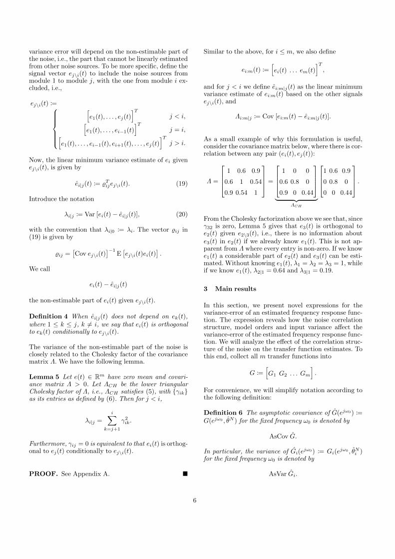
As a small example of why this formulation is useful,consider the covariance matrix below, where there is cor-relation between any pair (ei(t), ej(t)):

Λ =

1 0.6 0.9

0.6 1 0.54

0.9 0.54 1

=

1 0 0

0.6 0.8 0

0.9 0 0.44

︸ ︷︷ ︸

ΛCH

1 0.6 0.9

0 0.8 0

0 0 0.44

.

From the Cholesky factorization above we see that, sinceγ32 is zero, Lemma 5 gives that e3(t) is orthogonal toe2(t) given e2\3(t), i.e., there is no information aboute3(t) in e2(t) if we already know e1(t). This is not ap-parent from Λ where every entry is non-zero. If we knowe1(t) a considerable part of e2(t) and e3(t) can be esti-mated. Without knowing e1(t), λ1 = λ2 = λ3 = 1, whileif we know e1(t), λ2|1 = 0.64 and λ3|1 = 0.19.

3 Main results

In this section, we present novel expressions for thevariance-error of an estimated frequency response func-tion. The expression reveals how the noise correlationstructure, model orders and input variance affect thevariance-error of the estimated frequency response func-tion. We will analyze the effect of the correlation struc-ture of the noise on the transfer function estimates. Tothis end, collect all m transfer functions into

G :=[G1 G2 . . . Gm

].

For convenience, we will simplify notation according tothe following definition:

Definition 6 The asymptotic covariance of G(ejω0) :=G(ejω0 , θN ) for the fixed frequency ω0 is denoted by

AsCov G.

In particular, the variance of Gi(ejω0) := Gi(e

jω0 , θNi )for the fixed frequency ω0 is denoted by

AsVar Gi.

6

Define χk as the index of the first system that contains thebasis function Bk(ejω0). Notice that χk−1 is the numberof systems that do not contain the basis function.

Theorem 7 Let Assumption 1 hold. Suppose that theparameters θi ∈ Rni , i = 1, . . . ,m, are estimated usingweighted least-squares (9). Let the entries of θ be arrangedas follows:

θ = [θ1,1 . . . θm,1 θ1,2 . . . θm,2 . . . θ1,n1 . . .

. . . θm,n1θ2,n1+1 . . . θm,n1+1 . . . θm,nm

]T. (21)

and the corresponding weighted least-squares estimate be

denoted by ˆθ. Then, the covariance of ˆθ is

AsCov ˆθ =1

σ2diag(Λ1:m, Λχ2:m|χ2−1, . . . ,

. . . , Λχnm :m|χnm−1). (22)

In particular, the covariance of the parameters related tobasis function number k is given by

AsCov ˆθk =1

σ2Λχk:m|χk−1, (23)

where

ˆθk =[θχk,k . . . θm,k

]T,

and where, for χk ≤ i ≤ m,

AsVar θi,k =λi|χk−1σ2

. (24)

It also holds that

AsCov G =

nm∑k=1

[0χk−1 0

0 AsCov ˆθk

]|Bk(ejω0)|2, (25)

where AsCov ˆθk is given by (23) and 0χk−1 is a χk −1 × χk − 1 matrix with all entries equal to zero. Forχk = 1, 0χk−1 is an empty matrix. In (25), 0 denoteszero matrices of dimensions compatible to the diagonalblocks.

PROOF. See Appendix B. �

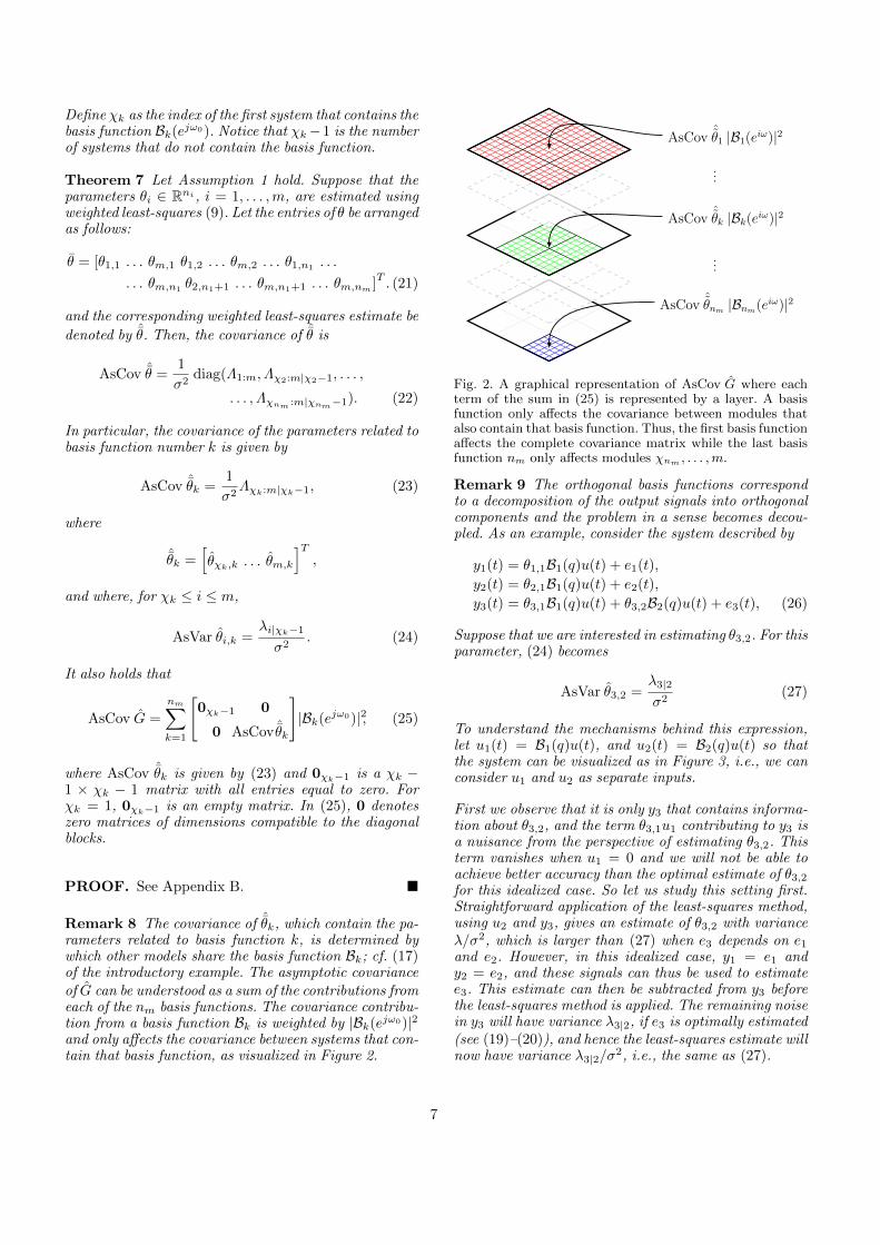
Remark 8 The covariance of ˆθk, which contain the pa-rameters related to basis function k, is determined bywhich other models share the basis function Bk; cf. (17)of the introductory example. The asymptotic covarianceof G can be understood as a sum of the contributions fromeach of the nm basis functions. The covariance contribu-tion from a basis function Bk is weighted by |Bk(ejω0)|2and only affects the covariance between systems that con-tain that basis function, as visualized in Figure 2.

AsCov ˆθ1 |B1(eiω)|2

AsCov ˆθk |Bk(eiω)|2

AsCov ˆθnm |Bnm(eiω)|2

...

...

Fig. 2. A graphical representation of AsCov G where eachterm of the sum in (25) is represented by a layer. A basisfunction only affects the covariance between modules thatalso contain that basis function. Thus, the first basis functionaffects the complete covariance matrix while the last basisfunction nm only affects modules χnm , . . . ,m.

Remark 9 The orthogonal basis functions correspondto a decomposition of the output signals into orthogonalcomponents and the problem in a sense becomes decou-pled. As an example, consider the system described by

y1(t) = θ1,1B1(q)u(t) + e1(t),

y2(t) = θ2,1B1(q)u(t) + e2(t),

y3(t) = θ3,1B1(q)u(t) + θ3,2B2(q)u(t) + e3(t), (26)

Suppose that we are interested in estimating θ3,2. For thisparameter, (24) becomes

AsVar θ3,2 =λ3|2σ2

(27)

To understand the mechanisms behind this expression,let u1(t) = B1(q)u(t), and u2(t) = B2(q)u(t) so thatthe system can be visualized as in Figure 3, i.e., we canconsider u1 and u2 as separate inputs.

First we observe that it is only y3 that contains informa-tion about θ3,2, and the term θ3,1u1 contributing to y3 isa nuisance from the perspective of estimating θ3,2. Thisterm vanishes when u1 = 0 and we will not be able toachieve better accuracy than the optimal estimate of θ3,2for this idealized case. So let us study this setting first.Straightforward application of the least-squares method,using u2 and y3, gives an estimate of θ3,2 with varianceλ/σ2, which is larger than (27) when e3 depends on e1and e2. However, in this idealized case, y1 = e1 andy2 = e2, and these signals can thus be used to estimatee3. This estimate can then be subtracted from y3 beforethe least-squares method is applied. The remaining noisein y3 will have variance λ3|2, if e3 is optimally estimated(see (19)–(20)), and hence the least-squares estimate willnow have variance λ3|2/σ2, i.e., the same as (27).

7

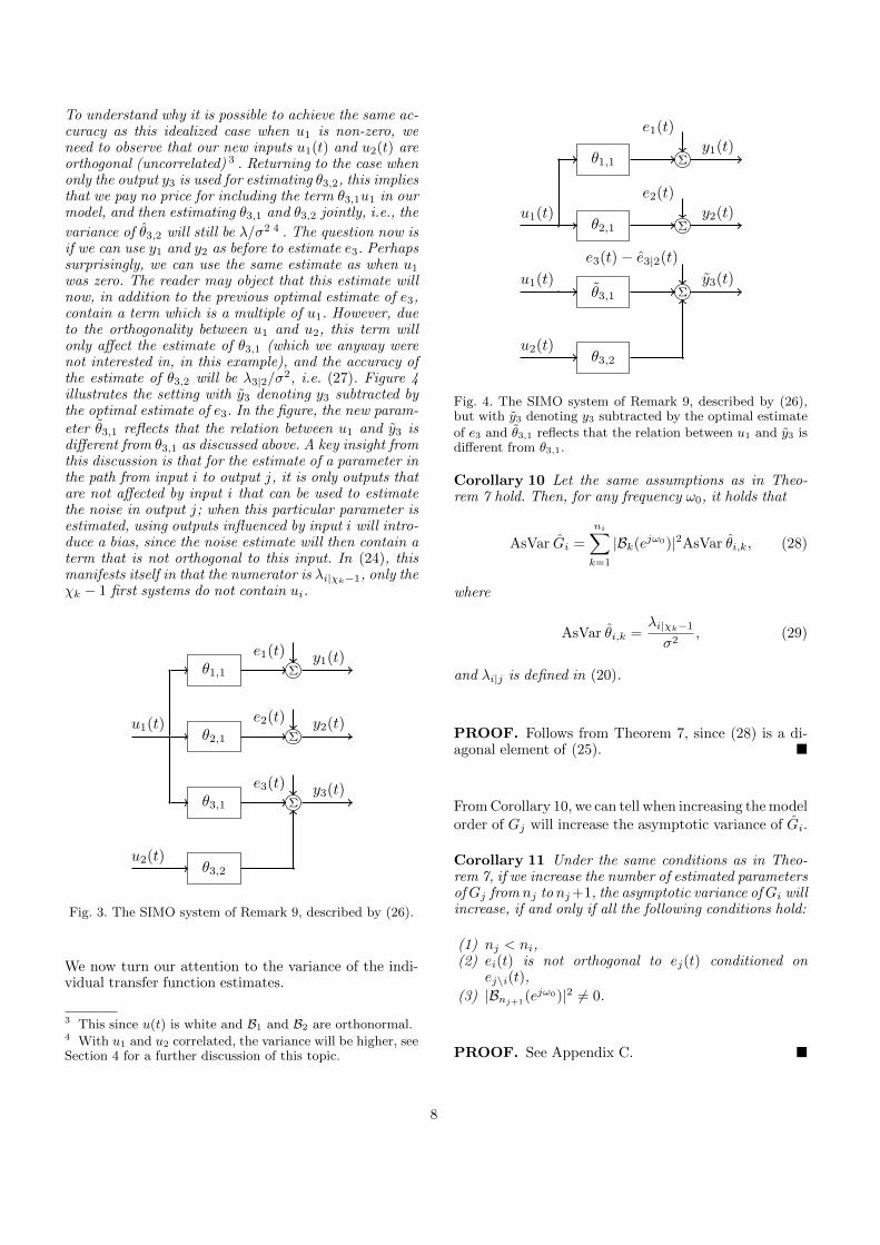
To understand why it is possible to achieve the same ac-curacy as this idealized case when u1 is non-zero, weneed to observe that our new inputs u1(t) and u2(t) areorthogonal (uncorrelated) 3 . Returning to the case whenonly the output y3 is used for estimating θ3,2, this impliesthat we pay no price for including the term θ3,1u1 in ourmodel, and then estimating θ3,1 and θ3,2 jointly, i.e., the

variance of θ3,2 will still be λ/σ2 4 . The question now isif we can use y1 and y2 as before to estimate e3. Perhapssurprisingly, we can use the same estimate as when u1was zero. The reader may object that this estimate willnow, in addition to the previous optimal estimate of e3,contain a term which is a multiple of u1. However, dueto the orthogonality between u1 and u2, this term willonly affect the estimate of θ3,1 (which we anyway werenot interested in, in this example), and the accuracy ofthe estimate of θ3,2 will be λ3|2/σ2, i.e. (27). Figure 4illustrates the setting with y3 denoting y3 subtracted bythe optimal estimate of e3. In the figure, the new param-eter θ3,1 reflects that the relation between u1 and y3 isdifferent from θ3,1 as discussed above. A key insight fromthis discussion is that for the estimate of a parameter inthe path from input i to output j, it is only outputs thatare not affected by input i that can be used to estimatethe noise in output j; when this particular parameter isestimated, using outputs influenced by input i will intro-duce a bias, since the noise estimate will then contain aterm that is not orthogonal to this input. In (24), thismanifests itself in that the numerator is λi|χk−1, only theχk − 1 first systems do not contain ui.

θ1,1 Σ

e1(t) y1(t)

u1(t)θ2,1 Σ

e2(t) y2(t)

θ3,1 Σ

e3(t) y3(t)

u2(t)θ3,2

Fig. 3. The SIMO system of Remark 9, described by (26).

We now turn our attention to the variance of the indi-vidual transfer function estimates.

3 This since u(t) is white and B1 and B2 are orthonormal.4 With u1 and u2 correlated, the variance will be higher, seeSection 4 for a further discussion of this topic.

θ1,1 Σ

e1(t)

y1(t)

u1(t)θ2,1 Σ

e2(t)

y2(t)

u1(t)θ3,1 Σ

e3(t)− e3|2(t)

y3(t)

u2(t)θ3,2

Fig. 4. The SIMO system of Remark 9, described by (26),but with y3 denoting y3 subtracted by the optimal estimateof e3 and θ3,1 reflects that the relation between u1 and y3 isdifferent from θ3,1.

Corollary 10 Let the same assumptions as in Theo-rem 7 hold. Then, for any frequency ω0, it holds that

AsVar Gi =

ni∑k=1

|Bk(ejω0)|2AsVar θi,k, (28)

where

AsVar θi,k =λi|χk−1σ2

, (29)

and λi|j is defined in (20).

PROOF. Follows from Theorem 7, since (28) is a di-agonal element of (25). �

From Corollary 10, we can tell when increasing the modelorder of Gj will increase the asymptotic variance of Gi.

Corollary 11 Under the same conditions as in Theo-rem 7, if we increase the number of estimated parametersofGj from nj to nj+1, the asymptotic variance ofGi willincrease, if and only if all the following conditions hold:

(1) nj < ni,(2) ei(t) is not orthogonal to ej(t) conditioned on

ej\i(t),(3) |Bnj+1

(ejω0)|2 6= 0.

PROOF. See Appendix C. �

8

Remark 12 Corollary 11 explicitly tells when an in-crease in the model order of Gj from nj to nj + 1 willincrease the variance of Gi. If nj ≥ ni, there will be noincrease in the variance of Gi, no matter how many ad-ditional parameters we introduce to the model Gj, whichwas also seen the introductory example in Section 2.2.Naturally, if ei(t) is orthogonal to ej(t) conditioned onej\i(t), ei|j(t) does not depend on ej(t) and there is no

increase in variance of Gi, cf. Remark 9.

3.1 A graphical representation of Corollary 11

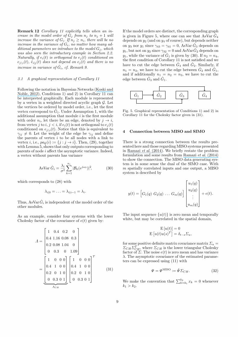
Following the notation in Bayesian Networks (Koski andNoble, 2012), Conditions 1) and 2) in Corollary 11 canbe interpreted graphically. Each module is representedby a vertex in a weighted directed acyclic graph G. Letthe vertices be ordered by model order, i.e., let the firstvertex correspond to G1. Under Assumption 1, with theadditional assumption that module i is the first modulewith order ni, let there be an edge, denoted by j → i,from vertex j to i, j < i, if ei(t) is not orthogonal to ej(t)conditioned on ej\i(t). Notice that this is equivalent toγij 6= 0. Let the weight of the edge be γij and definethe parents of vertex i to be all nodes with a link tovertex i, i.e., paG(i) := {j : j → i}. Then, (29), togetherwith Lemma 5, shows that only outputs corresponding toparents of node i affect the asymptotic variance. Indeed,a vertex without parents has variance

AsVar Gi =λiσ2

ni∑k=1

|Bk(ejω0)|2, (30)

which corresponds to (28) with

λi|0 = . . . = λi|i−1 = λi.

Thus, AsVar Gi is independent of the model order of theother modules.

As an example, consider four systems with the lowerCholesky factor of the covariance of e(t) given by:

Λ =

1 0.4 0.2 0

0.4 1.16 0.08 0.3

0.2 0.08 1.04 0

0 0.3 0 1.09

=

1 0 0 0

0.4 1 0 0

0.2 0 1 0

0 0.3 0 1

︸ ︷︷ ︸

ΛCH

1 0 0 0

0.4 1 0 0

0.2 0 1 0

0 0.3 0 1

T

(31)

If the model orders are distinct, the corresponding graphis given in Figure 5, where one can see that AsVar G4

depends on y2 (and on y4 of course), but depends neither

on y3 nor y1 since γ43 = γ41 = 0, AsVar G3 depends ony1, but not on y2 since γ32 = 0 and AsVarG2 depends ony1, while the variance of G1 is given by (30). If n2 = n4,the first condition of Corollary 11 is not satisfied and wehave to cut the edge between G4 and G2. Similarly, ifn1 = n2, we have to cut the edge between G2 and G1,and if additionally n1 = n2 = n3, we have to cut theedge between G3 and G1.

G1 G2 G3 G4

Fig. 5. Graphical representation of Conditions 1) and 2) inCorollary 11 for the Cholesky factor given in (31).

4 Connection between MISO and SIMO

There is a strong connection between the results pre-sented here and those regarding MISO systems presentedin Ramazi et al. (2014). We briefly restate the problemformulation and some results from Ramazi et al. (2014)to show the connection. The MISO data generating sys-tem is in some sense the dual of the SIMO case. Withm spatially correlated inputs and one output, a MISOsystem is described by

y(t) =[G1(q) G2(q) . . . Gm(q)

]u1(q)

u2(q)...

um(q)

+ e(t).

The input sequence {u(t)} is zero mean and temporallywhite, but may be correlated in the spatial domain,

E [u(t)] = 0

E[u(t)u(s)T

]= δt−sΣu,

for some positive definite matrix covariance matrixΣu =ΣCHΣ

TCH , where ΣCH is the lower triangular Cholesky

factor of Σ. The noise e(t) is zero mean and has varianceλ. The asymptotic covariance of the estimated parame-ters can be expressed using (11) with

Ψ = ΨMISO := ΨΣCH . (32)

We make the convention that∑k2k=k1

xk = 0 wheneverk1 > k2.

9

Theorem 13 (Theorem 4 in Ramazi et al. (2014))Under Assumption 1, but with n1 ≥ n2 ≥ . . . ,≥ nm, forany frequency ω0 it holds that

AsVar Gi =

m∑j=i

λ

σ2i|j

nj∑k=nj+1+1

|Bk(ejω0)|2, (33)

where nm+1 := 0 and σ2i|j is the variance of the non-

estimable part of ui(t) given uj\i(t).

Corollary 14 (Corollary 6 in Ramazi et al. (2014))Under Assumption 1, but with n1 ≥ n2 ≥ . . . ,≥ nm.Suppose that the order of block j is increased from nj tonj+1. Then there is an increase in the asymptotic vari-

ance of Gi if and only if all the following conditions hold:

(1) nj < ni,(2) ui(t) is not orthogonal to uj(t) conditioned on

uj\i(t),

(3) |Bnj+1(ejω0)|2 6= 0.

Remark 15 The similarities between Corollary 10 andTheorem 13, and between Corollary 11 and Corollary 14are striking. In both cases it is the non-estimable part ofthe input and noise, respectively, along with the estimatedbasis functions that are the key determinants for the re-sulting accuracy. Just as in Corollary 10, Theorem 13can be expressed with respect to the basis functions:

AsVar Gi =

ni∑k=1

AsVar θi,k |Bk(ejω0)|2. (34)

However, now

AsVar θi,k =λ

σ2i|χk

(35)

where σ2i|l is determined by the correlation structure of the

inputs ui(t) to the systems Gi(q, θi) that do share basisfunction Bk(q) (i = 1, . . . , χk). Note that in the SIMOcase we had

AsVar θi,k =λi|χk

σ2

where λi|χkis determined by the correlation structure of

the noise sources ei(t) affecting systems Gi(q, θi) thatdo not share basis function Bk(q) (i = 1, . . . , χk). Notethat (33) found in Ramazi et al. (2014) does not drawthe connection to the variance of the parameters. This ismade explicit in the alternate expressions (35) and (34).

The correlation between parameters related to the samebasis functions is not explored in Ramazi et al. (2014).In fact, it is possible to follow the same line of reasoningleading to Theorem 7 and arrive at the counter-part for

MISO systems. Let the first χk systems contain basisfunction k, so

AsVar ˆθMISOk = λ Σ−11:χk

where Σ1:χkdenotes the covariance matrix of the first

χk inputs. Hence

AsCov G = λ

n1∑k=1

[Σ−11:χk

0

0 0m−χk

]|Bk(ejω0)|2,

and

AsCov ˆθMISO = λ diag(Σ−11:χ1, Σ−11:χ2

, . . . , Σ−11:χnm). (36)

Note that, while the correlation between the noisesources is beneficial, the correlation in the input is detri-mental for the estimation accuracy. Intuitively, if we usethe same input to parallel systems, and only observe thesum of the outputs, there is no way to determine thecontribution from the individual systems. On the otherhand, as observed in the example in Section 2.2, if thenoise is correlated, we can construct equations with re-duced noise and improve the accuracy of our estimates.

This difference may also be understood from the struc-ture of Ψ , which through (11) determines the varianceproperties of any estimate. Consider a single SISO sys-tem G1 as the basic case. For the SIMO structure con-sidered in this paper, as noted before, ΨSIMO of (12) isblock upper triangular with m columns (the number ofoutputs), while ΨMISO is block lower triangular with asmany columns as inputs. ΨMISO is block lower triangu-lar since Ψ is block diagonal and ΣCH is lower triangu-lar in (32). Adding an output yj to the SIMO structurecorresponds to extending ΨSIMO with one column (andnj rows):

ΨSIMOe =

[ΨSIMO ?

0 ?

], (37)

where the zero comes from that ΨSIMOe also is block up-

per triangular. Since ΨMISO is block lower triangular,adding an input uj to the MISO structure extends ΨMISO

with nj rows (and one column):

ΨMISOe =

[ΨMISO 0

? ?

], (38)

where ? denotes the added column and added row re-spectively. Addition of columns to Ψ decreases the vari-ance ofG1, while addition of rows increases the variance.First, a short motivation of this will be given. Second,we will discuss the implication for the variance analysis.

10

Addition of one more column to Ψ in (37) decreases

the variance of G1. With Ψ =[ψ1 . . . ψm

], 〈Ψ, Ψ〉 =∑m

k 〈ψk, ψk〉, where 〈ψk, ψk〉 ≥ 0 for every k. The vari-

ance of the parameter estimate θN decreases with theaddition of a column, since

〈Ψe, Ψe〉−1 ≤ [〈ψm+1, ψm+1〉+ 〈Ψ, Ψ〉]−1 .

On the other hand, addition of rows leads to an increasein variance of G1, e.g., consider (18) in Lemma 3,

AsCov G1(θN ) = LTr∑

k=1

BSk (zo)∗BSk (zo) L,

where L = Σ−TCH

[1 0 . . . 0

]Tfor any number of inputs,

and {BSk }rk=1 is a basis for the linear span of the rows ofΨMISO. As can be seen from (38), the first rows of ΨMISO

eare the same as for ΨMISO and the first r basis functionscan therefore be taken the same (with a zero in the lastcolumn). To accommodate for the extra rows, ne extrabasis functions {BSk }r+ne

k=r+1 are needed. Thus, {BSk }r+ne

k=1

is a basis for the linear span of ΨMISOe . We see that the

variance of G1(θeN ) is larger than G1(θN ) since

AsCov G1(θeN ) = AsCov G1(θN )

+LTr+ne∑k=r+1

BSk (zo)∗BSk (zo) L,

and LTBSk (zo)∗BSk (zo)L ≥ 0 is positive semidefinite for

every k.

Every additional input of the MISO system correspondsto addition of rows to Ψ . The increase is strictly posi-tive provided that the explicit conditions in Corollary 14hold.

Every additional output of the SIMO system corre-sponds to the addition of one more column to Ψ . How-ever, the benefit of the additional columns is reduced bythe additional rows arising from the additional parame-ters that need to be estimated, cf. Corollary 11 and thepreceding discussion. When the number of additionalparameters has reached n1 or if e1(t) is orthogonal toej(t) conditioned on uj\1(t) the benefit vanishes com-pletely. The following examples clarify this point.

Example 16 We consider the same example as in Sec-tion 2.2 for three cases of model orders of the secondmodel, n2 = 0, 1, 2. These cases correspond to Ψ given bythe first n2 + 1 rows of

ΨSIMOe (q) =

q−1 −

√1− β2/βq−1

0 1/βq−1

0 1/βq−2

,

respectively. When only y1 is used (Ψ = q−1) :

AsVar θ1,1 = 〈Ψ, Ψ〉−1 = 1.

When n2 = 0, the second measurement gives a benefitdetermined by how strong the correlation is between thetwo noise sources:

AsVar θ1,1 = 〈Ψ, Ψ〉−1 = (1 + (1− β2)/β2)−1 = β2.

However, already if we have to estimate one parameterin G2 the benefit vanishes completely, i.e., for n2 = 1:

AsCov θ = 〈Ψ, Ψ〉−1 =

[1

√1− β2√

1− β2 1

].

The third case, n2 = 2, corresponds to the example inSection 2.2, which shows that the first measurement y1improves the estimate of θ2,2 (compared to only estimat-ing G2 using y2):

AsVar θ2,2 = λ2|1 = β2.

Example 17 We consider the corresponding MISO sys-tem with unit variance noise e(t) and u(t) instead havingthe same spectral factor

ΣCH =

[1 0√

1− β2 β

].

for β ∈ (0, 1]. We now study the impact of the secondinput u2(t) when

G1(q) = θ1,1q−1 + θ1,2q

−2, G2(q) =

n2∑k=1

θ2,kq−k

and n2 = 0, 1. These two cases correspond to Ψ given bythe first n2 + 2 rows of

ΨMISOe (q) =

q−1 0

q−2 0√1− β2q−1 βq−1

,respectively. When only u1 is used or G2 is known (Ψ =[q−1 q−2

]T):

AsCov θ1 = 〈Ψ, Ψ〉−1 = I.

When n2 = 1, the variance of θ1,1 is increased dependingon the correlation between the two inputs:

AsVar θ =1

β2

1 0 −

√1− β2

0 β2 0

−√

1− β2 0 1

.

11

Also notice that the asymptotic covariance of[θ1,1 θ2,1

]Tis given by Σ−1, the inverse of the covariance matrix of

u(t) and that AsVar θ2,2 = σ−11 . As β goes to zero the

variance of[θ1,1 θ2,1

]Tincreases and at β = 0 the two

inputs are perfectly correlated and we loose identifiability.

5 Effect of input spectrum

In this section we will see how a non white input spec-trum changes the results of Section 3. Using white noisefiltered through an AR-filter as input, we may use thedeveloped results to show where in the frequency rangethe benefit of the correlation structure is focused. Analternative approach, when a non-white input spectrumis used, is to change the basis functions as discussed inRemark 2. However, the effect of the input filter is in-ternalized in the basis functions and it is hard to distin-guish the effect of the input filter. We will instead useFIR basis functions for the SIMO system, which are notorthogonal with respect to the inner product induced bythe input spectrum, cf. Remark 2. We let the input filterbe given by

u(t) =1

A(q)w(t) (39)

where w(t) is a white noise sequence with variance σ2w

and the order na of A is less than the order of G1,i.e., na ≤ n1. In this case, following the derivations ofTheorem 7, it can be shown that

AsVar Gi =

ni∑k=1

AsVar θi,k|Bk(ejω0)|2 (40)

where

AsVar θi,k =λi|χk−1Φu(ω0)

and the basis functions Bk have changed due to the in-put filter. The solutions boil down to finding explicit ba-sis functions Bk for the well known case (Ninness andGustafsson, 1997) when

Span

{ΓnA(q)

}= Span

{q−1

A(q),q−2

A(q), . . . ,

q−n

A(q)

}where A(q) =

∏na

k=1(1− ξkq−1), |ξk| < 1 for some set ofspecified poles {ξ1, . . . , ξna

} and where n ≥ na. Then, itholds (Ninness and Gustafsson, 1997) that

Span

{ΓnA(q)

}= Span {B1, . . . ,Bn}

where {Bk} are the Takenaka-Malmquist functions givenby

Bk(q) :=

√1− |ξk|2q − ξk

φk−1(q), k = 1, . . . , n

φk(q) :=

k∏i=1

1− ξiqq − ξi

, φ0(q) := 1

and with ξk = 0 for k = na + 1, . . . , n. We summarizethe result in the following theorem:

Theorem 18 Let the same assumptions as in Theorem 7hold. Additionally the input u(t) is generated by an AR-filter as in (39). Then for any frequency ω0 it holds that

AsVar Gi =1

Φu(ω0)

(λi

na∑k=1

1− |ξk|2|ejω0 − ξk|2

+ λi(n1 − na)

+

i∑j=2

λi|j−1(nj − nj−1)

)(41)

PROOF. The proof follows from (40) with the basisfunctions given by the Takenaka-Malmquist functionsand using that φk−1(q) is all-pass, and for k > na, alsoBk(q) is all-pass. This means that |Bk(ejω)|2 = 1 for allk > na. �

Remark 19 The second sum in (41) is where the ben-efit from the correlation structure of the noise at theother sensors enters through λi|j−1. This contributionis weighted by 1/Φu(ω). The benefit thus enters mainlywhere Φu(ω) is small. The first sum gives a variance con-tribution that is less focused around frequencies close tothe poles (|ejω0 − ξk|2 is canceled by Φu(ω)). This contri-bution is not reduced by correlation between noise sources.Shaping the input thus gives a weaker effect on the asymp-totic variance than what is suggested by the asymptoticin model order result (1), and what would be the case ifthere would be no correlation between noise sources (re-placing λi|j−1 by λi in (41)).

For the example in Section 2.2 for filtered input withn1 = 2 , n2 = 3 and na = 1, (41) simplifies to

AsVar G2 =λ2σ2

+λ2

Φu(ω0)+

λ2|1Φu(ω0)

. (42)

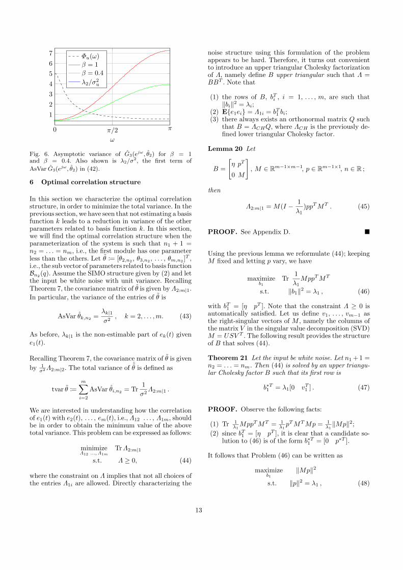
In Figure 6 the variance of G2 for an input filtered withA(q) = 1− 0.8q−1 is presented. The filter is of low-passtype and thus gives high input power at low frequen-cies which results in low variance at those frequencies.Correlation between noise sources decreases the variancemainly where Φu(ω) is small, i.e., at higher frequencies.

12

0 π/2 π

1

2

3

4

5

6

7

ω

Φu(ω)β = 1β = 0.4

λ2/σ2u

Fig. 6. Asymptotic variance of G3(ejω, θ2) for β = 1and β = 0.4. Also shown is λ2/σ

2, the first term of

AsVar G3(ejω, θ2) in (42).

6 Optimal correlation structure

In this section we characterize the optimal correlationstructure, in order to minimize the total variance. In theprevious section, we have seen that not estimating a basisfunction k leads to a reduction in variance of the otherparameters related to basis function k. In this section,we will find the optimal correlation structure when theparameterization of the system is such that n1 + 1 =n2 = . . . = nm, i.e., the first module has one parameterless than the others. Let θ := [θ2,n2

, θ3,n2, . . . , θm,n2

]T ,i.e., the sub vector of parameters related to basis functionBn2(q). Assume the SIMO structure given by (2) and letthe input be white noise with unit variance. RecallingTheorem 7, the covariance matrix of θ is given by Λ2:m|1.

In particular, the variance of the entries of θ is

AsVar θk,n2=λk|1σ2

, k = 2, . . . ,m. (43)

As before, λk|1 is the non-estimable part of ek(t) givene1(t).

Recalling Theorem 7, the covariance matrix of θ is given

by 1σ2Λ2:m|2. The total variance of

ˆθ is defined as

tvar θ :=

m∑i=2

AsVar θi,n2 = Tr1

σ2Λ2:m|1 .

We are interested in understanding how the correlationof e1(t) with e2(t), . . . , em(t), i.e., Λ12 . . . , Λ1m, shouldbe in order to obtain the minimum value of the abovetotal variance. This problem can be expressed as follows:

minimizeΛ12 ..., Λ1m

TrΛ2:m|1

s.t. Λ ≥ 0, (44)

where the constraint on Λ implies that not all choices ofthe entries Λ1i are allowed. Directly characterizing the

noise structure using this formulation of the problemappears to be hard. Therefore, it turns out convenientto introduce an upper triangular Cholesky factorizationof Λ, namely define B upper triangular such that Λ =BBT . Note that

(1) the rows of B, bTi , i = 1, . . . , m, are such that‖bi‖2 = λi;

(2) E{e1ei} = Λ1i = bT1 bi;(3) there always exists an orthonormal matrix Q such

that B = ΛCHQ, where ΛCH is the previously de-fined lower triangular Cholesky factor.

Lemma 20 Let

B =

[η pT

0 M

], M ∈ Rm−1×m−1, p ∈ Rm−1×1, n ∈ R ;

then

Λ2:m|1 = M(I − 1

λ1)ppTMT . (45)

PROOF. See Appendix D. �

Using the previous lemma we reformulate (44); keepingM fixed and letting p vary, we have

maximizeb1

Tr1

λ1MppTMT

s.t. ‖b1‖2 = λ1 , (46)

with bT1 = [η pT ]. Note that the constraint Λ ≥ 0 isautomatically satisfied. Let us define v1, . . . , vm−1 asthe right-singular vectors of M , namely the columns ofthe matrix V in the singular value decomposition (SVD)M = USV T . The following result provides the structureof B that solves (44).

Theorem 21 Let the input be white noise. Let n1 + 1 =n2 = . . . = nm. Then (44) is solved by an upper triangu-lar Cholesky factor B such that its first row is

b∗T1 = λ1[0 vT1 ] . (47)

PROOF. Observe the following facts:

(1) Tr 1λ1MppTMT = 1

λ1pTMTMp = 1

λ1‖Mp‖2;

(2) since bT1 = [η pT ], it is clear that a candidate so-lution to (46) is of the form b∗T1 = [0 p∗T ].

It follows that Problem (46) can be written as

maximizeb1

‖Mp‖2

s.t. ‖p‖2 = λ1 , (48)

13

whose solution is known to be (a rescaling of) the firstright singular vector of M , namely v1. Hence b∗T1 =λ1[0 vT1 ]. �

Remark 22 As has been pointed out in Section 2, Λis required to be positive definite. Thus, the ideal solu-tion provided by Theorem 21 is not applicable in practice,where one should expect that η, the first entry of b1, is al-ways nonzero. In this case, the result of Theorem 21 can

be easily adapted, leading to b∗T1 =[η√

1− η2

λ1vT1

].

7 Numerical examples

In this section, we illustrate the results derived in theprevious sections through three sets of numerical MonteCarlo simulations.

7.1 Effect of model order

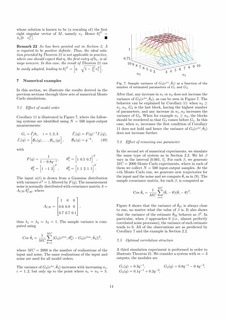
Corollary 11 is illustrated in Figure 7, where the follow-ing systems are identified using N = 500 input-outputmeasurements:

Gi = Γiθi, i = 1, 2, 3 Γi(q) = F (q)−1Γi(q),

Γi(q) =[B1(q), . . . ,Bni

(q)], Bk(q) = q−k, (49)

with

F (q) =1

1− 0.8q−1, θ01 =

[1 0.5 0.7

]T,

θ02 =[1 −1 2

]T, θ03 =

[1 1 2 1 1

]T.

The input u(t) is drawn from a Gaussian distributionwith variance σ2 = 1, filtered by F (q). The measurementnoise is normally distributed with covariance matrixΛ =ΛCHΛ

TCH , where

ΛCH =

1 0 0

0.6 0.8 0

0.7 0.7 0.1

,thus λ1 = λ2 = λ3 = 1. The sample variance is com-puted using

Cov θs =1

MC

MC∑k=1

|G3(ejω0 , θ03)−G3(ejω0 , θ3)|2,

where MC = 2000 is the number of realizations of theinput and noise. The same realizations of the input andnoise are used for all model orders.

The variance of G3(ejω, θ3) increases with increasing ni,i = 1, 2, but only up to the point where ni = n3 = 5.

3 4 5 6 7 8 9 10

345678910

0.75

1

n1n2

Fig. 7. Sample variance of G3(ejω, θ3) as a function of thenumber of estimated parameters of G1 and G2.

After that, any increase in n1 or n2 does not increase the

variance of G3(ejω, θ3), as can be seen in Figure 7. Thebehavior can be explained by Corollary 11: when n3 ≥n1, n2, G3 is the last block, having the highest numberof parameters, and any increase in n1, n2 increases thevariance of G3. When for example n1 ≥ n3, the blocksshould be reordered so that G3 comes before G1. In thiscase, when n1 increases the first condition of Corollary

11 does not hold and hence the variance of G3(ejω, θ3)does not increase further.

7.2 Effect of removing one parameter

In the second set of numerical experiments, we simulatethe same type of system as in Section 2.2. We let βvary in the interval [0.001, 1]. For each β, we generateMC = 2000 Monte Carlo experiments, where in each ofthem we collect N = 500 input-output samples. At thei-th Monte Carlo run, we generate new trajectories forthe input and the noise and we compute θi as in (9). Thesample covariance matrix, for each β, is computed as

Cov θs =1

MC

MC∑i=1

(θi − θ)(θi − θ)T.

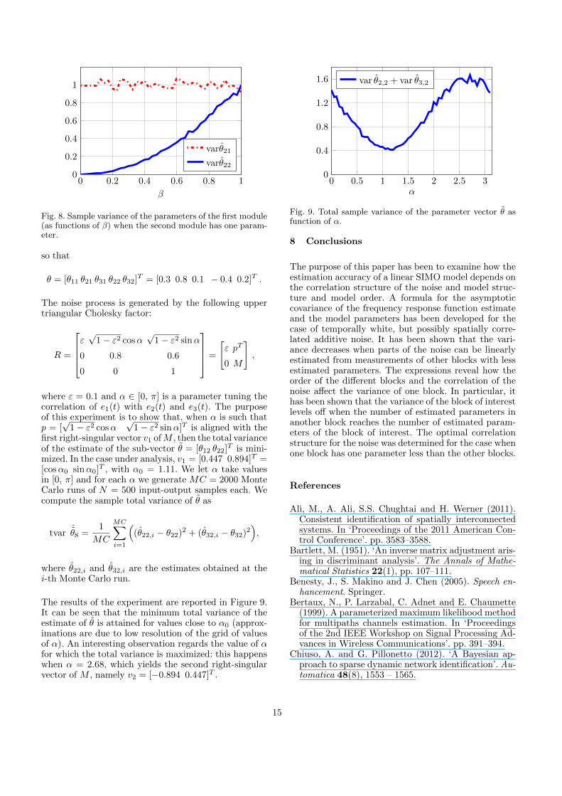
Figure 8 shows that the variance of θ21 is always closeto one, no matter what the value of β is. It also shows

that the variance of the estimate θ22 behaves as β2. Inparticular, when β approaches 0 (i.e., almost perfectlycorrelated noise processes), the variance of such estimatetends to 0. All of the observations are as predicted byCorollary 7 and the example in Section 2.2.

7.3 Optimal correlation structure

A third simulation experiment is performed in order toillustrate Theorem 21. We consider a system withm = 3outputs; the modules are

G1(q) = 0.3q−1, G2(q) = 0.8q−1 − 0.4q−2,G3(q) = 0.1q−1 + 0.2q−2,

14

0 0.2 0.4 0.6 0.8 10

0.2

0.4

0.6

0.8

1

β

varθ21

varθ22

Fig. 8. Sample variance of the parameters of the first module(as functions of β) when the second module has one param-eter.

so that

θ = [θ11 θ21 θ31 θ22 θ32]T = [0.3 0.8 0.1 − 0.4 0.2]T .

The noise process is generated by the following uppertriangular Cholesky factor:

R =

ε√

1− ε2 cosα√

1− ε2 sinα

0 0.8 0.6

0 0 1

=

[ε pT

0 M

],

where ε = 0.1 and α ∈ [0, π] is a parameter tuning thecorrelation of e1(t) with e2(t) and e3(t). The purposeof this experiment is to show that, when α is such thatp = [

√1− ε2 cosα

√1− ε2 sinα]T is aligned with the

first right-singular vector v1 ofM , then the total varianceof the estimate of the sub-vector θ = [θ12 θ22]T is mini-mized. In the case under analysis, v1 = [0.447 0.894]T =[cosα0 sinα0]T , with α0 = 1.11. We let α take valuesin [0, π] and for each α we generate MC = 2000 MonteCarlo runs of N = 500 input-output samples each. Wecompute the sample total variance of θ as

tvarˆθs =

1

MC

MC∑i=1

((θ22,i − θ22)2 + (θ32,i − θ32)2

),

where θ22,i and θ32,i are the estimates obtained at thei-th Monte Carlo run.

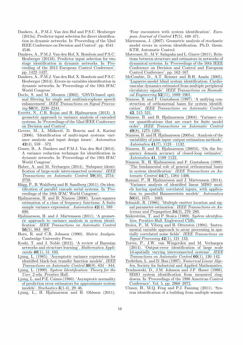
The results of the experiment are reported in Figure 9.It can be seen that the minimum total variance of theestimate of θ is attained for values close to α0 (approx-imations are due to low resolution of the grid of valuesof α). An interesting observation regards the value of αfor which the total variance is maximized: this happenswhen α = 2.68, which yields the second right-singularvector of M , namely v2 = [−0.894 0.447]T .

0 0.5 1 1.5 2 2.5 30

0.4

0.8

1.2

1.6

α

var θ2,2 + var θ3,2

Fig. 9. Total sample variance of the parameter vector θ asfunction of α.

8 Conclusions

The purpose of this paper has been to examine how theestimation accuracy of a linear SIMO model depends onthe correlation structure of the noise and model struc-ture and model order. A formula for the asymptoticcovariance of the frequency response function estimateand the model parameters has been developed for thecase of temporally white, but possibly spatially corre-lated additive noise. It has been shown that the vari-ance decreases when parts of the noise can be linearlyestimated from measurements of other blocks with lessestimated parameters. The expressions reveal how theorder of the different blocks and the correlation of thenoise affect the variance of one block. In particular, ithas been shown that the variance of the block of interestlevels off when the number of estimated parameters inanother block reaches the number of estimated param-eters of the block of interest. The optimal correlationstructure for the noise was determined for the case whenone block has one parameter less than the other blocks.

References

Ali, M., A. Ali, S.S. Chughtai and H. Werner (2011).Consistent identification of spatially interconnectedsystems. In ‘Proceedings of the 2011 American Con-trol Conference’. pp. 3583–3588.

Bartlett, M. (1951). ‘An inverse matrix adjustment aris-ing in discriminant analysis’. The Annals of Mathe-matical Statistics 22(1), pp. 107–111.

Benesty, J., S. Makino and J. Chen (2005). Speech en-hancement. Springer.

Bertaux, N., P. Larzabal, C. Adnet and E. Chaumette(1999). A parameterized maximum likelihood methodfor multipaths channels estimation. In ‘Proceedingsof the 2nd IEEE Workshop on Signal Processing Ad-vances in Wireless Communications’. pp. 391–394.

Chiuso, A. and G. Pillonetto (2012). ‘A Bayesian ap-proach to sparse dynamic network identification’. Au-tomatica 48(8), 1553 – 1565.

15

Dankers, A., P.M.J. Van den Hof and P.S.C. Heuberger(2013a). Predictor input selection for direct identifica-tion in dynamic networks. In ‘Proceeding of the 52ndIEEE Conference on Decision and Control’. pp. 4541–4546.

Dankers, A., P.M.J. Van den Hof, X. Bombois and P.S.C.Heuberger (2013b). Predictor input selection for twostage identification in dynamic networks. In ‘Pro-ceeding of the 2013 European Control Conference’.pp. 1422–1427.

Dankers, A., P.M.J. Van den Hof, X. Bombois and P.S.C.Heuberger (2014). Errors-in-variables identification indynamic networks. In ‘Proceedings of the 19th IFACWorld Congress’.

Doclo, S. and M. Moonen (2002). ‘GSVD-based opti-mal filtering for single and multimicrophone speechenhancement’. IEEE Transactions on Signal Process-ing 50(9), 2230–2244.

Everitt, N., C.R. Rojas and H. Hjalmarsson (2013). Ageometric approach to variance analysis of cascadedsystems. In ‘Proceedings of the 52nd IEEE Conferenceon Decision and Control’.

Gevers, M., L. Miskovic, D. Bonvin and A. Karimi(2006). ‘Identification of multi-input systems: vari-ance analysis and input design issues’. Automatica42(4), 559 – 572.

Gunes, B., A. Dankers and P.M.J. Van den Hof (2014).A variance reduction technique for identification indynamic networks. In ‘Proceedings of the 19th IFACWorld Congress’.

Haber, A. and M. Verhaegen (2014). ‘Subspace identi-fication of large-scale interconnected systems’. IEEETransactions on Automatic Control 59(10), 2754–2759.

Hagg, P., B. Wahlberg and H. Sandberg (2011). On iden-tification of parallel cascade serial systems. In ‘Pro-ceedings of the 18th IFAC World Congress’.

Hjalmarsson, H. and B. Ninness (2006). ‘Least-squaresestimation of a class of frequency functions: A finitesample variance expression’. Automatica 42(4), 589 –600.

Hjalmarsson, H. and J. Martensson (2011). ‘A geomet-ric approach to variance analysis in system identi-fication’. IEEE Transactions on Automatic Control56(5), 983 –997.

Horn, R. and C.R. Johnson (1990). Matrix Analysis.Cambridge University Press.

Koski, T. and J. Noble (2012). ‘A review of Bayesiannetworks and structure learning’. Mathematica Appli-canda 40(1), 51–103.

Ljung, L. (1985). ‘Asymptotic variance expressions foridentified black-box transfer function models’. IEEETransactions on Automatic Control 30(9), 834 – 844.

Ljung, L. (1999). System Identification: Theory for theUser. 2 edn. Prentice Hall.

Ljung, L. and P.E. Caines (1980). ‘Asymptotic normalityof prediction error estimators for approximate systemmodels’. Stochastics 3(1-4), 29–46.

Ljung, L., H. Hjalmarsson and H. Ohlsson (2011).

‘Four encounters with system identification’. Euro-pean Journal of Control 17(5), 449–471.

Martensson, J. (2007). Geometric analysis of stochasticmodel errors in system identification. Ph.D. thesis.KTH, Automatic Control.

Materassi, D., M.V. Salapaka and L. Giarre (2011). Rela-tions between structure and estimators in networks ofdynamical systems. In ‘Proceedings of the 50th IEEEConference on Decision and Control and EuropeanControl Conference’. pp. 162–167.

McCombie, D., A.T. Reisner and H.H. Asada (2005).‘Laguerre-model blind system identification: Cardio-vascular dynamics estimated from multiple peripheralcirculatory signals’. IEEE Transactions on Biomedi-cal Engineering 52(11), 1889–1901.

Ninness, B. and F. Gustafsson (1997). ‘A unifying con-struction of orthonormal bases for system identifi-cation’. IEEE Transactions on Automatic Control42, 515–521.

Ninness, B. and H. Hjalmarsson (2004). ‘Variance er-ror quantifications that are exact for finite modelorder’. IEEE Transactions on Automatic Control49(8), 1275–1291.

Ninness, B. and H. Hjalmarsson (2005a). ‘Analysis of thevariability of joint input–output estimation methods’.Automatica 41(7), 1123 – 1132.

Ninness, B. and H. Hjalmarsson (2005b). ‘On the fre-quency domain accuracy of closed-loop estimates’.Automatica 41, 1109–1122.

Ninness, B., H. Hjalmarsson and F. Gustafsson (1999).‘The fundamental role of general orthonormal basesin system identification’. IEEE Transactions on Au-tomatic Control 44(7), 1384–1406.

Ramazi, P., H. Hjalmarsson and J. Martensson (2014).‘Variance analysis of identified linear MISO mod-els having spatially correlated inputs, with applica-tion to parallel Hammerstein models’. Automatica50(6), 1675 – 1683.

Schmidt, R. (1986). ‘Multiple emitter location and sig-nal parameter estimation’. IEEE Transactions on An-tennas and Propagation 34(3), 276–280.

Soderstrom, T. and P. Stoica (1989). System identifica-tion. Prentice-Hall. Englewood Cliffs.

Stoica, P., M. Viberg and B. Ottersten (1994). ‘Instru-mental variable approach to array processing in spa-tially correlated noise fields’. IEEE Transactions onSignal Processing 42(1), 121–133.

Torres, P., J.W. van Wingerden and M. Verhaegen(2014). ‘Output-error identification of large scale1d-spatially varying interconnected systems’. IEEETransactions on Automatic Control 60(1), 130–142.

Trefethen, L. and D. Bau (1997). Numerical Linear Alge-bra. Society for Industrial and Applied Mathematics.

Trudnowski, D., J.M. Johnson and J.F. Hauer (1998).SIMO system identification from measured ring-downs. In ‘Proceedings of the 1998 American ControlConference’. Vol. 5. pp. 2968–2972.

Ulusoy, H., M.Q. Feng and P.J. Fanning (2011). ‘Sys-tem identification of a building from multiple seismic

16

records’. Earthquake Engineering & Structural Dy-namics 40(6), 661–674.

Van den Hof, P. M. J., Arne Dankers, P. S. C. Heubergerand X Bombois (2013). ‘Identification of dynamicmodels in complex networks with prediction errormethods - basic methods for consistent module esti-mates’. Automatica 49(10), 2994–3006.

Viberg, M. and B. Ottersten (1991). ‘Sensor array pro-cessing based on subspace fitting’. IEEE Transactionson Signal Processing 39(5), 1110–1121.

Viberg, M., P. Stoica and B. Ottersten (1997). ‘Max-imum likelihood array processing in spatially corre-lated noise fields using parameterized signals’. IEEETransactions on Signal Processing 45(4), 996–1004.

Wahlberg, B., H. Hjalmarsson and J. Martensson (2009).‘Variance results for identification of cascade systems’.Automatica 45(6), 1443–1448.

Yuan, Z. D. and L. Ljung (1984). ‘Black-box identifi-cation of multivariable transfer functions–asymptoticproperties and optimal input design’. InternationalJournal of Control 40(2), 233–256.

Zhu, Y. (1989). ‘Black-box identification of MIMO trans-fer functions: Asymptotic properties of prediction er-ror models’. International Journal of Adaptive Controland Signal Processing 3(4), 357–373.

Zhu, Y. (2001). Multivariable system identification forprocess control. Elsevier.

A Proof of Lemma 5

Let v(t) = Λ−1CHe(t) for some real valued random vari-able e(t) (Λ−1CH exists and is unique for Λ > 0 (Hornand Johnson, 1990)). Then Cov v(t) = I. Similarlye(t) = ΛCHv(t). The set {v1(t), . . . , vj(t)} is a func-tion of e1(t), . . . , ej(t) only and vice versa, for all1 ≤ j ≤ m. Thus, if e1(t), . . . , ej(t) are known, thenalso {v1(t), . . . , vj(t)} are known, but nothing is knownabout {vj+1(t), . . . , vm(t)}. Thus, for j < i the bestlinear estimator of ei(t) given e1(t), . . . , ej(t), is

ei|j(t) =

j∑k=1

γikvk(t), (A.1)

and

ei(t)− ei|j(t)

has variance

λi|j =

i∑k=j+1

γ2ik.

For the last part of the lemma, we realize that the de-pendence of ei|j(t) on ej(t) in Equation (A.1) is given byγij/γjj (since v1(t), . . . , vj−1(t) do not depend on ej(t)).Hence ei|j(t) depends on ej(t) if and only if γij 6= 0.

B Proof of Theorem 10

Before giving the proof of Theorem 10 we need the fol-lowing auxiliary lemma.

Lemma 23 Let Λ > 0 and real and its Cholesky factorΛCH be partitioned according to e1:χk−1 and eχk:m,

Λ =

[Λ1 Λ12

Λ21 Λ2

], ΛCH =

[(ΛCH)1 0

(ΛCH)21 (ΛCH)2

].

Then

Λχk:m|χk−1 = (ΛCH)2(ΛCH)T2 .

PROOF. By the derivations of Lemma A, for somev(t) with Cov v(t) = I, e(t) = ΛCHv(t) and v1:χ−1(t)are known since e1:χ−1(t) are known. Furthermoreeχk:m|χk−1(t) = (ΛCH)21v1:χ−1(t), which implieseχk:m|χk−1(t) − eχk:m|χk−1(t) = (ΛCH)2vχk:m(t) andthe results follows since Cov vχk:m(t) = I. �

The asymptotic variance is given by (11) with

Ψ(q) = Ψ(q)Λ−TCH .

Let n = n1 + · · ·+nm. From the upper triangular struc-ture of Λ−TCH and n1 ≤ n2 ≤ . . . ≤ nm, an orthonormalbasis for SΨ , the subspace spanned by the rows of Ψ , isgiven by

BSk (ejω) :=[Bk 0 . . . 0

], k=1, . . . , n1

BSk (ejω) :=[0 Bk−n1

0 . . .], k=n1 + 1, . . . , n2

... (B.1)

BSk (ejω) :=[. . . 0 Bk−n+nm

], k=n− nm+1, . . . , n.

First note that

∂G

∂θ= ΨΛTCH .

Then, using Theorem 3,

σ2 AsVar G = ΛCH

n∑k=1

BSk (ejω0)∗BSk (ejω0)ΛTCH .

Sorting the sum with respect to the basis functionsBk(ejω0), we get

σ2 AsCov Gi = ΛCH

nm∑k=1

|Bk(ejω0)|2[

0χk−1 0

0 I

]ΛTCH .

17

Using Lemma 23

AsCov G =1

σ2

nm∑k=1

[0χk−1 0

0 Λχk:m|χk−1

]|Bk(ejω0)|2.

Thus (25) follows. We now show the first part of thetheorem, that

AsCov ˆθ =1

σ2diag(Λ1:m, Λχ2:m|χ2−1, . . . , Λχnm :m|χnm−1).

The covariance of G can be expressed as

AsCov G = TAsCov ˆθ T ∗ (B.2)

where

T =[B1I(1) B2I(2) . . . Bnm

I(nm)],

I(k) =

[0

Im−χk+1

]∈ Rm×(m−χk+1).

However, (B.2) equals (25) for all ω and the theoremfollows.

C Proof of Corollary 11

To prove Corollary 11 we will use (28). First, we makethe assumption that j is the last module that has njparameters. This assumption is made for conveniencesince reordering all modules with nj estimated parame-ters does not change (28). First of all, we see that if

nj ≥ ni,

then (28) does not increase when nj increases. If instead

nj < ni,

the increase in variance is given by

γ2ij |Bnj+1(ejω0)|2,

which is non-zero iff γij 6= 0 and |Bnj+1(ejω0)|2 6= 0.From Lemma 5 the theorem follows.

D Proof of Lemma 20

The inverse of B is

B−1 =

[η−1 −qT

0 M−1

], qT := η−1pTM−1,

so that

Λ−1 = B−TB−1 =

[η−2 −qT η−1

−qη−1 M−TM−1 + qqT

].

Hence, using the Sherman–Morrison formula (Bartlett,1951)

Λ2:m|1 =(M−TM−1 + qqT

)−1= MMT − 1

kMMT qqTMMT

= MMT − 1

k

MppTMT

η2,

where

k = 1 + qTMMT q = 1 +pT p

η2

=η2 + pT p

η2=‖b1‖22η2

=λ1η2,

so (45) follows.

18