spatially distributed groundwater recharge estimated using
TRANSCRIPT
U.S. Department of the InteriorU.S. Geological Survey
Scientific Investigations Report 2014–5168 Version 2.0, February 2018
Prepared in cooperation with the County of Maui Department of Water Supply and the State of Hawai‘i Commission on Water Resource Management
Spatially Distributed Groundwater Recharge Estimated Using a Water-Budget Model for the Island of Maui, Hawai‘i, 1978–2007

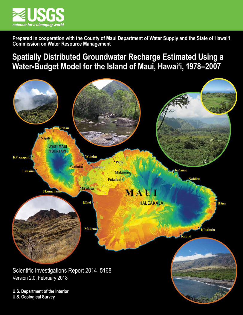
COVERTop left: View toward summit of West Maui Mountain from a forested ridge near Honokōhau Valley on northern West Maui Mountain, Island of Maui, Hawai‘i. Photograph by Sarah N. Rosa, U.S. Geological Survey, 2013. Top center: View of Waihe‘e River on northeastern West Maui Mountain, Island of Maui, Hawai‘i, 2009. Top right: View of Ke‘anae Valley, on eastern Haleakalā, Island of Maui, Hawai‘i. Photograph by Adam G. Johnson, U.S. Geological Survey, 2014. Top right inset: Taro fields near Ke‘anae, eastern coast of Haleakalā, Island of Maui, Hawai‘i. Photograph by Adam G. Johnson, U.S. Geological Survey, 2014. Bottom right: View toward southern flank of Haleakalā from the coastline near Kaupō, Island of Maui, Hawai‘i. Photograph by Adam G. Johnson, U.S. Geological Survey, 2013. Bottom left: View of shrubs, grass, and barren rock on a steep valley wall near Ukumehame Gulch on southern West Maui Mountain, Island of Maui, Hawai‘i. Photograph by Adam G. Johnson, U.S. Geological Survey, 2010. Center: Map of the Island of Maui, Hawai‘i, showing the relative distribution of estimated mean annual recharge for average climate conditions. Estimated recharge is shown using a spectral color scale with red representing very low recharge and dark blue representing very high recharge.
Spatially Distributed Groundwater Recharge Estimated Using a Water-Budget Model for the Island of Maui, Hawai‘i, 1978–2007
By Adam G. Johnson, John A. Engott, Maoya Bassiouni, and Kolja Rotzoll
Prepared in cooperation with the County of Maui Department of Water Supply and the State of Hawai‘i Commission on Water Resource Management
Scientific Investigations Report 2014–5168 Version 2.0, February 2018
U.S. Department of the InteriorU.S. Geological Survey

ii
U.S. Department of the InteriorRYAN K. ZINKE, Secretary
U.S. Geological SurveyWilliam H. Werkheiser, Deputy Director exercising the authority of the Director
U.S. Geological Survey, Reston, Virginia: 2018 First release: 2014, online Revised: February 2018 (ver. 2.0), online
For more information on the USGS—the Federal source for science about the Earth, its natural and living resources, natural hazards, and the environment—visit https://www.usgs.gov/ or call 1–888–ASK–USGS.
For an overview of USGS information products, including maps, imagery, and publications, visit https://store.usgs.gov.
Any use of trade, firm, or product names is for descriptive purposes only and does not imply endorsement by the U.S. Government.
Although this information product, for the most part, is in the public domain, it also may contain copyrighted materials as noted in the text. Permission to reproduce copyrighted items must be secured from the copyright owner.
Suggested citation: Johnson, A.G., Engott, J.A., Bassiouni, Maoya, and Rotzoll, Kolja, 2018, Spatially distributed groundwater recharge estimated using a water-budget model for the Island of Maui, Hawai`i, 1978–2007 (ver. 2.0, February 2018): U.S. Geological Survey Scientific Investigations Report 2014–5168, 53 p., https://doi.org/10.3133/sir20145168. ISSN 2328-0328 (online)
iii
Contents
Abstract ........................................................................................................................................................1Introduction ...................................................................................................................................................1
Purpose and Scope .............................................................................................................................4Previous Studies ..................................................................................................................................4
Description of Maui ......................................................................................................................................4Physical Setting ...................................................................................................................................4Climate ................................................................................................................................................5Hydrogeology .......................................................................................................................................5Surface Water ......................................................................................................................................7Soils ................................................................................................................................................7Land Cover ..........................................................................................................................................7
Water-Budget Model .....................................................................................................................................7Conceptual Model .............................................................................................................................10Model Calculations ...........................................................................................................................10
Model Input .................................................................................................................................................14Land Cover ........................................................................................................................................14
Impervious Surfaces .................................................................................................................15Rainfall ..............................................................................................................................................15
Monthly Rainfall ........................................................................................................................15Daily Rainfall .............................................................................................................................15
Fog Interception .................................................................................................................................16Irrigation .............................................................................................................................................17
Irrigation Estimates ...................................................................................................................17Irrigation Calibrations ................................................................................................................18
Septic-System Leaching ....................................................................................................................18Storm-Drain Systems .........................................................................................................................18Direct Runoff ......................................................................................................................................19
Computation of Seasonal Runoff-to-Rainfall Ratios..................................................................19Runoff-to-Rainfall Ratios Assigned to Ungaged Catchment Zones .........................................24Runoff-to-Rainfall Ratios Assigned to Gaged Basins within a Single Catchment Zone ............25Runoff-to-Rainfall Ratios Assigned to Gaged Basins with Multiple Catchment Zones..............25
Evapotranspiration .............................................................................................................................25Forest-Canopy Evaporation and Net Precipitation ....................................................................26Potential Evapotranspiration .....................................................................................................27
Reference Evapotranspiration .........................................................................................27Crop Coefficients .............................................................................................................27
Moisture-Storage Capacity of the Plant-Root Zone ..........................................................................30Direct Recharge .................................................................................................................................30Other Input .........................................................................................................................................30
Model Exclusions and Limitations ..............................................................................................................32Model Randomness ....................................................................................................................................33Water-Budget and Groundwater-Recharge Estimates ...............................................................................33
iv
Figures 1. Aquifer sectors and aquifer systems on the Island of Maui, Hawai‘i ...................................................2 2. Major geographical features on the Island of Maui, Hawai‘i. ...............................................................3 3. Mean annual rainfall (1978–2007) and locations of rain gages used in the water-budget calculations for Maui, Hawai‘i.......................................................................................................6 4. Land cover for Maui, Hawai‘i ...............................................................................................................8 5. Generalized water-budget flow diagrams for both forest and nonforest land covers ........................ 11 6. Mean runoff-to-rainfall ratios for the Dry-season months: May through October and Wet-season
months: November through April for drainage basins of selected stream-gaging stations and catchment zones on Maui, Hawai‘i ............................................................................................20
7. Mean annual reference evapotranspiration for Maui, Hawai‘i ...........................................................28 8. Calculated moisture-storage capacity of the plant-root zone for Maui ..............................................31 9. Absolute percentage change in island-wide recharge with each successive model simulation ........3310. The distribution of mean annual groundwater recharge for average climate conditions (1978–2007), Island of Maui, Hawai‘i, calculated using the water-budget model ......................4111. Fraction of total water inflow that becomes groundwater recharge in the water-budget calculations
for average climate conditions (1978–2007) Island of Maui, Hawai‘i .........................................4312. Percentage difference in mean annual groundwater recharge for drought conditions (1998–2002),
relative to that for average climate conditions (1978–2007), Island of Maui, Hawai‘i ................46
Water-Budget and Recharge Estimates for Average Climate Conditions ..........................................33Comparison with Water Resources Protection Plan .................................................................42Comparison with Previous Studies for the ‘Īao and Waihe‘e aquifer systems ..........................42Comparison with Evapotranspiration Estimates of Giambelluca and others (2014) .................44
Recharge for Drought Conditions ......................................................................................................45Sensitivity Analysis ............................................................................................................................45
Suggestions for Future Study and Additional Data Collection ....................................................................48Summary and Conclusions .........................................................................................................................48References Cited .......................................................................................................................................49
Tables 1. Previous water-budget studies for parts of Maui, Hawai‘i ...................................................................4 2. General types of land cover, as a fraction of aquifer system area, Maui, Hawai‘i ...............................9 3. Mean fog-interception rates used in the water-budget calculation for average climate conditions for Maui, Hawai‘i ........................................................................................................................16 4. Mean seasonal runoff-to-rainfall ratios for drainage basins of stream-gaging stations on Kaua‘i, O‘ahu and Maui, Hawai‘i ................................................................................................21 5. Regional-regression equations used to compute mean seasonal runoff-to-rainfall ratios for catchment zones in ungaged areas on Maui Hawai‘i.................................................................24 6. Land-cover parameters used in water-budget calculations for Maui, Hawai‘i ...................................29 7. Mean annual water-budget components from this study for aquifer sectors and all of Maui, Hawai‘i .......................................................................................................................................34 8. Mean annual water-budget components from this study for average climate and drought conditions and components from the Water Resources Protection Plan for aquifer systems of Maui, Hawai‘i .............................................................................................................................35
v
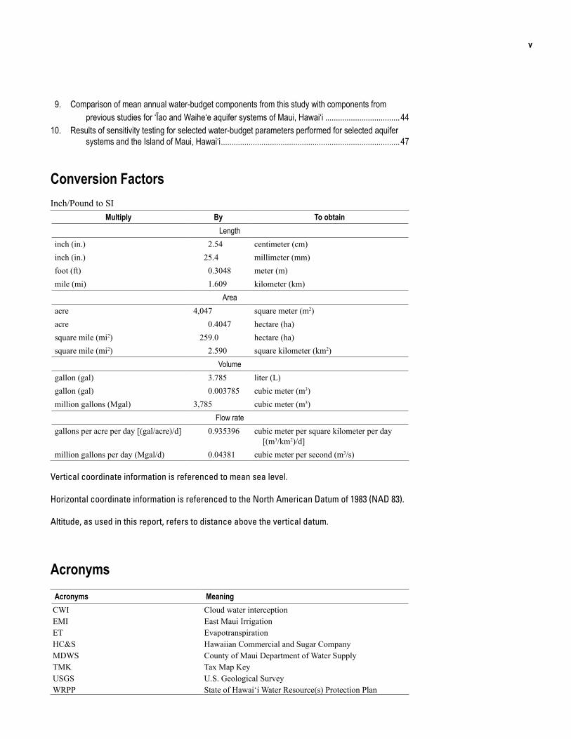
AcronymsAcronyms MeaningCWI Cloud water interceptionEMI East Maui IrrigationET EvapotranspirationHC&S Hawaiian Commercial and Sugar CompanyMDWS County of Maui Department of Water SupplyTMK Tax Map KeyUSGS U.S. Geological SurveyWRPP State of Hawai‘i Water Resource(s) Protection Plan
9. Comparison of mean annual water-budget components from this study with components from previous studies for ‘Īao and Waihe‘e aquifer systems of Maui, Hawai‘i ...................................4410. Results of sensitivity testing for selected water-budget parameters performed for selected aquifer
systems and the Island of Maui, Hawai‘i ....................................................................................47
Conversion FactorsInch/Pound to SI
Multiply By To obtainLength
inch (in.) 2.54 centimeter (cm)inch (in.) 25.4 millimeter (mm)foot (ft) 0.3048 meter (m)mile (mi) 1.609 kilometer (km)
Areaacre 4,047 square meter (m2)acre 0.4047 hectare (ha)square mile (mi2) 259.0 hectare (ha)square mile (mi2) 2.590 square kilometer (km2)
Volumegallon (gal) 3.785 liter (L)gallon (gal) 0.003785 cubic meter (m3)million gallons (Mgal) 3,785 cubic meter (m3)
Flow rategallons per acre per day [(gal/acre)/d] 0.935396 cubic meter per square kilometer per day
[(m3/km2)/d]million gallons per day (Mgal/d) 0.04381 cubic meter per second (m3/s)
Vertical coordinate information is referenced to mean sea level.
Horizontal coordinate information is referenced to the North American Datum of 1983 (NAD 83).
Altitude, as used in this report, refers to distance above the vertical datum.

vi
AcknowledgmentsThis study was conducted in cooperation with the County of Maui Department of Water
Supply and the State of Hawai‘i Commission on Water Resource Management. We thank Abby Frazier and Thomas Giambelluca of the University of Hawai‘i at Mānoa, Cary Yamashita of the County of Maui Department of Public Works, and Tui Anderson of the County of Maui Department of Water Supply for providing data and background information.
Spatially Distributed Groundwater Recharge Estimated Using a Water-Budget Model for the Island of Maui, Hawai‘i, 1978–2007
additional freshwater demand. Average water production by MDWS was about 37.5 million gallons per day (Mgal/d) on the Island of Maui in 2013 (County of Maui, Hawai‘i, Department of Water Supply, 2014). Projected water demands from MDWS on the Island of Maui in 2030 (Haiku Design & Analysis, 2007, 2009, 2010) are between about 12 and 57 percent more than the water production in 2013. Groundwater pumped from wells in the ‘Īao and Waihe‘e aquifer systems (fig. 1) is the chief source of freshwater for MDWS and is supplied to consumers in Wailuku, Kahului, Pā‘ia, and Kīhei (fig. 2). Average groundwater pumpage from the ‘Īao aquifer system by the MDWS in 2013 was about 84 percent of the sustainable yield (David Taylor, MDWS, written commun., 2014). In upcountry Maui, which includes areas near Makawao on northwest Haleakalā (fig. 2), MDWS is faced with “a pressing need for additional water production capacity” and a considerable backlog of more consumers who are waiting for new water meters (Haiku Design & Analysis, 2009). Surface water, the chief source of freshwater for MDWS’ consumers in upcountry Maui, is already at its “practical limits” during the drier summer months and during drought conditions (Haiku Design & Analysis, 2009). In addition to MDWS, private water systems on Maui pump substantial amounts of groundwater. Some of these private water systems may also have increased groundwater demands in the future.
Estimates of the spatial distribution of groundwater recharge for Maui are needed to evaluate the availability of fresh groundwater. Recharge is water derived from precipitation and other sources of water, such as irrigation and leakage from septic systems, infiltrating the ground and replenishing aquifers. Recharge is used by the State of Hawai‘i Commission on Water Resource Management in the calculation of sustainable-yield values for aquifer systems in the State (State of Hawai‘i, 2008). For much of Haleakalā, including parts of upcountry Maui, the spatial distribution of recharge has not been estimated since 1999 (Shade, 1999). Although more recent recharge estimates for the isthmus and West Maui Mountain (fig. 2) are available (Engott and Vana, 2007; Gingerich and Engott, 2012), new spatial datasets of rainfall and evapotranspiration (ET) for the Hawaiian Islands have been developed since these previous recharge studies.
AbstractDemand for freshwater on the Island of Maui is
expected to grow. To evaluate the availability of fresh groundwater, estimates of groundwater recharge are needed. A water-budget model with a daily computation interval was developed and used to estimate the spatial distribution of recharge on Maui for average climate conditions (1978–2007 rainfall and 2010 land cover) and for drought conditions (1998–2002 rainfall and 2010 land cover). For average climate conditions, mean annual recharge for Maui is about 1,309 million gallons per day, or about 44 percent of precipitation (rainfall and fog interception). Recharge for average climate conditions is about 39 percent of total water inflow consisting of precipitation, irrigation, septic leachate, and seepage from reservoirs and cesspools. Most recharge occurs on the wet, windward slopes of Haleakalā and on the wet, uplands of West Maui Mountain. Dry, coastal areas generally have low recharge. In the dry isthmus, however, irrigated fields have greater recharge than nearby unirrigated areas. For drought conditions, mean annual recharge for Maui is about 1,010 million gallons per day, which is 23 percent less than recharge for average climate conditions. For individual aquifer-system areas used for groundwater management, recharge for drought conditions is about 8 to 51 percent less than recharge for average climate conditions. The spatial distribution of rainfall is the primary factor determining spatially distributed recharge estimates for most areas on Maui. In wet areas, recharge estimates are also sensitive to water-budget parameters that are related to runoff, fog interception, and forest-canopy evaporation. In dry areas, recharge estimates are most sensitive to irrigated crop areas and parameters related to evapotranspiration.
IntroductionOn the Island of Maui, the demand for freshwater is
expected to increase. Groundwater is the chief source of freshwater for the County of Maui Department of Water Supply (MDWS) and is a potential source for satisfying
By Adam G. Johnson,1 John A. Engott,1 Maoya Bassiouni,1 and Kolja Rotzoll2
1U.S. Geological Survey.2Water Resources Research Center, University of Hawaiʻi.
2 Spatially Distributed Groundwater Recharge Estimated Using a Water-Budget Model for the Island of Maui, Hawai‘i
Pā‘ia Ka
ma‘ol
e
‘Īao
Ha‘ikū
Maka
wao
Kahu
lui
Waik
apū
Hono
kōwa
i
Hono
lua
Hono
pou
Laun
iupok
o
Waih
e‘e
Hono
kōha
u
Ukum
eham
e
Kaha
kuloa
Olow
alu
Waik
amoi
Ke‘an
ae
Luala
‘ilua
Naku
la
Kaupō
Kīpa
hulu
Waih
o‘i
Kawa
ipapa
Kūhiw
a
LAHA
INA
CENT
RAL
KO‘O
LAU
HĀNA
KAHI
KINU
I
WAI
LUKU
EXPL
ANAT
ION
Pā‘ia
Aquif
er se
ctor a
rea a
nd na
me
Aquif
er sy
stem
area
and n
ame
Sedim
entar
y dep
osits
(mod
ified f
rom
Sher
rod a
nd ot
hers,
2007
)
0-foo
t altit
ude c
ontou
r of to
p of W
ailuk
u Bas
alt (m
odifie
d fro
m Gi
nger
ich, 2
008)
0-foo
t altit
ude c
ontou
r of to
p of K
ula V
olcan
ics/ H
onom
anū
Basa
lt (mo
dified
from
Ging
erich
, 200
8)
CENT
RAL
Base
mod
ified f
rom
U.S.
Geo
logica
l Sur
vey
Natio
nal H
ydro
grap
hy D
atase
t, Univ
ersa
l Tr
ansv
erse
Mer
cator
proje
ction
, zon
e 4,
NAD8
3 datu
m.
156°
158°
160°
22°
20°
Hawa
i‘i
Molok
a‘iMa
ui
Kaho‘ol
awe
Lāna‘i
HAW
AI‘I
O‘ah
u
Kaua‘i
Ni‘ih
au
PACI
FIC
OCE
AN
156°
00'
156°
10'
156°
20'
156°
30'
156°
40'
21°0
0'
20°5
0'
20°4
0'
03
69
KILO
METE
RS
03
69
MILE
S
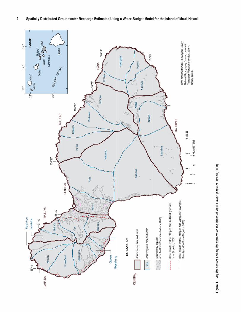
Figu
re 1.
Aq
uifer
secto
rs an
d aqu
ifer s
ystem
s on t
he Is
land o
f Mau
i, Haw
ai‘i (S
tate o
f Haw
ai‘i, 2
008)
.
Introduction 3
"
"
"
"
"
"
"
"
"
"
"
"
"
"
"
"
"
0
0
Pu‘u
Kuku
i5,7
88 fe
et
Pu‘u
‘Ula‘
ula
(Red
Hill)
10,02
3 fee
t
HALE
AKAL
Ā
ISTH
MUS
WES
T MA
UI
MOUN
TAIN
Kīpa
hulu
Valley
Kaupō Gap
Ke‘anae Valle
y
Upcountry
Hāna
Pā‘ia
Kaupō
Kīhe
i
Nāhik
u
Ke‘an
ae
Waie
hu
Nāpil
i
Māke
na
Maka
wao
Kahu
luiW
ailuk
u Mā‘al
aea
Laha
ina
Kīpa
hulu
Puka
lani
Kā‘an
apali
1000
10002000
4000
2000
40006000
8000
CONT
OUR
INTE
RVAL
, IN F
EET,
VARI
ESVE
RTIC
AL D
ATUM
IS LO
CAL M
EAN
SEA
LEVE
L
Base
mod
ified f
rom
U.S.
Geo
logica
l Sur
vey
Natio
nal H
ydro
grap
hy D
atase
t, Univ
ersa
l Tr
ansv
erse
Mer
cator
proje
ction
, zon
e 4,
NAD8
3 datu
m.
156°
00'
156°
10'
156°
20'
156°
30'
156°
40'
21°0
0'
20°5
0'
20°4
0'
03
69
KILO
METE
RS
03
69
MILE
S
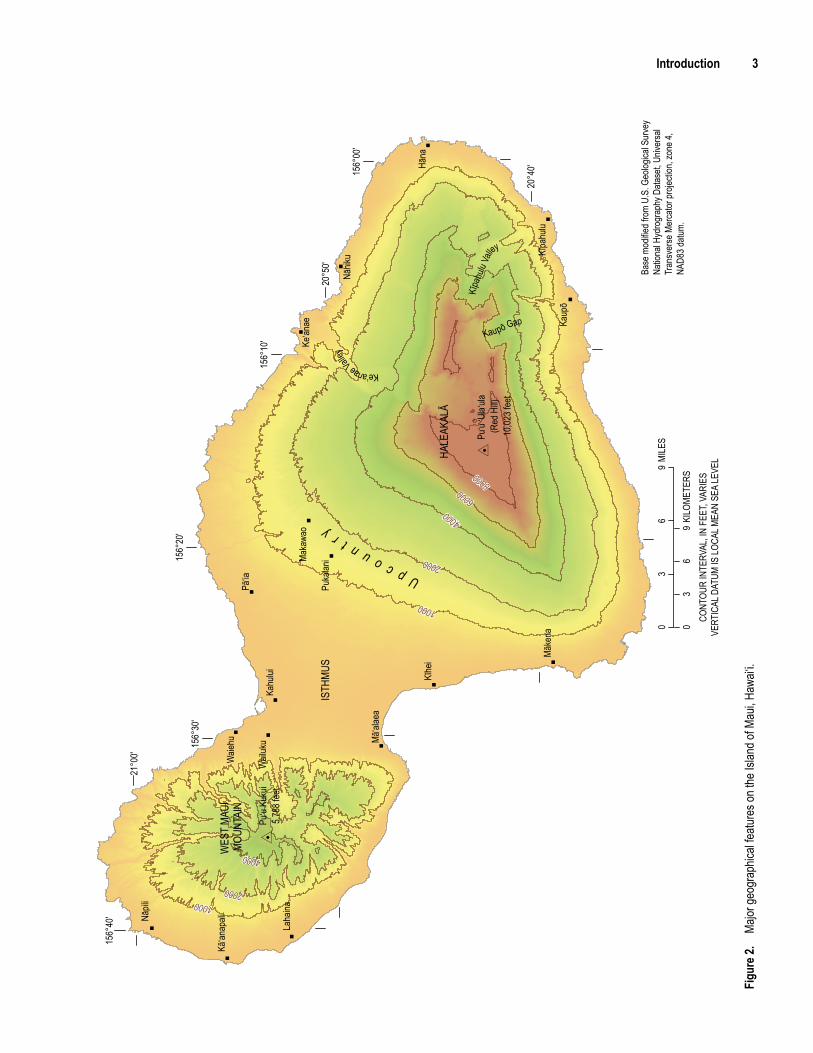
Figu
re 2.
Ma
jor ge
ogra
phica
l featu
res o
n the
Islan
d of M
aui, H
awai‘
i.
Introduction 3
4 Spatially Distributed Groundwater Recharge Estimated Using a Water-Budget Model for the Island of Maui, Hawai‘i
These new datasets of rainfall and ET (Frazier and others, 2016; Giambelluca and others, 2013; 2014) have better spatial and temporal resolution than the datasets that were used before. For this study, the water-budget model used by Gingerich and Engott (2012) was modified and expanded to include the entire Island of Maui. Recharge estimates were calculated using the new datasets in combination with the modified water-budget model. The recharge estimates from this study can be used in numerical groundwater models that have the capacity to evaluate the effects of additional groundwater withdrawals on groundwater levels, streamflow, coastal discharge, and salinities in public and private wells on Maui.
Purpose and ScopeThis report describes the spatial distribution of mean
annual groundwater recharge for the Island of Maui and the model that was used to estimate recharge for average and drought conditions. To estimate recharge, a water-budget model that uses a daily computational interval was devel-oped. Hydrological processes and physical conditions that affect recharge on Maui were simulated in the water-budget model using the most current data available, including data from maps of rainfall for each month during 1978–2007 and mean monthly reference grass evapotranspiration (Frazier and others, 2016; Giambelluca and others, 2013, 2014). The water-budget model and the most current datasets were used to estimate the spatial distribution of mean annual recharge for two scenarios (1) average climate conditions (1978–2007 rainfall and 2010 land cover), and (2) drought conditions (1998–2002 rainfall and 2010 land cover). Recharge esti-mates from this study were compared with estimates of mean recharge from previous water-budget studies. Finally, the sensitivity of recharge estimates to selected water-budget components was evaluated.
Previous StudiesSeveral previous water-budget studies estimated
recharge for various parts of Maui (table 1). Most of these previous water budgets used monthly or annual computa-tional intervals, which can lead to biased evapotranspiration and recharge estimates (Oki, 2008). In general, uncertainty in recharge estimates is less for water budgets computed using a shorter computational interval that is consistent with the physical processes being represented (Oki, 2008). The water budget for this report used a daily computational interval, which provides a more realistic simulation of rainfall, soil moisture, ET, and recharge.
The most recent estimates of recharge for areas in central and west Maui were those of Engott and Vana (2007) and Gingerich and Engott (2012). Engott and Vana (2007) developed a water-budget model with a daily computational interval to estimate recharge for central and west Maui for six time periods spanning
1926–2004. Their estimates incorporated historical rainfall and accounted for changes in land cover and agricultural irrigation. Recharge was also estimated for several hypothetical rainfall and land-use scenarios, including drought conditions and cessation of plantation-scale agriculture. Gingerich and Engott (2012) reassessed recharge for the Lahaina aquifer sector (fig. 1) using a modified version of the water-budget model of Engott and Vana (2007). The water-budget model was modified to (1) directly represent canopy-interception processes in forests, (2) distinguish between native and alien forests, and (3) account for differences in the transpiration properties of forests depending on their location with respect to the fog zone.
Reference AreaGingerich and Engott (2012) Lahaina aquifer sectorEngott and Vana (2007) west and central MauiShade (1999) part of Maui east of 156°30’ 00”Shade (1997) ‘Īao aquifer systemShade (1996) Lahaina aquifer sectorAustin, Tsutsumi and Associates
(1991)West Maui
State of Hawaii (1990) Entire island by aquifer systemTakasaki (1972) Central MauiTakasaki (1971) Southeast MauiYamanaga and Huxel (1970) Wailuku AreaDivision of Water and Land
Development (1970)Windward west Maui and cen-
tral MauiBelt, Collins and Associates
(1969)Lahaina District
Yamanaga and Huxel (1969) Lahaina DistrictCaskey (1968) ‘Īao and Waikapū Valleys
Table 1. Previous water-budget studies for parts of Maui, Hawai‘i.
Description of Maui The Island of Maui has an area of about 728 square
miles (mi2). For groundwater management purposes, the State of Hawai‘i Commission on Water Resource Manage-ment divides the Island of Maui into 6 aquifer sectors and 25 aquifer systems (fig. 1).
Physical SettingThe Island of Maui was built by two shield volca-
noes. The older West Maui Volcano is known as West Maui Mountain and may be extinct (fig. 2). The younger East Maui Volcano is known as Haleakalā and is considered dormant (Macdonald and others, 1983). The broad, gently sloping land between the two volcanoes is referred to as the isth-mus (Stearns and Macdonald, 1942). Erosion of West Maui Mountain has carved deep valleys and sharp-crested ridges,
Description of Maui 5
which radiate from near its summit, Pu‘u Kukui, at 5,788 feet (ft) (fig. 2). On Haleakalā, the rainy eastern slope has valleys that are separated by broad areas and ridges. The drier west-ern slope of Haleakalā is less incised and retains the broad, shield shape of the volcano. The summit of Haleakalā, Pu‘u ‘Ula‘ula (Red Hill), is at 10,023 ft.
ClimateWeather patterns in Hawai‘i are affected by the inter-
action between northeast trade winds and the topography of the Hawaiian Islands (Schroeder, 1993). The Hawaiian Islands are in the path of persistent trade winds that originate from the north Pacific anticyclone, which is a region of high atmospheric pressure usually located northeast of the Islands. Mountains of the Hawaiian Islands obstruct trade-wind air flow and create wetter climates on north- and northeast-fac-ing (windward) mountain slopes and drier climates on south-west-facing (leeward) mountain slopes (Sanderson, 1993). As moist air ascends windward mountain slopes, it cools and can form clouds. Persistent trade winds and orographic lifting of moist air result in recurrent clouds and frequent rainfall on windward slopes and near the peaks of all but the tallest mountains of the Hawaiian Islands (Giambelluca and others, 1986). Loss of moisture from air that ascends wind-ward slopes leads to relatively drier climates along leeward slopes in the rain shadow of the mountains.
When trade winds are present, the vertical develop-ment of clouds is restricted by the trade-wind inversion layer. Within the trade-wind inversion layer air temperature increases with altitude, whereas below the inversion layer air temperature generally decreases with altitude (Schro-eder, 1993). Cao and others (2007) determined the trade-wind inversion layer occurs about 82 percent of the time in Hawai‘i and has an average base altitude of about 7,100 ft. The altitude of the inversion, however, varies over time and space and is affected by thermal circulation patterns, such as land and sea breezes (Giambelluca and Nullet, 1991). Most of Maui is usually immersed in the moist air layer below the inversion. Areas near the summit of Haleakalā are high enough to extend into the layer of dry air above the inver-sion’s base altitude.
The variability of weather and rainfall patterns in Hawai‘i during the year is typically described in terms of dry and wet seasons. The dry season (May through September) has warm temperatures and steady trade winds that blow 80 to 95 percent of the time (Blumenstock and Price, 1967; Sanderson, 1993). The wet season (October through April) has cooler temperatures and less persistent trade winds. Statewide storm rainfall is more common during the rainy season when high- and low-pressure systems and frontal systems pass near the Islands (Giambelluca and others, 1986). Much of the rainfall on leeward sides of the Hawaiian Islands comes from these synoptic-scale systems (Schroeder, 1993). Low-pressure systems that develop to the west of the Hawaiian Islands can result in moist, southerly winds and
rainfall that may persist for more than a week (Schroeder, 1993). During the early part of 2006, for example, a series of low-pressure systems to the west of the Hawaiian Islands persisted for nearly seven weeks and generated an onslaught of storms that resulted in an unusual extended rainy period across the Islands (Nash and others, 2006).
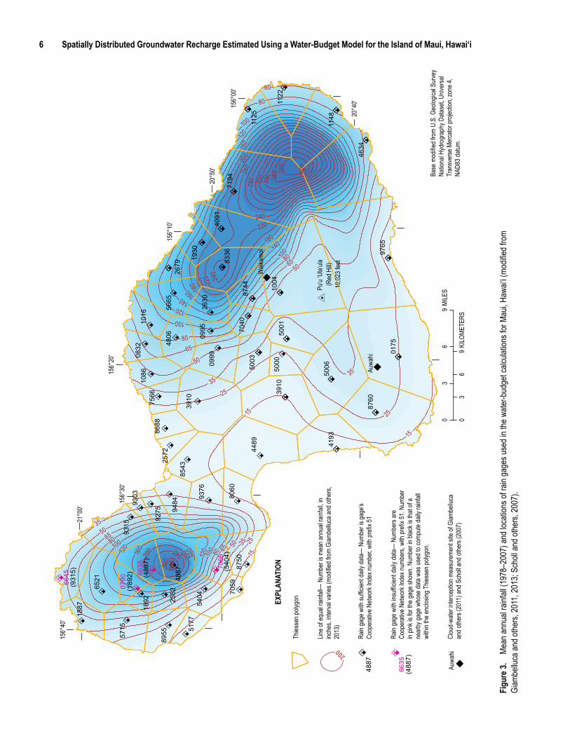
Steep gradients in mean annual rainfall patterns on Maui (fig. 3) reflect the influence of persistent trade winds and orographic rainfall (Giambelluca and others, 2013). On an island-wide basis, mean rainfall on Maui is about 81 inches per year (in/yr). Mean rainfall is more than 360 in/yr at Pu‘u Kukui, the summit of West Maui Mountain (figs. 2 and 3). About 5 mi southwest of Pu‘u Kukui, mean rainfall is less than 15 in/yr. Mean rainfall exceeds 100 in/yr for much of the interior uplands of West Maui Mountain. On Haleakalā, mean rainfall exceeds 200 in/yr on mid-altitude windward slopes. At a rain gage (not shown) near 5,400 ft altitude on windward Haleakalā, mean rainfall is about 404 in/yr, which is among the highest values in the Hawaiian Islands dur-ing 1978–2007 (Giambelluca and others, 2013). Leeward slopes in the rain shadow of Haleakalā are much drier. Mean rainfall is less than 25 in/yr for most leeward areas along the coastline and the isthmus. The summit area of Haleakalā is also relatively dry, with mean rainfall between about 35 and 50 in/yr.
HydrogeologyWest Maui Mountain and Haleakalā were built primarily
by volcanic eruptions and layers of lava flows (Langenheim and Clague, 1987). The layers of lava flows were intruded in places by dikes, which consist of dense, low-permeability rock that formed when magma supplying lava flows solidified in narrow, near-vertical fissures below the ground surface. In the inland region of West Maui Mountain, near-vertical dikes radiating in all directions from the summit impound groundwater in compartments of volcanic rock in the caldera and permeable lava flows on the flanks. The water table of the dike-impounded groundwater systems in the West Maui Mountain interior may be more than 3,500 ft above sea level (Stearns and Macdonald, 1942). Seaward of the dike-impounded systems within West Maui Mountain, freshwater-lens groundwater systems exist in the dike-free high-permeability volcanic rocks and sedimentary deposits (Gingerich, 2008). A freshwater-lens system consists of a lens-shaped freshwater body, an intermediate brackish-water transition zone, and underlying saltwater (for example, Gingerich and Engott, 2012, p. 12). Water levels of groundwater bodies in the dike-free volcanic rocks of West Maui Mountain are typically less than a few tens of feet above sea level (for example, Gingerich, 2008, p. 46). Fresh groundwater within the freshwater-lens system generally flows in a seaward direction from inland areas of West Maui Mountain toward the coast. Wedges of low-permeability sedimentary material referred to as caprock impede the seaward flow of fresh groundwater in freshwater-lens systems along parts of the northeast and southwest flanks of West Maui Mountain. Wedges of caprock
6 Spatially Distributed Groundwater Recharge Estimated Using a Water-Budget Model for the Island of Maui, Hawai‘i
9765
8760
7194
4634
4193
4091
1930
1148
1125
1122
0175
9484
9376
9315
9303
9275
8955
8750
8744
3910
8688
8543
8336
8060
7566
7066
(540
4)70
5970
40
6645
(931
5) (488
7)66
35
6521
5715
5665
5404
5177
500650
03
5001
5000
4887
4806
4489
3910
2679
2630
2572
2552
0790
(189
2)
1892
1887
1086
1016
1004
0999
0995
0832
2525
50
220 24
0
100
80
180 20
0
120
2515
355065
100
120
200 240
300
80
5035
6580
100
120 160 160
200
360
35
65
160
140
15
15
35
50
120
100
80
60
160
200
240
280 320 36
034
0 380
400
6580100
180220
240
140
0Pu
‘u ‘U
la‘ula
(R
ed H
ill)10
,023 f
eet
EXPL
ANAT
ION
Thies
sen p
olygo
n
Line o
f equ
al ra
infall
— N
umbe
r is m
ean a
nnua
l rainf
all, in
inc
hes,
inter
val v
aries
(mod
ified f
rom
Giam
bellu
ca an
d othe
rs,
2013
)
Rain
gage
with
suffic
ient d
aily d
ata—
Num
ber is
gage
’s Co
oper
ative
Netw
ork I
ndex
numb
er, w
ith pr
efix 5
1
Rain
gage
with
insu
fficien
t dail
y data
— N
umbe
rs ar
e Co
oper
ative
Netw
ork I
ndex
numb
ers,
with
prefi
x 51.
Numb
er
in pin
k is f
or th
e gag
e sho
wn. N
umbe
r in bl
ack i
s tha
t of a
ne
arby
gage
who
se da
ta wa
s use
d to c
ompu
te da
ily ra
infall
wi
thin t
he en
closin
g Thie
ssen
polyg
on.
Clou
d-wa
ter in
terce
ption
mea
sure
ment
site o
f Giam
bellu
ca
and o
thers
(201
1) an
d Sch
oll an
d othe
rs (2
007)
200
Auwa
hi
4887
6635
(488
7)
Waik
amoi
Auwa
hi
Base
mod
ified f
rom
U.S.
Geo
logica
l Sur
vey
Natio
nal H
ydro
grap
hy D
atase
t, Univ
ersa
l Tr
ansv
erse
Mer
cator
proje
ction
, zon
e 4,
NAD8
3 datu
m.
156°
00'
156°
10'
156°
20'
156°
30'
156°
40'
21°0
0'
20°5
0'
20°4
0'
03
69
KILO
METE
RS
03
69
MILE
S
Figu
re 3.
Me
an an
nual
rainf
all (1
978–
2007
) and
loca
tions
of ra
in ga
ges u
sed i
n the
wate
r-bud
get c
alcula
tions
for M
aui, H
awai‘
i (mod
ified f
rom
Giam
bellu
ca an
d othe
rs, 20
11, 2
013;
Scho
ll and
othe
rs, 20
07).
Water-Budget Model 7
between West Maui Mountain and Haleakalā also impede the flow of fresh groundwater between West Maui Mountain and the isthmus.
On northeast Haleakalā, in the area between Makawao and Ke‘anae Valley, fresh saturated groundwater occurs as (1) perched, high-level water held up by relatively low-permeability geologic layers above an unsaturated zone, and (2) a freshwater-lens system underlain by seawater (Gingerich, 1999a, 1999b). The perched groundwater is several tens of feet below the ground surface within layers of thick lava flows, ash, weathered clinker beds, and soils. Collectively, this assemblage of layers has low permeability that impedes the downward movement of the perched, high-level groundwater. An unsaturated zone and a freshwater-lens system are beneath the high-level groundwater. The freshwater-lens system is located within high-permeability basalt lava flows and has a water table that is several feet above sea level. In the area between Ke‘anae Valley and Nāhiku (fig. 2), the groundwater system appears to be saturated above sea level to altitudes greater than 2,000 ft. For southeast and south-west Haleakalā, information related to groundwater systems is sparse although perched and freshwater-lens systems are expected to be present.
Surface WaterStreams on Maui generally originate in the wet uplands of
West Maui Mountain and Haleakalā and flow toward the coast. The upper reaches of some streams on West Maui Mountain flow perennially and are fed by persistent rainfall and ground-water discharging from dike-impounded water bodies (Stearns and Macdonald, 1942). During dry-weather conditions, lower reaches of some streams on West Maui Mountain have reduced or no streamflow as a result of water captured by diversion systems and water infiltrating the subsurface (Gingerich, 2008; Gingerich and Engott, 2012). Streams on windward Haleakalā are fed by abundant rainfall and groundwater discharge (Gin-gerich, 1999a, 1999b). In the area between Makawao and Ke‘anae Valley (fig. 2), groundwater discharges to streams from a perched, high-level saturated groundwater system. East of Ke‘anae Valley, groundwater discharges to streams from a verti-cally extensive freshwater-lens system (Meyer, 2000). Water is diverted from many streams on windward Haleakalā and is mainly used to irrigate sugarcane in the isthmus. Stream reaches on leeward Haleakalā tend to be ephemeral.
SoilsFactors influencing soil conditions in the Hawaiian Islands
include parent material, duration of weathering, climate, topog-raphy, and drainage conditions (Macdonald and others, 1983). A soil’s ability to absorb and store water affects direct runoff, evapotranspiration, and recharge. Properties of a soil that con-trol its ability to absorb and store water include (1) soil texture, the relative percentages of sand-, silt-, and clay-sized particles, (2) porosity, a measure of how much water a soil can hold, and
(3) permeability, a measure of a soil’s ability to transmit water. Slope, vegetation, and soil-moisture content can also affect a soil’s ability to absorb water.
Soils on Maui were mapped and described by the Natural Resources Conservation Service (2006a). Soil properties were estimated to depths of 60 inches for most soils on Maui. Esti-mates of available water capacity, the quantity of water that a soil is capable of storing for use by plants, range between 0 and 0.40 inch of water per inch of soil. Areas containing soil hori-zons with zero available water capacity in the top 40 inches of soil include (1) steep, narrow ravines, (2) steep uplands on West Maui Mountain, and (3) leeward parts of Haleakalā and West Maui Mountain below 2,000 ft altitude. In general, soil horizons with zero available water capacity are associated with bedrock. Steep slopes may have thin soils overlying bedrock owing to erosion removing soil as fast as the soil forms (Macdonald and others, 1983).
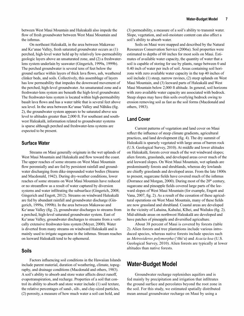
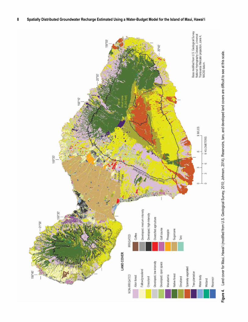
Land CoverCurrent patterns of vegetation and land cover on Maui
reflect the influence of steep climate gradients, agricultural practices, and land development (fig. 4). The dry summit of Haleakalā is sparsely vegetated with large areas of barren rock (U.S. Geological Survey, 2010). At middle and lower altitudes on Haleakalā, forests cover much of the wet windward slopes; alien forests, grasslands, and developed areas cover much of the arid leeward slopes. On West Maui Mountain, wet uplands are predominantly forests and shrublands, whereas dry lowlands are chiefly grasslands and developed areas. From the late 1800s to present, sugarcane fields have covered much of the isthmus (Dorrance and Morgan, 2000). During most of the 20th century, sugarcane and pineapple fields covered large parts of the lee-ward slopes of West Maui Mountain (for example, Engott and Vana, 2007, fig. 2). As a result of the cessation of these agricul-tural operations on West Maui Mountain, many of these fields are now grassland and shrubland. Coastal areas are developed in the vicinity of Lahaina, Kahului, Kīhei, and Wailuku (fig. 2). Mid-altitude areas on northwest Haleakalā are developed and have patches of pineapple and diversified agriculture.
About 38 percent of Maui is covered by forests (table 2). Alien forests and tree plantations include various intro-duced species, whereas native forests include species such as Metrosideros polymorpha (‘ōhi‘a) and Acacia koa (U.S. Geological Survey, 2010). Alien forests are typically at lower altitudes than native forests.
Water-Budget ModelGroundwater recharge replenishes aquifers and is
fed mainly by precipitation and irrigation that infiltrates the ground surface and percolates beyond the root zone in the soil. For this study, we estimated spatially distributed mean annual groundwater recharge on Maui by using a
8 Spatially Distributed Groundwater Recharge Estimated Using a Water-Budget Model for the Island of Maui, Hawai‘i
Figu
re 4.
La
nd co
ver f
or M
aui, H
awai‘
i (mod
ified f
rom
U.S.
Geo
logica
l Sur
vey,
2010
; Joh
nson
, 201
4). R
eser
voirs
, taro
, and
deve
loped
land
cove
rs ar
e diffi
cult t
o see
at th
is sc
ale.
Water-Budget Model 9
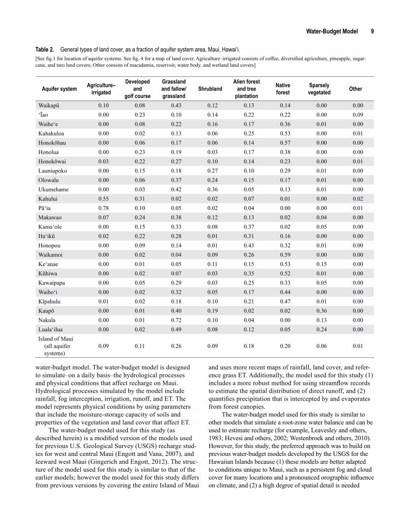
Aquifer system Agriculture– irrigated
Developed and
golf course
Grassland and fallow/ grassland
ShrublandAlien forest
and tree plantation
Native forest
Sparsely vegetated Other
Waikapū 0.10 0.08 0.43 0.12 0.13 0.14 0.00 0.00‘Īao 0.00 0.23 0.10 0.14 0.22 0.22 0.00 0.09Waihe‘e 0.00 0.08 0.22 0.16 0.17 0.36 0.01 0.00Kahakuloa 0.00 0.02 0.13 0.06 0.25 0.53 0.00 0.01Honokōhau 0.00 0.06 0.17 0.06 0.14 0.57 0.00 0.00Honolua 0.00 0.23 0.19 0.03 0.17 0.38 0.00 0.00Honokōwai 0.03 0.22 0.27 0.10 0.14 0.23 0.00 0.01Launiupoko 0.00 0.15 0.18 0.27 0.10 0.29 0.01 0.00Olowalu 0.00 0.06 0.37 0.24 0.15 0.17 0.01 0.00Ukumehame 0.00 0.03 0.42 0.36 0.05 0.13 0.01 0.00Kahului 0.55 0.31 0.02 0.02 0.07 0.01 0.00 0.02Pā‘ia 0.78 0.10 0.05 0.02 0.04 0.00 0.00 0.01Makawao 0.07 0.24 0.38 0.12 0.13 0.02 0.04 0.00Kama‘ole 0.00 0.15 0.33 0.08 0.37 0.02 0.05 0.00Ha‘ikū 0.02 0.22 0.28 0.01 0.31 0.16 0.00 0.00Honopou 0.00 0.09 0.14 0.01 0.43 0.32 0.01 0.00Waikamoi 0.00 0.02 0.04 0.09 0.26 0.59 0.00 0.00Ke‘anae 0.00 0.01 0.05 0.11 0.15 0.53 0.15 0.00Kūhiwa 0.00 0.02 0.07 0.03 0.35 0.52 0.01 0.00Kawaipapa 0.00 0.05 0.29 0.03 0.25 0.33 0.05 0.00Waiho‘i 0.00 0.02 0.32 0.05 0.17 0.44 0.00 0.00Kīpahulu 0.01 0.02 0.18 0.10 0.21 0.47 0.01 0.00Kaupō 0.00 0.01 0.40 0.19 0.02 0.02 0.36 0.00Nakula 0.00 0.01 0.72 0.10 0.04 0.00 0.13 0.00Luala‘ilua 0.00 0.02 0.49 0.08 0.12 0.05 0.24 0.00Island of Maui
(all aquifer systems)
0.09 0.11 0.26 0.09 0.18 0.20 0.06 0.01
Table 2. General types of land cover, as a fraction of aquifer system area, Maui, Hawai‘i.[See fig.1 for location of aquifer systems. See fig. 4 for a map of land cover. Agriculture–irrigated consists of coffee, diversified agriculture, pineapple, sugar-cane, and taro land covers; Other consists of macadamia, reservoir, water body, and wetland land covers]
water-budget model. The water-budget model is designed to simulate–on a daily basis–the hydrological processes and physical conditions that affect recharge on Maui. Hydrological processes simulated by the model include rainfall, fog interception, irrigation, runoff, and ET. The model represents physical conditions by using parameters that include the moisture-storage capacity of soils and properties of the vegetation and land cover that affect ET.
The water-budget model used for this study (as described herein) is a modified version of the models used for previous U.S. Geological Survey (USGS) recharge stud-ies for west and central Maui (Engott and Vana, 2007), and leeward west Maui (Gingerich and Engott, 2012). The struc-ture of the model used for this study is similar to that of the earlier models; however the model used for this study differs from previous versions by covering the entire Island of Maui
and uses more recent maps of rainfall, land cover, and refer-ence grass ET. Additionally, the model used for this study (1) includes a more robust method for using streamflow records to estimate the spatial distribution of direct runoff, and (2) quantifies precipitation that is intercepted by and evaporates from forest canopies.
The water-budget model used for this study is similar to other models that simulate a root-zone water balance and can be used to estimate recharge (for example, Leavesley and others, 1983; Hevesi and others, 2002; Westenbroek and others, 2010). However, for this study, the preferred approach was to build on previous water-budget models developed by the USGS for the Hawaiian Islands because (1) these models are better adapted to conditions unique to Maui, such as a persistent fog and cloud cover for many locations and a pronounced orographic influence on climate, and (2) a high degree of spatial detail is needed
10 Spatially Distributed Groundwater Recharge Estimated Using a Water-Budget Model for the Island of Maui, Hawai‘i
for defining the model subareas. The high degree of spatial detail allows the model to represent the wide range of climate conditions, vegetation, soils, and land uses on Maui.
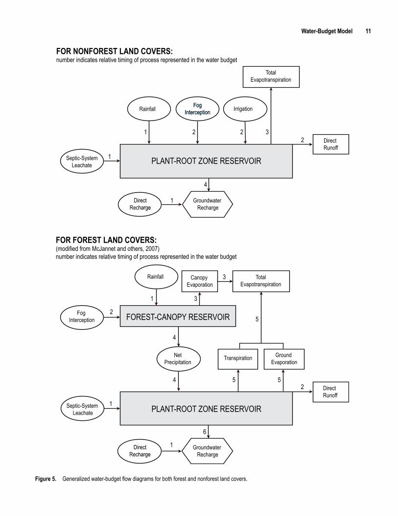
Conceptual Model The water-budget model used here to estimate groundwater
recharge is a “threshold-type” or “reservoir” model utilizing a variation of the Thornthwaite and Mather (1955) mass-balance procedure. The two generalized flow diagrams of the water-budget model—one for nonforest land covers and one for forest land covers are displayed in figure 5. The plant-root zone reservoir is included in the model for nonforest and forest land covers. The forest-canopy reservoir is included in the model for forest land covers only.
The volume of the plant-root zone reservoir is based on the estimated root depth of different plant types and the available water capacity of different soil types. The model uses a daily computational interval to account for water entering, leaving, and being stored within the plant-root zone reservoir. At the end of a day, if the volume of water entering the system exceeds the storage capacity of the plant-root zone reservoir, given the antecedent water content and water losses from ET, the reservoir overflows. This overflow is counted as groundwater recharge by the model. In some areas, recharge includes direct recharge from reservoir and cesspool seepage. All water infiltrating the substrate beneath the plant-root zone reservoir as overflow or direct recharge is considered recharge.
Direct runoff is the fraction of precipitation (rainfall and fog interception) that does not contribute to net moisture gain within the plant-root zone reservoir. Direct runoff excludes base flow, which is groundwater discharge to streams. Direct runoff is assumed either to be diverted to other areas or ultimately discharge to the ocean. Re-infiltration of direct runoff is not quantified in the model, although it is indirectly accounted for in the empirical functions used to compute direct runoff.
The forest-canopy reservoir is not treated as a true res-ervoir in the model calculations because precipitation is not allowed to be stored in it for more than a day. For each daily computational period, precipitation in the forest-canopy reser-voir either evaporates as canopy evaporation or reaches the soil as part of net precipitation. Net precipitation is computed as the sum of fog interception and rainfall minus canopy evaporation, and thus represents outflow from the forest-canopy reservoir. Net precipitation is partitioned into direct runoff and inflow to the plant-root zone. The plant-root zone reservoir and the forest-canopy reservoir are herein referred to as the plant-root zone and the forest canopy, respectively.
Model Calculations The water-budget model computes groundwater
recharge for the Island of Maui using input data that quantify the spatial and temporal distribution of rainfall, fog intercep-tion, irrigation, ET, direct runoff, soil type, land cover, and
seepage from reservoirs and septic systems. For the model calculations, the Island of Maui is subdivided into small areas with homogeneous properties, termed subareas. A map of subareas is generated using Esri ArcGIS software (www.esri.com) by intersecting (merging) spatial datasets that characterize the spatial distribution of rainfall, fog, irrigation, reference ET, direct runoff, soil type, and land cover. Inter-secting the spatial datasets resulted in 318,429 subareas–with an average area of about 1.5 acres–for the Maui water-budget model.
The water-budget model treats each subarea independently. Water transfers between subareas are not included in the model calculations. The model domain of each subarea extends verti-cally from the vegetation canopy to the base of the plant-root zone, the part of the soil and bedrock containing roots. Proper-ties of the substrate beneath the plant-root zone are not included in the model calculations.
For each subarea, the water-budget model calculates recharge on a daily basis for the period of the scenario. In this study, we used two scenarios: one for average climate condi-tions and one for drought conditions. Mean annual recharge for each scenario is determined for each subarea. Mean annual recharge for subareas is also summed over larger areas of inter-est, including Maui’s 25 aquifer systems.
For each subarea, the model calculates an interim moisture storage value at the start of each day. Interim moisture storage is the amount of water that enters the plant-root zone for the current day plus the amount of water already in the plant-root zone from the previous day. For the first day of the simulation, a value for the amount of water already in the plant-root zone from the previous day (initial soil moisture) is selected. For subareas with nonforest land covers, interim moisture storage, Xi, is given by the equation
Xi = Ri + Fi –Ui + Ii + Li + Wi + Mi-1, (1a)
where Xi = interim moisture storage for current day
[L], Ri = rainfall for current day [L], Fi = fog interception for current day [L], Ui = direct runoff for current day [L], Ii = irrigation for current day [L], Li = septic-system leachate for current day [L],
Wi = excess water from the impervious fraction of the subarea distributed over the pervious fraction of the subarea [L],
Mi-1 = moisture storage at the end of the previous day (i-1) [L], and
i = subscript designating current day.
For subareas with forest land covers, interim moisture storage is given by the equation
Water-Budget Model 11
Figure 5. Generalized water-budget flow diagrams for both forest and nonforest land covers.
PLANT-ROOT ZONE RESERVOIR
FOREST-CANOPY RESERVOIR
FOR FOREST LAND COVERS:(modified from McJannet and others, 2007)number indicates relative timing of process represented in the water budget
Canopy Evaporation
Groundwater Recharge
DirectRunoff
TotalEvapotranspiration
Transpiration Ground Evaporation
NetPrecipitation
Rainfall
Fog Interception
Septic-System Leachate
DirectRecharge
2
1 3
3
4
42
1
5
1
6
5
5
PLANT-ROOT ZONE RESERVOIR
FOR NONFOREST LAND COVERS:number indicates relative timing of process represented in the water budget
TotalEvapotranspiration
IrrigationFogInterception
FogInterceptionRainfall
Groundwater Recharge
Direct Runoff
DirectRecharge
Septic-SystemLeachate
2
1
12
2 3
4
1
12 Spatially Distributed Groundwater Recharge Estimated Using a Water-Budget Model for the Island of Maui, Hawai‘i
Xi = (NP)i – Ui + Li + Wi + Mi-1, (1b)where
(NP)i = net precipitation for current day [L].
For subareas with forest land covers, net precipitation is computed as precipitation minus canopy evaporation, which is the amount of precipitation that is intercepted by and evaporates from the leaves, stems, and trunks of a forest. Precipitation is the sum of rainfall and fog interception:
Pi = Ri + Fi (2)
where Pi = precipitation for current day [L].
Net precipitation is computed as:
(NP)i = Pi – (CE)i, (3)
where (CE)i = forest-canopy evaporation for current day
[L].
The water-budget model computes forest-canopy evapora-tion using an approach that is derived from the rainfall-intercep-tion model described by Gash and others (1995), herein referred to as the Gash model. Using this approach, canopy evaporation for a given day and location depends on precipitation amount, forest structure, and mean rates of evaporation and precipitation. The Gash model was modified for this study so that (1) pre-cipitation includes rainfall and fog interception, instead of rain only, and (2) water cannot be stored on the forest canopy for more than a day. The forest structure is characterized in terms of canopy cover, canopy capacity, trunk-storage capacity, and the proportion of precipitation diverted to stemflow. Canopy cover, c, is the fraction of a forested subarea that is covered by leaves, stems, and branches of trees. Canopy capacity, S, is the depth of water left on the canopy when rainfall and throughfall have ceased (Gash and Morton, 1978). Evaporation of water from tree trunks is accounted for by the model using the proportion of precipitation that is diverted to stemflow, p, and trunk-storage capacity, k, which is considered in terms of an equivalent depth of precipitation. The last parameter needed for the Gash model is the ratio of the mean evaporation rate to the mean precipita-tion rate during saturated conditions, V.
To compute forest-canopy evaporation, the first step is to determine the minimum depth of precipitation necessary to satu-rate the forest canopy, P’ (Gash and others, 1995). On the basis of equation 2 in Gash and others (1995), P’ for subareas with forest land covers is computed as
P’ = –{S ÷ (c × V)} × ln (1 – V). (4)
where P’ = precipitation necessary to saturate the
canopy [L], S = canopy capacity per unit of ground area [L]
(a constant), c = canopy cover per unit of ground area
[dimensionless], and V = ratio of mean evaporation rate to mean
precipitation rate during saturated conditions [dimensionless].
On the basis of the revised analytical form of the Gash model presented in table 1 of Gash and others (1995), forest-canopy evaporation for a given day, (CE)i, was computed for three canopy conditions as follows:
for Pi < P’, (CE)i = c × Pi ,
for Pi ≥ P’ and Pi ≤ k ÷ p, (CE)i = c × P’+ c × V × (Pi – P’) + p × Pi , for Pi ≥P’ and Pi > k ÷ p, (CE)i = c × P’ + c × V × (Pi – P’) + k, (5)
where k = trunk-storage capacity [L] (a constant), and p = proportion of precipitation diverted to
stemflow [dimensionless].
For each subarea with impervious surfaces, such as paved roads and buildings, the interim moisture-storage equations include the factor Wi (see equations 1a and 1b), which is a func-tion of the fraction of the subarea that is impervious. For subar-eas with no impervious surfaces, Wi is zero. The fraction of the subarea that is impervious, z, is used to separate, from the total rain that falls in a subarea, a depth of water that is treated com-putationally as though it fell on an impervious surface. Based on the rainfall-retention capacity of the impervious surface, some water is subtracted to account for direct evaporation. The remaining water is considered excess water, Wi. For subareas without storm-drain systems, Wi is added to the water budget of the pervious fraction of the model subarea. In this case, the total daily water input for the pervious fraction of a subarea includes excess water from the impervious fraction (equations 1a and 1b). For subareas with storm-drain systems, Wi is assumed to be collected by storm-drain systems and is added to runoff or to direct recharge, depending on location.
For subareas with impervious surfaces, excess water, Wi, is determined using the following conditions:
Water-Budget Model 13
X1i = Pi – Ui + Ti-1, (6)
for X1i ≤ N , Wi = 0, and X2i = X1i, for X1i > N , Wi = (X1i – N) × z ÷ (1 – z), and X2i = N, (7)
where
X1i = first interim moisture storage on the surface of impervious area for current day [L],
X2i = second interim moisture storage on the surface of impervious area for current day [L],
Ti–1 = water storage (ponded water) on the surface of impervious area at the end of the previous day (i –1) [L],
N = rainfall-retention capacity of the impervious surface (maximum amount of water storage on the surface of impervious area) [L], and
z = fraction of area that is impervious [dimensionless].
The water storage on the surface of the impervious area at the end of the current day, Ti, is determined from the equation:
for X2i ≤ Gi , Ti = 0,
for X2i > Gi , Ti = X2i – Gi, and (8)
where
Gi = reference ET for current day [L], and Ti = water storage (ponded water) on the
surface of impervious area at the end of day [L].
The next step in the water-budget computation is to determine the amount of water that will be removed from the plant-root zone by ET. Actual ET is a function of potential ET and interim moisture, Xi. The plant-root zone loses water to the atmosphere at the potential-ET rate if sufficient water is avail-able. At all sites, potential ET, (PE)i, is computed as the product of (1) reference ET, Gi, the potential ET of a grass reference surface, and (2) crop coefficient, kc, a factor that depends on vegetation and land cover.
(PE)i = kc × Gi (9)
where
(PE)i = potential-ET rate for the current day [L/T], and
kc = crop coefficient of land cover [dimensionless].
For moisture storage greater than or equal to a threshold value, Ci, the actual-ET rate is assumed to be equal to the potential-ET rate. For moisture storage less than Ci, the actual-ET rate is assumed to occur at a reduced rate that declines linearly with soil-moisture content:
for M ≥ Ci, , E = (PE)i , and for M < Ci and Ci > 0 E = M × (PE)i ÷ Ci , (10)
where E = instantaneous actual-ET rate [L/T], M = instantaneous moisture storage [L], and Ci = threshold moisture storage for the current
day below which the actual-ET rate is less than the potential-ET rate [L].
The threshold moisture storage, Ci, is estimated using the model of Allen and others (1998) for soil moisture. In this model, a depletion fraction, d, which ranges from 0 to 1, is defined as the fraction of maximum moisture storage that can be depleted from the plant-root zone before moisture stress causes a reduction in the actual-ET rate. Values for d are assigned to land-cover classes on the basis of data in Allen and others (1998). The threshold moisture, Ci, is estimated from d by the equation
Ci = (1 – d) × Mm , (11)
where
Mm = moisture-storage capacity of the plant-root zone [L].
d = depletion fraction [dimensionless].
The moisture-storage capacity of the plant-root zone, Mm, expressed as a depth of water, is equal to the plant-root depth, D, multiplied by the available water capacity of the soil, φ. Available water capacity is the difference between the volumetric field-capacity moisture content and the volumetric wilting-point moisture content:
Mm = D × φ , (12)
where
D = plant root depth [L], φ = available water capacity, θfc – θwp [L
3/L3], θfc = volumetric field-capacity moisture content
[L3/L3], and θwp = volumetric wilting-point moisture content
[L3/L3].
In the water-budget model, the actual-ET rate from the plant-root zone may be (1) equal to the potential-ET rate for part of the day and less than the potential-ET rate for the
14 Spatially Distributed Groundwater Recharge Estimated Using a Water-Budget Model for the Island of Maui, Hawai‘i
remainder of the day, (2) equal to the potential-ET rate for the entire day, or (3) less than the potential-ET rate for the entire day. The total ET from the plant-root zone during a day is a function of the potential-ET rate, (PE)i, interim moisture storage, Xi, and threshold moisture content, Ci. By recognizing that E = -dM/dt, the total depth of water removed by ET from the plant-root zone during a day, Ei, is determined as follows:
for Xi > Ci and Ci > 0, Ei = (PE)iti + Ci{1 – exp[–(PE)i(1-ti) ÷ Ci]},
for Xi > Ci and Ci = 0, Ei = (PE)iti,
for Xi ≤ Ci and Ci > 0, Ei = Xi{1 – exp[–(PE)i ÷ Ci]}, and
for Xi = Ci, and Ci = 0, Ei = 0, (13)
where Ei = evapotranspiration from the plant-root
zone during the day [L], ti = time during which moisture storage is
above Ci [T]. It ranges from 0 to 1 day and is computed as follows:
for (Xi – Ci) < (PE)i(1 day)
ti = (Xi – Ci) ÷ (PE)i, and for (Xi – Ci) ≥ (PE)i(1 day),
ti = 1. (14)
After accounting for runoff (equation 1a or 1b), actual ET from the plant-root zone for a given day is subtracted from the interim moisture storage, and any moisture remaining above the maximum moisture storage is assumed to be recharge. The daily rate of direct recharge from anthropogenic sources, including seepage from cesspools and reservoirs, is also added to daily recharge at this point. Recharge and moisture storage at the end of a given day are assigned according to the follow-ing conditions:
for Xi – Ei ≤ Mm, Qi = DR, and Mi = Xi – Ei , and
for Xi – Ei > Mm, Qi = (Xi– Ei – Mm) + DR, and Mi = Mm, (15)
where Qi = groundwater recharge during the day [L],
and Mi = moisture storage at the end of the current
day (i) [L], and DR = daily rate of direct recharge [L] (a
constant).
Model Input
Land CoverA land-cover map for Maui representative of 2010
conditions, herein referred to as the 2010 land-cover map, was developed by Johnson (2014) for this study. The 2010 land-cover map identifies 21 types of land cover (fig. 4) and was intersected with other spatial datasets when creating the map of subareas for the water-budget model. The 2010 land-cover map was used in the computation of recharge for both scenarios of this study: average climate conditions and drought conditions. The 2010 land-cover map was created by modifying the LANDFIRE Existing Vegetation Type map for Maui (U.S. Geological Survey, 2010), herein referred to as the Landfire map. Modifications to the Landfire map included converting it from a raster dataset to a vector data-set, combining similar land-cover classes, and adding bound-aries of golf courses and selected crops. These modifications were done using Esri ArcGIS software, as summarized next. Additional details are included in the metadata of Johnson (2014).
Some land-cover groups of the Landfire map were com-bined into more general classes for the 2010 land-cover map. Landfire groups “Hawaiian Dry Grassland,” “Hawaiian Mesic Grassland,” and “Introduced Perennial Grassland and Forbland” were combined into “Grassland” for the 2010 land-cover map (fig. 4). Landfire groups “Hawaiian Dry Shrubland,” “Hawaiian Mesic Shrubland,” and “Introduced Upland Vegetation – Shrub” were combined into “Shrubland.” Landfire groups “Hawaiian Dry Forest,” “Hawaiian Mesic Forest,” and “Hawaiian Rainfor-est” were combined into “Native forest.” The Landfire group “Introduced Upland Vegetation-Treed” was renamed as “Alien forest.”
Locations of golf courses and selected crops not specified in the Landfire map were delineated in the 2010 land-cover map to improve estimates of irrigation, ET, and recharge for parcels with these types of land cover. We defined the boundaries of sugarcane, coffee, pineapple, and taro fields, as well as golf courses, in the 2010 land-cover map (fig. 4) by using sources other than the Landfire map. We defined boundaries of sugar-cane fields by using a 2000–04 land-cover map by Engott and Vana (2007) and a plantation-divisions map (Hawaiian Com-mercial & Sugar Company, 2008). We digitized the boundar-ies of golf courses and fields of coffee and pineapple by using 2010–13 satellite imagery in Google Earth (earth.google.com) and recent orthoimagery (U.S. Department of Agriculture,
Model Input 15
2007). Fields of taro were digitized on the basis of those identi-fied in Gingerich and others (2007).
Parcels classified as agriculture in the Landfire map (other than those within fields of sugarcane, pineapple, or coffee) were reclassified by the authors in the 2010 land-cover map as either macadamia, diversified agriculture, fallow/grassland, low-intensity developed, or open-space developed using the 2000–04 land-cover map of Engott and Vana (2007), recent orthoimagery, and 2010–13 satellite imagery. Agriculture parcels with groves of trees on the east slope of West Maui Mountain were classified as macadamia. All other agriculture parcels that appeared in the imagery as being actively cultivated were classified as diversified agriculture. Additionally, we used recent orthoimagery and satellite imagery to digitize the boundaries of diversified-agriculture fields within the Kula Agricultural Park (fig. 4) in the 2010 land-cover map. These boundaries were digitized because water-supply data for Kula Agricultural Park were used to calibrate irrigation rates for diversified agriculture. Agriculture parcels that appeared in the imagery as uncultivated and mostly covered by grass were defined as fallow/grassland. Parcels defined as fallow/grassland include former pineapple fields on leeward West Maui Mountain that were abandoned when Maui Land & Pineapple Company ceased its pineapple operations there at the end of 2009 (Maui News, December 24, 2009). The fallow/grassland land-cover class likely includes parcels that were used as grazing pastures. Parcels defined as Agriculture in the Landfire map and that were adjacent to, but not within, the fields of sugarcane, pineapple, or coffee were classified in the 2010 land-cover map as either grassland, open-space developed, or low-intensity developed on the basis of the land cover for nearby parcels.
Impervious SurfacesImpervious surfaces include paved surfaces and buildings.
Excess water from the impervious fraction of a subarea, Wi, that is distributed to the pervious fraction of the subarea depends on the impervious fraction of the subarea, z. The impervious frac-tion of each subarea was computed from a map of impervious surfaces on Maui (National Oceanic and Atmospheric Adminis-tration, 2008).
Rainfall
Monthly RainfallMonthly rainfall-distribution grids for 1978–2007 were
used to estimate monthly rainfall distribution in the water-budget model. The monthly rainfall grids for 1978–2007, obtained from a 1920–2012 monthly rainfall-distribution dataset (Frazier and others, 2016), were selected because they have the same base period as the mean monthly and mean annual rainfall grids of the Rainfall Atlas of Hawai‘i (Giambelluca and others, 2013). The boundaries of the monthly rainfall grid cells were included in the polygon map
of subareas, and each subarea was assigned to a grid cell. Monthly rainfall for each subarea was computed in the model as the product of the monthly rainfall value from Frazier and others (2016) and a mean monthly adjustment factor. Adjustment factors were used because cell-by-cell comparisons between mean monthly rainfall calculated for 1978–2007 from the Frazier and others (2016) dataset and the mean monthly values in Giambelluca and others (2013) showed small differences. Each rainfall grid cell was assigned a set of 12 mean monthly adjustment factors, which ensured that mean monthly rainfall estimates of the water-budget model were consistent with those of Giambelluca and others (2013).
Daily RainfallEstimates of the actual rainfall pattern on Maui for
each day during 1978–2007 were not available and were not developed as part of this study. Although records of daily rainfall measurements at gages were available, reconstructing the actual daily rainfall pattern was not attempted because (1) records for many gages have considerable gaps, (2) the spatial interpolation of daily records for gages would have high uncertainty, and (3) the monthly rainfall maps of Frazier and others (2016) were considered to be the best dataset available for estimating historical rainfall patterns.
The water-budget model synthesized daily rainfall by disaggregating the monthly values of the 1978–2007 rainfall distribution maps using the method of fragments (for example, Oki, 2002). The method of fragments creates a synthetic sequence of daily rainfall from monthly rainfall by imposing the rainfall pattern from a rain gage with daily data. The synthesized daily rainfall data approximate the long-term average character of daily rainfall, such as frequency, duration, and intensity, but may not reproduce the historical daily rainfall record during 1978–2007.
Daily rainfall measurements at 52 rain gages on Maui during 1905–2011 were used to disaggregate monthly rainfall into daily rainfall for the water-budget model. Rain gages were selected on the basis of location and length and completeness of daily records. Daily rainfall data for the rain gages’ period of record were obtained from the National Climatic Data Center (www.ncdc.noaa.gov) and the USGS (http://waterdata.usgs.gov/hi/nwis/nwis). Thiessen polygons were drawn around each of the rain gages, and the daily rainfall pattern within each Thiessen polygon was assumed to be the same as the pattern at the rain gage within the Thiessen polygon (fig. 3).
For each rain gage, daily rainfall fragments were computed by dividing each daily rainfall measurement for a particular month by the total rainfall measured at the gage for that month. This resulted in a set of fragments for that particular month in which the total number of fragments was equal to the number of days in the month. Fragment sets were compiled for every gage for every month in which complete daily rainfall measurements were available. Fragment sets were grouped by month of the year and by rain gage. In the water-budget calculation, the fragment set to be used for a given gage for a given month was selected randomly from among all available sets for that gage for that month. Daily rainfall for a given month was synthesized
16 Spatially Distributed Groundwater Recharge Estimated Using a Water-Budget Model for the Island of Maui, Hawai‘i
by multiplying total rainfall for that month (from the monthly rainfall maps) by each fragment in the set, thereby providing daily rainfall, Ri, for equation 1a or 1b.
Owing to insufficient daily records, fragment sets for each of the 12 calendar months were not available for rain gages with Cooperative Station Network numbers 0790, 6635, 6645, and 7066 (fig. 3). These four gages were assigned fragment sets from nearby gages with similar amounts of mean rainfall. Gage 0790 was assigned the gage 1892 fragment set, gage 6635 the gage 4887 fragment set, gage 6645 the gage 9315 fragment set, and gage 7066 the gage 5404 fragment set.
Fog Interception
In Hawai‘i, fog most frequently occurs where mountain slopes are immersed in a persistent layer of clouds. Clouds can form when moist air cools and condenses as it is forced upslope by trade winds and by thermal circulation systems such as sea breezes. As fog flows near the land surface, vegetation may intercept some of the fog moisture. Fog moisture that accumu-lates on vegetation is called “fog interception” or “cloud-water interception.” At places where fog is frequent, intercepted fog moisture that drips from the vegetation to the ground can be a substantial part of the water budget (Ekern, 1964; Juvik and Ekern, 1978; Juvik and Nullet, 1995; Heath and Huebert, 1999; Scholl and others, 2007; Giambelluca and others, 2011; Taka-hashi and others, 2011). Areas in Hawai‘i that frequently have fog are in the “cloud zone,” which is between altitudes of about 2,000 and 8,200 ft (fig. 4; DeLay and Giambelluca, 2010). Fog can also form in areas above the cloud zone (Juvik and Ekern, 1978).
Much effort has been to done to quantify cloud-water interception (CWI) for forests in Hawai‘i. According to a sum-mary of fog research in Hawai‘i, CWI estimates range between 4 and 20 in/yr for most leeward sites within the cloud zone, and between 11 and 44 in/yr for most windward sites within the cloud zone (DeLay and Giambelluca, 2010). On Maui, Giam-belluca and others (2011) and Scholl and others (2007) used different approaches to estimate CWI for two forested sites on Haleakalā: Auwahi and Waikamoi (fig. 3). Auwahi is near 4,000 ft altitude on leeward Haleakalā; Waikamoi is near 6,400 ft altitude on windward Haleakalā. Using a canopy water-balance approach, Giambelluca and others (2011) determined CWI to be about 6.5 in/yr at Auwahi and about 48 in/yr at Waikamoi. Using a stable isotopic mixing-model approach, Scholl and others (2007) estimated that cloud water was 46 and 37 percent of total precipitation at Auwahi and Waikamoi, respectively. By combining the results of Scholl and others (2007) with 1978–2007 mean annual rainfall near Auwahi (about 29 in/yr) and Waikamoi (about 82 in/yr), we computed CWI to be about 25 in/yr at Auwahi, and 48 in/yr at Waikamoi.
Fog interception was quantified in the water-budget model for four land-cover classes: alien forest, native forest, tree plantation, and shrubland. On the basis of previous fog and CWI estimates for Hawai‘i, mean annual fog interception for forests
Altitude range, in feet above mean sea level Location
relative to cloud zone
Fog-interception rate, in inches per year
From To Leeward aspect
Windward aspect
0 <2,000 Below 0 0 2,000 8,200 Within 14 30 >8,200 <9,000 Above 10 18
9,000 and higher Above 6 6
Table 3. Mean fog-interception rates used in the water-budget calculation for average climate conditions for Maui, Hawai‘i.
[Fog-interception rates in this table were used for forest land covers: alien for-est, native forest, and tree plantation. For areas with shrubland land cover, fog-interception rates were assumed to be half of the rates in this table. See fig. 4 for land covers and the cloud zone for Maui. The altitude range of the cloud zone is based on areas with frequent cloud contact, as defined by DeLay and Giambelluca (2010). See fig. 6 for boundary between windward and leeward areas. <, less than; >, greater than]
on Maui was assumed to vary with altitude and aspect for the water budget (table 3). For forests below the typical base of the cloud zone (2,000 ft altitude), fog interception was assumed to be negligible in both leeward and windward areas. For forests within the cloud zone (2,000–8,200 ft altitude) mean annual fog interception was assumed to be near the midpoints of the ranges of the CWI measurements for leeward and windward sites in Hawai‘i (table 3). The midpoints of the ranges were used because the existing set of fog and CWI measurements in Hawai‘i may not be representative of the majority of the cloud-forest area across the state (DeLay and Giambelluca, 2010). For example, many of the CWI estimates in Hawai‘i are from fog-gage measurements in large clearings or along ridges, or are based on canopy water-balance measurements at forest edges. At such exposed areas and forest edges, wind velocity and fog density is much higher than within the canopy of a closed canopy forest (DeLay and Giambelluca, 2010). Hence the cloud-water input at these measurement sites, including Auwahi and Waikamoi, may be greater than cloud-water input for large areas of continuous forests (Giambelluca and others, 2011).
Mean annual fog interception was assumed to decrease uniformly with altitude from the values for the cloud zone to 6 in/yr near the Haleakalā summit (table 3). The assumption of decreasing fog interception with altitude above the cloud zone is based on the fog-altitude relation shown in figure 35.3 of and DeLay and Giambelluca (2010). A fog-intercep-tion rate of 6 in/yr is based on three fog-interception studies conducted at about 11,200 ft altitude on northern Mauna Loa, Island of Hawai‘i (Juvik and Perreira, 1974; Juvik and Ekern, 1978) and summarized in DeLay and Giambelluca (2010, table 35.1). Much of the area above the cloud zone on Maui is not forested but is sparsely vegetated or shrubland (fig. 4).
Mean annual fog-interception rates for shrubland sub-areas were assumed to be half of the rates for forest subareas
Model Input 17
(table 3). This assumption was also used in recent water budgets for Hawai‘i (for example, Engott and Vana, 2007; Engott, 2011), and is based on the premise that shrubs are usually shorter than trees and consequently have a smaller silhouette and less potential to intercept fog water. Fog inter-ception was assumed to be negligible at all altitudes for land-cover classes other than forests and shrubland. Coffee and macadamia land covers, which have the potential to intercept fog moisture, were assumed to have no fog interception for this study because they are at altitudes below the cloud zone (fig. 4).
Owing to the sparseness of monthly fog data for Maui, mean annual fog interception for a given subarea was appor-tioned equally to each month of the year in the water-budget calculations. Fog interception was assumed to occur only on days with rainfall. Daily fog interception was computed in the water budget as a fraction of daily rainfall equivalent to the ratio of mean monthly fog interception and mean monthly rainfall during 1978–2007. These resulting fog-to-rainfall ratios were used to compute recharge for average climate conditions and for drought conditions.
Estimating fog interception in the water budget requires many assumptions because the magnitude, temporal variability, and spatial variability of fog interception on Maui are not well known. A better understanding of these characteristics would improve fog-interception estimates of the water budget. The fog-to-rainfall ratios used to compute fog interception for this study, however, result in fog-interception values that are within the range of most CWI and fog-interception measurements in Hawai‘i. Because of the uncertainty in fog-interception rates on Maui, alternative fog-interception rates are evaluated in the Sensitivity Analysis section of this report.
IrrigationIrrigation was applied to golf courses and five agricultural
land covers: coffee, diversified agriculture, pineapple, sugar-cane, and taro (fig. 4). Irrigation was also applied to medium- and high-intensity developed subareas in order to simulate the watering of urban landscapes. Of these irrigated land-cover classes, sugarcane is the most expansive, totaling slightly less than 9 percent of the study area. The other irrigated land-cover classes total about 3 percent of the study area.
Irrigation EstimatesWe estimated irrigation rates using a demand-based
approach, similar to the approach used to estimate irrigation for the Hawaii Agricultural Water Use and Development Plan (Department of Natural Resources and Environmental Management, 2008). The estimated irrigation rate is intended to replenish the water content in the root zone to reach field capacity. Irrigation demand for a given subarea is esti-mated on the basis of monthly rainfall, runoff, and potential evapotranspiration:
for (PE)m + Um > Rm,
Im = {(PE)m + Um – Rm} ÷ g
for (PE)m + Um ≤ Rm,
Im = 0 (16)
where
(PE)m = potential evapotranspiration for month m [L] (varies by location),
Um = amount of runoff for month m [L], Rm = amount of rainfall for month m [L], Im = amount of irrigation for month m [L], and g = irrigation efficiency [dimensionless] (varies
by irrigation method).
Irrigation rates also depend on the efficiency, g, of the irrigation method. Irrigation efficiency is the ratio of volume of water consumed by vegetation to the volume of water applied for irrigation. Hawaiian Commercial & Sugar Company (HC&S) uses drip irrigation for its sugarcane fields. On the basis of information provided by HC&S, the water budget of Engott and Vana (2007) computed drip irrigation for HC&S’ sugarcane fields using an irrigation efficiency of 0.80. An irrigation efficiency of 0.80 was also used to compute sugar-cane irrigation in the water budget for this study. The irrigation efficiencies used in the water budget for all remaining irrigation methods were obtained from table 3.1 of Department of Natural Resources and Environmental Management (2008). Diversified agriculture and pineapple were assumed to use drip irrigation, which has an irrigation efficiency of 0.85. Coffee was assumed to use micro-spray irrigation, which has an irrigation efficiency of 0.80. Golf course, and medium- and high-intensity developed land covers were assumed to use sprinkler irrigation, which has an irrigation efficiency of 0.70.
For all irrigated land covers other than sugarcane, pine-apple, and taro, monthly irrigation estimated from equation 16 was allocated in equal amounts for each day of a given month. To simulate irrigation practices for sugarcane on Maui, as described in detail by Engott and Vana (2007) and briefly summarized here, irrigation rates for sugarcane were varied throughout the cultivation cycle. Sugarcane was assumed to have a 24-month cultivation cycle. For a given sugarcane field, irrigation water was applied during for the first 20 months of the cycle. Monthly irrigation during the first 20 months of the cycle was computed according to equation 16 and was equally apportioned to the field on days 1, 2, 3, 8, 9, 10, 15, 16, 17, 22, 23, 24, 28 of each month. No irrigation was applied to the field during the last 4 months of the 24-month cycle. The sugarcane was assumed to be harvested at the end of month 22 of the 24-month cycle. The field was assumed to be fallow during the last 2 months of the cycle. HC&S staggers its cultivation cycles of sugarcane fields such that about half the fields will
18 Spatially Distributed Groundwater Recharge Estimated Using a Water-Budget Model for the Island of Maui, Hawai‘i
be harvested in any one year. In the water-budget calculation, sugarcane fields were randomly divided into two groups such that half of each plantation began active cultivation at the start of the simulation and the other half after 12 months into the cultivation cycle.
Similar to the approach taken in Engott and Vana (2007) for pineapple irrigation, the monthly irrigation volume calculated for pineapple using equation 16 was uniformly distributed on days 1, 2, 3, 8, 9, 10, 15, 16, 17, 22, 23, 24, 28 of each month. Simulation of the pineapple cultivation cycle was not attempted in this study and irrigation was assumed for all months of the simulation period.
Owing to the nature of taro cultivation, the irrigation rate for taro was not computed using the demand-based approach (equation 16). Instead, the irrigation rate for taro was assumed to be 455 in/yr. A constant irrigation rate was used because wetland taro, which is grown in flood ponds, was assumed to have a constant recharge rate of 455 in/yr. A rate of 455 in/yr is the mean of the recharge rates derived from four water-use studies for various taro fields in Hawai‘i (Miles, 1931; Watson, 1964; La Pena and Melchor, 1984; Berg and others, 1997).
Irrigation CalibrationsIrrigation rates may be limited by the supply or availability
of irrigation water. Irrigation rates in the water-budget model for diversified agriculture, and medium- and high-intensity developed land covers were calibrated on the basis of histori-cal water-availability data. The calibrated irrigation rates for these land covers do not account for spatial variations in water availability or irrigation practices. Estimated irrigation rates for sugarcane were deemed to be consistent with average water availability. Irrigation rates for pineapple, coffee, taro, and tree plantations could not be calibrated because complete records of historical water availability were not readily available for areas with these land covers.
Irrigation rates for diversified agriculture were calibrated on the basis of water supplied to Kula Agricultural Park, on northwest Haleakalā (fig. 4). Mean annual water supplied to Kula Agricultural Park was about 0.56 Mgal/d for 2004–07 according to data provided by the County of Maui Depart-ment of Water Supply. If water losses are assumed to be 10 percent of the water supply, then about 0.50 Mgal/d is available for irrigation if other water uses are ignored. On the basis of rainfall during 2004–07 and an irrigation efficiency of 0.85, the demand-based water-budget irrigation rates for Kula Agricul-ture Park need to be multiplied by a calibration factor of 0.41 in order to be consistent with water availability. Irrigation practices for Kula Agricultural Park were assumed to be representative of irrigation practices for other areas with diversified agriculture on Maui. Accordingly, irrigation rates computed using equa-tion 16 were multiplied by 0.41 for all subareas with diversified agriculture on Maui.
Irrigation rates for medium- and high-intensity developed land covers computed using equation 16 were multiplied by
0.37. This calibration factor, 0.37, was derived for the Island of O‘ahu by the authors using historical water availability for irrigation of abundant urbanized areas on the southern part of O‘ahu. Better information regarding actual irrigation rates in urbanized areas on Maui would improve estimates of urban irrigation in the water-budget model.
Irrigation rates for sugarcane estimated in the water-budget model for average climate conditions were not adjusted because they were deemed consistent with average water available for irrigation. HC&S reported that average water availability was 7,689 gallons per acre per day [(gal/acre)/d] for the majority of its sugarcane fields during 1984–2007 (State of Hawai‘i, 2010, p. G-3). After accounting for the HC&S estimated system losses and industrial uses (State of Hawai‘i, 2010, Exhibit G-1), average water available for irrigating these sugarcane fields was about 6,720 (gal/acre)/d. Average irrigation estimates of the water-budget model for these sugarcane fields was about 6,139 (gal/acre)/d when we used rainfall for average climate conditions (1978–2007), and was about 6,163 (gal/acre)/d when we used rainfall for the HC&S long-term period (1984–2007); these irrigation esti-mates are less than average water availability.
Septic-System LeachingSome buildings and premises on Maui use on-site sys-
tems to dispose of wastewater. Whittier and El-Kadi (2013) compiled an inventory of on-site wastewater-disposal systems on Maui. For each tax map key (TMK) parcel, Whittier and El-Kadi (2013) specify the number and type (class) of on-site disposal systems and the total estimated wastewater effluent flux. For the water-budget calculation, all effluent flux for each TMK parcel was applied daily as a uniform depth over the parcel’s area. Each TMK parcel may contain one or more subareas. Hence all subareas, including those that do not have developed land cover, within a TMK parcel that contains an on-site disposal system can have septic effluent. For TMK parcels with cesspools, the effluent flux was considered direct recharge (fig. 5). For TMK parcels with other types of septic-systems, the effluent flux was added to the plant-root zone as septic-system leachate (fig. 5).
Storm-Drain SystemsSome developed areas on Maui have storm-drain systems
that collect and divert of rainwater that runs off the surface. Water collected by storm-drain systems may be diverted into streams, gulches, the ocean, infiltration basins, and drywells. Hence, storm-drain systems can affect the water budget. The County of Maui Department of Public Works (Cary Yamashita, oral commun., 2013) provided information to help define the areas on Maui that have storm-drain systems and where these systems dispose of water.
For this study, a general approach was used to account for water collected and disposed by storm-drain systems. In the
Model Input 19
water-budget calculation, subareas with medium- and high-intensity developed land covers were assumed to have storm-drain systems (fig. 4). For these subareas, excess water, Wi, that flows off of impervious surfaces was assumed to be col-lected by storm-drain systems instead of flowing to adjacent pervious surfaces (see equation 7). Excess water collected by storm-drain systems was counted in the water budget as either direct runoff or direct recharge, depending on location. For areas near Waiehu, Wailuku, Kahului, Pā‘ia, and Kīhei, excess water collected by storm-drain systems was counted as runoff because it was assumed to be diverted into streams, gulches, and the ocean (fig. 2). For areas near Lahaina, Kā‘anapali, and Nāpili, excess water collected by storm-drain systems was halved into runoff and recharge because it was assumed to be diverted into streams and gulches as well as infiltration basins and dry wells. All other subareas with storm drains were assumed to have systems that divert excess water into infiltration basins or drywells; excess water collected by these systems was counted as recharge. Exceptions to the general approach likely exist, but would require additional investiga-tion to identify and this was beyond the scope of the study. The effects on recharge owing to counting all excess water from medium- and high-intensity developed areas as either runoff or recharge are evaluated in the Sensitivity Analysis section of this report.
Direct Runoff
Direct runoff is the fraction of rainfall that does not contribute to net moisture gain within the plant-root zone (fig. 5). Direct runoff of rainfall consists of overland flow and subsurface storm flow that rapidly returns infiltrated water to the stream (Oki, 2003). In the water-budget calculation, direct runoff was estimated as a fraction of rainfall using runoff-to-rainfall ratios. This approach was used also in previous water-budget studies for Hawai‘i and other Pacific islands (for example, Izuka and others, 2005; Engott and Vana, 2007; Engott, 2011; Gingerich and Engott, 2012; Johnson, 2012) and was shown to provide reasonable estimates of regional average direct runoff using a minimal level of complexity.
The spatial variability of runoff-to-rainfall ratios depends on numerous factors including geology, climate, soil type, topography, and land use. Runoff-to-rainfall ratios are expected to be highest where the rainfall amount and intensity are high, permeability of the soils and substrate is low, slopes are steep, and soil moisture is high (Oki, 2003). The temporal variability in runoff-to-rainfall ratios reflects event characteris-tics, such as antecedent soil moisture and rainfall intensity. In Hawai‘i, runoff-to-rainfall ratios generally follow a seasonal pattern. Runoff-to-rainfall ratios are highest during the wet-season months and lowest during the dry-season months.
In the water-budget model, daily direct runoff, Ui, was computed by multiplying daily rainfall, Ri, with seasonal (wet and dry season) runoff-to-rainfall ratios assigned to drainage basins termed catchment zones. The
runoff-to-rainfall ratio used to compute direct runoff was either (1) the observed runoff-to-rainfall ratio if available for the time and location of interest, or (2) the mean seasonal runoff-to-rainfall ratio, determined from data or regres-sion equations, if the observed ratio was not available. For the analysis, May through October was considered the dry season; November through April was considered the wet season. Catchment zones were delineated by Rea and Skin-ner (2012) for a stream network developed using a 10-m digital elevation model and a flow-accumulation threshold of 20,000 cells. For our study, catchment zones were grouped into windward and leeward regions (fig. 6). The boundaries between windward and leeward regions on Maui’s two vol-canoes are based on topographic divides. The 20-inch mean annual isohyet was used as the boundary between the wind-ward region on West Maui Mountain and the leeward region on the isthmus. In general, the boundaries between windward and leeward regions are consistent with those determined in previous studies (Yamanaga, 1972, Oki and others, 2010).
Seasonal runoff-to-rainfall ratios assigned to catchment zones in the water-budget model were computed from data for drainage basins of stream-gaging stations. Catchment zones in ungaged areas were assigned mean seasonal runoff-to-rainfall ratios derived from regional-regression models. For each gaged drainage basin within a single catchment zone, observed seasonal and mean seasonal runoff-to-rainfall ratios for the gaged basin were assigned to the catchment zone. For each gaged drainage basin containing multiple catchment zones, observed seasonal and mean seasonal runoff-to-rainfall ratios for the gaged drainage basin were spatially disaggregated to each catchment zone within the gaged basin.
Computation of Seasonal Runoff-to-Rainfall RatiosRunoff and rainfall data for drainage basins of 55 stream-
gaging stations (25 on Maui, 13 on Kaua‘i and 17 on O‘ahu) were used to derive seasonal runoff-to-rainfall ratios for the water-budget model (table 4). Data for stations on Kaua‘i and O‘ahu were included in the analysis to derive broadly applicable empirical models for estimating direct runoff in ungaged areas. Stream-gaging stations selected for the runoff analysis had (1) at least eight complete years of daily mean discharge records between 1920 and 2007, (2) a drainage-basin area greater than 0.2 mi2, and (3) unregulated streamflow or regulated stream-flow with complete and reliable records of daily mean diverted flow available to reconstruct total streamflow at the gage. For drainage basins with more than one stream-gaging station, only the station at the lowest altitude was used in the runoff analysis because it had the largest drainage basin. Additionally, concur-rent streamflow data for two stations within a drainage basin was generally absent or insufficient for improving direct runoff estimates. The drainage basins of the selected stream-gaging stations were delineated using the USGS StreamStats applica-tion for Hawai‘i (Rosa and Oki, 2010). Rainfall within each drainage basin was computed using gridded maps of monthly
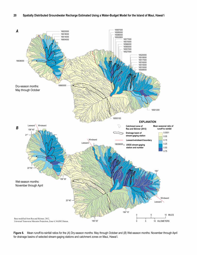
20 Spatially Distributed Groundwater Recharge Estimated Using a Water-Budget Model for the Island of Maui, Hawai‘i
Figure 6. Mean runoff-to-rainfall ratios for the (A) Dry-season months: May through October and (B) Wet-season months: November through April for drainage basins of selected stream-gaging stations and catchment zones on Maui, Hawai‘i.
#
#
######
#
#
#
#####
####
#
#
#
#
#
#
#
######
#
#
#
#####
####
#
#
#
#
#
0 5 10 KILOMETERS
5 10 MILES0
156°40'
156°30'
156°20'
156°10'
156°
21°
20°40'
20°50'
WindwardLeeward
LeewardWindward
Leeward Windward
165170001651800016520000
1651000016508000
1651500016516000
165660001657000016577000
165860001658500016587000
1655700016527000
16565000
16552800
16636000
1661800016620000
1661400016604500
16660000
16500100
16501200
Dry-season months:May through October
Wet-season months:November through April
Base modified from Rea and Skinner, 2012,Universal Transverse Mercator Projection, Zone 4, NAD83 Datum.
A
B Mean seasonal ratio of runoff to rainfall
EXPLANATION
16636000
USGS stream-gaging station and number
Leeward-windward boundary
0.050.0001
0.15
0.500.25
0.75
Drainage basin of stream-gaging station
Catchment zone ofRea and Skinner (2012)
Figure 6. Mean runoff-to-rainfall ratios for the (a) dry-season months (May through October) and (b) wet-season months (November through April) for drainage basins of selected stream-gaging stations and catchment zones on Maui, Hawai‘i.
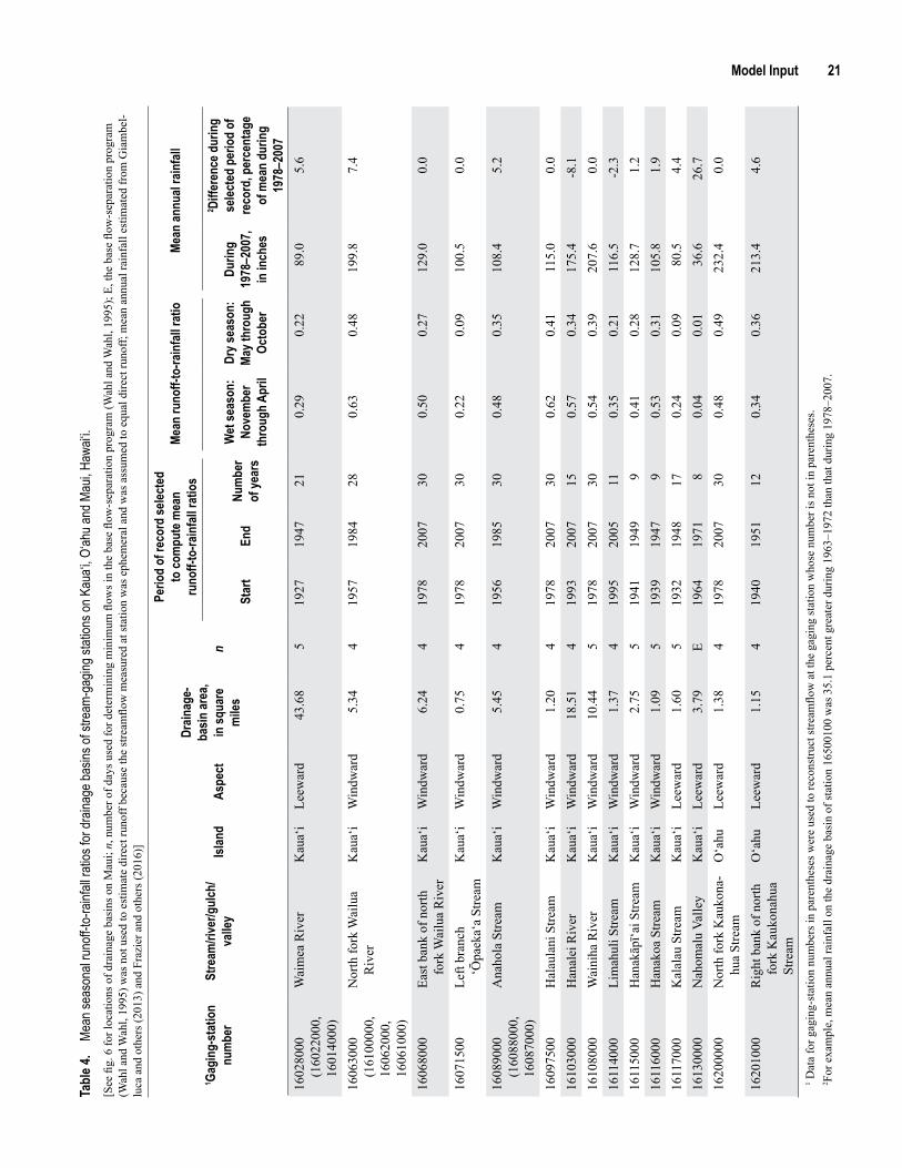
Model Input 21Ta
ble 4
. Me
an se
ason
al ru
noff-
to-ra
infall
ratio
s for
drain
age b
asins
of st
ream
-gag
ing st
ation
s on K
aua‘i
, O‘ah
u and
Mau
i, Haw
ai‘i.
1 Gagi
ng-s
tatio
n nu
mbe
rSt
ream
/rive
r/gul
ch/
valle
yIsl
and
Aspe
ct
Drain
age-
basin
area
, in
squa
re
mile
s n
Perio
d of
reco
rd se
lecte
d to
com
pute
mea
n ru
noff-
to-ra
infa
ll rat
ios
Mean
runo
ff-to
-rain
fall r
atio
Mean
annu
al ra
infa
ll
Star
tEn
dNu
mbe
r of
year
s
Wet
seas
on:
Nove
mbe
r th
roug
h Apr
il
Dry s
easo
n:
May t
hrou
gh
Octo
ber
Durin
g 19
78–2
007,
in in
ches
2 Diffe
renc
e dur
ing
selec
ted
perio
d of
re
cord
, per
cent
age
of m
ean
durin
g 19
78–2
007
1602
8000
(1
6022
000,
16
0140
00)
Wai
mea
Riv
erK
aua‘
iLe
ewar
d43
.68
519
2719
4721
0.29
0.22
89.0
5.6
1606
3000
(1
6100
000,
16
0620
00,
1606
1000
)
Nor
th fo
rk W
ailu
a R
iver
Kau
a‘i
Win
dwar
d5.
344
1957
1984
280.
630.
4819
9.8
7.4
1606
8000
East
ban
k of
nor
th
fork
Wai
lua
Riv
erK
aua‘
iW
indw
ard
6.24
419
7820
0730
0.50
0.27
129.
00.
0
1607
1500
Left
bran
ch
‘Ōpa
eka‘
a St
ream
Kau
a‘i
Win
dwar
d0.
754
1978
2007
300.
220.
0910
0.5
0.0
1608
9000
(1
6088
000,
16
0870
00)
Ana
hola
Stre
amK
aua‘
iW
indw
ard
5.45
419
5619
8530
0.48
0.35
108.
45.
2
1609
7500
Hal
aula
ni S
tream
Kau
a‘i
Win
dwar
d1.
204
1978
2007
300.
620.
4111
5.0
0.0
1610
3000
Han
alei
Riv
erK
aua‘
iW
indw
ard
18.5
14
1993
2007
150.
570.
3417
5.4
-8.1
1610
8000
Wai
niha
Riv
erK
aua‘
iW
indw
ard
10.4
45
1978
2007
300.
540.
3920
7.6
0.0
1611
4000
Lim
ahul
i Stre
amK
aua‘
iW
indw
ard
1.37
419
9520
0511
0.35
0.21
116.
5-2
.316
1150
00H
anak
āpī‘a
i Stre
amK
aua‘
iW
indw
ard
2.75
519
4119
499
0.41
0.28
128.
71.
216
1160
00H
anak
oa S
tream
Kau
a‘i
Win
dwar
d1.
095
1939
1947
90.
530.
3110
5.8
1.9
1611
7000
Kal
alau
Stre
amK
aua‘
iLe
ewar
d1.
605
1932
1948
170.
240.
0980
.54.
416
1300
00N
ahom
alu
Valle
yK
aua‘
iLe
ewar
d3.
79E
1964
1971
80.
040.
0136
.626
.716
2000
00N
orth
fork
Kau
kona
-hu
a St
ream
O‘a
huLe
ewar
d1.
384
1978
2007
300.
480.
4923
2.4
0.0
1620
1000
Rig
ht b
ank
of n
orth
fo
rk K
auko
nahu
a St
ream
O‘a
huLe
ewar
d1.
154
1940
1951
120.
340.
3621
3.4
4.6
[See
fig.
6 fo
r loc
atio
ns o
f dra
inag
e ba
sins
on
Mau
i; n,
num
ber o
f day
s use
d fo
r det
erm
inin
g m
inim
um fl
ows i
n th
e ba
se fl
ow-s
epar
atio
n pr
ogra
m (W
ahl a
nd W
ahl,
1995
); E,
the
base
flow
-sep
arat
ion
prog
ram
(W
ahl a
nd W
ahl,
1995
) was
not
use
d to
est
imat
e di
rect
runo
ff be
caus
e th
e st
ream
flow
mea
sure
d at
stat
ion
was
eph
emer
al a
nd w
as a
ssum
ed to
equ
al d
irect
runo
ff; m
ean
annu
al ra
infa
ll es
timat
ed fr
om G
iam
bel-
luca
and
oth
ers (
2013
) and
Fra
zier
and
oth
ers (
2016
)]
1 Dat
a fo
r gag
ing-
stat
ion
num
bers
in p
aren
thes
es w
ere
used
to re
cons
truct
stre
amflo
w a
t the
gag
ing
stat
ion
who
se n
umbe
r is n
ot in
par
enth
eses
.2 F
or e
xam
ple,
mea
n an
nual
rain
fall
on th
e dr
aina
ge b
asin
of s
tatio
n 16
5001
00 w
as 3
5.1
perc
ent g
reat
er d
urin
g 19
63–1
972
than
that
dur
ing
1978
–200
7.
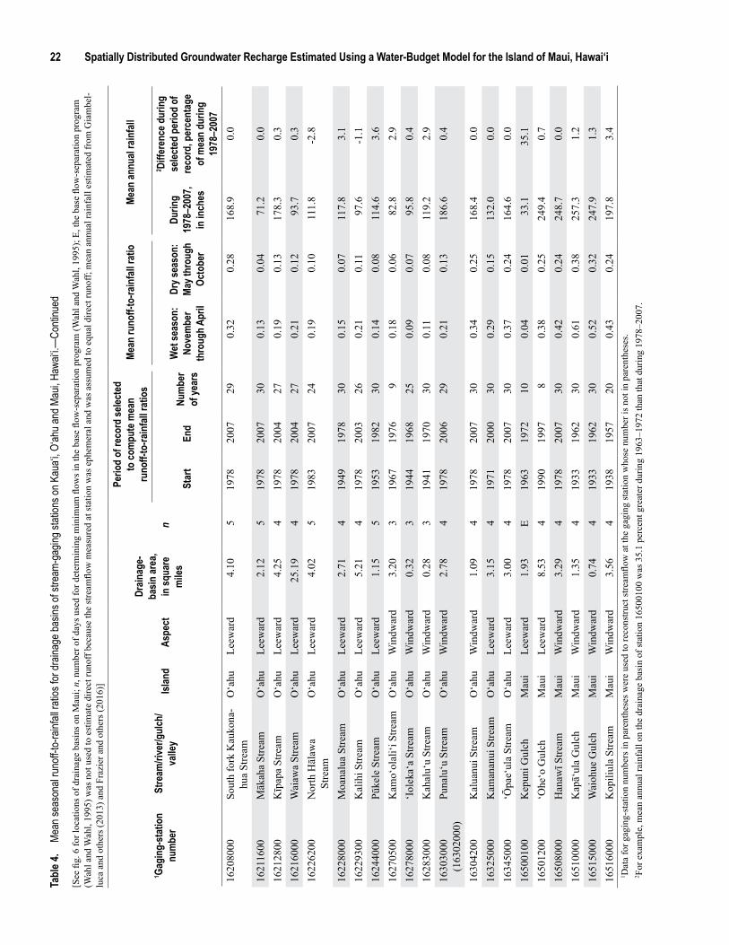
22 Spatially Distributed Groundwater Recharge Estimated Using a Water-Budget Model for the Island of Maui, Hawai‘i
1 Gagi
ng-s
tatio
n nu
mbe
rSt
ream
/rive
r/gul
ch/
valle
yIsl
and
Aspe
ct
Drain
age-
basin
area
, in
squa
re
mile
s n
Perio
d of
reco
rd se
lecte
d to
com
pute
mea
n ru
noff-
to-ra
infa
ll rat
ios
Mean
runo
ff-to
-rain
fall r
atio
Mean
annu
al ra
infa
ll
Star
tEn
dNu
mbe
r of
year
s
Wet
seas
on:
Nove
mbe
r th
roug
h Apr
il
Dry s
easo
n:
May t
hrou
gh
Octo
ber
Durin
g 19
78–2
007,
in in
ches
2 Diffe
renc
e dur
ing
selec
ted
perio
d of
re
cord
, per
cent
age
of m
ean
durin
g 19
78–2
007
1620
8000
Sout
h fo
rk K
auko
na-
hua
Stre
amO
‘ahu
Leew
ard
4.10
519
7820
0729
0.32
0.28
168.
90.
0
1621
1600
Māk
aha
Stre
amO
‘ahu
Leew
ard
2.12
519
7820
0730
0.13
0.04
71.2
0.0
1621
2800
Kīp
apa
Stre
amO
‘ahu
Leew
ard
4.25
419
7820
0427
0.19
0.13
178.
30.
316
2160
00W
aiaw
a St
ream
O‘a
huLe
ewar
d25
.19
419
7820
0427
0.21
0.12
93.7
0.3
1622
6200
Nor
th H
ālaw
a St
ream
O‘a
huLe
ewar
d4.
025
1983
2007
240.
190.
1011
1.8
-2.8
1622
8000
Moa
nalu
a St
ream
O‘a
huLe
ewar
d2.
714
1949
1978
300.
150.
0711
7.8
3.1
1622
9300
Kal
ihi S
tream
O‘a
huLe
ewar
d5.
214
1978
2003
260.
210.
1197
.6-1
.116
2440
00Pū
kele
Stre
amO
‘ahu
Leew
ard
1.15
519
5319
8230
0.14
0.08
114.
63.
616
2705
00K
amo‘
olal
i‘i S
tream
O‘a
huW
indw
ard
3.20
319
6719
769
0.18
0.06
82.8
2.9
1627
8000
‘Iol
eka‘
a St
ream
O‘a
huW
indw
ard
0.32
319
4419
6825
0.09
0.07
95.8
0.4
1628
3000
Kah
alu‘
u St
ream
O‘a
huW
indw
ard
0.28
319
4119
7030
0.11
0.08
119.
22.
916
3030
00
(163
0200
0)Pu
nalu
‘u S
tream
O‘a
huW
indw
ard
2.78
419
7820
0629
0.21
0.13
186.
60.
4
1630
4200
Kal
uanu
i Stre
amO
‘ahu
Win
dwar
d1.
094
1978
2007
300.
340.
2516
8.4
0.0
1632
5000
Kam
anan
ui S
tream
O‘a
huLe
ewar
d3.
154
1971
2000
300.
290.
1513
2.0
0.0
1634
5000
‘Ōpa
e‘ul
a St
ream
O‘a
huLe
ewar
d3.
004
1978
2007
300.
370.
2416
4.6
0.0
1650
0100
Kep
uni G
ulch
Mau
iLe
ewar
d1.
93E
1963
1972
100.
040.
0133
.135
.116
5012
00‘O
he‘o
Gul
chM
aui
Leew
ard
8.53
419
9019
978
0.38
0.25
249.
40.
716
5080
00H
anaw
ī Stre
amM
aui
Win
dwar
d3.
294
1978
2007
300.
420.
2424
8.7
0.0
1651
0000
Kap
ā‘ul
a G
ulch
Mau
iW
indw
ard
1.35
419
3319
6230
0.61
0.38
257.
31.
216
5150
00W
aioh
ue G
ulch
Mau
iW
indw
ard
0.74
419
3319
6230
0.52
0.32
247.
91.
316
5160
00K
opili
ula
Stre
amM
aui
Win
dwar
d3.
564
1938
1957
200.
430.
2419
7.8
3.4
Tabl
e 4.
Mean
seas
onal
runo
ff-to-
rainf
all ra
tios f
or dr
ainag
e bas
ins of
stre
am-g
aging
stati
ons o
n Kau
a‘i, O
‘ahu a
nd M
aui, H
awai‘
i.—Co
ntinu
ed
[See
fig.
6 fo
r loc
atio
ns o
f dra
inag
e ba
sins
on
Mau
i; n,
num
ber o
f day
s use
d fo
r det
erm
inin
g m
inim
um fl
ows i
n th
e ba
se fl
ow-s
epar
atio
n pr
ogra
m (W
ahl a
nd W
ahl,
1995
); E,
the
base
flow
-sep
arat
ion
prog
ram
(W
ahl a
nd W
ahl,
1995
) was
not
use
d to
est
imat
e di
rect
runo
ff be
caus
e th
e st
ream
flow
mea
sure
d at
stat
ion
was
eph
emer
al a
nd w
as a
ssum
ed to
equ
al d
irect
runo
ff; m
ean
annu
al ra
infa
ll es
timat
ed fr
om G
iam
bel-
luca
and
oth
ers (
2013
) and
Fra
zier
and
oth
ers (
2016
)]
1 Dat
a fo
r gag
ing-
stat
ion
num
bers
in p
aren
thes
es w
ere
used
to re
cons
truct
stre
amflo
w a
t the
gag
ing
stat
ion
who
se n
umbe
r is n
ot in
par
enth
eses
.2 F
or e
xam
ple,
mea
n an
nual
rain
fall
on th
e dr
aina
ge b
asin
of s
tatio
n 16
5001
00 w
as 3
5.1
perc
ent g
reat
er d
urin
g 19
63–1
972
than
that
dur
ing
1978
–200
7.
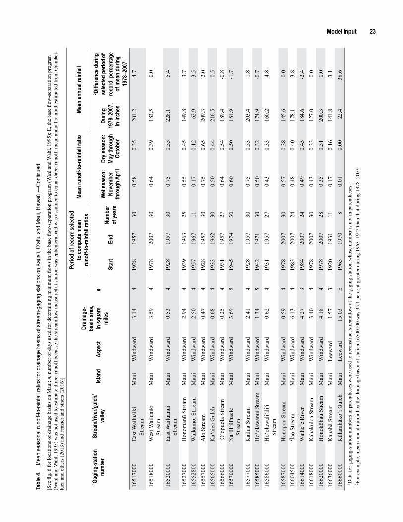
Model Input 23
1 Gagi
ng-s
tatio
n nu
mbe
rSt
ream
/rive
r/gul
ch/
valle
yIsl
and
Aspe
ct
Drain
age-
basin
area
, in
squa
re
mile
s n
Perio
d of
reco
rd se
lecte
d to
com
pute
mea
n ru
noff-
to-ra
infa
ll rat
ios
Mean
runo
ff-to
-rain
fall r
atio
Mean
annu
al ra
infa
ll
Star
tEn
dNu
mbe
r of
year
s
Wet
seas
on:
Nove
mbe
r th
roug
h Apr
il
Dry s
easo
n:
May t
hrou
gh
Octo
ber
Durin
g 19
78–2
007,
in in
ches
2 Diffe
renc
e dur
ing
selec
ted
perio
d of
re
cord
, per
cent
age
of m
ean
durin
g 19
78–2
007
1651
7000
East
Wai
luai
ki
Stre
amM
aui
Win
dwar
d3.
144
1928
1957
300.
580.
3520
1.2
4.7
1651
8000
Wes
t Wai
luai
ki
Stre
amM
aui
Win
dwar
d3.
594
1978
2007
300.
640.
3918
3.5
0.0
1652
0000
East
Wai
luan
ui
Stre
amM
aui
Win
dwar
d0.
534
1928
1957
300.
750.
5522
8.1
5.4
1652
7000
Hon
oman
ū St
ream
Mau
iW
indw
ard
2.94
419
3919
6325
0.55
0.45
149.
83.
716
5528
00W
aika
moi
Strr
eam
Mau
iW
indw
ard
2.50
419
5719
6711
0.17
0.12
62.9
3.5
1655
7000
Alo
Stre
amM
aui
Win
dwar
d0.
474
1928
1957
300.
750.
6520
9.3
2.0
1656
5000
Ka‘
aiea
Gul
chM
aui
Win
dwar
d0.
684
1933
1962
300.
500.
4421
6.5
-0.5
1656
6000
‘O‘o
puol
a St
ream
Mau
iW
indw
ard
0.25
419
3119
5727
0.64
0.54
189.
4-0
.816
5700
00N
a‘ili
‘ilih
aele
St
ream
Mau
iW
indw
ard
3.69
519
4519
7430
0.60
0.50
181.
9-1
.7
1657
7000
Kai
lua
Stre
amM
aui
Win
dwar
d2.
414
1928
1957
300.
750.
5320
3.4
1.8
1658
5000
Ho‘
olaw
anui
Stre
amM
aui
Win
dwar
d1.
345
1942
1971
300.
500.
3217
4.9
-0.7
1658
6000
Ho‘
olaw
ali‘i
li‘i
Stre
amM
aui
Win
dwar
d0.
624
1931
1957
270.
430.
3316
0.2
4.8
1658
7000
Hon
opou
Stre
amM
aui
Win
dwar
d0.
594
1978
2007
300.
570.
3814
5.6
0.0
1660
4500
‘Īao
Stre
amM
aui
Win
dwar
d6.
134
1983
2007
240.
480.
4017
8.1
-3.8
1661
4000
Wai
he‘e
Riv
erM
aui
Win
dwar
d4.
273
1984
2007
240.
490.
4518
4.6
-2.4
1661
8000
Kah
akul
oa S
tream
Mau
iW
indw
ard
3.40
419
7820
0730
0.43
0.33
127.
00.
016
6200
00H
onok
ōhau
Stre
amM
aui
Win
dwar
d4.
184
1978
2007
280.
350.
3120
0.3
0.0
1663
6000
Kan
ahā
Stre
amM
aui
Leew
ard
1.57
319
2019
3111
0.17
0.16
141.
83.
116
6600
00K
ūlan
ihāk
o‘i G
ulch
Mau
iLe
ewar
d15
.03
E19
6319
708
0.01
0.00
22.4
38.6
1 Dat
a fo
r gag
ing-
stat
ion
num
bers
in p
aren
thes
es w
ere
used
to re
cons
truct
stre
amflo
w a
t the
gag
ing
stat
ion
who
se n
umbe
r is n
ot in
par
enth
eses
.2 F
or e
xam
ple,
mea
n an
nual
rain
fall
on th
e dr
aina
ge b
asin
of s
tatio
n 16
5001
00 w
as 3
5.1
perc
ent g
reat
er d
urin
g 19
63–1
972
than
that
dur
ing
1978
–200
7.
Tabl
e 4.
Mean
seas
onal
runo
ff-to-
rainf
all ra
tios f
or dr
ainag
e bas
ins of
stre
am-g
aging
stati
ons o
n Kau
a‘i, O
‘ahu a
nd M
aui, H
awai‘
i.—Co
ntinu
ed[S
ee fi
g. 6
for l
ocat
ions
of d
rain
age
basi
ns o
n M
aui;
n, n
umbe
r of d
ays u
sed
for d
eter
min
ing
min
imum
flow
s in
the
base
flow
-sep
arat
ion
prog
ram
(Wah
l and
Wah
l, 19
95);
E, th
e ba
se fl
ow-s
epar
atio
n pr
ogra
m
(Wah
l and
Wah
l, 19
95) w
as n
ot u
sed
to e
stim
ate
dire
ct ru
noff
beca
use
the
stre
amflo
w m
easu
red
at st
atio
n w
as e
phem
eral
and
was
ass
umed
to e
qual
dire
ct ru
noff;
mea
n an
nual
rain
fall
estim
ated
from
Gia
mbe
l-lu
ca a
nd o
ther
s (20
13) a
nd F
razi
er a
nd o
ther
s (20
16)]
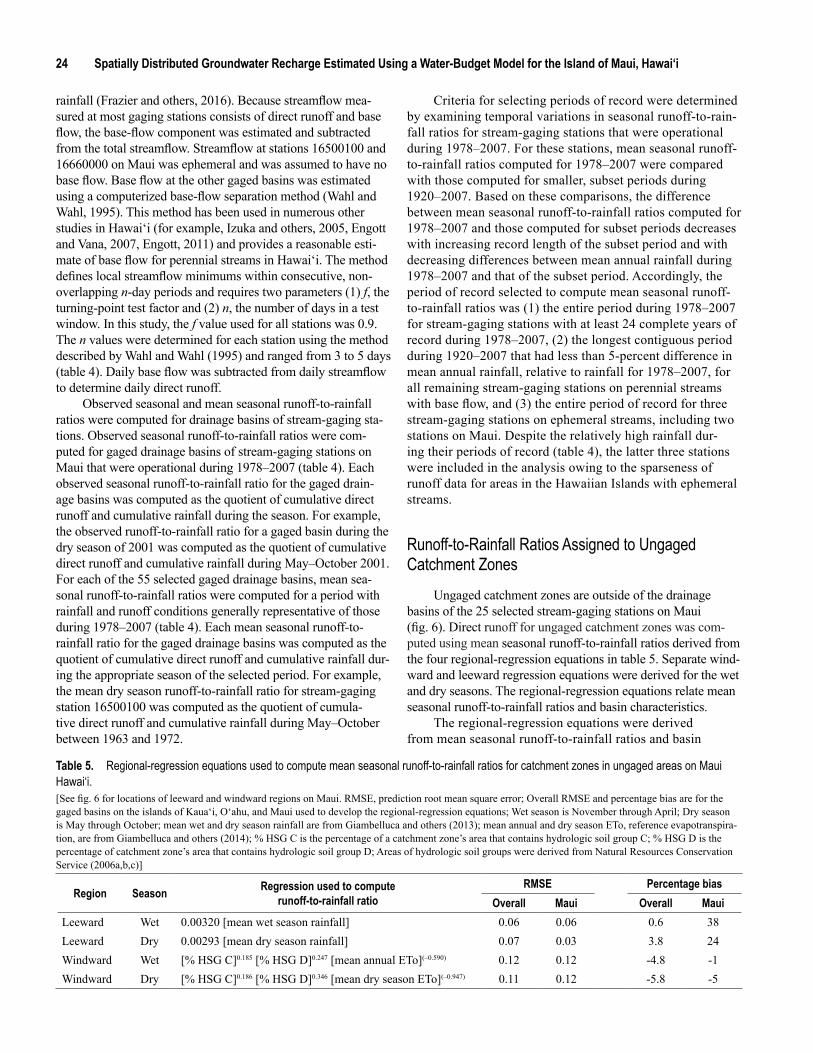
24 Spatially Distributed Groundwater Recharge Estimated Using a Water-Budget Model for the Island of Maui, Hawai‘i
rainfall (Frazier and others, 2016). Because streamflow mea-sured at most gaging stations consists of direct runoff and base flow, the base-flow component was estimated and subtracted from the total streamflow. Streamflow at stations 16500100 and 16660000 on Maui was ephemeral and was assumed to have no base flow. Base flow at the other gaged basins was estimated using a computerized base-flow separation method (Wahl and Wahl, 1995). This method has been used in numerous other studies in Hawai‘i (for example, Izuka and others, 2005, Engott and Vana, 2007, Engott, 2011) and provides a reasonable esti-mate of base flow for perennial streams in Hawai‘i. The method defines local streamflow minimums within consecutive, non-overlapping n-day periods and requires two parameters (1) f, the turning-point test factor and (2) n, the number of days in a test window. In this study, the f value used for all stations was 0.9. The n values were determined for each station using the method described by Wahl and Wahl (1995) and ranged from 3 to 5 days (table 4). Daily base flow was subtracted from daily streamflow to determine daily direct runoff.
Observed seasonal and mean seasonal runoff-to-rainfall ratios were computed for drainage basins of stream-gaging sta-tions. Observed seasonal runoff-to-rainfall ratios were com-puted for gaged drainage basins of stream-gaging stations on Maui that were operational during 1978–2007 (table 4). Each observed seasonal runoff-to-rainfall ratio for the gaged drain-age basins was computed as the quotient of cumulative direct runoff and cumulative rainfall during the season. For example, the observed runoff-to-rainfall ratio for a gaged basin during the dry season of 2001 was computed as the quotient of cumulative direct runoff and cumulative rainfall during May–October 2001. For each of the 55 selected gaged drainage basins, mean sea-sonal runoff-to-rainfall ratios were computed for a period with rainfall and runoff conditions generally representative of those during 1978–2007 (table 4). Each mean seasonal runoff-to-rainfall ratio for the gaged drainage basins was computed as the quotient of cumulative direct runoff and cumulative rainfall dur-ing the appropriate season of the selected period. For example, the mean dry season runoff-to-rainfall ratio for stream-gaging station 16500100 was computed as the quotient of cumula-tive direct runoff and cumulative rainfall during May–October between 1963 and 1972.
Criteria for selecting periods of record were determined by examining temporal variations in seasonal runoff-to-rain-fall ratios for stream-gaging stations that were operational during 1978–2007. For these stations, mean seasonal runoff-to-rainfall ratios computed for 1978–2007 were compared with those computed for smaller, subset periods during 1920–2007. Based on these comparisons, the difference between mean seasonal runoff-to-rainfall ratios computed for 1978–2007 and those computed for subset periods decreases with increasing record length of the subset period and with decreasing differences between mean annual rainfall during 1978–2007 and that of the subset period. Accordingly, the period of record selected to compute mean seasonal runoff-to-rainfall ratios was (1) the entire period during 1978–2007 for stream-gaging stations with at least 24 complete years of record during 1978–2007, (2) the longest contiguous period during 1920–2007 that had less than 5-percent difference in mean annual rainfall, relative to rainfall for 1978–2007, for all remaining stream-gaging stations on perennial streams with base flow, and (3) the entire period of record for three stream-gaging stations on ephemeral streams, including two stations on Maui. Despite the relatively high rainfall dur-ing their periods of record (table 4), the latter three stations were included in the analysis owing to the sparseness of runoff data for areas in the Hawaiian Islands with ephemeral streams.
Runoff-to-Rainfall Ratios Assigned to Ungaged Catchment Zones
Ungaged catchment zones are outside of the drainage basins of the 25 selected stream-gaging stations on Maui (fig. 6). Direct runoff for ungaged catchment zones was com-puted using mean seasonal runoff-to-rainfall ratios derived from the four regional-regression equations in table 5. Separate wind-ward and leeward regression equations were derived for the wet and dry seasons. The regional-regression equations relate mean seasonal runoff-to-rainfall ratios and basin characteristics.
The regional-regression equations were derived from mean seasonal runoff-to-rainfall ratios and basin
Region Season Regression used to compute runoff-to-rainfall ratio
RMSE Percentage bias Overall Maui Overall Maui
Leeward Wet 0.00320 [mean wet season rainfall] 0.06 0.06 0.6 38Leeward Dry 0.00293 [mean dry season rainfall] 0.07 0.03 3.8 24Windward Wet [% HSG C]0.185 [% HSG D]0.247 [mean annual ETo](–0.590) 0.12 0.12 -4.8 -1Windward Dry [% HSG C]0.186 [% HSG D]0.346 [mean dry season ETo](–0.947) 0.11 0.12 -5.8 -5
[See fig. 6 for locations of leeward and windward regions on Maui. RMSE, prediction root mean square error; Overall RMSE and percentage bias are for the gaged basins on the islands of Kaua‘i, O‘ahu, and Maui used to develop the regional-regression equations; Wet season is November through April; Dry season is May through October; mean wet and dry season rainfall are from Giambelluca and others (2013); mean annual and dry season ETo, reference evapotranspira-tion, are from Giambelluca and others (2014); % HSG C is the percentage of a catchment zone’s area that contains hydrologic soil group C; % HSG D is the percentage of catchment zone’s area that contains hydrologic soil group D; Areas of hydrologic soil groups were derived from Natural Resources Conservation Service (2006a,b,c)]
Table 5. Regional-regression equations used to compute mean seasonal runoff-to-rainfall ratios for catchment zones in ungaged areas on Maui Hawai‘i.
Model Input 25
characteristics for the 55 stream-gaging stations in table 4. Thirty basin characteristics–including those related to climate, soil, and vegetation– were evaluated as possible explanatory variables (not shown). The regional regres-sions in table 5 were selected because they had the lowest residual sum of squares and met the following criteria. First, all regression coefficients were statistically significant at a 5-percent significance level. Second, the sign and magnitude of the fitted coefficients were physically meaningful. Finally, the cross-validated results indicated less than 10 percent bias. For leeward catchment zones, wet season runoff-to-rainfall ratios were estimated on the basis of mean wet season rain-fall during 1978–2007 (Giambelluca and others, 2013); dry season runoff-to-rainfall ratios were estimated on the basis of mean dry season rainfall during 1978–2007. For windward catchment zones, wet season runoff-to-rainfall ratios were estimated on the basis of mean annual reference ET (Giam-belluca and others, 2014) and the percentage of the catch-ment zone’s area with hydrologic soil groups C and D (Natu-ral Resources Conservation Service, 2006a,b,c); dry season runoff-to-rainfall ratios were estimated on the basis of mean dry season reference ET and the percentage of the zone’s area with hydrologic soil groups C and D. The performance statistics of the regression equations in table 5 are used to examine the sensitivity of recharge to runoff-to-rainfall ratios (see Sensitivity Analysis).
Runoff-to-Rainfall Ratios Assigned to Gaged Basins within a Single Catchment Zone
Twelve of the selected stream-gaging stations on Maui have drainage basins with a single catchment zone (fig. 6). Nine of these stations (16500100, 16520000, 16557000, 16565000, 16566000, 16570000, 16585000, 16586000, and 16636000) were not operational during 1978–2007 (table 4). For the drainage basins of these nine stations, the model com-puted direct runoff by using mean seasonal runoff-to-rainfall ratios. For the drainage basins of the three remaining stations (16587000, 16618000, and 16620000), the model computed direct runoff by using (1) observed seasonal runoff-to-rainfall ratios, for seasons when observed ratios were available, and (2) mean seasonal runoff-to-rainfall ratios for seasons when observed ratios were not available.
Runoff-to-Rainfall Ratios Assigned to Gaged Basins with Multiple Catchment Zones
Thirteen of the selected stream-gaging stations on Maui (16501200, 16508000, 16510000, 16515000, 16516000, 16517000, 16518000, 16527000, 16552800, 16577000, 16604500, 16614000, and 16600000) have drainage basins containing multiple catchment zones (fig. 6). The model com-puted direct runoff for each of the catchment zones within these gaged basins by using adjusted seasonal runoff-to-rainfall ratios determined from equation 17:
(17)
where:
= adjusted runoff-to-rainfall ratio for catchment zone a during season t [dimensionless],
= mean runoff-to-rainfall ratio for catchment zone a estimated using the appropriate regional-regression equation (table 5) [dimensionless],
= number of catchment zones in the gaged basin b
[dimensionless],
= mean runoff-to-rainfall ratio for catchment zone i estimated using the regional-regression equations [dimensionless],
= rainfall for catchment zone i during season t [L3],
= observed runoff-to-rainfall ratio for the gaged basin b during season t. If the observed runoff-to-rainfall ratio for gaged basin b is not available during season t, the mean seasonal runoff-to-rainfall ratio is used (table 4) [dimensionless], and
= rainfall for gaged basin b during season t [L3].
Equation 17 uses the regional-regression models and seasonal rainfall to spatially disaggregate observed seasonal and mean seasonal runoff-to-rainfall ratios of a gaged basin for each catchment zone within a gaged basin. Hence, seasonal runoff-to-rainfall ratios were allowed to be spatially variable, instead of spatially uniform, across the catchment zones within gaged drainage basins containing multiple catchment zones.
EvapotranspirationEvapotranspiration (ET) is the sum of all water that is
evaporated or transpired from the forest canopy and plant-root zone. Evapotranspiration can be divided into three main evaporative processes (1) canopy evaporation, which is evaporation of intercepted rain and fog from the surface of vegetation; (2) ground evaporation, which is evaporation of water from the soil surface and overlying litter and mulch layers; and (3) transpiration, the process by which soil moisture taken up by vegetation is eventually evaporated through plant pores (Viessman and Lewis, 2003). Because these three processes are difficult to quantify individually, they are typically combined in water budgets.
Canopy evaporation in forested areas can substantially reduce the rainfall that reaches the ground beneath a forest
rr RRrr rfRR rfa t a,b t b t
i i ti
j, ,
,1∑ ×=
××
=
��
�
rra t,
RRa
j
RRi
rfi t,
rrb t,
rfb t,
26 Spatially Distributed Groundwater Recharge Estimated Using a Water-Budget Model for the Island of Maui, Hawai‘i
canopy (Gaskill, 2004; DeLay, 2005; McJannet and others, 2007; Giambelluca and others, 2011; Safeeq and Fares, 2014). Owing to the height of trees and their canopy structure, turbu-lent diffusion is much more efficient at removing intercepted water from forest canopies than from shorter vegetation. More-over, canopy evaporation in forests tends to operate on much shorter time scales (hours) than transpiration (weeks or longer) (Savenije, 2004). This enhanced rate of evaporation from a wet forest canopy makes realistic estimates of ET from forests pos-sible only if transpiration and canopy evaporation are evaluated separately (Shuttleworth, 1993).
For this study, total ET from subareas with forest land cov-ers is computed by separately estimating forest-canopy evapora-tion and combined ground evaporation and transpiration from the plant-root zone (fig. 5). Evaporation from the forest canopy and evapotranspiration from plant-root zone are added together to yield total ET. For subareas with nonforest land covers, ET is computed using a more traditional approach in which canopy evaporation, ground evaporation, and transpiration are not sepa-rately estimated (fig. 5). The concept of potential ET, combined with empirical models when soil moisture is limited, is used to estimate ground evaporation and transpiration in forests and total ET for all other land covers.
Forest-Canopy Evaporation and Net PrecipitationAs rain falls on a vegetated surface, a fraction of the
droplets will accumulate on the leaves, trunks, or stems of the vegetation. Additional moisture from fog interception may supplement the amount of water that accumulates on vegetation. Canopy evaporation is the part of precipitation that accumu-lates on and then evaporates from the vegetation (Gerrits and Savenije, 2011). Net precipitation is the part of precipitation that reaches the forest floor (fig. 5).
In this study, the Gash model was used to compute forest-canopy evaporation for the following reasons. First, the Gash method accounts for gaps in the forest canopy, and this allows for a sparse canopy to be differentiated from a dense canopy. Second, canopy evaporation during a period of precipitation is dependent on the amount of precipitation during that period. Third, the Gash model has the capacity to account for spatial differences in climate, including climate differences between windward and leeward forests. One disadvantage of the Gash model, however, is that it is theoretical. Therefore, one of the parameters of the Gash model used to compute canopy evapo-ration in the water-budget model was calibrated to the wet canopy evaporation maps of Giambelluca and others (2014) as described below. Use of the Gash model, instead of the mean wet-canopy evaporation maps, in the water-budget model allows forest-canopy evaporation to be computed on a daily basis in response to daily variations in precipitation.
Forest-canopy evaporation is computed in the water budget according to equations 4 and 5, which require rainfall and the following parameters (1) canopy cover, (2) canopy capacity, (3) trunk-storage capacity, (4) proportion of pre-cipitation diverted to stemflow, and (5) the ratio of the mean
evaporation rate to mean precipitation rate during saturated conditions, V. For the water-budget calculations, the values assigned to parameters 1–4 were derived from published data for areas in Hawai‘i. The values assigned to V were derived using maps of mean wet canopy evaporation for the Islands of Kaua‘i, O‘ahu, and Maui (Giambelluca and others, 2014). An analysis of the sensitivity of the water-budget results to selected Gash-model parameters is included in the Sensitiv-ity Analysis section of this report.
Canopy cover of forest land covers varies spatially across Maui. The canopy cover of each subarea with forest land cover in the water-budget model was estimated from a map of mean annual vegetation cover fraction (Giambelluca and others, 2014). This map quantifies the vegetation cover fraction at a spatial resolution of about 14 acres. A canopy cover of 0 implies an absence of canopy cover, whereas a value of 1 implies a dense canopy with no gaps. The esti-mated canopy-cover values for subareas with forest land covers in the water budget range from 0.03 to 1.
Canopy capacity, trunk-storage capacity, and the proportion of precipitation diverted to stemflow were assumed to be the same for all forests (table 6). Canopy capacity was set at 0.05 inches, the mean of the average values reported for six forested sites in Hawai‘i (DeLay, 2005, p. 42; Takahashi and others, 2011, Safeeq and Fares, 2014). Trunk-storage capacity was set at 0.01 inches, the mean of the values reported for four forest sites in Hawai‘i (DeLay, 2005, p. 42; Safeeq and Fares, 2014). The proportion of precipitation diverted to stemflow was assumed to be 0.04, the mean of the values reported for eight forest sites in Hawai‘i (Gaskill, 2004; DeLay, 2005, p. 42; Takahashi and others, 2011; Safeeq and Fares, 2014). Forest sites of Takahashi and others (2011) and Safeeq and Fares (2014) with an abundance of Psidium cattleianum (strawberry guava) had relatively high stemflow estimates ranging from 29 to 37 percent of rainfall. The relatively high stemflow values from these sites were excluded from the computed stemflow mean of 0.04 used in the water budget. The effect on recharge estimates owing to the use of a stemflow value of 0.37 for areas mapped as alien forests is examined in the Sensitivity Analysis section.
A map of mean annual wet canopy evaporation for the Hawaiian Islands (Giambelluca and others, 2014) was used to develop a regression model for estimating the spatial variability of V. This regression model was developed because estimates of V for sites in Hawai‘i are rare, and because canopy-evaporation estimates from the water-budget model are sensitive to V. The wet canopy evaporation map has mean annual wet canopy evaporation estimates at a spatial resolution of about 14 acres. To derive a regression model for estimating V, we first selected grid cells from the islands of Kaua‘i, O‘ahu, and Maui that consisted of forest land-cover classes only, based on the LANDFIRE Existing Vegetation Type map (U.S. Geological Survey, 2010). Data from Kaua‘i and O‘ahu were included in the analysis to supplement the data from Maui and provide the basis for
Model Input 27
a broadly applicable V value for Hawai‘i. Next, for each of the selected grid cells, we determined the “calibrated V value” needed for mean annual canopy evaporation from the Gash model for Kaua‘i, O‘ahu, and Maui to equal wet canopy evaporation from Giambelluca and others (2014). The water budgets were computed with various V values to determine the calibrated V values for the selected grid cells. Last, we examined associations between the calibrated V values and various other parameters of the selected grid cells including estimates of mean annual rainfall, reference ET, Penman-Monteith ET from Giambelluca and others (2014), and estimates of mean annual wind speed from AWS Truewind, LLC (2004). Estimates of V from a linear-regression model (equation 18) relating V to the quotient of mean annual wind speed and mean annual rainfall resulted in the best agreement, in terms of bias and root mean square error, between estimates of canopy evaporation from the wet canopy evaporation maps (Giambelluca and others, 2014) and the estimates from the Gash model for Kaua‘i, O‘ahu, and Maui. The spatial distribution of V was estimated as follows:
for w < 0.009, V = 0.01,
for 0.009 ≤ w ≤ 0.192, V = 2.677 × (w) – 0.014, and
for w > 0.192, V = 0.50, (18)
where
w = mean annual wind speed divided by mean annual rainfall [(meters/second)/inch)]
The variable w is the quotient of (1) mean annual wind speed, in meters per second, which was derived from a map of mean annual wind speed at height of about 100 ft above the land surface (AWS Truewind, 2004), and (2) 1978–2007 mean annual rainfall, in inches (Giambelluca and others, 2013). In general, estimates of V are less for wet areas than for dry areas. Grid cells that had calibrated V values that were outside the range of 0.01–0.50 were excluded from the derivation of equation 18. A range of 0.01–0.50 was established for this analysis on the basis of the range of published estimates of V. The low end of the range, 0.01, was determined by Hutjes and others (1990) for a humid, tropical forest site in the African Ivory Coast. The high end of the range, 0.50, is the mean value reported by Safeeq and Fares (2014) for a forest site on leeward O‘ahu. A similar range of mean V estimates (about 0.03–0.40) was determined for 54 sites located in various climate zones across Australia (Wallace and others, 2013, fig. 6c).
Potential EvapotranspirationPotential evapotranspiration (ET) is the maximum rate
that water can be removed from the plant-root zone by ET if soil moisture is nonlimiting (Giambelluca, 1983). The actual-ET rate is a function of potential ET, soil-moisture content, and threshold-moisture content (see equation 13). The actual-ET rate becomes less than the potential rate with the onset of soil-moisture stress. As the soil dries, capillary and adsorptive forces bind the remaining water to the soil matrix, reducing water flow to roots. Soil-moisture stress occurs when the decreasing flow of water to the root system induces a response in the plant to slow down transpiration and prevent desiccation. The threshold-moisture content at which a plant begins to react to soil drying varies with the type of plant.
Potential ET is controlled by atmospheric conditions, topography, and land-cover characteristics (Giambelluca, 1983). Maps of mean monthly reference ET produced by Giambel-luca and others (2014) were used in the water-budget model to estimate the influence of atmospheric conditions (radiation, air temperature, air humidity, and wind speed) on potential ET. Crop coefficients were used to estimate the integrated effects of land-cover and vegetation characteristics on potential ET. Potential ET for each subarea was computed in the water-budget model as the product of mean monthly reference ET and the crop coefficient assigned to the land cover (see equation 9).
Reference Evapotranspiration Reference ET is the potential ET of a hypothetical grass
surface with specific characteristics and optimum soil-water conditions for given climatic conditions (Allen and others, 1998). Reference ET is similar to pan evaporation, which has been used in previous water budgets for Maui and other Hawaiian Islands. Both pan evaporation and reference ET provide an index of the energy that is available for ET for a given area.
Maps of mean monthly reference ET (Giambelluca and others, 2014) for Maui were used in the water budget. These maps have the same grid resolution (about 14 acres) as the monthly rainfall maps produced by Frazier and others (2016). Mean annual reference ET ranges from about 28 to 113 inches on Maui (fig. 7). In general, mean annual reference ET is highest in dry lowlands, and is lowest in wet uplands within the cloud zone. In the water-budget calculation, monthly reference ET was not varied from year to year, and was assumed to equal mean monthly reference ET. Reference ET was assumed to be the same each day of a given month.
Crop Coefficients A crop coefficient is an empirically derived ratio of the
potential ET of a certain type of land cover and reference ET. Crop coefficients provide an index of the integrated effect of vegetation characteristics (reflectance, roughness, and plant physiology) on potential ET. Crop coefficients were assigned to each land-cover class (table 6). Crop coefficients were assumed
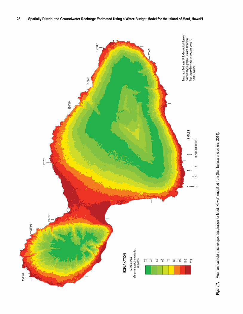
28 Spatially Distributed Groundwater Recharge Estimated Using a Water-Budget Model for the Island of Maui, Hawai‘i
40
Mean
annu
al re
feren
ce ev
apotr
ansp
iratio
n, in
inche
s 28 50 7060 80 100
11390
Base
mod
ified f
rom
U.S.
Geo
logica
l Sur
vey
Natio
nal H
ydro
grap
hy D
atase
t, Univ
ersa
l Tr
ansv
erse
Mer
cator
proje
ction
, zon
e 4,
NAD8
3 datu
m.
156°
00'
156°
10'
156°
20'
156°
30'
156°
40'
21°0
0'
20°5
0'
20°4
0'
03
69
KILO
METE
RS
03
69
MILE
S
EXPL
ANAT
ION
Figu
re 7.
Me
an an
nual
refer
ence
evap
otran
spira
tion f
or M
aui, H
awai‘
i (mod
ified f
rom
Giam
bellu
ca an
d othe
rs, 20
14).
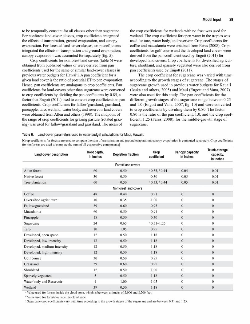
Model Input 29
Land-cover description Root depth, in inches Depletion fraction Crop
coefficientCanopy capacity,
in inches
Trunk-storage capacity, in inches
Forest land coversAlien forest 60 0.50 a 0.33, b 0.44 0.05 0.01Native forest 30 0.50 0.30 0.05 0.01Tree plantation 60 0.50 a 0.33, b 0.44 0.05 0.01
Nonforest land coversCoffee 48 0.40 0.91 0 0Diversified agriculture 10 0.35 1.00 0 0Fallow/grassland 39 0.60 0.95 0 0Macadamia 60 0.50 0.91 0 0Pineapple 18 0.50 0.30 0 0Sugarcane 24 0.65 c 0.31–1.25 0 0Taro 10 1.05 0.95 0 0Developed, open space 12 0.50 1.18 0 0Developed, low-intensity 12 0.50 1.18 0 0Developed, medium-intensity 12 0.50 1.18 0 0Developed, high-intensity 12 0.50 1.18 0 0Golf course 30 0.50 0.85 0 0Grassland 39 0.60 0.95 0 0Shrubland 12 0.50 1.00 0 0Sparsely vegetated 5 0.50 1.18 0 0Water body and Reservoir 1 1.00 1.05 0 0Wetland 39 0.50 1.18 0 0
Table 6. Land-cover parameters used in water-budget calculations for Maui, Hawai‘i.[Crop coefficients for forests are used to compute the sum of transpiration and ground evaporation; canopy evaporation is computed separately. Crop coefficients for nonforests are used to compute the sum of all evaporative components]
to be temporally constant for all classes other than sugarcane. For nonforest land-cover classes, crop coefficients integrated the effects of transpiration, ground evaporation, and canopy evaporation. For forested land-cover classes, crop coefficients integrated the effects of transpiration and ground evaporation; canopy evaporation was accounted for separately (fig. 5).
Crop coefficients for nonforest land covers (table 6) were obtained from published values or were derived from pan coefficients used for the same or similar land-cover classes in previous water budgets for Hawai‘i. A pan coefficient for a given land cover is the ratio of potential ET to pan evaporation. Hence, pan coefficients are analogous to crop coefficients. Pan coefficients for land-covers other than sugarcane were converted to crop coefficients by dividing the pan coefficients by 0.85, a factor that Engott (2011) used to convert crop coefficients to pan coefficients. Crop coefficients for fallow/grassland, grassland, pineapple, taro, wetland, water body, and reservoir land covers were obtained from Allen and others (1998). The midpoint of the range of crop coefficients for grazing pasture (rotated graz-ing) was used for fallow/grassland and grassland. The mean of
the crop coefficients for wetlands with no frost was used for wetland. The crop coefficient for open water in the tropics was used for taro, water body, and reservoir. Crop coefficients for coffee and macadamia were obtained from Fares (2008). Crop coefficients for golf course and the developed land covers were derived from the pan coefficient used by Engott (2011) for developed land covers. Crop coefficients for diversified agricul-ture, shrubland, and sparsely vegetated were also derived from pan coefficients used by Engott (2011).
The crop coefficient for sugarcane was varied with time according to the growth stages of sugarcane. The stages of sugarcane growth used in previous water budgets for Kaua‘i (Izuka and others, 2005) and Maui (Engott and Vana, 2007) were also used for this study. The pan coefficients for the different growth stages of the sugarcane range between 0.25 and 1.0 (Engott and Vana, 2007, fig. 10) and were converted to crop coefficients by dividing them by 0.80. The factor 0.80 is the ratio of the pan coefficient, 1.0, and the crop coef-ficient, 1.25 (Fares, 2008), for the middle-growth stage of sugarcane.
a Value used for forests inside the cloud zone, which is between altitudes of 2,000 and 8,200 feet.b Value used for forests outside the cloud zone.c Sugarcane crop coefficients vary with time according to the growth stages of the sugarcane and are between 0.31 and 1.25.
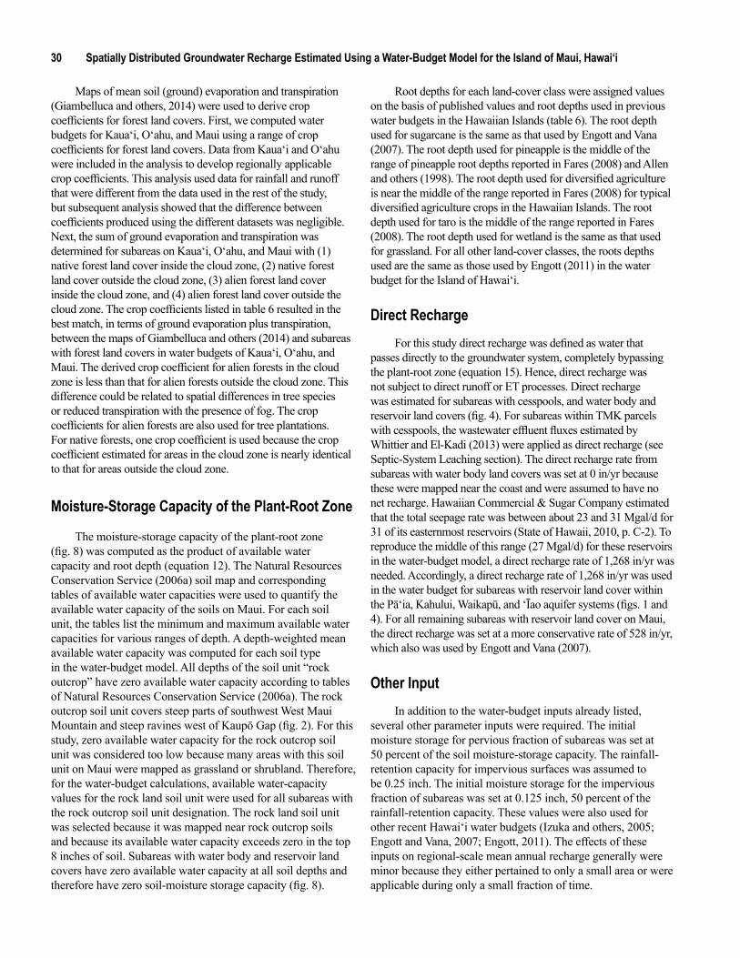
30 Spatially Distributed Groundwater Recharge Estimated Using a Water-Budget Model for the Island of Maui, Hawai‘i
Maps of mean soil (ground) evaporation and transpiration (Giambelluca and others, 2014) were used to derive crop coefficients for forest land covers. First, we computed water budgets for Kaua‘i, O‘ahu, and Maui using a range of crop coefficients for forest land covers. Data from Kaua‘i and O‘ahu were included in the analysis to develop regionally applicable crop coefficients. This analysis used data for rainfall and runoff that were different from the data used in the rest of the study, but subsequent analysis showed that the difference between coefficients produced using the different datasets was negligible. Next, the sum of ground evaporation and transpiration was determined for subareas on Kaua‘i, O‘ahu, and Maui with (1) native forest land cover inside the cloud zone, (2) native forest land cover outside the cloud zone, (3) alien forest land cover inside the cloud zone, and (4) alien forest land cover outside the cloud zone. The crop coefficients listed in table 6 resulted in the best match, in terms of ground evaporation plus transpiration, between the maps of Giambelluca and others (2014) and subareas with forest land covers in water budgets of Kaua‘i, O‘ahu, and Maui. The derived crop coefficient for alien forests in the cloud zone is less than that for alien forests outside the cloud zone. This difference could be related to spatial differences in tree species or reduced transpiration with the presence of fog. The crop coefficients for alien forests are also used for tree plantations. For native forests, one crop coefficient is used because the crop coefficient estimated for areas in the cloud zone is nearly identical to that for areas outside the cloud zone.
Moisture-Storage Capacity of the Plant-Root Zone
The moisture-storage capacity of the plant-root zone (fig. 8) was computed as the product of available water capacity and root depth (equation 12). The Natural Resources Conservation Service (2006a) soil map and corresponding tables of available water capacities were used to quantify the available water capacity of the soils on Maui. For each soil unit, the tables list the minimum and maximum available water capacities for various ranges of depth. A depth-weighted mean available water capacity was computed for each soil type in the water-budget model. All depths of the soil unit “rock outcrop” have zero available water capacity according to tables of Natural Resources Conservation Service (2006a). The rock outcrop soil unit covers steep parts of southwest West Maui Mountain and steep ravines west of Kaupō Gap (fig. 2). For this study, zero available water capacity for the rock outcrop soil unit was considered too low because many areas with this soil unit on Maui were mapped as grassland or shrubland. Therefore, for the water-budget calculations, available water-capacity values for the rock land soil unit were used for all subareas with the rock outcrop soil unit designation. The rock land soil unit was selected because it was mapped near rock outcrop soils and because its available water capacity exceeds zero in the top 8 inches of soil. Subareas with water body and reservoir land covers have zero available water capacity at all soil depths and therefore have zero soil-moisture storage capacity (fig. 8).
Root depths for each land-cover class were assigned values on the basis of published values and root depths used in previous water budgets in the Hawaiian Islands (table 6). The root depth used for sugarcane is the same as that used by Engott and Vana (2007). The root depth used for pineapple is the middle of the range of pineapple root depths reported in Fares (2008) and Allen and others (1998). The root depth used for diversified agriculture is near the middle of the range reported in Fares (2008) for typical diversified agriculture crops in the Hawaiian Islands. The root depth used for taro is the middle of the range reported in Fares (2008). The root depth used for wetland is the same as that used for grassland. For all other land-cover classes, the roots depths used are the same as those used by Engott (2011) in the water budget for the Island of Hawai‘i.
Direct RechargeFor this study direct recharge was defined as water that
passes directly to the groundwater system, completely bypassing the plant-root zone (equation 15). Hence, direct recharge was not subject to direct runoff or ET processes. Direct recharge was estimated for subareas with cesspools, and water body and reservoir land covers (fig. 4). For subareas within TMK parcels with cesspools, the wastewater effluent fluxes estimated by Whittier and El-Kadi (2013) were applied as direct recharge (see Septic-System Leaching section). The direct recharge rate from subareas with water body land covers was set at 0 in/yr because these were mapped near the coast and were assumed to have no net recharge. Hawaiian Commercial & Sugar Company estimated that the total seepage rate was between about 23 and 31 Mgal/d for 31 of its easternmost reservoirs (State of Hawaii, 2010, p. C-2). To reproduce the middle of this range (27 Mgal/d) for these reservoirs in the water-budget model, a direct recharge rate of 1,268 in/yr was needed. Accordingly, a direct recharge rate of 1,268 in/yr was used in the water budget for subareas with reservoir land cover within the Pā‘ia, Kahului, Waikapū, and ‘Īao aquifer systems (figs. 1 and 4). For all remaining subareas with reservoir land cover on Maui, the direct recharge was set at a more conservative rate of 528 in/yr, which also was used by Engott and Vana (2007).
Other InputIn addition to the water-budget inputs already listed,
several other parameter inputs were required. The initial moisture storage for pervious fraction of subareas was set at 50 percent of the soil moisture-storage capacity. The rainfall-retention capacity for impervious surfaces was assumed to be 0.25 inch. The initial moisture storage for the impervious fraction of subareas was set at 0.125 inch, 50 percent of the rainfall-retention capacity. These values were also used for other recent Hawai‘i water budgets (Izuka and others, 2005; Engott and Vana, 2007; Engott, 2011). The effects of these inputs on regional-scale mean annual recharge generally were minor because they either pertained to only a small area or were applicable during only a small fraction of time.
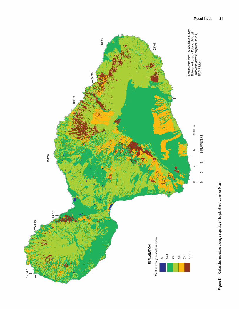
Model Input 31
0.01
Moist
ure-
stora
ge ca
pacit
y, in
inche
s
0 2.5 7.5 10.20
5.0
EXPL
ANAT
ION
Base
mod
ified f
rom
U.S.
Geo
logica
l Sur
vey
Natio
nal H
ydro
grap
hy D
atase
t, Univ
ersa
l Tr
ansv
erse
Mer
cator
proje
ction
, zon
e 4,
NAD8
3 datu
m.
156°
00'
156°
10'
156°
20'
156°
30'
156°
40'
21°0
0'
20°5
0'
20°4
0'
03
69
KILO
METE
RS
03
69
MILE
S
Figu
re 8.
Ca
lculat
ed m
oistur
e-sto
rage
capa
city o
f the p
lant-r
oot z
one f
or M
aui.

32 Spatially Distributed Groundwater Recharge Estimated Using a Water-Budget Model for the Island of Maui, Hawai‘i
Model Exclusions and LimitationsThe water-budget model has several limitations. As
described below, estimates of daily rainfall and runoff are the chief limitations of the model. We synthesized, rather than reconstructed, daily rainfall patterns during 1978–2007 from monthly rainfall maps using the method of fragments. Daily runoff was estimated from seasonal runoff-to-rainfall ratios. Additionally, some parameters and conditions excluded from the water-budget model were assumed to be inherent in other parameters used in the model, and could not be quantified owing to insufficient data, or were considered insignificant with respect to the study objectives.
Owing to sparseness of data and the use of synthesized daily rainfall, the water-budget model did not reconstruct the actual distributions of the water-budget components (rainfall, fog interception, irrigation, septic-system leachate, runoff, evapotranspiration, and recharge) on Maui each day during 1978–2007. The sets of rainfall fragments were assumed to represent the statistical properties of daily rainfall during 1978–2007 even though they may not have been from this period. The reconstruction of actual daily runoff was also prevented by the use of seasonal runoff-to-rainfall ratios and the assumption that runoff occurs in a single day in response to rainfall. Additionally, runoff may have been overestimated by the model on days with light rain and underestimated on days with intense rain. The water-budget model did, however, reproduce the spatial distribution of (1) monthly rainfall on Maui during 1978–2007 that was estimated by Frazier and others (2016), and (2) mean monthly and mean annual rainfall on Maui during 1978–2007 that was estimated by Giambelluca and others (2013). For gaged drainage basins, the water-budget model reproduced seasonal runoff estimates that were based on streamflow data from stream-gaging stations. Datasets for calibrating recharge estimates of the model, however, were not available.
To estimate runoff, recent water budgets for Maui (Engott and Vana, 2007; Gingerich and Engott, 2012) used mean monthly runoff-to-rainfall ratios, whereas this study used seasonal and mean seasonal runoff-to-rainfall ratios. Monthly and mean monthly runoff-to-rainfall ratios, although available for gaged drainage basins, were not used in this study for the following reasons. First, the regional-regression models (table 5) computed mean seasonal (not monthly) runoff-to-rainfall ratios. Assigning seasonal runoff-to-rainfall ratios to all areas was considered a more consistent approach than assigning monthly runoff-to-rainfall ratios to gaged drainage basins and seasonal runoff-to-rainfall ratios to ungaged drainage basins. Second, analysis of the variability of monthly runoff-to-rainfall ratios within a season indicated that a mean seasonal ratio was sufficient to predict monthly direct runoff. Observed monthly runoff for gaged basins, based on streamflow data, was compared with monthly runoff estimated using (1) mean monthly runoff-to-rainfall ratios and (2) mean seasonal
runoff-to-rainfall ratios. Based on these comparisons, runoff estimated from mean monthly runoff-to-rainfall ratios was not significantly better than runoff estimated from mean seasonal runoff-to-rainfall ratios. Last, compared to methods used in previous water budgets for Maui, the regional-regression models (table 5) were considered a more robust method for estimating runoff in ungaged areas.
Some parameters and conditions not included in the calculations of the water-budget model were inherent in other parameters used in the model. For example, the permeability and vertical hydraulic conductivity of the plant-root zone and underlying substrate were not included in the model calculations. Their effect on direct runoff, however, would be inherent in streamflow records used to derive runoff-to-rainfall ratios that were used to compute direct runoff in the model. Also assumed to be inherent in streamflow records were reductions in runoff owing to ET of interflow in the subsurface. The reduction in potential ET of the plant-root zone in response to evaporation from the forest canopy was not included in the model calculations; it was, however, likely accounted for in the forest crop coefficients, which were calibrated to maps of mean transpiration and ground evaporation produced by Giambelluca and others (2014).
Re-infiltration of direct runoff, water that runs off one subarea and then infiltrates the plant-root zone of a different subarea, was not explicitly considered in the water-budget model. Re-infiltration of direct runoff within gaged basins was assumed to be inherent in streamflow records used to derive runoff-to-rainfall ratios. Spatial variations in the re-infiltration of direct runoff within a drainage basin, however, were not accounted for in the model. For example, if re-infiltration of direct runoff was considerable within streambeds, then recharge may have been underestimated in intra-channel (streambed) areas and overestimated in inter-channel (non-streambed) areas. Surface water diversion systems, however, can reduce or prevent streambed seepage in lower reaches of many streams on Maui.
Some processes and conditions were excluded from the water-budget calculations. Interannual variations in potential ET were not accounted for in the model. Potential ET was also assumed to be uniform each day of the month and consequently may have been overestimated on cloudy days and underestimated on clear days. The errors caused by assuming uniform daily potential ET may be minor because the variation in daily potential ET for a given area is likely small compared to the variation in daily rainfall. For example, estimates of daily potential ET ranged from about 0.02 to 0.26 inches for three climate stations at altitudes between 2,500 and 5,770 ft on West Maui Mountain during November 2003 through November 2005 (Engott and Vana, 2007). In contrast, daily rainfall on Maui ranges from zero to tens of inches. For subareas with impervious surfaces, potential ET was not reduced to account for evaporation from impervious surfaces. Adjustments to reference ET at scales less than the
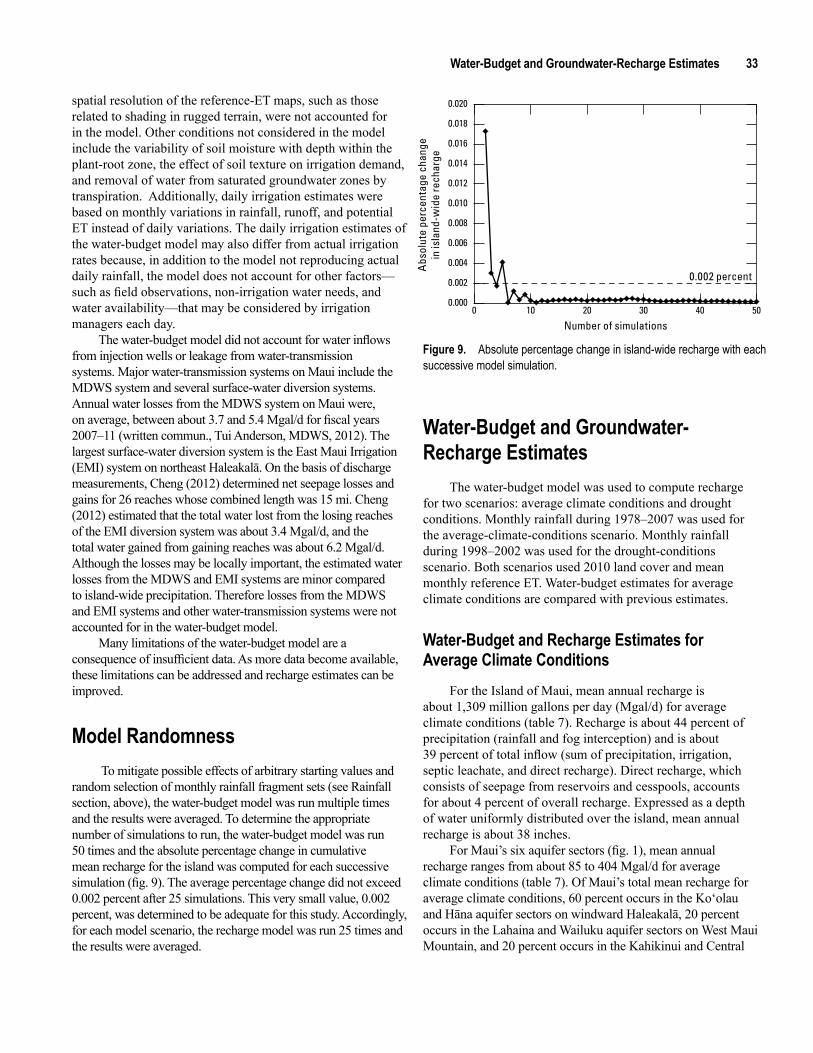
Water-Budget and Groundwater-Recharge Estimates 33
Figure 9. Absolute percentage change in island-wide recharge with each successive model simulation.
spatial resolution of the reference-ET maps, such as those related to shading in rugged terrain, were not accounted for in the model. Other conditions not considered in the model include the variability of soil moisture with depth within the plant-root zone, the effect of soil texture on irrigation demand, and removal of water from saturated groundwater zones by transpiration. Additionally, daily irrigation estimates were based on monthly variations in rainfall, runoff, and potential ET instead of daily variations. The daily irrigation estimates of the water-budget model may also differ from actual irrigation rates because, in addition to the model not reproducing actual daily rainfall, the model does not account for other factors—such as field observations, non-irrigation water needs, and water availability—that may be considered by irrigation managers each day.
The water-budget model did not account for water inflows from injection wells or leakage from water-transmission systems. Major water-transmission systems on Maui include the MDWS system and several surface-water diversion systems. Annual water losses from the MDWS system on Maui were, on average, between about 3.7 and 5.4 Mgal/d for fiscal years 2007–11 (written commun., Tui Anderson, MDWS, 2012). The largest surface-water diversion system is the East Maui Irrigation (EMI) system on northeast Haleakalā. On the basis of discharge measurements, Cheng (2012) determined net seepage losses and gains for 26 reaches whose combined length was 15 mi. Cheng (2012) estimated that the total water lost from the losing reaches of the EMI diversion system was about 3.4 Mgal/d, and the total water gained from gaining reaches was about 6.2 Mgal/d. Although the losses may be locally important, the estimated water losses from the MDWS and EMI systems are minor compared to island-wide precipitation. Therefore losses from the MDWS and EMI systems and other water-transmission systems were not accounted for in the water-budget model.
Many limitations of the water-budget model are a consequence of insufficient data. As more data become available, these limitations can be addressed and recharge estimates can be improved.
Model Randomness To mitigate possible effects of arbitrary starting values and
random selection of monthly rainfall fragment sets (see Rainfall section, above), the water-budget model was run multiple times and the results were averaged. To determine the appropriate number of simulations to run, the water-budget model was run 50 times and the absolute percentage change in cumulative mean recharge for the island was computed for each successive simulation (fig. 9). The average percentage change did not exceed 0.002 percent after 25 simulations. This very small value, 0.002 percent, was determined to be adequate for this study. Accordingly, for each model scenario, the recharge model was run 25 times and the results were averaged.
Water-Budget and Groundwater-Recharge Estimates
The water-budget model was used to compute recharge for two scenarios: average climate conditions and drought conditions. Monthly rainfall during 1978–2007 was used for the average-climate-conditions scenario. Monthly rainfall during 1998–2002 was used for the drought-conditions scenario. Both scenarios used 2010 land cover and mean monthly reference ET. Water-budget estimates for average climate conditions are compared with previous estimates.
Water-Budget and Recharge Estimates for Average Climate Conditions
For the Island of Maui, mean annual recharge is about 1,309 million gallons per day (Mgal/d) for average climate conditions (table 7). Recharge is about 44 percent of precipitation (rainfall and fog interception) and is about 39 percent of total inflow (sum of precipitation, irrigation, septic leachate, and direct recharge). Direct recharge, which consists of seepage from reservoirs and cesspools, accounts for about 4 percent of overall recharge. Expressed as a depth of water uniformly distributed over the island, mean annual recharge is about 38 inches.
For Maui’s six aquifer sectors (fig. 1), mean annual recharge ranges from about 85 to 404 Mgal/d for average climate conditions (table 7). Of Maui’s total mean recharge for average climate conditions, 60 percent occurs in the Ko‘olau and Hāna aquifer sectors on windward Haleakalā, 20 percent occurs in the Lahaina and Wailuku aquifer sectors on West Maui Mountain, and 20 percent occurs in the Kahikinui and Central
0.000
0.002
0.004
0.006
0.008
0.010
0.012
0.014
0.016
0.018
0.020
0 10 20 30 40 50
0.002 percent
Abs
olut
e pe
rcen
tage
cha
nge
in is
land
-wid
e re
char
ge
Number of simulations
Figure 9. Absolute percentage change in island-wide recharge with each successive model simulation.
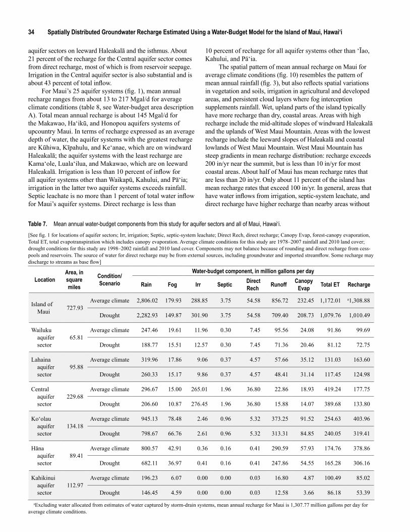
34 Spatially Distributed Groundwater Recharge Estimated Using a Water-Budget Model for the Island of Maui, Hawai‘i
Table 7. Mean annual water-budget components from this study for aquifer sectors and all of Maui, Hawai‘i.
LocationArea, in square miles
Condition/ Scenario
Water-budget component, in million gallons per day
Rain Fog Irr Septic Direct Rech Runoff Canopy
Evap Total ET Recharge
Island of Maui 727.93
Average climate 2,806.02 179.93 288.85 3.75 54.58 856.72 232.45 1,172.01 a1,308.88
Drought 2,282.93 149.87 301.90 3.75 54.58 709.40 208.73 1,079.76 1,010.49
Wailuku aquifer sector
65.81Average climate 247.46 19.61 11.96 0.30 7.45 95.56 24.08 91.86 99.69
Drought 188.77 15.51 12.57 0.30 7.45 71.36 20.46 81.12 72.75
Lahaina aquifer sector
95.88Average climate 319.96 17.86 9.06 0.37 4.57 57.66 35.12 131.03 163.60
Drought 260.33 15.17 9.86 0.37 4.57 48.41 31.14 117.45 124.98
Central aquifer sector
229.68Average climate 296.67 15.00 265.01 1.96 36.80 22.86 18.93 419.24 177.75
Drought 206.60 10.87 276.45 1.96 36.80 15.88 14.07 389.68 133.80
Ko‘olau aquifer sector
134.18Average climate 945.13 78.48 2.46 0.96 5.32 373.25 91.52 254.63 403.96
Drought 798.67 66.76 2.61 0.96 5.32 313.31 84.85 240.05 319.41
Hāna aquifer sector
89.41Average climate 800.57 42.91 0.36 0.16 0.41 290.59 57.93 174.76 378.86
Drought 682.11 36.97 0.41 0.16 0.41 247.86 54.55 165.28 306.16
Kahikinui aquifer sector
112.97Average climate 196.23 6.07 0.00 0.00 0.03 16.80 4.87 100.49 85.02
Drought 146.45 4.59 0.00 0.00 0.03 12.58 3.66 86.18 53.39
[See fig. 1 for locations of aquifer sectors; Irr, irrigation; Septic, septic-system leachate; Direct Rech, direct recharge; Canopy Evap, forest-canopy evaporation, Total ET, total evapotranspiration which includes canopy evaporation. Average climate conditions for this study are 1978–2007 rainfall and 2010 land cover; drought conditions for this study are 1998–2002 rainfall and 2010 land cover. Components may not balance because of rounding and direct recharge from cess-pools and reservoirs. The source of water for direct recharge may be from external sources, including groundwater and imported streamflow. Some recharge may discharge to streams as base flow]
aExcluding water allocated from estimates of water captured by storm-drain systems, mean annual recharge for Maui is 1,307.77 million gallons per day for average climate conditions.
aquifer sectors on leeward Haleakalā and the isthmus. About 21 percent of the recharge for the Central aquifer sector comes from direct recharge, most of which is from reservoir seepage. Irrigation in the Central aquifer sector is also substantial and is about 43 percent of total inflow.
For Maui’s 25 aquifer systems (fig. 1), mean annual recharge ranges from about 13 to 217 Mgal/d for average climate conditions (table 8, see Water-budget area description A). Total mean annual recharge is about 145 Mgal/d for the Makawao, Ha‘ikū, and Honopou aquifers systems of upcountry Maui. In terms of recharge expressed as an average depth of water, the aquifer systems with the greatest recharge are Kūhiwa, Kīpahulu, and Ke‘anae, which are on windward Haleakalā; the aquifer systems with the least recharge are Kama‘ole, Luala‘ilua, and Makawao, which are on leeward Haleakalā. Irrigation is less than 10 percent of inflow for all aquifer systems other than Waikapū, Kahului, and Pā‘ia; irrigation in the latter two aquifer systems exceeds rainfall. Septic leachate is no more than 1 percent of total water inflow for Maui’s aquifer systems. Direct recharge is less than
10 percent of recharge for all aquifer systems other than ‘Īao, Kahului, and Pā‘ia.
The spatial pattern of mean annual recharge on Maui for average climate conditions (fig. 10) resembles the pattern of mean annual rainfall (fig. 3), but also reflects spatial variations in vegetation and soils, irrigation in agricultural and developed areas, and persistent cloud layers where fog interception supplements rainfall. Wet, upland parts of the island typically have more recharge than dry, coastal areas. Areas with high recharge include the mid-altitude slopes of windward Haleakalā and the uplands of West Maui Mountain. Areas with the lowest recharge include the leeward slopes of Haleakalā and coastal lowlands of West Maui Mountain. West Maui Mountain has steep gradients in mean recharge distribution: recharge exceeds 200 in/yr near the summit, but is less than 10 in/yr for most coastal areas. About half of Maui has mean recharge rates that are less than 20 in/yr. Only about 11 percent of the island has mean recharge rates that exceed 100 in/yr. In general, areas that have water inflows from irrigation, septic-system leachate, and direct recharge have higher recharge than nearby areas without
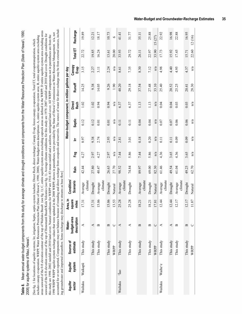
Water-Budget and Groundwater-Recharge Estimates 35
Aqui
fer
sect
orAq
uife
r sy
stem
Sour
ce o
f es
timat
e
Wat
er-
budg
et-a
rea
desc
riptio
n
Area
, in
squa
re
mile
s
Cond
ition
/ Sc
enar
io
Wat
er-b
udge
t com
pone
nt, in
milli
on g
allon
s per
day
Rain
Fog
IrrSe
ptic
Dire
ct
Rech
Runo
ffCa
nopy
Ev
apTo
tal E
TRe
char
ge
Wai
luku
Wai
kapū
This
stud
yA
17.3
1Av
erag
e cl
imat
e42
.44
4.27
8.97
0.12
1.02
14.2
53.
1522
.72
19.8
9
This
stud
yA
17.3
1D
roug
ht27
.80
2.97
9.38
0.12
1.02
9.38
2.27
19.8
512
.21
This
stud
yB
15.0
6Av
erag
e cl
imat
e40
.47
4.27
2.74
0.01
0.94
14.0
53.
1116
.24
18.1
7
This
stud
yB
15.0
6D
roug
ht26
.63
2.97
2.93
0.01
0.94
9.26
2.24
13.6
110
.73
WR
PPC
13.5
3N
atur
al27
.70
n/a
n/a
n/a
n/a
1.90
n/a
20.0
06
Wai
luku
‘Īao
This
stud
yA
25.2
8Av
erag
e cl
imat
e98
.52
7.44
2.81
0.11
6.37
40.2
08.
6133
.93
41.4
1
This
stud
yA
25.2
8D
roug
ht74
.84
5.86
3.01
0.11
6.37
29.1
87.
3529
.72
31.7
7
This
stud
yB
18.2
1Av
erag
e cl
imat
e89
.97
7.44
0.18
0.04
1.13
37.5
48.
3026
.11
35.1
1
This
stud
yB
18.2
1D
roug
ht69
.00
5.86
0.20
0.04
1.13
27.4
87.
1222
.97
25.8
8W
RPP
C17
.81
Nat
ural
82.3
0n/
an/
an/
an/
a33
.10
n/a
33.9
015
(27)
Wai
luku
Wai
he‘e
This
stud
yA
12.4
4Av
erag
e cl
imat
e61
.46
4.36
0.11
0.07
0.04
25.4
04.
9817
.73
22.9
2
This
stud
yA
12.4
4D
roug
ht49
.54
3.65
0.11
0.07
0.04
20.5
24.
4015
.92
16.9
8Th
is st
udy
B12
.17
Aver
age
clim
ate
61.0
44.
360.
090.
060.
0325
.25
4.95
17.4
522
.88
This
stud
yB
12.1
7D
roug
ht49
.23
3.65
0.09
0.06
0.03
20.4
14.
3715
.71
16.9
5W
RPP
C11
.87
Nat
ural
62.7
0n/
an/
an/
an/
a28
.30
n/a
22.6
012
(16)
Tabl
e 8.
Mean
annu
al wa
ter-b
udge
t com
pone
nts fr
om th
is stu
dy fo
r ave
rage
clim
ate an
d dro
ught
cond
itions
and c
ompo
nents
from
the W
ater R
esou
rces P
rotec
tion P
lan (S
tate o
f Haw
ai‘i, 1
990;
2008
) for
aquif
er sy
stems
of M
aui, H
awai‘
i.[S
ee fi
g. 1
for l
ocat
ions
of a
quife
r sys
tem
s; Ir
r, irr
igat
ion;
Sep
tic, s
eptic
-sys
tem
leac
hate
; Dire
ct R
ech,
dire
ct re
char
ge; C
anop
y Ev
ap, f
ores
t-can
opy
evap
orat
ion;
Tot
al E
T, to
tal e
vapo
trans
pira
tion,
whi
ch
incl
udes
can
opy
evap
orat
ion.
WR
PP, W
ater
Res
ourc
es P
rote
ctio
n Pl
an (S
tate
of H
awai
‘i, 1
990;
200
8). W
ater
-bud
get-a
rea
desc
riptio
ns: A
, ent
ire a
quife
r-sys
tem
are
a; B
, ent
ire a
quife
r-sys
tem
are
a ex
clud
ing
area
s sea
war
d of
the
0-ft
elev
atio
n co
ntou
r of t
he to
p of
Wai
luku
Bas
alt
(see
fig.
1);
C, e
ntire
aqu
ifer-s
yste
m a
rea
excl
udin
g ca
proc
k ar
eas a
s defi
ned
in th
e W
RPP
; D e
ntire
aqu
ifer-s
yste
m a
rea
excl
udin
g ar
eas
seaw
ard
of th
e 0-
ft el
evat
ion
cont
our o
f the
top
of H
onom
anū
Bas
alt/K
ula
Volc
anic
s (se
e fig
. 1).
Aver
age
clim
ate
cond
ition
s for
this
stud
y ar
e 19
78–2
007
rain
fall
and
2010
land
cov
er. D
roug
ht c
ondi
tions
for
this
stud
y ar
e 19
98–2
002
rain
fall
and
2010
land
cov
er. N
atur
al c
ondi
tions
for W
RPP
are
191
6–83
mea
n ra
infa
ll an
d a
unifo
rm, u
nirr
igat
ed la
nd c
over
. All
WR
PP c
ompo
nent
s not
in p
aren
thes
es a
re fr
om th
e 19
90 W
RPP
. WR
PP a
quife
r-sys
tem
rech
arge
val
ues t
hat w
ere
upda
ted
in th
e 20
08 W
RPP
, sho
wn
in p
aren
thes
es, w
ere
prov
ided
by
the
Stat
e of
Haw
ai‘i
Com
mis
sion
on
Wat
er R
esou
rce
Man
agem
ent.
n/a
, not
ac
coun
ted
for o
r not
repo
rted.
Com
pone
nts m
ay n
ot b
alan
ce b
ecau
se o
f rou
ndin
g an
d di
rect
rech
arge
from
ces
spoo
ls a
nd re
serv
oirs
. The
sour
ce o
f wat
er fo
r dire
ct re
char
ge m
ay b
e fr
om e
xter
nal s
ourc
es, i
nclu
d-in
g gr
ound
wat
er a
nd im
porte
d st
ream
flow.
Som
e re
char
ge m
ay d
isch
arge
to st
ream
s as b
ase
flow
]
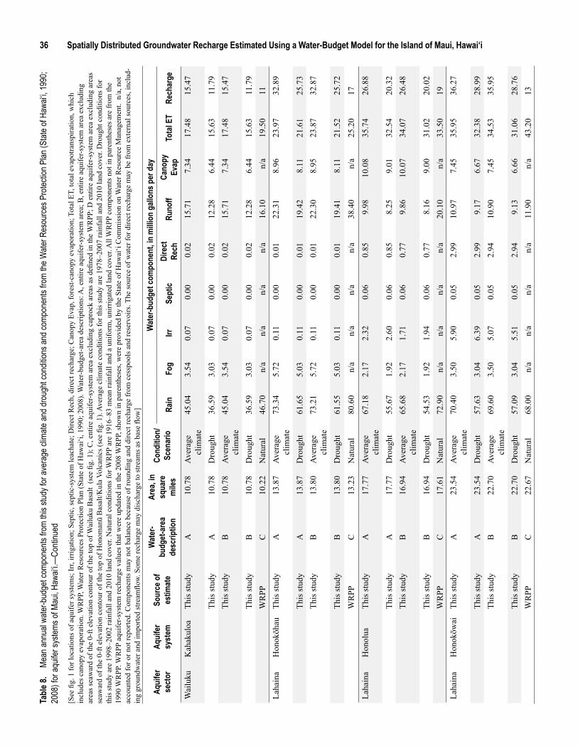
36 Spatially Distributed Groundwater Recharge Estimated Using a Water-Budget Model for the Island of Maui, Hawai‘i
Aqui
fer
sect
orAq
uife
r sy
stem
Sour
ce o
f es
timat
e
Wat
er-
budg
et-a
rea
desc
riptio
n
Area
, in
squa
re
mile
s
Cond
ition
/ Sc
enar
io
Wat
er-b
udge
t com
pone
nt, in
milli
on g
allon
s per
day
Rain
Fog
IrrSe
ptic
Dire
ct
Rech
Runo
ffCa
nopy
Ev
apTo
tal E
TRe
char
ge
Wai
luku
Kah
akul
oaTh
is st
udy
A10
.78
Aver
age
clim
ate
45.0
43.
540.
070.
000.
0215
.71
7.34
17.4
815
.47
This
stud
yA
10.7
8D
roug
ht36
.59
3.03
0.07
0.00
0.02
12.2
86.
4415
.63
11.7
9Th
is st
udy
B10
.78
Aver
age
clim
ate
45.0
43.
540.
070.
000.
0215
.71
7.34
17.4
815
.47
This
stud
yB
10.7
8D
roug
ht36
.59
3.03
0.07
0.00
0.02
12.2
86.
4415
.63
11.7
9W
RPP
C10
.22
Nat
ural
46.7
0n/
an/
an/
an/
a16
.10
n/a
19.5
011
Laha
ina
Hon
okōh
auTh
is st
udy
A13
.87
Aver
age
clim
ate
73.3
45.
720.
110.
000.
0122
.31
8.96
23.9
732
.89
This
stud
yA
13.8
7D
roug
ht61
.65
5.03
0.11
0.00
0.01
19.4
28.
1121
.61
25.7
3Th
is st
udy
B13
.80
Aver
age
clim
ate
73.2
15.
720.
110.
000.
0122
.30
8.95
23.8
732
.87
This
stud
yB
13.8
0D
roug
ht61
.55
5.03
0.11
0.00
0.01
19.4
18.
1121
.52
25.7
2
WR
PPC
13.2
3N
atur
al80
.60
n/a
n/a
n/a
n/a
38.4
0n/
a25
.20
17
Laha
ina
Hon
olua
This
stud
yA
17.7
7Av
erag
e cl
imat
e67
.18
2.17
2.32
0.06
0.85
9.98
10.0
835
.74
26.8
8
This
stud
yA
17.7
7D
roug
ht55
.67
1.92
2.60
0.06
0.85
8.25
9.01
32.5
420
.32
This
stud
yB
16.9
4Av
erag
e cl
imat
e65
.68
2.17
1.71
0.06
0.77
9.86
10.0
734
.07
26.4
8
This
stud
yB
16.9
4D
roug
ht54
.53
1.92
1.94
0.06
0.77
8.16
9.00
31.0
220
.02
WR
PPC
17.6
1N
atur
al72
.90
n/a
n/a
n/a
n/a
20.1
0n/
a33
.50
19La
hain
aH
onok
ōwai
This
stud
yA
23.5
4Av
erag
e cl
imat
e70
.40
3.50
5.90
0.05
2.99
10.9
77.
4535
.95
36.2
7
This
stud
yA
23.5
4D
roug
ht57
.63
3.04
6.39
0.05
2.99
9.17
6.67
32.3
828
.99
This
stud
yB
22.7
0Av
erag
e cl
imat
e69
.60
3.50
5.07
0.05
2.94
10.9
07.
4534
.53
35.9
5
This
stud
yB
22.7
0D
roug
ht57
.09
3.04
5.51
0.05
2.94
9.13
6.66
31.0
628
.76
WR
PPC
22.6
7N
atur
al68
.00
n/a
n/a
n/a
n/a
11.9
0n/
a43
.20
13
Tabl
e 8.
Mean
annu
al wa
ter-b
udge
t com
pone
nts fr
om th
is stu
dy fo
r ave
rage
clim
ate an
d dro
ught
cond
itions
and c
ompo
nents
from
the W
ater R
esou
rces P
rotec
tion P
lan (S
tate o
f Haw
ai‘i, 1
990;
2008
) for
aquif
er sy
stems
of M
aui, H
awai‘
i.—Co
ntinu
ed
[See
fig.
1 fo
r loc
atio
ns o
f aqu
ifer s
yste
ms;
Irr,
irrig
atio
n; S
eptic
, sep
tic-s
yste
m le
acha
te; D
irect
Rec
h, d
irect
rech
arge
; Can
opy
Evap
, for
est-c
anop
y ev
apor
atio
n; T
otal
ET,
tota
l eva
potra
nspi
ratio
n, w
hich
in
clud
es c
anop
y ev
apor
atio
n. W
RPP
, Wat
er R
esou
rces
Pro
tect
ion
Plan
(Sta
te o
f Haw
ai‘i,
199
0; 2
008)
. Wat
er-b
udge
t-are
a de
scrip
tions
: A, e
ntire
aqu
ifer-s
yste
m a
rea;
B, e
ntire
aqu
ifer-s
yste
m a
rea
excl
udin
g ar
eas s
eaw
ard
of th
e 0-
ft el
evat
ion
cont
our o
f the
top
of W
ailu
ku B
asal
t (s
ee fi
g. 1
); C
, ent
ire a
quife
r-sys
tem
are
a ex
clud
ing
capr
ock
area
s as d
efine
d in
the
WR
PP; D
ent
ire a
quife
r-sys
tem
are
a ex
clud
ing
area
s se
awar
d of
the
0-ft
elev
atio
n co
ntou
r of t
he to
p of
Hon
oman
ū B
asal
t/Kul
a Vo
lcan
ics (
see
fig. 1
). Av
erag
e cl
imat
e co
nditi
ons f
or th
is st
udy
are
1978
–200
7 ra
infa
ll an
d 20
10 la
nd c
over
. Dro
ught
con
ditio
ns fo
r th
is st
udy
are
1998
–200
2 ra
infa
ll an
d 20
10 la
nd c
over
. Nat
ural
con
ditio
ns fo
r WR
PP a
re 1
916–
83 m
ean
rain
fall
and
a un
iform
, uni
rrig
ated
land
cov
er. A
ll W
RPP
com
pone
nts n
ot in
par
enth
eses
are
from
the
1990
WR
PP. W
RPP
aqu
ifer-s
yste
m re
char
ge v
alue
s tha
t wer
e up
date
d in
the
2008
WR
PP, s
how
n in
par
enth
eses
, wer
e pr
ovid
ed b
y th
e St
ate
of H
awai
‘i C
omm
issi
on o
n W
ater
Res
ourc
e M
anag
emen
t. n
/a, n
ot
acco
unte
d fo
r or n
ot re
porte
d. C
ompo
nent
s may
not
bal
ance
bec
ause
of r
ound
ing
and
dire
ct re
char
ge fr
om c
essp
ools
and
rese
rvoi
rs. T
he so
urce
of w
ater
for d
irect
rech
arge
may
be
from
ext
erna
l sou
rces
, inc
lud-
ing
grou
ndw
ater
and
impo
rted
stre
amflo
w. S
ome
rech
arge
may
dis
char
ge to
stre
ams a
s bas
e flo
w]
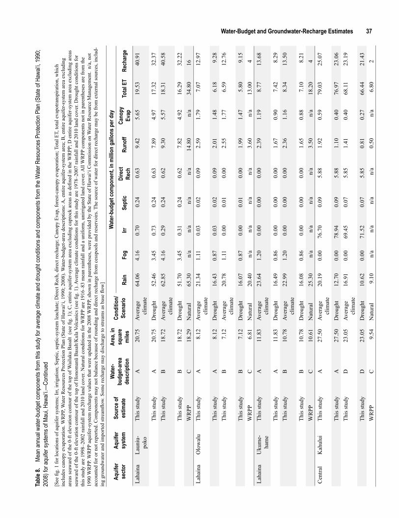
Water-Budget and Groundwater-Recharge Estimates 37
Aqui
fer
sect
orAq
uife
r sy
stem
Sour
ce o
f es
timat
e
Wat
er-
budg
et-a
rea
desc
riptio
n
Area
, in
squa
re
mile
s
Cond
ition
/ Sc
enar
io
Wat
er-b
udge
t com
pone
nt, in
milli
on g
allon
s per
day
Rain
Fog
IrrSe
ptic
Dire
ct
Rech
Runo
ffCa
nopy
Ev
apTo
tal E
TRe
char
ge
Laha
ina
Laun
iu-
poko
This
stud
yA
20.7
5Av
erag
e cl
imat
e64
.06
4.16
0.70
0.24
0.63
9.42
5.65
19.5
340
.91
This
stud
yA
20.7
5D
roug
ht52
.46
3.45
0.73
0.24
0.63
7.89
4.97
17.3
232
.37
This
stud
yB
18.7
2Av
erag
e cl
imat
e62
.85
4.16
0.29
0.24
0.62
9.30
5.57
18.3
140
.58
This
stud
yB
18.7
2D
roug
ht51
.70
3.45
0.31
0.24
0.62
7.82
4.92
16.2
932
.22
WR
PPC
18.2
9N
atur
al65
.30
n/a
n/a
n/a
n/a
14.8
0n/
a34
.80
16La
hain
aO
low
alu
This
stud
yA
8.12
Aver
age
clim
ate
21.3
41.
110.
030.
020.
092.
591.
797.
0712
.97
This
stud
yA
8.12
Dro
ught
16.4
30.
870.
030.
020.
092.
011.
486.
189.
28Th
is st
udy
B7.
12Av
erag
e cl
imat
e20
.78
1.11
0.00
0.01
0.00
2.55
1.77
6.59
12.7
6
This
stud
yB
7.12
Dro
ught
16.0
70.
870.
000.
010.
001.
991.
475.
809.
15W
RPP
C6.
81N
atur
al20
.40
n/a
n/a
n/a
n/a
3.60
n/a
13.0
04
Laha
ina
Uku
me-
ham
eTh
is st
udy
A11
.83
Aver
age
clim
ate
23.6
41.
200.
000.
000.
002.
391.
198.
7713
.68
This
stud
yA
11.8
3D
roug
ht16
.49
0.86
0.00
0.00
0.00
1.67
0.90
7.42
8.29
This
stud
yB
10.7
8Av
erag
e cl
imat
e22
.99
1.20
0.00
0.00
0.00
2.36
1.16
8.34
13.5
0
This
stud
yB
10.7
8D
roug
ht16
.08
0.86
0.00
0.00
0.00
1.65
0.88
7.10
8.21
WR
PPC
10.6
1N
atur
al25
.30
n/a
n/a
n/a
n/a
3.50
n/a
18.2
04
Cen
tral
Kah
ului
This
stud
yA
27.5
0Av
erag
e cl
imat
e20
.19
0.00
76.7
00.
095.
881.
920.
5979
.03
25.0
7
This
stud
yA
27.5
0D
roug
ht12
.70
0.00
78.9
40.
095.
881.
100.
4076
.97
23.0
6Th
is st
udy
D23
.05
Aver
age
clim
ate
16.9
10.
0069
.45
0.07
5.85
1.41
0.40
68.1
123
.19
This
stud
yD
23.0
5D
roug
ht10
.62
0.00
71.5
20.
075.
850.
810.
2766
.44
21.4
3W
RPP
C9.
54N
atur
al9.
10n/
an/
an/
an/
a0.
50n/
a6.
802
Tabl
e 8.
Mean
annu
al wa
ter-b
udge
t com
pone
nts fr
om th
is stu
dy fo
r ave
rage
clim
ate an
d dro
ught
cond
itions
and c
ompo
nents
from
the W
ater R
esou
rces P
rotec
tion P
lan (S
tate o
f Haw
ai‘i, 1
990;
2008
) for
aquif
er sy
stems
of M
aui, H
awai‘
i.—Co
ntinu
ed[S
ee fi
g. 1
for l
ocat
ions
of a
quife
r sys
tem
s; Ir
r, irr
igat
ion;
Sep
tic, s
eptic
-sys
tem
leac
hate
; Dire
ct R
ech,
dire
ct re
char
ge; C
anop
y Ev
ap, f
ores
t-can
opy
evap
orat
ion;
Tot
al E
T, to
tal e
vapo
trans
pira
tion,
whi
ch
incl
udes
can
opy
evap
orat
ion.
WR
PP, W
ater
Res
ourc
es P
rote
ctio
n Pl
an (S
tate
of H
awai
‘i, 1
990;
200
8). W
ater
-bud
get-a
rea
desc
riptio
ns: A
, ent
ire a
quife
r-sys
tem
are
a; B
, ent
ire a
quife
r-sys
tem
are
a ex
clud
ing
area
s sea
war
d of
the
0-ft
elev
atio
n co
ntou
r of t
he to
p of
Wai
luku
Bas
alt
(see
fig.
1);
C, e
ntire
aqu
ifer-s
yste
m a
rea
excl
udin
g ca
proc
k ar
eas a
s defi
ned
in th
e W
RPP
; D e
ntire
aqu
ifer-s
yste
m a
rea
excl
udin
g ar
eas
seaw
ard
of th
e 0-
ft el
evat
ion
cont
our o
f the
top
of H
onom
anū
Bas
alt/K
ula
Volc
anic
s (se
e fig
. 1).
Aver
age
clim
ate
cond
ition
s for
this
stud
y ar
e 19
78–2
007
rain
fall
and
2010
land
cov
er. D
roug
ht c
ondi
tions
for
this
stud
y ar
e 19
98–2
002
rain
fall
and
2010
land
cov
er. N
atur
al c
ondi
tions
for W
RPP
are
191
6–83
mea
n ra
infa
ll an
d a
unifo
rm, u
nirr
igat
ed la
nd c
over
. All
WR
PP c
ompo
nent
s not
in p
aren
thes
es a
re fr
om th
e 19
90 W
RPP
. WR
PP a
quife
r-sys
tem
rech
arge
val
ues t
hat w
ere
upda
ted
in th
e 20
08 W
RPP
, sho
wn
in p
aren
thes
es, w
ere
prov
ided
by
the
Stat
e of
Haw
ai‘i
Com
mis
sion
on
Wat
er R
esou
rce
Man
agem
ent.
n/a
, not
ac
coun
ted
for o
r not
repo
rted.
Com
pone
nts m
ay n
ot b
alan
ce b
ecau
se o
f rou
ndin
g an
d di
rect
rech
arge
from
ces
spoo
ls a
nd re
serv
oirs
. The
sour
ce o
f wat
er fo
r dire
ct re
char
ge m
ay b
e fr
om e
xter
nal s
ourc
es, i
nclu
d-in
g gr
ound
wat
er a
nd im
porte
d st
ream
flow.
Som
e re
char
ge m
ay d
isch
arge
to st
ream
s as b
ase
flow
]
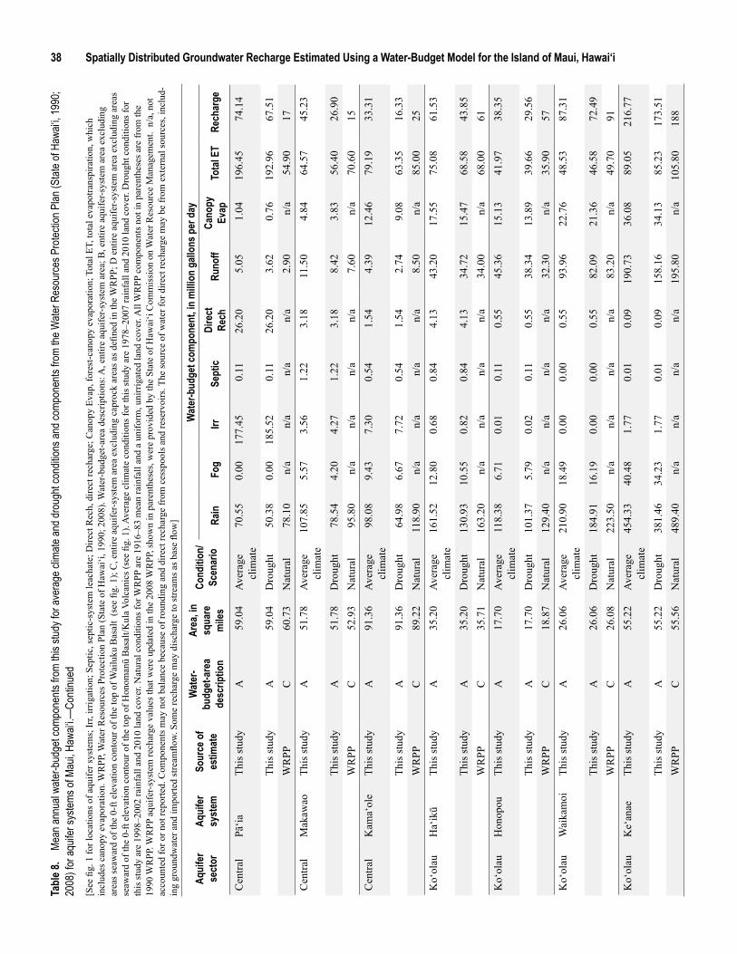
38 Spatially Distributed Groundwater Recharge Estimated Using a Water-Budget Model for the Island of Maui, Hawai‘i
Aqui
fer
sect
orAq
uife
r sy
stem
Sour
ce o
f es
timat
e
Wat
er-
budg
et-a
rea
desc
riptio
n
Area
, in
squa
re
mile
s
Cond
ition
/ Sc
enar
io
Wat
er-b
udge
t com
pone
nt, in
milli
on g
allon
s per
day
Rain
Fog
IrrSe
ptic
Dire
ct
Rech
Runo
ffCa
nopy
Ev
apTo
tal E
TRe
char
ge
Cen
tral
Pā‘ia
This
stud
yA
59.0
4Av
erag
e cl
imat
e70
.55
0.00
177.
450.
1126
.20
5.05
1.04
196.
4574
.14
This
stud
yA
59.0
4D
roug
ht50
.38
0.00
185.
520.
1126
.20
3.62
0.76
192.
9667
.51
WR
PPC
60.7
3N
atur
al78
.10
n/a
n/a
n/a
n/a
2.90
n/a
54.9
017
Cen
tral
Mak
awao
This
stud
yA
51.7
8Av
erag
e cl
imat
e10
7.85
5.57
3.56
1.22
3.18
11.5
04.
8464
.57
45.2
3
This
stud
yA
51.7
8D
roug
ht78
.54
4.20
4.27
1.22
3.18
8.42
3.83
56.4
026
.90
WR
PPC
52.9
3N
atur
al95
.80
n/a
n/a
n/a
n/a
7.60
n/a
70.6
015
Cen
tral
Kam
a‘ol
eTh
is st
udy
A91
.36
Aver
age
clim
ate
98.0
89.
437.
300.
541.
544.
3912
.46
79.1
933
.31
This
stud
yA
91.3
6D
roug
ht64
.98
6.67
7.72
0.54
1.54
2.74
9.08
63.3
516
.33
WR
PPC
89.2
2N
atur
al11
8.90
n/a
n/a
n/a
n/a
8.50
n/a
85.0
025
Ko‘
olau
Ha‘
ikū
This
stud
yA
35.2
0Av
erag
e cl
imat
e16
1.52
12.8
00.
680.
844.
1343
.20
17.5
575
.08
61.5
3
This
stud
yA
35.2
0D
roug
ht13
0.93
10.5
50.
820.
844.
1334
.72
15.4
768
.58
43.8
5W
RPP
C35
.71
Nat
ural
163.
20n/
an/
an/
an/
a34
.00
n/a
68.0
061
Ko‘
olau
Hon
opou
This
stud
yA
17.7
0Av
erag
e cl
imat
e11
8.38
6.71
0.01
0.11
0.55
45.3
615
.13
41.9
738
.35
This
stud
yA
17.7
0D
roug
ht10
1.37
5.79
0.02
0.11
0.55
38.3
413
.89
39.6
629
.56
WR
PPC
18.8
7N
atur
al12
9.40
n/a
n/a
n/a
n/a
32.3
0n/
a35
.90
57K
o‘ol
auW
aika
moi
This
stud
yA
26.0
6Av
erag
e cl
imat
e21
0.90
18.4
90.
000.
000.
5593
.96
22.7
648
.53
87.3
1
This
stud
yA
26.0
6D
roug
ht18
4.91
16.1
90.
000.
000.
5582
.09
21.3
646
.58
72.4
9W
RPP
C26
.08
Nat
ural
223.
50n/
an/
an/
an/
a83
.20
n/a
49.7
091
Ko‘
olau
Ke‘
anae
This
stud
yA
55.2
2Av
erag
e cl
imat
e45
4.33
40.4
81.
770.
010.
0919
0.73
36.0
889
.05
216.
77
This
stud
yA
55.2
2D
roug
ht38
1.46
34.2
31.
770.
010.
0915
8.16
34.1
385
.23
173.
51W
RPP
C55
.56
Nat
ural
489.
40n/
an/
an/
an/
a19
5.80
n/a
105.
8018
8
Tabl
e 8.
Mean
annu
al wa
ter-b
udge
t com
pone
nts fr
om th
is stu
dy fo
r ave
rage
clim
ate an
d dro
ught
cond
itions
and c
ompo
nents
from
the W
ater R
esou
rces P
rotec
tion P
lan (S
tate o
f Haw
ai‘i, 1
990;
2008
) for
aquif
er sy
stems
of M
aui, H
awai‘
i.—Co
ntinu
ed[S
ee fi
g. 1
for l
ocat
ions
of a
quife
r sys
tem
s; Ir
r, irr
igat
ion;
Sep
tic, s
eptic
-sys
tem
leac
hate
; Dire
ct R
ech,
dire
ct re
char
ge; C
anop
y Ev
ap, f
ores
t-can
opy
evap
orat
ion;
Tot
al E
T, to
tal e
vapo
trans
pira
tion,
whi
ch
incl
udes
can
opy
evap
orat
ion.
WR
PP, W
ater
Res
ourc
es P
rote
ctio
n Pl
an (S
tate
of H
awai
‘i, 1
990;
200
8). W
ater
-bud
get-a
rea
desc
riptio
ns: A
, ent
ire a
quife
r-sys
tem
are
a; B
, ent
ire a
quife
r-sys
tem
are
a ex
clud
ing
area
s sea
war
d of
the
0-ft
elev
atio
n co
ntou
r of t
he to
p of
Wai
luku
Bas
alt
(see
fig.
1);
C, e
ntire
aqu
ifer-s
yste
m a
rea
excl
udin
g ca
proc
k ar
eas a
s defi
ned
in th
e W
RPP
; D e
ntire
aqu
ifer-s
yste
m a
rea
excl
udin
g ar
eas
seaw
ard
of th
e 0-
ft el
evat
ion
cont
our o
f the
top
of H
onom
anū
Bas
alt/K
ula
Volc
anic
s (se
e fig
. 1).
Aver
age
clim
ate
cond
ition
s for
this
stud
y ar
e 19
78–2
007
rain
fall
and
2010
land
cov
er. D
roug
ht c
ondi
tions
for
this
stud
y ar
e 19
98–2
002
rain
fall
and
2010
land
cov
er. N
atur
al c
ondi
tions
for W
RPP
are
191
6–83
mea
n ra
infa
ll an
d a
unifo
rm, u
nirr
igat
ed la
nd c
over
. All
WR
PP c
ompo
nent
s not
in p
aren
thes
es a
re fr
om th
e 19
90 W
RPP
. WR
PP a
quife
r-sys
tem
rech
arge
val
ues t
hat w
ere
upda
ted
in th
e 20
08 W
RPP
, sho
wn
in p
aren
thes
es, w
ere
prov
ided
by
the
Stat
e of
Haw
ai‘i
Com
mis
sion
on
Wat
er R
esou
rce
Man
agem
ent.
n/a
, not
ac
coun
ted
for o
r not
repo
rted.
Com
pone
nts m
ay n
ot b
alan
ce b
ecau
se o
f rou
ndin
g an
d di
rect
rech
arge
from
ces
spoo
ls a
nd re
serv
oirs
. The
sour
ce o
f wat
er fo
r dire
ct re
char
ge m
ay b
e fr
om e
xter
nal s
ourc
es, i
nclu
d-in
g gr
ound
wat
er a
nd im
porte
d st
ream
flow.
Som
e re
char
ge m
ay d
isch
arge
to st
ream
s as b
ase
flow
]
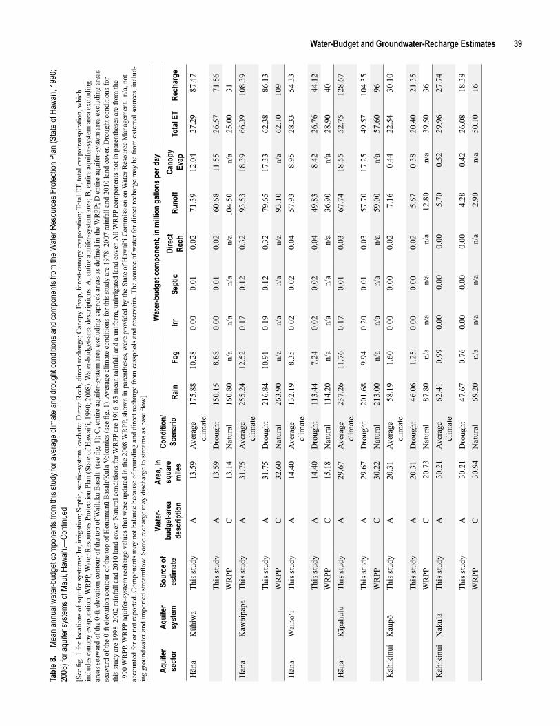
Water-Budget and Groundwater-Recharge Estimates 39
Aqui
fer
sect
orAq
uife
r sy
stem
Sour
ce o
f es
timat
e
Wat
er-
budg
et-a
rea
desc
riptio
n
Area
, in
squa
re
mile
s
Cond
ition
/ Sc
enar
io
Wat
er-b
udge
t com
pone
nt, in
milli
on g
allon
s per
day
Rain
Fog
IrrSe
ptic
Dire
ct
Rech
Runo
ffCa
nopy
Ev
apTo
tal E
TRe
char
ge
Hān
aK
ūhiw
aTh
is st
udy
A13
.59
Aver
age
clim
ate
175.
8810
.28
0.00
0.01
0.02
71.3
912
.04
27.2
987
.47
This
stud
yA
13.5
9D
roug
ht15
0.15
8.88
0.00
0.01
0.02
60.6
811
.55
26.5
771
.56
WR
PPC
13.1
4N
atur
al16
0.80
n/a
n/a
n/a
n/a
104.
50n/
a25
.00
31H
āna
Kaw
aipa
paTh
is st
udy
A31
.75
Aver
age
clim
ate
255.
2412
.52
0.17
0.12
0.32
93.5
318
.39
66.3
910
8.39
This
stud
yA
31.7
5D
roug
ht21
6.84
10.9
10.
190.
120.
3279
.65
17.3
362
.38
86.1
3W
RPP
C32
.60
Nat
ural
263.
90n/
an/
an/
an/
a93
.10
n/a
62.1
010
9H
āna
Wai
ho‘i
This
stud
yA
14.4
0Av
erag
e cl
imat
e13
2.19
8.35
0.02
0.02
0.04
57.9
38.
9528
.33
54.3
3
This
stud
yA
14.4
0D
roug
ht11
3.44
7.24
0.02
0.02
0.04
49.8
38.
4226
.76
44.1
2W
RPP
C15
.18
Nat
ural
114.
20n/
an/
an/
an/
a36
.90
n/a
28.9
040
Hān
aK
īpah
ulu
This
stud
yA
29.6
7Av
erag
e cl
imat
e23
7.26
11.7
60.
170.
010.
0367
.74
18.5
552
.75
128.
67
This
stud
yA
29.6
7D
roug
ht20
1.68
9.94
0.20
0.01
0.03
57.7
017
.25
49.5
710
4.35
WR
PPC
30.2
2N
atur
al21
3.00
n/a
n/a
n/a
n/a
59.0
0n/
a57
.60
96K
ahik
inui
Kau
pōTh
is st
udy
A20
.31
Aver
age
clim
ate
58.1
91.
600.
000.
000.
027.
160.
4422
.54
30.1
0
This
stud
yA
20.3
1D
roug
ht46
.06
1.25
0.00
0.00
0.02
5.67
0.38
20.4
021
.35
WR
PPC
20.7
3N
atur
al87
.80
n/a
n/a
n/a
n/a
12.8
0n/
a39
.50
36K
ahik
inui
Nak
ula
This
stud
yA
30.2
1Av
erag
e cl
imat
e62
.41
0.99
0.00
0.00
0.00
5.70
0.52
29.9
627
.74
This
stud
yA
30.2
1D
roug
ht47
.67
0.76
0.00
0.00
0.00
4.28
0.42
26.0
818
.38
WR
PPC
30.9
4N
atur
al69
.20
n/a
n/a
n/a
n/a
2.90
n/a
50.1
016
Tabl
e 8.
Mean
annu
al wa
ter-b
udge
t com
pone
nts fr
om th
is stu
dy fo
r ave
rage
clim
ate an
d dro
ught
cond
itions
and c
ompo
nents
from
the W
ater R
esou
rces P
rotec
tion P
lan (S
tate o
f Haw
ai‘i, 1
990;
2008
) for
aquif
er sy
stems
of M
aui, H
awai‘
i.—Co
ntinu
ed[S
ee fi
g. 1
for l
ocat
ions
of a
quife
r sys
tem
s; Ir
r, irr
igat
ion;
Sep
tic, s
eptic
-sys
tem
leac
hate
; Dire
ct R
ech,
dire
ct re
char
ge; C
anop
y Ev
ap, f
ores
t-can
opy
evap
orat
ion;
Tot
al E
T, to
tal e
vapo
trans
pira
tion,
whi
ch
incl
udes
can
opy
evap
orat
ion.
WR
PP, W
ater
Res
ourc
es P
rote
ctio
n Pl
an (S
tate
of H
awai
‘i, 1
990;
200
8). W
ater
-bud
get-a
rea
desc
riptio
ns: A
, ent
ire a
quife
r-sys
tem
are
a; B
, ent
ire a
quife
r-sys
tem
are
a ex
clud
ing
area
s sea
war
d of
the
0-ft
elev
atio
n co
ntou
r of t
he to
p of
Wai
luku
Bas
alt
(see
fig.
1);
C, e
ntire
aqu
ifer-s
yste
m a
rea
excl
udin
g ca
proc
k ar
eas a
s defi
ned
in th
e W
RPP
; D e
ntire
aqu
ifer-s
yste
m a
rea
excl
udin
g ar
eas
seaw
ard
of th
e 0-
ft el
evat
ion
cont
our o
f the
top
of H
onom
anū
Bas
alt/K
ula
Volc
anic
s (se
e fig
. 1).
Aver
age
clim
ate
cond
ition
s for
this
stud
y ar
e 19
78–2
007
rain
fall
and
2010
land
cov
er. D
roug
ht c
ondi
tions
for
this
stud
y ar
e 19
98–2
002
rain
fall
and
2010
land
cov
er. N
atur
al c
ondi
tions
for W
RPP
are
191
6–83
mea
n ra
infa
ll an
d a
unifo
rm, u
nirr
igat
ed la
nd c
over
. All
WR
PP c
ompo
nent
s not
in p
aren
thes
es a
re fr
om th
e 19
90 W
RPP
. WR
PP a
quife
r-sys
tem
rech
arge
val
ues t
hat w
ere
upda
ted
in th
e 20
08 W
RPP
, sho
wn
in p
aren
thes
es, w
ere
prov
ided
by
the
Stat
e of
Haw
ai‘i
Com
mis
sion
on
Wat
er R
esou
rce
Man
agem
ent.
n/a
, not
ac
coun
ted
for o
r not
repo
rted.
Com
pone
nts m
ay n
ot b
alan
ce b
ecau
se o
f rou
ndin
g an
d di
rect
rech
arge
from
ces
spoo
ls a
nd re
serv
oirs
. The
sour
ce o
f wat
er fo
r dire
ct re
char
ge m
ay b
e fr
om e
xter
nal s
ourc
es, i
nclu
d-in
g gr
ound
wat
er a
nd im
porte
d st
ream
flow.
Som
e re
char
ge m
ay d
isch
arge
to st
ream
s as b
ase
flow
]
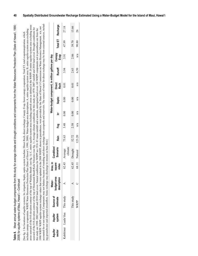
40 Spatially Distributed Groundwater Recharge Estimated Using a Water-Budget Model for the Island of Maui, Hawai‘i
Aqui
fer
sect
orAq
uife
r sy
stem
Sour
ce o
f es
timat
e
Wat
er-
budg
et-a
rea
desc
riptio
n
Area
, in
squa
re
mile
s
Cond
ition
/ Sc
enar
io
Wat
er-b
udge
t com
pone
nt, in
milli
on g
allon
s per
day
Rain
Fog
IrrSe
ptic
Dire
ct
Rech
Runo
ffCa
nopy
Ev
apTo
tal E
TRe
char
ge
Kah
ikin
uiLu
ala‘
ilua
This
stud
yA
62.4
5Av
erag
e cl
imat
e75
.63
3.48
0.00
0.00
0.01
3.94
3.91
47.9
927
.18
This
stud
yA
62.4
5D
roug
ht52
.72
2.58
0.00
0.00
0.01
2.63
2.86
39.7
013
.66
WR
PPC
68.1
1N
atur
al12
3.20
n/a
n/a
n/a
n/a
6.50
n/a
90.8
026
Tabl
e 8.
Mean
annu
al wa
ter-b
udge
t com
pone
nts fr
om th
is stu
dy fo
r ave
rage
clim
ate an
d dro
ught
cond
itions
and c
ompo
nents
from
the W
ater R
esou
rces P
rotec
tion P
lan (S
tate o
f Haw
ai‘i, 1
990;
2008
) for
aquif
er sy
stems
of M
aui, H
awai‘
i.—Co
ntinu
ed[S
ee fi
g. 1
for l
ocat
ions
of a
quife
r sys
tem
s; Ir
r, irr
igat
ion;
Sep
tic, s
eptic
-sys
tem
leac
hate
; Dire
ct R
ech,
dire
ct re
char
ge; C
anop
y Ev
ap, f
ores
t-can
opy
evap
orat
ion;
Tot
al E
T, to
tal e
vapo
trans
pira
tion,
whi
ch
incl
udes
can
opy
evap
orat
ion.
WR
PP, W
ater
Res
ourc
es P
rote
ctio
n Pl
an (S
tate
of H
awai
‘i, 1
990;
200
8). W
ater
-bud
get-a
rea
desc
riptio
ns: A
, ent
ire a
quife
r-sys
tem
are
a; B
, ent
ire a
quife
r-sys
tem
are
a ex
clud
ing
area
s sea
war
d of
the
0-ft
elev
atio
n co
ntou
r of t
he to
p of
Wai
luku
Bas
alt
(see
fig.
1);
C, e
ntire
aqu
ifer-s
yste
m a
rea
excl
udin
g ca
proc
k ar
eas a
s defi
ned
in th
e W
RPP
; D e
ntire
aqu
ifer-s
yste
m a
rea
excl
udin
g ar
eas
seaw
ard
of th
e 0-
ft el
evat
ion
cont
our o
f the
top
of H
onom
anū
Bas
alt/K
ula
Volc
anic
s (se
e fig
. 1).
Aver
age
clim
ate
cond
ition
s for
this
stud
y ar
e 19
78–2
007
rain
fall
and
2010
land
cov
er. D
roug
ht c
ondi
tions
for
this
stud
y ar
e 19
98–2
002
rain
fall
and
2010
land
cov
er. N
atur
al c
ondi
tions
for W
RPP
are
191
6–83
mea
n ra
infa
ll an
d a
unifo
rm, u
nirr
igat
ed la
nd c
over
. All
WR
PP c
ompo
nent
s not
in p
aren
thes
es a
re fr
om th
e 19
90 W
RPP
. WR
PP a
quife
r-sys
tem
rech
arge
val
ues t
hat w
ere
upda
ted
in th
e 20
08 W
RPP
, sho
wn
in p
aren
thes
es, w
ere
prov
ided
by
the
Stat
e of
Haw
ai‘i
Com
mis
sion
on
Wat
er R
esou
rce
Man
agem
ent.
n/a
, not
ac
coun
ted
for o
r not
repo
rted.
Com
pone
nts m
ay n
ot b
alan
ce b
ecau
se o
f rou
ndin
g an
d di
rect
rech
arge
from
ces
spoo
ls a
nd re
serv
oirs
. The
sour
ce o
f wat
er fo
r dire
ct re
char
ge m
ay b
e fr
om e
xter
nal s
ourc
es, i
nclu
d-in
g gr
ound
wat
er a
nd im
porte
d st
ream
flow.
Som
e re
char
ge m
ay d
isch
arge
to st
ream
s as b
ase
flow
]
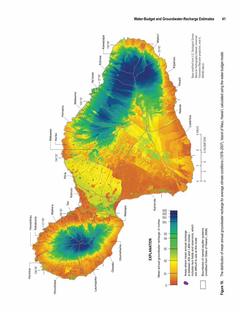
Water-Budget and Groundwater-Recharge Estimates 41
Figu
re 10
. The
distr
ibutio
n of m
ean a
nnua
l rech
arge
for a
vera
ge cl
imate
cond
itions
(197
8–20
07),
Islan
d of M
aui, H
awai‘
i, calc
ulated
using
the w
ater-b
udge
t mod
el.
Are
as w
here
mea
n an
nual
rec
harg
e is
bet
wee
n 45
5 an
d 1,
894
inch
es −
incl
udes
taro
fiel
ds a
nd r
eser
voirs
, whi
ch
are
diffi
cult
to s
ee a
t thi
s sc
ale
Bou
ndar
ies
of n
amed
aqu
ifer
syst
ems
(mod
ified
from
Sta
te o
f Haw
aiÿi,
200
8)
0
10
20
30
4050
100150
300200
Mea
n an
nual
gro
undw
ater
rec
harg
e, in
inch
es
EXPL
ANAT
ION
Base
mod
ified
from
U.S
. Geo
logi
cal S
urve
y N
atio
nal H
ydro
grap
hy D
atas
et, U
nive
rsal
Tr
ansv
erse
Mer
cato
r pro
ject
ion,
zone
4,
NAD
83 d
atum
.
Pä‘
ia
Kam
a‘ol
e
‘Ïao
Ha‘
ikü
Mak
awao
Kah
ului
Wai
kapü
Hon
oköw
ai
Hon
olua
Hon
opou
Laun
iupo
ko
Wai
he‘e
Hon
oköh
au
Uku
meh
ame
Kah
akul
oa
Olo
wal
u
Wai
kam
oi
Keÿ
anae
Lual
aÿilu
a
Nak
ula
Kau
pö
Kïp
ahul
u
Wai
hoÿi
Kaw
aipa
paK
ühiw
a
156°
00'
156°
10'
156°
20'
156°
30'
156°
40'
21°0
0'
20°5
0'
20°4
0'
03
69
KILO
MET
ERS
03
69
MIL
ES
Figu
re 10
. Th
e dist
ributi
on of
mea
n ann
ual g
roun
dwate
r rec
harg
e for
aver
age c
limate
cond
itions
(197
8–20
07),
Islan
d of M
aui, H
awai‘
i, calc
ulated
using
the w
ater-b
udge
t mod
el.
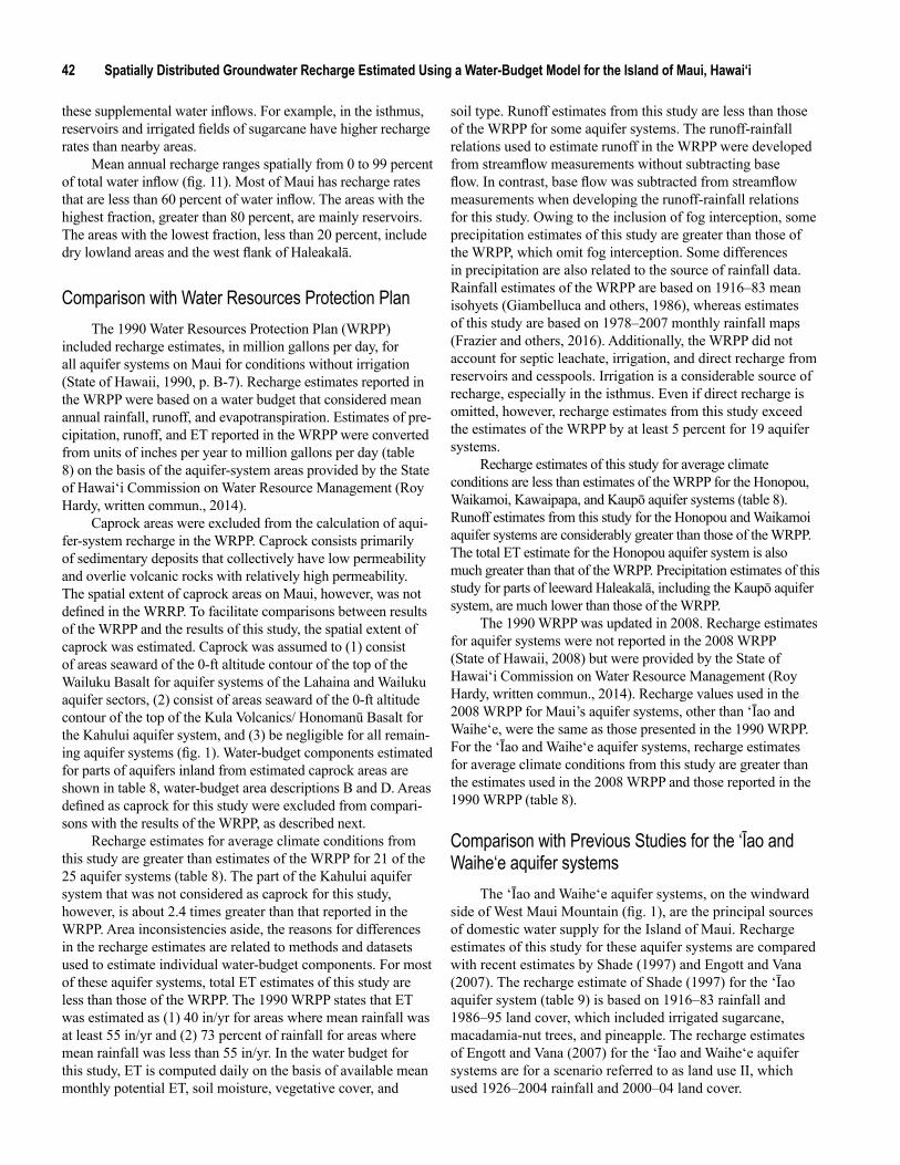
42 Spatially Distributed Groundwater Recharge Estimated Using a Water-Budget Model for the Island of Maui, Hawai‘i
these supplemental water inflows. For example, in the isthmus, reservoirs and irrigated fields of sugarcane have higher recharge rates than nearby areas.
Mean annual recharge ranges spatially from 0 to 99 percent of total water inflow (fig. 11). Most of Maui has recharge rates that are less than 60 percent of water inflow. The areas with the highest fraction, greater than 80 percent, are mainly reservoirs. The areas with the lowest fraction, less than 20 percent, include dry lowland areas and the west flank of Haleakalā.
Comparison with Water Resources Protection PlanThe 1990 Water Resources Protection Plan (WRPP)
included recharge estimates, in million gallons per day, for all aquifer systems on Maui for conditions without irrigation (State of Hawaii, 1990, p. B-7). Recharge estimates reported in the WRPP were based on a water budget that considered mean annual rainfall, runoff, and evapotranspiration. Estimates of pre-cipitation, runoff, and ET reported in the WRPP were converted from units of inches per year to million gallons per day (table 8) on the basis of the aquifer-system areas provided by the State of Hawai‘i Commission on Water Resource Management (Roy Hardy, written commun., 2014).
Caprock areas were excluded from the calculation of aqui-fer-system recharge in the WRPP. Caprock consists primarily of sedimentary deposits that collectively have low permeability and overlie volcanic rocks with relatively high permeability. The spatial extent of caprock areas on Maui, however, was not defined in the WRRP. To facilitate comparisons between results of the WRPP and the results of this study, the spatial extent of caprock was estimated. Caprock was assumed to (1) consist of areas seaward of the 0-ft altitude contour of the top of the Wailuku Basalt for aquifer systems of the Lahaina and Wailuku aquifer sectors, (2) consist of areas seaward of the 0-ft altitude contour of the top of the Kula Volcanics/ Honomanū Basalt for the Kahului aquifer system, and (3) be negligible for all remain-ing aquifer systems (fig. 1). Water-budget components estimated for parts of aquifers inland from estimated caprock areas are shown in table 8, water-budget area descriptions B and D. Areas defined as caprock for this study were excluded from compari-sons with the results of the WRPP, as described next.
Recharge estimates for average climate conditions from this study are greater than estimates of the WRPP for 21 of the 25 aquifer systems (table 8). The part of the Kahului aquifer system that was not considered as caprock for this study, however, is about 2.4 times greater than that reported in the WRPP. Area inconsistencies aside, the reasons for differences in the recharge estimates are related to methods and datasets used to estimate individual water-budget components. For most of these aquifer systems, total ET estimates of this study are less than those of the WRPP. The 1990 WRPP states that ET was estimated as (1) 40 in/yr for areas where mean rainfall was at least 55 in/yr and (2) 73 percent of rainfall for areas where mean rainfall was less than 55 in/yr. In the water budget for this study, ET is computed daily on the basis of available mean monthly potential ET, soil moisture, vegetative cover, and
soil type. Runoff estimates from this study are less than those of the WRPP for some aquifer systems. The runoff-rainfall relations used to estimate runoff in the WRPP were developed from streamflow measurements without subtracting base flow. In contrast, base flow was subtracted from streamflow measurements when developing the runoff-rainfall relations for this study. Owing to the inclusion of fog interception, some precipitation estimates of this study are greater than those of the WRPP, which omit fog interception. Some differences in precipitation are also related to the source of rainfall data. Rainfall estimates of the WRPP are based on 1916–83 mean isohyets (Giambelluca and others, 1986), whereas estimates of this study are based on 1978–2007 monthly rainfall maps (Frazier and others, 2016). Additionally, the WRPP did not account for septic leachate, irrigation, and direct recharge from reservoirs and cesspools. Irrigation is a considerable source of recharge, especially in the isthmus. Even if direct recharge is omitted, however, recharge estimates from this study exceed the estimates of the WRPP by at least 5 percent for 19 aquifer systems.
Recharge estimates of this study for average climate conditions are less than estimates of the WRPP for the Honopou, Waikamoi, Kawaipapa, and Kaupō aquifer systems (table 8). Runoff estimates from this study for the Honopou and Waikamoi aquifer systems are considerably greater than those of the WRPP. The total ET estimate for the Honopou aquifer system is also much greater than that of the WRPP. Precipitation estimates of this study for parts of leeward Haleakalā, including the Kaupō aquifer system, are much lower than those of the WRPP.
The 1990 WRPP was updated in 2008. Recharge estimates for aquifer systems were not reported in the 2008 WRPP (State of Hawaii, 2008) but were provided by the State of Hawai‘i Commission on Water Resource Management (Roy Hardy, written commun., 2014). Recharge values used in the 2008 WRPP for Maui’s aquifer systems, other than ‘Īao and Waihe‘e, were the same as those presented in the 1990 WRPP. For the ‘Īao and Waihe‘e aquifer systems, recharge estimates for average climate conditions from this study are greater than the estimates used in the 2008 WRPP and those reported in the 1990 WRPP (table 8).
Comparison with Previous Studies for the ‘Īao and Waihe‘e aquifer systems
The ‘Īao and Waihe‘e aquifer systems, on the windward side of West Maui Mountain (fig. 1), are the principal sources of domestic water supply for the Island of Maui. Recharge estimates of this study for these aquifer systems are compared with recent estimates by Shade (1997) and Engott and Vana (2007). The recharge estimate of Shade (1997) for the ‘Īao aquifer system (table 9) is based on 1916–83 rainfall and 1986–95 land cover, which included irrigated sugarcane, macadamia-nut trees, and pineapple. The recharge estimates of Engott and Vana (2007) for the ‘Īao and Waihe‘e aquifer systems are for a scenario referred to as land use II, which used 1926–2004 rainfall and 2000–04 land cover.
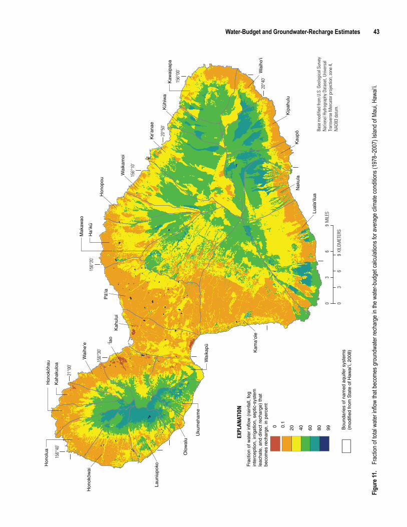
Water-Budget and Groundwater-Recharge Estimates 43
200.1
0 40 80 9960
EXPL
AN
ATIO
N
Frac
tion
of w
ater
inflo
w (
rain
fall,
fog
inte
rcep
tion,
irrig
atio
n, s
eptic
-sys
tem
le
acha
te, a
nd d
irect
rec
harg
e) th
at
beco
mes
rec
harg
e, in
per
cent
Bou
ndar
ies
of n
amed
aqu
ifer
syst
ems
(mod
ified
from
Sta
te o
f Haw
aiÿi,
200
8)
Figu
re 11
. Fra
ction
of to
tal w
ater in
flow
that b
ecom
es gr
ound
water
rech
arge
in th
e wate
r-bud
get c
alcula
tions
for a
vera
ge cl
imate
cond
itions
(197
8−20
07),
Islan
d of M
aui, H
awai‘
i.
Base
mod
ified
from
U.S
. Geo
logi
cal S
urve
y N
atio
nal H
ydro
grap
hy D
atas
et, U
nive
rsal
Tr
ansv
erse
Mer
cato
r pro
ject
ion,
zone
4,
NAD
83 d
atum
.
Pä‘
ia
Kam
a‘ol
e
‘Ïao
Ha‘
ikü
Mak
awao
Kah
ului
Wai
kapü
Hon
oköw
ai
Hon
olua
Hon
opou
Laun
iupo
ko
Wai
he‘e
Hon
oköh
au
Uku
meh
ame
Kah
akul
oa
Olo
wal
u
Wai
kam
oi
Keÿ
anae
Lual
aÿilu
a
Nak
ula
Kau
pö
Kïp
ahul
u
Wai
hoÿi
Kaw
aipa
paK
ühiw
a
156°
00'
156°
10'
156°
20'
156°
30'
156°
40'
21°0
0'
20°5
0'
20°4
0'
03
69
KILO
MET
ERS
03
69
MIL
ES
Figu
re 11
. Fr
actio
n of to
tal w
ater in
flow
that b
ecom
es gr
ound
water
rech
arge
in th
e wate
r-bud
get c
alcula
tions
for a
vera
ge cl
imate
cond
itions
(197
8–20
07) I
sland
of M
aui, H
awai‘
i.
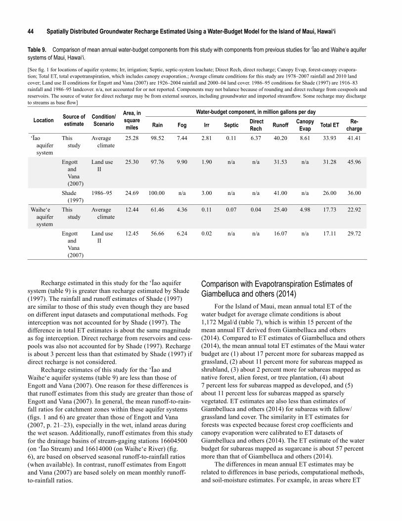
44 Spatially Distributed Groundwater Recharge Estimated Using a Water-Budget Model for the Island of Maui, Hawai‘i
Table 9. Comparison of mean annual water-budget components from this study with components from previous studies for ‘Īao and Waihe‘e aquifer systems of Maui, Hawai‘i.
Location Source of estimate
Condition/Scenario
Area, in square miles
Water-budget component, in million gallons per day
Rain Fog Irr Septic Direct Rech Runoff Canopy
Evap Total ET Re-charge
‘Īao aquifer system
This study
Average climate
25.28 98.52 7.44 2.81 0.11 6.37 40.20 8.61 33.93 41.41
Engott and Vana (2007)
Land use II
25.30 97.76 9.90 1.90 n/a n/a 31.53 n/a 31.28 45.96
Shade (1997)
1986–95 24.69 100.00 n/a 3.00 n/a n/a 41.00 n/a 26.00 36.00
Waihe‘e aquifer system
This study
Average climate
12.44 61.46 4.36 0.11 0.07 0.04 25.40 4.98 17.73 22.92
Engott and Vana (2007)
Land use II
12.45 56.66 6.24 0.02 n/a n/a 16.07 n/a 17.11 29.72
[See fig. 1 for locations of aquifer systems; Irr, irrigation; Septic, septic-system leachate; Direct Rech, direct recharge; Canopy Evap, forest-canopy evapora-tion; Total ET, total evapotranspiration, which includes canopy evaporation.; Average climate conditions for this study are 1978–2007 rainfall and 2010 land cover; Land use II conditions for Engott and Vana (2007) are 1926–2004 rainfall and 2000–04 land cover. 1986–95 conditions for Shade (1997) are 1916–83 rainfall and 1986–95 landcover. n/a, not accounted for or not reported. Components may not balance because of rounding and direct recharge from cesspools and reservoirs. The source of water for direct recharge may be from external sources, including groundwater and imported streamflow. Some recharge may discharge to streams as base flow]
Recharge estimated in this study for the ‘Īao aquifer system (table 9) is greater than recharge estimated by Shade (1997). The rainfall and runoff estimates of Shade (1997) are similar to those of this study even though they are based on different input datasets and computational methods. Fog interception was not accounted for by Shade (1997). The difference in total ET estimates is about the same magnitude as fog interception. Direct recharge from reservoirs and cess-pools was also not accounted for by Shade (1997). Recharge is about 3 percent less than that estimated by Shade (1997) if direct recharge is not considered.
Recharge estimates of this study for the ‘Īao and Waihe‘e aquifer systems (table 9) are less than those of Engott and Vana (2007). One reason for these differences is that runoff estimates from this study are greater than those of Engott and Vana (2007). In general, the mean runoff-to-rain-fall ratios for catchment zones within these aquifer systems (figs. 1 and 6) are greater than those of Engott and Vana (2007, p. 21–23), especially in the wet, inland areas during the wet season. Additionally, runoff estimates from this study for the drainage basins of stream-gaging stations 16604500 (on ‘Īao Stream) and 16614000 (on Waihe‘e River) (fig. 6), are based on observed seasonal runoff-to-rainfall ratios (when available). In contrast, runoff estimates from Engott and Vana (2007) are based solely on mean monthly runoff-to-rainfall ratios.
Comparison with Evapotranspiration Estimates of Giambelluca and others (2014)
For the Island of Maui, mean annual total ET of the water budget for average climate conditions is about 1,172 Mgal/d (table 7), which is within 15 percent of the mean annual ET derived from Giambelluca and others (2014). Compared to ET estimates of Giambelluca and others (2014), the mean annual total ET estimates of the Maui water budget are (1) about 17 percent more for subareas mapped as grassland, (2) about 11 percent more for subareas mapped as shrubland, (3) about 2 percent more for subareas mapped as native forest, alien forest, or tree plantation, (4) about 7 percent less for subareas mapped as developed, and (5) about 11 percent less for subareas mapped as sparsely vegetated. ET estimates are also less than estimates of Giambelluca and others (2014) for subareas with fallow/grassland land cover. The similarity in ET estimates for forests was expected because forest crop coefficients and canopy evaporation were calibrated to ET datasets of Giambelluca and others (2014). The ET estimate of the water budget for subareas mapped as sugarcane is about 57 percent more than that of Giambelluca and others (2014).
The differences in mean annual ET estimates may be related to differences in base periods, computational methods, and soil-moisture estimates. For example, in areas where ET

Water-Budget and Groundwater-Recharge Estimates 45
estimates of the water budget are much greater than those of Giambelluca and others (2014)–including sugarcane fields– soil-moisture estimates of the water budget may be greater than those of Giambelluca and others (2014). On the other hand, in areas where ET estimates of the water budget are less than those of Giambelluca and others (2014)–including abandoned agriculture fields mapped as fallow/grassland– soil-moisture estimates of the water budget may be less.
Recharge for Drought ConditionsMaui has experienced drought conditions in recent
years. For example, based on the 1978–2007 monthly rainfall datasets (Frazier and others, 2016), annual rainfall for the island of Maui was below average 8 out of the last 10 years (1998–2007). To assess the impact of drought conditions on recharge, rainfall during 1998–2002 was selected to repre-sent drought conditions on Maui because this period had the lowest 5-yr mean rainfall during 1978–2007. Other than rainfall, all water-budget inputs used to compute recharge for drought conditions were the same as those used for average climate conditions. Because the fog-to-rainfall ratios used for average climate conditions were also used for drought condi-tions, fog-interception rates for drought conditions were less than those for average climate conditions.
For the Island of Maui, recharge for drought condi-tions, about 1,010 Mgal/d (table 7), is 23 percent less than recharge for average climate conditions. For Maui’s aquifer systems, water-budget components estimated for drought conditions are shown in table 8. Aquifer-system precipitation for drought conditions ranges from 12 to 37 percent less than corresponding precipitation for average climate conditions. Aquifer-system recharge for drought conditions is about 8 to 51 percent less than corresponding recharge for average climate conditions.
The spatial pattern of mean annual recharge for drought conditions on the Island of Maui (not shown) resembles that for average climate conditions. Recharge for most areas, however, is lower for drought conditions (fig. 12). Hence, for most areas on the Island of Maui, recharge estimates are sensitive to precipitation. Compared with recharge for aver-age climate conditions, recharge decreases between 10 and 50 percent for most upland areas on West Maui Mountain and windward Haleakalā; recharge decreases by more than 50 percent in most unirrigated lowland areas on West Maui Mountain and on leeward Haleakalā. Recharge decreases by 10 percent or less for some irrigated areas, including the sugarcane fields in the isthmus. Subareas mapped as golf courses had slightly more recharge for drought conditions owing to relatively more sprinkler irrigation. In some areas, runoff may have been overestimated for drought condi-tions owing to use of mean seasonal runoff-to-rainfall ratios representative of 1978–2007. Overestimating runoff would result in underestimating recharge. On the other hand, the assumption of constant reference ET may have resulted in
underestimating ET for drought conditions, which would result in overestimating recharge.
Sensitivity AnalysisUncertainty exists in many of the water-budget inputs
used in this study. The inputs used in the water-budget calculations were considered to be those most reasonable. To analyze the effect that uncertainty in water-budget inputs has on estimated recharge, the water budget was rerun, changing one input value at a time within a reasonable range. The parameters tested were (1) available water capacity, (2) fog-interception rates, (3) root depth, (4) runoff-to-rainfall ratios, (5) crop coefficient, (6) canopy capacity, (7) ratio of mean evaporation rate to mean precipitation rate during saturated canopy conditions, and (8) the fate of excess water collected by storm-drain systems. Changes to trunk-storage capacity and the proportion of precipitation diverted to stemflow were also tested for subareas with forest land covers. For available water capacity, the low and high values published in Natural Resources Conservation Service (2006a) were tested. For fog-interception rates and root depths, the “baseline” values used in water-budget calculations for average climate and drought conditions were increased by 50 percent and decreased by 50 percent. Runoff-to-rainfall ratios were adjusted on the basis of bias and root-mean-square-error statistics (for Maui) of the region-regression models (table 5). For crop coefficients, baseline values were increased by 20 percent and decreased by 20 percent. Canopy-storage capacity values of 0.08 and 0.02 were tested. Values for V were increased by 0.10 units and were decreased by 0.10 units. For the latter case, however, V was assumed to be no less 0.01. Finally the effects of routing all water collected by storm-drain systems to runoff and to recharge were tested.
The recharge estimates for the sensitivity analysis were compared with recharge estimates for average climate condi-tions for Honokōwai, ‘Īao, Kahului, Kūhiwa, and Luala‘ilua aquifer systems and the Island of Maui (table 10). These five aquifer systems cover a range of climates on Maui. The Honokōwai and ‘Īao aquifer systems are on leeward and windward West Maui Mountain, respectively, and have steep rainfall gradients. The wet uplands of the Honokōwai aquifer system are mostly native forest; drier lowlands include alien forest, coffee, developed areas, and large areas of abandoned pineapple fields that are now fallow grasslands. Within the ‘Īao aquifer system, uplands are wet, steep, and mostly forest and shrubland; lowlands are drier and are a mixture of alien forest, macadamia, grassland, and developed areas. The area within the Kahului aquifer system, on the isthmus, is very dry but has substantial irrigation for sugarcane. The area within the Kūhiwa aquifer system, on windward Haleakalā, is very wet and is mostly forested. The area within the Luala‘ilua aquifer system, on southwest Haleakalā, is dry and is mostly grassland and sparsely vegetated (table 2).
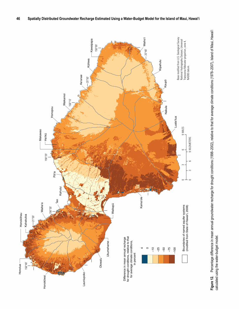
46 Spatially Distributed Groundwater Recharge Estimated Using a Water-Budget Model for the Island of Maui, Hawai‘i
Figu
re 12
. Per
centa
ge di
ffere
nce i
n mea
n ann
ual re
char
ge fo
r dro
ught
cond
itions
(199
8–20
02 ra
infall
), re
lative
to th
at for
aver
age c
limate
cond
itions
(197
8–20
07 ra
infall
), Isl
and o
f Ma
ui, H
awai‘
i, calc
ulated
using
the w
ater-b
udge
t mod
el.
Diff
eren
ce in
mea
n an
nual
rec
harg
e fo
r dr
ough
t con
ditio
ns, r
elat
ive
to th
at
for
aver
age
clim
ate
cond
ition
s,
in p
erce
nt
04
–10
–50
–25
–75
–100 Bou
ndar
ies
of n
amed
aqu
ifer
syst
ems
(mod
ified
from
Sta
te o
f Haw
aiÿi,
200
8)
Base
mod
ified
from
U.S
. Geo
logi
cal S
urve
y N
atio
nal H
ydro
grap
hy D
atas
et, U
nive
rsal
Tr
ansv
erse
Mer
cato
r pro
ject
ion,
zone
4,
NAD
83 d
atum
.
Pä‘
ia
Kam
a‘ol
e
‘Ïao
Ha‘
ikü
Mak
awao
Kah
ului
Wai
kapü
Hon
oköw
ai
Hon
olua
Hon
opou
Laun
iupo
ko
Wai
he‘e
Hon
oköh
au
Uku
meh
ame
Kah
akul
oa
Olo
wal
u
Wai
kam
oi
Keÿ
anae
Lual
aÿilu
a
Nak
ula
Kau
pö
Kïp
ahul
u
Wai
hoÿi
Kaw
aipa
paK
ühiw
a
156°
00'
156°
10'
156°
20'
156°
30'
156°
40'
21°0
0'
20°5
0'
20°4
0'
03
69
KILO
MET
ERS
03
69
MIL
ES
Figu
re 12
. Pe
rcenta
ge di
ffere
nce i
n mea
n ann
ual g
roun
dwate
r rec
harg
e for
drou
ght c
ondit
ions (
1998
–200
2), r
elativ
e to t
hat fo
r ave
rage
clim
ate co
nditio
ns (1
978–
2007
), Isl
and o
f Mau
i, Haw
ai‘i
calcu
lated
using
the w
ater-b
udge
t mod
el.
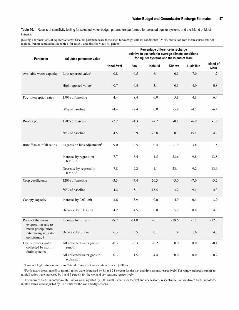
Water-Budget and Groundwater-Recharge Estimates 47
Parameter Adjusted parameter value
Percentage difference in recharge relative to scenario for average climate conditions
for aquifer systems and the Island of Maui
Honokōwai ‘Īao Kahului Kūhiwa Luala‘ilua Island of Maui
Available water capacity Low reported value1 0.8 0.5 6.1 0.1 7.0 1.2
High reported value1 -0.7 -0.4 -3.1 -0.1 -4.0 -0.8
Fog-interception rates 150% of baseline 4.4 8.4 0.0 5.8 4.8 6.4
50% of baseline -4.4 -8.4 0.0 -5.8 -4.5 -6.4
Root depth 150% of baseline -2.2 -1.3 -7.7 -0.1 -6.9 -1.9
50% of baseline 4.5 2.9 28.8 0.3 15.1 4.7
Runoff-to-rainfall ratios Regression bias adjustment2 9.0 -0.5 0.4 -1.9 3.8 1.5
Increase by regression RMSE3
-7.7 -8.4 -1.5 -23.6 -9.8 -13.8
Decrease by regression RMSE3
7.8 9.2 1.1 23.4 9.2 13.9
Crop coefficients 120% of baseline -3.3 -4.4 20.3 -3.0 -7.0 -3.2
80% of baseline 4.2 5.1 -15.5 3.2 9.1 4.3
Canopy capacity Increase by 0.03 unit -3.6 -3.9 0.0 -4.9 -0.4 -3.9
Decrease by 0.03 unit 4.2 4.5 0.0 5.2 0.4 4.3
Ratio of the mean evaporation rate to mean precipitation rate during saturated conditions, V
Increase by 0.1 unit -8.2 -11.8 -0.1 -18.6 -1.5 -12.7
Decrease by 0.1 unit 6.3 5.5 0.1 1.4 1.6 4.8
Fate of excess water collected by storm-drain systems
All collected water goes to runoff
-0.3 -0.3 -0.2 0.0 0.0 -0.1
All collected water goes to recharge
0.3 1.5 4.4 0.0 0.0 0.2
Table 10. Results of sensitivity testing for selected water-budget parameters performed for selected aquifer systems and the Island of Maui, Hawai‘i.[See fig.1 for locations of aquifer systems; baseline parameters are those used for average climate conditions; RMSE, prediction root mean square error of regional-runoff regression; see table 5 for RMSE and bias for Maui; %, percent]
1Low and high values reported in Natural Resources Conservation Service (2006a).2For leeward areas, runoff-to-rainfall ratios were decreased by 38 and 24 percent for the wet and dry seasons, respectively. For windward areas, runoff-to-
rainfall ratios were increased by 1 and 5 percent for the wet and dry seasons, respecitively.3For leeward areas, runoff-to-rainfall ratios were adjusted by 0.06 and 0.03 units for the wet and dry seasons, respectively. For windward areas, runoff-to-
rainfall ratios were adjusted by 0.12 units for the wet and dry seasons.
48 Spatially Distributed Groundwater Recharge Estimated Using a Water-Budget Model for the Island of Maui, Hawai‘i
Adjusting the fate of water collected by storm-drain systems had a minor effect on the recharge estimates for the five aquifer systems examined in this analysis (table 10). If all water collected by storm-drain systems is assumed to be runoff, then aquifer-system recharge decreases by less than 1 percent. If all water collected by storm-drain systems is assumed to be recharge, then aquifer-system recharge increases by less than 5 percent. Although considerable areas are developed in the ‘Īao and Honokōwai aquifer systems, these areas typically have much less rainfall than the forested areas farther inland. Simi-larly, for the Kahului aquifer system, rainfall for the developed land covers is much less than the sum of irrigation and direct recharge from reservoirs. Adjustments to canopy capacity changes recharge by less than 6 percent for each aquifer system examined.
Recharge estimates for windward-facing aquifer sys-tems (‘Īao and Kūhiwa) were most sensitive to adjustments to fog-interception rates, runoff-to-rainfall ratios, and V. This indicates the importance of fog, runoff, and canopy evaporation in the water budget for wet, forested areas. Adjustments to the remaining parameters tested affected recharge in these aquifer systems by no more than 6 percent. Recharge estimates for the Honokōwai aquifer system were also sensitive to runoff-to-rainfall ratios, and V. Adjustments to fog-interception rates, however, had less impact on recharge for this leeward-facing aquifer system relative to the windward-facing aquifer systems.
Recharge estimates for the dry aquifer systems on lee-ward Haleakalā (Kahului and Luala‘ilua) were more sensitive to available water capacity, root depth, and crop coefficients than the wetter aquifer systems examined. This indicates that moisture-storage capacity and ET, which are related to these three parameters, are important water-budget components in dry areas. Adjustments to fog-interception rates also had a notice-able effect on recharge for the Luala‘ilua aquifer system, which has patches of forest and shrubland in the cloud zone. Unlike recharge for the other aquifer systems examined, recharge for the Kahului aquifer system (1) was not sensitive to adjustments in runoff-to-rainfall ratios, and (2) increased when crop coef-ficients were increased. The reason for the latter difference is related to the chief source of recharge. Irrigation is the chief source of recharge for the Kahului aquifer system, whereas precipitation is the chief source of recharge in most unirrigated areas on Maui. In the water budget, increasing the crop coef-ficients for irrigated land covers increases potential ET and irrigation rates (see equation 16), which results in increased recharge rates.
For areas mapped as forests (native, alien, and tree plantation), recharge changes by 6 percent or less in response to selected adjustments to the baseline values used for trunk-storage capacity (0.01 inch), and the proportion of precipita-tion diverted to stemflow (0.04). Recharge for forested areas decreases by about 6 percent when the model uses a relatively high trunk-storage capacity value of 0.14 inch, the storage capacity determined by DeLay (2005) for epiphytes in a native cloud forest on the Island of Hawai‘i. Recharge for forested areas increases by about 2 percent when the model uses a
relatively low trunk-storage capacity value of 0.001 inch and decreases by 0.2 percent when the model uses a relatively high stemflow value of 0.10. For areas mapped as alien forest, recharge decreases by 0.4 percent when the model uses a stem-flow value of 0.37, determined by Safeeq and Fares (2014) for a site with an abundance of Psidium cattleianum.
Suggestions for Future Study and Additional Data Collection
The results of this study indicate that precipitation is a crit-ical dataset for estimating recharge. Future studies that estimate recharge would benefit from additional sites where precipitation is measured. A large part of Maui is in the cloud zone and thus has the potential to intercept fog moisture. Recharge estimates for areas in the cloud zone are sensitive to fog-interception estimates. Fog and recharge estimates of this study could be improved with a better understanding of the spatial and daily variability of fog on Maui and fog-interception rates for differ-ent types of vegetation.
Streamflow data from stream-gaging stations is essen-tial for determining direct runoff and base flow. Additionally, recharge estimates for most areas on Maui are sensitive to runoff-to-rainfall ratios. More stream-gaging stations on Maui would improve runoff and recharge estimates.
Irrigation is substantial on Maui, particularly for sugarcane on the isthmus. Records of water availability can be used to constrain irrigation rates of the water budget. Records of water applied to irrigated areas would help with replicating actual irrigation practices on Maui.
The gridded maps of ET-related parameters produced by Giambelluca and others (2014) were a valuable resource for estimating ET in the water budget of this study, although uncer-tainty in these parameters will result in uncertainty in recharge estimates. Recharge estimates could be further improved with estimates of the interannual and daily variations of reference ET across Maui. For example, ET measurements for different types of the dominant alien and native plants could be used to develop crop coefficients for land-cover types that are more specific than the general land-cover classes used here. Also helpful would be spatial estimates of V, which is the ratio of the mean evapora-tion rate to the mean precipitation rate during saturated canopy conditions. Additional canopy evaporation measurements on Maui could be used to confirm or calibrate the canopy evapora-tion estimates of the water-budget model.
Summary and ConclusionsThe main objective of this study was to determine the
spatial distribution of mean annual groundwater recharge for the Island of Maui. Recharge was computed with a water-budget model that used a daily computational interval. Hydrological
References Cited 49
processes and physical conditions that affect recharge on Maui were simulated in the water-budget model using the most cur-rent datasets available– including maps of 2010 land cover, 1978–2007 monthly rainfall, and mean monthly reference evapotranspiration. The model disaggregated monthly rainfall into daily rainfall using the method of fragments and daily rain-fall records from 52 rain gages. The water-budget model and the most current datasets available were used to estimate the spatial distribution of mean annual groundwater recharge for two scenarios: (1) average climate conditions, based on 2010 land cover and rainfall during 1978–2007 and (2) drought conditions, based on 2010 land cover and rainfall during 1998–2002.
For the Island of Maui, mean annual recharge is about 1,309 Mgal/d for average climate conditions. Recharge is about 44 percent of precipitation (sum of rainfall and fog interception) and is about 39 percent of total inflow (sum of precipitation, irrigation, septic-system leachate, and direct recharge).
The spatial pattern of mean annual recharge on Maui for average climate conditions resembles that of mean annual rain-fall, but it also reflects spatial variations in vegetation and soils, irrigation in agricultural and developed areas, and persistent cloud layers that envelop upland areas. Wet, upland parts of the island typically have more recharge than dry, coastal areas. Areas with the highest recharge include the mid-altitude slopes of windward Haleakalā and the uplands of West Maui Moun-tain. In addition to having high rainfall, these locations have considerable fog interception and low reference ET owing to persistent cloud cover. In general, areas that have water inflows from irrigation, septic-system leaching, and direct recharge have more total recharge than nearby areas without these supplemen-tal water inflows. Of Maui’s total mean recharge for average climate conditions, about 60 percent occurs in the Ko‘olau and Hāna aquifer sectors on windward Haleakalā. For Maui’s 25 aquifer systems, mean annual recharge ranges from about 13 to 217 Mgal/d for average climate conditions. Compared to the aquifer-system recharge estimates of the 1990 State of Hawai‘i Water Resources Protection Plan, recharge estimates from this study are (1) lower for the Honopou, Waikamoi, Kawaipapa, and Kaupō aquifer systems, and (2) higher for the remaining 21 aquifer systems on Maui. Compared to ET estimates of Giambelluca and others (2014), ET estimates of this study are (1) within 17 percent for areas mapped as forest, grassland, developed, shrubland, and sparsely vegetated and (2) about 57 percent greater for areas mapped as sugarcane.
Mean annual recharge on Maui for drought conditions, about 1,010 Mgal/d, is 23 percent less than recharge for average climate conditions. Aquifer-system precipitation for drought conditions ranges from 12 to 37 percent less than correspond-ing precipitation for average climate conditions. Aquifer-system recharge for drought conditions ranges from 8 to 51 percent less than corresponding recharge for average climate condi-tions. Compared with recharge for average climate conditions, recharge decreases between 10 and 50 percent for most upland areas on West Maui Mountain and on windward Haleakalā. Recharge decreases by more than 50 percent in most lowland areas on West Maui Mountain and on leeward Haleakalā.
Recharge decreases by 10 percent or less for some irrigated areas, including the sugarcane fields on the isthmus.
The spatial distribution of rainfall is the primary factor determining spatially distributed recharge estimates for most areas on Maui. Recharge estimates of the Maui water-budget model are also sensitive to runoff-to-rainfall ratios except in areas such as the isthmus, where irrigation exceeds precipita-tion. For wet areas, recharge estimates are also sensitive to fog-interception rates and forest-canopy evaporation. Recharge estimates in drier areas are more sensitive to irrigated crop areas and parameters that are related to ET: available water capacity, root depth, and crop coefficient. The assumption that all water collected by storm-drain systems in urban areas becomes either runoff or recharge has a minor effect on regional-scale recharge.
References Cited
Allen, R.G., Pereira, L.S., Raes, Dirk, and Smith, Martin, 1998, Crop evapotranspiration; guidelines for computing crop water requirements: Food and Agriculture Organization of the United Nations, FAO Irrigation and Drainage Paper 56, 300 p.
Austin, Tsutsumi and Associates, Inc., 1991, West Maui water master plan: County of Maui Department of Water Supply, 270 p.
AWS Truewind, LLC, 2004, Wind energy resource maps of Hawaii: Prepared for Hawai‘i Department of Business, Economic Development, and Tourism Strategic Industries Division, Honolulu, Hawai‘i, 17 p., accessed January 25, 2012, at http://planning.hawaii.gov/gis/download-gis-data/.
Belt, Collins and Associates, Ltd., 1969, A water source development plan for Lahaina District, Island of Maui: Hawai‘i Division of Water and Land Development Report R33, 101 p.
Berg, N., McGurk, B., and Calhoun, R.S., 1997, Hydrology and land use effects in the Hanalei National Wildlife Refuge, Kauai, Hawaii, Final Report, Interagency Agreement 14-48-0001-94588: Albany, Calif., United States Department of Agriculture Forest Service, Pacific Southwest Research Station, 62 p.
Blumenstock, D.I., and Price, Saul, 1967, Climate of Hawaii, in Climates of the States, no. 60-51, Climatography of the United States: U.S. Department of Commerce.
Cao, Guangxia, Giambelluca, T.W., Stevens, D.E., and Schroeder, T.A., 2007, Inversion variability in the Hawaiian trade wind regime: Journal of Climate, v. 20, p. 1145–1160, DOI: 10.1175/JCLI4033.1.
Caskey, M.C., 1968, The recharge of the Waikapu aquifer, Maui: Honolulu, University of Hawai‘i, M.S. thesis, 75 p.
50 Spatially Distributed Groundwater Recharge Estimated Using a Water-Budget Model for the Island of Maui, Hawai‘i
Cheng, C.L., 2012, Measurements of seepage losses and gains, East Maui Irrigation diversion system, Maui, Hawai‘i: U.S. Geological Survey Open-File Report 2012–1115, 23 p.
County of Maui, Hawai‘i, Department of Water Supply, 2014, Monthly water production, accessed March 13, 2014, at http://www.co.maui.hi.us/index.aspx?NID=572.
DeLay, J.K., 2005, Canopy water balance on an elfin cloud forest at Alakahi, Hawai‘i: Honolulu, University of Hawai‘i, M.S. thesis, 78 p.
DeLay, J.K., and Giambelluca, T.W., 2010, History of fog and cloud water interception research in Hawai‘i, in Bruijnzeel, L.A., Scatena, F.N., and Hamilton, L.S., eds., Tropical mon-tane cloud forests—Science for conservation and manage-ment: New York, Cambridge University Press, p. 332–341.
Department of Natural Resources and Environmental Man-agement, 2008, Hawaii agricultural water use and develop-ment plan—Report submitted to Hawai‘i Department of Agriculture by College of Tropical Agriculture and Human Resources, University of Hawai‘i at Manoa, Honolulu, Hawai‘i.
Division of Water and Land Development, 1970, Water for Kihei-Makena, Island of Maui: County of Maui Department of Water Supply Report R38, 89 p.
Ekern, P.C., 1964, Direct interception of cloud water on Lanai-hale, Hawaii: Soil Science Society of America Proceedings, v. 28, no. 3, p. 419–421.
Engott, J.A., and Vana, T.T., 2007, Effects of agricultural land-use changes and rainfall on ground-water recharge in central and west Maui, Hawai‘i, 1926–2004: U.S. Geological Sur-vey Scientific Investigations Report 2007–5103, 56 p.
Engott, J.A., 2011, A water-budget model and assessment of groundwater recharge for the Island of Hawai‘i: U.S. Geo-logical Survey Scientific Investigations Report 2011–5078, 53 p.
Fares, Ali, 2008, Water management software to estimate crop irrigation requirements for consumptive use permitting in Hawaii: State of Hawai‘i, Commission on Water Resource Management, at http://files.hawaii.gov/dlnr/cwrm/publishe-dreports/PR200808.pdf.
Frazier, A.G., Giambelluca, T.W., Diaz, H.F., and Needham, H.L., 2016, Comparison of geostatistical approaches to spatially interpolate month-year rainfall for the Hawaiian Islands: Inter-national Journal of Climatology, v. 36, no. 3, p. 1459–1470, at http://dx.doi.org/10.1002/joc.4437.
Gash, J.H.C., Lloyd, C.R., and Lachaud, G., 1995, Estimating sparse forest rainfall interception with an analytical model: Journal of Hydrology, v. 170, p 79–86.
Gash, J.H.C., and Morton, A.J., 1978, An application of the Rutter model to the estimation of the interception loss from Thetford Forest: Journal of Hydrology, v. 38, p 49–58.
Gaskill, T.G.R., 2004, Hydrology of forest ecosystems in the Honouliuli Preserve; implications for groundwater recharge and watershed restoration: Honolulu, University of Hawai‘i, Ph.D. dissertation, 177 p.
Gerrits, A.M.G, and Savenije, H.H.G., 2011, Interception, chap. 2.04 of Wilderer, Peter, ed., Treatise on Water Science, Volume 2—The Science of Hydrology: Elsevier, p. 89–101, at http://www.sciencedirect.com/science/referenceworks/9780444531995#ancv0015.
Giambelluca, T.W., 1983, Water balance of the Pearl Harbor-Honolulu basin, Hawaii, 1946–1975: University of Hawai‘i Water Resources Research Center Technical Report no. 151, 151 p.
Giambelluca, T.W., Chen, Q., Frazier, A.G., Price, J.P., Chen, Y.-L., Chu, P.-S., Eischeid, J.K., and Delparte, D.M., 2013, Online Rainfall Atlas of Hawai‘i: Bulletin of the American Meteorological Society v. 94, p. 313–316, doi: 10.1175/BAMS-D-11-00228.1, at http://rainfall.geography.hawaii.edu/.
Giambelluca, T.W., DeLay, J.K., Nullet, M.A., Scholl, M.A., and Gingerich, S.B., 2011, Canopy water balance of wind-ward and leeward Hawaiian cloud forests on Haleakalā, Maui, Hawai‘i: Hydrological Processes, v. 25, p. 438–447.
Giambelluca, T.W., and Nullet, Dennis, 1991, Influence of the trade-wind inversion on the climate of a leeward mountain slope in Hawaii: Climate Research, v. 1, p. 207–216.
Giambelluca, T.W., Nullet, M.A., and Schroeder, T.A., 1986, Rainfall atlas of Hawai‘i: Hawai‘i Department of Land and Natural Resources, Division of Water and Land Develop-ment Report R76, 267 p.
Giambelluca, T.W., Shuai, Xiufu, Barnes, M.L., Alliss, R.J., Longman, R.J., Miura, Tomoaki, Chen, Qi, Frazier, A.G., Mudd, R.G., Cuo, Lan, and Businger, A.D., 2014, Evapo-transpiration of Hawai‘i, final report: Submitted to U.S. Army Corps of Engineers–Honolulu District and Commis-sion on Water Resource Management, State of Hawai‘i, 178 p.
Gingerich, S.B., 1999a, Ground water and surface water in the Haiku area, East Maui, Hawaii: U.S. Geological Survey Water-Resources Investigations Report 98–4142, 38 p.
Gingerich, S.B., 1999b, Ground-water occurrence and contribution to streamflow, northeast Maui, Hawaii: U.S. Geological Survey Water-Resources Investigations Report 99–4090, 69 p.

References Cited 51
Gingerich, S.B., Yeung, C.W., Ibarra, Tracy-Joy N., and Engott, J.A., 2007, Water use in Wetland Kalo Cultiva-tion in Hawai‘i: U.S. Geological Survey Open-File Report 2007–1157, 68 p.
Gingerich, S.B., 2008, Ground-water availability in the Wai-luku area, Maui, Hawai‘i: U.S. Geological Survey Scientific Investigations Report 2008–5236, 95 p.
Gingerich, S.B., and Engott, J.A., 2012, Groundwater avail-ability in the Lahaina District, West Maui, Hawai‘i: U.S. Geological Survey Scientific Investigations Report 2012–5010, 90 p.
Hawaiian Commercial and Sugar Company, 2008, Map of Plantation Divisions: Puunene, Maui, Hawai‘i, Hawaiian Commercial and Sugar Company Engineering Department, scale 1:96,000.
Haiku Design & Analysis, 2007, Maui County water use and development plan, water use and demand, Department of Water Supply systems, draft: Haiku, Hawai‘i, 74 p.
Haiku Design & Analysis, 2009, Maui County water use and development plan, Upcountry District, report review draft: Haiku, Hawai‘i, 130 p.
Haiku Design & Analysis, 2010, Maui County water use and development plan, Central DWS District, plan update, exhibit A: Haiku, Hawai‘i, 165 p.
Heath, J.A., and Huebert, B.J., 1999, Cloudwater deposition as a source of fixed nitrogen in a Hawaiian montane forest: Biogeochemistry, v. 44, p. 119–134.
Hevesi, J.A., Flint, A.L., and Flint, L.E., 2002, Prelimi-nary estimates of spatially distributed net infiltration and recharge for the Death Valley Region, Nevada–California: U.S. Geological Survey Water-Resources Investigations Report 02-4010, 36 p.
Hutjes, R.W.A, Wierda, A., and Veen, A.W.L., 1990, Rainfall interception in the Tai Forest, Ivory Coast—Application of two simulation models to a humid tropical system: Journal of Hydrology, v. 114, p. 259–275.
Izuka, S.K., Oki, D.S., and Chen, C., 2005, Effects of irriga-tion and rainfall reduction on ground-water recharge in the Lihue Basin, Kauai, Hawaii: U.S. Geological Survey Scien-tific Investigations Report 2005–5146, 48 p.
Johnson, A.G., 2012, A water-budget model and estimates of groundwater recharge for Guam: U.S. Geological Survey Scientific Investigations Report 2012–5028, 53 p.
Johnson, A.G., 2014, Land use for the Island of Maui, Hawaii, circa 2010: U.S. Geological Survey digital data, at http://water.usgs.gov/lookup/getspatial?maui_land_use_circa_2010.
Juvik, J.O., and Ekern, P.C., 1978, A climatology of mountain fog on Mauna Loa, Hawai‘i Island: University of Hawai‘i Water Resources Research Center Technical Report no. 118, 63 p.
Juvik, J.O., and Perreira, D.J., 1974, Fog interception on Mauna Loa, Hawai‘i: Proceedings of the Association of American Geographers, v. 6, p. 22–24.
Juvik, J.O., and Nullet, Dennis, 1995, Relationships between rainfall, cloud-water interception, and canopy throughfall in a Hawaiian montane forest, chap. 11 of Hamilton, L.S., Juvik, J.O., and Scatena, F.N., eds., Tropical montane cloud forests: New York, Springer-Verlag, p. 165–182.
La Pena, R.S. de, and Melchor, F.M., 1984, Water use and efficiency in lowland taro production, in Symposium of the International Society for Tropical Root Crops, 6th, Lima, Peru, February 21–26, 1983, Proceedings: Lima, Peru , International Society for Tropical Root Crops, p. 97–102.
Langenheim, V.A.M., and Clague, D.A., 1987, The Hawaiian-Emperor volcanic chain, part II, stratigraphic framework of volcanic rocks of the Hawaiian Islands, chap. 1 of Decker, R.W., Wright, T.L., and Stauffer, P.H., eds., Volcanism in Hawaii: U.S. Geological Survey Professional Paper 1350, v. 1, p. 55–84.
Leavesley, G.H., Lichty, R.W., Troutman, B.M., and Saindon, L.G., 1983, Precipitation-runoff modeling system, user’s manual: U.S. Geological Survey Water-Resources Investi-gations Report 83–4238, 207 p.
Macdonald, G.A., Abbott, A.T., and Peterson, F.L., 1983, Vol-canoes in the sea (2d ed.): Honolulu, Hawai‘i, University of Hawai‘i Press, 517 p.
McJannet, David, Wallace, Jim, Fitch, Peter, Disher, Mark, and Reddell, Paul, 2007, Water balance of tropical rainfor-est canopies in north Queensland, Australia: Hydrological Processes, v. 21, p. 3473–3484.
Meyer, William, 2000, A reevaluation of the occurrence of ground water in the Nahiku area, East Maui, Hawaii, U.S. Geological Survey Professional Paper 1618, 81 p.
Miles, K., 1931, Report on study of water requirements of taro in Hanapēpē Valley, cooperative study by the Territory of Hawai‘i and McBryde Sugar Co.: ‘Ele‘ele, Hawai‘i, 52 p.
Nash, A., Rydell, N., and Kodama, K., 2006, Unprecedented extended wet period across Hawaii: Event summaries, National Weather Service Weather Forecast Office, Hono-lulu, HI, at http://www.prh.noaa.gov/hnl/pages/events/weeksrain/.

52 Spatially Distributed Groundwater Recharge Estimated Using a Water-Budget Model for the Island of Maui, Hawai‘i
National Oceanic and Atmospheric Administration, 2008, Coastal Services Center, Coastal Change Analysis Program (C-CAP) Land Cover, Maui, Hawaii 2006, at http://www.csc.noaa.gov/digitalcoast/dataregistry/#/.
Natural Resources Conservation Service, 2006a, Soil survey geographic (SSURGO) database for the island of Maui: U.S. Department of Agriculture, Natural Resources Conser-vation Service, at http://SoilDataMart.nrcs.usda.gov/.
Natural Resources Conservation Service, 2006b, Soil survey geographic (SSURGO) database for the island of Kauai: U.S. Department of Agriculture, Natural Resources Conser-vation Service, at http://SoilDataMart.nrcs.usda.gov/.
Natural Resources Conservation Service, 2006c, Soil survey geographic (SSURGO) database for the island of Oahu: U.S. Department of Agriculture, Natural Resources Conser-vation Service, at http://SoilDataMart.nrcs.usda.gov/.
Oki, D.S., 2002, Reassessment of ground-water recharge and simulated ground-water availability for the Hāwī area of North Kohala, Hawaii: U.S. Geological Survey Water-Resources Investigations Report 02–4006, 62 p.
Oki, D.S., 2003, Surface water in Hawaii: U.S. Geological Survey Fact Sheet 045–03.
Oki, D.S., 2008, The significance of accounting order for evapotranspiration and recharge in monthly and daily threshold-type water budgets: U.S. Geological Survey Sci-entific Investigations Report 2008–5163, 11 p.
Oki, D.S., Rosa, S.N., and Yeung, C.W., 2010, Flood-fre-quency estimates for streams on Kaua‘i, O‘ahu, Moloka‘i, Maui, and Hawai‘i, State of Hawai‘i: U.S. Geological Sur-vey Scientific Investigations Report 2010–5035, 121 p.
Rea, A., and Skinner, K.D., 2012, Geopatial datasets for water-shed delineation and characterization used in the Hawaii StreamStats web application: U.S. Geological Survey Data Series 680, 12 p. at http://water.usgs.gov/lookup/getspatial?ds680_statewidelayers.
Rosa, S.N., and Oki, D.S., 2010, Hawaii StreamStats—A web application for defining drainage-basin characteristics and estimating peak-streamflow statistics: U.S. Geological Survey Fact Sheet 2010–3052, 4 p., at http://water.usgs.gov/osw/streamstats/hawaii.html.
Safeeq, Mohammad, and Fares, Ali, 2014, Interception losses in three non-native Hawaiian forest stands: Hydrological Processes, v. 28, p. 237–254, DOI: 10.1002/hyp.9557.
Sanderson, Marie, 1993, Introduction, chap. 1 of Sanderson, Marie, ed., Prevailing trade winds: Honolulu, Hawai‘i, Uni-versity of Hawai‘i Press, p. 1–11.
Savenije, H.H.G., 2004, The importance of interception and why we should delete the term evapotranspiration from our vocabulary: Hydrological Processes, v. 18, p. 1507–1511.
Scholl, M.A., Giambelluca, T.W., Gingerich, S.B., Nullet, M.A., and Loope, L.L., 2007, Cloud water in windward and leeward mountain forests; the stable isotope signature of orographic cloud water: Water Resources Research, v. 43, W12411, 13 p.
Schroeder, Thomas, 1993, Climate controls, chap. 2 of Sander-son, Marie, ed., Prevailing trade winds: Honolulu, Hawai‘i, University of Hawai‘i Press, p. 12–36.
Shade, P.J., 1996, Water budget for the Lahaina District, Island of Maui, Hawaii: U.S. Geological Survey Water-Resources Investigations Report 96–4238, 27 p.
Shade, P.J., 1997, Water budget for the Iao area, Island of Maui, Hawaii: U.S. Geological Survey Water-Resources Investigations Report 97–4244, 25 p.
Shade, P.J., 1999, Water budget of East Maui, Hawaii: U.S. Geological Survey Water-Resources Investigations Report 98–4159, 36 p.
Sherrod, D.R., Sinton, J.M., Watkins, S.E., and Brunt, K.M., 2007, Geologic map of the State of Hawaii: U.S. Geological Survey Open-File Report 2007–1089.
Shuttleworth, W.J., 1993, Evaporation, chap. 4 of Maidment, D.R., ed., Handbook of hydrology: New York, McGraw-Hill, p. 4.1–4.53.
State of Hawai‘i, 1990, Water resources protection plan, vol-umes I and II, June 1990: State of Hawai‘i, Commission on Water Resource Management, variously paginated.
State of Hawai‘i, 2008, Water resource protection plan, June 2008: State of Hawai‘i, Commission on Water Resource Management, variously paginated.
State of Hawai‘i, 2010, Compilation of data submissions, Part II, PR-2010-01: Department of Land and Natural Resources, Commission on Water Resource Management.
Stearns, H.T., and Macdonald, G.A., 1942, Geology and ground-water resources of the island of Maui: Territory of Hawaii, Hawaii Division of Hydrography Bulletin 7, 344 p.
Takahashi, Mami, Giambelluca, T.W., Mudd, R.G, DeLay, J.K., Nullet, M.A., and Asner, G.P., 2011, Rainfall por-tioning and cloud water interception in native forest and invaded forest in Hawai‘i Volcanoes National Park: Hydrological Processes, v. 25, p. 448–464, DOI: 10.1002/hyp.7797.

References Cited 53
Takasaki, K.J., 1971, Preliminary report on the water resources of southeast Maui: Hawai‘i Department of Land and Natu-ral Resources, Division of Water and Land Development Circular C58, 36 p.
Takasaki, K.J., 1972, Preliminary report on the water resources of central Maui: Hawai‘i Department of Land and Natural Resources, Division of Water and Land Development Circu-lar C62, 59 p.
Thornthwaite, C.W., and Mather, J.R., 1955, The water bal-ance: Publications in Climatology, v. 8, no. 1, p. 1–104.
U.S. Department of Agriculture, 2007, Natural Color Ortho-photo Mosaic of the Island of Maui, Maui County, Hawaii: U.S. Department of Agriculture, Natural Resources Conser-vation Service, scale 1:12,000.
U.S. Geological Survey, 2010, LANDFIRE Existing Vegeta-tion Type (Refresh08): Earth Resources Observation and Science Center, U.S. Geological Survey, at http://landfire.cr.usgs.gov/viewer.
Viessman, Warren, Jr., and Lewis, G.L., 2003, Introduction to hydrology (5th ed.): Upper Saddle River, N.J., Prentice Hall, 612 p.
Wahl, K.L., and Wahl, T.L., 1995, Determining the flow of Comal Springs at New Braunfels, Texas: Proceedings of Texas Water ’95, a component conference of the American Society of Civil Engineers International Conference on Water Resources Engineering, 1st, San Antonio, Texas, 1995, p. 77–86.
Wallace, J., Macfarlane, C., McJannet, D., Ellis, T., Grigg, A., and van Dijk, A., 2013, Evaluation of forest intercep-tion estimation in the continental scale Australian Water Resources Assessment – Landscape (AWRA-L) model: Journal of Hydrology, v. 499, p. 210–223.
Watson, L.J., ed., 1964, Observations made with respect to irrigation and growth of taro at certain patches at Waiāhole and Kahaluu: Honolulu, Hawai‘i, City & County of Hono-lulu Board of Water Supply Water Resources Division in Reppun v. Board of Water Supply, variously paged.
Westenbroek, S.M., Kelson, V.A., Dripps, W.R., Hunt, R.J., and Bradbury, K.R., 2010, SWB—A modified Thornth-waite-Mather Soil-Water-Balance code for estimating groundwater recharge: U.S. Geological Survey Techniques and Methods, bk 6, chap. A31, 60 p.
Whittier, R.B., and El-Kadi, A.I., 2013, Human and environ-mental risk ranking of onsite sewage disposal systems for the Hawaiian Islands of Kauai, Maui, Molokai, and Hawaii (draft report January 2013): Department of Geology and Geophysics, University of Hawai‘i at Mānoa, Honolulu, Hawai‘i.
Yamanaga, George, and Huxel, C.J., 1969, Preliminary report on the water resources of the Lahaina District, Maui: Hawai‘i Department of Land and Natural Resources, Divi-sion of Water and Land Development Circular C51, 47 p.
Yamanaga, George, and Huxel, C.J., 1970, Preliminary report on the water resources of the Wailuku area, Maui: Hawai‘i Department of Land and Natural Resources, Division of Water and Land Development Circular C61, 43 p.
Yamanaga, George, 1972, Evaluation of the streamflow-data program in Hawaii: U.S Geological Survey Open-File Report 72–453, 37 p.

Page intentionally left blank

Menlo Park Publishing Service Center, California Manuscript approved for publication February 22, 2018 Edited by Larry Slack and Katherine Jacques Design and layout by Cory Hurd

Johnson and others—Spatially Distributed Groundwater Recharge Estim
ated Using a Water-Budget Model for the Island of Maui, Hawai‘i, 1978–2007
—Scientific Investigations Report 2014–5168 (ver. 2.0)
https://doi.org/10.3133/sir20145168ISSN 2328-0328 (online)