Information Sciences 179 (2009) 446–457

Contents lists available at ScienceDirect

Information Sciences

journal homepage: www.elsevier .com/locate / ins

Output feedback LMI tracking control conditions with H1 criterion foruncertain and disturbed T–S models

B. Mansouri a, N. Manamanni a, K. Guelton a,*, A. Kruszewski b, T.M. Guerra c

a CReSTIC, EA3804, Université de Reims Champagne-Ardenne, Moulin de la House BP1039, 51687 Reims Cedex 2, Franceb LAGIS, UMR CNRS 8146, Ecole Centrale de Lille, BP48, 59651 Villeneuve d’Ascq Cedex, Francec LAMIH, UMR CNRS 8530, Université de Valenciennes et du Hainaut Cambrésis, Le Mont Houy, 59313 Valenciennes Cedex 9, France

a r t i c l e i n f o a b s t r a c t

Article history:Received 30 June 2006Received in revised form 26 August 2008Accepted 8 October 2008

Keywords:Tracking controlOutput feedbackFuzzy Takagi–Sugeno modelsLinear matrix inequality (LMI)Quadratic stabilityH1 criterion

0020-0255/$ - see front matter � 2008 Elsevier Incdoi:10.1016/j.ins.2008.10.007

* Corresponding author. Tel.: +33 3 26 91 83 86;E-mail address: kevin.guelton@univ-reims.fr (K.

This work concerns the tracking problem of uncertain Takagi–Sugeno (T–S) continuousfuzzy model with external disturbances. The objective is to get a model reference basedoutput feedback tracking control law. The control scheme is based on a PDC structure, afuzzy observer and a H1 performance to attenuate the external disturbances. The stabilityof the whole closed-loop model is investigated using the well-known quadratic Lyapunovfunction. The key point of the proposed approaches is to achieve conditions under a LMI(linear matrix inequalities) formulation in the case of an uncertain and disturbed T–S fuzzymodel. This formulation facilitates obtaining solutions through interior point optimizationmethods for some nonlinear output tracking control problems. Finally, a simulation is pro-vided on the well-known inverted pendulum testbed to show the efficiency of the pro-posed approach.

� 2008 Elsevier Inc. All rights reserved.

1. Introduction

Design of robust tracking control for uncertain nonlinear systems has attracted great attention in the past few years.Among nonlinear control theory, the Takagi–Sugeno (T–S) fuzzy model-based approach has nowadays become popular sinceit showed its efficiency to control complex nonlinear systems and has been used for many applications, see e.g. [7,9]. Indeed,Takagi and Sugeno have proposed a fuzzy model to describe nonlinear models [26] as a collection of linear time invariantmodels blended together with nonlinear functions. A control law, called ‘‘parallel distributed compensation” (PDC), can besynthesized as a collection of feedback gains that are connected using the same nonlinear functions [36].

Stability and stabilization analyses, for several kind of T–S fuzzy model, have been strongly investigated through Lyapu-nov direct method, see [17,24,25,27] and references therein. The key point of the proposed approaches is to achieve condi-tions under LMIs (linear matrix inequalities) formulation. This formulation allows obtaining solutions through interior pointoptimization methods [3]. A lot of works, involving various specifications, are now available for state space feedback: robust-ness with bounded uncertainties [6,15,23,24,28], time delay models with or without uncertainties [4,37], using pole place-ment constraints for each linear models [14], including performance specifications H2, H1 [19,20,23,29], and more recentlyusing the circle criterion and its graphical interpretation in the frequency domain [2]. Complementary to these works andwith the growing interest on engineering applications of T–S models based stabilization, some studies have been doneregarding to output stabilization. These can be considered through two approaches. The first one uses a fuzzy observer

. All rights reserved.

fax: +33 3 26 91 31 06.Guelton).

B. Mansouri et al. / Information Sciences 179 (2009) 446–457 447

and is interesting when the premise variables are measured [11,21,38]. The second one involves dynamic state feedback[1,10,15,16,23,27,39].

Despite numerous works available, none of them seem able to define a LMI formulation for the problem of robust trajec-tory tracking for T–S uncertain and/or disturbed models, with H1 performance and in output feedback. Usually, the obtainedconditions are only expressed in terms of bilinear matrix inequality (BMI) [22,33]. Moreover, despite abundant literature onstability conditions of T–S fuzzy models, few authors have dealt with the tracking problem recently. Among this literature,some works are concerned with state feedback and H1 performances [27,30,33]. Let us quote that these works correspond tostraightforward extensions of previous results. Nevertheless, when dealing with T–S models with external disturbances [34]the results are not more LMI. For the general case of output tracking, the existing approaches are based on variable structurecontrol techniques [40] or on a switching controller using a reference model [18]. The only results available with PDC struc-ture are given under a BMI form and two steps algorithm based on two LMI problems is generally used [22,34]. Moreover,Tong et al. [32] have developed a similar result with parametric uncertainties, i.e. BMI conditions solved in two steps. Nev-ertheless, the developed conditions proposed in [32] are obtained in spite of the confusion of the state reconstruction errorand the tracking error leading to unsuitable conditions for tracking control based on an output feedback [5]. Let us quote thatthe solution (when it exists) using BMI algorithm is strongly depending on the initial conditions and therefore, no guaranteeof convergence is ensured. This can lead to conservative solutions and may leads to less practical applicability of the pro-posed approaches. This lack of results, understood as the deficiency of LMI formulation, may lead to the aim of this paper.

This paper is concerned with uncertain T–S continuous fuzzy model with external disturbances. The goal is to obtain amodel reference based robust output feedback tracking control law. This one includes a PDC structure with a fuzzy observerand external disturbances attenuation based on an H1 criterion. The stability of the whole closed-loop model is investigatedusing the well-known quadratic Lyapunov function. The main contribution of the paper is the proposition of a LMI formu-lation to derive the proposed robust output feedback control law.

The paper is presented as follows: Section 2 presents the T–S fuzzy models with uncertainties. The observer and the fuzzycontrol design using a reference model is developed in Section 3. The stability conditions, for the whole closed-loop system,derived in LMI formulation are developed in Section 4. Simulation results, showing the tracking performance of the well-known testbed of the inverted pendulum, with a fuzzy observer are given in Section 5 to show the applicability of the pro-posed approach.

2. T–S fuzzy models

Takagi–Sugeno fuzzy models allow describing nonlinear dynamical models by a set of linear time invariant (LTI) modelsinterconnected by nonlinear functions. Each rule associates a LTI model as a concluding part to a weight function obtainedfrom the premises [26]. In this paper, we focused on the class of uncertain and disturbed T–S fuzzy models [27]. The boundeduncertainties and external disturbances are added, in a classical way, to each nominal LTI models [28]. Thus, the ith rule canbe expressed as

If z1ðxðtÞÞ is Fi1 and . . . and zpðxðtÞÞ is Fip

Then_xðtÞ ¼ ½Ai þ DAiðtÞ�xðtÞ þ ½Bi þ DBiðtÞ�uðtÞ þuðtÞ;yðtÞ ¼ ½Ci þ DCiðtÞ�xðtÞ;

� ð1Þ

where Fij are the fuzzy set and r is the number of If–Then rules, xðtÞ 2 Rn is the state vector, uðtÞ 2 Rm is the input vector,Ai 2 Rn�n, Bi 2 Rn�m, uðtÞ 2 Rn is a bounded external disturbance and zðtÞ ¼ ½ z1ðxðtÞÞ � � � zpðxðtÞÞ � is the premises vectorbeing state dependent. The Lebesgue measurable uncertainties are defined as DAi(t) = HiDa(t)Eai, DBi(t) = HiDb(t)Ebi, wherematrices Hi, Eai and Ebi are constant and the uncertainties Da(t), Db(t) satisfy the classical bounded conditions [41]:DaT(t)Da(t) 6 I, DbT(t)D b(t) 6 I.

Given a pair of (x(t),u(t)), the fuzzy system is inferred as follows:

_xðtÞ ¼Pri¼1

hiðzðtÞÞ½ðAi þ DAiðtÞÞxðtÞ þ ðBi þ DBiðtÞÞuðtÞ� þuðtÞ;

yðtÞ ¼Pri¼1

hiðzðtÞÞCixðtÞ;

8>>><>>>: ð2Þ

where wiðzðtÞÞ ¼Qp

j¼1FijðzjðtÞÞ with wi (z(t)) P 0 andPr

i¼1wiðzðtÞÞ > 0, i = 1, . . . ,r. Fij(zi(t)) is the degree of membership of zi(t)in Fij, and

hiðzðtÞÞ ¼wiðzðtÞÞPri¼1wiðzðtÞÞ

for i ¼ 1; . . . ; r: ð3Þ

Therefore, the hi(z(t)), i = 1, . . . ,r hold a convex sum property:

Xr

i¼1

hiðzðtÞÞ ¼ 1; hiðzðtÞÞP 0; i ¼ 1; . . . ; r: ð4Þ

448 B. Mansouri et al. / Information Sciences 179 (2009) 446–457

At last, recall that there exists a systematic way to obtain (2) from a nonlinear model called the sector nonlinearity approach[27]. This one allows the T–S model matching exactly the nonlinear one on a compact set of the state space.

Two types of uncertainties may occur in the modeling of uncertain nonlinear systems. The first one, called ‘‘structuraluncertainty” is referred to as parametric uncertainties that are due to formalized unknown nonlinearities. The second type,known as ‘‘unstructured uncertainty” is often due to non-formalized modeling errors and external disturbances. Let us quotethat, taking into account these uncertainties in the control design can be understood as more practical applicability. Indeed,with the growing complexity of nonlinear systems, it is often necessary to make approximations in the dynamical modelingprocess. Therefore, the main objective is now to provide stability conditions, in terms of LMI, that ensure the tracking per-formance for uncertain T–S models.

3. Controller synthesis

In order to derive an output control law an additional observer is added. This one is based on the nominal model withoutuncertainties (2) and has the usual form [21,38]:

_xðtÞ ¼Pri¼1

hiðzðtÞÞ½AixðtÞ þ BiuðtÞ þ LiðyðtÞ � yðtÞÞ�

yðtÞ ¼Pri¼1

hiðzðtÞÞCixðtÞ

8>>><>>>: for i ¼ 1; . . . ; r; ð5Þ

where xðtÞ 2 Rn is the estimated state and Li is the observer gain for the ith LTI model. At last, note also that we are in thespecial case where the premises are supposed measurable, i.e. z(t) instead of zðtÞ in the general case. The former allows invarious cases a separation principle [38]. The latter case remains in a more complicated design [11].

To specify the desired trajectory, consider the following reference model [34]:

_xrðtÞ ¼ ArxrðtÞ þ rðtÞ; ð6Þ

where xr(t) is the reference state, Ar is a specified asymptotically stable matrix, and r(t) is a bounded reference input. Theattenuation of external disturbances is guaranteed considering the H1 performance related to the tracking error xr(t) � x(t)as follows [8,13,34]:

Z tf

0ð½xrðtÞ � xðtÞ�TQ ½xrðtÞ � xðtÞ�Þdt 6 g2

Z tf

0ðrðtÞTrðtÞ þuðtÞTuðtÞÞdt; ð7Þ

where tf denotes the final time, Q is a positive definite weighting matrix, and g is a specified attenuation level. At last, thecontrol law is based on the classical structure of a PDC law [36] sharing the same nonlinear functions as the T–S model:

uðtÞ ¼ �Xr

i¼1

hiðzðtÞÞKi½xrðtÞ � xðtÞ�; ð8Þ

where Ki are gain matrices with appropriate dimension. Let us consider the estimation error eoðtÞ ¼ xðtÞ � xðtÞ, the trackingerror ep(t) = x(t) � xr(t) and the state reference xr(t). The state vector for the global closed loop is ~xðtÞ ¼ ½ eo ep xr �T.Then,combining the control law (8), the system (2) and the observer (5), one obtains, after some easy manipulations, the fol-lowing closed-loop model:

_~xðtÞ ¼Xr

i¼1

Xr

j¼1

hiðzðtÞÞhjðzðtÞÞeAij~xðtÞ þ eS ~uðtÞ ð9Þ

with

eAij ¼Ai � LiCj � DBiKj DAi þ DBiKj DAi

�BiKj � DBiKj Ai þ BiKj þ DAi þ DBiKj Ai � Ar þ DAi

0 0 Ar

264375; eS ¼ I 0

I �I

0 I

264375; ~/ðtÞ ¼

uðtÞrðtÞ

� �:

Note that with the state vector ~xðtÞ, (7) can be written with eQ ¼ diag½0 Q 0 � and the disturbancesrðtÞTrðtÞ þuðtÞTuðtÞ ¼ ~/ðtÞT ~/ðtÞ:

Z tf

0

~xTðtÞeQ ~xðtÞdt 6 g2Z tf

0

~/TðtÞ~/ðtÞdt: ð10Þ

The objective is now to compute the gains Ki and Li from eAij described in (9) to ensure the asymptotic stability of the closed-loop model (9) guaranteeing the H1 tracking performance (10) for all ~/ðtÞ. A straightforward result is summarized in thefollowing theorem.

Theorem 1. For t > 0 and hi(z(t))hj(z(t)) – 0, with eAij, eS defined in (9), if there exist a matrix eP ¼ ePT > 0, and a positive constant gsuch that the following matrix inequalities are satisfied, i, j 2 {1, . . . , r}:

B. Mansouri et al. / Information Sciences 179 (2009) 446–457 449

� ii < 0;2

r�1� ii þ � ij þ � ji 6 0; i–j

(ð11Þ

with � ij ¼eAT

ijeP þ ePeAij þ eQ ePeSeSTeP �g2I

" #. Then the asymptotic stability of the closed-loop fuzzy system (9) is ensured and the H1

tracking control performance (10) is guaranteed with an attenuation level g.

Proof. Consider the following candidate Lyapunov function:

Vð~x; tÞ ¼ ~xTðtÞeP~xðtÞ with eP ¼ ePT > 0: ð12Þ

The stability of the closed-loop model (9) is satisfied under the H1 performance (10) with the attenuation level g if [7]:

_Vð~x; tÞ þ ~xTðtÞeQ ~xðtÞ � g2 ~/TðtÞ~/ðtÞ 6 0: ð13Þ

The condition (13) leads to

~xTðtÞXr

i¼1

Xr

j¼1

hihjðeATijeP þ ePeAij þ eQ Þ

" #~xðtÞ þ /TðtÞeSTeP~xðtÞ þ ~xTðtÞePeS ~/ðtÞ � g2 ~/TðtÞ~/ðtÞ 6 0 ð14Þ

or equivalently

~xðtÞ~/ðtÞ

� �TXr

i¼1

Xr

j¼1

hihj

eATijeP þ ePeAij þ eQ ePeSeSTeP �g2I

" #~xðtÞ~/ðtÞ

� �6 0; ð15Þ

which considering the work of Tuan et al. [35], is satisfied if conditions (11) hold. h

The goal is now to obtain a tractable LMI problem that allows searching the gain matrices (both for the control Ki and theobserver Li) and to prove the closed-loop stability (finding eP > 0Þ ensuring the prescribed attenuation level (g).

4. LMI formulation of the stability conditions

To propose LMI conditions for T–S models tracking control, the following lemmas are needed to put the further providedconditions into LMI.

Lemma 1 [41]. For real matrices X, Y and S = ST > 0 with appropriate dimensions and a positive constant c, the followinginequalities hold:

XTY þ YTX 6 cXTX þ c�1YTY ð16Þ

and

XTY þ YTX 6 XTS�1X þ YTSY: ð17Þ

Lemma 2. For real matrices A, B, W, Y, Z and a regular matrix Q with appropriate dimensions one has

Y þ BTQ�1B WT

W Z þ AQAT

" #< 0) Y WT þ BTAT

W þ AB Z

" #< 0: ð18Þ

Proof of Lemma 2. For real matrices A, B, W, Y, Z and a regular matrix Q with appropriate dimensions, the inequality:Y WT þ BTAT

W þ AB Z

� �< 0 can be rewritten as: Y WT

W Z

� �þ 0 BTAT

AB 0

� �< 0.

From the inequality (17), it exists a matrix Q > 0 such that

0A

� �½ B 0 � þ BT

0

" #½ 0 AT � 6

0A

� �Q ½0 AT � þ BT

0

" #Q�1½ B 0 � ð19Þ

that leads to (18) and ends the proof. h

Lemma 3 [11]. Let a matrix X < 0, a matrix X with appropriate dimension such that XTXX 6 0, and a scalar a, the followinginequality holds:

XTXX 6 �aðXT þ XÞ � a2X�1: ð20Þ

450 B. Mansouri et al. / Information Sciences 179 (2009) 446–457

Proof of Lemma 3. X is a negative definite matrix, then if XTXX 6 0, hence

9a 2 R such that : ðX þ aX�1ÞTXðX þ aX�1Þ 6 0

i:e: XTXX þ aðXT þ XÞ þ a2X�16 0: �

As usual, (�) will indicate a transpose quantity in a symmetric matrix. The main result is given in the following theorem.

Theorem 2. For all t > 0 and hi(z(t))hj(z(t)), if there exist matrices P1 ¼ PT1 > 0, P3 ¼ PT

3 > 0, N = NT > 0, Yi, Zi, positive constantsl1, l2, l3, l4, l5, l6, l7, l8 and g, such that the following LMI conditions are satisfied i, j 2 {1, . . . , r}:

� ii < 0;2

r�1� ii þ � ij þ � ji 6 0; i–j

(ð21Þ

with

and

Cij ¼

�2aN 0 ð�Þ ð�Þ ð�Þ 0 0 00 �2aN 0 0 0 0 0 ð�Þ

EbiYj 0 �l�11 I 0 0 0 0 0

EbiYj 0 0 �l�15 I 0 0 0 0

aI 0 0 0 P1Ai � ZiCj þ ATi P1 � CT

j ZTi ð�Þ ð�Þ P1

0 0 0 0 HTi P1 �ðl�1

1 þ l�12 þ l�1

3 Þ�1I 0 0

0 0 0 0 HTi P1 0 �l4I 0

0 aI 0 0 P1 0 0 �g2I

2666666666666664

3777777777777775;

Wij ¼

Wijð1;1Þ ð�Þ ð�Þ ð�Þ ð�Þ ð�Þ ð�Þ 0 ð�ÞN �Q�1 0 0 0 0 0 0 0

EbiYj 0 �l�12 I 0 0 0 0 0 0

EbiYj 0 0 �l�17 I 0 0 0 0 0

EaiN 0 0 0 �l�13 I 0 0 0 0

EaiN 0 0 0 0 �l�16 I 0 0 0

ATi � AT

r 0 0 0 0 0 ATr P3 þ P3Ar þ l4ET

aiEai ð�Þ ð�Þ0 0 0 0 0 0 Eai �l�1

8 0�I 0 0 0 0 0 P3 0 �g2I

266666666666666664

377777777777777775;

Wijð1;1Þ ¼ AiN þ BiYj þ NTATi þ YT

j BTi þ ðl�1

5 þ l�16 þ l�1

7 þ l�18 ÞHiH

Ti ;

then the asymptotic stability of the closed-loop fuzzy system (9) is ensured and the H1 tracking control performance (10) is guar-anteed with an attenuation level g. Moreover, if a solution exists, the gains Ki and Li are obtained using: Ki = YiN

�1 and Li ¼ P�11 Zi.

Proof. For a convenient design, let us assume that eP ¼ diag½ P1 P2 P2 �. Eq. (15) can be rewritten as

Xr

i¼1

Xr

j¼1

hiðzÞhjðzÞð ePij þ D ePijÞ 6 0 ð22Þ

with

ePij ¼

P1ðAi � LiCjÞ þ ðAi � LiCjÞTP1 ð�Þ 0 ð�Þ 0

�P2Bi P2ðAi þ BiKjÞ þ ðAi þ BiKjÞTP2 þ Q ð�Þ ð�Þ ð�Þ0 ðAT

i � ATr ÞP2 AT

r P3 þ P3Ar 0 ð�ÞP1 P2 0 �g2I 00 �P2 P3 0 �g2I

266666664

377777775

B. Mansouri et al. / Information Sciences 179 (2009) 446–457 451

and

D ePij ¼

�P1DBiKj � KTj DBT

i P1 ð�Þ ð�Þ 0 0

�P2DBiKj þ KTj DBT

i P1 þ DATi P1 P2ðDAi þ DBiKjÞ þ ðDAi þ DBiKjÞTP2 þ Q ð�Þ 0 0

DATi P1 DAT

i P2 0 0 00 0 0 0 00 0 0 0 0

266666664

377777775:

Then using the uncertainties structure defined in (2) and the well-known property given in Lemma 2,Pr

i¼1

Prj¼1hiðzÞhjðzÞD ePij

can be bounded as follows:

Xr

i¼1

Xr

j¼1

hiðzÞhjðzÞD ePij 6Xr

i¼1

Xr

j¼1

hiðzÞhjðzÞdiag d1ij d2ij d3i 0 0� �

ð23Þ

with

d1ij ¼ ðl1 þ l5ÞKTj ET

biEbiKj þ ðl�11 þ l�1

2 þ l�13 þ l�1

4 ÞP1HiHTi P1;

d2ij ¼ ðl2 þ l7ÞKTj ET

biEbiKj þ ðl�15 þ l�1

6 þ l�17 þ l�1

8 ÞP2HiHTi P2 þ ðl3 þ l6ÞE

TaiEai;

d3i ¼ ðl4 þ l8ÞETaiEai:

Then, the inequality (22) holds if

Xr

i¼1

Xr

j¼1

hihj

Hijð1;1Þ ð�Þ 0 ð�Þ 0�P2BiKj Hijð2;2Þ ð�Þ ð�Þ ð�Þ

0 ðATi � AT

r ÞP2 ATr P3 þ P3Ar þ d3i 0 ð�Þ

P1 P2 0 �g2I 00 �P2 P3 0 �g2I

26666664

37777775 6 0; ð24Þ

Hijð1;1Þ ¼ P1ðAi � LiCjÞ þ ðAi � LiCjÞTP1 þ d1ij;

Hijð2;2Þ ¼ P2ðAi þ BiKjÞ þ ðAi þ BiKjÞTP2 þ Q þ d2ij:

In order to rearrange the matrices involved in (24) a congruence with the full-rank matrix

I 0 0 0 00 0 I 0 00 0 0 I 00 I 0 0 00 0 0 0 I

266664377775 is made. Thus

(24) is equivalent to

Xr

i¼1

Xr

j¼1

hihj

Hijð1;1Þ ð�Þ ð�Þ 0 0P1 �g2I ð�Þ 0 0

�P2BiKj P2 Hijð2;2Þ ð�Þ ð�Þ0 0 ðAT

i � ATr ÞP2 AT

r P3 þ P3Ar þ d3 ð�Þ0 0 �P2 P3 �g2I

26666664

37777775 6 0: ð25Þ

Then, we proceed a bijective change of variables followed by a pre-post multiply of the inequality (25) bydiag½N N N I I � with N ¼ P�1

2 , Yi = KiN and Zi = P1Li, one obtains

ð26Þ

with

X1ij ¼P1Ai � ZiCj þ AT

i P1 � CTj ZT

i þ ðl�11 þ l�1

2 þ l�13 þ l�1

4 ÞP1HiHTi P1 P1

P1 �g2I

" #; ð27Þ

X2ij ¼ NAi þ BiYj þ ATi N þ YT

j BTi þ NQN þ ðl2 þ l7ÞY

Tj ET

biEbiYj þ ðl�15 þ l�1

6 þ l�17 þ l�1

8 ÞHiHTi þ ðl3 þ l6ÞNET

aiEaiN: ð28Þ

Looking to expressions (26)–(28) shows that the major point to allow an LMI formulation is the product N 00 N

� �X1ij

N 00 N

� �.

Now, applying Lemma 3 to the first diagonal block of (26), it yields

452 B. Mansouri et al. / Information Sciences 179 (2009) 446–457

N 00 N

� �X1ij

N 00 N

� �þ ðl1 þ l5ÞY

Tj ET

biEbiYj 00 0

� �6 �2a N 0

0 N

� �� a2X�1

1ij þðl1 þ l5ÞY

Tj ET

biEbiYj 00 0

� �¼ �2aN þ ðl1 þ l5ÞY

Tj ET

biEbiYj 00 �2aN

� �� a2X�1

1ij : ð29Þ

Then, applying the Schur complement, (29) becomes

�2aN þ ðl1 þ l5ÞYTj ET

biEbiYj 0 ð�Þ 00 �2aN 0 ð�ÞaI 0 Nijð3;3Þ ð�Þ0 aI P1 �g2I

2666437775 6 0 ð30Þ

with Nijð3;3Þ ¼ P1Ai � ZiCj þ ATi P1 � CT

j ZTi þ ðl�1

1 þ l�12 þ l�1

3 þ l�14 ÞP1HiH

Ti P1. Substituting (30) in (26), we obtain the follow-

ing inequality:

ð31Þ

with

Hijð1;1Þ ¼ �2aN þ ðl1 þ l5ÞYTj ET

biEbiYj;

Hijð3;3Þ ¼ P1Ai � ZiCj þ ATi P1 � CT

j ZTi þ ðl�1

1 þ l�12 þ l�1

3 þ l�14 ÞP1HiH

Ti P1;

Hijð5;5Þ ¼ NAi þ BiYj þ ATi N þ YT

j BTi þ NQN þ ðl2 þ l7ÞY

Tj ET

biEbiYj

þ ðl�15 þ l�1

6 þ l�17 þ l�1

8 ÞHiHTi þ ðl3 þ l6ÞNET

aiEaiN;

Hijð6;6Þ ¼ ATr P3 þ P3Ar þ ðl4 þ l8ÞE

TaiEai:

Applying Schur’s complement on the diagonal blocks Hij(1,1), Hij(3,3), and Hij(6,6), the conditions of Theorem 2 hold. h

Remark. The proposed approach provides quasi-LMI conditions where only the 4 scalars a, l1, l2 and l3 are required to ob-tain exact LMI conditions. Note that, in the previous literature, several BMI solutions are available [22,33] that can be solvedby iterative algorithms using two general eigenvalue problems (GEVP). Thus, these ones are strongly dependent on the ini-tialization and on the different variables set in each problem (number of epochs, feasibility radius, etc.) for the GEVP formu-lation. Providing LMI conditions allows preventing this problem.

5. Example and simulation

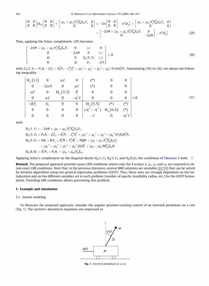
5.1. System modeling

To illustrate the proposed approach, consider the angular position tracking control of an inverted pendulum on a cart(Fig. 1). The system’s dynamical equations are expressed as

m

M( )u t

1( )x t

2l

m

M( )u t

1( )x t

2l

Fig. 1. Inverted pendulum on a car.

B. Mansouri et al. / Information Sciences 179 (2009) 446–457 453

_x1 ¼ x2;

_x2 ¼ ðmþMÞg sinðx1Þ�mlx22 sinðx1Þ cosðx1Þ�cosðx1Þu

l 13mþ4

3Mþm sin2ðx1Þð Þ ;

8<: ð32Þ

where x1(t) and x2(t) are respectively the angular position and velocity of the pendulum, u(t) is the force applied to the cart,m = 0.1 kg and M = 1 kg are respectively the masses of the pendulum and the cart, 2l = 1 m is the length of the pendulum andg = 9.8 m s�2.

Note that msin2(x1(t)) is small regarding to 13 mþ 4

3 M. Then, it will be assumed to be neglected. Therefore, the system (32)becomes

_x1 ¼ x2;

_x2 ¼ ðmþMÞg sinðx1Þ�cosðx1Þul3ð4MþmÞ þ �mlx2

2 sinðx1Þ cosðx1Þl3ð4MþmÞ :

8<: ð33Þ

Using the well-known sector nonlinearity approach [27], the goal is now to derive a T–S model from (33). Indeed, the abovemodel is constituted by three nonlinearities to be splitted: g1(x1(t)) = sin(x1(t)), g2(x1(t)) = cos(x1(t)) and g3ðx2ðtÞÞ ¼ x2

2ðtÞ.Let us consider that the velocity signal x2(t) is not available from measurements. Then, the nonlinear function x2

2ðtÞ is re-moved from the certain part of the T–S model. We assume that this nonlinear function is bounded as g3ðx2ðtÞÞ 2 ½0; �g3�. Then,we write it as an uncertainty and (33) can be written as

_x1 ¼ x2;

_x2 ¼ dðx1;uÞ þ Ddðx; uÞ

�ð34Þ

with dðx1; uÞ ¼ ðmþMÞgg1ðx1Þ�g2ðx1Þul3ð4MþmÞ , Ddðx1; x2;uÞ ¼ �mlg1ðx1Þg2ðx1Þ

l3ð4MþmÞ

�g3f ðx2Þ and f ðx2Þ ¼ g3ðx2Þ�g3

.

The T–S membership functions are obtained following the same procedure as presented in [12]. Let x1 2 [�h0,h0], then thenonlinear functions can be written as follows:

g1ðx1ðtÞÞ ¼ x11ðx1ðtÞÞx1ðtÞ þx2

1ðx1ðtÞÞsinðh0Þ

h0x1ðtÞ;

g2ðx1ðtÞÞ ¼ x12ðx1ðtÞÞ þx2

2ðx1ðtÞÞ cosðh0Þ;

where for i = 1,2 and j = 1,2 we have 0 6 xji 6 1 and

x11ðx1ðtÞÞ ¼

h0 sinðx1ðtÞÞ � x1ðtÞ sinðh0Þx1ðtÞðh0 � sinðh0ÞÞ

;

x21ðx1ðtÞÞ ¼ 1�x1

1ðx1ðtÞÞ ¼h0x1ðtÞ � h0 sinðx1ðtÞÞ

x1ðtÞðh0 � sinðh0ÞÞ; x1

2ðx1ðtÞÞ ¼cosðx1ðtÞÞ � cosðh0Þ

1� cosðh0Þ;

x22ðx1ðtÞÞ ¼ 1�x1

2ðx1ðtÞÞ ¼1� cosðx1ðtÞÞ

1� cosðh0Þ:

A way to reduce the computational complexity of the LMI conditions is to minimize the number of rules used to model thesystem [31]. With the previous nonlinear splitting, the obtained fuzzy model should have 4 rules. Nevertheless, it is still pos-sible to reduce this fuzzy model noticing that x1

1 and x12, respectively x2

1 and x22, are very closed [12]. Thus, for i = 1,2 we

assume that xi ¼ x1i ¼ x2

i and a 2 rules fuzzy model representing the nonlinear uncertain model (34) can be proposed as

_xðtÞ ¼P2i¼1

xiðtÞ½ðAi þ DAiðxðtÞÞÞxðtÞ þ BiuðtÞ�;

yðtÞ ¼ CxðtÞ

8><>: ð35Þ

with xðtÞ ¼ ½ x1ðtÞ x2ðtÞ �T, A1 ¼0 1

ðMþmÞgl3ð4MþmÞ 0

" #, A2 ¼

0 1ðMþmÞgl3ð4MþmÞ

sinðh0Þh0

0

" #, B1 ¼

0� 1

l3ð4MþmÞ

" #, B2 ¼

0� cosðh0Þ

l3ð4MþmÞ

" #, C ¼ ½1 0 �,

DA1ðxðtÞÞ ¼0 0

�mll3ð4MþmÞ

�g3f ðx2ðtÞÞ 0

" #and DA2ðxðtÞÞ ¼

0 0�ml

l3ð4MþmÞ

sinðh0Þ cosðh0Þh0

�g3f ðx2ðtÞÞ 0

" #.

Considering the uncertainties structure used to obtain Theorems 1 and 2, we can write DA1(t) = H1F1(t)Ea1 and

DA2(t) = H2F2(t)Ea2 with H1 ¼0�ml

l3ð4MþmÞ

" #, Ea1 ¼ ½ �g3 0 �, H2 ¼

0�ml

l3ð4MþmÞ

sinðh0Þ cosðh0Þh0

" #, Ea2 ¼ ½ �g3 0 �.

5.2. Simulation results

The simulation was performed with a maximum angular velocity set at 0.1 rad/s2, then �g3 ¼ 0:01. Note that when x1 = ±p/2, the system presents a singularity and so it is locally uncontrollable. To overcome this problem, the modeling space hasbeen reduced to x1(t) 2 [�h0,h0] with h0 = 22p/45.

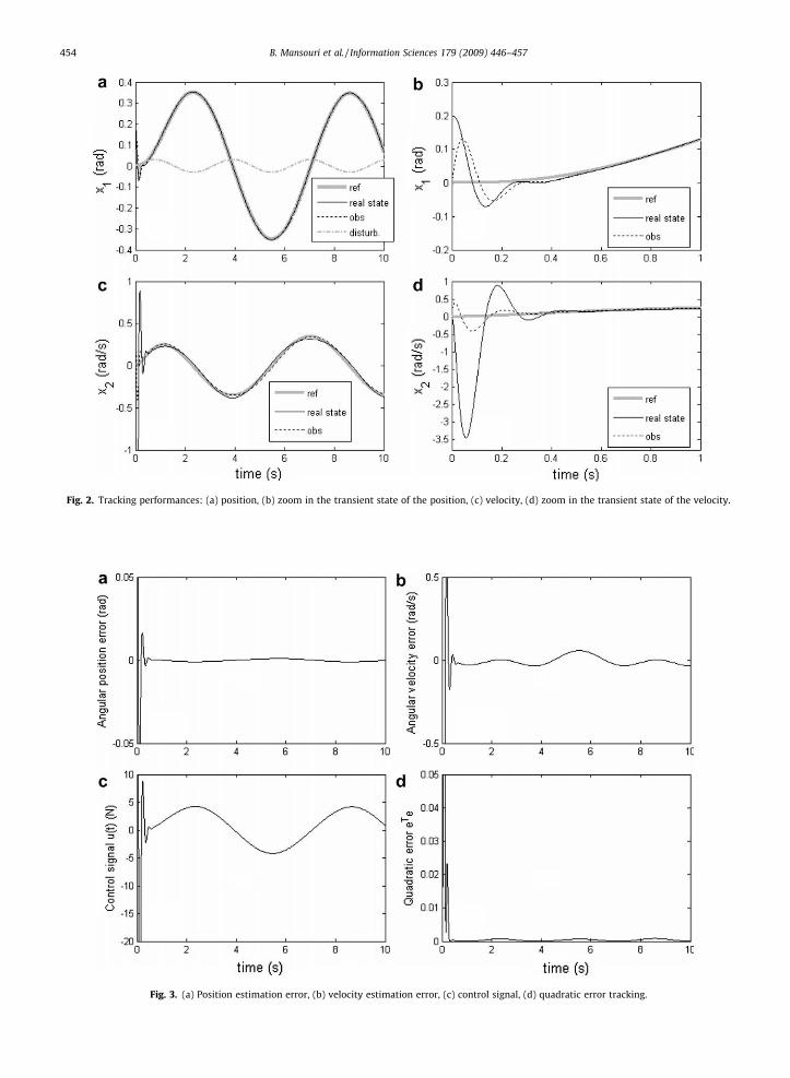
Fig. 2. Tracking performances: (a) position, (b) zoom in the transient state of the position, (c) velocity, (d) zoom in the transient state of the velocity.

Fig. 3. (a) Position estimation error, (b) velocity estimation error, (c) control signal, (d) quadratic error tracking.

454 B. Mansouri et al. / Information Sciences 179 (2009) 446–457

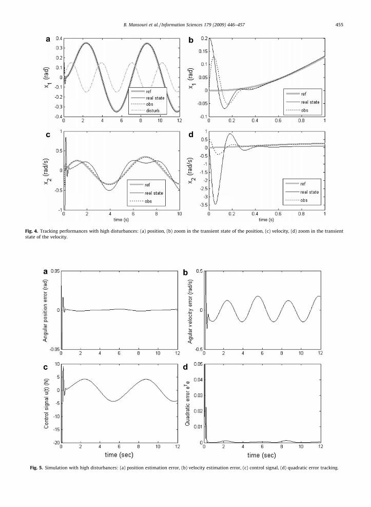
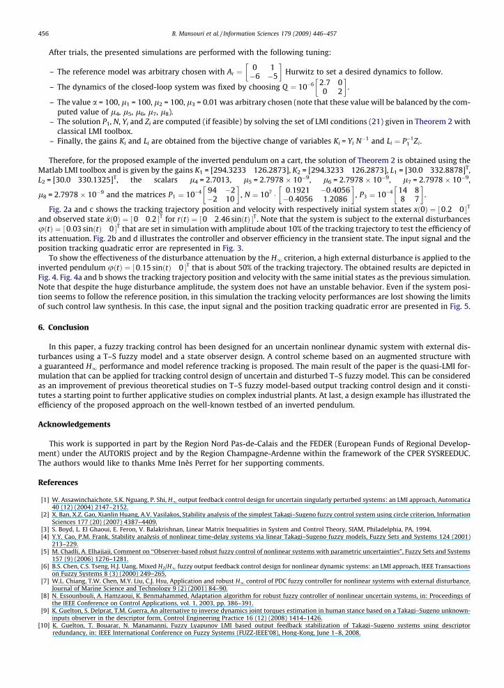
Fig. 5. Simulation with high disturbances: (a) position estimation error, (b) velocity estimation error, (c) control signal, (d) quadratic error tracking.

Fig. 4. Tracking performances with high disturbances: (a) position, (b) zoom in the transient state of the position, (c) velocity, (d) zoom in the transientstate of the velocity.

B. Mansouri et al. / Information Sciences 179 (2009) 446–457 455

456 B. Mansouri et al. / Information Sciences 179 (2009) 446–457

After trials, the presented simulations are performed with the following tuning:

– The reference model was arbitrary chosen with Ar ¼0 1�6 �5

� �Hurwitz to set a desired dynamics to follow.

– The dynamics of the closed-loop system was fixed by choosing Q ¼ 10�6 2:7 00 2

� �.

– The value a = 100, l1 = 100, l2 = 100, l3 = 0.01 was arbitrary chosen (note that these value will be balanced by the com-puted value of l4, l5, l6, l7, l8).

– The solution P1, N, Yi and Zi are computed (if feasible) by solving the set of LMI conditions (21) given in Theorem 2 withclassical LMI toolbox.

– Finally, the gains Ki and Li are obtained from the bijective change of variables Ki = Yi N�1 and Li ¼ P�11 Zi.

Therefore, for the proposed example of the inverted pendulum on a cart, the solution of Theorem 2 is obtained using theMatlab LMI toolbox and is given by the gains K1 = [294.3233 126.2873], K2 = [294.3233 126.2873], L1 = [30.0 332.8878]T,L2 = [30.0 330.1325]T, the scalars l4 = 2.7013, l5 = 2.7978 � 10�9, l6 = 2.7978 � 10�9, l7 = 2.7978 � 10�9,

l8 = 2.7978 � 10�9 and the matrices P1 ¼ 10�4 94 �2�2 10

� �, N ¼ 107 � 0:1921 �0:4056

�0:4056 1:2086

� �, P3 ¼ 10�4 14 8

8 7

� �.

Fig. 2a and c shows the tracking trajectory position and velocity with respectively initial system states xð0Þ ¼ ½0:2 0 �T

and observed state xð0Þ ¼ ½0 0:2 �T for rðtÞ ¼ ½0 2:46 sinðtÞ �T. Note that the system is subject to the external disturbancesuðtÞ ¼ ½0:03 sinðtÞ 0 �T that are set in simulation with amplitude about 10% of the tracking trajectory to test the efficiency ofits attenuation. Fig. 2b and d illustrates the controller and observer efficiency in the transient state. The input signal and theposition tracking quadratic error are represented in Fig. 3.

To show the effectiveness of the disturbance attenuation by the H1 criterion, a high external disturbance is applied to theinverted pendulum uðtÞ ¼ ½0:15 sinðtÞ 0 �T that is about 50% of the tracking trajectory. The obtained results are depicted inFig. 4. Fig. 4a and b shows the tracking trajectory position and velocity with the same initial states as the previous simulation.Note that despite the huge disturbance amplitude, the system does not have an unstable behavior. Even if the system posi-tion seems to follow the reference position, in this simulation the tracking velocity performances are lost showing the limitsof such control law synthesis. In this case, the input signal and the position tracking quadratic error are presented in Fig. 5.

6. Conclusion

In this paper, a fuzzy tracking control has been designed for an uncertain nonlinear dynamic system with external dis-turbances using a T–S fuzzy model and a state observer design. A control scheme based on an augmented structure witha guaranteed H1 performance and model reference tracking is proposed. The main result of the paper is the quasi-LMI for-mulation that can be applied for tracking control design of uncertain and disturbed T–S fuzzy model. This can be consideredas an improvement of previous theoretical studies on T–S fuzzy model-based output tracking control design and it consti-tutes a starting point to further applicative studies on complex industrial plants. At last, a design example has illustrated theefficiency of the proposed approach on the well-known testbed of an inverted pendulum.

Acknowledgements

This work is supported in part by the Region Nord Pas-de-Calais and the FEDER (European Funds of Regional Develop-ment) under the AUTORIS project and by the Region Champagne-Ardenne within the framework of the CPER SYSREEDUC.The authors would like to thanks Mme Inès Perret for her supporting comments.

References

[1] W. Assawinchaichote, S.K. Nguang, P. Shi, H1 output feedback control design for uncertain singularly perturbed systems: an LMI approach, Automatica40 (12) (2004) 2147–2152.

[2] X. Ban, X.Z. Gao, Xianlin Huang, A.V. Vasilakos, Stability analysis of the simplest Takagi–Sugeno fuzzy control system using circle criterion, InformationSciences 177 (20) (2007) 4387–4409.

[3] S. Boyd, L. El Ghaoui, E. Feron, V. Balakrishnan, Linear Matrix Inequalities in System and Control Theory, SIAM, Philadelphia, PA, 1994.[4] Y.Y. Cao, P.M. Frank, Stability analysis of nonlinear time-delay systems via linear Takagi–Sugeno fuzzy models, Fuzzy Sets and Systems 124 (2001)

213–229.[5] M. Chadli, A. Elhajjaji, Comment on ‘‘Observer-based robust fuzzy control of nonlinear systems with parametric uncertainties”, Fuzzy Sets and Systems

157 (9) (2006) 1276–1281.[6] B.S. Chen, C.S. Tseng, H.J. Uang, Mixed H2/H1 fuzzy output feedback control design for nonlinear dynamic systems: an LMI approach, IEEE Transactions

on Fuzzy Systems 8 (3) (2000) 249–265.[7] W.L. Chiang, T.W. Chen, M.Y. Liu, C.J. Hsu, Application and robust H1 control of PDC fuzzy controller for nonlinear systems with external disturbance,

Journal of Marine Science and Technology 9 (2) (2001) 84–90.[8] N. Essounbouli, A. Hamzaoui, K. Benmahammed, Adaptation algorithm for robust fuzzy controller of nonlinear uncertain systems, in: Proceedings of

the IEEE Conference on Control Applications, vol. 1, 2003, pp. 386–391.[9] K. Guelton, S. Delprat, T.M. Guerra, An alternative to inverse dynamics joint torques estimation in human stance based on a Takagi–Sugeno unknown-

inputs observer in the descriptor form, Control Engineering Practice 16 (12) (2008) 1414–1426.[10] K. Guelton, T. Bouarar, N. Manamanni, Fuzzy Lyapunov LMI based output feedback stabilization of Takagi–Sugeno systems using descriptor

redundancy, in: IEEE International Conference on Fuzzy Systems (FUZZ-IEEE’08), Hong-Kong, June 1–8, 2008.

B. Mansouri et al. / Information Sciences 179 (2009) 446–457 457

[11] T.M. Guerra, A. Kruszewski, L. Vermeiren, H. Tirmant, Conditions of output stabilization for nonlinear models in the Takagi–Sugeno’s form, Fuzzy Setsand Systems 157 (2006) 1248–1259.

[12] T.M. Guerra, L. Vermeiren, Stabilité et stabilisation à partir de modèles flous, in: L. Foulloy, S. Galichet, A.Titli (Eds.), Commande Floue 1: de lastabilisation à la supervision, Traités IC2, Hermes Lavoisier, Paris, 2001, pp. 59–98.

[13] N. Golea, A. Golea, K. Benmahammed, Fuzzy model reference adaptive control, IEEE Transactions on Fuzzy Systems 10 (4) (2002) 436–444.[14] S.K. Hong, R. Langari, An LMI-based H1 fuzzy control system design with TS framework, Information Sciences 123 (2000) 163–179.[15] D. Huang, S.K. Nguang, Robust H-infinity static output feedback control of fuzzy systems: an ILMI approach, IEEE Transactions on Systems, Man and

Cybernetics – Part B 36 (1) (2006) 216–222.[16] D. Huang, S.K. Nguang, Static output feedback controller design for fuzzy systems: an ILMI approach, Information Sciences 177 (14) (2007) 3005–3015.[17] W.C. Kim, S.C. Ahn, W.H. Kwon, Stability analysis and stabilisation of fuzzy state space models, Fuzzy Sets and Systems 71 (1995) 131–142.[18] H.K. Lam, H. Frank, F. Leung, K. Peter, S. Tam, A switching controller for uncertain nonlinear systems, IEEE Control Systems Magazine (2003) 7–14.[19] K.R. Lee, E.T. Jeung, H.B. Park, Robust fuzzy H1 control for uncertain nonlinear systems via state feedback: an LMI approach, Fuzzy Sets and Systems

120 (2001) 123–134.[20] Y.S. Liu, C.H. Fang, A new LMI-Based approach to relaxed quadratic stabilization of TS fuzzy control systems, in: Proceedings of the IEEE International

Conference on Systems Man and Cybernetics, 2003, pp. 2255–2260.[21] X.J. Ma, Z.Q. Sun, Y.Y. He, Analysis and design of fuzzy controller and fuzzy observer, IEEE Transactions on Fuzzy Systems 6 (1) (1998) 41–50.[22] N. Manamanni, B. Mansouri, A. Hamzaoui, J. Zaytoon, Relaxed conditions in tracking control design for T–S fuzzy model, JIFS – Journal of Intelligent and

Fuzzy Systems 18 (2) (2007) 185–210.[23] S.K. Nguang, P. Shi, Robust H-infinity output feedback control design for fuzzy dynamic systems with quadratic D stability constraints: an LMI

approach, Information Sciences 176 (2006) 2161–2191.[24] C.-W. Park, LMI-based robust stability analysis for fuzzy feedback linearization regulators with its applications, Information Sciences 152 (2003) 287–

301.[25] A. Sala, T.M. Guerra, R. Babuška, Perspectives of fuzzy systems and control, Fuzzy Sets and Systems 156 (3) (2005) 432–444.[26] T. Takagi, M. Sugeno, Fuzzy identification of systems and its application to modelling and control, IEEE Transactions on Systems, Man and Cybernetics

1115 (1985) 116–132.[27] K. Tanaka, H.O. Wang, Fuzzy Control System Design and Analysis, A Linear Matrix Inequality Approach, Wiley, New York, 2001.[28] K. Tanaka, T. Ikeda, H.O. Wang, Robust stabilization of a class of uncertain nonlinear systems via fuzzy control: quadratic stabilizability, H1 control

theory, and linear matrix inequalities, IEEE Transactions on Fuzzy Systems 4 (1) (1996).[29] K. Tanaka, T. Ikeda, H.O. Wang, Fuzzy regulators and fuzzy observers: relaxed stability conditions and LMI-based designs, IEEE Transactions on Fuzzy

Systems 6 (2) (1998).[30] T. Taniguchi, K. Tanaka, K. Yamafuji, H.O. Wang, A new PDC Fuzzy reference models, in: Proceedings of the IEEE International Fuzzy Systems

Conference, Seoul, Korea, 1999.[31] T. Taniguchi, K. Tanaka, H.O. Wang, Model construction rule reduction and robust compensation for generalized form of Takagi–Sugeno fuzzy systems,

IEEE Transactions on Fuzzy Systems 9 (4) (2001) 525–537.[32] S. Tong, T. Wang, H.X. Li, Fuzzy robust tracking control for uncertain nonlinear systems, International Journal of Approximate Reasoning 30 (2002) 73–

90.[33] C. Tseng, B. Chen, H1 decentralized fuzzy model reference tracking control design for nonlinear interconnected systems, IEEE Transactions on Fuzzy

Systems 9 (6) (2001) 795–809.[34] C. Tseng, B. Chen, H.J. Uang, Fuzzy tracking control design for nonlinear dynamic systems via TS fuzzy model, IEEE Transactions on Fuzzy Systems 9 (3)

(2001) 381–392.[35] H.D. Tuan, P. Apkarian, T. Narikiyo, Y. Yamamoto, Parameterized linear matrix inequality techniques in fuzzy control system design, IEEE Transactions

on Fuzzy Systems 9 (2) (2001) 324–332.[36] H.O. Wang, K. Tanaka, M. Griffin, An approach to fuzzy control of nonlinear systems: stability and design issues, IEEE Transactions on Fuzzy Systems 4

(1996) 14–23.[37] S. Xu, J. Lam, Robust H-infinity control for uncertain discrete-time-delay fuzzy systems via output feedback controllers, IEEE Transactions on Fuzzy

Systems 13 (1) (2005) 82–93.[38] J. Yoneyama, M. Nishikawa, H. Katayama, A. Ichikawa, Output stabilization of Takagi–Sugeno fuzzy systems, Fuzzy Sets and Systems 111 (2000) 253–

266.[39] M. Zerar, K. Guelton, N. Manamanni, Linear fractional transformation based H-infinity output stabilization for Takagi-Sugeno fuzzy models,

Mediterranean Journal of Measurement and Control 4 (3) (2008) 111–121.[40] F. Zheng, Q.G. Wang, T.H. Lee, Output tracking control of MIMO fuzzy nonlinear systems using variable structure control approach, IEEE Transactions

on Fuzzy Systems 10 (6) (2002).[41] K. Zhou, P.P. Khargonekar, Robust stabilization of linear systems with norm-bounded time-varying uncertainty, Systems Control Letters 10 (1988) 17–

20.