optimization of furnace residence time and ingots

Optimization of Furnace Residence Time and Ingots Positioning during the Heat Treatment Process of Large Size

Forged Ingots

by

Nima BOHLOOLI ARKHAZLOO

MANUSCRIPT-BASED THESIS PRESENTED TO ÉCOLE DE TECHNOLOGIE SUPÉRIEURE IN PARTIAL FULFILLMENT

FOR THE DEGREE OF DOCTOR OF PHILOSOPHY Ph.D.

MONTREAL, JANUARY 28TH 2020

ÉCOLE DE TECHNOLOGIE SUPÉRIEURE UNIVERSITÉ DU QUÉBEC

Nima Bohlooli Arkhazloo, 2020

This Creative Commons licence allows readers to download this work and share it with others as long as the

author is credited. The content of this work can’t be modified in any way or used commercially.

BOARD OF EXAMINERS

THIS THESIS HAS BEEN EVALUATED

BY THE FOLLOWING BOARD OF EXAMINERS Prof. Mohammad Jahazi, Thesis Supervisor Department of Mechanical Engineering at École de technologie supérieure Prof. Farzad Bazdidi-Tehrani, Thesis Co-supervisor School of Mechanical Engineering at Iran university of science and technology Prof. Vahé Nerguizian, President of the Board of Examiners Department of Electrical engineering at École de technologie supérieure Prof. Henri Champliaud, Member of the jury Department of Mechanical Engineering at École de technologie supérieure Prof. Louis Gosselin, External Evaluator Department of Mechanical Engineering at Université Laval

THIS THESIS WAS PRENSENTED AND DEFENDED

IN THE PRESENCE OF A BOARD OF EXAMINERS AND PUBLIC

JANUARY 22 ND 2020

AT ÉCOLE DE TECHNOLOGIE SUPÉRIEUR

ACKNOWLEDGEMENT

I would like to convey my earnest gratitude to my supervisor, Prof. Mohammad Jahazi,

whose support, guidance, expertise and patience added considerably to my research

experience and without him none of this would have been possible to achieve. I am thankful

to him for believing in my accomplishments and providing me with every opportunity to

assimilate. I would also wish to thank Prof. Farzad Bazdidi-Tehrani (my co-supervisor) for

his kind support, guidance and conveying numerical simulation expertise during my Ph.D.

program. He has helped me at all times during my presence in Iran University of Science and

Technology (IUST) and after that. I also extend my earnest gratitude to Dr. Mohammad

Jadidi, a post-doctoral researcher at IUST, for the fruitful discussions I held with him. He

enthusiastically helped me throughout my term with respect to CFD simulation and

numerical approaches.

Particular thanks are given to our Industrial partner, Finkl Steel, especially the R & D,

Metallurgy and Engineering Departments, for providing real-scale instrumentation and

measurements and their collaboration in this project.

Gratitude is also expressed for all CM2P members for their cooperation during the entire

journey of my Ph.D.

My utmost gratitude is given to my parents for their outstanding support, kindness, love and

constant motivation throughout this journey.

Optimisation du temps de résidence dans le four ainsi que le positionnement de lingots forgés de grande taille lors du processus de traitement thermique


RÉSUMÉ

Les pièces forgées de grande taille sont communément utilisées dans les industries de l’énergie et du transport (arbres de turbines, trains d’atterrissage, etc.). Ces pièces acquièrent leurs propriétés mécaniques supérieures (par exemple, la dureté) grâce à un processus de traitement thermique appelé trempe et revenu. Le processus de revenu (incluant le chauffage et le maintien en chauffe) a lieu dans des fours à gaz et a un impact direct sur les propriétés finales du produit en raison des modifications microstructurales majeures induites par l’effet de la température. Une fois que les paramètres de revenu sont contrôlés (temps et température) les propriétés des matériaux peuvent être généralement optimisées. Distribution non uniforme de la température autour des pièces qui résulte des interactions thermiques à l'intérieur du four ou du positionnement des brames, peut causer une variation dans les propriétés mécaniques d'une extrémité à l'autre de la pièce, une modification de la microstructure ou même initier des fissurations. Par contre, une optimisation du temps de séjour dans le four de traitement thermique peut réduire la consommation d’énergie et éviter les changements microstructuraux indésirables. Cependant, la production industrielle repose principalement sur des corrélations empiriques qui ne sont pas toujours fiables. La prédiction précise de la température en fonction du temps des pièces forgées de grande taille dans les fours de traitement thermique à gaz nécessite un examen quantitatif exhaustif de l'échauffement par la compréhension des interactions thermiques conjuguées complexes à l'intérieur du four. Les limites des études analytiques et la complexité et le coût des expérimentations ont rendu les simulations numériques une solution efficace pour analyser les problèmes de la dynamique des fluides (CFD) dans ce domaine d'étude. Cependant, parmi les études publiées sur les fours à gaz, les fours à petite échelle ou ceux avec un temps de fonctionnement plus court ont été principalement considérés (en utilisant différentes simplifications comme les calculs à l'état stationnaire) et ce principalement en raison de la complexité des phénomènes et des temps de calcul élevés. Par la suite, très peu d’études ont été consacrées à l’amélioration des modèles de chargement des pièces de grande taille dans les fours à gaz et à l’optimisation de leur temps de résidence. De plus, peu d’information est disponible dans la littérature sur les limites et particularités des différentes approches numériques permettant de calculer les interactions thermiques dans le flux réactif turbulent des fours de grande taille chauffés au gaz. À cet égard, l'objectif principal de ce projet est de fournir une analyse quantitative complète de la période transitoire du chauffage et une compréhension des interactions thermiques à l'intérieur du four afin d'optimiser, le temps de

VIII

séjour et l'uniformité de la température pendant le traitement thermique. Pour atteindre cet objectif, les étapes ci-après ont été suivies:

La première partie de cette étude, fournit une analyse transitoire complète des caractéristiques de chauffage des pièces forgées de grande taille dans un four à gaz, en utilisant des températures mesurées expérimentalement et des simulations CFD. Un modèle CFD 3D du four à gaz a été généré, incluant, la chambre de traitement thermique, et les brûleurs à gaz. Les interactions entre la chaleur et l’écoulement du fluide, incluant la turbulence, la radiation et la combustion, ont été simultanément considérées dans le modèle en utilisant respectivement les modèles DO et EDM. En outre, l'applicabilité du modèle de radiation S2S a été évaluée pour quantifier l'effet du produit de combustion dans le four et le facteur de forme dû à la radiation durant le transfert de chaleur. Des mesures de températures ont été réalisées à plusieurs endroits grâce à l’instrumentation d’un bloc forgé de grande taille et l'intérieur du four, pour l'analyse expérimentale du processus de chauffage et aussi pour la validation du modèle CFD. Un bon accord a été obtenu avec une erreur maximale d’environ 7% entre les prédictions numériques et les mesures expérimentales. Les résultats ont montré qu'en dépit de l'uniformité de la température du four sans chargement, chaque surface du bloc présentait des vitesses de chauffage différentes après le chargement (chargement simple) ; des différences de température allant jusqu’à 200 k. L’analyse des résultats a également révélée la fiabilité du modèle S2S et a mis en évidence l’importance du facteur de forme du rayonnement pour des besoins d’optimisation pour cette application. Les résultats ont été corrélés avec la géométrie du four, la formation de structures tourbillonnaires et les circulations du fluide autour de la pièce. Les données expérimentales et les prévisions du modèle CFD pourraient être directement utilisées pour l’optimisation du processus de traitement thermique forgées de grande taille.

La deuxième partie de cette étude vise à déterminer l’effet de la configuration du chargement (configuration des chargements multiples) sur la distribution de la température des pièces forgées lors du traitement thermique, afin d’obtenir une meilleure uniformité de température; qui par la suite favorise l’obtention de propriétés mécaniques homogènes. Cette partie vise également l’optimisation du temps de séjour des lingots forgés de grande taille dans un four de revenu, proposant une nouvelle méthodologie hybride combinant des simulations numériques CFD et une série de mesures expérimentales à base d’un dilatomètre à haute résolution. Des simulations transitoires CFD 3D validées par des mesures expérimentales de températures ont été utilisées pour évaluer l’impact des modèles de chargement et du calage (positionnement des cales) sur l’uniformité de la température et le temps de résidence des pièces forgées dans le four. Une analyse transitoire complète des caractéristiques de chauffage des pièces forgées (y compris une analyse des modes de transfert de chaleur) en utilisant quatre configurations de chargement différents a permis de quantifier l’impact des

IX

calages et leurs dimensions sur l’uniformité de la répartition de la température ainsi que sur le temps de séjour des produits. Les résultats ont montré que la non-uniformité de température peut aller jusqu'à 331 K pour un modèle de chargement conventionnel (non optimisé). L'influence positive de l'utilisation des cales et des espaceurs (cales entre les brames) a été approuvée et quantifiée à l'aide de l'approche développée. Il a été possible de réduire les non-uniformités identifiées jusqu'à 32% en modifiant la configuration du chargement à l'intérieur du four de traitement thermique. Cette approche hybride a permis de déterminer le temps de séjour optimal pour les lingots, et aussi permettre son amélioration jusqu’à peu près de 15,5% par rapport à la configuration classique (non optimisée). Cette approche a été validée et pourrait s’appliquer directement à l’optimisation de différents cycles de traitement thermique de pièces forgées de grande taille.

Enfin, la troisième partie de l'étude aborde les détails de la simulation numérique du procédé de traitement thermique de pièces forgées de grande taille dans des fours à gaz à échelle réelle. Plus précisément, l'évaluation du modèle de combustion non-premix avec l'équilibre chimique pour prévision précise de la température des pièces forgées, ainsi que les performances de six modèles de turbulence différents de RANS pour les projections d'analyse thermique sont discutés. À cet égard, les interactions thermiques à différents endroits du bloc forgé et dans des régions critiques telles que la région du brûleur, la stagnation et la région de sillage ont été réalisées à l'aide d'un modèle 3D périodique du four puis validé par des mesures expérimentales. Les résultats ont montré que le modèle périodique avec combustion non-premix est fiable pour l'analyse thermique du processus de traitement thermique avec un écart maximal d'environ 3% par rapport aux mesures expérimentales. Il a également été révélé que le choix du modèle de turbulence avait un effet significatif sur la prévision de la combustion et du transfert de chaleur autour du bloc. La prédiction du rapport ɛ/𝑘 par différents modèles de turbulence a montré une relation significative avec la combustion turbulente (telle que la longueur de la flamme du brûleur) et les prévisions de température du bloc, autour de la région de stagnation. Les modèles 𝑘 − ɛ Standard et réalisable en raison d'une prévision irréaliste de l'énergie cinétique de turbulence (sous-prévision du rapport ɛ/𝑘) ont entraîné une longueur de flamme plus courte et une sous-prévision de la température du bloc forgé autour de la région de stagnation. En suite, le modèle SST 𝑘 − 𝜔 a montré des prévisions raisonnables dans cette région. Le modèle RSM s'est révélé être le modèle de turbulence le plus fiable par rapport aux mesures expérimentales. De plus, un modèle 𝑘 − ɛ réalisable, mis à part une sous-prédiction sur la région de stagnation et la longueur de la flamme, pourrait efficacement prédire la température globale des pièces forgées lourdes avec une précision comparable à celle des données expérimentales et des prévisions du RSM.

Mots-clés: Traitement thermique, simulation CFD, four à gaz, mesures de température,

uniformité de la température, modélisation du rayonnement, configuration du chargement,

X

temps de résidence, mesures expérimentales, approche hybride, modélisation de la

turbulence, modélisation de la combustion,

Optimization of furnace residence time and ingots positioning during the heat treatment process of large size forged ingots


ABSTRACT

High-strength large size forgings which are widely used in the energy and transportation industries (e.g., turbine shaft, landing gears etc.) acquire significant mechanical properties (e.g., hardness) through a sequence of heat treatment processes, called Quench and Temper (Q&T). The heating process (tempering) that takes place inside gas-fired furnaces has a direct impact on the final properties of the product due to several major microstructural changes taking place at this step. Therefore, material properties are usually optimized by controlling the tempering process parameters such as time and temperature. A non-uniform temperature distribution around parts, as a result of thermal interactions inside the furnace or loading pattern, may result in the parts property variations from one end to another, changes in microstructure or even cracking. On the other hand, improvement of large products residence time inside the heat treatment furnace can minimize energy consumption and avoid undesirable microstructural changes. However, at the present time, the industrial production is mainly based on available empirical correlations which are costly and not always reliable. Accurate time-dependent temperature prediction of the large size forgings within gas-fired heat treatment furnaces requires a comprehensive quantitative examination of the heating process and an in-depth understanding of complex conjugate thermal interactions inside the furnace. Limitations in analytical studies and complexity and cost of experimentations have made numerical simulations such as computational fluid dynamics (CFD), effective methods in this field of study. However, among the rarely found studies on gas-fired furnaces, small-scale furnaces or those with shorter operation times were mainly considered (using different simplifications like steady-state calculations) because of complexity of the phenomena and large calculation times. Subsequently, there are very few studies on the improvement of the loading patterns of large-size steel parts inside the gas-fired furnaces and their relevant residence time optimization. Moreover, the limitation and strength of different numerical approaches to calculate thermal interactions in the turbulent reactive flow of the large size gas-fired batch type furnaces were addressed by few researchers in the literature. In this regard, the main objective of the present thesis is to provide a comprehensive quantitative analysis of transient heating and an understanding of thermal interactions inside the furnace so as to optimize the residence time and temperature uniformity of large size products during the heat treatment process. To attain this objective, the following milestones are pursued. The first part of this study provides a comprehensive unsteady analysis of large size forgings heating characteristics in a gas-fired heat treatment furnace employing experimentally measured temperatures and CFD simulations. A three-dimensional CFD model of the gas-fired furnace, including heat treating chamber and high momentum natural gas burners, was generated. The interactions between heat and fluid flow consisting of turbulence, combustion and radiation were simultaneously considered using the -k ε , EDM and DO models,

XII

respectively. The applicability of S2S radiation model to quantify the effect of participating medium and radiation view factor in the radiation heat transfer was also assessed. Temperature measurements at several locations of an instrumented large size forged block and within the heating chamber of the furnace were performed for experimental analysis of the heating process and validation of the CFD model. Good agreement with a maximum deviation of about 7% was obtained between the numerical predictions and the experimental measurements. The results showed that despite the temperature uniformity of the unloaded furnace, each surface of the product experienced different heating rates after loading (single loading) resulting in temperature differences of up to 200 K. Analysis of the results also revealed the reliability of the S2S model and highlighted the importance of radiation view factor for the optimization purposes in this application. Findings were correlated with the geometry of the furnace, formation of vortical structures and fluid flow circulations around the workpiece. The experimental data and CFD model predictions could directly be employed for optimization of the heat treatment process of large size steel components. The second part of this study aims to determine the effect of loading pattern (in the multiple loading configurations) on the temperature distribution of large size forgings during the heat treatment process within a gas-fired furnace to attain more temperature uniformity and consequently homogenous mechanical properties. This part also focuses on the improvement of residence time of large size forged ingots within a tempering furnace proposing a novel hybrid methodology combining CFD numerical simulations and a series of experimental measurements with high-resolution dilatometer. Transient 3D CFD simulations validated by experimental temperature measurements were employed to assess the impact of loading patterns and skids on the temperature uniformity and residence time of heavy forgings within the furnace. Comprehensive transient analysis of forgings heating characteristics (including heat transfer modes analysis) at four different loading patterns allowed quantifying the impact of skids and their dimensions on the temperature distribution uniformity as well as products residence time. Results showed that temperature non-uniformities of up to 331 K persist for non-optimum conventional loading pattern. The positive influence of skids and spacers applications was approved and quantified using the developed approach. It was possible to reduce the identified non-uniformities of up to 32 % through changing the loading pattern inside the heat treatment furnace. This hybrid approach allowed to determine an optimum residence time of large size slabs improving by almost 15.5 % in comparison with the conventional non-optimized configuration. This approach was validated and it could be directly applied to the optimization of different heat treatment cycles of large size forgings.

The third part of the study addresses the details of the numerical simulation of heat treatment process of large size forgings within real scale gas-fired furnaces. Specifically, assessment of chemical equilibrium non-premix combustion model for accurate temperature prediction of heavy forgings, as well as performance of six different RANS based turbulence models for predictions of turbulent phenomenon were discussed in this context. In this regard, thermal interactions at different locations of the forged block as well as critical regions such as burner area, stagnation and wake region were performed using a one-third periodic 3D model of the furnace and validated by experimental measurements. Results showed that the one-third periodic model with chemical equilibrium non-premix combustion is reliable for the thermal

XIII

analysis of the heat treatment process with a maximum deviation of about 3% with respect to the experimental measurements. It was also revealed that the choice of the turbulence model has a significant effect on the prediction of combustion and heat transfer around the block. Prediction of ɛ/k ratio by different turbulence models showed a significant relation to the turbulent combustion (such as burner flame length) and block temperature predictions, around the stagnation region. Standard and realizable 𝑘 − ɛ models, due to an unrealistic over prediction of turbulence kinetic energy (under-prediction of ɛ/k ratio), resulted in shorter flame length and under-prediction on the temperature of the forged block around the stagnation region; While, SST 𝑘 − 𝜔 model showed reasonable predictions in this region. RSM model was found as the most reliable turbulence model compared to the experimental measurements. Meanwhile, realizable 𝑘 − ɛ model apart from some under-prediction on the stagnation region and flame length could effectively predict the overall temperature of the heavy forgings with reasonable accuracy with respect to the experimental data and RSM predictions.

Keywords: Heat treatment, CFD simulation, Gas-fired furnace, Temperature measurements, Temperature uniformity, Radiation modeling, Loading pattern, Residence time, Experimental measurements, Hybrid approach, Turbulence modeling, Combustion modeling

TABLE OF CONTENTS

INTRODUCTION .....................................................................................................................1

CHAPTER 1 LITERATURE REVIEW ............................................................................7 1.1 Steel Heat Treatment......................................................................................................7 1.2 Tempering Process .........................................................................................................7 1.3 Heat Treatment Furnaces ...............................................................................................8 1.4 Tempering of Large Size Parts ......................................................................................9 1.5 Thermal Interactions inside a Gas-Fired Furnace ........................................................10

1.5.1 Conduction ................................................................................................ 11 1.5.2 Convection ................................................................................................ 12 1.5.3 Radiation ................................................................................................... 13 1.5.4 Combustion ............................................................................................... 13 1.5.5 Turbulence ................................................................................................ 14

1.6 Thermal Interactions Analyses inside Heat Treatment Furnaces ................................15 1.6.1 Analytical and Semi-Analytical Studies ................................................... 15 1.6.2 CFD Studies .............................................................................................. 16 1.6.3 CFD Analysis of Heat Treatment Furnaces without Combustion ............ 18 1.6.4 Gas-Fired Furnaces ................................................................................... 24

1.7 Challenges and Objectives ...........................................................................................30

CHAPTER 2 NUMERICAL DETAILS FOR THERMAL ANALYSIS OF HEAT TREATMENT PROCESS IN GAS-FIRED FURNACE ..........................33

2.1 Introduction ..................................................................................................................33 2.2 Computational Fluid Dynamics (CFD) ........................................................................33 2.3 Navier-Stokes Equations ..............................................................................................34 2.4 Species Transport .........................................................................................................36

2.4.1 The Eddy-Dissipation Model .................................................................... 37 2.4.2 Non-premixed Combustion ....................................................................... 38

2.5 Radiation ......................................................................................................................39 2.5.1 P-1 Radiation Model ................................................................................. 40 2.5.2 Discrete Ordinates Radiation Model (DO) ............................................... 41 2.5.3 Surface to Surface (S2S) Model ............................................................... 41

2.6 Turbulence ...................................................................................................................42 2.6.1 Reynolds Averaged Navier-Stokes (RANS) ............................................. 42 2.6.2 Two-Equation Turbulence models ............................................................ 44 2.6.3 Comparison between Turbulence Modeling Approaches ......................... 47

CHAPTER 3 EXPERIMENTAL MATERIALS AND METHODS ...............................51 3.1 Introduction ..................................................................................................................51 3.2 Furnace Description .....................................................................................................51 3.3 Temperature Measurements .........................................................................................53

XVI

3.4 Flow Measurements .....................................................................................................59 3.5 Calibration Test ............................................................................................................59

3.5.1 Block Measurements and Conductivity Calibration ................................. 61 3.5.2 Furnace Refractories Heat loss Calibration .............................................. 63

3.6 Laboratory Measurements ...........................................................................................65 3.7 Project Approach .........................................................................................................65

CHAPTER 4 EXPERIMENTAL AND UNSTEADY CFD ANALYSES OF THE HEATING PROCESS OF LARGE SIZE FORGINGS IN A GAS FIRED FURNACE ...........................................................................69

4.1 Introduction ..................................................................................................................72 4.2 Experimental procedures .............................................................................................74 4.3 Computational Details .................................................................................................76

4.3.1 Flow simulation ........................................................................................ 76 4.3.2 Radiation modeling ................................................................................... 77 4.3.3 Combustion modeling ............................................................................... 77 4.3.4 Numerical simulation procedure and boundary conditions ...................... 78

4.4 Results and Discussion ................................................................................................79 4.4.1 Experimental Analysis .............................................................................. 79 4.4.2 CFD Analysis ............................................................................................ 82

4.5 Conclusions ..................................................................................................................91

CHAPTER 5 THERMAL ANALYSIS OF FURNACE RESIDENCE TIME AND LOADING PATTERN DURING HEAT TREATMENT OF LARGE SIZE FORGINGS ........................................................................93

5.1 Introduction ..................................................................................................................96 5.2 Loading Patterns ........................................................................................................100 5.3 Methodology ..............................................................................................................102

5.3.1 Computational Details ............................................................................ 102 5.3.2 Forgings Temperature Measurements ..................................................... 104 5.3.3 Hybrid Approach .................................................................................... 104

5.4 Results and Discussion ..............................................................................................106 5.4.1 Validation ................................................................................................ 106 5.4.2 Loading Pattern Analysis ........................................................................ 107 5.4.3 Residence time improvement of forgings during isothermal

tempering process ................................................................................... 115 5.5 Conclusions ................................................................................................................116

CHAPTER 6 CFD SIMULATION OF A GAS-FIRED HEAT TREATMENT FURNACE: ASSESSMENT OF EQUILIBRIUM NON-PREMIX COMBUSTION AND DIFFERENT TURBULENCE MODELS ..........119

6.1 Introduction ................................................................................................................123 6.2 Furnace Description ...................................................................................................126 6.3 Numerical Details ......................................................................................................127

6.3.1 Flow and Energy modeling ..................................................................... 127 6.3.2 Combustion and radiation modeling ....................................................... 129

XVII

6.3.3 Simulation procedure .............................................................................. 130 6.4 Experimental measurements ......................................................................................132 6.5 Results and Discussion ..............................................................................................134

6.5.1 Validation of periodic CFD model and combustion approach ............... 134 6.5.2 Assessment of turbulence models ........................................................... 135

6.6 Conclusions ................................................................................................................148

CONCLUSION ..................................................................................................................151

RECOMMENDATIONS .......................................................................................................155

LIST OF REFERENCES .......................................................................................................157

LIST OF TABLES

Page Table 1.1 Temperature validation reported by J. Govardhan et al.

(Govardhan et al., 2011) ............................................................................28

Table 2.1 The values of the 𝑘 − ɛ model constants (ANSYS, 2016). .......................45

Table 3.1 Thermal conductivity of the gas-fired furnace refractories (Morgan thermal ceramics, 2015). .............................................................63

Table 4.1 Chemical analysis of the test forged ingot used for thermo-physical properties calculation % weight (Finkl Steel Inc.) ..........79

Table 4.2 Predicted heat distribution within the furnace. ..........................................82

Table 5.1 Chemical analysis of the investigated steel - Wt. % (Finkl Steel Inc.). .....................................................................................105

Table 5.2 Total temperature non-uniformity reduction of forgings for different loading patterns in comparison with conventional SK loading. .........................................................................109

Table 5.3 Residence time reduction of forgings at different loading patterns in comparison with conventional SK loading pattern. .............................114

Table 6.1 Chemical Analysis of the test Ingot - Weight % (Finkl Steel Inc). .........132

LIST OF FIGURES

Page

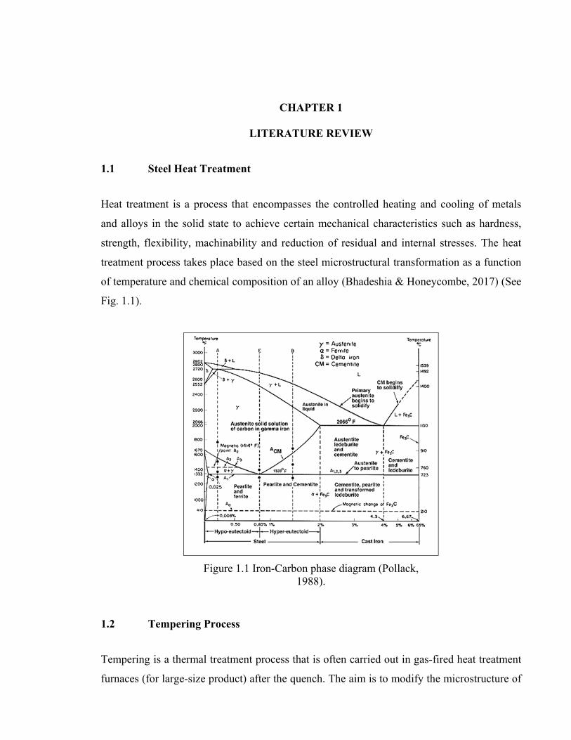
Figure 1.1 Iron-Carbon phase diagram (Pollack, 1988). ...............................................7

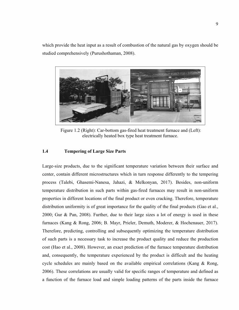
Figure 1.2 (Right): Car-bottom gas-fired heat treatment furnace and (Left): electrically heated box type heat treatment furnace. ....................................9

Figure 1.3 Thermal interactions and conjugate heat transfer within a gas-fired heat treatment furnace. ................................................................11

Figure. 1.4 Temperature dependant thermal conductivity of a steel slab (Tang et al., 2017). .....................................................................................12

Figure 1.5 Turbulent combustion visualized by numerical simulation (Vicquelin, 2010). ......................................................................................15

Figure 1.6 Prediction of heating and cooling rates with different convection heat transfer coefficients (Gao et al., 2000). ..............................................16

Figure 1.7 Right) pressure and left) temperature distribution prediction by CFD in the submerged arc furnace (Yang et al., 2006). ............................17

Figure 1.8 Temperature distribution prediction of H13 die using CFD simulation (Elkatatny et al., 2003). ............................................................18

Figure 1.9 Right) temperature contour of air quenched rail head and left) flow field of quenching medium (Gongfa et al., 2014). .....................19

Figure 1.10 Streamwise velocity contours of a gas quenching chamber loaded by plates and rectangular ingots (Macchion et al., 2004). .........................20

Figure 1.11 Left) velocity distribution and right) temperature in the gas quenching chamber (Z. J. Wang & Shang, 2010). .....................................21

Figure 1.12 Contours of temperature evolution in the a) electricaly heated furnace and b) heat treated block (Hao et al., 2008). .................................22

Figure 1.13 Optimization of furnace resicence time based on a) heating curves and b) temperature difference curves inside electretically heated furnace (Hao et al., 2008). ..............................................................23

Figure 1.14 Comparison of two different products loading patteren effects on the heat treatment process inside an electercally heated furnace (Kang & Rong, 2006). ...............................................................................24

XXII

Figure 1.15 Volume average temperature of a billet and its averaged heat flux over the length of furnace (B. Mayr, Prieler, Demuth, Moderer, et al., 2017). ...................................26

Figure 1.16 Temperature evolution of: a) the heat treating furnace and, b) the dredging impeller (Yang et al., 2007). .............................................27

Figure 1.17 Schematic sketch of circular furnace employed by Govardhan et al. (Govardhan et al., 2011). ...........................................................................28

Figure 1.18 The lab-scale gas-fired furnace studied by Mayr et al. (Mayr et al., 2015). ....................................................................................29

Figure 1.19 Semi industrial gas-fired furnace and its relative measurement points used in Mayr et al. numerical study (Mayr, Prieler, Demuth, Potesser, & Hochenauer, 2017). .........................29

Figure 1.20 Comparison between CFD results and experimental measurements in a semi-industrial size gas-fired furnace (Mayr, Prieler, Demuth, Potesser, et al., 2017)..........................................30

Figure 2.1 Comparison of computational cost per iteration for different available RANS models (ANSYS, 2016). .................................................48

Figure 3.1 Dimensions and geometry of the car bottom gas-fired furnace in the (a) front view and (b) side view sketches (Bohlooli Arkhazloo et al., 2019). .............................................................51

Figure 3.2 Self-induced turbulence within the gas-fired furnace (Pyradia Inc.). ........52

Figure 3.3 Schematic view of three zones of the furnace. ..........................................53

Figure 3.4 Experimental setup for temperature measurements of unloaded furnace in different locations of the furnace during the uniformity test. ...54

Figure 3.5 Temperature profile of furnace uniformity test and associated standard deviation. .....................................................................................55

Figure 3.6 Procedure of thermocouples embedding on the forged block: a) filling the drilled hole with iron powder, b) sealing, c) screw fixing and d) wire locating ..........................................................56

Figure 3.7 Installed thermocouples in the furnace chimneys for exhasut heat analysis. .................................................................................57

Figure 3.8 Schematic views of 11 thermocouples locations on the instrumented forged ingot. .........................................................................58

XXIII

Figure 3.9 Forged ingots including test block: (a) before and (b) after the heat treatment and opining of the furnace door. ................................................58

Figure 3.10 Installed flow metering devices on the gas-fired furnace burners to measure gas consumption. .........................................................................59

Figure 3.11 Schematic sketches of 17 thermocouples locations on the instrumented test block. .............................................................................60

Figure 3.12 Instrumented test block loaded on the car-bottom furnace. ......................61

Figure 3.13 Temperature dependant thermo-physical properties of the ingot estimated by JMatPro. ................................................................................62

Figure 3.14 Comparison between numerically predicted and measured temperature evolution of test block’s center point. ........................................................62

Figure 3.15 General energy balance in industrial furnaces (Mallela et al., 2019). .................................................................................64

Figure 3.16 Successive numerical/experimental steps of the research through optimization objective ................................................................................66

Figure 3.17 CFD simulations and subsequent optimization flowchart .........................67

Figure 4.1 Dimensions and geometry of the car bottom gas-fired furnace and (b) Schematic views of thermocouples locations on the instrumented forged ingot. .........................................................................74

Figure 4.2 Computational domain, including: (a) boundary conditions and (b) computational grids. ...................................................................................79

Figure 4.3 Experimentally measured temperature evolution of TCs on: (a) different surfaces of the forged ingot, (b) left, top and side surfaces, (c) right surface and (d) their relative temperature differences. .................................................................................................80

Figure 4.4 Comparison between numerically predicted and measured temperatures of the workpiece. ..................................................................83

Figure 4.5 Transient contours of temperature evolution of the forged ingot surfaces and furnace central cross section in 2D and 3D views, respectively. ...............................................................................................85

Figure 4.6 Transient history of a) total heat flux, b) radiation heat flux, and c) heat transfer coefficient for different surfaces. ...............................86

XXIV

Figure 4.7 Contours of temperature distribution on a) right surface, and b) bottom surface of the forged ingot at 𝑡 = 𝑡T/6. ....................................87

Figure 4.8 Streamlines of planes at a) between fixing bars and perpendicular to down burner face and b) center of fixing bars. ......................................89

Figure 4.9 Temperature contours of cross-sectional planes at the center of the forged ingot in: (a) longitudinal, (b) transversal and (c) lateral planes at 𝑡 = 𝑡T/6. .....................................................................90

Figure 5.1 Four different loading patterns of forgings using skids inside gas-fired heat treatment furnace: a) SK, b) DSK, c) SKC and d) DSKC. ...........................................................................................101

Figure 5.2 Computational domain, including: (a) boundary conditions of SK case study and (b) computational grids in SKC loading pattern. .......103

Figure 5.3 Validation of CFD simulations in fully loaded furnsce configurations. ..106

Figure 5.4 Temperature evolutions of forgings in conventional SK loading pattern. ..................................................................................107

Figure 5.5 Comparison of maximum identified temperature non-uniformities for different loading patterns at the surface of: a) large size, block and b) slab. ...............................................................................................108

Figure 5.6 Contours of temperature distribution in central cross sections of forgings at 𝑡 = 𝑡𝑇/6. a) SK, b) DSK, c) SKC, and d) DSKC. ................111

Figure 5.7 Transient history of a) maximum non-uniformity of forgings, b) total heat flux, c) convection heat transfer coefficient, and d) radiation heat flux on forgings surfaces with two different sizes of spacer skids. .........................................................................................112

Figure 5.8 Forgings average temperature evolution: a) large size block, b) slab and derivative of temperature evolution with respect to time, c) large size block, and d) slab in different loading pattrens. ..................113

Figure 5.9 Hardness measurements after isothermal tempering at 582oC for different holding times. ......................................................................116

Figure 6.1 Computation model boundary conditions. ...............................................131

Figure 6.2 Grid resolution of furnace domain and its details including gas-fired burner. ......................................................................................................132

XXV

Figure 6.3 CFD model inputs a) temperature dependent thermo-physical properties of steel parts estimated by JMatPro software, and b) measured furnace gas consumption. ....................................................133

Figure 6.4 Periodic CFD model including equilibrium non-premix combustion model validation. ..................................................................134

Figure 6.5 Comparison of temperature predictions by various turbulence models and experiment at different locations of forged block: a) stagnation point, b) side wall, and c) wake region at 𝑡 = 𝑡𝑇/6. ..........136

Figure 6.6 Time averaged temperature contours of a high momentum lower burner predicted by a) Standard 𝑘 − ɛ, b) Realizable 𝑘 − ɛ, c) standard 𝑘 − 𝜔, d) SST 𝑘 − 𝜔, e) RNG, and f) RSM models. ...........138

Figure 6.7 Mean temperature contours of lower burner as predicted by a) standard 𝑘 − ɛ, b) realizable 𝑘 − ɛ, c) standard 𝑘 − 𝜔, d) SST 𝑘 − 𝜔, e) RNG 𝑘 − ɛ, and f) RSM turbulence models. ..............140

Figure 6.8 Distribution of OH mass fraction in burner’s axial direction. .................141

Figure 6.9 Influence of turbulence modeling on axial distribution of a) mean mixture fraction, b) mixture fraction variance, c) scalar dissipation rate, and d) ɛ/k ratio at burner centerline. ..............................143

Figure 6.10 Turbulence kinetic energy contours of lower burner region by a) realizable 𝑘 − ɛ, b) SST 𝑘 − 𝜔, and c) RSM turbulence models. .......144

Figure 6.11 Temperature distribution of large size block predicted by three turbulence models at non-dimensional heights of a) 𝑌/𝐻=0.25, b) 𝑌/𝐻=0.5, and c) 𝑌/𝐻=0.75. ................................................................146

Figure 6.12 Streamlines at a plane along with lower burner centerline by a) realizable 𝑘 − ɛ, b) SST 𝑘 − 𝜔, and c) RSM models 𝑡 = 𝑡𝑇/6. .........148

XXVII

LIST OF ABBREVIATIONS 2D Two dimensional

3D Three dimensional

CFD Computational Fluid Dynamics

DO Discrete ordinates model

DSK Double Skid

DSKC Double skid + Central spacer skid

DTRM Discrete Transfer Radiation Model

HRC Rockwell C hardness

EDM Discrete ordinates model

EDC Eddy dissipation concept

Q&T Quench and temper

RANS Reynolds-averaged Navier–Stokes equations

RNG Re-normalization group

RSM Reynolds stress model

RFL Rich Flammability Limit

RTE Radiative transfer equation

RTE Radiative transport equation

S2S Surface to surface

SK Single Skid

SKC Single Skid + Central spacer skid

SST Shear stress transport

TC Thermocouple

TKE Turbulence kinetic energy

WSGGM Weighted-sum-of-gray-gases model

XXVIII

LIST OF SYMBOLS Latin symbols a Absorption coefficient

A Surface (m2)

d Characteristic dimension (m)

Dt Turbulence diffusivity

C1ɛ ,C2ɛ ,C3ɛ Constants in 𝑘 − ɛ equations

Cg, Cd Constants in mixture fraction variance transport equation 𝐸 Energy (J)

Fij View factor between surface 𝑘 and surface j

f Mean Mixture fraction 2f ′ Mixture fraction variance

Gk Turbulence kinetic energy production due to velocity gradient

Gb Turbulence kinetic energy production due to buoyancies

Gω Eddy dissipation rate production due to velocity gradient

g Gravity ( 2/m s ) ziJ Diffusive flux of chemical species

h Enthalpy ( /J kg )

h0 Convection heat transfer coefficient (W/m2.K)

H Block height

I Radiation intensity

K Conductivity (W/m.K)

k Turbulence kinetic energy ( 2 2/m s )

effk Effective thermal conductivity

L Furnace length in longitudinal direction

ls Turbulence length scale

mg Mass flux ( 2/ m .kg s )

n Refractive index

XXX

OH Hydroxide p Pressure (Pa)

iq The generic source term

rq Reaction heat term

sq The generic source term 𝑟 Position vector

zR Production rate of thz component

rR Net production of a specie in a reaction

,z rR Production rate of thz component

Re Reynolds number ( ud μ )

s Path length

sr Direction vector

s′r Scattering direction vector

zS Source term of thz component production

Sc Schmidt number

t Time (s)

T Temperature (K)

Tt Total heat treatment time

iu Reynolds-averaged velocity in tensor notation

iu′ Resolved fluctuating velocity components

U Time averaged velocity

Vs Velocity scale , Y, ZX Direction of coordinate axes

Yi Mass fraction of ith specie in the reaction

XXXI

Greek

symbols

ε Turbulence dissipation rate ( 2 3/m s )

kε Surface emissivity

ν Kinematic Viscosity ( 2 /m s )

tμ Turbulence eddy viscosity ( . /kg m s )

kΓ Turbulence kinetic energy diffusion coefficient

kΓ Eddy dissipation rate diffusion coefficient

ρ Density ( 3/kg m )

kρ Surface reflectivity

,k εσ σ Prenatal number for the kinetic energy and dissipation rate

respectively

tσ Constant in mixture fraction variance equation

, sσ σ Stefan-Boltzmann constant and scattering coefficient

' 'i ju uρ Reynolds stress ( 2/ m.kg s )

′Ω Solid angle

ω Specific dissipation rate

ϕ Phase function

λ Wavelength

ijτ Viscous stress tensor

Superscripts

' Fluctuations with respect to a Reynolds averaging

- Time averaging function

→ Vector

Subscripts

b Black body

XXXII

h Hot

, ,i j k Tonsorial indices

O Out

ox Oxygen

R Combustion reaction

Sec Secondary

s Source

T Total

t Turbulence

z thz species

λ Spectral parameter

Abbreviation




DSK Double Skid











SK Single Skid



INTRODUCTION

A significant number of high-strength steel parts such as medium-carbon low-alloy steel used

for different critical applications in energy and transportation, such as turbine shafts and

landing gears, acquire their required properties through a sequence of heat treatment

processes often called Quench and Temper (Q&T) (Bhadeshia & Honeycombe, 2017). This

is to attain some important properties such as hardness, toughness, corrosion resistance and

so on. Optimum process, which is an operation including the controlled heating and cooling

of metals and alloys in the solid state to obtain specific mechanical characteristics, is a

critical point and one of the most important parts of metallurgical engineering procedures.

The Tempering (a heating process after the initial casting and open die forgings) is one of the

most vital steps of the heat treatment having a direct influence on final delivered mechanical

properties of the products (Totten, 2006).

Generally, gas-fired furnaces are used in the steel plants to carry out the tempering process.

Heat transfer to the products primarily depends on temperature distribution inside the furnace

and it significantly affects the quality of the final part. Besides, the time of tempering directly

affects the acquired mechanical properties after the process. Hence, temperature and time are

usually used to optimize the final material properties of the products. The problem becomes

more acute and critical when it comes to the heat treatment of large size products for energy

and transportation industries (Bohlooli Arkhazloo et al., 2019).

A non-uniform temperature distribution may result in the property variation from one end to

another of the part, changes in microstructure, or even cracking. Different locations of blocks

inside the furnace, considering their mutual heat transfer and also between the blocks and the

heat sources may experience non-uniform heat transfer and consequently a non-uniform heat

treatment. Improvement of the loading patterns within the furnace can significantly increase

the temperature uniformity of the product during the process. Besides, it can also reduce the

residence time of products by increasing the heating rates of the work piece as a result of

changing in the heat transfer pattern.

2

On the other hand, reduction of residence time of large products inside the heat treatment

furnace can minimize energy consumption and avoid undesirable microstructural changes.

Required time for only one step of different stages of heat treating process can be more than

62 hours in the case of large size products (Gur & Pan, 2008). Therefore, optimization of

forgings ingots residence time inside gas-fired heat treating furnaces is of great importance in

the steel making industry. This improvement not only provides a better treatment, but also

leads to a cost effective production. The importance of residence time is more notable where

a significant number of large size ingots should be treated every day. In other words, even a

small reduction in the residence time of one product can lead to a considerable energy

savings. Thus, predicting and controlling the products’ transient temperature is an essential

task in the heat treatment process both from the performance and the cost points of view.

The current practice in industry for the heating cycle schedule is based on empirical

correlations and is mostly limited to monitoring of the furnace temperature as a function of

the furnace load (Zhang, Wen, Bai, Chen, & Long, 2009). Empirical correlations, however,

cannot be used to accurately predict temperature distribution in the products and very often

large deviations with the loading pattern or furnace configurations, are observed (Gur & Pan,

2008; Hao, Gu, Chen, Zhang, & Zuo, 2008; Wang et al., 2008).

Therefore, accurate time-dependent temperature prediction of the large size parts inside the

gas-fired heat treatment furnaces necessitates a quantitative examination of the transient

heating and comprehending of thermal interactions within the furnace. This analysis can

deliver information about the temperature evolution of products and improvement of

temperature uniformity, residence time and loading pattern of large-size steel parts in gas-

fired heat treating furnaces. However, understanding the complexities of the thermal

interactions along with the turbulent flow field as well as combustion and radiation within the

gas-fired heat treatment furnace is very challenging. These phenomena imposing strong non-

linear thermal boundary conditions make the analytical studies, which are generally limited

to linear problems, very complex and insufficient for accurate predictions (Gao, Reid, Jahedi,

& Li, 2000). On the other hand, experimentation of large-size products in the large scale

3

furnaces and reliable data acquisition is very challenging and expensive. Recently,

computational fluid dynamics (CFD) offering simultaneous analysis of turbulent fluid flow,

combustion and conjugate heat transfer has been employed to study large size industrial

furnaces (Chattopadhyay, Isac, & Guthrie, 2010). Different furnaces such as electrically

heated or gas quenching ones have been studied using CFD. However, very few studies focus

on the simulation of large-size heat treatment inside gas-fired batch-type furnaces due to their

complexity, as a result of reactive flow combined with turbulent transport process and

conjugate heat transfer including absorbing and emitting hot combustion products and long

processing. Hence, the number of published papers in the case of heat treatment furnaces is

few and most of the limited numerical studies have been devoted to one aspect of the process

(i.e., furnace chamber and its details such as burners or product heating characteristics,

solely) rather than simultaneous analysis of furnace thermal interactions (such as turbulent

combustion and radiation heat transfer) and its details including the product.

Considering the importance of accurate transient temperature prediction of large-size

products inside the gas-fired heat treatment furnaces and the lack of relevant information, the

first objective of the present thesis was on the experimental analysis and CFD simulations of

large-size products’ heat treatment inside gas-fired furnaces. Comprehensive analysis of the

conjugate heat transfer in the heat treatment process as well as identification of a correlation

between non-uniformity sources including furnace geometrical parameters (size, location of

burners and skids), loading pattern and vortical structures inside the furnace was other

secondary objectives of this study.

There are few studies on the improvement of large-size steel parts loading patterns inside the

gas-fired furnaces and their relevant residence time optimization. Therefore, investigation of

the loading patterns effect on temperature uniformity of large size forged ingots as well as

reduction of residence time inside the large size gas-fired furnaces, were other objectives of

the present thesis.

4

Due to the lack of enough systematic evaluation of the strengths and limitations of different

CFD approaches for the prediction of thermal interactions within the furnace, including

turbulence and combustion, the fourth objective of the present study was set to address this

limitation in the literature. In other words, finding an accurate combination of CFD models

that could deliver reliable prediction of burner domain (flow field) and product temperature

(scalar) with reasonable computational cost was the fourth objective of the present study. A

detailed analysis of turbulent combustion phenomena in the furnace was another secondary

objective of this part.

The present thesis is organized, as follows:

1. The thesis starts with an overview on the heat treatment process of large-size forgings

inside gas-fired furnaces in chapter 1. Different thermal interactions involved in the

heat treatment and their relative numerical approaches to be predicted by the CFD

simulation are discussed. Finally, the state-of-the-art on the analysis of heat treatment

of large size products inside gas-fired furnaces, their loading pattern and residence

time as well as numerical approaches to predict the process are identified.

2. Chapter 2 presents the details of the numerical approaches employed for simulating

the thermal interactions inside the gas-fired furnace. After a mathematical description

of each model, strengths and limitations of different approaches are discussed.

3. The elaboration of the industrial and laboratory scale experimental measurements are

presented in chapter 3. Details of instrumentations and measurements in a real scale

gas-fired heat treatment furnace (loaded large size forged ingots), as well as

laboratory scale experimentations are presented. Also, details of a calibration test

process to evaluate the measurement accuracy and employed thermo-physical

properties are discussed in this chapter.

4. Chapter 4 focuses on the experimental and numerical analyses of large size forgings

transient heating inside the gas-fired heat treatment furnace in the single loading

5

configuration. Heat transfer histories of different locations of the parts inside the

furnace as well as temperature uniformity analysis of the forgings based on the

analysis of conjugate heat transfer are presented. Details of the cause of temperature

non-uniformities including furnace geometrical design, loading pattern and fluid flow

circulation and their correlation with heat transfer modes (radiation, convection) are

discussed.

5. Chapter 5 discusses the effect of loading pattern on the temperature homogeneity of

the large-size products during the heat treatment process. The chapter also proposes a

new hybrid methodology (including CFD simulation and experimental

measurements) to optimize the residence time of large size forgings inside the heat

treatment furnace during different stages of tempering.

6. Chapter 6 presents details of CFD simulation of a gas-fired furnace comparing

different numerical approaches to predict the thermal interactions inside the gas-fired

heat treatment furnace. Details of turbulence and combustion modeling and their

relative strengths and limitations in this particular application are discussed. Finally,

after comprehensive analysis of numerical techniques, a computationally effective

methodology to predict the heat treatment process of large-size forgings inside gas-

fired heat treatment furnaces is proposed.

A summary covering all the concluding remarks concerning chapters 4 to 6 is presented in

the Conclusions section to link the outcomes of the thesis and present original contributions

of the study toward the thesis initial objectives.

CHAPTER 1

LITERATURE REVIEW

1.1 Steel Heat Treatment

Heat treatment is a process that encompasses the controlled heating and cooling of metals

and alloys in the solid state to achieve certain mechanical characteristics such as hardness,

strength, flexibility, machinability and reduction of residual and internal stresses. The heat

treatment process takes place based on the steel microstructural transformation as a function

of temperature and chemical composition of an alloy (Bhadeshia & Honeycombe, 2017) (See

Fig. 1.1).

Figure 1.1 Iron-Carbon phase diagram (Pollack, 1988).

1.2 Tempering Process

Tempering is a thermal treatment process that is often carried out in gas-fired heat treatment

furnaces (for large-size product) after the quench. The aim is to modify the microstructure of

8

the quenched part to acquire desired mechanical properties such as hardness, toughness,

ductility and dimensional stability (Speich & Leslie, 1972). The main two parameters that

control the tempering process are temperature and time at temperature. Depending on

chemical composition of a specific steel, its primary microstructure, and heating rate,

different microstructural changes takes place during certain temperature intervals and time.

Inaccurate selection of time and temperature of tempering can affect final mechanical

properties and can even produce cracks in the part (Canale, Yao, Gu, & Totten, 2008). There

are several methods to determine proper time and temperature of the tempering process.

Methods like Liščić and Filetin’ correlation (Liščić & Filetin, 1987) using linear regression

analysis for a specific temperature range of tempering have been used to calculate the

tempering temperature-time condition. Other methods like Holloman-Jaffe equation (Totten,

2006) were developed to predict the hardness of tempered steel parts. In all these equations,

having an accurate prediction of parts’ temperature during the heating up to the target

temperature (non-isothermal tempering) and soaking at the temperature (isothermal

tempering) is important.

1.3 Heat Treatment Furnaces

Heat treatment furnace that provides the heat treatment medium inside, is one of the most

vital equipment of heat treatment procedure which should be comprehensively studied to

achieve optimum heat treatment of metals. There are several types of heat treatment furnaces

that can be categorized based on their shape and movement of products within them (such as

box furnaces, pit furnaces or tip-up furnaces) or the energy used in them (like electrical

heated furnace or gas-fired heat treatment furnaces). Among different types of furnaces Gas-

fired heat treatment furnaces are extensively used for large-size high-strength steel products

such as medium-carbon low-alloy steels for different critical applications in the energy and

transportation industries. Natural gas usage in these furnaces provides the increased heat

treatment rate and reliable burning (Totten, 2006). Final material properties are usually

optimized by tempering parameters modification (such as temperature, time, etc.) in these

heat treatment furnaces (Yan, Han, Li, Luo, & Gu, 2017). To analyze these furnaces, burners

9

which provide the heat input as a result of combustion of the natural gas by oxygen should be

studied comprehensively (Purushothaman, 2008).

Figure 1.2 (Right): Car-bottom gas-fired heat treatment furnace and (Left): electrically heated box type heat treatment furnace.

1.4 Tempering of Large Size Parts

Large-size products, due to the significant temperature variation between their surface and

center, contain different microstructures which in turn response differently to the tempering

process (Talebi, Ghasemi-Nanesa, Jahazi, & Melkonyan, 2017). Besides, non-uniform

temperature distribution in such parts within gas-fired furnaces may result in non-uniform

properties in different locations of the final product or even cracking. Therefore, temperature

distribution uniformity is of great importance for the quality of the final products (Gao et al.,

2000; Gur & Pan, 2008). Further, due to their large sizes a lot of energy is used in these

furnaces (Kang & Rong, 2006; B. Mayr, Prieler, Demuth, Moderer, & Hochenauer, 2017).

Therefore, predicting, controlling and subsequently optimizing the temperature distribution

of such parts is a necessary task to increase the product quality and reduce the production

cost (Hao et al., 2008). However, an exact prediction of the furnace temperature distribution

and, consequently, the temperature experienced by the product is difficult and the heating

cycle schedules are mainly based on the available empirical correlations (Kang & Rong,

2006). These correlations are usually valid for specific ranges of temperature and defined as

a function of the furnace load and simple loading patterns of the parts inside the furnace

10

(Canale et al., 2008; Korad, Ponboon, Chumchery, & Pearce, 2013). Hence, large deviations

in the case of large-size products multiple loading patterns are observed (Cheng, Brakman,

Korevaar, & Mittemeijer, 1988; Gao et al., 2000; Primig & Leitner, 2011). On the other

hand, most of the metallurgical studies assume a constant heating rate in different locations

of the part, which is far from the reality and proves the need for accurate determination and

prediction of temperature evolution inside the gas-fired heat treatment furnaces and

subsequent analyses based on these temperature profiles.

An accurate temperature prediction of parts necessitates a quantitative analysis of thermal

interactions and their subsequent roles on the transient heating of large size parts inside gas-

fired heat treatment furnaces as detailed in the following sections.

1.5 Thermal Interactions inside a Gas-Fired Furnace

Heat is a form of energy that exchanges between several mediums due to temperature

differences. This transfer of energy which always takes place from the higher temperature

field to the lower one, according to the first law of thermodynamics, is the basis of the heat

transfer (Incropera, Lavine, Bergman, & DeWitt, 2007). Gas-fired heat treatment furnaces

transfer heat to the different location of parts through the three modes of heat transfer:

radiation, convection and conduction. As it can be seen in the schematic view of interactions

inside a heat treating furnace (Fig. 1.3) the three modes of heat transfer are playing their role

in a conjugate situation. Therefore, any analytical, experimental or numerical study should

consider the conjugate heat transfer to analyze the heat transfer rates. It should be noted that

these heat transfer modes take place in combination with the two main fluid flow related

interactions (combustion and turbulence) which will be discussed in the following sections.

11

Figure 1.3 Thermal interactions and conjugate heat transfer within a gas-fired heat treatment furnace.

1.5.1 Conduction

The conduction heat transfer is the most significant mode in a solid medium. The heat

transfer rate through a planar layer according to the Fourier’s law is:

dTQ kAdx

= −& (1.1)

In this equation, k, as thermal conductivity, is the material property that represents the ability

to conduct the heat in a material whether solid or fluid flow. Thermal conductivity of many

materials changes with temperature. This is also true for other thermo-physical properties of

material like specific heat. For instance, Fig. 1.4 shows the variation of a carbon steel thermal

conductivities and specific heats over a wide range of temperatures used by Tang et al. (Tang

et al., 2017) in their study. JMatPro software (Danon, Cho, De Jong, & Roekaerts, 2011) was

reported to be a reliable tool for the calculation of temperature dependent thermal

conductivities of different alloys (B. Mayr, Prieler, Demuth, Moderer, et al., 2017; Prieler,

Mayr, Demuth, Holleis, & Hochenauer, 2016; Tang et al., 2017).

12

Figure. 1.4 Temperature dependant thermal conductivity of a steel slab (Tang et al., 2017).

1.5.2 Convection

The Newton’s rule of cooling describes the rate of convection heat transfer (the heat transfer

that is actuated by the flow motion usually takes place with the mass transfer), convQ& , based

on the temperature gradient, the differences between the hot surface ( hT ) and the ambient

fluid temperature ( )aT and the heat transfer area, sA are as below:

( )conv o s h ah A T TQ = −& (1.2)

In this equation oh is the convection heat transfer coefficient. Several investigations in the

heat treatment field show that the convection heat transfer plays an important role in the heat

transfer in this process (Bhadeshia & Honeycombe, 2017; Totten, 2006). Although in some

furnaces such as electrically heated vacuum furnaces (Gao et al., 2000) the convection heat

transfer can be neglected, in majority of the furnaces the convection can be considered as a

significant phenomenon in the process. This heat transfer mode is dominant, especially at

low temperatures where the furnace undergoes the heating to reach to the soaking

temperature. The convection heat transfer is highly correlated with turbulence in turbulent

fluid flow.

13

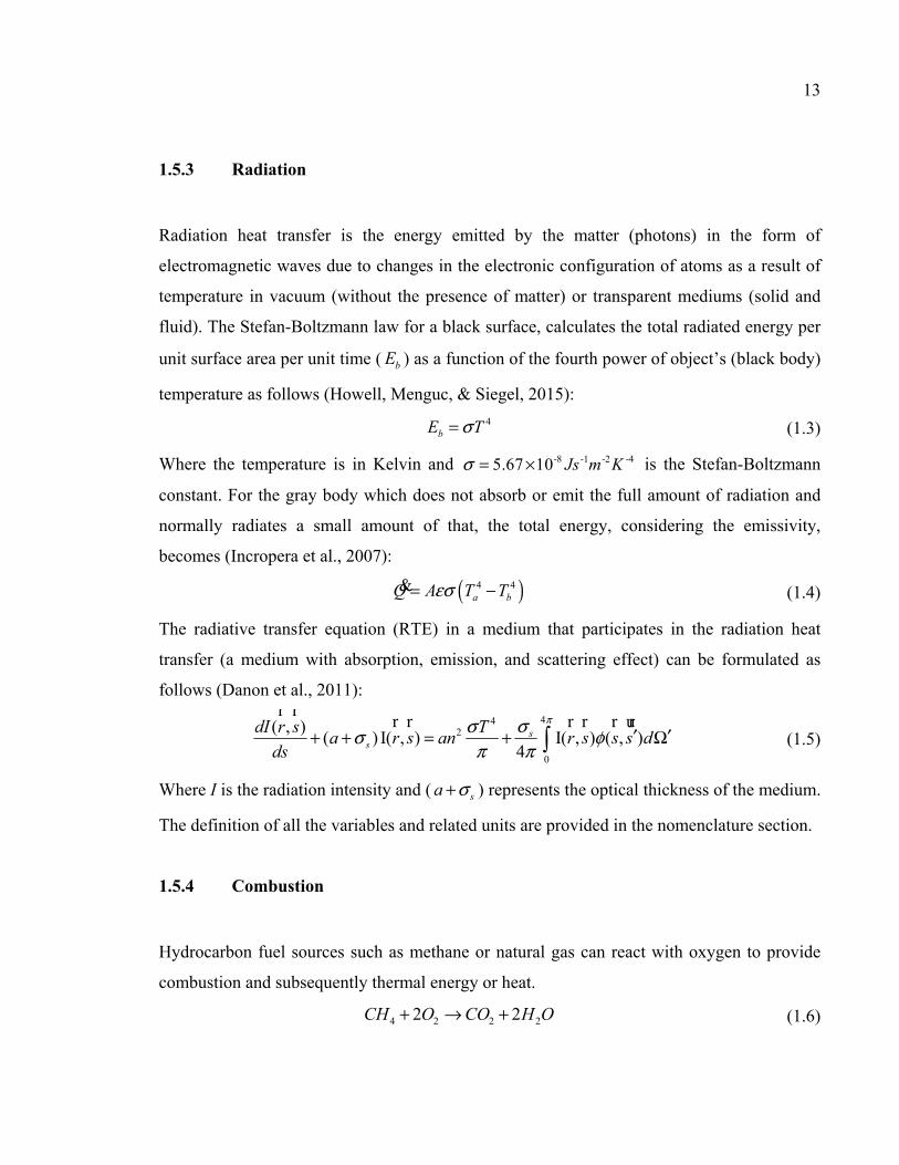
1.5.3 Radiation

Radiation heat transfer is the energy emitted by the matter (photons) in the form of

electromagnetic waves due to changes in the electronic configuration of atoms as a result of

temperature in vacuum (without the presence of matter) or transparent mediums (solid and

fluid). The Stefan-Boltzmann law for a black surface, calculates the total radiated energy per

unit surface area per unit time ( bE ) as a function of the fourth power of object’s (black body)

temperature as follows (Howell, Menguc, & Siegel, 2015): 4 bE Tσ= (1.3)

Where the temperature is in Kelvin and -8 -1 -2 -45.67 10 Js m Kσ = × is the Stefan-Boltzmann

constant. For the gray body which does not absorb or emit the full amount of radiation and

normally radiates a small amount of that, the total energy, considering the emissivity,

becomes (Incropera et al., 2007):

( )4 4 a bA TQ Tεσ= −& (1.4)

The radiative transfer equation (RTE) in a medium that participates in the radiation heat

transfer (a medium with absorption, emission, and scattering effect) can be formulated as

follows (Danon et al., 2011): 44

2

0

( , ) ( ) I( , ) I( , ) ( , )4

ss

dI r s Ta r s an r s s s dds

πσσσ φπ π

′ ′+ + = + Ωr r r r r r r ur

(1.5)

Where I is the radiation intensity and ( sa σ+ ) represents the optical thickness of the medium.

The definition of all the variables and related units are provided in the nomenclature section.

1.5.4 Combustion

Hydrocarbon fuel sources such as methane or natural gas can react with oxygen to provide

combustion and subsequently thermal energy or heat.

4 2 2 22 2CH O CO H O+ → + (1.6)

14

The oxygen availability and operating temperature can change the combustion efficiency and

also the combustion products. Incomplete combustion and CO production will take place in

combustion with insufficient oxygen content. Besides, the excess air, which means excess

oxygen, can affect the ratio of available heat. Combustion in any gas-fired heat treatment

furnaces plays the most important role in the system because:

• Combustion facilitator devices such as burners can be considered as the inlet boundary

condition for the main system such as a furnace.

• Combustion has a direct interaction with the radiation, convection and turbulence

which have their own impacts on the final goal.

Therefore, the combustion prediction in any combustion included application such as gas-

fired heat treatment furnaces should be thoroughly investigated.

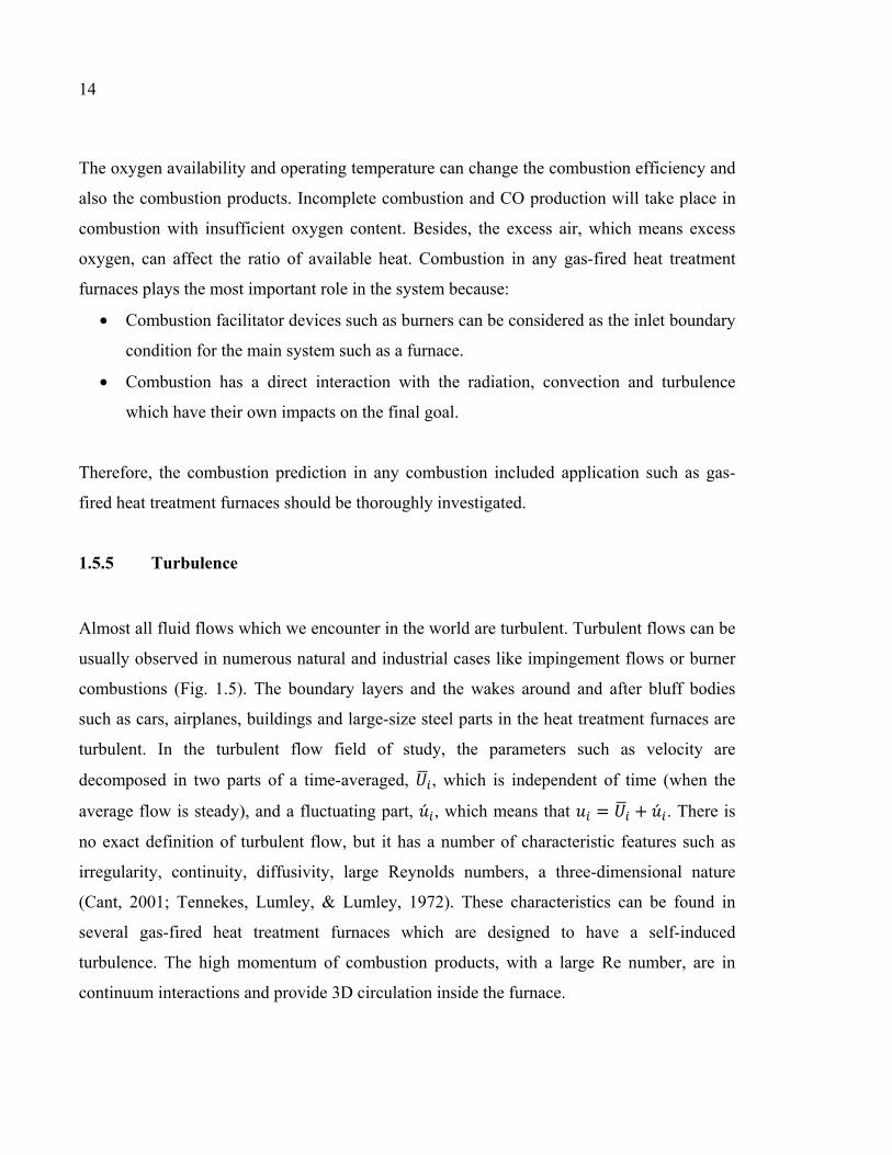
1.5.5 Turbulence

Almost all fluid flows which we encounter in the world are turbulent. Turbulent flows can be

usually observed in numerous natural and industrial cases like impingement flows or burner

combustions (Fig. 1.5). The boundary layers and the wakes around and after bluff bodies

such as cars, airplanes, buildings and large-size steel parts in the heat treatment furnaces are

turbulent. In the turbulent flow field of study, the parameters such as velocity are

decomposed in two parts of a time-averaged, 𝑈 , which is independent of time (when the

average flow is steady), and a fluctuating part, �́� , which means that 𝑢 = 𝑈 + �́� . There is

no exact definition of turbulent flow, but it has a number of characteristic features such as

irregularity, continuity, diffusivity, large Reynolds numbers, a three-dimensional nature

(Cant, 2001; Tennekes, Lumley, & Lumley, 1972). These characteristics can be found in

several gas-fired heat treatment furnaces which are designed to have a self-induced

turbulence. The high momentum of combustion products, with a large Re number, are in

continuum interactions and provide 3D circulation inside the furnace.

15

Figure 1.5 Turbulent combustion visualized by numerical simulation (Vicquelin, 2010).

1.6 Thermal Interactions Analyses inside Heat Treatment Furnaces

1.6.1 Analytical and Semi-Analytical Studies

Thermal interactions inside the gas-fired heat treatment furnaces importing strong non-linear

thermal boundary conditions to the loads make the thermal analysis of heat treatment process

very difficult. In the literature Chapman et al. (Chapman, Ramadhyani, & Viskanta, 1990) in

a semi-analytical study, assessed various material properties on the efficiency of heat treating

process in a direct fired batch reheating furnace. Gao et al. (Gao et al., 2000) using heat

conduction rule in solids, developed an analytical, practical virtual sphere method to estimate

the equilibrium time and heating/cooling rate in heat treatment furnaces. Their results proved

that the convection heat transfer rate could significantly differ from the empirically

calculated h values for specific furnaces. Singh et al. (Singh, Talukdar, & Coelho, 2015) in

their semi-analytical studies developed a heat-flow model to estimate temperature evolution

of products in different heat treatment processes such as heating in electrically furnaces, air

and water quenching. However, analytical analyses are generally limited to linear problems

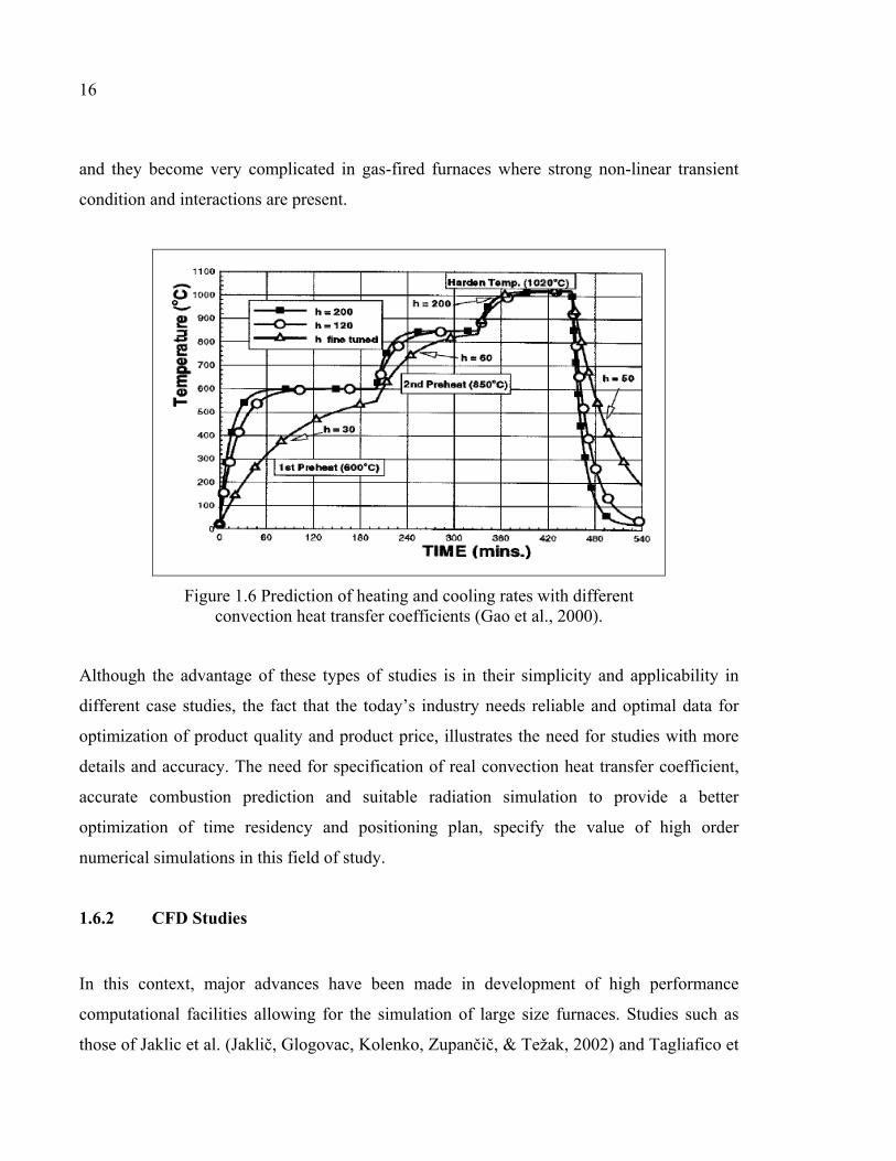
16

and they become very complicated in gas-fired furnaces where strong non-linear transient

condition and interactions are present.

Figure 1.6 Prediction of heating and cooling rates with different convection heat transfer coefficients (Gao et al., 2000).

Although the advantage of these types of studies is in their simplicity and applicability in

different case studies, the fact that the today’s industry needs reliable and optimal data for

optimization of product quality and product price, illustrates the need for studies with more

details and accuracy. The need for specification of real convection heat transfer coefficient,

accurate combustion prediction and suitable radiation simulation to provide a better

optimization of time residency and positioning plan, specify the value of high order

numerical simulations in this field of study.

1.6.2 CFD Studies

In this context, major advances have been made in development of high performance

computational facilities allowing for the simulation of large size furnaces. Studies such as

those of Jaklic et al. (Jaklič, Glogovac, Kolenko, Zupančič, & Težak, 2002) and Tagliafico et

17

al. (Tagliafico & Senarega, 2004) using finite-difference and finite element based methods

added more details to the analysis of load-furnace heating characteristics. Recently,

computational fluid dynamics (CFD) offering simultaneous analysis of turbulent fluid flow,

combustion and conjugate heat transfer has been used to simulate thermal flow field in

various metallurgical processes (Szajnar, Bartocha, Stawarz, Wróbel, & Sebzda, 2010; S. F.

Zhang et al., 2009; Zhou, Yang, Reuter, & Boin, 2007) (See Fig. 1.7). Yang et al. (Yang et

al., 2006) using the ANSYS Fluent software (ANSYS, 2016) performed CFD evaluation of

various metallurgical applications including: melting of aluminum scrap in a rotary furnace,

molten hot metal flow in a coke-bed blast furnace, electric arc furnace and gas-fired heat

treating furnaces. They used 𝑘 − ɛ turbulence model alongside with the EDM combustion

model. Several radiation models including, P-1, DTRM and Monte Carlo model (MCM)

have been evaluated in different industrial furnaces. The capability of these approaches to

predict the thermal interactions inside the furnace has been confirmed by the authors. They

also presented several data, including temperature evolution, melting curves and gas

consumption profiles proving the CFD applicability in predicting flow, temperature, mass

fraction and reaction distribution. Wang et al. (J. Wang et al., 2008) predicted the

temperature field of a gas quenching furnace using CFD simulation and Cosentino et al.

(Cosentino, Warnken, Gebelin, & Reed, 2013) investigated the non-uniform quenching effect

on the product properties.

Figure 1.7 Right) pressure and left) temperature distribution prediction by CFD in the submerged arc furnace (Yang et al., 2006).

18

1.6.3 CFD Analysis of Heat Treatment Furnaces without Combustion

One of the most basic investigations of heat treatment process using CFD is the study of

Elkatatny et al. (Elkatatny, Morsi, Blicblau, Das, & Doyle, 2003) who presented a CFD

simulation of high-pressure gas quenching of H13 die in a vacuum heat treatment furnace

(See Fig. 1.8). They suggested that a steady state simulation can be effectively used instead

of complete transient simulation in order to reduce the computational cost. It has been

reported that the CFD results were in good agreement with the experimental data and the

steady state solution was capable of accurate prediction of quenching treatment.

Figure 1.8 Temperature distribution prediction of H13 die using CFD simulation (Elkatatny et al., 2003).

Gongfa et al. (Gongfa et al., 2014) investigated the air quenching of heavy rail-head U71Mn

in both internal and external fields product using CFD. They could establish the flow

distribution, streamlines and temperature contours in internal and external fields. Using the

cooling rate calculation, provided by CFD simulation, they reported phase transformation on

the basis temperature gradient. Bergman (Bergman, 2012) provided a 2D simulation of a heat

treatment furnace, including the gas fluid flow and heat transfer into the product (turbine

structure). The significant impact of Reynolds number and buoyancy on the heat transfer rate

was reported. Besides, in the case of turbulence modeling, according to the authors, -k ω

model was proved to be a more reliable model in comparison to the standard -k ε and the

realizable -k ε models to predict the heat flux for highly turbulent fluid flow. Wang et al. (J.

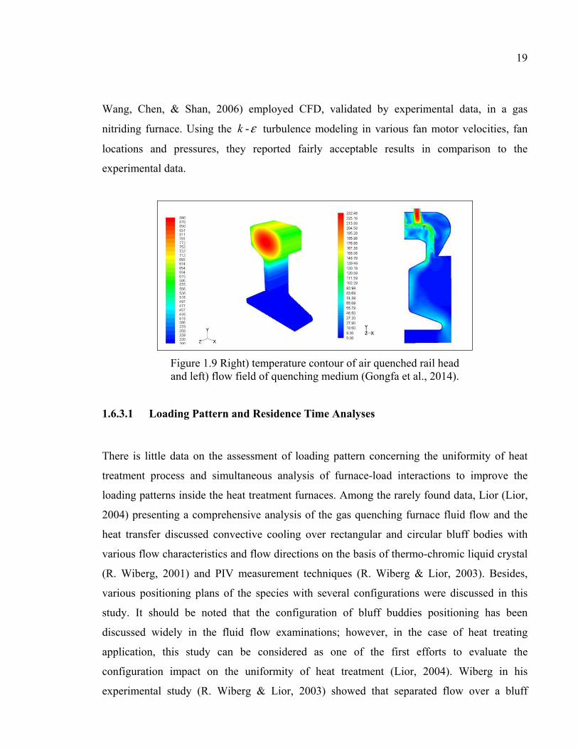
19

Wang, Chen, & Shan, 2006) employed CFD, validated by experimental data, in a gas

nitriding furnace. Using the -k ε turbulence modeling in various fan motor velocities, fan

locations and pressures, they reported fairly acceptable results in comparison to the

experimental data.

Figure 1.9 Right) temperature contour of air quenched rail head and left) flow field of quenching medium (Gongfa et al., 2014).

1.6.3.1 Loading Pattern and Residence Time Analyses

There is little data on the assessment of loading pattern concerning the uniformity of heat

treatment process and simultaneous analysis of furnace-load interactions to improve the

loading patterns inside the heat treatment furnaces. Among the rarely found data, Lior (Lior,

2004) presenting a comprehensive analysis of the gas quenching furnace fluid flow and the

heat transfer discussed convective cooling over rectangular and circular bluff bodies with

various flow characteristics and flow directions on the basis of thermo-chromic liquid crystal

(R. Wiberg, 2001) and PIV measurement techniques (R. Wiberg & Lior, 2003). Besides,

various positioning plans of the species with several configurations were discussed in this

study. It should be noted that the configuration of bluff buddies positioning has been

discussed widely in the fluid flow examinations; however, in the case of heat treating

application, this study can be considered as one of the first efforts to evaluate the

configuration impact on the uniformity of heat treatment (Lior, 2004). Wiberg in his

experimental study (R. Wiberg & Lior, 2003) showed that separated flow over a bluff

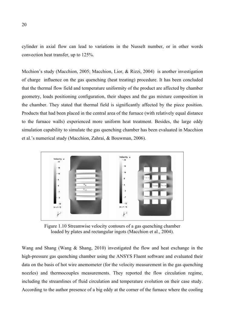
20

cylinder in axial flow can lead to variations in the Nusselt number, or in other words

convection heat transfer, up to 125%.

Mcchion’s study (Macchion, 2005; Macchion, Lior, & Rizzi, 2004) is another investigation

of charge influence on the gas quenching (heat treating) procedure. It has been concluded

that the thermal flow field and temperature uniformity of the product are affected by chamber

geometry, loads positioning configuration, their shapes and the gas mixture composition in

the chamber. They stated that thermal field is significantly affected by the piece position.

Products that had been placed in the central area of the furnace (with relatively equal distance

to the furnace walls) experienced more uniform heat treatment. Besides, the large eddy

simulation capability to simulate the gas quenching chamber has been evaluated in Macchion

et al.’s numerical study (Macchion, Zahrai, & Bouwman, 2006).

Figure 1.10 Streamwise velocity contours of a gas quenching chamber loaded by plates and rectangular ingots (Macchion et al., 2004).

Wang and Shang (Wang & Shang, 2010) investigated the flow and heat exchange in the

high-pressure gas quenching chamber using the ANSYS Fluent software and evaluated their

data on the basis of hot wire anemometer (for the velocity measurement in the gas quenching

nozzles) and thermocouples measurements. They reported the flow circulation regime,

including the streamlines of fluid circulation and temperature evolution on their case study.

According to the author presence of a big eddy at the corner of the furnace where the cooling

21

rate was slower than other position was confirmed showing the importance of vortical

structure in the present field of study. They also reported various cooling rates (with the

approximately 7.9% relative error) in different zones of the chamber according to the

location of products within the furnace.

Figure 1.11 Left) velocity distribution and right) temperature in the gas quenching chamber (Z. J. Wang & Shang, 2010).

X. Hao et al (Hao et al., 2008) in their case study, which was a vacuum electrically heated

furnace, using some simplification and optimization could propose a new heat treating time-

table. Based on several heating rates for different locations of the product they used North

American Die Casting Association (NADCA) suggestion to optimize the residence time of

the block inside an electrically heated furnace. This suggestion states that heating stage can

be started as soon as the temperature difference between surface and the center is less than

30°C (Hao et al., 2008).

22

Figure 1.12 Contours of temperature evolution in the a) electricaly heated furnace and b) heat treated block (Hao et al., 2008).

In Fig. 1.13, T1, T2 and T3 represent the corner, surface and the core of the workpiece and

TF is the furnace temperature. Heating curves and their mutual temperature differences

between the locations show a considerable extra residence time in products initial schedule.

As it can be seen in each heating stage bt which is the optimized residence time is shorter

than the t which had been used in their initial process. Their new proposed heat treating

procedure, considering the new heating rates and some simplifications, decreased the

residence time of the workpiece up to five hours. Although they just considered the

temperature as the main criterion (without considering the material microstructural changes

and mechanical properties based on various heating rates), their study proved the possible

contributions for the residence time improvement in the steel making industry.

Kang and Rong (Kang & Rong, 2006) studied the effect of small products loading patterns

on their heat treatment process within an electrically heated furnaces. Fig. 1.14 depicts the

comparison of loading pattern influence on temperature evolution of samples in their

numerical study. In this picture old and new are two different positioning plans and points 3

and 4 are two different locations of parts. As it can be seen there is a visible difference

between the two methods of product positioning temperature evolution. This difference is

more notable at low temperatures where the convection heat transfer is dominant. This study

23

and other similar analytical and numerical works demonstrate the importance of loading

pattern optimization.

Figure 1.13 Optimization of furnace resicence time based on a) heating curves and b) temperature difference curves inside electretically heated furnace (Hao et al., 2008).

24

Figure 1.14 Comparison of two different products loading patteren effects on the heat treatment process inside an

electercally heated furnace (Kang & Rong, 2006).

1.6.4 Gas-Fired Furnaces

Among the different types of industrial furnaces, gas-fired ones are commonly applied to

applications with large size products (Totten, 2006). Natural gas combustion can be found in

various furnaces including box and continuous ones such as pusher type and walking beam

reheating furnaces (Totten, 2006). Simulation of these furnaces is more complex due to the

existence of reactive flow combined with turbulent transport process and conjugate heat

transfer including absorbing and emitting hot combustion products. Little data is available in

the literature, probably due to above difficulties and the large volume of industrial furnaces

and large size products, which requires significant computational and experimental resources.

However, these challenges lately attracted researchers’ attention to this field of study.

Different gas-fired furnaces such as crucible or continues furnaces have been studied by

several researchers (Govardhan, Rao, & Narasaiah, 2011; B. Wu et al., 2008; C. Zhang, Ishii,

Hino, & Sugiyama, 2000).

Continuous reheating furnaces such as pusher type and walking beam furnaces, as gas-fired

furnaces, have also been the subject of several investigations. For example, Harish and Dutta

25

(Harish & Dutta, 2005) concentrated on the radiation simulation of slab reheat furnace.

Zhang et al. (Ishii, Zhang, & Hino, 2002) focused on the combustion modeling, provided

insight into the temperature distribution and thermal interactions inside gas-fired furnaces.

Recently, Liu et al. (Y. J. Liu, Li, Misra, Wang, & Wang, 2016) using CFD proposed a basic

model for increasing the temperature uniformity in reheating furnaces. Mayr et al. (B Mayr,

Prieler, Demuth, Potesser, & Hochenauer, 2017) proposed a one-step steady state CFD

approach and Tang et al. (Tang et al., 2017) with a combination of 3D CFD and 2D finite

difference methods (validated by experimental measurements) proposed time saving

approaches for optimization purposes (See Fig. 1.15). However continuous gas-fired

furnaces, due to their shorter processing time (regularly 2 hours (Tang et al., 2017)) in

comparison with the large size heat treating furnaces (24-48 hours in the case of large size

products (Gur & Pan, 2008)), require lower computational time for transient simulation.

Besides, the relatively simple geometry of these furnaces, which allow for simplification

such as steady state calculation in length or periodic transient simulation (B. Mayr, Prieler,

Demuth, Moderer, et al., 2017) made these furnaces an interesting case study for several

investigators. Employing models such as steady flame-let combustion model (SFM) (B.

Mayr, Prieler, Demuth, Moderer, et al., 2017) and numerical techniques such as 2D

interpolation (Tang et al., 2017) different methods have been proposed to reduce the

computational cost. Recently Garcia et al. (García, Colorado, Obando, Arrieta, & Amell,

2019) investigated the effect of burner locations on the performance of walking-beam type

reheating furnace using 3D steady state CFD calculation. According to the authors, burner

types and positions have significant impact on the performance of the furnace and product

quality.

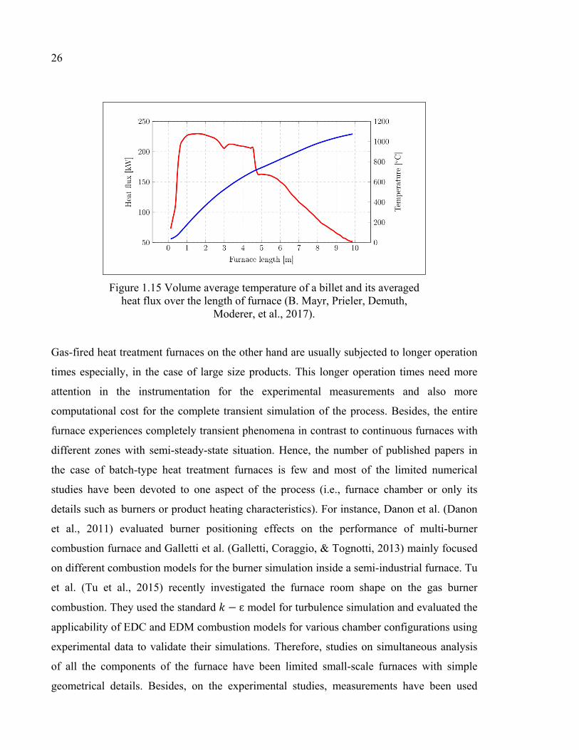
26

Figure 1.15 Volume average temperature of a billet and its averaged heat flux over the length of furnace (B. Mayr, Prieler, Demuth,

Moderer, et al., 2017).

Gas-fired heat treatment furnaces on the other hand are usually subjected to longer operation

times especially, in the case of large size products. This longer operation times need more

attention in the instrumentation for the experimental measurements and also more

computational cost for the complete transient simulation of the process. Besides, the entire

furnace experiences completely transient phenomena in contrast to continuous furnaces with

different zones with semi-steady-state situation. Hence, the number of published papers in

the case of batch-type heat treatment furnaces is few and most of the limited numerical

studies have been devoted to one aspect of the process (i.e., furnace chamber or only its

details such as burners or product heating characteristics). For instance, Danon et al. (Danon

et al., 2011) evaluated burner positioning effects on the performance of multi-burner

combustion furnace and Galletti et al. (Galletti, Coraggio, & Tognotti, 2013) mainly focused

on different combustion models for the burner simulation inside a semi-industrial furnace. Tu

et al. (Tu et al., 2015) recently investigated the furnace room shape on the gas burner

combustion. They used the standard 𝑘 − ɛ model for turbulence simulation and evaluated the

applicability of EDC and EDM combustion models for various chamber configurations using

experimental data to validate their simulations. Therefore, studies on simultaneous analysis

of all the components of the furnace have been limited small-scale furnaces with simple

geometrical details. Besides, on the experimental studies, measurements have been used

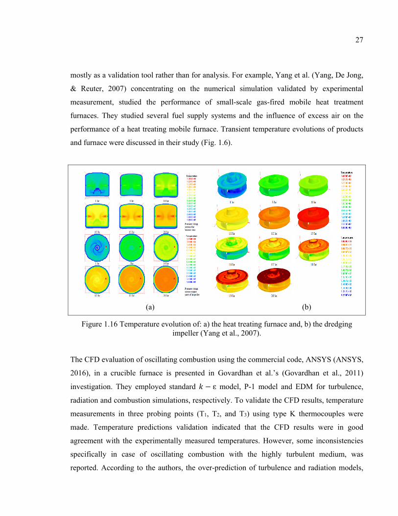
27

mostly as a validation tool rather than for analysis. For example, Yang et al. (Yang, De Jong,

& Reuter, 2007) concentrating on the numerical simulation validated by experimental

measurement, studied the performance of small-scale gas-fired mobile heat treatment

furnaces. They studied several fuel supply systems and the influence of excess air on the

performance of a heat treating mobile furnace. Transient temperature evolutions of products

and furnace were discussed in their study (Fig. 1.6).

(a) (b)

Figure 1.16 Temperature evolution of: a) the heat treating furnace and, b) the dredging impeller (Yang et al., 2007).

The CFD evaluation of oscillating combustion using the commercial code, ANSYS (ANSYS,

2016), in a crucible furnace is presented in Govardhan et al.’s (Govardhan et al., 2011)

investigation. They employed standard 𝑘 − ɛ model, P-1 model and EDM for turbulence,

radiation and combustion simulations, respectively. To validate the CFD results, temperature

measurements in three probing points (T1, T2, and T3) using type K thermocouples were

made. Temperature predictions validation indicated that the CFD results were in good

agreement with the experimentally measured temperatures. However, some inconsistencies

specifically in case of oscillating combustion with the highly turbulent medium, was

reported. According to the authors, the over-prediction of turbulence and radiation models,

28

inaccurate inlet boundary conditions and not sufficiently enough grid resolution were

considered as inaccuracy sources.

Figure 1.17 Schematic sketch of circular furnace employed by Govardhan et al. (Govardhan et al., 2011).

Table 1.1 Temperature validation reported by J. Govardhan et al. (Govardhan et al., 2011)

Time (min)

T1 (K) T2 (K) T3 (K)

Exp CFD Exp CFD Exp CFD

10 575 594 621 871 735 871

20 778 843 791 1040 1043 1080

30 921 912 977 1150 1051 1150

40 974 938 1053 1170 1123 1222

In another work, Mayr et al. (Bernhard Mayr, Prieler, Demuth, Potesser, & Hochenauer,

2015) employing experimental validation evaluated the applicability of steady state CFD

simulation for combustion modeling of flat burners, using steady laminar flame let model

(SFM), in a lab-scale heat treatment furnace; and reported on the performance of the furnace

as a function of fuel/oxidizer ratio.

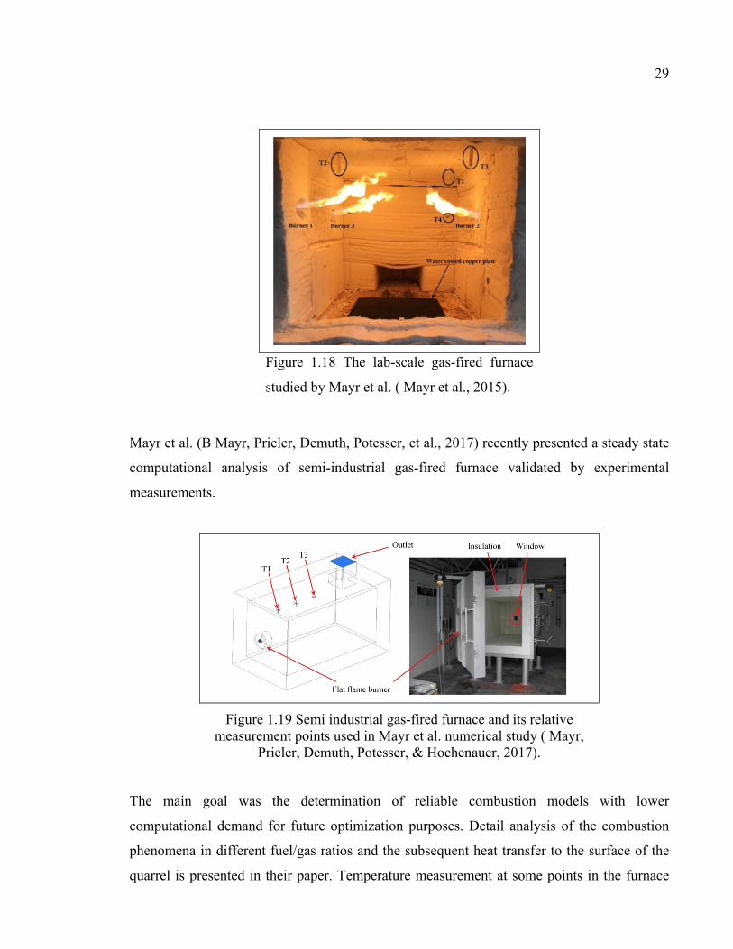
29

Figure 1.18 The lab-scale gas-fired furnace

studied by Mayr et al. ( Mayr et al., 2015).

Mayr et al. (B Mayr, Prieler, Demuth, Potesser, et al., 2017) recently presented a steady state

computational analysis of semi-industrial gas-fired furnace validated by experimental

measurements.

Figure 1.19 Semi industrial gas-fired furnace and its relative measurement points used in Mayr et al. numerical study ( Mayr,

Prieler, Demuth, Potesser, & Hochenauer, 2017).

The main goal was the determination of reliable combustion models with lower

computational demand for future optimization purposes. Detail analysis of the combustion

phenomena in different fuel/gas ratios and the subsequent heat transfer to the surface of the

quarrel is presented in their paper. Temperature measurement at some points in the furnace

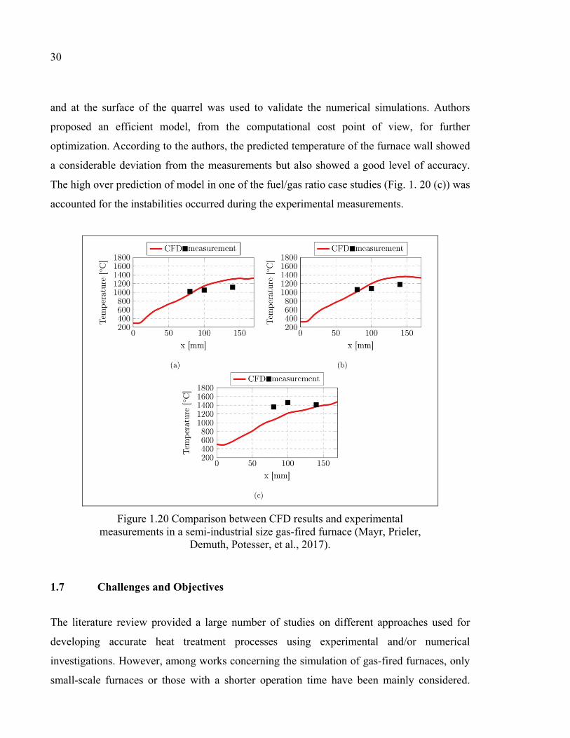
30

and at the surface of the quarrel was used to validate the numerical simulations. Authors

proposed an efficient model, from the computational cost point of view, for further

optimization. According to the authors, the predicted temperature of the furnace wall showed

a considerable deviation from the measurements but also showed a good level of accuracy.

The high over prediction of model in one of the fuel/gas ratio case studies (Fig. 1. 20 (c)) was

accounted for the instabilities occurred during the experimental measurements.

Figure 1.20 Comparison between CFD results and experimental measurements in a semi-industrial size gas-fired furnace (Mayr, Prieler,

Demuth, Potesser, et al., 2017).

1.7 Challenges and Objectives

The literature review provided a large number of studies on different approaches used for

developing accurate heat treatment processes using experimental and/or numerical

investigations. However, among works concerning the simulation of gas-fired furnaces, only

small-scale furnaces or those with a shorter operation time have been mainly considered.

31

Data on simultaneous analyses of thermal interactions inside industrial heat treatment

furnaces along with large size products heating characteristics are very rare. The majority of

the studies covered one part of the process, i.e. heating chamber and its details such as

burners, or products heating characteristic solely. Moreover, experimental measurements due

to technical challenges have been generally devoted to validating numerical results rather

than being used as tools to heat transfer analysis. Detail experimental analysis, especially for

the large size products, that encompasses high temperature gradient in their different

locations is in demand considering the state of literature. Thus, the first objective of the

present study is to comprehensively analyze the heat transfer in the heat treatment process of

large size ingots in full scale gas-fired furnaces using both experimental measurements and

CFD simulations. This part of the present thesis is aimed to address several missing links to

the scientific as well as industrial communities. Temperature uniformity of the large size

parts as a crucial parameter to evaluate the process efficiency was chosen to analyze the

transient history of large size forged ingots within an industrial gas-fired furnace.

Experimental measurement results and unsteady CFD predictions were used to analyze the

temperature evolution of a large size forged ingot in a single loading configuration during the

heat treatment process based on heat transfer modes in the furnace, fluid flow circulation, and

vortical structures.

Optimization of furnace residence time inside heat treatment furnaces can significantly affect

the production cost and fuel usage in the steel industry. On the other hand, this optimization

along with loading pattern improvement of steel parts in heat treatment furnaces can

guarantee the uniformity of heat treatment and consequently final products’ quality.

Residence time and loading pattern improvement were rarely addressed in the literature.

Among the few reported works, electrical furnaces and small products’ loading patterns were

only discussed. Therefore the second objective of the study is to carry out a thermal analysis

on furnace residence time and loading pattern of large size forgings inside gas-fired heat

treatment furnaces. Specifically, quantification of temperature non-uniformity in a non-

optimized loading pattern and possible improvement using skids and spacers were the

secondary objectives of this part. A novel hybrid experimental-numerical approach is

32

proposed to improve the residence time of large size steel parts inside gas-fired heat

treatment furnace.

Different numerical and experimental studies on the heat treatment process inside industrial

and laboratory scale furnaces were discussed in the presented literature review. However,

these studies were performed with different research purposes, like product temperature

prediction, combustion simulation, non-uniformity identification and loading pattern or

residence time optimization. This makes it difficult to evaluate the strength and limitations of

numerical approaches in CFD simulations for the prediction of thermal interactions like

turbulent convection or combustion within the gas-fired furnace. However, little data is

available on the systematic investigation of CFD results sensitivity to the numerical

approaches used in the modeling of gas-fired batch heat treatment furnaces. Therefore, the

third main objective of the present study is to assess the sensitivity of CFD predictions to

employed numerical techniques in order to have reliable and cost effective simulations of the

heat treatment process inside large size heat treatment furnaces. To this end, several

turbulence models as well as combustion modeling approaches were examined both for the

flow field and scalar predictions (temperature) near the burner and steel parts.

33

CHAPTER 2

NUMERICAL DETAILS FOR THERMAL ANALYSIS OF HEAT TREATMENT PROCESS IN GAS-FIRED FURNACE

2.1 Introduction

In the present chapter, the principal elements of the numerical approaches that will be

considered in the thesis will be presented. Specifically, the numerical models for radiation,

combustion, and turbulence modeling that will be assessed in the present study will be

introduced. An overall comparison of models for each phenomenon will be presented from

both computational cost and accuracy points of view.

2.2 Computational Fluid Dynamics (CFD)

Computational fluid dynamics (CFD) is a branch of mechanical engineering widely used in

various fluid dynamics and heat transfer phenomena. It has attracted many scientific

disciplines when dealing with the complicated applications where the conventional

experimental techniques are difficult to execute or expensive. Although CFD fundamentally

requires reliable experimental data to validate its predictions with, it can provide valuable

insight into the nature of fluid dynamics and the phenomena that the available experimental

facilities cannot capture. Typically a CFD code or software such as ANSYS FLUENT

(ANSYS, 2016) contains four main components (Ashgriz & Mostaghimi, 2002):

• Partial differential equations which are discretized to supply a numerical set of

equations that identify and describe the fluid flow, heat transfer, combustion or any

other flow related interactions.

• Grid generators that divide the flow domain into small grids or control volumes where

the equations are solved.

• Initial and boundary conditions describing the flow pattern that should be defined by

the user to obtain the reliable data. This part of CFD code is extremely dependent on

experimental data.

34

• Procedures that control the accuracy, and convergence of the solution.

Due to the wide range of CFD approaches and formulations, in the following sections the

most important numerical details that take part in the present project will be discussed. The

topics are selected based on the project demands and the literature review presented in the

previous chapter.

2.3 Navier-Stokes Equations

The most important set of equations to predict, describe and simulate the fluid flow, the

Navier-Stokes equations provide mathematical foundations of fluid flow, heat transfer, mass

transfer and any other fluid related phenomena. Basically, for an accurate and exact

prediction and description of all flows, the mass and momentum equations called as,

continuity and momentum equations should be solved. For the flows that deal with the heat

transfer or compressibility an additional equation, energy equation, should be considered. If

the target flow encompasses mixing of the species, the species conservation equation should

also be solved. Moreover, in the case of reacting flow model, the conservation equation for

the mixture reaction should be added. Finally in the case of turbulent flow, other additional

transport equations must be solved to consider the impact of turbulence on the fluid flow

field (Constantin & Foias, 1988; Patankar, 2018).

• Conservation of mass:

In general, for both compressible and incompressible fluid flows, the conservation of mass

equation called also continuity equation is given by (Patankar, 2018):

( ) . ρv mStρ∂ + ∇ =

∂ (2.1)

The definition of all the variables and related units are provided in the nomenclature page.

• Conservation of Momentum

35

Momentum equation, states that the algebraic summation of all the active forces on a control

volume should be equal to zero. The differential form of momentum equation is (Patankar,

2018):

( ) ( ) ( ) . ρv p . τv

v g Ft

ρρ

∂+ ∇ = −∇ + ∇ + +

∂ (2.2)

The stress tensor, τ, is defined as:

( ) 2 .3

Tµ v v vIτ = ∇ + ∇ − ∇ (2.3)

• Energy Equation

The general differential energy equation or energy conservation equation is:

( ) ( )( ) ( ). . v . Teff j j eff hj

E E p k h J v St

ρ ρ τ ∂ + ∇ + = ∇ ∇ − + + ∂

(2.4)

In this equation effk is the effective conductivity (summation of molecular and turbulent

conductivities), jJ is the diffusion flux of species j , and effτ is the effective stress tensor.

Turbulent thermal conductivity which can be determined using turbulence model should be

considered in case of turbulent flow. The first term of the right-hand side of Eq. 2.4

represents the conduction energy transformation in the fluid while the second and third ones

indicate the energy transfer caused by species diffusion and viscous dissipation, respectively

(Tennekes et al., 1972). Finally, the term Sh represents the chemical reaction heat and any

other volumetric heat sources such as radiation sources. In the above equation, the

relationship between the energy, E, and the sensible enthalpy, h, is (Incropera et al., 2007): 2

2

p vE hρ

= − +

(2.5)

Where for an ideal fluid on the basis of mass fraction of species j , jY :

j jj

h Y h=

(2.6)

• Solid Regions Energy Equation

The energy transport in the solid medium is described by the following equation (Incropera et

al., 2007):

36

( ) .( ) .( ) hh v h k T St

ρ ρ∂ + ∇ = ∇ ∇ +∂

(2.7)

The above equation terms are energy storage’s change with time, the energy convection

transfer due to motion in rotation or movement of solid, (the term v , is calculated from the

specific movement in the solid zone), conduction heat fluxes (first term in the right hand side

of the equation) and the volumetric heat sources in the solid medium, respectively.

2.4 Species Transport

To solve and model the mixing reactions such as combustion in the burners and the transport

of combustion products inside the furnace the conservation equation of species that includes

convection, diffusion and reaction source, should be considered for each component

(Bennett, 1962; Incropera et al., 2007). In the case of heat treatment, the species transport

with reaction is the objective approach. The species transport formulation for the local mass

fraction species of, Y , for the ith species is (B. Magnussen, 1981):

( ) ( ) . .i i i i iY vY J R St

ρ ρ∂ + ∇ = −∇ + +∂

(2.8)

In which iR is the net rate of the production of thi component by chemical reaction and iS

encompasses the other types of sources. The term iJ is the diffusion flux of species i, which

depends on the gradient of concentration and temperature. For the turbulent regime the mass

diffusion can be computed as follows:

, , ti i m i T i

t

Tj D Y DSc Tμρ

∇= − + ∇ −

(2.9)

where 𝑆𝑐 , 𝜇 , and 𝐷 are the turbulence Schmidt number, turbulence viscosity and the

turbulent diffusivity, respectively. To achieve the exact simulation of mass transfer or species

transport equation, all the terms and their modeling approaches should be considered and

evaluated alongside with the geometry. However, the most important term and the key

parameter to start the mass transfer solution is the reaction modeling. To determine the

reaction rates in equation (2.8) the three well-known approaches are:

• Laminar Finite-rate model

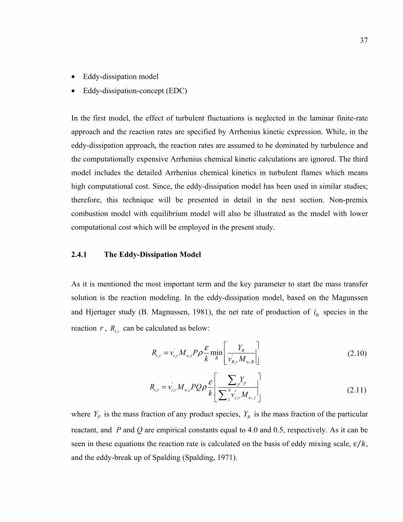
37

• Eddy-dissipation model

• Eddy-dissipation-concept (EDC)

In the first model, the effect of turbulent fluctuations is neglected in the laminar finite-rate

approach and the reaction rates are specified by Arrhenius kinetic expression. While, in the

eddy-dissipation approach, the reaction rates are assumed to be dominated by turbulence and

the computationally expensive Arrhenius chemical kinetic calculations are ignored. The third

model includes the detailed Arrhenius chemical kinetics in turbulent flames which means

high computational cost. Since, the eddy-dissipation model has been used in similar studies;

therefore, this technique will be presented in detail in the next section. Non-premix

combustion model with equilibrium model will also be illustrated as the model with lower

computational cost which will be employed in the present study.

2.4.1 The Eddy-Dissipation Model

As it is mentioned the most important term and the key parameter to start the mass transfer

solution is the reaction modeling. In the eddy-dissipation model, based on the Magunssen

and Hjertager study (B. Magnussen, 1981), the net rate of production of thi species in the

reaction r , ,i rR can be calculated as below:

', , , '

, ,

min Ri r i r w i R

R r w R

YR v Mv

Pk Mερ

=

(2.10)

', , , ''

, ,

pp

i r i r w i Nj r w jj

YR v M

k v MPQ ερ

=

(2.11)

where PY is the mass fraction of any product species, RY is the mass fraction of the particular

reactant, and P and Q are empirical constants equal to 4.0 and 0.5, respectively. As it can be

seen in these equations the reaction rate is calculated on the basis of eddy mixing scale, ɛ 𝑘⁄ ,

and the eddy-break up of Spalding (Spalding, 1971).

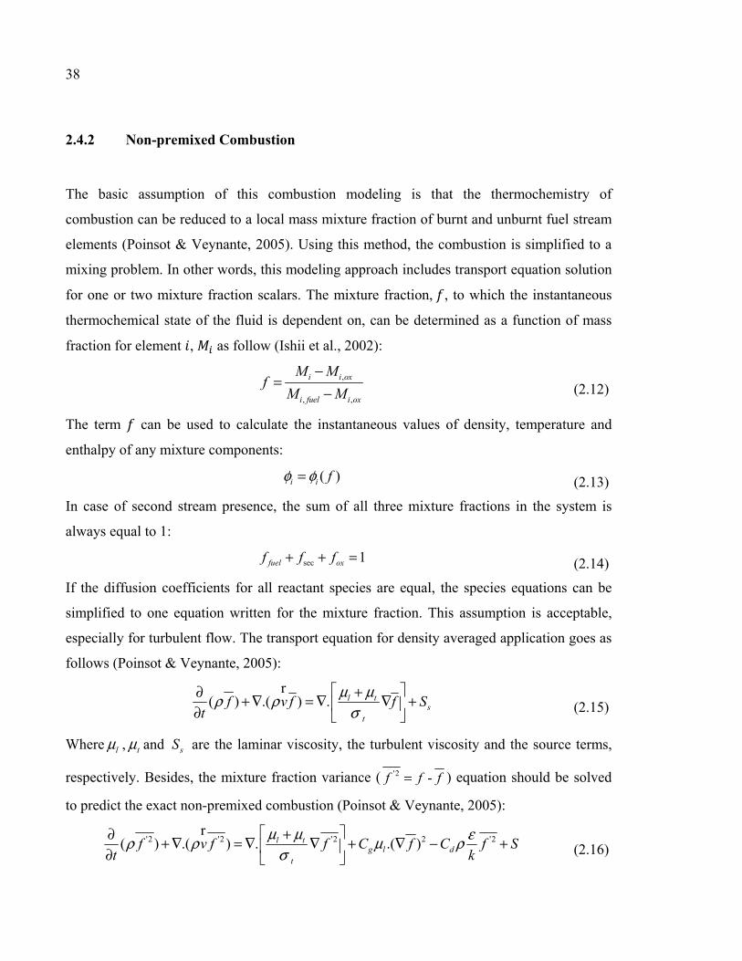
38

2.4.2 Non-premixed Combustion

The basic assumption of this combustion modeling is that the thermochemistry of

combustion can be reduced to a local mass mixture fraction of burnt and unburnt fuel stream

elements (Poinsot & Veynante, 2005). Using this method, the combustion is simplified to a

mixing problem. In other words, this modeling approach includes transport equation solution

for one or two mixture fraction scalars. The mixture fraction, 𝑓, to which the instantaneous

thermochemical state of the fluid is dependent on, can be determined as a function of mass

fraction for element 𝑖, 𝑀 as follow (Ishii et al., 2002):

,

, ,

i i ox

i fuel i ox

M Mf

M M−

=−

(2.12)

The term 𝑓 can be used to calculate the instantaneous values of density, temperature and

enthalpy of any mixture components:

( )i i fφ φ= (2.13) In case of second stream presence, the sum of all three mixture fractions in the system is

always equal to 1:

sec 1 fuel oxf f f+ + = (2.14) If the diffusion coefficients for all reactant species are equal, the species equations can be

simplified to one equation written for the mixture fraction. This assumption is acceptable,

especially for turbulent flow. The transport equation for density averaged application goes as

follows (Poinsot & Veynante, 2005):

( ) .( ) . l ts

t

f v f f St

μ μρ ρσ

+∂ + ∇ = ∇ ∇ + ∂

r (2.15)

Where lμ , tμ and sS are the laminar viscosity, the turbulent viscosity and the source terms,

respectively. Besides, the mixture fraction variance ( '2 -f f f= ) equation should be solved

to predict the exact non-premixed combustion (Poinsot & Veynante, 2005):

'2 '2 '2 2 '2( ) .( ) . .( )l tg l d

t

f v f f C f C f St k

μ μ ερ ρ μ ρσ

+∂ + ∇ = ∇ ∇ + ∇ − + ∂

r (2.16)

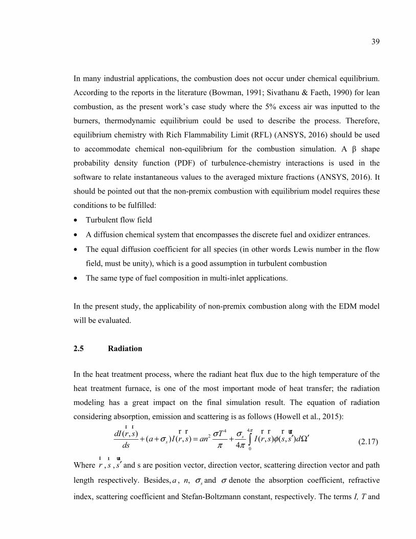
39

In many industrial applications, the combustion does not occur under chemical equilibrium.

According to the reports in the literature (Bowman, 1991; Sivathanu & Faeth, 1990) for lean

combustion, as the present work’s case study where the 5% excess air was inputted to the

burners, thermodynamic equilibrium could be used to describe the process. Therefore,

equilibrium chemistry with Rich Flammability Limit (RFL) (ANSYS, 2016) should be used

to accommodate chemical non-equilibrium for the combustion simulation. A β shape

probability density function (PDF) of turbulence-chemistry interactions is used in the

software to relate instantaneous values to the averaged mixture fractions (ANSYS, 2016). It

should be pointed out that the non-premix combustion with equilibrium model requires these

conditions to be fulfilled:

• Turbulent flow field

• A diffusion chemical system that encompasses the discrete fuel and oxidizer entrances.

• The equal diffusion coefficient for all species (in other words Lewis number in the flow

field, must be unity), which is a good assumption in turbulent combustion

• The same type of fuel composition in multi-inlet applications.

In the present study, the applicability of non-premix combustion along with the EDM model

will be evaluated.

2.5 Radiation

In the heat treatment process, where the radiant heat flux due to the high temperature of the

heat treatment furnace, is one of the most important mode of heat transfer; the radiation

modeling has a great impact on the final simulation result. The equation of radiation

considering absorption, emission and scattering is as follows (Howell et al., 2015): 44

2

0

( , ) ( ) ( , ) ( , ) ( , )4

ss

dI r s Ta I r s an I r s s s dds

πσσσ φπ π

′ ′+ + = + Ωr r r r r r r ur

(2.17)

Where rr

, sr

, s′ur

and s are position vector, direction vector, scattering direction vector and path

length respectively. Besides, a , n, sσ and σ denote the absorption coefficient, refractive

index, scattering coefficient and Stefan-Boltzmann constant, respectively. The terms I, T and

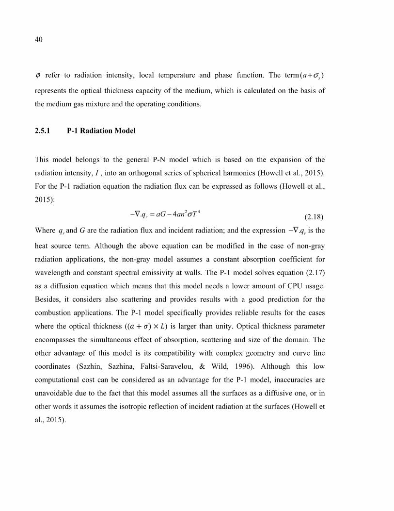
40

φ refer to radiation intensity, local temperature and phase function. The term( )sa σ+

represents the optical thickness capacity of the medium, which is calculated on the basis of

the medium gas mixture and the operating conditions.

2.5.1 P-1 Radiation Model

This model belongs to the general P-N model which is based on the expansion of the

radiation intensity, I , into an orthogonal series of spherical harmonics (Howell et al., 2015).

For the P-1 radiation equation the radiation flux can be expressed as follows (Howell et al.,

2015): 2 4. 4rq aG an Tσ−∇ = − (2.18)

Where rq and G are the radiation flux and incident radiation; and the expression . rq−∇ is the

heat source term. Although the above equation can be modified in the case of non-gray

radiation applications, the non-gray model assumes a constant absorption coefficient for

wavelength and constant spectral emissivity at walls. The P-1 model solves equation (2.17)

as a diffusion equation which means that this model needs a lower amount of CPU usage.

Besides, it considers also scattering and provides results with a good prediction for the

combustion applications. The P-1 model specifically provides reliable results for the cases

where the optical thickness ((𝑎 + 𝜎) × 𝐿) is larger than unity. Optical thickness parameter

encompasses the simultaneous effect of absorption, scattering and size of the domain. The

other advantage of this model is its compatibility with complex geometry and curve line

coordinates (Sazhin, Sazhina, Faltsi-Saravelou, & Wild, 1996). Although this low

computational cost can be considered as an advantage for the P-1 model, inaccuracies are

unavoidable due to the fact that this model assumes all the surfaces as a diffusive one, or in

other words it assumes the isotropic reflection of incident radiation at the surfaces (Howell et

al., 2015).

41

2.5.2 Discrete Ordinates Radiation Model (DO)

The DO radiation model (Chui & Raithby, 1993) modifies equation (2.17) to a transport

equation of radiation intensity by solving the equation for finite numbers of discrete solid

angles. This solution method is similar to the fluid flow equation’s solution. In the DO

coupled energy and intensity equations are solved simultaneously in each control volume.

This model considers the radiation equation in the direction sr as a field equation and for the

spectral intensity ( , )I r sλr r

using a gray-band model:

42

0.( ( , ) ) ( ) ( , ) ( , ) ( , )

4s

s bI r s s a I r s a n I I r s s s dπ

λ λ λ λ λσσ φπ

′ ′ ′∇ + + = + Ωr r r r r r r r r

(2.19)

Whereλ , aλ and bI λ is the wavelength, spectral absorption and black body intensity,

respectively. This model divides the radiation spectrum to m wavelengths band and integrates

the above equation over each interval. This integration results in transport equations for the

quantity Iλ λΔ . Therefore, total intensity in each direction and position will be:

( , ) ( , )k kk

I r s I r sλ λ= Δr r r r (2.20)

2.5.3 Surface to Surface (S2S) Model

In this model, the radiation heat transfer between two surfaces is a direct function of the

radiation view factor, also called the shape factor. This model which requires lower

computational costs in comparison with the DO model, ignores absorption, emission or

scattering effect of radiation by the medium. Therefore, the radiation energy balance is

calculated, as follows (Howell et al., 2015):

4, ,

1

k

N

out k k k kj out jj

q T F qε σ ρ=

= + (2.21)

In this equation, Fkj is the radiation view factor between surface k and surface j which is

calculated based on the size, separation distance and orientation of the surfaces.

42

2.6 Turbulence

Studies on turbulence can be divided into analytical solutions, experimental investigations

and numerical simulations. As a result of the highly nonlinear nature of turbulence,

including, analytical solutions are limited to very fundamental and simple applications such

as flow over a flat plate, etc. (Davidson, 2011). On the other hand, experimental

investigations have a significant role not only on the released information about various

applications, but also on the data production for numerical simulations. Although, high-tech

measurement techniques and facilities support the experimental investigations, the cost of

measurement in experimental trials and also the limitation of measurement in these

applications such as steel heat treatment highlight the role of numerical simulation in

turbulence determination. Development of the computational equipment over the last 20

years has led to wide employment of CFD for the simulation of turbulence problems from

simple applications to highly turbulent flow fields such as combustor simulations, turbine

blade film cooling and heat treatment industries (Bazdidi-Tehrani, Bohlooli, & Jadidi, 2015).

There are different approaches to solve the turbulent nature of fluid flows. The most well-

known and common methodology in turbulence area is the Reynolds Averaged Navier-

Stokes (RANS) models which are highly compatible with different phenomena, complex

geometries and different grid resolutions. Based on the literature review and the research

scope these models have been selected for the present study and discussed briefly in the next

sections.

2.6.1 Reynolds Averaged Navier-Stokes (RANS)

In the RANS based models the variables are usually decomposed into mean (time-averaged)

and fluctuating parts. The mean values can be achieved by Reynolds averaging (including the

time averaging, volume averaging and ensemble averaging) that has been introduced by

Reynolds in 1895. Time averaging which is the most common Reynolds averaging method

can be used when the turbulent flow has a steady or stationary nature which means that the

43

flow parameters do not vary in time average. The time averaging can be defined as (Bazdidi-

Tehrani, Hatami, & Abouata, 2017):

1( ) lim ( , )t T

Tt

F r f r t dtT

+

→∞

=

(2.22)

Using this formula, the parameters can be written as follows:

u U up P pT T T

′= +′= +′= +

(2.23)

Where ,u p , and T are the instantaneous velocity, pressure and temperature, respectively.

The terms ,U P , and T (also can be written as ,U P and T) represent the time-averaged parts

while the terms ,u p′ ′ , and T ′ are the fluctuating parts of velocity, temperature and pressure,

respectively. In should be noted that according to the continuity equation:

0

0

i

i

i

i

Uxux

∂ =∂∂ =∂

(2.24)

By imposing this decomposition to the Navier-Stokes equations, we have (Davidson, 2011):

( ) 0ii

Ut xρ ρ∂ ∂+ =

∂ ∂ (2.25)

( )( ) 2iij i j

i j

D U P S u uDt x xρ μ∂ ∂ ′ ′= − + −

∂ ∂ (2.26)

ii i

DT T u TDt x x

α ∂ ∂ ′ ′= − ∂ ∂

(2.27)

Where:

12

jiij

j i

UUSx x

∂∂= + ∂ ∂ (2.28)

The Eq. (1.8) also can be written as follows:

( )1 1ii ij i j i

j i j

U PU u u Fx x x

τ ρρ ρ

∂ ∂ ∂ ′ ′= − + − +∂ ∂ ∂

(2.29)

44

As it can be seen the difference between the fundamental Eq. (2.2) and the time-averaged Eq.

(2.29) is the term i ju uρ ′ ′ which is called Reynolds stress because it has the dimensions of

stress (Davidson, 2011). This term describes the effect of turbulent diffusion of momentum

which is stronger than the molecular viscosity in a fully turbulent flow. To close the set of

equations the Reynolds stress term should be modelled. One of the basic approaches is

Boussinesq hypothesis, called as constant eddy viscosity, which provides a relation between

the i ju uρ ′ ′ and the average velocity gradient, as follows (Schiestel, 1983):

23

ji ii j t t ij

j i i

UU Uu u kx x x

ρ μ ρ μ δ ∂ ∂ ∂′ ′− = + − + ∂ ∂ ∂

(2.30)

Where k or turbulence kinetic energy is given by:

( )2 2 21 ' ' '2

k u v w= + + (2.31)

There are several turbulence models for the description of i ju u′ ′ , that have various degrees of

complexity on the basis of extra partial differential (or transport) equations that must be

solved in addition to the three conservation equations. These models can be found from the

simplest algebraic or zero-equation model to the full Reynolds stress model (FRSM) and

nonlinear eddy viscosity models (Bazdidi-Tehrani, Mohammadi-Ahmar, Kiamansouri, &

Jadidi, 2015).

2.6.2 Two-Equation Turbulence models

Generally, the two-equation turbulence models employ the definition of the turbulence

viscosity as a function of velocity scale ( sV ) and length scale ( sl ) (Davidson, 2011).

t s sC V lμμ ρ= (2.32)

Where, the velocity scale is usually equal to 1/2k (or root mean square of turbulence kinetic

energy). On the other hand, the specification of length scale is different in various models

which in turn, provide several choices. For instance, the well-known 𝑘 − ɛ (Launder &

Spalding, 1972) turbulence model assumes that the length scale is proportional to the 3/2 /k ε ,

45

where ε is the turbulence dissipation rate. While, the -k ω model (Wilcox, 1998) uses the 1/2 /k ω .

2.6.2.1 𝒌 − 𝜺 Turbulence Model

The turbulence kinetic energy ( k ) and the turbulence dissipation rate (ε ) equations are the

two additional transport equations that the standard 𝑘 − ɛ model employs to close the

Reynolds averaged Navire-stokes equations (Davidson, 2011).

( ) ( ku ) ti k b M k

i j k j

kk G G Y St x x x

μρ ρ μ ρεσ

∂ ∂ ∂ ∂+ = + + + − − + ∂ ∂ ∂ ∂ (2.33)

2

1 3 2( ) ( u ) ( )ti k b

i j j

C G C G C St x x x k kε ε ε ε

ε

μ ε ε ερε ρε μ ρσ

∂ ∂ ∂ ∂+ = + + + − + ∂ ∂ ∂ ∂ (2.34)

Where kG and bG are the turbulence kinetic energy generations due to the velocity gradients

and buoyancies. MY and S represent the compressibility effect and the other source terms,

respectively. The ANSYS FLUENT (ANSYS, 2016) Commercial code uses the following

values for the constants in the above equations:

Table 2.1 The values of the 𝑘 − ɛ model constants (ANSYS, 2016).

Cμ 1C ε 2C ε kσ εσ

0.09 1.44 1.92 1 1.3

These values have been determined on the basis of various numerical simulations. However,

for special cases there are some corrections to these values such as those reported by Crasto

et al. (Crasto, 2007) for the atmospheric boundary layer applications. It should be noted that

the other branch of 𝑘 − ɛ models such as realizable and RNG 𝑘 − ɛ, were introduced on the

basis of the standard model and were employed in various applications such as heat treatment

furnaces (Bernhard Mayr et al., 2015). The major difference for realizable model after

modification of the standard model constants for more complex flow field, is the calculation

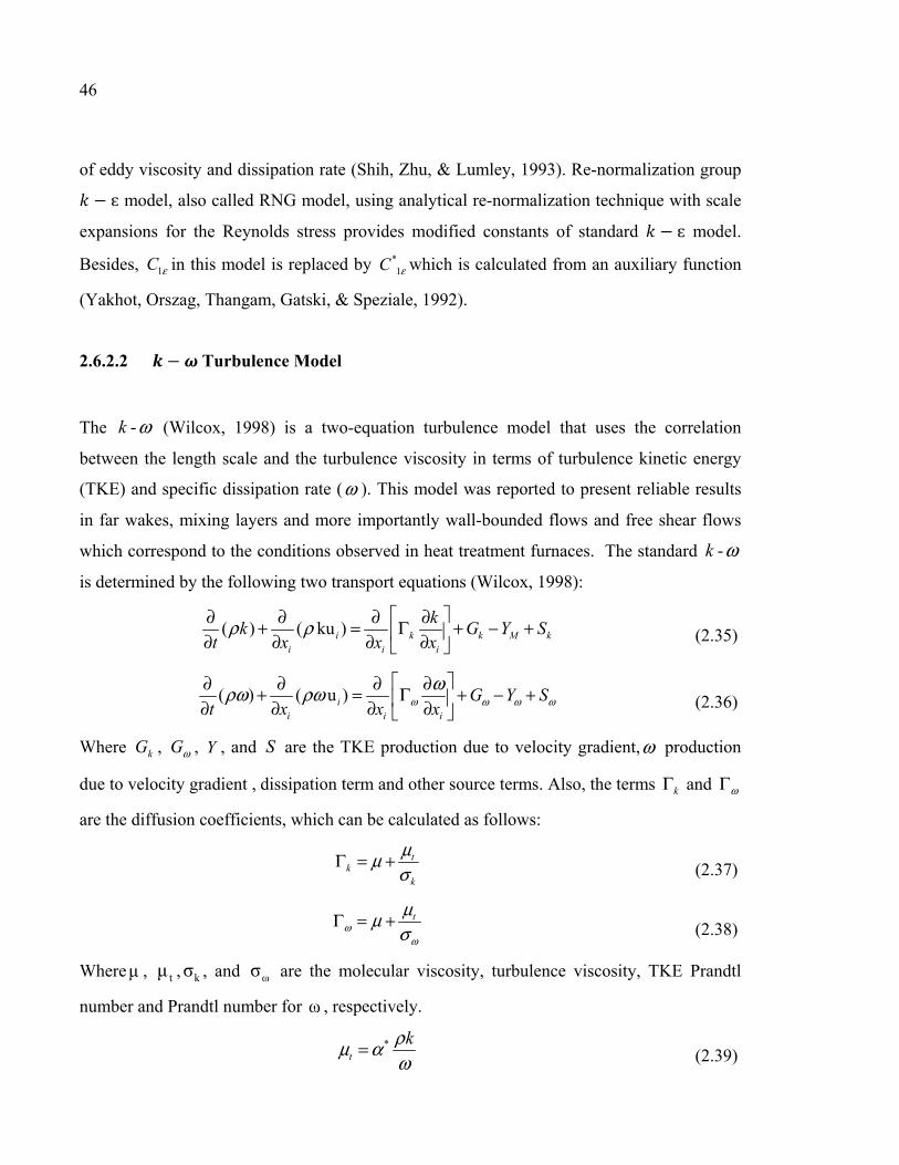
46

of eddy viscosity and dissipation rate (Shih, Zhu, & Lumley, 1993). Re-normalization group 𝑘 − ɛ model, also called RNG model, using analytical re-normalization technique with scale

expansions for the Reynolds stress provides modified constants of standard 𝑘 − ɛ model.

Besides, 1C ε in this model is replaced by *1C ε which is calculated from an auxiliary function

(Yakhot, Orszag, Thangam, Gatski, & Speziale, 1992).

2.6.2.2 𝒌 − 𝝎 Turbulence Model

The -k ω (Wilcox, 1998) is a two-equation turbulence model that uses the correlation

between the length scale and the turbulence viscosity in terms of turbulence kinetic energy

(TKE) and specific dissipation rate (ω ). This model was reported to present reliable results

in far wakes, mixing layers and more importantly wall-bounded flows and free shear flows

which correspond to the conditions observed in heat treatment furnaces. The standard -k ω

is determined by the following two transport equations (Wilcox, 1998):

( ) ( ku )i k k M ki i i

kk G Y St x x x

ρ ρ ∂ ∂ ∂ ∂+ = Γ + − + ∂ ∂ ∂ ∂

(2.35)

( ) ( u )ii i i

G Y St x x xω ω ω ω

ωρω ρω ∂ ∂ ∂ ∂+ = Γ + − + ∂ ∂ ∂ ∂

(2.36)

Where kG , Gω , Y , and S are the TKE production due to velocity gradient,ω production

due to velocity gradient , dissipation term and other source terms. Also, the terms kΓ and ωΓ

are the diffusion coefficients, which can be calculated as follows:

tk

k

μμσ

Γ = + (2.37)

tω

ω

μμσ

Γ = + (2.38)

Whereμ , tμ , kσ , and ωσ are the molecular viscosity, turbulence viscosity, TKE Prandtl

number and Prandtl number for ω , respectively.

*t

kρμ αω

= (2.39)

47

Where α* has the same role and meaning as Cµ in Eq. (2.32). In the -k ω model, α* is

calculated dynamically to provide a better compatibility with low Reynolds regions. Another

-k ω model that is modified to account for the transport of the principal turbulent shear

stress, is Shear-stress transport (SST) 𝑘 − 𝜔 model (Menter, 1994). This model has a

blending function to use the capabilities of near wall region of standard 𝑘 − 𝜔 model with

the free-stream independence of the 𝑘 − ɛ model in the far field. The definition of turbulent

viscosity as well as modeling constant is modified in SST 𝑘 − 𝜔 model with respect to

standard 𝑘 − 𝜔 model (Menter, 1994).

2.6.2.3 Reynolds Stress Model (RSM)

The Reynlods stress model (Cant, 2001; Launder, Reece, & Rodi, 1975) is one of the most

elaborate turbulence models and is the most physically sound RANS based model. In two

equation models, the turbulent viscosity is calculated using empirical or theoretical

correlations between turbulence kinetic energy and eddy dissipation rate for specific flow

conditions. The RSM model, on the other hand, solves all Reynolds stresses and turbulence

dissipation instead of using eddy-viscosity concept. Thereby, RSM solves seven turbulence

transport equations for three dimensional flows, considering the turbulence anisotropy (in

contrast to two equation models which assume isotropic turbulence field). This model is

more accurate for prediction of complex flows involving swirl, rotation and rapid changes

that correspond to the gas-fired heat treatment furnaces which use high momentum burners

and have a self-induced turbulence in the treatment chamber (Cant, 2001).

2.6.3 Comparison between Turbulence Modeling Approaches

Fig. 2.1 presents an overall illustration of comparison between above mentioned turbulence

modeling approaches from the computational cost point of view.

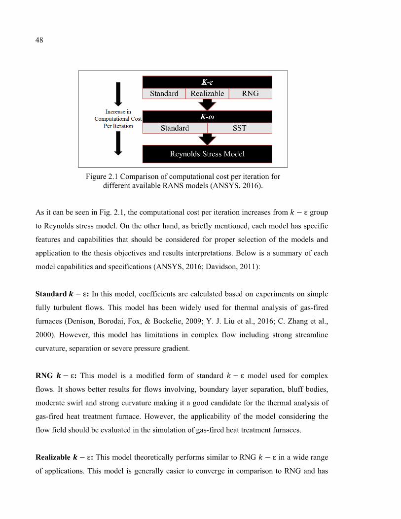
48

Figure 2.1 Comparison of computational cost per iteration for different available RANS models (ANSYS, 2016).

As it can be seen in Fig. 2.1, the computational cost per iteration increases from 𝑘 − ɛ group

to Reynolds stress model. On the other hand, as briefly mentioned, each model has specific

features and capabilities that should be considered for proper selection of the models and

application to the thesis objectives and results interpretations. Below is a summary of each

model capabilities and specifications (ANSYS, 2016; Davidson, 2011):

Standard 𝒌 − ɛ: In this model, coefficients are calculated based on experiments on simple

fully turbulent flows. This model has been widely used for thermal analysis of gas-fired

furnaces (Denison, Borodai, Fox, & Bockelie, 2009; Y. J. Liu et al., 2016; C. Zhang et al.,

2000). However, this model has limitations in complex flow including strong streamline

curvature, separation or severe pressure gradient.

RNG 𝒌 − ɛ: This model is a modified form of standard 𝑘 − ɛ model used for complex

flows. It shows better results for flows involving, boundary layer separation, bluff bodies,

moderate swirl and strong curvature making it a good candidate for the thermal analysis of

gas-fired heat treatment furnace. However, the applicability of the model considering the

flow field should be evaluated in the simulation of gas-fired heat treatment furnaces.

Realizable 𝒌 − ɛ: This model theoretically performs similar to RNG 𝑘 − ɛ in a wide range

of applications. This model is generally easier to converge in comparison to RNG and has

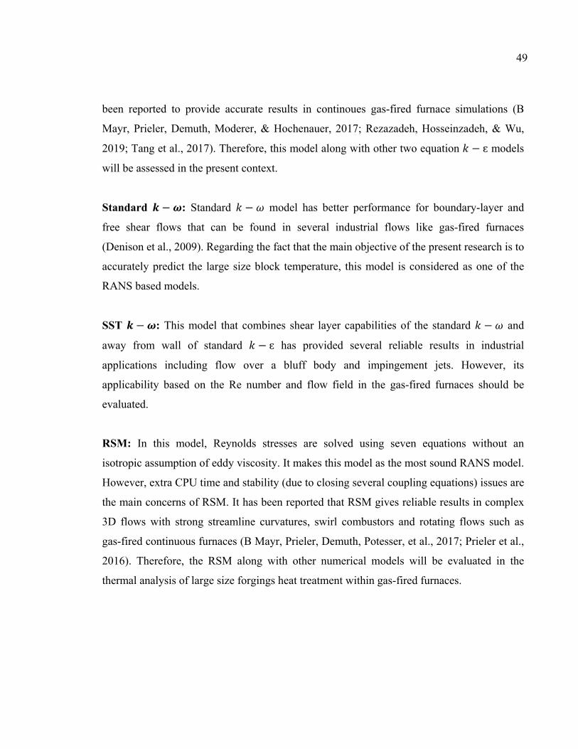
49

been reported to provide accurate results in continoues gas-fired furnace simulations (B

Mayr, Prieler, Demuth, Moderer, & Hochenauer, 2017; Rezazadeh, Hosseinzadeh, & Wu,

2019; Tang et al., 2017). Therefore, this model along with other two equation 𝑘 − ɛ models

will be assessed in the present context.

Standard 𝒌 − 𝝎: Standard 𝑘 − 𝜔 model has better performance for boundary-layer and

free shear flows that can be found in several industrial flows like gas-fired furnaces

(Denison et al., 2009). Regarding the fact that the main objective of the present research is to

accurately predict the large size block temperature, this model is considered as one of the

RANS based models.

SST 𝒌 − 𝝎: This model that combines shear layer capabilities of the standard 𝑘 − 𝜔 and

away from wall of standard 𝑘 − ɛ has provided several reliable results in industrial

applications including flow over a bluff body and impingement jets. However, its

applicability based on the Re number and flow field in the gas-fired furnaces should be

evaluated.

RSM: In this model, Reynolds stresses are solved using seven equations without an

isotropic assumption of eddy viscosity. It makes this model as the most sound RANS model.

However, extra CPU time and stability (due to closing several coupling equations) issues are

the main concerns of RSM. It has been reported that RSM gives reliable results in complex

3D flows with strong streamline curvatures, swirl combustors and rotating flows such as

gas-fired continuous furnaces (B Mayr, Prieler, Demuth, Potesser, et al., 2017; Prieler et al.,

2016). Therefore, the RSM along with other numerical models will be evaluated in the

thermal analysis of large size forgings heat treatment within gas-fired furnaces.

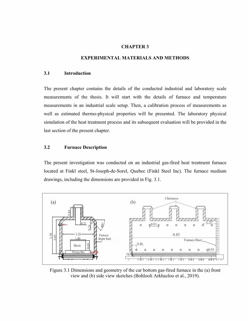
51

CHAPTER 3

EXPERIMENTAL MATERIALS AND METHODS

3.1 Introduction

The present chapter contains the details of the conducted industrial and laboratory scale

measurements of the thesis. It will start with the details of furnace and temperature

measurements in an industrial scale setup. Then, a calibration process of measurements as

well as estimated thermo-physical properties will be presented. The laboratory physical

simulation of the heat treatment process and its subsequent evaluation will be provided in the

last section of the present chapter.

3.2 Furnace Description

The present investigation was conducted on an industrial gas-fired heat treatment furnace

located at Finkl steel, St-Joseph-de-Sorel, Quebec (Finkl Steel Inc). The furnace medium

drawings, including the dimensions are provided in Fig. 3.1.

Figure 3.1 Dimensions and geometry of the car bottom gas-fired furnace in the (a) front view and (b) side view sketches (Bohlooli Arkhazloo et al., 2019).

52

Internal dimensions of the furnace in 𝑋, 𝑌 , and 𝑍 directions were 3.05 (m), 3.28 (m), and

8.83 (m), respectively. The furnace has 18 high-velocity Tempest cup burners (Fives North

American Combustion, Inc.) located on the two sides of the furnace, along the Z direction

with nine burners on the upper section of the furnace left wall, (upper burners) and the nine

other in the lower section of the right wall (lower burners). This asymmetric arrangement

improves temperature uniformity by self-induced recirculation and turbulence. Nine skids are

positioned between the burners for placing the forged blocks.

Figure 3.2 Self-induced turbulence within the gas-fired furnace (Pyradia Inc.).

The furnace temperature during the experimental measurements was controlled using

a Honeywell UDC 2500 PID controlling system. PID controller divided the furnace length

into three similar zones and by controlling the gas flow rate in each zone balanced the

geometrical effects (door or back-wall) on the temperature variations in these zones. It

allowed considering the one-third Periodic modeling of the furnace which is discussed in

chapter 6. Fig. 3.3 shows the three zones of the furnace and periodic lines considered in the

methodology of chapter 6.

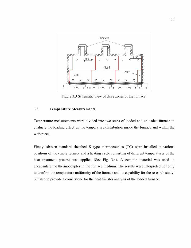
53

Figure 3.3 Schematic view of three zones of the furnace.

3.3 Temperature Measurements

Temperature measurements were divided into two steps of loaded and unloaded furnace to

evaluate the loading effect on the temperature distribution inside the furnace and within the

workpiece.

Firstly, sixteen standard sheathed K type thermocouples (TC) were installed at various

positions of the empty furnace and a heating cycle consisting of different temperatures of the

heat treatment process was applied (See Fig. 3.4). A ceramic material was used to

encapsulate the thermocouples in the furnace medium. The results were interpreted not only

to confirm the temperature uniformity of the furnace and its capability for the research study,

but also to provide a cornerstone for the heat transfer analysis of the loaded furnace.

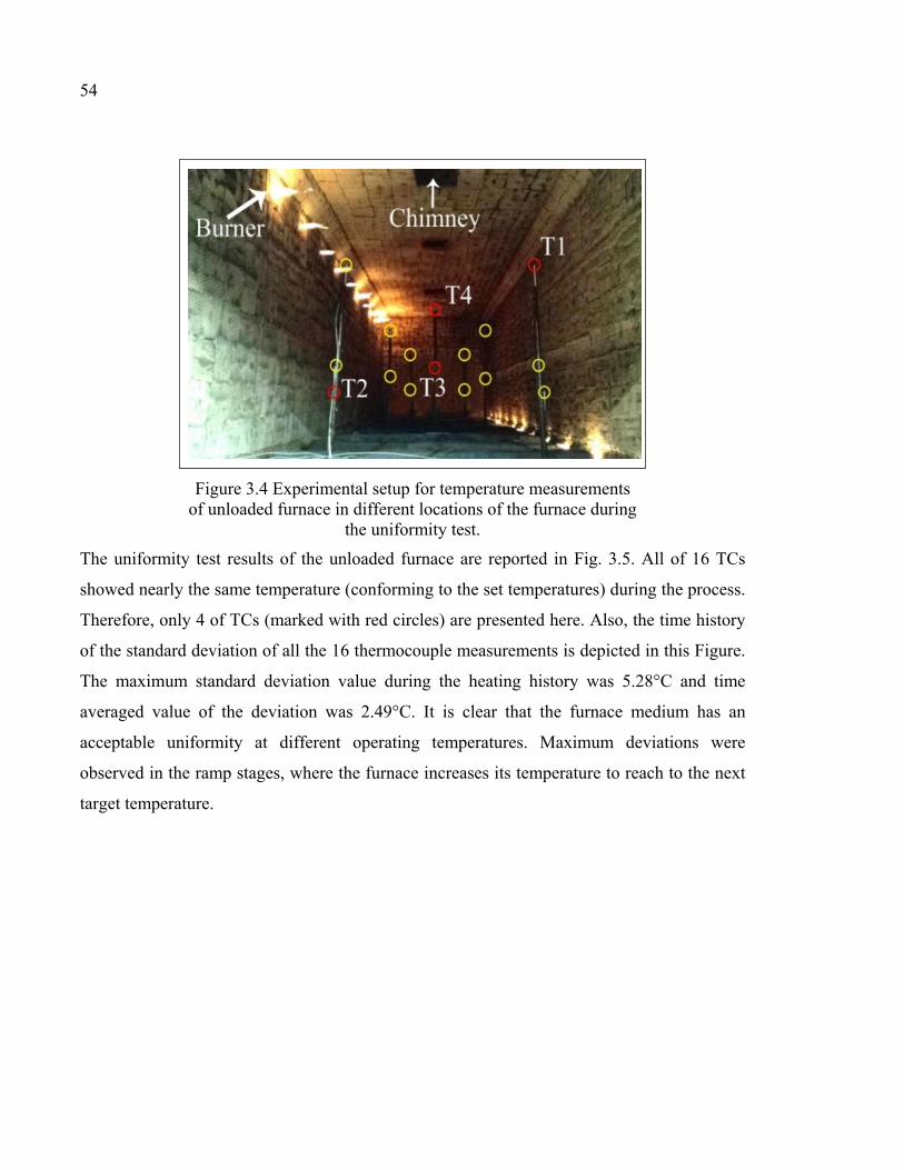
54

Figure 3.4 Experimental setup for temperature measurements of unloaded furnace in different locations of the furnace during

the uniformity test. The uniformity test results of the unloaded furnace are reported in Fig. 3.5. All of 16 TCs

showed nearly the same temperature (conforming to the set temperatures) during the process.

Therefore, only 4 of TCs (marked with red circles) are presented here. Also, the time history

of the standard deviation of all the 16 thermocouple measurements is depicted in this Figure.

The maximum standard deviation value during the heating history was 5.28°C and time

averaged value of the deviation was 2.49°C. It is clear that the furnace medium has an

acceptable uniformity at different operating temperatures. Maximum deviations were

observed in the ramp stages, where the furnace increases its temperature to reach to the next

target temperature.

55

Figure 3.5 Temperature profile of furnace uniformity test and associated standard deviation.

In the loaded furnace, step of the temperature measurements, transient temperature evolution

of a 1.4 × 0.89 ×2.72 (m3) forged ingot was recorded by placing 11 K-type thermocouples at

different locations of the block. TCs were installed at different surfaces of the forged block to

evaluate and analyze the heating pattern around the workpiece. To ensure a solid attachment

of all TCs, small holes (with the depth of 1(cm)) were drilled and thermocouples were solidly

embedded at the bottom of the holes. The empty space of the hole was filled with iron

powder of the same steel and the top of the hole was sealed with iron cement and a fixing

screw (See Fig. 3.6). The standard accuracy of the K-type thermocouples with a stainless

steel sheath according to ISA Standard is equal to ± 6.63 K (ISA Standard, 1982), for the

furnace operating temperature ranges.

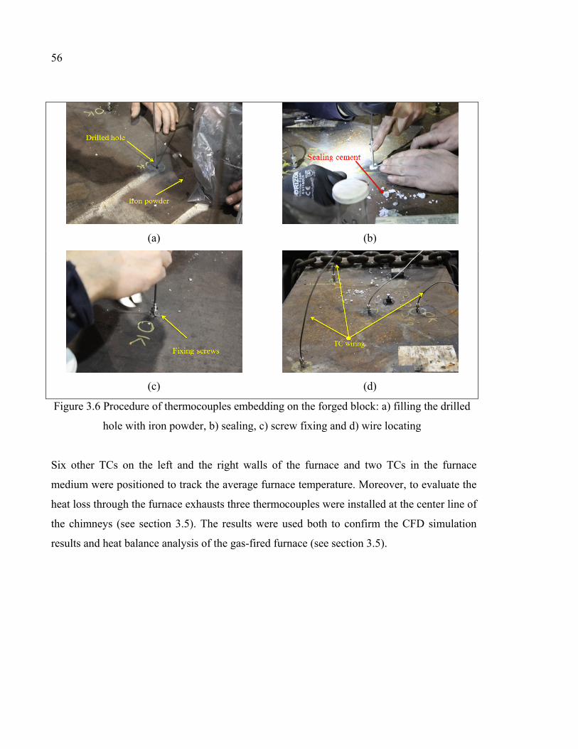
56

(a)

(b)

(c)

(d)

Figure 3.6 Procedure of thermocouples embedding on the forged block: a) filling the drilled

hole with iron powder, b) sealing, c) screw fixing and d) wire locating

Six other TCs on the left and the right walls of the furnace and two TCs in the furnace

medium were positioned to track the average furnace temperature. Moreover, to evaluate the

heat loss through the furnace exhausts three thermocouples were installed at the center line of

the chimneys (see section 3.5). The results were used both to confirm the CFD simulation

results and heat balance analysis of the gas-fired furnace (see section 3.5).

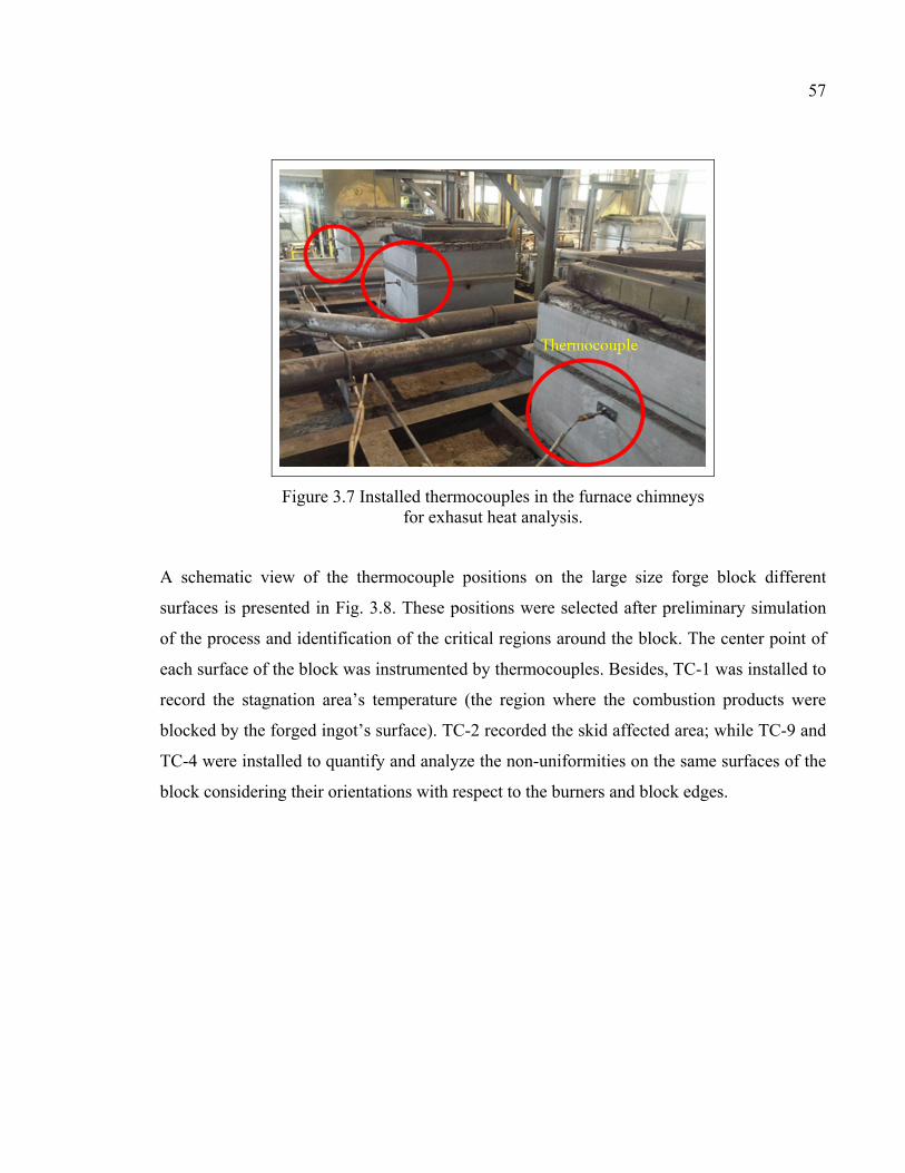
57

Figure 3.7 Installed thermocouples in the furnace chimneys for exhasut heat analysis.

A schematic view of the thermocouple positions on the large size forge block different

surfaces is presented in Fig. 3.8. These positions were selected after preliminary simulation

of the process and identification of the critical regions around the block. The center point of

each surface of the block was instrumented by thermocouples. Besides, TC-1 was installed to

record the stagnation area’s temperature (the region where the combustion products were

blocked by the forged ingot’s surface). TC-2 recorded the skid affected area; while TC-9 and

TC-4 were installed to quantify and analyze the non-uniformities on the same surfaces of the

block considering their orientations with respect to the burners and block edges.

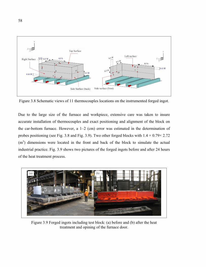
58

Figure 3.8 Schematic views of 11 thermocouples locations on the instrumented forged ingot.

Due to the large size of the furnace and workpiece, extensive care was taken to insure

accurate installation of thermocouples and exact positioning and alignment of the block on

the car-bottom furnace. However, a 1–2 (cm) error was estimated in the determination of

probes positioning (see Fig. 3.8 and Fig. 3.9). Two other forged blocks with 1.4 × 0.79× 2.72

(m3) dimensions were located in the front and back of the block to simulate the actual

industrial practice. Fig. 3.9 shows two pictures of the forged ingots before and after 24 hours

of the heat treatment process.

Figure 3.9 Forged ingots including test block: (a) before and (b) after the heat treatment and opining of the furnace door.

59

3.4 Flow Measurements

In the present study, gas flow metering were conducted using three pressure transducers

along with a mini-max Honeywell electronic gas volume correctors installed on the furnace.

Also, three pressure transducers were installed in three different zones of the furnace to

measure the air usage for the burners’ combustion. During the heat treatment process, the

furnace was working under 5% excess air.

Figure 3.10 Installed flow metering devices on the gas-fired furnace burners to measure gas consumption.

3.5 Calibration Test

A set of calibration test was conducted on a small size block before the real scale

measurements of the present study. The aim was to calibrate the measurement devices as

well as measurement procedure. Besides, evaluation of thermo-physical properties predicted

by the JMatPro software (Saunders, Guo, Li, Miodownik, & Schillé, 2003) and furnace

performance (through calculation of wall and chimney’s heat losses) were other objectives of

this set of experimental measurements.

Due to the difficulties in temperature measurement of the large size block’s center with the

elaborated measurement techniques (vulnerability to cracks), a small size forged ingot was

selected for this setup. The studied test block was a 0.51×0.77×1.03 (m3) forged ingot with

the same chemical composition of the project’s steel. The chemical composition of the high-

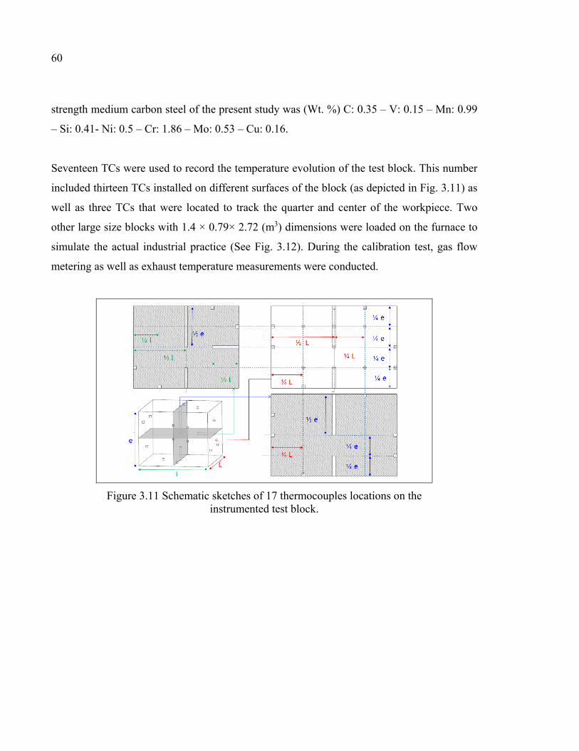
60

strength medium carbon steel of the present study was (Wt. %) C: 0.35 – V: 0.15 – Mn: 0.99

– Si: 0.41- Ni: 0.5 – Cr: 1.86 – Mo: 0.53 – Cu: 0.16.

Seventeen TCs were used to record the temperature evolution of the test block. This number

included thirteen TCs installed on different surfaces of the block (as depicted in Fig. 3.11) as

well as three TCs that were located to track the quarter and center of the workpiece. Two

other large size blocks with 1.4 × 0.79× 2.72 (m3) dimensions were loaded on the furnace to

simulate the actual industrial practice (See Fig. 3.12). During the calibration test, gas flow

metering as well as exhaust temperature measurements were conducted.

Figure 3.11 Schematic sketches of 17 thermocouples locations on the instrumented test block.

61

Figure 3.12 Instrumented test block loaded on the car-bottom furnace.

3.5.1 Block Measurements and Conductivity Calibration

To calibrate the measurement procedure and also validate the thermo-physical properties

estimated by JMatPro software a 3D thermal transient FEM model of the test block was

generated in ANSYS software. The experimentally measured temperatures at the surface of

the test block were imposed as the boundary conditions to the model including 129406

tetrahedron elements. Thermo-physical properties estimated by the JMatPro software

(depicted in Fig. 3.13) were used in the material properties specification of the model.

Results of the numerically predicted transient temperature history of the test block’s center

and corresponding experimentally measured temperature in the calibration test are presented

in Fig. 3.14.

62

Figure 3.13 Temperature dependant thermo-physical properties of the ingot estimated by JMatPro.

Figure 3.14 Comparison between numerically predicted and measured temperature evolution of test block’s center point.

Results showed a good agreement between the FEM predictions and experimental

measurements with a maximum deviation of 2.3%. The difference between the experimental

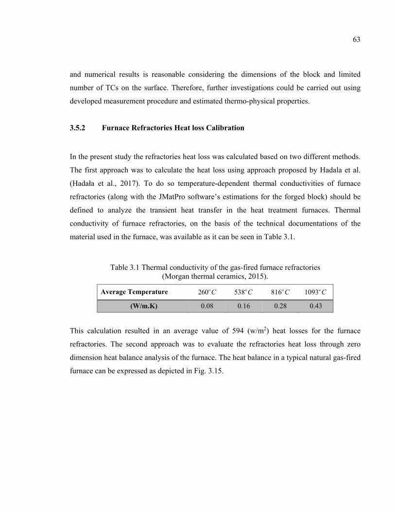
63

and numerical results is reasonable considering the dimensions of the block and limited

number of TCs on the surface. Therefore, further investigations could be carried out using

developed measurement procedure and estimated thermo-physical properties.

3.5.2 Furnace Refractories Heat loss Calibration

In the present study the refractories heat loss was calculated based on two different methods.

The first approach was to calculate the heat loss using approach proposed by Hadala et al.

(Hadała et al., 2017). To do so temperature-dependent thermal conductivities of furnace

refractories (along with the JMatPro software’s estimations for the forged block) should be

defined to analyze the transient heat transfer in the heat treatment furnaces. Thermal

conductivity of furnace refractories, on the basis of the technical documentations of the

material used in the furnace, was available as it can be seen in Table 3.1.

Table 3.1 Thermal conductivity of the gas-fired furnace refractories (Morgan thermal ceramics, 2015).

Average Temperature 260o C 538o C 816o C 1093o C

(W/m.K) 0.08 0.16 0.28 0.43

This calculation resulted in an average value of 594 (w/m2) heat losses for the furnace

refractories. The second approach was to evaluate the refractories heat loss through zero

dimension heat balance analysis of the furnace. The heat balance in a typical natural gas-fired

furnace can be expressed as depicted in Fig. 3.15.

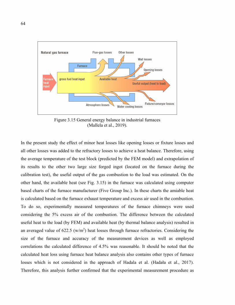
64

Figure 3.15 General energy balance in industrial furnaces (Mallela et al., 2019).

In the present study the effect of minor heat losses like opening losses or fixture losses and

all other losses was added to the refractory losses to achieve a heat balance. Therefore, using

the average temperature of the test block (predicted by the FEM model) and extrapolation of

its results to the other two large size forged ingot (located on the furnace during the

calibration test), the useful output of the gas combustion to the load was estimated. On the

other hand, the available heat (see Fig. 3.15) in the furnace was calculated using computer

based charts of the furnace manufacturer (Five Group Inc.). In these charts the amiable heat

is calculated based on the furnace exhaust temperature and excess air used in the combustion.

To do so, experimentally measured temperatures of the furnace chimneys were used

considering the 5% excess air of the combustion. The difference between the calculated

useful heat to the load (by FEM) and available heat (by thermal balance analysis) resulted in

an averaged value of 622.5 (w/m2) heat losses through furnace refractories. Considering the

size of the furnace and accuracy of the measurement devices as well as employed

correlations the calculated difference of 4.5% was reasonable. It should be noted that the

calculated heat loss using furnace heat balance analysis also contains other types of furnace

losses which is not considered in the approach of Hadala et al. (Hadała et al., 2017).

Therefore, this analysis further confirmed that the experimental measurement procedure as

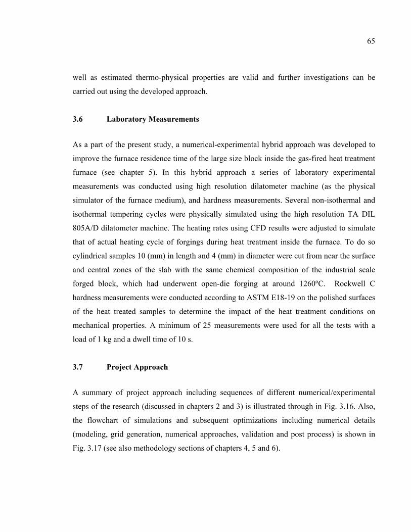
65

well as estimated thermo-physical properties are valid and further investigations can be

carried out using the developed approach.

3.6 Laboratory Measurements

As a part of the present study, a numerical-experimental hybrid approach was developed to

improve the furnace residence time of the large size block inside the gas-fired heat treatment

furnace (see chapter 5). In this hybrid approach a series of laboratory experimental

measurements was conducted using high resolution dilatometer machine (as the physical

simulator of the furnace medium), and hardness measurements. Several non-isothermal and

isothermal tempering cycles were physically simulated using the high resolution TA DIL

805A/D dilatometer machine. The heating rates using CFD results were adjusted to simulate

that of actual heating cycle of forgings during heat treatment inside the furnace. To do so

cylindrical samples 10 (mm) in length and 4 (mm) in diameter were cut from near the surface

and central zones of the slab with the same chemical composition of the industrial scale

forged block, which had underwent open-die forging at around 1260oC. Rockwell C

hardness measurements were conducted according to ASTM E18-19 on the polished surfaces

of the heat treated samples to determine the impact of the heat treatment conditions on

mechanical properties. A minimum of 25 measurements were used for all the tests with a

load of 1 kg and a dwell time of 10 s.

3.7 Project Approach

A summary of project approach including sequences of different numerical/experimental

steps of the research (discussed in chapters 2 and 3) is illustrated through in Fig. 3.16. Also,

the flowchart of simulations and subsequent optimizations including numerical details

(modeling, grid generation, numerical approaches, validation and post process) is shown in

Fig. 3.17 (see also methodology sections of chapters 4, 5 and 6).

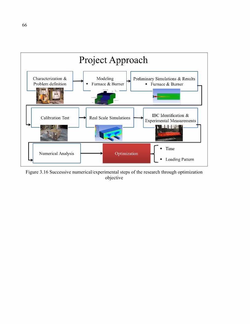
66

Figure 3.16 Successive numerical/experimental steps of the research through optimization objective

67

Figure 3.17 CFD simulations and subsequent optimization flowchart

69

CHAPTER 4

EXPERIMENTAL AND UNSTEADY CFD ANALYSES OF THE HEATING PROCESS OF LARGE SIZE FORGINGS IN A GAS FIRED FURNACE

Nima Bohlooli Arkhazlooa,*, Yassine Bouissaa, Farzad Bazdidi-Tehranib, Mohammad Jadidib, Jean-Benoît Morinc and Mohammad Jahazia

a Département de Génie Mécanique, École de Technologie Supérieure, Montréal, Québec, Canada H3C 1K3,

b School of Mechanical Engineering, Iran University of Science and Technology, Tehran, Iran 16846-13114

c Finkl Steel Inc., 100 McCarthy, Saint-Joseph-de-Sorel, Québec, Canada J3R 3M8

Paper published in Case Studies in Thermal Engineering, February 2019,

Abstract Comprehensive unsteady analysis of large size forged blocks heating characteristics in a gas-

fired heat treatment furnace was carried out employing experimentally measured

temperatures and computational fluid dynamics (CFD) simulations. Heat and fluid flow

interactions, consisting of turbulence, radiation and combustion, were simultaneously

considered using 𝑘 − ɛ, DO and EDM models in a three dimensional CFD model of the

furnace, respectively. Applicability of the S2S radiation model was also evaluated to quantify

the effect of participating medium and radiation view factor in the radiation heat transfer.

Temperature measurements at several locations of an instrumented large size forged block

and the furnace chamber were performed. A maximum deviation of about 7% was obtained

between the model predictions and the experimental measurements. Results showed that

despite the unloaded furnace had uniform temperature distribution, after loading, product

surfaces experienced different heating rates, resulting in temperature differences up to 200 K.

Findings were correlated with furnace geometry, vortical structures and flow circulations

around the workpiece. Besides, S2S model demonstrating reliable results highlighted the

70

importance of radiation view factor optimization in this application. The study could directly

be employed for optimization of the heat treatment process of large size steel components.

Keywords: Heat treatment, CFD simulation, Gas-fired furnace, Temperature measurement,

Heating uniformity, Radiation modeling

Nomenclature Latin symbols a Absorption coefficient 𝐸 Energy Fkj View factor between surface 𝑘 and surface j g Gravity ( 2/m s )

ziJ Diffusive flux of chemical species

h Enthalpy ( /J kg ) I Radiation intensity k Turbulence kinetic energy ( 2 2/m s ) keff Effective conductivity 𝑚 Mass flux ( 2/ m .kg s ) n Refractive index p Pressure (Pa)

iq , The generic source term

rq Reaction heat term 𝑟 Position vector zR Production rate of thz component

,z rR Production rate of thz component in the reaction

Re Reynolds number (ud μ ) Sc Schmidt number

zS Source term of thz component s Path length sr Direction vector s′r Scattering direction vector t Time (s)

Tt Total heat treatment time (s)

71

T Temperature (K) iu Reynolds-averaged velocity in tensor notation iu′ Resolved fluctuating velocity components

Y Mass fraction of species X, Y, Z Direction of coordinate axes Greek symbols ε Turbulence dissipation rate ( 2 3/m s )

kε Surface emissivity ′Ω Solid angle


tμ Turbulence eddy viscosity( . /kg m s ) σ Stefan-Boltzmann constant

sσ Scattering coefficient ρ Density ( 3/kg m )

kρ Surface reflectivity ' 'i ju uρ Reynolds stress ( 2/ m.kg s )

Superscripts ' Fluctuations with respect to a Reynolds averaging Subscripts eff Effective , ,i j k Tonsorial indices

z thz species Abbreviation 3D Three dimensional CFD Computational Fluid Dynamics DO Discrete ordinates model S2S Surface to surface

72

4.1 Introduction

A significant number of high strength steel parts used for critical applications in energy and

transportation industries acquire their required properties through a sequence of heat

treatment processes often called Quench and Temper (Q&T) (Totten, 2006). The heating

process is one of the most important steps since major microstructural changes (grain

refinement, phase transformation, etc.) take place, that have a direct impact on the final

mechanical properties (Kang and Rong, 2006). Hence, heat transfer from the furnace to the

work piece, which fundamentally depends on the temperature distribution inside the furnace,

significantly influences the quality of the final product (Gao et al., 2000). The process

becomes more critical when it comes to the heat treatment of large size parts, such as turbine

shafts. Specifically, a non-uniform temperature distribution may result in local changes in the

microstructure, leading to non-uniform properties in different locations of the final part.

Therefore, accurate temperature prediction of the parts necessitates a quantitative analysis of

the transient heating and an understanding of thermal interactions within the furnace.

Comprehending the complexities of the thermal field, along with the turbulent fluid flow

inside the heat treatment furnace is very challenging. Complicated load-gas-furnace thermal

interactions, including transient convection-radiation heat transfer, impose strong non-linear

thermal boundary conditions to the load. Chapman et al. (Chapman et al., 1990) employed

analytical and Gao et al. (Gao et al., 2000) used semi analytical methods, to develop general

correlations for the heat treatment schedule and temperature evolution of products. However,

analytical studies are generally limited to linear problems and become very complex when

non-linear transient conditions or interactions between phenomena are included. On the other

hand, experimental measurements in this particular field of study are very challenging;

especially, in the case of large size products, reliable data acquisition during the process is

more complex.

Therefore, numerical methods such as computational fluid dynamics (CFD) offering

simultaneous analysis of turbulent fluid flow, combustion and conjugate heat transfer could

73

be an excellent tool for simulating and subsequently optimizing the heat treatment process.

3D full scale numerical models are critical in the implementation process of smart

manufacturing technology’s (Industry 4.0) practices. Different furnaces such as electrically

heated or gas quenching furnaces have been studied using CFD (Cosentino et al., 2013; Hao

et al., 2008; J. Wang et al., 2008). However, among the above furnaces, the simulation of the

heat treatment in gas-fired furnaces are more complex due to reactive flow combined with

turbulent transport and conjugate heat transfer including absorbing and emitting hot

combustion products. Inherently, the problem is more acute when it comes to large size

furnaces and therefore little data is available in the scientific literature. Recently, Liu et al.

(Y. J. Liu et al., 2016) using CFD, proposed a basic model for increasing the uniformity in

continues gas-fired furnaces. Mayr et al. (B Mayr, Prieler, Demuth, Moderer, et al., 2017)

used a one-step steady state CFD approach and Tang et al. (Tang et al., 2018) a combination

of 3D CFD and 2D finite difference methods to predict temperature evolution in pusher type

gas-fired furnaces. However, very little data is available on large size batch type furnaces.

Besides, most of the experimental studies have been used as a validation tool of the

simulation. The limited published studies have been devoted to one aspect of the process

(i.e., burner positions, furnace chamber, or product heating characteristics). For example,

Danon et al. (Danon et al., 2011) assessed burner positioning effects on the performance of

multi-burner combustion furnace and Galletti et al. (Galletti et al., 2013) mainly focused on

different combustion models for the burner simulation inside a semi-industrial furnace.

Prieler et al. (Prieler et al., 2015) employing experimental validation demonstrated the

applicability of CFD for combustion modeling of flat burners in a lab-scale heat treatment

furnace. Recently, Mayr et al. (B. Mayr, Prieler, Demuth, Potesser, et al., 2017) presented a

combustion model, with lower computational demand, for semi-industrial gas-fired furnaces.

The objective of the present study is therefore to carry out a comprehensive analysis of heat

transfer in the heat treatment process of forged blocks in a large size gas-fired furnace

employing both experimental measurements and CFD simulation. The experimental data was

generated through the instrumentation of the furnace chamber (loaded and unloaded) as well

as the different surfaces of the block during the heat treatment process. Unsteady CFD

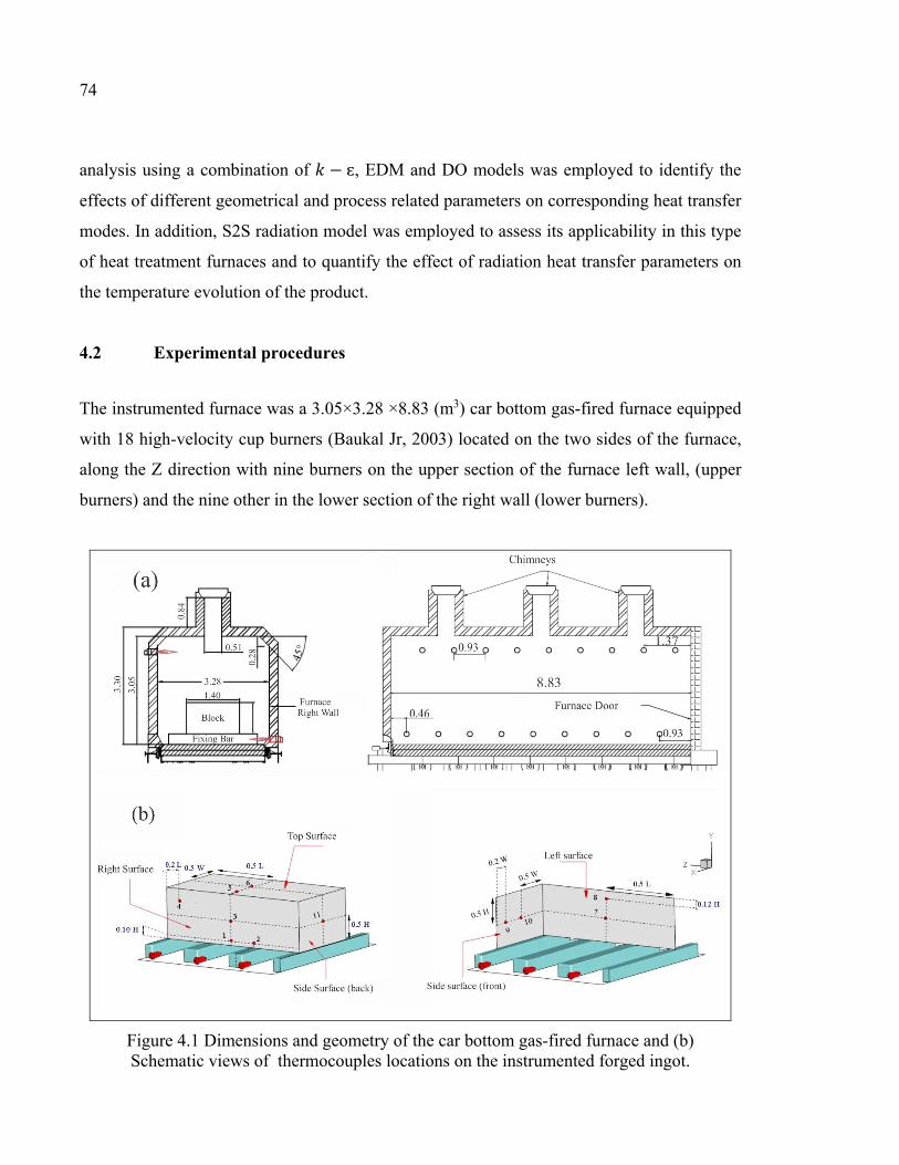
74

analysis using a combination of 𝑘 − ɛ, EDM and DO models was employed to identify the

effects of different geometrical and process related parameters on corresponding heat transfer

modes. In addition, S2S radiation model was employed to assess its applicability in this type

of heat treatment furnaces and to quantify the effect of radiation heat transfer parameters on

the temperature evolution of the product.

4.2 Experimental procedures

The instrumented furnace was a 3.05×3.28 ×8.83 (m3) car bottom gas-fired furnace equipped

with 18 high-velocity cup burners (Baukal Jr, 2003) located on the two sides of the furnace,

along the Z direction with nine burners on the upper section of the furnace left wall, (upper

burners) and the nine other in the lower section of the right wall (lower burners).

Figure 4.1 Dimensions and geometry of the car bottom gas-fired furnace and (b) Schematic views of thermocouples locations on the instrumented forged ingot.

75

Under ideal operational conditions, the burner flame length and the combustion product

velocity at the exit of burner should be 0.508 (m) and 107 (m/s), respectively. Nine fixing

bars with a cross section of 0.25 (m) × 0.25 (m) and a length of 2.60 (m) are positioned

between the burners for placing the forged ingots. The furnace was operated under a positive

pressure of approximately 0.2 (mbar) to minimize any air entry. The furnace medium

drawings, including the dimensions are provided in Fig. 4.1 (a). Experimental measurements

were divided into two steps of loaded and unloaded furnace to evaluate the loading effect on

the temperature distribution inside the furnace and on the forged block. Sixteen-standard

sheathed K-type thermocouples (TC) were installed at different positions of the unloaded

furnace; and temperature evolution during an entire heat treatment cycle (i.e. heating,

isothermal holding, and cooling). The results were used both to confirm the temperature

uniformity of the furnace and to provide a basis for the heat transfer analysis of the loaded

furnace.

Also, temperature evolution in the loaded furnace was recorded by placing 11 K-type TCs at

different locations of a 1.4 × 0.89 ×2.72 (m3) forged block. These thermocouples were fixed

to the different surfaces of the block to evaluate the heating pattern around the workpiece

(See Fig. 1(b)). To ensure a solid attachment of all TCs, small holes were drilled and TCs

were solidly embedded at the bottom of the holes. The empty space of the hole was filled

with iron powder of the same steel and the top of the hole was sealed with iron cement and a

fixing screw. The standard accuracy of the K-type thermocouples with a stainless steel sheath

is equal to 0.75 T± × (ISA Standard, 1982), which corresponds to an accuracy of ±6.63 (K)

for the furnace operating temperature ranges. Considering the large size of the furnace and

workpiece, extensive care was taken to insure accurate installation of the 11 TCs and exact

positioning and alignment of forged ingot on the car-bottom furnace; however, a 1–2 (cm)

error was estimated in the determination of probes positioning. In order to simulate heat

transfer conditions, as close as possible to real operational conditions, two other forged

blocks with 1.4 × 0.79× 2.72 (m3) dimensions were also placed in the front and back of the

instrumented block.

76

4.3 Computational Details

4.3.1 Flow simulation

A transient CFD simulation applying a pressure-based solver was employed to solve the

density weighted Reynolds-averaged Navier-Stokes (RANS) equations, as follows (ANSYS,

2016):

( ) 0uit xi

ρ ρ∂ ∂+ =∂ ∂

(4.1)

( ) ( ) ( )iji i j i j

j i j i

pu u u u u Ft x x x x

τρ ρ ρ

∂∂ ∂ ∂ ∂ ′ ′+ = − + − +∂ ∂ ∂ ∂ ∂

(4.2)

1( ) ( ) ( ) (k ) ( )

n

i i eff z z i ij i s szj j i i j

TE u h u p h J u u h qt x x x x x

ρ ρ τ ρ=

∂ ∂ ∂ ∂ ∂ ∂ ′ ′+ + = − + − +∂ ∂ ∂ ∂ ∂ ∂

r (4.3)

where, the stress tensor, 𝜏 , is given by:

23

ji lij ij

j i l

uu ux x x

τ μ μ δ ∂∂ ∂

= + − ∂ ∂ ∂ (4.4)

and the diffusive flux of combustion product species is defined by the Fick’s law:

t zz

k i

YJSc xμ ∂= −

∂

r

(4.5)

The definition of all the variables and related units are provided in the nomenclature page.

According to the literature (Liu et al., 2014) the two-equation standard -k ε turbulence model

(Launder & Spalding, 1972), could be reliably used to determine the turbulence associated

with the gas combustion in the gas-fired furnaces by solving the additional turbulence kinetic

energy (𝑘) and dissipation rate (ɛ) equations (Launder & Spalding, 1972).

77

4.3.2 Radiation modeling

In the present work, the discrete ordinates (DO) model (Chui & Raithby, 1993) was used to

solve the radiative transfer equation (RTE), Eq. (4.6), considering the absorption and

emission effects.

d I ( ⃗, ⃗)ds

( )sa Iσ+ + (𝑟, 𝑠) 42n

4sTa σσ

π π= +

4

0

Iπ

(𝑟, 𝑠) (𝑟, 𝑠) d ′Ω (4.6)

I is the radiation intensity and ( )sa σ+ is the optical thickness of the medium. Due to the

presence of combustion products the weighted-sum-of-gray-gases model (WSGGM) using

the coefficients provided by Smith et al. (Smith, Shen, & Friedman, 1982) was employed to

compute the radiative properties inside the furnace. For WSGGM model, the domain-based

approach was employed to calculate the mean beam length (ANSYS, 2016).

The applicability of the S2S model, as a computationally effective method in the optically

thin medium, was also evaluated in the present work along with the DO model. The S2S

model assumes any absorption, emission, or scattering of radiation by the medium can be

ignored; thereby, reducing the computational cost by only considering the surface-to-surface

radiation. In this model, the radiation heat transfer to a surface from another surface is a

direct function of the surface-to-surface view factor. Therefore, the radiation energy balance

for each surface follows Eq. (4.7). 4

, ,1

Nout k k k k kj out jj

q T F qε σ ρ=

= + (4.7)

kjF is the view factor between surface 𝑘 and surface j.

4.3.3 Combustion modeling

Combustion inside the burner and furnace domains was modeled using the eddy-dissipation

model (EDM). It should be noted that, because in the gas-fired furnace the burners create

high velocity combustion products, the Arrhenius chemical kinetic calculations were not

considered thereby the computational cost is significantly reduced. In EDM, the species

78

transport formulation for the local mass fraction species (Y ), for the zth species, was solved

assuming that the reaction rates were dominated by turbulence (B. F. Magnussen &

Hjertager, 1977) Therefore, the species transport equation becomes as follows (ANSYS,

2016):

( ) ( ) . .z z z z zY vY J R St

ρ ρ∂ + ∇ = −∇ + +∂

&& (4.8)

where, zR&represents the net production rate of the zth component. In the above equation, the

reaction rate is calculated on the basis of eddy mixing scale, 𝑘/ɛ, and the eddy-break

(Launder & Spalding, 1972).

4.3.4 Numerical simulation procedure and boundary conditions

CFD simulations were carried out using the finite-volume based ANSYS-FLUENT software

(ANSYS, 2016). The unsteady SIMPLE algorithm (H K Versteeg & Malalasekera, 2007)

was applied to 15,155,000 hexahedral non-uniform computational grids as illustrated in Fig.

4.2. Grid value includes 356,000 non-uniform cells in each burner domain (6,408,000 in total

for 18 burners) and finer grids near the burner exit to capture the combustion phenomenon

and heat and fluid flow coming from burners to the furnace domain. Non-uniformly

distributed grids with finer grid sizes near the walls and burner interfaces were employed to

consider the effects imposed by velocity and thermal boundary layers. Also, second order

discretization is used for the simulations. Averaged heat loss of 594 (W/m2), calculated based

on the approach proposed by Hadata et al. (Hadała et al., 2017), was applied to the furnace

walls. The emissivity of the furnace refractories and the steel workpiece were set to 0.75 and

0.8 (corresponding to an oxidized steel surface), respectively. The mass flow inlet boundary

conditions with averaged values of 0.018 (kg/s) and 0.516 (kg/s) were considered for the gas

and air inlets, respectively, while pressure outlet was considered for the chimney exhaust.

Calculations at each time step continued up to a convergence criterion (residual) of 10-5, 10-6,

and 10-9 for the continuity, energy and radiation equations, respectively.

79

Figure 4.2 Computational domain, including: (a) boundary conditions and (b) computational grids.

Table 4.1 Chemical analysis of the test forged ingot used for thermo-physical properties calculation % weight (Finkl Steel Inc.)

C Mn Si Mo Cr Ni Other

0.35 0.85 0.4 0.45 1.85 0.47 Micro-alloying

4.4 Results and Discussion

4.4.1 Experimental Analysis

The uniformity test results of the unloaded furnace showed a very conformity with the

predefined heating pattern with a maximum standard deviation value of 5.28°C during the

ramp stage with the furnace increasing its temperature to reach the target temperature.

80

Therefore, it can be considered that the unloaded furnace presents a good temperature

uniformity over its entire volume during the entire heat treatment cycle.

The measured temperature histories of different locations of the forged block are illustrated

in Fig. 4.3. The results reveal a clear difference in temperature evolution as a function of the

location of the TCs (i.e. considered face and TCs position on the surface).

Figure 4.3 Experimentally measured temperature evolution of TCs on: (a) different surfaces of the forged ingot, (b) left, top and side surfaces, (c) right surface and (d)

their relative temperature differences.

Usually, severity and continuity of the temperature gradient between the surface and the

center of the workpiece is one of the main concerns of steel making industries, as it directly

81

impacts the quality of the final product (Totten, 2006). However, Fig. 4.3 (a) shows that apart

from the temperature gradient inside the workpiece, differences in temperature can also be

found on the surfaces themselves (see Fig. 4.1 for locations of TCs). Although, temperatures

of all TCs on the surfaces ultimately converge to the target pre-defined temperature at the

end of the process, the temperature histories of different points of the forged ingot are not

identical. This variability in the heating history could affect the microstructural

transformations from one end to another end of the product (subsequently its properties), and

needs to be taken into consideration when developing microstructure based models of phase

transformation.

As indicated in Fig. 4.3, it is clear that the TC on the right surface (TC.1), located at a shorter

distance to the burner (lower burners) had higher temperatures in comparison to those of the

left and the top surfaces. Besides, TCs of the side surfaces (TC.10 and TC.11) had the

minimum temperatures during the process. These surfaces, due to their relative positions in

the furnace, were faced with adjacent forged blocks instead of furnace walls or burners; i.e.,

they had limitations regarding any direct thermal radiation from the furnace and due to the

small gap between the blocks, they had relatively smaller radiation view factors from the

furnace parts. Fig. 4.3(b) also shows that among the thermocouples on the other surfaces,

those that are closer to the right surface or product edges (TC.5, TC.8, and TC.9) had higher

values. The edge effect is also visible in Fig. 4.3(c) where it can be seen that TC.4 has

relatively higher temperatures as compared with the TC.3 and TC.2 on the same surface.

Another interesting finding is the relatively lower temperatures of the TC.2, which was

located above the fixing bar on the right surface. Although TC.2 had a relatively short

distance to the burner, in comparison with TC.4 and TC.3, it experienced lower temperatures.

Finally, the temperature differences between selected thermocouples in different faces are

presented in Fig. 4.3(d). It can be seen that the maximum difference between TC.1 (on the

right surface) and TC.10 (on the side surface) could reach up to 200 K. Further, this

difference for TC.1-TC.6 and TC.1-TC.7 could reach up to 140 K and 120 K, respectively.

Considering the previously discussed initial temperature uniformity of the unloaded furnace

82

at different temperatures, the observed non-uniformity could be correlated to the presence of

the forged ingots. Therefore, the transient heating history should be analyzed by considering

both convection and radiation heat transfer modes.

4.4.2 CFD Analysis

To comprehensively analyze the heating patterns, temperature non-uniformities and the share

of each heat transfer mode during the heat treatment process, CFD simulations results are

discussed in this section.

4.4.2.1 Validation

Table 2 shows the distribution of the available heat in different parts of the furnace, obtained

from the CFD analysis. The furnace efficiency was defined by the ratio of the net heat

received by the forged blocks and the available heat input to the furnace (78 GJ) as follows

(B Mayr, Prieler, Demuth, Moderer, et al., 2017):

ingotfurnace

available

QQ

η = (4.9)

Based on the measurements made on the gas flow meters installed on the furnace, furnace

efficiency was estimated to be 36.6%, while the CFD simulation predicted a value of 40.1%,

which are quite close considering the large size of the furnace. The observed difference is

probably due to a combination of factors such as air leakage into the furnace and difference

in the exact location of the TCs between the experimental and modeled conditions, which

cannot be really predicted by the model.

Table 4.2 Predicted heat distribution within the furnace.

Item Ingots Walls Flue Gas Fixing Bars Other Absorbed/lost heat (GJ) 28.08 7.65 25.74 9.2 5.42

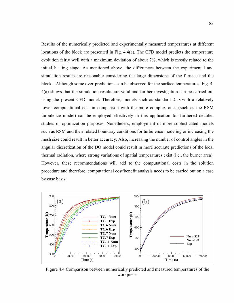
83

Results of the numerically predicted and experimentally measured temperatures at different

locations of the block are presented in Fig. 4.4(a). The CFD model predicts the temperature

evolution fairly well with a maximum deviation of about 7%, which is mostly related to the

initial heating stage. As mentioned above, the differences between the experimental and

simulation results are reasonable considering the large dimensions of the furnace and the

blocks. Although some over-predictions can be observed for the surface temperatures, Fig. 4.

4(a) shows that the simulation results are valid and further investigation can be carried out

using the present CFD model. Therefore, models such as standard -k ε with a relatively

lower computational cost in comparison with the more complex ones (such as the RSM

turbulence model) can be employed effectively in this application for furthered detailed

studies or optimization purposes. Nonetheless, employment of more sophisticated models

such as RSM and their related boundary conditions for turbulence modeling or increasing the

mesh size could result in better accuracy. Also, increasing the number of control angles in the

angular discretization of the DO model could result in more accurate predictions of the local

thermal radiation, where strong variations of spatial temperatures exist (i.e., the burner area).

However, these recommendations will add to the computational costs in the solution

procedure and therefore, computational cost/benefit analysis needs to be carried out on a case

by case basis.

Figure 4.4 Comparison between numerically predicted and measured temperatures of the workpiece.

84

Radiation view factor of the workpiece surfaces and participating medium are the two main

active parameters for the analysis of the radiation heat transfer, in the present application.

The influence of participating medium on the final temperature history was evaluated using

the S2S model and the results are reported in Fig. 4.4(b). It can be seen that, neglecting the

effect of combustion products participation in the absorbed radiation of the workpiece,

characteristic of the S2S model, produces about 1.5% over prediction in comparison to the

DO model. Thus, although DO model provides more accurate predictions, S2S model with

lower computational cost, can be effectively used in this application. Furthermore, because

98.5% of radiation heat transfer is controlled by the radiation view factor of the surfaces,

loading pattern optimization for this type of furnaces can be done only by view factor

optimization when the radiative heat transfer is considered.

4.4.2.2 Analysis of the heating process of the loaded furnace

Transient contours of temperature evolution of the loaded furnace (in an x-y plane) and ingot

surfaces during the heating process are depicted in Fig. 4.5. The simulation results clearly

confirm a non-uniform temperature distribution during the heating process as observed

during the experimental phase (Fig. 4.3). Ingot transient temperature history shows that the

side surfaces have relatively lower temperatures in comparison with the other surfaces.

Gradual heating from the right surface to the left and top surfaces and finally side surfaces is

evident. A maximum temperature difference of about 262 K exists from one side of the

product to the other.

Results of furnace heating history show that the temperature of the furnace starts increasing

from regions close to the burners, and then gradually extends to the center. Similarly, an

increase in temperature begins rapidly on the right side of the block where the lower burners

are located; while the left and side surfaces are heated latterly. Results also indicate that the

fluid in the vicinity of the left surface and the top surface was also heated with delay in

comparison with the right surface where the lower part of the right surface hindered the fluid

85

flow circulation (Fig. 4.5(e)). These findings further confirm the results reported in

experimental measurements.

Figure 4.5 Transient contours of temperature evolution of the forged ingot surfaces and furnace central cross section in 2D and 3D views, respectively.

Fig. 4.6 shows the transient history of average total heat flux, average radiation heat flux and

average surface heat transfer coefficient on the right, left and side surfaces of the workpiece

during the heat treatment process. A considerable difference between the total heat flux rates

in the first period of the process is revealed, which is in direct relation to the identified non-

uniformities (see Figs. 4.3 and 4.4). Both radiation and convection heat transfers modes show

the same identified differences in their transient histories. However, as it can be seen, the

right surface due to the high velocity of burner product, is mainly heated by the convection

heat transfer at the beginning of the process, while for the left surface, radiation heat transfer

plays the most important role due to the blockage of the fluid flow by the workpiece. The

results indicate that heat transfer coefficient in the first part of the process for the side surface

is less than those on the right and left surfaces and in the peak zone its value is 0.32 of the

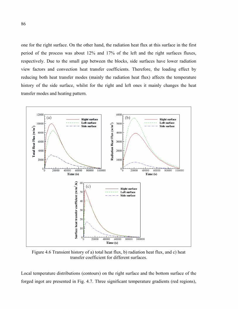
86

one for the right surface. On the other hand, the radiation heat flux at this surface in the first

period of the process was about 12% and 17% of the left and the right surfaces fluxes,

respectively. Due to the small gap between the blocks, side surfaces have lower radiation

view factors and convection heat transfer coefficients. Therefore, the loading effect by

reducing both heat transfer modes (mainly the radiation heat flux) affects the temperature

history of the side surface, whilst for the right and left ones it mainly changes the heat

transfer modes and heating pattern.

Figure 4.6 Transient history of a) total heat flux, b) radiation heat flux, and c) heat transfer coefficient for different surfaces.

Local temperature distributions (contours) on the right surface and the bottom surface of the

forged ingot are presented in Fig. 4.7. Three significant temperature gradients (red regions),

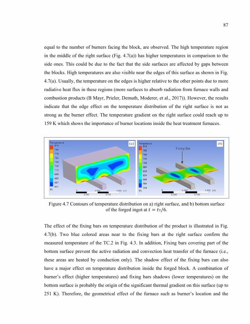
87

equal to the number of burners facing the block, are observed. The high temperature region

in the middle of the right surface (Fig. 4.7(a)) has higher temperatures in comparison to the

side ones. This could be due to the fact that the side surfaces are affected by gaps between

the blocks. High temperatures are also visible near the edges of this surface as shown in Fig.

4.7(a). Usually, the temperature on the edges is higher relative to the other points due to more

radiative heat flux in these regions (more surfaces to absorb radiation from furnace walls and

combustion products (B Mayr, Prieler, Demuth, Moderer, et al., 2017)). However, the results

indicate that the edge effect on the temperature distribution of the right surface is not as

strong as the burner effect. The temperature gradient on the right surface could reach up to

159 K which shows the importance of burner locations inside the heat treatment furnaces.

Figure 4.7 Contours of temperature distribution on a) right surface, and b) bottom surface of the forged ingot at 𝑡 = 𝑡T/6.

The effect of the fixing bars on temperature distribution of the product is illustrated in Fig.

4.7(b). Two blue colored areas near to the fixing bars at the right surface confirm the

measured temperature of the TC.2 in Fig. 4.3. In addition, Fixing bars covering part of the

bottom surface prevent the active radiation and convection heat transfer of the furnace (i.e.,

these areas are heated by conduction only). The shadow effect of the fixing bars can also

have a major effect on temperature distribution inside the forged block. A combination of

burner’s effect (higher temperatures) and fixing bars shadows (lower temperatures) on the

bottom surface is probably the origin of the significant thermal gradient on this surface (up to

251 K). Therefore, the geometrical effect of the furnace such as burner’s location and the

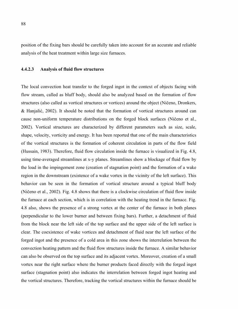
88

position of the fixing bars should be carefully taken into account for an accurate and reliable

analysis of the heat treatment within large size furnaces.

4.4.2.3 Analysis of fluid flow structures

The local convection heat transfer to the forged ingot in the context of objects facing with

flow stream, called as bluff body, should also be analyzed based on the formation of flow

structures (also called as vortical structures or vortices) around the object (Ničeno, Dronkers,

& Hanjalić, 2002). It should be noted that the formation of vortical structures around can

cause non-uniform temperature distributions on the forged block surfaces (Ničeno et al.,

2002). Vortical structures are characterized by different parameters such as size, scale,

shape, velocity, vorticity and energy. It has been reported that one of the main characteristics

of the vortical structures is the formation of coherent circulation in parts of the flow field

(Hussain, 1983). Therefore, fluid flow circulation inside the furnace is visualized in Fig. 4.8,

using time-averaged streamlines at x-y planes. Streamlines show a blockage of fluid flow by

the load in the impingement zone (creation of stagnation point) and the formation of a wake

region in the downstream (existence of a wake vortex in the vicinity of the left surface). This

behavior can be seen in the formation of vortical structure around a typical bluff body

(Ničeno et al., 2002). Fig. 4.8 shows that there is a clockwise circulation of fluid flow inside

the furnace at each section, which is in correlation with the heating trend in the furnace. Fig.

4.8 also, shows the presence of a strong vortex at the center of the furnace in both planes

(perpendicular to the lower burner and between fixing bars). Further, a detachment of fluid

from the block near the left side of the top surface and the upper side of the left surface is

clear. The coexistence of wake vortices and detachment of fluid near the left surface of the

forged ingot and the presence of a cold area in this zone shows the interrelation between the

convection heating pattern and the fluid flow structures inside the furnace. A similar behavior

can also be observed on the top surface and its adjacent vortex. Moreover, creation of a small

vortex near the right surface where the burner products faced directly with the forged ingot

surface (stagnation point) also indicates the interrelation between forged ingot heating and

the vortical structures. Therefore, tracking the vortical structures within the furnace should be

89

considered as an important parameter for the process optimization and multiple loading

scenarios. The effect of these structures is expected to be more significant at lower

temperatures, where the convective heat transfer mode could dominate the radiation one and

the maximum non-uniformity identified.

Figure 4.8 Streamlines of planes at a) between fixing bars and perpendicular to down burner face and b) center of fixing bars.

4.4.2.4 Assessment of heating process inside the large size forgings

Investigation of the temperature distribution inside the block can help to quantify the impact

of the non-uniform heating of the surfaces on the temperature evolution inside the forging. It

can be seen in Fig. 4.9 that the central planes also affected by non-uniform heating of the

surface and the same pattern of heating from the bottom and right side of the forged block to

the left, top and finally side surfaces is visible inside the workpiece. Cold area is mainly

extended longitudinally between two side surfaces. Fig. 4.9(c) also shows that the coldest

point in the lateral plane is actually not located at the center of the forged block and shifted

toward the left and top surfaces. The results clearly demonstrate that product loading,

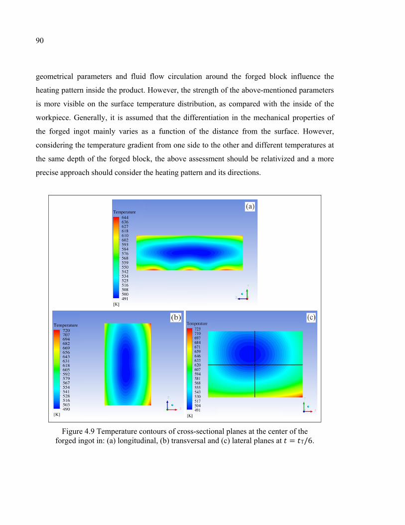
90

geometrical parameters and fluid flow circulation around the forged block influence the

heating pattern inside the product. However, the strength of the above-mentioned parameters

is more visible on the surface temperature distribution, as compared with the inside of the

workpiece. Generally, it is assumed that the differentiation in the mechanical properties of

the forged ingot mainly varies as a function of the distance from the surface. However,

considering the temperature gradient from one side to the other and different temperatures at

the same depth of the forged block, the above assessment should be relativized and a more

precise approach should consider the heating pattern and its directions.

Figure 4.9 Temperature contours of cross-sectional planes at the center of the forged ingot in: (a) longitudinal, (b) transversal and (c) lateral planes at 𝑡 = 𝑡T/6.

91

4.5 Conclusions

Comprehensive analysis of heat transfer in the heat treatment process of forged blocks in a

large size gas-fired heat treatment furnace was investigated in the present work.

Experimental temperature measurement and unsteady CFD simulations were employed for

simultaneous analysis of fluid flow interactions inside the furnace including turbulent

combustion, fluid flow structures and also conjugate heat transfer during the heating.

Concluding remarks are summarized as follows:

1. The developed 3D CFD model provided good agreement with experimentally

measured data.

2. Both DO and S2S radiation models could be reliably used for this application. An

over-prediction of less than 2% was predicted when using the S2S model in

comparison with the DO model, which indicates that the computationally effective

S2S model can be employed for this type of gas-fired heat treatment furnaces. The

analysis of the results also showed that radiation view factor has a higher contribution

than participating medium when analyzing radiation heat transfer during heat

treatment of large size components.

3. Analysis of experimental temperature measurements showed that the unloaded

furnace domain was uniform during the test. However, after loading, temperature

non-uniformities, up to 200 K, were found during the heating process, which could

affect microstructure evolution.

4. The influence of geometrical effects such as burner locations and fixing bars as

sources for temperature non-uniformities must be taken into consideration for

optimizing the heat treatment process of large size components.

5. The formation of vortical structures in the turbulent flow field results in significant

changes in the convection heat transfer of the affected area, which demonstrates the

92

interrelation between the heating pattern and the fluid flow structures inside the

furnace.

6. The developed CFD model was validated using experimental measurements. The

obtained data could be directly applied for the optimization of the operational

conditions and loading patterns of large size gas-fired heat treatment furnaces.

CHAPTER 5

THERMAL ANALYSIS OF FURNACE RESIDENCE TIME AND LOADING PATTERN DURING HEAT TREATMENT OF LARGE SIZE FORGINGS

Nima Bohlooli Arkhazlooa,*, Farzad Bazdidi-Tehranib, Jean-Benoît Morinc and Mohammad Jahazia

a Département de Génie Mécanique, École de Technologie Supérieure, Montréal,

H3C 1K3, Canada

b School of Mechanical Engineering, Iran University of Science and Technology, Tehran, 16846-13114, Iran

c Finkl Steel Inc., 100 McCarthy, Saint-Joseph-de-Sorel, QC J3R 3M8, Canada,

Paper submitted to Journal of Materials Processing Technology, In December 2019,

Abstract

A combination of unsteady 3D CFD simulations and experimental temperature

measurements was employed to determine the effect of loading patterns on the temperature

distribution within large size heavy steel forgings inside a gas-fired heat treatment furnace.

This was aimed to obtain a more homogenous temperature distribution. Besides, a hybrid

methodology using 3D numerical simulations and a high resolution dilatometer allowed

improving residence time of forgings inside the heat treatment furnace. The influence of the

loading patterns and skids on temperature distribution and residence time of forgings was

examined using four different loading patterns. Comprehensive unsteady thermal analysis of

the products heating allowed quantifying the impact of skids usage and their dimensions on

the extent of the uniformity of temperature distribution. The results were interpreted in terms

of the inter-relationship between the skids usage, their geometry, absorbed radiation and

convective heat fluxes. The analysis showed that temperature non-uniformities of up to 331K

could be produced for non-optimum loading patterns. Using the developed CFD approach it

was possible to reduce the temperature non-uniformity of different sizes of blocks up to 32%

via changing the loading pattern inside the furnace. Further, the large size slab’s residence

94

time was improved by almost 15.5% when employing the proposed hybrid approach. This

approach could directly be applied to the optimization of different heat treatment cycles of

large size forgings.

Keywords: Thermal analysis, Loading pattern, Temperature uniformity, Residence time,

Hybrid approach, Experimental measurements, Numerical simulation

Nomenclature Latin symbols a Absorption coefficient

d Characteristic dimension (m) 𝐸 Energy (J)

g Gravity ( 2/m s ) ziJ Diffusive flux of chemical species

h Enthalpy ( J/ kg )



p Pressure (Pa)




Sc Schmidt number


sq The generic source term

Re Reynolds number ( ud ν )

t Time (s)

T Temperature (K)

95




Y Mass fraction of species , ,x y z Direction of coordinate axes

Greek

symbols







Superscripts


Subscripts

, ,i j k Tonsorial indices tensor

z thz species

Abbreviation




DSK Double Skid



96

SK Single Skid



5.1 Introduction

Gas-fired furnaces are extensively used in the steel industry in the heat treatment process.

Specifically, in the case of heavy forgings made of high strength steels, a heat treatment

process called Quench and Temper (Q&T) is used to obtain the desired mechanical

properties (e.g., hardness). The Q&T process is carried out in two steps: initially the parts are

heated to a certain temperature and hold for a period of time before being quenched in water.

In the second step (tempering) the parts are heated to a lower temperature (non-isothermal

tempering) and kept for a period of time (isothermal tempering) before being air cooled. It is

of paramount importance to ensure a high quality heat treatment operation as major

microstructural changes (grain refinement, phase transformation, etc.) take place at this stage

which have a determining effect on the final mechanical properties (Canale et al., 2008; Kang

& Rong, 2006). According to the literature final mechanical properties and microstructural

features are affected significantly by tempering temperature and holding time inside the

furnace (Janjušević, Gulišija, Mihailović, & Patarić, 2009). Therefore, uniformity of the

heating process, in other words, the temperature distribution’s uniformity during the non-

isothermal tempering up to the target temperature is of great importance for the quality of

final products (Gao et al., 2000; B. Wu, Arnold, Arnold, Downey, & Zhou, 2007) specifically

for the large-size products (Bohlooli Arkhazloo et al., 2019; Gur & Pan, 2008). However,

considering that parts, are rarely single loaded in the furnace, their loading pattern (e.g.,

distances between the parts, stacking mode, etc.) as well as furnace geometry (burners’ and

skids’ positions), will influence temperature evolution within their volume resulting in non-

uniform temperature distribution that may affect the final properties. The possible use of

longer holding times is not a viable solution as it will bring other microstructural damages

and is not energy friendly (Hao et al., 2008). Hence, predicting, controlling and consequently

optimizing the heating process or the transient temperature of the part as a function of the

furnace temperature and the related thermal interactions and subsequently possible reduction

97

in the tempering process time, is a necessary task for energy saving and quality control (Hao

et al., 2008).

However, an exact prediction of the furnace temperature distribution and, consequently, the

temperature experienced by the product would require a more fundamental understanding of

the interactions between heat transfer parameters, process parameters and parts

configurations within the furnace. At the present time such data in thermal analysis of large

size products heating characteristics is not available and therefore often empirical

correlations are used to estimate the heat treatment cycle parameters (Kang & Rong, 2006).

These correlations are usually defined as a function of the total furnace load and selected

loading patterns of the parts inside the furnace (Korad et al., 2013). Hence, they show large

deviations in the case of multiple loadings and complex furnace configurations (Hao et al.,

2008). On the other hand, in most of the studies and evaluations in the field of metallurgy

(Cheng et al., 1988; Primig & Leitner, 2011; Talebi et al., 2017), the non-isothermal

tempering procedure was simplified assuming a constant heating rates rather than a variable

one which is actually experienced by the products in the real production cycle. The problem

is more acute in the case of large size products (that encompass high temperature gradient

from one end to another) at high temperatures due to operational difficulties and high costs of

experimentation. Therefore, employing a constant temperature and time in the correlations

such as Hollomon-Jaffe (Janjušević et al., 2009) may result in deviation from what is really

experienced by the large size forgings during the whole tempering process.

While both analytical and numerical methods could be used to study the problem, limitations

of analytical methods in solving coupled non-linear phenomena (i.e., turbulent combustion

along with conjugate heat transfer and fluid flow) do not allow their effective use in these

cases (Chapman et al., 1990; Gao et al., 2000). Computational fluid dynamics (CFD)

comprising various numerical methods has become in recent years a very cost effective and

reliable technique to study the thermal interactions inside the heat treatment furnaces. Several

studies such as those of Wang et al.(J. Wang et al., 2008), Hao et al. (Hao et al., 2008), Kang

and Rong (Kang & Rong, 2006) and Defaee et al. (Rad, Ashrafizadeh, & Nickaeen, 2017)

98

employing CFD, investigated flow and heat distributions inside electrically heated, gas

quenching and hot air treating furnaces.

Due to the complexity of the reactive flow analysis inside the gas-fired furnaces, the long

operating time of the heat treatment process and the totally transient conditions of the

process, little information is available regarding the transient studies of the real-scale gas-

fired heat treatment furnaces. The existing studies have been focused either on small- to

medium-scale gas-fired furnaces (Galletti et al., 2013) or simplified steady-state simulations

(Danon et al., 2011; García et al., 2019; B. Mayr, Prieler, Demuth, Moderer, et al., 2017;

Prieler, Demuth, Spoljaric, & Hochenauer, 2015; Prieler et al., 2016). For instance, Yang et

al. (Yang et al., 2007) studied the performance of small-scale mobile heat treatment furnaces

and Prieler et al. (Prieler, Mayr, et al., 2015) and Mayr et al. (B Mayr, Prieler, Demuth,

Potesser, et al., 2017) investigated the oxy fired laboratory-scale and semi-industrial gas-fired

furnaces heat distribution in a single loading configuration using steady-state assumption,

respectively.

Recently, Bohlooli et al. (Bohlooli Arkhazloo et al., 2019) reported on the experimental and

numerical analyses of the heating process of large size forged ingots inside a gas-fired

furnace. Comprehensive experimental analysis of instrumented large size ingot and gas-fired

furnace temperature’s history proved that large-scale products can affect the furnace

temperature’s uniformity and consequently products’ heating uniformity. A full-scale three-

dimensional (3D) model of the process revealed that the identified non-uniform heating of

the large-scale products had a relationship with the fluid flow structure, geometrical

parameters of the furnace (including burner locations) and loading patterns of ingots

(including their relative locations and distances). The effect of vortical structures and loading

pattern on the heat treatment process and temperature history of small scale products had

been mentioned in the numerical study of Wang and Shang (Z. J. Wang & Shang, 2010) who

investigated the flow and heat exchange in the high-pressure gas quenching chamber.

Macchion et al (Macchion, Zahrai, & Bouwman, 2005) Kang and Rong (Kang & Rong,

2006) and Korad et al. (Korad et al., 2013) also analyzed the loading pattern’s effect on the

99

heating and cooling rates of products in different furnaces. Concentrating on the

metallurgical aspects and toward reducing the process cost, the steady state CFD simulations

of indirect fired homogenization furnace (used for aluminum billet treatment) in Korad et

al.’s (Korad et al., 2013) study showed that different billets stacked in the furnace

experienced different temperature distributions (temperature non-uniformity) as a result of

loading pattern inside the furnace during the non-isothermal tempering. Macchion et al.

(Macchion et al., 2004) in a CFD simulation of gas quenching chamber of small parts pointed

out that the position of parts inside the furnace could significantly affect the temperature

uniformity of products during the heat treatment furnaces. Also, Kang and Rong (Kang &

Rong, 2006) using CFD simulations investigated the heating history (non-isothermal

tempering) of two different loading patterns of small size parts inside an electrically heated

furnace. Their study revealed that the loading pattern even in small size products could

change the heating history of the parts and furnace performance. However, up to now, little

data is available on the interactions between heat transfer parameters, stacking strategy, heat

treatment process variables (specifically temperature uniformity and heating time in non-

isothermal tempering) in relation to loading pattern of large size forgings inside gas-fired

furnaces. Besides, most of the studies investigating the effect of constant heating rates (rather

than a series of a variable heating rates resulting in real temperature history experienced by

the products inside the furnace) and subsequent certain holding times on the mechanical

properties of the steels (Ray, Ganguly, & Panda, 2003; Revilla, López, & Rodriguez-Ibabe,

2014; Talebi et al., 2017; B. B. Wu, Chen, Shang, Xie, & Misra, 2019; Zou, Ying, Zhang, &

Fang, 2010). Simultaneous analysis of isothermal and non-isothermal tempering history of

large size forgings inside gas-fired furnaces in order to reduce the residence time of the

products has not been addressed in the literature.

The present paper reports on an investigation aiming to address the above challenges using

3D CFD modeling complemented with experimental validation. Four possible loading

patterns of heavy forgings in a gas-fired furnace were analyzed. This is not only aimed to

have maximum temperature distribution’s uniformity and similar heating rates, but also to

reduce the time to reach the target temperature during the non-isothermal tempering stage.

100

Besides, a hybrid methodology combining 3D CFD numerical predictions and high

resolution dilatometer machine was introduced and used to further reduce the residence time

of the forgings during the isothermal tempering based on the real-life temperature experience

of steel parts in the large-size gas-fired furnaces.

5.2 Loading Patterns

The studied furnace was a 3.05× 3.28 × 8.83 (m3) batch type gas-fired furnace. The furnace

was heated by 18 high-velocity cup burners (Baukal Jr, 2003) including 9 upper burners

(located on the uppers section of the furnace left wall) and 9 lower burners (installed in the

lower section of the furnace right wall). Fig. 5.1 illustrates the furnace and four different

loading patterns used for the CFD simulations (See also Fig. 5.3). A total weight of 130

metric tons, corresponding to the loading capacity of a large size furnace, was fixed in all the

four patterns. Two types of forgings, called large size block and slab, with dimensions of 1.4

× 0.89 ×2.72 (m3) and 1.1×0.5×2.25 (m3), were used in different configurations. Blocks were

mounted on oxidized steel skids in car-bottom furnace. The following denominations were

used to characterize each of the four configurations:

Single Skid (SK): A combination of one large size block and one slab stacked on its

top.

DSK (Double skid): The second case study was used to see the effect of double

height skids in the gas-fired furnaces. According to the Bohlooli et al. (Bohlooli

Arkhazloo et al., 2019), lower burners in the furnace are one of the main root causes

of non-uniform temperature distributions. Therefore, this simulation will allow

quantifying the impact of the skid height.

SKC (Single skid + Central spacer): The third case study was aimed to evaluate the

effect of spacing skids (made of steel with an oxidized surface) on the stacking

patterns and subsequent uniformity and residence time of blocks in the heat treatment

101

furnaces. Two sizes of spacers with the cross-sectional dimensions of 0.254×0.245

(m2) and 0.127×0.127 (m2) were used.

DSKC (Double skid + Central spacer skid): A combination of double skids at the

bottom and center spacers between the large block and the slab was the fourth loading

pattern used for the simulations.

Figure 5.1 Four different loading patterns of forgings using skids inside gas-fired heat treatment furnace: a) SK, b) DSK, c) SKC and d) DSKC.

102

5.3 Methodology

5.3.1 Computational Details

The previously developed and validated CFD model in the authors’ study (Bohlooli

Arkhazloo et al., 2019) was employed as the basis for the numerical simulation. The transient

CFD simulations employing a pressure-based solver were carried out using the finite-volume

based ANSYS-FLUENT software (ANSYS, 2016) to solve the Reynolds-averaged Navier-

Stokes (RANS) equations, as follows (ANSYS, 2016).

( ) 0ii

ut xρ ρ∂ ∂+ =

∂ ∂

(5.1)

( ) ( ) ( )iji i j i j

j i j i


τρ ρ ρ

∂∂ ∂ ∂ ∂ ′ ′+ = − + − +∂ ∂ ∂ ∂ ∂

(5.2)

1( ) ( ) ( ) (k ) ( )

n



ρ ρ τ ρ=

∂ ∂ ∂ ∂ ∂ ∂ ′ ′+ + = − + − +∂ ∂ ∂ ∂ ∂ ∂

r

(5.3)

where, the stress tensor, ijτ , in the above momentum and energy equations (Eq. 5.2 and Eq.

5.3, respectively) is given by:

23

ji lij ij

j i l

uu ux x x

τ μ μ δ ∂∂ ∂

= + − ∂ ∂ ∂ (5.4)

and the diffusive flux of combustion product species (in Eq. 5.2) is defined by the Fick’s law:

t zz

k i

YJSc xμ ∂∂ = −

∂

r

(5.5)

The turbulent combustion and fluid flow were simulated using the standard 𝑘 − ɛ turbulence

model proposed by Spalding (Spalding, 1971). It must be noted that, the above model has

already been applied to gas-fired furnaces and its reliability had been approved (Ishii et al.,

2002; Y. Liu et al., 2014). Due to the high velocity of the combustion products coming from

the burner outlet, Arrhenius chemical kinetic calculations were not taken into account and the

eddy dissipation model (EDM) (B. F. Magnussen & Hjertager, 1977) was used to simulate

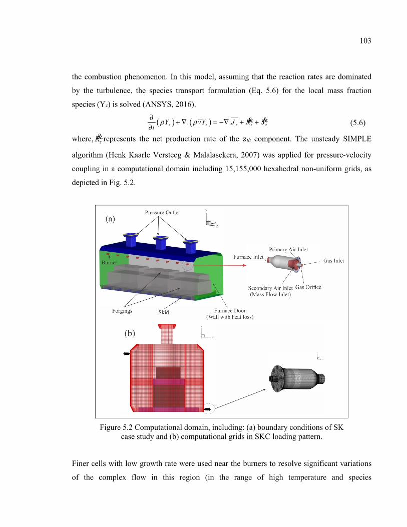
103

the combustion phenomenon. In this model, assuming that the reaction rates are dominated

by the turbulence, the species transport formulation (Eq. 5.6) for the local mass fraction

species (Yz) is solved (ANSYS, 2016).

( ) ( ) . .z z z z zY vY J R St

ρ ρ∂ + ∇ = −∇ + +∂

&& (5.6)

where, zR&represents the net production rate of the 𝑧th component. The unsteady SIMPLE

algorithm (Henk Kaarle Versteeg & Malalasekera, 2007) was applied for pressure-velocity

coupling in a computational domain including 15,155,000 hexahedral non-uniform grids, as

depicted in Fig. 5.2.

Figure 5.2 Computational domain, including: (a) boundary conditions of SK case study and (b) computational grids in SKC loading pattern.

Finer cells with low growth rate were used near the burners to resolve significant variations

of the complex flow in this region (in the range of high temperature and species

104

concentration gradient). The grid size includes 6,408,000 non-uniform cells in the burner

domains (356,000 cells in each burner). Grid independency tests were performed using two

other meshes including 10,597,900 and 19,712,100 cells. The difference between results of

the mesh with 15,155,000 and the fine mesh were negligible (See Fig. 5.3). Therefore the

medium mesh with 15,155,000 cells was used in the simulations. Further details of the

simulations procedure and boundary conditions specifications were discussed by Bohlooli et

al. (Bohlooli Arkhazloo et al., 2019). The discrete ordinates model DO (Raithby & Chui,

1990) using the weighted-sum-of-gray gases model (WSGGM) (Smith et al., 1982) was also

employed to solve the radiative transfer equation (RTE) considering the absorption and

emission effects of the furnace medium.

5.3.2 Forgings Temperature Measurements

This part of experimentations includes temperature measurements at the surface of the

forgings in the gas-fired heat treatment furnace. Measurements were conducted in a gas-fired

furnace at Finkl steel-Sorel (Finkl steel Inc.). The furnace with three relatively similar zones

was loaded with a total weight of 130 tons. Six K type thermocouples were embedded in

different locations of the parts in the central zone of the furnace. Details regarding other

characteristics of the furnace and the methods developed for reliable installation and

temperature reading are provided in a recent publication by Bohlooli et al. (Bohlooli

Arkhazloo et al., 2019).

5.3.3 Hybrid Approach

A hybrid methodology combining the CFD simulation results and experimental dilatometer

tests was used to determine the minimum heat treatment time that is required to achieve the

desired mechanical properties. Specifically, the transient temperature histories of the hottest

and coldest regions of the parts were first predicted by the developed CFD model. These two

points were then used as the critical points to evaluate and optimize the isothermal stage of

the heat treatment cycle. This methodology includes laboratory physical simulations of the

105

tempering cycle during the isothermal and non-isothermal tempering (acquired through the

CFD simulation) and subsequent hardness measurements of the steel for the critical points. It

was started with finding the hardness of samples after applying non-isothermal tempering

history of the critical points. Then several isothermal tempering were carried out to find an

equivalent isothermal tempering times leading to the measured hardness in step one and

desired hardness at the end of the tempering process. The difference between these two times

was considered as the optimum holding time in the isothermal part of the tempering process.

The chemical composition of the investigated high-strength low-alloy steel is provided in

Table 5.1. Cylindrical samples 10 mm in length and 4 mm in diameter were cut from near the

surface and central zones of the slab, which had underwent open-die forging at around

1260oC.

Table 5.1 Chemical analysis of the investigated steel - Wt. % (Finkl Steel Inc.).

Fe C Mn Si Mo Cr Ni Other Bal. 0.35 0.85 0.4 0.45 1.85 0.47 Micro-alloying

The initial tempering process of the present slabs with dimensions of 1.1×0.5×2.25 (m3) was

around 60 hours to achieve a nominal final hardness between 31-34 HRC (in the case of

multiple loading). This heat treatment cycle includes a nominal 24 hours of heating stage up

to 855 K (non-isothermal tempering) and 38 hours of holding at this temperature (isothermal

tempering). All the heat treatment cycles applied to the parts in the furnace were physically

simulated using the high-resolution TA DIL 805A/D dilatometer machine (TA instruments,

New Castle, DE, USA). The heating rates using the validated CFD results were adjusted to

simulate that of actual heating cycle of forgings during non-isothermal tempering. A prior

austenitization process (including heating up to 870oC, followed by 10 minutes holding at

this temperature for homogenization) and subsequent cooling rate of 3oC to produce a

martensitic microstructure resembling the expected microstructure on the surface of an actual

forging after water quenching (i.e., before starting the tempering process in the heat treatment

furnace) was considered for the sample preparations. Dilatometry tested samples were then

cut along their longitudinal axis and then polished according to standard metallography

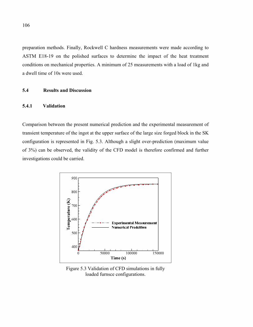
106

preparation methods. Finally, Rockwell C hardness measurements were made according to

ASTM E18-19 on the polished surfaces to determine the impact of the heat treatment

conditions on mechanical properties. A minimum of 25 measurements with a load of 1kg and

a dwell time of 10s were used.


5.4.1 Validation

Comparison between the present numerical prediction and the experimental measurement of

transient temperature of the ingot at the upper surface of the large size forged block in the SK

configuration is represented in Fig. 5.3. Although a slight over-prediction (maximum value

of 3%) can be observed, the validity of the CFD model is therefore confirmed and further

investigations could be carried.

Figure 5.3 Validation of CFD simulations in fully loaded furnsce configurations.

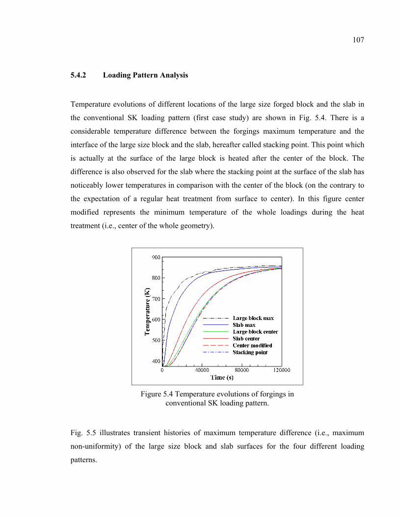
107

5.4.2 Loading Pattern Analysis

Temperature evolutions of different locations of the large size forged block and the slab in

the conventional SK loading pattern (first case study) are shown in Fig. 5.4. There is a

considerable temperature difference between the forgings maximum temperature and the

interface of the large size block and the slab, hereafter called stacking point. This point which

is actually at the surface of the large block is heated after the center of the block. The

difference is also observed for the slab where the stacking point at the surface of the slab has

noticeably lower temperatures in comparison with the center of the block (on the contrary to

the expectation of a regular heat treatment from surface to center). In this figure center

modified represents the minimum temperature of the whole loadings during the heat

treatment (i.e., center of the whole geometry).

Figure 5.4 Temperature evolutions of forgings in conventional SK loading pattern.

Fig. 5.5 illustrates transient histories of maximum temperature difference (i.e., maximum

non-uniformity) of the large size block and slab surfaces for the four different loading

patterns.

108

Figure 5.5 Comparison of maximum identified temperature non-uniformities for different loading patterns at the surface of: a) large size, block and b) slab.

Analysis of the data in Fig. 5.5 showed that a maximum non-uniformity of 331 K was

produced in the single skid (SK) case study in the large size block. This severe non-

uniformity could probably be related to the loading pattern of the blocks and geometrical

parameters of the furnace including the burners’ positions which were located on opposite

side of the furnace close to the bottom or top of the walls (Bohlooli Arkhazloo et al., 2019).

For example, the bottom right of the large block surface near the lower burners was very

rapidly heated while the upper surface, intersection of the stacked slab on the large size block

experienced lower heating rates and subsequently leaded to the identified non-uniformity.

However, it can be seen that the use of spacers as well as double-height skids in the DSK,

SKC and DSKC patterns (the second to fourth case studies) could reduce maximum non-

uniformity down to 293 K, 294 K and 246 K (approximately 11.4%, 11.1% and 25.6%

reductions), respectively. Besides, in Fig. 5.5 the area under each curve represents the total

non-uniformity of block during the heat treatment. Therefore, the differences from one case

to another would be representing the difference in total non-uniformities. Fig. 5.5 also shows

that shrinkage of the total non-uniformity (area under each curve) was clearly affected when

skids and spacers were used. As shown in Table 5.2, the combination of double-height skids

and central spacers in DSKC could lower the temperature non-uniformity of the large size

block up to 32%, which is a very significant gain. The effects of spacers and double-height

109

skids are also interpreted by using Fig. 5.5 and Table 5.2. The SKC case study giving a

reduction in the temperature non-uniformity of almost 21%, as compared with the 12% of

DSK, demonstrates a higher effectiveness of the central spacers in reducing temperature non-

uniformities.

Fig. 5.5 (b) and Table 5.2 summarize the trends observed for the slab. Specifically, the

maximum non-uniformity and total non-uniformity for the SKC case study were reduced by

7% and 18%, respectively. However, in contrast to the large block, under the DSK

configuration the maximum and total temperature non-uniformity increased compare to the

SK configuration. It is also interesting to know that for the DSKC case, while approximately

the same reduction in the total non-uniformity was observed; however, the maximum

temperature non-uniformity (pack of the curve) of the slab slightly increased by 2.6%. This

reverse effect could be related to the fact that the spacers in SKC loading pattern increasing

the treatment height, reduced the distance between the upper surface of the slab and upper

burners, leading to a higher temperature at this surface (see Fig. 5.6).

Table 5.2 Total temperature non-uniformity reduction of forgings for different loading patterns in comparison with conventional SK loading.

Forgings DSK SKC DSKC

Large-size block 12% 21% 32%

Slab -1% 18% 19%

Contours of the temperature distributions in the central cross-section of the forging blocks for

the four different loading patterns, 𝑡 = 𝑡T/6, are represented in Fig. 5.6. These are for when

the maximum temperature non-uniformity occurred in the SK case study (see Fig. 5.5). It

should be noted that a distance of 0.5 cm was considered (with a layer of air) between the

forged ingots corresponding to the real experience of forged block stacking due to their shape

which is not completely flat. However, in the case of existence of spacers a perfect contact

was considered due to the weight of blocks. It can be seen that in the SK configuration

considerable irregular temperature non-uniformities existed in the blocks from one end to

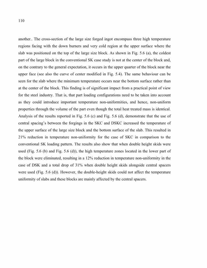
110

another.. The cross-section of the large size forged ingot encompass three high temperature

regions facing with the down burners and very cold region at the upper surface where the

slab was positioned on the top of the large size block. As shown in Fig. 5.6 (a), the coldest

part of the large block in the conventional SK case study is not at the center of the block and,

on the contrary to the general expectation, it occurs in the upper quarter of the block near the

upper face (see also the curve of center modified in Fig. 5.4). The same behaviour can be

seen for the slab where the minimum temperature occurs near the bottom surface rather than

at the center of the block. This finding is of significant impact from a practical point of view

for the steel industry. That is, that part loading configurations need to be taken into account

as they could introduce important temperature non-uniformities, and hence, non-uniform

properties through the volume of the part even though the total heat treated mass is identical.

Analysis of the results reported in Fig. 5.6 (c) and Fig. 5.6 (d), demonstrate that the use of

central spacing’s between the forgings in the SKC and DSKC increased the temperature of

the upper surface of the large size block and the bottom surface of the slab. This resulted in

21% reduction in temperature non-uniformity for the case of SKC in comparison to the

conventional SK loading pattern. The results also show that when double height skids were

used (Fig. 5.6 (b) and Fig. 5.6 (d)), the high temperature zones located in the lower part of

the block were eliminated, resulting in a 12% reduction in temperature non-uniformity in the

case of DSK and a total drop of 31% when double height skids alongside central spacers

were used (Fig. 5.6 (d)). However, the double-height skids could not affect the temperature

uniformity of slabs and these blocks are mainly affected by the central spacers.

111

Figure 5.6 Contours of temperature distribution in central cross sections of forgings at 𝑡 = 𝑡 /6. a) SK, b) DSK, c) SKC, and d) DSKC.

5.4.2.1 Influence of spacer skids size on heat transfer modes

The above results clearly demonstrated that the inclusion of the spacers in the analysis

affected the severity and distribution of temperature non-uniformity. Although, convection

and radiation are the two most important heat transfer mechanisms during the heat treatment

process of large size forgings in gas-fired furnaces (Totten, 2006), both from fundamental

and application points of view it is however important to quantify the role of each mode in

the presence of spacers. To this end, two different spacers with the cross-sectional areas of

0.254×0.245 (m2) (SKC) and 0.127×0.127 (m2), half-size SKC or SKHC, were considered

for the analysis and the results are reported in Fig. 5.7 (a-d). The results of Fig. 5.7 (a) show

that interestingly despite doubling the height and the width of the spacers, the total

temperature non-uniformity decreased by the same amount (about 21%). In Fig. 5.7 (b), the

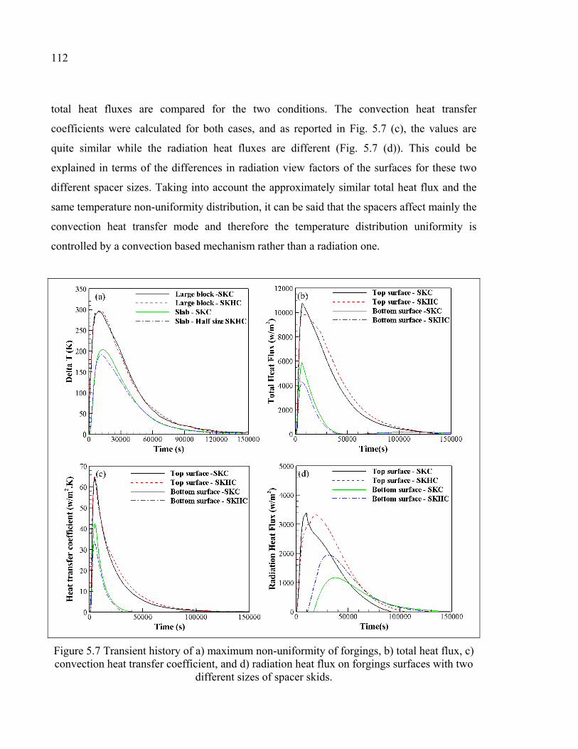
112

total heat fluxes are compared for the two conditions. The convection heat transfer

coefficients were calculated for both cases, and as reported in Fig. 5.7 (c), the values are

quite similar while the radiation heat fluxes are different (Fig. 5.7 (d)). This could be

explained in terms of the differences in radiation view factors of the surfaces for these two

different spacer sizes. Taking into account the approximately similar total heat flux and the

same temperature non-uniformity distribution, it can be said that the spacers affect mainly the

convection heat transfer mode and therefore the temperature distribution uniformity is

controlled by a convection based mechanism rather than a radiation one.

Figure 5.7 Transient history of a) maximum non-uniformity of forgings, b) total heat flux, c) convection heat transfer coefficient, and d) radiation heat flux on forgings surfaces with two

different sizes of spacer skids.

113

5.4.2.2 Influence of loading patterns on the non-isothermal tempering residence time

The evolution of transient average temperature of the forgings and derivation of temperature

with respect to time (heating rate) for the different loading patterns are presented in Fig. 5.8.

Figure 5.8 Forgings average temperature evolution: a) large size block, b) slab and derivative of temperature evolution with respect to time, c) large size block, and d) slab in

different loading pattrens.

It can be seen that positioning of skids and spacers inside the furnace and between the blocks

could affect the average transient temperature evolution of the forgings (Fig. 5.8 (a) and Fig.

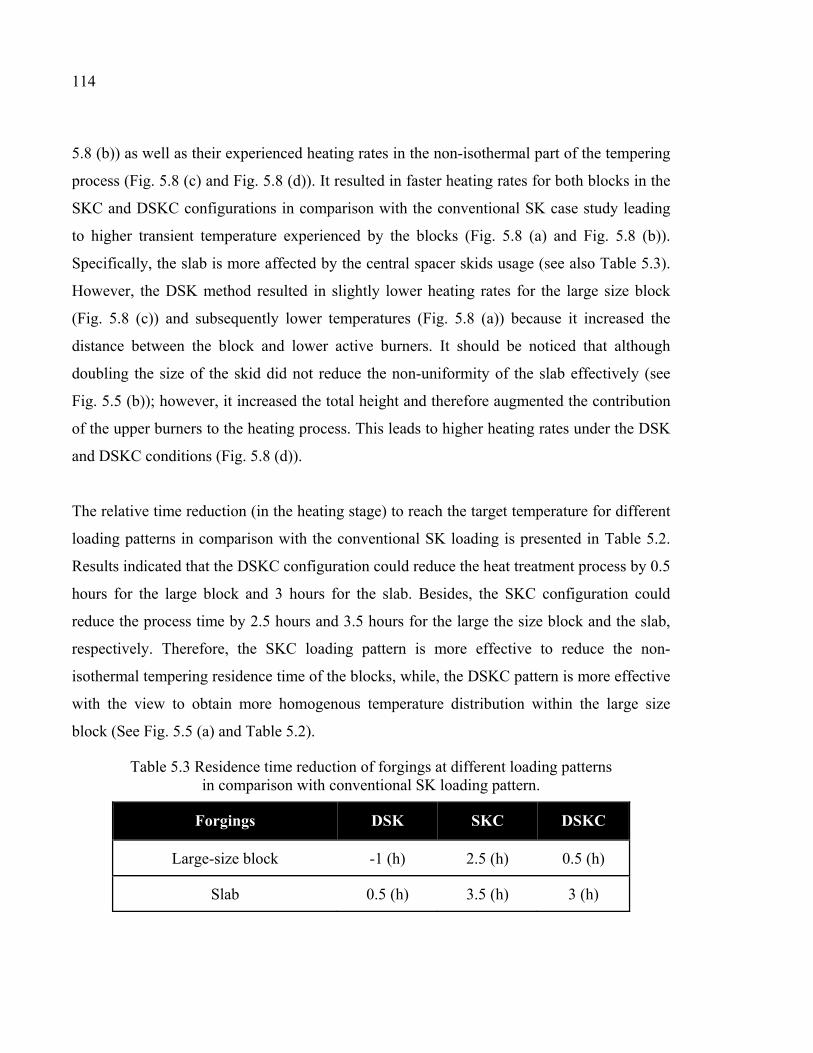
114

5.8 (b)) as well as their experienced heating rates in the non-isothermal part of the tempering

process (Fig. 5.8 (c) and Fig. 5.8 (d)). It resulted in faster heating rates for both blocks in the

SKC and DSKC configurations in comparison with the conventional SK case study leading

to higher transient temperature experienced by the blocks (Fig. 5.8 (a) and Fig. 5.8 (b)).

Specifically, the slab is more affected by the central spacer skids usage (see also Table 5.3).

However, the DSK method resulted in slightly lower heating rates for the large size block

(Fig. 5.8 (c)) and subsequently lower temperatures (Fig. 5.8 (a)) because it increased the

distance between the block and lower active burners. It should be noticed that although

doubling the size of the skid did not reduce the non-uniformity of the slab effectively (see

Fig. 5.5 (b)); however, it increased the total height and therefore augmented the contribution

of the upper burners to the heating process. This leads to higher heating rates under the DSK

and DSKC conditions (Fig. 5.8 (d)).

The relative time reduction (in the heating stage) to reach the target temperature for different

loading patterns in comparison with the conventional SK loading is presented in Table 5.2.

Results indicated that the DSKC configuration could reduce the heat treatment process by 0.5

hours for the large block and 3 hours for the slab. Besides, the SKC configuration could

reduce the process time by 2.5 hours and 3.5 hours for the large the size block and the slab,

respectively. Therefore, the SKC loading pattern is more effective to reduce the non-

isothermal tempering residence time of the blocks, while, the DSKC pattern is more effective

with the view to obtain more homogenous temperature distribution within the large size

block (See Fig. 5.5 (a) and Table 5.2).

Table 5.3 Residence time reduction of forgings at different loading patterns in comparison with conventional SK loading pattern.

Forgings DSK SKC DSKC

Large-size block -1 (h) 2.5 (h) 0.5 (h)

Slab 0.5 (h) 3.5 (h) 3 (h)

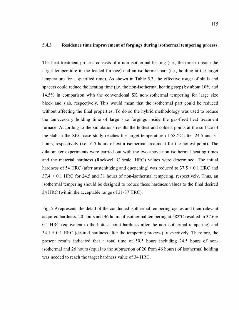
115

5.4.3 Residence time improvement of forgings during isothermal tempering process

The heat treatment process consists of a non-isothermal heating (i.e., the time to reach the

target temperature in the loaded furnace) and an isothermal part (i.e., holding at the target

temperature for a specified time). As shown in Table 5.3, the effective usage of skids and

spacers could reduce the heating time (i.e. the non-isothermal heating step) by about 10% and

14.5% in comparison with the conventional SK non-isothermal tempering for large size

block and slab, respectively. This would mean that the isothermal part could be reduced

without affecting the final properties. To do so the hybrid methodology was used to reduce

the unnecessary holding time of large size forgings inside the gas-fired heat treatment

furnace. According to the simulations results the hottest and coldest points at the surface of

the slab in the SKC case study reaches the target temperature of 582oC after 24.5 and 31

hours, respectively (i.e., 6.5 hours of extra isothermal treatment for the hottest point). The

dilatometer experiments were carried out with the two above non isothermal heating times

and the material hardness (Rockwell C scale, HRC) values were determined. The initial

hardness of 54 HRC (after austenitizing and quenching) was reduced to 37.5 ± 0.1 HRC and

37.4 ± 0.1 HRC for 24.5 and 31 hours of non-isothermal tempering, respectively. Thus, an

isothermal tempering should be designed to reduce these hardness values to the final desired

34 HRC (within the acceptable range of 31-37 HRC).

Fig. 5.9 represents the detail of the conducted isothermal tempering cycles and their relevant

acquired hardness. 20 hours and 46 hours of isothermal tempering at 582oC resulted in 37.6 ±

0.1 HRC (equivalent to the hottest point hardness after the non-isothermal tempering) and

34.1 ± 0.1 HRC (desired hardness after the tempering process), respectively. Therefore, the

present results indicated that a total time of 50.5 hours including 24.5 hours of non-

isothermal and 26 hours (equal to the subtraction of 20 from 46 hours) of isothermal holding

was needed to reach the target hardness value of 34 HRC.

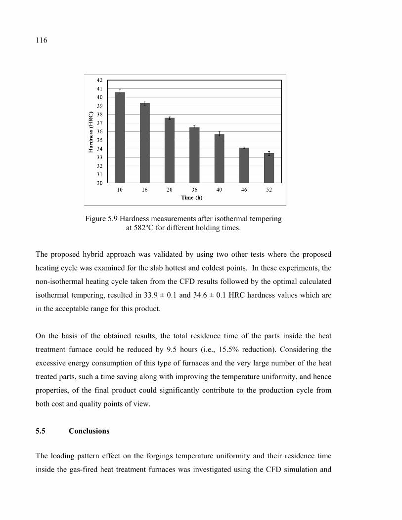
116

Figure 5.9 Hardness measurements after isothermal tempering at 582oC for different holding times.

The proposed hybrid approach was validated by using two other tests where the proposed

heating cycle was examined for the slab hottest and coldest points. In these experiments, the

non-isothermal heating cycle taken from the CFD results followed by the optimal calculated

isothermal tempering, resulted in 33.9 ± 0.1 and 34.6 ± 0.1 HRC hardness values which are

in the acceptable range for this product.

On the basis of the obtained results, the total residence time of the parts inside the heat

treatment furnace could be reduced by 9.5 hours (i.e., 15.5% reduction). Considering the

excessive energy consumption of this type of furnaces and the very large number of the heat

treated parts, such a time saving along with improving the temperature uniformity, and hence

properties, of the final product could significantly contribute to the production cycle from

both cost and quality points of view.

5.5 Conclusions

The loading pattern effect on the forgings temperature uniformity and their residence time

inside the gas-fired heat treatment furnaces was investigated using the CFD simulation and

117

experimental temperature measurements. Besides, a hybrid numerical-physical simulation

approach was introduced and performed to optimize the residence time of large size slabs

inside gas-fired heat treatment furnaces. The following conclusions can be drawn from the

present work:

1) Large size forgings in the non-optimized conventional loading pattern experienced

temperature non-uniformities up to 331 K due to furnace geometry and loading

pattern.

2) Using double size skids and central spacers reduced the temperature non-uniformity

of large size forgings inside the gas-fired furnace up to 32%.

3) Convection heat transfer was the dominant mechanism in the presence of central

spacers to affect the temperature uniformity of the heavy steel parts.

4) It was possible to reduce the total residence time of large size slabs (including non-

isothermal and isothermal tempering) by about 15.5% in the gas-fired heat treatment

furnace.

5) A hybrid methodology was proposed and validated for residence time optimization of

large size forging. The proposed approach could be applied to other furnace types or

part geometries.

CHAPTER 6

CFD SIMULATION OF A GAS-FIRED HEAT TREATMENT FURNACE: ASSESSMENT OF EQUILIBRIUM NON-PREMIX COMBUSTION AND DIFFERENT TURBULENCE MODELS

Nima Bohlooli Arkhazlooa,*, Farzad Bazdidi-Tehranib, Mohammad Jadidib, Jean-Benoît Morinc and Mohammad Jahazia

a Département de Génie Mécanique, École de Technologie Supérieure, Montréal, Québec, Canada H3C 1K3,

b School of Mechanical Engineering, Iran University of Science and Technology, Tehran, Iran 16846-13114

c Finkl Steel Inc., 100 McCarthy, Saint-Joseph-de-Sorel, Québec, Canada J3R 3M8

Paper submitted to Energy & Fuels, In December 2019,

Abstract

In this study transient computational fluid dynamics (CFD) simulations of a batch type gas-

fired heat treatment furnace were carried out in order to investigate the applicability of

equilibrium non-premix combustion model and the effect of different turbulence models on

the thermal interactions inside the furnace. A one-third periodic 3D model of the furnace,

employed for tempering of large size forgings, was used as the domain for the simulations.

The performances of several transient RANS based turbulence models along with the non-

premix combustion with equilibrium model approaches were evaluated. To do so, thermal

interactions analyses based on temperature measurements on an instrumented large size

block were performed in different locations of the forged blocks as well as critical regions in

the burner area, stagnation and wake regions. Results indicated that non-premix combustion

with chemical equilibrium could effectively be employed for combustion modeling of high-

momentum cup burner combustion and subsequently temperature prediction of the products.

A very good agreement, with a maximum deviation of about 4%, was obtained using the

120

periodic model indicating the reliability of the developed model. Prediction of ɛ 𝑘⁄ ratio

using different turbulence models could significantly affect mixture fraction variance and

subsequently flame length and product temperature at the stagnation point. RSM was found

as the most reliable turbulence model compared to the experimental measurements.

Furthermore, it was found that the realizable 𝑘 − ɛ model reasonably predicted the global

block temperature during the heat treatment process. However, it under-predicted the flame

length and block temperature in the stagnation region. While, the SST 𝑘 − 𝜔 model could

not capture the flow recirculation behind the block and over-predicted the block temperature

near the wake region and inside the block, it showed reasonable results in the stagnation

region which can be used for process optimization.

Keywords: Gas-fired furnace, Computational fluid dynamics (CFD), Turbulence modeling,

Equilibrium non-premix combustion, Flame length, Mixture fraction variance

Nomenclature Latin symbols d Characteristic dimension (m)

C1ɛ ,C2ɛ ,C3ɛ Constants in k − ɛ equations

Cg, Cd Constants in mixture fraction variance transport equation 𝐸 Energy (J)

f Mean Mixture fraction 2f ′ Mixture fraction variance

g Gravity ( 2/m s )

ziJ Diffusive flux of chemical species

h Enthalpy ( /j kg )

H Block height



121

L Furnace length in longitudinal direction


OH Hydroxide p Pressure (Pa)

iq , The generic source term

rq Reaction heat term respectively

sq The generic source term



Re Reynolds number ( ud μ )


Sc Schmidt number

t Time (s)

T Temperature (K)




, Y, ZX Direction of coordinate axes

Greek

symbols





,k εσ σ Prenatal number for the kinetic energy and dissipation rate,

respectively

122

tσ Constant in mixture fraction variance equation

, sσ σ Stefan-Boltzmann constant and scattering coefficient


′Ω Solid angle


Superscripts


Subscripts

, ,i j k Tensorial indices

z thz species

gas Gas

Abbreviation













123

6.1 Introduction

Steel industry extensively employs gas-fired heat treatment furnaces to raise the temperature

of steel parts to desired levels at which different metallurgical processes such as phase

transformation and carbide precipitation take place. This is to allow for achieving the

targeted mechanical properties (Totten, 2006). Final material properties are usually optimized

by tempering parameters modification (such as temperature, time, etc.) in the gas-fired heat

treatment furnaces (Kang & Rong, 2006; Yan et al., 2017). Therefore, accurate heat transfer

and temperature distribution prediction of the parts necessitates a comprehensive analysis of

thermal interactions and their subsequent effects on the transient temperature evolution of the

product within the furnace. This analysis should consider furnace operation complexities

including combustion, heat exchange within furnace, turbulence, flame, furnace

characteristics (geometry, bottom skids, etc.), the composition of the steel products, and their

internal heat conduction. However, due to the high temperatures, experimental measurements

in gas-fired furnaces are complex and expensive to perform (Gao et al., 2000). Measurements

and data acquisition become more difficult when it comes to the analysis of large size steel

parts’ heat treatment inside such furnaces. Besides, analytical studies due to their limitation

in non-linear transient applications show large deviations with the real thermal experiences of

the products (Gao et al., 2000). Therefore, due to the lack of such data, the current practice

for the heating cycle schedule is based on empirical correlations and is mostly limited on

monitoring of the furnace temperature as a function of the furnace load (Kang & Rong, 2006;

S. F. Zhang et al., 2009). Empirical correlations, however, cannot be used precisely to predict

products temperature and show large deviations with the loading pattern or furnace

configurations (Gur & Pan, 2008; Hao et al., 2008).

Recently, computational fluid dynamics (CFD) has been used for the evaluation of different

industrial furnaces and their relative thermal interactions (B Mayr, Prieler, Demuth, Moderer,

et al., 2017; Yang et al., 2006). Several studies such as those of Hao et al. (Hao et al., 2008),

Lior (Lior, 2004), Kang and Rong (Kang & Rong, 2006) and Wang et al. (J. Wang et al.,

2008) employed CFD to analyze the flow and thermal interactions within electrically heated

124

or gas quenching furnaces. However, due to the complexity of reactive flow, little data is

available for gas-fired heat treatment furnaces where the products are subjected to long

transient heating cycles. Gas-fired furnaces are mostly heated by high momentum gas-fired

burners. Owing to the high momentum of burner products and working temperatures, both

radiation and convection heat transfer modes are active in the heating process. Such furnaces,

aside from the existence of turbulent reactive flows inside the system, contain absorbing and

emitting hot combustion product gases which make the radiation simulation more complex.

Besides, probably due to the high computational cost of batch type gas-fired furnaces’

simulation, most of the studies have been focused on simplified cases. Specifically, steady-

state simulation of continoues heat treatment furnaces (Tang et al. (Tang et al., 2017) and

Mayr et al. (B Mayr, Prieler, Demuth, Moderer, et al., 2017)) or small scale or laboratory

scale heat treatment furnaces (such as those of Yang et al. (Yang et al., 2007), Prieler et al.

(Prieler, Mayr, et al., 2015), Govardhan et al. (Govardhan et al., 2011) and Mayr et al.(B

Mayr, Prieler, Demuth, Potesser, et al., 2017)) or only one part of the process rather than

simultaneous analysis of furnace domain and products heating (like Galletti et al, (Galletti et

al., 2013) and Danon et al. (Danon et al., 2011)) can be found in the literature. However, the

above studies have been performed with different research purposes, namely, product

temperature prediction, combustion simulation, non-uniformity identification and loading

pattern or residence time optimization. This makes it difficult to evaluate the strengths and

limitations of different CFD approaches for the prediction of thermal interactions such as

turbulent convection heat transfer within the furnace. Besides, a good agreement with CFD

simulations for temperature (scalar) is not necessarily the result of a correct flow-field

computation.

The accuracy of CFD predictions of the flow field are significantly affected by the applied

numerical modeling approaches (Tominaga & Stathopoulos, 2013). For example,

determination of proper turbulence modeling and combustion modeling approaches is of

great importance since they form the cornerstones of a CFD simulation and directly affect the

conjugate heat transfer (convection and radiation heat transfer to the load) and fluid flow

regime inside the furnace. Besides, such flow-field data provide complementary information

125

to the combustion evaluation in the gas-fired furnaces. Regions with high gradient of

velocity, rotation and mixing like wake region, flame region or stagnation region need to be

considered in a systematic approach. Therefore, high performance turbulence models are

required to capture the physics of the problem, while maintaining simplicity in the

formulation, stability in convergences and competitive computational time. However, very

few studies have systematically investigated the sensitivity of the results to these

computational approaches in large size furnaces. Among the few studies published on gas-

fired furnaces, Prieler et al. (Prieler, Demuth, et al., 2015) investigated the steady-state heat

transfer in oxygen enriched combustion environment in lab-scale and semi-industrial heat

treatment furnaces emphasizing on the application of steady flamelet model (SFM) for

combustion of oxy-fired burners. Three 𝑘 − ɛ group models as well as the RSM model were

compared and according to the authors, the realizable 𝑘 − ɛ along with RSM model showed

very similar results regarding temperature and flame length predictions. In another study

(Prieler et al., 2016), the same authors investigated the turbulence modeling of the process in

a walking hearth type reheating furnace and found that the realizable 𝑘 − ɛ model predicted

similar flame shape and temperature but a longer flame length in the vicinity of the burner

when compared to the RSM model. This resulted in 30-50 K over-prediction of furnace wall

temperature by the realizable 𝑘 − ɛ. However, there is no available data for the transient

simulation of large size steel parts inside batch type industrial heat treatment furnaces with

high momentum gas-fired burners. An accurate transient simulation requires a simultaneous

analysis of turbulence and combustion modeling in different critical points of the furnace and

the product.

The present paper aims to address the above challenges and uses different numerical

approaches to simulate the heat treatment process of large size steel parts inside a gas-fired

heat treatment furnace. In this regard, a one-third 3D CFD model of a large size gas-fired

furnace in a periodic configuration was proposed as the computational domain. Details of the

numerical simulations, including boundary conditions were specified and the model

predictions were experimentally validated by instrumenting the blocks with K type

thermocouples and recording temperature evolution during the heat treatment process. Then,

126

six different RANS based turbulence modeling approaches were assessed to determine the

most reliable predictions of turbulent flow field inside the gas-fired heat treatment furnace.

Besides, the applicability of a non-premix combustion model with a chemical equilibrium

model to simulate the combustion of high-momentum cup burner in the excess air mode was

assessed. Analysis of different critical points from turbulence and combustion points of view

was performed for the assessments. The results were analyzed and interpreted in terms of the

temperature predictions in critical regions inside the furnace and around the block, namely,

stagnation point, wake region etc. Analyses of flame length, vortical structures and

turbulence characteristics were considered for the analyses.

6.2 Furnace Description

The present investigation was conducted on a large size batch- type gas-fired heat treatment

furnace with the internal dimensions of 3.05 (m), 3.28 (m), and 8.83 (m), in the 𝑋, 𝑌 and 𝑍 directions, respectively. The furnace was heated by 18 high-momentum Tempest cup-

burners (Baukal Jr, 2003) located in an asymmetric arrangement. Nine burners were located

along the Z direction of the furnace on the upper section of the furnace left wall, and the

other nine burners were installed on the lower section of the furnace right wall. Nine skid

bars with the rectangular cross section of 0.25 (m) × 0.25 (m) were positioned between the

burners for placing the large size forged blocks. An approximately 0.2 (mbar) positive

pressure was considered in the design of the furnace to minimize air entry.

The combustion process in the Tempest burner was done in two steps; the primary air flow

(20% of total air) was mixed with gas before the ignition (at the primary chamber) and the

secondary air flow (80% of total air) was added to the mixture, afterward. The primary and

secondary chambers were fed by air swirls with a 45o angle slope. According to the

manufacturer, the flame length was 0.508 (m) and the combustion product velocity at the exit

of burner was 107 (m/s) for the nominal air pressure of 110 (kPa) at the burner inlet.

127

6.3 Numerical Details

6.3.1 Flow and Energy modeling

The Reynolds averaged Navier-Stokes (RANS) equations including continuity, momentum

and energy equations are defined as in Eq. 6.1 to Eq. 6.3. The solution to these equations in

the transient CFD simulations (i.e., to predict the time-dependent thermal interactions inside

the furnace) employing a double precision pressure-based solver, was carried out in the

finite-volume based ANSYS-FLUENT software (ANSYS, 2016), as follows.

( ) 0ii

ut xρ ρ∂ ∂+ =

∂ ∂

(6.1)

( ) ( ) ( )iji i j i j

j i j i


τρ ρ ρ

∂∂ ∂ ∂ ∂ ′ ′+ = − + − +∂ ∂ ∂ ∂ ∂

(6.2)

1( ) ( ) ( ) (k ) ( )

n



ρ ρ τ ρ=

∂ ∂ ∂ ∂ ∂ ∂ ′ ′+ + = − + − +∂ ∂ ∂ ∂ ∂ ∂

r

(6.3)

where, ρ, u, p, F, h, qi ,and keff represent fluid density, fluid velocity, pressure, body forces, enthalpy, generic source and effective heat conduction coefficient, respectively. In Eq. 6.2 and Eq. 6.3 ijτ is the stress tensor given by:

23

ji lij t t ij

j i l

uu ux x x

τ μ μ δ ∂∂ ∂

= + − ∂ ∂ ∂ (6.4)

and zJr

is the diffusive flux of combustion product species defined by the Fick’s law:

t zz

k i

YJSc xμ ∂∂ = −

∂

r

(6.5)

The group of two equation 𝑘 − ɛ models (standard, RNG and realizable) as well as the 𝑘 − 𝜔

models (standard and SST 𝑘 − 𝜔) along with RSM were assessed in the present study. The

standard 𝑘 − ɛ model, proposed by Launder and Spalding (Launder & Spalding, 1972), using

the Boussinesq’s isotropic linear eddy-viscosity concept, showed good agreement with the

experimental measurements according to the literature (Bohlooli Arkhazloo et al., 2019; Y.

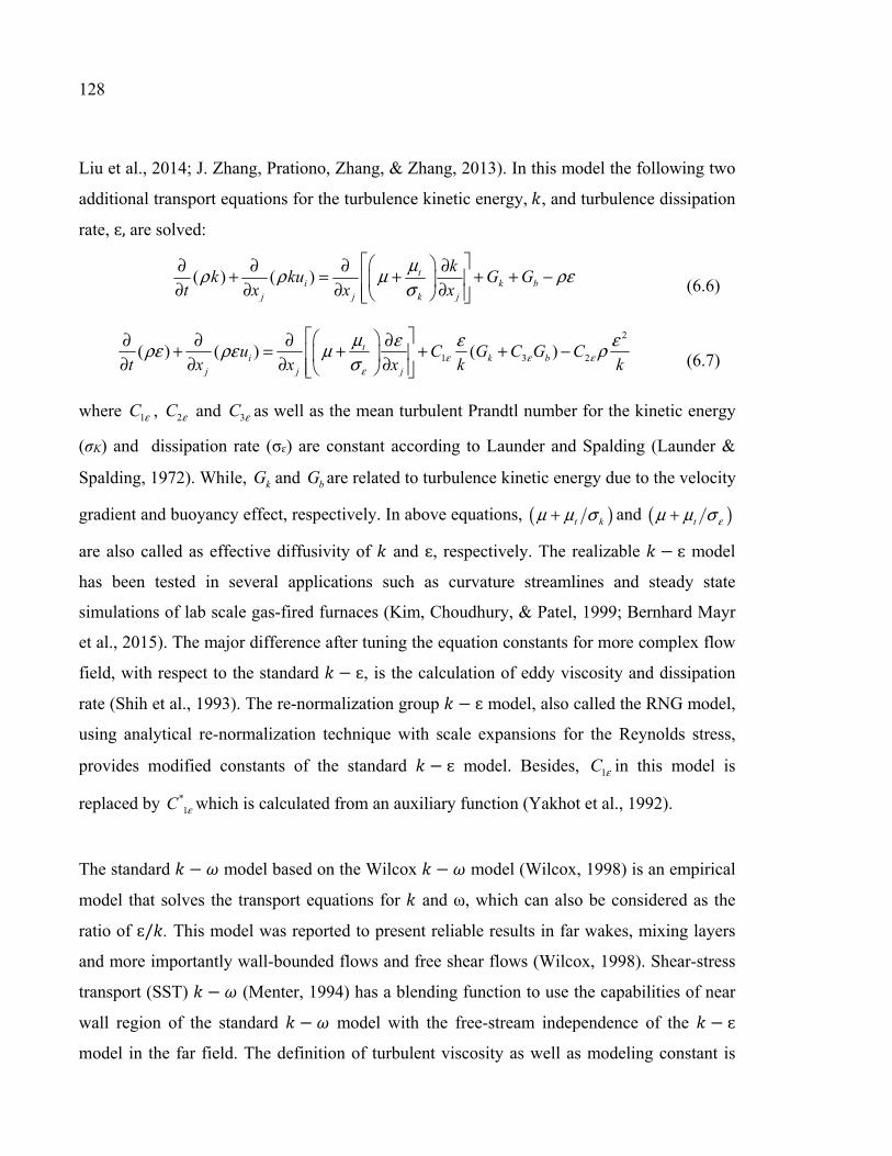
128

Liu et al., 2014; J. Zhang, Prationo, Zhang, & Zhang, 2013). In this model the following two

additional transport equations for the turbulence kinetic energy, 𝑘, and turbulence dissipation

rate, ɛ, are solved:

( ) ( ) ti k b

j j k j

kk ku G Gt x x x

μρ ρ μ ρεσ

∂ ∂ ∂ ∂+ = + + + − ∂ ∂ ∂ ∂ (6.6)

2

1 3 2( ) ( ) ( )ti k b

j j j

u C G C G Ct x x x k kε ε ε

ε

μ ε ε ερε ρε μ ρσ

∂ ∂ ∂ ∂+ = + + + − ∂ ∂ ∂ ∂ (6.7)

where 1C ε , 2C ε and 3C ε as well as the mean turbulent Prandtl number for the kinetic energy

(σK) and dissipation rate (σɛ) are constant according to Launder and Spalding (Launder &

Spalding, 1972). While, kG and bG are related to turbulence kinetic energy due to the velocity

gradient and buoyancy effect, respectively. In above equations, ( )t kμ μ σ+ and ( )t εμ μ σ+

are also called as effective diffusivity of 𝑘 and ɛ, respectively. The realizable 𝑘 − ɛ model

has been tested in several applications such as curvature streamlines and steady state

simulations of lab scale gas-fired furnaces (Kim, Choudhury, & Patel, 1999; Bernhard Mayr

et al., 2015). The major difference after tuning the equation constants for more complex flow

field, with respect to the standard 𝑘 − ɛ, is the calculation of eddy viscosity and dissipation

rate (Shih et al., 1993). The re-normalization group 𝑘 − ɛ model, also called the RNG model,

using analytical re-normalization technique with scale expansions for the Reynolds stress,

provides modified constants of the standard 𝑘 − ɛ model. Besides, 1C ε in this model is

replaced by *1C ε which is calculated from an auxiliary function (Yakhot et al., 1992).

The standard 𝑘 − 𝜔 model based on the Wilcox 𝑘 − 𝜔 model (Wilcox, 1998) is an empirical

model that solves the transport equations for 𝑘 and ω, which can also be considered as the

ratio of ɛ/𝑘. This model was reported to present reliable results in far wakes, mixing layers

and more importantly wall-bounded flows and free shear flows (Wilcox, 1998). Shear-stress

transport (SST) 𝑘 − 𝜔 (Menter, 1994) has a blending function to use the capabilities of near

wall region of the standard 𝑘 − 𝜔 model with the free-stream independence of the 𝑘 − ɛ model in the far field. The definition of turbulent viscosity as well as modeling constant is

129

modified in the SST 𝑘 − 𝜔 model with respect to the standard 𝑘 − 𝜔 model (Menter, 1994).

In the two equation models, the turbulent viscosity is calculated using empirical or theoretical

correlations between turbulence kinetic energy and eddy dissipation rate for the specific flow

conditions. The RSM model, on the other hand, solves all Reynolds stresses and turbulence

dissipation instead of using eddy-viscosity concept. In this respect, RSM solves seven

turbulence transport equations for 3D flows considering the turbulence anisotropy. This is in

contrast to the two equation models which assume isotropic turbulence field (Cant, 2001).

6.3.2 Combustion and radiation modeling

In the present study, the equilibrium non-premix combustion model was used to predict the

natural gas combustion inside the burner and furnace domains. The applicability of the eddy-

dissipation model (EDM) (B. F. Magnussen & Hjertager, 1977) for an accurate prediction of

the temperature distribution in large size forgings within gas-fired furnaces was recently

reported (Bohlooli Arkhazloo et al., 2019). Considering that in the Tempest burner natural-

gas and oxidizer enter into the reaction zone in distinct streams (20% of air with the gas

reacts in the primary chamber and 80% of air reacts in the secondary chamber) the

applicability of non-premix combustion with the chemical equilibrium model using β-shape

probability-density function (PDF) was assessed in the present investigation. The non-premix

with PDF model was developed for the turbulent diffusion flame with a fast chemistry

assuming that the reaction in the turbulent combustion is sufficiently rapid to reach

equilibrium resulting in lower computational cost in comparison with the EDM model

(Ismail, Ng, & Gan, 2012).

In the non-premix model, combustion is simplified to a mixing problem by assuming equal

diffusivities for all the species and species concentration is derived from the predicted

mixture fraction fields stored in a table (ANSYS, 2016). Therefore, computations of non-

linear reaction rates are avoided. The mixture fraction is defined as (Ishii, Zhang, &

Sugiyama, 1998):

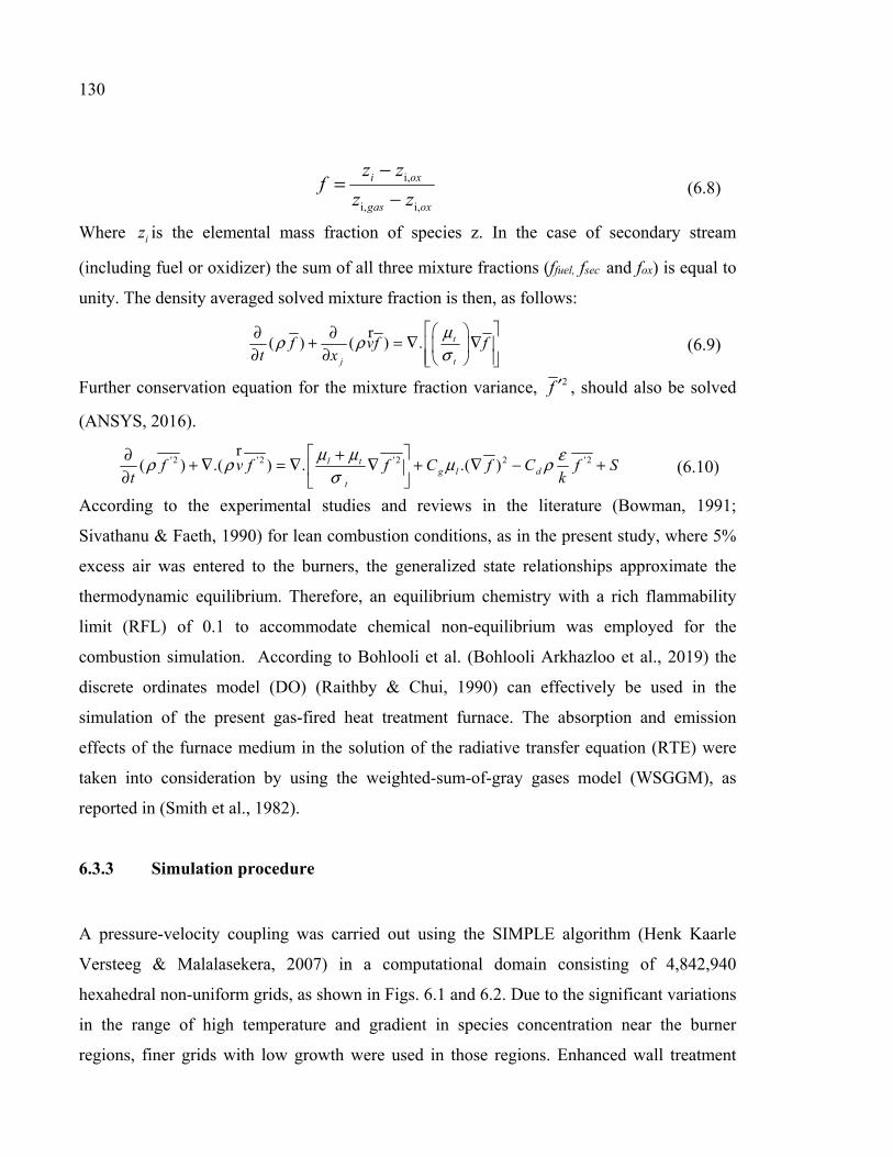
130

i,

i, i,

i ox

gas ox

z zf

z z−

=−

(6.8)

Where iz is the elemental mass fraction of species z. In the case of secondary stream

(including fuel or oxidizer) the sum of all three mixture fractions (ffuel, fsec and fox) is equal to

unity. The density averaged solved mixture fraction is then, as follows:

( ) ( ) . t

j t

f vf ft x

μρ ρσ

∂ ∂+ = ∇ ∇ ∂ ∂

r (6.9)

Further conservation equation for the mixture fraction variance, 2f ′ , should also be solved

(ANSYS, 2016).

'2 '2 '2 2 '2( ) .( ) . .( )l tg l d

t

f v f f C f C f St k

μ μ ερ ρ μ ρσ

+∂ + ∇ = ∇ ∇ + ∇ − + ∂

r (6.10)

According to the experimental studies and reviews in the literature (Bowman, 1991;

Sivathanu & Faeth, 1990) for lean combustion conditions, as in the present study, where 5%

excess air was entered to the burners, the generalized state relationships approximate the

thermodynamic equilibrium. Therefore, an equilibrium chemistry with a rich flammability

limit (RFL) of 0.1 to accommodate chemical non-equilibrium was employed for the

combustion simulation. According to Bohlooli et al. (Bohlooli Arkhazloo et al., 2019) the

discrete ordinates model (DO) (Raithby & Chui, 1990) can effectively be used in the

simulation of the present gas-fired heat treatment furnace. The absorption and emission

effects of the furnace medium in the solution of the radiative transfer equation (RTE) were

taken into consideration by using the weighted-sum-of-gray gases model (WSGGM), as

reported in (Smith et al., 1982).

6.3.3 Simulation procedure

A pressure-velocity coupling was carried out using the SIMPLE algorithm (Henk Kaarle

Versteeg & Malalasekera, 2007) in a computational domain consisting of 4,842,940

hexahedral non-uniform grids, as shown in Figs. 6.1 and 6.2. Due to the significant variations

in the range of high temperature and gradient in species concentration near the burner

regions, finer grids with low growth were used in those regions. Enhanced wall treatment

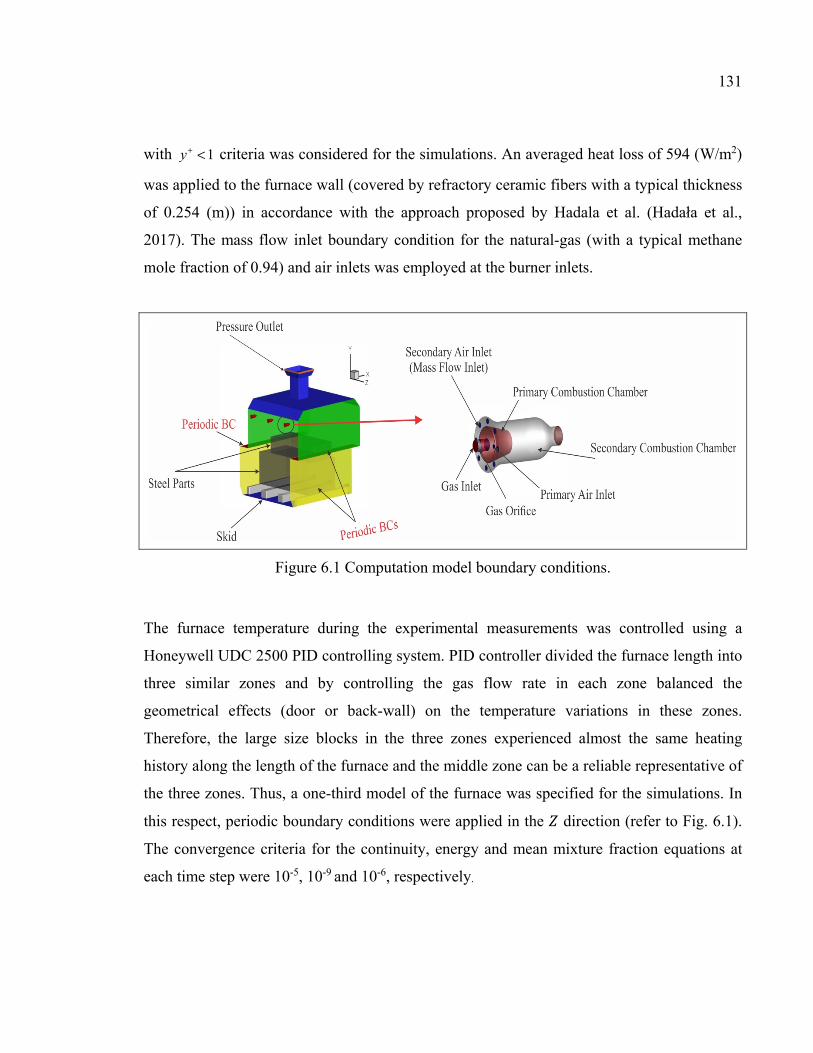
131

with 1y+ < criteria was considered for the simulations. An averaged heat loss of 594 (W/m2)

was applied to the furnace wall (covered by refractory ceramic fibers with a typical thickness

of 0.254 (m)) in accordance with the approach proposed by Hadala et al. (Hadała et al.,

2017). The mass flow inlet boundary condition for the natural-gas (with a typical methane

mole fraction of 0.94) and air inlets was employed at the burner inlets.

Figure 6.1 Computation model boundary conditions.

The furnace temperature during the experimental measurements was controlled using a

Honeywell UDC 2500 PID controlling system. PID controller divided the furnace length into

three similar zones and by controlling the gas flow rate in each zone balanced the

geometrical effects (door or back-wall) on the temperature variations in these zones.

Therefore, the large size blocks in the three zones experienced almost the same heating

history along the length of the furnace and the middle zone can be a reliable representative of

the three zones. Thus, a one-third model of the furnace was specified for the simulations. In

this respect, periodic boundary conditions were applied in the 𝑍 direction (refer to Fig. 6.1).

The convergence criteria for the continuity, energy and mean mixture fraction equations at

each time step were 10-5, 10-9 and 10-6, respectively.

132

Figure 6.2 Grid resolution of furnace domain and its details including gas-fired burner.

Due to the high amount of temperature variance during the heat treatment process,

temperature dependent thermo-physical properties were taken into account in the present

simulations. These properties were estimated using JMatPro software (JMatPro Users Guide

6.2.1.), as shown in Fig. 6.3 (a). The chemical compositions of the steel parts used in this

computation are presented in Table 6.1. The emissivity of steel parts, as oxidized steel

surface, was set to 0.8 while, refractories’ emissivity was set to 0.75. The pressure outlet

boundary conditions were assumed for the chimneys’ exhaust.

Table 6.1 Chemical Analysis of the test Ingot - Weight % (Finkl Steel Inc).

Fe C Mn Si Mo Cr Ni Other Bal. 0.35 0.85 0.4 0.45 1.85 0.47 Micro alloying

6.4 Experimental measurements

Transient temperature measurements of the block as well as gas and air flow metering of the

burners were carried out during the heat treatment process. Specifically, a 1.4×0.89×2.72

(m3) forged block and a 1.09×0.50×2.25 (m3) slab, placed on its upper surface, were

considered as the case study. The two other sets of blocks were positioned with the same

relative distance, so as not to disturb the uniformity in the 𝑍 direction. The K type

thermocouples were embedded at different locations of the block including the stagnation

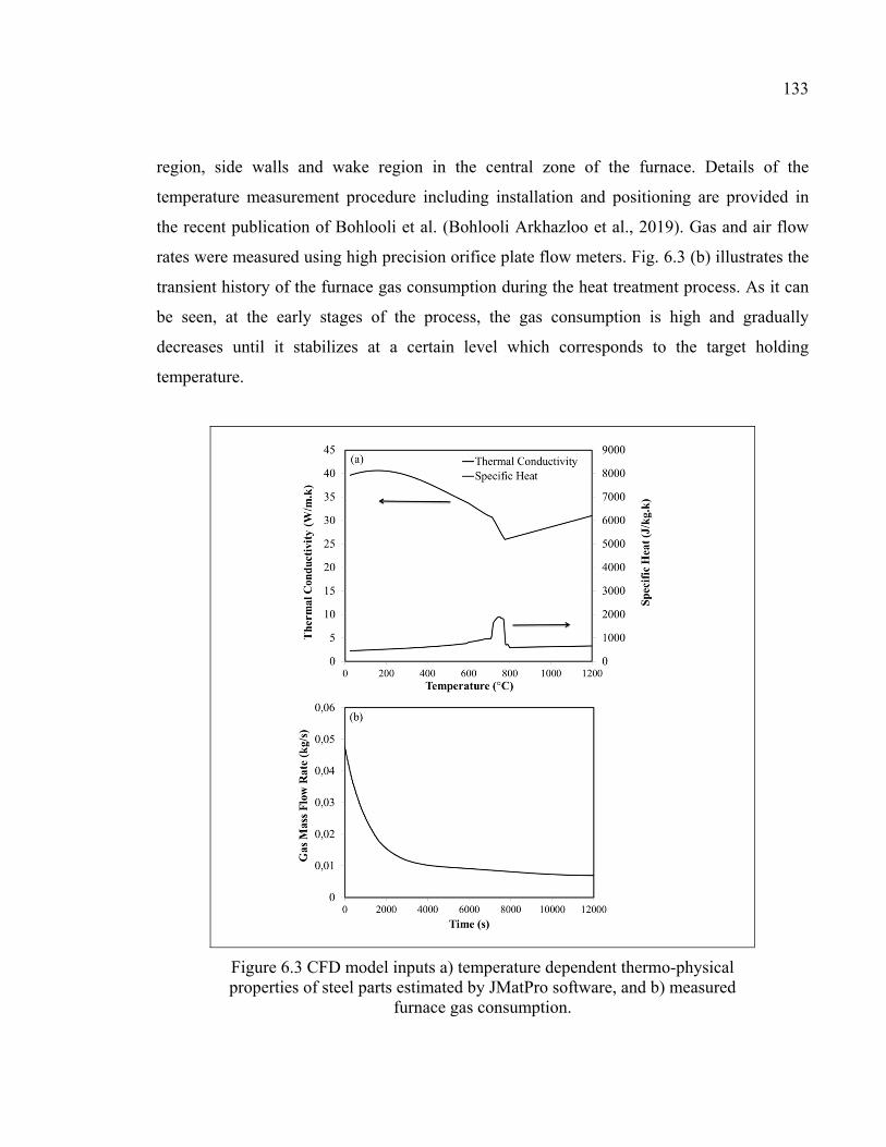
133

region, side walls and wake region in the central zone of the furnace. Details of the

temperature measurement procedure including installation and positioning are provided in

the recent publication of Bohlooli et al. (Bohlooli Arkhazloo et al., 2019). Gas and air flow

rates were measured using high precision orifice plate flow meters. Fig. 6.3 (b) illustrates the

transient history of the furnace gas consumption during the heat treatment process. As it can

be seen, at the early stages of the process, the gas consumption is high and gradually

decreases until it stabilizes at a certain level which corresponds to the target holding

temperature.

Figure 6.3 CFD model inputs a) temperature dependent thermo-physical properties of steel parts estimated by JMatPro software, and b) measured

furnace gas consumption.

134


6.5.1 Validation of periodic CFD model and combustion approach

A comparison between the CFD model predictions and the transient measured temperature is

presented in Fig. 6.4. The CFD model, consisting of the one-third periodic domain and

adopting the non-premix combustion with the equilibrium model together with the standard 𝑘 − ɛ model was used for the validation. It can be observed that the present CFD model

predicts the transient temperature history of the steel parts in the gas-fired furnace reasonably

well with a maximum over-prediction of 4%. Therefore, the chemical equilibrium non-

premix combustion model which requires a lower computational cost, as compared with

EDM, was employed as the basis for the assessment of turbulence modeling in the

investigated application.

Figure 6.4 Periodic CFD model including equilibrium non-premix combustion model validation.

135

6.5.2 Assessment of turbulence models

6.5.2.1 Temperature predictions of forged block

Accurate prediction of the temperature of bluff bodies and the corresponding flow fields in a

turbulent fluid flow is a challenging task (Ničeno et al., 2002). The thermal analysis of the

forged block mounted on the skid bars facing with burners’ flow stream, share several

similarities to the typical bluff bodies flow field such as stagnation point, wake region and

flow around the block (Bohlooli Arkhazloo et al., 2019). Therefore, these similarities were

used to analyze the thermal interactions in the present application. Fig. 6.5 represents the

temperature predictions by six various RANS based turbulence models at three different

locations of the forged block. Also, the measured data at the point in time (𝑡 = 𝑡 /6), where

the maximum temperature non-uniformity of the product was found (Bohlooli Arkhazloo et

al., 2019), are illustrated.

Accurate prediction of the stagnation point is one of the critical points when analyzing flow

over a bluff body and an impingement jet. Different turbulence models have been used to

predict the stagnation point’s temperature with various levels of accuracy, as reported by

Ničeno et al. (Ničeno et al., 2002) and Murakami (Murakami, 1993). In the present study, the

flow coming from the lower burners is faced with the right surface of the large block,

resulting in a stagnation point having similarities to an impingement jet application. Figure

6.5 (a) depicts the comparison between the measured temperature at a point (perpendicular to

the burner center line and 5 (cm) above the lower face of the block) in the stagnation region

and the corresponding predictions by the turbulence models. It can be seen that the standard

and realizable 𝑘 − ɛ models under-predicted by about 3.5% the temperature of the stagnation

region. This finding is in agreement with the results reported by Pulat et al. (Pulat, Isman,

Etemoglu, & Can, 2011) who also found that 𝑘 − ɛ group under-predicts the temperature of

the stagnation point in a typical impingement flow field.

136

Figure 6.5 Comparison of temperature predictions by various turbulence models and experiment at different locations of forged block: a) stagnation point, b) side wall, and c) wake region at 𝑡 =𝑡 /6.

137

On the other hand, the standard 𝑘 − 𝜔 and RNG 𝑘 − ɛ models showed a significant over-

prediction of the stagnation temperature, while, SST 𝑘 − 𝜔 and RSM lead to better

agreements with the experimental data. The capability of the SST 𝑘 − 𝜔 model in the

accurate prediction of the stagnation region regarding an impingement jet application has

been reported by several researchers (Ortega-Casanova & Castillo-Sanchez, 2017;

Zuckerman & Lior, 2006) and the present work confirms this for the application to gas-fired

furnaces. The better performance of SST 𝑘 − 𝜔 is probably due to the fact that the influence

of the viscous sub-layer is considered in this model. This allows for taking into account large

gradients of velocities, temperature and turbulence scalar quantities that are present near the

wall region and therefore provide a better representation of the actual conditions. Fig. 6.5 (a)

also shows that the RSM model solving all Reynolds stresses and turbulence dissipation and

considering turbulence anisotropy exhibited reliable predictions compared to the

experimental measurements.

Fig. 6.5 (b) displays the temperature predictions of different models for the region located at

the center of the block’s side wall (front and back walls). It should be noted that the

difference between temperature measurements on the side walls was less than 0.5% and,

therefore, only those for the front wall are illustrated. It can be seen that there is an

acceptable consistency between all the predictions and the experimental data with a

maximum deviation being about 3% for the RNG 𝑘 − ɛ model.

Furthermore, Fig. 6.5 (c) shows clearly that the wall in the wake region plays a critical role in

the selection process of the turbulence model. For instance, it can be seen that the realizable 𝑘 − ɛ model had more consistency with the measured data (2.3% under-prediction) among

the 𝑘 − ɛ group and the SST 𝑘 − 𝜔 model (about 3% over-prediction) from the 𝑘 − 𝜔 group

showed better predictions. The RSM model with 2.1% under-prediction concerning the

temperature prediction of the wall in the wake region showed reasonable consistency with

the measured data. On the basis of the above analysis and the temperature predictions of the

three different walls of the block, the RSM model can be considered as the most accurate

model in the context of the present study.

138

6.5.2.2 Combustion flow field predictions

Fig. 6.6 depicts the contours of time-averaged temperature around the high momentum

burner in the lateral plane perpendicular to the lower burners’ central cross-section.

Figure 6.6 Time averaged temperature contours of a high momentum lower burner predicted by a) Standard 𝑘 − ɛ, b)

Realizable 𝑘 − ɛ, c) standard 𝑘 − 𝜔, d) SST 𝑘 − 𝜔, e) RNG, and f) RSM models.

Results reveal that the standard and realizable 𝑘 − ɛ models (Figs. 6.6 (a) and 6.6 (b)) under-

predicted the flame temperature, as compared with the RSM model. Lower temperatures

were experienced around the stagnation line regarding these models’ predictions, while

standard 𝑘 − 𝜔 predicted the highest level of contour near the stagnation line (Fig. 6.6 (c)).

However, it should be mentioned that the standard and realizable 𝑘 − ɛ models could predict

the flame temperature fairly well in the lateral direction, whereas a thin flame is revealed as a

result of the simulation by standard 𝑘 − 𝜔 model. This is because the 𝑘 − 𝜔 model is

originally developed to solve the near-wall region. On the other hand, the standard 𝑘 − ɛ

model, which is well suited for high Reynolds number flows, is more reliable to solve the

turbulent core region of the flow near the burners. An over-prediction of the time-averaged

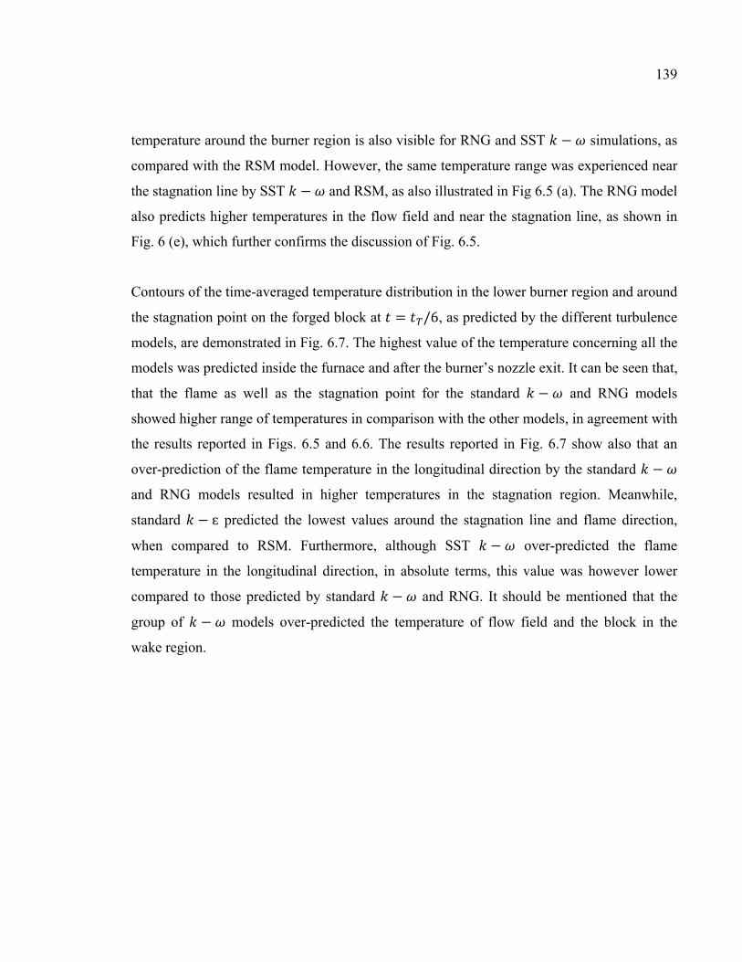
139

temperature around the burner region is also visible for RNG and SST 𝑘 − 𝜔 simulations, as

compared with the RSM model. However, the same temperature range was experienced near

the stagnation line by SST 𝑘 − 𝜔 and RSM, as also illustrated in Fig 6.5 (a). The RNG model

also predicts higher temperatures in the flow field and near the stagnation line, as shown in

Fig. 6 (e), which further confirms the discussion of Fig. 6.5.

Contours of the time-averaged temperature distribution in the lower burner region and around

the stagnation point on the forged block at 𝑡 = 𝑡 /6, as predicted by the different turbulence

models, are demonstrated in Fig. 6.7. The highest value of the temperature concerning all the

models was predicted inside the furnace and after the burner’s nozzle exit. It can be seen that,

that the flame as well as the stagnation point for the standard 𝑘 − 𝜔 and RNG models

showed higher range of temperatures in comparison with the other models, in agreement with

the results reported in Figs. 6.5 and 6.6. The results reported in Fig. 6.7 show also that an

over-prediction of the flame temperature in the longitudinal direction by the standard 𝑘 − 𝜔

and RNG models resulted in higher temperatures in the stagnation region. Meanwhile,

standard 𝑘 − ɛ predicted the lowest values around the stagnation line and flame direction,

when compared to RSM. Furthermore, although SST 𝑘 − 𝜔 over-predicted the flame

temperature in the longitudinal direction, in absolute terms, this value was however lower

compared to those predicted by standard 𝑘 − 𝜔 and RNG. It should be mentioned that the

group of 𝑘 − 𝜔 models over-predicted the temperature of flow field and the block in the

wake region.

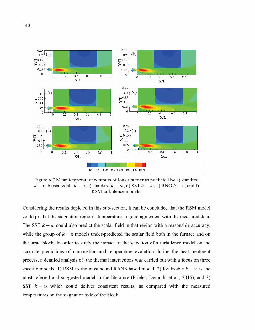
140

Figure 6.7 Mean temperature contours of lower burner as predicted by a) standard 𝑘 − ɛ, b) realizable 𝑘 − ɛ, c) standard 𝑘 − 𝜔, d) SST 𝑘 − 𝜔, e) RNG 𝑘 − ɛ, and f) RSM turbulence models.

Considering the results depicted in this sub-section, it can be concluded that the RSM model

could predict the stagnation region’s temperature in good agreement with the measured data.

The SST 𝑘 − 𝜔 could also predict the scalar field in that region with a reasonable accuracy,

while the group of 𝑘 − ɛ models under-predicted the scalar field both in the furnace and on

the large block. In order to study the impact of the selection of a turbulence model on the

accurate predictions of combustion and temperature evolution during the heat treatment

process, a detailed analysis of the thermal interactions was carried out with a focus on three

specific models: 1) RSM as the most sound RANS based model, 2) Realizable 𝑘 − ɛ as the

most referred and suggested model in the literature (Prieler, Demuth, et al., 2015), and 3)

SST 𝑘 − 𝜔 which could deliver consistent results, as compared with the measured

temperatures on the stagnation side of the block.

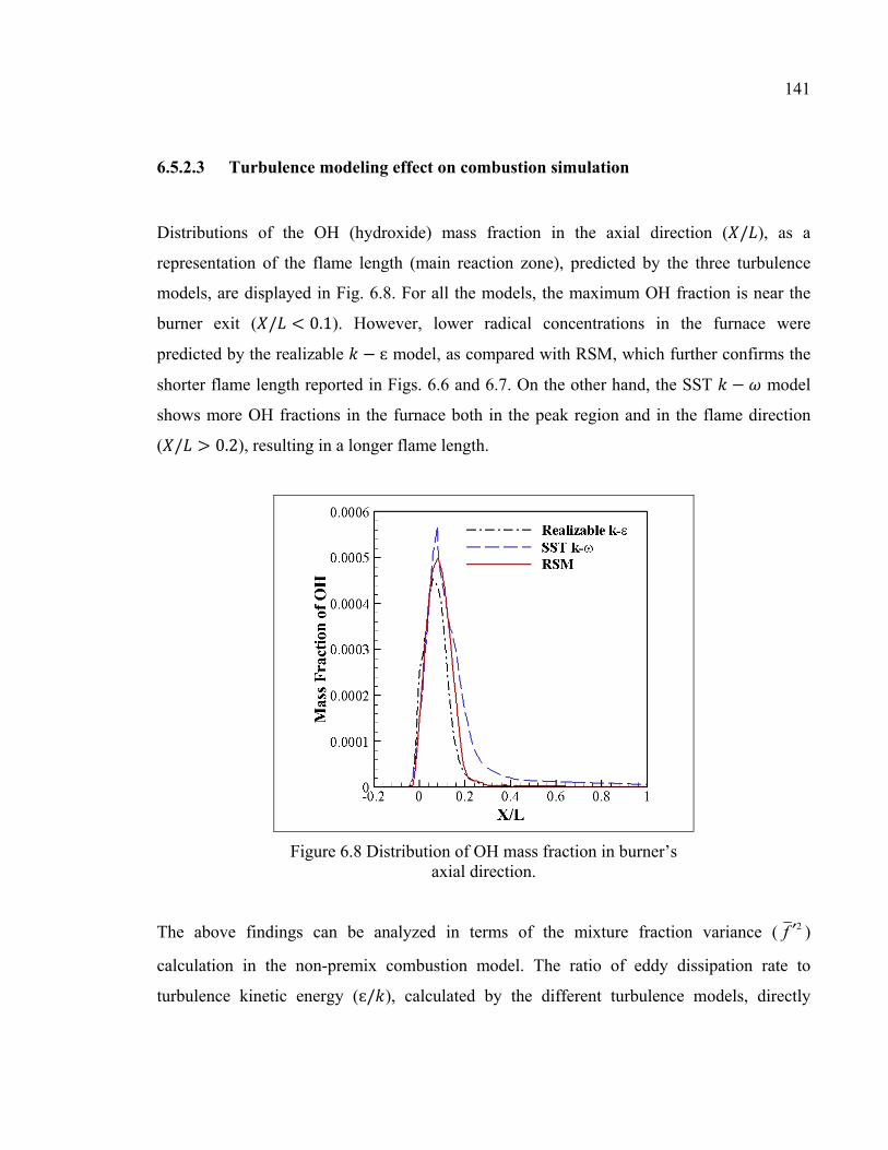
141

6.5.2.3 Turbulence modeling effect on combustion simulation

Distributions of the OH (hydroxide) mass fraction in the axial direction (𝑋/𝐿), as a

representation of the flame length (main reaction zone), predicted by the three turbulence

models, are displayed in Fig. 6.8. For all the models, the maximum OH fraction is near the

burner exit (𝑋/𝐿 < 0.1). However, lower radical concentrations in the furnace were

predicted by the realizable 𝑘 − ɛ model, as compared with RSM, which further confirms the

shorter flame length reported in Figs. 6.6 and 6.7. On the other hand, the SST 𝑘 − 𝜔 model

shows more OH fractions in the furnace both in the peak region and in the flame direction

(𝑋/𝐿 > 0.2), resulting in a longer flame length.

Figure 6.8 Distribution of OH mass fraction in burner’s axial direction.

The above findings can be analyzed in terms of the mixture fraction variance ( 2f ′ )

calculation in the non-premix combustion model. The ratio of eddy dissipation rate to

turbulence kinetic energy (ɛ/𝑘), calculated by the different turbulence models, directly

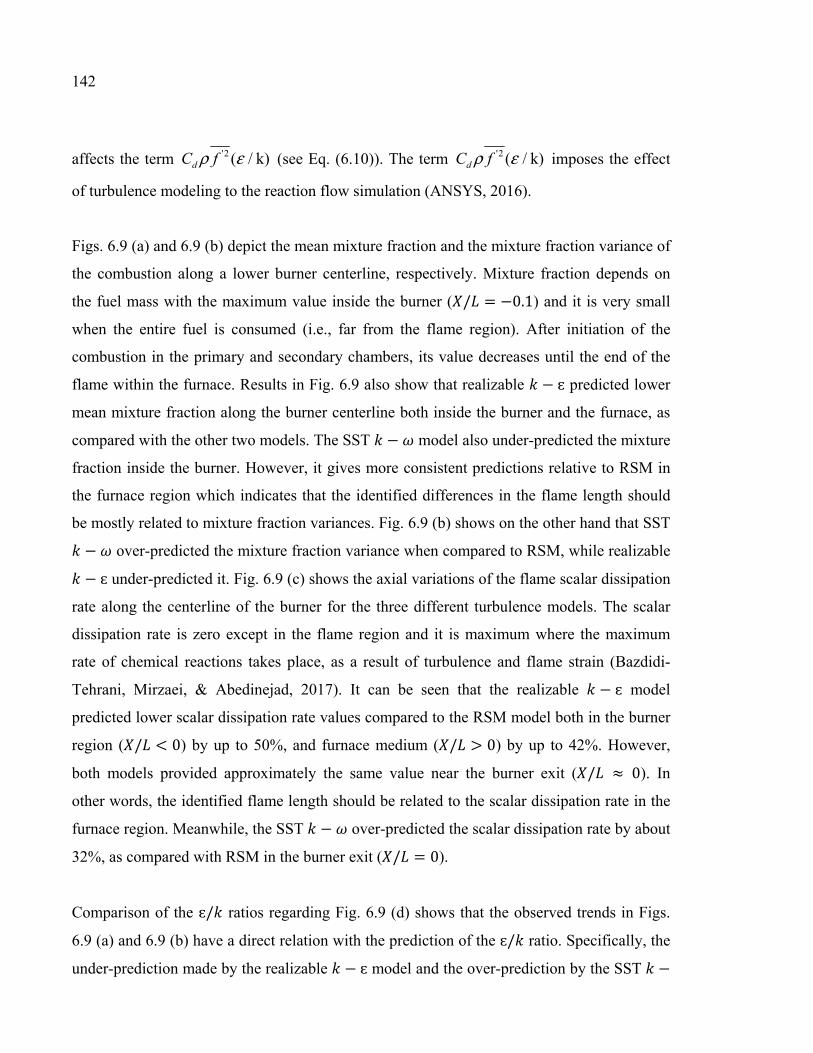
142

affects the term '2 ( / k)dC fρ ε (see Eq. (6.10)). The term '2 ( / k)dC fρ ε imposes the effect

of turbulence modeling to the reaction flow simulation (ANSYS, 2016).

Figs. 6.9 (a) and 6.9 (b) depict the mean mixture fraction and the mixture fraction variance of

the combustion along a lower burner centerline, respectively. Mixture fraction depends on

the fuel mass with the maximum value inside the burner (𝑋/𝐿 = −0.1) and it is very small

when the entire fuel is consumed (i.e., far from the flame region). After initiation of the

combustion in the primary and secondary chambers, its value decreases until the end of the

flame within the furnace. Results in Fig. 6.9 also show that realizable 𝑘 − ɛ predicted lower

mean mixture fraction along the burner centerline both inside the burner and the furnace, as

compared with the other two models. The SST 𝑘 − 𝜔 model also under-predicted the mixture

fraction inside the burner. However, it gives more consistent predictions relative to RSM in

the furnace region which indicates that the identified differences in the flame length should

be mostly related to mixture fraction variances. Fig. 6.9 (b) shows on the other hand that SST 𝑘 − 𝜔 over-predicted the mixture fraction variance when compared to RSM, while realizable 𝑘 − ɛ under-predicted it. Fig. 6.9 (c) shows the axial variations of the flame scalar dissipation

rate along the centerline of the burner for the three different turbulence models. The scalar

dissipation rate is zero except in the flame region and it is maximum where the maximum

rate of chemical reactions takes place, as a result of turbulence and flame strain (Bazdidi-

Tehrani, Mirzaei, & Abedinejad, 2017). It can be seen that the realizable 𝑘 − ɛ model

predicted lower scalar dissipation rate values compared to the RSM model both in the burner

region (𝑋/𝐿 < 0) by up to 50%, and furnace medium (𝑋/𝐿 > 0) by up to 42%. However,

both models provided approximately the same value near the burner exit (𝑋/𝐿 ≈ 0). In

other words, the identified flame length should be related to the scalar dissipation rate in the

furnace region. Meanwhile, the SST 𝑘 − 𝜔 over-predicted the scalar dissipation rate by about

32%, as compared with RSM in the burner exit (𝑋/𝐿 = 0).

Comparison of the ɛ/𝑘 ratios regarding Fig. 6.9 (d) shows that the observed trends in Figs.

6.9 (a) and 6.9 (b) have a direct relation with the prediction of the ɛ/𝑘 ratio. Specifically, the

under-prediction made by the realizable 𝑘 − ɛ model and the over-prediction by the SST 𝑘 −

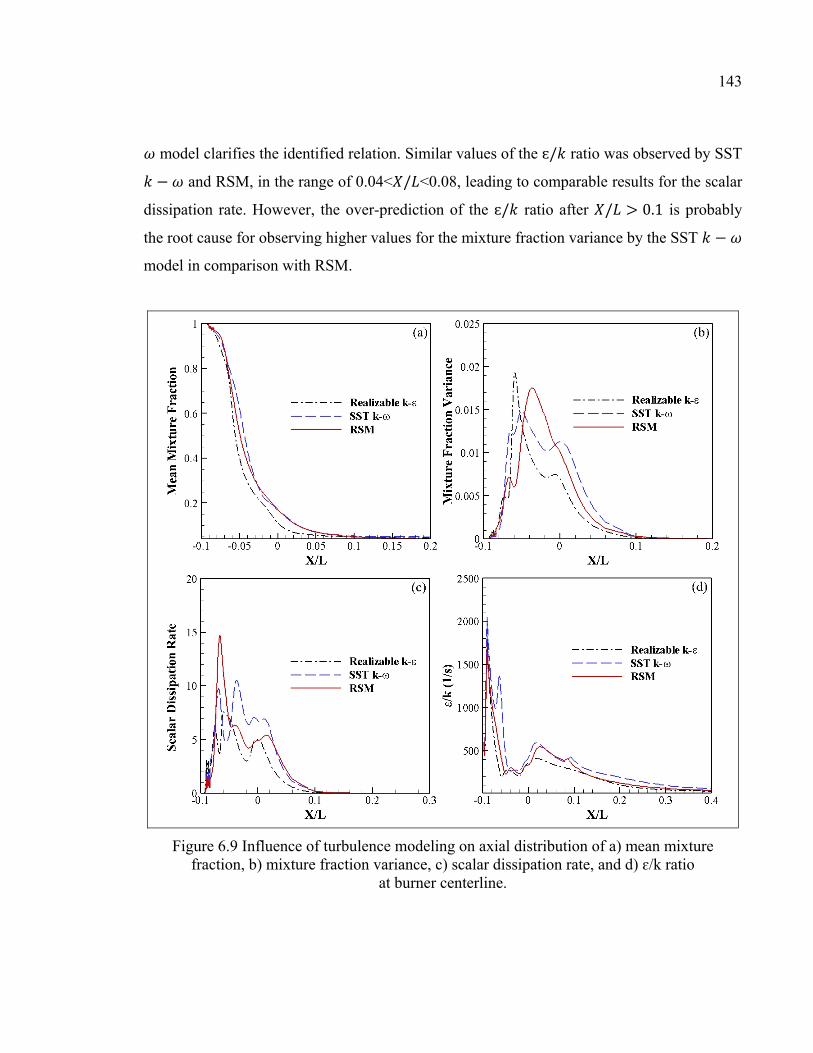
143

𝜔 model clarifies the identified relation. Similar values of the ɛ/𝑘 ratio was observed by SST 𝑘 − 𝜔 and RSM, in the range of 0.04<𝑋/𝐿<0.08, leading to comparable results for the scalar

dissipation rate. However, the over-prediction of the ɛ/𝑘 ratio after 𝑋/𝐿 > 0.1 is probably

the root cause for observing higher values for the mixture fraction variance by the SST 𝑘 − 𝜔

model in comparison with RSM.

Figure 6.9 Influence of turbulence modeling on axial distribution of a) mean mixture fraction, b) mixture fraction variance, c) scalar dissipation rate, and d) ɛ/k ratio

at burner centerline.

144

The observed trends in the ɛ/𝑘 ratio can be interpreted by analyzing the results of Fig. 6.10,

where the contours of the turbulence kinetic energy near the lower burner region are

depicted.

Figure 6.10 Turbulence kinetic energy contours of lower burner region by a) realizable 𝑘 − ɛ, b) SST 𝑘 − 𝜔, and c) RSM turbulence models.

It is revealed that the turbulence kinetic energy, TKE, was highly over-predicted near the

nozzle exit (0<𝑋/𝐿<0.1) and along the centerline by the realizable 𝑘 − ɛ model in

comparison with the other two models. This excessive TKE prediction could be related to an

over-estimation of the turbulence production term, because in realizable 𝑘 − ɛ an isotropic

eddy viscosity condition is assumed, which is a significant over-simplification for the present

case where a highly anisotropic flow field is present. The over-prediction of TKE by the

group of 𝑘 − ɛ models has already been mentioned in several turbulence included

applications pointing out the fact that the 𝑘 − ɛ models fail to resolve the normal stress

anisotropy (Leschziner, 2006; Tominaga & Stathopoulos, 2013). It should be noted that the

eddy viscosity models have some limitations in systems with rotation, swirl secondary

strains, large strain rates and impingement which should be taken into consideration in the

analysis (Tominaga & Stathopoulos, 2013). It can be seen that SST 𝑘 − 𝜔 gave a reasonably

similar range of TKE compared to RSM at the burner exit (𝑋/𝐿<0.1) which is in agreement

145

with the findings in Fig. 6.9 (d). Considering the negligible difference in the results of the

eddy dissipation predictions by different models, it can be concluded that the TKE prediction

has a direct impact on the ɛ/𝑘 ratio and, subsequently, on the scalar dissipation rate and the

mixture fraction variance.

6.5.2.4 Turbulence modeling impact on block’s temperature distribution

Investigation of the temperature distribution inside the forged block can help quantifying the

impact of turbulence modeling on the overall temperature distribution of the products within

gas-fired heat treatment furnaces. In this regard, Fig. 6.11 displays the temperature

distributions inside the forged block along three lateral lines, 𝑋/𝑊 (W indicates the width of

block), at the heights of 𝑌/𝐻= 0.25, 0.5, and 0.75. Increasing the height resulted in the

reduction of the temperature levels, which could be related to the presence of heating sources

(i.e., combustion of lower burners) adjacent to the bottom surface. Apart from the stagnation

point (see also Fig. 6.5), the three turbulence models provided similar predictions of the

temperature on the wall of the stagnation side. However, a slight over-prediction of the

temperature (a maximum of 2.6%) on the stagnation side was found for SST 𝑘 − 𝜔 at 𝑌/𝐻=0.75 (Fig. 6.11 (c)). Results indicate that all the models predicted almost the same

temperatures around the block center (𝑋/𝑊=0) at 𝑌/𝐻=0.25 and 0.5. However, the SST 𝑘 −𝜔 over-predicted the block temperature by about 7% in the center of the block, at 𝑌/𝐻=0.75.

In addition, SST 𝑘 − 𝜔 over-predicted the temperature of the wake region wall (by up to 9%

at 𝑌/𝐻=0.75) in comparison with RSM. On the other hand, Realizable 𝑘 − ɛ showed good

consistency with RSM, not only on the stagnation side, but also inside the block.

The above results demonstrate that the realizable 𝑘 − ɛ model could reasonably predict the

temperature evolution of the block within the gas-fired furnace. This particular model

characterized with a lower computational cost per iteration, as compared with RSM, could be

a reliable model for the block temperature predictions. Although, SST 𝑘 − 𝜔 showed

reasonable results on the stagnation line and computation of the maximum temperature of the

block (which can be used for the residence time optimization of the products inside the

146

furnace) it has limitations regarding the temperature predictions of the wake region.

However, an accurate prediction of the wake region behind the block is of great importance

for the temperature prediction as well as evaluation of turbulence modeling in applications

where large size parts are used.

Figure 6.11 Temperature distribution of large size block predicted by three turbulence models at non-dimensional heights of a) 𝑌/𝐻=0.25, b) 𝑌/𝐻=0.5, and c) 𝑌/𝐻=0.75.

147

6.5.2.5 Analysis of vortical structures

The influence of the vortical structures formation on the transient temperature history of the

forged block inside the furnace was discussed in a recent publication by Bohlooli et al.

(Bohlooli Arkhazloo et al., 2019). Fig. 6.12 represents the streamlines of flow field as

predicted by the three various turbulence models.

Although, inconsistencies can be observed on the upper side of the furnace, realizable 𝑘 − ɛ and SST 𝑘 − 𝜔 fairly captured the streamlines attached to the top surface of the slab.

However, realizable 𝑘 − ɛ could not capture the vortical structure on the top of the block. An

over-prediction of the turbulence kinetic energy by the group of 𝑘 − ɛ models results in a

high value of the eddy viscosity computation. Consequently, an excessive mixing effect

reduced the reversed flow on the top surface of the block. Besides, SST 𝑘 − 𝜔 and realizable 𝑘 − ɛ could not accurately predict the locations and strength of vortical structures on the

wake region. For example, the location of a strong recirculating vortex on the wake region

was not consistent for the three models. This may be related with the fact that the velocity

fluctuation induced by the vortices cannot be produced by the two equation models. A

similar behavior was reported by Tominaga and Stathopoulos (Tominaga & Stathopoulos,

2013) in the simulation of flow and dispersion around a cubic model building. According to

reference (Tominaga & Stathopoulos, 2013), the two equation RANS based models can not

accurately reproduce the vortex shedding velocity fluctuation behind the bluff body. This

inconsistency in the local prediction of the flow recirculation could be the reason for the

over- and under-prediction of the temperature at the wake side of the block by the SST 𝑘 − 𝜔

and the realizable 𝑘 − ɛ, respectively. The recirculating part was formed on the bigger

heights for SST 𝑘 − 𝜔, as compared with RSM, which could be related to the over-prediction

of the temperature at 𝑌/𝐻=0.75 in Fig. 6.11 (c), as a result of a reattachment of the high

temperature fluid to the block wall. On the other hand, although the realizable 𝑘 − ɛ could

not accurately predict the location of the vortical structure in comparison with the RSM, it

resulted in a similar attachment of the fluid flow near the wake region wall giving similar

temperatures in this region (see Fig. 6.11).

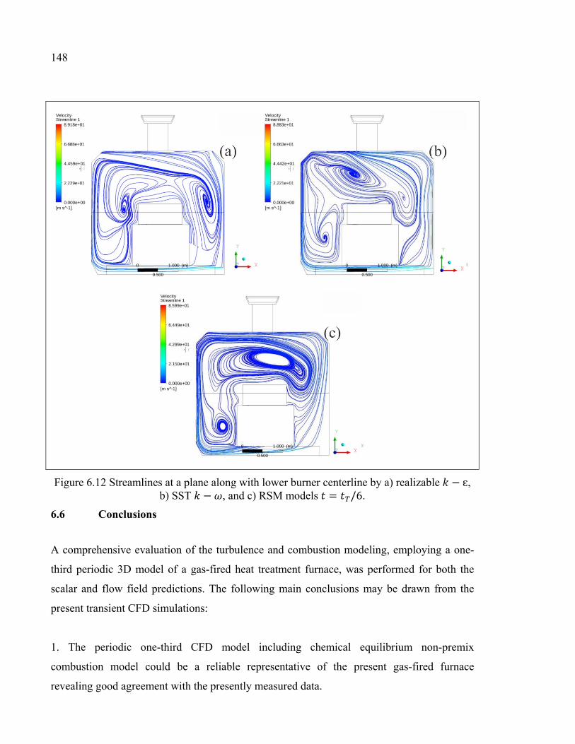
148

Figure 6.12 Streamlines at a plane along with lower burner centerline by a) realizable 𝑘 − ɛ, b) SST 𝑘 − 𝜔, and c) RSM models 𝑡 = 𝑡 /6.

6.6 Conclusions

A comprehensive evaluation of the turbulence and combustion modeling, employing a one-

third periodic 3D model of a gas-fired heat treatment furnace, was performed for both the

scalar and flow field predictions. The following main conclusions may be drawn from the

present transient CFD simulations:

1. The periodic one-third CFD model including chemical equilibrium non-premix

combustion model could be a reliable representative of the present gas-fired furnace

revealing good agreement with the presently measured data.

149

2. The present work showed that the choice of a turbulence model has a significant effect on

the prediction of combustion and heat transfer phenomena around the block and the burners.

3. Prediction of the ɛ/𝑘 ratio in the mean mixture fraction variance transport equation, which

changes the scalar dissipation rate in the combustion zone could directly affect the flame

length and heat transfer rates to the block. The 𝑘 − ɛ group of models by providing an over-

prediction of the turbulence kinetic energy and consequently under-prediction of the ɛ/𝑘

ratio, under- estimated the flame length and heat transfer rates around the burner compared to

the RSM and SST 𝑘 − 𝜔 models, as well as temperature measurements..

4. The RSM model could predict the most accurate results, as compared with the measured

data in the context of the present study.

5. Although some under-predictions were observed for the flame length and stagnation

region’s temperature predictions, the realizable 𝑘 − ɛ provided the block temperature history

and the wake region turbulence flow field with an acceptable consistency, as compared with

RSM.

6. The 𝑘 − 𝜔 group of models over-predicted the temperature field inside the large size

block, mainly due to a failure in capturing the wake region.

CONCLUSION

The work presented in this thesis focused on the numerical/experimental analysis of large

size forgings heat treatment process inside gas-fired furnaces. Thermal interactions inside the

furnace were analyzed to reduce temperature non-uniformity distribution of forgings as well

as reduction of their residence time inside large size gas-fired heat treatment furnaces. Details

of thermal interactions including combustion, radiation, and turbulence inside the furnace

were discussed. Also, a systematic investigation of strength and limitations of different

numerical models to simulate radiation, combustion and turbulence in the present context

was presented. Enlisted are the drawn conclusions from this research.

1. 3D CFD models including one-third periodic configuration covering practical details

of the furnace such as high momentum burners and fixing bars was capable enough to

capture the experimentally measured temperature evolution of the forged ingot.

2. Analysis of experimental temperature measurements showed that the unloaded

furnace domain was uniform during the test. However, after loading temperature non-

uniformities on the forged ingot surfaces (up to 200 K and 331 K for the conventional

single and multiple loading, respectively) were found during the process. Findings

indicate the forged ingots loading and their sizes, could affect the uniformity

performance of the furnace and subsequently the final product properties.

3. The identified temperature distribution non-uniformities were affected by influence of

geometrical effects (such as burner locations and fixing bars), turbulence flow field

(formation of vortical structures), and loading patterns inside the furnace. These items

should be taken into consideration for optimizing the heat treatment process of large

size components.

4. Taking the advantages of skids and spacers usage in the multiple loading

configurations can effectively help the process optimization. It could reduce the

152

temperature non-uniformity of large size forgings inside the gas-fired furnace up to

32%.

5. The hybrid methodology proposed and validated for residence time optimization of

large size forging in this work could be applied to other furnace types or steel alloys.

It was possible to reduce the total residence time of large parts by about 15.5% for the

process of this investigation.

6. It was found that the convection heat transfer was the dominant heat transfer

mechanism in the presence of central spacers to affect the temperature uniformity of

the heavy steel parts in gas-fired furnaces.

7. Analysis of results showed that the radiation view factor had a higher contribution

than participating medium in the radiation heat transfer mode during the process as

both DO an S2S model resulted in predictions with less than 2% differences.

Therefore, S2S model which is characterized by lower computational cost model

compared with DO, can be effectively used in the heat treatment analysis of large size

components.

8. Applicability of non-premix combustion with equilibrium model as a computationally

effective combustion model was approved along with EDM model for the context of

the present study.

9. The choice of the turbulence model in the present application had a significant effect

on the combustion and heat transfer phenomenon around the block and the burners.

Specifically, prediction of ɛ/𝑘 term by different models could directly affect the

mean mixture fraction variance and change the scalar dissipation rate in the

combustion zone, leading to changing in the flame length and heat transfer rates to

the block.

153

10. RSM model was approved as the soundest RANS based turbulence model in the

context of present study to accurately predict the thermal interactions in critical

regions around the block using standard suggested coefficients for the simulations.

11. The SST 𝑘 − 𝜔 model could also predict the scalar field in this region with a

reasonable accuracy.

12. It could be concluded that apart from some under-predictions observed for the flame

length and stagnation region’s temperature predictions by realizable 𝑘 − ɛ model, this

model could illustrate global block temperature history with an acceptable

consistency, as compared with RSM model and measurements.

13. Although the SST 𝑘 − 𝜔 model failed to capture the wake regions revealed an over-

predicted temperature field inside the large size block temperature, it resulted in

reasonable predictions in the stagnation point and burner combustion (which can be

used for the process optimization using developed hybrid technology). It should be

mentioned that the standard 𝑘 − 𝜔 model and the RNG 𝑘 − ɛ could not accurately

predict the thermal interactions, neither in the stagnation region, nor on the wake

region.

14. The developed CFD model and its data as well as experimental measurements

including hybrid methodology could be directly applied for the optimization of the

operational conditions and loading patterns during the heat treatment process of large

size forged ingots within gas-fired furnaces.

RECOMMENDATIONS The main purpose of present study was to carry out a comprehensive analysis of thermal

interactions during the heat treatment of large size forgings within gas-fired furnaces; and

subsequently to improve product’s residence time and loading pattern in this context. Apart

from directly applicable information to the real scale heat treatment of heavy forgings

provided by the present study, the following future investigations are suggested:

1) Application of hybrid methodology for other grades of steels for residence time

optimization of different large size heavy forgings. It is suggested to investigate

different metallurgical aspects (like residual stresses, microstructural transformations)

along with the hardness measurements for the further optimization.

2) In the present study natural gas and air at room temperature were employed for the

combustion. It is recommended to carry out an investigation on the pre-heated air

combustion effectiveness.

3) It was approved in this study that the radiation view factor was the dominant

parameter for accurate simulation of radiation heat transfer in the gas-fired furnace. It

is suggested to make analytical-numerical study on the optimization of radiation view

factor between large size forgings to further optimize the loading pattern within gas-

fired furnaces.

4) In the present study, temperature measurements of blocks were used as the main

criterion for the validation of numerical simulations. It is suggested to use particle

image velocimetry (PIV) measurement technique for further validation of combustion

process in the high-momentum gas-fired burner and subsequently investigate the

combustion products distributions within the furnace.

157

LIST OF REFERENCES

ANSYS. (2016). ANSYS Fluent Theory Guide. ANSYS Inc. Ashgriz, N., & Mostaghimi, J. (2002). An introduction to computational fluid dynamics.

Fluid Flow Handbook, 1, 1–49. Baukal Jr, C. E. (2003). Industrial burners handbook. CrC press. Bazdidi-Tehrani, F., Bohlooli, N., & Jadidi, M. (2015). Influence of film cooling jet inlet

boundary condition on large eddy simulation of model turbine blade leading edge. Progress in Computational Fluid Dynamics, an International Journal, 15(4), 214–227.

Bazdidi-Tehrani, F., Hatami, M., & Abouata, A. (2017). Effects of inlet and outlet boundary

conditions on the flow field of synthetic jets. Proceedings of the Institution of Mechanical Engineers, Part E: Journal of Process Mechanical Engineering, 231(2), 107–118.

Bazdidi-Tehrani, F., Mirzaei, S., & Abedinejad, M. S. (2017). Influence of Chemical

Mechanisms on Spray Combustion Characteristics of Turbulent Flow in a Wall Jet Can Combustor. Energy & Fuels, 31(7), 7523–7539.

Bazdidi-Tehrani, F., Mohammadi-Ahmar, A., Kiamansouri, M., & Jadidi, M. (2015).

Investigation of various non-linear eddy viscosity turbulence models for simulating flow and pollutant dispersion on and around a cubical model building. In Building Simulation (Vol. 8, pp. 149–166). Springer.

Bennett, C. (1962). 0. and JE Myers, Momentum. Heat and Mass Transfer", McGraw-Hill

Book Co., Inc., New York, NY, 291. Bergman, E. (2012). CFD Heat Transfer Validation of Turbine Structure Heat Treatment

Process. Bhadeshia, H., & Honeycombe, R. (2017). Steels: microstructure and properties.

Butterworth-Heinemann. Bohlooli Arkhazloo, N., Bouissa, Y., Bazdidi-Tehrani, F., Jadidi, M., Morin, J.-B., & Jahazi,

M. (2019). Experimental and unsteady CFD analyses of the heating process of large size forgings in a gas-fired furnace. Case Studies in Thermal Engineering, 14.

Bowman, C. T. (1991). Chemistry of gaseous pollutant formation and destruction. Fossil

Fuel Combustion. John Wiley & Sons, New York.

158

Canale, L. C. F., Yao, X., Gu, J., & Totten, G. E. (2008). A historical overview of steel tempering parameters. International Journal of Microstructure and Materials Properties, 3(4–5), 474–525.

Cant, R. S. (2001). SB Pope, Turbulent Flows, Cambridge University Press, Cambridge, UK.

Combustion and Flame, 125, 1361–1362. Chapman, K. S., Ramadhyani, S., & Viskanta, R. (1990). Modeling and parametric studies of

heat transfer in a direct-fired batch reheating furnace. Journal of Heat Treating, 8(2), 137–146.

Chattopadhyay, K., Isac, M., & Guthrie, R. I. L. (2010). Applications of Computational Fluid

Dynamics (CFD) in iron-and steelmaking: Part 1. Ironmaking & Steelmaking, 37(8), 554–561.

Cheng, L., Brakman, C. M., Korevaar, B. M., & Mittemeijer, E. J. (1988). The tempering of

iron-carbon martensite; dilatometric and calorimetric analysis. Metallurgical Transactions A, 19(10), 2415–2426.

Chui, E. H., & Raithby, G. D. (1993). Computation of radiant heat transfer on a

nonorthogonal mesh using the finite-volume method. Numerical Heat Transfer, 23(3), 269–288.

Constantin, P., & Foias, C. (1988). Navier-stokes equations. University of Chicago Press. Cosentino, F., Warnken, N., Gebelin, J.-C., & Reed, R. C. (2013). Numerical and

experimental study of post-heat treatment gas quenching and its impact on microstructure and creep in CMSX-10 superalloy. Journal of Materials Processing Technology, 213(12), 2350–2360.

Crasto, G. (2007). Numerical simulations of the atmospheric boundary layer. Universita

Degli Studi Di Cagliari: Cagliari, Italy. Danon, B., Cho, E. S., De Jong, W., & Roekaerts, D. J. E. M. (2011). Numerical

investigation of burner positioning effects in a multi-burner flameless combustion furnace. Applied Thermal Engineering, 31(17–18), 3885–3896. https://doi.org/10.1016/j.applthermaleng.2011.07.036.

Davidson, L. (2011). Fluid mechanics, turbulent flow and turbulence modeling. Chalmers

University of Technology, Goteborg, Sweden (Nov 2011) (Vol. 53). Denison, M., Borodai, S., Fox, R., & Bockelie, M. (2009). Multi-environment probability

density function method for modeling turbulent combustion in industrial equipment. In ASME 2009 International Mechanical Engineering Congress and Exposition (pp. 143–149). American Society of Mechanical Engineers.

159

Elkatatny, I., Morsi, Y., Blicblau, A. S., Das, S., & Doyle, E. D. (2003). Numerical analysis and experimental validation of high pressure gas quenching. International Journal of Thermal Sciences, 42(4), 417–423.

Finkl Steel Inc., M., Saint-Joseph-de-Sorel, QC J3R 3M8, Canada. Galletti, C., Coraggio, G., & Tognotti, L. (2013). Numerical investigation of oxy-natural-gas

combustion in a semi-industrial furnace: validation of CFD sub-models. Fuel, 109, 445–460.

Gao, M., Reid, C. N., Jahedi, M., & Li, Y. (2000). Estimating equilibration times and heating/cooling rates in heat treatment of workpieces with arbitrary geometry. Journal of Materials Engineering and Performance, 9(1), 62–71.

García, A. M., Colorado, A. F., Obando, J. E., Arrieta, C. E., & Amell, A. A. (2019). Effect

of the burner position on an austenitizing process in a walking-beam type reheating furnace. Applied Thermal Engineering, 153, 633–645.

Gongfa, L., Jia, L., Guozhang, J., Jianyi, K., Liangxi, X., Yikun, Z., & Fuwei, C. (2014).

Numerical simulation of flow , temperature and phase fields in U71Mn rail-head quenching process, 18(1), 61–70.

Govardhan, J., Rao, G. V. S., & Narasaiah, J. (2011). Experimental investigations and CFD

study of temperature distribution during oscillating combustion in a crucible furnace. Journal Homepage: Www. IJEE. IEEFoundation. Org, 2(5), 783–796.

Gur, C. H., & Pan, J. (2008). Handbook of Thermal Process Modeling Steels. CRC Press. Hadała, B., Malinowski, Z., & Rywotycki, M. (2017). Energy losses from the furnace

chamber walls during heating and heat treatment of heavy forgings. Energy, 139, 298–314.

Hao, X., Gu, J., Chen, N., Zhang, W., & Zuo, X. (2008). 3-D Numerical analysis on heating

process of loads within vacuum heat treatment furnace. Applied Thermal Engineering, 28(14–15), 1925–1931.

Harish, J., & Dutta, P. (2005). Heat transfer analysis of pusher type reheat furnace.

Ironmaking & Steelmaking, 32(2), 151–158. Howell, J. R., Menguc, M. P., & Siegel, R. (2015). Thermal radiation heat transfer. CRC

press. https://combustion.fivesgroup.com/. https://www.tainstruments.com.

160

Hussain, A. (1983). Coherent structures-Reality and myth.[in turbulent shear flow. Incropera, F. P., Lavine, A. S., Bergman, T. L., & DeWitt, D. P. (2007). Fundamentals of

heat and mass transfer. Wiley. ISA Standard. (1982). Temperature Measurement Thermocouples. Ishii, T., Zhang, C., & Hino, Y. (2002). Numerical study of the performance of a regenerative

furnace. Heat Transfer Engineering, 23(4), 23–33. Ishii, T., Zhang, C., & Sugiyama, S. (1998). Numerical simulations of highly preheated air

combustion in an industrial furnace. Journal of Energy Resources Technology, 120(4), 276–284.

Ismail, H. M., Ng, H. K., & Gan, S. (2012). Evaluation of non-premixed combustion and fuel

spray models for in-cylinder diesel engine simulation. Applied Energy, 90(1), 271–279. Jaklič, A., Glogovac, B., Kolenko, T., Zupančič, B., & Težak, B. (2002). A simulation of

heat transfer during billet transport. Applied Thermal Engineering, 22(7), 873–883. Janjušević, Z., Gulišija, Z., Mihailović, M., & Patarić, A. (2009). The investigation of

applicability of the Hollomon-Jaffe equation on tempering the HSLA steel. Chemical Industry and Chemical Engineering Quarterly/CICEQ, 15(3), 131–136.

JMatPro Users Guide 6.2.1. (n.d.). Ansys inc. Kang, J., & Rong, Y. (2006). Modeling and simulation of load heating in heat treatment

furnaces. Journal of Materials Processing Technology, 174(1–3), 109–114. Kim, S.-E., Choudhury, D., & Patel, B. (1999). Computations of complex turbulent flows

using the commercial code FLUENT. In Modeling complex turbulent flows (pp. 259–276). Springer.

Korad, T., Ponboon, M., Chumchery, N., & Pearce, J. T. H. (2013). Overview of Flow

Analysis Simulation in Improving Heat Treatment Conditions. CHIANG MAI JOURNAL OF SCIENCE, 40(5), 898–908.

Launder, B. E., Reece, G. J., & Rodi, W. (1975). Progress in the development of a Reynolds-

stress turbulence closure. Journal of Fluid Mechanics, 68(3), 537–566. Launder, B. E., & Spalding, D. B. (1972). Mathematical models of turbulence. Academic

press. Leschziner, M. A. (2006). Modelling turbulent separated flow in the context of aerodynamic

applications. Fluid Dynamics Research, 38(2–3), 174–210.

161

Lior, N. (2004). The cooling process in gas quenching. Journal of Materials Processing Technology, 155, 1881–1888.

Liščić, B., & Filetin, T. (1987). Computer-aided determination of the process parameters for

hardening and tempering structural steels. Heat Treatment of Metals, 3, 62. Liu, Y. J., Li, J. D., Misra, R. D. K., Wang, Z. D., & Wang, G. D. (2016). A numerical

analysis of slab heating characteristics in a rolling type reheating furnace with pulse combustion. Applied Thermal Engineering, 107, 1304–1312.

Liu, Y., Liu, Y., Tao, S., Liu, X., & Wen, Z. (2014). Three-dimensional analysis of gas flow

and heat transfer in a regenerator with alumina balls. Applied Thermal Engineering, 69(1–2), 113–122.

Macchion, O. (2005). CFD in the design of gas quenching furnace. KTH. Macchion, O., Lior, N., & Rizzi, A. (2004). Computational study of velocity distribution and

pressure drop for designing some gas quench chamber and furnace ducts. Journal of Materials Processing Technology, 155, 1727–1733.

Macchion, O., Zahrai, S., & Bouwman, J. W. (2005). On Heat Transfer within Gas

Quenching Furnace. IASME Transactions. Macchion, O., Zahrai, S., & Bouwman, J. W. (2006). Heat transfer from typical loads within

gas quenching furnace. Journal of Materials Processing Technology, 172(3), 356–362. Magnussen, B. (1981). On the structure of turbulence and a generalized eddy dissipation

concept for chemical reaction in turbulent flow. In 19th aerospace sciences meeting (p. 42).

Magnussen, B. F., & Hjertager, B. H. (1977). On mathematical modeling of turbulent

combustion with special emphasis on soot formation and combustion. In Symposium (international) on Combustion (Vol. 16, pp. 719–729). Elsevier.

Mallela, G., Paturu, P., Kumar, P. K., Komaleswararao, M., Sharma, S., & Vardhan, G. H.

(2019). Thermal efficiency and heat balance of reheating furnace of rolling mills. International Journal of Ambient Energy, 1–6.

Mayr, B., Prieler, R., Demuth, M., Moderer, L., & Hochenauer, C. (2017). CFD analysis of a

pusher type reheating furnace and the billet heating characteristic. Applied Thermal Engineering, 115, 986–994. https://doi.org/10.1016/j.applthermaleng, 2017.01.028.

162

Mayr, B., Prieler, R., Demuth, M., Potesser, M., & Hochenauer, C. (2017). Computational analysis of a semi-industrial furnace fired by a flat flame burner under different O2/N2ratios using the steady laminar flamelet approach. Journal of the Energy Institute, 90(4), 602–612. https://doi.org/10.1016/j.joei.2016.05.002.

Mayr, B, Prieler, R., Demuth, M., Moderer, L., & Hochenauer, C. (2017). CFD analysis of a

pusher type reheating furnace and the billet heating characteristic. Applied Thermal Engineering, 115, 986–994.

Mayr, B, Prieler, R., Demuth, M., Potesser, M., & Hochenauer, C. (2017). Computational

analysis of a semi-industrial furnace fired by a flat flame burner under different O2/N2 ratios using the steady laminar flamelet approach. Journal of the Energy Institute, 90(4), 602–612.

Mayr, Bernhard, Prieler, R., Demuth, M., Potesser, M., & Hochenauer, C. (2015). CFD and

experimental analysis of a 115 kW natural gas fired lab-scale furnace under oxy-fuel and air–fuel conditions. Fuel, 159, 864–875.

Menter, F. R. (1994). Two-equation eddy-viscosity turbulence models for engineering

applications. AIAA Journal, 32(8), 1598–1605. Murakami, S. (1993). Comparison of various turbulence models applied to a bluff body.

Journal of Wind Engineering and Industrial Aerodynamics, 46, 21–36. Ničeno, B., Dronkers, A. D. T., & Hanjalić, K. (2002). Turbulent heat transfer from a multi-

layered wall-mounted cube matrix: a large eddy simulation. International Journal of Heat and Fluid Flow, 23(2), 173–185.

Ortega-Casanova, J., & Castillo-Sanchez, S. I. (2017). On using axisymmetric turbulent

impinging jets swirling as Burger’s vortex for heat transfer applications. Single and multi-objective vortex parameters optimization. Applied Thermal Engineering, 121, 103–114.

Patankar, S. (2018). Numerical heat transfer and fluid flow. CRC press. Pyradia Inc., 5125 Rue J,-A,- Bombardier, Saint-Hubert, Canada, https://www.pyradia.com/. Poinsot, T., & Veynante, D. (2005). Theoretical and numerical combustion. RT Edwards,

Inc. Pollack, H. W. (1988). Materials science and metallurgy. Prieler, R., Demuth, M., Spoljaric, D., & Hochenauer, C. (2015). Numerical investigation of

the steady flamelet approach under different combustion environments. Fuel, 140, 731–743.

163

Prieler, R., Mayr, B., Demuth, M., Holleis, B., & Hochenauer, C. (2016). Prediction of the heating characteristic of billets in a walking hearth type reheating furnace using CFD. International Journal of Heat and Mass Transfer, 92, 675–688.

Prieler, R., Mayr, B., Demuth, M., Spoljaric, D., & Hochenauer, C. (2015). Application of

the steady flamelet model on a lab-scale and an industrial furnace for different oxygen concentrations. Energy, 91, 451–464.

Primig, S., & Leitner, H. (2011). Separation of overlapping retained austenite decomposition

and cementite precipitation reactions during tempering of martensitic steel by means of thermal analysis. Thermochimica Acta, 526(1–2), 111–117.

Pulat, E., Isman, M. K., Etemoglu, A. B., & Can, M. (2011). Effect of turbulence models and

near-wall modeling approaches on numerical results in impingement heat transfer. Numerical Heat Transfer, Part B: Fundamentals, 60(6), 486–519.

Purushothaman, R. (2008). Evaluation and improvement of heat treat furnace model. Rad, S. D., Ashrafizadeh, A., & Nickaeen, M. (2017). Numerical simulation of fluid flow and

heat transfer in an industrial continuous furnace. Applied Thermal Engineering, 117, 263–274.

Raithby, G. D., & Chui, E. H. (1990). A finite-volume method for predicting a radiant heat

transfer in enclosures with participating media. Journal of Heat Transfer, 112(2), 415–423.

Ray, P. K., Ganguly, R. I., & Panda, A. K. (2003). Optimization of mechanical properties of

an HSLA-100 steel through control of heat treatment variables. Materials Science and Engineering: A, 346(1–2), 122–131.

Revilla, C., López, B., & Rodriguez-Ibabe, J. M. (2014). Carbide size refinement by

controlling the heating rate during induction tempering in a low alloy steel. Materials & Design (1980-2015), 62, 296–304.

Rezazadeh, N., Hosseinzadeh, H., & Wu, B. (2019). Effect of burners configuration on

performance of heat treatment furnaces. International Journal of Heat and Mass Transfer, 136, 799–807.

Saunders, N., Guo, U. K. Z., Li, X., Miodownik, A. P., & Schillé, J.-P. (2003). Using

JMatPro to model materials properties and behavior. Jom, 55(12), 60–65. Sazhin, S. S., Sazhina, E. M., Faltsi-Saravelou, O., & Wild, P. (1996). The P-1 model for

thermal radiation transfer: advantages and limitations. Fuel, 75(3), 289–294.

164

Schiestel, R. (1983). Multiple scale concept in turbulence modeling. 2. reynolds stresses and turbulent fluxes of a passive scalar, algebraic modeling and simplified model using boussinesq hypothesis. journal de mecanique theorique et appliquee, 2(4), 601–628.

Shih, T.-H., Zhu, J., & Lumley, J. L. (1993). A realizable Reynolds stress algebraic equation

model. Singh, V. K., Talukdar, P., & Coelho, P. J. (2015). Performance evaluation of two heat

transfer models of a walking beam type reheat furnace. Heat Transfer Engineering, 36(1), 91–101.

Sivathanu, Y. R., & Faeth, G. M. (1990). Generalized state relationships for scalar properties

in nonpremixed hydrocarbon/air flames. Combustion and Flame, 82(2), 211–230. Smith, T. F., Shen, Z. F., & Friedman, J. N. (1982). Evaluation of coefficients for the

weighted sum of gray gases model. Journal of Heat Transfer, 104(4), 602–608. Spalding, D. B. (1971). Mixing and chemical reaction in steady confined turbulent flames. In

Symposium (International) on Combustion (Vol. 13, pp. 649–657). Elsevier. Speich, G. R., & Leslie, W. C. (1972). Tempering of steel. Metallurgical Transactions, 3(5),

1043–1054. Szajnar, J., Bartocha, D., Stawarz, M., Wróbel, T., & Sebzda, W. (2010). Computer

simulation of the impact of pulling parameters on the process of continuous ingot casting. Archives of Foundry Engineering, 10(1), 47–52.

Tagliafico, L. A., & Senarega, M. (2004). A simulation code for batch heat treatments.

International Journal of Thermal Sciences, 43(5), 509–517. Talebi, S., Ghasemi-Nanesa, H., Jahazi, M., & Melkonyan, H. (2017). In situ study of phase

transformations during non-isothermal tempering of bainitic and martensitic microstructures. Metals, 7(9), 346.

Tang, G., Wu, B., Bai, D., Wang, Y., Bodnar, R., & Zhou, C. (2018). CFD modeling and

validation of a dynamic slab heating process in an industrial walking beam reheating furnace. Applied Thermal Engineering, 132, 779–789.

Tang, G., Wu, B., Bai, D., Wang, Y., Bodnar, R., & Zhou, C. Q. (2017). Modeling of the slab

heating process in a walking beam reheating furnace for process optimization. International Journal of Heat and Mass Transfer, 113, 1142–1151. https://doi.org/10.1016/j.ijheatmasstransfer.2017.06.026.

165

Tennekes, H., Lumley, J. L., & Lumley, J. L. (1972). A first course in turbulence. MIT press. Tominaga, Y., & Stathopoulos, T. (2013). CFD simulation of near-field pollutant dispersion

in the urban environment: A review of current modeling techniques. Atmospheric Environment, 79, 716–730.

Totten, G. E. (2006). Steel heat treatment: metallurgy and technologies. crc Press. Tu, Y., Liu, H., Chen, S., Liu, Z., Zhao, H., & Zheng, C. (2015). Effects of furnace chamber

shape on the MILD combustion of natural gas. Applied Thermal Engineering, 76, 64–75.

Versteeg, H K, & Malalasekera, W. (2007). An introduction to computional fluid dynamics:

The finite volume method. Versteeg, Henk Kaarle, & Malalasekera, W. (2007). An introduction to computational fluid

dynamics: the finite volume method. Pearson education. Vicquelin, R. (2010). Tabulation de la cinétique chimique pour la modélisation et la

simulation de la combustion turbulente. Châtenay-Malabry, Ecole centrale de Paris. Wang, J., Chen, N. L., & Shan, X. X. (2006). Numerical simulation and measurement of

velocity distribution in a gas nitriding furnace. In Solid State Phenomena (Vol. 118, pp. 331–336). Trans Tech Publ.

Wang, J., Gu, J., Shan, X., Hao, X., Chen, N., & Zhang, W. (2008). Numerical simulation of

high pressure gas quenching of H13 steel. Journal of Materials Processing Technology, 202(1–3), 188–194.

Wang, Z. J., & Shang, X. F. (2010). Flow and Heat-Transfer Simulation Based on CFD and

Experimental Study during High-Pressure Gas Quenching. In Applied Mechanics and Materials (Vol. 29, pp. 1436–1440). Trans Tech Publ.

Wiberg, R. (2001). Heat flux and velocity measurements on and around a single quadratic

cylinder, and using groups of quadratic cylinders in the cross flow of air. Internal Report, Faxénlaboratoriet, Kungl. Tekniska Högskolan, Stockholm, Sweden.

Wiberg, Roland, & Lior, N. (2003). Convection heat transfer coefficients for axial flow gas

quenching of a cylinder. In Proceedings of the Fourth International Conference on Quenching and the Control of Distortion (Vol. 20, p. 23).

Wilcox, D. C. (1998). Turbulence modeling for CFD (Vol. 2). DCW industries La Canada,

CA.

166

Wu, B., Arnold, A. M., Arnold, E., Downey, G., & Zhou, C. Q. (2007). CFD analysis of batch-type reheating furnace. In ASME 2007 International Mechanical Engineering Congress and Exposition (pp. 753–759). American Society of Mechanical Engineers.

Wu, B. B., Chen, H., Shang, C. J., Xie, K. Y., & Misra, R. D. K. (2019). Effect of Tempering

Mode on the Microstructure and Mechanical Properties of a Lean Alloy Martensitic Steel: Conventional Reheating Versus Induction Reheating. Journal of Materials Engineering and Performance, 28(5), 2807–2815.

Wu, B., Roesel, T., Arnold, A. M., Xu, Z., Arnold, E., Downey, G., & Zhou, C. Q. (2008).

CFD Analysis of Batch-Type Reheating Furnace With Regeneratve Burners. In ASME 2008 Heat Transfer Summer Conference collocated with the Fluids Engineering, Energy Sustainability, and 3rd Energy Nanotechnology Conferences (pp. 225–234). American Society of Mechanical Engineers.

Yakhot, V., Orszag, S. A., Thangam, S., Gatski, T. B., & Speziale, C. G. (1992).

Development of turbulence models for shear flows by a double expansion technique. Physics of Fluids A: Fluid Dynamics, 4(7), 1510–1520.

Yan, G., Han, L., Li, C., Luo, X., & Gu, J. (2017). Characteristic of retained austenite

decomposition during tempering and its effect on impact toughness in SA508 Gr. 3 steel. Journal of Nuclear Materials, 483, 167–175.

Yang, Y., De Jong, R. A., & Reuter, M. A. (2007). CFD prediction for the performance of a

heat treatment furnace. Progress in Computational Fluid Dynamics, an International Journal, 7(2–4), 209–218.

Yang, Y., Zhou, B., Post, J. R., Scheepers, E., REUTE, M. A., & Boom, R. (2006).

Computational fluid dynamics simulation of pyrometallurgical processes. In Proc. 5th Int. Conf. CFD in the Minerals and Process Industries, CSIRO, Melbourne, Australia.

Zhang, C., Ishii, T., Hino, Y., & Sugiyama, S. (2000). The numerical and experimental study

of non-premixed combustion flames in regenerative furnaces. Journal of Heat Transfer, 122(2), 287–293.

Zhang, J., Prationo, W., Zhang, L., & Zhang, Z. (2013). Computational fluid dynamics

modeling on the air-firing and oxy-fuel combustion of dried Victorian brown coal. Energy & Fuels, 27(8), 4258–4269.

Zhang, S. F., Wen, L. Y., Bai, C. G., Chen, D. F., & Long, Z. J. (2009). Analyses on 3-D gas

flow and heat transfer in ladle furnace lid. Applied Mathematical Modelling, 33(6), 2646–2662.

167

Zhou, B., Yang, Y., Reuter, M. A., & Boin, U. M. J. (2007). CFD-based process modelling of a rotary furnace for aluminium scrap melting. Progress in Computational Fluid Dynamics, 7(2/4), 195.

Zou, D., Ying, H., Zhang, W., & Fang, X. (2010). Influence of tempering process on

mechanical properties of 00Cr13Ni4Mo supermartensitic stainless steel. Journal of Iron and Steel Research, International, 17(8), 50–54.

Zuckerman, N., & Lior, N. (2006). Jet impingement heat transfer: physics, correlations, and

numerical modeling. Advances in Heat Transfer, 39, 565–631.

optimization of furnace residence time and ingots

Documents