optimal motion synthesisdynamic modelling and numerical solving aspects

Multibody System Dynamics 8: 257–278, 2002.© 2002 Kluwer Academic Publishers. Printed in the Netherlands.

257

Optimal Motion Synthesis – Dynamic Modellingand Numerical Solving Aspects

GUY BESSONNET, PHILIPPE SARDAIN and STÉPHANE CHESSÉLaboratoire de Mécanique des Solides, CNRS-UMR6610, Université de Poitiers, SP2MI,Bd. M. & P. Curie, BP 30179, F-86962 Futuroscope Chasseneuil Cedex, France;E-mail: [email protected]

(Received: 7 November 2001; accepted in revised form: 4 July 2002)

Abstract. A general approach for generating optimal movements of actuated multi-jointed systemsis presented. The method is based on the implementation of the Pontryagin Maximum Principle(PMP) used as a mathematical optimization tool. It applies to mechanical systems with kinematictree-like topology such as serial robots, walking machines, and articulated biosystems. Emphasis isput on the choice of an appropriate dynamic model of the multibody system, together with the choiceof relevant performance criteria to be minimized for generating the optimal motion. It is shown thatthe Hamiltonian formalism is perfectly suitable to deal with the optimization problem using the PMP.On the other hand, prominence is given to performance criteria ensuring soft and efficient function-ing of the articulated systems. Two computing techniques for solving the optimization problem arepresented. Three numerical simulations demonstrate the applicability of the method.

Key words: movement numerical synthesis, optimal dynamics, optimization using Pontryagin’sMaximum Principle.

1. Introduction

Kinematic redundancies of controlled multi-link systems such as robot manipu-lators and legged-locomotion systems, result in movements complex to organize,governed by intricate dynamics. There is the need for creating movements well co-ordinated at joint level, ensuring a good distribution of joint actuating efforts, whileavoiding sharp interactions with the environment. The key problem consists in gen-erating, on the basis of a performance criterion to be defined, optimal movementsrespecting the technological capabilities of the mechanical system, together withsome constraints characterizing the motion task. This approach results in stating aconstraint optimal control problem which can combine a wide variety of conditionsand specifications.

The main fields of interest are robotics and mechanical biosciences. Optimalmotion synthesis of robot manipulators is aimed at generating fast, smooth and safemotions in order to improve output and achieve better functionning conditions forthe robot. It is also a good way to provide the robot controller – which coordinatesand gives input to joint actuators – with optimal reference trajectories it will be able

258 G. BESSONNET ET AL.

to play back efficiently. On the other hand, optimal synthesis of human movementscan be achieved to investigate their internal dynamics by comparing the optimizedmotion with its natural counterpart. This approach may help to understand andimprove as well, the dynamics of natural, pathological and athletic movements.

During the last three decades, a great deal of research has been devoted todynamics-based motion synthesis of controlled multibody systems. Various com-putational techniques have been developed to create optimal motions. Three mainapproaches can be distinguished.

An original method, especially designed to solve the minimum-time problemalong specified path followed by the tip or the gripper of a manipulator, was initi-ated by Bobrow et al. [1, 2]. Known as the phase-plane method, and later developedmainly in [3–8] this non-standard technique consists in considering the joint gen-eralized coordinates as functions of the curvilinear abscissa along the path. In thisway, the new phase variables are reduced to only two, while the acceleration alongthe path becomes simply the new control variable. This approach may help in cop-ing with the computational complexity of motion equations of serial manipulators.Ultimately, in [9, 10], the path was parameterized using knot points and splines inorder to solve the minimum-time problem along paths that avoid obstacles.

Unlike the phase-plane technique, both following methods deal with optim-ization of free motions. The first method consists in using parameter optimiza-tion techniques. It gives suboptimal solutions. The second, which implements thePontryagin Maximum Principle (PMP), yields formally exact optimal solutions.

Parameter optimization techniques have been used, e.g., in [11–13] for sagittalgait optimization, and in [14–17] for general motion optimization purpose. This ap-proach is based on the representation of motion coordinates by linear combinationsof basis functions such as, for example, cubic splines, orthogonal polynomials, ortrigonometric functions. Formal transformations allow the performance criterion tobe recast as a function of a finite set of discrete parameters. The resulting optimiza-tion problems are solved using sequential programming techniques. The computedsolutions are suboptimal. Some computational intricacy may appear in computingthe cost function and its gradient. Martin and Bobrow [16] discussed the fact thatthe gradient could require exact differentiation in order to bring sufficient accuracyin the iterative solving algorithms. For multibody systems with a great number ofdegrees of freedom this operation could be quite involved to carry out.

Dynamics-based motion optimization falls naturally into the scope of optimalcontrol theory which provides a powerful mathematical tool, the PMP, to deal withoptimal motion synthesis of controlled multibody systems. First attempts at im-plementing the PMP concerned the minimum-time control problem which resultsin discontinuous control inputs [18–20]. In [21, 22], this problem was indirectlydealt with using a mixed time-control input cost function, quadratic in the controlvariables. This smoothing additional term makes the optimal control problem non-singular. Quasi minimum-time solutions were computed by varying a weightingfactor acting as a perturbation term. Galicki [23], and Galicki and Ucinski [24]

OPTIMAL MOTION SYNTHESIS 259

used a variational form of the PMP to solve state-constrained optimal trajectory-planning problems. This approach was applied to generate optimal trajectories thatavoid an obstacle.

Numerical simulations presented in the references above-mentioned apply tosimple 2 and 3-link robots, and 5-link planar bipeds. In most cases the movementsgenerated have reduced amplitudes, while the computed optimal controls are non-smooth, which could create jerky motions. All previous approaches have sufferedfrom the same difficulties: (i) the dynamic modelling complexity which limits thenumber of degrees of freedom accounted for in existing numerical simulations,(ii) the numerical instabilities due to ill-conditioning of dynamic models whichaffect the algorithmic robustness of solving techniques.

The present paper is aimed at developing a general approach having the abilityof coping with these difficulties and limitations. Firstly, it must be underlined thatmulti-body systems are sensitive to any rough actuating torque variation, any jerk,which tends to affect the whole kinematic chain, especially the lighter distal links.Therefore, there is the need for exerting a good control over both active and passiveefforts transmitted to both the links and the physical environment. The PMP isperfectly suitable to exert such control on the dynamics of the mechanical system,because it makes it possible to exactly satisfy constraints and limitations specifiedon any forces and torques which contribute to generate the motion dynamics. Thisis the choice we put forward in this paper.

As the motion efficiency is also its quickness, a complete dynamic model mustbe accounted for in order to take into account Coriolis and centrifugal inertia forces.Furthermore, this model must be appropriate to the optimization technique imple-mented. It will be shown in Section 3 that the Hamiltonian dynamic model is thechoice required by the implementation of the PMP.

We have favored the introduction of performance criteria which generate smoothmotions. Moreover, the optimization problem being smoothed as well, the solvingalgorithms increase in efficiency.

The implementation of the PMP results in formulating two-point boundaryvalue problems. In spite of computational difficulties attached to the strong non-linearity together with the stiff numerical conditioning of complex dynamic mod-els, we will see that there exists efficient standard algorithms and computing codesfor solving the optimization problem considered as a two-point boundary valueproblem.

2. Stating the Motion Optimization Problem

We assume that the vector q = (q1, . . . , qn)T represents a full set of generalized

coordinates. The qi’s may be, for instance, the joint coordinates defined using theDenavit–Hartenberg construction (Figure 6 in Section 5.2).

Considering a finite interval of time [t0, t1], the motion equation can be formu-lated under the general form


t ∈ [t0, t1], F(q(t), q(t), q(t)) = τ a(t), (1)

where q, q stand for the first and second time-derivative of q, respectively, and τ a

is the vector of actuating torques.Introducing the new notation u(t) ≡ τ a(t), and setting x = (q, q), Equation (1)

can be solved in the phase velocity x, in the state-space form

x(t) = f(x(t),u(t)), (2)

where u stands for the actuating input vector of the optimal control problem weintend to state and solve.

2.1. BASIC STATEMENTS OF THE OPTIMAL CONTROL PROBLEM

We are searching for joint actuating inputs t → u(t) generating a state-phase tra-jectory t → x(t) through the equation of motion (2) by minimizing a performancecriterion J such that

u ∈ U ⊂ Rn, Minimize J (u, T ), (3)

where T = t1 − t0 is the overall motion time which may be optimized. U stands fora feasible set of control variables to be defined. Two possible contents of J will begiven in Sections 2.3 and 5.2.

The motion must satisfy some initial and final conditions, formally expressedas

x(t0) = x0, (4)

ϕ ∈ Rnϕ , nϕ ≤ 2n, ϕ(x(t1)) = 0, (5)

where the constraint on the final state may represent a variety of significant situ-ations. If the final state is completely specified, condition (5) simply becomes

x(t1) = x1. (5’)

The vectors x0 and x1 in (4) and (5’) stand for given values.In addition, the motion must fulfil some state constraints

i ≤ ng, gi(x(t)) ≤ 0, (6)

together with mixed constraints of the type

j ≤ nh, hj (x(t),u(t)) ≤ 0. (7)

Conditions (2) to (7) typically define an optimal control problem. Its general state-ments are detailed in the next subsections.


2.2. FEASIBLE SET OF CONTROL VARIABLES

The technological limitations of actuators can be accounted for by introducing boxconstraints of the type

t ∈ [t0, t1], i ≤ nu, umini ≤ ui(t) ≤ umax

i . (8)

In some situations it can be useful, indeed essential, to prescribe bounds onsome interaction forces, or kinetic loads. As such passive forces and torques dependlinearily on the actuating efforts, one obtains mixed inequality constraints of type(7), formulated as the linear-affine functions of the uk’s

t ∈ [t0, t1], j ≤ nh, hj (x(t),u(t)) ≡∑k≤nu

Bjk(x(t))uk(t) + Cj(x(t)) ≤ 0. (9)

In this way, one can specify limits on some interaction forces with the envir-onment, as well as account for unilaterality of contact for cooperating arms andwalking machines, and also take into account non-sliding conditions at unilateralcontact.

Note that conditions (8) define a feasible set of control variables which is aparallelepiped U in the nu-dimensional control space. Inequalities (9) eliminatehalf-spaces limited by hyper-planes that truncate the parallelepiped, and reduce itinto a convex polyhedron, that is to say a polytope Uh of Rnu . The feasible set Uh

may be time-dependent.One must emphasize the ability of the PMP to exactly satisfy the constraints

(8) and (9). This is a strong characteristic of the PMP. Also mention that onlyconstraints of type (8) have been taken into account in the literature.

2.3. PERFORMANCE CRITERION

We consider performance criteria defined by an integral functional of the type

J (u, T ) =t1∫

t0

�(x(t),u(t)) dt. (10)

The dependency of J on the traveling time T means that the final time t1 can beconsidered as free in some cases, in order to minimize T . In the field of robot-ics, various criteria of this type have been implemented. A number of them yielddiscontinuous inputs, which could create jerky motions. On the other hand, letus emphasize that robots, as well as legged-locomotion systems, work basicallyas movement generators, intrinsically limited in their motion performances byboth inertia and gravity forces. For this reason, it may be judicious to favor theminimization of actuating efforts. Thus, the Lagrangian

�1(x(t),u(t)) = (1 − µ)T + 1

2µ

nu∑i=1

aiu2i (t), µ ∈ ]0, 1] (11)


allows this requirement to be satisfied. Moreover, being quadratic in the ui’s, itwill ensure the continuity of the optimal ui’s [25], which may help to generatesmooth motions. The weighting factor µ makes it possible to adjust automaticallythe traveling time T with the level of saturation of the constraints the ui’s aresubmitted to. Note that the case µ = 0 is set aside because it defines the minimum-time problem which remains unsolved in the general non-linear case. Moreoverit produces discontinuous optimal controls of bang-bang type, switching betweentheir lower and upper bounds (see, for instance, [25]). Such discontinuities areincompatible with a sound and safe functioning of the mechanical system. Let usadd that ai’s are weighting and dimensioning coefficients, individually attached toeach ui . If ai > 1 the minimization effect is intensified on ui , and conversely, ifai < 1, the minimization of ui is weakened.

In fact, as we will see below, the Lagrangian �1 in (11) does not allow smoothmotions to be systematically generated. In order to really smooth the ui’s, Pontry-agin et al. [26] suggested to consider their time-derivatives as new control variables.This idea is implemented in Section 5.2.

2.4. NECESSARY CONDITIONS OF OPTIMALITY

The presence of state constraints (6) may be considered as a major difficulty indealing with the state-constrained optimal control problem (2–7) using the PMP.Indeed, such constraints yield costate functions (see below) subjected to jumpdiscontinuities at unknown entry point and exit point on any saturation arcs ofconstraints (6) (see, e.g., [26–28]). The problem which results is computationalyuntractable. Another approach consists in dealing with state constraints by imple-menting a penalty method similar to commonly used techniques in MathematicalProgramming.

We have chosen an exterior penalty method which is easy to use, and has provedto be efficient. It consists in minimizing the positive amount of constraints whenthey are infringed. Thus, setting

g+ = (g+1 , . . . , g

+ng)T , g+

i = 1

2(gi + |gi|), i = 1, . . . , ng

and defining the augmented Lagrangian

�r(x(t),u(t)) = �(x(t),u(t)) + 1

2r(g+(x(t)))TDg+(x(t)), (12)

where r is a penalty factor, and D is a weighting diagonal matrix, all constraints(6), (8), and (9) are accounted for by stating

u ∈ Uh, r great,minimize Jr(u, T ), Jr(u, T ) =t1∫

t0

�r(x(t),u(t)) dt. (13)


Weighting coefficients in D have the same function as the ai’s in (11). On theother hand, the penalty factor r is theoretically intended to tend towards infinity. Infact, finite numerical values about one thousand will be widely sufficient to ensurenegligible residual values of the functions g+

i .Finally, the original optimal control problem (2–7) is reformulated as the state-

unconstrained optimization problem (2), (4), (5), and (13). This problem can beeasily dealt with using the PMP.

Introducing the Hamiltonian function

w ∈ R2n, H(x,u,w) = wT f(x,u) − �r(x,u), (14)

the PMP states that (see, e.g., [25, 26]) if t → (x(t),u(t), T ) is a solution of (2),(4), (5), and (13), then there is a costate function t → w(t) ∈ R2n, and a constantmultiplier λ ∈ Rnϕ such that t → (x(t),u(t),w(t),λ, T ) is a solution of the costateequation

t ∈ [t0, t1], w(t)T = −∂H/∂x

≡ −(∂f/∂x)T w + ∂�r/∂x + r(h+)T D∂h/∂x (15)

and satisfies the final transversality condition

w(t1)T = −λT ∂ϕ

∂x(x(t1)), (16)

together with the maximality condition of the Hamiltonian function

∀t ∈ [t0, t1], H(x(t),u(t),w(t)) = maxv∈Uh

H(x(t), v,w(t)). (17)

Furthermore, the maximized Hamiltonian is equal to zero

t ∈ [t0, t1], H(x(t),u(t),w(t)) = 0. (18)

At this point, the optimization problem amounts to finding t → (x(t), u(t),w(t),λ, T ), satisfying (2), (4), (5), and (15) to (18). Let us underline that themaximality condition (17) allows the contraints (8) and (9) to be exactly satisfied.It makes it possible to compute the optimal control u as a function of both the statex and the costate w

ui(t) = Ui(x(t),w(t)). (19)

If only conditions (8) are accounted for, explicit expressions of ui’s are obtainedas saturation functions [25]. If, moreover, constraints (9) are taken into account,the ui’s which maximize H on the right-hand side of (18) must be found in thepolytope Uh, at every time t , for any given x(t), and w(t), by solving a quadraticprogramming problem. Then, as it will be shown in Section 4, the determinationof x, w, λ, and T can be easily reduced to solving a two point boundary valueproblem.


But, prior to solving this problem, it must be explicitly formulated. The statefunction f in (2), and its Jacobian matrix ∂f/∂x in (15) are the main formulationswhich must be fully stated. In common cases, they represent huge amounts ofarithmetic operations. This preliminary procedure can be costly to carry out, andcalls for specific algorithms.

3. Related Dynamic Modelling

As shown above, applying the PMP requires a set of motion equations solved inthe phase velocities. Hamiltonian dynamic formulation satisfies intrinsically thisrequirement. This is the choice we put forward in the context of optimal controltheory, whatever the number of degrees of freedom of the multibody system maybe.

At first, consider the Lagrangian formulation of equation (1) which can be statedas

d

dt

(∂L

∂q

)− ∂L

∂q= C(τ d + τ a), (20)

where L stands for the Lagrangian L(q, q) = K(q, q) − V (q) of the mechanicalsystem, V being the gravity potential, and K the kinetic energy defined as thequadratic form K(q, q) = (1/2)qT M(q)q. Moreover, τ d is the vector of jointdissipative torques which depends on (q, q), τ a is the vector of actuating torques(cf. Equation (1)), and C is a matrix equal to the unity matrix if each qi representsthe relative motion of the kinematic pair at ith joint. Equation (20) can be simplyrestated as

M(q)q + B(q, q) = Cτ a, (21)

where B represents the sum of centrifugal and Coriolis terms, gravity terms, anddissipative terms respectively:

B(q, q) = Cc(q, q)q + G(q) + D(q, q).

Then, setting τ a = u, v = q, Equation (21) may be reformulated as the twosubsystems solved in the phase velocities (q, v)

q = v, (22a)

v = M−1(q)B(q, v) + M−1(q)Cu. (22b)

If we set x = (qT , vT )T , Equations (22a, 22b) represent a 2n-order state equationof type (2).

Now, let us formulate Hamilton’s equations equivalent to (22a, 22b). They areobtained by introducing both the conjugate momentum p and the Hamiltonian H

of the mechanical system

p = ∂L

∂q, H = pT q − L(q, q). (23)


It follows from the expression of the kinetic energy K that p = ∂K/∂q = Mq,therefore q = ∂H/∂p = M−1p. Then, Lagrange’s equation (20) results with (23)in the two subsystems

q = ∂H

∂p, (24a)

p = −∂H

∂q+ Cτ d + Cu, (24b)

which can be easily recast in the more explicit form, for i ≤ n,

qi =n∑

i=1

M−1ij pj , (25a)

pi = −1

2pT ∂M−1

∂qip − ∂V

∂qi+ (Cτ d)i + (Cu)i. (25b)

At this stage, it should be noted that authors like Skowronski [29], andFlashner and Skowronski [30], considering equations as (24a, 24b), and later Chenand Desrochers [21] concerned with equations as (25a, 25b), emphasized thatHamilton’s equations are more appropriate than their Lagrangian counterparts toimplement the PMP. The main reason put forward is that control variables are freedfrom the inverse mass matrix in the Hamiltonian case (25b), while they are factor-ized by the same matrix in the Lagrangian formulation (22b). The latter case resultsin dealing with a more complex maximality condition (17) which yields optimalcontrols expressed as functions depending on M−1. We can add that this depend-ence is injected in the adjoint system through the gradient ∂f/∂x in (15). Therefore,the adjoint system can suffer from the numerical conditioning of the mass matrixM−1 which roughly defines, together with M, the numerical conditioning of thedynamic model.

Nevertheless, formulation (25b) is not suitable for modelling the dynamics ofmultibody systems. Due to the fact it is centered on the gradient of the inversematrix M−1, it becomes impracticable for systems having a significative number ofdegrees of freedom (d.o.f.) such as universal robot arms (6 d.o.f.), or biped systems(more than 6 d.o.f.). The matrix M−1 can be easily removed from (25b) by usingthe formula

∂M−1

∂qi= −M−1 ∂M

∂qiM−1.

Then, setting

F = (F1, . . . , Fn)T , Fi =

n∑i=1

M−1ij pj ,


the system (25a, 25b) becomes

qi = Fi(q,p), (26a)

pi = 1

2FT ∂M

∂qiF − ∂V

∂qi+ (Cτ d)i + (Cu)i. (26b)

Now, if we set

x = (qT ,pT )T = (q1, . . . , qn, p1, . . . , pn)T ≡ (x1, . . . , x2n)

T ,

Gi(x) ≡ Gi(q,p) = 1

2FT ∂M

∂qiF − ∂V

∂qi+ (Cτ d)i ,

G = (G1, . . . ,Gn)T ,

i ≤ n, fi(x) = Fi(x) ≡ Fi(q,p), fn+1(x) = Gi(x) + (Cu)i,

it follows that the two subsystems (26a, 26b) may be rewritten as

q = F(q,p), (27a)

p = G(q,p) + Cu, (27b)

or equivalently under the form of the 2n-order differential state equation

x = f(x,u) ≡ F(x) + Du, (28)

where f = (f1, . . . , f2n)T , F ≡ (FT ,GT )T = (F1, . . . , Fn,G1, . . . ,Gn)

T .With the formulation (26a, 26b), or equivalently (27a, 27b), Hamilton’s equa-

tions are perfectly structured for computing f in (28) and deriving its Jacobianmatrix as it appears in (15).

The Jacobian matrix of f must be exactly formulated to ensure numericalaccuracy. It can be split up into four n × n-submatrices as follows

∂f∂x

=(

F,q M−1

G,q −FT,q + Cτ d

,p

),

where, using the notations

M,q ≡ ∂M∂q

, M,q2 ≡ ∂2M∂q2

,

we have

F,q = −M−1M,qF, (29a)

G,q =(

1

2FT M,q2F + FT M,qF,q − V,q2

)+ Cτ d

,q. (29b)


The q-derivative of G represents a heavy amount of computations, mainly dueto the fact it depends on the Hessian of M. But, it can be easily shown that itsmain part in brackets is symmetric, which reduces noticeably its computationalcomplexity.

The formulations of M, M,q, M,q2 remain to be achieved, which constitutes alarge amount of further computations. A method for computing these matrices inexact, non-redundant, symbolic form is described in [31]. On the basis of these for-mulations together with the expressions (26a, 26b), (29a, 29b), we have developeda symbolic computing code which generates the state function f and its Jacobianmatrix in the same global computing scheme. The output file is directly used bythe numerical solver. In this way, all formulations and differentiations required inthe necessary optimality conditions of the optimization problem are exact, whichstrongly contributes to ensure both numerical accuracy and algorithmic stability.

4. Numerical Solving Aspects

We have used two main computing techniques to solve the problem which resultsfrom the implementation of the PMP.

4.1. SOLVING A DIFFERENTIAL-ALGEBRAIC PROBLEM

The maximality condition (17) constitutes the central interest of the PMP. It allowsthe optimal control u to be computed at every time as a function of both stateand costate variables as indicated in (19). In this way, after elimination of u bysubstitution, the state equation (2) (or (28) as well), and the costate equation (15)can be restated as the 4n-order differential system

t ∈ [t0, t1],{

x(t) = F1(x(t),w(t)),

w(t) = F2(x(t),w(t)).(30)

The unknowns x(t), w(t), λ, and T satisfy the additional conditions (4), (5), (6)and (18) that we group together under the form

t ∈ [t0, t1], H(x(t),w(t)) = 0, (31)

t = t0, x(t0) − x0 = 0, (32)

t = t1,

{(i) ϕ(x(t1)) = 0, (ii) x(t1) − x1 = 0, (33)w(t1)

T + λT ∂ϕ

∂x x(t1) = 0. (34)

Conditions (30) to (34) define a differential-algebraic problem we have solveddirectly using a shooting method described in [27] as a transition matrix algorithm.This algorithm is easy to implement. It has the ability to solve the optimizationproblem with any type of conditions, such as


− free final time,− terminal constraints,− time-varying feasible set of control defined by oblique constraints.

However, it lacks numerical robustness, especially when dealing with state-phaseconstraints of type (6) which require to solve the problem for a great numericalvalue of the penalty factor r. A more efficient approach which is less sensitive tonumerical ill-conditioning, is presented in the next subsection.

4.2. SOLVING A TWO-POINT BOUNDARY VALUE PROBLEM

The previous differential-algebraic problem can be recast as a bilocal ordinarydifferential problem. By rescaling the current time t such that τ = (t − t0)/T ,and setting

X(τ ) = x(t), W(τ ) = w(t), �(τ ) = λ, T (τ) = T ,

one obtains the set of ordinary differential equations

τ ∈ [0, 1],

X(τ ) = F1(X(τ ),W(τ )),

W(τ ) = F2(X(τ ),W(τ )),

�(τ ) = 0,T (τ ) = 0,

(35)

where the first two equations derive from the state and costate equations respect-ively, whereas the two trivial following ones express simply the fact that λ and T

are unknown constants.This (4n+ nϕ + 1)-order differential system satisfies an equal number of initial

and final conditions, namely

τ = 0, X(0) − x0 = 0. (36)

τ = 1,

W(1) + �T (1)∂ϕ

∂x(X(1)) = 0, (37)

ϕ(X(1)) = 0 or X(1) − x1 = 0, (38)

H(X(1),W(1)) = 0. (39)

In (39), H stands for the maximized Hamiltonian.As a result, an ordinary two-point boundary value problem is obtained. It can

be solved using standard algorithms implemented in computing software libraries.We have chosen the routine D02RAF of the NAG Fortran Library [32] whichimplements a finite difference scheme designed by Pereyra [33] for solving two-point boundary value problems. This computing code is quite efficient in solvingproblems of type (35–39) achieving optimal motion synthesis. It has a good nu-merical robustness, particularly when dealing with state constraints, using penalty


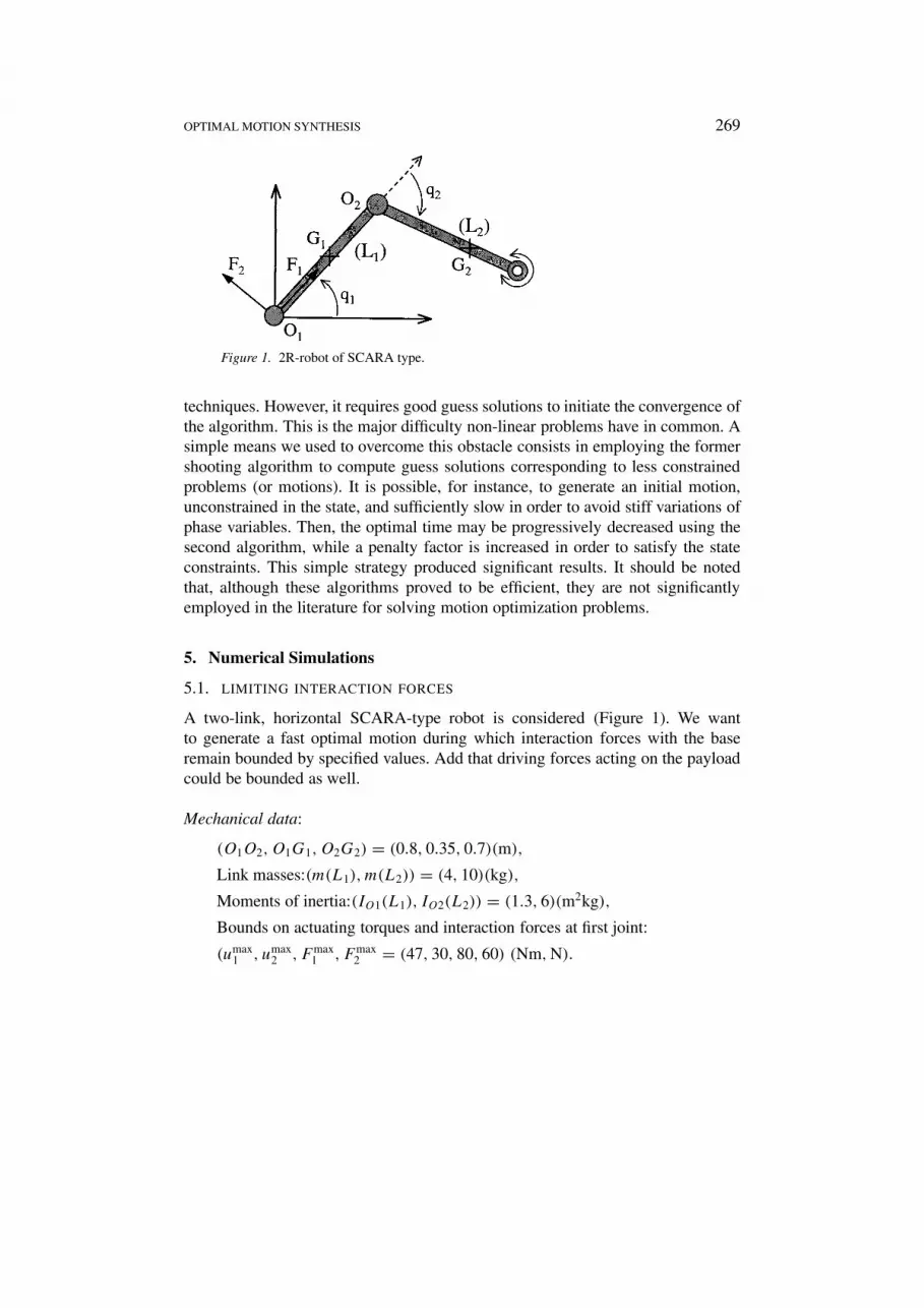
Figure 1. 2R-robot of SCARA type.

techniques. However, it requires good guess solutions to initiate the convergence ofthe algorithm. This is the major difficulty non-linear problems have in common. Asimple means we used to overcome this obstacle consists in employing the formershooting algorithm to compute guess solutions corresponding to less constrainedproblems (or motions). It is possible, for instance, to generate an initial motion,unconstrained in the state, and sufficiently slow in order to avoid stiff variations ofphase variables. Then, the optimal time may be progressively decreased using thesecond algorithm, while a penalty factor is increased in order to satisfy the stateconstraints. This simple strategy produced significant results. It should be notedthat, although these algorithms proved to be efficient, they are not significantlyemployed in the literature for solving motion optimization problems.

5. Numerical Simulations

5.1. LIMITING INTERACTION FORCES

A two-link, horizontal SCARA-type robot is considered (Figure 1). We wantto generate a fast optimal motion during which interaction forces with the baseremain bounded by specified values. Add that driving forces acting on the payloadcould be bounded as well.

Mechanical data:

(O1O2,O1G1,O2G2) = (0.8, 0.35, 0.7)(m),

Link masses:(m(L1),m(L2)) = (4, 10)(kg),

Moments of inertia:(IO1(L1), IO2(L2)) = (1.3, 6)(m2kg),

Bounds on actuating torques and interaction forces at first joint:

(umax1 , umax

2 , Fmax1 , Fmax

2 = (47, 30, 80, 60) (Nm,N).


Figure 2. Time charts of actuating torque u1.

Figure 3. Time charts of actuating torque u2.

Initial and final kinematic data:

Initial state:(q1, q2, q1, q2) = (0◦,−30◦, 0, 0),

Final state:(q1, q2, q1, q2) = (120◦,−30◦, 0, 0).

The performance criterion implemented is defined in (10), (11). In Figures 2to 5, the time evolution of u1, u2 and F1, F2 respectively, are plotted for threedecreasing traveling times T1 = 1.93 s, T2 = 1.43 s, and T3 = 1.34 s, obtained forthe following values of the weighting factor (see Equation (11) in Section 2.3): 0.8,0.4, 0.01 respectively. One can see that u1, u2 and F1, F2 are perfectly truncated attheir extremal authorized values. The shortest time T3 is very close to the minimumtime allowed by the constraints because, at every time, two of the four constraintsare saturated.

5.2. SMOOTHING OPTIMAL ACTUATING INPUTS

The inertia model of the industrial robot schematized in Figure 6 is fully taken intoaccount in the Hamiltonian dynamic model used to generate optimal motions. Themechanical characteristics of the robot are given in [34].


Figure 4. Time charts of interacting force F1.

Figure 5. Time charts of interacting force F2.

Figure 6. 6R-robot PUMA. Joint coordinates qi ’s are defined using Denavit–Hartenberg’sconstruction.


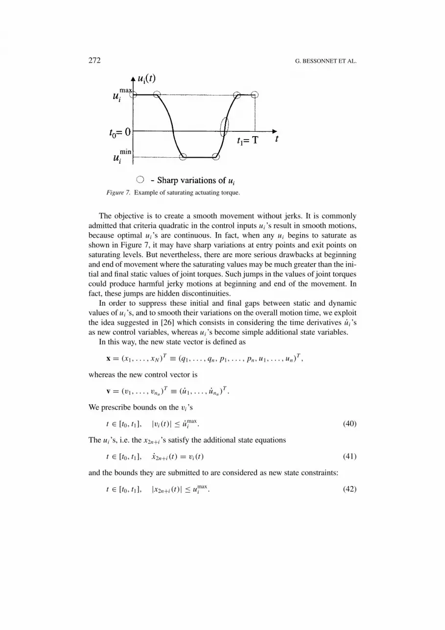
Figure 7. Example of saturating actuating torque.

The objective is to create a smooth movement without jerks. It is commonlyadmitted that criteria quadratic in the control inputs ui’s result in smooth motions,because optimal ui’s are continuous. In fact, when any ui begins to saturate asshown in Figure 7, it may have sharp variations at entry points and exit points onsaturating levels. But nevertheless, there are more serious drawbacks at beginningand end of movement where the saturating values may be much greater than the ini-tial and final static values of joint torques. Such jumps in the values of joint torquescould produce harmful jerky motions at beginning and end of the movement. Infact, these jumps are hidden discontinuities.

In order to suppress these initial and final gaps between static and dynamicvalues of ui’s, and to smooth their variations on the overall motion time, we exploitthe idea suggested in [26] which consists in considering the time derivatives ui’sas new control variables, whereas ui’s become simple additional state variables.

In this way, the new state vector is defined as

x = (x1, . . . , xN)T ≡ (q1, . . . , qn, p1, . . . , pn, u1, . . . , un)

T ,

whereas the new control vector is

v = (v1, . . . , vnu)T ≡ (u1, . . . , unu )

T .

We prescribe bounds on the vi’s

t ∈ [t0, t1], |vi(t)| ≤ umaxi . (40)

The ui’s, i.e. the x2n+i’s satisfy the additional state equations

t ∈ [t0, t1], x2n+i (t) = vi(t) (41)

and the bounds they are submitted to are considered as new state constraints:

t ∈ [t0, t1], |x2n+i (t)| ≤ umaxi . (42)


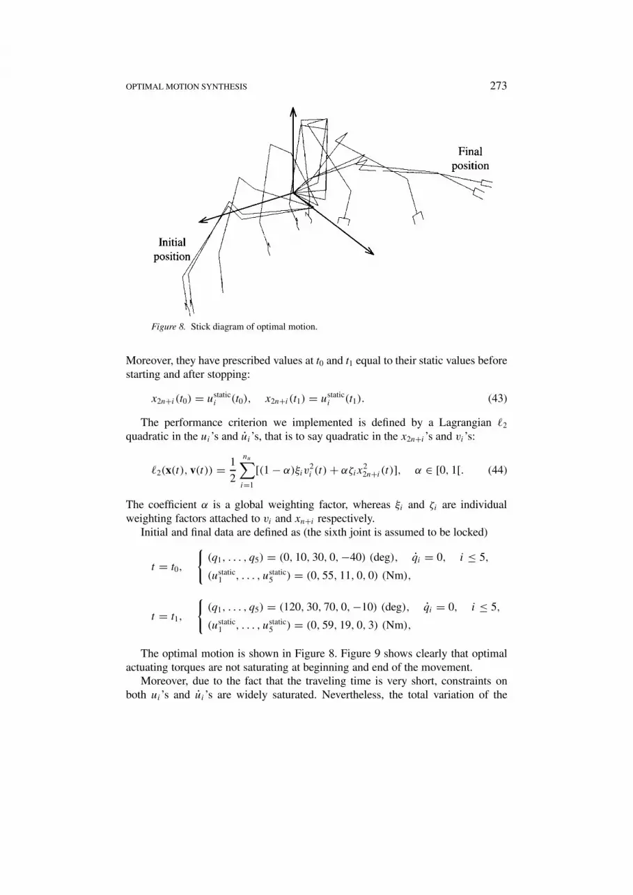
Figure 8. Stick diagram of optimal motion.

Moreover, they have prescribed values at t0 and t1 equal to their static values beforestarting and after stopping:

x2n+i (t0) = ustatici (t0), x2n+i (t1) = ustatic

i (t1). (43)

The performance criterion we implemented is defined by a Lagrangian �2

quadratic in the ui’s and ui’s, that is to say quadratic in the x2n+i’s and vi’s:

�2(x(t), v(t)) = 1

2

nu∑i=1

[(1 − α)ξiv2i (t) + αζix

22n+i (t)], α ∈ [0, 1[. (44)

The coefficient α is a global weighting factor, whereas ξi and ζi are individualweighting factors attached to vi and xn+i respectively.

Initial and final data are defined as (the sixth joint is assumed to be locked)

t = t0,

{(q1, . . . , q5) = (0, 10, 30, 0,−40) (deg), qi = 0, i ≤ 5,

(ustatic1 , . . . , ustatic

5 ) = (0, 55, 11, 0, 0) (Nm),

t = t1,

{(q1, . . . , q5) = (120, 30, 70, 0,−10) (deg), qi = 0, i ≤ 5,

(ustatic1 , . . . , ustatic

5 ) = (0, 59, 19, 0, 3) (Nm),

The optimal motion is shown in Figure 8. Figure 9 shows clearly that optimalactuating torques are not saturating at beginning and end of the movement.

Moreover, due to the fact that the traveling time is very short, constraints onboth ui’s and ui’s are widely saturated. Nevertheless, the total variation of the


Figure 9. Time charts of actuating torques; Qai stands for ui , i ≤ 5.

Figure 10. Mechanical biped with anthropomorphic locomotion system (LMS, Poitiers;INRIA-RA, Grenoble, France).

ui’s remains quite moderate, which would ensure really smooth functioning of therobot.

5.3. OPTIMAL GAIT OF A 7-LINK PLANAR BIPED

We are interested in generating impactless sagittal gait of a 7-link biped. The finalobjective is aimed at generating a three-dimenionsal gait in order to make the biped


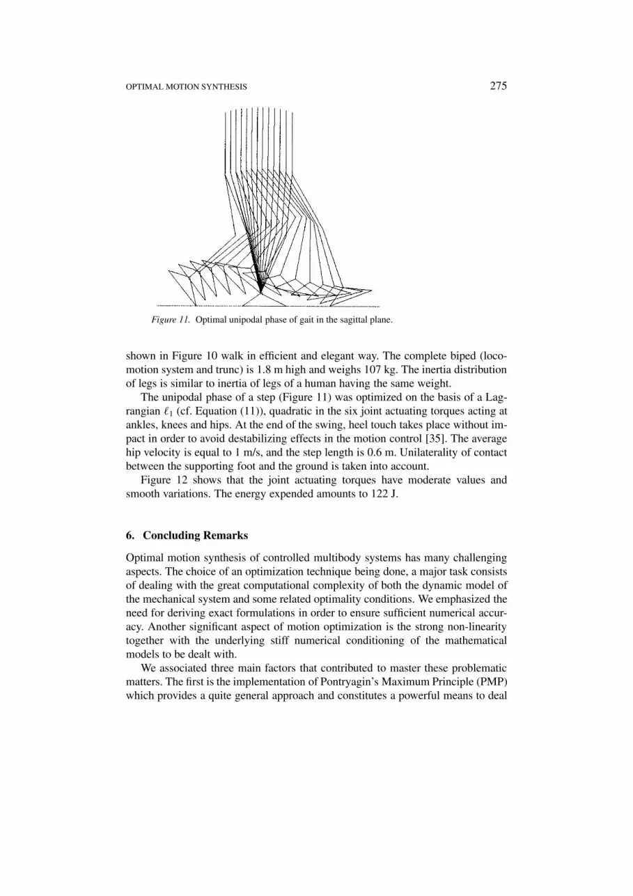
Figure 11. Optimal unipodal phase of gait in the sagittal plane.

shown in Figure 10 walk in efficient and elegant way. The complete biped (loco-motion system and trunc) is 1.8 m high and weighs 107 kg. The inertia distributionof legs is similar to inertia of legs of a human having the same weight.

The unipodal phase of a step (Figure 11) was optimized on the basis of a Lag-rangian �1 (cf. Equation (11)), quadratic in the six joint actuating torques acting atankles, knees and hips. At the end of the swing, heel touch takes place without im-pact in order to avoid destabilizing effects in the motion control [35]. The averagehip velocity is equal to 1 m/s, and the step length is 0.6 m. Unilaterality of contactbetween the supporting foot and the ground is taken into account.

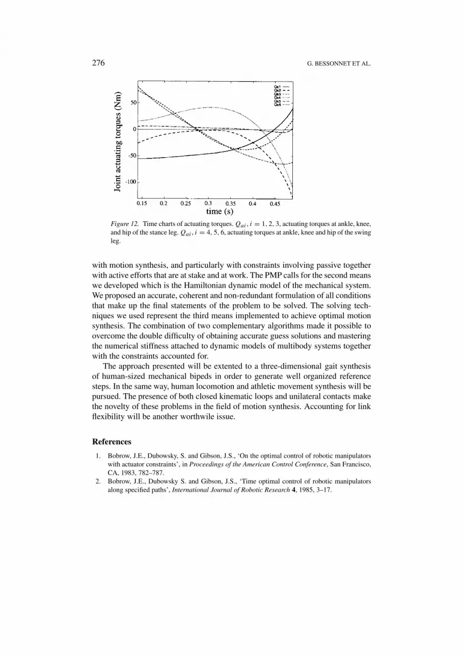
Figure 12 shows that the joint actuating torques have moderate values andsmooth variations. The energy expended amounts to 122 J.

6. Concluding Remarks

Optimal motion synthesis of controlled multibody systems has many challengingaspects. The choice of an optimization technique being done, a major task consistsof dealing with the great computational complexity of both the dynamic model ofthe mechanical system and some related optimality conditions. We emphasized theneed for deriving exact formulations in order to ensure sufficient numerical accur-acy. Another significant aspect of motion optimization is the strong non-linearitytogether with the underlying stiff numerical conditioning of the mathematicalmodels to be dealt with.

We associated three main factors that contributed to master these problematicmatters. The first is the implementation of Pontryagin’s Maximum Principle (PMP)which provides a quite general approach and constitutes a powerful means to deal


Figure 12. Time charts of actuating torques. Qai , i = 1, 2, 3, actuating torques at ankle, knee,and hip of the stance leg. Qai , i = 4, 5, 6, actuating torques at ankle, knee and hip of the swingleg.

with motion synthesis, and particularly with constraints involving passive togetherwith active efforts that are at stake and at work. The PMP calls for the second meanswe developed which is the Hamiltonian dynamic model of the mechanical system.We proposed an accurate, coherent and non-redundant formulation of all conditionsthat make up the final statements of the problem to be solved. The solving tech-niques we used represent the third means implemented to achieve optimal motionsynthesis. The combination of two complementary algorithms made it possible toovercome the double difficulty of obtaining accurate guess solutions and masteringthe numerical stiffness attached to dynamic models of multibody systems togetherwith the constraints accounted for.

The approach presented will be extented to a three-dimensional gait synthesisof human-sized mechanical bipeds in order to generate well organized referencesteps. In the same way, human locomotion and athletic movement synthesis will bepursued. The presence of both closed kinematic loops and unilateral contacts makethe novelty of these problems in the field of motion synthesis. Accounting for linkflexibility will be another worthwile issue.

References

1. Bobrow, J.E., Dubowsky, S. and Gibson, J.S., ‘On the optimal control of robotic manipulatorswith actuator constraints’, in Proceedings of the American Control Conference, San Francisco,CA, 1983, 782–787.

2. Bobrow, J.E., Dubowsky S. and Gibson, J.S., ‘Time optimal control of robotic manipulatorsalong specified paths’, International Journal of Robotic Research 4, 1985, 3–17.


3. Shiller, Z. and Dubowsky, S., ‘On the optimal control of robotic manipulators with actuatorand end-effector constraints’, in Proceedings IEEE International Conference on Robotics andAutomation, IEEE, New York, 1985, 614–620.

4. Shiller, Z. and Dubowsky, S., ‘Robot path planning with obstacles, actuator, gripper andpayload constraints’, International Journal of Robotics Research 8, 1989, 3–18.

5. Shin, K.G. and McKay, N.D., ‘Minimum-time control of robotic manipulators with geometricpath constraints’, IEEE Transactions on Automatic Control 30(6), 1985, 531–541.

6. Shin, K.G. and McKay, N.D., ‘Minimum cost trajectory planning for industrial robots’, Controland Dynamic Systems 9, 1991, 345–403.

7. Pfeiffer, F. and Johanni, R., ‘A concept for manipulator trajectory planning’, in ProceedingsIEEE International Conference on Robotics and Automation, San Francisco, CA, April 7–10,IEEE, New York, 1986, 1139–1405.

8. Slotine, J.J.E. and Yang, H.S., ‘Improving the efficiency of time optimal path followingalgorithms’, IEEE Transactions on Robotics and Automation 5, 1989, 118–124.

9. Shiller, Z. and Dubowsky, S., ‘On computing the global time-optimal motions of robotic ma-nipulators in the presence of obstacles’, IEEE Transactions on Robotics and Automation 7,1991, 785–797.

10. Shiller, Z., ‘Optimal robot motion planning and work-cell layout design’, Robotica 15, 1997,31– 40.

11. Beletskii, V.V. and Chudinov, P.S., ‘Parametric optimization in the problem of biped loco-motion’, Izvestiya Akademii Nauk SSSR Mekhanika Tverdogo Tela 12, 1977, 22–31.

12. Channon, P.H., Hopkins, S.H. and Pham, D.T., ‘Derivation of optimal walking motions for abipedal walking robot’, Robotica 10, 1992, 165–172.

13. Chevallereau, C. and Aoustin, Y., ‘Optimal reference trajectories for walking and running of abiped robot’, Robotica 19, 2001, 557–569.

14. Schmitt, D., Soni, A.H., Srinivasan, V. and Naganathan, G., ‘Optimal motion planning of robotmanipulators’, Journal of Mechanisms, Transmissions, and Automation in Design 107, 1985,239–244.

15. Yamamoto, M., Ozaki, H. and Mohri, A. ‘Planning of manipulator joint trajectories by aniterative method’, Robotica 6, 1988, 101–105.

16. Martin, B.J. and Bobrow, J.E., ‘Minimum effort motions for open chains manipulators withtask-dependent end-effector constraints’, International Journal of Robotics Research 18, 1999,213–324.

17. Wang, C.-Y.E., Bobrow, J.E. and Reinkensmeyer, D. J., ‘Swinging from the hip: Use of dynamicmotion optimization in the design of robotic gait rehabilitation’, in Proceedings of the IEEEInternational Conference on Robotics and Automation, Seoul, Korea, May 21–26, IEEE, NewYork, 2001, 1433–1438.

18. Kahn, M.E. and Roth, B., ‘The near-minimum-time control of open-loop articulated kinematicchains’, ASME Journal of Dynamic Systems, Measurement, and Control, September 1971, 164–172.

19. Weinreb, A. and Bryson, A.E., ‘Optimal control of systems with hard control bounds’, IEEETransactions on Automatic Control 30(11), 1985, 1135–1138.

20. Geering, H.P., Guzella, L., Hepner, S.A.R. and Onder, C.H., ‘Time-optimal motions of robotsin assembly tasks’, IEEE Transactions on Automatic Control 31(6), 1986, 512–518.

21. Chen, Y. and Desrochers, A.A., ‘A proof of the structure of the minimum-time control law ofrobotic manipulators using a Hamiltonian formulation’, IEEE Transactions on Robotics andAutomation 6(3), 1990, 388–393.

22. Bessonnet, G. and Lallemand, J.P., ‘Optimal trajectories of robot arms minimizing constrainedactuators and traveling time’, in IEEE International Conference on Robotics and Automation,Cincinnati, OH, IEEE, New York, 1990, 112–117.


23. Galicki, M., ‘The planning of robotic optimal motions in the presence of obstacles’, Interna-tional Journal of Robotic Research 17, 1998, 248–259.

24. Galicki, M. and Ucinski, D., ‘Time-optimal motions of robotic manipulators’, Robotica 18,2000, 659–667.

25. Lewis, F.L. and Syrmos, V.L., Optimal Control, John Wiley & Sons, New York, 1995.26. Pontryagin, L., Boltiansky, V., Gamkrelitze, A. and Mishchenko, E., The Mathematical Theory

of Optimal Processes, Wiley Intersciences, New York, 1962.27. Bryson, A.E. and Ho, Y.C., Applied Optimal Control, Hemisphere, New York, 1975.28. Ioffe, A.D. and Tihomirov, V.M., Theory of Extremal Problems, North-Holland, Amsterdam,

1979.29. Skowronski, J.M., Control Dynamics of Robotic Manipulators, Academic Press, Orlando, FL,

1986.30. Flashner, H. and Skowronski, J.M., ‘Model tracking control of Hamiltonian systems’, ASME

Journal of Dynamic Systems, Measurement, and Control 111, 1989, 656–660.31. Bessonnet, G., Sardain, P. and Danes, F., ‘Reducing high order derivations to algebraic opera-

tions in dynamic modelling for motion optimization purpose’, in Proceedings of 15th IMACSWorld Congress on Scientific Computer Modelling and Applied Mathematics, A. Sydow (ed.),Wissenschaft & Technik Verlag, Berlin, 1997, 337–342.

32. NAG Fortran Library, Routine D02RAF, 1992.33. Pereyra V., ‘Pasva 3: An adaptative finite difference fortran program for the first order non-

linear, ordinary boundary problem’, in Codes for Boundary Value Problems in OrdinaryDifferential Equations, Lecture Notes in Computer Science, Vol. 76 B. Childs, M. Scott, J.W.Daniel, E. Denman and P. Nelson (eds), Springer-Verlag, Berlin, 1979, 67–88.

34. Danes, F., ‘Critères et contraintes pour la synthèse optimale des mouvements de robots manip-ulateurs. Application à l’évitement d’obstacles’, Ph.D. Thesis, University of Poitiers, France,1998.

35. Blajer, W. and Schiehlen, W., ‘Walking without impacts as a motion/force control problem’,ASME Journal of Dynamic Systems, Measurement, and Control 114, 1992, 660–665.

optimal motion synthesisdynamic modelling and numerical solving aspects

Documents