online estimation of rf interference
TRANSCRIPT
Online Estimation of RF Interference
Nabeel Ahmed, Usman Ismail,Srinivasan Keshav
David R. Cheriton School of Computer Science,University of Waterloo, Waterloo, ON, Canada{n3ahmed, uismail, keshav}@cs.uwaterloo.ca
Konstantina PapagiannakiIntel Research,Pittsburgh, PA
ABSTRACTIncreased AP density in enterprise WLANs leads to increas-ing RF interference and decreasing performance. An im-portant step towards mitigating this problem is to constructprecise RF maps in the form of a conflict graph. Priorwork on conflict graph construction, mostly using bandwidthtests [17], suffers from two problems: a) It is limited to staticsettings and cannot support mobility, and b) It incurs sig-nificant measurement overhead and must be performed of-fline (e.g. overnight). An alternative to bandwidth tests is“micro-probing” [4] that operates on millisecond-level timescales. Micro-probing rapidly constructs the conflict grapheven while the network is in use (i.e. online). While inter-esting in principle, micro-probing has only been evaluatedin simulation. In this work, we empirically study micro-probing on a 40-node wireless testbed. In doing so, we notonly show that micro-probing is in fact practically realizable,but also present key insights that drive the design choices forour implementation. We benchmark micro-probing againstbandwidth tests and find that micro-probing is just as accu-rate but with up to a400 times reduction in overhead. Fi-nally, we argue that a successful implementation of micro-probing opens up the space for further innovations in real-time WLAN adaptation and optimization.
1. INTRODUCTIONDropping prices and demand for a mobile workforce have
caused a proliferation of wireless LANs in modern enter-prises. However, increased Access Point (AP) and clientdensity necessarily increases interference and potentially de-creases performance. There has been a considerable amountof prior work (described in Section 2.2) to address this prob-lem. Typically, these approaches model interference in the
Permission to make digital or hard copies of all or part of this work forpersonal or classroom use is granted without fee provided that copies arenot made or distributed for profit or commercial advantage and that copiesbear this notice and the full citation on the first page. To copy otherwise, torepublish, to post on servers or to redistribute to lists, requires prior specificpermission and/or a fee.ACM CoNEXT 2008, December 10-12, 2008, Madrid, SPAINCopyright 2008 ACM 978-1-60558-210-8/08/0012 ...$5.00.
RF spectrum using a conflict graph [11], where nodes rep-resent links in the network and edges appear between nodesthat cannot transmit simultaneously. For instance, if we ob-serve performance degradation when linksl1 and l2 are si-multaneously active, we say that those two links interfereand add an edge between the respective nodes. Note thatan edge may be added even if the two links interfere prob-abilistically, e.g. for 90% of the measurement period. Inother words, interference between two links is not ‘binary’,but instead a ratio between0 and 1, as we describe later.This model is then used to optimize configuration parame-ters such as channels and power levels for the network [6].Therefore, the conflict graph is an essential input to these al-gorithms. Note that the RF environment is constantly chang-ing and the conflict graph will therefore need to be updatedin realtime. This necessitates an online approach to interfer-ence estimation. We define an online approach as one thatmaps interference while the network is in operation, with lit-tle or no disruption in service, and with minimal changes toexisting network infrastructure.
Prior work on conflict graph construction mostly uses“bandwidth tests”, where a sender transmits packets at thehighest possible rate to one or more receivers, in the pres-ence and absence of simultaneous packet transmissions froma potential interferer [16, 17]. If the interferer’s presencecauses a drop in throughput, we infer that a conflict ex-ists. This conflict is represented as a conflict edge betweeneach link sourced at the interferer and the link being tested.However, this approach suffers from significant measure-ment overhead and can take hours to run even for a mod-est sized network of20 APs. Furthermore, it requires thatthe network be non-functional for the duration of the mea-surements to preserve measurement accuracy. This may beacceptable for measuring inter-AP conflicts overnight, butdoes not work for clients that come and go and actively usethe network. Finally, bandwidth tests also require the clientsto report measurements to the APs. These drawbacks makethem infeasible for online estimation of RF interference.
These problems led us to a different approach (dubbed“micro-probing”)which we proposed in prior work [4]. Micro-probing involves millisecond level active tests that are per-formed to determine the conflict graph edges. In theory,
micro-probing can rapidly and accurately construct the RFinterference map while the network is in use. Furthermore, itdoes not require client modifications and is, therefore, legacycompatible. The original evaluation of micro-probing fo-cused on simulations and does not capture aspects that makeit challenging to implement in the real world. Specifically,requirements for tightly synchronizing APs and silencingbackground noise while coordinating active tests is difficultto achieve in practice. In this paper, we take a first approachto implementing micro-probing and provide results on howwell these requirements can be realized. Furthermore, wecompare the accuracy and overhead of micro-probing withbandwidth testing, which is widely considered the “gold stan-dard” approach to RF interference estimation.
1.1 Key ContributionsThe following are the key contributions of our work:
• We prototype a system for micro-probing and bench-mark it against bandwidth tests. Micro-probing achievesaccuracies comparable to bandwidth tests while yield-ing up to a400 times reduction in measurement over-head; the testing time per link reduces from 30 secondsto only 20ms. As a result, a modest-sized network of20nodes can be measured in under20 seconds using micro-probing.
• We implement and evaluate a lightweight approach toAP synchronization called Reference Broadcast Syn-chronization (RBS) [10]. RBS sends UDP broadcastsover the wire from the controller to the APs to synchro-nize them. Our experiments reveal that we are able tosynchronize APs to within5 − 40us of each other. Fur-thermore, we attain such accuracies even in the presenceof cross-traffic on the wired backplane.
• We implement and evaluate silencing techniques thatuse 802.11’s virtual carrier-sense mechanism to brieflysilence the network to perform measurements. Wefind that although perfect silencing is hard to achievein all situations, it is possible when devices obey theIEEE 802.11 standard. We believe that silencing is alsobroadly applicable to other tasks such as network diag-nosis and troubleshooting.
• We propose the use of MAC service time (MST) tomeasure carrier-sensing interference between competingtransmitters. We experimentally evaluate MST and findthat with a few minor tweaks, we are able to achieve de-tection accuracies of up to 95%.
The rest of the paper is organized as follows. Section 2provides some background on conflict graphs and discussesexisting techniques for constructing such a graph. Section3covers the theory of micro-probing while Section 4 discussesthe design of our prototype implementation. Sections 5 and6 benchmark micro-probing’s core components and evaluateit’s performance against bandwidth tests. Discussion and fu-
AP1
AP4
AP3
C1
C3
C4
L1 L4
Connectivity
Interference
L3
L3
L4
AP2
C2L2
L2
L1
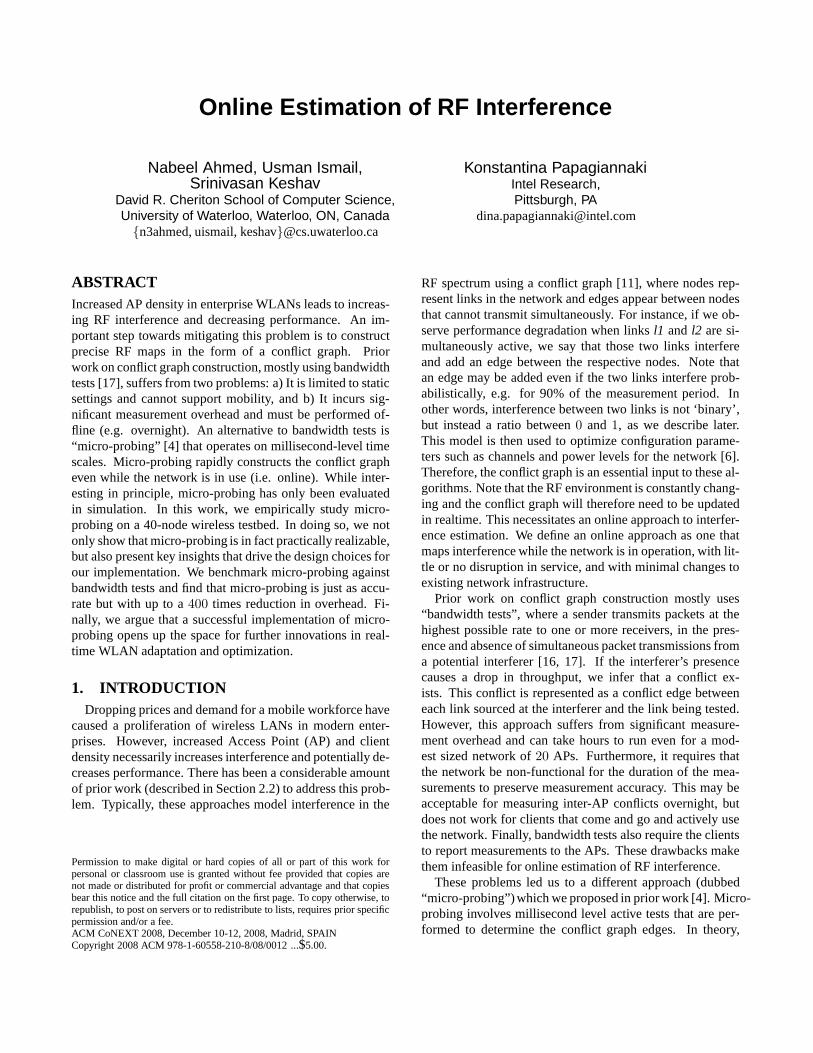
Figure 1: Bottom plane shows an example conflict graphfor the connectivity graph shown on top. Carrier-senseedges are shown in solid, whereas collision edges areshown as dashed arrows.
ture work are covered in Section 7 and the paper concludesin Section 8.
2. BACKGROUNDIn this section we define a conflict graph, and briefly out-
line existing approaches for its construction.
2.1 Conflict Graph (CG)A conflict graph captures conflict between pairs of links
in a wireless network. IfL1 is the link betweenAP1 andclientC1 andL2 is the link betweenAP2 and clientC2, thenthe conflict graph will feature an edge fromL1 to L2 if thethroughput fromAP2 to C2 decreases whenAP1 transmitsdata toC1. Notice that the conflict graph is adirectedgraphdue to the asymmetric nature of the wireless channel. Figure1 provides an example of such a conflict graph.
Conflict arises from two effects: i) transmittersAP1 andAP2 are within carrier sensing range of each other and there-fore share access to the medium, ii) the transmission fromAP2 to C2 interferes with the reception of a packet fromAP1 at receiverC1. The latter case is termed the “hidden ter-minal” problem. Note that because the conflict graph edgesare sourced at the APs, they are referred to as downlink con-flicts, i.e. they are from the APs to other APs/clients.
Both types of downlink conflict are sensitive to the trans-mission power and rate used by the transmitters. Reductionin transmission power may reduce the number of edges in theconflict graph. Increase in transmission rate can increase thenumber of edges in the conflict graph since decoding infor-mation at the receiver becomes less robust to channel errors.Finally, interference in a wireless network is also a functionof the activity of the different interferers. If wireless nodesdo not transmit, then no conflict arises. As a result, con-flict graphs should also be annotated with load information,based on the traffic models that are defined for the links inthe network. We refer the reader to [4, 12, 19] for examplesof some such traffic models.
2.1.1 Upstream Conflicts
So far we have covered scenarios in which interference iscaused by traffic that flows downstream from the AP to theclient. With the emergence of voice and video applicationsrunning on laptops and PDAs, interference sourced at theclient (i.e. upstream conflicts) will also become important.In prior work [4], we proposed mechanisms to detect suchconflicts. However, due to space limitations, we do not coverthem in this paper.
2.1.2 Multi-Interferer Conflicts
Note that the conflict graph described above only capturesinterference between pairs of links in the network. In practi-cal deployments, interference may be sourced from multipleinterferers in the neighbourhood of a link. Interference frommore than one source is not captured in the model discussedabove. However, Niculescu et al. [16] show that interfer-ence from each source can be treated independently and thecombined effect of all sources is simply the product of theirpairwise interferences. Therefore, a pairwise model (liketheone described above) can be used to compute the effect ofmultiple interferers as well. Thus, the focus of our work ison how to construct the pairwise model accurately and effi-ciently.
2.2 Existing approaches to CG constructionPrior work on conflict graph construction can be catego-
rized into passive and active techniques. We discuss each ofthem in turn.
2.2.1 Passive
Passive approaches collect traces using monitors deployedthroughout the building. Monitors are dedicated hardwaredevices that sniff wireless traffic and collect traces in orderto perform management tasks. The traces are processed at acentralized aggregation point and are subsequently fed intointerference inferencing algorithms. Jigsaw [7] and WiT [14]are examples of systems that adopt passive techniques. Pas-sive techniques are also popular among enterprise vendorssuch as Aruba [18], primarily because they don’t introduceany traffic into the network for measuring interference. Nev-ertheless, their predictive power is heavily dependent uponon how densely the monitors are deployed in the buildingbecause with increasing density the probability that a moni-tor is close to any given link increases. Furthermore, passivetechniquespredict interference from collected traces, hencethey are likely to be less accurate than active techniques thatdirectly measure interference.
2.2.2 Active
Active approaches typically operate in the following man-ner: A pair of links to be tested for mutual interference areinstructed to send broadcast traffic in parallel. Delivery ra-tios are computed for these links under these conditions anddelivery ratios are also computed when the links transmit in
isolation. The impact of interference is then computed usinga metric called the Broadcast Interference Ratio (BIR). BIRis defined as the number of packets successfully transmittedin the presence of interference against the number of packetstransmitted when no interference is present. BIR is alwaysless than or equal to 1. We now summarize approaches thatfall in this category.
Pure Measurement techniques:Padhye et al [17] pro-pose the idea of performing bandwidth tests (as describedabove) to detect interference. However, their approach iscomputationally expensive and can take hours to run, evenfor a network of20 nodes. Bandwidth tests also require re-ceiver statistics of successfully delivered packets to estimateinterference. This makes them infeasible for environmentswhere clients are not under administrative control.
Measurement-Modeling techniques:Reis et al [20] pro-pose an optimization on bandwidth testing where they com-bine measurements with modeling to reduce the overall num-ber of measurements. Their work was recently extendedfor the case of multiple interferers (as discussed in Section2.1.2), carrying different amounts of traffic load [12, 19].An element common to all such modeling-based proposalsis the use of RSSI to predict interference. Unfortunately,RSSI is only available if the 802.11 preamble for a packet isreceived correctly, i.e., the interferer is likely in communica-tion range of the receiver. Lee et al [13] address this limita-tion by proposing the use of two radios: a high-power radioto reach interferers outside of communication range and alow-power radio for normal communication. Nevertheless,like bandwidth tests, all these measurement schemes also re-quire receiver statistics, which makes them harder to deploy.Furthermore, these techniques are likely to be less accuratethan pure measurement schemes because they perform fewermeasurements and infer interference based on models thatmake simplifying assumptions about the RF environment.
There is also recent work that combines active and passivetechniques to measure interference, CMAPs [22]. CMAPsinfers interference using passive techniques but opportunis-tically disables carrier-sense whenever possible. However,the limitations of this approach are (i) It requires the interfer-ers to be in communication range, and (ii) It requires clientmodifications to report packet delivery statistics.
Aside from the interference mapping schemes discussedabove, there is also prior work on studying properties of RFinterference in wireless (and in particular, 802.11) networks.Niculescu et al. [16] highlight properties that can reduce theoverall complexity of measuring interference. These prop-erties include linearity of interference with respect to thesource’s sending rate, and independence of multiple inter-ferers (as discussed in Section 2.1.2). Das et al [8] study re-mote interferers that do not individually interfere, but whencombined can cause significant interference. However, theauthors point out that the occurrence of this phenomenon israre. These studies have added significantly to our under-
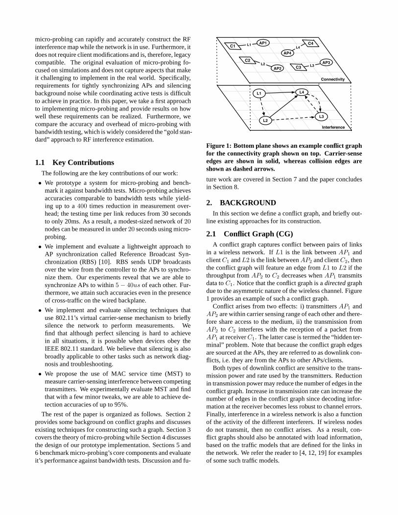
Passive Active M-ProbingLow Control Overhead X ✗ X
Accuracy ✗ X X
No Network Downtime X ✗ X
Low Feedback Delay ✗ ✗ X
No client modifications X ✗ X
Captures Weak Interferers ✗ X X
Table 1: Comparing active, passive, and micro-probingtechniques
standing of how RF interference impacts link quality andperformance in IEEE 802.11 networks.
2.2.3 Summary
We broadly classified prior work as either passive or ac-tive. The main underlying theme is that while passive tech-niques incur little to no cost in terms of measurement over-head, they are less accurate than active techniques. Con-versely, active techniques are more accurate than passivetechniques but suffer from high overhead. This dichotomymotivates the development of a new approach that capturesthe best of both worlds – micro-probing is an attempt toachieve this objective.
In order to put active, passive, and micro-probing tech-niques in perspective with our objective of implementing anonline approach to interference estimation, we outline thekey features that are necessary for building such a system.These features are listed in Table 1 and discussed in greaterdetail next.
Control overhead indicates whether or not a technique re-quires the use of measurement packets in order to estimateinterference. Active techniques by definition require suchpackets while passive techniques do not. On the other hand,active techniques are highly accurate because they directlymeasure interference between links whereas passive tech-niques only predict the same. However, active techniques re-quire excessive downtime for measuring interference whilepassive techniques do not. Both, active and passive schemessuffer from high feedback delay (i.e. slow response times)since active techniques have a lengthy measurement cyclewhile passive techniques have a lengthy processing cycle(trace merging/synchronization, time series analysis, etc).Active techniques also require client statistics and thereforeare not legacy compatible. Finally, weak interferers (i.e.those outside of communication range of the target link) arehard to capture using passive techniques while some activetechniques (e.g. bandwidth tests) can capture such cases. Insummary, both active and passive techniques lack at leastone feature necessary for online estimation of RF interfer-ence. In contrast, micro-probing incorporates all these fea-tures and is therefore our technique of choice for estimatingRF interference in an online fashion.
3. THEORY OF MICRO-PROBING
In this paper, we focus on detecting downlink conflictsfrom APs to neighbouring clients/APs. There are two typesof downlink conflict that can be captured in a conflict graph:i) conflict due to carrier sensing between contending APs,and ii) conflict due to an AP-client collision. Micro-probingimplements two different tests to differentiate between thetwo scenarios. Note that in terms of the conflict graph, aconflict due to carrier sensing can manifest itself as multipleconflict edges, one between every link emanating from eitherof the transmitters. However, in the case of conflict due tocollision, an edge will only exist between the affected linkand the link interfering with it.
Testing for CS interference: In order to test for CarrierSensing (CS) induced interference, we need to have bothwireless transmitters transmit at thesametime. Micro-probinginstructs one AP,APi, to initiate a series of broadcast trans-missions at well defined time instantst1, t2, ..., tm. APj , isthen instructed to also transmit at those exact same time in-stants, with a slight offset to ensureAPi acquires the channelfirst. If APj , is delayed by one frame time before transmit-ting, then we can infer that it is in CS range ofAPi. In ourimplementation, we use an estimate of MAC service time(MST) to detect such an event. Given that this test needs tobe performed between each pair of APs, the total number oftests required isO(N2), whereN is the number of APs inthe network.
Testing for collision induced interference: In order totest for collisions at the receiver we proceed as follows. Weinitiate a transmission betweenAPi and its client, sayC1, attime t0. APj is then instructed to send a broadcast frame atthe exact same time instant. IfAPi does not receive an ACKwithin SIFS, then one can infer a collision at the receiver1.This test is repeatedm times to account for temporal channelimpairments from affecting our tests.
Collision induced interference can typically be observedonly in the absence of carrier sensing induced interference;if the AP cannot simultaneously transmit, then testing forcollisions with neighbouring transmissions is unnecessary.Given that there are a total ofC clients (and therefore links)in the network, and there are N-1 APs that must be tested forinterference against each link, a total of O(CN) tests need tobe performed. However, because some APs are likely ex-posed terminals for each other, the number of actual tests isexpected to be much lower.
Silencing: Note that the interference tests described abovewould give incorrect results if they are conducted while othertraffic is being carried in the network. To ensure that thewireless medium is silent, we need to force all APs andclients in the neighbourhood to be silent. We do this by hav-ing the APs conducting the test broadcast a CTS-to-self orAck packet (with an appropriate NAV duration)beforeini-tiating a test. We study the efficacy of this method of si-lencing in Section 5. To ensure that the impact of silencingis minimized, we choose the smallest possible NAV that is
1We, as in prior work [17], assume good quality links
Controller
Test Coordinator
Wired
Control
Plane
I2
I1
Client1 Client2
AP1 AP2
Conflict Graph
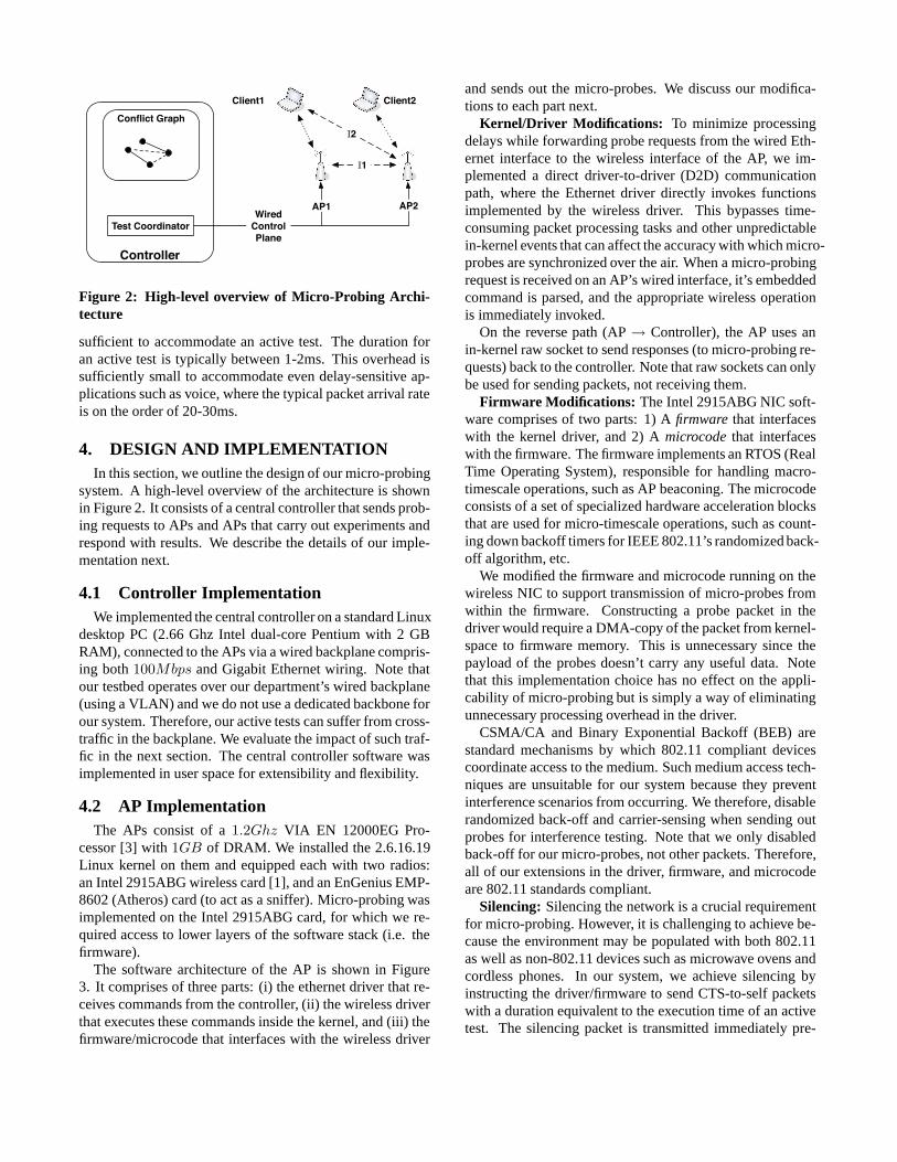
Figure 2: High-level overview of Micro-Probing Archi-tecture
sufficient to accommodate an active test. The duration foran active test is typically between 1-2ms. This overhead issufficiently small to accommodate even delay-sensitive ap-plications such as voice, where the typical packet arrival rateis on the order of 20-30ms.
4. DESIGN AND IMPLEMENTATIONIn this section, we outline the design of our micro-probing
system. A high-level overview of the architecture is shownin Figure 2. It consists of a central controller that sends prob-ing requests to APs and APs that carry out experiments andrespond with results. We describe the details of our imple-mentation next.
4.1 Controller ImplementationWe implemented the central controller on a standard Linux
desktop PC (2.66 Ghz Intel dual-core Pentium with 2 GBRAM), connected to the APs via a wired backplane compris-ing both100Mbps and Gigabit Ethernet wiring. Note thatour testbed operates over our department’s wired backplane(using a VLAN) and we do not use a dedicated backbone forour system. Therefore, our active tests can suffer from cross-traffic in the backplane. We evaluate the impact of such traf-fic in the next section. The central controller software wasimplemented in user space for extensibility and flexibility.
4.2 AP ImplementationThe APs consist of a1.2Ghz VIA EN 12000EG Pro-
cessor [3] with1GB of DRAM. We installed the 2.6.16.19Linux kernel on them and equipped each with two radios:an Intel 2915ABG wireless card [1], and an EnGenius EMP-8602 (Atheros) card (to act as a sniffer). Micro-probing wasimplemented on the Intel 2915ABG card, for which we re-quired access to lower layers of the software stack (i.e. thefirmware).
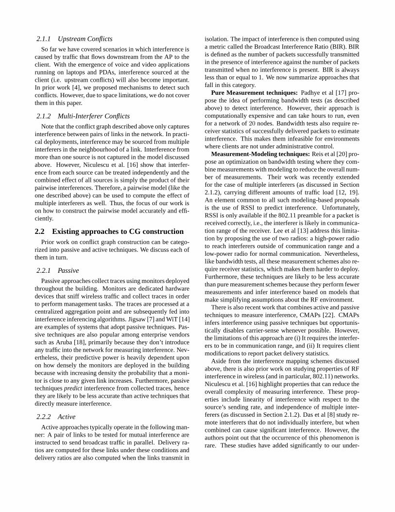
The software architecture of the AP is shown in Figure3. It comprises of three parts: (i) the ethernet driver that re-ceives commands from the controller, (ii) the wireless driverthat executes these commands inside the kernel, and (iii) thefirmware/microcode that interfaces with the wireless driver
and sends out the micro-probes. We discuss our modifica-tions to each part next.
Kernel/Driver Modifications: To minimize processingdelays while forwarding probe requests from the wired Eth-ernet interface to the wireless interface of the AP, we im-plemented a direct driver-to-driver (D2D) communicationpath, where the Ethernet driver directly invokes functionsimplemented by the wireless driver. This bypasses time-consuming packet processing tasks and other unpredictablein-kernel events that can affect the accuracy with which micro-probes are synchronized over the air. When a micro-probingrequest is received on an AP’s wired interface, it’s embeddedcommand is parsed, and the appropriate wireless operationis immediately invoked.
On the reverse path (AP→ Controller), the AP uses anin-kernel raw socket to send responses (to micro-probing re-quests) back to the controller. Note that raw sockets can onlybe used for sending packets, not receiving them.
Firmware Modifications: The Intel 2915ABG NIC soft-ware comprises of two parts: 1) Afirmware that interfaceswith the kernel driver, and 2) Amicrocodethat interfaceswith the firmware. The firmware implements an RTOS (RealTime Operating System), responsible for handling macro-timescale operations, such as AP beaconing. The microcodeconsists of a set of specialized hardware acceleration blocksthat are used for micro-timescale operations, such as count-ing down backoff timers for IEEE 802.11’s randomized back-off algorithm, etc.
We modified the firmware and microcode running on thewireless NIC to support transmission of micro-probes fromwithin the firmware. Constructing a probe packet in thedriver would require a DMA-copy of the packet from kernel-space to firmware memory. This is unnecessary since thepayload of the probes doesn’t carry any useful data. Notethat this implementation choice has no effect on the appli-cability of micro-probing but is simply a way of eliminatingunnecessary processing overhead in the driver.
CSMA/CA and Binary Exponential Backoff (BEB) arestandard mechanisms by which 802.11 compliant devicescoordinate access to the medium. Such medium access tech-niques are unsuitable for our system because they preventinterference scenarios from occurring. We therefore, disablerandomized back-off and carrier-sensing when sending outprobes for interference testing. Note that we only disabledback-off for our micro-probes, not other packets. Therefore,all of our extensions in the driver, firmware, and microcodeare 802.11 standards compliant.
Silencing: Silencing the network is a crucial requirementfor micro-probing. However, it is challenging to achieve be-cause the environment may be populated with both 802.11as well as non-802.11 devices such as microwave ovens andcordless phones. In our system, we achieve silencing byinstructing the driver/firmware to send CTS-to-self packetswith a duration equivalent to the execution time of an activetest. The silencing packet is transmitted immediately pre-
ceding the micro-probe transmission and this is performedbefore each and every test. We present results on the effec-tiveness of silencing in Section 5.
Synchronization: The controller communicates with theAPs participating in a test using a single broadcast UDPpacket. This serves two purposes. First, it provides eachAP with information on what action to perform for that test.In our implementation, we use a single control packet to en-code multiple actions for a test, one for each AP. Second, itallows us to synchronize APs to one another through the useof wired MAC layer broadcasts to supportreference-basedbroadcast synchronization(RBS) [10]. Reference broad-casts use the packet’s time-of-arrival at the APs tomutuallysynchronize them. A key underlying assumption is that allAPs receive the broadcast packet at the same time instant. Inthe next section, we evaluate the extent to which RBS-basedsynchronization can be achieved. Note that synchronizationaccuracy is dependent on the transmission duration of theprobes. For a probe of size1400 bytes, the transmissionduration is approximately1800us, at 6Mbps. Therefore,synchronization to within a few tens of microseconds is suf-ficient for probes of this size.
We now describe two alternative approaches that we laterabandoned in favor of RBS-based synchronization. The firstapproach is NTP-based synchronization [2]. Here, the con-troller is the master and the APs act as slaves. The master’sjob is to periodically synchronize the slaves to it’s own clock.Unfortunately, NTP is known to provide accuracies in therange of1 − 5ms, which is too inaccurate for our purposes.
The second approach is to synchronize APs with the helpof TSF timestamps encoded in the Beacons of neighbouringAPs, as is done in [7]. However, this approach is signifi-cantly more complex than RBS-based synchronization. Thecomplexity arises in situations where the APs performing thetest are not in communication range of each other and there-fore can’t decode one another’s Beacons. In this scenario,a third AP’s Beacons (that is in range of the other two) isrequired to support synchronization of the two APs. Thisis a significantly complex process, and as we show later, isunnecessary because we can achieve similar levels of accu-racy using a simple and lightweight RBS-based approach tosynchronization.
5. PERFORMANCE OF MICRO-PROBINGThe effectiveness of micro-probing depends on: 1) our
ability to tightly synchronize APs, 2) our ability to silencethe network before an experiment, and 3) our ability to useMAC service time (MST) as a mechanism to detect CS in-duced interference. In what follows, we evaluate the effec-tiveness of these techniques.
5.1 AP SynchronizationOur evaluation of AP synchronization is subdivided into:
1) Characterization of delays in our system, and 2) Analysis
AP
Client
ipw2200 firmware
ipw2200 Driver
Ethernet Driver
Ethernet Firmware
Controller
Wireless
RTT
D2D
Delay
AP
RTT
Wired
Delay
Controller
RTT
2195
(21)
27
(15)
2449
(42)
95
(18)
2585
(110)
Mean (Variance)
in microseconds
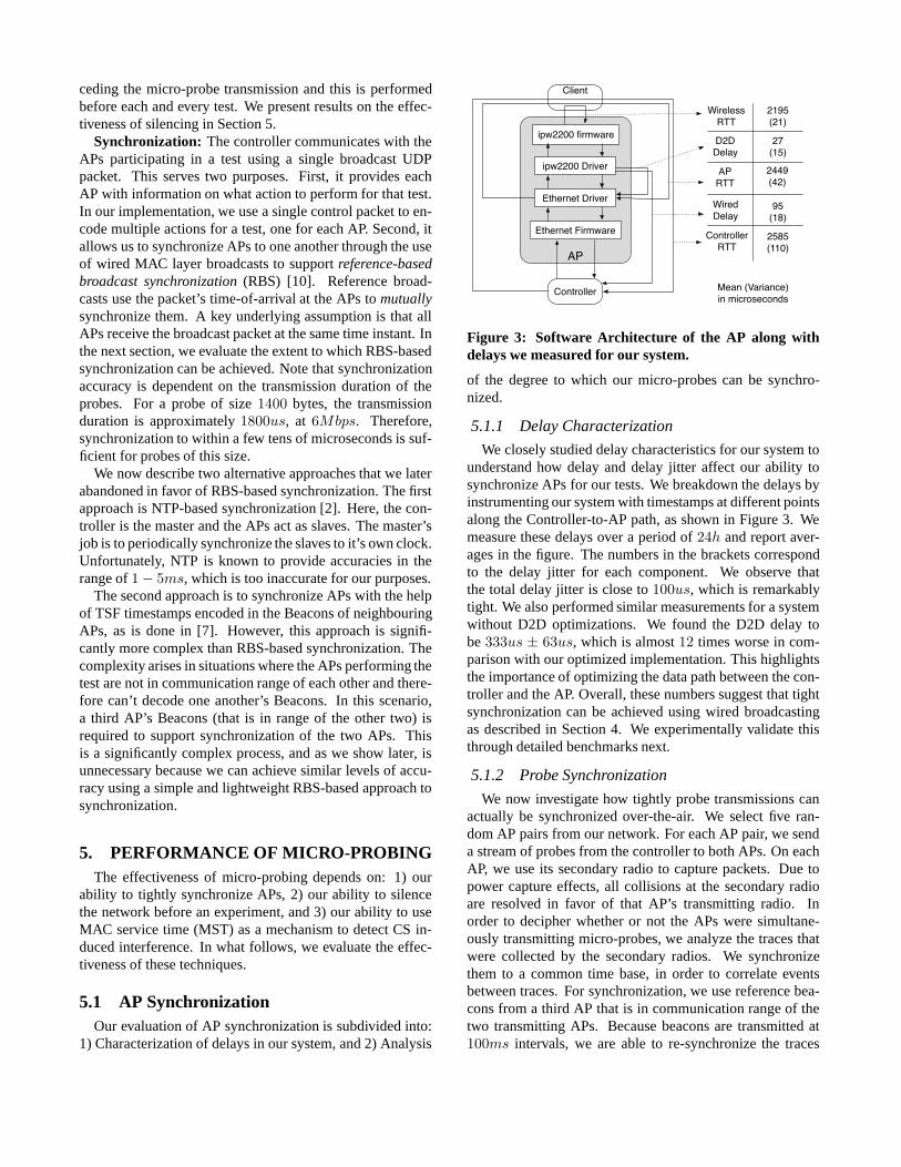
Figure 3: Software Architecture of the AP along withdelays we measured for our system.
of the degree to which our micro-probes can be synchro-nized.
5.1.1 Delay Characterization
We closely studied delay characteristics for our system tounderstand how delay and delay jitter affect our ability tosynchronize APs for our tests. We breakdown the delays byinstrumenting our system with timestamps at different pointsalong the Controller-to-AP path, as shown in Figure 3. Wemeasure these delays over a period of24h and report aver-ages in the figure. The numbers in the brackets correspondto the delay jitter for each component. We observe thatthe total delay jitter is close to100us, which is remarkablytight. We also performed similar measurements for a systemwithout D2D optimizations. We found the D2D delay tobe333us ± 63us, which is almost12 times worse in com-parison with our optimized implementation. This highlightsthe importance of optimizing the data path between the con-troller and the AP. Overall, these numbers suggest that tightsynchronization can be achieved using wired broadcastingas described in Section 4. We experimentally validate thisthrough detailed benchmarks next.
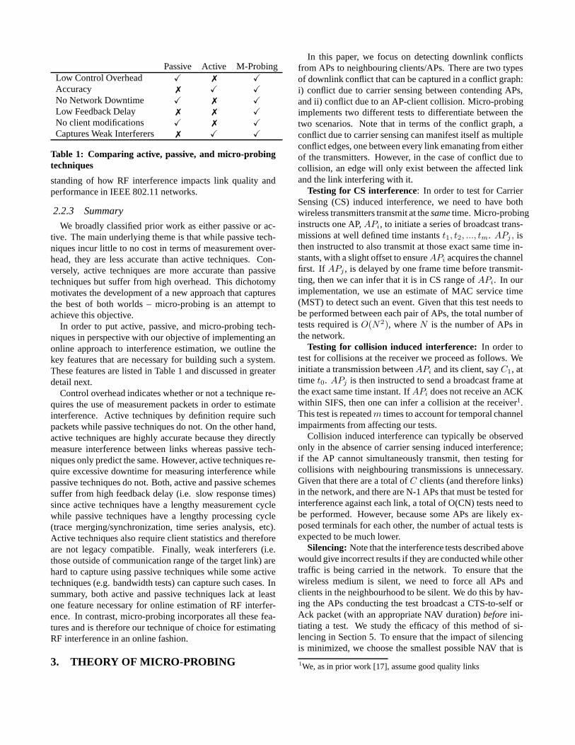
5.1.2 Probe Synchronization
We now investigate how tightly probe transmissions canactually be synchronized over-the-air. We select five ran-dom AP pairs from our network. For each AP pair, we senda stream of probes from the controller to both APs. On eachAP, we use its secondary radio to capture packets. Due topower capture effects, all collisions at the secondary radioare resolved in favor of that AP’s transmitting radio. Inorder to decipher whether or not the APs were simultane-ously transmitting micro-probes, we analyze the traces thatwere collected by the secondary radios. We synchronizethem to a common time base, in order to correlate eventsbetween traces. For synchronization, we use reference bea-cons from a third AP that is in communication range of thetwo transmitting APs. Because beacons are transmitted at100ms intervals, we are able to re-synchronize the traces
1
10
100
1000
0 200 400 600 800 1000 1200 1400 1600
Sta
rt T
ime
Dif
fere
nce
(u
Sec
s)
Packet Index
(a) Synchronization error between APs
10
20
30
40
50
60
70
80
90
100
1 10 100 1000
CD
F
Start Time Difference (uSecs)
(b) CDF of synchronization error
5
10
15
20
25
30
35
40
45
1 2 3 4 5
Sta
rt T
ime
Dif
fere
nce
(u
s)
Transmitter Pairs
(c) Mean synchronization error across5
links
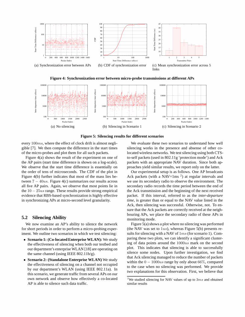
Figure 4: Synchronization error between micro-probe transmissions at different APs
100
1000
10000
100000
0 500 1000 1500 2000 2500
Inte
r-d
epar
ture
tim
e (u
Sec
s)
Packet Index
(a) No silencing
100
1000
10000
100000
0 500 1000 1500 2000 2500
Inte
r-d
epar
ture
tim
e (u
Sec
s)
Packet Index
(b) Silencing in Scenario1
100
1000
10000
100000
0 200 400 600 800 1000 1200 1400
Inte
r-d
epar
ture
tim
e (u
Sec
s)
Packet Index
(c) Silencing in Scenario2
Figure 5: Silencing results for different scenarios
every100ms, where the effect of clock drift is almost negli-gible [7]. We then compute the difference in the start timesof the micro-probes and plot them for all such packets.
Figure 4(a) shows the result of the experiment on one ofthe AP pairs (start time difference is shown on a log-scale).We observe that the start time difference is essentially onthe order of tens of microseconds. The CDF of the plot inFigure 4(b) further indicates that most of the mass lies be-tween7 − 40us. Figure 4(c) summarizes our results acrossall five AP pairs. Again, we observe that most points lie inthe10− 25us range. These results provide strong empiricalevidence that RBS-based synchronization is highly effectivein synchronizing APs at micro-second level granularity.
5.2 Silencing AbilityWe now examine an AP’s ability to silence the network
for short periods in order to perform a micro-probing exper-iment. We outline two scenarios in which we test silencing:
• Scenario 1: (Co-located Enterprise WLAN):We studythe effectiveness of silencing when both our testbed andour department’s enterprise WLAN [18] are operating onthe same channel (using IEEE 802.11b/g).
• Scenario 2: (Standalone Enterprise WLAN)We studythe effectiveness of silencing on a channel not occupiedby our department’s WLAN (using IEEE 802.11a). Inthis scenario, we generate traffic from several APs on ourown network and observe how effectively a co-locatedAP is able to silence such data traffic.
We evaluate these two scenarios to understand how wellsilencing works in the presence and absense of other co-located wireless networks. We test silencing using both CTS-to-self packets (used in 802.11g ‘protection mode’) and Ackpackets with an appropriate NAV duration. Since both ap-proaches yield similar results, we report only on the latter.
Our experimental setup is as follows. One AP broadcastsAck packets (with a NAV=1ms2) at regular intervals andwe use its secondary radio to observe the environment. Thesecondary radio records the time period between the end ofthe Ack transmission and the beginning of the next receivedpacket. If this interval, referred to as theinter-departuretime, is greater than or equal to the NAV value listed in theAck, then silencing was successful. Otherwise, not. To en-sure that the Ack packets are correctly received at the neigh-bouring APs, we place the secondary radio of these APs inmonitoring mode.
Figure 5(a) shows a plot where no silencing was performed(the NAV was set to1us), whereas Figure 5(b) presents re-sults for silencing with a NAV of1ms (for scenario 1). Com-paring these two plots, we can identify a significant cluster-ing of data points around the1000us mark on the secondplot. This indicates that silencing is able to successfullysilence some nodes. Upon further investigation, we findthat Ack silencing managed to reduce the number of packetswithin the0 − 1000us range by only about66%, comparedto the case when no silencing was performed. We providetwo explanations for this observation. First, we believe that
2We studied silencing for NAV values of up to3ms and obtainedsimilar results
0
20
40
60
80
100
0 2000 4000 6000
CD
F
MAC Service Time (uSecs)
AP 1AP 2
(a) CDF of MST without staggering
0
20
40
60
80
100
0 2000 4000 6000 8000
CD
F
MAC Service Time (uSecs)
50us100us200us300us400us
(b) CDF of AP1 with staggering
0
20
40
60
80
100
0 2000 4000 6000 8000
CD
F
MAC Service Time (uSecs)
50us100us200us300us400us
(c) CDF of AP2 with staggering
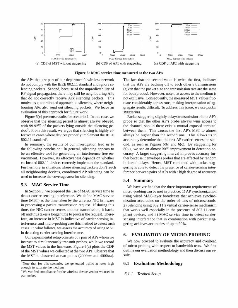
Figure 6: MAC service time measured at the two APs
the APs that are part of our department’s wireless networkdo not comply with the IEEE 802.11 standard and ignore si-lencing packets. Second, because of the unpredictability ofRF signal propagation, there may still be neighbouring APsthat do not correctly receive Ack silencing packets. Thismotivates a coordinated approach to silencing where neigh-bouring APs also send out silencing packets. We leave anevaluation of this approach for future work.
Figure 5(c) presents results for scenario 2. In this case, weobserve that the silencing period is almost always obeyed,with 99.92% of the packets lying outside the silencing pe-riod3. From this result, we argue that silencing is highly ef-fective in cases where devices properly implement the IEEE802.11 standard4.
In summary, the results of our investigation lead us tothe following conclusion: In general, silencing appears tobe an effective tool for generating an interference free en-vironment. However, its effectiveness depends on whetherco-located 802.11 devices correctly implement the standard.Furthermore, in situations where silencing packets don’t reachall neighbouring devices, coordinated AP silencing can beused to increase the coverage area for silencing.
5.3 MAC Service TimeIn Section 3, we proposed the use of MAC service time to
detect carrier-sensing interference. We define MAC servicetime (MST) as the time taken by the wireless NIC firmwarein processing a packet transmission request. If during thistime, the NIC carrier-senses another transmission, it backsoff and thus takes a longer time to process the request. There-fore, an increase in MST is indicative of carrier-sensing in-terference, and micro-probing uses this method to detect suchcases. In what follows, we assess the accuracy of using MSTin detecting carrier-sensing interference.
Our experimental setup consists of a pair of APs whom weinstruct to simultaneously transmit probes, while we recordthe MST values in the firmware. Figure 6(a) plots the CDFof the MST values we collected at the two APs. Observe thatthe MST is clustered at two points (2000us and4000us).
3Note that for this scenario, we generated traffic at rates highenough to saturate the medium4We verified compliance for the wireless device vendor we usedinour testbed
The fact that the second value is twice the first, indicatesthat the APs are backing off to each other’s transmissions(given that the packet size and transmission rate are the samefor both probes). However, note that access to the medium isnot exclusive. Consequently, the measured MST values fluc-tuate considerably across runs, making interpretation of ag-gregate results difficult. To address this issue, we usepacketstaggering.
Packet staggering slightly delays transmission of one AP’sprobe so that the other AP’s probe always wins access tothe channel, should there exist a mutual exposed terminalbetween them. This causes the first AP’s MST to almostalways be higher than the second one. This allows us toaccurately determine that the first AP carrier-senses the sec-ond, as seen in Figures 6(b) and 6(c). By staggering for50us, we see an almost20% improvement in detection ac-curacy. A larger staggering interval improves accuracy fur-ther because it envelopes probes that are affected by randomin-kernel delays. Hence, MST combined with packet stag-gering is able to detect the presence of carrier-sensing inter-ference between pairs of APs with a high degree of accuracy.
5.4 SummaryWe have verified that the three important requirements of
micro-probing can be met in practice: 1) AP synchronizationusing wired MAC-layer broadcasts that achieves synchro-nization accuracies on the order of tens of microseconds,2) Silencing using 802.11’s virtual carrier-sense mechanismthat works well especially in the presence of 802.11 com-pliant devices, and 3) MAC service time to detect carrier-sensing interference that in combination with packet stag-gering achieves accuracies of up to 90%.
6. EVALUATION OF MICRO-PROBINGWe now proceed to evaluate the accuracy and overhead
of micro-probing with respect to bandwidth tests. We firstoutline our evaluation methodology and then discuss our re-sults.
6.1 Evaluation Methodology
6.1.1 Testbed Setup
We compare micro-probing with bandwidth tests on a 40-node testbed spread out across two floors of our 120m x65m department building. As discussed earlier, each nodeis equipped with two 802.11a/b/g radios: an Intel 2915ABGwireless card [1] and an EnGenius EMP-8602 Atheros card.We use a data rate of6Mbps for all our experiments. Fur-thermore, we use1400 byte packets since we want to studythe effect of interference on real-world data traffic, whichtypically uses packet sizes equal to the Ethernet MTU. Ourexperiments use IEEE 802.11a, which is not used by othernetworks in our building. For bandwidth testing, we gener-ate traffic at rates high enough to saturate the medium. Atthe receiver, we measure the packet delivery ratio for eachlink.
For micro-probing, traffic is generated by the controllerand probe requests are broadcast to APs at 10ms intervals.The value of the control parameterm (the number of experi-ments to perform per link) is fixed at10. We later show howwe empirically derived this value for our testbed.
6.1.2 Evaluation Metrics
We compare bandwidth tests and micro-probing using theBIR metric described in Section 2.2. The BIR for bandwidthtests is computed as follows. We first measureRAB, thenumber of packets received by node B on link A→ B whenall competing nodes are silent. We then measureRC
AB, thenumber of packets received by B on the same link in thepresence of a competing transmitter C. Because antennas areomnidirectional, it does not matter whom C is transmittingto–in other words, all links with C as the transmitter are po-tentially in conflict with link A→ B. Then, BIR is computedas:
BIR = RCAB/RAB (1)
Note that a BIR of 0 means that link A→B cannot deliverpackets when C is active. This indicates that C and A arehidden terminals with respect to B. A BIR of 0.5 indicatesthat A and C share the air, when A is communicating with B,which means that A and C are exposed terminals. Finally, aBIR of 1 indicates that C does not interfere with link A→B.
For micro-probing, the BIR value is computed in the sameway as shown in Equation 1. However, the numerator isdifferent from bandwidth tests. Furthermore, the numer-ators for carrier-sensing and collision-induced interferenceare also distinct. The value in the denominator is the samefor micro-probing because this is the link delivery ratio inthe absence of interference. We now focus on computing thedelivery ratio in the presence of interference.
Carrier-sensing interference: In order to estimate theimpact of interference between two carrier-sensing senders,we adopt the following approach. We first send out probessynchronously from both APs. Ifm is the total number ofprobes sent out, then the number of timeslots for transmis-sion in an interference-limited scenario would ben+2∗(m−n), wheren is the number of “timely” successful transmis-sions. Notice that each transmission that was delayed willtake 2 time slots and thus we have to multiplym − n by 2.
0
0.2
0.4
0.6
0.8
1
1.2
212019181716151413121110987654321Mea
n B
road
cast
Inte
rfer
ence
Rat
io (
BIR
)
Link Pairs
Micro-PbBW tests
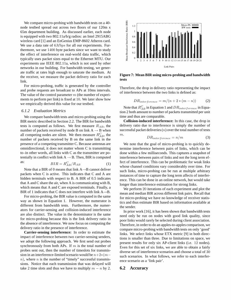
Figure 7: Mean BIR using micro-probing and bandwidthtests
Therefore, the drop in delivery ratio representing the impactof interference between the two links is defined as:
DRinterference = m/(n + 2 ∗ (m − n)) (2)
Note thatRCAB in Equation 1 andDRinterference in Equa-
tion 2 both amount to number of packets transmitted per unittime and thus are comparable.
Collision-induced interference: In this case, the drop indelivery ratio due to interference is simply the number ofsuccessful packet deliveries (n) over the total number of testsm.
DRinterference = n/m (3)
We note that the goal of micro-probing is to quickly de-termine interference between pairs of links, which can bedone within a few milliseconds. This captures a snapshot ofinterference between pairs of links and not the long term ef-fect of interference. This can be problematic for weak linkswhose channel conditions vary considerably over time. Forsuch links, micro-probing can be run at multiple arbitraryinstances of time to capture the long term affects of interfer-ence. This can be done in an online network, but would takelonger than interference estimation for strong links.
We perform20 iterations of each experiment and plot themean and median BIR across different link pairs. Recall thatfor micro-probing we have no knowledge of receiver statis-tics and thus estimate BIR based on information available atthe sender.
In prior work [16], it has been shown that bandwidth testsneed only be run on nodes with good link quality, sincepoor links would rarely be selected during client association.Therefore, in order to do an apples-to-apples comparison, wecompare micro-probing with bandwidth tests on only ‘good’links. We select links whose ETX metric [9] in both direc-tions is smaller than three. Due to limitations on space, wepresent results for only six AP-client links (i.e.12 nodes).Even for this set of six links, we are able to obtain a fairlydiverse set of interference scenarios and choose a total of30such scenarios. In what follows, we refer to each interfer-ence scenario as a ‘link pair’.
6.2 Accuracy
0
0.2
0.4
0.6
0.8
1
1.2
212019181716151413121110987654321Med
ian B
road
cast
Inte
rfer
ence
Rat
io (
BIR
)
Link Pairs
Micro-PbBW tests
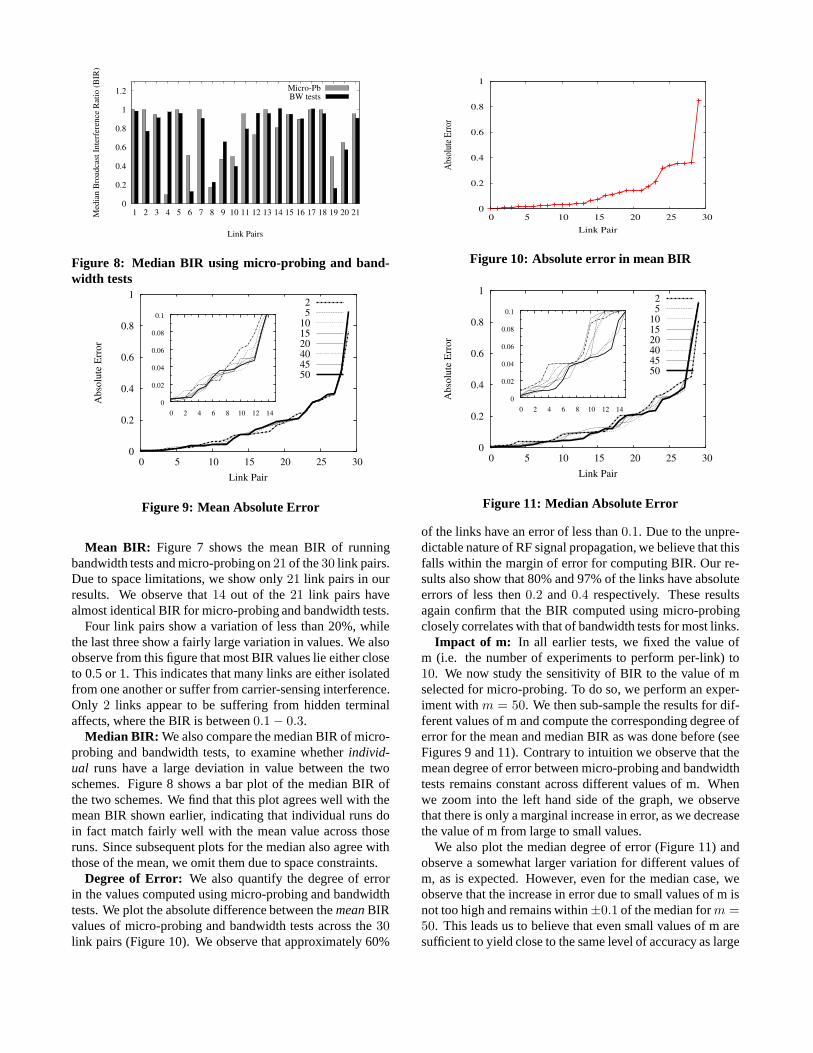
Figure 8: Median BIR using micro-probing and band-width tests
0
0.2
0.4
0.6
0.8
1
0 5 10 15 20 25 30
Ab
solu
te E
rro
r
Link Pair
25
101520404550
0
0.02
0.04
0.06
0.08
0.1
0 2 4 6 8 10 12 14
Figure 9: Mean Absolute Error
Mean BIR: Figure 7 shows the mean BIR of runningbandwidth tests and micro-probing on21 of the30 link pairs.Due to space limitations, we show only21 link pairs in ourresults. We observe that14 out of the21 link pairs havealmost identical BIR for micro-probing and bandwidth tests.
Four link pairs show a variation of less than 20%, whilethe last three show a fairly large variation in values. We alsoobserve from this figure that most BIR values lie either closeto 0.5 or 1. This indicates that many links are either isolatedfrom one another or suffer from carrier-sensing interference.Only 2 links appear to be suffering from hidden terminalaffects, where the BIR is between0.1 − 0.3.
Median BIR: We also compare the median BIR of micro-probing and bandwidth tests, to examine whetherindivid-ual runs have a large deviation in value between the twoschemes. Figure 8 shows a bar plot of the median BIR ofthe two schemes. We find that this plot agrees well with themean BIR shown earlier, indicating that individual runs doin fact match fairly well with the mean value across thoseruns. Since subsequent plots for the median also agree withthose of the mean, we omit them due to space constraints.
Degree of Error: We also quantify the degree of errorin the values computed using micro-probing and bandwidthtests. We plot the absolute difference between themeanBIRvalues of micro-probing and bandwidth tests across the30link pairs (Figure 10). We observe that approximately 60%
0
0.2
0.4
0.6
0.8
1
0 5 10 15 20 25 30
Abs
olut
e E
rror
Link Pair
Figure 10: Absolute error in mean BIR
0
0.2
0.4
0.6
0.8
1
0 5 10 15 20 25 30A
bso
lute
Err
or
Link Pair
25
101520404550
0
0.02
0.04
0.06
0.08
0.1
0 2 4 6 8 10 12 14
Figure 11: Median Absolute Error
of the links have an error of less than0.1. Due to the unpre-dictable nature of RF signal propagation, we believe that thisfalls within the margin of error for computing BIR. Our re-sults also show that 80% and 97% of the links have absoluteerrors of less then0.2 and0.4 respectively. These resultsagain confirm that the BIR computed using micro-probingclosely correlates with that of bandwidth tests for most links.
Impact of m: In all earlier tests, we fixed the value ofm (i.e. the number of experiments to perform per-link) to10. We now study the sensitivity of BIR to the value of mselected for micro-probing. To do so, we perform an exper-iment withm = 50. We then sub-sample the results for dif-ferent values of m and compute the corresponding degree oferror for the mean and median BIR as was done before (seeFigures 9 and 11). Contrary to intuition we observe that themean degree of error between micro-probing and bandwidthtests remains constant across different values of m. Whenwe zoom into the left hand side of the graph, we observethat there is only a marginal increase in error, as we decreasethe value of m from large to small values.
We also plot the median degree of error (Figure 11) andobserve a somewhat larger variation for different values ofm, as is expected. However, even for the median case, weobserve that the increase in error due to small values of m isnot too high and remains within±0.1 of the median form =50. This leads us to believe that even small values of m aresufficient to yield close to the same level of accuracy as large
0
0.2
0.4
0.6
0.8
1
1.2
1.4
0 5 10 15 20 25 30 35 40 45 50
Mea
n B
road
cast
Inte
rfer
ence
Rat
io (
BIR
)
Value of M
High BIRModerate BIR
Low BIR
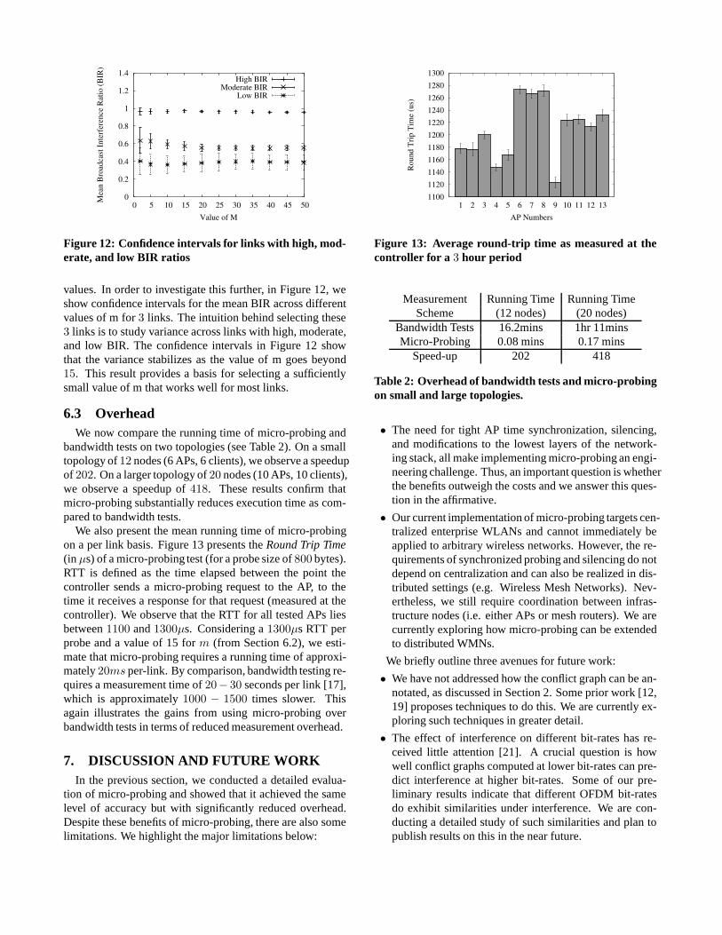
Figure 12: Confidence intervals for links with high, mod-erate, and low BIR ratios
values. In order to investigate this further, in Figure 12, weshow confidence intervals for the mean BIR across differentvalues of m for3 links. The intuition behind selecting these3 links is to study variance across links with high, moderate,and low BIR. The confidence intervals in Figure 12 showthat the variance stabilizes as the value of m goes beyond15. This result provides a basis for selecting a sufficientlysmall value of m that works well for most links.
6.3 OverheadWe now compare the running time of micro-probing and
bandwidth tests on two topologies (see Table 2). On a smalltopology of12 nodes (6 APs, 6 clients), we observe a speedupof 202. On a larger topology of20 nodes (10 APs, 10 clients),we observe a speedup of418. These results confirm thatmicro-probing substantially reduces execution time as com-pared to bandwidth tests.
We also present the mean running time of micro-probingon a per link basis. Figure 13 presents theRound Trip Time(in µs) of a micro-probing test (for a probe size of800 bytes).RTT is defined as the time elapsed between the point thecontroller sends a micro-probing request to the AP, to thetime it receives a response for that request (measured at thecontroller). We observe that the RTT for all tested APs liesbetween1100 and1300µs. Considering a1300µs RTT perprobe and a value of 15 form (from Section 6.2), we esti-mate that micro-probing requires a running time of approxi-mately20ms per-link. By comparison, bandwidth testing re-quires a measurement time of20− 30 seconds per link [17],which is approximately1000 − 1500 times slower. Thisagain illustrates the gains from using micro-probing overbandwidth tests in terms of reduced measurement overhead.
7. DISCUSSION AND FUTURE WORKIn the previous section, we conducted a detailed evalua-
tion of micro-probing and showed that it achieved the samelevel of accuracy but with significantly reduced overhead.Despite these benefits of micro-probing, there are also somelimitations. We highlight the major limitations below:
1100
1120
1140
1160
1180
1200
1220
1240
1260
1280
1300
1 2 3 4 5 6 7 8 9 10 11 12 13
Round T
rip T
ime
(us)
AP Numbers
Figure 13: Average round-trip time as measured at thecontroller for a 3 hour period
Measurement Running Time Running TimeScheme (12 nodes) (20 nodes)
Bandwidth Tests 16.2mins 1hr 11minsMicro-Probing 0.08 mins 0.17 mins
Speed-up 202 418
Table 2: Overhead of bandwidth tests and micro-probingon small and large topologies.
• The need for tight AP time synchronization, silencing,and modifications to the lowest layers of the network-ing stack, all make implementing micro-probing an engi-neering challenge. Thus, an important question is whetherthe benefits outweigh the costs and we answer this ques-tion in the affirmative.
• Our current implementation of micro-probing targets cen-tralized enterprise WLANs and cannot immediately beapplied to arbitrary wireless networks. However, the re-quirements of synchronized probing and silencing do notdepend on centralization and can also be realized in dis-tributed settings (e.g. Wireless Mesh Networks). Nev-ertheless, we still require coordination between infras-tructure nodes (i.e. either APs or mesh routers). We arecurrently exploring how micro-probing can be extendedto distributed WMNs.
We briefly outline three avenues for future work:
• We have not addressed how the conflict graph can be an-notated, as discussed in Section 2. Some prior work [12,19] proposes techniques to do this. We are currently ex-ploring such techniques in greater detail.
• The effect of interference on different bit-rates has re-ceived little attention [21]. A crucial question is howwell conflict graphs computed at lower bit-rates can pre-dict interference at higher bit-rates. Some of our pre-liminary results indicate that different OFDM bit-ratesdo exhibit similarities under interference. We are con-ducting a detailed study of such similarities and plan topublish results on this in the near future.
• We have not addressed the co-existence problem of micro-probing and normal data traffic. In particular, the effectof micro-probing on TCP traffic would be interesting tostudy and we plan to explore this in future work.
Innovations in WLAN Optimization: Micro-probingopens up the space for new WLAN optimization techniquesbecause of it’s ability to rapidly compute the conflict graphin an online fashion. In what follows, we briefly discuss twooptimization techniques that micro-probing facilitates:
• Fine-grained packet scheduling:DCF, although widelyused, is known to have performance problems in densedeployments. As a result, there have been proposals to-wards centralizing medium access control [5]. Theseproposals, however are difficult to realize in practice dueto a lack of realtime conflict information. Micro-probingcan provide such realtime information, making central-ized medium access control viable.
• Fine-grained power management:Most existing powercontrol techniques choose a single conservative powerlevel for each AP [15]. This is because they are un-able to handle hidden/exposed terminal problems thatcan arise from power control operating at finer granular-ities (e.g on a per-client basis). Micro-probing can dis-cover these conflicts in realtime and therefore facilitateeffective fine-grained power control.
8. SUMMARYWe present a first detailed evaluation on the feasibility of
micro-probing [4] – an online approach to estimating in-terference. A real-world implementation of micro-probingposes numerous challenges that include requirements formicrosecond-level AP synchronization and effective silenc-ing of the wireless medium. Our work is a first implemen-tation of micro-probing and we validate it on a40 nodewireless testbed. Through detailed performance benchmarkswe show that our implementation effectively addresses allthe implementation challenges. Furthermore, we show thatmicro-probing is just as accurate as bandwidth tests but witha substantial reduction in measurement overhead. These re-sults not only represent a significant advance in the field ofefficient interference mapping, but also motivate the designof new WLAN optimization techniques that were previouslynot possible.
9. REFERENCES[1] Intel 2915abg card. http://www.intel.com/.[2] Network time protocol. http://www.ntp.org.[3] VIA Technologies. URL: http://www.via.com.tw.[4] N. Ahmed and S. Keshav. Smarta: A self-managing
architecture for thin access points. InCoNEXT, 2006.[5] N. Ahmed, V. Shrivastava, A. Mishra, S. Banerjee,
S. Keshav, and K. Papagiannaki. Interferencemitigation in enterprise wlans through speculativescheduling. InMobiCom 2007.
[6] I. Broustis, K. Papagiannaki, S. V. Krishnamurthy,M. Faloutsos, and V. Mhatre. Mdg: measurementdriven guidelines for 802.11 wlan design. InMobiCom2007.
[7] Y.-C. Cheng, J. Bellardo, P. Benko, A. C. Snoeren,G. M. Voelker, and S. Savage. Jigsaw: solving thepuzzle of enterprise 802.11 analysis. InSigcomm2006.
[8] S. M. Das, D. Koutsonikolas, Y. C. Hu, andD. Peroulis. Characterizing multi-way interference inwireless mesh networks. InWiNTECH 2006.
[9] D. DeCouto, D. Aguayo, J. Bicket, and R. Morris. Ahigh-throughput path metric for multi-hop wirelessrouting. InMobiCom 2003.
[10] J. Elson, L. Girod, and D. Estrin. Fine-grained networktime synchronization using reference broadcasts.SIGOPS Oper. Syst. Rev., 36(SI):147–163, 2002.
[11] K. Jain, J. Padhye, V. N. Padmanabhan, and L. Qiu.Impact of interference on multi-hop wireless networkperformance. InMobiCom, 2003.
[12] A. Kashyap, S. Ganguly, and S. R. Das. Ameasurement-based approach to modeling linkcapacity in 802.11-based wireless networks. InMobiCom 2007.
[13] J. Lee, S.-J. Lee, W. Kim, D. Jo, T. Kwon, and Y. Choi.Rss-based carrier sensing and interference estimationin 802.11 wireless networks. InSECON, 2007.
[14] R. Mahajan, M. Rodrig, D. Wetherall, and J. Zahorjan.Analyzing the mac-level behavior of wirelessnetworks in the wild. InSigcomm 2006.
[15] V. Mhatre, K. Papagiannaki, and B. F. Interferencemitigation through power control in high density802.11 wlans. InINFOCOM 2007.
[16] D. Niculescu. Interference map for 802.11 networks.In IMC, 2007.
[17] J. Padhye, S. Agarwal, V. Padmanabhan, L. Qiu,A. Rao, and B. Zill. Estimation of link interference instatic multi-hop wireless networks. InIMC, 2005.
[18] W. paper from Aruba Networks. Advanced rfmanagement for wireless grids.http://tinyurl.com/4eyndu.
[19] L. Qiu, Y. Zhang, F. Wang, M. K. Han, andR. Mahajan. A general model of wireless interference.In MobiCom 2007.
[20] C. Reis, R. Mahajan, M. Rodrig, D. Wetherall, andJ. Zahorjan. Measurement-based models of deliveryand interference in static wireless networks. InSigcomm 2006.
[21] V. Sridhara, H. Shin, and B. S. Performance of802.11b/g in the interference limited regime. InICCCN, 2007.
[22] M. Vutukuru, K. Jamieson, and H. Balakrishnan.Harnessing Exposed Terminals in Wireless Networks.In NSDI 2008.