Online AppendixCentralized Admissions, Affirmative Action and Access of Low-income

Students to Higher Education

Ursula Mello

Table of Contents

A Data Appendix 2A.1 Data Access and Data Sources . . . . . . . . . . . . . . . . . . . . . . . . . . . . 2

A.1.1 INEP Microdata . . . . . . . . . . . . . . . . . . . . . . . . . . . . . . . 2A.1.2 SISU Data . . . . . . . . . . . . . . . . . . . . . . . . . . . . . . . . . . 2A.1.3 Affirmative Action Quotas Data . . . . . . . . . . . . . . . . . . . . . . . 2

A.2 Data Description . . . . . . . . . . . . . . . . . . . . . . . . . . . . . . . . . . . 3A.2.1 Student-level data . . . . . . . . . . . . . . . . . . . . . . . . . . . . . . . 3A.2.2 Institution-level data . . . . . . . . . . . . . . . . . . . . . . . . . . . . . 4A.2.3 Program-level data . . . . . . . . . . . . . . . . . . . . . . . . . . . . . . 4

B Self-declared Data 5B.1 Variable “Public-school Student (PS)” . . . . . . . . . . . . . . . . . . . . . . . . 6B.2 Variable “Public-school Non-white Student (PSNW)” . . . . . . . . . . . . . . . . 6B.3 Variable “Public-school Low-income Student (PSLI)” . . . . . . . . . . . . . . . . 8

C Missing Data and Sample Selection 10

D Replicability: Results at Program Level 13

E Affirmative Action Treatment 15E.1 Ethnic versus Non-Ethnic Quotas . . . . . . . . . . . . . . . . . . . . . . . . . . . 15E.2 Local Supply of PS and PSNW Students . . . . . . . . . . . . . . . . . . . . . . . 16E.3 Strategic High School Choice . . . . . . . . . . . . . . . . . . . . . . . . . . . . . 16

F Heterogeneity 18F.1 By Initial Share of Enrollments of Low-SES Students . . . . . . . . . . . . . . . . 18F.2 Persistence . . . . . . . . . . . . . . . . . . . . . . . . . . . . . . . . . . . . . . 19

G Robustness 20G.1 Spillovers and SUTVA . . . . . . . . . . . . . . . . . . . . . . . . . . . . . . . . 20G.2 Robustness of Out-of-state Students’ Outcome . . . . . . . . . . . . . . . . . . . . 23

H Additional Figures and Tables 27

1

A Data Appendix

A.1 Data Access and Data SourcesA.1.1 INEP Microdata

The identified versions of the Brazilian Census of Higher Education (CES) and the National Examof High School (ENEM) are available for researchers upon approval of research projects at theNational Institute for Educational Studies and Research (INEP). The steps required for projectapproval are carefully described in the following website: http://portal.inep.gov.br/web/guest/dados/sedap/solicitacao-de-acesso. Descriptions and codes from the raw data tothe results presented in this paper are available in the replication package.

A.1.2 SISU Data

Data on the implementation of the Sistema de Seleção Unificada (SISU) from 2010 to 2015 wereobtained from the BrazilianMinistry of Education (MEC) by request through the Electronic SystemService of Information (e-sic) of the Federal Government of Brazil. As determined by the Accessto Information Law (Law 12527/2011), individuals can directly ask public information and datato public institutions, which are required, by law, to provide the data or formally explain why therequest cannot be met. All data and information obtained through this channel are public domain.To obtain the SISU data, I opened a request destined to the Ministry of Education (protocol number23480004065201721) at http://www.esic.gov.br/. The data provided from the Ministry isavailable as part of the replication package in its original format.

A.1.3 Affirmative Action Quotas Data

Data on the implementation of Affirmative Action Quotas (AA) from 2010 to 2015 were collectedby the author from public admission documents available at universities’ websites (the so-called“Editais”) or directly provided by the higher education institutions. Federal institutions werecontacted through the Electronic System Service of Information of the Federal Government ofBrazil (http://www.esic.gov.br/). State institutions were contacted through similar channelsat the state level. As determined by the Access to Information Law (Law 12527/2011), individualscan directly ask public information and data to public institutions, which are required, by law, toprovide the data or formally explain why the request cannot be met. All data and informationobtained through this channel are public domain. I contacted each higher education institutionand researched their official websites. Through the documentation obtained, I built the aggregatedand harmonized institution-level dataset available in the replication package. The original pdfdocuments from admission processes and correspondence with institutions are available in this linkor contacting the author.

2

A.2 Data DescriptionA.2.1 Student-level data

I use data from the Census of Higher Education (CES) from 2010 to 2015 and from the NationalHigh School Exam (ENEM) from 2009 to 2014. From the CES individual student data of each yeart, I restrict the dataset for the cohort of incoming students of that specific year. This means that Ikeep only individuals for which the year of enrollment (defined by variable ANO_INGRESSSSO) isthe current year. I also restrict the sample for undergraduate students (CO_NIVEL_ACADEMICO=1)and I delete online degrees (keep only if CO_MODALIDADE_ENSINO=1). For years 2014 and 2015,I apply one additional restriction (keep only if IN_INGRESSO_TOTAL=1) to obtain the number ofincoming students as reported by the official statistics of INEP.Since the policies analyzed only affect public higher education institutions, I delete the private ones(keep if CO_CATEGORIA_ADMINISTRATIVA=1 or 2). Also, since I only have information regardingquota adoption from federal institutions and state universities, I delete state higher education centersand institutes, keeping only the state universities (drop if CO_ORGANIZACAO_ACADEMICA is differ-ent than 1 and CO_CATEGORIA_ADMINISTRATIVA =2). Only 17.6 percent of the total incomingstudents of State institutions attend a non-university type of institution (5.7 percent of all studentsfrom federal and state higher education institutions). Finally, I keep only individuals that join the in-stitution in a vacancy open for entrance through regular selection procedures. Apart from the usualyearly selection, institutions open vacancies for transfer students and some special programs. Sincethese spots are not usually subject to the quota policy nor the SISU, they are also deleted (keep ifIN_INGRESSO_PROCESSO_SELETIVO=1 for years 2010 to 2013 and IN_INGRESSO_VAGA_NOVA=1for years 2014 and 2015). The final Census of Higher Education incoming student sample used forthe analysis in this paper is comprised of 2,282,078 students: 362,634 in 2010, 370,123 in 2011,392,865 in 2012, 383,410 in 2013, 381,464 in 2014, and 391,582 in 2015.I merge the CES 2010-2015 student-level sample with the ENEM 2009-2014. The incoming cohortof year t is only matched with the ENEM data for year t-1, using the unique individual identificationnumber. The sample of matched individuals for which I have non-missing information on gradesis comprised of 1,829,037 individuals: 236,200 in the incoming CES cohort of 2010, 283,322 in2011, 307,475 in 2012, 320,174 in 2013, 332,589 in 2014 and 349,277 in 2015. Using informationof both CES and ENEM microdata, I create the main variables used in the analysis.Variables gender (female), age and disability come directly from variables IN_SEXO_ALUNO,NU_IDADE_ALUNO and IN_ALUNO_DEFICIENCIA, from the CES Microdata.The dummy variable for whether the individual attended high school in a public institution comesprimarily from the ENEM Socioeconomic Questionnaire. It is asked whether the individual at-tended the full 3 years of high school at a public institution. For the individuals with a missingvalue, I complement the information with variable CO_TIPO_ESCOLA_ENS_MEDIO, from the CESMicrodata, which asks in which type of school the individual concluded high school. However,I only do so after a consistency check of variable CO_TIPO_ESCOLA_ENS_MEDIO. This variablehas a high share of missing values in the earlier years (2010, 2011, 2012) - sometimes for allstudents in one institution. On other occasions, variable CO_TIPO_ESCOLA_ENS_MEDIO is wronglycoded, assuming only values 1 or zero for whole institutions. The consistency check proceeds asfollowing: (i) first, I compute the share of public-school students by institution using separately thevariable from ENEM (%(�#�") and from CES (%(��(); (ii) if (%(��( ≤ 0.25 or %(��( ≥ 0.8)

3

and (%(�#�" − %(��( ≤ −0.05 or %(�#�" − %(��( ≥ 0.05), then I consider %(��( to beinconsistent and, therefore, recode it as a missing for that institution-year.The dummy for whether the individual is declared to be non-white comes primarily from the ENEMMicrodata. The individual self-declares his ethnicity using five defined categories: white, black,mixed, indigenous, and Asian-descendants. For the individuals with a missing value for this vari-able, I complement the information with the variable CO_COR_RACA_ALUNO from the Microdata ofCES. Then, I create a dummy that is equal to one if the individual is non-white, i.e, if he belongs tocategories black, mixed, or indigenous. As usual for the studies in Brazil, Asian-descendants aregathered with whites.The dummy for whether the individual is from a low-income family is defined based on the answerof the family total income of the ENEM socioeconomic questionnaire. I define a dummy for lowincome if the individual comes from a family with a total income of less than 1 minimum wage.This is the only category completely comparable across years. Unfortunately, I cannot constructthe variable based on per capita income, due to the unavailability of detailed information on thenumber of members of the household.The dummy for whether the individual is an out-of-state student comes from the comparison ofvariables COD_UF_RESIDENCIA, which reports the state of residency at the time of the ENEM (yeart-1), and CO_UF_CURSO, which reports the state of higher-education enrollment (year t). If bothvariables are non-missing and differ, the individual moved states and is considered an out-of-statestudent.The ENEM Microdata reports results from four different parts of the exam, namely Sciences,Humanities, Languages, and Mathematics. I compute a simple average of these four components.Then, I standardize the final average so it has mean zero and standard deviation one considering alltest-takers of that specific year.

A.2.2 Institution-level data

From the institutional module of the Census of Higher Education Data from 2010 to 2015, I recoverinformation such as the state (CO_UF_IES) and the municipality (CO_MUNICIPIO_IES) where theinstitution is located, its type (university, center or institute, variableCO_ORGANIZACAO_ACADEMICA)and form of administration (federal, state, private, variable CO_CATEGORIA _ADMINISTRATIVA). Ialso construct three time-varying institutional controls, used in the robustness tests: the logarithm ofyearly resources, expenditures, and investments per student. Finally, using the unique institutionalcode CO_IES and year, I merge the external Affirmative Action Quotas Data.

A.2.3 Program-level data

From the program module of the Census of Higher Education Data from 2010 to 2015, I recoverinformation regarding the number of spots available for each program. This variable is directlyobserved in the CES Microdata (QT_VAGAS_NOVAS in 2014 and 2015, QT_VAGAS_PRINCIPAL in2013 and QT_VAGAS in 2010- 2012). I replace the number of spots with the number of incomingstudents whenever the first is equal to zero and the latter is positive. I construct a variable for theaverage number of applicants by dividing the original variable QT_INSC by the number of spotsoffered. Finally, using the unique program code CO_CURSO and year, I merge the external SISUData.

4

B Self-declared DataOne potential motive of concern is the self-declaratory nature of the information on the type ofschool, ethnicity, and income used for the construction of variables PS, PSNW, and PSLI in theanalysis. The variables for type of school and ethnicity are available both at the ENEM and theCES microdata, whether family income is available only at the ENEM.

Figure B.1 shows the timeline in which the datasets are collected. Students enroll at theENEM exam around May of year t-1, when they fill the ENEM socioeconomic questionnaire. Theinformation provided by the student at the time of ENEM is confidential, i.e., it is only available forstatistical and research purposes at the INEP and theMinistry of Education. Neither institutions norindividuals are able to access the identified information provided by a single student. Furthermore,the information provided at the time of ENEM is not used for application purposes nor for AAeligibility. Therefore, students do not have any incentives to alter their responses strategically atthe time of ENEM. Then, around October of year t-1, individuals take the ENEM exam.

Using ENEM’s grade, around January of year t, students apply to undergraduate vacancies atthe SISU system. At this time, they decide whether to apply for AA categories. Regardless of theirresponses in the socioeconomic questionnaire at the time of ENEM enrollment, they can applyto an AA vacancy. Although students could potentially misreport their information at this point,before enrollment, individuals approved to an AA vacancy need to provide proof of family incomeand type of school. Therefore, incentives for an untruthful declaration of income or type of schoolat the time of SISU are also minimal.

Figure B.1: Timeline for data collection

Around February, students need to enroll in the higher education institution. At this time,they usually fill an enrollment form, in which they need to declare their ethnicity, the type ofschool attended in high school, among other information. Then, institutions fill the CES microdatabased on this information provided by the students. Since this information is directly reported toinstitutions, it is expected that they are consistent with declarations made by students at the time

5

of SISU, once colleges will have access to both responses provided by students (although it is notnecessarily certain that they will cross-check them).

Below, I explain carefully how I construct variables PS, PSNW and PSLI and why I believethey are a reliable source of information for the study of the demographic composition of publicinstitutions in Brazil.

B.1 Variable “Public-school Student (PS)”This variable aims to measure whether the individual attended a public high school during the threeyears of upper-secondary education. This is the most important criterion for the AA Law of 2013and works as a proxy for low-socioeconomic status in Brazil.

The main source of this variable is the ENEM socioeconomic questionnaire, which explicitlycontains the question of whether the student attended ALL THREE years of high school in apublic school. For the students in the final year of high school, the INEP (responsible for datacollection) also provides the school code of the institution from which the student is graduating. Ifthis information is missing for a certain student, I use the information provided at the CES data asa complement. The CES registers the type of school the student graduated from in high school.

As mentioned previously, the information provided by the students at the time of ENEM isnot used for application purposes. Therefore, there are no incentives for a strategic declaration atthe time of ENEM. Moreover, even if individuals would be encouraged to misreport their type ofschool during the time of SISU or enrollment, to be eligible for AA, students approved through AAvacancies are required to provide proof of having attended a public high school, minimizing theopportunity for manipulation.

Yet, to provide additional evidence regarding the robustness of variable PS, I run my baselineresults using different measures of PS: (i) using the ENEM complemented with the CES adjusted(baseline); (ii) using only the ENEM variable; (iii) Only the CES adjusted; (iv) CES adjustedcomplementedwith ENEM; (v) ENEMcomplementedwith theCES external demographic database(as in Appendix C). Results are consistent among the specifications, as shown in Table B.1.

B.2 Variable “Public-school Non-white Student (PSNW)”Importantly, ethnicity is never used solely to determine eligibility for the AA Law. The studentneeds, primarily, to have had studied all three years of high school in a public school (PS). Then,only individuals that belong to group PS would, hypothetically, have incentives to manipulate theirethnicity to benefit from the subquotas available to non-whites.

Ethnicity is self-declared in both the ENEM and the CES microdata. As explained previously,the declaration provided by the student at the ENEM is confidential. This means that it is notaccessed by institutions and, then, could never be used as a means of cross-checking the ethnicityof the individual with respect to the declaration given at the moment of application. Therefore,I consider the declaration given at the time of ENEM the most reliable one. The individual hasno incentives and would have no benefits whatsoever by manipulating his or her ethnicity whenfilling the ENEM questionnaire. Furthermore, the variable for ethnicity provided at the ENEM hasconsiderably fewer missing variables if compared to the one from CES, as seen in Table B.2.

At the time of the application to higher education, the public-school student chooses whetherto apply to an AA spot as a white or a non-white individual. His choice is not affected by his

6

Table B.1: Robustness of Public School (PS) Variable

(1) (2) (3) (4) (5)Baseline Only ENEM Only CES CES+ENEM Baseline + External

(�(*?DC -0.0375*** -0.0402*** -0.0353** -0.0349** -0.0373***(0.0103) (0.00947) (0.0165) (0.0142) (0.0106)

��DC 0.0988*** 0.106*** 0.0380 0.0932*** 0.101***(0.0151) (0.0139) (0.0315) (0.0231) (0.0152)

(�(*?DCG��DC 0.0686*** 0.0566*** 0.162*** 0.0948*** 0.0481***(0.0198) (0.0184) (0.0432) (0.0259) (0.0180)

N 2021455 1815680 1291831 2021455 2189176Notes:This table reports results of the effect of (�(*?D,C , ��D,C , and their interaction on different definitions of theoutcome variable for enrollments of public-school (PS) students: (i) using the ENEM complemented with the CESadjusted, as in the baseline model (Column 1); (ii) using only the ENEM variable (Column 2); (iii) Only the CESadjusted (Column 3); (iv) CES adjusted complemented with ENEM (Column 4); (v) ENEM complemented with theCES external demographic database (Column 5). Treatment variables are demeaned. Standard errors in parenthesisare clustered at university level.

Table B.2: Descriptive Statistics on Variable Ethnicity

Information for Ethnicity Switcher(1) All Students (2) ENEM (3) CES (4) Both (5) Total (6) NW to W (7) W to NW

2010 362634 215292 141362 78493 9807 6332 34750.59 0.39 0.22 0.12 0.08 0.04

2011 370123 282024 159942 121789 13830 6381 74490.76 0.43 0.33 0.11 0.05 0.06

2012 392865 305301 169114 131714 16937 8460 84770.78 0.43 0.34 0.13 0.06 0.06

2013 383410 319869 181616 150769 19445 8551 108940.83 0.47 0.39 0.13 0.06 0.07

2014 381464 331710 257490 225000 29371 14205 151660.87 0.68 0.59 0.13 0.06 0.07

2015 391582 348768 297657 267018 32201 16894 153070.89 0.76 0.68 0.12 0.06 0.06

Notes: This table shows the quantitative of individuals with information for ethnicity in the ENEM, in the CES and inboth. For the individuals with two declarations of ethnicity, both in the ENEM and the CES, I then show the numberand percentage of switchers. For example, in 2015, there are 391.582 individuals in the universe (column 1). TheENEM presents information of ethnicity for 89% of them (column 2), and the CES for 76% (column 3). For 68%of individuals (column 4), I have two declarations, both in the ENEM and the CES. From these individuals with twodeclarations, 12% are switchers (column 5), i.e., give a different declaration in the ENEM and the CES. From these12%, 6% switch from non-white (NW) (column 6) to white (W) and 6% change from white to non-white (column 7).

7

declaration at the ENEM. Then, at the time of enrollment, the individual gives a third declaration ofethnicity, which is registered by the institution and made available at the CES. Since this declarationis directly reported to the institutions, it is more likely that it is consistent with the one given atthe moment of SISU application, which is also informed to the institution. Due to the reasonsmentioned above, I choose to use the student declaration at the time of ENEM as the primarysource of information. If the information is missing, I complement with the student declaration atthe CES.

Moreover, I study the consistency of this variable in different ways. Table B.2 presents acomparison between the variable ethnicity in the ENEM and the CES. From the individuals thatpresent a declaration of ethnicity in both datasets, around 11-13% switch. Yet, these changesdo not appear to follow a specific pattern. The moves are split between individuals that declarethemselves as whites at the time of ENEM and change to non-white at the CES and vice-versa.This information is consistent with the work of Senkevics (2021), who analyzes declarations ofethnicity by the same individual across 6 different editions of the ENEM (2011-2016) and findsthat variations occur similarly in both directions, from white to non-white and from non-white towhite. This pattern might reflect the fact that ethnicity in Brazil is a continuous, rather than a binaryvariable and certain individuals do change the way they define their ethnicity, not essentially as astrategic means to an end, but due to how they perceive their identity and how they would like to fitinside a certain group.

Having said that, I also run a set of robustness checks, with variables for ethnicity definedin different ways (Table B.3): (1) Prioritizing the ENEM with the CES as a complement, as inthe baseline model; (2) Only the ENEM variable; (3) Only the CES variable (4) Prioritizing theCES with the ENEM as a complement; (5) Baseline variable with additional complement fromCES external demographic data; (6) CES variable with CES external demographic dataset; (7)Baseline variable dropping switchers; (8) Only individuals with two identical declarations in CESand ENEM. Results are stable across specifications.

Finally, although ethnicity is, theoretically, easy to be manipulated, the reality, in practice, ismore delicate. With the rise of AA with racial criteria, many institutions have created a mechanismof control and accountability. If white public-school students declare to be non-white, they couldbe exposed to administrative processes that may result in expulsion. There is currently a strongmechanism of enforcement in place with support from student movements, the black movement,institutional boards, and the judiciary system. Therefore, the strategic manipulation of ethnicity isa risky practice and might lead to expulsion.

B.3 Variable “Public-school Low-income Student (PSLI)”The income information used to construct variable public-school low-income comes also from theENEM questionnaire. I define an individual to be from group PSLI if he or she belongs to groupPS and, additionally, if he or she comes from a family of a total income of less than or equal toone minimum wage. There are also no incentives for the manipulation of this variable. As withethnicity and public-school status, the declaration of income at the time of ENEM is not used orcross-checked with the information used for application and enrollment purposes. Additionally,an individual that applies to benefit from a public-school low-income AA vacancy would need toprovide official proof of both type of school and family income.

8

Table B.3: Robustness of PSNW Variable

(1) (2) (3) (4)Baseline Only ENEM Only CES CES+ENEM

(�(*?DC -0.0284*** -0.0308*** -0.0260 -0.0210**(0.00903) (0.00977) (0.0183) (0.00983)

��DC 0.0695*** 0.0797*** 0.109*** 0.0714***(0.0131) (0.0108) (0.0311) (0.0158)

(�(*?DCG��DC 0.0493*** 0.0526*** 0.0544 0.0537**(0.0176) (0.0163) (0.0380) (0.0230)

N 2014838 1886382 1562768 2014855

(5) (6) (7) (8)Baseline + External CES+External Drop Switcher Two Declarations

(�(*?DC -0.0280*** -0.0169* -0.0260*** -0.0326*(0.00837) (0.00995) (0.00960) (0.0174)

��DC 0.0668*** 0.0922*** 0.0696*** 0.117***(0.0130) (0.0178) (0.0143) (0.0231)

(�(*?DCG��DC 0.0462*** 0.0414* 0.0549*** 0.0643**(0.0176) (0.0233) (0.0208) (0.0297)

N 2067253 1841633 1940759 1360171Notes: This table reports results of the effect of (�(*?D,C , ��D,C , and their interaction on different definitions ofthe outcome variable for enrollments of public-school non-white (PSNW) students. Here, I keep the definition ofpublic-school student as in baseline and vary the definition of ethnicity: prioritizing the ENEM with the CES asa complement, as in the baseline model (Column 1); only the ENEM variable (Column 2); only the CES variable(Column 3); prioritizing the CES with the ENEM as a complement (Column 4); baseline variable with additionalcomplement from CES external demographic data (Column 5); CES variable with CES external demographic dataset(Column 6); baseline variable dropping individuals that switch declaration between the ENEM and the CES (Column7); only individuals with two identical declarations in CES and ENEM (Column 8). Treatment variables are demeaned.Standard errors in parenthesis are clustered at the university level.

9

C Missing Data and Sample SelectionAsmentioned in "Section VI.B -Missing Variables and Sample Selection", one of the most pressinginternal validity issues of my empirical strategy concerns the selection of outcomes, as I do not havedata on PS, PSNW, and PSLI status for all the incoming students. In this section, I investigate deeperwhether this sample selection might bias my estimates. First, I study whether the probability forthe information to be missing is systematically correlated with treatment status. I estimate the mainempirical model using, as the dependent variable, indicators that take the value 1 if the informationon these characteristics is available for individual i. The full adoption of SISU is correlated withan increase in the availability of information of the magnitude of 6 percentage points for PS andPSNW status, and 10 percentage points for PSLI (Table C.2). This is expected since individualsare required to take the ENEM exam for applying to a SISU-adopter institution. As for AA, therelationship between treatment adoption and sample participation is weaker, if any at all.

Having established that the selection of the outcomes is not random with respect to treatmentstatus, especially in the case of SISU, I investigate whether this introduces any bias to my results.To do so, I rely on external data containing information on the demographic characteristics of theuniverse of students enrolled in the Brazilian tertiary education system between 2009 and 2017(CES 2009-2017)1. Then, I create the adjusted variables PS*, PSNW*, and PSLI*, in whichmissing values for PS, PSNW, and PSLI are complemented with the information contained inthis external data source. A comparison between baseline and adjusted variables is available inTable C.1. This procedure increases the percentage of non-missing values, especially in the years2010-2012. For instance, in 2010, variable PS is available for 70% of the universe of students,while variable PS* is available for 92%. A similar improvement is observed for variables PSNWand PSLI.

This procedure substantially reduces the selection problem observed previously. As shown inTable C.2, Panel A, full adoption of SISU is not correlated with the availability of information whenPS* is used instead of PS. Moreover, it increases the availability of information by 2 percentagepoints for PSNW* (contrasting with 6 p.p. for PSNW) and by 7 percentage points for PSLI*(contrasting with 10 p.p. for PSLI). Then, in Panel B, I compare my baseline results with the onesusing variables PS*, PSNW*, and PSLI*. Results remain extremely similar, suggesting that thesample selection is not a major concern in my setting.

Finally, in Panel C, I perform a second exercise to corroborate these findings. I create SampleTop Half, which includes only programs in the bottom one half of the missing variables’ distributionfor each outcome. A comparison between the universe and Sample Top Half, for both the baselineand adjusted variables, is available in Table C.1. For Sample Top Half, we have non-missinginformation for 96.7% of the individuals for variable PS and 99.6% for PS* and the availability ofinformation is, at the minimum, 92.8% in 2010 for PS, the year with more missing values. Then, Iestimate the main empirical model in the restricted sample (Table C.2 Panel C). Presumably, in thesample with higher availability of information since the baseline year, the selection of outcomeswill have a low impact on the results. Estimates from Sample Top Half are very similar to theones in the universe. Taken together, the exercises presented in this section suggest that my resultsremain robust after a meticulous analysis of the missing-values concern.

1This dataset contains demographic characteristics of all students ever enrolled in higher education in Brazil from2009 to 2017, including all of the countries’ institutions, public and private, and students enrolled in all years of theirdegree.

10

Table C.1: Comparison of Baseline and Adjusted Variables

Panel A: Universe

Year PS PS* PSNW PSNW* PSLI PSLI* Obs

2010 Mean 53.8 55.7 23.8 26.4 7.0 6.2% Non Missing 69.8 92.2 74.1 89.0 63.5 71.9 362634

2011 Mean 54.8 55.3 26.7 27.6 11.7 11.2% Non Missing 88.3 96.9 87.9 94.4 83.3 86.8 370123

2012 Mean 56.6 56.8 28.5 29.2 10.3 9.9% Non Missing 89.3 97.4 88.5 94.9 84.2 87.5 392865

2013 Mean 57.5 58.0 30.5 31.3 13.3 13.2% Non Missing 97.1 100.0 94.0 97.5 90.4 91.1 383410

2014 Mean 59.9 60.0 34.0 34.1 14.7 14.5% Non Missing 96.8 100.0 95.8 98.4 92.1 93.3 381464

2015 Mean 63.0 62.7 36.0 36.0 15.7 15.5% Non Missing 97.4 100.0 97.1 98.8 93.1 94.3 391582

Total Mean 57.9 58.2 30.3 30.9 12.5 12.1% Non Missing 90.0 97.8 89.7 95.6 84.7 87.6 2282078

Panel B: Sample Top Half

2010 Mean 52.6 52.8 20.4 21.5 5.4 5.2 181266% Non Missing 92.8 97.6 91.7 96.7 85.2 88.5

2011 Mean 52.8 52.9 21.4 21.8 9.1 8.9 175402% Non Missing 96.1 99.0 94.4 97.5 92.7 94.5

2012 Mean 54.5 54.4 22.7 22.8 7.9 7.7 177824% Non Missing 95.7 99.1 94.7 98.1 93.2 95.0

2013 Mean 56.3 56.5 25.1 25.3 10.4 10.4 168903% Non Missing 98.6 99.9 97.0 98.8 96.0 96.4

2014 Mean 58.0 58.1 28.1 28.1 11.3 11.2 161753% Non Missing 98.6 100.0 98.7 99.5 97.2 97.5

2015 Mean 59.9 60.0 29.7 29.8 11.8 11.8 158709% Non Missing 99.2 100.0 99.0 99.6 97.8 98.1

Total Mean 55.6 55.7 24.5 24.8 9.3 9.2 1023857% Non Missing 96.7 99.2 95.8 98.3 93.5 94.9

Notes: PS, PSNW and PSLI refer to the variables public-school, public-school non-white and public-school low-income students, as defined in the baseline model. For individuals with missing information for such variables, I usean external complementary data source, as described in Section C, to construct the adjusted variables PS*, PSNW*and PSLI*. Panel A compares baseline and adjusted variables in the universe. Panel B contains the same comparisononly for programs in the bottom one half of the distribution of missing values of the respective outcome in the baselineyear. The number of observations of Panel B refers to the sample defined for variable PS.

11

Table C.2: Treatment Status and Sample Selection

(1) (2) (3) (4) (5) (6)

Panel A: Extent of Sample Selection

$1B%( $1B%(#, $1B%(!� $1B%(∗ $1B%(#,∗ $1B%(!�∗

(�(*?DC 0.0597*** 0.0574*** 0.0952*** 0.00180 0.0189** 0.0714***(0.0227) (0.0213) (0.0211) (0.00650) (0.00796) (0.0144)

��DC -0.0423 -0.0251 -0.0354 -0.0278 -0.0116 -0.0371**(0.0363) (0.0237) (0.0264) (0.0197) (0.0132) (0.0174)

(�(*?DCG��DC -0.0495 -0.0461 -0.0208 0.00379 0.00983 0.0322(0.0565) (0.0452) (0.0472) (0.0215) (0.0167) (0.0231)

N 2238832 2238832 2238832 2238832 2238832 2238832

Panel B: Results in Universe

PS PSNW PSLI PS* PSNW* PSLI*

(�(*?DC -0.0375*** -0.0284*** -0.0413*** -0.0373*** -0.0309*** -0.0388***(0.0103) (0.00903) (0.00662) (0.0106) (0.00841) (0.00609)

��DC 0.0988*** 0.0695*** 0.0240*** 0.101*** 0.0672*** 0.0224***(0.0151) (0.0131) (0.00601) (0.0152) (0.0109) (0.00615)

(�(*?DCG��DC 0.0686*** 0.0493*** 0.0193* 0.0481*** 0.0500*** 0.0166*(0.0198) (0.0176) (0.0101) (0.0180) (0.0158) (0.00969)

2021455 2014838 1905968 2189176 2140712 1969251

Panel C: Results in Sample Top Half

PS PSNW PSLI PS* PSNW* PSLI*

(�(*?DC -0.0303*** -0.0255** -0.0358*** -0.0281*** -0.0234** -0.0340***(0.0103) (0.00977) (0.00721) (0.0102) (0.00963) (0.00698)

��DC 0.0905*** 0.0693*** 0.0268*** 0.0874*** 0.0691*** 0.0257***(0.0187) (0.0129) (0.00797) (0.0182) (0.0124) (0.00776)

(�(*?DCG��DC 0.0516** 0.0382** 0.00570 0.0550** 0.0378** 0.00572(0.0223) (0.0180) (0.0134) (0.0220) (0.0174) (0.0134)

954822 967141 948176 964701 981539 968482

Notes: PS, PSNW and PSLI refer to the variables public-school, public-school non-white and public-school low-income students, as defined in the baseline model. For individuals with missing information for such variables, I usean external complementary data source, as described in Section C, to construct the adjusted variables PS*, PSNW*and PSLI*. A comparison of such variables is available in Table C.1. In Panel A, $1B%( is a dummy that takes value1 if I have information on public-school status for the student i enrolled, while it takes the value zero if it is missing.The other variables in Panel A are defined accordingly. Panel B contains results in the Universe with a comparisonbetween the baseline variables and the adjusted variables. Panel C contains results only for programs in the bottomone half of the distribution of missing values of the respective outcome in the baseline year. All columns in Panels Band C include controls for time and program-institution fixed effects, program number of spots and municipality trend.Treatment variables are demeaned. Standard errors in parenthesis are clustered at the university level.

12

D Replicability: Results at Program LevelThe main analysis of this paper is conducted at the individual level and, due to data protectionconstraints, it is only replicable in the safe environment for researchers (SEDAP) at the NationalInstitute of Educational Studies and Research (INEP), located in Brasília, Brazil. However, thesame analysis can be replicated at the program level, once identification comes from the comparisonof changes in the average enrollment rate of low-socioeconomic status (low-SES) groups withinthe same program and institution across time. This approach has the advantage of being replicableoutside SEDAP/INEP.

Therefore, the replication package of the this paper contains (i) an aggregated program-leveldataset with programs larger than 3 students (the ones smaller than 3 (2.98%) had to be deletedfor individual data protection); and (ii) versions of the codes that reproduce most of the Tablesand Figures presented in this manuscript at the program level. This allows interested parties toreproduce virtually the same analysis as the one conducted in this paper, but without the need toaccess the raw individual-level dataset. Further details are carefully described in the replicationpackage.

For comparison purposes, I reproduce below two of the main tables of results of the this paper- Table 5 and 8 -, with the program-level data available in the replication package. Results arevirtually the same as the ones produced at the individual level and shown in the main text.

Table D.1: Effect of SISU and AA on Enrollments of Public-school Students at Program Level

(1) (2) (3) (4) (5) (6)

(�(*?DC -0.0345*** -0.0364*** -0.0368*** -0.0332*** -0.0373*** -0.0401***(0.0112) (0.0116) (0.0117) (0.0113) (0.0106) (0.0105)

��DC 0.0777*** 0.0830*** 0.0831*** 0.0812*** 0.100*** 0.0986***(0.0173) (0.0173) (0.0173) (0.0155) (0.0149) (0.0143)

(�(*?DCG��DC 0.0749*** 0.0602** 0.0605** 0.0552** 0.0663*** 0.0652***(0.0285) (0.0273) (0.0274) (0.0264) (0.0206) (0.0203)

N 39524 38146 38146 38146 38146 38146

Time FE Yes Yes Yes Yes Yes YesInstitution FE Yes Yes Yes Yes Yes YesProgram-Institution FE Yes Yes Yes Yes YesProgram Number of Spots Yes Yes Yes YesState Linear Trend YesMunicipality Linear Trend Yes YesGender, age and disability Yes

Notes: This table reproduces Table 5 with data aggregated at the program level, weighted by the number of enrolledstudents by program. It reports results of different specifications of the effect of (�(*?D,C , ��D,C , and their interactionon enrollments of public-school (PS) students. Treatment variables are demeaned. Column (1) includes only timeand institution fixed-effects. Column (2) adds program-institution fixed effects. Column (3) includes a programtime-varying control on number of vacancies offered by major-institution. Column (4) adds a time-varying local lineartrend at the state level and column (5) at the municipality level. Column (6) includes controls for average age, gendercomposition and disability status by program. Standard errors in parenthesis are clustered at the university level.

13

Table D.2: Heterogeneity of Effects by Quartile of Competitiveness at Program Level

Quart 1 Quart 2 Quart 3 Quart 4 All

Panel A: Enrollments of In-state Public-school Students

(�(*?DC -0.100*** -0.0874*** -0.0461*** -0.0213** -0.0654***(0.0151) (0.0164) (0.0137) (0.00950) (0.00986)

��DC 0.0298** 0.0311* 0.0935*** 0.206*** 0.0933***(0.0143) (0.0166) (0.0174) (0.0213) (0.0128)

(�(*?DCG��DC 0.0224 0.0623* 0.0700*** 0.0392 0.0498***(0.0199) (0.0320) (0.0232) (0.0260) (0.0176)

Mean in Baseline 0.78 0.59 0.43 0.28 0.52N 8727 8473 7486 6915 38064

Panel B: Enrollments of In-state Private-school Students

(�(*?DC 0.0513*** 0.0417** 0.00294 -0.0508*** 0.0114(0.0114) (0.0173) (0.0141) (0.0125) (0.0106)

��DC -0.0147 -0.0233 -0.0777*** -0.197*** -0.0809***(0.0115) (0.0168) (0.0176) (0.0250) (0.0139)

(�(*?DCG��DC -0.0202 -0.0640* -0.0660** -0.0129 -0.0416*(0.0227) (0.0342) (0.0256) (0.0329) (0.0212)

Mean in Baseline 0.17 0.32 0.46 0.60 0.39N 8727 8473 7486 6915 38064

Panel C: Enrollments of Out-of-state Public-school Students

(�(*?DC 0.0262*** 0.0210*** 0.0177*** 0.0254*** 0.0229***(0.00493) (0.00417) (0.00444) (0.00500) (0.00307)

��DC -0.00658 0.00519 0.00524 0.0261*** 0.00731**(0.00616) (0.00463) (0.00531) (0.00784) (0.00362)

(�(*?DCG��DC 0.00679 0.0116 0.00398 0.0128 0.0104**(0.00888) (0.00764) (0.00734) (0.00825) (0.00514)

Mean in Baseline 0.035 0.040 0.042 0.027 0.036N 8727 8473 7486 6915 38064

Panel D: Enrollments of Out-of-state Private-school Students

(�(*?DC 0.0228*** 0.0247*** 0.0254*** 0.0467*** 0.0311***(0.00342) (0.00400) (0.00575) (0.00916) (0.00409)

��DC -0.00857** -0.0130** -0.0210*** -0.0356*** -0.0197***(0.00346) (0.00500) (0.00671) (0.0110) (0.00506)

(�(*?DCG��DC -0.00899* -0.00988 -0.00804 -0.0391** -0.0186**(0.00511) (0.00714) (0.00851) (0.0167) (0.00743)

Mean in Baseline 0.015 0.042 0.069 0.092 0.054N 8727 8473 7486 6915 38064

Notes: This table reproduces Table 8 with data aggregated at the program level, weighted by the number ofenrolled students by program. It reports reports results of the effect of (�(*?D,C , ��D,C , and their interactionon enrollments of different groups of students by quartile of competitiveness of the degree. Quart 1 standsfor the least competitive quartile, and Quart 4 for the most competitive one. Competition is measured byaverage grades of incoming students in the baseline year. Results are robust when competition is measuredas the average number of applications in baseline. Treatment variables are demeaned. All columns includetime fixed-effects, program-institution fixed effects, program number of spots and a municipality linear trend.Standard errors in parenthesis are clustered at the university level.

14

E Affirmative Action Treatment

E.1 Ethnic versus Non-Ethnic QuotasIn the baseline model (equation 1), the treatment variable ��DC ranges from 0 to 1 and defines thepercentage of vacancies at institution u and time t reserved to AA policies in total. The variableacquires value one when a share of fifty percent of quotas is adopted, i.e., when the national lawis completely implemented. Yet, ��DC is a sum of quotas reserved for non-white public-schoolstudents (��#,DC ) and public-school students of all ethnicities (��%(DC ). Although in the baselineanalysis I focus on the simpler aggregate measure of ��DC , as I aim to study the joint adoption ofaffirmative action and centralized assignments, in this Section, I present a more detailed analysisof the different components of the AA treatment.

Figure E.1: AA by Type

05

10

15

20

25

30

Level of Q

uota

s (

in %

)

2010 2011 2012 2013 2014 2015Year

Panel A: Quotas to PSNW

510

15

20

25

30

Level of Q

uota

s (

in %

)

2010 2011 2012 2013 2014 2015Year

Panel B: Quotas to PS

Brazil Northeast Southeast

South Center West North

Notes: In Panel A, I plot the average level of quotas destined for public-school non-white students ��#,DC in Brazilianpublic institutions in total and by each of the five broad geographic regions. In Panel B, I plot the quotas destined forpublic-school students irrespective of ethnicity ��%(DC .

Figure E.1 shows the expansion of ��#,DC and ��%(DC separately between 2010 and 2015 by theBrazilian five broad geographic regions. As shown in Panel A, there is a large jump between theyears 2012 and 2013 in the share of vacancies destined for public-school non-white students in

15

Brazilian public universities. For example, in 2012, in Brazil, 8.7% of vacancies were destinedfor group PSNW. This share increased to 17.9% in 2013, reaching 23.5% in 2015. Although thelevels differ across the broad five regions, as the share of participation of non-white individuals inthe population also differs, the expressive jump between the years 2012 and 2013 is similar. PanelB, instead, shows that the increase in the share of vacancies destined for public-school studentsirrespective of ethnicity increases more linearly.

To complement the analysis, I extend the baseline model by including both types of AA policiesas separate treatment variables:

.8?DC = V1(�(*?DC + V2��%(DC + V3(�(*?DC ∗ ��%(DC + V4��

#,DC + V5(�(*?DC ∗ ��#,DC

+W-?DC + X-8?DC + U?D + UC + U< ∗ C + Y8?DC ,

Table E.1 presents results of the estimation. It shows that full adoption of ��#,DC , i.e., a shiftfrom zero to fifty percent of quotas targeted at public-school non-white students would increaseenrollments of PS, PSNWand PSLI by 14.1, 12.5 and 5.8 percentage points. In turn, full adoption of��%(DC , i.e., a shift from zero to fifty percent of quotas targeted at public-school students irrespectiveof ethnicity would increase participation of PS, PSNW and PSLI by 6.1, 2.4 and 0 percentagepoints. This suggests that quotas that have both the ethnicity and the public-school criteria are moreefficient at expanding access to universities. Note, however, that policies adopted by institutionsare, by law, a combination between a shift in ��%(DC and a shift in ��#,DC . This means that, inpractice, no institution had a shift from zero to fifty percent of quotas reserved only to ��%(DC or to��#,DC separately. If we suppose that ��DC is equally divided between ��%(DC and ��#,DC , the totaleffect of the implementation of an AA policy would be 0.5 ∗ V2 + 0.5 ∗ V4, which would be equalto 10.1 percentage points for the enrollments of PS. This is very similar to treatment effect of ��DCestimated by equation (1) and shown in Table 6 Column (2), which is 9.9 percentage points.

E.2 Local Supply of PS and PSNW StudentsOne concern regarding the internal validity of the AA treatment is the existence of local andtime variation in the supply of PS and PSNW students. If this supply varies across high-schoolgraduating cohorts and municipalities and, more importantly, if AA adoption is correlated withthese variations, then my estimates could reflect simply a demographic adjustment rather than thecausal effect of AA on enrollments. Importantly, the linear trends of my main specification tryto capture such cohort variations at the state or municipality levels. Additionally, the placeboexperiment reported in Table 4 shows that institutions do not adopt AA in response to changes intheir demographic composition in the previous year (nor two years before). Finally, I estimate thebaseline model including, additionally, a time-varying control for the share of PS and of PSNWstudents among the cohort of individuals graduating from high school in the municipality in whichthe institution is located. Results, available upon request, are virtually the same, showing that AAtreatment is robust to changes in cohort size and composition.

E.3 Strategic High School ChoiceIndividuals need to attend all three years of high school at a public upper-secondary institution tobe eligible for a vacancy through the AA law. As shown in Mello (2019), the adoption of such law

16

Table E.1: AA Treatment Split by Ethnic and Non-ethnic Components

(1) (2) (3) (4) (5) (6)

PS PS PSNW PSNW PSLI PSLI

(�(*?DC -0.0399*** -0.0363*** -0.0295*** -0.0268*** -0.0417*** -0.0404***(0.0100) (0.0100) (0.00825) (0.00822) (0.00618) (0.00605)

��#,DC 0.162*** 0.141*** 0.134*** 0.125*** 0.0584*** 0.0575***(0.0204) (0.0196) (0.0168) (0.0191) (0.00771) (0.00845)

��%(DC 0.0706*** 0.0613*** 0.0325*** 0.0244** 0.00688 0.00239(0.0169) (0.0156) (0.0112) (0.0103) (0.00637) (0.00634)

(�(*?DC x ��#,DC 0.0662*** 0.0307 0.00403(0.0244) (0.0231) (0.0143)

(�(*?DC x ��%(DC 0.0568** 0.0504*** 0.0257**(0.0228) (0.0170) (0.0126)

Mean in baseline 0.54 0.54 0.24 0.24 0.07 0.07N 2021455 2021455 2014838 2014838 1905968 1905968

Notes: This table reports results of the effect of (�(*?D,C , ��D,C , and their interaction on enrollments of public-school (PS), non-white public-school (PSNW) and low-income public-school (PSLI) students. Unlike in the baselinespecification, the ��D,C treatment variable is decomposed in its two components: ��#,DC , quotas destined specificallyfor public-school non-white students and ��%(DC , quotas destined for public-school students irrespective of ethnicity.Treatment variables are demeaned. All columns include time fixed-effects, program-institution fixed effects, programnumber of spots and a municipality linear trend. Standard errors in parenthesis are clustered at the university level.

17

increases the strategic mobility from private to public institutions for high-school attendance by29%. However, this result does not affect the estimates of my sample in the period analyzed in thispaper. The AA Law was implemented in August 2012. Therefore, the first cohort that could havestrategically adjusted the choice of school to be eligible is the one starting high school in 2013.This cohort would finish high school in 2015 and start college in 2016. In this paper, I focus onincoming undergraduate students from 2010-2015, abstracting from the issue that could arise ifstudents had the opportunity to strategically choose their school.

F Heterogeneity

F.1 By Initial Share of Enrollments of Low-SES Students

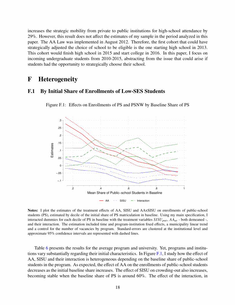
Figure F.1: Effects on Enrollments of PS and PSNW by Baseline Share of PS

−.1

−.05

0

.05

.1

.15

.2

.25

.3

Estim

ate

s

.2 .4 .6 .8 1

Mean Share of Public−school Students in Baseline

AA SISU Interaction

Notes: I plot the estimates of the treatment effects of AA, SISU and AAxSISU on enrollments of public-schoolstudents (PS), estimated by decile of the initial share of PS matriculation in baseline. Using my main specification, Iinteracted dummies for each decile of PS in baseline with the treatment variables (�(*?DC , ��DC - both demeaned -,and their interaction. The estimation included time and program-institution fixed effects, a municipality linear trendand a control for the number of vacancies by program. Standard-errors are clustered at the institutional level andapproximate 95% confidence intervals are represented with dashed lines.

Table 6 presents the results for the average program and university. Yet, programs and institu-tions vary substantially regarding their initial characteristics. In Figure F.1, I study how the effect ofAA, SISU and their interaction is heterogeneous depending on the baseline share of public-schoolstudents in the program. As expected, the effect of AA on the enrollments of public-school studentsdecreases as the initial baseline share increases. The effect of SISU on crowding-out also increases,becoming stable when the baseline share of PS is around 60%. The effect of the interaction, in

18

turn, is positive and stable across the initial distribution of PS. A similar pattern is observed forgroup PSNW and if the estimation is conducted by quartiles.

The fact that the treatment effect of AA and SISU vary substantially according to the baselineshare of PS is not surprising. The implementation of an AA in the form of quotas determinesan increase in the share of enrollments of public-school students mechanically. Despite that, ascommented in Section V.B, evidence suggests the existence of an additional behavioral response,which increases enrollments of PS students even in programs with originally more than 50% ofthis group. More important is the fact that programs with a lower share of public-school studentsin the baseline are also the most competitive and prestigious degrees in the country. This meansthat AA is changing remarkably the composition of programs previously not accessible to low-SESstudents and probably with higher future returns in the labor market.

As for SISU, it is also expected that its effect on crowding-out comes disproportionately fromprograms with a larger share of PS in the baseline. More precisely, the adoption of SISU seemsto have little effect in the first quartile and effects in the order of negative 3, 7 and 6 percentagepoints in the following quartiles of PS participation in the baseline. Again, this effect is partiallymechanical, since crowding-out can only occur where there exist public-school students in thefirst place. Yet, the pattern of the effect also reveals an unexpected behavioral response of localprivate-school students, as explained in Section V.A.

Finally, the interaction between SISU and AA is positive, significant and of relevant magnitudeacross all distribution of public-school student enrollment in the baseline. Thismeans that regardlessof the initial share of PS, the interaction of both policies creates an additional positive effect onenrollments that is not related to themechanical component that explains the heterogeneity observedfor AA or SISU.

F.2 PersistenceIn this section, I explore the persistence of the treatment effects. I extend the baseline equation (1)by adding two lagged treatment variables: (�(*?D,C−1, (�(*?D,C−2, ��?D,C−1, ��?D,C−2. Results areshown graphically in Figure F.2. The coefficients from variables (�(*?D,C and ��?D,C , measuredat time zero, are similar to the ones estimated using equation (1). The estimates from (�(*?D,C−1and (�(*?D,C−2 are, instead, close to zero. This means that, controlling for SISU adoption at time t,the SISU policy in the previous years does not have an effect beyond its contemporaneous changesin enrollments. This corroborates the analysis of the previous section. Behavioral changes to thecentralized system seem to occur promptly, in the same year of policy implementation.

In turn, the coefficients of ��?D,C−1 and ��?D,C−2 on enrollments are positive and significant,albeit small. For example, while the effect of ��?D,C on enrollments of public-school students is 10percentage points, the estimates for ��?D,C−1 and ��?D,C−2 are 2.1 and 2.4 percentage points. Thissuggests that part of students’ behavioral responses to AA does not occur immediately after policyimplementation. This is also in line with the findings discussed in section V.B. If AA inducesbehavioral responses that involve changing low-SES students’ aspirations, it is expected that part ofits effect would also occur with time. An interesting question is whether AA is capable of makingthese changes permanent.

19

Figure F.2: Persistence of the Treatment Effects

−.08

−.02

.04

.1

0 1 2

t = Time of Policy Implementation

Public−school Students

−.05

0

.05

.1

0 1 2

t = Time of Policy Implementation

Non−white Public−school

−.05

0

.05

0 1 2

t = Time of Policy Implementation

Low−income Public−school

−.05

0

.05

.1

0 1 2

t = Time of Policy Implementation

Out−of−State

SISU AA

Notes: I use the dataset from years 2012 to 2015 to test whether (�(*?D,C and ��D,C impact enrollments of publicschool, non-white public school, low-income public school and out-of-state students beyond the period t=0 in whichthe policies are implemented. In the graphs, I plot the estimated coefficients of (�(*?D,C and ��D,C , in time 0, andcoefficients of the additional terms (�(*?D,C−1, (�(*?DC−2, ��D,C−1 and ��D,C−2, in times 1 and 2, respectively. Theestimation included time and program-institution fixed effects, a municipality linear trend and a control for the numberof vacancies by program. Standard-errors are clustered at the institutional level and approximate 95% confidenceintervals are represented with dashed lines.

G Robustness

G.1 Spillovers and SUTVAThe existence of multiple institutions and programs treated simultaneously creates the possibilityof spillover effects that might bias the baseline results. Spillovers occur when the outcomes ofa certain unit of treatment are influenced not only by the changes observed in that specific unitbut also by changes in the treatment of other units. This would be a violation of the Stable UnitTreatment Value Assumption (SUTVA), which requires that the potential outcome of one unit isunaffected by the particular assignment of treatment on other units. In the case of large reforms,such as the ones analyzed in this paper, the potential for spillovers occurs in different dimensions.2

Since around 90 percent of students that attend public higher education in Brazil do it within-state, location is one of the most important determinants of college choice. Therefore, I firststudy the existence of spillovers at the local level and define variables (?8;;>E4A(�(*; ?DC =

2Note that, in this section, I focus on the study of spillovers within the public higher education market only. Resultsof section V.A suggest that SISU’s effects also spill over to the local private higher education market. Yet, privateinstitutions are not treated by AA or SISU. Therefore, this dimension of spillover effects is out of the scope of thispaper.

20

+020=284B(�(*;C−+020=284B(�(*; ?DC)>C0;+020=284B;C−)>C0;+020=284B; ?DC and (?8;;>E4A��; ?DC =

+020=284B��;C−+020=284B��; ?DC)>C0;+020=284B;C−)>C0;+020=284B; ?DC , where l is

the subscript for locality, defined either at the municipality or the state level. Then, I run thebaseline specification with these two additional measures of exposure. Table G.1 column (1) showsthat there are sizable local spillovers for AA. The full adoption of AA by other programs in thesame municipality of institution u decreases enrollments of PS at this institution by 6 percentagepoints. This means that, when controlling by this negative spillover, the estimate for the impact ofAA on institution u itself is higher than in the baseline specification. The impact of full adoptionof AA at institution u increases from 9.9 to 13.0 for PS in comparison to the specification withoutthe spillover measure. Therefore, the baseline estimates for AA may be downward biased and theestimates found in this section could be seen as an upper bound. In column (2), we do not observesimilar spillover effects when the locality is defined at the state level.

Table G.1 column (1) shows no evidence of local spillovers for SISU in the public highereducation market, while Table 7 shows that the centralized system increases enrollments of studentsfrom out of state. If in absence of treatment, the affected individuals would have attended anotherpublic higher education institution, this would consist of a violation of SUTVA and could biasthe estimated results. To minimize these concerns, I study the possibility of spillovers beyond thegeographic unit of the program.

I define a measure of national penetration of SISU and AA outside the geographic unit l of theprogram: #0C8>=0;(�(*;C = +020=284B(�(*C−+020=284B(�(*;C

)>C0;+020=284BC−)>C0;+020=284B;C and#0C8>=0;��;C =+020=284B��C−+020=284B��;C

)>C0;+020=284BC−)>C0;+020=284B;C .Column (3) shows that the national adoption of SISU, outside the municipality of program p, has apositive effect on enrollments of public-school students in program p before the adoption of SISU inp itself. This goes in line with the fact that SISU crowds out low-SES students in the municipalitieswhere it is adopted. As expected, the national adoption of AA has the opposite effect. Estimatesfor the national penetration of SISU and AA outside the state of program p are less precise, asshown in column (4). Importantly, columns (3) and (4) confirm that controlling for the nationalpenetration of SISU and AA outside the locality of program p (municipality or state) does notchange their causal impact on enrollments of public-school students. Panel B shows similar resultsfor public-school non-white students.

In conclusion, results from this section show that AA impacts enrollments in local educationmarkets, and controlling for these spillovers increases the magnitude of the causal effects of AA.Moreover, the national penetration of both SISU and AA outside the municipality of the programalso seems to affect enrollments of low-SES students in program p before it adopts either policy.This, in turn, does not appear to impact the magnitude of the direct effect of AA and SISU onenrollments of low-SES students. Therefore, although these spillover patterns are informative perse, the stability of the causal estimates of SISU and AA minimize our initial concerns regardingthe violation of SUTVA.

21

Table G.1: Effect of SISU and AA on Enrollments of Public-school and Public-schoolNon-White Students controlling for Spillovers on Public Higher Education Market

(1) (2) (3) (4)

Local NationalMunicipality State Out Munic. Out State

Panel A: Public-School Students

(�(*?DC -0.0315*** -0.0313*** -0.0260*** -0.0321***(0.0110) (0.0101) (0.00948) (0.00948)

��DC 0.130*** 0.0984*** 0.0903*** 0.0986***(0.0167) (0.0157) (0.0149) (0.0150)

(�(*?DCG��DC 0.0678*** 0.0683*** 0.0676*** 0.0669***(0.0190) (0.0195) (0.0187) (0.0194)

Spillover SISU -0.0151 -0.0355* 2.497*** 0.884(0.0111) (0.0201) (0.875) (0.536)

Spillover AA -0.0610*** -0.00829 -2.520* 0.0988(0.0162) (0.0250) (1.379) (0.425)

N 1991984 2021455 2021455 2021455

Panel B: Public-school Non-white Students

(�(*?DC -0.0244*** -0.0217** -0.0161** -0.0222***(0.00909) (0.00839) (0.00795) (0.00782)

��DC 0.0873*** 0.0646*** 0.0636*** 0.0655***(0.0129) (0.0121) (0.0117) (0.0118)

(�(*?DCG��DC 0.0484*** 0.0486*** 0.0471*** 0.0472***(0.0174) (0.0168) (0.0161) (0.0170)

Spillover SISU -0.0113 -0.0353* 2.699*** 0.945(0.0101) (0.0203) (0.899) (0.589)

Spillover AA -0.0317** 0.0252 -1.687 -0.496(0.0130) (0.0282) (1.270) (0.450)

N 1985963 2014838 2014838 2014838Notes: This table reports results of the effect of (�(*?D,C , ��D,C , and their interaction on enrollmentsof public-school and public-school non-white students, controlling for different measures of spillovereffects on the public higher education market. Treatment variables are demeaned. All columns in-clude time fixed-effects, program-institution fixed effects, program number of spots and a municipal-ity linear trend. Columns (1) and (2) include measures of local spillovers: (?8;;>E4A(�(*; ?DC =+ 020=284B(�(*;C−+ 020=284B(�(*;?DC

) >C0;+ 020=284B;C−) >C0;+ 020=284B;?DC and (?8;;>E4A��; ?DC =+ 020=284B��;C−+ 020=284B��;?DC

) >C0;+ 020=284B;C−) >C0;+ 020=284B;?DC . In col-umn (1), locality l defines the municipality and in (2) the state. Columns (3) and (4) include a mea-sure of national penetration outside the locality: #0C8>=0;(�(*;C = + 020=284B(�(*C−+ 020=284B(�(*;C

) >C0;+ 020=284BC−) >C0;+ 020=284B;C and#0C8>=0;��;C =

+ 020=284B��C−+ 020=284B��;C

) >C0;+ 020=284BC−) >C0;+ 020=284B;C ; column (3) outside the municipality, and (4) outside thestate. Standard errors in parenthesis are clustered at the university level.

22

G.2 Robustness of Out-of-state Students’ OutcomeAlthough results show that SISU increases enrollments of out-of-state students, Table 3 shows littleor no increase in the net proportion of this group. More precisely, this fraction decreases slightlyfrom 2010 (10.0%) to 2011 (9.2%) and then increases slightly again from 2011 to 2015 (10.2%).Treated programs represent a sizeable fraction of overall enrollments. On average, the adoption ofSISU increases from 19% in 2010 to 60% in 2015. The main estimates show that full adoptionof SISU increases enrollments of out-of-state students by, on average, 5 percentage points. Thiswould mean that, roughly, everything else constant, adoption of SISU would imply an increaseof 0.4x5=2p.p.on net enrollments of out-of-state students. Therefore, the stability in these overallshares shown in Table 3 can be rationalized by the existence of other time-varying factors thatdecrease enrollments of out-of-state students. If these factors are uncorrelated with SISU adoptionor could be controlled for in the empirical framework, they should not be an object of concern. If,however, these factors are correlated with SISU, they should be investigated with attention.

To better understand what factors could be behind the negative trend on enrollments of out-of-state students, I estimate the impact of SISU on this outcome in its simplest version, with only timeand program fixed effects, and then add, independently, different covariates. Results are shownin Table G.2. Column (1) shows that, in the simplest specification, the estimates for the yearfixed effects are negative and significant. Column (2) controls for state linear trends and column(3) for municipality linear trends. Now, the year fixed effects are close to zero in magnitude andinsignificant because they are absorbed by the linear trends, many of which are significant andpresent a negative coefficient (estimates of linear trends are not shown for the sake of simplicity).These linear trends control for possible time-varying shocks at the local level (e.g. economicshocks, cohort effects, local governmental policy). Despite the significant coefficients for the localtrends, their inclusion does not change the estimates of SISU. This means that, although negativelocal shocks could cause a decrease in enrollments of out-of-state students, they are uncorrelatedwith SISU. Column (4) includes the control for the number of vacancies by program, which is closeto zero. Columns (5) and (6) include the AA treatment, which also seems to have only a smallnegative effect on the enrollments of out-of-state students. Columns (7) and (8) include controlsfor local spillovers of SISU at the state and municipality levels, which are insignificant, showingthat adoption of SISU by other programs in the same geographic unit does not affect enrollmentsof out-of-state students at program p itself. Finally, in column (9), I include a control for thenational penetration of SISU outside the state of p. The magnitude of the coefficient is negativeand substantial.

This analysis suggests that two factors could be behind the overall stability of the net enrollmentsof out-of-state students, despite the substantial effect of SISU on increasing matriculation of thisgroup: (i) local negative time trends, which I control for in the empirical specification and,regardless, seem to be uncorrelated with SISU and AA and (ii) the national expansion of SISU,which attracts out-of-state students from programs before they join the centralized system.

This raises the question of whether controlling for the national penetration of SISU wouldimpact the causal estimates of the adoption of the centralized system in program p. To shed lighton this question, in Table G.3, I run the full baseline specification and include, additionally, themeasure for the national penetration of SISU (Columns 4 to 6). These estimates are sizeable andnegative, although not significant in column (4). Columns (2) and (5) include, additionally, fixedeffects for the student state of origin and columns (3) and (6) a state of origin linear trend. They

23

aim to control for characteristics of the students’ state of origin that affect migration decisions(e.g. local economic shock at the state of origin). Importantly, the variable for national SISUpenetration remains sizeable, negative and becomes statistically significant. Taken together, theseestimates suggest that the national adoption of SISU has a negative effect on the enrollments ofout-of-state students of program p before the adoption of SISU in program p itself. These resultsare in line with what Knight and Schiff (2021) find in their analysis of the Common Application inthe US. Importantly, though, is that even controlling for the national penetration and for the state oforigin’s fixed effects and trends, results for the causal effects of SISU on enrollments of out-of-statestudents remain positive, sizeable and significant, although slightly smaller in magnitude than inthe baseline estimates.

Finally, to confirm the robustness of the out-of-state student outcome, I also estimate the resultswith an alternative definition of the migration variable: using the place of birth instead of the placeof residence at the end of high school to define the origin of the student (Table G.3 Panel B). Thisminimizes concerns that students would move to their preferred college location to attend highschool, anticipating the migration effect. Using the alternative definition of migration, the averagenet enrollments of migrants increase from 14.2% in 2010 to 16.8% in 2015. Yet, results for thecausal effects of SISU remain virtually the same.

24

Table G.2: Robustness of Enrollments of Out-of-state Students

(1) (2) (3) (4) (5) (6) (7) (8) (9)

(�(*?DC 0.0565*** 0.0569*** 0.0535*** 0.0543*** 0.0542*** 0.0532*** 0.0523*** 0.0525*** 0.0495***(0.00681) (0.00654) (0.00713) (0.00711) (0.00714) (0.00671) (0.00735) (0.00739) (0.00649)

2011 -0.0102* -0.00561 -0.00551 -0.00566 -0.00594 -0.00643 -0.00570 -0.00539 0.00781(0.00561) (0.00409) (0.00408) (0.00408) (0.00405) (0.00400) (0.00423) (0.00418) (0.00718)

2012 -0.0101* -0.00219 -0.00227 -0.00238 -0.00351 -0.00398 -0.00222 -0.00208 -0.00829(0.00607) (0.00379) (0.00379) (0.00379) (0.00373) (0.00360) (0.00374) (0.00383) (0.00543)

2013 -0.0104 0.000939 0.000906 0.000750 0.000682 0.000123 0.00100 0.00104 -0.0116(0.00660) (0.00362) (0.00360) (0.00358) (0.00361) (0.00337) (0.00354) (0.00364) (0.00772)

2014 -0.0167*** -0.00208 -0.00192 -0.00197 -0.00183 -0.00202 -0.00195 -0.00194 0.00152(0.00621) (0.00183) (0.00181) (0.00180) (0.00184) (0.00180) (0.00183) (0.00184) (0.00242)

2015 -0.0179*** - - - - - - - -(0.00591)

(?>CB?DC 0.000110**(0.0000434)

��DC -0.0126** -0.00986(0.00609) (0.00670)

(�(*?DCG��DC -0.0113(0.0102)

Spillover SISU State 0.00726(0.0141)

Spillover SISU Mun 0.00193(0.00744)

National SISU -0.635*(0.357)

N 1873289 1873289 1873289 1873289 1873289 1873289 1873289 1846722 1873289

Time FE Yes Yes Yes Yes Yes Yes Yes Yes YesProgram-instit.FE Yes Yes Yes Yes Yes Yes Yes Yes YesState Trend YesMunicipality Trend Yes Yes Yes Yes Yes Yes Yes

Notes: This table reports results of different specifications of the effect of (�(*?D,C on enrollments of out-of-statestudents. Treatment variables are demeaned. All columns include year and program-institutions fixed-effects. Column(2) adds a state-specific linear trend. Columns (3) to (10) add municipality linear trends instead. Column (4)includes the program-level time-varying control for number of spots, column (5) the variable for AA treatment andcolumn (6) both AA and its interaction with SISU. Columns (7) and (8) include a variable of local spillover forSISU: (?8;;>E4A(�(*; ?DC =

+ 020=284B(�(*;C−+ 020=284B(�(*;?DC

) >C0;+ 020=284B;C−) >C0;+ 020=284B;?DC . Finally, column (9) includes a measure for nationalexposure to SISU: #0C8>=0;(�(*;C = + 020=284B(�(*C−+ 020=284B(�(*;C

) >C0;+ 020=284BC−) >C0;+ 020=284B;C . Subscripts l is the state in (7) and (9) and themunicipality in (8). Standard errors in parenthesis are clustered at the university level.

25

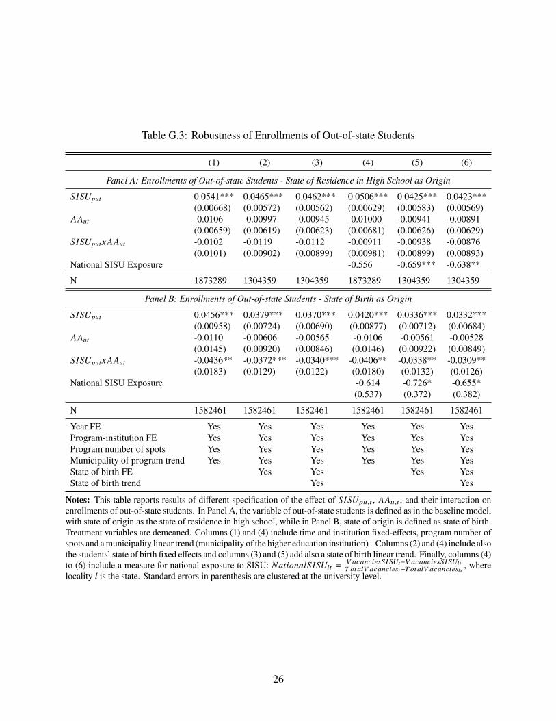
Table G.3: Robustness of Enrollments of Out-of-state Students

(1) (2) (3) (4) (5) (6)

Panel A: Enrollments of Out-of-state Students - State of Residence in High School as Origin

(�(*?DC 0.0541*** 0.0465*** 0.0462*** 0.0506*** 0.0425*** 0.0423***(0.00668) (0.00572) (0.00562) (0.00629) (0.00583) (0.00569)

��DC -0.0106 -0.00997 -0.00945 -0.01000 -0.00941 -0.00891(0.00659) (0.00619) (0.00623) (0.00681) (0.00626) (0.00629)

(�(*?DCG��DC -0.0102 -0.0119 -0.0112 -0.00911 -0.00938 -0.00876(0.0101) (0.00902) (0.00899) (0.00981) (0.00899) (0.00893)

National SISU Exposure -0.556 -0.659*** -0.638**

N 1873289 1304359 1304359 1873289 1304359 1304359

Panel B: Enrollments of Out-of-state Students - State of Birth as Origin

(�(*?DC 0.0456*** 0.0379*** 0.0370*** 0.0420*** 0.0336*** 0.0332***(0.00958) (0.00724) (0.00690) (0.00877) (0.00712) (0.00684)

��DC -0.0110 -0.00606 -0.00565 -0.0106 -0.00561 -0.00528(0.0145) (0.00920) (0.00846) (0.0146) (0.00922) (0.00849)

(�(*?DCG��DC -0.0436** -0.0372*** -0.0340*** -0.0406** -0.0338** -0.0309**(0.0183) (0.0129) (0.0122) (0.0180) (0.0132) (0.0126)

National SISU Exposure -0.614 -0.726* -0.655*(0.537) (0.372) (0.382)

N 1582461 1582461 1582461 1582461 1582461 1582461

Year FE Yes Yes Yes Yes Yes YesProgram-institution FE Yes Yes Yes Yes Yes YesProgram number of spots Yes Yes Yes Yes Yes YesMunicipality of program trend Yes Yes Yes Yes Yes YesState of birth FE Yes Yes Yes YesState of birth trend Yes Yes

Notes: This table reports results of different specification of the effect of (�(*?D,C , ��D,C , and their interaction onenrollments of out-of-state students. In Panel A, the variable of out-of-state students is defined as in the baseline model,with state of origin as the state of residence in high school, while in Panel B, state of origin is defined as state of birth.Treatment variables are demeaned. Columns (1) and (4) include time and institution fixed-effects, program number ofspots and amunicipality linear trend (municipality of the higher education institution) . Columns (2) and (4) include alsothe students’ state of birth fixed effects and columns (3) and (5) add also a state of birth linear trend. Finally, columns (4)to (6) include a measure for national exposure to SISU: #0C8>=0;(�(*;C = + 020=284B(�(*C−+ 020=284B(�(*;C

) >C0;+ 020=284BC−) >C0;+ 020=284B;C , wherelocality l is the state. Standard errors in parenthesis are clustered at the university level.

26

H Additional Figures and Tables

Table H.1: Correlation Between Treatment Jump and Baseline Covariates

Panel A: Regressions of Covariates on AA and SISU Treatment Jumps

�D<?��D,2010 �D<?(�(*

?D,2010

Coefficient Std. Error Coefficient Std. Error

Public School -0.08 0.045 -0.034 0.042Non-white PS -0.04 0.042 0.012 0.037Low Income PS -0.02 0.017 0.014 0.015Out-of-state 0.03 0.022 -0.032 0.017Grade Objective 0.15 0.150 -0.198 0.143Non-white -0.01 0.059 0.096 0.051Low Income -0.02 0.019 0.024 0.017Gender -0.02 0.015 0.010 0.011Age -0.03 0.305 -0.062 0.276Disability 0.00 0.002 0.001 0.002Spots 4.30 3.667 3.133 3.762

Panel B: Distribution of 2010-2015 Jump in Treatment

Min 0.00 0.00p(25) 0.00 0.00p(50) 0.36 0.27p(75) 0.82 1.00Max 1.00 1.00Mean 0.43 0.42Std. Dev. 0.41 0.43

N programs 4,988 4,988N institutions 134 134

Notes: To produce this table, I first compute variables �D<?��D,2010 = ��D,2015−��D,2010 and �D<?(�(*?D,2010 =

(�(*?D,2015 − (�(*?D,2010. Then, in Panel A, in each line, I show the results of a simple regression ofa covariate in year 2010 on the jump variable. For example, I run, separately, regressions: %(?D,2010 =

V + V1�D<?��D,2010 + Y?D,2010 and %(?D,2010 = U + U1�D<?

(�(*?D,2010 + Y?D,2010 and obtain V1 = −0.08 and

U1 = −0.034. I progress similarly with all the other covariates in Panel A. In Panel B, I present descriptivestatistics of �D<?��

D,2010 and �D<?(�(*?D,2010. Standard errors are clustered at the university level.

27

Table H.2: Robustness of Placebo Experiment

PS PSNW PSLI Out-of-state

Panel A: UF Linear Trend

(�(*?D,C -0.0393*** -0.0264*** -0.0403*** 0.0556***(0.0120) (0.00963) (0.00719) (0.00693)

(�(*?D,C+1 -0.00191 -0.00130 -0.00959 0.00279(0.0101) (0.00691) (0.00619) (0.00816)

��D,C 0.0794*** 0.0647*** 0.0249*** -0.00346(0.0170) (0.0135) (0.00725) (0.00770)

��D,C+1 -0.00875 -0.0243*** -0.0173*** -0.0118(0.0132) (0.00895) (0.00501) (0.00849)

(�(*?D,CG��D,C 0.0476 0.0337 0.00951 -0.0207*(0.0306) (0.0218) (0.0114) (0.0109)

Panel B: No Linear Trend

(�(*?D,C -0.0396*** -0.0236*** -0.0351*** 0.0523***(0.0124) (0.00880) (0.00622) (0.00694)

(�(*?D,C+1 -0.00854 0.00313 0.000162 0.00236(0.0113) (0.00862) (0.00616) (0.00893)

��D,C 0.0832*** 0.0740*** 0.0203** 0.00280(0.0189) (0.0146) (0.00873) (0.00901)

��D,C+1 -0.00602 -0.0163 -0.0105* -0.0115(0.0138) (0.0101) (0.00588) (0.00789)

(�(*?D,CG��D,C 0.0518* 0.0381 0.0262* -0.0258**(0.0306) (0.0246) (0.0134) (0.0110)

N 1585361 1580230 1494373 1473111Notes: This table reports results of a placebo experiment in which I use data from 2010 to 2014 to test trends of onepre-period for the main outcomes: enrollments of public-school (PS), non-white public-school (PSNW), low-incomepublic-school (PSLI) and out-of-state students. I plot the estimated coefficients of (�(*?D,C and ��D,C , in time 0, andcoefficients of the additional terms (�(*?D,C+1 and ��D,C+1, in time -1. Note that I use data from 2010 to 2014 to testwhether the adoption of SISU and AA in periods 2011 to 2015 were correlated to changes in the outcomes observedone period before implementation. The lack of data from years before 2010 prevents the extension of the analysis tofurther pre-periods. Results in both panels include controls for time and program-institution fixed effects and programnumber of spots. Panel A includes a state-linear trend, whereas Panel B does not include trends. Standard errors inparenthesis are clustered at the university level.

28

Table H.3: Different Specifications of Results for PSNW and PSLI

(1) (2) (3) (4) (5) (6)

Panel A: Public-school Non-white Students

(�(*?D,C -0.0191** -0.0207** -0.0210** -0.0250*** -0.0284*** -0.0323***(0.00897) (0.00940) (0.00939) (0.00878) (0.00903) (0.00908)

��D,C 0.0649*** 0.0690*** 0.0690*** 0.0575*** 0.0695*** 0.0686***(0.0119) (0.0124) (0.0124) (0.0112) (0.0131) (0.0127)

(�(*?D,CG��D,C 0.0483** 0.0434** 0.0437** 0.0391** 0.0493*** 0.0481***(0.0213) (0.0218) (0.0218) (0.0183) (0.0176) (0.0173)

N 2014838 2014838 2014838 2014838 2014838 2014838

Panel B: Public-school Low-income Students

(�(*?D,C -0.0344*** -0.0347*** -0.0350*** -0.0438*** -0.0413*** -0.0398***(0.00636) (0.00606) (0.00604) (0.00612) (0.00662) (0.00645)

��D,C 0.0137 0.0147* 0.0147* 0.0146** 0.0240*** 0.0239***(0.00877) (0.00853) (0.00854) (0.00611) (0.00601) (0.00598)

(�(*?D,CG��D,C 0.0349** 0.0318** 0.0321** 0.0150 0.0193* 0.0195*(0.0144) (0.0129) (0.0129) (0.00994) (0.0101) (0.0101)

N 1905968 1905968 1905968 1905968 1905968 1905968

Time FE Yes Yes Yes Yes Yes YesInstitution FE Yes Yes Yes Yes Yes YesProgram-Institution FE Yes Yes Yes Yes YesProgram Spots Yes Yes Yes YesState Linear Trend YesMunicipality Linear Trends Yes YesGender, age and disability Yes

Notes: This table reports results of different specification of the effect of (�(*?D,C , ��D,C and their interactionon enrollments of public-school non-white (PSNW) and public-school low-income (PSLI) students (Equation (??)).Treatment variables are demeaned. Column (1) includes only time and institution fixed-effects. Column (2) addsprogram-institution fixed effects. Column (3) includes a program time-varying control on number of vacancies offeredby major-institution. Column (4) adds a time-varying local linear trend at the state level and column (5) at themunicipality level. Finally, column (6) includes additionally individual-level time-varying controls. Standard errors inparenthesis are clustered at university level.

29

Table H.4: Robustness - Different Samples of Institutions

PS PSNW PSLI Out-of-State Grades

Panel A: Federal and State Universities

(�(*?DC -0.0335*** -0.0269*** -0.0393*** 0.0534*** 0.300***(0.0115) (0.0102) (0.00715) (0.00746) (0.0342)

��DC 0.110*** 0.0815*** 0.0248*** -0.0106 -0.0708***(0.0190) (0.0159) (0.00609) (0.00796) (0.0253)

(�(*?DCG��DC 0.0785*** 0.0579*** 0.00677 -0.00819 -0.000273(0.0223) (0.0194) (0.0115) (0.0114) (0.0404)

N 1811266 1805614 1715665 1684964 1626165

Panel B: Only Federal Institutions

(�(*?DC -0.0393*** -0.0330*** -0.0359*** 0.0487*** 0.299***(0.00990) (0.00906) (0.00657) (0.00713) (0.0322)

��DC 0.0885*** 0.0684*** 0.0165** -0.00636 -0.0291(0.0143) (0.0170) (0.00754) (0.00925) (0.0338)

(�(*?DCG��DC 0.0657*** 0.0433** 0.0255** -0.0176 -0.0804*(0.0187) (0.0201) (0.0116) (0.0116) (0.0417)

N 1478086 1477637 1423800 1410850 1377128

Panel C: Only Federal Universities

(�(*?DC -0.0368*** -0.0342*** -0.0320*** 0.0463*** 0.266***(0.0114) (0.0105) (0.00724) (0.00832) (0.0356)

��DC 0.0935*** 0.0825*** 0.0203** -0.00651 -0.0597*(0.0196) (0.0235) (0.00849) (0.0126) (0.0350)

(�(*?DCG��DC 0.0719*** 0.0465* 0.0153 -0.0176 -0.0523(0.0221) (0.0246) (0.0135) (0.0136) (0.0451)

N 1267897 1268413 1233497 1222525 1195605Notes: This table reports results of the effect of (�(*?D,C , ��D,C , and their interaction on enrollments of public-school(PS), non-white public-school (PSNW), low-income public-school (PSLI) and out-of-state students, as well as onaverage grades of enrolled students in the ENEM exam (in standard deviations), for different samples of institutions.Panel A includes Federal and State Universities, Panel B Federal Universities and Institutes, Panel C Federal Universitiesonly, while baseline estimates contain all three types of institutions. Treatment variables are demeaned. All columnsinclude time fixed-effects, program-institution fixed effects, program number of spots and a municipality linear trend.Standard errors in parenthesis are clustered at the university level.

30

Table H.5: Robustness - Different Sample Selections

PS PSNW PSLI Out-of-State Grades

Panel A: No first-year drop-outs

(�(*?DC -0.0349*** -0.0272*** -0.0395*** 0.0493*** 0.302***(0.0107) (0.00925) (0.00672) (0.00611) (0.0301)

��DC 0.104*** 0.0716*** 0.0254*** -0.0108* -0.0644***(0.0157) (0.0138) (0.00601) (0.00608) (0.0243)

(�(*?DCG��DC 0.0656*** 0.0490*** 0.0211** -0.00774 -0.0439(0.0206) (0.0187) (0.0105) (0.00914) (0.0366)

N 1759779 1753761 1656371 1627609 1568136

Panel B: Programs of at least 10 students

(�(*?DC -0.0377*** -0.0285*** -0.0413*** 0.0538*** 0.319***(0.0103) (0.00900) (0.00662) (0.00667) (0.0316)

��DC 0.0988*** 0.0697*** 0.0240*** -0.0104 -0.0540**(0.0152) (0.0131) (0.00602) (0.00659) (0.0253)

(�(*?DCG��DC 0.0682*** 0.0488*** 0.0192* -0.0105 -0.0446(0.0199) (0.0177) (0.0101) (0.0101) (0.0369)

N 2017909 2011235 1902948 1870622 1805246

Panel C: Drop 2010 and 2011

(�(*?DC -0.0528*** -0.0406*** -0.0513*** 0.0505*** 0.367***(0.00811) (0.00758) (0.00665) (0.00787) (0.0257)

��DC 0.0900*** 0.0616*** 0.0207*** -0.0127* -0.0234(0.0153) (0.0108) (0.00619) (0.00647) (0.0215)

(�(*?DCG��DC 0.0930*** 0.0570*** 0.0238** -0.00388 0.000135(0.0211) (0.0151) (0.0108) (0.0130) (0.0393)

N 1458108 1438380 1379693 1326417 1298652Notes: This table reports results of the effect of (�(*?D,C , ��D,C , and their interaction on enrollments of public-school(PS), non-white public-school (PSNW), low-income public-school (PSLI) and out-of-state students, as well as onaverage grades of enrolled students in the ENEM exam (in standard deviations), for different samples of the universe.In Panel A, I delete all first-year dropouts; in Panel B, I keep only programs larger than 9 students and in Panel C, I keeponly years 2012-2015. Treatment variables are demeaned. All columns include time fixed-effects, program-institutionfixed effects, program number of spots and a municipality linear trend. Standard errors in parenthesis are clustered atthe university level.

31

Table H.6: Robustness - Different Sample Selections

PS PSNW PSLI Out-of-State Grades

Panel A: Only Institutions with ENEM since Baseline

(�(*?DC -0.0327*** -0.0293*** -0.0353*** 0.0360*** 0.265***(0.0112) (0.0105) (0.00740) (0.00971) (0.0372)

��DC 0.0616*** 0.0589*** 0.0191** -0.0120 -0.0346(0.0159) (0.0141) (0.00890) (0.0111) (0.0432)

(�(*?DCG��DC 0.0750*** 0.0456** 0.0162 0.00117 0.00590(0.0200) (0.0178) (0.0151) (0.0173) (0.0500)

N 958991 954157 925763 923015 905920

Panel B: Drop Institutions with AA Bonus

(�(*?DC -0.0384*** -0.0270** -0.0462*** 0.0569*** 0.319***(0.0128) (0.0107) (0.00790) (0.00773) (0.0394)

��DC 0.113*** 0.0740*** 0.0249*** -0.00827 -0.0465(0.0159) (0.0145) (0.00683) (0.00751) (0.0302)

(�(*?DCG��DC 0.0702*** 0.0448** 0.0207* -0.0144 -0.0595(0.0222) (0.0202) (0.0108) (0.0112) (0.0476)

N 1708739 1700347 1602402 1574197 1516925

Panel C: Drop Institutions with AA with Racial Criteria Only

(�(*?DC -0.0385*** -0.0298*** -0.0426*** 0.0530*** 0.315***(0.0102) (0.00910) (0.00664) (0.00672) (0.0324)

��DC 0.100*** 0.0723*** 0.0271*** -0.00854 -0.0513*(0.0159) (0.0138) (0.00628) (0.00713) (0.0267)

(�(*?DCG��DC 0.0702*** 0.0484*** 0.0169* -0.0142 -0.0523(0.0197) (0.0177) (0.0101) (0.0103) (0.0379)

N 1806990 1801368 1711205 1689165 1633194Notes: This table reports results of the effect of (�(*?D,C , ��D,C , and their interaction on enrollments of public-school(PS), non-white public-school (PSNW), low-income public-school (PSLI) and out-of-state students, as well as onaverage grades of enrolled students in the ENEM exam (in standard deviations), for different samples of the universe.In Panel A, I keep only institutions that accept the ENEM exam as an admission mechanism since 2010; in Panel B,I drop institutions which had AA policies in form of bonus points instead of quotas before the national AA policyadoption in 2013; in Panel C, I drop institutions which had AA with a racial criterion only (without the public-schoolstudent criterion) before 2013. Treatment variables are demeaned. All columns include time fixed-effects, program-institution fixed effects, program number of spots and a municipality linear trend. Standard errors in parenthesis areclustered at the university level.

32

Table H.7: Robustness - Exploring Variation at the Institutional Level

PS PSNW PSLI Out-of-State Grades

(�(*?DC -0.0410*** -0.0306** -0.0487*** 0.0533*** 0.329***(0.0147) (0.0125) (0.00834) (0.00822) (0.0361)

��DC 0.0902*** 0.0635*** 0.0210*** -0.0110* -0.0475(0.0163) (0.0142) (0.00658) (0.00635) (0.0340)

(�(*?DCG��DC 0.101*** 0.0658*** 0.0271** -0.0117 -0.104**(0.0262) (0.0231) (0.0112) (0.0117) (0.0481)

N 2054025 2048093 1932267 1896255 1829037Notes: This table reports results of the effect of (�(*?D,C , ��D,C , and their interaction on enrollments of public-school(PS), non-white public-school (PSNW), low-income public-school (PSLI) and out-of-state students, as well as onaverage grades of enrolled students in the ENEM exam (in standard deviations). Here, the SISU treatment is collapsedat the level of the institution, instead of included at the program level, as in the baseline estimate. Moreover, I includeinstitution fixed effects instead of program fixed effects. Treatment variables are demeaned. All columns includeadditionally time fixed-effects, program number of spots and a municipality linear trend. Standard errors in parenthesisare clustered at the university level.

33