on the relevance of using artificial neural networks for estimating soil moisture content

Journal of Hydrology (2008) 362, 1–18

ava i lab le a t www.sc iencedi rec t . com

journal homepage: www.elsevier .com/ locate / jhydrol

On the relevance of using artificial neural networksfor estimating soil moisture content

Amin Elshorbagy *, K. Parasuraman

Centre for Advanced Numerical Simulation (CANSIM), Department of Civil and Geological Engineering,University of Saskatchewan, 57 Campus Drive, Saskatoon, SK, Canada S7N 5A9

Received 6 March 2008; received in revised form 1 August 2008; accepted 11 August 2008

00do

*

KEYWORDSSoil moisture content;Higher-order neuralnetworks;Modeling;Reconstructedwatersheds;Conceptual models

22-1694/$ - see front mattei:10.1016/j.jhydrol.2008.08

Corresponding author. TelE-mail address: amin.elsho

r ª 200.012

.: +1 306rbagy@u

Summary Soil moisture is a key variable that defines the land surface-atmosphere(boundary layer) interactions, by contributing directly to the surface energy balanceand water balance. This paper investigates the utility of the widely adopted data-drivenmodel, namely artificial neural networks (ANNs), for modeling the complex soil moisturedynamics. Datasets from three experimental soil covers (D1, D2, and D3), with thicknessof 0.50 m, 0.35 m, and 1.0 m, comprising a thin layer of peat mineral mix over varyingthickness of till, are considered in this study. Volumetric soil moisture contents at boththe peat and the till layers were modeled as a function of precipitation, air temperature,net radiation, and ground temperature at different layers. Initial simulations illustratedthat, in the absence of time-lagged meteorological variables, the ground temperatureis the most influential state variable for characterizing the soil moisture, highlightingthe strong link between the soil thermal properties and the corresponding moisture status.With the objective of extracting the maximum information from the most influential statevariables (ground temperature), a higher-order neural networks (HONNs) model wasdeveloped to characterize the soil moisture dynamics. The HONNs resulted in relativelyhigher correlation coefficient, than traditional ANNs, for some of the soil moisture simu-lations. Time-lagged inputs were used to improve the model performance and obtain opti-mum results. The ANN models performed better than a previously developed conceptualmodel for estimating the depth-averaged soil moisture content. Results from the studyindicate that modeling of soil moisture using ANNs is challenging but achievable, and itsperformance is largely influenced by the structure and formation of the soil covers, whichin turn governs the dynamics of soil moisture variability.ª 2008 Elsevier B.V. All rights reserved.

8 Elsevier B.V. All rights reserved.

9665414; fax: +1 306 9665427.sask.ca (A. Elshorbagy).

mailto:[email protected]

2 A. Elshorbagy, K. Parasuraman

Introduction

Soil moisture content is a major control on several hydrolog-ical processes. Soil moisture determines the partitioning ofavailable energy between latent and sensible heat (Entek-habi et al., 1996), and the magnitude of net radiation ab-sorbed by the surface (Eltahir, 1998). Kuczera (1983) andWooldridge (2003) have demonstrated that inclusion of soilmoisture data in hydrological modeling can yield substantialreductions in the uncertainty of model parameters. Also,accounting for soil water content on catchement scaleshave proven beneficial for flow prediction (Kitanidis andBras, 1980; Georgakakos and Smith, 1990; Wooldridge etal., 2003), and weather and climate studies (Georgakakosand Bae, 1994; Georgakakos et al., 1995). As these studiesclearly highlight the role of soil moisture in hydrologicalmodeling, the importance of understanding the dynamicsof soil moisture cannot be over-emphasized.

Conventionally, field soil moisture estimates can be ob-tained by the gravimetric method or by the Time DomainReflectometers (TDR). Although the field estimates of soilmoisture are reasonably reliable, the problems (labor inten-sive, time consuming, expensive) associated with directmeasurement of soil moisture, make these techniques quiteimpractical to characterize soil moisture patterns over anarea. Also, heterogeneity in topography, soil properties, cli-mate patterns, vegetation, and boundary conditions instilllarge amount of nonlinearity to the dynamics of soil mois-ture movement and distribution. Over the past decade,advancement in computer power and technology has mademeasurement of spatial distribution of soil moisture feasibleusing remote sensing techniques. However, soil moisturemeasured using these techniques may suffer from poor tem-poral resolution, and is representative of soil moisture con-tent of the top few centimeters. Fully distributed,continuous water balance models have also been used toestimate soil moisture patterns (e.g. Wood et al., 1992;Grayson et al., 1995). The accuracy of soil moisture esti-mated by these models depends on the model physics andthe number and configuration of soil layers, as well as theaccuracy, and the temporal and spatial nature of the inputdata. As evident from the large number of publications,coupled modeling-remote sensing techniques (e.g. Graysonet al., 1995; Makkeasorn et al., 2006) is the most widelyadopted procedure for characterizing soil moisture. Entek-habi et al. (1994) showed that the ability of such modelsto predict soil moisture averages over larger depths is se-verely limited by the noise introduced by micro-topographyand roughness of vegetation cover. Since most of the meth-ods have some limitations with regard to their ability incharacterizing the soil moisture dynamics, there is clearlyno single technique that can be adopted to estimate soilmoisture in an operational mode (Entekhabi, 1996).

In light of the problems associated with the measure-ment and modeling of soil moisture using the above tech-niques, this study investigates the utility of the mostwidely adopted data-driven model, namely the artificialneural networks (ANNs), for estimating soil moisture.Although a plethora of studies have been carried out inthe past to evaluate the efficacy of ANNs in hydrologicalmodeling, for example, rainfall–runoff modeling (Hsu

et al. 1995; Shamseldin 1997; Dawson and Wilby, 1998;Zhang and Govindaraju, 2000), streamflow forecasting (Kar-unanithi et al. 1994; Thirumalaiah et al. 1998), and rainfallforecasting (French et al. 1992; Zhang et al. 1997), the util-ity of ANNs in modeling soil moisture has rarely been re-ported in the literature. For modeling the rainfall–runoffrelationship using ANNs, Dawson and Wilby (1998) usedantecedent precipitation index based on earlier rainfall withthe objective of approximating the soil moisture fluctua-tions. In modeling the runoff in a humid forest catchmentusing ANNs, Gautam et al. (2000) showed that soil moisturedata obtained from 40 cm depth carry the integrated effectof the upstream catchment area, and are important for esti-mating stream discharge. These studies verify the impor-tance of accounting for soil moisture in ANN modeling ofhydrological processes. Since soil moisture has been shownto be an important variable in conceptual (e.g. Kitanidisand Bras, 1980; Georgakakos and Smith, 1990) and data-dri-ven (e.g. Dawson and Wilby, 1998; Gautam et al. 2000) mod-eling of geophysical processes, the results from this studywould be of interest to the hydrological community in gaug-ing the utility of ANNs in characterizing the most complexand the most important hydrological variable, namely, soilmoisture.

As neural networks belong to the category of data-drivenmodels, proper input selection is a crucial step in any ANNimplementation. The lack of pertinent inputs or the pres-ence of redundant inputs in neural network modeling se-verely impairs the ability of the network to learn thetarget patterns. Several methods have been proposed inthe literature to identify the effective inputs for neural net-work modeling, and a comprehensive treatise on this issuecan be found in Bowden et al. (2005). The problem of iden-tifying the effective inputs in neural network modeling is ill-posed if the pertinent variables for modeling a particularprocess are either not measured, or measured at differentspatial and temporal scales. Hence, neural network model-ers are often faced with the task of extracting the maximuminformation from the available (measured) independentvariables. Kim and Valdes (2003), and Anctil and Tape(2004) used wavelet decomposed signals of the independentvariables as inputs to neural network models, with the ideaof providing the neural networks with information at differ-ent frequencies. Bowden et al. (2006) used principal compo-nents analysis (PCA) to reduce the dimensionality of theinput dataset and to remove the collinearity present be-tween the independent variables. Modular neural networkswere also proposed with the aim of developing domaindependent input–output relationships (e.g. Zhang andGovindaraju, 2000; Parasuraman et al., 2006; Parasuramanand Elshorbagy, 2007). While the above discussed methodsare promising, they are not straight-forward to implement.This study investigates the ability of higher-order neuralnetworks (HONNs) (Gupta et al., 2003) to extract maximuminformation (judged by improved prediction accuracy) fromthe input data. The HONNs, in contrast to the widelyadopted first-order neural networks (FONNs), has the abilityto exploit self- and cross-correlation existing among inputs.The nonlinear and higher-order properties, if any, in the in-put space cannot be captured by the FONNs, as they employonly the linear correlation between the input vector and the

On the relevance of using artificial neural networks for estimating soil moisture content 3

weight vector. For the same problem, the HONNs usehigher-order correlations to learn the higher-order proper-ties in the input space. In general, the objectives of thisstudy can be stated as: (i) identifying the additional gains,if any, of considering HONNs for modeling soil moisture con-tents; (ii) evaluating the ability of neural networks in mod-eling and characterizing the depth-averaged soil moisturevalues of reconstructed watersheds (soil covers).

Study area and field data

Large scale mining in the Athabasca basin, Alberta, Canada,involves stripping of large amount of organic and glacialdeposits and a layer of saline/sodic cretaceous shale to gainaccess to the oil sands. Approximately 120,000 m3 of shaleoverburden is removed daily and is placed in storage areasthat will eventually cover a combined area of about80 km2 (Boese, 2003). Prior to mining, the shale overburdenis stable since it is over consolidated, confined, and is ex-posed only to saline/sodic pore fluids. However, once theshale is placed on the surface, it is exposed to fresh waterand oxygen and is susceptible to weathering, which in thelong run affects the stability of the pile (Barbour et al.,2001). In order to overcome this problem, the piles are re-contoured and capped with sufficient soil cover so thatthe amount of precipitation percolating below the root zonecan be minimized while maintaining enough moisture forvegetation. In this way, the overburden can be restored toits natural state by supporting vegetation. Over the years,several large scale soil cover (reconstructed watersheds)experiments are being conducted to assess the performanceof different reclamation strategies by studying the basicmechanisms that control the moisture movement withinthese covers. In particular, three experimental soil covers(D1, D2, and D3) were established in the year 1999. Theexperimental covers were constructed over the saline-sodicoverburden with thickness of 0.50 m, 0.35 m, and 1.0 m,comprising a thin layer of peat mineral mix over varyingthickness of secondary (glacial/till) soil. The layout of thesoil covers are shown in Fig. 1. Cover D1 consists of 20 cmof peat overlying 30 cm of till; cover D2 consists of 15 cmof peat overlying 20 cm of till, and cover D3 consists of20 cm of peat overlying 80 cm of till (Fig. 1).

The three soil covers are contoured in such a way thatthese soil covers can be considered as individual sub-water-sheds. Each of the sub-watersheds has an area of 1 ha(approximately 200 m long and 50 m wide), with a 5:1 slope(5 horizontal to 1 vertical). These reconstructed watersheds,compared to the natural watersheds, are not stable duringtheir initial stages, and hence evolve over time to achieve hy-dro-sustainability. In order to track the evolution (hydrolog-ical changes) of the watersheds, intensive instrumentationswere installed in these watersheds. Each watershed has anindividual soil station located at the middle of the slope,which measures the volumetric soil moisture content of thepeat (SMp) and the till (SMt) layers, twice a day. Soil moistureis measured using TDR principles with model CS615(Boese, 2003). The TDR sensors were installed laterallyinto the soil profile. Watershed D1 has eight TDR sensorsinstalled over a depth range of 0.05–1.00 m. Similarly, sevenTDR sensors were installed in watershed D2 over a depth

range of 0.05–0.80 m, and nine TDR sensors forwatershed D3 installed over a depth range of 0.05–1.70 m.Hourly values of soil temperature of peat (STp) and till (STt)layers are measured using thermisters buried in each of thewatersheds at the depth ranges corresponding to the TDRsensors in each watersheds. Consequently, D1, D2, and D3have eight, seven, and nine soil temperature sensors, respec-tively. A weather station located in the mid-slope of D2 mea-sures air temperature (AT), and precipitation (P). Similarly,Bowen station located at the mid-slope of D2 measures netradiation (NR) and energy fluxes. All the meteorological vari-ables are measured in an hourly scale. More details on thefield instrumentation program and the data collected canbe found in Boese (2003) and Elshorbagy et al. (2007).

Average daily values of precipitation, air temperature,soil temperature (STp and STt), net radiation (NR), and soilmoisture (SMp and SMt) are considered for simulation pur-poses. The ground temperature and soil moisture contentsare depth-averaged. As the soil stratum is frozen duringthe winter, only summer (May–September) time data areconsidered. Neglecting the year 1999, when the datasetwas incomplete, soil moisture data between 2000 and2005 are considered. As the reconstructed watershedsevolve over time to achieve hydro-sustainability, thefreeze–thaw cycles and decomposition of highly organicpeat layer increases the porosity of the soil and conse-quently increasing infiltration rates (Haigh, 2000). Hence,modeling the moisture dynamics of such evolving water-sheds would be adding to the already challenging task ofmodeling soil moisture. The following section, in brief, out-lines the ANN models adopted in this study.

Neural networks

Since a plethora of information on ANNs is available in theliterature (e.g. Haykin, 1999; ASCE Task Committee onApplication of Artificial Neural Networks in Hydrology,2000), the description of ANNs herein is brief, and limitedto the needs of this study. A three layered feed-forwardneural networks (FFNNs) model is conventionally adoptedin modeling hydrological processes. The three layeredFFNNs consist of ‘j’ input neurons, ‘k’ hidden neurons,and ‘l’ output neurons. These neurons are connected witheach other by means of connection weights and bias. Thehidden layer neurons usually employ sigmoidal activationfunction and the output layer neurons use linear activationfunction. These activation functions help in nonlinearlytransforming the inputs to the desired output. Symbolically,the three layered FFNNs can be represented as ANN(j,k, l).The development of a neural network model demands twooperations, namely, (i) training and (ii) testing. Training isa process by which the connection weights between differ-ent layers and the bias values of the neural networks areoptimized by minimizing the cost function. Once trained,the neural network model can be tested on an independentdataset that has not been used during the training process.

In ANN modeling of hydrological processes, the signifi-cant input variables for characterizing a particular processis usually determined by linear cross-correlation (Bowdenet al., 2005). Linear cross-correlation can only detect lineardependence between two variables, and is not suited for

Figure 1 Layout of soil covers (sub-watersheds), all axes units in meters.


capturing the nonlinear dependence between the inputs andthe output. Moreover for most hydrological processes, sig-nificant linear and higher-order correlations may exist be-tween the independent and the dependent variables.Nevertheless, the FONNs, which are the most widelyadopted neural network architecture for modeling hydrolog-ical process, do not have the ability to capture the higher-order correlations, as they employ only linear correlationbetween the input vector and the weight vector. In this re-gard, the robustness of the higher-order neural networks(HONNs), which can extract the higher-order correlationsbetween the components of the input patterns, is evalu-ated. Taylor and Commbes (1993) showed that the HONNshave good computational, storage, pattern recognition,and learning properties due to their ability to exploit thecross and self correlations between the inputs. This studyadopted the HONNs based on Gupta et al. (2003). The high-er-order neural units (HONUs) are the basic building blocksfor such a higher-order neural network. The HONUs containall the linear and nonlinear correlation terms of the inputcomponents to the order of N. A generalized structure ofthe HONU is a polynomial network that includes theweighted sums of products of selected input componentswith an appropriate power Fig. 2 shows the HONNs adoptedin this study, which is adopted from Gupta et al. (2003),where x1,x2, . . . ,xn, are the inputs, y is the correspondingoutput, and u(Æ) is a monotonic activation function. Consid-ering a first-order network (N = 1), the linear synaptic oper-ation (LSO) is given by Eq. (1)

z ¼Xni¼0

wixi ð1Þ

For N = 2, the quadratic synaptic operation (QSO) is given by(Redlapalli, 2004)

z ¼Xni¼0

Xnj¼i

wijxixj ð2Þ

Similarly for N = 3, the cubic synaptic operation (CSO) forthe neural unit can be written as

z ¼Xni¼0

Xnj¼i

Xnl¼j

wijlxixjxl ð3Þ

Accordingly, a general form for the Nth order neural unitscan be written as follows (Gupta et al., 2003):

z ¼ aþXni1

wi1xi1 þXni1;i2

wi1i2xi1xi2 þ � � �

þXni1;...;iN

wi1;...;iNxi1; . . . ; xiN ð4Þ

Typically, only second-order (N = 2) networks are usuallyemployed in practice to give a tolerable number of weights(Gupta et al., 2003). Hence, this study adopted the second-order networks. Considering x1 and x2 as the input variablesfor characterizing a process, a second-order network can beconstructed by using both the actual inputs (x1 and x2), andthe derived variables ðx21; x1x2; x22Þ required for the second-order polynomial, as inputs to the higher-order neural unit.In this way, the self and cross-correlations existing betweenthe input variables can be accounted for in ANN modeling.Symbolically, the output from the second-order neural unit(e.g. the case of two inputs) can be given by Eq. (5). Moreinformation on HONNs can be found in Gupta et al. (2003).

z ¼ aþ w1x1 þ w11x1x1 þ w12x1x2 þ w2x2 þ w22x2x2 ð5Þ

HONNs can be programmed (e.g. in MATLAB) so that the de-rived second-order inputs are computed internally, or they

w0

w1

w2

wn

.

.

.

w11

w12

wnn

.

.

.

W1...1

W1...2

Wn...n

.

.

.

.

.

.

.

.

1st ordercorrelation

2nd ordercorrelation

Nth ordercorrelation

.

.

.

.

.

.

.

.

.

x1

xn

x2

x12

xn2

x1x2

x1N

x1N-1x2

x1N

x1

x2

xn

.

.

.

.

a

x1

x2

xn

)(z y

.

.

.

.

.

.

.

.

.

.

.

.

.

.

.

.

.

.

.

.

.

.x

x

.

.

.

.

ϕ∑ .

Figure 2 Higher-order neural networks (Gupta et al., 2003).


can be computed externally and fed to the ANNs. Both wayslead to the same results, however, if derived inputs arecomputed internally, then the inputs will consist of all pos-sible combinations. External computations allow for con-structing partial HONNs (Input consists of some, not all,second-order inputs). The neural network models adoptedin this study employ tan-sigmoidal activation function inthe hidden layer neurons and linear activation function inthe output layer neurons. The neural network models weretrained using the Bayesian-regularization back propagationalgorithm (Demuth and Beale, 2001). Unlike other trainingalgorithms, where the cost function involves minimizingthe mean sum of squares of the network errors (MSE) alone,the cost function of the Bayesian-regularization back prop-agation algorithm involves minimizing both the MSE and themean of sum of squares of the network bias and connectionweights (MSW). The cost function used in the Bayesian-reg-ularization algorithm is presented in Eq. (6), where yi and y 0irepresent the measured and computed counterparts; a rep-resents the regularization parameter; n, and N representsthe number of training instances and the number of networkparameters, respectively. By minimizing both the MSE andMSW, the Bayesian-regularization algorithm improves thegeneralization property of the ANN model by developingnetworks with smaller weights and bias, and thus a smooth-er response that is less likely to over fit the data (Demuthand Beale, 2001). Conventionally, the optimal number ofhidden nodes and the network model parameters are deter-mined by trial-and-error method. Hence, this study adopteda similar approach to arrive at the optimal network config-uration, by performing a systematic search on number of

hidden neurons and user adjustable parameters, with theobjective of minimizing the cost function (Eq. (6)).

MSE�REG ¼1

n

Xni¼1

yi � y0i� �2 þ ð1þ aÞ 1

N

XNj¼1

W2j

!ð6Þ

Soil moisture modeling

In order to account for the evolving nature of the water-sheds in neural network modeling, the available dataset(2000–2005) was apportioned in such a way that every otherdata instance (alternating instances) appears in the trainingdataset, while the remaining instances make up the testingdataset. The number of instances considered for each oftraining and testing were 384. The correlation statistics be-tween the independent variables and the dependent vari-ables for sub-watersheds D1, D2, and D3, are presented inTable 1. Although there are no strong correlations betweeneach of the independent and the dependent variables (Table1), the most correlated variables are not the same for allthe three sub-watersheds (soil covers). For sub-watershedD1, NR has the highest correlation with SMp, and AT hasthe highest correlation with SMt; for sub-watershed D2,STt and STp have the highest correlation with SMp and SMt,respectively, signifying the link between the moisture statusof one layer and the thermal properties of the other layer;for sub-watershed D3, STt has the highest correlation withboth SMp and SMt, indicating the influence of the large stor-age and the thermal properties of till layer on both SMp andSMt of the thickest cover; D3 (Table 1).

Table 1 Correlation statistics between the independent and the dependent variables for the three sub-watersheds duringtraining and testing

Sub-watershed Variable Training Testing

SMp SMt SMp SMt

D1 P �0.11 �0.06 0.00 0.01AT 0.05 0.22 0.03 0.21NR 0.16 0.15 0.14 0.18STp �0.02 0.16 �0.02 0.15STt �0.11 0.02 �0.12 0.00

D2 P �0.09 �0.01 �0.04 0.00AT �0.12 0.16 �0.12 0.16NR 0.03 0.09 0.09 0.20STp �0.34 �0.21 �0.34 �0.22STt �0.35 �0.05 �0.36 �0.06

D3 P 0.02 0.09 0.03 0.08AT �0.18 0.16 �0.18 0.15NR 0.05 0.07 0.05 0.11STp �0.19 0.20 �0.17 0.20STt �0.21 0.23 �0.20 0.22


Several experiments (models) were considered to esti-mate the soil moisture content of the peat (SMp) and the till(SMt) layers, using different combinations of the indepen-dent variables, with the objective of finding the optimal in-put combination for modeling SMp and SMt. The independentvariables considered in this study are P, AT, NR, STp, andSTt. Since precipitation is the main source of soil moisture,it would have been coherent to use the precipitation of pre-vious days (Pt�1,Pt�2, . . . ,Pt�n) in estimating the soil mois-ture of a particular day. However, the first category ofexperiments in this study does not consider the precedingprecipitation for estimating soil moisture. It is hypothe-sized, and will be proved subsequently, that the effect ofthis phase lag can be implicitly accounted for by consideringsoil temperature as one of the inputs to the ANN model.Eltahir (1998) indicated that a positive feedback mechanismexists between soil moisture and rainfall as soil moistureconditions themselves reflect past occurrence of rainfall,and the feedback mechanism driven by the control of soilmoisture on surface albedo and Bowen ratio. This impliesthat an increase in soil moisture decreases the surface albe-do and Bowen ratio, which in turn increases the net radia-tion, and decreases the ground and surface temperature(Eltahir, 1998). Due to the link between rainfall, soil mois-ture, and soil temperature, the phase lag between theoccurrence of precipitation and its manifestation as soilmoisture would be reflected in the phase of soil tempera-ture. The phase of soil moisture and soil temperature wouldbe nearly identical due to the strong link between the soilthermal properties and soil moisture.

The second category of experiments considers precedingmeteorological variables for estimating soil moisture. Thesoil acts as a low-pass filter where there is a phase lag be-tween the occurrence of precipitation and other variablesand their manifestation as soil moisture. This phase lag isinfluenced by the atmospheric forcing on the soil strata,and as a result, keeps shifting over time. This shifting maybe more pronounced in the case of reconstructed water-sheds, where in addition to the atmospheric forcing, the

evolution of the reconstructed watersheds to reach sustain-ability constantly alters the hydraulic conductivity of thesoil strata, which in turn influences the phase lag. Becauseof the soil effect as a low-pass filter, it is hypothesized thatthe cumulative effect of the meteorological variables ismore important than the incremental daily effect. In otherwords, for example, instead of considering the precedingweek daily precipitation as seven input variables(Pt,Pt�1, . . . ,Pt�6), the summation of all values (R Pt7) canbe considered as one input. The favorable impact of reduc-ing the number of inputs on the model parameter estima-tion and robustness cannot be overemphasized. Theperformances of models developed in this study were eval-uated based on the root-mean squared error (RMSE), themean absolute relative error (MARE), and correlation coef-ficient (R). RMSE, MARE, and R are calculated using Eqs.(7)–(9), respectively, where N represents the number of in-stances presented to the model; yi and y 0i represent mea-sured and computed counterparts; and y represents themean of the corresponding variable.

RMSE ¼ 1

N

XNi¼1ðyi � y0iÞ

2

" #0:5ð7Þ

MARE ¼ 1

N

XNi¼1

yi � y0iyi

�� ð8Þ

R ¼

PNi¼1

yi � yið Þ y0i � y 0i� �

ffiffiffiffiffiffiffiffiffiffiffiffiffiffiffiffiffiffiffiffiffiffiffiffiffiffiffiffiffiffiffiffiffiffiffiffiffiffiffiffiffiffiffiffiffiffiffiffiffiffiffiffiPNi¼1

yi � yið Þ2PNi¼1

y 0i � y0i� �2s ð9Þ

Results and analysis

To understand the relationship between soil moisture con-tents at different layers (depths), and the arrangement


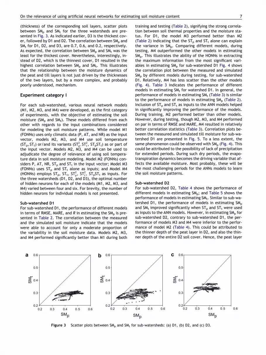
(thickness) of the corresponding soil layers, scatter plotsbetween SMp and SMt for the three watersheds are pre-sented in Fig. 3. As indicated earlier, D3 is the thickest cov-er, followed by D1 and D2. The correlation between SMp andSMt for D1, D2, and D3, are 0.7, 0.6, and 0.2, respectively.As expected, the correlation between SMp and SMt was theleast for the thickest cover. Nevertheless, interestingly, in-stead of D2, which is the thinnest cover, D1 resulted in thehighest correlation between SMp and SMt. This illustratesthat the relationship between the moisture dynamics ofthe peat and till layers is not just driven by the thicknessesof the two layers, but by a more complex, and probablypoorly understood, mechanism.

Experiment category I

For each sub-watershed, various neural network models(M1, M2, M3, and M4) were developed, as the first categoryof experiments, with the objective of estimating the soilmoisture (SMp and SMt). These models differed from eachother with regards to the input combinations consideredfor modeling the soil moisture patterns. While model M1(FONNs) uses only climatic data (P, AT, and NR) as the inputvector, models M2, M3, and M4 use soil temperature(STp,STt) or/and its variants (ST2

p; ST2t , STpSTt) as or part of

the input vector. Models M2, M3, and M4 can be used toadjudicate the degree of relevance of using soil tempera-ture data in soil moisture modeling. Model M2 (FONNs) con-siders P, AT, NR, STp and STt in the input vector; Model M3(FONNs) uses STp and STt alone as inputs; and Model M4(HONNs) employs STp, STt, ST2

p, ST2t , STpSTt as inputs. For

the three watersheds (D1, D2, and D3), the optimal numberof hidden neurons for each of the models (M1, M2, M3, andM4) varied between four and six. For brevity, the number ofhidden neurons for individual models is not presented.

Sub-watershed D1For sub-watershed D1, the performance of different modelsin terms of RMSE, MARE, and R in estimating the SMp is pre-sented in Table 2. The correlation between the measuredand the simulated soil moisture indicate that the modelswere able to account for only a moderate proportion ofthe variability in the soil moisture data. Models M2, M3,and M4 performed significantly better than M1 during both

SMp S0.2 0.3 0.4 0.5 0.6

SMt

SMt

0.2

0.3

0.4

0.5

0.6

0.2 0.30.2

0.3

0.4

0.5

0.6a b

Figure 3 Scatter plots between SMp and SMt fo

training and testing (Table 2), signifying the strong correla-tion between soil thermal properties and the moisture sta-tus. For D1, the model M3 performed better than M2(Table 2) indicating that the STp and STt alone can explainthe variance in SMp. Comparing different models, duringtesting, M4 outperformed the other models in estimatingSMp. This illustrates the ability of the HONNs in extractingthe maximum information from the most significant vari-ables in estimating SMp for sub-watershed D1 Fig. 4 showsthe correlation plot between the measured and simulatedSMp by different models during testing, for sub-watershedD1. Relatively, M4 has less scatter than the other models(Fig. 4). Table 3 indicates the performance of differentmodels in estimating SMt for watershed D1. In general, theperformance of models in estimating SMt (Table 3) is similarto the performance of models in estimating SMp (Table 2).Inclusion of STp and STt as inputs to the ANN models helpedin significantly improving the performance of the models.During training, M2 performed better than other models.However, during testing, though M2, M3, and M4 performedon par in terms of RMSE and MARE, M4 resulted in relativelybetter correlation statistics (Table 3). Correlation plots be-tween the measured and simulated till moisture for sub-wa-tershed D1 are presented in Fig. 5. To a less extent, thesame phenomenon could be observed with SMp (Fig. 4). Thiscould be attributed to the possibility of lack of precipitationfor extended periods. During such dry periods, the evapo-transpiration dynamics becomes the driving variable that af-fects the available moisture. Most probably, these will bethe most challenging periods for the ANNs models to learnthe soil moisture patterns.

Sub-watershed D2For sub-watershed D2, Table 4 shows the performance ofdifferent models in estimating SMp; and Table 5 shows theperformance of models in estimating SMt. Similar to sub-wa-tershed D1, the performance of models in estimating SMp

and SMt improved significantly when STp and STt were usedas inputs to the ANN models. However, in estimating SMp forsub-watershed D2, contrary to sub-watershed D1, the per-formance of models M3 and M4 were inferior to the perfor-mance of model M2 (Table 4). This could be attributed tothe thinner depth of the peat layer in D2, and also the thin-ner depth of the entire D2 soil cover. Hence, the peat layer

Mp SMp

SMt

0.4 0.5 0.6 0.2 0.3 0.4 0.5 0.60.2

0.3

0.4

0.5

0.6c

r sub-watersheds: (a) D1, (b) D2, and (c) D3.

Table 2 Performance measure of different models in estimating peat moisture content (cm/cm) of sub-watershed D1

Model Training Testing

RMSE MARE R RMSE MARE R

M1 0.051 0.098 0.18 0.051 0.099 0.128M2 0.040 0.073 0.644 0.046 0.083 0.507M3 0.043 0.081 0.547 0.043 0.081 0.552M4 0.042 0.076 0.597 0.042 0.077 0.581

M1, M2, and M3 are FONN models, whereas M4 is an HONN model.

Measured

Measured

Measured

Measured0.25 0.30 0.35 0.40 0.45 0.50 0.55 0.60

Sim

ulat

ed

0.3

0.4

0.5

0.6

0.25 0.30 0.35 0.40 0.45 0.50 0.55 0.60

0.3

0.4

0.5

0.6

0.25 0.30 0.35 0.40 0.45 0.50 0.55 0.60

Sim

ulat

ed

0.25

0.30

0.35

0.40

0.45

0.50

0.55

0.60

0.25 0.30 0.35 0.40 0.45 0.50 0.55 0.600.25

0.30

0.35

0.40

0.45

0.50

0.55

0.60

Sim

ulat

ed

Sim

ulat

ed

b a

c d

Figure 4 Comparison of measured vs. simulated peat moisture of cover D1 by (a) M1; (b) M2; (c) M3; and (d) M4 – testing.

Table 3 Performance measure of different models in estimating till moisture content (cm/cm) of sub-watershed D1



M1 0.018 0.050 0.236 0.018 0.050 0.209M2 0.015 0.0430 0.624 0.016 0.043 0.532M3 0.016 0.043 0.552 0.016 0.043 0.539M4 0.016 0.043 0.573 0.016 0.043 0.556


of D2 is more dynamic and responsive to the meteorologicalvariables. During testing, with RMSE, MARE, and R values of

0.061, 0.138, and 0.575, respectively, M2 outperformed theother models. The better performance of the M2 reiterates

Measured

Measured

Measured

Measured

0.22 0.24 0.26 0.28 0.30 0.32

Sim

ulat

ed

Sim

ulat

edSi

mul

ated

Sim

ulat

ed

0.22

0.24

0.26

0.28

0.30

0.32

0.22 0.24 0.26 0.28 0.30 0.320.22

0.24

0.26

0.28

0.30

0.32

0.22 0.24 0.26 0.28 0.30 0.320.22

0.24

0.26

0.28

0.30

0.32

0.22 0.24 0.26 0.28 0.30 0.320.22

0.24

0.26

0.28

0.30

0.32

a b

dc

Figure 5 Comparison of measured vs. simulated till moisture of cover D1 by (a) M1; (b) M2; (c) M3; and (d) M4 – testing.




M1 0.072 0.173 0.265 0.1 0.171 0.297M2 0.062 0.139 0.566 0.061 0.138 0.575M3 0.064 0.146 0.519 0.063 0.146 0.525M4 0.063 0.144 0.529 0.063 0.144 0.537




M1 0.023 0.067 0.167 0.023 0.067 0.179M2 0.014 0.039 0.807 0.015 0.041 0.774M3 0.014 0.0140 0.792 0.014 0.041 0.783M4 0.014 0.039 0.805 0.014 0.040 0.789


the strong influence of atmospheric forcing on the peatmoisture dynamics of sub-watershed D2. This underscoresthe need for considering P, AT, NR, STp, and STt for charac-terizing SMp of watershed D2 Fig. 6 shows the correlationplot between the measured and simulated values of SMp dur-ing testing, for watershed D2. From the large scatter in the

low-ranges of SMp (Fig. 6), it can be concluded that most ofthe models were unable to learn the moisture dynamics atlow-ranges. For watershed D2, the models were able to esti-mate SMt more accurately than SMp (Tables 4 and 5). Thismay be attributed to the reason that the upper peat layeracts like a buffer zone that trims the effect of the meteoro-

Measured0.20 0.25 0.30 0.35 0.40 0.45 0.50 0.55 0.60

Sim

ulat

ed

0.2

0.3

0.4

0.5

0.6

0.20 0.25 0.30 0.35 0.40 0.45 0.50 0.55 0.600.2

0.3

0.4

0.5

0.6

0.20 0.25 0.30 0.35 0.40 0.45 0.50 0.55 0.600.2

0.3

0.4

0.5

0.6

0.20 0.25 0.30 0.35 0.40 0.45 0.50 0.55 0.600.2

0.3

0.4

0.5

0.6

Measured

Sim

ulat

ed

Measured

Sim

ulat

ed

Measured

Sim

ulat

ed

b

dc

a



logical variables on the till layer, and thereby rendering SMt

less vulnerable to atmospheric forcing. During testing,compared to other models, the HONN model (M4) resultedin the highest R statistics. Nevertheless, models M2, M3,and M4 performed on par in terms of RMSE and MARE (Table5) Fig. 7 shows the correlation plots between the measuredand simulated SMt by different models. Disregarding M1, allthe other models were able to estimate SMt withreasonable accuracy over the entire modeling range(Fig. 7).

Sub-watershed D3The performance of different models in estimating SMp andSMt for sub-watershed D3 is presented in Tables 6 and 7,respectively. For sub-watershed D3, similar to sub-water-sheds D1 and D2, inclusion of STp and STt as inputs to theANN models improved the performance of the models inestimating soil moisture (SMp and SMt). However, theimprovement in the performance of the models for sub-wa-tershed D3 is not as significant as compared to sub-water-sheds D1 and D2. This may be attributed to the weakcorrelation (R = 0.2) existing between SMp and SMt. Due tothe association between soil thermal properties and mois-ture status, the weak correlation between SMp and SMt im-plies that the information content between STp and STtwould also be relatively weak. Hence, inclusion of STp andSTt as inputs to the ANN models was not able to appreciablyimprove the performance of the models in estimating the

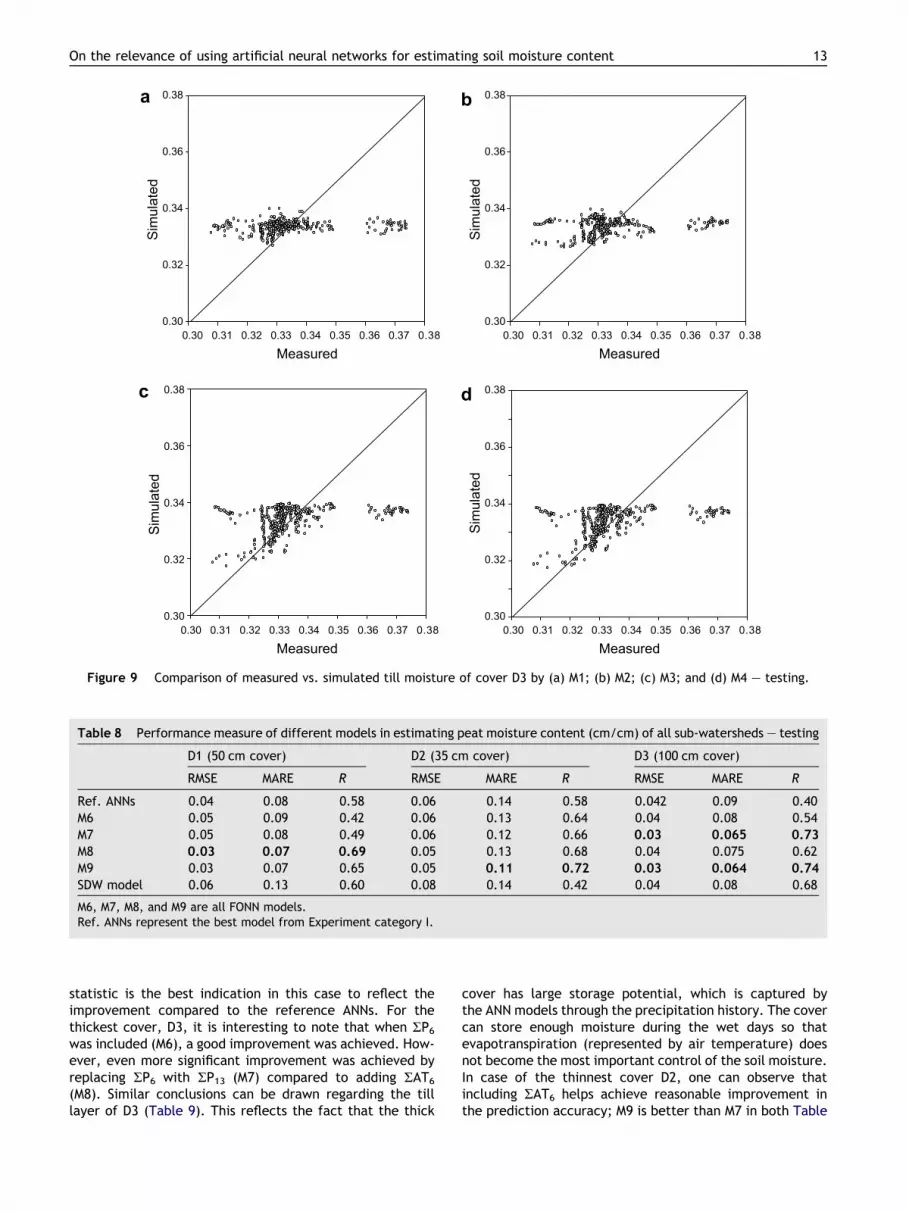
soil moisture of the thick cover D3. Due to the relativeincoherency between STp and STt, the effect is more pro-nounced in M4, where higher-order derivatives of the abovevariables were adopted for estimating SMp (Table 6). Thecorrelation plots between measured and simulated SMp forsub-watershed D3, are presented in Fig. 8. From the plots,it is evident that none of the models was able to learn thedynamics of SMp. In modeling SMt for sub-watershed D3, itis observed that inclusion of STp and STt as inputs to theANN models was able to improve the performance of themodels in terms of R statistics. However, the performancesof the models are comparable in terms of RMSE and MAREstatistics (Table 7) Fig. 9 shows the correlation betweenthe measured and the simulated SMt by different models.As can be seen from the plots, though M3 and M4 resultedin less scatter in a particular modeling range (Fig. 9), theoverall performance of the models are not convincing. Ingeneral, it can be concluded that all ANN models, withinthis first category of experiments, encountered difficultiesin learning the moisture patterns of sub-watershed D3.Since D3 is the thickest cover among the three covers con-sidered in this study, it implies that sub-watershed D3 re-sults in the highest phase-lag between the occurrence ofprecipitation and its manifestation as soil moisture. In otherwords, sub-watershed D3 has more storage effects than theother two sub-watersheds, and thereby is prone to moretopographic forcing. This makes modeling the soil moisturedynamics of sub-watershed D3, more intricate than model-

Measured Measured

MeasuredMeasured

0.20 0.22 0.24 0.26 0.28 0.30 0.32 0.34

Sim

ulat

ed

Sim

ulat

edSi

mul

ated

Sim

ulat

ed

0.20

0.22

0.24

0.26

0.28

0.30

0.32

0.34

0.20 0.22 0.24 0.26 0.28 0.30 0.32 0.340.20

0.22

0.24

0.26

0.28

0.30

0.32

0.34

0.20 0.22 0.24 0.26 0.28 0.30 0.32 0.340.20

0.22

0.24

0.26

0.28

0.30

0.32

0.34

0.20 0.22 0.24 0.26 0.28 0.30 0.32 0.340.20

0.22

0.24

0.26

0.28

0.30

0.32

0.34a

c

b

d





M1 0.044 0.092 0.275 0.044 0.093 0.279M2 0.044 0.091 0.293 0.044 0.091 0.296M3 0.043 0.087 0.328 0.044 0.089 0.326M4 0.044 0.092 0.215 0.045 0.093 0.211




M1 0.013 0.024 0.177 0.013 0.024 0.165M2 0.013 0.024 0.237 0.013 0.025 0.228M3 0.012 0.023 0.400 0.012 0.023 0.383M4 0.012 0.023 0.405 0.012 0.023 0.386


ing the soil moisture dynamics of sub-watersheds D1 and D2.This finding is in line with Entekhabi et al. (1994), where it isshown that the ability of models to predict soil moisture

averages over larger depths is severely limited by the noiseintroduced by the micro-topography and roughness of vege-tation cover.

Measured Measured

MeasuredMeasured

0.25 0.30 0.35 0.40 0.45 0.50

Sim

ulat

ed

Sim

ulat

edSi

mul

ated

Sim

ulat

ed

0.25

0.30

0.35

0.40

0.45

0.50

0.25 0.30 0.35 0.40 0.45 0.500.25

0.30

0.35

0.40

0.45

0.50

0.25 0.30 0.35 0.40 0.45 0.500.25

0.30

0.35

0.40

0.45

0.50

0.25 0.30 0.35 0.40 0.45 0.500.25

0.30

0.35

0.40

0.45

0.50

a b

dc



Experiment category II

In order to prove the hypothesis that the phase lag betweenthe occurrence of precipitation, and its manifestation assoil moisture can be implicitly accounted by consideringthe soil temperature as one of the inputs for characterizingsoil moisture, model M5 was constructed. Model M5 uses P

t�1, ATt�1, AT, NR, STp, and STt, as inputs to estimate SMp

and SMt. Pt�1 and ATt�1 indicates the preceding day precip-itation and air temperature, respectively. For brevity, onlythe testing statistics of model M5 is presented for the threesub-watersheds. For estimating the SMp of sub-watershedD1, M5 resulted in an RMSE of 0.048; MARE of 0.09; and Rof 0.39. The corresponding values for estimating SMt are0.016, 0.043, and 0.56. For estimating the SMp of sub-wa-tershed D2, M5 resulted in an RMSE of 0.062; MARE of0.14; and R of 0.56. The corresponding values for estimatingSMt are 0.015, 0.042, and 0.75. Similarly, for estimating theSMp of sub-watershed D3, M5 resulted in an RMSE of 0.042;MARE of 0.087; and R of 0.40. The corresponding valuesfor estimating SMt are 0.013, 0.024, and 0.23. Except forsimulating the SMp of sub-watershed D3, the performanceof M5 is either on par or poorer than the models, which donot consider the preceding climatic information as part ofthe input vector. These results clearly highlight the impor-tance of considering the soil temperature as an input forestimating the soil moisture patterns, except for signifi-cantly large depths (e.g. D3).

For each sub-watershed, additional experiments wereconducted to improve the accuracy of predicting the SMp

and SMt using the ANN models by incorporating more infor-mation about two processes that affect soil moisture;namely, the cumulative precipitation and evapotranspira-tion. The experiment M2, from the previous category, wasused as a base experiment to build on for improving the pre-diction accuracy. In addition to the current day’s precipita-tion (Pt), the daily precipitation of the previous six days canbe summed (RP6) and used as an input. Similarly, weeklyevapotranspiration may be represented using the cumula-tive air temperature (RAT6). Two weeks of precipitationand evapotranspiration can be represented by RP13 andRAT13, respectively, in addition to the current Pt and ATt.There is literally an infinite possible combination of inputs,and experiments conducted in this study cannot be exhaus-tive. However, Tables 8 and 9 present the results of four dif-ferent experiments (M6, M7, M8, and M9) as well as the bestexperiment from the previous section, which is referred toas the reference ANNs. Model M6 uses the same inputs asM2 (P, AT, NR, STp, and STt) plus RP6; M7 is the same asM2 plus RP13; M8 is M2 plus RP6 plus RAT6; and M9 is M2 plusRP13 plus RAT6.

For brevity, only testing results for the three sub-water-sheds are presented in Tables 8 and 9 for predicting the SMp

and SMt, respectively. Significant improvement in the pre-diction accuracy of the soil moisture of the upper peat layerwas achieved with all D1, D2, and D3 (Table 8). The R

Measured0.30 0.31 0.32 0.33 0.34 0.35 0.36 0.37 0.38

Sim

ulat

ed

0.30

0.32

0.34

0.36

0.38

Measured0.30 0.31 0.32 0.33 0.34 0.35 0.36 0.37 0.38

Sim

ulat

ed

0.30

0.32

0.34

0.36

0.38

Measured0.30 0.31 0.32 0.33 0.34 0.35 0.36 0.37 0.38

Sim

ulat

ed

0.30

0.32

0.34

0.36

0.38

Measured0.30 0.31 0.32 0.33 0.34 0.35 0.36 0.37 0.38

Sim

ulat

ed

0.30

0.32

0.34

0.36

0.38

a b

c d


Table 8 Performance measure of different models in estimating peat moisture content (cm/cm) of all sub-watersheds – testing

D1 (50 cm cover) D2 (35 cm cover) D3 (100 cm cover)

RMSE MARE R RMSE MARE R RMSE MARE R

Ref. ANNs 0.04 0.08 0.58 0.06 0.14 0.58 0.042 0.09 0.40M6 0.05 0.09 0.42 0.06 0.13 0.64 0.04 0.08 0.54M7 0.05 0.08 0.49 0.06 0.12 0.66 0.03 0.065 0.73

M8 0.03 0.07 0.69 0.05 0.13 0.68 0.04 0.075 0.62M9 0.03 0.07 0.65 0.05 0.11 0.72 0.03 0.064 0.74

SDW model 0.06 0.13 0.60 0.08 0.14 0.42 0.04 0.08 0.68

M6, M7, M8, and M9 are all FONN models.Ref. ANNs represent the best model from Experiment category I.


statistic is the best indication in this case to reflect theimprovement compared to the reference ANNs. For thethickest cover, D3, it is interesting to note that when RP6was included (M6), a good improvement was achieved. How-ever, even more significant improvement was achieved byreplacing RP6 with RP13 (M7) compared to adding RAT6(M8). Similar conclusions can be drawn regarding the tilllayer of D3 (Table 9). This reflects the fact that the thick

cover has large storage potential, which is captured bythe ANN models through the precipitation history. The covercan store enough moisture during the wet days so thatevapotranspiration (represented by air temperature) doesnot become the most important control of the soil moisture.In case of the thinnest cover D2, one can observe thatincluding RAT6 helps achieve reasonable improvement inthe prediction accuracy; M9 is better than M7 in both Table

Table 9 Performance measure of different models in estimating till moisture content (cm/cm) of all sub-watersheds – testing

D1 (50 cm cover) D2 (35 cm cover) D3 (100 cm cover)

RMSE MARE R RMSE MARE R RMSE MARE R

Ref. ANNs 0.016 0.04 0.56 0.014 0.04 0.79 0.012 0.02 0.39M6 0.016 0.043 0.56 0.014 0.04 0.78 0.011 0.023 0.45M7 0.016 0.042 0.56 0.014 0.04 0.80 0.01 0.022 0.56M8 0.013 0.037 0.70 0.011 0.036 0.84 0.011 0.023 0.52M9 0.012 0.036 0.70 0.011 0.036 0.84 0.01 0.022 0.59

SDW model 0.021 0.08 0.67 0.10 0.29 0.08 0.02 0.05 0.50


8 and Table 9. Unlike D3, moving from M6 to M8 is betterthan moving from M6 to M7. Even though precipitation isstill an important factor, evapotranspiration is a major con-trol of moisture on D2. The cover is thin and lacks the stor-age ability; therefore, it cannot store moisture from far inthe past. Evapotranspiration could really cause D2 to dryout. In case of the intermediate cover D1, both the peat(Table 8) and the till layers (Table 9) behaves in a way thatshow a balancing effect of both the storage and the precip-itation. Models M8 and M9 are significantly better than M6and M7; reflecting the need of presenting balanced memoryof both the storage and the precipitation.

Noting that all experiments of category II (M5–M9) arebased on FONN models, an additional HONN model (M10)was tested in this category. M10 was designed to be fullysecond-order ANN model based on the best performance re-ported in Table 8 and Table 9; i.e., M10 is a second-orderANNs of M8 for the peat layer of D1 cover, and a second-or-der ANNs of M9 for the peat layer of D2 and D3, as well as forthe till layer of all three covers. Other possibilities and sce-narios of fully and partial HONNs are endless, however,experiment M10 is considered sufficient for the purpose ofthis study. The only noticeable improvement achieved bythe use of HONNs (M10) over the FONNs is the increase inthe R statistic in the case of the peat layer of the thick coverD3 (slight increase from 0.74 to 0.77) as well as the till layer(considerable increase from 0.59 to 0.70). It can be con-cluded that second-order ANNs played a positive role inimproving the prediction of soil moisture in thicker cover.It might be possible that even higher-order ANNs could im-prove the results further. This should be subject to futureinvestigation.

Comparison between the ANNs and the conceptualSDW model

Even though the second category of experiments signifi-cantly improved the ANN model performance with regardto the estimation of the soil moisture content, it is desirableto measure such performance against a validated concep-tual model. Elshorbagy et al. (2005, 2007) developed asite-specific system dynamics watershed (SDW) model thatsimulates the various hydrological processes occurring inthe reconstructed watersheds; D1, D2, and D3. The modelis a lumped mechanistic model that was conceptualized asa control volume that simulates the water balance compo-nents among the two soil layers (peat and till) as well asthe underlying shale layer including evapotranspiration

and runoff on a daily basis. A combination of physicallybased formulations (e.g. Green-Ampt for infiltration and soilmoisture redistribution) and fitted-parameter formulations(e.g. actual evapotranspiration based on simulated soilmoisture index) was employed in formulating the SDW mod-el. More details on the model can be found in Elshorbagyet al. (2007). The model was extensively evaluated for thepurposes of design and hydrologic performance assessmentof reconstructed watersheds (Elshorbagy and Barbour,2007) as well as for management decision making (Elshor-bagy, 2006).

Even though it is infeasible to compare the input struc-ture of mechanistic and data-driven models, the input vari-ables and data needed for the SDW model are provided hereto facilitate the evaluation of the performances of the ANNmodels relative to the SDW model. The current version ofthe SDW model requires daily precipitation (P), average dai-ly air temperature (AT), daily net radiation (NR), relativehumidity (RH), average daily temperatures of both peatand till layers (STp and STt), and soil physical properties thatallow for the estimation of the soil water characteristiccurve (SWCC). However, it should be noted that by defini-tion of mechanistic models, the SDW model has the abilityto keep ‘‘indefinite’’ memory of past values (time-lagged)of input and simulated parameters through is tank (stock)component. At the same time, the SDW model can providesoil moisture content, actual evapotranspiration, and runoffas outputs. The SDW model has nine different calibrationparameters related to the processes of infiltration, evapo-transpiration, snowmelt, and runoff (Elshorbagy et al.,2007).

The performance of the SDW model in estimating the soilmoisture in the peat layer of the three sub-watersheds ispresented in Table 8. Clearly, the best ANN models per-formed reasonably better, and sometimes much better asin the case of D2, than the SDW model. The R statisticshould be noted in all covers. Similar conclusions can bedrawn with regard to the till layer (Table 9). It is interestingto note that the poor performance of the SDW model ap-plied to the thinnest cover D2 was significantly improvedand overcome by the ANN models. Elshorbagy et al. (2007)reported that the presence of macro pores and the steepslope of the covers make the influence of the surface runoffand the interflow dynamics more prominent with the thincover (D2). Such dynamics were difficult to capture withinthe conceptual SDW model, whereas the data-driven ANNswere less affected by such dynamics and phenomena. For vi-sual assessment of the second category of ANN experiments,

Measured0.2 0.3 0.4 0.5 0.6

Sim

ulat

ed

0.2

0.3

0.4

0.5

0.6

0.32

0.36

a

b


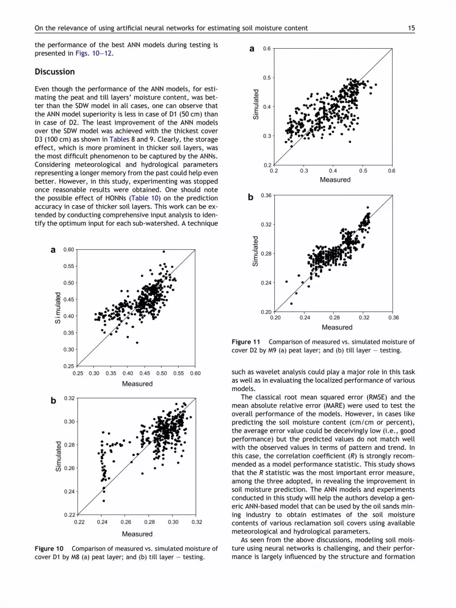
the performance of the best ANN models during testing ispresented in Figs. 10–12.

Discussion

Even though the performance of the ANN models, for esti-mating the peat and till layers’ moisture content, was bet-ter than the SDW model in all cases, one can observe thatthe ANN model superiority is less in case of D1 (50 cm) thanin case of D2. The least improvement of the ANN modelsover the SDW model was achieved with the thickest coverD3 (100 cm) as shown in Tables 8 and 9. Clearly, the storageeffect, which is more prominent in thicker soil layers, wasthe most difficult phenomenon to be captured by the ANNs.Considering meteorological and hydrological parametersrepresenting a longer memory from the past could help evenbetter. However, in this study, experimenting was stoppedonce reasonable results were obtained. One should notethe possible effect of HONNs (Table 10) on the predictionaccuracy in case of thicker soil layers. This work can be ex-tended by conducting comprehensive input analysis to iden-tify the optimum input for each sub-watershed. A technique

Measured0.25 0.30 0.35 0.40 0.45 0.50 0.55 0.60

Sim

ulat

ed

0.25

0.30

0.35

0.40

0.45

0.50

0.55

0.60

Measured

0.22 0.24 0.26 0.28 0.30 0.32

Sim

ulat

ed

0.22

0.24

0.26

0.28

0.30

0.32

a

b

Figure 10 Comparison of measured vs. simulated moisture ofcover D1 by M8 (a) peat layer; and (b) till layer – testing.

Measured0.20 0.24 0.28 0.32 0.36

Sim

ulat

ed

0.20

0.24

0.28


such as wavelet analysis could play a major role in this taskas well as in evaluating the localized performance of variousmodels.

The classical root mean squared error (RMSE) and themean absolute relative error (MARE) were used to test theoverall performance of the models. However, in cases likepredicting the soil moisture content (cm/cm or percent),the average error value could be deceivingly low (i.e., goodperformance) but the predicted values do not match wellwith the observed values in terms of pattern and trend. Inthis case, the correlation coefficient (R) is strongly recom-mended as a model performance statistic. This study showsthat the R statistic was the most important error measure,among the three adopted, in revealing the improvement insoil moisture prediction. The ANN models and experimentsconducted in this study will help the authors develop a gen-eric ANN-based model that can be used by the oil sands min-ing industry to obtain estimates of the soil moisturecontents of various reclamation soil covers using availablemeteorological and hydrological parameters.

As seen from the above discussions, modeling soil mois-ture using neural networks is challenging, and their perfor-mance is largely influenced by the structure and formation

Measured0.25 0.30 0.35 0.40 0.45 0.50

Mea

sure

d

0.25

0.30

0.35

0.40

0.45

0.50

Measured0.30 0.32 0.34 0.36 0.38

Sim

ulat

ed

0.30

0.32

0.34

0.36

0.38

a

b



of the soil strata. As expected and partially proven in thisstudy, the poorest performance of ANN models might beencountered during modeling the soil moisture phenomenonthat is influenced largely by the storage effect. The resultspresented in this study supports those presented by Elshor-bagy and Barbour (2007), in which the SDW model was usedto simulate the three sub-watersheds (D1, D2, and D3) overa period of 60 years. Elshorbagy and Barbour (2007) show

Table 10 Performance measure of HONNs (experiment category Iof all sub-watersheds – testing

D1 (50 cm cover) D2 (35 cm

RMSE MARE R RMSE

Peat layerM8/M9 0.03 0.07 0.69 0.05M10 0.03 0.06 0.70 0.05Till layerM8/M9 0.012 0.036 0.70 0.011M10 0.01 0.037 0.70 0.01

that D3 was always providing significantly more moisturefor evapotranspiration than D2 under all climatic condi-tions; indicating its ability to ‘‘store’’ water and release itfor vegetation at the time of need. D2 was more responsiveto climatic conditions and running short of water at times ofhigh evapotranspiration. This argument shows that the ANNmodels, developed in this study, are not only good from apredictive point of view but also conceptually meaningful.

Summary and conclusions

As soil moisture is one of the important factors, which influ-ence the boundary-layer climate, significant efforts havebeen made in the past to improve the accuracy of soil mois-ture estimation using statistical and remote-sensing tech-niques. The scarcity of field-scale models to estimate soilmoisture, and the success of artificial neural networks(ANNs) in modeling different hydrological processes warranttheir application to modeling the most complex and themost important hydrological variable, namely, soil mois-ture, at field scales. In this study, an attempt has beenmade to estimate soil moisture from readily available cli-matic data. Datasets from three reconstructed sub-water-sheds (D1, D2, and D3), located in northern Alberta,Canada, with thickness of 0.50 m, 0.35 m, and 1.0 m, com-prising a thin layer of peat mineral over varying thickness ofglacial till, was considered in this study. Depth-averagedsoil moisture contents at both the upper peat (SMp) andthe lower till (SMt) layers were modeled as function of pre-cipitation (P), air temperature (AT), net radiation (NR), andsoil temperature of peat (STp) and the till (STt) layers. Forthe three sub-watersheds, investigating the relationship be-tween the soil moisture dynamics of the peat and till layers,it is found that the moisture dynamics is not just driven bythe thickness of the soil layers, but by a more complex, andprobably poorly understood, mechanism. ANN models withdifferent input configurations were developed to estimatethe SMp and the SMt. In the absence of time-lagged meteo-rological variables, which reflect the history of the bound-ary conditions, STp and STt were found to be the mostimportant variables for modeling soil moisture. A higher-or-der neural network (HONN) model was developed usingthese variables, with the objective of extracting the maxi-mum information from the input vector. The performancesof the models were evaluated based on the root meansquared error (RMSE), the mean absolute relative error(MARE) and the correlation coefficient (R). Although, in

I) models in estimating peat and till moisture content (cm/cm)

cover) D3 (100 cm cover)

MARE R RMSE MARE R

0.11 0.72 0.03 0.064 0.740.10 0.74 0.03 0.06 0.77

0.036 0.84 0.01 0.022 0.590.036 0.82 0.01 0.02 0.70


some cases, the correlations between the measured and theestimated soil moisture for both the peat and the till layersare not very strong, the results are encouraging consideringthe large variance that exists between the independent andthe dependent variables. The better performance of theANN models considering soil temperature as one of the in-puts reiterates the strong link between the soil thermalproperties and the soil moisture status. This finding wouldbe of great importance to orient the future monitoring pro-gram of the reconstructed watersheds, where it is recom-mended to increase the intensity of soil temperaturemeasurement network system, and thereby possibly im-prove the accuracy of soil moisture estimates.

A second category of experiments were time-lagged in-puts were considered revealed the need to consider variabletime window to obtain optimum inputs and results for eachsub-watershed. The optimum inputs were found to matchwith the conceptual understanding of the significance/insig-nificance of the storage effect, which is based on the soillayering and thickness. For the three sub-watersheds, it ishard to generalize the best combination of inputs for char-acterizing soil moisture. This illustrates that the atmo-spheric forcing and the soil moisture response to suchforcing is influenced by the type, depth, and structure ofthe soil strata. In general, the results from this study indi-cate that modeling the soil moisture using ANNs is challeng-ing but achievable, and the model performance is largelyinfluenced by the structure of the soil strata. The results re-ported in this study are unique for three reasons: (i) theyestablished a link between readily available climatic vari-ables and soil-moisture, using ANNs; (ii) they evaluatedthe potential of adopting the ANNs for estimating soil mois-ture of reconstructed watersheds, where the dynamics ofatmospheric forcing and the soil moisture response to suchforcing change based on the soil cover layering and thick-ness; and (iii) they show that ANNs can perform as goodas, and possibly better, than conceptual watershed modelin estimating depth-averaged soil moisture content.

Acknowledgements

The authors gratefully acknowledge the financial support ofthe National Science and Engineering Research Council(NSERC) of Canada, the CEMA consortium, and the Depart-ment of Civil and Geological Engineering, University ofSaskatchewan.

References

Anctil, F., Tape, D.G., 2004. An exploration of artificial neuralnetwork rainfall–runoff forecasting combined with waveletdecomposition. J. Environ. Eng. Sci., S121–S128. doi:10.1139/S03-07.

ASCE Task Committee on Application of Artificial Neural Networks inHydrology, 2000. Artificial neural networks in hydrology. I:Preliminary concepts. J. Hydrol. Eng. 5 (2), 115–123.

Barbour, S.L., Boese, C., Stolte, B., 2001. Water balance forreclamation covers on oilsands mining overburden piles. In:Proceedings of the 54th Canadian Geotechnical Conference,Calgary, Alta., pp. 16–19 September 2001. Canadian Geotech-nical Society, Alliston, Ont. pp. 313–319.

Boese, K., 2003. The Design and Installation of a Field Instrumen-tation Program for the Evaluation of Soil-atmosphere WaterFluxes in a Vegetated Cover Over Saline/Sodic Shale Overbur-den, M.Sc. Thesis, University of Saskatchewan, Saskatoon,Sask.

Bowden, G.J., Dandy, G.C., Maier, H.R., 2005. Input determina-tion for neural network models in water resources applica-tions. Part 1 – background and methodology. J. Hydrol. 301,75–92.

Bowden, G.J., Dandy, G.C., Maier, H.R., 2006. An evaluation ofmethods for the selection of inputs for an artificial networkbased river model. In: Recknagel, F. (Ed.), Ecological Informat-ics. Springer, Berlin, Heidelberg, pp. 275–292.

Dawson, C.W., Wilby, R., 1998. An artificial neural networkapproach to rainfall–runoff modeling. Hydrol. Sci. J. 43, 47–66.

Demuth, H., Beale, M., 2001. Neural Network Toolbox Learning ForUse with MATLAB. The Math Works Inc, Natick, Mass.

Elshorbagy, A., 2006. Multicriterion decision analysis approach toassess the utility of watershed modeling for managementdecisions. Water Resour. Res. 42, W09407. doi:10.1029/2005WR00426.

Elshorbagy, A., Barbour, L., 2007. Probabilistic approach for designand hydrologic performance assessment of reconstructed water-sheds. J. Geotech. Geoenv. Eng. ASCE 133 (9), 1110–1118.

Elshorbagy, A., Jutla, A., Kells, J., 2007. Simulation of thehydrological processes on reconstructed watersheds using sys-tem dynamics. Hydrol. Sci. J. 52, 538–562.

Eltahir, E.A.B., 1998. A soil moisture-rainfall feedback mechanism,1: Theory and observations. Water Resour. Res. 34 (4), 765–776.

Entekhabi, D., Nakamura, H., Njoku, E.G., 1994. Solving the inverseproblem for soil moisture and temperature profiles by sequentialassimilation of multifrequency remotely sensed observations.IEEE Trans. Geosci. Remote Sensing 32 (2), 438–448.

Entekhabi, D., Rodriguez-Iturbe, I., Castelli, F., 1996. Mutualinteraction of soil moisture state and atmospheric processes.J. Hydrol. 184, 3–17.

French, M.N., Krajewski, W.F., Cuykendall, R.R., 1992. Rainfallforecasting in space and time using a neural network. J. Hydrol.137, 1–31.

Gautam, M.R., Watanabe, K., Saegusa, H., 2000. Runoff analysis inhumid forest catchment with artificial neural network. J.Hydrol. 235, 117–136.

Georgakakos, K.P., Bae, D.H., 1994. Climatic variability of soilwater in the American midwest: 1, Spatio-temporal analysis. J.Hydrol. 162, 379–390.

Georgakakos, K.P., Smith, G.F., 1990. On improved operationalhydrologic forecasting: results from a WMO real-time forecastingexperiment. J. Hydrol. 114, 17–45.

Georgakakos, K.P., Bae, D.H., Cayan, D.R., 1995. Hydroclimatologyof continental watersheds, temporal analyses. Water Resour.Res. 31 (3), 655–675.

Grayson, R.B., Bloschl, G., Moore, I.D., 1995. Distributed param-eter hydrologic modelling using vector elevation data: Thalesand TAPES-C. In: Singh, V.P. (Ed.), Computer Models ofWatershed Hydrology. Water Resources Pub. Highlands Ranch,Colorado, pp. 669–695.

Gupta, M.M., Jin, L., Homma, N., 2003. Static and Dynamic NeuralNetworks. John Wiley and Sons, Inc., Hoboken, New Jersey.

Haigh, M.J., 2000. The Aims of Land Reclamation, Land Recon-struction and Management, vol. 1. A.A. Balkema Publishers,Rotterdam, The Netherlands, pp. 1–20.

Haykin, S., 1999. Neural Networks: A Comprehensive Foundation,second ed. MacMillan, New York.

Hsu, K.L., Gupta, H.V., Sorooshian, S., 1995. Artificial neuralnetwork modeling of the rainfall–runoff process. Water Resour.Res. 31 (10), 2517–2530.

http://dx.doi.org/10.1139/S03-07

http://dx.doi.org/10.1139/S03-07

http://dx.doi.org/10.1029/2005WR00426

http://dx.doi.org/10.1029/2005WR00426


Karunanithi, N., Grenney, W.J., Whitley, D., Bovee, K., 1994.Neural networks for river flow prediction. J. Comput. Civil Eng. 8(2), 201–220.

Kim, T.W., Valdes, J.B., 2003. Nonlinear model for droughtforecasting based on a conjunction of wavelet transforms andneural networks. J. Hydrol. Eng. 8 (6), 319–328.

Kitanidis, P.K., Bras, R.L., 1980. Real time forecasting with aconceptual hydrologic model, 2. Applications and results. WaterResour. Res. 16 (6), 1034–1044.

Kuczera, G., 1983. Improved parameter inference in catchmentmodels; 2. Combining different kinds of hydrologic data andtesting their compatibility.Water Resour. Res. 19 (5), 1163–1172.

Makkeasorn, A., Chang, N.B., Beaman, M., Wyatt, C., Slater, C.,2006. Soil moisture estimation in a semiarid watershed usingRADARSAT-1 satellite imagery and genetic programming. WaterResour. Res. 42, W09401. doi:10.1029/2005WR00403.

Parasuraman, K., Elshorbagy, A., 2007. Cluster-based hydrologicprediction using genetic algorithm-trained neural networks. J.Hydrol. Eng., ASCE 12 (1), 52–62.

Parasuraman, K., Elshorbagy, A., Carey, S., 2006. Spiking-modularneural networks: A neural network modeling approach forhydrological processes. Water Resour. Res. 42, W05412.doi:10.1029/2005WR00431.

Redlapalli, S.K., 2004. Development of Neural Units with Higher-order Synaptic Weights Operations and Their Applications toLogic Circuits and Control Problems, M.Sc. Thesis, University ofSaskatchewan, Saskatoon, SK, Canada.

Shamseldin, A.Y., 1997. Application of a neural network techniqueto rainfall–runoff modeling. J. Hydrol. 199, 272–294.

Taylor, J.G., Commbes, S., 1993. Learning higher order correla-tions. Neural Networks 6 (3), 423–428.

Thirumalaiah, K., Deo, M.C., 1998. River stage forecasting usingartificial neural networks. J. Hydrol. Eng. 3 (1), 26–32.

Wood, E.F., Lettenmaier, D.P., Zartarian, V.G., 1992. A land-surface hydrology parameterization with subgrid variability forgeneral circulation models. J. Geophys. Res. 97, 2717–2728.

Wooldridge, S.A., Kalma, J.D., Walker, J.P., 2003. Importance ofsoil moisture measurements for inferring parameters in hydro-logic models of low-yielding ephemeral catchments. Environ.Model. Software 18 (1), 35–48.

Zhang, B., Govindaraju, S., 2000. Prediction of watershed runoffusing Bayesian concepts and modular neural networks. WaterResour. Res. 36 (3), 753–762.

Zhang, M., Fulcher, J., Scofield, R.A., 1997. Rainfall EstimationUsing Artificial Neural Network Group Neurocomputing, vol. 16.pp. 97–115.

http://dx.doi.org/10.1029/2005WR00403

http://dx.doi.org/10.1029/2005WR00431

on the relevance of using artificial neural networks for estimating soil moisture content

Documents