Advances in Water Resources 74 (2014) 44–53

Contents lists available at ScienceDirect

Advances in Water Resources

journal homepage: www.elsevier .com/ locate/advwatres

Potential of soil moisture observations in flood modelling: Estimatinginitial conditions and correcting rainfall

http://dx.doi.org/10.1016/j.advwatres.2014.08.0040309-1708/� 2014 Elsevier Ltd. All rights reserved.

⇑ Corresponding author.

Christian Massari a,⇑, Luca Brocca a, Tommaso Moramarco a, Yves Tramblay b, Jean-Francois Didon Lescot c

a Research Institute for Geo-Hydrological Protection, National Research Council, Perugia, Italyb Hydrosciences Montpellier, CNRS-IRD-UM1-UM2, Université Montpellier 2, Maison des Sciences de l’Eau, Place Eugène Bataillon, 34095 Montpellier Cedex 5, Francec UMR-7300 ESPACE CNRS, Départment de Géographie, Université de Nice-Sophia-Antipolis, Nice, France

a r t i c l e i n f o

Article history:Received 13 March 2014Received in revised form 30 June 2014Accepted 5 August 2014Available online 13 August 2014

Keywords:Soil moistureFloodsRainfall

a b s t r a c t

Rainfall runoff (RR) models are fundamental tools for reducing flood hazards. Although several studieshave highlighted the potential of soil moisture (SM) observations to improve flood modelling, muchresearch has still to be done for fully exploiting the evident connection between SM and runoff. As away of example, improving the quality of forcing data, i.e. rainfall observations, may have a great benefitin flood simulation. Such data are the main hydrological forcing of classical RR models but may sufferfrom poor quality and record interruption issues. This study explores the potential of using SM observa-tions to improve rainfall observations and set a reliable initial wetness condition of the catchment forimproving the capability in flood modelling. In particular, a RR model, which incorporates SM for its ini-tialization, and an algorithm for rainfall estimation from SM observations are coupled using a simple inte-gration method. The study carried out at the Valescure experimental catchment (France) demonstratesthe high information content retained by SM for RR transformation, thus giving new possibilities forimproving hydrological applications. Results show that an appropriate configuration of the two modelsallows obtaining improvement in flood simulation up to 15% in mean and 34% in median Nash Sutcliffeperformances as well as a reduction of the median error in volume and on peak discharge of about 30%and 15%, respectively.

� 2014 Elsevier Ltd. All rights reserved.

1. Introduction

It is widely recognised that the two most important climatevariables influencing runoff generation during floods are rainfalland soil moisture (SM). In particular, in flood modelling, rainfallrepresents the main input determining the magnitude of the floodevent, which, in turn, is strongly influenced by the initial SM con-ditions of the catchment.

SM measurements have been ever increasing available bothfrom in situ (e.g., International Soil Moisture Network ISMN,[23], satellite sensors (e.g., the Advanced SCATterometer ASCAT,[3], the Advanced Microwave Scanning Radiometer for Earthobservation AMSRE, [37], and the Soil Moisture and OceanSalinity Mission SMOS [28] and land surface models (e.g., [2]) atincreasing temporal and spatial resolutions [47]. Such anincreased availability has pushed several authors to employ theavailable SM estimates for determining the catchment initialconditions before a storm event for RR modelling[4,6,7,9,10,19,44–46]. Recently, Massari et al. [31] proposed to

explicitly embed the relationship existing between SM and themodel initial conditions into an event based RR model to simulatedischarge hydrographs. The model was called Simplified Continu-ous RR Model (SCRRM) because instead of modelling SM fromcontinuous precipitation and evapotranspiration data, like in clas-sical continuous RR models [5,9,15,30,42,43], it uses SM recordedfrom ground observations or satellite sensors to set the initialconditions of an event based model. That is, the temporal evolu-tion of SM is assessed via in situ or satellite observations and it isused as a proxy of the wetness state of the catchment to properlypredict flood hydrographs.

Rainfall data from ground stations, meteorological radar andsatellite sensors have been conventionally used for hydrologicalapplications. Such products are often (but not always) easily avail-able but are known to suffer from some limitations (such as therepresentativeness of the rain gauge stations with respect to thespatial variability of rainfall, [45]. To improve rainfall estimation,SM data have been recently employed by using simple and moreadvanced assimilation techniques [13,21,40]. For instance, Crowet al. [21] used remotely sensed SM observations to correct rainfallestimates in United States and West Africa showing that they can

C. Massari et al. / Advances in Water Resources 74 (2014) 44–53 45

broadly refine coarse-scale rainfall accumulations measurementswith low risk of degradation. Recently, Brocca et al. [13] proposedan innovative approach, which uses SM observations to directlyestimate rainfall by inverting the soil water balance equation.The algorithm, called SM2RAIN, was tested over three sites inEurope showing that it is able to satisfactorily reproduce rainfallwhen in situ SM observations are employed.

In the past decade, a few studies have been investigating theassimilation of in situ [1,16] and satellite SM observations[8,12,24,32,33,38,39] into RR modeling, obtaining contrastingresults and depending on several factors, i.e., different spatial–temporal scales, layer depth of the observed and modeled quan-tities and type of the assimilation technique [20]. In particular,Crow and Ryu [20] carried out a synthetic study where theassimilation of SM observations was used both to improvestorm-scale rainfall accumulations and the pre-storm SM condi-tions in the Sacramento hydrologic model [15]. The resultsshowed that their approach is more efficient at improving streamflow predictions than data assimilation techniques focusingsolely on the constraint of antecedent soil moisture conditions.Very recently, Chen et al. [17] extended the analysis to a realcase study using an integration of satellite SM observations high-lighting the benefit of the ‘‘dual’’ assimilation (i.e. for correctingboth stream flow and rainfall) but also listing some still unsolvedissues like the difficulty on estimating rainfall close to saturationconditions.

In this paper, to underline the relevance of the SM as a statevariable influencing the RR transformation, we show how theintegration of SM into a simple RR model both to set the appropri-ate initial conditions and to adjust observed rainfall cansignificantly improve the performance of the flood modelling. Dif-ferently from Crow and Ryu [20] here we use real (not synthetic)in situ data and a much simpler hydrological model (SCRRM, [31]and a data assimilation approach [8]. The choice of a simplemodel and an easy assimilation technique rely on the two follow-ing reasons: (1) the will to highlight the potential benefit of usingSM observations for flood modelling without being affected oncritical choices related to the model parameter setting or to thetype of the assimilation technique and (2) maintaining a limitednumber of parameters used in order to avoid over parameteriza-tion issues.

The simulations are carried out using rainfall, SM and runoffdata collected in the catchment of Valescure (3.83 km2) in France.The manuscript is organised as follow: Section 1 describes thehydrological model, the rainfall estimation method and the wayhow the integration of SM-derived rainfall and observed rainfallis carried out. In the same section, we describe the experimentmethodology and the performance scores used for evaluating theresults. Section 2 provides the description of the area and thedataset while Section 3 contains the results and the discussion.Eventually the paper presents the conclusions.

2. Methods

2.1. Hydrological model: SCRRM

The hydrological model used in this study is SCRRM [31]. Themodel is similar to MISDc (Modello Idrologico Semi-Distribuito incontinuo, [9] with the important difference that the temporal evo-lution of SM over a long-term period is assessed by using SMdirectly recorded from external sources instead of modelling itby a soil water balance component. The ‘‘observed’’ SM time series(i.e. those provided by external sources) are used to set the initialsaturation conditions in the framework of the Soil ConservationService-Curve Number method [41].

2.1.1. Estimation of losses and antecedent wetness conditionsSCRRM employs the SCS-CN method for estimation of losses.

The choice of the SCS-CN method is due to its wide use since1980 for operational applications. In particular, the partitioningof rainfall into runoff using the SCS-CN method for a storm relieson the following empirical equation:

Q ¼ ðP � FaÞ2

P � Fa þ SP P Fa ð1Þ

where Fa is the initial abstraction, S is the soil potential maximumretention, Q is the direct runoff depth, and P is the rainfall depth.The quantity Fa is considered linearly dependent on S by:

Fa ¼ kS ð2Þ

where k is the initial abstraction coefficient. Eq. (1) is extended forthe time evolution of the effective rainfall rate, e(t), within a givenstorm as in [35]:

eðtÞ ¼ dQdt¼ pðtÞðPðtÞ � FaÞðPðtÞ � Fa þ 2SÞ

ðPðtÞ � Fa þ SÞ2PðtÞP Fa ð3Þ

where p is the rainfall rate and PðtÞ ¼R t

0 pðsÞds.If the standard SCS method is used, S is estimated based on

dimensionless CN assessed as a function of land use, hydrologicalsoil group, and total precipitation of previous 5 days (API5, [41].However, as shown by many authors [4,6,7,9,19,44–46] for severalMediterranean catchments, this approach suffer from several lim-itations and drawbacks due to the inability of API5 to properlyidentify the initial wetness condition of the catchment before aflood event in basins characterised by high variability of the evapo-transpiration rate and noticeable seasonality.

To overcome the latter issues, SCRRM exploits the observedlinear behaviour between the wetness state of the soil and theparameter S [6,7] using the following relationship:

S ¼ amaxð1� heÞ ð4Þ

where he is the relative SM (or degree of saturation) and amax is aparameter to be estimated. Indeed, this behaviour has been foundaccurate in several catchments worldwide [4,6,10,19].

2.1.2. RoutingOnce the time evolution of effective rainfall is computed, the

routing to the outlet of the catchment is obtained from the convo-lution of the rainfall excess and the Geomorphological Instanta-neous Unit Hydrograph (GIUH), such as proposed by Gupta andWaymire [27]. In the model the lag time is evaluated throughthe relationship proposed by Melone et al. [34]:

L ¼ g1:19A0:33 ð5Þ

with L being the lag time (h), A the area of the catchment (km2), andg a parameter to be calibrated [36]. For this study, a lumped modelis employed even though the same modelling approach can be eas-ily applied to spatially distributed models.

To sum up, SCRRM exploits he and the rainfall data recordedduring a flood event (rainfall event in the following) as input datato simulate the flood hydrographs. The relationship between S andSM is a model relation embedded in the model structure and it isused to estimate the value of S for each event. The calibration ofSCRRM involves only three parameters: the coefficient of initialabstractions k, the parameter amax of the S� he relationship andthe parameter g of the lag time-area relationship.

For this study, a lumped model is employed even though thesame concept can be easily applied to spatially distributed models.

46 C. Massari et al. / Advances in Water Resources 74 (2014) 44–53

2.2. Rainfall estimation: SM2RAIN

Brocca et al. [13] developed a simple approach – namedSM2RAIN – for estimating rainfall accumulations through theknowledge of SM observations. The method is based on the inver-sion of the soil water balance equation, which allows to directlycalculating the rainfall as a function of SM. Considering a layerdepth Z [L] the balance equation can be expressed by

ZdsðtÞ=dt ¼ pðtÞ � evðtÞ � gðtÞ � rðtÞ ð6Þ

where s(t) is the relative saturation of the soil, t is the time and p(t),g(t), ev(t) and r(t) are the precipitation, drainage rate, evapotranspi-ration and runoff, respectively. The model assumes that during rain-fall, the evaporation rate is negligible [29]. In these conditions ev(t)can be assumed equal to zero. Neglecting the evapotranspirationrate during rainfall likely leads to not significant errors in floodmodelling especially in cold climates and at flood event scale. Thedrainage rate is calculated as gðtÞ ¼ asðtÞb, where a [L/T] and b [–]are two parameters expressing the non-linearity between drainagerate and soil saturation. Concerning runoff, it deserves a moredetailed discussion. Theoretically, r(t) can be formulated in termsof the dependence of the runoff on s(t) and p(t) by means of appro-priate formulations [25]. However, previous applications of themodel in many locations and for different precipitation regimes[13,14,18] have provided the same results either by consideringr(t) or removing it. Indeed, at dry conditions, where almost all theprecipitation is expected to enter into the soil and lateral fluxesare negligible (vertical fluxes dominate, [26], not including r(t) isnot a strong assumption. Also, at medium conditions we couldexpect that subsurface runoff is approximately taken into accountby the term g(t). Close to saturation conditions not consideringr(t) term could lead to significant errors with a substantial underes-timation of the rainfall [21]. However, in these conditions, express-ing r(t) as a function of s(t) such as in [25] cannot provide anyinformation about the runoff as it keeps constant over time. As aresults, the application of Eq. (6) with and without r(t) is found toprovide nearly the same results. In order to reduce parameteriza-tion, r(t) is not explicitly included in Eq. (6).

In summary, the small sensitivity of SM to rainfall close to sat-uration conditions may provide a significant underestimation ofthe rainfall excess, which in turn affects the performance of theflood modelling. To overcome the latter issue the estimated rainfallprovided by SM2RAIN is integrated with the observed rainfall as itwill be explained in the next section.

Based on all the previous assumptions and expressing p(t) as afunction of the other quantities allows to obtain the followingordinary differential equation:

P�ðtÞ ffi Zdsdtþ asðtÞb ð7Þ

In Eq. (7) p(t) has been denoted as P⁄(t) solely to highlight thedifference with the observed rainfall. The calibration of SM2RAINinvolves three parameters: the soil layer depth Z, and the parame-ters a and b of the drainage component.

2.3. Rainfall and soil moisture integration

In this study, to show how the integration of SM observationscan be used to improve rainfall observations and flood modelling,a simple approach is developed. In the approach the integratedrainfall Pint(t) is calculated as

PintðtÞ ¼ PobsðtÞ þ K½P�ðtÞ � PobsðtÞ� ð8Þ

where, K has the same role of the Kalman gain in classical dataassimilation techniques with the difference that, in this case, itdetermines the relative weight of the uncertainty in Pobs against

the one of the model prediction provided by SM2RAIN (P⁄). There-fore, Eq. (8) represents a way of integrating SM observations forboth improving Pobs – which can be affected by measurement errorsand spatial representativeness issues – and to overcome the issuesof SM2RAIN in estimating precipitation at saturation conditions. Ithas to note that in contrast with the classical assimilation tech-niques, where K may also vary in time, in this study we assume itas a constant (like in [8,22]). More appropriate assimilationschemes, more optimal in a statistical sense, can be applied withoutany restrictions and are expected to be tested in future investiga-tions. Further details about the determination of K are provided inSection 2.4.

Note that Eq. (8) integrates SM-derived precipitation from a sin-gle measurement location in the catchment with a mean arealrainfall derived from two rain gauges. Although this may appearto have a certain degree of inconsistency, Brocca et al. [11] inanalysing the temporal behaviour of the soil moisture in the area,revealed that the SM station selected in this study is highlyrepresentative of the spatially averaged soil moisture behaviourof the whole catchment. Therefore, the derived rainfall from itcan be assumed a good estimate of the mean areal rainfall in thecatchment.

2.4. Integration of soil moisture measurements: experimentmethodology

In the following, three different configurations of SCRRM andSM2RAIN are analysed in which SM is used either to set the initialconditions for the catchment within SCRRM and/or to adjustobserved rainfall by using estimated rainfall obtained fromSM2RAIN (Fig. 1).

Rainfall estimation from SM observations is obtained by twodifferent methods. The first method relies on the estimation ofthe rainfall by calibrating SM2RAIN against the observed rainfallrecorded during the flood events. Hereinafter, we refer to suchrainfall as PSM. In the second method, the three parameters ofSM2RAIN (Z, a and b) are included directly in the calibration proce-dure along with the three parameters of the hydrological model (k,g and amax). In practice, in the first method, PSM is obtained by anindependent calibration of SM2RAIN using observed rainfall,whereas, in the second method, no observed rainfall is used toset the parameters of SM2RAIN considering that the calibration iscarried out against the observed flood events.

In total six cases are analysed (Table 1). In Case 1 (Fig. 1(a)),only the observed rainfall is used and SM is solely used to set theinitial conditions for the catchment. As a result, only the parame-ters of the hydrological model need to be calibrated. For cases 2and 3 (Fig. 1(b)), the observed rainfall is replaced by the estimatedrainfall using SM2RAIN. In particular, in Case 2, SM2RAIN is cali-brated against the observed rainfall and PSM is used as input inSCRRM. Conversely, for Case 3, the rainfall is estimated viaSM2RAIN from SM observations by calibrating both SM2RAINand SCRRM altogether against the observed discharges. Case 3 isthe extreme case when no observed rainfall is known in the catch-ment. Case 2 is expected to behave in between Cases 1 and 3 and itis useful to understand the effect of the use of SM for flood model-ling neglecting the effect of the discharge calibration on the param-eters of SM2RAIN.

In all these three first cases, no integration is carried outbetween observed rainfall and the rainfall estimated from SMobservations. To show whether the inclusion of rainfall from SMis able to improve the performance in flood modelling, we analysethree other different cases in which the parameters of SCRRM andSM2RAIN are either calibrated or set constant, whereas the param-eter K is always calibrated. Such different configurations permit toassess the minimum and maximum gain in model performance (if

Fig. 1. Scheme of the different configurations used in the paper. In yellow the input data, in green the model used and in blue the model outputs. ‘‘Correction’’ box in redrefers to the correction of the observed rainfall using Eq. (8). he refers to the relative soil moisture at the beginning of the event. (For interpretation of the references to colourin this figure legend, the reader is referred to the web version of this article.)

Table 1summary of the six case studies presented. Calib. = Calibration, Pobs = observed rainfall, P⁄ = estimated rainfall from SM2RAIN, PSM = estimated rainfall from SM2RAIN calibratedagainst observed rainfall, Pint = corrected rainfall.

Case Rainfall data Calib. SCRRM Calib. SM2RAIN + SCRRM Calib. SM2RAIN Against Pobs Parameters to be calibrated against observed discharges

1 Pobs U k, g, amax

2 PSM U U k, g, amax

3 Psim ffi Z dsdt þ asb U k, g, amax, Z, a, b

4 Pint = Pobs + K (Pobs � PSM) U K5 Pint = Pobs + K (Pobs � PSM) U U k, g, amax, K6 Pint = Pobs + K (Pobs � Psim) U k, g, amax, Z, a, b, K

C. Massari et al. / Advances in Water Resources 74 (2014) 44–53 47

any) that the inclusion of SM observations is able to attain. To thisend, three case studies, Cases 4–6 (Fig. 1(c)) are analysed whichdiffer from Cases 2–3 in that the estimated rainfall is used solelyto adjust the observed rainfall by Eq. (8) and it is not used in placeof it. In particular, in Case 4, PSM (i.e. the same rainfall of Case 2) isused to improve observed rainfall, whereas the parameters ofSCRRM are set constant and equal to the ones obtained in Case 1(i.e., the only parameter being calibrated in this case is K). In Case5, PSM is used in Eq. (8) and the calibration involves only theparameters of SCRRM and K. Eventually, in Case 6, the parametersof SM2RAIN, SCRRM and K are calibrated altogether using observeddischarges. In Cases 4–6 the weight associated with the estimatedrainfall provided by SM observations is quantified by means of theparameter K.

To summarize, the estimated rainfall from SM observations is (i)not used (Case 1); (ii) used in place of the observed rainfall (Cases 2and 3); (iii) used to adjust observed rainfall by Eq. (8) (Cases 4–6)whereas in all the cases SM is used to set the initial wetnessconditions of the catchment.

2.5. Performance scores

2.5.1. Performance in flood modellingThe Nash–Sutcliffe efficiency coefficient, NS, is used as main

score to evaluate the agreement between simulated and observedhalf hourly discharge values

NS ¼ 1�PTeV

t¼1ðQ obs � Q simÞ2PTeV

t¼1ðQ obs � �Q obsÞ2 ð9Þ

where Q obs and Q sim are the observed and simulated discharges attime t respectively, �Q obs is the mean value of the observed dischargeduring the event and Tev is the event duration. In particular, asobjective function within the calibration procedure the meanNash–Sutcliffe, NS is calculated as

NS ¼PNeV

j¼1 NSj

NeVð10Þ

In Eq. (10) Nev is the number of the events considered whereasindex j refers to the event considered. For model calibration, a stan-dard gradient-based automatic optimisation method (‘fmincon’function in MATLAB�) is used.

In addition, to evaluate the performance of the model in repro-ducing flood events, median, NS50, maximum, NSmax, and mini-mum, NSmin, NS values are calculated for each case presented inthe previous section. Also, the percentage error on peak discharge:

EQp ¼ 100maxðQ obsÞ �maxðQ simÞ

maxðQ obsÞð11Þ

and the percentage error on direct runoff volume

EV ¼ 100PTeV

t Qobs �PTeV

t Q simPTeV

t Qobs

ð12Þ

48 C. Massari et al. / Advances in Water Resources 74 (2014) 44–53

are both evaluated for each event. Note that here we refer to therunoff in the stream channel.

To evaluate the amount of the improvement related to the inte-gration of SM observations in the hydrological model also the nor-malised value of the above performance scores is calculated. Thelatter is evaluated as the ratio between the performances obtainedin Case 2–6 with respect those obtained in Case 1. Values greater(lower) than one for NS (|EQp| and |EV|) designate an improvementin flood modelling, by contrast, values lower (greater) than onemeans that integrating SM observations produces deteriorationof the performance in flood modelling.

2.5.2. Performance in rainfall estimationFor the calibration of the parameters of SM2RAIN against

observed rainfall (i.e. to obtain PSM, see Section 2.4) the minimiza-tion of the Root Mean Squared Error, RMSE, is used as objectivefunction. Moreover, the correlation coefficient, R, and theNash–Sutcliffe index (between observed and estimated rainfall)are calculated to test the goodness of the results.

3. Study area and datasets

The Valescure catchment is a small headwater catchment of3.83 km2 (tributary of the Gardon watershed) located in the Southof France (Fig. 2), at the southern boundary of the Cévennes moun-tain area. The climate is Mediterranean, floods in the area occurmostly in autumn, driven by very intense rainy events that canexceed several hundred millimetres in 24 h. The catchment altitudeis ranging from 244 m to 815 m above the sea level with steepslopes (56% in average over the whole catchment area) and mostlyforested (holm oak and chestnut trees). The dominant flood gener-ating process, as for most of the Cévennes area, is soil saturation. Thesoils are usually not very thick but with high hydraulic conductivity

Fig. 2. Sketch of th

and they can store up to hundreds millimetres of rainfall before run-off occurs, depending on porosity, depth and soil moisture. There-fore the soil water deficit at the beginning of each event is a keypredictor to model floods in this type of catchment [44].

3.1. Hydro-meteorological data

Discharges and rainfall data are available in the catchment since2003 at fifteen minutes temporal resolution. Two rain gauge sta-tions are located at the outlet (Valescure, 270 m ASL), and nearthe centre of the catchment (Château, 310 m ASL). Rainfall gaugesare tipping buckets recorders of 400 cm2. The rainfall recorded inthe Château site was used for this study since it is the most com-plete record available and it is located centrally in the catchment.In addition, due to the small catchment size (3.83 km2) the precip-itation recorded can be assumed to be representative of the catch-ment precipitation, in particular for the most intense rainfallevents. Three rating curves are available depending on time periodat Valescure site at the outlet of the basin. For this study the ratingcurve developed after December 2006 was used, when a newgauge was installed. SM data collected by one representative auto-matic station (Latitude = 43.79�, Longitude = 4.35�) at a depth of30 cm was used measuring SM every fifteen minutes. The site islocated at 430 m above the sea level on grassy soil. Soil texture issandy loam. For further details of the hydro-meteorological dataplease refer to Tramblay et al. [44].

Available data were aggregated at 30 min temporal resolution.14 flood events were extracted from the period 2008–2011 witha peak discharge ranging between 1.3 and 8.9 m3/s. Detailed char-acteristics of the flood events in terms of duration, peak discharge,cumulated rainfall and runoff coefficients are shown in Table 2. Foreach event, direct runoff was evaluated as in Melone et al. [34] byusing a piecewise linear baseflow separation technique.

e study area.

C. Massari et al. / Advances in Water Resources 74 (2014) 44–53 49

4. Results and discussions

In the following, first we present the results of the estimation ofPSM obtained by SM2RAIN included in Cases 2, 4, and 5, then, weshow and discuss the results of the flood modelling for all the 6case studies identified in Section 2.4. All the simulations are carriedout with half-hour temporal resolution.

4.1. Rainfall estimation

The calibration of SM2RAIN is needed to produce a reliable esti-mation of rainfall. Since we are keen to understand the potential ofSM observations for flood modelling, the calibration is carried outon all 14-selected flood events by minimizing the RMSE between6-h cumulated observed and estimated rainfall. Generally, thereis no limitation in using a different time interval for the cumulatedrainfall calculation with high temporal resolution observations.However, if lower temporal resolutions are used (such as thoseof satellite observations) they may lead to errors in precipitationestimation especially in very dry climates and high permeable soilswhere the evapotranspiration rate is very high and the drainagerate is very fast. On the other hand, Brocca et al. [13,14] haveshown that the agreement between observed and soil moisture-driven rainfall increases considering larger cumulative rainfalldurations.

The calibrated parameters (using 6-h cumulated rainfall) yieldZ = 15.82 mm, a = 13.01 mm and b = 2.57 (e.g., Table 3, Case 2)while Fig. 3 displays the observed and estimated rainfall for eachflood event (solid lines separate each event from the other). Inthe figure, it can be seen a quite good agreement (R = 0.72 andRMSE = 14.1 mm) between observed and estimated rainfall exceptfor the first two events where the simulated rainfall is significantlyunderestimated. It is interesting to note that, in contrast with whatis expected from SM2RAIN assumptions – to systematically under-estimated rainfall peaks during flood events – this systematic biasdoes not seem to manifest. The reason for that deserves furtheranalyses and will be object of future studies. On the other hand,such a result lighten the assumptions related to the runoff in Eq.(6). The choice of 6-h for the cumulated rainfall represents a com-promise between calibration carried out at 0.5-h time step – whichyields the worst performance in terms of R (R = 0.57 andRMSE = 1.9 mm) – and, the 24 h cumulated rainfall (about equal

Table 2Duration D, maximum peak discharge Qmax, observed cumulated rainfall Pobs, runoffcoefficient R and antecedent wetness conditions in term of relative soil moisture he,for the selected events used in the study.

Event D Qmax Pobs Rc he

[h] [m3/s] [mm] [h]

21-Oct-2008 5.0 3.3 37.0 0.11 0.3931-Oct-2008 46.0 8.9 152.0 0.62 0.4414-Dec-2008 14.5 1.5 31.4 0.30 0.3930-Dec-2008 33.5 4.3 103.0 0.41 0.4101-Feb-2009 47.0 4.1 108.8 0.75 0.5420-Oct-2009 32.5 2.5 76.8 0.22 0.2414-Jan-2010 17.5 2.1 46.7 0.34 0.3516-Feb-2010 33.5 2.3 57.7 0.60 0.3325-Mar-2010 32.5 2.0 39.5 0.42 0.4230-Mar-2010 17.0 1.3 19.6 0.38 0.4010-May-2010 7.5 1.4 16.3 0.26 0.4720-Nov-2010 20.5 2.2 30.0 0.44 0.4321-Dec-2010 20.5 2.0 46.8 0.36 0.3522-Dec-2010 33.5 4.0 87.0 0.69 0.74Mean 25.8 3.0 60.9 0.42 0.42Median 26.5 2.2 46.8 0.40 0.40Max 47.0 8.9 152.0 0.75 0.73Min 5.0 1.3 16.3 0.11 0.24

to the mean event duration D, see Table 2) that provides R = 0.75and RMSE = 33.4 mm. Note that, for the first event (D = 5 h), the6-h calibration is calculated by setting the rainfall on the 6th hourto 0 mm/h. The same assumption is used for the other events whenD is not multiple of 6 h.

Another issue that seems to affect the results in terms of cor-rectly reproducing the rainfall pattern is the depth of SM observa-tions (i.e. 30 cm). Indeed, some events characterised by a doublepulse of precipitation show a sudden decrease of estimated rainfallafter the first pulse and a successive increase that tends to overes-timate observed rainfall (e.g. 22 December 2010). This is likely dueto the lag in the response of the SM sensor to rainfall inputs or tothe effect of lateral flow that may occur during high saturation con-ditions and heavy rainfall. We expect that shallower measurementdepths (5–8 cm) would alleviate such an issue due to the highersensitivity of the surface SM observations to the rainfall inputs.

The calibrated parameters obtained in this section are used toproduce PSM at half hourly time step which is then used in the ana-lysed case studies.

4.2. Flood modelling

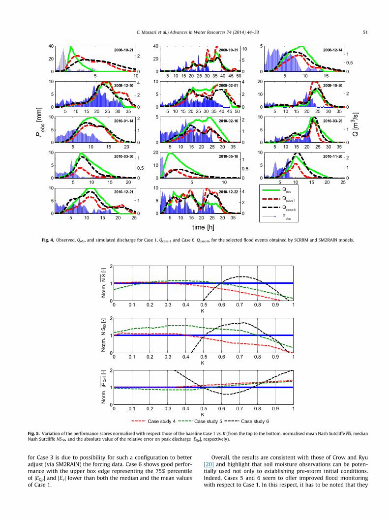
In this section, we present the performances obtained for thedifferent configurations of the models described in Section 2.4.The calibration is carried out for all case studies by maximisingNS. The values of the parameters obtained are presented in Table 3.Table 4 summarizes the value of NS obtained for each flood eventalong with the mean, the median, the maximum and the minimumNS. Case 1 yields NS = 0.48 with poor performance obtained for theevents of 21 October 2008, 30 March and 10 May 2010. Simulated(Qcase1) and observed discharge hydrographs (Qobs) are shown inFig. 4.

When only SM is used to estimate rainfall (Cases 2 and 3) thereis a slight degradation of the results (NS = 0.44 and 0.47, respec-tively). In particular, Case 2 provides the worst performance scoresin terms of NS among all the analysed case studies and comparableresults in NS50. Indeed, in Case 2 the use of only SM observationsdoes not allow to correctly represents the actual rainfall patternable to generate runoff (see Fig. 3), especially close to the satura-tion conditions where SM2RAIN provides larger underestimationof rainfall. For instance, the event of 1 February 2009 which showsa relatively high wetness condition at the beginning of the event(he = 0.54) provides a poor estimation of the rainfall pattern viaSM2RAIN (Fig. 3) which results in a low NS value in Table 4. Resultsof Case 3 are similar to Case 2 except that, in this case, the calibra-tion of the parameters of SM2RAIN – carried out along with thoseof SCRRM – helps to increase the performance scores for some ofthe selected events. In fact, in Case 3, the variations of the param-eters of SM2RAIN and SCRRM is clearly visible (see Table 3) forwhich, by way of example, amax strongly reduces to 136.6 mmwhile the parameters of SM2RAIN change significantly. The useof only SM observations for rainfall estimation is not always detri-mental (as shown in the second and the third column of Table 4 forthe event of 14 December 2008, 25 and 30 March 2010 and 21December 2010) and may provide considerable benefit to over-come potential errors in observed rainfall.

When the integration of observed rainfall and estimated rainfallvia SM2RAIN is taken into account by means of Eq. (8) (Cases 4–6),the performance scores in terms of NS increase progressively from0.51 to 0.66. In particular, for Case 4, when both the parameters ofSM2RAIN and SCRRM are constrained to the ones used for Case 2and Case 1, respectively, and leaving K to vary between 0 and 1,we see an improvement with respect to Case 1. However, theimprovement is limited to NS = 0.51 and NS50 = 0.53 (vs. NS = 0.48and NS50 = 0.49 of Case 1). Fig. 5 plots the normalised NS, NS50

and |EQp| for different K values for Cases 4–6. It can be seen that

Table 3parameters of SM2RAIN and SCRRM models obtained for the six analysed case studies.

Case 1 Case 2 Case 3 Case 4 Case 5 Case 6

k [–] 0.0001 0.0001 0.0001 0.0001 0.0001 0.0001g [–] 1.08 2.68 2.95 1.08 1.58 1.82amax [mm] 941.16 605.97 136.6 941.16 613.26 88.04Z [mm] 15.82 35.70 15.82 15.82 10.00a [mm] 13.01 4.80 13.01 13.01 4.11b [–] 2.57 2.23 2.57 2.57 3.25K [–] – – 0.16 0.36 0.71

42 120 174 246 324 396 450 516 582 636 678 7320

20

40

60

80

Rai

nfal

l [m

m/6

h]

t [h]

PobsPSM

Fig. 3. Observed Pobs, and estimated PSM 6-h cumulated rainfall for the 14 events selected in this study.

Table 4Nash–Sutcliffe performance scores obtained in the six selected case studies for each ofthe selected flood event. NS and NS50, Max and Min refer to mean, the median, theminimum and the maximum Nash Sutcliffe.

Event Case 1 Case 2 Case 3 Case 4 Case 5 Case 6

21-Oct-2008 0.01 �0.17 �0.24 0.25 �0.14 �0.5431-Oct-2008 0.78 0.62 0.66 0.89 0.89 0.8914-Dec-2008 0.64 0.82 0.74 0.52 0.72 0.8730-Dec-2008 0.73 0.75 0.84 0.81 0.79 0.8601-Feb-2009 0.84 0.38 0.46 0.86 0.88 0.7420-Oct-2009 0.47 0.39 0.50 0.83 0.89 0.8714-Jan-2010 0.86 0.68 0.71 0.76 0.84 0.9016-Feb-2010 0.40 0.03 0.13 0.30 0.49 0.5125-Mar-2010 0.62 0.73 0.73 0.62 0.81 0.8430-Mar-2010 0.10 0.75 0.86 0.15 0.62 0.8710-May-2010 0.11 �0.13 �0.11 0.01 0.00 0.2420-Nov-2010 0.43 0.28 0.31 0.53 0.85 0.8221-Dec-2010 0.50 0.71 0.71 0.49 0.72 0.8222-Dec-2010 0.22 0.26 0.24 0.08 �0.65 0.59NS 0.48 0.44 0.47 0.51 0.55 0.66NS50 0.49 0.51 0.58 0.53 0.76 0.83Max 0.86 0.82 0.86 0.89 0.89 0.90Min 0.01 �0.17 �0.24 0.01 �0.65 �0.54

50 C. Massari et al. / Advances in Water Resources 74 (2014) 44–53

using the integration in Case 4 does not produce significantbenefits. To explore further the integration between Pobs and PSM

by Eq. (8), in Case 5, the calibration is carried out only on theparameters of SCRRM and the parameter K. In Fig. 5 it can be seenthat the optimal K for NS range from 0.2 to 0.55 (the best K is 0.36).For NS50 and |EQp| the increments in performance are obtained for awider range of K values: K = 0–0.8 and K = 0–0.5, respectively.

Case 6 provides the best performance among the analysed casestudies with NS about 15% greater than Case 1. Overall, theimprovement in NS is present for most of the events except forthose of 21 October 2008 (that performs badly in every case study)and 01 February 2009 (which shows the problems already men-tioned above). Considering that K is assumed temporally constant,it is expected that allowing K to vary in time using data assimila-tion techniques, would produce even better performance. The inte-gration of rainfall with SM observations significantly improves the

flood modelling particularly for the events of 25–30 March 2010,20 November 2010 and 21 December 2010 as well as for the eventof 20 October 2009, for which (all the mentioned events) either therainfall accumulation is low or the wetness condition at the begin-ning of the event is dry. In particular, for the event of 21 December2010 – with NS = 0.89 – the benefit of the assimilation is significantas it would be expected by looking at the good results obtained forCases 2 and 3. For Case 6 the parameter K in Eq. (8) is equal to 0.71indicating that observed rainfall is corrected to about 70% of thedifferences between observed and simulated rainfall. It has to notethat such integration may account both for the errors in observedrainfall (if any) and errors in the underlying physical processes notwell taken into account by SCRRM. For Case 6 the benefit of theintegration is limited to optimal K values ranging from 0.6 to 0.8.The narrower range with respect to the Case 5 can be attributedto a different solution found by the calibration procedure. Althoughthis range is more contracted, the benefits of the integration aremuch larger giving, as a way of example, a NS50 almost twice largerthan Case 1.

Generally the benefit of the assimilation is more significant forsmaller events and less significant for high saturation conditionsand heavy rainfall event (as expected), whereas, events for whichSCRRM already performs very poorly are hard to be improved. Asan example, the events of 21 October 2008 and 10 May 2010 yieldbad performances for all the analysed case studies. For these twoevents the rainfall pattern is very different to the one observedfor the other selected events. In particular, they show a high rain-fall intensity concentrated in a short time period. Runoff coeffi-cients are very small (21 October 2008 has the smallest RC) andthe response of the catchment is faster with respect to the otherevents, thus SCRRM is not able to properly reproducing the floodhydrograph.

The box-plots in Fig. 6 of the absolute percentage error in vol-ume and on peak discharge confirm the previous findings. As itcan be seen, there is a progressive improvement both on peakdischarge and in volume from Case 3 to 6 both in median (red hor-izontal line) and in mean (black dot). Case 2 produces worst resultsamong all the analysed cases studies. The low error in volume

0

20

40

5 100

22008-10-21

0

20

40

5 10 15 20 25 30 35 40 45 500

5

102008-10-31

0

5

5 10 150

0.5

12008-12-14

0

5

10

5 10 15 20 25 30 350

2

42008-12-30

0

5

10

5 10 15 20 25 30 35 40 45 500

2

42009-02-01

0

10

20

5 10 15 20 25 30 350

2

2009-10-20

0

5

10

5 10 15 200

1

22010-01-14

0

5

5 10 15 20 25 30 350

1

22010-02-16

0

5

10

5 10 15 20 25 30 350

1

2010-03-25

0

5

10

5 10 15 200

0.5

12010-03-30

0

10

20

5 100

0.5

12010-05-10

0

5

10

5 10 15 20 250

1

22010-11-20

0

5

10

5 10 15 20 250

1

2010-12-21

0

5

10

5 10 15 20 25 30 350

2

42010-12-22

Pobs [

mm

]

Q [m

3 /s]

time [h]

Qobs

Qcase-1

Qcase-6

Pobs

Fig. 4. Observed, Qobs, and simulated discharge for Case 1, Qcase-1 and Case 6, Qcase-6, for the selected flood events obtained by SCRRM and SM2RAIN models.

0 0.1 0.2 0.3 0.4 0.5 0.6 0.7 0.8 0.9 10

1

2

K

Nor

m, N

S[-]

0 0.1 0.2 0.3 0.4 0.5 0.6 0.7 0.8 0.9 10

1

2

K

Nor

m.

NS 5

0[-]

0 0.1 0.2 0.3 0.4 0.5 0.6 0.7 0.8 0.9 10

1

2

K

Nor

m.

jEQ

Pj[

-]

Case study 4 Case study 5 Case study 6

Fig. 5. Variation of the performance scores normalised with respect those of the baseline Case 1 vs. K (from the top to the bottom, normalised mean Nash Sutcliffe NS, medianNash Sutcliffe NS50, and the absolute value of the relative error on peak discharge |EQp|, respectively).

C. Massari et al. / Advances in Water Resources 74 (2014) 44–53 51

for Case 3 is due to possibility for such a configuration to betteradjust (via SM2RAIN) the forcing data. Case 6 shows good perfor-mance with the upper box edge representing the 75% percentileof |EQp| and |Ev| lower than both the median and the mean valuesof Case 1.

Overall, the results are consistent with those of Crow and Ryu[20] and highlight that soil moisture observations can be poten-tially used not only to establishing pre-storm initial conditions.Indeed, Cases 5 and 6 seem to offer improved flood monitoringwith respect to Case 1. In this respect, it has to be noted that they

(a) (b)

0

10

20

30

40

50

60

70

80

90

1 2 3 4 5 6Case study

|EQp|

[%]

Mean

0

20

40

60

80

100

1 2 3 4 5 6Case study

|EV

| [%

]

Mean

Fig. 6. boxplots of the absolute value of the errors on peak discharge, |EQp| (a), and in runoff volume, |EV| (b).The horizontal red lines represent the medians; the upper and thelower edges of the blue boxes represent the 75% and the 25% percentiles; dashed black lines point to the minimum and maximum; red crosses are out-layers; black dots arethe means. (For interpretation of the references to color in this figure legend, the reader is referred to the web version of this article.)

52 C. Massari et al. / Advances in Water Resources 74 (2014) 44–53

are also based on a higher-number of fitted parameters whichmight reflect some degree of over-fitting. However, the improve-ment is significant not only for the calibration score (i.e., NS) butalso for the other considered indexes (i.e., |EQp| and |Ev|). In addi-tion, as a way of example, Case 3 is characterised by a larger num-ber of parameters with respect to Case 1 (the parameters of themodel SCRRM plus those of SM2RAIN calibrated altogether) butit does not provide any improvement in NS and |EQp|.

To further check the benefit of SM observations in flood model-ling, we have performed a calibration–validation procedure forCase 1 and Case 6. We used seven events in calibration (the 2nd,4th, 6th, 8th, 10th, 12th, 14th) and the other seven in validation(the 1st, 3rd, 5th, 7th, 9th, 11th and 13th). Using Case 1 as a base-line (as it was done for producing Fig. 5), we calculated the norma-lised NS obtaining 1.65 in 1.32 in calibration and validation,respectively (note that considering the calibration against all theselected events a normalised NS equal to 1.38 was obtained). Byswitching the events (i.e. using the second set of events in calibra-tion and the remainder of them in validation), we still obtained animprovement with normalised NS equal to 1.24 in calibration and1.33 in validation.

5. Conclusions

In this study, the potential of the use of SM observations forimproving flood modelling is highlighted by coupling a rainfallestimation method (SM2RAIN, [13,14]) and a simplified continuousRR model (SCRRM, [31]), using SM both to estimate rainfall and toinitialize the RR model. A simple integration technique is used tooptimally merge observed and estimated rainfall from SM observa-tions via SM2RAIN. Although the proposed approach is relativelysimple, the results demonstrate the high potential of SM data toimprove flood modelling. Indeed, an appropriate configuration ofSCRRM and SM2RAIN allows obtaining significant improvementof the selected performance scores with respect to the situationwhere SM observations are used solely to initialize the hydrologi-cal model.

The integration of different type of data and a deeper analysis ofthe assumptions associated with SM2RAIN can surely help toincrease the quality and the robustness of the proposed approach.Moreover, its applicability needs to be evaluated using differentsources of data including ground and remote sensing measure-ments worldwide.

In summary, this study highlights that SM observations retain ahigh information content and importance in flood modelling,which are, to our point of view, not yet fully taken into account.Moreover, due to the recent availability of improved-accuracy-soilmoisture estimates from remote sensing, the proposed method canbe potentially applied in partially gauged or even ungauged catch-ments. In this respect, this may have significant implications forpractical hydrological applications especially where observedrainfall data might be highly uncertain or scarce.

Acknowledgements

The writers would like to express special acknowledgments toanonymous reviewers for their valuable comments and remarks,which helped to improve the manuscript.

References

[1] Aubert D, Loumagne C, Oudin L. Sequential assimilation of soil moisture andstreamflow data in a conceptual rainfall runoff model. J. Hydrol. 2003;280(1–4):145–61. http://dx.doi.org/10.1016/S0022-1694(03)00229-4.

[2] Balsamo G, Albergel C, Beljaars A, Boussetta S, Brun E, Cloke H, Dee D, Dutra E,Pappenberger F, de Rosnay P, Muñoz Sabater J, Stockdale T, Vitart F. ERA-interim/land: a global land-surface reanalysis based on ERA-Interimmeteorological forcing. Era report series: European centre for medium rangeweather forecasts (ECWMF); 2012.

[3] Bartalis Z, Wagner W, Naeimi V, Hasenauer S, Scipal K, Bonekamp H, Figa J,Anderson C. Initial soil moisture retrievals from the METOP-A advancedscatterometer (ASCAT). Geophys Res Lett 2007;34(20):L20401. http://dx.doi.org/10.1029/2007GL031088.

[4] Beck HE, de Jeu RAM, Schellekens J, van Dijk AIJM, Bruijnzeel LA. Improvingcurve number based storm runoff estimates using soil moisture proxies.Selected topics in applied earth observations and remote sensing. IEEE J Sel TopAppl Earth Obs Remote Sens 2009;2:250–9. http://dx.doi.org/10.1109/JSTARS.2009.2031227.

[5] Beven K, Freer J. A dynamic TOPMODEL. Hydrol Process 2001;15:1993–2011.http://dx.doi.org/10.1002/hyp.252.

[6] Brocca L, Melone F, Moramarco T, Singh VP. Assimilation of observed soilmoisture data in storm rainfall-runoff modeling. J Hydrol Eng2009;14(2):153–65. http://dx.doi.org/10.1061/(ASCE)1084-0699(2009)14:2(153).

[7] Brocca L, Melone F, Moramarco T. Antecedent wetness conditions based on ERSscatterometer data in support to rainfall-runoff modeling. J Hydrol2009;364(1–2):73–86. http://dx.doi.org/10.1016/j.jhydrol.2008.10.007.

[8] Brocca L, Melone F, Moramarco T, Wagner W, Naeimi V, Bartalis Z, HasenauerS. Improving runoff prediction through the assimilation of the ASCAT soilmoisture product. Hydrol Earth Syst Sci 2010;14(10):1881–93. http://dx.doi.org/10.5194/hess-14-1881-2010.

[9] Brocca L, Melone F, Moramarco T. Distributed rainfall-runoff modelling forflood frequency estimation and flood forecasting. Hydrol Process2011;25(18):2801–13. http://dx.doi.org/10.1002/hyp.8042.

C. Massari et al. / Advances in Water Resources 74 (2014) 44–53 53

[10] Brocca L, Melone F, Moramarco T, Wagner W. What perspective in remotesensing of soil moisture for hydrological applications by coarse-resolutionsensors. In: Neale Christopher MU, Maltese Antonino, editors. Proc. SPIE, vol.8174; 2011b.

[11] Brocca L, Hasenauer S, Lacava T, Melone F, Moramarco T, Wagner W, Dorigo W,Matgen P, Martínez-Fernández J, Llorens P, Latron J, Martin C, Bittelli M. Soilmoisture estimation through ASCAT and AMSR-E sensors: an intercomparisonand validation study across Europe. Remote Sens Environ 2011;115:3390–408.http://dx.doi.org/10.1016/j.rse.2011.08.003.

[12] Brocca L, Moramarco T, Melone F, Wagner W, Hasenauer S, Hahn S.Assimilation of surface and root-zone ASCAT soil moisture products intorainfall-runoff modelling. IEEE Trans Geosci Remote Sens2012;50(7):2542–55. http://dx.doi.org/10.1109/TGRS.2011.2177468.

[13] Brocca L, Moramarco T, Melone F, Wagner W. A new method for rainfallestimation through soil moisture observations. Geophys Res Lett2013;40(5):853–8. http://dx.doi.org/10.1002/grl.50173.

[14] Brocca L, Ciabatta L, Massari C, Moramarco T, Hahn S, Hasenauer S, Kidd R,Dorigo W, Wagner W, Levizzani V. Soil as a natural rain gauge: estimatingglobal rainfall from satellite soil moisture data. J Geophys Res Atmos2014;119(9):5128–41. http://dx.doi.org/10.1002/2014JD021489.

[15] Burnash RJC, Ferral RL, McGuire RA. Report by the joint federal state riverforecasts center, Sacramento, CA; 1973.

[16] Chen F, Crow WT, Starks PJ, Moriasi DN. Improving hydrologic predictions ofcatchment model via assimilation of surface soil moisture. Adv Water Resour2011;34(4):526–36. http://dx.doi.org/10.1016/j.advwatres.2011.01.011.

[17] Chen F, Crow WT, Ryu D. Dual forcing and state correction via soil moistureassimilation for improved rainfall-runoff modeling. J Hydrometeorol 2014.http://dx.doi.org/10.1175/JHM-D-14-0002.1 (on line).

[18] Ciabatta L, Brocca L, Moramarco T, Wagner W. Comparison of different satelliterainfall products over the Italian territory. In: Conference Proceeding of XIIinternational IAEG congress, IAEG XII congress – Torino, September 15–19,2014; in press.

[19] Coustau M, Bouvier C, Borrell-Estupina V, Jourde H. Flood modelling with adistributed event-based parsimonious rainfall-runoff model: case of thekarstic Lez river catchment. Nat Hazards Earth Syst Sci 2012;12(4):1119–33.http://dx.doi.org/10.5194/nhess-12-1119-2012.

[20] Crow WT, Ryu D. A new data assimilation approach for improving runoffprediction using remotely-sensed soil moisture retrievals. Hydrol Earth SystSci 2009;13(1):1–16. http://dx.doi.org/10.5194/hess-13-1-200.

[21] Crow WT, van den Berg MJ, Huffman GJ, Pellarin T. Correcting rainfall usingsatellite-based surface soil moisture retrievals: the soil moisture analysisrainfall tool (SMART). Water Resour Res 2011;47:W08521. http://dx.doi.org/10.1029/2011WR010576.

[22] Dharssi I, Bovis KJ, Macpherson B, Jones CP. Operational assimilation of ASCATsurface soil wetness at the met office. Hydrol Earth Syst Sci2011;15(8):2729–46. http://dx.doi.org/10.5194/hess-15-2729-2011.

[23] Dorigo WA, Wagner W, Hohensinn R, Hahn S, Paulik C, Drusch M, MecklenburgS, van Oevelen P, Robock A, Jackson T. The international soil moisture network:a data hosting facility for global in situ soil moisture measurements. HydrolEarth Syst Sci 2011;15(5):1675–98. http://dx.doi.org/10.5194/hess-15-1675-2011.

[24] Francois C, Quesney A, Ottle C. Sequential assimilation of ERS-1 SAR data into acoupled land surface – hydrological model using an extended Kalman filter. JHydrometeorol 2003;4(2):473–87. http://dx.doi.org/10.1175/1525-7541(2003)4<473:SAOESD>2.0.CO;2.

[25] Georgakakos KP, Baumer OW. Measurement and utilization of on-site soilmoisture data. J Hydrol 1996;184(1–2):131–52. http://dx.doi.org/10.1016/0022-1694(95)02971-0.

[26] Grayson RB, Western AW, Chiew FHS, Böschl G. Preferred states in spatial soilmoisture patterns: local and nonlocal controls. Water Resour Res1997;33:2897–908. http://dx.doi.org/10.1029/97WR02174.

[27] Gupta V, Waymire C. A representation of an instantaneous unit hydrographfrom geomorphology. Water Resour Res 1980;16:855–62. http://dx.doi.org/10.1029/WR016i005p00855.

[28] Kerr YH, Waldteufel P, Wigneron J-P, Delwart S, Cabot F, Boutin J, EscorihuelaM-J, Font J, Reul N, Gruhier C, Juglea SE, Drinkwater MR, Hahne A, Martin-NeiraM, Mecklenburg S. The SMOS mission: new tool for monitoring key elementsof the global water cycle. Proc IEEE 2010;98:666–87. http://dx.doi.org/10.1109/JPROC.2010.2043032.

[29] Kirchner JW. Catchments as simple dynamical systems: catchmentcharacterization, rainfall-runoff modeling, and doing hydrology backward.Water Resour Res 2009;45:W02429. http://dx.doi.org/10.1029/2008WR006912.

[30] Manfreda S, Fiorentino M, Iacobellis V. DREAM: a distributed model for runoff,evapotranspiration, and antecedent soil moisture simulation. Adv Geosci2005;2:31–9. http://dx.doi.org/10.5194/adgeo-2-31-2005.

[31] Massari C, Brocca L, Barbetta S, Papathanasiou C, Mimikou M, Moramarco T.Using globally available soil moisture indicators for flood modelling inmediterranean catchments. Hydrol Earth Syst Sci 2014;10(8):10997–1033.http://dx.doi.org/10.5194/hess-18-839-2014.

[32] Matgen P, Fenicia F, Heitz S, Plaza D, de Keyser R, Pauwels VRN, Wagner W,Savenije H. Can ASCAT-derived soil wetness indices reduce predictiveuncertainty in well-gauged areas? A comparison with in situ soil moisturegauges in an assimilation application. Adv Water Resour 2012;44:49–65.http://dx.doi.org/10.1016/j.advwatres.2012.03.022.

[33] Meier P, Frömelt A, Kinzelbach W. Hydrological real-time modelling in theZambezi river basin using satellite-based soil moisture and rainfall data.Hydrol Earth Syst Sci 2011;15(3):999–1008. http://dx.doi.org/10.5194/hess-15-999-2011.

[34] Melone F, Corradini C, Singh VP. Lag prediction in ungauged basins: aninvestigation through actual data of the upper Tiber river valley. HydrolProcess 2002;16(5):1085–94. http://dx.doi.org/10.1002/hyp.313.

[35] Melone F, Neri N, Morbidelli R, Saltalippi C. A conceptual model for floodprediction in basins of moderate size. In: Hamza MH, editor. Appliedsimulation and modeling. California: IASTED Acta Press; 2001. p. 461–6.

[36] Moramarco T, Melone F, Singh VP. Assessment of flooding in urbanizedungauged basins: a case study in the Upper Tiber area – Italy. Hydrol Process2005;19:1909–24. http://dx.doi.org/10.1002/hyp.5634.

[37] Owe M, De Jeu R, Holmes T. Multisensor historical climatology of satellite-derived global land surface moisture. J Geophys Res 2008;113(F1):F01002.http://dx.doi.org/10.1029/2007JF000769.

[38] Pauwels VRN, Hoeben R, Verhoest NEC, DeTroch FP. The importance of thespatial patterns of remotely sensed soil moisture in the improvement ofdischarge predictions for small scale basins through data assimilation. J Hydrol2001;251(1–2):88–102. http://dx.doi.org/10.1016/S0022-1694(01)00440-1.

[39] Pauwels VRN, Hoeben R, Verhoest NEC, De Troch FP, Troch PA. Improvementsof TOPLATS-based discharge predictions through assimilation of ERS-basedremotely-sensed soil moisture values. Hydrol Process 2002;16(5):995–1013.http://dx.doi.org/10.1002/hyp.315.

[40] Pellarin T, Ali A, Chopin F, Jobard I, Bergès JC. Using space-borne surface soilmoisture to constrain satellite precipitation estimates over West Africa.Geophys Res Lett 2008;35:L02813. http://dx.doi.org/10.1029/2007GL032243.

[41] Soil Conservation Service (SCS). Hydrology, national engineeringhandbook. Washington, DC: Soil Conservation Service, USDA; 1993[supplement A, section 4].

[42] Sheikh V, Visser S, Stroosnijder L. A simple model to predict soil moisture:bridging event and continuous hydrological (BEACH) modelling. EnvironModell Softw 2009;24:542–56. http://dx.doi.org/10.1016/j.envsoft.2008.10.005.

[43] Todini E. The ARNO rainfall-runoff. J Hydrol 1996;175:339–82. http://dx.doi.org/10.1016/S0022-1694(96)80016-3.

[44] Tramblay Y, Bouvier C, Martin C, Didon-Lescot J-F, Todorovik D, Domergue JM.Assessment of initial soil moisture conditions for event-based rainfall-runoffmodelling. J Hydrol 2010;387(3–4):176–87. http://dx.doi.org/10.1016/j.jhydrol.2010.04.006.

[45] Tramblay Y, Bouvier C, Ayral P-A, Marchandise A. Impact of rainfall spatialdistribution on rainfall-runoff modelling efficiency and initial soil moistureconditions estimation. Nat Hazards Earth Syst Sci 2011;11(1):157–70. http://dx.doi.org/10.5194/nhess-11-157-2011.

[46] Tramblay Y, Bouaicha R, Brocca L, Dorigo W, Bouvier C, Camici S, Servat E.Estimation of antecedent wetness conditions for flood modelling in northernMorocco. Hydrol Earth Syst Sci 2012;16(11):4375–86. http://dx.doi.org/10.5194/hess-16-4375-2012.

[47] Wagner W, Bloschl G, Pampaloni P, Calvet J, Bizzarri B, Wigneron J, Kerr Y.Operational readiness of microwave remote sensing of soil moisture forhydrologic applications. Nordic Hydrol 2007;38(1):1–20. http://dx.doi.org/10.2166/nh.2007.029.