on self-concordant convex–concave functions

On Self-Concordant Convex-Concave Functions

Arkadi Nemirovski∗

April 19, 1999

Abstract

In this paper, we introduce the notion of a self-concordant convex-concave function, estab-lish basic properties of these functions and develop a path-following interior point methodfor approximating saddle points of “good enough” convex-concave functions – those whichadmit natural self-concordant convex-concave regularizations. The approach is illustratedby its applications to developing an exterior penalty polynomial time method for Semidef-inite Programming and to the problem of inscribing the largest volume ellipsoid into agiven polytope.

1 Introduction

Self-concordance-based approach to interior point methods for variational inequalities:state of the art. The self-concordance-based theory of interior point (IP) polynomial methods inConvex Programming [5] is commonly recognized as the standard approach to the design of theo-retically efficient IP methods for convex optimization programs. A natural question is whether thisapproach can be extended to other problems with convex structure, like saddle point problems forconvex-concave functions, and, more generally, variational inequalities with monotone operators. Thegoal of this paper is to make a step in this direction.

The indicated question was already considered in [5], Chapter 7. To explain what and why weintend to do, let us start with outlining the relevant results from [5].

We want to solve a variational inequality

(V) find z∗ ∈ clZ : (z − z∗)TA(z) ≥ 0 ∀z ∈ Z,

where Z is an open and, say, bounded convex set in RN and A(·) : Z → RN is a monotone operator.The domain Z of the inequality is equipped with a ϑ-self-concordant barrier (s.-c.b.) B ([5], Chapter2), and two classes of monotone operators on Z are considered:∗Faculty of Industrial Engineering and Management at Technion – the Israel Institute of Technology, Technion City,

Haifa 32000, Israel. e-mail: [email protected]. The research was partially funded by the Fund for thePromotion of Research at Technion, the G.I.F. contract No. I-0455-214.06/95 and the Israel Ministry of Science grant# 9636-1-96

1

(a) “self-concordant” (s.-c.);(b) “compatible with B”.

Both classes are defined in terms of certain differential inequalities imposed on A.

The variational inequalities which actually can be solved by the technique in question are thosewith operators of the type (b). In order to solve such an inequality, we associate with the operator ofinterest A the penalized family

{At(z) = tA(z) +B′(z)}t>0.

It turns out that every At is s.-c. and possesses a unique zero z∗(t) on Z, and that the path z∗(t)converges to the solution set of (V). In order to solve (V), we trace the indicated path:

Given current iterate (ti−1, zi−1) = (t, z) with z close, in certain precise sense, to z∗(t), weupdate (t, z) into a new pair (ti, zi) = (t+, z+), also close to the path, according to

(a) t+ = (1 + 0.01ϑ−1/2)t, (b) z+ = z − [(At+)′(z)]−1At+(z); (1)

here (At)′(z) is the Jacobian of the mapping At(·) at z.

It turns out that the outlined process converges to the set of solutions of (V) linearly (w.r.t. certainmeaningful accuracy measure) with the convergence ratio (1−O(1)ϑ−1/2).

The main ingredient of the complexity analysis of the outlined construction is an affine-invariantlocal theory of the Newton method for approximating zero of a s.-c. monotone operator. The methodis responsible for the “centering step” (1.b), and the penalty updating policy (1.a) is given by the desireto keep the previous iterate z in the domain of local quadratic convergence of the Newton method asapplied to At+ .

Note that in the potential case, i.e., when A(z) is the gradient field of a “good” (say, linear orquadratic) convex function f , the outlined scheme becomes the standard short-step IP method forminimizing f over Z, and the indicated complexity result yields the standard, the best known so fartheoretical complexity bound for the corresponding convex optimization program, which is a goodnews. The potential case, however, offers us much more, since here we possess not only a local, butalso a global affine-invariant convergence theory for the Newton method. As a result, in the potentialcase we may use instead of the penalty rate (1.a) other penalty updating policies as well, at the costof replacing a single pure Newton centering step (1.b) with several damped Newton steps, until therequired closeness to the new target point z∗(t+) is achieved. The number of required damped Newtonsteps can be bounded from above, in a universal data-independent fashion, via the residual

V (t+, z) = [t+f(z) +B(z)]−minz′

[t+f(z′) +B(z′)]

(t, z) being the previous iterate. Thus, in the potential case the Newton complexity (# of Newtonsteps in z per one updating of the penalty parameter t) of the path-following method in question canbe controlled not only for the worst-case oriented penalty updating policy (1.a), but for any otherpolicy capable to control the residuals V (t+, z). This observation provides us with possibility to tracethe path with “mediate” steps (arbitrary absolute constant instead of 0.01 in (1.a), see [5], Section3.2.6) or even with “long” on-line adjusted steps (see [6, 7]), which is very attractive for practicalcomputations.

In contrast to these favourable features of the potential case, in the case of a non-potential mono-tone operator A compatible with a s.-c.b. for clZ all which has been offered to the moment by the

2

self-concordance-based approach is the short-step policy (1.a). With current understanding of the sub-ject we are unable to say what happens with the method when the constant 0.01 in (1.a) is replacedby, say, 1. This is a definite bad news about the known so far extensions of the self-concordance-basedtheory to the case of variational inequalities: in order to get a complexity bound, no matter O(

√ϑ)-

one or worse, we should restrict ourselves with the worst-case-oriented and therefore very conservativeshort-step policy (1.a). This drawback of the theory finally comes from the fact that we have no globaltheory of convergence of the Newton method as applied to a (non-potential) s.-c. monotone operator.

The goal of this paper is to investigate the situation which is in-between the potential case andthe general monotone case, namely, the one of monotone mappings associated with convex-concavesaddle point problems. We intend to demonstrate that there exists a quite reasonable extension ofthe notion of a self-concordant convex function – the basic ingredient of the self-concordance-basedtheory of IP methods – to the case of convex-concave functions. The arising entities – self-concordantconvex-concave (s.-c.c.-c.) functions – possess a rich theory very similar to the theory developed in[5] for convex s.-c. functions. In particular, we develop a global theory of convergence of (a kind of)the Newton method as applied to the problem of approximating a saddle point of a s.-c.c.-c. function.Finally, this global theory allows us to build mediate-step path-following methods for approximatingsaddle point of a convex-concave function which is “compatible” with self-concordant barrier for itsdomain.

The contents of the paper is as follows. In Section 2 we introduce our central notion – the oneof a self-concordant convex-concave function – and investigate the basic properties of these functions.Section 3 is devoted to the duality theory for s.-c.c.-c. functions; the central result here is that the classin question is closed w.r.t. the Legendre transformation. The latter fact underlies the global theoryof (a kind of) the Newton method for approximating saddle point of a s.-c.c.-c. function (Section 5).Our main result here is that the number of Newton steps needed to pass from a point (x, y) from thedomain of a s.-c.c.-c. function f(x, y) to an ε-saddle point (x, y) – a point where

µ(x, y) ≡ supy′f(x, y′)− inf

x′f(x′, y) ≤ ε

– is bounded from above by a quantity of the type

Θ(µ(x, y)) +O(1) ln ln(ε−1 + 3),

where Θ(·) is a universal function and O(1) is an absolute constant. This result is very similar to thebasic result on the Newton method for minimizing a convex s.-c. function f : the number of Newtonsteps needed to pass from a point x of the domain of the function to an ε-minimizer of f – to a pointx where v(x) ≡ f(x)−min f ≤ ε – is bounded from above by O(1)[v(x) + ln ln(ε−1 + 3)].

Equipped with a global theory of our “working horse” – the Newton method for approximatingsaddle points of s.-c.c.-c. functions – we get the possibility to develop a general theory of path-followingmethod for approximating saddle points of convex-concave functions “compatible” with self-concordantbarriers for their domains. This development is carried out in Section 6. We conclude this Section byconstructing a polynomial time exterior penalty method for semidefinite programming problems (theconstruction works for linear and conic quadratic programming as well).

Finally, in Section 7 we apply our general constructions and results to the well-known problemof finding the maximum volume ellipsoid contained in a given polytope. This problem is of interest

3

for Control Theory (see [1]) and especially for Nonsmooth Convex Optimization, where it is the basicauxiliary problem arising in the Inscribed Ellipsoid method (Khachiyan, Tarasov, Erlikh [2]); the lattermethod, as applied to general convex problems, turns out to be optimal in the sense of Information-based Complexity Theory. The best known so far complexity estimates for finding an ε-optimal (withvolume ≥ (1 − ε) times the maximum one) ellipsoid inscribed into a n-dimensional polytope, givenby m = O(n) linear inequalities, are O(n4.5 ln(nε−1R)) and O(n3.5 ln(nε−1R) ln(nε−1 lnR)) arithmeticoperations (see [5], Chapter 6, and [3], respectively). Here R is an a priori known ratio of radii of twocentered at the origin Euclidean balls, the smaller being contained in, and the larger containing thepolytope. These complexity bounds are given by interior point methods as applied to the standardsemidefinite reformulation of the problem. The latter reformulation is of a “large” – O(n2) – designdimension. We demonstrate that the problem admits saddle point reformulation with “small” –O(n + m) – design dimension, and that the resulting saddle point problem can be straightforwardlysolved by the path-following method from Section 6; the arithmetic complexity of finding ε-optimalellipsoid in this manner turns out to be O(n3.5 ln(nε−1R)). In contrast to the complexity bounds from[5, 3], the indicated – better – bound arises naturally, without sophisticated ad hoc tricks heavilyexploiting problem’s structure.

The proofs of the major part of the results to be presented are rather technical. To improve thereadability of the paper, all such proofs are placed in Appendices.

2 Self-concordant convex-concave functions

In this section we introduce the main concept to be studied – the one of a self-concordant convex-concave (s.-c.c.-c.) function – and establish several basic properties of these functions.

2.1 Preliminaries: self-concordant convex functions

The notion of a s.-c.c.-c. function is closely related to the one of a self-concordant (s.-c.) convexfunction, see [5]. For reader’s convenience, we start with the definition of the latter notion.

Definition 2.1 Let X be an open nonempty convex domain in Rn. A function f : X → R is calledself-concordant (s.-c.) on X, if f is convex, C3 smooth and

(i) f is a barrier for X: f(xi)→∞ along every sequence of points xi ∈ X converging to a boundarypoint of X.

(ii) For every x ∈ X and h ∈ Rn one has

|D3f(x)[h, h, h]| ≤ 2(D2f(x)[h, h]

)3/2(2)

(from now on, Dkf(x)[h1, ..., hk] denotes k-th differential of a smooth function f taken at a point xalong directions h1, ..., hk).

If, in addition to (i), (ii), for some ϑ ≥ 1 and all x ∈ X, h ∈ Rn one has

|Df(x)[h]| ≤ ϑ1/2√D2f(x)[h, h],

then f is called ϑ-self-concordant barrier (s.-c.b.) for clX.A s.-c. function f is called nondegenerate, if f ′′(x) is nonsingular at least at one point (and then

– at every point, [5], Corollary 2.1.1) of the domain of the function.

4

For a nondegenerate s.-c. function f , the quantity

λ(f, x) =√

[f ′(x)]T [f ′′(x)]−1f ′(x) [x ∈ Domf ] (3)

is called the Newton decrement of f at x.

Note that what here is called self-concordance of a function in [5] is called strong self-concordance.A summary of the basic properties of convex s.-c. functions is as follows (for proofs, see [5, 4]):

Proposition 2.1 Let f be a convex s.-c. function. Then for every x ∈ Domf one has:

∀h : f(x) + hT f ′(x) + ρ

(−√hT f ′′(x)h

)≤ f(x+ h) ≤ f(x) + hT f ′(x) + ρ

(√hT f ′′(x)h

),

ρ(s) = −s− ln(1− s)(4)

(both f and ρ are +∞ outside their domains); in particular, if hT f ′′(x)h < 1, then x+ h ∈ Domf .Besides this,

hT f ′′(x)h < 1⇒

f ′′(x+ h) �(

1−√hT f ′′(x)h

)2

f ′′(x),

f ′′(x+ h) �(

1−√hT f ′′(x)h

)−2

f ′′(x)(5)

(from now on, an inequality A � B with symmetric matrices A,B of the same size means that A−Bis positive semidefinite).

In the case of a nondegenerate f one has

ρ (−λ(f, x)) ≤ f(x)− inf f ≤ ρ (λ(f, x)) . (6)

2.2 Self-concordant convex-concave functions: definition and local properties

We define the notion of a s.-c.c.-c. function as follows:

Definition 2.2 Let X,Y be open convex domains in Rn, Rm, respectively, and let

f(x, y) : X × Y → R

be C3 smooth function. We say that the function is self-concordant convex-concave on X × Y , if f isconvex in x ∈ X for every y ∈ Y , concave in y ∈ Y for every x ∈ X, and

(i) For every x ∈ X, [−f(x, ·)] is a barrier for Y , and for every y ∈ Y , f(·, y) is a barrier for X(ii) For every z = (x, y) ∈ X × Y and every dz = (dx, dy) ∈ Rn ×Rm one has

|D3f(z)[dz, dz, dz]| ≤ 2[dzTSf (z)dz]3/2, Sf (z) =(f ′′xx(z) 0

0 −f ′′yy(z)). (7)

A s.-c.c.-c. function f is called nondegenerate, if Sf (z) is positive definite for some (and then, as weshall see, for all) z ∈ Z.

Remark 2.1 Note that if f : X × Y → R is a s.-c.c.-c. function, then the convex function f(·, y) iss.-c. on X for every y ∈ Y , and the convex function −f(x, ·) is s.-c. on Y for every x ∈ X.

5

Our current goal is to establish several basic properties of s.-c.c.-c. functions.

Proposition 2.2 [Basic differential inequality and recessive subspaces] Let f(z) be a s.-c.c.-c. func-tion on Z = X × Y ⊂ Rn ×Rm. Then

(i) For every z ∈ Z and every triple dz1, dz2, dz3 of vectors from Rn ×Rm one has

|D3f(z)[dz1, dz2, dz3]| ≤ 23∏

j=1

√dzTj Sf (z)dzj (8)

(ii) Let E(z) = {dz = (dx, dy) | dzTSf (z)dz = 0}. Then

(ii.1) the subspace E(z) ≡ Ef is independent of z ∈ Z and is the direct sum of itsprojections Ef,x, Ef,y on Rn and Rm, respectively. In particular, if Sf is nondegenerateat some point of Z, then Sf is nondegenerate everywhere on Z.

(ii.2) Z = Z +Ef .

(iii) [Sufficient condition for nondegeneracy] If both X and Y do not contain straight lines, then fis nondegenerate.

The next statement says, roughly speaking, that a s.-c.c.-c. function f is fairly well approximatedby its second-order Taylor expansion at a point z ∈ Domf in the respective Dikin ellipsoid {z′|(z′ −z)TSf (z)(z′ − z) < 1}. This property (similar to the one of convex s.-c. functions) underlies all ourfurther developments.

Proposition 2.3 [Local properties] Let f : Z = X × Y → R, X ⊂ Rn, Y ⊂ Rm, be a s.-c.c.-c.function. Then

(i) For every z = (x, y) ∈ Z, the set W fx (z) = {x′ | (x′ − x)T f ′′xx(z)(x′ − x) < 1} is contained in

X, and the set W fy (z) = {y′ | (y′ − y)T [−f ′′yy(z)](y′ − y) < 1} is contained in Y .

(ii) Let z ∈ Z and h = (u, v) ∈ Rn ×Rm. Then

r ≡√hTSf (z)h < 1⇒

(a) z + h ∈ Z;(b) (1− r)2Sf (z) � Sf (z + h) � (1− r)−2Sf (z);(c) ∀(h1, h2 ∈ Rn ×Rm) :

|hT1 [f ′′(x+ z)− f ′′(x)]h2| ≤[

1(1−r)2 − 1

]√hT1 Sf (z)h1

√hT2 Sf (z)h2;

(d) ∀h′ ∈ Rn ×Rm :∣∣∣(h′)T [f ′(z + h)− f ′(z)− f ′′(z)h]∣∣∣ ≤ r2

1−r√

(h′)TSf (z)h′.

(9)

Relation to self-concordant monotone mappings. We conclude this section by demonstratingthat in the case of monotone mappings coming from convex-concave functions the notion of self-concordance of the mapping, as defined in [5], Chapter 7, is equivalent to self-concordance, as definedhere, of the underlying convex-concave function.

In [5], Chapter 7, a strongly self-concordant monotone mapping is defined as a single-valued C2

monotone mapping A(·) defined on an open convex domain Z such that

6

1. For every z ∈ Z and every triple of vectors h1, h2, h3 one has

|hT2∇2z(h

T1 A(z))h3| ≤ 2

3∏

i=1

√hTi A(z)hi, A(z) =

12

[A′(z) + [A′(z)]T

]; (10)

2. Whenever a sequence {zi ∈ Z} converges to a boundary point of Z, the sequence of matrices{A(zi)} is unbounded.

Proposition 2.4 Let f(x, y) : Z = X × Y → R be C3 convex-concave function, X, Y being openconvex sets in Rn, Rm, respectively. The function is s.-c.c.-c. if and only if the monotone mapping

A(x, y) =(f ′x(x, y)−f ′y(x, y)

): Z → Rn+m

is strongly self-concordant.

2.3 Saddle points of self-concordant convex-concave functions: existence anduniqueness

Our ultimate goal is to approximate saddle points of s.-c.c.-c. functions, and to this end we shouldknow when saddle points do exist. The simple necessary and sufficient condition to follow is completelysimilar to the fact that a convex s.-c. function attains its minimum if and only if it is below bounded:

Proposition 2.5 Let f(z) be a nondegenerate s.-c.c.-c. function on Z = X × Y ⊂ Rn ×Rm. Thenf possesses a saddle point on Z if and only if

(*) f(x0, ·) is above bounded on Y for some x0 ∈ X, and f(·, y0) is below bounded onX for some y0 ∈ Y .

Whenever (*) is the case, the saddle point of f on Z is unique.

3 Duality for self-concordant convex-concave functions

We are about to study the notion heavily exploited in the sequel – the one of the Legendre trans-formation of a nondegenerate s.-c.c.-c. function. The construction goes back to Rockafellar [8] anddefines the Legendre transformation of a convex-concave function f(x, y) as

f∗(ξ, η) = infy

supx

[ξTx+ ηT y − f(x, y)]

(cf. the definition of the Legendre transformation of a convex function f : f∗(ξ) = supx

[ξTx − f(x)]).

Our local goal is to describe the domain of the Legendre transformation of a nondegenerate s.-c.c.-c.function and to demonstrate that this transformation also is s.-c.c.-c.

Definition 3.1 Let f(z) be a s.-c.c.-c. function on Z = X × Y ⊂ Rn ×Rm. We say that a vectorξ ∈ Rn is x-appropriate for f , if the function ξTx − f(x, y) is above bounded on X for some y ∈ Y .Similarly, we say that a vector η ∈ Rm is y-appropriate for f , if the function ηT y − f(x, y) is belowbounded on Y for some x ∈ X. We denote by X∗(f) the set of those ξ which are x-appropriate for f ,and denote by Y ∗(f) the set of those η which are y-appropriate for f .

7

Proposition 3.1 Let f(z) be a nondegenerate s.-c.c.-c. function on Z = X × Y ⊂ Rn ×Rm. Then(i) The sets X∗(f) and Y ∗(f) are open nonempty convex sets in Rn, Rm, respectively;(ii) The set Z∗(f) = X∗(f) × Y ∗(f) is exactly the set of those pairs (ξ, η) ∈ Rn ×Rm for which

the functionfξ,η(x, y) = f(x, y)− ξTx− ηT y

possesses a saddle point (min in x, max in y) on X × Y ;(iii) The set Z∗(f) = X∗(f)× Y ∗(f) is exactly the image of the set Z under the mapping

z 7→ f ′(z)

and the mapping is a one-to-one twice continuously differentiable mapping of Z onto Z∗(f) with twicecontinuously differentiable inverse;

(iv) The functionf∗(ξ, η) = inf

y∈Ysupx∈X


is s.-c.c.-c. on Z∗(f) and is equal to

supx∈X

infy∈Y

[ξTx+ ηT y − f(x, y)],

and the mappingζ 7→ f ′∗(ζ)

is inverse to the mapping z 7→ f ′(z).

Definition 3.2 Let f : Z = X × Y → R be a nondegenerate s.-c.c.-c. function. The function

f∗ : Z∗(f) = X∗(f)× Y ∗(f)→ R

defined in Proposition 3.1 is called the Legendre transformation of f .

Theorem 3.1 The Legendre transformation f∗ of a nondegenerate s.-c.c.-c. function f is a nonde-generate s.-c.c.-c. function, and f is the Legendre transformation of f∗. Besides this, one has

{z ∈ Z, ζ = f ′(z)} ⇔ {ζ ∈ Z∗(f), z = f ′∗(ζ)} ⇒

(a) f ′′(z) = [f ′′∗ (ζ)]−1;(b) [f ′′(z)]−1Sf (z)[f ′′(z)]−1 = Sf∗(ζ);(c) f(z) + f∗(ζ) = ζT z.

(11)

4 Operations preserving self-concordance of convex-concave func-tions

In order to apply the machinery we are developing, we need tools to recognize self-concordance ofa convex-concave function. These tools are given by (A) a list of “raw materials” – simple s.-c.c.-c.functions, and (B) a list of “combination rules” preserving the property in question. The simplestversions of (A) and (B), following immediately from Definition 2.2, can be described as follows:

8

Proposition 4.1 (i) Let f(x, y) be a quadratic function of (x, y) which is convex in x ∈ Rn andconcave in y ∈ Rm. Then f is s.-c.c.-c. function on Rn ×Rm.

(ii) Let φ(x), ψ(y) be s.-c. convex functions on X ⊂ Rn, Y ⊂ Rm, respectively. Then f(x, y) =φ(x)− ψ(y) is a s.-c.c.-c. function on X × Y .

(iii) Let Xi ⊂ Rn, Yi ⊂ Rm, let αi ≥ 1, and let fi be s.-c.c.-c. function on Zi = Xi×Yi, i = 1, ..., k.

If the set Z =k⋂i=1

Zi is nonempty, then the function f(z) =k∑i=1

αifi(z) is s.-c.c.-c. on Z.

(iv) Let f(z) be s.-c.c.-c. function on Z = X × Y ⊂ Rn ×Rm, and let Π(u, v) =(x = Pu+ py = Qv + q

)

be affine mapping from Rν × Rµ to Rn × Rm with the image intersecting Z. Then the functionφ(u, v) = f(Π(u, v)) is s.-c.c.-c. on Π−1(Z).

More “advanced” combination rules (Propositions 4.3, 4.4 below) state, essentially, that mini-mization/maximization of a s.-c.c.-c. function with respect to (a part of) “convex”, respectively,“concave”, variables preserves the self-concordance. To arrive at the corresponding results, we startwith important by its own right “dual representation” of the extremum values of a s.-c.c.-c. function.

Proposition 4.2 Let f : Z = X × Y → R be a nondegenerate s.-c.c.-c. function, and let f∗ : Z∗ =X∗ × Y ∗ → R be the Legendre transformation of f . Then

(i) Whenever y ∈ Y , the function f(·, y) is below bounded on X if and only if 0 ∈ X∗ and thefunction ηT y − f∗(0, η) is below bounded on Y ∗. When it is the case, one has

infx∈X

f(x, y) = minx∈X

f(x, y) = minη∈Y ∗

[ηT y − f∗(0, η)]; (12)

(ii) Whenever x ∈ X, the function f(x, ·) is above bounded on Y if and only if 0 ∈ Y ∗ and thefunction ξTx− f∗(ξ, 0) is above bounded on X∗. When it is the case, one has

supy∈Y

f(x, y) = maxy∈Y

f(x, y) = maxξ∈X∗

[ξTx− f∗(ξ, 0)].

Proposition 4.3 Let f(x, y) : Z ≡ X × Y → R be a nondegenerate s.-c.c.-c. function. If the setX+ = {x ∈ X | sup

y∈Yf(x, y) <∞} is nonempty, then it is an open convex set, and the function

f(x) = supy∈Y

f(x, y) : X+ → R

is a s.-c. convex function on X+.Similarly, if the set Y + = {y ∈ Y | inf

x∈Xf(x, y) > −∞} is nonempty, then it is an open convex

set, and the negative of the function

f(y) = infx∈X

f(x, y) : Y + → R

is a s.-c. convex function on Y +.

In the case when one of the sets X, Y – say, Y – is bounded, the latter proposition can bestrengthened as follows:

9

Proposition 4.4 Let f : Z ≡ X × Y → R be a nondegenerate s.-c.c.-c. function, and let the set Ybe bounded. Let also y = (u, v) be a partitioning of the variables y, and let U be the projection of Yonto the u-space. Then the function

φ(x, u) = maxv:(u,v)∈Y

f(x, (u, v)) : X × U → R (13)

is nondegenerate s.-c.c.-c.

5 The Saddle Newton method

5.1 Outline of the method

The crucial role played by self-concordance in the theory of interior-point polynomial time methodsfor convex optimization comes from the fact that these functions are well-suited for the Newtonminimization. Specifically, if f is a nondegenerate s.-c. convex function, then a (damped) Newtonstep

x 7→ x+ = x− 11 + λ(f, x)

[f ′′(x)]−1f ′(x) (14)

(see (3)) maps Domf into itself and(A) reduces f at least by O(1), provided that λ(f, x) is not small: f(x+) ≤ f(x)− ρ(−λ(f, x));(B) always “nearly squares” the Newton decrement: λ(f, x+) ≤ 2λ2(f, x).Property (A) ensures global convergence of the Newton minimization method, provided that f is

below bounded: by (A), the number of Newton steps before a point x with λ(f, x) ≤ 0.25 is reached,does not exceed O(1)(f(x)− inf f), x being the starting point. Property (B) ensures local quadraticconvergence of the method in terms of the Newton decrement (and in fact – in terms of the residualf(x)−min f , since this residual can be bounded from above in terms of the Newton decrement solely,provided that the latter is less than 1). As a result, for every ε < 0.5, an ε-minimizer of f – a point xsatisfying f(x)−min f ≤ ε – can be found in no more than

O(1)(

[f(x)−min f ] + ln ln1ε

)(15)

steps of the damped Newton method (14).When passing from approximating the minimizer of a nondegenerate s.-c. convex function to

approximating the saddle point of a nondegenerate s.-c.c.-c. function f , a natural candidate to therole of the Newton iteration is something like

z 7→ z+ = z − γ(z)[f ′′(z)]−1f ′(z), (16)

γ(z) being a stepsize. For such a routine, there is no difficulty with extending (B) (see [5], Chapter 7)and thus – with establishing local quadratic convergence. There is, however, a severe difficulty withextending (A), and, consequently, with establishing global convergence of the method, since now itis unclear what could play the role of the Lyapunov function of the process, the role played in theminimization case by the objective itself. To overcome this difficulty, recall that process (16), startedat a point z, is a discretization of the “continuous time” process

d

dsz = −[f ′′(z)]−1f ′(z), z(0) = z,

10

and that the trajectory of the latter process is, up to the re-parameterization s 7→ t = exp{−s}, thepath given by

f ′(z(t)) = tf ′(z), 1 ≥ t ≥ 0, (17)

so that z(t) is the saddle point of a s.-c.c.-c. function ft(z) = f(z)− tzT f ′(z). Now, path (17) can betraced not only by (16), but via the path-following scheme

(tk, zk) 7→(tk+1 < tk, zk+1 = zk − [f ′′tk+1(zk)]−1f ′tk+1(zk)

), (t1, z1) = (1, z). (18)

An advantage of (18) as compared to (16) is that with a proper control of the rate at which thehomotopy parameter tk decreases with k, zk all the time is in the domain of quadratic convergence, asgiven by a straightforward “saddle point” extension of (B), of the Newton method as applied to ftk+1 .Thus, one can analyze process (18) on the basis of the results on local convergence of the Newtonmethod for approximating saddle points. The resulting complexity bound for (18) (see Theorem 5.1below) states that the number of steps of (18) required to reach an ε-saddle point – a point z satisfying

µ(f, z) ≡ supy′f(x, y′)− inf

x′f(x′, y) ≤ ε [z = (x, y)]

for ε < 0.5 is bounded from above by

Θ(µ(zini)) +O(1) ln ln1ε, (19)

where Θ(·) is an universal (i.e., problem-independent) continuous function on the nonnegative ray.Note that the residual µ(f, z) is a natural extension to the saddle point case of the usual residualφ(x)−minφ associated with the problem of minimizing a function φ (indeed, the latter problem canbe though of as the problem of finding a saddle point of the function f(x, y) ≡ φ(x), and µ(f, (x, y)) =φ(x)−minφ). Thus, the complexity bound (19) is of the same spirit as the bound (15), up to the factthat in the minimization case the universal function Θ(·) is just linear.

The goal of this section is to implement the outlined scheme and to establish (19).

5.2 Newton decrement and proximities

We start with introducing several quantities relevant to the construction outlined in the previoussubsection.

Definition 5.1 Let f : Z = X×Y → R be a nondegenerate s.-c.c.-c. function, and let z = (x, y) ∈ Z.We define• the Newton direction of f at z as the vector e(f, z) = [f ′′(z)]−1f ′(z);• the Newton decrement of f at z as the quantity ω(f, z) =

√eT (f, z)Sf (z)e(f, z);

• the weak proximity of z as the quantity µ(f, z) = supy′∈Y

f(x, y′)− infx′∈X

f(x′, y) ≤ +∞;

• the strong proximity of z as the quantity ν(f, z) =√

[f ′(z)]T [Sf (z)]−1f ′(z).

The following proposition establishes useful connections between the introduced entities.

11

Proposition 5.1 Let f : Z = X × Y → R be a nondegenerate s.-c.c.-c. function, and let f∗ : Z∗ =X∗ × Y ∗ → R be the Legendre transformation of f . Then

(i) One has

∀(z ∈ Z) : ω(f, z) =√

[f ′(z)]TSf∗(f ′(z))f ′(z). (20)

(ii) The set K(f) = {z ∈ Z | µ(f, z) <∞} is open, and µ(f, z) is continuous on K(f).(iii) The following properties are equivalent to each other:

(iii.1) K(f) is nonempty;(iii.2) f possesses a saddle point on Z;(iii.3) (0, 0) ∈ Z∗;(iii.4) there exists z ∈ Z with ω(f, z) < 1.

(iv) For all z ∈ Z one has

(a) ω(f, z) ≤ ν(f, z);

(b) ν(f, z) < 1⇒ µ(f, z) ≤ ρ(ν(f, z))[recall that ρ(s) =

{−s− ln(1− s), s < 1+∞, s ≥ 1

];

(c) z ∈ K(f)⇒ ν2(f,z)2(1+ν(f,z)) ≤ µ(f, z).

(21)(v) Let z ∈ Z be such that ω(f, z) < 1. Then the Newton iterate of z – the point z+ = z − e(f, z)

– belongs to Z, and

ν(f, z+) ≤ ω2(f, z)(1− ω(f, z))2

. (22)

(vi) Assume that K(f) 6= ∅, and let z∗ be the saddle point of f (it exists by (iii)). For everyz ∈ K(f) one has √

[z − z∗]TSf (z∗)[z − z∗] ≤ 2[µ(f, z) +

√µ(f, z)

]. (23)

5.3 The Saddle Newton method

Let f(x, y) : Z = X × Y → R be a nondegenerate s.-c.c.-c. function, and let z ∈ K(f). The SaddleNewton method for approximating the saddle point of f with starting point z is as follows.

Letft(z) = f(z)− tzT f ′(z), 0 ≤ t ≤ 1,

and let z∗(t) be the unique saddle point of the function ft, 0 ≤ t ≤ 1 1). In the method, we trace thepath z∗(t) as t→ +0, i.e., generate a sequence of pairs (ti, zi = (xi, yi)) such that

{ti ≥ 0} & {zi ∈ Z} & {νi ≡ ν(fti , zi) ≤ 0.1} (Pi)

We start the method with the pair (t1, z1) = (1, z) which clearly satisfies (P1). At i-th step, given apair (ti, zi) satisfying (Pi), we

1) The existence of z∗(t) is given by Proposition 5.1.(iii): since K(f) is nonempty, (0, 0) ∈ Z∗(f), and of coursef ′(z) ∈ Z∗(f), so that tf ′(z) ∈ Z∗(f) for all t ∈ [0, 1]. The uniqueness of z∗(t) follows from the fact that ft isnondegenerate.

12

1. Choose the smallest t = ti+1 ∈ [0, ti] satisfying the predicate

ω(ft, zi) ≤ 0.2

2. Setzi+1 = zi − [f ′′(zi)]−1f ′ti+1(zi). (24)

We are about to establish one of our central results – the efficiency bound for the Saddle Newtonmethod.

Theorem 5.1 Let f : X × Y → R be a nondegenerate s.-c.c.-c. function, and let the starting pointz be such that µ ≡ µ(f, z) <∞. As applied to (f, z), the Saddle Newton method possesses the follow-ing properties (Θ and Θ below are properly chosen universal positive continuous and nondecreasingfunctions on the nonnegative ray):

(i)All iterates (ti, zi) are well-defined and satisfy (Pi).(ii)Whenever ti+1 > 0, one has

ti − ti+1 ≥ Θ−1(µ).

In particular,i > Θ(µ) + 1⇒ ti = 0.

(iii) If i is such that ti = 0, then

νi+1 = ν(f, zi+1) ≤ ν2i

(1− νi)2. (25)

(iv) Let ε ∈ (0, 1). The method finds an ε-approximate saddle point zε of f :

ν(f, zε) ≤ ε [⇒ µ(f, zε) ≤ −ε− ln(1− ε)]

in no more thanΘ(µ(f, z)) +O(1) ln ln

(3ε

)

steps, O(1) being an absolute constant.

6 The path-following scheme

We are about to achieve our main target – developing an efficient interior point method for approxi-mating saddle point of a “good enough” convex-concave function, one which admits s.-c.c.-c. regular-izations. The method in question is based on the path-following scheme. Namely, let f : X × Y → Rbe the function in question. We associate with f and “good” (s.-c.) barriers F and G for clX, clY ,respectively, the family

ft(x, y) = tf(x, y) + F (x)−G(y),

t > 0 being penalty parameter; a specific regularity assumption we impose on f implies that allfunctions from the family are nondegenerate s.-c.c.-c. Under minimal additional assumptions (e.g., in

13

the case of bounded X,Y ) every function ft has a unique saddle point z∗(t) = (x∗(t), y∗(t)) on X×Y ,and the path z∗(t) converges to the saddle set of f in the sense that

µ(f, z∗(t)) ≡ supy∈Y

f(x∗(t), y)− infx∈X

f(x, y∗(t))→ 0, t→∞.

In the method, we trace the path z∗(t) as t → ∞. Namely, given a current iterate (ti, zi) with zi

“close”, in certain exact sense, to z∗(ti), we update it into a new pair (ti+1, zi+1) of the same typewith ti+1 = (1 +α)ti, the “penalty rate” α > 0 being a parameter of the scheme. In order to computezi+1, we apply to fti+1 the Saddle Newton method, zi being the starting point, and run the methoduntil closeness to the new target point z∗(ti+1) is restored.

We start our developments with specifying the regularity assumption we need.

6.1 Regular convex-concave functions

For an open convex domain G ⊂ Rk and a point u ∈ G let

πGu (h) = inf{t | u± t−1h ∈ G}

be the Minkowski function of the symmeterized domain (G−u)∩(u−G). In what follows, we associatewith a positive semidefinite k × k matirx Q the seminorm

‖ h ‖Q≡√hTQh

on Rk.

Definition 6.1 Let X ⊂ Rn, Y ⊂ Rm be open convex sets, let Z = X × Y and let f(x, y) : Z → Rbe a C3 function which is convex in x ∈ X for every y ∈ Y and is concave in y ∈ Y for every x ∈ X.Let also β ≥ 0.

(i) Let B be a convex s.-c. function on Z. We say that f is β-compatible with B, if for allz ∈ Z, h ∈ Rn ×Rm we have

|D3f(z)[h, h, h]| ≤ β ‖ h ‖2Sf (z)‖ h ‖B′′(z) .

(ii) We say that f is β-regular, if for all z ∈ Z, h ∈ Rn ×Rm one has

|D3f(z)[h, h, h]| ≤ β ‖ h ‖2Sf (z) πZz (h).

Note that a β-regular c.-c. function f : Z ≡ X × Y → R is β-compatible with any s.-c. convexfunction on Z, see Proposition 6.1.(i) below.

6.1.1 Examples of regular functions

Let us look at examples of regular functions. We start with the following evident observation:

Example 6.1 Let f(x, y) be a (perhaps nonhomogeneous) quadratic function convex in x ∈ Rn andconcave in y ∈ Rm. Then f is 0-regular on Rn ×Rm.

The next two examples are less trivial:

14

Example 6.2 LetS(y) : Rm → Sn

be a (perhaps nonhomogeneous) quadratic mapping taking values in the space Sn of symmetric n× nmatrices, and assume that the mapping is concave w.r.t. the cone Sn+ of positive semidefinite n × nmatrices:

λ ∈ [0, 1]⇒ S(λy′) + S((1− λ)y′′) � S(λy′ + (1− λ)y′′) ∀y′, y′′ ∈ Rm.

[example: S(y) = A + By + yTBT − yTCy, where y runs over the space of m × n matrices, A,B,Care fixed matrices of appropriate sizes, A,C are symmetric and C is positive semidefinite].

DenoteY = {y | S(y) ∈ Sn++},

Sn++ being the interior of Sn+, and let

f(x, y) = xTS(y)x : Z ≡ Rn × Y → R.

The function f is 5-regular.

Example 6.3 For a = (a1, ..., am)T ∈ Rm and u = (u1, ..., um)T ∈ Rm++, Rm

++ being the interior ofRm

+ , let ua = (ua11 , u

a22 , ..., u

amm )T . Now, let a, b ∈ Rm

+ be such that 0 ≤ ai ≤ 1, 0 ≤ bi, i = 1, ...,m. Thefunction

f(x, y) = ln Det(ETDiag(ya)Diag(x−b)E) : Z ≡ Rm++ ×Rm

++ → R,

E being an m× n matrix of rank n, is 21(1+ ‖ b ‖∞)2-regular.

The number of examples can be easily extended by applying “combination rules” as follows:

Proposition 6.1 (i) If f : X × Y → R is β-regular, f is β-compatible with any s.-c. function on Z.(ii) Let f(x, y) : X × Y → R be β-regular, and let X ′ ⊂ X, Y ′ ⊂ Y be nonempty open convex sets.

Then the restriction of f on X ′ × Y ′ is β-regular.

(iii) Let αi ≥ 0, Xi ⊂ Rn, Yi ⊂ Rm, let Zi = Xi × Yi, i = 1, ..., k, and let the set Z =k⋂i=1

Zi be

nonempty. Let also fi : Zi → R, i = 1, ..., k. If fi are βi-compatible with s.-c. functions Bi : Zi → R,

i = 1, ..., k, then the function f(z) =k∑i=1

αifi(z) : Z → R is (maxiβi)-compatible with the s.-c. function

B =∑iBi : Z → R. If fi are βi-regular on Zi, i = 1, ..., k, then f(z) is (max

iβi)-regular on Z.

(iv) Let Z = X × Y ⊂ Rn × Rm, and let Π(u, v) =(x = Pu+ py = Qv + q

)be an affine mapping from

Rν ×Rµ to Rn ×Rm with the image intersecting Z. If a function f : Z → R is β-compatible with as.-c. function B : Z → R, then the superposition

f+(u, v) = f(Π(u, v)) : Π−1(Z)→ R

is β-compatible with the s.-c. function B+(u, v) = B(Π(u, v)). If a function f : Z → R is β-regular,so is f+(u, v).

(v) Let f(x, y) : Z = X × Y → R be β-regular, and let

U = {(λ, u) | λ > 0, λ−1u ∈ X}, V = {(µ, v) | µ > 0, µ−1v ∈ Y }.Then the function

φ((λ, u), (µ, v)) = λµf(λ−1u, µ−1v) : U × V → R

is (4β + 9)-regular.

15

6.2 Path-following method: preliminaries

The following two results are basic for us:

Proposition 6.2 Let X ⊂ Rn, Y ⊂ Rm be open nonempty convex domains, let ϑ ≥ 1, and let F ,G be ϑ-s.-c. barriers for clX, clY , respectively. Assume that a function f : Z ≡ X × Y → R isβ-compatible with the s.-c.b. F (x) +G(y) for clZ, and that

(C) the matrices ∇2xx[f(x, y) +F (x)], ∇2

yy[G(y)− f(x, y)] are nondegenerate for some(x, y) ∈ Z.

Then the family

{ft(x, y) = γ [tf(x, y) + F (x)−G(y)]}t>0 , γ =(β + 2

2

)2

is comprised of nondegenerate s.-c.c.-c. functions.Condition (C) is for sure satisfied when X,Y do not contain lines.

Proposition 6.3 Under the same assumptions and in the same notation as in Proposition 6.2, assumethat a pair (t > 0, z = (x, y) ∈ Z) is such that

ν(ft, z) ≤ 0.1.

Thenµ(f, z) = sup

y∈Yf(x, y)− inf

x∈Xf(x, y) ≤ 4ϑ

t. (26)

Let also α > 0 andt+ = (1 + α)t.

Thenµ(ft+ , z) ≤ Rβ,ϑ(α) ≡ 0.25α

√γϑ+ 0.02(1 + α) + 2γϑ[α− ln(1 + α)]. (27)

In particular, for every χ ≥ 0

α =χ√γϑ⇒ µ(ft+ , z) ≤ 0.02 + 0.3χ+ χ2.

6.3 The Basic path-following method

Now we can present the Basic path-following method for approximating a saddle point of a convex-concave function f : Z = X × Y → R. We assume that

A.1. X ⊂ Rn, Y ⊂ Rm are open and convex;

A.2. f is β-compatible with the barrier F (x) + G(y) for clZ, F , G being given ϑ-s.-c. barriers for clX, clY , respectively, and there exists (x, y) ∈ X × Y such that both∇2xx[f(x, y) + F (x)] and ∇2

yy[G(y)− f(x, y)] are positive definite;

A.3. There exists y ∈ Y such that f(·, y) has bounded level sets {x ∈ X | f(x, y) ≤ a},a ∈ R, and there exists x ∈ X such that f(x, ·) has bounded level sets {y ∈ Y | f(x, y) ≥a}, a ∈ R.

16

Let us associate with f, F,G the family

{ft(x, y) = γ[tf(x, y) + F (x)−G(y)]}t≥0

[γ =

(β + 2

2

)2]

(28)

of convex-concave mappings Z → R. Note that the family is comprised of nondegenerate s.-c.c.-c.functions (Proposition 6.2).

Lemma 6.1 Under assumptions A.1 – A.3 every function ft, t > 0, has a unique saddle point z∗(t)on Z, and the path x∗(t) is continuously differentiable.

Now we can present the Basic path-following method associated with f, F,G:

Basic path-following method:

• Initialization: Find starting pair (t0, z0) ∈ R++ × Z such that

ν(ft0 , z0) ≤ 0.1 (P0)

• Step i, i ≥ 1: Given previous iterate (ti−1, zi−1) ∈ R++ × Z satisfying

ν(fti−1 , zi−1) ≤ 0.1, (Pi−1)

1. Set ti = (1 + α)ti−1, α > 0 being the parameter of the method2. Apply to g(z) ≡ fti(z) the Saddle Newton method from Section 5.3, z ≡ zi−1 being

the starting point. Run the method until a point satisfying the relation ν(g, ·) ≤ 0.1is generated, and take this point as zi. Step i is completed.

The efficiency of the Basic path-following method is given by the following

Theorem 6.1 Under assumptions A.1 – A.3 the Basic path-following method is well-defined (i.e.,for every i rule 2 yields zi in finitely many steps). The approximations zi = (xi, yi) generated by themethod satisfy the accuracy bound

supy∈Y

f(xi, y)− infx∈X

f(x, yi) ≤ (1 + α)−i4ϑt0.

The Newton complexity (# of Newton steps required by rule 2) of every iteration of the method can bebounded from above as

Θ∗(Rβ,ϑ(α)).

Here Θ∗(·) is a universal continuous function on the nonnegative ray and Rβ,θ is given by (27).In particular, with the setup

α =2χ

(β + 2)√ϑ

[χ > 0] (29)

the Newton complexity of every iteration of the Basic path-following method does not exceed a universalfunction of χ.

The result of the Theorem is an immediate consequence of Propositions 6.2 and 6.3.

Remark 6.1 In the case of bounded X,Y , in order to initialize the Basic path-following method onecan use the same scheme as in the optimization case, namely, find a tight approximation z0 to theminimizer of the barrier B(x, y) = γ(F (x) +G(y)) for clZ, say, one with λ(B, z0) ≤ 0.05. After sucha point is found, one may choose as t0 the largest t such that ν(ft, z0) ≤ 0.1 (such a t exists, sinceν(ft, z0) is continuous in t and ν(f0, z

0) = λ(B, z0)).

17

6.4 Self-concordant families associated with regular convex-concave functions

In some important cases family (28) is so simple that one can optimize analytically the functionsft(·, ·) in either x or y. Whenever it is the case, the Basic path-following method from the previoussection can be simplified, and the complexity bound can be slightly improved. Namely, let us add toA.1 – A.3 the assumption

A.4. The functionsΦ(t, x) = sup

y∈Yft(x, y)

are well-defined on X and “are available” (i.e., one can compute their values, gradientsand Hessians at every x ∈ X).

Note that under the assumptions A.1 – A.4 the family {Φ(t, ·)}t>0 is comprised of nondegenerates.-c. convex functions (Propositions 6.2 and 4.3), and by Lemma 6.1 the functions Φ(t, ·) are belowbounded on X, so that the path

x∗(t) = argminx

Φ(t, x)

is well-defined; it is the x-component of the path z∗(t) of the saddle points of the functions ft.Moreover, by A.4 for every ξ ∈ X and τ > 0 the function −fτ (ξ, ·) is a convex nondegenerate(see Proposition 6.2) s.-c. and below bounded function on Y ; consequently, there exists a uniquey ≡ y(τ, ξ) ∈ Y such that

Φ(τ, ξ) = fτ (ξ, y(τ, ξ)).

Consider the standard scheme of tracing the path x∗(t):

(S) Given an iterate (t, x) “close to the path” – satisfying the predicate

λ(Φ(t, ·), x) ≤ κ [< 0.1], (C(t, x))

we update it into a new iterate (t+, x+) with the same property as follows:• first, we compute the “improved” iterate

x = x− [∇2xxΦ(t, x)]−1∇xΦ(t, x); (30)

• second, we choose a t+ > t and apply to the function Φ(t+, ·) the Damped Newtonmethod

x 7→ x− 11 + λ(Φ(t+, ·), x)

[∇2xxΦ(t+, x)]−1∇xΦ(t+, x),

starting the method with x = x, until a point x+ such that λ(Φ(t+, ·), x+) ≤ κ is generated.

Theorem 6.2 Under assumptions A.1 – A.4 for every pair (t, x) satisfying (C(·, ·)) one has

supy∈Y

f(x, y)− infx∈X

supy∈Y

f(x, y) ≤ 4ϑt. (31)

Moreover, for every t+ > t the number of damped Newton steps required by the updating (S) does notexceed the quantity

O(1)

[ρ(κ) +

32

(1 +

√γϑ) t+ − t

t+ γϑ

[t+ − tt− ln

t+

t

]+ ln ln

1κ

], (32)

O(1) being an absolute constant.

18

Theorem 6.2 says, e.g., that under assumptions A.1 – A.4 we can trace the path of minimizersx∗(t) = argmin

x∈XΦ(t, x) of the functions Φ(t, x) = max

y∈Yft(x, y), increasing the penalty parameter t lin-

early at the rate (1 + O(1)(γϑ)−1/2) and accompanying every updating of t by an absolute constantNewton-type “corrector” steps in x. The outlined possibility to trace efficiently the path x∗(·) corre-lates to the fact that we can use the Basic path-following method to trace the path {(x∗(t), y∗(t))} ofsaddle points of the underlying family {ft(x, y)} of s.-c.c.-c. functions. Both processes have the sametheoretical complexity characteristics.

6.4.1 Application: Exterior penalty method for Semidefinite Programming

Consider a semidefinite program with convex quadratic objective:

φ(x) ≡ 12xTAx+ bTx→ min | A(x) � 0 [x ∈ Rn], (SDP)

A(x) being an affine mapping taking values in the space S = Sϑ of symmetric ϑ × ϑ matrices of agiven block-diagonal structure. For the sake of simplicity, we assume A to be positive definite.

Letf(x, y) = φ(x)− Tr(yA(x)) : Rn × S→ R;

this function clearly is convex-concave and therefore 0-regular (it is quadratic!). Given large positiveT , let us set

X = Rn, YT = {y ∈ S | 0 � y � 2TI},I being the unit matrix of the size ϑ. We have

maxy∈YT

f(x, y) = φ(x) + 2Tρ−(x),

where ρ−(x) is the sum of modulae of the negative eigenvalues of A(x); thus, for large T the saddlepoint of f on X ×YT is a good approximate solution to (SDP). Moreover, if (SDP) satisfies the Slatercondition – there exists x with positive definite A(x) – then, for all large enough T , the x-componentof a saddle point of f on X × YT is an exact optimal solution to (SDP). In order to approximatethis saddle point, we can use the Basic path-following method, choosing as F (x) the trivial barrier –identically zero – for X = Rn and choosing as G the (2ϑ)-s.-c. barrier

G(y) = − ln Det(y)− ln Det(2TI − y),

thus coming to the family

{ft(x, y) = t[φ(x)− Tr(yA(x))] + ln Det(y) + ln Det(2TI − y)}t>0 .

Since A is positive definite, our data satisfy the assumptions from Proposition 6.2, and we can applythe Basic path-following method to trace the path (x∗(t), y∗(t)) of saddle points of ft as t→∞, thusapproximating the solution to (SDP). Note that in the case in question the assumption A.4 also issatisfied: a straightforward computation yields

Φ(t, x) ≡ maxy∈YT

ft(x, y) = tφ(x) + ΦT (tA(x)),

ΦT (y) = Tr[T 2y2

(I + (I + T 2y2)1/2

)−1 − Ty]− ln Det

(I + (I + T 2y2)1/2

)+ 2 lnT.

19

Note that in both processes – tracing the saddle point path (x∗(t), y∗(t)) by the Basic path-followingmethod and tracing the path x∗(t) by iterating updating (S) – no problem of finding initial feasiblesolution to (SDP) occurs, so that the methods in question can be viewed as infeasible-start methods for(SDP) with

√ϑ-rate of convergence. Note also that the family {Φ(t, ·)} is in fact an exterior penalty

family: as t → ∞, the functions 1tΦ(t, x) converge to the function φ(x) + 2Tρ−(x), which, under the

Slater condition and for large enough value of T , is an exact exterior penalty function for (SDP).Note also that we could replace in the outlined scheme the set YT with another “bounded approx-

imation” of the cone Sϑ+, like YT = {0 � y,Tr(y) ≤ T} or YT = {0 � y,Tr(y2) ≤ T 2}, using as Gthe standard s.-c. barriers for the resulting sets. All indicated sets YT are simple enough to allow forexplicit computation of the associated functions Φ(t, ·) and lead therefore to polynomial time exteriorpenalty schemes. Our scheme works also for Linear and Conic Quadratic Programming problems (cf.[5], Section 3.4).

7 Application: Inscribing maximal volume ellipsoid into a polytope

7.1 The problem

Consider a (bounded) polytope represented as

Π = {ξ ∈ Rn | eTi ξ ≤ 1, i = 1, ...,m}.

We are interested to approximate the ellipsoid of the largest volume among those contained in thepolytope. This problem is of interest for Control Theory (see [1]) and especially for NonsmoothConvex Optimization, where it is the basic auxiliary problem arising in the Inscribed Ellipsoid method(Khachiyan, Tarasov, Erlikh [2]); the latter method, as applied to general convex problems, turns outto be optimal in the sense of Information-based Complexity Theory.

The best known so far complexity estimates for finding an ε-solution to the problem, i.e., foridentifying an inscribed ellipsoid with the volume ≥ (1 − ε) times the maximal one, in the case ofm = O(n) are O(n4.5 ln(nε−1R)) and O(n3.5 ln(nε−1R) ln(nε−1 lnR)) arithmetic operations, see [5],Chapter 6, and [3], respectively; here R is an a priori known ratio of radii of two centered at theorigin Euclidean balls, the smaller being contained in Π and the larger containing the polytope. Thesecomplexity bounds are given by interior point methods as applied to the standard setting of theproblem:

− ln DetA→ min s.t.√eTi A

2ei ≤ xi(ξ) ≡ 1− eTi ξ, i = 1, ...,m, A ∈ Sn++, (Pini)

where Sn++ is the interior of the cone Sn+ of positive semidefinite n× n matrices. The design variablesin the problem are a symmetric n×n matrix A and a vector ξ ∈ Rn which together define the ellipsoid{u = ξ+Av | vT v ≤ 1}, and the design dimension of the problem is O(n2). We shall demonstrate thatthe problem admits saddle point reformulation with “small” – O(m) – design dimension; moreover,the arising convex-concave function is O(1)-regular, O(1) being an absolute constant, so that one cansolve the resulting saddle point problem by the path-following method from Section 6. As a result,we come to the complexity bound O(n3.5 ln(nε−1R)). In contrast to the constructions from [5, 3], thisbound arises naturally, without sophisticated ad hoc tricks exploiting the specific structure of (Pini).

The rest of the section is organized as follows. We start with the saddle point reformulation of (Pini)and demonstrate that the arising convex-concave function indeed is O(1)-regular (Section 7.2). Section7.3 presents the Basic path-following algorithm as applied to the particular saddle point problem we

20

are interested in, including initialization scheme, issues related to recovering nearly-optimal ellipsoidsfrom approximate solutions to the saddle point problem and the overall complexity analysis of thealgorithm.

7.2 Saddle point reformulation of (Pini)

Note that for every feasible solution (ξ, A) to the problem one has ξ ∈ int Π, i.e.,

x(ξ) ≡ (x1(ξ), ..., xm(ξ))T > 0.

In other words, (Pini) is the optimization problem

V(ξ) ≡ inf{− ln DetA | A ∈ int Sn+, eTi A

2ei ≤ x2i (ξ), i = 1, ...,m} → min | x(ξ) > 0. (33)

Setting B = A2, we can rewrite the definition of V as

V(ξ) = inf{−12

ln DetB | B ∈ Sn++, eTi Bei − x2

i (ξ) ≤ 0, i = 1, ...,m} [ξ ∈ int Π].

The optimization problem in the right hand side of the latter relation clearly is convex in B andsatisfies the Slater condition; therefore

V(ξ) = supz∈Rm

+

infB∈Sn++

[−1

2ln DetB +

m∑

i=1

zi(eTi Bei − x2i (ξ))

]. (34)

It is easily seen that in the latter formula we can replace supz∈Rm

+

with supz∈Rm

++

. For z ∈ Rm++, optimization

with respect to B in (34) can be carried out explicitly: the corresponding problem is

infB∈Sm++

φ(B), φ(B) = −12

ln DetB +m∑

i=1

zi(Tr(BeieTi )− x2i (ξ));

for a positive definite symmetric B, we have

Dφ(B)[H] = Tr

([−1

2B−1 +

m∑

i=1

zieieTi

]H

).

Setting

Z = Diag(z), E = [e1; ...; em], B∗ =

[2m∑

i=1

zieieTi

]−1

=[2ETZE

]−1,

(B∗ is well defined, since z > 0 and E is of rank n – otherwise Π would be unbounded), we concludethat φ′(B∗) = 0, and therefore B∗ is the desired minimizer of the convex function φ. We now have

φ(B∗) = −12 ln Det([2ETZE]−1) +

m∑i=1

zi(Tr(B∗eieTi )− x2i (ξ))

= n ln 22 + 1

2 ln Det(ETZE) + Tr(B∗ETZE)−m∑i=1

zix2i (ξ)

= n ln 2+n2 + 1

2 ln Det(ETZE)−m∑i=1

zix2i (ξ).

21

Thus, (34) becomes

V(ξ) = n ln 2+n2 + sup

z∈Rm++

[12 ln Det(ETZE)−

m∑i=1

zix2i (ξ)

]

= n ln 2+n2 + sup

y∈Rm++

[12 ln Det(ETY X−1(ξ)E)− yTx(ξ)

],

Y = Diag(y), X(ξ) = Diag(x(ξ)) [substitution zi = yix−1i (ξ)].

We have proved the following

Proposition 7.1 Whenever ξ ∈ int Π, one has

V(ξ) =n ln 2 + n

2+ supy∈Rm

++

[12

ln Det(ETY X−1(ξ)E)− yTx(ξ)], Y = Diag(y), X(ξ) = Diag(x(ξ)).

Consequently, as far as the ξ-component of the solution is concerned, to solve (Pini) is the same as tosolve the saddle point problem

minξ∈int Π

supy∈Rm

++

f(ξ, y), f(ξ, y) = ln Det(ETY X−1(ξ)E)− 2yTx(ξ). (Ps)

Note that the equivalence between the problems (Pini) and (Ps) is only partial: the component A ofthe solution to (Pini) “is not seen explicitly” in (Ps). However, we shall see in Section 7.3 that thereis a straightforward computationally cheap way to update an “ε-approximate saddle point of f” intoan ε-solution to (Pini). Note also that in some applications, e.g., in the Inscribed Ellipsoid method,we are not interested in the A-part of a nearly optimal ellipsoid; all used by the method is the centerof such an ellipsoid, and this center is readily given by a good approximate saddle point of (Ps).

The following fact is crucial for us:

Proposition 7.2 The function f(ξ, y) defined in (Ps) is 84-regular on its domain Z = int Π×Rm++.

Proof. Indeed, from Example 6.3 we know that the function

g(x, y) = ln Det(ETDiag(y)Diag−1(x)E)

is 84-regular on Rm++×Rm

++. The function f(ξ, y) is obtained from g by affine substitution of argumentξ 7→ x(ξ) with subsequent adding bilinear function −2yTx(ξ), and these operations preserve regularityin view of Proposition 6.1.

7.3 Basic path-following method as applied to (Ps)

In view of Proposition 7.2, we can solve the saddle point problem (Ps) by the Basic path-followingmethod from Section 6. To this end we should first of all specify the underlying s.-c. barriers F (ξ) forΠ and G(y) for Rm

+ . Our choice is evident:

F (ξ) = −m∑

i=1

lnxi(ξ); G(y) = −m∑

i=1

ln yi,

which results in the parameter of self-concordance ϑ = m.

22

The next step is to check validity of the assumptions A.1 – A.3, which is immediate. Indeed, A.1is evident; A.2 is readily given by Propositions 7.2 and 6.1.(i). To verify A.3, it suffices to set ξ = 0,y = e, where e = (1, ..., 1)T ∈ Rm. Indeed, since in the case in question X = int Π is bounded, all weneed to prove is that the function g(y) = ln Det(ETDiag(y)E)− 2eT y on Y = Rm

++ has bounded levelsets {y ∈ Y | g(y) ≥ a}. This is evident, since

g(y) ≤ O(1 + ln ‖ y ‖∞)− 2eT y.

Thus, we indeed are able to solve (Ps) by the Basic path-following method as applied to the family{ft(ξ, y) = γ

[t ln Det

(ETDiag(y)Diag−1(x(ξ))E

)− 2tyTx(ξ)−

m∑

i=1

lnxi(ξ) +m∑

i=1

ln yi

]}

t>0

, (35)

γ being an appropriate absolute constant.For the sake of definiteness, let us speak about the Basic path-following method with the penalty

updating rate of type (29):α =

χ√ϑ, (36)

χ > 0 being the parameter of the method.To complete the description of the method, we should resolve the following issues:

• How to initialize the method, i.e., to find a pair (t0, z0) with ν(ft0 , z0) ≤ 0.1;

• How to convert a “nearly saddle point” of f to a “nearly maximal inscribed ellipsoid”.

These are the issues we are about to consider.

7.3.1 Initialization

Initialization of the Basic path-following method can be implemented as follows.We start with the Initialization Phase – approximating the analytic center of Π. Namely, we use

the standard interior point techniques to find “tight” approximation of the analytic center

ξ∗ = argminξ∈int Π

F (ξ) [F (ξ) = −m∑

i=1

lnxi(ξ)]

of the polytope Π. We terminate the Initialization Phase when a point ξ0 ∈ int Π such that√

[F ′(ξ0)]T [F ′′(ξ0)]−1F ′(ξ0) ≤ 0.052√γ

(37)

is generated and set

t0 = 0.05√2mγ

, y0 = [2t0X(ξ0)]−1e, e = (1, ..., 1)T ∈ Rm, z0 = (ξ0, y0).

We claim that the pair (t0, z0) can be used as the initial iterate in the path-following scheme:

Lemma 7.1 One has ν(ft0 , z0) ≤ 0.1.

23

7.3.2 Accuracy of approximate solutions

We start with the following

Proposition 7.3 Assume that a pair (t > 0, z = (ξ, y)) is such that ν(ft, z) ≤ 0.1, ft(·) being functionfrom family (35). Then

V(ξ)− infξ′∈int Π

V(ξ′) ≤ 2mt,

V being given by (33).

Proof. By Proposition 7.1, for every ξ′ ∈ int Π one has

V(ξ′) = c(n) +12

supy′∈Rm

++

f(ξ′, y′), (38)

while by Proposition 6.3 we have (note that in the case in question ϑ = m)

supy′∈Rm

++

f(ξ, y′)− infξ′∈int Π

f(ξ′, y) ≤ 4mt. (39)

It remains to note that

V(ξ) =︸︷︷︸(a)

c(n) +12

supy′∈Rm

++

f(ξ, y′) ≤︸︷︷︸(b)

2mt

+ c(n) +12

infξ′∈int Π

f(ξ′, y)

≤ 2mt

+ c(n) +12

infξ′∈int Π

supy′∈Rm

++

f(ξ′, y′) =︸︷︷︸(c)

2mt

+ infξ′∈int Π

V(ξ′),

with (a), (c) given by (38) and (b) given by (39).

We are about to prove the following

Proposition 7.4 Let 0 < δ ≤ 0.01, and let (t, z = (ξ, y)) be such that ν(ft, z) ≤ δ. Denote

Y = Diag(y); X = Diag(x(ξ)); B = (ETY X−1(ξ)E)−1;A = 2−1/2B1/2; A = (1 + 10δ)−1/2A; ε = 5m

2t + 15nδ.

and consider the ellipsoidW = {ξ + Au | uTu ≤ 1}

The ellipsoid W is contained in Π and is ε-optimal: for any ellipsoid W ′ ⊂ Π one has

ln Vol(W ′) ≤ ln Vol(W ) + ε, (40)

Vol being the n-dimensional volume.

24

7.3.3 Algorithm and complexity analysis

The entire path-following algorithm for solving the saddle point problem (Ps) is as follows:

Input: a matrix E specifying the polytope Π according to Π = {ξ | Eξ ≤ e}; a toleranceε ∈ (0, 1).

Initialization: apply the Initialization Phase from Section 7.3.1 to get a starting pair(t0 =

0.05√2mγ

, z0)

(41)

satisfying ν(ft0 , z0) ≤ 0.1, {ft}t>0 being given by (35).

Main Phase: starting with (t0, z0), apply the Basic path-following method with penaltyupdating rate (36) to trace the path of saddle points of the family {ft}. Terminate theprocess when for the first time an iterate (t, z = (y, ξ)) with t > 5mε−1 is generated.

Recovering of a nearly optimal ellipsoid: starting with z = z, apply to the s.-c. functionft(·) the Saddle Newton method (Section 5.3) until an iterate z with

ν(ft, z) < δ ≡ ε

30n

is generated. After it happens, use the pair (t, z) to build the resulting ellipsoid W asexplained in Proposition 7.4.

The complexity of the presented algorithm is given by the following

Theorem 7.1 Assume that for some R ≥ 1 the polytope Π contains the centered at 0 Euclidean ball ofa radius r and is contained in the concentric ball of the radius Rr. Assume also that the InitializationPhase is carried out by the standard path-following method for approximating the analytic center of apolytope, the method being started at the origin. Then for every given tolerance ε ∈ (0, 1)

(i) The algorithm terminates with an ε-optimal inscribed ellipsoid W , i.e., W ⊂ Π and

ln Vol(W ) ≥ ln Vol(W ′)− ε

for every ellipsoid W ′ ⊂ Π.(ii) The Newton complexity of the method – the total # of Newton steps in course of running the

algorithm – does not exceed

NNwt ≤ Θ+(χ)√m ln

(2mRε

), (42)

where Θ+(·) is a universal continuous function on the axis and χ > 0 is the parameter of the penaltyupdating rule from (36).

(iii) The arithmetic complexity of every Newton step does not exceed O(1)m3, O(1) being an abso-lute constant.

Proof. Below O(1)’s denote appropriate positive absolute constants.(i) is readily given by Proposition 7.4. Let us prove (ii). It is well-known (see, e.g., [5], Section 3.2.3)

that under the premise of the theorem the Newton complexity of the Initialization Phase does notexceed N (1) = O(1)

√m ln(2mR). In view of Theorem 6.1, (36) and (41) the Newton complexity of the

25

Main Phase does not exceed N (2) = Θ+(χ)√m ln(2m/ε). The Newton complexity of the Recovering

Phase, in view of the fact that

ν(ft, z) ≤ 0.1⇒ µ(ft, z) ≤ O(1)

(see (21.a)) and by virtue of Theorem 5.1, does not exceed N (3) = O(1) ln(2m/ε). (ii) is proved.It remains to prove (iii). The arithmetic cost of a step of the Initialization Phase, i.e., in the

path-following approximation of the analytic center of Π, is known to be ≤ O(1)m3, so that all weneed is to prove a similar bound for the arithmetic cost of a step at the two subsequent phases of thealgorithm. These latter steps are of the same arithmetic cost, and for the sake of definiteness we canfocus on a step of the Main Phase. The amount of computations at such a step is dominated by thenecessity (a) to compute, given (t, z = (ξ, y)), the gradient g = (ft)′(z) and the Hessian H = (ft)′′(z),and (b) to compute H−1g. The arithmetic cost of (b) clearly is O(1)m3, so that all we need is to geta similar bound for the arithmetic cost of (a).

It is easily seen that the amount of computations in (a) is dominated by the necessity to computeat a given point the gradient and the Hessian of the function

f(ξ, y) = ln Det(ETDiag(y)Diag−1(x(ξ))E).

The function in question is obtained from the function

φ(x, y) = ln Det(ETDiag(y)Diag−1(x)E)

by affine substitution of argument (ξ, y) 7→ (x(ξ), y), so that computation of the gradient and theHessian of f is equivalent to similar computations for φ plus O(1)mn2 ≤ O(1)m3 additional compu-tations needed to “translate” the arguments/results of the latter computation to those of the formerone. Thus, all we need is to demonstrate that it is possible to compute the gradient g and the HessianH of φ at a given point (x, y) ∈ Rm

++ ×Rm++ at the arithmetic cost O(1)m3.

Denoting h =(sr

)∈ Rm ×Rm, we have

hT g = Tr(A−1ETRX−1E)− Tr(A−1ETY X−2SE),X = Diag(x), Y = Diag(y), A = ETY X−1E, R = Diag(r), S = Diag(s).

In other words, the y- and the x-components of g are formed by the diagonal entries of the matrices(X−1EA−1ET ), (−EA−1ETY X−2), respectively; straightforward computation of these two matricesclearly costs O(1)m3 arithmetic operations, and this is the cost of computing g.

Now let h′ =(s′

r′

)∈ Rm ×Rm. We have

hTHh′ = −Tr(A−1ETR′X−1EA−1ETRX−1E)+Tr(A−1ETY S′X−2EA−1ETRX−1E)− Tr(A−1ETRS′X−2E)+Tr(A−1ETR′X−1EA−1ETY X−2SE)−Tr(A−1ETY X−2S′EA−1ETY X−2SE)−Tr(A−1ETR′X−2SE) + 2Tr(A−1ETY X−3S′SE),

R′ = Diag(r′), S′ = Diag(s′).

26

It is easily seen that

hTHh′ =7∑i=1

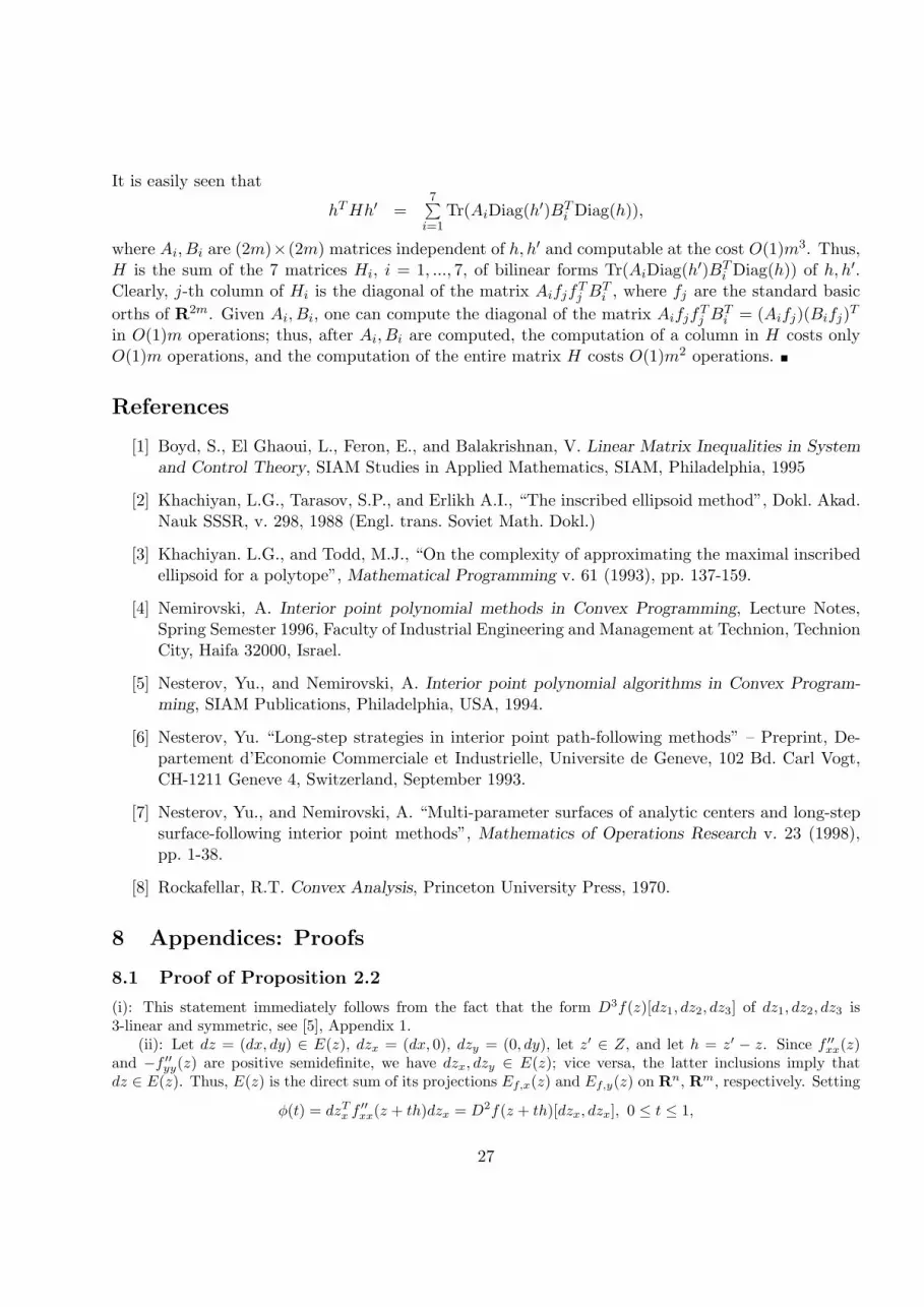
Tr(AiDiag(h′)BTi Diag(h)),

where Ai, Bi are (2m)×(2m) matrices independent of h, h′ and computable at the cost O(1)m3. Thus,H is the sum of the 7 matrices Hi, i = 1, ..., 7, of bilinear forms Tr(AiDiag(h′)BT

i Diag(h)) of h, h′.Clearly, j-th column of Hi is the diagonal of the matrix AifjfTj B

Ti , where fj are the standard basic

orths of R2m. Given Ai, Bi, one can compute the diagonal of the matrix AifjfTj BTi = (Aifj)(Bifj)T

in O(1)m operations; thus, after Ai, Bi are computed, the computation of a column in H costs onlyO(1)m operations, and the computation of the entire matrix H costs O(1)m2 operations.

References

[1] Boyd, S., El Ghaoui, L., Feron, E., and Balakrishnan, V. Linear Matrix Inequalities in Systemand Control Theory, SIAM Studies in Applied Mathematics, SIAM, Philadelphia, 1995

[2] Khachiyan, L.G., Tarasov, S.P., and Erlikh A.I., “The inscribed ellipsoid method”, Dokl. Akad.Nauk SSSR, v. 298, 1988 (Engl. trans. Soviet Math. Dokl.)

[3] Khachiyan. L.G., and Todd, M.J., “On the complexity of approximating the maximal inscribedellipsoid for a polytope”, Mathematical Programming v. 61 (1993), pp. 137-159.

[4] Nemirovski, A. Interior point polynomial methods in Convex Programming, Lecture Notes,Spring Semester 1996, Faculty of Industrial Engineering and Management at Technion, TechnionCity, Haifa 32000, Israel.

[5] Nesterov, Yu., and Nemirovski, A. Interior point polynomial algorithms in Convex Program-ming, SIAM Publications, Philadelphia, USA, 1994.

[6] Nesterov, Yu. “Long-step strategies in interior point path-following methods” – Preprint, De-partement d’Economie Commerciale et Industrielle, Universite de Geneve, 102 Bd. Carl Vogt,CH-1211 Geneve 4, Switzerland, September 1993.

[7] Nesterov, Yu., and Nemirovski, A. “Multi-parameter surfaces of analytic centers and long-stepsurface-following interior point methods”, Mathematics of Operations Research v. 23 (1998),pp. 1-38.

[8] Rockafellar, R.T. Convex Analysis, Princeton University Press, 1970.

8 Appendices: Proofs

8.1 Proof of Proposition 2.2

(i): This statement immediately follows from the fact that the form D3f(z)[dz1, dz2, dz3] of dz1, dz2, dz3 is3-linear and symmetric, see [5], Appendix 1.

(ii): Let dz = (dx, dy) ∈ E(z), dzx = (dx, 0), dzy = (0, dy), let z′ ∈ Z, and let h = z′ − z. Since f ′′xx(z)and −f ′′yy(z) are positive semidefinite, we have dzx, dzy ∈ E(z); vice versa, the latter inclusions imply thatdz ∈ E(z). Thus, E(z) is the direct sum of its projections Ef,x(z) and Ef,y(z) on Rn, Rm, respectively. Setting

φ(t) = dzTx f′′xx(z + th)dzx = D2f(z + th)[dzx, dzx], 0 ≤ t ≤ 1,

27

we get a continuously differentiable function on [0, 1]. We have

|φ′(t)| = |D3f(z + th)[dzx, dzx, h]| ≤ 2φ(t)√hTSf (z + th)h

(we have used (8)), and since φ(0) = 0, we have φ(t) = 0, 0 ≤ t ≤ 1. Thus, dzx ∈ Ef,x(z′). “Symmetric”reasoning implies that dzy ∈ Ef,y(z′), and since, as we just have seen, E(z′) = Ef,x(z′) + Ef,y(z′), we end upwith dz ∈ E(z′). (ii.1) is proved.

By Remark 2.1, f(·, y) is s.-c. on X for every y ∈ Y , and therefore, due to [5], Theorem 2.1.1.(ii), X =X + Ef,x. By similar reasons Y = Y + Ef,y, whence Z = Z + Ef .

(iii) is an immediate consequence of (ii.2).


(i): This is an immediate consequence of Remark 2.1 and Proposition 2.1.(ii): (ii.a) immediately follows from (i).(ii.b): For 0 ≤ t ≤ 1, denote

φ(t) = hTSf (z + th)h = φx(t) + φy(t),{φx(t) = D2f(z + th)[(u, 0), (u, 0)],φy(t) = −D2f(z + th)[(0, v), (0, v)].

We have (see (8))

|φ′x(t)| = |D3(z + th)[(u, 0), (u, 0), h]| ≤ 2φx(t)√φ(t)

|φ′y(t)| = |D3(z + th)[(0, v), (0, v), h]| ≤ 2φy(t)√φ(t)

}⇒ |φ′(t)| ≤ 2φ3/2(t), 0 ≤ t ≤ 1.

From the resulting differential inequality it immediately follows (note that r = φ1/2(0))

z + h ∈ Z ⇒ r

1 + rt≤√φ(t), 0 ≤ t ≤ 1; r < 1⇒

√φ(t) ≤ r

1− rt , 0 ≤ t ≤ 1. (43)

Now let dz = (dx, dy) ∈ Rn ×Rm, and let

ψ(t) = dzTSf (z + th)dz = ψx(t) + ψy(t),{ψx(t) = D2f(z + th)[(dx, 0), (dx, 0)],ψy(t) = −D2f(z + th)[(0, dy), (0, dy)],

t ∈ [0, 1]. We have (see (8))

|ψ′x(t)| = |D3(z + th)[(dx, 0), (dx, 0), h]| ≤ 2ψx(t)√φ(t)

|ψ′y(t)| = |D3(z + th)[(0, dy), (0, dy), h]| ≤ 2ψy(t)√φ(t)

}⇒ |ψ′(t)| ≤ 2ψ(t)

√φ(t), 0 ≤ t ≤ 1.

From the resulting differential inequality and (43) it immediately follows that if r < 1, then

ψ(t) ≥ (1− rt)2ψ(0), 0 ≤ t ≤ 1; ψ(t) ≤ (1− rt)−2ψ(0), 0 ≤ t ≤ 1. (44)

Since the resulting inequalities are valid for every dz, (ii.b) follows.(ii.c): Let r < 1, let h1, h2 ∈ Rn ×Rm, and let

ψi(t) = hTi Sf (z + th)hi, i = 1, 2; θ(t) = D2f(z + th)[h1, h2].

By (8), (43), (44) we have for 0 ≤ t ≤ 1:

|θ′(t)| = |D3f(z + th)[h1, h2, h]| ≤ 2√ψ1(t)

√ψ2(t)

√φ(t) ≤ 2r(1− rt)−3

√ψ1(0)ψ2(0),

28

whence for r < 1 one has

∀(h1, h2) : |hT1 [f ′′(z + h)− f ′′(z)]h2| ≤[

1(1− r)2

− 1]√

hT1 Sf (z)h1

√hT2 Sf (z)h2, (45)

as claimed in (ii.c).(ii.d): Let r < 1, and let h′ ∈ Rn ×Rm. We have

|(h′)T [f ′(z + h)− f ′(z)− f ′′(z)h]| = |1∫0

(h′)T [f ′′(z + th)− f ′′(z)]hdt|

≤︸︷︷︸(∗)

1∫0

[1

(1−tr)2 − 1]r√

(h′)TSf (z)h′dt = r2

1−r√

(h′)TSf (z)h′

((∗) is given by (45)), and (ii.d) follows.


“If” part: in the case in question the left hand side expression in (10) is

|D3f(x, y)[Jh1, h2, h3]|, J =(In 00 −Im

),

(from now on, Ik is the k × k unit matrix), while A(z) is exactly Sf (z). Thus, (10) implies that

|D3f(x, y)[h, h, h]| = |D3f(x, y)[J(Jh), h, h]| ≤ 2[hTSf (z)h][(Jh)TSf (z)Jh]1/2 = 2(hTSf (z)h)3/2

(note that JTSf (z)J = Sf (z)), as required in (7). It remains to verify Definition 2.2.(i). Let y ∈ Y and let{xi ∈ X} converge to a boundary point of X, so that the points zi = (xi, y) converge to a boundary pointof Z. According to [5], Proposition 7.2.1, the ellipsoids Wi = {z | (z − zi)TSf (zi)(z − zi) < 1} (recall thatSf (·) = A(·)) are contained in Z. Now let x0 ∈ X be a once for ever fixed point, and let ei = xi− x0. We claimthat the quantities δi =

√eTi f

′′xx(zi)ei tend to +∞. Indeed, since

(xi, y) = (xi + (1 + δi)−1ei, y) ∈Wi ⊂ Z,in the case of bounded {δi} the limit of xi, i.e., a boundary point of X, would be a convex combination, withpositive weights, of a limiting point of xi ∈ X and x0, which is impossible.

We now have

f(xi, y) = f(x0, y) + eTi f′x(x0, y) +

1∫

0

tgi(t)dt, gi(t) = eTi f′′xx(x0 + (1− t)ei, y)ei. (46)

Now note that in view of self-concordance of A(·) we clearly have

g′i(t) ≥ −2g3/2i (t), 0 ≤ t ≤ 1,

whence for 0 ≤ t ≤ 1

g−1/2i (t) ≤ g−1/2

i (0) + t⇒ gi(t) ≥ gi(0)(1 + t

√gi(0))2

=δ2i

(1 + tδi)2.

Consequently, the integral in (46) can be bounded from below by

1∫

0

tδ2i

(1 + tδi)2dt =

δi∫

0

s

(1 + s)2ds,

29

and since δi →∞ as i→∞, we see that the integral in (46) tends to +∞ as i grows. Since the remaining termsin the expression for f(xi, y) in (46) are bounded uniformly in i, we conclude that f(xi, y)→∞, as required inDefinition 2.2.(i). By symmetric reasons, f(x, yi) → −∞ whenever x ∈ X and a sequence {yi ∈ Y } convergesto a boundary point of Y . The “if” part is proved.

“Only if” part: Assuming f s.-c.c.-c. and taking into account Proposition 2.2.(i), we get

|hT2∇2z(h

T1 A(z))h3| = |D3f(z)[Jh1, h2, h3]| ≤ 2(hT1 J

TSf (z)Jh1)1/2(hT2 Sf (z)h2)1/2(hT3 Sf (z)h3)1/2,

as required in (10) (recall that A(z) = Sf (z) and JTSf (z)J = Sf (z)). Now, if a sequence {zi = (xi, yi) ∈Z} converges to a boundary point of Z, then the sequence of matrices A(zi) = Sf (zi) is unbounded due toProposition 2.3.(i). Thus, A(·) is a strongly self-concordant monotone operator.


If f possesses a saddle point on Z, then, of course, (*) takes place. In the case in question the saddle point isunique in view of the nondegeneracy of f .

It remains to verify that if f satisfies (*), then f possesses a saddle point on Z. Assume that f satisfies (*),and let x0, y0 be the corresponding points. Setting

φ(x) = supy∈Y

f(x, y),

we get a lower semicontinuous convex function on X (taking values in R ∪ {+∞}) which is finite at x0. Weclaim that the level set

X−(a) = {x ∈ X | φ(x) ≤ a}is compact for every a ∈ R. Indeed, the set clearly is contained in the set

X(a) = {x ∈ X | f(x, y0) ≤ a},and since f(·, y0) is a s.-c. nondegenerate below bounded function on X, X is a compact set (this is an immediatecorollary of [5], Proposition 2.2.3). Since φ is lower semicontinuous, X−(a) is a closed subset of X(a) and istherefore compact.

By “symmetric reasons”, the function

ψ(y) = infx∈X

f(x, y)

is an upper semicontinuous function on Y which is finite at y0 and has compact level sets

Y +(a) = {y ∈ Y | ψ(y) ≥ a}.Since φ has compact level sets and is finite at least at one point, φ attains its minimum on X at a convexcompact set X∗, and by similar reasons ψ attains its maximum on Y at a convex compact set Y ∗. In order toprove that f possesses a saddle point on Z, it suffices to demonstrate that the inequality in the following chain

a∗ ≡ maxy∈Y

ψ(y) ≤ minx∈X

φ(x) ≡ a∗

is in fact equality. Assume, on contrary, that a∗ < a∗, and let a ∈ (a∗, a∗). Denoting X(y) = {x ∈ X |f(x, y) ≤ a}, we conclude that

⋂y∈Y

X(y) = ∅. Since f(·, y) is a nondegenerate s.-c. function on X for every

y ∈ Y , the sets X(y) are closed; as we just have seen, X(y0) is compact. Consequently,⋂y∈Y

X(y) = ∅ implies

that⋂y∈Y ′

X(y) = ∅ for some finite subset Y ′ ∈ Y . In other words, maxy∈Y ′

f(x, y) ≥ a for every x ∈ X, and therefore

a convex combination∑y∈Y ′

λyf(x, y) is ≥ a everywhere on X. But∑y∈Y ′

λyf(x, y) ≤ f(x, y∗), y∗ =∑y∈Y ′

λyy, and

we see that infx∈X

f(x, y∗) ≥ a > a∗, which is a contradiction.

30


(i): Since f(·, y) is a nondegenerate s.-c. function on X for every y ∈ Y , by ([5], Theorem 2.4.1) the set

X∗(f, y) = {f ′x(x, y) | x ∈ X}

is open, nonempty and convex and is exactly the set of those ξ for which the function ξTx − f(x, y) is abovebounded on X. From these observations it immediately follows that X∗(f) =

⋃y∈Y

X∗(f, y); in particular, the

set X∗(f) is open. Let us prove that this set is convex. Indeed, assume that ξ1, ξ2 ∈ X∗(f), so that for somey1, y2 ∈ Y the functions ξTi x− f(x, yi) are above bounded on X, i = 1, 2. Whenever λ ∈ [0, 1], we have

λ[ξT1 x− f(x, y1)] + (1− λ)[ξT2 x− f(x, y2)] ≥ [λξ1 + (1− λ)ξ2]Tx− f(x, λy1 + (1− λ)y2),

so that λξ1 +(1−λ)ξ2 ∈ X∗(x, λy1 +(1−λ)y2) ⊂ X∗(f), and consequently X∗(f) is convex. Similar argumentsdemonstrate that Y ∗(f) also is open and convex.

(ii): Whenever (ξ, η) ∈ Z∗(f), the function fξ,η(x, y) (which is s.-c.c.-c. on Z by Proposition 4.1.(i) and isnondegenerate together with f) possesses property (*) from Proposition 2.5, and by this proposition it possessesa unique saddle point on Z. Vice versa, if (ξ, η) is such that fξ,η(z) possesses a saddle point (x∗, y∗) on Z, thefunction ξTx−f(x, y∗) is above bounded on X, and the function ηT y−f(x∗, y) is below bounded on Y , so that(ξ, η) ∈ Z∗(f).

(iii): If z0 ∈ Z, then z0 clearly is the saddle point of the function ff ′(z0)(·, ·) on Z, so that f ′(z0) ∈ Z∗(f) by(ii). Vice versa, if (ξ, η) ∈ Z∗(f), then the function fξ,η(z) possesses a saddle point z0 on Z by (ii); we clearlyhave (ξ, η) = f ′(z0). Thus, z 7→ f ′(z) maps Z onto Z∗(f). This mapping is a one-to-one mapping, since theinverse image of a point (ξ, η) ∈ Z∗(f) is exactly the saddle set of the function fξ,η(z) on Z, and the latter set,being nonempty, is a singleton by Proposition 2.5. It remains to prove that the mapping and its inverse aretwice continuously differentiable. To this end it suffices to verify that f ′′(z) is nonsingular for every z ∈ Z. Thelatter fact is evident: since f is convex-concave and nondegenerate, we have

f ′′(z) =(A QQT −B

)

with positive definite symmetric A,B, and a matrix of this type always is nonsingular. Indeed, assuming

Au+Qv = 0, QTu−Bv = 0,

multiplying the first equation by uT , the second by −vT and adding the results, we get uTAu + vTBv = 0,whence u = 0 and v = 0; consequently, Kerf ′′(z) = {0}.

(iv): First let us verify that f∗ is convex in ξ and concave in η on Z∗(f). Indeed,

f∗(ξ, η) = infy∈Y

supx∈X

[ξTx+ ηT y − f(x, y)] = infy∈Y

[ηT y + supx∈X

[ξTx− f(x, y)]],

so that f∗(ξ, η) is the lower bound of a family of affine functions of η and therefore it is concave in η. Convexityin ξ follows, via similar arguments, from the representation

f∗(ξ, η) = supx∈X

infy∈Y


coming from the fact that fξ,η(x, y) possesses a saddle point on Z when (ξ, η) ∈ Z∗(f), see (ii).Now let us prove that f∗ is differentiable and that the mapping ζ → f ′∗(ζ) is inverse to f ′(z). Indeed, let

ζ = (ξ, η) ∈ Z∗(f), so that the function fζ(x, y) possesses a unique saddle point zζ = (xζ , yζ) on Z ((ii) andProposition 2.5). Note that by evident reasons ζ = f ′(zζ). We claim that xζ is a subgradient of f∗(·, η) at the

31

point ξ, and yζ is the super-gradient of f∗(ξ, ·) at the point η. By symmetry, it suffices to prove the first claim,which is evident:

f∗(ξ′, η) = supx∈X

infy∈Y

[(ξ′)Tx+ ηT y − f(x, y)]

≥ infy∈Y

[(ξ′)Txζ + ηT y − f(xζ , y)] = (ξ′)Txζ + infy∈Y

[ηT y − f(xζ , y)]

= (ξ′ − ξ)Txζ + infy∈Y

[ξTxζ + ηT y − f(xζ , y)]

= (ξ′ − ξ)Txζ + [ξTxζ + ηT yζ − f(xζ , yζ)] [since (xζ , yζ) is a saddle point of fζ(·, ·)]= (ξ′ − ξ)Txζ + inf

y∈Ysupx∈X

[ξTx+ ηT y − f(x, y)] [by the same reasons]

= (ξ′ − ξ)Txζ + f∗(ξ, η).

Since, on one hand, the mapping ζ → zζ is inverse to the mapping z → f ′(z) and is therefore twice continuouslydifferentiable by (iii), and, on the other hand, the components of this mapping are partial sub- and supergradientsof f∗, the function f∗ is C3 smooth on Z∗(f), and its gradient mapping is inverse to the one of f . In particular,

{ζ = f ′(z)} ⇔ {z = f ′∗(ζ)} ⇒ {f ′′∗ (ζ) = [f ′′(z)]−1}. (47)

It remains to prove that f∗ is s.-c.c.-c. on Z∗(f). Let us first prove the corresponding differential inequality.We have

dζT f ′′∗ (ζ)dζ = dζT [f ′′(f ′∗(ζ))]−1dζ ⇒D3f∗(ζ)[dζ, dζ, dζ] = −D3f(f ′∗(ζ))[f ′′∗ (ζ)dζ, f ′′∗ (ζ)dζ, f ′′∗ (ζ)dζ] = −D3f(z)[dz, dz, dz],

[z = f ′∗(ζ), dz = f ′′∗ (ζ)dζ = [f ′′(z)]−1dζ.]

It follows that

|D3f∗(ζ)[dζ, dζ, dζ]| = |D3f(z)[dz, dz, dz]| ≤ 2(dζT [f ′′(z)]−1Sf (z)[f ′′(z)]−1dζ)3/2. (48)

Now let J =(In 00 −Im

). We have

Sf (z) =12

([f ′′(z)]J + J [f ′′(z)]) ,

whence

[f ′′(z)]−1Sf (z)[f ′′(z)]−1 = 12 [f ′′(z)]−1 ([f ′′(z)]J + J [f ′′(z)]) [f ′′(z)]−1 = 1

2

(J [f ′′(z)]−1 + [f ′′(z)]−1J

)= 1

2 (J [f ′′∗ (ζ)] + [f ′′∗ (ζ)]J) [we have used (47)]= Sf∗(ζ).

(49)Consequently, (48) becomes

|D3f∗(ζ)[dζ, dζ, dζ]| ≤ 2(dζTSf∗(ζ)dζ)3/2,

which is exactly the differential inequality required in Definition 2.2.It remains to prove that f∗(·, η) is a barrier for X∗(f) for every η ∈ Y ∗(f), and that −f∗(ξ, ·) is a barrier for

Y ∗(f) for every ξ ∈ X∗(f). By symmetry, it suffices to prove the first of these statements. Let us fix η ∈ Y ∗(f),and let a sequence {ξi ∈ X∗(f)} converge to a point ξ and be such that f∗(ξi, η) ≤ a for some a ∈ R and all i.We should prove that under these assumptions ξ ∈ X∗(f). Indeed, we have

−a ≤ −f∗(ξi, η) = infx∈X

supy∈Y

[f(x, y)− ξTi x− ηT y] =︸︷︷︸(a)

= supy∈Y

infx∈X

[f(x, y)− ξTi x− ηT y]

=︸︷︷︸(b)

minx∈X

[f(x, yi)− ξTi x− ηT yi] [yi ∈ Y ].(50)

32

with (a), (b) given by Proposition 3.1.(iv,ii), respectively. Since η ∈ Y ∗(f), there exists x0 ∈ X such that thefunction

g(y) = f(x0, y)− ηT y − ξTx0

is above bounded on Y . Since (−g) is s.-c. convex and nondegenerate on Y , the level set

Y + = {y ∈ Y | f(x0, y)− ηT y − ξTx0 ≥ −a− 1}

is compact (we already have mentioned this fact). We claim that all points yi, starting from some i0, belong toY +. Indeed, whenever yi 6∈ Y +, we have by (50)

−a ≤ minx∈X

[f(x, yi)− ξTi x− ηT yi] ≤ f(x0, yi)− ξTi x0 − ηT yi= [f(x0, yi)− ξTx0 − ηT yi] + (ξ − ξi)Tx0 < −a− 1 + (ξ − ξi)Tx0,

and the resulting inequality, due to ξi → ξ, can be valid for finitely many i’s only.Since Y + is compact and contains all yi except finitely many of them, we can, passing to a subsequence,

assume that yi ∈ Y + and yi converge to y0 ∈ Y + ⊂ Y . We claim that the function f(x, y0) − ξTx is belowbounded on X, which yields the desired contradiction. Indeed, by (50) we have for every x ∈ X and all i

−a ≤ f(x, yi)− ξTi x− ηT yi,

and passing to limit, we get−a ≤ f(x, y0)− ξTx− ηT y0,

so that f(x, y0)− ξTx ≥ −a+ ηT y0. Thus, ξ ∈ X∗(f).

8.6 Proof of Theorem 3.1

The fact that f∗ is s.-c.c.-c. is given by Proposition 3.1.(iv). The equivalence in the premise of (11) is statedby (47). Under this premise, the validity of (a), (b) is given by (47), (49), respectively. Now, under the premiseof (11) z clearly is the saddle point of the function f(z′)− ζT z′ of z′ ∈ Z, whence

f∗(ζ) = −[f(z)− ζT z],

as required in (c). Nondegeneracy of f∗ follows from (b). It remains to prove that the Legendre transformationof f∗ is exactly f . From Proposition 3.1.(iii,iv) it follows that the domain of the Legendre transformation of f∗is exactly Z, so that all we need is to prove that

(f∗)∗(x0, y0) = f(x0, y0)

for every (x0, y0) ∈ Z. This is immediate: setting ξ0 = f ′x(x0, y0), ζ0 = f ′y(x0, y0), we clearly have

f∗(ξ0, η0) = ξT0 x0 + ηT0 y0 − f(x0, y0),

and by Proposition 3.1.(iv)(f∗)′ξ(ξ0, η0) = x0, (f∗)′η(ξ0, η0) = y0,

whence(f∗)∗(x0, y0) = xT0 ξ0 + yT0 η0 − f∗(ξ0, η0) = f(x0, y0). .

33


By symmetry, it suffices to prove (i).“If” part and derivation of (12): Assume that 0 ∈ X∗ and the function ηT y − f∗(0, η) is below bounded on

Y ∗. Since the latter function is s.-c. on Y ∗ (Theorem 3.1 and Remark 2.1), it attains its minimum on Y ∗ atsome point η∗. Setting x∗ = (f∗)′ξ(0, η∗), we have f ′∗(0, η∗) = (x∗, y), whence by Theorem 3.1

f(x∗, y) = 0Tx∗ + ηT∗ y − f∗(0, η∗),while by Theorem 3.1 and Proposition 3.1 for every x ∈ X one has

f(x, y) = supξ∈X∗

infη∈Y ∗

[ξTx+ ηT y − f∗(ξ, η)] ≥ infη∈Y ∗

[ηT y − f∗(0, η)] = ηT∗ y − f∗(0, η∗),

and (12) follows.“Only if” part: assume that f(·, y) is below bounded on X. Then 0 ∈ X∗ by the definition of X∗, and

since f(·, y) is s.-c. on X (Remark 2.1), the function attains its minimum over X at some point x∗. Settingη∗ = f ′y(x∗, y), we get f ′(x∗, y) = (0, η∗), whence by Theorem 3.1 (0, η∗) is the saddle point of the function

f∗(ξ, η)− ξTx∗ − ηT y,so that the function f∗(0, η) − ηT y is above bounded in η ∈ Y ∗. Thus, the function ηT y − f∗(0, η) is belowbounded.


By symmetry, it suffices to prove the first statement. Convexity of X+ is evident. To prove openness, note thatif x ∈ X+, then −f(x, ·) is a nondegenerate s.-c. below bounded convex function on Y , so that f(x, ·) attainsits maximum on Y at a unique point y(x), and the Newton decrement of −f(x, ·) at y(x) is zero. Consequently,there exists a neighbourhood U of x such that the Newton decrements, taken at y(x), of the s.-c. on Y functions−f(x′, ·), x′ ∈ U , are < 1, and therefore the indicated functions are below bounded on Y ([5], Theorem 2.2.2.(i)).Thus, U ⊂ X+, whence X+ is open.

As we have seen, for x ∈ X+ the function f(x, ·) attains its maximum on Y at a unique point y(x) given by

f ′y(x, y(x)) = 0. (51)

Since f ′′yy is nondegenerate, by the Implicit Function Theorem (51) defines a C2 function y(·) on X+; conse-quently, the function

φ(x) = f(x, y(x)) ≡ maxy∈Y

f(x, y) : X+ → R

is C2 smooth (and clearly convex). Since by evident reasons

Dφ(x)[dx] = dxT f ′x(x, y(x)),

we see that in fact φ is C3-smooth.Let us prove that φ is s.-c. on X+. The barrier property is evident: if xi ∈ X+ and xi → x 6∈ X+, then

either x 6∈ X – and then φ(xi) ≥ f(xi, y)→∞, y ∈ Y being fixed, – or x ∈ X. In the latter case the sequenceof functions {f(xi, ·)} does not contain a uniformly above bounded on Y subsequence – otherwise f(x, ·) wereabove bounded on Y , which is not the case – and therefore φ(xi)→∞ as i→∞.

It remains to verify the differential inequality (2) responsible for self-concordance. Let us fix x ∈ X+ and adirection dx in the x-space, and let

y = y(x), dy = Dy(x)[dx], d2y = D2y(x)[dx, dx],

z = (x, y), dz = (dx, dy), f ′′(z) =(A BT

B −C).

34

We have for every h ∈ Rm and u ∈ X+:

Df(u, y(u))[(0, h)] = 0⇒ (a) D2f(u, y(u))[(dx,Dy(u)[dx]), (0, h)] = 0⇒ (b) D3f(u, y(u))[(dx,Dy(u)[dx]), (dx,Dy(u)[dx]), (0, h)]

+D2f(u, y(u))[(0, D2y(u)[dx, dx]), (0, h)] = 0.

(52)

Note that from (52.a) we getdy = C−1Bdx, (53)

while from (52.b) we get∀h ∈ Rm : hTCd2y = D3f(z)[dz, dz, (0, h)]. (54)

Now,Dφ(u)[dx] = Df(u, y(u))[(dx,Dy(u)[dx])] = Df(u, y(u))[(dx, 0)]

[since Df(u, y(u))[(0, h)] ≡ 0]⇒ D2φ(u)[dx, dx] = D2f(u, y(u))[(dx,Dy(u)[dx]), (dx, 0)]⇒ D3φ(u)[dx, dx, dx] = D3f(u, y(u))[(dx,Dy(u)[dx]), (dx,Dy(u)[dx]), (dx, 0)]

+D2f(u, y(u))[(0, D2y(u)[dx, dx]), (dx, 0)],

so thatD2φ(x)[dx, dx] = D2f(z)[(dx, dy), (dx, 0)] = dxTAdx+ dxTBT dy

=︸︷︷︸(a)

dxTAdx+ dyTCdy = dzTSf (z)dz;

D3φ(x)[dx, dx, dx] = D3f(z)[dz, dz, (dx, 0)] +D2f(z)[(0, d2y), (dx, 0)]= D3f(z)[dz, dz, (dx, 0)] + dxTBT d2y= D3f(z)[dz, dz, (dx, 0)] + (C−1Bdx)TCd2y=︸︷︷︸(b)

D3f(z)[dz, dz, (dx, 0)] +D3f(z)[dz, dz, (0, C−1Bdx)]

=︸︷︷︸(c)

D3f(z)[dz, dz, (dx, 0)] +D3f(z)[dz, dz, (0, dy)]

= D3f(z)[dz, dz, dz]

(55)

((a), (c) are given by (53), (b) is given by (54)), and since f is s.-c.c-c., we end up with

|D3φ(x)[dx, dx, dx]| ≤ 2(D2φ(x)[dx, dx]

)3/2.


First of all, the function φ is well-defined: since Y is bounded, f(x, ·) is above bounded on Y whenever x ∈ X,and consequently the function −f(x, (u, ·)) is below bounded on its domain whenever x ∈ X,u ∈ U . Since thelatter function is s.-c. ([5], Proposition 2.1.1.(i)), it attains its minimum.

Now let us prove that φ is s.-c.c.-c. Convexity-concavity of φ is evident. As we have seen, the maximum inthe right hand side of (13) is achieved, and the maximizer v(x, u) is unique, since f ′′vv is negative definite. Bythe latter reason and the Implicit Function Theorem the function v(x, u) is twice continuously differentiable onX × U , and since

Dφ(x, u)[(dx, du)] = Df(x, (u, v(x, u)))[(dx, (du, 0))]

due to f ′v(x, (u, v(x, u))) = 0, φ is C3 smooth.Let us verify the barrier properties required by Definition 2.2.(i). Let u ∈ U , and let {xi ∈ X} be a sequence

converging to a boundary point of X. Then φ(xi, u) ≥ f(xi, (u, v)), where v is such that (u, v) ∈ Y , andconsequently φ(xi, u)→∞, i→∞. Now let x ∈ X, and let {ui ∈ U} be a sequence converging to a boundarypoint of U . Passing to a subsequence we may suppose that vi = v(x, ui) has a limit (Y is bounded!), and of

35

course the limit of the sequence (ui, vi) is a boundary point of Y . Consequently, φ(x, ui) = f(x, (ui, vi))→ −∞,i→∞, as required.

In order to verify the differential inequality required in Definition 2.2(2), let us first note that the compu-tations which led to (55) do not use the s.-c.c.-c. property of the underlying function and in fact establish thefollowing

Lemma 8.1 Let g(p, q) be a C3 function defined in a neighbourhood of a point (p, q) such that g′q(p, q) = 0, and

let g′′(p, q) =(A BT

B −C)

with nonsingular C = −g′′qq(p, q). Then the equation g′q(p, q) = 0 in a neighbourhood

of p has a C2-smooth solution q(p), q(p) = q, the function h(p) = g(p, q(p)) is C3-smooth in a neighbourhood ofp, and for every vector dp in the p-space we have

D2h(p)[dp, dp] = drTSdr, D3h(p)[dp, dp, dp] = D3g(p, q)[dr, dr, dr],

where

dr = (dp, dq), dq = C−1Bdp, S =(A 00 C

).

In particular,h′′(p) = A+BTC−1B. (56)

Let w ≡ (x, u) ∈ X × U , and letg((x, u), v) = f(x, (u, v)).

Let also v = v(x, u), z = (x, (u, v)), and let

f ′′(z) =

Q BTu BTvBu −P DT

Bv D −R

, Q = f ′′xx(z),−P = f ′′uu(z),−R = f ′′vv(z).

Applying Lemma 8.1 to g (p = (x, u), q = v) with p = (x, u), q = v(x, u) and dp = (dx, du) being a direction inthe (x, u)-space, we get

D2φ(w)[dp, dp] = dzT

Q BTu 0Bu −P 00 0 R

dz,

dz =

dxdudv

, dv = R−1[Bvdx+Ddu]

;

D3φ(w)[dp, dp, dp] = D3f(z)[dz, dz, dz].

(57)

From (57) we get

φ′′xx(w)[dx, dx] = dxTQdx+ [R−1Bvdx]TR[R−1Bvdx] = dxTQdx+ dxTBTv R−1Bvdx;

−φ′′uu(w)[du, du] = duTPdu− duT [R−1Ddu]TR[R−1Ddu] = duTPdu− duTDTR−1Ddu,

whencedpTSφ(w)dp = dxTQdx+ dxTBTv R

−1Bvdx+ duTPdu− duTDTR−1Ddu. (58)

We have (see (57), (58))

dzTSf (z)dz = dxTQdx+ duTPdu+ dvTRdv − 2duTDT dv= dxTQdx+ duTPdu+ [R−1(Bvdx+Ddu)]TR[R−1(Bvdx+Ddu)]−2duTDT [R−1(Bvdx+Ddu)]

= dxTQdx+ duTPdu+ dxTBTv R−1Bvdx+ 2dxTBTv R−1Ddu

+duTDTR−1Ddu− 2duTDTR−1Bvdx− 2duTDTR−1Ddu= dxTQdx+ dxTBTv R

−1Bvdx+ duTPdu− duTDTR−1Ddu = dpTSφ(w)dp.

(59)

36

Thus,|D3φ(w)[dp, dp, dp]| = |D3f(z)[dz, dz, dz]|

≤ 2(dzTSf (z)dz)3/2 [since f is s.-c.c.-c.]= 2(dpTSφ(w)dp)3/2 [see (59)],

as required in (7). The fact that φ is nondegenerate is readily given by (59).


(i), (ii) are immediate consequnces of (11.b) and Proposition 4.3, respectively. Let us prove (iii).

(iii.1)⇔(iii.2): If z ∈ K(f), then 0 ∈ X∗ and 0 ∈ Y ∗, so that (0, 0) ∈ Z∗, and f possesses a saddlepoint on Z in view of Proposition 3.1. Vice versa, if f possesses a saddle point z∗ = (x∗, y∗) on Z,then clearly z∗ ∈ K(f) and therefore K(f) is nonempty.(iii.2)⇔(iii.3): This equivalence is an immediate consequence of Proposition 3.1.(iii.2)⇒(iii.4): This is evident, since ω(f, z∗) = 0 at a saddle point z∗ of f .(iii.4)⇒(iii.3): Given z ∈ Z with ω(f, z) < 1, consider the point ζ ≡ f ′(z) = (ξ, η). By (20),0 ∈ W f∗

ξ (ζ), so that 0 ∈ X∗ by Proposition 2.3.(i) as applied to f∗ (the latter function is s.-c.c.-c.and nondegenerate by Theorem 3.1). By symmetric reasons, 0 ∈ Y ∗, so that (0, 0) ∈ Z∗ = X∗×Y ∗.

(iv): Let us start with the following simple fact:

Lemma 8.2 Let A =(P RT

R −Q)

be a symmetric matrix with positive definite P , Q, and let S =(P 00 Q

).

Then A is nonsingular, and one has

A−1 � S−1 & A−1SA−1 � S−1.

In particular, if f : Z = X × Y → R is a nondegenerate s.-c.c.-c. function, then for every z ∈ Z one has

[f ′′(z)]−1Sf (z)[f ′′(z)]−1 � S−1f (z).

Proof of Lemma: Nonsingularity of A was established in the proof of Proposition 3.1. Since A is symmetricand nonsingular, to prove that A−1 � S−1 is the same as to prove that A � AS−1A, which is immediate:

AS−1A =(P RT

R −Q)(

P−1

Q−1

)(P RT

R −Q)

=(P +RTQ−1R

RP−1RT +Q

)= A+D,

where

D =(RTQ−1R −RT−R RP−1RT + 2Q

)�(RTQ−1R −RT−R Q

)� 0.

Similarly, in order to prove that A−1SA−1 � S−1, it suffices to prove that AS−1A − S � 0; from the above

computation, the latter difference is(RTQ−1R

RP−1RT

), i.e., it indeed is positive semidefinite.

By Lemma 8.2,

ω2(f, z) = (f ′(z))T [f ′′(z)]−1Sf (z)[f ′′(z)]−1f ′(z) ≤ (f ′(z))T [Sf (z)]−1f ′(z) = ν2(f, z),

as required in (21.a).To verify (21.b,c), denote

λx =√

(f ′x(z))T [f ′′xx(z)]−1f ′x(z), λy =√

(f ′y(z))T [−f ′′yy(z)]−1f ′y(z),

37

so thatν2(f, z) = λ2

x + λ2y. (60)

Setting z = (x, y) and taking into account Remark 2.1 and (6), we get

ρ(−λx) ≤ [f(z)− minx′∈X

f(x′, y)] ≤ ρ(λx), ρ(−λy) ≤ [maxy′∈Y

f(x, y′)− f(z)] ≤ ρ(λy). (61)

We see thatν(f, z) < 1⇒ µ(f, z) ≤ max{ρ(u) + ρ(v) | 0 ≤ u, v, u2 + v2 = ν2(f, z)},

and since the function ρ(s1/2) clearly is convex on [0, 1), we come to (21.b). Now, it is easily seen that

s ≥ 0⇒ ρ(−s) ≥ s2

2(1 + s),

whence in view of (61)λ2x

2(1 + λx)+

λ2y

2(1 + λy)≤ µ(f, z),

so that (60) yieldsν2(f, z)

2(1 + ν(f, z))≤ µ(f, z),

as required in (21.c).(v): The inclusion z+ ∈ Z is readily given by (9.a). To prove (22), note that by (9.d) for every h ∈ Rn×Rm

one hasω2(f, z)

1− ω(f, z)

√hTSf (z)h ≥ |hT (f ′(z+)− f ′(z) + f ′′(z)e(f, z))| = |hT f ′(z+)|,

while by (9.b) one has √hTSf (z)h ≤ (1− ω(f, z))−1

√hTSf (z+)h.

Consequently,

|hT f ′(z+)| ≤ ω2(f, z)(1− ω(f, z))2

√hTSf (z+)h ∀h,

which is nothing but (v).(vi): Let

z∗ = (x∗, y∗), z = (x, y), dx =√

(x− x∗)T f ′′xx(z∗)(x− x∗), dy =√−(y − y∗)T f ′′yy(z∗)(y − y∗).

Thenµ(f, z) = sup

y′∈Yf(x, y′)− inf

x′∈Xf(x′, y) ≥ f(x, y∗)− f(x∗, y)

≥ [f(x∗, y∗) + ρ(−dx)]− [f(x∗, y∗)− ρ(−dy)] = ρ(−dx) + ρ(−dy)

(we have used (4) and the fact that f ′(z∗) = 0). From the resulting inequality, as in the proof of (21.c), we get

d2x

2(1 + dx)+

d2y

2(1 + dy)≤ µ(f, z),

whence, after a simple computation, dx + dy ≤ 2[µ(f, z) +√µ(f, z)], and (23) follows.


In the proof to follow, Θi denote properly chosen universal positive continuous nondecreasing functions on thenonnegative ray.

38

Main Lemma. We start with the following technical result:

Lemma 8.3 For properly chosen Θ1(·), the following holds. Let f : Z = X×Y → R be a nondegenerate s.-c.c.-c. function, and let f∗ : Z∗ = X∗×Y ∗ → R be the Legendre transformation of f . Let also z1 ≡ (x1, y1) ∈ K(f),ζ1 ≡ (ξ1, η1) = f ′(z1), and let

zt = f ′∗(tζ1), 0 ≤ t ≤ 1.

Then for 0 ≤ t ≤ 1 one has

(a) ζT1 Sf∗(tζ1)ζ1 ≤ Θ1(µ(f, z1));(b) Θ−1

1 (µ(f, z1))Sf∗(ζ1) � Sf∗(tζ1) � Θ1(µ(f, z1))Sf∗(ζ1). (62)

Proof. Since K(f) is nonempty (it contains z1), f possesses a saddle point (Proposition 5.1.(iii)). Thus,(0, 0) ∈ Z∗, whence ζt ∈ Z∗, 0 ≤ t ≤ 1.

Let us denote

µx = f(x1, y1)−minx∈X

f(x, y1) [≥ 0]

µy = maxy∈Y

f(x1, y)− f(x1, y1) [≥ 0]

⇒ µ ≡ µ(f, (x1, y1)) = µx + µy;

g∗(ξ, η) = f∗(ξ, η)− ξTx1 − ηT y1.

10. Note that g∗ differs from f∗ by a linear function and is therefore a nondegenerate s.-c.c.-c. function onZ∗. Besides this, by construction ζ1 is a saddle point of g∗ on Z∗.

20. By (12) we have

minx∈X

f(x, y1) = minη∈Y ∗

[ηT y1 − f∗(0, η)] = minη∈Y ∗

[−g∗(0, η)] = − maxη∈Y ∗

g∗(0, η),

while by Theorem 3.1f(z1) = ξT1 x1 + ηT1 y1 − f∗(ξ1, η1) = −g∗(ξ1, η1).

Thus,maxη∈Y ∗

g∗(0, η)− g∗(ξ1, η1) = µx. (63)

By symmetric reasoning,g∗(ξ1, η1)− min

ξ∈X∗g∗(ξ, 0) = µy.

30. By 10, maxη∈Y ∗

g∗(ξ1, η) = g∗(ζ1), and since g∗(·, η) is convex on X∗, we get from (63)

maxη∈Y ∗

g∗(tξ1, η)− g∗(ζ1) ≤ µx, 0 ≤ t ≤ 1. (64)

By symmetric reasoning,g∗(ζ1)− min

ξ∈X∗g∗(ξ, tη1) ≤ µy, 0 ≤ t ≤ 1. (65)

40. Let ξt = tξ1, ηt = tη1, 0 ≤ t ≤ 1. Since ζ1 is a saddle point of g∗, the s.-c. on X∗ function

φ(ξ) = g∗(ξ, η1)

attains its minimum on X∗ at the point ξ1, and by (64) we have

φ(ξt) ≤ φ(ξ1) + µx, 0 ≤ t ≤ 1.

The latter inequality, due to the standard properties of s.-c. functions ([5], Section 2.2.4) combined with thefact that µx ≤ µ, implies that for t ∈ [0, 1] one has

Θ−12 (µ)φ′′(ξ1) � φ′′(ξt) � Θ2(µ)φ′′(ξ1), ξT1 φ

′′(ξ1)ξ1 ≤ Θ3(µ). (66)

39

50. Let h ∈ Rm, and letγ(t) = −hT (g∗)′′ηη(ξt, η1)h.

We have

|γ′(t)| = |D3g∗(ξt, η1)[(0, h), (0, h), (−ξ1, 0)]| ≤︸︷︷︸(a)

2γ(t)√ξT1 φ

′′(ξt)ξ1 ≤︸︷︷︸(b)

Θ4(µ)γ(t)

((a) is given by (8) as applied to g∗, (b) is given by (66)), so that

Θ−15 (µ)γ(1) ≤ γ(t) ≤ Θ5(µ)γ(1),

for all t ∈ [0, 1], whence

Θ−15 (µ)[−(g∗)′′ηη(ζ1)] � [−(g∗)′′ηη(ξt, η1)] � Θ5(µ)[−(g∗)′′ηη(ζ1)], 0 ≤ t ≤ 1. (67)

60. Now let us fix t ∈ [0, 1] and setψ(η) = −g∗(ξt, η);

note that ψ is a s.-c. function on Y ∗.By (64) we have

minη∈Y ∗

ψ(η) ≥ −g∗(ζ1)− µx, (68)

while for s ∈ [0, 1] it holds

ψ(ηs) = −g∗(ξt, ηs) ≤ − minξ∈X∗

g∗(ξ, ηs) ≤ −g∗(ζ1) + µy [we have used (65)].

Combining these relations, we see that

ψ(ηs) ≤ minη∈Y ∗

ψ(η) + µ, 0 ≤ s ≤ 1. (69)

70. From (69) and the same standard properties of s.-c. functions as in 40 we get for 0 ≤ s ≤ 1:

Θ−16 (µ)ψ′′(η1) � ψ′′(ηs) � Θ6(µ)ψ′′(η1), ηT1 ψ

′′(η1)η1 ≤ Θ7(µ);

combining this result with (67), we see that for s, t ∈ [0, 1] one has

Θ−18 (µ)[−(g∗)′′ηη(ζ1)] � [−(g∗)′′ηη(ξt, ηs)] � Θ8(µ)[−(g∗)′′ηη(ζ1)], ηT1 [−(g∗)′′ηη(ζ1)]η1 ≤ Θ9(µ). (70)

By symmetric reasoning,

Θ−18 (µ)(g∗)′′ξξ(ζ1) � (g∗)′′ξξ(ξt, ηs) � Θ8(µ)(g∗)′′ξξ(ζ1), ξT1 (g∗)′′ξξ(ζ1)ξ1 ≤ Θ9(µ). (71)

Relations (70) and (71) in view of f ′′∗ (ζ) ≡ g′′∗ (ζ) imply (62.a,b).

From Main Lemma to Theorem 5.1. (i): Since (t1, z1) clearly satisfies (P1), all we should prove isthe implication (Pi)⇒ (Pi+1).

10. Assume that i is such that (Pi) is valid. Setting

ei = [f ′′(zi)]−1(fti)′(zi), Qi = Sf (zi),

we get by (21.a)ωi ≡ ω(fti , zi) =‖ ei ‖Qi≤ νi ≡ ν(fti , zi) ≤ 0.1, (72)

40

the concluding inequality being given by (Pi). It follows that

0 ≤ t ≤ ti ⇒ ω(ft, zi) = ‖ [f ′′(zi)]−1f ′t(zi) ‖Qi=‖ [f ′′(zi)]−1[f ′ti(zi) + (ti − t)f ′(z)] ‖Qi

≤ ωi + (ti − t)γi, γi ≡‖ [f ′′(zi)]−1f ′(z) ‖Qi=‖ f ′(z) ‖Sf∗ (f ′(zi))(73)

(see (11.b)).20. Since ωi ≤ νi ≤ 0.1 by (72), (73) says that there indeed exists t ∈ [0, ti] such that ω(ft, zi) ≤ 0.2, so

that ti+1 is well-defined. Note also that by (73)

ti+1 > 0⇒ ω(fti+1 , zi) = 0.2⇒ ti − ti+1 ≥ 0.1γ−1i . (74)

30. For the sake of brevity, denote temporarily

g(z) = fti+1(z), d = g′(zi), e = [f ′′(zi)]−1d = [g′′(zi)]−1d.

By definition of ti+1 we haveσi ≡ ω(g, zi) =‖ e ‖Qi≤ 0.2,

whence (see (24) and (9.a))zi+1 = zi − e ∈ Z.

Moreover, by (9.d) and in view of ‖ e ‖Qi= σi ≤ 0.2 we have

∀(h ∈ Rn+m) : |hT g′(zi+1)| = |hT [g′(zi+1)− g′(zi) + g′′(zi)e]| ≤ σ2i

1− σi ‖ h ‖Qi ,

whence

‖ g′(zi+1) ‖Q−1i≤ σ2

i

1− σi ≤0.040.8

= 0.05. (75)

Now note that by (9.b)Sf (zi+1) � (1− ‖ e ‖Qi)2Sf (zi),

so that by (75)

ν(fti+1 , zi+1) ≡ ν(g, zi+1) =‖ g′(zi+1) ‖[Sf (zi+1)]−1≤ (1− ‖ e ‖Qi)−1 ‖ g′(zi+1) ‖[Sf (zi)]−1

= (1− ‖ e ‖Qi)−1 ‖ g′(zi+1) ‖Q−1i≤ σ2

i

(1−σi)2 ≤ 0.050.8 < 0.1.

(76)

Thus, (Pi+1) indeed is valid. (i) is proved.(ii): Assume that i is such that ti+1 > 0. By (74)

ti − ti+1 ≥ 0.1γ−1i , γi =‖ f ′(z) ‖Sf∗ (f ′(zi)) . (77)

Now letg(z) = fti(z), (78)

so that in view of (Pi) we have[ω(g, zi) ≤] ν(g, zi) ≤ 0.1 (79)

(the left inequality is given by (21.a)).

Lemma 8.4 Let g : Z = X × Y → R be a nondegenerate s.-c.c.-c. function, and let z0 = (x0, y0) ∈ Z be suchthat ω ≡ ω(g, z) ≤ 0.2. Then g possesses a saddle point z∗ on Z, and

‖ z∗ − z0 ‖Sf (z0)≤ ω + 2.7ω2. (80)

41

Proof. Consider the Newton iterate

z1 ≡ z0 − [g′′(z0)]−1g′(z0) = (x1, y1)

of z0. Same as in 30, z1 ∈ Z and

‖ z0 − z1 ‖Sf (z0)= ω, ν(g, z1) ≡ ν ≤ ω2

(1− ω)2[see (76)]. (81)

Let z∗ = (x∗, y∗) be the saddle point of g (it exists by Proposition 5.1.(iii)). Let us set

Q ≡ Sf (z∗) =(A 00 D

), rx =‖ x1 − x∗ ‖A, ry =‖ y1 − y∗ ‖B .

By (4) we have

maxy

g(x1, y) ≥ g(x1, y∗) ≥ g(z∗) + rx − ln(1 + rx), min

xg(x, y1) ≤ g(x∗, y1) ≤ g(z∗)− ry + ln(1 + ry),

whenceµ(g, z1) ≥ rx + ry − ln(1 + rx)− ln(1 + ry),

and at the same time

µ(g, z1) ≤ −ν − ln(1− ν)[ν ≤ ω2

(1− ω)2

]

(we have used (21.b) and (81)). Thus,

−ν − ln(1− ν) ≥ rx + ry − ln(1 + rx)− ln(1 + ry) (82)

Since ω ≤ 0.2, we have ν ≤ ω2

0.64 ≤ 0.07, and therefore −ν − ln(1 − ν) ≤ 0.53ν2 ≤ 0.0026. Consequently, from(82) it immediately follows that max[rx, ry] ≤ 0.25, whence rx + ry − ln(1 + rx) − ln(1 + ry) ≥ 0.4(r2

x + r2y).

Thus, (82) results in0.53ν2 ≥ 0.4(r2

x + r2y),

whence‖ z1 − z∗ ‖Q≤ 1.2ν ≤ 1.875ω2 ≤ 0.08.

The latter inequality, by (9.b), implies that

‖ z1 − z∗ ‖Sg(z1)≤ (1− 0.08)−1 ‖ z1 − z∗ ‖Q≤ 2.1ω2.

By the same (9.b), from (81) it follows that Sg(z1) � (1− ω)2Sg(z0), whence

‖ z1 − z∗ ‖Sg(z0)≤ (1− ω)−1 ‖ z1 − z∗ ‖Sg(z1)≤ 2.7ω2

(recall that ω ≤ 0.2). Combining this relation with (81), we come to (80).

Now we are ready to complete the proof of (ii). Applying Lemma 8.4 to the function g given by (78) andtaking into account (79), we see that

‖ zi − z∗(ti) ‖Sf (zi)≤ 0.1 + 2.7× 0.12 = 0.127. (83)

Now leth(ζ) = f∗(ζ)− (z∗(ti))T ζ : Z∗(f)→ R, ζi = f ′(zi), ζ∗i = f ′(z∗(ti)) = tif ′(z). (84)

We haveh′(ζi) = zi − z∗(ti), h′(ζ∗i ) = 0, h∗(z) = f(z + z∗(ti)),

42

so that

ω(h, ζi) =√

[zi − z∗(ti)]TSf (zi)[zi − z∗(ti)] [we have used (20)]≤ 0.127 [see (83)]

⇒ ‖ ζi − ζ∗i ‖Sf∗ (ζi) ≤ 0.127 + 2.7× (0.127)2 [we have used Lemma 8.4]≤ 0.171

⇒ Sf∗(ζi) ≤ (0.82)−2Sf∗(ζ∗i ) [we have used (9.b)]

= (0.82)−2Sf∗(tif ′(z)) [see (84)].

Consequently,γi =‖ f ′(z) ‖Sf∗ (f ′(zi))≤ 1.22 ‖ f ′(z) ‖

Sf∗ (tif ′(z))≤ Θ2(µ(f, z)),

(the concluding inequality is given by (62.a)). The resulting upper bound on γi combined with (77) implies (ii).(iii): In the case of ti = 0 one has (we use the same notation as in 30)

σi ≡ ω(g, zi) = ω(f, zi) ≤ ν(f, zi),

the latter inequality being given by (21.a). This inequality combined with (76) implies (25).(iv): By (ii) it takes no more than Θ10(µ(f, z)) steps to make ti equal to zero, and by (25) it takes at most

O(1) ln ln(3/ε) more steps to make ν(f, zi) less than ε.


(i) is an immediate consequence of the fact that whenever B is s.-c. on Z, the seminorm ‖ · ‖B′′(z) majoratesthe seminorm πZz (·), z ∈ Z (see [5], Theorem 2.1.1.(ii)).

The remaining statements, except (vi), are immediate consequences of definitions. To prove (vi), it clearlysuffices to demonstrate that the function

ψ(x, (µ, v)) = µf(x, µ−1v) : W = X × V → R

is (2β + 3)-regular.Let us fix a point w = (x, s = (µ, v)) ∈ W and a direction dw = (dx, ds = (dµ, dv)) in the (x, (µ, v))-space,

and letz = (x, µ−1v), δy = µ−1dv − µ−2dµv, dz = (dx, δy).

A straightforward computation yields (the derivatives of ψ are taken at w, the derivatives of f are taken at z):

Dψ[dw] = µDf [dz] + dµf ;D2ψ[dw, dw] = µD2f [dz, dz] + µDf [(0,−2µ−1dµδy)] + 2dµDf [dz]

= µD2f [dz, dz] + 2dµDf [(dx, 0)]⇒ D2ψ[(dx, 0), (dx, 0)] = µD2f [(dx, 0), (dx, 0)] ≥ 0,

D2ψ[(0, du), (0, du)] = µD2f [(0, δy), (0, δy)] ≤ 0,⇒ (a) dwTSψ(w)dw = µdzTSf (z)dz;

D3ψ[dw, dw, dw] = µD3f [dz, dz, dz]− 4µD2f [(dx, δy), (0, µ−1dµδy)]+2dµD2f [(dx, 0), (dx, δy)] + dµD2f [(dx, δy), (dx, δy)]

= µD3f [dz, dz, dz]− 4dµD2f [(dx, 0), (0, δy)]−4dµD2f [(0, δy), (0, δy)] + 2dµD2f [(dx, 0), (dx, 0)]+2dµD2f [(dx, 0), (0, δy)] + dµD2f [(dx, 0), (dx, 0)]+2dµD2f [(dx, 0), (0, δy)] + dµD2f [(0, δy), (0, δy)]

= µD3f [dz, dz, dz] + 3dµD2f [(dx, 0), (dx, 0)]−3dµD2f [(0, δy), (0, δy)]

⇒ (b) D3ψ(w)[dw, dw, dw] = µD3f(z)[dz, dz, dz] + 3dµµ dwTSψ(w)dw.

43

It remains to note thatmax{2µ−1dµ, πZz (dz)} ≤ 2πWw (dw). (85)

Indeed, assuming (85), we immediately get from (a), (b) and from regularity of f that

|D3ψ(w)[dw, dw, dw]| ≤ µβ(dzTSf (z)dz)πZz (dz) + 3|µ−1dµ|(dwTSψ(w)dw)≤ (2β + 3)πWw (dw)(dwTSψ(w)dw),

as claimed. To prove (85), note that the relation |µ−1dµ| ≤ πWw (dw) is evident, and all we need to prove is thatif w ± dw ∈ X × V , then z ± 0.5dz ∈ X × Y , i.e., that if |dµ| < µ and (µ± dµ)−1(v ± dv) ∈ Y , then

y± = µ−1v ± 0.5(µ−1dv − µ−2dµv) ∈ Y.

This is immediate: setting θ = µ−1dµ, r = µ−1v, dr = µ−1dv, we have |θ| < 1,

(1 + θ)−1(r + dr) ∈ Y, (1− θ)−1(r − dr) ∈ Y

and therefore

y+ ≡ r + 0.5[dr − θr]= [(1 + θ)(0.75− 0.25θ)](1 + θ)−1(r + dr) + [(1− θ)(0.25− 0.25θ)](1− θ)−1(r − dr)∈ Y,

y− ≡ r − 0.5[dr − θr]= [(1 + θ)(0.25 + 0.25θ)](1 + θ)−1(r + dr) + [(1− θ)(0.75 + 0.25θ)](1− θ)−1(r − dr)∈ Y

(note that [(1+θ)(0.75−0.25θ)]+ [(1−θ)(0.25−0.25θ)] = 1, [(1+θ)(0.25+0.25θ)]+ [(1−θ)(0.75+0.25θ)] = 1,and that all four weights in question are nonnegative).

8.13 Justification of Examples 6.2 and 6.3

Example 6.2. The convexity of Y is evident. Now, setting

z = (x, y) ∈ Z, dz = (dx, dy) ∈ Rn ×Rm, s = S(y), ds = DS(y)[dy], d2s = D2S(y)[dy, dy],

we have

Df(z)[dz] = 2dxT sx+ xT ds x;D2f(z)[dz, dz] = 2dxT s dx+ 4dxT ds x+ xT d2s x;

(a) dzTSf (z)dz = 2dxT s dx− xT d2s x = a2 + b2, a =√

2dxT s dx, b =√xT [−d2s]x;

(b) D3f(z)[dz, dz, dz] = 6dxT ds dx+ 6dxT d2s x.

(86)

Denoting π = πZz (dz), we have

π′ > π ⇒ y ± (π′)−1dy ∈ Y ⇒ S(y ± (π′)−1dy) > 0,

and since S(·) is quadratic,

S(y ± (π′)−1dy) = s± (π′)−1ds+12

(π′)−2d2s,

whence for all π′ > π it holdss± (π′)−1ds+

12

(π′)−2d2s > 0. (87)

Since d2s ≤ 0, we conclude, first, that π′ > π ⇒ s± (π′)−1ds > 0, whence

−πs ≤ ds ≤ πs; (88)

44

second, taking the arithmetic mean of the two inequalities in (87), we get π′ > π ⇒ 12 (π′)−2[−d2s] < s, whence

0 ≤ −d2s ≤ 2π2s. (89)

Finally we have

|D3f(z)[dz, dz, dz]| ≤ 6|dxT ds dx|+ 6|dxT [−d2s]x| [see (86.b)]≤ 6πdxT sdx+ 6

√dxT [−d2s]dx

√xT [−d2s]x [by (88) and since −d2s ≥ 0]

≤ 6πdxT s dx+ 6π√

2√dxT s dx

√xT [−d2s]x [see (89)]

= 3π(a2 + 2ab) [see (86.a)]≤ 5π(a2 + b2) = 5πdzTSf (z)dz.

Example 6.3. Let x, y ∈ Rm++ and let h =

(uv

)∈ Rm ×Rm. In the below computation, lowercase letters

like a, b, x, y, u, v denote m-dimensional vectors, and their uppercase counterparts stand for the correspondingdiagonal matrices: A = Diag(a), X = Diag(x), Y = Diag(y), ... We write Zd instead of Diag(zd) (z ∈ Rm

++, d ∈Rm); e stands for the m-dimensional vector of ones.

LetQ = Q(x, y) = ETX−bY aE;

thenDf(x, y)[h] = Tr( Q−1ET [−BX−b−eUY a +X−bAV Y a−e]E);

D2f(x, y)[h, h] = −Tr( Q−1ET [−BX−b−eUY a +X−bAV Y a−e]E×Q−1ET [−BX−b−eUY a +X−bAV Y a−e]E)

+Tr( Q−1ET [B(B + Im)X−b−2eU2Y a − 2ABX−b−eUV Y a−e

+A(A− Im)X−bY a−2eV 2]E);

D3f(x, y)[h, h, h] = 2Tr( Q−1ET [−BX−b−eUY a +X−bAV Y a−e]E×Q−1ET [−BX−b−eUY a +X−bAV Y a−e]E×Q−1ET [−BX−b−eUY a +X−bAV Y a−e]E)

−3Tr( Q−1ET [B(B + Im)X−b−2eU2Y a − 2ABX−b−eUV Y a−e

+A(A− Im)X−bY a−2eV 2]E

×Q−1ET [−BX−b−eUY a +X−bAV Y a−e]E)

+Tr( Q−1ET [−B(B + Im)(B + 2Im)X−b−3eU3Y a

+3B(B + Im)AX−b−2eY a−eU2V − 3BA(A− Im)X−b−eY a−2eUV 2

+A(A− Im)(A− 2Im)X−bY a−3eV 3]E).

(90)

Now let us setδU = UX−1, δV = V Y −1, P = X−b/2Y a/2EQ−1ETX−b/2Y a/2.

Note that P is an orthoprojector. We clearly have

D2f(x, y)[h, h] = −Tr(P [AδV −BδU ]P [AδV −BδU ]P )+Tr(P [B(B + Im)δU2 − 2ABδUδV +A(A− Im)δV 2]P )

⇒ D2f(x, y)[(u, 0), (u, 0)] = −Tr(PBδUPBδUP ) + Tr(PB(B + Im)δU2P )= Tr(PBδU2P ) + Tr(PBδU(Im − P )δUBP )≥ Tr(PBδU2P ) [since P is an orthoprojector]≥ 0;

−D2f(x, y)[(0, v), (0, v)] = Tr(PAδV PAδV P ) + Tr(PA(Im −A)δV 2P ) ≥ 0.

We see that f is convex in x and concave in y and that

hTSf (x, y)h ≥ Tr(PBδU2P ) + Tr(PAδV PδV AP ) + Tr(PA(Im −A)δV 2P ) ≡ ω2 = p2 + q2 + r2,p =‖ PB1/2δU ‖2, q =‖ PAδV P ‖2, r =‖ PA1/2(Im −A)1/2δV ‖2;

(91)

from now on, ‖ S ‖2=√

Tr(STS) stands for the Frobenius, and ‖ S ‖∞ – for the operator norm (maximumsingular value) of a matrix S.

45

Now, (90) can be rewritten as

D3f(x, y)[h, h, h] = 2Tr([P [AδV −BδU ]P ]3)−3Tr(P [B(B + Im)δU2 − 2ABδUδV +A(A− Im)δV 2]P [AδV −BδU ]P )+Tr(P [−B(B + Im)(B + 2Im)δU3 + 3B(B + Im)AδU2δV−3BA(A− Im)δUδV 2 +A(A− Im)(A− 2Im)δV 3]P ).

We have‖ δU ‖∞≤ π ≡ πRm

+×Rm+

(x,y) (h); ‖ δV ‖∞≤ π. (92)

Therefore2∣∣Tr([P [AδV −BδU ]P ]3

)∣∣ ≤ 2 ‖ P [AδV −BδU ]P ‖∞ ‖ P [AδV −BδU ]P ‖22≤ 2(1+ ‖ b ‖∞)π[‖ PBδUP ‖2 + ‖ PAδV P ‖2]2

[we have used (92)]≤ 2(1+ ‖ b ‖∞)π [q+ ‖ PBδUP ‖2]2

[we have used (91)]

≤ 2(1+ ‖ b ‖∞)π [q+ ‖ b ‖1/2∞ p]2

[since ‖ PBδUP ‖2≤‖ PB1/2δU ‖2 ‖ B1/2P ‖∞≤ p ‖ b ‖1/2∞ ]

≤ 2(1+ ‖ b ‖∞)(1+ ‖ b ‖1/2∞ )2πω2 ≤ 4(1+ ‖ b ‖∞)2πω2,

(93)

the first inequality being given by the following well-known fact:

Whenever the product of three matrices Q1, Q2, Q3 makes sense and is a square matrix, the traceof the product is in absolute value ≤ the product of the operator norm of one of the factors (nomatter which one) and the Frobenius norms of the two remaining factors.

Note that a byproduct of our reasoning is the inequality

‖ P [AδV −BδU ]P ‖2≤ (1+ ‖ b ‖1/2∞ )ω. (94)

By similar reasons,

3∣∣Tr(P[B(B + Im)δU2 − 2ABδUδV +A(A− Im)δV 2

]P [AδV −BδU ]P

)∣∣≤ 3 ‖ PB1/2δU ‖2 × ‖ B1/2(B + Im)δU − 2AB1/2δV ‖∞‖ P [AδV −BδU ]P ‖2

+3 ‖ PA1/2(Im −A)1/2δV ‖2 ‖ A1/2(Im −A)1/2δV ‖∞‖ P [AδV −BδU ]P ‖2≤ 3p [‖ b ‖1/2∞ (3+ ‖ b ‖∞)]π (1+ ‖ b ‖1/2∞ )ω + 3r (π/2) (1+ ‖ b ‖1/2∞ )ω≤ 10(1+ ‖ b ‖∞)2πω2 [we have used (91), (92), (94)];

(95)

∣∣Tr(P[−B(B + Im)(B + 2Im)δU3 + 3B(B + Im)AδU2δV − 3BA(A− Im)δUδV 2 +A(A− Im)(A− 2Im)δV 3

]P)∣∣

≤ ‖ PB1/2δU ‖22 ‖ (B + Im)(B + 2Im)δU ‖∞ +3 ‖ PB1/2δU ‖22 ‖ A(B + Im)δV ‖∞+3 ‖ PA1/2(Im −A)1/2δV ‖22 ‖ BδU ‖∞ + ‖ PA1/2(Im −A)1/2δV ‖22 ‖ (A− 2Im)δV ‖∞

≤[(1+ ‖ b ‖∞)(2+ ‖ b ‖∞) + 3(1+ ‖ b ‖∞) + 3 ‖ b ‖∞ +2

]πω2

≤ 7(1+ ‖ b ‖∞)2πω2 [we have used (91), (92)].(96)

Combining (91), (93), (95), (96), we come to

|D3f(x, y)[h, h, h]| ≤ 21(1+ ‖ b ‖∞)2πω2 = 21(1+ ‖ b ‖∞)2πRm

+×Rm+

(x,y) (h)(hTSf (x, y)h).


Let t > 0. The function ft clearly is convex in x ∈ X for every y ∈ Y , is concave in y ∈ Y for everyx ∈ X and satisfies the requirements from Definition 2.2.(i). In order to verify Definition 2.2.(ii), let us fix

46

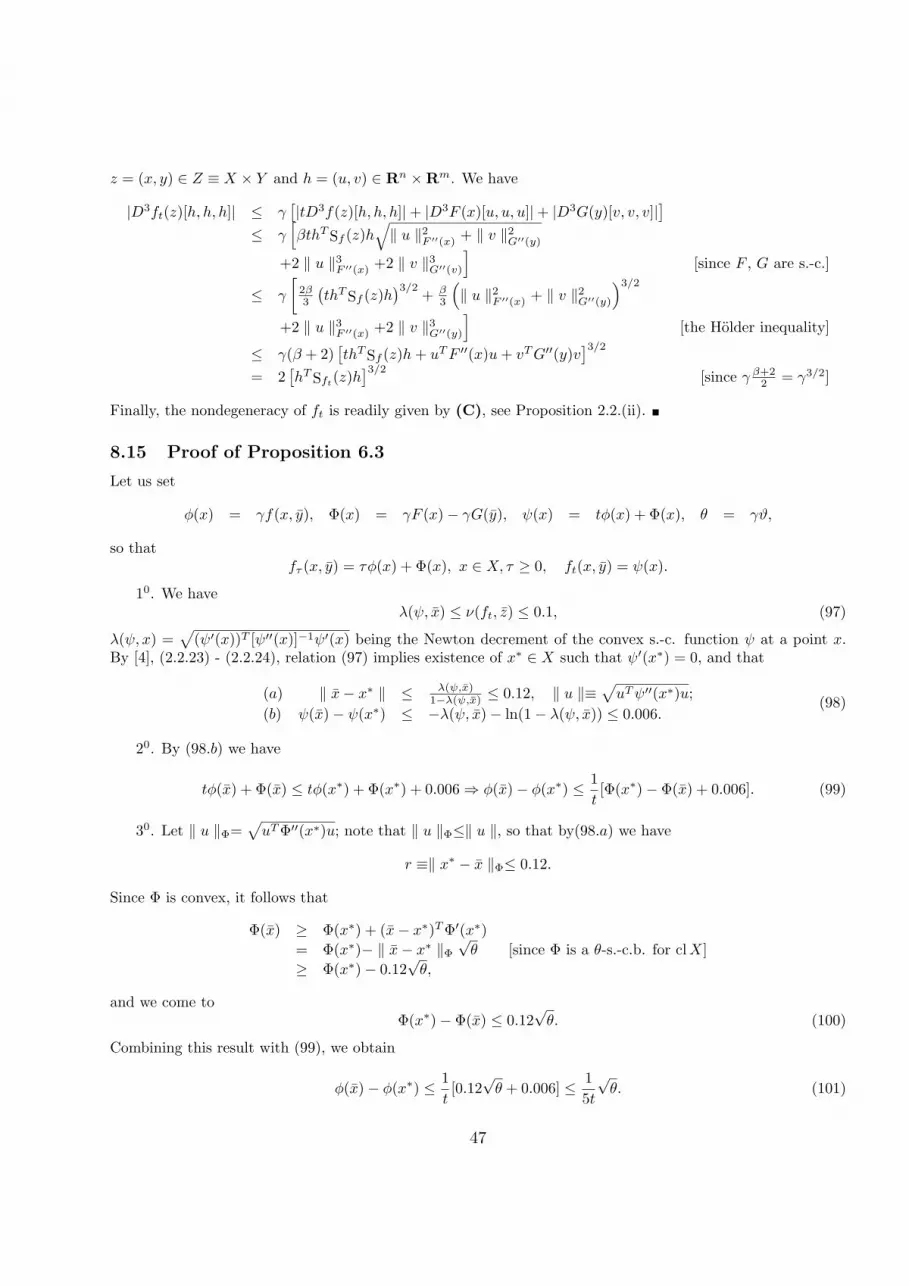
z = (x, y) ∈ Z ≡ X × Y and h = (u, v) ∈ Rn ×Rm. We have

|D3ft(z)[h, h, h]| ≤ γ[|tD3f(z)[h, h, h]|+ |D3F (x)[u, u, u]|+ |D3G(y)[v, v, v]|]

≤ γ[βthTSf (z)h

√‖ u ‖2F ′′(x) + ‖ v ‖2G′′(y)

+2 ‖ u ‖3F ′′(x) +2 ‖ v ‖3G′′(v)

][since F , G are s.-c.]

≤ γ

[2β3

(thTSf (z)h

)3/2 + β3

(‖ u ‖2F ′′(x) + ‖ v ‖2G′′(y)

)3/2

+2 ‖ u ‖3F ′′(x) +2 ‖ v ‖3G′′(y)

][the Holder inequality]

≤ γ(β + 2)[thTSf (z)h+ uTF ′′(x)u+ vTG′′(y)v

]3/2= 2

[hTSft(z)h

]3/2 [since γ β+22 = γ3/2]

Finally, the nondegeneracy of ft is readily given by (C), see Proposition 2.2.(ii).


Let us set

φ(x) = γf(x, y), Φ(x) = γF (x)− γG(y), ψ(x) = tφ(x) + Φ(x), θ = γϑ,

so thatfτ (x, y) = τφ(x) + Φ(x), x ∈ X, τ ≥ 0, ft(x, y) = ψ(x).

10. We haveλ(ψ, x) ≤ ν(ft, z) ≤ 0.1, (97)

λ(ψ, x) =√

(ψ′(x))T [ψ′′(x)]−1ψ′(x) being the Newton decrement of the convex s.-c. function ψ at a point x.By [4], (2.2.23) - (2.2.24), relation (97) implies existence of x∗ ∈ X such that ψ′(x∗) = 0, and that

(a) ‖ x− x∗ ‖ ≤ λ(ψ,x)1−λ(ψ,x) ≤ 0.12, ‖ u ‖≡

√uTψ′′(x∗)u;

(b) ψ(x)− ψ(x∗) ≤ −λ(ψ, x)− ln(1− λ(ψ, x)) ≤ 0.006.(98)

20. By (98.b) we have

tφ(x) + Φ(x) ≤ tφ(x∗) + Φ(x∗) + 0.006⇒ φ(x)− φ(x∗) ≤ 1t[Φ(x∗)− Φ(x) + 0.006]. (99)

30. Let ‖ u ‖Φ=√uTΦ′′(x∗)u; note that ‖ u ‖Φ≤‖ u ‖, so that by(98.a) we have

r ≡‖ x∗ − x ‖Φ≤ 0.12.

Since Φ is convex, it follows that

Φ(x) ≥ Φ(x∗) + (x− x∗)TΦ′(x∗)= Φ(x∗)− ‖ x− x∗ ‖Φ

√θ [since Φ is a θ-s.-c.b. for clX]

≥ Φ(x∗)− 0.12√θ,

and we come toΦ(x∗)− Φ(x) ≤ 0.12

√θ. (100)

Combining this result with (99), we obtain

φ(x)− φ(x∗) ≤ 1t[0.12

√θ + 0.006] ≤ 1

5t

√θ. (101)

47

Now let x ∈ X. We have

φ(x) ≥ φ(x∗) + (x− x∗)Tφ′(x∗)= φ(x∗)− 1

t (x− x∗)TΦ′(x∗) [since tφ′(x∗) + Φ′(x∗) = 0]≥ φ(x∗)− θ

t [since Φ is θ-s.-c.b. for clX, see [5], (2.3.2)].

From this relation and (101) it follows that

φ(x)− infXφ ≤ 1

5t

√θ +

1tθ ≤ 2θ

t,

whencef(x, y)− inf

x∈Xf(x, y) ≤ 2θ

tγ=

2ϑt.

Symmetric reasoning yields supy∈Y

f(x, y)− f(x, y) ≤ 2ϑt , and (26) follows.

40. By (99) we have

[t+φ(x) + Φ(x)]− [t+φ(x∗) + Φ(x∗)] ≤[t+

t − 1]

[Φ(x∗)− Φ(x)] + 0.006 t+

t

= α[Φ(x∗)− Φ(x)] + 0.006(1 + α)≤ 0.12α

√θ + 0.006(1 + α) [see (100)].

(102)

50. Now let x ∈ X. We have

t+φ(x) + Φ(x) ≥ t+φ(x∗) + t+(x− x∗)Tφ′(x∗) + Φ(x)= t+φ(x∗)− (1 + α)(x− x∗)TΦ′(x∗) + Φ(x) = t+φ(x∗) + Φ(x∗) + Ψα(x),

Ψα(x) = Φ(x)− Φ(x∗)− (1 + α)(x− x∗)TΦ′(x∗).(103)

The remaining reasoning reproduces the one of [5], Section 3.2.6. First, we claim that the function Ψα(x), forevery α ≥ 0 (in fact – even for α > −1) attains its minimum on X at a point x(α). Indeed, Φ is a θ-s.-c.b.for clX; consequently, the image of X under the mapping x 7→ Φ′(x) is the relative interior of a convex cone([5], Proposition 2.3.2 and Theorem 2.4.2). Since this cone clearly contains the point Φ′(x∗), it also containsthe points (1 + α)Φ′(x∗), so that there exists x(α) ∈ X with Φ′(x(α)) = (1 + α)Φ′(x∗), or, which is the same,with (Ψα)′(x(α)) = 0, as claimed.

From [5], Proposition 2.3.2 and Theorem 2.4.2 one can easily derive that x(α) can be chosen to satisfyx(0) = x∗ and to be differentiable in α. The point x(α) solves the equation

Φ′(x) = (1 + α)Φ′(x∗), (104)

and thereforeΦ′′(x(α))x′(α) = Φ′(x∗). (105)

Now letg(α) = Ψα(x(α)).

We haveg′(α) = [x′(α)]T [Φ′(x(α))− (1 + α)Φ′(x∗)]− (x(α)− x∗)TΦ′(x∗)

= −(x(α)− x∗)TΦ′(x∗) [since x = x(α) is a solution to (104)], (106)

whenceg′′(α) = −[x′(α)]TΦ′(x∗)

= minh

[2hTΦ′(x∗) + hTΦ′′(x(α))h] [see (105)]

= (1 + α)−2 minh

[2hTΦ′(x(α)) + hTΦ′′(x(α))h] [see (105)]

≥ −(1 + α)−2θ [since Φ is a θ-s.-c.b.].

(107)

48

Since x(0) = x∗, we get from (106), (107)

g(0) = 0; g′(0) = 0; g′′(α) ≥ −θ(1 + α)−2,

whenceα ≥ 0⇒ g(α) ≥ −θ[α− ln(1 + α)].

Consequently, (103) ensures that

infx∈X

[t+φ(x) + Φ(x)] ≥ [t+φ(x∗) + Φ(x∗)]− θ[α− ln(1 + α)].

Combining this result with (102), we come to

ft+(z)− infx∈X

ft+(x, y) ≤ 0.12α√θ + 0.006(1 + α) + θ[α− ln(1 + α)].

Symmetric reasoning implies that

supy∈Y

ft+(x, y)− ft+(z) ≤ 0.12α√θ + 0.006(1 + α) + θ[α− ln(1 + α)].

and (27) follows.

8.16 Proof of Lemma 6.1

Let us first prove the existence and the uniqueness of the saddle point z∗(t). Since ft is a nondegenerate s.-c.c.-c.function, it suffices to verify that ft(·, y) is below bounded on X, and f(x, ·) is above bounded on Y (Proposition2.5). By symmetry, we may prove the first statement only. Since g(x) = f(x, y) has bounded level sets and isconvex on X, it admits lower bound of the type g(x) ≥ a+ b ‖ x ‖2, x ∈ X, with b > 0, while for a ϑ-s.-c.b. Ffor clX we have (see [5], (2.3.3))

x ∈ X ⇒ F (x) ≥ F (x0) + ϑ ln(1− πx(x0)),

where x0 ∈ X is arbitrary and

πx(x0) = inf{t > 0 | x+ t−1(x0 − x) ∈ X}.

For a once for ever fixed x0 ∈ X, the quantity 1− πx(x0) is of course bounded from below by a function of thetype c/(1+ ‖ x ‖2). Thus,

ft(x, y) ≥ γ[tb ‖ x ‖2 −ϑ ln(1+ ‖ x ‖2) + const(t)],

and the right hand side in this inequality is below bounded for every t > 0.The fact that the path z∗(t) is continuously differentiable is readily given by the Implicit Function Theorem

(recall that the Hessian of a nondegenerate s.-c.c.-c. function is nondegenerate, see the proof of Proposition3.1.(iii)).


10. To prove (31), we start with the following observation:

Lemma 8.5 Let y = y(t, x). Then the Newton decrement ω(ft, (x, y)) of the s.-c.c.-c. function ft at the pointz = (x, y) is equal to the Newton decrement λ(Φ(t, ·), x) of the convex s.-c. function Φ(t, ·) at the point x.Moreover, the Newton iterate x of x given by (30) is exactly the x-component of the pair

z+ = z − [∇2ft(z)]−1∇ft(z).

49

Proof. Denoting Φ(t, ·) = Ψ(·), ft ≡ φ, let φ′′(z) =(A BT

B −C)

and g = φ′x(z). Since φ′y(z) = 0, the Newton

direction e = e(φ, z) =(pq

)of φ at z is the solution to the system of equations

Ap+BT q = g, Bp− Cq = 0,

whencep = (A+BTC−1B)−1g, q = C−1B(A+BTC−1B)−1g.

Since g = Ψ′(x) and Ψ′′(x) = A+BTC−1B (see (56)), we get

x = x− p, ω2(f, z) = pTAp+ qTCq = gT (A+BTC−1B)−1g = [Φ′(x)]T [Φ′′(x)]−1Φ′(x).

Lemma combined with (22) implies that

ν(ft, z+) ≤ λ2(Φ(t, ·), x)(1− λ(Φ(t, ·), x))2

≤ (0.1)2

(0.9)2≤ 0.1. (108)

By Proposition 6.3 it follows that

supy∈Y

f(x, y) ≤ infx∈X

f(x, y+) +4ϑt, (109)

where y+ is the y-component of z+. Since infx∈X

f(x, y+) ≤ infx∈X

supy∈Y

f(x, y), (31) follows.

20. Let us prove the bound (32). Since Φ(t, ·) is a s.-c. convex below bounded function on X, the numberof damped Newton steps in the updating (t, x) 7→ (t+, x+) is bounded from above by O(1)

[∆(t+) + ln ln 1

κ

],

where∆(t) = Φ(t, x)− min

x′∈XΦ(t, x′)

and O(1) is an absolute constant (see [5], Theorem 2.2.3). Thus, all we need is to verify that

t ≥ t⇒ ∆(t) ≤ ρ(κ) +32

(1 +

√γϑ) t− t

t+ +3γϑ

[t− tt− ln

t

t

]. (110)

Let z∗(t) = (x∗(t), y∗(t)) be the trajectory of saddle points of the functions ft; note that z∗(·) is continuouslydifferentiable by Lemma 6.1. As we remember,

Φ(t, x) = γ [tf(x, y(t, x)) + F (x)−G(y(t, x))] ,

with continuously differentiable function y(t, x) satisfying the relation

y = y(t, x)⇒ tf ′y(x, y)−G′(y) = 0.

From these relations we get (values of all functions and their derivatives are taken at the point (t, x, y(t, x))):

y′t = [G′′ − tf ′′yy]−1f ′y = [G′′ − tf ′′yy]−1t−1G′,Φ′t = γf,

Φ′′tt = γ[f ′y]T y′t = γt−1[G′]T y′t = γt−2[G′]T [G′′ − tf ′′yy]−1G′.(111)

Taking into account that G is a ϑ-s.c-c.b. and that f is concave in y, we come to

0 ≤ Φ′′tt(t, x) ≤ γϑt−2. (112)

Now, setting Ψ(x, y) = F (x)−G(y) we have (values of all functions and their derivatives are taken at the point(t, z∗(t))):

t∇zf +∇zΨ = 0⇒ d

dtz∗(t) = −[t∇2

zf +∇2zΨ]−1∇zf ⇒ d

dtz∗(t) = t−1[t∇2

zf +∇2zΨ]−1∇zΨ,

50

whenceddtΦ(t, x∗(t)) = γf,

− d2

dt2 Φ(t, x∗(t)) = −γ[∇zf ]T ddtz∗(t) = γt−2[∇zΨ]T [t∇2

zf +∇2zΨ]−1∇zΨ

≤ t−2γ2[∇zΨ]T [Sft(z∗(t))]−1∇zΨ [see Lemma 8.2]

≤ 2t−2γϑ,

(113)

the concluding inequality being given by Sft ≥ γ

(F ′′

G′′

), ∇zΨ =

(F ′

−G′)

and the fact that F,G are

ϑ-s.-c.b.’s.Since λ(Φ(t, ·), x) ≤ κ ≤ 0.1, we have

Φ(t, x) ≤ Φ(t, x) ≤ minx∈X

Φ(t, x) + ρ(κ)

(see [5], Theorem 2.2.1, and (6)). Consequently,

∆(t) ≤ ρ(κ). (114)

Besides this,

∆′(t) = Φ′t(t, x)− d

dtΦ(t, x∗(t)),

whence in view of (111), (112), (113)

∆′(t) = γ [f(x, y(t, x))− f(z∗(t))] (115)

and

∆′′(t) = Φ′′tt(t, x)− d2

dt2Φ(t, x∗(t)) ≤ 3γt−2ϑ. (116)

30. In view of the inequalities (114), (116) all we need to bound ∆(t+) from above is to bound from abovethe quantity

∆′(t) = γ [f(x, y)− f(z∗(t))] , y = y(t, x). (117)

(see (115)).30.1). For the sake of brevity, let g(x, y) = ft(x, y), z∗ ≡ (x∗, y∗) = z∗(t), and let

dx =√

[x− x∗]T g′′xx(z∗)[x− x∗], dy =√−[y+ − y∗]g′′yy(z∗)[y+ − y∗].

By (108), ν(g, z+) < 0.1; applying (21.b), we get µ(g, z+) ≤ ρ(0.1) ≤ 0.01, whence (see (23))√d2x + d2

y ≤ 2[µ(g, z+) +

√µ(g, z+)

]≤ 0.5. (118)

Since µ(g, z+) ≡ supyg(x, y)− inf

xg(x, y+) ≤ 0.01, the quantity g(z+) differs from the saddle value g(z∗) of g by

at most 0.01:

|g(z+)− g(z∗)| ≡ γ∣∣t[f(z+)− f(z∗)] + F (x)− F (x∗) +G(y∗)−G(y+)

∣∣ ≤ 0.01. (119)

We have g′′xx(z∗) � γF ′′(x∗), so that (x− x∗)T [γF ′′(x∗)](x− x∗) ≤ d2x. Therefore

γ|F (x)− F (x∗)| ≤ |(x− x∗)T (γF ′(x∗))|+ ρ(dx) [(4) as applied to γF ]≤ √

γϑdx + ρ(dx) [since γF is (γϑ)-s.-c.b.]≤ 0.5

√γϑ+ 0.45 [see (118)]

and similarly γ|G(y+)−G(y∗)| ≤ 0.45√γϑ+ 0.5. Thus, (119) implies that

γ|f(z∗)− f(z+)| ≤ 1 +√γϑ

t. (120)

51

30.2). Now consider the self-concordant function φ(y) = −γ [tf(x, y) + F (x)−G(y)]. This function attainsits minimum on Y at y = y, and from µ(g, z+) ≤ 0.01 it follows that φ(y+) − min

yφ(y) ≤ 0.01. Denoting

δ =√

[y+ − y]Tφ′′(y)[y+ − y] and applying (4), we get ρ(−δ) ≤ 0.01, whence δ ≤ 0.5. We have

0.01 ≥ φ(y+)− φ(y) = γ∣∣t[f(x, y+)− f(x, y)]− [G(y+)−G(y)]

∣∣ ,and from δ ≤ 0.5, same as in 30.1), it follows that γ|G(y+) − G(y)| ≤ 0.5

√γϑ + 0.45. Combining these

observations, we get

γ|f(z+)− f(x, y)| ≤ 0.5 + 0.5√γϑ

t,

which together with (120) and (117) implies that

∆′(t) ≤ 3(1 +√γϑ)

2t. (121)

Relations (114), (116) and (121) imply (110).

8.18 Proof of Lemma 7.1

Let h ∈ Rm, r ∈ Rn be two arbitrary vectors, and let

Y0 = Diag(y0), H = Y −10 Diag(h), X0 = X(ξ0),

R = X−10 Diag(Er), P = Y

1/20 X

−1/20 E(ETY0X

−10 E)−1ETX

−1/20 Y

1/20 .

Note that P is an orthoprojector.We have

hT f ′y(z0) = Tr((ETY0X

−10 E)−1ETDiag(h)X−1

0 E)− 2hTx(ξ0)

= Tr((ETY0X

−10 E)−1ETY0X

−10 HE

)− 2Tr(X0Y0H)= Tr(PH)− 2Tr(X0Y0H);

rT f ′ξ(z0) = Tr

((ETY0X

−10 E)−1ETY0X

−10 Diag(Er)X−1

0 E)

+ 2(y0)TEr= Tr

((ETY0X

−10 E)−1ETY0X

−10 RE

)+ 2Tr(Y0X0R)

= Tr(PR) + 2Tr(X0Y0R);hTG′′(y0)h+ rTF ′′(ξ0)r = hTY −2

0 h+ rTETX−20 Er

= Tr(H2 +R2);hTG′(y0) = −Tr(H);rTF ′(ξ0) = Tr(R).

Consequently,

γ−1(rT , hT )(ft0)′(z0) = t0Tr(PH) + t0Tr(PR)− 2t0Tr(Y0X0H) + 2t0Tr(Y0X0R) + Tr(H) + Tr(R)= t0Tr(PH) + t0Tr(PR) + 2Tr(R)

(122)(note that by construction 2t0Y0X0 = I, I being the unit m×m matrix). In view of (122) and due to the factthat P is an orthoprojector one has

∣∣(rT , hT )(ft0)′(z0)∣∣ ≤ γt0

√2mTr(H2 +R2) + 2γ|Tr(R)|,

while in view of (37)

|Tr(R)| = |rTF ′(ξ0)| ≤ 0.052√γ

√rTF ′′(ξ0)r =

0.052√γ

√Tr(R2);

thus, ∣∣(rT , hT )(ft0)′(z0)∣∣ ≤ γt0

√2mTr(H2 +R2) + 0.05

√γ√

Tr(R2) ≤ 0.1√γ√

Tr(H2 +R2)

52

(see the definition of t0). On the other hand,

(rT , hT )Sft0 (z0)(rh

)≥ γ[hTG′′(y0)h+ rTF ′′(ξ0)r] = γTr(H2 +R2),

and we conclude that for all h ∈ Rm, r ∈ Rn one has

∣∣(rT , hT )(ft0)′(z0)∣∣ ≤ 0.1

√(rT , hT )Sft0 (z0)

(rh

),

whence ν(ft0 , z0) ≤ 0.1, as claimed.


Let vol be the normalization of Vol which makes the normalized volume of the unit Euclidean ball equal to 1;of course, it suffices to prove (40) for the normalized volume vol instead of the standard volume Vol.

Let us set

Φ(λ) = γtf(ξ, λ), φ(λ) = γm∑i=1

lnλi, H(λ) = −[Φ(λ) + φ(λ)].

Note that since −ft(ξ, ·) differs from H(·) by a constant, the function H is s.-c. on Rm++, and its Newton

decrement at y (see Definition 2.1) is majorated by ν(ft, z). Thus, λ(H, y) ≤ δ ≤ 0.1, whence by [5], Theorem2.2.2, there exists y∗ ∈ Rm

++ such that

‖ y∗ − y ‖H′′(y)≤ 10δ, H ′(y∗) = 0. (123)

Let us setY∗ = Diag(y∗), B∗ = (ETY∗X−1E)−1, A∗ = 2−1/2B

1/2∗ ,

di = y∗i /xi(ξ), i = 1, ...,m, D = Diag(d1, d2, ..., dm).

The second relation in (123), after straightforward computation, implies that

eTi B∗ei = 2x2i (ξ)− t−1d−1

i , i = 1, ...,m, (124)

whenceeTi A

2∗ei = x2

i (ξ)− (2t)−1d−1i , i = 1, ...,m. (125)

Since di > 0 for all i, we conclude that the ellipsoid

W∗ = {ξ +A∗u | uTu ≤ 1}

is contained in Π.In view of (124) we have

n = Tr(B∗B−1∗ ) = Tr(B∗ETDE) = Tr([EB∗ET ]D)

=m∑i=1

eTi B∗eidi =m∑i=1

(2x2i (ξ)− t−1d−1

i )di =m∑i=1

2y∗i xi(ξ)−mt−1,

whencef(ξ, y∗) = − ln DetB∗ − 2(y∗)Tx(ξ) = − ln DetB∗ − n−mt−1.

On the other hand, due to Proposition 7.1 and to the second relation in (123) we have

V(ξ) =n ln 2 + n

2+

12f(ξ, y∗).

53

Combining our observations, we get

V(ξ) =n ln 2 + n

2− 1

2ln DetB∗ − n

2− m

2t= − ln DetA∗ − m

2t. (126)

Let V∗ be the infimum of V(·) over int Π. Proposition 7.3 states that

V(ξ) ≤ V∗ +2mt.

From this inequality and (126) we conclude that

ln vol(W∗) = ln DetA∗ ≥ −V∗ − 5m2t. (127)

Now, from the first relation in (123) and from the fact that Φ′′(y) ≤ 0 it follows that√√√√γ

m∑

i=1

(y∗i − yi)2y−2i =‖ y∗ − y ‖−φ′′(y)≤ 10δ,

whence(1− 10δ)yi ≤ y∗i ≤ (1 + 10δ)yi, i = 1, ...,m,

so that(1− 10δ)−1B � B∗ � (1 + 10δ)−1B, (128)

i.e.,‖ A∗u ‖2≥‖ Au ‖2 ∀u.

From this inequality and (125) it follows that W ⊂ Π. Finally, we have

ln DetA = −n2 ln(1 + 10δ) + ln DetA = −n2 ln(1 + 10δ)− n ln 22 + 1

2 ln DetB≥ −n2 ln(1 + 10δ)− n ln 2

2 + 12 ln DetB∗ + n

2 ln(1− 10δ)[we have used the first inequality in (128)]

= −n2 ln(

1+10δ1−10δ

)+ ln DetA∗

⇒ ln vol(W ) = ln DetA≥ ln vol(W∗)− n

2 ln(

1+10δ1−10δ

)≥ −V∗ − 5m

2t − n2 ln

(1+10δ1−10δ

)[see (127)]

≥ −V∗ − ε.

It remains to recall that (−V∗) is the logarithm of the normalized volume of the maximal ellipsoid contained inΠ.

54

on self-concordant convex–concave functions

Documents