Author's Accepted Manuscript

Convex and concave hulls for classificationwith support vector machine

Asdrúbal López Chau, Xiaoou Li, Wen Yu

PII: S0925-2312(13)00644-9DOI: http://dx.doi.org/10.1016/j.neucom.2013.05.040Reference: NEUCOM13493

To appear in: Neurocomputing

Received date: 1 June 2012Revised date: 19 March 2013Accepted date: 27 May 2013

Cite this article as: Asdrúbal López Chau, Xiaoou Li, Wen Yu, Convex andconcave hulls for classification with support vector machine, Neurocomputing,http://dx.doi.org/10.1016/j.neucom.2013.05.040

This is a PDF file of an unedited manuscript that has been accepted forpublication. As a service to our customers we are providing this early version ofthe manuscript. The manuscript will undergo copyediting, typesetting, andreview of the resulting galley proof before it is published in its final citable form.Please note that during the production process errors may be discovered whichcould affect the content, and all legal disclaimers that apply to the journalpertain.

www.elsevier.com/locate/neucom

Convex and Concave Hulls for Classification with

Support Vector Machine

Asdrubal Lopez Chau1,2, Xiaoou Li1, Wen Yu3,∗

1Departamento de Computacion, CINVESTAV-IPN

Mexico City, 07360, Mexico

2Universidad Autonoma del Estado de Mexico (UAEM)

Zumpango, Estado de Mexico, 55600, Mexico

2Departamento de Control Automatico, CINVESTAV-IPN

Mexico City, 07360, Mexico, yuw@ctrl.cinvestav.mx

∗Corresponding author

Abstract

The training of a support vector machine (SVM) has the time complexity of O(n3)

with data number n . Normal SVM algorithms are not suitable for classification of

large data sets. Convex hull can simplify SVM training, however the classification

accuracy becomes lower when there are inseparable points. This paper introduces

a novel method for SVM classification, called convex-concave hull. After grid pre-

processing, the convex hull and the concave (non-convex) hull are found by Jarvis

march method. Then the vertices of the convex-concave hull are applied for SVM

training. The proposed convex-concave hull SVM classifier has distinctive advantages

on dealing with large data sets with higher accuracy. Experimental results demonstrate

that our approach has good classification accuracy while the training is significantly

faster than the other training methods.

1 Introduction

Support Vector Machine (SVM) is a popular classification method in machine learning [30].

It minimizes the empirical classification error and maximizes the geometric margin. It offers

1

a hyperplane that represents the largest separation (or margin) between two classes [24].

However this kind of maximum-margin hyperplane may not exist because of class overlapping

or mislabeled examples. The soft margin SVM by introducing slack variables can find a

hyperplane that splits the examples as cleanly as possible. In order to find a separation

hyperplane, it is necessary to solve the Quadratic Programming Problem (QPP). This is

computational expensive, it has O(n3) time and O(n2) space complexities with n data [24].

so the standard SVM is unfeasible for large data sets [25].

Many researchers have tried to find possible methods to apply SVM classification for

large data sets. These methods can be divided into four types: a) reducing training data

sets (data selection), b) using geometric properties of SVM, c) modifying SVM classifiers,

d) decomposition, and e) the other methods. The data selection method chooses the objects

which are possible to be the support vectors (SV) [20]. These data are used for SVM training.

Generally, the number of the support vectors is much small compared with the whole data.

Clustering is another effective tool to reduce data set size, for example, hierarchical clustering

[33] and parallel clustering [26]. The sequential minimal optimization (SMO) [25] breaks the

large QP problem into a series of smallest possible QP problems. The projected conjugate

gradient (PCG) chunking scales somewhere between linear and cubic in the training set [8].

The geometric properties of SVM can also be used to reduce the training data. In sep-

arable case, the maximum-margin hyperplane is equivalent to finding the nearest neighbors

in the convex hulls of each class [2]. Neighborhood properties of the objects can be applied

to detect SV. In [18] an active learning model of sample selection is proposed. The model

is based on the measurement of neighborhood entropy. In [19] is proposed an algorithm

that selects the patterns in the overlap region around the decision boundary. The method

presented in [4] follows this trend but it uses fuzzy C-means clustering to select samples on

the boundaries of class distribution. The most popular geometric methods are the nearest

points problem (NPP) and the convex hull.

NPP was first reformulated to solve SVM classification in [18]. The data which are close

to those opposite label have high probability to be SV. The Euclidean distance between

these data and the opposite label are computed to find the shortest distance. The problem

of this method is the computation time is O(n2). Gilbert’s algorithm [12] is one of the first

algorithms for solving the minimum norm problem (MNP) in NPP. The MDM algorithm

suggested by Mitchell et al. [22] works faster than Gilbert’s algorithm. The NPP method is

also extended to solving the SMO-SVM optimization problem in the image processing [19].

Since the support vectors are usually located in local extremum or near extremum [1], using

extremes examples from the full training set can reduce training set [14].

2

The key problem is how to find the border of a data set. K-nearest neighbor (KNN)

method is a good method. The local data distribution and local geometrical property were

applied in [31][20]. Minimum enclosing ball is applied to SVM classification in [4]. Ap-

proximately optimal solutions of SVM are obtained by core vector machine (CVM) in [29].

Schlesinger-Kozinec (SK) algorithm [28] used the geometric interpretation of SVM. The

maximal margin classifier with a given precision for separable data was obtained.

Convex hull has been applied in training SVM in [1][2][21]. There are some algorithms

to compute the convex hull with finite points. Graham scan [13] finds all vertices of the

convex hull along its boundary by computing the direction of the cross product of the two

vectors. Jarvis’ march (Gift wrapping) [17] identifies the convex hull by angle comparisons

and wrapping a string around the point set. Divide and Conquer method [27] is applicable to

the three dimensional case. The incremental convex hull [23] and quick hull [9] give methods

to eliminate useless points.

In many real applications the data are not perfectly separated, and the kernel method

is not so powerful for nonlinear separation. In these cases, the closest points in the convex

hulls are no longer support vectors. In this case, the soft SVM . Although the soft margin

optimization with the slack variable, the penal parameter C effects the optimal performance

of SVMs can be applied directly. The optimization becomes a trade off between a large

margin and a small error penalty [24].

Another method is to use the reduced convex hull [21]. The intersection parts disappear

by reducing the convex hulls. The inseparable case becomes separable case. The main

disadvantage of the reduced convex hull is the convex hull has to be calculated in each

reducing step [2]. Variant SVM (v-SVM) [6] can make the intersection set be empty by the

choice of parameters. The v-SVM is similar with the reduced convex hull, the computation

process is complex.

Concave-convex procedure (CCCP) [32] separates the energy function into a convex func-

tion and a concave (non-convex) function. By using a non-convex loss function, it forms a

non-convex SVM. But some good properties of SVM, for example the maximum margin,

cannot be guaranteed [7], because the intersection parts of data sets are not satisfied convex

conditions.

In this paper we propose a new algorithm, called convex-concave hull, to search the points

that are on the outer boundaries of a set of points. By using Jarvis’ march method, we first

compute the convex hulls. Then the concave hulls are created by using the vertices of the

convex hull. In this way, the misleading points in the intersection become the vertices of the

concave hulls. The classification accuracy is increased compared with the other geometric

3

methods, such as the reduced convex hull SVM (RCHSVM) and v-SVM. The training time

is decreased considerably. The experimental results show that the accuracy obtained by our

convex-concave hull approach is very close to classic SVM methods, while the training time

is significantly shorter.

2 Convex and Concave Hull

2.1 Convex Hull

The convex hull (CH) of a set of points S is the minimum convex set that contains S.

Mathematically, CH is defined as

CH(X) :

{w =

n∑i=1

aixi, ai ≥ 0,n∑

i=1

ai = 1, xi ∈ X

}(1)

For SVM classification, a data set X has the general form as

X ={(xi, yi), xi ∈ Rd, yi = {+1,−1}

}(2)

where d is the number of features, yi is the label of object xi.

Let’s create two subsets X+ and X−, X = X+ ∪X−

X+ ={(xi, yi), xi ∈ Rd and yi = {+1}

}(3)

X− ={(xi, yi), xi ∈ Rd and yi = {−1}

}(4)

If CH(X+) ∩ CH(X−) = ∅, there is not intersection. It is called linearly separable. The

optimal separating hyperplane is determined by the closest pair of points that belong to X+

and X− [1][2]. The problem can be stated as

minxi∈X+xj∈X−

∥∑M

i=1 αixi −∑L

j=1 αjxj∥2∑Mi=1 αi = 1,

∑Lj=1 αj = 1, αi ≥ 0, αj ≥ 0

(5)

where | X+ | is the size of the set X+. Let us define | X+ |= M and | X− |= L.

In this linearly separable case, the ”‘hard”’ optimal separating hyperplane is a vector

that is normal to the line which joints the closest points, see Figure 1.

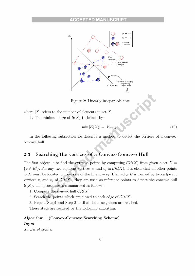
In the most case, the data are not linearly separable. The convex hulls intersect each

other, see Figure 2. (5) does not have solution. It is necessary to map the objects to a higher

dimensional space to allow mis-classification. The separating hyperplane is ”soft”. The soft

margin separating hyperplane is shown in Figure 2.

4

y=-1y=+1

w

Separating hyper plane

Figure 1: Linearly separable case

2.2 Concave Hull

In no-linearly separable case, most geometric methods have to shrink or reduce the convex

hull to avoid the overlapping. In our method, the convex hull is not changed. We detect

the objects that are close to exterior boundaries. In order to detect these objects, we use

concave hull. The border points B(X) of a set X ∈ R2 are vertices of a ”convex-concave

hull”, if they hold the following properties:

1. The vertices of a convex-concave hull B(X) are the vertices of a convex hull (CH) andthe points that are closed to the edges of CH

B(X) = VCH(X) ∪ CloseCH (6)

where VCH(X) is vertex set of the convex hull, CloseCH is the set that is closed to the edges

of the convex hull. The ”closeness” to an edge of CH(X) is different from point to point, so

there is no unique set of border points.

2. B(X) is not a convex hull. A set S ∈ R2 is said to be convex CH(X) if

x1, x2 ∈ S, then αx1 + (1− α)x2 ∈ S, for all α ∈ (0, 1) (7)

Generally, a polygon defined by (6) does not satisfy (7).

3. The border points must be part of the data set

B(X) ⊆ X (8)

It can be proved that (8) implies

max |B(X)| = |X| ∀ X (9)

5

Supportvectors

Optimal (soft margin)separatinghyper plane

Error

allowed

Misclassified

sample

Figure 2: Linearly inseparable case

where |X| refers to the number of elements in set X.

4. The minimum size of B(X) is defined by

min |B(X)| = |VCH(X)| (10)

In the following subsection we describe a method to detect the vertices of a convex-

concave hull.

2.3 Searching the vertices of a Convex-Concave Hull

The first object is to find the extreme points by computing CH(X) from given a set X =

{x ∈ R2}. For any two adjacent vertices vi and vj in CH(X), it is clear that all other points

in X must be located on one side of the line vi− vj. If an edge E is formed by two adjacent

vertices vi and vj of CH(X), they are used as reference points to detect the concave hull

B(X). The procedure is summarized as follows:

1. Compute the convex hull CH(X)

2. Search the points which are closed to each edge of CH(X)

3. Repeat Step1 and Step 2 until all local neighbors are reached.

These steps are realized by the following algorithm.

Algorithm 1 (Convex-Concave Searching Scheme)

Input

X: Set of points.

6

K: Number of candidates.

Output:

B(X):Convex-concave hull

Begin algorithm

// Set of vertices begins empty

B(X)← ∅Compute CH(X)

The vertices of CH(X) are v1,...,vn

for each pair of adjacent vertexes (vi, vj) do

θ ← compute angle defined by (vi, vj ) as cos−1

(−→vi ·−→vj

∥−→vi∥·∥−→vj∥

)//Detect points ”close” to edge (vi, vj )

Apply Algorithm 2 using (X, (vi, vj), K, θ)

B(X)← B(X) ∪ CloseCH

end for

End algorithm

We use Algorithm 2 to search the nearest points to the edges of CH(X). It works as

follows: Given a set of points X and two reference points vi, vj, the algorithm begins with

the point vi and finds its K nearest neighbors.

From each neighbor, we search the point vk such that which −−→vivk has the smallest angle

with respect to line −−→vivj

θmin = mink

[cos−1

( −−→vivk · −−→vivj∥−−→vivk∥ · ∥−−→vivj∥

)](11)

This procedure is repeated until vk = vj, see Figure 3. The closest points to the edge of

CH(X) are the nearest points to the edges of CH(X). Figure 3 shows an example where

K = 3

Algorithm 2 (Search the neareat points)

Input

X : A set of points

S: Two adjacent vertices {vi, vj} of CH(X)

K: Number of neighbors

θ : The previous angle angle between adjacent vertices

Output

7

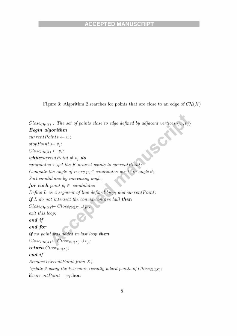
Figure 3: Algorithm 2 searches for points that are close to an edge of CH(X)

CloseCH(X) : The set of points close to edge defined by adjacent vertices {vi, vj}Begin algorithm

currentPoints← vi;

stopPoint← vj;

CloseCH(X) ← vi;

whilecurrentPoint = vj do

candidates←get the K nearest points to currentPoint;

Compute the angle of every pi ∈ candidates w.r.t. to angle θ;

Sort candidates by increasing angle;

for each point pi ∈ candidates

Define L as a segment of line defined by pi and currentPoint;

if L do not intersect the convex-concave hull then

CloseCH(X)← CloseCH(X) ∪ pi;

exit this loop;

end if

end for

if no point was added in last loop then

CloseCH(X)← CloseCH(X) ∪ vj;

return CloseCH(X);

end if

Remove currentPoint from X;

Update θ using the two more recently added points of CloseCH(X);

ifcurrentPoint = vjthen

8

Figure 4: Algorithm 2 with different K, (a)K = 9, (b) K = 4 and (c) K = 6.

return CloseCH(X);

end if

currentPoint← pi;

end while

End algorithm

Figure 4 shows an example of the convex-concave hull B(X) generated via Algorithm 1

and Algorithm 2. It is possible to obtain a different set B(X) by changing the parameter K

in Algorithm 2. In Figure 4, (a) K = 9, (b) K = 4, (c) K = 6. The greater the value of K

the most similar to the convex hull.

Remark 1 Algorithm 2 shows how the space between two consecutive extreme points is ex-

plored. This idea is similar to Jarvis’ march [17], where a set of points are wrapped. Jarvis’

march considers all points, whereas Algorithm 2 uses only local neighbors. Algorithm 2 runs

until the second extreme point in the argument is reached.

Remark 2 The convex-concave hull has the following advantages over KNN concave hull

[34]: 1) The starting and ending points of our algorithms are pre-set before by convex hull

9

method. It ensures all vertices of convex hull are always in the vertices of convex-concave

hull. 2) The angles in [34] are entirely depended on the previously computed ones. In our

method, the extreme points are used to compute the angles, so it is easy to implement. 3)

Our algorithm does not use recursive invocations. The stop point is added to the set of border

points when there are no more points, the search time is less than [34].

2.4 Properties of Convex-Concave Hull

In this section, we propose three interesting properties of our convex-concave hull methods.

These properties can be to formulate a simple pre-processing algorithm, which helps to find

the exterior boundaries of the points X fast.

Property 1 The vertexes of convex hull VCH(X) is a subset of the vertexes of convex-concave

hull B(X)

VCH(X) ⊆ B(X)

The searching algorithm first computes CH(X), then uses two extreme points vi and vj

in CH(X) to search concave points B(X). At the last iteration, B(X) contains all vertices

of CH(X).

Remark 3 The property 1 ensures that the optimal separating hyperplane can be obtained

in linearly separable cases, if B(X) is used for SVM training.

Property 2 A superset of the convex-concave hull B(X) can be obtained by detecting border

points by partitions of X, i.e., ∪i

B(X i) ⊇ B(X) ⊇ CH(X)

where X i is the partitions of X, ∩CH(X i) = ∅ and ∪X i = X.

Let us create j partitions on the input space X ∈ R2, i.e.,

∩X i = ∅ and ∪X i = X

Suppose each partition X i contains at least three points that belong to X. It is not difficult

to see that the vertices of convex hull VCH(X) is a subset of ∪VCH(Xi). We define two partitions

as CH(X1) and CH(X2). It is clear that

VCH(X) ⊂ VCH(X1) ∪ VCH(X2)

10

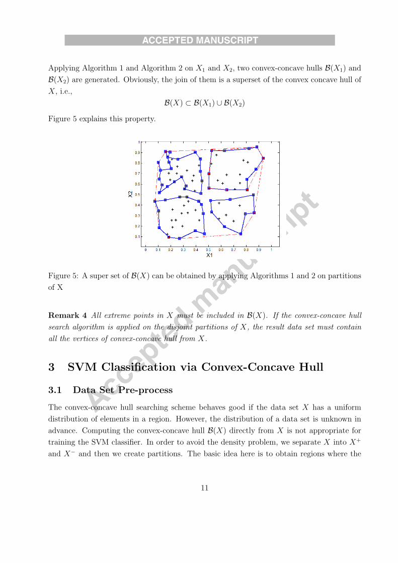
Applying Algorithm 1 and Algorithm 2 on X1 and X2, two convex-concave hulls B(X1) and

B(X2) are generated. Obviously, the join of them is a superset of the convex concave hull of

X, i.e.,

B(X) ⊂ B(X1) ∪ B(X2)

Figure 5 explains this property.

Figure 5: A super set of B(X) can be obtained by applying Algorithms 1 and 2 on partitions

of X

Remark 4 All extreme points in X must be included in B(X). If the convex-concave hull

search algorithm is applied on the disjoint partitions of X, the result data set must contain

all the vertices of convex-concave hull from X.

3 SVM Classification via Convex-Concave Hull

3.1 Data Set Pre-process

The convex-concave hull searching scheme behaves good if the data set X has a uniform

distribution of elements in a region. However, the distribution of a data set is unknown in

advance. Computing the convex-concave hull B(X) directly from X is not appropriate for

training the SVM classifier. In order to avoid the density problem, we separate X into X+

and X− and then we create partitions. The basic idea here is to obtain regions where the

11

distribution is more uniform than in the original ones. The property 2 allows us to claim

that all vertices of convex hull can be included in the vertexes of the convex concave hull

VCH(X) ⊆ VB(X)

In addition, the points in intersection of convex hulls are also included in B(X). This is

helpful for linearly inseparable cases for SVM classification. Property 1 gives guaranty

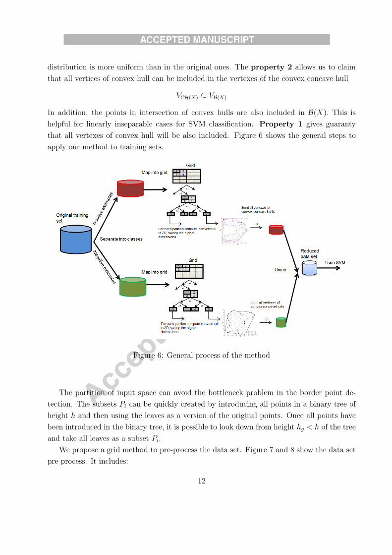
that all vertexes of convex hull will be also included. Figure 6 shows the general steps to

apply our method to training sets.

Figure 6: General process of the method

The partition of input space can avoid the bottleneck problem in the border point de-

tection. The subsets Pi can be quickly created by introducing all points in a binary tree of

height h and then using the leaves as a version of the original points. Once all points have

been introduced in the binary tree, it is possible to look down from height hg < h of the tree

and take all leaves as a subset Pi.

We propose a grid method to pre-process the data set. Figure 7 and 8 show the data set

pre-process. It includes:

12

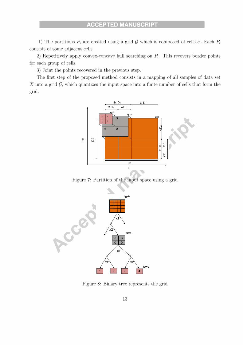
1) The partitions Pi are created using a grid G which is composed of cells cl. Each Pi

consists of some adjacent cells.

2) Repetitively apply convex-concave hull searching on Pi. This recovers border points

for each group of cells.

3) Joint the points recovered in the previous step.

The first step of the proposed method consists in a mapping of all samples of data set

X into a grid G, which quantizes the input space into a finite number of cells that form the

grid.

Figure 7: Partition of the input space using a grid

Figure 8: Binary tree represents the grid

13

We use four parameters to control the grid process: hg, ha, hb and K. Here hg is the

granularity of the grid, i.e., the height of the binary tree. ha is used to create the partitions

in higher dimensions. The binary tree is traverse down in the height of hb. K is used to

control the number of the neighbor points which are close to the edges of the convex hull.

The bigger the granularity, the finer the quantization. However, the amount of memory

required to store the grid is increased. This mapping from X into a G allows to maintain a

set of non repeated points, because they are mapped into the same cells, furthermore, this

can help to reduce the original number of points.

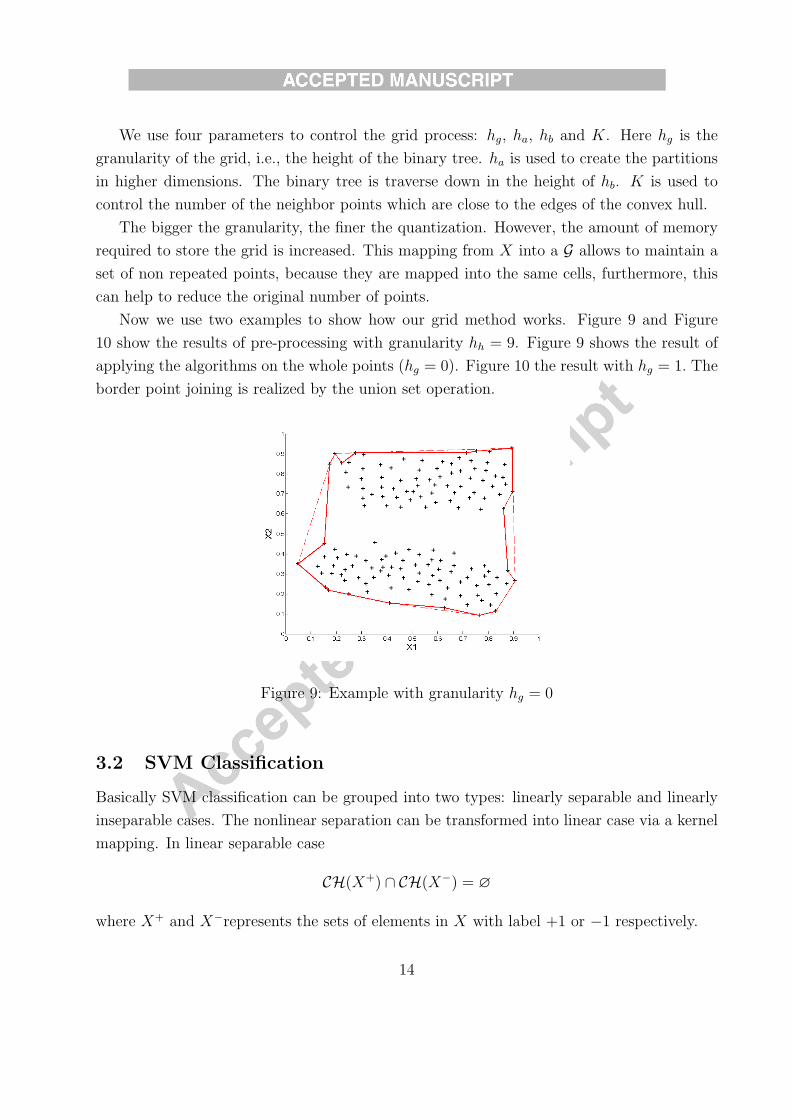
Now we use two examples to show how our grid method works. Figure 9 and Figure

10 show the results of pre-processing with granularity hh = 9. Figure 9 shows the result of

applying the algorithms on the whole points (hg = 0). Figure 10 the result with hg = 1. The

border point joining is realized by the union set operation.

Figure 9: Example with granularity hg = 0

3.2 SVM Classification

Basically SVM classification can be grouped into two types: linearly separable and linearly

inseparable cases. The nonlinear separation can be transformed into linear case via a kernel

mapping. In linear separable case

CH(X+) ∩ CH(X−) = ∅

where X+ and X−represents the sets of elements in X with label +1 or −1 respectively.

14

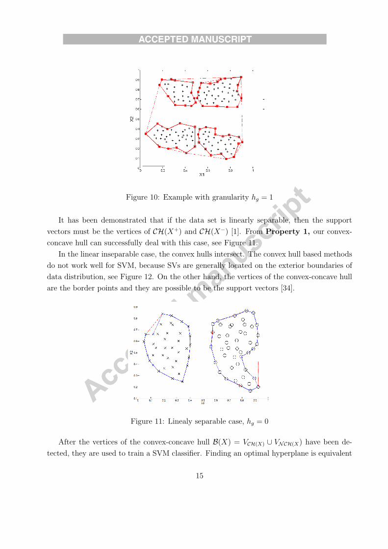
Figure 10: Example with granularity hg = 1

It has been demonstrated that if the data set is linearly separable, then the support

vectors must be the vertices of CH(X+) and CH(X−) [1]. From Property 1, our convex-

concave hull can successfully deal with this case, see Figure 11.

In the linear inseparable case, the convex hulls intersect. The convex hull based methods

do not work well for SVM, because SVs are generally located on the exterior boundaries of

data distribution, see Figure 12. On the other hand, the vertices of the convex-concave hull

are the border points and they are possible to be the support vectors [34].

Figure 11: Linealy separable case, hg = 0

After the vertices of the convex-concave hull B(X) = VCH(X) ∪ VNCH(X) have been de-

tected, they are used to train a SVM classifier. Finding an optimal hyperplane is equivalent

15

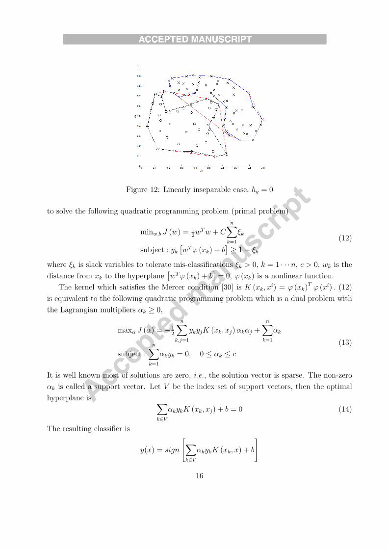
Figure 12: Linearly inseparable case, hg = 0

to solve the following quadratic programming problem (primal problem)

minw,b J (w) = 12wTw + C

n∑k=1

ξk

subject : yk[wTφ (xk) + b

]≥ 1− ξk

(12)

where ξk is slack variables to tolerate mis-classifications ξk > 0, k = 1 · · ·n, c > 0, wk is the

distance from xk to the hyperplane[wTφ (xk) + b

]= 0, φ (xk) is a nonlinear function.

The kernel which satisfies the Mercer condition [30] is K (xk, xi) = φ (xk)

T φ (xi) . (12)

is equivalent to the following quadratic programming problem which is a dual problem with

the Lagrangian multipliers αk ≥ 0,

maxα J (α) = −12

n∑k,j=1

ykyjK (xk, xj)αkαj +n∑

k=1

αk

subject :n∑

k=1

αkyk = 0, 0 ≤ αk ≤ c

(13)

It is well known most of solutions are zero, i.e., the solution vector is sparse. The non-zero

αk is called a support vector. Let V be the index set of support vectors, then the optimal

hyperplane is ∑k∈V

αkykK (xk, xj) + b = 0 (14)

The resulting classifier is

y(x) = sign

[∑k∈V

αkykK (xk, x) + b

]

16

where b is determined by Kuhn-Tucker conditions.

In our convex-concave hull SVM classification, the penal factor C can be selected very

small, because all misleading points are almost disappear by the concave algorithm. The

classification accuracy is improved. The other design parameters, such as the parameters of

the kernel, are chosen by the grid search method [24].

3.3 High-Dimension Case

Since the convex-concave hull searching algorithm of this paper must calculate angles, it

works in two-dimension space. In order to extend out method to high-dimension data set,

the dimension reduction is needed. The principal component analysis (PCA) is a common

method to reduce the dimension of data sets, but it is not suitable for large trainings sets.

The general approach for the high-dimension data is as the following:

1) Partition the input space to create a number of partitions X i. These partitions have

a more uniform distribution of objects.

2) Select two features from X i to create a set Y i ∈ R2. The Y i can be viewed as X i with

all its features fixed, at exception of two.

3) Apply convex-concave hull searching on Y i.

4) Explore fixed features for more points.

5) Join the points recovered in the previous steps.

It is well known that computing the convex hull in more than three dimensions is compu-

tational expensive. We solve this problem by searching the vertices of convex-concave hull in

several two-dimension spaces, see Figure 13. In order to extend convex-concave hull to more

than two dimensions, we create partitions on the higher dimensions and reduce temporally

the dimension of the data set in several steps. For each dimension we create one-dimensional

clusters. The center of the corresponding cluster is fixed. The final two-dimensional subsets

are formed with respect to the number of partitions of each dimension. We compute border

samples in these two-dimensional subsets and then get them back to their original dimension

with respect to the fixed center values.

The clustering algorithm is as following.

Algorithm 3 (Clustering higher dimensions)

Data

X :Data set

m:Index of a feature of X

Output

17

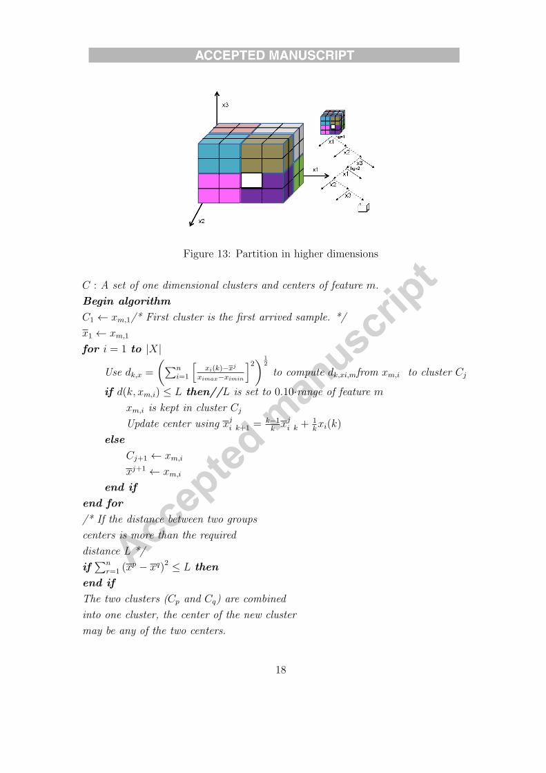
Figure 13: Partition in higher dimensions

C : A set of one dimensional clusters and centers of feature m.

Begin algorithm

C1 ← xm,1/* First cluster is the first arrived sample. */

x1 ← xm,1

for i = 1 to |X|

Use dk,x =

(∑ni=1

[xi(k)−xj

ximax−ximin

]2) 12

to compute dk,xi,mfrom xm,i to cluster Cj

if d(k, xm,i) ≤ L then//L is set to 0.10·range of feature m

xm,i is kept in cluster Cj

Update center using xji k+1 =

k−1kxji k +

1kxi(k)

else

Cj+1 ← xm,i

xj+1 ← xm,i

end if

end for

/* If the distance between two groups

centers is more than the required

distance L */

if∑n

r=1 (xp − xq)2 ≤ L then

end if

The two clusters (Cp and Cq) are combined

into one cluster, the center of the new cluster

may be any of the two centers.

18

end if

return C

End algorithm

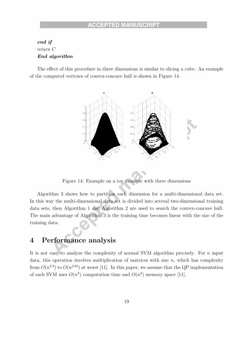
The effect of this procedure in three dimensions is similar to slicing a cube. An example

of the computed vertexes of convex-concave hull is shown in Figure 14.

Figure 14: Example on a toy example with three dimensions

Algorithm 3 shows how to partition each dimension for a multi-dimensional data set.

In this way the multi-dimensional data set is divided into several two-dimensional training

data sets, then Algorithm 1 and Algorithm 2 are used to search the convex-concave hull.

The main advantage of Algorithm 3 is the training time becomes linear with the size of the

training data.

4 Performance analysis

It is not easy to analyze the complexity of normal SVM algorithm precisely. For n input

data, this operation involves multiplication of matrices with size n, which has complexity

from O(n2.3) to O(n2.83) at worst [11]. In this paper, we assume that the QP implementation

of each SVM uses O(n3) computation time and O(n2) memory space [11].

19

4.1 Memory space

In the first step of our method, all examples in training set X are mapped into grid G by a

binary tree with the height hg (granularity). Considering the following facts:

• Each example has d dimensions and the data types are double (8 bytes),

• Each internal node in the binary tree occupies about 40 bytes (two references to the

child nodes and internal variables),

So the amount of memory to manage all examples in G is

23+hg (d+ 5)− 40 bytes

where hg is the height of the binary tree, d is the number of features in data set X.

This amount of memory is computed as follows: the maximum number of leaves in a

binary tree of height hg is given by 2hg , each leaf contains a vector of d features and each

feature is stored in 8 bytes, the amount of memory used by the leaves is

2hg · 8 · d = 2hg23 · d

It is well known that the number of internal nodes in a binary tree of height hg is given

by 2hg − 1. Because each internal node in the implemented binary tree uses about 40 bytes,

the amount of memory used for the internal nodes is

40 · (2hg − 1)

The total amount of memory used by the binary tree is composed of the leaves and the

internal nodes, i.e.,

(2hg23 · d) + 40 · (2hg − 1)

This can be simplified as 2hg·23·d+40·(2hg−1) = 2hg·23d+2hg·40−40 = 2hg·23·d+2hg·23·5−40.Grouping terms we obtain finally 2hg · 23(d+ 5)− 40 bytes.

This amount of memory is used when all leaves of the binary tree exist. In this case more

than one example is usually mapped into the same leaf of the tree. Reducing the amount

of memory originally required to allocate the training set X, i.e., 8 · |X| · d bytes. With |X|the size of training set, namely n.

The memory used by Algorithm 2 can be ignored, because they use a little memory space

compared with the binary tree.

20

4.2 Computation time

In order to analyze the computational cost of the proposed method, our method is separated

into:

• Create a grid G via a binary tree. The computing time for creating G is the example

inserting in a binary tree. It is O(n log2 n) with n = |X|.

• Detect the vertexes of the convex-concave hulls in partitions Yi by looking downward

tree from height ha down to height hb.

Algorithm 1 uses the partition Yi to obtain the vertexes of a convex hull. The cost is

O(|Yi| log2 |Yi|).

To simplify the analysis we consider a uniform distribution of examples, in this case the

size of Yi can be approximated as |X|2hb

. For Algorithm 2, the worst case occurs is that all

examples of Yi are considered as vertexes, usually Yi has a few elements. The computing

time is small compared with these few samples. In general case, Algorithm 2 searches a

small subset from Yi by the K-nearest neighbors method (KNN). The computing time of the

simple KNN is O(d|X|2). For our case it becomes O(d(

|X|2

22·(hb)

)).

• The total computation time in the pre-processing steps is

O(|X| log2 |X|) +O(|X|2hb

log2|X|2hb

) +O

(d

(|X|2

22·(hb)

))(15)

• SVM training uses the QPP solver. It takes O(n3) time and O(n2) space for X. On

the other hand, the number of vertexes of convex-concave hull is greater than the

vertexes of convex hull |B(X)| >> |VCH(H)|. However |B(X)| ≪ |X|, because not all

points are on boundary. The training time of using |B(X)| is lesser than using X , i.e.,

O(|B(X)|3) << O(|X|3)

5 Experiments

We used eight data sets to compare our algorithms with other methods. Four data sets are

available in UCI web site. The others are benchmark examples.

The data sets from UCI are Four class, Skin-no-skin Breast cancer and Haberman’s

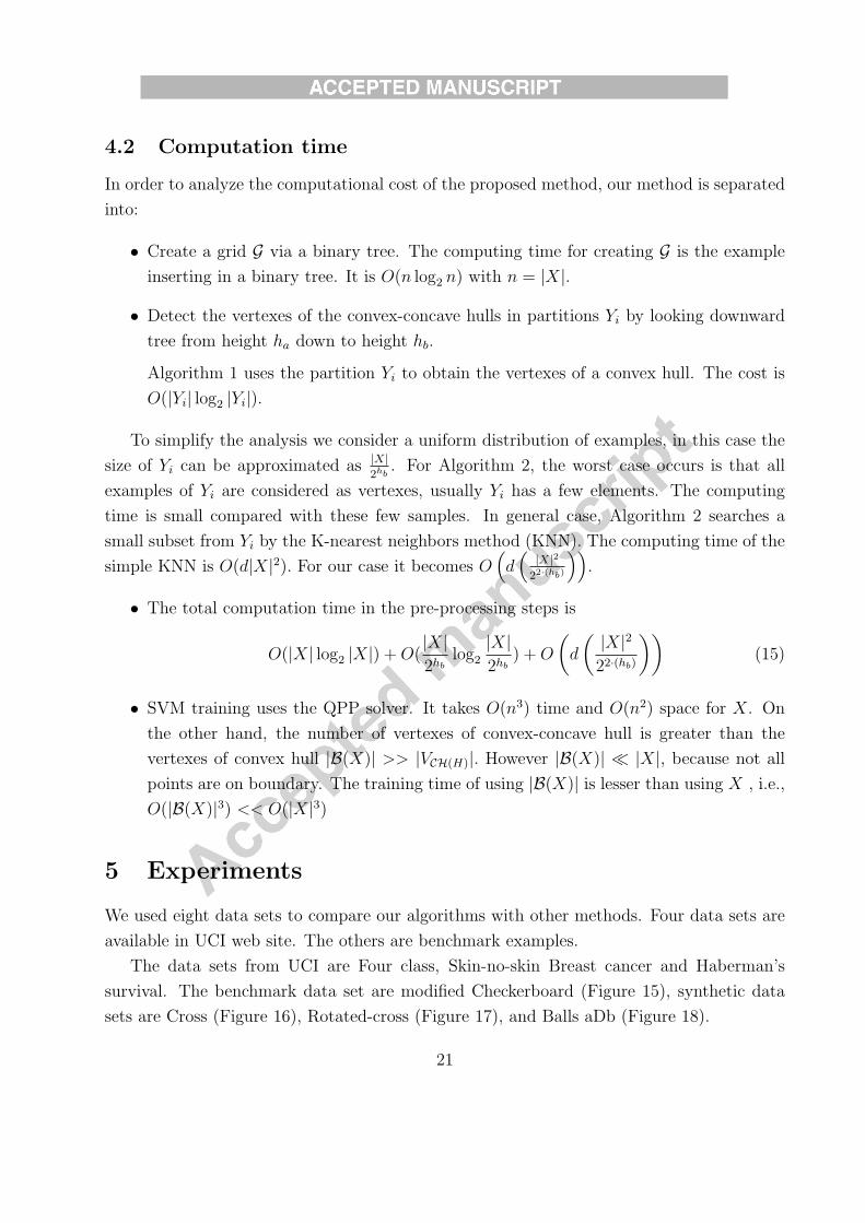
survival. The benchmark data set are modified Checkerboard (Figure 15), synthetic data

sets are Cross (Figure 16), Rotated-cross (Figure 17), and Balls aDb (Figure 18).

21

All of them are linearly inseparable. Table 1 shows a summary of the data sets used in

this paper. The synthetic data set Balls aDb has ”a” features and size ”b”×1000.All experiments were run on a computer with the following features: Core i7 2.2 GHz

processor, 8.0 GB RAM, Windows 7 operating system. The algorithms are implemented

in the Java language. The maximum amount of random access memory given to the Java

virtual machine is set to 2.0 GB. The reported results correspond to 100 runs of each

experiment. For each experiment, the training data are chosen randomly from 70% of the

data set, the rest of data are used for testing.

Figure 15: Checkerboard data set

Our algorithms are compared with SMO [25], library LIBSVM [5], and the reduced

convex hull SVM (RCHSVM) [21]. The SMO and LIBSVM are trained with the original

data set. Our convex-concave hull SVM (CCHSVM) uses the border points detected by

proposed algorithms.

The kernel used in all experiments is a radial basis function,

f (x, z) = exp

(−(x− z)T (x− z)

2γ2

)(16)

where γ was selected using the grid search method.

22

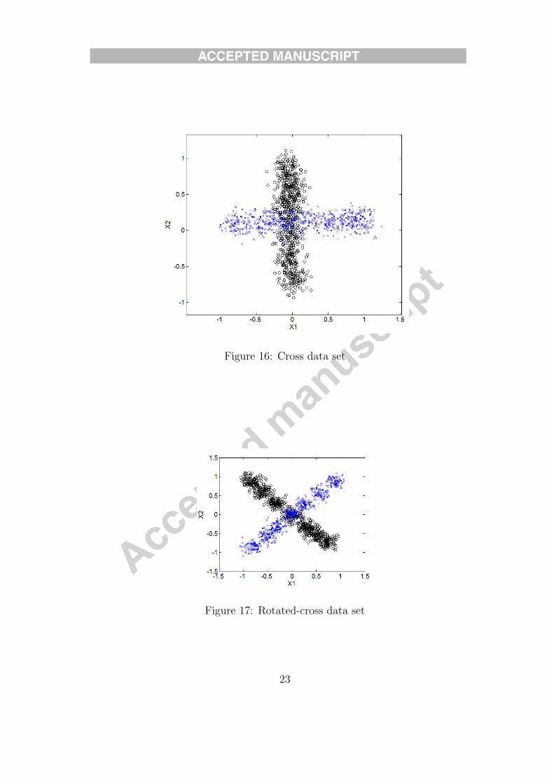
Figure 16: Cross data set

Figure 17: Rotated-cross data set

23

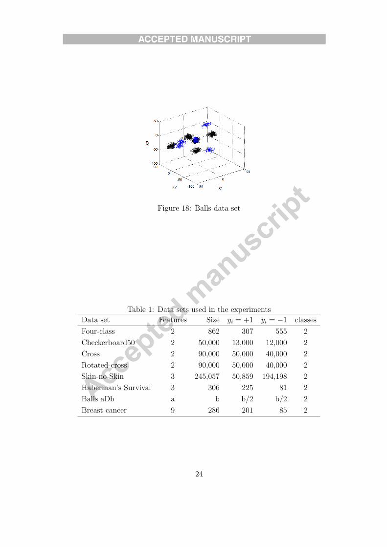
Figure 18: Balls data set

Table 1: Data sets used in the experiments

Data set Features Size yi = +1 yi = −1 classes

Four-class 2 862 307 555 2

Checkerboard50 2 50,000 13,000 12,000 2

Cross 2 90,000 50,000 40,000 2

Rotated-cross 2 90,000 50,000 40,000 2

Skin-no-Skin 3 245,057 50,859 194,198 2

Haberman’s Survival 3 306 225 81 2

Balls aDb a b b/2 b/2 2

Breast cancer 9 286 201 85 2

24

5.1 Experiment 1: Size of training set

In this experiment, we use the checkerboard data set [15] which is commonly used for eval-

uating SVM implementations. It is also useful to illustrate the scaling properties of our

algorithms.

We first exam how does the training data size affect the training time, and the classifi-

cation accuracy of our CCHSVM. We use 500, 1, 000, 2000, 5000, 10000, 50000 and 100000

examples to train CCHSVM and LibSVM. The comparison results of 100 runs of experi-

ments are shown in Table 2, here the columns Avg Acc and Avg training are the averages

of accuracy and training times respectively, the column stdDev is the standard deviation of

accuracy. In this experiment, the values γ = 0.9 and C = 1.0 which are chosen using the

grid search method. The parameters of the CCHSVM algorithm defined in section III are

K = 50, hg = 9, ha = 4 and hb = 8 which are also selected via a grid method.

We can see that our CCHSVM has less training time than LibSVM when the size of

training set is large, more than 5000. For small data sets, LibSVM is better than our

method. The classification accuracy of our method is slightly lesser than LibSVM. The size

of training set is important when the set contains thousands of examples. The pre-processing

reduces the size of training set.

When the data size in increased, the training time is increased with LibSVM. While our

method only increases a little. Although the classification accuracy cannot be improved

significantly when data size is very large, it does not get worse. The testing accuracy is still

acceptable.

5.2 Experiment 2: Parameters

The CCHSVM method has four parameters: hg, ha, hb and K. The hg controls the granu-

larity of the grid, i.e., the height of the binary tree. The parameter ha is used to create the

partitions in higher dimensions. The binary tree is traverse down to high hb. The parameter

K controls the number of neighbors to detect border points close to edges of convex hull.

We used the synthetic Balls3D40 data set (40, 000 examples) to analyze the effect of

parameters of algorithm. The LibSVM method was used as a reference. Table 3 shows the

results. In this experiment, γ = 1.9 and C = 2.5 which are from the grid method.

The most important effect of parameter K is to reduce the data size. K does not

contribute much on the classification accuracy and running time. The parameters hg and ha

25

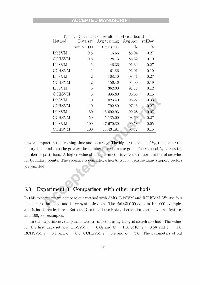
Table 2: Classification results for checkerboardMethod Data set Avg training Avg Acc stdDev

size ×1000 time (ms) % %

LibSVM 0.5 16.66 85.04 0.27

CCHSVM 0.5 28.13 85.32 0.19

LibSVM 1 46.36 91.34 0.27

CCHSVM 1 61.86 91.01 0.19

LibSVM 2 108.10 98.31 0.27

CCHSVM 2 156.46 94.90 0.19

LibSVM 5 362.00 97.12 0.12

CCHSVM 5 336.80 96.35 0.15

LibSVM 10 1023.40 98.27 0.33

CCHSVM 10 792.80 97.15 0.27

LibSVM 50 15,692.93 99.28 0.07

CCHSVM 50 5,185.00 98.60 0.27

LibSVM 100 47,670.80 99.58 0.05

CCHSVM 100 13,434.81 98.32 0.15

have an impact in the training time and accuracy. The higher the value of hg, the deeper the

binary tree, and also the greater the number of cells in the grid. The value of ha affects the

number of partitions. A higher value of this parameter involves a major number of searches

for boundary points. The accuracy is degraded when ha is low, because many support vectors

are omitted.

5.3 Experiment 3: Comparison with other methods

In this experiment we compare our method with SMO, LibSVM and RCHSVM. We use four

benchmark data sets and three synthetic ones. The Balls3D100 contain 100, 000 examples

and it has three features. Both the Cross and the Rotated-cross data sets have two features

and 100, 000 examples.

In this experiment, the parameters are selected using the grid search method. The values

for the first data set are: LibSVM γ = 0.68 and C = 1.0, SMO γ = 0.68 and C = 1.0,

RCHSVM γ = 0.1 and C = 0.5, CCHSVM γ = 0.9 and C = 3.0. The parameters of out

26

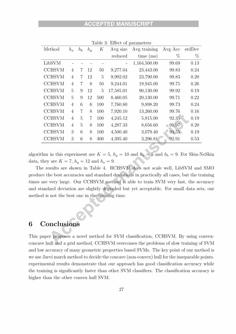
Table 3: Effect of parameters

Method ha hb hg K Avg size Avg training Avg Acc stdDev

reduced time (ms) % %

LibSVM - - - - - 1,164,500.00 99.69 0.13

CCHSVM 4 7 12 50 9,277.04 23,443.00 99.83 0.24

CCHSVM 4 7 12 5 9,992.02 23,790.00 99.83 0.20

CCHSVM 4 7 8 50 9,244.01 19,945.00 99.75 0.26

CCHSVM 5 9 12 5 17,585.01 90,130.00 99.92 0.19

CCHSVM 5 9 12 500 8,460.05 20,130.00 99.71 0.22

CCHSVM 4 6 6 100 7,760.80 9,898.20 99.73 0.24

CCHSVM 4 7 8 100 7,920.10 13,260.00 99.76 0.16

CCHSVM 4 5 7 100 4,245.12 5,815.00 92.35 0.19

CCHSVM 4 5 8 100 4,287.33 8,656.60 91.97 0.20

CCHSVM 3 6 8 100 4,500.40 3,079.40 94.55 0.19

CCHSVM 3 6 8 300 4,395.40 3,296.81 92.91 0.53

algorithm in this experiment are K = 5, hg = 10 and ha = 5 and hb = 9. For Skin-NoSkin

data, they are K = 7, hg = 12 and ha = 9.

The results are shown in Table 4. RCHSVM does not scale well, LibSVM and SMO

produce the best accuracies and standard deviations in practically all cases, but the training

times are very large. Our CCHSVM method is able to train SVM very fast, the accuracy

and standard deviation are slightly degraded but yet acceptable. For small data sets, our

method is not the best one in the training time.

6 Conclusions

This paper proposes a novel method for SVM classification, CCHSVM. By using convex-

concave hull and a grid method, CCHSVM overcomes the problems of slow training of SVM

and low accuracy of many geometric properties based SVMs. The key point of our method is

we use Jarvi march method to decide the concave (non-convex) hull for the inseparable points.

experimental results demonstrate that our approach has good classification accuracy while

the training is significantly faster than other SVM classifiers. The classification accuracy is

higher than the other convex hull SVM.

27

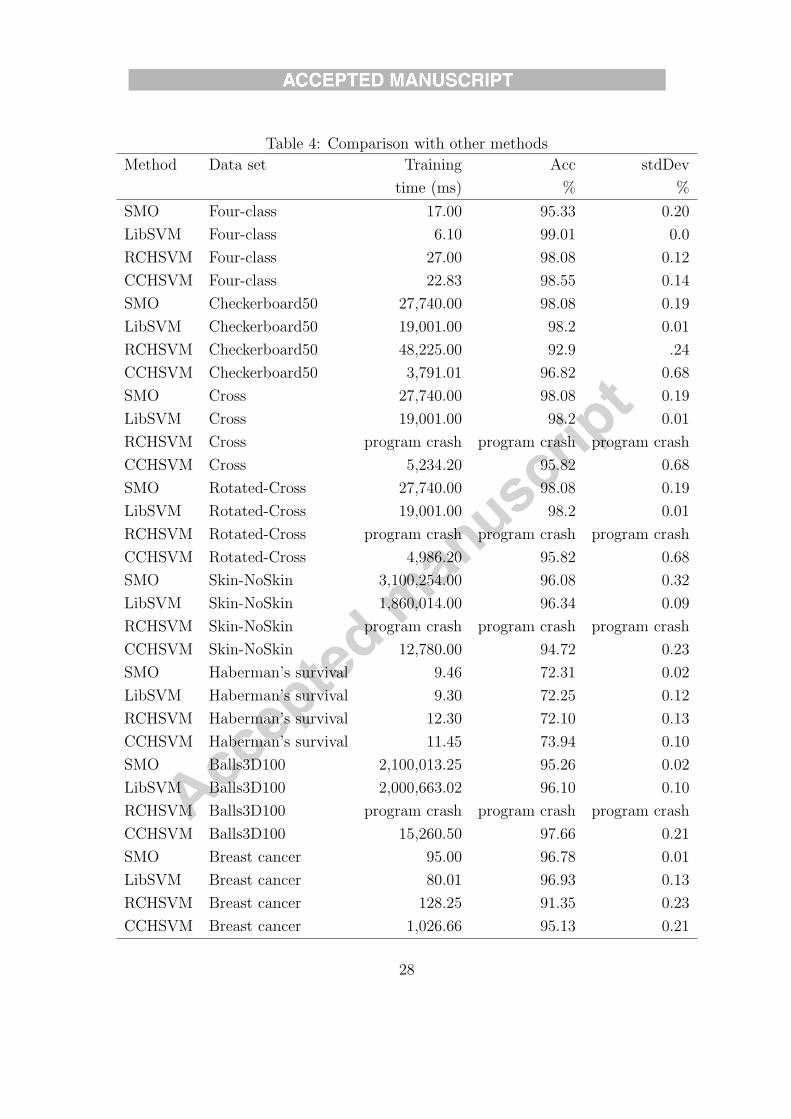
Table 4: Comparison with other methods

Method Data set Training Acc stdDev

time (ms) % %

SMO Four-class 17.00 95.33 0.20

LibSVM Four-class 6.10 99.01 0.0

RCHSVM Four-class 27.00 98.08 0.12

CCHSVM Four-class 22.83 98.55 0.14

SMO Checkerboard50 27,740.00 98.08 0.19

LibSVM Checkerboard50 19,001.00 98.2 0.01

RCHSVM Checkerboard50 48,225.00 92.9 .24

CCHSVM Checkerboard50 3,791.01 96.82 0.68

SMO Cross 27,740.00 98.08 0.19

LibSVM Cross 19,001.00 98.2 0.01

RCHSVM Cross program crash program crash program crash

CCHSVM Cross 5,234.20 95.82 0.68

SMO Rotated-Cross 27,740.00 98.08 0.19

LibSVM Rotated-Cross 19,001.00 98.2 0.01

RCHSVM Rotated-Cross program crash program crash program crash

CCHSVM Rotated-Cross 4,986.20 95.82 0.68

SMO Skin-NoSkin 3,100,254.00 96.08 0.32

LibSVM Skin-NoSkin 1,860,014.00 96.34 0.09

RCHSVM Skin-NoSkin program crash program crash program crash

CCHSVM Skin-NoSkin 12,780.00 94.72 0.23

SMO Haberman’s survival 9.46 72.31 0.02

LibSVM Haberman’s survival 9.30 72.25 0.12

RCHSVM Haberman’s survival 12.30 72.10 0.13

CCHSVM Haberman’s survival 11.45 73.94 0.10

SMO Balls3D100 2,100,013.25 95.26 0.02

LibSVM Balls3D100 2,000,663.02 96.10 0.10

RCHSVM Balls3D100 program crash program crash program crash

CCHSVM Balls3D100 15,260.50 97.66 0.21

SMO Breast cancer 95.00 96.78 0.01

LibSVM Breast cancer 80.01 96.93 0.13

RCHSVM Breast cancer 128.25 91.35 0.23

CCHSVM Breast cancer 1,026.66 95.13 0.21

28

Experimental results demonstrate that our approach has good classification accuracy

while the training is significantly faster than other SVM classifiers. The classification accu-

racy is higher than the other geometric methods such as reduced convex hull.

The training time of CCHSVM have been significantly reduced. For small data sets and

high dimension data, the accuracy of CCHSVM is maintained slightly lower than the classical

SVM classifiers which use the whole data set. However, in the case of larger data sets, the

classification accuracy are almost the same or even better than the other SVMs, because we

do not use soft margin method to deal with the misleading points, we use concave hull to

solve this problem.

References

[1] K.P. Bennett , E.J. Bredensteiner, Geometry in Learning, Geometry at Work, C. Gorini

editors, Mathematical Association of America, 132-145, 2000

[2] K.P. Bennett , E.J. Bredensteiner, Duality and Geometry in SVM Classifiers, 17th

International Conference on Machine Learning, San Francisco, CA, 2000

[3] M.Berg, O.Cheong, M.Kreveld, M.Overmars, Computational Geometry: Algorithms and

Applications, Springer-Verlag, 2008

[4] J.Cervantes, X.Li, W.Yu, K.Li, Support vector machine classification for large data sets

via minimum enclosing ball clustering, Neurocomputing, Vol.71, 611-619, 2008

[5] C-C.Chang and C-J.Lin, LIBSVM: A library for support vector machines,

http://www.csie.ntu.edu.tw/˜cjlin/libsvm, 2001.

[6] D.J. Crisp, C.J.C. Burges, A Geometric Interpretation of υ-SVM Classifiers, NIPS,

Vol.12, 244-250, 2000

[7] R.Collobert, F.Sinz, J.Weston, L.Bottou, Trading convexity for scalability, 23rd Inter-

national Conference on Machine Learning, 201-208, Pittsburgh, USA; 2006

[8] R.Collobert, S.Bengio, SVMTorch: Support vector machines for large regression prob-

lems, Journal of Machine Learning Research, Vol.1, 143-160, 2001.

[9] W.Eddy, A New Convex Hull Algorithm for Planar Sets, ACM Transactions on Math-

ematical Software Vol.3, No.4, 398–403, 1977

29

[10] V.Franc, V.Hlavac, An iterative algorithm learning the maximal margin classifier, Pat-

tern Recognition, Vol.36, 1985 –1996, 2003

[11] B.V.Gnedenko, Y.K.Belyayev, and A.D.Solovyev, Mathematical Methods of Reliability

Theory, NewYork: Academic Press, 1969

[12] E. G. Gilbert, An iterative procedure for computing the minimum of a quadratic form

on a convex set, SIAM J. on Control and Optimization, Vol.4, No.1, 61-79, 1966

[13] R.L.Graham, An Efficient Algorithm for Dutennining the Convex Hull of a Finite PIanar

Set, Information Processing Letters, Vol.1, 132-133, 1972

[14] G.Guo, J.-S.Zhang, Reducing examples to accelerate support vector regression, Pattern

Recognition Letters, Vol.28, 2173-2183, 2007

[15] T. K. Ho and E. M. Kleinberg. Checkerboard dataset, http://www.cs.wisc.edu/, 1996.

[16] C.-W.Hsu, C.-C.Chang, C.-J.Lin, A Practical Guide to Support Vector Classification,

Bioinformatics, Volume: 1, Issue: 1, 1-16, 2010.

[17] R.A.Jarvis, On the identification of the convex hull of a finite set of points in the plane,

Information Processing Letters, Vol.2, 18-21, 1973

[18] S. S. Keerthi, S. K. Shevade, C. Bhattacharyya, and K. R. K. Murthy, A Fast Iter-

ative Nearest Point Algorithm for Support Vector Machine Classifier Design, IEEE

Transactions on Neural Networks, Vol. 11, No.12, 124-137, 2001.

[19] S.S.Keerthi, E.G.Gilbert, Convergence of a Generalized SMO Algorithm for SVM Clas-

sifier Design. Machine Learning, 46, 351–360, 2002

[20] Y.Li, Selecting training points for one-class support vector machines, Pattern Recogni-

tion Letters, Vol.32, 1517-1522, 2011.

[21] M.E.Mavroforakis, S.Theodoridis, A Geometric Approach to Support Vector Machine

(SVM) Classification, IEEE Trans. Neural Networks, vol.17, no.3, pp.671-682, 2006. S

[22] B. F. Mitchell, V. F. Dem’yanov, and V. N. Malozemov, Finding the point of a polyhe-

dron closest to the origin, Vestinik Leningrad. Gos.Univ., Vol. 13, pp. 38-45, 1971

[23] M.Kallay, The Complexity of Incremental Convex Hull Algorithms, Information Pro-

cessing Letters, Vol.19, No.4, 197-212, 1984.

30

[24] N.Cristianini, J.Shawe-Taylor , An Introduction to Support Vector Machines and Other

Kernel-based Learning Methods , Cambridge University Press, 2000.

[25] J.Platt, Fast Training of support vector machine using sequential minimal optimization,

Advances in Kernel Methods: Support Vector Machine, MIT Press, Cambridge, MA,

1998.

[26] C.Pizzuti, D.Talia, P-Auto Class: Scalable Parallel Clustering for Mining Large Data

Sets, IEEE Trans. Knowledge and Data Eng., vol.15, no.3, pp.629-641, 2003.

[27] F.P.Preparata, S.J. Hong. Convex Hulls of Finite Sets of Points in Two and Three

Dimensions, Communications of the ACM , vol. 20, no. 2, pp. 87–93, 1977.

[28] M.I. Schlesinger, V.G. Kalmykov, A.A. Suchorukov, Sravnitelnyj, Comparative anal-

ysis of algorithms synthesising linear decision rule for analysis of complex hypotheses,

Automatika, Vol.1, 3-9, 1981.

[29] I.W. Tsang, J.T. Kwok, P.M.Cheung, Core Vector Machines: Fast SVM Training on

Very Large Data Sets, Journal of Machine Learning Research, Vol. 6, 363-392, 2005

[30] V.Vapnik, The Nature of Statistical Learning Theory, Springer, New York, 1995.

[31] C.Xia, W.Hsu, M.L.Lee, B.C.Ooi, BORDER: Efficient Computation of Boundary

Points, IEEE Trans. Knowledge and Data Eng., vol.18, no.3, pp.289-303, 2006.

[32] A. L. Yuille, A.Rangarajan, The Concave-Convex Procedure, Neural Computation, Vol.

15, No. 4, Pages 915-936, 2003

[33] H.Yu , J.Yang and J.Han , Classifying Large Data Sets Using SVMs with Hierarchical

Clusters, Proc. of the 9th ACM SIGKDD 2003, Washington, DC, USA, 2003.

[34] A.Moreira, M.Y.Santos, Concave Hull: A K-Nearest Neighbours Approach for the Com-

putation of the Region Occupied by a Set of Points, GRAPP (GM/R), Pages 61–68,

2007

[35] W.Yu, X.Li, On-line fuzzy modeling via clustering and support vector machines, Infor-

mation Sciences, Vol.178, 4264-4279, 2008.

31