normal forms of convex lattice polytopes
TRANSCRIPT

NORMAL FORMS OF CONVEX LATTICE POLYTOPES
ROLAND GRINIS AND ALEXANDER M. KASPRZYK
Abstract. We describe an algorithm for determining whether two convex polytopes P and Q,
embedded in a lattice, are isomorphic with respect to a lattice automorphism. We extend this
to a method for determining if P and Q are equivalent, i.e. whether there exists an affine lattice
automorphism that sends P to Q. Methods for calculating the automorphism group and affine
automorphism group of P are also described.
An alternative strategy is to determine a normal form such that P and Q are isomorphic if
and only if their normal forms are equal. This is the approach adopted by Kreuzer and Skarke
in their Palp software. We describe the Kreuzer–Skarke method in detail, and give an improved
algorithm when P has many symmetries. Numerous examples, plus two appendices containing
detailed pseudo-code, should help with any future reimplementations of these techniques. We
conclude by explaining how to define and calculate the normal form of a Laurent polynomial.
1. Introduction
Determining whether two convex polytopes P and Q, embedded in a lattice Λ, are isomorphic
with respect to a lattice automorphism is a fundamental computational problem. For example,
in toric geometry lattice polytopes form one of the key constructions of projective toric varieties,
and any classification must somehow address the issue of whether there exists an automorphism
of the underlying lattice sending P to Q. In general, any isomorphism problem can be solved in
one of two ways: on a case-by-case basis by constructing an explicit isomorphism between the
two objects, or by determining a normal form for each isomorphism class.
The first approach – dynamically constructing a lattice-preserving isomorphism in GLn(Z)
between the two polytopes – is discussed in §2. We describe one possible way to determine
isomorphism of polytopes via the labelled face graph G (P ) (see §2.1). This has the advantage
that it works equally well for rational polytopes and for polytopes of non-zero codimension. By
reducing the problem to a graph isomorphism question, well-developed tools such as Brendan
McKay’s Nauty software [McK81, McK] can then be applied.
Because our approach to isomorphism testing works equally well for rational polytopes, we
are able to answer when two polytopes are equivalent, i.e. when there exists an isomorphism
B ∈ GLn(Z) and lattice translation c ∈ Λ such that PB + c = Q. This is discussed in §2.4. We
can also calculate the automorphism group Aut(P ) ≤ GLn(Z) of P : this is a subgroup of the
automorphism group of G (P ), as explained in §2.5. Since our methods make no assumptions on
the codimension of P , by considering the automorphism group of P × {1} in Λ× Z we are able
to calculate the group of affine automorphisms AffAut(P ) ≤ GLn(Z) n Λ. As an illustration
Keywords: Convex polytope, computation, isomorphism, automorphism, normal form, Palp.
2010 Mathematics Subject Classification: 52B20 (Primary); 52B55, 52C07 (Secondary).1
arX
iv:1
301.
6641
v1 [
mat
h.C
O]
28
Jan
2013
2 R. GRINIS AND A. M. KASPRZYK
of our methods, we calculate the order of the automorphism group for each of the 473,800,776
four-dimensional reflexive polytopes [KS00]: see Table 1.
The second approach – to compute a normal form NF(P ) for each isomorphism class – is
discussed in §3. This is the approach adopted by Kreuzer and Skarke in their Palp soft-
ware [KS04], and was used to construct the classification of three- and four-dimensional reflexive
polytopes [KS98, KS00]. Briefly, row and column permutations are applied to the vertex–facet
pairing matrix PM of P , placing it in a form PMmax that is maximal with respect to a certain
ordering. This in turn defines an order in which to list the vertices of P ; the choice of basis is
fixed by taking the Hermite normal form. In §3.3 we address how this can be modified to give an
affine normal form for P , and in §3.4 we describe how Palp applies an additional reordering of
the columns of PMmax before computing the normal form. The Palp source code for computing
NF(P ) is analyzed in detail in Appendix A.
In §4 we address the problem of calculating PMmax. We describe an inductive algorithm which
attempts to exploit automorphisms of the matrix in order to simplify the calculation; pseudo-
code is given in Appendix B. Applying our algorithm to smooth Fano polytopes [Øbr07], which
often have large numbers of symmetries, illustrates the advantage of this approach: see §4.1 and
Table 2. We end by giving, in §5, an application of normal form to Laurent polynomials.
A note on implementation. The algorithms described in §2 were implemented using Magma
in 2008 and officially released as part of Magma V2.16 [BCP97, BBK09]; Palp normal form was
introduced by Kreuzer and Skarke in their Palp software [KS04] and reimplemented natively
in Magma V2.18 by the authors. The Magma algorithms1, including the reimplementation of
Palp normal form, have recently been ported to the Sage project [S+] by Samuel Gonshaw2,
assisted by Tom Coates and the second author, and should appear in the 5.6.0 release.
Acknowledgments. This work was motivated in part by discussions with Max Kreuzer during
August and September 2010, shortly before his death that November. We are honoured that
he found the time and energy for these conversations during this period. It forms part of the
collaborative Palp++ project envisioned in [Kre10].
Our thanks to Tom Coates for many useful discussions, to Harald Skarke and Dmitrii Pasech-
nik for several helpful comments on a draft of this paper, to John Cannon for providing copies of
the computational algebra software Magma, and to Andy Thomas for technical assistance. The
first author was funded by a Summer Studentship as part of Tom Coates’ Royal Society Uni-
versity Research Fellowship. The second author is supported by EPSRC grant EP/I008128/1.
2. Isomorphism testing via the face graph
Conventions. Throughout this section we work with very general convex polytopes; we assume
only that P ⊂ ΛQ := Λ ⊗ Q is a (non-empty) rational convex polytope, not necessarily of
maximum dimension in the ambient lattice Λ. The dual lattice Hom(Λ,Z) is denoted by Λ∗.
1Users of Magma can freely view and edit the package code. The relevant files are contained in the subdirectory
package/Geometry/ToricGeom/polyhedron/.2Gonshaw’s implementation is available from http://trac.sagemath.org/sage trac/ticket/13525.
NORMAL FORMS OF CONVEX LATTICE POLYTOPES 3
Given two polytopes P and P ′, how can we decide whether they are isomorphic and, if they
are, how can we construct an isomorphism between them? There are, of course, some obvious
checks that can quickly provide a negative answer. We give a few examples, although this list
is far from comprehensive.
• Do the dimensions of the polytopes agree?
• Does P contain the origin in its relative interior? Is the same true for P ′?
• Are P and P ′ both lattice polytopes?
• Are the f -vectors of P and P ′ equal?
• Do P and P ′ have the same number of primitive vertices?
• Are P and P ′ simplicial? Are they simple?
• If P is of codimension one then there exists a unique hyperplane H ⊂ ΛQ containing P ,
where H = {v ∈ ΛQ | 〈v, u〉 = k} for some non-negative rational value k and primitive
dual lattice point u ∈ Λ∗. In particular, k is invariant under change of basis. Does k
agree for both P and P ′?
• If P is of maximum dimension, any facet F can be expressed in the form F = {v ∈ P |〈v, uF 〉 = −cF }, where uF ∈ Λ∗ is a primitive inward-pointing vector normal to F , and
cF ∈ Q is the lattice height of F over the origin. The value of cF is invariant under
change of basis. Do the facet heights of P and P ′ agree, up to permutation?
• If P is a rational polytope, let rP be the smallest positive integer such that the dilation
rPP is a lattice polytope. Do rP and rP ′ agree?
Remark 2.1. From a computational point of view, the intention with the above list is to
suggest tests that are easy to perform. We assume that data such as the vertices and supporting
hyperplanes of P have already been calculated. Some computations, such as finding the f -vector,
are more involved, but since the calculations will be required in what follows it seems sensible
to use them at this stage.
In practice a number of other invariants may already be cached and could also be used: the
volume Vol(P ) or boundary volume Vol(∂P ); the number of lattice points |P ∩ Λ| or boundary
lattice points |∂P ∩ Λ|; the Ehrhart δ-vector; information about the polar polyhedron P ∗. In
particular cases some of this additional data may be easy to calculate; in general they are usually
more time-consuming to compute than the isomorphism test described below.
Remark 2.2. There are a few potential catches for the unwary when considering rational poly-
topes with dimP < dim Λ. For example, care needs to be taken when defining the supporting
hyperplanes. Also, the notion of (normalised) volume Vol(P ) requires some attention: the affine
sublattice aff(P ) ∩ Λ may be empty, forcing us to either accept that Vol(P ) can be undefined,
or to employ interpolation. There is a natural dichotomy between those polytopes whose affine
span contains the origin and those where 0 /∈ aff(P ). In the latter case, it is often better to
consider the cone CP := cone(P ) equipped with an appropriate grading such that dilations of
P can be realised by taking successive slices through CP .
4 R. GRINIS AND A. M. KASPRZYK
2.1. The labelled face graph. In order to determine isomorphism we make use of the face
graph G(P ) of P .
Definition 2.3. Let P be an n-dimensional polytope with f -vector (f−1, f0, . . . , fn), where
fk denotes the number of k-faces of P . By convention we set f−1 = fn = 1, representing,
respectively, the empty set ∅ and the polytope P . The face graph G(P ) is the graph consisting
of f−1 + f0 + . . . + fn vertices, where each vertex v corresponds to a face Fv. Two vertices v
and v′ are connected by an edge if and only if Fv′ ⊂ Fv and dimFv′ = dimFv + 1. Here the
dimension of the empty face ∅ is taken to be −1.
The face graph of a polytope is completely determined by the vertex–facet relations, and
is the standard tool for determining combinatorial isomorphism of polytopes. We augment
G(P ) by assigning labels to the vertices determined by some invariants of the corresponding
face. Reducing a symmetry problem to the study of a (labelled) graph is a well-established
computational technique: see, for example, [KS03, Pug05, MdlBW09, BSP+12]. The intention
is to decorate the graph with data capturing how P lies in the underlying lattice Λ. To that
end, we make the following definition.
Definition 2.4. For a point v ∈ ΛQ, let u ∈ Λ be the unique primitive lattice point such that
v = λu for some non-negative value λ (set u = 0, λ = 0 if v = 0). We define v to be given by
dλeu, i.e. v is the first lattice point after or equal to v on the ray defined by v. Let P ⊂ ΛQ
be a polytope with vertices V(P ). Then the index |P : Λ| of P is the index of the sublattice
generated by {u | u ∈ V(P )} in span(P ) ∩ Λ.
Definition 2.5. Let P be an n-dimensional polytope with face graph G(P ). To each vertex v
of G(P ) we assign the label{(dimFv), if Fv = ∅ or Fv = P ;
(dimFv, |Fv : Λ|), otherwise.
We denote this labelled graph by G (P ).
Remark 2.6. In place of the index |Fv : Λ|, it is tempting to use the volume Vol(Fv). However,
computing the index is basic linear algebra, whereas computing the volume is generally difficult.
2.2. Additional labels. When P contains the origin strictly in its interior, we can make use of
the special facets. Recall from [Øbr07, §3.1] that a facet F is said to be special if u ∈ cone(F ),
where u :=∑
v∈V(P ) v is the sum of the vertices of P . Since P contains the origin, there exists at
least one special facet; we can extend the labelling to indicate which vertices of G (P ) correspond
to a special facet.
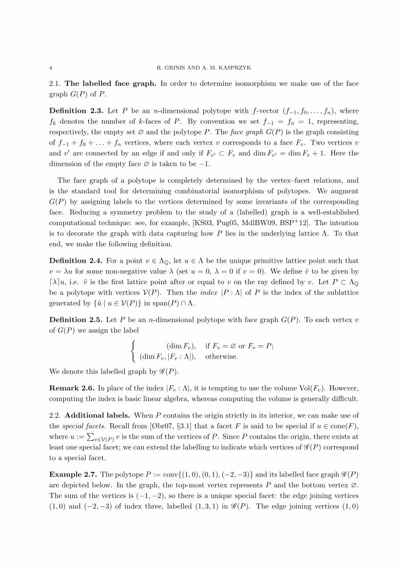
Example 2.7. The polytope P := conv{(1, 0), (0, 1), (−2,−3)} and its labelled face graph G (P )
are depicted below. In the graph, the top-most vertex represents P and the bottom vertex ∅.
The sum of the vertices is (−1,−2), so there is a unique special facet: the edge joining vertices
(1, 0) and (−2,−3) of index three, labelled (1, 3, 1) in G (P ). The edge joining vertices (1, 0)
NORMAL FORMS OF CONVEX LATTICE POLYTOPES 5
and (0, 1) is of index one and labelled (1, 1, 0); the remaining edge is of index two and labelled
(1, 2, 0). The final entry of each facet label is used to indicate whether this is a special facet.
(-2,-3)
(1,0)
(0,1) (2)
(-1)
(0,1) (0,1) (0,1)
(1,1,0) (1,2,0) (1,3,1)
If P is a rational polytope, the vertices of P provide an augmentation to the labelling of G (P ).
For any vertex v ∈ V(P ) there exists a primitive lattice point u ∈ Λ and a non-negative rational
value λ such that v = λu. Since λ is invariant under change of basis, the corresponding labels
can be extended with this information. (Note that λ = |v : Λ| when v is a lattice point, so this
only provides additional information in the rational case.)
We do not claim that these are the only easily-computed invariants that can be associated
with G (P ). Other possibilities include encoding the linear relations between the vertices V(P )
of P in the graph labelling, and, in the maximum dimensional case, adding information about
the lattice height of the supporting hyperplanes for each face.
2.3. Recovering the isomorphism. We now describe our algorithm for computing an iso-
morphism between two polytopes P and P ′. The initial step is to normalise the polytopes. If
P and P ′ are not of maximum dimension in the ambient lattice Λ, then we first restrict to the
sublattice span(P )∩Λ (and, respectively, span(P ′)∩Λ). It is possible that, even after restriction,
P and P ′ are of codimension one. In that case, we work with the convex hull conv(P ∪ {0}) (and
similarly for P ′). The important observations are that, after normalisation, P is of maximum
dimension, and that there exists at least one facet F0 of P such that 0 /∈ aff(F0).
Now we calculate an arbitrary graph isomorphism φ : G (P ) → G (P ′). By restricting to the
vertices of G (P ) corresponding to the vertices V(P ) of P , φ induces a map from the vertices of
P to the vertices of P ′. The two polytopes P and P ′ are isomorphic only if φ exists, and any
isomorphism Φ : Λ→ Λ mapping P to P ′ can be factored as φ ◦ χ, where χ ∈ Aut(G (P )).
It remains to decide whether a particular choice of χ ∈ Aut(G (P )) determines a lattice
isomorphism φ ◦ χ : Λ → Λ sending P to P ′. For this we make use of the facet F0. By
construction F0 is of codimension one, and does not lie in a hyperplane containing the origin.
Hence there exists a choice of vertices v1, . . . , vn of F0 which generate ΛQ (over Q). Denote
the image of vi in P ′ by v′i, and consider the n × n matrices V and V ′ whose rows are given
by, respectively, the vi and the v′i. In order for φ ◦ χ to be a lattice map we require that
6 R. GRINIS AND A. M. KASPRZYK
B := V −1V ′ ∈ GLn(Z). In order for this to be an isomorphism from P to P ′ we require that
{vB | v ∈ V(P )} = V(P ′).
Remark 2.8. We make two brief observations. First, in practice the automorphism group
Aut(G (P )) is often small. Second, it is an easy exercise in linear algebra to undo our normali-
sation process, lifting B back to act on the original polytope.
2.4. Testing for equivalence. Recall that two polytopes P, P ′ ⊂ ΛQ are said to be equivalent
if there exists an isomorphism B ∈ GLn(Z) and a translation c ∈ Λ such that PB + c = P ′.
Definition 2.9. Let V(P ) be the set of vertices of a polytope P . Then the vertex average of P
is the point
bP :=1
|V(P )|∑
v∈V(P )
v ∈ ΛQ.
Two polytopes P and P ′ are equivalent if and only if bP − bP ′ ∈ Λ and P − bP is isomorphic
to P ′ − bP ′ .
Example 2.10. Consider the simplices
P := conv{(0, 0, 0), (2, 1, 1), (1, 2, 1), (1, 1, 2)},
P ′ := conv{(0, 1, 2), (1, 0, 0), (3, 1, 4), (4, 2, 6)}.
The vertex averages are bP = (1, 1, 1) and bP ′ = (2, 1, 3), and (P − bP )B = P ′ − bP ′ , where
B :=
2 1 3
−2 0 −1
1 0 1
Hence P and P ′ are equivalent.
2.5. Determining the automorphism group of a polytope. We can use the labelled face
graph G (P ) to compute the automorphism group Aut(P ). We simply use the elements χ of
Aut(G (P )) to construct Aut(P ) ≤ GLn(Z). Notice that there is no requirement that P is
of maximum dimension in the ambient lattice Λ. Given this, we can also compute the affine
automorphism group AffAut(P ). Begin by embedding P at height one in the lattice Λ × Z(equivalently, consider the cone CP spanned by P with appropriate grading). We refer to this
embedded image of P as P . The action of the automorphism group Aut(P ) on P restricts to an
action on P , realising the full group of affine lattice automorphisms of P . A detailed discussion of
polyhedral symmetry groups and their applications can be found in [BEK84, BDSS09, BSP+12].
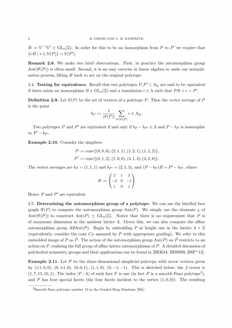
Example 2.11. Let P be the three-dimensional simplicial polytope with seven vertices given
by (±1, 0, 0), (0,±1, 0), (0, 0, 1), (1, 1, 0), (0,−1,−1). This is sketched below; the f -vector is
(1, 7, 15, 10, 1). The index |F : Λ| of each face F is one (in fact P is a smooth Fano polytope3),
and P has four special facets (the four facets incident to the vertex (1, 0, 0)). The resulting
3Smooth Fano polytope number 13 in the Graded Ring Database [BK].
NORMAL FORMS OF CONVEX LATTICE POLYTOPES 7
labelled graph G (P ) has automorphism group of order four, however Aut(P ) has order two, and
is generated by the involution (0, 0, 1) 7→ (0,−1,−1).
Example 2.12. The four-dimensional centrally symmetric polytope P with vertices
± (1, 0, 0, 0),±(0, 1, 0, 0),±(0, 0, 1, 0),±(0, 0, 0, 1),
± (1,−1, 0, 0),±(1, 0,−1, 0),±(1, 0, 0,−1),±(0, 1,−1, 0),±(0, 1, 0,−1),
± (1, 0,−1,−1),±(0, 1,−1,−1),±(1, 1,−1,−1)
is the reflexive realisation of the 24-cell, with f -vector (1, 24, 96, 96, 24, 1). It is unique amongst
all 473,800,776 reflexive polytopes in having |Aut(P )| = 1152; in fact Aut(P ) is isomorphic to
the Weyl group W (F4). In particular, P must be self-dual. The number of four-dimensional
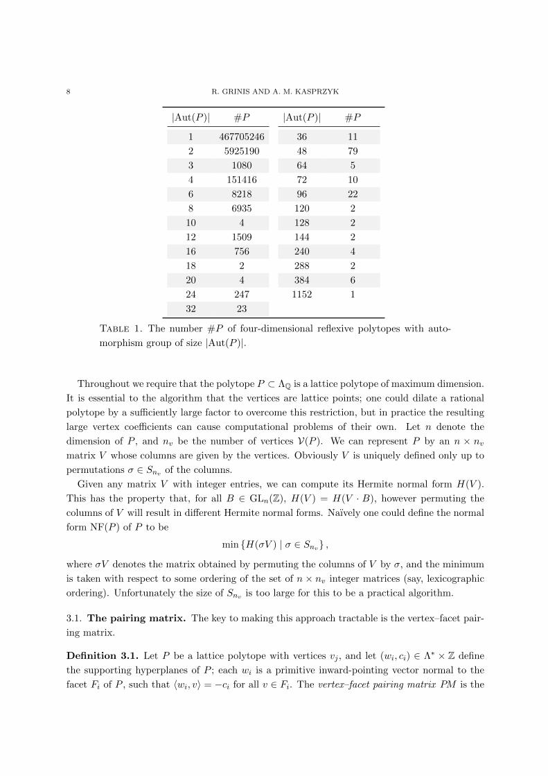
reflexive polytopes with |Aut(P )| of given size are recorded in Table 1.
Example 2.13. Let P = conv{(0, 0), (1, 0), (0, 1)} be the empty simplex in Z2. Then Aut(P ) is
of order two, corresponding to reflection in the line x = y. To compute the affine automorphism
group AffAut(P ) of P , we consider P = conv{(0, 0, 1), (1, 0, 1), (0, 1, 1)}. The group Aut(P ) is
of order six, generated by −1 0 0
−1 1 0
1 0 1
and
0 −1 0
1 −1 0
0 1 1
.
The first generator corresponds to the involution exchanging the vertices (0, 0) and (1, 0) of P ,
whilst the second generator corresponds to rotation of P about its barycentre (1/3, 1/3), given
by
(x, y) 7→ (x− 1/3, y − 1/3)
(0 −1
1 −1
)+ (1/3, 1/3) = (x, y)
(0 −1
1 −1
)+ (0, 1).
3. Normal forms
The method for determining isomorphism adopted by Kreuzer and Skarke in the software
package Palp [KS04] is to generate a normal form for the polytope P . We shall briefly sketch
their approach. Their algorithm is described in detail in Appendix A.
8 R. GRINIS AND A. M. KASPRZYK
|Aut(P )| #P
1 467705246
2 5925190
3 1080
4 151416
6 8218
8 6935
10 4
12 1509
16 756
18 2
20 4
24 247
32 23
|Aut(P )| #P
36 11
48 79
64 5
72 10
96 22
120 2
128 2
144 2
240 4
288 2
384 6
1152 1
Table 1. The number #P of four-dimensional reflexive polytopes with auto-
morphism group of size |Aut(P )|.
Throughout we require that the polytope P ⊂ ΛQ is a lattice polytope of maximum dimension.
It is essential to the algorithm that the vertices are lattice points; one could dilate a rational
polytope by a sufficiently large factor to overcome this restriction, but in practice the resulting
large vertex coefficients can cause computational problems of their own. Let n denote the
dimension of P , and nv be the number of vertices V(P ). We can represent P by an n × nvmatrix V whose columns are given by the vertices. Obviously V is uniquely defined only up to
permutations σ ∈ Snv of the columns.
Given any matrix V with integer entries, we can compute its Hermite normal form H(V ).
This has the property that, for all B ∈ GLn(Z), H(V ) = H(V · B), however permuting the
columns of V will result in different Hermite normal forms. Naıvely one could define the normal
form NF(P ) of P to be
min {H(σV ) | σ ∈ Snv} ,
where σV denotes the matrix obtained by permuting the columns of V by σ, and the minimum
is taken with respect to some ordering of the set of n × nv integer matrices (say, lexicographic
ordering). Unfortunately the size of Snv is too large for this to be a practical algorithm.
3.1. The pairing matrix. The key to making this approach tractable is the vertex–facet pair-
ing matrix.
Definition 3.1. Let P be a lattice polytope with vertices vj , and let (wi, ci) ∈ Λ∗ × Z define
the supporting hyperplanes of P ; each wi is a primitive inward-pointing vector normal to the
facet Fi of P , such that 〈wi, v〉 = −ci for all v ∈ Fi. The vertex–facet pairing matrix PM is the
NORMAL FORMS OF CONVEX LATTICE POLYTOPES 9
nf × nv matrix with integer coefficients
PMij := 〈wi, vj〉+ ci.
In other words, the ij-th entry of PM correspond to the lattice height of vj above the facet
Fi. This is clearly invariant under the action of GLn(Z). It is also invariant under (lattice)
translation of P . Permuting the vertices of P corresponds to permuting the columns of PM ,
and permuting the facets of P corresponds to permuting the rows of PM . Thus there is an
action of Snf × Snv on PM : given σ = (σf , σv) ∈ Snf × Snv ,
(σPM)ij := PMσf (i),σv(j).
There is a corresponding action on V given by restriction:
σV := σvV.
Let PMmax denote the maximal matrix (ordered lexicographically) obtained from PM by
the action of Snf × Snv , realised by some element σmax. Let Aut(PMmax) ≤ Snf × Snv be the
automorphism group of PMmax. Then:
Definition 3.2. The normal form of P is
NF(P ) = min {H(σ ◦ σmaxV ) | σ ∈ Aut(PMmax)} .
Remark 3.3. Let G be the group generated by the action of Aut(PM) on the columns of PM .
Then Aut(P ) ≤ G. Hence we have an alternative method for constructing the automorphism
group when P is a lattice polytope of maximum dimension.
Example 3.4. Consider the three-dimensional polytope P with vertices (1, 0, 0), (0, 1, 0), (0, 0, 1),
(−1, 0, 1), (0, 1,−1), (0,−1, 0), (0, 0,−1); P is isomorphic to the polytope in Example 2.11 via
the change of basis 0 −1 −1
1 0 0
0 −1 0
.
With the vertices in the order written above, and some choice of order for the facets, the vertex–
facet pairing matrix is given by
PM =
1 0 0 0 1 2 2
0 0 0 1 1 2 2
2 0 1 0 0 2 1
0 0 1 2 0 2 1
0 2 0 1 3 0 2
1 2 0 0 3 0 2
0 1 2 3 0 1 0
0 2 2 3 1 0 0
3 2 2 0 1 0 0
3 1 2 0 0 1 0
.
10 R. GRINIS AND A. M. KASPRZYK
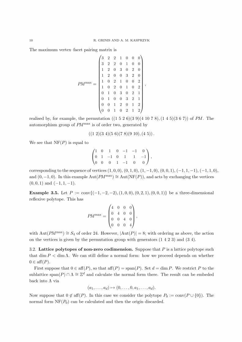
The maximum vertex–facet pairing matrix is
PMmax =
3 2 2 1 0 0 0
3 2 2 0 1 0 0
1 2 0 3 0 2 0
1 2 0 0 3 2 0
1 0 2 1 0 0 2
1 0 2 0 1 0 2
0 1 0 3 0 2 1
0 1 0 0 3 2 1
0 0 1 2 0 1 2
0 0 1 0 2 1 2
,
realised by, for example, the permutation ((1 5 2 6)(3 9)(4 10 7 8), (1 4 5)(3 6 7)) of PM . The
automorphism group of PMmax is of order two, generated by
((1 2)(3 4)(5 6)(7 8)(9 10), (4 5)) .
We see that NF(P ) is equal to 1 0 1 0 −1 −1 0
0 1 −1 0 1 1 −1
0 0 0 1 −1 0 0
,
corresponding to the sequence of vertices (1, 0, 0), (0, 1, 0), (1,−1, 0), (0, 0, 1), (−1, 1,−1), (−1, 1, 0),
and (0,−1, 0). In this example Aut(PMmax) ∼= Aut(NF(P )), and acts by exchanging the vertices
(0, 0, 1) and (−1, 1,−1).
Example 3.5. Let P := conv{(−1,−2,−2), (1, 0, 0), (0, 2, 1), (0, 0, 1)} be a three-dimensional
reflexive polytope. This has
PMmax =
4 0 0 0
0 4 0 0
0 0 4 0
0 0 0 4
,
with Aut(PMmax) ∼= S4 of order 24. However, |Aut(P )| = 8; with ordering as above, the action
on the vertices is given by the permutation group with generators (1 4 2 3) and (3 4).
3.2. Lattice polytopes of non-zero codimension. Suppose that P is a lattice polytope such
that dimP < dim Λ. We can still define a normal form: how we proceed depends on whether
0 ∈ aff(P ).
First suppose that 0 ∈ aff(P ), so that aff(P ) = span(P ). Set d = dimP . We restrict P to the
sublattice span(P ) ∩ Λ ∼= Zd and calculate the normal form there. The result can be embeded
back into Λ via
(a1, . . . , ad) 7→ (0, . . . , 0, a1, . . . , ad).
Now suppose that 0 6∈ aff(P ). In this case we consider the polytope P0 := conv(P ∪ {0}). The
normal form NF(P0) can be calculated and then the origin discarded.
NORMAL FORMS OF CONVEX LATTICE POLYTOPES 11
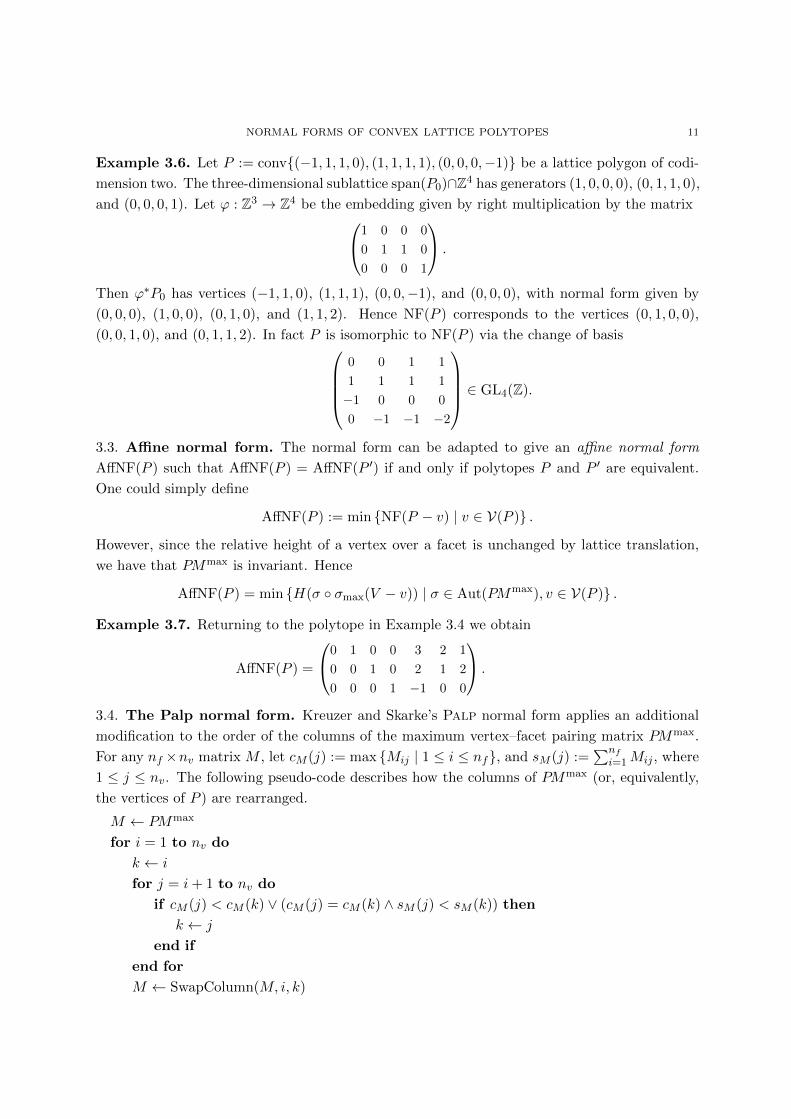
Example 3.6. Let P := conv{(−1, 1, 1, 0), (1, 1, 1, 1), (0, 0, 0,−1)} be a lattice polygon of codi-
mension two. The three-dimensional sublattice span(P0)∩Z4 has generators (1, 0, 0, 0), (0, 1, 1, 0),
and (0, 0, 0, 1). Let ϕ : Z3 → Z4 be the embedding given by right multiplication by the matrix1 0 0 0
0 1 1 0
0 0 0 1
.
Then ϕ∗P0 has vertices (−1, 1, 0), (1, 1, 1), (0, 0,−1), and (0, 0, 0), with normal form given by
(0, 0, 0), (1, 0, 0), (0, 1, 0), and (1, 1, 2). Hence NF(P ) corresponds to the vertices (0, 1, 0, 0),
(0, 0, 1, 0), and (0, 1, 1, 2). In fact P is isomorphic to NF(P ) via the change of basis0 0 1 1
1 1 1 1
−1 0 0 0
0 −1 −1 −2
∈ GL4(Z).
3.3. Affine normal form. The normal form can be adapted to give an affine normal form
AffNF(P ) such that AffNF(P ) = AffNF(P ′) if and only if polytopes P and P ′ are equivalent.
One could simply define
AffNF(P ) := min {NF(P − v) | v ∈ V(P )} .
However, since the relative height of a vertex over a facet is unchanged by lattice translation,
we have that PMmax is invariant. Hence
AffNF(P ) = min {H(σ ◦ σmax(V − v)) | σ ∈ Aut(PMmax), v ∈ V(P )} .
Example 3.7. Returning to the polytope in Example 3.4 we obtain
AffNF(P ) =
0 1 0 0 3 2 1
0 0 1 0 2 1 2
0 0 0 1 −1 0 0
.
3.4. The Palp normal form. Kreuzer and Skarke’s Palp normal form applies an additional
modification to the order of the columns of the maximum vertex–facet pairing matrix PMmax.
For any nf ×nv matrix M , let cM (j) := max {Mij | 1 ≤ i ≤ nf}, and sM (j) :=∑nf
i=1Mij , where
1 ≤ j ≤ nv. The following pseudo-code describes how the columns of PMmax (or, equivalently,
the vertices of P ) are rearranged.
M ← PMmax
for i = 1 to nv do
k ← i
for j = i+ 1 to nv do
if cM (j) < cM (k) ∨ (cM (j) = cM (k) ∧ sM (j) < sM (k)) then
k ← j
end if
end for
M ← SwapColumn(M, i, k)
12 R. GRINIS AND A. M. KASPRZYK
end for
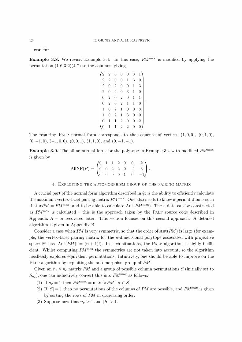
Example 3.8. We revisit Example 3.4. In this case, PMmax is modified by applying the
permutation (1 6 3 2)(4 7) to the columns, giving
2 2 0 0 0 3 1
2 2 0 0 1 3 0
2 0 2 0 0 1 3
2 0 2 0 3 1 0
0 2 0 2 0 1 1
0 2 0 2 1 1 0
1 0 2 1 0 0 3
1 0 2 1 3 0 0
0 1 1 2 0 0 2
0 1 1 2 2 0 0
.
The resulting Palp normal form corresponds to the sequence of vertices (1, 0, 0), (0, 1, 0),
(0,−1, 0), (−1, 0, 0), (0, 0, 1), (1, 1, 0), and (0,−1,−1).
Example 3.9. The affine normal form for the polytope in Example 3.4 with modified PMmax
is given by
AffNF(P ) =
0 1 1 2 0 0 2
0 0 2 2 0 −1 3
0 0 0 0 1 0 −1
.
4. Exploiting the automorphism group of the pairing matrix
A crucial part of the normal form algorithm described in §3 is the ability to efficiently calculate
the maximum vertex–facet pairing matrix PMmax. One also needs to know a permutation σ such
that σPM = PMmax, and to be able to calculate Aut(PMmax). These data can be constructed
as PMmax is calculated – this is the approach taken by the Palp source code described in
Appendix A – or recovered later. This section focuses on this second approach. A detailed
algorithm is given in Appendix B.
Consider a case when PM is very symmetric, so that the order of Aut(PM) is large (for exam-
ple, the vertex–facet pairing matrix for the n-dimensional polytope associated with projective
space Pn has |Aut(PM)| = (n + 1)!). In such situations, the Palp algorithm is highly ineffi-
cient. Whilst computing PMmax the symmetries are not taken into account, so the algorithm
needlessly explores equivalent permutations. Intuitively, one should be able to improve on the
Palp algorithm by exploiting the automorphism group of PM .
Given an nr × nc matrix PM and a group of possible column permutations S (initially set to
Snc), one can inductively convert this into PMmax as follows:
(1) If nr = 1 then PMmax = max {σPM | σ ∈ S}.(2) If |S| = 1 then no permutations of the columns of PM are possible, and PMmax is given
by sorting the rows of PM in decreasing order.
(3) Suppose now that nr > 1 and |S| > 1.
NORMAL FORMS OF CONVEX LATTICE POLYTOPES 13
(a) Let Rmax := max {σPMi | σ ∈ S, 1 ≤ i ≤ nr} be the largest row in PM , up to the
action of S.
(b) Set S′ := {σ ∈ S | σRmax = Rmax}.(c) For each row 1 ≤ i ≤ nr such that there exists a permutation σ ∈ S with σPMi =
Rmax, consider the matrix M(i) obtained from σPM by deleting the i-th row. If
M(i)∼= M(j) for some j < i, then skip this case. Otherwise let Mmax
(i) be the
(nr−1)×nc matrix obtained by inductively applying this process with PM ←M(i)
and S ← S′.
(d) Set Mmax to be the maximum of all such Mmax(i) . Then
PMmax =
(Rmax
Mmax
).
4.1. Test case: the database of smooth Fano polytopes. The algorithm described in
Appendix B, which we shall hereafter refer to as Symm, was implemented by the authors and
compared against the Palp algorithm. As Examples 4.1 and 4.2 illustrate, the difference in
run-time between the two approaches can be considerable.
Example 4.1. Let P be the six-dimensional polytope4 with 14 vertices
± (1, 0, 0, 0, 0, 0),±(0, 1, 0, 0, 0, 0),±(0, 0, 1, 0, 0, 0),±(0, 0, 0, 1, 0, 0),
± (0, 0, 0, 0, 1, 0),±(0, 0, 0, 0, 0, 1),±(1, 1, 1, 1, 1, 1).
The automorphism group Aut(PM) is of order 10,080. On our test machine the Palp algorithm
took 512.88 seconds, whereas the Symm algorithm took only 5.83 seconds.
Example 4.2. Let P be the six-dimensional polytope5 with 12 vertices
(1, 0, 0, 0, 0, 0), (0, 1, 0, 0, 0, 0), (0, 0, 1, 0, 0, 0), (0, 0, 0, 1, 0, 0), (0, 0, 0, 0, 1, 0),
(0, 0, 0, 0, 0, 1), (−1,−1,−1, 1, 1, 1), (0, 0, 1,−1, 0, 0), (0, 0,−1, 0, 0, 0),
(0, 1, 1,−1,−1,−1), (0,−1,−1, 0, 0, 0), (0, 0, 0, 0,−1,−1).
The automorphism group Aut(PM) is of order 16; the Palp algorithm took 0.55 seconds whilst
the Symm algorithm took 4.30 seconds.
Table 2 contains timing data comparing the Palp algorithm with the Symm algorithm.
This data was collected by sampling polytopes from Øbro’s classification of smooth Fano poly-
topes [Øbr07]. For each smooth polytope P selected, the calculation was performed for both P
and P ∗. In small dimensions the number of polytopes, and the time required for the computa-
tions, is small enough that the entire classification can be used. It is important to emphasise
that the smooth Fano polytopes are atypical in that they can be expected to have a large
number of symmetries, and so favour Symm. Experimental evidence suggests that the ratio
4Smooth Fano polytope number 1930 in the Graded Ring Database [BK].5Smooth Fano polytope number 1854 in the Graded Ring Database [BK].
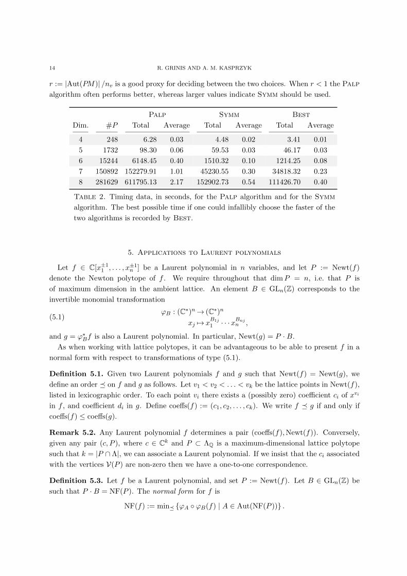
14 R. GRINIS AND A. M. KASPRZYK
r := |Aut(PM)| /nv is a good proxy for deciding between the two choices. When r < 1 the Palp
algorithm often performs better, whereas larger values indicate Symm should be used.
Palp Symm Best
Dim. #P Total Average Total Average Total Average
4 248 6.28 0.03 4.48 0.02 3.41 0.01
5 1732 98.30 0.06 59.53 0.03 46.17 0.03
6 15244 6148.45 0.40 1510.32 0.10 1214.25 0.08
7 150892 152279.91 1.01 45230.55 0.30 34818.32 0.23
8 281629 611795.13 2.17 152902.73 0.54 111426.70 0.40
Table 2. Timing data, in seconds, for the Palp algorithm and for the Symm
algorithm. The best possible time if one could infallibly choose the faster of the
two algorithms is recorded by Best.
5. Applications to Laurent polynomials
Let f ∈ C[x±11 , . . . , x±1n ] be a Laurent polynomial in n variables, and let P := Newt(f)
denote the Newton polytope of f . We require throughout that dimP = n, i.e. that P is
of maximum dimension in the ambient lattice. An element B ∈ GLn(Z) corresponds to the
invertible monomial transformation
(5.1)ϕB : (C∗)n→ (C∗)n
xj 7→ xB1j
1 · · ·xBnjn ,
and g = ϕ∗Bf is also a Laurent polynomial. In particular, Newt(g) = P ·B.
As when working with lattice polytopes, it can be advantageous to be able to present f in a
normal form with respect to transformations of type (5.1).
Definition 5.1. Given two Laurent polynomials f and g such that Newt(f) = Newt(g), we
define an order � on f and g as follows. Let v1 < v2 < . . . < vk be the lattice points in Newt(f),
listed in lexicographic order. To each point vi there exists a (possibly zero) coefficient ci of xvi
in f , and coefficient di in g. Define coeffs(f) := (c1, c2, . . . , ck). We write f � g if and only if
coeffs(f) ≤ coeffs(g).
Remark 5.2. Any Laurent polynomial f determines a pair (coeffs(f),Newt(f)). Conversely,
given any pair (c, P ), where c ∈ Ck and P ⊂ ΛQ is a maximum-dimensional lattice polytope
such that k = |P ∩ Λ|, we can associate a Laurent polynomial. If we insist that the ci associated
with the vertices V(P ) are non-zero then we have a one-to-one correspondence.
Definition 5.3. Let f be a Laurent polynomial, and set P := Newt(f). Let B ∈ GLn(Z) be
such that P ·B = NF(P ). The normal form for f is
NF(f) := min� {ϕA ◦ ϕB(f) | A ∈ Aut(NF(P ))} .

NORMAL FORMS OF CONVEX LATTICE POLYTOPES 15
Example 5.4. Consider the Laurent polynomial
f = 2x2y +1
x+
3
xy.
Then NF(P ) has vertices (1, 0), (0, 1), and (−1,−1), with corresponding transformation matrix
B =
(0 −1
−1 1
)∈ GL2(Z).
Under this transformation,
ϕ∗Bf = 3x+ y +2
xy
and coeffs(ϕ∗Bf) = (2, 0, 1, 3). The automorphism group Aut(NF(P )) ∼= S3 acts by permuting
the non-zero elements in the coefficient vector, hence
NF(f) = 3x+ 2y +1
xy.
A naıve implementation of Laurent normal form faces a serious problem: listing the points
in a polytope is computationally expensive, and will often be the slowest part of the algorithm
by many orders of magnitude. With a little care this can be avoided. What is really needed
in Definition 5.3 is not the entire coefficient vector, but the closure of the non-zero coefficients
under the action of Aut(NF(P )). We illustrate this observation with an example.
Example 5.5. Consider the Laurent polynomial
f = x50y50z50 + x50y30 +x30z30
y40+
x10
y40z20+ xyz +
y40z20
x10+
y40
x30z30+
1
x50y30+
1
x50y50z50.
Set P = Newt(f). Notice that |P ∩ Λ| = 285241; enumerating the points in P is clearly not the
correct approach. The normal form NF(P ) is given by change of basis
B =
−3 −4 −6
5 7 10
−12 −16 −23
∈ GL3(Z),
with
g := ϕ∗Bf = x650y880z1270 + x500y650z950 + x10 + y10+1
y10+
1
x10+
1
x10y13z19+
1
x500y650z950+
1
x650y880z1270.
The automorphism group G := Aut(NF(P )) is of order two, generated by the involution u 7→ −u.
We consider the closure of the nine lattice points corresponding to the exponents of g under
the action of G. The only additional point is (10, 13, 19). Thus we can express coeffs(g) with
respect to these ten points:
coeffs(g) = (1, 1, 1, 1, 1, 1, 1, 0, 1, 1).
The key observation is that the action of G on g will not introduce any additional points, hence
the lexicographically smallest coefficient sequence with respect to these points will also be the

16 R. GRINIS AND A. M. KASPRZYK
smallest coefficient sequence with respect to all the points of NF(P ). By applying the involution
we obtain the smaller coefficient sequence (1, 1, 0, 1, 1, 1, 1, 1, 1, 1), hence
NF(f) = x650y880z1270 + x500y650z950 + x10y13z19+x10 + y10+
1
y10+
1
x10+
1
x500y650z950+
1
x650y880z1270.
We conclude this section by remarking that the automorphism group Aut(f) ≤ GLn(Z) of
a Laurent polynomial f can easily be constructed from Aut(Newt(f)) by restricting to the
subgroup that leaves coeffs(f) invariant.
Appendix A. The Kreuzer–Skarke algorithm
We describe in detail the algorithm used by Kreuzer and Skarke in Palp [KS04] to compute
the normal form of a lattice polytope P of maximum dimension n. Any such polytope can be
represented by a n× nv matrix V whose columns correspond to the vertices of P . This matrix
is unique up to permutation of columns and the action of GLn(Z); i.e. one can change the order
of the vertices and the underlying basis for the lattice to obtain a different matrix V ′.
The Palp normal form is a unique representation of the polytope P such that if Q is any
other maximum dimensional lattice polytope, then P and Q are isomorphic if and only if their
normal forms are equal. For any matrix V with integer entries, and any G ∈ GLn(Z), the
Hermite normal form of G · V is uniquely defined. The question is how to define a canonical
order for the vertices, since permuting the vertices will lead to a different Hermite normal form.
In what follows, the line numbers refer to the Palp source file Polynf.c6. We have chosen
our notation to correspond as closely as possible to the source code. The algorithm will be
described in eight stages:
A.1. The pairing matrix;
A.2. The maximal pairing matrix;
A.3. Constructing the first row;
A.4. Computing the restricted automorphism group, step I;
A.5. Constructing the k-th row;
A.6. Updating the set of permutations;
A.7. Computing the restricted automorphism group, step II;
A.8. Computing the normal form of the polytope.
A.1. The pairing matrix. We start by constructing the pairing matrix PM .
Line: 197 (Init rVM VPM)
Input: A list of vertices and a list of equations for the supporting hyperplanes.
Output: The pairing matrix PM .
6Palp 1.1, updated November 2, 2006. http://hep.itp.tuwien.ac.at/∼kreuzer/CY/palp/palp-1.1.tar.gz
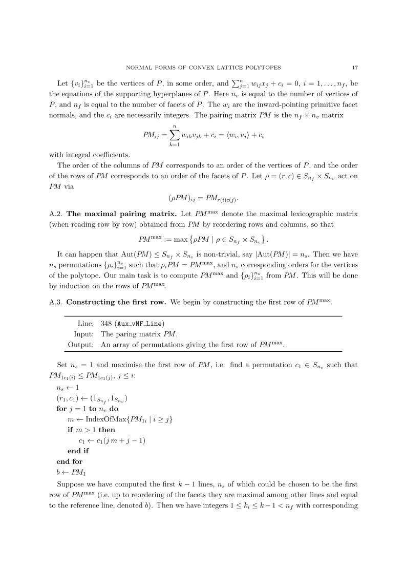
NORMAL FORMS OF CONVEX LATTICE POLYTOPES 17
Let {vi}nvi=1 be the vertices of P , in some order, and∑n
j=1wijxj + ci = 0, i = 1, . . . , nf , be
the equations of the supporting hyperplanes of P . Here nv is equal to the number of vertices of
P , and nf is equal to the number of facets of P . The wi are the inward-pointing primitive facet
normals, and the ci are necessarily integers. The pairing matrix PM is the nf × nv matrix
PMij =
n∑k=1
wikvjk + ci = 〈wi, vj〉+ ci
with integral coefficients.
The order of the columns of PM corresponds to an order of the vertices of P , and the order
of the rows of PM corresponds to an order of the facets of P . Let ρ = (r, c) ∈ Snf × Snv act on
PM via
(ρPM)ij = PMr(i)c(j).
A.2. The maximal pairing matrix. Let PMmax denote the maximal lexicographic matrix
(when reading row by row) obtained from PM by reordering rows and columns, so that
PMmax := max{ρPM | ρ ∈ Snf × Snv
}.
It can happen that Aut(PM) ≤ Snf × Snv is non-trivial, say |Aut(PM)| = ns. Then we have
ns permutations {ρi}nsi=1 such that ρiPM = PMmax, and ns corresponding orders for the vertices
of the polytope. Our main task is to compute PMmax and {ρi}nsi=1 from PM . This will be done
by induction on the rows of PMmax.
A.3. Constructing the first row. We begin by constructing the first row of PMmax.
Line: 348 (Aux vNF Line)
Input: The paring matrix PM .
Output: An array of permutations giving the first row of PMmax.
Set ns = 1 and maximise the first row of PM , i.e. find a permutation c1 ∈ Snv such that
PM1c1(i) ≤ PM1c1(j), j ≤ i:ns ← 1
(r1, c1)← (1Snf , 1Snv )
for j = 1 to nv do
m← IndexOfMax{PM1i | i ≥ j}if m > 1 then
c1 ← c1(j m+ j − 1)
end if
end for
b← PM1
Suppose we have computed the first k − 1 lines, ns of which could be chosen to be the first
row of PMmax (i.e. up to reordering of the facets they are maximal among other lines and equal
to the reference line, denoted b). Then we have integers 1 ≤ ki ≤ k−1 < nf with corresponding
18 R. GRINIS AND A. M. KASPRZYK
permutations ρi = (ri, ci) ∈ Snf × Snv , i = 1, . . . , ns, and a reference line defined by b := PMk1
such that:
PMkici(j) = bc1(j), i = 1, . . . , ns, j = 1, . . . , nv.
Set ri = (1 ki) to be the permutation which moves the line in question to the first row of PM .
Now we consider the k-th row of PM . Find the maximal element maxj{PMkj}, say PMkm,
and let cns+1 = (1m). We compare this against the reference line. If PMkcns+1(1) < bc1(1) then
continue with the next line (or stop if we are at the last line), otherwise continue constructing
cns+1. If maxj>1{PMkcns+1(j)} = PMkcns+1(m) then let cns+1 7→ cns+1 (2m) and verify that
PMkcns+1(2) < bc1(2); if this inequality fails to hold then continue with the next element.
If the line k is not less than the reference line b then we set rns+1 = (1 k) and have two cases
to consider:
(1) If PMkcns+1(j) = bc1(j), j = 1, . . . , nv, then we have a new case of symmetry. We set
kns+1 := k and increment the number of symmetries ns.
(2) Otherwise we have found a (lexicographically) bigger row and so obtain a new reference
line. We set b := PMk, k1 := k, and ρ1 := (rns+1, cns+1), and reset the number of
symmetries ns.
for k = 2 to nf do
(rns+1, cns+1)← (1Snf , 1Snv )
m← IndexOfMax{PMkcns+1(j) | j ≥ 1
}if m > 1 then
cns+1 ← cns+1(1m)
end if
d← PMkcns+1(1) − bc1(1)if d < 0 then
continue
end if
for i = 2 to nv do
m← IndexOfMax{PMkcns+1(j) | j ≥ i
}if m > 1 then
cns+1 ← cns+1(im+ i− 1)
end if
if d=0 then
d← PMkcns+1(i) − bc1(i)if d < 0 then
break
end if
end if
end for
if d < 0 then
continue
NORMAL FORMS OF CONVEX LATTICE POLYTOPES 19
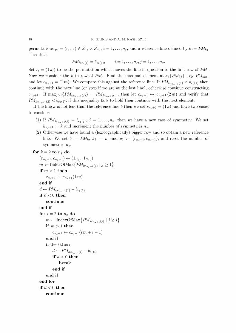
end if
rns+1 ← rns+1(1 k)
if d = 0 then
ns ← ns + 1
else
(r1, c1)← (rns+1, cns+1)
ns ← 1
b← PMk
end if
end for
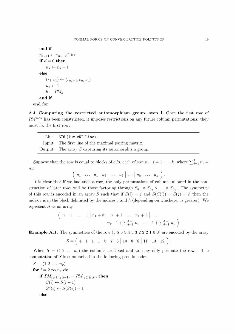
A.4. Computing the restricted automorphism group, step I. Once the first row of
PMmax has been constructed, it imposes restrictions on any future column permutations: they
must fix the first row.
Line: 376 (Aux vNF Line)
Input: The first line of the maximal pairing matrix.
Output: The array S capturing its automorphism group.
Suppose that the row is equal to blocks of ai’s, each of size ni , i = 1, . . . , k, where∑k
i=1 ni =
nv: (a1 . . . a1 a2 . . . a2 . . . ak . . . ak
).
It is clear that if we had such a row, the only permutations of columns allowed in the con-
struction of later rows will be those factoring through Sn1 × Sn2 × . . . × Snk . The symmetry
of this row is encoded in an array S such that if S(i) = j and S(S(i)) = S(j) = h then the
index i is in the block delimited by the indices j and h (depending on whichever is greater). We
represent S as an array(n1 1 . . . 1 n1 + n2 n1 + 1 . . . n1 + 1 . . .
nv 1 +∑k−1
i=1 ni . . . 1 +∑k−1
i=1 ni
)Example A.1. The symmetries of the row (5 5 5 5 4 3 3 2 2 2 1 0 0) are encoded by the array
S =(
4 1 1 1 5 7 6 10 8 8 11 13 12).
When S = (1 2 . . . nv) the columns are fixed and we may only permute the rows. The
computation of S is summarised in the following pseudo-code:
S ← (1 2 . . . nv)
for i = 2 to nv do
if PMr1(1)c1(i−1) = PMr1(1)c1(i) then
S(i)← S(i− 1)
S2(i)← S(S(i)) + 1
else

20 R. GRINIS AND A. M. KASPRZYK
S(i)← i
end if
end for
A.5. Constructing the k-th row. Proceeding by induction on the rows, we construct the
remaining rows of PMmax.
Line: 289 (Aux vNF Line)
Input: PM , the permutations {pi}nsi=1, and the array S.
Output: The k-th line of the maximal pairing matrix.
Assume we have computed the first l−1 < nf−1 rows of PMmax and the associated symmetry
array S (notice that the last row of PMmax need not be computed as it is completely determined),
together with ns distinct permutations ρi = (ri, ci) ∈ Snf × Snv such that
PMmaxkj = PMri(k)ci(j) for all 1 ≤ j ≤ nv, 1 ≤ k < l, 1 ≤ i ≤ ns.
We have to consider each configuration given by the permutations {ρi}nsi=1. For each configu-
ration we generally obtain nρ ways to construct the line l, moreover some constructions might
give a smaller line, hence ns will have to be updated as we proceed. Let ns record the initial
value of ns.
First consider the case k = ns. We will construct a candidate line for the l-th row of PMmax;
this will be our reference line against which the other cases will be compared. If a greater
candidate is found, all the preceding computations will have to be deleted and redone with the
new candidate. If a given case lead to a smaller line than the reference, it will have to be deleted.
Initially set the local number of symmetries, nρ, to zero and initialise the permutation ρnρ =
ρk. We start with the line rnρ(l) by finding the maximal element of the first symmetry block.
Suppose that
max{PMrnρ (l)cnρ (i)
| 1 ≤ i ≤ S(1)}
= PMrnρ (l)cnρ (m).
Then we update cnρ to cnρ (1m). This maximal value is saved in the reference line which we
denote lr (if it were already constructed, k < ns, we move straight to the tests below). We
increment nρ by one to reflect this new candidate, initialise ρnρ = pk, and proceed to consider
the maximal entries in the first symmetry block for other lines rk(s), s = l + 1, . . . , nf .
Inductively, suppose we have considered s−1 lines where nρ of them have a maximal element
in the first symmetry block equal to the one of the reference line lr(1), and the others have
smaller values. We also have rnρ = rk from the initialisation. Consider the line rnρ(s) and find
its maximal element in 1, . . . , S(1) as above, updating cnρ . Now if PMrnρ (s)cnρ (1)< lr(1) then
proceed to the case s + 1, if possible. Otherwise rnρ 7→ rnρ (l s) and there are two possibilities:
if PMrnρ (s)cnρ (1)= lr(1) then increase the number of symmetries nρ 7→ nρ+ 1 and move to s+ 1,
after initialising the new permutation ρnρ = ρk; if PMrnρ+1(s)cnρ+1(1) > lr(1) then redefine the
first element of the reference line lr(1) := PMrnρ (s)cnρ (1), update the first permutation ρ0 = ρnρ ,
and reset nρ = 1 ready for the next permutation ρnρ = ρk.

NORMAL FORMS OF CONVEX LATTICE POLYTOPES 21
c← 1
nρ ← 0
ccf ← cf
(rnρ , cnρ)← (rk, ck)
for s = l to nf do
for j = 2 to S(1) do
if PMrnρ (s)cnρ (c)< PMrnρ (s)cnρ (j)
then
cnρ ← cnρ(c j)
end if
end for
if ccf = 0 then
lr(1)← PMrnρ (s)cnρ (1)
rnρ ← rnρ(l s)
nρ ← nρ + 1
ccf ← 1
(rnρ , cnρ)← (rk, ck)
else
d← PMrnρ (s)cnρ (1)− lr(1)
if d < 0 then
continue
else if d = 0 then
rnρ ← rnρ(l s)
nρ ← nρ + 1
(rnρ , cnρ)← (rk, ck)
else
lr(1)← PMrnρ (s)cnρ (1)
cf ← 0
(r1, c1)← (rnρ , cnρ)
nρ ← 1
(rnρ , cnρ)← (rk, ck)
ns ← k
rnρ ← rnρ(l s)
end if
end if
end for
Note that the initial value of the comparison flag cf is 0. This indicates that the reference
line has not been initialised; it is also reset to zero when a greater candidate is found. We will
see later how cf is updated.
We need to construct other elements of lr. Inductively, suppose we are constructing the entry i
of lr and we have nρ symmetries with corresponding permutations ρj , j = 0, . . . , nρ−1. If nρ = 0

22 R. GRINIS AND A. M. KASPRZYK
we move to the next configuration k−1 after having updated the symmetries accordingly, i.e. we
do not save the current configuration. Otherwise, start with the last j = nρ − 1. Determine
where the corresponding block of symmetry ends for i by looking at the maximum of S(i) and
S2(i), which we will call h. Then compute
max{PMrj(l)cj(λ) | i ≤ λ ≤ h
}= PMrj(l)cj(m)
and update cj 7→ cj (im) . This value is saved in the reference line lr(i). Then we consider
(inductively) any cases of symmetry with j < nρ − 1 and compute the i-th entry in the same
manner as above: if PMrj(l)cj(i) = lr(i) then continue with the next j; if PMrj(l)cj(i) < lr(i) then
the current case is removed and we update nρ 7→ nρ − 1; finally if PMrj(l)cj(i) > lr(i) then all
cases previously considered are irrelevant, so we let nρ = j + 1 and the reference line is updated
lr(i) = PMrj(l)cj(i).
for c = 2 to nv do
h← S(c)
ccf ← cf
if h < c then
h← S(h)
end if
s← nρ
while s > 0 do
s← s− 1
for j = c+ 1 to h do
if PMrs(l)cs(c) < PMrs(l)cs(j) then
cs ← cs(cj)
end if
end for
if ccf = 0 then
lr(c)← PMrs(l)cs(c)
ccf ← 1
else
d← PMrs(l)cs(c) − lr(c)if d < 0 then
nρ ← nρ − 1
if nρ > s then
(rs, cs)← (rnρ , cnρ)
end if
else if d > 0 then
lr(c)← PMrs(l)cs(c)
cf ← 0
nρ ← s+ 1
NORMAL FORMS OF CONVEX LATTICE POLYTOPES 23
ns ← k
end if
end if
end while
end for
A.6. Updating the set of permutations. The last step in the construction of the line l is to
organise the new symmetries for a given case k.
Line: 333 (Aux vNF Line)
Input: The permutations {pi}nsi=1 and the newly computed {ρi}nρ−1i=0 .
Output: The updated set {pi}nsi=1.
Recall that ns denotes the number of symmetries we had before performing the computations
for the line l of PMmax, and ns ≤ ns represents the updated number symmetries. Our current
construction of the line l may well introduce new symmetries, so-called local symmetries, of
which there are nρ. We can have nρ = 0, in which case all the configurations in the case k
lead to a smaller candidate for l. When nρ > 0 the local symmetries are represented by the set
{ρi}nρ−1i=0 of new permutations.
We now update the array of all permutations. If ns > k we set ρk = ρns ; we want the set of
permutations {ρi}nsi=1 to be updated so that the only cases which need to be considered are those
with index i < k. Since we are appending nρ new permutations at end for the indices i ≥ ns,
so ns → ns + nρ − 1. If nρ = 0 then nothing is appended and ns decreases by one as required.
Finally, we update the comparison flag cf to reflect the current number of symmetries.
ns ← ns − 1
if ns > k − 1 then
(rk, ck)← (rns+1, cns+1)
end if
cf ← ns + nρ
for s = 0 to nρ − 1 do
(rns+1, cns+1)← (rs, cs)
ns ← ns + 1
end for
A.7. Computing the restricted automorphism group, step II. Once a new row of PMmax
has been compute we need to update S to reflect the symmetries of this row. This is done by
restricting the blocks previously delimited by S to reflect any additional constraints imposed by
the row.
24 R. GRINIS AND A. M. KASPRZYK
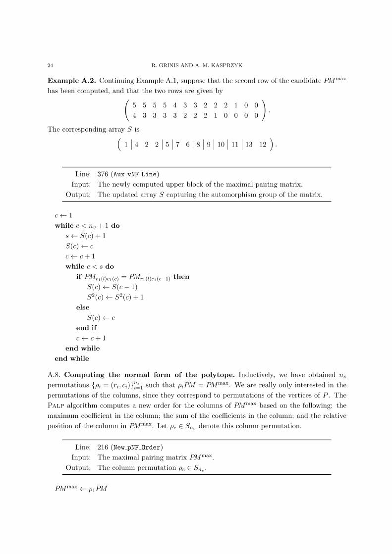
Example A.2. Continuing Example A.1, suppose that the second row of the candidate PMmax
has been computed, and that the two rows are given by(5 5 5 5 4 3 3 2 2 2 1 0 0
4 3 3 3 3 2 2 2 1 0 0 0 0
).
The corresponding array S is(1 4 2 2 5 7 6 8 9 10 11 13 12
).
Line: 376 (Aux vNF Line)
Input: The newly computed upper block of the maximal pairing matrix.
Output: The updated array S capturing the automorphism group of the matrix.
c← 1
while c < nv + 1 do
s← S(c) + 1
S(c)← c
c← c+ 1
while c < s do
if PMr1(l)c1(c) = PMr1(l)c1(c−1) then
S(c)← S(c− 1)
S2(c)← S2(c) + 1
else
S(c)← c
end if
c← c+ 1
end while
end while
A.8. Computing the normal form of the polytope. Inductively, we have obtained ns
permutations {ρi = (ri, ci)}nsi=1 such that ρiPM = PMmax. We are really only interested in the
permutations of the columns, since they correspond to permutations of the vertices of P . The
Palp algorithm computes a new order for the columns of PMmax based on the following: the
maximum coefficient in the column; the sum of the coefficients in the column; and the relative
position of the column in PMmax. Let ρc ∈ Snv denote this column permutation.
Line: 216 (New pNF Order)
Input: The maximal pairing matrix PMmax.
Output: The column permutation ρc ∈ Snv .
PMmax ← p1PM
NORMAL FORMS OF CONVEX LATTICE POLYTOPES 25
pc ← 1SnvMmax ←
{max1≤i≤nf
{PMmax
ij
}| 1 ≤ j ≤ nv
}Smax ←
{∑1≤i≤nf PM
maxij | 1 ≤ j ≤ nv
}for i = 1 to nv do
k ← i
for j = i+ 1 to nv do
if (Mmaxj < Mmax
k ) ∨ ((Mmaxj = Mmax
k ) ∧ (Smaxj < Smax
k )) then
k ← j
end if
end for
if k 6= i then
Mmax ← SwapRow(Mmax, i, k)
Smax ← SwapRow(Smax, i, k)
pc ← pc(i k)
end if
end for
Given the column permutations ρc and ci, i = 1 . . . , ns, we obtain a permutation of the
vertices of P , and hence of the columns of the vertex matrix V . We let Vi denote this reordered
vertex matrix. The remaining freedom – the action of GLn(Z) corresponding to the choice of
lattice basis – is removed by computing the Hermite normal form H(Vi).
Line: 134 (GLZ Make Trian NF)
Input: A matrix with integer coefficents.
Output: The Hermite normal form of the matrix.
The Palp normal form is simply the minimum amongst the H(Vi).
Line: 399 (Aux Make Triang)
Input: The column permutations ρc and {ci}nsi=1, and the vertex matrix V .
Output: The normal form.
Appendix B. Calculating the maximum pairing matrix
Let M be an nr × nc matrix. Recall that we define an action of σ = (σr, σc) ∈ Snr × Snc on
the rows and columns of M via (σM)ij := Mσr(i),σc(j), and that we call two matrices M and M ′
isomorphic if there exists some permutation σ ∈ Snr × Snc such that σ(M) = M ′. We begin by
briefly describing one approach to determining when two matrices are isomorphic.
Given a matrix M , we associate a bipartite graph G(M) with nr + nc vertices, where the
vertices vi, vnr+j are connected by an edge Eij for all 1 ≤ i ≤ nr, 1 ≤ j ≤ nc. Each edge
Eij is labelled with the corresponding value Mij . The vertices vi, 1 ≤ i ≤ nr, are labelled
26 R. GRINIS AND A. M. KASPRZYK
with one colour, whilst the vertices vnr+j , 1 ≤ j ≤ nc, are labelled with a second colour. This
distinguishes between vertices representing rows of M and vertices representing columns of M .
Clearly two matrices M and M ′ are isomorphic if and only if the graphs G(M) and G(M ′) are
isomorphic. We note also that the automorphism group Aut(M) ≤ Snr × Snc is given by the
automorphism group of G(M).
We now describe a recursive algorithm to compute PMmax from PM . For readability, we shall
split this algorithm into three parts, with a brief discussion preceding each part.
Input: A matrix PM .
Output: The maximal matrix PMmax.
Throughout we set nr and nc equal to, respectively, the number of rows and the number of
columns of the input matrix PM . A vector s of length nc is used to represent the permitted
permutations of the columns of PM . Initially s is defined as
s = (a, . . . , a) ∈ Znc ,
where a := 1 + maxPMij is larger than any entry of the matrix PM . At each step of the
recursion, the value of nc remains unchanged, but the value of nr will decrease by one as a row
of PM is removed from consideration. The vector s will be modified to reflect the symmetries of
the previously steps; two coefficients sj and sk are equal if and only if the columns j and k can
be exchanged without affecting the computations so far. By construction s will always satisfy:
(1) either sj = sj+1 or sj = sj+1 + 1, for each 1 ≤ j < nc;
(2) snc = a.
The first stage is to calculate the maximum possible row Rmax of PM , where each row is
sorted in decreasing order. Once done, we update the vector s to reflect the possible column
permutations that will leave Rmax unchanged.
Ri ← Sort≥{(sj , PMij) | 1 ≤ j ≤ nc}Ri ← (Rij2 | 1 ≤ j ≤ nc)Rmax ← max {Ri | 1 ≤ i ≤ nr}s′ ← s
for j = nc − 1 to 1 by −1 do
if sj = sj+1 ∧Rmaxj 6= Rmax
j+1 then
for k = 1 to j do
s′k ← s′k + 1
end for
end if
end for
Next we collect together all non-isomorphic ways of writing PM with Rmax as the first row.
These possibilities are recorded in the set M.
M← {}

NORMAL FORMS OF CONVEX LATTICE POLYTOPES 27
for i = 1 to nr such that Ri = Rmax do
M ← SwapRow(PM, 1, i)
T ← Sort≥{(sj ,M1j , j) | 1 ≤ j ≤ nc}τ ← permutation in Snc sending j to Tj3
M ← τ(M)
M ←M
M1 ← s′
if∧M ′∈M
(M ′ 6∼= M
)then
M←M∪ {M}end if
end for
When all possible symmetries of the columns have been exhausted, the vector s′ will be equal
to the sequence
(a+ nc − 1, a+ nc − 2, . . . , a).
If this is the case, then PMmax is the maximum matrix inM, once the rows have been placed in
decreasing order. If there remain symmetries to explore, then we recurse on each of the matrices
in M using the new permutation vector s′; PMmax is given by the largest resulting matrix.
if nr = 1 then
PMmax ← Rmax
else if s′1 = s′nc + nc − 1 then
PMmax ← max {SortRows≥(M) |M ∈M}else
M′ ← {}for M ∈M do
M ′ ← RemoveRow(M, 1)
M ′ ← (recurse with PM ←M ′ and s← s′)
M′ ←M′ ∪ {M ′}end for
PMmax ← VerticalJoin(Rmax,maxM′)end if
References
[BBK09] Gavin Brown, Jaros law Buczynski, and Alexander M. Kasprzyk, Convex polytopes and poly-
hedra, Handbook of Magma Functions, Edition 2.16, November 2009, available online at
http://magma.maths.usyd.edu.au/.
[BCP97] Wieb Bosma, John Cannon, and Catherine Playoust, The Magma algebra system. I. The user lan-
guage, J. Symbolic Comput. 24 (1997), no. 3-4, 235–265, Computational algebra and number theory
(London, 1993).
[BDSS09] David Bremner, Mathieu Dutour Sikiric, and Achill Schurmann, Polyhedral representation conversion
up to symmetries, Polyhedral computation, CRM Proc. Lecture Notes, vol. 48, Amer. Math. Soc.,
Providence, RI, 2009, pp. 45–71.
28 R. GRINIS AND A. M. KASPRZYK
[BEK84] Jurgen Bokowski, Gunter Ewald, and Peter Kleinschmidt, On combinatorial and affine automor-
phisms of polytopes, Israel J. Math. 47 (1984), no. 2-3, 123–130.
[BK] Gavin Brown and Alexander M Kasprzyk, The Graded Ring Database, online, access via
http://grdb.lboro.ac.uk/.
[BSP+12] David Bremner, Mathieu Dutour Sikiric, Dmitrii V. Pasechnik, Thomas Rehn, and Achill Schurmann,
Computing symmetry groups of polyhedra, arXiv:1210.0206 [math.CO].
[Kre10] Maximilian Kreuzer, PALP++ project proposal, unfinished draft, available online at
http://hep.itp.tuwien.ac.at/∼www/palp++.pdf, September 2010.
[KS98] Maximilian Kreuzer and Harald Skarke, Classification of reflexive polyhedra in three dimensions, Adv.
Theor. Math. Phys. 2 (1998), no. 4, 853–871.
[KS00] , Complete classification of reflexive polyhedra in four dimensions, Adv. Theor. Math. Phys.
4 (2000), no. 6, 1209–1230.
[KS03] Volker Kaibel and Alexander Schwartz, On the complexity of polytope isomorphism problems, Graphs
Combin. 19 (2003), no. 2, 215–230.
[KS04] Maximilian Kreuzer and Harald Skarke, PALP, a package for analyzing lattice polytopes with appli-
cations to toric geometry, Computer Phys. Comm. 157 (2004), 87–106.
[McK] Brendan D. McKay, The Nauty graph automorphism software, online, access via
http://cs.anu.edu.au/∼bdm/nauty/.
[McK81] , Practical graph isomorphism, Proceedings of the Tenth Manitoba Conference on Numerical
Mathematics and Computing, Vol. I (Winnipeg, Man., 1980), vol. 30, 1981, pp. 45–87.
[MdlBW09] C. Mears, M. Garcia de la Banda, and M. Wallace, On implementing symmetry detection, Constraints
14 (2009), no. 4, 443–477.
[Øbr07] Mikkel Øbro, An algorithm for the classification of smooth Fano polytopes, arXiv:0704.0049v1
[math.CO], classifications available from http://grdb.lboro.ac.uk/.
[Pug05] Jean-Francois Puget, Automatic detection of variable and value symmetries, Principles and Practice
of Constraint Programming (Peter van Beek, ed.), vol. 3709, Springer, 2005, pp. 475–489.
[S+] W. A. Stein et al., Sage Mathematics Software, available online at http://www.sagemath.org/.
Trinity College, University of Cambridge, Cambridge, CB2 1TQ, UK
E-mail address: [email protected]
Department of Mathematics, Imperial College London, London, SW7 2AZ, UK
E-mail address: [email protected]