observations of solitary wave dynamics of film flows

J. Fluid Mech. (2001), vol. 435, pp. 191–215. Printed in the United Kingdom

c© 2001 Cambridge University Press

191

Observations of solitary wave dynamicsof film flows

By M. V L A C H O G I A N N I S AND V. B O N T O Z O G L O UDepartment of Mechanical and Industrial Engineering, University of Thessaly,

GR-38334 Volos, Greece

(Received 20 April 2000 and in revised form 10 November 2000)

Experimental results are reported on non-stationary evolution and interactions ofwaves forming on water and water–glycerol solution flowing along an inclined plane.A nonlinear wave generation process leads to a large number of solitary humpswith a wide variety of sizes. A fluorescence imaging method is applied to capturethe evolution of film height in space and time with accuracy of a few microns.Coalescence – the inelastic interaction of solitary waves resulting in a single hump – isfound to proceed at a timescale correlated to the difference in height between theinteracting waves. The correlation indicates that waves of similar height do not merge.Transient phenomena accompanying coalescence are reported. The front-runningripples recede during coalescence, only to reappear when the new hump recovers itsteardrop shape. The tail of the resulting solitary wave develops an elevated substraterelative to the front, which decays exponentially in time; both observations aboutthe tail confirm theoretical predictions. In experiments with water, the elevated backsubstrate is unstable, yielding to a tail oscillation with wavelength similar to that ofthe front-running ripples. This instability plays a key role in two complex interactionphenomena observed: the nucleation of a new crest between two interacting solitaryhumps and the splitting of a large hump (that has grown through multiple coalescenceevents) into solitary waves of similar size.

1. IntroductionRecent progress in the theory of nonlinear dynamics of falling film flows has centred

on the existence and properties of coherent structures, or dissipative solitary waves. Aseries of simplified equations have been developed over the last three decades (Benney1966; Shkadov 1967; Prokopiou, Cheng & Chang 1991; Yu et al. 1995; Lee & Mei1996; Nguyen & Balakotaiah 2000), resulting from the full Navier–Stokes equationsby a long-wave approximation and by various order-of-magnitude assumptions forthe pertinent dimensionless Reynolds and Weber numbers Re and We. Intensiveanalytical and numerical scrutiny of these equations, based on dynamical systemstechniques, has revealed multiple families of stationary solutions bifurcating from theprimary instability of the flat film (Demekhin, Tokarev & Shkadov 1991; Trifonov& Tsvelodub 1991; Tsvelodub & Trifonov 1992; Chang, Demekhin & Kopelevich1993; Chang 1994; Lee & Mei 1996). Few numerical simulations of the full Navier–Stokes equations have been undertaken (Bach & Villadsen 1984; Kheshgi & Scriven1987; Ho & Patera 1990; Malamataris & Papanastasiou 1991; Salamon, Armstrong& Brown 1994) and all are restricted to relatively small Re. Therefore, the limits ofvalidity of the approximate equations are still a matter of active research.

192 M. Vlachogiannis and V. Bontozoglou

On the other hand, detailed experimental records of solitary wave dynamics in filmflows are not very numerous. The pioneering work of Kapitza & Kapitza (1949),as well as later contributions (Stainthorp & Allen 1965; Jones & Whitaker 1966;Krantz & Goren 1971; Pearson & Whitaker 1977) mainly deal with the wavelengthand speed of small-amplitude waves in the inception region. Alekseenko, Nakoryakov& Pokusaev (1985) have measured wave growth rates and compared them with thepredictions of linear stability theory. They also documented the relation betweenheight and speed of solitary waves and even anticipated some of the modern resultson wave–wave interaction. Chu & Dukler (1974) and Yu et al. (1995) have measuredthe downstream evolution of a falling film towards a highly irregular state.

A series of papers by Gollub and coworkers (Liu, Paul & Gollub 1993; Liu &Gollob 1994) has decisively confirmed the predictions of linear stability theory, as wellas the role of subharmonic and sideband instabilities in initiating the transition fromnoise-sustained, small-scale disturbances (of the length of the linearly most unstablewave) to large-scale coherent structures. In addition, Liu & Gollub (1994) have studiedthe dynamics of two-dimensional solitary waves experimentally and – among otherfinding – have clearly demonstrated the interaction between solitary waves leading tocoalescence.

Solitary wave interaction is a central topic of nonlinear theories and has been con-sidered in various contexts. Non-dissipative systems – the Korteweg–de Vries equationbeing a prime example – are predicted to exhibit elastic collisions, whereby humps ofdifferent size pass through one another preserving their original features with onlya change in phase (Mei 1989). Numerical simulations of dissipative systems indicatethat coalescence, i.e. totally inelastic collisions like the ones observed by Liu & Gollub(1994), take place under certain circumstances.

However, coalescence is only one of the possible simulation outcomes. Chang,Demekhin & Kalaidin (1995), studying analytically and numerically the verticalfalling film flow on a flat plate, have predicted the formation of bounded pairsand double-hump pulses as a result of the balance between attractive and repulsiveinteractions of approaching solitary waves. Kerchman & Frenkel (1994), investigatingaxisymmetric film flow over a vertical fibre, have numerically computed almost elasticcollisions between drops of unequal size. However, Liu & Gollub (1994) have observednothing but coalescence interactions between solitary waves; thus, the other predictedevents appear as yet unconfirmed by experiment.

Chang et al. (1995) have developed a detailed theory of solitary wave dynamics,based on the interaction of the tail of a preceding hump with the front-runningripples of the following hump. Their theory predicts that a coalescence event resultsin the transient formation of an excited hump, which is higher than the typicalsolitary wave for the specific flow conditions and possesses a hydraulic jump at thetail. While moving downstream, the exited hump gradually decays by releasing fluidfrom the hydraulic jump. Both the wave height and the back substrate level tendasymptotically to the normal values, unless another solitary wave is encountered anda new coalescence takes place. The ingredients of this predicted mechanism appearnot to have been confirmed experimentally.

Though falling film flow has emerged as a prominent paradigm for testing nonlineardynamic system theories, a limitation has been noted: more specifically, the main diffi-culty in exhaustively studying solitary wave dynamics through falling film experimentslies in the rapid development of three-dimensional instabilities (Chang et al. 1994; Liu,Schneider & Gollub 1995). These secondary instabilities typically wreck the possibilityof recording persistent interactions of two-dimensional structures (Balmforth 1995).

Observations of solitary wave dynamics of film flows 193

With respect to the above, the goal of the present work is to create a large number oftwo-dimensional solitary waves over a short fetch by a nonlinear generation process,and thus to be able to observe rich interactions. This is accomplished by introducingperiodic flow pulses, similarly to the procedure adopted by Alekseenko et al. (1985).The main difference from their work is that the film is now unstable even at the baseflow rate; as a result, more intense interactions develop over a short fetch.

2. Experimental method2.1. Experimental set-up

In this section, we first describe the experimental apparatus for producing andperturbing the film flow. We then describe the fluorescence imaging system, which isused to obtain quantitative measurements of the film thickness as a function of timeand space. Finally, we discuss the image processing analysis, which involves extensiveuse of appropriate software.

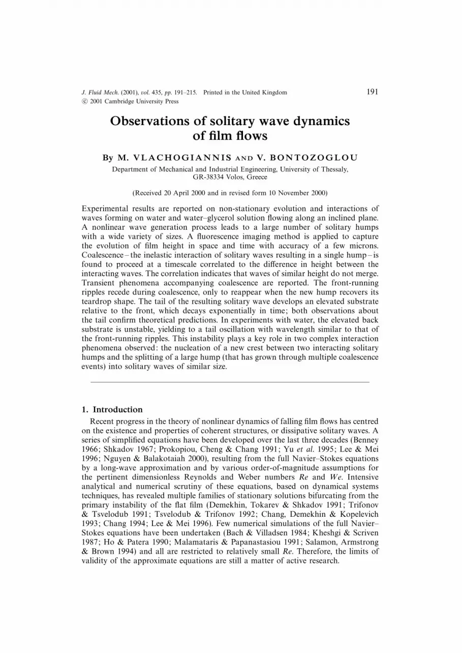
The experimental apparatus is shown schematically in figure 1. An elevated overflowtank is used to maintain a constant liquid head. Flow rate is varied by a manuallyoperated valve, and is determined by measuring the volume of liquid flowing out ofthe channel over a known period of time. All experimental measurements are madeat steady state, i.e. after a constant flow rate has been achieved. The fluid is stored inthe collection tank (see figure 1), from where it is pumped to the overhead tank. Thecollection tank has no stiff connections with other parts of the experimental device,and the pump is submerged into the water to minimize transmission of vibrations.

From the overhead tank, the fluid is directed by three elastic tubes to the distributorhead. A timer-controlled on/off electro-valve is located at a bypass exit below thedistributor head, in order to disturb the film flow by blocking the bypass stream andthus creating an extra flow surge at the channel entrance. The above perturbation sys-tem (timer, electro-valve) can accommodate disturbances with a range of frequenciesfrom 0.1 to 1 Hz. The extent of each disturbance depends on the time duration of theflow surge, which is varied in the range 0.2–2.0 s. An alternative perturbation systemused involves an oscillating stopcock, which blocks the exit of the bypass stream tothe collection tank. The stopcock is driven by a variable-frequency motor spanning afrequency range of 1–10 Hz.

The main channel is made of Plexiglas and has length 800 mm, width 250 mmand height 20 mm. The entire apparatus is mounted on rubber sheet to reduce theinfluence of any vibrations. The channel can operate at an inclination angle ϕ rangingfrom 0◦ to 60◦. However, the range used in the present work is 2◦–7◦. This allows theamplification rate of waves to be adjusted in connection with the imposed disturbance,so that meaningful observations are made in the available channel length.

The liquids used in the experiments are pure water and a 28% by weight so-lution of glycerol in water. Two-dimensional waves are more stable against three-dimensional disturbances in the water–glycerol solution, permitting observations athigher Reynolds numbers or steeper inclination angles. The liquid is changed foreach set of experiments and the viscosity of water–glycerol solutions is determinedindirectly by measuring the refractive index with a refractometer. Physical prop-erties of the water–glycerol solution at 25 ◦C (working temperature, ± 1 ◦C) arekinematic viscosity ν = 2.13× 10−6 m2 s−1, surface tension σ = 70 ± 1 × 10−3 N m−1

and density ρ = 1066.4 kg m−3. The surface tension of pure water is taken asσ = 72± 1× 10−3 N m−1.

https://www.researchgate.net/publication/243825094_Wave_Formation_on_a_Vertical_Falling_Liquid_Film?el=1_x_8&enrichId=rgreq-1a5ee84b-c7c4-4330-9480-cc19bda85e5d&enrichSource=Y292ZXJQYWdlOzIzMTk0ODk3MztBUzoxMDE0NjEyNzQ5MjMwMzRAMTQwMTIwMTY2MjA0OQ==

194

M.

Vla

chogia

nnis

and

V.

Bonto

zoglo

u3

4

5

6

7

2

1

8

9

Figure 1. Sketch of the experimental apparatus: 1. collection tank; 2. current-voltage transformer; 3. overflow tank; 4. distributor head; 5. on/offelectro valve; 6. removable test surface; 7. CCD camera Sony XC-77/77CE; 8. PC with frame grabber board; 9. UV light lamps.


The Kapitza number, Ka = σ/ρ g1/3 ν4/3, which characterizes the liquid that is used,is 3365 for water, and 1102 for the water–glycerol solution. The Reynolds number ofthe flow is defined as Re = q/ν = 〈u〉hN/ν, where q is the volumetric flow rate perunit width, hN is the Nusselt film thickness and 〈u〉 is the average streamwise velocity.The flow is also characterized by the We number, defined as We = σ/ρ〈u〉2 hN . Theuse of two liquids with different viscosities offers some flexibility as noted above.However, the resulting variation in Kapitza number is too small to permit a detailedinvestigation of its effect.

2.2. Fluorescence imaging method

In order to describe the spatial and temporal dynamics for nonlinear waves, it isnecessary to obtain space–time measurements. To achieve this, we use the fluorescenceimaging method described by Liu et al. (1993). In our experiments, we dope the fluidwith a small concentration, about 200–300 p.p.m. of dye (sodium salt of fluorescein;C20H10O5Na2), which fluoresces under ultraviolet light and which has been proved toleave the relevant physical properties of the liquid unaffected. The ultraviolet (UV)source consists of two high-intensity lamps (Philips, TL20/05), which are locatedabove the lateral edges of the test surface at a specific distance from the film plane.The above parameters (dye, concentration of dye, ultraviolet source, distance fromthe film plane) are kept as close to constant as possible, with the calibration takingcare of small variations.

A high-resolution CCD camera (Sony XC-77/77CE) and a monochrome framegrabber board (Data Translation DT3155) are used to acquire and digitize the flowimages up to a maximum speed of 20 frames per second. A combination of twooptical filters (green corrective, yellow subtractive) mounted on the camera assuresthat only light in the fluorescence wavelength range is recorded. Acquired images aredigitized at 576×768 pixels with 8-bit of resolution and each frame corresponds to an85 mm×114 mm window of channel area. To increase the grabbing speed, we store theimages in the random access memory (RAM) by using commercial (HLImage++),as well as in-house software, and then we save them on the hard disk.

The light intensity in the image plane is found to vary linearly with the localfilm thickness. The relation between the fluorescence intensity I(x, y, t) and the filmthickness h(x, y, t) is modelled by the expression

I(x, y, t) = a(x, y) h(x, y, t) + b(x, y). (1)

The two linear coefficients vary with the (x, y) location because of non-uniformityof the UV light field; they also depend on the parameters mentioned above andon the kind of solution used. Thus, the calibration procedure produces independenta and b values for each pixel of the field of view. Calibration is based on theconclusion of linear stability theory – verified experimentally by Liu et al. (1993) –that the critical Reynolds number for growth of the most unstable disturbance isRec = 5

6cotϕ, where ϕ is the inclination angle of the wall. Therefore, in the stable

range of Reynolds numbers and inclination angles, the film thickness is equal to theNusselt film thickness.

This assertion has also been confirmed by independent measurement of the filmthickness by a contact needle and a displacement micrometer. The technique usedinvolves imposition of a small voltage difference between the tip of the metallicneedle and the liquid inside the channel, which is conducting. The needle is graduallylowered towards the surface of the stable film and, as soon as it touches the surface,the electric circuit closes and an alarm is activated. The absolute agreement between

https://www.researchgate.net/publication/231892045_Measurement_of_the_Primary_Instabilities_of_Film_Flows?el=1_x_8&enrichId=rgreq-1a5ee84b-c7c4-4330-9480-cc19bda85e5d&enrichSource=Y292ZXJQYWdlOzIzMTk0ODk3MztBUzoxMDE0NjEyNzQ5MjMwMzRAMTQwMTIwMTY2MjA0OQ==



0.3

0.2

0.1

01 116 231 346 461 576

0

50

100

150

200

250a

b

Number of pixels

Val

ue o

f co

effi

cien

t a

Val

ue o

f co

effi

cien

t b

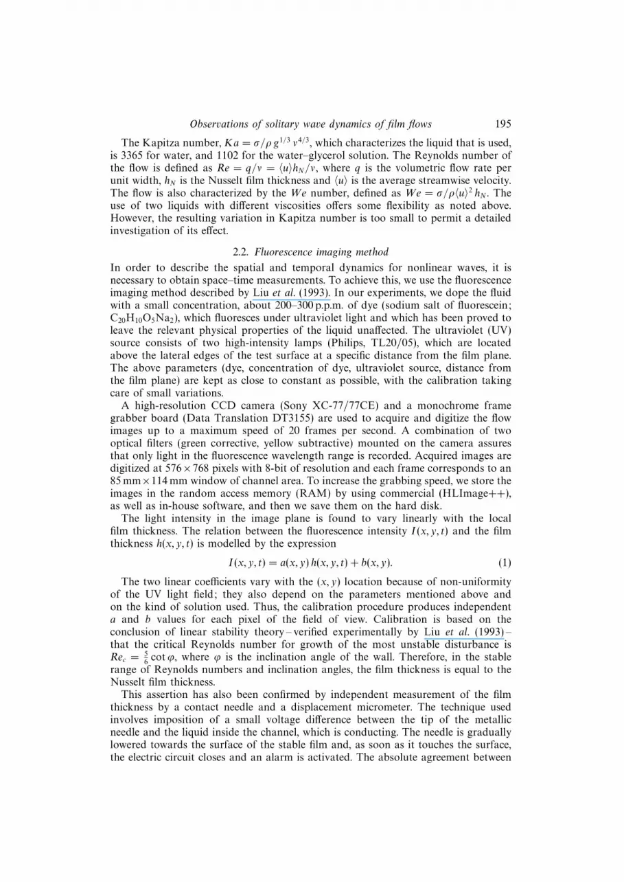
Figure 2. The two coefficients a, b for each pixel along a transverse line. A 28%wt water–glycerolsolution is sued in this experiment.

measurements and predictions based on Nusselt theory, serves as a consistency checkof the channel levelling and of the accuracy of the imposed flow rate and inclinationangle.

Data taken in the above stable range are used to derive the correlation betweenfluorescent light intensity and the known film thickness. The linear relation (1) isalways found to be satisfactory (accurate to within 2–5% for film thickness in therange of 0.2–2.0 mm) and a and b are obtained by a best fit. As for the variation of aand b over the image, an indicative example of the pixel values on a line profile in thetransverse direction is shown in figure 2. A high-frequency error, due to digitizationnoise, appears and is eliminated by applying a convolution filter at the incomingimages. The matrix of a and b values is used for the specific experimental run, andthe calibration is repeated with every new set of experiments because the UV lightintensity gradually fades with time.

2.3. Image analysis

Image processing is accomplished by using the MATLAB software. Each image, whichcorresponds to a snapshot of the field of view at a specific time instant, is convertedinto a two-dimensional matrix (576× 768 elements). By treating images as matrices,we add flexibility in analysing and displaying data. The usual forms of presentationare instantaneous profile scans in the streamwise or the transverse direction and timeseries at one or multiple locations.

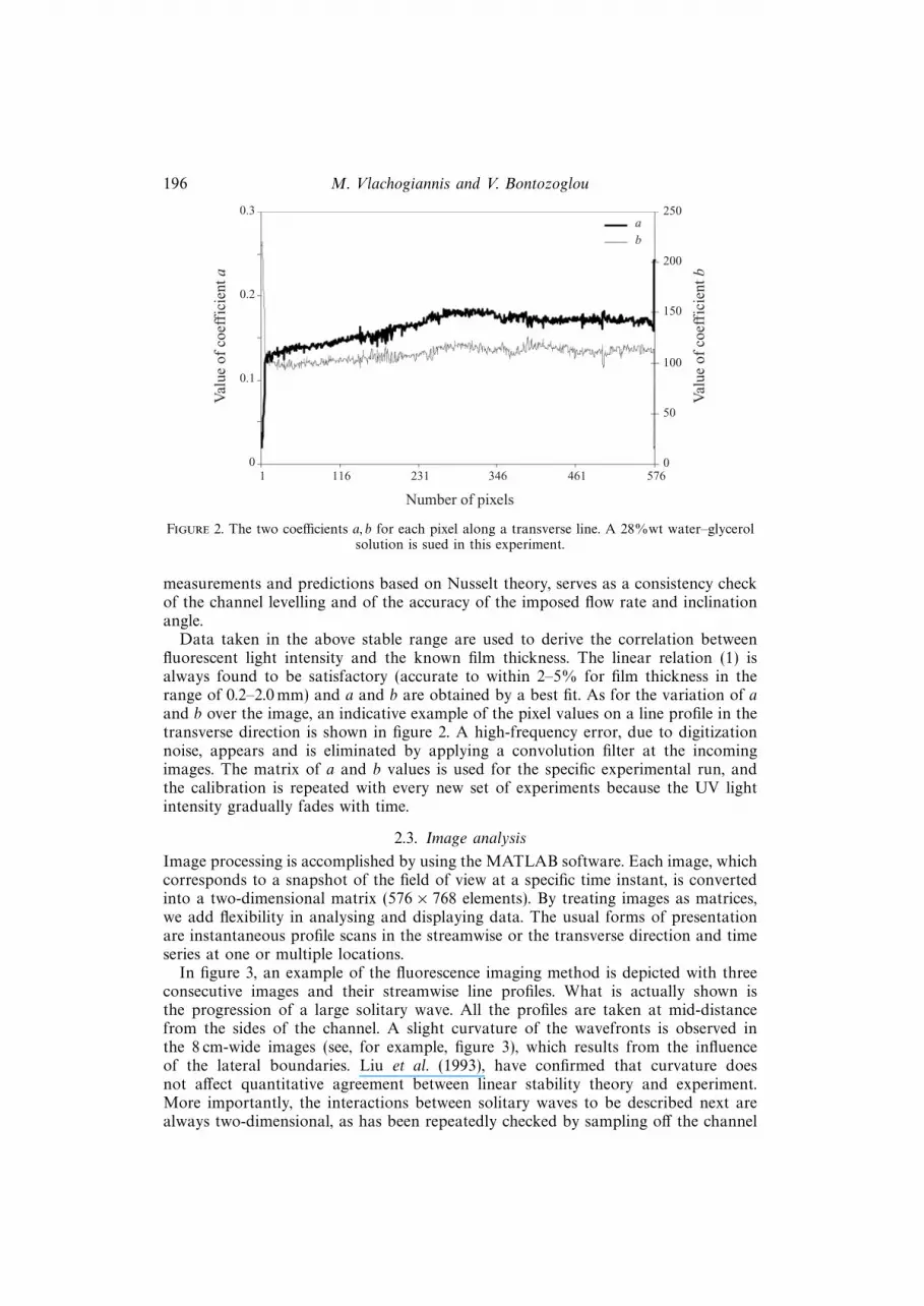
In figure 3, an example of the fluorescence imaging method is depicted with threeconsecutive images and their streamwise line profiles. What is actually shown isthe progression of a large solitary wave. All the profiles are taken at mid-distancefrom the sides of the channel. A slight curvature of the wavefronts is observed inthe 8 cm-wide images (see, for example, figure 3), which results from the influenceof the lateral boundaries. Liu et al. (1993), have confirmed that curvature doesnot affect quantitative agreement between linear stability theory and experiment.More importantly, the interactions between solitary waves to be described next arealways two-dimensional, as has been repeatedly checked by sampling off the channel



Flow direction t = 0.6 s t = 0.7 s

t = 0.8 s

1.2

1.1

1.0

0.9500 520 540 560 580 600 620

Downstream distance (mm)

h/h N

1.2

1.1

1.0

0.9500 520 540 560 580 600 620


1.2

1.1

1.0

0.9500 520 540 560 580 600 620


h/h N

Figure 3. An example of consecutive fluorescence images and the corresponding line profiles h(x)for water film at ϕ = 5◦, Re = 27 and Ka = 3365.


Downstream distance (cm)

1.2

1.1

1.0

0.9

52 53 54 55 56 57 58 59 60

hhN

2 cm left side

2 cm right side

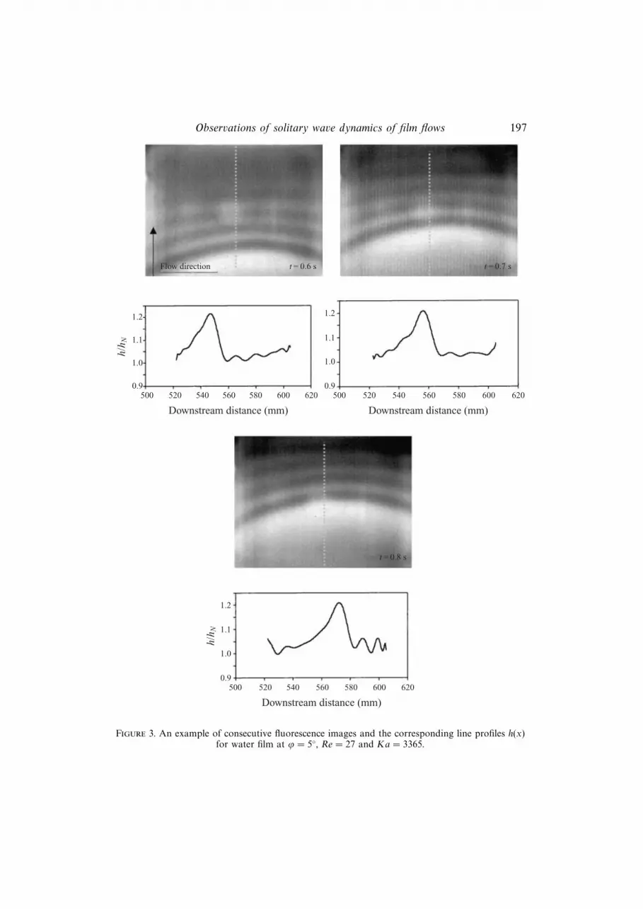
Figure 4. Two streamwise line profiles displaced symmetrically a distance 2 cm from the centreline.The inclination angle is ϕ = 4◦ and aqueous solution of glycerol (28%wt) is used.

centreline. An example of such a check is shown in figure 4, where streamwise lineprofiles at two locations, symmetric about the centreline, are plotted. The distancebetween the two line profiles is 4 cm – or 2 cm from the centreline – and quantitativeagreement is evident indicating that the waves are two-dimensional.

3. Outline of experimental realization3.1. Generation of series of solitary waves

Before embarking into detailed documentation of specific events, it is necessary todescribe in gross terms the experiment performed. A base film flow is established at aflow rate, q0, above the limit of linear stability. The flow is periodically disturbed byblocking a bypass stream below the distributor head, and thus creating an extra flowsurge, ∆q = q1−q0, at the channel entrance. The frequency of this disturbance is verylow (typically f = 0.1667 Hz, or period T = 6 s), so that each surge evolves fairlyindependently, separated from the preceding and the following ones by stretches ofsubstrate. The duration of a flow surge, t1, is varied in the range 0.2–1.0 s.

The flow is characterized by Re defined in terms of the mean flow rate as

Re =〈q〉ν

=(t0 q0 + t1 q1)/(t0 + t1)

ν, (2)

where t0 = T − t1 is the duration of the base flow per period. Each surge results inan elevation of the liquid level at the entrance roughly in the order of 5% of theNusselt film thickness corresponding to the base flow rate, q0. Thus, an elongated butnot very high hump is formed, that readily disintegrates into a series of waves, whichevolve into solitary humps.

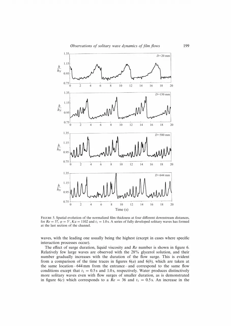
The downstream evolution of the inlet disturbance, in a representative run withglycerol solution at Re = 37, inclination angle ϕ = 5◦ and surge duration t1 = 1.0 s,is shown in figure 5. What are actually depicted are film height time series at fourpoints, located at distances 20, 150, 580 and 644 mm from the entrance to the channel.The general trend is that the inlet surge disintegrates into a series of large-amplitude


Time (s)

hhN

1.35

1.15

0.95

0.750 2 4 6 8 10 12 14 16 18 20

hhN

1.35

1.15

0.95

0.750 2 4 6 8 10 12 14 16 18 20

hhN

1.35

1.15

0.95

0.750 2 4 6 8 10 12 14 16 18 20

hhN

1.35

1.15

0.95

0.750 2 4 6 8 10 12 14 16 18 20

D=644 mm

D=580 mm

D=150 mm

D=20 mm

Figure 5. Spatial evolution of the normalized film thickness at four different downstream distances,for Re = 37, ϕ = 5◦, Ka = 1102 and t1 = 1.0 s. A series of fully developed solitary waves has formedat the last section of the channel.

waves, with the leading one usually being the highest (except in cases where specificinteraction processes occur).

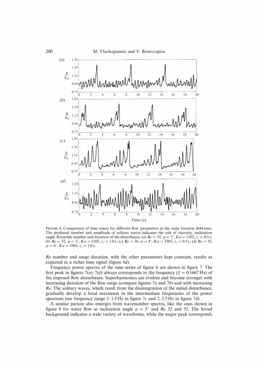
The effect of surge duration, liquid viscosity and Re number is shown in figure 6.Relatively few large waves are observed with the 28% glycerol solution, and theirnumber gradually increases with the duration of the flow surge. This is evidentfrom a comparison of the time traces in figures 6(a) and 6(b), which are taken atthe same location – 644 mm from the entrance – and correspond to the same flowconditions except that t1 = 0.5 s and 1.0 s, respectively. Water produces distinctivelymore solitary waves even with flow surges of smaller duration, as is demonstratedin figure 6(c) which corresponds to a Re = 36 and t1 = 0.5 s. An increase in the


Time (s)

hhN

1.35

1.15

0.95

0.750 2 4 6 8 10 12 14 16 18 20

hhN

1.35

1.15

0.95

0.750 2 4 6 8 10 12 14 16 18 20

hhN

1.35

1.15

0.95

0.750 2 4 6 8 10 12 14 16 18 20

hhN

1.35

1.15

0.95

0.750 2 4 6 8 10 12 14 16 18 20

1.55

1.55

1.55

(d)

(c)

(b)

(a)

Figure 6. Comparison of time traces for different flow parameters at the same location (644 mm).The produced number and amplitude of solitary waves indicates the role of viscosity, inclinationangle, Reynolds number and duration of the disturbance. (a) Re = 52, ϕ = 3◦, Ka = 1102, t1 = 0.5 s;(b) Re = 52, ϕ = 3◦, Ka = 1102, t1 = 1.0 s; (c) Re = 36, ϕ = 4◦, Ka = 3365, t1 = 0.5 s; (d) Re = 52,ϕ = 4◦, Ka = 3365, t1 = 1.0 s.

Re number and surge duration, with the other parameters kept constant, results asexpected in a richer time signal (figure 6d).

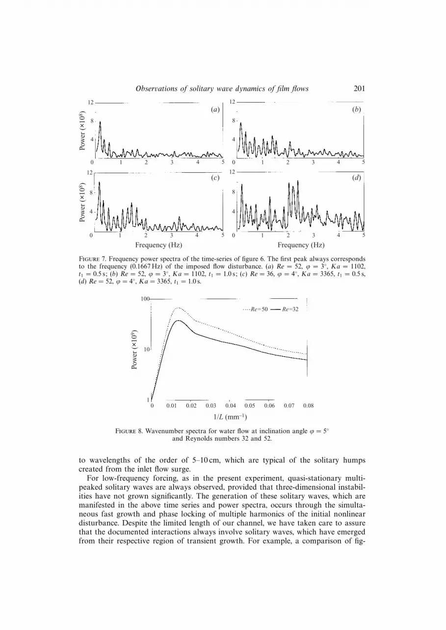
Frequency power spectra of the time series of figure 6 are shown in figure 7. Thefirst peak in figures 7(a)–7(d) always corresponds to the frequency (f = 0.1667 Hz) ofthe imposed flow disturbance. Superharmonics are evident and become stronger withincreasing duration of the flow surge (compare figures 7a and 7b) and with increasingRe. The solitary waves, which result from the disintegration of the initial disturbance,gradually develop a local maximum in the intermediate frequencies of the powerspectrum (see frequency range 1–1.5 Hz in figure 7c and 2–2.5 Hz in figure 7d).

A similar picture also emerges from wavenumber spectra, like the ones shown infigure 8 for water flow at inclination angle ϕ = 5◦ and Re 32 and 52. The broadbackground indicates a wide variety of waveforms, while the major peak corresponds


12

8

4

0 1 2 3 4 5

12

8

4

0 1 2 3 4 5

12

8

4

0 1 2 3 4 5

Frequency (Hz)

12

8

4

0 1 2 3 4 5

Frequency (Hz)

(a) (b)

(c) (d)

Pow

er (

×108 )

Pow

er (

×108 )

Figure 7. Frequency power spectra of the time-series of figure 6. The first peak always correspondsto the frequency (0.1667 Hz) of the imposed flow disturbance. (a) Re = 52, ϕ = 3◦, Ka = 1102,t1 = 0.5 s; (b) Re = 52, ϕ = 3◦, Ka = 1102, t1 = 1.0 s; (c) Re = 36, ϕ = 4◦, Ka = 3365, t1 = 0.5 s,(d) Re = 52, ϕ = 4◦, Ka = 3365, t1 = 1.0 s.

100

10

10 0.01 0.02 0.03 0.04 0.05 0.06 0.07 0.08

Re=32Re=50

1/L (mm–1)

Pow

er (

×109 )

Figure 8. Wavenumber spectra for water flow at inclination angle ϕ = 5◦and Reynolds numbers 32 and 52.

to wavelengths of the order of 5–10 cm, which are typical of the solitary humpscreated from the inlet flow surge.

For low-frequency forcing, as in the present experiment, quasi-stationary multi-peaked solitary waves are always observed, provided that three-dimensional instabil-ities have not grown significantly. The generation of these solitary waves, which aremanifested in the above time series and power spectra, occurs through the simulta-neous fast growth and phase locking of multiple harmonics of the initial nonlineardisturbance. Despite the limited length of our channel, we have taken care to assurethat the documented interactions always involve solitary waves, which have emergedfrom their respective region of transient growth. For example, a comparison of fig-


4

3

2

1

040 50 60 70 80 90 100 110

u =7°U=5°U=3°

Reynolds number

r.m.s.distr.m.s.undist

Figure 9. The ratio of r.m.s. values of appropriate sections of the time traces, for disturbed andundisturbed flow, as a function of the Reynolds number.

ures 5(c) and 5(d) indicates that the height of the solitary humps remains on theaverage constant in the last part of the channel. However, a true asymptotic state isactually never reached in the present experiments, because of the repeated wave–waveinteractions (see, for example, the second wave in figure 5d). With a much longerchannel, one would expect a spanwise instability to develop and render the small-scale structure three-dimensional, though the large-scale features have been reportedto remain two-dimensional in an average sense (Liu & Gollub 1994).

Waves also grow from the rippled substrate between the major groups of solitarywaves. These minor waves are lower than those developing directly from the flowsurge, and in most cases the two can be easily distinguished. The role of subharmonicand sideband instabilities – as described by Liu & Gollub (1994) for an unforcedfilm – is essential in the development of these new waves. However, their growth ratein the present experiment is significantly higher than that of their natural counterpartsin a purely noise-sustained film.

The above assertion is demonstrated by performing experiments at the same Reand inclination angle but without flow surges. The results in figure 9 show theroot-mean-square (r.m.s.) values of appropriate sections of the time traces, both withand without the entrance disturbance (excluding, in the case of forcing, the sectionswith major solitary waves), plotted as a function of Re. The enhanced evolution ofsubstrate instabilities into minor solitary waves in the forced experiments is attributedto the high amplitude and the broad frequency spectrum of the inlet disturbance,which continuously radiates energy. The simultaneous existence of the major andminor waves permits the investigation of interactions between solitary humps of agreat variety of sizes.

3.2. Time-periodic nature of observed interactions

The interactions between large solitary waves – formed by the disintegration of theentrance flow surge – and between these and the smaller ones developing on thesubstrate provide the basis for all the observations to be discussed in the rest ofthe paper. The interactions – as manifested by the instantaneous snapshots of theview window – seem at first sight of confusing complexity. However, up to moderatevalues of Re (of the order of 50), they are repeated with impressive faithfulnesssurge after surge. Upon systematic inspection, the high irregularity of the free-surface

https://www.researchgate.net/publication/252978115_Solitary_Wave_Dynamics_of_Film_Flows?el=1_x_8&enrichId=rgreq-1a5ee84b-c7c4-4330-9480-cc19bda85e5d&enrichSource=Y292ZXJQYWdlOzIzMTk0ODk3MztBUzoxMDE0NjEyNzQ5MjMwMzRAMTQwMTIwMTY2MjA0OQ==


1.55

1.35

1.15

0.95

0 2 4 6 8 10 12 14 16 18 20

Time (s)

hmax

hN

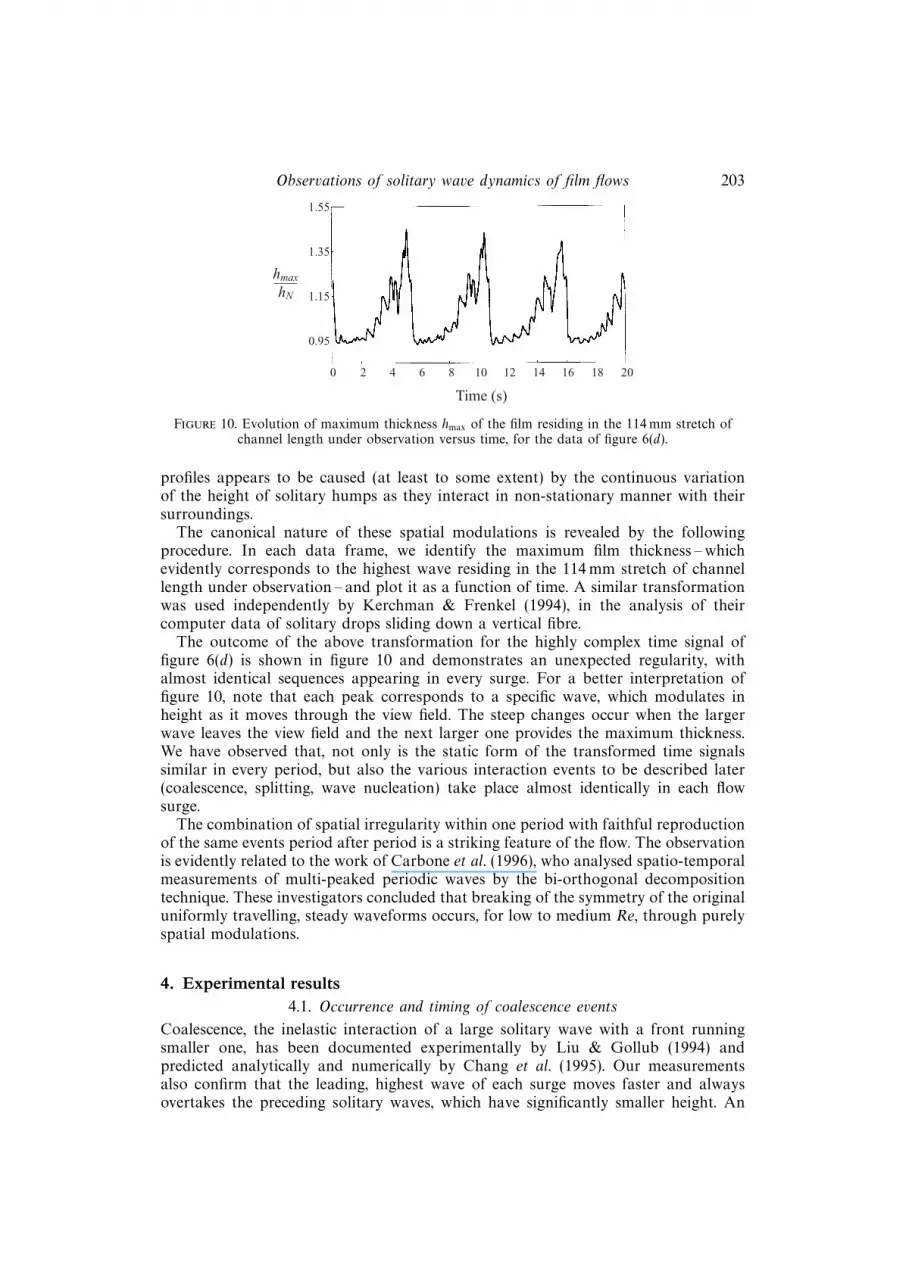
Figure 10. Evolution of maximum thickness hmax of the film residing in the 114 mm stretch ofchannel length under observation versus time, for the data of figure 6(d).

profiles appears to be caused (at least to some extent) by the continuous variationof the height of solitary humps as they interact in non-stationary manner with theirsurroundings.

The canonical nature of these spatial modulations is revealed by the followingprocedure. In each data frame, we identify the maximum film thickness – whichevidently corresponds to the highest wave residing in the 114 mm stretch of channellength under observation – and plot it as a function of time. A similar transformationwas used independently by Kerchman & Frenkel (1994), in the analysis of theircomputer data of solitary drops sliding down a vertical fibre.

The outcome of the above transformation for the highly complex time signal offigure 6(d) is shown in figure 10 and demonstrates an unexpected regularity, withalmost identical sequences appearing in every surge. For a better interpretation offigure 10, note that each peak corresponds to a specific wave, which modulates inheight as it moves through the view field. The steep changes occur when the largerwave leaves the view field and the next larger one provides the maximum thickness.We have observed that, not only is the static form of the transformed time signalssimilar in every period, but also the various interaction events to be described later(coalescence, splitting, wave nucleation) take place almost identically in each flowsurge.

The combination of spatial irregularity within one period with faithful reproductionof the same events period after period is a striking feature of the flow. The observationis evidently related to the work of Carbone et al. (1996), who analysed spatio-temporalmeasurements of multi-peaked periodic waves by the bi-orthogonal decompositiontechnique. These investigators concluded that breaking of the symmetry of the originaluniformly travelling, steady waveforms occurs, for low to medium Re, through purelyspatial modulations.

4. Experimental results4.1. Occurrence and timing of coalescence events

Coalescence, the inelastic interaction of a large solitary wave with a front runningsmaller one, has been documented experimentally by Liu & Gollub (1994) andpredicted analytically and numerically by Chang et al. (1995). Our measurementsalso confirm that the leading, highest wave of each surge moves faster and alwaysovertakes the preceding solitary waves, which have significantly smaller height. An

https://www.researchgate.net/publication/223590636_Space-time_description_of_the_splitting_and_coalescence_of_wave_fronts_in_film_flows?el=1_x_8&enrichId=rgreq-1a5ee84b-c7c4-4330-9480-cc19bda85e5d&enrichSource=Y292ZXJQYWdlOzIzMTk0ODk3MztBUzoxMDE0NjEyNzQ5MjMwMzRAMTQwMTIwMTY2MjA0OQ==



hhN

0.25 hN

520 540 560 580 600T

ime

(Dt=

0.1

s)

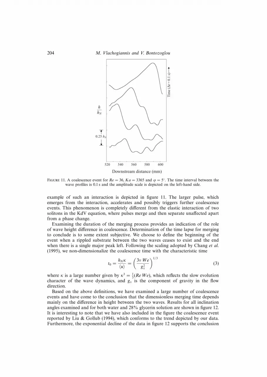
Figure 11. A coalescence event for Re = 36, Ka = 3365 and ϕ = 5◦. The time interval between thewave profiles is 0.1 s and the amplitude scale is depicted on the left-hand side.

example of such an interaction is depicted in figure 11. The larger pulse, whichemerges from the interaction, accelerates and possibly triggers further coalescenceevents. This phenomenon is completely different from the elastic interaction of twosolitons in the KdV equation, where pulses merge and then separate unaffected apartfrom a phase change.

Examining the duration of the merging process provides an indication of the roleof wave height difference in coalescence. Determination of the time lapse for mergingto conclude is to some extent subjective. We choose to define the beginning of theevent when a rippled substrate between the two waves ceases to exist and the endwhen there is a single major peak left. Following the scaling adopted by Chang et al.(1995), we non-dimensionalize the coalescence time with the characteristic time

t0 =hNκ

〈u〉 =

(3ν We

g2x

)1/3

(3)

where κ is a large number given by κ3 = 13(ReWe), which reflects the slow evolution

character of the wave dynamics, and gx is the component of gravity in the flowdirection.

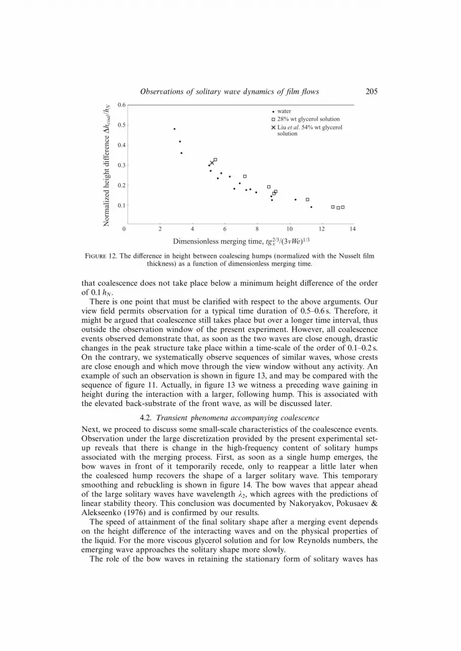
Based on the above definitions, we have examined a large number of coalescenceevents and have come to the conclusion that the dimensionless merging time dependsmainly on the difference in height between the two waves. Results for all inclinationangles examined and for both water and 28% glycerin solution are shown in figure 12.It is interesting to note that we have also included in the figure the coalescence eventreported by Liu & Gollub (1994), which conforms to the trend depicted by our data.Furthermore, the exponential decline of the data in figure 12 supports the conclusion


0.6

0.5

0.4

0.3

0.2

0.1

0 2 4 6 8 10 12 14

water28% wt glycerol solutionLiu et al. 54% wt glycerolsolution

Nor

mal

ized

hei

ght d

iffe

renc

e D

h coa

l/hN

Dimensionless merging time, tgx2/3/(3mWe)1/3

Figure 12. The difference in height between coalescing humps (normalized with the Nusselt filmthickness) as a function of dimensionless merging time.

that coalescence does not take place below a minimum height difference of the orderof 0.1 hN .

There is one point that must be clarified with respect to the above arguments. Ourview field permits observation for a typical time duration of 0.5–0.6 s. Therefore, itmight be argued that coalescence still takes place but over a longer time interval, thusoutside the observation window of the present experiment. However, all coalescenceevents observed demonstrate that, as soon as the two waves are close enough, drasticchanges in the peak structure take place within a time-scale of the order of 0.1–0.2 s.On the contrary, we systematically observe sequences of similar waves, whose crestsare close enough and which move through the view window without any activity. Anexample of such an observation is shown in figure 13, and may be compared with thesequence of figure 11. Actually, in figure 13 we witness a preceding wave gaining inheight during the interaction with a larger, following hump. This is associated withthe elevated back-substrate of the front wave, as will be discussed later.

4.2. Transient phenomena accompanying coalescence

Next, we proceed to discuss some small-scale characteristics of the coalescence events.Observation under the large discretization provided by the present experimental set-up reveals that there is change in the high-frequency content of solitary humpsassociated with the merging process. First, as soon as a single hump emerges, thebow waves in front of it temporarily recede, only to reappear a little later whenthe coalesced hump recovers the shape of a larger solitary wave. This temporarysmoothing and rebuckling is shown in figure 14. The bow waves that appear aheadof the large solitary waves have wavelength λ2, which agrees with the predictions oflinear stability theory. This conclusion was documented by Nakoryakov, Pokusaev &Alekseenko (1976) and is confirmed by our results.

The speed of attainment of the final solitary shape after a merging event dependson the height difference of the interacting waves and on the physical properties ofthe liquid. For the more viscous glycerol solution and for low Reynolds numbers, theemerging wave approaches the solitary shape more slowly.

The role of the bow waves in retaining the stationary form of solitary waves has



hhN

0.2 hN

520 540 560 580 600

Tim

e (D

t=0.

1 s)

Figure 13. The interaction of a preceding wave with a larger following hump, which does not leadto coalescence (Re = 27, ϕ = 5◦, Ka = 3365).


hhN

0.1 hN

520 540 560 580 600

Tim

e (D

t=0.

1 s)

k2

Figure 14. The temporary smoothing and rebuckling after a coalescence event(Re = 27, Ka = 3365, ϕ = 5◦).



520 540 560 580 600

hhN

1.25

1.15

1.05

0.95

0.85

0.75

0.65

t =13.1 st =13.2 s

hb

hf

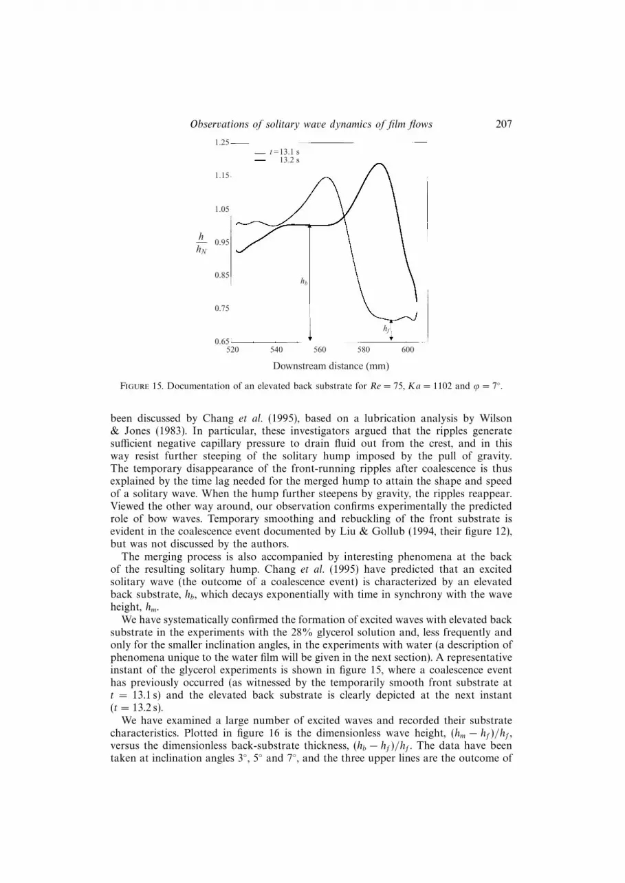
Figure 15. Documentation of an elevated back substrate for Re = 75, Ka = 1102 and ϕ = 7◦.

been discussed by Chang et al. (1995), based on a lubrication analysis by Wilson& Jones (1983). In particular, these investigators argued that the ripples generatesufficient negative capillary pressure to drain fluid out from the crest, and in thisway resist further steeping of the solitary hump imposed by the pull of gravity.The temporary disappearance of the front-running ripples after coalescence is thusexplained by the time lag needed for the merged hump to attain the shape and speedof a solitary wave. When the hump further steepens by gravity, the ripples reappear.Viewed the other way around, our observation confirms experimentally the predictedrole of bow waves. Temporary smoothing and rebuckling of the front substrate isevident in the coalescence event documented by Liu & Gollub (1994, their figure 12),but was not discussed by the authors.

The merging process is also accompanied by interesting phenomena at the backof the resulting solitary hump. Chang et al. (1995) have predicted that an excitedsolitary wave (the outcome of a coalescence event) is characterized by an elevatedback substrate, hb, which decays exponentially with time in synchrony with the waveheight, hm.

We have systematically confirmed the formation of excited waves with elevated backsubstrate in the experiments with the 28% glycerol solution and, less frequently andonly for the smaller inclination angles, in the experiments with water (a description ofphenomena unique to the water film will be given in the next section). A representativeinstant of the glycerol experiments is shown in figure 15, where a coalescence eventhas previously occurred (as witnessed by the temporarily smooth front substrate att = 13.1 s) and the elevated back substrate is clearly depicted at the next instant(t = 13.2 s).

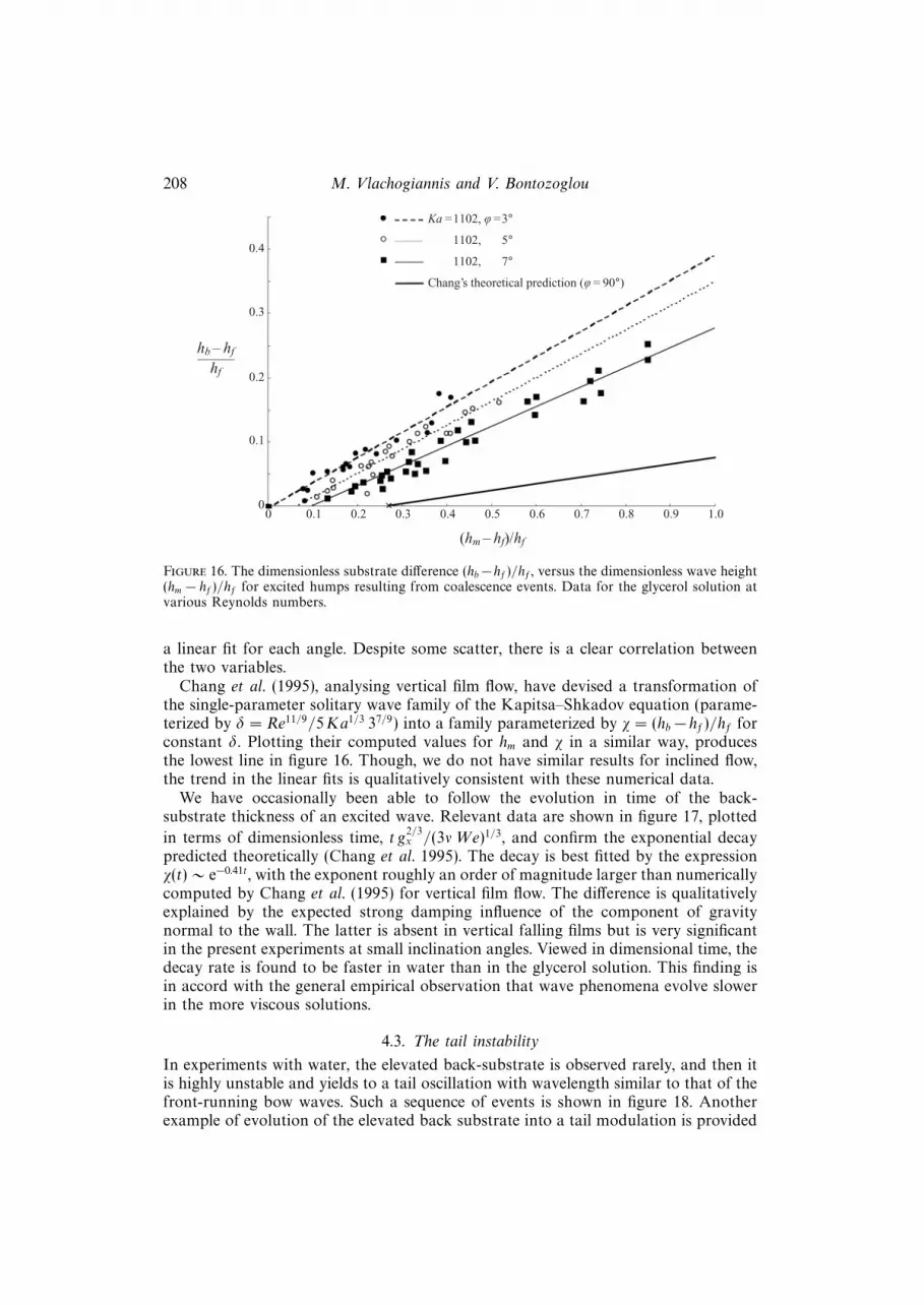
We have examined a large number of excited waves and recorded their substratecharacteristics. Plotted in figure 16 is the dimensionless wave height, (hm − hf)/hf ,versus the dimensionless back-substrate thickness, (hb − hf)/hf . The data have beentaken at inclination angles 3◦, 5◦ and 7◦, and the three upper lines are the outcome of


0.4

0.3

0.2

0.1

00 0.1 0.2 0.3 0.4 0.5 0.6 0.7 0.8 0.9 1.0

Ka =1102, u =3°

Ka =1102, u =5°

Ka =1102, u =7°

Chang’s theoretical prediction (u = 90°)

hb – hf

hf

(hm – hf)/hf

Figure 16. The dimensionless substrate difference (hb−hf)/hf , versus the dimensionless wave height(hm − hf)/hf for excited humps resulting from coalescence events. Data for the glycerol solution atvarious Reynolds numbers.

a linear fit for each angle. Despite some scatter, there is a clear correlation betweenthe two variables.

Chang et al. (1995), analysing vertical film flow, have devised a transformation ofthe single-parameter solitary wave family of the Kapitsa–Shkadov equation (parame-terized by δ = Re11/9/5Ka1/3 37/9) into a family parameterized by χ = (hb−hf)/hf forconstant δ. Plotting their computed values for hm and χ in a similar way, producesthe lowest line in figure 16. Though, we do not have similar results for inclined flow,the trend in the linear fits is qualitatively consistent with these numerical data.

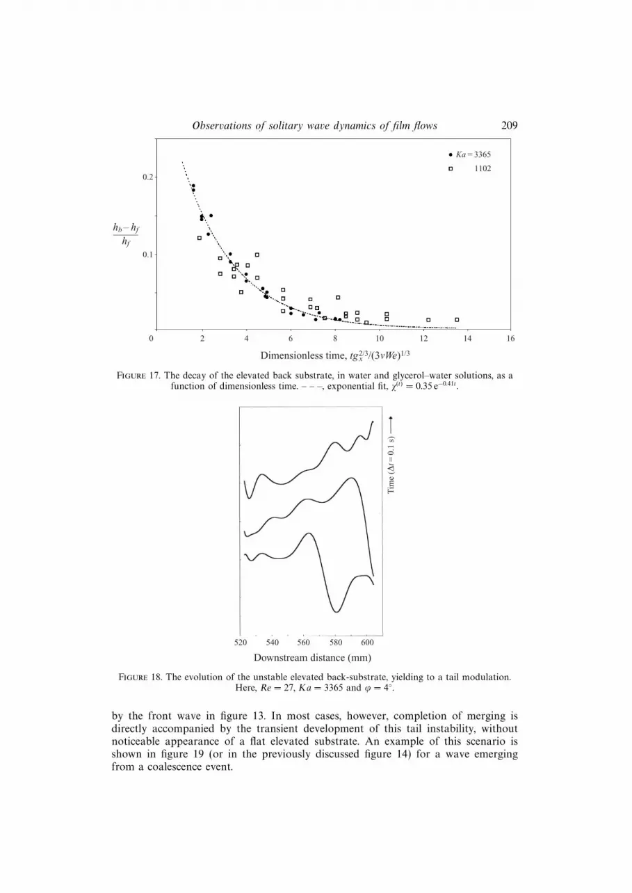
We have occasionally been able to follow the evolution in time of the back-substrate thickness of an excited wave. Relevant data are shown in figure 17, plotted

in terms of dimensionless time, t g2/3x /(3ν We)1/3, and confirm the exponential decay

predicted theoretically (Chang et al. 1995). The decay is best fitted by the expressionχ(t) ∼ e−0.41t, with the exponent roughly an order of magnitude larger than numericallycomputed by Chang et al. (1995) for vertical film flow. The difference is qualitativelyexplained by the expected strong damping influence of the component of gravitynormal to the wall. The latter is absent in vertical falling films but is very significantin the present experiments at small inclination angles. Viewed in dimensional time, thedecay rate is found to be faster in water than in the glycerol solution. This finding isin accord with the general empirical observation that wave phenomena evolve slowerin the more viscous solutions.

4.3. The tail instability

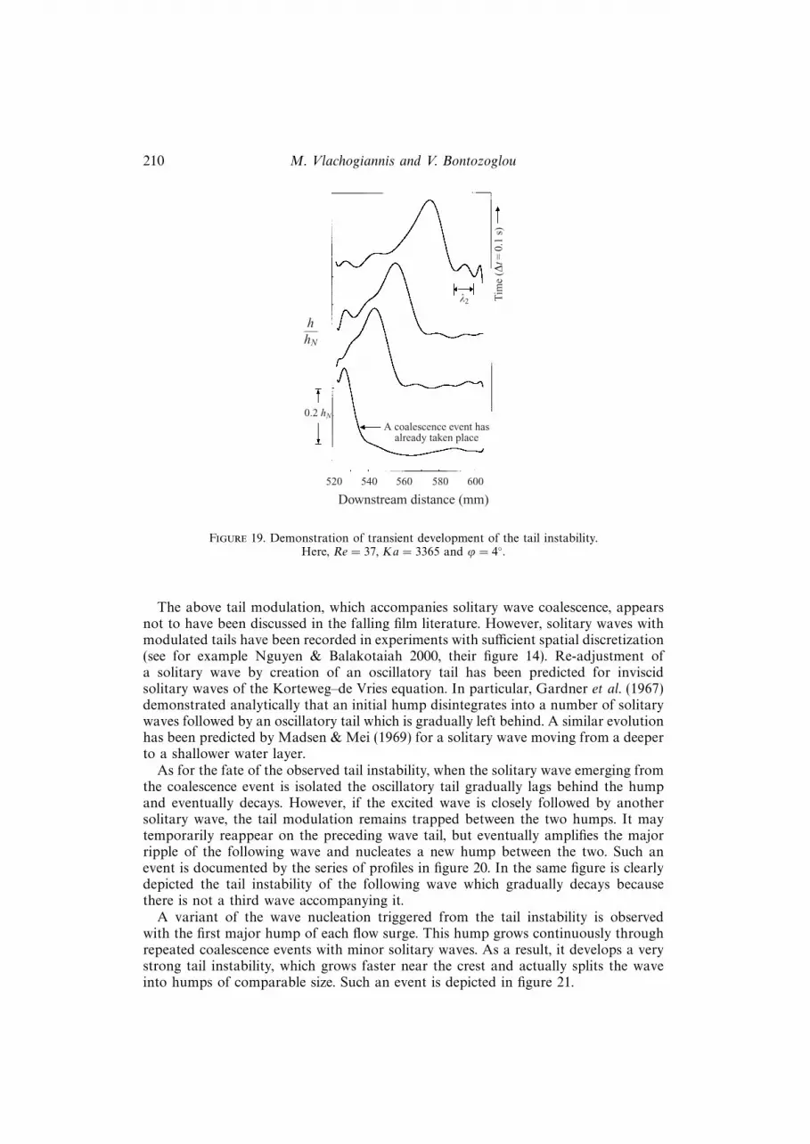
In experiments with water, the elevated back-substrate is observed rarely, and then itis highly unstable and yields to a tail oscillation with wavelength similar to that of thefront-running bow waves. Such a sequence of events is shown in figure 18. Anotherexample of evolution of the elevated back substrate into a tail modulation is provided


0.2

0.1

0 2 4 6 8 10 12 14

Ka = 3365

Dimensionless time, tgx2/3/(3mWe)1/3

hb – hf

hf

16

Ka =1102

Figure 17. The decay of the elevated back substrate, in water and glycerol–water solutions, as afunction of dimensionless time. – – –, exponential fit, χ(t) = 0.35 e−0.41t.


520 540 560 580 600

Tim

e (D

t=0.

1 s)

Figure 18. The evolution of the unstable elevated back-substrate, yielding to a tail modulation.Here, Re = 27, Ka = 3365 and ϕ = 4◦.

by the front wave in figure 13. In most cases, however, completion of merging isdirectly accompanied by the transient development of this tail instability, withoutnoticeable appearance of a flat elevated substrate. An example of this scenario isshown in figure 19 (or in the previously discussed figure 14) for a wave emergingfrom a coalescence event.



hhN

0.2 hN

520 540 560 580 600

Tim

e (D

t=0.

1 s)

k2

A coalescence event hasalready taken place

Figure 19. Demonstration of transient development of the tail instability.Here, Re = 37, Ka = 3365 and ϕ = 4◦.

The above tail modulation, which accompanies solitary wave coalescence, appearsnot to have been discussed in the falling film literature. However, solitary waves withmodulated tails have been recorded in experiments with sufficient spatial discretization(see for example Nguyen & Balakotaiah 2000, their figure 14). Re-adjustment ofa solitary wave by creation of an oscillatory tail has been predicted for inviscidsolitary waves of the Korteweg–de Vries equation. In particular, Gardner et al. (1967)demonstrated analytically that an initial hump disintegrates into a number of solitarywaves followed by an oscillatory tail which is gradually left behind. A similar evolutionhas been predicted by Madsen & Mei (1969) for a solitary wave moving from a deeperto a shallower water layer.

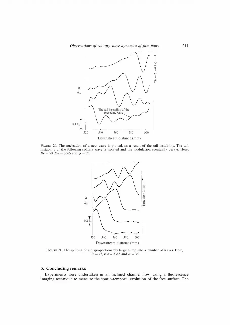
As for the fate of the observed tail instability, when the solitary wave emerging fromthe coalescence event is isolated the oscillatory tail gradually lags behind the humpand eventually decays. However, if the excited wave is closely followed by anothersolitary wave, the tail modulation remains trapped between the two humps. It maytemporarily reappear on the preceding wave tail, but eventually amplifies the majorripple of the following wave and nucleates a new hump between the two. Such anevent is documented by the series of profiles in figure 20. In the same figure is clearlydepicted the tail instability of the following wave which gradually decays becausethere is not a third wave accompanying it.

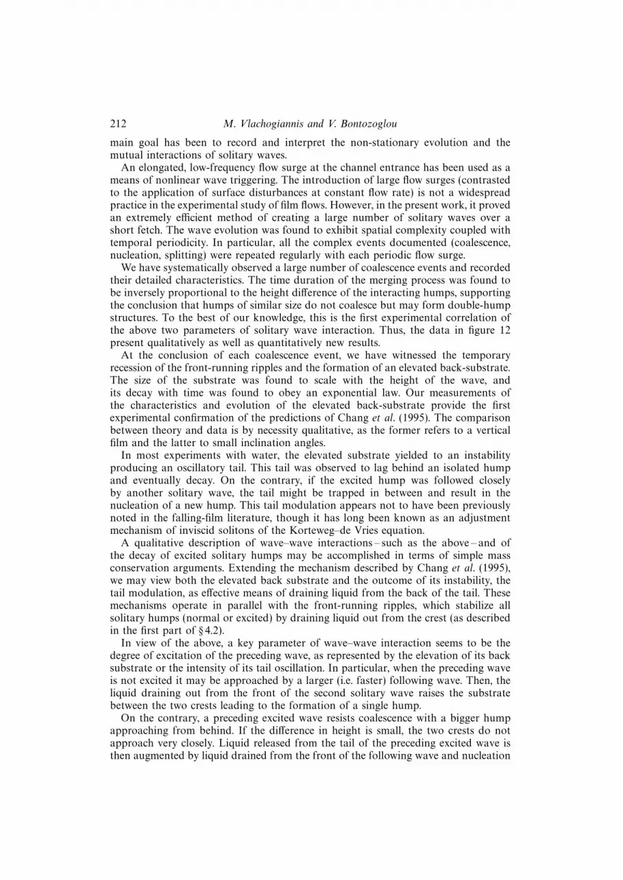
A variant of the wave nucleation triggered from the tail instability is observedwith the first major hump of each flow surge. This hump grows continuously throughrepeated coalescence events with minor solitary waves. As a result, it develops a verystrong tail instability, which grows faster near the crest and actually splits the waveinto humps of comparable size. Such an event is depicted in figure 21.



hhN

0.1 hN

520 540 560 580 600

Tim

e (D

t=0.

1 s)

The tail instability of thepreceding wave

Figure 20. The nucleation of a new wave is plotted, as a result of the tail instability. The tailinstability of the following solitary wave is isolated and the modulation eventually decays. Here,Re = 50, Ka = 3365 and ϕ = 3◦.


hhN

0.2 hN

520 540 560 580 600

Tim

e (D

t=0.

1 s)

Figure 21. The splitting of a disproportionately large hump into a number of waves. Here,Re = 75, Ka = 3365 and ϕ = 3◦.

5. Concluding remarksExperiments were undertaken in an inclined channel flow, using a fluorescence

imaging technique to measure the spatio-temporal evolution of the free surface. The


main goal has been to record and interpret the non-stationary evolution and themutual interactions of solitary waves.

An elongated, low-frequency flow surge at the channel entrance has been used as ameans of nonlinear wave triggering. The introduction of large flow surges (contrastedto the application of surface disturbances at constant flow rate) is not a widespreadpractice in the experimental study of film flows. However, in the present work, it provedan extremely efficient method of creating a large number of solitary waves over ashort fetch. The wave evolution was found to exhibit spatial complexity coupled withtemporal periodicity. In particular, all the complex events documented (coalescence,nucleation, splitting) were repeated regularly with each periodic flow surge.

We have systematically observed a large number of coalescence events and recordedtheir detailed characteristics. The time duration of the merging process was found tobe inversely proportional to the height difference of the interacting humps, supportingthe conclusion that humps of similar size do not coalesce but may form double-humpstructures. To the best of our knowledge, this is the first experimental correlation ofthe above two parameters of solitary wave interaction. Thus, the data in figure 12present qualitatively as well as quantitatively new results.

At the conclusion of each coalescence event, we have witnessed the temporaryrecession of the front-running ripples and the formation of an elevated back-substrate.The size of the substrate was found to scale with the height of the wave, andits decay with time was found to obey an exponential law. Our measurements ofthe characteristics and evolution of the elevated back-substrate provide the firstexperimental confirmation of the predictions of Chang et al. (1995). The comparisonbetween theory and data is by necessity qualitative, as the former refers to a verticalfilm and the latter to small inclination angles.

In most experiments with water, the elevated substrate yielded to an instabilityproducing an oscillatory tail. This tail was observed to lag behind an isolated humpand eventually decay. On the contrary, if the excited hump was followed closelyby another solitary wave, the tail might be trapped in between and result in thenucleation of a new hump. This tail modulation appears not to have been previouslynoted in the falling-film literature, though it has long been known as an adjustmentmechanism of inviscid solitons of the Korteweg–de Vries equation.

A qualitative description of wave–wave interactions – such as the above – and ofthe decay of excited solitary humps may be accomplished in terms of simple massconservation arguments. Extending the mechanism described by Chang et al. (1995),we may view both the elevated back substrate and the outcome of its instability, thetail modulation, as effective means of draining liquid from the back of the tail. Thesemechanisms operate in parallel with the front-running ripples, which stabilize allsolitary humps (normal or excited) by draining liquid out from the crest (as describedin the first part of § 4.2).

In view of the above, a key parameter of wave–wave interaction seems to be thedegree of excitation of the preceding wave, as represented by the elevation of its backsubstrate or the intensity of its tail oscillation. In particular, when the preceding waveis not excited it may be approached by a larger (i.e. faster) following wave. Then, theliquid draining out from the front of the second solitary wave raises the substratebetween the two crests leading to the formation of a single hump.

On the contrary, a preceding excited wave resists coalescence with a bigger humpapproaching from behind. If the difference in height is small, the two crests do notapproach very closely. Liquid released from the tail of the preceding excited wave isthen augmented by liquid drained from the front of the following wave and nucleation



hhN

0.2 hN

520 540 560 580 600

Tim

e (D

t=0.

1 s)

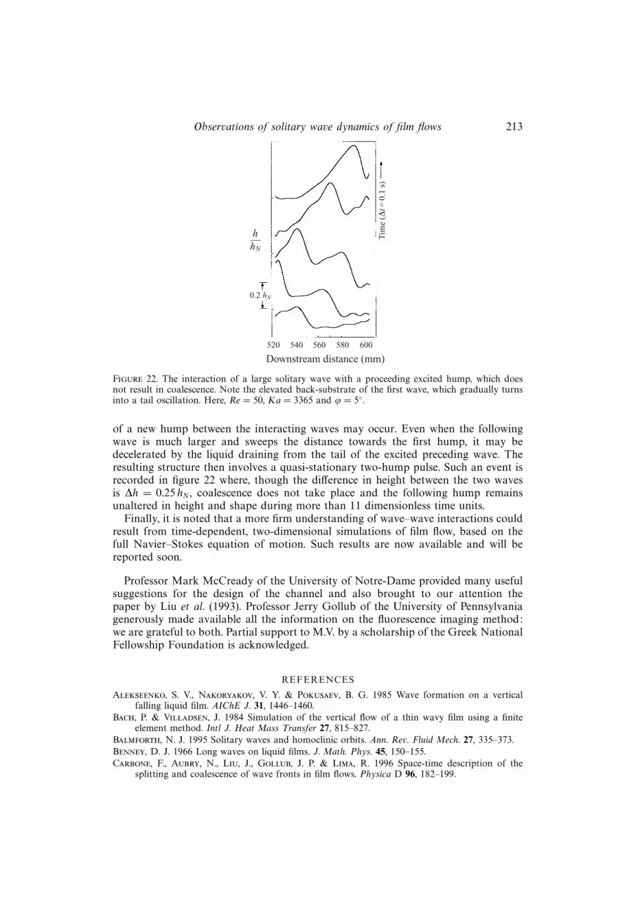
Figure 22. The interaction of a large solitary wave with a proceeding excited hump, which doesnot result in coalescence. Note the elevated back-substrate of the first wave, which gradually turnsinto a tail oscillation. Here, Re = 50, Ka = 3365 and ϕ = 5◦.

of a new hump between the interacting waves may occur. Even when the followingwave is much larger and sweeps the distance towards the first hump, it may bedecelerated by the liquid draining from the tail of the excited preceding wave. Theresulting structure then involves a quasi-stationary two-hump pulse. Such an event isrecorded in figure 22 where, though the difference in height between the two wavesis ∆h = 0.25 hN , coalescence does not take place and the following hump remainsunaltered in height and shape during more than 11 dimensionless time units.

Finally, it is noted that a more firm understanding of wave–wave interactions couldresult from time-dependent, two-dimensional simulations of film flow, based on thefull Navier–Stokes equation of motion. Such results are now available and will bereported soon.

Professor Mark McCready of the University of Notre-Dame provided many usefulsuggestions for the design of the channel and also brought to our attention thepaper by Liu et al. (1993). Professor Jerry Gollub of the University of Pennsylvaniagenerously made available all the information on the fluorescence imaging method:we are grateful to both. Partial support to M.V. by a scholarship of the Greek NationalFellowship Foundation is acknowledged.

REFERENCES

Alekseenko, S. V., Nakoryakov, V. Y. & Pokusaev, B. G. 1985 Wave formation on a verticalfalling liquid film. AIChE J. 31, 1446–1460.

Bach, P. & Villadsen, J. 1984 Simulation of the vertical flow of a thin wavy film using a finiteelement method. Intl J. Heat Mass Transfer 27, 815–827.

Balmforth, N. J. 1995 Solitary waves and homoclinic orbits. Ann. Rev. Fluid Mech. 27, 335–373.

Benney, D. J. 1966 Long waves on liquid films. J. Math. Phys. 45, 150–155.

Carbone, F., Aubry, N., Liu, J., Gollub, J. P. & Lima, R. 1996 Space-time description of thesplitting and coalescence of wave fronts in film flows. Physica D 96, 182–199.


Chang, H.-C. 1986 Traveling waves on fluid interfaces: normal form analysis of the Kuramoto–Sivashinsky equation. Phys. Fluids 29, 3142–3147.

Chang, H.-C. 1989 Onset of nonlinear waves on falling films. Phys. Fluids A 1, 1314–1327.

Chang, H.-C. 1994 Wave evolution on a falling film. Ann. Rev. Fluid Mech. 26, 103–136.

Chang, H.-C., Cheng, M., Demekhin, E. A. & Kopelevich, D. I. 1994 Secondary and tertiaryexcitation of three-dimensional patterns on a falling film. J. Fluid Mech. 270, 251–275.

Chang, H.-C., Demekhin, E. A. & Kalaidin, E. 1995 Interaction dynamics of solitary waves on afalling film. J. Fluid Mech. 294, 123–154.

Chang, H.-C., Demekhin, E. A. & Kopelevich, D. I. 1993 Nonlinear evolution of waves on afalling film. J. Fluid Mech. 250, 433–480.

Cheng, M. & Chang, H.-C. 1992 Subharmonics instabilities of finite-amplitude monochromaticwaves. Phys. Fluids A 4, 505–523.

Cheng, M. & Chang, H.-C. 1995 Competition between sideband and subharmonic secondaryinstability on a falling film. Phys. Fluids 7, 34–54.

Chu, K. I. & Dukler, A. E. 1974 Statistical characteristics of thin wavy films. AIChE J. 20, 695–706.

Demekhin, E. A., Tokarev, G. Yu. & Shkadov, V. Ya. 1991 Hierarchy of bifurcations of space-periodic structures in a nonlinear model of active dissipative media. Physica D 52, 338–361.

Dukler, A. E. 1976 The wavy gas–liquid interface. Chem. Engng Educ. 108–120.

Gardner, C. S., Greene, J. M., Kruskal, M. D. & Miura, R. A. 1967 Method for solving theKorteweg–de Vries equation. Phys. Rev. Lett. 19, 1095–1096.

Ho, L.-W. & Patera, A. T. 1990 A Legendre spectral element method for simulation of unsteadyincompressible viscous free-surface flows. Comput. Meth. Appl. Mech. Engng 80, 355–366.

Jones, L. O. & Whitaker, S. 1966 An experimental study of falling liquid films. AIChE J. 12,525–531.

Kapitza, P. L. & Kapitza, S. P. 1949 Wave flow of thin fluid layers of liquid. Zh. Eksp. Teor. Fiz.19, 105–120; also in Collected Works of L. P. Kapitza (ed. D. Ter Haar). Pergamon, Oxford,1965.

Kerchman, V. I. & Frenkel, A. L. 1994 Interactions of coherent structures in a film flow: simulationsof a highly nonlinear evolution equation. Theor. Comput. Fluid Dyn. 6, 235–254.

Kheshgi, H. S. & Scriven, L. E. 1987 Distributed film flow on a vertical plate. Phys. Fluids 30,990–997.

Krantz, W. B. & Goren, S. L. 1971 Stability of thin liquid films flowing down a plane. Ind. EngngChem. Fundam. 10, 91–101.

Lee, J.-J. & Mei, C. C. 1996 Stationary waves on an inclined sheet of viscous fluid at high Reynoldsand moderate Weber numbers. J. Fluid Mech. 307, 191–229.

Liu, J. & Gollub, J. P. 1994 Solitary wave dynamics of film flows. Phys. Fluids 6, 1702–1712.

Liu, J., Paul, J. D. & Gollub, J. P. 1993 Measurements of the primary instabilities of film flow.J. Fluid Mech. 250, 69–101.

Liu, J., Schneider, J. B. & Gollub, J. P. 1995 Three-dimensional instabilities of film flows. Phys.Fluids 7, 55–67.

Madsen, O. S. & Mei, C. C. 1969 The transformation of a solitary wave over an uneven bottom.J. Fluid Mech. 39, 781–791.

Malamataris, N. T. & Papanastasiou, T. D. 1991 Unsteady free surface flows on truncated domains.Ind. Engng Chem. Res. 30, 2210–2219.

Mei, C. C. 1989 The Applied Dynamics of Ocean Surface Waves, pp. 554–559. World Scientific.

Nakoryakov, V. E., Pokusaev, B. G. & Alekseenko, S. V. 1976 Two-dimensional roll waves onvertical falling liquid films. Sov. J. Engng Phys. 30, 780.

Nguyen, L. T. & Balakotaiah, V. 2000 Modeling and experimental studies of wave evolution onfree falling viscous films. Phys. Fluids 12, 2236–2256.

Pearson, F. W. & Whitaker, S. 1977 Some theoretical and experimental observation of wavestructure of falling liquid films. Ind. Engng Chem. Fundam. 16, 401–408.

Prokopiou, T., Cheng, M. & Chang, H.-C. 1991 Long waves on inclined films at high Reynoldsnumber. J. Fluid Mech. 222, 665–691.

Salamon, T. R., Armstrong, R. C. & Brown, R. A. 1994 Traveling waves on inclined films:numerical analysis by the finite-element method. Phys. Fluids 6, 2202–2220.


Shkadov, V. Ya. 1967 Wave conditions in the flow of thin layer of a viscous liquid under the actionof gravity. Izvz. Akad. Nauk. SSSR, Mekh. Zhidk i Gaza 1, 43–50.

Stainthorp, F. P. & Allen, J. M. 1965 The development of ripples on the surface of liquid filmflowing inside a vertical tube. Trans. Inst. Chem. Engrs 43, 85–91.

Trifonov, Yu. Ya. & Tsvelodub, O. Yu. 1991 Nonlinear waves on the surface of a falling liquidfilm. Part 1. Waves of the first family and their stability. J. Fluid Mech. 229, 531–554.

Tsvelodub, O. Yu. & Trifonov, Yu. Ya. 1992 Nonlinear waves on the surface of a falling liquidfilm. Part 2. Bifurcations of the first-family waves and other types of nonlinear waves. J. FluidMech. 244, 149–169.

Whitaker, S. 1964 Effect of surface active agents on stability of falling liquid films. Ind. EngngChem. Fundam. 3, 132–142.

Wilson, S. D. & Jones, A. F. 1983 The entry of a falling film into a pool and the air-entrainmentproblem. J. Fluid Mech. 128, 219–230.

Yu, L.-Q., Wasden, F. K., Dukler, A. E. & Balakotaiah, V. 1995 Nonlinear evolution of waveson falling films at high Reynolds number. Phys. Fluids 7, 1886–1902.

observations of solitary wave dynamics of film flows

Documents