multi-speed solitary waves of nonlinear schrödinger systems

arX

iv:1

504.

0497

6v2

[m

ath.

AP]

27

May

201

5

MULTI-SPEED SOLITARY WAVES

OF NONLINEAR SCHRODINGER SYSTEMS:

THEORETICAL AND NUMERICAL ANALYSIS

FANNY DELEBECQUE, STEFAN LE COZ, AND RADA M. WEISHAUPL

Abstract. We consider a system of coupled nonlinear Schrodinger equationsin one space dimension. First, we prove the existence of multi-speed solitarywaves, i.e solutions to the system with each component behaving at large timesas a solitary wave. Then, we investigate numerically the interaction of two soli-tary waves supported each on one component. Among the possible outcomes,we find elastic and inelastic interactions, collision with mass extraction andreflexion.

Contents

1. Introduction 21.1. The theoretical result 31.2. The numerical experiments 42. Existence of multi-speed solitary waves 53. Uniform estimates 63.1. The bootstrap argument 63.2. Modulation 73.3. Energy estimates and coercivity 83.4. Almost-conservation of the localized momentum 123.5. Control of the modulation parameters 143.6. Conclusion 144. Numerical schemes 154.1. The time-splitting spectral method 154.2. The normalized gradient flow 165. Numerical experiments 165.1. Purely elastic interaction 175.2. Symmetric collision 185.3. Dispersive inelastic interaction 195.4. Reflexion 20Appendix A. Proof of the modulation lemma 21References 24

Date: October 5, 2018.2010 Mathematics Subject Classification. 35Q55(35C08,35Q51,37K40).Key words and phrases. solitons, solitary waves, nonlinear Schrodinger systems.The work of F. D. is partially supported by PHC AMADEUS 2014 31471ZK.

The work of S. L. C. is partially supported by ANR-11-LABX-0040-CIMI within the programANR-11-IDEX-0002-02, ANR-14-CE25-0009-01 and PHC AMADEUS 2014 31471ZK.

The work of R.M.W. is supported by the FWF Hertha-Firnberg Program, Grant T402-N13and Austrian-French Project WTZ-Amadee FR 18/2014.

1

http://arxiv.org/abs/1504.04976v2

2 F. DELEBECQUE, S. LE COZ, AND R. M. WEISHAUPL

1. Introduction

We consider the following nonlinear Schrodinger system:{i∂tu1 + ∂xxu1 + µ1|u1|2u1 + β|u2|2u1 = 0,

i∂tu2 + ∂xxu2 + µ2|u2|2u2 + β|u1|2u2 = 0,(NLS)

where for j = 1, 2 we have uj : R× R → C, µj > 0, and β ∈ R \ {0}.When µ1 = µ2 = β, system (NLS), also called Manakov system has been intro-

duced by Manakov (see [21] for example) as an asymptotic model for the propaga-tion of electric fields in waveguides. In this particular case, it is to be noticed thatthe usual roles of x and t are inverted to study the evolution of the electrical fieldalong the propagation axis.

It has also been used later on to model the evolution of light in optical fiber links.One of the main limiting effects of transmission in optical fiber links is due to thepolarization mode dispersion (PMD). It can be explained by the birefringence effect,i.e the fact that the electric field is a vector field and that the refraction index ofthe medium depends on the polarization state (see e.g [1, 2]). The evolution of twopolarized modes of an electrical field in a birefringent optical fiber link can indeedbe modeled by (NLS) in the case where µ1 = µ2 and β measures the strengthof the cross phase modulation which depends of the fiber (see [21]). Randomlyvarying birefringence is studied adding random coefficients in both nonlinearityand coupling terms of (NLS) (see for example [15])

In higher dimensions, systems of nonlinear coupled Schrodinger equations ap-pears in various physical situations such as the modeling of the interaction of twoBose-Einstein condensates in different spin states.

Systems of type (NLS) have also been studied from the mathematical point ofview. When µ1 = µ2 = β, in dimension 1, the system (NLS) has the particularity tobe completely integrable. Hence explicit calculations of solutions are possible andone can exhibit a variety of “truly” nonlinear solutions like solitons, multi-solitonsor breathers (see e.g. the book [1]). The integrability property is however notrobust, and the slightest change in the parameters µ1, µ2 and β destroys it. Manyworks (see, among many others, [3, 8, 14, 29]) have been devoted to the study ofthe stationary version of (NLS)

{∂xxφ1 + µ1|φ1|2φ1 + β|φ2|2φ1 = ω1φ1,

∂xxφ2 + µ2|φ2|2φ2 + β|φ1|2φ2 = ω2φ2,(1)

that one obtains when looking for standing waves solutions

(u1, u2)(t, x) = (eiω1tφ1(x), eiω2tφ2(x)).

When standing waves exist, it is natural to study their stability and again manyworks have been devoted to this problem (see, again among many others, [16, 20, 26,28]). Existence and stability of standing waves are often proved using variationaltechniques. The analysis of (1) through variational techniques is very subtle and theintroduction of new ideas is necessary to understand the full picture (see [27]). Notethat (NLS) is Galilean-invariant. Hence a Galilean transform modifies a standingwave into a solitary wave traveling at some non-zero speed.

Our goal in this paper is to provide a new point of view on the study of thissystem. We aim at understanding better the behavior in large times of solutions

MULTI-SPEED SOLITARY WAVES OF NONLINEAR SCHRODINGER SYSTEMS 3

starting at initial time as two scalar solitary waves carried by the two different com-ponents. We will use a mixture of theoretical and numerical tools, a combinationseldom seen when dealing with this kind of problems.

First, we propose to push further a study initiated in [17] on the multi-speedsolitary waves of system (NLS) and followed up for a different nonlinearity in [30].A multi-speed solitary wave is a solution of (NLS) which behaves at large time astwo solitary waves. Here and as in [17], we restrict ourselves to the case where thecomposing solitary waves are each carried on only one component of the system.In other words, taken independently, each component behaves as a scalar solitarywave at large time. Our first aim is to remove the high speed assumption underwhich the main result in [17] was proved. We therefore consider the system (NLS)in dimension 1 and benefit from the fact that scalar solitary waves are in that caseorbitally stable (see e.g [11]).

Our next aim is to investigate further the properties of multi-speed solitarywaves solutions when they are crossing at positive time. Our theoretical result(Theorem 1) indeed only guarantees existence of multi-speed solitary wave solutionsto (NLS) when no interaction can occur at large time between the composing waves.But what happens when two solitary waves carried by different components collide?Due to the possible complexity of the phenomenon and the lack of appropriatetheoretical tools to study it, we proceed the following numerical experiment. Wetake as initial data solitons on each components, both away from 0 but facing eachother for the direction of propagation. Among the possible outcomes, we find elasticand inelastic interactions, interaction with mass exctraction, and reflexion.

1.1. The theoretical result. Before stating our main theoretical result, let usgive a few preliminaries.

Let Qω ∈ H1(R) be the unique positive radial ground state solution to

− ∂xxQω + ωQω − |Qω|2Qω = 0, Qω > 0, Qω ∈ H1rad(R). (2)

From simple calculations we note that the following scaling occurs:

Qω(x) :=√ω Q1(

√ωx). (3)

For j = 1, 2, consider ωj > 0, γj ∈ R, xj , vj ∈ R and define

Rj(t, x) = ei(ωjt− 1

4|vj |2t+ 1

2vj ·x+γj)

√1

µjQωj

(x− vjt− xj). (4)

The function Rj is a solitary wave solution to

i∂tu+ ∂xxu+ µj |u|2u = 0. (5)

In this paper, we want to investigate the existence of solutions to (NLS) whereeach component behaves like a solitary wave Rj solution to the scalar equation (5).Our main theoretical result is the following.

Theorem 1. Let µ1, µ2 > 0 and β ∈ R \ {0}. For j = 1, 2, take vj , xj , γj ∈ R,ωj > 0 and consider the ground state profile Qωj

solution to (2) and the soliton Rj

defined in (4). Then, there exist C > 0, T0 > 0 and(u1, u2

)solution to (NLS) on

the time interval [T0,+∞) such that for all t ∈ [T0,+∞), we have∥∥∥∥(u1(t)u2(t)

)−(R1(t)R2(t)

)∥∥∥∥H1×H1

6 Ce−√ω∗v∗t,


where ω∗ = 12304 min{ω1, ω2} and v∗ = |v1 − v2|.

Remark 1. Compare to [17, Theorem 1], the main differences are the following.Our result is valid for any speeds, whereas the one in [17] required a high speedassumption. We restrict ourselves to dimension 1 to have stable solitons (in [17],any dimension was allowed). The overall proof strategy is similar, but in our case weneed to perform several technical refinements which include in particular workingwith localized momenta and modulated waves.

In addition, we are introducing the technical artefact consisting into introducingarbitrary constants in the definition (15) of the global action. This is a new featurefor this type of analysis, which is quite surprising as usually such a flexibility is notallowed by the algebra of the problem.

The scheme of the proof is inspired by the one developed for the study of multi-solitons in scalar nonlinear Schrodinger equations in [12, 13, 23, 25] (see also [9] fora similar approach applied to Klein-Gordon equations). It consists in solving (NLS)backward in time, taking as final data a couple of solitary waves

(R1(T

n), R2(Tn)),

for an increasing sequence of times T n → +∞. Thus we get a sequence(un1 , u

n2

)

of solutions to (NLS) on a time interval (−∞, T n] such that(un1 (T

n), un2 (T

n))=(

R1(Tn), R2(T

n)). We then have to prove the existence of a time T0, independent

of n such that for n large enough,(un1 , u

n2

)is close to

(R1, R2

)on [T0, T

n]. Thekey tools at hand to prove Theorem 1 are

• uniform in n estimates

∀t ∈ [T0, Tn],

∥∥∥∥(un1 (t)

un2 (t)

)−(R1(t)R2(t)

)∥∥∥∥H1×H1

6 Ce−√ω∗v∗t,

• a compactness argument that gives the existence of(u01, u

02

)∈ H1(R) ×

H1(R) such that(un1 , u

n2

)converges strongly in Hs(R) (s ∈ [0, 1)) towards(

u01, u

02

).

Remark 2. The method used to obtain Theorem 1 is a powerful tool to obtain sharpexistence results for multi-solitons composed of ground states. Another approachrelying on a fixed point argument has been developed for nonlinear Schrodingerequations in [18, 19]. This approach is very flexible and allows to prove existenceof solutions more complicated than the ones in Theorem 1 like infinite trains ofsolitons or multi-kinks. The main drawback is that it always requires a large speedassumption.

We also have tested numerically if the multi-speed solitary wave configurationwas stable provided the starting waves are well-ordered and well-separated. Inother words, we took the interaction to be small at the origin and the composingwaves going away from each other. With such a well-prepared initial configuration,we remain close to a similar configuration in large time. This suggests that themulti-speed solitary waves are stable (no matter the coupling parameter). Notethat this is expected due to the fact that each wave taken individually is stable.We have however no theoretical mean to verify this conjecture. Similar difficultiesarise in the analysis of the stability for multi-solitons in nonlinear scalar Schrodingerequations (see e.g. [24]).

1.2. The numerical experiments. We solve the system (NLS) in one dimen-sion by adapting the time-splitting spectral method described in [7]. This method


is unconditionally stable, time reversible, of spectral-order accuracy in space andsecond-order accuracy in time, and it conserves the discrete total mass [5]. Onecan refer to [4] for other possible schemes and their properties.

We will also compute the real valued ground state (minimizer of the energyon fixed L2 mass constraints) of the system (1) using a normalized gradient flowapproach. This will be used to make the comparison between the outcome of theinteraction between two solitary waves and a solitary wave with profile (φ1, φ2).

As already mentioned, the experiment consists in taking as initial data the initialdata of two solitary waves facing each other, each on one component.

We considered four cases, the first one being the integrable case, where we expectthe solitons after the interaction to move with the same velocity and amplitude.Apart when µ1 = µ2 = β, the system is not integrable, hence we do not expectpure elastic interaction between solitons. However, there are still regimes wherewe expect the outcome of interaction between solitons to be also a multi-speedssolitary wave, different from the input at two level: first, there are modificationsin the speeds and amplitudes of the composing solitons. Second, there is a loss ofa bit of energy, mass and momentum into a small dispersive remainder. In certaincases, we have been able to identify the profiles of the outcome of the interactionsas ground states of the stationary system (1).

The rest of this paper is organized as follows. In Section 2, we prove Theorem 1assuming uniform estimates. In Section 3, we prove the uniform estimates. Thenumerical methods are described in Section 4, and the numerical experiments arepresented in Section 5. Appendix A contains the proof of a modulation result.

2. Existence of multi-speed solitary waves

This short section is devoted to the proof of Theorem 1, assuming uniform esti-mates proved in the next section.

In this section and in the next one, we assume that µ1, µ2 > 0 and β ∈ \{0} arefixed constants and that we are given for j = 1, 2 soliton parameters ωj , vj , xj , γj ∈R. Denote by Qωj

and Rj the corresponding profile and soliton.We make the assumption that

0 < v1 = −v2. (6)

Since (NLS) is Galilean invariant, this assumption can be done without loss ofgenerality. This will simplify calculations later on.

Note that it follows from classical arguments (see [10]) that the Cauchy prob-lem for (NLS) is globally well-posed in the energy space H1(R) ×H1(R) and alsoin L2(R) × L2(R). In particular, for any initial data (u0

1, u02) ∈ H1(R) × H1(R)

there exists a unique global solution (u1, u2) of (NLS) in C(R, H1(R) × H1(R)) ∩C1(R, H−1(R)×H−1(R)).

Let (T n) be an increasing sequence of times such that T n → +∞ as n →+∞. Let (un

1 , un2 ) be the sequence of solutions to (NLS) defined by solving (NLS)

backward on (−∞, T n] with final data (un1 , u

n2 )(T

n) =(R1, R2

)(T n). The proof of

Theorem 1 then relies on the following two ingredients.First, we have uniform estimates on the distance between the sequence

(un1 , u

n2

)

and the multi-speed solitary wave profile(R1, R2

).


Proposition 3 (Uniform estimates). There exist T0 > 0, n0 ∈ N such that, for alln > n0 and for all t ∈ [T0, T

n] we have∥∥∥∥(un1

un2

)(t)−

(R1

R2

)(t)

∥∥∥∥H1×H1

6 e−√ω∗v∗t,

where, as in Theorem 1, ω∗ = 12304 min{ω1, ω2} and v∗ = |v1 − v2|.

The proof of Proposition 3 is rather involved and we postpone it to Section 3.The next ingredient is a compactness result on the initial data

(un1 , u

n2

)(T0).

This result was already present in this form in [17] and we recall it without proof.

Proposition 4 (Compactness). There exists(u01, u

02

)∈ H1(R)×H1(R) such that,

up to a subsequence,(un1 , u

n2

)(T0) converges strongly towards

(u01, u

02

)in Hs(R) ×

Hs(R) for all s ∈ [0, 1).

With these two ingredients in hand, we can now conclude the proof of Theorem 1.

Proof of Theorem 1. Let (u1, u2) be the solution on R of the Cauchy problem (NLS)with initial data (u0

1, u02) at t = T0. By H1(R) × H1(R) boundedness and local

well-posedness of the Cauchy problem in Hs(R) × Hs(R) for all s ∈ [0, 1), wehave weak convergence in H1(R)×H1(R) of (un

1 , un2 )(t) towards (u1, u2)(t) for any

t ∈ R. Combined with the uniform estimates of Proposition 3, this implies for allt ∈ [T0,+∞) that∥∥∥∥(u1

u2

)(t)−

(R1

R2

)(t)

∥∥∥∥H1×H1

6 lim infn→+∞

∥∥∥∥(un1

un2

)(t)−

(R1

R2

)(t)

∥∥∥∥H1×H1

6 Ce−√ω∗v∗t.

This concludes the proof of Theorem 1. �

3. Uniform estimates

This section is devoted to the proof of Proposition 3. In all this section, T n and(un1 , u

n2

)are given as in the beginning of Section 2.

3.1. The bootstrap argument. We first reduce the proof of Proposition 3 to theproof of the following bootstrap result.

Proposition 5 (Bootstrap argument). There exist T0 > 0 and n0 ∈ N such thatfor all n > n0 and for any t0 ∈ [T0, T

n] the following property is satisfied. If for allt ∈ [t0, T


un2

)(t)−

(R1

R2

)(t)

∥∥∥∥H1×H1

6 e−√ω∗v∗t, (7)

then for all t ∈ [t0, Tn] we have∥∥∥∥(un1

un2

)(t)−

(R1

R2

)(t)

∥∥∥∥H1×H1

61

2e−

√ω∗v∗t. (8)

The proof of Proposition 5 will occupy us for most of the rest of this section.We divided it into several steps. We first perform a geometrical decomposition ofthe sequence (un

1 , un2 ) onto the manifold of multi-speed solitary waves in order to

obtain orthogonality conditions. We then introduce an action-like functional, whichturns out to be coercive due to our orthogonality conditions. This functional is nota conserved quantity, but since it is made with localized conservations laws it is


almost conserved. Using that property and a control on the geometrical modulationparameters, we are able to conclude the proof of Proposition 5.

Before going on with the details of the proof of Proposition 5, let us show howit implies Proposition 3.

Proof of Proposition 3. Since we have (un1 , u

n2 )(T

n) = (Rn1 , R

n2 )(T

n) at the finaltime T n, by continuity there exists a minimal time t0 such that for all t ∈ [t0, T

n]we have ∥∥∥∥

(un1

un2

)(t)−

(R1

R2

)(t)

∥∥∥∥H1×H1

6 e−√ω∗v∗t. (9)

We prove that t0 = T0 by contradiction. Assume that t0 > T0. By Proposition 5,for all t ∈ [t0, T


un2

)(t)−

(R1

R2

)(t)

∥∥∥∥H1×H1

61

2e−

√ω∗v∗t.

Therefore by continuity there exists t00 < t0 such that on [t00, Tn] estimate (9) is

satisfied. This however contradicts the minimality of t0. Hence t0 = T0 and thisconcludes the proof. �

For the rest of Section 3, T0 > 0 and n0 ∈ N will be large enough fixed numbers,and we assume the existence of t0 > T0 such that for all t ∈ [t0, T

n] the bootstrapassumption (7) is verified, i.e. we have

∥∥∥∥(un1

un2

)(t)−

(R1

R2

)(t)

∥∥∥∥H1×H1

6 e−√ω∗v∗t. (10)

Our final goal is now to prove that in fact (8) holds for all t ∈ [t0, Tn].

3.2. Modulation. Let us start with a decomposition lemma for our sequence ofapproximated multi-speed solitary waves.

Lemma 6 (Modulation). There exist C > 0 and C1 functions

ωj : [t0, Tn] → (0,+∞), xj : [t0, T

n] → R, γj : [t0, Tn] → R, j = 1, 2,

such that if for j = 1, 2 we denote by Rj the modulated wave

Rj(t, x) = ei(1

2vj ·x+γj(t)) 1

√µj

Qωj(t)(x− xj(t)), (11)

then for all t ∈ [t0, Tn] the functions defined by

(ε1ε2

)(t) =

(un1

un2

)(t)−

(R1

R2

)(t)

satisfy for j = 1, 2 and for all t ∈ [t0, Tn] the orthogonality conditions

(εj(t), Rj(t)

)2=(εj(t), iRj(t)

)2=(εj(t), ∂xRj(t)

)2= 0. (12)

Moreover, for all t ∈ [t0, Tn], we have

2∑

j=1

|∂tωj(t)|2 + |∂txj(t)− vj |2 +

∣∣∣∣∣∂tγj(t) +v2j4

− ωj(t)

∣∣∣∣∣

2

6 C

∥∥∥∥(ε1ε2

)(t)

∥∥∥∥2

H1×H1

+ Ce−3√ω

∗v∗t. (13)


Remark 7. It is to be noticed that estimate (13) clearly implies that, for T0 largeenough, for j = 1, 2, and for all t ∈ [t0, T

n], we have

xj(t) >v∗

2√2t > 2L and ωj(t) > 1152ω∗.

Moreover, a better estimate can be obtained for ωj and will be stated later on inLemma 12.

This type of modulation result is classical in the literature dealing with solitarywaves of nonlinear dispersive equations (see e.g. the fundamental paper of We-instein [31] for an early version or [24] for a recent approach). Its proof consistsessentially in the application of the implicit function theorem combined with the useof the evolution equation to find equation (13) for the evolution of the modulationparameters. We refer to the appendix for the details of the proof.

3.3. Energy estimates and coercivity. In this subsection, we analyze the dif-ferent quantities that are conserved or almost-conserved in our coupled-vectorialproblem. Remember that in the case of the scalar equation (5) the energy, massand momentum, defined as follows, are conserved along the flow of (5):

E(u, µj) :=1

2‖∂xu‖2L2 −

µj

4‖u‖4L4 , M(u) :=

1

2‖u‖2L2 , P (u) :=

1

2Im

∫

R

u∂xudx.

The solution Qω we chose of equation (2) is known to be the unique positive radialground state of the action S := E(·, 1)+ωM . Consequently, each soliton Rj definedby (4) is a critical point of the scalar functional Sj defined by

Sj := E(·, µj) +

(ωj +

v2j4

)M + vjP. (14)

Coercivity properties of linearizations of Sj-like functionals are the key tool of theanalysis of multi-solitons interaction (see for example [17, 23]).

In the vectorial case we are interested in here, the coupled system (NLS) admitsits own conservation laws. In particular, the mass of each component is preserved, asin the scalar case. However, the coupling does not preserve conservation of the scalarenergy and momentum for each component and we only have conservation of thetotal energy (made of individual energies plus a coupling term) and total momentum(sum of the scalar momenta). More precisely, total energy, total momentum, andscalar masses of the whole system (defined as follows) are conserved quantities forthe flow of system (NLS):

E(u1

u2

):= E(u1, µ1) + E(u2, µ2)−

β

2

∫

R

|u1|2|u2|2dx,

P(u1

u2

):= P (u1) + P (u2), Mj

(u1

u2

):= M(uj), j = 1, 2.

In order to use the conservation of the momentum as in the scalar case, we hereneed to localize the momentum of each soliton, as was done in [12, 13] for the scalarmass and momentum. Note that this was not needed for the analysis in [17]. Letus define the cut-off functions

χ1L(x) = χ

(xL

), χ2

L = 1− χ1L,


where L > 0 is arbitrary but fixed and χ is a C3 function such that

0 6 χ 6 1 on R, χ(x) = 0 for x 6 −1, χ(x) = 1 for x > 1, χ′> 0 on R,

and satisfies, for some positive constant C and for all x ∈ R the estimates

(χ′(x))2 6 Cχ(x), (χ′′(x))2 6 Cχ′(x).

Localized momenta Pjloc are defined by:

Pjloc

(u1

u2

)=

1

2Im

∫

R

(u1∂xu1 + u2∂xu2

)χjLdx, j = 1, 2.

Remark that P = P1loc + P2

loc. Note that since we are assuming (6) the momentaabove defined are localized around each composing solitary wave of the profile. Theadvantage of having made assumption (6) is that the cut-off does not depend ontime. This will simplify our next calculations.

In the sequel, we are interested in the following global action:

S(u1

u2

)= E

(u1

u2

)+∑

j=1,2

(ωj(t) +

v2j4

)Mj

(u1

u2

)+∑

j=1,2

vjPjloc

(u1

u2

)

+ C1(β, v1)M2

(u1

u2

)+ C2(β, v2)M1

(u1

u2

), (15)

where Cj(β, vj) are positive constants depending only on β and vj and whose exactvalues will be decided later on. Note that the action implicitly depends on t viaωj. It is to be noted that, in this work, we have the freedom to add these twocoupled-mass terms that do not appear in the usual definition of S-like functionals.This is a key point in our analysis.

Let us now state in the following lemma several estimates related to the local-ization of R1 and R2 and which will be of great use in the sequel.

Lemma 8. For j = 1, 2, if T0 is large enough, then for all t ∈ [t0, Tn] and for all

x ∈ R we have(|Rj(t, x)|+ |∂xRj(t, x)|

)χ3−jL (x) 6 C(1 + |vj |)e−3

√ω∗v∗te−

√ω∗|x|, (16)

∏

k=1,2

(|Rk(t, x)|+ |∂xRk(t, x)|

)6 C(1 + |v1|+ |v2|)2e−3

√ω∗v∗te−

√ω∗|x|. (17)

Lemma 8 follows from the support properties of the cut-off function and theexponential localization of the solitons profiles. Indeed, recall that in fact, theprofile Q = Q1 is explicitly known

Q(x) = 2 sech(x),

and it follows that Q and its derivatives are exponentially decaying, i.e. for anyη < 1 we have

|Qxx|+ |Qx|+ |Q| 6 Cηe−η|x|.

Proof of Lemma 8. We prove only (16), the proof of (17) following from similar(simpler) arguments. For simplicity in notation, assume j = 1, the case j = 2 beingperfectly symmetric. Due to the exponential decay of the soliton profiles, we have

|R1(t, x)| 6 Ce−3

4

√ω1|x−x1|


The cut-off function χ2L is supported on (−∞, L], and since for T0 large enough

x1 > 2L, for x ∈ (−∞, L] we have (we recall here Remark 7)

|x− x1| > |x|, and |x− x1| >1

2|x1|.

As a consequence, we have

|R1(t, x)|χ2L(x) 6 Ce−

1

4

√ω1|x1|e−

1

4

√ω1|x|.

In addition, as noticed in Remark 7, we have

x1 >v∗

2√2t, and ω1 > 1152ω∗,

which implies|R1(t, x)|χ2

L(x) 6 Ce−3√ω∗v∗te−

√ω∗|x|.

The derivative ∂xR1 is treated in the same way, with the only difference that |v1|now appears in the estimate, due to the term ei

1

2v1·x in the definition (11) of R1.

This finishes the proof. �

Lemma 9 (Expansion of the global action S). For all t ∈ [t0, Tn] we have

S(u1

u2

)= S

(R1

R2

)+H

(ε1ε2

)+O(e−3

√ω∗v∗t), (18)

H(ε1ε2

)= Hfree

(ε1ε2

)+Hcoupled

(ε1ε2

),

with

Hfree

(ε1ε2

)=∑

j=1,2

(1

2‖∂xεj‖2L2 +

1

2

(ωj +

v2j4

)‖εj‖2L2 − µj

∫

R

|εj |2|Rj |2dx

− µj

2Re

∫

R

ε2j R2jdx+

1

2vj Im

∫

R

εj∂xεjχjLdx

)

and

Hcoupled

(ε1ε2

)= C1(β, v1)‖ε2‖2L2 + C2(β, v2)‖ε1‖2L2

− β

2

∫

R

(|ε1|2|R2|2 + |ε2|2|R1|2

)dx

+1

2v1Im

∫

R

ε2∂xε2χ1Ldx+

1

2v2Im

∫

R

ε1∂xε1χ2Ldx.

Proof of Lemma 9. First note that, according to the definition (15) of S,

S(u1

u2

)=∑

j=1,2

Sj(uj) + vj ·(Pjloc

(u1

u2

)− P (ui)

)

+ C1(β, v1)M(u1) + C2(β, v2)M(u2)−β

2

∫

R

|u1|2|u2|2dx, (19)

where Sj denote the same functional as Sj (see the definition (14)) with ωj instead

of ωj . For j = 1, 2, let us expand uj(t) = Rj(t) + εj(t) in the expression of Sj . Asimple computation leads to:

Sj(Rj + εj) = Sj(Rj) + S′j(Rj)εj +

⟨S′′j (Rj)εj , εj

⟩+O(‖εj‖3H1)


Now, as Rj is a critical point of the scalar functional Sj , we have

S′j(Rj) = 0,

and thus

Sj(Rj + εj) = Sj(Rj) +⟨S′′j (Rj)εj , εj

⟩+O(‖εj‖3H1 ), (20)

where

⟨S′′j (Rj)εj , εj

⟩=

1

2‖∂xεj‖2L2 +

1

2

(ωj +

v2j4

)‖εj‖2L2 +

1

2vjIm

∫

R

εj∂xεjdx

− µj

2Re

∫

R

ε2j R2jdx− µj

∫

R

|εj|2|Rj |2dx. (21)

Let us now develop the remaining terms in (19). As far as the momentum part isconcerned, we write the expansion for j = 1 for simplicity:

P1loc

(R1 + ε1R2 + ε2

)− P (R1 + ε1)

= −Im

∫

R

R1∂xR1χ2Ldx+ Im

∫

R

R2∂xR2χ1Ldx

− Im

∫

R

(R1∂xε1 + ε1∂xR1

)χ2Ldx+ Im

∫

R

(R2∂xε2 + ε2∂xR2

)χ1Ldx

− Im

∫

R

ε1∂xε1χ2Ldx+ Im

∫

R

ε2∂xε2χ1Ldx. (22)

Concerning the β coupling part in (19), we get:∫

R

|R1 + ε1|2|R2 + ε2|2dx

=

∫

R

|R1|2|R2|2dx+ 2Re

∫

R

(|R1|2R2ε2 + |R2|2R1ε1

)dx

+

∫

R

(|ε1|2|R2|2 + |ε2|2|R1|2 + 4Re(ε1R1)Re(ε2R2)

)dx

+ 2

∫

R

(|ε2|2Re(ε1R1) + |ε1|2Re(ε2R2)

)dx+

∫

R

|ε1|2|ε2|2dx. (23)

Finally, the extra-masses terms in (19) expand into

M(Rj+εj) =1

2‖Rj+εj‖2L2 = M(Rj)+

(Rj , εj

)2+M(εj) = M(Rj)+M(εj), (24)

where we have used the orthogonality conditions (12) to obtain the last equality.In (22) and (23), all terms containing a product of solitons or cut-off functions withdifferent indices/exponents are of order O(e−3

√ω∗v∗t) by Lemma 8. The terms

containing a degree 3 or higher term in (ε1, ε2) are also of order O(e−3√ω∗v∗t) by

the bootstrap assumption (10). Therefore, gathering (19)-(20)-(21)-(22)-(23)-(24)together gives:

S(R1 + ε1R2 + ε2

)= S

(R1

R2

)+Hfree

(ε1ε2

)+Hcoupled

(ε1ε2

)+O(e−3

√ω∗v∗t).

This concludes the proof. �


Lemma 10 (Coercivity of H). There exists λ > 0 such that, for any t0 ∈ [T0, Tn]

and for all t ∈ [t0, Tn]:

Hfree

(ε1ε2

)> 2λ

(‖ε1‖2H1 + ‖ε2‖2H1

), (25)

Hcoupled

(ε1ε2

)> λ

(‖ε1‖2L2 + ‖ε2‖2L2

)− λ

(‖∂xε1‖2L2 + ‖∂xε2‖2L2

), (26)

and thus:

H(ε1ε2

)> λ

∥∥∥∥(ε1ε2

)∥∥∥∥2

H1×H1

. (27)

Proof. The proof of (25) is classical (see for example [17, 23]) and we omit it. Itremains to prove (26). It is readily seen that for Cj(β, vj) large enough, we have

C1(β, v1)‖ε2‖2L2 + C2(β, v2)‖ε1‖2L2 −β

2

∫

R

(|ε1|2|R2|2 + |ε2|2|R1|2

)dx

>1

2

(C1(β, v1)‖ε2‖2L2 + C2(β, v2)‖ε1‖2L2

).

As far as the momentum parts of Hcoupled are concerned, for example for j = 1:

v12Im

∫

R

ε1∂xε1χ2Ldx > −v1

2

∫

R

|ε1∂xε1χ2L|dx

> −v12‖ε1‖2‖∂xε1‖2

> − v214λ

‖ε1‖2L2 − λ‖∂xε1‖2L2 .

For C(β, vj), j = 1, 2 large enough, i.e such that

∑

j=1,2

(1

2C(β, vj)−

v2j4λ

)> λ,

we thus have:

Hcoupled

(ε1ε2

)> λ

(‖ε1‖2L2 + ‖ε2‖2L2

)− λ

(‖∂xε1‖2L2 + ‖∂xε2‖2L2

).

Combining estimates (25) and (26) on Hfree and Hcoupled finally gives (27). �

3.4. Almost-conservation of the localized momentum. In this section, weinvestigate the conservation of the localized momentum and, inspired by [23], westate the following lemma:

Lemma 11. There exists C > 0 (independent of L) such that if L and T0 are largeenough then for all t ∈ [t0, T

n] and for j = 1, 2 we have∣∣∣∣P

jloc

(u1

u2

)(t)− Pj

loc

(u1

u2

)(T n)

∣∣∣∣ 6C

Le−2

√ω∗v∗t. (28)

Proof of Lemma 11. Let us prove the lemma in the case j = 1, the case j = 2 beingperfectly similar. We first compute the time derivative of P1

loc:

d

dtP1loc(t) =

1

2Im

∫

R

∂tu1∂xu1χ( xL

)dx+

1

2Im

∫

R

u1∂x,tu1χ( xL

)dx. (29)


Let us call term A and B respectively the first and the second term of the righthand side in equality (29):

A =1

2Im

∫

R

∂tu1∂xu1χ( xL

)dx, B =

1

2Im

∫

R

u1∂x∂tu1χ( xL

)dx.

Using the fact that u(t) =

(u1(t)u2(t)

)is a solution to (NLS), we readily get (formally,

but this will be justified when integrating):

∂tu1∂xu1 = i∂xxu1∂xu1 + iµ1|u1|2u1∂xu1 + iβ|u2|2u1∂xu1 (30)

∂x∂tu1 = −i∂xxxu1 − iµ1∂x

(|u1|2u1

)− iβ∂x

(|u2|2u1

). (31)

About term A: Equation (30) provides us with the following decomposition of termA:

A =1

2Re

∫

R

∂xxu1∂xu1χ( xL

)dx+

1

2µ1Re

∫

R

|u1|2u1∂xu1χ(xL

)dx

+1

2βRe

∫

R

|u2|2u1∂xu1χ( xL

)dx.

Integrating by part in each term of A finally gives:

A = − 1

4L

∫

R

|∂xu1|2χ′( xL

)dx− 1

8Lµ1

∫

R

|u1|4χ′( xL

)dx

+1

2βRe

∫

R

|u2|2u1∂xu1χ( xL

)dx. (32)

About term B: Equation (31) provides us with the following decomposition of termB:

B = −1

2Re

∫

R

u1∂xxxu1χ( xL

)dx− 1

2µ1Re

∫

R

u1∂x

(|u1|2u1

)χ( xL

)dx

− 1

2βRe

∫

R

u1∂x

(|u2|2u1

)χ( xL

)dx.

As for the A term, integrating by parts (several times if necessary) in each termfinally leads to:

B = − 3

4L

∫

R

|∂xu1|2χ′( xL

)dx+

1

4L3

∫

R

|u1|2χ′′′( xL

)dx

+3

8Lµ1

∫

R

|u1|4χ′( xL

)dx

+1

2βRe

∫

R

|u2|2u1∂xu1χ(xL

)dx+

1

2LβRe

∫

R

|u2|2|u1|2χ′( xL

)dx. (33)

Combining (32) and (33), and using the fact that χ′ and χ′′′ are supported on[−L,L] lead to the following estimate:∣∣∣∣d

dtP1loc(t)

∣∣∣∣ 6C

L

∫ L

−L

(|∂xu1|2 + |u1|2 + |u1|4

)dx+C

∫

R

|u2|2(|u1|2 + |∂xu1|2

)χ1L(x)dx.

(34)


Note that for x ∈ [−L,L], T0 large enough, and using (13) we have (see Lemma 8for similar arguments)

|∂xRj(t, x) +Rj(t, x)| 6 Ce−√

ωj |x−xj| 6 Ce−1

2

√ωj |xj| 6 Ce−3

√ω∗v∗t.

Note that C here depends on vj . Expanding now uj = Rj + εj , in (34), using theabove estimate and Lemma 8, we obtain

∣∣∣∣d

dtP1loc(t)

∣∣∣∣ 6C

L

∥∥∥∥(ε1ε2

)∥∥∥∥2

H1×H1

+O(e−3√ω∗v∗t).

The result follows integrating in time between t and T n and using the bootstrapassumption (10). �

3.5. Control of the modulation parameters. We now give an estimate of thevariations of ω1 with respect to time. This estimate is better than (13) given bythe modulation lemma.

Lemma 12 (Variations of ωj(t)). For j = 1, 2 and for all t ∈ [t0, Tn], we have

|ωj(t)− ωj| 6 C‖εj(t)‖2L2 .

Proof. This estimate is due to the choice of the modulation orthogonality condition(εj(t), Rj(t)

)2= 0, and the conservation of the mass of each component:

0 = ‖uj‖22 − ‖Rj‖22 = ‖Rj‖22 − ‖Rj‖22 + ‖εj‖22= (ωj − ωj)

∂

∂ω |ω=ωj

‖Qω‖22 +O(|ωj − ωj|2) + ‖εj‖22.

Since ∂∂ω |ω=ωj

‖Qω‖22 < 0, this concludes the proof. �

3.6. Conclusion. With the elements of the previous subsections in hand, we cannow conclude the proof of Proposition 5.

End of the proof of Proposition 5. Recall that we have made the bootstrap assump-tion (10) and that our goal is to prove that for all t ∈ [t0, T

n] we have in fact thebetter estimate ∥∥∥∥

(un1

un2

)−(R1

R2

)∥∥∥∥H1×H1

61

2e−

√ω∗v∗t. (35)

Let us first expand

∥∥∥∥(un1 (t)

un2 (t)

)−(R1(t)R2(t)

)∥∥∥∥H1×H1

6

∥∥∥∥(un1 (t)

un2 (t)

)−(R1(t)

R2(t)

)∥∥∥∥H1×H1

+

∥∥∥∥(R1(t)

Rn2 (t)

)−(R1(t)R2(t)

)∥∥∥∥H1×H1

6

∥∥∥∥(ε1(t)ε2(t)

)∥∥∥∥H1×H1

+ C∑

j=1,2

|ωj − ωj |+∑

j=1,2

O(|ωj − ωj |2).

By Lemma 12, the part involving |ωj − ωj| is controlled by the ε-part. Hence tofinish the proof it is sufficient to control ε. Using successively the coercivity of H


given in (27), the expansion (18) of the global action S, the conservation of energyand mass, and the almost conservation of localized momenta (28), we obtain

∥∥∥∥(ε1(t)ε2(t)

)∥∥∥∥2

H1×H1

6 CH(ε1(t)ε2(t)

)

6 S(u1(t)u2(t)

)− S

(R1(t)

R2(t)

)+O(e−3

√ω∗v∗t) 6

C

Le−2

√ω∗v∗t.

Therefore, choosing L large enough we obtain the required estimate (35). Thisconcludes the proof of Proposition 5. �

4. Numerical schemes

We describe here the numerical methods that we will be using in the next section.

4.1. The time-splitting spectral method. We start by the time-splitting spec-tral method that we use to solve (NLS) numerically. The equations are solved on abounded interval I = (−a, a). We use a uniform spatial grid with mesh size h > 0and grid points xk = x0 + kh, k = 0, . . . ,K, where K + 1 ∈ N is the (odd) numberof grid points. Then h = 2a/K. The time grid is given by tn = t0 + nτ , n ∈ N0,where τ > 0 is the time step size and t0 the initial time. We set (uj)

nk := uj(tn, xk),

where j = 1, 2, k = 0, . . . ,K, and n ∈ N0. We split the system (NLS) into the twosubsystems

i∂tuj = −µj |uj|2uj − β|u3−j |2uj, j = 1, 2, (36)

i∂tuj = −1

2∂xxuj, j = 1, 2, (37)

considered on [tn, tn+1] and subject to some initial data. These subsystems aresolved as follows.

Step 1: Computing the evolution of (36) we observe that the quantities |uj|2remain unchanged. Therefore, we “freeze” these values at time tn and solvethe resulting linear ODEs exactly in the interval [tn, tn + τ/2], giving attime tn + τ/2:

(u1)∗k = exp

(iτ

2

(µ1|(u1)

nk |2 + β|(u2)

nk |2))

(u1)nk ,

and analogously for (u2)∗k.

Step 2: We solve (37) for j = 1, 2 in the interval [tn, tn + τ ], discretized inspace by the Fourier spectral method and solved exactly in time:

(uj)∗∗k =

1

K + 1

K/2∑

m=−K/2

exp(−iτ ν2m

)(uj)

∗m exp

(iνm(xk − x0)

), j = 1, 2,

where νm = 2πm/(xK − x0) and

(uj)∗m =

K∑

l=0

(uj)∗l exp (−iνm(xl − x0)) , m = −K

2, . . . ,

K

2.

Step 3: We solve (36) on [tn + τ/2, tn+1] using the discretization of Step 1with (uj)

∗∗k instead of (uj)

nk and obtain (uj)

n+1k .


4.2. The normalized gradient flow. We will also need to compute the groundstate solution of the following elliptic system with fixed masses

{−∂xxφ1 + ω1φ1 − µ1φ

31 − βφ2

2φ1 = 0,

−∂xxφ2 + ω2φ2 − µ2φ32 − βφ2

1φ2 = 0.(38)

To that purpose, we use the normalized gradient flow. The problem can also beviewed as a nonlinear eigenvalue problem with ω1, ω2 being the eigenvalues, whichcan be computed from the corresponding eigenfunctions (j = 1, 2):

ωφj =

∫

R

(−|∂xφj |2 + µjφ

4j + βφ2

1φ22

)dx

∫

R

φ2jdx

.

We solve (38) by normalized gradient flow with given (a1, a2), such that:∫

R

φ21dx = a21 and

∫

R

φ22dx = a22.

The standard gradient flow with discrete normalization consists in introducing animaginary time in the nonlinear Schrodinger equations, thus looking at the imag-inary time propagation (t → −it) and after every step project the solutions suchthat the L2-norms are equal to (a21, a

22). In [6] the authors present the normalized

gradient flow, prove it is energy diminishing, and propose numerical methods to dis-cretize it. Hereafter we adapted the normalized gradient flow for the given systemand discretized it by a semi-implicit Backward Euler finite differences scheme. For(φj)

nk = φj(t

n, xk) being the discrete solution, xk = x0 + k · h the grid points withk = 0, 1, . . . ,K − 1,K and the time sequence 0 < t1 < t2 < · · · < tn < tn+1 < . . .with τ = tn+1 − tn we have the following discretization of the normalized gradientflow:

Step 1: We first solve on [tn, tn+1] with initial data φj(tn, xk):

(φj)∗k − (φj)

nk

τ=

(φj)∗k+1 − 2(φj)

∗k + (φj)

∗k−1

h2+ µj |(φj)

nk |2(φj)

∗k + β|(φ3−j)

nk |2(φj)

∗k

with j = {1, 2}. As solution we get (φj)∗k.

Step 2: (φj)∗k is then normalized to get finally (φj)

n+1k

(φj)n+1k =

ak(φj)∗k

‖(φj)∗k‖L2

.

For t → +∞ we obtain the ground state solution (φ1, φ2) of (38) with L2-norms

equal to (a21, a22) and frequency parameters (ωφ1

1 , ωφ2

2 ).

5. Numerical experiments

Our ansatz for the initial data in the next experiments is the following.

uj(t0, x) = ei(ωjt0−v2

j t/4+vjx/2)Qωj(x− vjt0 − xj) j = 1, 2 (39)

with Qω defined in (3). Without loss of generality, we may assume that 0 < v1 =−v2 (Galilean invariance), hence the soliton on the first component will be travelingto the right and the soliton on the second component will be traveling to the left.We will also assume that x1 = x2 = 0 (invariance by translation in time and space)and to guarantee that our solitons on the first and second components are positioned


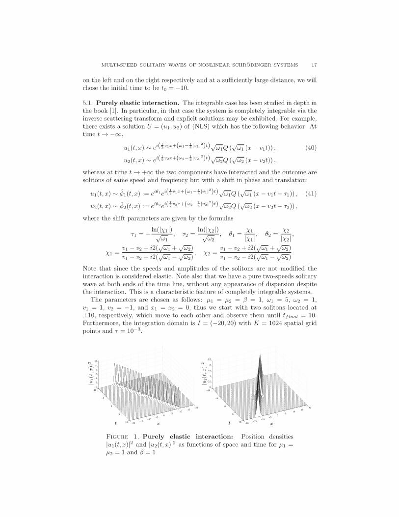
on the left and on the right respectively and at a sufficiently large distance, we willchose the initial time to be t0 = −10.

5.1. Purely elastic interaction. The integrable case has been studied in depth inthe book [1]. In particular, in that case the system is completely integrable via theinverse scattering transform and explicit solutions may be exhibited. For example,there exists a solution U = (u1, u2) of (NLS) which has the following behavior. Attime t → −∞,

u1(t, x) ∼ ei(1

2v1x+(ω1− 1

4|v1|2)t)√ω1Q (

√ω1 (x− v1t)) , (40)

u2(t, x) ∼ ei(1

2v2x+(ω2− 1

4|v2|2)t)√ω2Q (

√ω2 (x− v2t)) ,

whereas at time t → +∞ the two components have interacted and the outcome aresolitons of same speed and frequency but with a shift in phase and translation:

u1(t, x) ∼ φ1(t, x) := eiθ1ei(1

2v1x+(ω1− 1

4|v1|2)t)√ω1Q (

√ω1 (x− v1t− τ1)) , (41)

u2(t, x) ∼ φ2(t, x) := eiθ2ei(1

2v2x+(ω2− 1

4|v2|2)t)√ω2Q (

√ω2 (x− v2t− τ2)) ,

where the shift parameters are given by the formulas

τ1 = − ln(|χ1|)√ω1

, τ2 =ln(|χ2|)√

ω2, θ1 =

χ1

|χ1|, θ2 =

χ2

|χ2|,

χ1 =v1 − v2 + i2(

√ω1 +

√ω2)

v1 − v2 + i2(√ω1 −

√ω2)

, χ2 =v1 − v2 + i2(

√ω1 +

√ω2)

v1 − v2 − i2(√ω1 −

√ω2)

.

Note that since the speeds and amplitudes of the solitons are not modified theinteraction is considered elastic. Note also that we have a pure two-speeds solitarywave at both ends of the time line, without any appearance of dispersion despitethe interaction. This is a characteristic feature of completely integrable systems.

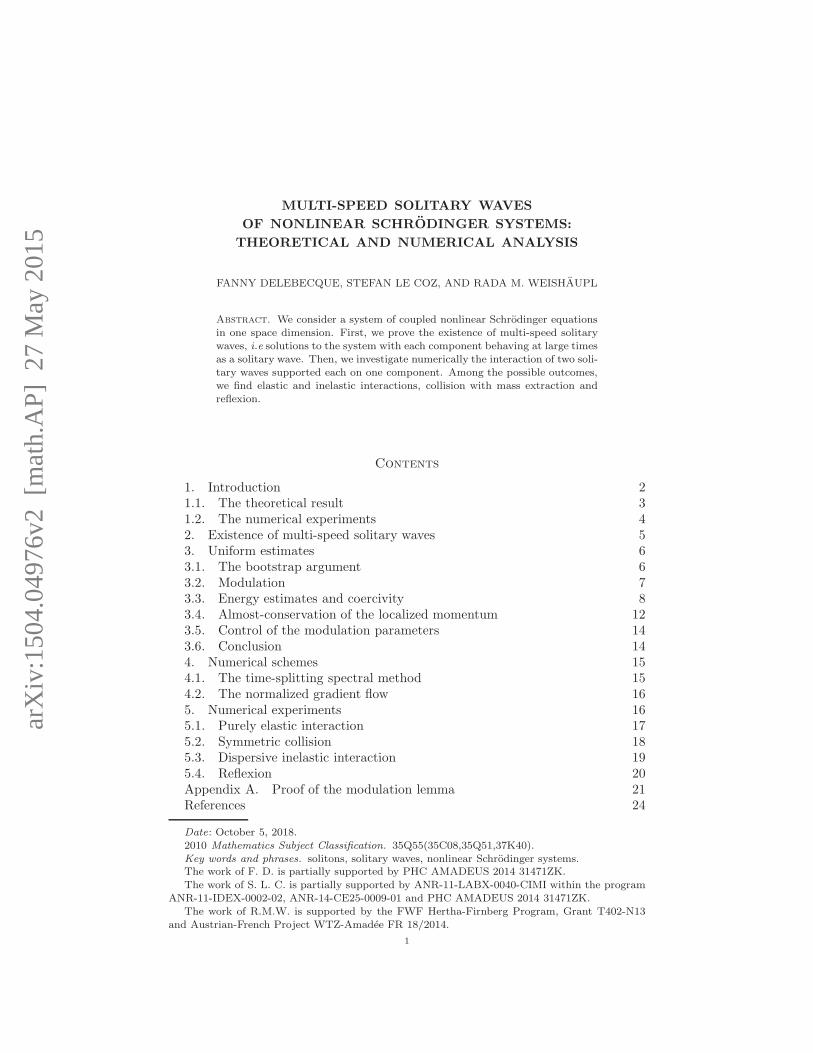
The parameters are chosen as follows: µ1 = µ2 = β = 1, ω1 = 5, ω2 = 1,v1 = 1, v2 = −1, and x1 = x2 = 0, thus we start with two solitons located at±10, respectively, which move to each other and observe them until tfinal = 10.Furthermore, the integration domain is I = (−20, 20) with K = 1024 spatial gridpoints and τ = 10−3.

−10

−5

0

5

10 −20−15

−10−5

05

1015

20

0

2

4

6

8

10

12

xt

|u1(t,x)|

2

−10

−5

0

5

10 −20−15

−10−5

05

1015

20

0

0.5

1

1.5

2

2.5

xt

|u2(t,x)|

2

Figure 1. Purely elastic interaction: Position densities|u1(t, x)|2 and |u2(t, x)|2 as functions of space and time for µ1 =µ2 = 1 and β = 1


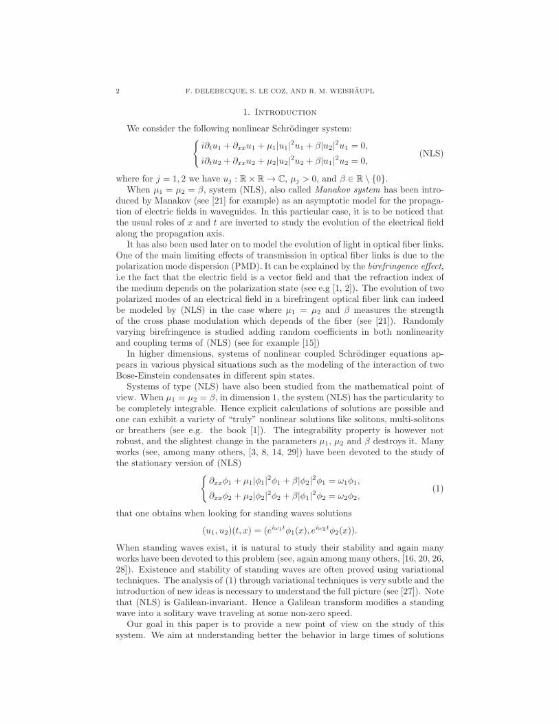
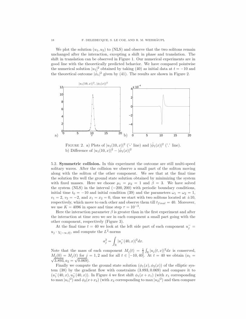
We plot the solution (u1, u2) to (NLS) and observe that the two solitons remainunchanged after the interaction, excepting a shift in phase and translation. Theshift in translation can be observed in Figure 1. Our numerical experiments are ingood line with the theoretically predicted behavior. We have compared pointwisethe numerical solution |u1|2 obtained by taking (40) as initial data at t = −10 and

the theoretical outcome |φ1|2 given by (41). The results are shown in Figure 2.

a)0 5 10 15 20

0

2

4

6

8

10

12|u1(10, x)|

2, |φ1(x)|2

x b) 0 5 10 15 20

−4

−2

0

2

4x 10−4

Figure 2. a) Plots of |u1(10, x)|2 (’-’ line) and |φ1(x)|2 (’.’ line).

b) Difference of |u1(10, x)|2 − |φ1(x)|2

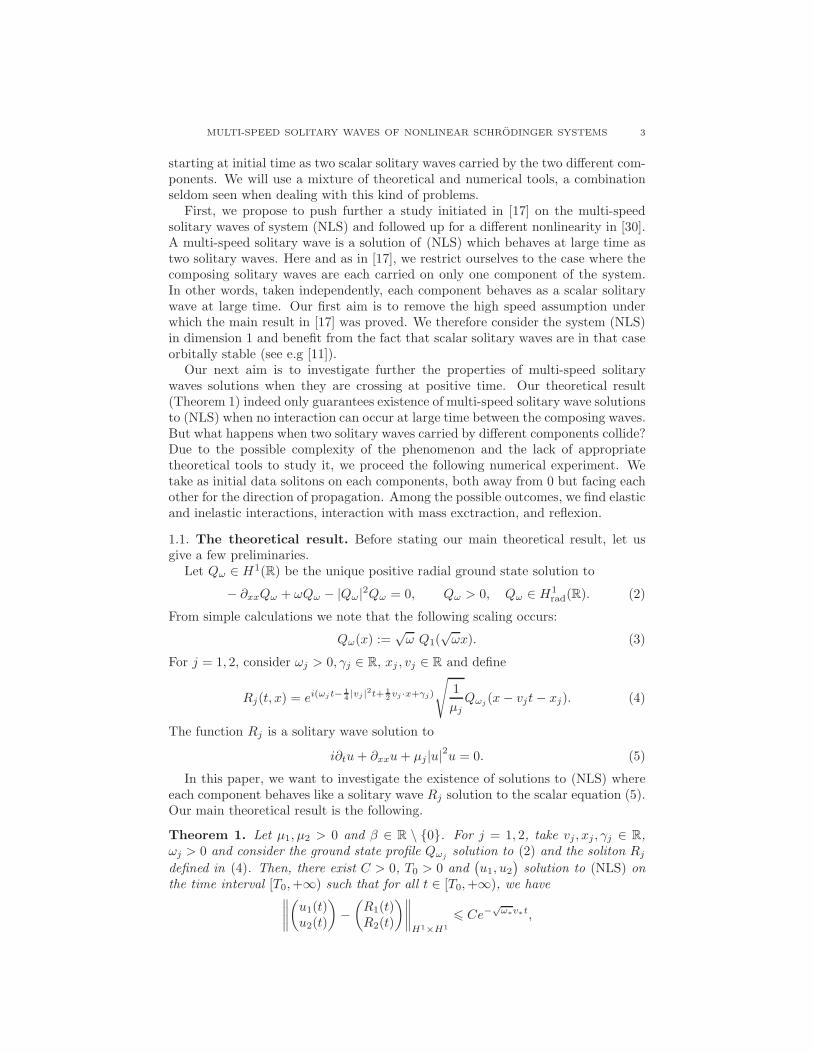
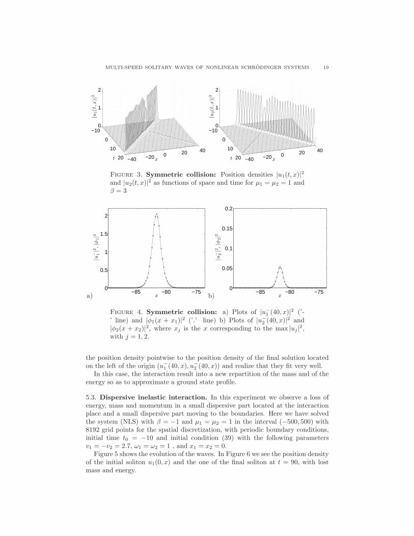
5.2. Symmetric collision. In this experiment the outcome are still multi-speedsolitary waves. After the collision we observe a small part of the soliton movingalong with the soliton of the other component. We see that at the final timethe solution fits well the ground state solution obtained by minimizing the systemwith fixed masses. Here we choose µ1 = µ2 = 1 and β = 3. We have solvedthe system (NLS) in the interval (−200, 200) with periodic boundary conditions,initial time t0 = −10 and initial condition (39) and the parameters ω1 = ω2 = 1,v1 = 2, v2 = −2, and x1 = x2 = 0, thus we start with two solitons located at ±10,respectively, which move to each other and observe them till tfinal = 40. Moreover,we use K = 4096 in space and time step τ = 10−3.

Here the interaction parameter β is greater than in the first experiment and afterthe interaction at time zero we see in each component a small part going with theother component, respectively (Figure 3).

At the final time t = 40 we look at the left side part of each component u−j =

uj · χ[−∞,0], and compute the L2-norms

a2j =

∫

R

|u−j (40, x)|2dx.

Note that the mass of each component Mj(t) = 12

∫R|uj(t, x)|2dx is conserved,

Mj(0) = Mj(t) for j = 1, 2 and for all t ∈ [−10, 40]. At t = 40 we obtain (a1 =√3.893, a2 =

√0.069).

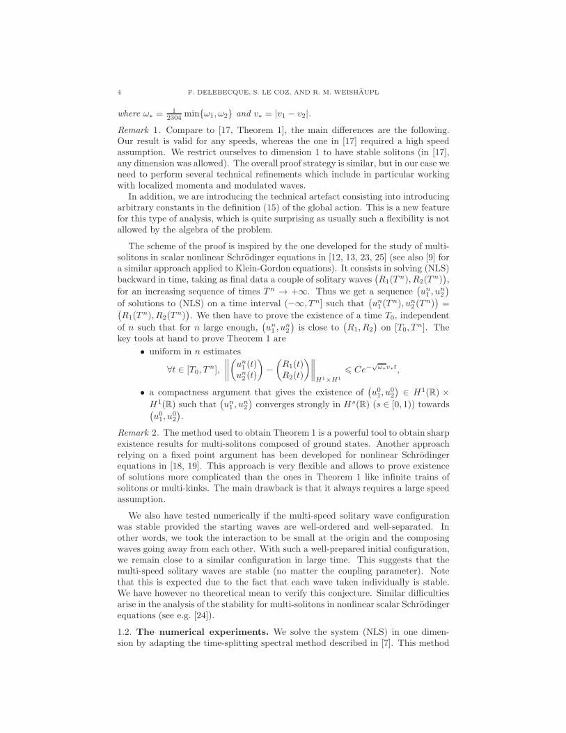
Finally we compute the ground state solution (φ1(x), φ2(x)) of the elliptic sys-tem (38) by the gradient flow with constraints (3.893, 0.069) and compare it to(u−

1 (40, x), u−2 (40, x)). In Figure 4 we first shift φ1(x+ x1) (with x1 corresponding

to max |u1|2) and φ2(x+x2) (with x2 corresponding to max |u2|2) and then compare


−10

0

10

20 −40 −20 0 20 40

0

1

2

xt

|u1(t,x)|

2

−10

0

10

20 −40 −20 0 20 40

0

1

2

xt

|u2(t,x)|

2

Figure 3. Symmetric collision: Position densities |u1(t, x)|2and |u2(t, x)|2 as functions of space and time for µ1 = µ2 = 1 andβ = 3

a)−85 −80 −75

0

0.5

1

1.5

2

x

|u− 1|2,|φ

1|2

b)−85 −80 −75

0

0.05

0.1

0.15

0.2

x

|u− 2|2,|φ

2|2

Figure 4. Symmetric collision: a) Plots of |u−1 (40, x)|2 (’-

’ line) and |φ1(x + x1)|2 (’.’ line) b) Plots of |u−2 (40, x)|2 and

|φ2(x + x2)|2, where xj is the x corresponding to the max |uj|2,with j = 1, 2.

the position density pointwise to the position density of the final solution locatedon the left of the origin (u−

1 (40, x), u−2 (40, x)) and realize that they fit very well.

In this case, the interaction result into a new repartition of the mass and of theenergy so as to approximate a ground state profile.

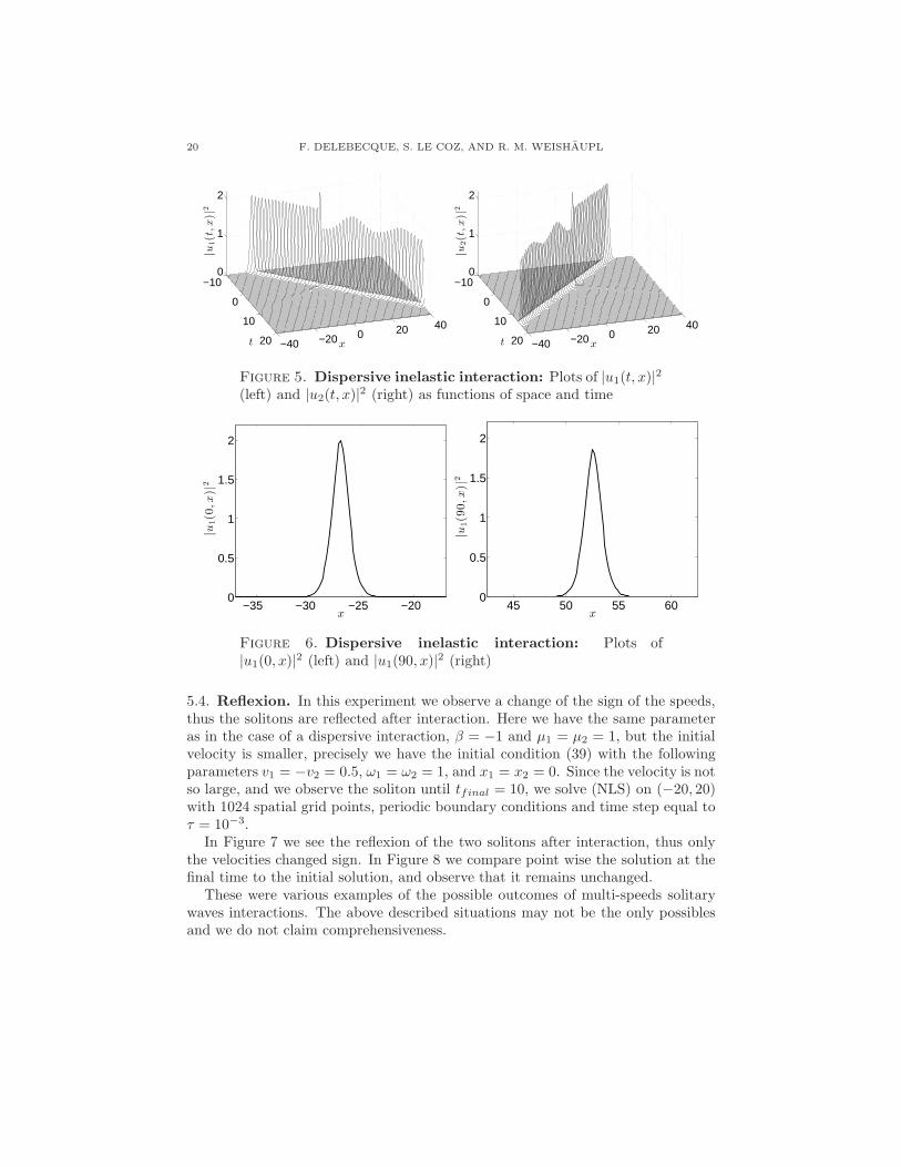
5.3. Dispersive inelastic interaction. In this experiment we observe a loss ofenergy, mass and momentum in a small dispersive part located at the interactionplace and a small dispersive part moving to the boundaries. Here we have solvedthe system (NLS) with β = −1 and µ1 = µ2 = 1 in the interval (−500, 500) with8192 grid points for the spatial discretization, with periodic boundary conditions,initial time t0 = −10 and initial condition (39) with the following parametersv1 = −v2 = 2.7, ω1 = ω2 = 1 , and x1 = x2 = 0.

Figure 5 shows the evolution of the waves. In Figure 6 we see the position densityof the initial soliton u1(0, x) and the one of the final soliton at t = 90, with lostmass and energy.


−10

0

10

20 −40 −20 0 20 40

0

1

2

xt

|u1(t,x)|

2

−10

0

10

20 −40 −20 0 20 40

0

1

2

xt

|u2(t,x)|

2

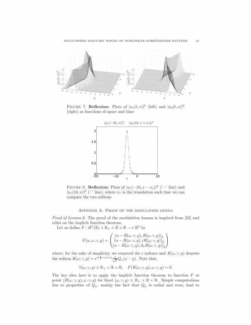
Figure 5. Dispersive inelastic interaction: Plots of |u1(t, x)|2(left) and |u2(t, x)|2 (right) as functions of space and time

−35 −30 −25 −200

0.5

1

1.5

2

x

|u1(0,x)|

2

45 50 55 600

0.5

1

1.5

2

x

|u1(90,x)|

2

Figure 6. Dispersive inelastic interaction: Plots of|u1(0, x)|2 (left) and |u1(90, x)|2 (right)

5.4. Reflexion. In this experiment we observe a change of the sign of the speeds,thus the solitons are reflected after interaction. Here we have the same parameteras in the case of a dispersive interaction, β = −1 and µ1 = µ2 = 1, but the initialvelocity is smaller, precisely we have the initial condition (39) with the followingparameters v1 = −v2 = 0.5, ω1 = ω2 = 1, and x1 = x2 = 0. Since the velocity is notso large, and we observe the soliton until tfinal = 10, we solve (NLS) on (−20, 20)with 1024 spatial grid points, periodic boundary conditions and time step equal toτ = 10−3.

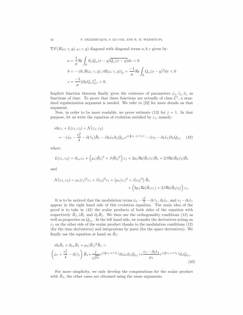
In Figure 7 we see the reflexion of the two solitons after interaction, thus onlythe velocities changed sign. In Figure 8 we compare point wise the solution at thefinal time to the initial solution, and observe that it remains unchanged.

These were various examples of the possible outcomes of multi-speeds solitarywaves interactions. The above described situations may not be the only possiblesand we do not claim comprehensiveness.


−10

−5

0

5

10

−10 −8 −6 −4 −2 0 2 4 6 8 10

0

0.5

1

1.5

2

t

x

|u1(t,x)|

2

−10

−5

0

5

10

−10 −8 −6 −4 −2 0 2 4 6 8 10

0

0.5

1

1.5

2

t

x

|u2(t,x)|

2

Figure 7. Reflexion: Plots of |u1(t, x)|2 (left) and |u2(t, x)|2(right) as functions of space and time

−20 −10 0 100

0.5

1

1.5

2

x

|u1(−10, x)|2, |u1(10, x + x1)|2

Figure 8. Reflexion: Plots of |u1(−10, x− x1)|2 (’−’ line) and|u1(10, x)|2 (’.’ line), where x1 is the translation such that we cancompare the two solitons

Appendix A. Proof of the modulation lemma

Proof of Lemma 6. The proof of the modulation lemma is inspired from [23] andrelies on the implicit function theorem.

Let us define F : H1(R)× R+ × R× R −→ R3 by

F (u, ω, γ, y) =

(u−R(ω, γ, y), R(ω, γ, y))2(u−R(ω, γ, y), iR(ω, γ, y))2(u−R(ω, γ, y), ∂xR(ω, γ, y))2

where, for the sake of simplicity, we removed the i indexes and R(ω, γ, y) denotes

the soliton R(ω, γ, y) = ei(1

2v·x+γ) 1√

µQω(x− y). Note that,

∀(ω, γ, y) ∈ R+ × R× R, F (R(ω, γ, y), ω, γ, y) = 0.

The key idea here is to apply the implicit function theorem to function F atpoint (R(ω, γ, y), ω, γ, y) for fixed (ω, γ, y) ∈ R+ × R × R. Simple computationsdue to properties of Qω, mainly the fact that Qω is radial and even, lead to


∇F (R(ω, γ, y), ω, γ, y) diagonal with diagonal terms a, b, c given by:

a =1

µRe

∫

R

∂ωQω(x− y)Qω(x− y)dx < 0

b = − (∂γR(ω, γ, y), iR(ω, γ, y))2 =−1

µRe

∫

R

Qω(x− y)2dx < 0

c =−1

µ‖∂kQω‖2L2 < 0.

Implicit function theorem finally gives the existence of parameters ωj, γj , xj asfunctions of time. To prove that these functions are actually of class C1, a stan-dard regularization argument is needed. We refer to [22] for more details on thatargument.

Now, in order to be more readable, we prove estimate (13) for j = 1. In thatpurpose, let us write the equation of evolution satisfied by ε1, namely:

i∂tε1 + L(ε1, ε2) +N (ε1, ε2)

= −(ω1 −v214

− ∂tγ1)R1 − i∂tω1∂ωQω1ei(

1

2v1·x+γ1) − i(v1 − ∂tx1)∂xQω1

. (42)

where

L(ε1, ε2) = ∂xxε1 +(µ1|R1|2 + β|R2|2

)ε1 + 2µ1Re(R1ε1)R1 + 2βRe(R2 ε2)R1

and

N (ε1, ε2) = µ1|ε1|2ε1 + β|ε2|2ε1 +(µ1|ε1|2 + β|ε2|2

)R1

+(2µ1Re(R1ε1) + 2βRe(R2 ε2)

)ε1.

It is to be noticed that the modulation terms ω1− v2

1

4 −∂tγ1, ∂tω1, and v1−∂tx1

appear in the right hand side of this evolution equation. The main idea of theproof is to take in (42) the scalar products of both sides of the equation with

respectively R1, iR1 and ∂xR1. We then use the orthogonality conditions (12) aswell as properties on Qω1

. In the left hand side, we transfer the derivatives acting onε1 on the other side of the scalar product thanks to the modulation conditions (12)(for the time derivatives) and integrations by parts (for the space derivatives). We

finally use the equation at hand on R1:

i∂tR1 + ∂xxR1 + µ1|R1|2R1 =(ω1 +

v214

− ∂tγ1

)R1+

j√µ1

ei(1

2v1·x+γ1)∂tω1∂ωQω1

+iv1 − ∂tx1

µ1ei(

1

2v1·x+γ1)∂xQω1

.

(43)

For more simplicity, we only develop the computations for the scalar productwith R1, the other cases are obtained using the same arguments.


Taking the scalar product with R1 in equation (42) leads to:

(i∂tε1 + L(ε1, ε2) +N (ε1, ε2), R1

)2= −

(ω1 −

v214

− ∂tγ1

)‖R1‖2

− ∂tω1Re

∫

R

iei(1

2v1·x+γ1)∂ωQω1

R1dx

− (v1 − ∂tx1)Re

∫

R

iei(1

2v1·x+γ1)∂xQω1

R1dx (44)

Right hand side of (44): First, using equation (11) leads to:

Re

∫

R

iei(1


R1dx =1√µ1

Im

∫

R

∂ωQω1(x)Qω1

(x− x1)dx = 0

and

Re

∫

R

iei(1

2v1·x+γ1)∂xQω1

R1dx =1√µ1

Im

∫

R

∂xQω1(x)Qω1

(x− x1)dx = 0.

Thus, (44) reduces to:

(i∂tε1 + L1(ε1, ε2) +N (ε1, ε2), R1

)2= −

(ω1 −

v214

− ∂tγ1

)‖R1‖2. (45)

Left hand side of (45):

First, deriving modulation condition(ε1, R1

)2= 0 with respect to time gives:

(i∂tε1, R1

)2=(ε1, i∂tR1

)2.

Let us now develop(L(ε1, ε2), R1

)2:

(L(ε1, ε2), R1

)2=(ε1, ∂xxR1 + 3µ1|R1|2R1 + β|R2|2R1

)2+ 2β

(ε2, |R1|2R2

)2.

Finally,(N (ε1, ε2), R1

)2read:

(N (ε1, ε2), R1

)2=(µ1|ε1|2ε1 + β|ε2|2ε1, R1

)2+((µ1|ε1|2 + β|ε2|2)R1, R1

)2

+((

2µ1Re(R1ε1) + 2βRe(R2ε2))ε1, R1

)2

Equation (45) thus leads to the left hand side term:(ε1, i∂tR1 + ∂xxR1 + µ1|R1|2R1

)2+ β

(ε1, |R2|2R1

)2+ 2µ1

(ε1, |R1|2R1

)2

+ 2β(ε2, |R1|2R2

)2+(N (ε1, ε2), R1

)2.

Now, using equation (43) satisfied by R1 gives:(ε1, i∂tR1 + ∂xxR1 + µ1|R1|2R1

)2

= (ω1 −v214

− ∂tγ1)(ε1, R1

)2+ ∂tω1

(ε1,

i√µ1

ei(1


)

2

+ (v1 − ∂tx1)

(ε1,

i√µ1

ei(1

2v1·x+γ1)∂xQω1

)

2

.


Finally, modulation condition(ε1, R1

)2= 0 leads to

(ω1 −v214

− ∂tγ1)‖R1‖2 + ∂tω1

(ε1,

i√µ1

ei(1


)

2

+ (v1 − ∂tx1)

(ε1,

i√µ1

ei(1

2v1·x+γ1)∂xQω1

)

2

= −2µ1

(ε1, |R1|2R1

)2−β(ε1, |R2|2R1

)2−2β

(ε2, |R1|2R2

)2−(N (ε1, ε2), R1

)2.

(46)

Thanks to Lemma 8, it is readily seen that most terms in this equation are of orderO(‖ε‖2). Finally, (46) can be re-written in a simpler way:

(‖R1‖2 + a1(t)

)(ω1 −

v214

− ∂tγ1) + a2(t)∂tω1 + a3(t)(v1 − ∂tx1) = b1(t)

where, for all t ∈ [t0, Tn], |a1(t)|+ |a2(t)|+ |a3(t)|+ |b1(t)| 6 C‖ε(t)‖2.

With the same kind of arguments, taking in (42) scalar product with iR1 and

i∂xR1 respectively, we get two other equations that can be re-written as a linear

system solved by the ”modulation vector” Mod(t) =

ω1(t)− v2

1

4 − ∂tγ1(t)∂tω1(t)

v1 − ∂tx1(t)..

This linear system takes the following form:

(Γ(t) +A(t))Mod(t) = B(t)

where

Γ(t) =

‖R1‖ 0 00

∫R∂ωQω1

(x)Qω1(x− x1(t))dx 0

v12 ‖R1‖ 0 −‖∂xQω1

‖22

and, with the help of Lemma 8, for all t ∈ [t0, Tn], ‖A(t)‖, ‖B(t)‖ 6 C‖ε‖2, and

hence (13). �

References

[1] M. J. Ablowitz, B. Prinari, and A. D. Trubatch. Discrete and continuous nonlinearSchrodinger systems, volume 302 of London Mathematical Society Lecture Note Series. Cam-bridge University Press, Cambridge, 2004.

[2] G. Agrawal. Nonlinear fiber optics. Optics and Photonics. Academic Press, 2007.[3] A. Ambrosetti and E. Colorado. Standing waves of some coupled nonlinear Schrodinger equa-

tions. J. Lond. Math. Soc. (2), 75(1):67–82, 2007.[4] X. Antoine, W. Bao, and C. Besse. Computational methods for the dynamics of the nonlinear

Schrodinger/Gross-Pitaevskii equations. Comput. Phys. Commun., 184(12):2621–2633, 2013.[5] W. Bao. Ground states and dynamics of multicomponent Bose-Einstein condensates. Multi-

scale Model. Simul., 2:210–236, 2004.[6] W. Bao and Q. Du. Computing the ground state solution of Bose-Einstein condensates by a

normalized gradient flow. SIAM J Sci. Comput., 25:1674–1697, 2003.[7] W. Bao, D. Jaksch, and P. Markowich. Numerical solution of the Gross-Pitaevskii equation

for Bose-Einstein condensates. Journal of Computartional Physics, 187:318–342, 2003.

[8] T. Bartsch and Z.-Q. Wang. Note on ground states of nonlinear Schrodinger systems. J.Partial Differential Equations, 19(3):200–207, 2006.

[9] J. Bellazzini, M. Ghimenti, and S. Le Coz. Multi-solitary waves for the nonlinear Klein-Gordon equation. Comm. Partial Differential Equations, 39(8):1479–1522, 2014.


[10] T. Cazenave. Semilinear Schrodinger equations. New York University – Courant Institute,New York, 2003.

[11] T. Cazenave and P.-L. Lions. Orbital stability of standing waves for some nonlinearSchrodinger equations. Comm. Math. Phys., 85(4):549–561, 1982.

[12] R. Cote and S. Le Coz. High-speed excited multi-solitons in nonlinear Schrodinger equations.J. Math. Pures Appl. (9), 96(2):135–166, 2011.

[13] R. Cote, Y. Martel, and F. Merle. Construction of multi-soliton solutions for the L2-supercritical gKdV and NLS equations. Rev. Mat. Iberoam., 27(1):273–302, 2011.

[14] D. G. de Figueiredo and O. Lopes. Solitary waves for some nonlinear Schrodinger systems.Ann. Inst. H. Poincare Anal. Non Lineaire, 25(1):149–161, 2008.

[15] J. Garnier and R. Marty. Effective pulse dynamics in optical fibers with polarization modedispersion. Wave motion, 43(7):544–560, 2006.

[16] H. Hajaiej. Orbital stability of standing waves of some ℓ-coupled nonlinear Schrodinger equa-tions. Commun. Contemp. Math., 14(6):1250039, 10, 2012.

[17] I. Ianni and S. Le Coz. Multi-speed solitary wave solutions for nonlinear Schrodinger systems.J. Lond. Math. Soc. (2), 89(2):623–639, 2014.

[18] S. Le Coz, D. Li, and T.-P. Tsai. Fast-moving finite and infinite trains of solitons for nonlinearSchrodinger equations. Proc. Edinb. Math. Soc. (2), to appear.

[19] S. Le Coz and T.-P. Tsai. Infinite soliton and kink-soliton trains for nonlinear Schrodinger

equations. Nonlinearity, 27(11):2689–2709, 2014.[20] L. A. Maia, E. Montefusco, and B. Pellacci. Orbital stability property for coupled nonlinear

Schrodinger equations. Adv. Nonlinear Stud., 10(3):681–705, 2010.[21] S. V. Manakov. On the theory of two-dimensional stationary self-focusing of electromagnetic

waves. Journal of Experimental and Theoretical Physics, 38, 1974.[22] Y. Martel and F. Merle. Instability of solitons for the critical generalzed Korteweg-de-Vries

equation. Geom. Funct. Anal., 11:74–123, 2001.[23] Y. Martel and F. Merle. Multi solitary waves for nonlinear Schrodinger equations. Ann. Inst.

H. Poincare Anal. Non Lineaire, 23(6):849–864, 2006.[24] Y. Martel, F. Merle, and T.-P. Tsai. Stability in H

1 of the sum of K solitary waves for somenonlinear Schrodinger equations. Duke Math. J., 133(3):405–466, 2006.

[25] F. Merle. Construction of solutions with exactly k blow-up points for the Schrodinger equationwith critical nonlinearity. Comm. Math. Phys., 129(2):223–240, 1990.

[26] E. Montefusco, B. Pellacci, and M. Squassina. Energy convexity estimates for non-degenerateground states of nonlinear 1D Schrodinger systems. Commun. Pure Appl. Anal., 9(4):867–884, 2010.

[27] N. V. Nguyen and Z.-Q. Wang. Existence and stability of a two-parameter family of solitarywaves for a 2-coupled nonlinear Schrodinger system. preprint, 2015.

[28] M. Ohta. Stability of solitary waves for coupled nonlinear Schrodinger equations. NonlinearAnal., 26(5):933–939, 1996.

[29] B. Sirakov. Least energy solitary waves for a system of nonlinear Schrodinger equations inRn. Comm. Math. Phys., 271(1):199–221, 2007.

[30] Z. Wang and S. Cui. Multi-speed solitary wave solutions for a coherently coupled nonlinearschrodinger system. Journal of Mathematical Physics, 56(2):1089–7658, 2015.

[31] M. I. Weinstein. Modulational stability of ground states of nonlinear Schrodinger equations.SIAM J. Math. Anal., 16:472–491, 1985.

(Fanny Delebecque and Stefan Le Coz) Institut de Mathematiques de Toulouse, Univer-

site Paul Sabatier, 118 route de Narbonne, 31062 Toulouse Cedex 9, France

E-mail address, Fanny Delebecque: [email protected]

E-mail address, Stefan Le Coz: [email protected]

(Rada M.Weishaupl) Faculty of Mathematics, University of Vienna, Oskar-Morgenstern-

Platz 1, 1090 Vienna, Austria

E-mail address, Rada M. Weishaupl: [email protected]

multi-speed solitary waves of nonlinear schrödinger systems

Documents