observations of gulf stream ring 83-e and their interpretation using feature models

JOURNAL OF GEOPHYSICAL RESEARCH, VOL. 95, NO. C8, PAGES 13,043-13,063, AUGUST 15, 1990

Observations of Gulf Stream Ring 83-E and Their Interpretation Using Feature Models

SCOTT M. GLENN • AND GEORGE Z. FORRISTALL

Shell Development Company, Houston, Texas

PETER CORNILLON AND GEORGE MILKOWSKI

Graduate School of Oceanography, University of Rhode Island, Kingston

Analysis techniques were developed to track and estimate the propagation velocity, size, shape, orientation, and swirl velocity of Gulf Stream warm core rings. The methods involve fitting idealized warm core ring feature models to observed surface fronts in the satellite imagery, to expendable bathythermograph survey data, and to satellite-tracked drifting buoy data. The ring feature models are analytic structure functions with adjustable parameters. In this case the ring is modeled as an isolated translating elliptic paraboloid with a swirl velocity that increases linearly with distance from the center. Use of the feature models is illustrated with data collected from warm core ring 83-E. Gradient currents based on the bathythermograph survey of ring 83-E and the feature model agree well with currents measured by expendable current profilers. A comparison of the time series of ring 83-E feature model parameters indicates that not only is the feature model analysis of the buoy track an effective method for tracking and monitoring the evolution of Gulf Stream rings, it also provides useful forecasts of ring locations based simply on a persisted propagation velocity. These techniques were used to provide real time support for exploratory deepwater drilling operations off the U.S. east coast.

1. INTRODUCTION

Between Cape Hatteras and the Grand Banks of New- foundland, northward meanders of the Gulf Stream regularly extend far into the slope water region, growing narrower at the base until breaking off as distinct anticyclonic warm core rings. Confined between the continental shelf break and the Gulf Stream, the warm core rings tend to propagate to the west or southwest in the slope water until they are absorbed by another Gulf Stream meander or are forced to coalesce with the Gulf Stream off Cape Hatteras.

Using an airborne infrared radiometer and air-deployed expendable bathythermographs (XBTs), Saunders [1971] observed the formation of a warm core ring from a Gulf Stream meander and tracked the ring as it propagated through a current meter mooring. Gotthardt [1973] later reported the formation of a warm ring larger and more elliptical than Saunder's [1971] ring. Warm core rings also can be readily identified in satellite infrared images of the sea surface either by their warm temperature relative to the slope water or by their entrainment of filaments of colder shelf water or warmer Gulf Stream water. Gotthardt and

Potocsky [1974] used satellite very high resolution radiometer (VHRR) imagery combined with in situ ship and aircraft deployed XBTs to track a warm ring for 4 months until its coalescence with the Gulf Stream. Since 1974, the Marine Climatology Investigation (MCI) (formerly Atlantic Environ- mental Group) of the National Marine Fisheries Service has named approximately 10 warm core rings per year that either form in or propagate into the region west of 60øW. Each

1Now at Department of Earth and Planetary Sciences, Harvard University, Cambridge, Massachusetts.

Copyright 1990 by the American Geophysical Union.

Paper number 90JC00361. 0148-0227/90/90JC-00361505.00

named ring is tracked and its life history reported in year end summaries [e.g., Bisagni, 1976; $ano and Fairfield, 1989]. Lai and Richardson [1977], Richardson et al. [1978], and Halliwell and Mooers [1979] similarly used a combination of the satellite VHRR imagery and in situ XBT data to track warm core rings and determine size, distribution, and lifetime statistics. In addition, Richardson [1980] used satellite- tracked drifting buoys to continuously monitor the long term movement of both the warm rings to the north and the cold rings to the south of the Gulf Stream. The three buoys deployed in warm rings, however, only remained in the rings for about 1 month, a time period much shorter than that observed for cold rings.

More recently, Brown et al. [1986] used the MCI analyses and found that for the 87 warm rings named from 1974 to 1983, the average semi-major axis length at formation was 75 km, the average ring lifetime was 130 days but the distribution was bimodal with averages of 54 days and 229 days for short- and long-lived rings, the average semi-major axis length just before coalescence with the Gulf Stream was 35 km, and the average propagation speed (integrated path length divided by ring lifetime) was 5.6 km/d. Similarly, Auer [1987] used the National Weather Service/National Earth Satellite Service Oceanographic Analysis charts from May 1980 through May 1985 to compute statistics for 115 warm core rings, finding that the average radius at the time of formation was 76 km, the average lifetime was 119 days, and the average propagation speed of 6.8 km/d was much larger than the average propagation velocity of 2.4 km/d, suggesting an erratic propagation path.

Extensive interdisciplinary studies of several warm core rings were conducted in 1981-1982 [Joyce, 1985]. Brown et al. [1983] tracked warm ring 81-D using the digital data obtained from the Advanced Very High Resolution Radiom- eter (AVHRR) on board the NOAA satellites and calculated a time series of ring center locations and of major and minor

13,043

lyo_2

Highlight

lyo_2

Highlight

lyo_2

Highlight

lyo_2

Highlight

lyo_2

Highlight

lyo_2

Highlight

lyo_2

Highlight

13,044 GLENN ET AL.: OBSERVATIONS AND MODELS OF GULF STREAM RING

axes lengths and orientations. Joyce [1984] describes detailed star-shaped XBT and acoustic Doppler current meter measurements made in the same ring. Hooker and Olson [ 1984] report the results of a detailed comparison of ring 82-B center location estimates over a 13-day period derived from the AVHRR, XBTs, conductivity-temperature-depth profilers (CTDs), and a LORAN-C drifting buoy. Evans et al. [1985], Joyce and Kennelly [1985], Olson et al. [1985], and Schmitt and Olson [1985] give detailed accounts of the physical history of 82-B obtained from AVHRR imagery, XBT and CTD surveys, and an acoustic Doppler current profiler. Kunze and Lueck [1986] later report on expendable current profiler (XCP) measurements also made in 82-B. Finally, Joyce and Stalcup [1985] and Kunze [1986] discuss two extensive XBT and XCP surveys conducted on ring 82-I spaced 10 days apart in January 1983.

A warm core ring tracking program set up in 1983-1984 in support of exploratory deepwater drilling operations is discussed by Milkowski et al. [1987]. Guided by AVHRR images of the warm core rings, XBT and XCP surveys were conducted on rings that approached the drill sites. In addition, an Argos-tracked drifting buoy was deployed near ring center to provide continuous estimates of the ring' s position, propagation velocity, and swirl velocity over time. On the basis of these estimates, forecasts giving projected ring arrival dates and expected currents within the rings were transmitted to the drill ship three times per week for 16 months. Of the five rings surveyed and tracked during this program, the most extensive data set was assembled for warm core ring 83-E. A unique aspect of the ring 83-E data set is that the tracking buoy remained in the ring for 2 months, allowing for the first time a continuous comparison of AVHRR data with in situ data over a significant portion of a warm core ring's lifetime.

To aid in the interpretation of the ring 83-E data, we adopt feature models for the kinematic structure of a warm core

ring. The feature models are analytic structure functions with adjustable parameters. The focus of this paper is a description of new techniques for fitting the feature models to typical Gulf Stream ring data, illustration of their use with data we collected in warm core ring 83-E, and reconstruction of the physical history of ring 83-E based on the feature model fits. Section 2 describes the ring 83-E data obtained from the AVHRR, the XBT and XCP survey, and the Argos-tracked drifting buoy. Section 3 discusses the development of the warm core ring feature models and the techniques used to obtain the best fit feature model parameters. Section 4 is a comparison of the time histories of the feature model parameters obtained from the ring 83-E data. In section 5 we summarize our results.

2. RING 83-E OBSERVATIONS

In early April 1983, warm core ring 83-B began to interact with a large northward meander of the Gulf Stream near the New England Seamounts. On the basis of the analyses of available satellite infrared imagery by the National Weather Service/National Earth Satellite Service and the Atlantic

Environmental Group of the National Marine Fisheries Service, ring 83-B was absorbed during the interaction, and warm core ring 83-E was formed just west of the New England Seamounts near year day 111 (April 21). After its formation, ring 83-E was tracked in near real time using

digital AVHRR data available from the NOAA 6, NOAA 7, and NOAA 8 satellites (Plate 1). (Plate 1 is shown here in black and white. The color version can be found in the

separate color section in this issue.) The data analysis techniques used to process the AVHRR data are discussed by Milkowski et al. [ 1987] and are briefly reviewed here. The images were carefully navigated (i.e., the correspondence between display coordinates, satellite coordinates, and geodetic coordinates were established). The software to accom- plish this makes use of high-resolution ephemerides (satellite positions) as a first guess of the location of the data in the geodetic coordinate system. The analyst adjusts the position and attitude of the satellite to minimize the separation between the continental outline (displayed over the image in a graphic overlay) and the land-water boundary evident in the satellite data. These corrections are generally quite small, of the order of several pixels (approximately 1 km 2 each). An experienced operator can navigate a satellite pass to within a single pixel, 1 km. Following navigation, NOAA 7 data were atmospherically corrected using the two-channel algorithm of McClain et al. [ 1985] to produce SST fields from the radiance data. For NOAA 6 and NOAA 8, which do not have the two spectral channels in the 9- to 11-/zm window required by the split window technique, channel 4 radiances were used. Finally, the SST and channel 4 radiance fields were remapped (rectified) to a 512 x 512 element image using a pseudo-Mercator (f plane) projection.

Beginning late on day 164 (June 13), a 2-day shipboard XBT and XCP survey was conducted on ring 83-E near 39øN, 70øW (Plate lb). The drop locations of the 45 XBTs deployed in ring 83-E are superimposed on the contours of the 10øC isotherm depth in Figure la. The 10øC depth contours were generated using a combination of Laplacian and spline interpolation with an over-relaxation procedure to interpolate the XBT data to a regular grid. A sample XBT section through the approximate ring center from southwest to northeast is given in Figure 2. The strongest horizontal temperature gradients are confined to the upper 200 m, while the 6øC isotherm near 500 m is relatively flat. The maximum depth of the 10øC isotherm barely exceeds 350 m, which can be compared to 350 m for 82-1, 550 m for 82-B, 700 m for 81-D, 600 m for Richardson et al.'s [1978] ring J, and in excess of 400 m for Saunders' [1971] ring.

During the XBT survey, 18 XCPs were successfully deployed concentrated in regions with large horizontal temperature gradients. The XCP probe falls through the water at about 5 m/s while measuring the electric potential generated by the motion of sea water through the Earth' s magnetic field [Sanford et al., 1982]. Data from the probe are sent back to the surface on an XBT wire. Current versions of the XCPs

use a radio transmitter floating on the surface to send the data back to the ship, but on our early models the wire link ran directly to the processor. To avoid magnetic interference from the ship's hull, a fuse was used to release the probes from foam floats once they had drifted some distance astern. The XCP measures velocity relative to a generally small but unknown reference velocity that is constant with depth. On the assumption that the swirl velocity of ring 83-E was surface intensified and insignificant below 600 m, the reference velocity was estimated following Sanford et al. [1987] by averaging the velocity between 600 m and the bottom of the profile, which usually was near 900 m. This reference velocity, which usually was less than 5 cm/s, was subtracted

GLENN ET AL ' OBSERVATIONS AND MODELS OF GULF STREAM RING 13,045

. ,,•-•:::,' '.;..?.•' . •':" .......•.!

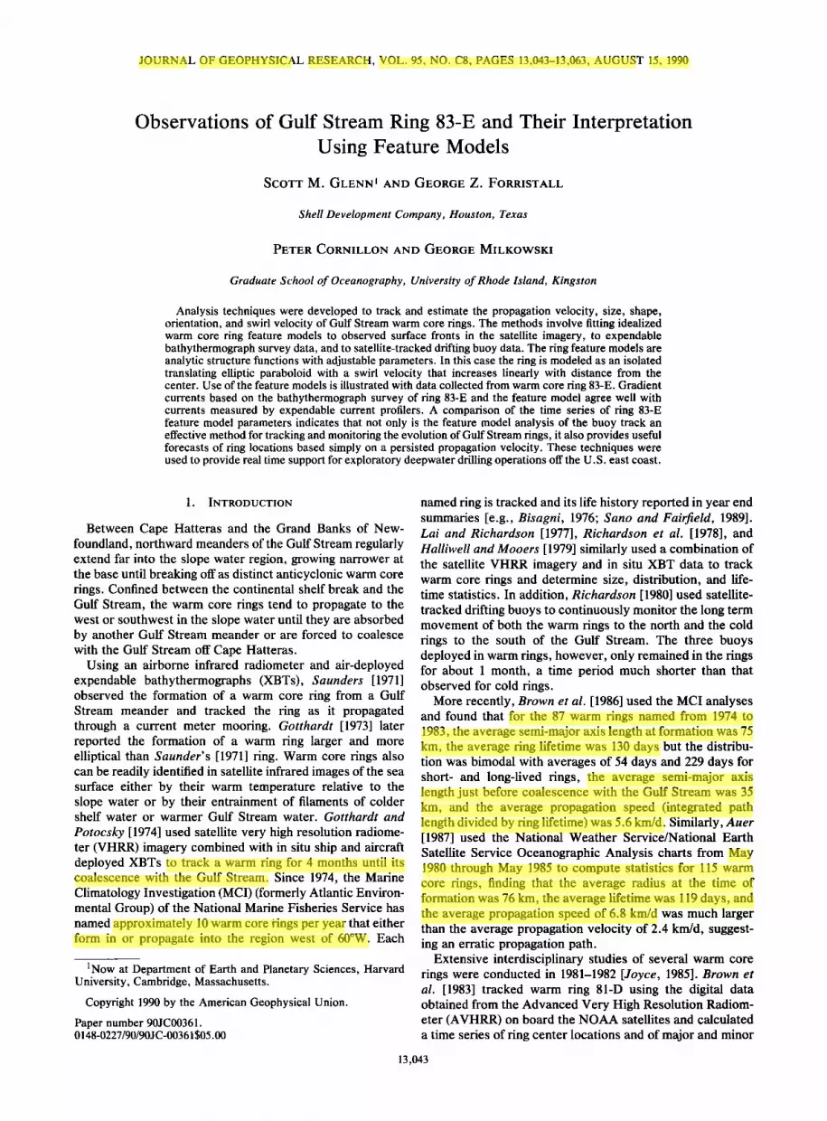
Plate 1. History of ring 83-E as observed in the satellite AVHRR imagery. (a) Day 118, 39.19øN, 67.97øW: after formation. (b) Day 165, 38.90øN, 69.82øW, start of the sucvey; (c) Day 174, 38.91øN, 70.06øW: interaction with a Gulf Stream meander. (d) Day 195, 38.57øN, 71.61øW: relative isolation from the Gulf Stream. (e) Day 221, 37.84øN, 72.96øW: prior to loosing the tracking buoy. (f) Day 252, 36.88øN, 74.39øW: prior to absorption. Ring center locations are derived from feature model fits to a single isotherm contour around the ring. The buoy track is superimposed on Plates lc-le; the arrow marks the buoy location at the time of the image. (The color version of this figure can be found in the separate color section in this issue.)

13,046 GLENN ET AL.' OBSERVATIONS AND MODELS OF GULF STREAM RING

39.5øN

• 39.0øN

38.5øN

70.5øW 70.0øW 69.5øW

Longitude

WARM CORE RING 83-E XBT DROP LOCATIONS.

69.0øW

39.5øN

• 39.0ON- ,,•

30 c•/s O

38.5øN

70.5øW 70.0øW 69.5øW

Longitude

WARM CORE RING 83-E XCP 50 M. VELOCITY VECTORS

69 0øW

Fig. 1. XBT and XCP survey coverage of ring 83-E' (a) XBT drop locations and the depth in meters of the 10øC isotherm, and (b) XCP velocity vectors at 50 m and the depth in meters of the feature model fit to the 10øC isotherm. XBTs 38 and 39 and XCP 6 are labeled.

from each profile. Similar analysis procedures were followed by Kunze and Lueck [1986] and Kunze [1986] for XCPs deployed in warm core rings.

Figure lb shows velocity vectors obtained by averaging the resulting XCP profiles from 45 m to 55 m depth to give a representative near surface current. The largest near surface currents were found in a band about 15-35 km from ring center on the north side. The nonzero velocity at ring center is associated with strong fluctuations similar to those identified by Kunze and Lueck [1986] and Kunze [1986] as near-inertial waves trapped by the ring. A hodograph of the

5 øC - •00

,,•,• 300

400

500

0 10 20 30 40 50 60 70

Range (kilometers)

WARM CORE RING 83-E XBT SECTION.

Fig. 2. Vertical XBT section in ring 83-E from southwest to northeast approximately through ring center. XBT drop locations are marked by arrows.

XCP dropped at ring center (38.97øN, 69.71øW) is plotted in Figure 3a. The velocity vector turns clockwise with depth consistent with a downward propagating near-inertial wave. The velocity fluctuations are largest near 250 m, just below the region with the strongest horizontal temperature gradients observed in Figure 2. Kunze and Lueck [1986] and Kunze [1986] observed the largest near-inertial wave ampli- tudes just below the high negative vorticity core of rings 82-B and 82-I. In Figure 3b the current speed profile from XCP 6 deployed in the high swirl velocity region (39.05øN, 69.37øW) is plotted as the solid line. The velocity profile indicates there is substantial shear in the upper 300 m, in contrast to Kunze and Lueck's [1986] ring 82-B XCP measurements which showed virtually no shear in a thick ther- mostat. The velocity maximum in Figure 3b is subsurface, similar to Kunze's [1986] measurements in 82-I. Joyce and Stalcup [1985] point out that the subsurface velocity maximum in 82-I was consistent with a reversal in the horizontal

density gradient observed at that depth. The maximum speed in Figure 3b is about 39 cm/s near a depth of 50 m, the maximum recorded by an XCP in ring 83-E. This speed is less than the peak speeds of 50 cm/s found by Kunze [1986] in 82-I, 1 m/s found by Joyce and Kennelly [1985] in ring 82-B, 2 m/s found by Joyce [1984] in ring 81-D, and 70 cm/s found by Saunders [1971]. Ring 83-E was surveyed west of the measurement sites of 81-D and 82-I, but east of the measurement sites of 82-B and Saunders' [1971] ring. Even though all five rings were 1-2 months old at the time of the measurements, ring 83-E was weaker than the previous rings.

A number of the XBTs were deployed on lines through the center of 83-E, so reasonable estimates of azimuthal gradient currents could be calculated. Since no salinity measurements were made on the cruise, the standard reference T-S curve of Armi and Bray [ 1982] was used to calculate dynamic heights. Joyce [1984] found good agreement between the standard curve and a CTD cast from the center of ring 81-D. Velocities were calculated from the dynamic heights using the gradient current equation

GLENN ET AL.' OBSERVATIONS AND MODELS OF GULF STREAM RING 13,047

:3O I I I I I I I I I I

25

20

15

1o 1oo n•.,•

-g0

-•0

I I I I 15 I I • I I I -30 -25 -20 -15 -10 - 0 5 I 15 20 25 30

U - East (era/see)

WARM CORE RING 83-E CENTER XCP HODOGRAPH.

Fig. 3a

0

•,,"• 100

200

• 300-

//

400 -

500 //'"/ Legend XCP 6

XBT 58-59

600 I

o ,o ,,o Speed (cm/s ec)

Fig. 3b

Fig. 3. XCP measured velocity profiles in ring 83-E: (a) Hodograph of the ring center XCP profile from a depth of 100 m to 400 m, and (b) current speed profile in the high swirl velocity region measured by XCP 6 and calculated from XBTs 38 and 39 using the gradient current relation.

u 2 OD fu ....

r Or

Since the velocities in 83-E were rather small, the centripetal term in equation 1 changes the results by only about 10%. The dashed line in Figure 3b shows the gradient current between XBTs 38 (39.05øN, 69.37øW) and 39 (39.01øN, 69.49øW). The velocity is relative to a level of no motion at 600 m. The gradient current is very similar to that measured by the nearby XCP except for the higher speed measured by the XCP near 50 m.

40øN { /l' ' I .-"J , r") ,," / . ,.-leo

E 38oN --t / 22OP/' - •"%',•,•*•o / / .-'

I / ,/ -• '""" / / ,,"

37øN t III I'/ '"' IIoo ,'

75øW 74øW 73øW 72øW 71 øW 70øW 69øW

Longitude

WARM CORE RING 83-E BUOY TRACK.

Fig. 4. Track of the Argos buoy deployed in ring 83-E. The first observation of each day is marked with a circle. Numbers are year days. Depth contours are 200 m, 2000 m, and 4000 m.

As the shipboard XBT and XCP survey of ring 83-E was nearing completion, the approximate ring center was determined from the available XBT data by the method to be discussed in section 3.2. An Argos tracked drifting buoy drogued at 100 m was deployed near the ring center on day 166 (June 15) at 38.97øN, 69.70øW as measured by the shipboard LORAN. After the survey, ring 83-E was tracked in real time using the Argos buoy locations and the AVHRR imagery. Except for a brief encounter with a Gulf Stream meander on days 174-175 (Plate lc), ring 83-E drifted to the southwest, parallel to the shelf break, away from the imme- diate influence of the Gulf Stream (Plate ld). The Argos buoy tracked 83-E until it spun out on day 230 (August 18) (Plate l e). Later, on day 239 (August 27), the buoy ran aground in 100 m of water at 37.75øN, 74.24øW, where it remained for 4 days, indicating that the drogue was still attached. After the Argos buoy left ring 83-E, we continued to track the ring in the satellite imagery until it was absorbed by the Gulf Stream off Cape Hatteras near day 254 (Septem- ber 11) (Plate lf). A total of 66 AVHRR images of ring 83-E were analyzed, 36 of which occurred between the start of the shipboard survey and the day the Argos buoy left the ring.

The buoy track for days 166-230 is plotted in Figure 4. The circles mark the first reported position of each day. Although it is possible to obtain 6-10 new Argos buoy positions per day, communication procedures with Service Argos were not finalized until day 182, resulting in the partial loss of data over the first 2 weeks of the buoy deployment. For days 166-170, only 1-2 positions per day were recovered, and for days 171-181, only 3-6 positions per day were recovered. Beginning on day 182, however, all the buoy locations obtained by Service Argos were saved and are included here. Note that no buoy locations were available on day 218. The buoy completed about 10 loops around the ring center as 83-E propagated to the southwest through the slope water. Inertial waves appear in the buoy trajectory after day 203 as the small crescents superimposed on the large loops. The inertial waves slowly decay until they are no longer obvious after day 211. Appearance of the inertial waves coincides

lyo_2

Sticky Note

speed ~ 500km/(230-170days) ~ 8km/day.

lyo_2

Highlight


with the passage of a severe storm in which gale force winds were reported in the vicinity of ring 83-E [Mariners Weather Log, 1984].

3. WARM CORE RING FEATURE MODELS

Historical observations of warm core rings indicate that the horizontal structure viewed in AVHRR data often is

approximately elliptical, that vertical XBT temperature sec- tions usually have a parabolic bowl shape, and that the ring swirl velocity increases almost linearly with radius over much of the ring's interior. This shape resembles a theoret- ical warm core ring in geostrophic balance and undergoing solid body rotation, which leads to parabolically shaped isopycnals. Dynamical models of rings [Flied, 1977, 1979; Csanady, 1979; Nor, 1983, 1985; Cushman-Roisin et al., 1985; Cushman-Roisin, 1989] often assume a simplified circular or elliptical shape with parabolic interfaces. In the Gulf Stream region, Robinson et al. [1988] use analytic feature models of the Gulf Stream and rings with adjustable parameters to obtain the necessary three-dimensional velocity structure to initialize a dynamical model from commonly available oceanographic data. The swirl velocity in the warm core ring feature model initially increases linearly with radius, then drops off exponentially. Adjustable feature model parameters such as the ring center location, maximum swirl velocity, and ring radius are estimated from satellite imagery and XBT data. The analysis techniques adopted here also make use of the feature model approach and could provide an efficient means of estimating the ring feature model parameters for input to dynamical models.

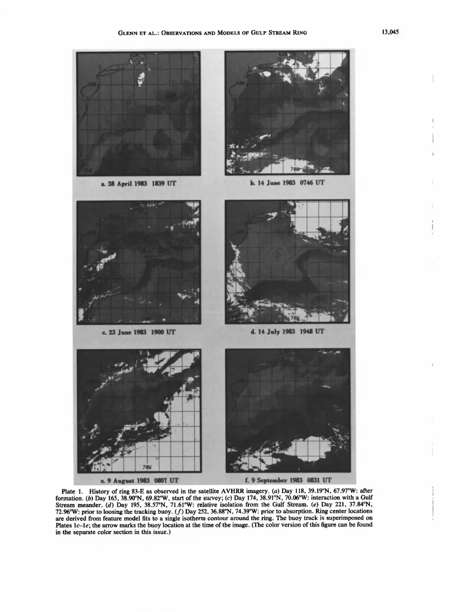
The warm core ring feature models used here for data analysis are based on the conceptual model of a warm core ring shaped like an elliptic paraboloid with a linearly increasing swirl velocity. The feature models are fit to the AVHRR imagery, the XBT data, and the Argos-tracked drifting buoy locations to obtain the best fit feature model parameters. The time histories of the best fit parameters then are compared and used to interpret the life histories of a ting. Brown et al. [1983] adopted this technique and fit ellipses to digitized isothermal contours around rings observed in the satellite sea surface temperature data. Their ellipse-fitting routines are adopted here. Hooker and Olson [1984] describe the simple extension of Brown et al.'s [1983] technique to XBT survey data, suggesting that the locations of a given isotherm at a single specified depth around the ring could be found by interpolation so that the same ellipse-fitting routines could be used. The feature model fitting routine developed here for the XBT data adopts a new approach that fits the isotherm depth measured by every XBT directly. Kirwan et al. [1984] used a translating ellipse feature model to analyze Argos buoy data collected in several Gulf of Mexico warm eddies. Their original analysis technique required significant preprocessing of the buoy location data (conversion to velocities, resampling, and filtering), followed by subjective determina- tion of the six velocity values that were used to determine six feature model parameters. In contrast, the fitting routine developed here makes use of all the buoy location data directly, eliminating the preprocessing and the subjective choice of velocity points.

The analytic structure functions for the warm core ring feature models are formulated in the standard coordinate

system pictured in Figure 5. The x, y coordinate system is

Y1

.... X X 1 I I

I Xo

Fig. 5. Coordinate system definition for the feature model structure functions.

fixed with x positive to the east and y positive to the north. The x l, Y l axes have the same orientation as x, y, but the x l, Yl origin is located at ring center (x = Xo, y = Yo). The x2, y2 axes share a common origin with Xl, Y l but are oriented at an angle 0 with respect to x l, Y l. The angle 0 is measured positive counterclockwise from east and is chosen so that the x2 axis is in line with an axis of the elliptic paraboloid. The vertical coordinate is measured positive upward from z = 0 at the ocean surface. Latitudes • and longitudes A are transformed into the x, y coordinate system using standard f or •3 plane projections

x = (A- Ac) cos •c (2) I+C

y = s(• - •c) (3)

where the x, y origin is assumed to be located at the central latitude •c and longitude A c, the scale factor s (= 111.12 km/deg) converts degrees to horizontal distances, and the optional fl plane correction factor C is given by

s

C = - (• - •c) tan •c (4) R

where R is the radius of the Earth. Since Gulf Stream ring radii usually are less than about 100 km, the •3 plane correction factor often is less than 0.01, and f plane navigation (C = 0) is sufficiently accurate.

Once the data have been located in the x, y coordinate system, feature models are fit to the satellite sea surface temperature field, the three-dimensional XBT temperature and derived dynamic height fields, and the Argos buoy track by the method of least squares. The feature models used for each data type are described separately in the next three subsections. In section 4 the results of the feature model

analysis are presented and compared.

3.1. A VHRR Feature Model

Warm core rings are identified in the satellite-derived imagery either by their warm sea surface temperature rela-

GLENN ET AL.: OBSERVATIONS AND MODELS OF GULF STREAM RING 13,049

tive to the slope water, or by the anticyclonic circulation patterns generated by the entrainment of warmer Gulf Stream or colder shelf water. We assume that the observed

warm core ring is approximately elliptical, and that closed contours around the ring can be subjectively identified and digitized. The contour digitization was performed by two analysts. The first analyst digitized as many separate, closed contours as were visible when the image was displayed on a 512 x 512 color monitor (typically 3 to 15). Analyst 1 concentrated on images available while the Argos buoy was in ring 83-E. The second analyst digitized the one contour that appeared to best represent the ring in each image for the entire life cycle of ring 83-E. An ellipse then was least squares fit [Brown et al., 1983] to each of the contours. The ring parameters available from the fits are the ring center location, the major and minor axis lengths, and the orientation of the semi-major axis measured counterclockwise from east. Multiple estimates of the ring center, axis lengths, and orientation obtained by the first analyst for each satellite pass were averaged. Ring propagation velocities were estimated by differencing the center locations obtained from subsequent satellite images.

The ellipse fitting method of estimating ring parameters also was compared to the perpendicular bisector method described by Hooker and Olson [1984]. In a detailed comparison, Cornilion et al. [1989] found that the two methods returned essentially the same results for ring 83-E. Hooker and Olson [ 1984] had also compared these two methods with a third estimate, that of simply averaging all the digitized points around a closed contour. They found that for ring 82-B the ellipse-fitting method and the perpendicular bisector method generated superior but comparable results. Be- cause the ellipse-fitting procedure of Brown et al. [1983] is conceptually similar to the approach adopted for the XBTs and Argos-tracked buoy, and because it generated similar results to the perpendicular bisector method for two very different rings, the method is adopted here.

3.2. XBT Feature Model

Olson and Spence [ 1978] describe a method of determining Gulf Stream ring center positions from star-shaped XBT surveys. A six-pointed star survey pattern was performed located around the approximate ring center (in this case a cold ring) determined from an initial XBT transect. The location of the intersection of a selected isotherm with a

selected depth was determined by interpolation, giving 12 points around the ring. The points were connected with line segments, and the perpendicular bisectors of each line were segment drawn. The intersections of the perpendicular bisectors were averaged and taken as the ring center. They estimated that this method gives the ring center to within +5 km. Hooker and Olson [1984] applied this method to a five-pointed star survey of warm core ring 82-B. They discuss an iterative procedure that discards perpendicular bisector intersections greater than 2 standard deviations from the mean location, recalculates the mean and standard deviation, and repeats the procedure until the minimum standard deviation and thus the optimum center location is found. They also indicate that the center estimates using these techniques are reproducible to within 5-7 km but that the optimization routines require the XBT data to be smoothed by a 10-km averaging window. As a simple alter-

native, Joyce and Stalcup [1985] calculated the centroid of the average temperature from 200 m to 400 m from selected XBTs deployed in ring 82-1 and found that the centroid agreed to within 6 km of estimates generated using Hooker and Olson's [1984] techniques.

For the method developed here, isothermal surfaces obtained from the XBT surveys of warm core rings are assumed to have the characteristic bowl shape. Any one of these isothermal surfaces can be mapped into the x, y coordinate system of Figure 5 and an elliptic paraboloid feature model fit by the method of least squares. The expression for an elliptic paraboloid in the x2, Y2 system is

x• y• z a2+• l+- d

(5)

where a and b are the ellipse semi-axis lengths at the surface and d is the paraboloid center depth. Applying the usual transformations to the x, y coordinate system, the equation for the depth of the isotherms given by an elliptic paraboloid feature model centered at x0, Y0 and oriented at an angle 0 with respect to the x axis becomes

z(x,y)=-d{1 [(x-x0) cos0+(y-y0)sin0] 2 a 2

[-(x- x0) sin 0 + (y -Y0) cos 0] 2} - b2 (6)

The ring is assumed to remain stationary (x 0, Y0, and 0 are constant) without change of size (a, b, and d are constant) over the time period of the XBT survey.

Each XBT drop defines an isotherm depth Zi at a given location Xi, Yi. Values for the unknown model parameters (x0, Y0, a, b, 0, and d) are determined by fitting the feature model (equation (6)) to the XBT isotherm depths. The best fit values for the model parameters are taken to be the values that minimize the sum of the squared distances between the XBT measured isotherm depths, Zi, and the modeled isotherm depths, z(Xi, Yi), computed from (6)

N

S--' Z [Zi- z(Xi, yi)]2 i=1

(7)

where N is the number of XBT drops. A minimum of six XBT drops are needed to uniquely determine the six model parameters. Practical experience has shown that at least one XBT drop should be located in each quadrant of the ellipse. If one quadrant is left empty, the least squares fitting routine may form a hyperbolic paraboloid opening in the unconstrained quadrant.

Using the f plane approximation, the latitude and longitude of all the XBTs dropped in ring 83-E were transformed into the x, y coordinate system. The elliptic paraboloid feature model was fit to the depth of each whole numbered isotherm from 6øC to 19øC. Between 31 and 46 XBTs were

used for each fit. The average center location, aspect ratio (b/a), and axis orientations then were calculated by averaging the 14 individual results from each isotherm. In addition, the elliptic paraboloid feature model was fit to the dynamic height calculated from each of the XBT profiles as described in section 2. All ring parameters determined from the XBT


feature model fits were assigned to the average time of the survey.

3.3. Argos Buoy Feature Model

The looping motion of Argos tracked drifting buoys deployed in warm core rings is generated by the orbital motion of the buoy about a propagating ring center. Methods used to determine the ring center location, center propagation velocity, and the ring swirl velocity from a time series of buoy positions have been described by Richardson et al. [1979] and Kirwan et al. [1984, 1988].

Richardson et al. [1979] first limited their buoy data to the two best fixes per day to reduce the buoy location error. A cubic spline was used to resample the good fixes at equal 12 hour intervals. The resampled buoy positions were used to plot buoy trajectories and calculate buoy velocities. These results were used to infer the ring center position and propagation velocity, along with the buoy orbital period, radius, and tangential swirl velocity.

Kirwan et al. [1984] also used a cubic spline to resample their Argos buoy position data at equal time intervals. The resampled positions were used to compute the north-south and east-west components of the buoy velocity. The velocity time series then were low-pass filtered to remove high- frequency contamination such as inertial oscillations. Three successive extremes finally were chosen subjectively from each filtered velocity component to solve for the six inde- pendent parameters representing a ring center propagation velocity and an elliptical and exponentially diverging swirl velocity. An improved analysis technique was described by Kirwan et al. [1988], but the data processing required was even more labor intensive. The original position data was edited, resampled, and filtered; the time derivatives then were calculated to fourth-order accuracy, edited, resampled, and filtered; and finally the feature model parameters were calculated, edited, resampled, and filtered. Using these editing and processing techniques for several buoys deployed in Gulf of Mexico warm eddies, Kirwan et al. [1988] found that a data window consisting of only seven 6-hour time intervals could be marched through the resampled data to generate a time series of feature model parameters. Although this technique has the advantage over that of Kirwan et al. [1984] in that it does not require the feature model parameters to be constant for one full revolution of the buoy, it comes with the warning that inconsequential errors in the buoy position data can be amplified first by the conversion to velocities and even further by the inversion to feature model parameters.

Rather than using a time series of derived buoy velocities, the analysis technique presented here works directly with the original, irregularly spaced in time, buoy position data. The feature model assumes the buoy trajectory is composed of an orbital motion about a propagating center and deter- mines the model parameters by a least squares fit to the buoy positions. This eliminates the need to resample and filter the data and to calculate time derivatives. Because all of the

position data are used for the model fit, the subjective choice of extrema required by Kirwan et al. [1984], and the necessary low pass filtering to aid that choice, is eliminated. The resulting technique is considerably streamlined and is easily automated, requiring the potential user only to specify what section of the trajectory is to be fit in order to evaluate ring location, propagation, and orbital parameters.

As before, the feature model equations are developed in the coordinate systems shown in Figure 5. In the x2, Y2 coordinate system, the equations for a linearly diverging, elliptical orbit centered at x2 = Y2 = 0 are

x2(t) = a(1 + Dt) cos (- oat + qb) (8)

Y2(t) = b(1 + Dt) sin (-oat (9)

In these equations, t is time, a and b are the semi-axis lengths, D is the divergence, oa is the angular frequency of the buoy orbit, and qb is the t = 0 phase of the buoy orbit. For ease in interpretation here, the buoy orbit is assumed to be anticyclonic for oa > 0. The buoy swirl velocity is given by the time derivatives of (8) and (9).

dx2 = aoa(1 + Dt) sin (-oat + &) + aD cos (-oat + qb) (10)

dy2 = -boa(1 + Dt) cos (-oat + &) + bD sin (-oat

(11)

The buoy angular momentum per unit mass about the x2, Y2 origin becomes

dy2 dx2

x2 -•-- Y2 -•-= -(1 + Dt)2aboa (12) Note that the buoy swirl velocity is maximum (minimum) along the semi-minor (semi-major) axis, and that only when the divergence is zero is the angular momentum per unit mass constant and equal to -aboa.

Assuming that the ring center propagation velocity is constant and applying the usual transformations, the equations for the buoy track in the x, y coordinate system can be written as

x(t) = Xo + ut + (1 + Dt)[a cos 0 cos (-oat

- b sin 0 sin (-oat + qb)] (13)

y(t) = Yo + vt + (1 + Dt)[a sin 0 cos (-oat

+ b cos 0 sin (-oat + qb)] (14)

where u and v are the x and y components of the center propagation velocity, and x0, Y0 is the t = 0 center position.

The buoy track feature model parameters (x0, Y0, u, v, a, b, D, 0, oa, and 40 then are determined by finding the least squares fit to a given set of buoy positions. Argos buoy latitude and longitude time series can be mapped into the x, y coordinate system using (2) and (3) to generate a buoy location Xi, Yi for each time T i. Evaluating feature model equations (13) and (14) at T i gives the modeled buoy location, defined here as x(Ti), y(Ti). The least squares fit model parameters are found by minimizing the sum of the squared distances between the actual buoy positions, Xi, Yi, and the modeled buoy positions x(Ti), y(Ti)

N

S = Z {[Xi- x(ri)] 2 + [Yi- y(ri)] 2} i=1

(15)

Because there are 10 free model parameters, at least 10 buoy locations are required to obtain a unique fit. As with the XBT


feature model, practical experience has shown that data should be available in all four quadrants to force the ellipse to close with reasonable model parameters. This translates into the requirement that each feature model fit use close to one full orbit of buoy location data. The model parameters are assumed to remain constant for that orbital time period.

In (13) and (14) the linear divergence factor (1 + Dt) is simply the truncated Taylor series expansion of an exponential factor e Dt. The exponential factor could have been used following Kirwan et al. [ 1984]; however, the resulting deriv- ative of S with respect to D gives an equation that cannot be solved explicitly for D. When the linear divergence factor is used, a simple explicit solution for D is obtained. Because the explicit solution greatly simplifies the search for model parameters that minimize S, the linear divergence factor is adopted here. If ]Dt] is usually small, as was noted by Kirwan et al. [1984] for three buoys deployed in a Gulf of Mexico warm eddy, there should be little difference between the two forms.

In addition to the basic feature model just described, experiments also were conducted using both more and less restrictive feature models. Two less restrictive versions

were tested, one in which the center was allowed to undergo constant acceleration, and one in which the ellipse was allowed to rotate. If only one orbit of buoy location data was used, the accelerating center feature model was not able to consistently partition the curvature in the buoy track into the curvature associated with the accelerating center and that associated with the orbital ellipse. Similarly, the rotating ellipse feature model could not consistently differentiate between the ellipse rotation and the orbital motion if only one buoy orbit was used. It was found that these less restrictive versions required about one and one half orbits of buoy location data to obtain reasonable feature model parameters. The less restrictive feature models therefore was

abandoned, since including center acceleration or ellipse rotation required other model parameters to be constant over a longer period of time.

Two more restrictive forms of the basic feature model also

were tested. One restriction was to assume that the orbital ellipse was nondiverging (D -= 0). An additional restriction was to assume that the nondiverging orbit was circular (a -- b -- r, where r is the orbital radius). Experiments with the basic feature model and the two more restrictive versions

indicated that they all performed well when fit to one orbit of buoy location data, so results from all three are presented. The simplest model, labeled "circle," assumes the buoy orbit is circular and nondiverging. The second model, labeled "ellipse," allows the orbit to be elliptical, but requires it to be nondiverging. The most complex model, labeled "diverging ellipse," allows the orbit to be elliptical and linearly diverging.

4. RING 83-E FEATURE MODEL RESULTS

4.1. XBT Fits and Gradient Currents

As was described in section 3.2, the elliptic paraboloid feature model was fit to the depth of each whole numbered isotherm between 6øC and 19øC. The isotherm fits produced an average (+_standard deviation) ellipse center location of 38.96øN (+_0.04 ø = +_4.4 km), 69.72øW (+_0.02 ø = +_ 1.7 km), an aspect ratio (b/a) of 0.753 (+_0.143), and an orientation for the major axis of 7.1 ø (-+9.9 ø) west of north. The elliptic

40-

w 30-

o 20- o

.•_

• •0-

o o o øx / o

A 00• A 0

0 I0 0 30 40

XCP Velocity (cm/sec)

Fig. 6. Gradient current velocities compared to measured XCP velocities. The gradient currents were calculated from the feature model fit to the dynamic height field derived from all the XBTs (circles) and dynamic heights between adjacent pairs of XBTs (triangles).

parabo!oid fit to the 10øC isotherm contoured at depths of 270 m, 300 m, and 330 m is illustrated in Figure lb. These results were found to be insensitive to the use of a 10 x 10

km spatial averaging window. The center location generated from the spatially averaged data was well within 1 km, the aspect ratio differed by 3%, and the orientation angle remained unchanged.

Since the XBT survey actually required about 40 hours to complete, the sensitivity to the assumption that the ring propagation velocity could be neglected in the feature model was tested. The ring propagation velocity estimated from satellite images just before and after the survey was used to translate the XBT drop locations to the average survey time. The adjusted XBT locations were found to have little effect on the resulting feature model fits. For example, the average center location obtained from the translated XBTs differed

by only 4 km from the nontranslated result. Therefore only results from the nontranslated XBTs are presented here.

In good agreement with the isotherm fits, the fit to the surface dynamic topography calculated from the XBTs relative to 600 m gave an ellipse with a center at 38.97øN, 69.72øW and an aspect ratio of 0.862 with the major axis oriented 15 ø west of north. The fitted dynamic height of the center of the ring was only about 12 cm higher than the height outside the ring. Applying the gradient current relation to a parabolic dynamic height model gives velocities which increase linearly from the center of the ring to its edge. Currents on the major axis of the ellipse are smaller than those on the minor axis. The circles in Figure 6 show a comparison between these feature model gradient currents and the near surface currents from the XCPs. The triangles show the gradient currents calculated from pairs of XBTs near XCPs. The gradient velocities show little bias and rms scatter of about 10 cm/s with respect to the XCP velocities. Similar calculations were made by Cooper et al. [ 1990] for a warm-core ring in the Gulf of Mexico. They also found good agreement between XCP measurements and a gradient current model except for a strong surface jet in one quadrant of the ring. The 10 cm/s scatter is of about the same size as the residual from the azimuthally averaged velocities calculated


4 i

CIRCLE

ELLIPSE

DIVERGING ELLIPSE

o • I • I • I I I • I • I •so •7o •so •o ,,oo ,,•o

YEAR DAY

Fig. 7. Time series of orbital periods generated by the buoy feature models.

230

by Joyce and Kennelly [1985] in ring 82-B. One of the largest discrepancies occurred at the ring center, where the gradient current was zero but the XCP measured a near surface

current of 17 cm/s associated with the near-inertial wave

discussed in section 2. The comparisons indicate that the gradient current model applied to an elliptic paraboloid fit to the dynamic height field gives a useful representation of the kinematics of ring 83-E. The geometric mean angular velocity calculated using the gradient current relation along the major and minor axes of the fit is 1.52 x 10 -5 rad/s, corresponding to an orbital period of 4.77 days.

4.2. Orbital Periods

The buoy orbital period is the most critical parameter to establish for the buoy feature models. Recall that approximately one full orbit of buoy data should be used to obtain reasonable model fits. If fewer data are used, the best fit ellipse may extend too far into any unconstrained quadrant of the orbit, and if more data are used, the model parameters are held constant longer than necessary. Although the actual buoy orbital periods are not known in advance, it is clear from the plot of the buoy positions that the orbital period is somewhat less than 1 week long. Several different size data windows ranging from 4 to 8 days in duration were used. The data window was stepped ahead 1 day at a time through the 2 months of position data, the three feature models were fit to the buoy locations in each data window, and the resulting model parameters were assigned to the central time of each window. Finally, the data windows with durations closest to the orbital periods generated by the feature models were chosen as optimal. The orbital periods derived from the optimal size windows are plotted in Figure 7.

Two distinct regions can be identified in this plot. Except for the limited duration increase over days 174 and 175, the orbital period before day 196 is relatively constant (T • 5 days) and in good agreement with the gradient current model

estimate. Recall that days 174-175 correspond to the time period of the interaction with the Gulf Stream meander illustrated in Plate 1 c. After day 196 there is a sharp increase to a longer and more variable orbital period (T • 7 - 1 days). The optimal data window size was chosen as 5 days before and including day 195, and 7 days for day 196 and after. The data windows all start at 0000 UT on the first day, and end at 2400 UT on the final day. Since both data windows are an odd number of days long, all model parameters are assigned to 1200 UT on the central day. Although the periods from the ellipse and diverging ellipse feature models track each other very closely, there is an oscillatory variation in the circle feature model results that is particularly significant before day 182 and after day 198.

4.3. Ellipse Semi-Axis Lengths

The lengths of the orbital ellipse semi-axes generated by the buoy feature models are plotted in Figure 8. In this plot, neither axis is restricted to be the semi-major axis. Instead, one axis was labeled the a axis and its development was tracked so that it remained the a axis. As illustrated in Figure 8, the a axis began as the semi-major axis, temporarily switched to the semi-minor axis over days 185-186, and then, on day 196, changed permanently into the semi-minor axis. Between days 185 and 196, when the major-minor axis switch was occurring, the lengths of the a and b axes are quite similar. Before and after this time interval, the buoy orbit is considerably more elliptical.

Figure 8 illustrates the interesting feature that the radius generated using the circle feature model oscillates between the major and minor semi-axes. Since highs and lows in the circular radii correspond to highs and lows in the circular orbital periods, the swirl velocities generated using the circle model will be much smoother than either of these parameters. Figure 8 also indicates that the axes lengths generated


5O

o

16o

R: CIRCLE

A: ELLIPSE

B: ELLIP SE A: DIVERGING ELLIPSE

B: DIVERGING ELLIPSE

, I , .I I I I I I I I' I ,• 170 180 190 200 210 220 230

YEAR DAY

Fig. 8. Time series of orbital ellipse semi-axes lengths generated by the buoy feature models.

by the ellipse and diverging ellipse feature models are very similar. The largest difference occurs in the a axis lengths around day 176, which differ by at most 20%. Comparing both the orbital periods and semi-axis lengths generated by these two feature models naturally leads one to reconsider the necessity of including the orbital divergence factor in the model for ring 83-E.

4.4. Angular Momenta

The results plotted in Figures 7 and 8 can be combined as in (12) to give the angular momentum per unit mass. The actual quantity plotted in Figure 9, however, is the absolute

value of (12), which greatly facilitates comparisons with Figures 7 and 8.

On days 180-195, the estimates of angular momentum per unit mass obtained from all three feature models track each

other very closely. During this time period, Figure 8 indicates that the ring shape is close to circular, and Figure 7 indicates that the period is approximately constant. The decrease and subsequent increase in the angular momentum is associated with the decrease and subsequent increase in the average buoy radius, behavior consistent with a ring in solid body rotation.

Before day 180 and after day 195, the ring shape is more

15000

12500

10000

7500

5000

2500

I I i I I I : I •

fl

! !1. !i I! 11 • I I' II

I II III/

., I1!•

I i I

1

II II

i i, ii I[ II I| II

! I

CIRCLE

ELLIPSE

DIVERGING ELLIPSE

160 170 180 190 200 210 220 230 YEAR DAY

Fig. 9. Time series of the orbital angular momenta (magnitude) per unit mass generated by the buoy feature models.


0.4

-0.4 ß ,

160

i

!

DIVERGING ELLIPSE

, I , I • ! • I ,• I • ! • 170 180 190 200 210 220 230

YEAR DAY

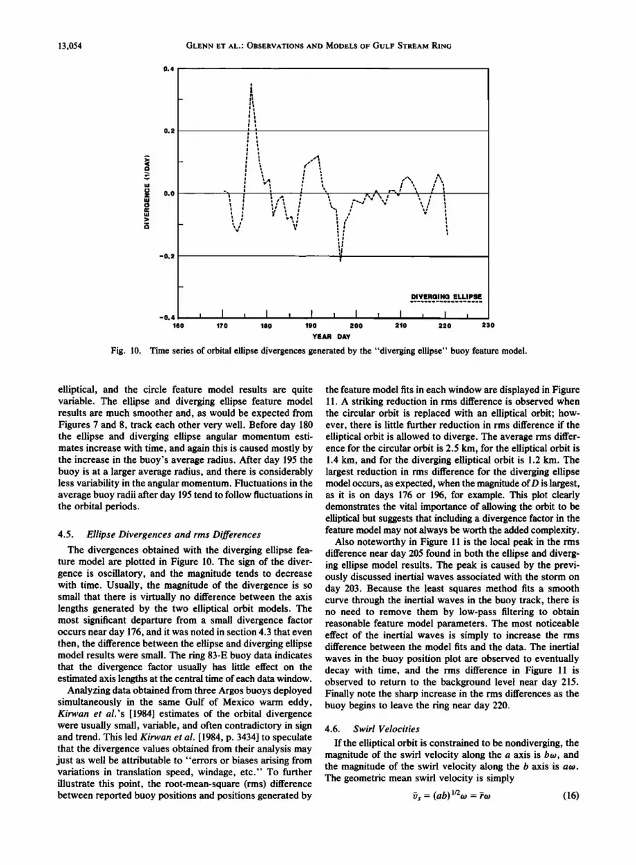
Fig. 10. Time series of orbital ellipse divergences generated by the "diverging ellipse" buoy feature model.

elliptical, and the circle feature model results are quite variable. The ellipse and diverging ellipse feature model results are much smoother and, as would be expected from Figures 7 and 8, track each other very well. Before day 180 the ellipse and diverging ellipse angular momentum estimates increase with time, and again this is caused mostly by the increase in the buoy's average radius. After day 195 the buoy is at a larger average radius, and there is considerably less variability in the angular momentum. Fluctuations in the average buoy radii after day 195 tend to follow fluctuations in the orbital periods.

4.5. Ellipse Divergences and rms Differences

The divergences obtained with the diverging ellipse feature model are plotted in Figure 10. The sign of the divergence is oscillatory, and the magnitude tends to decrease with time. Usually, the magnitude of the divergence is so small that there is virtually no difference between the axis lengths generated by the two elliptical orbit models. The most significant departure from a small divergence factor occurs near day 176, and it was noted in section 4.3 that even then, the difference between the ellipse and diverging ellipse model results were small. The ring 83-E buoy data indicates that the divergence factor usually has little effect on the estimated axis lengths at the central time of each data window.

Analyzing data obtained from three Argos buoys deployed simultaneously in the same Gulf of Mexico warm eddy, Kirwan et al.'s [1984] estimates of the orbital divergence were usually small, variable, and often contradictory in sign and trend. This led Kirwan et al. [1984, p. 3434] to speculate that the divergence values obtained from their analysis may just as well be attributable to "errors or biases arising from variations in translation speed, windage, etc." To further illustrate this point, the root-mean-square (rms) difference between reported buoy positions and positions generated by

the feature model fits in each window are displayed in Figure 11. A striking reduction in rms difference is observed when the circular orbit is replaced with an elliptical orbit; however, there is little further reduction in rms difference if the elliptical orbit is allowed to diverge. The average rms difference for the circular orbit is 2.5 km, for the elliptical orbit is 1.4 km, and for the diverging elliptical orbit is 1.2 km. The largest reduction in rms difference for the diverging ellipse model occurs, as expected, when the magnitude of D is largest, as it is on days 176 or 196, for example. This plot clearly demonstrates the vital importance of allowing the orbit to be elliptical but suggests that including a divergence factor in the feature model may not always be worth the added complexity.

Also noteworthy in Figure 11 is the local peak in the rms difference near day 205 found in both the ellipse and diverging ellipse model results. The peak is caused by the previ- ously discussed inertial waves associated with the storm on day 203. Because the least squares method fits a smooth curve through the inertial waves in the buoy track, there is no need to remove them by low-pass filtering to obtain reasonable feature model parameters. The most noticeable effect of the inertial waves is simply to increase the rms difference between the model fits and the data. The inertial

waves in the buoy position plot are observed to eventually decay with time, and the rms difference in Figure 11 is observed to return to the background level near day 215. Finally note the sharp increase in the rms differences as the buoy begins to leave the ring near day 220.

4.6. Swirl Velocities

If the elliptical orbit is constrained to be nondiverging, the magnitude of the swirl velocity along the a axis is b•o, and the magnitude of the swirl velocity along the b axis is a•o. The geometric mean swirl velocity is simply

•s = (ab) •aoo = ?•o (16)


5

4

3

2•

I •

0

160

I

I I I I

- ii I i I I i I l l

-- II I I I ii

_ II I I: il. il . . l

f, / i i

i I • /l II ': I - i I [' I I I• I Ii :, • I 61 ' I I ,

I•1 I •1 •, I 11 I

I ß • .,, i • ,,:: V

OlROLE

ELLIPSE

DIVERGING ELLIPSE

i I , I i I • I • I i I I 170 180 190 200 210 220 230

YEAR DAY

Fig. 11. Time series of rms differences between reported buoy positions and positions generated by the buoy feature models.

where ? is the geometric mean radius. The geometric mean swirl velocity generated by the ellipse feature model is plotted versus mean radius in Figure 12. Subsequent points in time are connected with lines so that the time history of the swirl velocity can be traced as the buoy makes its way from the center of the ring to the outside edge.

Before day 196, the mean radius of the buoy was within the range 10 km < ? < 25 km. Except for the deviation caused by the increase in buoy orbital period on days 174

and 175, the ring appears to be in solid body rotation with an average (+-standard deviation) angular velocity of 1.52 (+_0.07) x 10 -5 rad/s. Recall that an average angular velocity of 1.52 x 10 -5 rad/s was obtained by applying the gradient current relation to the feature model fit of the XBT-derived

dynamic height field. The maximum swirl velocity during this time was 36 cm/s at a radius of 25 km. This compares very well with the maximum XCP measured velocity of 39 cm/s at a radius of 31 km at 50 m depth.

4O

3O

2O

ELLIPSE

DAY 170-173

DAY 174-175

DAY 176-196

DAY 197-220

o • I i I I I i I • ! I I I I • o s lO :5 20 25 30 35 40

MEAN RADIUS (KILOMETERS)

Fig. 12. Mean swirl velocity versus mean radius as generated by the "ellipse" buoy feature model.

13,056 GLENN ET AL..' OBSERVATIONS AND MODELS OF GULF STREAM RING

8O

160

0 0 0 0

o o d ,',

;.•. ,!',• j tr BUOY: CIRCLE

/N SATELLITE: ANALYST I 0 SATELLITE: ANALYST 2

I , I , I , I I , I

YEAR DAY

230

Fig. 13. Time series of the ellipse mean radii generated by the buoy and AVHRR feature models.

After day 196, the mean buoy orbital radius increased into the range 25 km < ? < 37 km. The buoy swirl velocity in this region remained approximately constant near 30 cm/s, with a reduced average angular velocity of 0.99 (-0.10) x 10 -5 rad/s.

4.7. Mean Radii

The geometric mean radii of the buoy orbits calculated using all three buoy feature models are compared in Figure 13 to the geometric mean radii calculated from the elliptical fits to the observed fronts in the AVHRR images. The average of all the AVHRR-derived mean radii is 56 km, a value about twice as large as the radius of maximum swirl velocity obtained from the buoy and XCPs. Figure 13 dramatically illustrates that although the buoy exhibits a trend toward increasing radius, at all times the buoy was well within the high thermal gradient contours judged to best represent ring 83-E in the satellite images.

4.8. Ellipse Aspect Ratios

The ellipse aspect ratio is defined here as the ratio of the b axis length to the a axis length. This was done specifically to preserve the effect of the major-minor axis switch observed in the data. Results are plotted from the feature model analysis of the buoy, the AVHRR, and the XBT data in Figure 14. Although the ring in the satellite images does not appear to switch major and minor axes on day 185 or 186 as it did in the buoy results, both the AVHRR and the buoy derived ellipses switch their axes near day 196. The larger scatter in the AVHRR-derived estimates may be due to the motions of surface filaments entrained by the ring that effect the instantaneous ring shape.

At the beginning of the time series, the XBT-derived ellipse is found to have an aspect ratio much closer to 1 than the ellipses derived from the AVHRR data near day 165. Similarly, most of the buoy-derived ellipses have aspect

ratios closer to 1 than the AVHRR ellipses. Although the feature model fits to the observed surface fronts in the

AVHRR data produce larger, more elliptical rings for 83-E, the AVHRR ring shapes may be more elliptical, since they are derived from instantaneous satellite images. The buoy and XBT ring shapes represent averages over short time intervals during which the ellipse orientation may have changed.

4.9. Ellipse Orientations

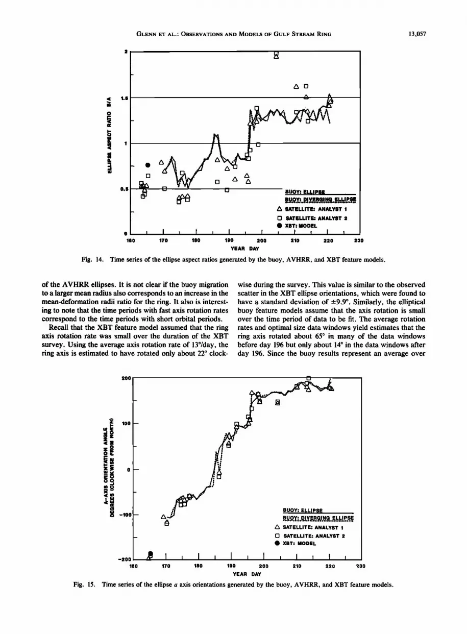
Ellipse orientation was determined by tracking the orientation of the a axis in the elliptical fits to the Argos buoy, AVHRR, and XBT data. The orientation as plotted in Figure 15 is measured positive clockwise from true north. The orientation calculated from all three data types is found to be in remarkable agreement throughout the data set.

The a-axis orientation initially is near -200 ø. The a axis rotates clockwise at a variable rate through north to about +200 ø. Except for the approximately 1 week duration delay on days 173-180, the axis rotation rate is much faster before day 196 than it is after day 196. Average axis rotation rates begin near 13ø/day before day 173, slow to about 2ø/day for days 173-180, return to about 13ø/day for days 180-196, and finally go back to about 2ø/day after day 196. Cushman- Roisin et al. [1985] list 9ø/day as a typically observed warm ring axis rotation rate, while Spence and Legeckis [1981] observed the axis of an elliptical cold ring to rotate 22ø/day. The Cushrnan-Roisin et al. [1985] model indicates that increasing the ratio of the geometric mean radius to the deformation radius decreases the axis rotation rate. In this

case, a reduction from 13ø/day to 2ø/day requires this ratio to increase from about 3.5 to about 6 (a factor of 1.7). Although in Figure 13 there is a distinct increase over days 190 through 200 in the mean buoy radii from about 16 km to about 30 km (a factor of 1.9), there is no notable change in the mean radii


1. S

0. S

A 0

A

.

,BUOY: EL•,IP•E

SATELLITE: ANALYST 1


XBT: MODEL I [ I •

210 220

o, t I , I ] I , I 160 170 180 190 200 230

YEAR DAY

Fig. 14. Time series of the ellipse aspect ratios generated by the buoy, AVHRR, and XBT feature models.

of the AVHRR ellipses. It is not clear if the buoy migration to a larger mean radius also corresponds to an increase in the mean-deformation radii ratio for the ring. It also is interesting to note that the time periods with fast axis rotation rates correspond to the time periods with short orbital periods.

Recall that the XBT feature model assumed that the ring axis rotation rate was small over the duration of the XBT

survey. Using the average axis rotation rate of 13ø/day, the ring axis is estimated to have rotated only about 22 ø clock-

wise during the survey. This value is similar to the observed scatter in the XBT ellipse orientations, which were found to have a standard deviation of ---9.9 ø. Similarly, the elliptical buoy feature models assume that the axis rotation is small over the time period of data to be fit. The average rotation rates and optimal size data windows yield estimates that the ring axis rotated about 65 ø in many of the data windows before day 196 but only about 14 ø in the data windows after day 196. Since the buoy results represent an average over

200 [3 ß

lOO

o

-lOO

-200

16o

I , I I [ I 170 180 190 200

YEAR DAY

BUOY: ELLIPSE

BU,•,Y: DIVERGING ELLIPSE e....



XBT: MODEL

210 22O '•30

Fig. 15. Time series of the ellipse a axis orientations generated by the buoy, AVHRR, and XBT feature models.


the time interval of the fit, this could explain why the AVHRR fits almost always are more elliptical than the buoy fits before day 196, but are in better agreement after day 196.

4.10. Center Locations

Brown et al. [1983] compared theft AVHRR-derived centers with the centers derived from the XBT star surveys of ring 81-D. Compared with the first XBT survey, the satellite- derived center was about 8 km south. Compared with the second XBT survey, the several satellite derived centers were located 6-40 km approximately northwest. Hooker and Olson [1984] fit separate straight lines through their AVHRR- and their XBT/CTD-derived center locations for

ring 82-B over a 13-day period. They found that the displace- ment of the satellite-derived line relative to the XBT/CTD

derived line ranges from 11.6 km to 1.1 km, approximately to the southwest. We found that for ring 83-E the two satellite- derived center locations closest in time to the XBT survey were located 2 km northeast and 11 km southeast of the

XBT-derived center. Even though ring 83-E was much weaker than 81-D or 82-B, the magnitude of the offsets between the AVHRR- and XBT/CTD-derived centers is similar.

A 2-month time series of in situ ring center locations is available from the feature model fits to the Argos buoy track. Center latitude and longitude versus time are plotted in Figures 16a and 16b. Although there is good agreement between the feature model fits to all three data types, the figures clearly illustrate how the buoy feature model results tend to form a smooth line through the scatter in the satellite-derived center locations. The satellite center loca-

tions generated by analyst 1 from multiple isotherm contours usually were closer to the buoy-derived centers than those generated by analyst 2 using single contours. Some of the scatter in the AVHRR estimates may be due to entrainment of surface water filaments on one side of the ring, causing a mismatch between the surface and subsurface temperature contours. Another cause may be the degradation of the sea surface thermal contrast due to summertime heating.

Though there is little difference between the center locations generated by the three buoy feature models, the ellipse model did produce a smoother center track than either the circle or diverging ellipse model. Using the ellipse model buoy centers as a standard for comparison, the AVHRR derived centers are found to have an average (_+standard deviation) offset of 5.0 (_+ 7.0) km north and 1.9 (_+ 12.2) km west (see Milkowski et al. [ 1987] for details). Flierl [1981] has shown that Eulerian estimates of ring center locations should be displaced north of Lagrangian estimates for westward propagating warm tings. In contrast to Hooker and Olson's [1984] results for ring 82-B, the AVHRR-derived center locations for ring 83-E do appear to be more Eulerian than Lagrangian by this criterion.

4.11. Center Propagation Velocities

The ring propagation velocity can be calculated from the AVHRR data by differencing the center locations discussed in the previous subsection. By this technique, Brown et al. [1986] found an average propagation speed of 5.6 (_+ 1.7) km/d for 87 warm core rings located west of 60øW. Auer [1987] found an average propagation speed of 6.8 (_+4.9)

km/d for 115 warm core rings, most of which were west of 50øW, with no significant geographical trends in his results. Cornilion et al. [ 1989] found an average propagation speed of 7.3 (_+2.7) km/d for five warm rings, a value which dropped to 5.0 (_+2.6) km/d when only the warm rings west of the New England Seamounts were included.

Center propagation velocity is one of the parameters determined directly by the feature model fits to the Argos buoy data. The AVHRR and Argos buoy derived propagation speeds are compared in Figure 17. It is immediately obvious from this plot that the instantaneous center propagation speeds obtained from the AVHRR data are much more variable (and sometimes unrealistically high) when compared with the values calculated from the Argos buoy data. The variability is simply due to the larger scatter in the AVHRR-derived center locations, suggesting that accurate estimates of the instantaneous ring propagation velocity sometimes can be difficult to obtain from AVHRR images. An average propagation velocity for ring 83-E was also determined by fitting straight lines through the analyst 1 AVHRR center latitude and center longitude time series. The slopes of the lines give a propagation velocity of 5.7 km/d directed 111 ø west of north, a speed well within the Brown et al. [1986], Auer [1987], and Cornilion et al. [1989] ranges.

Even though there is less variability in the buoy-derived estimates than the AVHRR-derived estimates, there still is significant scatter between the results obtained from the three buoy feature models. Same-day estimates of propagation velocity can differ by as much as 5 km/d. The elliptical orbit model, however, does generate a much more stable estimate of the center propagation speed than the other model fits. This reinforces the statement that it is critical to

include ellipticity in the feature model orbit and suggests that including the divergence factor may actually degrade the quality of some feature model parameters. The average propagation speed calculated using the ellipse model was 6.0 (_+ 1.8) km/d, in good agreement with the average propagation speed derived from the straight line fit to the AVHRR centers.

4.12. Forecast Center Locations

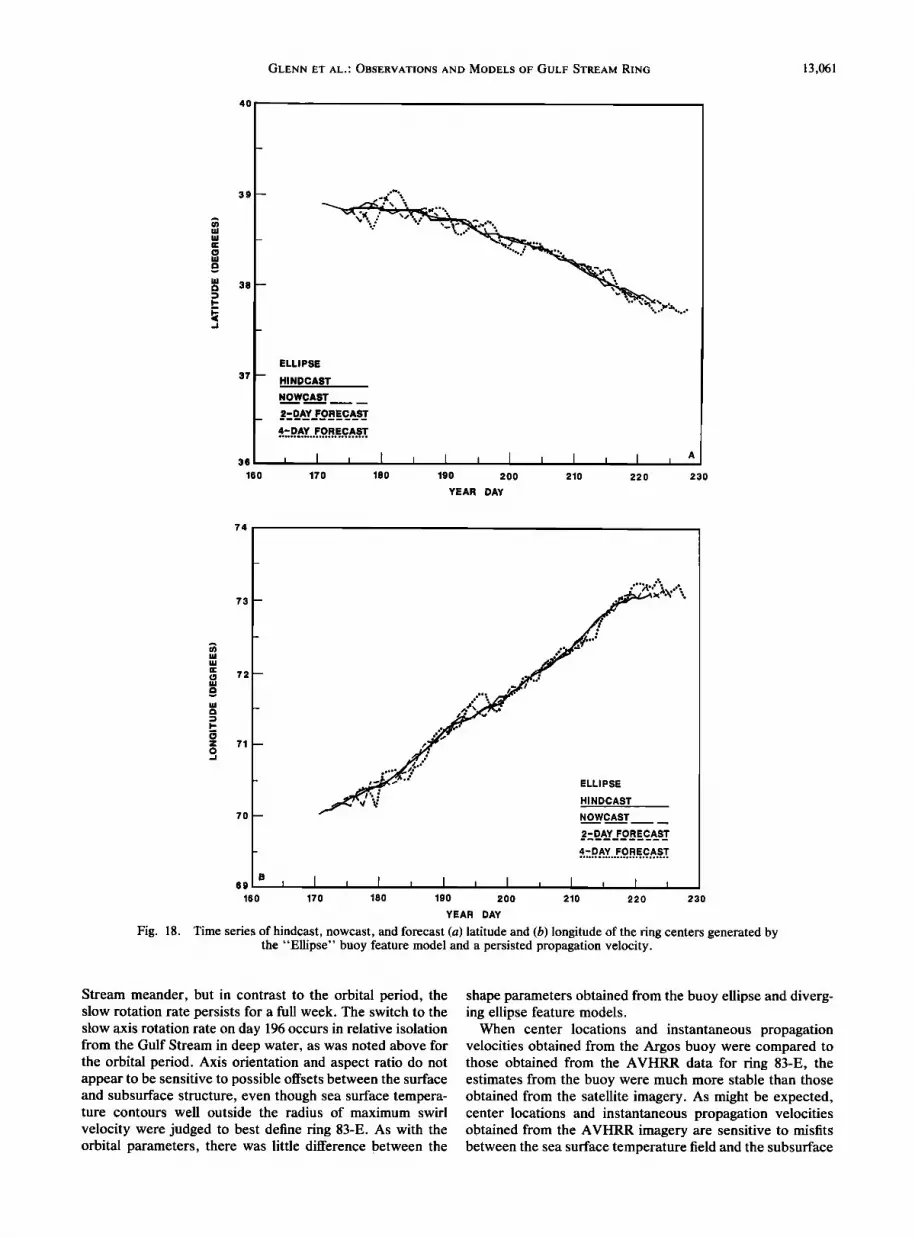
Given a ring center location and a propagation velocity, the propagation velocity can be assumed to persist for a given number of days to generate a forecast ring center location. The best forecast will be obtained using the most stable estimates for the ring center location and propagation velocity, which in this case are obtained from the ellipse feature model for the buoy data. Using these results, the predicted center latitude and longitude versus time are shown in Figures 18a and 18b. In these figures, the line labeled hindcast is the center location at 1200 UT on the

central day of each data window. This is the same line plotted in Figures 16a and 16b, and it serves as the starting point for the persisted velocity forecast. The line labeled nowcast is the predicted center location for the ring at 1200 UT on the final day of the data window. The lines labeled 2- and 4-day forecasts are the predicted 1200 UT locations 2 and 4 days beyond the data window. Comparing Figures 16 and 18, one sees that the ellipse feature model for the buoy could be used to generate a 4-day persisted velocity forecast of ring 83-E center locations with less scatter than the center locations derived from the AVHRR image analysis.

lyo_2

Highlight

lyo_2

Highlight

lyo_2

Highlight

lyo_2

Highlight


4O

36

160

BUOY: CIRCLE

BUOY: ELLIPSE

/• SATELLITE: ANALYST 1

[] SATELLITE: ANALYST 2

O XBT: MODEL

170 180 190 200 210 220

YEAR DAY

A

230

74

72

B 69 I

160

7O

BUOY: CIRCLE

BUOY: ELLIPSE

/X SATELLITE: ANALYST 1

[] SATELLITE: ANALYST 2

O XBT: MODEL

I • I • I • I • I • I • 4?0 480 490 200 240 220 2ao

YEAR DAY

Fig. 16. Time series of (a) latitude and (b) longitude of the ring centers generated by the buoy, AVHRR, and XBT feature models.

5. SUMMARY AND CONCLUSIONS

We have presented an efficient means of estimating the location, propagation velocity, size, shape, orientation, and swirl velocity of Gulf Stream rings from typically available data using feature models. As our basic Gulf Stream ring feature model, we have adopted a steadily translating, elliptic paraboloid with a swirl velocity that increases linearly with distance from the center. By the method of least squares, we obtained estimates of the feature model parameters by fitting the model to AVHRR, XBT, and Argos buoy

data. The fitting routines were sufficiently robust that they could be easily automated for real-time applications.

The AVHRR data were analyzed by fitting an ellipse to digitized closed contours around the ring to obtain estimates of the ring center location and the axes lengths and orientation. Ring propagation velocities were obtained by differencing center locations from images adjacent in time. The XBT data were analyzed by fitting an elliptic paraboloid to the depth of a given isotherm and to the derived dynamic height field to generate estimates of the center location, axes


;; BUOY: CIRCLE '=': BUOY: ELLI •'•'E --

25 i; BuOy: DIVERGING ELLIPSE'

iil= ii .=,=, ,•; '•: • A •

160 170 180 190 200 210 220 230

YEAR DAY

Fig. 17. Time series of ring propagation velocities generated by the buoy and AVHRR feature models.

lengths, orientation, and center depth or height. The gradient current relation was used to calculate swirl velocity. The Argos buoy data were analyzed by fitting a diverging elliptic orbital motion about a steadily translating center to the buoy track to obtain estimates of the center location and propagation velocity, the axes lengths and orientations, the orbital period, swirl velocity, and divergence. The orbital motion in the Argos buoy model was further constrained to be either nondiverging elliptical or nondiverging circular.

The feature model analysis techniques were developed to provide real time support for exploratory deepwater drilling operations. The techniques were illustrated with data collected from warm core ring 83-E as part of that support program. Ring 83-E formed west of the New England Seamounts near day 111, was surveyed with XBTs and XCPs beginning on day 164, and was seeded with an Argos buoy on day 166. Gradient currents calculated from the feature model fit to the XBT derived dynamic height field agreed well with XCP measurements, indicating that currents in ring 83-E were relatively weak, not exceeding 40 cm/s. The Argos buoy remained in ring 83-E until day 230 as the ring propagated to the southwest, allowing a continuous comparison of satellite imagery with in situ data over a 2-month period. After loosing the tracking buoy, ring 83-E continued to propagate southwest until its coalescence with the Gulf Stream off Cape Hatteras near day 254.

The Argos buoy feature model orbital parameters obtained for ring 83-E could be divided into two groups. Before day 196 (except days 174 and 175), the orbital period was approximately 5 days, the mean radius of the buoy orbit was less than 25 km, and the ring appeared to be in solid body rotation with an angular momentum highly dependent on average radius. After day 196, the buoy orbital period increased to about 7 days, the mean orbital radius was greater than 25 km, the swirl velocity was relatively constant, and small variations in the angular momentum fol-

lowed the small variations in average radius. The longer orbital periods experienced on days 174-175 occurred near the time of close approach of a Gulf Stream meander. The switch to the consistently longer orbital periods and larger radii on day 196, however, occurred while the ring was in relative isolation from the Gulf Stream and over deep uniform topography (see Figure 4). The advantage of the two ellipse models over the circle model was clearly demon- strated by the oscillation of the circular orbital radius between the major and minor semi-axis results, the oscillation of the circular orbital period to keep the swirl velocity approximately constant, and the reduction in rms differences generated by the elliptical orbit fits. The orbital divergence for the entire data set usually was small, so orbital parameters obtained from the ellipse and the diverging ellipse feature models were very similar. From consideration of the orbital parameters alone, it was not clear which elliptical orbit generates the most useful results.

Ring 83-E shape parameters obtained from the Argos buoy then were compared with those obtained from the AVHRR and the XBTs. The mean radii obtained from the Argos buoy were always well within the mean radii of the fits to the AVHRR contours. The aspect ratio of the buoy orbital ellipses and the XBT-derived ellipses usually were closer to 1 than the fits to the AVHRR contours, especially before day 196. The difference in aspect ratios may be caused by axis rotation, since the AVHRR estimates are instantaneous and the XBT and buoy estimates are averages over short time intervals. Both the buoy and AVHRR results agree that the major and minor axes of the ring switched near day 196. The ellipse orientations obtained from the buoy and the AVHRR agreed remarkably well. Both the Argos buoy and the AVHRR data indicate that the clockwise rotation of ring 83-E's axis was slower for days 173-180 and after day 196 than it was at other times. The slow axis rotation on days 173-180 begins at the time of the interaction with a Gulf

GLENN ET AL ' OBSERVATIONS AND MODELS OF GULF STREAM RING 13,061

4O

36

160

ELLIPSE

HINDCAST

NOWCAST

2-DAY FORECAST

170 180 190 200 210

YEAR DAY

220

A

230

74

69

160

•,• ELLIPSE • t',: HINDCAST • NOWCAST

2-DAY FORECAST

•7o •8o •9o 200 2•o •,•,o •,3o

YEAR DAY

Fig. 18. Time series of hindcast, nowcast, and forecast (a) latitude and (b) longitude of the ring centers generated by the "Ellipse" buoy feature model and a persisted propagation velocity.

Stream meander, but in contrast to the orbital period, the slow rotation rate persists for a full week. The switch to the slow axis rotation rate on day 196 occurs in relative isolation from the Gulf Stream in deep water, as was noted above for the orbital period. Axis orientation and aspect ratio do not appear to be sensitive to possible offsets between the surface and subsurface structure, even though sea surface temperature contours well outside the radius of maximum swirl

velocity were judged to best define ring 83-E. As with the orbital parameters, there was little difference between the

shape parameters obtained from the buoy ellipse and diverging ellipse feature models.

When center locations and instantaneous propagation velocities obtained from the Argos buoy were compared to those obtained from the AVHRR data for ring 83-E, the estimates from the buoy were much more stable than those obtained from the satellite imagery. As might be expected, center locations and instantaneous propagation velocities obtained from the AVHRR imagery are sensitive to misfits between the sea surface temperature field and the subsurface


structure. It also appears that including the divergence factor in the buoy feature model leads to less stable estimates of location and propagation velocity, suggesting that for these calculations it may be best to constrain the feature model to zero divergence. AVHRR-derived centers were on average displaced north of the buoy ellipse feature model-derived centers, as would be expected if the satellite imagery re- flected Eulerian measurements. Although there was significant scatter in the instantaneous propagation velocities obtained from the AVHRR data by differencing center locations adjacent in time, the average propagation speed obtained from a best fit straight line to the center locations was 5.7 km/d. The Ellipse feature model applied to the buoy data generated an average propagation speed of 6 km/d with little trend over the 2-month time period. Four-day forecasts of ring center location generated by simply persisting the ellipse buoy model's instantaneous propagation velocity were found to be within the scatter of the AVHRR estimated

centers, thereby illustrating its effectiveness as a forecasting tool for offshore operations.

Acknowledgments. Shell Offshore, Inc., and Shell Development Company provided funding for this work. Jim Feeney of Horizon Marine, Inc., coordinated the shipboard survey. Tom Sanford of the University of Washington accompanied us on the survey and provided advice on XCP deployments, data processing, and interpretation. Charlie Gutierrez of Shell Development Company contributed to the buoy data analysis. Rick Weyer of the University of Rhode Island contributed to the satellite imagery analysis. The image processing software was developed by O. Brown, R. Evans, J. Brown, and A. Li at the University of Miami with Office of Naval Research funding. The continuing support of the Miami group is gratefully acknowledged.

REFERENCES

Armi, L., and N. A. Bray, A standard analytic curve of potential temperature versus salinity for the western North Atlantic, J. Phys. Oceanogr., 12, 384-387, 1982.

Auer, S. J., Five-year climatological survey of the Gulf Stream system and its associated rings, J. Geophys. Res., 92, 11,709- 11,726, 1987.

Bisagni, J. J., Passage of anticyclonic Gulf Stream eddies through Deep Water Dumpsite 106 during 1974 and 1975, NOAA Dumpsite Eval. Rep. 76-1, 39 pp., U.S. Dep. of Commer., 1976.

Brown, O. B., D. B. Olson, J. W. Brown, and R. H. Evans, Satellite infrared observation of the kinematics of a warm-core ring, Aust. J. Mar. Freshw. Res., 34, 535-545, 1983.

Brown, O. B., P. C. Cornilion, S. R. Emerson, and H. M. Carle, Gulf Stream warm rings: A statistical study of their behavior, Deep Sea Res., 33, 1459-1473, 1986.

Cooper, C., G. Z. Forristall, and T. M. Joyce, Velocity and hydrographic structure of two Gulf of Mexico warm-core rings, J. Geophys. Res., 95(C2), 1663-1679, 1990.

Cornilion, P., R. Weyer, and G. Flierl, Translational velocity of warm core rings relative to the slope water, J. Phys. Oceanogr., 19, 1319-1334, 1989.

Csanady, G. T., The birth and death of a warm core ring, J. Geophys. Res., 84, 777-780, 1979.

Cushman-Roisin, B., On the role of filamentation in the merging of anticyclonic lenses, J. Phys. Oceanogr., 19, 253-258, 1989.

Cushman-Roisin, B., W. H. Heil, and D. Nof, Oscillations and rotations of elliptical warm-core rings, J. Geophys. Res., 90, 11,756-11,764, 1985.

Evans, R. H., K. S. Baker, O. B. Brown, and R. C. Smith, Chronology of warm-core ring 82-B, J. Geophys. Res., 90, 8803- 8811, 1985.

Flierl, G. R., The application of linear quasigeostrophic dynamics to Gulf Stream rings, J. Phys. Oceanogr., 7, 365-379, 1977.

Flierl, G. R., A simple model for the structure of warm and cold core rings, J. Geophys. Res., 84, 777-780, 1979.

Flierl, G. R., Particle motions in large-amplitude wave fields, Geophys. Astrophys. Fluid Dyn., 18, 39-74, 1981.

Gotthardt, G. A., Observed formation of a Gulf Stream anticyclonic eddy, J. Phys. Oceanogr., 3, 237-238, 1973.

Gotthardt, G. A., and G. J. Potocsky, Life cycle of a Gulf Stream anticyclonic eddy observed from several oceanographic plat- forms, J. Phys. Oceanogr., 4, 131-134, 1974.

Halliwell, G. R., and C. N. K. Mooers, The space-time structure and variability of the shelf water-slope water front and Gulf Stream temperature fronts and associated warm core rings, J. Geophys. Res., 84, 7077-7725, 1979.

Hooker, S. B., and D. B. Olson, Center of mass estimation in closed vortices: A verification in principle and practice, J. Atmos. Oceanic Technol., 1,247-255, 1984.

Joyce, T. M., Velocity and hydrographic structure of a Gulf Stream warm core ring, J. Phys. Oceanogr., 14, 936-947, 1984.

Joyce, T. M., Gulf Stream warm-core ring collection: An introduction, J. Geophys. Res., 90, 8801-8802, 1985.

Joyce, T. M., and M. A. Kennelly, Upper-ocean velocity structure of Gulf Stream warm core ring 82B, J. Geophys. Res., 90, 8839-8844, 1985.

Joyce, T. M., and M. C. Stalcup, Wintertime convection in a Gulf Stream warm core ring, J. Phys. Oceanogr., 15, 1032-1042, 1985.

Kirwan, A.D., Jr., W. J. Merrell, Jr., J. K. Lewis, R. E. Whitaker, and R. Legeckis, A model for the analysis of drifter data with an application to a warm core ring in the Gulf of Mexico, J. Geophys. Res., 89, 3425-3438, 1984.

Kirwan, A.D., Jr., J. K. Lewis, A. W. Indest, P. Reinersman, and I. Quintero, Observed and simulated kinematic properties of Loop Current rings, J. Geophys. Res., 93, 1189-1198, 1988.

Kunze, E., The mean and near-inertial velocity fields in a warm-core ring, J. Phys. Oceanogr., 16, 1444-1461, 1986.

Kunze, E., and R. Lueck, Velocity profiles in a warm core ring, J. Phys. Oceanogr., 16, 991-995, 1986.

Lai, D. V., and P. L. Richardson, Distribution and movement of Gulf Stream rings, J. Phys. Oceanogr., 7, 670-683, 1977.

Mariners Weather Log, Marine weather review, North Atlantic weather log, July, August and September 1983, 28, 23-30, 1984.

McClain, E. R., W. G. Pichel, and C. C. Walton, Comparative performance of AVHRR-based multichannel sea surface temper- atures, J. Geophys. Res., 90, 11,587-11,601, 1985.

Milkowski, G., P. Cornilion, and S. M. Glenn, A warm core ring prediction program in support of offshore drilling activities, Mar. Technol. Soc. J., 21, 22-32, 1987.

Nof, D., On the migration of isolated eddies with application to Gulf Stream rings, J. Mar. Res., 41,399-425, 1983.

Nof, D., On the ellipticity of isolated anticyclonic eddies, Tellus, Ser. A, 37, 77-86, 1985.

Olson, D. B., and T. W. Spence, Asymmetric disturbances in the frontal zone of a Gulf Stream ring, J. Geophys. Res., 83, 4691- 4695, 1978.

Olson, D. B., R. W. Schmitt, M. Kennelly, and T. M. Joyce, A two-layer diagnostic model of the long-term physical evolution of warm core ring 82B, J. Geophys. Res., 90, 8813-8822, 1985.

Richardson, P. L., Gulf Stream ring trajectories, J. Phys. Ocean- ogr., 10, 90-104, 1980.

Richardson, P. L., R. E. Cheney, and L. V. Worthington, A census of Gulf Stream rings, spring 1975, J. Geophys. Res., 83, 6136- 6144, 1978.

Richardson, P. L., J. J. Wheat, and D. Bennett, Free drifting, satellite tracked buoy trajectories in the Gulf Stream system 1975-1978, Tech. Rep. 79-4, 159 pp., Woods Hole Oceanogr. Inst., 1979.

Robinson, A. R., M. A. Spall, and N. Pinardi, Gulf Stream simula- tions and the dynamics of ring and meander processes, J. Phys. Oceanogr., 18, 1811-1853, 1988.

Sanford, T. B., R. G. Drever, J. H. Dunlap, and E. A. D'Asaro, Design, operation and performance of an expendable temperature and velocity profilers (XTVP), Tech. Rep. 8110, 83 pp., Appl. Phys. Lab., Univ. of Wash., Seattle, 1982.

Sanford, T. B., P. G. Black, J. R. Haustein, J. W. Feeney, G. Z. Forristall, and J. F. Price, Ocean response to a hurricane, 1, Observations, J. Phys. Oceanogr., 17, 2065-2083, 1987.

Sano, M.P., and C. P. Fairfield, Anticyclonic warm-core Gulf Stream rings off the northeastern United States during 1988, paper

GLENN ET AL.: OBSERVATIONS AND MODELS OF GULF STREAM RING 13,063

presented at Scientific Council Meeting, Northwest Atl. Fish. Organ., Dartmouth, Nova Scotia, 1989.

Saunders, P.M., Anticyclonic eddies formed from shoreward meanders of the Gulf Stream, Deep Sea Res., 18, 1207-1219, 1971.

Schmitt, R. W., and D. B. Olson, Wintertime convection in warm- core rings: Thermocline ventilation and the formation of meso- scale lenses, J. Geophys. Res., 90, 8823-8837, 1985.

Spence, T. W., and R. Legeckis, Satellite and hydrographic observations of low-frequency wave motions associated with a cold core Gulf Stream ring, J. Geophys. Res., 86, 1945-1953, 1981.

P. Cornilion and G. Milkowski, Graduate School of Oceanogra- phy, University of Rhode Island, Kingston, RI 02881.

G. Z. Forristall, Shell Development Company, P.O. Box 481, Houston, TX 77001.

S. M. Glenn, Department of Earth and Planetary Sciences, Pierce Hall, Harvard University, 29 Oxford Street, Cambridge, MA 02138.

(Received October 11, 1989; revised January 19, 1990;

accepted January 23, 1990.)


, ' _L 83E

I I,

75W 78W

a• 28 April 1983 1839 UT

• 83E

b. 14 June 1983 0346 UT

• 23 June 1983 1900 UT d. 14 July 1983 1948 UT

75u•. •

ß '-"i'"- F

701,1 7•1• ' '• - 78U

e. 9 August 1983 0807 IYF L 9 •eptember 1983 0831 LFT

Plate 1 [Glenn et al.]. History of ring 83-E as observed in the satellite AVHRR imagery. (a) Day 118, 39.19øN, 67.97øW: after formation. (b) Day 165, 38.90øN, 69.82øW, start of the survey; (c) Day 174, 38.91øN, 70.06øW: interaction with a Gulf Stream meander. (d) Day 195, 38.57øN, 71.61øW: relative isolation from the Gulf Stream. (e) Day 221, 37.84øN, 72.96øW: prior to loosing the tracking buoy. (f) Day 252, 36.88øN, 74.39øW: prior to absorption. Ring center locations are derived from feature model fits to a single isotherm contour around the ring. The buoy track is superimposed on Plates lc-le; the arrow marks the buoy location at the time of the image.

observations of gulf stream ring 83-e and their interpretation using feature models

Documents