numerical study of some high pm10 levels episodes
TRANSCRIPT
Numerical Study of Some High Pm10 Levels
Episodes
Angelina Todorova1), Georgi Gadzhev1), Georgi Jordanov1), Dimiter Syrakov2), Kostadin
Ganev1), Nikolai Miloshev1), Maria Prodanova2)
1Geophysical Institute, Bulgarian Academy of Sciences, Acad. G. Bonchev Str., Bl.3, Sofia 1113, Bulgaria2National Institute of Meteorology and Hydrology, Bulgarian Academy of Sciences, 66 Tzarigradsko Chausee,
Sofia 1784, Bulgaria
Introduction
Goal of the study
To examine the abilities and limitations of US EPA Models 3 system
To evaluate the role of different processes of transport and transformation in forming
PM10 concentration peaks
Case
Germany, January-April 2003
Some major PM episodes were observed
These episodes had already been applied for model intercomparison and studying model
simulation abilities in the frame of COST Action 728 (aimed at clarifying the reasons for the
shortcomings in the simulations and at the choice of optimal model set-ups, inputs and
parameters). The present study is part of COST 728 activities as well, but focuses mostly
at studying the role of different processes in the PM10 pattern formation and their
contribution to the PM10 peaks in the period of interest.
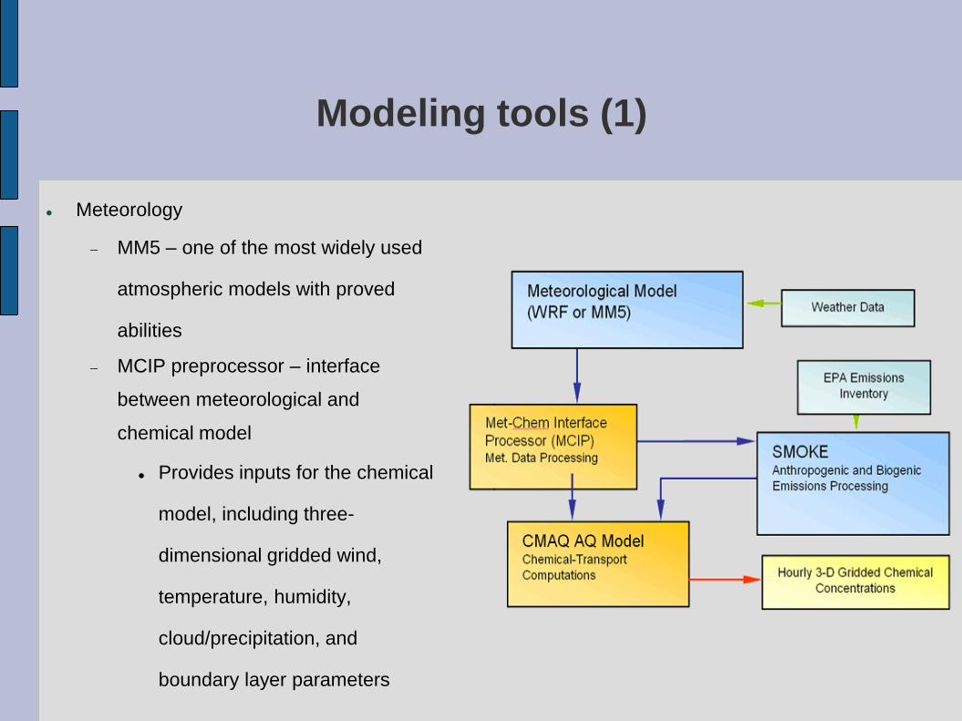
Modeling tools (1)
Meteorology
MM5 – one of the most widely used
atmospheric models with proved
abilities
MCIP preprocessor – interface
between meteorological and
chemical model
Provides inputs for the chemical
model, including three-
dimensional gridded wind,
temperature, humidity,
cloud/precipitation, and
boundary layer parameters
Modeling tools (2)
Emissions
Based on TNO emissions inventory, speciation and temporal profiles according to US
EPA's methodology
E-CMAQ – specially developed code to generate emissions for Bulgaria
SMOKE - the Sparse Matrix Operator Kernel Emissions Modelling System.
Used to merge biogenic, area and point source emissions
CMAQ Chemical Transport Model v4.6
Multi-pollutant, multiscale air quality model for simulating all atmospheric and land
processes that affect the transport, transformation, and deposition of atmospheric
pollutants and/or their precursors
Modeling tools (3)
CMAQ Chemical Transport Model v4.6
Chemical options
mechanism - Carbon Bond IV (CB4) (Gery et al., 1989) with 36 species and 93
reactions (including 11 photochemical reactions)
Aqueous-Phase Chemistry
EBI solver (Eulerian iterative method)
ISORROPIA aerosol model (Nenes et al., 1998).
VOC splitted to 10 lump pollutants and PM2.5 to 5 groups of aerosol
The Models-3 “Integrated Process Rate Analysis” option is applied to discriminate the
role of different dynamic and chemical processes for the formation of the observed
high PM10 concentration episodes.
Model configuration (1)
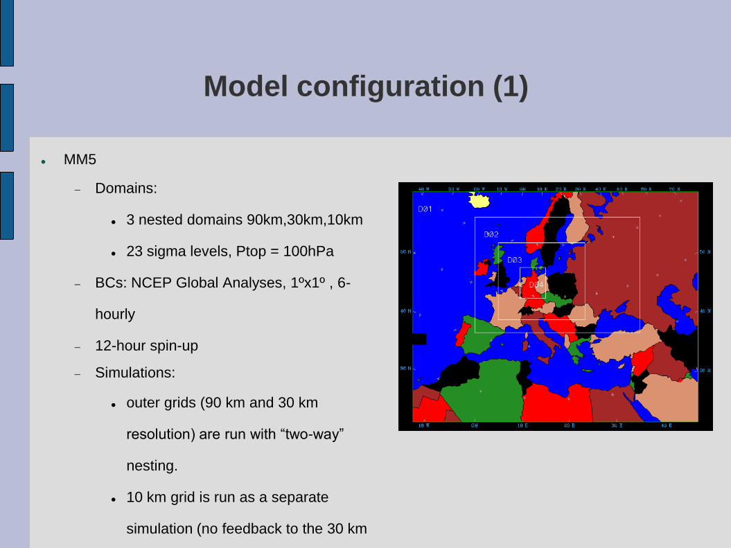
MM5
Domains:
3 nested domains 90km,30km,10km
23 sigma levels, Ptop = 100hPa
BCs: NCEP Global Analyses, 1ºx1º , 6-
hourly
12-hour spin-up
Simulations:
outer grids (90 km and 30 km
resolution) are run with “two-way”
nesting.
10 km grid is run as a separate
simulation (no feedback to the 30 km
domain )
Model configuration (2)
EMISSIONS:
TNO inventory
Resolution is 0.25 0.125 longitude-latitude, that is on average 15 15 km
Emissions divided in 10 SNAPs (Selected Nomenclature for Air Pollution)
classifying pollution sources according the processes leading to polution release
in the atmosphere (EMEP/CORINAIR, 2002).
8 pollutants: CH4, CO, NH3, NMVOC (VOC), NOx, SOx, PM10 and PM2.5
GIS technology is applied to produce girded input from this data base.
Specially prepared computer codes for:
temporal allocation based on daily, weekly and monthly profiles, provided by
Builtjes et al. (2003). The temporal profiles are country-, pollutant- and SNAP-
specific
speciation procedures, depending on the Chemical Mechanism (CM) used
Model configuration (3)
CMAQ
simulations were carried out for the two inner domains with 30 and 10 km resolution
IC:
Default profiles for both domains are used at the beginning of the simulation
Concentration fields obtained at the end of a day’s run used as initial condition for
the next day.
BC:
Default profiles used for the 30-km domain during the whole period.
Nested boundary conditions from the 30-km to the 10-km domain.
“Integrated Process Rate Analysis”
The processes that are considered are: advection, diffusion, mass adjustment,
emissions, dry deposition, chemistry, aerosol processes and cloud
processes/aqueous chemistry.
Case study - observations
From Feb 10 on, Central Europe was under the influence of a high pressure system. In this
time, the meteorological conditions in Northern Germany were characterized by low wind
speed leading to high PM concentrations in large parts of Northern Germany (peak from
Feb 11 to Feb 13).
On Feb 16, wind direction turned to North-West, and increasing wind speeds drove cold
and cleaner air into Germany. Already from Feb 17 on, south-easterly wind led again to a
steady increase of the PM10 concentration.
Toward the end of the month, a warm front moved over Germany from southwest to
northeast. This air mass frontier became nearly stationary in the middle of Germany. Until
March 3, this front moved slightly forward and backwards over the northern part of
Germany. Thus, several stations in the area of investigation were under the influence of
daily changing weather conditions.Peak PM10 concentrations are observed between Feb
28 and March 4.
Numerical Simulations - meteorology
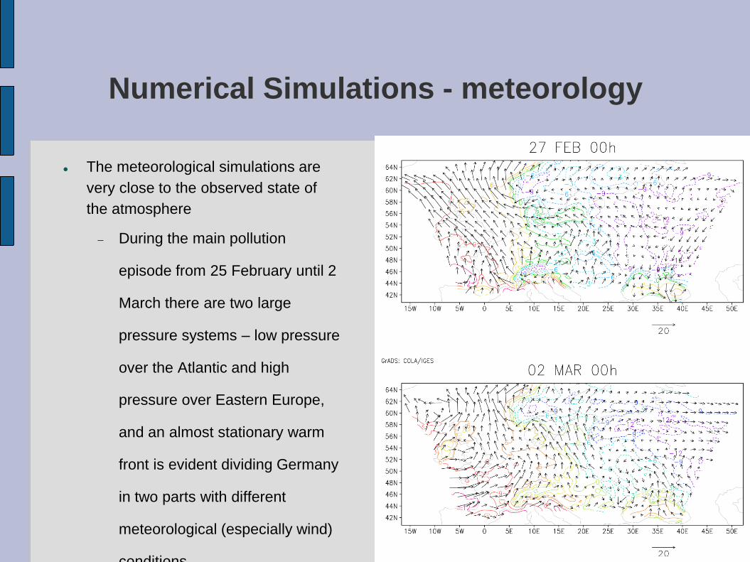
The meteorological simulations are
very close to the observed state of
the atmosphere
During the main pollution
episode from 25 February until 2
March there are two large
pressure systems – low pressure
over the Atlantic and high
pressure over Eastern Europe,
and an almost stationary warm
front is evident dividing Germany
in two parts with different
meteorological (especially wind)
conditions.
Numerical Simulations – surface
concentrations (1)
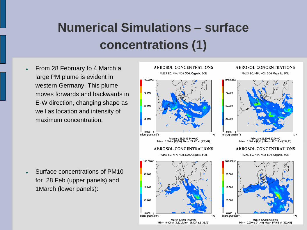
From 28 February to 4 March a
large PM plume is evident in
western Germany. This plume
moves forwards and backwards in
E-W direction, changing shape as
well as location and intensity of
maximum concentration.
Surface concentrations of PM10
for 28 Feb (upper panels) and
1March (lower panels):
Numerical Simulations – surface
concentrations (2)
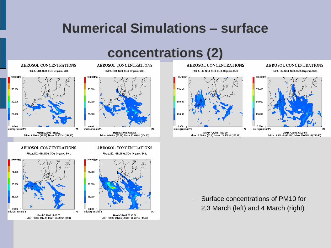
Surface concentrations of PM10 for
2,3 March (left) and 4 March (right)
Numerical Simulations – surface
concentrations (3)
40 50 60 70 80 90
Julian day
0
40
80
120
160
PM
10
[u
g/m
^^3]
DE02
simulated-30km
measured
simulated-10 km
40 50 60 70 80 90
Julian day
0
40
80
120
160
PM
10 [
ug/m
^^3]
DE03
simulated-30km
measured
simulated-10km
40 50 60 70 80 90
Julian day
0
40
80
120
160
PM
10 [
ug/m
^^3]
DE04
simulated-30km
measured
simulated-10km
40 50 60 70 80 90
Julian day
0
40
80
120
160
PM
10 [
ug/m
^^3]
DE05
simulated-30km
measured
simulated-10km
40 50 60 70 80 90
Julian day
0
40
80
120
160
PM
10 [
ug/m
^^3]
DE07
simulated-30km
measured
simulated-10km
40 50 60 70 80 90
Julian day
0
40
80
120
160
PM
10 [
ug/m
^^3]
DE08
simulated-30km
measured
simulated-10km
40 50 60 70 80 90
Julian day
0
40
80
120
160
PM
10 [
ug/m
^^3]
DE09
simulated-30km
measured
simulated-10km
40 50 60 70 80 90
Julian day
0
40
80
120
160
PM
10 [
ug/m
^^3]
DE41
simulated-30km
measured
simulated-10km
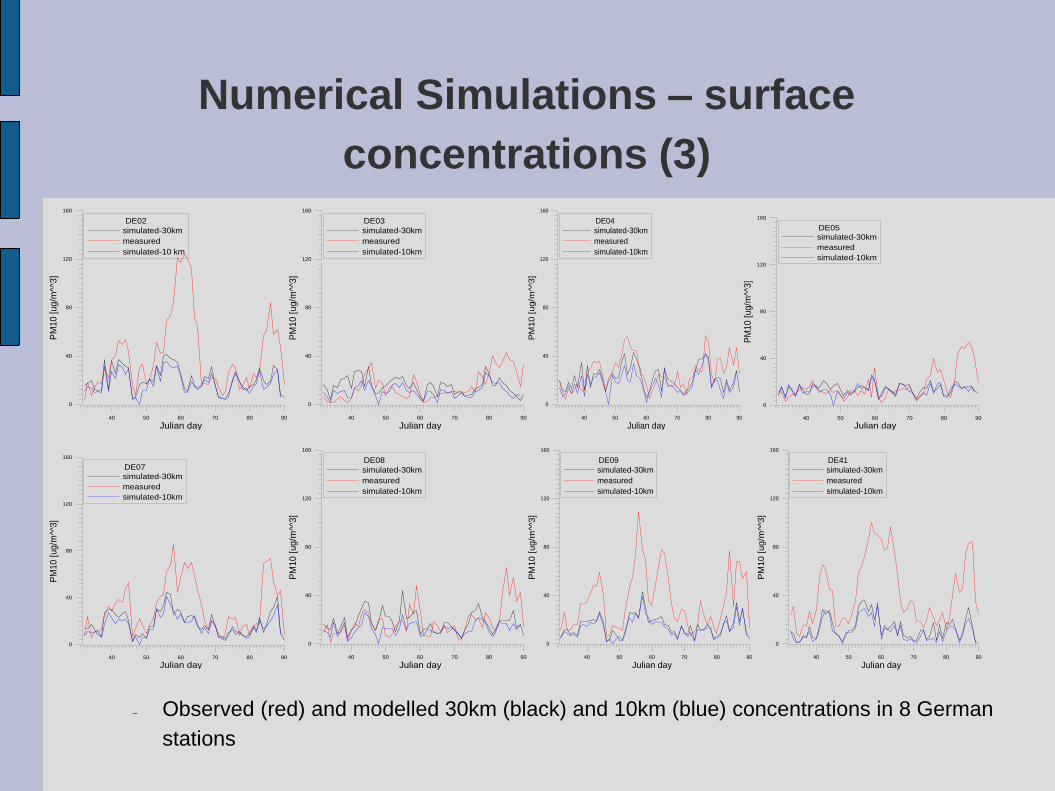
Observed (red) and modelled 30km (black) and 10km (blue) concentrations in 8 German
stations
Numerical Simulations – process analysis
(1)
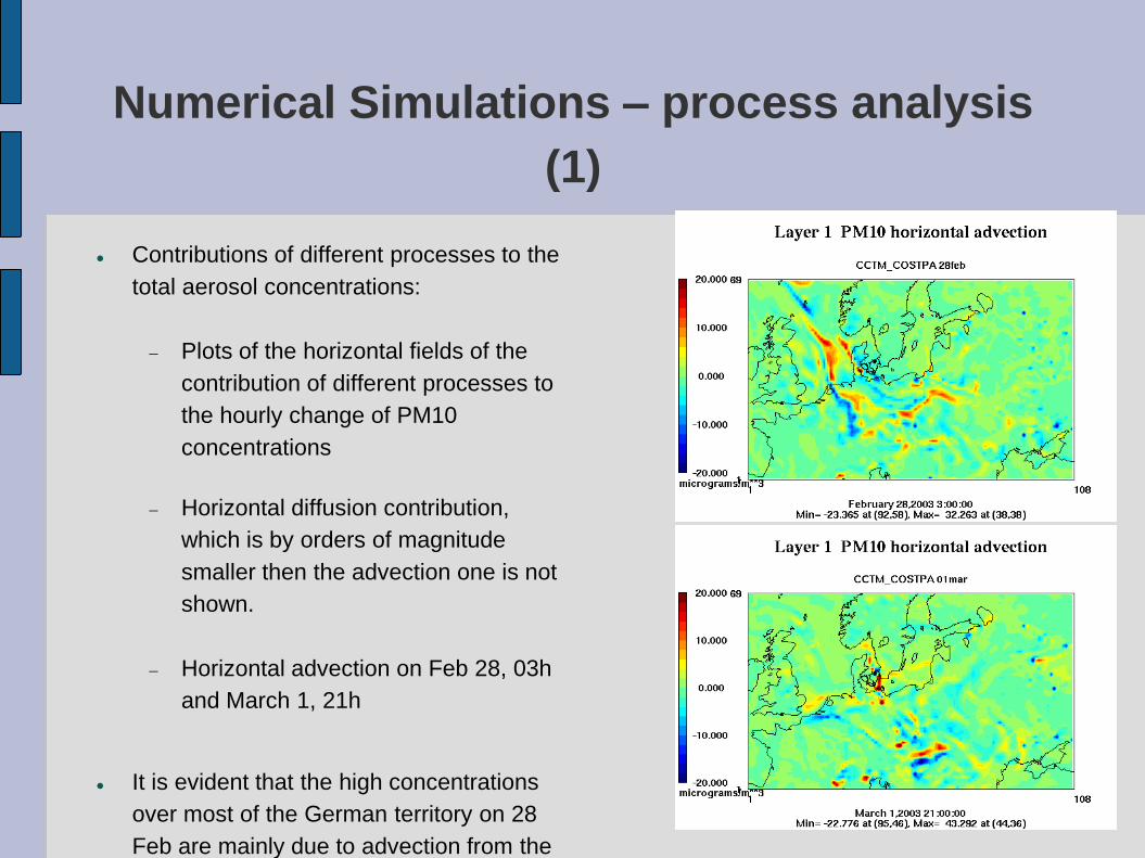
Contributions of different processes to the
total aerosol concentrations:
Plots of the horizontal fields of the
contribution of different processes to
the hourly change of PM10
concentrations
Horizontal diffusion contribution,
which is by orders of magnitude
smaller then the advection one is not
shown.
Horizontal advection on Feb 28, 03h
and March 1, 21h
It is evident that the high concentrations
over most of the German territory on 28
Feb are mainly due to advection from the
west.
Numerical Simulations – process analysis
(2)
Numerical Simulations – process analysis
(3)
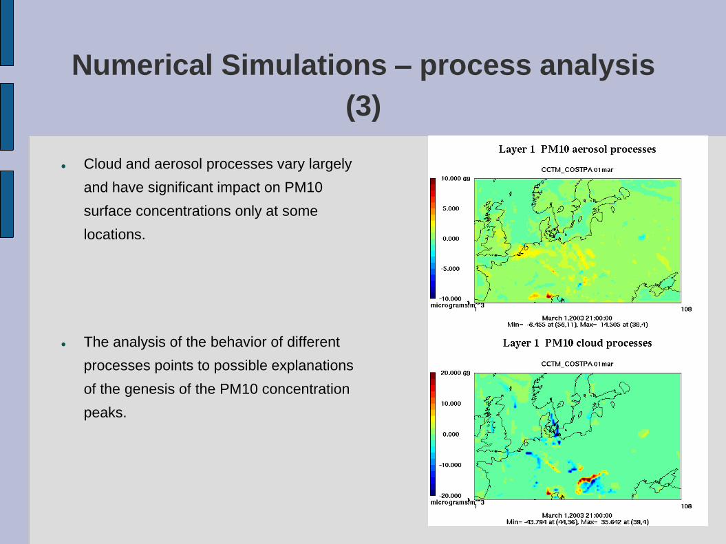
Cloud and aerosol processes vary largely
and have significant impact on PM10
surface concentrations only at some
locations.
The analysis of the behavior of different
processes points to possible explanations
of the genesis of the PM10 concentration
peaks.
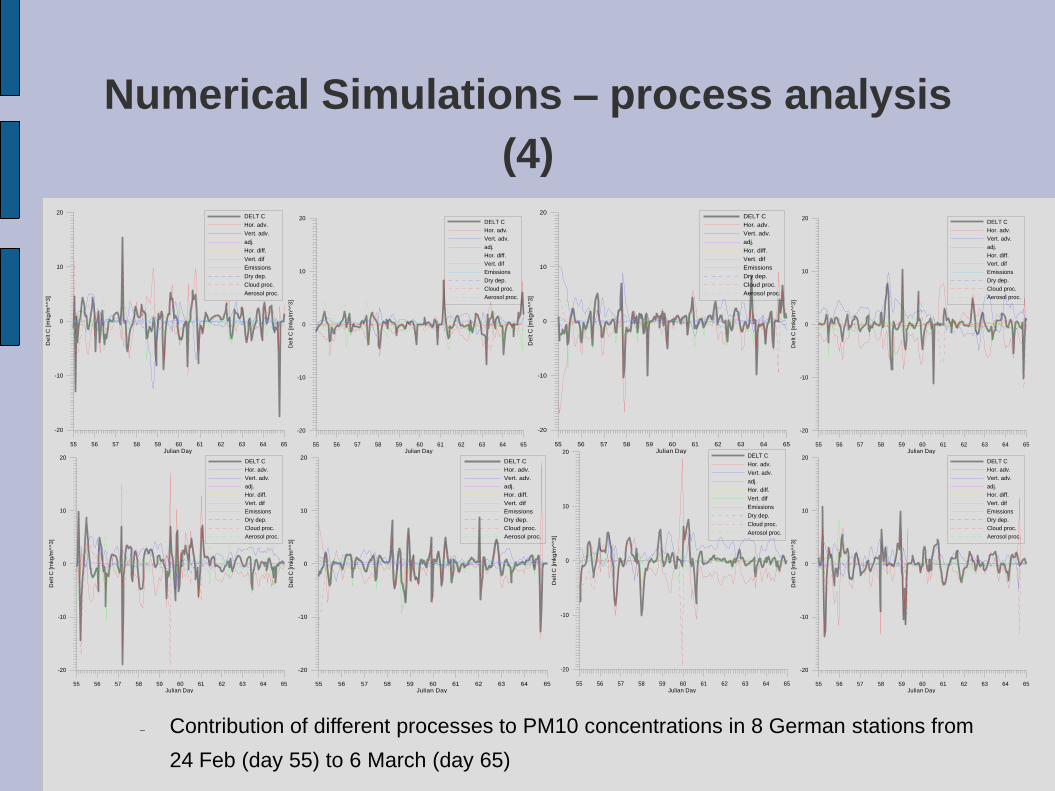
Numerical Simulations – process analysis
(4)
55 56 57 58 59 60 61 62 63 64 65Julian Day
-20
-10
0
10
20
De
lt C
[m
kg
/m^^3
]
DELT C
Hor. adv.
Vert. adv.
adj.
Hor. diff.
Vert. dif
Emissions
Dry dep.
Cloud proc.
Aerosol proc.
55 56 57 58 59 60 61 62 63 64 65Julian Day
-20
-10
0
10
20
De
lt C
[m
kg
/m^^3
]
DELT C
Hor. adv.
Vert. adv.
adj.
Hor. diff.
Vert. dif
Emissions
Dry dep.
Cloud proc.
Aerosol proc.
55 56 57 58 59 60 61 62 63 64 65Julian Day
-20
-10
0
10
20
De
lt C
[m
kg
/m^^3
]
DELT C
Hor. adv.
Vert. adv.
adj.
Hor. diff.
Vert. dif
Emissions
Dry dep.
Cloud proc.
Aerosol proc.
55 56 57 58 59 60 61 62 63 64 65Julian Day
-20
-10
0
10
20
De
lt C
[m
kg
/m^^3
]
DELT C
Hor. adv.
Vert. adv.
adj.
Hor. diff.
Vert. dif
Emissions
Dry dep.
Cloud proc.
Aerosol proc.
55 56 57 58 59 60 61 62 63 64 65Julian Day
-20
-10
0
10
20
De
lt C
[m
kg
/m^^3
]
DELT C
Hor. adv.
Vert. adv.
adj.
Hor. diff.
Vert. dif
Emissions
Dry dep.
Cloud proc.
Aerosol proc.
55 56 57 58 59 60 61 62 63 64 65Julian Day
-20
-10
0
10
20
De
lt C
[mkg
/m^^3
]
DELT C
Hor. adv.
Vert. adv.
adj.
Hor. diff.
Vert. dif
Emissions
Dry dep.
Cloud proc.
Aerosol proc.
55 56 57 58 59 60 61 62 63 64 65Julian Day
-20
-10
0
10
20
De
lt C
[m
kg
/m^^3
]
DELT C
Hor. adv.
Vert. adv.
adj.
Hor. diff.
Vert. dif
Emissions
Dry dep.
Cloud proc.
Aerosol proc.
55 56 57 58 59 60 61 62 63 64 65Julian Day
-20
-10
0
10
20
De
lt C
[m
kg
/m^^3
]
DELT C
Hor. adv.
Vert. adv.
adj.
Hor. diff.
Vert. dif
Emissions
Dry dep.
Cloud proc.
Aerosol proc.
Contribution of different processes to PM10 concentrations in 8 German stations from
24 Feb (day 55) to 6 March (day 65)
Conclusions
The simulated meteorological fields agree well with the patterns described in the case
study definition.
Agreement of CMAQ model results with observations
The qualitative agreement between modelled and observed PM10 surface
concentrations is good for both domains
Enhancing the horizontal spatial resolution does not improve the results significantly,
so most probably the observed PM10 peaks are a result of large-scale processes
The quantitative agreement for most of the stations is reasonable
Process Analysis: the contributions of different processes change very quickly with
time and these changes for the different stations hardly correlate at all
The analysis of the behavior of different processes does not give clear explanation of the
genesis of the PM10 concentration peaks, but at least outlines the most important and
dominant processes and points to possible explanations of the genesis.
Acknowledgements
The present work is supported by EC through 6FP project ACCENT (GOCE-CT-2002-
500337), NATO SfP project ESP.EAP.SFPP 981393, COST Actions 728 and ES0602 and
ESF project № BG051PO001-3.3.04-33/28.08.2009
Special thanks to EURASAP for providing travel support for the present workshop
G. Gadzhev is World Federation of Scientists grantholder.
Deep gratitude to all organizations providing free of charge data and software: US EPA,
US NCEP, European institutions like EMEP, EEA, UBA and many others. Special thanks
to the Netherlands Organization for Applied Scientific research (TNO) for providing high-
resolution European anthropogenic emission inventory.

Thank You!