Nuclear Magnetic Resonance: Spin-Spin andSpin-Lattice Relaxation Times

Adrian Thompson

Physics 134 Advanced LaboratoryLab Partner: Oscar Flores

University of California, Santa Cruz

May 18, 2014

Abstract

The fundamentals of pulsed nuclear magnetic resonance (PNMR) were investigated in aseries of experiments using a sample of mineral oil, a benchtop magnet, and a radio frequency(RF) pulse programmer. The apparatus was set up to observe a free induction decay (FID)signal response in the sample magnetization and measure the homogeneity in the staticmagnetic field contour. The spin-lattice (T1) and spin-spin (T2) relaxation times of thesample were measured to be 7.48± 0.39 ms and 22.69± 0.82 ms, respectively.

1 Introduction

Pulsed nuclear magnetic resonance (NMR) has many applications in modern science, with someexamples being the medical imaging of biological systems or spectroscopy in organic and inorganicchemistry. In these experiments we focus on the core principles of spin-spin and spin-latticerelaxation times, which are characteristic time scales during non-equilibrium conditions imposedon materials by external fields. We used a sample of mineral oil as a material, and a benchtopNMR magnet and pulse programmer to observe the aforementioned phenomena. These apparatusare discussed in further detail in section 2.

1.1 The Resonance Condition and Larmor Precession

The following discussion can be found in [5]. Please see [6] as well.Protons have spin angular momentum and an associated magnetic moment, and their response toexternal magnetic fields is an increasingly valuable phenomenon in modern applications. The spinvector S = ~l and the magnetic moment vector µ are aligned and related by a proportionalityconstant called the gyromagnetic ratio;

µ = γS (1)

µ = γ~l (2)

In an external, uniform magnetic field, the energy of these dipoles is given by

E = −µ ·Bext (3)

1

Taking the uniform field in a coordinate system (x, y, z) as B = B0z, we evaluate the energy bycombining the above equations.

E = −µzB0

= −γ~lzB0

For fermions, lz = ±12

and therefore the energy spacing between these two states is

∆E = |E 12− E− 1

2|

= | − γ~(1

2)B0 + γ~(−1

2)B0|

= γ~B0

The quantum mechanical treatment allows the expression of this energy difference as ∆E = ~ω0,so

ω0 = γB0. (4)

The frequency ω0 is known as the Larmor precession frequency. Larmor precession is the classicalmechanical notion of the precession of the angular momentum vector J precessing about an appliedmagnetic field B. Classically, ω0 = qB

2mfor a charge q. However, a quantum mechanical treatment

must include the “g-factor” with g not necessarily 1;

ω0 =qgB

2m

giving

γ =qg

2m.

Quantum mechanically, ω0 is a photon frequency associated with the change of energy states fromlz = 1

2(parallel) to lz = −1

2(antiparallel).

1.2 Relaxation Times

With an external field B = B0z causing the precession of all the magnetic moments µi in a samplevolume, we can define a net magnetization:

M =N∑i=1

µi. (5)

As B is applied, random variations in the sample cause dephasing in the Larmor precessions onthe magnetic moments. When thermal equilibrium is attained, a symmetry in the precessionphases is extant such that there is no net magnetization in the xy plane. If we pulse a transversemagnetic field (TM field) in the xy plane, the magnetic moments (spins) in the sample get offsetby an angle away from the z direction.

There are two relaxation processes that can be observed during this non-equilibrium condition.Firstly, the spins in the sample will return to their equilibrium precession about B0z; secondly, thepulse will bring all of the moments into phase with each other, thus breaking the phase symmetry,and they will take time to dephase again. These processes relax to equilibrium exponentially,each with characteristic time constants. The former process has a time constant called the “spin-lattice” relaxation time (T1) and the latter has a time constant called the “spin-spin” relaxation

2

time (T2). These times contain some information about how a material’s molecular or atomicconstituents communicate electronically with neighboring atoms and molecules in the “lattice”(spin-lattice) and the interaction between spins in a given molecule (spin-spin). In spin-lattice,the nuclei are returning to their equilibrium precession while returning energy to the lattice ther-mally. Here, the word “lattice” is used loosely to mean the isotropic environment surroundingany constituent, like a molecule, in the material.

2 Methods

2.1 Apparatus and Procedure

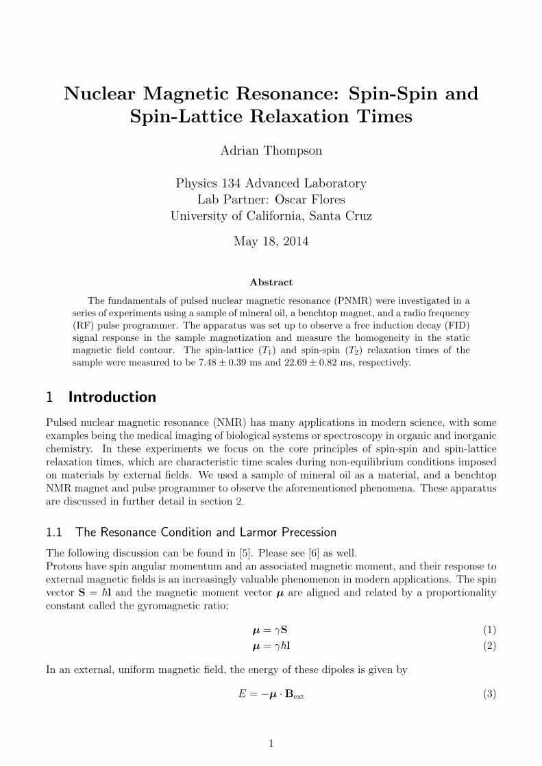
The full apparatus schematic is shown in figure 1. The devices we used are detailed below infigures 2, 3, and 4.

Figure 1: The block diagram for the device chain used to send pulses and mix the FID and echosignals with the pulsed frequency [3].

3

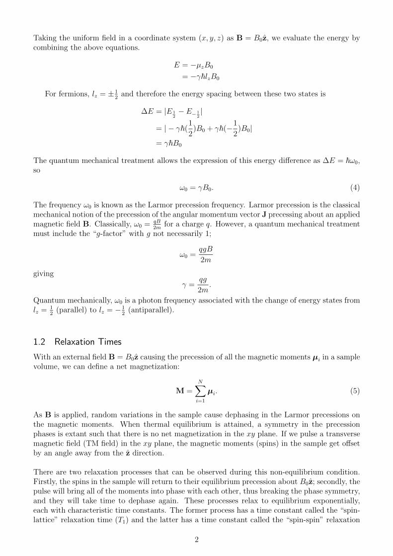
Figure 2: The TeachSpin PM 1501 magnet.

The magnet shown in Figure 2 is capable of applying static and pulsed fields. A sample canbe inserted into a vertical capsule in the center of the device. Permanent magnets provide astatic field, in what we labeled the z direction, across the sample. The sample is flanked bytwo Helmholtz coils, which provide the pulsed field out of or into the plane of the chassis face,perpendicular to the static field. The knobs on the side and front of the magnet can be usedto adjust the sample position in the xy plane; we used this feature to find the most ”flat” orhomogeneous regime of the static field as a preliminary step to measuring pulse responses.

4

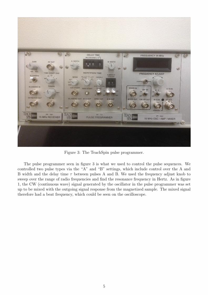
Figure 3: The TeachSpin pulse programmer.

The pulse programmer seen in figure 3 is what we used to control the pulse sequences. Wecontrolled two pulse types via the “A” and “B” settings, which include control over the A andB width and the delay time τ between pulses A and B. We used the frequency adjust knob tosweep over the range of radio frequencies and find the resonance frequency in Hertz. As in figure1, the CW (continuous wave) signal generated by the oscillator in the pulse programmer was setup to be mixed with the outgoing signal response from the magnetized sample. The mixed signaltherefore had a beat frequency, which could be seen on the oscilloscope.

5

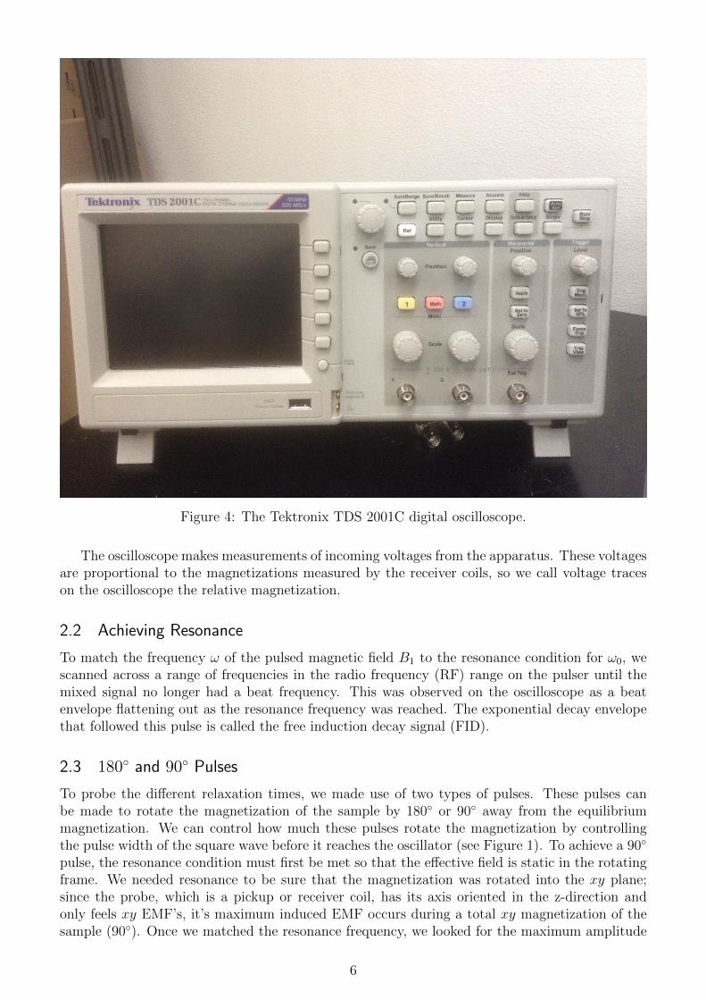
Figure 4: The Tektronix TDS 2001C digital oscilloscope.

The oscilloscope makes measurements of incoming voltages from the apparatus. These voltagesare proportional to the magnetizations measured by the receiver coils, so we call voltage traceson the oscilloscope the relative magnetization.

2.2 Achieving Resonance

To match the frequency ω of the pulsed magnetic field B1 to the resonance condition for ω0, wescanned across a range of frequencies in the radio frequency (RF) range on the pulser until themixed signal no longer had a beat frequency. This was observed on the oscilloscope as a beatenvelope flattening out as the resonance frequency was reached. The exponential decay envelopethat followed this pulse is called the free induction decay signal (FID).

2.3 180◦ and 90◦ Pulses

To probe the different relaxation times, we made use of two types of pulses. These pulses canbe made to rotate the magnetization of the sample by 180◦ or 90◦ away from the equilibriummagnetization. We can control how much these pulses rotate the magnetization by controllingthe pulse width of the square wave before it reaches the oscillator (see Figure 1). To achieve a 90◦

pulse, the resonance condition must first be met so that the effective field is static in the rotatingframe. We needed resonance to be sure that the magnetization was rotated into the xy plane;since the probe, which is a pickup or receiver coil, has its axis oriented in the z-direction andonly feels xy EMF’s, it’s maximum induced EMF occurs during a total xy magnetization of thesample (90◦). Once we matched the resonance frequency, we looked for the maximum amplitude

6

in the free induction decay signal; this was the sign of a true 90◦ pulse.

For a 180◦ pulse, we expected no FID tail. This is because a 180◦ pulse rotates the magnetiza-tion to an unstable equilibrium position through the transformation Mz → −Mz. In truth, eachof the nucleon spins have x and y components along their precession, but phase symmetry acrossthe sample destructively interferes to produce only a net Mz (use equation 5 setting

∑Ni=1 µx = 0,∑N

i=1 µy = 0). Since the pickup coils in the magnet probe do not pickup any z magnetization,no signal can be observed as M is constrained to the z axis during its return to equilibrium. Toobtain this, we varied the duration (or width) of the square wave until the FID tail was minimalon the oscilloscope screen.

2.4 Spin-Lattice Relaxation Time T1

M(t) = M0(1− e−tT1 ) (6)

Equation 6 describes the magnetization’s exponential growth toward equilibrium. T1 is the spin-lattice relaxation time. Notice that as t→∞, the magnetization returns to equilibrium. What isobserved in the lab is actually an exponential decay from the pickup coils measuring diminishingxy magnetization. Therefore, the equation that models our oscilloscope FID signal trace is

M(t) = M0e− tT1 (7)

To obtain an approximation of T1, we sent a 90◦ pulse to rotate the spins of the sample into thexy plane. We observed the FID pulse on the oscilloscope and We used a 180◦ pulse followed by a90◦ pulse and plotted the height of the FID signal from the 90◦ pulse as a function of the delaytime τ .

2.5 Spin-Spin Relaxation Time T2

The spin-spin relaxation time T2, like T1, also satisfies a decaying exponential, but this time onlyin the x and y directions. The full magnetization equation as a function of t for T2 is

M(t) = M0e− 1

6( tT2

)3(8)

(see [1]). Since our apparatus does not measure z magnetization, the actual relationship we lookedfor is given in equation 9, found in [3]:

Mx,y(t) = M0e− tT2 (9)

The spin-lattice and spin-spin relaxations are happening simultaneously as the sample magnetiza-tion is displaced from equilibrium. The way we separated the two phenomena into two observableswas by a M-G (Meiboom-Gill) series of pulses, based on the Carr-Purcell method [2]. Explicitly,we used a 90◦ pulse followed by a 180◦ pulse. This is the Carr-Purcell method described in pages34-35 of [3] or in [2]. The 90◦ pulse rotates the moments µi into the xy plane; they will beundergoing FID, but their precessions will also be dephasing back to a symmetric magnetization.Before their FID finishes (i.e. before T1), a 180◦ pulse displaces the moments to precess in theopposite direction, still in the xy plane. This allows the moments to completely rephase while inthe xy plane, decoupled from their normal FID paths. The moment that they rephase incurs amaximum readout voltage in the pickup coil, which can be seen on the oscilloscope as a ”hump” ;

7

this is called a spin-echo signal. The delay time, τ , between the two pulses is the same as the delaytime between the second pulse and the spin-echo. We then plotted the spin-echo pulse height as afunction of twice the delay time, 2τ . This extracted T2 for us without simultaneously measuringT1 [3];

M(2τ) = M0e− 2τT2 (10)

We used a modified version of the Carr-Purcell method called the Meiboom-Gill or M-G method.Everything remains mathematically the same, but a phase-shift technique during the pulse se-quence ensures that a true 180◦ pulse has been achieved [4]. This technique was used by simplyturning on the “M-G” switch on the pulse programmer.

2.6 Errors and Data Software

We used an estimation method to determine the errors made on the relative magnetization mea-sured by the oscilloscope trace. We used the cursor function on the oscilloscope to measure theseheights; since the trace was quite noisy (see figures 6 and 8), we took the error on the trace to behalf the width of the trace. We approximated half the width to be 0.07 Volts, so we took σM(t)

for both T1 and T2 measurements to be ±0.07.The data collected was fit using Gnuplot’s Levenberg-Marquardt algorithm, which determined forus a reduced Chi-Squared (χ2) value. We could easily obtain the true χ2 after multiplying by thedegrees of freedom ν. We then used an online chi-squared calculator [7] to obtain a confidencevalue α from the χ2 value (this is the error function result erf(χ2, ν); see [7] for the exact formula).

3 Results

3.1 Magnetic Field Homogeneity

We first needed to determine a linear regime to place our sample. We plotted the FID height asa function of the sample’s position in the yz plane (moving in y, perpendicular to the static fieldand parallel to the pulse direction. The flattest part of the curve, in the neighborhood of −1.5cm, is where we decided the most homogeneous part of the field was. We used that position tosetup our pulses for the following parts of the experiment.

8

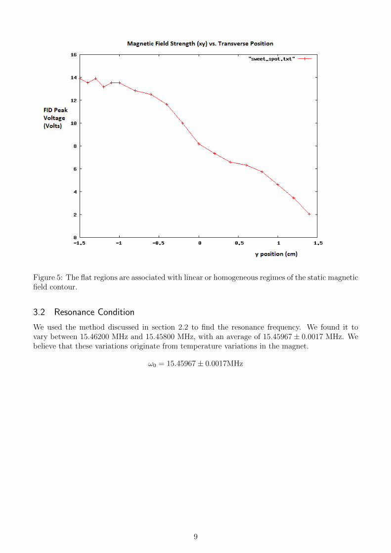
Figure 5: The flat regions are associated with linear or homogeneous regimes of the static magneticfield contour.

3.2 Resonance Condition

We used the method discussed in section 2.2 to find the resonance frequency. We found it tovary between 15.46200 MHz and 15.45800 MHz, with an average of 15.45967± 0.0017 MHz. Webelieve that these variations originate from temperature variations in the magnet.

ω0 = 15.45967± 0.0017MHz

9

3.3 Spin-Lattice Relaxation Time T1

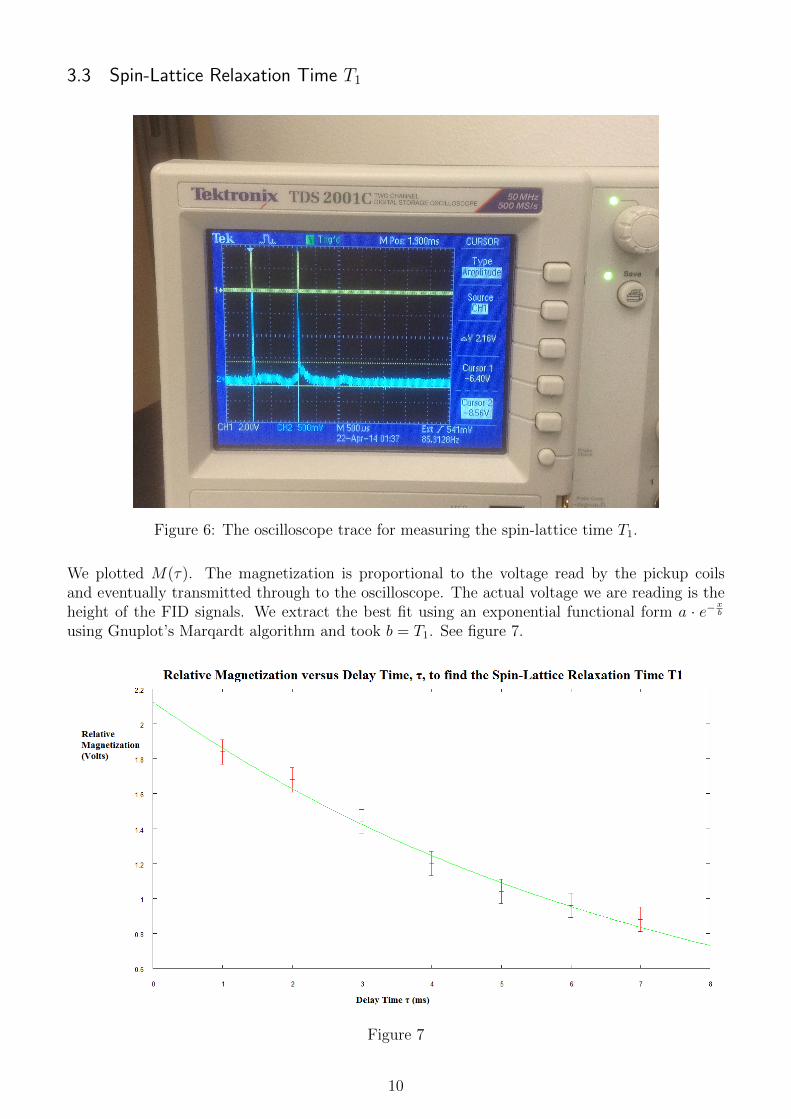
Figure 6: The oscilloscope trace for measuring the spin-lattice time T1.

We plotted M(τ). The magnetization is proportional to the voltage read by the pickup coilsand eventually transmitted through to the oscilloscope. The actual voltage we are reading is theheight of the FID signals. We extract the best fit using an exponential functional form a · e−x

b

using Gnuplot’s Marqardt algorithm and took b = T1. See figure 7.

Figure 7

10

T1 = 7.48± 0.39 ms

Degrees of Freedom ν = 5

χ2 = 2.0696

Confidence Value α = 0.8394

3.4 Spin-Spin Relaxation Time T2

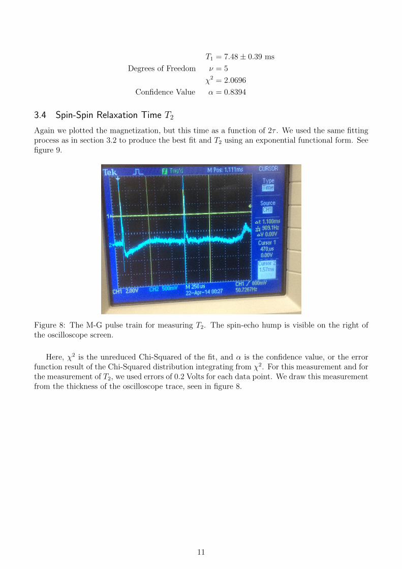
Again we plotted the magnetization, but this time as a function of 2τ . We used the same fittingprocess as in section 3.2 to produce the best fit and T2 using an exponential functional form. Seefigure 9.

Figure 8: The M-G pulse train for measuring T2. The spin-echo hump is visible on the right ofthe oscilloscope screen.

Here, χ2 is the unreduced Chi-Squared of the fit, and α is the confidence value, or the errorfunction result of the Chi-Squared distribution integrating from χ2. For this measurement and forthe measurement of T2, we used errors of 0.2 Volts for each data point. We draw this measurementfrom the thickness of the oscilloscope trace, seen in figure 8.

11

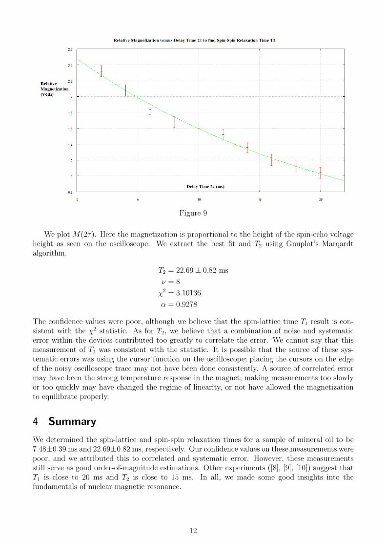
Figure 9

We plot M(2τ). Here the magnetization is proportional to the height of the spin-echo voltageheight as seen on the oscilloscope. We extract the best fit and T2 using Gnuplot’s Marqardtalgorithm.

T2 = 22.69± 0.82 ms

ν = 8

χ2 = 3.10136

α = 0.9278

The confidence values were poor, although we believe that the spin-lattice time T1 result is con-sistent with the χ2 statistic. As for T2, we believe that a combination of noise and systematicerror within the devices contributed too greatly to correlate the error. We cannot say that thismeasurement of T1 was consistent with the statistic. It is possible that the source of these sys-tematic errors was using the cursor function on the oscilloscope; placing the cursors on the edgeof the noisy oscilloscope trace may not have been done consistently. A source of correlated errormay have been the strong temperature response in the magnet; making measurements too slowlyor too quickly may have changed the regime of linearity, or not have allowed the magnetizationto equilibrate properly.

4 Summary

We determined the spin-lattice and spin-spin relaxation times for a sample of mineral oil to be7.48±0.39 ms and 22.69±0.82 ms, respectively. Our confidence values on these measurements werepoor, and we attributed this to correlated and systematic error. However, these measurementsstill serve as good order-of-magnitude estimations. Other experiments ([8], [9], [10]) suggest thatT1 is close to 20 ms and T2 is close to 15 ms. In all, we made some good insights into thefundamentals of nuclear magnetic resonance.

12

5 Appendix

5.1 Acknowledgments

We would like to thank Alice Durant for her help with setting up the correct connections withwhich to observe free induction decay. We also thank professor David Smith for helping us viewthe raw mixer output in order to clearly see the beat frequencies.

References

[1] Black, Eric D. ”Nuclear Magnetic Resonance (NMR).” California Institute of Technology(2008): n. pag. Physics 77.

[2] H. Y. Carr and E. M. Purcell, Effects of diffusion on free precession in nuclear magneticresonance experiments, Phys. Rev. 94 (3), 630-638 (1954).

[3] TeachSpin, Inc. “Pulsed Nuclear Magnetic Spectrometer”. Lab handbook. Tri-Main Center2495 Main Street, Suite 409 Buffalo, NY 14214-2153. November 1997. Web.

[4] S. Meiboom, D. Gill: Rev of Sci Instruments 29, 6881 (1958) The description of phase shifttechnique that opened up multiple pulse techniques to measuring very long T2’s in liquids. Web.

[5] Griffiths, David J. Introduction to Quantum Mechanics. Upper Saddle River, NJ: PearsonPrentice Hall, 2005. Print.

[6] Kibble, T. W. B. Classical Mechanics. Kibble. London: McGraw-Hill, 1973. Print.

[7] Walker, John. Chi-Square Calculator. Fourmilab Switzerland. John Walker, n.d. Web. 26 Feb.2014.https://www.fourmilab.ch/rpkp/experiments/analysis/chiCalc.html.

[8] Bianchini, L., and L. Coffey. ”NMR Techniques Applied to Mineral Oil, Water, andEthanol.” (2010): n. pag. Physics Department, Brandeis University, MA, 02453. Web. 13 May2014. http://fraden.brandeis.edu/courses/phys39/phys39%20reports%20S2010/Bianchini-NMR.pdf.

[9] Mallen, David, Callie Fiedler, and Andy Vesci. ”Analysis of Mineral Oil and Glycerin throughPNMR.” USD Department of Physics (2011): n. pag. 27 Mar. 2011. Web. 13 May 2014.http://home.sandiego.edu/ severn/p480w/NMRDJM.pdf.

[10] Patel, Birju. ”Pulsed NMR.” Department of Physics and Astronomy, The JohnsHopkins University, Baltimore, MD 21218 (2006): n. pag. 23 Oct. 2006. Web.http://www.pha.jhu.edu/courses/173 308/SampleLabs/Pulsed%20NMR Birju%20Patel.pdf.

13