nowcasting credit demand in turkey with google trends data-google trend verisi kullanılarak...
TRANSCRIPT
160
Volume X
Issue 2(32)
Spring 2015
ISSN-L 1843 - 6110 ISSN 2393 - 5162

Journal of Applied Economic Sciences
Volume X, Issue 2(32), Spring2015
161
Editorial Board
Editor in Chief
PhD Professor Laura GAVRILĂ (ex ŞTEFĂNESCU)
Managing Editor
PhD Associate Professor Mădălina CONSTANTINESCU
Executive Editor
PhD Professor Ion Viorel MATEI
International Relations Responsible
Pompiliu CONSTANTINESCU
Proof – readers
Ana-Maria Trantescu – English
Redactors
Andreea-Denisa Ionițoiu
Cristiana Bogdănoiu
Sorin Dincă


Journal of Applied Economic Sciences
Volume X, Issue 2(32), Spring2015
165
Editorial Advisory Board
Claudiu ALBULESCU, University of Poitiers, France, West University of Timişoara, Romania
Aleksander ARISTOVNIK, Faculty of Administration, University of Ljubljana, Slovenia
Muhammad AZAM, School of Economics, Finance & Banking, College of Business, Universiti Utara, Malaysia
Cristina BARBU, Spiru Haret University, Romania
Christoph BARMEYER, Universität Passau, Germany
Amelia BĂDICĂ, University of Craiova, Romania
Gheorghe BICĂ, Spiru Haret University, Romania
Ana BOBÎRCĂ, Academy of Economic Science, Romania
Anca Mădălina BOGDAN, Spiru Haret University, Romania
Jean-Paul GAERTNER, l'Institut Européen d'Etudes Commerciales Supérieures, France
Shankar GARGH, Editor in Chief of Advanced in Management, India
Emil GHIŢĂ, Spiru Haret University, Romania
Dragoş ILIE, Spiru Haret University, Romania
Elena Doval, Spiru Haret University, Romania
Camelia DRAGOMIR, Spiru Haret University, Romania
Arvi KUURA, Pärnu College, University of Tartu, Estonia
Rajmund MIRDALA, Faculty of Economics, Technical University of Košice, Slovakia
Piotr MISZTAL, Technical University of Radom, Economic Department, Poland
Simona MOISE, Spiru Haret University, Romania
Marco NOVARESE, University of Piemonte Orientale, Italy
Rajesh PILLANIA, Management Development Institute, India
Russell PITTMAN, International Technical Assistance Economic Analysis Group Antitrust Division, USA
Kreitz RACHEL PRICE, l'Institut Européen d'Etudes Commerciales Supérieures, France
Andy ŞTEFĂNESCU, University of Craiova, Romania
Laura UNGUREANU, Spiru Haret University, Romania
Hans-Jürgen WEIßBACH, University of Applied Sciences - Frankfurt am Main, Germany
Faculty of Financial Management Accounting Craiova No 4. Brazda lui Novac Street, Craiova, Dolj, Romania Phone: +40 251 598265 Fax: + 40 251 598265
European Research Center of Managerial Studies in Business Administration http://www.cesmaa.eu Email: [email protected] Web: http://cesmaa.eu/journals/jaes/index.php
Journal of Applied Economic Sciences Volume X, Issue 2 (32) Spring 2015
166
Journal of Applied Economic Sciences
Journal of Applied Economic Sciences is a young economics and interdisciplinary research journal, aimed
to publish articles and papers that should contribute to the development of both the theory and practice in the field
of Economic Sciences.
The journal seeks to promote the best papers and researches in management, finance, accounting,
marketing, informatics, decision/making theory, mathematical modelling, expert systems, decision system
support, and knowledge representation. This topic may include the fields indicated above but are not limited to
these.
Journal of Applied Economic Sciences be appeals for experienced and junior researchers, who are
interested in one or more of the diverse areas covered by the journal. It is currently published quarterly with three
general issues in Winter, Spring, Summer and a special one, in Fall.
The special issue contains papers selected from the International Conference organized by the European
Research Centre of Managerial Studies in Business Administration (www.cesmaa.eu) and Faculty of Financial
Management Accounting Craiova in each October of every academic year. There will prevail the papers
containing case studies as well as those papers which bring something new in the field. The selection will be
made achieved by:
Journal of Applied Economic Sciences is indexed in SCOPUS www.scopus.com, CEEOL www.ceeol.org,
EBSCO www.ebsco.com, RePEc www.repec.org and in IndexCopernicus www.indexcopernicus.com databases.
The journal will be available on-line and will be also being distributed to several universities, research
institutes and libraries in Romania and abroad. To subscribe to this journal and receive the on-line/printed
version, please send a request directly to [email protected].
Journal of Applied Economic Sciences
Volume X, Issue 2(32), Spring2015
167
Journal of Applied Economic Sciences
ISSN-L 1843 - 6110
ISSN 2393 – 5162
Table of Contents
Jozef GLOVA
Time series models and cointegration in stock portfolio selection …169
Adrian IONESCU, Cornel IONESCU
The impact of innovation orientation on market performance of Romanian …176
B2B firms
Patrik JANGL
The effect of market orientation on innovation of Czech and German …182 high - tech firms
Khadidja LAHMER, Ali KHALFI
Is Algeria ready to integrate the knowledge-based economy? …195
Samia NASREEN, Sofia ANWAR
How economic and financial integration affects financial stability in …207
South Asia: evidence from panel cointegration analysis
Martina NOVOTNÁ
The effect of industry and corporate characteristics on bond rating …223
Iveta PALEČKOVÁ
Estimation of banking efficiency determinants in the Czech Republic …234
13
12
14
16
17
18
15
Journal of Applied Economic Sciences Volume X, Issue 2 (32) Spring 2015
168
Jindra PETERKOVÁ, Zuzana WOZNIAKOVÁ
The Czech innovative enterprise …243
Jaka SRIYANA
Long run fiscal disequilibrium: an Indonesian case …253
Loredana VĂCĂRESCU HOBEANU
The performances assessment - assessment methods and techniques of the …262
professional performances
Woraphon WATTANATORN, Sarayut NATHAPHAN,
Chaiyuth PADUNGSAKSAWASDI
Bank-related asset management firm and risk taking in mutual fund …279
tournament: evidence from ASEAN economic community
Ömer ZEYBEK, Erginbay UĞURLU
Nowcasting credit demand in Turkey with Google trends data …293
Renata NESPORKOVA, Jan SIDOR
Comparison of Countries by the Systems of Health Insurance …301
19
20
10
22
21
23
24
Journal of Applied Economic Sciences
Volume X, Issue 2(32), Spring2015
169
TIME SERIES MODELS AND COINTEGRATION IN STOCK PORTFOLIO SELECTION
Jozef GLOVA
Technical University of Košice, Faculty of Economics
Abstract:
Cointegration has become the prevalent statistical tool in applied economics. It is a powerful technique
for investigating long term dependence in multivariate time series. Our paper describes a specific portfolio
selection method based on cointegration. We construct cointegration model in two stages: at first we examines
the association in a long term equilibrium between the prices of a set of financial assets, and in the second stage
we use a dynamic model of correlation, called an error correction model based on linear regression analysis of
returns. We considered an allocation into portfolio consisting of Dow Jones Industrial Average components and
thereafter we compare long term return and risk profile of portfolio focus on cointegration selection process
and index DJIA. The cointegration technique enabled us to use long calibration period and provided that
portfolio weights do not change too much over time and outperform the index DJIA in post-sample performance
measurement.
Keywords: portfolio selection, cointegration, portfolio risk and return, index tracking, linear regression.
JEL Classification: C51, C52, G12, G32
1. Introduction
The conventional construction of a financial portfolio is based on an analysis of the correlation
structure among the particular financial assets involved in the portfolio. It was Harry Max Markowitz
(1952) in early 1950’s who published a revolutionary paper on how does one select an efficient set of
risky investment or so called efficient frontier. This theory provides the first quantitative view of
portfolios variance, where co-movements in securities returns are considered. So, the variance of
portfolios is not a simple product of the particular investment proportion and their variances. Instead
of it one has to consider covariance structure implicitly involved in multi-variate distribution of
securities returns. Almost three decades ago the general approach RiskMetrics was developed by J.P.
Morgan during the late 1980’s and has been commonly applied by financial market participants for
more than two decades. Unfortunately the concept lacks of accuracy if the correlation structure
varying in time. From this perspective the traditional portfolio needs rebalance repeatedly, what could
increase the cost structure of the portfolio dramatically. In general the use of the traditional concept is
delimited and depends on the level of change within the portfolio volatility.
While the traditional approach considers historical time series returns of the selected set of
financial assets and their replication against the return of a particular index the cointegration analysis
uses assets‘ time series appearing and behaving as random processes or processes of the so-called
random walk. In our study we use the second mentioned concept, cointegration. The classical papers
on cointegration are by Granger (1986) and Engle and Granger (1987).
The cointegration is based on the long-term relationship between time series. One can consider
the cointegration, if there is such linear combination of the non-stationary time series that is stationary.
The passive index tracking strategy tries to achieve equal return as well as the underlying index, and
concurrently tries to diminish the volatility of the tracking error, thus a difference between the
portfolio return and underlying index.
The paper is divided as follows: at the beginning we briefly start with an overview of time
series stationarity, a specific assumption that is expected to be fulfilled for applying the cointegration
approach. A difference between correlation and cointegration is being explained in a brief form.
Further we describe cointegration analysis and the possible fields and forms of its applicability. All
this effort is summarized in an overview the theory and the state of the art. Engle-Granger method has
been applied as a technical part of our research methodology. We considered an allocation into
portfolios consisting of Dow Jones Industrial Average (DJIA) components. At first we describe
Journal of Applied Economic Sciences Volume X, Issue 2 (32) Spring 2015
170
methodology with a description of data and later the further attributes for asset allocation are specified.
Beyond the current research in this field we consider particular modifications of key parameters and
them sensibility change in a form of different number of stocks, reselection interval, calibration period
and strategy used as well as level of transaction expenses. At the end the discussion is provided.
2. Literature review
Passive and active equity portfolio management style is usually discussed and described in
economics literature. The crucial phase in the investment process is allocation what for equity style
portfolios means stock picking or stock selection. It was Harry M. Markowitz (1952, 1959) who made
the first quantitative and empirical contribution to portfolio selection. According to Reilly and Brown
(2012) no middle ground exists between active and passive equity management strategies. They also
argue that “hybrid” active/passive equity portfolio management style exists, in a form of enhanced
indexing, but such styles are variations of active management philosophies.
Focusing on passive equity portfolio management means a long-term buy-and-hold strategy.
Very often some authors like Gibson (2013) or Nofsinger (2013) referee about indexing strategy,
because of the goal of tracking an index. In this context only occasional rebalancing is needed,
specifically because dividends and their reinvesting, stocks merge or change in the index construction.
In traditional literature one can find three basic techniques for constructing a passive index portfolio –
full replication, sampling, and quadratic optimization or programming. Full replication technique helps
ensure close tracking, but it may be suboptimal because of transaction cost connecting with purchase
of many securities and dividend reinvestments. With sampling technique we need to buy a
representative sample of stacks that comprise the benchmark index. The last passive technique is
quadratic optimization or quadratic programming based on historical information on price changes and
correlations between securities as inputs to a computer program that determines the composition of a
portfolio that minimize tracking error with the benchmark. This technique lack of accuracy because it
relies on historical price changes and correlation. According to Alexander (2008) correlation reflects
co-movements in returns, which are liable to great instabilities over time. Returns have ‘no memory’
of a trend so correlation is intrinsically a short term measure. As she further explains that is why
portfolios that have allocations based on a correlation matrix commonly require frequent rebalancing
and long-short strategies that are based only on correlations cannot guarantee long term performance
because there is no mechanism to ensure the reversion of long and short portfolios. That’s the reason
why Alexander (1999), Alexander and Dimitriu (2005) and Dunis and Ho (2005) proposed to use
cointegration analysis as a sound statistical methodology for modelling the long term equilibrium.
In general we can say cointegration and correlation are related but different concepts. High
correlation does not automatically imply high correlation nor vice versa. If there is cointegration or
not, high correlation can occur. But to distinguish both terms we need to note that correlation tells us
nothing about the long term relationship or behaviour between two assets. So correlation is not
adequate measure over long periods of time. Correlation only reflects co-movements in returns, which
have no ‘memory’ of a trend, so is intrinsically a short term measure.
As we already mentioned in our papers in Glova (2013a, b), the co-movements between stocks
can be due to a single or multiple indices. So the correlation or covariance structure of security returns
might be obtained by relating the return on a stock to the return on a stock market index or other non-
market indices. Unfortunately as mentioned by Alexander (2008) so created portfolios require frequent
rebalancing because there is nothing to prevent the tracking error from behaving in the unpredictable
manner of random walk.
To conclude, since correlation tells us nothing about long term performance there is a need to
augment standard risk-return modelling methodologies to consider long term trends in prices.
Therefore as mentioned by Alexander and Dimitriu (2005) portfolio management strategies based on
cointegrated financial assets should be more effective in the long term.
3. Data and methodology
We use the financial data on the DJIA to construct our own portfolio based on cointegration.
We preselected 15 different stocks with the highest Pearson correlation coefficient with the DJIA.
Time period spreads from December 29, 2000 till December 31, 2013 and it is based on daily close
prices of the selected stocks. Data have been downloaded from Yahoo Finance financial portal. The
Journal of Applied Economic Sciences
Volume X, Issue 2(32), Spring2015
171
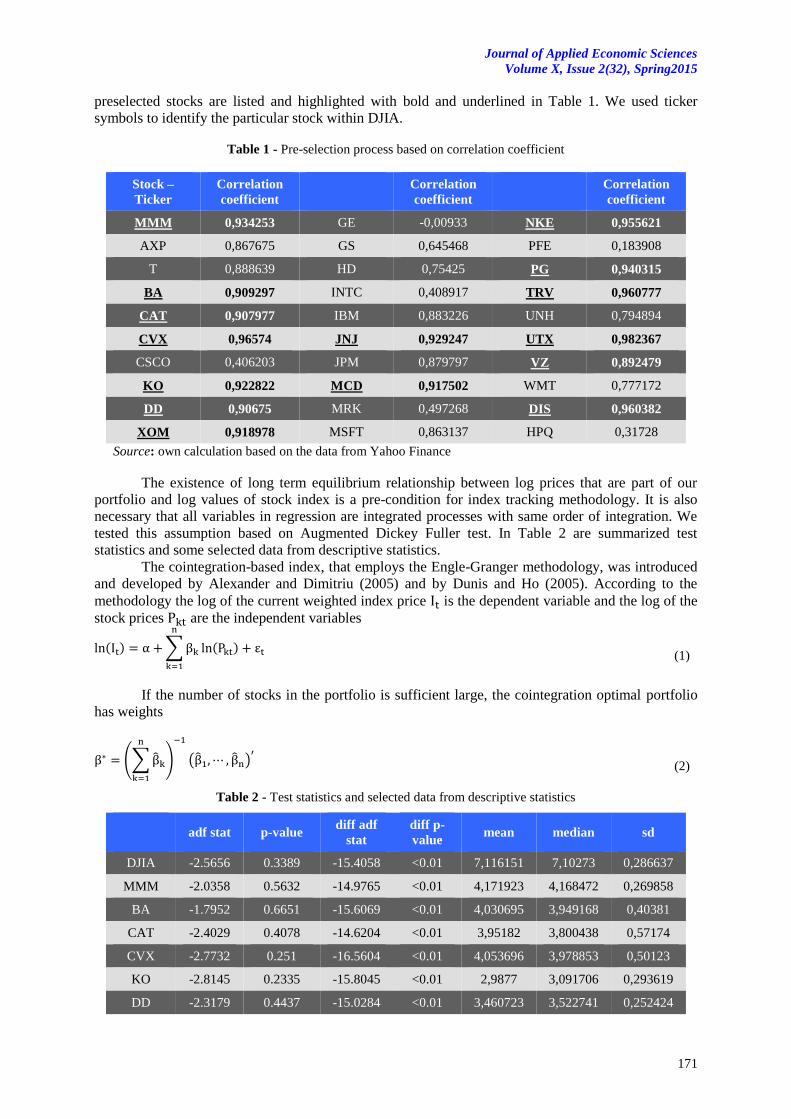
preselected stocks are listed and highlighted with bold and underlined in Table 1. We used ticker
symbols to identify the particular stock within DJIA.
Table 1 - Pre-selection process based on correlation coefficient
Stock –
Ticker
Correlation
coefficient
Correlation
coefficient
Correlation
coefficient
MMM 0,934253 GE -0,00933 NKE 0,955621
AXP 0,867675 GS 0,645468 PFE 0,183908
T 0,888639 HD 0,75425 PG 0,940315
BA 0,909297 INTC 0,408917 TRV 0,960777
CAT 0,907977 IBM 0,883226 UNH 0,794894
CVX 0,96574 JNJ 0,929247 UTX 0,982367
CSCO 0,406203 JPM 0,879797 VZ 0,892479
KO 0,922822 MCD 0,917502 WMT 0,777172
DD 0,90675 MRK 0,497268 DIS 0,960382
XOM 0,918978 MSFT 0,863137 HPQ 0,31728
Source: own calculation based on the data from Yahoo Finance
The existence of long term equilibrium relationship between log prices that are part of our
portfolio and log values of stock index is a pre-condition for index tracking methodology. It is also
necessary that all variables in regression are integrated processes with same order of integration. We
tested this assumption based on Augmented Dickey Fuller test. In Table 2 are summarized test
statistics and some selected data from descriptive statistics.
The cointegration-based index, that employs the Engle-Granger methodology, was introduced
and developed by Alexander and Dimitriu (2005) and by Dunis and Ho (2005). According to the
methodology the log of the current weighted index price is the dependent variable and the log of the
stock prices are the independent variables
( ) ∑ ( )
(
(1)
If the number of stocks in the portfolio is sufficient large, the cointegration optimal portfolio
has weights
(∑
)
( )
(
(2)
Table 2 - Test statistics and selected data from descriptive statistics
adf stat p-value
diff adf
stat
diff p-
value mean median sd
DJIA -2.5656 0.3389 -15.4058 <0.01 7,116151 7,10273 0,286637
MMM -2.0358 0.5632 -14.9765 <0.01 4,171923 4,168472 0,269858
BA -1.7952 0.6651 -15.6069 <0.01 4,030695 3,949168 0,40381
CAT -2.4029 0.4078 -14.6204 <0.01 3,95182 3,800438 0,57174
CVX -2.7732 0.251 -16.5604 <0.01 4,053696 3,978853 0,50123
KO -2.8145 0.2335 -15.8045 <0.01 2,9877 3,091706 0,293619
DD -2.3179 0.4437 -15.0284 <0.01 3,460723 3,522741 0,252424
Journal of Applied Economic Sciences Volume X, Issue 2 (32) Spring 2015
172
XOM -2.1475 0.5159 -16.0362 <0.01 4,084463 3,964202 0,39877
JNJ -2.4047 0.407 -15.4202 <0.01 3,923952 3,92214 0,217917
MCD -3.4879 0.04343 -15.0976 <0.01 3,701549 3,625511 0,625699
NKE -3.4485 0.04723 -15.6388 <0.01 3,154444 3,14433 0,574842
PG -2.9542 0.1743 -15.2178 <0.01 3,912623 3,848129 0,294671
TRV -2.9786 0.164 -15.9509 <0.01 3,626738 3,691693 0,326625
UTX -2.9357 0.1822 -15.6732 <0.01 3,968592 3,893412 0,417218
VZ -2.3703 0.4216 -15.4705 <0.01 3,162517 3,236234 0,278395
DIS -2.3524 0.4291 -15.5949 <0.01 3,282789 3,313332 0,378482
Source: own calculation
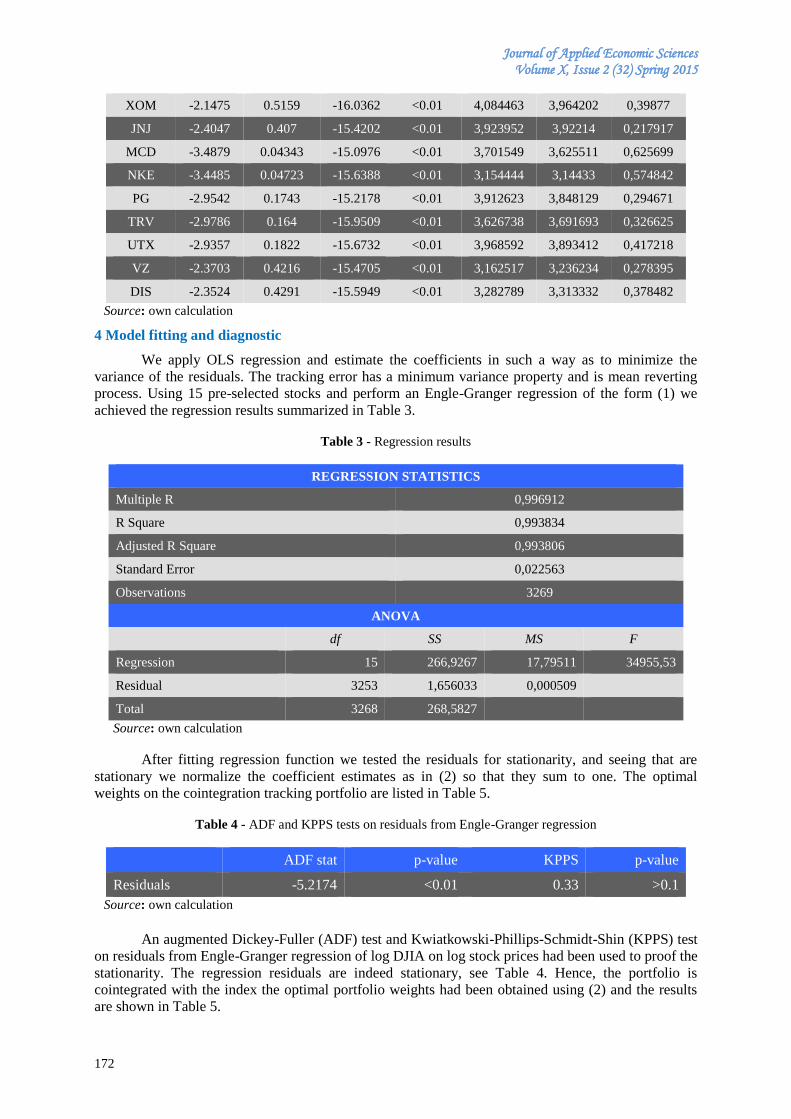
4 Model fitting and diagnostic
We apply OLS regression and estimate the coefficients in such a way as to minimize the
variance of the residuals. The tracking error has a minimum variance property and is mean reverting
process. Using 15 pre-selected stocks and perform an Engle-Granger regression of the form (1) we
achieved the regression results summarized in Table 3.
Table 3 - Regression results
REGRESSION STATISTICS
Multiple R 0,996912
R Square 0,993834
Adjusted R Square 0,993806
Standard Error 0,022563
Observations 3269
ANOVA
df SS MS F
Regression 15 266,9267 17,79511 34955,53
Residual 3253 1,656033 0,000509
Total 3268 268,5827
Source: own calculation
After fitting regression function we tested the residuals for stationarity, and seeing that are
stationary we normalize the coefficient estimates as in (2) so that they sum to one. The optimal
weights on the cointegration tracking portfolio are listed in Table 5.
Table 4 - ADF and KPPS tests on residuals from Engle-Granger regression
ADF stat p-value KPPS p-value
Residuals -5.2174 <0.01 0.33 >0.1
Source: own calculation
An augmented Dickey-Fuller (ADF) test and Kwiatkowski-Phillips-Schmidt-Shin (KPPS) test
on residuals from Engle-Granger regression of log DJIA on log stock prices had been used to proof the
stationarity. The regression residuals are indeed stationary, see Table 4. Hence, the portfolio is
cointegrated with the index the optimal portfolio weights had been obtained using (2) and the results
are shown in Table 5.
Journal of Applied Economic Sciences
Volume X, Issue 2(32), Spring2015
173
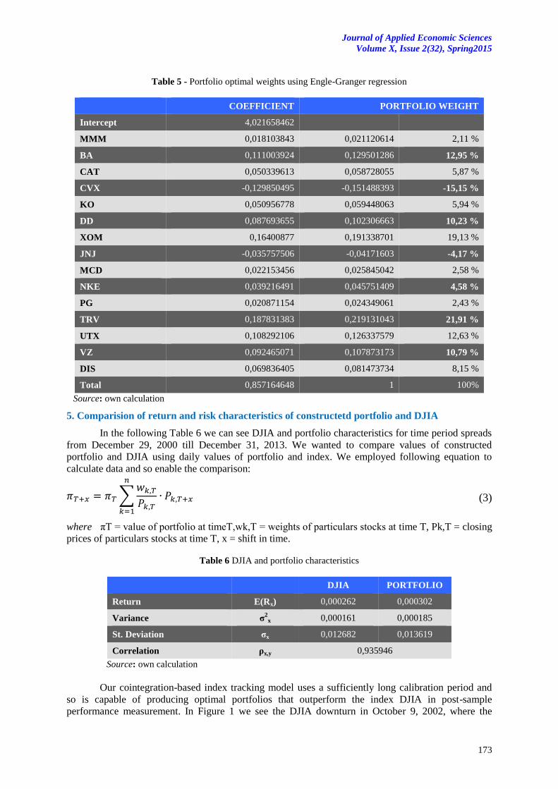
Table 5 - Portfolio optimal weights using Engle-Granger regression
COEFFICIENT PORTFOLIO WEIGHT
Intercept 4,021658462
MMM 0,018103843 0,021120614 2,11 %
BA 0,111003924 0,129501286 12,95 %
CAT 0,050339613 0,058728055 5,87 %
CVX -0,129850495 -0,151488393 -15,15 %
KO 0,050956778 0,059448063 5,94 %
DD 0,087693655 0,102306663 10,23 %
XOM 0,16400877 0,191338701 19,13 %
JNJ -0,035757506 -0,04171603 -4,17 %
MCD 0,022153456 0,025845042 2,58 %
NKE 0,039216491 0,045751409 4,58 %
PG 0,020871154 0,024349061 2,43 %
TRV 0,187831383 0,219131043 21,91 %
UTX 0,108292106 0,126337579 12,63 %
VZ 0,092465071 0,107873173 10,79 %
DIS 0,069836405 0,081473734 8,15 %
Total 0,857164648 1 100%
Source: own calculation
5. Comparision of return and risk characteristics of constructetd portfolio and DJIA
In the following Table 6 we can see DJIA and portfolio characteristics for time period spreads
from December 29, 2000 till December 31, 2013. We wanted to compare values of constructed
portfolio and DJIA using daily values of portfolio and index. We employed following equation to
calculate data and so enable the comparison:
∑
(3)
where πT = value of portfolio at timeT,wk,T = weights of particulars stocks at time T, Pk,T = closing
prices of particulars stocks at time T, x = shift in time.
Table 6 DJIA and portfolio characteristics
DJIA PORTFOLIO
Return E(Rx) 0,000262 0,000302
Variance σ2
x 0,000161 0,000185
St. Deviation σx 0,012682 0,013619
Correlation ρx,y 0,935946
Source: own calculation
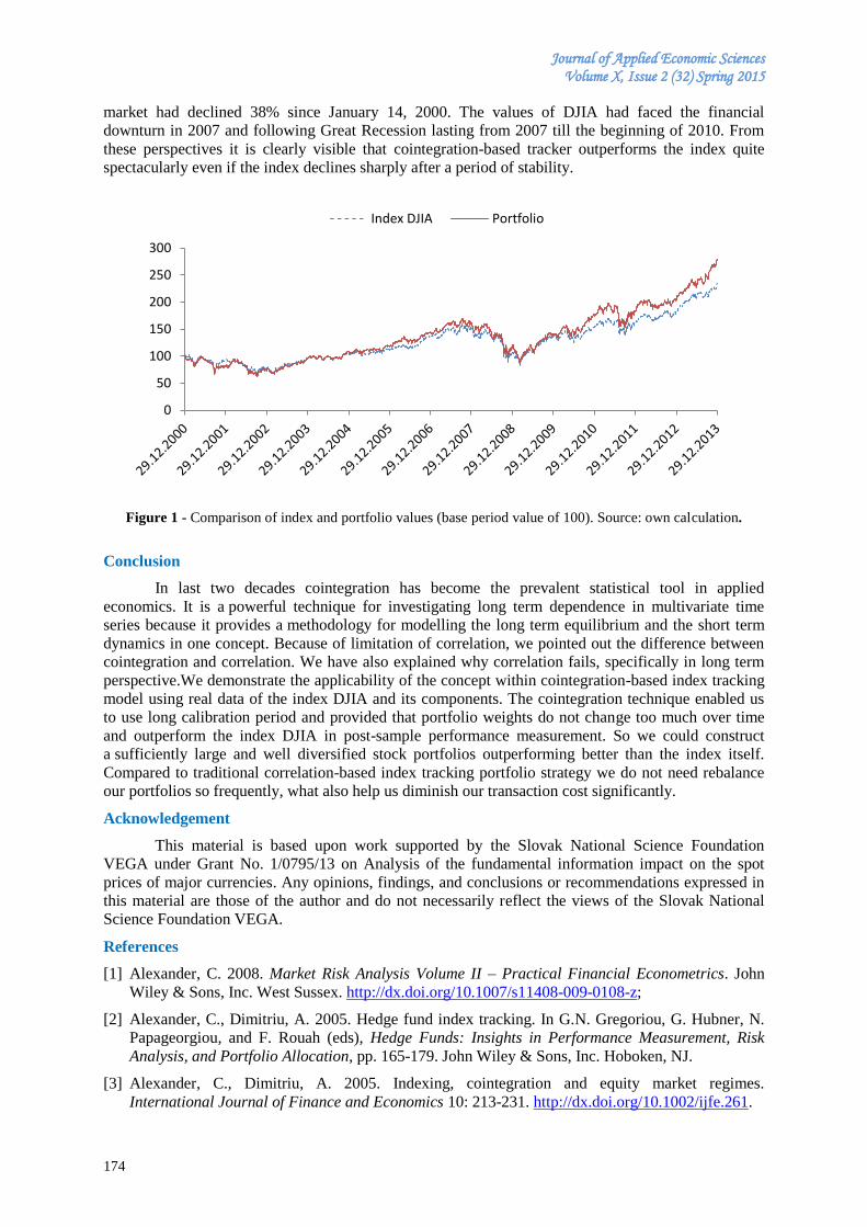
Our cointegration-based index tracking model uses a sufficiently long calibration period and
so is capable of producing optimal portfolios that outperform the index DJIA in post-sample
performance measurement. In Figure 1 we see the DJIA downturn in October 9, 2002, where the
Journal of Applied Economic Sciences Volume X, Issue 2 (32) Spring 2015
174
market had declined 38% since January 14, 2000. The values of DJIA had faced the financial
downturn in 2007 and following Great Recession lasting from 2007 till the beginning of 2010. From
these perspectives it is clearly visible that cointegration-based tracker outperforms the index quite
spectacularly even if the index declines sharply after a period of stability.
Figure 1 - Comparison of index and portfolio values (base period value of 100). Source: own calculation.
Conclusion
In last two decades cointegration has become the prevalent statistical tool in applied
economics. It is a powerful technique for investigating long term dependence in multivariate time
series because it provides a methodology for modelling the long term equilibrium and the short term
dynamics in one concept. Because of limitation of correlation, we pointed out the difference between
cointegration and correlation. We have also explained why correlation fails, specifically in long term
perspective.We demonstrate the applicability of the concept within cointegration-based index tracking
model using real data of the index DJIA and its components. The cointegration technique enabled us
to use long calibration period and provided that portfolio weights do not change too much over time
and outperform the index DJIA in post-sample performance measurement. So we could construct
a sufficiently large and well diversified stock portfolios outperforming better than the index itself.
Compared to traditional correlation-based index tracking portfolio strategy we do not need rebalance
our portfolios so frequently, what also help us diminish our transaction cost significantly.
Acknowledgement
This material is based upon work supported by the Slovak National Science Foundation
VEGA under Grant No. 1/0795/13 on Analysis of the fundamental information impact on the spot
prices of major currencies. Any opinions, findings, and conclusions or recommendations expressed in
this material are those of the author and do not necessarily reflect the views of the Slovak National
Science Foundation VEGA.
References
[1] Alexander, C. 2008. Market Risk Analysis Volume II – Practical Financial Econometrics. John
Wiley & Sons, Inc. West Sussex. http://dx.doi.org/10.1007/s11408-009-0108-z;
[2] Alexander, C., Dimitriu, A. 2005. Hedge fund index tracking. In G.N. Gregoriou, G. Hubner, N.
Papageorgiou, and F. Rouah (eds), Hedge Funds: Insights in Performance Measurement, Risk
Analysis, and Portfolio Allocation, pp. 165-179. John Wiley & Sons, Inc. Hoboken, NJ.
[3] Alexander, C., Dimitriu, A. 2005. Indexing, cointegration and equity market regimes.
International Journal of Finance and Economics 10: 213-231. http://dx.doi.org/10.1002/ijfe.261.
0
50
100
150
200
250
300
Index DJIA Portfolio
Journal of Applied Economic Sciences
Volume X, Issue 2(32), Spring2015
175
[4] Dunis, C., Ho, R. 2005. Cointegration portfolios of European equities for index tracing and market
neutral strategies. Journal of Asset Management 6: 33-52. http://dx.doi.org/10.1057/
palgrave.jam.2240164.
[5] Engle, R.F., Granger, C.W. J. 1987. Co-integration and error correction: Representation,
estimation and testing. Econometrica,55(2): 251-276. http://dx.doi.org/10.2307/1913236;
[6] Gibson, R.C., Sidoni, CH. J. 2013. Asset Allocation. Balancing Financial Risk. McGraw-Hill.
[7] Glova, J. 2013a. Determinacia systematickeho rizika kmenovej akcie v modeli casovo-
premenliveho fundamentalneho beta, E+M Ekonomie a Management, 16(2): 139.
[8] Glova, J., Pastor, D. 2013. Country risk modelling using time-varying fundamental beta approach:
A Visegrad group countries and Romania perspective. Journal of Applied Economic Sciences,
8(4): 450-456.
[9] Glova, J. (2013b). Exponential Smoothing Technique in Correlation Structure Forecasting of
Visegrad Country Indices. Journal of Applied Economic Sciences, 8(2): 184-190.
[10] Markowitz, H.M. 1952. Portfolio Selection. Journal of Finance, pp. 77-91. http://dx.doi.org/
10.1111/j.1540-6261.1952.tb01525.x;
[11] Markowitz, H.M. 1959. Portfolio Selection. Efficient Diversification of Investments. John Wiley
& Sons, Inc., New York. http://dx.doi.org/10.2307/3006625;
[12] Nofsinger, J. 2013. Psychology of Investing. Pearson Series in Finance. Prentice Hall.
[13] Reilley, F. K., Brown, K.C. 2012. Investment Analysis & Portfolio Management. South-Western
Cengage Learning.
Journal of Applied Economic Sciences Volume X, Issue 2 (32) Spring 2015
176
THE IMPACT OF INNOVATION ORIENTATION ON MARKET PERFORMANCE OF ROMANIAN B2B FIRMS
Adrian IONESCU
Faculty of Economics and Business Administration, Timișoara
West University of Timisoara, Romania
Cornel IONESCU
Institute of National Economy, Romanian Academy
Abstract Literature examines the impact of innovation orientation on firms’ performance and often demonstrates
a direct and positive relationship between the two concepts. However, few empirical studies are analyzing the
relationship between innovation orientation and market performance constructs, one of the most important being
customer satisfaction. This paper presents a review of innovation orientation concept and empirically
investigates the relationship between innovation orientation and customer satisfaction using data from 95
companies in Romania working mainly in the B2B domain. The results confirm previous exploratory research,
namely that there is a direct, positive and strong link between innovation orientation and customer satisfaction
within Romanian B2B companies.
Keywords: Innovation orientation, innovation, performance, customer satisfaction, innovation in Romania.
JEL Classification: M21, O31, M00
1. Introduction
Innovation is currently one of the most important problems of organizations.
Carr (1999) states that firms innovate on many levels such as those related to business models,
products, services, processes and distribution channels in order to maintain or conquest new markets,
distanced themselves from the competition and ensure a long-term survival and growth particularly
when they activate in complex and extremely turbulent environments (Freeman, 1994; Lawless and
Anderson, 1996).
In the literature (Freeman 1994; Miles and Snow 1978; Van de Ven et al. 1999) a special
attention has been given to the innovation types and diffusion, without taking into account the
organizational innovation process as a permanent and major objective. Regarding this situation
Tushman (1997) reported that innovation itself is not necessarily the key to long term success of firms.
Instead, a company's success is based on innovation in the global orientation of the firm. This
orientation produces the continuous innovation capabilities with multiple effects on the performance
both inside and outside the organization.
This paper aims to present the possible effects resulting from the adoption by the organizations
of the strategic orientation towards innovation and empirically demonstrate the positive effect of
innovation orientation on customer satisfaction within Romanian companies.
2. The concept of innovation orientation
Manu (1992) defined innovation orientation as all innovation programs within an organization.
He says that this type of orientation has a strategic nature as gives companies a way to approach the
markets. Manu and Siriam (1996) conceptualized innovation orientation as a multi-component
construct containing the introduction of new products, research and development expenses related to
the order of entry on the market.
Amabile (1997) stated that the most important elements of innovation orientation are
represented by a certain value attached to creativity and innovation in general, an orientation toward
risk, a sense of pride within the organization members, their enthusiasm about what they can do and
by an offensive strategy of assuming the future.
Berthon, Hulber and Pitt (1999) define innovation orientation as related to those companies
who devote their energies towards inventing and perfecting superior products. This conceptualization
incorporates both approaches on innovation orientation namely openness to innovation (Zaltman,
Duncan and Holbek 1973) and the capability for innovation (Burns and Stalker 1977).
Journal of Applied Economic Sciences
Volume X, Issue 2(32), Spring2015
177
Worren, Moore and Cardona (2002) conceptualized innovation oriented as being the link
between product modularity and an organization strategic intent to develop new products or enter new
markets with its existing products.
Given the broad scope of innovation and the increased complexity as a result of the deepening
of the conceptual basis, Siguaw, Simpson, and Enz (2006) almost 10 years after the first
conceptualization of the orientation, say that the typology proposed by Manu and Siriam fails to
consider both organizational beliefs or culture and the organization knowledge structure that could
promote or inhibit innovation of a company.
In an attempt to bring together and complete the conceptual shortcomings of the literature and
the lack of consensus, Siguaw, Simpson, and Enz (2006) define the innovation orientation as a multi-
dimensional knowledge structure consisting of learning philosophy, strategic direction and trans-
functioning beliefs of a company that guides and directs all organizational strategies and actions,
including also those embedded in formal and informal behaviors, skills and business processes to
promote innovative thinking and facilitate the development, evolution and implementation of
innovations.
This definition conceptualizes innovation orientation as a set of understandings about the
innovation made in the structure of the firm knowledge that influence organizational activities, but not
as a specific set of normative behaviors (Siguaw, Simpson, and Enz 2006).
The approach proposed by Siguaw, Simopson and Enz (2006) separates the organizational
beliefs of effective actions by considering innovation orientation as a structure of knowledge rather
than an organizational culture or a mixture of rules and behaviors. In this expansive approach, the
knowledge capital of an organization is constantly enriched to identify the next steps for maintaining
innovativeness (Martin and Salomon 2003).
The innovation orientation, in the formula proposed by the authors, has academic support that
comes from emerging researches that suggest the importance of collective understandings which direct
or guide the organization and its employees in order to engage in activities designed to encourage,
value and reward innovation efforts (Damanpour 1991; Schlegelmilch, Diamantopoulus and Kreuz
2003; Siguaw, Simopson and Enz 2006). The innovation orientation is a real source of competitive
advantage, primarily due to the development of organizational knowledge and strategic intentions that
direct functional skills such as human resources, marketing and operations (Siguaw, Simpson, and Enz
2006).
The innovation orientation concept is closely considered in relation with market orientation.
Concerning this, Jaworski and Kohli (1996), two reputable authors known for conceptualizing and
studying the market orientation, argued that innovation was erroneously excluded from the market-
oriented models, this being actually a result of this orientation. Similarly, Han et al. al. (1998) stated
that literature has only recently begun to study the effects of market orientation on innovation.
However, market-oriented companies tend to be more innovative as they respond more quickly to the
dynamic needs of consumers (Narver and Slater, 1990). Narver and Slater (1994) suggest that market-
oriented organizations are better positioned to anticipate consumer needs which they are responding
with innovative products.
To emphasize the importance of the concept, an empirical study conducted by Deshpande,
Farley and Webster (1997) on the comparative market performance of the companies in England,
France, Germany, Japan and the United States suggests that the effects of innovation orientation on
performance are even more important than those of market orientation.
3. The effects of innovation orientation on firms’ performance
Review of the literature revealed a diverse range of links between different aspects of focusing
on innovation and marketing strategies, cost and performance, and links related to environment
organizations.
A first important step in studying the link between innovation and performance orientation
was made by Manu and Siriam (1996) that on the basis of considering the concept in a multi-
dimensional manner, developed a specific typology of organizations. The authors propose four types
of innovation-oriented firms. The first type is the product innovator, group characterized by the
highest rate of introduction of new products in both absolute and relative terms. A characteristic of this
type are the relatively large expenditures allocated to research and development of new products.
Journal of Applied Economic Sciences Volume X, Issue 2 (32) Spring 2015
178
Expenditure on processes research and development are at a relatively average level compared to the
sample average. Such organizations have entered the market relatively late.
The second type is represented by process innovators, characterized by the highest spending
on processes research and development but relatively average levels of R&D expenditure allocated to
products. For the second type, the relative number of new products introduced is small and the
absolute number is moderate. This type of organization has entered the market earlier.
The third type is the late entrants and lack of innovation organizations, characterized by
having the lowest rates of introduction of new products and relatively low spending on research and
development, both for products and processes.
The fourth type is the past pioneers, which is characterized by the lowest expenses for research
and development, both for products and processes as well as the lowest rate of introduction of new
products and services on the market.
A second phase of the research was to study the allocation of a certain kind of marketing
strategy for each type of organization identified in the first phase of research. More recent studies
confirm that the innovation orientation is a powerful determinant of business performance of
companies, independent of market turbulence in which they operate. Companies that want to embrace
this orientation must develop and implement an organizational culture that integrates market
orientation, learning orientation and entrepreneurial orientation (Hult et. al. 2004).
Research focusing on innovation orientation impact was also discussed by Peng and Dai
(2010). Regarding the effect on innovation results they showed that orientation has a positive impact
on the number, rate and type of innovations that a firm produces. According to studies conducted by
Tushman and O'Reilly, 1996, innovation oriented firms develop more disruptive innovations. At the
consumers and competitors levels the research of the two reveals that innovation oriented
organizations has a higher level of customer service, a higher loyalty and a better picture. At the
competitors’ level, the benefits are also on the side of innovative organizations. Thus, according to the
study by Lyon and Ferrier (2002) there is a direct link between market share and the number of new
products launched. The research shows that employees working in innovation oriented companies
have a higher level of job satisfaction, an effect confirmed by Zhou et al. (2005). Given the fact that
the study of Peng and Dai (2010) had an exploratory character we found interesting to investigate if
their hypothesis is empirically confirmed also for Romanian companies. Thus we verify:
H1: A high level of innovation orientation has a direct, positive and significant
influence on customer satisfaction.
4. Research methodology
According to previous guidelines of specialists (Iacobucci, Churchill, 2010), developing a
sampling plan involves several steps. In a first step we defined the statistical population under
investigation. Given the strategic nature of the questions we have decided that it is necessary that the
statistical population included in the research to be represented only by top-level managers. The
sampling frame was a executives database personally prepared, containing identifying data for a
number of 1,200 top managers of companies activating in Romania. Regarding the sampling method,
we opted for a non-probabilistic sampling: convenience sampling. The profile characteristics of the
firms included in the survey were analyzed using the following criteria: scope, turnover, and number
of employees, type of market and foundation year. Most companies participating in the survey (55%)
are medium and large companies operating mainly in B2B. Of the 1,200 people contacted, 98
responded favorably to the questionnaire, representing a response rate of 8.1% which we appreciate as
very good for the online administration. Data collection from respondents was done through an
electronic service management. The completion request contained a letter of intent in which the scope
and importance of the research were presented. A strong emphasis was placed on respecting the
condition of confidentiality related to both the name of the respondent and the name of the company
which he represents. Treating data collected was performed using univariate statistical analysis
methods, bivariate and multivariate. Establishing normal distribution of the variables and the
reliability and validity of measurement scales were based on using statistical tests. Also, for model
validation statistical testing of hypothesis was performed.
The statistical analysis of data had the following steps:
Journal of Applied Economic Sciences
Volume X, Issue 2(32), Spring2015
179
Uni and bivariate data analysis in order to obtain some responses related to the research
objectives. Testing the normality of values distribution of the variables included in the research model.
Testing the reliability of measurement scales.
Determination of the factorial scores.
Testing the validity of the concepts used in the research model.
Testing the formulated hypothesis.
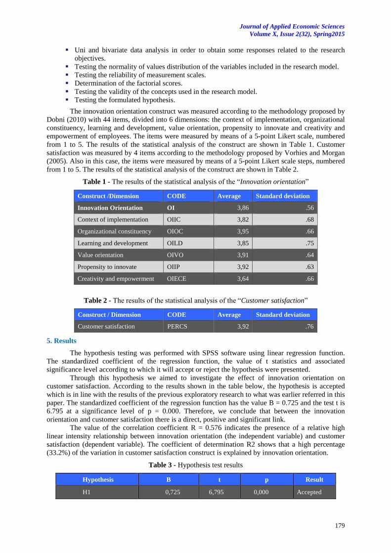
The innovation orientation construct was measured according to the methodology proposed by
Dobni (2010) with 44 items, divided into 6 dimensions: the context of implementation, organizational
constituency, learning and development, value orientation, propensity to innovate and creativity and
empowerment of employees. The items were measured by means of a 5-point Likert scale, numbered
from 1 to 5. The results of the statistical analysis of the construct are shown in Table 1. Customer
satisfaction was measured by 4 items according to the methodology proposed by Vorhies and Morgan
(2005). Also in this case, the items were measured by means of a 5-point Likert scale steps, numbered
from 1 to 5. The results of the statistical analysis of the construct are shown in Table 2.
Table 1 - The results of the statistical analysis of the “Innovation orientation”
Construct /Dimension CODE Average Standard deviation
Innovation Orientation OI 3,86 .56
Context of implementation OIIC 3,82 .68
Organizational constituency OIOC 3,95 .66
Learning and development OILD 3,85 .75
Value orientation OIVO 3,91 .64
Propensity to innovate OIIP 3,92 .63
Creativity and empowerment OIECE 3,64 .66
Table 2 - The results of the statistical analysis of the “Customer satisfaction”
Construct / Dimension CODE Average Standard deviation
Customer satisfaction PERCS 3,92 .76
5. Results
The hypothesis testing was performed with SPSS software using linear regression function.
The standardized coefficient of the regression function, the value of t statistics and associated
significance level according to which it will accept or reject the hypothesis were presented.
Through this hypothesis we aimed to investigate the effect of innovation orientation on
customer satisfaction. According to the results shown in the table below, the hypothesis is accepted
which is in line with the results of the previous exploratory research to what was earlier referred in this
paper. The standardized coefficient of the regression function has the value B = 0.725 and the test t is
6.795 at a significance level of p = 0.000. Therefore, we conclude that between the innovation
orientation and customer satisfaction there is a direct, positive and significant link.
The value of the correlation coefficient R = 0.576 indicates the presence of a relative high
linear intensity relationship between innovation orientation (the independent variable) and customer
satisfaction (dependent variable). The coefficient of determination R2 shows that a high percentage
(33.2%) of the variation in customer satisfaction construct is explained by innovation orientation.
Table 3 - Hypothesis test results
Hypothesis B t p Result
H1 0,725 6,795 0,000 Accepted
Journal of Applied Economic Sciences Volume X, Issue 2 (32) Spring 2015
180
Conclusions and limitations
Romanian managers must understand and encourage the adoption of a strategic innovation
orientation of the organizations they lead. The benefits of this type of strategic orientation are multiple
and the caused effects have a direct and positive impact on market performance even in a highly
competitive context, volatile and uncertain. Although due to the sampling method the result of this
research cannot be considered representative for all Romanian companies, the study findings are a
strong signal for considering these directions in the management strategies of the current and future
executives in Romania, especially those working in the highly competitive domains where innovation
is the basis of the competitive advantage.
Aknowledgement
This paper received financial support from the "Academic excellence routes in doctoral and
post-doctoral research - READ" project co-financed by the European Social Fund, by 2007-2013
Sectorial Operational Program for Human Development, agreement no. POSDRU/159/1/5/S/137926.
References
[1] Ajay, K. and Jaworski, B. J. 1990. Market Orientation: The Construct, Research Propositions, and
Managerial Implications. The Journal of Marketing, Vol. 54, No. 2.
[2] Baker, W., Sinkula, J. 1999. Learning Orientation, Market Orientation, and Innovation: Integrating
and Extending Models of Organizational Performance, Journal of Market Focused Management,
4.
[3] Baker, W., Sinkula, J. 2005. Market Orientation and the New Product Paradox, J PROD INNOV
MANAG 22.
[4] Berthon, P., Hulbert, J., Pitt, L. 2004. Innovation or customer orientation? An empirical
investigation, European Journal of Marketing Vol. 38 No. 9/10.
[5] Damanpour F. 1991. Organizational innovation: a meta-analysis of effects of determinants and
moderators, Acad. Manage. J. 34
[6] Deshpandé, R., Farley, J., Webster, F. 1993. Corporate Culture, Customer Orientation, and
Innovativeness in Japanese Firms: A Quadrad Analysis, The Journal of Marketing, Vol. 57, No. 1.
[7] Dobni, C. B. 2010. The relationship between an innovation orientation and competitive strategy,
International Journal of Innovation Management Vol. 14, No. 2.
[8] Guan, C, Yam, R., Tang, E. , Lau, A. 2009. Innovation strategy and performance during economic
transition: Evidences in Beijing, China, Research Policy 38.
[9] Hernandez-Espallardo, M. 2008. The role of market orientation and organizational learning ,
European Journal of Innovation Management.
[10] Hult, T., Hurley, R., Knight, G. 2004. Innovativeness: Its antecedents and impact on business
performance, Industrial Marketing Management 33.
[11] Hurley, R., Hult, T. 1998. Innovation, Market Orientation, and Organizational Learning: An
Integration and Empirical Examination, The Journal of Marketing, Vol. 62, No. 3. in New
Product Ideation, J PROD INNOV MANAG 28.
[12] Jaworski, B. 1988. Toward a Theory of Marketing Control: Environmental Context, Control
Types, and Consequences, The Journal of Marketing, Vol. 52, No. 3.
[13] Jaworski, B.J. & Kohli, A.K. 1996. Market orientation: review, refinement and roadmap. Journal
of Market-focused Management (1): 119-135.
[14] Jimenez-Jimenez, D., Sanz-Valle, R. 2011. Innovation, organizational learning and performance.
Journal of Business Research 64.

Journal of Applied Economic Sciences
Volume X, Issue 2(32), Spring2015
181
[15] Kalyanaram, G. and Urban, G. L. 1992. Dynamic Effects of the Order of Entry on Market Share,
Trial Penetration, and Repeat Purchases for Frequently Purchased Consumer Goods, Marketing
Science,Vol. 11.
[16] Manu, F. 1992. Innovation Orientation, Environment and Performance: A Comparison of U.S.
and European Markets, Journal of International Business Studies, Vol. 23, No. 2.
[17] Manu, F., Siriam, V. 1996. Innovation, Marketing Strategy, Enviroment and Performance,
Journal of Business Research 35.
[18] Melia, M., Perez, A., Dobon, S. 2009. The influence of innovation orientation on the
Internationalization of SMEs in the service sector, The Service Industries Journal 30: 5.
[19] Napoli, J. 2010. The Impact of Nonprofit Brand Orientation on Organisational Performance,
Journal of Marketing Management, 22: 7.
[20] Peng, S., Dai D. 2010. Research on Innovation Orientation Outcomes, 3rd International
Conference on Information Management, Innovation Management and Industrial Engineering.
[21] Siguaw et al. 2006. Judy A. Siguaw, Penny M. Simpson and Cathy A.Enz, Conceptualizing
innovation orientation: A framework for study and integration of innovation research, J Prod
Innov Manage 23.
[22] Siguaw, J., Diamantopoulos, A. 1995. Measuring Market Orientation: some evidence on Narver
and Slater’s three-components scale. Journal of Strategic Marketing 3.
[23] Sinkula, J.M., Baker, W. E. and Noordewier, T. 1997. A Framework for Market-Based
Organizational Learning: Linking Values, Knowledge, and Behavior. Journal of the Academy of
Marketing Science Vol. 25.
[24] Sivadas, E. and Dwyer, F.R. 2000. An examination of organizational factors influencing new
product success in internal and alliance-based processes. Journal of Marketing Vol. 64.
[25] Slater, S. F. and Narver, J. C. 1998. Customer-led and market-oriented: let's not confuse the two.
Strategic Management Journal, Vol. 19.
[26] Slater, S. F. and Narver, J. C. 1999. Market-oriented is more than being customer-led. Strategic
Management Journal, Vol. 20.
[27] Tajeddini, K. 2010. Effect of customer orientation and entrepreneurial orientation on
innovativeness: Evidence from the hotel industry in Switzerland, Tourism Management 31.
[28] Tuominen, M., Hyvonen, S. 2004. Organizational Innovation Capability: A Driver for
Competitive Superiority in Marketing Channels Int. Rev. of Retail, Distribution and Consumer
Research.
[29] Tushman, M. L. and O'Reilly, C. A. III 1997. Winning through Innovation: A Practical Guide to
Leading Organizational Change and Renewal. Boston: Harvard Business School Press.
[30] Verhees, F., Meulenberg, M. 2004. Market Orientation, Innovativeness, Product Innovation, and
Performance in Small Firms, Journal of Small Business Management 42. Vol. 14, No. 3.
[31] Vorhies, D. W., & Morgan, N. A. 2005. Benchmarking marketing capabilities for sustained
competitive advantage. Journal of Marketing, 69(1): 80-94.
[32] Weerawardena, J., O’Cass, A., Julian, C. 2006. Does industry matter? Examining the role of
industry structure and organizational learning in innovation and brand performance, Journal of
Business Research 59.
[33] Zhou, K., Gao, G., Yang, Z., Zhou, N. 2005. Developing strategic orientation in China:
antecedents and consequences of market and innovation orientations, Journal of Business
Research 58.
Journal of Applied Economic Sciences Volume X, Issue 2 (32) Spring 2015
182
THE EFFECT OF MARKET ORIENTATION ON INNOVATION OF CZECH AND GERMAN HIGH-TECH FIRMS
Patrik JANGL
Tomas Bata University in Zlin
Faculty of Management and Economics, Czech Republic
Abstract: Aim of the article is to find out the causal relationship between dimensions of market orientation (MO)
and innovation (INOV). Market orientation was studied as a four-dimensional construct and innovation as a one-
dimensional. Market orientation in this study is understood as a process of getting information about customers
and competitors, spreading and integrating these information within the company and reactions to these
information in the form of a coordinated actions. The studied sample was represented by the Czech (N=164) and
German (N=187) high-tech firms in manufacturing industries. Selection of firms was carried out in Albertina and
Hoppenstedt database. Respondents in managerial ranks completed the questionnaire and marked their rate of
approval with individual statements on a seven point Likert scale. The way to achieve the goals is to quantify
market orientation by constructing indices of market orientation. Index of market orientation and innovation was
calculated as an arithmetic mean of the measured values. The main method to reach the target was multiple
regression analysis. The research confirmed hypothesis about existence of the relation between three dimensions
of market orientation - customer intelligence generation (CUIG), intelligence dissemination & integration (IDI),
responsiveness to market intelligence (RMI) and innovation in Czech Republic and Germany. No significant
relationship was detected between dimension competitor intelligence generation (COIG) and innovation in either
of the two countries.
Keywords: customer intelligence generation, competitor intelligence generation, intelligence dissemination&
integration, responsiveness to market intelligence, market orientation, innovation, high-tech sector,
Czech Republic, Germany
JEL Classification: M31, M10
1. Introduction
Company market orientation and innovation has been a popular research topic worldwide. The
earlier empirical studies have confirmed that market-oriented companies are more successful in the
market. Every company is market-oriented to a certain extent; otherwise it could not stand up to the
competition in the current market. The question for managers is how market-oriented their company
is, for example when compared to the competition. Not only managers, but also other employees in all
departments, must realise and understand the elements, and especially the essence, of the marketing
model of market orientation. However, this is of no guarantee that the company actually acts
according to the principles of market orientation. Aim of this work is to contribute to a better
understanding of this strategic concept also in the Czech and German business environment and to
show whether the implementation of market orientation concept positively affects innovation in
companies. Managers´ interest in the issue increases every year. This is proven, among other things,
by their growing interest in the research results and a large number of new publications on this topic.
The high-tech industry is a typical example of an environment where innovation is largely represented.
For this reason, the research in hand focuses on this particular sector.
2. Measuring market orientation
There are a large number of strategic orientations of the company, e.g. product orientation,
profit orientation or customer orientation (Karlíček 2013). Customer orientation is sometimes
considered identical with market orientation (Deshpandé, Farley, Webster 1993). Others argue that
customer orientation is insufficient and other stakeholders in the market must be taken into account.
Kotler et al. (2013) considers competition and customers to be the most important stakeholders.
Kaňovská and Tomášková (2014) in their concept of market orientation, also include distributors and
suppliers, economic environment, technology and staff among important stakeholders. Different
concepts have led to the creation of numerous definitions. However, there are two dominant
Journal of Applied Economic Sciences
Volume X, Issue 2(32), Spring2015
183
approaches created by foreign authors (Kohli, Jaworski and Narver, Slater), providing a concept
suitable for our cultural environment. These provide a partial overview of the issue and show the
direction in which the further research can navigate. Kohli and Jaworski (1990) understand market
orientation as a corporate philosophy. According to them, market orientation can be defined as a
process of obtaining market information and it dissemination, integration and use. Other pioneers in
area of measuring market orientation of companies were Narver and Slater (1990). They emphasize
that market orientation is a part of the corporate culture and that it contributes to the creation of the
added value for the customer.
Market orientation is predominantly measured on a five or seven-point Likert scale. It is thus a
subjective sort of measurement. The main respondents are generally senior managers with sufficient
knowledge about the company across all departments. During the past two decades, a large number of
studies in various countries and industries have been conducted. The authors Dwairi, Bhuian and
Jurkus (2007) replicated the research of Kohli and Jaworski (1990) of market orientation in a strong
growth and highly competitive environment of the Jordanian banking sector. They focused on
monitoring the determinants of market orientation, which according to the authors may be just as
important as the consequences of market orientation. Regression models were used to test the
hypotheses. The results corresponded with the conclusions of the original authors, Kohli and Jaworski
(1990), who are widely recognised as the pioneers of the concept of market orientation measuring.
Their results suggest that top management is an important factor for the company to become market-
oriented. The authors take issue with the conclusions of Hofstede's cultural typology. Hofstede
identified Jordan as a country with fixed cultural characteristics that are incompatible with market
orientation. Given the results, the authors conclude that the model of market orientation is not
necessarily culture-bound. A study of that time (Kuada and Buatsi, 2005) also brought similar results.
Frejková and Chalupský (2013) aimed to determine the relationship between market
orientation and Customer Relationship Management (CRM). They proved that there is a certain
dependency between the two concepts based on the empirical data obtained from companies in the
field of aviation. Recent publications on Czech high-tech companies explored the relationship between
market orientation and strategic behaviour (Kaňovská and Tomášková, 2014), and modification of the
model of market orientation (Jangl, 2014). Tuominen, Rajala and Möller (2004) analysed the
relationship between market orientation and customer intimacy. The main objective of the study by
Kumar, Subramanian and Strandholm (2011) was to explore the impact of corporate strategy on the
relationship of market orientation and company performance on a sample of 159 American hospitals.
Market orientation was measured using a scale originally designed by Narver and Slater (1990) with
modifications for medical environments (Kumar, Subramanian and Yauger, 1998). Porter´s generic
strategies were measured using a scale proposed by Narver and Slater (1990), also modified for the
medical environment. The findings of their study generally offer support for the claims of Narver and
Slater (1990) and Kohli and Jaworski (1990) that market orientation has a positive impact on business
performance regardless of the type of the company. Chang and Chen (1998) tested the relationship
between market orientation, service quality and profitability of brokerage firms in Taiwan. They
concluded that market orientation has a positive and significant effect on both the quality of services,
as well as on company performance. At the same time, they found out that market orientation does not
affect performance solely through service quality.
Market orientation may affect performance directly or indirectly through other intermediaries.
The aim of the authors Panigyrakis and Theodoridis (2007) was to explore market orientation in the
context of the retail environment in the Greek market and the effect of market orientation on
performance of companies in this sector. Supermarket branch managers were chosen as the
respondents. To measure market orientation, the authors used MARKOR developed by Kohli,
Jaworski and Kumar (1993). A significantly positive effect of market orientation on corporate results
was detected. The results showed that retail chains in Greece implement the concept of market
orientation. In contrast, Bodlaj (2010) dealt with the influence of responsive and proactive market
orientation on innovation and corporate performance. Using the methods of structural equitation
modelling, Bodlaj analysed data obtained from 325 Slovenian companies and found no significant link
between proactive market orientation and innovation performance, nor between reactive market
orientation and innovation performance.
Journal of Applied Economic Sciences Volume X, Issue 2 (32) Spring 2015
184
3. Measuring innovation
Innovation is the successful implementation of creative ideas within an organization (Amabile,
1988). Thompson (1965) cited in Calaton, Cavusgil, Zhao (2002) defines innovation as follows: the
generation, acceptance, and implementation of new ideas, processes, products, or services. According
to Trommsdorff, Steinhoff (2009, p. 19) a rapid development of technologies is currently the biggest
external drive of innovation (e.g. this includes new information and communication technology,
nanotechnology, biotechnology, neurophysiology etc.). Furthermore, the same authors report a
significant innovation pressure on businesses and in the long run only those able to can keep up, will
survive. In order to keep up, it is necessary to have continuous information about the strategic situation
of the company, and also about the development in the field, about the target customers and the
competition. The factors of innovation drivers seem to be very different and interactive among
themselves. If the company aims to maximize its profits, it must offer its customers modern and high
quality products.
According to Nožička and Grossová (2012), innovative products are more likely to succeed in
competitive markets. The authors confirmed the relationship between market orientation and business
performance of innovative companies in the two regions of the Czech Republic. Measuring innovation
is also covered in Serna, Guzman, Castro (2013) in Mexican manufacturing plants (N=286), Remli et
al. (2013) in Malaysia, Bastič and Leskovar-Špacapan (2006) in Slovenian companies (N=82),
Manzano, Küster and Vila (2005) in Spanish textile companies or Agarwal, Erramilli and Dev (2003)
in the hospitality industry. Hurley and Hult (1998) investigated the connection between innovation,
market orientation and corporate culture in the USA. Calatone, Cavusgil, Zhao (2002) tested the
relationship between Learning Orientation, Innovation Capability and Firm Performance on a sample
of US firms (N=187). The authors confirm the positive effect of learning orientation on firm
innovativeness. Ma, Zhu, Hou (2011) in China, arrived at the conclusion that learning orientation
positively affects the process innovation that lead to an improved firm performance.
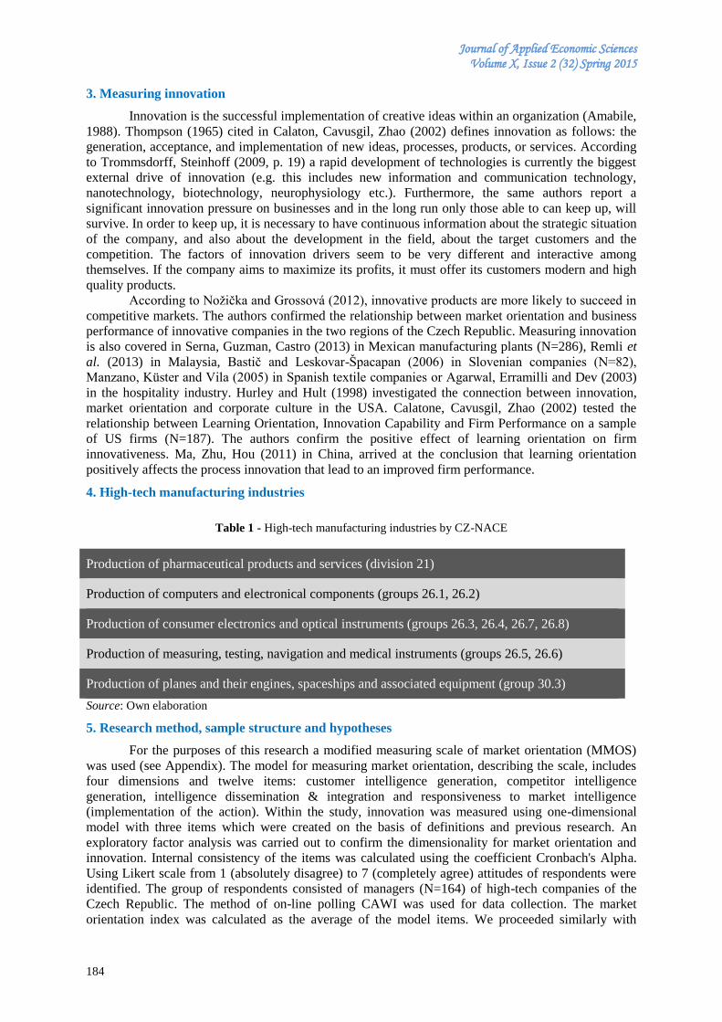
4. High-tech manufacturing industries
Table 1 - High-tech manufacturing industries by CZ-NACE
Production of pharmaceutical products and services (division 21)
Production of computers and electronical components (groups 26.1, 26.2)
Production of consumer electronics and optical instruments (groups 26.3, 26.4, 26.7, 26.8)
Production of measuring, testing, navigation and medical instruments (groups 26.5, 26.6)
Production of planes and their engines, spaceships and associated equipment (group 30.3)
Source: Own elaboration
5. Research method, sample structure and hypotheses
For the purposes of this research a modified measuring scale of market orientation (MMOS)
was used (see Appendix). The model for measuring market orientation, describing the scale, includes
four dimensions and twelve items: customer intelligence generation, competitor intelligence
generation, intelligence dissemination & integration and responsiveness to market intelligence
(implementation of the action). Within the study, innovation was measured using one-dimensional
model with three items which were created on the basis of definitions and previous research. An
exploratory factor analysis was carried out to confirm the dimensionality for market orientation and
innovation. Internal consistency of the items was calculated using the coefficient Cronbach's Alpha.
Using Likert scale from 1 (absolutely disagree) to 7 (completely agree) attitudes of respondents were
identified. The group of respondents consisted of managers (N=164) of high-tech companies of the
Czech Republic. The method of on-line polling CAWI was used for data collection. The market
orientation index was calculated as the average of the model items. We proceeded similarly with
Journal of Applied Economic Sciences
Volume X, Issue 2(32), Spring2015
185
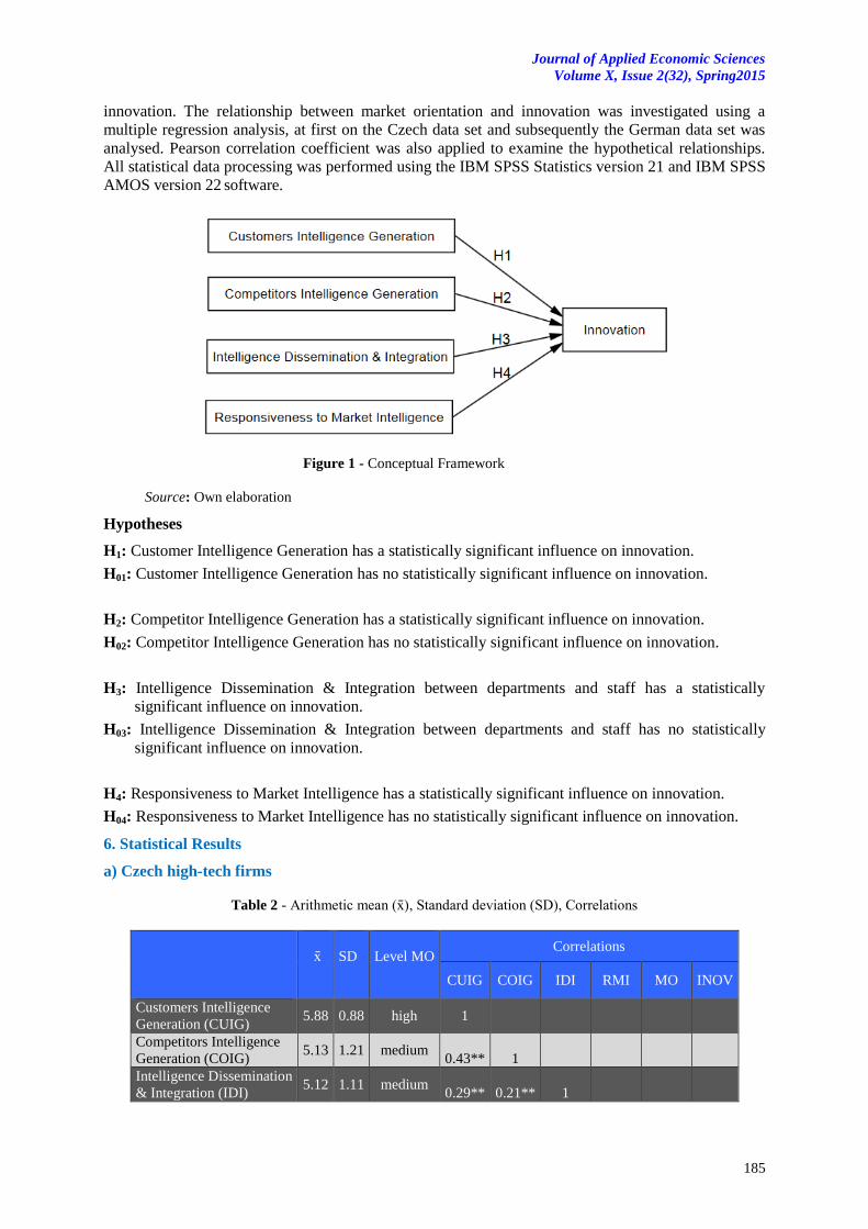
innovation. The relationship between market orientation and innovation was investigated using a
multiple regression analysis, at first on the Czech data set and subsequently the German data set was
analysed. Pearson correlation coefficient was also applied to examine the hypothetical relationships.
All statistical data processing was performed using the IBM SPSS Statistics version 21 and IBM SPSS
AMOS version 22 software.
Figure 1 - Conceptual Framework
Source: Own elaboration
Hypotheses
H1: Customer Intelligence Generation has a statistically significant influence on innovation.
H01: Customer Intelligence Generation has no statistically significant influence on innovation.
H2: Competitor Intelligence Generation has a statistically significant influence on innovation.
H02: Competitor Intelligence Generation has no statistically significant influence on innovation.
H3: Intelligence Dissemination & Integration between departments and staff has a statistically
significant influence on innovation.
H03: Intelligence Dissemination & Integration between departments and staff has no statistically
significant influence on innovation.
H4: Responsiveness to Market Intelligence has a statistically significant influence on innovation.
H04: Responsiveness to Market Intelligence has no statistically significant influence on innovation.
6. Statistical Results
a) Czech high-tech firms
Table 2 - Arithmetic mean (x ), Standard deviation (SD), Correlations
x
SD
Level MO
Correlations
CUIG COIG IDI RMI MO INOV
Customers Intelligence
Generation (CUIG) 5.88 0.88 high 1
Competitors Intelligence
Generation (COIG) 5.13 1.21 medium
0.43** 1
Intelligence Dissemination
& Integration (IDI) 5.12 1.11 medium
0.29** 0.21** 1
Journal of Applied Economic Sciences Volume X, Issue 2 (32) Spring 2015
186
Responsiveness to Market
Intelligence (RMI) 4.67 1.13 low
0.35** 0.46** 0.41** 1
Market Orientation (MO) 5.20 0.78 medium 0.68** 0.75** 0.67** 0.78** 1
Innovation (INOV) 5.25 1.03 medium 0.41** 0.30** 0.49** 0.45** 0.57** 1
Source: Own elaboration
Note: ˂ 5 (low level), ˂5; 5.5˃ (medium level), ˃ 5.5 (high level); ** Pearson correlation is
significant at 0.01 level.
Based on an index of Cronbach's alpha and exploratory factor analyses, dimensionality of the
model was confirmed. Market orientation is indeed made up of four factors and innovation of one
factor. Cronbach's alpha coefficient of 0.83 was detected, which is considered a favourable result. The
minimum recommended value is 0.6 to 0.7 (Hair, 2006). After removing an item, the coefficient value
would not increase. The highest rating was found in the factor: Customer Intelligence Generation
(x =5.88). The lowest average rating factor was: Responsiveness to Market Intelligence (x =4.6 ). The
other two factors were evaluated approximately the same by the respondents - Competitors
Intelligence Generation (x =5.13) and Intelligence Dissemination Integration (x =5.12). Their
arithmetic means and standard deviations are very similar. The overall market orientation index
(x =5.20) was calculated as the arithmetic average of the four dimensions (12 items). The overall
innovation index (x =5.25) was calculated as the arithmetic average of the three items (see Apendix).
Multiple linear regression
Independent variables in the model represent the given dimensions of market orientation and
the dependent variable is innovation.
The expected model is of the following form:
(6.1)
All correlations are statistically significant. The items are not highly correlated, which means
fulfilment of the assumed absence of multicollinearity. VIF (variable inflation factor) is below the
value of 5, the tolerance value is not less than 0.2. Multiple normality was verified by a histogram of
standardised residuals and pp plot of standardised residuals. A histogram of standardised residuals
forms a Gaussian curve, a symmetric bell-shaped distribution. Standardised residuals are located along
the line of normal distribution. The linearity of the relationships among variables and
homoscedasticity were verified by a scatterplot of standardised residuals and standardised predicted
values. The graph of standardised residuals in relation to the standardised predicted values shows no
pattern.
Model properties – Czech high-tech firms
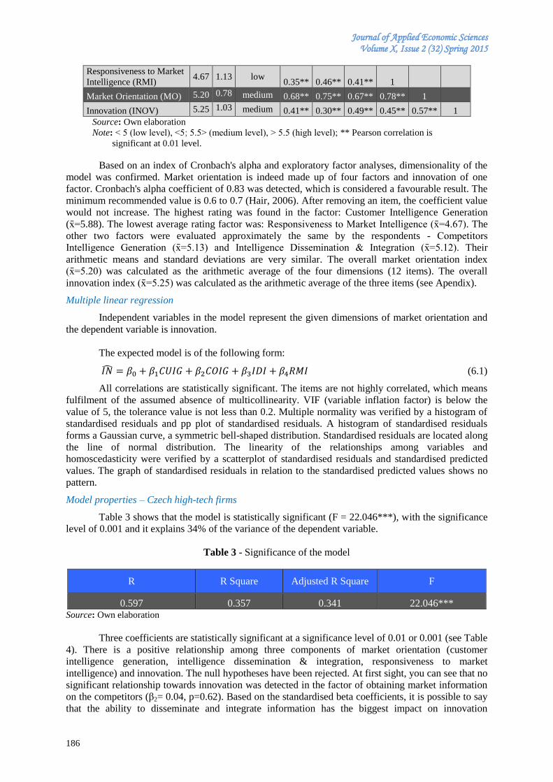
Table 3 shows that the model is statistically significant (F = 22.046***), with the significance
level of 0.001 and it explains 34% of the variance of the dependent variable.
Table 3 - Significance of the model
R R Square Adjusted R Square F
0.597 0.357 0.341 22.046*** Source: Own elaboration
Three coefficients are statistically significant at a significance level of 0.01 or 0.001 (see Table
4). There is a positive relationship among three components of market orientation (customer
intelligence generation, intelligence dissemination & integration, responsiveness to market
intelligence) and innovation. The null hypotheses have been rejected. At first sight, you can see that no
significant relationship towards innovation was detected in the factor of obtaining market information
on the competitors (β2= 0.04, p=0.62). Based on the standardised beta coefficients, it is possible to say
that the ability to disseminate and integrate information has the biggest impact on innovation
Journal of Applied Economic Sciences
Volume X, Issue 2(32), Spring2015
187
(β3=0.32***). The acquisition of information about customers and company's ability to use the
information have the same impact on innovation (β1= β4 =0.22***).
Table 4 - Coefficients
Unstandardised
Coefficients
Standardised
Coefficients t-Value Results
Model B Std.
Error Beta
Constant 1.073* 0.490 2.190
Customers Intelligence
Generation (CUIG) 0.261** 0.086 0.22*** 3.055 Reject H01
Competitors Intelligence
Generation (COIG) 0.032 0.064 0.04 0.496 Accept H02
Intelligence Dissemination
& Integration (IDI) 0.301*** 0.066 0.32*** 4.584 Reject H03
Responsiveness to Market
Intelligence (RMI) 0.200** 0.071 0.22*** 2.181 Reject H04
Note: ***(p˂0.001), **(p˂0.01), *(p˂0.05) , INOV (dependent variable)
Source: Own elaboration
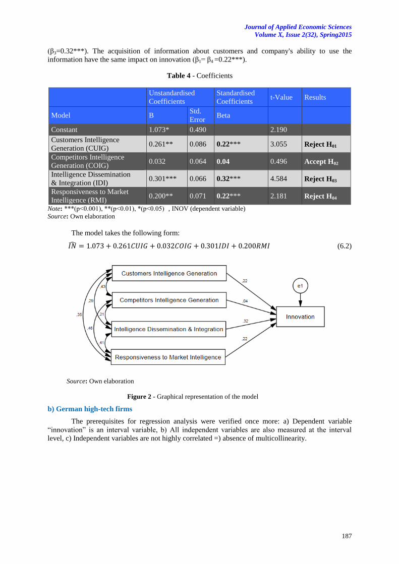
The model takes the following form:
(6.2)
Source: Own elaboration
Figure 2 - Graphical representation of the model
b) German high-tech firms
The prerequisites for regression analysis were verified once more: a) Dependent variable
“innovation” is an interval variable, b) All independent variables are also measured at the interval
level, c) Independent variables are not highly correlated =) absence of multicollinearity.
Journal of Applied Economic Sciences Volume X, Issue 2 (32) Spring 2015
188
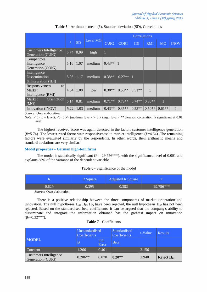
Table 5 - Arithmetic mean (x ), Standard deviation (SD), Correlations
x
SD
Level MO
Correlations
CUIG COIG IDI RMI MO INOV
Customers Intelligence
Generation (CUIG) 5.74 0.99 high 1
Competitors
Intelligence
Generation (COIG)
5.16 1.07 medium 0.43** 1
Intelligence
Dissemination
& Integration (IDI)
5.03 1.17 medium 0.38** 0.27** 1
Responsiveness to
Market
Intelligence (RMI)
4.64 1.08 low 0.38** 0.50** 0.51** 1
Market Orientation
(MO) 5.14 0.81 medium 0.71** 0.73** 0.74** 0.80** 1
Innovation (INOV) 5.22 1.03 medium 0.43** 0.35** 0.53** 0.50** 0.61** 1
Source: Own elaboration
Note: ˂ 5 (low level), ˂5; 5.5˃ (medium level), ˃ 5.5 (high level); ** Pearson correlation is significant at 0.01
level
The highest received score was again detected in the factor: customer intelligence generation
(x =5.74). The lowest rated factor was: responsiveness to market intelligence (x =4.64). The remaining
factors were evaluated similarly by the respondents. In other words, their arithmetic means and
standard deviations are very similar.
Model properties – German high-tech firms
The model is statistically significant (F = 29.756***), with the significance level of 0.001 and
explains 38% of the variance of the dependent variable.
Table 6 - Significance of the model
R R Square Adjusted R Square F
0.629 0.395 0.382 29.756***
Source: Own elaboration
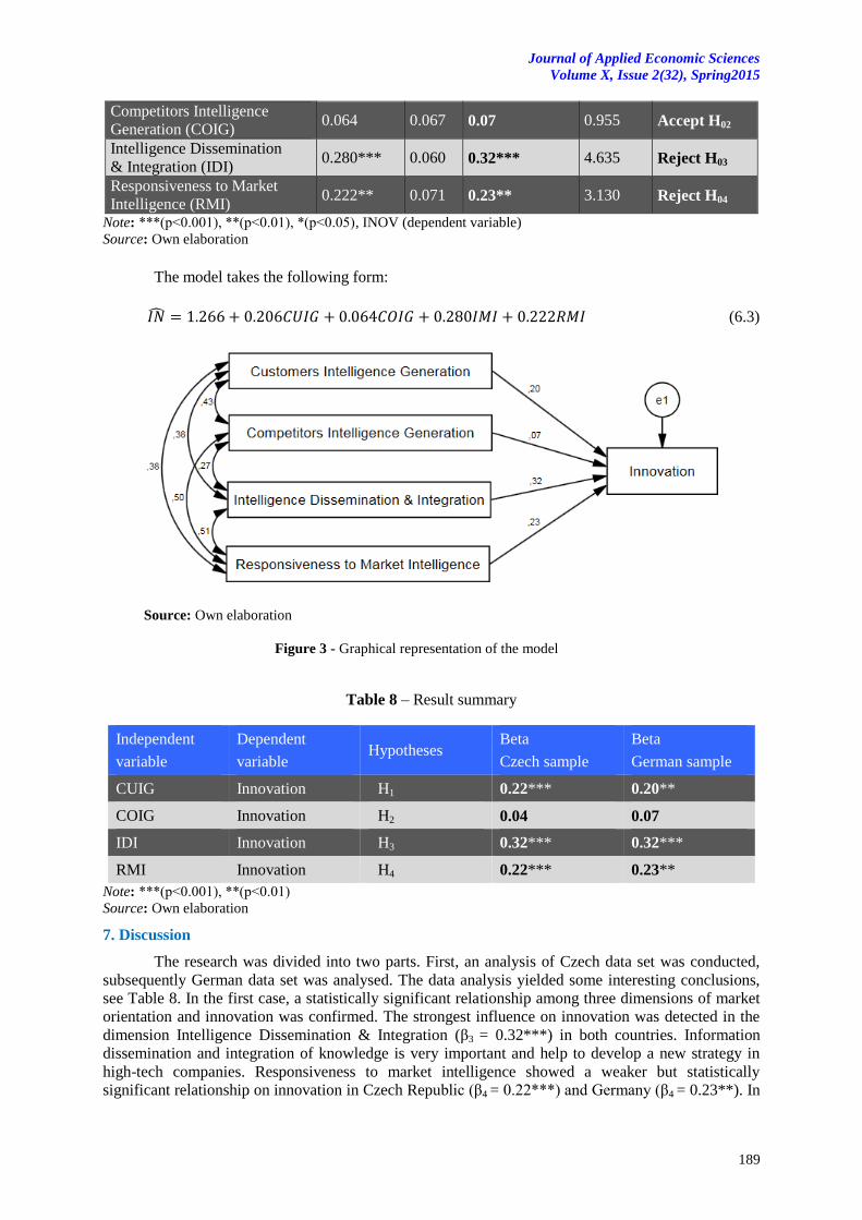
There is a positive relationship between the three components of market orientation and
innovation. The null hypotheses H01, H03, H04 have been rejected, the null hypothesis H02 has not been
rejected. Based on the standardised beta coefficients, it can be argued that the company's ability to
disseminate and integrate the information obtained has the greatest impact on innovation
(β3=0.32***).
Table 7 - Coefficients
MODEL
Unstandardised
Coefficients
Standardised
Coefficients t-Value Results
B Std.
Error Beta
Constant 1.266 0.401
3.156
Customers Intelligence
Generation (CUIG) 0.206** 0.070 0.20** 2.940 Reject H01
Journal of Applied Economic Sciences
Volume X, Issue 2(32), Spring2015
189
Competitors Intelligence
Generation (COIG) 0.064 0.067 0.07 0.955 Accept H02
Intelligence Dissemination
& Integration (IDI) 0.280*** 0.060 0.32*** 4.635 Reject H03
Responsiveness to Market
Intelligence (RMI) 0.222** 0.071 0.23** 3.130 Reject H04
Note: ***(p˂0.001), **(p˂0.01), *(p˂0.05), INOV (dependent variable)
Source: Own elaboration
The model takes the following form:
(6.3)
Source: Own elaboration
Figure 3 - Graphical representation of the model
Table 8 – Result summary
Independent
variable
Dependent
variable Hypotheses
Beta
Czech sample
Beta
German sample
CUIG Innovation H1 0.22*** 0.20**
COIG Innovation H2 0.04 0.07
IDI Innovation H3 0.32*** 0.32***
RMI Innovation H4 0.22*** 0.23**
Note: ***(p˂0.001), **(p˂0.01)
Source: Own elaboration
7. Discussion
The research was divided into two parts. First, an analysis of Czech data set was conducted,
subsequently German data set was analysed. The data analysis yielded some interesting conclusions,
see Table 8. In the first case, a statistically significant relationship among three dimensions of market
orientation and innovation was confirmed. The strongest influence on innovation was detected in the
dimension Intelligence Dissemination & Integration (β3 = 0.32***) in both countries. Information
dissemination and integration of knowledge is very important and help to develop a new strategy in
high-tech companies. Responsiveness to market intelligence showed a weaker but statistically
significant relationship on innovation in Czech Republic (β4 = 0.22***) and Germany (β4 = 0.23**). In
Journal of Applied Economic Sciences Volume X, Issue 2 (32) Spring 2015
190
practice, responsiveness to market intelligence would mean for example launching a new product on
the market. And finally obtaining market information about the customers has similarly strong
significant relationship in Czech Republic (β1 = 0.22***) and Germany (β1=0.20**). No significant
relationship towards innovation was detected in the factor of competitors intelligence generation in
Czech Republic (β2 = 0.04) and Germany (β2 = 0.07). Using a multiple regression data analysis, we
confirmed that the factors have the greatest influence on innovation when acting simultaneously. Also
Pearson correlation coefficient is greater in the case of simultaneous action than in each dimension
separately. Such a finding can also be found in foreign literature, e.g. in the conclusion of Al-Dmour
and Basheer (2012) regarding the telecommunication and information sector. Similar results were
obtained by for example (Runing, Harsono and Haryono, 2014), who argue that the focus on
customers and competition has a positive and significant impact on technological innovation.
Kaňovská and Tomášková (2012) found a positive, significant relationship between competition
orientation and firm performance.
The simplified scale used in this work (see Appendix) may serve managers to evaluate the
degree of market orientation in their company at any time. The final score is to be achieved either by
summing or as an arithmetic mean of all responses (index of market orientation). According to
Frejková and Chalupský (2013) companies with a market orientation index 5.5 and higher, can be
described as highly market-oriented, and companies with a value below 5 as weak market-oriented
ones. It follows that companies with a value in the interval ˂5; 5.5˃ are moderately market-oriented.
The researched high-tech firms were of a medium/moderate level of market orientation in Czech
Republic (x =5.20) and Germany (x =5.14). There is, therefore, room for their improvement in the
future. It seems appropriate to point out that the results should be collected at regular intervals (the
author recommends to do so annually) and compared not only internally, within the company, but also
with other companies in the same sector e.g. through benchmarking. Furthermore, the results suggest
that the highest index value of market orientation was achieved in the dimension Customer
Intelligence Generation in Czech Republic (x =5.88) and Germany (x =5.74). This may indicate that
companies are indeed able to obtain valuable information about their customers. There are several
ways worth mentioning, e.g. data analysis of customer complaints, frequent personal meetings with
key customers, regular survey of hidden needs, etc. As for information dissemination & integration,
the index values are rather average (x =5.12) in Czech Republic and (x =5.03) in Germany, which may
be explained by the level of internal company communication. Especially in large companies that
employ thousands of employees, there may be certain complications in sharing information and its
transformation into knowledge. If there is a lack of formal, informal, horizontal and vertical
communication within the company, then information and knowledge is not shared in a timely and
sufficient manner among all departments. In practice, it usually happens that the marketing department
does not cooperate effectively with the production, sale and purchase departments. Then the newly
developed product does not sell well if customers are not interested in it. The spirit of competition
rather than cooperation often dominates in the companies between its departments. Karlíček et al.
(2014) and Kotler, Rackham and Krishnaswamy (2006) also claim the same. The lowest value was
detected in the response to market information (x =4.64) in Czech Republic and (x =4.67) in Germany.
This testifies to the fact that high-tech firms, although much interested in the market development, do
not know how to process such information sufficiently and promptly and use it for a strategic action.
In the Czech Republic, many companies seem unwilling to invest in market research or to hold
regular meetings of all company departments. The entire process is time-limited. Time is the greatest
enemy of innovative companies, therefore the response or strategic reaction to market intelligence
must follow immediately in the dynamic environment of high-tech companies. A similar survey of
implementation of market orientation in 88 high-tech companies was conducted by Chalupský et al.
(2009). The team used a different measurement (the method of Tomášková) and determined the
average value of market orientation (x =5.2) in the Czech Republic. This finding is consistent with the
current result values of this work (x =5.2).
Conclussion
The aim of this article was to test the relationships between market orientation and innovation
in Czech and German high-tech companies. The results are to serve as further evidence of a positive
significant relationship between market orientation and innovation. The research included 164
Journal of Applied Economic Sciences
Volume X, Issue 2(32), Spring2015
191
respondents from the Czech Republic and 187 from Germany who ranked their answers using a Likert
scale ranging from 1 (absolutely disagree) to 7 (completely agree) for each item in the questionnaire.
The statistical analysis clearly confirmed three hypothetical relationships in both countries.
Obtaining market information about customers positively affects corporate innovation. The
dissemination and integration of information within the company and the subsequent implemented
action also have a positive impact on innovation. As for monitoring the competition, its positive effect
on innovation has not been confirmed in this study. However, a similar research in the Czech Republic
and Germany does not exist at the moment. Therefore further research in this area is highly
recommended.
Based on the results, it may be stated that Czech and German high-tech companies are
moderately market-oriented. The highest index score was reached in obtaining market information
about customers (Customer Intelligence Generation). Obtaining market information about competitors
(Competitors Intelligence Generation (COIG) ranked second. The lowest index value was detected in
the dimension Responsiveness to Market Information (RMI). The study also showed that large high-
tech companies do not display difficulties in obtaining market information. The problem arises with
coordination of the information flow, its converting into knowledge and implementation of the
subsequent strategic action.
Acknowledgements
The Author is thankful to the Internal Grant Agency of FaME TBU No. IGA/FaME/2013/029
(Measurement of market orientation of a firm and development of a new model with a focus on
contemporary trends in management and marketing) for financial support to carry out this research.
References
[1] Agarwal, S., Erramilli, M.K., Dev, C.S. 2003. Market orientation and performance in service
firms: role of innovation. Journal of Services Marketing 17(1):68-82.
[2] Al-Dmour, H.H., Basheer, E. 2012. The Effect of Market Orientation on Service Innovation: A
Study on the Information and Communication Technology (Ict) Sector in Jordan. International
Journal of Humanities and Social Science, 2(19):232-253.
[3] Amabile, T.M. 1988. A model of creativity and innovation in organizations. Research in
Organizational Behavior. 10:123-167.
[4] Bastič, M., Leskovar-Špacapan, G. 2006. The Impact of Market Knowledge on the Innovation
Process of Slovenian Firms. Proceedings of the 6th WSEAS International Conference on
Simulation, Modelling and Optimization. Lisbon, Portugal, 633-638.
[5] Bodlaj, M. 2010. The impact of responsive and proactive market orientation on innovation and
business performance. Economic and Business Review, 12(4):241-261.
[6] Calantone, R.J., Cavusgil, S.T., Zhao, Y. 2002. Learning orientation, firm innovation capability,
and firm performance. Industrial Marketing Management, 31(6):515-524. DOI: 10.1016/S0019-
8501(01)00203-6.
[7] Deshpandé, R., Farley J.U., Webster F.E. 1993. Corporate culture, customer orientation, and
innovativeness in Japanese Firms: A Quadrad Analysis. Journal of Marketing, 57(1):23-37.
[8] Drucker, P.F. 1993. Inovace a podnikavost: praxe a principy. Praha: Management Press.
[9] Dwairi, M., Bhuian, S.N., Jurkus, A. 2007. Revisiting the pioneering market orientation model in
an emerging economy. European Journal of Marketing, 41(7):713-721. DOI: 10.1108/030905
60710752357
[10] Frejková, D., Chalupský, V. 2013. Souvislost mezi řízením vztahů k zákazníkům (CRM) a tržní
orientací (MO) a vliv velikosti podniku a typu trhu na CRM a MO. Trendy ekonomiky
a managementu, VII(17):52-60.
[11] Hair, J., et al. 2010. Multivariate data analysis, USA: Pearson Prentice Hall, Inc.
Journal of Applied Economic Sciences Volume X, Issue 2 (32) Spring 2015
192
[12] Hurley, R.F., Hult, G.T.M. 1998. Innovation, Market Orientation, and Organizational Learning:
An Integration and Empirical Examination. Journal of Marketing 62(3):42-54. DOI:
10.2307/1251742.
[13] Chalupský, V., et al. 2009. Výzkum implementace tržní orientace u hi-tech firem, Brno: FP VUT.
[14] Chang, T.Z., Chen, S. 1998. Market orientation, service quality and profitability: a conceptual
model and empirical evidence. The Journal of Services Marketing, 12(4):246-264. DOI: 10.1108/
08876049810226937.
[15] Jangl, P. 2014. Market Orientation of Firms and its Measurement. In Proceedings of the 2nd
International Scientific Conference focused on Economics and Business Management in the 21st
Century. Ostrava, Czech Republic. 217-222.
[16] Kaňovská, L., Tomášková, E. 2012. Competitor Orientation at Hi-tech Companies. Trendy
ekonomiky a management, VI(10):45-52.
[17] Kaňovská, L., Tomášková, E. 2014. Market Orientation and strategic behaviour at high-tech
companies. E+M: Ekonomie a Management, 17(4):86-100. DOI: 10.15240/tul/001/2014-4-007.
[18] Karlíček, M., et al. 2013. Základy marketingu. Czech Republic: Grada.
[19] Karlíček, M., et al. 2014. Role marketingu ve firmách, Czech Republic: VeRBuM.
[20] Kohli, A.K., Jaworski, B.J. 1990. Market Orientation: The Construct, Research Propositions, and
Managerial Implications. Journal of Marketing, 54:1-18. DOI: 10.2307/1251866
[21] Kohli, A.K., Jaworski, B.J., Kumar, A. 1993. MARKOR: A Measure of Market Orientation.
Journal of Marketing Research, 30:467-477. DOI: 10.2307/3172691
[22] Kotler, P., et al. 2013. Marketing. Pearson Australia.
[23] Kotler, P., Rackham, N., Krishnaswamy, S. 2006. Ending the War Between Sales and Marketing.
Harvard Business Review, 51(4):1-12.
[24] Kuada, J., Buatsi, S.N. 2005. Market Orientation and Management Practices in Ghanaian Firms:
Revisiting the Jaworski and Kohli Framework. Journal of International Marketing, 13(1):58-88.
DOI: 10.1509/jimk.13.1.58.58539.
[25] Kumar, K., Subramanian, R., Strandholm, K. 2011. Market Orientation And Performance: Does
Organizational Strategy Matter? Journal of Applied Business Research, 18(1):37-49.
[26] Kumar, K., Subramanian, R., Yauger, C. 1998. Examining the Market Orientation-Performance
Relationship: A Context-Specific Study. Journal of Management, 24(2):201-233. DOI:
10.1016/S0149-2063(99)80060-9.
[27] Ma, W., Zhu, G., Hou, Y. 2011. Learning Orientation, Process Innovation, and Firm Performance
in Manufacturing Industry. Advances in Information Sciences & Service Sciences, 3(11):1-8.
DOI: 10.4156/AISS.vol3.issue11.44
[28] Manzano, J.A., Küster, I., Vila, N. 2005. Market orientation and innovation: an inter-relationship
analysis. European Journal of Innovation Management, 8(4):437-452. DOI:
10.1108/14601060510627812
[29] Mohr, J.J., Sengupta, S., Slater, S. 2014. Marketing of High Technology products and
Innovations. England: Pearson Education Limited.
[30] Narver, J.C., Slater, S.F. 1990. The Effect of a Market Orientation on Business Profitability.
Journal of Marketing, 54(4):20-34. DOI: 10.2307/1251757.
[31] Narver, J.C., Slater, S.F. 1995. Market orientation and the learning organization. Journal of
Marketing, 59(3):63-74. DOI: 10.2307/1252120.
[32] Nožička, J., Grosová, S. 2012. Měření tržní orientace ve vzorku malých a středních inovačních
podniků. Acta Universitatis Bohemiae Meridionales, 15(1):31-42.

Journal of Applied Economic Sciences
Volume X, Issue 2(32), Spring2015
193
[33] Panigyrakis, G.G., Theodoridis, P.K. 2007. Market Orientation and Performance: An Empirical
Investigation in the Retail Industry in Greece. Journal of Retailing and Consumer Services, 14(2):
137-149. DOI: 10.1016/j.jretconser.2006.05.003.
[34] Remli, N., et al. 2013. A proposed Conceptual Framework for Market Orientation and Innovation
towards Takaful Performance in Malaysia. International Journal of Business and Management,
8(7):100-105. DOI: 10.5539/ijbm.v8n7p100.
[35] Runing, H.S., Harsono, M., Haryono, T. 2014. The Relationship between Strategy Orientation
and Marketing Performance: The Role of Organizational Change Capability. American
International Journal of Contemporary Research, 4(1):221-229.
[36] Serna, M.C.M., Guzman, G.M., Castro, S.Y.P. 2013. The Relationship between Market
Orientation and Innovation in Mexican Manufacturing SME´s. Advances in Management &
Applied Economics, 3(5):125-137.
[37] Thompson, A.V. 1965. Bureaucracy and Innovation. Administrative Science Quarterly, 10(1):1-
20. DOI: 10.2307/2391646.
[38] Trommsdorff, V., Steinhoff, F. 2009. Marketing inovací. Praha: C. H. Beck.
[39] Tuominen, M., Rajala, A., Möller, K. 2004. Market-driving versus market-driven: Divergent roles
of market orientation in business relationships. Industrial Marketing Management, 33(3):207-
217. DOI: 10.1016/j.indmarman.2003.10.010

Journal of Applied Economic Sciences Volume X, Issue 2 (32) Spring 2015
194
APPENDIX
A) The Modified Market Orientation Scale (MMOS)
Customers Intelligence Generation
1. We systematically collect and evaluate data about satisfaction or non-satisfaction of
customers.
2. We have regular meetings with customers in order to learn their future expectations in time.
3. We permanently strive for a deeper understanding of the hidden needs and requirements of
customers.
Competitors Intelligence Generation
4. We monitor mutually competing firms in our branch.
5. We perform evaluation of strong and weak points of major competitors.
6. We try to predict a future behaviour of competititors.
Intelligence Dissemination & Integration
7. We inform each other about successful and unsuccessful experience with customers across all
company departments.
8. In our company we hold a lot of formal and informal talks where we solve present business
success, market opportunities or risks.
9. Market information are integrated in this workplace before decisions are made.
Responsiveness to Market Intelligence
10. Our reaction to the competitor’s price campaign is very short. 11. Principles of market segmentation control development of new products in our firm.
12. We react immediately if the competition launches intensive advertising campaign aimed at our
customers.
B) Innovation
13. Company climate can be called creative.
14. Our attitude to innovations is positive.
15. Help in developing new ideas is always readily available.
Journal of Applied Economic Sciences
Volume X, Issue 2(32), Spring2015
195
IS ALGERIA READY TO INTEGRATE THE KNOWLEDGE-BASED ECONOMY?
Khadidja LAHMER
Faculty of Economics, Commerce and Management Sciences
University of Boumerdes, Algeria
Ali KHALFI
Faculty of Economics and Management Sciences
University of Algiers 3, Algeria
[email protected] Abstract:
This paper focuses on the problem of Algerian economy mutation, from an economy based on oil as the
sole source of income, to a knowledge economy based on competence of human resources and knowledge to
achieve economic growth. This paper try to find answers to the following questions: what is the position of
Algeria against the indicators of the Knowledge economy compared to the rest of the world? What mechanisms
and policies that should be put in place to integrate Algeria in this new economy? Based on a comparative
analysis we examine the readiness of the Algerian economy to Integrate Knowledge economy. The study adopts
The World Bank methodology based on the four pillars– institutional regime, education, innovations and ICT. It
summarizes both positive and negative sides, difficulties, and relies on the possible actions to resolve them
regarding the attainment of the relevant national objectives. The study revealed that Algeria should pursue a
long-term strategy for the development of knowledge, focusing on achieving a real rate of growth.
Keywords: Knowledge-based economy; methodology of the World Bank; knowledge indicators; information
and communication technologies
JEL Classification: F15, F63, H52, I23, O38
1. Introduction
Nowadays, Algeria is living in the rhythm of significant changes characterized by the
proliferation of new information and communications technologies (ICTs) and an exceptional
technological progress that led to the appearance of a new form of economic development, namely the
knowledge-based economy. According to economists, knowledge-based economy is an essential
element for passing the status of developing country to that of a developed country, to the extent that
knowledge is the key to economic growth and the indicator of the power of nations.
Algeria must take advantage of this new economy with what it offers itself as challenges and
opportunities for sustainable development. But this can only be achieved through the establishment of
a clear strategy, especially as the Algerian economy, although it is still lagging behind compared to
economic growth, is characterized by a number of favourable factors.
This paper focuses on the problem of Algerian economy mutation, from an economy based on
oil as the sole source of income, to a knowledge economy based on competence of human resources
and knowledge to achieve economic growth.
The main issue addressed in the context of this paper focuses on the study of the readiness of
Algeria to integrate into an economy based on knowledge and find answers to the following questions:
- What is the situation of Algeria against the indicators of the new economy compared to the rest of
the world? - What mechanisms and policies that should be put in place to integrate Algeria in this new
economy?
Our study is based on the following assumptions: First, the Algerian economy has all the
components allowing heading for the knowledge-based economy. Second, Algeria has still not
adopted the knowledge economy. The importance of the study lies in the understanding of the
situation in Algeria related to the knowledge economy context, especially as the experiences around
the world have proved that this approach is a fundamental factor in the passage from the status of low-
income countries to that of developed countries, like Malaysia case. The objective of this study is to
identify the performance of the Algerian economy in the different areas of the knowledge economy by
exploiting the methodology of the World Bank that defines the framework of the knowledge economy
and its fundamentals.
Journal of Applied Economic Sciences Volume X, Issue 2 (32) Spring 2015
196
The methodology adopted in our study is based on a comparative analysis of the variables and
indicators of the knowledge economy in Algeria, compared to other countries, according to the
available data from different sources corresponding to the period between 2003 and 2013. Indeed, it
was in 2003, through the first Conference of Marseille, that has started the interest of integration of
Algeria in this new economy. This conference has been followed by several other conferences dealing
with the same subject. To consider various aspects of this thematic, the study will discuss the
following points:
Introduction to the knowledge economy.
Indicators of the knowledge economy.
Orientation towards knowledge-based economy in Algeria.
2. The knowledge economy
The knowledge economy concept is widely used in the literature of economics. However,
before defining it, the concepts of information and knowledge must be clarified.
2.1. Information and knowledge
The information represents the data for decision making (Salah Eddine 2001). These data are
useful to achieve specific goals at a specific period of time and are based, to a large extent, on the
ability of the recipient to take advantage of it.
Knowledge consists of data, information, recommendations and innovations or all symbolic
structures supported by man or acquired by the Company (United Nations 2009). Knowledge is also
regarded as the symbiosis of experience, values, previous information and expert views that present a
framework for the evaluation and adoption of new information and experiences (Rabhi 2008). The
concept of knowledge is broader than the information the extent that it is the combination of
information, experience, expertise and sensory abilities of people to reach a new and useful knowledge
for society. Knowledge comes in two forms: codified and tacit. Codified knowledge is clear and can
be transcribed as mathematical equations, laws or regulations. While tacit knowledge, more personal
and limited in the human mind, is difficult to measure and manageable.
2.2. Definition of knowledge economy
Although the role of knowledge and its effects on the economy are nothing new, the
knowledge economy is changing rapidly, very large scale, which induces a change in economic
thought with all the specificities distinguished from classical economics, raising debates and
discussions and highlighting several names: new economy, digital economy, virtual economy and
several definitions:
The knowledge economy means moving the centre of gravity of the raw materials and
capitalist infrastructure to the data concentration, learning and research centres and the
development of artificial cognitive system (Rabhi 2008).
The Asia-Pacific Economic Cooperation (APEC) defines the knowledge economy as an
economy based mainly on knowledge production, dissemination and use as a main driver for
the development of wealth and hands of work in all economic sectors (Al Hachimi et al.
2007).
It is an economy in which the production of goods and services is based increasingly on the
volume of knowledge, in large quantities, to become the main source of wealth creation
(Djeflat 2006a-2006b).
In general, the knowledge economy is an economy in which knowledge plays a key role in the
economic activity, the basis is the human factor, able to produce, use and disseminate knowledge to
achieve economic growth.
2.3. The specifics of the knowledge economy
The knowledge economy has its specific characteristics from those of knowledge,
distinguishing in many aspects (United Nations 2009):
The growing role of innovation and scientific research.
Lifelong learning as a basis for economic productivity and competitiveness.
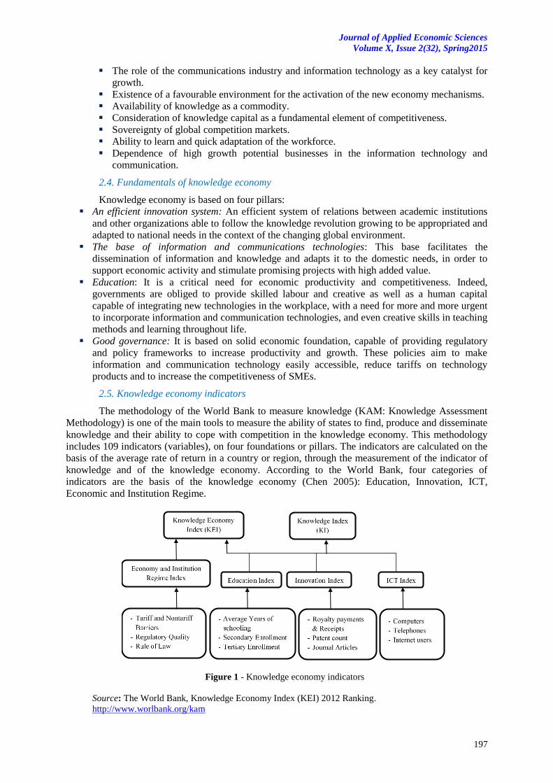
Journal of Applied Economic Sciences
Volume X, Issue 2(32), Spring2015
197
The role of the communications industry and information technology as a key catalyst for
growth.
Existence of a favourable environment for the activation of the new economy mechanisms.
Availability of knowledge as a commodity.
Consideration of knowledge capital as a fundamental element of competitiveness.
Sovereignty of global competition markets.
Ability to learn and quick adaptation of the workforce.
Dependence of high growth potential businesses in the information technology and
communication.
2.4. Fundamentals of knowledge economy
Knowledge economy is based on four pillars:
An efficient innovation system: An efficient system of relations between academic institutions
and other organizations able to follow the knowledge revolution growing to be appropriated and
adapted to national needs in the context of the changing global environment.
The base of information and communications technologies: This base facilitates the
dissemination of information and knowledge and adapts it to the domestic needs, in order to
support economic activity and stimulate promising projects with high added value.
Education: It is a critical need for economic productivity and competitiveness. Indeed,
governments are obliged to provide skilled labour and creative as well as a human capital
capable of integrating new technologies in the workplace, with a need for more and more urgent
to incorporate information and communication technologies, and even creative skills in teaching
methods and learning throughout life.
Good governance: It is based on solid economic foundation, capable of providing regulatory
and policy frameworks to increase productivity and growth. These policies aim to make
information and communication technology easily accessible, reduce tariffs on technology
products and to increase the competitiveness of SMEs.
2.5. Knowledge economy indicators
The methodology of the World Bank to measure knowledge (KAM: Knowledge Assessment
Methodology) is one of the main tools to measure the ability of states to find, produce and disseminate
knowledge and their ability to cope with competition in the knowledge economy. This methodology
includes 109 indicators (variables), on four foundations or pillars. The indicators are calculated on the
basis of the average rate of return in a country or region, through the measurement of the indicator of
knowledge and of the knowledge economy. According to the World Bank, four categories of
indicators are the basis of the knowledge economy (Chen 2005): Education, Innovation, ICT,
Economic and Institution Regime.
Figure 1 - Knowledge economy indicators
Source: The World Bank, Knowledge Economy Index (KEI) 2012 Ranking.
http://www.worlbank.org/kam
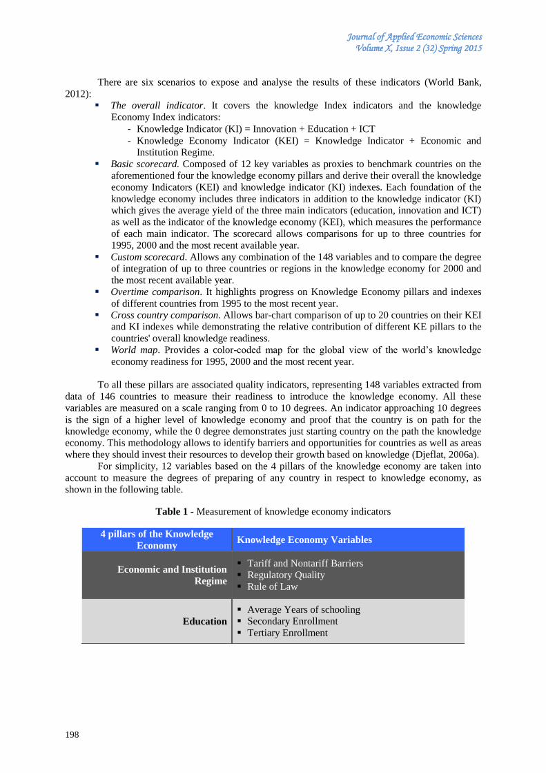
Journal of Applied Economic Sciences Volume X, Issue 2 (32) Spring 2015
198
There are six scenarios to expose and analyse the results of these indicators (World Bank,
2012):
The overall indicator. It covers the knowledge Index indicators and the knowledge
Economy Index indicators:
- Knowledge Indicator (KI) = Innovation + Education + ICT
- Knowledge Economy Indicator (KEI) = Knowledge Indicator + Economic and
Institution Regime.
Basic scorecard. Composed of 12 key variables as proxies to benchmark countries on the
aforementioned four the knowledge economy pillars and derive their overall the knowledge
economy Indicators (KEI) and knowledge indicator (KI) indexes. Each foundation of the
knowledge economy includes three indicators in addition to the knowledge indicator (KI)
which gives the average yield of the three main indicators (education, innovation and ICT)
as well as the indicator of the knowledge economy (KEI), which measures the performance
of each main indicator. The scorecard allows comparisons for up to three countries for
1995, 2000 and the most recent available year.
Custom scorecard. Allows any combination of the 148 variables and to compare the degree
of integration of up to three countries or regions in the knowledge economy for 2000 and
the most recent available year.
Overtime comparison. It highlights progress on Knowledge Economy pillars and indexes
of different countries from 1995 to the most recent year.
Cross country comparison. Allows bar-chart comparison of up to 20 countries on their KEI
and KI indexes while demonstrating the relative contribution of different KE pillars to the
countries' overall knowledge readiness.
World map. Provides a color-coded map for the global view of the world’s knowledge
economy readiness for 1995, 2000 and the most recent year.
To all these pillars are associated quality indicators, representing 148 variables extracted from
data of 146 countries to measure their readiness to introduce the knowledge economy. All these
variables are measured on a scale ranging from 0 to 10 degrees. An indicator approaching 10 degrees
is the sign of a higher level of knowledge economy and proof that the country is on path for the
knowledge economy, while the 0 degree demonstrates just starting country on the path the knowledge
economy. This methodology allows to identify barriers and opportunities for countries as well as areas
where they should invest their resources to develop their growth based on knowledge (Djeflat, 2006a).
For simplicity, 12 variables based on the 4 pillars of the knowledge economy are taken into
account to measure the degrees of preparing of any country in respect to knowledge economy, as
shown in the following table.
Table 1 - Measurement of knowledge economy indicators
4 pillars of the Knowledge
Economy Knowledge Economy Variables
Economic and Institution
Regime
Tariff and Nontariff Barriers
Regulatory Quality
Rule of Law
Education
Average Years of schooling
Secondary Enrollment
Tertiary Enrollment
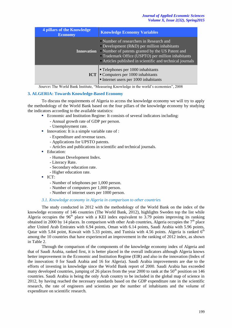
Journal of Applied Economic Sciences
Volume X, Issue 2(32), Spring2015
199
4 pillars of the Knowledge
Economy Knowledge Economy Variables
Innovation
Number of researchers in Research and
Development (R&D) per million inhabitants
Number of patents granted by the US Patent and
Trademark Office (USPTO) per million inhabitants
Articles published in scientific and technical journals
ICT
Telephones per 1000 inhabitants
Computers per 1000 inhabitants
Internet users per 1000 inhabitants
Source: The World Bank Institute, “Measuring Knowledge in the world’s economies”, 2008
3. ALGERIA: Towards Knowledge-Based Economy
To discuss the requirements of Algeria to access the knowledge economy we will try to apply
the methodology of the World Bank based on the four pillars of the knowledge economy by studying
the indicators according to the available statistics:
Economic and Institution Regime: It consists of several indicators including:
- Annual growth rate of GDP per person.
- Unemployment rate.
Innovation: It is a simple variable rate of :
- Expenditure and revenue taxes.
- Applications for UPSTO patents.
- Articles and publications in scientific and technical journals.
Education:
- Human Development Index.
- Literacy Rate.
- Secondary education rate.
- Higher education rate.
ICT:
- Number of telephones per 1,000 person.
- Number of computers per 1,000 person.
- Number of internet users per 1000 person.
3.1. Knowledge economy in Algeria in comparison to other countries
The study conducted in 2012 with the methodology of the World Bank on the index of the
knowledge economy of 146 countries (The World Bank, 2012), highlights Sweden top the list while
Algeria occupies the 96th place with a KEI index equivalent to 3.79 points improving its ranking
obtained in 2000 by 14 places. In comparison with other Arab countries, Algeria occupies the 7th place
after United Arab Emirates with 6.94 points, Oman with 6.14 points, Saudi Arabia with 5.96 points,
Qatar with 5.84 point, Kuwait with 5.33 points, and Tunisia with 4.56 points. Algeria is ranked 6th
among the 10 countries that have experienced an improvement in the ranking of 2012 index, as shown
in Table 2.
Through the comparison of the components of the knowledge economy index of Algeria and
that of Saudi Arabia, ranked first, it is better placed in the overall indicators although Algeria knows
better improvement in the Economic and Institution Regime (EIR) and also in the innovation (Index of
the innovation: 0 for Saudi Arabia and 16 for Algeria). Saudi Arabia improvements are due to the
efforts of investing in knowledge since the World Bank report of 2000. Saudi Arabia has exceeded
many developed countries, jumping of 26 places from the year 2000 to rank at the 50th position on 146
countries. Saudi Arabia is being the only Arab country to be included in the global map of science in
2012, by having reached the necessary standards based on the GDP expenditure rate in the scientific
research, the rate of engineers and scientists per the number of inhabitants and the volume of
expenditure on scientific research.
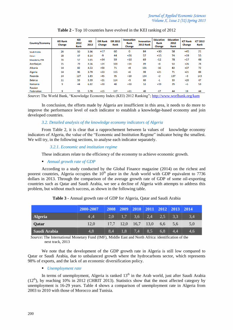
Journal of Applied Economic Sciences Volume X, Issue 2 (32) Spring 2015
200
Table 2 - Top 10 countries have evolved in the KEI ranking of 2012
Source: The World Bank, “Knowledge Economy Index (KEI) 2012 Ranking”; http://www.worlbank.org/kam
In conclusion, the efforts made by Algeria are insufficient in this area, it needs to do more to
improve the performance level of each indicator to establish a knowledge-based economy and join
developed countries.
3.2. Detailed analysis of the knowledge economy indicators of Algeria
From Table 2, it is clear that a rapprochement between la values of knowledge economy
indicators of Algeria, the value of the “Economic and Institution Regime” indicator being the smallest.
We will try, in the following sections, to analyse each indicator separately.
3.2.1. Economic and institution regime
These indicators relate to the efficiency of the economy to achieve economic growth.
Annual growth rate of GDP
According to a study conducted by the Global Finance magazine (2014) on the richest and
poorest countries, Algeria occupies the 10th place in the Arab world with GDP equivalent to 7736
dollars in 2013. Through the comparison of the average growth rate of GDP of some oil-exporting
countries such as Qatar and Saudi Arabia, we see a decline of Algeria with attempts to address this
problem, but without much success, as shown in the following table.
Table 3 - Annual growth rate of GDP for Algeria, Qatar and Saudi Arabia
2000-2007 2008 2009 2010 2011 2012 2013 2014
Algeria 4 ,4 0,2 1,7 3,6 2,4 2,5 3,3 3,4
Qatar 12,0 71,1 12,0 16,7 13,0 6,6 5,6 5,0
Saudi Arabia 4,8 8,4 1,8 7,4 8,5 6,8 4,4 4,6
Source: The International Monetary Fund (IMF), Middle East and North Africa: identification of the
next track, 2013
We note that the development of the GDP growth rate in Algeria is still low compared to
Qatar or Saudi Arabia, due to unbalanced growth where the hydrocarbons sector, which represents
98% of exports, and the lack of an economic diversification policy.
Unemployment rate
In terms of unemployment, Algeria is ranked 13th in the Arab world, just after Saudi Arabia
(12th), by reaching 10% in 2012 (CHRIT 2013). Statistics show that the most affected category by
unemployment is 16-29 years. Table 4 shows a comparison of unemployment rate in Algeria from
2003 to 2010 with those of Morocco and Tunisia.
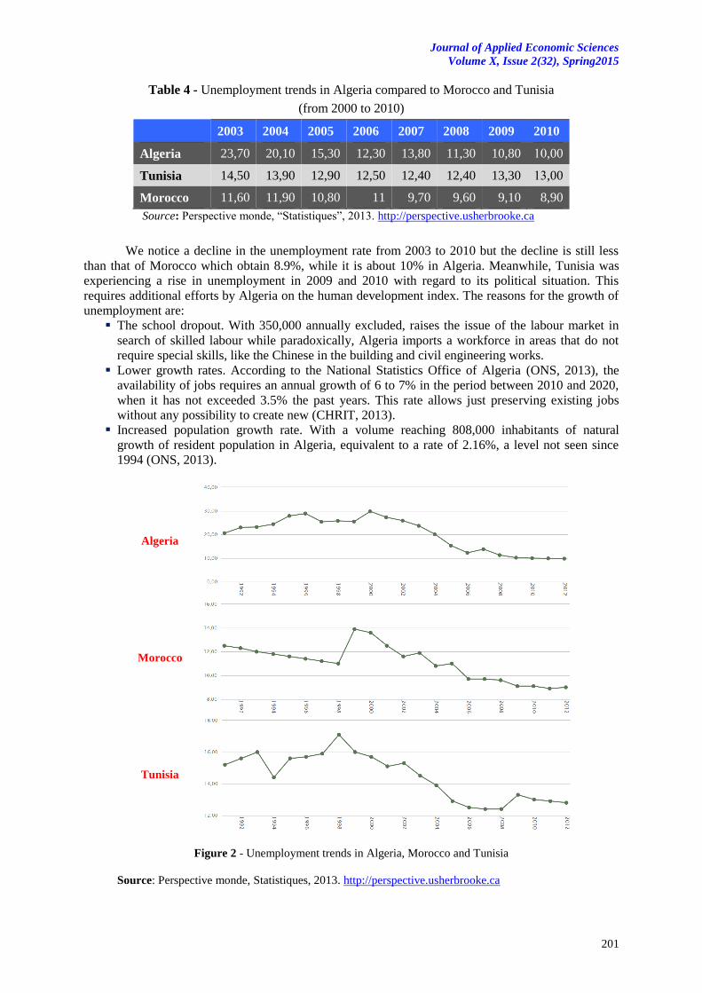
Journal of Applied Economic Sciences
Volume X, Issue 2(32), Spring2015
201
Table 4 - Unemployment trends in Algeria compared to Morocco and Tunisia
(from 2000 to 2010)
2003 2004 2005 2006 2007 2008 2009 2010
Algeria 23,70 20,10 15,30 12,30 13,80 11,30 10,80 72,00
Tunisia 14,50 13,90 12,90 12,50 12,40 12,40 13,30 71,00
Morocco 11,60 11,90 10,80 11 9,70 9,60 9,10 8,90
Source: Perspective monde, “Statistiques”, 2013. http://perspective.usherbrooke.ca
We notice a decline in the unemployment rate from 2003 to 2010 but the decline is still less
than that of Morocco which obtain 8.9%, while it is about 10% in Algeria. Meanwhile, Tunisia was
experiencing a rise in unemployment in 2009 and 2010 with regard to its political situation. This
requires additional efforts by Algeria on the human development index. The reasons for the growth of
unemployment are:
The school dropout. With 350,000 annually excluded, raises the issue of the labour market in
search of skilled labour while paradoxically, Algeria imports a workforce in areas that do not
require special skills, like the Chinese in the building and civil engineering works.
Lower growth rates. According to the National Statistics Office of Algeria (ONS, 2013), the
availability of jobs requires an annual growth of 6 to 7% in the period between 2010 and 2020,
when it has not exceeded 3.5% the past years. This rate allows just preserving existing jobs
without any possibility to create new (CHRIT, 2013).
Increased population growth rate. With a volume reaching 808,000 inhabitants of natural
growth of resident population in Algeria, equivalent to a rate of 2.16%, a level not seen since
1994 (ONS, 2013).
Algeria
Morocco
Tunisia
Figure 2 - Unemployment trends in Algeria, Morocco and Tunisia
Source: Perspective monde, Statistiques, 2013. http://perspective.usherbrooke.ca
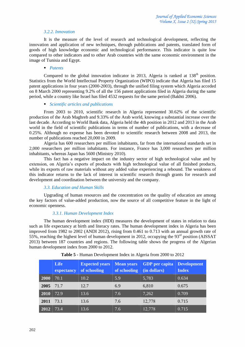
Journal of Applied Economic Sciences Volume X, Issue 2 (32) Spring 2015
202
3.2.2. Innovation
It is the measure of the level of research and technological development, reflecting the
innovation and application of new techniques, through publications and patents, translated form of
goods of high knowledge economic and technological performance. This indicator is quite low
compared to other indicators and to other Arab countries with the same economic environment in the
image of Tunisia and Egypt.
Patents
Compared to the global innovation indicator in 2013, Algeria is ranked at 138th position.
Statistics from the World Intellectual Property Organization (WIPO) indicate that Algeria has filed 15
patent applications in four years (2000-2003), through the unified filing system which Algeria acceded
on 8 March 2000 representing 9.2% of all the 156 patent applications filed in Algeria during the same
period, while a country like Israel has filed 4532 requests for the same period (Bakhti 2006).
Scientific articles and publications
From 2003 to 2010, scientific research in Algeria represented 30.62% of the scientific
production of the Arab Maghreb and 9.33% of the Arab world, knowing a substantial increase over the
last decade. According to World Bank data, Algeria held the 4th position in 2012 and 2013 in the Arab
world in the field of scientific publications in terms of number of publications, with a decrease of
0.25%. Although no expense has been devoted to scientific research between 2008 and 2013, the
number of publications reached 20,000 in 2009.
Algeria has 600 researchers per million inhabitants, far from the international standards set in
2,000 researchers per million inhabitants. For instance, France has 3,000 researchers per million
inhabitants, whereas Japan has 5600 (Ministry 2010).
This fact has a negative impact on the industry sector of high technological value and by
extension, on Algeria’s exports of products with high technological value of all finished products,
while its exports of raw materials without any added value experiencing a rebound. The weakness of
this indicator returns to the lack of interest in scientific research through grants for research and
development and coordination between the university and the company.
3.3. Education and Human Skills
Upgrading of human resources and the concentration on the quality of education are among
the key factors of value-added production, now the source of all competitive feature in the light of
economic openness.
3.3.1. Human Development Index
The human development index (HDI) measures the development of states in relation to data
such as life expectancy at birth and literacy rates. The human development index in Algeria has been
improved from 1982 to 2002 (ANDI 2012), rising from 0.461 to 0.713 with an annual growth rate of
55%, reaching the highest level of human development in 2012, occupying the 93rd
position (AISSAT
2013) between 187 countries and regions. The following table shows the progress of the Algerian
human development index from 2000 to 2012.
Table 5 - Human Development Index in Algeria from 2000 to 2012
Life
expectancy
Expected years
of schooling
Mean years
of schooling
GDP per capita
(in dollars)
Development
Index
2000 70.1 10.2 5.9 5,783 0.634
2005 71.7 12.7 6.9 6,810 0.675
2010 72.9 13.6 7.6 7,262 0.709
2011 73.1 13.6 7.6 70,111 0.715
2012 73.4 13.6 7.6 70,111 0.715
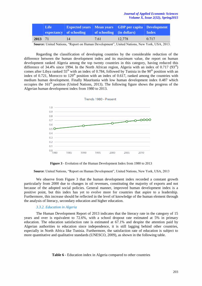
Journal of Applied Economic Sciences
Volume X, Issue 2(32), Spring2015
203
Life
expectancy
Expected years
of schooling
Mean years
of schooling
GDP per capita
(in dollars)
Development
Index
2013 71 14 16.7 70,111 26171
Source: United Nations, “Report on Human Development”, United Nations, New York, USA, 2013.
Regarding the classification of developing countries by the considerable reduction of the
difference between the human development index and its maximum value, the report on human
development ranked Algeria among the top twenty countries in this category, having reduced this
difference of 34.4% since 1994. In the North African region, Algeria with an index of 0.717 (93rd
)
comes after Libya ranked 55th with an index of 0.784, followed by Tunisia in the 90
th position with an
index of 0.721, Morocco to 129th position with an index of 0.617, ranked among the countries with
medium human development. Finally Mauritania with low human development index 0.487 which
occupies the 161th position (United Nations, 2013). The following figure shows the progress of the
Algerian human development index from 1980 to 2013.
Figure 3 - Evolution of the Human Development Index from 1980 to 2013
Source: United Nations, “Report on Human Development”, United Nations, New York, USA, 2013
We observe from Figure 3 that the human development index recorded a constant growth
particularly from 2000 due to changes in oil revenues, constituting the majority of exports and not
because of the adopted social policies. General manner, improved human development index is a
positive point, but this index has yet to evolve more for countries that aspire to a leadership.
Furthermore, this increase should be reflected in the level of knowledge of the human element through
the analysis of literacy, secondary education and higher education.
3.3.2. Education in Algeria
The Human Development Report of 2013 indicates that the literacy rate in the category of 15
years and over is equivalent to 72.6%, with a school dropout rate estimated at 5% in primary
education. The education satisfaction rate is estimated at 67.1% and despite the attention paid by
Algerian authorities to education since independence, it is still lagging behind other countries,
especially in North Africa like Tunisia. Furthermore, the satisfaction rate of education is subject to
more quantitative and qualitative standards (UNESCO, 2009), as shown in the following table.
Table 6 - Education index in Algeria compared to other countries
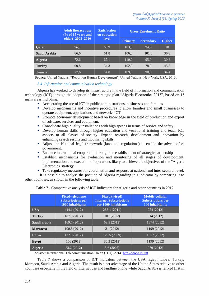
Journal of Applied Economic Sciences Volume X, Issue 2 (32) Spring 2015
204
Adult literacy rate
(% of 15 years and
older)- 2005–2010
Satisfaction
on education
level
Gross Enrolment Ratio
Primary Secondary Higher
Qatar 3.,1 69,9 103,0 94,0 10
Saudi Arabia 86,6 61,8 106,0 101,0 36,8
Algeria 72,6 67,1 110,0 95,0 30,8
Turkey 90,8 54,3 102,0 78,0 45,8
Tunisia 77,6 54,8 109,0 90,0 34,4
Source: United Nations, “Report on Human Development”, United Nations, New York, USA, 2013.
3.4. Information and communication technology
Algeria has worked to develop its infrastructure in the field of information and communication
technology (ICT) through the adoption of the strategic plan “Algeria Electronics 2013”, based on 13
main areas including:
Accelerating the use of ICT in public administrations, businesses and families
Develop mechanisms and incentive procedures to allow families and small businesses to
operate equipment, applications and networks ICT.
Promote economic development based on knowledge in the field of production and export
of software, services and equipment.
Consolidate high quality installations with high speeds in terms of service and safety.
Develop human skills through higher education and vocational training and teach ICT
aspects to all classes of society. Expand research, development and innovation by
enhancing search results and mobilizing skills.
Adjust the National legal framework (laws and regulations) to enable the advent of e-
government.
Enhance international cooperation through the establishment of strategic partnerships.
Establish mechanisms for evaluation and monitoring of all stages of development,
implementation and execution of operations likely to achieve the objectives of the "Algeria
Electronics' strategy.
Take regulatory measures for coordination and response at national and inter-sectoral level.
It is possible to analyse the position of Algeria regarding this indicator by comparing it to
other countries, as shown in the following table.
Table 7 - Comparative analysis of ICT indicators for Algeria and other countries in 2012
Fixed-telephone
Subscriptions per
1000 inhabitants
Fixed (wired)
Internet Subscriptions
per 1000 inhabitants
Mobile-cellular
Subscriptions per
100 inhabitants
USA 444.1 (2012) 283.1 (2011) 954 (2012)
Turkey 187.3 (2012) 107 (2012) 914 (2012)
Saudi arabia 169.7 (2012) 69.5 (2012) 1874 (2012)
Morrocco 100.8 (2012) 21 (2012) 1199 (2012)
Libya 132.3 (2012) 129.5 (2009) 1557 (2012)
Egypt 106 (2012) 30.2 (2012) 1199 (2012)
Algeria 83.2 (2012) 5.6 (2005) 979 (2012)
Source: International Telecommunication Union (ITU). 2014. http://www.itu.int
Table 7 shows a comparison of ICT indicators between the USA, Egypt, Libya, Turkey,
Morocco, Saudi Arabia and Algeria. The result is a net advantage of the United States relative to other
countries especially in the field of Internet use and landline phone while Saudi Arabia is ranked first in
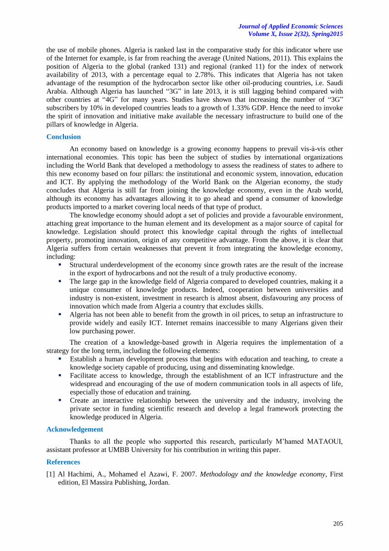
Journal of Applied Economic Sciences
Volume X, Issue 2(32), Spring2015
205
the use of mobile phones. Algeria is ranked last in the comparative study for this indicator where use
of the Internet for example, is far from reaching the average (United Nations, 2011). This explains the
position of Algeria to the global (ranked 131) and regional (ranked 11) for the index of network
availability of 2013, with a percentage equal to 2.78%. This indicates that Algeria has not taken
advantage of the resumption of the hydrocarbon sector like other oil-producing countries, i.e. Saudi
Arabia. Although Algeria has launched “3G” in late 2013, it is still lagging behind compared with
other countries at “4G” for many years. Studies have shown that increasing the number of “3G”
subscribers by 10% in developed countries leads to a growth of 1.33% GDP. Hence the need to invoke
the spirit of innovation and initiative make available the necessary infrastructure to build one of the
pillars of knowledge in Algeria.
Conclusion
An economy based on knowledge is a growing economy happens to prevail vis-à-vis other
international economies. This topic has been the subject of studies by international organizations
including the World Bank that developed a methodology to assess the readiness of states to adhere to
this new economy based on four pillars: the institutional and economic system, innovation, education
and ICT. By applying the methodology of the World Bank on the Algerian economy, the study
concludes that Algeria is still far from joining the knowledge economy, even in the Arab world,
although its economy has advantages allowing it to go ahead and spend a consumer of knowledge
products imported to a market covering local needs of that type of product.
The knowledge economy should adopt a set of policies and provide a favourable environment,
attaching great importance to the human element and its development as a major source of capital for
knowledge. Legislation should protect this knowledge capital through the rights of intellectual
property, promoting innovation, origin of any competitive advantage. From the above, it is clear that
Algeria suffers from certain weaknesses that prevent it from integrating the knowledge economy,
including:
Structural underdevelopment of the economy since growth rates are the result of the increase
in the export of hydrocarbons and not the result of a truly productive economy.
The large gap in the knowledge field of Algeria compared to developed countries, making it a
unique consumer of knowledge products. Indeed, cooperation between universities and
industry is non-existent, investment in research is almost absent, disfavouring any process of
innovation which made from Algeria a country that excludes skills.
Algeria has not been able to benefit from the growth in oil prices, to setup an infrastructure to
provide widely and easily ICT. Internet remains inaccessible to many Algerians given their
low purchasing power.
The creation of a knowledge-based growth in Algeria requires the implementation of a
strategy for the long term, including the following elements:
Establish a human development process that begins with education and teaching, to create a
knowledge society capable of producing, using and disseminating knowledge.
Facilitate access to knowledge, through the establishment of an ICT infrastructure and the
widespread and encouraging of the use of modern communication tools in all aspects of life,
especially those of education and training.
Create an interactive relationship between the university and the industry, involving the
private sector in funding scientific research and develop a legal framework protecting the
knowledge produced in Algeria.
Acknowledgement
Thanks to all the people who supported this research, particularly M’hamed MATAOUI,
assistant professor at UMBB University for his contribution in writing this paper.
References
[1] Al Hachimi, A., Mohamed el Azawi, F. 2007. Methodology and the knowledge economy, First
edition, El Massira Publishing, Jordan.
Journal of Applied Economic Sciences Volume X, Issue 2 (32) Spring 2015
206
[3] Bakhti, I., Douis, M.T. 2006. Patents as economic competitiveness indicator Algeria and the Arab
States, EL BAHITH Journal, 4: 149-155.
[4] Chrit, H. 2013. La situation du chômage en Algérie et ses causes. http://iefpedia.com/
arab/?=29882
[5] Aissat, C. 2013. L’indice de développement humain de l’Algérie: 93ème, un classement mirage.
Published May 2013. http://dzactiviste.info/lindice-de-developpement-humain-de-lalgerie-93eme-
un-classement-mirage/
[6] Chen, D. H., Dahlman, C. J. 2005. The knowledge economy, the KAM methodology and World
Bank operations, World Bank Institute Working Paper.
[7] Djeflat, A. 2006. L'économie fondée sur la connaissance: état des lieux et perspectives pour
l'Algérie. Editions Dar El Adib, Algeria.
[8] Djeflat, A. 2006. Economie fondée sur la connaissance: enjeux et perspectives.
[11] Nida Mohamed el Najar 2012. The role of human resource management in the production of
information in the era of knowledge economy, case studies from the University of Gaza, Master
Thesis, Gaza University, 2012.
[14] Rabhi M. A. 2008. Knowledge Management, First edition, Safa Publishing, Jordan.
[15] Salah Eddine Abdelmounaem 2001. Economics of accounting information and management
systems (Arabic Version), New University Publishing, Alexandria, Egypt.
*** ANDI. 2013. Forte augmentation de l’indice de developpement humain de l’Algerie entre 1990 et
2012, http://www.andi.dz/index.php/ar/presse/806
*** International Telecommunication Union (ITU). 2014. http://www.itu.int
*** Ministry of Higher Education and Scientific Research. 2010. Algeria, the third in Africa in terms
of scientific research, Report, Algeria.
*** Office Nationale des Statistiques (ONS). 2013. Démographie Algérienne, http://www.ones.dz
*** Perspective Monde. 2013. Statistiques. http://perspective.usherbrooke.ca
*** The Global Finance Magazine. 2014. The Richest Countries in the World, https://www.gfmag.
com/global-data/economic-data/richest-countries-in-the-world
*** The International Monetary Fund (IMF). 2013. Middle East and North Africa: identification of the
next track. http://www.imf.org/external/arabic/pubs/ft/reo/2013/mcd/mena0513a.pdf
*** The World Bank Institute. 2008. Measuring Knowledge in the world’s economies.
*** The World Bank. 2012. Knowledge Economy Index (KEI) 2012 Ranking. http://www.worlbank.
org/kam
*** UNESCO Institute for Statistics 2009. The second generation of literacy statistics, Canada.
*** United Nations 2009. Arab Human Development Report 2009: Building a Knowledge Society,
United Nations, New York, USA.
*** United Nations 2013. Report on Human Development, United Nations, New York, USA.
http://hdr.undp.org/en/countries/profiles/DZA
*** United Nations Economic and Social Commission for Western Asia 2011. Promotion of
information technology and communications sector to meet the challenges of the knowledge
economy, November 2011, Lebanon.
Journal of Applied Economic Sciences
Volume X, Issue 2(32), Spring2015
207
HOW ECONOMIC AND FINANCIAL INTEGRATION AFFECTS FINANCIAL STABILITY IN SOUTH ASIA: EVIDENCE FROM
PANEL COINTEGRATION ANALYSIS
Samia NASREEN
Department of Economics
Government College University Faisalabad, Punjab, Pakistan
Sofia ANWAR
Department of Economics
Government College University Faisalabad, Punjab, Pakistan
Abstract
Using the aggregate financial stability index (AFSI) which measures the gradual progression and
changes in financial market stability, this paper conducts an empirical evaluation of the impact of financial and
economic integration on the financial stability for South Asia. All selected variables (AFSI, economic
integration, financial integration, economic growth, government consumption expenditure) are found to be
integrated of order one, cross-sectionally dependent and cointegrated in South Asian panel. Long-run results
estimated by applying fully modified OLS (FMOLS) and pooled mean group (PMG) estimator techniques
suggest that financial integration and economic integration are not helpful in increasing the financial stability of
South Asian financial markets. The findings of the study offers new implications for monetary authorities and
policy makers in developing countries.
Keywords: financial stability; economic integration; financial integration; AFSI; South Asia
JEL Classification: F15; F36; G01
1. Introduction
Financial stability is said to exist when financial system is able to utilize capital on most
profitable investment projects without major disturbances (Reserve bank of India 2013). In other
words, a financial system is stable only when it is capable of encouraging the performance of economy
and of fighting financial disruptions that arise endogenously or as a result of adverse and unanticipated
events (Schinasi 2004). Practically, the stability of financial markets encourages and ensures the
sustainability of integration process and reduces at the same time the risk of asymmetric shocks. In
contrast, financial turmoil negatively effects the process of economic and financial integration.
The literature has provided various alternative definitions of financial integration. Here, we
present the most commonly used definition of Baele et al. (2004) and Weber (2006) i.e. the market for
a given set of financial instruments and services is fully integrated if all potential market participants
have the same relevant characteristics: (1) they follow a same set of rules in their decisions relating to
financial instruments and services; (2) they have equal access to same set of financial instruments and
services; and (3) they treated equally when they participate in the market. Most of the definitions of
financial integration are closely linked to the law of one price. The law of one price states that assets
having identical risks and returns should be priced identically regardless of where they are transacted.
According to McCarthy (1996) economic integration have two main elements: (1) removal of
barriers to economic and business activities; and (2) involvement of participants in an economic
activity without any discrimination. Economic integration may take different forms. According to
Balassa (1962), the process of economic integration is divided into four different stages. The first is a
Free Trade Area (FTA), second is a Customs Union (CU), third is a Common Market (CM), and
fourth is an Economic Union. Panagariya (2000, 288) used the term PTA which stands for Preferential
Trade Area, Preferential Trade Agreement or Preferential Trade Arrangement. PTA is a wider term
that can be used to describe FTAs, CUs and arrangements involving partial trade preferences.
The economic and financial integration around the globe increased significantly during the late
1980s and early 1990s. Globalization and technological advances in payment and communication
system have bring the countries closer to each other, accelerating the volume of their trade and
integrating their financial markets. The developing countries of the world are adopting more prudent
Journal of Applied Economic Sciences Volume X, Issue 2 (32) Spring 2015
208
policies to open up their economies and eliminating capital control barriers to attract foreign capital
and increase the volume of merchandize trade.
South Asian countries have started to opening up their economies in the late 1980s. South Asia
is much more integrated in the global world today than it was in 1980. Much of the fabulous economic
growth that the region experienced in late 1990s and 2000s is the result of trade and financial market
liberalization policies pursued by most of South Asian countries. Trade as percentage of GDP more
than doubled between 1990 and 2010 in India and Bangladesh. In spite of trade liberalization policies,
trade as a percentage of GDP in South Asia is still lower than that of other developing region. In South
Asia, trade to GDP ratio was 45.49 percent in year 2012 which is far below the corresponding average
of 87.23 percent of East Asia and Pacific and 66.32 percent for low and middle income countries
(World Bank, 2012).
The objective of current paper is to explore the impact of economic and financial integration
on the financial stability of South Asia. To do so, we first develop an aggregate financial stability
index (AFSI). The AFSI involves the aggregation of sub-indices covering financial sector
development, vulnerability and soundness. Trade openness and the sum of foreign assets and liabilities
as percentage of GDP are used to measure economic integration and financial integration,
respectively. For empirical estimation, the study applies panel cointegration techniques developed by
Pedroni (2001) to examine cointegration between variables while causality analysis is conducted by
applying a modified version of Granger causality test developed by Dumitrescu and Hurlin (2012).
The Fully Modified Ordinary Least squares (FMOLS) and Pooled Mean Group (PMG) estimators are
used to show linear relationship between financial stability, economic integration and financial
integration in long-run.
The rest of the paper is organized as follows: Section 2 presents literature review; Section 3
describes the procedure of AFSI; Section 4 provides methodology; Section 5 explains empirical results
and their interpretation and last Section 6 concludes the empirical findings.
2. Review of literature
Empirically, economists seem to agree that financial integration increases the incidence of
banking and currency crisis, thus lead to financial fragility. Demirguc-Kunt and Detragiache (1998)
and (1999) tested the financial liberalization and financial instability hypothesis using the data of wide
range of developed and developing countries. Dummy variable is used to represent banking crisis
which takes the value 1 for crisis and 0 for absence of crisis. Empirical results estimated by employing
multivariate logit model indicates that financial liberalization positively and significantly increased the
probability of banking crisis in sample countries.
Cerra and Saxena (2007) showed that crisis significantly reduces the overall supply of finance
which depresses the level of growth. However, the authors found no role of financial liberalization in
aggravating crisis. On the other hand, financially open economies experiences have a smaller degree
of decline in financial supply and thus, the smaller effect of business cycle on financial development
and growth channels. In other words, financial integration does not stop the flow of financial supply
even during crisis and does not disturb financial stability in greater amount. Ho (2009) discussed the
financial integration position of Macao using simple statistical analysis. The results confirmed that
Macao has high degree of financial integration with the rest of the world. Moreover, financial
integration promotes financial stability in Macao but at the same time it limits the autonomy of
financial institutions.
Fowowe (2010) explored the impact of financial liberalization on financial instability in
Nigeria by applying auto-regressive distributed lag (ARDL) model. To measure financial instability,
the author used standard deviation of the ratio of domestic credit provided by banking sector. Financial
integration is measured by a composite index derived by using principle component analysis (PCA)
technique. The index comprises privatization and restructuring of banks, interest rate reform,
strengthening of prudential regulation, capital account liberalization, stock market liberalization and
free entry of banks. The result showed that financial integration reduces financial instability in Nigeria
both in long-run and short-run.
Vogel and Winkler (2011) investigated the role of foreign banks during financial crisis in
emerging economies. The author used the difference of the average of pre-shock flows and post shock
flows to measure instability in bank flows. Foreign bank role is measured by share of assets held by
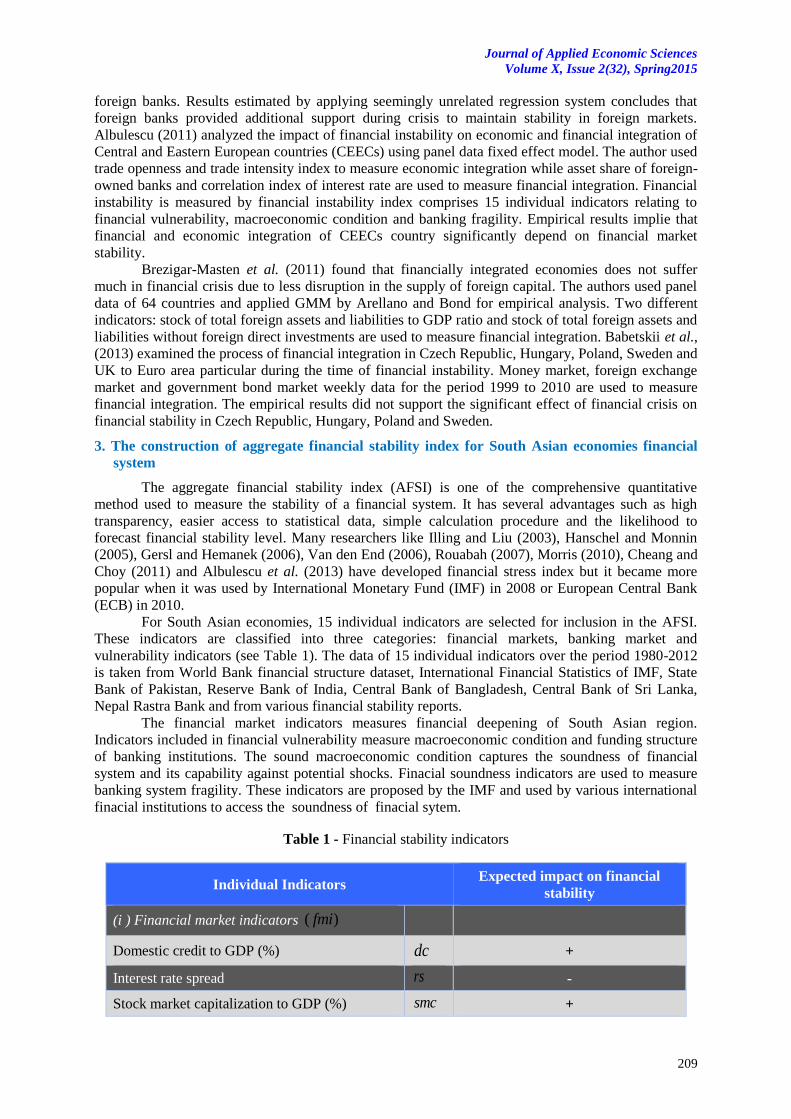
Journal of Applied Economic Sciences
Volume X, Issue 2(32), Spring2015
209
foreign banks. Results estimated by applying seemingly unrelated regression system concludes that
foreign banks provided additional support during crisis to maintain stability in foreign markets.
Albulescu (2011) analyzed the impact of financial instability on economic and financial integration of
Central and Eastern European countries (CEECs) using panel data fixed effect model. The author used
trade openness and trade intensity index to measure economic integration while asset share of foreign-
owned banks and correlation index of interest rate are used to measure financial integration. Financial
instability is measured by financial instability index comprises 15 individual indicators relating to
financial vulnerability, macroeconomic condition and banking fragility. Empirical results implie that
financial and economic integration of CEECs country significantly depend on financial market
stability.
Brezigar-Masten et al. (2011) found that financially integrated economies does not suffer
much in financial crisis due to less disruption in the supply of foreign capital. The authors used panel
data of 64 countries and applied GMM by Arellano and Bond for empirical analysis. Two different
indicators: stock of total foreign assets and liabilities to GDP ratio and stock of total foreign assets and
liabilities without foreign direct investments are used to measure financial integration. Babetskii et al.,
(2013) examined the process of financial integration in Czech Republic, Hungary, Poland, Sweden and
UK to Euro area particular during the time of financial instability. Money market, foreign exchange
market and government bond market weekly data for the period 1999 to 2010 are used to measure
financial integration. The empirical results did not support the significant effect of financial crisis on
financial stability in Czech Republic, Hungary, Poland and Sweden.
3. The construction of aggregate financial stability index for South Asian economies financial
system
The aggregate financial stability index (AFSI) is one of the comprehensive quantitative
method used to measure the stability of a financial system. It has several advantages such as high
transparency, easier access to statistical data, simple calculation procedure and the likelihood to
forecast financial stability level. Many researchers like Illing and Liu (2003), Hanschel and Monnin
(2005), Gersl and Hemanek (2006), Van den End (2006), Rouabah (2007), Morris (2010), Cheang and
Choy (2011) and Albulescu et al. (2013) have developed financial stress index but it became more
popular when it was used by International Monetary Fund (IMF) in 2008 or European Central Bank
(ECB) in 2010.
For South Asian economies, 15 individual indicators are selected for inclusion in the AFSI.
These indicators are classified into three categories: financial markets, banking market and
vulnerability indicators (see Table 1). The data of 15 individual indicators over the period 1980-2012
is taken from World Bank financial structure dataset, International Financial Statistics of IMF, State
Bank of Pakistan, Reserve Bank of India, Central Bank of Bangladesh, Central Bank of Sri Lanka,
Nepal Rastra Bank and from various financial stability reports.
The financial market indicators measures financial deepening of South Asian region.
Indicators included in financial vulnerability measure macroeconomic condition and funding structure
of banking institutions. The sound macroeconomic condition captures the soundness of financial
system and its capability against potential shocks. Finacial soundness indicators are used to measure
banking system fragility. These indicators are proposed by the IMF and used by various international
finacial institutions to access the soundness of finacial sytem.
Table 1 - Financial stability indicators
Individual Indicators Expected impact on financial
stability
(i ) Financial market indicators ( )fmi
Domestic credit to GDP (%) dc +
Interest rate spread rs -
Stock market capitalization to GDP (%) smc +
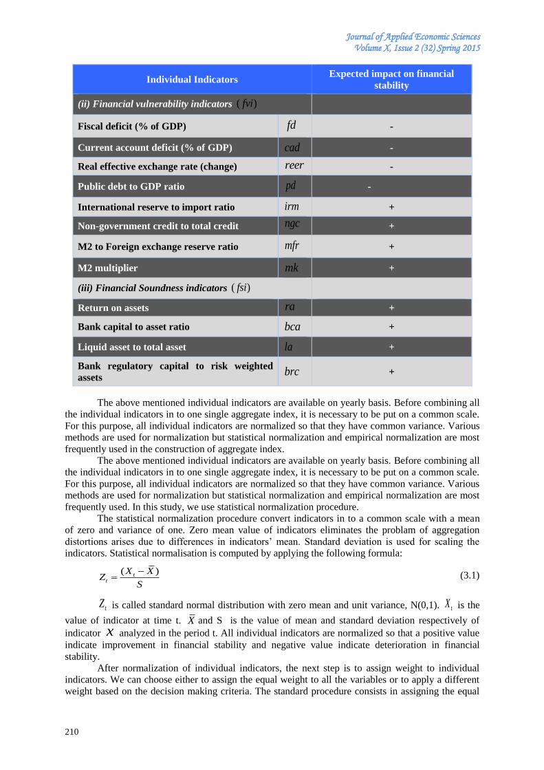
Journal of Applied Economic Sciences Volume X, Issue 2 (32) Spring 2015
210
Individual Indicators Expected impact on financial
stability
(ii) Financial vulnerability indicators ( )fvi
Fiscal deficit (% of GDP) fd -
Current account deficit (% of GDP) cad -
Real effective exchange rate (change) reer -
Public debt to GDP ratio pd -
International reserve to import ratio irm +
Non-government credit to total credit ngc +
M2 to Foreign exchange reserve ratio mfr +
M2 multiplier mk +
(iii) Financial Soundness indicators ( )fsi
Return on assets ra +
Bank capital to asset ratio bca +
Liquid asset to total asset la +
Bank regulatory capital to risk weighted
assets brc +
The above mentioned individual indicators are available on yearly basis. Before combining all
the individual indicators in to one single aggregate index, it is necessary to be put on a common scale.
For this purpose, all individual indicators are normalized so that they have common variance. Various
methods are used for normalization but statistical normalization and empirical normalization are most
frequently used in the construction of aggregate index.
The above mentioned individual indicators are available on yearly basis. Before combining all
the individual indicators in to one single aggregate index, it is necessary to be put on a common scale.
For this purpose, all individual indicators are normalized so that they have common variance. Various
methods are used for normalization but statistical normalization and empirical normalization are most
frequently used. In this study, we use statistical normalization procedure.
The statistical normalization procedure convert indicators in to a common scale with a mean
of zero and variance of one. Zero mean value of indicators eliminates the problam of aggregation
distortions arises due to differences in indicators’ mean. Standard deviation is used for scaling the
indicators. Statistical normalisation is computed by applying the following formula:
( )tt
X XZ
S
(3.1)
tZ is called standard normal distribution with zero mean and unit variance, N(0,1). tX is the
value of indicator at time t. X and S is the value of mean and standard deviation respectively of
indicator x analyzed in the period t. All individual indicators are normalized so that a positive value
indicate improvement in financial stability and negative value indicate deterioration in financial
stability.
After normalization of individual indicators, the next step is to assign weight to individual
indicators. We can choose either to assign the equal weight to all the variables or to apply a different
weight based on the decision making criteria. The standard procedure consists in assigning the equal
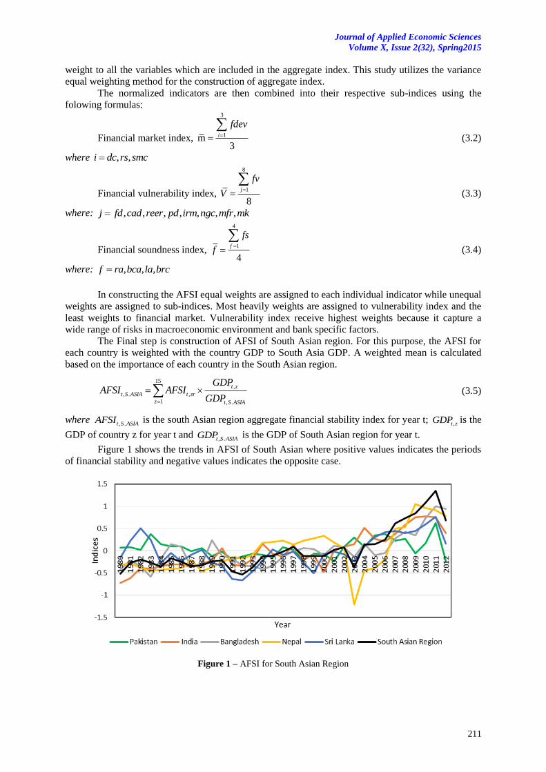
Journal of Applied Economic Sciences
Volume X, Issue 2(32), Spring2015
211
weight to all the variables which are included in the aggregate index. This study utilizes the variance
equal weighting method for the construction of aggregate index.
The normalized indicators are then combined into their respective sub-indices using the
folowing formulas:
Financial market index,
3
1m3
i
fdev
(3.2)
where , ,i dc rs smc
Financial vulnerability index,
8
1
8
j
fv
V
(3.3)
where: , , , , , , ,j fd cad reer pd irm ngc mfr mk
Financial soundness index,
4
1
4
f
fs
f
(3.4)
where: , , ,f ra bca la brc
In constructing the AFSI equal weights are assigned to each individual indicator while unequal
weights are assigned to sub-indices. Most heavily weights are assigned to vulnerability index and the
least weights to financial market. Vulnerability index receive highest weights because it capture a
wide range of risks in macroeconomic environment and bank specific factors.
The Final step is construction of AFSI of South Asian region. For this purpose, the AFSI for
each country is weighted with the country GDP to South Asia GDP. A weighted mean is calculated
based on the importance of each country in the South Asian region.
15,
, . ,
1 , .
t z
t S ASIA t zr
z t S ASIA
GDPAFSI AFSI
GDP
(3.5)
where , .t S ASIAAFSI is the south Asian region aggregate financial stability index for year t;
,t zGDP is the
GDP of country z for year t and , .t S ASIAGDP is the GDP of South Asian region for year t.
Figure 1 shows the trends in AFSI of South Asian where positive values indicates the periods
of financial stability and negative values indicates the opposite case.
Figure 1 – AFSI for South Asian Region
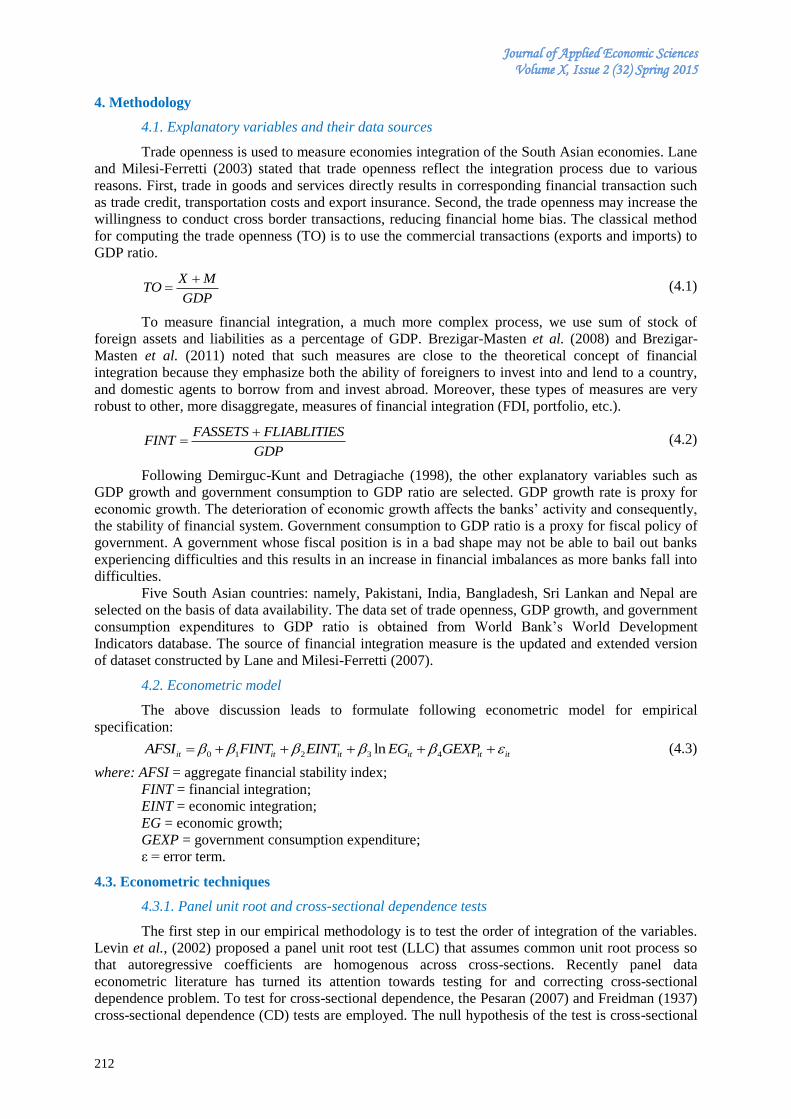
Journal of Applied Economic Sciences Volume X, Issue 2 (32) Spring 2015
212
4. Methodology
4.1. Explanatory variables and their data sources
Trade openness is used to measure economies integration of the South Asian economies. Lane
and Milesi-Ferretti (2003) stated that trade openness reflect the integration process due to various
reasons. First, trade in goods and services directly results in corresponding financial transaction such
as trade credit, transportation costs and export insurance. Second, the trade openness may increase the
willingness to conduct cross border transactions, reducing financial home bias. The classical method
for computing the trade openness (TO) is to use the commercial transactions (exports and imports) to
GDP ratio.
X MTO
GDP
(4.1)
To measure financial integration, a much more complex process, we use sum of stock of
foreign assets and liabilities as a percentage of GDP. Brezigar-Masten et al. (2008) and Brezigar-
Masten et al. (2011) noted that such measures are close to the theoretical concept of financial
integration because they emphasize both the ability of foreigners to invest into and lend to a country,
and domestic agents to borrow from and invest abroad. Moreover, these types of measures are very
robust to other, more disaggregate, measures of financial integration (FDI, portfolio, etc.).
FASSETS FLIABLITIESFINT
GDP
(4.2)
Following Demirguc-Kunt and Detragiache (1998), the other explanatory variables such as
GDP growth and government consumption to GDP ratio are selected. GDP growth rate is proxy for
economic growth. The deterioration of economic growth affects the banks’ activity and consequently,
the stability of financial system. Government consumption to GDP ratio is a proxy for fiscal policy of
government. A government whose fiscal position is in a bad shape may not be able to bail out banks
experiencing difficulties and this results in an increase in financial imbalances as more banks fall into
difficulties.
Five South Asian countries: namely, Pakistani, India, Bangladesh, Sri Lankan and Nepal are
selected on the basis of data availability. The data set of trade openness, GDP growth, and government
consumption expenditures to GDP ratio is obtained from World Bank’s World Development
Indicators database. The source of financial integration measure is the updated and extended version
of dataset constructed by Lane and Milesi-Ferretti (2007).
4.2. Econometric model
The above discussion leads to formulate following econometric model for empirical
specification:
0 1 2 3 4lnit it it it it itAFSI FINT EINT EG GEXP (4.3)
where: AFSI = aggregate financial stability index;
FINT = financial integration;
EINT = economic integration;
EG = economic growth;
GEXP = government consumption expenditure;
ε = error term.
4.3. Econometric techniques
4.3.1. Panel unit root and cross-sectional dependence tests
The first step in our empirical methodology is to test the order of integration of the variables.
Levin et al., (2002) proposed a panel unit root test (LLC) that assumes common unit root process so
that autoregressive coefficients are homogenous across cross-sections. Recently panel data
econometric literature has turned its attention towards testing for and correcting cross-sectional
dependence problem. To test for cross-sectional dependence, the Pesaran (2007) and Freidman (1937)
cross-sectional dependence (CD) tests are employed. The null hypothesis of the test is cross-sectional
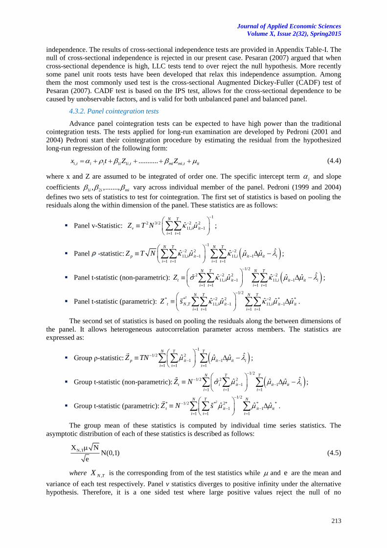
Journal of Applied Economic Sciences
Volume X, Issue 2(32), Spring2015
213
independence. The results of cross-sectional independence tests are provided in Appendix Table-I. The
null of cross-sectional independence is rejected in our present case. Pesaran (2007) argued that when
cross-sectional dependence is high, LLC tests tend to over reject the null hypothesis. More recently
some panel unit roots tests have been developed that relax this independence assumption. Among
them the most commonly used test is the cross-sectional Augmented Dickey-Fuller (CADF) test of
Pesaran (2007). CADF test is based on the IPS test, allows for the cross-sectional dependence to be
caused by unobservable factors, and is valid for both unbalanced panel and balanced panel.
4.3.2. Panel cointegration tests
Advance panel cointegration tests can be expected to have high power than the traditional
cointegration tests. The tests applied for long-run examination are developed by Pedroni (2001 and
2004) Pedroni start their cointegration procedure by estimating the residual from the hypothesized
long-run regression of the following form:
, 1 1 , ,...........i t i i i i t mi mi t itx t Z Z (4.4)
where x and Z are assumed to be integrated of order one. The specific intercept term i and slope
coefficients 1 2, ,.......,i i mi vary across individual member of the panel. Pedroni (1999 and 2004)
defines two sets of statistics to test for cointegration. The first set of statistics is based on pooling the
residuals along the within dimension of the panel. These statistics are as follows:
Panel v-Statistic:
1
2 3/2 2 2
11, 1
1 1
ˆ ˆN T
v i it
i t
Z T N
;
Panel -statistic: 1
2 2 2
11, 1 11, 1
1 1 1 1
ˆˆ ˆˆ ˆ ˆN T N T
p i it i it it i
i t i t
Z T N
;
Panel t-statistic (non-parametric): 1/2
2 2 2 2
11, 1 11, 1
1 1 1 1
ˆˆ ˆˆ ˆ ˆN T N T
t i it i it it i
i t i t
Z
;
Panel t-statistic (parametric): 2
1/2
* * 2 2 2 * *
, 11, 1 11, 1
1 1 1 1
ˆ ˆˆ ˆ ˆN T N T
t N T i it i it it
i t i t
Z s
.
The second set of statistics is based on pooling the residuals along the between dimensions of
the panel. It allows heterogeneous autocorrelation parameter across members. The statistics are
expressed as:
Group ρ-statistic: 1
1/2 2
1 1
1 1 1
ˆˆ ˆ ˆN T T
p it it it i
i t t
Z TN
;
Group t-statistic (non-parametric): 1/2
1/2 2 2
1 1
1 1 1
ˆˆ ˆ ˆ ˆN T T
t i it it it i
i t t
Z N
;
Group t-statistic (parametric):2
1/2
* 1/2 * 2* * *
1 1
1 1 1
ˆ ˆ ˆN T N
t it it it
i t t
Z N s
.
The group mean of these statistics is computed by individual time series statistics. The
asymptotic distribution of each of these statistics is described as follows:
N,TX NN(0,1)
e
(4.5)
where TNX , is the corresponding from of the test statistics while and e are the mean and
variance of each test respectively. Panel v statistics diverges to positive infinity under the alternative
hypothesis. Therefore, it is a one sided test where large positive values reject the null of no
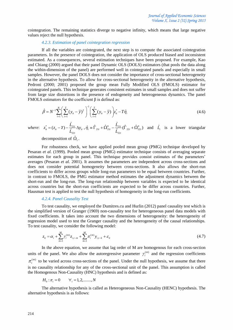
Journal of Applied Economic Sciences Volume X, Issue 2 (32) Spring 2015
214
cointegration. The remaining statistics diverge to negative infinity, which means that large negative
values reject the null hypothesis.
4.2.3. Estimation of panel cointegration regression
If all the variables are cointegrated, the next step is to compute the associated cointegration
parameters. In the presence of cointegration, the application of OLS produced biased and inconsistent
estimated. As a consequences, several estimation techniques have been proposed. For example, Kao
and Chiang (2000) argued that their panel Dynamic OLS (DOLS) estimators (that pools the data along
the within-dimension of the panel) are performed well in cointegrated panels and especially in small
samples. However, the panel DOLS does not consider the importance of cross-sectional heterogeneity
in the alternative hypothesis. To allow for cross-sectional heterogeneity in the alternative hypothesis,
Pedroni (2000; 2001) proposed the group mean Fully Modified OLS (FMOLS) estimator for
cointegrated panels. This technique generates consistent estimates in small samples and does not suffer
from large size distortions in the presence of endogeneity and heterogeneous dynamics. The panel
FMOLS estimators for the coefficient β is defined as:
1
1 2 *
1 1 1
ˆ ˆ( ) ( )N T T
it it it i
i t t
N y y y y z T
(4.6)
where: * 0 021 2121 21 22 22
22 22
ˆ ˆˆ ˆˆ ˆˆ( ) , ( )
ˆ ˆi i
it it it i i i i i
i i
L Lz z z y
L L and ˆ
iL is a lower triangular
decomposition of ˆ i .
For robustness check, we have applied pooled mean group (PMG) technique developed by
Pesaran et al. (1999). Pooled mean group (PMG) estimator technique consists of averaging separate
estimates for each group in panel. This technique provides consist estimates of the parameters’
averages (Pesaran et al. 2001). It assumes the parameters are independent across cross-sections and
does not consider potential homogeneity between cross-sections. It also allows the short-run
coefficients to differ across groups while long-run parameters to be equal between countries. Further,
in contrast to FMOLS, the PMG estimator method estimates the adjustment dynamics between the
short-run and the long-run. The long-run relationship between variables is expected to be identical
across countries but the short-run coefficients are expected to be differ across countries. Further,
Hausman test is applied to test the null hypothesis of homogeneity in the long-run coefficients.
4.2.4. Panel Causality Test
To test causality, we employed the Dumitres.cu and Hurlin (2012) panel causality test which is
the simplified version of Granger (1969) non-causality test for heterogeneous panel data models with
fixed coefficients. It takes into account the two dimensions of heterogeneity: the heterogeneity of
regression model used to test the Granger causality and the heterogeneity of the causal relationships.
To test causality, we consider the following model:
( ) ( )
, ,
1 1
M Mm m
it i i i t m i i t k it
m m
z z y
(4.7)
In the above equation, we assume that lag order of M are homogenous for each cross-section
units of the panel. We also allow the autoregressive parameter ( )m
i and the regression coefficients
( )m
i to be varied across cross-sections of the panel. Under the null hypothesis, we assume that there
is no causality relationship for any of the cross-sectional unit of the panel. This assumption is called
the Homogenous Non-Causality (HNC) hypothesis and is defined as:
0 : 0 1,2,.......,i iH N
The alternative hypothesis is called as Heterogeneous Non-Causality (HENC) hypothesis. The
alternative hypothesis is as follows:
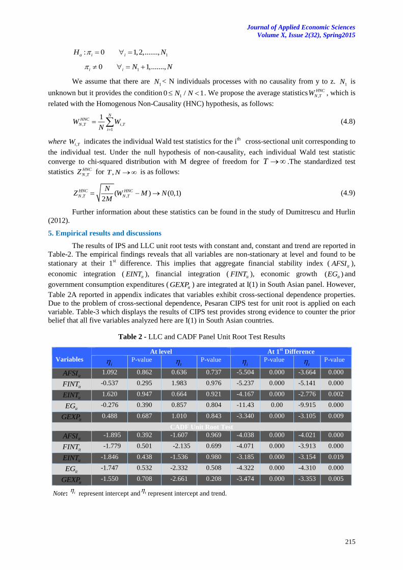
Journal of Applied Economic Sciences
Volume X, Issue 2(32), Spring2015
215
1: 0 1,2,.......,a i iH N
10 1,.......,i i N N
We assume that there are 1N < N individuals processes with no causality from y to z.
1N is
unknown but it provides the condition10 / 1N N . We propose the average statistics ,
HNC
N TW , which is
related with the Homogenous Non-Causality (HNC) hypothesis, as follows:
, ,
1
1 NHNC
N T i T
i
W WN
(4.8)
where ,i TW indicates the individual Wald test statistics for the i
th cross-sectional unit corresponding to
the individual test. Under the null hypothesis of non-causality, each individual Wald test statistic
converge to chi-squared distribution with M degree of freedom for T .The standardized test
statistics ,
HNC
N TZ for ,T N is as follows:
, ,( ) (0,1)2
HNC HNC
N T N T
NZ W M N
M (4.9)
Further information about these statistics can be found in the study of Dumitrescu and Hurlin
(2012).
5. Empirical results and discussions
The results of IPS and LLC unit root tests with constant and, constant and trend are reported in
Table-2. The empirical findings reveals that all variables are non-stationary at level and found to be
stationary at their 1st difference. This implies that aggregate financial stability index (
itAFSI ),
economic integration (itEINT ), financial integration (
itFINT ), economic growth ( )itEG and
government consumption expenditures (itGEXP ) are integrated at I(1) in South Asian panel. However,
Table 2A reported in appendix indicates that variables exhibit cross-sectional dependence properties.
Due to the problem of cross-sectional dependence, Pesaran CIPS test for unit root is applied on each
variable. Table-3 which displays the results of CIPS test provides strong evidence to counter the prior
belief that all five variables analyzed here are I(1) in South Asian countries.
Table 2 - LLC and CADF Panel Unit Root Test Results
Variables
At level At 1st Difference
i P-value t P-value
i P-value t P-value
itAFSI 1.092 0.862 0.636 0.737 -5.504 0.000 -3.664 0.000
itFINT -0.537 0.295 1.983 0.976 -5.237 0.000 -5.141 0.000
itEINT 1.620 0.947 0.664 0.921 -4.167 0.000 -2.776 0.002
itEG -0.276 0.390 0.857 0.804 -11.43 0.00 -9.915 0.000
itGEXP 0.488 0.687 1.010 0.843 -3.340 0.000 -3.105 0.009
CADF Unit Root Test
itAFSI -1.895 0.392 -1.607 0.969 -4.038 0.000 -4.021 0.000
itFINT -1.779 0.501 -2.135 0.699 -4.071 0.000 -3.913 0.000
itEINT -1.846 0.438 -1.536 0.980 -3.185 0.000 -3.154 0.019
itEG -1.747 0.532 -2.332 0.508 -4.322 0.000 -4.310 0.000
itGEXP -1.550 0.708 -2.661 0.208 -3.474 0.000 -3.353 0.005
Note: i represent intercept and t represent intercept and trend.
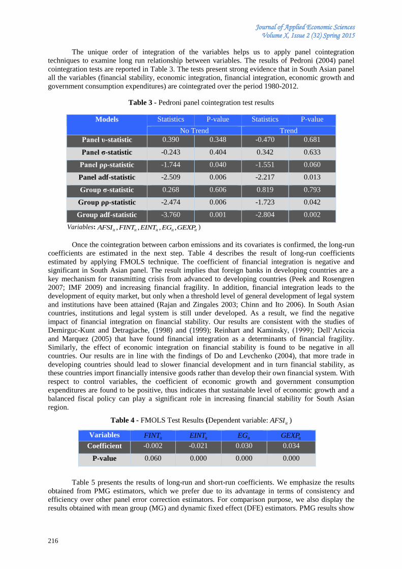
Journal of Applied Economic Sciences Volume X, Issue 2 (32) Spring 2015
216
The unique order of integration of the variables helps us to apply panel cointegration
techniques to examine long run relationship between variables. The results of Pedroni (2004) panel
cointegration tests are reported in Table 3. The tests present strong evidence that in South Asian panel
all the variables (financial stability, economic integration, financial integration, economic growth and
government consumption expenditures) are cointegrated over the period 1980-2012.
Table 3 - Pedroni panel cointegration test results
Models Statistics P-value Statistics P-value
No Trend Trend
Panel υ-statistic 0.390 0.348 -0.470 0.681
Panel σ-statistic -0.243 0.404 0.342 0.633
Panel ρρ-statistic -1.744 0.040 -1.551 0.060
Panel adf-statistic -2.509 0.006 -2.217 0.013
Group σ-statistic 0.268 0.606 0.819 0.793
Group ρρ-statistic -2.474 0.006 -1.723 0.042
Group adf-statistic -3.760 0.001 -2.804 0.002
Variables: , , , ,it it it it itAFSI FINT EINT EG GEXP )
Once the cointegration between carbon emissions and its covariates is confirmed, the long-run
coefficients are estimated in the next step. Table 4 describes the result of long-run coefficients
estimated by applying FMOLS technique. The coefficient of financial integration is negative and
significant in South Asian panel. The result implies that foreign banks in developing countries are a
key mechanism for transmitting crisis from advanced to developing countries (Peek and Rosengren
2007; IMF 2009) and increasing financial fragility. In addition, financial integration leads to the
development of equity market, but only when a threshold level of general development of legal system
and institutions have been attained (Rajan and Zingales 2003; Chinn and Ito 2006). In South Asian
countries, institutions and legal system is still under developed. As a result, we find the negative
impact of financial integration on financial stability. Our results are consistent with the studies of
Demirguc-Kunt and Detragiache, (1998) and (1999); Reinhart and Kaminsky, (1999); Dell‘Ariccia
and Marquez (2005) that have found financial integration as a determinants of financial fragility.
Similarly, the effect of economic integration on financial stability is found to be negative in all
countries. Our results are in line with the findings of Do and Levchenko (2004), that more trade in
developing countries should lead to slower financial development and in turn financial stability, as
these countries import financially intensive goods rather than develop their own financial system. With
respect to control variables, the coefficient of economic growth and government consumption
expenditures are found to be positive, thus indicates that sustainable level of economic growth and a
balanced fiscal policy can play a significant role in increasing financial stability for South Asian
region.
Table 4 - FMOLS Test Results (Dependent variable:itAFSI )
Variables itFINT
itEINT itEG
itGEXP
Coefficient -0.002 -0.021 0.030 0.034
P-value 0.060 0.000 0.000 0.000
Table 5 presents the results of long-run and short-run coefficients. We emphasize the results
obtained from PMG estimators, which we prefer due to its advantage in terms of consistency and
efficiency over other panel error correction estimators. For comparison purpose, we also display the
results obtained with mean group (MG) and dynamic fixed effect (DFE) estimators. PMG results show
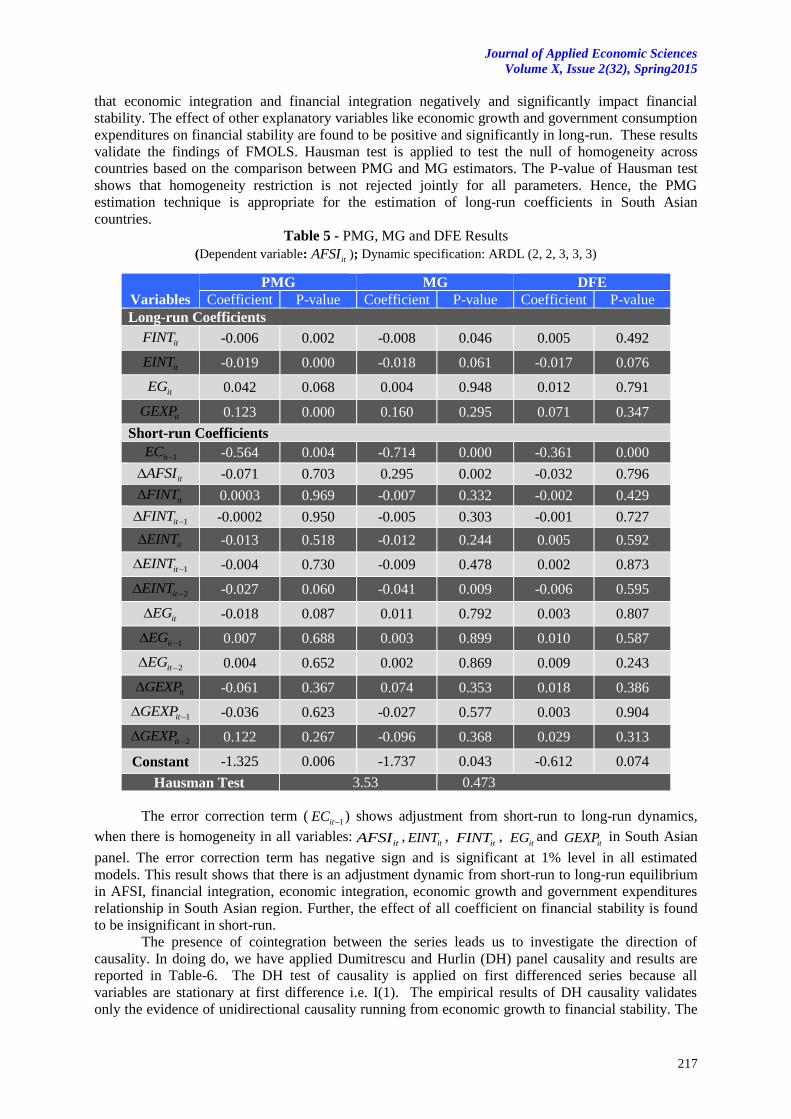
Journal of Applied Economic Sciences
Volume X, Issue 2(32), Spring2015
217
that economic integration and financial integration negatively and significantly impact financial
stability. The effect of other explanatory variables like economic growth and government consumption
expenditures on financial stability are found to be positive and significantly in long-run. These results
validate the findings of FMOLS. Hausman test is applied to test the null of homogeneity across
countries based on the comparison between PMG and MG estimators. The P-value of Hausman test
shows that homogeneity restriction is not rejected jointly for all parameters. Hence, the PMG
estimation technique is appropriate for the estimation of long-run coefficients in South Asian
countries.
Table 5 - PMG, MG and DFE Results
(Dependent variable:itAFSI ); Dynamic specification: ARDL (2, 2, 3, 3, 3)
Variables
PMG MG DFE
Coefficient P-value Coefficient P-value Coefficient P-value
Long-run Coefficients
itFINT -0.006 0.002 -0.008 0.046 0.005 0.492
itEINT -0.019 0.000 -0.018 0.061 -0.017 0.076
itEG 0.042 0.068 0.004 0.948 0.012 0.791
itGEXP 0.123 0.000 0.160 0.295 0.071 0.347
Short-run Coefficients
1itEC -0.564 0.004 -0.714 0.000 -0.361 0.000
itAFSI -0.071 0.703 0.295 0.002 -0.032 0.796
itFINT 0.0003 0.969 -0.007 0.332 -0.002 0.429
1itFINT -0.0002 0.950 -0.005 0.303 -0.001 0.727
itEINT -0.013 0.518 -0.012 0.244 0.005 0.592
1itEINT -0.004 0.730 -0.009 0.478 0.002 0.873
2itEINT -0.027 0.060 -0.041 0.009 -0.006 0.595
itEG -0.018 0.087 0.011 0.792 0.003 0.807
1itEG 0.007 0.688 0.003 0.899 0.010 0.587
2itEG 0.004 0.652 0.002 0.869 0.009 0.243
itGEXP -0.061 0.367 0.074 0.353 0.018 0.386
1itGEXP -0.036 0.623 -0.027 0.577 0.003 0.904
2itGEXP 0.122 0.267 -0.096 0.368 0.029 0.313
Constant -1.325 0.006 -1.737 0.043 -0.612 0.074
Hausman Test 3.53 0.473
The error correction term (1itEC ) shows adjustment from short-run to long-run dynamics,
when there is homogeneity in all variables:itAFSI ,
itEINT , itFINT ,
itEG and itGEXP in South Asian
panel. The error correction term has negative sign and is significant at 1% level in all estimated
models. This result shows that there is an adjustment dynamic from short-run to long-run equilibrium
in AFSI, financial integration, economic integration, economic growth and government expenditures
relationship in South Asian region. Further, the effect of all coefficient on financial stability is found
to be insignificant in short-run.
The presence of cointegration between the series leads us to investigate the direction of
causality. In doing do, we have applied Dumitrescu and Hurlin (DH) panel causality and results are
reported in Table-6. The DH test of causality is applied on first differenced series because all
variables are stationary at first difference i.e. I(1). The empirical results of DH causality validates
only the evidence of unidirectional causality running from economic growth to financial stability. The
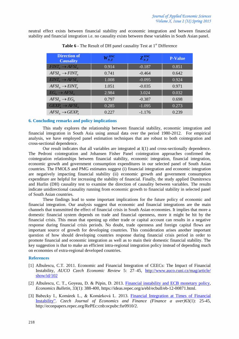
Journal of Applied Economic Sciences Volume X, Issue 2 (32) Spring 2015
218
neutral effect exists between financial stability and economic integration and between financial
stability and financial integration i.e. no causality exists between these variables in South Asian panel.
Table 6 - The Result of DH panel causality Test at 1st Difference
Direction of
Causality ,
HNC
N TW
,
HNC
N TZ P-Value
it itFINT AFSI 0.914 -0.187 0.851
it itAFSI FINT 0.741 -0.464 0.642
it itEINT AFSI 1.008 -0.095 0.924
it itAFSI EINT 1.051 -0.035 0.971
it itEG AFSI 2.984 3.024 0.032
it itAFSI EG 0.797 -0.387 0.698
it itGEXP AFSI 0.285 -1.095 0.273
it itAFSI GEXP 0.227 -1.176 0.239
6. Concluding remarks and policy implications
This study explores the relationship between financial stability, economic integration and
financial integration in South Asia using annual data over the period 1980-2012. For empirical
analysis, we have employed panel estimation techniques that are robust to both cointegration and
cross-sectional dependence.
Our result indicates that all variables are integrated at I(1) and cross-sectionally dependence.
The Pedroni cointegration and Johansen Fisher Panel cointegration approaches confirmed the
cointegration relationships between financial stability, economic integration, financial integration,
economic growth and government consumption expenditures in our selected panel of South Asian
countries. The FMOLS and PMG estimates suggest (i) financial integration and economic integration
are negatively impacting financial stability (ii) economic growth and government consumption
expenditure are helpful for increasing the stability of financial. Finally, the study applied Dumitrescu
and Hurlin (DH) causality test to examine the direction of causality between variables. The results
indicate unidirectional causality running from economic growth to financial stability in selected panel
of South Asian countries.
These findings lead to some important implications for the future policy of economic and
financial integration. Our analysis suggest that economic and financial integrations are the main
channels that transmitted the effect of financial crisis in South Asian economies. It implies that more a
domestic financial system depends on trade and financial openness, more it might be hit by the
financial crisis. This mean that opening up either trade or capital account can results in a negative
response during financial crisis periods. No doubt, trade openness and foreign capital flows are
important source of growth for developing countries. This consideration arises another important
question of how should developing countries response during financial crisis period in order to
promote financial and economic integration as well as to main their domestic financial stability. The
key suggestion is that to make an efficient intra-regional integration policy instead of depending much
on economies of extra-regional developed countries.
References
[1] Albulescu, C.T. 2011. Economic and Financial Integration of CEECs: The Impact of Financial
Instability, AUCO Czech Economic Review 5: 27–45, http://www.auco.cuni.cz/mag/article/
show/id/102
[2] Albulescu, C. T., Goyeau, D. & Pépin, D. 2013. Financial instability and ECB monetary policy,
Economics Bulletin, 33(1): 388-400, https://ideas.repec.org/a/ebl/ecbull/eb-12-00871.html.
[3] Babecky I., Komárek L., Komárková L. 2013. Financial Integration at Times of Financial
Instability”. Czech Journal of Economics and Finance (Finance a uver)63(1): 25-45,
http://econpapers.repec.org/RePEc:cnb:ocpubc:fsr0910/2.
Journal of Applied Economic Sciences
Volume X, Issue 2(32), Spring2015
219
[4] Brezigar-Masten, A., Coricelli, F., & Masten, I. 2008. Non-linear growth effects of financial
development: Does financial integration matter”? Journal of International Money and Finance,
27(2): 295-313, www.cesruc.org/uploads/soft/130221/1-130221151518.pdf.
[5] Brezigar-Masten, A., Coricelli, F., & Masten, I. 2011. Financial Integration and Financial
Development in Transition Economies: What Happens During Financial Crises”? Economic and
Business Review 13(1-2): 119-137, www.fiw.ac.at/.../30
[6] Baele, L., A., Ferrando, A., Hordahl, P., Krylova, E., & Monnet, C. 2004. Measuring financial
integration in the euro area, ECB Occasional Paper No. 14, citeseer.ist.psu.edu/viewdoc/summary?
doi=10.1.1.165.5886
[7] Balassa B. 1962. The Theory of Economic Integration. London, http://www.unz.org/Pub/
BalassaBela-1962
[8] Cerra V., & Saxena, S.C. 2007. Growth dynamics: the myth of economic recovery. BIS Working
Papers 226, Bank for International Settlements (), www.bis.org/publ/work226.pdf
[9] Chinn, M.D., Ito H., 2006. What matters for financial development? Capital controls, institutions,
and interactions, Journal of Development Economics, 8: 163–192, econpapers.repec.
org/RePEc:eee:deveco:v:81:y:2006:i:1:p:163-192
[10] Cheng, N., Choy I. 2010. Aggregate Financial Stability Index for an Early Warning System”,
Monetary Authority of Macao, www.amcm.gov.mo/.../AFSI_en.pdf
[11] Demirguc-Kent, A., Detragiache, E., 1998. Financial Liberalization and Financial Fragility.
Policy Research Working Paper Series 1917. The World Bank. Washington D.C,
elibrary.worldbank.org/doi/book/10.1596/1813-9450-1917.
[12] Demirguc-Kunt, A., Detragiache E. 1998. Financial Liberalization and Financial Fragility, in B.
Pleskovic and J.E. Stiglitz (eds.), Annual World Bank Conference on Development Economics
1998, World Bank. Washington D.C., https://books.google.com/books?id=Kyz1NtP4NQIC
[13] Dell'Ariccia G., Marquez, R. 2006. Lending Booms and Lending Standards, Journal of Finance,
American Finance Association 61(5): 2511-2546, www.jstor.org/stable/3874718
[14] Do, Q.T., Levchenko, A.A., Trade and financial development, World Bank Working Paper 3347
(2004), www.alevchenko.com/wps3347.pdf
[15] Dumitrescu, E. and Hurlin, C. 2012. Testing for Granger Non-Causality in Heterogeneous Panels.
Economic Modelling 29(4): 1450-1460, www.sciencedirect.com/science/.../S0264999312000491
[16] Friedman, M. 1937. The Use of Ranks to Avoid the Assumption of Norma Implicit in the
Analysis of Variance, Journal of the American Statistics Association, 32: 675-701,
www.citeulike.org/user/mdifranc/article/3492147
[17] Fowowe, B. 2010. Financial Liberalization and Financial Fragility in Nigeria. Central Bank of
Nigeria Economic and Financial Review, 48(1): 71-92, www.cenbank.org/.../Economic%20and%
20Financial%20Review%20Vo
[18] Gersl, A. & Hermanek, J. 2007. Financial Stability Indicators: Advantages and Disadvantages of
Their Use in the Assessment of the Financial System Stability, Czech National Bank, CNB
Financial Stability Report. Prague, Czech National Bank, 69–79, www.cnb.cz/en/financial_
stability/fs_reports/.../FSR_2006_article_2.pdf
[19] Granger, C.W.J. 1969. Investigating causal relation by econometric and cross-sectional method.
Econometrica, 37: 424–438, https://ideas.repec.org/a/ecm/emetrp/v37y1969i3p424-38.html
[20] Hanschel, E. & Monnin, P. 2005. Measuring and Forecasting Stress in the Banking Sector:
Evidence from Switzerland. Basel, Bank for International Settlements, BIS Paper No. 22: 431–
449, bis.hasbeenforeclosed.com/publ/bppdf/bispap22v.pdf
[21] Ho, N.W. 2009. Financial Integration: Concepts and Impacts. Macao Monetary Research
Bulletin, 10: 69-84, www.amcm.gov.mo/.../Financial%20Integ...
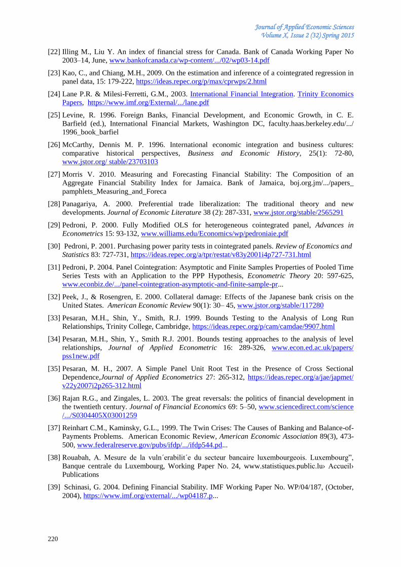
Journal of Applied Economic Sciences Volume X, Issue 2 (32) Spring 2015
220
[22] Illing M., Liu Y. An index of financial stress for Canada. Bank of Canada Working Paper No
2003–14, June, www.bankofcanada.ca/wp-content/.../02/wp03-14.pdf
[23] Kao, C., and Chiang, M.H., 2009. On the estimation and inference of a cointegrated regression in
panel data, 15: 179-222, https://ideas.repec.org/p/max/cprwps/2.html
[24] Lane P.R. & Milesi-Ferretti, G.M., 2003. International Financial Integration. Trinity Economics
Papers, https://www.imf.org/External/.../lane.pdf
[25] Levine, R. 1996. Foreign Banks, Financial Development, and Economic Growth, in C. E.
Barfield (ed.), International Financial Markets, Washington DC, faculty.haas.berkeley.edu/.../
1996_book_barfiel
[26] McCarthy, Dennis M. P. 1996. International economic integration and business cultures:
comparative historical perspectives, Business and Economic History, 25(1): 72-80,
www.jstor.org/ stable/23703103
[27] Morris V. 2010. Measuring and Forecasting Financial Stability: The Composition of an
Aggregate Financial Stability Index for Jamaica. Bank of Jamaica, boj.org.jm/.../papers_
pamphlets_Measuring_and_Foreca
[28] Panagariya, A. 2000. Preferential trade liberalization: The traditional theory and new
developments. Journal of Economic Literature 38 (2): 287-331, www.jstor.org/stable/2565291
[29] Pedroni, P. 2000. Fully Modified OLS for heterogeneous cointegrated panel, Advances in
Econometrics 15: 93-132, www.williams.edu/Economics/wp/pedroniaie.pdf
[30] Pedroni, P. 2001. Purchasing power parity tests in cointegrated panels. Review of Economics and
Statistics 83: 727-731, https://ideas.repec.org/a/tpr/restat/v83y2001i4p727-731.html
[31] Pedroni, P. 2004. Panel Cointegration: Asymptotic and Finite Samples Properties of Pooled Time
Series Tests with an Application to the PPP Hypothesis, Econometric Theory 20: 597-625,
www.econbiz.de/.../panel-cointegration-asymptotic-and-finite-sample-pr...
[32] Peek, J., & Rosengren, E. 2000. Collateral damage: Effects of the Japanese bank crisis on the
United States. American Economic Review 90(1): 30– 45, www.jstor.org/stable/117280
[33] Pesaran, M.H., Shin, Y., Smith, R.J. 1999. Bounds Testing to the Analysis of Long Run
Relationships, Trinity College, Cambridge, https://ideas.repec.org/p/cam/camdae/9907.html
[34] Pesaran, M.H., Shin, Y., Smith R.J. 2001. Bounds testing approaches to the analysis of level
relationships, Journal of Applied Econometric 16: 289-326, www.econ.ed.ac.uk/papers/
pss1new.pdf
[35] Pesaran, M. H., 2007. A Simple Panel Unit Root Test in the Presence of Cross Sectional
Dependence,Journal of Applied Econometrics 27: 265-312, https://ideas.repec.org/a/jae/japmet/
v22y2007i2p265-312.html
[36] Rajan R.G., and Zingales, L. 2003. The great reversals: the politics of financial development in
the twentieth century. Journal of Financial Economics 69: 5–50, www.sciencedirect.com/science
/.../S0304405X03001259
[37] Reinhart C.M., Kaminsky, G.L., 1999. The Twin Crises: The Causes of Banking and Balance-of-
Payments Problems. American Economic Review, American Economic Association 89(3), 473-
500, www.federalreserve.gov/pubs/ifdp/.../ifdp544.pd...
[38] Rouabah, A. Mesure de la vuln´erabilit´e du secteur bancaire luxembourgeois. Luxembourg”,
Banque centrale du Luxembourg, Working Paper No. 24, www.statistiques.public.lu› Accueil›
Publications
[39] Schinasi, G. 2004. Defining Financial Stability. IMF Working Paper No. WP/04/187, (October,
2004), https://www.imf.org/external/.../wp04187.p...

Journal of Applied Economic Sciences
Volume X, Issue 2(32), Spring2015
221
[40] Vogel, U., Winkler A. 2010. Foreign banks and financial stability in emerging markets: evidence
from the global financial crisis. Frankfurt School Working Paper No. 149, www.frankfurt-
school.de/clicnetclm/fileDownload.do?goid...
[41] Weber, A. A. 2006. European Financial Integration and (its Implications for) Monetary Policy”.
Bank for International Settlements, https://www.ecb.europa.eu/.../financialintegrationine...
[42] Van den End, J.W. 2006. Indicator and boundaries of financial stability. DNB Working Paper No
97, www.dnb.nl/.../Working%20Paper%2097_tcm4
*** Reserve Bank of India, Financial stability report, Issue 7, June 2013, www.rbi.org.in/scripts/
publications.aspx
*** International Monetary Fund (IMF). 2009. World economic outlook: crisis and recovery. April,
http:/www.imf.org/external/pubs/ft/weo/2009/01/pdf/text.pdf
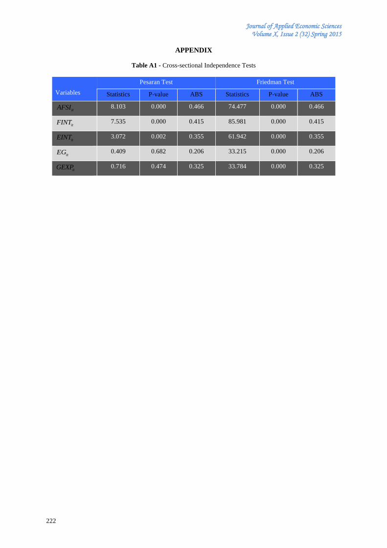
Journal of Applied Economic Sciences Volume X, Issue 2 (32) Spring 2015
222
APPENDIX
Table A1 - Cross-sectional Independence Tests
Variables
Pesaran Test Friedman Test
Statistics P-value ABS Statistics P-value ABS
itAFSI 8.103 0.000 0.466 74.477 0.000 0.466
itFINT 7.535 0.000 0.415 85.981 0.000 0.415
itEINT 3.072 0.002 0.355 61.942 0.000 0.355
itEG 0.409 0.682 0.206 33.215 0.000 0.206
itGEXP 0.716 0.474 0.325 33.784 0.000 0.325
Journal of Applied Economic Sciences
Volume X, Issue 2(32), Spring2015
223
THE EFFECT OF INDUSTRY AND CORPORATE CHARACTERISTICS ON BOND RATING
Martina NOVOTNÁ
Faculty of Economics, VŠB
Technical University of Ostrava, Czech Republic
Abstract: The objective of the paper is to analyse the effect of selected quantitative and qualitative variables on
corporate bond rating. The primary focus is paid to the application of ordinal logistic regression and estimation
of three models that are derived on the basis of macroeconomic, industry and financial variables. The overall
results suggest that there are sectors with a higher probability of better rating assessment. Based on the
analysis, we can conclude that although there is a significant association between industry sector and bond
rating, the most significant predictors of rating are financial indicators of size and profitability of firms. The
results of the analysis should be taken into account when the primary interest is to assess unrated companies or
to evaluate the impact of financial performance on current rating.
Keywords: bond rating, credit risk, ordinal logistic regression, model estimation, prediction
JEL Classification: G24, G32
1. Introduction
Corporate bond rating can be considered as an assessment of the creditworthiness of bond
issues. Two main rating agencies, S P and Moody’s, emphasise that credit ratings are forward
looking. It means that in addition to analysing historical information, they also assess the potential
impact of foreseeable future events. The mentioned rating agencies have been recently criticized for
not sufficient response in terms of not downgrading some securities prior to the financial crisis and
this is the main reason why many countries have adopted new regulations on the services of rating
agencies. In spite of the recent development, the influence of rating agencies on financial markets is
still significant. As a result, it is essential to understand rating, the ways how it is measured and main
factors of rating assessment.
The paper aims to analyse the relationships between credit rating and selected quantitative and
qualitative factors. The purpose is to estimate the influence of macroeconomic indicators, industry
characteristics and accounting variables on corporate bond rating by means of ordinal logistic
regression. The structure of the paper is as follows: Firstly, the methodology of logistic regression will
be described and the next part will be devoted to the use of the ordinal logistic regression on the data
of selected companies. The estimated models will be then presented and interpreted in the next part of
the paper. Finally, the overall results and recommendations will be summarized in the conclusion.
2. Importance of credit rating models
Corporate bond rating is essentially associated with the presence of credit risk. As Joseph
(2013, 15) states, the credit risk exists whenever a product or service is obtained without paying for it.
The report on the credit risk of fixed income securities is provided by credit rating agencies which
highlight some key features about their rating provided. The Standard Poor’s consider credit ratings
as the opinions about the ability and willingness of an issuer to meet financial obligations in full and
on time. Thus, ratings are evidently associated with the credit quality of an individual debt issue and
the relative likelihood that the issue may default. Each rating agency uses its own methodology in
measuring creditworthiness and uses its own rating scales. Many countries have adopted new
regulations on the services of rating agencies in response to recent financial crisis. In addition to
national or regional solutions such as European credit rating agency, there is an initiative for the
establishment of international non-profit credit rating agency called INCRA1. Although the credibility
of rating agencies has been deteriorated in the context of financial crisis, they currently put a lot of
effort to improve their reliability and improve their position. Nevertheless, as mentioned above, the
1 An International Non-Profit Credit Rating Agency (INCRA). Bertelsmann Foundation, available online:
http://www.bfna.org/category/publication-type/incra
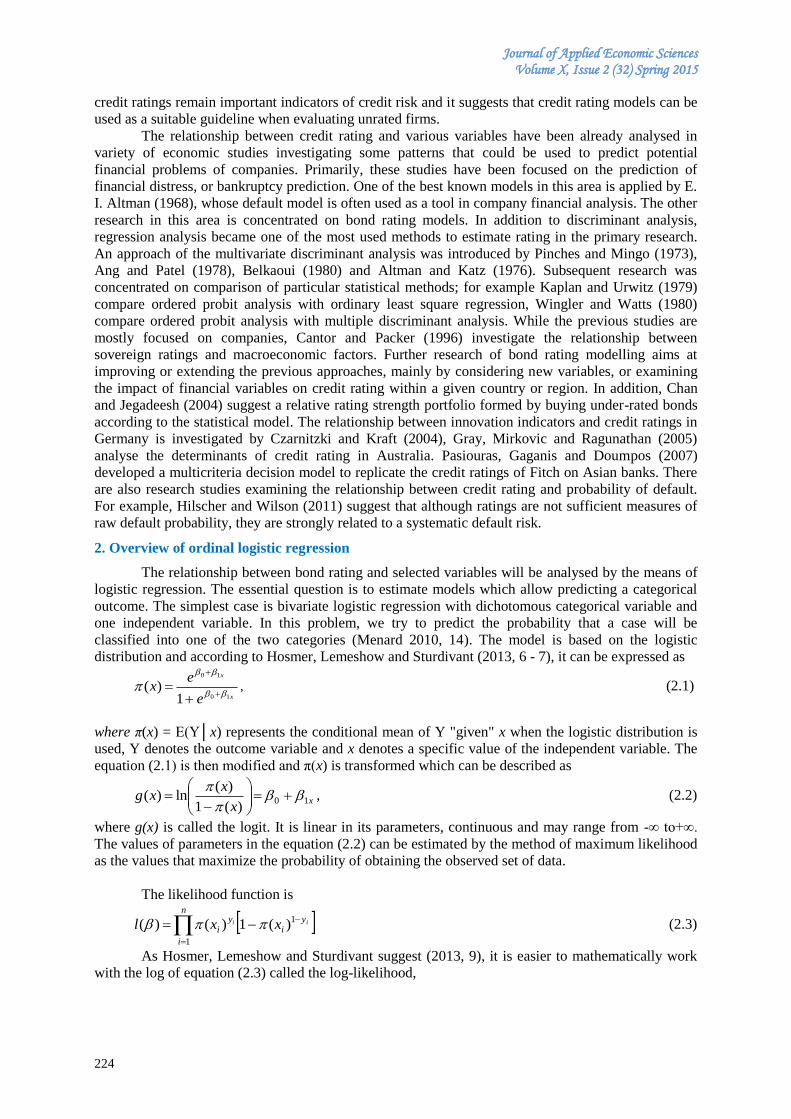
Journal of Applied Economic Sciences Volume X, Issue 2 (32) Spring 2015
224
credit ratings remain important indicators of credit risk and it suggests that credit rating models can be
used as a suitable guideline when evaluating unrated firms.
The relationship between credit rating and various variables have been already analysed in
variety of economic studies investigating some patterns that could be used to predict potential
financial problems of companies. Primarily, these studies have been focused on the prediction of
financial distress, or bankruptcy prediction. One of the best known models in this area is applied by E.
I. Altman (1968), whose default model is often used as a tool in company financial analysis. The other
research in this area is concentrated on bond rating models. In addition to discriminant analysis,
regression analysis became one of the most used methods to estimate rating in the primary research.
An approach of the multivariate discriminant analysis was introduced by Pinches and Mingo (1973),
Ang and Patel (1978), Belkaoui (1980) and Altman and Katz (1976). Subsequent research was
concentrated on comparison of particular statistical methods; for example Kaplan and Urwitz (1979)
compare ordered probit analysis with ordinary least square regression, Wingler and Watts (1980)
compare ordered probit analysis with multiple discriminant analysis. While the previous studies are
mostly focused on companies, Cantor and Packer (1996) investigate the relationship between
sovereign ratings and macroeconomic factors. Further research of bond rating modelling aims at
improving or extending the previous approaches, mainly by considering new variables, or examining
the impact of financial variables on credit rating within a given country or region. In addition, Chan
and Jegadeesh (2004) suggest a relative rating strength portfolio formed by buying under-rated bonds
according to the statistical model. The relationship between innovation indicators and credit ratings in
Germany is investigated by Czarnitzki and Kraft (2004), Gray, Mirkovic and Ragunathan (2005)
analyse the determinants of credit rating in Australia. Pasiouras, Gaganis and Doumpos (2007)
developed a multicriteria decision model to replicate the credit ratings of Fitch on Asian banks. There
are also research studies examining the relationship between credit rating and probability of default.
For example, Hilscher and Wilson (2011) suggest that although ratings are not sufficient measures of
raw default probability, they are strongly related to a systematic default risk.
2. Overview of ordinal logistic regression
The relationship between bond rating and selected variables will be analysed by the means of
logistic regression. The essential question is to estimate models which allow predicting a categorical
outcome. The simplest case is bivariate logistic regression with dichotomous categorical variable and
one independent variable. In this problem, we try to predict the probability that a case will be
classified into one of the two categories (Menard 2010, 14). The model is based on the logistic
distribution and according to Hosmer, Lemeshow and Sturdivant (2013, 6 - 7), it can be expressed as
x
x
e
ex
10
10
1)(
, (2.1)
where π(x) = E(Y│x) represents the conditional mean of Y "given" x when the logistic distribution is
used, Y denotes the outcome variable and x denotes a specific value of the independent variable. The
equation (2.1) is then modified and π(x) is transformed which can be described as
xx
xxg 10
)(1
)(ln)(
, (2.2)
where g(x) is called the logit. It is linear in its parameters, continuous and may range from -∞ to+∞.
The values of parameters in the equation (2.2) can be estimated by the method of maximum likelihood
as the values that maximize the probability of obtaining the observed set of data.
The likelihood function is
ii yi
n
i
yi xxl
1
1
)(1)()( (2.3)
As Hosmer, Lemeshow and Sturdivant suggest (2013, 9), it is easier to mathematically work
with the log of equation (2.3) called the log-likelihood,
Journal of Applied Economic Sciences
Volume X, Issue 2(32), Spring2015
225
n
i
iiii xyxylL1
1ln1ln)(ln)( . (2.4)
The simplest dichotomous case can be then extended by considering more than one
independent variable or by increasing the number of categorical outcome. If this is the case, then the
multinomial logistic regression is applied. If the scale of a multiple category is ordinal, it is advised to
preferably use the ordinal logistic regression which respects the natural ranking of categorical
outcome. Hosmer, Lemeshow and Sturdivant (2013, 289) state that even in these cases the
multinomial logistic regression could be used, but it must be realised that not taking into account the
natural ordering of outcome variable, estimated models may not address the questions asked of the
analysis. Menard (2010, 193) describes ordinal variables as either crude measurement of a variable
that could be measured on an interval or ratio scale, or measurement of an abstract characteristic for
which there is a no natural metric or unit of measurement.
If we use the ordinal logistic regression, we can choose more regression models, specifically
the adjacent-category, the continuation ratio and the proportional odds models. The ordinal logistic
model can be briefly described according to Hosmer, Lemeshow and Sturdivant (2013, 290 - 291) as
follows: We assume that the ordinal outcome variable, Y, can take on K + 1 values coded 0,1,…,K.
The probability that the outcome is equal to k conditional on a vector, x, of p covariates is denoted as
Pr (Y=k│x ) = Φk (x). When we assume an ordinal model we have to decide what outcomes to
compare and what the most reasonable model is for the logit. There are three main following
alternatives: Compare each response to the next larger response (adjacent-category logistic model);
compare each response to all lower responses (continuation-ratio logistic model); or compare the
probability of an equal or smaller response to the probability of a larger response (proportional odds
model).
In this paper, the proportional odds model will be used. As Hosmer, Lemeshow and Sturdivant
(2013, 292) propose this model is most frequently used ordinal logistic regression model. With the
proportional odds model we compare the probability of an equal or smaller response, Y ≤ k, to the
probability of a larger response, Y > k,
βxxxx
xxx
x
xx
k
Kkk
kk
ΦΦΦ
ΦΦΦ
kY
kYc
...
...ln
Pr
Prln
21
10 (2.5)
for k = 0,1, …, K - 1. In the case when K = 1 the model is simplified to the usual logistic regression
model in that it yields odds ratios of Y = 0 versus Y = 1. The method which is used to fit the model is
based on an adaptation of the multinomial likelihood for K = 2.
The basic procedure involves the following steps (Hosmer, Lemeshow and Sturdivant, 2013,
292):
The expressions defining the model-specific logits are used to create an equation defining
Φk (x) as a function of the unknown parameters.
The values of a K + 1 dimensional multinomial outcome, z' = (z0, z1, …, zk), are created from
the ordinal outcome as zk = 1 if y = k and zk = 0 otherwise , where only one value of z is equal
to 1.
The likelihood for a sample of n independent observations, (yi, xi), i = 1, 2,…,n, is:
n
i
z
iK
z
i
z
iKiiil
1
10 ...10 xxxβ , (2.6)
where β denotes both the p slope coefficients and the K model-specific intercept coefficients. Then,
the log-likelihood function is
n
i
z
iK
z
i
z
iiKiiizl
1
100 ...ln)( 10 xxxβ . (2.7)
When applying the method, it should be checked whether the assumption of proportional odds
is supported by the data, or to assess goodness of fit for the model. The tests compare the model (2.5)
to an augmented model in which the coefficients for the model covariates are allowed to be different:
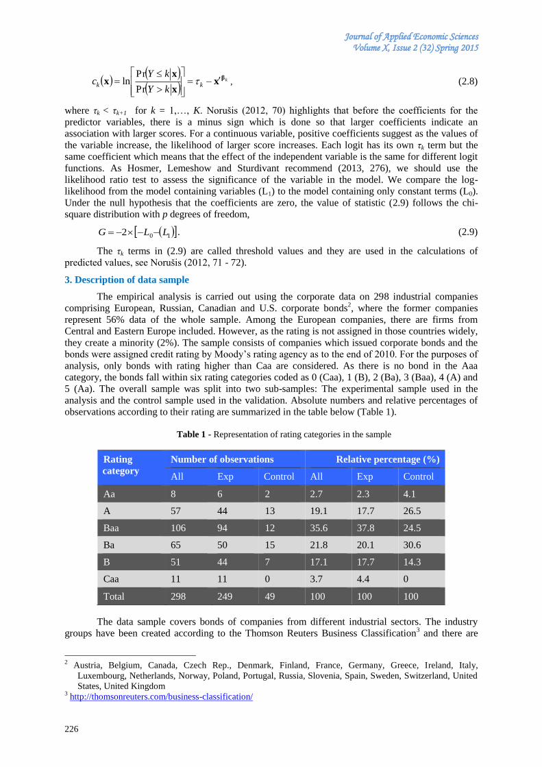
Journal of Applied Economic Sciences Volume X, Issue 2 (32) Spring 2015
226
k
kkkY
kYc
βx
x
xx
Pr
Prln , (2.8)
where τk < τk+1 for k = 1,…, K. Norušis (2012, 0) highlights that before the coefficients for the
predictor variables, there is a minus sign which is done so that larger coefficients indicate an
association with larger scores. For a continuous variable, positive coefficients suggest as the values of
the variable increase, the likelihood of larger score increases. Each logit has its own τk term but the
same coefficient which means that the effect of the independent variable is the same for different logit
functions. As Hosmer, Lemeshow and Sturdivant recommend (2013, 276), we should use the
likelihood ratio test to assess the significance of the variable in the model. We compare the log-
likelihood from the model containing variables (L1) to the model containing only constant terms (L0).
Under the null hypothesis that the coefficients are zero, the value of statistic (2.9) follows the chi-
square distribution with p degrees of freedom,
102 LLG . (2.9)
The τk terms in (2.9) are called threshold values and they are used in the calculations of
predicted values, see Norušis (2012, 1 - 72).
3. Description of data sample
The empirical analysis is carried out using the corporate data on 298 industrial companies
comprising European, Russian, Canadian and U.S. corporate bonds2, where the former companies
represent 56% data of the whole sample. Among the European companies, there are firms from
Central and Eastern Europe included. However, as the rating is not assigned in those countries widely,
they create a minority (2%). The sample consists of companies which issued corporate bonds and the
bonds were assigned credit rating by Moody’s rating agency as to the end of 2010. For the purposes of
analysis, only bonds with rating higher than Caa are considered. As there is no bond in the Aaa
category, the bonds fall within six rating categories coded as 0 (Caa), 1 (B), 2 (Ba), 3 (Baa), 4 (A) and
5 (Aa). The overall sample was split into two sub-samples: The experimental sample used in the
analysis and the control sample used in the validation. Absolute numbers and relative percentages of
observations according to their rating are summarized in the table below (Table 1).
Table 1 - Representation of rating categories in the sample
Rating
category
Number of observations Relative percentage (%)
All Exp Control All Exp Control
Aa 8 6 2 2.7 2.3 4.1
A 57 44 13 19.1 17.7 26.5
Baa 106 94 12 35.6 37.8 24.5
Ba 65 50 15 21.8 20.1 30.6
B 51 44 7 17.1 17.7 14.3
Caa 11 11 0 3.7 4.4 0
Total 298 249 49 100 100 100
The data sample covers bonds of companies from different industrial sectors. The industry
groups have been created according to the Thomson Reuters Business Classification3 and there are
2 Austria, Belgium, Canada, Czech Rep., Denmark, Finland, France, Germany, Greece, Ireland, Italy,
Luxembourg, Netherlands, Norway, Poland, Portugal, Russia, Slovenia, Spain, Sweden, Switzerland, United
States, United Kingdom 3 http://thomsonreuters.com/business-classification/
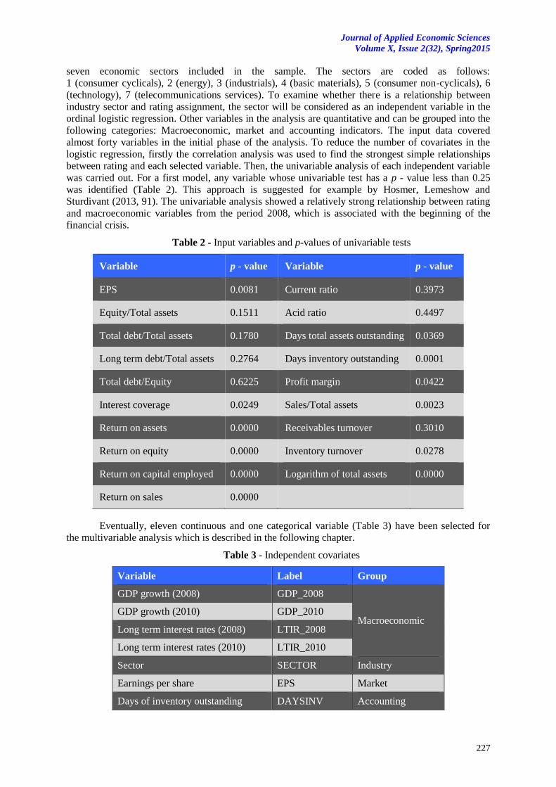
Journal of Applied Economic Sciences
Volume X, Issue 2(32), Spring2015
227
seven economic sectors included in the sample. The sectors are coded as follows:
1 (consumer cyclicals), 2 (energy), 3 (industrials), 4 (basic materials), 5 (consumer non-cyclicals), 6
(technology), 7 (telecommunications services). To examine whether there is a relationship between
industry sector and rating assignment, the sector will be considered as an independent variable in the
ordinal logistic regression. Other variables in the analysis are quantitative and can be grouped into the
following categories: Macroeconomic, market and accounting indicators. The input data covered
almost forty variables in the initial phase of the analysis. To reduce the number of covariates in the
logistic regression, firstly the correlation analysis was used to find the strongest simple relationships
between rating and each selected variable. Then, the univariable analysis of each independent variable
was carried out. For a first model, any variable whose univariable test has a p - value less than 0.25
was identified (Table 2). This approach is suggested for example by Hosmer, Lemeshow and
Sturdivant (2013, 91). The univariable analysis showed a relatively strong relationship between rating
and macroeconomic variables from the period 2008, which is associated with the beginning of the
financial crisis.
Table 2 - Input variables and p-values of univariable tests
Variable p - value Variable p - value
EPS 0.0081 Current ratio 0.3973
Equity/Total assets 0.1511 Acid ratio 0.4497
Total debt/Total assets 0.1780 Days total assets outstanding 0.0369
Long term debt/Total assets 0.2764 Days inventory outstanding 0.0001
Total debt/Equity 0.6225 Profit margin 0.0422
Interest coverage 0.0249 Sales/Total assets 0.0023
Return on assets 0.0000 Receivables turnover 0.3010
Return on equity 0.0000 Inventory turnover 0.0278
Return on capital employed 0.0000 Logarithm of total assets 0.0000
Return on sales 0.0000
Eventually, eleven continuous and one categorical variable (Table 3) have been selected for
the multivariable analysis which is described in the following chapter.
Table 3 - Independent covariates
Variable Label Group
GDP growth (2008) GDP_2008
Macroeconomic GDP growth (2010) GDP_2010
Long term interest rates (2008) LTIR_2008
Long term interest rates (2010) LTIR_2010
Sector SECTOR Industry
Earnings per share EPS Market
Days of inventory outstanding DAYSINV Accounting
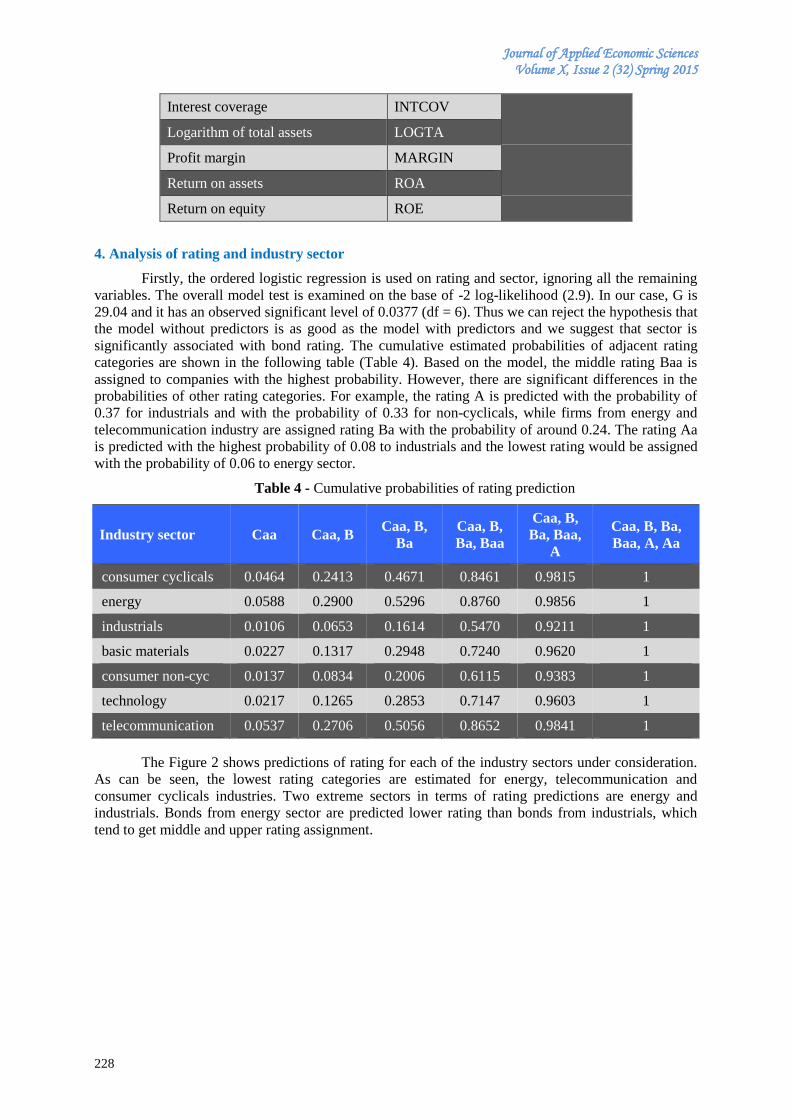
Journal of Applied Economic Sciences Volume X, Issue 2 (32) Spring 2015
228
Interest coverage INTCOV
Logarithm of total assets LOGTA
Profit margin MARGIN
Return on assets ROA
Return on equity ROE
4. Analysis of rating and industry sector
Firstly, the ordered logistic regression is used on rating and sector, ignoring all the remaining
variables. The overall model test is examined on the base of -2 log-likelihood (2.9). In our case, G is
29.04 and it has an observed significant level of 0.0377 (df = 6). Thus we can reject the hypothesis that
the model without predictors is as good as the model with predictors and we suggest that sector is
significantly associated with bond rating. The cumulative estimated probabilities of adjacent rating
categories are shown in the following table (Table 4). Based on the model, the middle rating Baa is
assigned to companies with the highest probability. However, there are significant differences in the
probabilities of other rating categories. For example, the rating A is predicted with the probability of
0.37 for industrials and with the probability of 0.33 for non-cyclicals, while firms from energy and
telecommunication industry are assigned rating Ba with the probability of around 0.24. The rating Aa
is predicted with the highest probability of 0.08 to industrials and the lowest rating would be assigned
with the probability of 0.06 to energy sector.
Table 4 - Cumulative probabilities of rating prediction
Industry sector Caa Caa, B Caa, B,
Ba
Caa, B,
Ba, Baa
Caa, B,
Ba, Baa,
A
Caa, B, Ba,
Baa, A, Aa
consumer cyclicals 0.0464 0.2413 0.4671 0.8461 0.9815 1
energy 0.0588 0.2900 0.5296 0.8760 0.9856 1
industrials 0.0106 0.0653 0.1614 0.5470 0.9211 1
basic materials 0.0227 0.1317 0.2948 0.7240 0.9620 1
consumer non-cyc 0.0137 0.0834 0.2006 0.6115 0.9383 1
technology 0.0217 0.1265 0.2853 0.7147 0.9603 1
telecommunication 0.0537 0.2706 0.5056 0.8652 0.9841 1
The Figure 2 shows predictions of rating for each of the industry sectors under consideration.
As can be seen, the lowest rating categories are estimated for energy, telecommunication and
consumer cyclicals industries. Two extreme sectors in terms of rating predictions are energy and
industrials. Bonds from energy sector are predicted lower rating than bonds from industrials, which
tend to get middle and upper rating assignment.
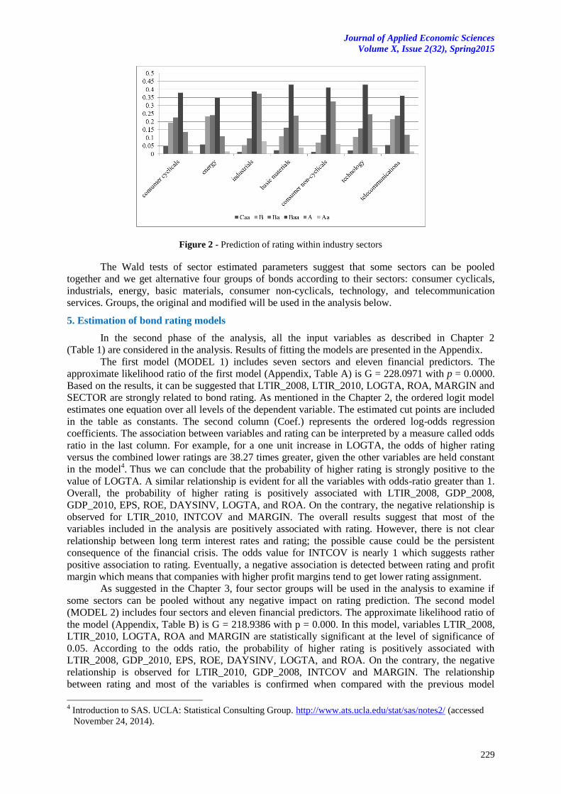
Journal of Applied Economic Sciences
Volume X, Issue 2(32), Spring2015
229
Figure 2 - Prediction of rating within industry sectors
The Wald tests of sector estimated parameters suggest that some sectors can be pooled
together and we get alternative four groups of bonds according to their sectors: consumer cyclicals,
industrials, energy, basic materials, consumer non-cyclicals, technology, and telecommunication
services. Groups, the original and modified will be used in the analysis below.
5. Estimation of bond rating models
In the second phase of the analysis, all the input variables as described in Chapter 2
(Table 1) are considered in the analysis. Results of fitting the models are presented in the Appendix.
The first model (MODEL 1) includes seven sectors and eleven financial predictors. The
approximate likelihood ratio of the first model (Appendix, Table A) is G = 228.0971 with p = 0.0000.
Based on the results, it can be suggested that LTIR_2008, LTIR_2010, LOGTA, ROA, MARGIN and
SECTOR are strongly related to bond rating. As mentioned in the Chapter 2, the ordered logit model
estimates one equation over all levels of the dependent variable. The estimated cut points are included
in the table as constants. The second column (Coef.) represents the ordered log-odds regression
coefficients. The association between variables and rating can be interpreted by a measure called odds
ratio in the last column. For example, for a one unit increase in LOGTA, the odds of higher rating
versus the combined lower ratings are 38.27 times greater, given the other variables are held constant
in the model4. Thus we can conclude that the probability of higher rating is strongly positive to the
value of LOGTA. A similar relationship is evident for all the variables with odds-ratio greater than 1.
Overall, the probability of higher rating is positively associated with LTIR_2008, GDP_2008,
GDP_2010, EPS, ROE, DAYSINV, LOGTA, and ROA. On the contrary, the negative relationship is
observed for LTIR_2010, INTCOV and MARGIN. The overall results suggest that most of the
variables included in the analysis are positively associated with rating. However, there is not clear
relationship between long term interest rates and rating; the possible cause could be the persistent
consequence of the financial crisis. The odds value for INTCOV is nearly 1 which suggests rather
positive association to rating. Eventually, a negative association is detected between rating and profit
margin which means that companies with higher profit margins tend to get lower rating assignment.
As suggested in the Chapter 3, four sector groups will be used in the analysis to examine if
some sectors can be pooled without any negative impact on rating prediction. The second model
(MODEL 2) includes four sectors and eleven financial predictors. The approximate likelihood ratio of
the model (Appendix, Table B) is G = 218.9386 with p = 0.000. In this model, variables LTIR_2008,
LTIR_2010, LOGTA, ROA and MARGIN are statistically significant at the level of significance of
0.05. According to the odds ratio, the probability of higher rating is positively associated with
LTIR_2008, GDP_2010, EPS, ROE, DAYSINV, LOGTA, and ROA. On the contrary, the negative
relationship is observed for LTIR_2010, GDP_2008, INTCOV and MARGIN. The relationship
between rating and most of the variables is confirmed when compared with the previous model
4 Introduction to SAS. UCLA: Statistical Consulting Group. http://www.ats.ucla.edu/stat/sas/notes2/ (accessed
November 24, 2014).
Journal of Applied Economic Sciences Volume X, Issue 2 (32) Spring 2015
230
however the effect of macroeconomic variables is ambiguous. Based on p-values, this model suggests
that there is positive relationship between rating and GDP_2008 while a negative association of rating
and GDP_2010.
Finally, the model (MODEL 3) ignoring industry sectors was estimated (Appendix, Table C).
The likelihood ratio of this model is G = 217.0149 with p = 0.0000. Variables LTIR_2008,
LTIR_2010, LOGTA, ROA and MARGIN are statistically significant at .05 level of significance,
GDP_2010 and DAYSINV are significant at a higher level of .10. The direction of the association
between rating and each variable is the same as in the previous model, namely the negative
relationship between profit margin and rating is confirmed.
The estimated models were used for bond rating prediction to assess their prediction ability.
The first model (MODEL 1) correctly classified 59.3 % of cases of the analytical sample in total;
however there are differences among individual rating categories. The model predicts more bonds as
Ba and B when compared to the observed data. When the model was used on the control sample
comprising 38 bonds not included in the analysis, it correctly classified 63.2% of cases. Next, the
model with four sectors (MODEL 2) was used to classify bonds into rating categories. The model
correctly classified 60.3% cases of the analytical sample, and 63.2% of the control sample. The
classification ability of both models is comparable. The final model without sectors (MODEL 3),
correctly classified 58.8% cases in the analytical sample and 66.7% cases in the control sample. To
summarize, the classification ability of models is similar, there are only small differences. As the
greatest hit ratio was achieved with the last model ignoring the industry sector, this model can be
assumed as the most suitable prediction model. This model contains eleven quantitative variables
including four macroeconomic indicators.
Conclusion
The paper was devoted to the empirical analysis of the effect of selected qualitative and
quantitative variables on credit bond rating. The most significant variables were identified and used
for the model estimations based on the empirical data of corporate bonds as to the end of 2010. The
models were derived by the ordinal logistic regression and three proportional-odds models were
estimated. Special attention was paid to the relationship between rating assessment and industry
sector. It was proved that the industry sector is significantly associated with bond rating. The results of
the analysis suggest that companies from the sectors of industrials and non-cyclicals have the higher
probability of better rating assessment when compared to other sectors.
Next, all the input variables, both quantitative and qualitative, were used in the multivariable
analysis. Three models were estimated according to the input variables. The overall results show that
there are three financial indicators with the significant effect on bond rating: the size of the company
measured by logarithm of total assets, return on assets and profit margin. The probability of better
rating assessment is strongly positive to the value of company assets, the same holds for the return on
equity. On the contrary, the negative relationship was observed for the profit margin. The findings of
the analysis suggest that companies with higher profit margins are considered as more risky, their
performance can deteriorate during bad times and they are assigned lower rating grades. Based on the
analysis, macroeconomic indicators were not identified as suitable predictors of rating, although there
is a significant relationship between rating and long-term interest rates. The predictive ability of all
three models is similar; however the model with the quantitative variables only has the highest hit
ratio. The results of the analysis should be taken into account when the primary interest is to assess
unrated companies or to evaluate the impact of financial performance on current rating. Thus, the
practical use of models lies in the area of management decision process and managing credit risk.
Acknowledgement
This paper was supported within Operational Programme Education for Competitiveness –
Project No. CZ.1.07/2.3.00/20.0296 and SGS Project 2015/75.
References
[1] Altman, Edward I. 1968. Financial ratios, discriminant analysis and the prediction of corporate
bankruptcy. Journal of Finance, 23(4): 589-609. http://dx.doi.org/10.1111/j.1540-6261.1968.
tb00843.x
Journal of Applied Economic Sciences
Volume X, Issue 2(32), Spring2015
231
[2] Altman, Edward I., and Steven Katz. 1976. Statistical bond rating classification using financial
and accounting data. M. Schiff and G. Sorter, eds.: Topical Research in Accounting.
[3] Ang, James S., and Kiritkumar Patel, A. 1975. Bond rating methods: Comparison and validation.
Journal of Finance, 30(2): 631-640. http://dx.doi.org/10.1111/j.1540-6261.1975. tb01836.x
[4] Belkaoui, Ahmed. 1980. Industrial bond ratings: A discriminant analysis approach. Working
paper. University of Ottawa.
[5] Cantor, R., Packer, F. 1996. Determinants and Impacts of Sovereign Credit Ratings. Economic
Policy Review 2: 37–53. http://www.newyorkfed.org/research/epr/96v02n2/ 9610cant.pdf
[6] De Laurentis, Giacomo, Renato Maino, and Luca Moletni. 2010. Developing, validating and using
internal ratings. Methodologies and case studies. First Edition. John Wiley & Sons, Ltd.
[7] Czarnitzki, Dirk, and Kornelius Kraft. 2004. Innovation indicators and corporate credit ratings:
evidence from German firms. Economics Letters, 82: 377-384. http://dx.doi.org/10.1016/
j.econlet.2003.09.016
[8] Gray, Stephen, Alexsander Mirkovic, Vanitha Ragunathan. 2006. The determinants of credit
ratings: Australian evidence, Australian Journal of Management 31(2): 333-354. http://dx.doi.
org/10.1177/031289620603100208
[9] Hilscher, Jens, and Wilson Mungo. 2012. Credit ratings and credit risk. Is one measure enough?
Working paper. Brandeis University and Oxford University. http://people.brandeis.edu/~hilscher/
CreditRatings_HilscherWilson_Jan2012.pdf
[10] Hosmer, David W., Stanley Lemeshow, and Rodney X. Sturdivant. 2013. Applied logistic
regression. Third Edition. John Wiley & Sons, Inc.
[11] Chan, Konan, and Narasimhan Jegadeesh. 2004. Market-Based Evaluation for Models to Predict
Bond Ratings. Review of Pacific Basin Financial Markets and Policies, 7(2): 153-172.
http://dx.doi.org/10.1142/S0219091504000081
[12] Joseph, Ciby. 2013. Advanced credit risk. Analysis and management. 1st Edition. John Wiley &
Sons, Ltd.
[13] Kaplan, Robert S., and Gabriel Urwitz. 1979. Statistical models of bond ratings: A
methodological inquiry. Journal of Business 52(2): 231-261. http://dx.doi.org/10.1086/296045
[14] Norušis, Marija J. 2012. IBM SPSS Statistics 19 Advanced Statistical Procedures Companion.
Prentice Hall, Inc.
[15] Pasiouras, Fotios, Gaganis Chrysovalantis, Michael Doumpos. @007. A multicriteria
discrimination approach for the credit rating of Asian banks. Annals of Finance, 3: 351-367.
http://dx.doi.org/10.1007/s10436-006-0052-0
[16] Pinches, George E., Kent A. Mingo. 1973. A multivariate analysis of industrial bond ratings.
Journal of Finance, 28(1): 1-18. http://dx.doi.org/10.1111/j.1540-6261.1973. tb01341.x
[17] Rerolle, J., Rimaud, C. 2009. Does independent credit research add value? Alternative
Intelligence Quotient, 32: 31-37. http://www.spreadresearch.com/uploads/pdf/user/unsecure/
AIQarticle.pdf
[18] Wingler, T.R., Watts, J.M. 1980. An analysis of bond rating changes in the electric utility
industry. The Financial Review, 15(4): 1-89. http://dx.doi.org/10.1111/j.1540-6288. 1980.
tb01601.x
*** Standard Poor’s. Guide to Credit Rating Essentials. What are credit ratings and how do they
work? http://img.en25.com/Web/StandardandPoors/SPCreditRatingsGuide.pdf
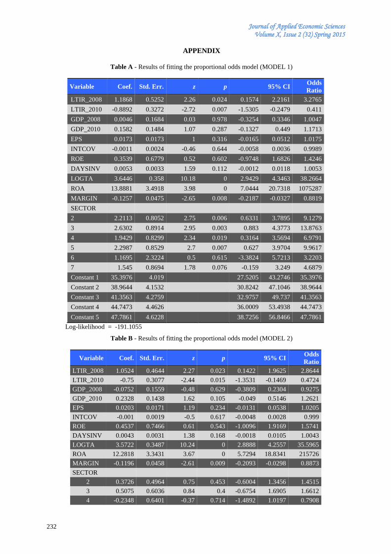
Journal of Applied Economic Sciences Volume X, Issue 2 (32) Spring 2015
232
APPENDIX
Table A - Results of fitting the proportional odds model (MODEL 1)
Variable Coef. Std. Err. z p 95% CI Odds
Ratio
LTIR_2008 1.1868 0.5252 2.26 0.024 0.1574 2.2161 3.2765
LTIR_2010 -0.8892 0.3272 -2.72 0.007 -1.5305 -0.2479 0.411
GDP_2008 0.0046 0.1684 0.03 0.978 -0.3254 0.3346 1.0047
GDP_2010 0.1582 0.1484 1.07 0.287 -0.1327 0.449 1.1713
EPS 0.0173 0.0173 1 0.316 -0.0165 0.0512 1.0175
INTCOV -0.0011 0.0024 -0.46 0.644 -0.0058 0.0036 0.9989
ROE 0.3539 0.6779 0.52 0.602 -0.9748 1.6826 1.4246
DAYSINV 0.0053 0.0033 1.59 0.112 -0.0012 0.0118 1.0053
LOGTA 3.6446 0.358 10.18 0 2.9429 4.3463 38.2664
ROA 13.8881 3.4918 3.98 0 7.0444 20.7318 1075287
MARGIN -0.1257 0.0475 -2.65 0.008 -0.2187 -0.0327 0.8819
SECTOR
2 2.2113 0.8052 2.75 0.006 0.6331 3.7895 9.1279
3 2.6302 0.8914 2.95 0.003 0.883 4.3773 13.8763
4 1.9429 0.8299 2.34 0.019 0.3164 3.5694 6.9791
5 2.2987 0.8529 2.7 0.007 0.627 3.9704 9.9617
6 1.1695 2.3224 0.5 0.615 -3.3824 5.7213 3.2203
7 1.545 0.8694 1.78 0.076 -0.159 3.249 4.6879
Constant 1 35.3976 4.019
27.5205 43.2746 35.3976
Constant 2 38.9644 4.1532
30.8242 47.1046 38.9644
Constant 3 41.3563 4.2759
32.9757 49.737 41.3563
Constant 4 44.7473 4.4626
36.0009 53.4938 44.7473
Constant 5 47.7861 4.6228 38.7256 56.8466 47.7861
Log-likelihood = -191.1055
Table B - Results of fitting the proportional odds model (MODEL 2)
Variable Coef. Std. Err. z p 95% CI Odds
Ratio
LTIR_2008 1.0524 0.4644 2.27 0.023 0.1422 1.9625 2.8644
LTIR_2010 -0.75 0.3077 -2.44 0.015 -1.3531 -0.1469 0.4724
GDP_2008 -0.0752 0.1559 -0.48 0.629 -0.3809 0.2304 0.9275
GDP_2010 0.2328 0.1438 1.62 0.105 -0.049 0.5146 1.2621
EPS 0.0203 0.0171 1.19 0.234 -0.0131 0.0538 1.0205
INTCOV -0.001 0.0019 -0.5 0.617 -0.0048 0.0028 0.999
ROE 0.4537 0.7466 0.61 0.543 -1.0096 1.9169 1.5741
DAYSINV 0.0043 0.0031 1.38 0.168 -0.0018 0.0105 1.0043
LOGTA 3.5722 0.3487 10.24 0 2.8888 4.2557 35.5965
ROA 12.2818 3.3431 3.67 0 5.7294 18.8341 215726
MARGIN -0.1196 0.0458 -2.61 0.009 -0.2093 -0.0298 0.8873
SECTOR
2 0.3726 0.4964 0.75 0.453 -0.6004 1.3456 1.4515
3 0.5075 0.6036 0.84 0.4 -0.6754 1.6905 1.6612
4 -0.2348 0.6401 -0.37 0.714 -1.4892 1.0197 0.7908
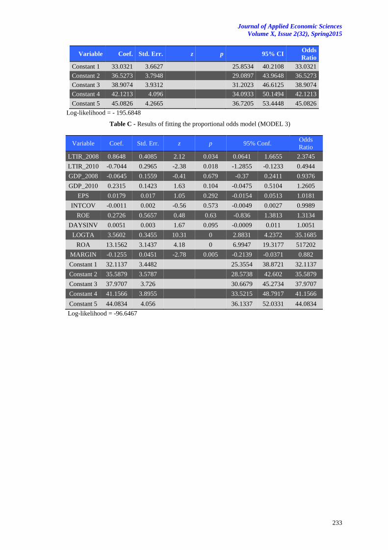
Journal of Applied Economic Sciences
Volume X, Issue 2(32), Spring2015
233
Variable Coef. Std. Err. z p 95% CI Odds
Ratio
Constant 1 33.0321 3.6627
25.8534 40.2108 33.0321
Constant 2 36.5273 3.7948
29.0897 43.9648 36.5273
Constant 3 38.9074 3.9312
31.2023 46.6125 38.9074
Constant 4 42.1213 4.096
34.0933 50.1494 42.1213
Constant 5 45.0826 4.2665 36.7205 53.4448 45.0826
Log-likelihood = - 195.6848
Table C - Results of fitting the proportional odds model (MODEL 3)
Variable Coef. Std. Err. z p 95% Conf. Odds
Ratio
LTIR_2008 0.8648 0.4085 2.12 0.034 0.0641 1.6655 2.3745
LTIR_2010 -0.7044 0.2965 -2.38 0.018 -1.2855 -0.1233 0.4944
GDP_2008 -0.0645 0.1559 -0.41 0.679 -0.37 0.2411 0.9376
GDP_2010 0.2315 0.1423 1.63 0.104 -0.0475 0.5104 1.2605
EPS 0.0179 0.017 1.05 0.292 -0.0154 0.0513 1.0181
INTCOV -0.0011 0.002 -0.56 0.573 -0.0049 0.0027 0.9989
ROE 0.2726 0.5657 0.48 0.63 -0.836 1.3813 1.3134
DAYSINV 0.0051 0.003 1.67 0.095 -0.0009 0.011 1.0051
LOGTA 3.5602 0.3455 10.31 0 2.8831 4.2372 35.1685
ROA 13.1562 3.1437 4.18 0 6.9947 19.3177 517202
MARGIN -0.1255 0.0451 -2.78 0.005 -0.2139 -0.0371 0.882
Constant 1 32.1137 3.4482
25.3554 38.8721 32.1137
Constant 2 35.5879 3.5787
28.5738 42.602 35.5879
Constant 3 37.9707 3.726
30.6679 45.2734 37.9707
Constant 4 41.1566 3.8955
33.5215 48.7917 41.1566
Constant 5 44.0834 4.056 36.1337 52.0331 44.0834
Log-likelihood = -96.6467
Journal of Applied Economic Sciences Volume X, Issue 2 (32) Spring 2015
234
ESTIMATION OF BANKING EFFICIENCY DETERMINANTS IN THE CZECH REPUBLIC
Iveta PALEČKOVÁ
Silesian University, School of Business Administration, Karviná
Abstract:
The aim of this paper is to estimate the banking efficiency determinants of the Czech commercial banks
during the period 2001-2013. For estimation of banking efficiency we applied the Data Envelopment Analysis
on data of the Czech commercial banks. We simultaneously use two alternative specifications of Data
Envelopment Analysis approach, specifically CCR model and BCC model that differ in returns to scale
assumption. The determinants of banking efficiency were estimated using the panel data analysis. The results of
the paper show that the level of capitalization, credit risk, liquidity risk and riskiness of portfolio had a positive
impact on banking efficiency. Gross domestic product per capita had a negative impact on banking efficiency.
We found that in BCC model, the liquidity risk and riskiness of portfolio had a positive impact on efficiency in
the Czech banking sector. Other determinants were not statistical significant in this model. Banks with a higher
ratio of loans to deposit, ratio of loans to assets, higher ratio of equity to total assets were more efficient than
other commercial banks in the Czech banking sector. The impact of the ownership structure was not statistical
significant during the analyzed period.
Keywords: bank specific factors, Czech banking sector, Data Envelopment Analysis, efficiency, market specific
factors.
JEL Classification: G21, C58
1. Introduction
The Czech financial system can be characterized as a bank-based system and banks play an
important role in the economy. The transformation and consolidation of the Czech banking sector was
carried out during the 1990s. From 1998–2001, a second round of privatization occurred with the sale
to foreigners of majority equity interests in four large Czech banks: Československá obchodní banka
(ČSOB), Česká spořitelna (ČS), Komerční banka (KB) and Investiční a poštovní banka (IPB). ČSOB,
ČS and KB are still the dominant players in the market.
The aim of the paper is to estimate the banking efficiency determinants of the Czech
commercial banks over the period 2001-2013. First, we estimated the efficiency of the Czech banking
sector. We employed the non-parametric approach, especially the Data Envelopment Analysis (DEA)
on the data of the Czech commercial banks. We simultaneously use two alternative specifications of
DEA approach, specifically CCR model and BCC model that differ in returns to scale assumption.
Next, we examined the determinants of the banking efficiency in the Czech banking industry.
The structure of the paper is following. Next chapter presents empirical literature. Third
section describes methodology, especially DEA approach. Next Section presents data and selection of
variables and fifth section shows empirical analysis and results. Last section concludes this paper.
2. Literature review
Empirical studies on the determinants of banking efficiency consider bank specific factors and
macroeconomics factors. Stavárek (2005) estimated determinants of banking efficiency in Visegrad
countries during the period 1999-2003. He found that bank-specific factors were significant and
macroeconomics factor were not significant besides GDP. Košak and Zajc (2006) estimated
determinants of efficiency in the new EU member countries. They found a negative relationship of the
intermediation ratio and density of demand. The deposit per capita and population were positively
associated with cost efficiency. ROA and ROE were positively related to efficiency.
As showed Akin et al. (2009) and Vu and Nahm (2013), bank-specific characteristics include
bank size, equity over total assets, return on assets or equity, loans-to-total assets, type of ownership,
bank configuration. Empirical literature review showed that there is no common consensus exists
about effects of banking efficiency determinants.
Bank size is generally measured by banks’ amount of assets. E.g. Grigorian and Manole
Journal of Applied Economic Sciences
Volume X, Issue 2(32), Spring2015
235
(2002), Mercan et al. (2003), Williams and Nguyen (2005), Rezitis (2007) or Vu and Nahm (2013)
found a positive relationship between bank size and banking efficiency. On the other hand, Isık and
Hassan (2002), Chen et al. (2005) or Akin et al. (2009) discovered a negative effect of bank size on
banking efficiency. Grigorian and Manole (2002), Altunbas et al. (2007), Chortareas et al. (2009) and
Vu and Nahm (2013) found a positive relationship between the level of capitalisation and banking
efficiency. In contrast, Pasiouras et al. (2007) and Cavallo and Rossi (2002) found that the level of
capitalisation had a negative impact on efficiency. Ariff and Can (2009) and Sanchez et al. (2013)
found that banks with higher ROE were more efficient.
As Vu and Nahm (2013) showed, some studies consider the influences of various types of
risk, such as liquidity risk, credit risk and management risk. Berger and Mester (1997) found that
banks with a higher ratio of loans to total assets (proxy for credit risk) were more profit efficient than
other banks in the US banking sector. Yildirim and Philippatos (2007) also found a positive
relationship between the ratio of loans to total asset and efficiency. In contrast, Brissimis et al. (2008)
and Havrylchyk (2006) found a negative relationship between the credit risk and efficiency. Brissimis
et al. (2008) found a negative relationship between the liquidity risk and bank efficiency. Ariff and
Can (2008) found that it had a positive impact on efficiency.
Gross domestic product (GDP) was used as a market specific factor in empirical studies.
Maudos et al. (2002), Hasan et al. (2009) and Vu and Nahm (2013) showed the positive relationship
between GDP and banking efficiency. Perera et al. (2007) considered other factors as well and found
that banking markets with high levels of market concentration, monetisation, interest rates and GDP
growth rate tend to achieve higher efficiency in South Asian. In contrast, Thoraneenitiyan and Avkiran
(2009) found that the overall level of economic development (GDP) had a negative effect on bank
efficiency in East Asian countries. Furthermore, Brissimis et al. (2008) examined a positive
relationship between profit efficiency and short-term interest rates. Also Vu and Nahm (2013) found
that a low-inflation rate provide a favourable environment for banks to improve their profitability.
3. The theoretical framework
The study of the efficient frontier began with Farrell (1957), who defined a simple measure of
a firm’s efficiency that could account for multiples inputs. The Data Envelopment Analysis is
a mathematical programming technique that measures the efficiency of a decision-making unit (DMU)
relative to other similar DMUs with the simple restriction that all DMUs lie on or below the efficiency
frontier (Seiford and Thrall, 1990). DEA calculates the relative efficiency of each DMU in relation to
all the other DMUs by using the actual observed values for the inputs and outputs of each DMU. It
also identifies, for inefficient DMUs, the sources and level of inefficiency for each of the inputs and
outputs (Charnes et al., 1995). The term DEA was first introduced by Charnes et al. (1978) based on
the research of Farrell (1957). CCR model is the basic DEA model as introduced by Charnes et al.
(1978). This model was modified by Banker et al. (1984) and became the BCC model which
accommodates variable returns to scale. The CCR model presupposes that there is no significant
relationship between the scale of operations and efficiency by assuming constant returns to scale
(CRS) and it delivers the overall technical efficiency. The constant returns to scale assumption is only
justifiable when all DMUs are operating at an optimal scale. However, firms or DMUs in practice
might face either economies or diseconomies to scale. Thus, if one makes the CRS assumption when
not all DMUs are operating at the optimal scale, the computed measures of technical efficiency will be
contaminated with scale efficiencies. Banker et al. (1984) extended the CCR model by relaxing the
CRS assumption. The resulting BCC model was used to assess the efficiency of DMUs characterized
by variable returns to scale (VRS).
This methodology allows handling different types of input and output together. A DEA model
can be constructed either to minimize inputs or to maximize outputs. An input orientation objects at
reducing the input amounts as much as possible while keeping at least the present output levels, while
an output orientation aims at maximizing output levels without increasing the use of inputs.
DEA begins with a fractional programming formulation. Assume that there are n DMUs to be
evaluated. Each consumes different amounts of i inputs and produces r different outputs, i.e. DMUj
consumes xji amounts of input to produce yji amounts of output. It is assumed that these inputs, xji, and
outputs, yji, are non-negative, and each DMU has at least one positive input and output value. The
productivity of DMU can be written as:
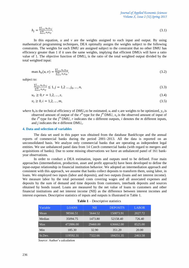
Journal of Applied Economic Sciences Volume X, Issue 2 (32) Spring 2015
236
∑
∑
. (3.1)
In this equation, u and v are the weights assigned to each input and output. By using
mathematical programming techniques, DEA optimally assigns the weights subject to the following
constraints. The weights for each DMU are assigned subject to the constraint that no other DMU has
efficiency greater than 1 if it uses the same weights, implying that efficient DMUs will have a ratio
value of 1. The objective function of DMUk is the ratio of the total weighted output divided by the
total weighted input:
( ) ∑
∑
, (3.2)
subject to:
∑
∑
(3.3)
(3.4)
(3.5)
where h0 is the technical efficiency of DMU0 to be estimated, ur and vi are weights to be optimized, yrj is
observed amount of output of the rth
type for the jth
DMU, xij is the observed amount of input of
the ith
type for the jth
DMU, r indicates the s different outputs, i denotes the m different inputs,
and j indicates the n different DMUs.
4. Data and selection of variables
The data set used in this paper was obtained from the database BankScope and the annual
reports of commercial banks during the period 2001–2013. All the data is reported on an
unconsolidated basis. We analyze only commercial banks that are operating as independent legal
entities. We use unbalanced panel data from 14 Czech commercial banks (with regard to mergers and
acquisitions of banks). Due to some missing observations we have an unbalanced panel of 161 bank-
year observations.
In order to conduct a DEA estimation, inputs and outputs need to be defined. Four main
approaches (intermediation, production, asset and profit approach) have been developed to define the
input-output relationship in financial institution behavior. We adopted an intermediation approach and
consistent with this approach, we assume that banks collect deposits to transform them, using labor, in
loans. We employed two inputs (labor and deposits), and two outputs (loans and net interest income).
We measure labor by the total personnel costs covering wages and all associated expenses and
deposits by the sum of demand and time deposits from customers, interbank deposits and sources
obtained by bonds issued. Loans are measured by the net value of loans to customers and other
financial institutions and net interest income (NII) as the difference between interest incomes and
interest expenses. Descriptive statistics of inputs and outputs is illustrated in Table 1.
Table 1 – Descriptive statistics
Variable LOANS NII DEPOSITS LABOR
Mean 98566.51 5644.52 150873.91 2027.72
Median 35094.75 1473.80 52158.40 726.40
Max 472886.00 29460.00 636662.00 8525.00
Min 185.30 32.90 351.20 20.00
St.Dev. 119592.31 7322.66 184251.35 2463.58
Source: Author’s calculation
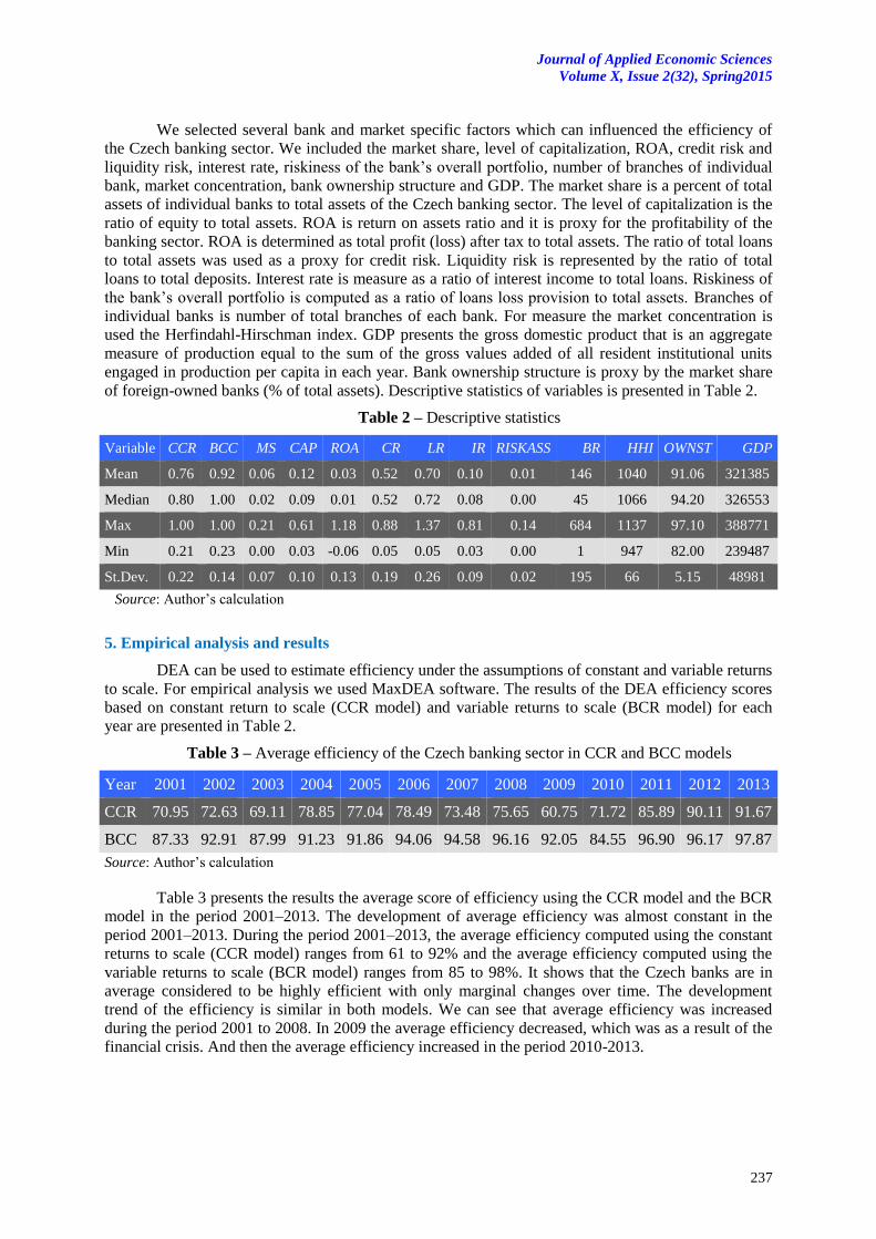
Journal of Applied Economic Sciences
Volume X, Issue 2(32), Spring2015
237
We selected several bank and market specific factors which can influenced the efficiency of
the Czech banking sector. We included the market share, level of capitalization, ROA, credit risk and
liquidity risk, interest rate, riskiness of the bank’s overall portfolio, number of branches of individual
bank, market concentration, bank ownership structure and GDP. The market share is a percent of total
assets of individual banks to total assets of the Czech banking sector. The level of capitalization is the
ratio of equity to total assets. ROA is return on assets ratio and it is proxy for the profitability of the
banking sector. ROA is determined as total profit (loss) after tax to total assets. The ratio of total loans
to total assets was used as a proxy for credit risk. Liquidity risk is represented by the ratio of total
loans to total deposits. Interest rate is measure as a ratio of interest income to total loans. Riskiness of
the bank’s overall portfolio is computed as a ratio of loans loss provision to total assets. Branches of
individual banks is number of total branches of each bank. For measure the market concentration is
used the Herfindahl-Hirschman index. GDP presents the gross domestic product that is an aggregate
measure of production equal to the sum of the gross values added of all resident institutional units
engaged in production per capita in each year. Bank ownership structure is proxy by the market share
of foreign-owned banks (% of total assets). Descriptive statistics of variables is presented in Table 2.
Table 2 – Descriptive statistics
Variable CCR BCC MS CAP ROA CR LR IR RISKASS BR HHI OWNST GDP
Mean 0.76 0.92 0.06 0.12 0.03 0.52 0.70 0.10 0.01 146 1040 91.06 321385
Median 0.80 1.00 0.02 0.09 0.01 0.52 0.72 0.08 0.00 45 1066 94.20 326553
Max 1.00 1.00 0.21 0.61 1.18 0.88 1.37 0.81 0.14 684 1137 97.10 388771
Min 0.21 0.23 0.00 0.03 -0.06 0.05 0.05 0.03 0.00 1 947 82.00 239487
St.Dev. 0.22 0.14 0.07 0.10 0.13 0.19 0.26 0.09 0.02 195 66 5.15 48981
Source: Author’s calculation
5. Empirical analysis and results
DEA can be used to estimate efficiency under the assumptions of constant and variable returns
to scale. For empirical analysis we used MaxDEA software. The results of the DEA efficiency scores
based on constant return to scale (CCR model) and variable returns to scale (BCR model) for each
year are presented in Table 2.
Table 3 – Average efficiency of the Czech banking sector in CCR and BCC models
Year 2001 2002 2003 2004 2005 2006 2007 2008 2009 2010 2011 2012 2013
CCR 70.95 72.63 69.11 78.85 77.04 78.49 73.48 75.65 60.75 71.72 85.89 90.11 91.67
BCC 87.33 92.91 87.99 91.23 91.86 94.06 94.58 96.16 92.05 84.55 96.90 96.17 97.87
Source: Author’s calculation
Table 3 presents the results the average score of efficiency using the CCR model and the BCR
model in the period 2001–2013. The development of average efficiency was almost constant in the
period 2001–2013. During the period 2001–2013, the average efficiency computed using the constant
returns to scale (CCR model) ranges from 61 to 92% and the average efficiency computed using the
variable returns to scale (BCR model) ranges from 85 to 98%. It shows that the Czech banks are in
average considered to be highly efficient with only marginal changes over time. The development
trend of the efficiency is similar in both models. We can see that average efficiency was increased
during the period 2001 to 2008. In 2009 the average efficiency decreased, which was as a result of the
financial crisis. And then the average efficiency increased in the period 2010-2013.
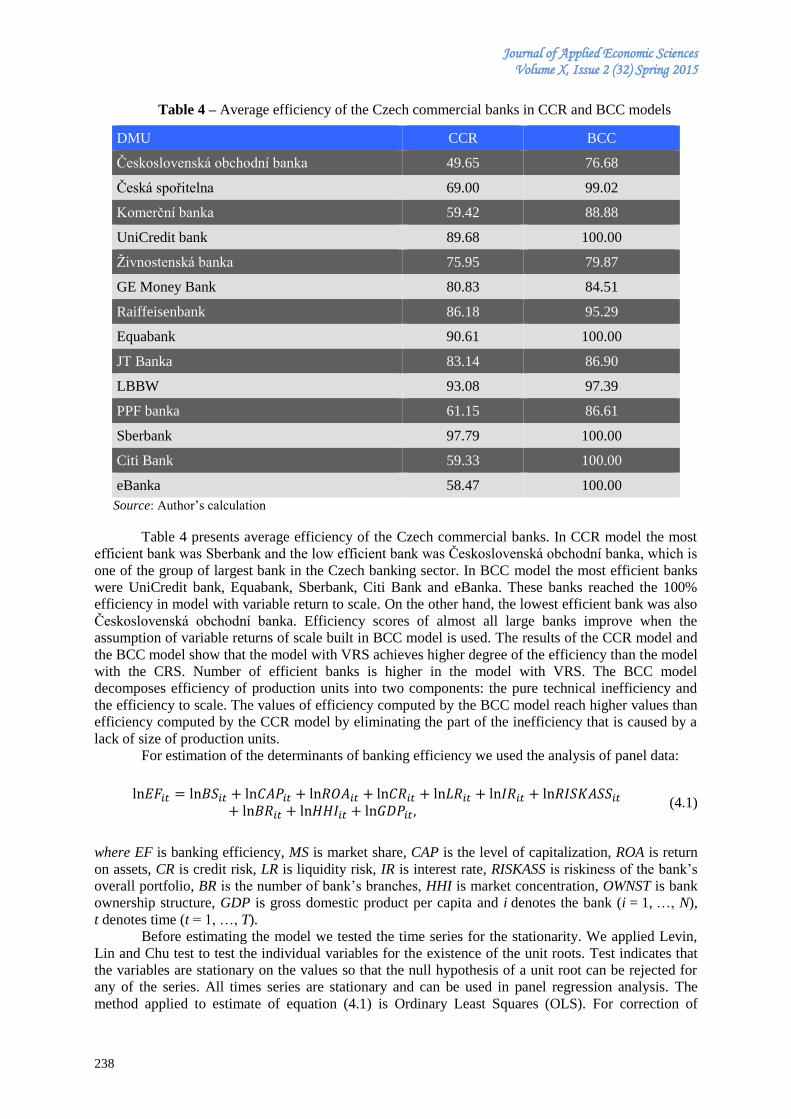
Journal of Applied Economic Sciences Volume X, Issue 2 (32) Spring 2015
238
Table 4 – Average efficiency of the Czech commercial banks in CCR and BCC models
DMU CCR BCC
Československá obchodní banka 49.65 76.68
Česká spořitelna 69.00 99.02
Komerční banka 59.42 88.88
UniCredit bank 89.68 100.00
Živnostenská banka 75.95 79.87
GE Money Bank 80.83 84.51
Raiffeisenbank 86.18 95.29
Equabank 90.61 100.00
JT Banka 83.14 86.90
LBBW 93.08 97.39
PPF banka 61.15 86.61
Sberbank 97.79 100.00
Citi Bank 59.33 100.00
eBanka 58.47 100.00
Source: Author’s calculation
Table 4 presents average efficiency of the Czech commercial banks. In CCR model the most
efficient bank was Sberbank and the low efficient bank was Československá obchodní banka, which is
one of the group of largest bank in the Czech banking sector. In BCC model the most efficient banks
were UniCredit bank, Equabank, Sberbank, Citi Bank and eBanka. These banks reached the 100%
efficiency in model with variable return to scale. On the other hand, the lowest efficient bank was also
Československá obchodní banka. Efficiency scores of almost all large banks improve when the
assumption of variable returns of scale built in BCC model is used. The results of the CCR model and
the BCC model show that the model with VRS achieves higher degree of the efficiency than the model
with the CRS. Number of efficient banks is higher in the model with VRS. The BCC model
decomposes efficiency of production units into two components: the pure technical inefficiency and
the efficiency to scale. The values of efficiency computed by the BCC model reach higher values than
efficiency computed by the CCR model by eliminating the part of the inefficiency that is caused by a
lack of size of production units.
For estimation of the determinants of banking efficiency we used the analysis of panel data:
(4.1)
where EF is banking efficiency, MS is market share, CAP is the level of capitalization, ROA is return
on assets, CR is credit risk, LR is liquidity risk, IR is interest rate, RISKASS is riskiness of the bank’s
overall portfolio, BR is the number of bank’s branches, HHI is market concentration, OWNST is bank
ownership structure, GDP is gross domestic product per capita and i denotes the bank (i = 1, …, N),
t denotes time (t = 1, …, T).
Before estimating the model we tested the time series for the stationarity. We applied Levin,
Lin and Chu test to test the individual variables for the existence of the unit roots. Test indicates that
the variables are stationary on the values so that the null hypothesis of a unit root can be rejected for
any of the series. All times series are stationary and can be used in panel regression analysis. The
method applied to estimate of equation (4.1) is Ordinary Least Squares (OLS). For correction of
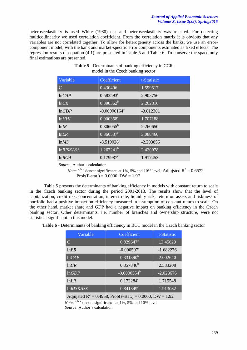
Journal of Applied Economic Sciences
Volume X, Issue 2(32), Spring2015
239
heteroscedasticity is used White (1980) test and heteroscedasticity was rejected. For detecting
multicollinearity we used correlation coefficient. From the correlation matrix it is obvious that any
variables are not correlated together. To allow for heterogeneity across the banks, we use an error-
component model, with the bank and market-specific error components estimated as fixed effects. The
regression results of equation (4.1) are presented in Table 5 and Table 6. To conserve the space only
final estimations are presented.
Table 5 - Determinants of banking efficiency in CCR
model in the Czech banking sector
Variable Coefficient t-Statistic
C 0.430406
1.599517
lnCAP 0.583593a
2.903756
lnCR 0.390362b
2.262816
lnGDP -0.00000164a
-3.812301
lnHHI 0.000358c
1.707188
lnIR 0.306055b
2.260650
lnLR 0.360537a
3.088460
lnMS -3.519028b
-2.293856
lnRISKASS 1.267241b
2.420078
lnROA 0.179987c
1.917453
Source: Author’s calculation
Note: a, b, c
denote significance at 1%, 5% and 10% level; Adjujsted R2 = 0.6572,
Prob(F-stat.) = 0.0000, DW = 1.97
Table 5 presents the determinants of banking efficiency in models with constant return to scale
in the Czech banking sector during the period 2001-2013. The results show that the level of
capitalization, credit risk, concentration, interest rate, liquidity risk, return on assets and riskiness of
portfolio had a positive impact on efficiency measured in assumption of constant return to scale. On
the other hand, market share and GDP had a negative impact on banking efficiency in the Czech
banking sector. Other determinants, i.e. number of branches and ownership structure, were not
statistical significant in this model.
Table 6 - Determinants of banking efficiency in BCC model in the Czech banking sector
Variable Coefficient t-Statistic
C 0.829647a
12.45629
lnBR -0.000597c
-1.682276
lnCAP 0.331390b
2.002640
lnCR 0.357846b
2.533208
lnGDP -0.0000554b
-2.028676
lnLR 0.172284c
1.715548
lnRISKASS 0.841349c
1.913032
Adjujsted R2 = 0.4958, Prob(F-stat.) = 0.0000, DW = 1.92
Note: a, b, c
denote significance at 1%, 5% and 10% level
Source: Author’s calculation
Journal of Applied Economic Sciences Volume X, Issue 2 (32) Spring 2015
240
Table 6 presents the results of determinants of banking efficiency in models with variable
return to scale in the Czech banking sector during the period 2001-2013. We found that only number
of branches, level of capitalization, credit risk, liquidity risk, riskiness of overall portfolio and GDP
were statistical significant in BCC model. Other estimated determinants included in this model were
not statistical significant. It can be seen that level of capitalization, credit risk, liquidity risk and
riskiness of overall portfolio had a positive impact on efficiency in the Czech banking sector. On the
other hand, GDP had and number of branches had negative impact on banking efficiency in the Czech
banking industry.
We can conclude that banks with a higher ratio of loans to deposit and a higher ratio of loans
to total assets were more efficient than other Czech commercial banks. We found a positive
relationship between the level of capitalization of the Czech commercial banks and banking efficiency.
Next result is that the gross domestic product per capita had a negative impact on banking efficiency
in the Czech banking industry. This result confirm the conclusion of Grigorian and Manole (2002),
Altunbas et al. (2007), Chortareas, Girardone, and Ventouri (2009) and Vu and Nahm (2013) in
banking sectors.
Conclusion
The aim of the paper was to examine the determinants of banking efficiency in the Czech
banking sector over the period 2001-2013. First, we employed the Data Envelopment Analysis to
estimate the efficiency of the Czech commercial banks during the period 2001-2013. We found that
the most efficient bank was Sberbank and the lowest efficient bank was Československá obchodní
banka. Next, we estimated determinants of banking efficiency using panel data analysis. We found
that in both model the level of capitalization, credit risk, liquidity risk and riskiness of portfolio had a
positive impact on banking efficiency and GDP a negative influence on efficiency of the Czech
banking industry. Concentration, interest rate and return on assets had a positive impact on banking
efficiency in model with constant return to scale. The results show a negative relationship between
market share and efficiency in CCR model. On the other hands, number of branches had a negative
impact in BCC model. Large banks were lower efficient than other banks in the banking sector. It is
confirmed the results of regression analysis that market share had a negative impact on banking
efficiency. Banks with a higher ratio of loans to deposit, ratio of loans to assets, higher ratio of equity
to total assets were more efficient than other commercial banks in the Czech banking sector. In CCR
model and in BCC model, the impact of the ownership structure was not statistical significant during
the analyzed period.
Acknowledgements
Research behind this paper was supported by the Internal Grant System of the Silesian University under the project IGS/10/2014 “Determinants of inefficiency of the Czech commercial banks”.
References
[1] Akin, A., Kiliç, M., Zađm, S. 2009. Determinants of Bank Efficiency in Turkey: A Two Stage
Data Envelopment Analysis, International Symposium on Suistainable Development. Sarajevo,
Bosnia and Herzegovina, 32-41.
[2] Altunbas, Y., Carbo, S., Gardener, E.P.M., Molynuex, P. 2007. Examining the Relationship
Between Capital, Risk and Efficiency in European Banking, European Financial Management,
13(1): 49–70. doi: 10.1111/j.1468-036X.2006.00285.x
[3] Ariff, M., Can, L. 2008. Cost and Profit Efficiency of Chinese Banks: A Non-Parametric Analysis,
China Economic Review 19(2): 260–273. http://dx.doi.org/10.1016/j.chieco.2007.04.001
[4] Ariff, M., Can, L. 2009. IMF Bank-Restructuring Efficiency Outcomes: Evidence from East Asia,
Journal of Financial Services Research 35(2): 167–187. doi: 10.1007/s10693-008-0047-2
[5] Banker, R.D., Chanes, A., Cooper, W. 1984. Some Model for Estimating Technical and Scale
Inefficiencies in Data Envelopment Analysis, Management Science, 30: 1078-1092.
http://dx.doi.org/10.1287/mnsc.30.9.1078

Journal of Applied Economic Sciences
Volume X, Issue 2(32), Spring2015
241
[6] Berger, A.N., Mester, L.J. 1997. Inside the Black Box: What Explains Differences in the
Efficiencies of Financial Institutions?, Journal of Banking and Finance 21(7): 895–947.
[7] Brissimis, S.N., Delis, M. D., Papanikolaou, N. I. 2008. Exploring the Nexus Between Banking
Sector Reform and Performance: Evidence from Newly Acceded EU Countries, Journal of
Banking and Finance 32(12): 2674–2683. doi: 10.1016/j.jbankfin.2008.07.002
[8] Cavallo, L., Rossi, S.P.S. 2002. Do Environmental Variables Affect the Performance and
Technical Efficiency of European Banking Systems? A Parametric Analysis Using the Stochastic
Frontier Approach, European Journal of Finance 8: 123–146. doi: 10.1080/13518470110076277
[9] Charnes A., Cooper, W.W., Lewin, A.Y., Seiford L.M. 1995. Data Envelopment Analysis: Theory,
Methodology and Applications, New York: Springer-Verlag.
[10] Charnes, A., Cooper, W.W., Rhodes, E. 1978. Measuring the Efficiency of Decision Making
Units, European Journal of Operational Research 2: 429–444. doi:10.1016/0377-2217(78)90138-
8
[11] Chen, X., Michael S. Brown, K. 2005. Banking efficiency in China: Application of DEA to pre-
and postderegulation eras: 1993-2000, China Economic Review, 16: 229-245. doi:
10.1016/j.chieco.2005.02.001
[12] Chortareas, G. E., Girardone, C., Ventouri, A. 2009. Efficiency and Productivity of Greek Banks
in the EMU Era, Applied Financial Economics 19: 1317–1328. doi: 10.1080/09603100802599506
[13] Farrell, M.J. 1957. The Measurement of Productive Efficiency,. Journal of the Royal Statistical
Society (Series A) 120(2): 253–281.
[14] Grigorian, D.A., Manole, V. 2002. Determinants of Commercial Bank Performance in Transition:
An Application of Data Envelopment Analysis, Policy Research Working Paper, No. 2850,
Washington DC: World Bank.
[15] Hasan, I., Wachtel, P., Zhou, M. 2009. Institutional Development, Financial Deepening and
Economic Growth: Evidence from China, Journal of Banking and Finance, 33(1): 157–170. doi:
10.2478/revecp-2013-0009
[16] Havrylchyk, O. 2006. Efficiency of the Polish Banking Industry: Foreign Versus Domestic
Banks, Journal of Banking and Finance 30(7): 1975–1996. doi: 10.1016/j.jbankfin.2005.07.009
[17] Isık, I., Hassan M.K. 2002. Technical, Scale and Allocative Efficiencies of Turkish Banking
Industry, Journal of Banking and Finance 26: 719-766. doi: 10.1016/S0378-4266(01)00167-4
[18] Košak, M., Zajc, P. 2006. Determinants of bank efficiency differences in the new EU member
countries, Financial Stability Report, Expert Papers, Ljubljana: Bank of Slovenia.
[19] Maudos, J., Pastor, J.M., Perez, F., Quesada, J. 2002. Cost and Profit Efficiency in European
Banks, Journal of International Financial Markets, Institutions and Money, 12(1): 33–58. doi:
10.1016/S1042-4431(01)00051-8
[20] Mercan, M., Arnold R., Reha Y., Ahmet, B.E. 2003. The Effect of Scale and Mode of Ownership
on the Financial Performance of the Turkish Banking Sector: Results of a DEA-Based Analysis,
Socio-Economic Planning Sciences, 37: 185-202. doi: 10.1016/S0038-0121(02)00045-9
[21] Pasiouras, F., Tanna, S., Zopounidis, C. 2007. Regulations, Supervision and Banks’ Cost and
Profit Efficiency Around the World: A Stochastic Frontier Approach. SSRN eLibrary, avaible at
http://ssrn.com/paper=970373
[22] Perera, S., Skully, M., Wickramanayake, J. 2007. Cost Efficiency in South Asian Banking: The
Impact of Bank Size, State Ownership and Stock Exchange Listings, International Review of
Finance 7(1/2): 35–60. doi: 10.1111/j.1468-2443.2007.00067.x
[23] Rezitis, N.A. 2007. Efficiency and Productivity Effects of Bank Mergers: Evidence from the
Greek Banking Industry, Economic Modelling, 25: 236-254. doi: 10.1016/j.econmod.2007.04.013
Journal of Applied Economic Sciences Volume X, Issue 2 (32) Spring 2015
242
[24] Sanchez, B., Hassan, M.K., Barkus, J. R. 2013. Efficiency Determinants and Dynamic Efficiency
Changes in Latin American Banking Industries, JCC: The Business and Economic Research
Journal, 6(1): 27-52. http://dx.doi.org/10.7835/jcc-berj-2013-0080
[25] Seiford, L.M., Thrall, R.M. 1990. Recent developments in DEA: the mathematical programming
approach to frontier analysis, Journal of Econometrics, 46: 7–38. doi: 10.1016/0304-
4076(90)90045-U
[26] Stavárek, D. 2005. Restrukturalizace bankovních sektorů a efektivnost bank v zemích Visegrádské
skupiny, Karviná: Silesian University.
[27] Thoraneenitiyan, N., Avkiran, N.K. 2009. Measuring the Impact of Restructuring and Country-
Specific Factors on the Efficiency of Post-Crisis East Asian Banking Systems: Integrating DEA
with SFA, Socio-Economic Planning Sciences, 43(4): 240–252. doi:10.1016/j.seps.2008.12.002
[28] Vu, H., Nahm, D. 2013. The determinants of profit efficiency of banks in Vietnam, Journal of the
Asia Pacific Economy, 18: 615-631. doi: 10.1080/13547860.2013.803847
[29] White, H. 1980. A heteroskedastic-consistent covariance matrix estimator and a direct test of
heteroskedasticity, Econometrica, 48: 817-838. doi:10.2307/1912934
[30] Williams, J., Nguyen, N. 2005. Financial Liberalisation, Crisis, and Restructuring: A
Comparative Study of Bank Performance and Bank Governance in South East Asia, Journal of
Banking and Finance, 29(8–9): 2119–2154. doi: 10.1016/j.jbankfin.2005.03.011
[31] Yildirim, H. S., Philippatos, G. 2007. Efficiency of Banks: Recent Evidence from the Transition
Economies of Europe, 1993-2000, The European Journal of Finance, 13: 123–143. doi:
10.1080/13518470600763687
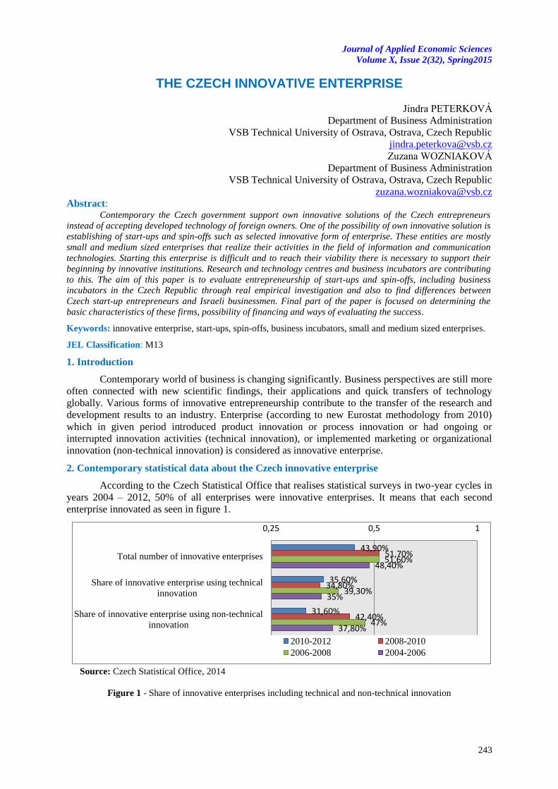
Journal of Applied Economic Sciences
Volume X, Issue 2(32), Spring2015
243
THE CZECH INNOVATIVE ENTERPRISE
Jindra PETERKOVÁ
Department of Business Administration
VSB Technical University of Ostrava, Ostrava, Czech Republic
Zuzana WOZNIAKOVÁ
Department of Business Administration
VSB Technical University of Ostrava, Ostrava, Czech Republic
Abstract: Contemporary the Czech government support own innovative solutions of the Czech entrepreneurs
instead of accepting developed technology of foreign owners. One of the possibility of own innovative solution is
establishing of start-ups and spin-offs such as selected innovative form of enterprise. These entities are mostly
small and medium sized enterprises that realize their activities in the field of information and communication
technologies. Starting this enterprise is difficult and to reach their viability there is necessary to support their
beginning by innovative institutions. Research and technology centres and business incubators are contributing
to this. The aim of this paper is to evaluate entrepreneurship of start-ups and spin-offs, including business
incubators in the Czech Republic through real empirical investigation and also to find differences between
Czech start-up entrepreneurs and Israeli businessmen. Final part of the paper is focused on determining the
basic characteristics of these firms, possibility of financing and ways of evaluating the success.
Keywords: innovative enterprise, start-ups, spin-offs, business incubators, small and medium sized enterprises.
JEL Classification: M13
1. Introduction
Contemporary world of business is changing significantly. Business perspectives are still more
often connected with new scientific findings, their applications and quick transfers of technology
globally. Various forms of innovative entrepreneurship contribute to the transfer of the research and
development results to an industry. Enterprise (according to new Eurostat methodology from 2010)
which in given period introduced product innovation or process innovation or had ongoing or
interrupted innovation activities (technical innovation), or implemented marketing or organizational
innovation (non-technical innovation) is considered as innovative enterprise.
2. Contemporary statistical data about the Czech innovative enterprise
According to the Czech Statistical Office that realises statistical surveys in two-year cycles in
years 2004 – 2012, 50% of all enterprises were innovative enterprises. It means that each second
enterprise innovated as seen in figure 1.
Source: Czech Statistical Office, 2014
Figure 1 - Share of innovative enterprises including technical and non-technical innovation
43,90%
35,60%
31,60%
51,70%
34,80%
42,40%
51,60%
39,30%
47%
48,40%
35%
37,80%
0,25 0,5 1
Total number of innovative enterprises
Share of innovative enterprise using technical
innovation
Share of innovative enterprise using non-technical
innovation
2010-2012 2008-2010
2006-2008 2004-2006
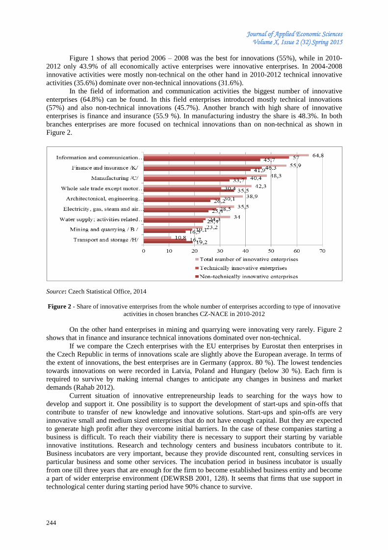
Journal of Applied Economic Sciences Volume X, Issue 2 (32) Spring 2015
244
Figure 1 shows that period 2006 – 2008 was the best for innovations (55%), while in 2010-
2012 only 43.9% of all economically active enterprises were innovative enterprises. In 2004-2008
innovative activities were mostly non-technical on the other hand in 2010-2012 technical innovative
activities (35.6%) dominate over non-technical innovations (31.6%).
In the field of information and communication activities the biggest number of innovative
enterprises (64.8%) can be found. In this field enterprises introduced mostly technical innovations
(57%) and also non-technical innovations (45.7%). Another branch with high share of innovative
enterprises is finance and insurance (55.9 %). In manufacturing industry the share is 48.3%. In both
branches enterprises are more focused on technical innovations than on non-technical as shown in
Figure 2.
Source: Czech Statistical Office, 2014
Figure 2 - Share of innovative enterprises from the whole number of enterprises according to type of innovative
activities in chosen branches CZ-NACE in 2010-2012
On the other hand enterprises in mining and quarrying were innovating very rarely. Figure 2
shows that in finance and insurance technical innovations dominated over non-technical.
If we compare the Czech enterprises with the EU enterprises by Eurostat then enterprises in
the Czech Republic in terms of innovations scale are slightly above the European average. In terms of
the extent of innovations, the best enterprises are in Germany (approx. 80 %). The lowest tendencies
towards innovations on were recorded in Latvia, Poland and Hungary (below 30 %). Each firm is
required to survive by making internal changes to anticipate any changes in business and market
demands (Rahab 2012).
Current situation of innovative entrepreneurship leads to searching for the ways how to
develop and support it. One possibility is to support the development of start-ups and spin-offs that
contribute to transfer of new knowledge and innovative solutions. Start-ups and spin-offs are very
innovative small and medium sized enterprises that do not have enough capital. But they are expected
to generate high profit after they overcome initial barriers. In the case of these companies starting a
business is difficult. To reach their viability there is necessary to support their starting by variable
innovative institutions. Research and technology centers and business incubators contribute to it.
Business incubators are very important, because they provide discounted rent, consulting services in
particular business and some other services. The incubation period in business incubator is usually
from one till three years that are enough for the firm to become established business entity and become
a part of wider enterprise environment (DEWRSB 2001, 128). It seems that firms that use support in
technological center during starting period have 90% chance to survive.
Journal of Applied Economic Sciences
Volume X, Issue 2(32), Spring2015
245
In the Czech Republic business incubators started to appear in 2004 (when the Czech Republic
became a member of European Union), because of the opportunity to use financial resources from
structural funds. In this country there are differences among regions in the sense of number of
incubators and also provided services. Start-up activities are supported also by CzechInvest and
Ministry of industry and trade, which organize project named CzechAccelerator. The aim is to support
penetration of the Czech start-ups to the foreign markets. Even if there exist variable forms of
enterprises supporting emergence of start-ups and spin-offs, there is not a big number of them. Israel,
whose size corresponds to the Czech Republic, one start-up company after another without any major
problems appears there. In the Czech Republic we can see a different situation. There does not exist
any institution controlling and managing starting and running start-up firms. Situation is similar in the
case of spin-offs that are linked with the universities. There exists a lot of logistic parks in the Czech
Republic. It was found that there are many new logistic parks in the Czech Republic, whose launch
was often facilitated by the state and more parks are under construction (Jurásková, Macurová 2013).
On the basis of realized empirical survey this paper monitors start-ups and spin-offs in the
Czech Republic, brings determination of these firms’ characteristics and finally this paper points out
differences between enterprise environment in the Czech Republic and Israel.
3. Theoretical literature overview
3.1 Determination of start-up firm including financing
According to the English-Czech explanatory dictionary start-up is something such as a new
business you create or cause to start. There exist a number of definitions of start-up firm from the
business point of view. According to Duda start-up is a starting firm that builds its core business on
innovative idea (DUDA 2013). It means that start-up firm brings new product or this firm produces it
on the basis of new technological processes or provides services in the way no one else knows.
Similarly author Audretsch (2011) defines start-up firm. It is a firm that offers new products, uses new
way of production or opens up new markets to customers or suppliers. This author also identifies
innovative start-ups according to the rate of inputs or value added related to research and development.
Firms or branches are innovative if the firms invest more than 3.5% of its inputs to research and
development. And they are “high-tech” in the case this rate is higher than 8.5%. But there is not
determined which inputs are considered to be research and development inputs.
The main goal of a start-up is to grow or to achieve better position in the market compared to
competitors. Founders of these firms focus on finding a market niche in the industrial branch they aim
to fill and to create a temporal monopoly (Bartoš 2002). For start-ups at the beginning it is very
important to focus on its development not only to be focused on results. Business incubators help start-
ups with this development – they provide quality consulting services or help them with the education.
At the same time start-up firm success is related to “Start-up feeling”. It means to be enthusiastic while
starting own business. But in many cases when this enthusiasm disappears a promising firm becomes
“grey mouse” and its activities slowly finish. Common characteristics of existing definitions
describing start-up firm are: newly established firm, new innovative solution, needed support of
business incubator, core business is mainly information and communication technology and necessary
start-up feeling.
For development start-up firms use following source of financing (Srpová 2008, 2010):
Own sources – they enable immediate starting business and founder is the only one owner.
But financing by using own sources is more difficult and slow.
Bank loan – total costs connected with loan are relatively high. But in the case firm pays its
payables regularly the bank does not want to influence business activities of the debtor
(Srpová 2010).
Factoring – entrepreneur advance his claim to factoring company, that accepts all the
liability and entrepreneur has his money immediately.
Business angels – investors which for longer period invest own money to start-up firms
with high potential and takes fair share from the entrepreneurship. Except money business
angles provide also know-how and contacts (Woods 2008).
Venture capital – is capital invested to starting, running and further development of start-up
firm. Capital is provided and there is expected share in firms registered capital.
Journal of Applied Economic Sciences Volume X, Issue 2 (32) Spring 2015
246
Private equity – private capital provided starting firms in order to gain share in registered
capital. In return for their money, knowledge and experiences capital providers require
significant asset share.
Choice of way of financing start-up firms relate to actual firm lifecycle period (establishing,
growing, expansion, maturity). Innovative firms face important business risks in the time they start
and develop new products. Basically two situations can happen: firstly new product can be
unsuccessful or on the other hand product can be successful and can generate more than average
profit.
3.2 Determination of spin-off firm
According to the English-Czech explanatory dictionary spin-off is something useful that
unexpectedly results from an activity. Poláček and Attl (2006) define a spin-off firm (sometimes we
can find spin-out) as one that rises by using intangible assets as capital stock into a newly rising
corporation (e.g. university know-how). Shane (2004) defines a university spin-off firm such as a
newly established firm that partially uses intellectual assets that come from some university.
Spin-off firm is founded in order to use and develop intellectual property of university in the
form of product or service accepted in the market. Students or researchers of university usually found
this kind of firm and they use know-how, knowledge and findings they obtained at the university.
Firms can have this intellectual property from the university when they pay for it or sign a licence.
Spin-off firm can be founded with a share of university or without it. Kislingerová (2011) divides
spin-offs into two groups:
Spin-offs that are founded by academics and are its employees or by students;
Spin-offs that are founded by university graduates.
Literature focused on spin-offs emphasizes the key role of the researcher who becomes a
manager (Lockett et al. 2003; Murray 2004). According to a case study of Turin (Salvador, 2010)
local spin-offs are young firms with a low capital and few employees. Most of these entities are
service firms rather than product ones. The main sector of activity is biotechnology and chemical-
pharmaceutical, aerospace and transport, informatics and telecommunication and environment. These
are the sectors in which Turin incubators and science parks as well as the Polytechnic and the
University, are most specialized. These spin-offs are micro-firms but deal most of all in the
international market (Salvador 2010). According to the literature, spin-off founders are influenced by a
desire of autonomy and independence (O`shea et al. 2005; Shane 2004), and possibility to use reached
research results.
It is necessary to consider the results of the case study of Turin which was based on interviews
and answers of the questionnaire. It was determined that in general, academics choose not to leave
university jobs (Salvador 2010). The fact is that the inventor does not have to run a new firm every
day. He can be involved in technical activities of the innovation (Wright et al. 2004b). The growing
role of science parks in helping universities balance their 21th century missions in education, research
and commercialization is necessary (Wessner 2009). According to statistical results of Link and Scott
(200 ) “the organizational nature of the university-park relationship is important”. Universities with a
connection to spin-off firms are key tool for implementation of research results. The positive attitude
of universities toward spin-offs is a recent phenomenon (Wright et al. 2004b; Shane 2004).
The major difference between start-ups and spin-offs is in its founder. Spin-offs are usually
founded by students or researchers of particular university or former university graduates. In the case
of start-ups any kind of private person can be its founder.
3.3 The differences in approach to entrepreneurship in selected countries
According to Srpová (2008) and Kuratko (2011) the main assumption to success in business
are entrepreneur characteristics and his or her approach to realizing business activities. The most
important entrepreneur features are perservance, responsibility and initiative. At the same time
entrepreneur has to monitor and utilize opportunities and own strengths, apply concept of price,
quality and flexibility in accordance to entrepreneur environment. Entrepreneur features are till certain
extend influenced by his values, habits and culture of particular country. It can be inspiring to compare
approach to entrepreneurship in the Czech Republic and Israel as shown in Table 1.
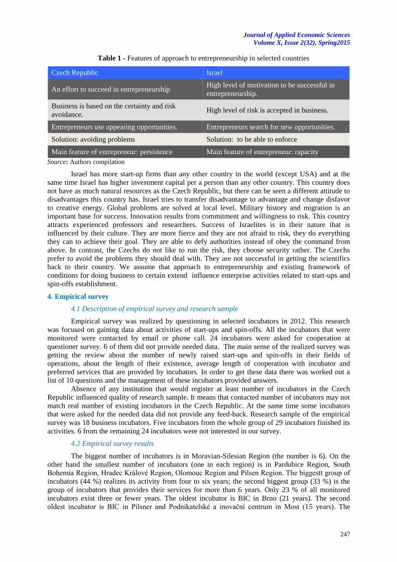
Journal of Applied Economic Sciences
Volume X, Issue 2(32), Spring2015
247
Table 1 - Features of approach to entrepreneurship in selected countries
Czech Republic Israel
An effort to succeed in entrepreneurship High level of motivation to be successful in
entrepreneurship.
Business is based on the certainty and risk
avoidance. High level of risk is accepted in business.
Entrepreneurs use appearing opportunities. Entrepreneurs search for new opportunities.
Solution: avoiding problems Solution: to be able to enforce
Main feature of entrepreneur: persistence Main feature of entrepreneur: rapacity
Source: Authors compilation
Israel has more start-up firms than any other country in the world (except USA) and at the
same time Israel has higher investment capital per a person than any other country. This country does
not have as much natural resources as the Czech Republic, but there can be seen a different attitude to
disadvantages this country has. Israel tries to transfer disadvantage to advantage and change disfavor
to creative energy. Global problems are solved at local level. Military history and migration is an
important base for success. Innovation results from commitment and willingness to risk. This country
attracts experienced professors and researchers. Success of Israelites is in their nature that is
influenced by their culture. They are more fierce and they are not afraid to risk, they do everything
they can to achieve their goal. They are able to defy authorities instead of obey the command from
above. In contrast, the Czechs do not like to run the risk, they choose security rather. The Czechs
prefer to avoid the problems they should deal with. They are not successful in getting the scientifics
back to their country. We assume that approach to entrepreneurship and existing framework of
conditions for doing business to certain extend influence enterprise activities related to start-ups and
spin-offs establishment.
4. Empirical survey
4.1 Description of empirical survey and research sample
Empirical survey was realized by questioning in selected incubators in 2012. This research
was focused on gaining data about activities of start-ups and spin-offs. All the incubators that were
monitored were contacted by email or phone call. 24 incubators were asked for cooperation at
questioner survey. 6 of them did not provide needed data. The main sense of the realized survey was
getting the review about the number of newly raised start-ups and spin-offs in their fields of
operations, about the length of their existence, average length of cooperation with incubator and
preferred services that are provided by incubators. In order to get these data there was worked out a
list of 10 questions and the management of these incubators provided answers.
Absence of any institution that would register at least number of incubators in the Czech
Republic influenced quality of research sample. It means that contacted number of incubators may not
match real number of existing incubators in the Czech Republic. At the same time some incubators
that were asked for the needed data did not provide any feed-back. Research sample of the empirical
survey was 18 business incubators. Five incubators from the whole group of 29 incubators finished its
activities. 6 from the remaining 24 incubators were not interested in our survey.
4.2 Empirical survey results
The biggest number of incubators is in Moravian-Silesian Region (the number is 6). On the
other hand the smallest number of incubators (one in each region) is in Pardubice Region, South
Bohemia Region, Hradec Králové Region, Olomouc Region and Pilsen Region. The biggestt group of
incubators (44 %) realizes its activity from four to six years; the second biggest group (33 %) is the
group of incubators that provides their services for more than 6 years. Only 23 % of all monitored
incubators exist three or fewer years. The oldest incubator is BIC in Brno (21 years). The second
oldest incubator is BIC in Pilsner and Podnikatelské a inovační centrum in Most (15 years). The
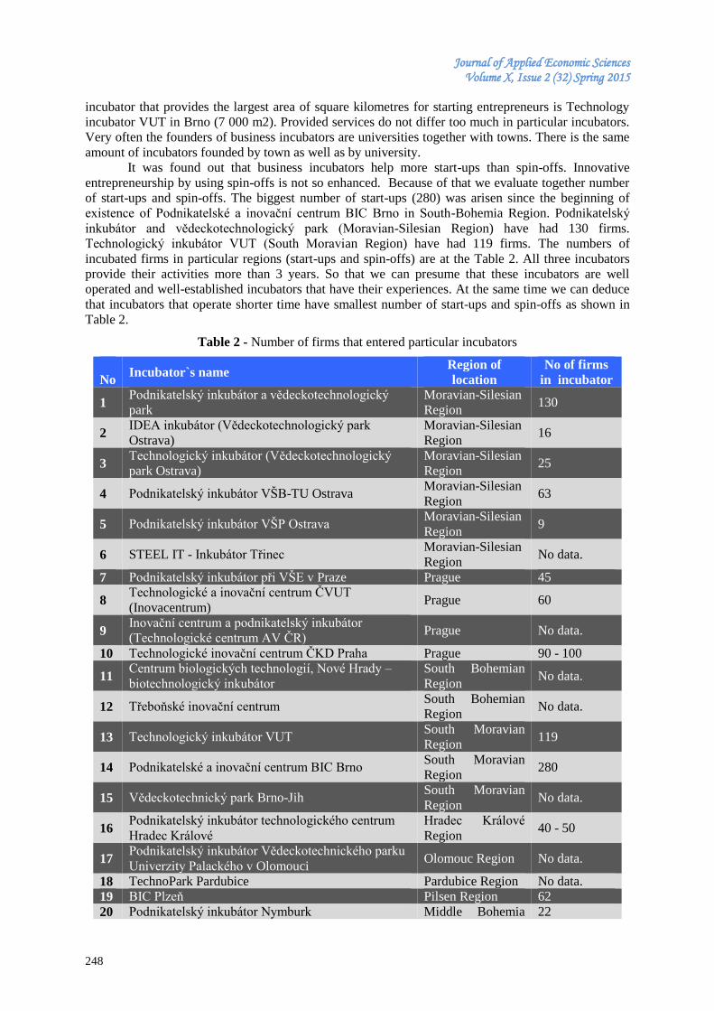
Journal of Applied Economic Sciences Volume X, Issue 2 (32) Spring 2015
248
incubator that provides the largest area of square kilometres for starting entrepreneurs is Technology
incubator VUT in Brno (7 000 m2). Provided services do not differ too much in particular incubators.
Very often the founders of business incubators are universities together with towns. There is the same
amount of incubators founded by town as well as by university.
It was found out that business incubators help more start-ups than spin-offs. Innovative
entrepreneurship by using spin-offs is not so enhanced. Because of that we evaluate together number
of start-ups and spin-offs. The biggest number of start-ups (280) was arisen since the beginning of
existence of Podnikatelské a inovační centrum BIC Brno in South-Bohemia Region. Podnikatelský
inkubátor and vědeckotechnologický park (Moravian-Silesian Region) have had 130 firms.
Technologický inkubátor VUT (South Moravian Region) have had 119 firms. The numbers of
incubated firms in particular regions (start-ups and spin-offs) are at the Table 2. All three incubators
provide their activities more than 3 years. So that we can presume that these incubators are well
operated and well-established incubators that have their experiences. At the same time we can deduce
that incubators that operate shorter time have smallest number of start-ups and spin-offs as shown in
Table 2.
Table 2 - Number of firms that entered particular incubators
No Incubator`s name
Region of
location
No of firms
in incubator
1 Podnikatelský inkubátor a vědeckotechnologický
park
Moravian-Silesian
Region 130
2 IDEA inkubátor (Vědeckotechnologický park
Ostrava)
Moravian-Silesian
Region 16
3 Technologický inkubátor (Vědeckotechnologický
park Ostrava)
Moravian-Silesian
Region 25
4 Podnikatelský inkubátor VŠB-TU Ostrava Moravian-Silesian
Region 63
5 Podnikatelský inkubátor VŠP Ostrava Moravian-Silesian
Region 9
6 STEEL IT - Inkubátor Třinec Moravian-Silesian
Region No data.
7 Podnikatelský inkubátor při VŠE v Praze Prague 45
8 Technologické a inovační centrum ČVUT
(Inovacentrum) Prague 60
9 Inovační centrum a podnikatelský inkubátor
(Technologické centrum AV ČR) Prague No data.
10 Technologické inovační centrum ČKD Praha Prague 90 - 100
11 Centrum biologických technologií, Nové Hrady –
biotechnologický inkubátor
South Bohemian
Region No data.
12 Třeboňské inovační centrum South Bohemian
Region No data.
13 Technologický inkubátor VUT South Moravian
Region 119
14 Podnikatelské a inovační centrum BIC Brno South Moravian
Region 280
15 Vědeckotechnický park Brno-Jih South Moravian
Region No data.
16 Podnikatelský inkubátor technologického centrum
Hradec Králové
Hradec Králové
Region 40 - 50
17 Podnikatelský inkubátor Vědeckotechnického parku
Univerzity Palackého v Olomouci Olomouc Region No data.
18 TechnoPark Pardubice Pardubice Region No data.
19 BIC Plzeň Pilsen Region 62
20 Podnikatelský inkubátor Nymburk Middle Bohemia 22
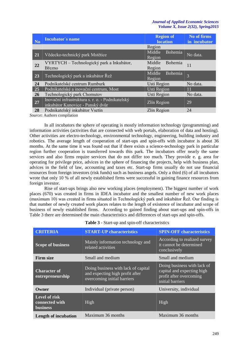
Journal of Applied Economic Sciences
Volume X, Issue 2(32), Spring2015
249
No Incubator`s name
Region of
location
No of firms
in incubator
Region
21 Vědecko-technický park Mstětice Middle Bohemia
Region No data.
22 VYRTYCH – Technologický park a Inkubátor,
Březno
Middle Bohemia
Region 11
23 Technologický park a inkubátor Řež Middle Bohemia
Region 3
24 Podnikatelské centrum Rumburk Usti Region No data.
25 Podnikatelské a inovační centrum, Most Usti Region 11
26 Technologický park Chomutov Usti Region No data.
27 Inovační infrastruktura s. r. o. - Podnikatelský
inkubátor Kunovice - Panský dvůr Zlín Region 29
28 Podnikatelský inkubátor Vsetín Zlín Region 24 Source: Authors compilation
In all incubators the sphere of operating is mostly information technology (programming) and
information activities (activities that are connected with web portals, elaboration of data and hosting).
Other activities are electro-technology, environmental technology, engineering, building industry and
robotics. The average length of cooperation of start-ups and spin-offs with incubator is about 36
months. At the same time it was found out that if there exists a science-technology park in particular
region further cooperation is transferred towards this park. The incubators offer nearly the same
services and also firms require services that do not differ too much. They provide e. g. area for
operating for privilege price, advices in the sphere of financing the projects, help with business plan,
advices in the field of law, accounting and taxes etc. Start-up firms usually do not use financial
resources from foreign investors (risk funds) such as business angels. Only a third (6) of all incubators
wrote that only 10 % of all newly established firms were successful in gaining finance resources from
foreign investor.
Rise of start-ups brings also new working places (employment). The biggest number of work
places (670) was created in firms in IDEA incubator and the smallest number of new work places
(maximum 10) was created in firms situated in Technologický park and inkubátor Řež. Our finding is
that number of newly created work places relates to the length of existence of incubator and scope of
business of newly established firms. According to gained finding about start-ups and spin-offs in
Table 3 there are determined the main characteristics and differences of start-ups and spin-offs.
Table 3 - Start-up and spin-off characteristics
CRITERIA START-UP characteristics SPIN-OFF characteristics
Scope of business Mainly information technology and
related activities
According to realized survey
it cannot be determined
conclusively
Firm size Small and medium Small and medium
Character of
entrepreneurship
Doing business with lack of capital
and expecting high profit after
overcoming initial barriers
Doing business with lack of
capital and expecting high
profit after overcoming
initial barriers
Owner Individual (private person) University, individual
Level of risk
connected with
business
High High
Length of incubation Maximum 36 months Maximum 36 months
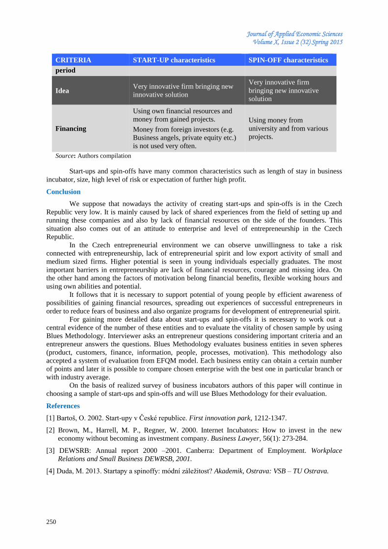
Journal of Applied Economic Sciences Volume X, Issue 2 (32) Spring 2015
250
CRITERIA START-UP characteristics SPIN-OFF characteristics
period
Idea Very innovative firm bringing new
innovative solution
Very innovative firm
bringing new innovative
solution
Financing
Using own financial resources and
money from gained projects.
Money from foreign investors (e.g.
Business angels, private equity etc.)
is not used very often.
Using money from
university and from various
projects.
Source: Authors compilation
Start-ups and spin-offs have many common characteristics such as length of stay in business
incubator, size, high level of risk or expectation of further high profit.
Conclusion
We suppose that nowadays the activity of creating start-ups and spin-offs is in the Czech
Republic very low. It is mainly caused by lack of shared experiences from the field of setting up and
running these companies and also by lack of financial resources on the side of the founders. This
situation also comes out of an attitude to enterprise and level of entrepreneurship in the Czech
Republic.
In the Czech entrepreneurial environment we can observe unwillingness to take a risk
connected with entrepreneurship, lack of entrepreneurial spirit and low export activity of small and
medium sized firms. Higher potential is seen in young individuals especially graduates. The most
important barriers in entrepreneurship are lack of financial resources, courage and missing idea. On
the other hand among the factors of motivation belong financial benefits, flexible working hours and
using own abilities and potential.
It follows that it is necessary to support potential of young people by efficient awareness of
possibilities of gaining financial resources, spreading out experiences of successful entrepreneurs in
order to reduce fears of business and also organize programs for development of entrepreneurial spirit.
For gaining more detailed data about start-ups and spin-offs it is necessary to work out a
central evidence of the number of these entities and to evaluate the vitality of chosen sample by using
Blues Methodology. Interviewer asks an entrepreneur questions considering important criteria and an
entrepreneur answers the questions. Blues Methodology evaluates business entities in seven spheres
(product, customers, finance, information, people, processes, motivation). This methodology also
accepted a system of evaluation from EFQM model. Each business entity can obtain a certain number
of points and later it is possible to compare chosen enterprise with the best one in particular branch or
with industry average.
On the basis of realized survey of business incubators authors of this paper will continue in
choosing a sample of start-ups and spin-offs and will use Blues Methodology for their evaluation.
References
[1] Bartoš, O. 2002. Start-upy v České republice. First innovation park, 1212-1347.
[2] Brown, M., Harrell, M. P., Regner, W. 2000. Internet Incubators: How to invest in the new
economy without becoming as investment company. Business Lawyer, 56(1): 273-284.
[3] DEWSRB: Annual report 2000 –2001. Canberra: Department of Employment. Workplace
Relations and Small Business DEWRSB, 2001.
[4] Duda, M. 2013. Startapy a spinoffy: módní záležitost? Akademik, Ostrava: VSB – TU Ostrava.
Journal of Applied Economic Sciences
Volume X, Issue 2(32), Spring2015
251
[5] Dziuba, B. 2011. IBI NET – Particular benefits for countries of the Baltic Sea Region. Ibi-net 3.
Available at: http://www.ibi-net.eu/uploads/filedir/newsletter_ibinet_issue3.pdf. [Accessed May
28, 2014].
[6] Hackett, S.M., Dilts, D.M. 2004b. A systematic review of business incubation research. Journal of
Technology Transfer 29(1): 55-82.
[7] Jurásková, K., Macurová, P. The study of logistic parks in the Czech Republic. Journal of Apled
Economic Sciences 8(3): 299-310.
[8] Kislingerová, E. 2011. Nová ekonomika. Nové přéležitosti? Praha: C. H. Beck.
[9] Konečný, M., Skokan, K., Zamarský, V. 2001. Inovační centra: Transferová inovační pracoviště,
inkubátory pro výchovu inovačních podnikatelů: vědecko-technické parky. Ostrava: VŠB-TU
Ostrava.
[10] Kulakowski, E.C., Chronister, L.U. 2006. Research Administration and Management. Johns and
Bartlett.
[11] Lalkaka, R., Bishop, J. 1996. Business Incubators in Economic Development: an initial
assessment in countries. New York: United Nations Development Programme.
[12] Link, A.N., Scott, J.T. 2003. US science parks: The diffusion of an innovation and its effects on
the academic missions of universities. International Journal of Industrial Organization, 21(9):
1323-1356.
[13] Link, A.N., Scott, J.T. 2006. US university parks. Journal of Productivity Analysis, 25(1-2): 43-
55.
[14] Link, A.N., Scott, J.T. 2007. The economics of university research parks. Oxford Review of
Economic Policy 4: 661-674.
[15] Lockett, A., Wright, M., Franklin, S. 2003. Technology transfer and universities` spin-out
strategies. Small Business Economics 20(2): 185-200.
[16] Murray, F. 2004. The role as academic inventors in entrepreneurial firms: Sharing the laboratory
life. Research Policy, 34(4): 643-659.
[18] O`shea, R.P., Allen, T. J., CHevalier, A., Roche, F. 2005. Entrepreneurial orientation, technology
transfer and spinoff performance of US universities. Research Policy, 34(7): 994-1009.
[19] Poláček, B., Attl, J. 2006. Posudek znalce a podnik. Praha: C. H. Beck.
[20] Rahab, S. 2012. Innovativeness Model Of Small And Medium Enterprises Based On Market
Orientation and Learning Orientation: Testing Moderating Effect Of Business Operation Mode.
Procedia Economics and Finance. Elsevier: 97 – 109.
[21] Salvador, E. 2010. Are science parks and incubators good “brand names” for spin-offs? The case
study of Turin. Journal of Technology Transfer, 36(2): 203-232.
[22] Senor, D., Singer, S. 2011. Start-up nation: příběh izraelského hospodářského zázraku. Praha:
Aligier.
[23] Shane, S. 2004. Academic Entrepreneurship: University Spinoffs and Wealth Creation.
Cheltenham: Edwar Elgar.
[24] Techen, B. 2011. IBI NET – Particular benefits for countries of the Baltic Sea Region. Ibi-net 3.
Available at: www.ibi-net.eu/uploads/filedir/newsletter_ibinet_issue3.pdf. [Accessed May 28,
2014].
[25] Wessner, C.W. 2009. Understanding research, science and technology parks: Global best
practice. National research council of the National Academies. in: The National Academic Press,
Washington, Available at: www.nap.edu/catalog/12546.html. [Accessed May 28, 2014].

Journal of Applied Economic Sciences Volume X, Issue 2 (32) Spring 2015
252
[26] Wright, M., Clarysee, B., Mustar, P., Lockett, A. 2007. Academic entrepreneurship in Europe.
Cheltenham: Edwar Elgar.
[27] Wright, M., Vohora, A., Lockett, A. 2004b. The formation of high-tech university spinouts: The
role as joint ventures and venture capital investors. Journal of Technology Transfer, 29(3-4): 287-
310.
*** National Commission on Entrepreneurship. 2000. Building Companies, Building Communities:
Entrepreneurs in the New Economy. Washington, available at: D.C. http://www.zeromillion.com/
files/entrepreneurs-in-new-economy.pdf [Accessed May 28, 2014].
Journal of Applied Economic Sciences
Volume X, Issue 2(32), Spring2015
253
LONG RUN FISCAL DISEQUILIBRIUM. AN INDONESIAN CASE
Jaka SRIYANA
Department of Economics, Islamic University of Indonesia, Indonesia
Abstract This study attempts to provide an evidence of fiscal disequilibrium in Indonesia. The model considers
elaborating government expenditure model. For this purpose, this research employs an error correction model
to test the existence of fiscal equilibrium. In this case, the model captures output, population, and tax revenue as
the determinant variables of government expenditure for the period 1970-2012. The short run model shows that
population and tax revenue are statistically significant in affecting government expenditure. Meanwhile,
changesin tax revenue has negative effect to government expenditure growth which potentially creates fiscal
gap. Furthermore, this finding reveals the existence of fiscal disequilibrium in Indonesia. Furthermore, these
findings recommend that government likely considers increasing tax ratio rather than reviewing government
size.
Keywords: fiscal, government, expenditure, budget, deficit, policy.
JEL Clasiffication: H 53, H 62, C 22
1. Introduction
The issues of fiscal policy and public finance management have been a long interest of many
economists. Tanzi (1982) initiated an analysis of fiscal disequilibrium in developing countries. In his
paper, he pointed out that the causes of fiscal disequilibrium are export boom, price inelastic tax
system, public enterprise performance, increased expenditure produced by political exigencies or
administrative weaknesses, and worsening terms of trade. Other issues that emerged in some papers
are fiscal imbalance as well as the debate of optimum government size and its relationship to other
main macroeconomic variables (Auerbach 2011). Moreover, Ekinci (2011) noted that expansion of
government size even slows down economic growth. In most developing countries, government size
has positive correlation with government expenditure which generally grows annually.
Following Sobhee (2003), the attempt to provide an empirical model of demand for public
goods could be inferred as an alternative way to find a proper government expenditure. In recent years,
Indonesian economy has experienced a stable growth rate averaging five per cent in real terms,
thereby improving the macroeconomic fundamentals including the public finances. Thus, it would be
interesting to capture the evolutionary forces that have governed the fiscal policy in Indonesia over the
last three decades through modelling the government expenditure.
A major problem of recent Indonesian fiscal management is to avoid fiscal trap that could
trigger a new economic crisis. One of the important dimensions of this challenge is to conduct fiscal
policy to support a stable economic growth, low inflation, and increasing employment. Furthermore,
the central government has applied an expansionary fiscal policy in the last decade. However, this
policy could not boost fiscal capacity in this period. During this time, Indonesian government has been
experiencing sharp increases in its expenditure which has lead to a stable economic growth. Based on
Indonesia’s finance ministry report 2012, government expenditure grew by 282.8.7% from 2002 to
2011; meanwhile the tax revenue only increased by 243.7% in the same period. However, the
significant increase in government budget did not mean that the fiscal capacity has become more
stable. A simple indicator is that government expenditure has grown faster than its of government
revenue, potentially making the government embark upon a potential fiscal trap.
As concluded by Marks (2004), it seems the government budget was not sustainable in the
long run in Indonesia. The budget structure was imbalanced, where government expenditure grew
faster than revenue as a consequence of exchange rate volatility. The government expenditure was
dominated by operating expenditure which might not seem to be potential to create new tax sources.
Unfortunately, the vulnerability to external shock, such as world oil price could undermine the fiscal
sustainability given the huge proportion of oil subsidy in the budget. This phenomenon is reliable
reason to analyze fiscal equilibrium in order to provide an alternative prudent fiscal policy. In this
Journal of Applied Economic Sciences Volume X, Issue 2 (32) Spring 2015
254
paper, we intend to extend the analysis of fiscal equilibrium by modelling an empirical evidence of
government expenditure.
2. Literature review
Fiscal equilibrium occurred on the condition that permanent government expenditures were
covered by permanent government revenues (Tanzi 1982). Some papers have focused on the analysis
of government expenditure behaviour for various data. The analysis mostly concerns with the
relationship between government expenditure and other economic variables, such as tax revenue,
economic growth, and government budget deficit (Ghartey 2010; Sobhee 2003; Tsaurai & Odhiambo
2013). The development of government expenditure could be traced back to Wagner´s law which
states that government activity increases as the economy grows. (Sobhee 2003) provided additional
insights through the empirical evidence of the demand function for the public goods in a developing
small economy. He first established a long-term relationship between quantity demanded of public
goods, median voter’s income, price and population. Supporting evidence in favour of the Buchanan
and Wagner hypothesis, he found that fiscal deficit have led to a reduction in the perceived tax-price
of public goods that have further increased public spending.
Ekinci (2011) noted that a positive share of government in economic activities changes
downward as the relative size of government grows. The demand for public goods rises and is
consistent with the increasing ability to collect the necessary funds. As countries become more
developed, higher demand for public goods which automatically leads to increased government
expenditure also requires an increase in tax revenue. Schaltegger & Torgler (2006) as well as
Nurudeen & Usman (2010) revealed that government expenditure negatively influenced economic
growth. This result was not in line with Ghosh & Gregoriou (2008) who found that government
expenditure play a strong positive impact on economic growth. (Tsaurai & Odhiambo 2013) pointed
out that there is a unidirectional causal flow from economic growth to government expenditure, both
in the short run and in the long run.
Some recent studies support an active fiscal policy as an implementation of the Keynesian
proposition (Hall 2009; Ramey 2011; Ratha 2012; Saleh & Nair 2006). The Keynesian theory
proposes the role of expansive fiscal policy to support aggregate demand and economic growth. The
government expenditure should act as a stabilization policy and increasing during the recession, while
it should be reduced during the economic booms. This concept recommends an active fiscal policy and
relies on the size of government expenditure.
The budget constraint proposition explains that government expenditure equals with sum up of
tax revenues, budget deficit and increase in borrowing. In a balance budget system, an increase in
taxes is followed by an increase in government expenditure. Thus, there is a causal relationship
between changes in government spending and taxes (Ghartey 2010). According to Tanzi (1982), to
avoid fiscal disequilibrium, a country with rapid increase government expenditure must consequently
attempts to raise taxes revenue. (Ghartey 2010) also found that in developing countries, reduction in
taxes is commonly means of controlling government spending. The attempt of governments to raise
taxes in reducing budget deficit could be the principal source of fuelling higher spending. Thus, in an
increasing tax, then lead to cause government spending to increase. Furthermore, reducing or limiting
tax receipts in the short-term and constraining government expenditure create cost of government
activities in the long-run. In this situation, a country tends to meet a fiscal disequilibrium in the long
run.
Another interesting finding of the study conducted by Ghartey (2010) was that in the short-
term rises in taxes cause government spending changes for some developing countries. Meanwhile, in
the long-run, taxes and spending remain independent because the government which controls both
fiscal instruments has failed to balance the national budget. However, government spending tends to
be disbursed without considering sources of financing. Several previous empirical results also
described similar situation (Baghestani & McNown 1994; Narayan & Narayan 2006). Empirical
analysis of government expenditure model will provide insight as to how fiscal policies might help to
control the government expenditure growth. If the factors affecting government expenditure could be
elaborated, then it will be expected to provide some strategies in the government budget management.
In contrast, the impact of revenue growth on government expenditure is also a significant
Journal of Applied Economic Sciences
Volume X, Issue 2(32), Spring2015
255
consideration for government to strengthen the fiscal capacity. These are the importance of examining
the government expenditure model on the fiscal policy implementation.
3. Model specification and method of analysis
In line with the objective to analyze the long run behaviour of government expenditure, this
research employed cointegration and error correction model (ECM) as widely used in previous
researches (Ghartey 2010; Khan 2012; Sobhee 2003; Tsaurai & Odhiambo 2013). This approach does
not only encompass both level and difference in the variables which capture the short and long run
properties of the model, but also provides an attractive statistical framework and represents the
concept of long run relationship between two or more variables. With respect to the concept of
cointegration, we need to analyze the time series properties of economic variables. In the case where
the variables in question are not stationary or cointegrated series, the regression equations related to
time series data are spurious. It means that testing for unit root and cointegration can be considered as
a pre-test before estimating a valid ECM regression.
A complete consideration of dynamic specification including ECM is important in
construction of economic models. The dynamic analysis involves the description of some economic
variables as a function of a set of lagged explanatory variables. With respect to this issue, this section
explains error correction model adopted from Tsaurai & Odhiambo (2013).
To illustrate the government expenditure model, the economy can be assumed in long run
equilibrium. In the case of the government sector, it can be assumed that government expenditure
adjusts periodically to its equilibrium. This may be caused by some economic variables that probably
come from both endogenous and exogenous variables. According to Sobhee, (2003), long run model
of government expenditure may be formulized as follows:
G* = A Yb N
c T
d (1)
The long run model of government expenditure (G*) is assumed to capture output (Y),
population (N), and government revenue (T). In linear log form, equation (1) will be:
Log Gt* = Log A + b Log Yt + c Log Nt + d Log Tt + (2)
If the adjustment of expenditure G to its long run equilibrium G* is gradual, then the level of
expenditure will respond to changes in independent variables, and G will move gradually toward its
equilibrium level. Following Ghartey (2010), to capture this process we adopted a general
autoregressive distributed lag model in period t:
Log Gt = a + b1 Log Yt + c1 Log Nt + d1
Log Tt+ b2 Log Yt-1+ c2 Log Nt-1
+ d2 Ln Tt-1 + Log Gt-1 + t; (3)
To reflect the steady state, equation (3) can be rearranged as the error correction model:
Log Gt = a + b1 Log Yt + c1 Log Nt + d1
Log Tt +
λ [Log Gt-1 - ( Log Yt-1 + Log Nt-1 + Log Tt-1)] + t (4)
Log Gt = a + b1 Log Yt + c1 Log Nt + d1
Log Tt + λ ECTt-1 + t (5)
In equation (5), it implies that b1, c1, and
d1
are the short-run elasticity of government
expenditure with respect to output, population, and government revenue respectively. While the error
correction term (ECTt-1), which is λ [Ln Gt-1 - (Ln Yt-1 + Ln Nt-1 + Ln Tt-1)], explains level of
deviations from short run disequilibrium to the long-run equilibrium, and where δ is the long-run
elasticity of government expenditure with respect to all independent variables. In addition, λ is
Journal of Applied Economic Sciences Volume X, Issue 2 (32) Spring 2015
256
expected to be statistically significant. This coefficient also reflects the level of adjustment of
government expenditure from its past disequilibrium.
Moreover, to examine the existence of a co-integration relationship between government
expenditure and its dependent variables this research uses the recently developed ARDL-bounds
testing approach. According to Tsaurai & Odhiambo (2013), the ARDL model used in this study can
be expressed as follows:
Log Gt = a +
m
i ib1
Log Yt-i +
n
i ic1
Log Nt-i +
p
i id1
Log Tt-i +
q
i ie1
Log Gt-i + 1 Log Yt-1 + 2
Log Nt-1 + 3
Log Tt-1 +
4 Log Gt-1 + vt (6)
The long run model is estimated by normalizing the coefficients of the lagged dependent
variables in equation (6). To provide an estimable technique to test the existing of long run dynamic
equilibrium between government expenditure and its explanatory variables, this equation could be
written in other form as follows:
Log Gt = a +
m
i ib1
Log Yt-i +
n
i ic1
Log Nt-i +
p
i id1
Log Tt-i +
q
i ie1
Log Gt-i + λ ECTt-1 + vt (7)
A negative and significant error correction term (λ) would indicate co-integration that is long
run equilibrium among the underlying variables (Ghartey 2010). The optimum lag length of the ADL
model is chosen by using information criteria such as Schwarz criterion (SBC) and Akaike
information criterion (AIC). The error correction term also measures the speed of adjustment from
short run deviations to a long-run equilibrium. If it is statistically significant and has negative sign, it
means that the set of variables are cointegrated. The Johansen, (1991) cointegration technique is used
to test the long run equilibrium relationship among the variables of interest.
4. Empirical results and discussion
This research employs annual data which include government expenditure (Gt), Gross
Domestic Product (Yt), population (Nt) and tax revenue (Tt) for the period 1970-2012, all of which are
in natural logarithm of real terms. Data are obtained from several annual reports of International
Financial Statistics, World Bank.
Figure 1 reports the behaviour of government expenditure and tax revenue. Government
expenditure sharply increased in the period of 1985-1997, as well as tax revenue. Because of financial
crisis that occurred in 1997, both variables tend to have lower growth until 2010. The lower value of
tax revenue comparing to government expenditure implies that the government experiences budget
deficit which slightly declined in 1990-2000. For the rest of the period, budget deficit was in a
moderate level which is successfully controlled around 2% of GDP. Other important fiscal indicator,
Indonesia’s tax ratio is around 12% of GDP which is only a half of the average in ASEAN countries
that is around 24.5% of GDP. This low tax ratio could be caused by low tax rate, narrow tax base, or
low compliance rate. Other factors that may cause this problem are weakness of institutional capacity
and low quality of government staffs.
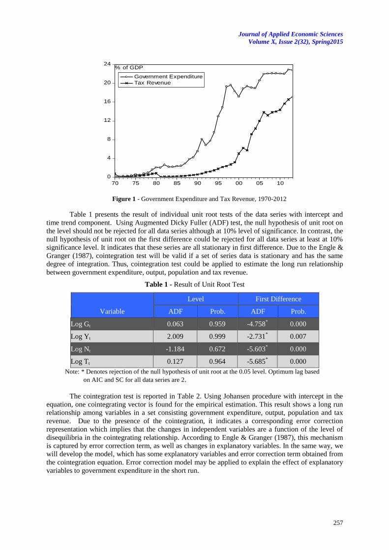
Journal of Applied Economic Sciences
Volume X, Issue 2(32), Spring2015
257
Figure 1 - Government Expenditure and Tax Revenue, 1970-2012
Table 1 presents the result of individual unit root tests of the data series with intercept and
time trend component. Using Augmented Dicky Fuller (ADF) test, the null hypothesis of unit root on
the level should not be rejected for all data series although at 10% level of significance. In contrast, the
null hypothesis of unit root on the first difference could be rejected for all data series at least at 10%
significance level. It indicates that these series are all stationary in first difference. Due to the Engle &
Granger (1987), cointegration test will be valid if a set of series data is stationary and has the same
degree of integration. Thus, cointegration test could be applied to estimate the long run relationship
between government expenditure, output, population and tax revenue.
Table 1 - Result of Unit Root Test
Variable
Level First Difference
ADF Prob. ADF Prob.
Log Gt 0.063 0.959 -4.758* 0.000
Log Yt 2.009 0.999 -2.731* 0.007
Log Nt -1.184 0.672 -5.603* 0.000
Log Tt 0.127 0.964 -5.685* 0.000
Note: * Denotes rejection of the null hypothesis of unit root at the 0.05 level. Optimum lag based
on AIC and SC for all data series are 2.
The cointegration test is reported in Table 2. Using Johansen procedure with intercept in the
equation, one cointegrating vector is found for the empirical estimation. This result shows a long run
relationship among variables in a set consisting government expenditure, output, population and tax
revenue. Due to the presence of the cointegration, it indicates a corresponding error correction
representation which implies that the changes in independent variables are a function of the level of
disequilibria in the cointegrating relationship. According to Engle & Granger (1987), this mechanism
is captured by error correction term, as well as changes in explanatory variables. In the same way, we
will develop the model, which has some explanatory variables and error correction term obtained from
the cointegration equation. Error correction model may be applied to explain the effect of explanatory
variables to government expenditure in the short run.
0
4
8
12
16
20
24
70 75 80 85 90 95 00 05 10
Government Expenditure
Tax Revenue
% of GDP
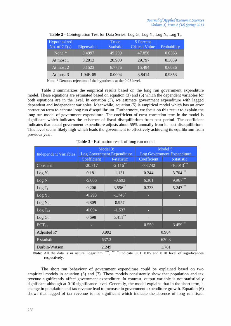
Journal of Applied Economic Sciences Volume X, Issue 2 (32) Spring 2015
258
Table 2 - Cointegration Test for Data Series: Log Gt, Log Yt, Log Nt, Log Tt.
Hypothesized Trace 5 Percent
No. of CE(s) Eigenvalue Statistic Critical Value Probability
None * 0.4997 49.299 47.856 0.0363
At most 1 0.2913 20.900 29.797 0.3639
At most 2 0.1523 6.7776 15.494 0.6036
At most 3 1.04E-05 0.0004 3.8414 0.9853
Note: * Denotes rejection of the hypothesis at the 0.05 level.
Table 3 summarizes the empirical results based on the long run government expenditure
model. These equations are estimated based on equation (3) and (5) which the dependent variables for
both equations are in the level. In equation (3), we estimate government expenditure with lagged
dependent and independent variables. Meanwhile, equation (5) is empirical model which has an error
correction term to capture long run disequilibrium. Furthermore, we focus on this result to explain the
long run model of government expenditure. The coefficient of error correction term in the model is
significant which indicates the existence of fiscal disequilibrium from past period. The coefficient
indicates that actual government expenditure adjusts about 55% annually from its past disequilibrium.
This level seems likely high which leads the government to effectively achieving its equilibrium from
previous year.
Table 3 - Estimation result of long run model
Independent Variables
Model 3:
Log Government Expenditure
Model 5:
Log Government Expenditure
Coefficient t-statistic Coefficient t-statistic
Constant -20.717 -2.116**
-73.742 -10.013***
Log Yt 0.181 1.131 0.244 3.704***
Log Nt -5.006 -0.692 6.301 9.967***
Log Tt 0.206 3.596**
0.333 5.247***
Log Yt-1 -0.293 -1.746* - -
Log Nt-1 6.809 0.957 - -
Log Tt-1 -0.094 -1.537 - -
Log Gt-1 0.698 5.411**
- -
ECT t-1 - - 0.550 3.459***
Adjusted R2 0.992 0.984
F statistic 637.3 620.8
Durbin-Watson 2.249 1.781
Note: All the data is in natural logarithm. ***
, **
, * indicate 0.01, 0.05 and 0.10 level of significances
respectively.
The short run behaviour of government expenditure could be explained based on two
empirical models in equation (6) and (7). These models consistently show that population and tax
revenue significantly affect government expenditure. In contrast, output variable is not statistically
significant although at 0.10 significance level. Generally, the model explains that in the short term, a
change in population and tax revenue lead to increase in government expenditure growth. Equation (6)
shows that lagged of tax revenue is not significant which indicate the absence of long run fiscal
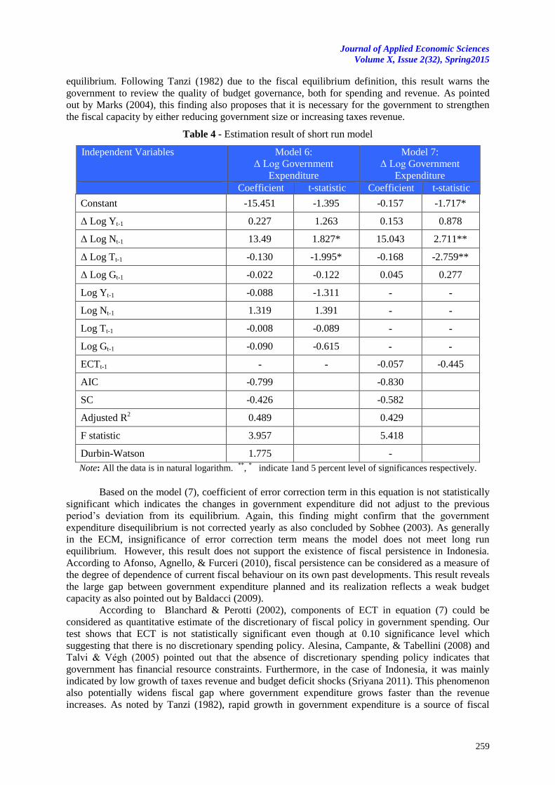
Journal of Applied Economic Sciences
Volume X, Issue 2(32), Spring2015
259
equilibrium. Following Tanzi (1982) due to the fiscal equilibrium definition, this result warns the
government to review the quality of budget governance, both for spending and revenue. As pointed
out by Marks (2004), this finding also proposes that it is necessary for the government to strengthen
the fiscal capacity by either reducing government size or increasing taxes revenue.
Table 4 - Estimation result of short run model
Independent Variables Model 6:
Δ Log Government
Expenditure
Model 7:
Δ Log Government
Expenditure
Coefficient t-statistic Coefficient t-statistic
Constant -15.451 -1.395 -0.157 -1.717*
Δ Log Yt-1 0.227 1.263 0.153 0.878
Δ Log Nt-1 13.49 1.827* 15.043 2.711**
Δ Log Tt-1 -0.130 -1.995* -0.168 -2.759**
Δ Log Gt-1 -0.022 -0.122 0.045 0.277
Log Yt-1 -0.088 -1.311 - -
Log Nt-1 1.319 1.391 - -
Log Tt-1 -0.008 -0.089 - -
Log Gt-1 -0.090 -0.615 - -
ECTt-1 - - -0.057 -0.445
AIC -0.799 -0.830
SC -0.426 -0.582
Adjusted R2 0.489 0.429
F statistic 3.957 5.418
Durbin-Watson 1.775 -
Note: All the data is in natural logarithm. **
, * indicate 1and 5 percent level of significances respectively.
Based on the model (7), coefficient of error correction term in this equation is not statistically
significant which indicates the changes in government expenditure did not adjust to the previous
period’s deviation from its equilibrium. Again, this finding might confirm that the government
expenditure disequilibrium is not corrected yearly as also concluded by Sobhee (2003). As generally
in the ECM, insignificance of error correction term means the model does not meet long run
equilibrium. However, this result does not support the existence of fiscal persistence in Indonesia.
According to Afonso, Agnello, & Furceri (2010), fiscal persistence can be considered as a measure of
the degree of dependence of current fiscal behaviour on its own past developments. This result reveals
the large gap between government expenditure planned and its realization reflects a weak budget
capacity as also pointed out by Baldacci (2009).
According to Blanchard & Perotti (2002), components of ECT in equation (7) could be
considered as quantitative estimate of the discretionary of fiscal policy in government spending. Our
test shows that ECT is not statistically significant even though at 0.10 significance level which
suggesting that there is no discretionary spending policy. Alesina, Campante, & Tabellini (2008) and
Talvi Végh (2005) pointed out that the absence of discretionary spending policy indicates that
government has financial resource constraints. Furthermore, in the case of Indonesia, it was mainly
indicated by low growth of taxes revenue and budget deficit shocks (Sriyana 2011). This phenomenon
also potentially widens fiscal gap where government expenditure grows faster than the revenue
increases. As noted by Tanzi (1982), rapid growth in government expenditure is a source of fiscal
Journal of Applied Economic Sciences Volume X, Issue 2 (32) Spring 2015
260
disequilibrium. Furthermore, this finding confirms the existence of long run fiscal disequilibrium in
Indonesia.
This estimation results exhibit that changes in population will lead to an increase in
government spending in the short run, while an increase in output does not play an important role in
determining government expenditure. In the case of Indonesia, lagged tax variable has negative
coefficient which indicates that as tax revenue rises, it lowers government expenditure growth. This is
suspected that an increase in tax revenue was not allocated into productive projects thereby potentially
creating fiscal imbalance. This is a main problem in fiscal management as a result of fiscal
disequilibrium. In other words, the fiscal capacity may be threatened in the future. It could be inferred
that government should aware of fiscal disequilibrium threat that may caused by government
expenditure growth in the next years. The government will potentially have a smaller capacity to
finance its spending for both operating and development activities. Prudent fiscal policies to increase
the tax ratio are rational option rather than cutting government spending.
Concluding remarks
This study attempts to provide an alternative evidence of fiscal equilibrium analysis in
Indonesia. For this purpose, in this research we intend to extend the modelling of government
expenditure using error correction model. The short run empirical model shows that population and
tax revenue are statistically significant in affecting government expenditure change. In addition,
changes in government expenditure did not adjust to the previous period’s deviation from its
equilibrium. This finding confirms that the government expenditure disequilibrium is not corrected
yearly. However, this study does not support the existence of fiscal persistence and discretionary
spending policy. The absence of discretionary spending policy indicates that government has financial
resource constraints.
This finding explains an intensive effect of population change on government expenditure
growth. This study also informs that lagged tax variable has negative correlation with government
expenditure growth. This is suspected that increase in tax revenue potentially creates fiscal imbalance.
Furthermore, this finding reveals the existence of fiscal disequilibrium in Indonesia. This is a main
problem in fiscal management that arises from rapid growth in government expenditure. The
government should avoid more severe fiscal disequilibrium threat in the next years by increasing tax
ratio. Furthermore, this study considers increasing taxes revenue than reviewing size of government
expenditure. Some alternative policies such as strengthening government institution and improving the
bureaucracy capacity are more rational than government size.
Acknowledgment:
The author would like to thank Directorate General of Higher Education, The Ministry of
Education and Cultural, Republic of Indonesia for the Stranas Research Grant in 2012.
References
[1] Afonso, A., Agnello, L., Furceri, D. 2010. Fiscal Policy Responsiveness, Persistence, and
Discretion. Public Choice 145(3): 503–30.
[2] Alesina, A., Campante, F., Tabellini, G. 2008. Why is Fiscal Policy often Pro-cyclical. Journal of
the European Economic Association 6(5): 1006–36.
[3] Auerbach, A.J. 2011. Long-Term Fiscal Sustainability in Major Economies. In BIS Working Paper
Series (p. No.361). http://dx.doi.org/10.2139/ssrn.1971166
[4] Baghestani, H., McNown, R. 1994. Do revenues or expenditures respond to budgetary
disequilibria? Southern Economic Journal 61(2): 311–322.
[5] Baldacci, E. 2009. Neither Sailing Against the Wind, nor Going with the Flow: Cyclicality of
Fiscal Policy in Indonesia. In IMF Country Report (p. No. 09/231).
[6] Blanchard, O., Perotti, R. 2002. An Empirical Characterization of the Dynamic Effects of Changes
in Government Spending and Taxes on Output. Quarterly Journal of Economics 117(4): 1329–68.
Journal of Applied Economic Sciences
Volume X, Issue 2(32), Spring2015
261
[7] Ekinci, A. 2011. What Is The Optimum Size of Government: A Suggestion References.
International Journal of Economics and Finance Studies 3(1): 45–54.
[8] Engle, R.F., Granger, C.W.J. 1987. Co-Integration and Error Correction: Representation,
Estimation, and Testing. Econometrica 55(2): 251–76.
[9] Ghartey, E.E. 2010. Government expenditures and revenues causation: some Caribbean empirical
evidence. Applied Econometrics and International Development 10(2): 149–165.
[10] Ghosh, S., Gregoriou, A. 2008. The composition of government spending and growth: is current
or capital spending better? Oxford Economic Papers 60(3): 484–516.
[11] Hall, R.E. 2009. By How Much Does GDP Rise if the Government Buys More Output?
Brookings Papers on Economic Activity 2:183–231.
[12] Johansen, S. 1991. Estimation and Hypothesis Testing of Cointegration Vectors in Gaussian
Vector Autoregressive Models. Econometrica 59(6): 1551–1580.
[13] Marks, S.V. 2004. Fiscal sustainability and solvency: theory and recent experience in Indonesia.
Bulletin of Indonesian Economic Studies 40(2): 227–242. http://dx.doi.org/10.1080/
0007491042000205295
[14] Narayan, P.K., Narayan, S. 2006. Government revenue and government expenditure nexus:
evidence from developing countries. Applied Economics, 38(3): 285–291.
[15] Nurudeen, A., Usman, A. 2010. Government expenditure and economic growth in Nigeria.
Business and Economics Journal 4(1): 1–11.
[16] Ramey, V.A. 2011. Identifying Government Shocks: It’s All in the Timing. Quarterly Journal
of Economics 126(1): 1–50.
[17] Ratha, A. 2012. Twin Deficits or Distant Cousins? Evidence from India. South Asia Economic
Journal 13(1): 51–68. http://dx.doi.org/10.1177/139156141101300103
[18] Saeed, S., Khan, M.A. 2012. Twin deficits hypothesis : the case of Pakistan 19 2-2008.
International Journal of Economics, Commerce and Research 2(1): 11–25.
[19] Saleh, A. S., Nair, M. 2006. The twin deficits phenomena in Philippines: An empirical
investigation. International Journal of Economic Research 3(2): 165–179.
[20] Schaltegger, C. A., Torgler, B. 2006. Growth effects of public expenditure on the state and local
level: evidence from a sample of rich governments. Applied Economics 38(10): 1181–1192.
[21] Sobhee, S. K. 2003. An Error Correction Model of the Median Voter ’ s Demand for Public
Goods in Mauritius. Economic Issues 8(1972): 47–61.
[22] Sriyana, J. 2011. The Effect of Budget Deficit Shock on Government Spending: An Empirical
Case in Indonesia. International Journal of Business and Development Studies 3(1): 41–58.
[23] Talvi, E., Végh, C. 2005. Tax Base Variability and Pro-cyclical Fiscal Policy. Journal of
Economic Development 78(1): 156–90.
[24] Tanzi, V. 1982. Fiscal disequilibrium in developing countries. World Development 10(12):
1069–1082. http://dx.doi.org/10.1016/0305-750X(82)90019-5.
[25] Tsaurai, K., Odhiambo, N.M. 2013. Government expenditure and economic growth in
Zimbabwe : an ARDL-bounds testing approach. Int. J. Economic Policy in Emerging Economies
6(1): 78–90.
Journal of Applied Economic Sciences Volume X, Issue 2 (32) Spring 2015
262
THE PERFORMANCES ASSESSMENT - ASSESSMENT METHODS AND TECHNIQUES OF THE PROFESSIONAL PERFORMANCES
Loredana VĂCĂRESCU HOBEANU
Faculty of Financial Management Accounting Craiova
Spiru Haret University, Romania
Abstract: The human resources management requires the continuous improvement of the employees ' activity in
order to achieve the mission and organizational goals The advantageous use of the human resources
management presupposes the existence of a system of performances assessment, of a system of the employees’
boost and of a reward results system. The professional performances assessment of the company staff is a
concern of the human resources management, with the multiple implications on all the other activities of the
organization, influencing in a considerable measure the organizational climate, because with the help of this
there can be determined the degree to which its employees achieve their responsibilities.
The need to appreciate the employees’ professional performances generated the elaboration of the
multiple methods and techniques of staff appreciation and gave birth to the systems of the performances
assessment. More and more organizations are currently aware that they must have implemented their own
professional performances assessment system for the employees.
Keywords: assessment methods, criteria, professional performances, organization, human resources, employees
JEL classification: M 54, M53
1. Introduction
Professional performances assessment of employees of an organization is an activity of the
human resources management which is a spreading increasingly wider area, becoming a strategic
activity in the process management of the human resources.
Professional performances assessment of employees from an organizational system constitutes
an act of great responsibility, as it is the basis for the adoption of the strategic decisions affecting the
future evolution of the entire system. From here, the need to use the most appropriate assessment
methods and techniques arises, and the use of honest assessors to capture more accurately the actual
situation of the assessed field.
Performances assessment should be undertaken as well as there would be expected of an
institution activity, the juncture evolution of the economy is accompanied by numerous processes of
change affecting, under quantitative and qualitative report the institution staff. These changes require a
continuous assessment process of the results of the staff activity on chian of the entire existential flow
of the human resources from the institution, starting from recruitment, evolution on hierachical scale
taking into account the professional performances and the motivation according to the obtained results.
Knowing the carried out performances means a real understanding of the way how the tasks
are met, how there is given the efficiency at work, it gives the confidence in self forces, constituting a
mobilizer factor, a positive attitude towards the work.
Through the professional performances assessment there is established the reached level of the
individual or group, at the analysis moment, giving the possibility of adoptions of decisions regarding
the continuous improvement of it.
The purpose of the assessment is to assist in the taking of decisions that affects the individuals,
decisions that should have an objective and fair foundation. The need for this activity is dictated by:
the structural analysis and expression, determining the deviations from the goals and carrying out the
necessary corrections, determining the directions and improvement procedures for the staff training,
the reduction of the risks resulting from the maintenance and promotion of incompetent people, a
better allocation of workers on the job, a fair wage, an increase in the competitive ability of the
institution.
Over time, due to the need to evaluate the staff and its performance, there were developed
various methods and techniques of assessment. As a result, a variety of techniques, processes, methods
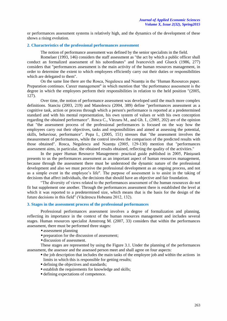
Journal of Applied Economic Sciences
Volume X, Issue 2(32), Spring2015
263
or performances assessment systems is relatively high, and the dynamics of the development of these
shows a rising evolution.
2. Characteristics of the professional performances assessment
The notion of performance assessment was defined by the senior specialists in the field.
Romelaer (1993, 146) considers the staff assessment as "the act by which a public officer shall
conduct an formalized assessment of his subordinates" and Ivancevich and Glueck (1986, 277)
considers that "performances assessment is the main activity of the human resources management, in
order to determine the extent to which employees efficiently carry out their duties or responsibilities
which are delegated to them".
On the same line there are the Rosca, Negulescu and Neamţu in the ‘Human Resources paper.
Preparation continues. Career management" in which mention that ‘the performance assessment is the
degree in which the employees perform their responsibilities in relation to the held position "(2005,
127).
Over time, the notion of performance assessment was developed until the much more complex
definitions. Stanciu (2003, 219) and Manolescu (2004, 389) define "performances assessment as a
cognitive task, action or process through which a person's performance is reported at a predetermined
standard and with his mental representation, his own system of values or with his own conception
regarding the obtained performance". Rosca C., Vărzaru M., and Gh. I., (2005, 202) are of the opinion
that "the assessment process of the professional performances is focused on the way how the
employees carry out their objectives, tasks and responsibilities and aimed at assessing the potential,
skills, behaviour, performance". Popa I., (2005, 151) stresses that "the assessment involves the
measurement of performances, while the control involves the comparison of the predicted results with
those obtained". Rosca, Negulescu and Neamţu (2005, 129-130) mention that "performances
assessment aims, in particular, the obtained results obtained, reflecting the quality of the activities."
In the paper Human Resource Management- practical guide published in 2005, Pânişoară
presents to us the performances assessment as an important aspect of human resources management,
because through the assessment there must be understood the dynamic nature of the professional
development and also we must perceive the professional development as an ongoing process, and not
as a simple event in the employee’s life". The purpose of assessment is to assist in the taking of
decisions that affect individuals, the decisions that should have an objective and fair foundation.
“The diversity of views related to the performances assessment of the human resources do not
fit but supplement one another. Through the performances assessment there is established the level at
which it was reported to a predetermined size, which means that is the basis for the design of the
future decisions in this field” (Văcărescu Hobeanu 2012, 132).
3. Stages in the assessment process of the professional performances
Professional performances assessment involves a degree of formalization and planning,
reflecting its importance in the context of the human resources management and includes several
stages. Human resources specialist Amstrong M. (2007, 33) considers that within the performances
assessment, there must be performed three stages:
assessment planning
preparation for the discussion of assessment;
discussion of assessment.
These stages are represented by using the Figure 3.1. Under the planning of the performances
assessment, the assessor and the assessed person meet and shall agree on four aspects:
the job description that includes the main tasks of the employee job and within the actions in
limits in which this is responsible for getting results;
defining the objectives and standards;
establish the requirements for knowledge and skills;
defining expectations of competence.
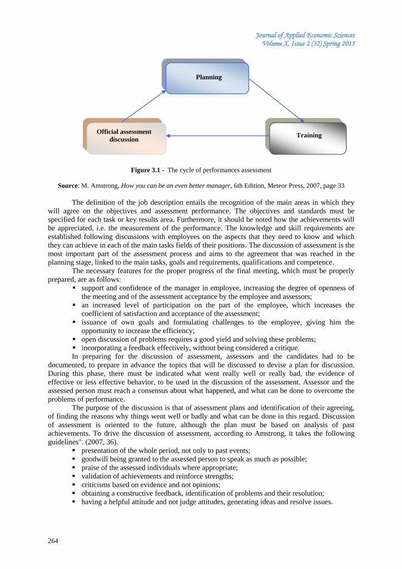
Journal of Applied Economic Sciences Volume X, Issue 2 (32) Spring 2015
264
Figure 3.1 - The cycle of performances assessment
Source: M. Amstrong, How you can be an even better manager, 6th Edition, Meteor Press, 2007, page 33
The definition of the job description entails the recognition of the main areas in which they
will agree on the objectives and assessment performance. The objectives and standards must be
specified for each task or key results area. Furthermore, it should be noted how the achievements will
be appreciated, i.e. the measurement of the performance. The knowledge and skill requirements are
established following discussions with employees on the aspects that they need to know and which
they can achieve in each of the main tasks fields of their positions. The discussion of assessment is the
most important part of the assessment process and aims to the agreement that was reached in the
planning stage, linked to the main tasks, goals and requirements, qualifications and competence.
The necessary features for the proper progress of the final meeting, which must be properly
prepared, are as follows:
support and confidence of the manager in employee, increasing the degree of openness of
the meeting and of the assessment acceptance by the employee and assessors;
an increased level of participation on the part of the employee, which increases the
coefficient of satisfaction and acceptance of the assessment;
issuance of own goals and formulating challenges to the employee, giving him the
opportunity to increase the efficiency;
open discussion of problems requires a good yield and solving these problems;
incorporating a feedback effectively, without being considered a critique.
In preparing for the discussion of assessment, assessors and the candidates had to be
documented, to prepare in advance the topics that will be discussed to devise a plan for discussion.
During this phase, there must be indicated what went really well or really bad, the evidence of
effective or less effective behavior, to be used in the discussion of the assessment. Assessor and the
assessed person must reach a consensus about what happened, and what can be done to overcome the
problems of performance.
The purpose of the discussion is that of assessment plans and identification of their agreeing,
of finding the reasons why things went well or badly and what can be done in this regard. Discussion
of assessment is oriented to the future, although the plan must be based on analysis of past
achievements. To drive the discussion of assessment, according to Amstrong, it takes the following
guidelines". (2007, 36).
presentation of the whole period, not only to past events;
goodwill being granted to the assessed person to speak as much as possible;
praise of the assessed individuals where appropriate;
validation of achievements and reinforce strengths;
criticisms based on evidence and not opinions;
obtaining a constructive feedback, identification of problems and their resolution;
having a helpful attitude and not judge attitudes, generating ideas and resolve issues.
Planning
Training Official assessment
discussion
Journal of Applied Economic Sciences
Volume X, Issue 2(32), Spring2015
265
In the report drawn up by the assessor there will be pointed out the strengths and weaknesses
as well as suggestions for personal development. The development plan targets two issues: improved
efficiency of the employee on the held position and the preparation of staff for promotion. In addition
to the development plan, the discussion must include assessment and fixing of performance objectives
for the next period, which should be clear and achievable, supported by assessed.
At the end of the discussion, the assessment report shall be drawn up, based on the information
obtained during the course of the discussion, which must contain: the performance feedback obtained
on the current post and it gives information about the strengths and weaknesses of employees, to
include the objectives of the future and the possibilities of development. The assessment of the
activity, when it is done properly and objectively, constitutes a useful tool for improving the
employees’ performances.
4. Basic methods and techniques of professional performances assessment
The quality of determinations related to performance depends largely on the quality of the
methods or systems of assessment which are different depending on the wished goal.
There are two categories of evaluative methods means: objective and subjective methods. In
the category of objective methods included tests of knowledge or evidence of professional competence
to assess the quality of the professional activity and results in terms of final product for the assessment
skills.
The methods are based on subjective opinions, assessments of significant individuals close to
the assessed person. In this category there are: scales/graphic assessment rubrics, checklists, ordering
through the employees comparison the forced choice, paired comparison, through the method of
forced distribution. The choice of method depends on the purpose of assessment, the importance of the
approach, the available time/resources.
The diversity of methods, techniques, procedures or systems of performance assessment is
great, and the dynamics of their development has seen a growing trend. The period for performance
assessment is of few months until a year. The assessment shall be to the entire performance at work,
either to one or more aspects of the performance.
Lefter et al. noted that "there is no ideal procedure, the used performances assessment, the
methods and the techniques are the expression of certain factors that influence the performance
assessment scheme, such as: the history and culture of the organization; the size of the organization
and scope of work; strategic guidelines; practices used to the staff employment, remuneration and
promotion of staff; work environment "(Lefter V, Deaconu A, Marinaş C, Puia R 2008, 248).
According to Manolescu "the necessity of staff assessment or of performances assessment in
the workplace, regardless of their field of activity, led, ultimately, to the development of numerous
methods and techniques for assessing the staff or to the apparition of the performances assessment
systems. Thus, an attempt was made to answer, in fact, not only to some questions about why we
assess or who should make the performance assessment, but also to the question: "what are the
specific methods and techniques or the most appropriate performances assessment systems?"
(Manolescu A. 2004, 42).
Matis, Nica and Rusu say "the quality of the determinations related to performance depends
largely on the quality of the methods or systems of assessment which are different depending on the
purpose, which implies:
the validity of the results;
fidelity of the determinations;
equivalence of the results;
internal homogeneity;
the sensitivity of the used instruments (Mathis R. L., Nica P., Rusu C. 1997, 181-189).
These authors show through Table 4.1 a classification of methods of the performances
assessment.
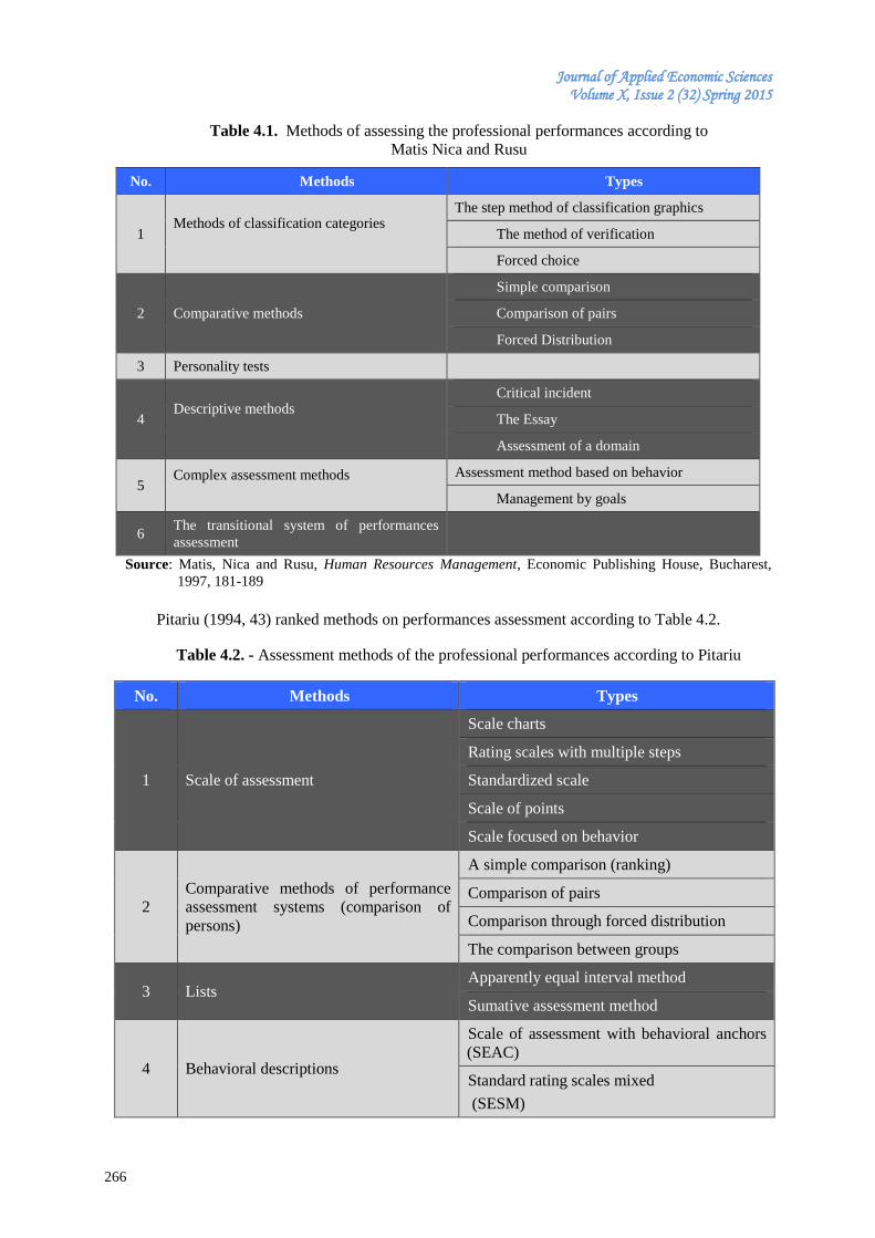
Journal of Applied Economic Sciences Volume X, Issue 2 (32) Spring 2015
266
Table 4.1. Methods of assessing the professional performances according to
Matis Nica and Rusu
No. Methods Types
1 Methods of classification categories
The step method of classification graphics
The method of verification
Forced choice
2 Comparative methods
Simple comparison
Comparison of pairs
Forced Distribution
3 Personality tests
4 Descriptive methods
Critical incident
The Essay
Assessment of a domain
5 Complex assessment methods
Assessment method based on behavior
Management by goals
6 The transitional system of performances
assessment
Source: Matis, Nica and Rusu, Human Resources Management, Economic Publishing House, Bucharest,
1997, 181-189
Pitariu (1994, 43) ranked methods on performances assessment according to Table 4.2.
Table 4.2. - Assessment methods of the professional performances according to Pitariu
No. Methods Types
1 Scale of assessment
Scale charts
Rating scales with multiple steps
Standardized scale
Scale of points
Scale focused on behavior
2
Comparative methods of performance
assessment systems (comparison of
persons)
A simple comparison (ranking)
Comparison of pairs
Comparison through forced distribution
The comparison between groups
3 Lists Apparently equal interval method
Sumative assessment method
4 Behavioral descriptions
Scale of assessment with behavioral anchors
(SEAC)
Standard rating scales mixed
(SESM)
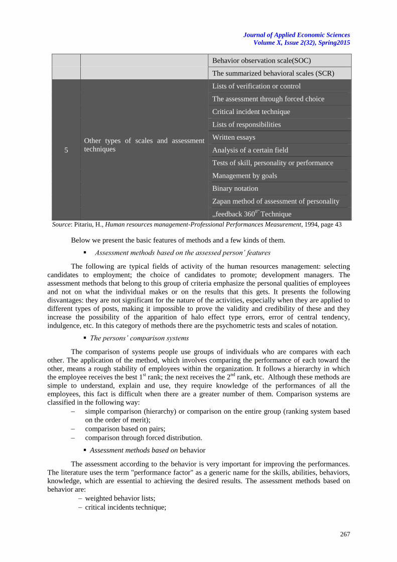
Journal of Applied Economic Sciences
Volume X, Issue 2(32), Spring2015
267
Behavior observation scale(SOC)
The summarized behavioral scales (SCR)
5
Other types of scales and assessment
techniques
Lists of verification or control
The assessment through forced choice
Critical incident technique
Lists of responsibilities
Written essays
Analysis of a certain field
Tests of skill, personality or performance
Management by goals
Binary notation
Zapan method of assessment of personality
„feedback 3600”
Technique
Source: Pitariu, H., Human resources management-Professional Performances Measurement, 1994, page 43
Below we present the basic features of methods and a few kinds of them.
Assessment methods based on the assessed person’ features
The following are typical fields of activity of the human resources management: selecting
candidates to employment; the choice of candidates to promote; development managers. The
assessment methods that belong to this group of criteria emphasize the personal qualities of employees
and not on what the individual makes or on the results that this gets. It presents the following
disvantages: they are not significant for the nature of the activities, especially when they are applied to
different types of posts, making it impossible to prove the validity and credibility of these and they
increase the possibility of the apparition of halo effect type errors, error of central tendency,
indulgence, etc. In this category of methods there are the psychometric tests and scales of notation.
The persons’ comparison systems
The comparison of systems people use groups of individuals who are compares with each
other. The application of the method, which involves comparing the performance of each toward the
other, means a rough stability of employees within the organization. It follows a hierarchy in which
the employee receives the best 1st rank; the next receives the 2
nd rank, etc. Although these methods are
simple to understand, explain and use, they require knowledge of the performances of all the
employees, this fact is difficult when there are a greater number of them. Comparison systems are
classified in the following way:
simple comparison (hierarchy) or comparison on the entire group (ranking system based
on the order of merit);
comparison based on pairs;
comparison through forced distribution.
Assessment methods based on behavior
The assessment according to the behavior is very important for improving the performances.
The literature uses the term "performance factor" as a generic name for the skills, abilities, behaviors,
knowledge, which are essential to achieving the desired results. The assessment methods based on
behavior are:
weighted behavior lists;
critical incidents technique;
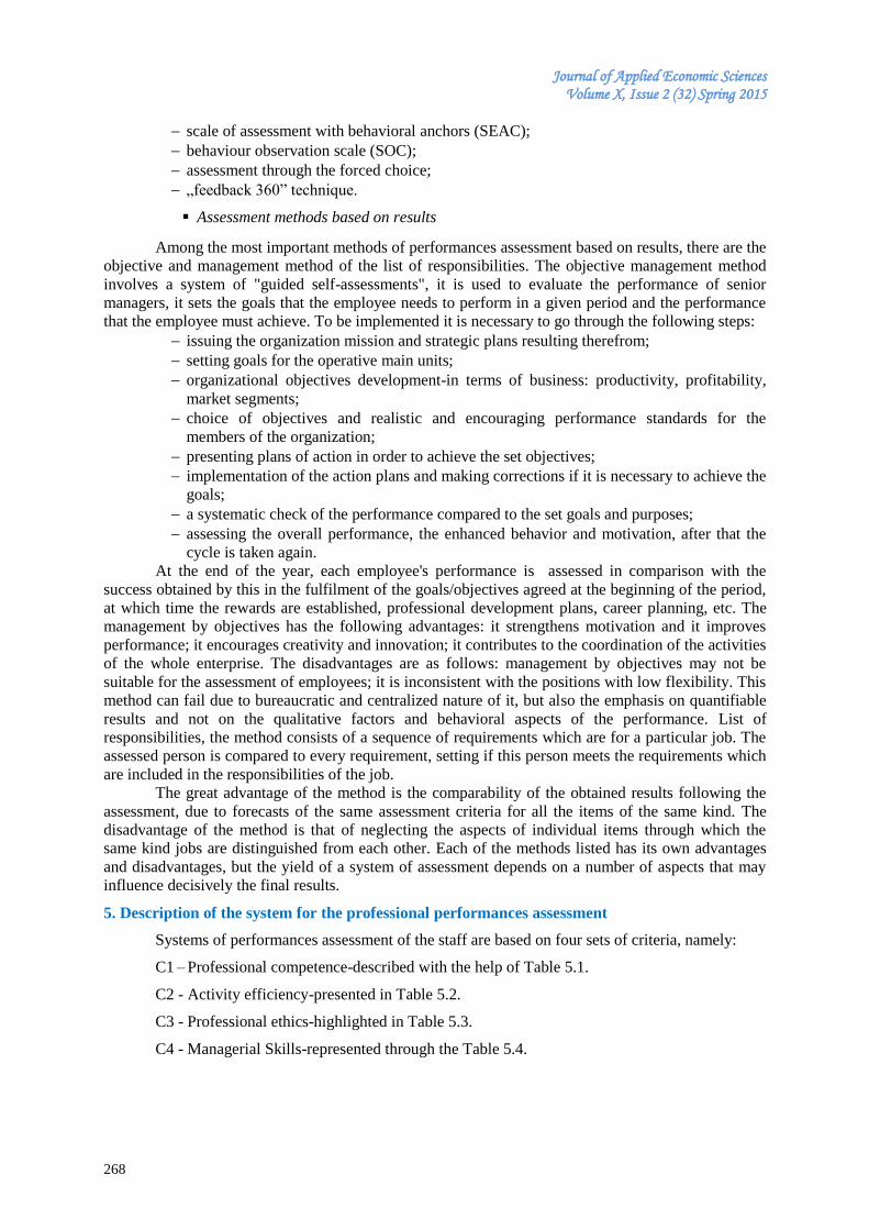
Journal of Applied Economic Sciences Volume X, Issue 2 (32) Spring 2015
268
scale of assessment with behavioral anchors (SEAC);
behaviour observation scale (SOC);
assessment through the forced choice;
„feedback 360” technique.
Assessment methods based on results
Among the most important methods of performances assessment based on results, there are the
objective and management method of the list of responsibilities. The objective management method
involves a system of "guided self-assessments", it is used to evaluate the performance of senior
managers, it sets the goals that the employee needs to perform in a given period and the performance
that the employee must achieve. To be implemented it is necessary to go through the following steps:
issuing the organization mission and strategic plans resulting therefrom;
setting goals for the operative main units;
organizational objectives development-in terms of business: productivity, profitability,
market segments;
choice of objectives and realistic and encouraging performance standards for the
members of the organization;
presenting plans of action in order to achieve the set objectives;
implementation of the action plans and making corrections if it is necessary to achieve the
goals;
a systematic check of the performance compared to the set goals and purposes;
assessing the overall performance, the enhanced behavior and motivation, after that the
cycle is taken again.
At the end of the year, each employee's performance is assessed in comparison with the
success obtained by this in the fulfilment of the goals/objectives agreed at the beginning of the period,
at which time the rewards are established, professional development plans, career planning, etc. The
management by objectives has the following advantages: it strengthens motivation and it improves
performance; it encourages creativity and innovation; it contributes to the coordination of the activities
of the whole enterprise. The disadvantages are as follows: management by objectives may not be
suitable for the assessment of employees; it is inconsistent with the positions with low flexibility. This
method can fail due to bureaucratic and centralized nature of it, but also the emphasis on quantifiable
results and not on the qualitative factors and behavioral aspects of the performance. List of
responsibilities, the method consists of a sequence of requirements which are for a particular job. The
assessed person is compared to every requirement, setting if this person meets the requirements which
are included in the responsibilities of the job.
The great advantage of the method is the comparability of the obtained results following the
assessment, due to forecasts of the same assessment criteria for all the items of the same kind. The
disadvantage of the method is that of neglecting the aspects of individual items through which the
same kind jobs are distinguished from each other. Each of the methods listed has its own advantages
and disadvantages, but the yield of a system of assessment depends on a number of aspects that may
influence decisively the final results.
5. Description of the system for the professional performances assessment
Systems of performances assessment of the staff are based on four sets of criteria, namely:
C1 – Professional competence-described with the help of Table 5.1.
C2 - Activity efficiency-presented in Table 5.2.
C3 - Professional ethics-highlighted in Table 5.3.
C4 - Managerial Skills-represented through the Table 5.4.
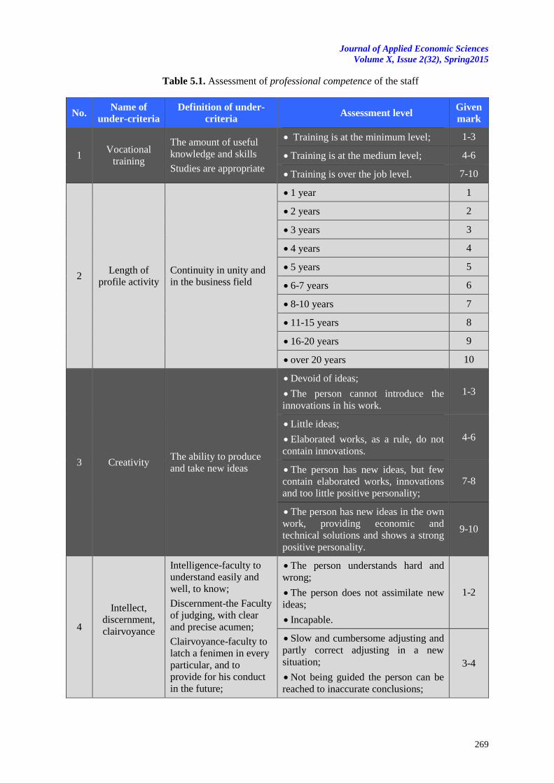
Journal of Applied Economic Sciences
Volume X, Issue 2(32), Spring2015
269
Table 5.1. Assessment of professional competence of the staff
No. Name of
under-criteria
Definition of under-
criteria Assessment level
Given
mark
1 Vocational
training
The amount of useful
knowledge and skills
Studies are appropriate
Training is at the minimum level; 1-3
Training is at the medium level; 4-6
Training is over the job level. 7-10
2 Length of
profile activity
Continuity in unity and
in the business field
1 year 1
2 years 2
3 years 3
4 years 4
5 years 5
6-7 years 6
8-10 years 7
11-15 years 8
16-20 years 9
over 20 years 10
3 Creativity The ability to produce
and take new ideas
Devoid of ideas;
The person cannot introduce the
innovations in his work.
1-3
Little ideas;
Elaborated works, as a rule, do not
contain innovations.
4-6
The person has new ideas, but few
contain elaborated works, innovations
and too little positive personality;
7-8
The person has new ideas in the own
work, providing economic and
technical solutions and shows a strong
positive personality.
9-10
4
Intellect,
discernment,
clairvoyance
Intelligence-faculty to
understand easily and
well, to know;
Discernment-the Faculty
of judging, with clear
and precise acumen;
Clairvoyance-faculty to
latch a fenimen in every
particular, and to
provide for his conduct
in the future;
The person understands hard and
wrong;
The person does not assimilate new
ideas;
Incapable.
1-2
Slow and cumbersome adjusting and
partly correct adjusting in a new
situation;
Not being guided the person can be
reached to inaccurate conclusions;
3-4
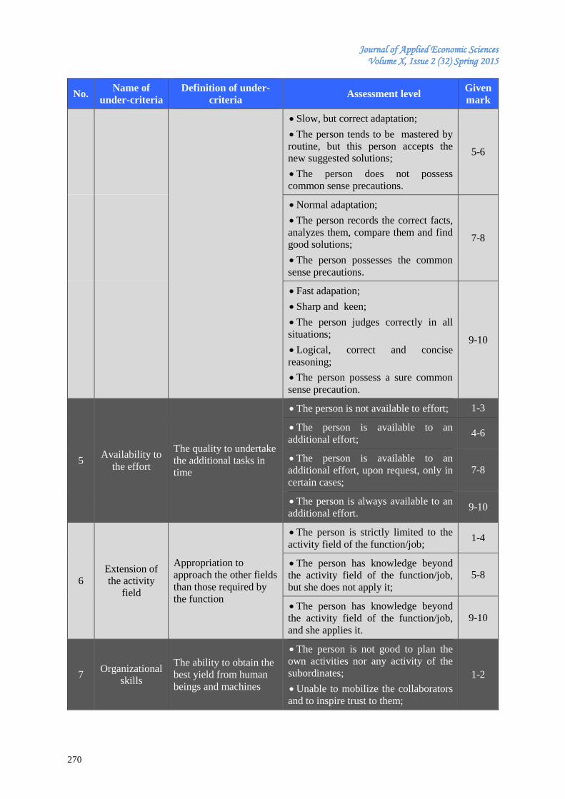
Journal of Applied Economic Sciences Volume X, Issue 2 (32) Spring 2015
270
No. Name of
under-criteria
Definition of under-
criteria Assessment level
Given
mark
Slow, but correct adaptation;
The person tends to be mastered by
routine, but this person accepts the
new suggested solutions;
The person does not possess
common sense precautions.
5-6
Normal adaptation;
The person records the correct facts,
analyzes them, compare them and find
good solutions;
The person possesses the common
sense precautions.
7-8
Fast adapation;
Sharp and keen;
The person judges correctly in all
situations;
Logical, correct and concise
reasoning;
The person possess a sure common
sense precaution.
9-10
5 Availability to
the effort
The quality to undertake
the additional tasks in
time
The person is not available to effort; 1-3
The person is available to an
additional effort; 4-6
The person is available to an
additional effort, upon request, only in
certain cases;
7-8
The person is always available to an
additional effort. 9-10
6
Extension of
the activity
field
Appropriation to
approach the other fields
than those required by
the function
The person is strictly limited to the
activity field of the function/job; 1-4
The person has knowledge beyond
the activity field of the function/job,
but she does not apply it;
5-8
The person has knowledge beyond
the activity field of the function/job,
and she applies it.
9-10
7 Organizational
skills
The ability to obtain the
best yield from human
beings and machines
The person is not good to plan the
own activities nor any activity of the
subordinates;
Unable to mobilize the collaborators
and to inspire trust to them;
1-2
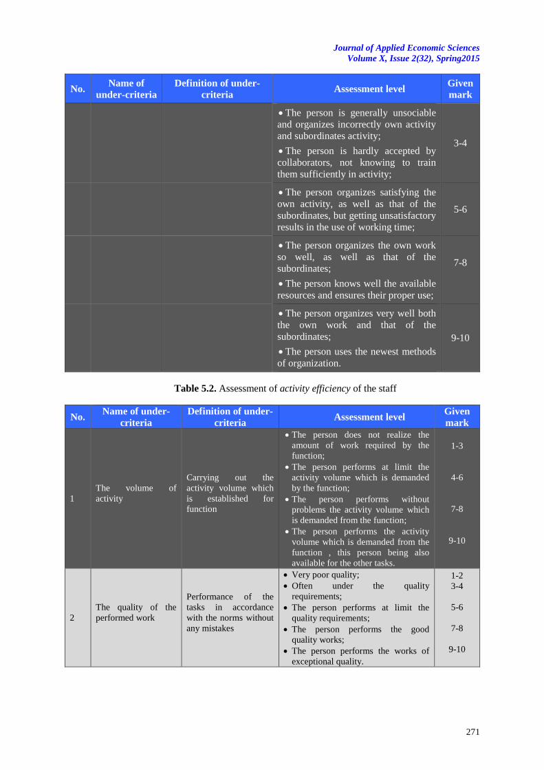
Journal of Applied Economic Sciences
Volume X, Issue 2(32), Spring2015
271
No. Name of
under-criteria
Definition of under-
criteria Assessment level
Given
mark
The person is generally unsociable
and organizes incorrectly own activity
and subordinates activity;
The person is hardly accepted by
collaborators, not knowing to train
them sufficiently in activity;
3-4
The person organizes satisfying the
own activity, as well as that of the
subordinates, but getting unsatisfactory
results in the use of working time;
5-6
The person organizes the own work
so well, as well as that of the
subordinates;
The person knows well the available
resources and ensures their proper use;
7-8
The person organizes very well both
the own work and that of the
subordinates;
The person uses the newest methods
of organization.
9-10
Table 5.2. Assessment of activity efficiency of the staff
No. Name of under-
criteria
Definition of under-
criteria Assessment level
Given
mark
1
The volume of
activity
Carrying out the
activity volume which
is established for
function
The person does not realize the
amount of work required by the
function;
The person performs at limit the
activity volume which is demanded
by the function;
The person performs without
problems the activity volume which
is demanded from the function;
The person performs the activity
volume which is demanded from the
function , this person being also
available for the other tasks.
1-3
4-6
7-8
9-10
2
The quality of the
performed work
Performance of the
tasks in accordance
with the norms without
any mistakes
Very poor quality;
Often under the quality
requirements;
The person performs at limit the
quality requirements;
The person performs the good
quality works;
The person performs the works of
exceptional quality.
1-2
3-4
5-6
7-8
9-10
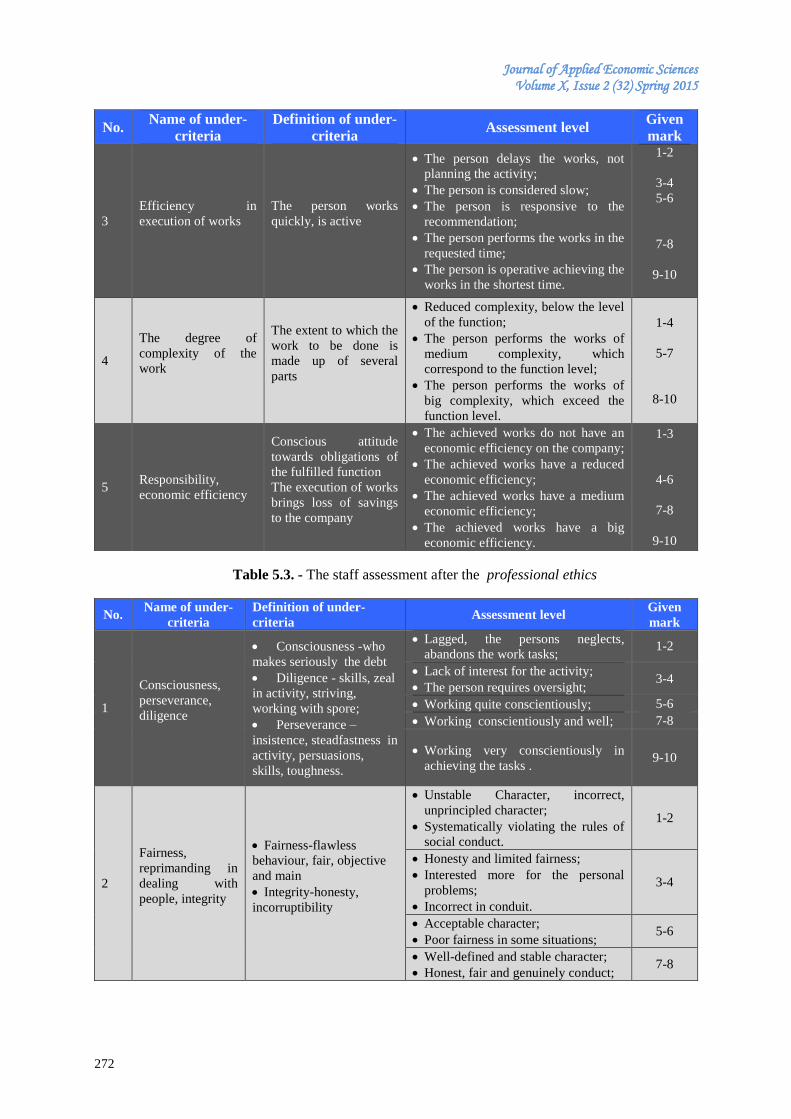
Journal of Applied Economic Sciences Volume X, Issue 2 (32) Spring 2015
272
No. Name of under-
criteria
Definition of under-
criteria Assessment level
Given
mark
3
Efficiency in
execution of works
The person works
quickly, is active
The person delays the works, not
planning the activity;
The person is considered slow;
The person is responsive to the
recommendation;
The person performs the works in the
requested time;
The person is operative achieving the
works in the shortest time.
1-2
3-4
5-6
7-8
9-10
4
The degree of
complexity of the
work
The extent to which the
work to be done is
made up of several
parts
Reduced complexity, below the level
of the function;
The person performs the works of
medium complexity, which
correspond to the function level;
The person performs the works of
big complexity, which exceed the
function level.
1-4
5-7
8-10
5 Responsibility,
economic efficiency
Conscious attitude
towards obligations of
the fulfilled function
The execution of works
brings loss of savings
to the company
The achieved works do not have an
economic efficiency on the company;
The achieved works have a reduced
economic efficiency;
The achieved works have a medium
economic efficiency;
The achieved works have a big
economic efficiency.
1-3
4-6
7-8
9-10
Table 5.3. - The staff assessment after the professional ethics
No. Name of under-
criteria
Definition of under-
criteria Assessment level
Given
mark
1
Consciousness,
perseverance,
diligence
Consciousness -who
makes seriously the debt
Diligence - skills, zeal
in activity, striving,
working with spore;
Perseverance –
insistence, steadfastness in
activity, persuasions,
skills, toughness.
Lagged, the persons neglects,
abandons the work tasks; 1-2
Lack of interest for the activity;
The person requires oversight; 3-4
Working quite conscientiously; 5-6
Working conscientiously and well; 7-8
Working very conscientiously in
achieving the tasks . 9-10
2
Fairness,
reprimanding in
dealing with
people, integrity
Fairness-flawless
behaviour, fair, objective
and main
Integrity-honesty,
incorruptibility
Unstable Character, incorrect,
unprincipled character;
Systematically violating the rules of
social conduct.
1-2
Honesty and limited fairness;
Interested more for the personal
problems;
Incorrect in conduit.
3-4
Acceptable character;
Poor fairness in some situations; 5-6
Well-defined and stable character;
Honest, fair and genuinely conduct; 7-8
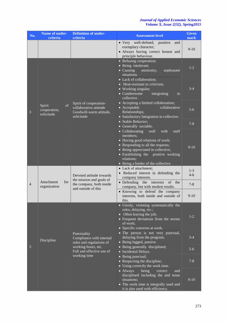
Journal of Applied Economic Sciences
Volume X, Issue 2(32), Spring2015
273
No. Name of under-
criteria
Definition of under-
criteria Assessment level
Given
mark
Very well-defined, positive and
exemplary character;
Always having correct honest and
principle behaviour.
9-10
3
Spirit of
cooperation,
solicitude
Spirit of cooperation-
collaborative attitude
Goodwill-warm attitude,
solicitude
Refusing cooperation;
Being intolerant;
Causing animosity, unpleasant
situations.
1-2
Lack of collaboration;
Heat-resistant to criticism;
Working singular;
Cumbersome integrating in
collective .
3-4
Accepting a limited collaboration;
Acceptable collaborative
Relationships;
Satisfactory Integration in collective.
5-6
Stable Behavior;
Generally sociable. 7-8
Collaborating well with staff
members;
Having good relations of work;
Responding to all the requests;
Being appreciated in collective;
Establishing the positive working
relations;
Being a binder of the collective.
9-10
4 Attachment for
organization
Devoted attitude towards
the mission and goals of
the company, both inside
and outside of this
Lack of attachment;
Reduced interest in defending the
company interests.
1-3
4-6
Defending the interests of the
company, but with modest results. 7-8
Knowing to defend the company
interests, both inside and outside of
this.
9-10
5
Discipline
Punctuality
Compliance with internal
rules and regulations of
working hours, etc.
Full and effective use of
working time
Unruly, violating systematically the
rules, delaying, etc.;
Often leaving the job;
Frequent deviations from the norms
of work;
Specific concerns at work.
1-2
The person is not very punctual,
delaying from the program;
Being lagged, passive.
3-4
Being generally disciplined;
Incidental Delays. 5-6
Being punctual;
Respecting the discipline;
Using correctly the work time.
7-8
Always being correct and
disciplined including the and tense
situations;
The work time is integrally used and
it is also used with efficiency.
9-10
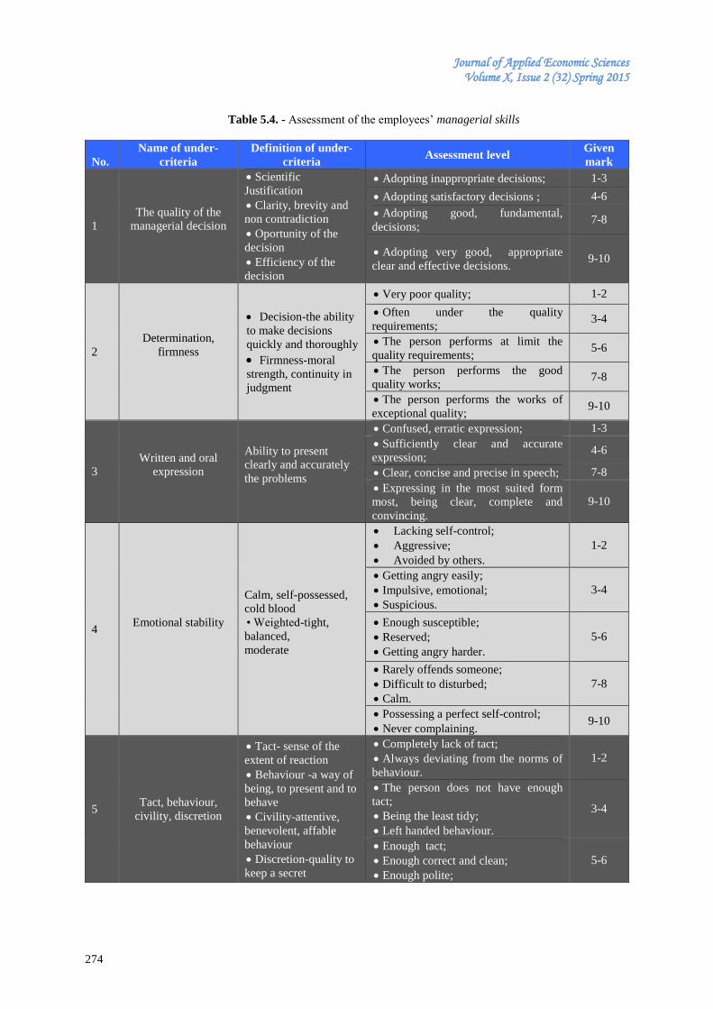
Journal of Applied Economic Sciences Volume X, Issue 2 (32) Spring 2015
274
Table 5.4. - Assessment of the employees’ managerial skills
N
No.
Name of under-
criteria
Definition of under-
criteria Assessment level
Given
mark
1
The quality of the
managerial decision
Scientific
Justification
Clarity, brevity and
non contradiction
Oportunity of the
decision
Efficiency of the
decision
Adopting inappropriate decisions; 1-3
Adopting satisfactory decisions ; 4-6
Adopting good, fundamental,
decisions; 7-8
Adopting very good, appropriate
clear and effective decisions. 9-10
2
Determination,
firmness
Decision-the ability
to make decisions
quickly and thoroughly
Firmness-moral
strength, continuity in
judgment
Very poor quality; 1-2
Often under the quality
requirements; 3-4
The person performs at limit the
quality requirements; 5-6
The person performs the good
quality works; 7-8
The person performs the works of
exceptional quality; 9-10
3
Written and oral
expression
Ability to present
clearly and accurately
the problems
Confused, erratic expression; 1-3
Sufficiently clear and accurate
expression; 4-6
Clear, concise and precise in speech; 7-8
Expressing in the most suited form
most, being clear, complete and
convincing.
9-10
4 Emotional stability
Calm, self-possessed,
cold blood
• Weighted-tight,
balanced,
moderate
Lacking self-control;
Aggressive;
Avoided by others.
1-2
Getting angry easily;
Impulsive, emotional;
Suspicious.
3-4
Enough susceptible;
Reserved;
Getting angry harder.
5-6
Rarely offends someone;
Difficult to disturbed;
Calm.
7-8
Possessing a perfect self-control;
Never complaining. 9-10
5 Tact, behaviour,
civility, discretion
Tact- sense of the
extent of reaction
Behaviour -a way of
being, to present and to
behave
Civility-attentive,
benevolent, affable
behaviour
Discretion-quality to
keep a secret
Completely lack of tact;
Always deviating from the norms of
behaviour.
1-2
The person does not have enough
tact;
Being the least tidy;
Left handed behaviour.
3-4
Enough tact;
Enough correct and clean;
Enough polite;
5-6
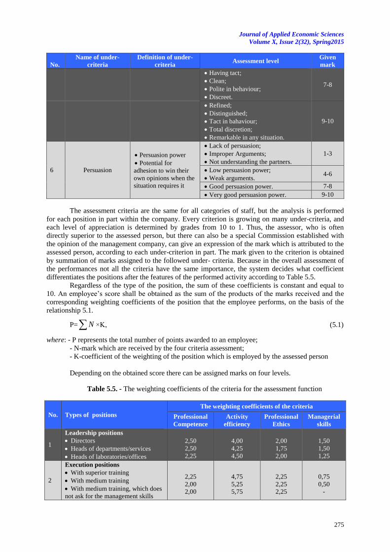
Journal of Applied Economic Sciences
Volume X, Issue 2(32), Spring2015
275
N
No.
Name of under-
criteria
Definition of under-
criteria Assessment level
Given
mark
Having tact;
Clean;
Polite in behaviour;
Discreet.
7-8
Refined;
Distinguished;
Tact in bahaviour;
Total discretion;
Remarkable in any situation.
9-10
6 Persuasion
Persuasion power
Potential for
adhesion to win their
own opinions when the
situation requires it
Lack of persuasion;
Improper Arguments;
Not understanding the partners.
1-3
Low persuasion power;
Weak arguments. 4-6
Good persuasion power. 7-8
Very good persuasion power. 9-10
The assessment criteria are the same for all categories of staff, but the analysis is performed
for each position in part within the company. Every criterion is growing on many under-criteria, and
each level of appreciation is determined by grades from 10 to 1. Thus, the assessor, who is often
directly superior to the assessed person, but there can also be a special Commission established with
the opinion of the management company, can give an expression of the mark which is attributed to the
assessed person, according to each under-criterion in part. The mark given to the criterion is obtained
by summation of marks assigned to the followed under- criteria. Because in the overall assessment of
the performances not all the criteria have the same importance, the system decides what coefficient
differentiates the positions after the features of the performed activity according to Table 5.5.
Regardless of the type of the position, the sum of these coefficients is constant and equal to
10. An employee’s score shall be obtained as the sum of the products of the marks received and the
corresponding weighting coefficients of the position that the employee performs, on the basis of the
relationship 5.1.
P=N ×K, (5.1)
where: - P represents the total number of points awarded to an employee;
- N-mark which are received by the four criteria assessment;
- K-coefficient of the weighting of the position which is employed by the assessed person
Depending on the obtained score there can be assigned marks on four levels.
Table 5.5. - The weighting coefficients of the criteria for the assessment function
No. Types of positions
The weighting coefficients of the criteria
Professional
Competence
Activity
efficiency
Professional
Ethics
Managerial
skills
1
Leadership positions
Directors
Heads of departments/services
Heads of laboratories/offices
2,50
2,50
2,25
4,00
4,25
4,50
2,00
1,75
2,00
1,50
1,50
1,25
2
Execution positions
With superior training
With medium training
With medium training, which does
not ask for the management skills
2,25
2,00
2,00
4,75
5,25
5,75
2,25
2,25
2,25
0,75
0,50
-
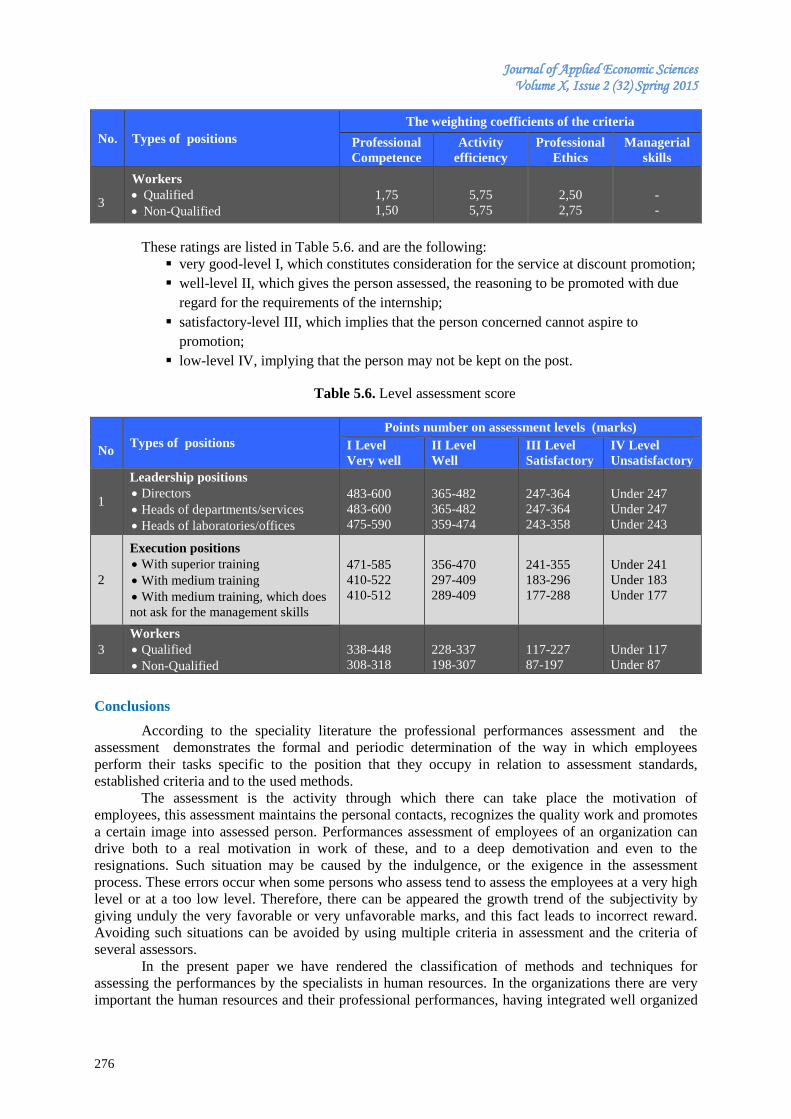
Journal of Applied Economic Sciences Volume X, Issue 2 (32) Spring 2015
276
No. Types of positions
The weighting coefficients of the criteria
Professional
Competence
Activity
efficiency
Professional
Ethics
Managerial
skills
3
3
Workers
Qualified
Non-Qualified
1,75
1,50
5,75
5,75
2,50
2,75
-
-
These ratings are listed in Table 5.6. and are the following:
very good-level I, which constitutes consideration for the service at discount promotion;
well-level II, which gives the person assessed, the reasoning to be promoted with due
regard for the requirements of the internship;
satisfactory-level III, which implies that the person concerned cannot aspire to
promotion;
low-level IV, implying that the person may not be kept on the post.
Table 5.6. Level assessment score
N
No Types of positions
Points number on assessment levels (marks)
I Level
Very well
II Level
Well
III Level
Satisfactory
IV Level
Unsatisfactory
1
Leadership positions
Directors
Heads of departments/services
Heads of laboratories/offices
483-600
483-600
475-590
365-482
365-482
359-474
247-364
247-364
243-358
Under 247
Under 247
Under 243
2
Execution positions
With superior training
With medium training
With medium training, which does
not ask for the management skills
471-585
410-522
410-512
356-470
297-409
289-409
241-355
183-296
177-288
Under 241
Under 183
Under 177
3
Workers
Qualified
Non-Qualified
338-448
308-318
228-337
198-307
117-227
87-197
Under 117
Under 87
Conclusions
According to the speciality literature the professional performances assessment and the
assessment demonstrates the formal and periodic determination of the way in which employees
perform their tasks specific to the position that they occupy in relation to assessment standards,
established criteria and to the used methods.
The assessment is the activity through which there can take place the motivation of
employees, this assessment maintains the personal contacts, recognizes the quality work and promotes
a certain image into assessed person. Performances assessment of employees of an organization can
drive both to a real motivation in work of these, and to a deep demotivation and even to the
resignations. Such situation may be caused by the indulgence, or the exigence in the assessment
process. These errors occur when some persons who assess tend to assess the employees at a very high
level or at a too low level. Therefore, there can be appeared the growth trend of the subjectivity by
giving unduly the very favorable or very unfavorable marks, and this fact leads to incorrect reward.
Avoiding such situations can be avoided by using multiple criteria in assessment and the criteria of
several assessors.
In the present paper we have rendered the classification of methods and techniques for
assessing the performances by the specialists in human resources. In the organizations there are very
important the human resources and their professional performances, having integrated well organized
Journal of Applied Economic Sciences
Volume X, Issue 2(32), Spring2015
277
systems in which there are managed the assessment techniques and methods being characteristic for
the concerned fields.
I mentioned that each of the described methods has its own advantages and disadvantages, but
the effectiveness of an assessment system depends on various factors which may influence the
decisive final results. Thus, it is necessary that all the involved elements be justified and properly
applied. We cannot rule out that one method is better than another, each of these being used with more
or less success, depending on the needs of the assessment.
The human resources performances assessment should not be limited only to the previous
performance measurement but there must be estimated the upcoming performances. For the purpose of
the employees’ professional targeting it is very important the discussion between assessors and the
assessed person. The assessment results generate the proposed concrete programs at local, national or
European professional level for the professional development of the resources and professional
opportunities. The assessment system of the performances, with the manner in which it manages its
results, influences the size of the employees’ rewards, their relationships with superiors, the quality of
the undertaken activities undertaken, the possibilities of promotion, the overall performance of the
organization.
In this regard, because of the importance of the performances assessment for obtaining the
sustainable competitive advantage of the organizations, it is essential that every organization devise its
own assessment system for the employees’ professional performances.
References
[1] Amstrong, M. 2007. How to be a better manager, The sixth Edition, Meteor Press Publishing
House, Bucharest.
[2] Armstrong, M. 1996. A Handbook of Personnel Management Practice, 6th Edition Kogan Page
Publishers, London,
[3] Bühner R. 1994. Personal-Management, Landsberg, Verlag Moderne Industrie.
[4] Burlea-Şchiopoiu, A., 2008. Human Resources Management, Universitaria Publishing House,
Craiova.
[5] Citeau, P.J. 2008. Gestion des ressources humaines: principes généraux et cas pratiques, Sirey.
[6] Constantin, T. 2002. Human Resources Management, European Institute Publishing House, Iaşi,
[7] Dowling, P., Schuller, R., Welch, D.E. 2003. International Dimensions of Human Resource
Management. Second edition, Wadsworth Publishing Company, Belmont, California.
[8] Ivancevich, J.M., Glueck, W.F. 1986. Foundations of Personnel Human Resource Management,
Business Publications Inc. Texas.
[9] Lefter, V., Deaconu, A., Marinaş, C., Puia, R. 2008. Human Resources Management –Theory and
practice, Economic Publishing House, Bucharest.
[10] Lefter, V., Puia, R.Ş. 2011. Human Resources Management – Theory and practice. Second
Edition, Economic Publishing House, Bucharest.
[11] Manolescu, A., Lefter, V., Deaconu, A. 2007. Human Resources Management Economic
Publishing House, Bucharest.
[12] Manolescu, A. 1998. Human Resources Management, RAI Publishing House, Bucharest.
[13] Manolescu, A. 2004. Human Resources Management. The fourth edition, Economic Publishing
House.
[14] Mathis, R.L., Nica P., Rusu, C. 1997. Human Resources Management, Economic Publishing
House, Bucharest.
[15] Mathis R., Jackson, J. H. 2003. Human resource management, Ed.South-Western,

Journal of Applied Economic Sciences Volume X, Issue 2 (32) Spring 2015
278
[16] Milkovich, G. T., Boudreau, J. W. 1991. Human Resource Management, Sixth Edition, Irwin,
Boston.
[17] Milkovich, G. T., Bourdeau, J. W. 1988. Personnel/ Human Resorce Management: A Diagnostic
Approach, Plano, Business Publications, Inc., Texas.
[18] Negulescu, C. M. 2002. Human Resource and Professional Performance, Romanian Written
Publishing House, Craiova.
[19] Pânişoară, I. O., Pânişoară, G. 2005. Human Resources Management – Practical guide, Second
Edition, Polirom Publishing House, Bucharest.
[20] Pitariu, H.D. 1994. Human Resources Management - Professional Performances Measurement,
All Economic Publishing House, Bucharest.
[21] Popa, I. 2005. General Management, ASE Publishing House, Bucharest.
[22] Romelaer, P. 1993. Gestion des ressources humaines, Edition Armand Colin, Paris.
[23] Roşca, C. 2004. Human Resources Management Third Edition, Universitaria Publishing House,
Certi, Craiova.
[24] Roşca, C., Roşca, D., Negulescu, M. C., Neamţu, M. 2005. Human Resources. Continuous
Training. Career management, Universitaria Publishing House, Craiova.
[25] Roşca, C., Vărzaru, M., Roşca, Gh. I., (coord.) 2005. Human Resources - Management and
administration, Economic Publishing House, Bucharest.
[26] Roşca, C., Roşca, D., 2005. Human Resources: Management, Strategies, Politics, Universitaria
Publishing House, Craiova.
[27] Stanciu, Ş., Leovaridis, C. 2003. Human Resources Management. Tests and case studies, Bren
Publishing House, Bucharest.
[28] Stephen, P., Robbins, David A. De Cenzo. 2008. Fundamentals of Management, Publisher:
Prentice Hall,
[29] Torrington, D., Hall, L. 1995. Personnel Management. HRM in action, Prentice Hall, Oxford.
[30] Văcărescu Hobeanu, L. 2012. Professional performances management in the system of higher
education from Romania, SITECH Publishing House, Craiova.
Journal of Applied Economic Sciences
Volume X, Issue 2(32), Spring2015
279
BANK-RELATED ASSET MANAGEMENT FIRM AND RISK TAKING IN MUTUAL FUND TOURNAMENT: EVIDENCE FROM ASEAN
ECONOMIC COMMUNITY
Woraphon WATTANATORN
Thammasat Business School, Thammasat University, Thailand
Sarayut NATHAPHAN
Mahidol University International College, Mahidol University, Thailand
Chaiyuth PADUNGSAKSAWASDI
Thammasat Business School, Thammasat University, Thailand
Abstract:
We examine risk-taking behavior of mutual funds in ASEAN Economic Community by applying
parametric approach to determine whether it complies with the tournament hypothesis. The “winner” mutual
funds tend to reduce their risk in the second half of the year to maintain their status or ranking, while the
“loser” mutual funds adjust their portfolios to be riskier in the expectation of a better result by the end of the
year. In the market that dominated by commercial bank-related asset management companies, we find solid
evidence that the winner funds reduce their portfolio risk, while the loser funds increase their exposure. The type
of asset management company affects funds’ risk-taking behavior. Bank-related winner funds exhibit higher
risk-taking behavior in the second half of the year compared to non-bank related funds.
Keywords: mutual funds, risk-taking, tournament behavior, bank affiliated funds.
JEL Classification: G11; G23; O16.
1. Introduction
There are two schools of thought explaining the risk taking behavior in mutual fund industry,
namely the tournament behavior hypothesis and the strategic behavior hypothesis. The first theory
postulates that interim loser funds are more volatile than winner funds during the second half of the
year because loser funds want to be among the top performing funds by the year’s end in order to earn
a new investment flow (Koski and Pontiff 1999, Taylor 2003, Goriaev, Nijman, and Werker 2005,
Acker and Duck 2006, Kempf and Ruenzi 2008, Kempf, Ruenzi, and Thiele 2009, Chevalier and
Ellison 1995, Brown, Harlow, and Starks 1996). Alternatively, the second theory discusses from the
winner funds’ perspective, which they adjust their portfolio risks more than loser funds do during the
second half of the year in order to either maintain or boost performance (Qiu 2003, Benson, Faff, and
Nowland 2007, Hallahan, Faff, and Benson 2008, Jans and Otten 2008, and Hallahan and Faff 2009).
Nathaphan and Chunhachinda 2012 hint that asset management companies (AMCs) having
relationship with commercial bank AMCs hereafter bank-related (BR) AMCs, introduce higher growth
from new investment flow compared to non-bank-related (NBR) AMCs. They show that both types
behave significantly different. In addition, the tournament hypotheses show that the winner funds have
incentive to reduce risk to secure their position in mutual fund tournament in the second part of the
year. The loser funds have incentive to take more risk to capture the higher performance in the second
part of the year Therefore, in this study, we group AMCs into BR and non-bank-related (NBR) funds
as prior literature. In addition, these funds possess different portfolio allocations due to different
information advantages and styles (Massa and Rehman 2008 and Hao and Yan 2012). However, none
of previous study focuses on the difference between the structure of AMCs and their risk taking
behavior. To fill this literature gap, the different risk taking behavior between BR and NBR funds is
documented by this study. We find that the structure of AMCs affects risk taking behavior of loser
funds - the BR loser funds increase funds volatility higher than that of NBR loser funds.
Most of the previous researches are conducted in developed markets, but there are few reports
from emerging economies. The studying of emerging markets would have important contributions
since emerging markets illustrate significant growth. Also, their rapid rate of growth has led to an
Journal of Applied Economic Sciences Volume X, Issue 2 (32) Spring 2015
280
increase in their share of the global market (Kearney 2012). Emerging markets differ from developed
markets in many aspects. First, emerging markets have higher average sample returns and volatility
than developed market. Besides, these higher returns have been found to have high serial correlation
and also found to be predictable (Bekaert and Harvey 1997 and Harvey 1995). High serial correlation
is the result of inefficient information by which are documented insider trading in emerging markets.
Therefore, this difference raises more concern over the results found in developed countries’ markets
(Huij and Post 2011).
This paper investigates the risk taking behavior of mutual funds in four ASEAN Economic
Community (AEC) countries, namely Indonesia, Malaysia, Singapore, and Thailand1 over the period
of 2008-2013. The overall results are consistent to tournament hypothesis. Given the a convexity
relationship between new investment fund-flows and past performances shown in Chevalier and
Ellison 1995, Ferreira et al. 2012, Sirri and Tufano 1998, we further analyze whether the structure of
asset management companies (AMCs) affects its risk taking behavior of mutual funds in annual
tournament setting. In sum, AMCs adjust their portfolio risks in response to a new investment fund-
flow leading to more fees to AMCs.
We further improve a model to capture evidence of risk-taking behavior that has taken into
account the effects of the interim performance and industry structure. The panel corrected standard
error regression to reveal the behavior of the winner and the loser funds is employed. We contribute to
prior literature, the development of mutual fund industry, and corporate finance as follows. First, our
results demonstrate different levels of the tournament behavior in AEC markets. We find that each
market possesses a unique fund flow pattern, leading to a different level of the tournament behavior.
Second, tournament behavior is found in Thailand, specifically in August while other countries have
less evidence of tournament behavior. We notice that the winner funds are lowering their portfolio risk
in the latter part of the year. This study also provides the evidence confirming the existence of mean
reversion property of fund volatility in all market. Last, the bank-related AMCs managed mutual funds
expose to risk shifting comparing with NBR AMCs in BR AMCs dominated market – Thailand.
Moreover, for Thailand, we find the tournament behavior in two of three assessment period but not for
NBR group. Controlling for specific fund characteristics, we conclude that the tournament effect exists
in the BR AMCs dominated market.
The remainder of this paper is organized as follows. Section 2 shows the review of literature
and development of the hypothesis. Section 3 describes the data, methodology, and industry overview.
Section 4 shows the empirical results and the last section is conclusion.
2. Literature review
2.1 Fund flow – performance relationship
Sirri and Tufano (1998) demonstrate that the positive relationship of fund flow and
performance is a convex function. However, poor performing funds are not penalized by the same
proportion of outflow (Chevalier and Ellison 1995 and Sirri and Tufano 1998), thus the convexity
differs from market to market. Ferreira et al. (2012) point out that this relationship depends on the
level of investors’ education, the level of accessibility to information, and the development of financial
markets. They also suggest that the convexity is more sensitive in less developed markets. Therefore,
the relationship pushes AMCs to take more risks in order to capture future fund flow, particularly in
emerging markets.
2.2 Tournament Behavior
The tournament behavior model was first developed in 1996 by Brow, Harlow and Starks
(BHS). They implicitly assume that investors observe the mutual fund’s year-end ranking and utilize
this information for their investment allocation. Therefore, this motivates AMCs to compete for top
positions in the annual tournament. In addition, they find that the asymmetric effect of convexity in
fund flow performance relationship motivates poorly performed funds to increase their portfolio risk
to be higher than winner funds in order to enhance their performances by the end of the year. Several
1 The sample data are accounted for 79.01% of AEC economic size at the end of 2012. We obtain the GDP data
from ASEAN statistical yearbook.
Journal of Applied Economic Sciences
Volume X, Issue 2(32), Spring2015
281
pieces of evidence demonstrate the tournament effect in the US sample. The evidence supports the
existence of tournament in that the interim loser funds increase portfolio risk to catch up the
performance while the interim winner funds prefer to lock in their top position for example by
indexing (Chen and Pennacchi 2009, Chevalier and Ellison 1995, Dass, Massa, and Patgiri 2008,
Kempf and Ruenzi 2008, Kempf, Ruenzi, and Thiele 2009, and Schwarz 2012). Some research,
however, rejects the tournament hypothesis in the US market based. Busse (2001) find the tournament
exist because of biased estimation (Busse 2001). Others find support of strategic hypothesis in that the
winner funds increase risk more than loser funds (Qiu 2003, Tourani‐Rad, Jans, and Otten 2008).
Acker and Duck (2006) provide the first study of tournament behavior outside the US market,
with the dataset containing UK investment trusts. They find evidence support tournament behavior and
suggest that it has a positive relationship with market conditions. Benson et al. (2007) document those
derivatives users behave strategically. Their result contradicts Koski and Pontiff’s finding. The
evidence is also inconclusive outside of the US sample, with a study of Australian superannuation
funds showing strategic behavior dominated tournament behavior (Hallahan, Faff, and Benson 2008).
Hallanhan and Faff (2009) find evidence of tournament behavior on sample of Australian equity funds
between 1989 and 2001.
Only limited studies have been conducted in emerging areas. The prior evidence on emerging
areas is neither persistent nor conclusive. For example, Ko and Ha (2011) study the Korean equity
funds. Their results show that the tournament behavior is not persistent (KO and HA 2011). Ramiah et
al. (2012) apply non-parametric test and document both tournament and strategic behavior in
conventional Malaysian funds (Ramiah et al. 2012).
To fulfill the gap, the comparison between four largest economic in AEC, leads to a clearer
result. This is because emerging market and developed market have different market characteristics.
Therefore, our sample can depict the result in both emerging markets and developed market.
Furthermore, as the AMCs in this region can be classified into BR and NBR (Nathaphan and
Chunhachinda 2012). These BR and NBR AMCs have different investment fund flow. In addition, BR
and NBR AMCs have different portfolio allocations due to the exploitation of different information.
BR funds have an advantage from privileged information on clients: lending information, for example
(Massa and Rehman 2008). Furthermore, BR funds are likely to hold their clients’ stocks improperly
(Hao and Yan 2012). As a result of improper allocation, BR funds lose portfolio diversification and
have greater volatility in the second half of the year. The recent research documents the evidence
showing that the investment bank managed funds have lower funds’ alpha compare with non-bank
managed funds. Lead to the conclusion of conflict of interest found in investment bank managed funds
(Berzins, Liu, and Trzcinka 2013). Finally, the high return and high volatile characteristics of
emerging markets demonstrate the importance of diversified portfolios and the influence of risk-taking
behavior by mutual funds.
We propose to test the tournament effect in the emerging market context through the
hypotheses below;
H1: There is a relationship between the interim performance and the risk adjustment of funds.
H2A: There is a negative relationship between the interim performance and the risk
adjustment of winner funds.
H2B: There is a positive relationship between the interim performance and the risk adjustment
of loser funds.
H3: BR and NBR funds have different effects on risk-taking behavior due to their interim
performance.
3. Data and methodology
In this study, we obtain data from various sources. Data on monthly asset under management
(AUM), net asset value (NAV), total return, net flow, annual reported net expense ratio, and turnover
ratio are obtained from Morningstar Direct database. The risk-free rate and market return are obtained
from DataStream.
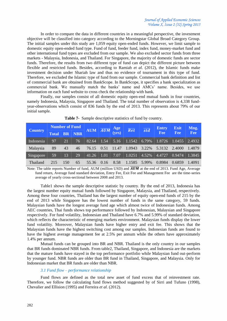
Journal of Applied Economic Sciences Volume X, Issue 2 (32) Spring 2015
282
In order to compare the data in different countries in a meaningful perspective, the investment
objective will be classified into category according to the Morningstar Global Broad Category Group.
The initial samples under this study are 1,059 equity open-ended funds. However, we limit sample to
domestic equity open-ended fund type. Fund of fund, feeder fund, index fund, money-market fund and
other international fund types are excluded from our sample. We also excluded sector funds from three
markets - Malaysia, Indonesia, and Thailand. For Singapore, the majority of domestic funds are sector
funds. Therefore, the results from two different type of fund can depict the different picture between
flexible and restricted funds. Besides, according to Ramiah et al. (2012), the Islamic funds make
investment decision under Shariah law and thus no evidence of tournament in this type of fund.
Therefore, we excluded the Islamic type of fund from our sample. Commercial bank definition and list
of commercial bank are obtained from BankScope. In BankScope, it specifies a bank specialization as
commercial bank. We manually match the banks’ name and AMCs’ name. Besides, we use
information on each fund website to cross check the relationship with bank.
Finally, our samples consist of all domestic equity open-end mutual funds in four countries,
namely Indonesia, Malaysia, Singapore and Thailand. The total number of observation is 4,338 fund-
year-observations which consist of 836 funds by the end of 2013. This represents about 79% of our
initial sample.
Table 7- Sample descriptive statistics of fund by country.
Country Number of Fund
AUM Age
(yrs)
Entry
Fee
Exit
Fee
Mng.
Fee Total BR NBR
Indonesia 97 21 76 82.64 1.54 5.16 1.1542 6.79% 1.8726 1.0455 2.4932
Malaysia 89 43 46 76.15 0.51 11.47 1.0943 3.22% 5.3132 2.4000 1.4879
Singapore 59 13 29 41.26 1.01 7.07 1.0251 4.52% 4.4727 0.9474 1.3845
Thailand 215 150 65 55.36 0.16 8.58 1.1585 5.99% 0.8984 0.6859 1.4091
Note: The table reports Number of fund, AUM (million USD) and at the end of 2013. Fund Age, Average
fund return, Average fund standard deviation, Entry Fee, Exit Fee and Management Fee are the time-series
average of yearly cross-sectional between 2008 and 2013.
Table1 shows the sample descriptive statistic by country. By the end of 2013, Indonesia has
the largest number equity mutual funds followed by Singapore, Malaysia, and Thailand, respectively.
Among these four countries, Thailand has the largest number of equity open-end funds of 215 by the
end of 2013 while Singapore has the lowest number of funds in the same category, 59 funds.
Malaysian funds have the longest average fund age which almost twice of Indonesian funds. Among
AEC countries, Thai funds shows top performance followed by Indonesian, Malaysian and Singapore
respectively. For fund volatility, Indonesian and Thailand have 6.7% and 5.99% of standard deviation,
which reflects the characteristic of emerging markets environment. Malaysian funds display the lower
fund volatility. Moreover, Malaysian funds have higher entry and exit fee. This shows that the
Malaysian funds have the highest switching cost among our samples. Indonesian funds are found to
have the highest average management fee at 2.5% per annum while the others have approximately
1.4% per annum.
Mutual funds can be grouped into BR and NBR. Thailand is the only country in our samples
that BR funds dominated NBR funds. From table2, Thailand, Singapore, and Indonesia are the markets
that the mature funds have stayed in the top performance portfolio while Malaysian fund out-perform
by younger fund. NBR funds are older than BR fund in Thailand, Singapore, and Malaysia. Only for
Indonesian market that BR funds are older than NBR.
3.1 Fund flow – performance relationship
Fund flows are defined as the total new asset of fund excess that of reinvestment rate.
Therefore, we follow the calculating fund flows method suggested by of Sirri and Tufuno (1998),
Chevalier and Ellision (1995) and Ferreira et al. (2012).
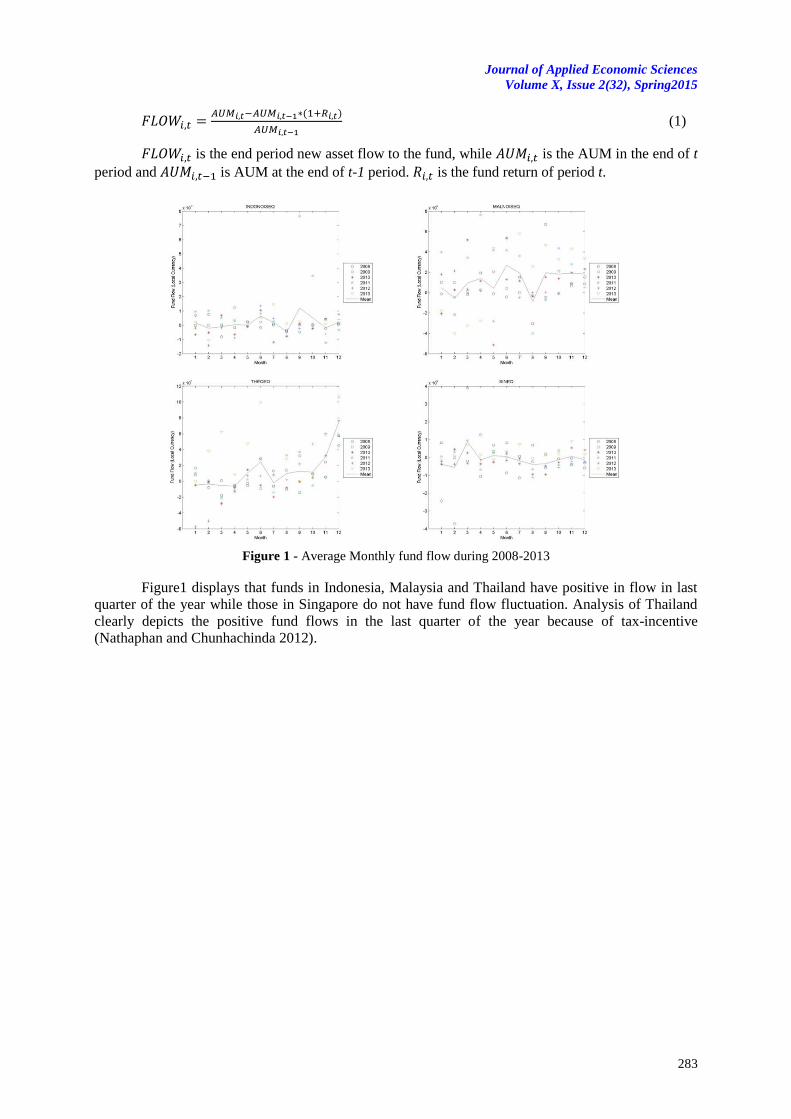
Journal of Applied Economic Sciences
Volume X, Issue 2(32), Spring2015
283
( )
(1)
is the end period new asset flow to the fund, while is the AUM in the end of t
period and is AUM at the end of t-1 period. is the fund return of period t.
Figure 1 - Average Monthly fund flow during 2008-2013
Figure1 displays that funds in Indonesia, Malaysia and Thailand have positive in flow in last
quarter of the year while those in Singapore do not have fund flow fluctuation. Analysis of Thailand
clearly depicts the positive fund flows in the last quarter of the year because of tax-incentive
(Nathaphan and Chunhachinda 2012).
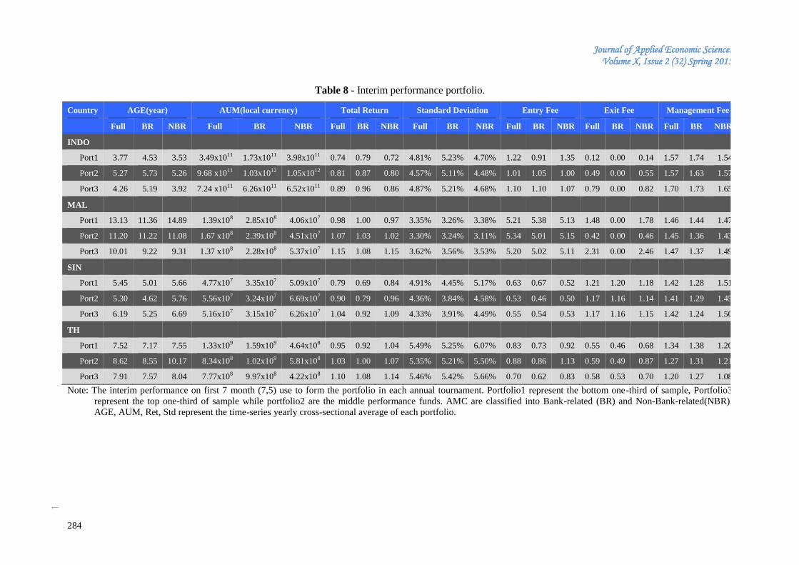
Journal of Applied Economic Sciences Volume X, Issue 2 (32) Spring 2015
284
Table 8 - Interim performance portfolio.
Country AGE(year) AUM(local currency) Total Return Standard Deviation Entry Fee Exit Fee Management Fee
Full BR NBR Full BR NBR Full BR NBR Full BR NBR Full BR NBR Full BR NBR Full BR NBR
INDO
Port1 3.77 4.53 3.53 3.49x10¹¹ 1.73x10¹¹ 3.98x10¹¹ 0.74 0.79 0.72 4.81% 5.23% 4.70% 1.22 0.91 1.35 0.12 0.00 0.14 1.57 1.74 1.54
Port2 5.27 5.73 5.26 9.68 x10¹¹ 1.03x10¹² 1.05x10¹² 0.81 0.87 0.80 4.57% 5.11% 4.48% 1.01 1.05 1.00 0.49 0.00 0.55 1.57 1.63 1.57
Port3 4.26 5.19 3.92 7.24 x10¹¹ 6.26x10¹¹ 6.52x10¹¹ 0.89 0.96 0.86 4.87% 5.21% 4.68% 1.10 1.10 1.07 0.79 0.00 0.82 1.70 1.73 1.65
MAL
Port1 13.13 11.36 14.89 1.39x10⁸ 2.85x10⁸ 4.06x10⁷ 0.98 1.00 0.97 3.35% 3.26% 3.38% 5.21 5.38 5.13 1.48 0.00 1.78 1.46 1.44 1.47
Port2 11.20 11.22 11.08 1.67 x10⁸ 2.39x10⁸ 4.51x10⁷ 1.07 1.03 1.02 3.30% 3.24% 3.11% 5.34 5.01 5.15 0.42 0.00 0.46 1.45 1.36 1.43
Port3 10.01 9.22 9.31 1.37 x10⁸ 2.28x10⁸ 5.37x10⁷ 1.15 1.08 1.15 3.62% 3.56% 3.53% 5.20 5.02 5.11 2.31 0.00 2.46 1.47 1.37 1.49
SIN
Port1 5.45 5.01 5.66 4.77x10⁷ 3.35x10⁷ 5.09x10⁷ 0.79 0.69 0.84 4.91% 4.45% 5.17% 0.63 0.67 0.52 1.21 1.20 1.18 1.42 1.28 1.51
Port2 5.30 4.62 5.76 5.56x10⁷ 3.24x10⁷ 6.69x10⁷ 0.90 0.79 0.96 4.36% 3.84% 4.58% 0.53 0.46 0.50 1.17 1.16 1.14 1.41 1.29 1.45
Port3 6.19 5.25 6.69 5.16x10⁷ 3.15x10⁷ 6.26x10⁷ 1.04 0.92 1.09 4.33% 3.91% 4.49% 0.55 0.54 0.53 1.17 1.16 1.15 1.42 1.24 1.50
TH
Port1 7.52 7.17 7.55 1.33x10⁹ 1.59x10⁹ 4.64x10⁸ 0.95 0.92 1.04 5.49% 5.25% 6.07% 0.83 0.73 0.92 0.55 0.46 0.68 1.34 1.38 1.20
Port2 8.62 8.55 10.17 8.34x10⁸ 1.02x10⁹ 5.81x10⁸ 1.03 1.00 1.07 5.35% 5.21% 5.50% 0.88 0.86 1.13 0.59 0.49 0.87 1.27 1.31 1.21
Port3 7.91 7.57 8.04 7.77x10⁸ 9.97x10⁸ 4.22x10⁸ 1.10 1.08 1.14 5.46% 5.42% 5.66% 0.70 0.62 0.83 0.58 0.53 0.70 1.20 1.27 1.08
Note: The interim performance on first 7 month (7,5) use to form the portfolio in each annual tournament. Portfolio1 represent the bottom one-third of sample, Portfolio3
represent the top one-third of sample while portfolio2 are the middle performance funds. AMC are classified into Bank-related (BR) and Non-Bank-related(NBR).
AGE, AUM, Ret, Std represent the time-series yearly cross-sectional average of each portfolio.
Jo
urn
al o
f Ap
plied
Eco
no
mic S
ciences
Vo
lum
e X
, Issue 2
(32
), Sp
ring
20
15
28
1
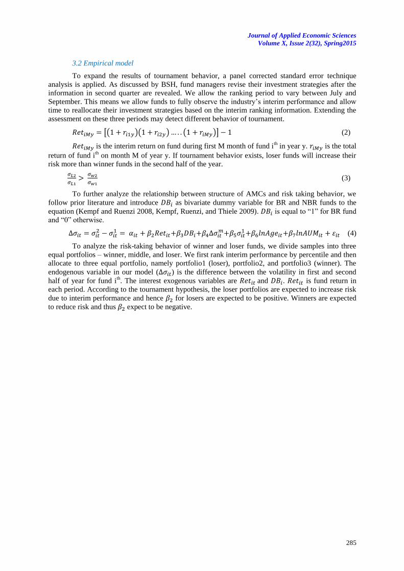
Journal of Applied Economic Sciences
Volume X, Issue 2(32), Spring2015
285
3.2 Empirical model
To expand the results of tournament behavior, a panel corrected standard error technique
analysis is applied. As discussed by BSH, fund managers revise their investment strategies after the
information in second quarter are revealed. We allow the ranking period to vary between July and
September. This means we allow funds to fully observe the industry’s interim performance and allow
time to reallocate their investment strategies based on the interim ranking information. Extending the
assessment on these three periods may detect different behavior of tournament.
[( )( ) ( )] (2)
is the interim return on fund during first M month of fund ith in year y. is the total
return of fund ith on month M of year y. If tournament behavior exists, loser funds will increase their
risk more than winner funds in the second half of the year.
(3)
To further analyze the relationship between structure of AMCs and risk taking behavior, we
follow prior literature and introduce as bivariate dummy variable for BR and NBR funds to the
equation (Kempf and Ruenzi 2008, Kempf, Ruenzi, and Thiele 2009). is equal to “1” for BR fund
and “0” otherwise.
(4)
To analyze the risk-taking behavior of winner and loser funds, we divide samples into three
equal portfolios – winner, middle, and loser. We first rank interim performance by percentile and then
allocate to three equal portfolio, namely portfolio1 (loser), portfolio2, and portfolio3 (winner). The
endogenous variable in our model ( ) is the difference between the volatility in first and second
half of year for fund ith. The interest exogenous variables are and . is fund return in
each period. According to the tournament hypothesis, the loser portfolios are expected to increase risk
due to interim performance and hence for losers are expected to be positive. Winners are expected
to reduce risk and thus expect to be negative.
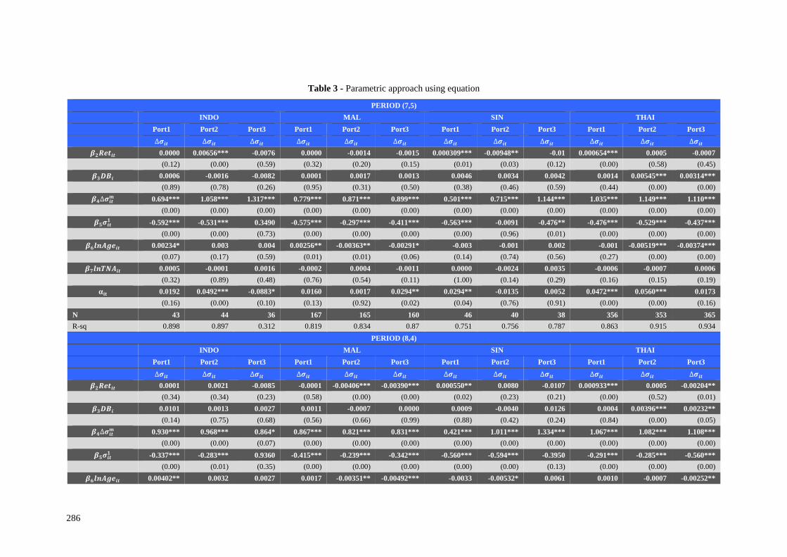
Journal of Applied Economic Sciences Volume X, Issue 2 (32) Spring 2015
286
Table 3 - Parametric approach using equation
PERIOD (7,5)
INDO MAL SIN THAI
Port1 Port2 Port3 Port1 Port2 Port3 Port1 Port2 Port3 Port1 Port2 Port3
0.0000 0.00656*** -0.0076 0.0000 -0.0014 -0.0015 0.000309*** -0.00948** -0.01 0.000654*** 0.0005 -0.0007
(0.12) (0.00) (0.59) (0.32) (0.20) (0.15) (0.01) (0.03) (0.12) (0.00) (0.58) (0.45)
0.0006 -0.0016 -0.0082 0.0001 0.0017 0.0013 0.0046 0.0034 0.0042 0.0014 0.00545*** 0.00314***
(0.89) (0.78) (0.26) (0.95) (0.31) (0.50) (0.38) (0.46) (0.59) (0.44) (0.00) (0.00)
0.694*** 1.058*** 1.317*** 0.779*** 0.871*** 0.899*** 0.501*** 0.715*** 1.144*** 1.035*** 1.149*** 1.110***
(0.00) (0.00) (0.00) (0.00) (0.00) (0.00) (0.00) (0.00) (0.00) (0.00) (0.00) (0.00)
-0.592*** -0.531*** 0.3490 -0.575*** -0.297*** -0.411*** -0.563*** -0.0091 -0.476** -0.476*** -0.529*** -0.437***
(0.00) (0.00) (0.73) (0.00) (0.00) (0.00) (0.00) (0.96) (0.01) (0.00) (0.00) (0.00)
0.00234* 0.003 0.004 0.00256** -0.00363** -0.00291* -0.003 -0.001 0.002 -0.001 -0.00519*** -0.00374***
(0.07) (0.17) (0.59) (0.01) (0.01) (0.06) (0.14) (0.74) (0.56) (0.27) (0.00) (0.00)
0.0005 -0.0001 0.0016 -0.0002 0.0004 -0.0011 0.0000 -0.0024 0.0035 -0.0006 -0.0007 0.0006
(0.32) (0.89) (0.48) (0.76) (0.54) (0.11) (1.00) (0.14) (0.29) (0.16) (0.15) (0.19)
0.0192 0.0492*** -0.0883* 0.0160 0.0017 0.0294** 0.0294** -0.0135 0.0052 0.0472*** 0.0560*** 0.0173
(0.16) (0.00) (0.10) (0.13) (0.92) (0.02) (0.04) (0.76) (0.91) (0.00) (0.00) (0.16)
N 43 44 36 167 165 160 46 40 38 356 353 365
R-sq 0.898 0.897 0.312 0.819 0.834 0.87 0.751 0.756 0.787 0.863 0.915 0.934
PERIOD (8,4)
INDO MAL SIN THAI
Port1 Port2 Port3 Port1 Port2 Port3 Port1 Port2 Port3 Port1 Port2 Port3
0.0001 0.0021 -0.0085 -0.0001 -0.00406*** -0.00390*** 0.000550** 0.0080 -0.0107 0.000933*** 0.0005 -0.00204**
(0.34) (0.34) (0.23) (0.58) (0.00) (0.00) (0.02) (0.23) (0.21) (0.00) (0.52) (0.01)
0.0101 0.0013 0.0027 0.0011 -0.0007 0.0000 0.0009 -0.0040 0.0126 0.0004 0.00396*** 0.00232**
(0.14) (0.75) (0.68) (0.56) (0.66) (0.99) (0.88) (0.42) (0.24) (0.84) (0.00) (0.05)
0.930*** 0.968*** 0.864* 0.867*** 0.821*** 0.831*** 0.421*** 1.011*** 1.334*** 1.067*** 1.082*** 1.108***
(0.00) (0.00) (0.07) (0.00) (0.00) (0.00) (0.00) (0.00) (0.00) (0.00) (0.00) (0.00)
-0.337*** -0.283*** 0.9360 -0.415*** -0.239*** -0.342*** -0.560*** -0.594*** -0.3950 -0.291*** -0.285*** -0.560***
(0.00) (0.01) (0.35) (0.00) (0.00) (0.00) (0.00) (0.00) (0.13) (0.00) (0.00) (0.00)
0.00402** 0.0032 0.0027 0.0017 -0.00351** -0.00492*** -0.0033 -0.00532* 0.0061 0.0010 -0.0007 -0.00252**
Jo
urn
al o
f Ap
plied
Eco
no
mic S
ciences
Vo
lum
e X
, Issue 2
(32
), Sp
ring
20
15
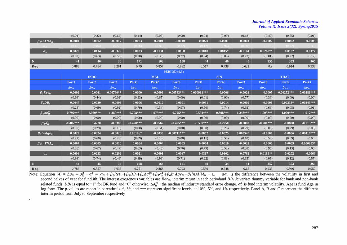
Journal of Applied Economic Sciences
Volume X, Issue 2(32), Spring2015
287
(0.01) (0.32) (0.62) (0.14) (0.05) (0.00) (0.24) (0.09) (0.18) (0.47) (0.55) (0.01)
0.0004 0.0002 -0.0017 0.0003 0.0001 -0.0010 0.0020 -0.0001 0.0041 -0.0002 0.0002 0.0005
(0.45) (0.84) (0.50) (0.66) (0.89) (0.22) (0.12) (0.94) (0.39) (0.70) (0.72) (0.30)
0.0020 0.0114 -0.0329 0.0033 -0.0131 0.0168 -0.0018 0.0815* -0.0184 0.0260** 0.0132 0.0177
(0.92) (0.63) (0.53) (0.78) (0.35) (0.27) (0.94) (0.08) (0.77) (0.01) (0.22) (0.12)
N 41 46 36 171 163 158 44 40 40 356 353 365
R-sq 0.883 0.784 0.281 0.79 0.857 0.832 0.517 0.738 0.621 0.9 0.914 0.938
PERIOD (9,3)
INDO MAL SIN THAI
Port1 Port2 Port3 Port1 Port2 Port3 Port1 Port2 Port3 Port1 Port2 Port3
0.0002 -0.0061 -0.00790** 0.0000 -0.0006 -0.00583*** 0.000911*** -0.0006 -0.0026 0.0005 -0.00252*** -0.00281***
(0.66) (0.44) (0.02) (0.23) (0.65) (0.00) (0.01) (0.90) (0.77) (0.39) (0.00) (0.00)
0.0047 -0.0020 0.0003 0.0006 0.0010 0.0001 0.0031 -0.0014 0.0009 -0.0008 0.00338* 0.00343***
(0.28) (0.69) (0.92) (0.79) (0.54) (0.97) (0.56) (0.74) (0.92) (0.66) (0.05) (0.01)
0.792*** 1.060*** 1.280*** 0.798*** 1.075*** 0.725*** 0.593*** 0.898*** 1.248*** 1.003*** 1.000*** 1.012***
(0.00) (0.00) (0.00) (0.00) (0.00) (0.00) (0.00) (0.00) (0.00) (0.00) (0.00) (0.00)
-0.407*** 0.4720 -0.3380 -0.420*** -0.0562 -0.425*** -0.539*** -0.2250 -0.2880 -0.201*** -0.0808 -0.215***
(0.00) (0.29) (0.15) (0.00) (0.51) (0.00) (0.00) (0.28) (0.29) (0.00) (0.29) (0.00)
0.0022 -0.0024 -0.0026 0.00186* -0.0030 -0.00711*** -0.0052 -0.0025 0.00554* -0.0007 -0.0006 -0.00416***
(0.27) (0.68) (0.28) (0.09) (0.10) (0.00) (0.11) (0.50) (0.10) (0.58) (0.69) (0.00)
0.0007 -0.0005 0.0010 0.0004 0.0004 0.0003 0.0004 0.0010 -0.0033 0.0000 0.0009 0.000953*
(0.26) (0.67) (0.47) (0.63) (0.48) (0.76) (0.79) (0.52) (0.38) (0.95) (0.13) (0.06)
-0.0006 -0.0233 -0.0202 0.0021 -0.0001 -0.0067 0.0317 -0.0102 0.0762 0.0189** -0.0202 -0.0066
(0.98) (0.74) (0.46) (0.89) (0.99) (0.71) (0.22) (0.83) (0.15) (0.05) (0.12) (0.57)
N 44 45 34 168 163 161 49 34 41 357 353 364
R-sq 0.786 0.557 0.635 0.751 0.868 0.793 0.559 0.748 0.65 0.935 0.946 0.957
Note: Equation (4) =
is the difference between the volatility in first and
second halves of year for fund ith. The interest exogenous variables are interim return in each periodand ,bivariate dummy variable for bank and non-bank
related funds. is equal to “1” for BR fund and “0” otherwise. , the median of industry standard error change.
is fund interim volatility. Age is fund Age in
log form. The p-values are report in parenthesis. *, **, and *** represent significant levels, at 10%, 5%, and 1% respectively. Panel A, B and C represent the different
interim period from July to September respectively
.
Journal of Applied Economic Sciences VolumeX, Issue 2 (32) Spring 2015
288
The control variable includes , the median change of industry volatility to control the
segment volatility change. The funds’ volatility is expected to have mean reversion. Therefore, is
introduced to control the mean reversion of volatility (Kempf and Ruenzi 2008, Kempf, Ruenzi, and
Thiele 2009). Age and AUM are introduced as the log form. The younger the fund, the less the
tracking record stand. Hence, the young fund was likely to take more risk. (Chevalier and Ellison
1995, Ferreira et al. 2012, Huang, Sialm, and Zhang 2011)
4. Empirical result
In Table 3, we apply panel corrected standard error regression to analyze the model. To fully
reveal behaviors of the funds, we perform the regression using three assessment periods. The result
from table4 show the regression result from equation (4).
In panel A, we find less evidence of tournament. We cannot reject H2A for all countries. All
winner fund’s portfolio have negatively insignificant coefficients. However, we can reject the H2B for
Singapore and Thailand. This shows that the loser funds in both countries participate in risk taking
behavior to boost their performance. is positively significant only for Thailand, BR AMCs
dominated market.
In Panel B, we can reject all hypotheses in Thai market. This is a strong evidence of
tournament behavior in Thai market, particularly in August. The coefficients of loser funds are
strongly positively significant ( ) and those of winner portfolios are strongly
negatively significant ( ) at 1% and 5% level respectively. Besides, the coefficient of
for Thai market are positive and significantly different from zero at 1% level. Singapore funds
show the evidence that the loser funds increase portfolio risk ( ) in latter part of the
year. Although we found negative sign preserved for winner funds, we cannot reject the null
hypothesis that was significantly different from zero in this market. For Malaysian funds, we find
that winner funds lower their portfolio volatility but not loser funds as in the previous research.
Nonetheless, Indonesia funds have no relationship in this interim period.
In Panel C, we can reject the null hypothesis H2A as we find that winner funds in every
country lower their portfolio risk in second part of the year. We can reject the null hypothesis H2A for
winner funds in three countries—Indonesia, Malaysia, and Thailand. Although we cannot reject this
null hypothesis for Singapore, the negative sign of does preserve. Moreover, the result for
Thailand hold as previous results for .
We can reject the H3 for Thai market. Although preserves with negative sign, we cannot
reject the null hypothesis H2A for all countries in this interim period. and are found to be
strongly and positively significant for winner funds in Thai market. , the segment industry change,
is positively significant as expected, as well as , the first part of the year volatility, that captures the
mean reversion of volatility is found to be negatively significant. is found to be insignificant for all
markets in our sample.
The result from Table3 provides the strong evidence of risk shifting behavior of BR AMCs in
Thai market. Therefore, we further analyst the tournament effect in Thailand. We separate mutual fund
sample in Thai market into BR and NBR to study the difference between them.
Table4 shows that in July and August period of sample from Thai market, in Panel A, there is
the evidence of tournament behavior that can reject H2A and H2B for funds in both groups. We find
that is positively significant, while is negatively and significant. In Panel B, we also reject the
null hypothesis H2A and H2B for BR AMCs group, but not for NBR group. This evidence supports
the tournament behavior existing in Thai market especially in BR AMCs group. Furthermore, we can
reject H2B for NBR AMCs. This means that the loser fund in NBR AMCs also shift risk in latter part
of the year to stimulate their fund position. Although we cannot reject H2A for winner funds in NBR
AMCs, the negative sign of is preserved. In Panel C, we can reject H2A but we cannot reject H2B
in both groups. This means that winner funds in both groups lower portfolios risk to secure the year
end position.
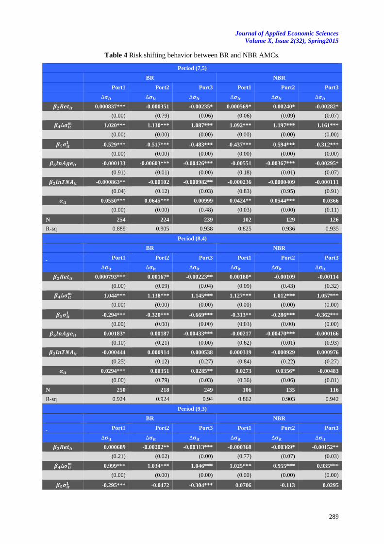
Journal of Applied Economic Sciences
Volume X, Issue 2(32), Spring2015
289
Table 4 Risk shifting behavior between BR and NBR AMCs.
Period (7,5)
BR NBR
Port1 Port2 Port3 Port1 Port2 Port3
0.000837*** -0.000351 -0.00235* 0.000569* 0.00240* -0.00282*
(0.00) (0.79) (0.06) (0.06) (0.09) (0.07)
1.020*** 1.130*** 1.087*** 1.092*** 1.197*** 1.161***
(0.00) (0.00) (0.00) (0.00) (0.00) (0.00)
-0.529*** -0.517*** -0.483*** -0.437*** -0.594*** -0.312***
(0.00) (0.00) (0.00) (0.00) (0.00) (0.00)
-0.000133 -0.00603*** -0.00426*** -0.00551 -0.00367*** -0.00295*
(0.91) (0.01) (0.00) (0.18) (0.01) (0.07)
-0.000863** -0.00102 -0.000982** -0.000236 -0.0000409 -0.000111
(0.04) (0.12) (0.03) (0.83) (0.95) (0.91)
0.0550*** 0.0645*** 0.00999 0.0424** 0.0544*** 0.0366
(0.00) (0.00) (0.48) (0.03) (0.00) (0.11)
N 254 224 239 102 129 126
R-sq 0.889 0.905 0.938 0.825 0.936 0.935
Period (8,4)
BR NBR
Port1 Port2 Port3 Port1 Port2 Port3
0.000793*** 0.00167* -0.00223** 0.00180* -0.00109 -0.00114
(0.00) (0.09) (0.04) (0.09) (0.43) (0.32)
1.044*** 1.138*** 1.145*** 1.127*** 1.012*** 1.057***
(0.00) (0.00) (0.00) (0.00) (0.00) (0.00)
-0.294*** -0.320*** -0.669*** -0.313** -0.286*** -0.362***
(0.00) (0.00) (0.00) (0.03) (0.00) (0.00)
0.00183* 0.00187 -0.00433*** -0.00217 -0.00470*** -0.000166
(0.10) (0.21) (0.00) (0.62) (0.01) (0.93)
-0.000444 0.000914 0.000538 0.000319 -0.000929 0.000976
(0.25) (0.12) (0.27) (0.84) (0.22) (0.27)
0.0294*** 0.00351 0.0285** 0.0273 0.0356* -0.00483
(0.00) (0.79) (0.03) (0.36) (0.06) (0.81)
N 250 218 249 106 135 116
R-sq 0.924 0.924 0.94 0.862 0.903 0.942
Period (9,3)
BR NBR
Port1 Port2 Port3 Port1 Port2 Port3
0.000689 -0.00202** -0.00313*** -0.000368 -0.00369* -0.00152**
(0.21) (0.02) (0.00) (0.77) (0.07) (0.03)
0.999*** 1.034*** 1.046*** 1.025*** 0.955*** 0.935***
(0.00) (0.00) (0.00) (0.00) (0.00) (0.00)
-0.295*** -0.0472 -0.304*** 0.0706 -0.113 0.0295
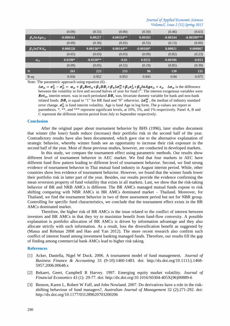
Journal of Applied Economic Sciences VolumeX, Issue 2 (32) Spring 2015
290
(0.00) (0.55) (0.00) (0.50) (0.46) (0.63)
-0.000561 0.00217 -0.00334** 0.00183 -0.00344 -0.00590***
(0.69) (0.30) (0.02) (0.53) (0.13) (0.00)
0.000226 0.00136** 0.00144** -0.00160* 0.00021 0.000867
(0.65) (0.03) (0.03) (0.09) (0.82) (0.23)
0.0190* -0.0330** -0.01 0.0251 -0.00396 -0.013
(0.09) (0.05) (0.52) (0.19) (0.85) (0.39)
N 261 223 233 96 130 131
R-sq 0.936 0.952 0.953 0.943 0.94 0.975
Note: The parametric approach using equation (6) .
is the difference
between the volatility in first and second halves of year for fund ith
. The interest exogenous variables were
interim return. was in each periodand was, bivariate dummy variable for bank and non-bank
related funds. is equal to “1” for BR fund and “0” otherwise. , the median of industry standard
error change. is fund interim volatility. Age is fund Age in log form. The p-values are report in
parenthesis. *, **, and *** represent significant levels, at 10%, 5%, and 1% respectively. Panel A, B and
C represent the different interim period from July to September respectively.
Conclusion
After the original paper about tournament behavior by BHS (1996), later studies document
that winner (the loser) funds reduce (increase) their portfolio risk in the second half of the year.
Contradictory results have also been documented, which gave rise to the alternative explanation of
strategic behavior, whereby winner funds see an opportunity to increase their risk exposure in the
second half of the year. Most of those previous studies, however, are conducted in developed markets.
In this study, we compare the tournament effect using parametric methods. Our results show
different level of tournament behavior in AEC market. We find that four markets in AEC have
different fund flow pattern leading to different level of tournament behavior. Second, we find strong
evidence of tournament behavior in Thai mutual fund industry in August interim period. While, other
countries show less evidence of tournament behavior. However, we found that the winner funds lower
their portfolio risk in latter part of the year. Besides, our results provide the evidence confirming the
mean reversion property of fund volatility that exists in all markets. Last, we show that the risk-taking
behavior of BR and NRB AMCs is different. The BR AMCs managed mutual funds expose to risk
shifting comparing with NBR AMCs in BR AMCs dominated market – Thailand. Moreover, for
Thailand, we find the tournament behavior in two of three assessment period but not for NBR group.
Controlling for specific fund characteristics, we conclude that the tournament effect exists in the BR
AMCs dominated market.
Therefore, the higher risk of BR AMCs is the issue related to the conflict of interest between
investors and BR AMCs in that they try to maximize benefit from fund-flow convexity. A possible
explanation is portfolio allocation of BR AMCs is driven by information advantage and they also
allocate strictly with such information. As a result, loss the diversification benefit as suggested by
(Massa and Rehman 2008 and Hao and Yan 2012). The more recent research also confirm such
conflict of interest found among investment banking managed funds. Therefore, our results fill the gap
of finding among commercial bank AMCs lead to higher risk taking.
References
[1] Acker, Daniella, Nigel W Duck. 2006. A tournament model of fund management. Journal of
Business Finance & Accounting 33 (9‐10):1460-1483. doi: http://dx.doi.org/10.1111/j.1468-
5957.2006.00648.x
[2] Bekaert, Geert, Campbell R Harvey. 1997. Emerging equity market volatility. Journal of
Financial Economics 43 (1): 29-77. doi: http://dx.doi.org/10.1016/S0304-405X(96)00889-6
[3] Benson, Karen L, Robert W Faff, and John Nowland. 2007. Do derivatives have a role in the risk-
shifting behaviour of fund managers?, Australian Journal of Management 32 (2):271-292. doi:
http://dx.doi.org/10.1177/031289620703200206
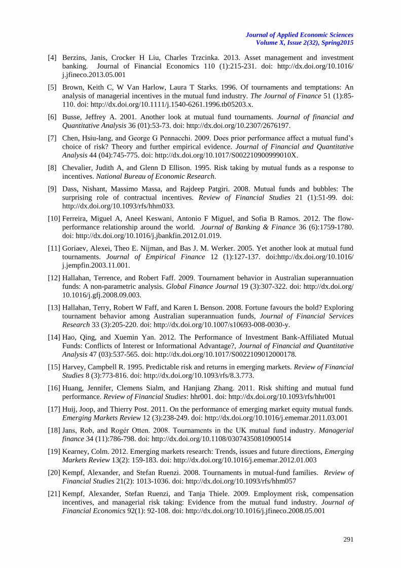
Journal of Applied Economic Sciences
Volume X, Issue 2(32), Spring2015
291
[4] Berzins, Janis, Crocker H Liu, Charles Trzcinka. 2013. Asset management and investment
banking. Journal of Financial Economics 110 (1):215-231. doi: http://dx.doi.org/10.1016/
j.jfineco.2013.05.001
[5] Brown, Keith C, W Van Harlow, Laura T Starks. 1996. Of tournaments and temptations: An
analysis of managerial incentives in the mutual fund industry. The Journal of Finance 51 (1):85-
110. doi: http://dx.doi.org/10.1111/j.1540-6261.1996.tb05203.x.
[6] Busse, Jeffrey A. 2001. Another look at mutual fund tournaments. Journal of financial and
Quantitative Analysis 36 (01):53-73. doi: http://dx.doi.org/10.2307/2676197.
[7] Chen, Hsiu-lang, and George G Pennacchi. 2009. Does prior performance affect a mutual fund’s
choice of risk? Theory and further empirical evidence. Journal of Financial and Quantitative
Analysis 44 (04):745-775. doi: http://dx.doi.org/10.1017/S002210900999010X.
[8] Chevalier, Judith A, and Glenn D Ellison. 1995. Risk taking by mutual funds as a response to
incentives. National Bureau of Economic Research.
[9] Dass, Nishant, Massimo Massa, and Rajdeep Patgiri. 2008. Mutual funds and bubbles: The
surprising role of contractual incentives. Review of Financial Studies 21 (1):51-99. doi:
http://dx.doi.org/10.1093/rfs/hhm033.
[10] Ferreira, Miguel A, Aneel Keswani, Antonio F Miguel, and Sofia B Ramos. 2012. The flow-
performance relationship around the world. Journal of Banking & Finance 36 (6):1759-1780.
doi: http://dx.doi.org/10.1016/j.jbankfin.2012.01.019.
[11] Goriaev, Alexei, Theo E. Nijman, and Bas J. M. Werker. 2005. Yet another look at mutual fund
tournaments. Journal of Empirical Finance 12 (1):127-137. doi:http://dx.doi.org/10.1016/
j.jempfin.2003.11.001.
[12] Hallahan, Terrence, and Robert Faff. 2009. Tournament behavior in Australian superannuation
funds: A non-parametric analysis. Global Finance Journal 19 (3):307-322. doi: http://dx.doi.org/
10.1016/j.gfj.2008.09.003.
[13] Hallahan, Terry, Robert W Faff, and Karen L Benson. 2008. Fortune favours the bold? Exploring
tournament behavior among Australian superannuation funds, Journal of Financial Services
Research 33 (3):205-220. doi: http://dx.doi.org/10.1007/s10693-008-0030-y.
[14] Hao, Qing, and Xuemin Yan. 2012. The Performance of Investment Bank-Affiliated Mutual
Funds: Conflicts of Interest or Informational Advantage?, Journal of Financial and Quantitative
Analysis 47 (03):537-565. doi: http://dx.doi.org/10.1017/S0022109012000178.
[15] Harvey, Campbell R. 1995. Predictable risk and returns in emerging markets. Review of Financial
Studies 8 (3):773-816. doi: http://dx.doi.org/10.1093/rfs/8.3.773.
[16] Huang, Jennifer, Clemens Sialm, and Hanjiang Zhang. 2011. Risk shifting and mutual fund
performance. Review of Financial Studies: hhr001. doi: http://dx.doi.org/10.1093/rfs/hhr001
[17] Huij, Joop, and Thierry Post. 2011. On the performance of emerging market equity mutual funds.
Emerging Markets Review 12 (3):238-249. doi: http://dx.doi.org/10.1016/j.ememar.2011.03.001
[18] Jans, Rob, and Rogér Otten. 2008. Tournaments in the UK mutual fund industry. Managerial
finance 34 (11):786-798. doi: http://dx.doi.org/10.1108/03074350810900514
[19] Kearney, Colm. 2012. Emerging markets research: Trends, issues and future directions, Emerging
Markets Review 13(2): 159-183. doi: http://dx.doi.org/10.1016/j.ememar.2012.01.003
[20] Kempf, Alexander, and Stefan Ruenzi. 2008. Tournaments in mutual-fund families. Review of
Financial Studies 21(2): 1013-1036. doi: http://dx.doi.org/10.1093/rfs/hhm057
[21] Kempf, Alexander, Stefan Ruenzi, and Tanja Thiele. 2009. Employment risk, compensation
incentives, and managerial risk taking: Evidence from the mutual fund industry. Journal of
Financial Economics 92(1): 92-108. doi: http://dx.doi.org/10.1016/j.jfineco.2008.05.001
Journal of Applied Economic Sciences VolumeX, Issue 2 (32) Spring 2015
292
[22] KO, KWANGSOO, and YEONJEONG HA. 2011. Mutual Fund Tournaments and Structural
Changes in an Emerging Fund Market: The Case of Korea, Seoul Journal of Business 17 (1).
[23] Koski, Jennifer Lynch, and Jeffrey Pontiff. 1999. How are derivatives used? Evidence from the
mutual fund industry. The journal of finance 54(2): 791-816. doi: http://dx.doi.org/10.1111/0022-
1082.00126
[24] Massa, Massimo, and Zahid Rehman. 2008. Information flows within financial conglomerates:
Evidence from the banks–mutual funds relation. Journal of Financial Economics 89(2): 288-306.
doi: http://dx.doi.org/10.1016/j.jfineco.2007.10.002
[25] Nathaphan, Sarayut, and Pornchai Chunhachinda. 2012. Determinants of growth for Thai mutual
fund industry. International Research Journal of Finance and Economics (86).
[26] Qiu, Jiaping. 2003. Termination risk, multiple managers and mutual fund tournaments, European
Finance Review 7(2): 161-190. doi: http://dx.doi.org/10.1023/A:1024533132105
[27] Ramiah, Vikash, Imad Moosa, Ben O'Neill, Milica Backulja, Amel Yacoub, Terry Hallahan, and
John Vaz. 2012. Tournament behaviour in Malaysian managed funds. International Journal of
Managerial Finance 8(4): 381-399. doi: http://dx.doi.org/10.1108/17439131211261288
[28] Schwarz, Christopher G. 2012. Mutual fund tournaments: The sorting bias and new evidence.
Review of Financial Studies 25(3): 913-936. doi: http://dx.doi.org/10.1093/rfs/hhr091
[29] Sirri, Erik R, and Peter Tufano. 1998. Costly search and mutual fund flows. The journal of
finance 53(5): 1589-1622. doi: http://dx.doi.org/10.1111/0022-1082.00066
[30] Taylor, Jonathan. 2003. Risk-taking behavior in mutual fund tournaments. Journal of Economic
Behavior&Organization 50(3): 373-383. doi: http://dx.doi.org/10.1016/S0167-2681(02)00028-8
[31] Tourani‐Rad, Alireza, Rob Jans, and Rogér Otten. 2008. Tournaments in the UK mutual fund
industry. Managerial Finance 34(11): 786-798. doi:http://dx.doi.org/10.1108/030743508
10900514
Journal of Applied Economic Sciences
Volume X, Issue 2(32), Spring2015
293
NOWCASTING CREDIT DEMAND IN TURKEY WITH GOOGLE
TRENDS DATA
Ömer ZEYBEK
ING Bank Turkey Analytic CRM Dept., Maslak, İstanbul, Turkey
Erginbay UĞURLU
Hitit University, FEAS, Department of Economics, Turkey
Abstract: Age of Big Data and internet has brought variety of opportunities for social researchers on identifying
on-going social trends instantly. As internet user base grew exponentially, major internet content search
companies have begun to offer data mining products which could extract attitude of on-going trends and identify
new trends on web as well. Since 2009, as a pioneer on these web analytics solutions Google has launched
Google Trends service, which enables to researchers to examine change of trend on specific keywords. We use
weekly Google Trends Index of “General Purpose Loan” (GT) and total out-standing volume of Turkish
banking system from the data period of first week of March 2011 to second week of September 2014. In this
paper we test whether the Google Analytics search index series can be used as a consistent forecaster of
national general purpose loan (GPL) demand in Turkey. We show how to use search engine data to forecast
Turkish GPL demand. The results show that Google search query data is successful at nowcasting GPL demand.
Keywords: Nowcasting web analytics, forecasting, general purpose loan.
JEL classification: C53
1. Introduction
Public and private data providers periodically release indicators on level of economic and
financial activities for various sectors. However, due to difficulties in data collection and statistical
calculation procedures, announcement of figures could be lagged for a period of time. In addition to
this, data such as GDP or IP are subsequently revised due to post publication collection of updated
observations. Unless short-dated delays up to three months are tolerable for economic policy and trend
analysis, on marketing strategy decisions and monetary interventions of central banks side, these
delays could cause very serious short-comings in decision making processes. So, it became a common
practice for researchers to forecast current conditions when the real data is delayed. This process, the
forecasting of present time could be referred as now casting which is a contraction of now and
forecasting.
(Hendry et al. 2013) defines now-casting as “any procedure that uses additional information
when producing contemptuous aggregate data, beyond just cumulating observed disaggregates as now-
casting”. Beside that definition, (Banbura et al. 2010) generalizes time interval of forecasts and
defines “now” as near future, now and near past. Originally as a procedure generally used by
meteorologist, ‘the now casting’ could be defined as predicting today’s or near future’s weather
conditions, based on extensive past meteorology data. But considering economics side, it’s a fact that
quality of recent data is more suspicious compared to definite meteorology data. For example GDP or
IP indices employed as consistent estimators, could be updated after initial publication of data.
However, the idea made now-casting important was spill over of monetary economics and
government’s tendency to react spontaneous actions on any disequilibrium occurred in market
environment. As stated in (Evans 2005) although, individual customers or firms are aware of their
contemptuous activities, information about current state of economic activity is widely dispersed
among economic agents. So this phenomenon causes disintegration between economic reality and
already published data, thus markets and trading environment falls short on information on current
state of economics. For example, as a major indicator of progress in economic activity the GDP
indices are the most vulnerable data releases to this adverse effect.
This paper was presented in The International Conference on Economic Sciences and Business Administration
(ICESBA 2014), 24 October 2014, Bucharest, Romania.
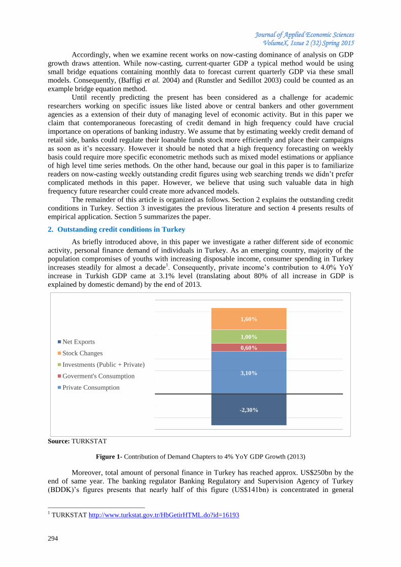
Journal of Applied Economic Sciences VolumeX, Issue 2 (32) Spring 2015
294
Accordingly, when we examine recent works on now-casting dominance of analysis on GDP
growth draws attention. While now-casting, current-quarter GDP a typical method would be using
small bridge equations containing monthly data to forecast current quarterly GDP via these small
models. Consequently, (Baffigi et al. 2004) and (Runstler and Sedillot 2003) could be counted as an
example bridge equation method.
Until recently predicting the present has been considered as a challenge for academic
researchers working on specific issues like listed above or central bankers and other government
agencies as a extension of their duty of managing level of economic activity. But in this paper we
claim that contemporaneous forecasting of credit demand in high frequency could have crucial
importance on operations of banking industry. We assume that by estimating weekly credit demand of
retail side, banks could regulate their loanable funds stock more efficiently and place their campaigns
as soon as it’s necessary. However it should be noted that a high frequency forecasting on weekly
basis could require more specific econometric methods such as mixed model estimations or appliance
of high level time series methods. On the other hand, because our goal in this paper is to familiarize
readers on now-casting weekly outstanding credit figures using web searching trends we didn’t prefer
complicated methods in this paper. However, we believe that using such valuable data in high
frequency future researcher could create more advanced models.
The remainder of this article is organized as follows. Section 2 explains the outstanding credit
conditions in Turkey. Section 3 investigates the previous literature and section 4 presents results of
empirical application. Section 5 summarizes the paper.
2. Outstanding credit conditions in Turkey
As briefly introduced above, in this paper we investigate a rather different side of economic
activity, personal finance demand of individuals in Turkey. As an emerging country, majority of the
population compromises of youths with increasing disposable income, consumer spending in Turkey
increases steadily for almost a decade1. Consequently, private income’s contribution to 4.0% YoY
increase in Turkish GDP came at 3.1% level (translating about 80% of all increase in GDP is
explained by domestic demand) by the end of 2013.
Source: TURKSTAT
Figure 1- Contribution of Demand Chapters to 4% YoY GDP Growth (2013)
Moreover, total amount of personal finance in Turkey has reached approx. US$250bn by the
end of same year. The banking regulator Banking Regulatory and Supervision Agency of Turkey
(BDDK)’s figures presents that nearly half of this figure (US$141bn) is concentrated in general
1 TURKSTAT http://www.turkstat.gov.tr/HbGetirHTML.do?id=16193
3,10%
0,60%
1,00%
1,60%
-2,30%
Net Exports
Stock Changes
Investments (Public + Private)
Goverment's Consumption
Private Consumption
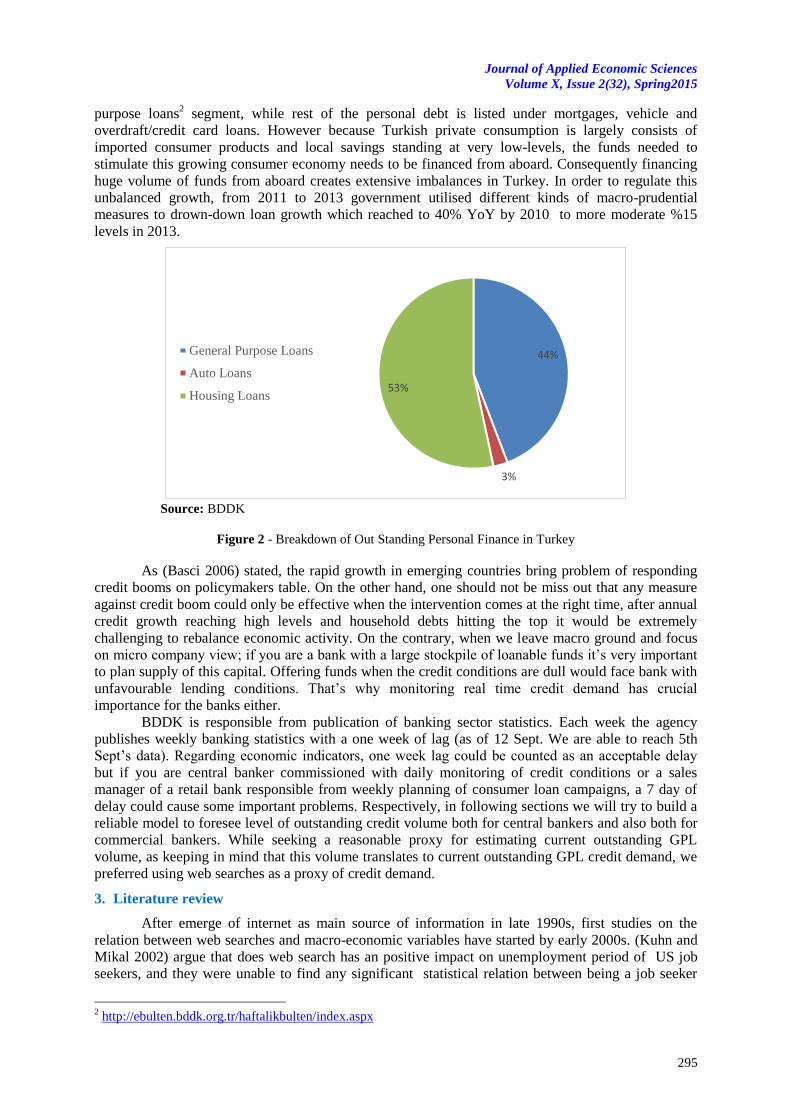
Journal of Applied Economic Sciences
Volume X, Issue 2(32), Spring2015
295
purpose loans2 segment, while rest of the personal debt is listed under mortgages, vehicle and
overdraft/credit card loans. However because Turkish private consumption is largely consists of
imported consumer products and local savings standing at very low-levels, the funds needed to
stimulate this growing consumer economy needs to be financed from aboard. Consequently financing
huge volume of funds from aboard creates extensive imbalances in Turkey. In order to regulate this
unbalanced growth, from 2011 to 2013 government utilised different kinds of macro-prudential
measures to drown-down loan growth which reached to 40% YoY by 2010 to more moderate %15
levels in 2013.
Source: BDDK
Figure 2 - Breakdown of Out Standing Personal Finance in Turkey
As (Basci 2006) stated, the rapid growth in emerging countries bring problem of responding
credit booms on policymakers table. On the other hand, one should not be miss out that any measure
against credit boom could only be effective when the intervention comes at the right time, after annual
credit growth reaching high levels and household debts hitting the top it would be extremely
challenging to rebalance economic activity. On the contrary, when we leave macro ground and focus
on micro company view; if you are a bank with a large stockpile of loanable funds it’s very important
to plan supply of this capital. Offering funds when the credit conditions are dull would face bank with
unfavourable lending conditions. That’s why monitoring real time credit demand has crucial
importance for the banks either.
BDDK is responsible from publication of banking sector statistics. Each week the agency
publishes weekly banking statistics with a one week of lag (as of 12 Sept. We are able to reach 5th
Sept’s data). Regarding economic indicators, one week lag could be counted as an acceptable delay
but if you are central banker commissioned with daily monitoring of credit conditions or a sales
manager of a retail bank responsible from weekly planning of consumer loan campaigns, a 7 day of
delay could cause some important problems. Respectively, in following sections we will try to build a
reliable model to foresee level of outstanding credit volume both for central bankers and also both for
commercial bankers. While seeking a reasonable proxy for estimating current outstanding GPL
volume, as keeping in mind that this volume translates to current outstanding GPL credit demand, we
preferred using web searches as a proxy of credit demand.
3. Literature review
After emerge of internet as main source of information in late 1990s, first studies on the
relation between web searches and macro-economic variables have started by early 2000s. (Kuhn and
Mikal 2002) argue that does web search has an positive impact on unemployment period of US job
seekers, and they were unable to find any significant statistical relation between being a job seeker
2 http://ebulten.bddk.org.tr/haftalikbulten/index.aspx
44%
3%
53%
General Purpose Loans
Auto Loans
Housing Loans
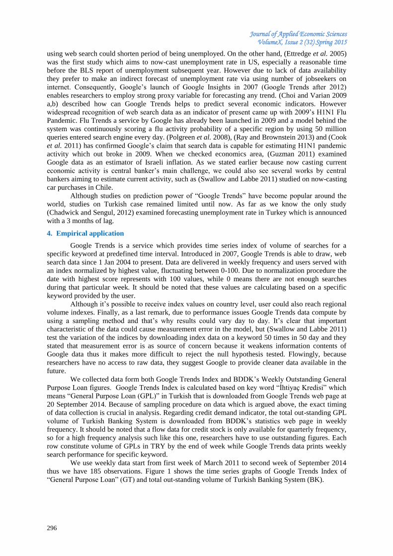
Journal of Applied Economic Sciences VolumeX, Issue 2 (32) Spring 2015
296
using web search could shorten period of being unemployed. On the other hand, (Ettredge et al. 2005)
was the first study which aims to now-cast unemployment rate in US, especially a reasonable time
before the BLS report of unemployment subsequent year. However due to lack of data availability
they prefer to make an indirect forecast of unemployment rate via using number of jobseekers on
internet. Consequently, Google’s launch of Google Insights in 200 (Google Trends after 2012)
enables researchers to employ strong proxy variable for forecasting any trend. (Choi and Varian 2009
a,b) described how can Google Trends helps to predict several economic indicators. However
widespread recognition of web search data as an indicator of present came up with 2009’s H1N1 Flu
Pandemic. Flu Trends a service by Google has already been launched in 2009 and a model behind the
system was continuously scoring a flu activity probability of a specific region by using 50 million
queries entered search engine every day. (Polgreen et al. 2008), (Ray and Brownstein 2013) and (Cook
et al. 2011) has confirmed Google’s claim that search data is capable for estimating H1N1 pandemic
activity which out broke in 2009. When we checked economics area, (Guzman 2011) examined
Google data as an estimator of Israeli inflation. As we stated earlier because now casting current
economic activity is central banker’s main challenge, we could also see several works by central
bankers aiming to estimate current activity, such as (Swallow and Labbe 2011) studied on now-casting
car purchases in Chile.
Although studies on prediction power of “Google Trends” have become popular around the
world, studies on Turkish case remained limited until now. As far as we know the only study
(Chadwick and Sengul, 2012) examined forecasting unemployment rate in Turkey which is announced
with a 3 months of lag.
4. Empirical application
Google Trends is a service which provides time series index of volume of searches for a
specific keyword at predefined time interval. Introduced in 2007, Google Trends is able to draw, web
search data since 1 Jan 2004 to present. Data are delivered in weekly frequency and users served with
an index normalized by highest value, fluctuating between 0-100. Due to normalization procedure the
date with highest score represents with 100 values, while 0 means there are not enough searches
during that particular week. It should be noted that these values are calculating based on a specific
keyword provided by the user.
Although it’s possible to receive index values on country level, user could also reach regional
volume indexes. Finally, as a last remark, due to performance issues Google Trends data compute by
using a sampling method and that’s why results could vary day to day. It’s clear that important
characteristic of the data could cause measurement error in the model, but (Swallow and Labbe 2011)
test the variation of the indices by downloading index data on a keyword 50 times in 50 day and they
stated that measurement error is as source of concern because it weakens information contents of
Google data thus it makes more difficult to reject the null hypothesis tested. Flowingly, because
researchers have no access to raw data, they suggest Google to provide cleaner data available in the
future.
We collected data form both Google Trends Index and BDDK’s Weekly Outstanding General
Purpose Loan figures. Google Trends Index is calculated based on key word “İhtiyaç Kredisi” which
means “General Purpose Loan (GPL)” in Turkish that is downloaded from Google Trends web page at
20 September 2014. Because of sampling procedure on data which is argued above, the exact timing
of data collection is crucial in analysis. Regarding credit demand indicator, the total out-standing GPL
volume of Turkish Banking System is downloaded from BDDK’s statistics web page in weekly
frequency. It should be noted that a flow data for credit stock is only available for quarterly frequency,
so for a high frequency analysis such like this one, researchers have to use outstanding figures. Each
row constitute volume of GPLs in TRY by the end of week while Google Trends data prints weekly
search performance for specific keyword.
We use weekly data start from first week of March 2011 to second week of September 2014
thus we have 185 observations. Figure 1 shows the time series graphs of Google Trends Index of
“General Purpose Loan” (GT) and total out-standing volume of Turkish Banking System (BK).
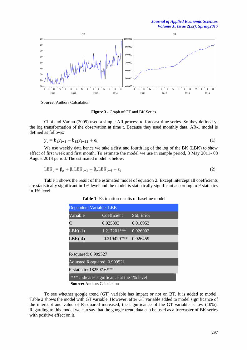
Journal of Applied Economic Sciences
Volume X, Issue 2(32), Spring2015
297
10
20
30
40
50
60
70
80
90
I II III IV I II III IV I II III IV I II III
2011 2012 2013 2014
GT
40,000
50,000
60,000
70,000
80,000
90,000
100,000
I II III IV I II III IV I II III IV I II III
2011 2012 2013 2014
BK
Source: Authors Calculation
Figure 3 - Graph of GT and BK Series
Choi and Varian (2009) used a simple AR process to forecast time series. So they defined yt
the log transformation of the observation at time t. Because they used monthly data, AR-1 model is
defined as follows:
(1)
We use weekly data hence we take a first and fourth lag of the log of the BK (LBK) to show
effect of first week and first month. To estimate the model we use in sample period, 3 May 2011- 08
August 2014 period. The estimated model is below:
β β
β
ε (2)
Table 1 shows the result of the estimated model of equation 2. Except intercept all coefficients
are statistically significant in 1% level and the model is statistically significant according to F statistics
in 1% level.
Table 1- Estimation results of baseline model
Dependent Variable: LBK
Variable Coefficient Std. Error
C 0.025893 0.018953
LBK(-1) 1.217201*** 0.026902
LBK(-4) -0.219420*** 0.026459
R-squared: 0.999527
Adjusted R-squared: 0.999521
F-statistic: 182597.6***
*** indicates significance at the 1% level
Source: Authors Calculation
To see whether google trend (GT) variable has impact or not on BT, it is added to model.
Table 2 shows the model with GT variable. However, after GT variable added to model significance of
the intercept and value of R-squared increased, the significance of the GT variable is low (10%).
Regarding to this model we can say that the google trend data can be used as a forecaster of BK series
with positive effect on it.
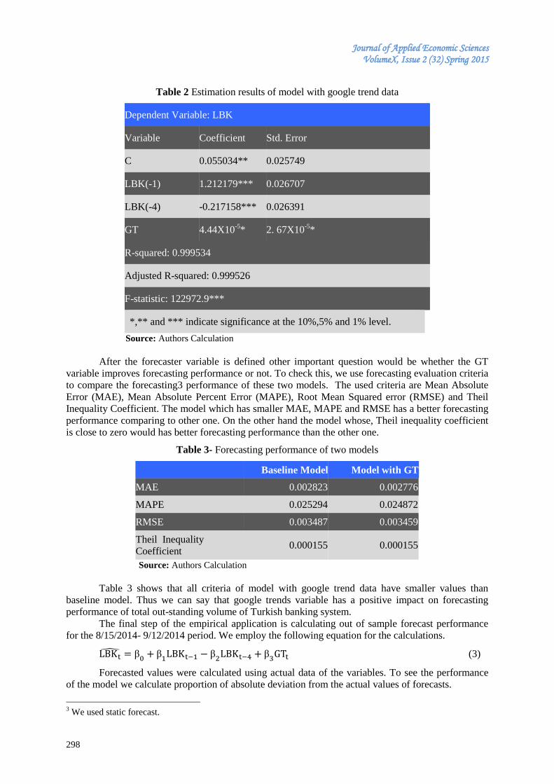
Journal of Applied Economic Sciences VolumeX, Issue 2 (32) Spring 2015
298
Table 2 Estimation results of model with google trend data
Dependent Variable: LBK
Variable Coefficient Std. Error
C 0.055034** 0.025749
LBK(-1) 1.212179*** 0.026707
LBK(-4) -0.217158*** 0.026391
GT 4.44X10-5
* 2. 67X10-5
*
R-squared: 0.999534
Adjusted R-squared: 0.999526
F-statistic: 122972.9***
*,** and *** indicate significance at the 10%,5% and 1% level.
Source: Authors Calculation
After the forecaster variable is defined other important question would be whether the GT
variable improves forecasting performance or not. To check this, we use forecasting evaluation criteria
to compare the forecasting3 performance of these two models. The used criteria are Mean Absolute
Error (MAE), Mean Absolute Percent Error (MAPE), Root Mean Squared error (RMSE) and Theil
Inequality Coefficient. The model which has smaller MAE, MAPE and RMSE has a better forecasting
performance comparing to other one. On the other hand the model whose, Theil inequality coefficient
is close to zero would has better forecasting performance than the other one.
Table 3- Forecasting performance of two models
Baseline Model Model with GT
MAE 0.002823 0.002776
MAPE 0.025294 0.024872
RMSE 0.003487 0.003459
Theil Inequality
Coefficient 0.000155 0.000155
Source: Authors Calculation
Table 3 shows that all criteria of model with google trend data have smaller values than
baseline model. Thus we can say that google trends variable has a positive impact on forecasting
performance of total out-standing volume of Turkish banking system.
The final step of the empirical application is calculating out of sample forecast performance
for the 8/15/2014- 9/12/2014 period. We employ the following equation for the calculations.
β β
β
β
(3)
Forecasted values were calculated using actual data of the variables. To see the performance
of the model we calculate proportion of absolute deviation from the actual values of forecasts.
3 We used static forecast.
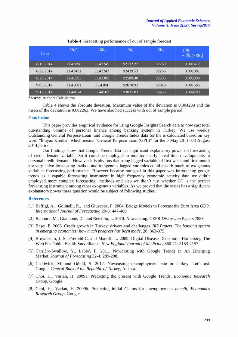
Journal of Applied Economic Sciences
Volume X, Issue 2(32), Spring2015
299
Table 4 Forecasting performance of out of sample forecast
Term
|(
) |
8/15/2014 11.43098 11.43245 92132.22 92268 0.001472
8/22/2014 11.43431 11.43243 92439.53 92266 0.001881
8/29/2014 11.43592 11.43383 92588.48 92395 0.002094
9/05/2014 11.43681 11.4384 92670.92 92818 0.001585
9/12/2014 11.44074 11.44503 93035.83 93436 0.004283
Source: Authors Calculation
Table 4 shows the absolute deviation. Maximum value of the deviation is 0.004283 and the
mean of the deviation is 0.002263. We have also had success with out of sample period.
Conclusion
This paper provides empirical evidence for using Google Insights Search data to now cast total
out-standing volume of personal finance among banking system in Turkey. We use weekly
Outstanding General Purpose Loan and Google Trends Index data for the is calculated based on key
word “İhtiyaç Kredisi” which means “General Purpose Loan (GPL)” for the 3 May 2011- 08 August
2014 period.
Our findings show that Google Trends data has significant explanatory power on forecasting
of credit demand variable. So it could be employed to monitor nearly - real time developments in
personal credit demand. However it is obvious that using lagged variable of first week and first month
are very naïve forecasting method and indigenous lagged variables could absorb much of exogenous
variables forecasting performance. However because our goal in this paper was introducing google
trends as a capable forecasting instrument in high frequency economic activity data we didn’t
employed more complex forecasting methods and also we didn’t test whether GT is the perfect
forecasting instrument among other exogenous variables. As we proved that the series has a significant
explanatory power these question would be subject of following studies.
References
[1] Baffigi, A., Golinelli, R., and Giuseppe, P. 2004. Bridge Models to Forecast the Euro Area GDP.
International Journal of Forecasting 20-3: 447-460
[2] Banbura, M., Giannone, D., and Reichlin, L. 2010. Nowcasting, CEPR Discussion Papers 7883
[3] Başçı, E. 2006. Credit growth in Turkey: drivers and challenges. BIS Papers, The banking system
in emerging economies: how much progress has been made, 28: 363-375.
[4] Brownstein, J. S., Freifeld C. and Madoff, L. 2009. Digital Disease Detection—Harnessing The
Web For Public Health Surveillance. New England Journal of Medicine, 360-21: 2153-2157.
[5] Carrière-Swallow, Y., Labbé, F. 2011. Nowcasting with Google Trends in An Emerging
Market. Journal of Forecasting 32-4: 289-298.
[6] Chadwick, M. and Gönül, S. 2012. Nowcasting unemployment rate in Turkey: Let’s ask
Google. Central Bank of the Republic of Turkey, Ankara.
[7] Choi, H., Varian, H. 2009a. Predicting the present with Google Trends, Economic Research
Group, Google
[8] Choi, H., Varian, H. 2009b. Predicting initial Claims for unemployment benefit, Economics
Research Group, Google
Journal of Applied Economic Sciences VolumeX, Issue 2 (32) Spring 2015
300
[9] Cook Samantha et al. 2011. Assessing Google Flu Trends Performance in the United States during
the 2009 Influenza Virus A (H1N1) Pandemic. PLoS ONE 6-8: 1-8 doi:10.1371/journal.pone.
0023610
[10] Etterdge, M., Gerdes, J., Karuga, G. 2005. Using web bazed search data to predict macro
economic statistics. Communications of the ACM, 48-11: 87 -92.
[11] Euro Surveillance 2009. Bulletin Europeen sur les Maladies Transmissibles = European
Communicable Disease Bulletin, 14-44: 429-433
[12] Evans, M.D.D. 2005. Where Are We Now? Real-Time Estimates of the Macroeconomy.
International Journal of Central Banking l-2
[13] Guzman, Giselle. “Internet search behavior as an economic forecasting tool: The case of inflation
expectations” Journal of Economic And Social Measurement 2011: 36-3: 119-167.
[14] Castle, J., Hendry, D., Kitov, O. 2013. Forecasting and Nowcasting Macroeconomic Variables :
A Methodological Overview. Oxford University Department of Economics Series Working
Papers No.674
[15] Kuhn, P., Skuterud, M. 2002. Internet Job Search and Unemployment Durations. IZA Discussion
Paper Series, No. 613
[16] Polgreen, P., et al. 2008. Using internet searches for influenza surveillance.” Clinical Infectious
Diseases 47: 1443–1448.
[17] Rünstler, G Sédillot, F. 2003. Short-term estimates of euro area real GDP by means of monthly
data. European Central Bank Working Paper Series 0276
[18] Wilson, N. et al. 2009. Interpretıng “Google Flu Trends” Data For Pandemıc H1N1 Influenza:
The New Zealand Experıence.” Eurosurveillance 14-44:1-3
Journal of Applied Economic Sciences
Volume X, Issue 2(32), Spring2015
301
COMPARISON OF COUNTRIES BY THE SYSTEMS OF HEALTH INSURANCE
Renata NESPORKOVA
Business School Ostrava plc., Czech Republic
Jan SIDOR
Slovak Medical University in Bratislava
Faculty of Public Health, Slovak Republic
Abstract:
Health care systems are different in different countries. Although there are significant differences
among them, in particular with regard to methods of financing, regulation, management and organization, their
common feature are ambitions to achieve the primary objective in terms of improving the health status of the
population in the country and therefore solve the daily question of prioritization of satisfying health needs. The
reasons for the rising costs in the health care systems are multi-dimensional. We can mention in particular
deterioration of the general condition of the human environment, way of life and raising the level of human
medicine, which requires expensive equipment by medical technique, medications, highly qualified personnel,
etc. The submitted article provides a macro view to the issue of efficiency of health care systems, public health
and its main objective was the evaluation and classification of countries ranking according to used health
insurance system. Reported outcomes constitute a valuable analytical platform for the design hypotheses in the
issue of health care systems effectiveness, as well as subsequent research in this area.
Keywords: systems of health insurance, public health insurance, private health insurance, Beveridge model,
Bismarck model, health care.
JEL Classification: I11, I13, I19.
1. Introduction
All developed countries have ensured the care of the health of its population (Barták, 2012).
Public health is the science and art of protecting and improving the community health through health
education, health promotion, research and disease prevention strategies. It is the knowledge and
application of multidisciplinary, population-based research methods, teaching and implementation
including various academic disciplines (WHO) (Michalski et al. 2014; Michalski, 2014a, b). WHO
defined in the 1988 public health as "the science and art relating to how it is possible through the joint
efforts of the society to prolong life, prevent disease and promote health." With the use of this term is
also linked to many unclear definitions and imprecise terms. We follow the referred definition,
because it reflects the social activities that aim to protect, maintain and improve the health of the
population care (Mura and Buleca, 2012; Mura et al. 2012; Szabo et al. 2013). For public health is
typical population approach to health because the object of interest is the state of entire population
health or population groups, which are in terms of to the health risk-bearing (Soltes and Gavurova,
2014a,b). At present, these groups represent mainly the elderly, the disabled, children of one parent or
dysfunctional families, ethnic minorities, immigrants, long-term unemployed, etc. In the current view
and approach to the definition of public health is a clear emphasis on social and political concept
based on medical aspects, aimed at improving health, prolonging life and improving the quality of
whole population life through health promotion, disease prevention and other forms of healthcare
interventions (Rovný et al. 2011).
2. Healthcare systems of developed countries
Health care systems in developed countries can be classified according to the way how people
in the country pay for provided medical services in the so-called public health, funded by tax through
the state budget, health care financed by public health insurance – so called "Bismarck model" and
health care largely market-oriented, where the crucial role is playing private health insurance (Szabo
and Sidor, 2014; Pudlo and Szabo, 2014; Dorčák et al. 2014; Barták, 2012; Barták and Dlouhý, 2013).
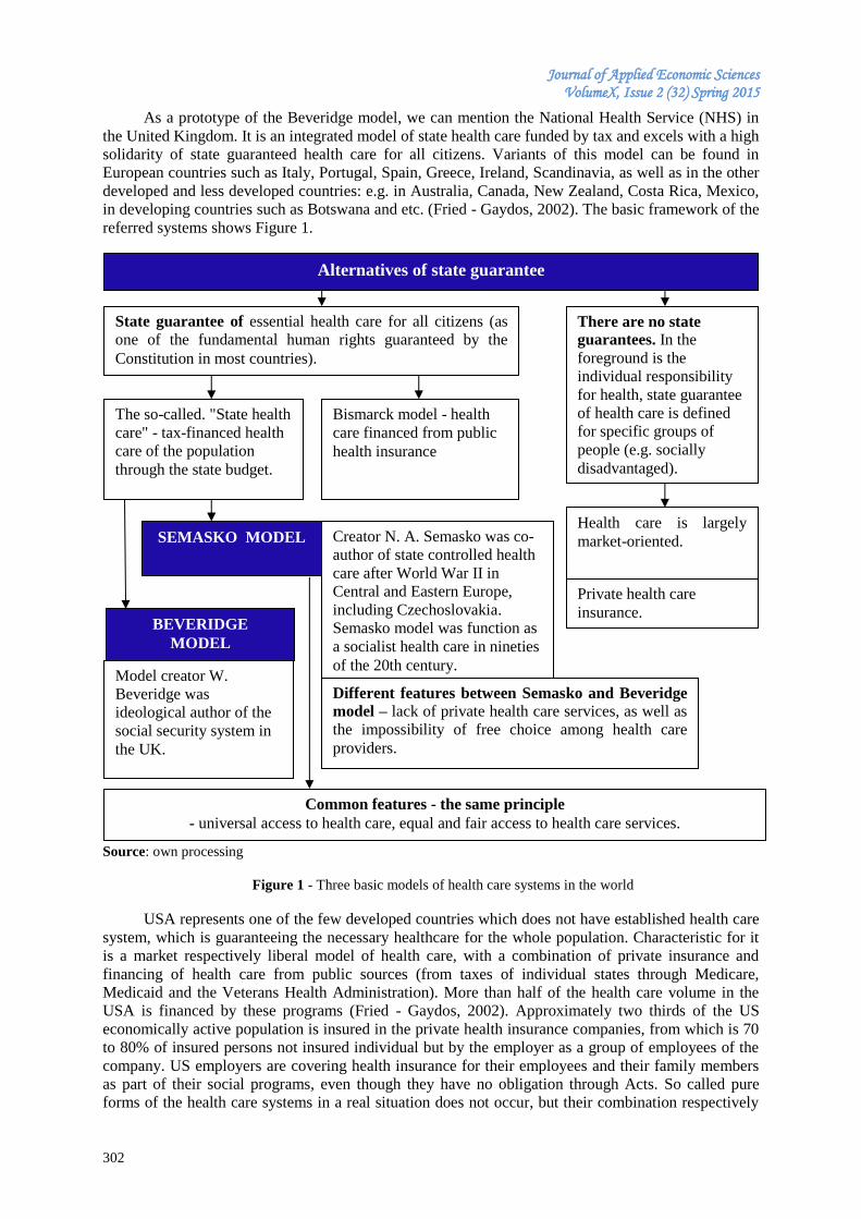
Journal of Applied Economic Sciences VolumeX, Issue 2 (32) Spring 2015
302
As a prototype of the Beveridge model, we can mention the National Health Service (NHS) in
the United Kingdom. It is an integrated model of state health care funded by tax and excels with a high
solidarity of state guaranteed health care for all citizens. Variants of this model can be found in
European countries such as Italy, Portugal, Spain, Greece, Ireland, Scandinavia, as well as in the other
developed and less developed countries: e.g. in Australia, Canada, New Zealand, Costa Rica, Mexico,
in developing countries such as Botswana and etc. (Fried - Gaydos, 2002). The basic framework of the
referred systems shows Figure 1.
Source: own processing
Figure 1 - Three basic models of health care systems in the world
USA represents one of the few developed countries which does not have established health care
system, which is guaranteeing the necessary healthcare for the whole population. Characteristic for it
is a market respectively liberal model of health care, with a combination of private insurance and
financing of health care from public sources (from taxes of individual states through Medicare,
Medicaid and the Veterans Health Administration). More than half of the health care volume in the
USA is financed by these programs (Fried - Gaydos, 2002). Approximately two thirds of the US
economically active population is insured in the private health insurance companies, from which is 70
to 80% of insured persons not insured individual but by the employer as a group of employees of the
company. US employers are covering health insurance for their employees and their family members
as part of their social programs, even though they have no obligation through Acts. So called pure
forms of the health care systems in a real situation does not occur, but their combination respectively
The so-called. "State health
care" - tax-financed health
care of the population
through the state budget.
Bismarck model - health
care financed from public
health insurance
Health care is largely
market-oriented.
State guarantee of essential health care for all citizens (as
one of the fundamental human rights guaranteed by the
Constitution in most countries).
There are no state
guarantees. In the
foreground is the
individual responsibility
for health, state guarantee
of health care is defined
for specific groups of
people (e.g. socially
disadvantaged).
BEVERIDGE
MODEL
SEMASKO MODEL
Model creator W.
Beveridge was
ideological author of the
social security system in
the UK.
Creator N. A. Semasko was co-
author of state controlled health
care after World War II in
Central and Eastern Europe,
including Czechoslovakia.
Semasko model was function as
a socialist health care in nineties
of the 20th century.
Common features - the same principle
- universal access to health care, equal and fair access to health care services.
Different features between Semasko and Beveridge
model – lack of private health care services, as well as
the impossibility of free choice among health care
providers.
Alternatives of state guarantee
Private health care
insurance.

Journal of Applied Economic Sciences
Volume X, Issue 2(32), Spring2015
303
variants. Therefore, in any country in the world it is not possible to find such a health care system,
which would be financed from only one source (Gavurová et al. 2014). As reported by Kuvíková
(2004), there are not two countries, which should have the same methods of health financing. Priorities
of public health in the EU countries are varying. On the one hand we can talk about institutional unity
in terms of legislative provision, but the differences are in terms of administrative. For comparison, we
choose nine countries and specify the main characteristics of their public health (Table 1).
Table 1 - Comparison of the public health specificities in selected countries
Specifics of public health care in selected countries
Finland
well-elaborated system of occupational health,
existence of Institute of the Finnish Institute of Occupational Health, which is research and
advisory institute, whose main objectives are research, training of professionals for health
and safety at work, advisory services and dissemination of information,
important role are playing health centres at regional level, which ensure a high level: the care
of mother and child, immunization program, screening of breast cancer for women in the age
group of 50-99 years, screening of cervical cancer for women in the age group of 50-60
years,
priority issues in the field of health education are smoking, nutrition, physical inactivity,
reproductive health, reduce the consumption of unsuitable products and the like. Through
health education are influenced eating habits.
United Kingdom
for the support and maintenance of public health is responsible the Ministry of Health and the
National Health System,
the primary responsibility of the Ministry of Health is leading the development and
implementation of health strategies (documents "Saving Lives, Our Healthier Nation"),
primary responsibility for the fulfilment of public health priorities have health institutions,
many competencies of public health are delimited on local respectively regional authorities,
each health institution in their organizational structure has "department of public health"
which annually compiles a report on the state of the population of the territory, including
strategies for improvement at the national level,
in 1992 were developed new approaches to public health - White Paper - Health of Nation. It
contains priorities and quantifiable targets for the reduction of mortality in cardiovascular
disease, stroke, cancers, mental diseases, venereal diseases and injuries,
harsh criticism of "Health of Nation" for the emphasis on individual behavior to explain the
poor health status of the population, the underestimation of important social determinants of
health of the poor.
Hungary
in 1991 was founded the National Office of Public Health and Medicine, which is responsible
for the supervision of the population health status, immunization program, monitoring the
quality of drinking water, air, water, health and food safety, care about working conditions,
HIV / AIDS, as well as toxicology,
the national level is represented by 7 institutions of public health,
at the regional level 9 + 1 (including the capital) are public healthcare institutions, 114
municipal and 22 district centres,
application of multi-source financing.
France
area of preventive occupational medicine and environmental health is very strong,

Journal of Applied Economic Sciences VolumeX, Issue 2 (32) Spring 2015
304
treatment prevails over prevention,
at the national level is established the Commission for Public Health,
the existence of a public healthcare institutions network and Institute of Health and Medical
Research,
public health system is centralized.
Denmark
the existence of three-level public health system - national, regional and communal,
at the national level are established 8 departments of public health,
institutions at the regional level are responsible for hospital care and health promotion,
institutions at the municipal level are responsible for health protection,
the existence of the National Programme for Health is approved by the government, the
priorities are common with the international priorities of public health,
established system of financing through tax policy - high redistribution of taxes.
Germany
system of financing differs from previous,
implemented prevention programs and projects, including the immunization program and the
public health is funded through health insurance,
at the state level is centred public health issue,
the scientific research activities in public health and the involvement of universities are
positive evaluated,
the federal level and state level legislation is fundamental in the public health.
Austria
at the federal level are established six federal institutions for the quality of drinking water, air,
hospital care, transmissible diseases, including HIV, AIDS
2/3 of health protection and promotion is funded by health insurance (the remaining part is
covered by grants, EU, private funds, etc.),
state is defining national priorities and maintain a system of government tasks,
at regional level are established departments of health protection, counselling services and
education of the population to health.
Sweden
according to international standards, the health status of the population is one of the best
in the country have the longest life expectancy (76.2 years for men, 81.4 years for women), in
the world ranking belong to the countries with the oldest population,
effective programs implemented by Swedish government are oriented for example to the
diseases and mortality from cardiovascular diseases and diseases due to alcohol,
Committee for Public Health published in 1991, the National Strategy for Health, which
included tactics to improve the health state of the Swedish population,
in 1992 was established by the Swedish Government the National Institute of Public Health,
where implementation of its plans for health promotion focuses on alcohol, drugs, tobacco,
unintentional injuries, women exposed to specific health risks,
governments privileges are primarily preventive measures, such as struggle against alcohol
addiction, currently receives in the attention the question of unemployment, the environment
and etc.,
it is addresses the long-term question of environmental and with it related environmental
health risks: environmental pollution and traffic, radon in soil, smoking, noise.
Norway
public health is organized in a three-level system
in order to minimize the distance between the environment and the patient were maximum
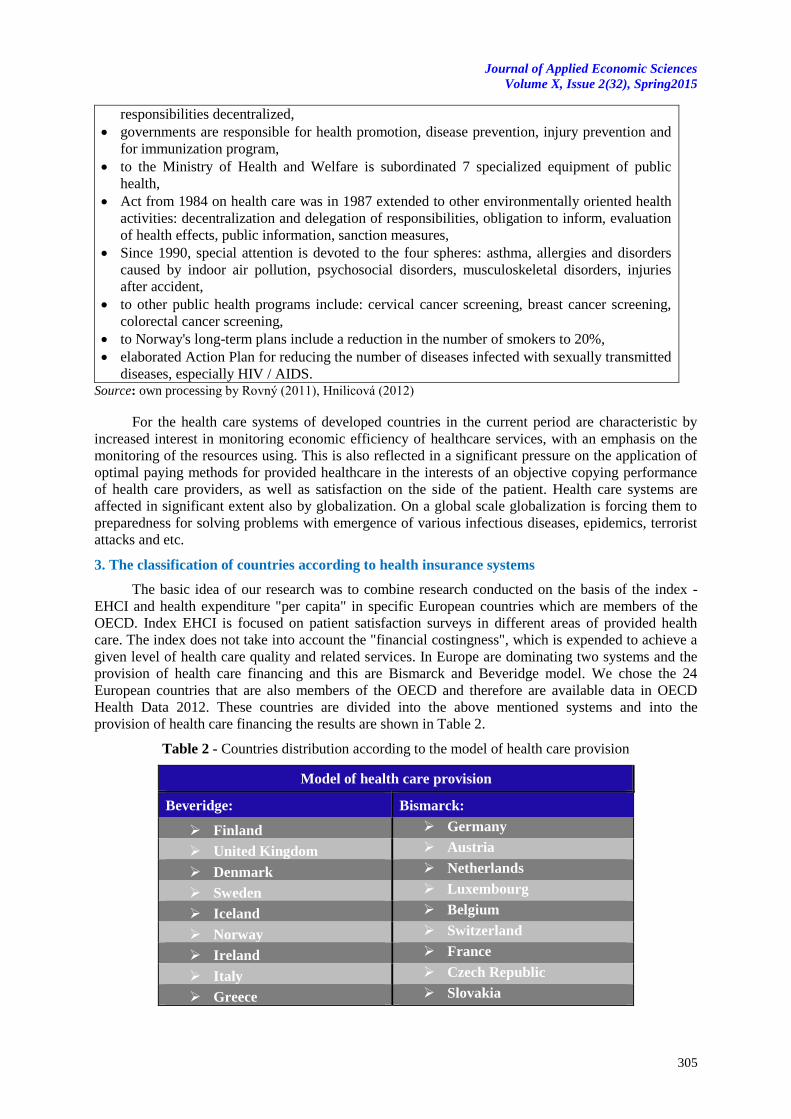
Journal of Applied Economic Sciences
Volume X, Issue 2(32), Spring2015
305
responsibilities decentralized,
governments are responsible for health promotion, disease prevention, injury prevention and
for immunization program,
to the Ministry of Health and Welfare is subordinated 7 specialized equipment of public
health,
Act from 1984 on health care was in 1987 extended to other environmentally oriented health
activities: decentralization and delegation of responsibilities, obligation to inform, evaluation
of health effects, public information, sanction measures,
Since 1990, special attention is devoted to the four spheres: asthma, allergies and disorders
caused by indoor air pollution, psychosocial disorders, musculoskeletal disorders, injuries
after accident,
to other public health programs include: cervical cancer screening, breast cancer screening,
colorectal cancer screening,
to Norway's long-term plans include a reduction in the number of smokers to 20%,
elaborated Action Plan for reducing the number of diseases infected with sexually transmitted
diseases, especially HIV / AIDS. Source: own processing by Rovný (2011), Hnilicová (2012)
For the health care systems of developed countries in the current period are characteristic by
increased interest in monitoring economic efficiency of healthcare services, with an emphasis on the
monitoring of the resources using. This is also reflected in a significant pressure on the application of
optimal paying methods for provided healthcare in the interests of an objective copying performance
of health care providers, as well as satisfaction on the side of the patient. Health care systems are
affected in significant extent also by globalization. On a global scale globalization is forcing them to
preparedness for solving problems with emergence of various infectious diseases, epidemics, terrorist
attacks and etc.
3. The classification of countries according to health insurance systems
The basic idea of our research was to combine research conducted on the basis of the index -
EHCI and health expenditure "per capita" in specific European countries which are members of the
OECD. Index EHCI is focused on patient satisfaction surveys in different areas of provided health
care. The index does not take into account the "financial costingness", which is expended to achieve a
given level of health care quality and related services. In Europe are dominating two systems and the
provision of health care financing and this are Bismarck and Beveridge model. We chose the 24
European countries that are also members of the OECD and therefore are available data in OECD
Health Data 2012. These countries are divided into the above mentioned systems and into the
provision of health care financing the results are shown in Table 2.
Table 2 - Countries distribution according to the model of health care provision
Model of health care provision
Beveridge: Bismarck:
Finland Germany
United Kingdom Austria
Denmark Netherlands
Sweden Luxembourg
Iceland Belgium
Norway Switzerland
Ireland France
Italy Czech Republic
Greece Slovakia
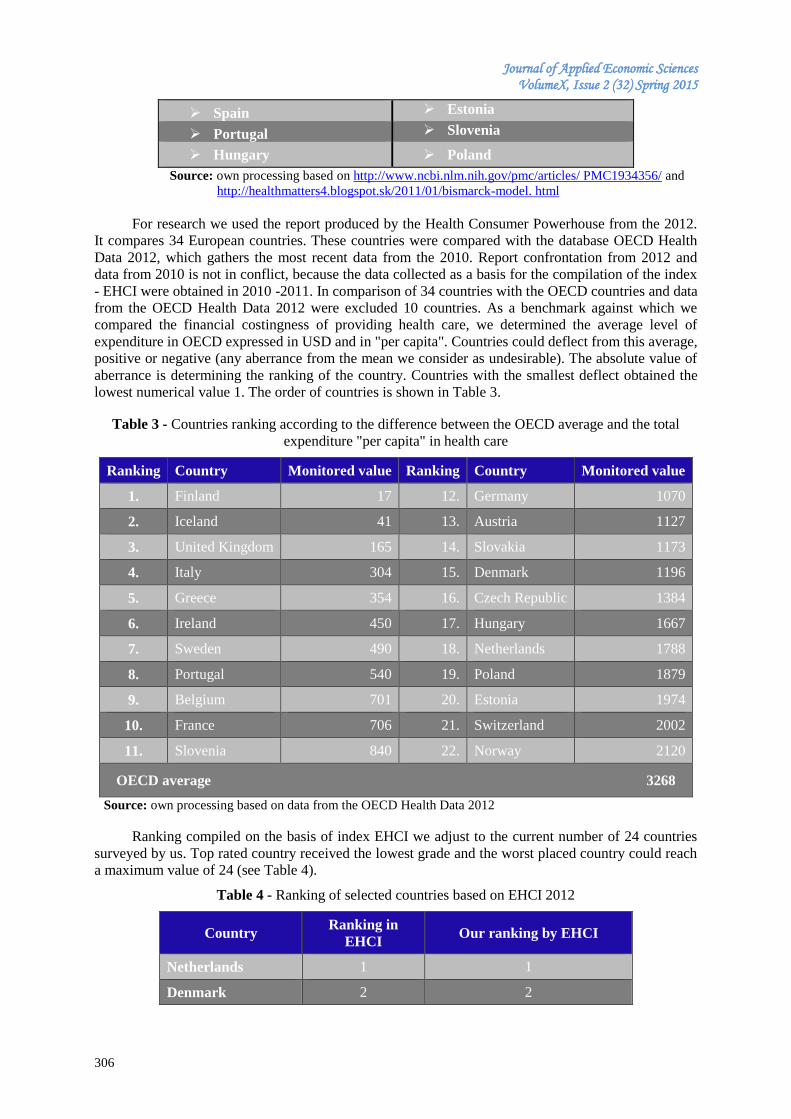
Journal of Applied Economic Sciences VolumeX, Issue 2 (32) Spring 2015
306
Spain Estonia
Portugal Slovenia
Hungary Poland
Source: own processing based on http://www.ncbi.nlm.nih.gov/pmc/articles/ PMC1934356/ and
http://healthmatters4.blogspot.sk/2011/01/bismarck-model. html
For research we used the report produced by the Health Consumer Powerhouse from the 2012.
It compares 34 European countries. These countries were compared with the database OECD Health
Data 2012, which gathers the most recent data from the 2010. Report confrontation from 2012 and
data from 2010 is not in conflict, because the data collected as a basis for the compilation of the index
- EHCI were obtained in 2010 -2011. In comparison of 34 countries with the OECD countries and data
from the OECD Health Data 2012 were excluded 10 countries. As a benchmark against which we
compared the financial costingness of providing health care, we determined the average level of
expenditure in OECD expressed in USD and in "per capita". Countries could deflect from this average,
positive or negative (any aberrance from the mean we consider as undesirable). The absolute value of
aberrance is determining the ranking of the country. Countries with the smallest deflect obtained the
lowest numerical value 1. The order of countries is shown in Table 3.
Table 3 - Countries ranking according to the difference between the OECD average and the total
expenditure "per capita" in health care
Ranking Country Monitored value Ranking Country Monitored value
1. Finland 17 12. Germany 1070
2. Iceland 41 13. Austria 1127
3. United Kingdom 165 14. Slovakia 1173
4. Italy 304 15. Denmark 1196
5. Greece 354 16. Czech Republic 1384
6. Ireland 450 17. Hungary 1667
7. Sweden 490 18. Netherlands 1788
8. Portugal 540 19. Poland 1879
9. Belgium 701 20. Estonia 1974
10. France 706 21. Switzerland 2002
11. Slovenia 840 22. Norway 2120
OECD average 3268
Source: own processing based on data from the OECD Health Data 2012
Ranking compiled on the basis of index EHCI we adjust to the current number of 24 countries
surveyed by us. Top rated country received the lowest grade and the worst placed country could reach
a maximum value of 24 (see Table 4).
Table 4 - Ranking of selected countries based on EHCI 2012
Country Ranking in
EHCI Our ranking by EHCI
Netherlands 1 1
Denmark 2 2
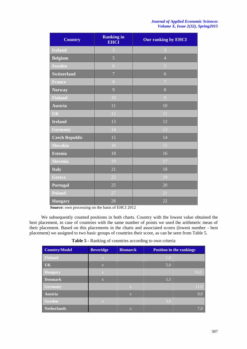
Journal of Applied Economic Sciences
Volume X, Issue 2(32), Spring2015
307
Country Ranking in
EHCI Our ranking by EHCI
Iceland 3 3
Belgium 5 4
Sweden 6 5
Switzerland 7 6
France 8 7
Norway 9 8
Finland 10 9
Austria 11 10
UK 12 11
Ireland 13 12
Germany 14 13
Czech Republic 15 14
Slovakia 16 15
Estonia 18 16
Slovenia 19 17
Italy 21 18
Greece 22 19
Portugal 25 20
Poland 27 21
Hungary 28 22
Source: own processing on the basis of EHCI 2012
We subsequently counted positions in both charts. Country with the lowest value obtained the
best placement, in case of countries with the same number of points we used the arithmetic mean of
their placement. Based on this placements in the charts and associated scores (lowest number - best
placement) we assigned to two basic groups of countries their score, as can be seen from Table 5.
Table 5 - Ranking of countries according to own criteria
Country/Model Beveridge Bismarck Position in the rankings
Finland x 1,0
UK x 5,0
Hungary x 16,0
Denmark x 5,5
Germany x 11,0
Austria x 9,0
Sweden x 3,0
Netherlands x 7,0
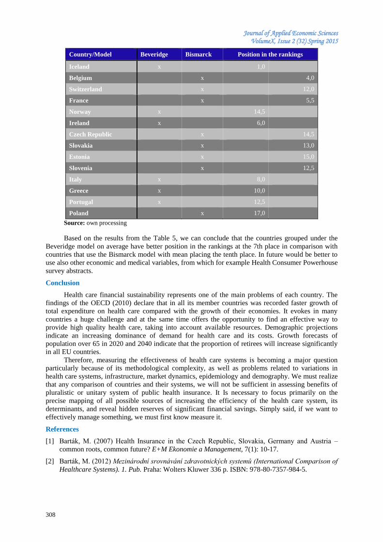
Journal of Applied Economic Sciences VolumeX, Issue 2 (32) Spring 2015
308
Country/Model Beveridge Bismarck Position in the rankings
Iceland x 1,0
Belgium x 4,0
Switzerland x 12,0
France x 5,5
Norway x 14,5
Ireland x 6,0
Czech Republic x 14,5
Slovakia x 13,0
Estonia x 15,0
Slovenia x 12,5
Italy x 8,0
Greece x 10,0
Portugal x 12,5
Poland x 17,0
Source: own processing
Based on the results from the Table 5, we can conclude that the countries grouped under the
Beveridge model on average have better position in the rankings at the 7th place in comparison with
countries that use the Bismarck model with mean placing the tenth place. In future would be better to
use also other economic and medical variables, from which for example Health Consumer Powerhouse
survey abstracts.
Conclusion
Health care financial sustainability represents one of the main problems of each country. The
findings of the OECD (2010) declare that in all its member countries was recorded faster growth of
total expenditure on health care compared with the growth of their economies. It evokes in many
countries a huge challenge and at the same time offers the opportunity to find an effective way to
provide high quality health care, taking into account available resources. Demographic projections
indicate an increasing dominance of demand for health care and its costs. Growth forecasts of
population over 65 in 2020 and 2040 indicate that the proportion of retirees will increase significantly
in all EU countries.
Therefore, measuring the effectiveness of health care systems is becoming a major question
particularly because of its methodological complexity, as well as problems related to variations in
health care systems, infrastructure, market dynamics, epidemiology and demography. We must realize
that any comparison of countries and their systems, we will not be sufficient in assessing benefits of
pluralistic or unitary system of public health insurance. It Is necessary to focus primarily on the
precise mapping of all possible sources of increasing the efficiency of the health care system, its
determinants, and reveal hidden reserves of significant financial savings. Simply said, if we want to
effectively manage something, we must first know measure it.
References
[1] Barták, M. (200 ) Health Insurance in the Czech Republic, Slovakia, Germany and Austria –
common roots, common future? E+M Ekonomie a Management, 7(1): 10-17.
[2] Barták, M. (2012) Mezinárodní srovnávání zdravotnických systemů (International Comparison of
Healthcare Systems). 1. Pub. Praha: Wolters Kluwer 336 p. ISBN: 978-80-7357-984-5.
Journal of Applied Economic Sciences
Volume X, Issue 2(32), Spring2015
309
[3] Barták, M., Dlouhý, M. (2013) Mezinárodní srovnávání zdravotnických služeb a systémů.
(International comparison of the health services and systems), Revizní a posudkové lékařství, 16
(4): 123 – 128.
[4] Dorčák, P., Pollák, F., Szabo, S. (2014). Analysis of the possibilities of improving an online reputation of public institutions. IDIMT-2014, Sept. 10–12. Poděbrady: IDIMT Networking
Societies-Cooperation and Conflict 22ndInterdisciplinary Information and Management Talks,
2014, p. 275-281, ISBN 978-3-99033-3402.
[5] Fried, B., Gaydos, L. (2002). World Health Systems. Challenges and Perspectives, Health Care
Administration Press, Chicago, 2002.
[6] Gavurova, B., Soltes, M., Balloni, A.J. (2014). Ekonomicky vyznam vyuzivania informacno-
komunikacnych technologii v systeme zdravotnictva. (The Economic Importance of Using of ICT
in the Health System), Ekonomicky casopis, 62(1): 83-104.
[7] Hnilicová, H. (2012). Úvod do studia zdravotníckych systémů. (06.08.2012) http://usm.lf1.cuni.
cz/download/uvod_do_zs.pdf
[8] Kuvíková, H. (2004). Zdravotnícke systémy sveta v kontexte zvyšovania reálnych finančných
zdrojov. In: Ekonomický časopis, 52 (8): 960-963.
[9] Kroneman M.W., Zee J. (2012). Bismarck or Beverage: a beauty contest between dinosaurs.
(29.08.2012), http://www.ncbi.nlm.nih.gov/pmc/articles/PMC1934356/
[10] Michalski, G. (2014a). Effective Working Capital Investment - German Firms Case, In:
Quantitative method in economics multiple decision making XVII, Proceedings of the 17th
International Conference -Virt, Slovakia 2014, pp. 176-181, ISBN 978-80-225-3868-8.
[11] Michalski, G., Honova, I., Hon, M., et al. (2014). Entrepreneurial Financial Liquidity
Management Experiences and Perspectives in EU and Outside EU: German, Austrian and French
Data Illustration, In: Proceedings of the 2nd
International Conference on European Integration
(ICEI 2014), pp. 484 – 491.
[12] Michalski, G. (2014b). Financial Markets Turmoils and Firms Cash Levels in Real Economy, in:
The role of financial sector in supporting the economic recovery of CEE countries, 8th
International Conference on Currency, Banking and International Finance: 10 - 11 September
2014, Bratislava, Slovak Republic, Ekonóm, 2014. ISBN 978-80-225-3926-5.
[13] Mura, L., Buleca, J. (2012). Evaluation of Financing Possibilities of Small and Medium Industrial
Enterprises, Procedia Economics and Finance, 3: 217-222.
[14] Mura, L., Buleca, J., Zelenakova, L., Qineti, A., Kozelova, D. (2012). An analysis of selected
aspects of international business in Slovak dairies in the EU framework, Mljekarstvo, 62(3): 219-
226.
[15] Pudlo, P., Szabo, S. (2014). Logistic Costs of Quality and Their Impact on Degree of Operation
Level, Journal of Applied Economic Sciences, Volume IX, 3(29): 468-475, http://cesmaa.eu/
journals/jaes/files/JAES_2014_Fall.pdf
[16] Rovný, I. a kol. (2011). Vybrané kapitoly verejného zdravotníctva. 1. pub. Bratislava: 2011, pp.
591. ISBN 978-80-89057-33-7.
[17] Szabo, S., Sidor, J. (2014). The performance measurement system–potentials and barriers for its
implementation in healthcare facilities, Journal of Applied Economic Sciences, Volume IX, 3(29):
728-735, http://cesmaa.eu/journals/jaes/files/JAES_2014_Fall.pdf.
[18] Szabo, Z.K., Šoltés, M., Herman, E. (2013). Innovative Capacity and Performance of Transition
Economies: Comparative Study at the Level of Enterprises, E+M Ekonomie a Management,
16(1): 52-68.
[19] Šoltés, V., Gavurová, B. (2014a). The Functionality Comparison of the Health Care Systems by
the Analytical Hierarchy Process Method, In: E+M Ekonomie a Management, 17(3): 100-118.

Journal of Applied Economic Sciences VolumeX, Issue 2 (32) Spring 2015
310
[20] Šoltés, V., Gavurová, B. (2014b). Analysis of Selected Demographic Aspects of Day Surgery in
Slovak Health Policy, Journal of Applied Economic Sciences, 9(3): 476-486.
*** OECD. (2012). Health Data 2012. (29. 08. 2012), http://www.oecd.org/health/health policies
anddata/oecdhealthdata2012-frequentlyrequesteddata.htm.
*** The Bismarck Model. 2012. (29.08.2012), http://healthmatters4.blogspot.sk/2011/01/bismarck-
model.html.
*** WHO. (2008). Health Financing policy: a guide for decision-makers. (29.08.2012),
http://www.euro.who.int/data/assets/pdf_file/0004/78871/E91422.pdf.
ISSN 1843-6110