nonlinear structure formation with the environmentally dependent dilaton
TRANSCRIPT

arX
iv:1
102.
3692
v1 [
astr
o-ph
.CO
] 1
7 Fe
b 20
11
Nonlinear Structure Formation with the Environmentally Dependent Dilaton
Philippe Brax,1, ∗ Carsten van de Bruck,2, † Anne-Christine. Davis,3, ‡ Baojiu Li,3, 4, § and Douglas J. Shaw3, ¶
1Institut de Physique Theorique, CEA, IPhT, CNRS, URA 2306, F-91191Gif/Yvette Cedex, France2Department of Applied Mathematics, University of Sheffield, Hounsfield Road, Sheffield S3 7RH, UK
3DAMTP, Centre for Mathematical Sciences, University of Cambridge, Wilberforce Road, Cambridge CB3 0WA, UK4Kavli Institute for Cosmology Cambridge, Madingley Road, Cambridge CB3 0HA, UK
(Dated: June 18, 2013)
We have studied the nonlinear structure formation of the environmentally dependent dilatonmodel using N-body simulations. We find that the mechanism of suppressing the scalar fifth forcein high-density regions works very well. Within the parameter space allowed by the solar systemtests, the dilaton model predicts small deviations of the matter power spectrum and the massfunction from their ΛCDM counterparts. The importance of taking full account of the nonlinearityof the model is also emphasized.
I. INTRODUCTION
Modifying gravity on large scales is one of the plausi-ble ways of explaining the recent acceleration of the ex-pansion of the universe. So far, the construction of validmodels of modified gravity has been fraught with difficul-ties. The most serious one is already present in the orig-inal Pauli-Fierz formulation of massive gravity [1] andinvolves the existence of a ghost in curved backgrounds1.This phenomenon seems to be generic as suggested by Os-trograski’s theorem[2] which states that higher derivativetheories have a Hamiltonian which is unbounded frombelow. Higher dimensional versions of modified gravitysuch as the DGP model [4] also suffer from the presenceof a ghost in their spectrum at low energy. This problemis nicely avoided in f(R) models [5] which turn out tobe equivalent to a particular type of scalar-tensor the-ories [6]. In these models, the compatibility with solarsystem and laboratory tests of gravity is not straightfor-ward and can only be achieved thanks to the so-calledchameleon mechanism [7–12]. Indeed, the existence of anearly massless scalar field on cosmological scales couldjeopardize gravity locally. This issue is common to allknown models of dark energy coupled to matter [13].In a large class of dark energy models involving a lin-ear coupling to matter and a non-linear potential, thechameleon mechanism, whereby the scalar field mass be-comes dependent on the ambient environment, would besufficient to hide away the dark energy field locally. Sim-ilarly, in models of gravity such as the DGP or Galileon[14, 15] theories for which a shift symmetry only allowfor non-linearities in the scalar field kinetic terms, theVainshtein mechanism [16] can be at play and preventthe existence of a fifth force locally. In this paper, we will
∗ Email address: [email protected]† Email address: [email protected]‡ Email address: [email protected]§ Email address: [email protected]¶ Email address: [email protected] For a new formulation of massive gravity in the so called decou-pling limit see [3]
focus on a different type of models involving a scalar field.These models are inspired from the string dilaton in thestrong coupling regime [17–19]. Their gravitational va-lidity relies on an environmentally dependent form of theDamour-Polyakov mechanism [20] whereby the couplingto matter is driven to vanish cosmologically. Here, thecoupling to matter is negligible in dense regions and inthe vicinity of dense bodies. This prevents the existenceof a fifth force in galaxies. Constraints on the parameterspace of these models springing from local tests of gravityhave already been obtained in [21]. Here we will study thecosmology of these models in the non-linear regime whenstructures form (see [22] for an analysis of the bispec-trum of matter distribution in this model). This requireslarge computer simulations. As a result, we have accessto non-linear properties of the dilaton models such as thenon-linear power spectrum or the number of dark matterhalos for a given mass. Moreover we will be able to probehow much the local tests of gravity constrain large scalestructure formation and deviations from general relativ-ity. We find that the dilaton models differ from GR atmost at the level of a few percent once the local (i.e.solar–system) constraints have been imposed. Althoughpossibly detectable in principle, observing such small de-viations will be challenging in the near future.The arrangement of this paper is as follows: in Sect. II
we briefly review the dilaton model under study and de-rive the field equations in the Newtonian limit, whichare relevant for the study of structure formation on sub-horizon scales and at late times. In Sect. III we describethe algorithm and code of our N -body simulations, andperform relevant tests of the code. More technical detailsare given in the appendices. The numerical results andtheir analysis are summarised in Sect. IV and finally weconclude in Sect. V. The metric convention is (−,+,+,+)and we use c = 1 unless stated otherwise.
II. THE ENVIRONMENTALLY DEPENDENT
DILATON
In this section we very briefly summarise the essen-tial ingredients of the environmentally dependent dilaton

2
model, which will be used for the simulations and discus-sions below. For more details about the model the readeris referred to [21].
A. The Model
The dilaton model is fully specified by the followingEinstein-Hilbert action in the Einstein frame:
S =
∫ √−gd4x[
R
2κ2− k2(ϕ)
κ2∇aϕ∇aϕ− V (ϕ)
]
+Sm
(
Ψi, A2(ϕ)gab;ϕ
)
, (1)
in which g is the determinant of the metric gab, κ2 ≡ 8πG
with G the gravitational constant, ϕ is the dilaton field,and V (ϕ) its potential, which is derived from string the-ory in the strong coupling limit. In the matter action Sm,Ψi collectively represents the matter fields and A2(ϕ)gabis the metric governing the geodesics of matter particles.In the Einstein frame, the particles feel an extra, or fifth,force whose strength is determined by the coupling func-tion β(ϕ) ≡ [lnA(ϕ)],ϕ where a comma denotes partial
differentiation. The function k(ϕ) is given by
k(ϕ) ≈ λ−1√
1 + 3λ2β2ϕ (2)
where λ is a constant. Throughout this paper Latinindices a, b, c, . . . run over 0, 1, 2, 3 and Greek indicesα, β, . . . run over 1,2,3.Varying the action with respect to the metric gab, we
obtain the total energy-momentum tensor of the model,
κ2Tab = κ2A(ϕ)Tmab − κ2gabV (ϕ)
+k2(ϕ) [2∇aϕ∇bϕ− gab∇cϕ∇cϕ] (3)
where Tmab is the energy-momentum tensor for fluid mat-
ter, i.e., baryons, radiation and cold dark matter (CDM).Note that there is a factor A(ϕ) in front of Tm
ab. Tabm is
not, in general, conserved but instead:
∇aTabm =
A,ϕ(ϕ)
A(ϕ)
[
Tm∇bφ− T abm ∇aφ
]
. (4)
For pressureless dust, where T abm = ρmu
aub, uaua =
−1, Eq. (4) implies that the usual continuity equationholds, ∇a(ρmu
a) = 0, and hence ρm is conserved. In aRobertson–Walker spacetime, this means that the usualconservation equation for matter still holds:
˙ρm + 3Hρm = 0, (5)
in which ˙≡ d/dt, subscript m denotes matter, H = a/ais the background expansion rate with a the scale fac-tor, and an overbar stands for the background value ofa physical quantity. The gravitational field equation, orEinstein’s equation, is given as usual:
Gab ≡ Rab −1
2gabR = κ2Tab, (6)
where Gab, Rab and R are respectively the Einstein ten-sor, Ricci tensor and Ricci scalar.Varying the action with respect to the scalar field ϕ,
we obtain its equation of motion:
∇a [k(ϕ)∇aϕ]
=4πG
k(ϕ)[−V (ϕ) − β(ϕ) (A(ϕ)Tm − 4V (ϕ))] (7)
where Tm is the trace of Tmab. The energy-momentum ten-
sor of an individual particle with mass m0 at position r0is given by
T abm (r) =
m0√−g δ (r− r0) ra0 r
b0, (8)
where r is the general spatial coordinate. Using theBianchi identity we get
ra0 + Γabcr
b0r
c0 = −β(ϕ)∇aϕ− β(ϕ)ϕra0 , (9)
in which Γabc is the Levi-Civita connection. Clearly, if β =
0 then this reduces to the geodesic equation in generalrelativity, as expected.Eqs. (6, 3, 7, 9) contain all the physics for the analysis
below, though to implement them in N -body simulationswe still have to simplify them using appropriate approxi-mations. These will be carried out below.In this paper, we focus on the particular model of [21],
which is motivated from string theory, specified by
A(ϕ) = 1 +1
2A2 (ϕ− ϕ0)
2, (10)
β(ϕ) = A2 (ϕ− ϕ0) , (11)
k2(ϕ) = 3A22 (ϕ− ϕ0)
2+ λ−2, (12)
V (ϕ) = A4(ϕ)V0e−ϕ (13)
where A2 ≫ 1 is a parameter and ϕ0 is the current back-ground value of ϕ. V0 is another parameter of mass di-mension 4. Because the potential is exponential, we arefree to shift the value of ϕ so that ϕ0 = 0. ClearlyVc = V0e
−ϕ0 = V0 should be chosen carefully so that itcan play the role of dark energy today. Both the param-eters A2 and λ are crucially constrained by local tests.In the numerical simulations, we will choose values of theparameters which are on the verge of the allowed parame-ter space in order to enhance the possible effects on largescales.
B. Nonrelativistic Limit
Eqs. (6, 3, 7, 9) are general relativistic equations.To implement them into N -body simulations for largescale structure formation, it suffices to work in the non-relativistic limits, since the simulations only probe weak-gravity regime and small volumes compared with the cos-mos.We write the perturbed metric in the conformal New-
tonian gauge as
ds2 = −a2(1 + 2φ)dτ2 + a2(1− 2ψ)γµνdxµdxν (14)

3
where τ, xµ are respectively the conformal time and co-moving coordinate, γµν is the metric of a 3-D Euclideanspace, and φ, ψ respectively the Newtonian potential andthe perturbation to the spatial curvature. For complete-ness, we list the expressions of the components of Gab
in terms of the metric variables using our convention inAppendix A.Let us first look at the scalar field equation of motion
Eq. (7). For this, we define ξ such that ∇aξ = k(ϕ)∇aϕ,and write ∇a [k(ϕ)∇aϕ] to first order in the metric per-turbation variables as
a2∇a [k(ϕ)∇aϕ] ≈ −(1− 2φ)ξ′′ +∇2xξ
−ξ′[
2a′
a(1− 2φ)− (φ′ + 3ψ′)
]
where ′ ≡ d/dτ , and ∇x is the derivative with respect tothe comoving coordinate x. Substituting this expressioninto Eq. (7), and removing the background equation ofmotion
[k(ϕ)ϕ′]′+ 2
a′
ak(ϕ)ϕ′
=4πGa2
k(ϕ)[V (ϕ)− β(ϕ) (A(ϕ)ρm + 4V (ϕ))] , (15)
we obtain the perturbation part of this equation:
∇x · [k(ϕ)∇xϕ]
≈ 4πGa2
k(ϕ)β(ϕ) [A(ϕ)ρm + 4V (ϕ)]− V (ϕ)
−4πGa2
k(ϕ)β(ϕ) [A(ϕ)ρm + 4V (ϕ)]− V (ϕ) . (16)
Note that in the above derivation we have dropped terms
such as φ′, ψ′ and a′
a φ, since we are working in the quasi-static limit in which the time derivative of a quantity ismuch smaller than its spatial gradient, i.e., |∇xφ| ≫ |φ′|.Using the expressions given in Appendix A, we can
write the 00-component of the Ricci scalar as
a2R00 ≈ −∇2
xφ+ 3
[
a′′
a−(
a′
a
)2]
(1− 2φ)
−3ψ′′ − 3(1− 2φ)a′
a(φ′ + ψ′)
again up to first order in the perturbed metric variables.Similarly,
8πGT ≈ −8πG [A(ϕ)ρm + 4V (ϕ)]
+k2(ϕ)2
a2(1− 2φ)ϕ′2
where T is the trace of the total energy-momentum ten-sor. Then the 00-component of the Einstein equation
Rab = 8πG
(
Tab −1
2gabT
)
, (17)
with the background part, i.e., the Raychaudhuri equa-tion,
3
[
a′′
a−(
a′
a
)2]
= −4πGA(ϕ)ρma2
−2k2(ϕ)ϕ′2 + 8πGV (ϕ)a2 (18)
removed, can be written as
∇2xΦ ≈ 4πG [A(ϕ)ρm − A(ϕ)ρm] a
3
−8πG [V (ϕ)− V (ϕ)] a3, (19)
where we have defined Φ ≡ aφ for convenience.Finally, for the equation of motion of matter particles,
Eq. (9), using the relationship between physical coordi-nates r and comoving distance x, we can rewrite it as
x+ 2a
ax = − 1
a3∇xΦ− 1
a3∇x(aϕ) − βϕx. (20)
Defining the conjugate momentum to x as p = a2x, thisequation could be decomposed as
dx
dt=
p
a2, (21)
dp
dt= −1
a∇xΦ− 1
aβ(ϕ)∇x(aϕ)− β(ϕ)ϕp. (22)
Note that there are two components of the fifth force, asdiscussed in [25]Eqs. (16, 19, 21, 22) are all that we need to put into the
N -body simulation code to study structure formation inthe nonlinear regime. Before that we have to discretisethese equations and write them using code units, so thatthey can be applied on a mesh with finite grid size. Theselengthy expressions are given in Appendix B, where wealso discuss the subtleties in the numerical implementa-tion.
III. THE N-BODY SIMULATIONS
In this section we briefly describe the algorithm andmodel specifications of the N -body simulations we haveperformed. We also give results for the tests of the code,which show that the scalar-field solver works quite well.
A. Outline of the Simulation Algorithm
For our simulations we have used a modified version ofthe publicly-available N -body code MLAPM [27]. The mod-ifications we have made follow the detailed prescriptionof Ref. [25], and here we only give a brief description.The MLAPM code has two sets of meshes: the first in-
cludes a series of increasingly refined regular meshes cov-ering the whole cubic simulation box, with respectively4, 8, 16, · · · , Nd cells on each side, where Nd is the size ofthe domain grid, which is the most refined of these reg-ular meshes. This set of meshes are needed to solve the

4
Poisson equation using multigrid method or fast Fouriertransform (for the latter only the domain grid is neces-sary). When the particle density in a cell exceeds a pre-defined threshold, the cell is further refined into eightequally sized cubic cells; the refinement is done on acell-by-cell basis and the resulting refinement could havearbitrary shape which matches the true equal-densitycontours of the matter distribution. This second set ofmeshes are used to solve the Poisson equation using thelinear Gauss-Seidel relaxation scheme.The dilaton field is the most important ingredient in
the model studied here, and we have to solve it to obtaindetailed information about the fifth force. In our N -bodycode, we have added a new scalar field solver which isbased on Eqs. (B13, B14, B15, B16). It uses a nonlin-ear Gauss-Seidel scheme for the relaxation iteration andthe same criterion for convergence as the default Pois-son solver in MLAPM. But it uses V-cycle [28] instead ofthe self-adaptive scheme in arranging the Gauss-Seideliterations.The value of u (see definition in Appendix B) solved in
this way is then used to calculate the total energy den-sity including that of the scalar field, and this completesthe computation of the source term to the modified Pois-son equation. The latter is then solved using fast Fouriertransform on the domain grid and Gauss-Seidel relax-ation on refinements, according to Eq. (B18).With the gravitational potential Φ and the scalar field
u at hand, we can use Eq. (B20) to evaluate the total forceon the particles and update their momenta/velocities.Then Eq. (B19) is used to advance the particles in space.For more details about the implementation see [25].
B. Simulation Details
The physical parameters we use in the simulations areas follows: the present dark-energy fractional energy den-sity ΩΛ = 0.743 and Ωm = 0.257, H0 = 71.9 km/s/Mpc,ns = 0.963 and σ8 = 0.769. We use two sets of simula-tion box which have sizes of 32h−1 Mpc and 64h−1 Mpcrespectively, in which h = H0/(100 km/s/Mpc). We sim-ulate four models, with parameters (A2, λ) = (4×10⁶, 2),(4 × 10⁵, 10), (2 × 10⁵, 100) and (2 × 10⁶, 30). These pa-rameters are chosen so that they predict local fifth forceswhich are allowed by current experiments and observa-tions2. In all those simulations, the particle number is2563, so that the mass resolution is 1.114× 10⁹h−1 M⊙
for the 64h−1 Mpc simulations and 1.393× 10⁸h−1 M⊙
for the 32h−1 Mpc simulations. The domain grid is a128 × 128 × 128 cubic and the finest refined grids have
2 The values are taken from near the boundary of the allowedregion in the parameter space in Fig. 1 of [21]. As a result weexpect that they should give us the biggest effect on large-scalestructure while satisfying constraint from local experiments.
FIG. 1. A first test of the scalar field solver. For this test weuse a simulation box of 256h−1 Mpc on each side, and set thedensity field to be homogeneous in the box. The exact value ofβ, βth, is known analytically. The differences between βth theinitial guess of β in the grid cells along the x-axis are shown assymbols, while that between βth and the β after relaxation areshown as the continuous curve. Clearly the relaxation worksaccurately.
16384 cells on each side, corresponding to a force resolu-tion of about 12h−1 kpc and 6h−1 kpc respectively forthe two sets of simulations. The force resolution deter-mines the smallest scale on which the numerical resultsare reliable. We have also run a ΛCDM simulation withthe same physical parameters.Our simulations are purely N -body, which means that
baryonic physics has not been included in the numericalcode. We use the same initial conditions for the dilatonand the ΛCDM simulations, because before the initialredshift zi = 49 the fifth force is strongly suppressedso that the effect of the dilaton on the matter powerspectrum is negligible.
C. Code Tests
Before displaying the numerical results from the N -body simulations, we show some evidence that our nu-merical procedure works correctly. As our modificationto the default MLAPM code is only in the scalar field part,we focus on tests of the scalar field solver and the fifthforce only.The scalar field solver uses the nonlinear Gauss-Seidel
relaxation scheme to compute β, and an indicator thatit works is to show that, given the initial guess of thesolution that is very different from the true solution, therelaxation could produce the latter within a reasonablenumber of iterations. Consider a simulation box with ho-mogeneous density, then the true solution to β, βth, couldbe calculated analytically. We therefore make an initialguess for β which is randomly scattered around βth and
5
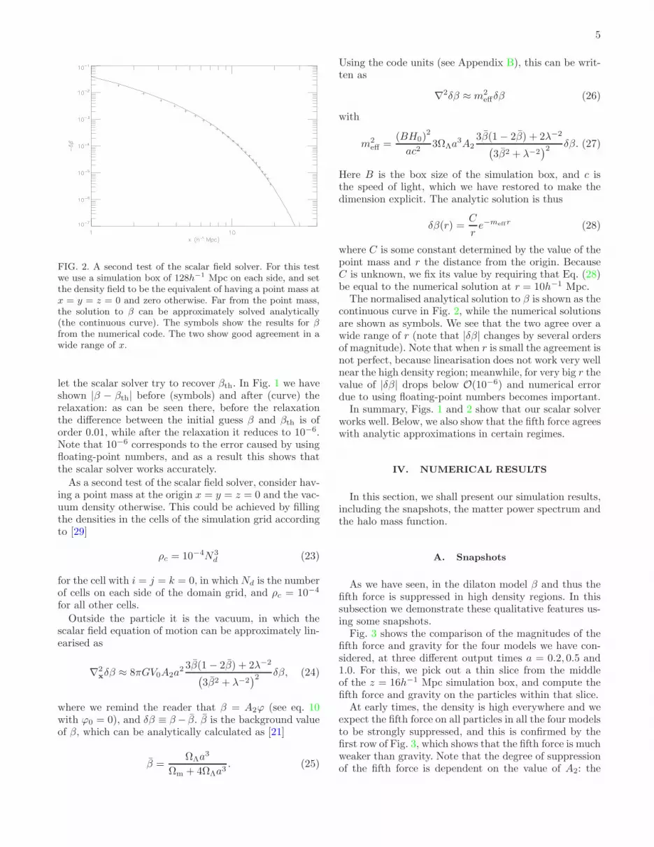
FIG. 2. A second test of the scalar field solver. For this testwe use a simulation box of 128h−1 Mpc on each side, and setthe density field to be the equivalent of having a point mass atx = y = z = 0 and zero otherwise. Far from the point mass,the solution to β can be approximately solved analytically(the continuous curve). The symbols show the results for βfrom the numerical code. The two show good agreement in awide range of x.
let the scalar solver try to recover βth. In Fig. 1 we haveshown |β − βth| before (symbols) and after (curve) therelaxation: as can be seen there, before the relaxationthe difference between the initial guess β and βth is oforder 0.01, while after the relaxation it reduces to 10−6.Note that 10−6 corresponds to the error caused by usingfloating-point numbers, and as a result this shows thatthe scalar solver works accurately.
As a second test of the scalar field solver, consider hav-ing a point mass at the origin x = y = z = 0 and the vac-uum density otherwise. This could be achieved by fillingthe densities in the cells of the simulation grid accordingto [29]
ρc = 10−4N3d (23)
for the cell with i = j = k = 0, in whichNd is the numberof cells on each side of the domain grid, and ρc = 10−4
for all other cells.
Outside the particle it is the vacuum, in which thescalar field equation of motion can be approximately lin-earised as
∇2xδβ ≈ 8πGV0A2a
2 3β(1− 2β) + 2λ−2
(
3β2 + λ−2)2
δβ, (24)
where we remind the reader that β = A2ϕ (see eq. 10with ϕ0 = 0), and δβ ≡ β− β. β is the background valueof β, which can be analytically calculated as [21]
β =ΩΛa
3
Ωm + 4ΩΛa3. (25)
Using the code units (see Appendix B), this can be writ-ten as
∇2δβ ≈ m2effδβ (26)
with
m2eff =
(BH0)2
ac23ΩΛa
3A2
3β(1− 2β) + 2λ−2
(
3β2 + λ−2)2
δβ. (27)
Here B is the box size of the simulation box, and c isthe speed of light, which we have restored to make thedimension explicit. The analytic solution is thus
δβ(r) =C
re−meffr (28)
where C is some constant determined by the value of thepoint mass and r the distance from the origin. BecauseC is unknown, we fix its value by requiring that Eq. (28)be equal to the numerical solution at r = 10h−1 Mpc.The normalised analytical solution to β is shown as the
continuous curve in Fig. 2, while the numerical solutionsare shown as symbols. We see that the two agree over awide range of r (note that |δβ| changes by several ordersof magnitude). Note that when r is small the agreement isnot perfect, because linearisation does not work very wellnear the high density region; meanwhile, for very big r thevalue of |δβ| drops below O(10−6) and numerical errordue to using floating-point numbers becomes important.In summary, Figs. 1 and 2 show that our scalar solver
works well. Below, we also show that the fifth force agreeswith analytic approximations in certain regimes.
IV. NUMERICAL RESULTS
In this section, we shall present our simulation results,including the snapshots, the matter power spectrum andthe halo mass function.
A. Snapshots
As we have seen, in the dilaton model β and thus thefifth force is suppressed in high density regions. In thissubsection we demonstrate these qualitative features us-ing some snapshots.Fig. 3 shows the comparison of the magnitudes of the
fifth force and gravity for the four models we have con-sidered, at three different output times a = 0.2, 0.5 and1.0. For this, we pick out a thin slice from the middleof the z = 16h−1 Mpc simulation box, and compute thefifth force and gravity on the particles within that slice.At early times, the density is high everywhere and we
expect the fifth force on all particles in all the four modelsto be strongly suppressed, and this is confirmed by thefirst row of Fig. 3, which shows that the fifth force is muchweaker than gravity. Note that the degree of suppressionof the fifth force is dependent on the value of A2: the

6
FIG. 3. The magnitude of the fifth force (the vertical axis) versus that of gravity (the horizontal axis), for the particles (blackpoints) selected from a thin slice of the 32h−1 Mpc simulation box. We show this for the four models we have simulated and atthree different output times, as given in the subtitle of each panel. Note that both forces are expressed using the internal unit(see Appendix B), which is H2
0/B times the physical force unit.
larger A2 is, the more the fifth force is suppressed. Also,the fifth force is weaker in higher density regions (wheregravity is stronger) than in lower density regions (wheregravity is weaker), showing a strong dependence on theenvironment.As the Universe expands, the overall density decreases
and the fifth force becomes stronger, which could be seenin the lower rows of Fig. 3. If there is no suppression onthe fifth force, then its strength should be
α =β2
3β2 + λ−2(29)
times that of gravity [21]. For comparison, in the low-est row (a = 1) we have over-plotted α times gravity ascontinuous curves. We can see that in the model withsmaller A2 (the middle two columns) Eq. (29) gives arelatively good description of the fifth force at least insome regions. But for the models with big A2 (the firstand fourth columns) the fifth force is strongly suppressedeven today.Since β determines the strength of the fifth force
[cf. Eq. 9], we are also interested in it. Fig. 4 shows the
values of β as a function of position in the same slices asFig. 3. As expected, at very early times (a = 0.2) β ≪ 1because the fifth force is strongly suppressed. As the Uni-verse expands, β increases (the colour on the points be-comes blue rather than black), but in the high densityregions β remains very small. Also, for the models withbig A2 (the first and fourth columns) the values of β inhigh and low density regions tend to have stronger con-trast, showing stronger environment-dependence. This isclearer in the third row, which shows the result at a = 1.0.This is consistent with what we have seen in Fig. 3.
B. Matter Power Spectrum
The nonlinear matter power spectrum is an importantstructure formation observable and could be used to dis-tinguish amongst different structure formation scenarios.In Ref. [21] it has been shown that the growth rate oflinear matter density perturbations in the dilaton modeldiffers from that of ΛCDM only slightly, and therefore thedilaton model (with its parameters constrained by solar

7
FIG. 4. (Colour Online) The colour scale plot of the value of β as a function of coordinates x, y, for the same thin slice ofthe 32h−1 Mpc simulation box as in Fig. 3. We show this for the four models we have simulated and at three different outputtimes, as given in the subtitle of each panel. Each point represents a particle, and the colour of the point depends on the valueof β at the position of that particle: for all the panels the lightest colour (white) denotes β = 0.3 and the darkest colour (black)denotes β = 10−7; the blue colour is interpolated linearly between these two extremes
system tests) does not deviate at more than the percentlevel from ΛCDM in practice. On the other hand, the fifthforce in the dilaton model has a finite range and is ex-pected to only take effect on the scales of galaxy clusters(∼ O(Mpc)) and smaller, which already fall into the non-linear regime. We are therefore interested in seeing howthe fifth force affects the growth of density perturbationson these scales.
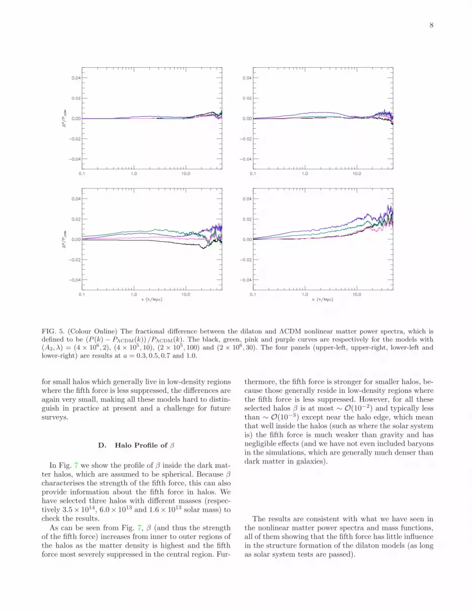
Fig. 5 displays the fractional difference of the dilatonnonlinear matter power spectrum from that of the ΛCDMmodel, defined as (P (k)− PΛCDM(k)) /PΛCDM(k). Fromthis we can see that the difference is strongly suppressedeven on small scales where the fifth force is expected totake effect. This is different from the linear perturbationprediction of [21] (c.f. Fig. 3 therein), which shows thatthe growth rate of density perturbation on small scales issignificantly higher than that on large scales. The reasonfor this is that by linearising the scalar field equation,the nonlinearity of the dilaton model, which is the verymechanism that suppresses the fifth force in high densityregions, is artificially removed (at least partially), and the
strength of the fifth force is determined by the average,instead of the local, matter density. In contrast, the N -body simulation overcomes this problem by taking fullaccount of the suppression of the fifth force.The results indicate that it is even more difficult to
use the nonlinear matter power spectrum to constrainthe dilaton model or distinguish it from ΛCDM as thedifferences to the ΛCDM power spectrum are only a fewpercent on very small length scales at late times.
C. Mass Function
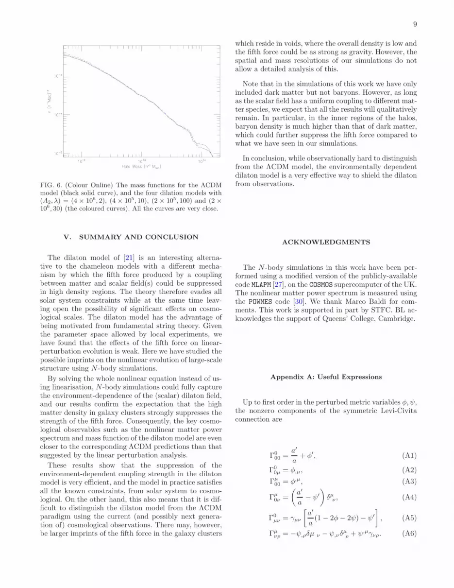
The halo mass function is another key structure forma-tion observable. It is defined to be the number density ofdark matter halos within a given mass range. Clearly, incase of a fifth force which could boost the clustering ofmatter, we expect more halos to form. In Fig. 6 we haveshown the mass functions of the dilaton models comparedwith that of ΛCDM, at z = 0. Although the dilaton mod-els do have higher mass functions than ΛCDM, especially
8
FIG. 5. (Colour Online) The fractional difference between the dilaton and ΛCDM nonlinear matter power spectra, which isdefined to be (P (k)− PΛCDM(k)) /PΛCDM(k). The black, green, pink and purple curves are respectively for the models with(A2, λ) = (4 × 10⁶, 2), (4 × 10⁵, 10), (2 × 10⁵, 100) and (2 × 10⁶, 30). The four panels (upper-left, upper-right, lower-left andlower-right) are results at a = 0.3, 0.5, 0.7 and 1.0.
for small halos which generally live in low-density regionswhere the fifth force is less suppressed, the differences areagain very small, making all these models hard to distin-guish in practice at present and a challenge for futuresurveys.
D. Halo Profile of β
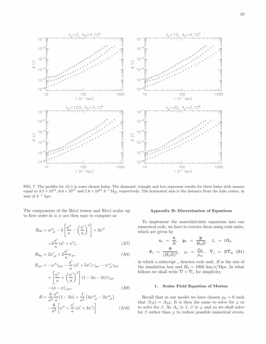
In Fig. 7 we show the profile of β inside the dark mat-ter halos, which are assumed to be spherical. Because βcharacterises the strength of the fifth force, this can alsoprovide information about the fifth force in halos. Wehave selected three halos with different masses (respec-tively 3.5× 10¹⁴, 6.0× 10¹³ and 1.6× 10¹³ solar mass) tocheck the results.As can be seen from Fig. 7, β (and thus the strength
of the fifth force) increases from inner to outer regions ofthe halos as the matter density is highest and the fifthforce most severely suppressed in the central region. Fur-
thermore, the fifth force is stronger for smaller halos, be-cause those generally reside in low-density regions wherethe fifth force is less suppressed. However, for all theseselected halos β is at most ∼ O(10−2) and typically lessthan ∼ O(10−3) except near the halo edge, which meanthat well inside the halos (such as where the solar systemis) the fifth force is much weaker than gravity and hasnegligible effects (and we have not even included baryonsin the simulations, which are generally much denser thandark matter in galaxies).
The results are consistent with what we have seen inthe nonlinear matter power spectra and mass functions,all of them showing that the fifth force has little influencein the structure formation of the dilaton models (as longas solar system tests are passed).
9
FIG. 6. (Colour Online) The mass functions for the ΛCDMmodel (black solid curve), and the four dilation models with(A2, λ) = (4 × 10⁶, 2), (4 × 10⁵, 10), (2 × 10⁵, 100) and (2 ×
106, 30) (the coloured curves). All the curves are very close.
V. SUMMARY AND CONCLUSION
The dilaton model of [21] is an interesting alterna-tive to the chameleon models with a different mecha-nism by which the fifth force produced by a couplingbetween matter and scalar field(s) could be suppressedin high density regions. The theory therefore evades allsolar system constraints while at the same time leav-ing open the possibility of significant effects on cosmo-logical scales. The dilaton model has the advantage ofbeing motivated from fundamental string theory. Giventhe parameter space allowed by local experiments, wehave found that the effects of the fifth force on linear-perturbation evolution is weak. Here we have studied thepossible imprints on the nonlinear evolution of large-scalestructure using N -body simulations.
By solving the whole nonlinear equation instead of us-ing linearisation, N -body simulations could fully capturethe environment-dependence of the (scalar) dilaton field,and our results confirm the expectation that the highmatter density in galaxy clusters strongly suppresses thestrength of the fifth force. Consequently, the key cosmo-logical observables such as the nonlinear matter powerspectrum and mass function of the dilaton model are evencloser to the corresponding ΛCDM predictions than thatsuggested by the linear perturbation analysis.
These results show that the suppression of theenvironment-dependent coupling strength in the dilatonmodel is very efficient, and the model in practice satisfiesall the known constraints, from solar system to cosmo-logical. On the other hand, this also means that it is dif-ficult to distinguish the dilaton model from the ΛCDMparadigm using the current (and possibly next genera-tion of) cosmological observations. There may, however,be larger imprints of the fifth force in the galaxy clusters
which reside in voids, where the overall density is low andthe fifth force could be as strong as gravity. However, thespatial and mass resolutions of our simulations do notallow a detailed analysis of this.
Note that in the simulations of this work we have onlyincluded dark matter but not baryons. However, as longas the scalar field has a uniform coupling to different mat-ter species, we expect that all the results will qualitativelyremain. In particular, in the inner regions of the halos,baryon density is much higher than that of dark matter,which could further suppress the fifth force compared towhat we have seen in our simulations.
In conclusion, while observationally hard to distinguishfrom the ΛCDM model, the environmentally dependentdilaton model is a very effective way to shield the dilatonfrom observations.
ACKNOWLEDGMENTS
The N -body simulations in this work have been per-formed using a modified version of the publicly-availablecode MLAPM [27], on the COSMOS supercomputer of the UK.The nonlinear matter power spectrum is measured usingthe POWMES code [30]. We thank Marco Baldi for com-ments. This work is supported in part by STFC. BL ac-knowledges the support of Queens’ College, Cambridge.
Appendix A: Useful Expressions
Up to first order in the perturbed metric variables φ, ψ,the nonzero components of the symmetric Levi-Civitaconnection are
Γ000 =
a′
a+ φ′, (A1)
Γ00µ = φ,µ, (A2)
Γµ00 = φ,µ, (A3)
Γµ0ν =
(
a′
a− ψ′
)
δµν , (A4)
Γ0µν = γµν
[
a′
a(1 − 2φ− 2ψ)− ψ′
]
, (A5)
Γµνρ = −ψ,ρδµ ν − ψ,νδ
µρ + ψ,µγνρ. (A6)
10
FIG. 7. The profiles for β(r) in some chosen halos. The diamond, triangle and box represent results for three halos with massesequal to 3.5× 10¹⁴, 6.0× 10¹³ and 1.6× 10¹³ h−1M⊙ respectively. The horizontal axis is the distance from the halo centre, in
unit of h−1 kpc.
The components of the Ricci tensor and Ricci scalar upto first order in φ, ψ are then easy to compute as
R00 = φ,µ,µ − 3
[
a′′
a−(
a′
a
)2]
+ 3ψ′′
+3a′
a(φ′ + ψ′) , (A7)
R0µ = 2ψ′,µ + 2
a′
aφ,µ, (A8)
Rµν = −ψ′′γµν − a′
a(φ′ + 5ψ′) γµν − ψ,ρ
,ργµν
+
[
a′′
a+
(
a′
a
)2]
(1− 2φ− 2ψ)γµν
−(φ− ψ),µν , (A9)
R =6
a2a′′
a(1− 2φ) +
1
a2(
4ψ,µ,µ − 2φ,µ,µ
)
− 6
a2
[
ψ′′ +a′
a(φ′ + 3ψ′)
]
. (A10)
Appendix B: Discretisation of Equations
To implement the nonrelativistic equations into ournumerical code, we have to rewrite them using code units,which are given by
xc =x
B, pc =
p
H0B, tc = tH0,
Φc =Φ
(H0B)2, ρc =
ρmρm
, ∇c = B∇x (B1)
in which a subscript c denotes code unit, B is the size ofthe simulation box and H0 = 100h km/s/Mpc. In whatfollows we shall write ∇ = ∇c for simplicity.
1. Scalar Field Equation of Motion
Recall that in our model we have chosen ϕ0 = 0 suchthat β(ϕ) = A2ϕ. It is then the same to solve for ϕ orto solve for β. As A2 ≫ 1, β ≫ ϕ and so we shall solvefor β rather than ϕ to reduce possible numerical errors.

11
The equation of motion for β could be obtained simplyby multiplying that for ϕ by A2:
∇x · [k(β)∇xβ]
≈ 4πGA2a2
k(β)[β A(β)ρm + 4V (β)] − V (β)
−4πGA2a2
k(β)
[
β
A(β)ρm + 4V (β)]
− V (β)
,(B2)
where we have used β instead of ϕ as the variable.
As discussed in [21], β characterises the strength of thefifth force. In high density environments, β ≪ 1 so thatthe fifth force is too weak to be measured; in low den-sity regions, however, we have β ∼ 0.23 today, indicatingthat the fifth force is roughly as strong as gravity. Fur-thermore, Eq. (B2) does not say anything about the signof β.
Obviously, because β ranges from O(
10−6)
to O(1),using β directly in the numerical code could easily causebig numerical errors in the regions where β is small. Onealternative is to use ln(β) as a new variable, but this
does not necessarily work because β might be negative.Therefore, in this work, we shall use a different variableu ≡ β1/n, with n being some odd positive integer, asthe redefined scalar field. More explicitly, we shall adoptn = 9 which guarantees that u ∼ O(0.1−1), i.e., u spansa much smaller range than β, making it easier to controlnumerical errors. Furthermore, n being odd makes surethat u is never undefined even if β < 0.In terms of u, we have
k(u) =√
3u2n + λ−2, (B3)
A(u) = 1 +u2n
2A2
, (B4)
V (u) =
(
1 +u2n
2A2
)4
V0 exp
(
−un
A2
)
. (B5)
Then, defining
λ ≡ 8πGV03H2
0
, (B6)
and using the code units defined above, we could rewritethe scalar equation of motion Eq. (B2) as
ac2
(BH0)2∇ · (b∇u)
≈ A2
k(u)
[
3
2
(
1 +u2n
2A2
)
Ωmρc + 6λa3(
1 +u2n
2A2
)4
exp
(
−un
A2
)
]
un − 3
2λa3
(
1 +u2n
2A2
)4
exp
(
−un
A2
)
− A2
k(β)
[
3
2
(
1 +β2
2A2
)
Ωm + 6λa3(
1 +β2
2A2
)4
exp
(
− β
A2
)
]
β − 3
2λa3
(
1 +β2
2A2
)4
exp
(
− β
A2
)
(B7)
where we have defined
b(u) = nun−1√
3u2n + λ−2, (B8)
and β is the background value of β, which can be com-puted as [21]
β =ΩΛa
3
Ωm + 4ΩΛa3. (B9)
The full equation for u, Eq. (B7), contains the quan-tity ∇ · (b∇u). To discretise it, we shall assume that thediscretisation is performed on a grid with grid spacing h.We shall require second order precision which is the sameas the default Poisson solver in MLAPM, and then ∇u inone dimension can be written as
∇u → ∇huj =uj+1 − uj−1
2h(B10)
where a subscript j means that the quantity is evalu-ated on the j-th point. The generalisation to the threedimensional case is straightforward.The factor b in∇·(b∇u) makes this a standard variable
coefficient problem. We need also to discretise b, and doit in this way (again for one dimension) [23]:
∇ · (b∇u)
→ 1
h2
[
bj+ 1
2
uj+1 − uj
(
bj+ 1
2
+ bj− 1
2
)
+ bj− 1
2
uj−1
]
,(B11)
in which bj± 1
2
= 12(bj + bj±1). Generalising this to three
dimensions, we have

12
∇ · (b∇u) → 1
h2
[
bi+ 1
2,j,kui+1,j,k − ui,j,k
(
bi+ 1
2,j,k + bi− 1
2,j,k
)
+ bi− 1
2,j,kui−1,j,k
]
+1
h2
[
bi,j+ 1
2,kui,j+1,k − ui,j,k
(
bi,j+ 1
2,k + bi,j− 1
2,k
)
+ bi,j− 1
2,kui,j−1,k
]
+1
h2
[
bi,j,k+ 1
2
ui,j,k+1 − ui,j,k
(
bi,j,k+ 1
2
+ bi,j,k− 1
2
)
+ bi,j,k− 1
2
ui,j,k−1
]
. (B12)
Then the discrete version of Eq. (B7) is
Lh (ui,j,k) = 0, (B13)
in which
Lh (ui,j,k) =1
h2ac2
(BH0)2
[
bi+ 1
2,j,kui+1,j,k − ui,j,k
(
bi+ 1
2,j,k + bi− 1
2,j,k
)
+ bi− 1
2,j,kui−1,j,k
]
+1
h2ac2
(BH0)2
[
bi,j+ 1
2,kui,j+1,k − ui,j,k
(
bi,j+ 1
2,k + bi,j− 1
2,k
)
+ bi,j− 1
2,kui,j−1,k
]
+1
h2ac2
(BH0)2
[
bi,j,k+ 1
2
ui,j,k+1 − ui,j,k
(
bi,j,k+ 1
2
+ bi,j,k− 1
2
)
+ bi,j,k− 1
2
ui,j,k−1
]
− A2√
3u2ni,j,k + λ−2
3
2
(
1 +u2ni,j,k2A2
)
Ωmρc + 6λa3
(
1 +u2ni,j,k2A2
)4
exp
(
−uni,j,kA2
)
uni,j,k
+A2
√
3u2ni,j,k + λ−2
3
2λa3
(
1 +u2ni,j,k2A2
)4
exp
(
−uni,j,kA2
)
+A2
√
3β2 + λ−2
[
3
2
(
1 +β2
2A2
)
Ωm + 6λa3(
1 +β2
2A2
)4
exp
(
− β
A2
)
]
β
− A2√
3β2 + λ−2
3
2λa3
(
1 +β2
2A2
)4
exp
(
− β
A2
)
. (B14)
Then the Newton-Gauss-Seidel iteration says that we canobtain a new (and usually more accurate) solution of u,unewi,j,k, using our knowledge about the old (and less acu-
rate) solution uoldi,j,k as
unewi,j,k = uoldi,j,k −Lh(
uoldi,j,k
)
∂Lh(
uoldi,j,k
)
/∂ui,j,k. (B15)
The old solution will be replaced with the new one oncethe latter is ready, using a red-black Gauss-Seidel sweep-ing scheme. Note that
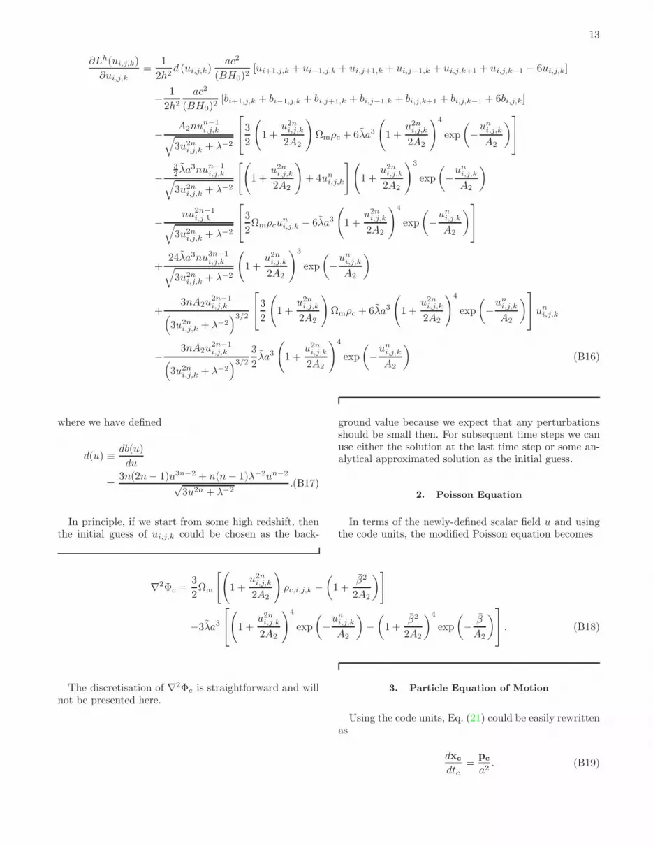
13
∂Lh(ui,j,k)
∂ui,j,k=
1
2h2d (ui,j,k)
ac2
(BH0)2[ui+1,j,k + ui−1,j,k + ui,j+1,k + ui,j−1,k + ui,j,k+1 + ui,j,k−1 − 6ui,j,k]
− 1
2h2ac2
(BH0)2[bi+1,j,k + bi−1,j,k + bi,j+1,k + bi,j−1,k + bi,j,k+1 + bi,j,k−1 + 6bi,j,k]
−A2nu
n−1i,j,k
√
3u2ni,j,k + λ−2
3
2
(
1 +u2ni,j,k2A2
)
Ωmρc + 6λa3
(
1 +u2ni,j,k2A2
)4
exp
(
−uni,j,kA2
)
−32λa3nun−1
i,j,k√
3u2ni,j,k + λ−2
[(
1 +u2ni,j,k2A2
)
+ 4uni,j,k
](
1 +u2ni,j,k2A2
)3
exp
(
−uni,j,kA2
)
−nu2n−1
i,j,k√
3u2ni,j,k + λ−2
3
2Ωmρcu
ni,j,k − 6λa3
(
1 +u2ni,j,k2A2
)4
exp
(
−uni,j,kA2
)
+24λa3nu3n−1
i,j,k√
3u2ni,j,k + λ−2
(
1 +u2ni,j,k2A2
)3
exp
(
−uni,j,kA2
)
+3nA2u
2n−1i,j,k
(
3u2ni,j,k + λ−2
)3/2
3
2
(
1 +u2ni,j,k2A2
)
Ωmρc + 6λa3
(
1 +u2ni,j,k2A2
)4
exp
(
−uni,j,kA2
)
uni,j,k
−3nA2u
2n−1i,j,k
(
3u2ni,j,k + λ−2
)3/2
3
2λa3
(
1 +u2ni,j,k2A2
)4
exp
(
−uni,j,kA2
)
(B16)
where we have defined
d(u) ≡ db(u)
du
=3n(2n− 1)u3n−2 + n(n− 1)λ−2un−2
√3u2n + λ−2
.(B17)
In principle, if we start from some high redshift, thenthe initial guess of ui,j,k could be chosen as the back-
ground value because we expect that any perturbationsshould be small then. For subsequent time steps we canuse either the solution at the last time step or some an-alytical approximated solution as the initial guess.
2. Poisson Equation
In terms of the newly-defined scalar field u and usingthe code units, the modified Poisson equation becomes
∇2Φc =3
2Ωm
[(
1 +u2ni,j,k2A2
)
ρc,i,j,k −(
1 +β2
2A2
)
]
−3λa3
(
1 +u2ni,j,k2A2
)4
exp
(
−uni,j,kA2
)
−(
1 +β2
2A2
)4
exp
(
− β
A2
)
. (B18)
The discretisation of ∇2Φc is straightforward and willnot be presented here.
3. Particle Equation of Motion
Using the code units, Eq. (21) could be easily rewrittenas
dxc
dtc=
pc
a2. (B19)

14
Similarly, Eq. (22) becomes
dpc
dtc= −1
a∇Φc −
1
a
nu2n−1i,j,k
A2
ac2
(BH0)2∇u
− 1
A2
uni,j,kaβ
H0
pc. (B20)
[1] V. A. Rubakov and P. G. Tinyakov, Phys. Usp. 51 759(2008) and references therein.
[2] R. P. Woodard, Lect. Notes Phys. 720, 403 (2007).[3] C. de Rham, G. Gabadadze and A. J. Tolley,
arXiv:1011.1232 [hep-th].[4] G. Dvali, G. Gabadadze and M. Porrati,
Phys. Lett. B485, 208 (2000).[5] T. P. Sotiriou and V. Faraoni, Rev. Mod. Phys. 82, 451
(2010).[6] The Scalar-Tensor Theory of Gravitation, Y. Fujii and
K. -i Maeda, Cambridge University Press, 2003.[7] J. Khoury and A. Weltman, Phys. Rev. Lett. 93, 171104
(2004).[8] J. Khoury and A. Weltman, Phys. Rev. D69, 044026
(2004).[9] D. F. Mota and D. G. Shaw, Phys. Rev. Lett. 97, 151102
(2006).[10] D. F. Mota and D. G. Shaw, Phys. Rev. D75, 063501
(2007).[11] B. Li and J. D. Barrow, Phys. Rev. D75, 084010 (2007).[12] P. Brax, C. Van de Bruck, A.-C. Davis and D. J. Shaw
Phys. Rev. D78, 104021 (2008).[13] S. M. Carroll, Phys. Rev. Lett. 81 (1998) 3067
[arXiv:astro-ph/9806099].[14] N. Chow and J. Khoury, Phys. Rev. D80, 024037 (2009).[15] A. De Felice and S. Tsujikawa, Phys. Rev. Lett. 105,
111301 (2010).[16] A. I. Vainshtein, Phys. Lett. B39, 393 (1972).[17] M. Gasperini, F. Piazza and G. Veneziano, Phys. Rev. D
65 (2002) 023508 [arXiv:gr-qc/0108016].
[18] T. Damour, F. Piazza and G. Veneziano, Phys. Rev. Lett.89 (2002) 081601 [arXiv:gr-qc/0204094].
[19] T. Damour, F. Piazza and G. Veneziano, Phys. Rev. D66 (2002) 046007 [arXiv:hep-th/0205111].
[20] T. Damour and A. M. Polyakov, Nucl. Phys. B423, 532(1994).
[21] P. Brax, C. van de Bruck, A.-C. Davis and D. J. Shaw(2010), arXiv:1005.3735 [astro-ph.CO].
[22] F. Bernardeau and P. Brax (2011), arXiv:1102.1907[astro-ph.CO].
[23] B. Li and H. Zhao, Phys. Rev. D 80, 044027 (2009).[24] B. Li and H. Zhao, Phys. Rev. D 81, 104047 (2009).[25] B. Li and J. D. Barrow, Phys. Rev. D 83, 024007 (2011).[26] B. Li, D. F. Mota and J. D. Barrow, Astrophys. J., 728,
109 (2011).[27] A. Knebe, A. Green and J. Binney, Mon. Not. R. As-
tron. Soc., 325, 845 (2001).[28] W. H. Press, B. P. Flannery, S. A. Teukolsky and
W. T. Vetterling, Numerical Recipes in C: The Art ofScientific Computing, Cambridge University Press, 1988.
[29] H. Oyaizu, Phys. Rev. D 78, 123523 (2008).[30] S. Colombi, A. H. Jaffe, D. Novikov and C. Pichon,
Mon. Not. R. Astron. Soc. 303, 511 (2009).[31] E. Bertschinger, arXiv:astro-ph/9506070.[32] S. P. D. Gill, A. Knebe and B. K. Gibson, Mon. Not.
Roy. Astron. Soc. 351, 399 (2004).