non-linear analysis of infilled frames - core
TRANSCRIPT
NON-LINEAR ANALYSIS OF INFILLED FRAMES
(PART ONE)
VO L . I.
By
Abolghasem Saneinejad
A
THESIS
Submitted to the Department of
Civil and Structural Engineering,
in partial fulfilment of the
requirements for the
Degree of
Doctor of Philosophy
UNIVERSITY OF SHEFFIELD
May, 1990
SUMMARY
This thesis is concerned with the analysis of
building frames acting compositely with infilling wall
panels. The significance of the composite action is
emphasized and previous work on infilled frames is reviewed.
The existing methods of analysis are categorized and their
analytical assumptions are highlighted. It is concluded
that more accurate results may be obtained from the
development of a non-linear finite element analysis. The
finite element method is reviewed and new elements for
representing beams, interfaces and loading are developed.
Failure criteria for concrete under multiaxial stress and
also failure criteria for masonry under uniaxial compression
are developed. The non-linear elastoplastic behaviour of
concrete is modelled using the concept of equivalent
uniaxial strain and the model is extended for cracked
materials. Elastoplastic models are also developed for
ductile materials(steel) for secant and incremental changes
of stresses and strains. These models and the newly
developed elements are incorporated into the finite element
analysis which is numerically implemented by a new computer
program, NEPAL. A number of steel frames with concrete
inf ills covering the practical range of beam, column and
infill strengths and also wall panel aspect ratios, are
analysed using this program. The finite element results are
compared with the predictions of a range of existing methods
of analysis and their limitations are discussed in detail.
A new method of hand analysis is developed, based on a
rational elastic and plastic analysis allowing for limited
ductility of the infill and also limited deflection of the
frame at the peak load. The new method is shown to be
capable of providing the necessary information for design
purposes with reasonable accuracy, taking into account the
effects of strength and stiffness of the beams and columns,
the aspect ratio for the infill, the semi-rigid joints and
the condition of the frame-infill interfaces (co-efficient
of friction and lack of fit). It is concluded that simple
and economical design approaches can be established for
frames with infilling walls.

ACKNOWLEDGEMENTS
The author would like to thank Mr. B. Hobbs for
his continual support and encouragement which made this
work possible.
TABLE OF CONTENTS
PART ONE
List of Tables xvii
List of Figures xix
Notations xxvii
CHAPTER 1 Introduction 1
CHAPTER 2 ReViewofPreviousWork 6
2.1 Introduction 6
2.2 Behaviour of Infilled Frames underRacking load 6
2.3 Early Work and the Concept ofDiagonal Strut 9
2.4 Theories Based on Infill/FrameStiffness Parameter 12
2.4.1 General 12
2.4.2 Stafford Smith Observations on theBehaviour of Infilled Frames Subjectedto Racking Load 13
2.4.3 Stafford Smith's Theoretical Analysis 15
2.4.4 Lateral Strength of Infilled Frames 20
2.4.5 Lateral Stiffness of Infilled Frames 25
2.4.6 Behaviour of Masonry Infilled Framesunder Racking Load 28
2.5 Empirical Method of Analysis Based onStiffness Parameter, XII 30 -
2.5.1 Empirical Data and Analysis of Infill 30
2.5.2 Analysis of Frame 33
- iv -
2.53 comments 34
2.6 Design Recommendations for ElasticAnalysis of Infilled Steel Frames 37
2.6.1 General 37
2.6.2 The Basis of the Method 37
2.6.3 Infill Design 38
2.6.4 Design of Frame 41
2.6.5 Comparison 43
2.7 Theories Based on Frame/InfillStrength Parameter 44
2.7.1 General 44
2.7.2 Wood Classification for Collapse ofInfilled Frame 45
2.7.3 Wood's Plastic Analysis of InfilledFrames 47
2.7.4 Axial and Shear Forces in Frame Members 53
2.7.5 Application of Wood Method forAnalysis of Multi-bay and Multi-StoreyFrames With or without Panels 53
2.7.6 Discussion of Wood Method 54
2.7.7 Plastic Analysis of Infilled Frameswith Application of the Yield Line Method 55
2.8 Liauw et al Plastic Method 57
2.8.1 Finite Element Analyses 57
2.8.2 Collapse Modes and Loads 60
2.8.3 Comparison With Experimental Results 65
2.8.4 Using the Liauw et al Plastic Methodfor Analysis of Single-Bay Multi-StoreyInfilled Frames 66
Discussion of Liauw et al Method 67
2.9 Conclusion from The Literature Review 69
CIIMYFER 3 TheFiniteElementTechnique 73
3.1 General 73
3.2 Finite Element Concept 73
3.3 Newton Raphson Iteration 74
3.4 Finite Element Formulation 76
3.4.1 General 76
3.4.2 Element Displacement Functions 77
3.4.3 Element Strain Functions 78
3.4.4 Stress-strain Relation 79
3.4.5 Element Stiffness Matrix 80
3.4.6 Element Equivalent Nodal Forces 91
3.5 Local Normalized Coordinates 82
3.5.1 Definitions 82
3.5.2 Evaluation of the Integrals in Termsof Local Normalized Coordinates 83
3.6 Numerical Integration 85
3.7 Contribution of Reinforcementto R.0 Elements 87
3.7.1 General 87
3.7.2 Uniformly Distributed Reinforcement 88
3.7.3 A Single Bar Parallel to One ofthe Element Local Coordinates 89
3.8 Some Requirements of the F.EDiscretization 91
3.9 Masonry Wall Discretization 95
3.9.1 General 95
3.9.2 Standard 3-D Element 95
3..3 Newly Developed 3-D Four-node Element 96
3.9.4 Plane-Stress Equivalent Elements 98
3.9.5 Plane-stress Equivalent Units andLaminar Joints 98
- vi -
3.9.6 Plane-stress Masonry-Equivalent andInterface Elements 100
3.9.7 Super Element of Masonry 101
3.9.8 Conclusion on the Choices of MasonryElements 101
3.10 Interface Discretization 103
3.10.1 General 103
3.10.2 Algorithm of Linkage Element 104
3.10.3 Newly Developed Interface Element 107
3.11 Frame Discretization 112
3.11.1 General 112
3.11.2 Non-conforming Rectangular element 114
3.11.3 Proposed Rectangular Beam Element 116
3.12 Choice Of Masonry Infilled FrameSubdivision 119
3.13 Choices of Concrete Infilled FrameSubdivision 122
CHAPTER 4 Constitutive Formulation of Materials 123
4.1 General 123
4.2 The Existing Fracture Models 124
4.3 Proposed Constitutive Formulationfor Brittle Materials Under UniaxialCompression 130
4.3.1 Stress-Strain Relation 130
4.3.2 Poisson's Ratio 134
4.3.3 Loading-Unloading-Reloading Behaviour 136
4.4 Brittle Materials Subjected to UniaxialTension 138
44.Failure Criteria 140
4..1 General 140 .
4.5.2 Proposed Failure Criterion of BrittleMaterials under Triaxial Compression 144
4•5•3 Proposed Failure Criterion for BrittleMaterials under TriaxialCompression-Tension 147
4•5•4 Proposed Failure Criterion for BrittleMaterials under Tension-Compression 149
4•5•5 Proposed Failure Criterion forBrittle Materials Under Triaxial Tension 149
4.6 Proposed Constitutive Formulationfor Brittle Materials UnderMultiaxial Stresses . 150
4.6.1 General 150
4.6.2 Equivalent Uniaxial Strains (EUS) 153
4.6.3 Proposed Stress-EUS RelationshipFormulation 153
4.6.4 EUS at Peak Load 156
4.6.5 Transformation of EUS to Real strainsand Vice-versa 159
4.6.6 Proportional Unloading and Reloading 163
4.6.7 Proposed Incremental Stress-strainRelationship 168
4.7 Non-proportional Loading 171
4.7.1 Stress-strain Relationship 171
4.7.2 Poisson's Ratios underNon-proportional Loading 173
4.7.3 Proposed Incremental Stress-strainRelationship for Non-proportionalLoad Increment 174
4.8 Cracking and Cracked Eaterials 175
4.8.1 Cracking 175
4.8.2 Cracked Materials 176
4.8.3 Proposed Slip-dilatancy Crack Model 178
4.t.3.1 General Concept 178
4.8.3.2 Stress-strain Relationship for CrackedMaterials under Plane Stress Conditions 179
4.8.3.3 Material with Open Cracks 181
4.8.3.4 Material with Closed Cracks 182
4.8.3.5 Material with Interlocked Cracks 182
4.8.4 Proposed Incremental Stress-strainRelationship for Cracked Materials 183
4.8.5 Proposed Model for Double Sets of Cracks 186
4.8.5.1 General Concept and Definitions 186
4.8.5.2 Material with Closed Minor Cracks 187
4.8.5.3 Materials with Open Minor Cracks 190
4.8.6 Proposed Incremental Stress-strainRelationship for Double Cracked Materials 194
4.9 Constitutive Formulation for Steel 296
4.9.1 General Characteristics of Steel 196
4.9.2 Proposed Model for Stress-StrainRelationship of Steel Materialunder Uniaxial Stress 198
4.9.3 Failure Criteria of Steel 199
4.9.4 Stress-strain Relationship ofDuctile Material 201
4.9.4.1 Definitions and Basis of Elastic-PerfectPlasticity Theory 201
4.9.4.2 Stress-Strain Relationship underMultiaxial Stress Conditions 203
4.9.4.3 Stress-Strain Relationship forPlane Stress Loading 206
4.9.5 Incremental Stress-Strain Relationshipfor Ductile Materials 207
4.9.5.1 In Elastic State 207
4.9.5.2 In Elastoplastic State 209
4.9.5.3 Under Plane Stresses and inElastoplastic State 211
4.2.6 Stress-strain Relationship forReinforcement within a R.0 Element 212
440 Constitutive Formulation for MechanicalBehaviour of Interfaces and Joints 213
4.10.1 General 213
4.10.2 Yielding, Slip and Separation Criteria 214
4.10.3 Stress-Relative Displacement Relationshipof Interfaces 218
4.10.3.1 General 218
4.10.3.2 Proposed Model Based on ExperimentalObservations 219
4.10.4 Determination of the State of an Interface 223
4.10.4.1 General 223
4.10.4.2 New State of a Previously Fully BondedInterface 224
4.10.4.3 New State of a Previously PartiallyBonded Interface 227
4.10.4.4 New State of a Totally Debonded Interface 230
4.10.4.5 Proposed Incremental [D] Matrix 232
4.11 Constitutive Formulation for Masonry 234
CHAPTER 5 Numerical Implementation and
Programming 236
5.1 General 236
5.2 Characteristics of Program NEPAL 236
5.3 Loading Procedure 237
5.4 Criteria for Convergence 240
5.5 Examination of The Proposed F.E Analysis 243
5.5.1 General 243
5.5.2 R.0 Beam Without Shear Reinforcement 244
5.5.3 R.C. Beam with Shear Reinforcement 246
5.5.4 Square Steel Frame Subjected to Racking 248
5.5.5 Micro-concrete infilled Steel FrameSubjected to Racking 249
5.6 Conclusion 257
PART TWO
CHAPTER 6 Application of The Finite Element
Analysis and Discussion 259
6.1 Aims and Scope 259
6.2 Infill Size and Proportion 259
6.3 Frame Members 261
6.4 Infill Material 261
6.5 Frame-Infill Interface 264
6.6 Infilled Frames Analysed 264
6.7 Open Frames 266
6.8 Infilled Frames 268
6.8.1 General 268
6.8.2 Load-Deflection Diagrams 268
6.8.3 Frame Forces 274
6.8.4 Infill Stresses 275
6.8.5 Frame-Infill Interaction 275
6.9 Discussion of Overall Behaviourof Infilled Frames 278
6.9.1 General 278
6.9.2 Elastic State 278
6.9.3 Elastoplastic State 278
6.9.4 Plastic State 279
6.9.5 Some Exceptions for Strong Frames 281
6.9.6 Comments 281
6.10 Discussion on Normal Force atFrame-infillInterface 281
6.10.1 General 281
6.10.2 Effect of Infill Aspect Ratio 283
6.10.3 Effect of Beam to Column Strength Ratio 283
6.10.4 Effect of Frame/Infill Strength Ratio 283
6.10.5 Effect of Diagonal Cracking 284
6.10.6 Effect of Coefficient of Friction 284
6.11 Discussion on Shear Force atFrame-infill Interface 284
6.12 Discussion on Infill Stress Distribution 286
6.12.1 General 286
6.12.2 Loaded Corners 286
6.12.3 Central Region 287
6.13 Discussion on Frame Forces 290
6.13.1 General 290
6.13.2 Axial Forces 290
6.13.3 Shear Forces 291
6.13.4 Bending Moment 293
CHAPTER 7 Proposed Method of Analysis
and Comparison 296
7.1 Introduction 296
7.1.1 General 296
7.1.2 Basis of The Analysis 298
7.2 Frame-infill Interaction 299
7.3 Frame-infill Contact Lengths 304
7.4 Infill Boundary Stresses 306
7.5 Lateral Deflection 310:
7.6 Frame Bending Moments 312
7.1 Frame Forces 313
7.8 Peak Horizontal Load 314
7.9 Modes of Displacement and Failure 315
7.9.1 Frame Failure 315
7.9.2 Infill Failure 315
7.9.3 Infilled Frame Failure 318
7.10 Cracking Load 319
7.11 Stiffness 323
7.12 Special cases with Square Infills 323
7.13 Balancing Friction at Infill Boundary 325
7.14 Design Chart 326
7.15 Frames Without Plastic Hinge at thePeak Load 330
7.16 Comparison Programme 331
7.17 Results used in The Comparison Programme 332
7.17.1 The Finite Element Analysis Results 332
7.17.2 Experimental Results 332
7.18 The Methods of Analysis Involved inComparison 335
7.19 Comparison of Peak Racking Load, Hc 336
7.19.1 General 338
7.19.2 Methods Based on Stiffness Parameter lh 341
7.19.3 Wood Method (W) 345
7.19.4 Liauw Method (L) 347
7.19.5 Proposed Method (P) 349
7.20 Comparison of the Estimated CrackingLoad,Ht 352
7.21 Comparison of the Estimated InitialStiffness, KO 354
7.22 Comparison of Estimated Frame, Bending Moments 357
7.23 Comparison of the PredictedFrameAxial Forces 360
7.24 Comparison of Estimated Frame Shear Forces 361
7.25 Comments 362
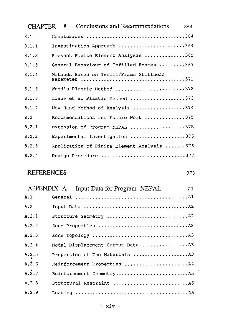
CHAPTER 8 Conclusions and Recommendations 364
8.1 Conclusions 364
8.1.1 Investigation Approach 364
8.1.2 Present Finite Element Analysis 365
8.1.3 General Behaviour of Infilled Frames 367
8.1.4 Methods Based on Infill/Frame StiffnessParameter 371
8.1.5 Wood's Plastic Method 372
8.1.6 Liauw et al Plastic Method 373
8.1.7 New Hand Method of Analysis 374
8.2 Recommendations for Future Work 375
8.2.1 Extension of Program NEPAL 375
8.2.2 Experimental Investigation 376
8.2.3 Application of Finite Element Analysis 376
8.2.4 Design Procedure 377
REFERENCES 378
APPENDIX A Input Data for Program NEPAL Al
A.1 General Al
A.2 Input Data A2
A.2.1 Structure Geometry A2
A.2.2 Zone Properties A2
A.2.3 Zone Topology A3
A.2.4 Nodal Displacement Output Data A3
A.2.5 Properties of The Materials A3:
A.2.6 Reinforcement Properties A4
A.2.7 Reinforcement Geometry AS -
A.2.8 Structural Restraint A5
A.2.9 Loading AS
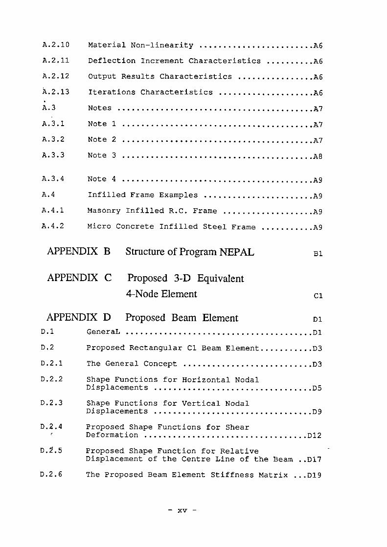
A.2.10 Material Non-linearity A6
A.2.11 Deflection Increment Characteristics A6
A.2.12 Output Results Characteristics A6
A.2.13 Iterations Characteristics A6
A.3 Notes A7
A.3.1 Note 1 A7
A.3.2 Note 2 A7
A.3.3 Note 3 A8
A.3.4 Note 4 A9
A.4 Infilled Frame Examples A9
A.4.1 Masonry Infilled R.C. Frame A9
A.4.2 Micro Concrete Infilled Steel Frame A9
APPENDIX B Structure of Program NEPAL Bl
APPENDIX C Proposed 3-D Equivalent
4-Node Element Cl
APPENDIX I) Proposed Ekwn Element D1
D.1 GeneraL D1
D.2 Proposed Rectangular Cl Beam Element D3
D.2.1 The General Concept D3
D.2.2 Shape Functions for Horizontal NodalDisplacements D5
D.2.3 Shape Functions for Vertical NodalDisplacements D9
D.2.4 Proposed Shape Functions for ShearDeformation D12
D.2.5 Proposed Shape Function for RelativeDisplacement of the Centre Line of the Beam ..D17
D.2.6 The Proposed Beam Element Stiffness Matrix ...D19
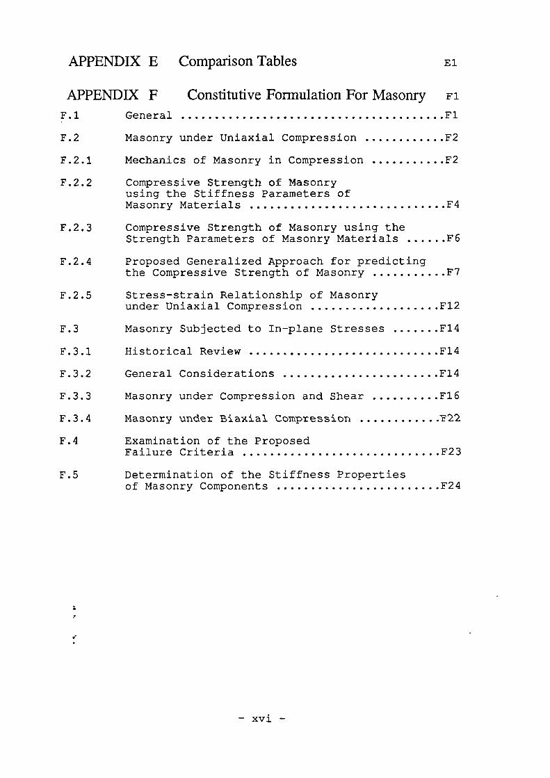
APPENDEKE Comparison Tables El
APPENDIX F Constitutive Formulation For Masonry FlF.1 General Fl
F.2 Masonry under Uniaxial Compression F2
F.2.1 Mechanics of Masonry in Compression F2
F.2.2 Compressive Strength of Masonryusing the Stiffness Parameters ofMasonry Materials F4
F.2.3 Compressive Strength of Masonry using theStrength Parameters of Masonry Materials F6
F.2.4 Proposed Generalized Approach for predictingthe Compressive Strength of Masonry F7
F.2.5 Stress-strain Relationship of Masonryunder Uniaxial Compression F12
F.3 Masonry Subjected to In-plane Stresses F14
F.3.1 Historical Review F14
F.3.2 General Considerations F14
F.3.3 Masonry under Compression and Shear F16
F.3.4 Masonry under Biaxial Compression 722
F.4 Examination of the ProposedFailure Criteria F23
F.5 Determination of the Stiffness Propertiesof Masonry Components F24
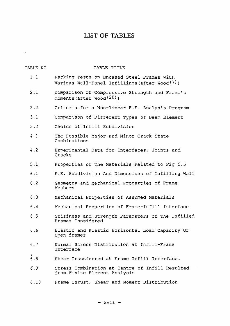
LIST OF TABLES
TABLE NO TABLE TITLE
1.1 Racking Tests on Encased Steel Frames withVarious Wall-Panel Infillings(after Wood(7))
2.1 comparison of Compressive Strength and Frame'smoments (after Wood(20))
2.2 Criteria for a Non-linear F.E. Analysis Program
3.1 Comparison of Different Types of Beam Element
3.2 Choice of Infill Subdivision
4.1 The Possible Major and Minor Crack StateCombinations
4.2 Experimental Data for Interfaces, Joints andCracks
5.1 Properties of The Materials Related to Fig 5.5
6.1 F.E. Subdivision And Dimensions of Infilling Wall
6.2 Geometry and Mechanical Properties of FrameMembers
6.3 Mechanical Properties of Assumed Materials
6.4 Mechanical Properties of Frame-Infill Interface
6.5 Stiffness and Strength Parameters of The InfilledFrames Considered
6.6 Elastic and Plastic Horizontal Load Capacity OfOpen frames
6.7 Normal Stress Distribution at Infill-FrameInterface
:
6.8 Shear Transferred at Frame Inf ill Interface.
6.9 Stress Combination at Centre of Infill Resulted -from Finite Element Analysis
6.10 Frame Thrust, Shear and Moment Distribution
7.1 Frame Forces
7.2 Comparison of The Collapse Racking load, Hc
7.3 Deviation of Hc(%) for Frames with Low ac Value
. 7.4 Comparison of diagonal Tension Load, Ht
7.5 Comparison of Stiffness, KO
7.6 Comparison of Bending Moment at LoadedCorners
7.7 Comparison of Bending Moment at the UnloadedCorners
7.8 Comparison of Column Bending Moment, M3c
7.9 Comparison of Column Axial Force, Ncl
7.10 Comparison of Column Shear Force, Sci
A.1 Data Listing for R.0 Frame with Masonry Infill.
A.2 Data Listing for Steel Frame with Concrete inf ill
B.1 The Structure Charts of Program 'NEPAL'
B.2 List Of Variable Names Used in Program 'NEPAL'
C.1 Strain Distribution in The Proposed Plane3-D Equivalent Element
E.1 to 12 Finite Element Analysis of Infilled Frames.
E.13to 39 Hand Analysis of Infilled frames
F.1 Comparison of The Proposed Calculated andExperimental Compressive Strength of Brickwork
:,
LIST OF FIGURES
FIGURE NO FIGURE TITLE
2.1 Notations
2.2 Behaviour of Infilled Frame.
2.3 Infilled Frame Under Diagonal Loading.
2.4 Diagonally Loaded Infilled Frame andInteractive Forces (after Stafford Smith(12))
2.5 Typical Load-Deflection Curve for ConcreteInfilled Steel Frame
2.6 Length of Contact as Function of Xla (afterStafford Smith(-2))
2.7 Infill Theoretical Stress Diagram for a/h'=3/8(after Stafford Smith(12))
2.8 P/R as Function of Xh (after StaffordSmith(-2))
2.9 Infilled Frame
2.10 Diagonal Strength of Concrete Infill as aFunction of Xh
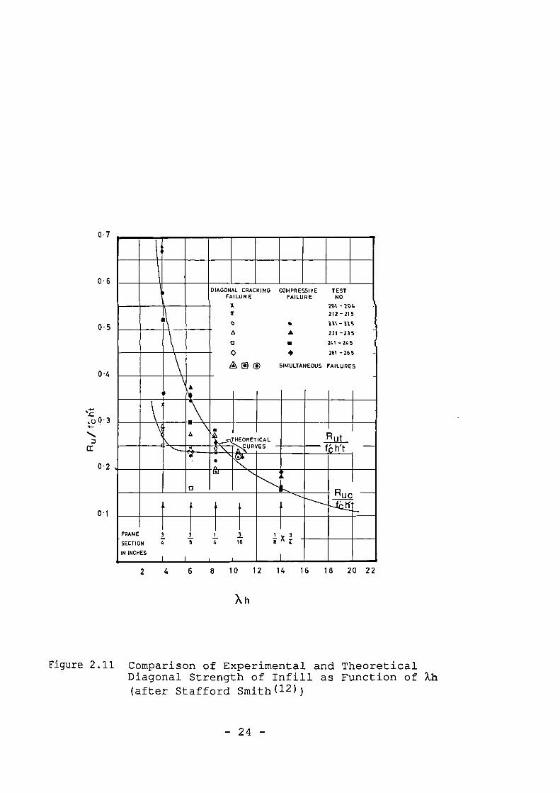
2.11 Comparison of Experimental and TheoreticalDiagonal Strength of Infill as Function of Xh
(after Stafford Smith(12))
2.12 Experimental and Theoretical Effective Width ofDiagonal Strut as Function of Length of Contact(after Stafford Smith(12))
2.13 Equivalent Strut Width as Function of Xia forStiffness Proposes (after Stafford Smith andCarter (12))
- 2.14
Shear Failure Criterion for Masonry UnderVertical Compression and Horizontal Shear.
2.15 Shear Strength of Infill as a Function of Xh(after Stafford smith and Carter(13))
FIGURE NO FIGURE TTTLE
2.16
2.17
2.18
2.19
2.20
2.21
2.22
2.23
2.24
2.25
2.26
Variation of Strength of Infills of Model andFull-scale Brickwork (after Mainstone(9))
Variation of Strength of Infills of MicroConcrete (after Mainstone(9))
Variation of Stiffness of Infills of Model andFull-Scale Brickwork (after Mainstone(9))
Variation of Stiffness of Infills of MicroConcrete (after Mainstone(9))
Comparison of Various Methods of Analysis ofInfilled Frame Based on MI
Idealized Plastic Failure Modes for InfilledFrames (after Wood(20))
Perspective View of Nielsen's (21) Square YieldCriterion for Unreinforced Wall, after Wood(20)
Infilled Frame Shear Mode of Collapse, Mode'S'; (after Wood(20))
Infilled Frame Shear Rotation Mode ofCollapse, Mode 'SR' (after wood(20))
Infilled Frame Diagonal Compression Mode ofCollapse, Mode 'DC' (after Wood(20))
Design Chart for Determination of OptionalCorrection to fs (after Wood(20))
2.27 Appropriate Penalty Factor (after Wood(20))
2.28 Variation of yp against aspect ratio ofpanel.
2.29 Finite Element and Experimental Results ofLiauw et al(24)
2.30 Results of F.E. Analysis (24 ) in The Third Storyof The Model Before and After Peak Load.
1.2.31 Mode 1 - Corner crushing with Failure inColumns (after Liauw et al(25))
2.32 Mode 2 - Corner Crushing with Failure inBeams (after Liauw et al(25))
FIGURE NO FIGURE 1 1 1 LE
2.33 Mode 3 - Diagonal Crushing (Span Greater thanHeight) (after Liauw et al(25))
2.34 Comparison of Liauw et al (25 ) estimated loadwith Experimental Results.
2.35 Failure Modes of Multistorey Infilled Frames.(after Liauw et al(25))
3.1 Newton Raphson Iteration
3.2 Geometry of a Quadrilateral Element.
3.3 Numerical Integration
3.4 Reinforcement Modelling.
3.5 The Most Used Isoparametric Elements
3.6 Masonry 3.D F.E Subdivision
3.7 3.D Equivalent 4-node Element
3.8 2-D Masonry F.E Subdivision Using LaminarJoints
3.9 2-D Masonry F.E Subdivision Using MasonryEquivalent Elements and Zero Thick Interfaces
3.10 The Modes of Joint Failure in a Masonry super-Element
3.11 Modelling of an Interface by Linkage Elements
3.12 Modelling of an Interface Segment by TheProposed 4-node Element
3.13 Wilson et al (44) Non-Conforming Beam Element.
3.14 Linear Elastic Analysis of Infilled Framewith Various F.E Subdivision Mesh
3.15 Effect of Scaling The Size of MasonryElements on The Typical Infill Crack Pattern
4.1 Linear Elasticity Fracture Model
f4.2 Non-Linear Elasticity Fracture Model
4.3 Elastic Perfect Plasticity Fracture Model
4.4 Elastic Work-Hardening Plasticity FractureModel
FIGURE NO FIGURE TITLE
4.5 The Elastoplastic Fracture Model of Darwin andPeknold(47)
4.6 Comparison of the Proposed Formulation withExperiments of Kupfer et al(55)
4.7 Comparison of Actual and ProposedComplete Stress-strain Curves of Concrete.
4.8 Comparison of the Proposed Value for Poisson'sRatio with the Experimental Results(55)
4.9
Concrete Under Unloading and Reloading
4.10
Stress strain Curve of Concrete in Tension
4.11
Drucker-Prager and Von Mises Yield Surfaces inPrincipal Stress Space.
4.12
Mohr-Coulomb and Tresca Yield Surface inPrincipal Stress Space (after Zienkiewitcz(36))
4.13 Comparison of the Proposed Failure Criteriafor Concrete under Biaxial Compression withthe Experimental Results of Kupfer et al(55)
4.14 Typical Triaxial Test Arrangements
4.15 Comparison of the Proposed Failure Criteriawith Experimental Results of Kupfer et al(55)
4.16 Experimental Stress-strain Relationship ofConcrete under Biaxial Loading.
4.17 Equivalent Uniaxial Stress-strain Curves
4.18 Comparison of The Proposed AnalyticalPrediction of Equivalent Uniaxial Strains atPeak Load with Some Experimental Data
4.19 Comparison of the Proposed Prediction of ThePoisson's Ratio at Peak Stress withExperimental Results of Kupfer et al(55)
4.20 Comparison of the predicted and actual Stress-strain Diagrams for concrete under biaxialCompression; Gi=0, 02/G3=0.52
,4.21 Comparison of the predicted and actual Stress- .strain Diagrams for concrete under BiaxialCompression and tention; G2=0, G1/G2=-0.052
FIGURE NO FIGURE TITLE
4.22 Stress and Equivalent Uniaxial StrainRelationship of Concrete under ProportionalMultiaxial Unloading and Reloading
4.23
Proposed Model for Relationship of NormalizedValues of Stress and Equivalent Uniaxial Stainof Concrete under Proportional loading
4.24 Comparison of The Proposed Prediction ofUnloading Modulus of Elasticity with Karsanand Jersa( 60 ) Formula.
4.25 Proposed Model for Non-Proportional TriaxialLoad Increment
4.26 Different Fracture Criteria for Concrete inTension
4.27 Crack Modelling.
4.28 Possible States of a Single Cracked Material.
4.29 Determination of One Co-efficient for bothCrack Dilatancy and friction
4.30 Double Cracked Material
4.31 Possible States of Double Cracked Materials.
4.32 Stress-strain Curves for Steel(after Chen(39));
4.33 Proposed Stress-strain Relationship Models forSteel.
4.34 Von Mises Yield Criterion on The Co-ordinatePlane a3=0
4.35 Criteria for Inelastic Behaviour of anInterface
4.36 Concrete-on-steel Shear-relative DisplacementRelationship
4.37 Behaviour of Bed-Joints of Grouted ConcreteBlock Masonry under Precompression
4.38 Typical Shear Stress-Tangential DisplacementCurves for Interfaces under Constant NormalStress
4.39 Proposed Constitutive Model for Fully bondedInterfaces
4.40
4.41
5.1
5.2
5.3
5.4
5.5
5.6
5.7
5.8
5.9
FIGURE NO FIGURE 'TILE
Proposed Constitutive Model for PartiallyBonded Interface
Proposed Constitutive Model of Totally DebondedInterface
Proposed Load Application.
F.E Analysis of RC Beam under Centre PointLoad.
Comparison of The F.E Analysis of RC Beam WithExperimental Results of Bresler et al(95)
Comparison of The F.E Analysis of an Open SteelFrame with Experimental Values (29)
Comparison of The F.E Analysis of Model SteelConcrete Infilled Frame With ExperimentalResults (29)
F.E Results at Station 1 (Ah=0.382mm).(a)Frame, (b)Interface and (c)Infill
F.E Results at Station 2 (Ah=0.678mm);(a)Frame, (b)Interface and (c)Infill
F.E Results at Station 3 (Ah=0.934mm);(a)Frame, (b)Interface and (c)Infill
F.E Results at Station 4 (Ah=1.54mm);(a)Frame, (b)Interface and (c)Infill
6.1 Infilled Frame Under Diagonal Loading
6.2 Typical Open Frame Load-Deflection Diagram
6.3 to 7 Load-Deflection Diagrams, Results of F.EAnalysis
6.8 F.E. Analysis Results of Infilled Frame MMUR2at Working Stress Load Level.
6.9 F.E. Analysis Results of Infilled Frame MMUR2at Peak Load Level
6.10 Typical Progressive Failure Stages of InfilledFrame under Racking
!. 6.11 Biaxial Stress Combinations of Infill in Highly'Stressed Regions Leading to Crushing orCracking
FIGURE NO FIGURE TITLE
7.1 Proposed Frame-Inf ill Interaction Forces;a)wall, b)column, c)moment diagram
7.2 Deformation of Infilled Frames;
a)columns only, b)beams only
7.3 Proposed Infill Boundary Stresses;a)boundary stresses, b)at column interfacec)at beam interface
7.4 Frame forces; a)Horizontal Forces Equilibrium,b) Column forces,c) Column Bending Moment Diagram
7.5 Upper Limit for Length of Contact
7.6 Graphical Representation of Failure Modes
7.7 Chart for adjusting gc, Pc and ac
7.8 Application of The Chart;a)high gc b)low gc
7.9 Comparison of Various Methods of Analysis withFinite Element and Test Results ofHorisontal Collapse Load, R.
7.10 Comparison of Various Methods of Analysis withFinite Element and Test Results of;a)Cracking load, Ht, b)Stiffness, KO.
A.1 Code Number for Geometry of Interface
A.2
R.0 Masonry-infilled Frame Subdivision Lay-out.
A.3
Reinforcement Data of The Frame Tested bySamai(8)
A.4
Steel Concrete-infilled Frame SubdivisionLay-out
D.1
Deformation of a Beam Segment under ArbitraryForces
; D . 2
Modes of Deformation of the Proposed BeamElement Resulting from Nodal Displacements.
t:D.3
Deformation of the Proposed Beam Element Due toDisplacement of the Proposed 5th Node
D.4
Displacement of Centre Line of a Beam Due toEffect of the Poissin's Ratio
FIGURE NO FIGURE TITLE
F.1 Proposed Constitutive Model for Partially
Bonded Interface
F.2
Proposed Constitutive Model of Totally DebondedInterface
F.3
Stress Distribution within the Components ofMasonry under Uniaxial Compression.
F.4
Charts to Estimate the Compressive Strength ofMasonry.
F.5
Comparison of the Proposed Masonry FailureCriteria with Experimental Data; 0=45.
F.6 Comparison of the Proposed Masonry FailureCriteria with Experimental Data; 0=67.5.
F.7 Comparison of the Proposed Masonry FailureCriteria with Experimental Data; 0=67.5.
NOTATIONS
a = Length of contact between column and infill
a = Vector of nodal displacements
a = Length of element
A = A constant controlling failure criteria of brittlematerial under biaxial compression-tention
b = Height of element
[B] = Element strain function matrix
c = A constant value used in failure criteria of brittlematerial under multiaxial compression
d = Diagonal length of a panel
D = A parameter controlling the falling branch of stress-strain curve
[D] = Stress-strain relation matrix
[Dt]= Tangent stress-strain relation matrix
e = Normalized EUS; e = Eius/aiuc
eE = Normalized EUS on the envelope stress-strain curve
ep . Normalized plastic EUS
E = Secant modulus
Eo . Initial tangent modulus
Eb . Modulus of elasticity of beams of a frame
Ec . Modulus of elasticity of columns of a frame
Ec . Secant modulus at peak unconfined uniaxial compression:
Eff. = Modulus of elasticity of frame members
Ei= . Initial modulus of elasticity of infill
Es = Secant modulus at peak stresses
Est = Secant modulus at peak uniaxial tension
Et = Tangent modulus
Eui = Tangent modulus in proportional unloading
EUS = Equivalent Uniaxial Strain
fc' = Standard cylinder strength of concrete
fcu = Standard cube strength of concrete
fbc = Equal biaxial compression strength_the = fbc/ac
= A parameter related to variation of poisson's ratio
F = Diagonal load transferred by frame alone
ft = Direct tensile strength of concrete
ftb . Joint tensile bond strength
fsb = Joint shear bond strength
fm = Mortar compressive strength on cylinder
fpr = Masonry prism strength
g = A parameter controlling EUS curves
h' = Height of infill
h = Height of column measured o/c of beams
H = Weighting coefficient in numerical integration
H = Horizontal load carried by an infilled frame; index uindicates the ultimate load and indices t and csignify the tensile and compressive failure modesrespectively
I = Moment of inertia
If = Moment of inertia of frame members
Ib = Moment of inertia of the beams in a frame
Ic = Moment of inertia of the columns in a frame
[K] = Structure stiffness matrix
[Kt] = Structure tangent stiffness matrix
[K] e Element stiffness matrix
[Kt] e=Element tangent stiffness matrix
- xxviii -
k = Material constant controling the Poisson's ratio
l' = Length of infill
1 = Length of beams measured o/c of columns
m = Strength parameter in Wood's Theory
Mp = Plastic resisting moment of frame members
[N] = Strain/stress relation matrix
N = Shape function
P = Total diagonal load transferred by infilled frame
{P} Vector of external loads
q = A constant controling the failure criterion of brittlematerial under multiaxial compression
NI Vector of equivalent nodal forces
{q} e= Vector of element equivalent nodal forces
R = Diagonal load transferred by an infilled frame;index u indicates the ultimate load and indicest and c signify the tensile and compressive failuremodes respectively
{R} = Vector of out-of-balanced nodal forces
S = Normalized principal stress
t = Wall or element thickness
ti . Thickness of infill
ts . Thickness of equivalent steel layer
[T] = Transformation matrix
u,v = Total displacement components along x and y coordinaterespectively
w = Overall change in thickness
w = width of opening of a crack or an interface
w : = An specified width of diagonal strut of infilled frame
we' = Effective width of diagonal strut of infill (indicesk, c and t denote the values corresponding tothe diagonal compressive strength and diagonalcracking load respectively)
x,y,z =Structure coordinates
11) = Penalty factor in Wood's method
{c} = Vector of total strain.
fejp) = Vector of total plastic strain
{es1} =Vector of total equivalent-joint-slip strain in jointmaterial
fes0 =Vector of total equivalent-joint-separation strain injoint material
{CI} = Vector of EUS
eiu = EUS in principal coordinates
eilic= Equivalent uniaxial strain at peak stress
Cc = Strain corresponding to ac in uniaxial unconfined
loading
Et = Strain corresponding to at in uniaxial direct tension
{e12} =Vector of projection of equivalent uniaxial strain onequivalent uniaxial envelope curves
eiuE= The component of {euE} corresponding to the principalcoordinate
{cup} =Vector of equivalent uniaxial plastic residual strainafter full unloading
eiup= The component of {&up} corresponding to ith principaldirection
Stiffness parameter in Stafford Smith method
Poisson's ratio
vo Initial Poisson's ratio
v * , V • Incremental Poisson's ratio
Coefficient of friction of interface
Volumetric steel ratio of its equivalent layer
0 Normal and shear stresses respectively.a , Vector of stress in structure coordinates
faI T = [ ax, ay, az, Yxy,Yyz,Yzx]
ac Unconfined uniaxial compressive strength. (-ye)
ac = - ( 0.90 to 0.96)fc' (-ye)
pa',T 1 =Normal and shear stresses on yield surface;
they appear with various suffixes:-al', 02'and G3' (for principal directions),ale, ay', aZ', Txy', Tyz', Tzx' (for an arbitrarydiresctions)
6dt = Diagonal tensile stress at centre of the infill to
cause tensile failure
Normalized coordinates
CHAPTER ONE
Introduction
Framed buildings normally contain wall panels
whose prime function is to either separate spaces within the
building or to complete the building envelope. The
properties of these walls and their position within the
structural frame may be so chosen that they can also have a
significant influence on the response of the structure
subjected to side sway. Such structural configurations are
termed "Infilled Frames" and have been investigated by a
number of researchers.
The history of work on infilled frames dates back
to the mid 1950's when the design of rigid-jointed multi-
storey frames was being revolutionized as a result of work
done by Wood et al (1,2), Beaufoy et al( 3) and Chandler(4)
and Livesley et al (5) , wherein "The degree of restraint
method" and application of the critical load in the new
elastoplastic design of these structures were being
developed. According to the new design method, which was
reported later by "The Joint Committee( 6 )", the stability of
rigid multistorey framed structures would significantly
improve and considerable economy would be achieved if side
sway is resisted separately by walls and floors or bracing.
However, in this method no allowance was given for the
contribution of the infilling walls in limiting side sway of
framed structures due to the lack of understanding of the
behaviour of infilled frames. Wood( 7) , 1958, concluded that
"there had been a neglect in the past to study the
stiffening effect of cladding of tall buildings." He listed
a series of in-plane racking tests, Table 1.1, on encased
steel frames with various wall panel infillings. This table
shows the significance of the infilling walls in reducing
side sway of multistorey buildings.
Since then even though the potential economy and
efficiency of infilled frame construction has always been
evident, its use still has not been widely accepted,
primarily due to lack of theory. During the last three
decades a few analytical approaches have been developed. A
summary of previous work is give n in Chapter 2. These
methods can generally be classified into the following
categories:
i) The approaches based on linear elasticity theories.
ii) The approaches using perfect plasticity theories.
The assumptions made in these approaches vary widely, and
the predictions of strength and stiffness also vary widely.
Attempts to verify these approaches using
experimental results have not been totally successful
because the experimental data are significantly affected by
variations in the properties of the materials. It is not
feasible to measure all the necessary information, such as
stresses in the infill and also in the frame members.
The finite element method, however, as a powerful
and fast growing technique, has become a popular method for
- 2 -

solving highly indeterminate problems. Therefore, quite a
few finite element analyses have ben developed for infilled
frames during the past ten years mainly using either pure
elasticity or perfect plasticity theories with allowance for
separation and slip of the joints. The results of these
analyses have been used to examine the aforementioned
elastic and plastic methods. These are reviewed in Chapter
2. The rather large discrepancy between the two groups of
approaches indicates that study of infilled frames still
lacksa rational analysis accounting for both elastic and
plastic behaviour of the structure.
The prime objective of this study has therefore,
been to develop a finite element program particularly
written for the analysis of infilled frames and examine the
existing methods. It was desirable that such a program
should be capable of simulating the non-linear behaviour of
frame, infill and their interfaces as accurately as
possible. In order to satisfy these requirements it was
necessary to inve .stigate the materials behaviour in detail
and to develop suitable mathematical models for their
mechanical response. This work is covered in Chapter 4. In
order to improve the accuracy and economy of the finite
element analysis, new elements such as beam, interface and
loading elements needed to be developed. These elements and
also the basis of the finite element method are described in
Chapter 3. These efforts led to the finite element analysis
computer program "NEPAL" written by the author. This
program is introduced in Chapter 5. This chapter also
reports the tests carried out to examine the performance of
the program in solving some non-linear structural problems.
The next phase of the work was to study the
behaviour of infilled frames within practical ranges of
beam, column and infill strength and also the infill aspect
ratio. Computation and results of analysis of these frames
are described and discussed in Chapter 6 leading to the
necessity of proposing a new hand method of analysis based
on both elastic and plastic behaviour of the materials and
limited infill strain at collapse load. Development of such
a method is described in Chapter 7. This chapter also deals
with comparison of the results of the newly developed method
with the results of the finite element analysis and
previously existing experiments and methods.
The final chapter presents the conclusions drawn
from the present investigation and recommendations and
suggestions to carry on the work in the future.
:
.-
- 4 -
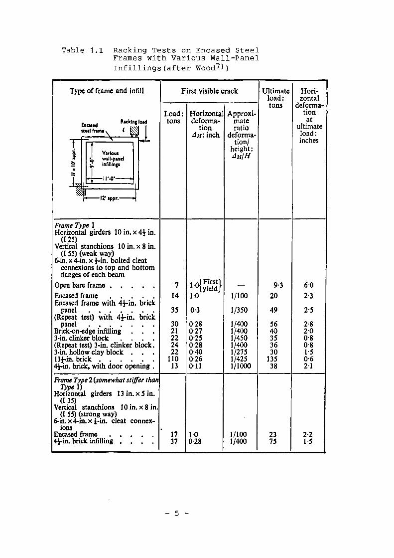
Table 1.1 Racking Tests on Encased SteelFrames with Various Wall-PanelInfillings(after Wood7))
Type of frame and infill First visible crack Ultimateload:tons
Hod-zontal
deforma-Load : Horizontal Approxi- tion
hamooadEmoted
tons deforms-tion
materatio
atultimate
steel (rune ( \•e• 4H: inch deforma-
tion/height:Lhillf
load:inches
•VariouswaIlldam.
_ .7,;, InnIripII
11,4r
lg.,
mappt
Frame Type 1Horizontal girders 10 in. x 4 .1 in.
(I 25)Vertical stanchions 10 in. x 8 in.
(I 55) (weak way)6-in, x 4-in. x 1-in, bolted cleat
connexions to top and bottomflanges of each beam
Open bare frame 7 , .,,f First}' nyield
_ 9.3 6.0
Encased frame . . . . . 14 1 .0 1/100 20 2.3Encased frame with 41-in, brick
panel . . . . . . . 35 0. 3 1/350 49 2.5(Repeat test) with 4i-in. brick
panel . . . . . . . 30 0 . 28 1/4.00 56 2.8Brick-on-edge infilling . . . 21 0 .27 1/400 40 2.03-in, clinker block . . . . 22 0 .25 1/450 35 0-8(Repeat test) 3-in, clinker block. 24 0 .28 1/400 36 0.83-in, hollow clay block . . . 22 0 .40 1/275 30 1.5131--in. brick 110 0.26 1/425 135 0.64I-in, brick, with door opening . 13 0 . 11 1/1000 38 2.1
Frame Type 2 (somewhat stiffer thanType 1)
Horizontal girders 13 in. x 5 in.(I 35)
Vertical stanchions 10 in. x 8 in.(I 55) (strong way)
6-in. x 4-in. x fin, cleat connex-.
ions .Encased frame 17 1-0 1/100 23 2.241--in. brick milling . . . . 37 0 .28 1/400 75 1.5
CHAPTER TWO
Review of Previous Work
2.1 Introduction
The composite behaviour of an infilled frame is a
complex statically indeterminate problem. Since 1958 this
topic has been the subject of several separate
investigations at various institutions throughout the world.
The approaches to the problem have varied widely.
Considering the different assumptionsmade, it is not
surprising that the predictions of stiffness and strength
have also varied widely. A detailed review of previous
experimental and theoretical investigations has been given
by Samai (8) . In this chapter the intention is to briefly
review the behaviour of infilled frame and to summarize the
main stages in the development of its analysis and
understanding of its behaviour.
22 Behaviour of Infilled Frames under Racking Load
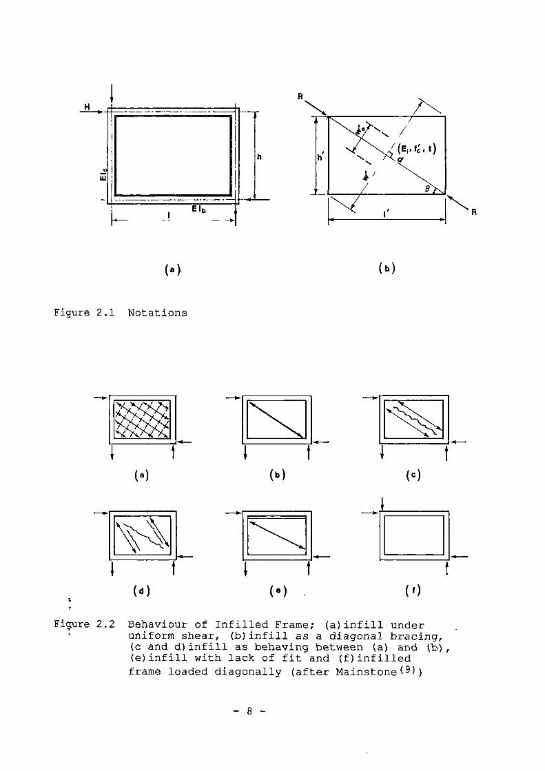
Fig 2.1 shows a rectangular single bay single
storey infilled frame under racking load, H.
Mainstone( 8 )described the behaviour of this composite
structure as follows:
If, before loading, the infill fits the frame
perfectly, its initial behaviour will lie somewhere between
the extremes illustrated in Figs 2.2(a) and 2.2(b). The
- 6 -
maximum possible contribution to resisting the load will be
achieved by a state of uniform shear throughout, calling
for continuous transfer of shear along the interfaces with
the frame plus continuous tension on beams and continuous
compression on columns for non-square frames, Fig 2.2(a).
Considered as a diagonal strut, the infill may then be said
to have an effective width, w', Fig 2.1(b).
At the other extreme, the interface reactions will
be concentrated to the corners and the distribution of
stress will be highly non-uniform, leading to a behaviour
equivalent to that of a much narrower strut Fig 2.2(b).
Between the two extremes the interface reactions
will always be distributed over finite lengths of the beams
and columns i.e, BF and BG in Fig 2.4, unlike the
concentrated reactions of a true diagonal strut, Fig 2.2(b).
Some changes in the mode of deformation of the frame will be
induced leading to a further increase in the composite
stiffness. Diagonal cracking, if it precedes crushing of
the infill, will modify this initial behaviour by creating,
in effect, two or more struts in place of the original one,
Figs 2.2(c), 2.2(d). Quite marked changes in the mode of
deformation of the frame may then result from redistribut-
ions of the interface reactions.
If, before loading, the infill does not fit
perfectly, the interface reactions and the resulting
behaviour will be further modified. A continuous gap at the
tog, for instance, will mean that load can be transmitted to-
the infill only by compression and shear on the vertical
faces. The alignment of the effective strut will then be
-T
4.
..il
// (E I , f, t)
o'
0
I'EIb
(a)
(b)
(d)
( a )
f)
.n-•••
(a)
(b)
Figure 2.1 Notations
Figure 2.2 Behaviour of Infilled Frame; (a)infill underuniform shear, (b)infill as a diagonal bracing,(c and d)infill as behaving between (a) and (b),(e)infill with lack of fit and (f)infilledframe loaded diagonally (after Mainstone(9))
8
H-R(h')3C0se Ic [1+ — Cote] Cos0
24EIc Ibsd (2.1)
somewhat different initially, Fig 2.2(e), and there will be
a tendency for the infill to slip and rotate until it bears
on the beam and column at the loaded corners.
An infilled frame may be loaded diagonally as shown in Fig
2.2(f). This type of loading produces compression in the
windward column in place of tension that would arise in
practice as shown in Fig 2.2(a) to (e).
The real behaviour of an infill in resisting a
racking load is more complex than that of a simple diagonal
strut. However the early work on the subject was based on
idealization of the infill as a simple diagonal strut
2.3 Early Work and the Concept of Diagonal Strut
Serious experimental and analytical investigation
on infilled frames was started in 1958 by Polyakov(10).
He suggested the possibility of considering the effect of
the infilling wall in each panel as equivalent to diagonal
bracing Fig 2.3(b). This suggestion was later taken up by
Holmes (11) , 1961. He represented the inf ill by a pin-
jointed strut connecting the loaded corners as shown in
Fig 2.3(b). He also concluded that, at failure, the
deflection of the composite wall and frame is small in
comparison with the deflection of the bare frame.the
Therefore, the frame members remain in elastic stage up to
failure load. Accordingly, he calculated the change in the
frame diagonal, Esd, as:
9
The shortening of the equivalent strut at failure was also
calculated as:
8d = Ecd
(2.2)
8d = ech'/Sin0
(2.3)
where ec denotes the strain in the infill at failure.
The value of Ec was taken as 0.002 as a safe limiting value
for concrete infill. From Eq 2.1 and 2.3 the horizontal
load at failure, H, was derived by Holmes( 11 ) as follows:
24EIcEc+AfcCose (2.4)
ICh' 2 [1 + — Cote] Sin0Cos0
Ib
Where R is replaced by the product of the cross sectional
area, A, of the equivalent strut and the crushing stmength
of the infill, fc• Holmes (11 ) showed that, for strength
purposes,td/3 best represents the value of A for the
infilled frames tested. However, the theoretical
deflections at the ultimate load, corresponding to the
proposed value of A, were generally much lower than those of
the companion experimental deflections.
The Holmes one third rule for determining the
width of the diagonal strut is independent of infill/frame
strength and stiffness parameters. However, as will be seen
later in this chapter, the behaviour of an infilled frame is
highly dependent on these parameters.
- 10 -
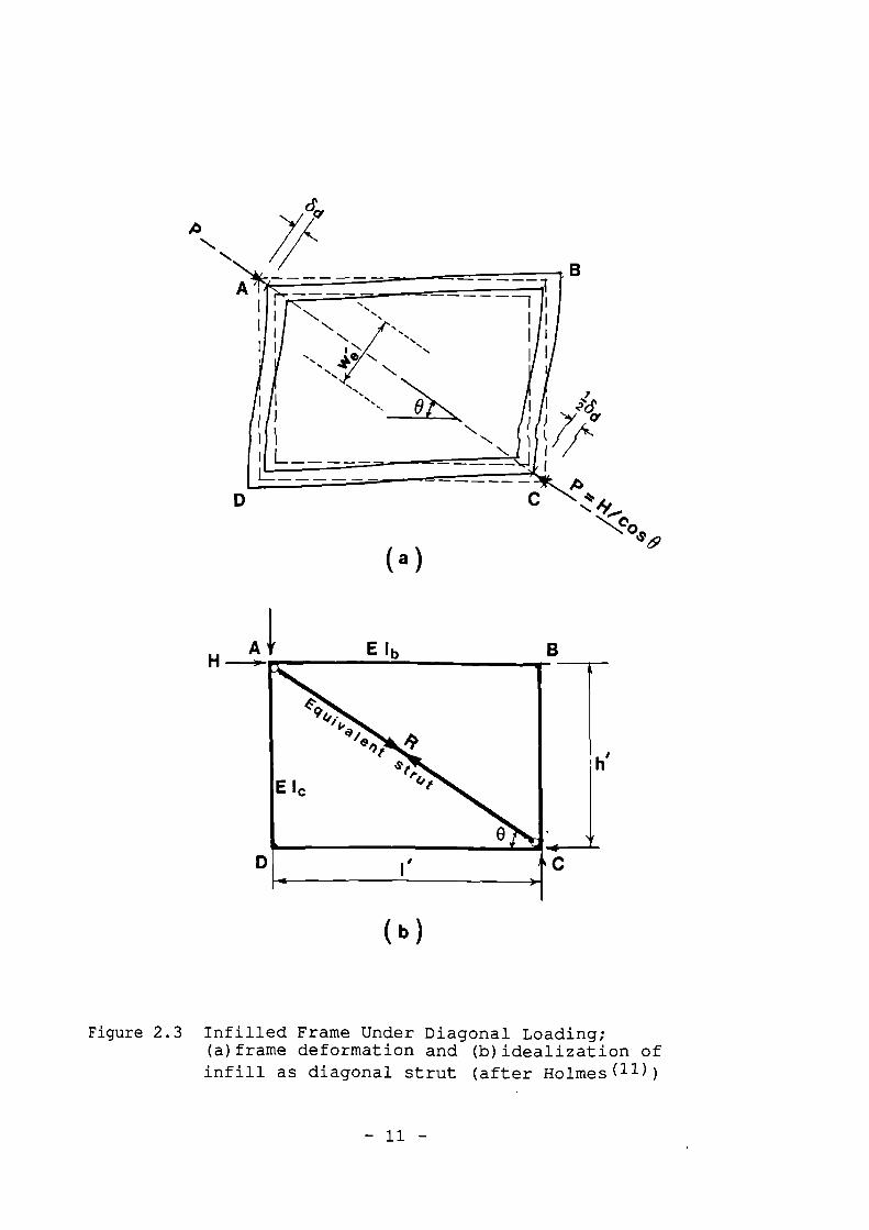
D I , C
( b )
Figure 2.3 Infilled Frame Under Diagonal Loading;(a)frame deformation and (b)idealization ofinfill as diagonal strut (after Holmes(--))
Holmes (11 )' approximation, although crude, may be
considered as the basis for later work especially the work
done by Stafford Stith( 12 ), 1966, which is summarized in the
following sections.
2. 41 Theories Based on Infill/Frame Stiffness Parameter
2.4.1
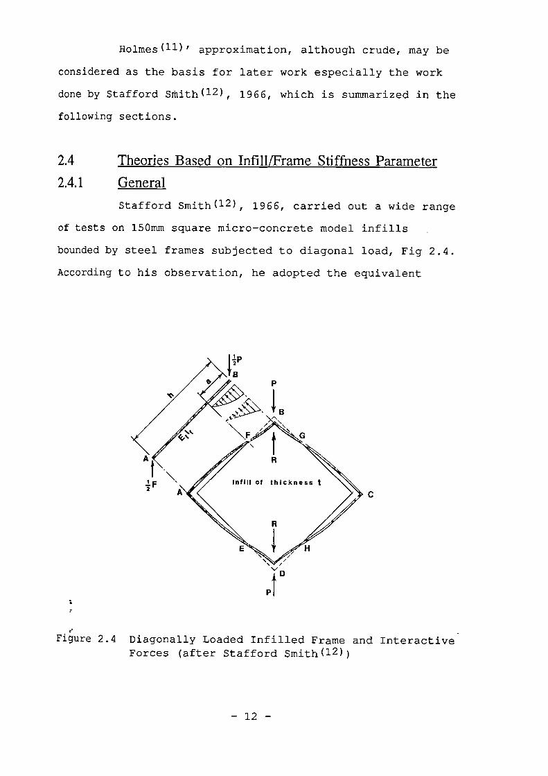
Stafford Smith( 12 ), 1966, carried out a wide range
of tests on 150mm square micro-concrete model infills
bounded by steel frames subjected to diagonal load, Fig 2.4.
According to his observation, he adopted the equivalent
eFigure 2.4 Diagonally Loaded Infilled Frame and Interactive
Forces (after Stafford Smith(12))
- 12 -
diagonal strut in representing the effect of inf ill.
However, Stafford Smith did not share the view of the one
third rule proposed by Holmes( 11 ) which is described in
Section 2.3. Instead, he pointed out that the width of the
equivalent diagonal strut is determined by the finite
lengths of contact between the frame and the infill at the
loaded corners, Fig 2.4.
Stafford Smith and Carter( 13 ), 1969, expanded the
work of Stafford Smith to deal with rectangular and
multistorey infilled frames. Also they further studied the
stiffness of such structures. A review of their work is
given in the following sections.
2.4.2 Stafford Smith Observations on the Behaviour of
Infilled Frames Subjected to Racking Load
When an infilled frame is under either horizontal
or diagonal load, Fig 2.4, the infill and the frame separate
over a large part of the length of each side and contact
remains only adjacent to the corners at the ends of the
compression diagonal. As the load is increased, failure
occurs eventually in either the frame or the infill as
follows:
i) frame failure results from tension in the windward
column or from shearing of the columns or beams.
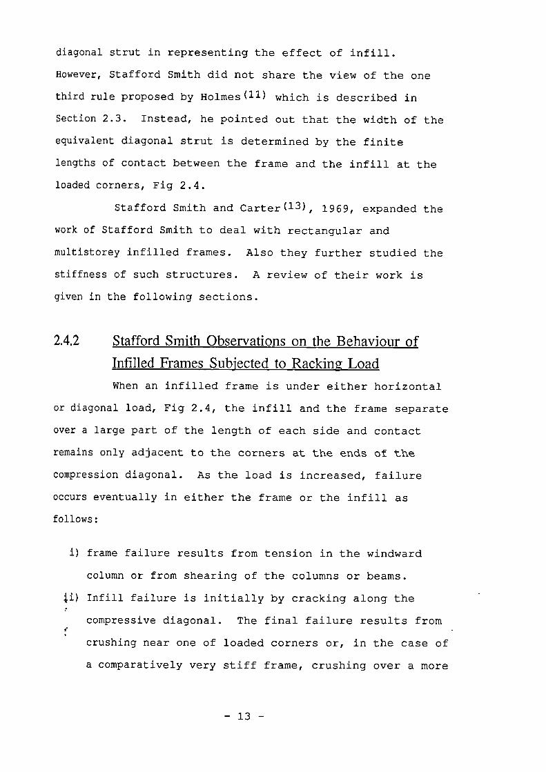
ii) Infill failure is initially by cracking along the
compressive diagonal. The final failure results from
crushing near one of loaded corners or, in the case of
a comparatively very stiff frame, crushing over a more
- 13 -
II
II
/I Cracking
11,111 Crushing
A
general interior region of the infill. However, if
the infill is of brick masonry an alternative
possibility of shearing failure along the plane of the
bed-joints may arise.
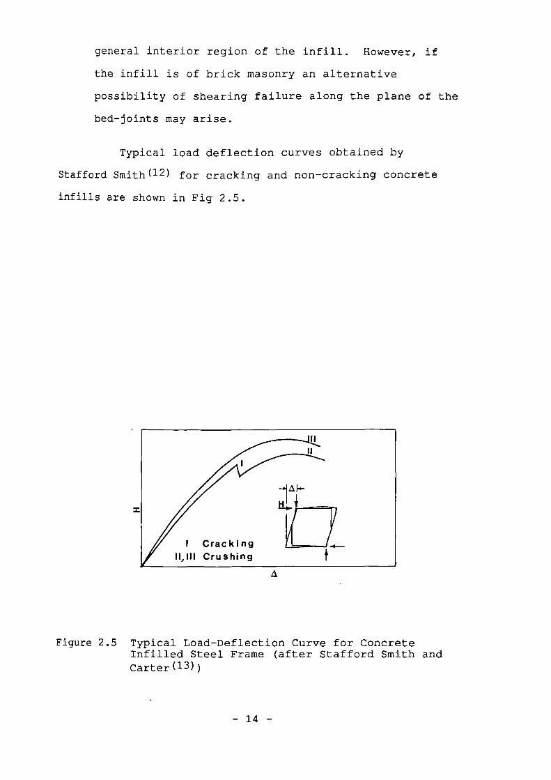
Typical load deflection curves obtained by
Stafford Smith (12) for cracking and non-cracking concrete
infills are shown in Fig 2.5.
Figure 2.5 Typical Load-Deflection Curve for ConcreteInfilled Steel Frame (after Stafford Smith andCarter (13))
- 14 -
2.4.3 Stafford Smith's Theoretical Analysis
Stafford - Smith( 12 ) carried out extensive
theoretical work using elasticity theory to derive the
length of contact and strength and stiffness of infilled
frames as follows.
Fig 2.4 shows a square infill frame subjected to
diagonal load illustrating the model infilled frames tested
by Stafford Smith( 12) . Consider the side AFB, in Fig 2.4,
of which FB remains in contact with the infill. Assuming a
triangularly distributed reaction along FB, the bending and
equilibrium equations were derived for the separate lengths,
AF and FB; these then were related by the continuity
conditions at point F. A further equation for the energy of
AB and one-quarter of the infill, allowed Stafford Smith to
reduce the whole set to a single equation in terms of Xh and
a/h' where:
EitiA.h =h
(2.5)
4EfIfh'
represents the infill/frame stiffness parameter. A similar
analysis was carried out, using a parabolic distribution of
the reaction along FB to produce an alternative equation
relating a/h' and Ala. The solutions of these equations
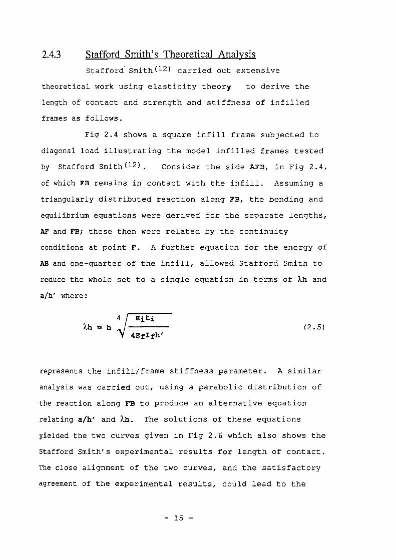
yielded the two curves given in Fig 2.6 which also shows the
Stafford Smith's experimental results for length of contact.
The close alignment of the two curves, and the satisfactory
agreement of the experimental results, could lead to the
- 15 -
h' 2Xh
OA 0.2 0.3 0.4 0.5
a
h'
Eq 2.6
TRIANGULAR --"fSOLUTION
PARABOLICSOLUTION
O TESTS 201-204
• TESTS 21-215
• TESTS 221- 225
30
25
20
15
X h'
10
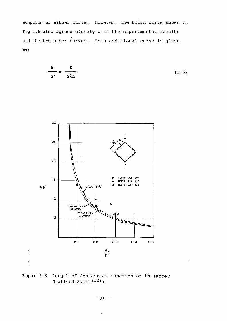
adoption of either curve. However, the third curve shown in
Fig 2.6 also agreed closely with the experimental results
and the two other curves. This additional curve is given
by:
a it
(2.6)
Figure 2.6 Length of Contact as Function of Xh (afterStafford Smith(12))
- 16 -
which was adapted from the equation for the length of
contact of a free beam on an elastic foundation subjected to
a concentrated load, following the analysis of Hetenyi et
al (14) . Because the third curve was more conveniently
expressed algebraically than the other two, and in other
respects was equally acceptable, it was adopted by Stafford
Smith for later use in the analysis.
The stiffness parameter, Xh, was later generalized
by Stafford Smith and Carter( 13) to allow for rectangular
walls as follows:
4. / EitiXII = h Sin20\
4EcIch'
(2.7)
Since an elastic theory was used in the analysis, the length
of contact remained constant during the course of loading.
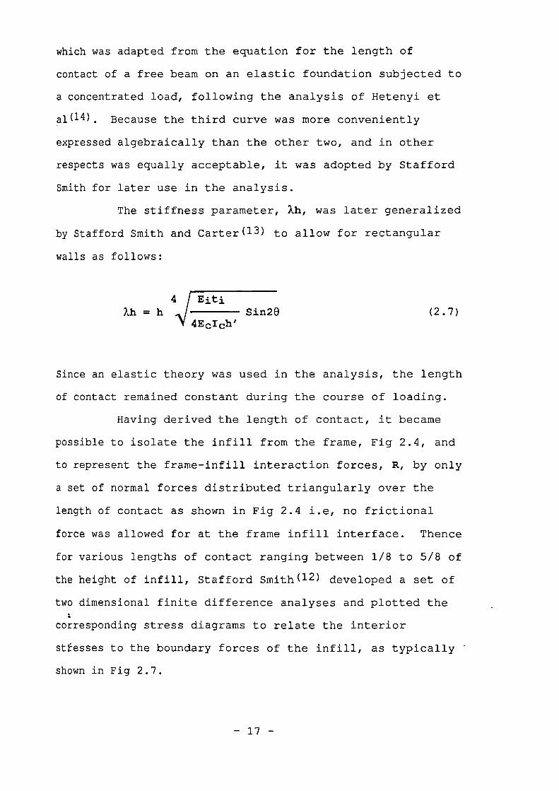
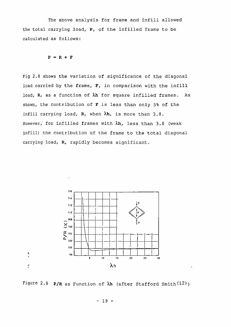
Having derived the length of contact, it became
possible to isolate the infill from the frame, Fig 2.4, and
to represent the frame-infill interaction forces, R, by only
a set of normal forces distributed triangularly over the
length of contact as shown in Fig 2.4 i.e, no frictional
force was allowed for at the frame infill interface. Thence
for various lengths of contact ranging between 1/8 to 5/8 of
the height of infill, Stafford Smith (12) developed a set of
two dimensional finite difference analyses and plotted the;
corresponding stress diagrams to relate the interior
stfesses to the boundary forces of the infill, as typically
shown in Fig 2.7.
- 17 -
PANEL OF UNIT THICKNESS
100LOAD
UNITS
In order to study the contribution of the frame,
Stafford Smith, this time, represented the infill
interaction forces by triangularly distributed normal forces
acting over the length of contact on each side of the frame,
Fig 2.4. Thence, he calculated the load carried by the
frame alone, F, by developing an energy analysis of the
redundant system which was repeated for various lengths of
contact within the same range as above.
11 UNITS
LINE OF UNIFORM PRINCIPAL COMPRESSIVE STRESS
LINE OF UNIFORM PRINCIPAL TENSILE STRESS
PRINCIPAL COMPRESSIVE STRESS TRAJECTORY
-•-•- PRINCIPAL TENSILE STRESS TRAJECTORY
VALUES OF STRESS GIVEN IN LOAD UNITS PER SOUARE LENGTH UNIT
Figure 2.7 Infill Theoretical Stress Diagram for a/h'=3/8(after Stafford Smith(12))
- 18 -
5
10 15 20 25 30
116
114
112
110
108
106
CC 104
0-102
100
98
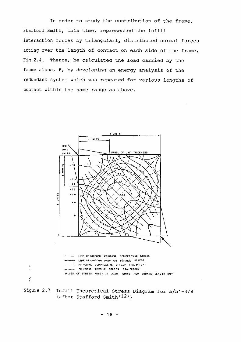
The above analysis for frame and infill allowed
the total carrying load, P, of the infilled frame to be
calculated as follows:
P = R + F
Fig 2.8 shows the variation of significance of the diagonal
load carried by the frame, F, in comparison with the infill
load, R, as a function of Mia for square infilled frames. As
shown, the contribution of F is less than only 5% of the
infill carrying load, R, when XII, is more than 3.8.
However, for infilled frames with MI, less than 3.8 (weak
infill) the contribution of the frame to the total diagonal
carrying load, R, rapidly becomes significant.
Xh
Figure 2.8 P/R as Function of Xla (after Stafford Smith(12))
- 19 -
hn
h 2
V
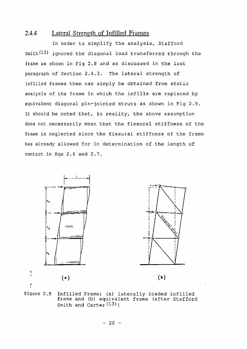
2.4.4 Lateral Strength of Infilled Frames
In order to simplify the analysis, Stafford
Smith (12 ) ignored the diagonal load transferred through the
frame as shown in Fig 2.8 and as discussed in the last
paragraph of Section 2.4.3. The lateral strength of
infilled frames then can simply be obtained from static
analysis of the frame in which the infills are replaced by
equivalent diagonal pin-jointed struts as shown in Fig 2.9.
It should be noted that, in reality, the above assumption
does not necessarily mean that the flexural stiffness of the
frame is neglected since the flexural stiffness of the frame
has already allowed for in determination of the length of
contact in Eqs 2.6 and 2.7.
( a )
(b)
Figure 2.9 Infilled Frame; (a) laterally loaded infilledframe and (b) equivalent frame (after StaffordSmith and Carter(-3))
- 20 -
Collapse of an infilled frame may occur through
failure either of the frame or of the infill. Failure of
the frame can result from tension in windward columns or
shear in the beams, columns or their connections. If
however, the frame is adequately strong, collapse will
eventually occur by compression failure of the infill
propagating from one of the loaded corners or, in the case
of a comparatively very stiff frame, crushing over a more
general interior region of the infill. Compressive failure
of infill may be preceded by a diagonal cracking along the
compressive diagonal.
Infill failure modes and loads were formulated by
Stafford Smith (12 ) for square panels. The work was later
generalized for masonry infills, rectangular panels and
multi-storey infilled frames by Stafford Smith and
Carter (13) . These are described as follows.
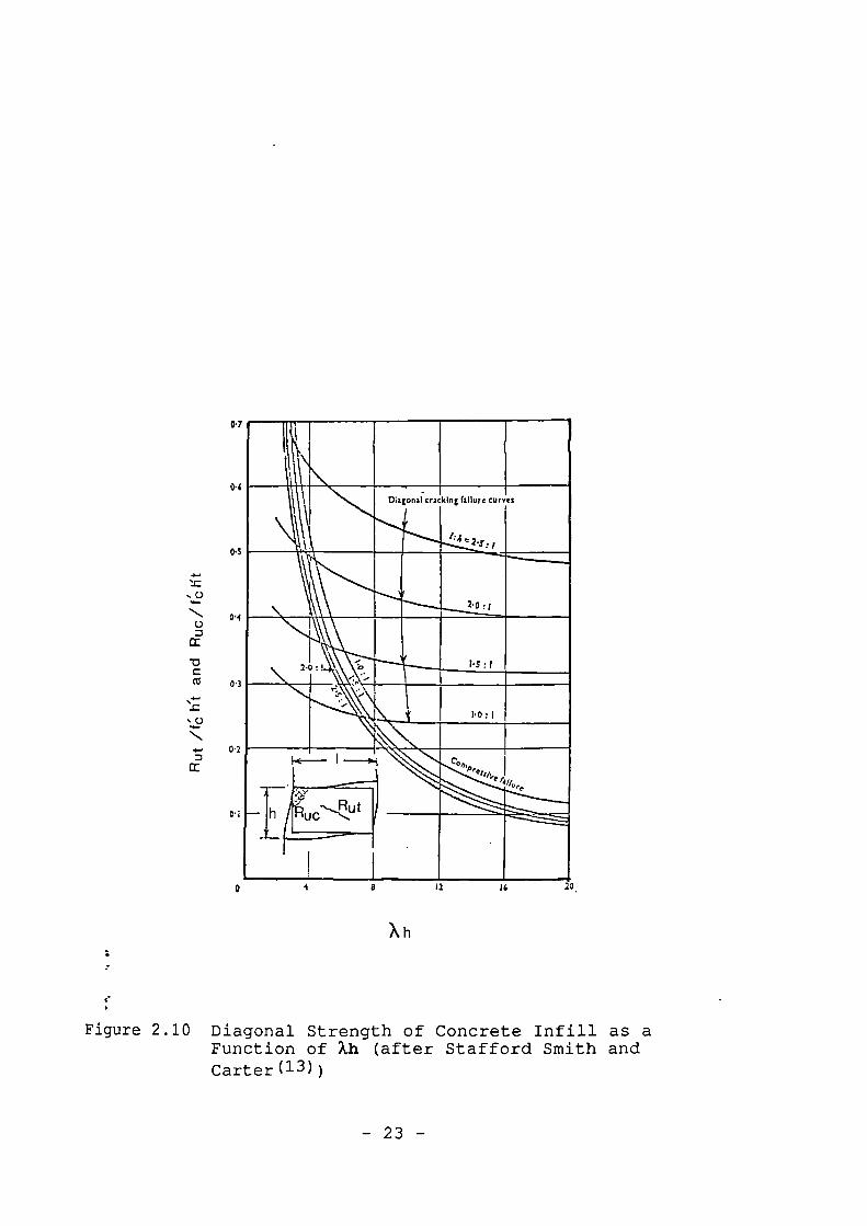
a) Diagonal Cracking of Infill
The diagonal force necessary to cause cracking of
the infill, Rut, is that which would produce a maximum
principal tensile stress in the infill equal to the tensile
failure strength of the infill material. From the maximum
principal tensile stress values taken from the infill stress
diagrams, Fig 2.7, and Eq 2.6 a series of curves were
constructed by Stafford Smith and Carter (13) to relate the
d4gonal cracking load, Rut, to XII for various panel
leligth/height proportions. Fig 2.10 shows these curves
where Ft' is replaced by 0.1fc', a reasonable value for
concrete tensile strength, thus allowing the basic parameter
- 21 -
for expressing the cracking strength, Rut/( ft' h ' t), to be
converted to Ruc/(fc'h't) and thereby permitting a direct
comparison of the cracking and compressive failure curves on
the same graph. Fig 2.10 also shows that the greater is the
length/height proportion of the infill, or the smaller is
the value of Xh, i.e the stiffer is the column relative to
the infill, the greater is the diagonal cracking strength of
infill.
b) Compressive Failure of Infill
The onset of this mode of failure is gradual.
Therefore, the collapse may be assumed to be due to a
plastic like failure within one of the loaded corners
surrounded by lengths of contact, a. Allowing for a uniform
crushing stress, fc', within this region, the diagonal
compressive failure load, Ruc, was derived as follows.
Ruc = atifc'Sec0 (2.8)
Substituting for a from Eq 2.6 the above equation may be
written in its non-dimensional form as:
Ruc n
= Sea
(2.9)fc'h't 2Xh
which is also plotted in Fig 2.10. The above theoretical
tensile and compressive infill failure loads and the test
results obtained by Stafford Smith (12) are compared in
Fig 2.11 showing a fairly good agreement.
- 22 -
04
0•5
.0
004
03
43'02
CC
1 I
......
MnonmdcN ftft ra am,u
:ii,
e--• ----\N
H1:1
ki::!nr
RUC-RUt
4
2
16
20.
X h
Figure 2.10 Diagonal Strength of Concrete Infill as aFunction of Xh (after Stafford Smith andCarter (13))
- 23 -
0.7
0-6
0-5
0.4
0.2
0•1
DIAGONAL
X
FAILURE
*0
A
0
& 1:3
CRACKING
®
COMPRESSIVEFAILURE
••a•
SIMULTANEOUS
TESTNO
201 - 20
212 - 21
1 lt - us231 -23
241 - 24 5
261 -265
FAILURES
4 .
5
5
a
1
THEORETICAL Rut
fich't
•
0
RUC
_FUME
SECTION
IN INCHES
3
I
7.
I 1 13 1 3I 7. 16
1 1i
1i v 3A
1
2 4 6 8 10 12 14 16 18 20 22
X h
Figure 2.11 Comparison of Experimental and TheoreticalDiagonal Strength of Infill as Function of 2di(after Stafford Smith(12))
- 24 -
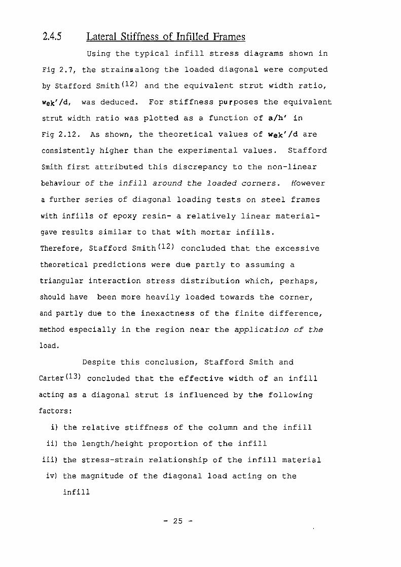
2.4.5 Lateral Stiffness of Infilled Frames
Using the typical infill stress diagrams shown in
Fig 2.7, the strainsalong the loaded diagonal were computed
by Stafford Smith( 12 ) and the equivalent strut width ratio,
wele/d, was deduced. For stiffness purposes the equivalent
strut width ratio was plotted as a function of a/h' in
Fig 2.12. As shown, the theoretical values of wek'id are
consistently higher than the experimental values. Stafford
Smith first attributed this discrepancy to the non-linear
behaviour of the infill around the loaded corners. However
a further series of diagonal loading tests on steel frames
with infills of epoxy resin- a relatively linear material-
gave results similar to that with mortar infills.
Therefore, Stafford Smith (12) concluded that the excessive
theoretical predictions were due partly to assuming a
triangular interaction stress distribution which, perhaps,
should have been more heavily loaded towards the corner,
and partly due to the inexactness of the finite difference,
method especially in the region near the application of the
load.
Despite this conclusion, Stafford Smith and
Carter (13) concluded that the effective width of an infill
acting as a diagonal strut is influenced by the following
factors:
i) the relative stiffness of the column and the infill
ii) the length/height proportion of the infill
iii)the stress-strain relationship of the infill material
iv) the magnitude of the diagonal load acting on the
inf ill
- 25 -
0.4
a
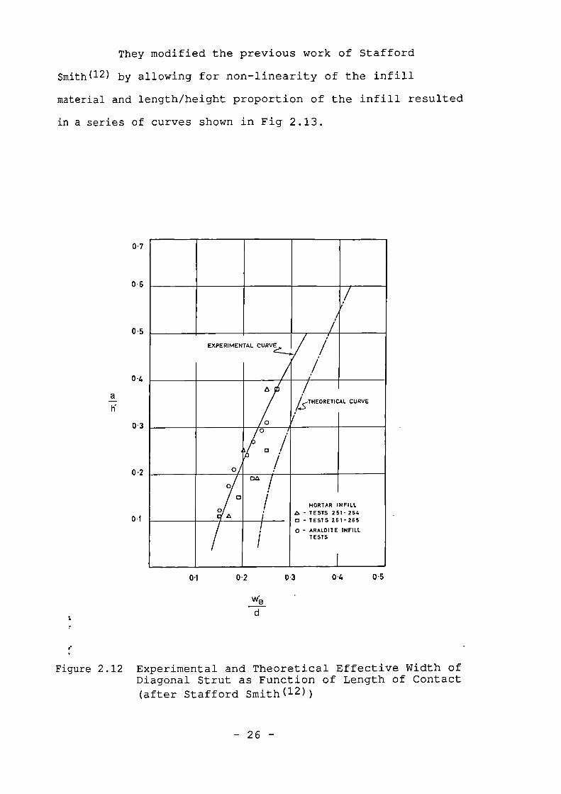
They modified the previous work of Stafford
Smith (12) by allowing for non-linearity of the infill
material and length/height proportion of the infill resulted
in a series of curves shown in Fig 2.13.
0.7
0.6
0.5
0.3
0.2
0•1
CURVE /1/
/,/'1EXPERIMENTAL
//sTHEORETICAL CURVE
0
/
0 n
A 0 //0
/ DA/
/ MORTAR IN FILLAN - TESTS 251- 2540 - TESTS 261-265
/ 0 - ARALDIT E INFILLITESTS
I
01
02
0.4
0.5
We
Figure 2.12 Experimental and Theoretical Effective Width ofDiagonal Strut as Function of Length of Contact(after Stafford Smith(-2))
- 26 -
OS 05
0 44
0 3 03
INC 0
0 2 02,
"an •
0 RiR c • I 1 0I
0 12 16 0
VALUE OF All
PANEL PROPORT IONS 1:1
CS OS
04
03 0.3
5.
02
R,
i0I 0I
.0
....--...
,nlic,,,"
1 TIC1717
N,R .1Y
4 a a
16VALUE OF X h
PANEL PROPORTIONS 11: I
n.......l.,,,
AiR, . 1n-.O a .< k It, •I'
RUC; 7'
4 8 12 6
a
16
VALUE OF A n VALUE CF AR
PANEL nCPORTIONS 2 0:1
PANEL PROPORTIONS 25:1
Figure 2.13 Equivalent Strut Width as Function of Xh forStiffness Proposes (after Stafford Smith andCarter(12))
- 27 -
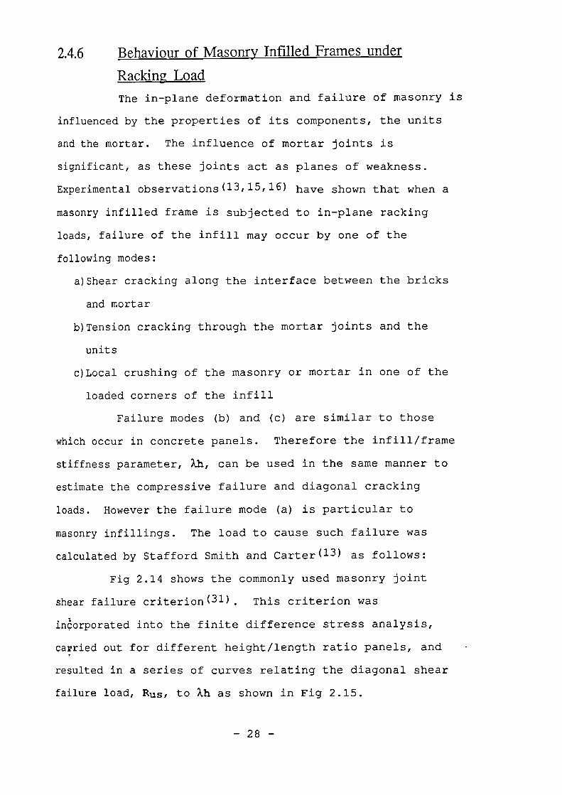
2.4.6 Behaviour of Masonry Infilled Frames under
Racking Load
The in-plane deformation and failure of masonry is
influenced by the properties of its components, the units
and the mortar. The influence of mortar joints is
significant, as these joints act as planes of weakness.
Experimental observations( 13 , 15 , 16 ) have shown that when a
masonry infilled frame is subjected to in-plane racking
loads, failure of the infill may occur by one of the
following modes:
a)Shear cracking along the interface between the bricks
and mortar
b)Tension cracking through the mortar joints and the
units
c)Local crushing of the masonry or mortar in one of the
loaded corners of the infill
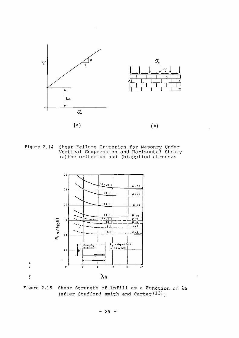
Failure modes (b) and (c) are similar to those
which occur in concrete panels. Therefore the infill/frame
stiffness parameter, Xh, can be used in the same manner to
estimate the compressive failure and diagonal cracking
loads. However the failure mode (a) is particular to
masonry infillings. The load to cause such failure was
calculated by Stafford Smith and Carter (13) as follows:
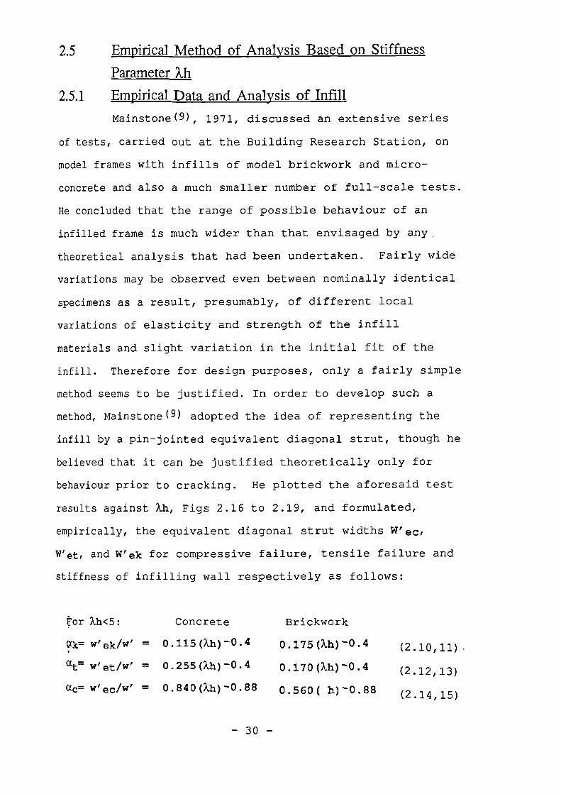
Fig 2.14 shows the commonly used masonry joint
shear failure criterion (31) This criterion was
inaorporated into the finite difference stress analysis,
carried out for different height/length ratio panels, and
resulted in a series of curves relating the diagonal shear
failure load, Rus, to Xh as shown in Fig 2.15.
- 28 -
cinLULLLJ1 I I
11111
7:rh..21.1p . 0 6
20:1 p 206
s.....'.."-----........P=06
„__ 1: A 2-TFIH1. I-, = 0....,,....__ 20i — =_--
11 = 0n ..... -..-. ....___. 1-5:1 11.0
........ ...... 1.0:1 -- A = 0
R Is diagonal force
1-17(
C3 Tied by inC11mmmotmom
1
30
25
20
OS
( a )
(b)
Figure 2.14 Shear Failure Criterion for Masonry UnderVertical Compression and Horizontal Shear;(a)the criterion and (b)applied stresses
0
4
8
12
16
:0
Xh
Figure 2.15 Shear Strength of Infill as a Function of(after Stafford smith and Carter(13))
- 29 -
2.5 Empirical Method of Analysis Based on Stiffness
Parameter Ah
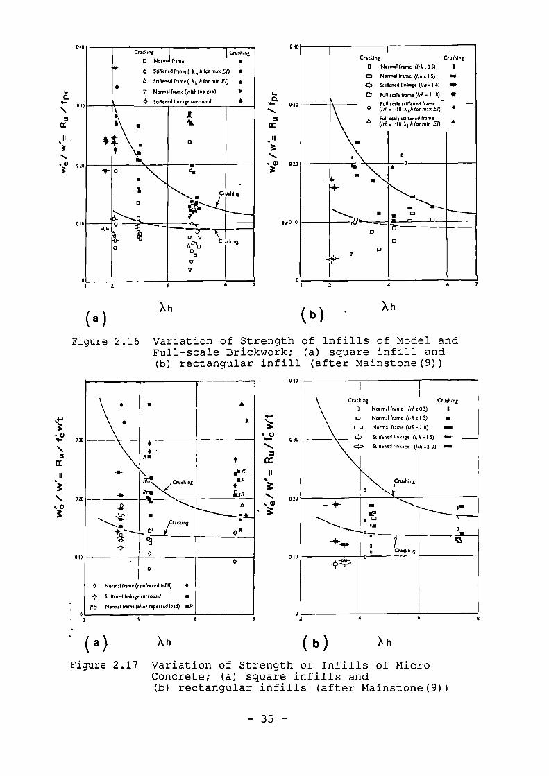
2.5.1 Empirical Data and Analysis of Infill
Mainstone( 9 ), 1971, discussed an extensive series
of tests, carried out at the Building Research Station, on
model frames with infills of model brickwork and micro-
concrete and also a much smaller number of full-scale tests.
He concluded that the range of possible behaviour of an
infilled frame is much wider than that envisaged by any.
theoretical analysis that had been undertaken. Fairly wide
variations may be observed even between nominally identical
specimens as a result, presumably, of different local
variations of elasticity and strength of the infill
materials and slight variation in the initial fit of the
infill. Therefore for design purposes, only a fairly simple
method seems to be justified. In order to develop such a
method, Mainstone( 9 ) adopted the idea of representing the
infill by a pin-jointed equivalent diagonal strut, though he
believed that it can be justified theoretically only for
behaviour prior to cracking. He plotted the aforesaid test
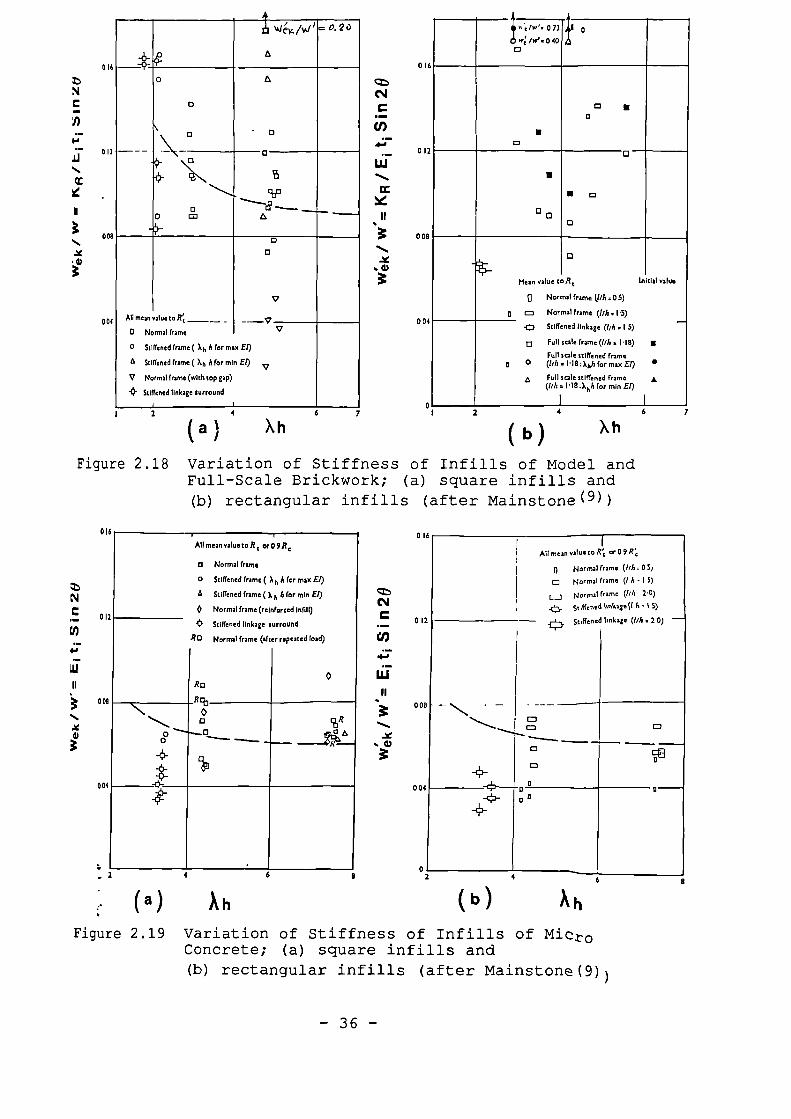
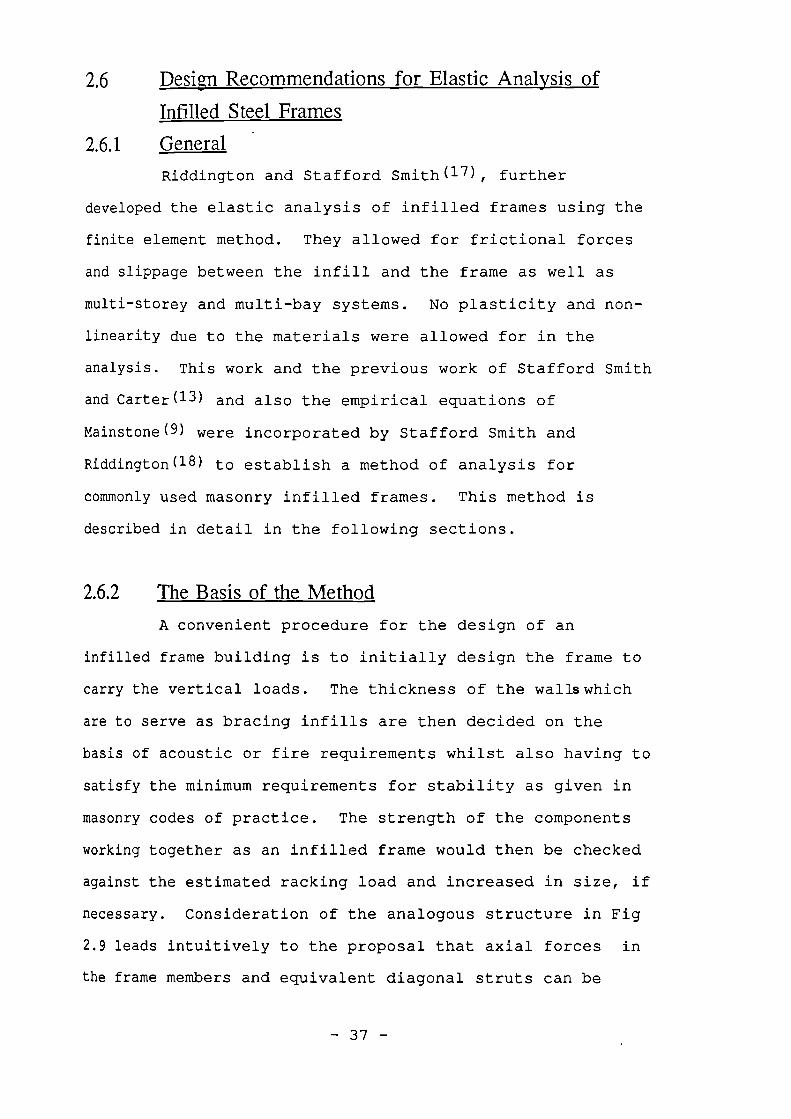
results against Xh, Figs 2.16 to 2.19, and formulated,
empirically, the equivalent diagonal strut widths Wec,
W et, and W'ek for compressive failure, tensile failure and
stiffness of infilling wall respectively as follows:
For Xh<5: Concrete Brickwork
ak= Wekhe 0.115(2./)-0.4 0.175(?11)-0.4 (2.10,11)
at= leethe 0.255(21)-0.4 0.170(Xh)-0.4 (2.12,13)
ac= 0.840(Xh)-0.88 0.560( h)-0.88 (2.14,15)
- 30 -
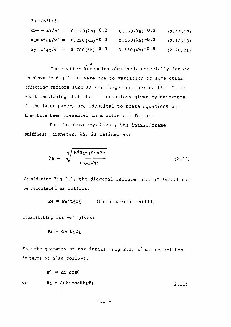
For 54k.h<8:
ak= se ek/w '
at= se et/w '
ac= w 'eche
= 0.110(Xh) -0 • 3 0.160(Xh)-0-3 (2.16,17)
= 0.220(Xh) -0 • 3 0.150(Xh)-0•3 (2.18,19)
= 0.780(Xh) -0.8 0.520(Xh)-0.8 (2.20,21)
theThe scatter in results obtained, especially for ak
as shown in Fig 2.19, were due to variation of some other
affecting factors such as shrinkage and lack of fit. It is
worth mentioning that the equations given by Mainstone
in the later paper, are identical to these equations but
they have been presented in a different format.
For the above equations, the infillfframe
stiffness parameter, Xh, is defined as:
4h4EitiSinnXh =
(2.22)
4EcIch'
Considering Fig 2.1, the diagonal failure load of infill can
be calculated as follows:
Ri = we'tifi (for concrete infill)
Substituting for we' gives:
Ri = aw'tifi
From the geometry of the infill, Fig 2.1, w'can be written
in terms of h'as follows:
w' = 2h'cose
or Ri = 2ah'cosOtifi (2.23)
- 31 -
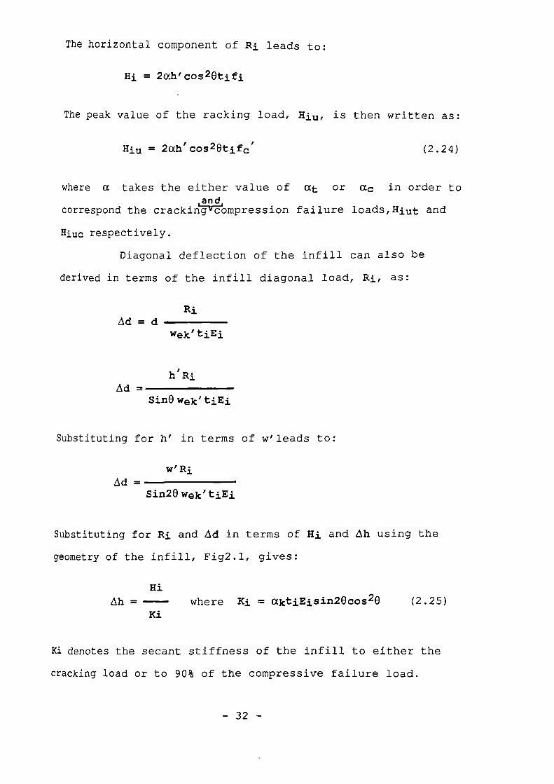
The horizontal component of Ri leads to:
Hi = 2ah'cos2Otifi
The peak value of the racking load, Hiu, is then written as:
Hiu = 2ah'cos 2 9tifc' (2.24)
where a takes the either value of at or 0:c in order to
correspond the crackin-T7E-ompression failure loads, Hiut and
Hiuc respectively.
Diagonal deflection of the infill can also be
derived in terms of the infill diagonal load, Ili, as:
RiAd = d
wek'tiEi
h'RiAd
Sin() wek' t±E±
Substituting for h f in terms of veleads to:
w'RiAd -
Sinn wek' tiEi
Substituting for Ri and Ad in terms of Hi and Ah using the
geometry of the infill, Fig2.1, gives:
HiAh = where Ki = akt1Eisin28cos 20 (2.25)
Ki
Ki denotes the secant stiffness of the infill to either the
cracking load or to 90% of the compressive failure load.
- 32 -
2.5.2 Analysis of Frame
Diagonal compression of the infill permits the
frame to deform diagonally and resists a portion of the
diagonal load, ie.
R = Ri + Rf
This relation for the horizontal loads is written as:
H = Hi + Hf
The stiffness of the composite structure becomes:
K = Ki + Kf where Kf = Hf/Ah
Mainstone(9) concluded that "provided that the
peripheral joints between the infill and the frame are well
filled, the composite elastic stiffness of the infilled
frame will usually be that of the infill." He thenthe
suggested to neglect the frame contribution in calculation •
of the cracking load and stiffness. For the collapse load,
however, he suggested either to neglect the frame
contribution or allow for the full plastic strength of the
frame while assuming no infill exists. In order to
establish a consistent approach for the later references in
this study, the author decided to account for the elastic
contribution of the frame assuming that no infill exists.
and the strength of the frame may not exceed the plastic
collapse load of the bare frame. This modification is
described below.
Using the elastic approach suggested by
- 33 -
Holmes( 11 ), Eq 2.1 to 2.4, the frame contribution to
diagonal load has been derived by the author as follows:
Hf = Ah/Ke (2.26)
where Kf, the frame stiffness is written as:
24EfIcKf-
h'3[1+(Ic/Ib)CotO]
Substituting for Ah from Eq 2.25 and replacing the
appropriate terms of stiffness by X.h in accord to Eq 2.22
the above relation can be arranged to give:
Hf = 4Hi (2.27)
where:6(h/h')
-ak (?.I) 4 [1+ (Iblic) cote] cos20
2.5.3 Comments
Fig 2.20 compares the Mainstone( 9 ) empirical
equations and the theoretical method of Stafford Smith and
Carter (13 ). As seen the two methods generally follow the
same trend. However for length/height ratios greater than
unity, the predictions of the two methods for compressive
failure of the infilled frame are quite different.
Later Stafford Smith and Riddington (18) modified
the theoretical method of Stafford Smith and Carter( 13 ) so
as, presumably, to make it closer to the experimental
results formulated by Mainstone (9 ). This is described in the
following section.
- 34 -
040
0.
0 30
CC
II .
0 10
0
••=,
• ID 0 20
if 0.10
0."—••=,
cc
040
030
Cracking
at=1
-C:3-
CI
Normal frame (Rh =OS)Normal frame ph • I S)
Stiffened linkage (1/h • 1 5)
Full scale frame (1/h • 118)
Full scale stiffened frame(Ph • 118 A bh for max El)
Full scale stiffened frame(lth • 118 :X h h for min El)
Crushingiishin
Am-
II
•
A
o„,*-*
—
0
0 1 2 4 6
•
0
010
0
0 Normal frame ( einforced in611) •
Stiffened linkage surround 4
RD Normal frame (after repeated load) • R
0
-040
• U'6.• 030•••••
•II
020• 137
0 10
b)
h
6
Cracking Crushing
0 Normal frame Ids .05)
0 Normal frame (1,h • 1 5)
l= Normal frame (Ws .2 0)
422- Stiffened linkage ((,h • I 5) 461-
.43 Stiffened linkage (Iii .2 0) mi.
Crushing
cI
Crackii
•
Cracking I i01101111
0 Normal frame ao Stiffened frame ( ) h h for max El) •
a Stiff:—.4 frame ( À h h for mln El) •
V Normal frame (with top gap) •
* Stiffened linkage surround 4
••
1AL
0
•
%
13
4
PCrushing
ra-v----4—DV
AC/300
0
V
V
\
Cr eking
7
(a) Xh
(b)
X h
Figure 2.16 Variation of Strength of Infills of Model andFull-scale Brickwork; (a) square infill and(b) rectangular infill (after Mainstone(9))
2
4
6
8
(a)
Xh
Figure 2.17 Variation of Strength of Infills of MicroConcrete; (a) square infills and(b) rectangular infills (after Mainstone(9))
- 35 -
*.c
II/ 41,A/ i
A
. 0.24)
o a
0
\ - 13
\\130
1::)- liNs41
•n,..„
0
93°......._15,
o 03 A
0
0
v
All mean value to lei V0 Normal frame V
0 Stiffened frame ( ) h h for max El)
0 Stiffened frame ( )i, is for min El) v
17 Normal frame (with top gap)
'4) Stiffened linkage surround
1 t
2 4 6
7
(a ) Xh
0i
n e/w'•
w:
0 73
/w' • 0 40
i 0
0 •0
coIII
0
U
o o
ot 0
o
o
Mean value to R , Initial value
0 Normal frame (1111.0 5)
0 o Normal frame (1111.1S)—
-143. Stiffened linkage (1/h .1 5)
1:1 Full scale frame (1/1,. NB) •
Full scale stiffened frame0 0 UM • 1 . 18 :khh for max El) •
Full scale stiffened frame •(lM= 1 . 18:y for mmn El)
1 I2
4
6
7
b ) Xh0
0 16
012
008
004
0 16
004
008 R
0 ''''.."•••••CI0
(10
004
R--
4
016
012
All mean value toR , or 0 9Rc
0 Normal frame
0 Stiffened frame ( h for max El)
a Stiffened frame ( h for min El)
0 Normal frame (reinforced 1n1111)
0 16
012
All mean value to r, or 09 rc
Normal frame (Rh s 0 5)
Norma l frame (l h - IS)
LJ Normal frame (fdi 2.0)
Stiffe ne d Isnkage CI Is - 5)
4l Stiffened linkage surround
RD Normal frame (after repeated load)
Stiffen ed linkage (lris . 2 0)
An (b)
004
6
8
Àh
008
Figure 2.18 Variation of Stiffness of Infills of Model andFull-Scale Brickwork; (a) square infills and(b) rectangular infills (after Mainstone(9))
Figure 2.19 Variation of Stiffness of Infills of microConcrete; (a) square infills and(b) rectangular infills (after Mainstone(9))
- 36 -
2.6 Design Recommendations for Elastic Analysis of
Infilled Steel Frames
2.6.1 General
Riddington and Stafford Smith( 17 ), further
developed the elastic analysis of infilled frames using the
finite element method. They allowed for frictional forces
and slippage between the infill and the frame as well as
multi-storey and multi-bay systems. No plasticity and non-
linearity due to the materials were allowed for in the
analysis. This work and the previous work of Stafford Smith
and Carter( 13 ) and also the empirical equations of
Mainstone( 9 ) were incorporated by Stafford Smith and
Riddington( 18 ) to establish a method of analysis for
commonly used masonry infilled frames. This method is
described in detail in the following sections.
2.6.2 The Basis of the Method
A convenient procedure for the design of an
infilled frame building is to initially design the frame to
carry the vertical loads. The thickness of the walls which
are to serve as bracing infills are then decided on the
basis of acoustic or fire requirements whilst also having to
satisfy the minimum requirements for stability as given in
masonry codes of practice. The strength of the components
working together as an infilled frame would then be checked
against the estimated racking load and increased in size, if
necessary. Consideration of the analogous structure in Fig
2.9 leads intuitively to the proposal that axial forces in
the frame members and equivalent diagonal struts can be
- 37 -
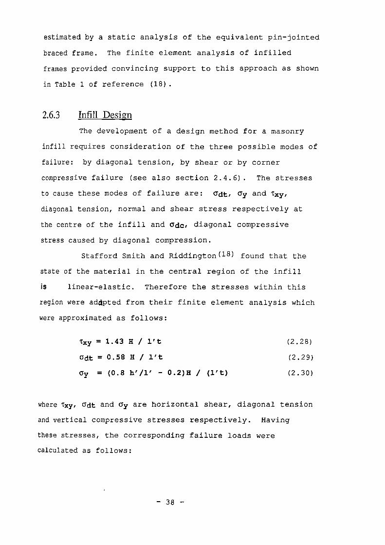
estimated by a static analysis of the equivalent pin-jointed
braced frame. The finite element analysis of infilled
frames provided convincing support to this approach as shown
in Table 1 of reference (18).
2.6.3 InfiII Design
The development of a design method for a masonry
infill requires consideration of the three possible modes of
failure: by diagonal tension, by shear or by corner
compressive failure (see also section 2.4.6). The stresses
to cause these modes of failure are: adt, ay and Txy,
diagonal tension, normal and shear stress respectively at
the centre of the infill and adc, diagonal compressive
stress caused by diagonal compression.
Stafford Smith and Riddington( 18 ) found that the
state of the material in the central region of the infill
is linear-elastic. Therefore the stresses within this
region were addpted from their finite element analysis which
were approximated as follows:
Txy = 1.43 H / l't (2.28)
adt = 0.58 H / l't (2.29)
ay = (0.8 h'/1' - 0.2)H / (1't) (2.30)
where Txy, adt and ay are horizontal shear, diagonal tension
and vertical compressive stresses respectively. Having
these stresses, the corresponding failure loads were
calculated as follows:
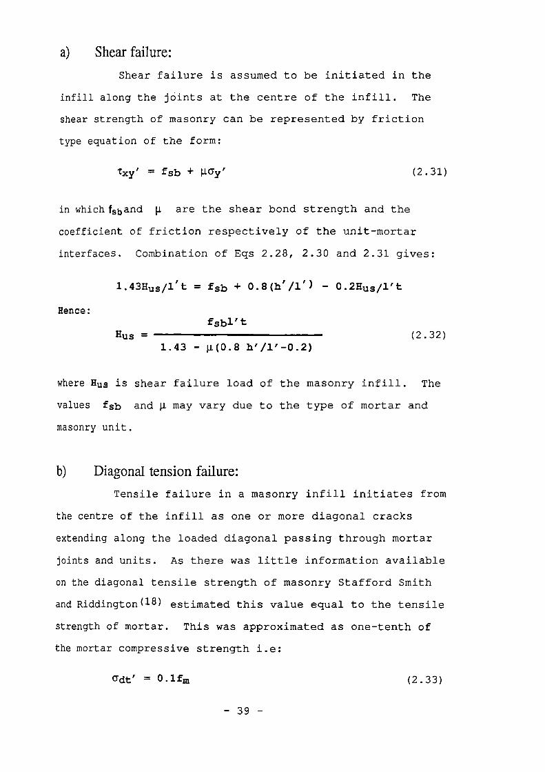
a) Shear failure:
Shear failure is assumed to be initiated in the
infill along the jOints at the centre of the infill. The
shear strength of masonry can be represented by friction
type equation of the form:
Txy' = fsb Ilay' (2.31)
in whichfs b and 11 are the shear bond strength and the
coefficient of friction respectively of the unit-mortar
interfaces. Combination of Eqs 2.28, 2.30 and 2.31 gives:
1.43Hus/l't = fsb + 0.8(h'/1') - 0.2Husil't
Hence:
fsbl'tHug - (2.32)
1.43 - h'/1'-0.2)
where Hug is shear failure load of the masonry infill. The
values fsb and may vary due to the type of mortar and
masonry unit.
b) Diagonal tension failure:
Tensile failure in a masonry infill initiates from
the centre of the infill as one or more diagonal cracks
extending along the loaded diagonal passing through mortar
joints and units. As there was little information available
on the diagonal tensile strength of masonry Stafford Smith
and Riddington (18) estimated this value equal to the tensile
strength of mortar. This was approximated as one-tenth of
the mortar compressive strength i.e:
adt' = 0.1fm
(2.33)
- 39 -
Combination of Eqs 2.33 and 2.29 results in:
Hut = 0.172 fm l't (2.34)
Eci 2.34 estimates the diagonal cracking load, Hut, for
masonry inf ill.
c) Compressive failure of the infal corners:
Stafford Smith and Riddington( 18 ) found that
unlike the stress within the central region of the infill,
the compressive stresses occurred in the loaded corners were
extremely sensitive to the 7h value which was simplified for
design purposes as follows:
Eitih' 3Xh=
(2.35)
4Ecic
It should be noted that, in the above equation the term
Sinn is omitted and the difference between h' and h is
ignored as compared to Eq 2.7.
Since compressive failure occurs, presumably, in a
plastic manner and the results obtained from the linear-
elastic finite element analysis (17) were not sufficiently
accurate, Stafford Smith and Riddington( 18 ) adopted the
empirical equation of Mainstone (9) , Eqs 2.15, to derive the
horizontal compressive collapse load, Huc, as follows:
w' and w'ec may be substituted in Eq 2.15 as:
w' = 2h'/Cos9
se ec = Ruc/fprt
to give:
- 40 -
- 41 -SHEFFIELD
UNIVERSITYLIBRARX
(Ruc/fprt)
0.56(Xh)-0.88(2h' Cos0 )
The horizontal compressive failure load, Huc, can be related
to Ruc as:
Huc = RucCose
Substituting for Ruc leads to:
Huc = 1.12 ah)-0.88h'tfprcos20
This equation for concrete becomes:
Huc = 1.68010 - 0.88h'tfc'cos2e
(2.36a)
(2.36b)
2.6.4 Design of Frame
a) Axial forces in frame members:
The axial forces due to vertical loads should be
calculated on the basis of the tributary areas. The axial
forces in the members due to horizontal loading can be
estimated by a simple static analysis of an equivalent frame
with the columns pin-jointed at each storey level, the beams
pin-jointed at their ends and the infills considered as
diagonal pin-jointed bracing struts.
b) Bending moments and shear forces in frame members:
Frame members must be also able to withstand
bending moments and shear forces induced as a result of
inexactness of the assumption of the infill acting as a pin-
jointed diagonal bracing. In reality the infill bears
against the beam and column members over part of their
lengths. The finite element analysis (17) showed that the
bending moment in the frame members are not likely to exceed
5% the total horizontal force, H, times the height of the
columns, h'. Therefore the columns must be able to resist a
bending moment of Hh'/20 and a shear force equal to H.
The beams must also be designed for bending
moments and shear forces in addition to the axial forces
calculated as above. If an upper beam of an infilled panel
is not restrained by an infill above, it should be designed
to withstand a mid-span hogging moment of Hh'/20 in
combination with the moment due to vertical dead loads. The
beam and its connections must be able to carry an upwards
shear force of Hh'/1' in combination with the shear force
due to vertical dead loads.
Where the beam below an infill is not restrained
by an infill below, the beam must be able to withstand a
mid-span sagging moment of Hh'/20 in addition to the moment
due to dead and live loads. The beam and its connections
must be able to carry a downwards shear force of Hh'/1' in
addition to the shear force due to dead and live loads.
c) Deflection of frame:
A crude but conservative, ie. excessive estimate
of horizontal deflection of infilled frame, can be made by
''treating the frame as pin-jointed and each infill as a
diagonal pin-jointed bracing strut with a cross-sectional
area equal to one-tenth of its diagonal length times its
thickness and an elastic modulus of 7x10³ Nimm2.
- 42 -
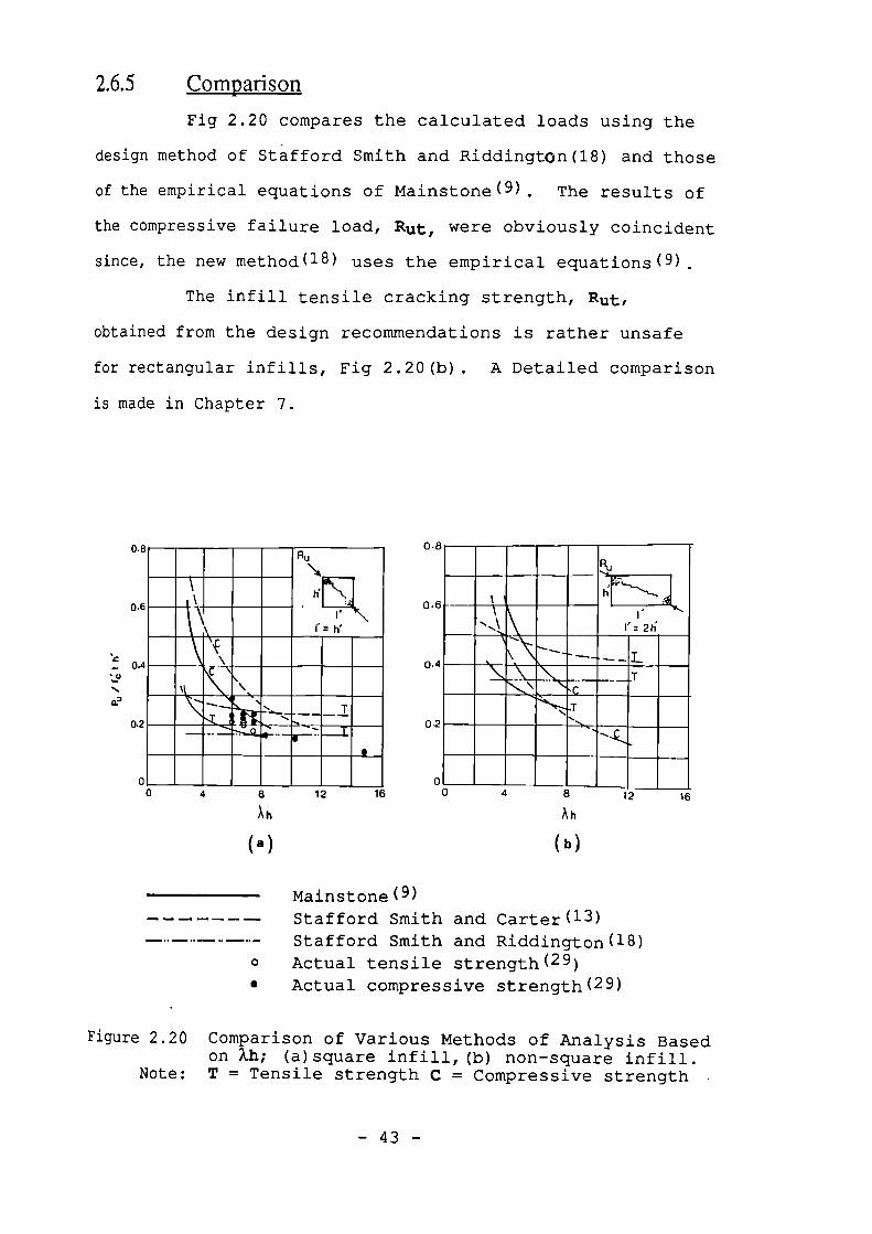
RU
\
1
A%
% r=wr
\
- T
____c_
I211
Mil-
E
0.6
0.8
0.4
02
0.8
0.6
0.4
0.2
2.6.5 Comparison
Fig 2.20 compares the calculated loads using the
design method of St -afford Smith and Riddington(18) and those
of the empirical equations of Mainstone( 9 ). The results of
the compressive failure load, Rut, were obviously coincident
since, the new method( 18 ) uses the empirical equations(9).
The infill tensile cracking strength, Rut,
obtained from the design recommendations is rather unsafe
for rectangular infills, Fig 2.20(b). A Detailed comparison
is made in Chapter 7.
4
8
12 16
12
An
An
(a)
(b)
Mainstone(9)n•n•n n111 Stafford Smith and Carter(13)
Stafford Smith and Riddington(18)o Actual tensile strength(29)• Actual compressive strength(29)
Figure 2.20 Comparison of Various Methods of Analysis Basedon Xla; (a)square infill,(b) non-square infill.
Note: T = Tensile strength C = Compressive strength -
— 43 —
2:7 Theories Based on Frame/Infill Strength Parameter
2.7.1 General -
The theoretical investigations on the behaviour of
infilled frames, up to 1978, were based generally on
elasticity theories. However as discussed in Section
2.6.3(c) these theories fail to establish a rational
criteria for compressive failure of the infill. Because
such failure occurs gradually and is associated with
distinct modes of distortion of the frame, it indicates the
existence of particular mechanisms by which plastic like
collapse occurs. This was well understood by Wood( 20 ) who
published his paper titled "Plasticity; Composite Action and
Collapse Design of Reinforced Shear Wall Panels in Frames"
and opened a new chapter in the analysis and understanding
of the behaviour of infilled frames. He identified four
possible modes of collapse as illustrated in Fig 2.21 and
developed a rational plastic analysis based on a
frame/infill strength parameter utilizing Nielsen( 21 ) square
yield criterion within yielding zones.
Later, in 1981, an alternative treatment of the
plastic analysis was given by May (22). He used the same
principles as Wood except he used the yield line method of
analysis in plasticity theories. The results were identical
to those of Wood. This method was also capable of
predicting the collapse loads and modes of infills with
openings.
2.7.2 Wood Classification for Collapse of Infilled Frame
Wood( 20 ) studied a large number of tests carried
out at the Building Research Establishment by various
investigators. The majority of the tests involved masonry
panels. Four distinct types of plastic collapse modes were
identified as follows:
a) Shear mode "S"
Fig 2.21(a) shows the collapse mode of
a very strong frame and a weak wall where plastic hinges
formed at the joints of the frame. The beams and the
columns remained straight producing a pure shear strain in
the wall. This referred to as the shear mode "S".
b) Shear rotation mode "SIC'
Fig 2.21(b) shows the collapse mode of a
relatively stronger wall where a plastic hinge appeared in
each beam at the intersection of the discontinuity lines
which clearly separate apparently unstrained rigid corner
regions (top left and bottom right) from a central shear
region where massive distortion has taken place. The
umstrained corners merely undergo a rigid body rotation, and
therefore, this mode is called the shear rotation mode "SR".
c) Diagonal compression mode "DC"
The stronger is the wall relative to the frame,
the. greater is the distance between the unstrained corner
and the plastic hinge in the beam. With a very strong wall,
or weak frame, the hinge appears nearer the opposite corner
- 45 -
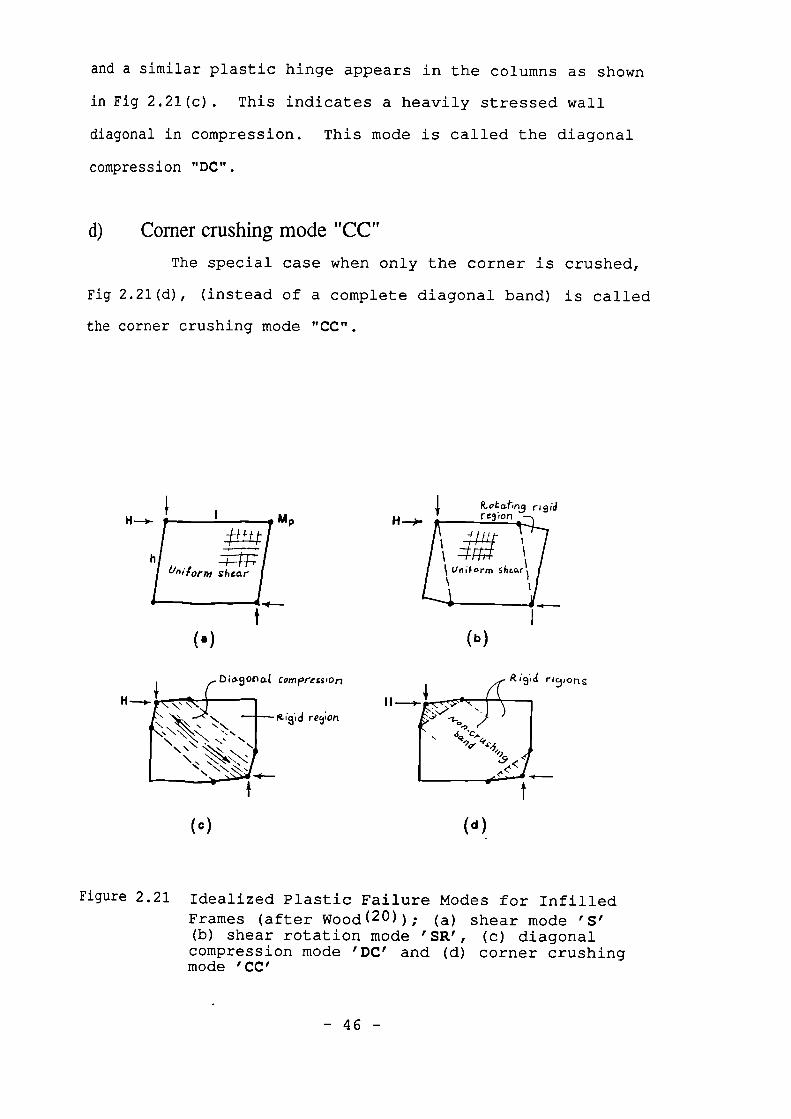
( a )
(b)
Diagonal compression CU91cl rly,ons
uI-
d reyion
(c)
(d)
and a similar plastic hinge appears in the columns as shown
in Fig 2.21(c). This indicates a heavily stressed wall
diagonal in compression. This mode is called the diagonal
compression "DC".
d) Corner crushing mode "02"The special case when only the corner is crushed,
Fig 2.21(d), (instead of a complete diagonal band) is called
the corner crushing mode "CC".
H Mp
lini torm shear,
-f-f'tti
Figure 2.21 Idealized Plastic Failure Modes for InfilledFrames (after Wood (20 )); (a) shear mode 'S'(b) shear rotation mode 'SR', (c) diagonalcompression mode 'DC' and (d) corner crushingmode 'CC'
- 46 -
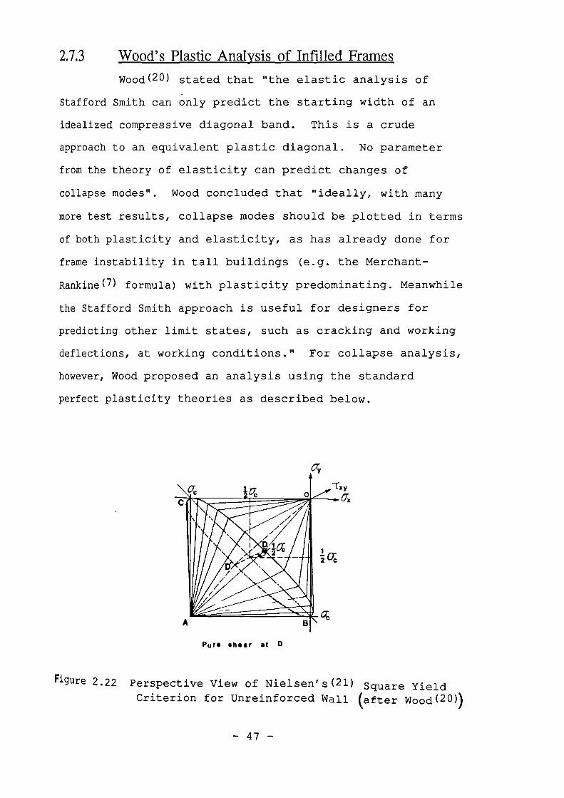
2.7.3 Wood's Plastic Analysis of Infdled Frames
Wood( 20 ) stated that "the elastic analysis of
Stafford Smith can only predict the starting width of an
idealized compressive diagonal band. This is a crude
approach to an equivalent plastic diagonal. No parameter
from the theory of elasticity can predict changes of
collapse modes". Wood concluded that "ideally, with many
more test results, collapse modes should be plotted in terms
of both plasticity and elasticity, as has already done for
frame instability in tall buildings (e.g. the Merchant-
Rankine (7) formula) with plasticity predominating. Meanwhile
the Stafford Smith approach is useful for designers for
predicting other limit states, such as cracking and working
deflections, at working conditions." For collapse analysis,
however, Wood proposed an analysis using the standard
perfect plasticity theories as described below.
Pur• shear at D
Figure 2.22 Perspective View of Nielsen's(21) Square YieldCriterion for Unreinforced Wall (after Wood(20))
- 47 -
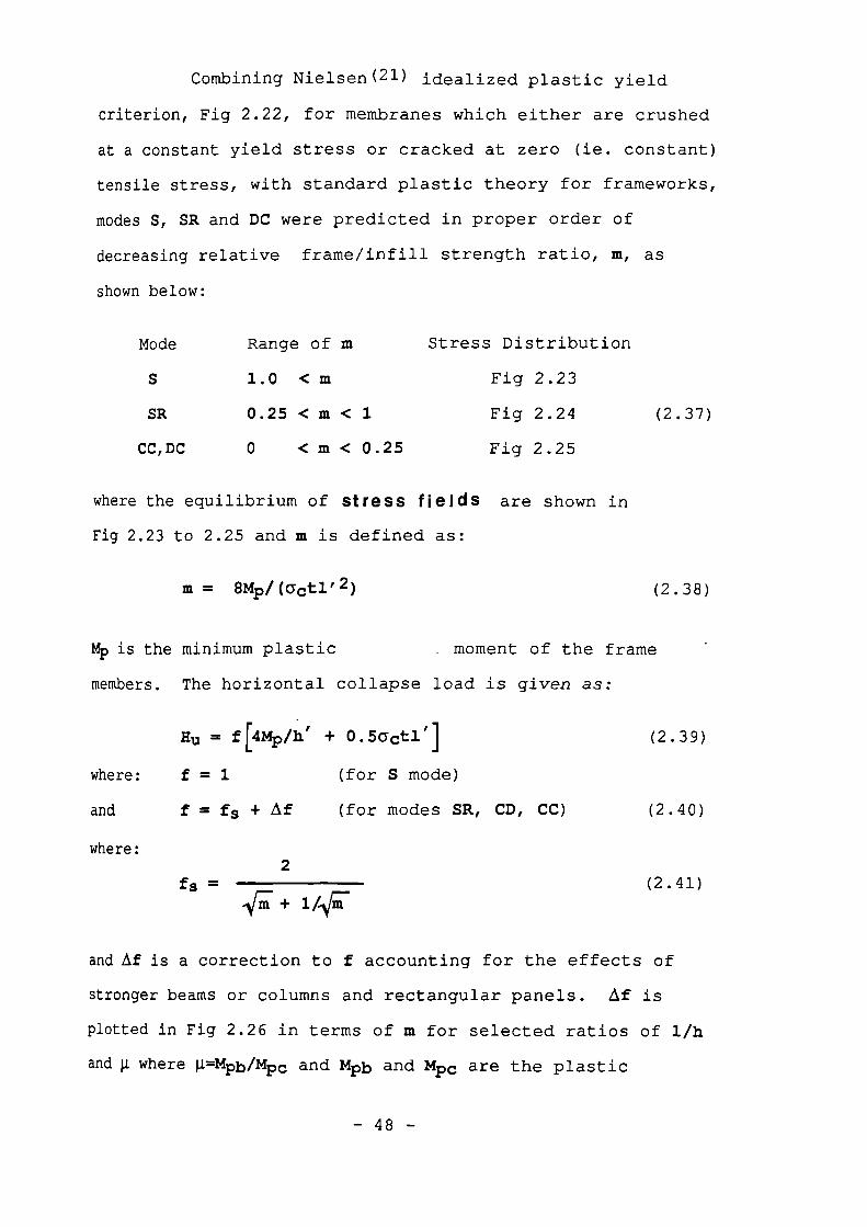
Combining Nielsen( 21 ) idealized plastic yield
criterion, Fig 2.22, for membranes which either are crushed
at a constant yield stress or cracked at zero (ie. constant)
tensile stress, with standard plastic theory for frameworks,
modes S, SR and DC were predicted in proper order of
decreasing relative frame/infill strength ratio, m, as
SIHNM below:
Mode
Range of m
Stress Distribution
1.0 < m
Fig 2.23
SR
0.25 < m < 1
Fig 2.24
(2.37)
CC, DC
0 < m < 0.25
Fig 2.25
where the equilibrium of stress fields are shown in
Fig 2.23 to 2.25 and m is defined as:
In = 8Mp/(actl' 2 ) (2.38)
Hp is the minimum plastic moment of the frame
members. The horizontal collapse load is given as:
Hu = f[4Mp/h' + 0.5actll (2.39)
where: f = 1 (for S mode)
and f = fs + if (for modes SR, CD, CC) (2.40)
where:2
fs —1/7a + 1 /IR;
(2.41)
and Af is a correction to f accounting for the effects of
stronger beams or columns and rectangular panels. Af is
plotted in Fig 2.26 in terms of m for selected ratios of 1/h
and g where g=mpb/mpc and Mpb and Mpc are the plastic
- 48 -
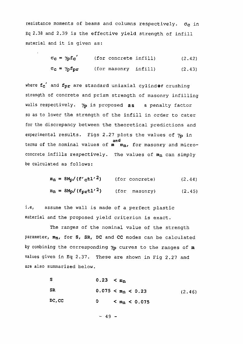
resistance moments of beams and columns respectively. ac in
Eq 2.38 and 2.39 is the effective yield strength of infill
material and it is given as:
ac = Ypfc'
(for concrete infill) (2.42)
G C = Ypfpr
(for masonry infill) (2.43)
where fc' and fpr are standard uniaxial cylinder crushing
strength of concrete and prism strength of masonry infilling
walls respectively. lip is proposed as a penalty factorso as to lower the strength of the infill in order to cater
for the discrepancy between the theoretical predictions and
experimental results. Figs 2.27 plots the values of yp inand
terms of the nominal values of m mn, for masonry and micro-
concrete infills respectively. The values of mn can simply
be calculated as follows:
ran = 8Mp/(f'ctl'2)
(for concrete)
(2.44)
Mn = 8mp/(fprt1'2)
(for masonry)
(2.45)
i.e, assume the wall is made of a perfect plastic
material and the proposed yield criterion is exact.
The ranges of the nominal value of the strength
parameter, mn, for S, SR, DC and CC modes can be calculated
by combining the corresponding yp curves to the ranges of m
values given in Eq 2.37. These are shown in Fig 2.27 and
are also summarized below.
0.23 <
SR 0.075 < mn < 0.23 (2.46)
DC,CC 0 < ran < 0.075
- 49 -
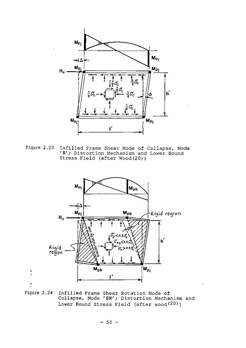
Hu
19re9ion
Hun(---•
iof pfrc
24-+410-2 C
loeJr 4 4 c4,
-IP"' -0- -42
31.-
MPi
Figure 2.23 Infilled Frame Shear Mode of Collapse, Mode'S'; Distortion Mechanism and Lower BoundStress Field (after Wood(20))
•011(n..
(1)
Figure 2.24 Infilled Frame Shear Rotation Mode ofCollapse, Mode 'SR'; Distortion Mechanism andLower Bound Stress Field (after wood(20))
- 50 -
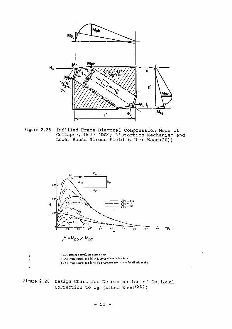
Hu
Mpb
Mpc
1/h -— — 1/ h -
1/h 113
03 Cl- 0-5 06 07 0-8 0-9 1-0in
Figure 2.25 Infilled Frame Diagonal Compression Mode ofCollapse, Mode 'DC'; Distortion Mechanism andLower Bound Stress Field (after Wood(20))
=Mpb Mpc
I (strong beams), use chart direct
If p.< I (weak beams) and 1,/,h= I, use is values in brackets
If p< I (weak beams) and 1/,,K= 1 .5 or 10, use is. w I curve for all values of is
Figure 2.26 Design Chart for Determination of OptionalCorrection to fs (after Wood(20))
- 51 -
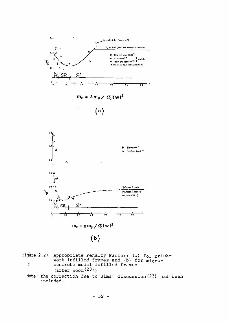
0 6
yp
• mah..mne 5
A Stafford Smith 10
A
Enforced S mode
(lainmnes models
men reWu )
nln= 8n1p/Crc' tw 12
(b)
(a)
Sperm! clinker block wall
V, 0 . 45 (limit for enforced S mode)
O ORE full-scale tests"
• Main:tones I models+ Kuhr and Hendry II'3 Means of identical specimens
s.
I I '4 00 6 08 1.0 1.2
0
in n = 8rnp/ gctWi2
Figure 2.27 Appropriate Penalty Factor; (a) for brick-work infilled frames and (b) for micro-concrete model infilled frames(after Wood(20))
Note: the correction due to Sims' discussion(23) has beenincluded.
- 52 -
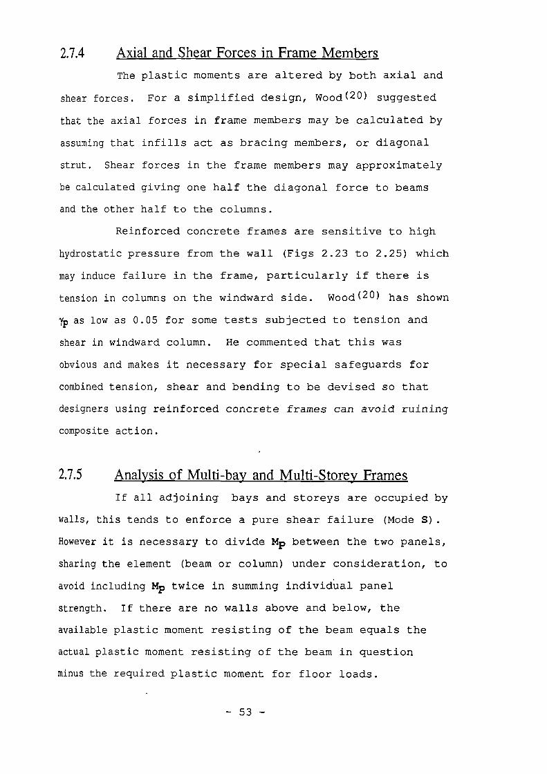
2.7.4 Axial and Shear Forces in Frame Members
The plastic moments are altered by both axial and
shear forces. For a simplified design, Wood( 20 ) suggested
that the axial forces in frame members may be calculated by
assuming that infills act as bracing members, or diagonal
strut. Shear forces in the frame members may approximately
be calculated giving one half the diagonal force to beams
and the other half to the columns.
Reinforced concrete frames are sensitive to high
hydrostatic pressure from the wall (Figs 2.23 to 2.25) which
may induce failure in the frame, particularly if there is
tension in columns on the windward side. Wood (20) has shown
as low as 0.05 for some tests subjected to tension and
shear in windward column. He commented that this was
obvious and makes it necessary for special safeguards for
=Joined tension, shear and bending to be devised so that
designers using reinforced concrete frames can avoid ruining
composite action.
2.7.5 Analysis of Multi-bay and Multi-Storey Frames
If all adjoining bays and storeys are occupied by
walls, this tends to enforce a pure shear failure (Mode S).
However it is necessary to divide Mp between the two panels,
sharing the element (beam or column) under consideration, to
mid including Mp twice in summing individual panel
strength. If there are no walls above and below, the
available plastic moment resisting of the beam equals the
actual plastic moment resisting of the beam in question
minus the required plastic moment for floor loads.
- 53 -
The columns completely free of wall panels are to
be designed by any acceptable no-sway design method. Columns
involved in shear panel design, must be relatively free of
buckling effects. It is suggested( 20 ) that P/PEuler should
not exceed 0.5 with rigid joints or 0.25 with pinned joints.
2.7.6 Discussion of Wood Method
Wood's plastic method was discussed by Mainstone,
Stafford Smith and Sims (23 ). A summary of the major points
of this discussion is given below.
Mainstone referred to the enforced shear mode
tests (with weak frame joints) carried out in British
Research Station. In these tests, infill strain was far
from uniform, both when the panel reached its peak strength
and subsequently. Therefore he suggested that the shear
mode S to be regarded as an ideal limit rather than as a
real material mode.
Sims felt that the role of yp is more complex than
just being a penalty for the use of idealized plasticity
theory for a material showing limited plasticity. In
deriving it from test results, it must also contain effects
from other parameters not considered in the basic theory,
e.g. the effect of elastic deformations and the use of an
idealized yield criterion.
Admitting the Sims' view (23 ), Wood himself stated
th;tt "The next important advance must come from finite
element or similar analysis allowing for elastoplasticity of-
infilling wall with restricted plastic strain. Outstanding
research now lies in determining an extra theory to deal
- 54 -
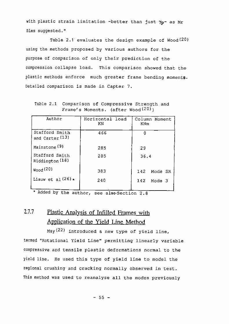
with plastic strain limitation -better than just yp- as Mr
Sims suggested."
Table 2.1evaluates the design example of Wood(20)
using the methods proposed by various authors for the
purpose of comparison of only their prediction of the
compression collapse load. This comparison showed that the
plastic methods enforce much greater frame bending moments.
Detailed comparison is made in Capter 7.
Table 2.1 Comparison of Compressive Strength andFrame's Moments. (after Wood(20))
Author Horizontal loadKN
Column MomentKNm
Stafford Smithand Carter(13)
466 0
Mainstone (9 ) 285 29
Stafford Smith 285 36.4Riddington(18)
Wood (2 ° ) 383 142 Mode SR
Liauw et al(28)* 240 142 Mode 3
. _.. . _
e by the author, see also .Section 2.8
2.7.7 Plastic Analysis of Infilled Frames with
Application of the Yield Line Method
May( 22 ) introduced a new type of yield line,
termed "Rotational Yield Line" permitting linearly variable
compressive and tensile plastic deformations normal to the
yield line. He used this type of yield line to model the
regional crushing and cracking normally observed in test.
This method was used to reanalyse all the modes previously
- 55 -
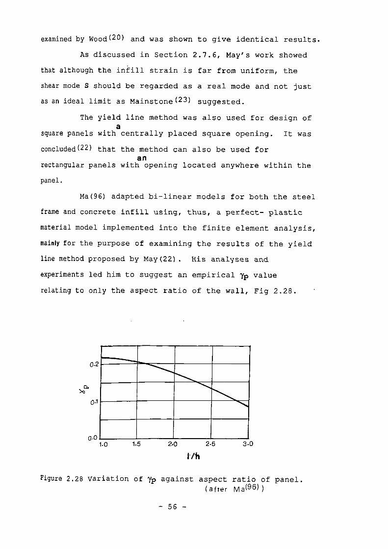
0.2
0.1
0.0
1.0 15 ZO 25 3.0
examined by Wood( 20 ) and was shown to give identical results.
As discussed in Section 2.7.6, May's work showed
that although the infill strain is far from uniform, the
shear mode S should be regarded as a real mode and not just
as an ideal limit as Mainstone (23) suggested.
The yield line method was also used for design ofa
spare panels with centrally placed square opening. It was
concluded( 22 ) that the method can also be used foran
rectangular panels with opening located anywhere within the
Ma(96) adapted bi-linear models for both the steel
frame and concrete infill using, thus, a perfect- plastic
material model implemented into the finite element analysis,
mainly for the purpose of examining the results of the yield
line method proposed by May(22). His analyses and
experiments led him to suggest an empirical yp value
relating to only the aspect ratio of the wall, Fig 2.28.
Figure 2.28 Variation of yp against aspect ratio of panel.(after Ma (96) )
— 56 —
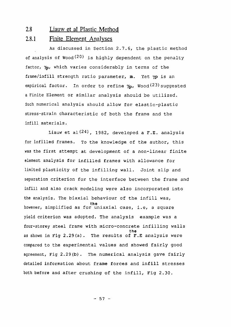
2.8 LiatIvy et al Plastic Method
2.8.1 Finite Element Analyses
As discussed in Section 2.7.6, the plastic method
of analysis of Wood( 20) is highly dependent on the penalty
factor, yp, which varies considerably in terms of the
frame/infill strength ratio parameter, m. Yet yp is an
empirical factor. In order to refine 7 ,p, Wood(23)suggested
a Finite Element or similar analysis should be utilized.
Such numerical analysis should allow for elastic-plastic
stress-strain characteristic of both the frame and the
infill materials.
Liauw et al(24), 1982, developed a F.E. analysis
for infilled frames. To the knowledge of the author, this
was the first attempt at development of a non-linear finite
element analysis for infilled frames with allowance for
limited plasticity of the infilling wall. Joint slip and
separation criterion for the interface between the frame and
infill and also crack modeling were
the analysis. The biaxial behaviourthe
however, simplified as for uniaxial
also incorporated into
of the infill was,
case, i.e, a square
yield criterion was adopted. The analysis example was a
four-storey steel frame with micro-concrete infilling wallsthe
as shown in Fig 2.29(a). The results of F.E analysis were
=pared to the experimental values and showed fairly good
agreement, Fig 2.29(b). The numerical analysis gave fairly
detailed information about frame forces and infill stresses
both before and after crushing of the infill, Fig 2.30.
- 57 -
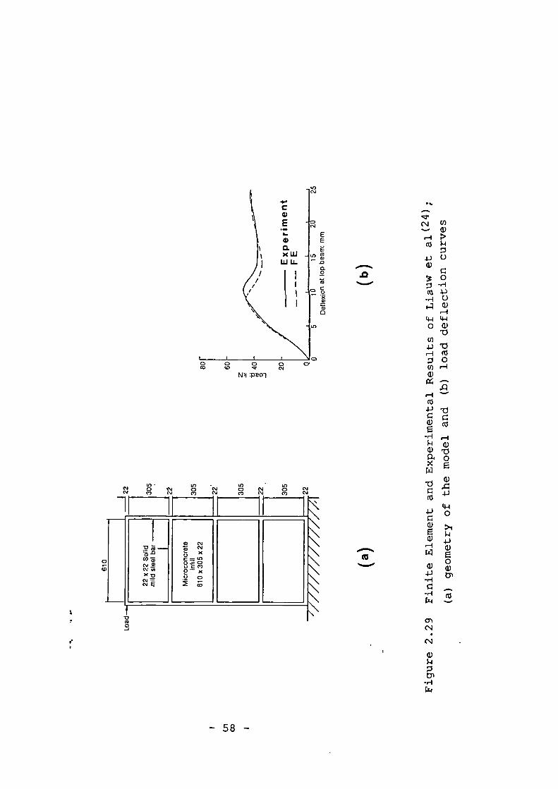
LLI
LLI
I
CV
ni
.0
0.
Cu
4:1
(\1
(0
4-)a)
(/)G)
o"H
- 5 8 -
-.° ;171
CI) TDc.)as, a)
gl t-
I
-•••••••
0
CD N
a) "xc = Loo - oa . ) "E cl2 ' x
0
G
0
CD
•nnn.,
CO
• - LOCV 0
▪ CV
•
CV c csJ CO
.ar
:peoi
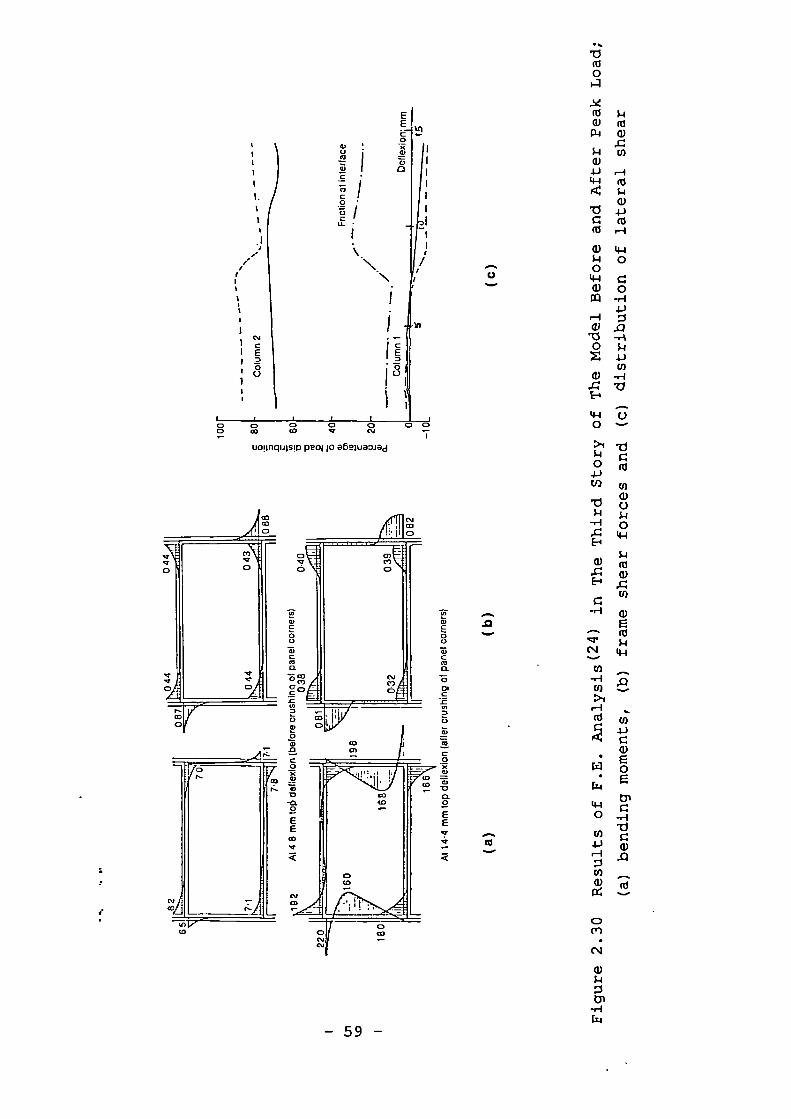
uo!inquisp o afieluaalad
cC
CO
- 59 -
•n••.
••nn•
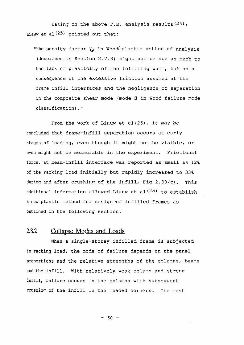
Basing on the above F.E. analysis results(24),
Liaum et al( 25 ) pointed out that:
"the penalty factor 113 in Woo&plastic method of analysis
(described in Section 2.7.3) might not be due as much to
the lack of plasticity of the infilling wall, but as a
consequence of the excessive friction assumed at the
frame infill interfaces and the negligence of separation
in the composite shear mode (mode S in Wood failure mode
classification)."
From the work of Liauw et al(25), it may be
concluded that frame-infill separation occurs at early
stages of loading, even though it might not be visible, or
even might not be measurable in the experiment. Frictional
force, at beam-infill interface was reported as small as 12%
of the racking load initially but rapidly increased to 33%
during and after crushing of the infill, Fig 2.30(c). This
additional information allowed Liauw et al (25 ) to establish
anew plastic method for design of infilled frames as
outlined in the following section.
2.8.2 Collapse Modes and Loads
When a single-storey infilled frame is subjected
to racking load, the mode of failure depends on the panel
proportions and the relative strengths of the columns, beams
and the infill. With relatively weak column and strong
failure occurs in the columns with subsequent
crushing of the infill in the loaded corners. The most
- 60 -
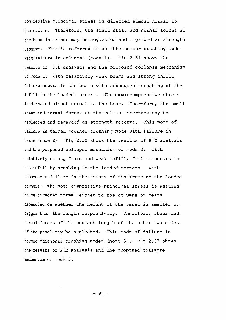
compressive principal stress is directed almost normal to
the column. Therefore, the small shear and normal forces at
the beam interface may be neglected and regarded as strength
reserve. This is referred to as "the corner crushing mode
with failure in columns" (mode 1). Fig 2.31 shows the
results of F.E analysis and the proposed collapse mechanism
of mode 1. With relatively weak beams and strong infill,
failure occurs in the beams with subsequent crushing of the
infill in the loaded corners. The targestcompressive stress
is directed almost normal to the beam. Therefore, the small
shear and normal forces at the column interface may be
neglected and regarded as strength reserve. This mode of
failure is termed "corner crushing mode with failure in
beams"(mode 2). Fig 2.32 shows the results of F.E analysis
and the proposed collapse mechanism of mode 2. With
relatively strong frame and weak infill, failure occurs in
the infill by crushing in the loaded corners with
subsequent failure in the joints of the frame at the loaded
corners. The most compressive principal stress is assumed
to be directed normal either to the columns or beams
depending on whether the height of the panel is smaller or
bigger than its length respectively. Therefore, shear and
normal forces of the contact length of the other two sides
of the panel may be neglected. This mode of failure is
termed "diagonal crushing mode" (mode 3). Fig 2.33 shows
the results of F.E analysis and the proposed collapse
mechanism of mode 3.
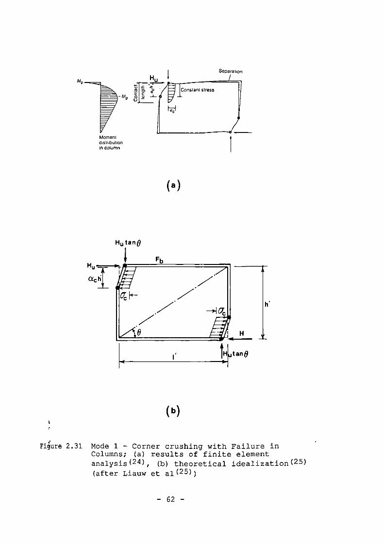
- MP
H u A
acti
H .Z-Hoc
Ae
Momentdistributionin column
(a)
Hutan0
Hiu tanO
7
Figlire 2.31 Mode 1 - Corner crushing with Failure inColumns; (a) results of finite elementanalysis (24) , (b) theoretical idealization(25)(after Liauw et al(25))
- 62 -
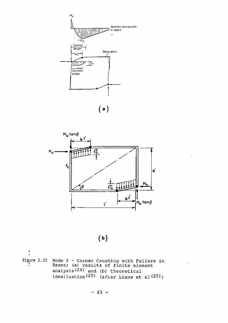
Mr)
-PIP
Contact
length 1
a bh —I Separation
(a)
H u tan°
b'' 0-
(b)
Moment distributionin beam
cr.
A
Hu-4.0--
H tane
qT
Hu
ti
;,
Figure 2.32 Mode 2 - Corner Crushing with Failure in• Beams; (a) results of finite element
analysis( 24 ) and (b) theoreticalidealization (25 ) (after Liauw et al(25))
- 63 -
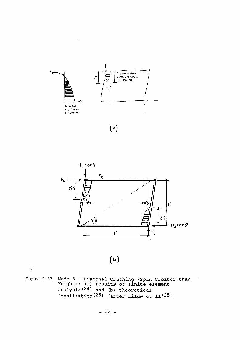
1
Momentdistributionin column
MP
(a)
Approxrrnatelyparabolic stressdistribution
Ft'
Hutan0
Hu
Wo
(b):
Figure 2.33 Mode 3 - Diagonal Crushing (Span Greater thanHeight); (a) results of finite elementanalysis( 24 ) and (b) theoreticalidealization (25) (after Liauw et al(25))
- 64 -
Examination of upper and lower bound solutions
(carried out by Liauw et al ( 25 / 33 ) ) and minimization of the
horizontal collapse racking load,Hu, led to the following
relations:
Hu = macth'
m is the minimum of the following values:
1/2For mode 1: ml = mic = [2 (Mpj+Mpc) / (acth i 2 )] (2.48)
2 1/2For mode 2: m2 = mib/tane = [2 (Mpj+Mpb) / (tanOacth' 2 )] (2.49)
For mode 3: m3 = mi 2+k/6 = 4Mpj/ (acth' 2 ) +k/6 (2.50)
where k is given as:
For h 1 /1 1 <l: k = (2/3)0 - (1/2)02
(2.51)
For h 1 /1 1 >1: k = [(2/3)13 - (1/2)131Cot20
(2.52)
13 may be taken as 1/3 so as to match with the experimental
results. The indexed m values are frame/infill strength
parameters. The indices denote the part of the frame under
consideration; b for beam, c for column and j for joint. ac
is the compressive strength of the infill. Liauw et al (25)
did not specify whether fc' or fcu was meant by ac, but it
may reasonably be taken as fc' for concrete and fpr for
masonry.
2.83 Comparison With apminmaud Results
The experimental results of Barua and
Mallick (26) , Mallick and Severn (27) , Mainstone (9) and Kadir
and Hendry (28) were p art ly compared with the proposed method in
- 65 -
Fig 2.34 showing a fairly good agreement. Examination of
the values of 0 ranging between 1/4 to 1/2 showed( 25 ) that
equal to 1/3 gives reasonably accurate and also on the
safe side results. Table 2.2 compares this method with all
the other available methods for predicting the collapse load
and column plastic moment of a masonry infilled frame.
2.8.4 Using the Limy et al Plastic Method for Analysis
of Single-Bay Multi-Storey Intllled Frames
The collapse modes of multi-storey infilled frames
are basically the same as those of single-storey. However
many different combinations are possible; some typical
collapse modes are shown in Fig 2.35.
Idauw et al( 25 ) proposed that the design of such structures
should be carried out storey by storey based on simple
design rules. They developed the standard energy approach
and derived the m values for the top storey as:
ml = mjc
m2 = mjbitan0
m3 = mj2+(1/6)k
and for other storeys as:
ml = mc
m2 = mbitanO
m3 = mi2+(1/6)k
where:
mc = 4Mpc/(acth'2)
mb = 414pb/(acth'2)
(2.53)
(2.54)
(2.55)
- 66 -
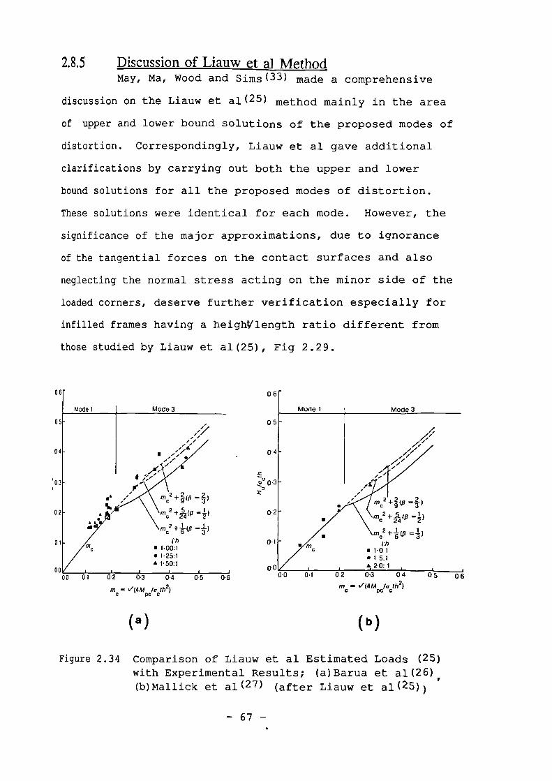
01
00
Mode 1 Mode 3
06
05
0.4
C 9 w 3 'm 2 +.5.1,R =1}
C 24 72 1
m c
• 1 . 0 1• 1 5.1• 2 . 0: 1
0 . 1 02 0.3 04 05
mc V(4M /cr th2)
pC C
(b)
Z'
0-2
0-1
000-0 0600 0 . 1 0.2 0.3 4 0 0.6
mc = VO aM l th2)
PC C
(a)
+2-(11 =2-19 3m 2 + 15_ 0 =1,
c 24 2'2 1
MC +—OP -fith
• 1.00:1• 1.25:1• F50:1
2.8.5 Discussion of Liauw et al MethodMay, Ma, Wood and Sims( 33 ) made a comprehensive
discussion on the Liauw et al (25 ) method mainly in the area
of upper and lower bound solutions of the proposed modes of
distortion. Correspondingly, Liauw et al gave additional
clarifications by carrying out both the upper and lower
bound solutions for all the proposed modes of distortion.
These solutions were identical for each mode. However, the
significance of the major approximations, due to ignorance
of the tangential forces on the contact surfaces and also
neglecting the normal stress acting on the minor side of the
loaded corners, deserve further verification especially for
infilled frames having a heighVlength ratio different from
those studied by Liauw et al (25), Fig 2.29.
06
Model Mode 3
05
04
'o
02
Figure 2.34 Comparison of Liauw et al Estimated Loads (25)with Experimental Results; (a)Barua et al(26),(b)Mallick et al (27) (after Liauw et al(25))
— 67 —
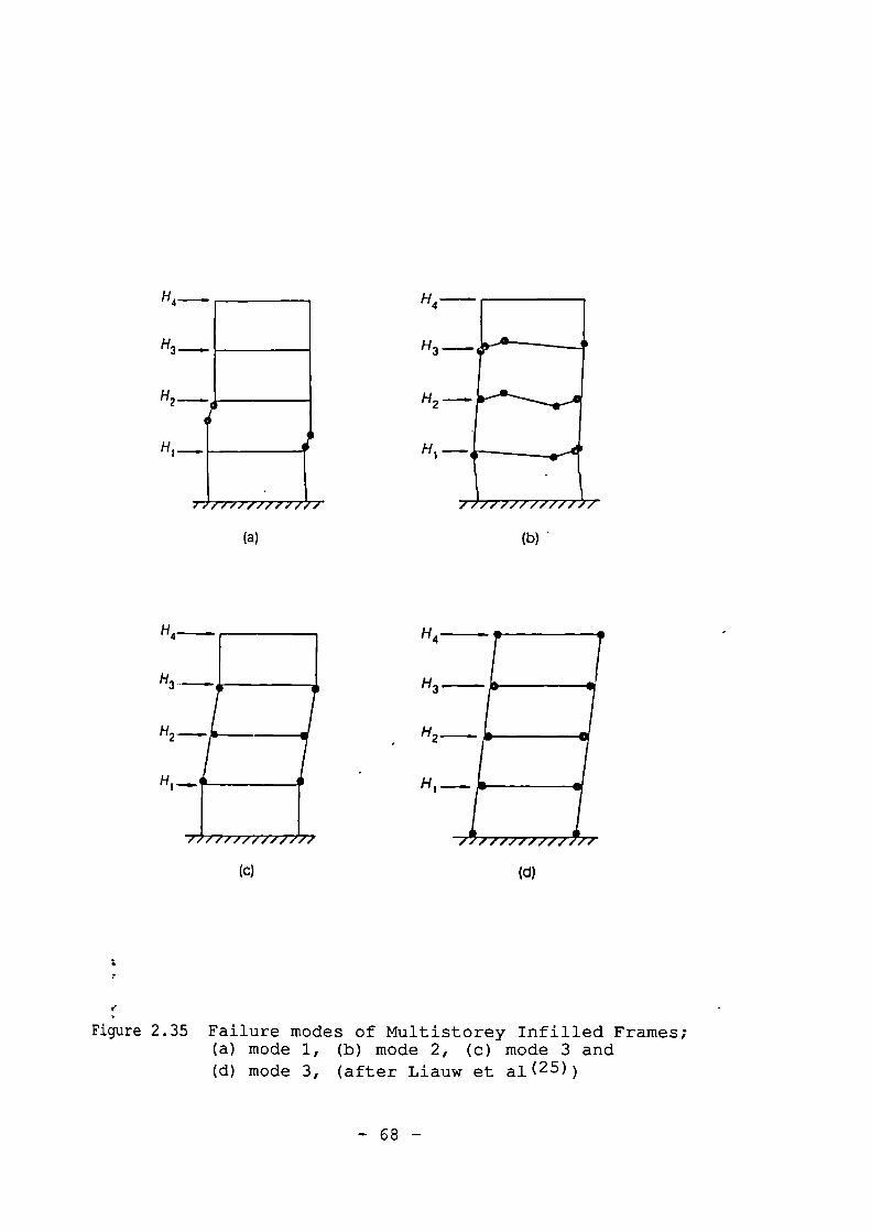
H4
H3
H2
(a)
(b)
(c)
(d)
Figure 2.35 Failure modes of Multistorey Infilled Frames;(a) mode 1, (b) mode 2, (c) mode 3 and(d) mode 3, (after Liauw et al(25))
- 68 -
2.9 Conclusion From The Literature Review
Attempts at developing a design method for
infilled frames have resulted in two distinct categories of
methods;
a) The methods based on the infill/frame stiffness
parameter, MI, described in Sections 2.3 to 2.6 and
b) The methods based on the frame/infill strength
parameter, m, described in Sections 2.7 and 2.8.
The former methods assume the frame remains in an elastic
state up to the peak load. The latter methods, however, use
the plasticity theories, thus indicating that both the frame
and the infill experience plasticity before the peak loadbeen
has reached when the frame undergoesa plastic collapse
mechanism upon which the peak load can be calculated.
The current investigation, thus, may be extended
to study the true behaviour of infilled frames. By an
experimental approach, one may not discover whether the
frame or infill experiences plasticity first. However,the
previous experiments( 20 , 29 ) have proved occurrence of the
frame plasticity only after the peak load.
On the other hand, the Finite Element method has
proved to be a powerful device in solving highly
Indeterminate problems. Wood( 23 ), discussing his plastic
method, stated that "The next important advance must come
from Finite Element analysis, allowing for elastoplasticity
of infilling wall with restricted plastic strain." Such a
Finite Element analysis should simulate the infilled frame
behaviour as truly and as accurately as possible.
- 69 -
Table 2.2 lists the features, which will enhance
he analysis, if they can be incorporated with a finite
lement analysis.
able 2.2 also lists those features (marked by x) that have
een included in some previously developed Finite Element
nalysis programs, written particularly for infilled frame
tructures.
The main objective of this study is, thus, to
evelop a Finite Element analysis program, enhanced by as
any as possible of the desired features listed in
able 2.2. Such a program may then be used to examine the
egree of accuracy of the existing methods. Also, it is
esirable to examine the significance of the effect of those
arameters and variables that are not included in these
ethods. The next step, then, would be the inclusion of the
ariables and parameters, which have proven to have
ignificant effects on the behaviour of infilled frames.
Having developed such a program, it is possible to
arry out A parametric study and to examine the effects of
he variables on the overall behaviour of infilled frames.
uch variables include material properties, dimension of the
rame or infill, vertical loading, lack of fit,
recompression, order of application of loads, position and
ize of any opening, other frame combinations such as multi-
torey and multi-bay panels and degree of restraint of frame
minections (rigid, semi-rigid, hinge). Such a parametric
tudy could provide a set of data for development of a code
t practice for design of infilled frames.
The criteria for design of infilled frame
structures can be established with respect to the following
requirements:
i) Limit states of serviceability such as: deflection,
cracking, separation, slip (if desired to be prevented
or limited for structures of particular purpose), and
spalling of the infill material at the loaded corners,
should it happen well before the peak load has reached.
ii)Limit state of collapse; permitting an acceptable
range of plastic strain for the material in question.
:,
e
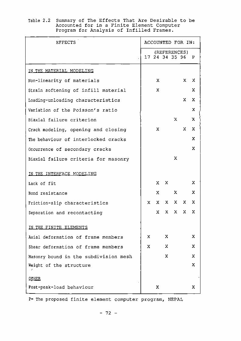
Table 2.2 Summary of The Effects That Are Desirable to beAccounted for in a Finite Element ComputerProgram for Analysis of Infilled Frames.
EFFECTS ACCOUNTED FOR IN:
17(REFERENCES)24 34 35 96 P
IN THE MATERIAL MODELING
Non-linearity of materials X X
Strain softening of infill material
Loading-unloading characteristics X X
Variation of the Poisson's ratio X
Biaxial failure criterion X X
Crack modeling, opening and closing X X X
The behaviour of interlocked cracks X
Occurrence of secondary cracks X
Biaxial failure criteria for masonry X
IN THE INTERFACE MODELING
Lack of fit X X X
Bond resistance X X X
Friction-slip characteristics X X X X X X
Separation and recontacting X X X X X
IN THE FINITE ELEMENTS
Axial deformation of frame members
Shear deformation of frame members
Masonry bound in the subdivision mesh
Weight of the structure
OTHER
Post-peak-load behaviour
P= The proposed finite element computer program, NEPAL
- 72 -
, CHAPTER THREE
The Finite Element Technique
3.1 General
The review of previous work on the behaviour of
irffilled frames led to selection of The finite element
technique for study of the non-linear behaviour of infilled
frames in this investigation.
The finite element method is described in
standard texts, eg. Zienkiewicz( 36 ). In this chapter, only
the principles will briefly be described in order to
establish a notation for the later descriptions and
developments.
In order to simulate the actual behaviour of
infilled frames as close as possible, all the features
listed in , Table 2.2 will be regarded as the minimum
requirements for the proposed finite element analysis
computer program.
12 Finite Element Concept
The finite element method is a technique used for
solving partial differential equations by discretizing these
equations in their space dimensions to give finite elements.
The regional matrix equations, written for nodal points of
elements, are summed resulting in global matrix equations.
In structural engineering applications of this
- 73 -
method, the body of the structure is subdivided into
elements being linked together by nodes. The global matrix
equations take the form of:
{P} = [K]{a} (3.1)
which relates the nodal forces vector, {P}, to the nodal
displacements vector, {a}, where [K] denotes the stiffness
matrix of the structure under consideration. In a linearsymmetric
elastic analysis [K] is a square matrix of constant terms
resulting from the geometry and the mechanical properties of
the materials of the structure. Eqs 3.1 are, thus, a set of
linear simultaneous equations which can be solved directly.
When non-linearity of material is desired to be accounted
for, pc] becomes a function of current nodal displacements
causing the Eqs 3.1 to become non-linear. Such equations
cannot be solved directly. However, there are numerical •
solutions to such equations as described in the following
section. .
13 Newton Raphson Iteration
The most frequently used iteration schemes for the
solution of non-linear finite element equations are of the
Newton Raphson type( 36 ) illustrated in Fig 3.1. In this
method, equilibrium conditions, at completion of each load
increment, are satisfied by successive approximation of the
form:
{Ri(n)} = ( Pi-q()} = [Ki(n-1)]{Aai(n)} (3.2)
- 74 -
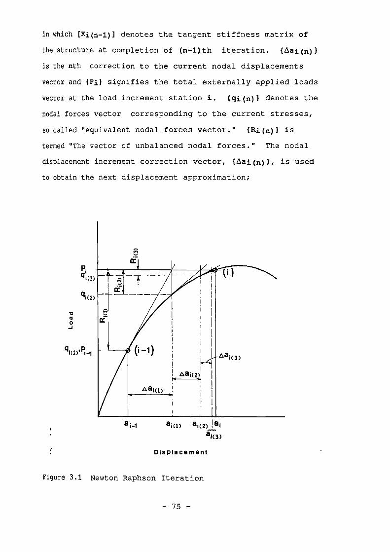
in which [Ki(n-1)] denotes the tangent stiffness matrix of
the structure at completion of (n-1)th iteration. {Aai(n)}
is the nth correction to the current nodal displacements
vector and signifies the total externally applied loads
vector at the load increment station i. {qi(n)} denotes the
nodal forces vector corresponding to the current stresses,
so called "equivalent nodal forces vector." (Ri(n)} is
termed "The vector of unbalanced nodal forces." The nodal
displacement increment correction vector, {Aai(n)}, is used
to obtain the next displacement approximation;
r. Displacement
Figure 3.1 Newton Raphson Iteration
- 75 -
{ ai(n)} = ( ai(n-1)} + (Aai(n)} (3.3)
Iterations are repeated, Fig 3.1, until an appropriate
convergence criterion is satisfied. When such convergence
is achieved the external loads vector, RI, is increased to
a higher level. The procedure is continued until a desired
load level is reached or complete failure of the structure
takes place.
14 Finite Element Formulation
14.1 General
Non-linear finite element analysis reduces to
solution of linear tangential displacement equations, Eqs
3.2, involving the tangent stiffness matrix of the
structure, [K]. [K] is a matrix of currently constant terms
which are computed by assembling the terms of the elements'
tangent stiffness matrices, [K] e . The technique of
assembling is widely described in standard finite element
texts (36 , 37) . An element tangent stiffness matrix, [K]e,
relates the element unbalanced nodal forces vector, {AF}, to
the element nodal displacements vector, {Aa} e , as follows:
{AF) = [K] e {Aa} e(3.4)
The overall equivalent nodal forces vector, (ql,
also results from assembling the elements equivalent nodal
nv.ces, {q} e . Derivation of [K] a and {ci} e are given in
standard texts of finite element( 36 , 37) but it is
convenient to review the principles in order to establish a
notation for later descriptions. For the sake of
- 76 -
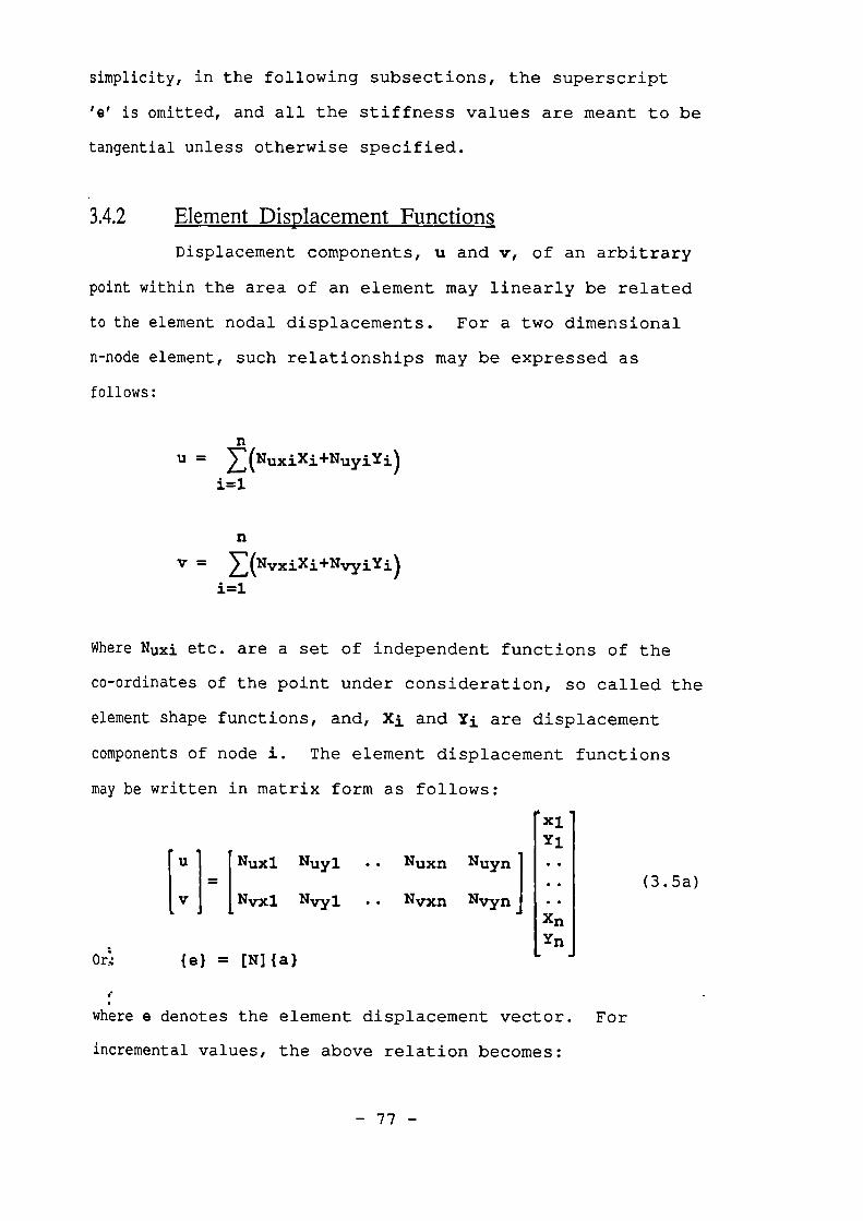
simplicity, in the following subsections, the superscript
'e' is omitted, and all the stiffness values are meant to be
tangential unless otherwise specified.
3.4.2 Element Displacement Functions
Displacement components, u and v, of an arbitrary
point within the area of an element may linearly be related
to the element nodal displacements. For a two dimensional
n-node element, such relationships may be expressed as
follows:
U = E(NuxiXi+NuyiYi)
i=1
V = (isivxiXi+NvyiYi)
i=1
Where Nuxi etc. are a set of independent functions of the
co-ordinates of the point under consideration, so called the
element shape functions, and, Xi and Yi are displacement
components of node i. The element displacement functions
maybe written in matrix form as follows:
V
rux1
Nvxl
Nuyl
Nvyl
Nuxn
Nvxn
Nuynl
Nvyn
X1
Y1• •
• •
• •
(3.5a)
(e) = [N]{a}Or
where e denotes the element displacement vector. For
incremental values, the above relation becomes:
- 77 -
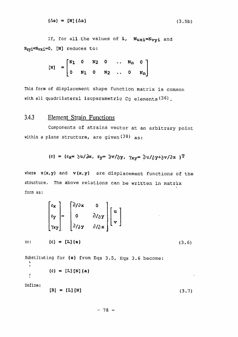
[
ex
Cy
'Yxy
{AO = [N]{Aa} (3.5b)
If, for all the values of i, Nuxi=Nvyi and
Nuyi=Nvxi=0, [N] reduces to:
[Ni 0 N2 0 Nn 0[N] =
0 Ni 0 N2 .. 0 Nn
This form of displacement shape function matrix is common
with all quadrilateral isoparametric Co elements (38) .
3.4.3 Element Strain Functions
Components of strains vector at an arbitrary point
within a plane structure, are given( 38 ) as:
{e} = {Ex= .�0.2/x, Cy= -avlbY, 7xy= .au/OY+6v/Dx 1T
where u(x,y) and v(x,y) are displacement functions of the
structure. The above relations can be written in matrix
form as:
[Dix 0 1u
0 3/Dy
2 /a y a/a x
or: {c} = [L]{e} (3.6)
Substituting for fe} from Eqs 3.5, Eqs 3.6 become:
fel = (LUNUal
Define:[B] = [L][N] (3.7)
- 78 -
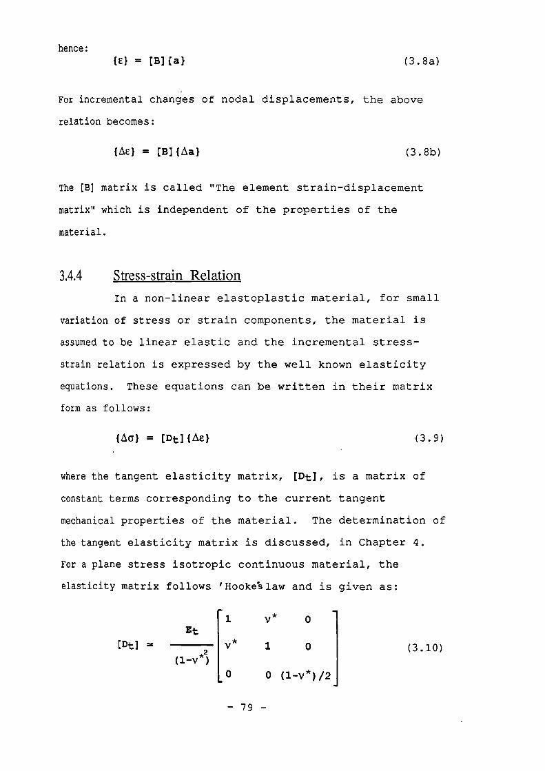
(3.10)
hence:{e} = [B] (a) (3.8a)
For incremental changes of nodal displacements, the above
relation becomes:
{Ae} = [B](Aal (3.8h)
The [B] matrix is called "The element strain-displacement
matrix" which is independent of the properties of the
material.
3.4.4 Stress-strain Relation
In a non-linear elastoplastic material, for small
variation of stress or strain components, the material is
assumed to be linear elastic and the incremental stress-
strain relation is expressed by the well known elasticity
equations. These equations can be written in their matrix
form as follows:
{A} = [DO(Ael (3.9)
where the tangent elasticity matrix, [Dt], is a matrix of
constant terms corresponding to the current tangent
mechanical properties of the material. The determination of
the tangent elasticity matrix is discussed, in Chapter 4.
Fora plane stress isotropic continuous material, the
elasticity matrix follows 'Hookeslaw and is given as:
[1 v* oEt
[Dt] = v* 1 o(1-v
*2)
0 0 (1-v*)/2
- 79 -
*where Et and v are the tangent values of modulus of
elasticity and Poisson's ratio of the material respectiviy.
3.4.5 Element Stiffness Matrix
Since changes in internal stresses and strains are
due to changes in element nodal forces and displacements,
one of the energy methods may be used to derive the
stiffness matrix of an element as shown below.
If the material behaviour is linear-elastic
between the two stations, the total internal strain energy
may be calculated as:
II = 1/2 (Ae}T{a}ciV
V
Substituting for {a) from Eqs 3.9, gives:
1
i
1:7 = 1/2 LAE} T [Dt] {AE}dV
V
Substituting for {Le} from Eqs 3.8b, leads to:
II = (1/2) {Aa} T [f[B1 T [Dt ] [B]dV] {Aa}
V
The work done by external nodal forces may also be
calculated as:
W = ( 1/2) (Aa}T{AF}
- 80 -
where AF denotes the changes in the nodal forces vector.
Equating the internal and external energy, U and W, AF can
be derived as follows:
{AF} = [f[13] [Dt] [13] dlarl {Aa}
V
Comparison of the above equation with Eq 3.4 leads to the
element tangent stiffness matrix as follows:
iMe= [B]T[Dt][B]dV (3.11)
V
Note that the integration must be carried out over the
volume of the element.
3.4.6 Element Equivalent Nadal Forces
Using the same energy method as used in previous
section, the equivalent nodal forces vector, q, may be
derived in term of the stress vector as follows:
iU = 1/2 {e}T{a}ciV
V
Substituting for {e} from Eqs. (3.8a), gives:
U = (1/2){a} T [B]T{a}dV
V
- 81 -
The work done by the nodal forces may be written as:
W= (1/2)(a}T{q}e
Equating U and W and solving for (q) e , leads to:
. {q} e = j([B]T{a}dV
(3.12)
V
15 Local Normalized Coordinates
3.5.1 Definitions
Fig 3.2 shows mapping of a quadrilateral elemer\t
into normalized local coordinates, E, and T. The origii-‘ of
the normalized coordinates, 0(--0, 1=0), is located at the
intersection of bisectors of opposite sides of the
quadrilateral. Normalization of the local co-ordinates
requires that,
711=-1
U=-1 , 12=41
3=-1-1, 1 3=4-1
4-=-1- 1 , 14=-1
It is convenient to convert Eqs 3.11 and 3.12 into
local normalized coordinates because,
a) The element shape functions are normally worked out in
terms of local normalized coordinates in order to be
e independent of geometry and location of the element.
b) Local normalized coordinates allow the integrations of
- 82 -
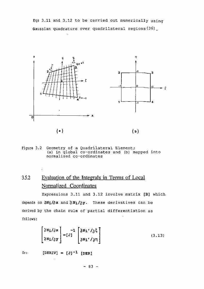
2
+1
3
41 -1
.x0
( a ) (b)
Eqs 3.11 and 3.12 to be carried out numerically using
Gaussian quadrature over quadrilateral regions (36)
Figure 3.2 Geometry of a Quadrilateral Element;(a) in global co-ordinates and (b) mapped intonormalized co-ordinates
3.5.2 Evaluation of the Integrals in Thins of Local
Normalized Coordinates
Expressions 3.11 and 3.12 involve matrix [B] which
depends on bkli/ax and /./j/ay. These derivatives can be
derived by the chain rule of partial differentiation as
follows:
ri/jx1 -1 ri'/otl=[J]
Z Ni/aY OViai
Or: [DERrV] = [J] -1 [DER]
(3.13)
- 83 -
where Ni' is the displacement shape function of the ith node
of the element in terms of local normalized coordinates,
and 1.1, and [J] is the Jacobian matrix expressed as:
[ax/g ay/at[J] =
axial ay/al(3.14)
The terms of [J] matrix can be calculated only
when coordinates of any arbitrary point in global
coordinates are known in terms of the normalized
coordinates, ie. x = P(,1) and y = Q(,.11). When the
element is isoparametric (i.e the shape functions defining
geometry and function are the same), x and y are given(36)
as follows:
x = N1'Xi+N2 1 X2+ Nn'Xn =
i=1
y = N1'Y1+N2'Y'2+ Nn'Yn =
i=1
where Xi and Yi are coordinates of the nodal points of the
element in global coordinates system. Substituting for x
and y into relation 3.14, the [J] matrix can be derived in
terms of and n and the coordinates of nodal points of the
element as follows:
Xl Yi
[J] =
/g BITn' /at I
brri'/� 71 aNni/al
(3.15)
Or; [J] = [DER][COORD]
- 84 -
Even when the element is not isoparametric, the
Jacobian matrix can still be calculated using a new set of
shape functions, Ni", (specially used for this purpose)
being compatible with the geometry of the element.
The determinant of Jacobian matrix, must also
be evaluated for transformation of the integrals involving
dxdy as follows (39)
+1 +1
f(t,q)dV = t fict,n) IJIdtd1 (3.16)
-1 -1
Where t denotes the thickness of the element and f(,1)
signifies either functions of Eqs 3.11 or Eqs 3.12.
16 Numerical Integrationthe
Calculation of element stiffness matrix, [K] e , and
equivalent nodal forces, {q} e , led to integrals of type:
+1 +1
I = t f ff (,11) IJIdtd11
-1 -1
Analytical evaluation of such integral at this
form is impractical as far as applications of numerical
analysis is concerned. Therefore, in practice,
such integrals are evaluated numerically using gaussian
quadrature over quadrilateral regions. The quadrature rules
are all of the form:
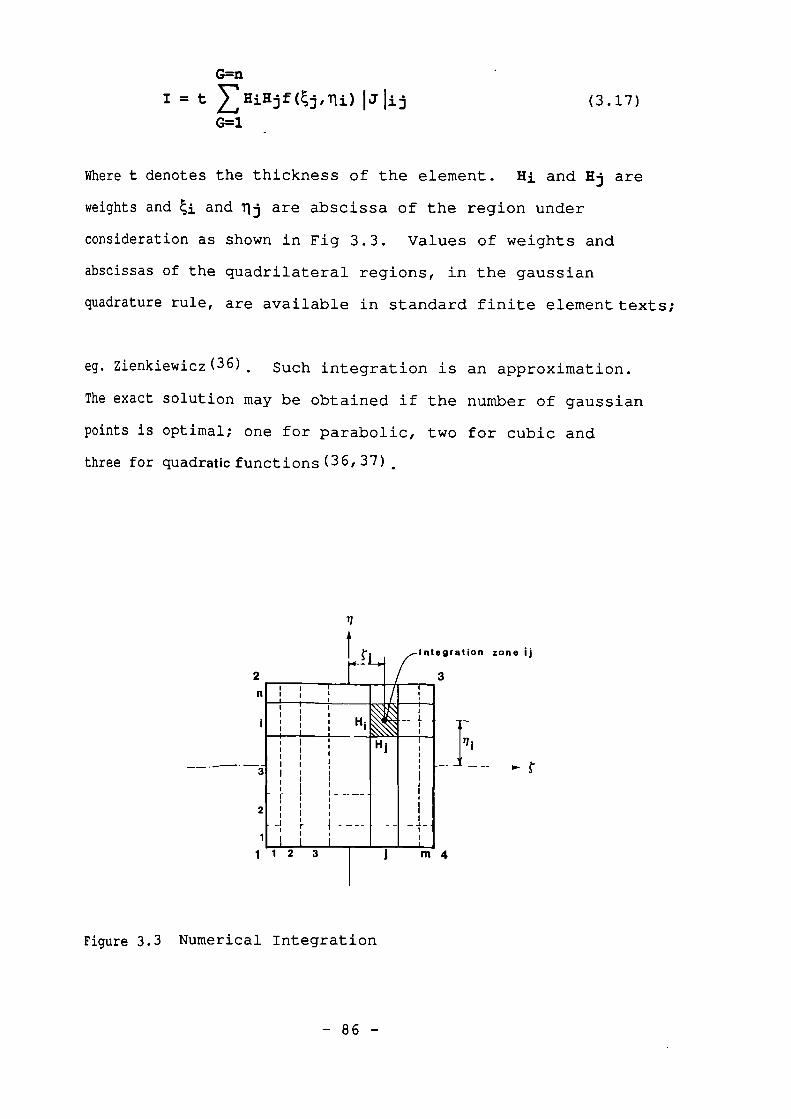
III
,-,.n:k. \\
Hi
Ii
I- _ 1
:
I1
111
i
iHI
IIII
- .1I
------i1
I
I- -J, 1r I
i ---- -- ,
Ii I11
2
1
G=n
I = t E HiHi f (tjr lii.) I J lij
(3.17)
G=1
Where t denotes the thickness of the element. Hi and Hj are
weights and ti and are abscissa of the region underconsideration as shown in Fig 3.3. Values of weights and
abscissas of the quadrilateral regions, in the gaussian
padrature rule, are available in standard finite element texts;
eg. Zienkiewicz( 36 ). Such integration is an approximation.
The exact solution may be obtained if the number of gaussian
points is optimal; one for parabolic, two for cubic and
three for quadraticfunctions(36,37).
1Integration zone
3
1123 m4
Figure 3.3 Numerical Integration
- 86 -
3.7 Contribution of Reinforcement to R.0 Elements
3.7.1 General
It has been customary to consider the two
constituents, concrete and steel reinforcement, as separate
contributors to the overall stiffness and strength using the
principle of superposition.
It is common to assume full kinematic continuity
between concrete and steel, at least at nodal points on
element boundaries. However, the two materials are highly
unequal in their behaviour; Young's modulus for steel bar is
one order higher than that of concrete, and unlike that of
concrete, the stress-strain relation of steel is symmetric
intension and compression. The limited reinforcement-
concrete bond strength results in:
a) bond failure and sliding of reinforcing bars,
b) local deformation of reinforcement in cracked concrete
(doweling effect) and
c) tension stiffening effect of uncracked concrete
between cracks.
In order to reduce the errors due to such effects, various
adjustments in properties of constituent materials have been
specified, Chen (39). These are discussed in Chapter 4.
Having made such adjustments, reinforcement may
be modeled as:
a) two-node bar element or
b) anisotropic equivalent solid layer stuck on the
surface of the element where it is applicable or
c) Single bar stuck on the surface of the element.
The choice of two-node bar element greatly increases the
- 87 -
size of the global stiffness matrix. Therefore, the other
two models were adopted in this work.
Contribution of reinforcement is to be
superimposed to that of the concrete as described in the
following sections.
3.7.2 Uniformly Distributed Reinforcement
As shown in Fig 3.4(a, b), a uniformly distributed
reinforcement with rate of rs may be modeled by an
anisotropic steel layer with thickness of rst and having
full strength and stiffness in direction of the
reinforcement and zero strength and stiffness normal to this
direction, where t is the thickness of the element.
The contribution of reinforcement of this type to
the element properties may be computed in exactly the same
way as described for the element itself. This contribution
maybe superimposed directly. i.e:
I = Ic + I s (3.18)
Where I denotes either integrals of Eqs 3.11 and 3.12 and
subscripts c and s specify concrete and steel materials
respectively.
In the particular case when reinforcement is
uniformly distributed, the second integration, Is, can be
eliminated by including the mechanical properties of the
steel layers into that of the concrete as follows:,
e[D] = [Do] + rsl[Dsl] + rs2[Ds2] + ... (3.19)
{a) = ( ac) + rsl{ asl} + rs2{ as2} + ... (3.20)
- 88 -
where [Dsi] denotes the stress-strain relation matrix for
ith layer of reinforcement. This will be studied in
Section 4.9.6.
3.7.3
A Single Bar Parallel to One of the Element Local
Coordinates
A single bar within an element is assumed to be
stuck on the surface of the element and follows the
displacement function of the element Fig 3.4(c, d). The
contribution of such a bar can be computed by dividing it
into parts and integrating the contribution of these parts
numerically. When the reinforcing bar is extended parallel
to one of the local co-ordinates, say as shown in
Fig 3.4(c), the numerical integration of its contribution
can be computed as follows:
Is = 2trsHi f(i,11s) s;
(3.21)
The multiplier 2trs represents the integration of the rate
of reinforcement, trs, between 71=-1 to 11=-1-1.
By altering the corresponding indices in Eq 3.21,
Eg3.22 can be written for a steel bar extended parallel to
Ti as follows:
Is = E2trsili f (s,1ni alis (3.22)
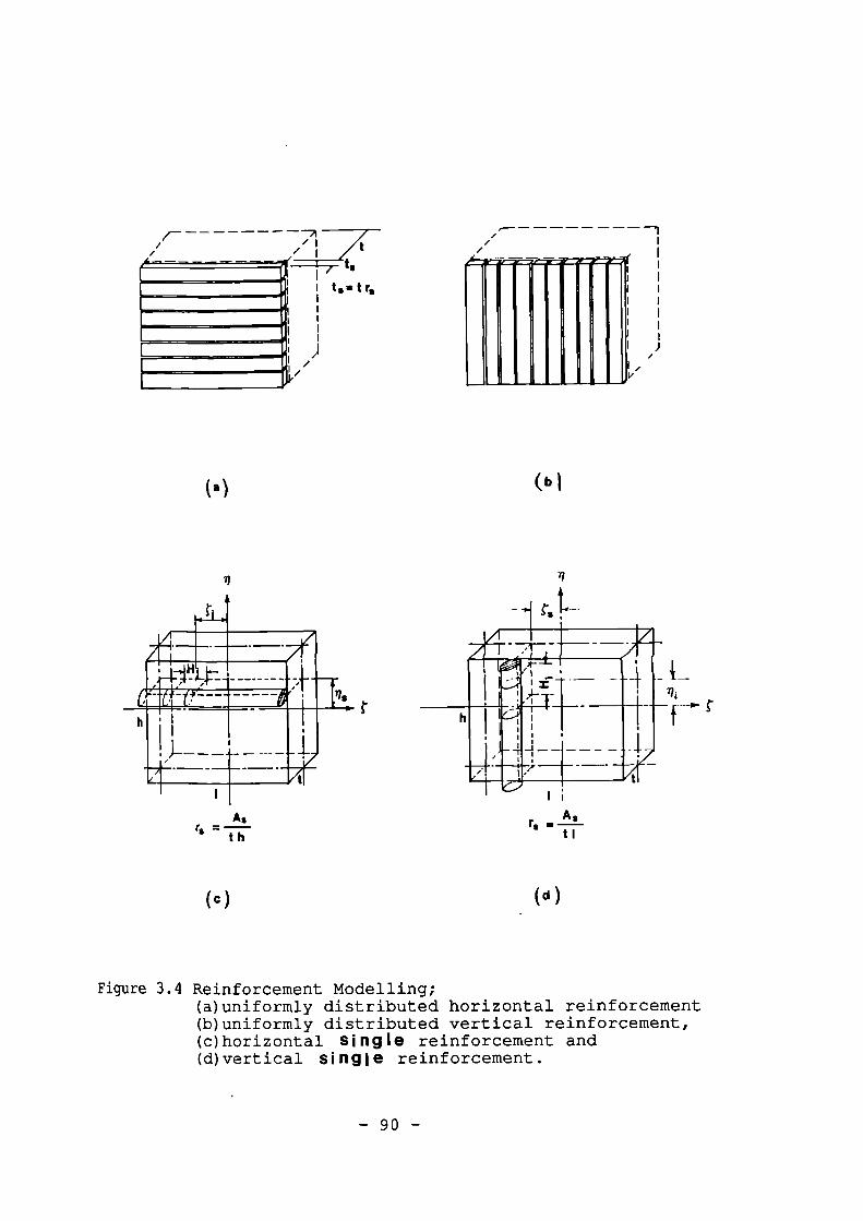
//
1
,
Asr s =
t h
1r______ ..._
/-
7t //
i ts t
tog t r,I
Ii
I
(s)
n
(b i
n
( c )
(d)
Figure 3.4 Reinforcement Modelling;(a)uniformly distributed horizontal reinforcement(b)uniformly distributed vertical reinforcement,(c)horizontal single reinforcement and(d)vertical single reinforcement.
- 90 -
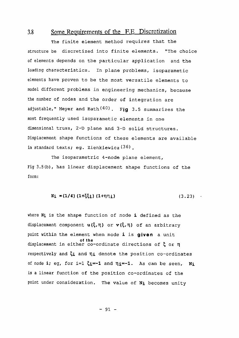
18 Some Requirements of the RE Discretization
The finite element method requires that the
structure be discretized into finite elements. "The choice
of elements depends on the particular application and the
loading characteristics. In plane problems, isoparametic
elements have proven to be the most versatile elements to
model different problems in engineering mechanics, because
the mmther of nodes and the order of integration are
adjustable," Meyer and Bath (40) . Fig 3.5 summarizes the
most frequently used isoparametic elements in one
dimensional truss, 2-D plane and 3-D solid structures.
Displacement shape functions of these elements are available
in standard texts; eg. Zienkiewicz(36).
The isoparametric 4-node plane element,
Fig 3.5(b), has linear displacement shape functions of the
form:
Ni =(1/4) (1+j) (3.23)
where Ni is the shape function of node i defined as the
displacement component u(t,fi) or v(,71) of an arbitrary
point within the element when node i is given a unitof the
displacement in either co-ordinate directions of t or
respectively and ti and fli denote the position co-ordinates
of node i; eg, for 1=1 ti=-1 and ni=-1. As can be seen, Ni
is a linear function of the position co-ordinates of the
point under consideration. The value of Ni becomes unity
- 91 -
when the point under consideration is located at node i and
becomes zero when the point is located at any other nodal
pints. This is a necessary condition for a displacement
shape function (36) . For any element configuration, the
sides of an isoparametic 4-node element remain straight.
However, in an 8-node element, Fig 3.5(c), the sides follow
a parabolic curve. Therefore, the shape functions of an
8-node plane element are to the second power of the position
coordinates of the point under consideration as presented
below.
i=1,3,5,7; Ni = (1/4) (1-1-i) (1-Tpu) (tti+ririi-1)
i=2,6; Ni=(1/2) (1-Ftti) (1-712)
(3.24)
i=4,8; Ni=(1/2) (1-Eirrii) (1-t2)
Isoparametric 12-node (cubic) element, Fig 3.5(d), has yet
more flexibility to follow the displacement variations.
Nowadays there is a tendency to use more elaborate elements
for the sake of economy and accuracy(36).
In non-linear finite element analyses of
structures, the displacement equations must be solved
several times, involving a considerable amount of
computation time. The computation time for equation solving
is approximately in proportion to N2W. Where N and W are the
total number of nodal displacement freedoms and the half-
band-width of the global stiffness matrix respectively.
Therefore, considerable care must be used in choosing the
type of elements and the way the structure is subdivided and the
- 92 -
nodes are numbered in order that the size of the global
stiffness matrix becomes as small as possible. The size of
the stiffness matrix may considerably be reduced by a coarse
subdivision of parabolic or even cubic elements. But the
choice of element is also structure dependent. Therefore,
the efficiency and compatibility of a selected element must
be examined for the structure in question. For this
purpose, the computer program "ELCO", which is the
linear and elastic version of program "NEPAL", was
used. Program "ELCO" is capable of solving linear problems
with almost any type of element including some new proposed
elements described in the following sections. Program
"NEPAL" will be discussed in Chapter 5.
Application of the finite element method in the
analysis of infilled frame structures requires specific
considerations in:
a)the finite element discretization of:
i) infilling wall,
ii) frame and
iii) wall/frame interfaces.
b)the mechanical modeling of the materials.
These are studied in the rest of this chapter and Chapter 4.
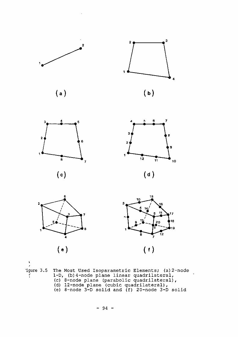
10
15
( a )
( b )
(c) ( d )
( e )
( f )
:r
'igure 3.5 The Most Used Isoparametric Elements; (a)2-nodee 1-D, (b)4-node plane linear quadrilateral,
(c) 8-node plane (parabolic quadrilateral),(d) 12-node plane (cubic quadrilateral),(e) 8-node 3-D solid and (f) 20-node 3-D solid
- 94 -
1.9 Masonry INdl Discretization
L9.1 General
Masonry is made of mortar joints and masonry units
dth different mechanical properties. When masonry is
;ubjected to in-plane loading, some out-of-plane interactive
forces develop at interfaces of mortar joints and masonry
mits as a result of effects of the poisson's ratio and
Aasticity of the mortar joints. Therefore, the behaviour
)f masonry is three dimensional and elastoplastic.
3.92 Standard 34) Elements
Standard finite element procedure suggests masonry
pediscretized into a set of 8-node and 6-node solid 3-D
?lements as shown in FIG 3.6. Also a set of 3-D interface
?lements with zero thickness must be included with the
subdivision in order that the mechanical behaviour of
unit/joint interfaces can be allowed for. This involves 72
nodal displacement freedoms per masonry unit. Such a high
number of displacement freedoms demands a very expensive
finite element analysis.
Therefore, the number of displacement freedoms
should somehow be reduced. The following sections discuss
some other choices with lesser number of displacement
freedoms.
- 95 -
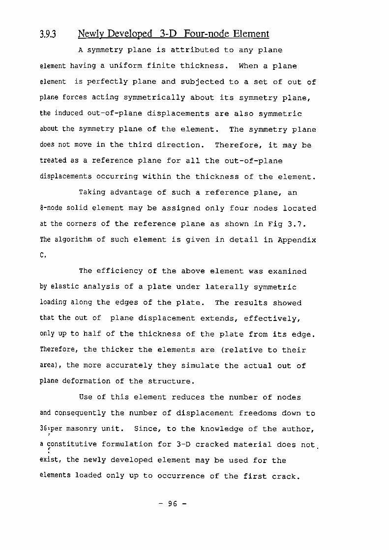
3.9.3 Newly Developed 3-1) Four-node Element
A symmetry plane is attributed to any plane
element having a uniform finite thickness. When a plane
element is perfectly plane and subjected to a set of out of
plane forces acting symmetrically about its symmetry plane,
the induced out-of-plane displacements are also symmetric
about the symmetry plane of the element. The symmetry plane
does not move in the third direction. Therefore, it may be
treated as a reference plane for all the out-of-plane
displacements occurring within the thickness of the element.
Taking advantage of such a reference plane, an
8-node solid element may be assigned only four nodes located
at the corners of the reference plane as shown in Fig 3.7.
The algorithm of such element is given in detail in Appendix
C.
The efficiency of the above element was examined
by elastic analysis of a plate under laterally symmetric
loading along the edges of the plate. The results showed
that the out of plane displacement extends, effectively,
only up to half of the thickness of the plate from its edge.
Therefore, the thicker the elements are (relative to their
area), the more accurately they simulate the actual out of
plane deformation of the structure.
Use of this element reduces the number of nodes
and consequently the number of displacement freedoms down to
36zper masonry unit. Since, to the knowledge of the author,
a constitutive formulation for 3-D cracked material does not
exist, the newly developed element may be used for the
elements loaded only up to occurrence of the first crack.
- 96 -
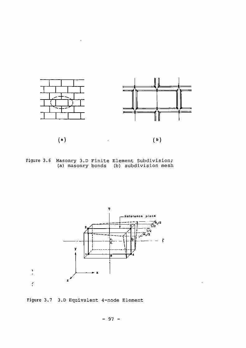
Reference plane
/2
t/2/W3 /2
-
z/ X
(a)
Figure 3.6 Masonry 3.D Finite Element Subdivision;(a) masonry bonds (b) subdivision mesh
Figure 3.7 3.D Equivalent 4-node Element
- 97 -
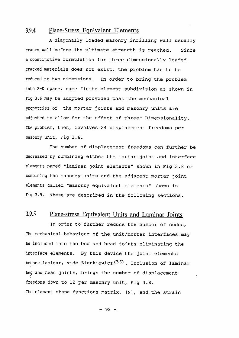
3.9.4 Plane-Stress Equivalent Elements
A diagonally loaded masonry infilling wall usually
cracks well before its ultimate strength is reached. Since
a constitutive formulation for three dimensionally loaded
cracked materials does not exist, the problem has to be
reduced to two dimensions. In order to bring the problem
into 2-D space, same finite element subdivision as shown in
Fig 3.6 may be adopted provided that the mechanical
properties of the mortar joints and masonry units are
adjusted to allow for the effect of three- Dimensionality.
The problem, then, involves 24 displacement freedoms per
masonry unit, Fig 3.6.
The number of displacement freedoms can further be
decreased by combining either the mortar joint and interface
elements named "laminar joint elements" shown in Fig 3.8 or
combining the masonry units and the adjacent mortar joint
elements called "masonry equivalent elements" shown in
Fig 3.9. These are described in the following sections.
3.9.5 Plane-stress Equivalent Units and Laminar Joints
In order to further reduce the number of nodes,
The mechanical behaviour of the unit/mortar interfaces may
be included into the bed and head joints eliminating the
interface elements. By this device the joint elements
bmae laminar, vide Zienkiewicz (36 ). Inclusion of laminar
bed and head joints, brings the number of displacement
freedoms down to 12 per masonry unit, Fig 3.8.
The element shape functions matrix, [N], and the strain
- 98 -
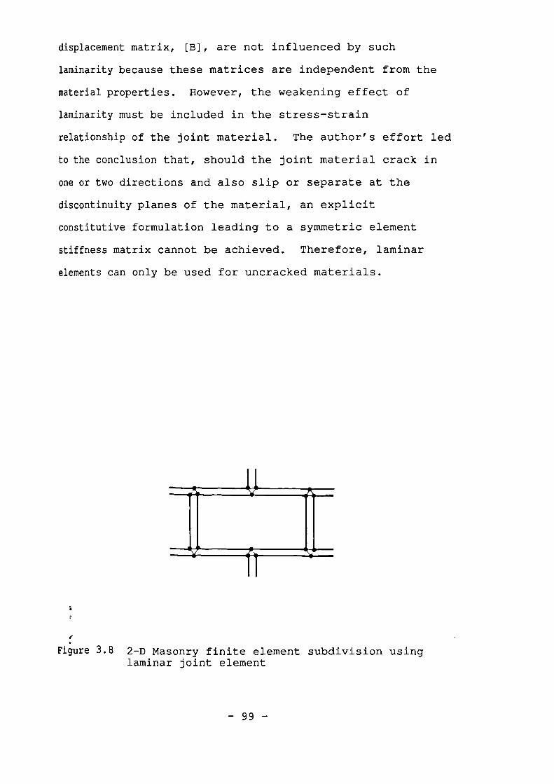
displacement matrix, [B], are not influenced by such
laminarity because these matrices are independent from the
material properties. However, the weakening effect of
laminarity must be included in the stress-strain
relationship of the joint material. The author's effort led
to the conclusion that, should the joint material crack in
one or two directions and also slip or separate at the
discontinuity planes of the material, an explicit
constitutive formulation leading to a symmetric element
stiffness matrix cannot be achieved. Therefore, laminar
elements can only be used for uncracked materials.
Figure 3.8 2-D Masonry finite element subdivision usinglaminar joint element
— 99 —
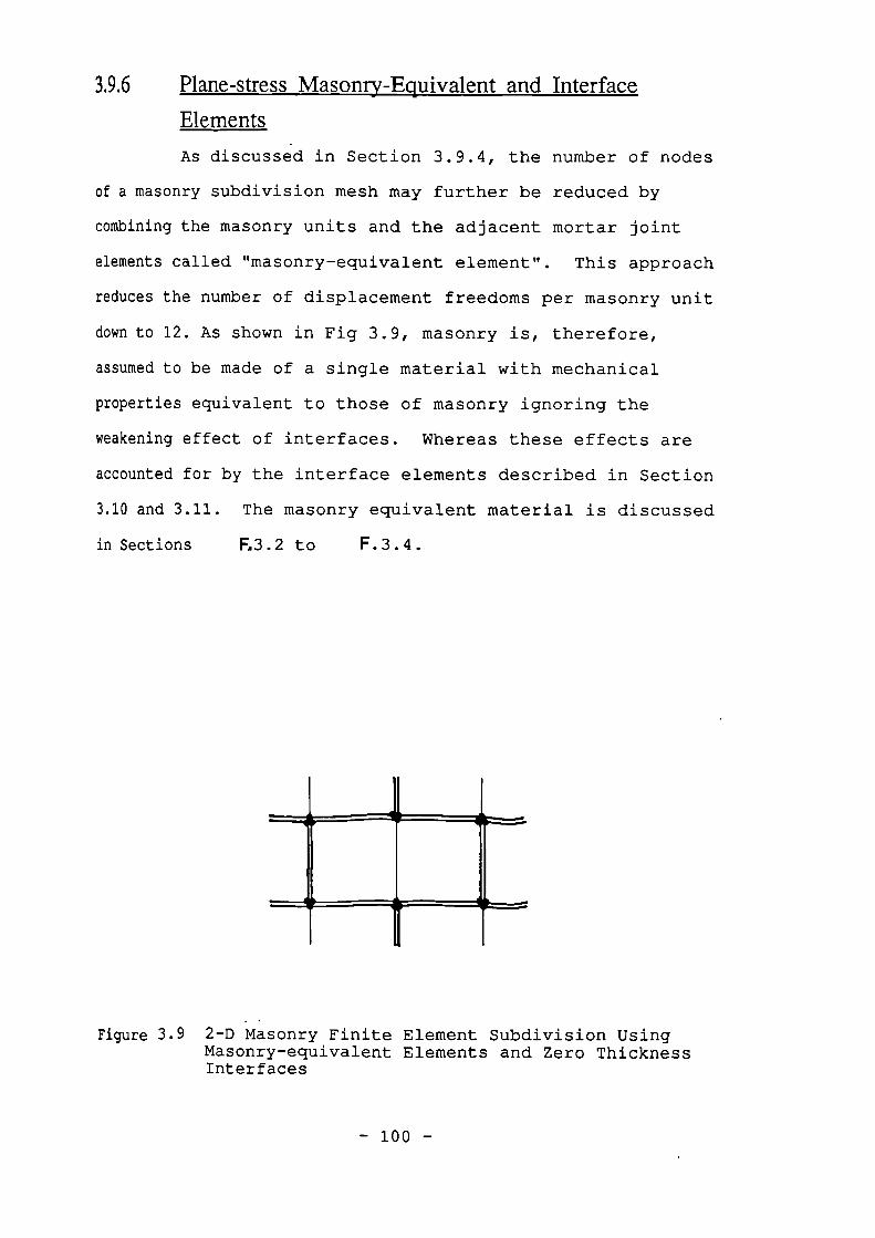
3.9.6 Plane-stress Masonry-Equivalent and Interface
Elements
As discussed in Section 3.9.4, the number of nodes
of a masonry subdivision mesh may further be reduced by
combining the masonry units and the adjacent mortar joint
elements called "masonry-equivalent element". This approach
reduces the number of displacement freedoms per masonry unit
thm to 12. As shown in Fig 3.9, masonry is, therefore,
assumed to be made of a single material with mechanical
properties equivalent to those of masonry ignoring the
weakening effect of interfaces. Whereas these effects are
accounted for by the interface elements described in Section
3.10 and 3.11. The masonry equivalent material is discussed
in Sections R3.2 to F.3.4.
Figure 3.9 2-D Masonry Finite Element Subdivision UsingMasonry-equivalent Elements and Zero ThicknessInterfaces
- 100 -
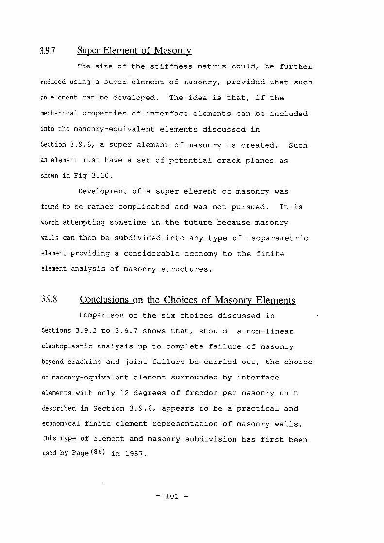
19.7 Super Element of Masonry
The size of the stiffness matrix could, be further
reduced using a super element of masonry, provided that such
an element can be developed. The idea is that, if the
mechanical properties of interface elements can be included
into the masonry-equivalent elements discussed in
Section 3.9.6, a super element of masonry is created. Such
an element must have a set of potential crack planes as
shown in Fig 3.10.
Development of a super element of masonry was
found to be rather complicated and was not pursued. It is
worth attempting sometime in the future because masonry
walls can then be subdivided into any type of isoparametric
element providing a considerable economy to the finite
element analysis of masonry structures.
3.9.8 Conclusions on the Choices of Masonry Elements
Comparison of the six choices discussed in
Sections 3.9.2 to 3.9.7 shows that, should a non-linear
elastoplastic analysis up to complete failure of masonry
beyond cracking and joint failure be carried out, the choice
of masonry-equivalent element surrounded by interface
elements with only 12 degrees of freedom per masonry unit
described in Section 3.9.6, appears to be a'practical and
economical finite element representation of masonry walls.
This type of element and masonry subdivision has first been
used by Page(86) in 1987.
- 101 -
1 1 I
I I
I I
I 1
(a)
o'
n• n=1
(b) (c )
so°
1I- -.1
1i1- .,
I
1
r- J1
-1 r---L_1
TL .1 I__
r-j r -1 r--. I I"I L
Iill
I
(d)
(e)
Note: 2 more discontinuity angles exists; which are:r similar to (d) and (c) with -ye slope.
Figure 3.10 The Modes of Joint Failure in a Masonry SuperElement; (a)concrete block masonry,(b) failure through bed joints and(c,d,e,) failure through bed and head joints
- 102 -
110 Interface Discretization
3.10.1 General
The significance of the behaviour of the frame-
infill interface was discussed in section 2.2. The
mechanical properties of interfaces are described in
Chapter 4. In this section, only the geometry of the
interfaces is discussed.
The geometry of interfaces was first modeled by
Goodman (41) in 1968 for finite element analysis of rocks.
The Goodman's interface element consists of a four-node
element having 8 degrees of freedom and zero thickness.
Since the stiffness matrix of this element resulted from a
direct algebraic integration rather than the standard
numerical summation, such an element can be considered to
have only one sampling point representing the whole length
of the interface held by the element.
An equivalent element but much simpler element
than that of Goodman, is the well known two-node linkage
element with four degrees of freedom used by Riddington(17)
and also by Liauw et al( 24 ). Linkage elements have a
variety of applications in the finite element method; eg.
reinforcement-concrete bond problems, cracking and rock
joints. The stiffness matrix of a linkage element is given
in Section 3.10.2 as to provide a basic notation to the
subject.
In this study, however, the popular linkage
element was not satisfactory, as so many elements were
required to obtain a detailed stress distribution diagram
- 103 -
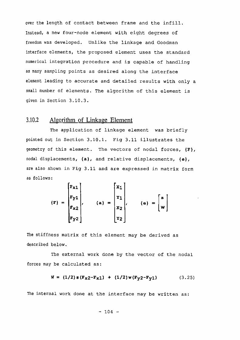
over the length of contact between frame and the inf ill.
Instead, a new four-node element with eight degrees of
freedom was developed. Unlike the linkage and Goodman
interface elements, the proposed element uses the standard
numerical integration procedure and is capable of handling
as many sampling points as desired along the interface
element leading to accurate and detailed results with only a
gran number of elements. The algorithm of this element is
given in Section 3.10.3.
3.10.2 Algorithm of Linkage Element
The application of linkage element was briefly
pointed out in Section 3.10.1. Fig 3.11 illustrates the
geometry of this element. The vectors of nodal forces, (F),
nodal displacements, (al, and relative displacements, (e),
are also shown in Fig 3.11 and are expressed in matrix form
as follows:
xl
Fyl Y1(F) (a) = (e) =
Fx2 X2
Fy2 Y2
{:1
The stiffness matrix of this element may be derived as
described below.
The external work done by the vector of the nodal
forces may be calculated as:
W = (1/2)s(Fx2 -Fxl) (1/2)w(Fy2-Fyl) (3.25)
The internal work done at the interface may be written as:
- 104 -
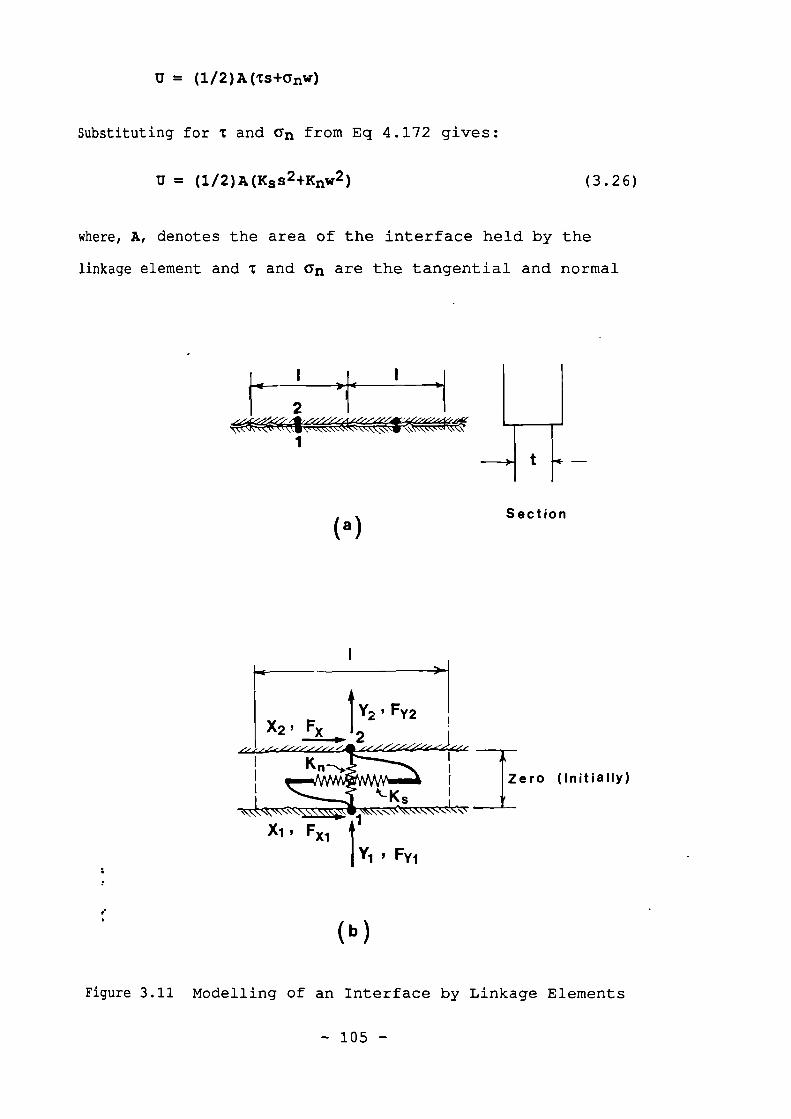
( a ) Section
Zero (Initially)
Xi, Fx1 t
I Yi FY1
t.
b )
Figure 3.11 Modelling of an Interface by Linkage Elements
- 105 -
= (1/2)A(Ts+anw)
Substituting for T and On from Eq 4.172 gives:
= (1/2)A(K3 s 2 +Knw2 ) (3.26)
where, A, denotes the area of the interface held by the
linkage element and T and an are the tangential and normal
stresses uniformly distributed over this area. Ks and Kn
are the tangential and normal stiffnesses of the interface
expressed as Newtons per cubic millimeter (VImm3).
Substituting for the relative displacements, s and w, into
Eqs 3.25, and 3.26, where:
S = X2 - X1 and w = Y2 Y1
and equating these equations, gives:
2(X2-X1) ( Fx2-Fx1) + (Y2-Y1) (Fy2-Fyi) = A [Ks (X2-X1) +Kn
Equating the independent terms from the both sides of the
above equation leads to:
Fx2 - Fx1 = AK3(X2-K1)
Fy2 - Fyl = AKn(Y2-Y1)
Allowing the external forces to act independently, the above
equations result in:
Fx1 = A(+K3X1-K3K2)
Fyi = A(+KnY1-KnY2)
= A ( -KsX1+K3K2)Fx2
Fy2 = A(-KnY2+KnY2)
which can be written in their matrix form as:
Fxl Ks 0 -Ks 0Mir
X1
Fyl 0 Kn 0 -Kn YlA
Fx2 -Ks 0 Ks 0 X2
Fy2 0 -Kn 0 Kn Y2
- 106 -
or: = [K] e {a} (3.27)
where [K] e denotes the stiffness matrix of the linkage
element.
Since this linkage element permits only a uniform
stress to develop over the area of the interface, a new
interface element was developed as described in the
following section.
3.10.3 Islevity Developed Interface Element
The stress and strain gradients along the length
of contact between frame and the infill (especially within
the regions close to the loaded corners) are significant.
Therefore, a reasonably acceptable interface element should
permit, at least, linearly variable relative displacements
along the length of the element. Therefore a new interface
element was developed to satisfy such requirement as
described below.
Fig 3.12(a) shows a segment of a horizontal
Interface. This segment may be represented by a four node
element and mapped into normalized co-ordinates with,
originally, zero thickness as shown in Fig 3.12(b). Define
s and w as the relative transversal and normal displacements
of an arbitrary point along the interface. The proposed
sign convention for s and w is given in Fig 3.12(c).
The relative displacements, s and w, may be
related to the nodal displacements vector, (a}, as follows:
s = NIX' + N2X2 + N3X3 + N4X4
w = N1Y1 + N2Y2 + N3Y3 + N4Y4
- 107 -
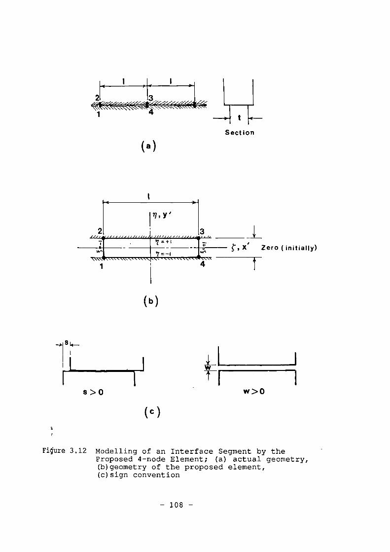
\ \
41
s > 0
t 14—
Section
(a)
r2 3/...1 I
7•=1.1
X Zero ( initially)•'1=-1
(c)
Filure 3.12 Modelling of an Interface Segment by theProposed 4-node Element; (a) actual geometry,(b)geometry of the proposed element,(C) sign convention
- 108 -
or:
or:
Y1
[ s
Ni 0 N20 N30 N40 X2
Y2X3
w 0 N1 0 N2 0 N30 N4 Y3X4Y4
(el = [N]fa} (3.28)
where Ni to N4 denote the relative displacement shape
functions of node 1 to node 4 respectively, ie. Ni is the
relative interface displacement at any point along the
interface due to the nodal displacement of node 1 equals to
unity. Since there are only two nodes on each side of the
element, a set of linear shape functions best suit the
relative displacements of the interface. Such shape
functions are proposed as:
Ni = -(1/2)(1-4)
N2 = +(1/2) (1-4)
N3 = +(1/2) (1+)
N4 = -(1/2)(1+)
or generally expressed as only one equation:
Ni = (1/2)Tli(1+4) (3.29)
where 4i and qi are the normalized co-ordinates of node i.
The external work done by the nodal forces vector,
(FY, can be written as:
W = (1/2){a}T{F} (3.30)
- 109 -
U = (1/2) Jife}T{6}dA
A
1or:
U = (1/2)t f e}T{61dx
0
(3.31)
T I rs 0 1r I{ a } = =
an 0 Kn w
or:{ a } = [D](e) (3.32)
where:
{a}T = (X1, Yl, X2, Y2, X3, Y3, X4, Y4}
and
(F) T = {Fx1,Fyl,Fx2,Fy2,Fx3,Fy3,Fx4,F1,4}
The internal work done over the area of the
interface can be written as:
The stress vector, 0}, is related to the relative displace-
ments, Eq 4.172, as follows:
Substituting for (0 from Eq 3.32 into Eq 3.31 andconverting the integral into the normalized coordinates
leads to:
+1
iU = (1/4)1t fe)T[D]fe)dt
(3.33)
-1
Substituting for {a} from Eq 3.28 and equating to Eq 3.30
gives:
- 110 -
or:
+1
(1/2){a}T{F} = (1/4){a}T[lt iN]T[D][N]cg]{a}
-1
+1
{F} = [(1/2)+T[D][N]d41{a}
-1Defining:
= [K]e{a}
and solving for [K] e leads to:
+1
[K] e = (1/2)1t iN1T[D1[1,11g
-1
(3.34)
where [K] e denotes the element stiffness matrix of the
proposed element. When small nodal displacements is
involved, [D] must be replaced by [Dt]. In the form of
numerical integration, the expression 3.34 becomes:
i=n
[K] e = (1/2)1t EHi[Ni]T[Di][Ni]
(3.35)i=1
where Hj signifies the weight of the ith sampling point.
Using the same energy approach the equivalentnodal forces, {q} e , can be derived as:
+1 .
{q} e = tli [N]T{a}g
-1
and the numerical integration leads to:
i=n
{q} e = (1/2)1tEHi[NiVrfai)
(3.36)
i=1
It should be mentioned that if only one sampling point is
assigned to this element, it becomes identical to the
linkage element.
The proposed element permits as many Gaussian
integration points as required to be allocated within each
element. This feature allows partial slip and/or partial
separation within only one element. As will be shown in
Section 5.5.5, the proposed linear interface element
significantly enhances the simulation of the mechanical
behaviour of an interface.
3.11 Frame Discretization
3.11.1 General
A frame can be subdivided into its components;
beams, columns, and connection blocks. These components are
normally subjected to bending moment, axial and shear
forces. In computer aided analyses mainly for design
purposes, frame members are normally replaced by
2-node bending elements with allowance for only their
bending flexibility( 36 ). King et al( 42 ) and Liauw et al(24)
used this standard beam element in their finite element
analyses of concrete infilled steel frames. For infilled
frame structures, however, such an element may not be
acceptable even if the effect of either or both the axial
and shear forces are included into the element algorithm for
- 112 -
the following reasons:
a) By ignoring the thickness of the members and the
resulting corner blocks at the beam-column connections,
the geometry may be significantly different from that
of the actual structure and this may affect the frame-
infill interaction behaviour and,
b) Should the material become partially non-linear and/or
plastic somewhere in the beam element, a numerical
integration across the element cannot be carried out,
because the integration is done algebraically over the
depth of the element based on the assumptions of linear
elasticity.
Therefore a planar element with finite thickness is needed
so that the above requirements can be fulfilled.
An appropriate beam element may be sought within
the family of isoparametric quadrilateral elements shown in.
Fig 3.5(b, c, d). Riddington( 17 ) used the 4-node linear
elements packed into two rows as shown in Table 3.1. It has•
been shown( 36 ) that such a simple element cannot simulate
the curvature induced by bending, its deflection is 40% less
and its bending and shear stresses are approximately four
times greater than those resulting from beam theory(38),
Table 3.1. Riddington ignored these discrepancies, perhaps,
because he specifically concentrated on the axial
deformation of the frame members.
The efficiency and accuracy of the results would,
however, rapidly improve by using a more sophisticated
element within the family of isoparametric quadrilateral
- 113 -
elements including some non-standard elements such as 6 and
10-node elements, whose shape functions can be derived with
minor effort (36) This was investigated by carrying out a
umber of trial analyses with different elements. Table 3.1
=pares the finite element analysis results of a cantilever
beam subdivided into variety of such elements with the
result obtained from the well known elasticity theory
described by Timoshenko et al (38). Notice that this theory
allows for the effects of shear deformation and the
Poisson's ratio. Table 3.1 shows that 10-node element leads
to fairly accurate results with allowance made for parabolic
shear strain distribution across the beam. Its computation
time, however is approximately 6 times greater than that of
the 4-node element used by Riddington(17).
Attempts to develop an efficient beam element have
led to:
a) a 6-node non-conforming rectangular element developed
by Wilson et al( 44 ) in 1973 and
b) the proposed 6-node element developed by the
Author.
These are discussed in sections 3.11.2 and 3.11.3
respectively.
3.11.2 Non-Conforming Rectangular Element
Wilson et al( 44 ) introduced two additional
displacement shape functions to the linear quadrilateral
element, as illustrated in Fig 3.13(b, c). The new element
became a 6-node element with corner-node shape functions of:
- 114 -
Ni = (1/4)(14-iini)(14-tti) (3•37)
and two imaginary internal independent nodes with the
following shape functions.
N5 (1-0 (3.38)
N 6 (1-n2) (3.39)
Clearly, the deformations between the adjacent
elements are non-conforming. Table 3.1 shows that by using
this type of element, the computed deflections and stresses
for the cantilever beam example considerably improves in
comparison with the conforming linear 4-node element. The
deflections are only 2% lower than the exact values
calculated by beam theory.
Further tests on the above element showed( 36 ) that
when the cantilever beam is loaded in such a way that no
shear force is produced in the beam, the computed deflection
would become much closer to the exact value indicating that
this element does not allow for shear deformation.
It is also worth mentioning that the parabolic
shape functions N5 and N6 do not comply with the true
bending curvature of that segment of the beam which contains
apoint of inflexion. Points of inflexion are always
expected in frame members especially close to the loaded
corners.
In order to ensure allowance for shear deformation
and to maintain the true beam curvature, a new beam element
was developed as described in the following section.
- 115 -
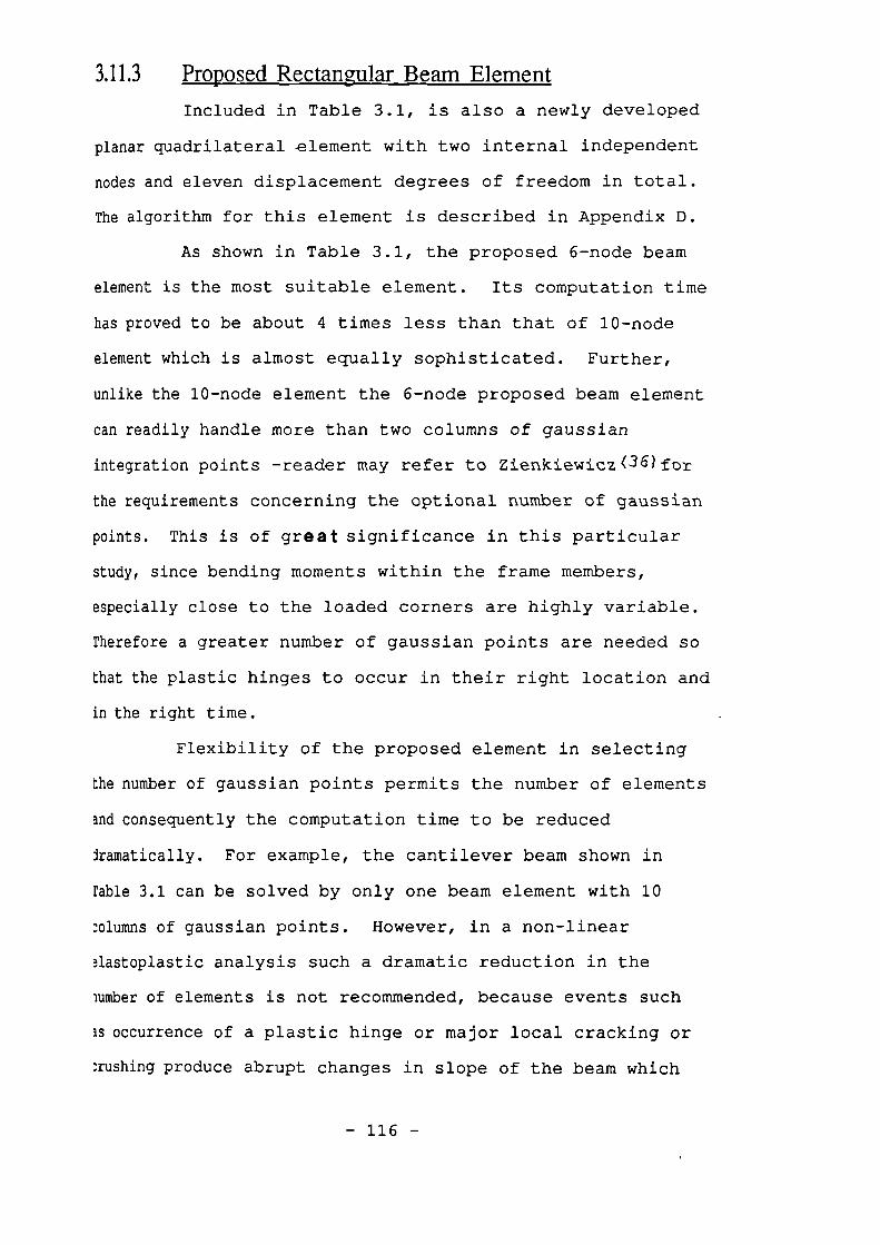
3.11.3 Proposed Rectangular Beam Element
Included in Table 3.1, is also a newly developed
planar quadrilateral -element with two internal independent
nodes and eleven displacement degrees of freedom in total.
The algorithm for this element is described in Appendix D.
As shown in Table 3.1, the proposed 6-node beam
element is the most suitable element. Its computation time
has proved to be about 4 times less than that of 10-node
element which is almost equally sophisticated. Further,
unlike the 10-node element the 6-node proposed beam element
can readily handle more than two columns of gaussian
integration points -reader may refer to Zienkiewicz(36)for
the requirements concerning the optional number of gaussian
points. This is of great significance in this particular
study, since bending moments within the frame members,
especially close to the loaded corners are highly variable.
Therefore a greater number of gaussian points are needed so
that the plastic hinges to occur in their right location and
in the right time.
Flexibility of the proposed element in selecting
the number of gaussian points permits the number of elements
amiconsequently the computation time to be reduced
lramatically. For example, the cantilever beam shown in
Fable 3.1 can be solved by only one beam element with 10
columns of gaussian points. However, in a non-linear
alastoplastic analysis such a dramatic reduction in the
lumber of elements is not recommended, because events such
is occurrence of a plastic hinge or major local cracking or
:rushing produce abrupt changes in slope of the beam which
- 116 -
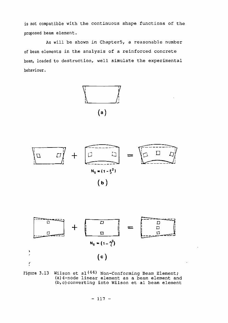
0
- -A
0
is not compatible with the continuous shape functions of the
proposed beam element.
As will be shown in Chapter5, a reasonable number
of beam elements in the analysis of a reinforced concrete
beam, loaded to destruction, well simulate the experimental
behaviour.
_
( a )
c
Figure 3.13 Wilson et al( 44 ) Non-Conforming Beam Element;(a)4-node linear element as a beam element and(b,c)converting into Wilson et al beam element
- 117 -
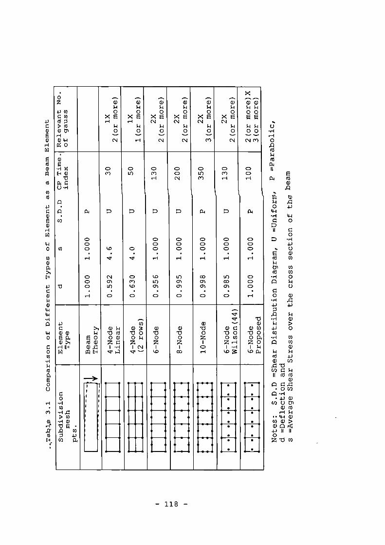
— 118 —
•Z
41 EnA cf)al 0> (IIa) triH0) 4-IA 0
o,.....
a)
0>E,-1
1.40
N
___a)P0
X EH
P0
r-1
.,.....a)
..10
XN
$-4o
CV
,.....
a)
0><EN
o
N
.......
a)3-i0
>EN
1-i0
cf)
a)P0
X 5N
Po
(N
>40)0)
1-100EE-1-100NC")
a)5
-.-I XE-1 a)
Tia4 A(J -I-1
A
A
U)
(/)
t
a
000
H
C)0o
H
CDco
l.0.
vi
N01Lr)
0
CDLr)
CD.
v
oCY)l0
•0
0roH
CDCDC>
H
koLn01
CD
CD(oN
00CD
..-1
Lr)0101
.0
CDLOCr)
a
CD0C>
H
000101
0
0(Y)H
CD0CD
.H
tf)co01
•0
0cpI-1
1
a
0CDCD
.I-1
0.o0
•H
4--I
0)0)E04a) >-,
H E-Ifil
>.,p
5 o(I) a)0J,P:1 El
a) $-1'(U00)Z 0
I -HV I-4
co41) 3
rti 0o PZIN
•q• —
a)'00Z
ILO
a)730Z
I00
a)'00Z
1cDH
.-.•qnvo
a)"0 00U)Z -I
I -Hll)
'Cia)
a) Ea'0 0o04Z 0
I $-iV) Cy
o•Hu)-H 4> En
-.-I a)'0 5 •.0 coco 0.,
--)1'1...-.1
,II 1
iI N..
.. esN II
(I)a)
E-1
4.)
a)
a)tk
0
0
04
0C.)
3.12 Choice Of Masonry Infilled Rune Subdivision
Blockwork infilling walls of single storey
normally consist of at least 12 courses of blockwork. The
exact subdivision of such a masonry panel into single block
elements, when the masonry equivalent and interface elements
described in Sections 3.9.6 and 3.9.8 are used, involve
12x6x12 = 864 nodal displacements, added to which there are
the nodal displacements of the boundary frame. Solution of
such a high number of equations several times in a non-
linear elastoplastic analysis is uneconomical.
The computation time of the problem can be
reduced, however, by the choice of a subdivision mesh based
on imaginary larger masonry units and proportionally thicker
mortar joints and consequently lesser number of courses of
blockwork, while keeping the size of the panel unchanged.
This choice is acceptable provided that such a subdivision
mesh is still fine enough to maintain a reasonable accuracy
of stress distribution and also not to change the state and
pattern of the cracks and the state of bed and head joints.
In order to select a suitable subdivision mesh
some elastic finite element analyses were carried out on 12,
10, 8 and 4-course blockwork infills allowing for no joint
failure. The results are plotted in Fig 3.14 comparing the
stress distribution along the infill diagonal and the frame-
infill boundary for the examples tested. As shown, the
results of 12 and 10-course blockwork infills are identical
showing that these meshes are sufficiently fine. The
results of
8-course blockwork infill is in a fairly good agreement with
— 119 —
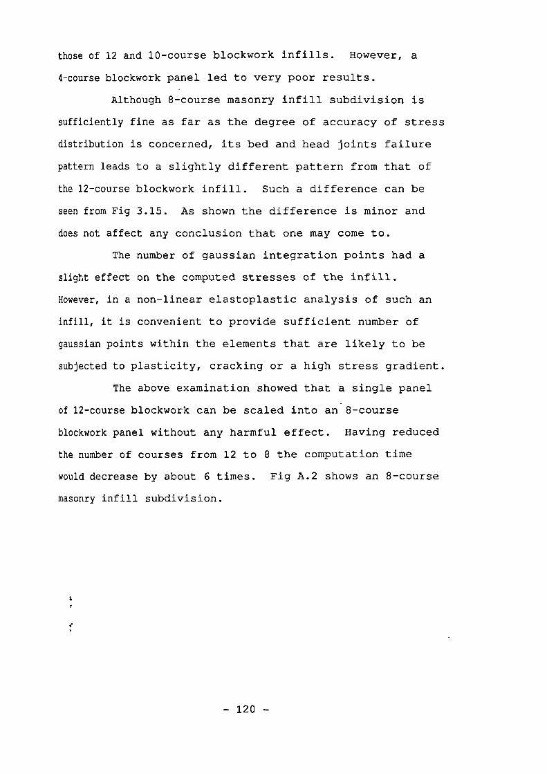
those of 12 and 10-course blockwork infills. However, a
4-course blockwork panel led to very poor results.
Although 8-course masonry inf ill subdivision is
sufficiently fine as far as the degree of accuracy of stress
distribution is concerned, its bed and head joints failure
pattern leads to a slightly different pattern from that of
the 12-course blockwork infill. Such a difference can be
seen from Fig 3.15. As shown the difference is minor and
does not affect any conclusion that one may come to.
The number of gaussian integration points had a
slight effect on the computed stresses of the infill.
However, in a non-linear elastoplastic analysis of such an
it is convenient to provide sufficient number of
gatissian points within the elements that are likely to be
subjected to plasticity, cracking or a high stress gradient.
The above examination showed that a single panel
of 12-course blockwork can be scaled into an 8-course
blockwork panel without any harmful effect. Having reduced
the number of courses from 12 to 8 the computation time
would decrease by about 6 times. Fig A.2 shows an 8-course
masonry infill subdivision.
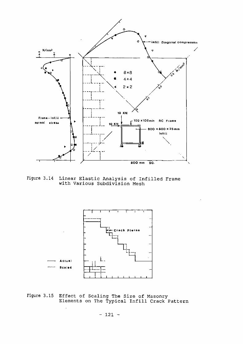
Frame— infill
normal stread
--I9-1. Crack Pterne
L.
— Actual
Scaled
I
Infill Diagonal compression
N/mm2
Figure 3.14 Linear Elastic Analysis of Infilled Framewith Various Subdivision Mesh
Figure 3.15 Effect of Scaling The Size of MasonryElements on The Typical Infill Crack Pattern
- 121 -
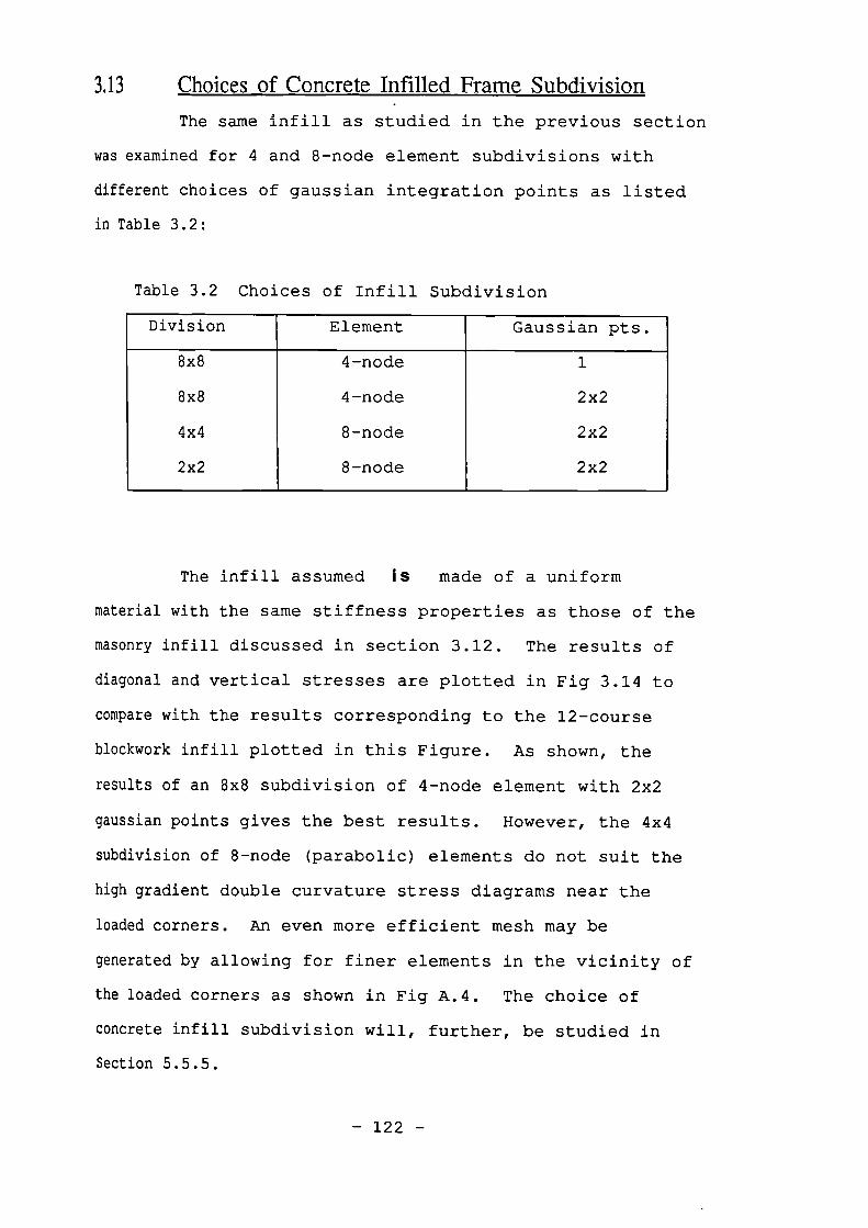
3.13 Choices of Concrete Infilled Frame Subdivision
The same infill as studied in the previous section
was examined for 4 and 8-node element subdivisions with
different choices of gaussian integration points as listed
in Table 3.2:
Table 3.2 Choices of Infill Subdivision
Division Element Gaussian pts.
8x8
8x8
4x4
2x2
4-node
4-node
8-node
8-node
1
2x2
2x2
2x2
The infill assumed IS made of a uniform
material with the same stiffness properties as those of the
masonry infill discussed in section 3.12. The results of
diagonal and vertical stresses are plotted in Fig 3.14 to
compare with the results corresponding to the 12-course
blockwork infill plotted in this Figure. As shown, the
results of an 8x8 subdivision of 4-node element with 2x2
gaussian points gives the best results. However, the 4x4
subdivision of 8-node (parabolic) elements do not suit the
high gradient double curvature stress diagrams near the
loaded corners. An even more efficient mesh may be
generated by allowing for finer elements in the vicinity of
the loaded corners as shown in Fig A.4. The choice of
concrete infill subdivision will, further, be studied in
Section 5.5.5.
- 122 -
CHAPTER FOUR
Constitutive Formulation of
Materials
41
The F.E formulation has been described in
Chapter 3. Calculation of the incremental stress-strain
relation matrix, (Dt], and also the current stress vector,
NI, in terms of the current strains and loading history
are dependent on the mechanical behaviour of the
materials which is discussed in this chapter.
The mechanical behaviour of the material normally
used in infilled frames are non-linear and elastoplastic.
The significance of the effect of non-linearity and
plasticity of material in the analysis of infilled frames
has been discussed in Chapter 2 and the various sources of
mm-linearity has been Outlined in Table 2.2. It has also
been concluded in Section 2.9, that an acceptable infilled
frame analysis must be enhanced by a set of fairly accurate
material models so as to simulate the elastoplastic
behaviour of the constituents of the structure (frame and
infill) as well as the interface between these constituents.
Since different materials behaves differently, the commonly
used materials may be categorized into the following groups;
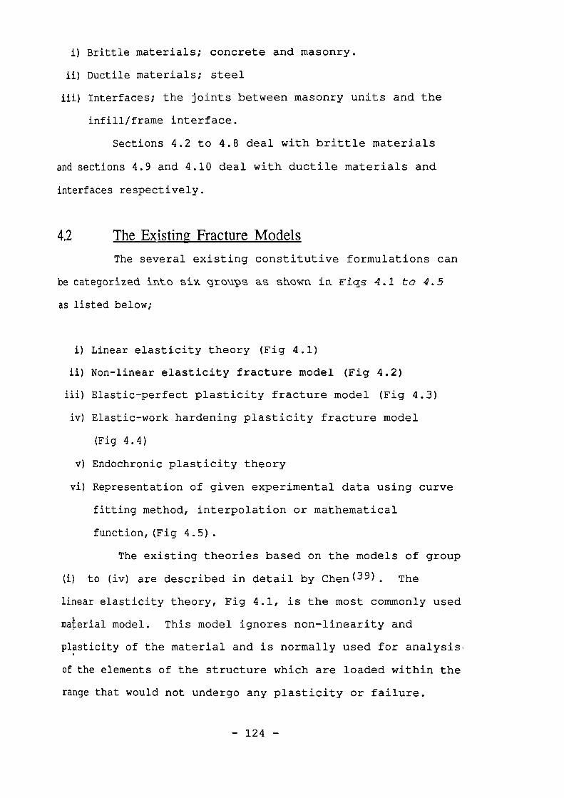
i) Brittle materials; concrete and masonry.
ii)Ductile materials; steel
iii)Interfaces; the joints between masonry units and the
infill/frame interface.
Sections 4.2 to 4.8 deal with brittle materials
and sections 4.9 and 4.10 deal with ductile materials and
interfaces respectively.
4.2 The Existing Fracture Models
The several existing constitutive formulations can
be categorized into six grovps as stown in Figs 4.1 to 4.5
as listed below;
i) Linear elasticity theory (Fig 4.1)
ii)Non-linear elasticity fracture model (Fig 4.2)
iii)Elastic-perfect plasticity fracture model (Fig 4.3)
Elastic-work hardening plasticity fracture model
(Fig 4.4)
v) Endochronic plasticity theory
vi) Representation of given experimental data using curve
fitting method, interpolation or mathematical
function, (Fig 4.5).
The existing theories based on the models of group
(i) to (iv) are described in detail by Chen( 39 ). The
linear elasticity theory, Fig 4.1, is the most commonly used
material model. This model ignores non-linearity and
plasticity of the material and is normally used for analysis-
of the elements of the structure which are loaded within the
range that would not undergo any plasticity or failure.
- 124 -

The models of groups (ii) to (iv), illustrated in
Figs 4.2 to 4.4 respectively, are based on idealization of
material by an elastic or plastic model. These models are
neither exact nor impressively accurate but even so they
may be rather complicated. Because of the idealization of
the behaviour of the material, these models are disconti-
nuous material models dividing the material responses into
several stages. However, the actual behaviour of a non-
cracked material is continuous. Further, such discontinuous
models, while simplifying the problem, are the source of
numerical difficulties ( 39 ) . Nevertheless the elastic-
perfect plasticity fracture model (for both tension and
compression) suits steel material. This will be discussed
in section 4.9.
The endochronic theory has received much attention
in recent years because it is based on a continuous model.
This model was originated by Valanis (45 ) (1971) for metal,
based on the concept of P Entrinsic time." The theory does
not require a specific definition of yielding. Bazant ( 46 ) •
(1976) extended the theory to describe the behaviour of
brittle materials. For concrete, the formulation of the
endochronic model is based on an extensive set of functions
which fit nearly all the experimentally observed effects.
However, "this model involves a rather high number of
material parameters. Therefore further research in refining
this theory is needed," Chen (39) .
Since the aforesaid purely theoretical models
involve extensive numerical work, in practice, either a
simple uniaxial model is generalized to form a three-
- 125 -
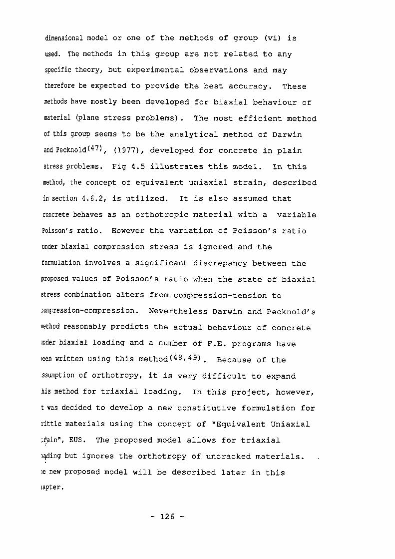
dimensional model or one of the methods of group (vi) is
used. The methods in this group are not related to any
specific theory, but experimental observations and may
therefore be expected to provide the best accuracy. These
methods have mostly been developed for biaxial behaviour of
material (plane stress problems) . The most efficient method
of this group seems to be the analytical method of Darwin
and Pecknold (47 ) , (1977) , developed for concrete in plain
stress problems. Fig 4.5 illustrates this model. In this
method, the concept of equivalent uniaxial strain, described
In section 4.6.2, is utilized. It is also assumed that
concrete behaves as an orthotropic material with a variable
Poisson's ratio. However the variation of Poisson's ratio
under biaxial compression stress is ignored and the
formulation involves a significant discrepancy between the
proposed values of Poisson' s ratio when the state of biaxial
stress combination alters from compression-tension to
:ompression-compression. Nevertheless Darwin and Pecknold's
nethod reasonably predicts the actual behaviour of concrete
Inder biaxial loading and a number of F.E. programs have
,een written using this method (48 , 49 ) . Because of the
ssumption of orthotropy, it is very difficult to expand
his method for triaxial loading. In this project, however,
t was decided to develop a new constitutive formulation for
rittle materials using the concept of "Equivalent Uniaxial
tfain", EUS. The proposed model allows for triaxial
)4ding but ignores the orthotropy of uncracked materials.
le new proposed model will be described later in this
lapter.
- 126 -
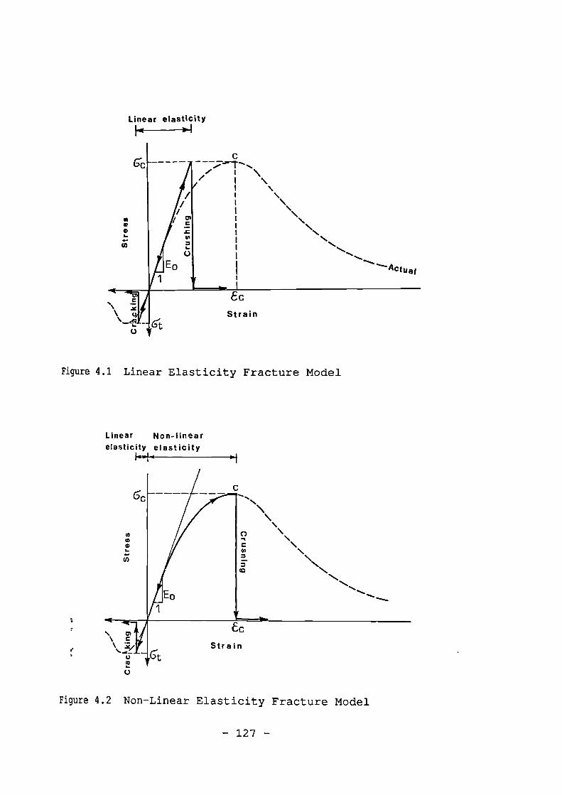
C--.03-----r---,
s,........
Linear elasticity
1E
//i
o)c2enc...0
. . i\
1 ./ 1 .
1 .1 .1 .
11111I
111
. . . .
s, s,s, ss ....„.__
Actual
6-t
EC
Strain
Figure 4.1 Linear Elasticity Fracture Model
Linear Non-linear
elasticity elasticitylapi 4 , i
Figure 4.2 Non-Linear Elasticity Fracture Model
- 127 -
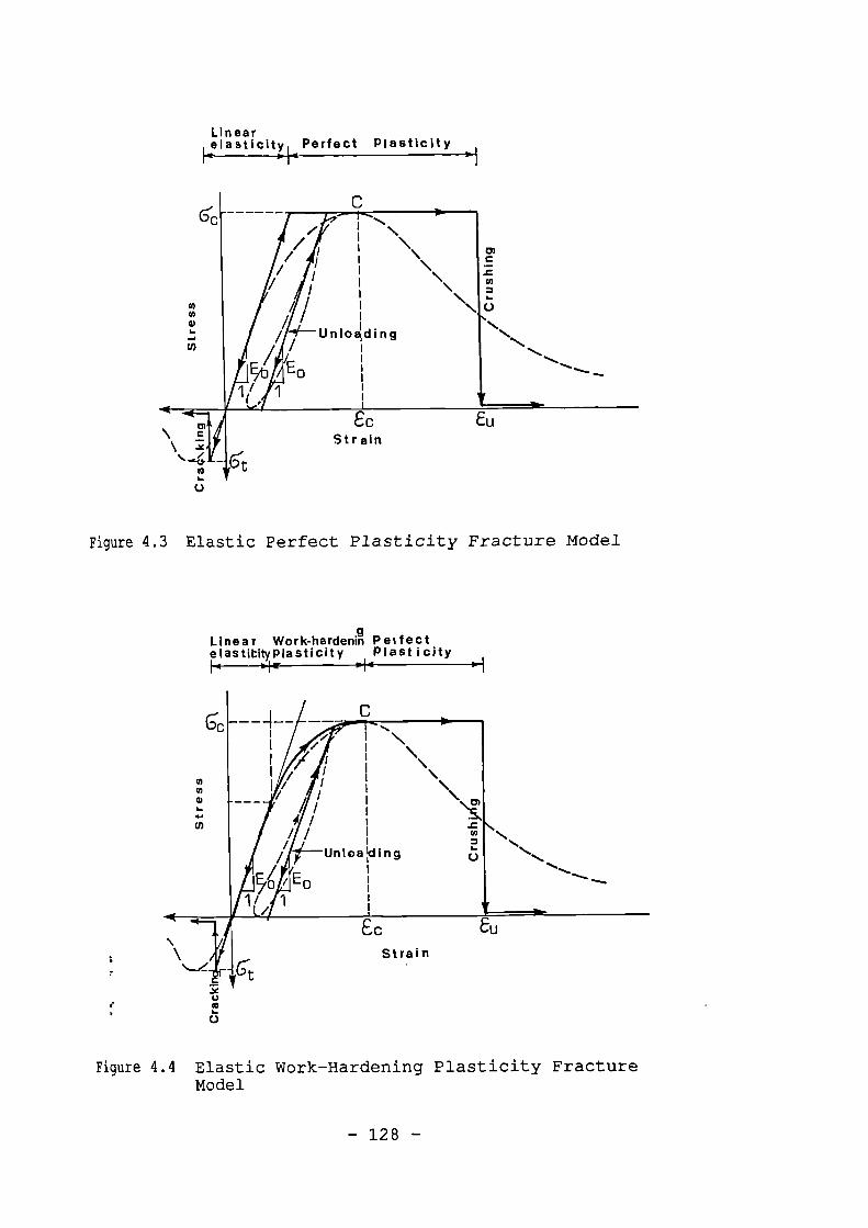
Ec
EuStrain
eu
Linear, elasticity Perfect Plasticity
1-1
/ \
/ \/ 1 \ cn
c/ \ I'
/ \/ / \ co;
=\
/ I Unloading
nn-.
/
,f0 Eo
-,,..,
----...
1 1
Figure 4.3 Elastic Perfect Plasticity Fracture Model
Linear Work-hardenin PeifectelastibityPlasticity Plasticity
Figure 4.4 Elastic Work-Hardening Plasticity FractureModel
- 128 -
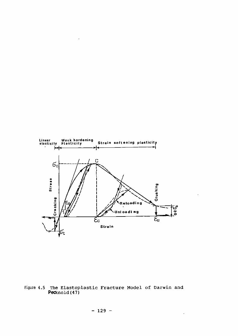
/ Reloading
Unloading
EcStrain
0.10
Linear Woik hardeningelasticity Plasticity Strain soft ening plasticity
Figure 4.5 The Elastoplastic Fracture Model of Darwin andPeCknold(47)
- 129 -
E
- 2)(--)+ (E
---)2
EC Cc
:,
4.3 Proposed Constitutive Formulation for Brittle
Materials Under Uniaxial Compression
4.3.1 Stress-Strain Relation
The typical stress-strain relationship for
concrete subjected to uniaxial compression is shown in Fig
4.6(a). Concrete has a nearly linear-elastic behaviour up
to about 30 percent of its compressive strength ac. For
stresses above this point the stress-strain curve shows a
gradual increase in curvature up to the peak point, ac, due
to extension of microcracks. Beyond this peak, the stress-
strain curve has a falling branch until crushing failure
occurs at some ultimate strain, E.Wischers (50) (1978) carried out a series of
uniaxial loading tests on necked specimens in order to
exclude the confinement effect of the end platens. The
results of these tests are plotted in Fig 4.7. As shown the
shape of the stress-strain curve is similar for concrete of
low, medium and high strength. However, a high-strength
concrete behaves in a more brittle manner, the stress
dropping off more sharply than it does for concrete with
lower strength.
For the rising branch of the stress-strain curves,
the well known Saenz ( 51 ) equation may be adopted as follows;
E
G = EO (4.1)
:.
ghere a and e are the stress and strain and Eo and Ec(Ec=adec) are the initial tangent and secant modulus at
- 130 -
peak respectively and Ec is the strain at peak stress.
Eq4.1 for Eo/Ec<2 gives an unrealistic point of inflexion
somewhere on the curve. The following proposed equation
thus may be used when E0/Ec<2;
6 = Eo (4.2)EO e g
1+ - 1 )(---)Ec cc
where1 Eo
g - and <2
(4.3)1 - E0/E0 EC
It should be noted that for E0/Ec=2 equations 4.2
and 4.1 are identical, thus continuity between the two
is maintained.
For the falling branch of the stress-strain curve,
several observations and data (50 to 60) and especially the
work of Wischers (50) , Fig 4.7, were studied and compared, to
derive the following proposed simple equation:
aca - ( 4.4)
1 + D( -1)2
EC
where for concrete:
ac 2.15D = 10 (- 5( 0.25
100 )(4.5)
It should be mentioned that Eq 4.4 is independent of the
initial stiffness of the material. The tangent value of the
modulus of elasticity, Et, may be derived by differentiation
ofEqs 4.1, 4.2 and 4.3 in terms of e for E0/Ec > 2 as:
- 131 -
Et - (4.6)E C E 22
[1 + (— - 2)(—) +EC EC CC
and for Eo/Ec < 2 as:
E0[1 - E g
ecEt - (4.7)
E 0 e g-12[1 +(_..__ 1)(—)
Ec EC
and for the falling branch as:
-2EcDEC
Et - (4.8)_ 112 ] 2
[1 + DEC I
As shown in Fig 4.7 the proposed Eqs 4.1 to 4.5 agree well
with a wide range of possible concrete and mortar strengths.
These equations were not examined for brittle materials
other than concrete and mortar but it seems only Eq 4.5
needs some adjustments should a brittle material other than
concrete be used.
The above formulation requires only the initial
tangent modulus, Eo, and the strain at peak, C, and the
unconfined uniaxial strength, ac, to be determined by test
orfany other means for the complete uniaxial stress-strain
curve to be plotted.
- 132 -
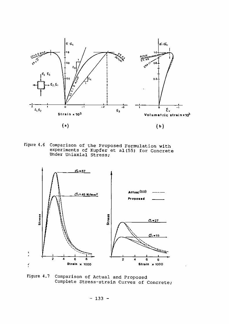
tGc
Ev
Volumetric strain x103
(b)
0.5
( a)
Actual (50) ----
Proposed
0".=.27
CC = 15
;
6 8 2 4 6 8Strain x 1000 Strain x 1000
aaI.
•1;
Figure 4.6 Comparison of the Proposed Formulation withexperiments of Kupfer et al(55) for ConcreteUnder Uniaxial Stress;
Figure 4.7 Comparison of Actual and ProposedComplete Stress-strain Curves of Concrete;
— 133 —
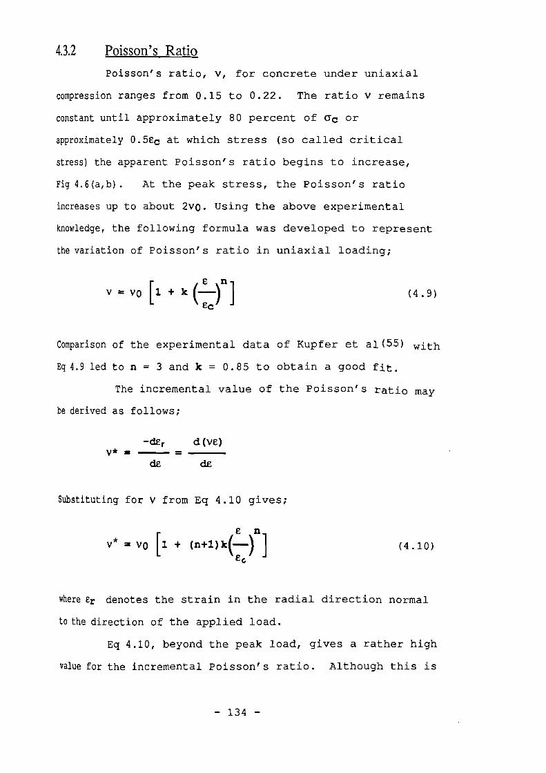
4.12 Poisson's Ratio
Poisson's ratio, V, for concrete under uniaxial
compression ranges from 0.15 to 0.22. The ratio v remains
constant until approximately 80 percent of ac or
approximately 0.5Ec at which stress (so called critical
stress) the apparent Poisson's ratio begins to increase,
Fig 4.6(a,b). At the peak stress, the Poisson's ratio
increases up to about 2v0. Using the above experimental
knowledge, the following formula was developed to represent
the variation of Poisson's ratio in uniaxial loading;
,C fl1.
iV = vo [ + k H
e.(4.9)
Comparison of the experimental data of Kupfer et al (55) with
Eq 4.9 led to n = 3 and k = 0.85 to obtain a good fit.
The incremental value of the Poisson's ratio may
be derived as follows;
v* = -dE r
= d(ve)
de dE
Substituting for V from Eq 4.10 gives;
e n
v * = vo [1 + (n+l)kH ]
EG
(4.10)
where Cr denotes the strain in the radial direction normal
to the direction of the applied load.
Eq 4.10, beyond the peak load, gives a rather high
value for the incremental Poisson's ratio. Although this is
- 134 -
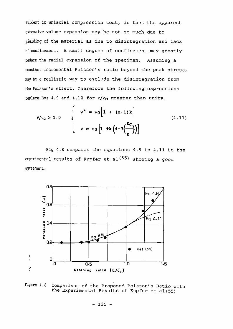
evident in uniaxial compression test, in fact the apparent
extensive volume expansion may be not so much due to
yielding of the material as due to disintegration and lack
of confinement. A small degree of confinement may greatly
reduce the radial expansion of the specimen. Assuming a
constant incremental Poisson's ratio beyond the peak stress,
may be a realistic way to exclude the disintegration from
the Poisson's effect. Therefore the following expressions
Eqs 4.9 and 4.10 for thanreplace eiec greater unity.
Fig 4.8 compares the equations 4.9 to 4.11 to the
experimental results of Kupfer et al (55) showing a good
agreement.
v/vc > 1. 0{ v * = vo [1 + (n+1) k]
ecv = vo [1 +k (4-3ED]
e
(4.11)
0.8
0.60-do4I.
;a.
0.2
:r 0
Eq 4.9
• ...1
49
• Ref (55)
0 05 10
15
f
Straning ratio (E/Ec)
Figure 4.8 Comparison of the Proposed Poisson's Ratio withthe Experimental Results of Kupfer et al (55)
- 135 -
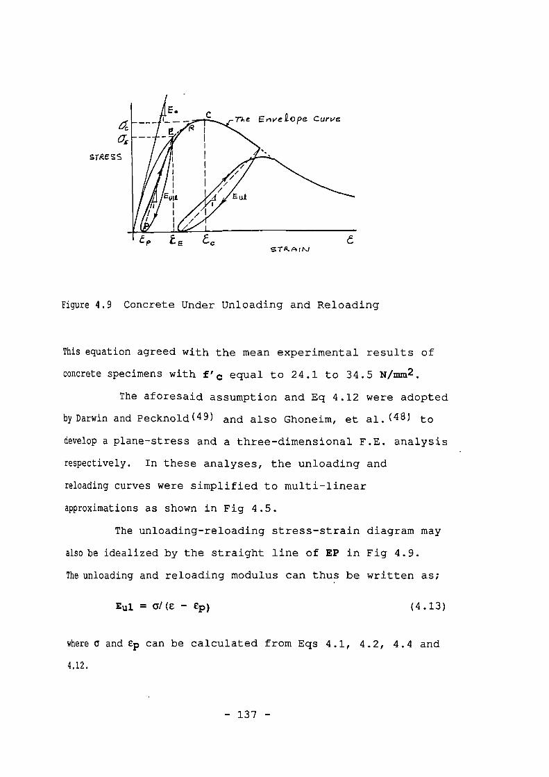
aThe EnveiOpe Curve
STRESS
EsTA.AI
Figure 4.9 Concrete Under Unloading and Reloading
This equation agreed with the mean experimental results of
concrete specimens with f' c equal to 24.1 to 34.5 N/mm2
The aforesaid assumption and Eq 4.12 were adopted
by Darwin and Pecknold( 49 ) and also Ghoneim, et al. (48) to
develop a plane-stress and a three-dimensional F.E. analysis
respectively. In these analyses, the unloading and
reloading curves were simplified to multi-linear
approximations as shown in Fig 4.5.
The unloading-reloading stress-strain diagram may
also be idealized by the straight line of EP in Fig 4.9.
The unloading and reloading modulus can thus be written as;
Eul = (e — CP)
(4.13)
where a and ep can be calculated from Eqs 4.1, 4.2, 4.4 and
4.12.
- 137 -
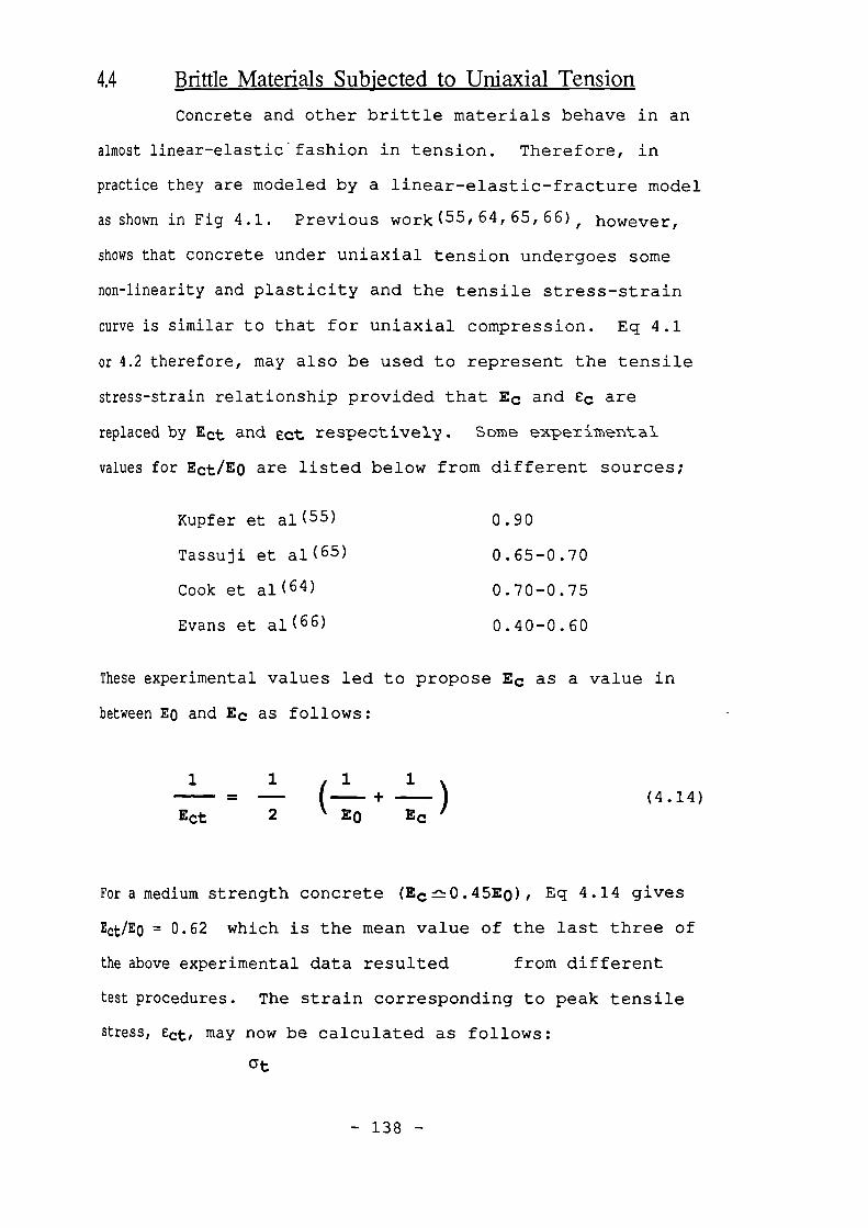
4.4 Brittle Materials Subjected to Uniaxial Tension
Concrete and other brittle materials behave in an
almost linear-elastic - fashion in tension. Therefore, in
practice they are modeled by a linear-elastic-fracture model
as shown in Fig 4.1. Previous work (55164,65,66), however,
shows that concrete under uniaxial tension undergoes some
non-linearity and plasticity and the tensile stress-strain
curve is similar to that for uniaxial compression. Eq 4.1
or 4.2 therefore, may also be used to represent the tensile
stress-strain relationship provided that Ec and Cc are
replaced by Et and cot respectively. Some experimental_
values for Ect/E0 are listed below from different sources;
Kupfer et al (55)
0.90
Tassuji et al (65)
0.65-0.70
Cook et al (64) 0.70-0.75
Evans et al (66) 0.40-0.60
These experimental values led to propose Ec as a value in
between Eo and Ec as follows:
1. 1 1k + -
Et 2 EO Ec(4.14)
For a medium strength concrete (Ec0.45E0) , Eq 4.14 gives
Ect/E0 = 0.62 which is the mean value of the last three of
the above experimental data resulted from different
test procedures. The strain corresponding to peak tensile
stress, Cot, may now be calculated as follows:
at
- 138 -
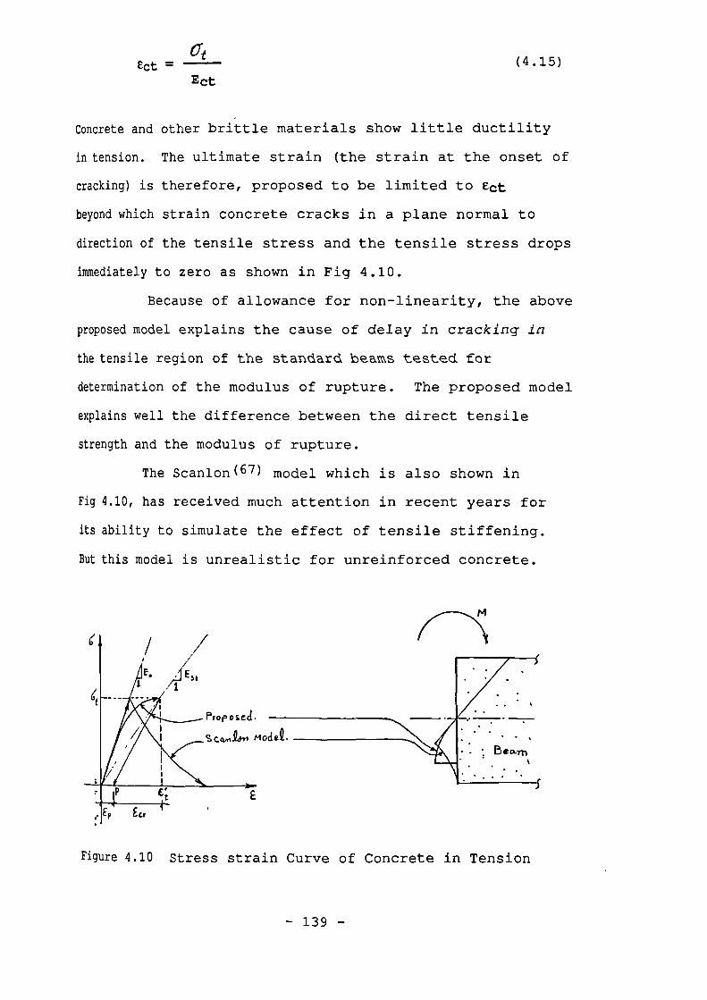
Ect = Ct
(4.15)
Ect
Concrete and other brittle materials show little ductility
In tension. The ultimate strain (the strain at the onset of
cracking) is therefore, proposed to be limited to Ect
beyond which strain concrete cracks in a plane normal to
direction of the tensile stress and the tensile stress drops
immediately to zero as shown in Fig 4.10.
Because of allowance for non-linearity, the above
proposed model explains the cause of delay in cracking- in
the tensile region of the standard beams tested for
determination of the modulus of rupture. The proposed model
explains well the difference between the direct tensile
strength and the modulus of rupture.
The Scanlon (67) model which is also shown in
Fig 4.10, has received much attention in recent years for
its ability to simulate the effect of tensile stiffening.
But this model is unrealistic for unreinforced concrete.
Figure 4.10 Stress strain Curve of Concrete in Tension
- 139 -
5 Failure Criteria
5.1 Chmvmd
In formulating failure criteria for materials, a
7oper definition of failure must be defined. Criteria such
; yielding, initiation of cracking, load-carrying capacity,
id extent of deformation have been used to define failure.
this section failure is defined as the maximum load-
xrying capacity of a test specimen or an element.
Le strength of materials under multiaxial stresses is a
notion of the state of stress and cannot be predicted by
mitation of simple compressive and shearing stresses
dependently of each other.
A failure criterion of isotropic materials based
on state of stress must be an invariant function of the
ate of stress, ie, independent of the choice of the
ordinate system by which stress is defined. One method of
presenting such a function is to use the principal
resses le,
f(a1,02,03) = K (4.16)
indicate the general functional form of the failure
iterion. It is known( 39 ) that any invariant symmetric
lotion of the state of stress can also be expressed in
:xis of the three stress invariants of II, J2 and J3 or
•and 0 , where 0 is the angle from the positive a l axis
1 lies in the deviatoric plane, Chen( 39 ). Thus one can
)lace Eq 4.16 by:
- 140 -
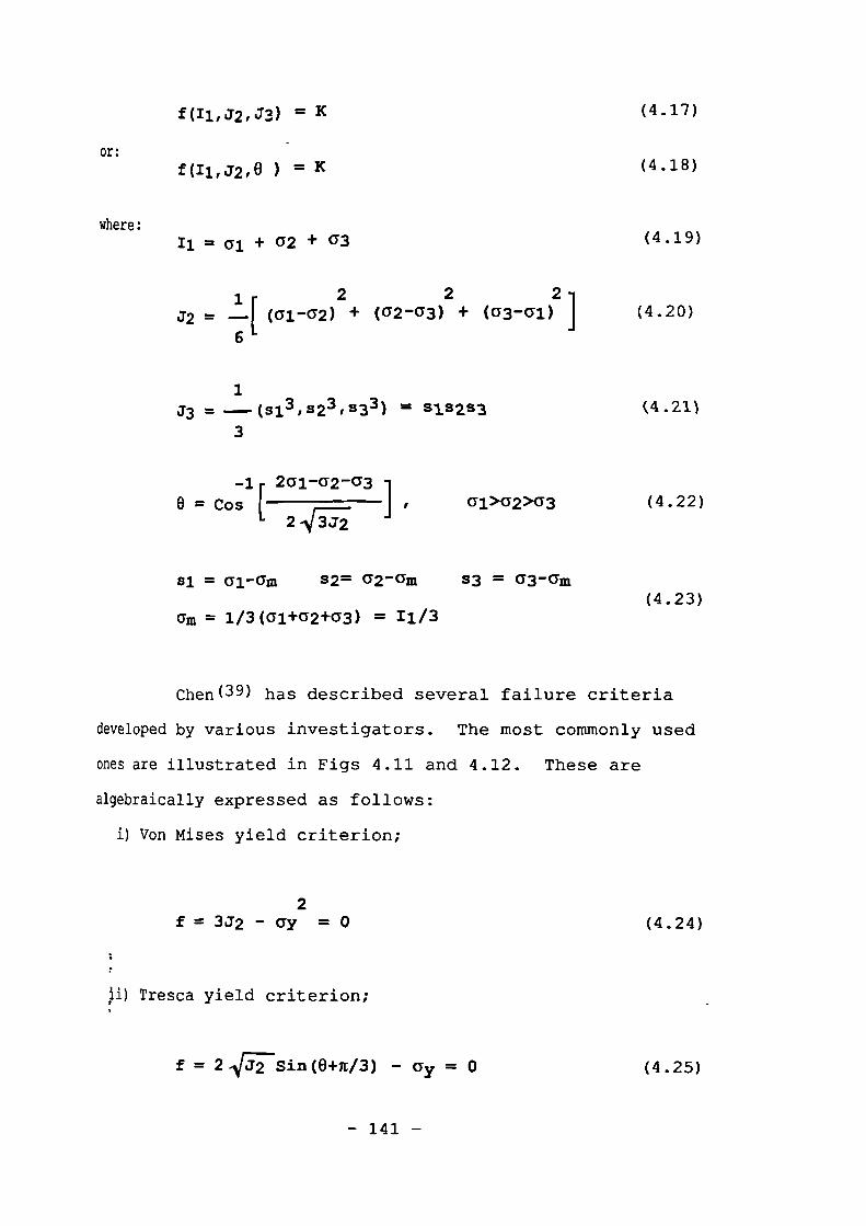
f ( 11072, 473) = K
f( 11,J210 ) = Kor:
where:Ii = al + a2 + 03
(4.19)
2 2
J2 = 1 [ (al-a2) + ( 02-a3) + 03- 051;2 ]
)(4.20
6
13 3 s,3 -J3 = (si-,s2 . a ) - s1s2s3 (4.213
3
-14 2al-a2-a3 ] ,0 = Cos
0-1>G2>G3211iT2-
(4.22)
Si = al-am 52= a2-am S3 = 63-Gm
(4.23)Gm = 1/3(al+a2+ $53) = 11/3
Chen (39) has described several failure criteria
developed by various investigators. The most commonly used
ones are illustrated in Figs 4.11 and 4.12. These are
algebraically expressed as follows:
i) Von Mises yield criterion;
2f = 3J2 - ay =0 (4.24)
:7
i) Tresca yield criterion;
f = 2 1/Sin(0+7E/3) - ay = 0 (4.25)
- 141 -
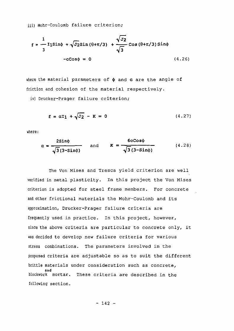
iii)Mohr-Coulomb failure criterion;
1 1/72%Simi) + 1177-2Sin (8+7c/3) + — Cos (6+7c/3) Sin4)
3 Iii
-cCos4) = 0 (4.26)
where the material parameters of 4) and c are the angle of
friction and cohesion of the material respectively.
iv)Drucker-Prager failure criterion;
f = cal + 14/772 - K = 0 (4.27)
where:
2Sin4) 6cCos0
a and K — (4.28)157(3-Sin0 ) 15-(3-Sin0
The Von Mises and Tresca yield criterion are well
verified in metal plasticity. In this project the Von Mises
criterion is adopted for steel frame members. For concrete
and other frictional materials the Mohr-Coulomb and its
approximation, Drucker-Prager failure criteria are
frequently used in practice. In this project, however,
since the above criteria are particular to concrete only, it
was decided to develop new failure criteria for various
stress combinations. The parameters involved in the
proposed criteria are adjustable so as to suit the different
brittle materials under consideration such as concrete,and
blockwork mortar. These criteria are described in the
following section.
f=
- 142 -
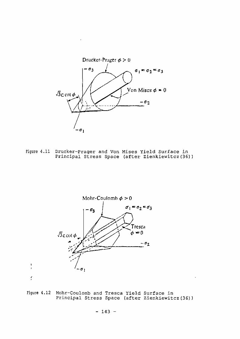
Drucker-Prager > 0
63 61 11 Q2 C3
Von Miscs 1. 0Cot Cto
-a]
Figure 4.11 Drucker-Prager and Von Mises Yield Surface inPrincipal Stress Space (after Zienkiewitcz (36) )
Mohr-Coulomb 0 >0
fri=ca=a3
Figure 4.12 Mohr-Coulomb and Tresca Yield Surface inPrincipal Stress Space (after Zienkiewitcz (36) )
- 143 -
4,5.2 Proposed Failure Criterion of Brittle Materials
under Triaxial Compression
Using the principal stresses, al, a2 and u3 while:
0 > al > a2 > a3 (comp. -ve)
The following stress function is proposed in order to
incorporate the variation in material types;
f - + (Ye2 = 0 (4.29)
203-0.2) (a3-01)(a2-01)
al 12{1 + c(---)
ac
_2 al 12fbc[1 + kc(--)
ac
where fbc = fbc/ac denotes the ratio of equal-biaxial
compressive strength to the unconfined uniaxial compressive
strength. q is a material constant value controlling the
curvature of the failure surface in the tensile and
compressive meridians (Fig 4.14). c is the slope of the
compressive meridian at al=ac and k is a constant relating
the tensile meridian to the compressive meridian. These
constant values may be adjusted to suit any brittle material
using the following approach.
a) Biaxial Compression
When al becomes zero, Eq. 4.29 reduces to:
f = 03 2 + 02 2 - (2-1/Fisc2 )a2a3 - ac2 = 0 (4.30)
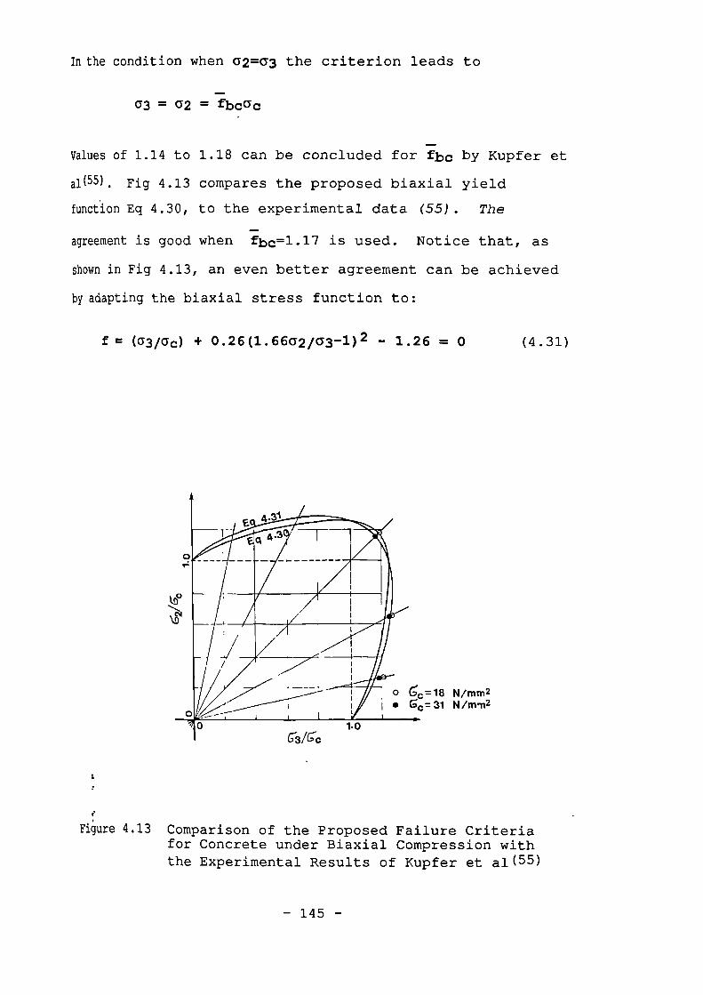
Inthecondition when 02=03 the criterion leads to
-03 = 02 = fbcac
_Values of 1.14 to 1.18 can be concluded for fbc by Kupfer et
al (55) . Fig 4.13 compares the proposed biaxial yield
function Eq 4.30, to the experimental data (55). The-
agreement is good when fbc=1.17 is used. Notice that, as
shown in Fig 4.13, an even better agreement can be achieved
by adapting the biaxial stress function to:
f = ( a3/ac) + 0.26(1.66a2/a3-1) 2 - 1.26 = 0 (4.31)
fFigure 4.13 Comparison of the Proposed Failure Criteria
for Concrete under Biaxial Compression withthe Experimental Results of Kupfer et al(55)
- 145 -
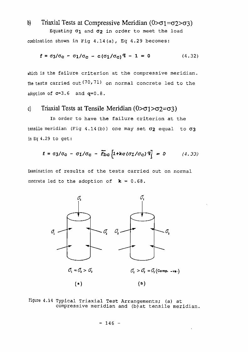
b) Triaxial Tests at Compressive Meridian (0>a1=c72>$53)Equating al and a2 in order to meet the load
combination shown in Fig 4.14 (a), Eq 4.29 becomes:
f = a3/ac - allac - c(al/ac) cl - 1 = 0 (4.32)
which is the failure criterion at the compressive meridian.
The tests carried out (70 / 7 11 on normal concrete led to the
adoption of c=3.6 and q=0.8.
c) Triaxial Tests at Tensile Meridian (0>alx52=(53)
In order to have the failure criterion at the
tensile meridian (Fig 4.14 (b) ) one may set a2 equal to (33
in Eq 4.29 to get:
f = a3/ac - a1/crc - fbc pkc tai/ac) g/ = 0 (4.33)
Examination of results of the tests carried out on normal
concrete led to the adoption of k = 0.68.
0; >4 =4(Comp. -vs.)
(a) ( b )
Figure 4.14 Typical Triaxial Test Arrangements; (a) atcompressive meridian and (b) at tensile meridian.
- 146 -
By the same procedure as followed in this section
for normal concrete the constant parameters fbc, q, c and k
can be determined for any other brittle materials. While k
and fix are expected to have only small variations for
different brittle materials, q and c are expected to vary
considerably. The experimental results of Khoo and
Hendry( 72) suggest c=1.91 and q=0.73 for the mortar types
commonly used in masonry.
4.5.3 Proposed Failure Criterion for Brittle Materials
under Triaxial Compression-Tension
Using the principal stresses, while:
Y3 < (52 < 0 < al (comp. -ve)
the failure surface function is proposed as follows:
f= (a3-2) 2 + ( ccal) 2 +A ( aal) (a3+a2) + ( 1 /Fbc2 ) a2a3 -ac2 = 0
(4.34)
Mere a denotes the ratio of unconfined uniaxial compressive
strength, Cc, to direct tensile strength, at, and A is a
constant controlling the curvature of the failure surface in
biaxial compression-tension. This constant is highly
variable and can be adjusted for any brittle material as
will be discussed later. The above criterion may be examined
using the available test results as follows:
a)- Biaxial Compression (1=0)
When al equals zero, Eq 4.34 becomes identical to -
Eg 4.30. This proves the continuity of Eq 4.34 and Eq 4.29.
- 147 -
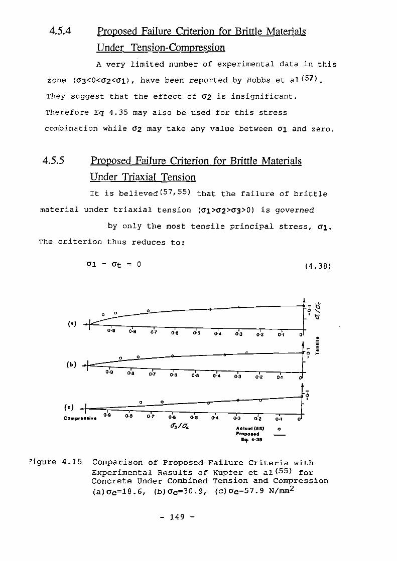
al - at = 0
(4.38)
7 t)'NI0
(a)0 .9 0-8 04 0-6 0-5 04 0-3 0-2
0-1
0
70I-
(b)
(c)0-9
Compressive 0-8 0-7 0-6 0-5 0-4 0-3 0-2
01 lac Aotual (55) 0Proposed
Eq. 4-35
00-1
00
4.5.4 Proposed Failure Criterion for Brittle Materials
Under Tension-Compression
A very limited number of experimental data in this
zone (a3<0<a2<a1), have been reported by Hobbs et al (57)
They suggest that the effect of a2 is insignificant.
Therefore Eq 4.35 may also be used for this stress
combination while a2 may take any value between al and zero.
4.5.5 Proposed Failure Criterion for Brittle Materials
Under Triaxial Tension
It is believed (57 , 55) that the failure of brittle
material under triaxial tension (al>a2>a3>0) is governed
by only the most tensile principal stress, al.
The criterion thus reduces to:
Figure 4.15 Comparison of Proposed Failure Criteria withExperimental Results of Kupfer et al( 55) forConcrete Under Combined Tension and Compression
(a)ac=18.6, (b)ac=30.9, (c)ac=57.9 N/mm2
- 149 -
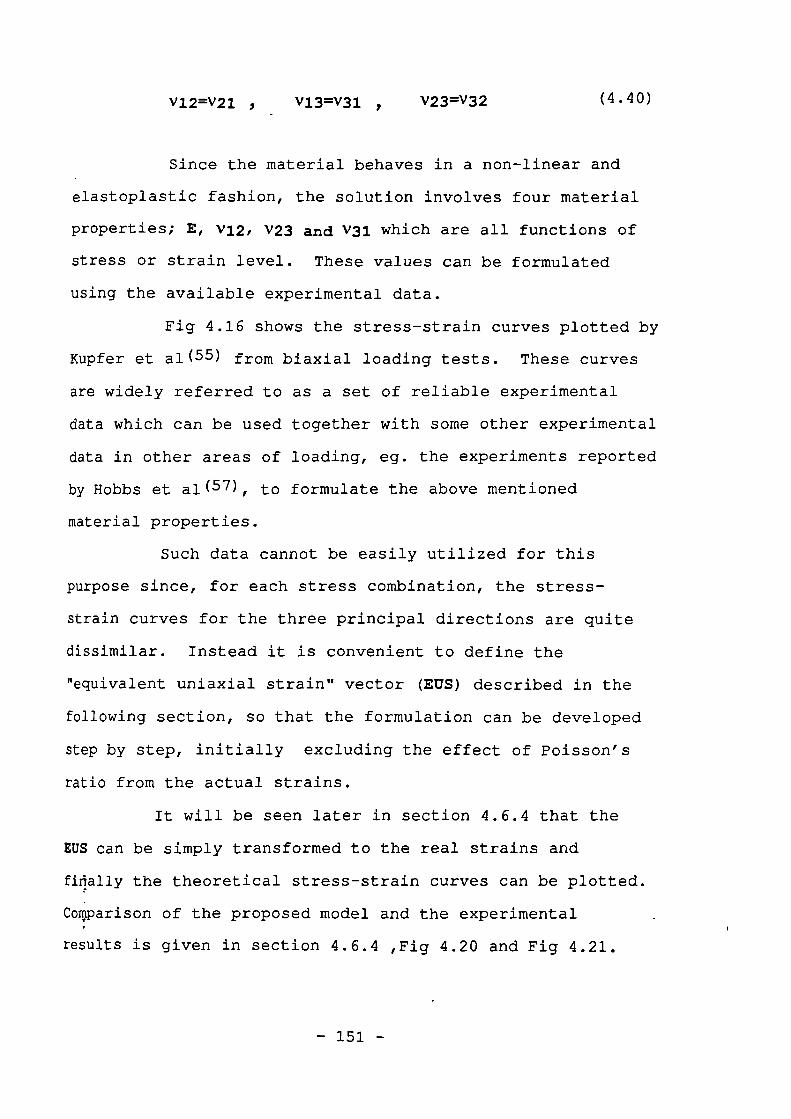
V12=V21 , V13=V31 7
V23=V3 2
(4.40)
Since the material behaves in a non-linear and
elastoplastic fashion, the solution involves four material
properties; E, v12, V23 and V31 which are all functions of
stress or strain level. These values can be formulated
using the available experimental data.
Fig 4.16 shows the stress-strain curves plotted by
Kupfer et al( 55 ) from biaxial loading tests. These curves
are widely referred to as a set of reliable experimental
data which can be used together with some other experimental
data in other areas of loading, eg. the experiments reported
by Hobbs et al (57), to formulate the above mentioned
material properties.
Such data cannot be easily utilized for this
purpose since, for each stress combination, the stress-
strain curves for the three principal directions are quite
dissimilar. Instead it is convenient to define the
"equivalent uniaxial strain" vector (EUS) described in the
following section, so that the formulation can be developed
step by step, initially excluding the effect of Poisson's
ratio from the actual strains.
It will be seen later in section 4.6.4 that the
EUS can be simply transformed to the real strains and
finally the theoretical stress-strain curves can be plotted.,
Couerison of the proposed model and the experimental
results is given in section 4.6.4 ,Fig 4.20 and Fig 4.21.
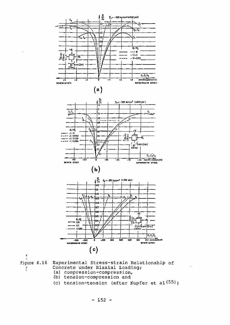
1•10211.1= .2 ..tC2
Ps.pp c -328 Itp/cm2 (4650 psi)
11011111111'WANIII I °' mumn11 Elgi-08,--
61/6'2
- 1 / 0
1/ 1 ---- -1/-052
20 5crn(2in)(791n)
CI. C2
CI
.61
4 •tensile strain
.1 4 3 mm/radoww4compresswestrom
(a)
pp .-326 kp/cm2 (4650 psi )
CI
•4ga"
p-4—
4muiro20(19in)
£ 1 . E2.C2
(b)
-Q50 -10 -15.10 .05tensile strain
-20 rnm/in (0001in/h)compressive strain
Pe
..2
- .
.11
31.10
MUM..m.n CI CZ
CClE
. /F-11 A AdUME ' MIMI=
Mill IIIVIM ,
g .qP, i
--yarMI'
WWIIWA-)g)— Ili
: ----- 1/055
‘,, tc
al ',... JAIir
(29In)1- 20+5cm(2Dh)
1 CI.C2.E3
-004 -002
0 .002 034
COS 038 (DO 012 noon Ma
compressive stroh
tensile strain
(C)
Figure 4.16 Experimental Stress-strain Relationship ofConcrete under Biaxial Loading;(a) compression-compression,(b) tension-compression and(c) tension-tension (after Kupfer et al(55))
- 152 -
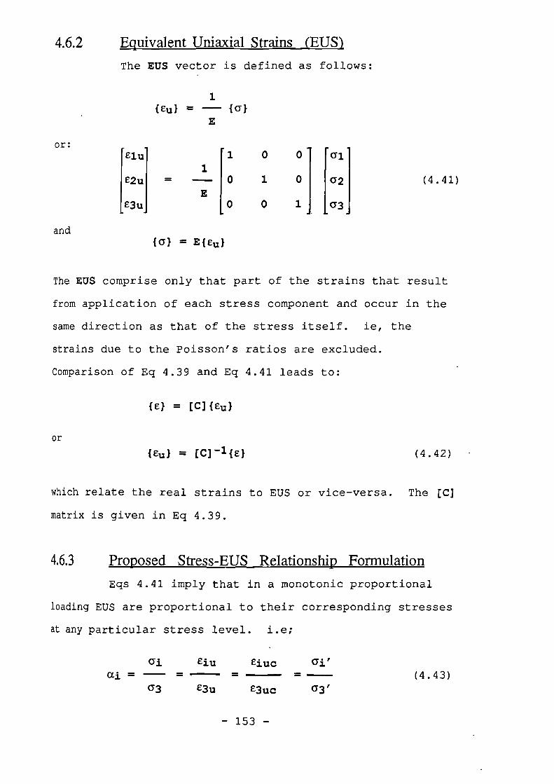
ai'
a3'(4.43)
4.6.2 Equivalent Uniaxial Strains (EUS)
The EUS vector is defined as follows:
1
or:Clu
E2u
E3u
{a}
0 1 0
I 1
0 0
0 0 1 I.
al
a2
a3
(4.41)
{Cu} =
1
and( 0 } = E{CI}
The EUS comprise only that part of the strains that result
from application of each stress component and occur in the
same direction as that of the stress itself. ie , the
strains due to the Poisson's ratios are excluded.
Comparison of Eq 4.39 and Eq 4.41 leads to:
fel = [c]{eul
or
{ Cu} = [C]1{e}
(4.42)
which relate the real strains to EUS or vice-versa. The [C]
matrix is given in Eq 4.39.
4.6.3 Proposed Stress-EUS Relationship Formulation
Eqs 4.41 imply that in a monotonic proportional
loading EUS are proportional to their corresponding stresses
at any particular stress level. i.e;
ai eiU Eiucai =
a3 E3u E3uc
- 153 -
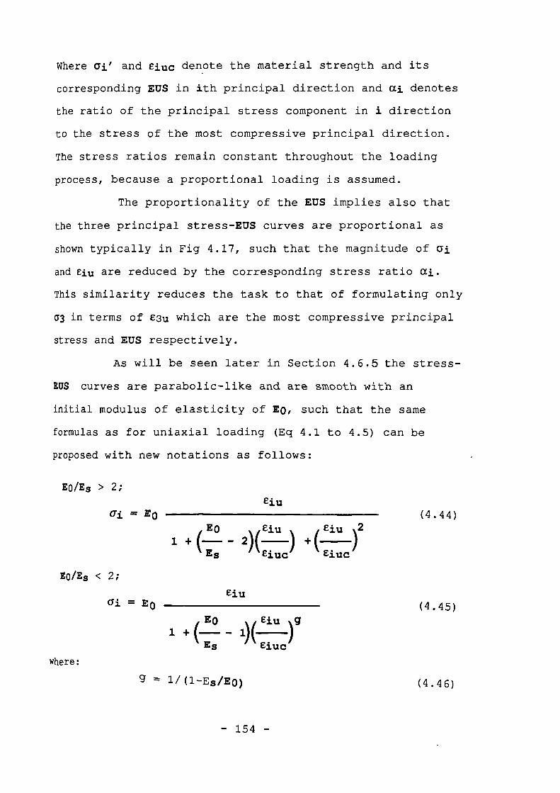
Where ai' and ei lic denote the material strength and its
corresponding EUS in ith principal direction and ai denotes
the ratio of the principal stress component in i direction
to the stress of the most compressive principal direction.
The stress ratios remain constant throughout the loading
process, because a proportional loading is assumed.
The proportionality of the EUS implies also that
the three principal stress-EUS curves are proportional as
shown typically in Fig 4.17, such that the magnitude of ai
and Ciu are reduced by the corresponding stress ratio ai.
This similarity reduces the task to that of formulating only
u3 in terms of E3u which are the most compressive principal
stress and EUS respectively.
As will be seen later in Section 4.6.5 the stress-
EUS curves are parabolic-like and are smooth with an
initial modulus of elasticity of Eo, such that the same
formulas as for uniaxial loading (Eq 4.1 to 4.5) can be
proposed with new notations as follows:
EO/Es > 2;
eiu
0• = EO (4.44)
eiu 2
1 + ( Eo ciu
— 2)(—) + (--)
Es eiUC eiUC
EO/Es < 2;
eiuai = Eci
Eo ciu )g1 + (--. — 1)(—
Es eiuc
Where:
(4.45)
g = 1 /(1-Es/E0) (4.46)
- 154 -
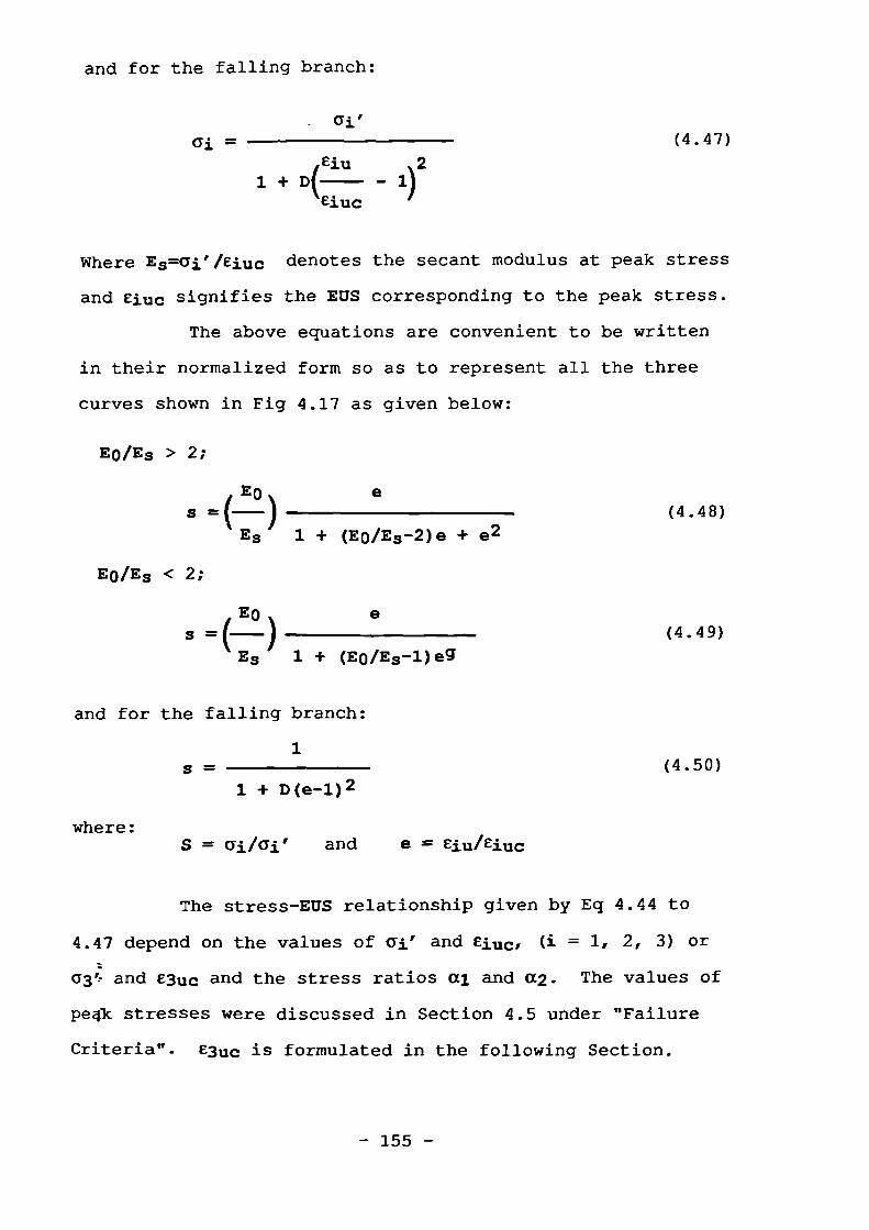
and for the falling branch:
- (4.47)
1 4. Dru 1)2
EiUC
Where Es=ai' denotes the secant modulus at peak stress
and Eiuc signifies the EUS corresponding to the peak stress.
The above equations are convenient to be written
in their normalized form so as to represent all the three
curves shown in Fig 4.17 as given below:
EØ/E 3 > 2;
EOS-(---)
Es 1 + (E0/Es -2)e + e2
EO/Es < 2;
EOs =(--)
Es 1 + (E0/E3-1)eg
(4.48)
(4.49)
and for the falling branch:
1S (4.50)
1 + D(e-1)2
where:S = ca/cri' and e = Eiu/Eiuc
The stress-WS relationship given by Eq 4.44 to
4.47 depend on the values of al: and Eiuc, (i = 1, 2, 3) or
av- and E3lic and the stress ratios al and a2. The values of
pe41( stresses were discussed in Section 4.5 under "Failure
Criteria". E3uc is formulated in the following Section.
- 155 -
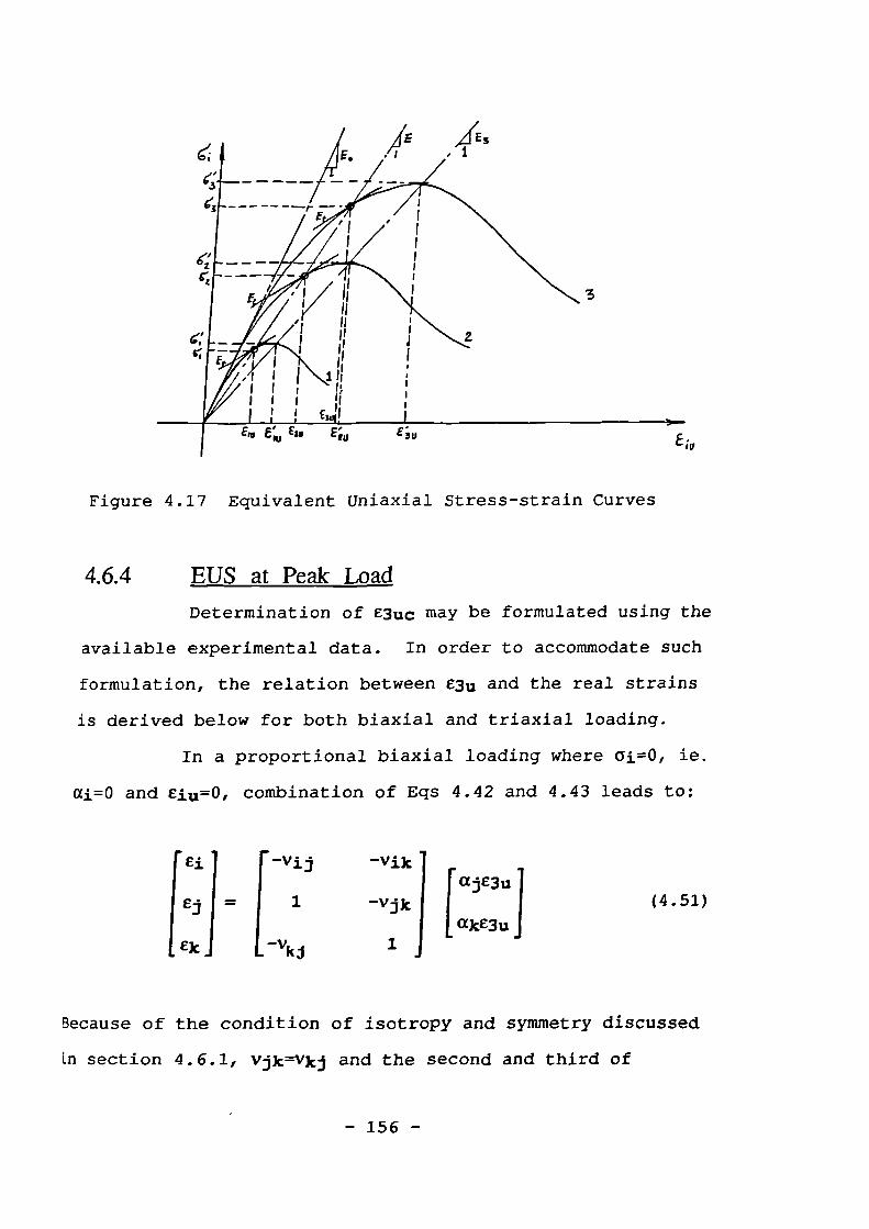
Figure 4.17 Equivalent Uniaxial Stress-strain Curves
4.6.4 EljS at Peak IANId
Determination of E3uc may be formulated using the
available experimental data. In order to accommodate such
formulation, the relation between e3u and the real strains
is derived below for both biaxial and triaxial loading.
In a proportional biaxial loading where a3 =0, ie.
ai=0 and ciu=0, combination of Eqs 4.42 and 4.43 leads to:
Ei-VijlajE3u1
Eji = 1 -Vjkalce3u
IIA110 1
(4.51)
Because of the condition of isotropy and symmetry discussed
in section 4.6.1, vjk=Vkj and the second and third of
— 156 —
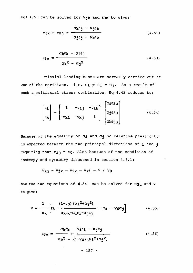
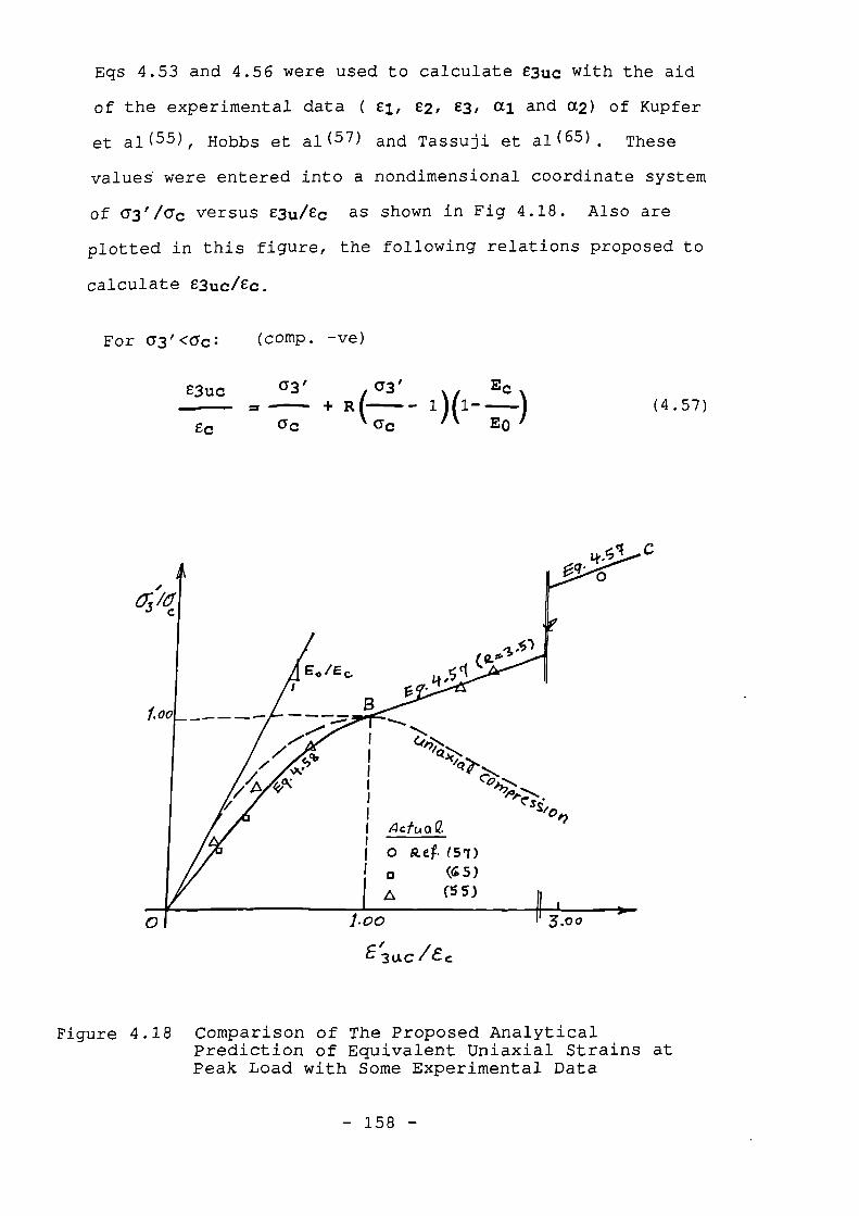
e3uc
EC
Eqs 4.53 and 4.56 were used to calculate e3uc with the aid
of the experimental data ( ci, e2, e3, al and a 2) of Kupfer
et al (55), Hobbs et al (57) and Tassuji et al (65) These
values' were entered into a nondimensional coordinate system
of a3'/ac versus E3u/ec as shown in Fig 4.18. Also are
plotted in this figure, the following relations proposed to
calculate Quc/Ec.
For G3'<6c: (comp. -ve)
a3 , a3' Ec+ R - 1)(1-
Eo )60 aC
(4.57)
Figure 4.18 Comparison of The Proposed AnalyticalPrediction of Equivalent Uniaxial Strains atPeak Load with Some Experimental Data
- 158 -
For 0>3'>c:
03 1(21c_). 0 (___) [(i, Ec )
Ec ac EO
Ec wY3'12R]
EO ac(4.58)
and for 0:73'>0
E3uc
EC
Ec a3f
= 0 .5 (1 +EO ac
(4.59)
where R is a material constant. R=3.5 suits normal concrete.
4.6.5 Transformation of E1JS to Real Strains and
Vice-versa
EUS and real strains can be converted to each
other using Eqs 4.42. These equations involve the [c]
matrix defined in section 4.6.1. In a multiaxially and
proportionally loaded isotropic material, this matrix
involves 3 independent Poisson's ratios as follows:
V12=V21, V23=V32
and V13=v31
The Poisson's ratios can be formulated according
to the available experimental data. Eqs 4.52 and 4.55
relate the Poisson's ratios at any stress level to the
strains of a biaxially and triaxially loaded material
respectively. Examination of the experimental results of
Kupfer et al (55) led to an expansion of Eq 4.9 (proposed for
uniaxial loading) to account for biaxial and multiaxial
loading as follows:
v ji = vij = vo 11 + kfij (e) n i (4.60)
- 159 -
where e denotes the straining ratio i.e. e = Eiu/eiuc
and k and n are material constants. k = 0.85 and n = 3
suits normal concrete. fij is proposed as follows:
For al' < 0: (comp. -ve)
1(01'-aj')/acif • • - '3
al' q1 + c (—)
ac
(4.61)
For al' > 0:
fij = kai i -aj')/aci - 2 1 al i /aci (4.62)
where c and q are defined in section 4.5.2 and al' denotes
the most tensile stress at the peak. These formulas agree
well with the experimental results of Kupfer et al( 55) at
peak loads as shown in Fig 4.19. Eq 4.60 covers all the
possible states of load combination.
The incremental and secant values of Poisson's
ratios are related as follows:
Vij dEj = d(vijeij)
-where Vij and vij are the incremental and secant Poisson's
ratios respectively for calculating the strain in the ith
principal direction induced by the strain in the jth
principal direction. From the above relation the
incremental and secant values of Poisson's ratios can be
calculated in terms of each other as follows:
d(vij.e)
de
- 160 -
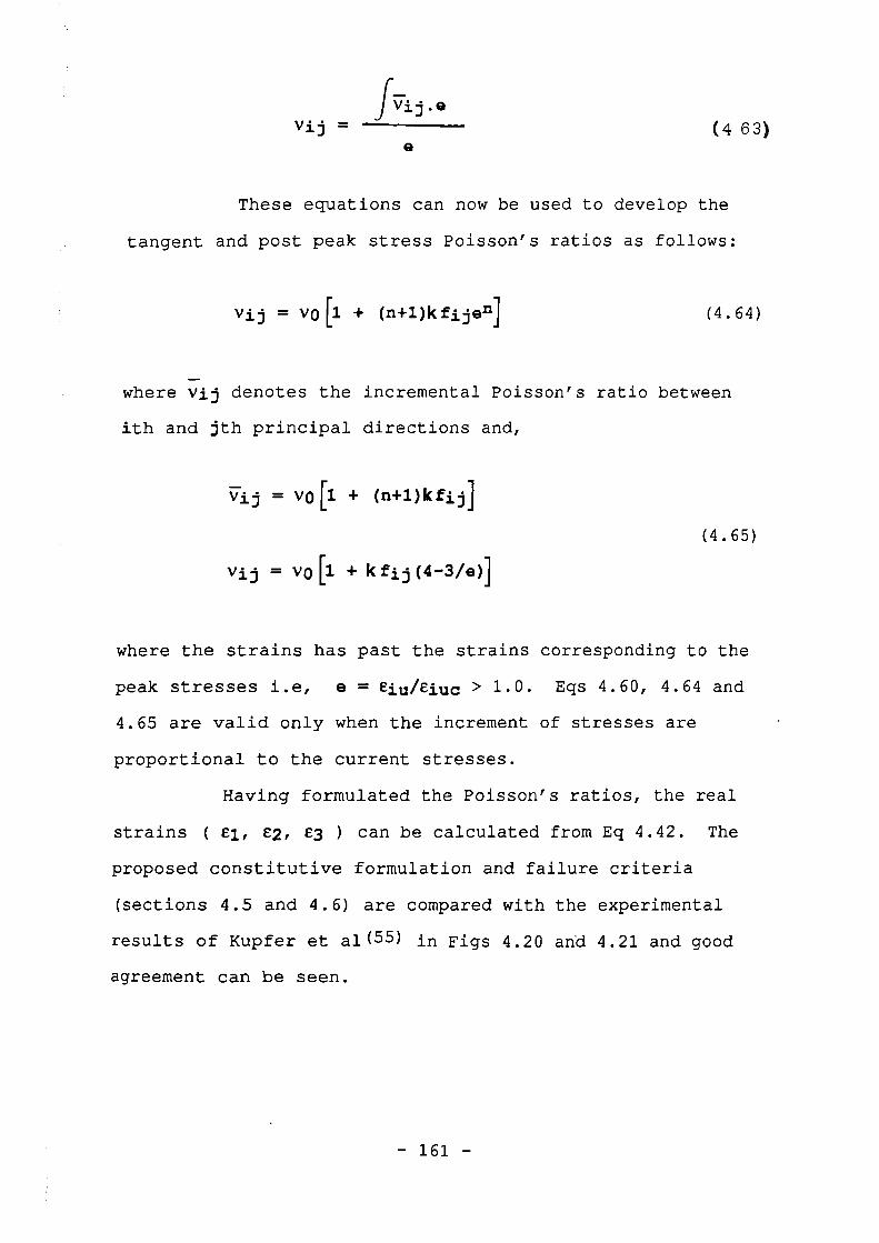
vi j - (4 63)
These equations can now be used to develop the
tangent and post peak stress Poisson's ratios as follows:
vij = vo [1 + (n+1)kfijen] (4.64)
where vij denotes the incremental Poisson's ratio between
ith and jth principal directions and,
= v o n + (n+l)kfiii
vij = vo [1 + k fii (4-3/e)]
(4.65)
where the strains has past the strains corresponding to the
peak stresses i.e, e = eiu/eiuc > 1.0. Eqs 4.60, 4.64 and
4.65 are valid only when the increment of stresses are
proportional to the current stresses.
Having formulated the Poisson's ratios, the real
strains ( El, E2, E3 ) can be calculated from Eq 4.42. The
proposed constitutive formulation and failure criteria
(sections 4.5 and 4.6) are compared with the experimental
results of Kupfer et al( 55 ) in Figs 4.20 and 4.21 and good
agreement can be seen.
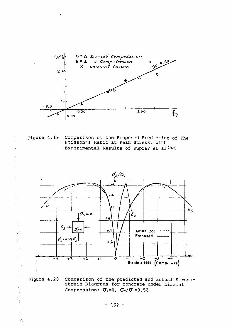
0
I . 2o-0.2
1.000.2 01
1 1
..., "'' n
, I
;
I
1
1(13 4,0
-53
62 ..0.520;1
,
e•
0.4 Actual (55) -----I Proposed
D .2. _
-1 -2. -3 -LtStrain x 1000 (Comp. -ve)
_
O 0 A Bic-x Ici..Q Corr>preS5AVV7• w A e. ComD.-tewstor) a
X unia xice.e Tch.s/Oh 0.
Figure 4.19 Comparison of the Proposed Prediction of ThePoisson's Ratio at Peak Stress, withExperimental Results of Kupfer et al(55)
0.130
Figure 4.204.20 Comparison of the predicted and actual Stress-strain Diagrams for concrete under biaxialCompression; 6 1=0, 62/a3=0.52
- 162 -
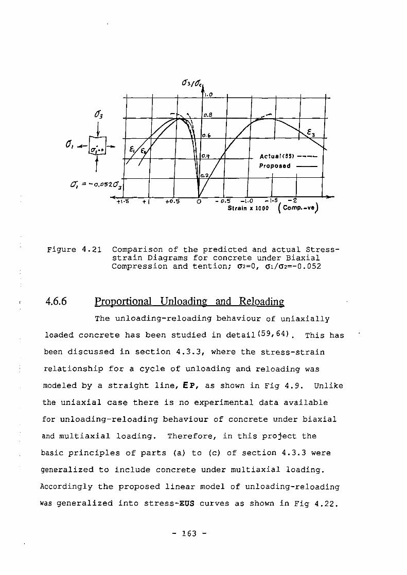
0.3 o.S
LIIn1110 Actual (55)
Proposed
•cr •D
0, •
Cr3/Grc,
A1.0
••••nn•n
0.2
Cri
4-0.5 0 - 0.5 -1.0 - 1 . 5 -2Strain x 1000 ( Comp.-ve)
Figure 4.21 Comparison of the predicted and actual Stress-strain Diagrams for concrete under BiaxialCompression and tention; a2=0, al/a2=-0.052
4.6.6 Proportional Unloading and Reloading
The unloading-reloading behaviour of uniaxially
loaded concrete has been studied in detail (59,64). This has
been discussed in section 4.3.3, where the stress-strain
relationship for a cycle of unloading and reloading was
modeled by a straight line, EP, as shown in Fig 4.9. Unlike
the uniaxial case there is no experimental data available
for unloading-reloading behaviour of concrete under biaxial
and multiaxial loading. Therefore, in this project the
basic principles of parts (a) to (c) of section 4.3.3 were
generalized to include concrete under multiaxial loading.
Accordingly the proposed linear model of unloading-reloading
was generalized into stress-MIS curves as shown in Fig 4.22.
- 163 -
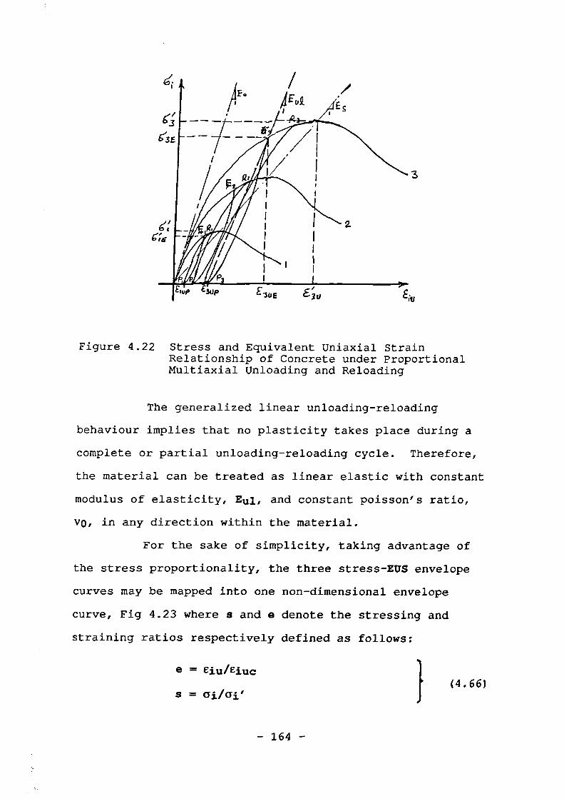
Figure 4.22 Stress and Equivalent Uniaxial StrainRelationship of Concrete under ProportionalMultiaxial Unloading and Reloading
The generalized linear unloading-reloading
behaviour implies that no plasticity takes place during a
complete or partial unloading-reloading cycle. Therefore,
the material can be treated as linear elastic with constant
modulus of elasticity, Eul, and constant poisson's ratio,
vo, in any direction within the material.
For the sake of simplicity, taking advantage of
the stress proportionality, the three stress-WS envelope
curves may be mapped into one non-dimensional envelope
curve, Fig 4.23 where s and e denote the stressing and
straining ratios respectively defined as follows:
e = eiu/Eiuc(4.66)
S =
- 164 -
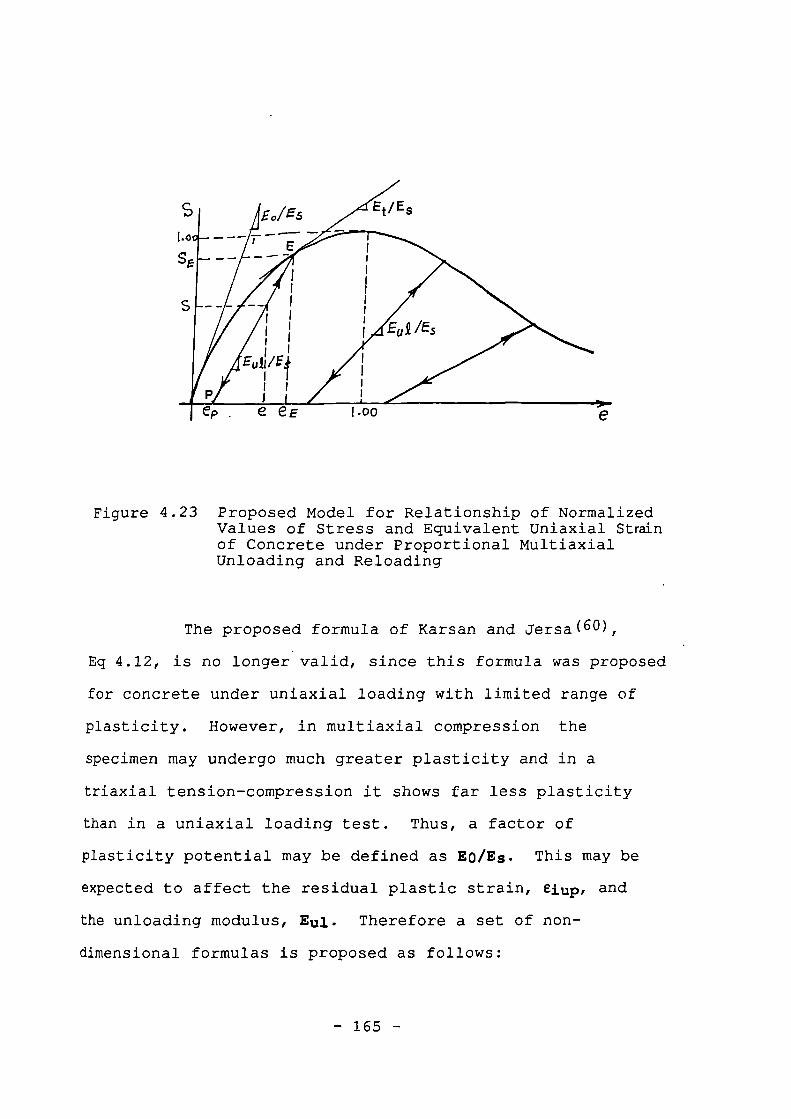
Figure 4.23 Proposed Model for Relationship of NormalizedValues of Stress and Equivalent Uniaxial Stalinof Concrete under Proportional MultiaxialUnloading and Reloading
The proposed formula of Karsan and Jersa(60),
Eq 4.12, is no longer valid, since this formula was proposed
for concrete under uniaxial loading with limited range of
plasticity. However, in multiaxial compression the
specimen may undergo much greater plasticity and in a
triaxial tension-compression it shows far less plasticity
than in a uniaxial loading test. Thus, a factor of
plasticity potential may be defined as EO/Es. This may be
expected to affect the residual plastic strain, eiup, and
the unloading modulus, Eul. Therefore a set of non-
dimensional formulas is proposed as follows:
- 165 -
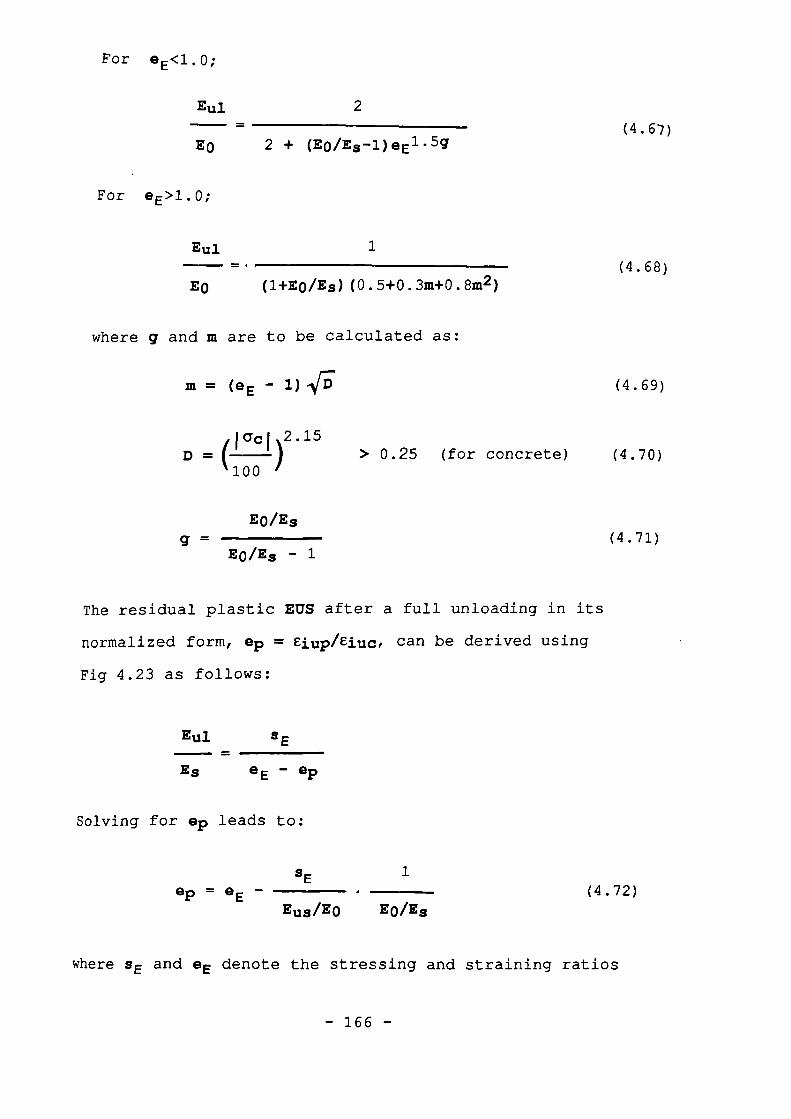
EO
For eE>1.0;
Eul
2 + (E0/Es-1)eE1-5g
1
(4.67)-
For A <1 0.E • •
Eul 2
(4.68)-
Eo (1+Eo/Es)(0.5+0.3m+0.8m2)
where g and in are to be calculated as:
in = (e E - (4.69)
D = ilack2.15> 0.25 (for concrete) (4.70)
'100
Eo/Es(4.71)
Eo/Es - 1
The residual plastic EDS after a full unloading in its
normalized form, ep = elup/Eiuc, can be derived using
Fig 4.23 as follows:
Eul s E-
Es eE - Gp
Solving for ep leads to:
sE 1ep = eE (4.72)
Eus/E0 EO/Es
where s E and eE denote the stressing and straining ratios
- 166 -
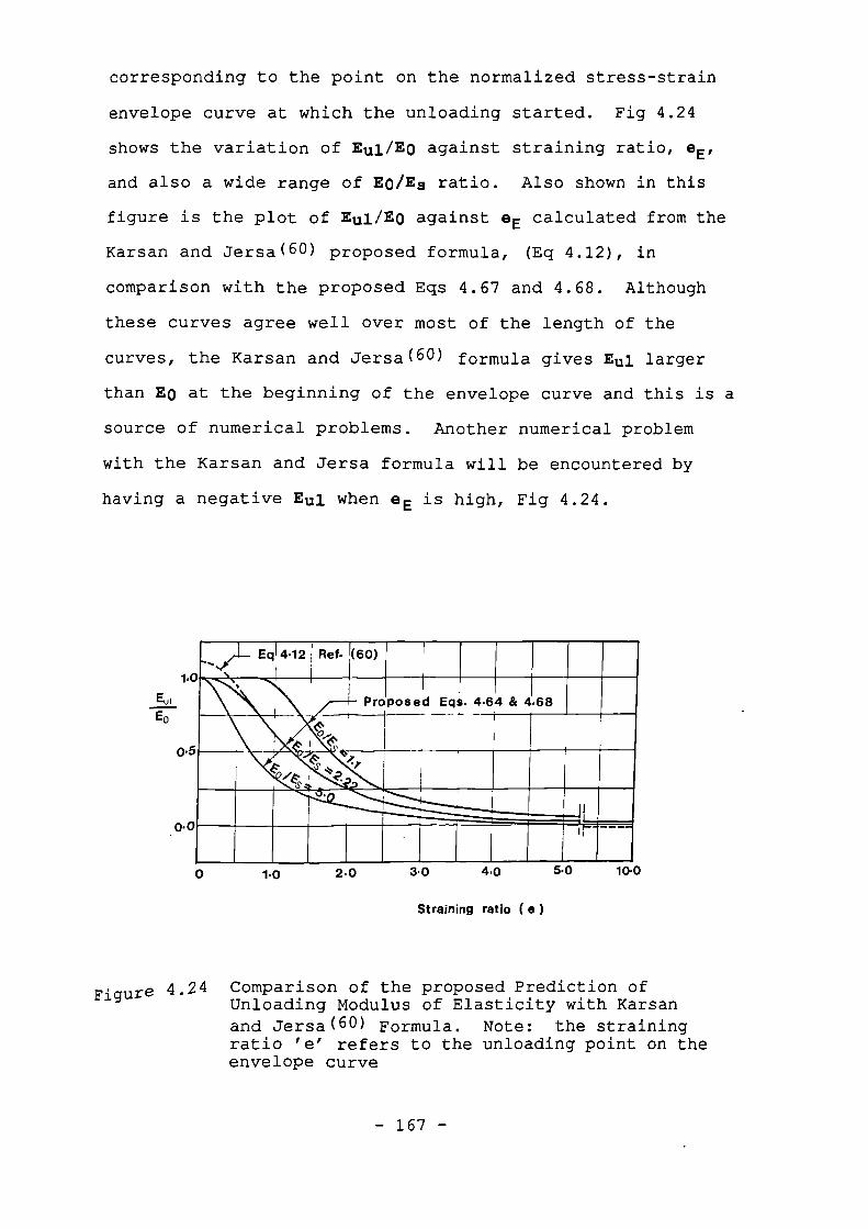
corresponding to the point on the normalized stress-strain
envelope curve at which the unloading started. Fig 4.24
shows the variation of Eui/E0 against straining ratio, GE,
and also a wide range of E0/Es ratio. Also shown in this
figure is the plot of Eul/E0 against e E calculated from the
Karsan and Jersa( 60 ) proposed formula, (Eq 4.12), in
comparison with the proposed Eqs 4.67 and 4.68. Although
these curves agree well over most of the length of the
curves, the Karsan and Jersa( 60) formula gives Eul larger
than Eo at the beginning of the envelope curve and this is a
source of numerical problems. Another numerical problem
with the Karsan and Jersa formula will be encountered by
having a negative Eui when GE is high, Fig 4.24.
o 1.0
2.0
30
40
5 .0 10.0
Straining ratio ( e )
Figure 4.2 4 Comparison of the proposed Prediction ofUnloading Modulus of Elasticity with Karsanand Jersa( 60 ) Formula. Note: the strainingratio 'e' refers to the unloading point on theenvelope curve
- 167 -
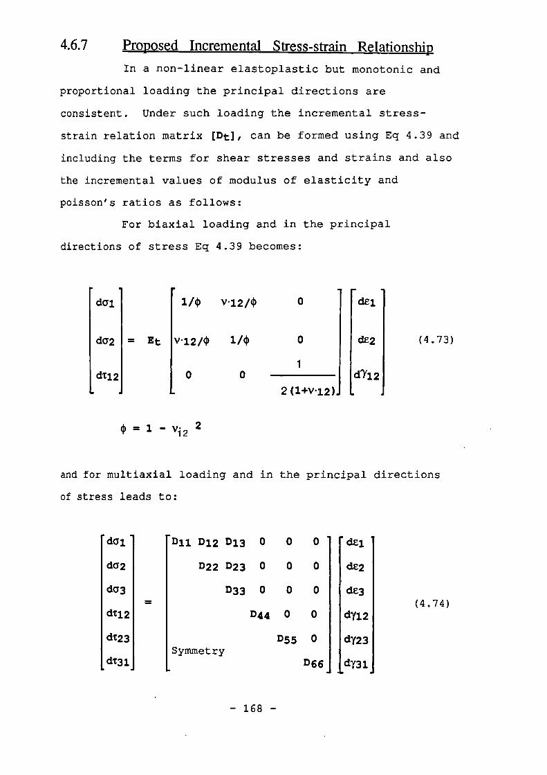
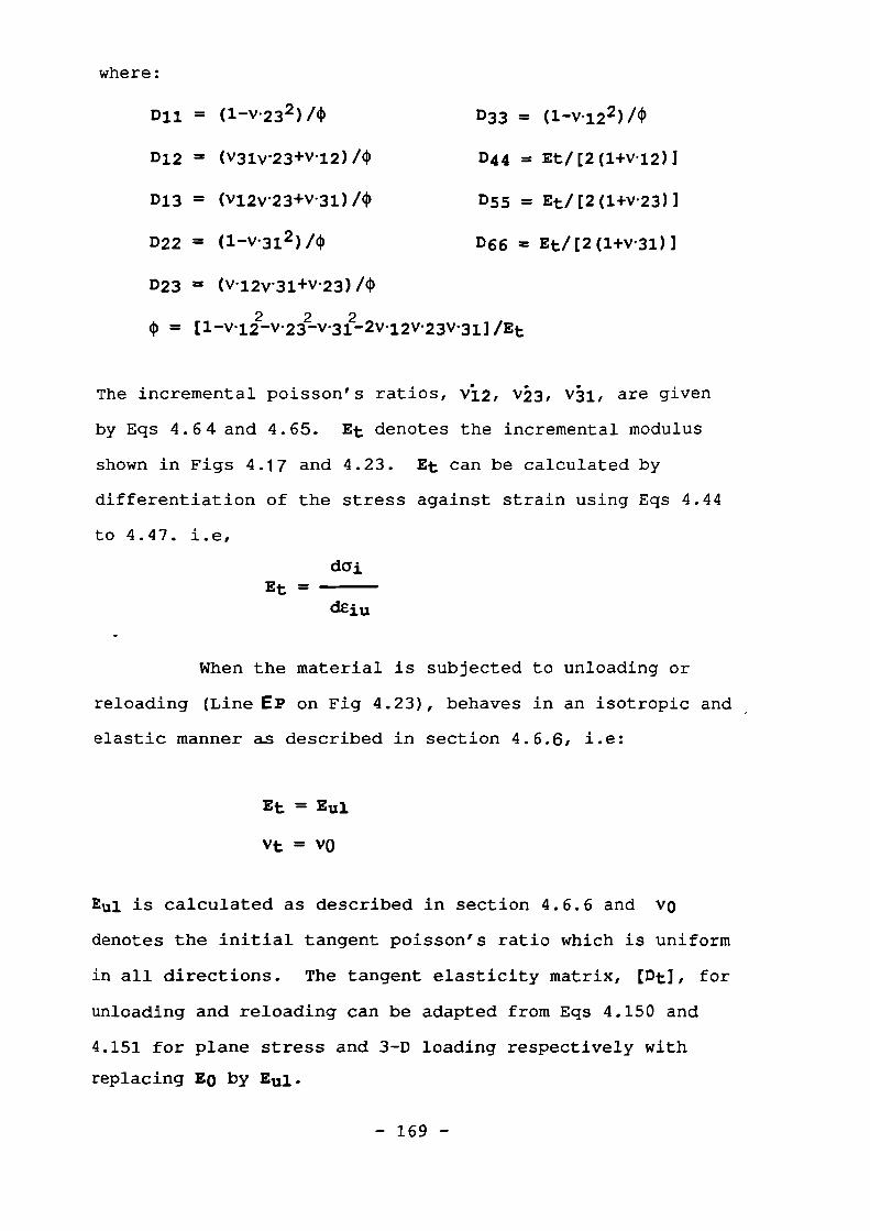
where:
Dll = (1 -V.232)/0 D33 = (1-v•122)/0
D12 = (v31w23+v12)/0 D44 = Et/[2(1+v12)]
D13 = (v12w23+v-31)/4) D55 = Et/[2(1+v'23)]
D22 = (1-v-31 2 ) /4) D66 = Et/[2(1+v.31)]
D23 = (v12w31+v•23)/4)
0 = El_v.122v.232v.33.2_2v-i2v.23v*31] /Et
The incremental Poisson's ratios, v12, v3, vii, are given
by Eqs 4.64 and 4.65. Et denotes the incremental modulus
shown in Figs 4.17 and 4.23. Et can be calculated by
differentiation of the stress against strain using Eqs 4.44
to 4.47. i.e,
daiEt =
dEiu
V'
When the material is subjected to unloading or
reloading (Line EP on Fig 4.23), behaves in an isotropic and
elastic manner as described in section 4.6.6, i.e:
Et = El
Vt = VO
Eul is calculated as described in section 4.6.6 and VO
denotes the initial tangent poisson's ratio which is uniform
in all directions. The tangent elasticity matrix, [Dt], for
unloading and reloading can be adapted from Eqs 4.150 and
4.151 for plane stress and 3-D loading respectively with
replacing Eo by Eul-
- 169 -
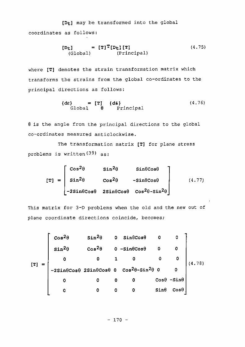
(4.77)
0
0
(4.78)[T] =
[Dt] may be transformed into the global
coordinates as follows:
[Dt] = [T]T[Dt][T](Global) (Principal)
(4.75)
where [T] denotes the strain transformation matrix which
transforms the strains from the global co-ordinates to the
principal directions as follows:
(4.76)0.0 = [T] {d&}Global 0 Principal
0 is the angle from the principal directions to the global
co-ordinates measured anticlockwise.
The transformation matrix [T] for plane stress
problems is written (39) as:
{
Cos 20 Sin20 SineCose
[T] = Sin2 8 Cos20 -Sin0Cose
-2SineCose 2SineCose Cos20-Sin20
This matrix for 3-D problems when the old and the new out of
plane coordinate directions coincide, becomes;
Cos20 Sin20 0 SineCos0 0 0
Sin2 0 Cos20 0 -SineCose 0 0
0 0 1 0 0 0
-2SineCose 2SineCos0 0 Cos 20-Sin20 0 0
0 0 0 Cos() -Sine
0 0 0 Sine Cos°
Based on the proposed model, when the material is
subjected to unloading or reloading the transformed (Dt]
becomes identical to the original one because the poisson's
ratio is uniform in all directions and no variation in the
mechanical properties can be imagined for changing the
coordinate directios.
4.7 Non-proportional Loading
4.7.1 Stress-strain Relationship
The model described in sections 4.6.1 to 4.6.7 is
proposed for proportional loading. But the behaviour and
deformation of an infilled frame are associated with some
discontinuities and non-proportionalities as a result of
lack of fit, plasticity and also the following events:
-occurrence of plastic hinges in frame members.
-shear failure or slip at joints
-cracking in either frame or infill materials.
-local crushing especially at the loaded corners of panel
These events induce some stress redistributions
which are not necessarily proportional to the current
stresses. As a result, the principal directions may rotate
and in some regions the material may be subject to unloading
while the external loads have not changed.
In order to account for such non-proportional
changes, the following approach has been employed to
determine the true path in the stress-strain co-ordinate
system.
- 171 -
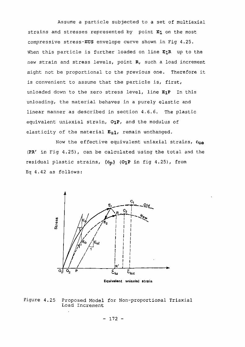
Ei -....
Assume a particle subjected to a set of multiaxial
strains and stresses represented by point El on the most
compressive stress-EUS envelope curve shown in Fig 4.25.
When this particle is further loaded on line EiR up to the
new strain and stress levels, point R, such a load increment
might not be proportional to the previous one. Therefore it
is convenient to assume that the particle is, first,
unloaded down to the zero stress level, line Ell" In this
unloading, the material behaves in a purely elastic and
linear manner as described in section 4.6.6. The plastic
equivalent uniaxial strain, 01P, and the modulus of
elasticity of the material Eul, remain unchanged.
Now the effective equivalent uniaxial strains, Eue
(PR' in Fig 4.25), can be calculated using the total and the
residual plastic strains, RIO (01P in fig 4.25), from
Eq 4.42 as follows:
A
lonP
a iu Eitic
Equivalent uniaxial strain
Figure 4.25 Proposed Model for Non-proportional TriaxialLoad Increment
- 172 -
{Cue} = [C1 -1 { e - ep} (4.79)
Where [C] involves the secant Poisson's ratios discussed in
Section 4.6.2.
The effective EUS values permit the new stress
proportions to be calculated and the new stress-EUS envelope
curve, 02E2C2, to be drawn such that the unloading line
(corresponding to the current unloading modulus, Eui or E2P
in Fig 4.25) matches the unloading line of the old envelope
curve, ElP. This permits the material to be reloaded on the
unloading line up to point E2 on the new envelope curve
while undergoing the new stress proportions.
The loading is further continued with the same
stress proportion as that of the reloading up to point R
where the total effective EUS is met.
4.7.2 Poisson's Ratios under Non-proportional Loading
The Secant Poisson's ratios can be calculated from
Eq 4.63 which involves an integration. The integral must be
carried out over the whole path of the stress-EUS curve. As
shown in Fig 4.25, a non-proportional loading can be
converted into a linear elastic branch, line PE2, with a
constant tangential poisson's ratio equal to the initial
poisson's ratio, vo, and a non-linear elastoplastic branch,
curve E2R, with variable Poisson's ratio as given by
Eqs 4.64 and 4.65. For the case when eR is less than unity
the integral can be split into the linear and non-linear
parts. ie ;
- 173 -
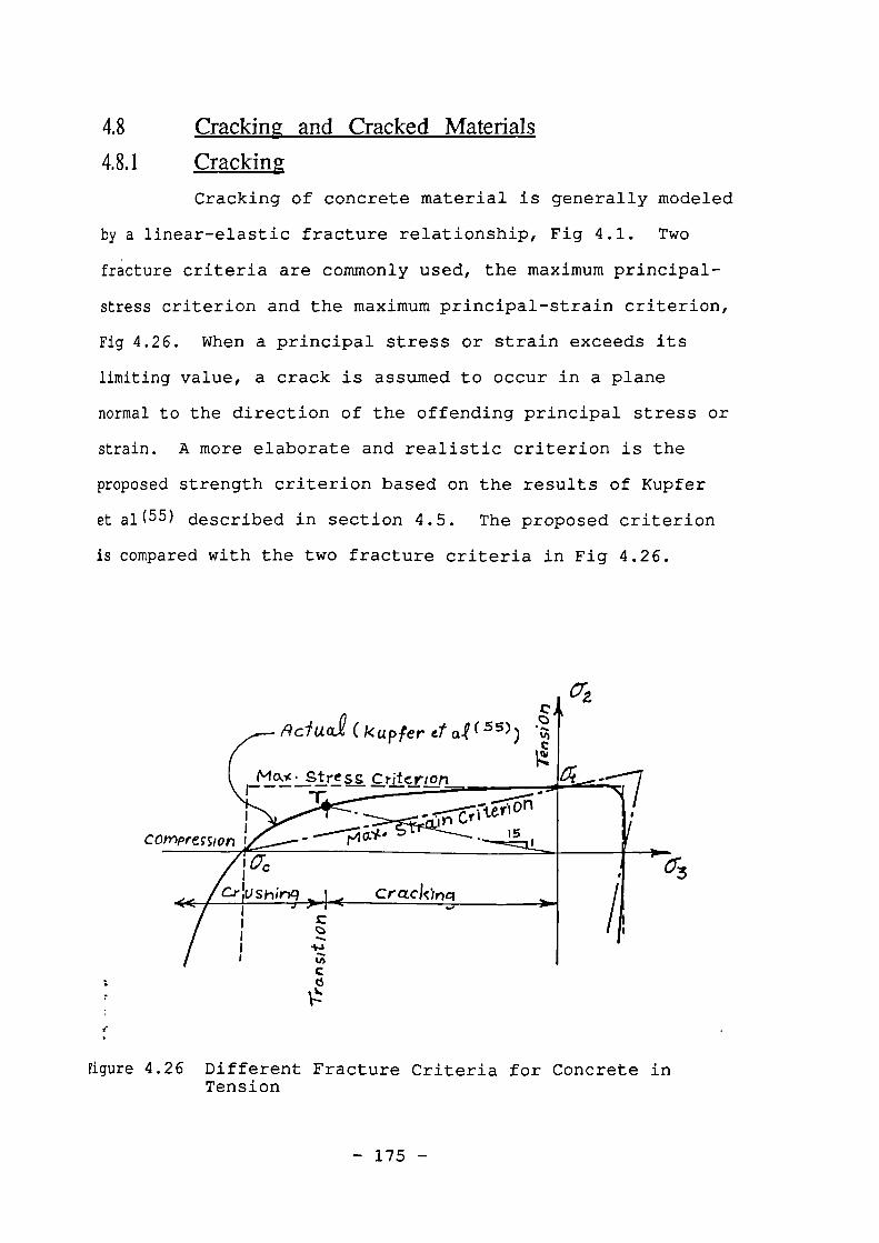
According to the experiment of Kupfer et al (55) , at the
biaxial failure surface, when the absolute value of the
ratio of tensile to compressive principal stresses exceeds
approximately 1/15, the mode of failure is tension cut off
at the peak stress. Otherwise the material fails by a
gradual crushing. In this project, the above specified
tensile/compressive stress ratio, 1/15, was generalized to
multiaxial loading as the transition between the tensile and
compressive failure modes while the effect of intermediate
principal stress on this transition was ignored.
4.8.2 Cracked Material
Once a crack has formed, it is generally assumed
that no tensile stress can be supported across the crack.
However, material parallel to the crack is still capable of
carrying stress according to the uniaxial or biaxial
conditions prevailing parallel to the crack. On increased
loading, further cracks are allowed to occur.
In reinforced concrete cracks are more frequent
and therefore, the crack width is less than in unreinforced
concrete. The following effects proved to have a major
influence on the behaviour of a cracked reinforced concrete
element (39)
i) tensile stiffening
fi) aggregate interlockiii) dowel action
The tensile stiffening effect is usually accounted
for indirectly as follows:
a) By assuming that the loss of tensile strength in
concrete appears gradually.
b) By increasing the stiffness of steel.
The former choice was first introduced by Scanlon( 67 ) as
shown in Fig 4.10 and is more popular, but the latter choice
seems to be more convenient for infilled frame structures
composed of different materials, including concrete blocks
and mortar which are not necessarily reinforced and for
which the Scanlon model may lead to unrealistic results.
The aggregate interlock is usually accounted for
by assuming a perfect or partial shearing stiffness for
crack surfaces (39). In this project, however, the
interlocking behaviour is accounted for by a proposed new
approach to crack modeling given in the following sections.
The dowelling action effect is either ignored or
allowed for by increasing the shearing stiffness at crack
surfaces.
Cracks in a cracked material may close and open
again in later stages of the loading. Opening and closing
of cracks is measured by crack strain, ecrf which is assumed
to be distributed uniformly within the material. In the
following sections the mechanical behaviour of a cracked
naterial is modeled for plane stress condition.
Phis model also deals with double sets of cracks ine
different orientations.
4.8.3 Proposed Slip-dilatancy Crack Model
4.8.3.1 Clervmd Concept
Consider a particle of brittle material under
biaxial stresses loaded to failure. When the criteria
outlined in section 4.8.1 are met, the material fails in a
tensile manner i.e. the particle would crack through one or
more planes perpendicular to the most tensile principal
stress direction, Fig 4.27(a). The surface of such cracks
within the material is irregular and rough, Fig 4.27(b).
If normal stress across the crack is constant, any
relative tangential displacement, s, or slip, between the
opposite surfaces of the crack, is always accompanied by a
relative normal displacement, w, or crack width. This is
called "crack dilatancy". Based on this phenomenon the
shape of the crack surface may be idealized as a regular
trapezoidal shape as shown in Fig 4.27(c) with a dilatancy
angle of a where:
=Tana = — (4.82)
denotes the dilatancy ratio. The value of 0 can be adjusted
by changing the angle a in order to agree with the
experiments on the material in question.
A crack may either be closed, interlocked or open
as=shown in Fig 4.27. The state of the crack can be
determined as described in Sections 4.8.3.3 to 4.8.3.5. The
following section deals with the stress-strain relationship
of a cracked material under plane stress conditions.
- 178 -
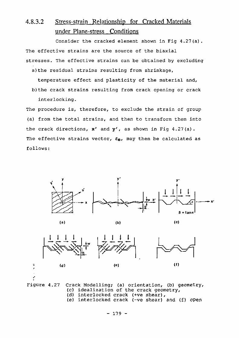
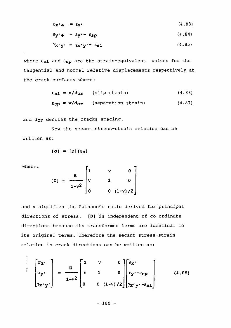
ax' 1
'tx'
1
.1 V 0 Ilex'
V 1 0
0 0 (1-V)/2 Yx'y'-Esi
,
(4.88)1-v2
ey,-espE
=
Ex'e = ex' (4.83)
Ey'e = Cy' - esp (4.84)
Yx'y' = Yx'y'- Cs]. (4.85)
where esi and esp are the strain-equivalent values for the
tangential and normal relative displacements respectively at
the crack surfaces where:
e51 = s/dcr (slip strain) (4.86)
Esp = w/dcr (separation strain) (4.87)
and dcr denotes the cracks spacing.
Now the secant stress-strain relation can be
written as:
{a} = [El](40
where:V 0
E[D] = V 1
{1
0
}
1-v20 0 (1-v)/2
and v signifies the Poisson's ratio derived for principal
directions of stress. [D] is independent of co-ordinate
directions because its transformed terms are identical to
its original terms. Therefore the secant stress-strain
relation in crack directions can be written as:
:
- 180 -
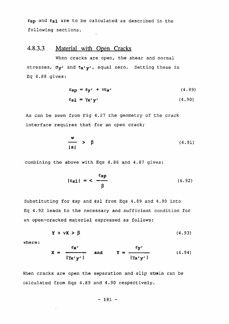
4.8.3.4 Material with Closed Cracks
When cracks are closed, no relative displacement
prevails at the crack surfaces i.e: $ = w = 0. It may,
thus, be concluded from Eqs 4.86 and 4.87 that es1=Zsp= 0.
The frictional resistance at a crack may be
assumed to be mainly due to the geometry of the surface,
which was idealized as a trapezoidal shape in Fig 4.27 (c).
Therefore the surface friction over the parts of the crack
surface in contact, may be ignored and it may be assumed
that the forces are transferred normal to these parts as
shown in Fig 4.27(d) or 4.27(e). The above assumptions lead
to the conclusion that should a crack remains closed, the
following inequality must be satisfied:
Itx'y'l < -Pay' (4.95)
Substituting for ay f and Tx l y , from Eq 4.88 (while equating
es1 and Esp to zero) into Eq 4.95, leads to:
1—v
Y + vX < — (4.96)213
which is the necessary and sufficient condition to ensure
the cracks are closed.
4.8.3.5 Material with Interlocked Cracks
When neither of the conditions of Eq 4.93 and 4.96
are,satisfied, the cracks are interlocked. The interactive
forces, are therefore transferred normal to the surfaces in .
contact as shown in Fig 4.27(d) and (e) and the following
relations can be derived:
- 182 -
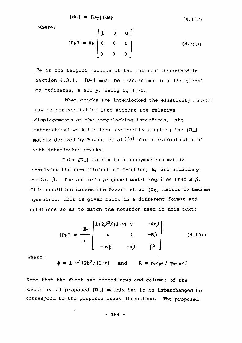
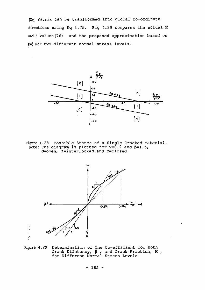
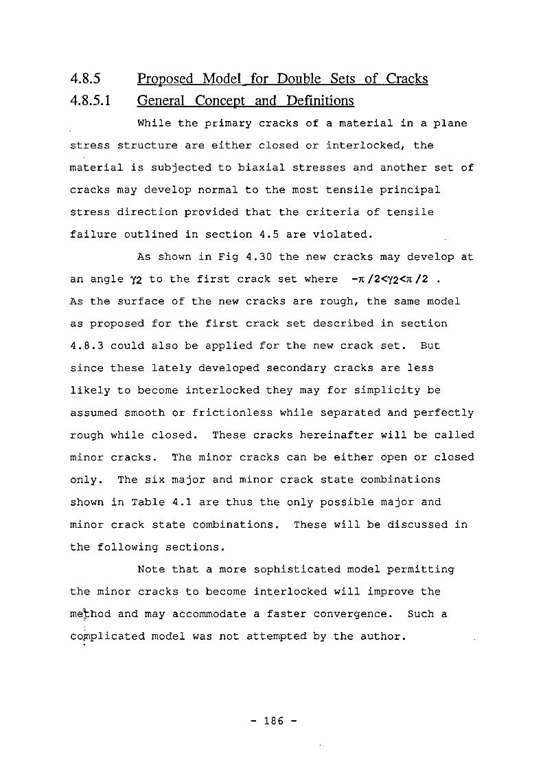
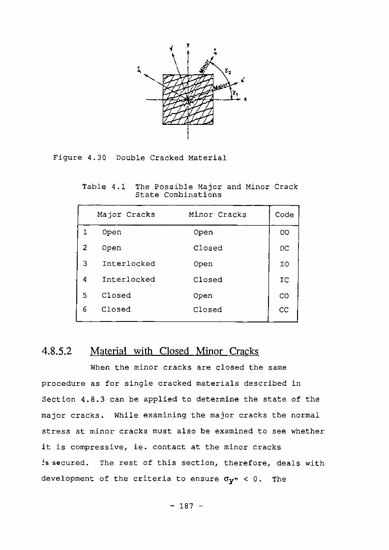
1
Figure 4.30 Double Cracked Material
Table 4.1 The Possible Major and Minor CrackState Combinations
Major Cracks Minor Cracks Code
1 Open Open 00
2 Open Closed OC
3 Interlocked Open IO
4 Interlocked Closed IC
5 Closed Open CO
6 Closed Closed CC
4.8.5.2 Material with Closed Minor Cracks
When the minor cracks are closed the same
procedure as for single cracked materials described in
Section 4.8.3 can be applied to determine the state of the
major cracks. While examining the major cracks the normal
stress at minor cracks must also be examined to see whether
it is compressive, ie. contact at the minor cracks
!s secured. The rest of this section, therefore, deals with
development of the criteria to ensure ay ,' < 0. The
- 187 -
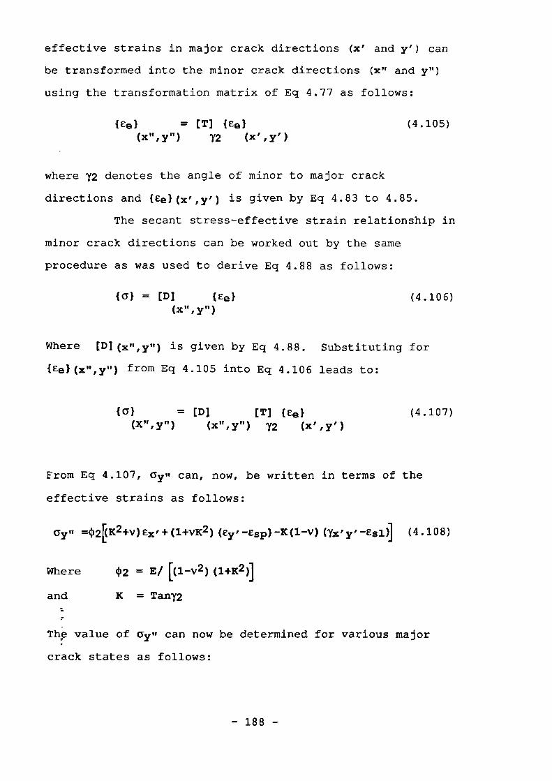
effective strains in major crack directions (x' and y') can
be transformed into the minor crack directions (x" and y")
using the transformation matrix of Eq 4.77 as follows:
(Eel ) = [T] (Ee) (4.105)(x",1'") (x' ,y'
where y2 denotes the angle of minor to major crack
directions and (Ce)(x,,yr) is given by Eq 4.83 to 4.85.
The secant stress-effective strain relationship in
minor crack directions can be worked out by the same
procedure as was used to derive Eq 4.88 as follows:
{a} = [D] (Ee}
(4.106)(xu,Y")
Where (1)1(x",yn) is given by Eq 4.88. Substituting for
i Etsa(x",y") from Eq 4.105 into Eq 4.106 leads to:
{a} = [D] (T]
(4.107)(X",y") (x",17")
From Eq 4.107, (Tr can, now, be written in terms of the
effective strains as follows:
ay" =02P+V) Ex , +( 1+vK2 )(ey' -esp) -K ( 1-v )(Tx'y' -Es1)] (4.108)
Where
and
(1)2
K
= E/
= Tany2
[(1-v2 ) (1+K2)}
The value of ale, can now be determined for various major
crack states as follows:
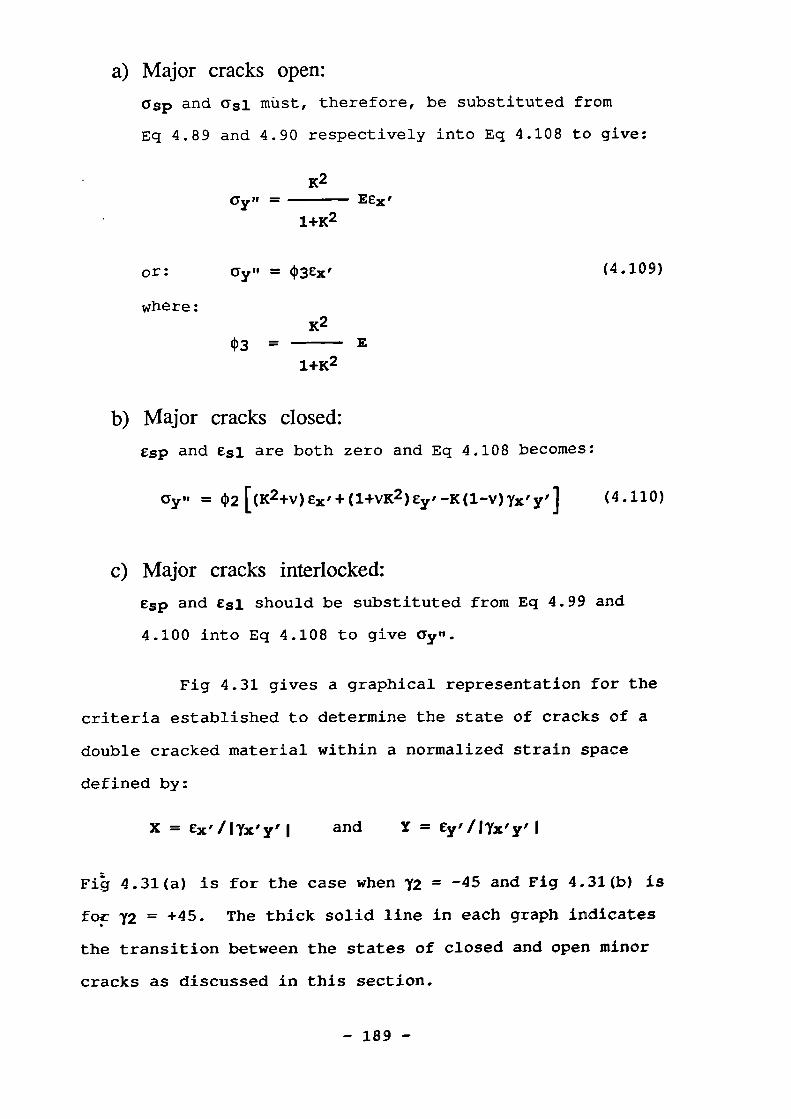
or:
where:
a) Major cracks open:
asp and as1 must, therefore, be substituted from
Eq 4.89 and 4.90 respectively into Eq 4.108 to give:
K2
Gy" Eex,1+K2
ay" = 03ex'
K2(03
1+K2
(4.109)
b) Major cracks closed:
Esp and esi are both zero and Eq 4.108 becomes:
ay" = [ (K2+v)ex,+(l+v1C2)ey,-K(1-v)Yx'Yl (4.110)
c) Major cracks interlocked:
Esp and es1 should be substituted from Eq 4.99 and
4.100 into Eq 4.108 to give Glo.
Fig 4.31 gives a graphical representation for the
criteria established to determine the state of cracks of a
double cracked material within a normalized strain space
defined by:
x = ex , / l yx'y'l and Y = ey,/iYx'y'l
Fig 4.31(a) is for the case when 72 = -45 and Fig 4.31(b) is
for 72 = +45. The thick solid line in each graph indicates
the transition between the states of closed and open minor
cracks as discussed in this section.
- 189 -
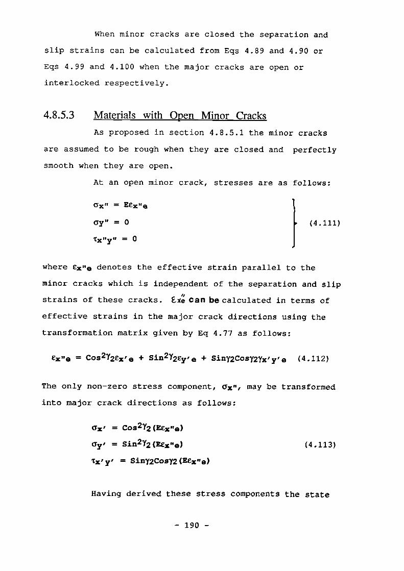
ax" = Eex"e
ay" = 0
Tx”y" = 0
When minor cracks are closed the separation and
slip strains can be calculated from Eqs 4.89 and 4.90 or
Eqs 4.99 and 4.100 when the major cracks are open or
interlocked respectively.
4.8.5.3 Materials with Open Minor Cracks
As proposed in section 4.8.5.1 the minor cracks
are assumed to be rough when they are closed and perfectly
smooth when they are open.
At an open minor crack, stresses are as follows:
where Ex ne denotes the effective strain parallel to the
minor cracks which is independent of the separation and slip
strains of these cracks. Ex: canbe calculated in terms of
effective strains in the major crack directions using the
transformation matrix given by Eq 4.77 as follows:
Ex n e = Cos2Y2ex , e + Sin2Y2ey , e + Siny2 CO372Yx f y i e (4.112)
The only non-zero stress component, 03e, may be transformed
into major crack directions as follows:
ax' = COS2Y2(EEKne)
ay, = Sin272(EEK"e)
(4.113)
TX 1 y1 = Sin72CO572(Etele)
Having derived these stress components the State
- 190 -
of the major cracks can thence be verified as described
below:
a) Major cracks interlocked (J0):
From Eq 4.97 the necessary condition for
equilibrium of stresses at major cracks can be written as:
Rxx'y' = -Pay'
(4.114)
Substituting for Tx'y' and ay , from Eq 4.113 leads to:
K = Tany2 = - (4.115)
Eq 4.115 is the only condition for an open-minor-crack
material to become interlocked at its major cracks. This
condition is independent of the effective strains, but it
depends on the angle of the minor cracks to the major ones,
Y2- Any arbitrary major crack separation strain,esp, leads
to a unique Exe" which is the only non-zero stress
component. This will be further verified below.
We may define an arbitrary major crack separation
strain, Esp, and its corresponding slip strain, esl, and
write Eq 4.112 in terms of the total strains as follows:
cycl e = Cos2Y2Ex , + Sin2Y2(Ey , -esp) + Siny2CosY2(Yx'y'-es1)
Substituting for E51 as given by Eq 4.100 leads to:
Exue = Cos2Y2Ex , + Sin2Y2Ey , + Siny2CosY2yx'y'
-esl(Sin2Y2 + (R/13)Siny2Cosy2)
- 191 -
Substituting the value of R/0 from Eq 4.115, the 4th term of
the above equation vanishes showing that the values of major
crack strains do not affect the value of Ex il e and
subsequently the values of the stresses of Eq 4.113 have no
influence on Ex"e.
The above conclusion proves that the state of
interlocked-open, IO, may occur only when the angle of minor
to major cracks takes a certain value given by Eq 4.115 and
it is only a mechanism by which material can alter from IO
to CO state without any influence on the existing stresses.
Therefore the IO state may be substituted by its alternative
state, CO, without any harming effect.
b) Major cracks closed (CO):
When the stress normal to the major cracks is
compressive, the state of these cracks is either interlocked
or closed. Since with open minor cracks any interlocked
major cracks can alter into closed major cracks, as
discussed in the preceding subsection, the condition of
Gy , <0 is the necessary and sufficient condition in an open-
minor-crack material for its major cracks remain closed.
Considering Eq 4.113, such a condition can be written as:
Ex"e < 0
(4.116)
Sihce major cracks are closed, exne=E20 and the above,
condition can be written as:
EX" < 0
(4.117)
. - 192 -
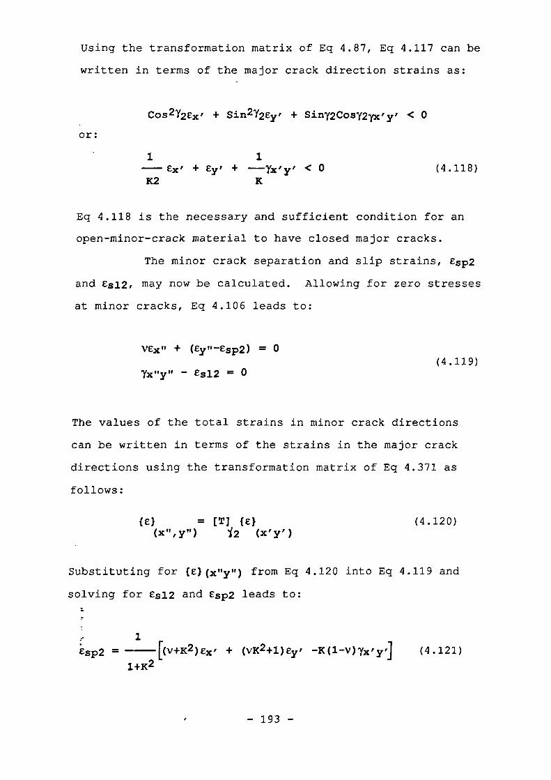
es12 =1+1(2
[2K (Ey' --ex' ) + (1-K2 )Yx'y]
(4.122)
c) Major cracks open (00):
A material with open minor cracks may also have
open major cracks. The double crack combination states are
graphically represented in Fig 4.31.
4.8.6 Proposed Incremental Stress-strain Relationship
for Double Cracked Materials
The incremental stress-strain relationship of a
double cracked material can be determined using a similar
approach to that given in Section 4.8.4 as follows:
a)Either major or minor cracks open (OC or CO):
[Dt] must be taken the same as in Eq 4.103, but it must
be written for the directions of the open cracks.
b)The both crack sets open (00):
The material has no stiffness; [Dt] = 0.
C) Interlocked-closed (IC):
[Dt] is to be formed as given by Eq 4.104
d)Closed-closed (CC):
[Dt] is to be formed as if no crack exists.
The above calculated [Dt] must be transformed into the
global co-ordinates using Eq 4.75.
. - 194 -
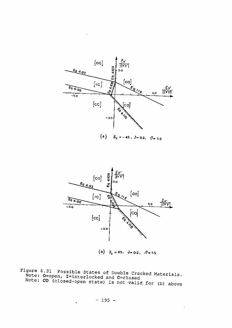
(a ) X2 = - 45 , %),= 0 .2, 1.5
( b) X2 =45 1?--T. 0 .2, p4=1.5
Figure 4.31 Possible States of Double Cracked Materials.Note: 0=open, I=interlocked and C=closedNote: CO (closed-open state) is not valid for (b) above
- 195 -
4.9 Constitutive Formulation for Steel
4.9.1 ammil Characteristics of Steel
The general characteristics of steel are described
in the standard text books, eg. Chen (39) . Only a brief
description is given here in order to establish the basis
and notations upon which the constitutive formulation for
steel is structured.
Fig 4.32 shows some typical stress-strain curves
for different qualities of steel. The stress-strain curves
for steel grades 40, 50 and 60 which are normally used in
steel structures, are characterized normally by the
following general features:
i) An initial linear-elastic part up to (ay, Cy);
ii) a yield plateau from Cy to est (the typical ratio of
Est/Cy is 8 to 15),
iii) a strain-hardening part from est to the ultimate
strain, Eu, then a strain softening part (Cu to ef),
iv) an ultimate strength of 1.55 times the yield strength,
As the strength of the steel increases, its
capacity for inelastic deformation, or ductility decreases.
As shown in Fig 4.32, for grade 75 and higher the yield
plateau in the stress-strain curve disappears.
The stress-strain curves for steel are generally
assumed to be identical in tension and compression. The
stress-strain relationship for steel subjected to unloading
and reloading is approximately linear-elastic with a
stiffness equal to the initial modulus of elasticity of
steel, Fig 4.32 (b).
- 196 -
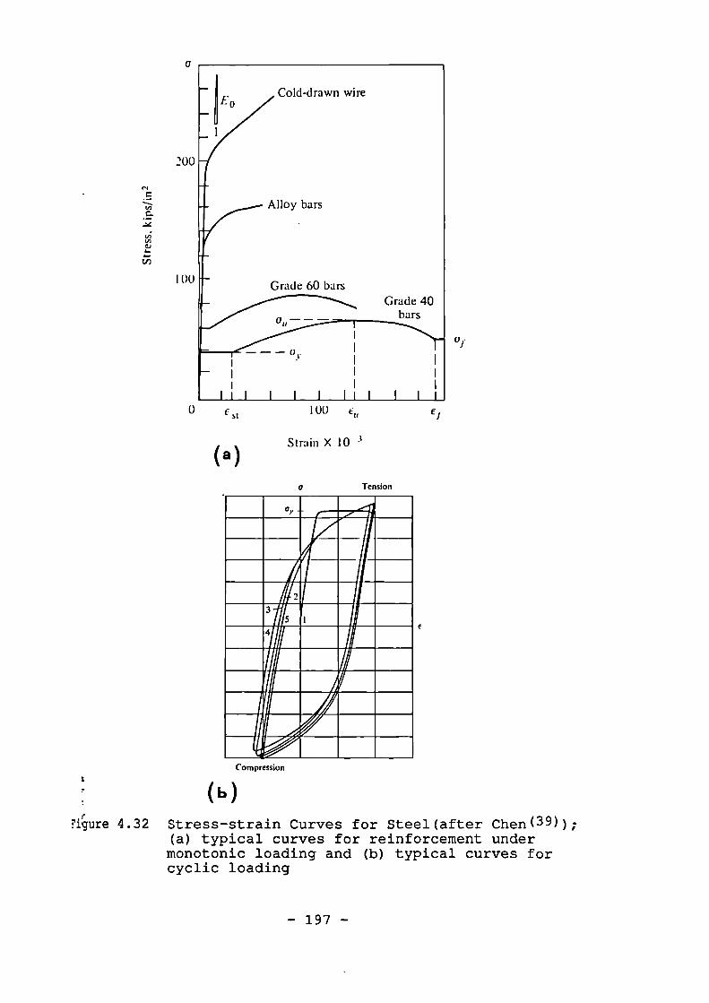
200
Grade 60 barsGrade 40
bars
IOU
111
It 1 1 1 1
100f st
II Itu
Tension0
Compression
Alloy bars
( a )
Strain X 10 3
Cold-drawn wire
b
Ei;pre 4.32 Stress-strain Curves for Steel (after Chen(39));(a) typical curves for reinforcement undermonotonic loading and (b) typical curves forcyclic loading
— 197 —
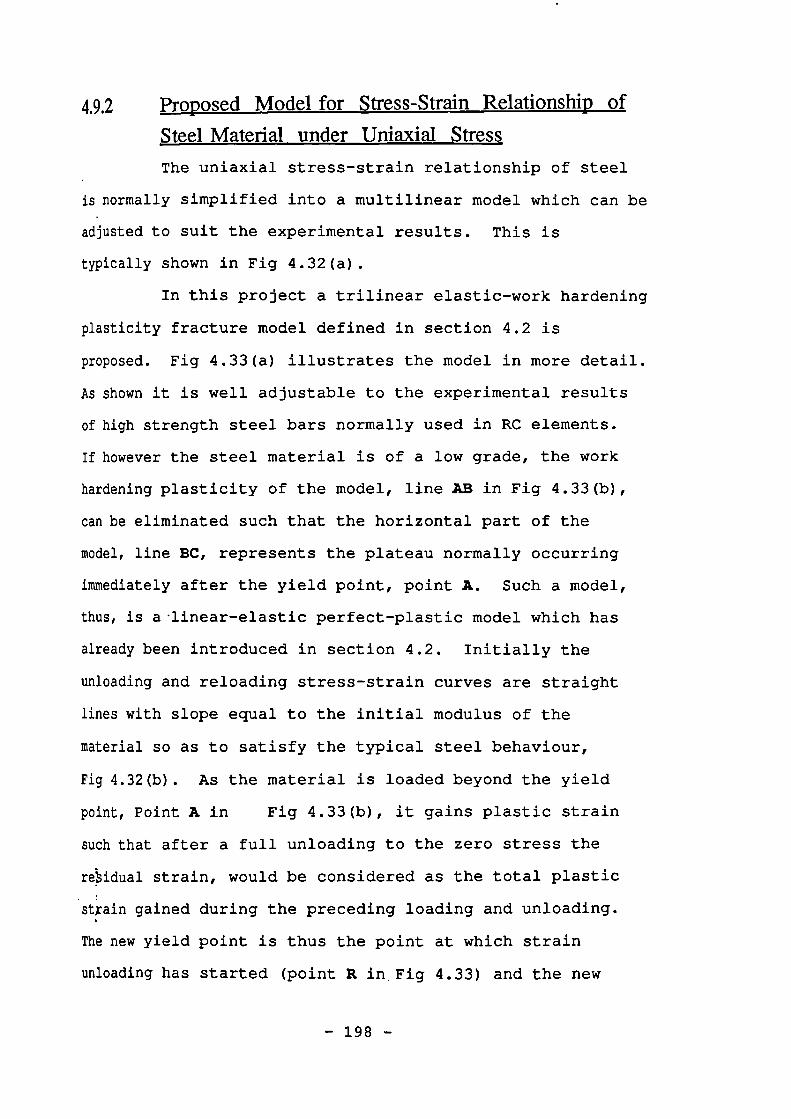
4.9.2 Proposed Model for Stress-Strain Relationship of
Steel Material under Uniaxial Stress
The uniaxial stress-strain relationship of steel
Is normally simplified into a multilinear model which can be
adjusted to suit the experimental results. This is
typically shown in Fig 4.32(a).
In this project a trilinear elastic-work hardening
plasticity fracture model defined in section 4.2 is
proposed. Fig 4.33(a) illustrates the model in more detail.
As shown it is well adjustable to the experimental results
of high strength steel bars normally used in RC elements.
If however the steel material is of a low grade, the work
hardening plasticity of the model, line AB in Fig 4.33(b),
can be eliminated such that the horizontal part of the
model, line BC, represents the plateau normally occurring
immediately after the yield point, point A. Such a model,
thus, is a . linear-elastic perfect-plastic model which has
already been introduced in section 4.2. Initially the
unloading and reloading stress-strain curves are straight
lines with slope equal to the initial modulus of the
material so as to satisfy the typical steel behaviour,
Fig 4.32(b). As the material is loaded beyond the yield
point, Point A in Fig 4.33(b), it gains plastic strain
such that after a full unloading to the zero stress the
residual strain, would be considered as the total plastic
strain gained during the preceding loading and unloading.
The new yield point is thus the point at which strain
unloading has started (point R in Fig 4.33) and the new
- 198 -
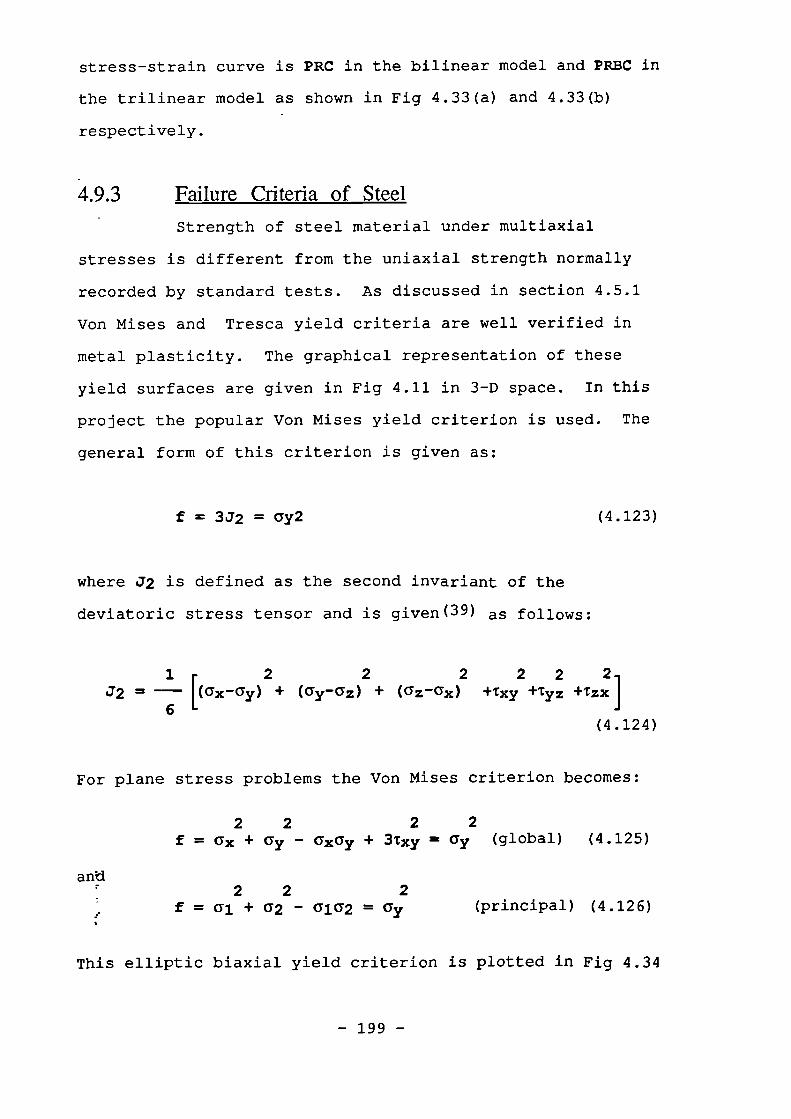
stress-strain curve is PRC in the bilinear model and PRBC in
the trilinear model as shown in Fig 4.33(a) and 4.33(b)
respectively.
4.9.3 Failure Criteria of Steel
Strength of steel material under multiaxial
stresses is different from the uniaxial strength normally
recorded by standard tests. As discussed in section 4.5.1
Von Mises and Tresca yield criteria are well verified in
metal plasticity. The graphical representation of these
yield surfaces are given in Fig 4.11 in 3-D space. In this
project the popular Von Mises yield criterion is used. The
general form of this criterion is given as:
f = 3J2 = Gy2 (4.123)
where J2 is defined as the second invariant of the
deviatoric stress tensor and is given( 39 ) as follows:
02 = [(ax-ay) + (ay-az) + ( az-ax) +txy +Tyz -Przx]6
(4.124)
For plane stress problems the Von Mises criterion becomes:
2 2 2 2f = ax + ay axoy + aticy = ay (global) (4.125)
and, 2 2 2
e f = al + a2 - ala2 = ay (principal) (4.126)
This elliptic biaxial yield criterion is plotted in Fig 4.34
1
- 199 -
AB
Ef
Strain
(a)
Comp,
Figure 4.33 Proposed Stress-strain Relationship Model forSteel; (a) high strength steel and (b) low andmedium strength steel
Tension
Comp
Figure 4.34 Von Mises Yield Criterion on The Co-ordinatePlane a3=0
— 200 —
4.9.4 Stress-strain Relationship of Ductile Material
4.9.4.1 Definitions and Basis of Elastic-Perfect
Plasticity Theory
The uniaxial stress-strain relation discussed in
section 4.9.2 led to a linear elastic-Perfect plasticity
fracture model as shown in Fig 4.33. A similar model may be
adopted for multiaxially loaded material. The general
behaviour under a complex stress state can be defined by the
following statements (39)
The material is elastic until it reaches the yield
limit i.e, until a function of the stress components reaches
a certain value. This is known as the yield function, yield
surface or yield criterion. Such a function, as discussed
in section 4.5.1, is generally given as follows:
f ( aij) = K
(4.127)
In the Von Mises criterion the yield surface is given as:
f Cri j 1/5712 =
or1
)= J2 = ---ay2 = k2 (4.128)3
Then plastic deformation takes place without
limit. For the plastic flow to continue, the state of
stress must remain on the yield surface. This is known as
the criterion for loading or consistency condition(39).
C) fdf = daij = 0
(4.129)
aij
- 201 -
a aij1 a gdzij (p) = dA (4.131)
A 3 fClEij (P) = dA (4.132)
3 crij
This flow strain is permanent; i.e. it remains
when the stresses are removed or when the stress intensity
drops below the yield value. This is known as the criterion
for unloading algebraically expressed as:
Dfdf - daij < 0
(4.130)
In general the yield function, Eq 4.128, represents a six
dimensional stress space. Only a 2-D representation of this
function is shown in Fig. 4.34. The stress point cannot go
outside the yield surface and plastic flow occurs when the
stress point is on the yield surface and the additional
loading daij must lie in the tangent plane as shown in
Fig 4.34.
It is not obvious whether there exists a necessary
connection between f and the plastic strain-increment vector
dcii(p)- In general, we can introduce the concept of
plastic-potential function g(aii), which enables us to write
the equations of plastic flow in the form
Where cl,kis a positive scalar factor of proportionality.
It is normally acceptable in metal plasticity to
assume that the yield function and plastic potential
coincide; i.e. f = g. Thus,
- 202 -
and plastic flow develops along the normal to the yield
surface. Relation 4.132 is called the associated flow
rule (39)
4.9.4.2 Stress-Strain Relationship under Multiaxial Stress
Conditions
Based on the particulars of the elastic-perfect
plasticity theory outlined in Section 4.9.4.1, the overall
stress-strain relation has been developed as follows:
When a particle of a ductile material is loaded to
the yield surface, it is actually forced to a new strain
level which includes plastic strains such that:
10 = { ce} + { ep} + {i tp} (4.133)
where (e) and {ee} denote the total elastoplastic strain and
the total elastic strain vector respectively. ielo)
signifies the accumulated plastic strain vector not
including the plastic strains, (A&O, achieved during the
current load increment.
The stresses are directly related to the elastic
strains as given in Eq 4.73 or 4.74 for 2 and 3 dimensional
stress space respectively. These relations may generally be
written as:
la) = [De]fee}
{ Ee} = Plena} (4.134):.,
The secant form of the elasticity matrix, [De], and its
inverse matrix, [Ne], are formed by the elastic poisson's
ratio Vo and the initial tangent elasticity modulus, Eo.
- 203 -
Substituting for feel from Eq 4.134 into Eq 4.133 leads to:
(C) = ( e-E0 = [N]{0} + { AZO (4.135)
A stress-strain relation may be established from
Eq 4.135 only when {Aepl can be related to the current
stress vector (al. This may be achieved by writing Eq 4.132
for the Von Mises yield criterion as follows:
f = .72 ; as given by Eq 4.128
Aeij(p) = A X 3.12
3aij
Substituting for J2 from Eq 4.124 leads to:
AEij (P) = Asii
where sij denotes the deviatoric stresses. For principal
directions, the above relation leads to:
Acji(p)= AX(ai-am) (4.136)
where am is the hydrostatic stress defined as:
1am = ---(01+02+a3) (4.137)
3
Substituting for am from Eqs 4.137, Eq 4.136 can be written
in matrix form as:
(AE:pl =1---AX3
2
-1
-1
-1
2
-1
-1
-1
2
{a} (4.138)
- 204 -
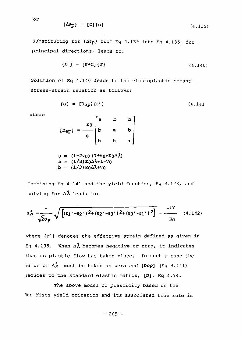
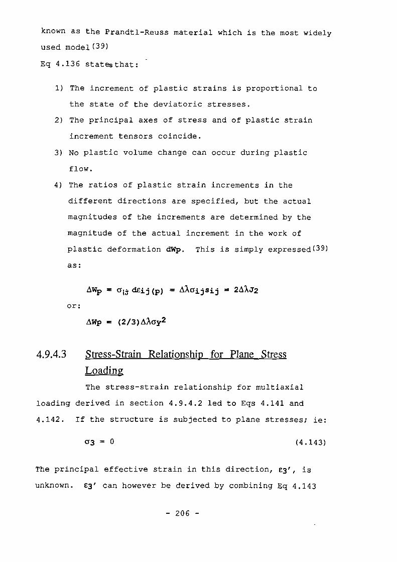
known as the Prandtl-Reuss material which is the most widely
used model(39)
Eq 4.136 statesthat:
1) The increment of plastic strains is proportional to
the state of the deviatoric stresses.
2) The principal axes of stress and of plastic strain
increment tensors coincide.
3) No plastic volume change can occur during plastic
flow.
4) The ratios of plastic strain increments in the
different directions are specified, but the actual
magnitudes of the increments are determined by the
magnitude of the actual increment in the work of
plastic deformation dWp. This is simply expressed(39)
as:
AWp = ala.C1Eij(p) = AAaijSij = 2A11.72
or:
AWp = (2/3)AAay2
4.9.4.3 Stress-Strain Relationship for Plane Stress
Loading
The stress-strain relationship for multiaxial
loading derived in section 4.9.4.2 led to Eqs 4.141 and
4.142. If the structure is subjected to plane stresses; ie:
CY3 = 0
(4.143)
The principal effective strain in this direction, e3', isunknown. e3' can however be derived by combining Eq 4.143
- 206 -
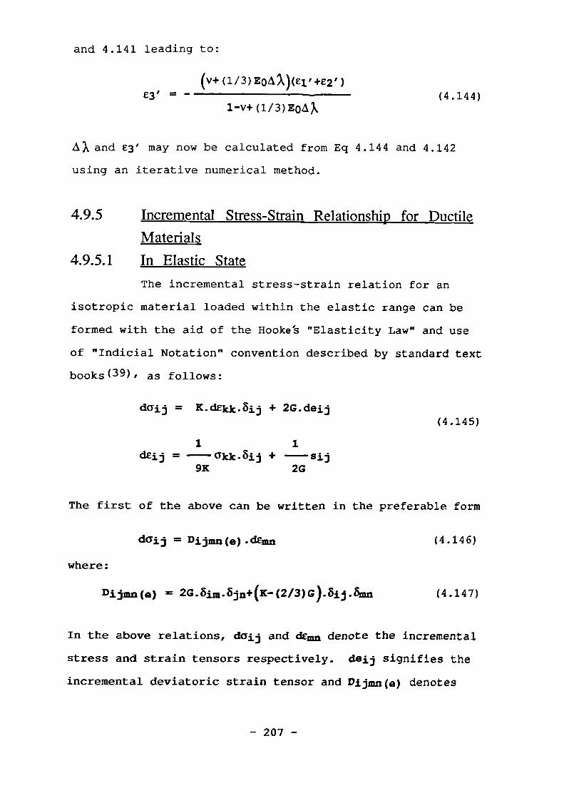
and 4.141 leading to:
£3' - (v+(1/3)E0,01/4)(el'+e2')
(4.144)1-V+(1/3)E0AN
La and £3' may now be calculated from Eq 4.144 and 4.142
using an iterative numerical method.
4.9.5 Incremental Stress-Strain Relationship for Ductile
Materials
4.9.5.1 In Elastic State
The incremental stress-strain relation for an
isotropic material loaded within the elastic range can be
formed with the aid of the Hooke's "Elasticity Law" and use
of "Indicial Notation" convention described by standard text
books (39) , as follows:
daij = K.dEkk.Bij + 2G.deij(4.145)
deij = ok1c.8ij + ----sij9K 2G
The first of the above can be written in the preferable form
daij = Dijmn(e)Akinn (4.146)
where:
Dijmn (e) = 2G. Sim .3jn+ (K- (2/3) G).45ij.3mn (4.147)
In the above relations, daij and &Ina denote the incremental
stress and strain tensors respectively. deij signifies the
incremental deviatoric strain tensor and Dijmn(e) denotes
-207 -
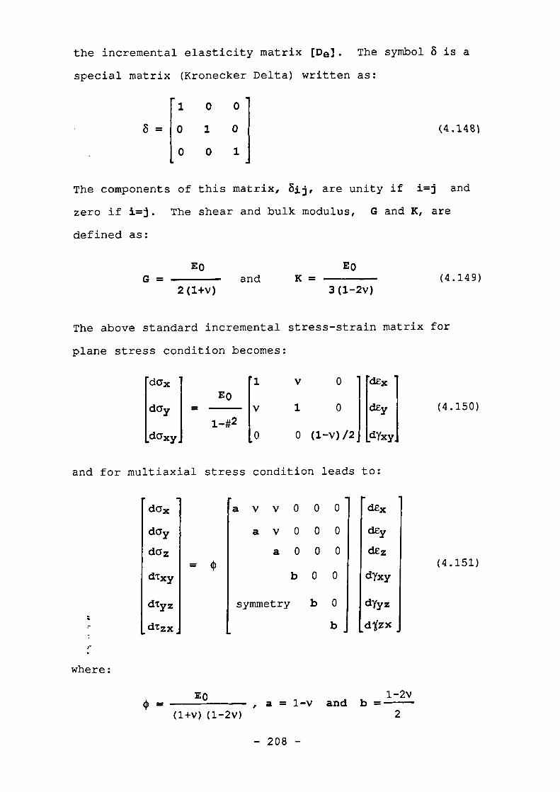
the incremental elasticity matrix [De]. The symbol 8 is a
special matrix (Kronecker Delta) written as:
1 0 0 I
8 = [0 1 0
0 0 1
(4.148)
The components of this matrix, Sij, are unity if i=j and
zero if i=j. The shear and bulk modulus, G and K, are
defined as:
E0 EOG — and K — (4.149)
2(1+v) 3(1-2v)
The above standard incremental stress-strain matrix for
plane stress condition becomes:
[dGx 1 v 0 l[dEx 1E0
day 1 = v 1 0 dEy1-#2
dazy 0 0 (1-v)/2 dYxy
(4.150)
and for multiaxial stress condition leads to:
•
n•••n
daz
duYdaz
d'czy
dt yz
citzx- -
= 4)
-a v v
a v
a
symmetry
b
000
000
000
0
b
eV
0
0
b
dEz
dEy
dez
dYxy
dyyz
di(zx.
(4.151)
:
where:
En
1-2v4) - a = 1-v and b =
(1+v)(1-2v) 2
- 208 -
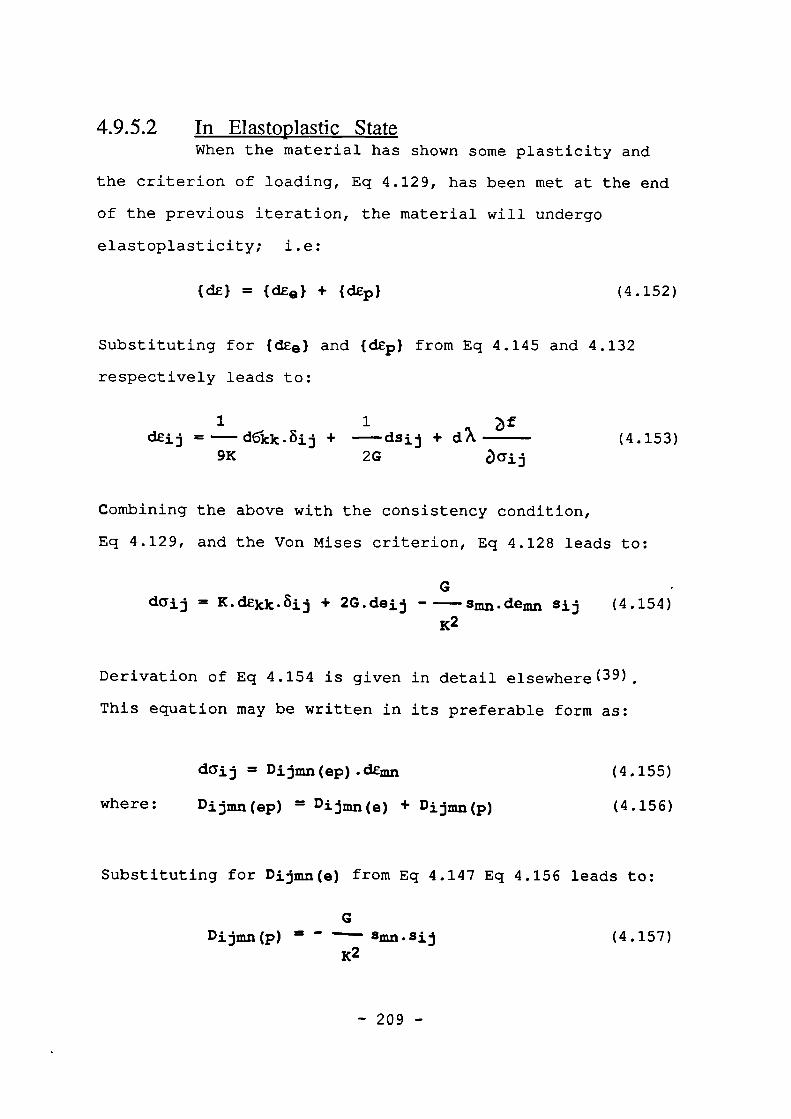
In Elastoplastic State When the material has shown some plasticity and
the criterion of loading, Eq 4.129, has been met at the end
of the previous iteration, the material will undergo
elastoplasticity; i.e:
{dc} = {dEe} + {dep} (4.152)
Substituting for (dee) and (dEp) from Eq 4.145 and 4.132
respectively leads to:
1 1dEij =
d6kk .sij + ---dsii + dn (4.153)9K 2G aaij
Combining the above with the consistency condition,
Eq 4.129, and the Von Mises criterion, Eq 4.128 leads to:
daij =K.dekk•Oij + 2G.deij - smn.demn sij (4.154)
K2
Derivation of Eq 4.154 is given in detail elsewhere(39).
This equation may be written in its preferable form as:
daij = Dijmn(ep). dEmn (4.155)
where: Dijmn(ep) = Dijmn(e) + Dijmn(p)
(4.156)
Substituting for Dijmn(e) from Eq 4.147 Eq 4.156 leads to:
Dijmn(p) =
smn.sij (4.157)K2
-209 -
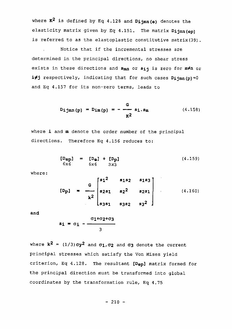
and
Si = (31
where K2 is defined by Eq 4.128 and Dijmn(e) denotes the
elasticity matrix given by Eq 4.151. The matrix Dijmn(ep)
is referred to as the elastoplastic constitutive matrix(39).
Notice that if the incremental stresses are
determined in the principal directions, no shear stress
exists in these directions and smn or sij is zero for mft ori0j respectively, indicating that for such cases Dijmn(p)=0and Eq 4.157 for its non-zero terms, leads to
Dijmn(p) = Dim(p) = - Si.Sm (4.158)
K2
where i and m denote the order number of the principal
directions. Therefore Eq 4.156 reduces to:
[Delp] = [De] + [pp]
(4.159)6x6 6x6 3x8
where:
[Dp] =
si2 s1s2 s1s3
s2s1 $2 232s1 •k2
3331 s3s2 33 2
al+024-03
3
(4.160)
where k2 = (1/3)ay2 and 01,02 and a3 denote the current
principal stresses which satisfy the Von Mises yield
criterion, Eq 4.128. The resultant [Dep] matrix formed for
the principal direction must be transformed into global
coordinates by the transformation rule, Eq 4.75
- 210 -
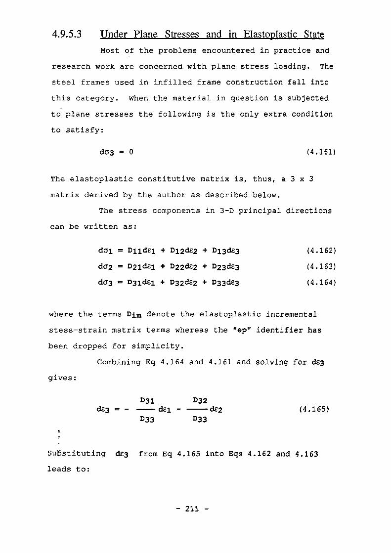
4.9.5.3 Under Plane Stresses and in Elastoplastic State
Most of the problems encountered in practice and
research work are concerned with plane stress loading. The
steel frames used in infilled frame construction fall into
this category. When the material in question is subjected
to plane stresses the following is the only extra condition
to satisfy:
da3 = 0 (4.161)
The elastoplastic constitutive matrix is, thus, a 3 x 3
matrix derived by the author as described below.
The stress components in 3-D principal directions
can be written as:
dal = Dlidel + D12dE2 + D13dE3
(4.162)
da2 = D21de1 + D22dE2 + D23dE3
(4.163)
da3 = D31de1 + D32dE2 + D33dE3 (4.164)
where the terms Dim denote the elastoplastic incremental
stess-strain matrix terms whereas the "ep" identifier has
been dropped for simplicity.
Combining Eq 4.164 and 4.161 and solving for dt3
gives:
D31 D32
dEl - dE2
(4.165)D33 D33
z
Substituting dE3 from Eq 4.165 into Eqs 4.162 and 4.163
leads to:
- 211 -
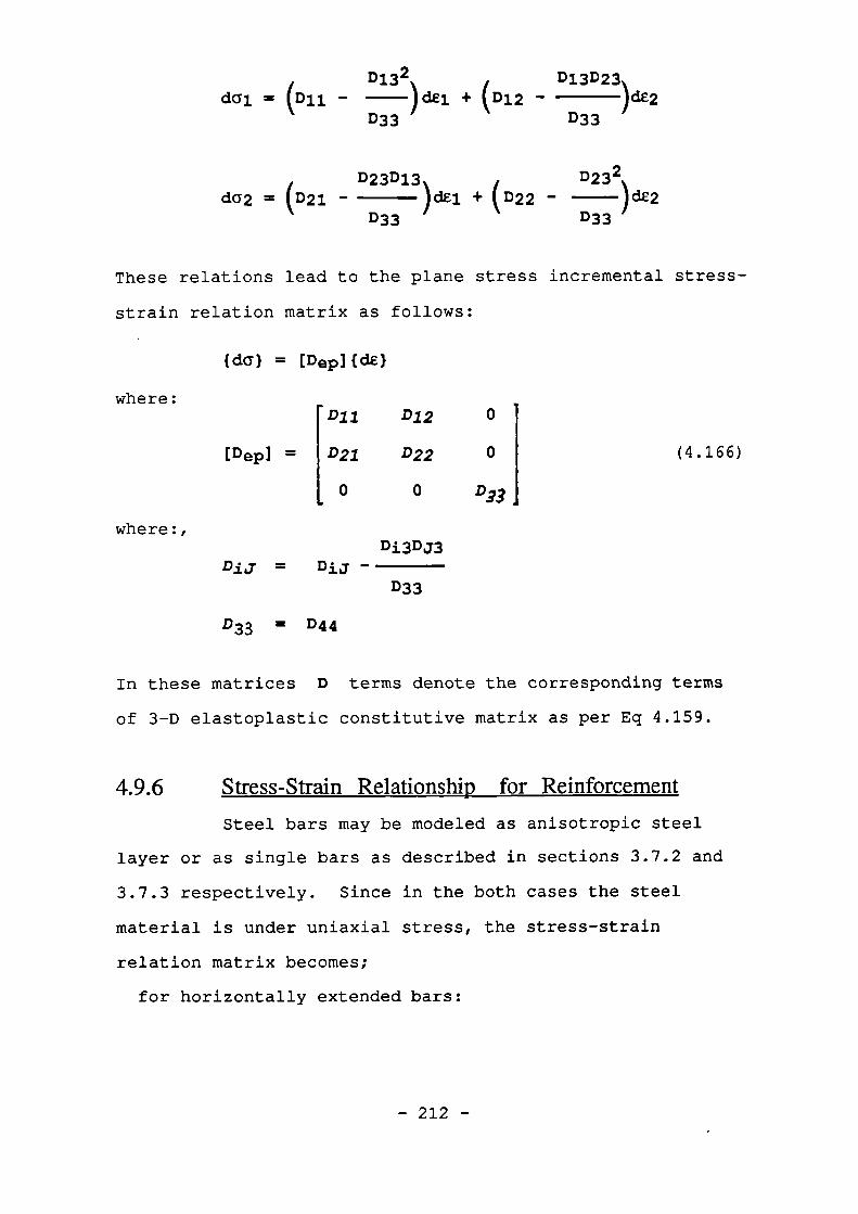
Di3D23x)del + ( D 12 - )dE2
D33 D33dal = (D11 -
D132
da2 = (D21 -D23D13
D33)olti + ( D22 -
D232)de2
D33
These relations lead to the plane stress incremental stress-
strain relation matrix as follows:
where:
(dal
[Dep] =
= (Dep]{de}
D11 012
D21 D22
0 0{
o
o
Dv
(4.166)
where:,Di3Dj3
Dij = Dij D33
D33 = D44
In these matrices D terms denote the corresponding terms
of 3-D elastoplastic constitutive matrix as per Eq 4.159.
4.9.15 Stress-Strain Relationship for Reinforcement
Steel bars may be modeled as anisotropic steel
layer or as single bars as described in sections 3.7.2 and
3.7.3 respectively. Since in the both cases the steel
material is under uniaxial stress, the stress-strain
relation matrix becomes;
for horizontally extended bars:
Esirsi 0 o
Psi] = 0 0 0 I (4.167a)
0 0 0
and for vertically extended bars:
0 0
0[ p si] = 0 Esirsi 01
I 0 o o
(4.167b)
where Esi and rsi denote the incremental modulus of
elasticity and the ratio of the group i steel bars
respectively, within the integration zone under
consideration. For an inclined group of bars, [Dsi] may be
computed by transforming Eq 4.167a into the appropriate
angle using Eq 4.77.
4.10 Constitutive Formulation for Mechanical Behaviour
of Interfaces and Joints
4.10.1 General
The step by step development of the F.E
representation of interfaces has been discussed in detail in
Chapter 3, leading to the new proposed interface element
described in section 3.10.3. While the geometrical
formulation was accomplished by introducing the proposed
shape functions, the mechanical behaviour of interfaces is
yet to be modelled. This constitutes the following:
i) The criteria under which yielding, slip and/or
separation occur.
- 213 -
ii) The strain-relative displacement relationship of the
interfaces both for the incremental changes and for
the overall values.
These are discussed in the following sections.
4.10.2 Yielding, Slip and Separation Criteria
The shear strength and behaviour of interfaces and
joints has been studied by mamy investigators( 76 to 81) .
The shear strength of a bonded interface is generally
considered as comprising:
i) bond shear strength of the interface
ii) the frictional resistance of the interface
The frictional resistance of the interface is
normally calculated as the product of the normal stress an
and the coefficient of friction, g, where is normally
assumed to be constant for all normal stress levels. These
lead to the "bond shear failure criterion" of the interface
expressed algebraically as follows:
IT! = abs - gunor:
(4.168)RX = abs - gun
where R is assigned either +1 or -1 when T is positive or
negative respectively and the sign of an is considered to be
-ve. for compression.
When the interface is not bonded or it has totally
debonded in the course of loading, the first term in the
- 214 -
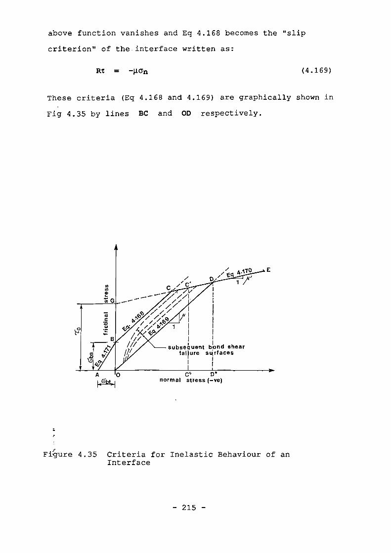
above function vanishes and Eq 4.168 becomes the "slip
criterion" of the interface written as:
Itt = -gan (4.169)
These criteria (Eq 4.168 and 4.169) are graphically shown in
Fig 4.35 by lines BC and OD respectively.
//' c'
, 1V--- / //I I---- ////// I/ II. /
fI 1be I//' Nt)
// V 1 I Ik,
I I/// °).. I 10/ 1 subse4uent brond shear
failure surfacesI
II
I I
// EA ge ' •
1
Io-C" D6
normal stress (—ye)
:
,Figure 4.35 Criteria for Inelastic Behaviour of an
Interface
- 215 -
When the interface constitutes a thin layer of a
relatively soft material, like mortar in the bed joints of
masonry structures, another effect may become the source of
the permanent shear displacement by mean of plastic shear
deformation or yielding of the confined joint material.
This has been studied by Page( 79 ) and Hegemier( 91 ) for the
bed joints of brick and grouted hollow concrete block
masonry respectively. Such a criterion may be idealized by
a straight line (line GE) with g' slope. As shown in
Fig 4.35 the joint "yielding criterion" can be algebraically
expressed as:
RE = TO - ll'an (4.170)
Fig 4.35 also shows the proposed "bond tensile
failure criterion", represented by line AB to specify the
normal tension and frictional shear stresses causing this
type of failure. The function to represent the bond tensile
failure criterion is, thus, written as:
RT
an+ = 1 (4.171)
abs abt
where subs and at denote bond shear and tensile strength of
the interface respectively.
Table 4.2 lists some experimentally recorded-,
values of the mechanical properties of interfaces and joints
dealt with in practice.
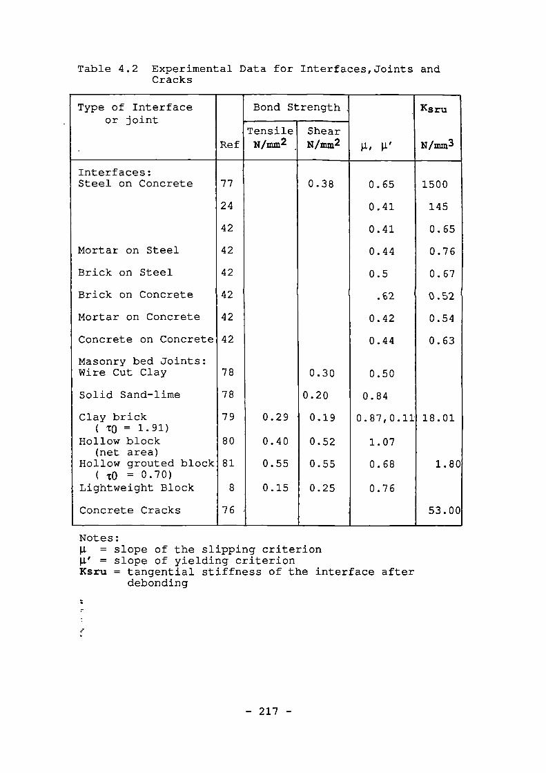
Table 4.2 Experimental Data for Interfaces,Joints andCracks
Type of Interfaceor joint
-Ref
Bond Strength. .
g, pLI
Ksru
NiMM3
.
TensileN imm2 .
ShearN/mm2
Interfaces:Steel on Concrete 77 0.38 0.65 1500
24 0.41 145
42 0.41 0.65
Mortar on Steel 42 0.44 0.76
Brick on Steel 42 0.5 0.67
Brick on Concrete 42 .62 0.52
Mortar on Concrete 42 0.42 0.54
Concrete on Concrete 42 0.44 0.63
Masonry bed Joints:Wire Cut Clay 78 0.30 0.50
Solid Sand-lime 78 0.20 0.84
Clay brick 79 0.29 0.19 0.87,0.11 18.01( To = 1.91)
Hollow block(net area)
80 0.40 0.52 1.07
Hollow grouted block 81 0.55 0.55 0.68 1.80( TO = 0.70)
Lightweight Block 8 0.15 0.25 0.76
Concrete Cracks 76 - . 53.00
Notes:p. = slope of the slipping criteriong' = slope of yielding criterionKsru = tangential stiffness of the interface after
debonding
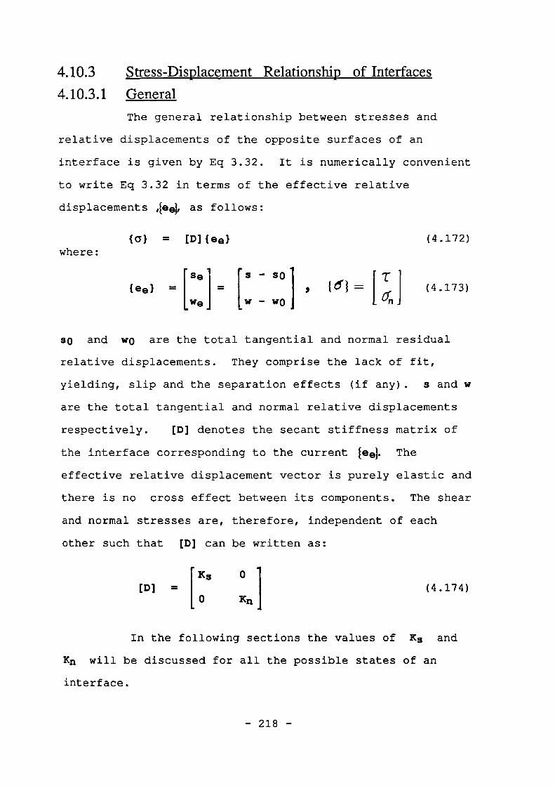
{ee} =w - WO
4.10.3 Stress-Displacement Relationship of Interfaces
4.10.3.1 General
The general relationship between stresses and
relative displacements of the opposite surfaces of an
interface is given by Eq 3.32. It is numerically convenient
to write Eq 3.32 in terms of the effective relative
displacements 4ei4 as follows:
(a} = [Dflee} (4.172)where:
rr .1
=P tei ,, (4.173)un
so and wo are the total tangential and normal residual
relative displacements. They comprise the lack of fit,
yielding, slip and the separation effects (if any). s and w
are the total tangential and normal relative displacements
respectively. [D] denotes the secant stiffness matrix of
the interface corresponding to the current feel. The
effective relative displacement vector is purely elastic and
there is no cross effect between its components. The shear
and normal stresses are, therefore, independent of each
other such that [D] can be written as:
[Ks 0[D] =
1
0 Kn(4.174)
In the following sections the values of Ks and
Kn will be discussed for all the possible states of an
interface.
- 218 -
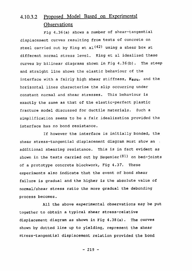
4.10.3.2 Proposed Model Based on Experimental
Observations Fig 4.36(a) shows a number of shear-tangential
displacement curves resulting from tests of concrete on
steel carried out by King et al( 42) using a shear box at
different normal stress level. King et al idealized these
curves by bilinear diagrams shown in Fig 4.36(b). The steep
and straight line shows the elastic behaviour of the
interface with a fairly high shear stiffness, Ksru, and the
horizontal lines characterize the slip occurring under
constant normal and shear stresses. This behaviour is
exactly the same as that of the elastic-perfect plastic
fracture model discussed for ductile materials. Such a
simplification seems to be a fair idealization provided the
interface has no bond resistance.
If however the interface is initially bonded, the
shear stress-tangential displacement diagram must show an .
additional shearing resistance. This is in fact evident as
shown in the tests carried out by Hegemier (81) on bed-joints
of a prototype concrete blockwork, Fig 4.37. These
experiments also indicate that the event of bond shear
failure is gradual and the higher is the absolute value of
normal/shear stress ratio the more gradual the debonding
process becomes.
All the above experimental observations may be put
together to obtain a typical shear stress-relative
displacement diagram as shown in Fig 4.38(a). The curves
shown by dotted line up to yielding, represent the shear
stress-tangential displacement relation provided the bond
- 219 -
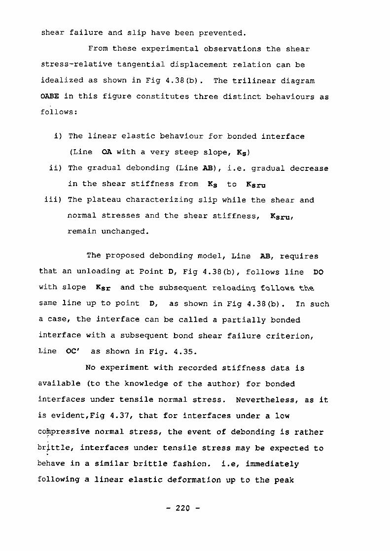
shear failure and slip have been prevented.
From these experimental observations the shear
stress-relative tangential displacement relation can be
idealized as shown in Fig 4.38(b). The trilinear diagram
OABE in this figure constitutes three distinct behaviours as
follows:
i) The linear elastic behaviour for bonded interface
(Line OA with a very steep slope, Ks)
ii) The gradual debonding (Line AB), i.e. gradual decrease
in the shear stiffness from Ks to Ksru
iii) The plateau characterizing slip while the shear and
normal stresses and the shear stiffness, Ksruf
remain unchanged.
The proposed debonding model, Line AB, requires
that an unloading at Point D, Fig 4.38(b), follows line DO
with slope Ksr and the subsequent reloading follotgs the
same line up to point D, as shown in Fig 4.38(b). In such
a case, the interface can be called a partially bonded
interface with a subsequent bond shear failure criterion,
Line OC' as shown in Fig. 4.35.
No experiment with recorded stiffness data is
available (to the knowledge of the author) for bonded
interfaces under tensile normal stress. Nevertheless, as it
is evident,Fig 4.37, that for interfaces under a low
cotipressive normal stress, the event of debonding is rather
brittle, interfaces under tensile stress may be expected to
behave in a similar brittle fashion. i.e, immediately
following a linear elastic deformation up to the peak
-220 -
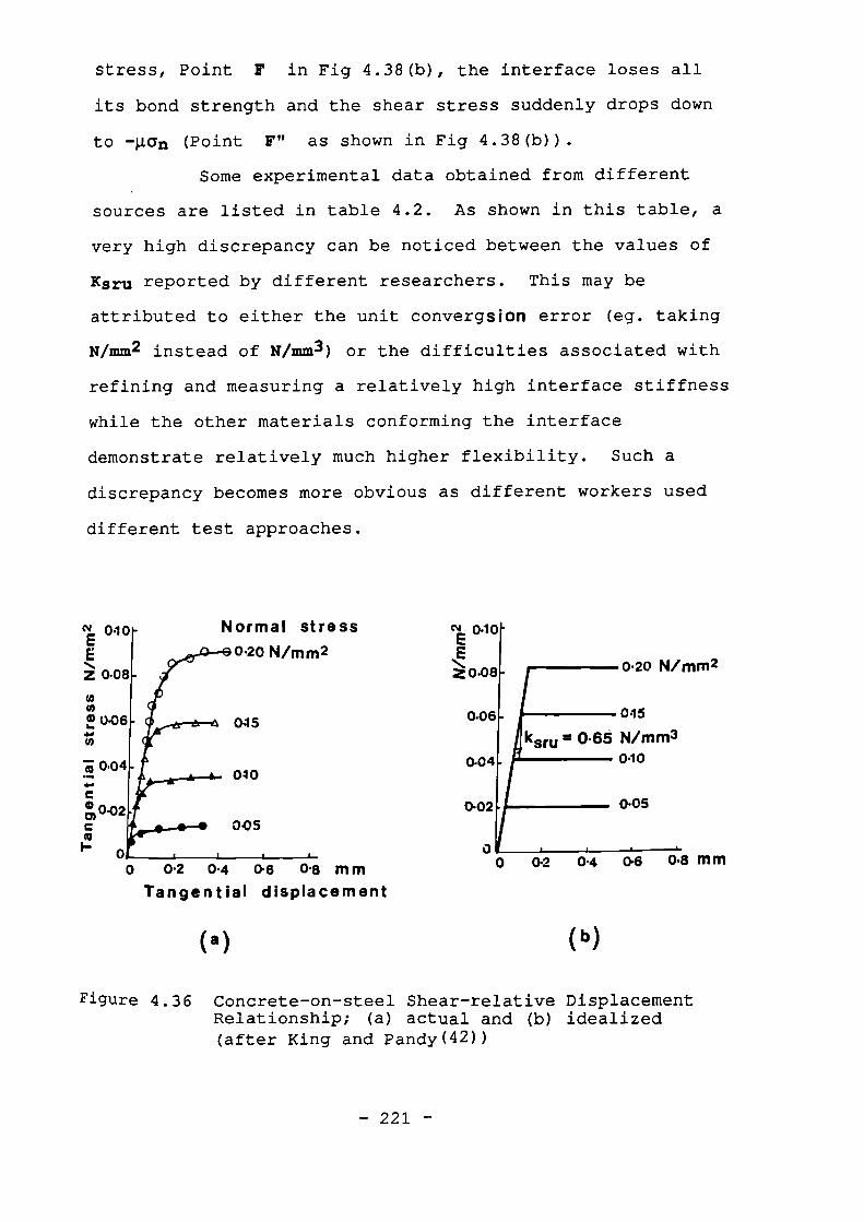
Normal stress0-20 N/mm2
045
040
005
(4 040
Z 0-08
! U46
To 0.04
/2042
oio
0 • 20 N/mm2
0;15
u = 0.66 N/mm30•10
0•05
0-2 0 •4 043 0 .8 111141
(b)
Z048
0-06
0-04
0-02
stress, Point F in Fig 4.38(b), the interface loses all
its bond strength and the shear stress suddenly drops down
to -gun (Point as shown in Fig 4.38(b)).
Some experimental data obtained from different
sources are listed in table 4.2. As shown in this table, a
very high discrepancy can be noticed between the values of
Ksru reported by different researchers. This may be
attributed to either the unit convergsiOn error (eg. taking
N/mm2 instead of N/mm3 ) or the difficulties associated with
refining and measuring a relatively high interface stiffness
while the other materials conforming the interface
demonstrate relatively much higher flexibility. Such a
discrepancy becomes more obvious as different workers used
different test approaches.
0 01 0 •4 0 .6 08 mmTangential displacement
(a)
Figure 4.36 Concrete-on-steel Shear-relative DisplacementRelationship; (a) actual and (b) idealized(after King and Pandy(42))
- 221 -
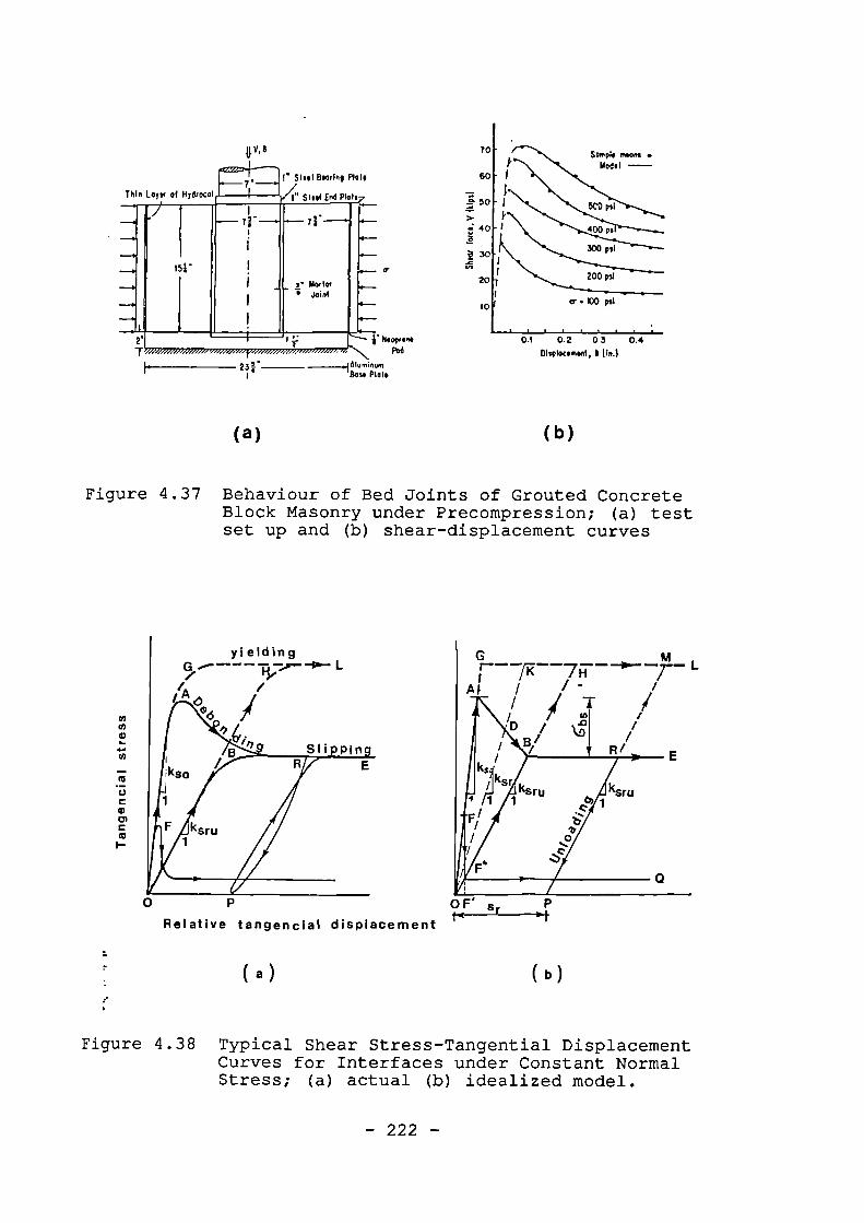
..._-7-7.-__.1 r)tee I Bearing P1olo
Thin Low of Hydrocol I r/1" Sleol End Plo17..._
r-
--.--
i
-.
—4.
—+ 151- I
i) yr —...— 71-_.......__1
i—. 4
1 4—--•
I _ 3- Odor lotI Joinl
I4—
0.1 0.2 03 0.4
DIspknomord. tin.)
Nooron4Pod
23:.1 BomPio10
yieldingL
OF' srt4
Relative tangencial displacement
( a )
b )
(a)
(b)
Figure 4.37 Behaviour of Bed Joints of Grouted ConcreteBlock Masonry under Precompression; (a) testset up and (b) shear-displacement curves
Figure 4.38 Typical Shear Stress-Tangential DisplacementCurves for Interfaces under Constant NormalStress; (a) actual (b) idealized model.
- 222 -
No experimental data is available for shear and
normal stiffness of a fully bonded interface. Theoretically,
they must be set to very high values. When the interface
has a finite thickness (bed and head-joints in masonry), the
above discussed values of stiffness must also include the
additional flexibility induced by the finite thickness and
presumably soft mortar joints. This will be discussed later
in Section 4.11
4.10.4 Determination of the State of an Interface
4.10.4.1 General
Assume s and w are the tangential and normal
relative displacements at a gaussian point within an
interface from which the previously acquired yielding and
slip, and also the initially specified lack of fit, are
excluded. Further assume that the interface inelastic
behaviour (yielding, debonding, slipping and separation)
during the current iteration is somehow prevented.
i.e. so = wO = 0. Using s and w from Eq 4.172 and the
latest values of the shearing stiffness, Ksr, the shear and
normal stresses may then be calculated. These stresses can
be coupled with the criteria by which the interface would
possibly undergo one of the inelastic events as shown in
Figs 4.39 to 4.41.
As shown in these figures the calculated stresses
simply indicate that what is going to happen to the
interface as a result of the current changes in the relative
displacements. This permits the changes to the inelastic
relative displacements to be calculated and the new state of
- 223 -
the interface to be determined as discussed in the following
sections.
4.10.4.2 New State of a Previously Fully Bonded Interface
As shown in Fig 4.39(b) Lines EF, FC and CG divide
the stress space into 4 zones indicating whether the
interface is subjected to debonding leading to separation,
debonding possibly leading to slip, yielding or resuming the
elastic state. These lines have already been defined in
Section 4.10.2 by Eqs 4.171, 4.168 and 4.170 as bond tensile
failure; bond shear failure, and the interface (Joint)
yielding criteria respectively. If point P ( the point
representing the shear and normal stresses calculated in the
manner described in Section 4.10.4.1) takes a position above
one of these lines the indicated inelastic event would take
place. The induced inelastic displacements and the
subsequent stresses can be calculated as follows:
a) Debonding Interface Leading to Separation
The graphical representation of this state is
shown for point P4 on Fig 4.39. In a separated interface no
shear and normal stress develops. Therefore:
new slip = ssl = s and separation = wsp = w (4.175)
and an = T = 0 (4.176);
Debonding Interface Leading to Partial Debonding
Allow the interface to debond gradually until
- 224 -
](4.179)
point P1 drops down to Pl f on the appropriate subsequent
debonding surface as shown in Fig 4.39. Clearly, such a
drop is possible by assuming a partially debonded interface
with shear stiffness of Ksr rather than that of the fully
bonded interface, Kso. The new stiffness, Ksr, may also be
used to specify the rate of debonding as shown in
Fig 4.39(a). Ksr can be calculated as follows:
Line AB in Fig 4.39(a) can be formulated using the
co-ordinates of points A and B i.e.
Y - YA Y - YB- (4.177)
x - xA x - xl3
where
abs - gan -ganKs0
KsruA
and BMos - gan -gan
using the unknown partially debonded shearing stiffness,
Ksr, Line OP' can be written as:
y = Ksrx (4.178)
Elimination of y from these two equations leads to Ksr in
terms of the absolute value of the shear displacement Rsi
(the x co-ordinate of intercept of the two lines) as
follows.
Kr. = 1 [gan/Ksru + Rs
-gan + abs Rs gan/Ksru + (ab5-gan)/Ks0
e
The stresses may now be calculated as:
- 225 -
an = vaCn and T = sKsr (4.180)
Since the interface is still partially bonded no separation
or slip can occur. R takes the value either +1 or -1 so as
to make Rs always positive.
c) Debonding Interface Leading to Total Dabonding
For point P3 in Fig 4.39, the absolute value of
shear displacement, Rs3, may exceed sb indicating that the
interface has totally debonded and some slip has taken
place. This case will be discussed in Section 4.10.4.4 (b)
d) Fully Bonded Interface Undergoing Yielding
Allow for a prescribed residual yielding
displacement, Sy, for point P2 as shown in Fig 4.39(a) so
that the new position of this point, P2', meets the yielding
criterion, Line CG. Then sy can be calculated from
Fig 4.39(a) as:
-Wan 'CO
Sy = S (4.181)
RKSO
and= KSO( S - Sy) and an = Knw (4.182)
e) Fully Bonded Interface Resuming Elastic State
No separation or slip has occurred and the already
calculated elastic stresses are the true values. ie ,
T = SKS° and an = WKn (4.183)
- 226 -
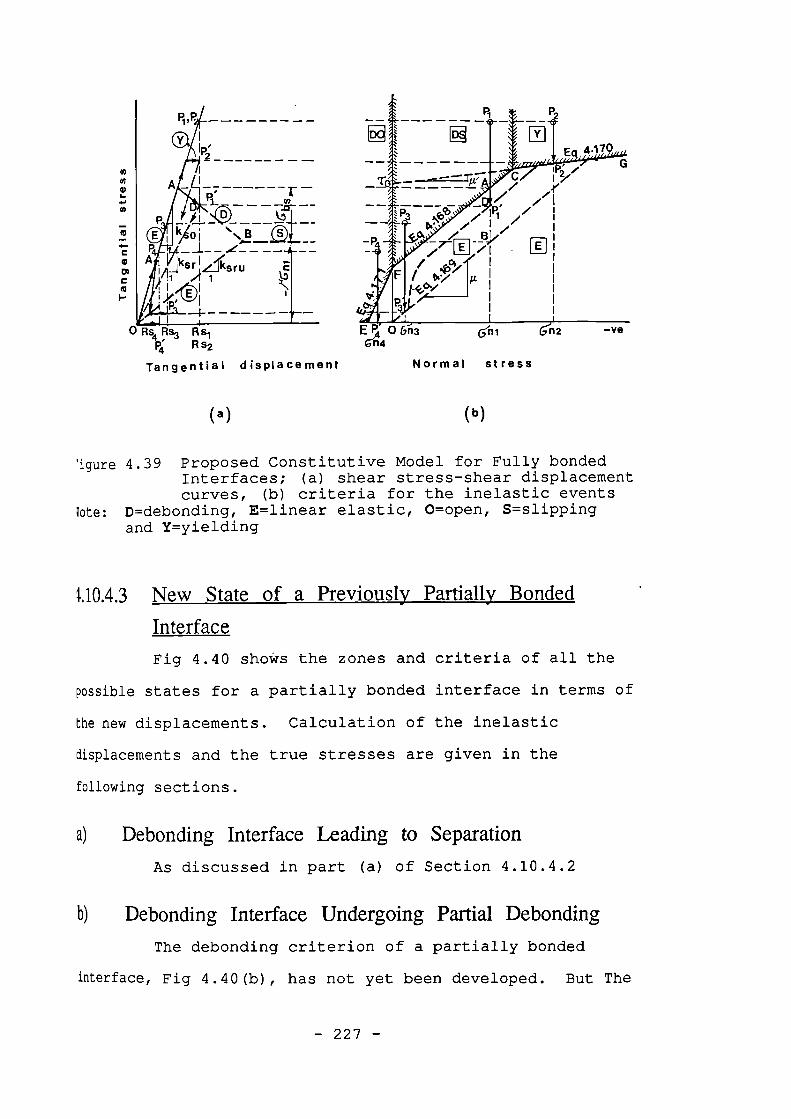
0 RS4 RS3 RS1134' Rs2
Tangential displacement Normal stress
(a)
(b)
'igure 4.39 Proposed Constitutive Model for Fully bondedInterfaces; (a) shear stress-shear displacementcurves, (b) criteria for the inelastic events
iote: D=debonding, E=linear elastic, 0=open, S=slippingand Y=yielding
1.10.4.3 New State of a Previously Partially Ekmicled
Interface
Fig 4.40 shows the zones and criteria of all the
possible states for a partially bonded interface in terms of
he new displacements. Calculation of the inelastic
displacements and the true stresses are given in the
following sections.
Debonding Interface Leading to Separation
As discussed in part (a) of Section 4.10.4.2
Diebanding Interface Undergoing Partial Debonding
The debonding criterion of a partially bonded
interface, Fig 4.40(b), has not yet been developed. But The
- 227 -
Sy = S (4.186)
same approach as used in part (b) of Section 4.10.4.2 may be
employed. For the value of current an and previous value of
Ksr and from Fig 4.40(a), the value of 11% can be calculated
for point D on the debonding criterion (Line AB) as follows:
1 - pittd = + abs (4.184)
abs1 - p
ganwhere
KsO/Ksr(4.185)
Ks°/Ksru - 1
Ksr is the shear stiffness of the interface at the end of
the previous iteration. Now if the absolute value of shear
(say for point P1) is higher than R.Td, the interface is
subjected to further debonding and the procedure to
calculate the new value of Ksr and stresses is exactly the
same as given in part (b) of Section 4.10.4.2. Note the
location of point C' calculated in Clause (d) of this
section.
Debonding Interface Leading to Total f)etxmding
This will be discussed in Section 4.10.4.4(b)
d) Partially Bonded Interface Undergoing Yielding
Permit a residual yielding shear displacement, sy,
and proceed as described in part (d) of Section 4.10.4.2
leading to:
+ TO
RKsr
- 228 -
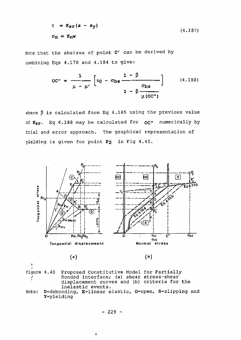
I.
Rrd7
,rAk r ®e
sr (New)I ii
UI II
T = Ksr( s - Sy)
an = KW
Note that the absissa of point C' can be derived by
combining Eqs 4.170 and 4.184 to give:
11 - 0oc” - [TO abs
obs1 0
g(OC")
(4.187)
(4.188)
where 3 is calculated form Eq 4.185 using the previous value
of Ksr. Eq 4.188 may be calculated for OC" numerically by
trial and error approach. The graphical representation of
yielding is given for point P2 in Fig 4.40.
0 Rsi Rs2Rs5 0n2
U5
Tangential displacement Normal stress
(a)
(b)
Figure 4.40 Proposed Constitutive Model for PartiallyBonded Interface; (a) shear stress-sheardisplacement curves and (b) criteria for theinelastic events.
Note: D=debonding, E=linear elastic, 0=open, S=slipping andY=yielding
- 229 -
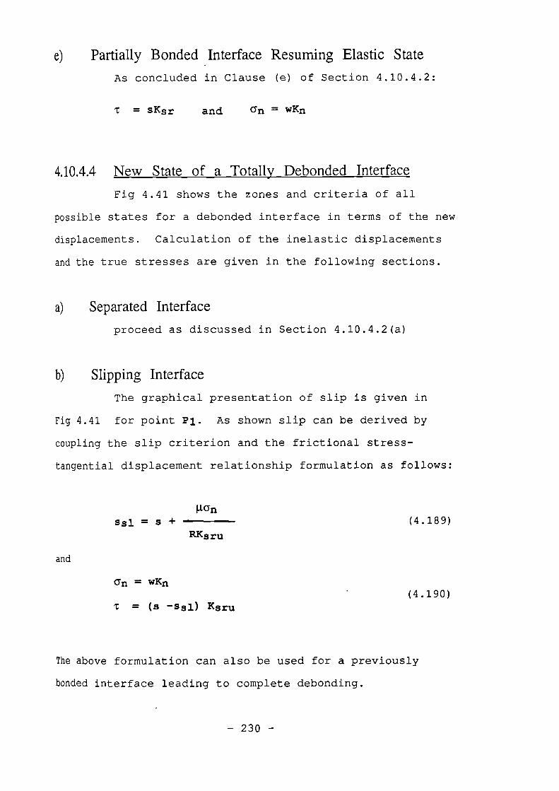
e) Partially Bonded Interface Resuming Elastic State
As concluded in Clause (e) of Section 4.10.4.2:
T = SKr and an = WKn
4.10.4.4 New State of a Totally EM)onded Interface
Fig 4.41 shows the zones and criteria of all
possible states for a debonded interface in terms of the new
displacements. Calculation of the inelastic displacements
and the true stresses are given in the following sections.
Separated Interface
proceed as discussed in Section 4.10.4.2(a)
b) Slipping Interface
The graphical presentation of slip is given in
Fig 4.41 for point P. As shown slip can be derived by
coupling the slip criterion and the frictional stress-
tangential displacement relationship formulation as follows:
ssl = s + (4.189)RKsru
and
an = WKn(4.190)
T = (S -ssl) Ksru
The above formulation can also be used for a previously
bonded interface leading to complete debonding.
- 230 -
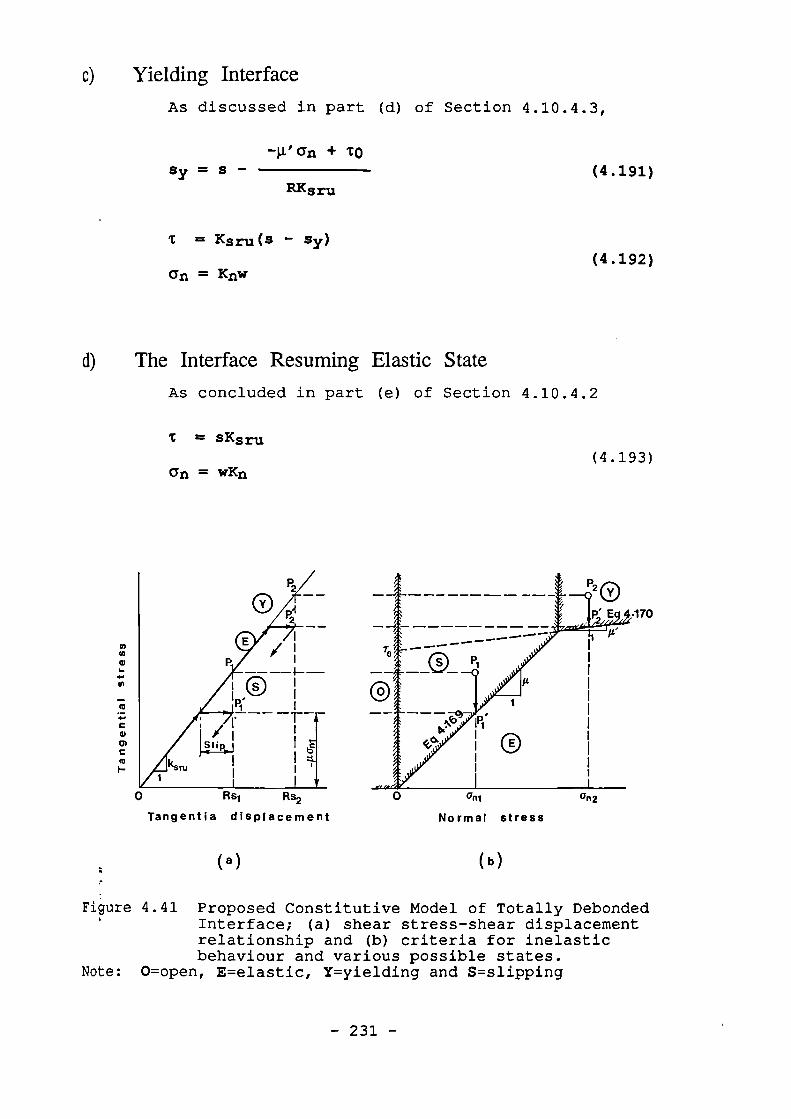
an = WKu
0 Rs/ Rs2
Tangentia displacement
(4.193)
.170
Un2
Normal stress
0 Yielding Interface
As discussed in part (d) of Section 4.10.4.3,
-W an TOSy = S (4.191)
KKsru
T = Ksru(s - Sy)(4.192)
an = Knw
d) The Interface Resuming Elastic State
As concluded in part (e) of Section 4.10.4.2
T = sKsru
(a)
(b)
Figure 4.41 Proposed Constitutive Model of Totally DebondedInterface; (a) shear stress-shear displacementrelationship and (b) criteria for inelasticbehaviour and various possible states.
Note: 0=open, E=elastic, Y=yielding and S=slipping
- 231 -
4.10.4.5 Proposed Incremental [TO Matrix
The incremental stress-relative displacement
relation in its general form can be written as:
[ids= ]Pt]
rd:n1 dw(4.194)
When the interface is separated, no stress will be
transferred through the interface requiring, thus, the [Dt]
matrix to be a null matrix.
If the incremental changes have not produced any
gradual inelastic changes, such as yielding, debonding or
contacted slip, the shear and normal components of the
incremental stresses and displacements are independent of
each other. Therefore Eqs 4.194 can be written as:
[
dT 1d un
= [Ks
0
0] rsKn dw
I(4.195)
where Ks is the current elastic shear stiffness of the
interface taking values of Kso, Ksr or Ksru for a fully
bonded, partially bonded or a totally debonded interface
respectively, Figs 4.39 to 4.41.
If however one of the gradual inelastic events
occurs during the incremental displacements, a precise
tangent elasticity matrix [Dt] can be derived by:
differentiation of the stress components, T and an, from the
formulation provided in Sections 4.10.4.2 to 4.10.4.4 as
follows:
- 232 -
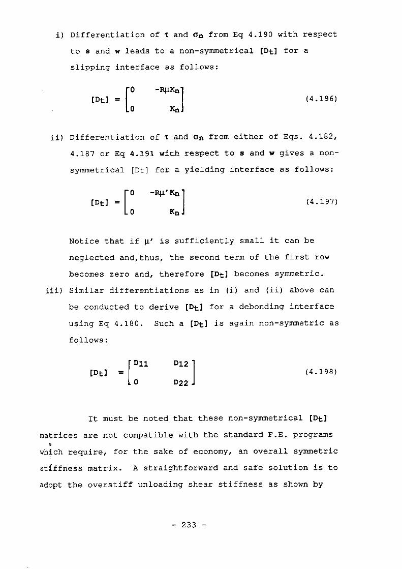
i) Differentiation of T and an from Eq 4.190 with respect
to s and w leads to a non-symmetrical [Dt] for a
slipping interface as follows:
[Dt] =
[0 -141K1
0 Kn
(4.196)
ii) Differentiation of T and an from either of Eqs. 4.182,
4.187 or Eq 4.191 with respect to s and w gives a non-
symmetrical [Dt] for a yielding interface as follows:
[Dt] =
][
0 -RA'Kn
0 Kn(4.197)
Notice that if g' is sufficiently small it can be
neglected and,thus, the second term of the first row
becomes zero and, therefore [Dt] becomes symmetric.
iii) Similar differentiations as in (i) and (ii) above can
be conducted to derive [Dt] for a debonding interface
using Eq 4.180. Such a [Dt] is again non-symmetric as
follows:
[ Dll D12 1[Dt] = (4.198)
0 D22 i
It must be noted that these non-symmetrical [Dt]
matrices are not compatible with the standard F.E. programs
which require, for the sake of economy, an overall symmetric
stiffness matrix. A straightforward and safe solution is to
adopt the overstiff unloading shear stiffness as shown by
- 233 -
the heavy dotted lines in Figs. 4.39 to 4.41. Even so it
causes a slow convergence. Therefore Eq 4.195 may be
considered as the general incremental stress-displacement
relationship, unless a solution of unsymmetric equations is
incorporated with the F.E program. Such a solution is
included with the program "NEPAL".
4.11 Constitutive Formulation for Masonry
The finite element representation of masonry has
briefly been discussed in Section 3.9. Of the element types
studied, the 4-node element made of the proposed plane-
stress equivalent material, representing both the units and
the joints, separated by interface elements, Fig 3.9, was
found to be the most economical, practical and simplest
available choice. The proposed 2-D material facilitates
the possibility of simulating the masonry behaviour beyond
its peak stress. Such a representation constitutes two
distinct stiffness and strength contributors as follows:
i) The proposed plane-stress masonry equivalent material
which must (on the basis of plane stress-strain
constitutive relationship) simulate the combined 3-D
mechanical behaviour of masonry units and mortar joints
while assuming the interface of the equivalent material
elements remain intact.
ii) The interfaces of the proposed equivalent material
elements. These line elements are assumed to pass
e through the midplane of the bed and head joints. Such
interfaces must simulate all the inelastic behaviour of
the joints such as debonding, slip and separation.
- 234 -
The strength and stiffness of these contributors
can be determined experimentally. Analytical approaches are
also available which are rather complicated. A new approach
has also been developed by the author to calculate the
mechanical properties of masonry. Since these approaches
were not actually used in the finite element analysis, they
will be described in Appendix F.
CHAPTER FIVE
Numerical Implementation
and Programming
5.1 General
This chapter deals with the numerical
implementation of the finite element technique described in
Chapter 3, using the material constitutive formulations
developed in Chapters 4. The numerical analyses are
incorporated into the finite element computer program
"NEPAL" developed by the author. This program may be used
for plane stress problems in general and for infilled frame
structure in particular. A guide to running program NEPAL
is given in Appendix A followed by a number of notes and
examples. Appendix B describes the structure of the program
and lists the variable names involved.
5.2 Characteristics of Program NEPAL
Table 2.2 lists The characteristics that are
incorporated into the computer program NEPAL. As seen this
program accounts for almost all the desirable features
listed in the table. It is also possible with this program
to account for the weight of the structure and lack of fit
of the infill. However implementation of masonry as abeen
single material has ' not yet accomplished. But masonry
regarded as a composition of the units and the joints, can
- 236 -
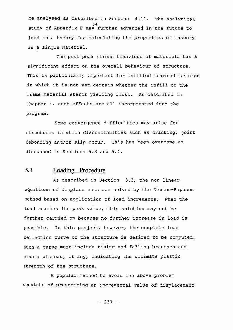
be analysed as described in Section 4.11. The analyticalbe
study of Appendix F may further advanced in the future to
lead to a theory for calculating the properties of masonry
as a single material.
The post peak stress behaviour of materials has a
significant effect on the overall behaviour of structure.
This is particularly important for infilled frame structures
in which it is not yet certain whether the infill or the
frame material starts yielding first. As described in
Chapter 4, such effects are all incorporated into the
program.
Some convergence difficulties may arise for
structures in which discontinuities such as cracking, joint
debonding and/or slip occur. This has been overcome as
discussed in Sections 5.3 and 5.4.
5.3 Loading Procedure
As described in Section 3.3, the non-linear
equations of displacements are solved by the Newton-Raphson
method based on application of load increments. When the
load reaches its peak value, this solution may not be
further carried on because no further increase in load is
possible. In this project, however, the complete load
deflection curve of the structure is desired to be computed.
Such a curve must include rising and falling branches and
also a plateau, if any, indicating the ultimate plastic
strength of the structure.
A popular method to avoid the above problem
consists of prescribing an incremental value of displacement
- 237 -
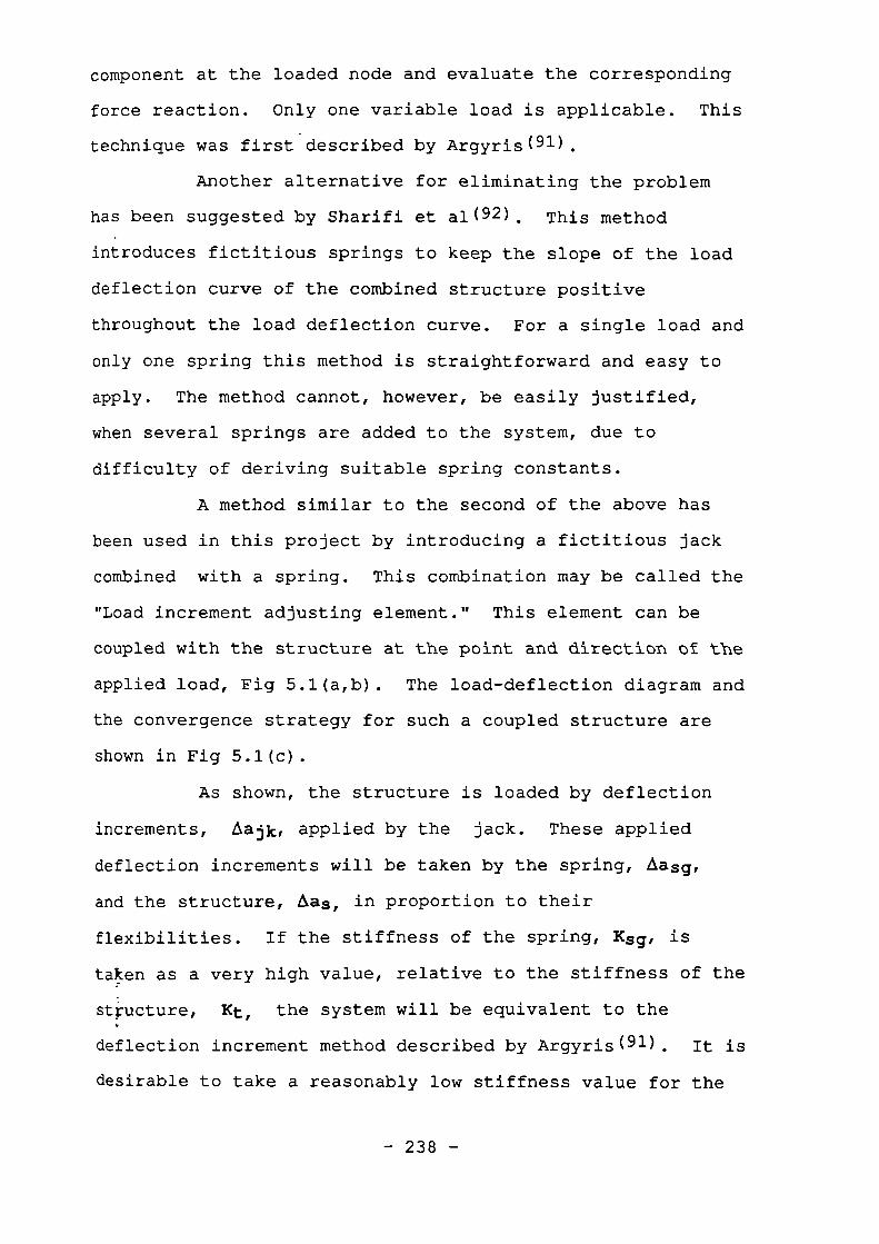
component at the loaded node and evaluate the corresponding
force reaction. Only one variable load is applicable. This
technique was first described by Argyris(91).
Another alternative for eliminating the problem
has been suggested by Sharifi et al (92) This method
introduces fictitious springs to keep the slope of the load
deflection curve of the combined structure positive
throughout the load deflection curve. For a single load and
only one spring this method is straightforward and easy to
apply. The method cannot, however, be easily justified,
when several springs are added to the system, due to
difficulty of deriving suitable spring constants.
A method similar to the second of the above has
been used in this project by introducing a fictitious jack
combined with a spring. This combination may be called the
"Load increment adjusting element." This element can be
coupled with the structure at the point and direction of the
applied load, Fig 5.1(a,b). The load-deflection diagram and
the convergence strategy for such a coupled structure are
shown in Fig 5.1(c).
As shown, the structure is loaded by deflection
increments, Aajk, applied by the jack. These applied
deflection increments will be taken by the spring, hasg,
and the structure, has, in proportion to their
flexibilities. If the stiffness of the spring, Ksg, is
taken as a very high value, relative to the stiffness of the
structure, Kt, the system will be equivalent to the
deflection increment method described by Argyris( 91 ). It is
desirable to take a reasonably low stiffness value for the
- 238 -
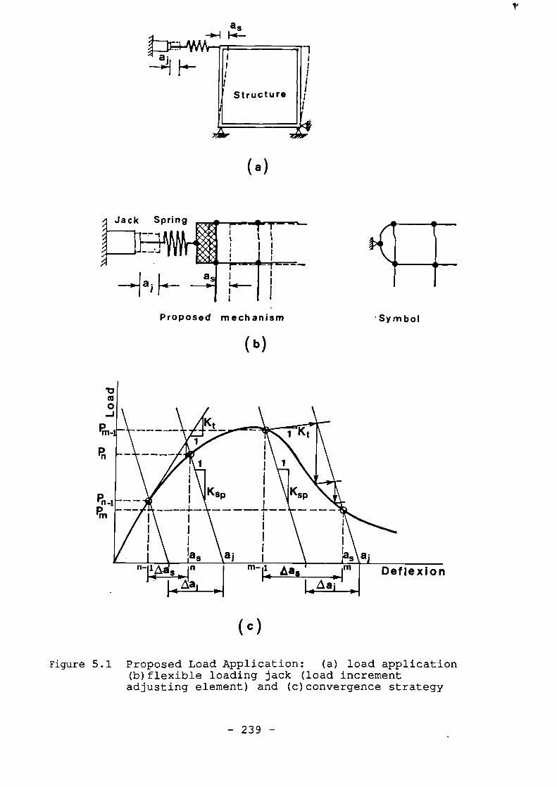
'Symbol
(a)
Proposed mechanism
(b)
t
(c)
Figure 5.1 Proposed Load Application: (a) load application(b)flexible loading jack (load incrementadjusting element) and (c)convergence strategy
- 239 -
spring so that the structure undergoes a gradual increase in
the load and deflection, in a similar fashion to the
behaviour of a real structure. If a very stiff spring is
used the behaviour will simulate a displacement control load
in which some unloading may occur.
Criteria for Convergence
The iteration must continue until the convergence
criteria are met. To examine the convergence of the
iteration, basically, three solution variables can be used:
the incremental displacements, the out-of-balance forces and
the incremental internal energy (40). Since the incremental
approach used in this project is based on nearly uniform
deflection increments, the first of the above variables was
found to be most convenient. Therefore the convergence was
based on the examination of the nodal displacement vector as
follows.
The solution for the corrections to the nodal
displacements is said to be converged when the maximum of
the absolute value of these corrections (so called the
maximum norm) becomes smaller than a prescribed displacement
tolerance. This can be expressed as:
Aa(max)
REF
A4max)=The maximum of the absolute value of change in the
nodal displacements.
REF= A reference value related to the deflection
increments which is normally taken as the current
deflection increment but in this project it is
defined as:
REF = 1/2(Amax + Amin) (5.2)
so as to maintain a uniform precision throughout the
analysis.
Amax and Amin = the specified maximum and minimum allowed
deflection increments.
Y
A prescribed displacement tolerance taking a value
of order 10 -3 to 10 -6 , Bergan et al(93).
For this particular type of structure (infilled
frames) y=2x10⁻³ was found to give results not more
than 1% different from that of y= 10- 6 . A high value for y
is tempting from the view point of economy, but it may lead
to severe inaccuracy and divergence.
The iterative scheme described previously would
converge only if the non-linearities occurring in the
current step are sufficiently small. The more severe the
non-linearities are, or the greater the number of
discontinuity events is, the smaller the step that must be
taken to ensure convergence. In practice, the magnitude of
the next load or deflection increment will be decided using,
the magnitude of the previous step and the number ofe
iterations taken to get into convergence. In order to keep
the number of iterations close to the desired number of
- 241 -
L ( j ) = A (i-i) (5.3)
iterations, DITR, Crisfield( 94 ) suggested a very simple
formula to calculate the length of the next incremental step
as follows:
DITR
ITR(i -1)
A0.-1) = The value of the previous load increment
ITR(i-1).= The number of iterations taken in the previous
step
Program NEPAL, however, uses a newly proposed
formula as follows:
EITR(i-1)]A(i) = 1.67[1 REF + A(i_i)
DITR(5.4)
where DITR denotes the specified desired number of
iterations within each increment and EITR(i-1) denotes the
effective number of iterations.
This formula was found to suit better the analysis
of infilled frames involving so many discontinuity events
such as: cracking, crushing, interfaces or joints debonding
or slip, which demand a greater number of iterations in
order to deal with the sudden changes in the course of
convergence. The effective number of iterations is to be
calculated as follows:
z., EITR(i-1) = ITR(i-1) - I (5.5)
e
where I equals to the number of iterations within the last
- 242 -
increment during which at least one damaging event
(cracking, crushing or debonding) has taken place. The
total number of iterations within each load or deflection
increment may be restricted to a prescribed number, MAXITR
so as to prevent a possible divergence.
No straightforward rule is available to determine
the values of DITR, MAXITR, Amax and Amin so that a
guaranteed convergence and a reasonable accuracy can be
ensured. The following guideline has however been
established by the author after several examinations on
highly non-linear problems including infilled frames:
Amin = 1/20 to 1/40 of the expected deflection
at the peak load.
Amax = 2 x Amin
DITR = 4 to 6
MAXITR = 2 x DITR
5.5 Examination of The Proposed F.E Analysis
5.5.1 Genel-a
In Chapter 3 a number of examinations were carried
out to test the performance of the proposed elements and the
proposed subdivision layouts using the standard elastic
material model. In the following sections the intention is
to further examine those elements and also examine the
performance of the proposed non-linear and elastoplastic
finite element analysis approach, ie. Program NEPAL, in
- 243 -
predicting the strength, stiffness and the mode of failure
and distortion of the structures. The following sections
discuss such examinations carried out on two reinforced
concrete beams, a model steel frame with micro-concrete
inf ill.
5.5.2 R.C. Beam Without Shear Reinforcement
Fig 5.2 compares the experimental and the finite
element analysis results of a reinforced concrete beam with
tested by Bresler et al( 95 ). The
of the strength, stiffness and the
a good agreement with the
The following observations are,
however, worth mentioning.
The load-deflection curve from the finite element
analysis, Fig 5.2(c), remains below the experimental one
after the flexural tensile cracks develop. This is obvious
as the tensile stiffening due to cracked concrete is
ignored. If, however, this effect was accounted for by
increasing the modulus of elasticity of the tensile steel
bars, the two curves would have agreed much better.
As shown in Fig 5.2, the 6-node beam element
proved to be advantageous over the 10-node isoparametric
element.
Variation of the interlocking factor, 0, described
in:Section 4.8.3.5, between 1.0 and 1.5 does not affect the
results indicating the fact that a crack would be unlikely
to become interlocked when no reinforcement crosses it.
no shear reinforcement
analytical predictions
mode of failure are in
experimental results.
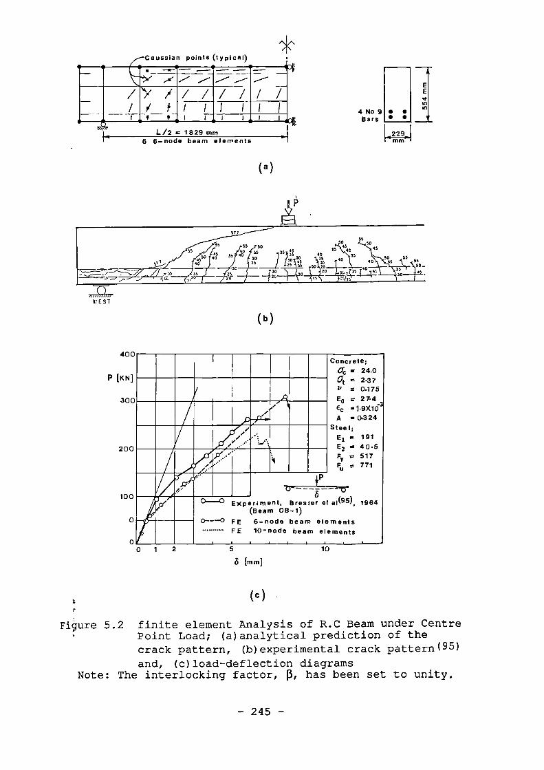
• •• •4 No 9Bars
6 6-node beam elementsL/2 = 1829 mm
1.4229.1
mm
577
55 555
(3'55045;50 40
3 5
1 ::.- .312.7z 40
-7----12:1=4;,.,4,.;,,,.,_6,0
T"r-..-=--• _.- -1"
WEST
b )
12351 50 1 7 40 _ 40 45
130 45 -11.1?3‘r N 134,T3545
35 140 55
35
5045 0
50
5550
45
55Q_45
Gaussian points (typical)____
..../ ,/
I
---,eir .....".. ...,/ ...../..
•- -
/ / / / / / /I- 1•
(a)
3530
400
P [KN]
300
200
100
0
I Concrete;ac = 24.04 = 2.37
P = 0.175E0 = 27•43€c .1-9X10-A • 0.324
Steel;E 1 • 191E2 .. 40.5F sr 517YFu = 771
Al
A
IiI(Beam6-node
10-node
Experiment,O
Brasier et al ( ), 796408-1)
beam elements
beam elements
FEFE
0---0-----*
1
2
5
10
[mm]
Figure 5.2 finite element Analysis of R.0 Beam under Centre• Point Load; (a)analytical prediction of the
crack pattern, (b)experimental crack pattern(95)and, (c)load-deflection diagrams
Note: The interlocking factor, 0, has been set to unity.
- 245 -
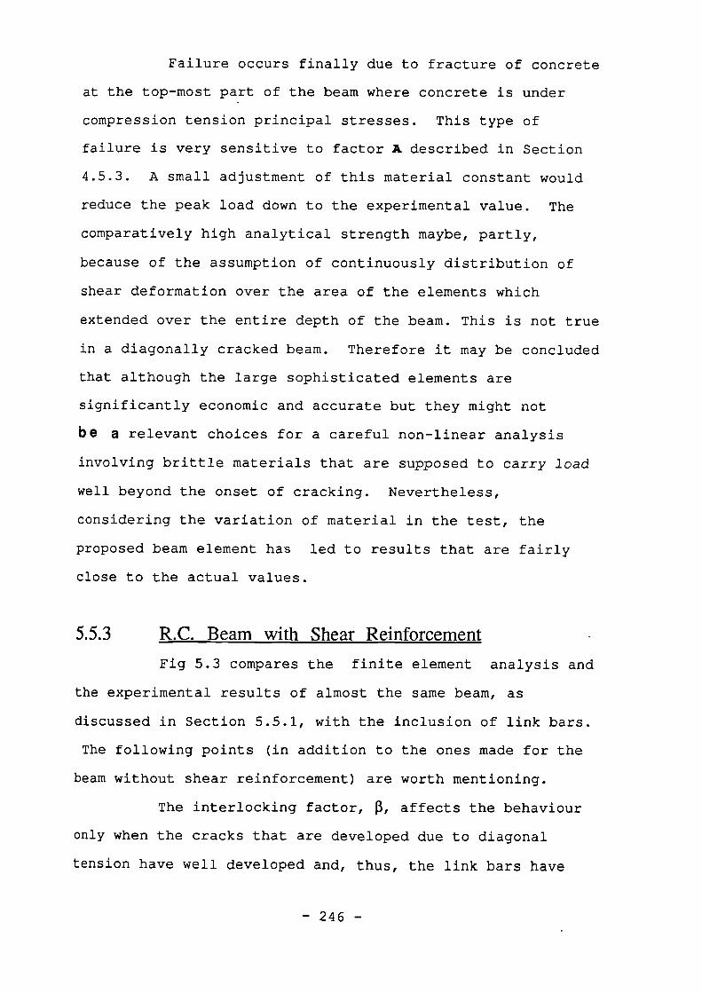
Failure occurs finally due to fracture of concrete
at the top-most part of the beam where concrete is under
compression tension principal stresses. This type of
failure is very sensitive to factor A described in Section
4.5.3. A small adjustment of this material constant would
reduce the peak load down to the experimental value. The
comparatively high analytical strength maybe, partly,
because of the assumption of continuously distribution of
shear deformation over the area of the elements which
extended over the entire depth of the beam. This is not true
in a diagonally cracked beam. Therefore it may be concluded
that although the large sophisticated elements are
significantly economic and accurate but they might not
be a relevant choices for a careful non-linear analysis
involving brittle materials that are supposed to carry load
well beyond the onset of cracking. Nevertheless,
considering the variation of material in the test, the
proposed beam element has led to results that are fairly
close to the actual values.
5.5.3 R.C. Beam with Shear Reinforcement
Fig 5.3 compares the finite element analysis and
the experimental results of almost the same beam, as
discussed in Section 5.5.1, with the inclusion of link bars.
The following points (in addition to the ones made for the
beam without shear reinforcement) are worth mentioning.
The interlocking factor, 0, affects the behaviour
only when the cracks that are developed due to diagonal
tension have well developed and, thus, the link bars have
- 246 -
.
.. A!
Concrete;(7c.• 23.2 N/mm2Igt = 2.4p .. 0475E = 30Ec = 1 . 9 x10_3A n 0.307
Steel bars;Main Links
Ei c 192 203E2 m 40.5 4.5Fy = 517 310Fu 771 32= 7
P18
:, • It
• :(i
--re "sr../Willidligillilill
,,0-0 F E p = 1-3
*--• F E . p - 1.5
e,---o FE fi = 2.00
'
0-0 Experiment (95)„ bepm X,B-1 „
CrL 8=365m m
,./
f
2 N
No 2 a,19mm
4 No 9
•—•
• 0•_.
EIttoIn
229
500
400
300
100
0.200
become effective.
The abrupt drop in the applied load at the
occurrence of the major diagonal cracks could not have been
recorded by the loading machine, with no control on
deflection, used by Bresler et al( 95 ). This reasoning would
explain the experimental curve with no such an abrupt load
decrease. The same conclusions as drawn for the beam
without link bars also apply this case.
0
2
5
10
mm
Figure 5.3 Comparison of The finite element Analysis ofReinforced Concrete Beam (With Shearreinforcement) under Centre Point Loadwith Experimental results of Bresler et al(95)
- 247 -
5.5.4 Square Steel Frame Subjected to Racking
Fig 5.4 compares the finite element analysis
results of an open steel frame with experimental results
recorded by the author (29) . As shown they agree well,
indicating that both the proposed beam element and the
adopted ductile material model would well simulate the
geometry and the mechanical behaviour of the structure.
Nevertheless, the following points are worth mentioning.
Apparently the modulus of elasticity of the frame
material, steel, must have been slightly lower than reported
in the experiment. It seems only 5• percent reduction in
the modulus of elasticity would bring the first part of the
two curves together.
The analytical load deflection curve looks like a
multi-linear line. This may be due to the stepwise
numerical integration approximation over the plastic regions
at the vicinity of the corners. Increaskig the number of
Gaussian points in both horizontal and the vertical
directions within the elements attached to the corners will
improve the analytical curve so as to look more natural and
smooth. But such an upgrading involves extra computation
time.
The ultimate strength of steel must have been more
than the experimentally recorded value. This can be
adjusted by increasing the value of ru of steel by only 2%.
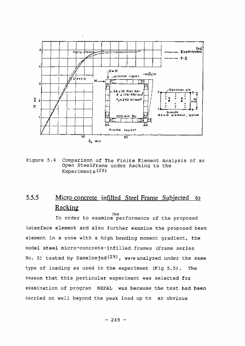
I (29 )F Ily •lasti
---
Experiment--
_ -
F. E
/ HIV-
i_plastic rigion --,411}-4-/ E astic
ea241111110 MB
gm1
1//
rigI 25 x15 Flat bar 2 11 I1
"Gaussian pts
E175 KN/mm 1 1
II
II Fy=252 N/mm2
It
/ • 151mm
4-1111W:
1 1 6-nodeBeam element, typicalmm Sq . rfivill
*AOii300
14....xkm•„,, •
Frame layout
204 mm
Figure 5.4 Comparison of The Finite Element Analysis of anOpen SteelFrame under Racking to theExperiments (29)
5.5.5 Micro-concrete infilled Steel Frame Subjected to
Rackingthe
In order to examine performance of the proposed
interface element and also further examine the proposed beam
element in a zone with a high bending moment gradient, the
model steel micro-concrete-infilled frames (Frame series
No. 5) tested by Saneinejad (29) , were analyzed under the same
type of loading as used in the experiment (Fig 5.5). The
reason that this particular experiment was selected for
examination of program NEPAL was because the test had been
carried on well beyond the peak load up to an obvious
4
- 249 -
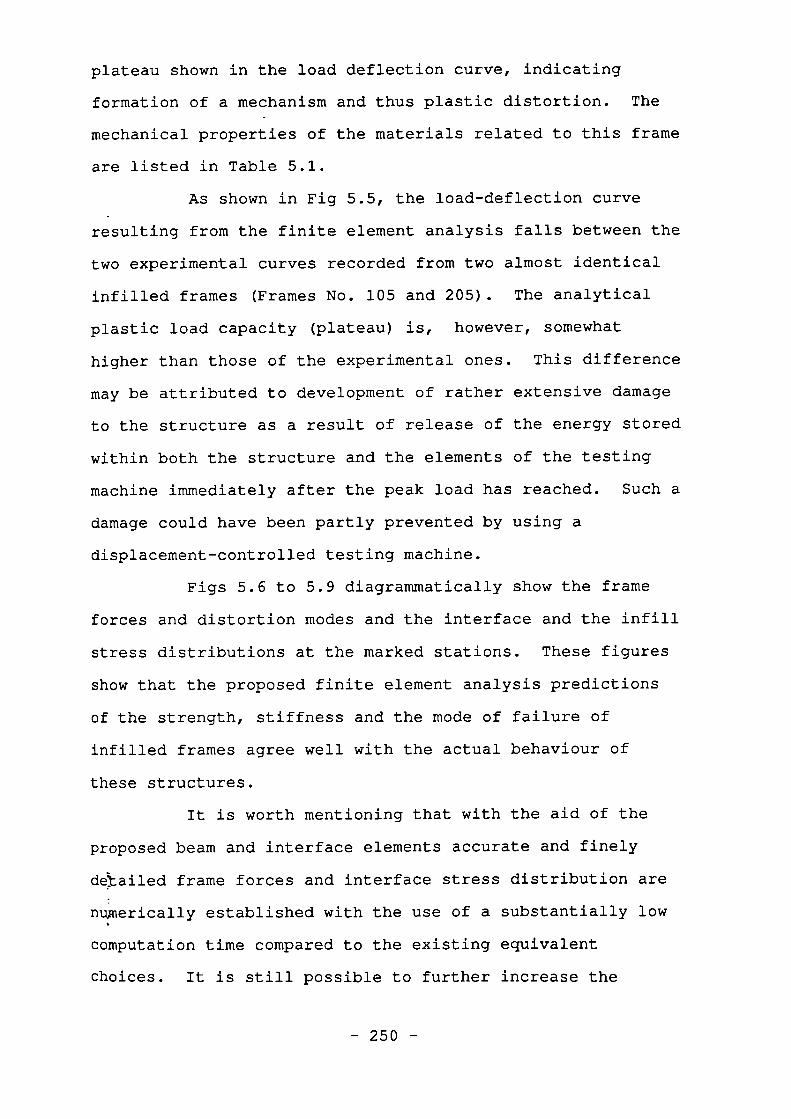
plateau shown in the load deflection curve, indicating
formation of a mechanism and thus plastic distortion. The
mechanical properties of the materials related to this frame
are listed in Table 5.1.
As shown in Fig 5.5, the load-deflection curve
resulting from the finite element analysis falls between the
two experimental curves recorded from two almost identical
infilled frames (Frames No. 105 and 205). The analytical
plastic load capacity (plateau) is, however, somewhat
higher than those of the experimental ones. This difference
may be attributed to development of rather extensive damage
to the structure as a result of release of the energy stored
within both the structure and the elements of the testing
machine immediately after the peak load has reached. Such a
damage could have been partly prevented by using a
displacement-controlled testing machine.
Figs 5.6 to 5.9 diagrammatically show the frame
forces and distortion modes and the interface and the infill
stress distributions at the marked stations. These figures
show that the proposed finite element analysis predictions
of the strength, stiffness and the mode of failure of
infilled frames agree well with the actual behaviour of
these structures.
It is worth mentioning that with the aid of the
proposed beam and interface elements accurate and finely
detailed frame forces and interface stress distribution are
numerically established with the use of a substantially low•
computation time compared to the existing equivalent
choices. It is still possible to further increase the
- 250 -
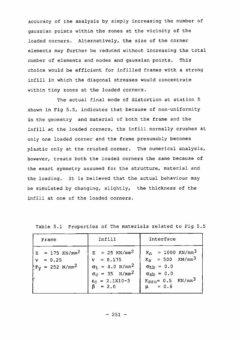
accuracy of the analysis by simply increasing the number of
gaussian points within the zones at the vicinity of the
loaded corners. Alternatively, the size of the corner
elements may further be reduced without increasing the total
number of elements and nodes and gaussian points. This
choice would be efficient for infilled frames with a strong
infill in which the diagonal stresses would concentrate
within tiny zones at the loaded corners.
The actual final mode of distortion at station 5
shown in Fig 5.5, indicates that because of non-uniformity
in the geometry and material of both the frame and the
infill at the loaded corners, the infill normally crushes at
only one loaded corner and the frame presumably becomes
plastic only at the crushed corner. The numerical analysis,
however, treats both the loaded corners the same because of
the exact symmetry assumed for the structure, material and
the loading. It is believed that the actual behaviour may
be simulated by changing, slightly, the thickness of the
infill at one of the loaded corners.
Table 5.1 Properties of The materials related to Fig 5.5
Frame Inf ill Interface
E = 175 KN /mm2
V = 0.25
tFy = 252 N/mm2
r
E = 25 KN/mm2
v = 0.175
at = 4.0 N/mm 2
GC = 35 N/mm2
Cc = 2.1X10-30 =2.0
Kn = 1000 KN/mm3
Ks = 500 KN/mm3
(kb = 0.0
'ash) = 0.0
Ksru= 0.5 KN/mm3g = 0.6
- 251 -
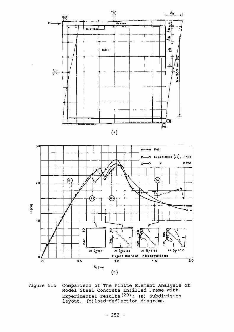
--• F•E
•Experiment (29), p105
FXS0-0
(11112,
PE
IF4 ci)
WIT(•
4.111IN
S3
t
\\Thk I.Airliffill
.144ikkilitk. ! Iir- —
--I-—I-- --
1
•— -•—
1
1
r—1
,•
•V
.----4
0
1°i"elL_
—1 2 4 \ 1
‘(?['*\\\01
i •
Jr.
At Oh -04 At 6.0.85hExperimental
At 6.1.55hobservations
At 500.0
30
20
10
6h
X
Ci
•• .F"m.
'raw,.
•0
1
_
/ —1-Will
—../
I
--1
1
i
.---.4-14.
/
I
I•
1
I
i
I
L_
I
(''1111.•
(a)
05
10
15 20
6 11 [min]
( b )
Figure 5.5 Comparison of The Finite Element Analysis ofModel Steel Concrete Infilled Frame WithExperimental results( 29 ); (a) Subdivisionlayout, (b)load-deflection diagrams
- 252 -
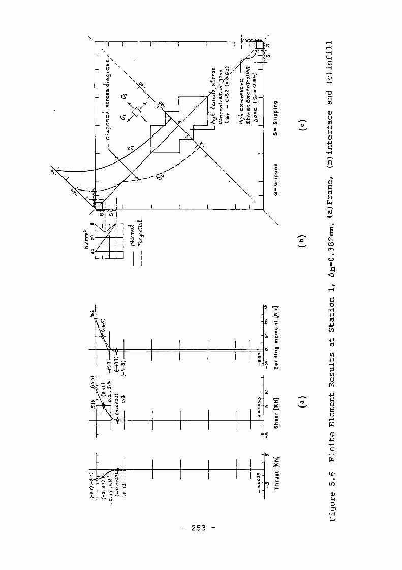
cp,
'
0 ..) .,
u e u)a. e. AS
4.4 c') 0
.C.? t's14.n trl
li
/ c _
csCu t. ONN 1.-- •i7, C atrb 4i o41 ,
‘- o to —Ci. uEk...)0 V)
U VI 0-Z %. 0
.) 4, tos ti)
0.
0.
CI)•••"*.
d 6
'''.44 C 0gu...tsn ak c.) ...,
I
r,
,c:7)
el- ors-
a
I
in
— 253 —
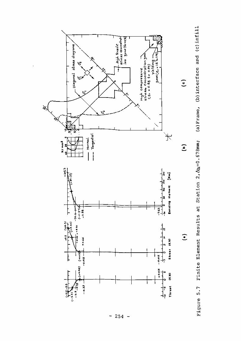
In
+ pro
z
t"
or.••n
••n•nJ2
75.
gz
III
• 4
f
U
.c
to
7
Omer.,
••••••••
%Et
in coN
In U1in 1
on
— 254 —
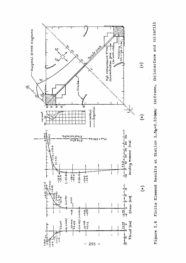
Aig••••••111.A••••••••
16.4•11111••••••• •IIII••••••
-3.14S,0 lc104.4-013
V1.4.S7J/
LI;
louN gtz flint
0
—
•
-6.
01Cr)
4—)
c4VA CO
N• I 1O
I.
0 0
00 r-.
4-*
— 255 —
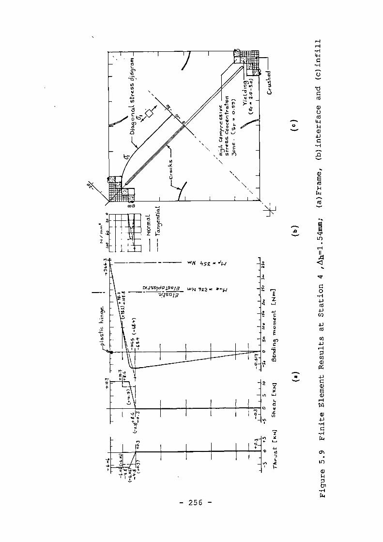
”n-o_
- 256 -
5.6 Conclusions
The finite element analysis tests carried out in
this chapter assisted to examine the computer program
"NEPAL" against the requirements outlined in table 2,2. The
results also led to the following conclusions:
1) The proposed material and interface models simulated,
closely, the behaviour of the structures at the peak and
beyond the peak load.
2) The proposed incremental [D]ep matrix developed for
ductile material (steel) subjected to plane stress
condition, Eq 4.166, performs exelentty.
3) Although significantly economic, the choice of large
elements with sophisticated shape functions is not the
most accurate choice for a non-linear analysis
involving materials subjected to discontinuous
displacements such as a cracked concrete carrying load
well beyond the onset of cracking.
4) Considering the variation of material in the test, the
proposed beam element leads to results that are
fairly close to the actual values.
5) The effect of tensile stiffening on the stiffness of
r.c. beams is significant. This can be accounted for
by increasing the modulus of elasticity of the tensile
steel bars after the tensile cracks,caused by flexure,
are developed.
- 257 -
6) The crack interlocking affects the results of strength
and stiffness only when the cracks are intercepted by
reinforcing bars. These reinforcements become
• effective after the cracks have well developed.
7) The proposed crack interlocking model well simulated
the behaviour of r.c beams with shear reinforcement
subjected to high shear force.
8) the proposed crack modeling well simulated occurrence
of the secondary cracks. These cracks develop only
after the primary cracks become interlocked and
are under a high shear stress.
9) The proposed interface element together with the
proposed interface mechanics model, well simulates the
behaviour of the interfaces resulting in smooth and
fairly accurate stress distribution diagrams involving
four possible states of bonded (intact), gripped,
slipping and open.
10) The proposed deflection increment approach assists
preventing the errors such as unnecessamy cmacking ot
the material, and debonding and/or over-slipping the
interfaces.
11) The proposed finite element analysis can be extended
successfully well beyond the peak load with
satisfactory convergence. However for structures
subjected to a sudden failure such as a beam subjected
to shear failure, the analysis may not be continued
much beyond the peak load.
- 258 -