Newton Iterations in Implicit Time-Stepping Scheme forDifferential Linear Complementarity Systems

Xiaojun Chen1 Shuhuang Xiang2

10 June 2010

Abstract. We propose a generalized Newton method for solving the system of nonlinearequations with linear complementarity constraints in the implicit or semi-implicit time-stepping scheme for differential linear complementarity systems (DLCS). We choose a spe-cific solution from the solution set of the linear complementarity constraints to define alocally Lipschitz continuous right-hand-side function in the differential equation. Moreover,we present a simple formula to compute an element in the Clarke generalized Jacobian ofthe solution function. We show that the implicit or semi-implicit time-stepping schemeusing the generalized Newton method can be applied to a class of DLCS including the non-degenerate matrix DLCS and hidden Z-matrix DLCS, and has a superlinear convergencerate. To illustrate our approach, we show that choosing the least-element solution fromthe solution set of the Z-matrix linear complementarity constraints can define a Lipschitzcontinuous right-hand-side function with a computable Lipschitz constant.

Keywords: differential linear complementarity problem, least-norm solution, least-elementsolution, nondegenerate matrix, Z-matrix, generalized Newton method.

AMS Subject Classifications: 90C30, 90C33

1 Introduction

Given four matrices A ∈ Rm×m, B ∈ Rm×n, N ∈ Rn×m, M ∈ Rn×n, and two Lipschitzcontinuous functions f : R → Rm and g : R → Rn, we consider the ordinary differentiallinear complementarity system (DLCS):

x(t) = Ax(t) + By(t) + f(t)y(t) ∈ SOL(Nx(t) + g(t),M)x(0) = x0, t ∈ [0, T ],

(1.1)

where SOL(Nx(t)+g(t),M) ⊆ Rn is the solution set of the following linear complementarityproblem (LCP):

0 ≤ y(t) ⊥ Nx(t) + g(t) + My(t) ≥ 0. (1.2)

The nonnegativity notation and orthogonality notation in (1.2) express that for i = 1, . . . , n,

yi(t) ≥ 0, (Nx(t) + g(t) + My(t))i ≥ 0, yi(t)(Nx(t) + g(t) + My(t))i = 0.

1Department of Applied Mathematics, The Hong Kong Polytechnic University, Kowloon, Hong Kong.Email: maxjchen@polyu.edu.hk. This author’s work is supported partly by the Research Grants Council ofHong Kong.

2Department of Applied Mathematics and Software, Central South University, Changsha, Hunan 410083,P. R. China. Email: xiangsh@mail.csu.edu.cn. This author’s work is supported partly by NSF of China(No.10771218).

1

The DLCS (1.1) has wide applications in engineering and economics. In the last decade,numerous research articles on DLCS have been published in the areas of applied mathemat-ics, operations research, civil engineering, electrical engineering, transportation sciences,etc. See [1, 4, 10, 12, 13, 14, 19, 21].

A popular numerical method for solving the DLCS is the time-stepping method, whichuses a finite-difference formula to approximate the derivative x. In particular, this methoddivides the time interval [0, T ] into Nh subintervals

0 = th,0 < th,1 < · · · < th,Nh= T,

where th,i+1 − th,i = h = T/Nh, i = 0, . . . , Nh − 1. Starting from xh,0 = x0 ∈ Rm, wecompute two finite sets of vectors

xh,1, xh,2, · · · , xh,Nh ⊂ Rm and yh,1, yh,2, · · · , yh,Nh ⊂ Rn

by the recursion: for i = 0, 1, · · · , Nh − 1,

xh,i+1 = xh,i + h[A(θxh,i + (1− θ)xh,i+1) + Byh,i+1 + f(th,i+1)

],

yh,i+1 ∈ SOL(Nxh,i+1 + g(th,i+1),M),(1.3)

where θ ∈ [0, 1] is a scalar to distinguish an explicit (θ = 1), an implicit (θ = 0), or a semi-implicit (θ ∈ (0, 1)) scheme. In this paper, we consider the implicit scheme and semi-implicitscheme.

A critical part in numerical implementation of the time-stepping scheme is to find a goodsolution yh,i+1 in the solution set SOL(Nxh,i+1 + g(th,i+1),M). In many cases, the solutionset SOL(Nxh,i+1 + g(th,i+1),M) is neither convex nor bounded. Using some vector in thesolution set can cause the numerical method unstable or make the linear complementaryproblem unsolvable in the next step. Moreover, at each time step of the implicit scheme orsemi-implicit scheme, xh,i+1 is a solution u∗ of the following system of nonsmooth equationswith linear complementarity constraints

u = H(u) := (1 + hθA)xh,i + h [(1− θ)Au + By(u) + f(th,i+1)]y(u) ∈ SOL(Nu + g(th,i+1),M).

(1.4)

This system has to be solved efficiently and accurately. A bad numerical solution of thenonsmooth equations (1.4) at one time step can cause the final numerical results failure.In this paper, we choose a solution from the solution set SOL(Nu + g(th,i+1),M) to definea Lipschitz continuous solution function y(·). Moreover, we present a simple formula tocompute an element in the Clarke generalized Jacobian of the solution function, which willbe used for the generalized Newton method to solve the system of nonsmooth equations(1.4) at each time step of the implicit scheme and semi-implicit scheme.

In Section 2, we study how to choose a solution y(q) from the solution set SOL(q, M)such that y is locally Lispchitz with respect to q. By the Rademacher Theorem [7], a locallyLipschitz function is differentiable almost everywhere. Hence, we can define the Clarkegeneralized Jacobian [7]

∂y(q) = co lim y′(qk) : qk → q, qk ∈ Ωy,

2

where Ωy denotes the set of points at which y is differentiable, and “co” denotes the convexhull. To use the generalized Newton method for solving (1.4), we show that

−(I −D + DM)−1D ∈ ∂y(q) (1.5)

if I−D+DM is nonsingular, where D =diag(d1, . . . , dn) is a diagonal matrix with diagonals

di =

1, yi(q) > 00, otherwise.

It is easy to see that −(I−D+DM)−1 is nonsingular if and only if the principal submatrixMJ,J is nonsingular, where J = i | yi > 0. Hence we can use (1.5) and the generalizedNewton method to solve (1.4) if all principal minors of M are nonzero.

For a given matrix M , let MJ,K be the submatrix of M whose entries of M are indexedby the sets J,K ∈ 1, . . . , n. If J = K, the submatrix MJ,K is called a principal submatrixof M . The determinant of a principal submatrix of M is called a principal minor of M .

A matrix M is called a nondegenerate matrix if all principal minors of M are nonzero[8]. A nondegenerate matrix is also called a nonzero principal minor matrix or principallynonsingular matrix [3, 17, 23]. A matrix M is called a P-matrix (N-matrix), if all principalminors of M are positive (negative). M is called an NP-matrix (PN-matrix) if each k × kprincipal minor of M has sign(−1)k ((−1)k+1) [17]. Obviously, the class of nondegeneratematrices includes the class of P-matrices, N-matrices, NP-matrices and PN-matrices. Suchmatrices have many applications in engineering and economics [3, 8, 9, 17]. It is worthnoting that M is a P-matrix if and only if the matrix I − D + DM is nonsingular for alldi ∈ [0, 1] [11]. A matrix M is a nondegenerate matrix if and only if the matrix I−D+DMis nonsingular for all di ∈ 0, 1.

In Section 3, we propose a generalized Newton method to solve (1.4) with a Lipschitzsolution function y(Nu + g(th,i+1)) from SOL(Nu + g(th,i+1),M), and an element from∂y(Nu + g(th,i+1)) given in (1.5). We prove the generalized Newton method starting fromxh,i is well-defined and superlinearly convergent. Moreover, we present an error bound of anumerical solution to the true solution of (1.4).

We use the class of Z-matrices to show that the implicit scheme and the semi-implicitscheme using Newton’s method can be applied to the DLCS (1.1) without the non-singularityassumption on the matrix M . A matrix M ∈ Rn×n is called a Z-matrix, if its off-diagonalelements are non-positive. An M-matrix is a Z-matrix. The Z-matrix LCP arises from thefinite element or finite difference discretization of free boundary problems, reaction-diffusionproblems and journal bearing problems [2, 8, 9, 22, 24].

If M is a Z-matrix and the feasible set

FEA(q, M) = y | q + My ≥ 0, y ≥ 0

is nonempty, then the solution set SOL(q, M) is nonempty [8], and there is a least-elementsolution in SOL(q, M). A solution x∗ of LCP(q, M) is called a least-element solution if x∗ ≤ xfor all x ∈ SOL(q, M), which can be obtained by solving the following linear programming

minimize eT ysubject to q + My ≥ 0, y ≥ 0,

(1.6)

3

where e ∈ Rn with ei = 1, i = 1, . . . , n [8]. We show that the least-element solution ofLCP(q, M) is global Lipschitz continuous with the following Lipschitz constant

L = max‖M−1

J,J‖ | MJ,J is nonsingular for J ⊆ 1, . . . , n

.

Moreover, we show that L∞ defined by the ‖ · ‖∞ is much smaller than the constant givenby Mangasarian and Shiau [15].

In Section 4, we use the constant L to derive a time interval [0, T0], such that thefollowing least-element LCS has a unique solution (x∗, y∗) such that x∗ is continuouslydifferentiable and y∗ is Lipschitz continuous on [0, T0].

Least-Element LCS

x(t) = Ax(t) + By(x(t)) + f(t)y(x(t)) = argmin eT v

subject to v ∈ SOL(Nx(t) + g(t),M)x(0) = x0, t ∈ [0, T ].

(1.7)

Moreover, we show that the following implicit least-element time-stepping scheme con-verges to (x∗, y∗) linearly, and the generalized Newton method using (1.5) is well-definedand superlinearly converges to a solution u∗ of (1.4) from xh,i on the interval [0, T0].

Implicit Least-Element Time-Stepping Scheme (ILETS scheme)

xh,i+1 = xh,i + h(Axh,i+1 + Byh,i+1 + f(th,i+1))yh,i+1 = argmin eT v | 0 ≤ v ⊥ Nxh,i+1 + g(th,i+1) + Mv ≥ 0. (1.8)

In [14], Han, Tiwari, Camlibel, and Pang, proposed the following scheme.Implicit Least-Norm Time-Stepping Scheme (ILNTS scheme)

xh,i+1 = xh,i + h(Axh,i+1 + Byh,i+1 + f(th,i+1))yh,i+1 = argmin ‖v‖2 | 0 ≤ v ⊥ Nxh,i+1 + g(th,i+1) + Mv ≥ 0. (1.9)

They showed that using such least-norm solutions of the discrete-time subproblems, an im-plicit Euler scheme is convergent for passive initial-value DLCS. Obviously, a least-elementsolution is a least-norm solution. Moreover, if M is a Z-matrix, then [8]

argmin eT v | 0 ≤ v ⊥ q + Mv ≥ 0 = argmin eT v | v ≥ 0, q + Mv ≥ 0.

Hence, (1.8) can be considered as an implementation version of the implicit least-normtime-stepping scheme proposed in [14] for the Z-matrix DLCS.

Throughout this paper, we use ‖x‖ to denote the maximum norm ‖x‖ := maxt∈[0,T ]

‖x(t)‖for a function x defined on [0, T ] or ‖x‖ := max

1≤i≤m|xi| for a vector x ∈ Rm. Let Jc denote

the complementarity set of J . Let e denote the vector whose all entries are one. We say afunction is differentiable if it is F-differentiable.

2 Solution function y(q) of LCP(q, M)

Let RLCP (M) denote the LCP-Range of M which is the set of all vectors q such thatSOL(q, M) 6= ∅. M is called a Q-matrix if RLCP (M) = Rn [8, 16]. It is known that M

4

is a P-matrix if and only if RLCP (M) = Rn and SOL(q, M) is singleton for any q ∈ Rn

[8]. However, in general, SOL(q, M) can be empty or unbounded. Using some concepts,such as the least-norm solution and the least-element solution [6, 8, 14], we may definea single valued solution function y(·) on an open set Ω in RLCP (M). In this section, wefirst give a necessary and sufficient condition for a single valued solution function y(·) tobe differentiable at q ∈ Ω. Next, we present a simple formula to compute an element inthe Clarke generalized Jacobian of y(·) at q ∈ Ω and give computable Lipschitz constantsof y(·) in Ω for nondegenerate matrices and Z-matrices.

For a single valued solution function y(q) ∈SOL(q, M), we define the following indexsets:

Jq = i | yi(q) > 0Iq = i | (My(q) + q)i > 0

Kq = i | (My(q) + q)i = qi = 0.

We say y(q) is nondegenerate if Kq = ∅. We define the diagonal matrix Dq whose diagonalelements are

(Dq)ii =

1, i ∈ Jq

0, otherwise.

Lemma 2.1 Suppose that Ω ⊆ RLCP (M) is an open set. Let y be a continuous functiondefined on Ω such that y(q) ∈ SOL(q, M) for q ∈ Ω. Denote J = Jq and D = Dq. Then yis differentiable at q if and only if y(q) is nondegenerate and MJ,J is nonsingular. In thecase y(·) is differentiable at q, we have

y′(q) = −(I −D + DM)−1D. (2.1)

Proof: Suppose that y(q) is nondegenerate. By the continuity of y, there is a neighborhoodof q such that for any p in the neighborhood, we have

yJ(p) > 0, yJc(p) = 0, (My(p) + p)J = 0, (My(p) + p)Jc > 0.

Hence we obtain(I −D)y(p) + D(My(p) + p) = 0.

If J is empty, then D = 0. This implies y(p) ≡ 0 in the neighborhood. If J is not emptyand MJ,J is nonsingular, then the matrix I −D + DM is nonsingular. This implies that

y(p) = −(I −D + DM)−1Dp

is the unique solution of SOL(p,M) in the neighborhood. Hence in both cases, y is differ-entiable at q and (2.1) holds.

Conversely, we assume that y is differentiable at q. Let G(y(p)) = min(y(p),My(p)+ p)for p ∈ Ω. Since G(y(p)) ≡ 0, G is differentiable and G′(y(p)) ≡ 0. Moreover, we have

(My′(q) + I)J = 0 and y′Jc(q) = 0.

This impliesMJ,Jy′J,J(q) + IJ,J = 0 and MJ,Jy′J,Jc(q) = 0.

5

Hence MJ,J is nonsingular, y′J,J(q) = −M−1J,J and y′J,Jc(q) = 0. Moreover, I −D + DM is

nonsingular, and(I −D + DM)y′(q) = −D.

We obtain (2.1). Now, we show y(q) is nondegenerate. Suppose there is i ∈ Jc such that

(My(q) + q)i = y(q)i = 0.

By the argument in the proof of Proposition 5.8.2 of [8], we have

(My(q) + q)′i = y′(q)i = 0,

which impliesMi,·y′·,i(q) + 1 = 0, (2.2)

where Mi,· is the ith-row of M and y′·,i(q) is the ith-column of y′(q). By the argumentabove, y′·,i(q) = 0. This contradicts to (2.2). Hence y(q) is nondegenerate.

2.1 Nondegenerate matrix

In this subsection, we consider the class of nondegenerate matrices [3, 8, 17, 23]. Thisclass of matrices contains several classes of matrices characterized by the sign of the deter-minants of principal submatrices such as P-matrices whose principal minors are all positive.

Theorem 2.1 Suppose that Ω ⊆ RLCP (M) is an open set. Let y be a continuous functiondefined on Ω such that y(q) ∈ SOL(q, M) for q ∈ Ω. Assume that any principle submatrixMJ,J of M is nonsingular then y is locally Lipschitz continuous in Ω with Lipschitz constant

L = maxJ⊆1,...,n

‖M−1J,J‖. (2.3)

Moreover, the Clarke generalized Jacobian of y is defined by

∂y(q) = colim y′(p) = −(I −Dp + DpM)−1Dp : p → q, y(p) is nondegenerate.

In addition,−(I −Dq + DqM)−1Dq ∈ ∂y(q). (2.4)

Proof: Take q ∈ Ω. If y(q) is nondegenerate, then by the first part of the proof for Lemma2.1, we know that there is a neighborhood Nq ⊆ Ω of q such that for any p ∈ Nq,

y(p) = −(I −Dq + DqM)−1Dp.

Hence, y is differentiable and Lipschitz continuous in Nq with Lipschitz constant

‖(I −Dq + DqM)−1Dq‖ = ‖M−1Jq ,Jq

‖ ≤ L.

Moreover, (2.4) holds with ∂y(q) = y′(q).For the case y(q) is degenerate, there is a neighborhood Nq ⊆ Ω of q such that for

p ∈ Nq,Jq ⊂ Jp and Iq ⊂ Ip.

6

For i ∈ Kq, if yi(p) = 0, then(I(y(q)− y(p)))i = 0.

If yi(p) > 0, then (My(q) + q)i = (My(p) + p)i = 0, which gives

(M(y(q)− y(p)))i = −(q − p)i.

Hence for any p ∈ Nq, we have

(I −Dpq + DpqM)(y(q)− y(p)) = −Dpq(q − p),

where Dpq is a diagonal matrix with diagonals

(Dpq)ii =

1, i ∈ Jq and i ∈ Kq ∩ Jp

0, otherwise.

Hence, y is Lipschitz continuous in Nq with Lipschitz constant L.Therefore, y is locally Lipschitz continuous in Ω. By the Rademacher Theorem, y is

almost everywhere differentiable in Ω. By Lemma 2.1, we obtain the Clarke Jacobian∂y(q).

In addition, it is easy to see that for any positive number ε, y(q + ε(I −D)e) = y(q) is anondegenerate solution of LCP(q+ε(I−Dq)e,M). Hence y is differentiable at q+ε(I−D)eand y′(q + ε(I −Dq)e) = −(I −Dq + DqM)−1Dq. This implies

limε↓0

y′(q + ε(I −Dq)e) = −(I −Dq + DqM)−1Dq ∈ ∂y(q).

Corollary 2.1 Suppose that M is a P-matrix. Then for any p, q ∈ Rn, we have

‖y(q)− y(p)‖ ≤ L‖p− q‖, (2.5)

where L is defined in (2.3).

Proof: It is known that for any q ∈ Rn, LCP(q, M) has a unique solution y(q) and y(·) isglobally Lipschitz continuous in Rn [8]. By [7, Proposition 2.6.5], we have

y(p)− y(q) ∈ co∂y([p, q])(p− q),

where [p, q] is the segment between p and q. From Theorem 2.1, for any element C ∈∂y([p, q]), we have ‖C‖ ≤ L. Hence (2.5) holds.

It was shown in [11] that M is a P-matrix if and only if I −D + DM is nonsingular forany diagonal matrix D with diagonals Dii ∈ [0, 1]. In [5], we showed that

‖y(q)− y(p)‖ ≤ maxDii∈[0,1]

‖(I −D + DM)−1D‖‖p− q‖ (2.6)

for M being a P-matrix. Obviously, we have

L = maxJ⊆1,...,n

‖M−1J,J‖ = max

Dii∈0,1‖(I −D + DM)−1D‖ ≤ max

Dii∈[0,1]‖(I −D + DM)−1D‖.

7

Hence the error bound (2.5) is shaper than (2.6). Furthermore, the error bound (2.5) canbe used for a larger class of matrices than the class of the P-matrix. We use the followingexample to illustrate Theorem 2.1 and the new Lipschitz constant L.

Example 2.1 Consider the LCP(M, q) with a nondegenerate matrix M =(

1 10 −1

).

The solution set has the following form

SOL(q, M) = ∅, if q2 < 0;

SOL(q, M) =(

00

),

(0q2

), if q1 ≥ 0, q2 ≥ 0;

SOL(q, M) =( −q1

0

),

(max(−q1 − q2, 0)

q2

), if q1 ≤ 0, q2 ≥ 0.

The matrix I −D + DM is nonsingular if the diagonal matrix D having Dii ∈ 0, 1,but I −D + DM may be singular for Di,i ∈ [0, 1], for instance, D2,2 = 0.5.

We can define a single valued solution function in SOL(q, M) by the solution of thefollowing optimization problem

y(q) = argmin ‖Cv − b‖22 : v ∈ SOL(q, M), q2 ≥ 0 ,

where C ∈ R2×2 is a positive semidefinite matrix and b ∈ R2 is a vector. If we choose C = Iand b = 0, then it is the least-norm solution [8]. However, the least-norm solution is notunique in the region q : q1 < 0, q2 ≥ 0. Let us choose C =diag(0, 1) and b = 0. Then wehave a piecewise linear single valued solution function

y(q) =

(0, 0)T , q1 ≥ 0, q2 ≥ 0(−q1, 0)T , q1 ≤ 0, q2 ≥ 0

in SOL(q, M). The function y(·) is Lipschitz continuous with the Lipschitz constant L = 1and it is continuously differentiable in the region q | q1 < 0, q2 > 0 ∪ q | q1 > 0, q2 > 0.Moreover the Clarke generalized Jacobian at q with q1 = 0 and q2 > 0 has the version

∂y(q) =( −α 0

0 0

), α ∈ [0, 1]

.

Remark 2.1 If M is a positive semi-definite matrix and the solution set SOL(q, M) isnonempty, then the solution set SOL(q, M) is convex and has a unique least-norm solution[8]. Hence we can define a single valued function by the least-norm solution. However,the least-norm solution is not necessarily Lipschitz continuous for M being positive semi-definite. See Example 3.4 in [15].

2.2 Z-matrix

Now we consider M is a Z-matrix. In this case, M can be singular and the solution setSOL(q, M) can be nonempty or unbounded. It is known that if the feasible set FEA(q, M)is not empty, then there is a unique least-element solution in the solution set SOL(q, M)when M is a Z-matrix [8]. In the following, we denote the least-element solution by y(q)if SOL(q, M) 6= ∅ and show the solution function is globally Lipschitz in RLCP (M) with acomputable Lipschitz constant.

8

Lemma 2.2 Suppose that M ∈ Rn×n is a Z-matrix. If q ∈ RLCP (M), then for any p ≥ q,we have p ∈ RLCP (M) and y(p) ≤ y(q).

Proof: It directly follows from that for any q ∈ RLCP (M), the least-element solution y(q)of LCP(q, M) is the solution of the linear program (1.6) and FEA(q, M) ⊆FEA(p,M).

Theorem 2.2 Let M ∈ Rn×n be a Z-matrix, q ∈ RLCP (M), and y(q) be the least-elementsolution of LCP(q, M). With the index set J = Jq and diagonal matrix D = Dq, thefollowing statements hold.

(i) MJ,J is nonsingular for J 6= ∅;(ii) y(q) = −(I −D + DM)−1Dq;(iii) ‖(I−D+DM)−1D‖ ≤ L := max ‖M−1

α,α‖ |Mα,α is nonsingular for α ⊆ 1, . . . , n ;(iv) There is a neighborhood Nq of q such that SOL(p,M) 6= ∅ for any p ∈ Nq. Thus,

we have −(I −D + DM)−1D ∈ ∂y(q).

Proof: Note that we can choose a permutation matrix U ∈ Rn×n such that

UDUT =(

IJ,J 00 0

)and UMUT =

(MJ,J MJ,Jc

MJc,J MJc,Jc

).

Thus

U(I −D + DM)UT =(

MJ,J MJ,Jc

0 I

). (2.7)

Since LCP(Uq, UM) and LCP(q, M) are equivalent, without loss of generality, we assumeU = I in (2.7), J = 1, 2, . . . , k and

M =(

MJ,J MJ,Jc

MJc,J MJc,Jc

), y(q) =

(yJ(q)

0

), q =

(qJ

qJc

).

Note that yJ(q) > 0. It follows MJ,JyJ(q) + qJ = 0. If MJ,J is singular, then there exist anonzero vector x0 ∈ R|J | and a sufficiently small real positive number δ such that

MJ,Jx0 = 0, yJ(q)± δx0 > 0, MJ,J(yJ(q)± δx0) + qJ = 0.

Hence yJ(q) ± δx0 ∈ FEA(qJ ,MJJ) and qJ ∈ RLCP (MJ,J). Since MJ,J is also a Z-matrix,then there is a unique least-element solution yJ ∈ SOL(qJ ,MJ,J) such that

min(yJ ,MJ,JyJ + qJ) = 0, yJ ≤ yJ(q) and yJ ≤ yJ(q)± δx0. (2.8)

From (2.8), we see that yJ ≤ yJ(q) and yJ 6= yJ(q) due to that x0 6= 0. Let y = (yTJ , 0)T .

Since MJc,J ≤ 0 andMJc,JyJ + qJc ≥ MJc,JyJ(q) + qJc ≥ 0,

then it derives that My + q ≥ 0. Therefore, y = (yTJ , 0)T ∈ FEA(q, M) and y = (yT

J , 0)T ≥y(q) = (yJ(q)T , 0)T . It is a contradiction with yJ ≤ yJ(q) and yJ 6= yJ(q). Hence MJ,J isnonsingular.

(ii) From the nonsingularity of MJ,J , expression (2.7) with U = I implies that I−D+DMis nonsingular and

(I −D + DM)−1D =(

MJ,J MJ,Jc

0 I

)−1

D =(

M−1J,J 0

0 0

). (2.9)

9

From (I −D)y(q) + D(My(q) + q) = 0 and (2.9), we obtain the desired results.(iii) This result is directly from (2.9).(iv) If y(q) > 0, then by the discussion above, D = I and M is nonsingular. Moreover

from y(q) = −M−1q > 0, there is a neighborhood of q such that for each point p in thisneighborhood, the corresponding LCP(p,M) is solvable and y(p) = −M−1p > 0. Hencey(·) is differentiable at q and y′(q) = −M−1 = −(I −D + DM)−1 with D = I.

Now we consider the case that y(q) has zero entries. Let us define

q(ε) = q + ε(I −D)e, for ε > 0

that is, qi(ε) = qi for i ∈ J and qi(ε) = qi + ε for i ∈ Jc.By Lemma 2.2, q(ε) ∈ RLCP (M) and y(q(ε)) ≤ y(q). From the Lipschitz continuity of

y(·), we haveq(ε) ↓ q, y(q(ε)) ↑ y(q) as ε ↓ 0.

This, together with min(y(q),My(q) + q) = 0, derives that for all sufficiently small ε > 0

yJ(q(ε)) = −M−1J,JqJ(ε) > 0, yJc(q(ε)) ≡ 0

(My(q(ε)) + q(ε))Jc = MJc,JyJ(q(ε)) + qJc + εeJc ≥ MJc,JyJ(q) + qJc + εeJc > 0.

This implies that y(q(ε)) is a strictly complementarity solution and the index sets of nonzeroentries of y(q) and y(q(ε)) are identical. Furthermore, for each fixed q(ε), we can choosesufficiently small η > 0 such that for all p ∈ B(0, 1) := p | ‖p‖ ≤ 1,

ηM−1J,JpJ < −M−1

J,JqJ(ε), ηMJc,JM−1J,JpJ − ηpJc < qJc(ε)−MJc,JM−1

J,JqJ(ε), (2.10)

since B(0, 1) is a closed bounded compact set and

yJ(q(ε)) = −M−1J,JqJ(ε) > 0, qJc(ε)−MJc,JM−1

J,JqJ(ε) = (My(q(ε)) + q(ε))Jc > 0. (2.11)

Set z ∈ Rn with zJ = −M−1J,J(q(ε) + ηp)J and zJc = 0. It is easy to verify from (2.11) that

z ∈ Rn+ and z ∈ FEA(q(ε) + ηp, M).

Hence q(ε) + ηp ∈ RLCP (M) for all small η and p ∈ B(0, 1), that is, q(ε) is an interiorpoint of RLCP (M). This, with that y(q(ε)) is a strictly complementarity solution and y(·)is Lipschitz continuous, implies y(·) is differentiable at q(ε). Moreover, from (ii) of thistheorem,

y′(q(ε)) ≡ −(I −D + DM)−1D

for all small ε > 0, which implies −(I −D + DM)−1D ∈ ∂y(q).In particular, for the case J = ∅, we have q ≥ 0 and y(q) = 0. Choose q(ε) = q+εe. Since

q(ε) > 0 for all ε > 0, it is easy to verify that q(ε) is an interior point of RLCP (M). Notethat y(q(ε)) ≡ 0 and My(q(ε)) + q(ε) > 0. Thus y is differentiable at q(ε) and y′(q(ε)) ≡ 0.This yields 0 ∈ ∂y(q). We complete the proof.

Theorem 2.3 Suppose M ∈ Rn×n is a Z-matrix. Let y(p) and y(q) be the least-elementsolutions of LCP(p,M) and LCP(q, M), respectively, for any p, q ∈ LCP-Range(M). Thenwe have

‖y(p)− y(q)‖ ≤ L‖p− q‖. (2.12)

10

Proof: It is easy to see that for any λ ∈ [0, 1], the feasible set FEA(λq +(1−λ)p,M) is notempty and thus we have the least-element solution y(λq+(1−λ)p) of LCP(λq+(1−λ)p,M).From Theorem 2.2, we can see y(·) is Lipschitz continuous on the segment between p andq. Therefore, y(·) is almost everywhere differentiable on the segment between p and q, andwe can write

y(p)− y(q) =∫ 1

0y′(λq + (1− λ)p)(p− q)dλ.

See [7, Proposition 2.6.5]. Moreover, if y is differentiable, then we have y′(λq + (1− λ)p) =∂y(λq + (1− λ)p). Hence by (iii) and (iv) of Theorem 2.2, we complete the proof.

In the following, we show that the Lipschitz constant L is much smaller than the constantderived by Mangasarian and Shiau [15].

By Theorem 3.11.18 in [8], y(p) and y(q) are the unique solutions of the following linearprogramming problems, respectively,

maximize −eT z

subject to( −M−I

)z ≤

(p0

),

maximize −eT z

subject to( −M−I

)z ≤

(q0

).

(2.13)

Hence, applying the perturbation error bound for linear programming problems in [15]yields

‖y(p)− y(q)‖ ≤ υ∞(M)‖p− q‖, (2.14)

where

υ∞(M) = supu,v

‖u‖1 | ‖uT P‖1 = 1 and rows of P :=

(MI

)corresponding

to nonzero elements of u are linearly independent

.

Proposition 2.1 For any matrix M ∈ Rn×n, the following inequality holds

L∞ ≤ υ∞(M). (2.15)

Proof: Let W =diag(U,U) be a block matrix, where U ∈ Rn×n is a permutation matrix.Then we have

supu∈R2n

‖u‖1 | ‖uT P‖1 = 1, u ∈ U= sup

u∈R2n

‖Wu‖1 | ‖(Wu)T WP‖1 = 1, u ∈ U

= supu∈R2n

‖Wu‖1 | ‖(Wu)T WPU‖1 = 1, u ∈ U,

where

U = u ∈ R2n | rows of P corresponding to nonzero elements of u are linearly independent.

Hence, we haveυ∞

(UMUT

)= υ∞(M).

Then for any nonsingular principle submatrix MJ,J , without loss of generality, we assume

M =(

MJ,J MJ,Jc

MJc,J MJc,Jc

)and I =

(IJ,J 00 IJc,Jc

).

11

Let b ∈ R|J | with bi = 1 and bj = 0 for j 6= i, j = 1, . . . , |J | such that ‖M−TJ,J b‖1 = ‖M−T

J,J ‖1.

Note that ‖M−TJ,J ‖1 = ‖M−1

J,J‖∞. Define v =

(M−T

J,J b

−MTJc,JM−T

J,J b

)∈ Rn. Then

‖vT

(MJ,J MJ,Jc

0 I

)‖1 = ‖b‖1 = 1, rank

(MJ,J MJ,Jc

0 I

)= n

and ‖v‖1 ≥ ‖M−TJ,J b‖1 = ‖M−1

J,J‖∞, which implies υ∞ (M) ≥ L∞.

Remark 2.2. The Lipschitz constant υ∞(M) is generally quite difficult to compute and itis often much larger than L∞. Consider

M =(

0 0−τ 0

), τ > 0.

It is easy to find L∞ = 0 and υ∞(M) ≥ 1τ→∞, as τ → 0.

Note that L = L if all principal submatrices of M are nonsingular.

3 Convergence of the generalized Newton method

In this section, we consider the convergence of the generalized Newton method for solving(1.4). We set θ = 0, for the simplicity. Similar results hold for θ ∈ (0, 1).

We redefine the function H : Rm → Rm by

H(u) = xh,i + h[Au + By(u) + f(th,i+1)]y(u) ∈ SOL(q(u),M),

(3.1)

whereq(u) := Nu + g(th,i+1).

We show that for a certain time step size h > 0, xh,i+1 is the unique solution of

F (u) = u−H(u) = 0 (3.2)

near xh,i, and the generalized Newton method

uk+1 = uk − V −1k F (uk) (3.3)

converges to xh,i+1 from the starting point u0 = xh,i, where

Vk = I − h[A−B(I −Dk + DkM)−1DkN ] ∈ ∂F (uk) with Dk = Dq(uk).

Letκ = ‖A‖+ L‖B‖‖N‖.

We take h < 1/κ, and set

γ =h‖Axh,i + Byh,i + f(th,i+1)‖

1− hκ, B(xh,i, γ) = z : ‖z − xh,i‖ ≤ γ.

12

Lemma 3.1 Assume that M is nondegenerate matrix or a Z-matrix, and q(z) ∈ RLCP (M)for all z ∈ B(xh,i, γ). Then (3.2) has a solution in B(xh,i, γ).

Proof: Suppose u ∈ B(xh,i, γ). By Theorem 2.1 and Theorem 2.2, there is v(u) ∈SOL(Nu+g(th,i+1),M) such that

‖H(u)− xh,i‖ ≤ h(‖Axh,i + Byh,i + f(th,i+1)‖+ ‖A(u− xh,i) + B(v(u)− v(xh,i))‖)

≤ h(‖Axh,i + Byh,i + f(th,i+1)‖+ (‖A‖+ L‖B‖‖N‖)γ)

= γ.

This implies that H(u) ∈ B(xh,i, γ). Hence H maps B(xh,i, γ) into B(xh,i, γ). Suppose thatu,w ∈ B(xh,i, γ). Using Theorem 2.1 and Theorem 2.2 again, we obtain

‖H(u)−H(w)‖ = h‖A(u− w) + B(v(u)− v(w))‖ ≤ hκ‖u− w‖.Hence H : B(xh,i, γ) → B(xh,i, γ) is a contraction mapping. By the Banach fixed pointtheorem [18], H has a fixed point in B(xh,i, γ), which is the solution of (3.2) in B(xh,i, γ).

Under the conditions of Lemma 3.1, we can choose y(u) from SOL(q(u),M) such thatF is a Lipschitz continuous function in B(xh,i, γ). By the Rademacher Theorem [7], F isdifferentiable almost everywhere. Therefore, we can define the Clarke generalized Jacobian

∂F (x) = co lim F ′(xk) : xk → x, xk ∈ ΩF ,where ΩF denotes the set of points at which F is differentiable, and co denotes the convexhull.

From the convergence analysis of the generalized Newton method for nonsmooth equa-tions in [20], we know that under the condition that F is well-defined in a domain containingxh,i+1 and all matrices in ∂F (xh,i+1) are nonsingular, there is a neighborhood of xh,i+1 suchthat the generalized Newton method (3.3) converges to the fixed point xh,i+1 of H super-linearly from any starting point in the neighborhood. However, it is too hard to find suchneighborhood and too strong to assume all matrices in ∂F (xh,i+1) are nonsingular for aZ-matrix DLCS.

In the following, we show that for certain small h, the generalized Newton method(3.3), with the starting point u0 = xh,i and a special matrix Vk in the generalized Jacobian∂F (uk), is well-defined and converges to xh,i+1 superlinearly. Moreover, we give a methodto compute the matrix Vk ∈ ∂F (uk).

The following theorem presents a nonsingular matrix in the generalized Jacobian ∂F (u).

Theorem 3.1 Let J = Jq and D = Dq. Under the assumption of Lemma 3.1, we have

V (u) = I − h[A−B(I −D + DM)−1DN ] ∈ ∂F (u).

Proof: To show V (u) ∈ ∂F (u), it is sufficient to show that there is a sequence uk suchthat uk → u, y′(q(uk)) is differentiable and

y′(q(uk)) = −(I −D + DM)−1DN,

since it implies that F is differentiable at uk and

F ′(uk) = I − h[A−B(I −D + DM)−1DN ].

13

For sufficiently small ε > 0, we set

qε(u) = q(u) + ε(I −D)e.

From the proof of Theorem 2.1 and Theorem 2.2, we see that y(qε(u)) = y(q(u)) is anondegenerate solution of LCP(qε(u),M). Hence y is differentiable at qε(u) and qε(u)+ηp ∈RLCP (M) for all small η and p ∈ B(0, 1).

We choose a sequence of positive numbers εk with limk→∞

εk = 0.

Case 1: rank(N) = n: Since N is of full row rank, for each εk, we set uk = u +εkN

T (NNT )−1(I −D)e. Then uk is a solution of the linear equations

Nuk = Nu + εk(I −D)e and limk→∞

uk = u.

Then y is differentiable at qεk(u) = q(u) + εk(I − D)e = q(uk) = Nuk + g(th,i+1) and

y′(q(uk)) = −(I −D + DM)−1DN.Case 2: rank(N) < n: Assume n ≤ m. We choose a sequence of positive numbers η`

with lim`→∞

η` = 0, and an n× n diagonal matrix

Λ = diag(λ1, . . . , λn), (|λi| = 1, i = 1, 2, . . . , n)

such that Λu ≥ 0 and

rank(N + η`N1) = n, for ` = 1, 2, . . . ,

where N1 := (Λ, 0) ∈ Rn×m, since the leading mth-order principle submatrix of N has atmost n different eigenvalues.

Define q`(u) = (N + η`N1)u + g(th,i+1). Since

q`(u) ≥ q(u) and lim`→∞

q`(u) = q(u),

by assumptions of this theorem, LCP(q`(u),M) has a solution y(q`(u)), and

lim`→∞

y(q`(u)) = y(q(u)).

Define D` =diag(d`1, . . . , d

`n) with

d`i =

1, yi(q`(u)) > 00, otherwise.

Following the proof for Case 1, we have y is differentiable at

q`(uk) = q`(u) + εk(I −D`)e

andy′(q`(uk)) = −(I −D` + D`M)−1D`(N + η`N1).

Moreover, from the definition of q`(uk), we have

‖q`(uk)− q(u)‖ ≤ ‖q`(uk)− q`(u)‖+ ‖q`(u)− q(u)‖≤ εkn + ‖q`(u)− q(u)‖ → 0 as k →∞, ` →∞.

14

Taking a subsequence q`i(uki) of q`(uk) and using

y′(q`i(uki)) = −(I −D`i

+ D`iM)−1D`i

(N + η`iN1)

we obtainlim

`i→∞(I − h[A−B(I −D`i

+ D`iM)−1D`i

(N + η`iN1)]

)

= I − h[A−B(I −D + DM)−1DN ] ∈ ∂F (u).

Finally, we consider the case that rank(N) < n and n > m. Let us consider the equiva-lent augmented LCP(N u+g(th,i+1),M), where N = (N, 0) ∈ Rn×n and u = (uT , 0)T ∈ Rn,then LCP(N u + g(th,i+1),M) and LCP(Nu + g(th,i+1),M) have the same solutions. Fromthe above proof for rank(N) < n and n ≤ m, we can get the generalized Jacobian of theaugmented function. Note that the generalized Jacobian of the augmented function con-fined to Rm is the generalized Jacobian of the original function [7]. We complete the proof.

Now we present the convergence theorem of the generalized Newton method (3.3). Let

γ1 =h‖Axh,i + Byh,i + f(th,i+1)‖

1− 3hκ, B(xh,i, γ1) = z : ‖z − xh,i‖ ≤ γ1.

Theorem 3.2 Under the assumptions of Lemma 3.1, if 3hκ < 1, then the generalizedNewton method (3.3) with the starting point xh,i converges to xh,i+1 superlinearly.

Proof: For u ∈ B(xh,i, γ1), we define

G(u) = u− V (u)−1F (u),

whereV (u) = I − h[A−B(I −Dq(u) + Dq(u)M)−1Dq(u)N ].

Recall

L = max ‖M−1α,α‖ | Mα,α is nonsingular for α ⊆ 1, . . . , n and κ = ‖A‖+L‖B‖‖N‖.

We obtain

‖A−B(I −Dq(u) + Dq(u)M)−1Dq(u)N‖ ≤ ‖A‖+ ‖B‖‖(I −Dq(u) + Dq(u)M)−1Dq(u)‖‖N‖≤ ‖A‖+ L‖B‖‖N‖≤ κ.

Hence, the assumption 3hκ < 1 implies that V (u) is nonsingular and

‖V (u)−1‖ ≤ 11− h‖A−B(I −Dq(u) + Dq(u)M)−1Dq(u)N‖

≤ 11− hκ

. (3.4)

Similar to the proof of Lemma 3.1, we have

‖H(u)− xh,i‖ ≤ h(‖Axh,i + Byh,i + f(th,i+1)‖+ κγ1

)

15

and thus

‖G(u)− xh,i‖ ≤ ‖V (u)−1(V (u)(u− xh,i)− u + H(u)‖≤ ‖V (u)−1‖‖(I − V (u))(u− xh,i)‖+ ‖V (u)−1‖‖H(u)− xh,i‖≤ hκγ1

1− hκ+

h‖Axh,i + Byh,i + f(th,i+i)‖+ hκγ1

1− hκ= γ1.

(3.5)

Therefore, for any u ∈ B(xh,i, γ1), G(u) is well-defined and G(u) ∈ B(xh,i, γ1). By theBanach fixed point theorem, G has a fixed point u in B(xh,i, γ1). By the definition of Gand (3.4), u is also a fixed point of H in B(xh,i, γ1). Moreover, from

‖H(u)−H(w)‖ ≤ hκ‖u− w‖, for u,w ∈ B(xh,i, γ1),

H is a contraction mapping on B(xh,i, γ1). Hence u is the unique fixed point of H inB(xh,i, γ1). We set xh,i+1 = u.

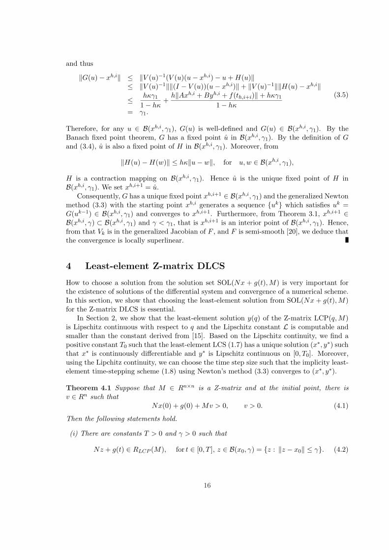
Consequently, G has a unique fixed point xh,i+1 ∈ B(xh,i, γ1) and the generalized Newtonmethod (3.3) with the starting point xh,i generates a sequence uk which satisfies uk =G(uk−1) ∈ B(xh,i, γ1) and converges to xh,i+1. Furthermore, from Theorem 3.1, xh,i+1 ∈B(xh,i, γ) ⊂ B(xh,i, γ1) and γ < γ1, that is xh,i+1 is an interior point of B(xh,i, γ1). Hence,from that Vk is in the generalized Jacobian of F , and F is semi-smooth [20], we deduce thatthe convergence is locally superlinear.

4 Least-element Z-matrix DLCS

How to choose a solution from the solution set SOL(Nx + g(t),M) is very important forthe existence of solutions of the differential system and convergence of a numerical scheme.In this section, we show that choosing the least-element solution from SOL(Nx + g(t),M)for the Z-matrix DLCS is essential.

In Section 2, we show that the least-element solution y(q) of the Z-matrix LCP(q, M)is Lipschitz continuous with respect to q and the Lipschitz constant L is computable andsmaller than the constant derived from [15]. Based on the Lipschitz continuity, we find apositive constant T0 such that the least-element LCS (1.7) has a unique solution (x∗, y∗) suchthat x∗ is continuously differentiable and y∗ is Lipschitz continuous on [0, T0]. Moreover,using the Lipchitz continuity, we can choose the time step size such that the implicity least-element time-stepping scheme (1.8) using Newton’s method (3.3) converges to (x∗, y∗).

Theorem 4.1 Suppose that M ∈ Rn×n is a Z-matrix and at the initial point, there isv ∈ Rn such that

Nx(0) + g(0) + Mv > 0, v > 0. (4.1)

Then the following statements hold.

(i) There are constants T > 0 and γ > 0 such that

Nz + g(t) ∈ RLCP (M), for t ∈ [0, T ], z ∈ B(x0, γ) = z : ‖z − x0‖ ≤ γ. (4.2)

16

(ii) The least-element LCS (1.7) has a unique solution (x∗, y∗) ∈ C1[0, T0]×C[0, T0], where

T0 = minT,γ

c0 + κγ, c0 = ‖Ax0 + By0 + f‖, κ = ‖A‖+ L‖B‖‖N‖.

(iii) If the time step size h < 1/3κ, then the generalized Newton method (3.3) with thestarting point xh,i converges to xh,i+1 superlinearly, which is the unique fixed point ofH(u) defined by

H(u) = xh,i + h[Au + By(u) + f(th,i+1)]y(u) = agrmineT v | v ∈ SOL(q(u),M).

(iv) For the implicity least-element time-stepping scheme (1.8), we have the error bound

‖xh,i − x(th,i)‖ ≤ O(h). (4.3)

Proof: (i) Let x0(t) ≡ x0. Condition (4.1) indicates that the feasible set FEA(Nx(0) +g(0),M) has an interior point v. Hence there are constants T > 0 and γ > 0 such that (4.2)holds.

(ii) From (4.2) the solution set SOL(Nx0(t) + g(t),M) 6= ∅ for all t ∈ [0, T0]. Let

y(x0(t)) = argmineT v|Nx0(t) + g(t) + Mv ≥ 0, v ≥ 0.

Then by Theorem 2.2, y(x0(·)) is Lipschitz continuous in [0, T0].Now we define sequences xk and yk over [0, T0] by the following recursion, for

k = 1, 2, . . .,

xk+1(t) = x0(t) +∫ t

0(Axk(s) + By(xk(s)) + f(s)) ds

y(xk+1(t)) = argmineT v|Nxk+1(t) + g(t) + Mv ≥ 0, v ≥ 0.(4.4)

Now we show xk(t) ∈ B(x0, γ) for t ∈ [0, T0] and k = 1, 2, . . . . Note that

‖x1(t)− x0(t)‖ = ‖∫ t

0(Ax0(s) + By(x0(s)) + f(s))ds‖ ≤ c0T0 ≤ γ.

Suppose ‖xk(t)− x0(t)‖ ≤ γ. From Theorem 2.2, we have

‖xk+1(t)− x0(t)‖ ≤ (‖A‖+ L‖B‖‖N‖)T0γ + c0T0

≤ T0(γκ + c0)≤ γ.

Thus xk(t) ∈ B(x0, γ) for t ∈ [0, T0] and k = 0, 1, . . .. Moreover, we have

‖xk+1 − xk‖ ≤ (‖A‖+ L‖B‖‖N‖)T0‖xk − xk−1‖≤ (κT0)kc0T0

= c0T0

(κγ

c0 + κγ

)k

.

17

Then xk is a Cauchy sequence in C[0, T0] and thus there is x∗ ∈ C[0, T0] such thatlim

k→∞xk = x∗ and

x∗(t) = x0(t) +∫ t

0(Ax∗(s) + By(x∗(s)) + f(s))ds

for t ∈ [0, T0]. This implies that x∗ is a solution of the least-element LCS (1.7). Moreover,from the Lipschitz continuity of y and f , x = Ax + By + f is continuous on [0, T0], that is,x∗ ∈ C1[0, T0].

Now we show that the solution x∗ is unique. Suppose there are two solutions u and v.Then by the Lipschitz continuity of the least-element solution y, we have

‖u− v‖ ≤ (‖A‖+ L‖B‖‖N‖)T0‖u− v‖ = κT0‖u− v‖.

Since κT0 < 1, we must have u = v.(iii) This result is directly from Theorem 3.2.(iv) Since the right-hand-side function Ax(t) + y(x(t)) + f(t) is Lipschitz continuous on

[0, T0], the implicit least-element time-stepping scheme (1.8) has at least linear convergencerate.

Now we use the following example to illustrate the least-element LCS (1.7) and theimplicit least-element time-stepping scheme (1.8) for the differential Z-matrix LCS.

Example 4.1 We consider the following differential Z-matrix LCS

d

dt

(x1

x2

)=

[ −α1 00 −α2

](x1

x2

)+

[α3 0 0 −α3

0 α4 α4 0

]

y1

y2

y3

y4

+ f(t)

0 ≤

y1

y2

y3

y4

⊥

−1 00 10 11 0

(x1

x2

)+

1 0 0 00 0 −1 00 −1 0 00 0 0 1

y1

y2

y3

y4

+ g(t) ≥ 0.

(4.5)

The given matrices and functions in this example are

A =[ −α1 0

0 −α2

], B =

[ −α3 0 0 α3

0 α4 α4 0

], N =

−1 00 10 11 0

,

M =

1 0 0 00 0 −1 00 −1 0 00 0 0 1

, f(t) =

(α5 sin(ωt)

0

), g(t) ≡ 0.

We can compute the Lipschitz constant L of the least-element solution y(·) and find

L = 1 and κ = ‖A‖+ L‖B‖‖N‖ = maxα1, α2, α3, α4.

18

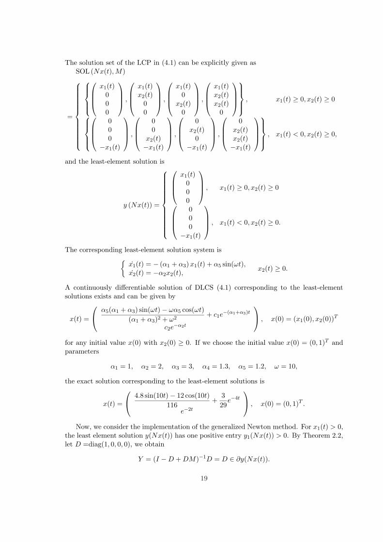
The solution set of the LCP in (4.1) can be explicitly given asSOL (Nx(t),M)

=

x1(t)000

,

x1(t)x2(t)

00

,

x1(t)0

x2(t)0

,

x1(t)x2(t)x2(t)

0

, x1(t) ≥ 0, x2(t) ≥ 0

000

−x1(t)

,

00

x2(t)−x1(t)

,

0x2(t)

0−x1(t)

,

0x2(t)x2(t)−x1(t)

, x1(t) < 0, x2(t) ≥ 0,

and the least-element solution is

y (Nx(t)) =

x1(t)000

, x1(t) ≥ 0, x2(t) ≥ 0

000

−x1(t)

, x1(t) < 0, x2(t) ≥ 0.

The corresponding least-element solution system is

x1(t) = − (α1 + α3) x1(t) + α5 sin(ωt),x2(t) = −α2x2(t),

x2(t) ≥ 0.

A continuously differentiable solution of DLCS (4.1) corresponding to the least-elementsolutions exists and can be given by

x(t) =

α5(α1 + α3) sin(ωt)− ωα5 cos(ωt)(α1 + α3)2 + ω2

+ c1e−(α1+α3)t

c2e−α2t

, x(0) = (x1(0), x2(0))T

for any initial value x(0) with x2(0) ≥ 0. If we choose the initial value x(0) = (0, 1)T andparameters

α1 = 1, α2 = 2, α3 = 3, α4 = 1.3, α5 = 1.2, ω = 10,

the exact solution corresponding to the least-element solutions is

x(t) =

4.8 sin(10t)− 12 cos(10t)116

+329

e−4t

e−2t

, x(0) = (0, 1)T .

Now, we consider the implementation of the generalized Newton method. For x1(t) > 0,the least element solution y(Nx(t)) has one positive entry y1(Nx(t)) > 0. By Theorem 2.2,let D =diag(1, 0, 0, 0), we obtain

Y = (I −D + DM)−1D = D ∈ ∂y(Nx(t)).

19

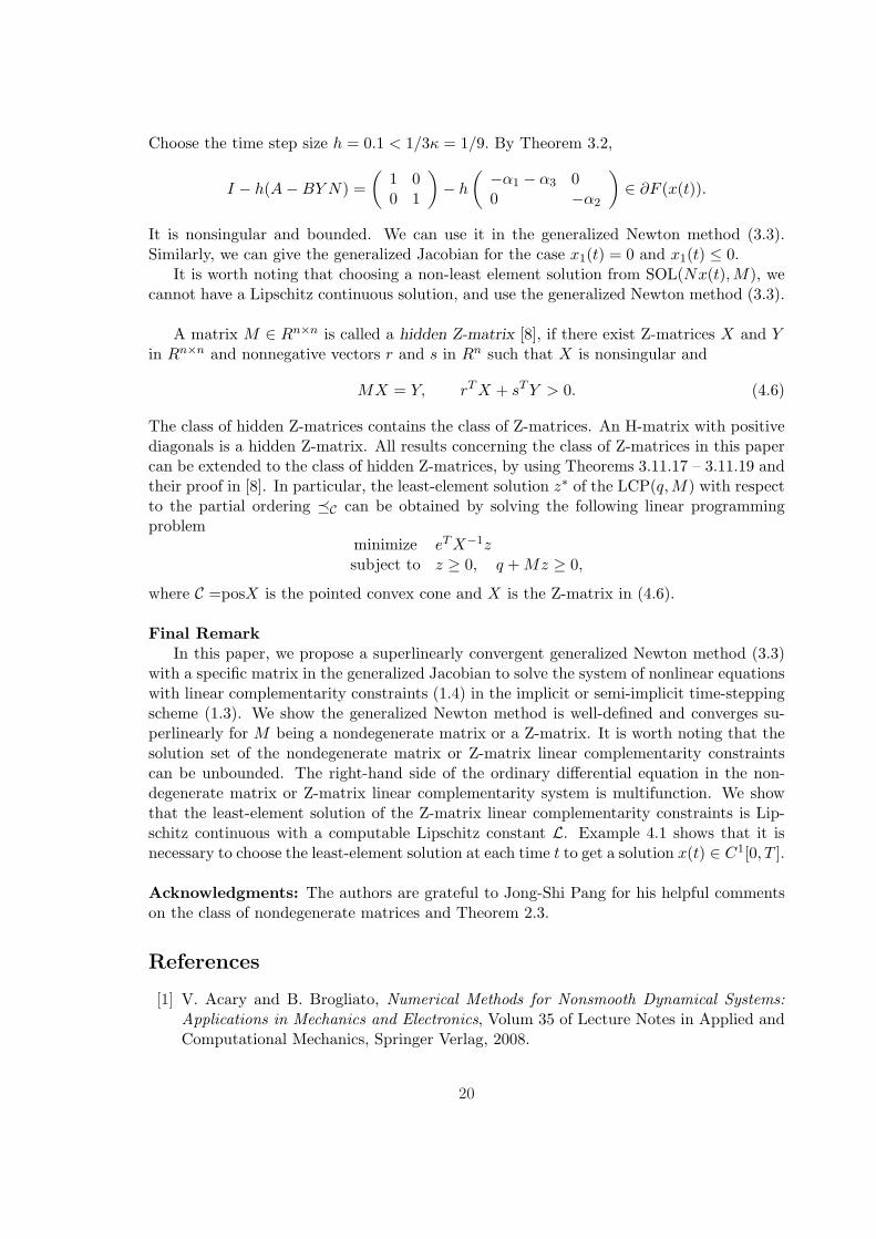
Choose the time step size h = 0.1 < 1/3κ = 1/9. By Theorem 3.2,

I − h(A−BY N) =(

1 00 1

)− h

( −α1 − α3 00 −α2

)∈ ∂F (x(t)).

It is nonsingular and bounded. We can use it in the generalized Newton method (3.3).Similarly, we can give the generalized Jacobian for the case x1(t) = 0 and x1(t) ≤ 0.

It is worth noting that choosing a non-least element solution from SOL(Nx(t),M), wecannot have a Lipschitz continuous solution, and use the generalized Newton method (3.3).

A matrix M ∈ Rn×n is called a hidden Z-matrix [8], if there exist Z-matrices X and Yin Rn×n and nonnegative vectors r and s in Rn such that X is nonsingular and

MX = Y, rT X + sT Y > 0. (4.6)

The class of hidden Z-matrices contains the class of Z-matrices. An H-matrix with positivediagonals is a hidden Z-matrix. All results concerning the class of Z-matrices in this papercan be extended to the class of hidden Z-matrices, by using Theorems 3.11.17 – 3.11.19 andtheir proof in [8]. In particular, the least-element solution z∗ of the LCP(q, M) with respectto the partial ordering ¹C can be obtained by solving the following linear programmingproblem

minimize eT X−1zsubject to z ≥ 0, q + Mz ≥ 0,

where C =posX is the pointed convex cone and X is the Z-matrix in (4.6).

Final RemarkIn this paper, we propose a superlinearly convergent generalized Newton method (3.3)

with a specific matrix in the generalized Jacobian to solve the system of nonlinear equationswith linear complementarity constraints (1.4) in the implicit or semi-implicit time-steppingscheme (1.3). We show the generalized Newton method is well-defined and converges su-perlinearly for M being a nondegenerate matrix or a Z-matrix. It is worth noting that thesolution set of the nondegenerate matrix or Z-matrix linear complementarity constraintscan be unbounded. The right-hand side of the ordinary differential equation in the non-degenerate matrix or Z-matrix linear complementarity system is multifunction. We showthat the least-element solution of the Z-matrix linear complementarity constraints is Lip-schitz continuous with a computable Lipschitz constant L. Example 4.1 shows that it isnecessary to choose the least-element solution at each time t to get a solution x(t) ∈ C1[0, T ].

Acknowledgments: The authors are grateful to Jong-Shi Pang for his helpful commentson the class of nondegenerate matrices and Theorem 2.3.

References

[1] V. Acary and B. Brogliato, Numerical Methods for Nonsmooth Dynamical Systems:Applications in Mechanics and Electronics, Volum 35 of Lecture Notes in Applied andComputational Mechanics, Springer Verlag, 2008.

20

[2] G. Alefeld and Z. Wang, Error estimation for nonlinear complementarity problems vialinear systems with interval data, Numer. Funct. Anal. Optim., 29(2008), 243-267.

[3] M. Banaji, P. Donnell and S. Baigent, P matrix properties injectivity, and stability inchemical reactions systems, SIAM J. Appl. Math., 67(2007), 1523-1547.

[4] M.K. Camlibel, W.P.M.H. Heemels and J.M. Schumacher, Consistency of a time-stepping method for a class of piecewise-linear networks, IEEE Tran. on Circuits andSystems-I: Fundamental Theory and Applications, 49(2002), 349-357.

[5] X. Chen and S. Xiang, Perturbation bounds of P-matrix linear complementarity prob-lems, SIAM J. Optim., 18(2007), 1250-1265.

[6] X. Chen and S. Xiang, Implicit solution function of P0 and Z matrix complemantarityconstraints, Math. Program. Ser. A, Online First.

[7] F.H. Clarke, Optimization and Nonsmooth Analysis, SIAM Publisher, Philadelphia,1990.

[8] R.W. Cottle, J.-S. Pang and R.E. Stone, The Linear Complementarity Problem, Aca-demic Press, Boston, MA, 1992.

[9] M.C. Ferris and J.-S. Pang, Engineering and economic applications of complementarityproblems, SIAM Rev., 39(1997), 669-713.

[10] T.L. Friesz, Danamic Optimization and Differential Games, International Series inOperations Research and Management Science, Vol. 135, Springer, 2010.

[11] S.A. Gabriel and J.J. More, Smoothing of mixed complementarity problems, in Com-plementarity and Variational Problems: State of the Art, M.C. Ferris and J.-S.Pang,eds., SIAM, Philadelphia, 1997, 105-116.

[12] B. Gavrea, M. Anitescu and F. A. Potra, Convergence of a class of semi-implicit time-stepping schemes for nonsmooth rigid multibody dynamics, SIAM J. Optim., 19(2008),969-1001.

[13] L. Han and J.-S. Pang, Non-zenoness of a class of differential quasi-variational in-equalities, Math. Program., Ser. A, 121(2010), 171-199.

[14] L. Han, A. Tiwari, M.K. Camlibel and J.-S. Pang, Convergence of time-steppingschemes for passive and extended linear complementarity systems, SIAM J. Numer.Anal., 47(2009), 3768-3796.

[15] O.L. Mangasarian and T.-H. Shiau, Lipschitz continuity of solutions of linear inequal-ities, programs and compplementarity problems, SIAM J. Control. Optim., 25(1987),583-595.

[16] D.Q. Naiman and R.E. Stone, A homological characterization of Q-matrices, Math.Oper. Res., 23(1998), 463-478.

[17] H. Nikaido, Convex Structures and Economic Theory, Academic Press, New York,1968.

21

[18] J.M. Ortega and W.C. Rheinboldt, Iterative Solution of Nonlinear Equations in SeveralVariables, Academic Press, New York, 1970.

[19] J.-S. Pang and D.E. Stewart, Differential variational inequalities, Math. Program. Ser.,A, 113(2008), 345-424.

[20] L. Qi and D. Sun, A nonsmooth version of Newton’s method, Math. Program., Ser. A,58(1993), 353-367.

[21] J.M. Schumacher, Complementarity systems in optimization, Math. Program., Ser. B,101(2004), 263-295.

[22] U. Schafer, An anclosure method for free boundary problems based on a linear comple-mentarity problem with interval data, Numer. Funct. Anal. Optim., 22(2001), 991-1011.

[23] J.R. Torregrosa, C. Jordan and R. el-Ghamry, The nonsingular matrix completionproblem, Int. J. Contemp. Math. Sciences, 2(2007), 349 - 355.

[24] Z. Wang and Y. Yuan, Componentwise error bounds for linear complementarity prob-lems, to appear in IMA J. Numer. Anal., (2009).

[25] J.J. Ye, Optimality conditions for optimization problems with complementarity con-straints, SIAM J. Optim., 9(1999), 374-387.

22