Copyright Undertaking

This thesis is protected by copyright, with all rights reserved.

By reading and using the thesis, the reader understands and agrees to the following terms:

1. The reader will abide by the rules and legal ordinances governing copyright regarding the use of the thesis.

2. The reader will use the thesis for the purpose of research or private study only and not for distribution or further reproduction or any other purpose.

3. The reader agrees to indemnify and hold the University harmless from and against any loss, damage, cost, liability or expenses arising from copyright infringement or unauthorized usage.

IMPORTANT

If you have reasons to believe that any materials in this thesis are deemed not suitable to be distributed in this form, or a copyright owner having difficulty with the material being included in our database, please contact lbsys@polyu.edu.hk providing details. The Library will look into your claim and consider taking remedial action upon receipt of the written requests.

Pao Yue-kong Library, The Hong Kong Polytechnic University, Hung Hom, Kowloon, Hong Kong

http://www.lib.polyu.edu.hk

i

ESTIMATION OF AIRCRAFT TRIP FUEL

CONSUMPTION: A NOVEL SELF-ORGANIZING

MACHINE LEARNING CONSTRUCTIVE NEURAL

NETWORK

WAQAR AHMED KHAN

PhD

The Hong Kong Polytechnic University

2020

ii

The Hong Kong Polytechnic University

Department of Industrial and Systems Engineering

Estimation of Aircraft Trip Fuel Consumption: A

Novel Self-Organizing Machine Learning

Constructive Neural Network

WAQAR AHMED KHAN

A thesis submitted in partial fulfilment of the

requirements for the degree of Doctor of Philosophy

May 2020

iii

Certificate of Originality

I hereby declare that this thesis is my own work and that, to the best of my knowledge and

belief, it reproduces no material previously published or written, nor material that has been

accepted for the award of any other degree or diploma, except where due acknowledgement

has been made in the text.

__________________________ (Signed)

KHAN, Waqar Ahmed (Name of student)

iv

Abstract

Accurate estimation of aircraft fuel consumption is critical for airlines in terms of safety and

profitability. Recently, the growth in the aviation industry worldwide has made accurate fuel

estimation an important research topic. It can be revealed that the demand for passengers and

cargos has increased by 7.4% and 3.4% respectively in 2018 as compared to the level in 2017.

Similarly, in 2006, the airline industry fuel consumption was 69 billion gallons and it was

forecasted that it will change to 97 billion gallons in 2019. Despite these pleasing economic

conditions for airlines, the increase in jet fuel prices and restrictions to protect environmental

degradation comprises a lot of challenges. It was forecasted that jet fuel prices will increase by

31.18% in 2019 as compared to those in 2015. International authorities stress to reduce carbon

dioxide (CO2) emissions by 50% in 2050 and reduce fuel consumption by 1.5% per year to

avoid ozone depletion. In the future, international authorities are planning to make it mandatory

for airlines to certify their aircraft according to CO2 certification standards. These challenges

and restrictions force airlines operating organizations to control excess fuel consumption.

Furthermore, among various airline operating expenses, fuel consumption cost accounts for the

highest contribution of 28.2% of the total operating cost. A slight change in fuel prices can

create an enormous impact on airlines operating expenses making it more valuable to study.

The increasing awareness for environmental protection by international authorities in

conjunction with growing fuel prices and boosting demand from tourism are encouraging

airline operating companies to adopt competitive strategies in fuel management to control

excess fuel consumption for long-term sustainability.

In current practice, estimation of fuel consumption for a flight trip is usually done by an energy

balance approaches (EAs). However, according to the existing literature, the information

needed to determine the coefficients are not always available in a real scenario and a lot of

v

flight testing need to be performed to generate data which may make the EAs expensive. The

unavailability of data may result in the usage of global parameters with default values rather

than local parameters, which may lead to inaccurate results. The complex mathematical

computation, high testing and consultation cost, expert involvement, and estimation errors,

which may become worse in certain conditions limit EA methods applicability. Later, machine

learning backpropagation neural networks (BPNNs) was proposed to provide an alternative to

EAs. The main limitation of earlier works on the application of a BPNNs for fuel estimation is

that they only covered a small number of aircraft types with limited flight data. The reasons for

this may be the weak generalization performance and slow convergence drawbacks of a BPNN

based on trial-and-error approaches to select the best hyperparameters. Besides, BPNN based

fuel estimation models were proposed by considering low-level operational parameters with

the future recommendation of incorporating more parameters that may have a significant effect

on fuel consumption. Other than EAs and BPNNs, many other models for fuel estimation are

proposed in the literature by considering distinct flight phases. Their cumulative effect to

estimate fuel for the whole journey may even result in the suboptimal estimation.

The application of neural networks (NNs) is gaining much popularity in the airline sector to

improve its various operations and enhance services. Limiting our study scope to EA and

BPNN based fuel estimation models, the actual performance of aircraft usually deviates from

such estimation. The required quantity of fuel needed for a safe journey is dependent on many

operational parameters and estimation methods. Loading suboptimal or abundant fuel in

aircraft may result in deviation of fuel from estimation. The fuel deviation may be either

positive or negative known as overestimation or underestimation, respectively. Therefore, extra

fuel is loaded in the discrepancy reservoirs based on experience because of less confidence in

the estimation methods and to meet unforeseen conditions and accounts for aircraft

deterioration. This increases the weight of the aircraft, requiring more thrust to balance drag

vi

and weight. Ultimately more fuel is consumed, and more frequent aircraft maintenance is

required than planned.

To overcome the above limitations of trip fuel estimation, our objectives are threefold: i) to

formulate a model and define an objective function of minimizing fuel deviation, ii) to propose

a novel self-organizing constructive neural network (CNN) featuring a cascade topology and

capable of analytically calculating connection weight coefficients to achieve better

generalization performance and faster learning speed, and iii) to apply the novel CNN for

minimizing fuel deviation and make performance comparison with the existing airline energy

approach (AEA) and the BPNN. The purpose is to achieve better estimation by adding high-

level operational parameters, avoid using global operational parameters, eliminate the need for

a trial-and-error approach, reduce the number of hyperparameter adjustments and expert

involvement. We consider that insufficient attempts have been reported in the literature

concerning estimates of trip fuel using CNNs along with high-dimensional data for the entire

trip flight phases collectively. A comparative study of the proposed CNN with the existing

AEA and the BPNN gives an important managerial insight. The numerical results demonstrate

that the trip fuel estimation by the proposed CNN achieves better results compared to AEA and

BPNN while requiring the shortest time compared to the BPNN. The significant improvement

in trip fuel estimation creates greater confidence in the proposed CNN given that it may

eliminate the need for adding more fuel based solely on experience.

vii

List of Publications

International Journal Publications

Khan, W.A., Chung, S.H., Ma, H.L., Liu, S.Q. and Chan, C.Y. (2019), “A novel self-

organizing constructive neural network for estimating aircraft trip fuel consumption”,

Transportation Research Part E: Logistics and Transportation Review, Vol. 132, pp. 72–

96.

Khan, W.A., Chung, S.H., Awan, M.U. and Wen, X. (2019a), “Machine learning facilitated

business intelligence (Part I): Neural networks learning algorithms and applications”,

Industrial Management & Data Systems, Vol. 120 No. 1, pp. 164–195.

Khan, W.A., Chung, S.H., Awan, M.U. and Wen, X. (2019b), “Machine learning facilitated

business intelligence (Part II): Neural networks optimization techniques and

applications”, Industrial Management & Data Systems, Vol. 120 No. 1, pp. 128–163.

International Conference Proceedings

Khan, W.A., Chung, S.H. and Chan, C.Y. (2018), “Cascade principal component least squares

neural network learning algorithm”, 2018 24th International Conference on Automation

and Computing (ICAC), IEEE, pp. 1–6.

Khan, W.A., Chung, S.H., Awan, M.U. and Wen, X. (2019c), “Improving the convergence

and extracting useful information from high dimensional big data with neural networks”,

2019 International Conference on Business, Big-Data, and Decision Sciences (ICBBD),

pp. 40–41.

viii

Acknowledgment

Firstly, I would like to express my sincere gratitude to my supervisor Dr. Sai-Ho Chung for his

trust, patience, support, motivation, and encouragement during my Ph.D. period. His guidance

helped me in all the time of my research work and writing of this thesis. I could not have

imagined a better supervisor and mentor than him for my Ph.D. study. Honestly, without his

support, I would not be able to achieve this milestone.

My sincere thanks also go to my co-supervisor Dr. Ching Yuen Chan who provided me an

opportunity to join his team. Without his precious support, it would not be possible to conduct

this research.

Many thanks to Prof. Shi Qiang Liu, Dr. Muhammad Usman Awan, Dr. MA Hoi Lam, and Dr.

Wen Xin for their discussions, feedbacks, and suggestions in improving the quality of research.

Last, but not least, I wish to express special thanks to my parents, wife, and friends for

supporting me spiritually throughout my Ph.D. period and my life in general.

ix

Table of Contents

Certificate of Originality ........................................................................................................ iii

Abstract .................................................................................................................................... iv

List of Publications ................................................................................................................ vii

Acknowledgment ................................................................................................................... viii

Table of Contents .................................................................................................................... ix

List of Figures ......................................................................................................................... xii

List of Tables ......................................................................................................................... xiv

List of Abbreviations ............................................................................................................ xvi

Chapter 1. Introduction .......................................................................................................... 1

1.1 Research background ..................................................................................................... 1

1.2 Problem statements ........................................................................................................ 5

1.3 Research objectives ........................................................................................................ 7

1.4 Research contributions ................................................................................................... 8

1.5 Research scope and significance .................................................................................. 10

1.6 Structure of the thesis................................................................................................... 11

Chapter 2. Literature Review ............................................................................................... 13

2.1 Aircraft fuel estimation ................................................................................................ 13

2.1.1 EAs based fuel estimation ................................................................................ 14

2.1.2 BPNNs based fuel estimation ........................................................................... 16

2.1.3 Estimation methods other than NN-based machine learning methodologies .. 18

2.2 Neural networks learning algorithms and optimization techniques ............................. 19

2.2.1 Survey methodology ........................................................................................ 21

2.2.1.1 Source of literature ............................................................................... 21

2.2.1.2 The philosophy of the review work ...................................................... 25

2.2.1.3 Classification schemes ......................................................................... 26

2.2.2 FNN: An overview ........................................................................................... 31

2.2.3 Learning algorithms and applications .............................................................. 33

2.2.3.1 Gradient learning algorithms for network training .............................. 33

2.2.3.2 Gradient free algorithms ....................................................................... 41

2.2.4 Optimization techniques and applications ........................................................ 51

x

2.2.4.1 Optimization algorithms for learning rate ............................................ 51

2.2.4.2 Bias and variance (underfitting and overfitting) minimization

algorithms ............................................................................................. 58

2.2.4.3 Constructive topology FNN ................................................................. 66

2.2.4.4 Metaheuristic search algorithms ........................................................... 71

2.3 Discussion .................................................................................................................... 75

Chapter 3. Trip Fuel Model Formulation for Minimizing Fuel deviation ....................... 82

3.1 Introduction .................................................................................................................. 82

3.2 Fuel consumption and deviation problem framework ................................................. 84

3.3 Model formulation ....................................................................................................... 87

3.3.1 Complex high-level operational parameters ................................................... 87

3.3.1.1 Statistical analysis and extraction ........................................................ 87

3.3.1.2 Influence of extracted parameters on the fuel consumption ................ 88

3.3.2 Mathematical and data-driven solution methods ............................................. 91

3.3.2.1 Relationship between mathematical and data-driven methods ............ 97

3.3.2.2 Significance of the proposed method ................................................. 100

3.3.3 Trip fuel model formulation ........................................................................... 103

3.4 Summary .................................................................................................................... 108

Chapter 4. A Novel Self-Organizing Constructive Neural Network Algorithm ............ 111

4.1 Introduction ................................................................................................................ 111

4.2 Convergence limitations of CasCor and its extensions .............................................. 112

4.3 Orthogonal linear transformation and ordinary least squares .................................... 115

4.4 Cascade principal component least squares neural network ...................................... 116

4.4.1 Lemma and statement ..................................................................................... 117

4.4.2 Analytically determining hidden units input connection weights .................. 117

4.4.3 Analytically determining hidden units output connection weights ................ 119

4.4.4 Adding hidden layers ..................................................................................... 120

4.4.5 Hyperparameters ............................................................................................ 120

4.4.6 Convergence theoretical justification ............................................................. 121

4.5 Experimental work ..................................................................................................... 125

4.5.1 Artificial benchmarking problems ................................................................. 126

4.5.1.1 Two Spiral classification task ............................................................ 126

xi

4.5.1.2 SinC function approximation regression task .................................... 128

4.5.2 Real-world problems ...................................................................................... 129

4.5.3 Selection of hidden units in the hidden layers ................................................ 134

4.5.4 Role of connecting only newly added hidden layer to the output layer ......... 137

4.6 Summary .................................................................................................................... 140

Chapter 5. Reducing the Negative Role of Global Parameters with Default Values and

Varying Operational Parameters Effect on the Trip Fuel Estimation ........ 142

5.1 Introduction ................................................................................................................ 142

5.2 Problem context ......................................................................................................... 143

5.3 Data analytics for fuel consumption .......................................................................... 143

5.4 Solution methods and computational results ............................................................. 144

5.4.1 Proposed method and existing methods ......................................................... 144

5.4.2 Trip fuel estimation methods performance analysis and discussion .............. 145

5.4.2.1 Combined model ................................................................................ 145

5.4.2.2 Individual models ............................................................................... 149

5.5 Summary .................................................................................................................... 160

Chapter 6. Conclusion and Future Work .......................................................................... 162

6.1 Conclusion ................................................................................................................. 162

6.2 Future work ................................................................................................................ 169

Appendix A. Neural Networks Learning Algorithms and Optimization Techniques

Applications ................................................................................................ 175

References ............................................................................................................................. 192

xii

List of Figures

Figure Title Page

Figure 1.1. Fuel cost (US$ billion) and cost per barrel (US$) 2

Figure 1.2. Passenger demand (RPK) 2

Figure 1.3. Cargo demand (FTK) 3

Figure 1.4. Fuel consumption and carbon dioxide emission 3

Figure 2.1. Articles distribution 22

Figure 2.2. Articles published over time 25

Figure 2.3. Algorithms distribution categories wise 29

Figure 2.4. Algorithms proposed over time 30

Figure 2.5. Papers distribution categories wise 30

Figure 3.1. Fuel estimation before flight and consumption after the flight 85

Figure 3.2. BPNN learning algorithm network 96

Figure 4.1. CasCor learning algorithm network 114

Figure 4.2. CPCLS learning algorithm network 118

Figure 4.3. Two spiral classification task 126

Figure 4.4. SinC function regression task 128

Figure 4.5. Smooth and stable convergence of CPCLS 133

Figure 4.6. Hidden units generation effect on generalization performance of

CPCLS

135

Figure 4.7. Hidden units generation effect on learning of CPCLS 136

Figure 4.8. Hidden units generation effect on network of CPCLS 136

Figure 4.9 Shuffled dataset results of LHL and AHL 138

Figure 4.10. Different test size dataset results of LHL and AHL 139

xiii

Figure 5.1. Fuel deviation (combined model) 148

Figure 5.2. Fuel deviation interval (combined model) 148

Figure 5.3. Fuel deviation (𝑆𝑅𝐻𝑈𝑆𝐼) 153

Figure 5.4. Fuel deviation (𝑆𝑅𝐻𝐷) 153

Figure 5.5. Fuel deviation (𝑆𝑅𝑈𝑆1𝐻 ) 153

Figure 5.6. Fuel deviation (𝑆𝑅𝑈𝑆2𝐻 ) 154

Figure 5.7. Fuel deviation (𝑆𝑅𝑈𝐾𝐻 ) 154

Figure 5.8. Fuel deviation (𝑆𝑅𝐻𝑈𝑆2) 154

Figure 5.9. Fuel deviation (𝑆𝑅𝐻𝑈𝐾) 155

Figure 5.10. Fuel deviation (𝑆𝑅𝐻𝐴) 155

Figure 5.11. Fuel deviation interval (𝑆𝑅𝐻𝑈𝑆𝐼) 156

Figure 5.12. Fuel deviation interval (𝑆𝑅𝐻𝐷) 156

Figure 5.13. Fuel deviation interval (𝑆𝑅𝑈𝑆1𝐻 ) 156

Figure 5.14. Fuel deviation interval (𝑆𝑅𝑈𝑆2𝐻 ) 157

Figure 5.15. Fuel deviation interval (𝑆𝑅𝑈𝐾𝐻 ) 157

Figure 5.16. Fuel deviation interval (𝑆𝑅𝐻𝑈𝑆2) 157

Figure 5.17. Fuel deviation interval (𝑆𝑅𝐻𝑈𝐾) 158

Figure 5.18. Fuel deviation interval (𝑆𝑅𝐻𝐴) 158

xiv

List of Tables

Table Title Page

Table 2.1. Articles source description 23

Table 2.2. Classification of FNN published algorithms 27

Table 3.1. Correlation analysis of selected operational parameters with trip fuel

consumption

88

Table 3.2. Relationship between the mathematical method and data-driven

method

99

Table 3.3. Relationship among existing BPNN-based fuel estimation models

and the proposed method

102

Table 4.1. Generalization accuracy and learning speed of two spiral

classification task

127

Table 4.2. Generalization performance and learning speed of SinC regression

task

128

Table 4.3. Dataset extracted from UCI 130

Table 4.4. Algorithms comparison on real world regression problems 131

Table 4.5. Algorithms comparison on real world classification problems 132

Table 4.6. CPCLS and CasCor extensions comparison 134

Table 4.7. Connecting hidden layers to output unit in CPCLS 138

Table 5.1. Trip fuel deviation by AEA, BPNN and CPCLS (combined model) 146

Table 5.2. Performance improvement comparison (combined model) 146

Table 5.3. Trip fuel deviation by the AEA, BPNN and CPCLS (individual

models)

151

Table 5.4. Performance accuracy comparison (individual models) 151

xv

Table A.1. Applications of gradient learning algorithms 176

Table A.2. Applications of gradient free learning algorithms 179

Table A.3. Applications of optimization algorithms for learning rate 184

Table A.4. Applications of bias and variance minimization algorithms 186

Table A.5. Applications of constructive algorithms 188

Table A.6. Applications of metaheuristic search algorithms 190

xvi

List of Abbreviations (Alphabetical order)

AdaGrad Adaptive Gradient algorithm

Adam Adaptive Moment estimation

AEA Airline Energy balance Approach

AFBM Advanced Fuel Burn Model

AFCM Aircraft Fuel Consumption Model

AHL All Hidden Layers

APSO Adaptive Particle Swarm Optimization

BADA Base of Aircraft Data

B-ELM Bidirectional Extreme Learning Machine

BFGS Broyden–Fletcher–Goldfarb–Shanno

BP Backpropagation

BPNN Backpropagation Neural Network

CasCor Cascade-Correlation neural network

CCOEN Cascade Correntropy Network

CG Conjugate Gradient method

COG Centre of Gravity

CI-ELM Convex Incremental Extreme Learning Machine

CNN Constructive Neural Network

CNNE Constructive Neural Network Ensemble

CO2 Carbon Dioxide

CPCLS Cascade Principal Component Least Squares Neural Network

DAOI-ELM Orthogonal Incremental Extreme Learning Machine based on the

Driving Amount

xvii

EA Energy balance Approach

ECNN Evolving Cascade Neural Network

EI-ELM Enhanced Incremental Extreme Learning Machine

ELM Extreme Learning Machine

EMA Exponential Moving weighted Average

EM-ELM Error Minimized Extreme Learning Machine

Eurocontrol European Organization for the Safety of Air Navigation

FAA Federal Aviation Administration

FCNN Faster Cascade Neural Network

FNN Feedforward Neural Network

FTKs Freight Tonne Kilometers

GA Genetic Algorithm

GANN Genetic Algorithm based Feedforward Neural Network

GD Gradient Descent

GHG Greenhouse Gases

GN Gauss-Newton

GPR Gaussian Process Regression

GRNN General Regression Neural Network

H-ELM Hierarchical Extreme Learning Machine

IATA International Air Transport Association

I-ELM Incremental Extreme Learning Machine

IFNNRWs Iterative Feedforward Neural Networks with Random Weights

IPSO-EM-ELM Particle Swarm Optimization Error Minimized Extreme Learning

Machine

LHL Last Hidden Layer

xviii

LM Levenberg-Marquardt

ML-ELM Multilayer Extreme Learning Machine

NBN Neuron by Neuron

NFL No Free Lunch theorem

NM Newton Method

NN Neural Network

No-Prop No-Propagation

OAA Optimized Approximation Algorithm

OI-ELM Orthogonal Incremental Extreme Learning Machine

OLSCN Orthogonal Least Squares based Cascade Network

OPF Operational Performance Files

OS-ELM Online Sequential Extreme Learning Machine

PNN Probabilistic Neural Network

PSO Particle Swarm Optimization

PSONN Particle Swarm Optimization based Feedforward Neural Network

QP Quickprop

quasi NM Quasi Newton Method

RPKs Revenue Passenger Kilometers

RProp Resilient Propagation

SGD Stochastic Gradient Descent

SLFN Single Layer Feedforward Neural network

SNRF Signal to Noise Ratio Figure

𝑆𝑅𝐻𝐴 Sector route from departure airport at Australia and arrival airport at

Hong Kong

xix

𝑆𝑅𝐻𝐷 Sector route from departure airport at Dubai and arrival airport at

Hong Kong

𝑆𝑅𝑈𝐾𝐻 Sector route from departure airport at Hong Kong and arrival airport

at the United Kingdom

𝑆𝑅𝐻𝑈𝐾 Sector route from departure airport at the United Kingdom and

arrival airport at Hong Kong

𝑆𝑅𝑈𝑆1𝐻 Sector route from departure airport at Hong Kong and arrival

airport-one at the United States of America

𝑆𝑅𝐻𝑈𝑆𝐼 Sector route from departure airport-one at United States of America

and arrival airport at Hong Kong

𝑆𝑅𝑈𝑆2𝐻 Sector route from departure airport at Hong Kong and arrival

airport-two at the United States of America

𝑆𝑅𝐻𝑈𝑆2 Sector route from departure airport-two at United States of America

and arrival airport at Hong Kong

TOW Takeoff Weight

TSFC Thrust-Specific Fuel Consumption

W-ELM Weighted Extreme Learning Machine

WOA Whale Optimization Algorithm

1

Chapter 1. Introduction

Chapter 1 is about Introduction and is organized as follows. Section 1.1 is about the research

background. Section 1.2 concisely give statements of the problem by highlighting existing

research gaps. Section 1.3 is about research objectives to add knowledge to the existing

literature. Section 1.4 explains the research contributions. Section 1.5 briefly discusses research

scope and significance, and Section 1.6 elaborates on the structure of the thesis.

1.1 Research background

The calculation of the amount of trip fuel is essential for an aircraft to safely reach the

destination. Consequently, it receives much attention in the aviation sector. Controlling excess

fuel consumption has become one of the major concerns for airline operating organizations

given that it contributes to increasing operating expenses (Sheng et al., 2019). Globally, during

the last decade, fuel cost accounts for an average contribution of 28.2% of the total operating

cost among various airline operating expenses. Therefore, it is critical to design methodologies

for accurately planning the trip fuel required for each flight (IATA, 2019). The required

quantity of trip fuel loaded in an aircraft depends on many operational parameters and

estimation methods. Loading suboptimal trip fuel may result in the utilization of fuel from the

supplementary reservoir, whereas abundant trip fuel may increase the ramp weight. Both

situations are undesirable for the smooth operation of an airline. Utilizing supplementary

reservoir fuels, which are reserved to meet unexpected flight conditions such as bad weather,

alternative airport divergence, airport congestion, and hold-on, may create uncertainty for the

flight crew. Conversely, loading abundant fuel may ensure a safe journey but with an additional

cost in terms of excess fuel consumption and early aircraft maintenance. In both scenarios, the

actual trip fuel consumed during each flight significantly deviates from the estimated trip fuel.

2

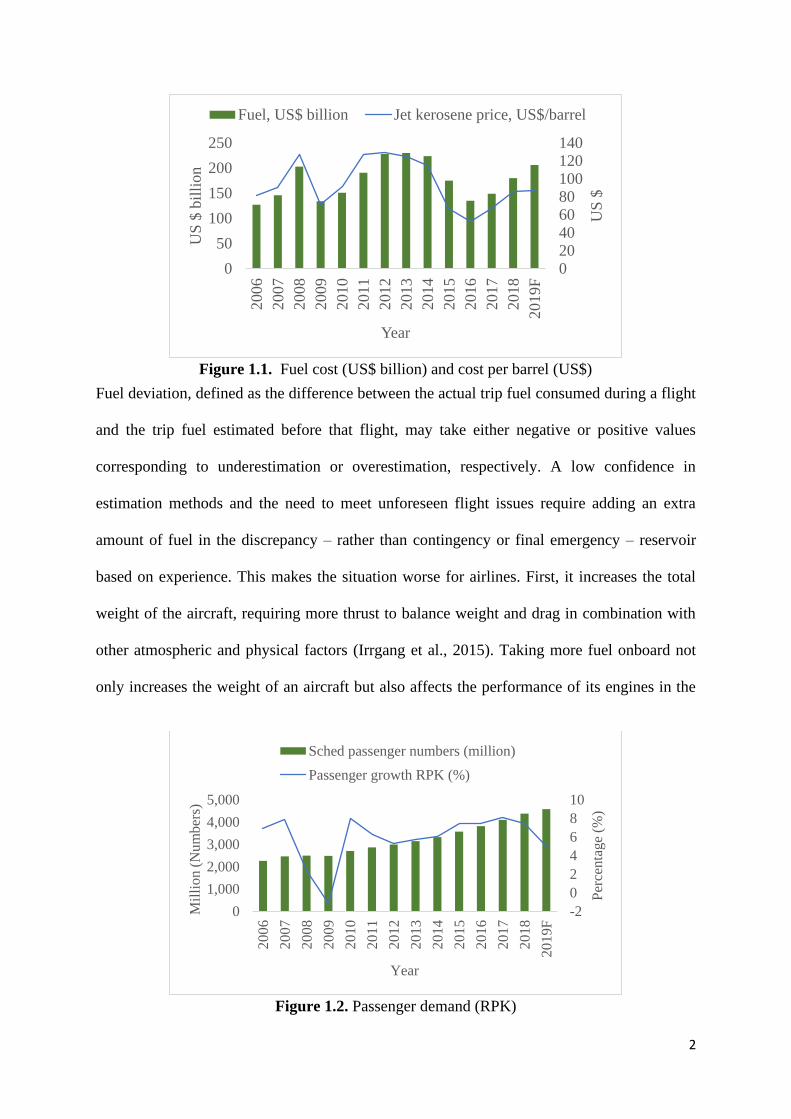
Fuel deviation, defined as the difference between the actual trip fuel consumed during a flight

and the trip fuel estimated before that flight, may take either negative or positive values

corresponding to underestimation or overestimation, respectively. A low confidence in

estimation methods and the need to meet unforeseen flight issues require adding an extra

amount of fuel in the discrepancy – rather than contingency or final emergency – reservoir

based on experience. This makes the situation worse for airlines. First, it increases the total

weight of the aircraft, requiring more thrust to balance weight and drag in combination with

other atmospheric and physical factors (Irrgang et al., 2015). Taking more fuel onboard not

only increases the weight of an aircraft but also affects the performance of its engines in the

Figure 1.1. Fuel cost (US$ billion) and cost per barrel (US$)

020406080100120140

0

50

100

150

200

250

2006

2007

2008

2009

2010

2011

2012

2013

2014

2015

2016

2017

2018

2019F

US

$

US

$ b

illi

on

Year

Fuel, US$ billion Jet kerosene price, US$/barrel

Figure 1.2. Passenger demand (RPK)

-2

0

2

4

6

8

10

0

1,000

2,000

3,000

4,000

5,000

20

06

20

07

20

08

20

09

20

10

20

11

20

12

20

13

20

14

20

15

20

16

20

17

20

18

20

19F

Per

cen

tage

(%)

Mil

lio

n (

Nu

mb

ers)

Year

Sched passenger numbers (million)

Passenger growth RPK (%)

3

long run by burning more fuel per unit distance. This ultimately shortens the lifetime of

engines, which need more frequent maintenance than planned (Abdelghany et al., 2005).

Moreover, an aircraft may require more fuel to burn than a brand-new one and the pilots may

be unaware of the actual amount of wear (deterioration) in the aircraft or may not know how

the wear is calculated by particular estimation methods. As a result, the pilots will demand

more fuel as a buffer in the discrepancy reservoir of the aircraft (Irrgang et al., 2015).

Therefore, the objective of reaching the destination with the smallest possible amount of fuel

left in the trip tank or utilized from the supplementary tank constitutes a challenging task to

accomplish.

Figure 1.3. Cargo demand (FTK)

-15

-10

-5

0

5

10

15

2025

0

10

20

30

40

50

60

70

20

06

20

07

20

08

20

09

20

10

20

11

2012

20

13

20

14

20

15

20

16

20

17

20

18

20

19F

Per

cen

atge

(%)

Mil

lio

n to

nn

es

Year

Freight tonnes (million) Cargo growth FTK (%)

Figure 1.4. Fuel consumption and carbon dioxide emission

0

20

40

60

80

100

0

200

400

600

800

1000

20

06

20

07

20

08

20

09

20

10

20

11

20

12

20

13

20

14

20

15

20

16

20

17

20

18

20

19F

US

bil

lio

n g

allo

ns

Mil

lio

n to

nn

es

Year

CO2 emissions, million tonnes

Fuel consumption, US billion gallons

4

Excess fuel consumption is disadvantageous for airlines both economically and

environmentally. Economically, because the increasing trend of fuel prices and a low

confidence in estimation methods may lead to more costs for airline operating organizations to

ensure smooth operations while meeting the growing need of passengers and cargo. Figure 1.1

shows the trend of increasing jet fuel prices. In 2019, the forecast has been that fuel prices will

increase by 31.18% as compared to those in 2015 (IATA, 2019). This forces airlines to adopt

risk management strategies such as fuel hedging and fuel ferrying, which may not be useful in

many cases (Merkert and Swidan, 2019; Sibdari et al., 2018). Fuel hedging and fuel ferrying

are certainly good strategies, but they become expensive when fuel prices fall ̶ fuel hedging ̶

and because of the high aircraft maintenance cost associated with loading excess fuel from

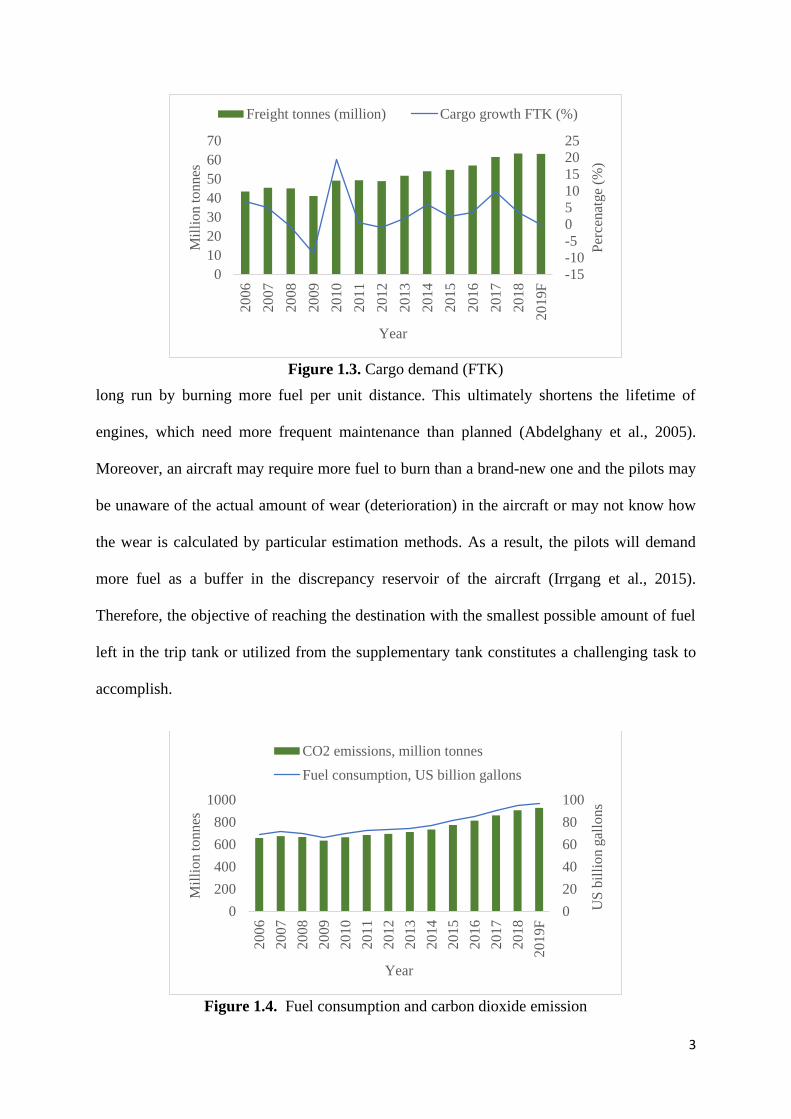
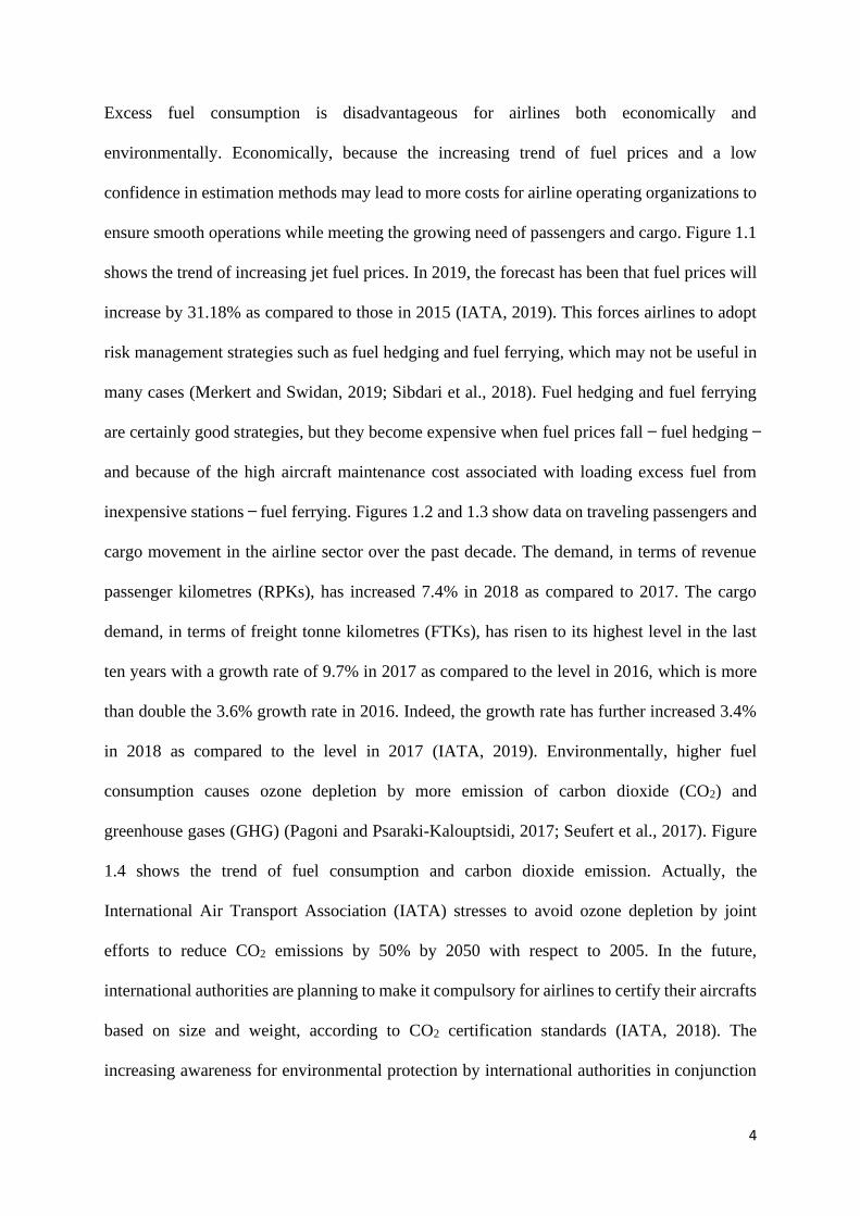
inexpensive stations ̶ fuel ferrying. Figures 1.2 and 1.3 show data on traveling passengers and

cargo movement in the airline sector over the past decade. The demand, in terms of revenue

passenger kilometres (RPKs), has increased 7.4% in 2018 as compared to 2017. The cargo

demand, in terms of freight tonne kilometres (FTKs), has risen to its highest level in the last

ten years with a growth rate of 9.7% in 2017 as compared to the level in 2016, which is more

than double the 3.6% growth rate in 2016. Indeed, the growth rate has further increased 3.4%

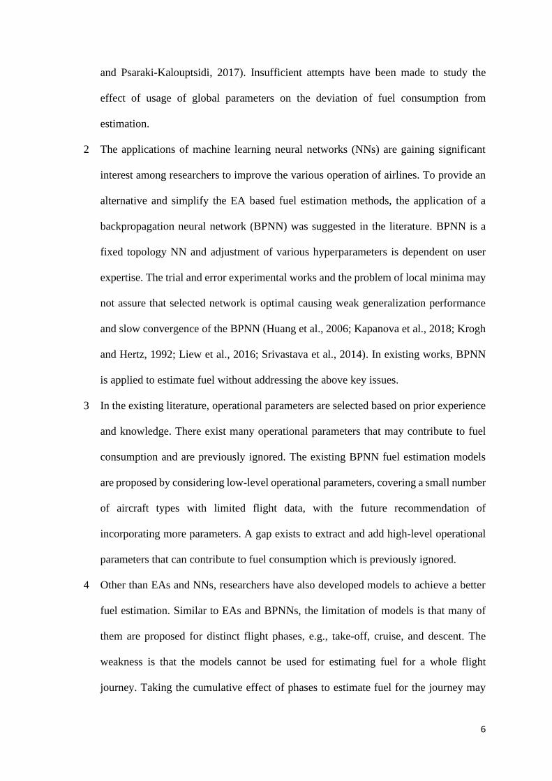
in 2018 as compared to the level in 2017 (IATA, 2019). Environmentally, higher fuel

consumption causes ozone depletion by more emission of carbon dioxide (CO2) and

greenhouse gases (GHG) (Pagoni and Psaraki-Kalouptsidi, 2017; Seufert et al., 2017). Figure

1.4 shows the trend of fuel consumption and carbon dioxide emission. Actually, the

International Air Transport Association (IATA) stresses to avoid ozone depletion by joint

efforts to reduce CO2 emissions by 50% by 2050 with respect to 2005. In the future,

international authorities are planning to make it compulsory for airlines to certify their aircrafts

based on size and weight, according to CO2 certification standards (IATA, 2018). The

increasing awareness for environmental protection by international authorities in conjunction

5

with growing fuel prices and boosting demand from tourism are encouraging airline operating

companies to adopt competitive strategies in fuel management to control excess fuel

consumption for long-term sustainability.

1.2 Problem statements

Accurately estimating the trip fuel for an aircraft has become an important research topic

because of profitability and safety issues. Several models have been studied in the literature,

however, still many gaps exist to improve and add a contribution to the existing literature. The

research gaps that need to be addressed are:

1 In current practice, estimation of fuel consumption for a flight trip is usually done by

an energy balance mathematical approaches (EAs). The most popular of them are the

Simmod simulation program, developed from the so-called advanced fuel burn model

(AFBM) (Collins, 1982) by the Federal Aviation Administration (FAA) (Baklacioglu,

2016), and the base of aircraft data (BADA) developed by the European Organization

for the Safety of Air Navigation (Eurocontrol) (Nuic, 2014). However, the actual

performance of a flight usually deviates from such estimation. Firstly, the information

needed to determine fuel flow is not always available in a real scenario and a great deal

of flight testing is needed to generate the parameter data, what may make the EAs

expensive technique to adopt (Trani and Wing-Ho, 1997). The parameters include

engine constants, airspeed, aircraft mass, atmospheric density, extra thrust needed for

ascending, and wing area (Huang et al., 2017). Secondly, aircraft fuel estimation may

not be accurate in EA methods owing to outdated existing databases and the

unavailability of data for all types of aircrafts and engines (Yanto and Liem, 2018). The

unavailability of data may result in the usage of more global parameters with default

values rather than local parameters, what in turn may lead to inaccurate results (Pagoni

6

and Psaraki-Kalouptsidi, 2017). Insufficient attempts have been made to study the

effect of usage of global parameters on the deviation of fuel consumption from

estimation.

2 The applications of machine learning neural networks (NNs) are gaining significant

interest among researchers to improve the various operation of airlines. To provide an

alternative and simplify the EA based fuel estimation methods, the application of a

backpropagation neural network (BPNN) was suggested in the literature. BPNN is a

fixed topology NN and adjustment of various hyperparameters is dependent on user

expertise. The trial and error experimental works and the problem of local minima may

not assure that selected network is optimal causing weak generalization performance

and slow convergence of the BPNN (Huang et al., 2006; Kapanova et al., 2018; Krogh

and Hertz, 1992; Liew et al., 2016; Srivastava et al., 2014). In existing works, BPNN

is applied to estimate fuel without addressing the above key issues.

3 In the existing literature, operational parameters are selected based on prior experience

and knowledge. There exist many operational parameters that may contribute to fuel

consumption and are previously ignored. The existing BPNN fuel estimation models

are proposed by considering low-level operational parameters, covering a small number

of aircraft types with limited flight data, with the future recommendation of

incorporating more parameters. A gap exists to extract and add high-level operational

parameters that can contribute to fuel consumption which is previously ignored.

4 Other than EAs and NNs, researchers have also developed models to achieve a better

fuel estimation. Similar to EAs and BPNNs, the limitation of models is that many of

them are proposed for distinct flight phases, e.g., take-off, cruise, and descent. The

weakness is that the models cannot be used for estimating fuel for a whole flight

journey. Taking the cumulative effect of phases to estimate fuel for the journey may

7

even lead to higher fuel deviation. It should be noted that complete flight trip fuel

consumption is dependent on many operational parameters and their changing

behaviour at the departure airport, cruise phase, and arrival airport.

5 Lastly, insufficient work exists that has studied the effect of dividing the high

dimensional historical data into chunks (portions) of data on fuel estimation, by

considering all phases collectively, using machine learning NNs. Machine learning

algorithms are highly dependent on historical datasets and application of an algorithm

that may give better results regardless of a change in data structure and size is gaining

an important consideration.

1.3 Research objectives

The purpose of this work is to develop a novel machine learning NN algorithm having

characteristics of better generalization performance and learning speed to handle efficiently

real and large-scale aircraft trip fuel estimation problems. The aim is to eliminate the need for

a trial-and-error approach, reduce the number of hyperparameter adjustments, usage of global

parameters, outdated database, and expert involvement. We consider that insufficient attempts

have been reported in the literature concerning the estimation of trip fuel using feedforward

constructive neural networks (CNNs) along with high-dimensional data for the entire trip flight

phases collectively. More specifically, the research objectives can be concisely described

below:

1 To formulate the trip fuel estimation model and define an objective function of

minimizing fuel deviation. Relevant operational parameters that can contribute to fuel

consumption will be extracted from the real historical high dimensional data of one of

the international airlines operating in Hong Kong. The extracted operational parameters

will be incorporated in the newly formulated model to estimate trip fuel for all phases

8

collectively. This objective will facilitate addressing the first four research gaps

identified in Section 1.2.

2 To develop a novel machine learning NN algorithm having characteristics of better

generalization performance and faster learning speed with a fewer hyperparameter

adjustment. The roadmap is to conduct a comprehensive review of the existing

literature, carried out in the last three decades, that proposed to improve the feedforward

neural networks (FNNs) learning algorithms and optimization techniques. Based on

extensive review and understanding of the merits, limitations, recent research trends

and research gaps in FNNs we plan to develop a novel CNN. The basic idea is to

generate linearly independent hidden units in each hidden layer from analytically

calculation of input units and connect only the last hidden layer to the output unit

through output connection weight having maximum error convergence property. This

objective will facilitate addressing second and fifth research gaps as identified in

Section 1.2.

3 To apply a novel CNN for minimizing the fuel deviation. The performance comparison

of novel CNN with an existing airline energy balance approach (AEA) and a traditional

BPNN will be made to understand the effectiveness of proposed CNN in minimizing

fuel deviation. This objective will mainly address all research gaps as identified in

Section 1.2.

1.4 Research contributions

Early attempts to estimate the trip fuel by EAs have gained popularity. However, the successful

wide use of machine learning in many applications has changed the interest of the airlines

operating organization. The unavailability of data related to local parameters, complex

mathematical formulations, and expertise involvement limits the applicability of EAs. The

9

application of BPNNs as an alternative to EAs constitutes an attempt to overcome the above

limitations with improved results. However, the existing BPNN-based fuel estimation models

only cover a small number of aircraft types with limited flight data. The possible reasons are

the random generation and iteratively tuning of the connection weights on both sides of BPNNs

by gradient-based learning algorithms. This may create a complex co-adaptation by generating

redundant hidden units, thereby contributing less to error convergence. The adjustment of local

and global hyperparameters with the connection weights may require many experimental trials

to obtain an optimal fixed-topology network. These problems increase the expertise

requirement as well as cause weak generalization performance and slow convergence.

The application of traditional machine learning NNs for airline trip fuel estimation is not

straightforward. Extensive knowledge is required to fit the algorithm to the model. The varying

nature of airline input parameters and the high dimensionality of data might be challenging for

traditional BPNNs to accurately estimate the trip fuel with the aforementioned limitations. The

same problem has been observed in our experimental work (discussed in Chapter 5). Similarly,

in the current literature, the application of fixed-topology BPNNs for fuel estimation is limited

in scope by considering a few aircraft types, flight data, and operational parameters. This means

that the application of machine learning NNs on the varying nature of operational parameters

and the high dimensionality of data is still an open area. To overcome the limitations of BPNNs,

this study proposes a CNN featuring a self-organizing cascading architecture and capable of

analytically calculating connection weights. These characteristics generate linearly

independent (non-redundant) hidden units having the capability of maximum error reduction.

The proposed CNN thus achieves a better generalization performance and converges

significantly faster than traditional BPNNs.

10

The application of the proposed CNN with varying operational parameters and high-

dimensional data for airline trip fuel estimation can bring a breakthrough improvement

compared to existing fuel estimation methods. Unlike EAs, the advantages of the proposed

CNN are that it requires neither the involvement and consultation of an expert for a complex

mathematical formulation nor the cost to determine the coefficients. In addition, it can work

with any type of available data. Compared to BPNNs, the proposed CNN avoids the fixed-

topology trail-and-error experimental works with too much adjustment of hyperparameters and

iterative tuning of the connection weights. These advantages simplify the implementation of

high-dimensional data with the objective of achieving better trip fuel estimation with fast

convergence. A comparative study has been performed among the proposed self-organizing

CNN, AEA, and a BPNN to estimate airline trip fuel. To make the study more valuable, the

comparison is not limited to high-dimensional data and its varying operational parameters

(referred to as a combined model in Section 5.4.2.1). We also include the portion of data

resulting from dividing high-dimensional data into a small dataset representing the same

behaviour within operational parameters (referred to as individual models in Section 5.4.2.2).

The significant improvement in trip fuel estimation and the learning speed in both models

(combined model and individual models) increase the confidence in that the proposed CNN

may eliminate the need of adding more fuel-based solely on experience.

1.5 Research scope and significance

The main focus of the research is to formulate a machine learning CNN model for aircraft trip

fuel estimation that is able to handle practical large-scale problems. The work will help to add

knowledge to the existing literature from two different viewpoints: academically and

practically. Academically, the research work will help to fill the identified research gaps in the

area of aircraft trip fuel estimation and machine learning as discussed in Section 1.2.

11

Practically, the research findings will provide insights into the aviation industry in controlling

airlines’ excess fuel consumption. Furthermore, it will add a contribution to the global goal of

IATA to make an average improvement in fuel efficiency of 1.5% per year (IATA, 2018).

1.6 Structure of the thesis

The thesis is organized as follows:

▪ Chapter 2 is about the literature review. This chapter is further divided into two major

sections followed by discussion. Section 2.1 is about the literature review explaining

mainly existing aircraft fuel estimation models. Section 2.2 is about literature review

explaining mainly FNNs learning algorithms and optimization techniques with their

merits, limitations, a shift in research trends, and real-world applications. Section 2.3

summarizes the research gaps.

▪ Chapter 3 explains the framework of fuel consumption and its deviation from the

estimation. The relevant operational parameters that may contribute to fuel

consumption are extracted and their relationships to fuel consumption are explained in

detail. The relationship between mathematical and data-driven methods is constructed

and the significance of the proposed method is elaborated. Then, the trip fuel estimation

model is formulated, and the objective function is defined.

▪ Chapter 4 is about the novel self-organizing CNN. This chapter initially explains

existing CNN and its extension convergence limitations. Then, a novel self-organizing

CNN learning algorithm is proposed and explained with supporting lemma and

theoretical justification. Finally, various set of artificial benchmarking and real-world

application dataset is used to demonstrate the generalization performance and learning

speed of proposed CNN.

12

▪ Chapter 5 is about aircrafts trip fuel estimation and comparison. The chapter describes

the data and pre-processing techniques. Then experimental work is carried out by

estimating trip fuel by novel CNN and making a comparison with AEA and BPNN.

Major findings are discussed in detail to get a better insight.

▪ Chapter 6 concludes the thesis by explaining the limitations of existing work and

possible future research directions.

▪ The application of FNNs in solving real-world problems, described in Chapter 2, are

presented in Appendix A.

13

Chapter 2. Literature Review

In Chapter 2, a literature review is carried out for two topics: aircraft fuel estimation, and FNNs

learning algorithms and optimization techniques. Firstly, for aircraft fuel estimation (Section

2.1), the existing fuel estimation models based on EAs (Subsection 2.1.1) and BPNNs

(Subsection 2.1.2) are reviewed. Later, other estimation methods are also reviewed in

Subsection 2.1.3 to enrich the content. Secondly, for neural networks learning algorithms and

optimization techniques (Section 2.2), we conducted a comprehensive review to understand

noteworthy contributions made in the area of the FNN and their merits and limitations; to

identify new research directions that will help to design novel and efficient algorithm. The

survey methodology of comprehensive review is discussed in Subsection 2.2.1. Subsection

2.2.2 gives a brief introduction to FNN. Learning algorithms and their applications are

reviewed in Subsection 2.2.3, whereas, optimization techniques and their applications are

reviewed in Subsection 2.2.4. Finally, in Section 2.3, the summary of the literature review and

research gaps of fuel estimation and FNN are identified and elaborated.

2.1 Aircraft fuel estimation

The trip fuel containing a maximum portion of fuel weight must be considered for

improvement. A small improvement in fuel estimation can bring significant savings in fuel

consumption and substantial cost benefit (Jensen et al., 2013). Irrgang et al. (2015) concluded

from their work on aircraft fuel optimization analytics that the optimal amount of fuel should

be accurately determined, resulting in the minimum amount of fuel remaining at the destination

airport. Taking extra fuel increases the weight of the aircraft, which results in more fuel

consumption than required. Turgut et al. (2014) worked on the fuel flow during the cruise

phase. They suggested that reducing the aircraft weight by 1 tonne, increasing the flying

14

altitude by 100 ft, and reducing the cruise speed by 1 knot may result in a reduction of per-hour

fuel consumption of 15-21 kg, 26-28 kg, and 7.7-8.7 kg, respectively. Taking more fuel

increases the weight of the aircraft, and in consequence, more fuel is consumed with higher

maintenance costs (Abdelghany et al., 2005). Therefore, more efficient and effective methods

are needed to make the estimation models applicable (Choi et al., 2016).

2.1.1 EAs based fuel estimation

Early attempts made use of EAs to estimate the fuel for aircrafts. EAs are based on extensive

mathematical formulations and are derived from the basic concept of energy balance. They

assume static constants of aircraft performance and a dynamic input of the path profile. The

energy balance can be expressed in terms of the energy the aircraft gains and losses as it travels

along the prescribed path profile. During each flight operation, as a result of the change in

kinetic and potential energies, the aircraft suffers energy losses because of drag. These losses

are adjusted by a certain amount of thrust to maintain the energy balance. Thus, an aircraft can

be viewed as a system undergoing energy losses and gains that should be continuously balanced

by the consumption of fuel energy. Collins (1982) derived an algorithm for fuel estimation

based on such energy balance approach by considering the description of aircraft configuration,

weight, and path profile. The path profile depends on a change in true airspeed, altitude, and

flight time. Collins (1982) explained that various aircraft-specific constants need to be

determined for each aircraft to define the relationship between drag and lift/weight coefficients

and to define the relationship between fuel consumption and energy gain from the thrust as a

function of velocity and altitude. Experimental work demonstrated that the algorithm could

result in saving more than two million US gallons of fuel annually. The accuracy check of the

algorithm with Eastern Airlines demonstrated its effectiveness with a difference of less than

3%. This algorithm, known as AFBM, was developed by the Mitre corporation under the FAA

15

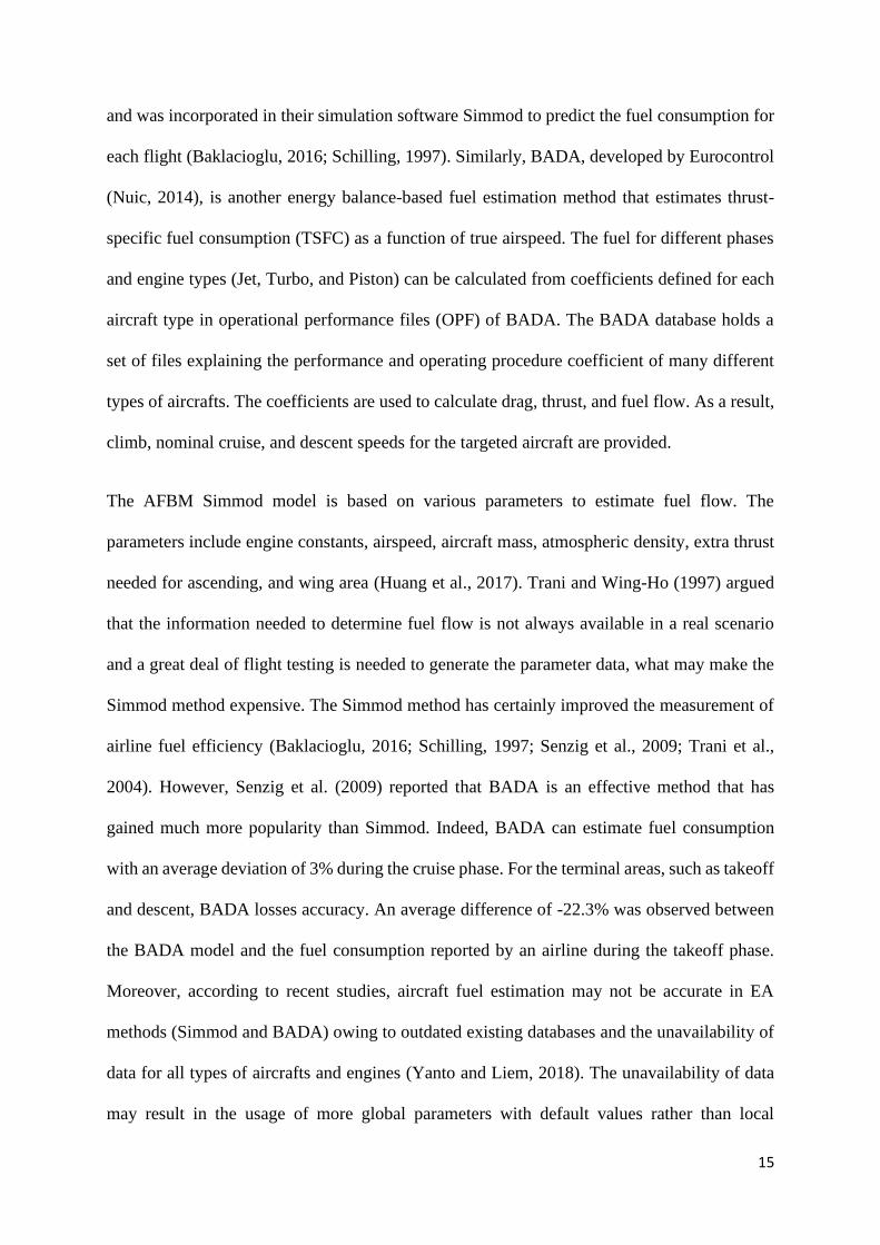
and was incorporated in their simulation software Simmod to predict the fuel consumption for

each flight (Baklacioglu, 2016; Schilling, 1997). Similarly, BADA, developed by Eurocontrol

(Nuic, 2014), is another energy balance-based fuel estimation method that estimates thrust-

specific fuel consumption (TSFC) as a function of true airspeed. The fuel for different phases

and engine types (Jet, Turbo, and Piston) can be calculated from coefficients defined for each

aircraft type in operational performance files (OPF) of BADA. The BADA database holds a

set of files explaining the performance and operating procedure coefficient of many different

types of aircrafts. The coefficients are used to calculate drag, thrust, and fuel flow. As a result,

climb, nominal cruise, and descent speeds for the targeted aircraft are provided.

The AFBM Simmod model is based on various parameters to estimate fuel flow. The

parameters include engine constants, airspeed, aircraft mass, atmospheric density, extra thrust

needed for ascending, and wing area (Huang et al., 2017). Trani and Wing-Ho (1997) argued

that the information needed to determine fuel flow is not always available in a real scenario

and a great deal of flight testing is needed to generate the parameter data, what may make the

Simmod method expensive. The Simmod method has certainly improved the measurement of

airline fuel efficiency (Baklacioglu, 2016; Schilling, 1997; Senzig et al., 2009; Trani et al.,

2004). However, Senzig et al. (2009) reported that BADA is an effective method that has

gained much more popularity than Simmod. Indeed, BADA can estimate fuel consumption

with an average deviation of 3% during the cruise phase. For the terminal areas, such as takeoff

and descent, BADA losses accuracy. An average difference of -22.3% was observed between

the BADA model and the fuel consumption reported by an airline during the takeoff phase.

Moreover, according to recent studies, aircraft fuel estimation may not be accurate in EA

methods (Simmod and BADA) owing to outdated existing databases and the unavailability of

data for all types of aircrafts and engines (Yanto and Liem, 2018). The unavailability of data

may result in the usage of more global parameters with default values rather than local

16

parameters, which in turn may lead to inaccurate results (Pagoni and Psaraki-Kalouptsidi,

2017). Complex mathematical computation, high testing and consultation cost, expert

involvement, and estimation errors, which may become worse in certain conditions, limit EA

applicability.

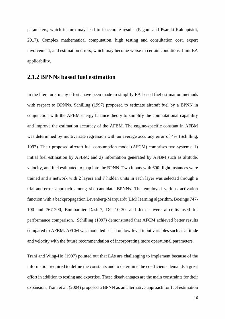
2.1.2 BPNNs based fuel estimation

In the literature, many efforts have been made to simplify EA-based fuel estimation methods

with respect to BPNNs. Schilling (1997) proposed to estimate aircraft fuel by a BPNN in

conjunction with the AFBM energy balance theory to simplify the computational capability

and improve the estimation accuracy of the AFBM. The engine-specific constant in AFBM

was determined by multivariate regression with an average accuracy error of 4% (Schilling,

1997). Their proposed aircraft fuel consumption model (AFCM) comprises two systems: 1)

initial fuel estimation by AFBM; and 2) information generated by AFBM such as altitude,

velocity, and fuel estimated to map into the BPNN. Two inputs with 600 flight instances were

trained and a network with 2 layers and 7 hidden units in each layer was selected through a

trial-and-error approach among six candidate BPNNs. The employed various activation

function with a backpropagation Levenberg-Marquardt (LM) learning algorithm. Boeings 747-

100 and 767-200, Bombardier Dash-7, DC 10-30, and Jetstar were aircrafts used for

performance comparison. Schilling (1997) demonstrated that AFCM achieved better results

compared to AFBM. AFCM was modelled based on low-level input variables such as altitude

and velocity with the future recommendation of incorporating more operational parameters.

Trani and Wing-Ho (1997) pointed out that EAs are challenging to implement because of the

information required to define the constants and to determine the coefficients demands a great

effort in addition to testing and expertise. These disadvantages are the main constraints for their

expansion. Trani et al. (2004) proposed a BPNN as an alternative approach for fuel estimation

17

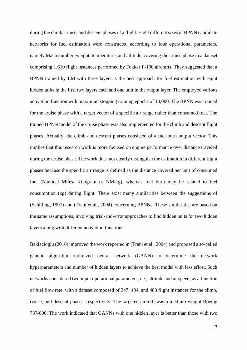
during the climb, cruise, and descent phases of a flight. Eight different sizes of BPNN candidate

networks for fuel estimation were constructed according to four operational parameters,

namely Mach number, weight, temperature, and altitude, covering the cruise phase in a dataset

comprising 1,610 flight instances performed by Fokker F-100 aircrafts. They suggested that a

BPNN trained by LM with three layers is the best approach for fuel estimation with eight

hidden units in the first two layers each and one unit in the output layer. The employed various

activation function with maximum stopping training epochs of 10,000. The BPNN was trained

for the cruise phase with a target vector of a specific air range rather than consumed fuel. The

trained BPNN model of the cruise phase was also implemented for the climb and descent flight

phases. Actually, the climb and descent phases consisted of a fuel burn output vector. This

implies that this research work is more focused on engine performance over distance traveled

during the cruise phase. The work does not clearly distinguish the estimation in different flight

phases because the specific air range is defined as the distance covered per unit of consumed

fuel (Nautical Miles/ Kilogram or NM/kg), whereas fuel burn may be related to fuel

consumption (kg) during flight. There exist many similarities between the suggestions of

(Schilling, 1997) and (Trani et al., 2004) concerning BPNNs. These similarities are based on

the same assumptions, involving trial-and-error approaches to find hidden units for two hidden

layers along with different activation functions.

Baklacioglu (2016) improved the work reported in (Trani et al., 2004) and proposed a so-called

genetic algorithm optimized neural network (GANN) to determine the network

hyperparameters and number of hidden layers to achieve the best model with less effort. Such

networks considered two input operational parameters, i.e., altitude and airspeed, as a function

of fuel flow rate, with a dataset composed of 347, 404, and 483 flight instances for the climb,

cruise, and descent phases, respectively. The targeted aircraft was a medium-weight Boeing

737-800. The work indicated that GANNs with one hidden layer is better than those with two

18

hidden layers and achieve improved results for the climb and descent phases compared to a

previously suggested model (Trani et al., 2004).

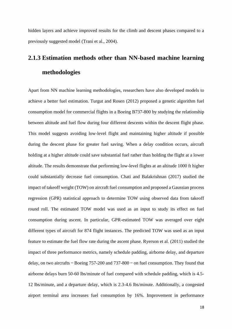
2.1.3 Estimation methods other than NN-based machine learning

methodologies

Apart from NN machine learning methodologies, researchers have also developed models to

achieve a better fuel estimation. Turgut and Rosen (2012) proposed a genetic algorithm fuel

consumption model for commercial flights in a Boeing B737-800 by studying the relationship

between altitude and fuel flow during four different descents within the descent flight phase.

This model suggests avoiding low-level flight and maintaining higher altitude if possible

during the descent phase for greater fuel saving. When a delay condition occurs, aircraft

holding at a higher altitude could save substantial fuel rather than holding the flight at a lower

altitude. The results demonstrate that performing low-level flights at an altitude 1000 ft higher

could substantially decrease fuel consumption. Chati and Balakrishnan (2017) studied the

impact of takeoff weight (TOW) on aircraft fuel consumption and proposed a Gaussian process

regression (GPR) statistical approach to determine TOW using observed data from takeoff

round roll. The estimated TOW model was used as an input to study its effect on fuel

consumption during ascent. In particular, GPR-estimated TOW was averaged over eight

different types of aircraft for 874 flight instances. The predicted TOW was used as an input

feature to estimate the fuel flow rate during the ascent phase. Ryerson et al. (2011) studied the

impact of three performance metrics, namely schedule padding, airborne delay, and departure

delay, on two aircrafts ̶ Boeing 757-200 and 737-800 ̶ on fuel consumption. They found that

airborne delays burn 50-60 lbs/minute of fuel compared with schedule padding, which is 4.5-

12 lbs/minute, and a departure delay, which is 2.3-4.6 lbs/minute. Additionally, a congested

airport terminal area increases fuel consumption by 16%. Improvement in performance

19

measurements by eliminating the above three delays by econometric methods can reduce

airborne fuel consumption.

2.2 Neural networks learning algorithms and optimization

techniques

The importance of FNN is increasing every day due to its property of processing big nonlinear

data like in the human brains. It can discover a hidden pattern in the data by entering raw data

in the input, passing layer by layer until it arrives at the output in the forward direction. The

model is trained to correctly estimate unseen data (also known as test data) referred to as the

generalization performance of FNN. The ideal FNN is considered to have better generalization

performance and may require less learning time (also known as convergence rate) to train the

model. Generalization performance can be defined as the ability of an algorithm to accurately

predict values on previously unseen samples (Yeung et al., 2007), whereas, learning time can

be defined as the ability of the algorithm to train a model quickly. Both “generalization

performance” and “learning time” are key performance indicators for FNNs and are used by

researchers to demonstrate the effectiveness of their proposed algorithms. Some of the

drawbacks that may affect the generalization performance and learning speed of FNNs include

local minima, saddle points, plateau surfaces, hyperparameters adjustment, trial and error

experimental work, tuning connection weights, deciding hidden units and layers, and many

others. The drawbacks that limit FNN applicability may become worse with inappropriate user

expertise and insufficient theoretical information. For instance, how to define network size,

hidden units, hidden layers, connection weights, learning rate, topology, and many others.

In the literature, the answers to the above problems are not so straightforward. Researchers

have proposed several learning algorithms and optimization techniques, that benefit in

20

improving the FNN, with the main motivation to get a better generalization performance in the

shortest possible network training time. In the existing literature surveys, several authors have

reviewed FNN algorithms by performing a comparative study of different algorithms within

the same class (for instance: constructive algorithms comparison based on data, and many

others), studying the application area (for instance: business, engineering, and many others)

and specific class surveys (for instance: network ensemble survey and many others). For

instance, Zhang (2000) focused on and surveyed the recent development of neural networks

for classification problems. The review included the link between the neural and conventional

classifiers and demonstrated that neural networks are a competitive alternative to the traditional

classifiers. Other contributions include examining the issues of posterior probability

estimation, feature selection, and the trade-off between learning and generalization. Hunter et

al. (2012) performed a comparative study among different types of learning algorithms and

network topology so as to select a proper neural network size and architecture for better

generalization performance. LeCun et al. (2015) reviewed deep learning and provided in-depth

knowledge of backpropagation, convolutional neural network, and recurrent neural networks.

The success in deep learning is that it requires little engineering by hand and new algorithms

will accelerate its progress much more. Tkáč and Verner (2016) provided a systematic review

of neural network applications over two decades and disclosed that most of the application

areas included financial distress and bankruptcy. Cao et al. (2018) presented a survey on tuning

free random weights neural networks from the perspective of deep learning. The traditional

deep learning iterative algorithms are far slower and have the problem of local minima. The

survey suggests that the computing efficiency of deep learning increases due to the combination

of traditional deep learning and tuning free random weights neural networks.

In the above studies, the focus is only on the specific type of algorithms or their applications

which limits their scope. The existing studies are more focused on comparing and selecting a

21

suitable algorithm within their class which is solely based on expertise and available

application data. It does not clearly identify the research directions over the past decades.

Researchers have made efforts to reduce the drawbacks of FNNs, however, a comprehensive

review is missing, and an open challenge is to gather the answers for the drawbacks in one

platform. Therefore, we carried out a comprehensive literature review and classified it into six

categories based on the algorithms proposed, and investigated their applications in real-world

management, engineering, and health sciences problems, so as to understand the researchers’

current interests and directions in overcoming FNN drawbacks. Our review contributes to the

existing literature not only by summarizing the recent developments in FNN algorithms and

classifying them into six categories according to the nature of algorithms, but also by exploring

the applications of the proposed algorithms in solving real-world management, engineering,

and health sciences problems and demonstrating the great potential for their practical

utilization. Moreover, we propose several interesting and crucial future research directions

regarding FNNs which are believed to be useful for the development of the area.

2.2.1 Survey methodology

2.2.1.1 Source of literature

The objective of the study is to identify and classify the learning algorithms and optimization

techniques that have contributed to improving the generalization performance and learning

speed of FNNs. Therefore, a comprehensive review has been conducted to get in-depth

knowledge of the existing work and to understand researchers’ contributions and work

directions. Furthermore, the authors discuss the future research directions so as to contribute in

strengthening the literature. To accomplish these objectives, the literature surveyed in the study

was explored from seven different sources: IEEE Xplore -IEEE, ScienceDirect- Elsevier,

22

Emerald Insight, arXiv- Cornell University, SpringerLink- Springer, Taylor & Francis and

Google Scholar. The survey is based on articles in journals, conference proceedings, archives,

technical reports, books, and academic lectures. The focus was to select articles published in

the last three decades mainly in the period 1986-2018. However, the articles that contribute

significant knowledge to the existing literature and one out of time frame (For instance, the

year 1985 and earlier) are also included to support and deepen the review.

The research contributions and its applications in FNN are numerous and cannot be covered in

one study. Four keywords that are related to FNN were used to search for articles in the above-

mentioned databases: “generalization performance”, “learning rate”, “overfitting”, and “fixed

and cascade architecture”. Moreover, the combination of keywords was also used to get

relevant articles. The duplicated articles in the databases, non-English language, and matched

keywords but out of scope were discarded. The screening process was limited to articles

belonging to the Q1 category of ranked journals, issued by either “Scientific Journal Rankings

- SJR” or “Journal Citation Reports - JCR” in the year 2018. However, to strengthen the review,

a small number of highly cited conference papers and articles belonging to Q2, Q3, and Q4

journals with more than 500 citations, and articles from other sources (such as online achieves,

books, technical reports, and websites) with more than 100 citations were also considered. All

the searched article’s abstracts and the conclusions were completely reviewed along with the

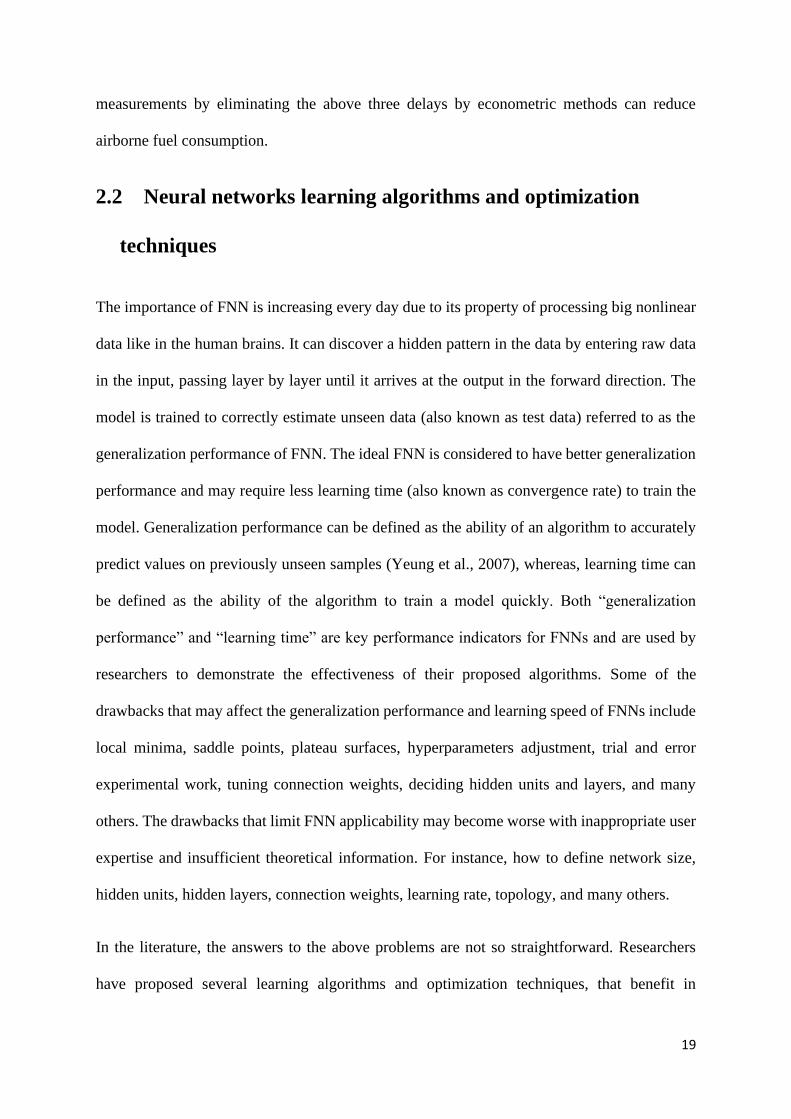
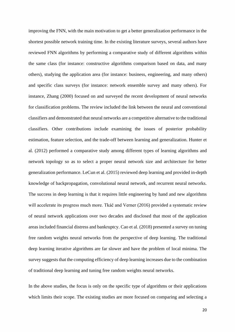
full text to screen high-quality relevant literature. This resulted in a total of 80 articles. Figure

Figure 2.1. Articles distribution

Journal Articles

63 Nos.; 78.75%

Conference Proceedings

10Nos.; 12.50%

arXiv online Archives

3 Nos.; 3.75%

Books

2 No.; 2.50%

Technical Report

1No.; 1.25%

Academic Lecture

1No.; 1.25%

23

2.1 shows the distribution of the articles along with the number and percentage in each

category. In the 80 articles, 63 (78.75%) are journal papers, 10 (12.50%) conference papers, 3

(3.75%) online arXiv archives, 2 (2.50%) books, 1 (1.25%) technical report, and 1 (1.25%)

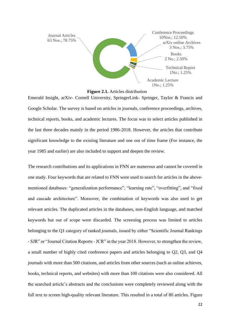
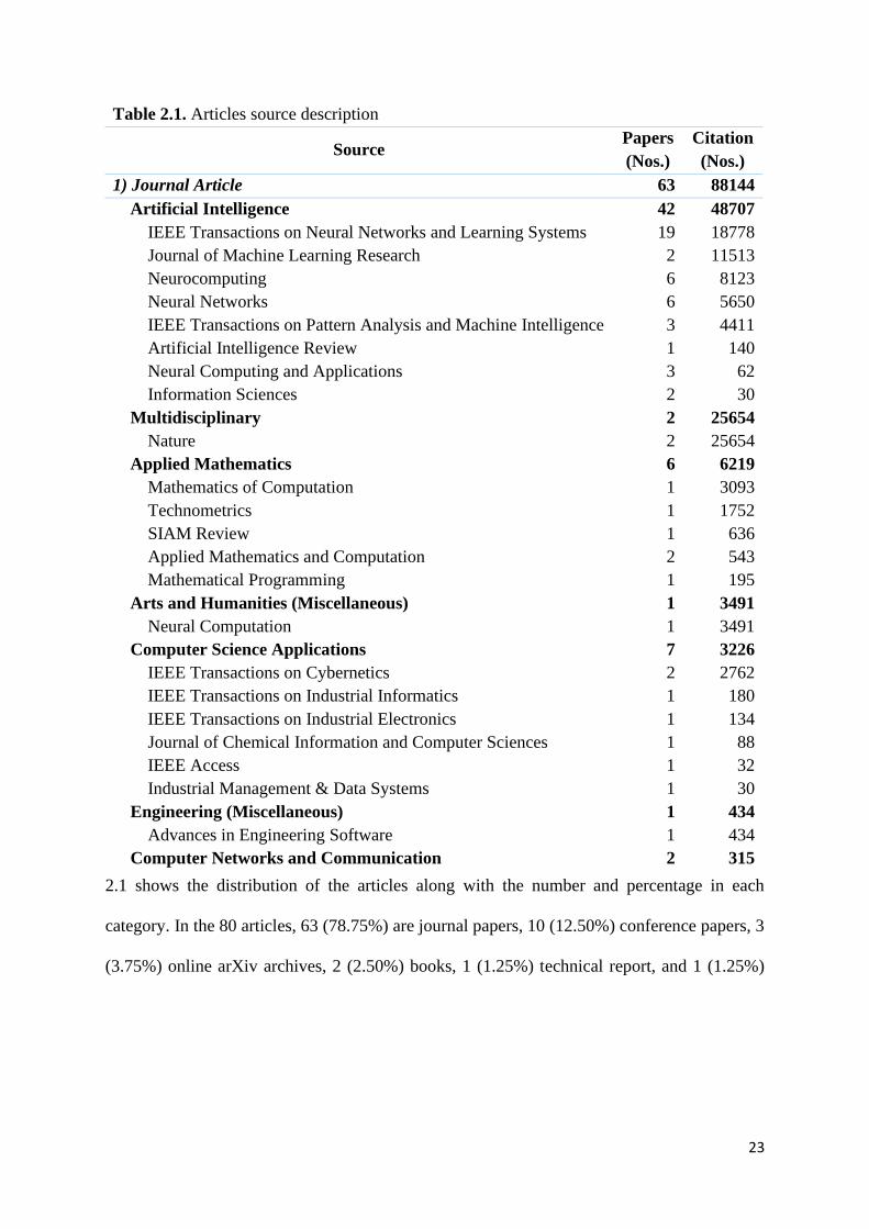
Table 2.1. Articles source description

Source Papers

(Nos.)

Citation

(Nos.)

1) Journal Article 63 88144

Artificial Intelligence 42 48707

IEEE Transactions on Neural Networks and Learning Systems 19 18778

Journal of Machine Learning Research 2 11513

Neurocomputing 6 8123

Neural Networks 6 5650

IEEE Transactions on Pattern Analysis and Machine Intelligence 3 4411

Artificial Intelligence Review 1 140

Neural Computing and Applications 3 62

Information Sciences 2 30

Multidisciplinary 2 25654

Nature 2 25654

Applied Mathematics 6 6219

Mathematics of Computation 1 3093

Technometrics 1 1752

SIAM Review 1 636

Applied Mathematics and Computation 2 543

Mathematical Programming 1 195

Arts and Humanities (Miscellaneous) 1 3491

Neural Computation 1 3491

Computer Science Applications 7 3226

IEEE Transactions on Cybernetics 2 2762

IEEE Transactions on Industrial Informatics 1 180

IEEE Transactions on Industrial Electronics 1 134

Journal of Chemical Information and Computer Sciences 1 88

IEEE Access 1 32

Industrial Management & Data Systems 1 30

Engineering (Miscellaneous) 1 434

Advances in Engineering Software 1 434

Computer Networks and Communication 2 315

24

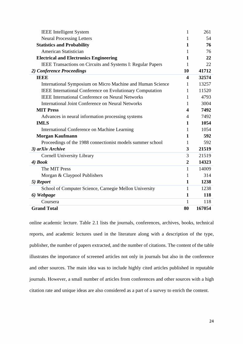
online academic lecture. Table 2.1 lists the journals, conferences, archives, books, technical

reports, and academic lectures used in the literature along with a description of the type,

publisher, the number of papers extracted, and the number of citations. The content of the table

illustrates the importance of screened articles not only in journals but also in the conference

and other sources. The main idea was to include highly cited articles published in reputable

journals. However, a small number of articles from conferences and other sources with a high

citation rate and unique ideas are also considered as a part of a survey to enrich the content.

IEEE Intelligent System 1 261

Neural Processing Letters 1 54

Statistics and Probability 1 76

American Statistician 1 76

Electrical and Electronics Engineering 1 22

IEEE Transactions on Circuits and Systems I: Regular Papers 1 22

2) Conference Proceedings 10 41712

IEEE 4 32574

International Symposium on Micro Machine and Human Science 1 13257

IEEE International Conference on Evolutionary Computation 1 11520

IEEE International Conference on Neural Networks 1 4793

International Joint Conference on Neural Networks 1 3004

MIT Press 4 7492

Advances in neural information processing systems 4 7492

IMLS 1 1054

International Conference on Machine Learning 1 1054

Morgan Kaufmann 1 592

Proceedings of the 1988 connectionist models summer school 1 592

3) arXiv Archive 3 21519

Cornell University Library 3 21519

4) Book 2 14323

The MIT Press 1 14009

Morgan & Claypool Publishers 1 314

5) Report 1 1238

School of Computer Science, Carnegie Mellon University 1 1238

6) Webpage 1 118

Coursera 1 118

Grand Total 80 167054

25

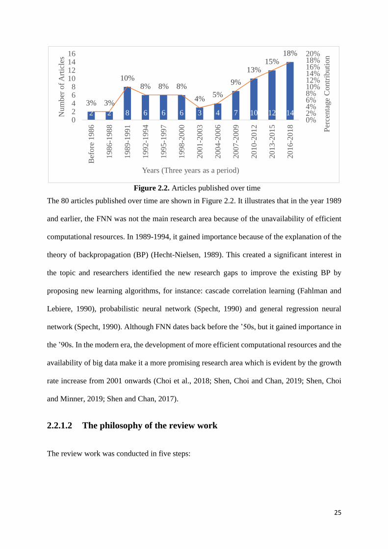
The 80 articles published over time are shown in Figure 2.2. It illustrates that in the year 1989

and earlier, the FNN was not the main research area because of the unavailability of efficient

computational resources. In 1989-1994, it gained importance because of the explanation of the

theory of backpropagation (BP) (Hecht-Nielsen, 1989). This created a significant interest in

the topic and researchers identified the new research gaps to improve the existing BP by

proposing new learning algorithms, for instance: cascade correlation learning (Fahlman and

Lebiere, 1990), probabilistic neural network (Specht, 1990) and general regression neural

network (Specht, 1990). Although FNN dates back before the ’50s, but it gained importance in

the ’90s. In the modern era, the development of more efficient computational resources and the

availability of big data make it a more promising research area which is evident by the growth

rate increase from 2001 onwards (Choi et al., 2018; Shen, Choi and Chan, 2019; Shen, Choi

and Minner, 2019; Shen and Chan, 2017).

2.2.1.2 The philosophy of the review work

The review work was conducted in five steps:

Figure 2.2. Articles published over time

2 2 8 6 6 6 3 4 7 10 12 14

3% 3%

10%8% 8% 8%

4%5%

9%

13%15%

18%

0%2%4%6%8%10%12%14%16%18%20%

02468

10121416

Bef

ore

1986

19

86-1

98

8

1989-1

991

1992-1

994

1995-1

997

1998-2

000

2001-2

003

2004-2

006

2007-2

009

2010-2

012

2013-2

015

2016-2

018 Per

centa

ge

Contr

ibuti

on

Num

ber

of

Art

icle

s

Years (Three years as a period)

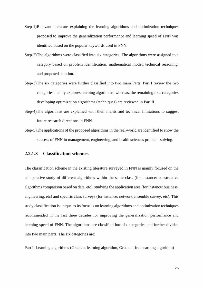
26

Step-1) Relevant literature explaining the learning algorithms and optimization techniques

proposed to improve the generalization performance and learning speed of FNN was

identified based on the popular keywords used in FNN.

Step-2) The algorithms were classified into six categories. The algorithms were assigned to a

category based on problem identification, mathematical model, technical reasoning,

and proposed solution.

Step-3) The six categories were further classified into two main Parts. Part I review the two

categories mainly explores learning algorithms, whereas, the remaining four categories

developing optimization algorithms (techniques) are reviewed in Part II.

Step-4) The algorithms are explained with their merits and technical limitations to suggest

future research directions in FNN.

Step-5) The applications of the proposed algorithms in the real-world are identified to show the

success of FNN in management, engineering, and health sciences problem-solving.

2.2.1.3 Classification schemes

The classification scheme in the existing literature surveyed in FNN is mainly focused on the

comparative study of different algorithms within the same class (for instance: constructive

algorithms comparison based on data, etc), studying the application area (for instance: business,

engineering, etc) and specific class surveys (for instance: network ensemble survey, etc). This

study classification is unique as its focus is on learning algorithms and optimization techniques

recommended in the last three decades for improving the generalization performance and

learning speed of FNN. The algorithms are classified into six categories and further divided

into two main parts. The six categories are:

Part I: Learning algorithms (Gradient learning algorithm, Gradient-free learning algorithm)

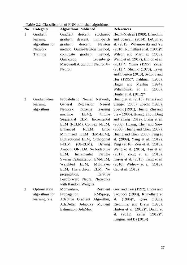
27

Table 2.2. Classification of FNN published algorithms

No. Category Algorithms Published References

1 Gradient

learning

algorithms for

Network

Training

Gradient descent, stochastic

gradient descent, mini-batch

gradient descent, Newton

method, Quasi-Newton method,

conjugate gradient method,

Quickprop, Levenberg-

Marquardt Algorithm, Neuron by

Neuron

Hecht-Nielsen (1989), Bianchini

and Scarselli (2014), LeCun et

al. (2015), Wilamowski and Yu

(2010), Rumelhart et al. (1986)*,

Wilson and Martinez (2003),

Wang et al. (2017), Hinton et al.

(2012)*, Ypma (1995), Zeiler

(2012)*, Shanno (1970), Lewis

and Overton (2013), Setiono and

Hui (1995)*, Fahlman (1988),

Hagan and Menhaj (1994),

Wilamowski et al. (2008),

Hunter et al. (2012)*

2 Gradient-free

learning

algorithms

Probabilistic Neural Network,

General Regression Neural

Network, Extreme learning

machine (ELM), Online

Sequential ELM, Incremental

ELM (I-ELM), Convex I-ELM,

Enhanced I-ELM, Error

Minimized ELM (EM-ELM),

Bidirectional ELM, Orthogonal

I-ELM (OI-ELM), Driving

Amount OI-ELM, Self-adaptive

ELM, Incremental Particle

Swarm Optimization EM-ELM,

Weighted ELM, Multilayer

ELM, Hierarchical ELM, No

propagation, Iterative

Feedforward Neural Networks

with Random Weights

Huang et al. (2015), Ferrari and

Stengel (2005), Specht (1990),

Specht (1991), Huang, Zhu and

Siew (2006), Huang, Zhou, Ding

and Zhang (2012), Liang et al.

(2006), Huang, Chen and Siew

(2006), Huang and Chen (2007),

Huang and Chen (2008), Feng et

al. (2009), Yang et al. (2012),

Ying (2016), Zou et al. (2018),

Wang et al. (2016), Han et al.

(2017), Zong et al. (2013),

Kasun et al. (2013), Tang et al.

(2016), Widrow et al. (2013),

Cao et al. (2016)

3 Optimization

algorithms for

learning rate

Momentum, Resilient

Propagation, RMSprop,

Adaptive Gradient Algorithm,

AdaDelta, Adaptive Moment

Estimation, AdaMax

Gori and Tesi (1992), Lucas and

Saccucci (1990), Rumelhart et

al. (1986)*, Qian (1999),

Riedmiller and Braun (1993),

Hinton et al. (2012)*, Duchi et

al. (2011), Zeiler (2012)*,

Kingma and Ba (2014)

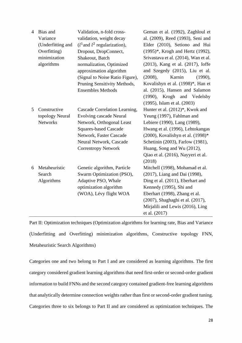
28

Part II: Optimization techniques (Optimization algorithms for learning rate, Bias and Variance

(Underfitting and Overfitting) minimization algorithms, Constructive topology FNN,

Metaheuristic Search Algorithms)

Categories one and two belong to Part I and are considered as learning algorithms. The first

category considered gradient learning algorithms that need first-order or second-order gradient

information to build FNNs and the second category contained gradient-free learning algorithms

that analytically determine connection weights rather than first or second-order gradient tuning.

Categories three to six belongs to Part II and are considered as optimization techniques. The

4 Bias and

Variance

(Underfitting and

Overfitting)

minimization

algorithms

Validation, n-fold cross-

validation, weight decay

(𝑙1and 𝑙2 regularization),

Dropout, DropConnect,

Shakeout, Batch

normalization, Optimized

approximation algorithm

(Signal to Noise Ratio Figure),

Pruning Sensitivity Methods,

Ensembles Methods

Geman et al. (1992), Zaghloul et

al. (2009), Reed (1993), Seni and

Elder (2010), Setiono and Hui

(1995)*, Krogh and Hertz (1992),

Srivastava et al. (2014), Wan et al.

(2013), Kang et al. (2017), Ioffe

and Szegedy (2015), Liu et al.

(2008), Karnin (1990),

Kovalishyn et al. (1998)*, Han et

al. (2015), Hansen and Salamon

(1990), Krogh and Vedelsby

(1995), Islam et al. (2003)

5 Constructive

topology Neural

Networks

Cascade Correlation Learning,

Evolving cascade Neural

Network, Orthogonal Least

Squares-based Cascade

Network, Faster Cascade

Neural Network, Cascade

Correntropy Network

Hunter et al. (2012)*, Kwok and

Yeung (1997), Fahlman and

Lebiere (1990), Lang (1989),

Hwang et al. (1996), Lehtokangas

(2000), Kovalishyn et al. (1998)*

Schetinin (2003), Farlow (1981),

Huang, Song and Wu (2012),

Qiao et al. (2016), Nayyeri et al.

(2018)

6 Metaheuristic

Search

Algorithms

Genetic algorithm, Particle

Swarm Optimization (PSO),

Adaptive PSO, Whale

optimization algorithm

(WOA), Lévy flight WOA

Mitchell (1998), Mohamad et al.

(2017), Liang and Dai (1998),

Ding et al. (2011), Eberhart and

Kennedy (1995), Shi and

Eberhart (1998), Zhang et al.

(2007), Shaghaghi et al. (2017),

Mirjalili and Lewis (2016), Ling

et al. (2017)

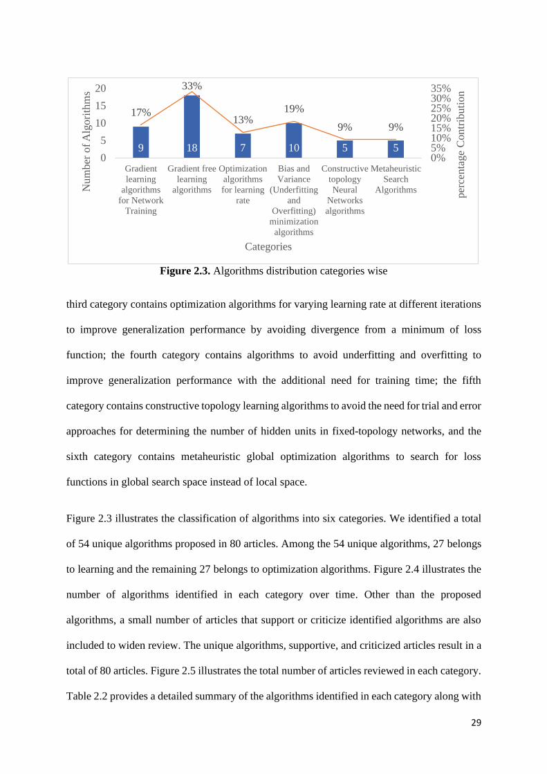
29

third category contains optimization algorithms for varying learning rate at different iterations

to improve generalization performance by avoiding divergence from a minimum of loss

function; the fourth category contains algorithms to avoid underfitting and overfitting to

improve generalization performance with the additional need for training time; the fifth

category contains constructive topology learning algorithms to avoid the need for trial and error

approaches for determining the number of hidden units in fixed-topology networks, and the

sixth category contains metaheuristic global optimization algorithms to search for loss

functions in global search space instead of local space.

Figure 2.3 illustrates the classification of algorithms into six categories. We identified a total

of 54 unique algorithms proposed in 80 articles. Among the 54 unique algorithms, 27 belongs

to learning and the remaining 27 belongs to optimization algorithms. Figure 2.4 illustrates the

number of algorithms identified in each category over time. Other than the proposed

algorithms, a small number of articles that support or criticize identified algorithms are also

included to widen review. The unique algorithms, supportive, and criticized articles result in a

total of 80 articles. Figure 2.5 illustrates the total number of articles reviewed in each category.

Table 2.2 provides a detailed summary of the algorithms identified in each category along with

Figure 2.3. Algorithms distribution categories wise

9 18 7 10 5 5

17%

33%

13%19%

9% 9%

0%5%10%15%20%25%30%35%

0

5

10

15

20

Gradient

learning

algorithms

for Network

Training

Gradient free

learning

algorithms

Optimization

algorithms

for learning

rate

Bias and

Variance

(Underfitting

and

Overfitting)

minimization

algorithms

Constructive

topology

Neural

Networks

algorithms

Metaheuristic

Search

Algorithms

per

centa

ge

Con

trib

uti

on

Num

ber

of

Alg

ori

thm

s

Categories

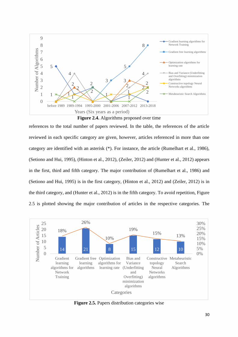
30

references to the total number of papers reviewed. In the table, the references of the article

reviewed in each specific category are given, however, articles referenced in more than one

category are identified with an asterisk (*). For instance, the article (Rumelhart et al., 1986),

(Setiono and Hui, 1995), (Hinton et al., 2012), (Zeiler, 2012) and (Hunter et al., 2012) appears

in the first, third and fifth category. The major contribution of (Rumelhart et al., 1986) and

(Setiono and Hui, 1995) is in the first category, (Hinton et al., 2012) and (Zeiler, 2012) is in

the third category, and (Hunter et al., 2012) is in the fifth category. To avoid repetition, Figure

2.5 is plotted showing the major contribution of articles in the respective categories. The

Figure 2.4. Algorithms proposed over time

5

12

1

23

5

8

2

3

2

4

2

4

11

1 21

2 2

0

1

2

3

4

5

6

7

8

9

before 1989 1989-1994 1995-2000 2001-2006 2007-2012 2013-2018

Num

ber

of

Alg

ori

thm

s

Years (Six years as a period)

Gradient learning algorithms for

Network Training

Gradient free learning algorithms

Optimization algorithms for

learning rate

Bias and Variance (Underfitting

and Overfitting) minimization

algorithms

Constructive topology Neural

Networks algorithms

Metaheuristic Search Algorithms

Figure 2.5. Papers distribution categories wise

14 21 8 15 12 10

18%

26%

10%

19%15%

13%

0%5%10%15%20%25%30%

0

5

10

15

20

25

Gradient

learning

algorithms for

Network

Training

Gradient free

learning

algorithms

Optimization

algorithms for

learning rate

Bias and

Variance

(Underfitting

and

Overfitting)

minimization

algorithms

Constructive

topology

Neural

Networks

algorithms

Metaheuristic

Search

Algorithms

Num

ber

of

Art

icle

s

Categories

31

distribution in Figures 2.3-2.5 and content in Table 2.2 shows the researchers interest and trend

in specific categories. The distribution and content explain that the research directions are

changing from complex gradient-based algorithms to gradient-free algorithms, fixed topology

to constructive topology, hyperparameter initial guess work to analytically calculation, and

converging algorithms at a global minimum rather than the local minimum. In another sense,

the categories may be considered as an opportunity for discovering research gaps and further

improvement can bring a significant contribution.

2.2.2 FNN: An overview

FNN is a parallel information processing structure consisting of a processing element known

as neurons (hidden units), interconnected together with unidirectional distributed channels

known as connections. Each processing neuron receives an incoming connection from all input

features, sum and activate it using nonlinear activation function, and branch it to as many

connections as desired. The processing neuron output which can be of any mathematical type

depends upon input features with its weighted sum and activation function (Hecht-Nielsen,

1989). The FNN concept originated by motiving from the human brain neuron functioning

system. The human brain has approximately 100 billion neurons that communicate through

thousands of electro-chemical connections and send signals to other neurons if the sum of

connections exceeds a certain threshold. The number of hidden layers in FNN determines its

architecture. The input layer consisting of input features 𝑥 with an added bias 𝑏𝑢 are connected

to the hidden layers ℎ through the input connection weights 𝑤𝑖𝑐𝑤. The hidden layer sums the

product (𝑤𝑖𝑐𝑤𝑥) and squash it through the nonlinear activation function 𝑓ℎ𝑢(𝑧). The hidden

layer with an added bias 𝑏𝑜 and the output layer are connected by the output connection weights

𝑤𝑜𝑐𝑤. The output layer sums the product (𝑤𝑜𝑐𝑤𝑓ℎ𝑢(𝑧)) and squash it through the nonlinear

activation function 𝑓𝑜𝑢(𝑧) to estimate output vector �̂�. The values of �̂� at the output layer are

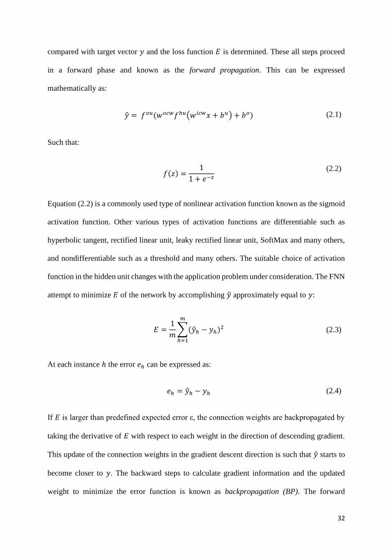
32

compared with target vector 𝑦 and the loss function 𝐸 is determined. These all steps proceed

in a forward phase and known as the forward propagation. This can be expressed

mathematically as:

�̂� = 𝑓𝑜𝑢(𝑤𝑜𝑐𝑤𝑓ℎ𝑢(𝑤𝑖𝑐𝑤𝑥 + 𝑏𝑢) + 𝑏𝑜) (2.1)

Such that:

𝑓(𝑧) =

1

1 + 𝑒−𝑧

(2.2)

Equation (2.2) is a commonly used type of nonlinear activation function known as the sigmoid

activation function. Other various types of activation functions are differentiable such as

hyperbolic tangent, rectified linear unit, leaky rectified linear unit, SoftMax and many others,

and nondifferentiable such as a threshold and many others. The suitable choice of activation

function in the hidden unit changes with the application problem under consideration. The FNN

attempt to minimize 𝐸 of the network by accomplishing �̂� approximately equal to 𝑦:

𝐸 =1

𝑚∑(�̂�ℎ − 𝑦ℎ)

2

𝑚

ℎ=1

(2.3)

At each instance ℎ the error 𝑒ℎ can be expressed as:

𝑒ℎ = �̂�ℎ − 𝑦ℎ (2.4)

If 𝐸 is larger than predefined expected error ε, the connection weights are backpropagated by

taking the derivative of 𝐸 with respect to each weight in the direction of descending gradient.

This update of the connection weights in the gradient descent direction is such that �̂� starts to

become closer to 𝑦. The backward steps to calculate gradient information and the updated

weight to minimize the error function is known as backpropagation (BP). The forward

33

propagation and backpropagation complete one iteration 𝑖 and are known as FNN training.

After each iteration, the error function 𝐸𝑖 is recalculated and compared with 𝐸𝑖−1. If 𝑖 reaches

to its predefined maximum limit or 𝐸𝑖 converges/starts increasing the training is stopped, else

it is continued. The training of FNN is influenced by several reasons as highlighted in the

introduction section and may be overcome by various experimental trial and error works with

appropriate learning algorithms and optimization techniques for fast and efficient convergence.

2.2.3 Learning algorithms and applications

In this section, the authors made an effort to explain FNN learning algorithms merits and

technical limitations in order to understand the FNN drawbacks and needed user expertise, so

as to identify research gaps and future directions. The proposed algorithms in the selected

literature were reviewed to understand the inspiration, research gaps, merits, limitations, and

application areas. In current practice, a single algorithm in FNN is not sufficient for all types

of applications. There is always a trade-off between network generalization performance and

learning speed. Some algorithms have the advantage of being more efficient than others but

may be constrained by memory requirements, complex architecture, and/or more learning time.

Since the early FNN development, many improvements have been made and many of them are

mentioned below:

2.2.3.1 Gradient learning algorithms for network training

The first category is the learning algorithms proposed based on the BP gradient information

concept, which is considered the reason for creating significant interest in the FNN topic. The

BP gradient learning algorithms can be further subcategorized into two types: first-order and

second-order. The first-order gradient trains the FNN by calculating the gradient information

and updated weight to reach a minimum of a loss function. The first-order derivative of the

34

error with respect to weight is calculated at the output layer at each iteration and is distributed

back to the whole network. However, the first order BP is considered slow because of the

computation of the first-order gradient information at each iteration. This increases the learning

time and possibility of the algorithm to be stuck in a local minimum. Researchers made efforts

to improve the learning speed by incorporating second-order gradient information to reach the

loss function faster. Wilamowski and Yu (2010) explained that first-order learning methods

might need an excessive number of hidden units and iterations for convergence which can

reduce the generalization performance for unseen data. Whereas second-order learning

algorithms are powerful in learning, but the complexity increases with increasing network size.

A lot of computational memory is needed to store the Jacobian 𝐉 and Hessian Matrix 𝐇𝐧 along

with their inverses, which can make it difficult for large training datasets.

a) First-order gradient algorithms

The popular and well known first-order learning algorithms among the BP family class is

Gradient descent (GD). It backpropagates the error with respect to connection weights 𝑤

through layers to minimize a loss function 𝐸 until it converges to minimal error (Rumelhart et

al., 1986) :

∇𝐸 =𝜕𝐸

𝜕𝑤𝑖=

𝜕𝐸

𝜕𝑜𝑢𝑡𝑖

𝜕𝑜𝑢𝑡𝑖𝜕𝑛𝑒𝑡𝑖

𝜕𝑛𝑒𝑡𝑖𝜕𝑤𝑖

(2.5)

where ∇𝐸 is a partial derivative of the error with respect to weight 𝑤, 𝑜𝑢𝑡𝑖 is the activation

output and 𝑛𝑒𝑡𝑖 is the weighted sum of inputs of the hidden unit. The updated weight 𝑤𝑖+1

needed for the next iteration can be expressed as:

𝑤𝑖+1 = 𝑤𝑖−∝ ∇𝐸 (2.6)

35

where ∝ is a learning rate hyperparameter. For the sake of simplicity in this study, the

connection weights 𝑤 in the equations refer to all types of connection weights in the network,

unless otherwise specified. The GD convergence is considered to be slow because the loss

function is computed based on the whole training dataset. An increase in data size makes it

slower and more time consuming for large application datasets (Wilson and Martinez, 2003).

Therefore, an improved form of GD known as Stochastic GD (SGD) was proposed to compute

the gradient on each training data instance. If the loss function is convex, it converges faster

than GD to a global minimum, otherwise, a local minimum is guaranteed (Wang et al., 2017).

The issue with SGD is that its convergence is not smooth compared to GD and overshoots

during training on some iterations, which may be controlled to some extent by adjustment of

learning rate. The drawbacks of both GD and SGD can be overcome by Mini Batch GD that

takes equal size mini-batches 𝑁 of training data instead of whole training data or single training

instance. Mini batch SD is more favorable due to its hybrid characteristics: a stable and better

convergence rate (Hinton et al., 2012).

For GD:

𝑤𝑖+1 = 𝑤𝑖−∝ ∇𝐸, (𝑥, 𝑎) (2.7)

For SGD:

𝑤𝑖+1 = 𝑤𝑖−∝ ∇𝐸, (𝑥ℎ, 𝑎ℎ) (2.8)

For Mini batch GD:

𝑤𝑖+1 = 𝑤𝑖−∝ ∇𝐸, (𝑥ℎ:ℎ+𝑁 , 𝑎ℎ:ℎ+𝑁) (2.9)

36

The drawbacks of first-order GD and its variant algorithms (SGD and Mini batch GD) are that

the number of iterations comparatively increases which makes them far slower and liable to be

stuck at a local minimum.

b) Second-order gradient algorithms

The convergence problem of the first-order gradient was improved by applying the second-

order form. The Newton method (NM), a second-order derivative, was proposed to increase the

convergence by modifying GD to the second-order Hessian inverse matrix 𝐇𝐧−𝟏 along with

the first-order ∇𝐸 to take larger steps towards the minimum of an objective function (Ypma,

1995):

𝑤𝑖+1 = 𝑤𝑖−∝ 𝐇𝐧−𝟏∇𝐸 (2.10)

NM makes use of the second-order 𝐇𝐧 and its inverse 𝐇𝐧−𝟏 to minimize the loss function

which makes it computationally expensive and unfeasible for real large model applications

(Zeiler, 2012). The small networks with fewer parameters may be trained with NM to take

advantage of the better convergence speed compared to GD. The Quasi-Newton method (quasi

NM) was proposed to address the drawback of NM and simplified by approximating the inverse

of the 𝐇𝐧 from the first order derivative. It updates the approximated 𝐇𝐧 and its inverse 𝐇𝐧−𝟏

after each iteration which makes it computationally less expensive compared to NM (Shanno,

1970). Among several techniques Broyden–Fletcher–Goldfarb–Shanno (BFGS) has gained

much popularity in applications (Lewis and Overton, 2013). It computes 𝐇𝐧 and 𝐇𝐧−𝟏

expressed as:

𝐇𝐧𝐢+𝟏 = 𝐇𝐧𝐢 +𝑜𝑖𝑜𝑖

𝑇

𝑜𝑖𝑇𝜎𝑖

−𝐇𝐧𝐢𝜎𝑖𝜎𝑖

𝑇𝐇𝐧𝐢𝑻

𝜎𝑖𝑇𝐇𝐧𝐢𝜎𝑖

(2.11)

Similarly, it's inverse 𝐇𝐧−𝟏can be calculated from the Sherman-Morrison formula:

37

𝐇𝐧𝐢+𝟏−𝟏 = (𝐼 −

𝜎𝑖𝑜𝑖𝑇

𝑜𝑖𝑇𝜎𝑖)𝐇𝐧𝐢

−𝟏 (𝐼 −𝑜𝑖𝜎𝑖

𝑇

𝑜𝑖𝑇𝜎𝑖) +

𝜎𝑖𝜎𝑖𝑇

𝑜𝑖𝑇𝜎𝑖

(2.12)

Such that:

𝑜𝑖 = ∇𝐸𝑖+1 − ∇𝐸𝑖 (2.13)

𝜎𝑖 = 𝑤𝑖+1 − 𝑤𝑖 (2.14)

𝑤𝑖+1 = 𝑤𝑖+∝ 𝑑𝑖 (2.15)

𝑑𝑖 = −𝐇𝐧𝐢−𝟏∇𝐸𝑖 (2.16)

The algorithm is initialized by the initial value of 𝑤0 and 𝐇𝐧0. Mostly, 𝐇𝐧0 is initially given

the value of the identity matrix 𝐇𝐧0 = 𝐼. The algorithm first computes the position 𝑑0, as

shown in Equation (2.16), from the initial inverse 𝐇𝐧𝟎−𝟏 and ∇𝐸0, then determines new weights,

as shown in Equation (2.15), based on optimal step size ∝. The change in weights 𝜎𝑖, as shown

in Equation (2.14), and change in the first-order derivative 𝑜𝑖, as shown in Equation (2.13), are

used to approximate 𝐇𝐧 and its inverse 𝐇𝐧−𝟏, as shown in Equation (2.11) and (2.12),

respectively. This algorithm continues until 𝑤𝑖 converges. The quasi NM is more efficient than

the NM but requires computational memory which limits its applicability to medium-sized

problems. To overcome the memory problem and contribute to improving the convergence rate

(Setiono and Hui, 1995), a conjugate gradient method (CG) was proposed. For a conjugate, the

gradient of the two vectors needs to be orthogonal to reach a minimum of the cost function. If

not orthogonal, it means the second vector needs to travel along the previous vector to be nearer

to a minimum point. Mostly, in GD, it takes slightly larger steps and deviates from the minimal

point. The objective of conjugate gradient descent is to take a step along the gradient so that

38

the next gradient vector should be orthogonal and nearer to zero error. The first orthogonal

vector 𝑑0 can be computed from the initial guess such that:

𝑑0 = ∇𝐸0 (2.17)

The next orthogonal vector 𝑑𝑖+1 can be expressed as:

𝑑𝑖+1 = ∇𝐸𝑖+1 + 𝛽𝑑𝑖 (2.18)

where 𝛽 is used to calculate new orthogonal vector direction and is known as a conjugate

hyperparameter. The weights are updated as per below rule:

𝑤𝑖+1 = 𝑤𝑖+∝ 𝑑𝑖 (2.19)

The conjugate gradient descent iteratively finds the best orthogonal gradient vector based on

the previous vector with an inner product equal to zero and then updates the weight parameters.

The advantage of CG over GD is that it converges faster but compared to other methods such

as quasi NM and Levenberg Marquardt (LM), its convergence rate is lower. In terms of

memory, due to its second-order, it needs more memory as compared to GD and less memory

compared to quasi NM and LM (Hagan and Menhaj, 1994). To overcome the problem of both

GD slow convergence and second-order gradient algorithms memory, Quickprop (QP) was

proposed. QP is a second-order iterative learning algorithm based on Newton’s method used

to find a minimum of the loss function. The purpose of QP development was to speed up the

convergence process by taking much larger steps to reach a minimum of the loss function rather

than GD infinitesimal small steps in the weight space (Fahlman, 1988). The algorithm proceeds

like GD, but for each weight, it keeps a copy of ∇𝐸𝑖−1and ∆𝑤𝑖−1:

∆𝑤𝑖 =∇𝐸𝑖

∇𝐸𝑖−1 − ∇𝐸𝑖∆𝑤𝑖−1 (2.20)

39

It shows that error vs. weight can be approximated by an upward parabola and change in the

slope of the error curve by each weight is not affected by all the other weights that are changing

at the same time. For each weight, it computes the gradient change and weight changes to

determine the parabola: and rapidly jumps to a minimum of this parabola.

To make learning faster, the Levenberg-Marquardt Algorithm (LM) was proposed by

combining both Gauss-Newton (GN) and GD to compute the best gradient direction. It is a

method to solve nonlinear least-squares problems to minimize the sum of the squared error

(Hagan and Menhaj, 1994). Instead of directly computing the 𝐇𝐧 it works with gradient vector

and 𝐉. The gradient vector ∇𝐸 of the loss function can be computed as:

∇𝐸 = 2𝐉𝑇𝑒 (2.21)

The 𝐇𝐧 can be approximated from the equation below:

∇2𝐸 = 𝐇𝐧 = 2𝐉𝑇𝐉 (2.22)

The weight parameter improvement process in LM is iterative such as:

∆𝑤𝑖 = [𝐉𝑇𝐉 + 𝜇𝐼]−1𝐉𝑇𝑒 (2.23)

where 𝐼 is an identity matrix and 𝜇 is damping hyperparameter factor. The 𝜇 is adjusted in each

iteration to create a balance between the GN and GD methods. If the objective function

achievement is fast, 𝜇 is divided by some factor to bring the algorithm closer to GN and if

objective function achievement is slow in each iteration, 𝜇 is multiplied by some factor so as

to move towards GD. In many applications, LM is very fast and converges to the local

minimum rapidly, which may not be the global minimum. The LM has the disadvantage that it

cannot be used with other loss functions such as cross-entropy and cannot be applied to

constructive types of neural networks (Hunter et al., 2012). The 𝐉 becomes large and needs a

40

lot of memory with an increase in network size, limiting its application in a large dataset.

Therefore the learning speed of LM is less evident compared to GD when the network size

increases (Wilamowski and Yu, 2010). The LM limits its application to a fixed topology neural

network. Therefore, Neuron by Neuron (NBN) was proposed to compute the gradient vector

and the 𝐉 for arbitrarily constructive neural networks. Wilamowski et al. (2008) highlighted

that several improvements have been proposed in second-order learning algorithms, but much

better results can be achieved from Newton and LM methods. The NBN was proposed to

simplify the Jacobian calculation and make it workable for constructive algorithms. The

Jacobian is expressed in a square matrix of the first-order partial derivative:

𝐉 =𝜕𝑒

𝜕𝑤 (2.24)

NBN calculates the Jacobian in gradient vector form instead of the matrix by performing: 1)

Forward computation, 2) Backward computation, and finally, 3) Calculating the Jacobian

elements. In the forward computation, the inputs are processed to get the neuron output, which

is further processed to get the target output. During forward computation, the value of the slope

of the neuron activation function is stored for the backward stage. In the backward step, the

Jacobian element is computed by multiplying the neuron delta with its slope and input weights.

Finally, instead of using the 𝐉 to store values, they are summed into a gradient vector:

∇𝐸 =𝜕𝑒

𝜕𝑤𝑒 (2.25)

This enables NBN to be used with the constructive algorithm but with the additional cost of

more memory requirement compared to LM. Hunter et al. (2012) argued that NBN is not

perfect, but it can compete with other similar algorithms. Their experimental work showed that

NBN achieved much better results than GD and almost similar results to LM.

41

c) Application of Gradient Learning Algorithms

Various applications of gradient learning algorithms are explained and listed in Appendix A.

2.2.3.2 Gradient free algorithms

The gradient learning algorithms randomly assign connection weights to the network and

iteratively tune them to get the optimal weight for a network with better error minimization

capability. The disadvantages associated with gradient learning algorithms are that they require

user expertise to build an optimal FNN. A better choice of hyperparameters such as learning

rate, momentum, regularization, and initial weight may improve the convergence but needs a

lot of trial and error approach to get the best possible parameters. This may cause gradient

learning algorithms to trap the FNN at a local minimum which may be far away from the global

minimum and may affect the generalization performance. In terms of convergence rate, it can

be increased by assigning a large learning rate, however, the algorithm will become unstable,

whereas for a low learning rate it may converge slowly and may take even hours, days, or

months to solve a large dataset with complex patterns.

Researchers made an extensive effort to improve the gradient learning algorithms. Huang et al.

(2015) comment that improvement in gradient learning leads to faster learning speed and better

generalization performance, but still most of them cannot guarantee a global solution.

Researchers proposed that the issues associated with gradient learning algorithms can be fixed

in a state-of-the-art way by learning FNN without gradient learning algorithms, known as

gradient-free learning in the forward steps. The gradient-free algorithms eliminate the need for

chain delta rule to calculate the derivative of the loss function with respect to each weight and

updating them for the next iteration. Some of the advantages of gradient-free algorithms are:

1) They are simple, fast, and do not need complex hyperparameter adjustments, 2) no need for

42

backpropagating error, and 3) can work directly with both differentiable and non-differentiable

activation functions (Ferrari and Stengel, 2005). The gradient-free algorithms are useful in that

they reduce training time significantly, however, a drawback is that it increases network

complexity. The number of hidden unit’s generation increases many times which may cause

overfitting. The following are popular algorithms that eliminate the use of gradient information.

a) Probability and General Regression

Probabilistic Neural Network (PNN) was proposed for classification problems (Specht, 1990),

and, General Regression Neural Network (GRNN) for regression problems (Specht, 1991).

Both algorithms were proposed to address the slowness of the backpropagation FNN (BPNN)

by doing one pass learning. They are similar in structure and do not need iterative tuning and

work in a highly parallel structure. PNN finds the decision boundaries between pattern, whereas

GRNN estimates the continuous dependent variable. The network architecture consists of four

layers: input, pattern, summation, and output. The output layer can be expressed as:

�̂�ℎ =∑𝑦ℎ 𝑒

−(𝑑ℎ2

2𝜎2)

∑𝑒−(𝑑ℎ2

2𝜎2)

(2.26)

where 𝑑ℎ2 is Euclidean distance and 𝑒

−(𝑑ℎ2

2𝜎2) is the activation function. The best value of kernel

𝜎 is estimated by a holdout or validation method. PNN and GRNN are considered faster than

the BPNN and learn in one pass, which means the forward direction. The major drawback is

that it requires more memory space compared to BPNN and separate algorithms are built for

classification and regression problems.

b) Extreme Learning Machine

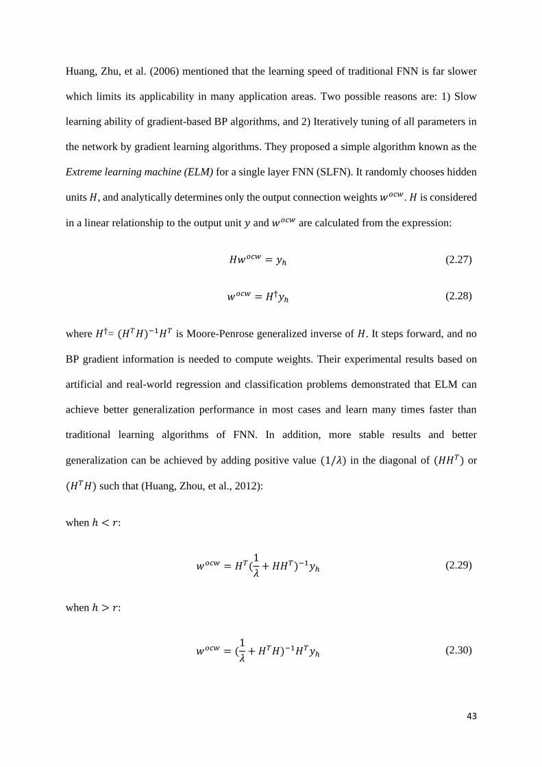
43

Huang, Zhu, et al. (2006) mentioned that the learning speed of traditional FNN is far slower

which limits its applicability in many application areas. Two possible reasons are: 1) Slow

learning ability of gradient-based BP algorithms, and 2) Iteratively tuning of all parameters in

the network by gradient learning algorithms. They proposed a simple algorithm known as the

Extreme learning machine (ELM) for a single layer FNN (SLFN). It randomly chooses hidden

units 𝐻, and analytically determines only the output connection weights 𝑤𝑜𝑐𝑤. 𝐻 is considered

in a linear relationship to the output unit 𝑦 and 𝑤𝑜𝑐𝑤 are calculated from the expression:

𝐻𝑤𝑜𝑐𝑤 = 𝑦ℎ (2.27)

𝑤𝑜𝑐𝑤 = 𝐻ϯ𝑦ℎ (2.28)

where 𝐻ϯ= (𝐻𝑇𝐻)−1𝐻𝑇 is Moore-Penrose generalized inverse of 𝐻. It steps forward, and no

BP gradient information is needed to compute weights. Their experimental results based on

artificial and real-world regression and classification problems demonstrated that ELM can

achieve better generalization performance in most cases and learn many times faster than

traditional learning algorithms of FNN. In addition, more stable results and better

generalization can be achieved by adding positive value (1/𝜆) in the diagonal of (𝐻𝐻𝑇) or

(𝐻𝑇𝐻) such that (Huang, Zhou, et al., 2012):

when ℎ < 𝑟:

𝑤𝑜𝑐𝑤 = 𝐻𝑇(1

𝜆+ 𝐻𝐻𝑇)−1𝑦ℎ (2.29)

when ℎ > 𝑟:

𝑤𝑜𝑐𝑤 = (1

𝜆+ 𝐻𝑇𝐻)−1𝐻𝑇𝑦ℎ (2.30)

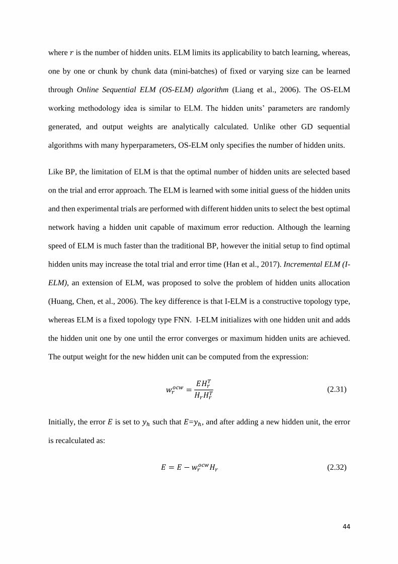
44

where 𝑟 is the number of hidden units. ELM limits its applicability to batch learning, whereas,

one by one or chunk by chunk data (mini-batches) of fixed or varying size can be learned

through Online Sequential ELM (OS-ELM) algorithm (Liang et al., 2006). The OS-ELM

working methodology idea is similar to ELM. The hidden units’ parameters are randomly

generated, and output weights are analytically calculated. Unlike other GD sequential

algorithms with many hyperparameters, OS-ELM only specifies the number of hidden units.

Like BP, the limitation of ELM is that the optimal number of hidden units are selected based

on the trial and error approach. The ELM is learned with some initial guess of the hidden units

and then experimental trials are performed with different hidden units to select the best optimal

network having a hidden unit capable of maximum error reduction. Although the learning

speed of ELM is much faster than the traditional BP, however the initial setup to find optimal

hidden units may increase the total trial and error time (Han et al., 2017). Incremental ELM (I-

ELM), an extension of ELM, was proposed to solve the problem of hidden units allocation

(Huang, Chen, et al., 2006). The key difference is that I-ELM is a constructive topology type,

whereas ELM is a fixed topology type FNN. I-ELM initializes with one hidden unit and adds

the hidden unit one by one until the error converges or maximum hidden units are achieved.

The output weight for the new hidden unit can be computed from the expression:

𝑤𝑟𝑜𝑐𝑤 =

𝐸𝐻𝑟𝑇

𝐻𝑟𝐻𝑟𝑇 (2.31)

Initially, the error 𝐸 is set to 𝑦ℎ such that 𝐸=𝑦ℎ, and after adding a new hidden unit, the error

is recalculated as:

𝐸 = 𝐸 − 𝑤𝑟𝑜𝑐𝑤𝐻𝑟 (2.32)

45

Adding hidden units one by one results in redundant hidden units in I-ELM which will make

network size large and complex. Some of the hidden unit’s contribution to error reduction

might be very low and can be omitted. Efforts were made to compact the I-ELM network size

without losing generalization accuracy. Convex I-ELM (CI-ELM) was proposed to recalculate

the 𝑤𝑜𝑐𝑤 based on Barron’s convex optimization technique to improve the convergence rate

of I-ELM (Huang and Chen, 2007). In CI-ELM, 𝑤𝑟𝑜𝑐𝑤 for the randomly generated hidden unit

is calculated as:

𝑤𝑟𝑜𝑐𝑤 =

𝐸. [𝐸 − (𝐹 − 𝐻𝑟]𝑇

[𝐸 − (𝐹 − 𝐻𝑟]. [𝐸 − (𝐹 − 𝐻𝑟]𝑇 (2.33)

where 𝐹 = 𝑦 is the target vector. It recalculates the 𝑤𝑜𝑐𝑤 of all existing hidden units if 𝑟 > 1,

and error as expressed below:

𝑤𝑖𝑜𝑐𝑤 = (1 − 𝑤𝑟

𝑜𝑐𝑤)𝑤𝑖𝑜𝑐𝑤 (2.34)

𝐸 = (1 − 𝑤𝑟𝑜𝑐𝑤)𝐸 − 𝑤𝑟

𝑜𝑐𝑤(𝐹 − 𝐻𝑟) (2.35)

CI-ELM can converge faster with more compact architecture while maintaining I-ELM

simplicity and efficiency. Similarly, Enhanced I-ELM (EI-ELM) was proposed to compact I-

ELM by adding some sets of candidate units and selecting a candidate unit as a hidden unit

having a maximum capability of error reduction (Huang and Chen, 2008). The hidden unit

addition in I-ELM might take it nearer or farther away from the loss function. The hidden units

farther away from the loss function may not contribute to error reduction and can be omitted.

The EI-ELM adds some candidate units and one nearer to the loss function is selected as a new

hidden unit and added to the network. In such a case, the number of hidden units in EI-ELM

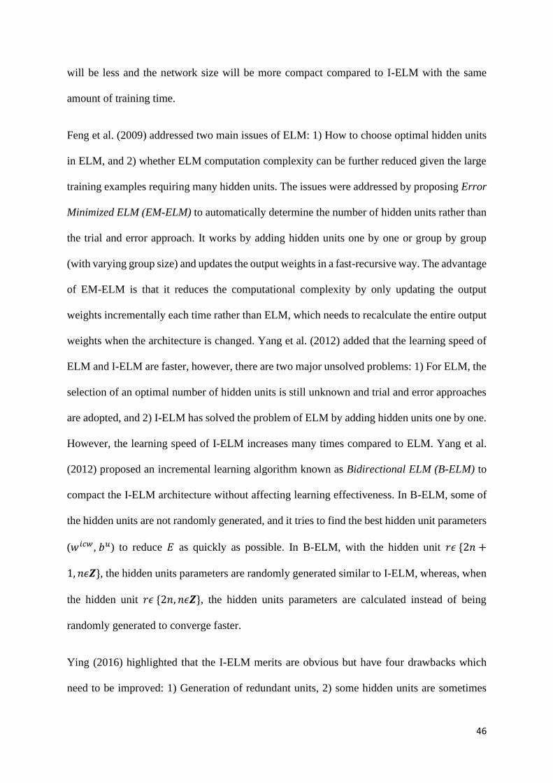
46

will be less and the network size will be more compact compared to I-ELM with the same

amount of training time.

Feng et al. (2009) addressed two main issues of ELM: 1) How to choose optimal hidden units

in ELM, and 2) whether ELM computation complexity can be further reduced given the large

training examples requiring many hidden units. The issues were addressed by proposing Error

Minimized ELM (EM-ELM) to automatically determine the number of hidden units rather than

the trial and error approach. It works by adding hidden units one by one or group by group

(with varying group size) and updates the output weights in a fast-recursive way. The advantage

of EM-ELM is that it reduces the computational complexity by only updating the output

weights incrementally each time rather than ELM, which needs to recalculate the entire output

weights when the architecture is changed. Yang et al. (2012) added that the learning speed of

ELM and I-ELM are faster, however, there are two major unsolved problems: 1) For ELM, the

selection of an optimal number of hidden units is still unknown and trial and error approaches

are adopted, and 2) I-ELM has solved the problem of ELM by adding hidden units one by one.

However, the learning speed of I-ELM increases many times compared to ELM. Yang et al.

(2012) proposed an incremental learning algorithm known as Bidirectional ELM (B-ELM) to

compact the I-ELM architecture without affecting learning effectiveness. In B-ELM, some of

the hidden units are not randomly generated, and it tries to find the best hidden unit parameters

(𝑤𝑖𝑐𝑤, 𝑏𝑢) to reduce 𝐸 as quickly as possible. In B-ELM, with the hidden unit 𝑟𝜖 {2𝑛 +

1, 𝑛𝜖𝒁}, the hidden units parameters are randomly generated similar to I-ELM, whereas, when

the hidden unit 𝑟𝜖 {2𝑛, 𝑛𝜖𝒁}, the hidden units parameters are calculated instead of being

randomly generated to converge faster.

Ying (2016) highlighted that the I-ELM merits are obvious but have four drawbacks which

need to be improved: 1) Generation of redundant units, 2) some hidden units are sometimes

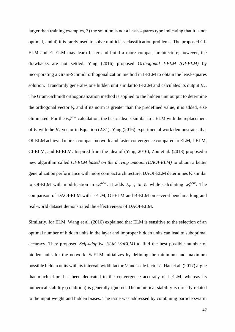
47

larger than training examples, 3) the solution is not a least-squares type indicating that it is not

optimal, and 4) it is rarely used to solve multiclass classification problems. The proposed CI-

ELM and EI-ELM may learn faster and build a more compact architecture; however, the

drawbacks are not settled. Ying (2016) proposed Orthogonal I-ELM (OI-ELM) by

incorporating a Gram-Schmidt orthogonalization method in I-ELM to obtain the least-squares

solution. It randomly generates one hidden unit similar to I-ELM and calculates its output 𝐻𝑟.

The Gram-Schmidt orthogonalization method is applied to the hidden unit output to determine

the orthogonal vector 𝑉𝑟 and if its norm is greater than the predefined value, it is added, else

eliminated. For the 𝑤𝑟𝑜𝑐𝑤 calculation, the basic idea is similar to I-ELM with the replacement

of 𝑉𝑟 with the 𝐻𝑟 vector in Equation (2.31). Ying (2016) experimental work demonstrates that

OI-ELM achieved more a compact network and faster convergence compared to ELM, I-ELM,

CI-ELM, and EI-ELM. Inspired from the idea of (Ying, 2016), Zou et al. (2018) proposed a

new algorithm called OI-ELM based on the driving amount (DAOI-ELM) to obtain a better

generalization performance with more compact architecture. DAOI-ELM determines 𝑉𝑟 similar

to OI-ELM with modification in 𝑤𝑟𝑜𝑐𝑤. It adds 𝐸𝑟−1 to 𝑉𝑟 while calculating 𝑤𝑟

𝑜𝑐𝑤. The

comparison of DAOI-ELM with I-ELM, OI-ELM and B-ELM on several benchmarking and

real-world dataset demonstrated the effectiveness of DAOI-ELM.

Similarly, for ELM, Wang et al. (2016) explained that ELM is sensitive to the selection of an

optimal number of hidden units in the layer and improper hidden units can lead to suboptimal

accuracy. They proposed Self-adaptive ELM (SaELM) to find the best possible number of

hidden units for the network. SaELM initializes by defining the minimum and maximum

possible hidden units with its interval, width factor 𝑄 and scale factor 𝐿. Han et al. (2017) argue

that much effort has been dedicated to the convergence accuracy of I-ELM, whereas its

numerical stability (condition) is generally ignored. The numerical stability is directly related

to the input weight and hidden biases. The issue was addressed by combining particle swarm

48

optimization (PSO) and EM-ELM called IPSO-EM-ELM. The algorithm proposed to add one

by one hidden units to the existing network. PSO is recommended to optimize the input weight

and hidden bias in the new hidden unit. The optimal hidden unit is selected based on not only

the minimum error of training data but also considering the condition value of the hidden unit

output matrix. The output weight needs to be incrementally updated similar to EM-ELM.

Zong et al. (2013) highlighted that ELM provides better performance, however, none of the

work in ELM mentioned the problem of unbalanced data distribution. Typically, imbalance

class distributions are balanced by adopting either sampling techniques (oversampling or

undersampling) or algorithmic approaches. They proposed an algorithm named as Weighted

ELM (W-ELM) to handle both binary and multi-class imbalance data problems. Unlike, ELM

which considers all training examples as equal, W-ELM adds a penalty term to the errors

corresponding to different inputs. Similar to Equations (2.29) and (2.30), derived two versions

of 𝑤𝑜𝑐𝑤 were:

when ℎ < 𝑟:

𝑤𝑜𝑐𝑤 = 𝑈𝑇(1

𝜆+𝑊𝐻𝐻𝑇)−1𝑊𝑦ℎ (2.36)

when ℎ > 𝑟:

𝑤𝑜𝑐𝑤 = (1

𝜆+ 𝐻𝑇𝑊𝐻)−1𝐻𝑇𝑊𝑦ℎ (2.37)

where 𝑊 is a diagonal weight matrix defined for every training example. It determines what

degree of re-balance the user concerns and how much the boundary can be further pushed

towards the majority class. When the training example comes from a minority class, it is

assigned a relatively higher value of 𝑊 than the others. The experimental work demonstrates

that W-ELM not only obtains better generalization performance compared to ELM on the

49

imbalanced dataset by allocating importance to minority class compared to majority class but

also maintains good performance on the well-balanced dataset.

ELM and its variant are mainly focused on classification and regression problems and still

encounter difficulties in natural scenes (e.g., signals and visual) and practical applications

(voice recognition and image classification) due to its shallow architecture which is unable to

learn features even with a large number of hidden units. In many cases, a multilayer solution

is required for feature learning before classification is performed (Tang et al., 2016). Kasun et

al. (2013) proposed Multilayer ELM (ML-ELM) for classification based on the ELM

autoencoder (ELM-AE). ELM was modified to ELM-AE by keeping the output the same as

the input for autoencoder and estimating the weight for the hidden layer. The number of

successive hidden layers was calculated in the same manner as the ELM methodology to create

layer weights for ML-ELM. Finally, the output layer weight for ML-ELM is calculated using

regularized least squares. Tang et al. (2016) highlighted that the encoded output from ELM-

AE is directly fed into the last layer for decision making before applying the least-squares,

without random feature mapping which violates the ELM universal approximation-based

theories. Tang et al. (2016) proposed a new Hierarchical ELM (H-ELM) consisting of two

parts: unsupervised feature encoding based on the new 𝑙1 regularized ELM autoencoder to

extract multilayer sparse features of input data, and supervised feature classification based on

ELM is applied for decision making. H-ELM is based on the universal approximation

capability theories of ELM and the results demonstrate its superior performance over ELM and

other FNN autoencoders.

c) Semi Gradient and Iterative Algorithms

The No-propagation (No-Prop) simplifies the learning mechanism of multi-layer BPFNN by

randomly generating 𝑤𝑖𝑐𝑤 and hidden connection weights 𝑤ℎ𝑐𝑤 and only iteratively train 𝑤𝑜𝑐𝑤

50

by the BP learning algorithm (Widrow et al., 2013). The algorithm cannot be considered as

complete gradient-free learning because it uses gradient information in its last layer. However,

due to its random generation of 𝑤𝑖𝑐𝑤 and 𝑤ℎ𝑐𝑤, and only tuning the last layer 𝑤𝑜𝑐𝑤, it is named

as No-Prop. The No-Prop guarantee to minimize the loss function when the number of training

patterns is less than or equal to 𝑤𝑜𝑐𝑤 connecting the last hidden layer to the output units. This

criterion is referred to as the least mean square error capacity (LMS capacity). The No-Prop

algorithm explains that when the training pattern is under or at LMS capacity, the output unit

will deliver the desired output pattern perfectly and the generalization performance will be like

BP with much faster results. However, if the training pattern is overcapacity, BP works better

than No-Prop. In such a case, increasing the number of hidden units in the last layer will

increase the number of output weights and again the training pattern will become under or at

capacity, and the performance of No-Prop will increase.

Cao et al. (2016) argued that the random generation of hidden units’ parameters, and the

analytical calculation of output weights become infeasible and the generalization performance

drops when the dataset is extremely large. Iterative Feedforward Neural Networks with

Random Weights (IFNNRWs) was proposed to overcome the issues generated from random

generation. The iterative algorithm IFNNRWs is developed which iteratively tunes the output

connection weight based on 𝑙2 model. It randomly generates the input weight and hidden units

but iteratively calculates 𝑤𝑜𝑐𝑤 as expressed below:

𝑤𝑖+1𝑜𝑐𝑤 =

1

1 + 𝜆((𝐼 − 𝐻𝑇𝐻)𝑤𝑖

𝑜𝑐𝑤 + 𝐻𝑇𝐻) (2.38)

The advantages of this algorithm are that 𝑙2 regularization improves its generalization

performance. Unlike algorithms which are based on Moore-Penrose generalized Inverse of

51

hidden units, which consumes a lot of memory with the number of examples increasing,

IFNNRWs is more stable and unaffected by increasing the number of hidden units.

d) Application of Gradient free learning Algorithms

Various applications of gradient-free learning algorithms are explained and listed in Appendix

A.

2.2.4 Optimization techniques and applications

This section covers the remaining four categories (i.e., Optimization algorithms for learning

rate, Bias and Variance (Underfitting and Overfitting) minimization algorithms, Constructive

topology Neural Networks, Metaheuristic search algorithms) explaining mainly the

optimization techniques as summarized in Table 2.2. The optimization algorithms (techniques)

are explained along with their merits and technical limitations in order to understand the FNN

drawbacks and needed user expertise, so as to identify research gaps and future directions. The

list of applications mentioned in each category gives an indication of the successful

implementation of optimization techniques in various real-world management, engineering,

and health sciences problems. The sections below explain the algorithms categories and their

subcategories:

2.2.4.1 Optimization algorithms for learning rate

BP gradient learning algorithms are powerful and have been extensively studied to improve

the convergence. The important global hyperparameter that sets the position of new weight for

BP is the learning rate ∝. If ∝ is too large, the algorithms may diverge from a minimum loss

function and will oscillate around it, however, if ∝ is too small it will converge very slowly.

The suboptimal ∝ can cause FNN to trip into a local minimum or saddle point. A saddle point

52

can be defined as a point where the function has both minimum and maximum directions (Gori

and Tesi, 1992).

The algorithms in this category, that improve the convergence of BP by optimizing ∝, are based

on knowledge of exponential moving weighted average (EMA) statistical technique (Lucas and

Saccucci, 1990) and its bias correction (Kingma and Ba, 2014). EMA is best suitable when

the data is noisy, and it helps to make it denoise by taking a moving average of the previous

values to define the next sequence in the data. With an initial guess of ∆𝑤𝑜 = 0, the next

sequence can be computed from the expression:

∆𝑤𝑖 = 𝛽∆𝑤𝑖−1 + (1 − 𝛽)∇𝐸𝑖 (2.39)

where 𝛽 is a moving exponential hyperparameter with value [0,1]. Hyperparameter 𝛽 plays an

important role in EMA. Firstly, it approximates the moving average ∆𝑤𝑖 by 1/(1 − 𝛽) which

means higher the value of 𝛽, the more values will be averaged and the data trend will be less

noisy, whereas, a lower value of 𝛽 will average less values and the trend will fluctuate more.

Secondly, for a higher value of 𝛽, more importance will be given to the previous weights as

compared to the derivative values. Moreover, it is discovered that during the initial sequence,

the trend is biased and is further away from the original function due to the initial guess ∆𝑤𝑜 =

0. This results in much lower values which can be improved by computing the bias such that:

∆𝑤𝑖 =𝛽∆𝑤𝑖−1 + (1 − 𝛽)∇𝐸𝑖

1 − 𝛽𝑖 (2.40)

The effect of 1 − 𝛽𝑖 in the dominator decreases with increasing iteration 𝑖. Therefore, 1 − 𝛽𝑖

has more influence on the starting iteration and can generate a sequence with better results.

When the ∝ is small, the gradient slowly moves towards the minimum, whereas, a large ∝ will

oscillate the gradient along the long and short axis of the minimum error valley. This reduces

53

gradient movement towards the long axis which faces towards the minimum. The momentum

minimizes the short axis of oscillation while adding more contributions along the long axis

moves the gradient in larger steps towards the minimum with fewer iterations (Rumelhart et

al., 1986). Equation (2.39) can be modified for momentum:

∆𝑤𝑖𝑎 = 𝛽𝑎∆𝑤𝑖−1

𝑎 + (1 − 𝛽𝑎)∇𝐸𝑖 (2.41)

𝑤𝑖+1 = 𝑤𝑖−∝ ∆𝑤𝑖𝑎 (2.42)

where 𝛽𝑎 is the momentum hyperparameter controlling the exponential decay. The new weight

is a linear function of both the current gradient and weight change during the previous step

(Qian, 1999). Riedmiller and Braun (1993) argued that in practice, it is always not true that

momentum will make learning more stable. The momentum parameter 𝛽𝑎 is equally

problematic due to the learning parameter ∝ and no general improvement can be achieved.

Despite ∝, the second factor that effects the ∆𝑤𝑖 is the unforeseeable behaviour of the

derivative ∇𝐸𝑖 whose magnitude will be different for different weights. The Resilient

Propagation (RProp) algorithm was developed to avoid the problem of blurred adaptivity of

∇𝐸𝑖 and changes the size of ∆𝑤𝑖 directly without considering ∇𝐸𝑖. For each weight 𝑤𝑖+1, the

size of the update value ∆𝑖 is computed based on the local gradient information:

∆𝑖= {𝜂+ ∗ ∆𝑖−1 , 𝑖𝑓 ∇𝐸𝑖−1 ∗ ∇𝐸𝑖 > 0 𝜂− ∗ ∆𝑖−1 , 𝑖𝑓 ∇𝐸𝑖−1 ∗ ∇𝐸𝑖 < 0

∆𝑖−1 , 𝑒𝑙𝑠𝑒 (2.43)

where 𝜂+ and 𝜂− are increasing and decreasing hyperparameters. The basic intention is that

when the algorithm jumps over the minimum, ∆𝑖 is decreased by the 𝜂− factor and if it retains

the sign it is accelerated by the 𝜂+ increasing factor. The weight update ∆𝑤𝑖 is decreased if the

derivative is positive and increased if the derivative is negative such that:

54

∆𝑤𝑖 = {−∆𝑖 , 𝑖𝑓 ∇𝐸𝑖 > 0 +∆𝑖 , 𝑖𝑓 ∇𝐸𝑖 < 00 , 𝑒𝑙𝑠𝑒

(2.44)

𝑤𝑖+1 = 𝑤𝑖 + ∆𝑤𝑖 (2.45)

RProp has an advantage over BP in that it gives equal importance to all weights during learning.

In BP the size of derivative decreases for weights that are far from the output and they are less

modified compared to other weights, which make it slower. RProp is dependent on the sign

rather than derivative magnitude which gives equal importance to far away weights. Hinton et

al. (2012) addressed that RProp does not work with mini-batches because it treats all mini-

batches as equivalent. They proposed RMSProp by combining the robustness of RProp, the

efficiency of mini-batches, and gradient average over mini-batches. RMSprop is a minibatch

version of RProp by keeping a moving average of square gradient such that:

∆𝑤𝑖𝑏 = 𝛽𝑏∆𝑤𝑖−1

𝑏 + (1 − 𝛽𝑏)∇𝐸𝑖2 (2.46)

𝑤𝑖+1 = 𝑤𝑖 −

(

∝

√∆𝑤𝑖𝑏

)

∇𝐸𝑖

(2.47)

Like 𝛽𝑎, 𝛽𝑏 is a hyperparameter that controls the exponential decay. When the gradient is in

the short axis, the moving average will be large which will slow down the gradient, whereas,

in the long axis, the moving average will be small which will accelerate the gradient. For

optimal results, Hinton et al. (2012) recommended using 𝛽𝑏 = 0.9.

On the contrary, the Adaptive Gradient Algorithm (AdaGrad) performs informative gradient-

based learning by incorporating knowledge of the geometry of the data observed during each

iteration (Duchi et al., 2011). The features that occur infrequently are assigned a larger ∝

55

because they are more informative, while features that occur frequently are given a small ∝.

AdaGrad computes matrix 𝐺 as the 𝑙2 norm of all previous gradients:

∆𝑤𝑖 = (∝

√𝐺𝑖)∇𝐸𝑖 (2.48)

𝑤𝑖+1 = 𝑤𝑖 − ∆𝑤𝑖 (2.49)

This algorithm is more suitable for high spare dimensionality data. The above equations

increase the learning rate for more spare data and decrease the learning rate for low spare data.

The ∝ is scaled based on 𝐺 and ∇𝐸𝑖 to give a parameter specific learning rate. The main

drawback of AdaGrad is that it accumulates the squared gradient which grows after each

iteration. This shrinks the ∝ and it becomes infinitesimally small and limits the purpose of

gaining additional information (Zeiler, 2012). Therefore, AdaDelta was proposed based on the

idea extracted from AdaGrad to improve two main issues in learning: 1) shrinkage of ∝, and

2) manually selecting the ∝ (Zeiler, 2012). Accumulating the sum of the squared gradients

shrinks the ∝ in AdaGrad and this can be controlled by restricting the previous gradient to a

fixed size 𝑠. This restriction will not accumulate gradient to infinity and more importance will

go to the local gradient. The gradient can be restricted by accumulating an exponential decaying

average of the square gradient. Assume at 𝑖 the running average of the gradient is 𝐸[∇𝐸2]𝑖

then:

𝐸[∇𝐸2]𝑖 = 𝛽𝑐𝐸[∇𝐸2]𝑖−1 + (1 − 𝛽

𝑐)∇𝐸𝑖2 (2.50)

Like AdaGrad, taking the square root 𝑅𝑀𝑆 of the parameter 𝐸[∇𝐸2]𝑖:

𝑅𝑀𝑆𝑖 = √𝐸[∇𝐸2]𝑖 + 𝜖 (2.51)

56

where the constant 𝜖 is added to condition the denominator for approaching zero. The update

parameter ∆𝑤𝑖 can be expressed as:

∆𝑤𝑖 = (∝

𝑅𝑀𝑆𝑖) ∇𝐸𝑖 (2.52)

𝑤𝑖+1 = 𝑤𝑖 + ∆𝑤𝑖 (2.53)

The performance of this method on FNN is better with no manual setting of the ∝, insensitivity

to hyperparameters, and robust to large gradients and noise. However, it requires some extra

computation per iteration over GD and requires expertise in selecting the best hyperparameters.

Similarly, the concept of both first and second moments of gradients was incorporated in

Adaptive Moment Estimation (Adam). It requires first-order gradient information to compute

the individual ∝ for parameters from an exponential moving average of first and second

moments of gradients (Kingma and Ba, 2014). For parameter updating, it combines the idea of

both the exponential moving average of gradients like momentum and an exponential moving

average of square gradients like RMSProp and AdaGrad. The moving average of the gradient

is an estimate of the 1st moment (mean) and the square gradient is an estimate of the 2nd moment

(the uncentered variable) of the gradient. Like momentum and RMSProp, 1st-moment

estimation and 2nd-moment estimation can be expressed in Equations (2.41) and (2.46)

respectively. The above estimations are initialized with 0’s vectors which make it biased

towards zero during the initial iterations. This can be corrected by computing the bias

correction such as:

∆𝑤𝑖𝑎′ =

∆𝑤𝑖𝑎

1 − (𝛽𝑎)𝑖 (2.54)

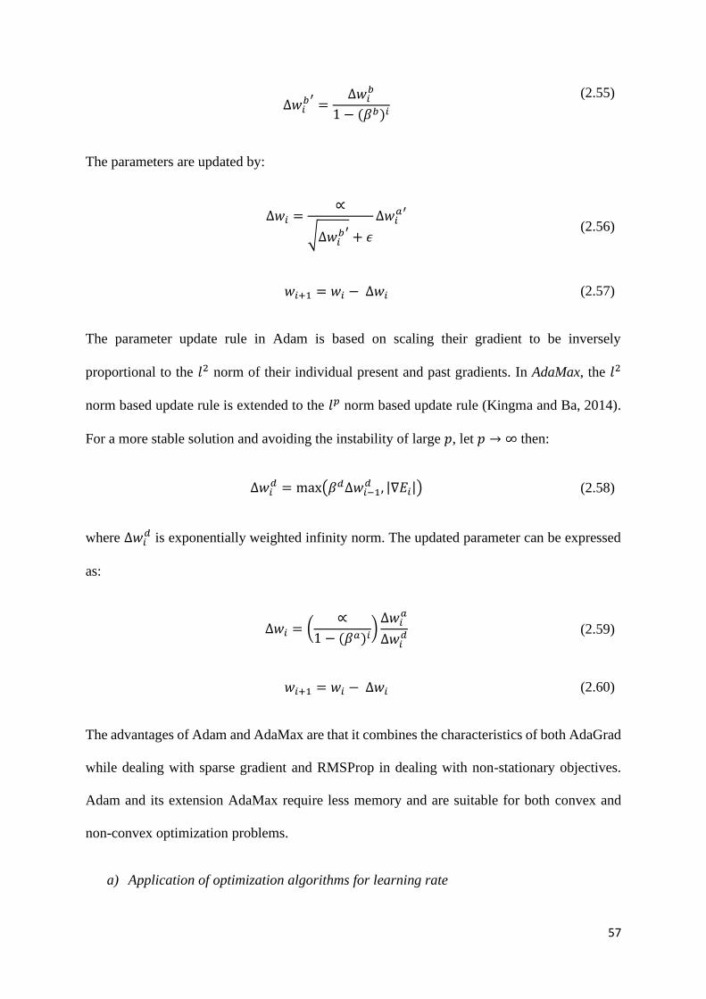
57

∆𝑤𝑖

𝑏′ =∆𝑤𝑖

𝑏

1 − (𝛽𝑏)𝑖

(2.55)

The parameters are updated by:

∆𝑤𝑖 =

∝

√∆𝑤𝑖𝑏′ + 𝜖

∆𝑤𝑖𝑎′

(2.56)

𝑤𝑖+1 = 𝑤𝑖 − ∆𝑤𝑖 (2.57)

The parameter update rule in Adam is based on scaling their gradient to be inversely

proportional to the 𝑙2 norm of their individual present and past gradients. In AdaMax, the 𝑙2

norm based update rule is extended to the 𝑙𝑝 norm based update rule (Kingma and Ba, 2014).

For a more stable solution and avoiding the instability of large 𝑝, let 𝑝 → ∞ then:

∆𝑤𝑖𝑑 = max(𝛽𝑑∆𝑤𝑖−1

𝑑 , |∇𝐸𝑖|) (2.58)

where ∆𝑤𝑖𝑑 is exponentially weighted infinity norm. The updated parameter can be expressed

as:

∆𝑤𝑖 = (∝

1 − (𝛽𝑎)𝑖)∆𝑤𝑖

𝑎

∆𝑤𝑖𝑑 (2.59)

𝑤𝑖+1 = 𝑤𝑖 − ∆𝑤𝑖 (2.60)

The advantages of Adam and AdaMax are that it combines the characteristics of both AdaGrad

while dealing with sparse gradient and RMSProp in dealing with non-stationary objectives.

Adam and its extension AdaMax require less memory and are suitable for both convex and

non-convex optimization problems.

a) Application of optimization algorithms for learning rate

58

Various applications of optimization algorithms for learning rate are explained and listed in

Appendix A.

2.2.4.2 Bias and variance (underfitting and overfitting) minimization

algorithms

The best FNN should be able to truly approximate the training and testing data. Researchers

extensively studied FNN to avoid high bias and variance to improve convergence

approximations. The high bias is referred to a problem known as underfitting and high variance

is referred to as overfitting. Underfitting occurs when the network is not properly trained and

the patterns in the training data are not fully discovered. It occurs before the convergence point

and, in this case, the generalization performance (also known as test data performance) does

not deviate much from the training data performance. That is the reason that the underfitting

region has high bias and low variance. In contrast, overfitting occurs after the convergence

point when the network is overtrained. In this scenario, the training error is in a continuous

state of decreasing whereas the testing error starts increasing. The overfitting is known as

having the properties of low bias and high variance. The high variance in training and the

testing error occurs because the network trains the noise in the training data which might be

not part of the actual model data. The best choice is to choose a model that balances bias and

variance, which is known as bias and variance trade-off. Bias and variance trade-off allows

FNN to discover all patterns in the training data and simultaneously give better generalization

performance (Geman et al., 1992).

For simplicity, the bias-and-variance trade-off point is referred to as the convergence point.

The FNN should be stopped from further training when it approaches the convergence point to

balance bias (underfitting) and variance (overfitting). The most popular method to identify and

stop the FNN at the convergence point is to select suitable validation data. Validation datasets

59

and test datasets are used interchangeably and are unseen data held back from the training data

to check the network performance. The error estimate by the training data is not a useful

estimator and comparing its performance with the validation dataset generalization

performance can help to identify the convergence point (Zaghloul et al., 2009). One of the

drawbacks associated with the validation technique is that the dataset should be large enough

to split it (Reed, 1993). This makes it unsuitable for small datasets especially complicated data

with few instances and many variables. When sufficient data is not available, the n-fold cross-

validation technique can be considered as an alternative to the validation technique (Seni and

Elder, 2010). The n-fold cross-validation technique splits data randomly into n-equal sized data

subsamples. The FNN is repeated n times by allocating one subsample for testing and the

remaining n-1 for the training model. The n-subsample is allocated once for each testing.

Finally, the n-results are averaged to get a single accurate estimation. The suitable selection of

n-fold size is based on dataset complexity and network size which make this technique

challenging for complicated applications.

The underfitting problem is easily detectable and therefore the literature has focused on

proposing techniques for improving overfitting. A large size network has a greater possibility

to overfit as compared to a smaller size (Setiono and Hui, 1995). Similarly, overfitting chances

increase when the network degree of freedom (such as weights) increases significantly from

the training sample (Reed, 1993). These two problems have gained greater attention and led to

the development of the techniques, explained below, to avoid overfitting analytically rather

than trial and error approaches. The algorithms for this category are subcategorized into

regularization, pruning, and ensembles.

a) Regularization Algorithms

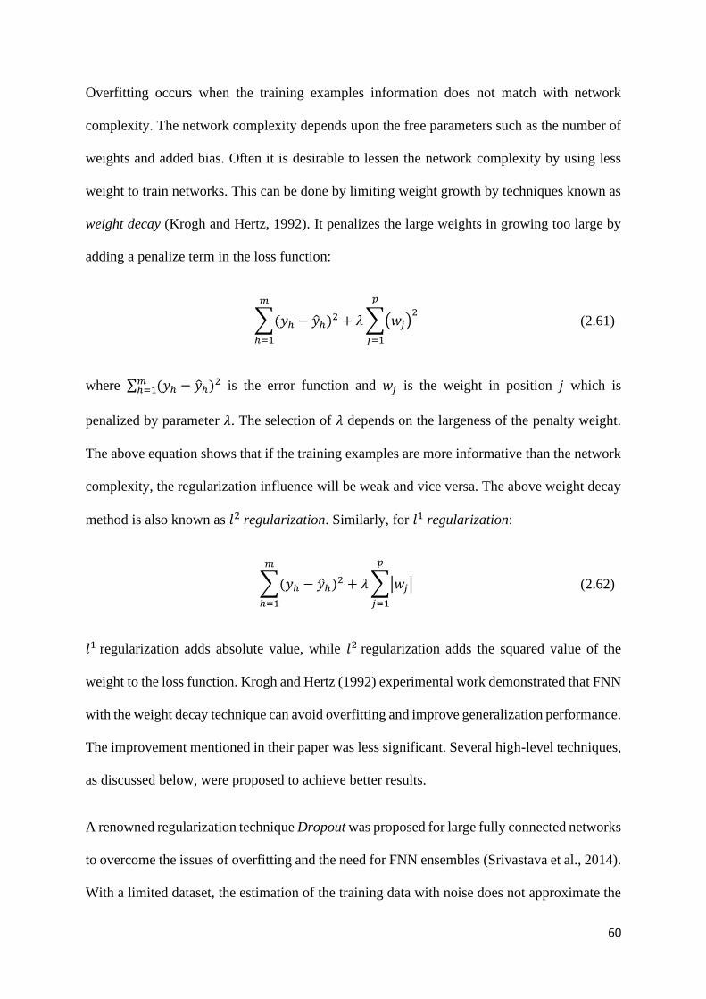
60

Overfitting occurs when the training examples information does not match with network

complexity. The network complexity depends upon the free parameters such as the number of

weights and added bias. Often it is desirable to lessen the network complexity by using less

weight to train networks. This can be done by limiting weight growth by techniques known as

weight decay (Krogh and Hertz, 1992). It penalizes the large weights in growing too large by

adding a penalize term in the loss function:

∑(𝑦ℎ − �̂�ℎ)2

𝑚

ℎ=1

+ 𝜆∑(𝑤𝑗)2

𝑝

𝑗=1

(2.61)

where ∑ (𝑦ℎ − �̂�ℎ)2𝑚

ℎ=1 is the error function and 𝑤𝑗 is the weight in position 𝑗 which is

penalized by parameter 𝜆. The selection of 𝜆 depends on the largeness of the penalty weight.

The above equation shows that if the training examples are more informative than the network

complexity, the regularization influence will be weak and vice versa. The above weight decay

method is also known as 𝑙2 regularization. Similarly, for 𝑙1 regularization:

∑(𝑦ℎ − �̂�ℎ)2

𝑚

ℎ=1

+ 𝜆∑|𝑤𝑗|

𝑝

𝑗=1

(2.62)

𝑙1 regularization adds absolute value, while 𝑙2 regularization adds the squared value of the

weight to the loss function. Krogh and Hertz (1992) experimental work demonstrated that FNN

with the weight decay technique can avoid overfitting and improve generalization performance.

The improvement mentioned in their paper was less significant. Several high-level techniques,

as discussed below, were proposed to achieve better results.

A renowned regularization technique Dropout was proposed for large fully connected networks

to overcome the issues of overfitting and the need for FNN ensembles (Srivastava et al., 2014).

With a limited dataset, the estimation of the training data with noise does not approximate the

61

testing data which leads to overfitting. Firstly, this happens because each parameter during the

gradient update influences the other parameters, which creates a complex coadaptation among

the hidden units. This coadaptation can be broken by removing some hidden units from the

network. Secondly, during FNN ensembles, combining the average of many outputs of a

separately trained FNN is an expensive task. Training many FNN requires many trial and error

approaches to find the best possible hyperparameters, which makes it a daunting task and needs

a lot of computation efforts. Dropout avoids overfitting by temporarily dropping the units

(hidden and visible) along with all connections with certain random probability during the

network forward steps. Training FNN with dropout means training 2n thinned networks where

n is a number of units in FNN. During testing time, it is not recommended to take an average

of the prediction from all thinned trained FNNs. It is best to use a single FNN during the testing

time without dropout. The weights of this single FNN provide a scaled down version of all the

trained weights. If the unit output is denoted by 𝑦𝑖′, input by 𝑥𝑖

′ with weight by 𝑤′, than the

dropout is expressed as:

𝑦𝑖′ = 𝑟 ∗ 𝑓(𝑤′𝑥𝑖

′) (2.63)

where 𝑟 is a vector of the independent Bernoulli random variable with * denoting an element

wise product. The downside of dropout is that its training time is 2-3 times longer than the

standard FNN for the same architecture. However, the experimental results achieved by

dropout compared to FNN are remarkable. DropConnect, a generalization of Dropout, is

another regularization technique for a large fully connected layer FNN to avoid overfitting

(Wan et al., 2013). The key difference between Dropout and DropConnect is in their dropping

mechanism. The Dropout temporarily drops the units along with their connection weights,

whereas, DropConnect randomly drops a subset of weight connections with a random

probability. The technique is like Dropout and the key difference is that DropConnect drops

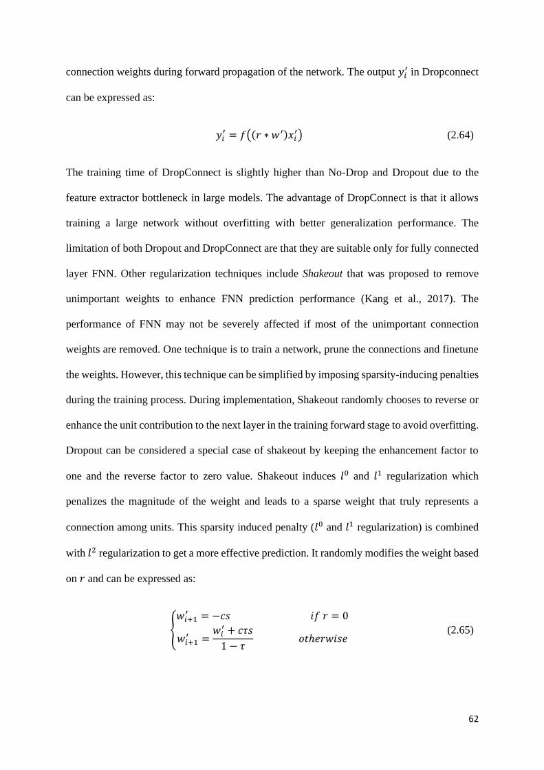
62

connection weights during forward propagation of the network. The output 𝑦𝑖′ in Dropconnect

can be expressed as:

𝑦𝑖′ = 𝑓((𝑟 ∗ 𝑤′)𝑥𝑖

′) (2.64)

The training time of DropConnect is slightly higher than No-Drop and Dropout due to the

feature extractor bottleneck in large models. The advantage of DropConnect is that it allows

training a large network without overfitting with better generalization performance. The

limitation of both Dropout and DropConnect are that they are suitable only for fully connected

layer FNN. Other regularization techniques include Shakeout that was proposed to remove

unimportant weights to enhance FNN prediction performance (Kang et al., 2017). The

performance of FNN may not be severely affected if most of the unimportant connection

weights are removed. One technique is to train a network, prune the connections and finetune

the weights. However, this technique can be simplified by imposing sparsity-inducing penalties

during the training process. During implementation, Shakeout randomly chooses to reverse or

enhance the unit contribution to the next layer in the training forward stage to avoid overfitting.

Dropout can be considered a special case of shakeout by keeping the enhancement factor to

one and the reverse factor to zero value. Shakeout induces 𝑙0 and 𝑙1 regularization which

penalizes the magnitude of the weight and leads to a sparse weight that truly represents a

connection among units. This sparsity induced penalty (𝑙0 and 𝑙1 regularization) is combined

with 𝑙2 regularization to get a more effective prediction. It randomly modifies the weight based

on 𝑟 and can be expressed as:

{

𝑤𝑖+1′ = −𝑐𝑠 𝑖𝑓 𝑟 = 0

𝑤𝑖+1′ =

𝑤𝑖′ + 𝑐𝜏𝑠

1 − 𝜏 𝑜𝑡ℎ𝑒𝑟𝑤𝑖𝑠𝑒

(2.65)

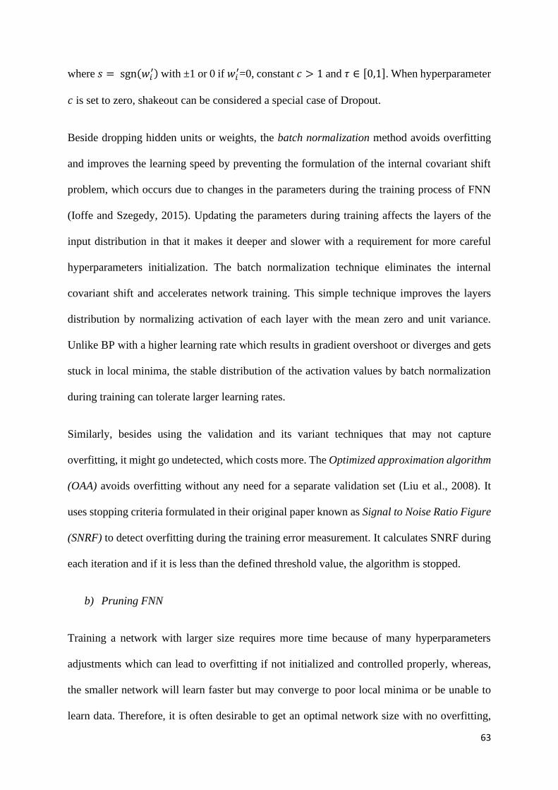
63

where 𝑠 = sgn(𝑤𝑖′) with ±1 or 0 if 𝑤𝑖

′=0, constant 𝑐 > 1 and 𝜏 ∈ [0,1]. When hyperparameter

𝑐 is set to zero, shakeout can be considered a special case of Dropout.

Beside dropping hidden units or weights, the batch normalization method avoids overfitting

and improves the learning speed by preventing the formulation of the internal covariant shift

problem, which occurs due to changes in the parameters during the training process of FNN

(Ioffe and Szegedy, 2015). Updating the parameters during training affects the layers of the

input distribution in that it makes it deeper and slower with a requirement for more careful

hyperparameters initialization. The batch normalization technique eliminates the internal

covariant shift and accelerates network training. This simple technique improves the layers

distribution by normalizing activation of each layer with the mean zero and unit variance.

Unlike BP with a higher learning rate which results in gradient overshoot or diverges and gets

stuck in local minima, the stable distribution of the activation values by batch normalization

during training can tolerate larger learning rates.

Similarly, besides using the validation and its variant techniques that may not capture

overfitting, it might go undetected, which costs more. The Optimized approximation algorithm

(OAA) avoids overfitting without any need for a separate validation set (Liu et al., 2008). It

uses stopping criteria formulated in their original paper known as Signal to Noise Ratio Figure

(SNRF) to detect overfitting during the training error measurement. It calculates SNRF during

each iteration and if it is less than the defined threshold value, the algorithm is stopped.

b) Pruning FNN

Training a network with larger size requires more time because of many hyperparameters

adjustments which can lead to overfitting if not initialized and controlled properly, whereas,

the smaller network will learn faster but may converge to poor local minima or be unable to

learn data. Therefore, it is often desirable to get an optimal network size with no overfitting,

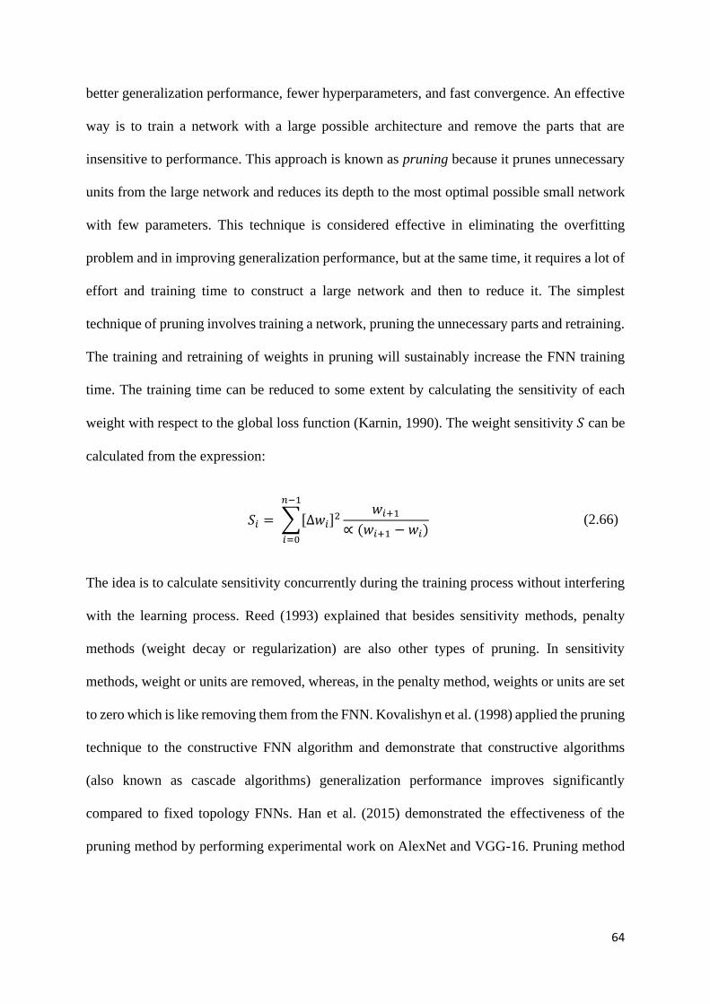
64

better generalization performance, fewer hyperparameters, and fast convergence. An effective

way is to train a network with a large possible architecture and remove the parts that are

insensitive to performance. This approach is known as pruning because it prunes unnecessary

units from the large network and reduces its depth to the most optimal possible small network

with few parameters. This technique is considered effective in eliminating the overfitting

problem and in improving generalization performance, but at the same time, it requires a lot of

effort and training time to construct a large network and then to reduce it. The simplest

technique of pruning involves training a network, pruning the unnecessary parts and retraining.

The training and retraining of weights in pruning will sustainably increase the FNN training

time. The training time can be reduced to some extent by calculating the sensitivity of each

weight with respect to the global loss function (Karnin, 1990). The weight sensitivity 𝑆 can be

calculated from the expression:

𝑆𝑖 = ∑[∆𝑤𝑖]2

𝑛−1

𝑖=0

𝑤𝑖+1∝ (𝑤𝑖+1 − 𝑤𝑖)

(2.66)

The idea is to calculate sensitivity concurrently during the training process without interfering

with the learning process. Reed (1993) explained that besides sensitivity methods, penalty

methods (weight decay or regularization) are also other types of pruning. In sensitivity

methods, weight or units are removed, whereas, in the penalty method, weights or units are set

to zero which is like removing them from the FNN. Kovalishyn et al. (1998) applied the pruning

technique to the constructive FNN algorithm and demonstrate that constructive algorithms

(also known as cascade algorithms) generalization performance improves significantly

compared to fixed topology FNNs. Han et al. (2015) demonstrated the effectiveness of the

pruning method by performing experimental work on AlexNet and VGG-16. Pruning method

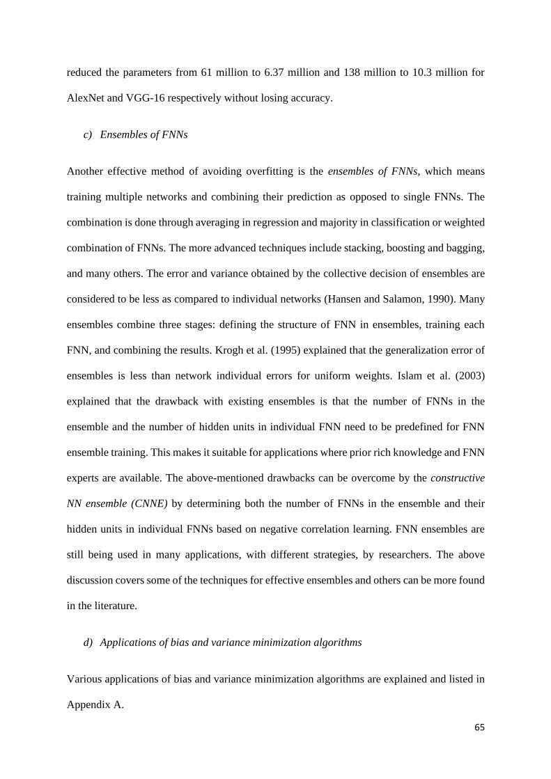
65

reduced the parameters from 61 million to 6.37 million and 138 million to 10.3 million for

AlexNet and VGG-16 respectively without losing accuracy.

c) Ensembles of FNNs

Another effective method of avoiding overfitting is the ensembles of FNNs, which means

training multiple networks and combining their prediction as opposed to single FNNs. The

combination is done through averaging in regression and majority in classification or weighted

combination of FNNs. The more advanced techniques include stacking, boosting and bagging,

and many others. The error and variance obtained by the collective decision of ensembles are

considered to be less as compared to individual networks (Hansen and Salamon, 1990). Many

ensembles combine three stages: defining the structure of FNN in ensembles, training each

FNN, and combining the results. Krogh et al. (1995) explained that the generalization error of

ensembles is less than network individual errors for uniform weights. Islam et al. (2003)

explained that the drawback with existing ensembles is that the number of FNNs in the

ensemble and the number of hidden units in individual FNN need to be predefined for FNN

ensemble training. This makes it suitable for applications where prior rich knowledge and FNN

experts are available. The above-mentioned drawbacks can be overcome by the constructive

NN ensemble (CNNE) by determining both the number of FNNs in the ensemble and their

hidden units in individual FNNs based on negative correlation learning. FNN ensembles are

still being used in many applications, with different strategies, by researchers. The above

discussion covers some of the techniques for effective ensembles and others can be more found

in the literature.

d) Applications of bias and variance minimization algorithms

Various applications of bias and variance minimization algorithms are explained and listed in

Appendix A.

66

2.2.4.3 Constructive topology FNN

FNN with a fixed number of hidden layers and units are known as fixed-topology networks

which can be either shallow (single) or deep (more than one) depending on the application task.

Whereas, the FNN that starts with the simplest network and then adds hidden units until the

error convergence is known as a constructive (or cascade) topology network. The drawbacks

associated with fixed typology FNNs are that the hidden layers and units need to be predefined

before training initialization. This needs a lot of trial and error to find the optimal hidden units

in the layers. If too many hidden layers and units are selected, the training time will increase,

whereas, if fewer layers and hidden units are selected, it might result in poor convergence.

Constructive topology networks have advantages over fixed topologies that in it start with a

minimal simple network and then adds hidden layers with some predefined hidden units until

error convergence occurs. This eliminates the need for trial and error approaches and

automatically constructs the network. Recent studies have shown that constructive algorithms

are more powerful than fixed algorithms. Hunter et al. (2012) in their FNNs comparative study

explained that a constructive network can solve the Parity-63 problem with only 6 hidden units

compared to a fixed network that required 64 hidden units. The training time is proportional to

the hidden unit’s quantity. Adding more hidden units will cause the network to be slow because

of more computational work. The computational training time of constructive algorithms is

much better than in a fixed topology. However, it does not mean that the generalization

performance of constructive networks will be always superior to a fixed network. A more

careful approach is needed to handle hidden units with a lot of connections and parameters to

stop the addition of further hidden units to avoid decreasing generalization performance (Kwok

and Yeung, 1997).

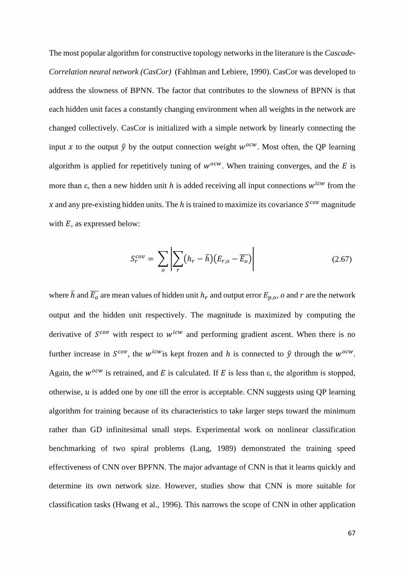
67

The most popular algorithm for constructive topology networks in the literature is the Cascade-

Correlation neural network (CasCor) (Fahlman and Lebiere, 1990). CasCor was developed to

address the slowness of BPNN. The factor that contributes to the slowness of BPNN is that

each hidden unit faces a constantly changing environment when all weights in the network are

changed collectively. CasCor is initialized with a simple network by linearly connecting the

input 𝑥 to the output �̂� by the output connection weight 𝑤𝑜𝑐𝑤. Most often, the QP learning

algorithm is applied for repetitively tuning of 𝑤𝑜𝑐𝑤. When training converges, and the 𝐸 is

more than ε, then a new hidden unit ℎ is added receiving all input connections 𝑤𝑖𝑐𝑤 from the

𝑥 and any pre-existing hidden units. The ℎ is trained to maximize its covariance 𝑆𝑐𝑜𝑣 magnitude

with 𝐸, as expressed below:

𝑆𝑟𝑐𝑜𝑣 = ∑|∑(ℎ𝑟 − ℎ̅)(𝐸𝑟,𝑜 − 𝐸𝑜̅̅ ̅)

𝑟

|

𝑜

(2.67)

where ℎ̅ and 𝐸𝑜̅̅ ̅ are mean values of hidden unit ℎ𝑟 and output error 𝐸𝑝,𝑜, 𝑜 and 𝑟 are the network

output and the hidden unit respectively. The magnitude is maximized by computing the

derivative of 𝑆𝑐𝑜𝑣 with respect to 𝑤𝑖𝑐𝑤 and performing gradient ascent. When there is no

further increase in 𝑆𝑐𝑜𝑣, the 𝑤𝑖𝑐𝑤is kept frozen and ℎ is connected to �̂� through the 𝑤𝑜𝑐𝑤.

Again, the 𝑤𝑜𝑐𝑤 is retrained, and 𝐸 is calculated. If 𝐸 is less than ε, the algorithm is stopped,

otherwise, 𝑢 is added one by one till the error is acceptable. CNN suggests using QP learning

algorithm for training because of its characteristics to take larger steps toward the minimum

rather than GD infinitesimal small steps. Experimental work on nonlinear classification

benchmarking of two spiral problems (Lang, 1989) demonstrated the training speed

effectiveness of CNN over BPFNN. The major advantage of CNN is that it learns quickly and

determine its own network size. However, studies show that CNN is more suitable for

classification tasks (Hwang et al., 1996). This narrows the scope of CNN in other application

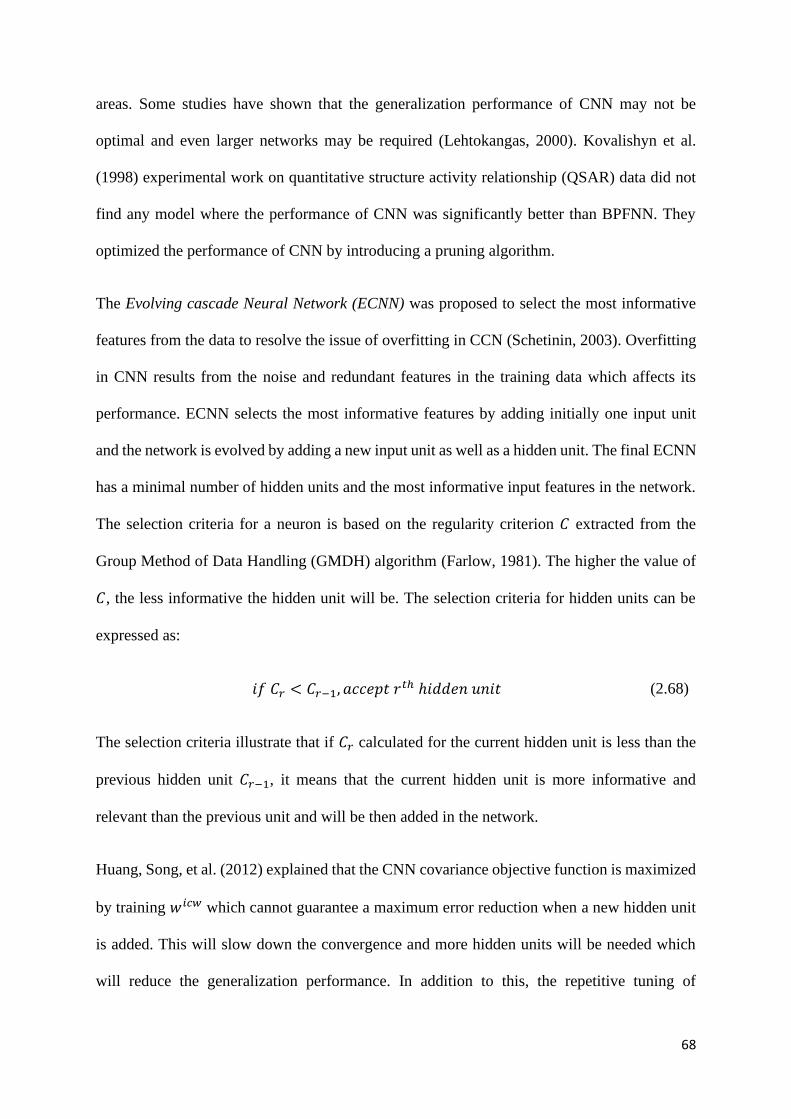
68

areas. Some studies have shown that the generalization performance of CNN may not be

optimal and even larger networks may be required (Lehtokangas, 2000). Kovalishyn et al.

(1998) experimental work on quantitative structure activity relationship (QSAR) data did not

find any model where the performance of CNN was significantly better than BPFNN. They

optimized the performance of CNN by introducing a pruning algorithm.

The Evolving cascade Neural Network (ECNN) was proposed to select the most informative

features from the data to resolve the issue of overfitting in CCN (Schetinin, 2003). Overfitting

in CNN results from the noise and redundant features in the training data which affects its

performance. ECNN selects the most informative features by adding initially one input unit

and the network is evolved by adding a new input unit as well as a hidden unit. The final ECNN

has a minimal number of hidden units and the most informative input features in the network.

The selection criteria for a neuron is based on the regularity criterion 𝐶 extracted from the

Group Method of Data Handling (GMDH) algorithm (Farlow, 1981). The higher the value of

𝐶, the less informative the hidden unit will be. The selection criteria for hidden units can be

expressed as:

𝑖𝑓 𝐶𝑟 < 𝐶𝑟−1, 𝑎𝑐𝑐𝑒𝑝𝑡 𝑟𝑡ℎ ℎ𝑖𝑑𝑑𝑒𝑛 𝑢𝑛𝑖𝑡 (2.68)

The selection criteria illustrate that if 𝐶𝑟 calculated for the current hidden unit is less than the

previous hidden unit 𝐶𝑟−1, it means that the current hidden unit is more informative and

relevant than the previous unit and will be then added in the network.

Huang, Song, et al. (2012) explained that the CNN covariance objective function is maximized

by training 𝑤𝑖𝑐𝑤 which cannot guarantee a maximum error reduction when a new hidden unit

is added. This will slow down the convergence and more hidden units will be needed which

will reduce the generalization performance. In addition to this, the repetitive tuning of

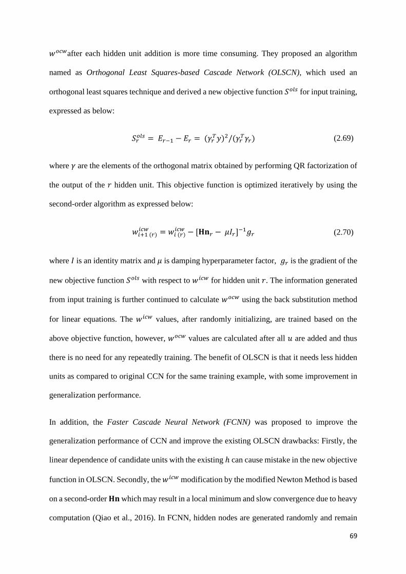
69

𝑤𝑜𝑐𝑤after each hidden unit addition is more time consuming. They proposed an algorithm

named as Orthogonal Least Squares-based Cascade Network (OLSCN), which used an

orthogonal least squares technique and derived a new objective function 𝑆𝑜𝑙𝑠 for input training,

expressed as below:

𝑆𝑟𝑜𝑙𝑠 = 𝐸𝑟−1 − 𝐸𝑟 = (𝛾𝑟

𝑇𝑦)2/(𝛾𝑟𝑇𝛾𝑟) (2.69)

where 𝛾 are the elements of the orthogonal matrix obtained by performing QR factorization of

the output of the 𝑟 hidden unit. This objective function is optimized iteratively by using the

second-order algorithm as expressed below:

𝑤𝑖+1 (𝑟)𝑖𝑐𝑤 = 𝑤𝑖 (𝑟)

𝑖𝑐𝑤 − [𝐇𝐧𝑟 − 𝜇𝐼𝑟]−1𝑔𝑟 (2.70)

where 𝐼 is an identity matrix and 𝜇 is damping hyperparameter factor, 𝑔𝑟 is the gradient of the

new objective function 𝑆𝑜𝑙𝑠 with respect to 𝑤𝑖𝑐𝑤 for hidden unit 𝑟. The information generated

from input training is further continued to calculate 𝑤𝑜𝑐𝑤 using the back substitution method

for linear equations. The 𝑤𝑖𝑐𝑤 values, after randomly initializing, are trained based on the

above objective function, however, 𝑤𝑜𝑐𝑤 values are calculated after all 𝑢 are added and thus

there is no need for any repeatedly training. The benefit of OLSCN is that it needs less hidden

units as compared to original CCN for the same training example, with some improvement in

generalization performance.

In addition, the Faster Cascade Neural Network (FCNN) was proposed to improve the

generalization performance of CCN and improve the existing OLSCN drawbacks: Firstly, the

linear dependence of candidate units with the existing ℎ can cause mistake in the new objective

function in OLSCN. Secondly, the 𝑤𝑖𝑐𝑤 modification by the modified Newton Method is based

on a second-order 𝐇𝐧 which may result in a local minimum and slow convergence due to heavy

computation (Qiao et al., 2016). In FCNN, hidden nodes are generated randomly and remain

70

unchanged as inspired by randomly mapping algorithms. The 𝑤𝑜𝑐𝑤 connecting both input and

hidden units to output units are calculated after the addition of all the necessary input and

hidden units. The FCNN initializes, with no input and hidden units in the network. The bias

unit is added to the network and input units are added one by one with error calculation for

each input unit. When there are no input units to be added, a pool of candidate units is randomly

generated. The candidate unit with the maximum capability to error reduction computed from

the reformulated modified index is added as a hidden unit to the network. When a maximum

number of hidden units or defined thresholds are achieved, the addition of hidden units is

stopped. Finally, the output units are calculated by back substitution computing like OLSCN.

The experimental comparison among FCNN, OLSCN, and CNN demonstrated that FCNN

achieved better generalization performance and fast learning, however, the network

architecture size increases many times.

Nayyeri et al. (2018) proposed to use a correntropy based objective function with a sigmoid

kernel to adjust the 𝑤𝑖𝑐𝑤 of the newly added hidden unit rather than a covariance (correlation)

objective function. The success of correlation heavily relies on the Gaussian and linearity

assumptions, whereas, the properties of correntropy are to make the network more optimal in

nonlinear and non-Gaussian terms. The new algorithm with a correntropy objective function

based on a sigmoid kernel is named as Cascade Correntropy Network (CCOEN). Similar to

other cascade algorithms described above, 𝑤𝑖𝑐𝑤 is optimized by using correntropy objective

function 𝑆𝑐𝑡 with sigmoid:

𝑆𝑟𝑐𝑡 = max

𝑈𝑟(∑(tanh(а𝑟⟨𝐸𝑟−1, 𝐻𝑟⟩ + 𝑐)) − 𝐶‖𝑤𝑟

𝑖𝑐𝑤‖2

𝑟

𝑖=1

) (2.71)

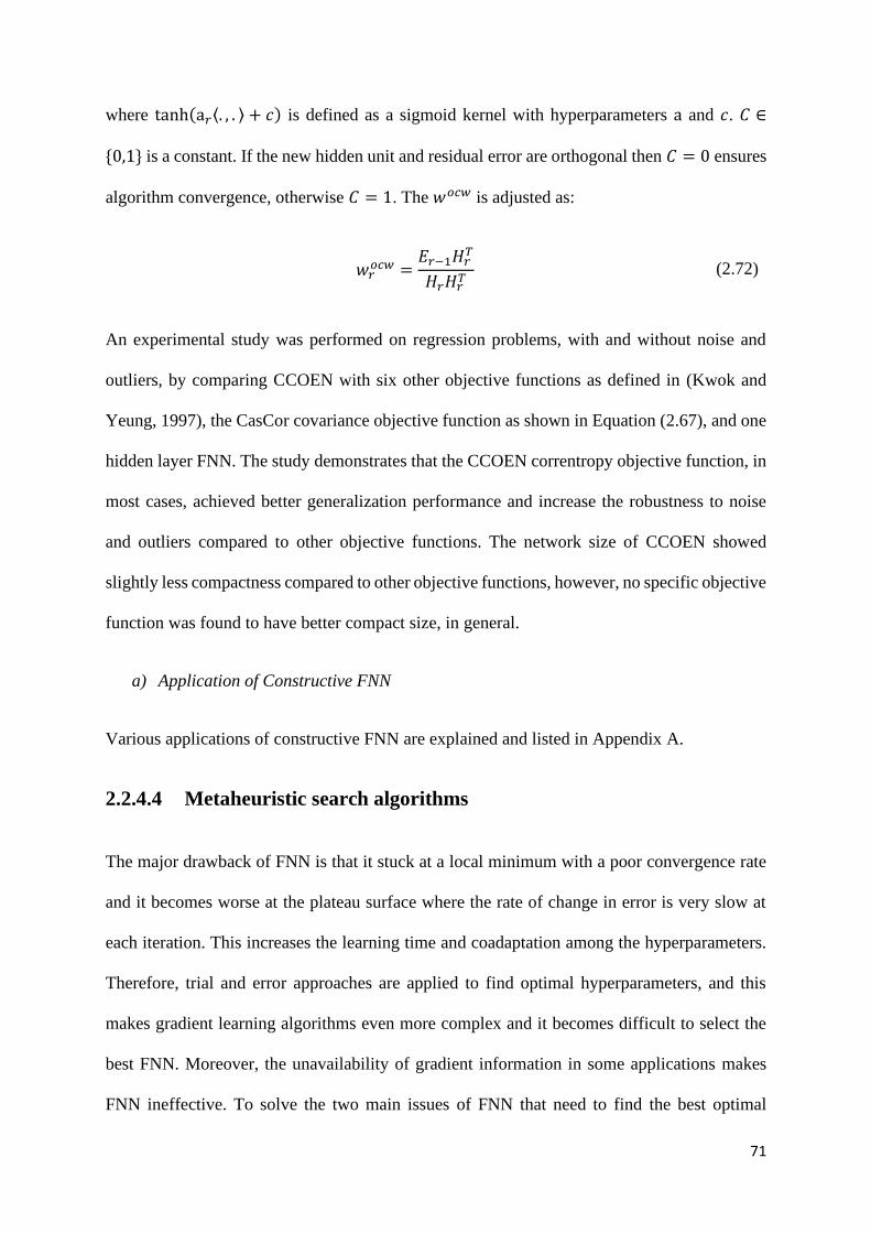
71

where tanh(а𝑟⟨. , . ⟩ + 𝑐) is defined as a sigmoid kernel with hyperparameters а and 𝑐. 𝐶 ∈

{0,1} is a constant. If the new hidden unit and residual error are orthogonal then 𝐶 = 0 ensures

algorithm convergence, otherwise 𝐶 = 1. The 𝑤𝑜𝑐𝑤 is adjusted as:

𝑤𝑟𝑜𝑐𝑤 =

𝐸𝑟−1𝐻𝑟𝑇

𝐻𝑟𝐻𝑟𝑇 (2.72)

An experimental study was performed on regression problems, with and without noise and

outliers, by comparing CCOEN with six other objective functions as defined in (Kwok and

Yeung, 1997), the CasCor covariance objective function as shown in Equation (2.67), and one

hidden layer FNN. The study demonstrates that the CCOEN correntropy objective function, in

most cases, achieved better generalization performance and increase the robustness to noise

and outliers compared to other objective functions. The network size of CCOEN showed

slightly less compactness compared to other objective functions, however, no specific objective

function was found to have better compact size, in general.

a) Application of Constructive FNN

Various applications of constructive FNN are explained and listed in Appendix A.

2.2.4.4 Metaheuristic search algorithms

The major drawback of FNN is that it stuck at a local minimum with a poor convergence rate

and it becomes worse at the plateau surface where the rate of change in error is very slow at

each iteration. This increases the learning time and coadaptation among the hyperparameters.

Therefore, trial and error approaches are applied to find optimal hyperparameters, and this

makes gradient learning algorithms even more complex and it becomes difficult to select the

best FNN. Moreover, the unavailability of gradient information in some applications makes

FNN ineffective. To solve the two main issues of FNN that need to find the best optimal

72

hyperparameters and to make it useable with no gradient information, the application of

metaheuristic algorithms such as genetic algorithm, particle swarm optimization, and whale

optimization algorithm is implemented in combination with FNN. The major contribution of

the applications of a metaheuristic algorithm is that it may converge at a global minimum rather

than the local minimum by moving from a local search to a global search. Therefore, these are

more suitable for global optimization problems. The metaheuristic algorithms are good for

identifying the best hyperparameters and convergence at a global minimum, but they have

drawbacks in the high memory requirements and processing time.

a) Genetic Algorithm

Genetic Algorithm (GA) is a metaheuristic technique belonging to the class of evolutionary

algorithms (EA) inspired by Darwinian theory about evolution and natural selection and was

invented by John Holland in the 1960s (Mitchell, 1998). It is used to find a solution for

optimization problems by performing chromosome encoding, fitness selection, crossover, and

mutation. Like BP, it is used to train FNNs to find the best possible hyperparameters.

Researchers demonstrated that the generalization performance of GA is better than BP

(Mohamad et al., 2017) with the additional need for training time. Liang and Dai (1998)

highlighted the same issue by applying GA to FNN. They demonstrated that the performance

of GA is better than BP, but the training time increased. Ding et al. (2011) proposed that GA

performance can be improved by integrating the concept of both BP gradient information and

GA genetic information to train an FNN for superior generalization performance. GA is good

for global searching, whereas, BP is appropriate for local searching. The algorithm first uses

GA to optimize the initial weights by searching for better search space and then uses BP to fine

tune and search for an optimal solution. Experimental results demonstrated that FNN trained

on the hybrid approach of GA and BP achieved better generalization performance than

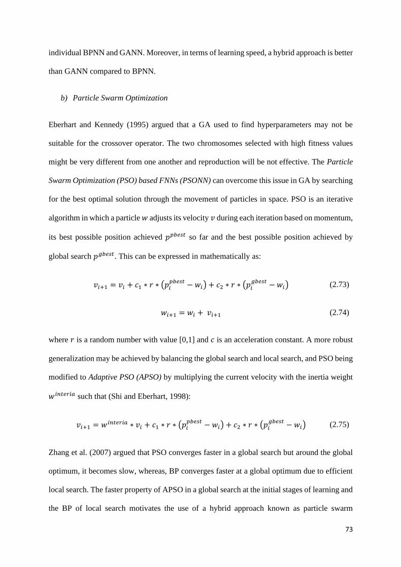
73

individual BPNN and GANN. Moreover, in terms of learning speed, a hybrid approach is better

than GANN compared to BPNN.

b) Particle Swarm Optimization

Eberhart and Kennedy (1995) argued that a GA used to find hyperparameters may not be

suitable for the crossover operator. The two chromosomes selected with high fitness values

might be very different from one another and reproduction will be not effective. The Particle

Swarm Optimization (PSO) based FNNs (PSONN) can overcome this issue in GA by searching

for the best optimal solution through the movement of particles in space. PSO is an iterative

algorithm in which a particle 𝑤 adjusts its velocity 𝑣 during each iteration based on momentum,

its best possible position achieved 𝑝𝑝𝑏𝑒𝑠𝑡 so far and the best possible position achieved by

global search 𝑝𝑔𝑏𝑒𝑠𝑡. This can be expressed in mathematically as:

𝑣𝑖+1 = 𝑣𝑖 + 𝑐1 ∗ 𝑟 ∗ (𝑝𝑖𝑝𝑏𝑒𝑠𝑡 − 𝑤𝑖) + 𝑐2 ∗ 𝑟 ∗ (𝑝𝑖

𝑔𝑏𝑒𝑠𝑡− 𝑤𝑖) (2.73)

𝑤𝑖+1 = 𝑤𝑖 + 𝑣𝑖+1 (2.74)

where 𝑟 is a random number with value [0,1] and 𝑐 is an acceleration constant. A more robust

generalization may be achieved by balancing the global search and local search, and PSO being

modified to Adaptive PSO (APSO) by multiplying the current velocity with the inertia weight

𝑤𝑖𝑛𝑡𝑒𝑟𝑖𝑎 such that (Shi and Eberhart, 1998):

𝑣𝑖+1 = 𝑤𝑖𝑛𝑡𝑒𝑟𝑖𝑎 ∗ 𝑣𝑖 + 𝑐1 ∗ 𝑟 ∗ (𝑝𝑖

𝑝𝑏𝑒𝑠𝑡 − 𝑤𝑖) + 𝑐2 ∗ 𝑟 ∗ (𝑝𝑖𝑔𝑏𝑒𝑠𝑡

− 𝑤𝑖) (2.75)

Zhang et al. (2007) argued that PSO converges faster in a global search but around the global

optimum, it becomes slow, whereas, BP converges faster at a global optimum due to efficient

local search. The faster property of APSO in a global search at the initial stages of learning and

the BP of local search motivates the use of a hybrid approach known as particle swarm

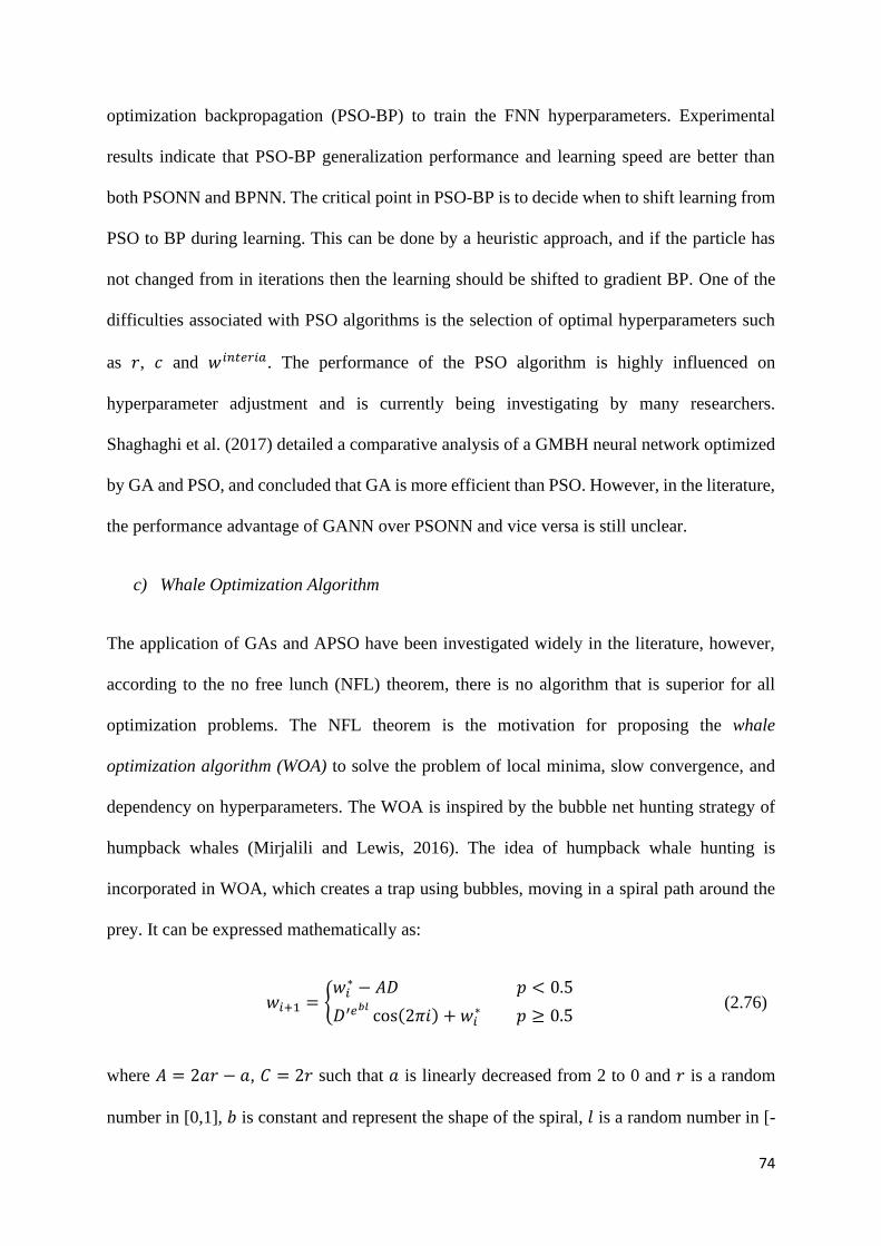
74

optimization backpropagation (PSO-BP) to train the FNN hyperparameters. Experimental

results indicate that PSO-BP generalization performance and learning speed are better than

both PSONN and BPNN. The critical point in PSO-BP is to decide when to shift learning from

PSO to BP during learning. This can be done by a heuristic approach, and if the particle has

not changed from in iterations then the learning should be shifted to gradient BP. One of the

difficulties associated with PSO algorithms is the selection of optimal hyperparameters such

as 𝑟, 𝑐 and 𝑤𝑖𝑛𝑡𝑒𝑟𝑖𝑎. The performance of the PSO algorithm is highly influenced on

hyperparameter adjustment and is currently being investigating by many researchers.

Shaghaghi et al. (2017) detailed a comparative analysis of a GMBH neural network optimized

by GA and PSO, and concluded that GA is more efficient than PSO. However, in the literature,

the performance advantage of GANN over PSONN and vice versa is still unclear.

c) Whale Optimization Algorithm

The application of GAs and APSO have been investigated widely in the literature, however,

according to the no free lunch (NFL) theorem, there is no algorithm that is superior for all

optimization problems. The NFL theorem is the motivation for proposing the whale

optimization algorithm (WOA) to solve the problem of local minima, slow convergence, and

dependency on hyperparameters. The WOA is inspired by the bubble net hunting strategy of

humpback whales (Mirjalili and Lewis, 2016). The idea of humpback whale hunting is

incorporated in WOA, which creates a trap using bubbles, moving in a spiral path around the

prey. It can be expressed mathematically as:

𝑤𝑖+1 = {𝑤𝑖∗ − 𝐴𝐷 𝑝 < 0.5

𝐷′𝑒𝑏𝑙cos(2𝜋𝑖) + 𝑤𝑖

∗ 𝑝 ≥ 0.5 (2.76)

where 𝐴 = 2𝑎𝑟 − 𝑎, 𝐶 = 2𝑟 such that 𝑎 is linearly decreased from 2 to 0 and 𝑟 is a random

number in [0,1], 𝑏 is constant and represent the shape of the spiral, 𝑙 is a random number in [-

75

1,1], and 𝑝 is a random number in [0,1]. 𝐷′ = |𝑤𝑖∗ − 𝑤𝑖| is the distance between the best

solution obtained so far and current position and 𝐷 = |𝐶𝑤𝑖∗ − 𝑤𝑖|. The first part of the above

equation represents the encircling mechanism and the second part represents the bubble net

technique. Like GAs and APSO, the search process starts with candidate solutions and then

improves it until defined criteria are achieved. In WOA, search agents are assigned and their

fitness functions are calculated. The position of the search agent is updated by computing

Equation (2.76). The process is repeated until the maximum number of iterations is achieved.

Ling et al. (2017) mentioned that WOA disadvantageous of slow convergence, low precision,

and being trapped in a local minimum because of lack of population diversity. They argued

that WOA is more useful for solving low dimensional problems, however, when dealing with

high dimensional and multi-model problems, its solution is not quite optimal. To overcome the

WOA drawbacks, an extension known as the Lévy flight WOA was proposed to enhance the

convergence by avoiding the local minimum.

d) Application of metaheuristic search algorithms

Various applications of metaheuristic search algorithms are explained and listed in Appendix

A.

2.3 Discussion

The application of NNs is gaining much popularity in the airline sector to improve its various

operations and enhance services. For instance, Lin and Vlachos (2018) proposed an analytical

framework, known as “Importance-Performance-Impact-Analysis”, to improve customer

satisfaction from airlines by incorporating techniques such as BPNNs, decision-making trail,

and evaluation laboratory. Cui and Li (2017) studied airline efficiency measures under “Carbon

Neutral Growth from 2020” and used a BPNN to predict the CO2 emission volume for an

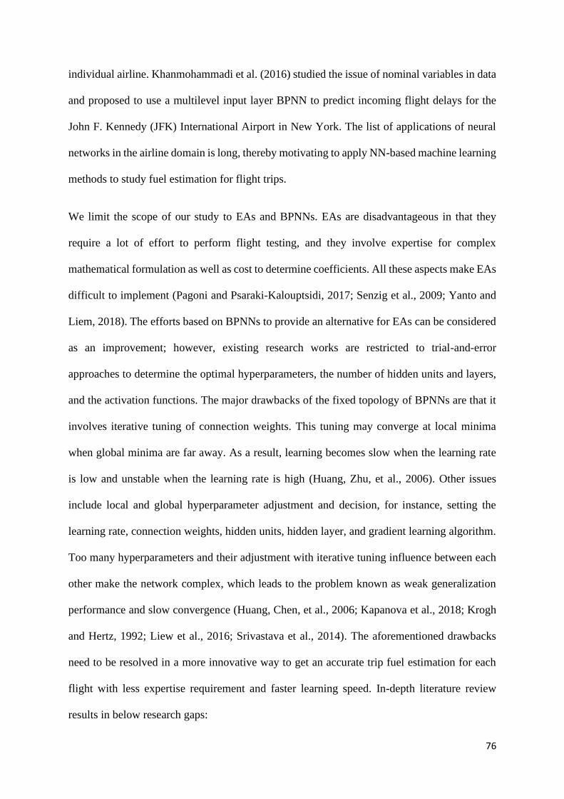
76

individual airline. Khanmohammadi et al. (2016) studied the issue of nominal variables in data

and proposed to use a multilevel input layer BPNN to predict incoming flight delays for the

John F. Kennedy (JFK) International Airport in New York. The list of applications of neural

networks in the airline domain is long, thereby motivating to apply NN-based machine learning

methods to study fuel estimation for flight trips.

We limit the scope of our study to EAs and BPNNs. EAs are disadvantageous in that they

require a lot of effort to perform flight testing, and they involve expertise for complex

mathematical formulation as well as cost to determine coefficients. All these aspects make EAs

difficult to implement (Pagoni and Psaraki-Kalouptsidi, 2017; Senzig et al., 2009; Yanto and

Liem, 2018). The efforts based on BPNNs to provide an alternative for EAs can be considered

as an improvement; however, existing research works are restricted to trial-and-error

approaches to determine the optimal hyperparameters, the number of hidden units and layers,

and the activation functions. The major drawbacks of the fixed topology of BPNNs are that it

involves iterative tuning of connection weights. This tuning may converge at local minima

when global minima are far away. As a result, learning becomes slow when the learning rate

is low and unstable when the learning rate is high (Huang, Zhu, et al., 2006). Other issues

include local and global hyperparameter adjustment and decision, for instance, setting the

learning rate, connection weights, hidden units, hidden layer, and gradient learning algorithm.

Too many hyperparameters and their adjustment with iterative tuning influence between each

other make the network complex, which leads to the problem known as weak generalization

performance and slow convergence (Huang, Chen, et al., 2006; Kapanova et al., 2018; Krogh

and Hertz, 1992; Liew et al., 2016; Srivastava et al., 2014). The aforementioned drawbacks

need to be resolved in a more innovative way to get an accurate trip fuel estimation for each

flight with less expertise requirement and faster learning speed. In-depth literature review

results in below research gaps:

77

1 EAs are based on complex energy balance mathematical formulation which needs a lot

of expertise and cost to determine many coefficients making it difficult to implement.

A lot of flight testing is needed to generate information about parameters and to

determine coefficients. The EAs needed some of the information about aircrafts types

and engines to determine the amount of fuel needed for a journey. The unavailability

of such information and usage of an outdated existing database having global

parameters with default values rather than local parameters may result in inaccurate

estimation of fuel by EAs. In the literature, an insufficient attempt has been made to

study the effect of using global parameters on the deviation of fuel from estimation

using a practical example.

2 The popularity of machine learning BPNN in the aviation sector and particularly in

estimating fuel consumption has gained much popularity to provide as an alternative to

EAs. Regarding methodology, in exiting studies, the pitfall is that no clear direction

exists that has explained the reason for recommended fixed topology architecture for

estimating fuel. The selection of hidden units, hidden layers, connection weight, and

learning rate requires much human intervention and inappropriate hyperparameter

selection may cause the algorithm to converge at suboptimal solution leading to higher

fuel deviation. A lot of trial and error experimental need to be performed to find the

best hyperparameters and which even become more difficult when dealing with high

dimensional real data. Another technical drawback of BPNN is that it converges at local

minima when global minima are far away, and computational time is highly dependent

on gradient derivation and learning speed.

3 It is observed that the selection of operational parameters was considered based on prior

experience and knowledge, whereas, their relationship to fuel consumption was

unnoticed. Moreover, existing BPNN based estimation models are trained by

78

considering low-level operational parameters. For instance, Schilling (1997) model was

based on a low-level operational parameter such as altitude and velocity with the future

recommendation of incorporating more parameters. However, Trani et al. (2004) also

used low-level operational parameters such as Mach number, weight, temperature, and

altitude, and according to a recent study, Baklacioglu (2016) also used low-level

operational parameters such as altitude and velocity for estimating fuel consumption.

In the literature, a gap still exists to add high-level operational parameters that can

contribute to minimizing fuel deviation which was ignored previously.

4 Most studies formulated to overcome fuel estimation limitations are proposed taking

into consideration either take-off, cruise or descent phase. The suggested models may

fail to work on all phases efficiently. For instance, the model proposed for take-off may

not perform accurately for decent because of a change in operational parameters. Some

models proposed to estimate fuel for phases separately and accumulate them to know

the final fuel needed for the journey. This approach can even result in higher deviation

because the amount of overestimation or underestimation in each phase may

cumulatively lead to higher fuel deviation. Therefore, it is important to have a model

that can efficiently estimate fuel for all phases collectively to ensure profitability and

safety.

5 Once developed, the performance of the same architecture machine learning NN may

no longer be suitable for learning the same application if data structure and size

changes. How to improve existing machine learning algorithms that may give the same

and accurate result regardless of a change in data structure and size is gaining attraction.

In the literature, fuel is estimated based on available small dimensional data and no

effort has been made to check the performance of an algorithm on varying nature of

data. The comparison of the difference in fuel deviation by considering all sectors high

79

dimensional data and reducing the dataset into small chunks (portions) need

considerable attention. The algorithm having a minimal difference in performance

regardless of a change in data structure and size means that algorithm estimation

accuracy does not decrease with the change in data dimensional.

An important question arises: Which machine learning NN algorithm will be more suitable to

address the above-mentioned research gaps? A comprehensive review of FNNs in Section 2.2

gives insight that existing improvement is not straightforward, and researchers are making

continuous efforts to propose algorithms that are computationally efficient and have better

generalization performance. By analyzing the existing research, we consider that following

seven research gaps that need considerable attention in order to improve existing FNNs:

1 Activation function: The importance of using nonlinear activation function in hidden

layers of FNNs is clear, however, it is still unclear in the literature which activation

function is more suitable for a particular application and data structure.

2 Efficient and compact Algorithm with fewer hyperparameters: Gradient free learning

algorithms are simple to apply because of no backpropagation, whereas, gradient

learning algorithms have compact architecture. Efforts are needed to design algorithm

has both characteristics of gradient-free learning and compact architecture.

3 Connection weight initialization: The purpose of FNN is to find the best optimal

connection weights that can generate optimal results. The question arises: What should

be the best possible initial weights for the network? Traditional FNN is dependent on

the initial weight value because it calculates the derivative of the total error with respect

to weight to get a minimum of the objective function. Assigning suboptimal weights

will cause the network to have more iterations and subsequently decreases its

performance. The issue is resolved to some extent by a new approach that analytically

80

calculates the connection weights on the output side by randomly generating hidden

units. However, existing neural networks can be further strengthened by calculating all

connection weights (including input connection and output connection) analytically to

generate hidden units, explaining maximum variance in the dataset. This may also help

to further improve the generalization and learning speed by compacting the size of the

network.

4 Data structure: Future research may include designing FNN architecture with less

complexity with the characteristics of learning noisy data without overfitting. Few

attempts have been made to study the effect of data size and structure on FNN

algorithms. The availability of training data in many applications (for instance, medical

science and so on) is limited (small data rather than big data) and costly (Choi et al.,

2018; Shen, Choi and Minner, 2019). Once trained, the same model may become

unstable for less or more data within the same application and may result in a loss of

generalization ability. Each time, for the same application area and algorithm, a new

model is needed to be trained with a different set of parameters. Future research on

designing an algorithm that can approximate the problem task equally, regardless of

data size (instance) and shape (features), will be a breakthrough achievement.

5 Eliminating the need for data pre-processing and transformation: Wrong application

of pre-processing and transformation techniques may result in suboptimal results.

Future algorithms are needed that may be less sensitive to outliers and noisy data and

do not need to reduce the magnitude of data.

6 A hybrid approach for real-world applications: Researchers most often use publicly

available real-world data to compare their results with other popular algorithms.

Frequently using the same real-world applications data may cause specific data to

become a benchmark. The best practice may be to use a hybrid approach of well-known

81

data in the field along with new data applications during the comparative study of

algorithms. This may create and maintain users’ interest in FNNs over the passage of

time

7 A number of hidden units needed: The analytical calculation of hidden units to deal

with high dimensional large datasets, rather than trial and error, is gaining interest. The

number of hidden units needed in either single or multiple layers such that no

dependency exists can ensure maximum error reduction of a network.

Addressing all the above FNNs research gaps in current work is difficult. The work is more

focused on two important research gaps “Connection weight initialization” and “Data

structure” that need researchers' attention.

In summary, in order to address the above research gaps of fuel estimation and FNNs, the trip

fuel model is formulated, and a novel machine learning algorithm is proposed. A computational

comparison of the proposed algorithm is made with other known popular algorithms using

artificial benchmarking and real-world datasets to demonstrate its effectiveness. Lastly, the

proposed algorithm is applied to estimate trip fuel for airlines using historical real data. The

comparison of the proposed algorithm with existing AEA and BPNN based fuel models are

also made to enrich the literature.

82

Chapter 3: Trip fuel Model Formulation for Minimizing

Fuel Deviation

3.1 Introduction

In this chapter, our main focus is to formulate a model for estimating trip fuel. Prior to

formulating the model and defining an objective function, the framework of fuel consumption

and its deviation from estimation is concisely explained. Before the commencement of each

flight, various amounts of fuel are loaded in aircraft to meet certain requirements. The trip fuel,

comprising a large portion of various other fuels, is loaded to ensure the smooth journey. The

difference in trip fuel estimated and consumed after flight enables us to understand the reasons

causing the overestimation and underestimation of fuel. The major reason for causing higher

fuel deviation from estimation is because of unreliable estimation techniques and ignoring

some of the operational parameters that may highly contribute to fuel consumption. The

methods (or estimation techniques) that are popular to estimate fuel for aircraft are of two types:

mathematical method and a data-driven method. The mathematical methods help to provide a

physical understanding of the system. However, in a real application, mathematical methods

might be difficult to implement and inaccurate because a lot of information needed to represent

the relationship among variables (Kuo and Kusiak, 2019). Machine learning (data-driven) are

considered ideally suitable for learning from historical data to make a better-informed decision,

time and cost-saving. Among machine learning, NNs are more popular to solve problems

because of their universal approximation capability (Ferrari and Stengel, 2005; Hornik et al.,

1989; Huang, Chen, et al., 2006). It can solve any complex nonlinear problem more accurately

which is difficult using classical statistical techniques (Kumar et al., 1995; Tkáč and Verner,

2016; Tu, 1996). The NN range of applications is numerous and some areas include regression

83

estimation (Chung et al., 2017; Deng et al., 2019; Kummong and Supratid, 2016; Teo et al.,

2015), image processing (Dong et al., 2016; Mohamed Shakeel et al., 2019), image

segmentation (Chen et al., 2018), video processing (Babaee et al., 2018), speech recognition

(Abdel-Hamid et al., 2014), text classification (Kastrati et al., 2019; Zaghloul et al., 2009), face

classification and recognition (Yin and Liu, 2018), human action recognition (Ijjina and

Chalavadi, 2016), risk analysis (Nasir et al., 2019) and many others. With modern information

technology advancement, the challenging issue of high dimensional, non-linear, noisy and

unbalanced data is continuously growing and varying at a rapid rate so that it demands efficient

learning algorithms and optimization techniques. The data may become a costly resource if not

analysed properly. Machine learning is gaining popularity in all aspects from data gathering to

discovering knowledge and its role in enhancing business decisions is gaining significant

interest (Bottani et al., 2019; Hayashi et al., 2010; Kim et al., 2019; Lam et al., 2014; Li et al.,

2018; Mori et al., 2012; Wang et al., 2005; Wong et al., 2018).

Efforts are being made to overcome the challenges by building optimal NNs that may extract

useful patterns from the data and generate information for better-informed decision making.

Extensive knowledge and theoretical information are required to build NNs having the

characteristics of better generalization performance and learning speed. The generalization

performance and learning speed are the two criteria that play an essential role in deciding on

the use of learning algorithms and optimization techniques to build optimal NNs. Depending

upon the application and data structure, the user might prefer either better generalization

performance or faster learning speed, or a combination of both. In its simplest form, NN with

a single hidden layer is powerful in solving many problems, given that there are a sufficient

number of hidden units in the layer (Nguyen and Widrow, 1990). The application of NNs in

diverse topics is not simple and expertise is needed to build an optimal network to achieve the

84

intended results in the shortest possible time. More specifically, in our work, mathematical

methods can be referred to as EAs and data-driven methods can be referred to as NNs.

The use of global parameters rather than local parameters and the need for complex

mathematical calculations to determine the coefficient may cause a higher deviation of fuel

from estimation in EAs. BPNN is a suitable alternative, however, the weak generalization

performance and slow learning speed with needed user expertise may limit its application for

estimating fuel consumption. Unlike existing estimation methods in which operational

parameters are selected based on experience and knowledge, this research work segregates and

incorporates all those parameters which have a relationship to fuel consumption. This work

also considered some other important operational parameters that were ignored in the existing

literature. The statistical analysis and explanation show that extracted operational parameters

have a strong effect on fuel consumption and cannot be ignored. In the end, a model is

formulated, and the objective function of minimizing fuel deviation is defined.

The Chapter is organized as follows. Section 3.2 concisely explains the framework of fuel

consumption and its deviation from estimation. Section 3.3 is about complex high-level

operational parameters extraction and showing their relationship to fuel consumption,

constructing the relationship between mathematical and data-driven methods. Furthermore, the

significance of the proposed method is also elaborated before formulating a model for trip fuel.

Section 3.4 summarizes the chapter.

3.2 Fuel consumption and deviation problem framework

In this study, we work on a dataset obtained from an international airline operating in Hong

Kong. Currently, it experiences the usual problem of excess fuel consumption that increases its

fuel expenses. Before each flight operation, the flight plan is prepared such that it contains

85

details about the amount of fuel to be loaded in the tank reservoirs. Figure. 3.1 illustrate the

framework by showing various amounts of takeoff fuel (𝑡𝑜𝑓) needed for flight trips with fuel

deviation, including

𝑡𝑜𝑓 = 𝑓(𝑡𝑎𝑥𝑖, 𝑡𝑟𝑖𝑝 𝑓𝑢𝑒𝑙, 𝑐𝑜𝑛𝑡𝑖𝑛𝑔𝑒𝑛𝑐𝑦, 𝑒𝑥𝑡𝑟𝑎, 𝑑𝑖𝑠𝑐𝑟𝑒𝑝𝑎𝑛𝑐𝑦,

𝑎𝑙𝑡𝑒𝑟𝑛𝑎𝑡𝑒, 𝑓𝑖𝑛𝑎𝑙 𝑟𝑒𝑠𝑒𝑟𝑣𝑒) (3.1)

1) Taxi Fuel: Amount of fuel needed to operate an auxiliary power unit, start the engine,

and cover the ground distance before starting the takeoff.

2) Trip Fuel: Amount of fuel needed for normal flight operation from the takeoff at the

departure airport to landing at the arrival airport.

3) Contingency Fuel: Additional fuel loaded to meet holding and insufficient block fuel.

4) Extra Fuel: Additional fuel loaded to manage bad weather conditions and/or airport

congestion.

5) Discrepancy Fuel: Additional fuel loaded according to experience to meet unforeseen

conditions and/or account for aircraft deterioration.

6) Alternate Fuel: Additional fuel loaded to fly to an alternate airport if required.

7) Final Reserve Fuel: Last emergency reservoir to handle any uncertain situation.

Figure 3.1. Fuel estimation before flight and consumption after the flight

86

The trip fuel consists of a large portion of the aircraft reservoir, whereas, other fuels are loaded

based on requirements and to meet international regulation for a safe journey. Currently, the

airline trip fuel estimation is based on various factors such as flight time, weight, wind speed,

altitude, speed, etc. This estimated trip fuel is loaded to aircraft with other additional reserves

for smooth flight operations. As illustrated in Figure 3.1, after flight operations, the actual trip

fuel usually deviates from estimated fuel. The difference between fuel consumed and estimated

is known as fuel deviation. The fuel deviation may be positive or negative. When actual fuel

consumed is less than fuel estimated then it is considered that fuel was overestimated, and fuel

deviation is positive. Contrary, when actual fuel consumed is more than fuel estimated that it

is considered that fuel was underestimated, and fuel deviation is negative. Both situations are

undesirable for the smooth operation of aircraft. Fuel comprises a major portion of the aircraft

weight and its overestimation can cause an increase in the total weight of the aircraft, which

needs more thrust and force to balance the increase in weight and drag with other features,

resulting in more fuel consumption. Similarly, underestimation can create safety issues.

Underestimated fuel may create problems in reaching the destination safely and may need

utilization of some fuel from the supplementary reservoirs which are held back for other

reasons and emergency purposes. This creates less confidence in the fuel estimation system

and additional fuel is loaded based on experience in the discrepancy reservoir.

Other than fuel deviation, suboptimal fuel loading may cause some other major drawbacks:

adding extra fuel in a discrepancy reservoir may result in worse management control and may

need more frequent aircraft maintenance than planned which may shorten the life of engine

causing huge economic losses to airlines. The major reason for causing higher fuel deviation

from estimation is because of ignoring some of the operational parameters that may highly

contribute to fuel consumption and unreliable estimation methods.

87

3.3 Model formulation

This section is divided into three major subsections. In Subsection 3.3.1, the real historical data

is statistically analysed to extract complex high-level operational parameters that significantly

influence fuel consumption. In Subsection 3.3.2, the mathematical and data-driven methods are

elaborated, and their relationship is constructed. Furthermore, the significance of the proposed

method is also explained to understand the purpose and need of the work. Subsection 3.3.3 is

about trip fuel model formulation. The model is formulated by defining an objective function

of minimizing fuel deviation and to overcome the existing limitations.

3.3.1 Complex high-level operational parameters

3.3.1.1 Statistical analysis and extraction

To achieve the objectives of better fuel estimation with less expertise requirement and faster

learning speed, our study focuses on analysing high-dimensional data (Choi et al., 2018; Chung

et al., 2015). These high-dimensional data were provided by the airline and contain details

about historical real flights operated from April 2015 to March 2017. The useful operational

parameters are extracted from data that contributes to fuel consumption. The extracted data are

applied to estimate the trip fuel before each flight and compare it with actual consumed fuel to

measure fuel deviation in absolute percentage error. The comparative study is performed

among existing AEA, a BPNN, and the proposed CNN (discussed in Section 4.4). These

methods are used to estimate fuel for each flight. The one leading to a lesser fuel deviation is

considered for its effectiveness.

During each flight operation, the aircraft generates a considerable amount of high-dimensional

data with many operational parameters. The selection of relevant operational parameters plays

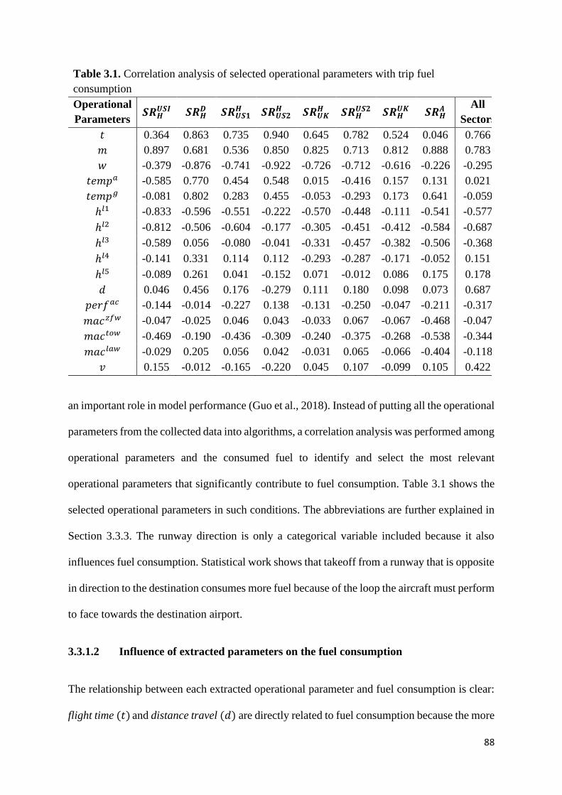
88

an important role in model performance (Guo et al., 2018). Instead of putting all the operational

parameters from the collected data into algorithms, a correlation analysis was performed among

operational parameters and the consumed fuel to identify and select the most relevant

operational parameters that significantly contribute to fuel consumption. Table 3.1 shows the

selected operational parameters in such conditions. The abbreviations are further explained in

Section 3.3.3. The runway direction is only a categorical variable included because it also

influences fuel consumption. Statistical work shows that takeoff from a runway that is opposite

in direction to the destination consumes more fuel because of the loop the aircraft must perform

to face towards the destination airport.

3.3.1.2 Influence of extracted parameters on the fuel consumption

The relationship between each extracted operational parameter and fuel consumption is clear:

flight time (𝑡) and distance travel (𝑑) are directly related to fuel consumption because the more

Table 3.1. Correlation analysis of selected operational parameters with trip fuel

consumption

Operational

Parameters 𝑺𝑹𝑯

𝑼𝑺𝑰 𝑺𝑹𝑯𝑫 𝑺𝑹𝑼𝑺𝟏

𝑯 𝑺𝑹𝑼𝑺𝟐𝑯 𝑺𝑹𝑼𝑲

𝑯 𝑺𝑹𝑯𝑼𝑺𝟐 𝑺𝑹𝑯

𝑼𝑲 𝑺𝑹𝑯𝑨

All

Sectors

𝑡 0.364 0.863 0.735 0.940 0.645 0.782 0.524 0.046 0.766

𝑚 0.897 0.681 0.536 0.850 0.825 0.713 0.812 0.888 0.783

𝑤 -0.379 -0.876 -0.741 -0.922 -0.726 -0.712 -0.616 -0.226 -0.295

𝑡𝑒𝑚𝑝𝑎 -0.585 0.770 0.454 0.548 0.015 -0.416 0.157 0.131 0.021

𝑡𝑒𝑚𝑝𝑔 -0.081 0.802 0.283 0.455 -0.053 -0.293 0.173 0.641 -0.059

ℎ𝑙1 -0.833 -0.596 -0.551 -0.222 -0.570 -0.448 -0.111 -0.541 -0.577

ℎ𝑙2 -0.812 -0.506 -0.604 -0.177 -0.305 -0.451 -0.412 -0.584 -0.687

ℎ𝑙3 -0.589 0.056 -0.080 -0.041 -0.331 -0.457 -0.382 -0.506 -0.368

ℎ𝑙4 -0.141 0.331 0.114 0.112 -0.293 -0.287 -0.171 -0.052 0.151

ℎ𝑙5 -0.089 0.261 0.041 -0.152 0.071 -0.012 0.086 0.175 0.178

𝑑 0.046 0.456 0.176 -0.279 0.111 0.180 0.098 0.073 0.687

𝑝𝑒𝑟𝑓𝑎𝑐 -0.144 -0.014 -0.227 0.138 -0.131 -0.250 -0.047 -0.211 -0.317

𝑚𝑎𝑐𝑧𝑓𝑤 -0.047 -0.025 0.046 0.043 -0.033 0.067 -0.067 -0.468 -0.047

𝑚𝑎𝑐𝑡𝑜𝑤 -0.469 -0.190 -0.436 -0.309 -0.240 -0.375 -0.268 -0.538 -0.344

𝑚𝑎𝑐𝑙𝑎𝑤 -0.029 0.205 0.056 0.042 -0.031 0.065 -0.066 -0.404 -0.118

𝑣 0.155 -0.012 -0.165 -0.220 0.045 0.107 -0.099 0.105 0.422

89

the aircraft is airborne, the more the fuel it will consume. Flight duration and covered distance

significantly contribute to aircraft operational expenses. The cost index (CI) is used to adjust

the speed (𝑣) of aircraft to a trade-off between higher operational expenses or more fuel-saving

(Edwards et al., 2016). The operational expenses can include crew time, leasing rate, plan

maintenance, landing and take-off fees, and ground services. All of them play major roles in

deciding whether to keep the aircraft airborne to make the airline profitable. The CI ranges

from 0 to 999 and is expressed as

𝐶𝐼 =𝐹𝑙𝑦𝑖𝑛𝑔 𝐶𝑜𝑠𝑡

𝐹𝑢𝑒𝑙 𝐶𝑜𝑠𝑡 (3.2)

When fuel is expensive, the CI will be lower, which means a slower speed of the aircraft.

Operating an aircraft at low-speed results in a higher climb rate due to excessive engine thrust

and, simultaneously, it is recommended to fly at a higher altitude to lower fuel consumption.

Similarly, when fuel is cheap, the CI will be higher, and a faster aircraft will operate to be less

airborne to reduce the amount of operational cost at the cost of more consumed fuel. Note that

the CI shortens or lengthens the airborne phase by changing the aircraft speed depending on

fuel prices and operational expenses to cut overall expenses.

The ramp weight (𝑚) can be expressed according to the following combination (Pagoni and

Psaraki-Kalouptsidi, 2017):

𝑚 = 𝑧𝑓𝑤 + 𝑡𝑜𝑓 (3.3)

Zero fuel weight (𝑧𝑓𝑤) is the total weight of an aircraft including crew, passengers, and

unusable fuel, minus the total weight of the usable fuel. During flight operation, the 𝑧𝑓𝑤

remains constant whereas 𝑡𝑜𝑓 weight decreases over time because of its continuous

90

consumption. This reduces the value of 𝑚 for an aircraft and ultimately decreases fuel

consumption over time.

A suitable choice of wind direction (𝑤) has a significant influence on fuel consumption. The

headwind that blows in a direction opposite to the aircraft is more favorable during takeoff and

landing. The aerofoils can generate more lift during takeoff and more induced drag during

landing. Tailwind that blows in the direction of the aircraft flight path is helpful during the

cruise phase as the aircraft travels faster and saves fuel at the same ground speed (Irrgang et

al., 2015). The ground speed is determined by the vector sum of aircraft speed, wind speed,

and direction. Headwind subtracts from the ground speed, while tailwind is added to the ground

speed.

The altitude (ℎ) can be used to assess the aerodynamic performance of an aircraft at certain

atmospheric conditions. Flying at higher altitudes can significantly save fuel consumption

because of less drag (Turgut and Rosen, 2012). Simultaneously, it may face a problem of low-

density air for fuel combustion that may result in more fuel flow to the engine. Therefore, the

altitude is adjusted for a non-standard temperature known as density altitude and can be

expressed as

𝐷𝐴 = 𝑃𝐴 + (118.8 𝑓𝑡/ C𝑜 )(𝑂𝐴𝑇 − 𝐼𝑆𝐴 𝑇𝑒𝑚𝑝) (3.4)

𝑃𝐴 = ℎ + (30𝑓𝑡/𝑚𝑖𝑙𝑙𝑖𝑏𝑎𝑟)(1013𝑚𝑖𝑙𝑙𝑖𝑏𝑎𝑟 − 𝑄𝑁𝐻) (3.5)

where 𝐷𝐴 is the density altitude in feet, 𝑃𝐴 is the pressure altitude in feet, 𝑄𝑁𝐻 is the

atmospheric pressure in millibar, 𝑂𝐴𝑇 is the outside air temperature in degree Celsius, and

𝐼𝑆𝐴 𝑇𝑒𝑚𝑝 is the international standard atmospheric temperature in degree Celsius. Aircrafts

are designed for specific optimal altitude, what minimizes fuel consumption. A change in that

altitude may cause aircrafts to burn more fuel (Diao and Chen, 2018).

91

The weight and balance of aircrafts can be expressed in terms of the percentage of the mean

aerodynamic chord (𝑚𝑎𝑐) (Dancila et al., 2013).

𝑚𝑎𝑐% =

((∑ 𝑤𝑖𝑎𝑖

𝑁𝑖=1 )𝑚 − 𝑙𝑒𝑚𝑎𝑐)

𝑡𝑒𝑚𝑎𝑐 − 𝑙𝑒𝑚𝑎𝑐

(3.6)

where (∑ 𝑤𝑖𝑎𝑖

𝑁𝑖=1 )

𝑚 is defined as the center of gravity (COG) with 𝑤 denoting component weights

and 𝑎 denoting the arm value, defined both as the moment arm (𝑤𝑎). 𝑙𝑒𝑚𝑎𝑐 and 𝑡𝑒𝑚𝑎𝑐 are

the leading-edge mean aerodynamic chord and tail-edge mean aerodynamic chord,

respectively. Improper distribution of aircraft weight may shift its COG forward and may need

more tail lift force for stable flight. The tail force ultimately increases the aircraft angle of

attack, which may cause aircrafts to face more induced drag. Therefore, the aircraft weight

balance (at the center of aircraft) should be maintained at zero fuel weight during takeoff and

landing phases to avoid the generation of excess induced drag and reduce fuel consumption.

The location and direction of the runway have clear effects on fuel consumption (Singh and

Sharma, 2015). Runway directions are identified by a number within the range 1 to 36, which

are magnetic azimuths in decadegrees. A runway number 09 means pointing toward the east

(90°), 18 means pointing toward the south (180°), 27 means pointing toward the west (270°),

and 36 means pointing toward the north (360°). Furthermore, if there is more than one runway

in the same direction, then the location is differentiated with a letter as follows: L for left, C

for a center, and R for right. It is more favorable to take off from a runway that faces the

headwind direction. However, it can also be a source of excess fuel consumption. If that

favorable runway is in the opposite direction to the allocated flight path, the aircraft must take

a loop to head towards the allocated path.

3.3.2 Mathematical and data-driven solution methods

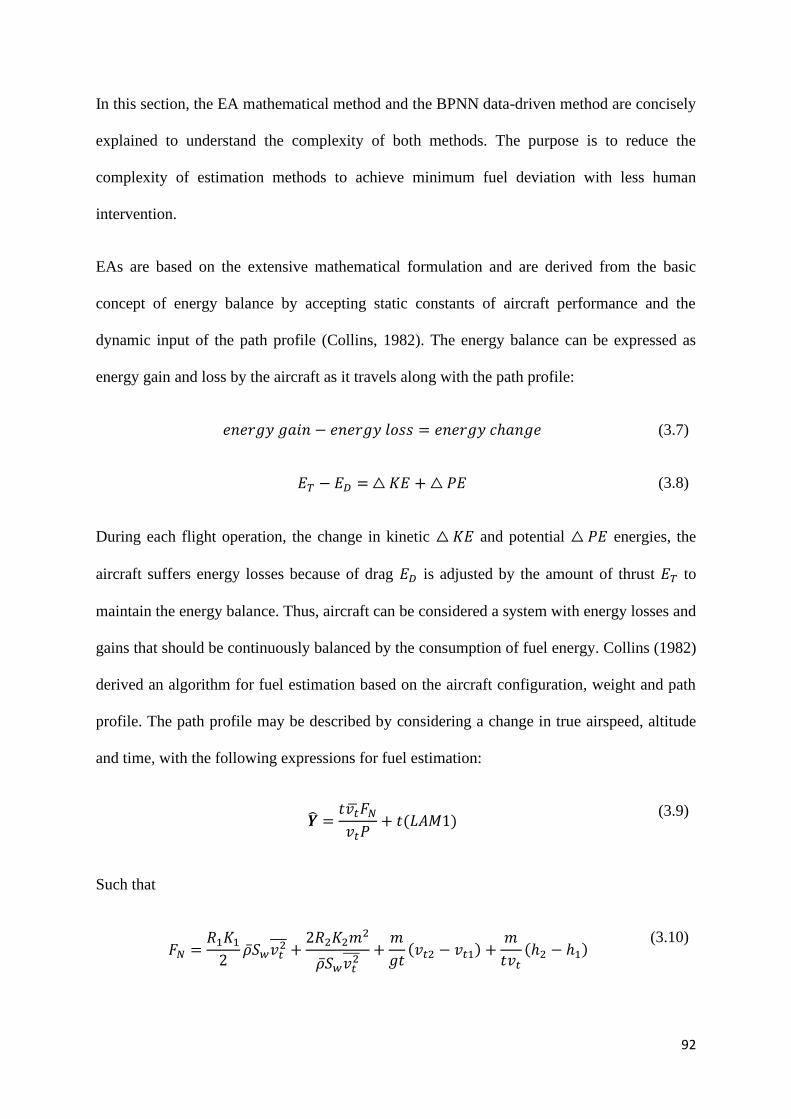
92

In this section, the EA mathematical method and the BPNN data-driven method are concisely

explained to understand the complexity of both methods. The purpose is to reduce the

complexity of estimation methods to achieve minimum fuel deviation with less human

intervention.

EAs are based on the extensive mathematical formulation and are derived from the basic

concept of energy balance by accepting static constants of aircraft performance and the

dynamic input of the path profile (Collins, 1982). The energy balance can be expressed as

energy gain and loss by the aircraft as it travels along with the path profile:

𝑒𝑛𝑒𝑟𝑔𝑦 𝑔𝑎𝑖𝑛 − 𝑒𝑛𝑒𝑟𝑔𝑦 𝑙𝑜𝑠𝑠 = 𝑒𝑛𝑒𝑟𝑔𝑦 𝑐ℎ𝑎𝑛𝑔𝑒 (3.7)

𝐸𝑇 − 𝐸𝐷 = △ 𝐾𝐸 + △ 𝑃𝐸 (3.8)

During each flight operation, the change in kinetic △𝐾𝐸 and potential △ 𝑃𝐸 energies, the

aircraft suffers energy losses because of drag 𝐸𝐷 is adjusted by the amount of thrust 𝐸𝑇 to

maintain the energy balance. Thus, aircraft can be considered a system with energy losses and

gains that should be continuously balanced by the consumption of fuel energy. Collins (1982)

derived an algorithm for fuel estimation based on the aircraft configuration, weight and path

profile. The path profile may be described by considering a change in true airspeed, altitude

and time, with the following expressions for fuel estimation:

�̂� =

𝑡𝑣�̅�𝐹𝑁𝑣𝑡𝑃

+ 𝑡(𝐿𝐴𝑀1) (3.9)

Such that

𝐹𝑁 =

𝑅1𝐾12

�̅�𝑆𝑤𝑣𝑡2̅̅ ̅ +

2𝑅2𝐾2𝑚2

�̅�𝑆𝑤𝑣𝑡2̅̅ ̅+𝑚

𝑔𝑡(𝑣𝑡2 − 𝑣𝑡1) +

𝑚

𝑡𝑣𝑡(ℎ2 − ℎ1)

(3.10)

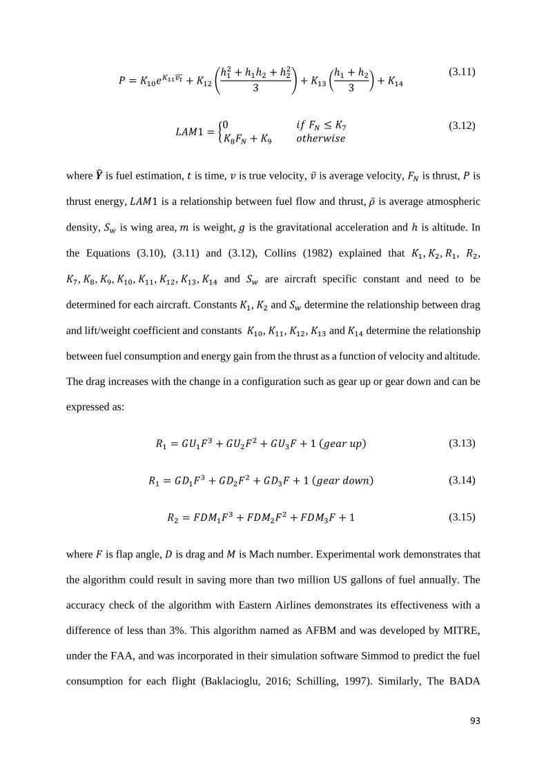
93

𝑃 = 𝐾10𝑒

𝐾11𝑣𝑡̅̅ ̅ + 𝐾12 (ℎ12 + ℎ1ℎ2 + ℎ2

2

3) + 𝐾13 (

ℎ1 + ℎ23

) + 𝐾14 (3.11)

𝐿𝐴𝑀1 = {

0 𝑖𝑓 𝐹𝑁 ≤ 𝐾7𝐾8𝐹𝑁 + 𝐾9 𝑜𝑡ℎ𝑒𝑟𝑤𝑖𝑠𝑒

(3.12)

where �̂� is fuel estimation, 𝑡 is time, 𝑣 is true velocity, �̅� is average velocity, 𝐹𝑁 is thrust, 𝑃 is

thrust energy, 𝐿𝐴𝑀1 is a relationship between fuel flow and thrust, �̅� is average atmospheric

density, 𝑆𝑤 is wing area, 𝑚 is weight, 𝑔 is the gravitational acceleration and ℎ is altitude. In

the Equations (3.10), (3.11) and (3.12), Collins (1982) explained that 𝐾1, 𝐾2, 𝑅1, 𝑅2,

𝐾7, 𝐾8, 𝐾9, 𝐾10, 𝐾11, 𝐾12, 𝐾13, 𝐾14 and 𝑆𝑤 are aircraft specific constant and need to be

determined for each aircraft. Constants 𝐾1, 𝐾2 and 𝑆𝑤 determine the relationship between drag

and lift/weight coefficient and constants 𝐾10, 𝐾11, 𝐾12, 𝐾13 and 𝐾14 determine the relationship

between fuel consumption and energy gain from the thrust as a function of velocity and altitude.

The drag increases with the change in a configuration such as gear up or gear down and can be

expressed as:

𝑅1 = 𝐺𝑈1𝐹3 + 𝐺𝑈2𝐹

2 + 𝐺𝑈3𝐹 + 1 (𝑔𝑒𝑎𝑟 𝑢𝑝) (3.13)

𝑅1 = 𝐺𝐷1𝐹3 + 𝐺𝐷2𝐹

2 + 𝐺𝐷3𝐹 + 1 (𝑔𝑒𝑎𝑟 𝑑𝑜𝑤𝑛) (3.14)

𝑅2 = 𝐹𝐷𝑀1𝐹3 + 𝐹𝐷𝑀2𝐹

2 + 𝐹𝐷𝑀3𝐹 + 1 (3.15)

where 𝐹 is flap angle, 𝐷 is drag and 𝑀 is Mach number. Experimental work demonstrates that

the algorithm could result in saving more than two million US gallons of fuel annually. The

accuracy check of the algorithm with Eastern Airlines demonstrates its effectiveness with a

difference of less than 3%. This algorithm named as AFBM and was developed by MITRE,

under the FAA, and was incorporated in their simulation software Simmod to predict the fuel

consumption for each flight (Baklacioglu, 2016; Schilling, 1997). Similarly, The BADA

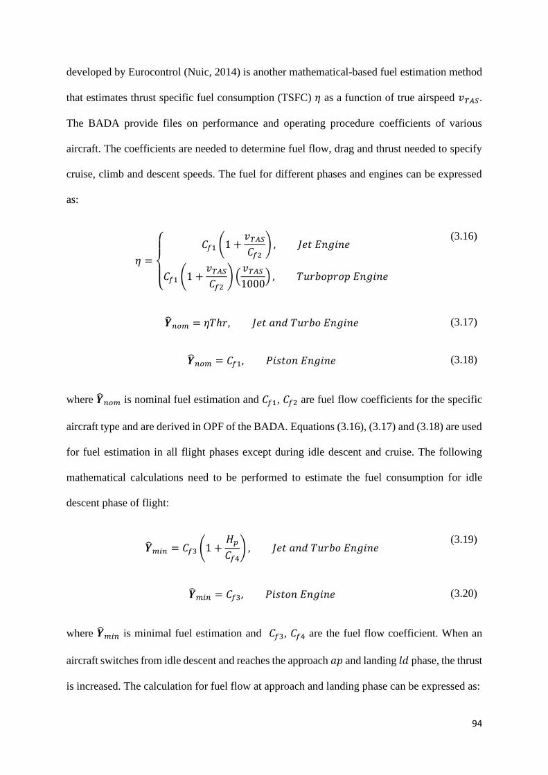
94

developed by Eurocontrol (Nuic, 2014) is another mathematical-based fuel estimation method

that estimates thrust specific fuel consumption (TSFC) 𝜂 as a function of true airspeed 𝑣𝑇𝐴𝑆.

The BADA provide files on performance and operating procedure coefficients of various

aircraft. The coefficients are needed to determine fuel flow, drag and thrust needed to specify

cruise, climb and descent speeds. The fuel for different phases and engines can be expressed

as:

𝜂 =

{

𝐶𝑓1 (1 +

𝑣𝑇𝐴𝑆𝐶𝑓2

) , 𝐽𝑒𝑡 𝐸𝑛𝑔𝑖𝑛𝑒

𝐶𝑓1 (1 +𝑣𝑇𝐴𝑆𝐶𝑓2

) (𝑣𝑇𝐴𝑆1000

) , 𝑇𝑢𝑟𝑏𝑜𝑝𝑟𝑜𝑝 𝐸𝑛𝑔𝑖𝑛𝑒

(3.16)

�̂�𝑛𝑜𝑚 = 𝜂𝑇ℎ𝑟, 𝐽𝑒𝑡 𝑎𝑛𝑑 𝑇𝑢𝑟𝑏𝑜 𝐸𝑛𝑔𝑖𝑛𝑒 (3.17)

�̂�𝑛𝑜𝑚 = 𝐶𝑓1, 𝑃𝑖𝑠𝑡𝑜𝑛 𝐸𝑛𝑔𝑖𝑛𝑒 (3.18)

where �̂�𝑛𝑜𝑚 is nominal fuel estimation and 𝐶𝑓1, 𝐶𝑓2 are fuel flow coefficients for the specific

aircraft type and are derived in OPF of the BADA. Equations (3.16), (3.17) and (3.18) are used

for fuel estimation in all flight phases except during idle descent and cruise. The following

mathematical calculations need to be performed to estimate the fuel consumption for idle

descent phase of flight:

�̂�𝑚𝑖𝑛 = 𝐶𝑓3 (1 +

𝐻𝑝

𝐶𝑓4) , 𝐽𝑒𝑡 𝑎𝑛𝑑 𝑇𝑢𝑟𝑏𝑜 𝐸𝑛𝑔𝑖𝑛𝑒

(3.19)

�̂�𝑚𝑖𝑛 = 𝐶𝑓3, 𝑃𝑖𝑠𝑡𝑜𝑛 𝐸𝑛𝑔𝑖𝑛𝑒 (3.20)

where �̂�𝑚𝑖𝑛 is minimal fuel estimation and 𝐶𝑓3, 𝐶𝑓4 are the fuel flow coefficient. When an

aircraft switches from idle descent and reaches the approach 𝑎𝑝 and landing 𝑙𝑑 phase, the thrust

is increased. The calculation for fuel flow at approach and landing phase can be expressed as:

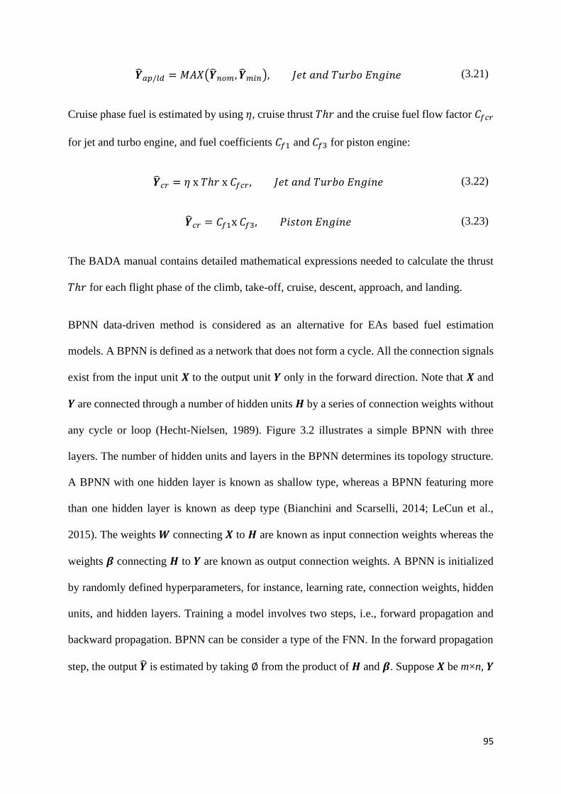
95

�̂�𝑎𝑝/𝑙𝑑 = 𝑀𝐴𝑋(�̂�𝑛𝑜𝑚, �̂�𝑚𝑖𝑛), 𝐽𝑒𝑡 𝑎𝑛𝑑 𝑇𝑢𝑟𝑏𝑜 𝐸𝑛𝑔𝑖𝑛𝑒 (3.21)

Cruise phase fuel is estimated by using 𝜂, cruise thrust 𝑇ℎ𝑟 and the cruise fuel flow factor 𝐶𝑓𝑐𝑟

for jet and turbo engine, and fuel coefficients 𝐶𝑓1 and 𝐶𝑓3 for piston engine:

�̂�𝑐𝑟 = 𝜂 x 𝑇ℎ𝑟 x 𝐶𝑓𝑐𝑟, 𝐽𝑒𝑡 𝑎𝑛𝑑 𝑇𝑢𝑟𝑏𝑜 𝐸𝑛𝑔𝑖𝑛𝑒 (3.22)

�̂�𝑐𝑟 = 𝐶𝑓1x 𝐶𝑓3, 𝑃𝑖𝑠𝑡𝑜𝑛 𝐸𝑛𝑔𝑖𝑛𝑒 (3.23)

The BADA manual contains detailed mathematical expressions needed to calculate the thrust

𝑇ℎ𝑟 for each flight phase of the climb, take-off, cruise, descent, approach, and landing.

BPNN data-driven method is considered as an alternative for EAs based fuel estimation

models. A BPNN is defined as a network that does not form a cycle. All the connection signals

exist from the input unit 𝑿 to the output unit 𝒀 only in the forward direction. Note that 𝑿 and

𝒀 are connected through a number of hidden units 𝑯 by a series of connection weights without

any cycle or loop (Hecht-Nielsen, 1989). Figure 3.2 illustrates a simple BPNN with three

layers. The number of hidden units and layers in the BPNN determines its topology structure.

A BPNN with one hidden layer is known as shallow type, whereas a BPNN featuring more

than one hidden layer is known as deep type (Bianchini and Scarselli, 2014; LeCun et al.,

2015). The weights 𝑾 connecting 𝑿 to 𝑯 are known as input connection weights whereas the

weights 𝜷 connecting 𝑯 to 𝒀 are known as output connection weights. A BPNN is initialized

by randomly defined hyperparameters, for instance, learning rate, connection weights, hidden

units, and hidden layers. Training a model involves two steps, i.e., forward propagation and

backward propagation. BPNN can be consider a type of the FNN. In the forward propagation

step, the output �̂� is estimated by taking ∅ from the product of 𝑯 and 𝜷. Suppose 𝑿 be m×n, 𝒀

96

be m×q, 𝑯 be m×r, 𝑾𝒊𝒄𝒘 be n×r, and 𝑾𝒐𝒄𝒘 be r×q matrices. The estimation of output �̂� can

be expressed as:

�̂� = ∅(𝑯𝑾𝒐𝒄𝒘) (3.24)

where

𝑯 = ∅(𝑿𝑾𝒊𝒄𝒘 + 𝑏). (3.25)

The objective function is the sum-of-squares error (SSE):

𝑆𝑆𝐸 = 𝐸 =∑(�̂�𝑖 − 𝒀𝑖)2

𝑚

𝑖=1

(3.26)

If 𝐸 < 𝜀, where 𝜀 is the predefined target error, the algorithm stops. Otherwise, a

backpropagation (BP) iterative learning algorithm is applied in the backward propagation step

to train the model. The BP learning algorithm works on either first-order or second-order

gradient information. In its simplest form, for a first-order derivative, the gradient error E with

respect to the connection weights can be calculated by the chain rule:

Figure 3.2. BPNN learning algorithm network

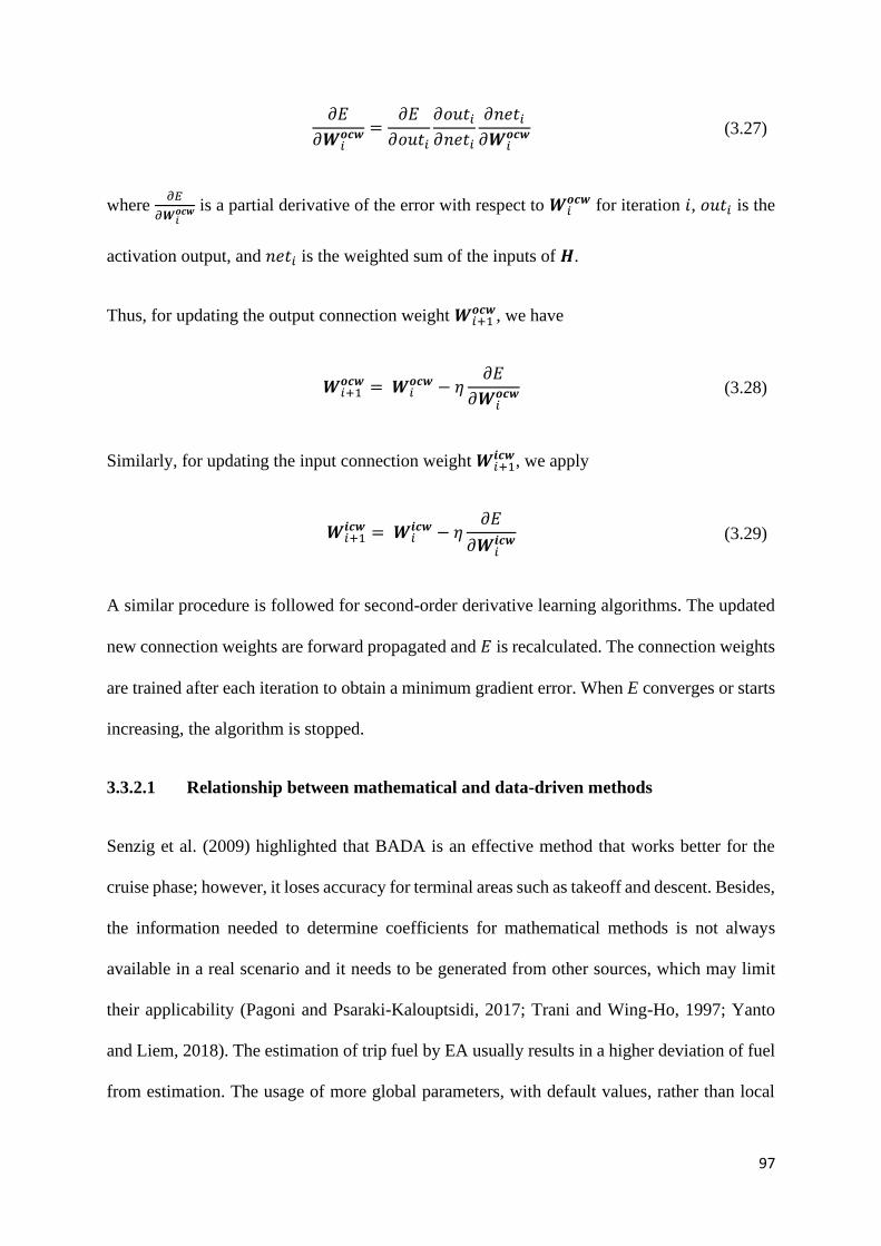
97

𝜕𝐸

𝜕𝑾𝑖𝒐𝒄𝒘 =

𝜕𝐸

𝜕𝑜𝑢𝑡𝑖

𝜕𝑜𝑢𝑡𝑖𝜕𝑛𝑒𝑡𝑖

𝜕𝑛𝑒𝑡𝑖𝜕𝑾𝑖

𝒐𝒄𝒘 (3.27)

where 𝜕𝐸

𝜕𝑾𝑖𝒐𝒄𝒘 is a partial derivative of the error with respect to 𝑾𝑖

𝒐𝒄𝒘 for iteration 𝑖, 𝑜𝑢𝑡𝑖 is the

activation output, and 𝑛𝑒𝑡𝑖 is the weighted sum of the inputs of 𝑯.

Thus, for updating the output connection weight 𝑾𝑖+1𝒐𝒄𝒘, we have

𝑾𝑖+1𝒐𝒄𝒘 = 𝑾𝑖

𝒐𝒄𝒘 − 𝜂𝜕𝐸

𝜕𝑾𝑖𝒐𝒄𝒘 (3.28)

Similarly, for updating the input connection weight 𝑾𝑖+1𝒊𝒄𝒘, we apply

𝑾𝑖+1𝒊𝒄𝒘 = 𝑾𝑖

𝒊𝒄𝒘 − 𝜂𝜕𝐸

𝜕𝑾𝑖𝒊𝒄𝒘

(3.29)

A similar procedure is followed for second-order derivative learning algorithms. The updated

new connection weights are forward propagated and 𝐸 is recalculated. The connection weights

are trained after each iteration to obtain a minimum gradient error. When E converges or starts

increasing, the algorithm is stopped.

3.3.2.1 Relationship between mathematical and data-driven methods

Senzig et al. (2009) highlighted that BADA is an effective method that works better for the

cruise phase; however, it loses accuracy for terminal areas such as takeoff and descent. Besides,

the information needed to determine coefficients for mathematical methods is not always

available in a real scenario and it needs to be generated from other sources, which may limit

their applicability (Pagoni and Psaraki-Kalouptsidi, 2017; Trani and Wing-Ho, 1997; Yanto

and Liem, 2018). The estimation of trip fuel by EA usually results in a higher deviation of fuel

from estimation. The usage of more global parameters, with default values, rather than local

98

parameters and complex mathematical calculation requiring information about many

coefficient results in the suboptimal estimation of fuel. BPNN has gained much popularity in

estimating fuel consumption and its usage may overcome EA limitations to some extents,

however, it has certain problems that can influence its generalization performance and learning

speed causing higher fuel deviation (Huang, Zhu, et al., 2006; Srivastava et al., 2014). The

major drawbacks are:

1. being trapped in a local minimum when the global minimum is far away

2. facing a problem of saddle point

3. the convergence decreases at plateau surface

4. network performance is affected by hyperparameter initialization and adjustment

5. needs trial and error approaches and expert involvement

6. repeatedly tuning of connection weights

7. hidden units and layers adjustments.

In addition to the drawbacks mentioned above, the following human expertise significantly

affects the fuel estimation results of BPNNs:

1. What should be the network size and depth i.e. shallow or deep?

2. How many hidden units should be generated by each hidden layer?

3. How many hidden layers will be sufficient for deep learning?

4. What should be network initial connection weights and learning rate?

5. How should the hyperparameters be adjusted?

6. What should be the size of the dataset during network training?

7. Which learning algorithm should be implemented?

8. Which network topology is more efficient i.e. fixed or cascade?

99

9. What should be the criteria for increasing or decreasing the global and local

hyperparameters?

10. What type of activation function should be used in hidden units?

The relationship between mathematical and data-driven methods is illustrated in Table 3.2. The

drawbacks and user expertise of both EA and BPNN need to be addressed by proposing an

efficient machine learning algorithm that having characteristics of better generalization

performance and learning speed.

Table 3.2. Relationship between the mathematical method and data-driven method

Description EA mathematical method BPNN data-driven method

Approach A mathematical formulation of the

model.

Input operational parameters and

output labels for the network.

Information

source

A lot of flight testing need to

perform to generate information and

calculate parameters such as engine

constants, airspeed, aircraft mass,

atmospheric density, extra thrust

needed for ascending, and wing

area, etc.

Ability to extract information from

historical data.

Performance Performance increases by

incorporating local parameters

rather than global parameters.

Prediction performance increases

with the high dimensional dataset.

Expertise Human expertise having deep

domain knowledge and

understanding of mathematical

formulation are favorable.

A lot of human intervention is needed

to define hyperparameters and select

optimal fixed topology. Training is a

challenging phase.

Suitability More suitable for estimating fuel for

the cruise phase rather than terminal

areas such as take-off and descent

phase.

Performance depends upon the

information in historical data.

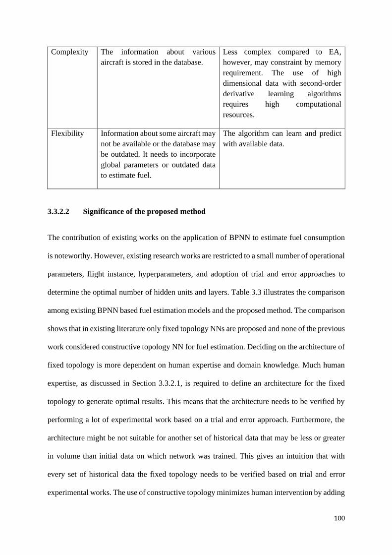
100

Complexity The information about various

aircraft is stored in the database.

Less complex compared to EA,

however, may constraint by memory

requirement. The use of high

dimensional data with second-order

derivative learning algorithms

requires high computational

resources.

Flexibility Information about some aircraft may

not be available or the database may

be outdated. It needs to incorporate

global parameters or outdated data

to estimate fuel.

The algorithm can learn and predict

with available data.

3.3.2.2 Significance of the proposed method

The contribution of existing works on the application of BPNN to estimate fuel consumption

is noteworthy. However, existing research works are restricted to a small number of operational

parameters, flight instance, hyperparameters, and adoption of trial and error approaches to

determine the optimal number of hidden units and layers. Table 3.3 illustrates the comparison

among existing BPNN based fuel estimation models and the proposed method. The comparison

shows that in existing literature only fixed topology NNs are proposed and none of the previous

work considered constructive topology NN for fuel estimation. Deciding on the architecture of

fixed topology is more dependent on human expertise and domain knowledge. Much human

expertise, as discussed in Section 3.3.2.1, is required to define an architecture for the fixed

topology to generate optimal results. This means that the architecture needs to be verified by

performing a lot of experimental work based on a trial and error approach. Furthermore, the

architecture might be not suitable for another set of historical data that may be less or greater

in volume than initial data on which network was trained. This gives an intuition that with

every set of historical data the fixed topology needs to be verified based on trial and error

experimental works. The use of constructive topology minimizes human intervention by adding

101

hidden units at each hidden layer and the process continues until error convergence. This makes

CNN more like deep learning having multiple hidden units and hidden layers in the network.

Unlike fixed topology, CNN advantageous in that it is not affected by the change in the

historical data set. For historical data that may be less or greater than initial data, the CNN

network gets to learn in smaller or larger sizes respectively.

It should be noted that low-level operational parameters, e.g. altitude, speed, and weight, are

commonly used for estimation in existing BPNN models and many other important operational

parameters are ignored that have a significant effect on fuel consumption. The importance of

operational parameters in estimating fuel consumption cannot disagree. Machine learning

algorithms depend on historical data and incorporating operational parameters that contribute

to fuel consumption can improve the generalization performance of the network. Studying low

operational parameters in existing works is because of low generalization performance and

slower convergence of BPNN with a lot of expertise needed to define hyperparameters. To

address this issue, the present work incorporates high-level operational parameters in the

proposed method that have a significant effect on fuel consumption.

Another important point that strengthens this work is that we considered high dimensional data

covering large fleet and various sectors to estimate fuel for all phases collectively. The flights

performed by various aircraft in same or different sector assists to generate data covering

different geographical regions. Studying a single aircraft or single sector may make it difficult

for NNs to capture the varying behavior of the operational parameters. For instance, if aircraft-

A is used for sector-A, then the network learned might be unsuitable to predict fuel for sector-

B using the same aircraft. The sector-A geographical conditions might be different from sector-

B. Similarly, if sector-A use aircraft-A, then the network learned might be unsuitable for

102

aircraft-B. The performance of aircraft-A might be different from aircraft-B. One may be newer

or older than another.

The existing methods for fuel estimation are proposed depending on some constraint

conditions. The constraints include proposing methodologies for either take-off, climb, cruise

or descent flight phases with limited data, aircraft types and inadequate consideration of

different sectors. Taking the cumulative effect of distinct flight phases may result in even

higher fuel deviation. In the proposed model, distinct flight phases are considered as one

complete trip. The fuel is estimated for all-sectors and individual sectors to understand the

effect of operational parameters and their varying behavior on fuel consumption.

Table 3.3. Relationship among existing BPNN-based fuel estimation models and the

proposed method

Dataset

Description

(Schilling, 1997) (Trani et al.,

2004)

(Baklacioglu,

2016)

Proposed Work

Methodology Backpropagation

Levenberg

Marquart Neural

Network

Backpropagation

Levenberg

Marquart Neural

Network

Genetic

algorithm

optimized

neural

network

Novel CNN

proposed in

Chapter-4

Operational

Parameters

Altitude, Speed Mach number,

Altitude,

Weight,

Temperature

Altitude,

True Air

Speed

Flight Time,

Weight, Wind,

Temperature

Deviation at the air,

Temperature

Deviation at the

ground, Altitude

(1st level), Altitude

(2nd Level),

Altitude (3rd

Level), Altitude

(4th Level),

Altitude (5th

Level), Distance,

Aircraft

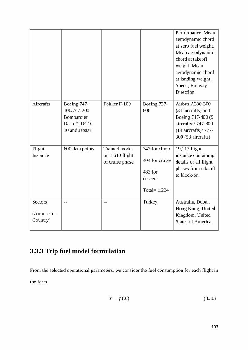
103

Performance, Mean

aerodynamic chord

at zero fuel weight,

Mean aerodynamic

chord at takeoff

weight, Mean

aerodynamic chord

at landing weight,

Speed, Runway

Direction

Aircrafts Boeing 747-

100/767-200,

Bombardier

Dash-7, DC10-

30 and Jetstar

Fokker F-100 Boeing 737-

800

Airbus A330-300

(31 aircrafts) and

Boeing 747-400 (9

aircrafts)/ 747-800

(14 aircrafts)/ 777-

300 (53 aircrafts)

Flight

Instance

600 data points Trained model

on 1,610 flight

of cruise phase

347 for climb

404 for cruise

483 for

descent

Total= 1,234

19,117 flight

instance containing

details of all flight

phases from takeoff

to block-on.

Sectors

(Airports in

Country)

-- -- Turkey Australia, Dubai,

Hong Kong, United

Kingdom, United

States of America

3.3.3 Trip fuel model formulation

From the selected operational parameters, we consider the fuel consumption for each flight in

the form

𝒀 = 𝑓(𝑿) (3.30)

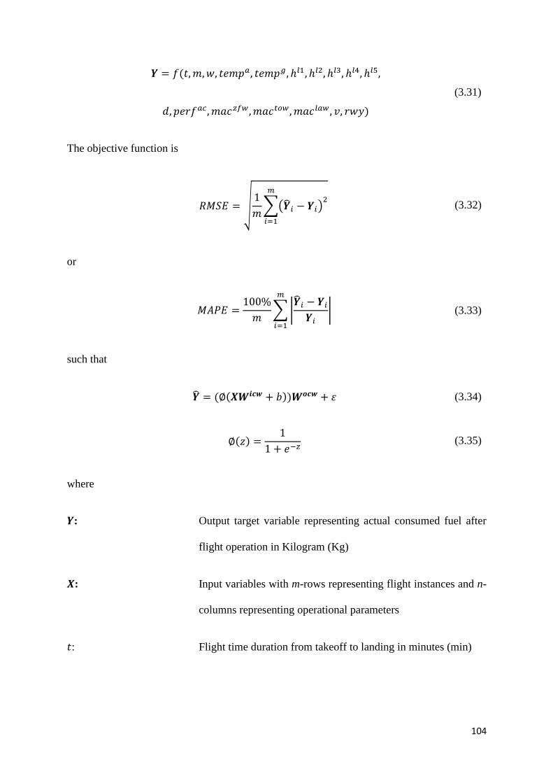
104

𝒀 = 𝑓(𝑡,𝑚,𝑤, 𝑡𝑒𝑚𝑝𝑎, 𝑡𝑒𝑚𝑝𝑔, ℎ𝑙1, ℎ𝑙2, ℎ𝑙3, ℎ𝑙4, ℎ𝑙5,

𝑑, 𝑝𝑒𝑟𝑓𝑎𝑐, 𝑚𝑎𝑐𝑧𝑓𝑤,𝑚𝑎𝑐𝑡𝑜𝑤, 𝑚𝑎𝑐𝑙𝑎𝑤, 𝑣, 𝑟𝑤𝑦)

(3.31)

The objective function is

𝑅𝑀𝑆𝐸 = √1

𝑚∑(�̂�𝑖 − 𝒀𝑖)

2𝑚

𝑖=1

(3.32)

or

𝑀𝐴𝑃𝐸 =100%

𝑚∑|

�̂�𝑖 − 𝒀𝑖𝒀𝑖

|

𝑚

𝑖=1

(3.33)

such that

�̂� = (∅(𝑿𝑾𝒊𝒄𝒘 + 𝑏))𝑾𝒐𝒄𝒘 + 𝜀 (3.34)

∅(𝑧) =1

1 + 𝑒−𝑧 (3.35)

where

𝒀: Output target variable representing actual consumed fuel after

flight operation in Kilogram (Kg)

𝑿: Input variables with m-rows representing flight instances and n-

columns representing operational parameters

𝑡: Flight time duration from takeoff to landing in minutes (min)

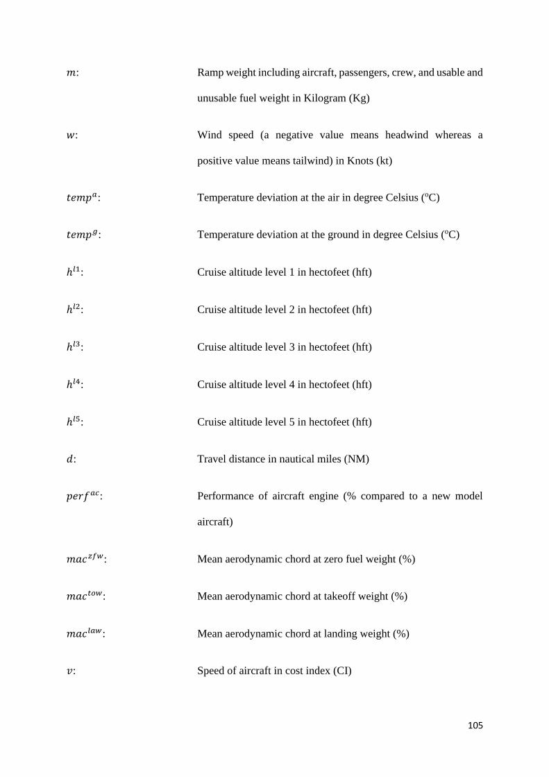
105

𝑚: Ramp weight including aircraft, passengers, crew, and usable and

unusable fuel weight in Kilogram (Kg)

𝑤: Wind speed (a negative value means headwind whereas a

positive value means tailwind) in Knots (kt)

𝑡𝑒𝑚𝑝𝑎: Temperature deviation at the air in degree Celsius (oC)

𝑡𝑒𝑚𝑝𝑔: Temperature deviation at the ground in degree Celsius (oC)

ℎ𝑙1: Cruise altitude level 1 in hectofeet (hft)

ℎ𝑙2: Cruise altitude level 2 in hectofeet (hft)

ℎ𝑙3: Cruise altitude level 3 in hectofeet (hft)

ℎ𝑙4: Cruise altitude level 4 in hectofeet (hft)

ℎ𝑙5: Cruise altitude level 5 in hectofeet (hft)

𝑑: Travel distance in nautical miles (NM)

𝑝𝑒𝑟𝑓𝑎𝑐: Performance of aircraft engine (% compared to a new model

aircraft)

𝑚𝑎𝑐𝑧𝑓𝑤: Mean aerodynamic chord at zero fuel weight (%)

𝑚𝑎𝑐𝑡𝑜𝑤: Mean aerodynamic chord at takeoff weight (%)

𝑚𝑎𝑐𝑙𝑎𝑤: Mean aerodynamic chord at landing weight (%)

𝑣: Speed of aircraft in cost index (CI)

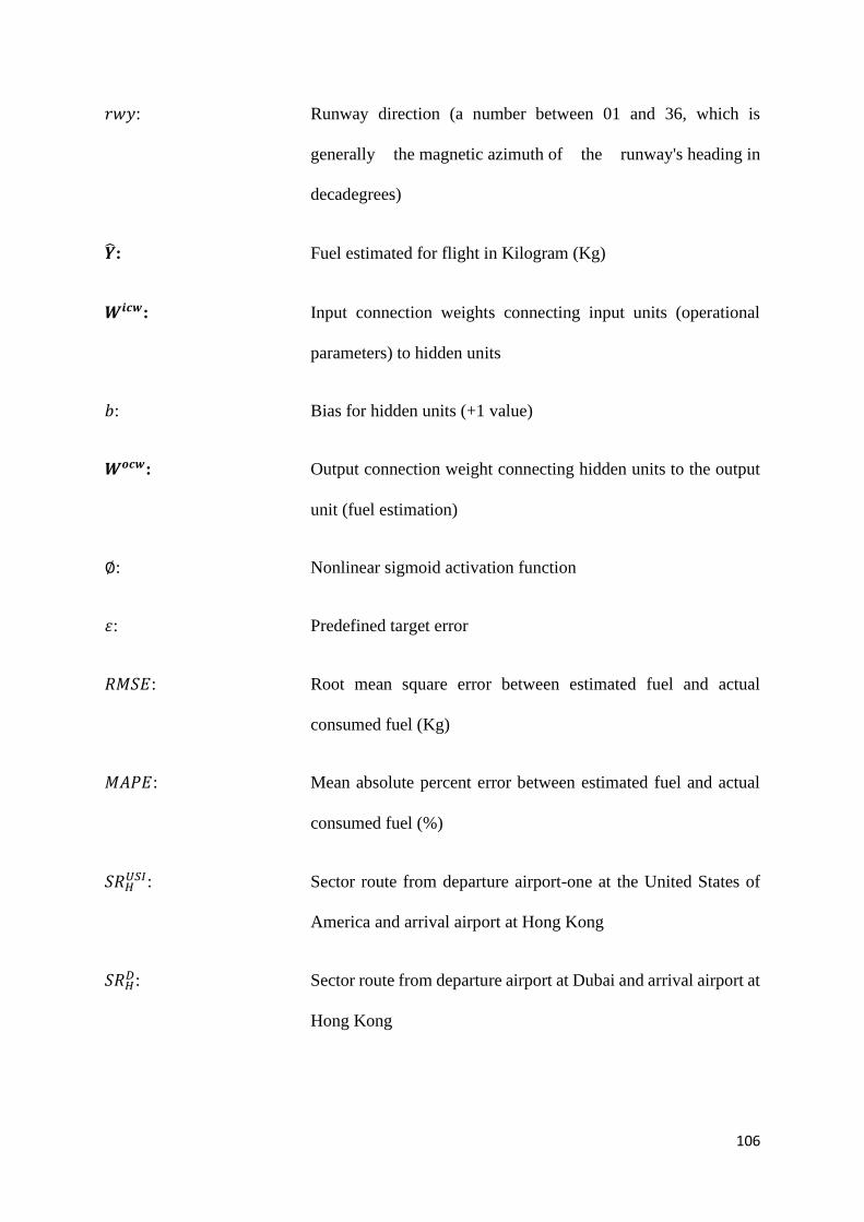
106

𝑟𝑤𝑦: Runway direction (a number between 01 and 36, which is

generally the magnetic azimuth of the runway's heading in

decadegrees)

�̂�: Fuel estimated for flight in Kilogram (Kg)

𝑾𝒊𝒄𝒘: Input connection weights connecting input units (operational

parameters) to hidden units

𝑏: Bias for hidden units (+1 value)

𝑾𝒐𝒄𝒘: Output connection weight connecting hidden units to the output

unit (fuel estimation)

∅: Nonlinear sigmoid activation function

𝜀: Predefined target error

𝑅𝑀𝑆𝐸: Root mean square error between estimated fuel and actual

consumed fuel (Kg)

𝑀𝐴𝑃𝐸: Mean absolute percent error between estimated fuel and actual

consumed fuel (%)

𝑆𝑅𝐻𝑈𝑆𝐼: Sector route from departure airport-one at the United States of

America and arrival airport at Hong Kong

𝑆𝑅𝐻𝐷: Sector route from departure airport at Dubai and arrival airport at

Hong Kong

107

𝑆𝑅𝑈𝑆1𝐻 : Sector route from departure airport at Hong Kong and arrival

airport-one at the United States of America

𝑆𝑅𝑈𝑆2𝐻 : Sector route from departure airport at Hong Kong and arrival

airport-two at the United States of America

𝑆𝑅𝑈𝐾𝐻 : Sector route from departure airport at Hong Kong and arrival

airport at the United Kingdom

𝑆𝑅𝐻𝑈𝑆2: Sector route from departure airport-two at United States of

America and arrival airport at Hong Kong

𝑆𝑅𝐻𝑈𝐾: Sector route from departure airport at the United Kingdom and

arrival airport at Hong Kong

𝑆𝑅𝐻𝐴: Sector route from departure airport at Australia and arrival airport

at Hong Kong

The objective functions (3.32) or (3.33) correspond to fuel deviation and their purpose is to

achieve the smallest deviation by estimating a value of �̂� that approximately represents 𝒀. The

RMSE objective function (3.32) measures the performance of the estimation method by

determining the difference between the estimated �̂� and the actual consumed 𝒀. The

measurement scale is identical to that of 𝒀. The RMSE tends to give more importance to a

higher deviation by computing its square error. Actually, this is a more useful metric for

comparison given that a higher deviation is undesirable. The MAPE objective function (3.33)

measures the performance in percentage accuracy by determining the absolute difference

between the estimated �̂� and actual consumed 𝒀. The percentage accuracy helps to make a

more informed decision by comparing the deviation of the estimation methods on an absolute

108

scale. In the NN, the value of �̂�, as shown in Equation (3.34), can be estimated by determining

coefficients of connection weights 𝑾𝒊𝒄𝒘 and 𝑾𝒐𝒄𝒘. Hidden units can be generated in-between

connection weights by using a nonlinear sigmoid activation function ∅ , as shown in Equation

(3.35), to truly approximate 𝒀 from 𝑿.

3.4 Summary

In this chapter, we explained the framework of fuel consumption and its deviation from the

estimation, extracted complex high-level operational parameters that contribute to fuel

estimation and explained their relationship, and formulated a model with an objective function

to minimize a fuel deviation. The trip fuel deviation arises from the overestimation or

underestimation of fuel because of less confidence in existing estimation techniques and

ignoring some of the operational parameters that may contribute to fuel consumption.

Overestimation increases the weight of an aircraft and hence more fuel is needed to balance

thrust and drag. Underestimation may create a safety issue by utilizing some of the fuel reserved

in supplementary reservoirs that may be needed for other purposes or emergency landing.

The two methods used to estimate fuel consumption for aircraft, known as a mathematical

method and data-driven method, are explained. The mathematical methods are helpful in

physical understanding of the system; however, it is equally challenging to practice. It is

difficult to apply because information about aircraft is not always available and needs expert

knowledge. The EA mathematical methods are best suitable for cruise phases and loss accuracy

for the terminal areas. There are separate mathematical equations for estimating fuel

consumption for each distinct flight phase which needed a lot of flight testing to generate

information about parameters. Some of the information about aircraft such as engine design,

wing area, aerodynamic properties, thrust needed, etc and the situation at arrival or departure

109

airport such as atmospheric condition may not be available in a real scenario and need to apply

global parameters with default values rather than local parameters.

Compared to the mathematical method, data-driven methods are generally favorable because

of their ability to learn from historical data. Among various machine learning data-driven

methods, NNs are more popular because of their universal approximation ability. The

prediction performance of BPNNs is highly dependent on the dataset and hyperparameter

initialization and adjustment. This involves human intervention by doing a lot of trial and error

experimental work which makes the training phase a challenging task to accomplish. In some

cases, the use of second-order learning algorithms, which are considered better than first-order

learning algorithms, is selected for training. The second-order learning algorithms are

constraints by memory requirement. This demand for more computational resources when high

dimensional data is available.

Existing work on the application of BPNN to estimate fuel consumption for aircraft is limited

in scope. The work covered the small number of aircraft with limited flight data and operational

parameters with a future recommendation of incorporating high-level operational parameters.

The main reason for this is weak generalization performance and slow convergence of BPNN

with the need for human intervention to decide and adjust hyperparameters.

The limitation needs to be addressed more innovatively by proposing an algorithm that has

cascade architecture and able to calculate connection weights analytically. The cascade

architecture of CNN helps to generate hidden units in hidden layers until error convergence.

This makes it work like deep learning with a less human intervention needed. The objective of

reaching a destination with less fuel deviation is an important research topic to ensure

profitability and safety. A model is formulated, to overcome existing limitations and

complexity, with the objective to minimize fuel deviation by estimating fuel for each flight that

110

may truly approximate actual fuel consumed. The model incorporates extracted operational

parameters to estimate the fuel, and calculate the difference from actual fuel consumed to

measure the fuel deviation.

111

Chapter 4. A Novel Self-Organizing Constructive Neural

Network Algorithm

4.1 Introduction

NNs following the universal approximation theorem may map any complex nonlinear function

more accurately compared to other statistical parametric methods (Ferrari and Stengel, 2005;

Hornik et al., 1989; Kumar et al., 1995). The rapidly growing interest in NNs (Au et al., 2008;

Lin and Vlachos, 2018; Ruiz-Aguilar et al., 2014), and particularly in CNNs (Chung et al.,

2017), motivates the study of their application to the airline sector. CNNs are considered to be

more powerful compared to standard fixed NNs (Hunter et al., 2012; Wilamowski et al., 2008).

The major drawbacks of BPNNs limiting their applicability are their weak generalization

performance and learning speed. The generalization performance is weak in the sense that it

may stop at local minima of the function if global minima are far away. The learning speed

(also known as convergence rate) is slow and dependent on the learning rate and BP learning

algorithms. When the learning rate is small, it converges slowly, and when the learning rate is

large, it becomes unstable. The BP learning can be considered time-consuming because of the

repetitive tuning of the connection weights in forward and backward steps with other

hyperparameters (Huang, Zhu, et al., 2006). This may create a complex co-adaptation among

the parameters and hidden units that demands further attention in regularization (Srivastava et

al., 2014). Moreover, with respect to the drawbacks mentioned above, the human expertise of

defining the structure of the network based on trial and errors significantly affects the

generalization performance and learning speed of BPNNs.

The drawbacks and expertise issues need to be solved in a more innovative way to improve

generalization performance and learning speed. To overcome the above limitations, we propose

112

a self-organizing cascade topology-based CNN capable of analytically calculating connection

weights and requiring less expertise by eliminating the need for complex hyperparameter

initialization and adjustment. The objective is to improve the performance of the estimation

model with less expertise involvement and obtain results with fast learning speed. Inspired

from the gradient-free learning algorithms (Chapter 2, Subsection 2.2.3.2) having the property

of calculating analytically output connection weights and constructive topology FNN (Chapter

2, Subsection 2.2.4.3) have the property of adding hidden units in the hidden layer, this work

proposes new algorithm. The novel algorithm may also assist in overcoming the exiting FNNs

research gaps identified in Chapter 2.

The rest of the Chapter is organized as follows. Section 4.2 discusses CasCor and its extension

with convergence limitations. Section 4.3 briefly explains existing orthogonal linear

transformation and ordinary least squares methodologies. In Section 4.4, we propose a novel

CNN. Section 4.5 is about experimental work to demonstrate the performance of proposed

CNN on artificial and real-world problems. Section 4.6 summarizes the chapter.

4.2 Convergence limitations of CasCor and its extensions

To address the learning issues of BPNNs, the so-called cascade correlation learning algorithm

(CasCor) was proposed to add hidden units sequentially to the network (Fahlman and Lebiere,

1990). CasCor begins with the minimal network by linearly connecting 𝑿 to 𝒀 through

randomly generated 𝑾𝒐𝒄𝒘. The values of 𝑾𝒐𝒄𝒘 are iteratively tuned (or trained) by the QP

learning algorithm to minimize 𝐸. When training converges and 𝐸 is greater than 𝜀, it adds

𝑯𝒌 (𝑘 = 1,2, … . , 𝑙) one at a time to the network, which receives randomly generated 𝑾𝒊𝒄𝒘

from all 𝑿 and any pre-existing 𝑯𝒌−𝟏. The 𝑯𝒌 is not yet connected to 𝒀. The values of 𝑾𝒊𝒄𝒘

are iteratively tuned to maximize the covariance objective function between 𝑯𝒌 and 𝐸. When

113

the covariance objective function converges, 𝑯𝒌 is added to 𝒀 by freezing 𝑾𝒊𝒄𝒘, and 𝑾𝒐𝒄𝒘 is

once again iteratively tuned by QP. This process continues and finally stops when 𝐸 converges

or starts increasing. The QP quickly reaches the loss function by taking a much larger step

rather than infinitesimal steps (Fahlman, 1988). The advantage of CasCor over fixed-topology

BPNNs is that it can learn complex tasks more quickly as well as determine its own network

topology. In addition, it is economical and has no underfitting issue. The network of CasCor is

illustrated in Figure 4.1.

The growing applications of CNN-based algorithms concluded that CasCor learning speed is

better than that of BPNNs, but its generalization performance might be not optimal. Hwang et

al. (1996) and Lehtokangas (2000) highlighted that CasCor works better with classification

tasks compared to regression tasks and this may make it unsuitable for some applications. Liang

and Dai (1998) made an effort to improve the generalization performance of CasCor on

classification problems by using a genetic algorithm, at the additional cost of requiring more

training time. Kovalishyn et al. (1998) studied the application of CasCor on the quantitative

structural activity relationship and did not achieve any dramatic increase in performance

compared to BPNNs. The reasons may be (i) the chaotic behavior and numerical instability of

the iterative QP learning algorithm and (ii) no guarantee of maximum error reduction by the

covariance objective function when a new hidden unit is added.

Firstly, QP during iterative tuning takes a much larger step to move towards the loss function

based on information of past and current gradient. If the current gradient is in the opposite

direction from the past gradient, the QP may cross the minimum of the loss function and moves

towards the opposite direction of the valley, from where it needs to come back (Fahlman, 1988).

This may cause the QP to act chaotically across the minimum valley of the loss function.

Banerjee et al. (2011) explained that QP becomes numerically unstable if the current iteration

114

gradient becomes closer or equal to the previous iteration gradient. In such a case, the weight

difference will become zero and the QP formula will remain zero even if the gradient changes.

Secondly, Huang et al. (2012) argued that the CasCor covariance objective function may not

guarantee a maximum error reduction when a new hidden unit is added. In addition, the

repeatedly iterating tuning of 𝑾𝒐𝒄𝒘 can be more time-consuming. They proposed OLSCN by

reformulating the objective function based on ordinary least squares for the training of 𝑾𝒊𝒄𝒘,

which needs to be further optimized by the second-order Newton’s method. Qiao et al. (2016)

explained that updating weights by Newton’s method may cause OLSCN to converge at a local

minimum with an increase in computational burden. They proposed FCNN to add a

contribution to the CNN. The FCNN works by selecting linearly independent instances of 𝑿

by the Gram–Schmidt orthogonalization method and a hidden unit from a pool of candidate

units by a modified index (MI) method.

In FCNN Theorem 3.1 (Qiao et al., 2016), described that one or many candidate units may

have no multicollinearity with existing input or hidden units. The hidden unit’s column matrix

may not be certainly full rank due to the random initialization of input connection weights.

Therefore, the hidden unit is selected from the candidate pool by MI having maximum error

Figure 4.1. CasCor learning algorithm network

115

reduction capability among the existing pool. This makes sure that the selected hidden unit

from the pool will have maximum error reduction capability in the existing pool, however,

network best error reduction cannot be guaranteed. Firstly, if in the existing pool, some of the

candidate units get linearly dependent than the selection of the best hidden unit by MI also

declines. Secondly, the hidden unit generated in the existing hidden layer may do not guarantee

that the next hidden unit generation will contribute to more error reduction. These drawbacks

may result in the generation of redundant hidden units in the network causing suboptimal

performance. Experimental work (Qiao et al., 2016) having Figure 9 explains the same problem

of not achieving smooth convergence upon the addition of hidden units. The objective of

achieving smooth and better convergence at each subsequent hidden layer is not achieved. To

add a contribution and overcome above discussed limitations of CasCor and its extension, we

propose to generate linearly independent hidden units and calculate all connection weights

analytically rather than the random generation or gradient iterative tuning.

4.3 Orthogonal linear transformation and ordinary least

squares

This section explains two existing methodologies that will assist in calculating analytically the

connection weights for the proposed algorithm. The generated hidden units must be linearly

independent of each other to ensure better convergence.

The orthogonal linear transformation (OLT) method is helpful in linearly transforming one

variable into another variable orthogonally (Jolliffe, 2002). This can be achieved by the

eigendecomposition of the symmetric matrix by calculating the eigenvalue and the

corresponding eigenvector. Suppose 𝑿 be m×n, 𝒀 be m×q, 𝑯 be m×r, 𝑾𝒊𝒄𝒘 be n×r, and 𝑾𝒐𝒄𝒘

be r×q matrices. Initially, OLT determines the covariance 𝑪 symmetric matrix with a number

116

other than diagonal represents the covariance among n-features of variable 𝑿. The

eigendecomposition of 𝑪 generates eigenvalues λ. The largest λ explaining maximum

variability in the datasets are selected and corresponding eigenvectors are calculated. The

calculated 𝑾𝒊𝒄𝒘 linearly transform 𝑿 to a new variable named as hidden unit 𝑯. The new

variable 𝑯 is generated from 𝑿, therefore, 𝑯 dimension will be always less than or equal to 𝑿

i.e. 𝑟 ≤ 𝑛.

Ordinary least squares (OLS) minimizes the error between actual and predicted variables. The

unknown parameter 𝑾𝒐𝒄𝒘 is determined by taking Moore Penrose pseudo-inverse of matrix 𝑯

and taking the product with 𝒀 (Goldberger, 1964). Finally, the �̂� is estimated by taking the

product of 𝑯 and 𝑾𝒐𝒄𝒘. The calculated �̂� is compared with 𝒀 to calculate the error.

Calculating connection weights 𝑾𝒊𝒄𝒘 and 𝑾𝒐𝒄𝒘 analytically may facilitate in generating and

connecting hidden units to an output unit that is linearly independent ensuring smooth and

better convergence. The concept of OLT and OLS may facilitate in calculating analytically

connection weights for the proposed algorithm, and further improvement in cascade

architecture of the existing CasCor and its extensions may result in better convergence.

4.4 Cascade principal component least squares neural network

Motivated by the cascade architecture of CasCor, we propose a new CNN by improving the

original CasCor and its extensions. The key idea is to analytically determine connection

weights on both sides of the network rather than iterative tuning or random generation with

modified cascade architecture. We propose to analytically determine 𝑾𝒊𝒄𝒘 by the OLT of 𝑿,

whereas 𝑾𝒐𝒄𝒘 by the OLS method. The proposed CNN algorithm is named the cascade

principal component least squares (CPCLS) neural network.

117

In the following subsections, lemma and supporting statements with remarks are discussed.

The remarks generated from lemma and statement will facilitate in designing an efficient

algorithm that has the property of calculating connection weights analytically to obtain the best

least-squares solution from linearly independent hidden units.

4.4.1 Lemma and statement

Lemma 1: Given a standard SLFN with 𝑁 hidden nodes and activation function 𝑔: 𝑅 → 𝑅,

which is infinitely differentiable in any interval, for 𝑁 arbitrary distinct samples (xi, yi), where

xiϵ 𝐑𝐧 and 𝑦iϵ 𝐑𝐦, for any 𝑤𝑖𝑖𝑐𝑤 and 𝑏𝑖 randomly chosen from any intervals of 𝐑𝐧 and 𝐑,

respectively, according to any continuous probability distribution, then with probability one,

the hidden layer output matrix 𝑯 of the SLFN is invertible and ||𝑯𝑾𝒐𝒄𝒘 − 𝒀|| = 𝟎 (Huang,

Zhu, et al., 2006).

Remark 1: Lemma 1 suggests that generated hidden units in a layer must be invertible (linearly

independent) to each other to obtain better convergence.

Statement 1: The orthogonal linear transformation of variables into linearly independent

variables can be achieved by calculating eigenvalue and eigenvector from the

eigendecomposition of the symmetric matrix (Jolliffe, 2002).

Remark 2: Statement 1 confirms that new variables generated will be always linearly

independent of each other.

4.4.2 Analytically determining hidden units input connection

weights

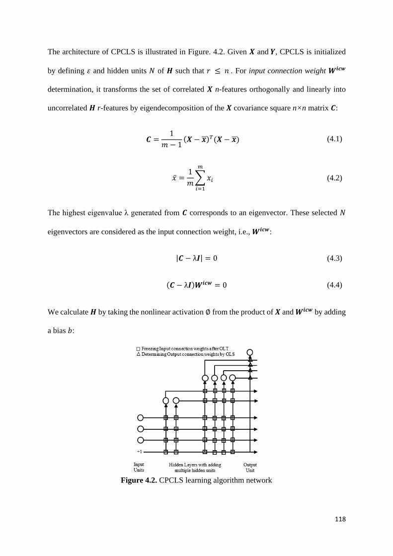
118

The architecture of CPCLS is illustrated in Figure. 4.2. Given 𝑿 and 𝒀, CPCLS is initialized

by defining 𝜀 and hidden units 𝑁 of 𝑯 such that 𝑟 ≤ 𝑛 . For input connection weight 𝑾𝒊𝒄𝒘

determination, it transforms the set of correlated 𝑿 n-features orthogonally and linearly into

uncorrelated 𝑯 r-features by eigendecomposition of the 𝑿 covariance square n×n matrix 𝑪:

𝑪 =1

𝑚 − 1(𝑿 − �̅�)𝑇(𝑿 − �̅�) (4.1)

�̅� =1

𝑚∑ 𝑥𝑖

𝑚

𝑖=1

(4.2)

The highest eigenvalue λ generated from 𝑪 corresponds to an eigenvector. These selected 𝑁

eigenvectors are considered as the input connection weight, i.e., 𝑾𝒊𝒄𝒘:

|𝑪 − λ𝑰| = 0 (4.3)

(𝑪 − λ𝑰)𝑾𝒊𝒄𝒘 = 0 (4.4)

We calculate 𝑯 by taking the nonlinear activation ∅ from the product of 𝑿 and 𝑾𝒊𝒄𝒘 by adding

a bias 𝑏:

Figure 4.2. CPCLS learning algorithm network

119

𝑯 = ∅(𝑿𝑾𝒊𝒄𝒘 + 𝑏) (4.5)

The orthogonal linear transformation by eigendecomposition of 𝑪 generates 𝑯, which explains

the maximum variance in the data, which in turn can help to estimate trip fuel more accurately.

4.4.3 Analytically determining hidden units output connection

weights

The maximum variance in 𝑯 becomes more linear in a relationship with 𝒀, and the sum of

squared errors can be minimized through OLS by calculating for output connection weight, i.e.,

𝑾𝒐𝒄𝒘:

𝑾𝒐𝒄𝒘 = (𝑯𝑻𝑯)−𝟏𝑯𝑻𝒀 (4.6)

where (𝑯𝑻𝑯)−𝟏𝑯𝑻 is the Moore-Penrose pseudo-inverse of 𝑯. We estimate the trip fuel �̂� by

linearly transferring 𝑯 (4.5) through 𝑾𝒐𝒄𝒘 (4.6):

�̂� = 𝑯𝑾𝒐𝒄𝒘 (4.7)

We calculate fuel deviation in (3.32) or (3.33) by subtracting the actual consumed fuel 𝒀 from

the estimated trip fuel �̂�.

If (3.32) or (3.33) is less than 𝜀, we stop; otherwise, another hidden layer 𝑯𝒌 with 𝑁′ hidden

units are added with respect to the previously added hidden layer 𝑯𝒌−𝟏 having 𝑁 hidden units

until the desired performance is achieved. The newly added hidden layer 𝑯𝒌 will receive all

the connections from 𝑿 and from any pre-existing hidden layers, i.e., 𝑯𝒌−𝟏. In other words, the

previously calculated 𝑯𝒌−𝟏 becomes a part of 𝑿, such that

120

𝑿 = (𝑿, 𝑯𝒌−𝟏) (4.8)

𝑁 = 𝑁 + 𝑁′ (4.9)

The steps from Equation (4.1) to (4.7) are repeated.

4.4.4 Adding hidden layers

Equation (4.8) implies that only newly added 𝑯𝒌 will connect to 𝒀 and will eliminate previous

connections, i.e., 𝑯𝒌−𝟏, 𝑯𝒌−𝟐, etc. This helps to avoid linear dependencies among hidden units

in the multiple hidden layers. For better illustration, consider an example in Figure 4.2, where

the hidden layers are initialized with 𝑁=2 and 𝑁′=2. It implies that the first hidden layer (hidden

layer 1) is initialized with 𝑁=2 hidden units and the algorithm is then trained. If the error

resulting from training is larger than 𝜀, then another hidden layer (hidden layer 2) is added with

𝑁′=2 hidden units with respect to hidden units of previous layers (𝑁 = 𝑁 + 𝑁′ = 2+2= 4 hidden

units in the hidden layer 2). Again, the algorithm is trained, and the error is calculated by

connecting only a newly added hidden layer (hidden layer 2) to the output unit and by

eliminating a previous hidden layer (hidden layer 1) from the output connections weight. These

steps continue until the targeted value of 𝜀 is achieved.

4.4.5 Hyperparameters

The advantages of CPCLS that makes it superior compared to CasCor and its extensions is the

generation of non-redundant and linearly independent multiple hidden units in the layers. The

linearly independent hidden units generated by an OLT of the operational parameters help to

achieve the best least squares solution. Similarly, to avoid the linear dependency among hidden

layers, a cascade architecture is improved by connecting only the newly added hidden layer to

the output, with all previous connections being eliminated. Besides, the input units are

121

connected to the output unit through hidden units to avoid the input unit’s linear dependency.

Multiple hidden units can be generated in hidden layers to converge faster. These

characteristics help CPCLS to converge faster and ensure maximum error reduction when the

new hidden layer is added. However, the problem of overfitting and slow convergence should

be avoided while generating multiple hidden units. To further elaborate the overfitting and

convergence complexity issues of the algorithm, experimental work in Subsection 4.5.3 is

performed to study the effect of hidden unit generation on network performance. The

achievement of estimation results in the shortest possible computational time along with

minimum hyperparameter initialization, such as 𝑯 and 𝜀, makes CPCLS more favorable. Other

properties include no iterative tuning, no random generation, no trial-and-error to find the best

hyperparameters, and less human intervention.

4.4.6 Convergence theoretical justification

CPCLS proposed to connect only a new added hidden layer to the output unit and eliminate

previous connections to avoid linear dependence among hidden layers. In this Subsection, we

theoretical justified that adding only the newly added layer contributes to error convergence. If

all hidden layers are connected to the output unit then it will create an extra burden on the

network. Besides, if there exists linear dependence among hidden units in hidden layers that

will cause low performance of the network.

Suppose two eigenvectors 𝑤1𝑖𝑐𝑤 and 𝑤2

𝑖𝑐𝑤 are generated from the eigendecomposition of 𝑪.

Both vectors can be considered orthogonal if and only if the inner product is zero, i.e.,

𝑤1𝑖𝑐𝑤. 𝑤2

𝑖𝑐𝑤 = 0 or 𝑤1𝑖𝑐𝑤𝑇

𝑤2𝑖𝑐𝑤 = 0. Where 𝑇 in superscript is the transpose of a matrix.

We have:

122

𝑪𝑤1𝑖𝑐𝑤 = 𝜆1𝑤1

𝑖𝑐𝑤 (4.10)

and

𝑪𝑤2𝑖𝑐𝑤 = 𝜆2𝑤2

𝑖𝑐𝑤 (4.11)

To prove that 𝑤1 and 𝑤2 are orthogonal:

𝜆1(𝑤1𝑖𝑐𝑤. 𝑤2

𝑖𝑐𝑤)

= (𝜆1𝑤1𝑖𝑐𝑤). 𝑤2

𝑖𝑐𝑤

= (𝑪𝑤1𝑖𝑐𝑤). 𝑤2

𝑖𝑐𝑤

= (𝑪𝑤1𝑖𝑐𝑤) 𝑇𝑤2

𝑖𝑐𝑤

= 𝑤1𝑖𝑐𝑤𝑇

𝑪𝑇𝑤2𝑖𝑐𝑤

= 𝑤1𝑖𝑐𝑤𝑇

𝑪𝑤2𝑖𝑐𝑤

= 𝑤1𝑖𝑐𝑤𝑇

𝜆2𝑤2𝑖𝑐𝑤

= 𝜆2(𝑤1𝑖𝑐𝑤𝑇

𝑤2𝑖𝑐𝑤)

= 𝜆2(𝑤1𝑖𝑐𝑤. 𝑤2

𝑖𝑐𝑤) (4.12)

𝑪 = 𝑪𝑻 because 𝑪 is a symmetric matrix. From mathematical work, we have:

𝜆1(𝑤1𝑖𝑐𝑤. 𝑤2

𝑖𝑐𝑤) = 𝜆2(𝑤1𝑖𝑐𝑤. 𝑤2

𝑖𝑐𝑤) (4.13)

(𝜆1 − 𝜆2)(𝑤1𝑖𝑐𝑤. 𝑤2

𝑖𝑐𝑤) = 0 (4.14)

Since 𝜆1 − 𝜆2 ≠ 0, because both are different. So, we have:

123

𝑤1𝑖𝑐𝑤. 𝑤2

𝑖𝑐𝑤 = 0 (4.15)

Equation (4.15) implies that 𝑤1𝑖𝑐𝑤 and 𝑤2

𝑖𝑐𝑤 are orthogonal and linearly independent in

eigenmatrix 𝑾𝒊𝒄𝒘. Suppose if two hidden units ℎ𝑘1 and ℎ𝑘2

are generated from 𝑤1𝑖𝑐𝑤 and 𝑤2

𝑖𝑐𝑤

in the first hidden layer, that will be also orthogonal, i.e., ℎ𝑘1⊥ ℎ𝑘2

. This theoretical

justification supports Lemma 1, that generated hidden units in the layer are linearly

independent (inevitable) and hence ||𝑯𝑾𝒐𝒄𝒘 − 𝒀|| = 𝟎 ensuring convergence of the network.

Now, suppose if more than one hidden layer is added in the network. If ℎ𝑘−11 and ℎ𝑘−12

are

generated in 𝑯𝒌−𝟏 by 𝑤𝑘−1𝑖𝑐𝑤

1 and 𝑤𝑘−1

𝑖𝑐𝑤2, and ℎ𝑘1

and ℎ𝑘2 are generated in 𝑯𝒌 by 𝑤𝑘

𝑖𝑐𝑤1 and

𝑤𝑘𝑖𝑐𝑤

2, then equal chance exists that it may or may not be linearly independent. i.e., 𝑯𝒌−𝟏 ⊥

𝑯𝒌 or 𝑯𝒌−𝟏 ⟂̸𝑯𝒌. In 𝑯𝒌−𝟏 ⟂̸𝑯𝒌 case, it may be not orthogonal and may not support lemma 1

and hence ||𝑯𝑾𝒐𝒄𝒘 − 𝒀|| ≠ 𝟎

Algorithm 4.1. CPCLS algorithm summary

In a training dataset (𝑿, 𝒀), let 𝑿 be input variable matrix m×n, 𝒀 be output variable m×q

matrix.

1. Initialize the network by defining number 𝑁 of hidden units in the first hidden layer

such that the number of hidden units less than or equal to input variable, i.e., r ≤ n.

2. Learn the network by defining the criteria of convergence error 𝜀. Compare 𝜀 with

network estimated error 𝐸:

While 𝐸 > 𝜀

a. Input connection weights 𝑾𝒊𝒄𝒘: Determine eigenvectors 𝑾𝒊𝒄𝒘 from the orthogonal

linear transformation of 𝑿. Calculate symmetric matrix 𝑪 and perform its

124

eigendecomposition. The extracted eigenvalue and its corresponding eigenvector are

selected as 𝑾𝒊𝒄𝒘 of matrix n×r:

𝑪 =1

𝑚 − 1(𝑿 − �̅�)𝑇(𝑿 − �̅�)

|𝑪 − λ𝑰| = 0

(𝑪 − λ𝑰)𝑾𝒊𝒄𝒘 = 0

b. Hidden units 𝑯: Generate a linearly independent 𝑯 of matrix m×r by passing the net

of 𝑿 and 𝑾𝒊𝒄𝒘 through activation function ∅:

𝑯 = ∅(𝑿𝑾𝒊𝒄𝒘)

c. Output connection weights 𝑾𝒐𝒄𝒘: Calculate the pseudo-inverse of 𝑯 and take the

product with 𝒀 to determine 𝑾𝒐𝒄𝒘 matrix of r×q:

𝑾𝒐𝒄𝒘 = (𝑯𝑻𝑯)−𝟏𝑯𝑻𝒀

d. Predicted output �̂�: Take the product of calculated 𝑯 and 𝑾𝒐𝒄𝒘 to estimate the

output:

�̂� = 𝑯𝑾𝒐𝒄𝒘

e. Network Error 𝐸: Take the difference between the �̂� and the 𝒀:

𝐸 = (�̂� − 𝒀)2

f. Column stack 𝑯 with 𝑿:

𝑿 = (𝑿, 𝑯)

125

g. Calculate 𝑁 for the proceeding 𝑯 by defining and adding 𝑁′ to existing 𝑁 such that p

≤ n:

𝑁 = 𝑁 + 𝑁′

end

4.5 Experimental work

The generalization performance and learning speed of the proposed algorithm CPCLS are

compared with the traditional algorithms on artificial benchmarking and real-world dataset

problems. The artificial benchmarking problems include the two-spiral classification task and

the function approximation of the SinC regression task. For comparison of real-world

problems, the classification and regression dataset problems are taken from the UCI machine

learning repository. The numerical work was carried out in Netmaker v0.9.5.2 and Anaconda

Spyder Python v3.2.6. Netmaker is a powerful simulation software designed in C programming

for building neural networks and has a built-in QP CasCor programming code. CPCLS, BPNN,

and SaELM simulation were carried out in Python, whereas, CasCor simulation was carried

out in the Netmaker. The limitation of this research work is that the CasCor programming code

is designed in the C programming language. Generally speaking, simulation in different

programming codes will not imitate the comparison because C programming execution is faster

than python. The dataset input and output has been normalized in the range [0,1] to make it

compatible with the sigmoid nonlinear activation function ∅(𝑧) = 1/(1 + 𝑒−𝑧) used in the

hidden units.

The work is divided into two parts: artificial benchmarking problems and real-world problems.

In artificial benchmarking problems, CPCLS is compared with CasCor on two spiral

classifications and the SinC function regression task. A comparison with two spiral

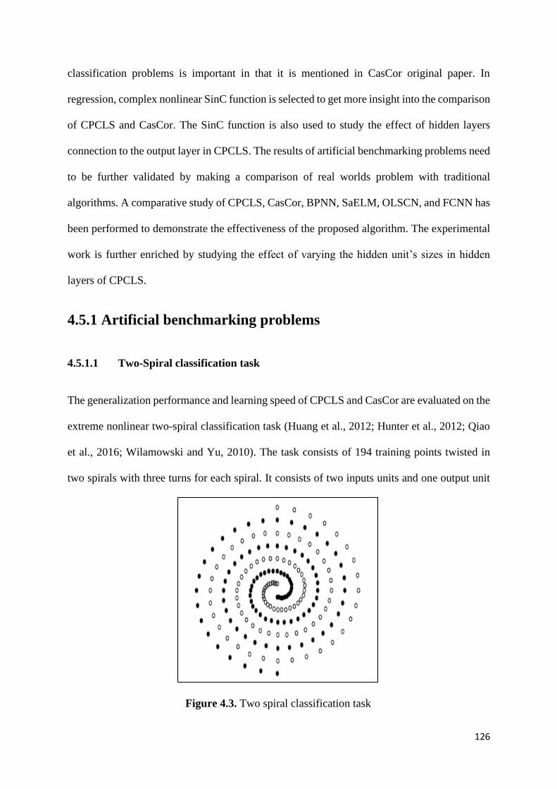
126

classification problems is important in that it is mentioned in CasCor original paper. In

regression, complex nonlinear SinC function is selected to get more insight into the comparison

of CPCLS and CasCor. The SinC function is also used to study the effect of hidden layers

connection to the output layer in CPCLS. The results of artificial benchmarking problems need

to be further validated by making a comparison of real worlds problem with traditional

algorithms. A comparative study of CPCLS, CasCor, BPNN, SaELM, OLSCN, and FCNN has

been performed to demonstrate the effectiveness of the proposed algorithm. The experimental

work is further enriched by studying the effect of varying the hidden unit’s sizes in hidden

layers of CPCLS.

4.5.1 Artificial benchmarking problems

4.5.1.1 Two-Spiral classification task

The generalization performance and learning speed of CPCLS and CasCor are evaluated on the

extreme nonlinear two-spiral classification task (Huang et al., 2012; Hunter et al., 2012; Qiao

et al., 2016; Wilamowski and Yu, 2010). The task consists of 194 training points twisted in

two spirals with three turns for each spiral. It consists of two inputs units and one output unit

Figure 4.3. Two spiral classification task

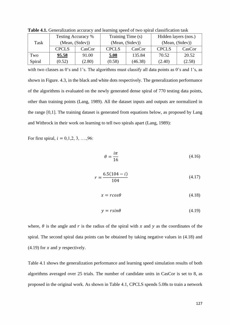
127

with two classes as 0’s and 1’s. The algorithms must classify all data points as 0’s and 1’s, as

shown in Figure. 4.3, in the black and white dots respectively. The generalization performance

of the algorithms is evaluated on the newly generated dense spiral of 770 testing data points,

other than training points (Lang, 1989). All the dataset inputs and outputs are normalized in

the range [0,1]. The training dataset is generated from equations below, as proposed by Lang

and Witbrock in their work on learning to tell two spirals apart (Lang, 1989):

For first spiral, 𝑖 = 0,1,2, 3, ….,96:

𝜃 =𝑖𝜋

16 (4.16)

𝑟 =6.5(104 − 𝑖)

104 (4.17)

𝑥 = 𝑟𝑐𝑜𝑠𝜃 (4.18)

𝑦 = 𝑟𝑠𝑖𝑛𝜃 (4.19)

where, 𝜃 is the angle and 𝑟 is the radius of the spiral with 𝑥 and 𝑦 as the coordinates of the

spiral. The second spiral data points can be obtained by taking negative values in (4.18) and

(4.19) for 𝑥 and 𝑦 respectively.

Table 4.1 shows the generalization performance and learning speed simulation results of both

algorithms averaged over 25 trials. The number of candidate units in CasCor is set to 8, as

proposed in the original work. As shown in Table 4.1, CPCLS spends 5.08s to train a network

Table 4.1. Generalization accuracy and learning speed of two spiral classification task

Task

Testing Accuracy %

(Mean, (Stdev))

Training Time (s)

(Mean, (Stdev))

Hidden layers (nos.)

(Mean, (Stdev))

CPCLS CasCor CPCLS CasCor CPCLS CasCor

Two

Spiral

95.58

(0.52)

91.00

(2.80)

5.08

(0.58)

135.84

(46.38)

70.52

(2.40)

20.52

(2.58)

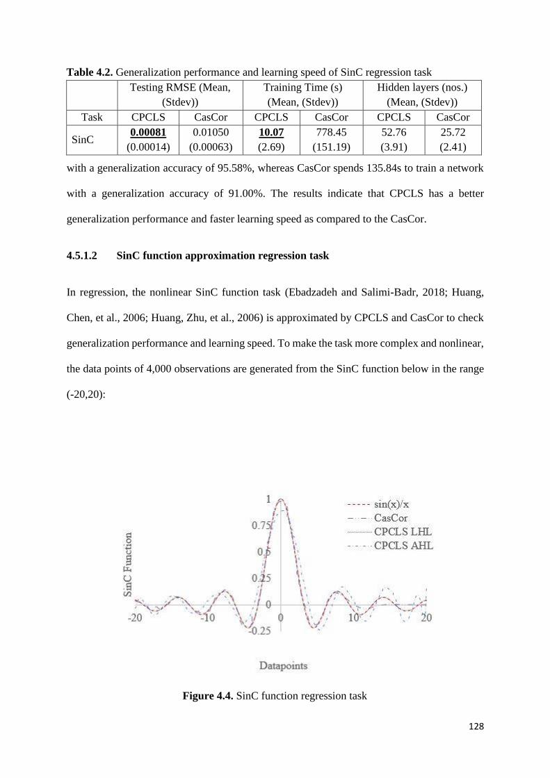
128

with a generalization accuracy of 95.58%, whereas CasCor spends 135.84s to train a network

with a generalization accuracy of 91.00%. The results indicate that CPCLS has a better

generalization performance and faster learning speed as compared to the CasCor.

4.5.1.2 SinC function approximation regression task

In regression, the nonlinear SinC function task (Ebadzadeh and Salimi-Badr, 2018; Huang,

Chen, et al., 2006; Huang, Zhu, et al., 2006) is approximated by CPCLS and CasCor to check

generalization performance and learning speed. To make the task more complex and nonlinear,

the data points of 4,000 observations are generated from the SinC function below in the range

(-20,20):

Figure 4.4. SinC function regression task

Table 4.2. Generalization performance and learning speed of SinC regression task

Testing RMSE (Mean,

(Stdev))

Training Time (s)

(Mean, (Stdev))

Hidden layers (nos.)

(Mean, (Stdev))

Task CPCLS CasCor CPCLS CasCor CPCLS CasCor

SinC 0.00081

(0.00014)

0.01050

(0.00063)

10.07

(2.69)

778.45

(151.19)

52.76

(3.91)

25.72

(2.41)

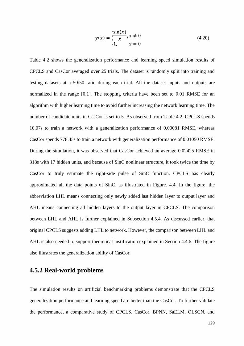
129

𝑦(𝑥) = {sin(𝑥)

𝑥, 𝑥 ≠ 0

1, 𝑥 = 0 (4.20)

Table 4.2 shows the generalization performance and learning speed simulation results of

CPCLS and CasCor averaged over 25 trials. The dataset is randomly split into training and

testing datasets at a 50:50 ratio during each trial. All the dataset inputs and outputs are

normalized in the range [0,1]. The stopping criteria have been set to 0.01 RMSE for an

algorithm with higher learning time to avoid further increasing the network learning time. The

number of candidate units in CasCor is set to 5. As observed from Table 4.2, CPCLS spends

10.07s to train a network with a generalization performance of 0.00081 RMSE, whereas

CasCor spends 778.45s to train a network with generalization performance of 0.01050 RMSE.

During the simulation, it was observed that CasCor achieved an average 0.02425 RMSE in

318s with 17 hidden units, and because of SinC nonlinear structure, it took twice the time by

CasCor to truly estimate the right-side pulse of SinC function. CPCLS has clearly

approximated all the data points of SinC, as illustrated in Figure. 4.4. In the figure, the

abbreviation LHL means connecting only newly added last hidden layer to output layer and

AHL means connecting all hidden layers to the output layer in CPCLS. The comparison

between LHL and AHL is further explained in Subsection 4.5.4. As discussed earlier, that

original CPCLS suggests adding LHL to network. However, the comparison between LHL and

AHL is also needed to support theoretical justification explained in Section 4.4.6. The figure

also illustrates the generalization ability of CasCor.

4.5.2 Real-world problems

The simulation results on artificial benchmarking problems demonstrate that the CPCLS

generalization performance and learning speed are better than the CasCor. To further validate

the performance, a comparative study of CPCLS, CasCor, BPNN, SaELM, OLSCN, and

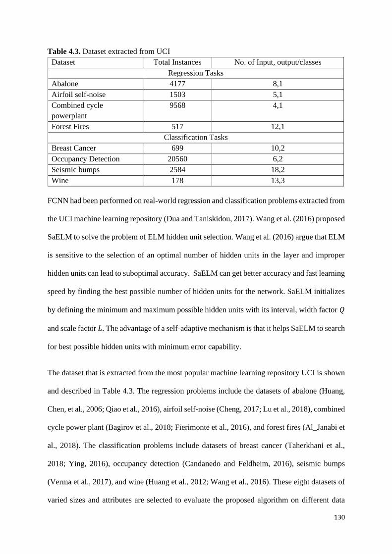
130

FCNN had been performed on real-world regression and classification problems extracted from

the UCI machine learning repository (Dua and Taniskidou, 2017). Wang et al. (2016) proposed

SaELM to solve the problem of ELM hidden unit selection. Wang et al. (2016) argue that ELM

is sensitive to the selection of an optimal number of hidden units in the layer and improper

hidden units can lead to suboptimal accuracy. SaELM can get better accuracy and fast learning

speed by finding the best possible number of hidden units for the network. SaELM initializes

by defining the minimum and maximum possible hidden units with its interval, width factor 𝑄

and scale factor 𝐿. The advantage of a self-adaptive mechanism is that it helps SaELM to search

for best possible hidden units with minimum error capability.

The dataset that is extracted from the most popular machine learning repository UCI is shown

and described in Table 4.3. The regression problems include the datasets of abalone (Huang,

Chen, et al., 2006; Qiao et al., 2016), airfoil self-noise (Cheng, 2017; Lu et al., 2018), combined

cycle power plant (Bagirov et al., 2018; Fierimonte et al., 2016), and forest fires (Al_Janabi et

al., 2018). The classification problems include datasets of breast cancer (Taherkhani et al.,

2018; Ying, 2016), occupancy detection (Candanedo and Feldheim, 2016), seismic bumps

(Verma et al., 2017), and wine (Huang et al., 2012; Wang et al., 2016). These eight datasets of

varied sizes and attributes are selected to evaluate the proposed algorithm on different data

Table 4.3. Dataset extracted from UCI

Dataset Total Instances No. of Input, output/classes

Regression Tasks

Abalone 4177 8,1

Airfoil self-noise 1503 5,1

Combined cycle

powerplant

9568 4,1

Forest Fires 517 12,1

Classification Tasks

Breast Cancer 699 10,2

Occupancy Detection 20560 6,2

Seismic bumps 2584 18,2

Wine 178 13,3

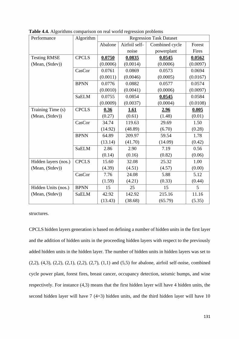
131

structures.

CPCLS hidden layers generation is based on defining a number of hidden units in the first layer

and the addition of hidden units in the proceeding hidden layers with respect to the previously

added hidden units in the hidden layer. The number of hidden units in hidden layers was set to

(2,2), (4,3), (2,2), (2,1), (2,2), (2,7), (1,1) and (5,5) for abalone, airfoil self-noise, combined

cycle power plant, forest fires, breast cancer, occupancy detection, seismic bumps, and wine

respectively. For instance (4,3) means that the first hidden layer will have 4 hidden units, the

second hidden layer will have 7 (4+3) hidden units, and the third hidden layer will have 10

Table 4.4. Algorithms comparison on real world regression problems

Performance Algorithm Regression Task Dataset

Abalone Airfoil self-

noise

Combined cycle

powerplant

Forest

Fires

Testing RMSE

(Mean, (Stdev))

CPCLS 0.0750

(0.0006)

0.0835

(0.0014)

0.0545

(0.0006)

0.0562

(0.0097)

CasCor 0.0761

(0.0011)

0.0869

(0.0046)

0.0573

(0.0005)

0.0694

(0.0167)

BPNN 0.0776

(0.0010)

0.0882

(0.0041)

0.0577

(0.0006)

0.0574

(0.0097)

SaELM 0.0755

(0.0009)

0.0854

(0.0037)

0.0545

(0.0004)

0.0584

(0.0108)

Training Time (s)

(Mean, (Stdev))

CPCLS 0.36

(0.27)

1.61

(0.61)

2.96

(1.48)

0.005

(0.01)

CasCor 34.74

(14.92)

119.63

(48.89)

29.69

(6.70)

1.50

(0.28)

BPNN 64.89

(13.14)

209.97

(41.70)

59.54

(14.09)

1.78

(0.42)

SaELM 2.86

(0.14)

2.90

(0.16)

7.19

(0.82)

0.56

(0.06)

Hidden layers (nos.)

(Mean, (Stdev))

CPCLS 15.60

(4.39)

32.08

(4.51)

25.32

(4.57)

1.00

(0.00)

CasCor 7.76

(1.59)

24.08

(4.21)

5.88

(0.33)

5.12

(0.44)

Hidden Units (nos.)

(Mean, (Stdev))

BPNN 15 25 15 5

SaELM 42.92

(13.43)

142.92

(38.68)

215.16

(65.79)

11.16

(5.35)

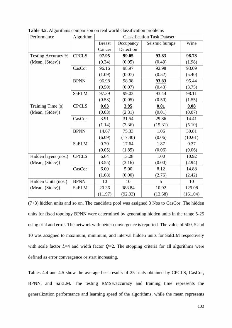
132

(7+3) hidden units and so on. The candidate pool was assigned 3 Nos to CasCor. The hidden

units for fixed topology BPNN were determined by generating hidden units in the range 5-25

using trial and error. The network with better convergence is reported. The value of 500, 5 and

10 was assigned to maximum, minimum, and interval hidden units for SaELM respectively

with scale factor 𝐿=4 and width factor 𝑄=2. The stopping criteria for all algorithms were

defined as error convergence or start increasing.

Tables 4.4 and 4.5 show the average best results of 25 trials obtained by CPCLS, CasCor,

BPNN, and SaELM. The testing RMSE/accuracy and training time represents the

generalization performance and learning speed of the algorithms, while the mean represents

Table 4.5. Algorithms comparison on real world classification problems

Performance Algorithm Classification Task Dataset

Breast

Cancer

Occupancy

Detection

Seismic bumps Wine

Testing Accuracy %

(Mean, (Stdev))

CPCLS 97.95

(0.34)

99.05

(0.05)

93.83

(0.43)

98.78

(1.98)

CasCor 96.16

(1.09)

98.97

(0.07)

92.98

(0.52)

93.09

(5.40)

BPNN 96.98

(0.50)

98.98

(0.07)

93.83

(0.43)

95.44

(3.75)

SaELM 97.39

(0.53)

99.03

(0.05)

93.44

(0.50)

98.11

(1.55)

Training Time (s)

(Mean, (Stdev))

CPCLS 0.03

(0.03)

3.95

(2.31)

0.01

(0.01)

0.08

(0.07)

CasCor 3.91

(1.14)

31.54

(3.36)

29.86

(15.31)

14.41

(5.10)

BPNN 14.67

(6.09)

75.33

(17.40)

1.06

(0.06)

30.81

(10.61)

SaELM 0.70

(0.05)

17.64

(1.85)

1.87

(0.06)

0.37

(0.06)

Hidden layers (nos.)

(Mean, (Stdev))

CPCLS 6.64

(3.55)

13.28

(3.16)

1.00

(0.00)

10.92

(2.94)

CasCor 6.00

(1.08)

5.00

(0.00)

8.12

(2.76)

14.88

(2.42)

Hidden Units (nos.)

(Mean, (Stdev))

BPNN 10 10 5 10

SaELM 20.36

(11.97)

388.84

(92.93)

10.92

(13.58)

129.08

(161.04)

133

average and stdev represents standard deviation results of 25 trials. The regression problems

were evaluated by RMSE and classification problems were evaluated by accuracy.

As observed in Tables 4.4 and 4.5, that performance in terms of generalization and learning of

proposed CPCLS is better compared to other algorithms. The best results in terms of

generalization and learning speed are highlighted bold with underlined in Tables 4.4 and 4.5.

In Table 4.4, for combined cycle power plant the generalization performance of CPCLS and

SaELM is similar to the advantage of CPCLS is that it took 2.96s compared to SaELM of 7.19s.

In Table 4.5, for seismic bumps classification, the generalization accuracy of CPCLS and

BPNN is similar to the advantage of CPCLS is that it took 0.01s compared to BPNN of 1.06s.

To demonstrate and understand the convergence of CPCLS, the abalone dataset convergence

of 25 trials can be visualized from Figure 4.5. The figure shows that the convergence of CPCLS

is stable and smooth during the addition of hidden units and minimum deviation within each

trial was observed.

The performance comparison of CPCLS with CasCor and other popular machine learning is

clear, however, CPCLS comparison with CasCor extension named as OLSCN and FCNN is

also needed. The simulation results of OLSCN and FCNN are acquired from their primary

articles because of the unavailability of original programs. To ensure a fair comparison, the

Figure 4.5. Smooth and stable convergence of CPCLS

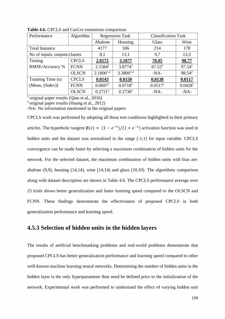
134

CPCLS work was performed by adopting all those test conditions highlighted in their primary

articles. The hyperbolic tangent ∅(𝑧) = (1 − 𝑒−𝑧)/(1 + 𝑒−𝑧) activation function was used in

hidden units and the dataset was normalized in the range [-1,1] for input variable. CPCLS

convergence can be made faster by selecting a maximum combination of hidden units for the

network. For the selected dataset, the maximum combination of hidden units with bias are:

abalone (9,9), housing (14,14), wine (14,14) and glass (10,10). The algorithms comparison

along with dataset description are shown in Table 4.6. The CPCLS performance average over

25 trials shows better generalization and faster learning speed compared to the OLSCN and

FCNN. These findings demonstrate the effectiveness of proposed CPCLS in both

generalization performance and learning speed.

4.5.3 Selection of hidden units in the hidden layers

The results of artificial benchmarking problems and real-world problems demonstrate that

proposed CPCLS has better generalization performance and learning speed compared to other

well-known machine learning neural networks. Determining the number of hidden units in the

hidden layer is the only hyperparameter than need be defined prior to the initialization of the

network. Experimental work was performed to understand the effect of varying hidden unit

Table 4.6. CPCLS and CasCor extensions comparison

Performance Algorithm Regression Task Classification Task

Abalone Housing Glass Wine

Total Instance 4177 506 214 178

No of inputs, outputs/classes 8,1 13,1 9,7 13,3

Testing

RMSE/Accuracy %

CPCLS 2.0572 3.1877 70.05 98.77

FCNN 2.15841 3.87741 67.521 97.541

OLSCN 2.18001,2 3.38001,2 -NA- 98.542

Training Time (s)

(Mean, (Stdev))

CPCLS 0.0143 0.0150 0.0138 0.0117

FCNN 0.06971 0.07181 0.05171 0.04281

OLSCN 0.27211 0.27381 -NA- -NA- 1 original paper results (Qiao et al., 2016) 2 original paper results (Huang et al., 2012)

-NA- No information mentioned in the original papers

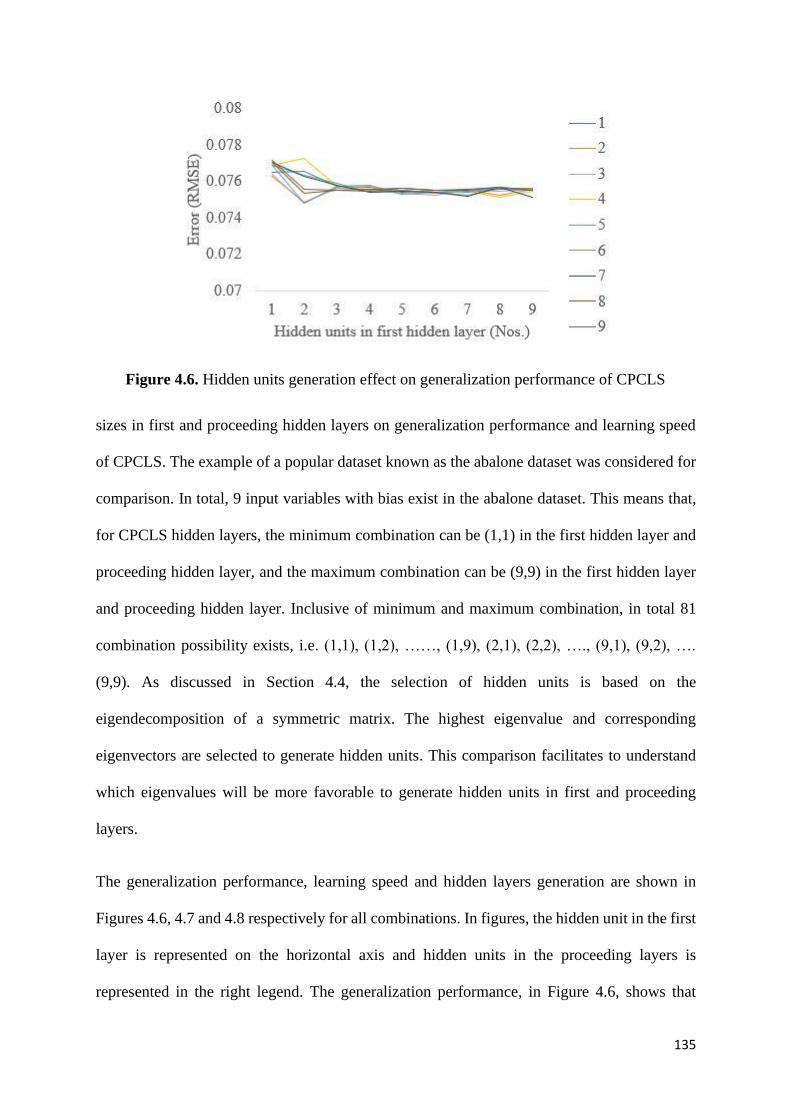
135

sizes in first and proceeding hidden layers on generalization performance and learning speed

of CPCLS. The example of a popular dataset known as the abalone dataset was considered for

comparison. In total, 9 input variables with bias exist in the abalone dataset. This means that,

for CPCLS hidden layers, the minimum combination can be (1,1) in the first hidden layer and

proceeding hidden layer, and the maximum combination can be (9,9) in the first hidden layer

and proceeding hidden layer. Inclusive of minimum and maximum combination, in total 81

combination possibility exists, i.e. (1,1), (1,2), ……, (1,9), (2,1), (2,2), …., (9,1), (9,2), ….

(9,9). As discussed in Section 4.4, the selection of hidden units is based on the

eigendecomposition of a symmetric matrix. The highest eigenvalue and corresponding

eigenvectors are selected to generate hidden units. This comparison facilitates to understand

which eigenvalues will be more favorable to generate hidden units in first and proceeding

layers.

The generalization performance, learning speed and hidden layers generation are shown in

Figures 4.6, 4.7 and 4.8 respectively for all combinations. In figures, the hidden unit in the first

layer is represented on the horizontal axis and hidden units in the proceeding layers is

represented in the right legend. The generalization performance, in Figure 4.6, shows that

Figure 4.6. Hidden units generation effect on generalization performance of CPCLS

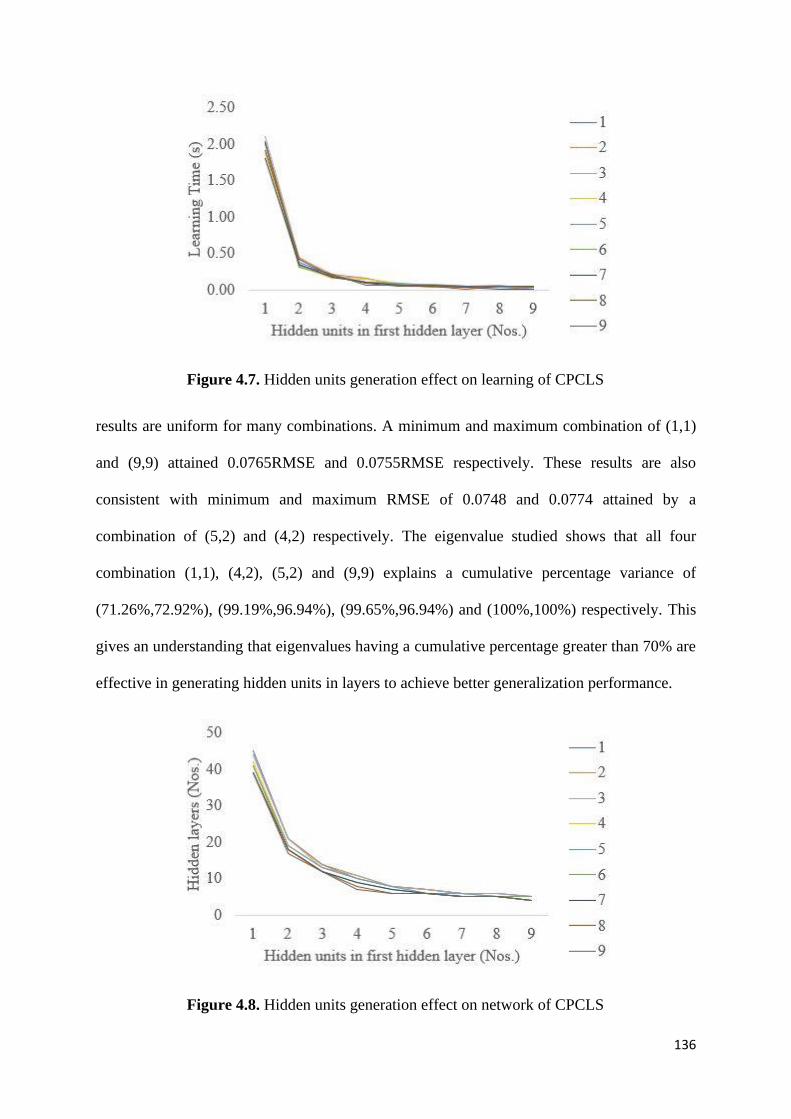
136

results are uniform for many combinations. A minimum and maximum combination of (1,1)

and (9,9) attained 0.0765RMSE and 0.0755RMSE respectively. These results are also

consistent with minimum and maximum RMSE of 0.0748 and 0.0774 attained by a

combination of (5,2) and (4,2) respectively. The eigenvalue studied shows that all four

combination (1,1), (4,2), (5,2) and (9,9) explains a cumulative percentage variance of

(71.26%,72.92%), (99.19%,96.94%), (99.65%,96.94%) and (100%,100%) respectively. This

gives an understanding that eigenvalues having a cumulative percentage greater than 70% are

effective in generating hidden units in layers to achieve better generalization performance.

Figure 4.7. Hidden units generation effect on learning of CPCLS

Figure 4.8. Hidden units generation effect on network of CPCLS

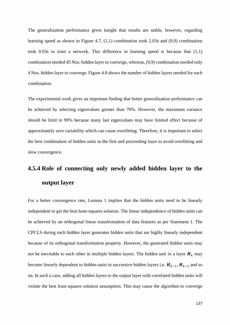
137

The generalization performance gives insight that results are stable, however, regarding

learning speed as shown in Figure 4.7, (1,1) combination took 2.03s and (9,9) combination

took 0.03s to train a network. This difference in learning speed is because that (1,1)

combination needed 45 Nos. hidden layer to converge, whereas, (9,9) combination needed only

4 Nos. hidden layer to converge. Figure 4.8 shows the number of hidden layers needed for each

combination.

The experimental work gives an important finding that better generalization performance can

be achieved by selecting eigenvalues greater than 70%. However, the maximum variance

should be limit to 99% because many last eigenvalues may have limited effect because of

approximately zero variability which can cause overfitting. Therefore, it is important to select

the best combination of hidden units in the first and proceeding layer to avoid overfitting and

slow convergence.

4.5.4 Role of connecting only newly added hidden layer to the

output layer

For a better convergence rate, Lemma 1 implies that the hidden units need to be linearly

independent to get the best least-squares solution. The linear independence of hidden units can

be achieved by an orthogonal linear transformation of data features as per Statement 1. The

CPCLS during each hidden layer generates hidden units that are highly linearly independent

because of its orthogonal transformation property. However, the generated hidden units may

not be inevitable to each other in multiple hidden layers. The hidden unit in a layer 𝑯𝑘 may

become linearly dependent to hidden units in successive hidden layers i.e. 𝑯𝑘−1, 𝑯𝑘−2 and so

on. In such a case, adding all hidden layers to the output layer with correlated hidden units will

violate the best least-squares solution assumption. This may cause the algorithm to converge

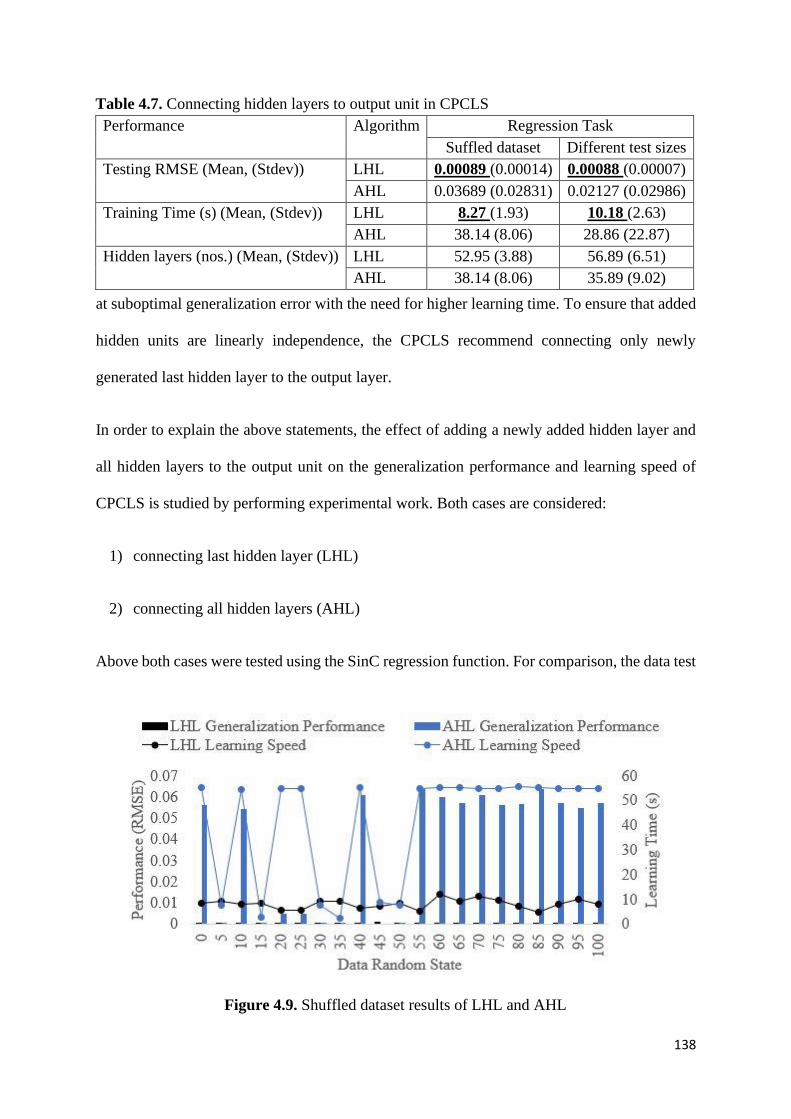
138

at suboptimal generalization error with the need for higher learning time. To ensure that added

hidden units are linearly independence, the CPCLS recommend connecting only newly

generated last hidden layer to the output layer.

In order to explain the above statements, the effect of adding a newly added hidden layer and

all hidden layers to the output unit on the generalization performance and learning speed of

CPCLS is studied by performing experimental work. Both cases are considered:

1) connecting last hidden layer (LHL)

2) connecting all hidden layers (AHL)

Above both cases were tested using the SinC regression function. For comparison, the data test

Figure 4.9. Shuffled dataset results of LHL and AHL

Table 4.7. Connecting hidden layers to output unit in CPCLS

Performance Algorithm Regression Task

Suffled dataset Different test sizes

Testing RMSE (Mean, (Stdev)) LHL 0.00089 (0.00014) 0.00088 (0.00007)

AHL 0.03689 (0.02831) 0.02127 (0.02986)

Training Time (s) (Mean, (Stdev)) LHL 8.27 (1.93) 10.18 (2.63)

AHL 38.14 (8.06) 28.86 (22.87)

Hidden layers (nos.) (Mean, (Stdev)) LHL 52.95 (3.88) 56.89 (6.51)

AHL 38.14 (8.06) 35.89 (9.02)

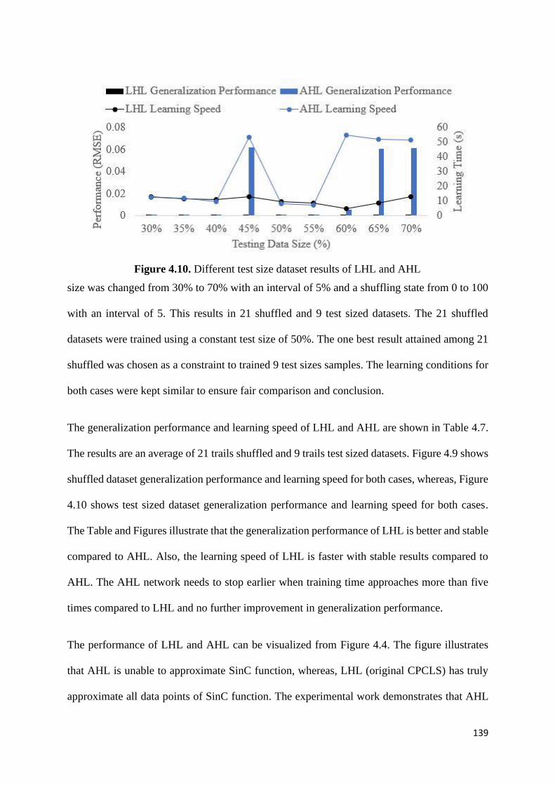
139

size was changed from 30% to 70% with an interval of 5% and a shuffling state from 0 to 100

with an interval of 5. This results in 21 shuffled and 9 test sized datasets. The 21 shuffled

datasets were trained using a constant test size of 50%. The one best result attained among 21

shuffled was chosen as a constraint to trained 9 test sizes samples. The learning conditions for

both cases were kept similar to ensure fair comparison and conclusion.

The generalization performance and learning speed of LHL and AHL are shown in Table 4.7.

The results are an average of 21 trails shuffled and 9 trails test sized datasets. Figure 4.9 shows

shuffled dataset generalization performance and learning speed for both cases, whereas, Figure

4.10 shows test sized dataset generalization performance and learning speed for both cases.

The Table and Figures illustrate that the generalization performance of LHL is better and stable

compared to AHL. Also, the learning speed of LHL is faster with stable results compared to

AHL. The AHL network needs to stop earlier when training time approaches more than five

times compared to LHL and no further improvement in generalization performance.

The performance of LHL and AHL can be visualized from Figure 4.4. The figure illustrates

that AHL is unable to approximate SinC function, whereas, LHL (original CPCLS) has truly

approximate all data points of SinC function. The experimental work demonstrates that AHL

Figure 4.10. Different test size dataset results of LHL and AHL

140

results maybe not optimal in many cases compared to LHL. Furthermore, during all trails, it is

observed that CPCLS with LHL gives better and stable results with lesser deviation.

4.6 Summary

In this Chapter, experimental work demonstrates that the newly proposed algorithm known as

CPCLS achieves better generalization performance and faster learning speed, with improved

cascade architecture and tuning free learning method, as compared to similar constructive and

traditional algorithms. CPCLS has several noteworthy features:

▪ The proposed algorithm has achieved better generalization performance. Experimental

results show that improvement in the cascade architecture creates less burden on the

network and it converges more efficiently towards the target error. The proposed

algorithm works more analytically by determining the optimal connection weights,

rather than the gradient optimization and random generation techniques. Determining

the input connection weights analytically by OLT helps in generating linearly

independent hidden units, explaining the maximum variance in the dataset with

maximum error reduction capability.

▪ The learning speed is fast due to analytically calculating connection weights in the

forward step. Unlike the gradient method and random generation, that are involved in

finding optimal connection weights. CPCLS takes only a forward step to calculate the

target error by analytically calculating the connection weights on both sides of the

network.

▪ CasCor needs a lot of human expertise to control the learning because of the QP large

steps which can cause the network to behave chaotically. The QP can encounter the

problem of zero derivative difference which needs extra control to stop the iterations

141

early to prevent overflow problems in the network. CPCLS advantage over QP CasCor

that of tuning free learning.

▪ CPCLS better network generalization performance validates that the hidden layers

generated are capable of maximum error reduction.

▪ Like other gradient-free learning algorithms i.e.; SaELM, the proposed algorithm can

work directly with differential activation functions (e.g. sigmoid, hyperbolic tangent,

rectified linear unit and so on) and nondifferential activation function (e.g.; threshold).

Gradient-based methods cannot handle nondifferential activation functions directly

because of their differentiation property.

▪ The proposed algorithm has solved the problem of linearly dependent input features and

hidden units. It reduces the chance of multicollinearity by orthogonally transforming the

set of any correlated input units and any pre-existing hidden units into uncorrelated

hidden units. The newly added last hidden layer with characteristics of linearly

independent hidden units is connected to the output layer for the best least-squares

solution.

▪ The proposed method is easy to apply in many application areas because of the small

number of user-specified hyperparameters, such as hidden units addition and target

error.

The better generalization performance and learning ability of CPCLS on nonlinear benchmark

problems and real-world problems, verify that it can be efficiently applied to other application

tasks.

142

Chapter 5. Reducing the Negative Role of Global

Parameters with Default Values and Varying Operational

Parameters Effect on the Trip Fuel Estimation

5.1 Introduction

The usage of global parameters with default values rather than local parameters with an

outdated database in the complex mathematical formulation may cause EAs higher fuel

deviation. The low generalization performance and slow learning speed of BPNN may make it

inappropriate to extract information from high-level operational parameters having varying

behaviour among different sectors. To estimate a trip fuel with less deviation, requiring less

expertise, and achieving faster learning speed, real high-dimensional data were provided by an

airline that historically performed international flights in various regions over two years. The

dataset consists of several operational parameters that may or may not contribute to fuel

consumption. For better estimation, the useful operational parameters were first extracted, as

reported in Table 3.1. In our study, the extracted operational parameters are represented by 𝑿

and the objective is to predict the trip fuel �̂� that truly represents the actual consumed trip fuel

𝒀. Two cases were considered for estimating trip fuel consumption. In the first case, all sectors

in the dataset were considered as a combined model. In the second case, each sector was

considered as an individual model. A sector is defined as an airway route starting from the

departure airport and ending in the arrival airport. A comparison of proposed CPCLS is

performed with AEA and BPNN to demonstrate its effectiveness. The study illustrates that the

AEA is highly affected by the usage of global parameters, and the BPNN generalization

performance and learning speed start decreasing with high dimensional data having high-level

operational parameters.

143

The rest of the Chapter is organized as follows. Section 5.2 is about the problem context. In

Section 5.3, fuel consumption data analytics is elaborated. In Section 5.4, solution methods and

their performance analysis are performed by considering two models: combined model

(Subsection 5.4.2.1) and individual model (Subsection 5.4.2.2). Moreover, a comparison is also

made, and major findings are discussed. Section 5.5 concludes this chapter by summarizing

major findings.

5.2 Problem context

The effect of usage of global parameters with default values rather than local parameters,

outdated database, complex mathematical formulation, hyperparameters adjustment, human

intervention and varying nature of operational parameters may cause a negative role by

deviating fuel consumption from estimation. The proposed CPCLS that has characteristics of

better generalization performance and faster learning speed with less human intervention needs

to apply to estimate aircraft trip fuel to demonstrate its effectiveness as a decision tool for

airlines. All the experimental work was carried out in Anaconda Spyder Python v3.2.6

programming language. The dataset was normalized in the range [0,1]. One hot encoding was

performed on categorical variables to represent it in a binary vector. The nonlinear sigmoid

activation function was used in the hidden layers to make it compatible with the dataset. For

both cases, the dataset was split into a 50:50 ratio for training and testing. The stopping criteria

for the algorithms were defined as error convergence or start increasing.

5.3 Data analytics for fuel consumption

The set of real data that we obtained from an international airline operating in Hong Kong

consists of 19,117 international passenger and cargo flights operated among eight sectors

covering different geographical regions. The flights were performed from April 2015 to March

144

2017 by 107 wide-body aircrafts distributed as Airbus A330-300 (31 aircrafts) and Boeing 747-

400 (9 aircrafts)/747-800 (14 aircrafts)/777-300 (53 aircrafts). The data consist of detailed

information on operational parameters related to 1) carrier with aircraft performance and

operations, 2) date/time of departure and arrival per sector with crew allocation, 3) weather and

atmospheric conditions, 4) sector and aircraft local and global conditions, and 5) fuel

requirements at different tanks and consumption levels. Among the collected data, instead of

putting all operational parameters into algorithms, we work in a more novel way by extracting

the relevant high-level operational parameters contributing to fuel consumption, as summarised

in Table 3.1.

5.4 Solution methods and computational results

5.4.1 Proposed method and existing methods

Three estimation methods were used for the comparative study, namely AEA, BPNN, and the

proposed CPCLS. The comparison is important to study the performance of CPCLS compared

to existing AEA and BPNN. For AEA, the estimated and actual consumed fuel information

was retrieved from available data. CPCLS is compared to AEA in terms of fuel deviation,

whereas its comparison with BPNN is in terms of both fuel deviation and learning speed. The

limitation of the study is that the computational time for AEA is not mentioned because the

information is not available in the historical dataset provided by the airline. The CPCLS is

initialized with 5 hidden units in the first layer and 15 added hidden units in the next hidden

layers with respect to previously added hidden units. Among different trial-and-error

approaches, BPNN is selected, with 10 hidden units and 0.5 learning rate as the best

hyperparameters for the network.

145

5.4.2 Trip fuel estimation methods performance analysis and

discussion

The main objective of our study is to develop a method capable of accurately and efficiently

estimating trip fuel; however, a comparison with existing methods plays an important role in

demonstrating effectiveness. To study the effect of operational parameters, the fuel is estimated

for the following two types of models:

5.4.2.1 All sectors combined for fuel estimation (referred to as a combined model)

5.4.2.2 Sector-wise fuel estimation (referred to as individual models)

5.4.2.1 Combined model

In this model, the trip fuel is estimated by considering all eight sectors of the 19,117 flights as

a combined model. The selection of operational parameters and their data trend plays a major

role in examining and analysing the estimation method. The significant difference in

operational parameter ranges and standard deviation may make estimating trip fuel accurately

a challenging task. The runway direction parameter is a categorical variable with 26 different

runway directions for eight sectors. One hot encoding pre-processing technique is applied to

each runway direction to represent it in a binary vector. It translates runway direction features

into 26 subfeatures as a binary value with 1 representing existence and 0 representing no

existence. All the flight phases such as takeoff, climb, cruise, descent, and approach are

considered as one entire flight trip.

Table 5.1 shows the trip fuel deviation resulting from AEA, BPNN, and CPCLS. The values

of Mean, StDev, Min, Q1, Med, Q3, Max, Ran, and IQR under the column absolute percent

error (APE) respectively refer to the mean, standard deviation, minimum, first quartile, median,

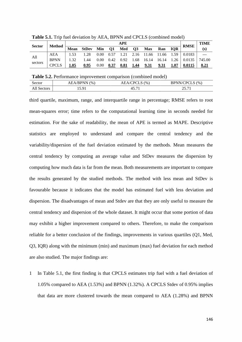
146

third quartile, maximum, range, and interquartile range in percentage; RMSE refers to root

mean-squares error; time refers to the computational learning time in seconds needed for

estimation. For the sake of readability, the mean of APE is termed as MAPE. Descriptive

statistics are employed to understand and compare the central tendency and the

variability/dispersion of the fuel deviation estimated by the methods. Mean measures the

central tendency by computing an average value and StDev measures the dispersion by

computing how much data is far from the mean. Both measurements are important to compare

the results generated by the studied methods. The method with less mean and StDev is

favourable because it indicates that the model has estimated fuel with less deviation and

dispersion. The disadvantages of mean and Stdev are that they are only useful to measure the

central tendency and dispersion of the whole dataset. It might occur that some portion of data

may exhibit a higher improvement compared to others. Therefore, to make the comparison

reliable for a better conclusion of the findings, improvements in various quartiles (Q1, Med,

Q3, IQR) along with the minimum (min) and maximum (max) fuel deviation for each method

are also studied. The major findings are:

1 In Table 5.1, the first finding is that CPCLS estimates trip fuel with a fuel deviation of

1.05% compared to AEA (1.53%) and BPNN (1.32%). A CPCLS Stdev of 0.95% implies

that data are more clustered towards the mean compared to AEA (1.28%) and BPNN

Table 5.1. Trip fuel deviation by AEA, BPNN and CPCLS (combined model)

Sector Method APE

RMSE TIME

(s) Mean StDev Min Q1 Med Q3 Max Ran IQR

All

sectors

AEA 1.53 1.28 0.00 0.57 1.21 2.16 11.66 11.66 1.59 0.0183 ---

BPNN 1.32 1.44 0.00 0.42 0.92 1.68 16.14 16.14 1.26 0.0135 745.00

CPCLS 1.05 0.95 0.00 0.37 0.81 1.44 9.31 9.31 1.07 0.0115 8.21

Table 5.2. Performance improvement comparison (combined model)

Sector AEA/BPNN (%) AEA/CPCLS (%) BPNN/CPCLS (%)

All Sectors 15.91 45.71 25.71

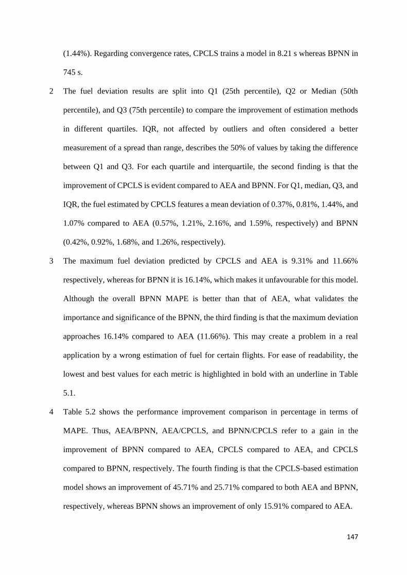
147

(1.44%). Regarding convergence rates, CPCLS trains a model in 8.21 s whereas BPNN in

745 s.

2 The fuel deviation results are split into Q1 (25th percentile), Q2 or Median (50th

percentile), and Q3 (75th percentile) to compare the improvement of estimation methods

in different quartiles. IQR, not affected by outliers and often considered a better

measurement of a spread than range, describes the 50% of values by taking the difference

between Q1 and Q3. For each quartile and interquartile, the second finding is that the

improvement of CPCLS is evident compared to AEA and BPNN. For Q1, median, Q3, and

IQR, the fuel estimated by CPCLS features a mean deviation of 0.37%, 0.81%, 1.44%, and

1.07% compared to AEA (0.57%, 1.21%, 2.16%, and 1.59%, respectively) and BPNN

(0.42%, 0.92%, 1.68%, and 1.26%, respectively).

3 The maximum fuel deviation predicted by CPCLS and AEA is 9.31% and 11.66%

respectively, whereas for BPNN it is 16.14%, which makes it unfavourable for this model.

Although the overall BPNN MAPE is better than that of AEA, what validates the

importance and significance of the BPNN, the third finding is that the maximum deviation

approaches 16.14% compared to AEA (11.66%). This may create a problem in a real

application by a wrong estimation of fuel for certain flights. For ease of readability, the

lowest and best values for each metric is highlighted in bold with an underline in Table

5.1.

4 Table 5.2 shows the performance improvement comparison in percentage in terms of

MAPE. Thus, AEA/BPNN, AEA/CPCLS, and BPNN/CPCLS refer to a gain in the

improvement of BPNN compared to AEA, CPCLS compared to AEA, and CPCLS

compared to BPNN, respectively. The fourth finding is that the CPCLS-based estimation

model shows an improvement of 45.71% and 25.71% compared to both AEA and BPNN,

respectively, whereas BPNN shows an improvement of only 15.91% compared to AEA.

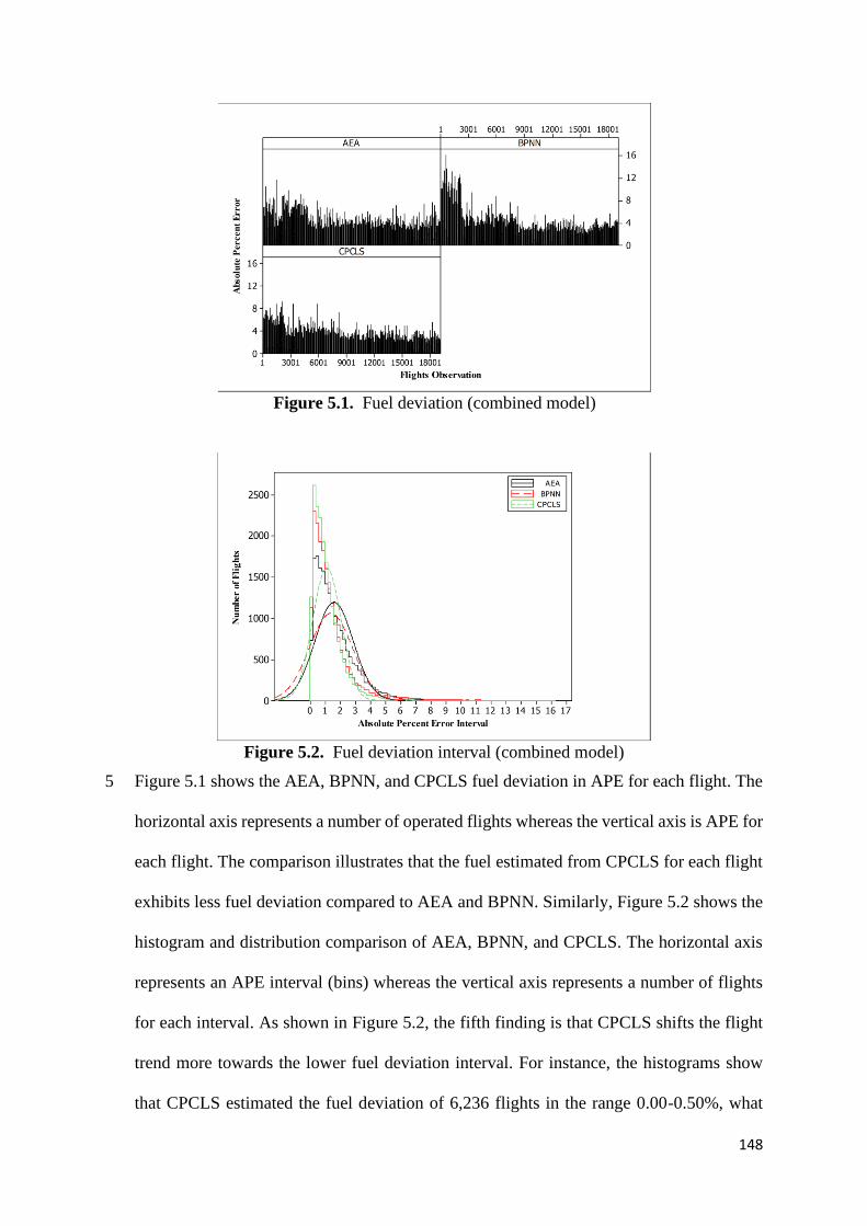
148

5 Figure 5.1 shows the AEA, BPNN, and CPCLS fuel deviation in APE for each flight. The

horizontal axis represents a number of operated flights whereas the vertical axis is APE for

each flight. The comparison illustrates that the fuel estimated from CPCLS for each flight

exhibits less fuel deviation compared to AEA and BPNN. Similarly, Figure 5.2 shows the

histogram and distribution comparison of AEA, BPNN, and CPCLS. The horizontal axis

represents an APE interval (bins) whereas the vertical axis represents a number of flights

for each interval. As shown in Figure 5.2, the fifth finding is that CPCLS shifts the flight

trend more towards the lower fuel deviation interval. For instance, the histograms show

that CPCLS estimated the fuel deviation of 6,236 flights in the range 0.00-0.50%, what

Figure 5.1. Fuel deviation (combined model)

Figure 5.2. Fuel deviation interval (combined model)

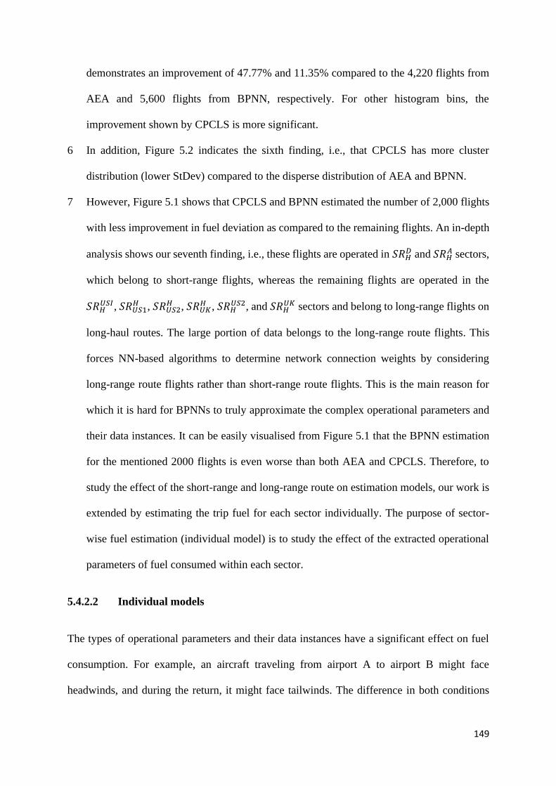
149

demonstrates an improvement of 47.77% and 11.35% compared to the 4,220 flights from

AEA and 5,600 flights from BPNN, respectively. For other histogram bins, the

improvement shown by CPCLS is more significant.

6 In addition, Figure 5.2 indicates the sixth finding, i.e., that CPCLS has more cluster

distribution (lower StDev) compared to the disperse distribution of AEA and BPNN.

7 However, Figure 5.1 shows that CPCLS and BPNN estimated the number of 2,000 flights

with less improvement in fuel deviation as compared to the remaining flights. An in-depth

analysis shows our seventh finding, i.e., these flights are operated in 𝑆𝑅𝐻𝐷 and 𝑆𝑅𝐻

𝐴 sectors,

which belong to short-range flights, whereas the remaining flights are operated in the

𝑆𝑅𝐻𝑈𝑆𝐼, 𝑆𝑅𝑈𝑆1

𝐻 , 𝑆𝑅𝑈𝑆2𝐻 , 𝑆𝑅𝑈𝐾

𝐻 , 𝑆𝑅𝐻𝑈𝑆2, and 𝑆𝑅𝐻

𝑈𝐾 sectors and belong to long-range flights on

long-haul routes. The large portion of data belongs to the long-range route flights. This

forces NN-based algorithms to determine network connection weights by considering

long-range route flights rather than short-range route flights. This is the main reason for

which it is hard for BPNNs to truly approximate the complex operational parameters and

their data instances. It can be easily visualised from Figure 5.1 that the BPNN estimation

for the mentioned 2000 flights is even worse than both AEA and CPCLS. Therefore, to

study the effect of the short-range and long-range route on estimation models, our work is

extended by estimating the trip fuel for each sector individually. The purpose of sector-

wise fuel estimation (individual model) is to study the effect of the extracted operational

parameters of fuel consumed within each sector.

5.4.2.2 Individual models

The types of operational parameters and their data instances have a significant effect on fuel

consumption. For example, an aircraft traveling from airport A to airport B might face

headwinds, and during the return, it might face tailwinds. The difference in both conditions

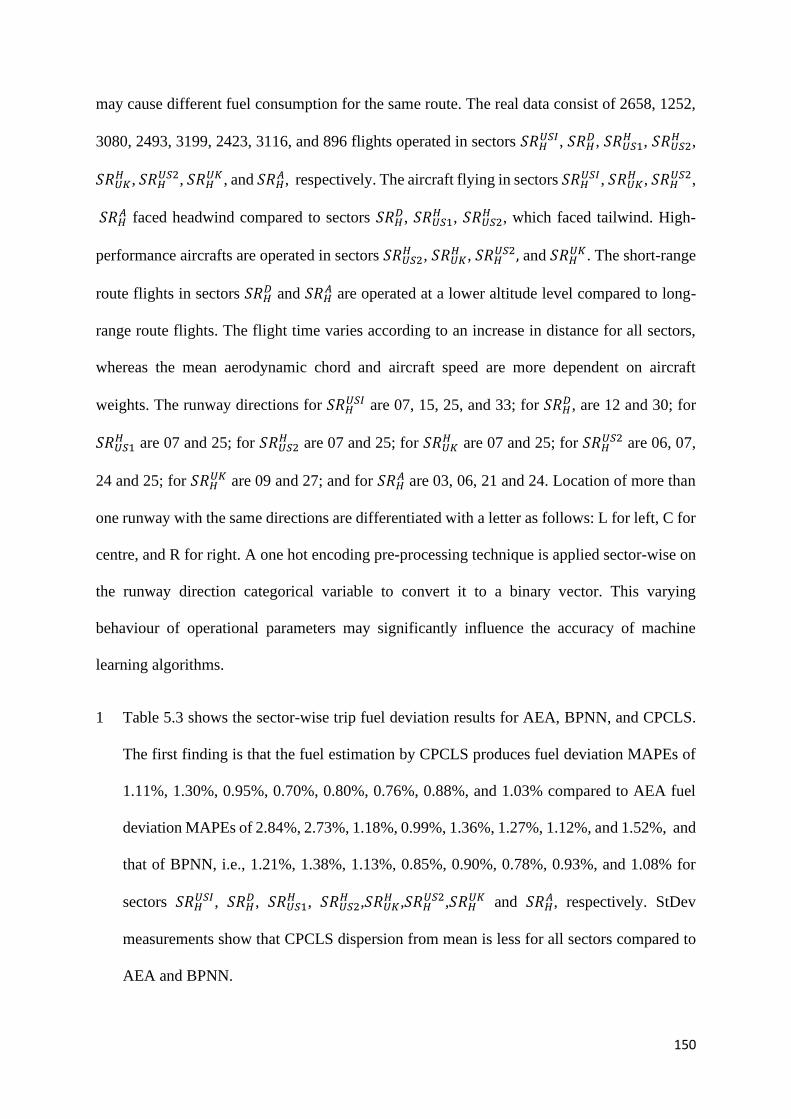
150

may cause different fuel consumption for the same route. The real data consist of 2658, 1252,

3080, 2493, 3199, 2423, 3116, and 896 flights operated in sectors 𝑆𝑅𝐻𝑈𝑆𝐼, 𝑆𝑅𝐻

𝐷, 𝑆𝑅𝑈𝑆1𝐻 , 𝑆𝑅𝑈𝑆2

𝐻 ,

𝑆𝑅𝑈𝐾𝐻 , 𝑆𝑅𝐻

𝑈𝑆2, 𝑆𝑅𝐻𝑈𝐾, and 𝑆𝑅𝐻

𝐴, respectively. The aircraft flying in sectors 𝑆𝑅𝐻𝑈𝑆𝐼, 𝑆𝑅𝑈𝐾

𝐻 , 𝑆𝑅𝐻𝑈𝑆2,

𝑆𝑅𝐻𝐴 faced headwind compared to sectors 𝑆𝑅𝐻

𝐷, 𝑆𝑅𝑈𝑆1𝐻 , 𝑆𝑅𝑈𝑆2

𝐻 , which faced tailwind. High-

performance aircrafts are operated in sectors 𝑆𝑅𝑈𝑆2𝐻 , 𝑆𝑅𝑈𝐾

𝐻 , 𝑆𝑅𝐻𝑈𝑆2, and 𝑆𝑅𝐻

𝑈𝐾. The short-range

route flights in sectors 𝑆𝑅𝐻𝐷 and 𝑆𝑅𝐻

𝐴 are operated at a lower altitude level compared to long-

range route flights. The flight time varies according to an increase in distance for all sectors,

whereas the mean aerodynamic chord and aircraft speed are more dependent on aircraft

weights. The runway directions for 𝑆𝑅𝐻𝑈𝑆𝐼 are 07, 15, 25, and 33; for 𝑆𝑅𝐻

𝐷, are 12 and 30; for

𝑆𝑅𝑈𝑆1𝐻 are 07 and 25; for 𝑆𝑅𝑈𝑆2

𝐻 are 07 and 25; for 𝑆𝑅𝑈𝐾𝐻 are 07 and 25; for 𝑆𝑅𝐻

𝑈𝑆2 are 06, 07,

24 and 25; for 𝑆𝑅𝐻𝑈𝐾 are 09 and 27; and for 𝑆𝑅𝐻

𝐴 are 03, 06, 21 and 24. Location of more than

one runway with the same directions are differentiated with a letter as follows: L for left, C for

centre, and R for right. A one hot encoding pre-processing technique is applied sector-wise on

the runway direction categorical variable to convert it to a binary vector. This varying

behaviour of operational parameters may significantly influence the accuracy of machine

learning algorithms.

1 Table 5.3 shows the sector-wise trip fuel deviation results for AEA, BPNN, and CPCLS.

The first finding is that the fuel estimation by CPCLS produces fuel deviation MAPEs of

1.11%, 1.30%, 0.95%, 0.70%, 0.80%, 0.76%, 0.88%, and 1.03% compared to AEA fuel

deviation MAPEs of 2.84%, 2.73%, 1.18%, 0.99%, 1.36%, 1.27%, 1.12%, and 1.52%, and

that of BPNN, i.e., 1.21%, 1.38%, 1.13%, 0.85%, 0.90%, 0.78%, 0.93%, and 1.08% for

sectors 𝑆𝑅𝐻𝑈𝑆𝐼, 𝑆𝑅𝐻

𝐷, 𝑆𝑅𝑈𝑆1𝐻 , 𝑆𝑅𝑈𝑆2

𝐻 ,𝑆𝑅𝑈𝐾𝐻 ,𝑆𝑅𝐻

𝑈𝑆2,𝑆𝑅𝐻𝑈𝐾 and 𝑆𝑅𝐻

𝐴, respectively. StDev

measurements show that CPCLS dispersion from mean is less for all sectors compared to

AEA and BPNN.

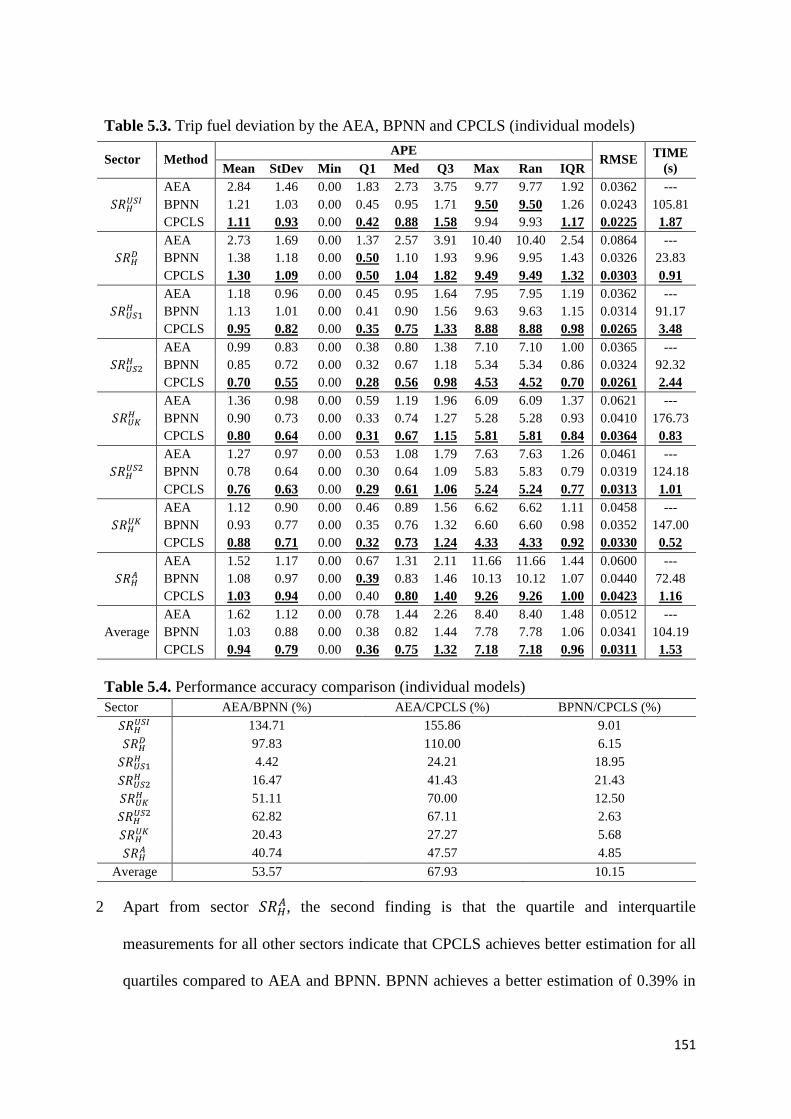
151

2 Apart from sector 𝑆𝑅𝐻𝐴, the second finding is that the quartile and interquartile

measurements for all other sectors indicate that CPCLS achieves better estimation for all

quartiles compared to AEA and BPNN. BPNN achieves a better estimation of 0.39% in

Table 5.3. Trip fuel deviation by the AEA, BPNN and CPCLS (individual models)

Sector Method APE

RMSE TIME

(s) Mean StDev Min Q1 Med Q3 Max Ran IQR

𝑆𝑅𝐻𝑈𝑆𝐼

AEA 2.84 1.46 0.00 1.83 2.73 3.75 9.77 9.77 1.92 0.0362 ---

BPNN 1.21 1.03 0.00 0.45 0.95 1.71 9.50 9.50 1.26 0.0243 105.81

CPCLS 1.11 0.93 0.00 0.42 0.88 1.58 9.94 9.93 1.17 0.0225 1.87

𝑆𝑅𝐻𝐷

AEA 2.73 1.69 0.00 1.37 2.57 3.91 10.40 10.40 2.54 0.0864 ---

BPNN 1.38 1.18 0.00 0.50 1.10 1.93 9.96 9.95 1.43 0.0326 23.83

CPCLS 1.30 1.09 0.00 0.50 1.04 1.82 9.49 9.49 1.32 0.0303 0.91

𝑆𝑅𝑈𝑆1𝐻

AEA 1.18 0.96 0.00 0.45 0.95 1.64 7.95 7.95 1.19 0.0362 ---

BPNN 1.13 1.01 0.00 0.41 0.90 1.56 9.63 9.63 1.15 0.0314 91.17

CPCLS 0.95 0.82 0.00 0.35 0.75 1.33 8.88 8.88 0.98 0.0265 3.48

𝑆𝑅𝑈𝑆2𝐻

AEA 0.99 0.83 0.00 0.38 0.80 1.38 7.10 7.10 1.00 0.0365 ---

BPNN 0.85 0.72 0.00 0.32 0.67 1.18 5.34 5.34 0.86 0.0324 92.32

CPCLS 0.70 0.55 0.00 0.28 0.56 0.98 4.53 4.52 0.70 0.0261 2.44

𝑆𝑅𝑈𝐾𝐻

AEA 1.36 0.98 0.00 0.59 1.19 1.96 6.09 6.09 1.37 0.0621 ---

BPNN 0.90 0.73 0.00 0.33 0.74 1.27 5.28 5.28 0.93 0.0410 176.73

CPCLS 0.80 0.64 0.00 0.31 0.67 1.15 5.81 5.81 0.84 0.0364 0.83

𝑆𝑅𝐻𝑈𝑆2

AEA 1.27 0.97 0.00 0.53 1.08 1.79 7.63 7.63 1.26 0.0461 ---

BPNN 0.78 0.64 0.00 0.30 0.64 1.09 5.83 5.83 0.79 0.0319 124.18

CPCLS 0.76 0.63 0.00 0.29 0.61 1.06 5.24 5.24 0.77 0.0313 1.01

𝑆𝑅𝐻𝑈𝐾

AEA 1.12 0.90 0.00 0.46 0.89 1.56 6.62 6.62 1.11 0.0458 ---

BPNN 0.93 0.77 0.00 0.35 0.76 1.32 6.60 6.60 0.98 0.0352 147.00

CPCLS 0.88 0.71 0.00 0.32 0.73 1.24 4.33 4.33 0.92 0.0330 0.52

𝑆𝑅𝐻𝐴

AEA 1.52 1.17 0.00 0.67 1.31 2.11 11.66 11.66 1.44 0.0600 ---

BPNN 1.08 0.97 0.00 0.39 0.83 1.46 10.13 10.12 1.07 0.0440 72.48

CPCLS 1.03 0.94 0.00 0.40 0.80 1.40 9.26 9.26 1.00 0.0423 1.16

Average

AEA 1.62 1.12 0.00 0.78 1.44 2.26 8.40 8.40 1.48 0.0512 ---

BPNN 1.03 0.88 0.00 0.38 0.82 1.44 7.78 7.78 1.06 0.0341 104.19

CPCLS 0.94 0.79 0.00 0.36 0.75 1.32 7.18 7.18 0.96 0.0311 1.53

Table 5.4. Performance accuracy comparison (individual models)

Sector AEA/BPNN (%) AEA/CPCLS (%) BPNN/CPCLS (%)

𝑆𝑅𝐻𝑈𝑆𝐼 134.71 155.86 9.01

𝑆𝑅𝐻𝐷 97.83 110.00 6.15

𝑆𝑅𝑈𝑆1𝐻 4.42 24.21 18.95

𝑆𝑅𝑈𝑆2𝐻 16.47 41.43 21.43

𝑆𝑅𝑈𝐾𝐻 51.11 70.00 12.50

𝑆𝑅𝐻𝑈𝑆2 62.82 67.11 2.63

𝑆𝑅𝐻𝑈𝐾 20.43 27.27 5.68

𝑆𝑅𝐻𝐴 40.74 47.57 4.85

Average 53.57 67.93 10.15

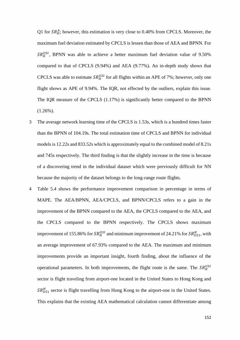
152

Q1 for 𝑆𝑅𝐻𝐴; however, this estimation is very close to 0.40% from CPCLS. Moreover, the

maximum fuel deviation estimated by CPCLS is lessen than those of AEA and BPNN. For

𝑆𝑅𝐻𝑈𝑆𝐼, BPNN was able to achieve a better maximum fuel deviation value of 9.50%

compared to that of CPCLS (9.94%) and AEA (9.77%). An in-depth study shows that

CPCLS was able to estimate 𝑆𝑅𝐻𝑈𝑆𝐼 for all flights within an APE of 7%; however, only one

flight shows as APE of 9.94%. The IQR, not effected by the outliers, explain this issue.

The IQR measure of the CPCLS (1.17%) is significantly better compared to the BPNN

(1.26%).

3 The average network learning time of the CPCLS is 1.53s, which is a hundred times faster

than the BPNN of 104.19s. The total estimation time of CPCLS and BPNN for individual

models is 12.22s and 833.52s which is approximately equal to the combined model of 8.21s

and 745s respectively. The third finding is that the slightly increase in the time is because

of a discovering trend in the individual dataset which were previously difficult for NN

because the majority of the dataset belongs to the long-range route flights.

4 Table 5.4 shows the performance improvement comparison in percentage in terms of

MAPE. The AEA/BPNN, AEA/CPCLS, and BPNN/CPCLS refers to a gain in the

improvement of the BPNN compared to the AEA, the CPCLS compared to the AEA, and

the CPCLS compared to the BPNN respectively. The CPCLS shows maximum

improvement of 155.86% for 𝑆𝑅𝐻𝑈𝑆𝐼 and minimum improvement of 24.21% for 𝑆𝑅𝑈𝑆1

𝐻 , with

an average improvement of 67.93% compared to the AEA. The maximum and minimum

improvements provide an important insight, fourth finding, about the influence of the

operational parameters. In both improvements, the flight route is the same. The 𝑆𝑅𝐻𝑈𝑆𝐼

sector is flight traveling from airport-one located in the United States to Hong Kong and

𝑆𝑅𝑈𝑆1𝐻 sector is flight travelling from Hong Kong to the airport-one in the United States.

This explains that the existing AEA mathematical calculation cannot differentiate among

153

the varying behaviour of operational parameters. The use of global parameters for the both

Figure 5.3. Fuel deviation (𝑆𝑅𝐻

𝑈𝑆𝐼)

Figure 5.4. Fuel deviation (𝑆𝑅𝐻

𝐷)

Figure 5.5. Fuel deviation (𝑆𝑅𝑈𝑆1

𝐻 )

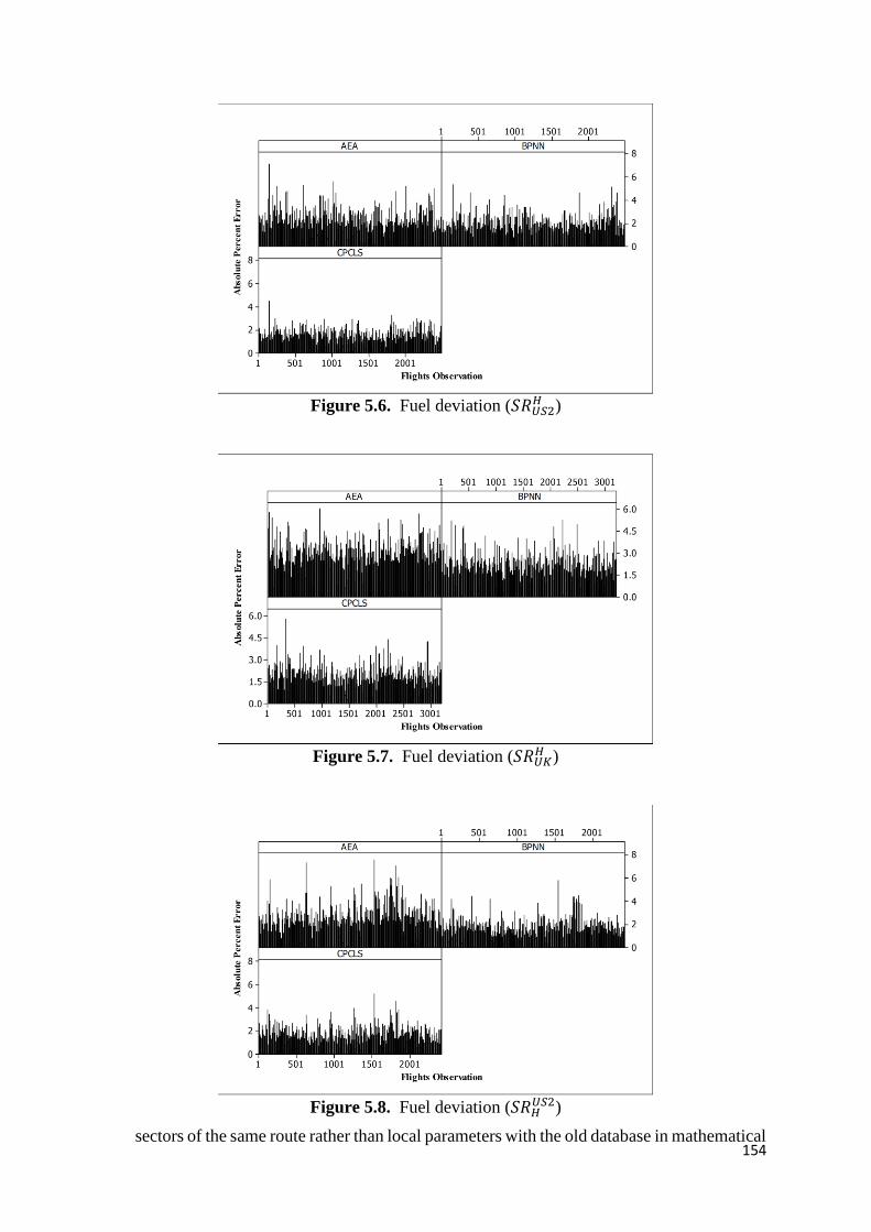
154

sectors of the same route rather than local parameters with the old database in mathematical

Figure 5.6. Fuel deviation (𝑆𝑅𝑈𝑆2

𝐻 )

Figure 5.7. Fuel deviation (𝑆𝑅𝑈𝐾

𝐻 )

Figure 5.8. Fuel deviation (𝑆𝑅𝐻

𝑈𝑆2)

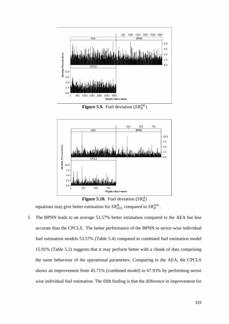
155

equations may give better estimation for 𝑆𝑅𝑈𝑆1𝐻 compared to 𝑆𝑅𝐻

𝑈𝑆𝐼.

5 The BPNN leads to an average 53.57% better estimation compared to the AEA but less

accurate than the CPCLS. The better performance of the BPNN in sector-wise individual

fuel estimation models 53.57% (Table 5.4) compared to combined fuel estimation model

15.91% (Table 5.2) suggests that it may perform better with a chunk of data comprising

the same behaviour of the operational parameters. Comparing to the AEA, the CPCLS

shows an improvement from 45.71% (combined model) to 67.93% by performing sector

wise individual fuel estimation. The fifth finding is that the difference in improvement for

Figure 5.9. Fuel deviation (𝑆𝑅𝐻

𝑈𝐾)

Figure 5.10. Fuel deviation (𝑆𝑅𝐻

𝐴)

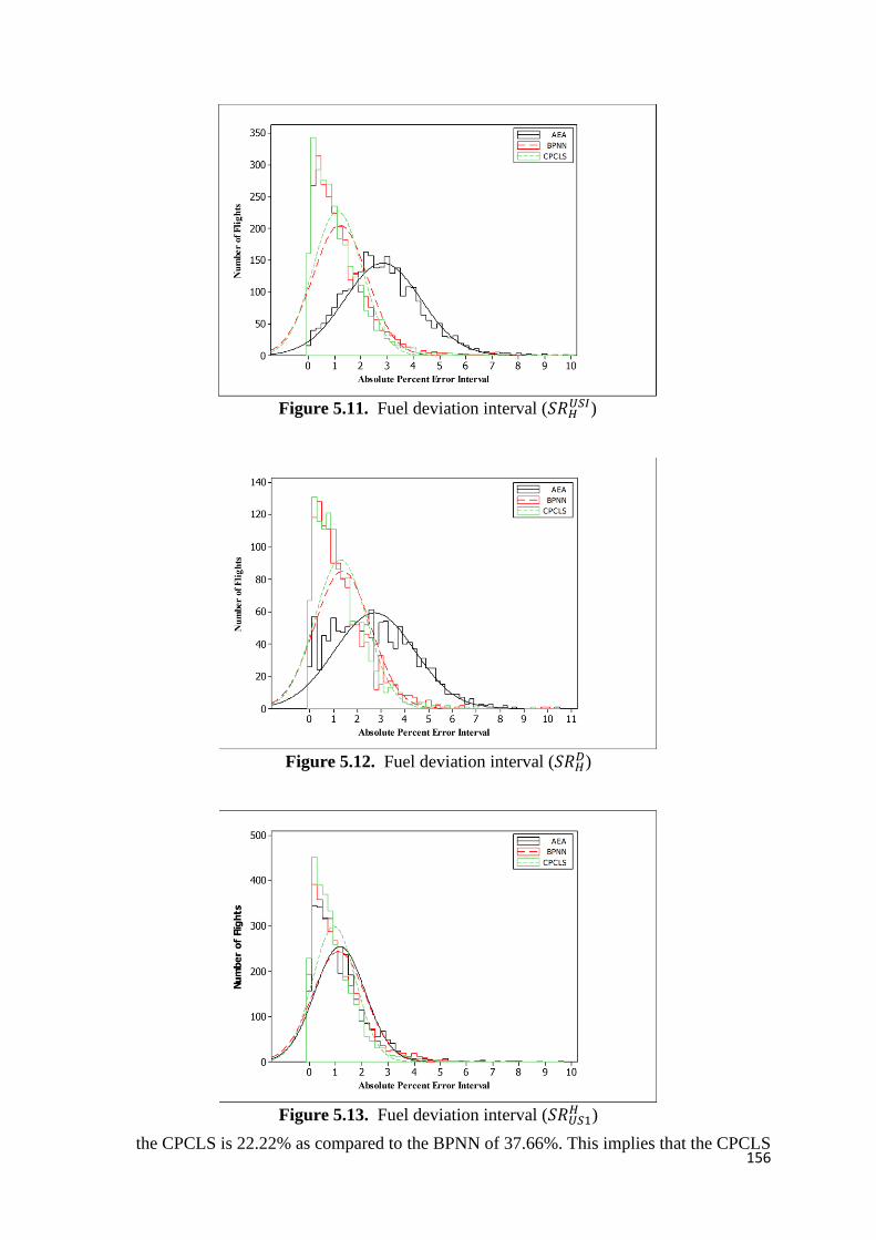
156

the CPCLS is 22.22% as compared to the BPNN of 37.66%. This implies that the CPCLS

Figure 5.11. Fuel deviation interval (𝑆𝑅𝐻

𝑈𝑆𝐼)

Figure 5.12. Fuel deviation interval (𝑆𝑅𝐻

𝐷)

Figure 5.13. Fuel deviation interval (𝑆𝑅𝑈𝑆1

𝐻 )

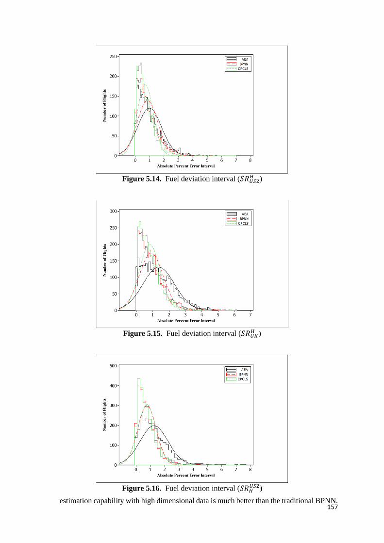
157

estimation capability with high dimensional data is much better than the traditional BPNN.

Figure 5.14. Fuel deviation interval (𝑆𝑅𝑈𝑆2

𝐻 )

Figure 5.15. Fuel deviation interval (𝑆𝑅𝑈𝐾

𝐻 )

Figure 5.16. Fuel deviation interval (𝑆𝑅𝐻

𝑈𝑆2)

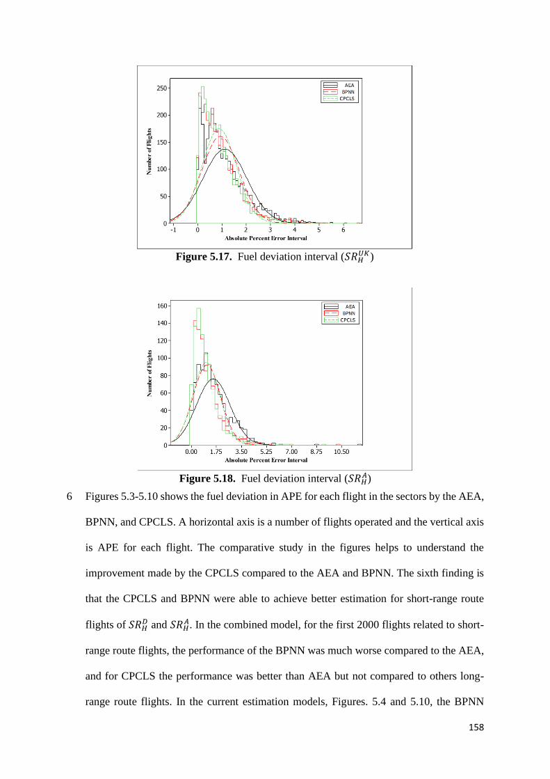
158

6 Figures 5.3-5.10 shows the fuel deviation in APE for each flight in the sectors by the AEA,

BPNN, and CPCLS. A horizontal axis is a number of flights operated and the vertical axis

is APE for each flight. The comparative study in the figures helps to understand the

improvement made by the CPCLS compared to the AEA and BPNN. The sixth finding is

that the CPCLS and BPNN were able to achieve better estimation for short-range route

flights of 𝑆𝑅𝐻𝐷 and 𝑆𝑅𝐻

𝐴. In the combined model, for the first 2000 flights related to short-

range route flights, the performance of the BPNN was much worse compared to the AEA,

and for CPCLS the performance was better than AEA but not compared to others long-

range route flights. In the current estimation models, Figures. 5.4 and 5.10, the BPNN

Figure 5.18. Fuel deviation interval (𝑆𝑅𝐻

𝐴)

Figure 5.17. Fuel deviation interval (𝑆𝑅𝐻

𝑈𝐾)

159

achieves better estimation than the AEA, and the CPCLS achieves better estimation

compared to both AEA and BPNN. Similarly, for all other sectors, Figures 5.3, 5.5-5.9,

the APE of each flights shows better results for the CPCLS compared to the AEA and

BPNN.

7 As mentioned earlier that sector 𝑆𝑅𝐻𝑈𝑆𝐼 and 𝑆𝑅𝑈𝑆1

𝐻 follow the same route but travel in the

opposite direction. Comparative study of Figure 5.3 and 5.5, shows that the AEA estimated

APE for flights is much higher for 𝑆𝑅𝐻𝑈𝑆𝐼 (MAPE 2.84%) compared to 𝑆𝑅𝑈𝑆1

𝐻 (MAPE

1.18%). The reason is using the same global parameter for both sectors rather than local

parameters. Based on historical data, the seventh finding is that the CPCLS minimized this

issue and shows APE for both sectors (Figures 5.3 and 5.5) almost identical. For other

sectors having the same route, for instance 𝑆𝑅𝐻𝑈𝑆2,𝑆𝑅𝑈𝑆2

𝐻 and 𝑆𝑅𝑈𝐾𝐻 , 𝑆𝑅𝐻

𝑈𝐾, the figures show

the same issue of usage of global hyperparameter and old database by the AEA. The 𝑆𝑅𝐻𝑈𝑆2

shows higher APE compared to 𝑆𝑅𝑈𝑆2𝐻 , and 𝑆𝑅𝑈𝐾

𝐻 shows higher APE compared to 𝑆𝑅𝐻𝑈𝐾.

This demonstrates the main limitation, as highlighted in the literature review Chapter 2, of

the EA based methods.

8 Figures 5.11- 5.18 shows the histogram and distribution comparison of the AEA, BPNN,

and CPCLS. The histograms indicate that the CPCLS fuel deviation is spread on less APE

bins with a major focus on estimating flights contributing to less deviation bins. For most

sectors, the eighth finding is that the distribution of CPCLS is more clustered as compared

to the AEA and BPNN. For instance, in Figures 5.11 and 5.12, the bell shape of 𝑆𝑅𝐻𝑈𝑆𝐼 and

𝑆𝑅𝐻𝐷 sectors show that the AEA method fuel deviation exists mainly in the bins 1.50-

3.50%, whereas, the CPCLS distribution peak shape shows that the fuel deviation exists in

0.00-1.00%. In Figures 5.13, 5.16, 5.18 for 𝑆𝑅𝑈𝑆1𝐻 , 𝑆𝑅𝐻

𝑈𝑆2, 𝑆𝑅𝐻𝐴, the distribution of BPNN

is almost identical to the AEA or CPCLS. For all sectors, the histogram and distribution

trend of the CPCLS illustrates that it attempts to estimate trip fuel for flights with less

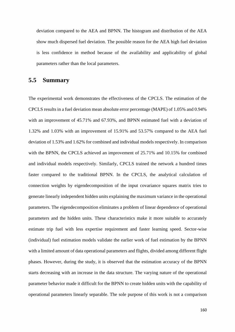
160

deviation compared to the AEA and BPNN. The histogram and distribution of the AEA

show much dispersed fuel deviation. The possible reason for the AEA high fuel deviation

is less confidence in method because of the availability and applicability of global

parameters rather than the local parameters.

5.5 Summary

The experimental work demonstrates the effectiveness of the CPCLS. The estimation of the

CPCLS results in a fuel deviation mean absolute error percentage (MAPE) of 1.05% and 0.94%

with an improvement of 45.71% and 67.93%, and BPNN estimated fuel with a deviation of

1.32% and 1.03% with an improvement of 15.91% and 53.57% compared to the AEA fuel

deviation of 1.53% and 1.62% for combined and individual models respectively. In comparison

with the BPNN, the CPCLS achieved an improvement of 25.71% and 10.15% for combined

and individual models respectively. Similarly, CPCLS trained the network a hundred times

faster compared to the traditional BPNN. In the CPCLS, the analytical calculation of

connection weights by eigendecomposition of the input covariance squares matrix tries to

generate linearly independent hidden units explaining the maximum variance in the operational

parameters. The eigendecomposition eliminates a problem of linear dependence of operational

parameters and the hidden units. These characteristics make it more suitable to accurately

estimate trip fuel with less expertise requirement and faster learning speed. Sector-wise

(individual) fuel estimation models validate the earlier work of fuel estimation by the BPNN

with a limited amount of data operational parameters and flights, divided among different flight

phases. However, during the study, it is observed that the estimation accuracy of the BPNN

starts decreasing with an increase in the data structure. The varying nature of the operational

parameter behavior made it difficult for the BPNN to create hidden units with the capability of

operational parameters linearly separable. The sole purpose of this work is not a comparison

161

of the CPCLS with AEA and BPNN. The main contribution is to propose and apply the self-

organizing CNN algorithm that gives better estimation accuracy with less expertise

requirement and faster learning speed. The significant improvement of 67.93% by the proposed

CPCLS method in existing airline fuel estimation (i.e., AEA) will directly benefit in

eliminating excess fuel consumption.

162

Chapter 6. Conclusion and Future Work

6.1 Conclusion

This work addresses airline trip fuel deviation from estimated values, which results in excessive

fuel consumption. Accurate fuel estimation is crucial for airlines to ensure safety and

profitability. Nowadays, the aviation industry is growing at a significant rate and improvement

in various operations can ensure long term sustainability. Among various operating expenses,

fuel cost contributes to an average 28.2% which makes it more valuable to design a method

that may accurately estimate fuel for each flight journey. It has been noticed that fuel

consumption demand is increasing each year. The forecasted demand was to reach 97 billion

gallons in 2019 compared to the level of 2006 because of an increase in demand of passengers

and cargos. These promising economic opportunities may become a threat if airlines are unable

to handle problems of increase in jet fuel prices and international authorities regulations to

protect environmental degradation. It was forecasted that jet fuel prices will increase by 31.18%

in 2019 compared to the 2015 level. Besides, to protect environmental degradation and avoid

ozone depletion, international authorities stress to reduce CO2 emissions by 50% by 2050 with

respect to 2005 and reduce fuel consumption 1.5% per year. In the future, international

authorities are planning to make it compulsory for airlines to certify their aircraft based on size

and weight, according to CO2 certification standards. The growing demand with high fuel

prices and increasing awareness for environmental protection are encouraging airlines to adopt

competitive strategies in fuel management to control excess fuel consumption for long-term

sustainability.

163

In the existing literature, the efforts made by researchers to address the fuel estimation problem

are noteworthy. However, there are still some research gaps that need considerable attention.

The research gaps are concisely summarized as follows:

1 The most popular fuel estimation methods that are currently in practice by various

airlines are based on energy balance mathematical formulation. It is identified that the

actual performance of aircraft usually deviates from such estimation. The EAs need

information about many coefficients to determine the amount of fuel needed for each

journey. Firstly, the information about coefficients is not always available in a real

scenario and a lot of flight testing is needed to perform to generate such information.

This makes the method expensive to adopt. Secondly, the unavailability of such

information may lead to the use of global parameters with default values rather than

local parameters which may result in inaccurate estimation. In current literature, an

insufficient attempt has been made to study the effect of using global parameters on the

deviation of fuel from estimation using a practical example.

2 The popularity of the application of machine learning NNs in the aviation sector to

improve various operations is significant. The BPNN based fuel estimation was

proposed to provide an alternative to EAs. A pitfall is that BPNN is a fixed topology

NN and adjustment of various hyperparameters is based on human expertise. The

BPNN drawbacks of trial and error experimental work to determine network and

convergence at local minima may not assure that the selected network is optimal

causing weak generalization performance and slow convergence. In existing works,

BPNN is applied to estimate fuel without addressing the above key issues.

3 In the existing literature, the operational parameters are selected based on prior

experience and knowledge. There may exist some operational parameters that may also

contribute to fuel consumption and are unnoticed. BPNN based fuel estimation models

164

are learned on low-level operational parameters with the future recommendation of

incorporating more parameters. In literature, the research gap still exists to incorporate

high-level operational parameters that are previously ignored.

4 Likewise, EAs and BPNNs, many other models are proposed to estimate fuel for

distinct flight phases. The cumulative effect of distinct phases to estimate fuel for the

complete journey may even lead to higher fuel deviation. Therefore, it is important to

have a model that can efficiently estimate fuel for all phases collectively to ensure

profitability and safety.

5 The trained NN performance may no longer be suitable for learning the same

application if data structure and size changes. How to improve the machine learning

NNs that give the same performance regardless of change is data structure and size is

gaining significant consideration.

To address the above research gaps, we conducted our work in three main stages to achieve

three objectives discussed in Chapter 1, Section 1.3. The first stage is discussed in Chapter 3,

in which we discussed the framework and model is formulated to achieve an objective function

of minimizing fuel deviation. The significance of the proposed work and its relationship to

existing methods is constructed to understand the purpose and need of the work. Chapter 3

mainly addresses the first four research gaps. The second stage is discussed in Chapter 4, in

which novel CNN is proposed to avoid trial and error experimental work by analytically

calculating connection weights with improved cascade architecture. This chapter mainly

addresses research gaps second and fifth. The third stage is discussed in Chapter 5, in which

comparative study among proposed CPCLS, AEA and BPNN is performed. The chapter

provides important managerial insight and mainly addresses all research gaps.

165

In Chapter 3, prior to formulating model and defining an objective function, a framework of

fuel consumption and its deviation from estimation problem, and useful operational parameters

that can contribute to fuel consumption are explained. The problem of fuel deviation arises

because of the inappropriate selection of estimation methods and operational parameters. Low

confidence in existing estimation methods results in adding more fuel in discrepancy reservoirs

other than contingency and supplementary reservoirs to ensure a smooth journey. This

ultimately increases the total weight of the aircraft and results in more fuel consumption. This

problem is known as overestimation and concern profitability issues. Also, loading suboptimal

fuel, known as underestimation, may concern safety issues. Therefore, the objective of reaching

a designation airport with minimal deviation cannot be achieved. The methods used for

estimating fuel consumption are mainly divided into two types: the mathematical method and

data-driven method. Mathematical methods are advantageous that they provide the physical

understanding of the system, however, according to the recent studies many challenges exist in

real practice. The mathematical methods need a lot of information to define the relationship

among variables, difficult to study system non-linearities, and need expert involvement.

Machine learning data-driven methods are considered a viable tool for discovering hidden

patterns or information from historical data. Among many machine learning algorithms, NNs

are generally favorable because of their universal approximation capability. However, existing

BPNN based fuel estimation models are limited in scope by considering low-level operational

parameters with few aircraft types with the future recommendation of incorporating high-level

operational parameters. The reason for this is low generalization performance and slow

convergence drawbacks of BPNN. Moreover, it requires much human intervention to decide

and adjust hyperparameters. In addition, selecting operational parameters based on prior

experience or knowledge and using global values may consequence in inaccurate results. In

this chapter, a trip fuel estimation model is formulated by considering the first four research

166

gaps. The useful operational parameters representing historical real data that can contribute to

fuel consumption are extracted and added to the model. The objective function of minimizing

fuel deviation is defined. Rather than estimating fuel for distinct phases, the model is based on

estimating fuel for all phases collectively.

In Chapter 4, a novel self-organizing CNN is proposed. The objective is to improve the

performance of the estimation model with less expertise involvement and obtain results with

fast learning speed. A comprehensive review of FNNs was conducted (Chapter 2, Section 2.2)

to understand the merits and limitations along with applications of various algorithms. Based

on three decades of review of FNN, we classified the literature into six categories. Those six

categories are gradient learning algorithms, gradient-free learning algorithms, optimization

algorithms for learning rate, bias and variance (Underfitting and Overfitting) minimization

algorithms, constructive topology FNN, and metaheuristic search algorithms. Following the

literature review, we identified some research gaps in the existing FNNs. Those research gaps

are studying the effect of activation functions, designing efficient and compact algorithm with

fewer hyperparameters, analytically calculating connection weights rather than a random

generation and gradient optimization, change in a data structure, eliminating the need for data

pre-processing and transformation, adopting a hybrid approach for real-world applications, and

determining analytically a number of hidden units. Inspired from the gradient-free learning

algorithms (Chapter 2, Subsection 2.2.3.2) having the property of calculating analytically

output connection weights and the constructive topology FNN (Chapter 2, Subsection 2.2.4.3)

having the property of adding hidden units in the hidden layer, we proposed new algorithm.

Efforts were also made to address two research gaps of “calculating connection weights rather

than a random generation and gradient optimization” and “change in data structure” in the

proposed algorithm. Combining the concept of two categories and two research gaps result in

a novel algorithm named as cascade principal component least squares (CPCLS) neural

167

network. The characteristics of CPCLS is that it analytically determines connection weights

rather than gradient or random generation and add multiple linearly independent hidden units

in the hidden layer to improve and make convergence faster. Experimental work was conducted

on artificial benchmarking and real-world problems to demonstrate the superiority of CPCLS.

The work shows that proposed CPCLS achieved better generalization performance and faster

learning speed compared to other known NNs, such as CasCor, BPNN, SaELM, OLSCN, and

FCNN. The theoretical justification and experimental work demonstrated that hidden units

generated in the hidden layer, and connecting only newly added last hidden layer to output

layer ensures maximum convergence.

In chapter 5, the novel CPCLS is applied to the fuel estimation model to achieve the objective

function of minimal fuel deviation and reduce the negative role of global parameters and

varying operational parameters on fuel consumption. The purpose was to eliminate the need

for a trial-and-error approach and reduce the number of hyperparameter adjustments and expert

involvement. We consider that insufficient attempts have been reported in the literature

concerning the estimation of trip fuel using CNNs along with high-dimensional data for the

entire trip flight phases collectively. A comparative study with the existing AEA and a

traditional BPNN to estimate trip fuel prove that our work is unique in studying the sectors

both in combination and individually by considering all flight phases as a complete flight trip.

Unlike AEA and BPNN, the proposed CPCLS does not require complex mathematical

formulation, a trial-and-error approach, gradient derivative techniques, or too many

hyperparameter initializations. This makes it superior to estimate trip fuel accurately with fewer

expertise requirements and faster learning speed. Previously, the entire trip was divided into

different flight phases, namely takeoff, climb, cruise, descent, and approach, to propose a fuel

estimation model with limited flight data restricted to a small number of aircraft or generated

by a simulation planner. In our study, we analyzed high-dimensional data associated with 107

168

wide-body aircrafts ̶ Airbus A330-300 (31 aircrafts) and Boeing 747-400 (9 aircrafts)/747-

800 (14 aircrafts)/777-300 (53 aircrafts) ̶ that operated a total of 19,117 real international

passenger and cargo flights in eight sectors over two years. Comparative study results

demonstrate that the trip fuel estimation by the proposed CPCLS achieves better results while

requiring the shortest time compared to AEA and BPNN. The CPCLS exhibits an average

improvement of 45.71% and 25.71% for a combined eight-sector model, and 67.93% and

10.15% for a sector-wise individual model, compared to AEA and BPNN, respectively. The

significant improvement in trip fuel estimation creates greater confidence in the proposed

CPCLS given that it may eliminate the need for adding more fuel-based solely on experience.

In summary, educationally, the experimental work on the varying nature of operational

parameters and high dimensionality of data demonstrates the effectiveness of CPCLS, which,

with low fuel deviation and more stable results, demonstrates that can be effectively employed

for estimating trip fuel for each flight. The better and faster estimation results of the self-

organizing CPCLS is because of its analytical calculation of network connection weights

explaining maximum variance in the operational parameters. Thus, CPCLS is a promising

machine learning tool for estimating flight trip fuel. In practical applications, the proposed

CPCLS will be beneficial to airlines by accurately planning the amount of flight trip fuel. This

may avoid the need for extra fuel to be loaded in the aircraft and helps in better management

control. Flight planners and pilots will be more confident with trip fuel estimation and will

avoid the requirement for extra fuel in the discrepancy tank. The weight of aircraft will

decrease, which will not only reduce fuel consumption but also will increase the lifetime of the

engines. The flight planner may suggest and select a suitable airways route by simulating

different combinations of operational parameters to reach the destination with fewer fuel

requirements. Furthermore, controlling excess fuel consumption may benefit in contributing to

less environmental pollution, preventing the scarce jet fuel from natural resources from being

169

wasted, as well as surviving with growing fuel prices, less unplanned aircraft maintenance,

fewer fuel surcharges, and more competitiveness by fulfilling the demand of passengers and

cargo.

6.2 Future Work

This work has addressed the problem of fuel deviation by formulating a model and proposing

a novel CNN. However, there are still some limitations that need to be addressed in future

work. Several important research directions are summarized as:

1. In this work, our main focus was to minimize the fuel deviation by accurately estimating

trip fuel. The work is about predictive analytics that mainly addresses the fuel

estimation and deviation problem. How to identify the alternative routes having less

fuel requirement shall be addressed in the future by performing prescriptive analytics.

The formulated model in Chapter 3 can be extended to estimate aircraft horizontal and

vertical trajectories along with trip fuel estimation. Initial prediction of trajectories by

machine learning and further optimization by mathematical modelling or reinforcement

learning may help to discover alternative routes having less fuel requirement. Currently,

airlines follow the routes as per international guidelines. Identifying the alternative

routes having less fuel requirement may facilitate airlines for making long term

contingency plans.

2. In Chapter 4, OLT was achieved by the eigendecomposition of the covariance

symmetric matrix. Other than the covariance matrix, correlation and single value

decomposition methods can also be applied to achieve OLT. Besides, the experimental

work was performed by considering only the popular sigmoid activation function.

Future direction is to consider other OLT methods and activation functions and study

170

their effects on the performance and learning speed of novel CPCLS. Additionally, its

consequence on trip fuel estimation needs to explore in the future.

3. In Chapter 5, CPCLS is compared to AEA in terms of fuel deviation, whereas its

comparison with BPNN is in terms of both fuel deviation and learning speed. The

computational time for AEA was not considered because the information was not

available in the historical dataset provided by the airline. How much CPCLS is

computational better than AEA is still unclear. This is the main practical limitations in

applying the proposed fuel estimation model in the airline industry. The computational

comparison between CPCLS and AEA maybe explore in the future to facilitate airlines

operating companies in understanding the true benefits of the proposed algorithm.

In addition to the above research directions, some new research directions were identified in

Chapter 2 Section 2.3 to add a contribution to the existing FNNs literature. The research

directions are summarized as:

1. Activation function: Few attempts have been made to study the effect of using various

types of activation functions on FNN. Karlik and Olgac (2011) made a comparison of

popular activation functions including uni-polar sigmoid, bi-polar sigmoid, tangent

hyperbolic, radial bias function and conic section function along with gradient-based

algorithms for fixed topology FNN. The limitation of this experimental work was in

using 10 hidden units and 40 hidden units with 100 iterations and 500 iterations

respectively. Moreover, the data structure, normalization techniques, learning

algorithms, and hyperparameters were not clearly stated in the experimental work. The

experimental results demonstrated that tangent hyperbolic activation function

performance is better than the others. However, it can be observed in various studies

that the sigmoid activation function application is more common compared to tangent

171

hyperbolic function. The importance of hidden units and their activation functions is

clear and is used in every type of FNN. The studies of various activation functions

performance based on fixed and constructive topology, along with gradient algorithms

and gradient-free algorithms, still need researcher attention.

2. Efficient and compact Algorithm with fewer hyperparameters: The gradient learning

algorithms are favorable because of compact size, whereas, gradient-free learning

algorithms are favorable because of gradient-free learning and fast convergence. The

gradient-free algorithms network size becomes much larger which increases its

complexity and the chance of overfitting increases. The best FNN may be considered

to be one having the characteristics of compact architecture with a small number of

hidden units and connection weights. It may analytically calculate hidden units and

connection weights, need fewer hyperparameters and reaches a global minimum in less

training time. There is always a trade-off between network generalization performance

and learning speed. Some algorithms have the advantage of being more efficient than

others but may be constrained by memory requirements, complex architecture, and/or

more learning time. Therefore, more efforts are needed to construct efficient and fast

algorithms with fewer hyperparameters, that are computationally simple and have a

compact size.

3. Eliminating the need for data pre-processing and transformation: Better results of

machine learning algorithms are highly dependent on data pre-processing and the

transformation steps. In pre-processing, various algorithms/techniques are adapted to

clean data to reduce noise, outliers, and missing values, whereas, in transformation,

various algorithms/techniques are adapted to transform the data into formats and forms,

by encoding or standardization, that is appropriate for machine learning. Both steps are

performed prior to feeding data into FNN and are adopted in many algorithms.

172

Insufficient knowledge or inappropriate application of pre-processing and

transformation techniques may cause the algorithm to wrongly conclude the findings.

Future algorithms may be designed that are less sensitive to noise, outliers, missing

values, and do not need a specific form of reducing data features magnitude to a

common scale.

4. A hybrid approach for real-world applications: Researchers demonstrate the

effectiveness of the proposed algorithm either on benchmarking or on real-world

problems or a combination of both. The study of all six categories applications

(Appendix A) gives a clear indication that the interest in researchers proposed

algorithms on real-world problems is rapidly increasing. Traditionally, in 2000 and

earlier, experimental work for demonstrating the effectiveness of proposed algorithms

was limited to artificial benchmarking problems. The possible reasons were the

unavailability of database sources and user reluctance in using FNN. In the literature

survey, it is noticed that nowadays researchers most often use real-world data to ensure

consistency and compare their results with other popular published known algorithms.

Frequently using the same real-world applications data may cause specific data to

become a benchmark. The same issue has been observed in all categories and especially

in the second category. It is important to avoid causing specific data to become a

benchmark because that data may become unsuitable for practical application in the

future with the passage of time. The role of high dimensional, nonlinear, noisy and

unbalanced big data is changing at a rapid rate. The best practice may be to use a hybrid

approach of well-known data in the field along with new data applications during the

comparative study of algorithms. This may increase and maintain user interest in FNN

over the passage of time.

173

5. Hidden units’ analytical calculation: The successful application of learning and

regularization algorithms on complex high dimensional big data application areas,

involving more than 50,000 instances, to improve the convergence of deep neural

networks is noteworthy. The maximum error reduction property of hidden units in deep

neural networks is dependent on connection weights and activation function

determination. More research work is needed to focus on hidden units’ analytical

calculations to avoid the trial and error approach. Calculating the optimal number of

hidden units and connection weights for single or multiple hidden layers in the network,

such that no linear dependence exists may help in achieving better and stable

generalization performance. Similarly, future research work may give clear direction to

users about the application of different activation functions for enhancing business

decisions.

It should be noticed that two other research gaps named “connection weight initialization” and

“data structure” were also identified in Chapter 2 (Section 2.3). This work has addressed both

research gaps to some extent, however, some further improvements are needed to improve

FNNs:

1. Connection weight initialization: In Chapter 2, we explain that existing NNs can be

further strengthened by calculating all connection weights (including input connection

and output connection) analytically to generate hidden units, explaining maximum

variance in the dataset. This may also help to further improve the generalization and

learning speed by compacting the size of the network. From work in Chapter 4, we

concluded that generalization and learning speed has improved, however, the network

size is not compact. How to improve FNNs to make the network compact and avoid

overfitting need further attention in the future.

174

2. Data structure: In Chapter 2, we explain that few attempts have been made to study the

effect of data size and features on FNN algorithms. Future research on designing an

algorithm that can approximate the problem task equally, regardless of data size

(instance) and shape (features), will be a breakthrough achievement. From work in

Chapter 5, we concluded that the difference in improvement for the CPCLS is 22.22%

as compared to the BPNN of 37.66% by changing data from high dimensional to

chunks. This implies that the CPCLS estimation capability with high dimensional data

is much better than the traditional BPNN. The difference in improvement should be on

the lower side. Lower the difference means that algorithm performance on high

dimensional and chunks are approximately similar. CPCLS difference is lower,

however, future research work is needed to further improve FNNs algorithm that may

give a much lower difference.

175

Appendix A. Neural Networks Learning Algorithms and

Optimization Techniques Applications

A.1 Application of gradient learning algorithms

The gradient learning algorithms have gained much attention from researchers compared to

traditional statistical techniques. Gradient learning algorithms help to make a more informed

decision from the available information. Table A.1 highlights some of the applications of

gradient learning algorithms that researchers used to demonstrate the effectiveness of

algorithms during the comparative study. Before the year 2000, the range of real-world

applications appears to be on the low side. The gradient learning algorithms are among the

early attempts that researchers investigated to build FNN. In the early attempt phase, the

possible reason for the unavailability of public real-world application data sources and less

research interest might have forced researchers to rely highly on using artificial benchmarking

data.

The successful application of gradient learning algorithms is dependent on user expertise in

deciding and adjusting the hyperparameters correctly. The major concern of researchers and

users in gradient learning algorithms is to find a method for the network to converge faster. It

is believed that SGD helps to achieve generalization performance many times faster than for

batch learning. Wilson and Martinez (2003) demonstrated that SGD was able to achieve the

required accuracy, on average, 20 times faster compared to batch learning during classifying

real-world problems such as credit card requests, patient diabetes, flower species, beverages

types, religions in the country, crime, voters, and various health diseases. Similarly, while

dealing with problems having more than 1000 instances such as satellite images, shuttle

controls and displaying seven-segment digits, the SGD achieved the required accuracy, on

176

average, 70 times faster than in batch learning. Increasing the data size further reduces the

speed of batch learning and may take more than 300 times longer compared to SGD for

problems having instances greater than 10,000.

The issue with first-order gradient learning is slow learning ability and their usage in a fixed

topology neural network can make the task more time-consuming. Deciding on too many

hidden units in the network may decrease the learning speed and cause the network to become

Table A.1. Applications of gradient learning algorithms

Application Description

Hepatitis Predicting whether the patient will survive or die suffering from

hepatitis (Wilson and Martinez, 2003)

Animals Classifying animals into seven classes based on their physical

characteristics (Wilson and Martinez, 2003)

Flowers species Classifying the flowers into different species from available

information on the width and length of petals and sepals (Wilson and

Martinez, 2003)

Beverages Identifying the type of beverages in term of its physical and chemical

characteristics (Wilson and Martinez, 2003)

Country religion Predicting the religion of the countries from the information such as

population size and their flag colours (Wilson and Martinez, 2003)

Object detection Predicting whether object is rock or mine from the signal information

obtained from various sensors (Wilson and Martinez, 2003)

Crime Identifying of glass type used in crime scene based on chemical oxide

content such as sodium, potassium, calcium, iron and many others

(Wilson and Martinez, 2003)

Voters Classifying voters based on their education, crime, immigration, tax

payers and many others (Wilson and Martinez, 2003)

Heart diseases Diagnosing and categorizing the presence of heart diseases in a patient

by studying the previous history of drug addiction, health issues, blood

tests, and many others (Wilson and Martinez, 2003)

Liver disorder Diagnosing alcohol-related liver disorder based on the reports of

various blood tests (Wilson and Martinez, 2003)

Earth atmosphere Determining the strength of ions and free electrons on the layer of earth

atmosphere (Wilson and Martinez, 2003)

Outdoor objects

segmentation

Segmenting the outdoor images into many different classes such as

window, path, sky and many others (Wilson and Martinez, 2003)

Vowel recognition Recognizing vowel of different or same languages in the speech mode

(Wilson and Martinez, 2003)

177

slow and unstable. Using second-order gradient learning algorithms overcomes the first-order

limitation but is constrained by the memory requirement. Setiono and Hui (1995) demonstrated

that by using second-order learning algorithms, such as quasi NM along with constructive

neural network, limits the growth of hidden units and is helpful in achieving the required

accuracy in less time. Their work on breast cancer problems, was able to improve prediction

accuracy rate 2.92% to 3.15%.

Similar to GD popularity, another widely used learning algorithm in many application areas

and embedded in many simulation packages for training network is LM. The learning of LM

is considered to be, on average, 16 – 136 times faster than another second-order CG (Hagan

and Menhaj, 1994), but limits their applicability to the least square loss function and fixed

topology neural networks. Hunter et al. (2012) explained that second-order NBN can be applied

to the constructive neural network as an alternative, with performance identical to LM.

Breast cancer Diagnosing breast cancer as a malignant or benign based on the feature

extracted from the cell nucleus (Setiono and Hui, 1995; Wilson and

Martinez, 2003)

Credit card Deciding to approve or reject credit card request based on the available

information such as credit score, income level, gender age, sex, and

many others (Wilson and Martinez, 2003)

Diabetes Diagnosing whether the patient has diabetes based on certain

diagnostic measurements (Wilson and Martinez, 2003)

Silhouette vehicle

images

classification

Classifying image into different types of vehicle based on the feature

extracted from the silhouette (Wilson and Martinez, 2003)

Seven segment

display

Predicting number one to nine in seven segmental display (Wilson and

Martinez, 2003)

Mushroom Differentiating poisonous and non-poisonous mushroom based on the

mushroom different physical characteristics (Wilson and Martinez,

2003)

Shuttle Deciding the type of control suitable for the shuttle during an auto

landing rather than manual control (Wilson and Martinez, 2003)

English letters Identifying black and white image as one of the English letters among

twenty-six capital letters (Wilson and Martinez, 2003)

178

A.2 Application of gradient-free learning algorithms

Many authors have successfully demonstrated the effectiveness of gradient-free learning

algorithms in a wide range of applications, consisting of a variety of applications in the

management, engineering, and health sciences domain. The notable applications include

various areas, but is not limited to, supply chains and logistics, financial analysis, marketing

and sales, management information systems, decision support systems, product and process

improvements, manufacturing cost reduction, business improvements, and health services.

Table A.2 illustrates the range of applications of gradient-free learning algorithms. In the

literature, gradient-free learning algorithms are mostly compared with gradient learning

algorithms by considering the application areas shown in Table A.2. The gradient-free learning

algorithms are relatively new compared to the gradient learning algorithms and are

continuously gaining the attention of researchers.

The gradient learning algorithms disadvantages face a problem of local minimum which can

reduce the generalization performance, and iterative tuning of connection weights may cause

the learning to be more time-consuming. Gradient free learning algorithms are considered to

have faster convergence with more stable results on many application problems. For instance,

the application of the gradient-free learning algorithm (e.g. ELM) on various problems such as

predicting stock prices, house prices, automobile prices, species age, cancer, diabetes drug

compounds, aircraft ailerons and elevators, and adults income found that generalization

performance improves by, on average, 0.12 times with learning speed, on average, 20 times

faster than gradient learning algorithms. Moreover, on large complex problems such as

predicting soil types, segmenting objects, and shuttle control, the ELM improved accuracy, on

average, 6% and achieved prediction a thousand times faster than the gradient learning

algorithms.

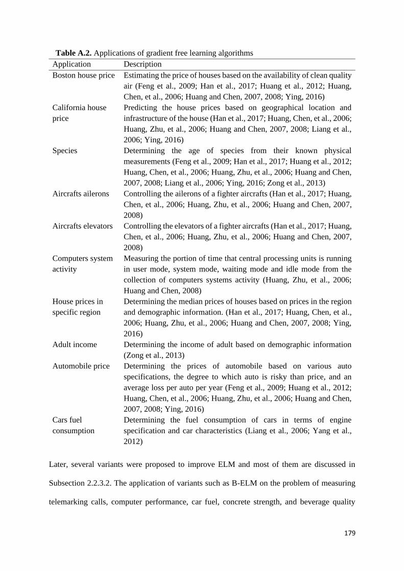
179

Later, several variants were proposed to improve ELM and most of them are discussed in

Subsection 2.2.3.2. The application of variants such as B-ELM on the problem of measuring

telemarking calls, computer performance, car fuel, concrete strength, and beverage quality

Table A.2. Applications of gradient free learning algorithms

Application Description

Boston house price Estimating the price of houses based on the availability of clean quality

air (Feng et al., 2009; Han et al., 2017; Huang et al., 2012; Huang,

Chen, et al., 2006; Huang and Chen, 2007, 2008; Ying, 2016)

California house

price

Predicting the house prices based on geographical location and

infrastructure of the house (Han et al., 2017; Huang, Chen, et al., 2006;

Huang, Zhu, et al., 2006; Huang and Chen, 2007, 2008; Liang et al.,

2006; Ying, 2016)

Species Determining the age of species from their known physical

measurements (Feng et al., 2009; Han et al., 2017; Huang et al., 2012;

Huang, Chen, et al., 2006; Huang, Zhu, et al., 2006; Huang and Chen,

2007, 2008; Liang et al., 2006; Ying, 2016; Zong et al., 2013)

Aircrafts ailerons Controlling the ailerons of a fighter aircrafts (Han et al., 2017; Huang,

Chen, et al., 2006; Huang, Zhu, et al., 2006; Huang and Chen, 2007,

2008)

Aircrafts elevators Controlling the elevators of a fighter aircrafts (Han et al., 2017; Huang,

Chen, et al., 2006; Huang, Zhu, et al., 2006; Huang and Chen, 2007,

2008)

Computers system

activity

Measuring the portion of time that central processing units is running

in user mode, system mode, waiting mode and idle mode from the

collection of computers systems activity (Huang, Zhu, et al., 2006;

Huang and Chen, 2008)

House prices in

specific region

Determining the median prices of houses based on prices in the region

and demographic information. (Han et al., 2017; Huang, Chen, et al.,

2006; Huang, Zhu, et al., 2006; Huang and Chen, 2007, 2008; Ying,

2016)

Adult income Determining the income of adult based on demographic information

(Zong et al., 2013)

Automobile price Determining the prices of automobile based on various auto

specifications, the degree to which auto is risky than price, and an

average loss per auto per year (Feng et al., 2009; Huang et al., 2012;

Huang, Chen, et al., 2006; Huang, Zhu, et al., 2006; Huang and Chen,

2007, 2008; Ying, 2016)

Cars fuel

consumption

Determining the fuel consumption of cars in terms of engine

specification and car characteristics (Liang et al., 2006; Yang et al.,

2012)

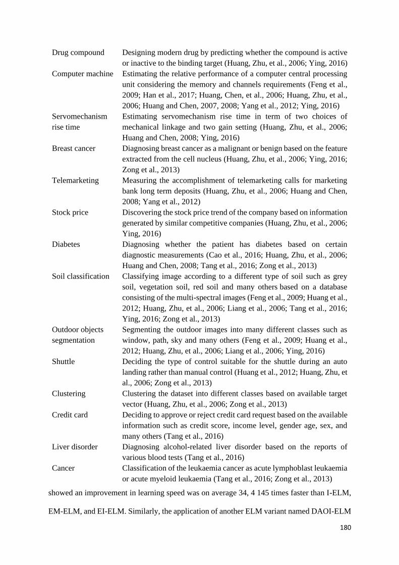
180

showed an improvement in learning speed was on average 34, 4 145 times faster than I-ELM,

EM-ELM, and EI-ELM. Similarly, the application of another ELM variant named DAOI-ELM

Drug compound Designing modern drug by predicting whether the compound is active

or inactive to the binding target (Huang, Zhu, et al., 2006; Ying, 2016)

Computer machine Estimating the relative performance of a computer central processing

unit considering the memory and channels requirements (Feng et al.,

2009; Han et al., 2017; Huang, Chen, et al., 2006; Huang, Zhu, et al.,

2006; Huang and Chen, 2007, 2008; Yang et al., 2012; Ying, 2016)

Servomechanism

rise time

Estimating servomechanism rise time in term of two choices of

mechanical linkage and two gain setting (Huang, Zhu, et al., 2006;

Huang and Chen, 2008; Ying, 2016)

Breast cancer Diagnosing breast cancer as a malignant or benign based on the feature

extracted from the cell nucleus (Huang, Zhu, et al., 2006; Ying, 2016;

Zong et al., 2013)

Telemarketing Measuring the accomplishment of telemarketing calls for marketing

bank long term deposits (Huang, Zhu, et al., 2006; Huang and Chen,

2008; Yang et al., 2012)

Stock price Discovering the stock price trend of the company based on information

generated by similar competitive companies (Huang, Zhu, et al., 2006;

Ying, 2016)

Diabetes Diagnosing whether the patient has diabetes based on certain

diagnostic measurements (Cao et al., 2016; Huang, Zhu, et al., 2006;

Huang and Chen, 2008; Tang et al., 2016; Zong et al., 2013)

Soil classification Classifying image according to a different type of soil such as grey

soil, vegetation soil, red soil and many others based on a database

consisting of the multi-spectral images (Feng et al., 2009; Huang et al.,

2012; Huang, Zhu, et al., 2006; Liang et al., 2006; Tang et al., 2016;

Ying, 2016; Zong et al., 2013)

Outdoor objects

segmentation

Segmenting the outdoor images into many different classes such as

window, path, sky and many others (Feng et al., 2009; Huang et al.,

2012; Huang, Zhu, et al., 2006; Liang et al., 2006; Ying, 2016)

Shuttle Deciding the type of control suitable for the shuttle during an auto

landing rather than manual control (Huang et al., 2012; Huang, Zhu, et

al., 2006; Zong et al., 2013)

Clustering Clustering the dataset into different classes based on available target

vector (Huang, Zhu, et al., 2006; Zong et al., 2013)

Credit card Deciding to approve or reject credit card request based on the available

information such as credit score, income level, gender age, sex, and

many others (Tang et al., 2016)

Liver disorder Diagnosing alcohol-related liver disorder based on the reports of

various blood tests (Tang et al., 2016)

Cancer Classification of the leukaemia cancer as acute lymphoblast leukaemia

or acute myeloid leukaemia (Tang et al., 2016; Zong et al., 2013)

181

in studying the stock market, forest burning, concrete strength, beverage quality achieved more

stable and smooth results compared to the B-ELM and the fluctuating results of I-ELM and

Gene expression

level

Analysing the gene correlation expression level in different tissues of

the tumor colon and normal colon (Tang et al., 2016; Zong et al., 2013)

Object

discrimination

Discriminating stars from galaxy using broadband photometric

information (Huang et al., 2012)

Mushroom Differentiating poisonous and non-poisonous mushroom based on

mushroom different physical characteristics (Tang et al., 2016)

Flowers species Classifying the flowers into different species from available

information on the width and length of petals and sepals (Huang et al.,

2012; Tang et al., 2016; Wang et al., 2016; Zong et al., 2013)

Crime Identifying glass type used in crime scene based on chemical oxide

content such as sodium, potassium, calcium, iron and many others

(Cao et al., 2016; Huang et al., 2012; Tang et al., 2016; Ying, 2016;

Zong et al., 2013)

DNA splicing Recognizing exon/intron and intron/exon boundaries in the DNA

splicing (Huang et al., 2012; Liang et al., 2006; Tang et al., 2016; Zong

et al., 2013)

Industrial strike

volume

Estimating the industrial strike volume for the next fiscal year

considering key factors such as unemployment, inflation and labor

unions (Huang et al., 2012)

Weather

forecasting

Forecasting weather in terms of cloud appearance (Huang et al., 2012)

Dihydrofolate

reductase

inhibition

Predicting the inhibition of dihydrofolate reductase by pyrimidines

(Huang et al., 2012; Huang and Chen, 2008)

Human body fats Determining the percentage of human body fats from key physical

factors such as weight, age, chest size and other body parts

circumference (Huang et al., 2012)

Heart diseases Diagnosing and categorizing the presence of heart diseases in a patient

by studying the previous history of drug addiction, health issues, blood

tests, and many others (Huang et al., 2012)

Mental disorder Testing mental behaviour of the patient from inflated balloons (Huang

et al., 2012)

Earthquake

strength

Forecasting the strength of earthquake given its latitude, longitude and

focal point (Huang et al., 2012)

Presidential

election

Estimating the proportion of voter in the presidential election based on

key factors such as education, age, and income (Huang et al., 2012)

Robot end effector Determining the distance of robot end effector from a target based on

the robot positions and angles (Huang and Chen, 2008)

Concrete strength Determining slump, flow and compressive strength of the concrete

from influencing ingredients such as cement, water, ash, and many

others (Yang et al., 2012; Zou et al., 2018)

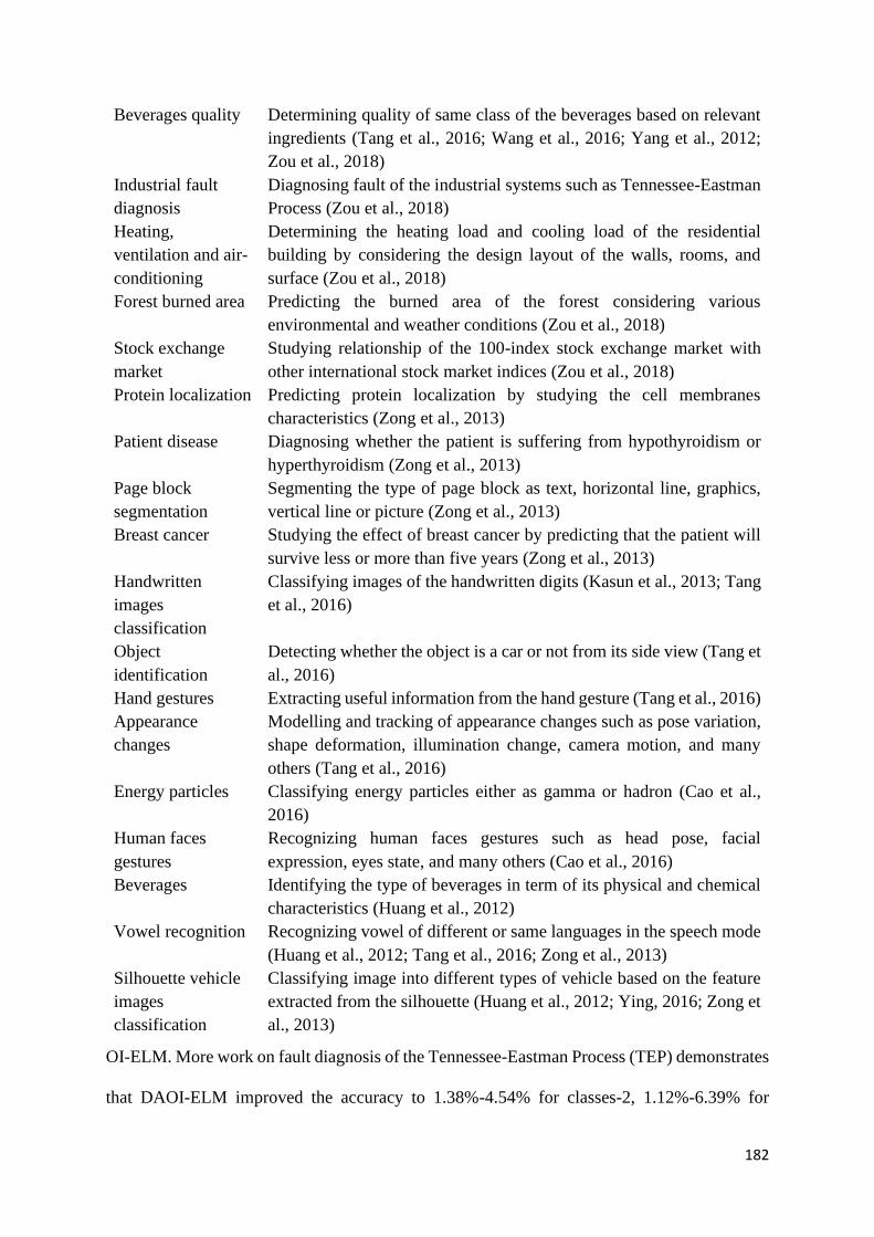
182

OI-ELM. More work on fault diagnosis of the Tennessee-Eastman Process (TEP) demonstrates

that DAOI-ELM improved the accuracy to 1.38%-4.54% for classes-2, 1.12%-6.39% for

Beverages quality Determining quality of same class of the beverages based on relevant

ingredients (Tang et al., 2016; Wang et al., 2016; Yang et al., 2012;

Zou et al., 2018)

Industrial fault

diagnosis

Diagnosing fault of the industrial systems such as Tennessee-Eastman

Process (Zou et al., 2018)

Heating,

ventilation and air-

conditioning

Determining the heating load and cooling load of the residential

building by considering the design layout of the walls, rooms, and

surface (Zou et al., 2018)

Forest burned area Predicting the burned area of the forest considering various

environmental and weather conditions (Zou et al., 2018)

Stock exchange

market

Studying relationship of the 100-index stock exchange market with

other international stock market indices (Zou et al., 2018)

Protein localization Predicting protein localization by studying the cell membranes

characteristics (Zong et al., 2013)

Patient disease Diagnosing whether the patient is suffering from hypothyroidism or

hyperthyroidism (Zong et al., 2013)

Page block

segmentation

Segmenting the type of page block as text, horizontal line, graphics,

vertical line or picture (Zong et al., 2013)

Breast cancer Studying the effect of breast cancer by predicting that the patient will

survive less or more than five years (Zong et al., 2013)

Handwritten

images

classification

Classifying images of the handwritten digits (Kasun et al., 2013; Tang

et al., 2016)

Object

identification

Detecting whether the object is a car or not from its side view (Tang et

al., 2016)

Hand gestures Extracting useful information from the hand gesture (Tang et al., 2016)

Appearance

changes

Modelling and tracking of appearance changes such as pose variation,

shape deformation, illumination change, camera motion, and many

others (Tang et al., 2016)

Energy particles Classifying energy particles either as gamma or hadron (Cao et al.,

2016)

Human faces

gestures

Recognizing human faces gestures such as head pose, facial

expression, eyes state, and many others (Cao et al., 2016)

Beverages Identifying the type of beverages in term of its physical and chemical

characteristics (Huang et al., 2012)

Vowel recognition Recognizing vowel of different or same languages in the speech mode

(Huang et al., 2012; Tang et al., 2016; Zong et al., 2013)

Silhouette vehicle

images

classification

Classifying image into different types of vehicle based on the feature

extracted from the silhouette (Huang et al., 2012; Ying, 2016; Zong et

al., 2013)

183

classes-4 and 4.36%-5.47% for classes-8 fault compared to BP, I-ELM, CI-ELM, and OI-ELM.

The DAOI-ELM application shows that it obtained better generalization performance with

compact architecture; however, the learning speed of DAOI-ELM is not clearly illustrated in

their work. The ELM and many of its variants are advantageous in that they randomly generate

hidden units and analytically calculate output connection weights which make them simple and

easy to train network. However, randomly generating hidden units may cause the network size

to increase largely which increases the chances of overfitting.

The application of semi gradient and iterative tuning algorithms such as IFNNRWs

demonstrated its effectiveness on classification problems of identifying crime object, energy

particles, human face gestures, and diabetes, but cannot approximate regression problems well.

Another limitation is an increase in the training time of IFNNRWs due to repetitively tuning

of the output connection weights.

A.3 Application of optimization algorithms for learning rate

The learning algorithms are found to have applications in complex domain problem-solving.

The high dimensional data with a lot of features may make the task difficult to solve with an

initial guess and manual settings of the parameter such as learning rate. Deciding on a large

learning rate may make the network unstable causing the generalization performance to be

poor, whereas, a small learning rate may reduce the learning speed. The algorithms in this

English letters Identifying black and white image as one of the English letters among

twenty-six capital letters (Feng et al., 2009; Huang et al., 2012; Tang

et al., 2016; Ying, 2016)

Handwritten text

recognition

Recognizing isolated, touching, overlapping and cursive handwritten

text from digital images of the city, states, Zip codes, and alphanumeric

characters (Huang et al., 2012; Tang et al., 2016; Zong et al., 2013)

Basketball winning Predicting basketball winning team based on players, team formation

and actions information (Huang et al., 2012)

184

category help to adjust the learning rate on each iteration and move the gradients faster towards

the long axis of the valley for better performance. Table A.3 contains some of the applications

on complex task problem-solving. AdaGrad solved the problem of newspaper articles

classification by improving various categories performance, on average, by 9%-109%.

Similarly, for the subcategory image classification problem, AdaGrad was able to improve the

precision by 2.09% - 9.8%. The graphical representation of the AdaDelta results showed that

it gained the highest accuracy on speech recognition of English data. The application of Adam

on multiclass logistics regression, multilayer neural networks and convolutional neural

networks for classification of handwritten images, object images, and movie reviews

graphically showed that Adam has a better generalization performance by having a smaller

convergence per iteration. The above problems illustrate that the application of optimization

Table A.3. Applications of optimization algorithms for learning rate

Application Description

Game decision

rule

Predicting decision rules for the Nine Men’s Morris game (Riedmiller

and Braun, 1993)

Census Predicting whether the individual has income above or below the

average income based on certain demographic and employment-related

information (Duchi et al., 2011)

Newspaper articles Classifying the newspapers articles into four major categories such as

economics, commerce, medical, and government with multiple more

specific categories (Duchi et al., 2011)

Subcategories

image

classification

Classifying thousands of images in each of their individual subcategory

(Duchi et al., 2011)

Handwritten

images

classification

Classifying images of the handwritten digits (Duchi et al., 2011;

Kingma and Ba, 2014; Zeiler, 2012)

English data

recognition

Recognizing speech from several hundred hours of the US English data

collected from voice IME, voice search and read data (Zeiler, 2012)

Movie reviews Classifying review of the movies either positive or negative to know

the sentiment of the reviewers (Kingma and Ba, 2014)

Digital images

classification

Classifying the images into one of a category such as an airplane, deer,

ship, frog, horse, truck, cat, dog, bird and automobile (Kingma and Ba,

2014)

185

algorithms for the learning rate are more suitable for high dimension complex datasets to avoid

manual adjustment of the learning rate.

A.4 Applications of bias and variance minimization algorithms

The algorithms in this category improve the generalization performance of the network and

include applications that cannot be solved by a simple network, and more sophisticated

knowledge is needed to avoid overfitting in gaining better performance. The regularization,

pruning, and ensembles methods are implemented by training many networks simultaneously

to get the average best results. The limitation of this category is that it requires more learning

time compared to the standard networks for convergence. The limitation can be minimized by

adopting a hybrid approach using learning optimization algorithms and this category. Besides,

the limitation of regularization techniques such as dropout, DropConnect, and shakeout are that

they are suitable to work with fully connected neural networks.

Table A.4 shows some of the applications in areas such as classification, recognition,

segmentation, and forecasting. Shakeout work on the classification of high dimensional digital

images and complex handwritten digits images, comprising more than 50,000 images,

improved the accuracy by about 0.95%-2.85% and 1.63%-4.55% respectively for fully

connected neural networks. For classifying more than 50,000 house number images generated

from google street views, DropConnect slightly enhanced the accuracy to 0.02%-0.03%.

Similarly, DropConnect work on 3D object recognition achieved a better accuracy of 0.34%.

Shakeout and DropConnect show promising results on highly complex data, however, the

popularity and success of the dropout technique in many applications is comparatively high.

Some applications of dropout include classifying species images into their classes and

subclasses, recognizing the different dialect speech, classifying newspaper articles into

different categories, detecting human diseases by predicting alternative splicing and classifying

186

hundred and thousands of images into different categories. Dropout, because of its property of

dropping hidden unit to avoid overfitting, achieved an average more than 5% better accuracy

for the mentioned applications.

The application of the ensemble technique CNNE on various problems, such as assessing credit

card requests, diagnosing breast cancer, diagnosing diabetes, identifying objects used in

Table A.4. Applications of bias and variance minimization algorithms

Application Description

Handwritten

images

classification

Classifying the images of hand-written numerals with 20% flip rate

(Geman et al., 1992)

Text to speech

conversion

Learning to convert English text to speech (Krogh and Hertz, 1992)

Credit card Deciding to approve or reject credit card request based on the available

information such as credit score, income level, gender age, sex, and

many others (Islam et al., 2003)

Breast cancer Diagnosing breast cancer as a malignant or benign based on the feature

extracted from the cell nucleus (Islam et al., 2003)

Diabetes Diagnosing whether the patient has diabetes based on certain

diagnostic measurements (Islam et al., 2003)

Crime Identifying glass type used in crime scene based on chemical oxide

content such as sodium, potassium, calcium, iron and many others

(Islam et al., 2003)

Heart diseases Diagnosing and categorizing the presence of heart diseases in a patient

by studying the previous history of drug addiction, health issues, blood

tests, and many others (Islam et al., 2003)

English letters Identifying black and white image as one of the English letters among

twenty-six capital letters (Islam et al., 2003)

Soybean defects Determining the type of defect in soybean based on physical

characteristics of the plant (Islam et al., 2003)

Energy

consumption

Predicting the hourly consumption of building electricity and

associated cost based on environmental and weather conditions (Liu et

al., 2008)

Robot arm

acceleration

Estimating the angular acceleration of the robot arm based on a

position, velocity, and torque (Liu et al., 2008)

Semiconductor

manufacturing

Analysing semiconductor manufacturing by examining the number of

dies in a wafer that pass electrical tests (Seni and Elder, 2010)

Credit defaulter Predicting credit defaulters based on the credit score information (Seni

and Elder, 2010)

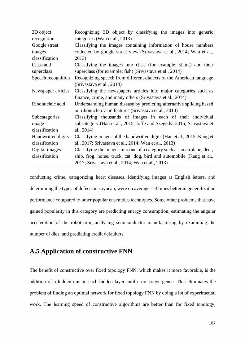
187

conducting crime, categorizing heart diseases, identifying images as English letters, and

determining the types of defects in soybean, were on average 1-3 times better in generalization

performance compared to other popular ensembles techniques. Some other problems that have

gained popularity in this category are predicting energy consumption, estimating the angular

acceleration of the robot arm, analysing semiconductor manufacturing by examining the

number of dies, and predicting credit defaulters.

A.5 Application of constructive FNN

The benefit of constructive over fixed topology FNN, which makes it more favorable, is the

addition of a hidden unit in each hidden layer until error convergence. This eliminates the

problem of finding an optimal network for fixed topology FNN by doing a lot of experimental

work. The learning speed of constructive algorithms are better than for fixed topology,

3D object

recognition

Recognizing 3D object by classifying the images into generic

categories (Wan et al., 2013)

Google street

images

classification

Classifying the images containing information of house numbers

collected by google street view (Srivastava et al., 2014; Wan et al.,

2013)

Class and

superclass

Classifying the images into class (for example: shark) and their

superclass (for example: fish) (Srivastava et al., 2014)

Speech recognition Recognizing speech from different dialects of the American language

(Srivastava et al., 2014)

Newspaper articles Classifying the newspapers articles into major categories such as

finance, crime, and many others (Srivastava et al., 2014)

Ribonucleic acid Understanding human disease by predicting alternative splicing based

on ribonucleic acid features (Srivastava et al., 2014)

Subcategories

image

classification

Classifying thousands of images in each of their individual

subcategory (Han et al., 2015; Ioffe and Szegedy, 2015; Srivastava et

al., 2014)

Handwritten digits

classification

Classifying images of the handwritten digits (Han et al., 2015; Kang et

al., 2017; Srivastava et al., 2014; Wan et al., 2013)

Digital images

classification

Classifying the images into one of a category such as an airplane, deer,

ship, frog, horse, truck, cat, dog, bird and automobile (Kang et al.,

2017; Srivastava et al., 2014; Wan et al., 2013)

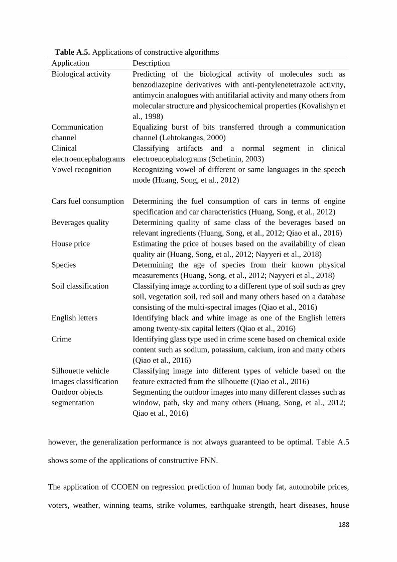
188

however, the generalization performance is not always guaranteed to be optimal. Table A.5

shows some of the applications of constructive FNN.

The application of CCOEN on regression prediction of human body fat, automobile prices,

voters, weather, winning teams, strike volumes, earthquake strength, heart diseases, house

Table A.5. Applications of constructive algorithms

Application Description

Biological activity Predicting of the biological activity of molecules such as

benzodiazepine derivatives with anti-pentylenetetrazole activity,

antimycin analogues with antifilarial activity and many others from

molecular structure and physicochemical properties (Kovalishyn et

al., 1998)

Communication

channel

Equalizing burst of bits transferred through a communication

channel (Lehtokangas, 2000)

Clinical

electroencephalograms

Classifying artifacts and a normal segment in clinical

electroencephalograms (Schetinin, 2003)

Vowel recognition Recognizing vowel of different or same languages in the speech

mode (Huang, Song, et al., 2012)

Cars fuel consumption Determining the fuel consumption of cars in terms of engine

specification and car characteristics (Huang, Song, et al., 2012)

Beverages quality Determining quality of same class of the beverages based on

relevant ingredients (Huang, Song, et al., 2012; Qiao et al., 2016)

House price Estimating the price of houses based on the availability of clean

quality air (Huang, Song, et al., 2012; Nayyeri et al., 2018)

Species Determining the age of species from their known physical

measurements (Huang, Song, et al., 2012; Nayyeri et al., 2018)

Soil classification Classifying image according to a different type of soil such as grey

soil, vegetation soil, red soil and many others based on a database

consisting of the multi-spectral images (Qiao et al., 2016)

English letters Identifying black and white image as one of the English letters

among twenty-six capital letters (Qiao et al., 2016)

Crime Identifying glass type used in crime scene based on chemical oxide

content such as sodium, potassium, calcium, iron and many others

(Qiao et al., 2016)

Silhouette vehicle

images classification

Classifying image into different types of vehicle based on the

feature extracted from the silhouette (Qiao et al., 2016)

Outdoor objects

segmentation

Segmenting the outdoor images into many different classes such as

window, path, sky and many others (Huang, Song, et al., 2012;

Qiao et al., 2016)

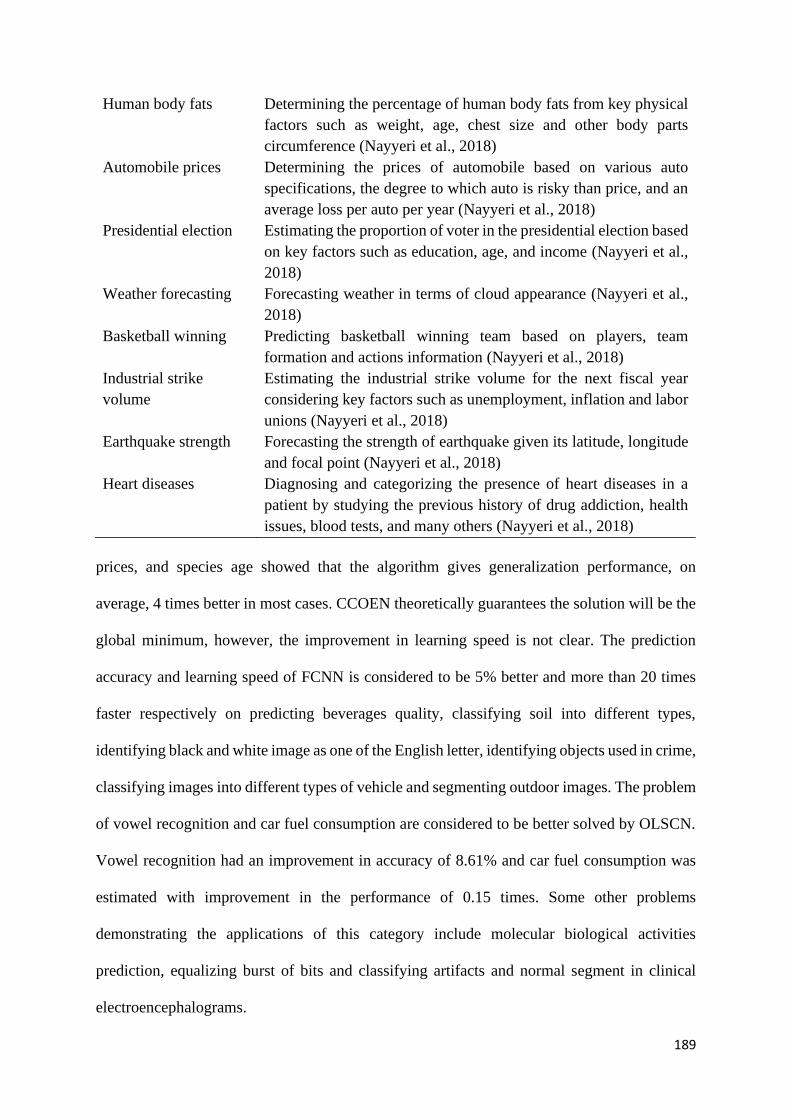
189

prices, and species age showed that the algorithm gives generalization performance, on

average, 4 times better in most cases. CCOEN theoretically guarantees the solution will be the

global minimum, however, the improvement in learning speed is not clear. The prediction

accuracy and learning speed of FCNN is considered to be 5% better and more than 20 times

faster respectively on predicting beverages quality, classifying soil into different types,

identifying black and white image as one of the English letter, identifying objects used in crime,

classifying images into different types of vehicle and segmenting outdoor images. The problem

of vowel recognition and car fuel consumption are considered to be better solved by OLSCN.

Vowel recognition had an improvement in accuracy of 8.61% and car fuel consumption was

estimated with improvement in the performance of 0.15 times. Some other problems

demonstrating the applications of this category include molecular biological activities

prediction, equalizing burst of bits and classifying artifacts and normal segment in clinical

electroencephalograms.

Human body fats Determining the percentage of human body fats from key physical

factors such as weight, age, chest size and other body parts

circumference (Nayyeri et al., 2018)

Automobile prices Determining the prices of automobile based on various auto

specifications, the degree to which auto is risky than price, and an

average loss per auto per year (Nayyeri et al., 2018)

Presidential election Estimating the proportion of voter in the presidential election based

on key factors such as education, age, and income (Nayyeri et al.,

2018)

Weather forecasting Forecasting weather in terms of cloud appearance (Nayyeri et al.,

2018)

Basketball winning Predicting basketball winning team based on players, team

formation and actions information (Nayyeri et al., 2018)

Industrial strike

volume

Estimating the industrial strike volume for the next fiscal year

considering key factors such as unemployment, inflation and labor

unions (Nayyeri et al., 2018)

Earthquake strength Forecasting the strength of earthquake given its latitude, longitude

and focal point (Nayyeri et al., 2018)

Heart diseases Diagnosing and categorizing the presence of heart diseases in a

patient by studying the previous history of drug addiction, health

issues, blood tests, and many others (Nayyeri et al., 2018)

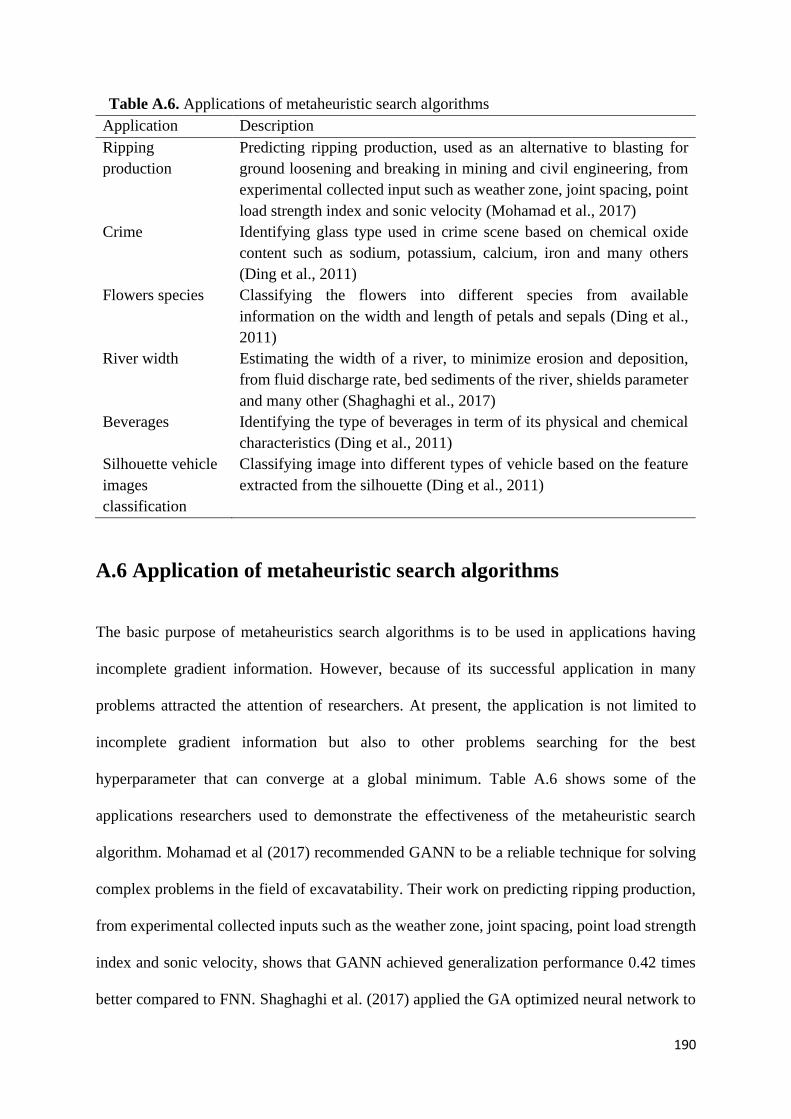
190

A.6 Application of metaheuristic search algorithms

The basic purpose of metaheuristics search algorithms is to be used in applications having

incomplete gradient information. However, because of its successful application in many

problems attracted the attention of researchers. At present, the application is not limited to

incomplete gradient information but also to other problems searching for the best

hyperparameter that can converge at a global minimum. Table A.6 shows some of the

applications researchers used to demonstrate the effectiveness of the metaheuristic search

algorithm. Mohamad et al (2017) recommended GANN to be a reliable technique for solving

complex problems in the field of excavatability. Their work on predicting ripping production,

from experimental collected inputs such as the weather zone, joint spacing, point load strength

index and sonic velocity, shows that GANN achieved generalization performance 0.42 times

better compared to FNN. Shaghaghi et al. (2017) applied the GA optimized neural network to

Table A.6. Applications of metaheuristic search algorithms

Application Description

Ripping

production

Predicting ripping production, used as an alternative to blasting for

ground loosening and breaking in mining and civil engineering, from

experimental collected input such as weather zone, joint spacing, point

load strength index and sonic velocity (Mohamad et al., 2017)

Crime Identifying glass type used in crime scene based on chemical oxide

content such as sodium, potassium, calcium, iron and many others

(Ding et al., 2011)

Flowers species Classifying the flowers into different species from available

information on the width and length of petals and sepals (Ding et al.,

2011)

River width Estimating the width of a river, to minimize erosion and deposition,

from fluid discharge rate, bed sediments of the river, shields parameter

and many other (Shaghaghi et al., 2017)

Beverages Identifying the type of beverages in term of its physical and chemical

characteristics (Ding et al., 2011)

Silhouette vehicle

images

classification

Classifying image into different types of vehicle based on the feature

extracted from the silhouette (Ding et al., 2011)

191

estimate the width of a river and found a 0.40 times better generalization performance. Besides,

it was reported that neural networks optimized by GA are more efficient than PSO. Ding et al.

(2011) worked on predicting flower species, beverages type, identifying objects used in crime

and classifying images showed that the hybrid approach of GA and BP achieved a prediction

accuracy on average 2%-3% better than GA and BP. The study further explained that the

accuracy of BP in the above problems is better than GA. Furthermore, it was concluded that

the GA needs more learning time compared to BP and this learning speed can be increased to

some extent by using the hybrid approach. The hybrid approach achieved learning speed 0.05

times better than GA but was still slower than BP.

192

References

Abdel-Hamid, O., Mohamed, A., Jiang, H., Deng, L., Penn, G. and Yu, D. (2014),

“Convolutional neural networks for speech recognition”, IEEE/ACM Transactions on

Audio, Speech, and Language Processing, Vol. 22 No. 10, pp. 1533–1545.

Abdelghany, K., Abdelghany, A. and Raina, S. (2005), “A model for the airlines’ fuel

management strategies”, Journal of Air Transport Management, Vol. 11 No. 4, pp. 199–

206.

Al_Janabi, S., Al_Shourbaji, I. and Salman, M.A. (2018), “Assessing the suitability of soft

computing approaches for forest fires prediction”, Applied Computing and Informatics,

Elsevier, Vol. 14 No. 2, pp. 214–224.

Au, K.F., Choi, T.M. and Yu, Y. (2008), “Fashion retail forecasting by evolutionary neural

networks”, International Journal of Production Economics, Elsevier, Vol. 114 No. 2, pp.

615–630.

Babaee, M., Dinh, D.T. and Rigoll, G. (2018), “A deep convolutional neural network for video

sequence background subtraction”, Pattern Recognition, Elsevier Ltd, Vol. 76, pp. 635–

649.

Bagirov, A., Taheri, S. and Asadi, S. (2019), “A difference of convex optimization algorithm

for piecewise linear regression”, Journal of Industrial & Management Optimization, Vol.

15 No. 2, pp. 909–932.

Baklacioglu, T. (2016), “Modeling the fuel flow-rate of transport aircraft during flight phases

using genetic algorithm-optimized neural networks”, Aerospace Science and Technology,

Elsevier Masson SAS, Vol. 49, pp. 52–62.

Banerjee, P., Singh, V.S., Chatttopadhyay, K., Chandra, P.C. and Singh, B. (2011), “Artificial

neural network model as a potential alternative for groundwater salinity forecasting”,

Journal of Hydrology, Elsevier, Vol. 398 No. 3–4, pp. 212–220.

Bianchini, M. and Scarselli, F. (2014), “On the complexity of neural network classifiers: A

comparison between shallow and deep architectures”, IEEE Transactions on Neural

Networks and Learning Systems, IEEE, Vol. 25 No. 8, pp. 1553–1565.

Bottani, E., Centobelli, P., Gallo, M., Kaviani, M.A., Jain, V. and Murino, T. (2019),

“Modelling wholesale distribution operations: an artificial intelligence framework”,

Industrial Management & Data Systems, Emerald Publishing Limited, Vol. 119 No. 4,

pp. 698–718.

Candanedo, L.M. and Feldheim, V. (2016), “Accurate occupancy detection of an office room

from light, temperature, humidity and CO2 measurements using statistical learning

models”, Energy and Buildings, Elsevier, Vol. 112, pp. 28–39.

193

Cao, F., Wang, D., Zhu, H. and Wang, Y. (2016), “An iterative learning algorithm for

feedforward neural networks with random weights”, Information Sciences, Elsevier Inc.,

Vol. 328, pp. 546–557.

Cao, W., Wang, X., Ming, Z. and Gao, J. (2018), “A review on neural networks with random

weights”, Neurocomputing, Elsevier, Vol. 275, pp. 278–287.

Chati, Y.S. and Balakrishnan, H. (2017), “Statistical modeling of aircraft engine fuel”, Twelfth

USA/Europe Air Traffic Management Research and Development Seminar (ATM 2017).

Chen, L.-C., Papandreou, G., Kokkinos, I., Murphy, K. and Yuille, A.L. (2018), “DeepLab:

Semantic image segmentation with deep convolutional nets, atrous convolution, and fully

connected CRFs”, IEEE Transactions on Pattern Analysis and Machine Intelligence,

IEEE, Vol. 40 No. 4, pp. 834–848.

Cheng, Y. (2017), “Backpropagation for fully connected cascade networks”, Neural

Processing Letters, Springer, Vol. 46 No. 1, pp. 293–311.

Choi, T.-M., Cai, Y.-J. and Shen, B. (2018), “Sustainable fashion supply chain management:

A system of systems analysis”, IEEE Transactions on Engineering Management, IEEE,

Vol. 66 No. 4, pp. 730–745.

Choi, T.M., Chiu, C.H. and Chan, H.K. (2016), “Risk management of logistics systems”,

Transportation Research Part E: Logistics and Transportation Review, Elsevier, Vol. 90,

pp. 1–6.

Choi, T.M., Wallace, S.W. and Wang, Y. (2018), “Big data analytics in operations

management”, Production and Operations Management, Wiley Online Library, Vol. 27

No. 10, pp. 1868–1883.

Chung, S.H., Ma, H.L. and Chan, H.K. (2017), “Cascading delay risk of airline workforce

deployments with crew pairing and schedule optimization”, Risk Analysis, Wiley Online

Library, Vol. 37 No. 8, pp. 1443–1458.

Chung, S.H., Tse, Y.K. and Choi, T.M. (2015), “Managing disruption risk in express logistics

via proactive planning”, Industrial Management & Data Systems, Emerald Group

Publishing Limited, Vol. 115 No. 8, pp. 1481–1509.

Collins, B.P. (1982), “Estimation of aircraft fuel consumption”, Journal of Aircraft, Vol. 19

No. 11, pp. 969–975.

Cui, Q. and Li, Y. (2017), “Airline efficiency measures under CNG2020 strategy: An

application of a Dynamic By-production model”, Transportation Research Part A: Policy

and Practice, Elsevier, Vol. 106, pp. 130–143.

Dancila, B.D., Botez, R. and Labour, D. (2013), “Fuel burn prediction algorithm for cruise,

constant speed and level flight segments”, Aeronautical Journal, Vol. 117 No. 1191, pp.

194

491–504.

Deng, C., Miao, J., Ma, Y., Wei, B. and Feng, Y. (2019), “Reliability analysis of chatter

stability for milling process system with uncertainties based on neural network and fourth

moment method”, International Journal of Production Research, Taylor & Francis, pp.

1–19.

Diao, X. and Chen, C.-H. (2018), “A sequence model for air traffic flow management rerouting

problem”, Transportation Research Part E: Logistics and Transportation Review,

Elsevier, Vol. 110, pp. 15–30.

Ding, S., Su, C. and Yu, J. (2011), “An optimizing BP neural network algorithm based on

genetic algorithm”, Artificial Intelligence Review, Vol. 36 No. 2, pp. 153–162.

Dong, C., Loy, C.C., He, K. and Tang, X. (2016), “Image super-resolution Using deep

convolutional networks”, IEEE Transactions on Pattern Analysis and Machine

Intelligence, Vol. 38 No. 2, pp. 295–307.

Dua, D. and Taniskidou, E.K. (2017), “UCI Machine Learning Repository”, available at:

http://archive.ics.uci.edu/ml (accessed 28 March 2018).

Duchi, J., Hazan, E. and Singer, Y. (2011), “Adaptive subgradient methods for online learning

and stochastic optimization”, Journal of Machine Learning Research, Vol. 12, pp. 2121–

2159.

Ebadzadeh, M.M. and Salimi-Badr, A. (2018), “IC-FNN: A novel fuzzy neural network with

interpretable, intuitive, and correlated-contours fuzzy rules for function approximation”,

IEEE Transactions on Fuzzy Systems, IEEE, Vol. 26 No. 3, pp. 1288–1302.

Eberhart, R. and Kennedy, J. (1995), “A new optimizer using particle swarm theory”,

Proceedings of the Sixth International Symposium on Micro Machine and Human Science

MHS’95., pp. 39–43.

Edwards, H.A., Dixon-Hardy, D. and Wadud, Z. (2016), “Aircraft cost index and the future of

carbon emissions from air travel”, Applied Energy, Elsevier, Vol. 164, pp. 553–562.

Fahlman, S.E. (1988), An Empirical Study of Learning Speed in Back-Propagation Networks,

School of Computer Science, Carnegie Mellon University, Pittsburgh PA 15213.

Fahlman, S.E. and Lebiere, C. (1990), “The cascade-correlation learning architecture”, in

Lippmann, R.P., Moody, J.E. and Touretzky, D.S. (Eds.), Advances in Neural Information

Processing Systems, Morgan Kaufmann, Denver, pp. 524–532.

Farlow, S.J. (1981), “The GMDH algorithm of Ivakhnenko”, The American Statistician, Vol.

35 No. 4, pp. 210–215.

Feng, G., Huang, G.-B., Lin, Q. and Gay, R.K.L. (2009), “Error minimized extreme learning

195

machine with growth of hidden nodes and incremental learning”, IEEE Trans. Neural

Networks, Vol. 20 No. 8, pp. 1352–1357.

Ferrari, S. and Stengel, R.F. (2005), “Smooth function approximation using neural networks”,

IEEE Transactions on Neural Networks, Vol. 16 No. 1, pp. 24–38.

Fierimonte, R., Barbato, M., Rosato, A. and Panella, M. (2016), “Distributed learning of

random weights fuzzy neural networks”, International Conference on Fuzzy Systems,

IEEE, pp. 2287–2294.

Geman, S., Doursat, R. and Bienenstock, E. (1992), “Neural networks and the bias/variance

dilemma”, Neural Computation, Vol. 4 No. 1, pp. 1–58.

Goldberger, A.S. (1964), “Classical linear regression”, Econometric Theory, New York: John

Wiley & Sons., pp. 156–212.

Gori, M. and Tesi, A. (1992), “On the problem of local minima in backpropagation”, IEEE

Transactions on Pattern Analysis & Machine Intelligence, IEEE, Vol. 14 No. 1, pp. 76–

86.

Guo, X., Grushka-Cockayne, Y. and De Reyck, B. (2018), “Forecasting airport transfer

passenger flow using real-time data and machine learning”, SSRN Electronic Journal,

available at:https://doi.org/10.2139/ssrn.3245609.

Hagan, M.T. and Menhaj, M.B. (1994), “Training feedforward networks with the Marquardt

algorithm”, IEEE Transactions on Neural Networks, Vol. 5 No. 6, pp. 989–993.

Han, F., Zhao, M.-R., Zhang, J.-M. and Ling, Q.-H. (2017), “An improved incremental

constructive single-hidden-layer feedforward networks for extreme learning machine

based on particle swarm optimization”, Neurocomputing, Elsevier, Vol. 228, pp. 133–142.

Han, S., Pool, J., Tran, J. and Dally, W.J. (2015), “Learning both weights and connections for

efficient neural networks”, in Cortes, C., Lawrence, N.D., Lee, D.D., Sugiyama, M. and

Garnett, R. (Eds.), Advances in Neural Information Processing Systems, MIT press,

Montreal, pp. 1135–1143.

Hansen, L.K. and Salamon, P. (1990), “Neural network ensembles”, IEEE Transactions on

Pattern Analysis and Machine Intelligence, Vol. 12 No. 10, pp. 993–1001.

Hayashi, Y., Hsieh, M.-H. and Setiono, R. (2010), “Understanding consumer heterogeneity: A

business intelligence application of neural networks”, Knowledge-Based Systems,

Elsevier, Vol. 23 No. 8, pp. 856–863.

Hecht-Nielsen, R. (1989), “Theory of the backpropagation neural network”, International Joint

Conference on Neural Networks, Vol. 1, IEEE, Washington DC, pp. 593–605 vol.1.

Hinton, G.E., Srivastava, N. and Swersky, K. (2012), “Lecture 6a- overview of mini-batch

196

gradient descent”, COURSERA: Neural Networks for Machine Learning, available at:

http://www.cs.toronto.edu/~tijmen/csc321/slides/lecture_slides_lec6.pdf (accessed 19

July 2018).

Hornik, K., Stinchcombe, M. and White, H. (1989), “Multilayer feedforward networks are

universal approximators”, Neural Networks, Vol. 2 No. 5, pp. 359–366.

Huang, C., Xu, Y. and Johnson, M.E. (2017), “Statistical modeling of the fuel flow rate of GA

piston engine aircraft using flight operational data”, Transportation Research Part D:

Transport and Environment, Elsevier, Vol. 53, pp. 50–62.

Huang, G.-B. and Chen, L. (2007), “Convex incremental extreme learning machine”,

Neurocomputing, Elsevier, Vol. 70 No. 16–18, pp. 3056–3062.

Huang, G.-B. and Chen, L. (2008), “Enhanced random search based incremental extreme

learning machine”, Neurocomputing, Vol. 71 No. 16–18, pp. 3460–3468.

Huang, G.-B., Chen, L. and Siew, C.K. (2006), “Universal approximation using incremental

constructive feedforward networks with random hidden nodes”, IEEE Transactions on

Neural Networks, Vol. 17 No. 4, pp. 879–892.

Huang, G.-B., Zhou, H., Ding, X. and Zhang, R. (2012), “Extreme learning machine for

regression and multiclass classification”, IEEE Transactions on Systems, Man, and

Cybernetics. Part B, Cybernetics, Vol. 42 No. 2, pp. 513–29.

Huang, G.-B., Zhu, Q.-Y. and Siew, C.-K. (2006), “Extreme learning machine: theory and

applications”, Neurocomputing, Vol. 70 No. 1–3, pp. 489–501.

Huang, G., Huang, G.-B., Song, S. and You, K. (2015), “Trends in extreme learning machines:

A review”, Neural Networks, Elsevier, Vol. 61, pp. 32–48.

Huang, G., Song, S. and Wu, C. (2012), “Orthogonal least squares algorithm for training

cascade neural networks”, IEEE Transactions on Circuits and Systems I: Regular Papers,

Vol. 59 No. 11, pp. 2629–2637.

Hunter, D., Yu, H., Pukish III, M.S., Kolbusz, J. and Wilamowski, B.M. (2012), “Selection of

proper neural network sizes and architectures—A comparative study”, IEEE Transactions

on Industrial Informatics, Vol. 8 No. 2, pp. 228–240.

Hwang, J.-N., You, S.-S., Lay, S.-R. and Jou, I.-C. (1996), “The cascade-correlation learning:

A projection pursuit learning perspective”, IEEE Transactions on Neural Networks, Vol.

7 No. 2, pp. 278–289.

IATA. (2018), “Fact Sheet Climate Change & CORSIA”, Online, available at:

https://www.iata.org/pressroom/facts_figures/fact_sheets/Documents/fact-sheet-climate-

change.pdf (accessed 7 May 2018).

197

IATA. (2019), “Industry facts and statistics”, Online, available at:

https://www.iata.org/pressroom/facts_figures/fact_sheets/Pages/index.aspx (accessed 5

August 2019).

Ijjina, E.P. and Chalavadi, K.M. (2016), “Human action recognition using genetic algorithms

and convolutional neural networks”, Pattern Recognition, Elsevier, Vol. 59, pp. 199–212.

Ioffe, S. and Szegedy, C. (2015), “Batch Normalization: Accelerating deep network training

by reducing internal covariate shift”, available at:https://doi.org/10.1007/s13398-014-

0173-7.2.

Irrgang, M.E., Kaul, C.E., Hall, A.E., Klerk, A.D., Elham and Boozarjomehri. (2015), “Aircraft

fuel optimization analytics”.

Islam, M., Yao, X. and Murase, K. (2003), “A constructive algorithm for training cooperative

neural network ensembles”, IEEE Transactions on Neural Networks, Vol. 14 No. 4, pp.

820–834.

Jensen, L., Hansman, R.J., Venuti, J.C. and Reynolds, T. (2013), “Commercial airline speed

optimization strategies for reduced cruise fuel consumption”, 2013 Aviation Technology,

Integration, and Operations Conference, pp. 1026–1038.

Jolliffe, I.T. (2002), Principal Component Analysis, edited by 2, Springer-Verlag, New York.

Kang, G., Li, J. and Tao, D. (2017), “Shakeout: A new approach to regularized deep neural

network training”, IEEE Transactions on Pattern Analysis and Machine Intelligence, Vol.

40 No. 5, pp. 1245–1258.

Kapanova, K.G., Dimov, I. and Sellier, J.M. (2018), “A genetic approach to automatic neural

network architecture optimization”, Neural Computing and Applications, Springer, Vol.

29 No. 5, pp. 1481–1492.

Karlik, B. and Olgac, V. (2011), “Performance analysis of various activation functions in

generalized MLP architectures of neural networks”, International Journal of Artificial

Intelligence And Expert Systems (IJAE), Vol. 1 No. 4, pp. 111–122.

Karnin, E.D. (1990), “A simple procedure for pruning back-propagation trained neural

networks”, IEEE Transactions on Neural Networks, Vol. 1 No. 2, pp. 239–242.

Kastrati, Z., Imran, A.S. and Yayilgan, S.Y. (2019), “The impact of deep learning on document

classification using semantically rich representations”, Information Processing &

Management, Elsevier, Vol. 56 No. 5, pp. 1618–1632.

Kasun, L.L.C., Zhou, H., Huang, G. and Vong, C. (2013), “Representational learning with

extreme learning machine for big data”, IEEE Intelligent System, Vol. 28 No. 6, pp. 31–

34.

198

Khanmohammadi, S., Tutun, S. and Kucuk, Y. (2016), “A new multilevel input layer artificial

neural network for predicting flight delays at JFK airport”, Procedia Computer Science,

Elsevier, Vol. 95, pp. 237–244.

Kim, Y.-S., Rim, H.-C. and Lee, D.-G. (2019), “Business environmental analysis for textual

data using data mining and sentence-level classification”, Industrial Management & Data

Systems, Emerald Publishing Limited, Vol. 119 No. 1, pp. 69–88.

Kingma, D.P. and Ba, J. (2014), “Adam: A Method for Stochastic Optimization”, pp. 1–15.

Kovalishyn, V. V, Tetko, I. V, Luik, A.I., Kholodovych, V. V, Villa, A.E.P. and Livingstone,

D.J. (1998), “Neural network studies. 3. variable selection in the cascade-correlation

learning architecture”, Journal of Chemical Information and Computer Sciences, Vol. 38

No. 4, pp. 651–659.

Krogh, A. and Hertz, J.A. (1992), “A simple weight decay can improve generalization”, in

Hanson, S.J., Cowan, J.D. and Giles, C.L. (Eds.), Advances in Neural Information

Processing Systems, Morgan Kaufmann, Denver, pp. 950–957.

Krogh, A. and Vedelsby, J. (1995), “Neural Network Ensembles, Cross Validation, and Active

Learning”, in Touretzky, D.S., Mozer, M. and Hasselmo, M.E. (Eds.), Advances in Neural

Information Processing Systems, MIT press, Denver, pp. 231–238.

Kumar, A., Rao, V.R. and Soni, H. (1995), “An empirical comparison of neural network and

logistic regression models”, Marketing Letters, Vol. 6 No. 4, pp. 251–263.

Kummong, R. and Supratid, S. (2016), “Thailand tourism forecasting based on a hybrid of

discrete wavelet decomposition and NARX neural network”, Industrial Management and

Data Systems, Vol. 116 No. 6, pp. 1242–1258.

Kuo, Y.-H. and Kusiak, A. (2019), “From data to big data in production research: the past and

future trends”, International Journal of Production Research, Taylor & Francis, Vol. 57

No. 15–16, pp. 4828–4853.

Kwok, T.-Y. and Yeung, D.-Y. (1997), “Constructive algorithms for structure learning in

feedforward neural networks for regression problems”, IEEE Transactions on Neural

Networks, Vol. 8 No. 3, pp. 630–645.

Lam, H.Y., Ho, G.T.S., Wu, C.-H. and Choy, K.L. (2014), “Customer relationship mining

system for effective strategies formulation”, Industrial Management & Data Systems,

Emerald Group Publishing Limited, Vol. 114 No. 5, pp. 711–733.

Lang, K.J. (1989), “Learning to tell two spirals apart”, Proceedings of the 1988 Connectionist

Models Summer School, Morgan Kaufmann, pp. 52–59.

LeCun, Y., Bengio, Y. and Hinton, G. (2015), “Deep learning”, Nature, Nature Publishing

Group, Vol. 521 No. 7553, pp. 436–444.

199

Lehtokangas, M. (2000), “Modified cascade-correlation learning for classification”, IEEE

Transactions on Neural Networks, Vol. 11 No. 3, pp. 795–798.

Lewis, A.S. and Overton, M.L. (2013), “Nonsmooth optimization via quasi-Newton methods”,

Mathematical Programming, Vol. 141 No. 1–2, pp. 135–163.

Li, M., Ch’ng, E., Chong, A.Y.L. and See, S. (2018), “Multi-class Twitter sentiment

classification with emojis”, Industrial Management & Data Systems, Emerald Publishing

Limited, Vol. 118 No. 9, pp. 1804–1820.

Liang, H. and Dai, G. (1998), “Improvement of cascade correlation learning”, Information

Sciences, Vol. 112 No. 1–4, pp. 1–6.

Liang, N.-Y., Huang, G.-B., Saratchandran, P. and Sundararajan, N. (2006), “A fast and

accurate online sequential learning algorithm for feedforward networks”, IEEE

Transactions on Neural Networks, Vol. 17 No. 6, pp. 1411–1423.

Liew, S.S., Khalil-Hani, M. and Bakhteri, R. (2016), “An optimized second order stochastic

learning algorithm for neural network training”, Neurocomputing, Elsevier, Vol. 186, pp.

74–89.

Lin, Z. and Vlachos, I. (2018), “An advanced analytical framework for improving customer

satisfaction: A case of air passengers”, Transportation Research Part E: Logistics and

Transportation Review, Elsevier, Vol. 114, pp. 185–195.

Ling, Y., Zhou, Y. and Luo, Q. (2017), “Lévy flight trajectory-based whale optimization

algorithm for global optimization.”, IEEE Access, Vol. 5 No. 99, pp. 6168–6186.

Liu, Y., Starzyk, J.A. and Zhu, Z. (2008), “Optimized approximation algorithm in neural

networks without overfitting”, IEEE Transactions on Neural Networks, Vol. 19 No. 6, pp.

983–995.

Lu, X., Ming, L., Liu, W. and Li, H.-X. (2018), “Probabilistic regularized extreme learning

machine for robust modeling of noise data”, IEEE Transactions on Cybernetics, IEEE,

Vol. 48 No. 8, pp. 2368–2377.

Lucas, J.M. and Saccucci, M.S. (1990), “Exponentially weighted moving average control

schemes: Properties and enhancements”, Technometrics, IEEE, Vol. 32 No. 1, pp. 1–12.

Merkert, R. and Swidan, H. (2019), “Flying with(out) a safety net: Financial hedging in the

airline industry”, Transportation Research Part E: Logistics and Transportation Review,

Elsevier, Vol. 127, pp. 206–219.

Mirjalili, S. and Lewis, A. (2016), “The whale optimization algorithm”, Advances in

Engineering Software, Elsevier Ltd, Vol. 95, pp. 51–67.

Mitchell, M. (1998), “Genetic Algorithms: An Overview”, in Watson, T., Robbins, C., Belew,

200

R.K., Wilson, S.W., Holland, J.H., Waltz, D.L. and Koza, J.R. (Eds.), An Introduction to

Genetic Algorithms, MIT press, London, England, pp. 1–15.

Mohamad, E.T., Faradonbeh, R.S., Armaghani, D.J., Monjezi, M. and Majid, M.Z.A. (2017),

“An optimized ANN model based on genetic algorithm for predicting ripping production”,

Neural Computing and Applications, Springer, Vol. 28 No. 1, pp. 393–406.

Mohamed Shakeel, P., Tobely, T.E. El, Al-Feel, H., Manogaran, G. and Baskar, S. (2019),

“Neural network based brain tumor detection using wireless infrared imaging sensor”,

IEEE Access, IEEE, Vol. 7, pp. 5577–5588.

Mori, J., Kajikawa, Y., Kashima, H. and Sakata, I. (2012), “Machine learning approach for

finding business partners and building reciprocal relationships”, Expert Systems with

Applications, Elsevier, Vol. 39 No. 12, pp. 10402–10407.

Nasir, M., South-Winter, C., Ragothaman, S. and Dag, A. (2019), “A comparative data analytic

approach to construct a risk trade-off for cardiac patients’ re-admissions”, Industrial

Management & Data Systems, Emerald Publishing Limited, Vol. 119 No. 1, pp. 189–209.

Nayyeri, M., Yazdi, H.S., Maskooki, A. and Rouhani, M. (2018), “Universal approximation by

using the correntropy objective function”, IEEE Transactions on Neural Networks and

Learning Systems, IEEE, Vol. 29 No. 9, pp. 4515–4521.

Nguyen, D. and Widrow, B. (1990), “Improving the learning speed of 2-layer neural networks

by choosing initial values of the adaptive weights”, International Joint Conference on

Neural Networks, Vol. 3, IEEE, San Diego CA, pp. 21–26.

Nuic, A. (2014), User Manual for the Base of Aircraft Data (BADA) Revision 3.12, European

Organisation for the Safety of Air Navigation, available at:

https://www.eurocontrol.int/sites/default/files/field_tabs/content/documents/sesar/user-

manual-bada-3-12.pdf.

Pagoni, I. and Psaraki-Kalouptsidi, V. (2017), “Calculation of aircraft fuel consumption and

CO2 emissions based on path profile estimation by clustering and registration”,

Transportation Research Part D: Transport and Environment, Elsevier, Vol. 54, pp. 172–

190.

Qian, N. (1999), “On the momentum term in gradient descent learning algorithms”, Neural

Networks, Vol. 12 No. 1, pp. 145–151.

Qiao, J., Li, F., Han, H. and Li, W. (2016), “Constructive algorithm for fully connected cascade

feedforward neural networks”, Neurocomputing, Elsevier, Vol. 182, pp. 154–164.

Reed, R. (1993), “Pruning algorithms-a survey”, IEEE Transactions on Neural Networks, Vol.

4 No. 5, pp. 740–747.

Riedmiller, M. and Braun, H. (1993), “A direct adaptive method for faster backpropagation

201

learning: the RPROP algorithm”, IEEE International Conference on Neural Networks,

Vol. 1993, IEEE, pp. 586–591.

Ruiz-Aguilar, J.J., Turias, I.J. and Jiménez-Come, M.J. (2014), “Hybrid approaches based on

SARIMA and artificial neural networks for inspection time series forecasting”,

Transportation Research Part E: Logistics and Transportation Review, Elsevier, Vol. 67,

pp. 1–13.

Rumelhart, D.E., Hinton, G.E. and Williams, R.J. (1986), “Learning representations by back-

propagating errors”, Nature, Vol. 323 No. 6088, pp. 533–536.

Ryerson, M.S., Hansen, M. and Bonn, J. (2011), “Fuel consumption and operational

performance”, 9th USA/Europe Air Traffic Management Research and Development

Seminar, pp. 1–10.

Schetinin, V. (2003), “A learning algorithm for evolving cascade neural networks”, Neural

Processing Letters, Springer, Vol. 17 No. 1, pp. 21–31.

Schilling, G.D. (1997), Modeling Aircraft Fuel Consumption with a Neural Network, Doctoral

Dissertation, Virginia Tech.

Seni, G. and Elder, J. (2010), “Model complexity, model selection and regularization”, in

Grossman, R. (Ed.), Ensemble Methods in Data Mining: Improving Accuracy Through

Combining Predictions, Morgan & Claypool Publishers, Chicago, pp. 21–40.

Senzig, D.A., Fleming, G.G. and Iovinelli, R.J. (2009), “Modeling of terminal-area airplane

fuel consumption”, Journal of Aircraft, Vol. 46 No. 4, pp. 1089–1093.

Setiono, R. and Hui, L.C.K. (1995), “Use of a quasi-Newton method in a feedforward neural

network construction algorithm”, IEEE Transactions on Neural Networks, Vol. 6 No. 1,

pp. 273–277.

Seufert, J.H., Arjomandi, A. and Dakpo, K.H. (2017), “Evaluating airline operational

performance: A Luenberger-Hicks-Moorsteen productivity indicator”, Transportation

Research Part E: Logistics and Transportation Review, Elsevier, Vol. 104, pp. 52–68.

Shaghaghi, S., Bonakdari, H., Gholami, A., Ebtehaj, I. and Zeinolabedini, M. (2017),

“Comparative analysis of GMDH neural network based on genetic algorithm and particle

swarm optimization in stable channel design”, Applied Mathematics and Computation,

Elsevier, Vol. 313, pp. 271–286.

Shanno, D.F. (1970), “Conditioning of quasi-Newton methods for function minimization”,

Mathematics of Computation, Vol. 24 No. 111, pp. 647–647.

Shen, B. and Chan, H.-L. (2017), “Forecast information sharing for managing supply chains in

the big data era: Recent development and future research”, Asia-Pacific Journal of

Operational Research, World Scientific, Vol. 34 No. 01, pp. 1740001-1-1740001–26.

202

Shen, B., Choi, T.-M. and Chan, H.-L. (2019), “Selling green first or not? A Bayesian analysis

with service levels and environmental impact considerations in the Big Data Era”,

Technological Forecasting and Social Change, Elsevier, Vol. 144, pp. 412–420.

Shen, B., Choi, T.-M. and Minner, S. (2019), “A review on supply chain contracting with

information considerations: information updating and information asymmetry”,

International Journal of Production Research, Taylor & Francis, Vol. 57 No. 15–16, pp.

4898–4936.

Sheng, D., Li, Z.-C. and Fu, X. (2019), “Modeling the effects of airline slot hoarding behavior

under the grandfather rights with use-it-or-lose-it rule”, Transportation Research Part E:

Logistics and Transportation Review, Elsevier, Vol. 122, pp. 48–61.

Shi, Y. and Eberhart, R. (1998), “A modified particle swarm optimizer”, 1998 IEEE

International Conference on Evolutionary Computation Proceedings. IEEE World

Congress on Computational Intelligence (Cat. No.98TH8360), IEEE, pp. 69–73.

Sibdari, S., Mohammadian, I. and Pyke, D.F. (2018), “On the impact of jet fuel cost on airlines’

capacity choice: Evidence from the U.S. domestic markets”, Transportation Research

Part E: Logistics and Transportation Review, Elsevier, Vol. 111, pp. 1–17.

Singh, V. and Sharma, S.K. (2015), “Fuel consumption optimization in air transport: a review,

classification, critique, simple meta-analysis, and future research implications”, European

Transport Research Review, Springer, Vol. 7 No. 2, p. 12.

Specht, D.F. (1990), “Probabilistic neural networks”, Neural Networks, Vol. 3 No. 1, pp. 109–

118.

Specht, D.F. (1991), “A general regression neural network”, IEEE Transactions on Neural

Networks, Vol. 2 No. 6, pp. 568–576.

Srivastava, N., Hinton, G., Krizhevsky, A., Sutskever, I. and Salakhutdinov, R. (2014),

“Dropout: A simple way to prevent neural networks from overfitting”, Journal of Machine

Learning Research, Vol. 15 No. 1, pp. 1929–1958.

Taherkhani, A., Belatreche, A., Li, Y. and Maguire, L.P. (2018), “A supervised learning

algorithm for learning precise timing of multiple spikes in multilayer spiking neural

networks”, IEEE Transactions on Neural Networks and Learning Systems, IEEE, Vol. 29

No. 11, pp. 5394–5407.

Tang, J., Deng, C. and Huang, G.-B. (2016), “Extreme learning machine for multilayer

perceptron”, IEEE Transactions on Neural Networks and Learning Systems, Vol. 27 No.

4, pp. 809–821.

Teo, A.-C., Tan, G.W.-H., Ooi, K.-B., Hew, T.-S. and Yew, K.-T. (2015), “The effects of

convenience and speed in m-payment”, Industrial Management & Data Systems, Vol. 115

203

No. 2, pp. 311–331.

Tkáč, M. and Verner, R. (2016), “Artificial neural networks in business: Two decades of

research”, Applied Soft Computing, Vol. 38, pp. 788–804.

Trani, A., Wing-Ho, F., Schilling, G., Baik, H. and Seshadri, A. (2004), “A neural network

model to estimate aircraft fuel consumption”, AIAA 4th Aviation Technology, Integration

and Operations (ATIO) Forum, American Institute of Aeronautics and Astronautics,

Reston, Virigina, p. 6401.

Trani, A.A. and Wing-Ho, F. (1997), Enhancements to SIMMOD : A Neural Network Post-

Processor to Estimate Aircraft Fuel Consumption Phase I Final Report.

Tu, J. V. (1996), “Advantages and disadvantages of using artificial neural networks versus

logistic regression for predicting medical outcomes”, Journal of Clinical Epidemiology,

Vol. 49 No. 11, pp. 1225–1231.

Turgut, E.T., Cavcar, M., Usanmaz, O., Canarslanlar, A.O., Dogeroglu, T., Armutlu, K. and

Yay, O.D. (2014), “Fuel flow analysis for the cruise phase of commercial aircraft on

domestic routes”, Aerospace Science and Technology, Vol. 37, pp. 1–9.

Turgut, E.T. and Rosen, M.A. (2012), “Relationship between fuel consumption and altitude for

commercial aircraft during descent: Preliminary assessment with a genetic algorithm”,

Aerospace Science and Technology, Vol. 17 No. 1, pp. 65–73.

Verma, L.K., Kishore, N. and Jharia, D.C. (2017), “Predicting dangerous seismic events in

active coal mines through data mining”, International Journal of Applied Engineering

Research, Vol. 12 No. 5, pp. 567–571.

Wan, L., Zeiler, M., Zhang, S., LeCun, Y. and Fergus, R. (2013), “Regularization of neural

networks using dropconnect”, International Conference on Machine Learning, pp. 109–

111.

Wang, G.-G., Lu, M., Dong, Y.-Q. and Zhao, X.-J. (2016), “Self-adaptive extreme learning

machine”, Neural Computing and Applications, Springer, Vol. 27 No. 2, pp. 291–303.

Wang, J., Wu, X. and Zhang, C. (2005), “Support vector machines based on K-means

clustering for real-time business intelligence systems”, International Journal of Business

Intelligence and Data Mining, Citeseer, Vol. 1 No. 1, pp. 54–64.

Wang, L., Yang, Y., Min, R. and Chakradhar, S. (2017), “Accelerating deep neural network

training with inconsistent stochastic gradient descent”, Neural Networks, Elsevier, Vol.

93, pp. 219–229.

Widrow, B., Greenblatt, A., Kim, Y. and Park, D. (2013), “The No-Prop algorithm: A new

learning algorithm for multilayer neural networks”, Neural Networks, Elsevier Ltd, Vol.

37, pp. 182–188.

204

Wilamowski, B.M., Cotton, N.J., Kaynak, O. and Dundar, G. (2008), “Computing gradient

vector and Jacobian matrix in arbitrarily connected neural networks”, IEEE Transactions

on Industrial Electronics, Vol. 55 No. 10, pp. 3784–3790.

Wilamowski, B.M. and Yu, H. (2010), “Neural network learning without backpropagation”,

IEEE Transactions on Neural Networks, Vol. 21 No. 11, pp. 1793–1803.

Wilson, D.R. and Martinez, T.R. (2003), “The general inefficiency of batch training for

gradient descent learning”, Neural Networks, Elsevier, Vol. 16 No. 10, pp. 1429–1451.

Wong, T.C., Haddoud, M.Y., Kwok, Y.K. and He, H. (2018), “Examining the key determinants

towards online pro-brand and anti-brand community citizenship behaviours: a two-stage

approach”, Industrial Management & Data Systems, Emerald Publishing Limited, Vol.

118 No. 4, pp. 850–872.

Yang, Y., Wang, Y. and Yuan, X. (2012), “Bidirectional extreme learning machine for

regression problem and its learning effectiveness”, IEEE Transactions on Neural

Networks and Learning Systems, IEEE, Vol. 23 No. 9, pp. 1498–1505.

Yanto, J. and Liem, R.P. (2018), “Aircraft fuel burn performance study: A data-enhanced

modeling approach”, Transportation Research Part D: Transport and Environment,

Elsevier, Vol. 65, pp. 574–595.

Yeung, D.S., Ng, W.W.Y., Wang, D., Tsang, E.C.C. and Wang, X.-Z. (2007), “Localized

Generalization Error Model and Its Application to Architecture Selection for Radial Basis

Function Neural Network”, IEEE Transactions on Neural Networks, IEEE, Vol. 18 No.

5, pp. 1294–1305.

Yin, X. and Liu, X. (2018), “Multi-task convolutional neural network for pose-invariant face

recognition”, IEEE Transactions on Image Processing, Vol. 27 No. 2, pp. 964–975.

Ying, L. (2016), “Orthogonal incremental extreme learning machine for regression and

multiclass classification”, Neural Computing and Applications, Springer, Vol. 27 No. 1,

pp. 111–120.

Ypma, T.J. (1995), “Historical development of the Newton–Raphson method”, SIAM Review,

Society for Industrial and Applied Mathematics, Vol. 37 No. 4, pp. 531–551.

Zaghloul, W., Lee, S.M. and Trimi, S. (2009), “Text classification: neural networks vs support

vector machines”, Industrial Management & Data Systems, Vol. 109 No. 5, pp. 708–717.

Zeiler, M.D. (2012), “ADADELTA: An adaptive learning rate method”, available

at:https://doi.org/http://doi.acm.org.ezproxy.lib.ucf.edu/10.1145/1830483.1830503.

Zhang, G.P. (2000), “Neural networks for classification: a survey”, IEEE Transactions on

Systems, Man, and Cybernetics, Part C (Applications and Reviews), IEEE, Vol. 30 No. 4,

pp. 451–462.

205

Zhang, J.R., Zhang, J., Lok, T.M. and Lyu, M.R. (2007), “A hybrid particle swarm

optimization-back-propagation algorithm for feedforward neural network training”,

Applied Mathematics and Computation, Vol. 185 No. 2, pp. 1026–1037.

Zong, W., Huang, G.-B. and Chen, Y. (2013), “Weighted extreme learning machine for

imbalance learning”, Neurocomputing, Elsevier, Vol. 101, pp. 229–242.

Zou, W., Xia, Y. and Li, H. (2018), “Fault diagnosis of Tennessee-Eastman process using

orthogonal incremental extreme learning machine based on driving amount”, IEEE

Transactions on Cybernetics, IEEE, Vol. 48 No. 12, pp. 3403–3410.