IEEE TRANSACTIONS ON AUTOMATIC CONTROL, VOL. 47, NO. 2, FEBRUARY 2002 241

New Results on the Synthesis of PID ControllersGuillermo J. Silva, Aniruddha Datta, and S. P. Bhattacharyya

Abstract—This paper considers the problem of stabilizinga first-order plant with dead-time using a proportional-in-tegral-derivative (PID) controller. Using a version of theHermite–Biehler Theorem applicable to quasipolynomials, thecomplete set of stabilizing PID parameters is determined for bothopen-loop stable and unstable plants. The range of admissibleproportional gains is first determined in closed form. For eachproportional gain in this range the stabilizing set in the space ofthe integral and derivative gains is shown to be either a trapezoid,a triangle or a quadrilateral. For the case of an open-loop unstableplant, a necessary and sufficient condition on the time delay isdetermined for the existence of stabilizing PID controllers.

Index Terms—Closed-loop systems, delay systems, proportional-integral-derivative (PID) control, reduced-order systems, stability.

I. INTRODUCTION

T HE majority of control systems in the world are operatedby proportional-integral-derivative (PID) controllers. In-

deed, it has been reported that 98% of the control loops in thepulp and paper industries are controlled by single-input single-output PI controllers [1] and that in process control applications,more than 95% of the controllers are of the PID type [2]. Similarstatistics hold in the motion control and aerospace industries.

Given the widespread industrial use of PID controllers, it isclear that even a small percentage improvement in PID designcould have a tremendous impact worldwide. Despite this, it isunfortunate that currently there is not much theory dealing withPID designs. Indeed, most of the industrial PID designs are stillcarried out using only empirical techniques and the mathemat-ically elegant and sophisticated theories developed in the con-text of modern optimal control cannot be applied to them. Thisrepresents a significant gap between the theory and practice ofautomatic control.

Over the last four decades, numerous methods have been de-veloped for setting the parameters of P, PI, and PID controllers.Some of these methods are based on characterizing the dynamicresponse of the plant to be controlled with a first-order modelwith time delay. It is interesting to note that even though most ofthese tuning techniques by and large provide satisfactory results,the set of all stabilizing PID controllers for these first-ordermodels with dead time remains unknown. This fact motivatedthe present paper. Our objective was to provide a complete so-

Manuscript received July 7, 2000; revised September 30, 2001. Recom-mended by Associate Editor B. Bernhardsson. This work was supported inpart by the National Science Foundation under Grant ECS-9903488, the TexasAdvanced Technology Program under Grant 000512-0099-1999, and theNational Cancer Institute under Grant CA90301.

G. J. Silva is with the IBM Server Group, Austin, TX 78758 USA (e-mail:guilsilv@us.ibm.com).

A. Datta and S. P. Bhattacharyya are with the Department of Electrical En-gineering, Texas A & M University, College Station, TX 77843-3128 USA(e-mail: datta@ee.tamu.edu; bhatt@ee.tamu.edu).

Publisher Item Identifier S 0018-9286(02)02063-9.

lution to the problem of characterizing the set of all PID gainsthat stabilize a given first-order plant with time delay.

In earlier work [3], a generalization of the Hermite–BiehlerTheorem was derived and then used to compute the set of all sta-bilizing PID controllers for a given linear, time invariant plantdescribed by arational transfer function. The approach devel-oped in [3] constitutes the first attempt to find a characterizationof all stabilizing PID controllers for a given plant. However, thesynthesis results presented in that reference cannot be applieddirectly to plants containing time delays since they were ob-tained for plants described byrational transfer functions.

Plants with time delays give rise to characteristic equationscontaining quasipolynomials. Our approach in this paper will beto make use of a version of the Hermite–Biehler Theorem ap-plicable to quasipolynomials. Such a result was derived by Pon-tryagin in [4]. Pontryagin’s theorems have been earlier used todevelop graphical criteria to study the stability of systems withtime delays (see [5] and the references therein). These refer-ences dating back to the 1960s represent the substantial progressmade by several researchers in studying the stability of timedelay systems with up totwo variable parameters. The PIDproblem considered in this paper, however, involves three ad-justable parameters and is considerably more difficult.

The solution to the PID stabilization problem presented hereis based on first determining the range of the proportional pa-rameter for which a stabilizing PID controller exists. Then, fora fixed value of the proportional parameter in that range, it isshown that the set of stabilizing integral and derivative gainvalues lie in a convex polygon (either a trapezoid, a triangle ora quadrilateral). Furthermore, the boundaries of these polygonscan be generated using straightforward computations. The re-sults of this paper show that, contrary to popular belief, there isa need for substantial theory in PID control. Moreover, it is ourbelief that this is precisely the direction of research needed toclose the theory-practice gap that has arisen in the control field.

II. M AIN RESULTS

Systems with step responses like the one shown in Fig. 1 arecommonly modeled as first order processes with a time delay[2], and can be mathematically described by

(2.1)

where represents the steady-state gain of the plant,repre-sents the time delay, and represents the time constant of theplant.

Consider now the feedback control system shown in Fig. 2where is the command signal, is the output of the plant,

given by (2.1) is the plant to be controlled, and is the

0018–9286/02$17.00 © 2002 IEEE

242 IEEE TRANSACTIONS ON AUTOMATIC CONTROL, VOL. 47, NO. 2, FEBRUARY 2002

Fig. 1. Open-loop step response.

Fig. 2. Feedback control system.

controller. In this paper, we focus on the case when the controlleris of the PID type, i.e.,

The objective is to determine the set of controller parameters( , , ) for which the closed-loop system is stable.

Next, we state the main results of this paper.

A. Open-Loop Stable Plant

In this case . Furthermore, we make the standing as-sumption that and .

Theorem 2.1:The range of values for which a givenopen-loop stable plant, with transfer function as in (2.1),can be stabilized using a PID controller is given by

(2.2)

where is the solution of the equation

(2.3)

in the interval . For values outside this range, there areno stabilizing PID controllers. The complete stabilizing regionis given by: (see Fig. 3)

1) For each , the cross-section of thestabilizing region in the space is the trapezoid.

2) For , the cross-section of the stabilizing regionin the space is the triangle .

3) For each, the cross-section of the stabilizing region in

the space is the quadrilateral.The parameters , necessary for deter-

mining the boundaries of , and can be determined usingequations (4.13), (4.14), (4.10), (4.11), (4.18) where,

are the positive-real solutions of (4.6) arranged in as-cending order of magnitude.

Fig. 3. The stabilizing region of (k , k ) for: (a)�(1=k) < k < 1=k. (b)k = 1=k. (c) 1=k < k < k .

B. Open-Loop Unstable Plant

In this case, in (2.1). Furthermore, let us assume thatand .

Theorem 2.2:A necessary and sufficient condition for theexistence of a stabilizing PID controller for the open-loop un-stable plant (2.1) is . If this condition is satisfied,then the range of values for which a given open-loop unstableplant, with transfer function as in (2.1), can be stabilizedusing a PID controller is given by

(2.4)

where is the solution of the equation

(2.5)

in the interval . In the special case of , wehave . For values outside this range, there are nostabilizing PID controllers. Moreover, the complete stabilizingregion is characterized by: (see Fig. 4)

For each ,, the cross section of the stabilizing region in thespace is the quadrilateral.

The parameters and , necessary for deter-mining the boundary of are as defined in the statement ofTheorem 2.1.

III. PRELIMINARY RESULTS FORANALYZING SYSTEMS WITH

TIME DELAYS

Many problems in process control engineering involve timedelays. These time delays lead to dynamic models with charac-teristic equations of the form

(3.1)

where , for , are polynomials withreal coefficients. Characteristic equations of this form are

SILVA et al.: NEW RESULTS ON THE SYNTHESIS OF PID CONTROLLERS 243

Fig. 4. The stabilizing region of (k , k ) for k < k < �(1=k).

known as quasipolynomials. It can be shown that the so calledHermite–Biehler Theorem for Hurwitz polynomials [6], [7],does not carry over to arbitrary functions of the complexvariable . Pontryagin [4] studied entire functions of the form

, where is a polynomial in two variables andis called a quasipolynomial. Based on Pontryagin’s results,a suitable extension of the Hermite–Biehler Theorem can bedeveloped (see [8], [7] and the references therein) to study thestability of certain classes of quasipolynomials characterizedas follows. If in (3.1) we make the assumptions

A1) and for ;A2) ,

then instead of (3.1) we can consider the quasipolynomial

(3.2)

Since does not have any finite zeros, the zeros of areidentical to those of . The quasipolynomial , how-ever, has a principal term [8], i.e., the coefficient of the termcontaining the highest powers ofand is nonzero. It thenfollows that this quasipolynomial is either of thedelayor of theneutraltype [9]. This being the case, the stability of the systemwith characteristic equation (3.1) is equivalent to the conditionthat all the zeros of be in the open left-half plane. We willsay equivalently that is Hurwitz or is stable. The followingtheorem gives necessary and sufficient conditions for the sta-bility of [8].

Theorem 3.1:Let be given by (3.2), and write

where and represent respectively the real and imag-inary parts of . Under assumptions A1) and A2),is stable if and only if

1) and have only simple real roots and theseinterlace;

2) , for some in ( ,);

where and denote the first derivative with respectto of and , respectively.

In the rest of this paper, we will be making use of this theoremto provide a solution to the PID stabilization problem for first-order plants with dead time. A crucial step in applying the abovetheorem to check stability is to ensure that and haveonly real roots. Such a property can be ensured by using thefollowing result, also due to Pontryagin [8].

Theorem 3.2:Let and denote the highest powers ofand respectively in . Let be an appropriate constant

such that the coefficients of terms of highest degree in anddo not vanish at . Then for the equations

or to have only real roots, it is necessary and suffi-cient that in the intervals

or have exactly real roots starting with asufficiently large .

IV. STABILIZATION USING A PID CONTROLLER

We first analyze the system shown in Fig. 2 without the timedelay, i.e., . In this case, the closed-loop characteristicequation of the system is given by

Since this is a second-order polynomial, closed loop stabilityis equivalent to all the coefficients having the same sign. As-suming that the steady-state gainof the plant is positive theseconditions are

and (4.1)

or

and (4.2)

Now, a minimal requirement for any control design is that thedelay-free closed-loop system be stable. Consequently, it willbe henceforth assumed in this paper that the PID gains used tostabilize the plant with delay always satisfy one of the condi-tions (4.1) or (4.2).

Next, consider the case where the time delay of the plantmodel is different from zero. The closed-loop characteristicequation of the system is then

Due to the presence of the exponential term, the number of rootsof the above quasipolynomial may be infinite. This makes theproblem of analyzing the stability of the closed-loop system adifficult one. However, we can make use of Theorems 3.1 and3.2 to solve the stability problem and find the set of stabilizingPID controllers.

We start by rewriting the quasipolynomial as

244 IEEE TRANSACTIONS ON AUTOMATIC CONTROL, VOL. 47, NO. 2, FEBRUARY 2002

Substituting , we have

where

From the expressions for and , it is clear thatthe controller parameter only affects the imaginary partof whereas the parameters and affect the realpart of . Moreover, these three controller parametersappear affinely in and . These facts are exploitedin applying Theorems 3.1 and 3.2 to determine the range ofstabilizing PID gains.

We now consider two different cases.

A. Open-Loop Stable Plant ( )

The proof of the main result Theorem 2.1 makes use of severallemmas. These are presented next.

Lemma 4.1:The imaginary part of has only simplereal roots if and only if

(4.3)

where is the solution of the equation

in the interval .Proof: With the change of variables the real and

imaginary parts of can be expressed as

(4.4)

(4.5)

From (4.5), we can compute the roots of the imaginary part, i.e.,. This gives us the following equation:

Then either

or

(4.6)

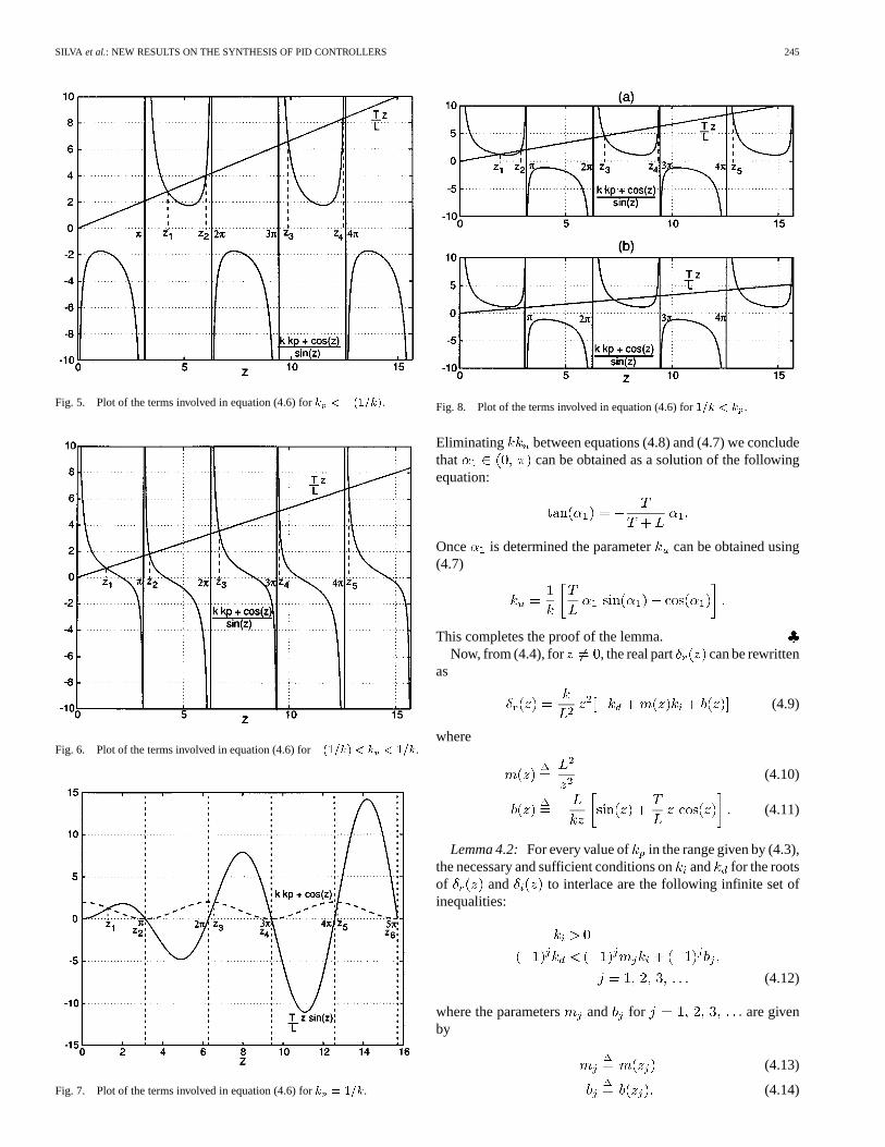
From this it is clear that one root of the imaginary part is .The other roots are difficult to find since we need to solve (4.6)analytically. However, we can plot the terms involved in equa-tion (4.6) and graphically examine the nature of the solution. Letus denote the positive-real roots of (4.6) by, ,arranged in increasing order of magnitude. There are now fourdifferent cases to consider.

Case 1) . In this case, we sketchand to obtain

the plots shown in Fig. 5.Case 2) . In this case, we graph

and to obtain theplots shown in Fig. 6.

Case 3) . In this case, we sketch andto obtain the plots shown in Fig. 7.

Case 4) . In this case, we sketchand to obtain the plots

shown in Fig. 8(a) and (b). The plot in Fig. 8(a)corresponds to the case where ,and is the largest number so that the plot of

intersects the linetwice in the interval ( ). The plot in Fig. 8(b)corresponds to the case where and the plotof does not intersect the line

twice in the interval ( ).Let us now use Theorem 3.2 to check if has only real

roots. Substituting in the expression for , we seethat for the new quasipolynomial in, and . Nextwe choose to satisfy the requirement that .Now from Figs. 6–8(a), we see that in each of these cases,i.e., for , has three real roots inthe interval , including a root atthe origin. Since is an odd function of , it follows thatin the interval , will have 5 real roots.Also observe from Figs. 6–8(a) that has a real root inthe interval . Thus has realroots in the interval . Moreover,it is clear from Figs. 6–8(a) that has two real roots ineach of the intervals and

for Hence,it follows that has exactly real roots in

for . Hence, fromTheorem 3.2, we conclude that for ,has only real roots. Also note that the cases and

corresponding to Figs. 5 and 8(b), respectively, do notmerit any further consideration since using Theorem 3.2, onecan easily argue that in these cases, all the roots of willnot be real, thereby ruling out closed-loop stability. It only re-mains to determine the upper boundon the allowable valueof . From the definition of , it follows that ifthe plot of intersects the lineonly once in the interval ( ). Let us denote by the valueof for which this intersection occurs. Then, we know that for

we have

(4.7)

Moreover, at , the line is tangent to the plot of. Thus

(4.8)

SILVA et al.: NEW RESULTS ON THE SYNTHESIS OF PID CONTROLLERS 245

Fig. 5. Plot of the terms involved in equation (4.6) fork < �(1=k).

Fig. 6. Plot of the terms involved in equation (4.6) for�(1=k) < k < 1=k.

Fig. 7. Plot of the terms involved in equation (4.6) fork = 1=k.

Fig. 8. Plot of the terms involved in equation (4.6) for1=k < k .

Eliminating between equations (4.8) and (4.7) we concludethat can be obtained as a solution of the followingequation:

Once is determined the parameter can be obtained using(4.7)

This completes the proof of the lemma.Now, from (4.4), for , the real part can be rewritten

as

(4.9)

where

(4.10)

(4.11)

Lemma 4.2:For every value of in the range given by (4.3),the necessary and sufficient conditions onand for the rootsof and to interlace are the following infinite set ofinequalities:

(4.12)

where the parameters and for are givenby

(4.13)

(4.14)

246 IEEE TRANSACTIONS ON AUTOMATIC CONTROL, VOL. 47, NO. 2, FEBRUARY 2002

Proof: From Condition 1 of Theorem 3.1, the roots ofand have to interlace in order for the quasipolyno-

mial to be stable. Thus, we evaluate at the roots ofthe imaginary part . For , using (4.4) we obtain

(4.15)

For , where , using (4.9) we obtain

(4.16)

Interlacing of the roots of and is equivalent to[since Lemma 4.1 implies that is necessarily

greater than , which in view of the stability require-ments (4.1) for the delay-free case implies that ],

, , , and so on. Using this factand equations (4.15) and (4.16) we obtain

Thus, intersecting all these regions in the– space, we ob-tain the set of ( , ) values for which the roots of and

interlace for a given fixed value of . Notice that all theseregions are half planes with their boundaries being lines withpositive slopes . This completes the proof of the lemma.

As pointed out in the proof of Lemma 4.2, the inequalitiesgiven by (4.12) represent half planes in the space ofand .Their boundaries are given by lines with the following equa-tions:

for

The focus of the remainder of this subsection will be to showthat this intersection is nonempty. We will also determine theintersection of thiscountably infinite numberof half planes in acomputationally tractable way. To this end, let us denote bythe -coordinate of the intersection of the line ,

, with the line . From (4.13) and(4.14), it is not difficult to show that

(4.17)

In a similar fashion, let us now denote by the -coordinateof the intersection of the line , ,with the line . Using (4.13) and (4.14) it can be onceagain shown that

(4.18)

We now state three important technical lemmas that willallow us to develop an algorithm for solving the PID stabi-lization problem of an open-loop stable plant ( ). Theselemmas show the behavior of the parameters, and ,

, for different values of the parameterinside the range proposed by Lemma 4.1. The proofs of these

lemmas are long and technical and are therefore presented inAppendix A.

Lemma 4.3: If then

i) for odd values of ;ii) and as for even values of;iii) for odd values of .Lemma 4.4: If then

i) for odd values of ;andii) for even values of .Lemma 4.5: If

where is the solution of the equation

in the interval , then

i) for odd values of ;ii) for even values of ;iii) for even values of ;iv) , .

We are now ready to prove Theorem 2.1.Proof of Theorem 2.1:To ensure the stability of the

quasipolynomial we need to check the two conditionsgiven in Theorem 3.1.

Step 1) We first check Condition 2 of Theorem 3.1

for some in . Let us take .Thus, and . We also have

Recall that and . Thus, if we pick

and (4.19)

or

and

we have . Notice that from these condi-tions one can safely discard from theset of values for which a stabilizing PID controllercan be found.

Step 2) Next, we check condition 1 of Theorem 3.1, i.e.,and have only simple real roots and these

interlace. From Lemma 4.1, we know that the rootsof are all real if and only if the parameter liesinside the range

, where is the solution of the equation

SILVA et al.: NEW RESULTS ON THE SYNTHESIS OF PID CONTROLLERS 247

in the interval . Now, from the proof of Lemma4.2, we see that interlacing of the roots of and

leads to the following set of inequalities

We now show that for , where, all these regions do have a

nonempty intersection. Notice first that the slopes of theboundary lines of these regions decrease with. Moreover, inthe limit we have:

Using this fact we have the following observations.

1) When , the intersection is given bythe trapezoid sketched in Fig. 3(a). This region can befound using the properties stated in Lemma 4.3.

2) When , the intersection is given by the trianglesketched in Fig. 3(b). This region can be found using

the properties stated in Lemma 4.4.3) When , the intersection is given by the

quadrilateral sketched in Fig. 3(c). This region can befound using the properties stated in Lemma 4.5.

Now, for values of in , the interlacing propertyand the fact that the roots of are all real can be used inTheorem 3.2 to guarantee that also has only real roots.Thus, for values of inside this range there is a solution tothe PID stabilization problem for a first-order open-loop stableplant with time delay. For values of outside this range theaforementioned problem does not have a solution. This com-pletes the proof of the theorem.

Remark 4.1:For , i.e., no time delay, one can solve(2.3) analytically to obtain . Using this value, theupper bound in (2.2) evaluates out to, which is consistentwith the condition imposed on by (4.1), for one of the sce-narios arising in the delay-free case. Also, by plotting the graphsof and versus , it is easy to see thatas decreases, the intersection approaches . By sub-stituting for from (2.3) into the upper bound in (2.2) anddifferentiating with respect to , it can be shown that as in-creases from 2.0288 and approaches, the upper bound in (2.2)monotonically decreases to (see also Fig. 9). This showsthat as increases, the range of values shrinks, and thisis consistent with the empirical observation in [2, p. 16].

In view of Theorem 2.1, we now propose an algorithm todetermine the set of stabilizing parameters for the plant (2.1)with .

Algorithm for Determining Stabilizing PIDParameters

Step 1 : Pick a in the range dictatedby Theorem 2.1.Step 2 : Find the roots and of equa-tion (4.6).Step 3 : Compute the parameters and

, associated with the previously

Fig. 9. Plot of the upper bound in (2.2) as a function of� .

found by using equations (4.13) and(4.14).Step 5 : Determine the stabilizing regionin the – space using Fig. 3.Step 6 : Go to Step 1.

B. Open-Loop Unstable Plant ( )

The proof of the main result Theorem 2.2 follows similarsteps as in the case of Theorem 2.1. First, the following lemmawhich is the unstable plant counterpart of Lemma 4.1 shows thatthe range of values for which PID stabilization is possible canbe determined exactly.

Lemma 4.6:For , the imaginary part ofhas only simple real roots if and only if

(4.20)

where is the solution of the equation

in the interval . In the special case of , we have. For , the roots of the imaginary part of

are not all real.Proof: The proof follows along the same lines as that of

Lemma 4.1 with appropriate modifications which are fairly ob-vious. The only nonobvious change is that in treating Case 1,i.e., , one has to make use of the following lemmato establish that for , the roots of the imaginary partof are not all real, regardless of the value ofin thisrange. By Theorem 3.1, this implies instability.

Lemma 4.7: If , then the curvesand do not intersect in the

interval regardless of the value of in ( ).Proof: The proof can be found in Appendix B.Proof of Theorem 2.2:The proof is similar to that of The-

orem 2.1 and is based on developing the appropriate counter-parts of Lemmas 4.2 and 4.5. Due to space limitations, we omitthe details and refer the interested reader to [10].

248 IEEE TRANSACTIONS ON AUTOMATIC CONTROL, VOL. 47, NO. 2, FEBRUARY 2002

A similar algorithm to the one presented in the previoussubsection can now be developed to solve the PID stabilizationproblem of an open-loop unstable plant. One only needs tosweep the parameter over the interval proposed by Theorem2.2 and use Fig. 4 to find the stabilizing region of )values at each admissible value of.

V. CONCLUDING REMARKS

In this paper we have presented a procedure to determine thecomplete set of stabilizing PID controllers for a given first-orderplant with dead-time. The procedure is based on first deter-mining the range of proportional gain values for which a so-lution to the PID stabilization problem exists. Then, it is shownthat for a fixed proportional gain value inside this range, thestabilizing integral and derivative gain values lie inside a re-gion with known shape and boundaries. Furthermore, it has beendemonstrated that this region can be characterized in a compu-tationally tractable manner. By sweeping over the entire rangeof allowable proportional gain values and determining the sta-bilizing regions in the space of the integral and derivative gains,the complete set of stabilizing PID controllers can be deter-mined. The results presented here are based on an extension ofthe Hermite–Biehler Theorem to quasipolynomials. It is our be-lief that the results of this paper will form the basis for devel-oping computationally efficient tools for PID controller designand analysis.

APPENDIX APROOF OFLEMMAS 4.3, 4.4,AND 4.5

We begin by making the following observations which followfrom the proof of Lemma 4.1.

Remark A.1:Notice from Figs. 6–8(a), for, the odd roots of (4.6), i.e., where

are getting closer to as in-creases. So in the limit for odd values ofwe have:

Moreover, since the cosine function is monotonically decreasingbetween and for odd values of , in view of theprevious observation we have:

Remark A.2:From Figs. 6 and 8(a) notice that for, the even roots of (4.6), i.e., where

are getting closer to as increases. Soin the limit for even values of we have:

We also notice in Fig. 6 that these roots approach fromthe right whereas in Fig. 8(a) they approach from theleft. Now, since the cosine function is monotonically decreasingbetween and ( ) and is mono-tonically increasing between and ( ),we have:

for . In the particular case ofFig. 7, i.e., , we notice that

.Before proving Lemmas 4.3, 4.4, and 4.5, we first state and

prove the following technical lemmas that will simplify the sub-sequent analysis.

Lemma A.1:Consider the functiondefined by

where and are natural numbers and, , are asdefined in (4.14). Then, for , , ,

can be equivalently expressed as

Proof: We will first show that for ,, the following identity holds:

(A.1)

Now for , from (4.6), we obtain

Now from (4.14) we can rewrite as follows:

[using (A.1)]

Now, since , , satisfy (4.6), we can rewrite theprevious expression as shown in the equation at the bottom ofthe next page. Thus, we finally obtain

Before stating the next lemma, we introduce the standardsignum function defined by

if

if

if

SILVA et al.: NEW RESULTS ON THE SYNTHESIS OF PID CONTROLLERS 249

Lemma A.2:Consider the functiondefined by

where and are natural numbers and, , are asdefined in (4.17). If and , , ,then

Proof: First, since , , satisfies (4.6), wecan rewrite as follows:

(A.2)

Now, using (A.2) the function can be equivalentlyexpressed as

Once more we use the fact that, , satisfies(4.6):

[since ]

Thus, the function is given by

Now, since , then . Also, since ,, , then and

. Thus, from the previous expression forit is clear that

This completes the proof of the lemma.Lemma A.3:Consider the function

defined by

where and are natural numbers and , , areas defined in (4.18). If and , ,

, then

Proof: As in the previous proof, we use the fact that,, satisfies (4.6). Thus, can be rewritten as

follows:

(A.3)

Now, following the same procedure used in the proof of LemmaA.2 we obtain

Now, since , then . Also, since, , , then

and . Thus, from the previous expression forit is clear that

This completes the proof of the lemma.

Proof of Lemma 4.3

i) First we show that for odd values of . Recallfrom Fig. 6 that is either in the first or second quadrant forodd values of . Thus, for . For

and , we have

[using (4.6)]

[since ]

[using (A.1)]

250 IEEE TRANSACTIONS ON AUTOMATIC CONTROL, VOL. 47, NO. 2, FEBRUARY 2002

Next, we show that for odd values of . Since in thiscase, i.e., for , for odd values of ,from Lemma A.1 we have

Now, since then . We alsoknow that and for odd values of . Then,from the previous expression for and recalling that

, we have

From Remark A.1 we know that . Then

and for odd values of . Thus, we have shown that

for odd values of

ii) We now show that for even values of . FromFig. 6 we see that is either in the third or fourth quadrant foreven values of. Thus, in this case. Since

and we have

[using (4.6)]

[since ]

[using (A.1)]

Note that as , . Then, .iii) It only remains for us to show the properties of the param-

eter when takes on odd values. From (A.2) we have

Now, since then . Also note that. Moreover, when takes on odd values then

. Thus we conclude that for odd values of .We now make use of Lemma A.2 to determine the sign of thequantity

Since and for odd values of , the conditionsin Lemma A.2 are satisfied and we obtain

We mentioned earlier that for odd values ofwe haveand we also have for an open-loop stable

plant. Then, , so that. Thus, we conclude that

for odd values of

This completes the proof of the lemma.

A. Proof of Lemma 4.4

i) We first consider the case of odd values of. The prooffollows from substituting (A.1) into (4.14) since , forodd values of :

[using (A.1)]

[since ]

[using (4.6)].

ii) Now, for even values of from Fig. 7 we see that. Then, and in this case.

Thus, from (4.14) we conclude that for even valuesof . This completes the proof of this lemma.

B. Proof of Lemma 4.5

First, we make a general observation regarding the roots,when the parameter is inside the interval

. From Fig. 8(a), we seethat these roots lie either in the first or second quadrant. Then

for (A.4)

i) We now consider the case of odd values of. Sinceand we have

[using (4.6)]

[using (A.1) and (A.4)]

We now show that . Since for odd values of, from Lemma A.1 we have

Now, since then . We also know thatand . Then, from the previous expression for

we have

From Remark A.1, we have that . Then

and for odd values of . Thus, we have shown that

for odd values of

SILVA et al.: NEW RESULTS ON THE SYNTHESIS OF PID CONTROLLERS 251

ii) We now consider the case of even values of the parameter. Since and we have

[using (4.6)]

[using (A.1) and (A.4)]

We now show that for this case. We know thatfor even values of . Then, from Lemma A.1, we have

Once more since then . We also knowthat and . Then, from the previous expressionfor we have

From Remark A.2, we have that for evenvalues of the parameter. Using this fact we obtain

and for even values of . Thus, we have shown that

for even values of

iii) We now consider the properties of the parameter. From(A.3), we have

Clearly since then . Also notice that. Thus, since we conclude that

for even values of the parameter. We now invokeLemma A.3 and evaluate the function at ,

Since and for even values of , then wehave

We know from Remark A.2 that for evenvalues of , and also that . Then, ,so that . Thus, we have shownthat

for even values of

iv) We show first that . Since , , fromLemma A.1 we have

We know that and . Moreover, sincewe obtain the following:

As we can see from Fig. 8(a), both and are in the intervaland . Since the cosine function is monotonically

decreasing in then . Thus

Hence, we have . Finally we show that . To doso, we invoke Lemma A.3 and evaluate the functionat , :

Since and , , the conditions inLemma A.3 are satisfied and we obtain

We already pointed out that and sincewe have

Thus, and this completes the proof of the lemma.

APPENDIX BPROOF OFLEMMA 4.7

Let us define the function by

Consider , such that . Then, for any, we have

[since ]

Thus for any fixed , is monotonically in-creasing with respect to . Hence, for we have

This means that if the line does not intersect the curvein , then it will not intersect any other

curve in .

252 IEEE TRANSACTIONS ON AUTOMATIC CONTROL, VOL. 47, NO. 2, FEBRUARY 2002

Fig. 10. Plot of the curvef (z; �(1=k)) and the line(T=L)z.

Observe that

Accordingly, define a continuous extension of toby

Clearly, the curve intersects the line at. This is depicted in Fig. 10. Also, note that the slope of

the tangent to at is given by

Clearly, if this slope is less than or equal to then we areguaranteed that no further intersections will take place in the in-terval . Since on ,it follows that if , then the curve willnot intersect the line in the interval . This com-pletes the proof.

REFERENCES

[1] W. L. Bialkowski, “Control of the pulp and paper making process,” inThe Control Handbook, W. S. Levine, Ed. New York: IEEE Press,1996, pp. 1219–1242.

[2] K. Astrom and T. Hagglund,PID Controllers: Theory, Design, andTuning. Research Triangle Park, NC: Instrument Society of America,1995.

[3] A. Datta, M. T. Ho, and S. P. Bhattacharyya,Structure and Synthesis ofPID Controllers. London, U.K.: Springer-Verlag, 2000.

[4] L. S. Pontryagin, “On the zeros of some elementary transcendental func-tion” (in English),Amer. Math. Society Translation, vol. 2, pp. 95–110,1955.

[5] J. S. Karmarkar and D. D. Siljak, “Stability analysis of systems withtime delay,”Proc. IEE, vol. 117, no. 7, pp. 1421–1424, July 1970.

[6] F. R. Gantmacher,The Theory of Matrices. New York: Chelsea, 1959.[7] S. P. Bhattacharyya, H. Chapellat, and L. H. Keel,Robust Control: The

Parametric Approach. Upper Saddle River, NJ: Prentice-Hall, 1995.[8] R. Bellman and K. L. Cooke, Differential-Difference Equa-

tions. London, U.K.: Academic, 1963.[9] V. L. Kharitonov and A. P. Zhabko, “Robust stability of time-delay sys-

tems,”IEEE Trans. Automat. Contr., vol. 39, Dec. 1994.[10] G. J. Silva, A. Datta, and S. P. Bhattacharyya, “New results on the syn-

thesis of PID controllers,” Dept. of Electrical Engineering, Texas A&MUniv., College Station, TX, Tech. Rep. 00-01, Feb. 2000.

Guillermo J. Silva was born in Lima, Peru, in 1973.He received the B.S. degree in electronics engi-neering from the Pontificia Universidad Catolica delPeru, and the Ph.D. degree in electrical engineeringfrom Texas A&M University, College Station, in1995 and 2000, respectively.

During his graduate studies at Texas A&M Uni-versity, he worked as an Assistant Lecturer in LinearControl Systems, and participated in the PanamaCanal Project as a design engineer (sponsored by thePanama Canal Commission). He also directed the

setting of the Control Engineering Laboratory for the Department of ElectricalEngineering. Currently, he works as a development engineer in the low-leveland open firmware group at IBM in Austin, TX. His research interests includetime-delay systems, robust and nonfragile control, stabilization using the PIDcontroller, and process control.

Aniruddha Datta received the B.Tech. degree inelectrical engineering from the Indian Institute ofTechnology, Kharagpur, the M.S.E.E. degree fromSouthern Illinois University, Carbondale, and theM.S. (applied mathematics) and Ph.D. degrees fromthe University of Southern California, Los Angeles,in 1985, 1987, and 1991, respectively.

In August 1991, he joined the Department of Elec-trical Engineering at Texas A&M University, wherehe is currently an Associate Professor. His areas ofinterest include adaptive control, robust control, and

PID control. He is the author of the bookAdaptive Internal Model Control(NewYork: Springer-Verlag, 1998), and a co-authorStructure and Synthesis of PIDControllers(New York: Springer-Verlag, 2000).

Dr. Datta currently serves as an Associate Editor of the IEEE TRANSACTIONS

ON AUTOMATIC CONTROL.

S. P. Bhattacharyyawas born in Yangon, Myanmar,in 1946. He received the B.Tech. degree from the In-dian Institute of Technology, Bombay, and the Ph.D.degree from Rice University, Houston, TX, in 1967and 1971, respectively.

His contributions to control theory include thegeometric solution of the multivariable servomech-anism problem, the structure of robust and unknowninput observers, pole assignment algorithm usingSylvester’s equation, computation of the parametricstability margin, a generalization of Kharitonov’s

Theorem, the fragility of optimal controllers and stabilization using PIDcontrollers. These are documented in four books, and 80 journal and 100conference papers.