a study of computational verb pid controllers - citeseerx

INTERNATIONAL JOURNAL OF COMPUTATIONAL COGNITION (HTTP://WWW.IJCC.US), VOL. 7, NO. 3, SEPTEMBER 2009 61

A Study of Computational Verb PID Controllers:Structures and Designs

Ge Yang and Tao Yang

Abstract— Computational verb PID controller is a new typeof intelligent PID controller. Compared to conventional PIDcontrollers and other intelligent PID controllers such as fuzzyPID controllers, computational verb PID controllers employcomputational verb theory to infer the three kinds of gains in PIDcontrollers - Kp, Ki, Kd. In this paper, the design of conventionalPID controller, fuzzy PID controller and computational verb PIDcontroller are presented in detail and the control results aresimulated and studied for a given control plant. To facilitate pa-rameter adjustments, the GUI for tuning computational verb PIDcontrollers is taken as an example for the purpose of describingthe design procedure of MATLAB GUI. Copyright c© 2009 Yang’sScientific Research Institute, LLC. All rights reserved.

Index Terms— Computational verb, PID controller, fuzzy PIDcontroller, computational verb PID controller, MATLAB GUI.

I. INTRODUCTION

COMPUTATIONAL verb PID controllers(verb PID con-trollers, for short) are one of the earliest industrial

applications of computational verb theory[12]. The first designof verb PID controller was presented in [9], [10]. In 2005,the first textbook[1] to include verb PID controller into astandard undergraduate course was published. In China, theverb PID controllers were widely studied[4], [5] and appliedto different industrial applications. The latest design of verbPID controllers are presented in [13]. In this paper, basedon a model of linear motor presented in [4], we designedthree kinds of PID controllers including: conventional, fuzzyand verb PID controllers, and compared their controllingperformances.

The organization of this paper is as follows. In Section II,the basic knowledge of PID controller is presented. In Sec-tion III, the model based on which the three kinds of PIDcontrollers are studied is introduced. In Section IV, a con-ventional PID controller is designed and the tuning methodand simulation result are given. In Section V, a fuzzy PIDcontroller is designed and the tuning method and simulationresult are given. In Section VI, a verb PID controller is

Manuscript received May 20, 2009; September 25, 2009.Ge Yang, Department of Electronic Engineering, Xiamen University, Xia-

men 361005, P.R. China. Tao Yang, Department of Electronic Engineering,Xiamen University, Xiamen 361005, P.R. China. Department of CognitiveEconomics, Department of Electrical Engineering and Computer Sciences,Yang’s Scientific Research Institute, 1303 East University Blvd., #20882,Tucson, Arizona 85719-0521, USA. Email: [email protected](T. Yang).

Acknowledgment: The first author would like to thank Mr. Yi Guo forsharing and discussing computational verb theory, and thank Ms. Xiaoli Linfor continuous supporting.

Publisher Item Identifier S 1542-5908(09)10312-3/$20.00Copyright c©2009 Yang’s Scientific Research Institute, LLC. Allrights reserved. The online version posted on September 30, 2009 athttp://www.YangSky.com/ijcc/ijcc73.htm

designed and the tuning method and simulation result aregiven. In Section VII, the control results of the three kindsof PID controllers are compared and studied. In Section VIII,the GUI for verb PID controller is taken as an example toillustrate the design method of MATLAB GUI. Section IXconcludes this paper and proposes how to improve the verbPID controller.

II. INTRODUCTION OF PID CONTROLLER

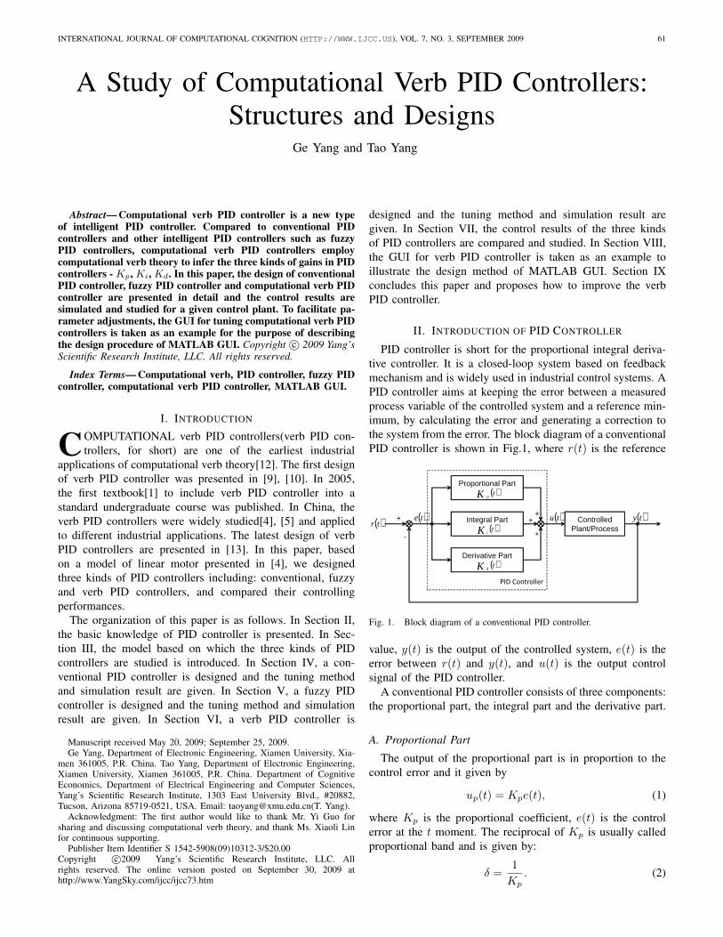
PID controller is short for the proportional integral deriva-tive controller. It is a closed-loop system based on feedbackmechanism and is widely used in industrial control systems. APID controller aims at keeping the error between a measuredprocess variable of the controlled system and a reference min-imum, by calculating the error and generating a correction tothe system from the error. The block diagram of a conventionalPID controller is shown in Fig.1, where r(t) is the reference

ControlledPlant/Process

Proportional Part

Integral Part

Derivative Part

+

-

PID Controller

+

+

+

( )tK i

( )tK d

( )tK p

( )tr( )te ( )ty( )tu

Fig. 1. Block diagram of a conventional PID controller.

value, y(t) is the output of the controlled system, e(t) is theerror between r(t) and y(t), and u(t) is the output controlsignal of the PID controller.

A conventional PID controller consists of three components:the proportional part, the integral part and the derivative part.

A. Proportional Part

The output of the proportional part is in proportion to thecontrol error and it given by

up(t) = Kpe(t), (1)

where Kp is the proportional coefficient, e(t) is the controlerror at the t moment. The reciprocal of Kp is usually calledproportional band and is given by:

δ =1

Kp. (2)

62 INTERNATIONAL JOURNAL OF COMPUTATIONAL COGNITION (HTTP://WWW.IJCC.US), VOL. 7, NO. 3, SEPTEMBER 2009

The proportional coefficient is used to accelerate system’sresponse, improve control precision, and decrease the steadystate error but cannot eliminate it. A larger Kp leads to afaster response, but a larger overshoot. An excessively largeKp will cause instability and oscillation. A smaller Kp slowsdown system’s response, decreases control precision, extendsadjusting time and thereby worsens the dynamic and statisticcharacteristics of the controlled system.

B. Integral Part

The integral part is given by

ui(t) = Ki

∫ t

0

e(t)dt. (3)

The integral part is used to eliminate the steady state error.Increasing Ki helps to eliminate the steady state error faster,but will cause a larger overshoot and a longer settling time.

C. Derivative Part

The derivative part is given by:

ud(t) = Kdde(t)dt

. (4)

The derivative part is used to improve the dynamic charac-teristic of the controlled system. It can control the overshoot,shorten the settling time and improve the stability, but willmake the system unstable to the interference if Kd is exces-sively large.[3][7]

D. Common Form for a PID Controller’s Output

The output control signal of a PID controller is describedas follows:

u(t) = Kp(t)e(t) + Ki(t)∫ t

0

e(t)dt + Kd(t)de(t)dt

, (5)

where u(t) is the output control signal, e(t) is the controlerror, and Kp, Ki, Kd refer to the proportional gain, integralgain and derivative gain, respectively. And Kp, Ki, Kd satisfythe following equations:

Ki(t) = Kp(t)Ti

, (6)Kd(t) = KpTd, (7)

where Ti and Td refer to the integration time and derivativetime, respectively.

As the PID controllers will be implemented in a digitalsystem in this paper, the following discrete-time form shouldbe useful[13]:

u(k) = Kp(k)e(k) + Ki(k)Ts

k∑

i=0

e(i) +Kd(k)

Ts∆e(k), (8)

where Ts is the sampling period of the digital system, u(k) ande(k) are the control signal and control error at the samplingtime kTs, respectively. Kp(k), Ki(k) and Kd(k) are theproportional, integral and derivative gains at the sampling timekTs.

III. THE MODEL TO BE STUDIED

In this paper, we choose a linear motor model as the testbedfor studying different kinds of PID controllers. The model wasillustrated in details in a master thesis[4]. And we just drawout from the thesis the displacement-voltage transfer equationof this model:

tf =24272

s2 + 14s + 6068. (9)

All the PID controllers to be discussed later in this paperwill aim at controlling the linear motor to generate a one-unitdisplacement with a short convergence time, a small overshootand a weak oscillation. And in order to express a more directimpression, we will use mostly the control error of the systemnot the motor’s displacement to evaluate performance of eachcontroller.

IV. CONVENTIONAL PID CONTROLLER

The conventional PID controller is the base of the otherkinds of PID controllers including the computational verbcontroller. To make this paper self-contained, a conventionalPID controller will be designed and studies in this section.

A. Design a Conventional PID Controller

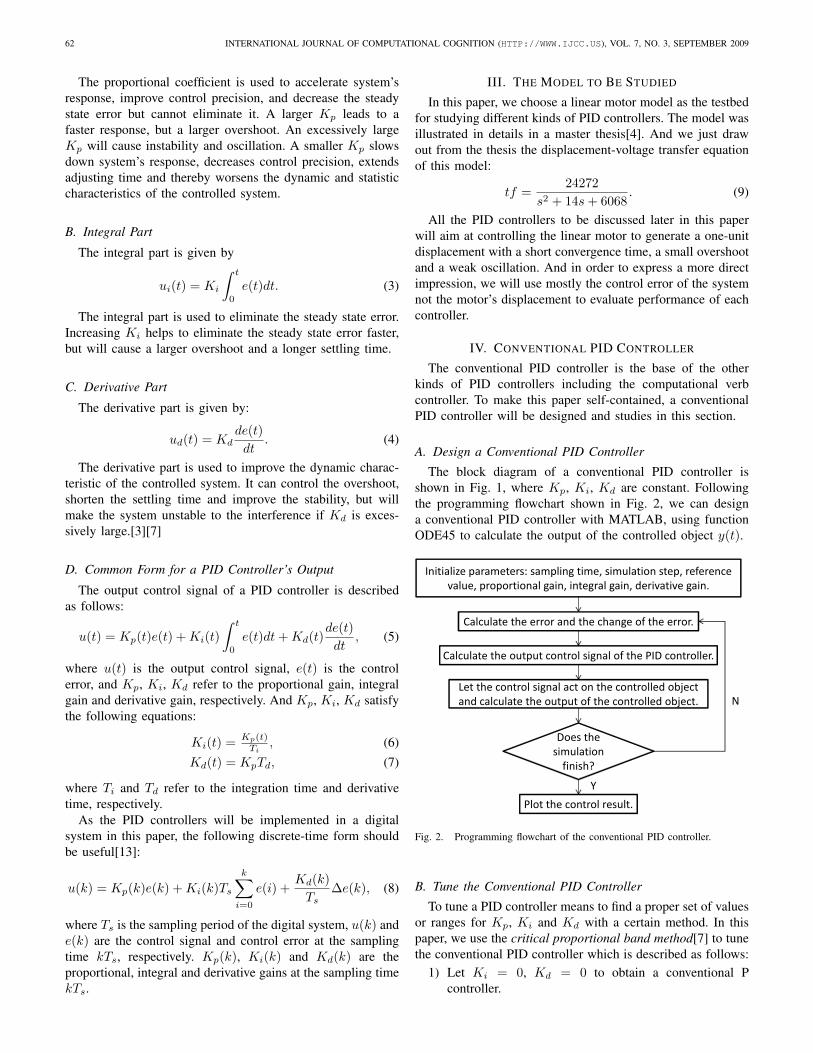
The block diagram of a conventional PID controller isshown in Fig. 1, where Kp, Ki, Kd are constant. Followingthe programming flowchart shown in Fig. 2, we can designa conventional PID controller with MATLAB, using functionODE45 to calculate the output of the controlled object y(t).

Initialize parameters: sampling time, simulation step, reference value, proportional gain, integral gain, derivative gain.

Does the simulation

finish?

Calculate the error and the change of the error.

Calculate the output control signal of the PID controller.

Let the control signal act on the controlled object and calculate the output of the controlled object.

Plot the control result.Y

N

Fig. 2. Programming flowchart of the conventional PID controller.

B. Tune the Conventional PID Controller

To tune a PID controller means to find a proper set of valuesor ranges for Kp, Ki and Kd with a certain method. In thispaper, we use the critical proportional band method[7] to tunethe conventional PID controller which is described as follows:

1) Let Ki = 0, Kd = 0 to obtain a conventional Pcontroller.

YANG & YANG, A STUDY OF COMPUTATIONAL VERB PID CONTROLLERS 63

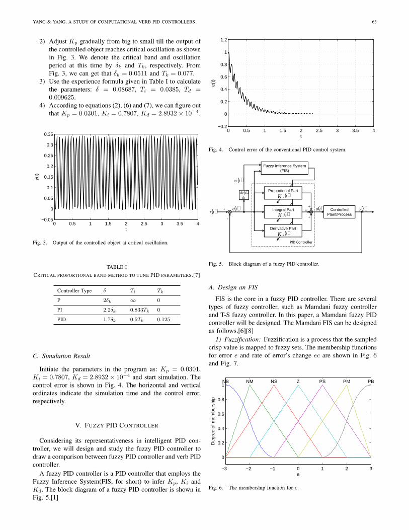
2) Adjust Kp gradually from big to small till the output ofthe controlled object reaches critical oscillation as shownin Fig. 3. We denote the critical band and oscillationperiod at this time by δk and Tk, respectively. FromFig. 3, we can get that δk = 0.0511 and Tk = 0.077.

3) Use the experience formula given in Table I to calculatethe parameters: δ = 0.08687, Ti = 0.0385, Td =0.009625.

4) According to equations (2), (6) and (7), we can figure outthat Kp = 0.0301, Ki = 0.7807, Kd = 2.8932× 10−4.

0 0.5 1 1.5 2 2.5 3 3.5 4−0.05

0

0.05

0.1

0.15

0.2

0.25

0.3

0.35

y(t)

t

Fig. 3. Output of the controlled object at critical oscillation.

TABLE ICRITICAL PROPORTIONAL BAND METHOD TO TUNE PID PARAMETERS.[7]

Controller Type δ Ti Tk

P 2δk ∞ 0

PI 2.2δk 0.833Tk 0

PID 1.7δk 0.5Tk 0.125

C. Simulation Result

Initiate the parameters in the program as: Kp = 0.0301,Ki = 0.7807, Kd = 2.8932× 10−4 and start simulation. Thecontrol error is shown in Fig. 4. The horizontal and verticalordinates indicate the simulation time and the control error,respectively.

V. FUZZY PID CONTROLLER

Considering its representativeness in intelligent PID con-troller, we will design and study the fuzzy PID controller todraw a comparison between fuzzy PID controller and verb PIDcontroller.

A fuzzy PID controller is a PID controller that employs theFuzzy Inference System(FIS, for short) to infer Kp, Ki andKd. The block diagram of a fuzzy PID controller is shown inFig. 5.[1]

0 0.5 1 1.5 2 2.5 3 3.5 4−0.2

0

0.2

0.4

0.6

0.8

1

1.2

e(t)

t

Fig. 4. Control error of the conventional PID control system.

Fuzzy Inference System (FIS)


Proportional Part

Integral Part

Derivative Part

+

-

PID Controller

+

+

+

( )tK i

( )tK d

( )tK p

( )tr( )te ( )ty( )tu

( )dt

tde

( )tec

Fig. 5. Block diagram of a fuzzy PID controller.

A. Design an FIS

FIS is the core in a fuzzy PID controller. There are severaltypes of fuzzy controller, such as Mamdani fuzzy controllerand T-S fuzzy controller. In this paper, a Mamdani fuzzy PIDcontroller will be designed. The Mamdani FIS can be designedas follows.[6][8]

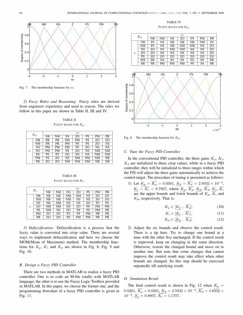
1) Fuzzification: Fuzzification is a process that the sampledcrisp value is mapped to fuzzy sets. The membership functionsfor error e and rate of error’s change ec are shown in Fig. 6and Fig. 7.

−3 −2 −1 0 1 2 3

0

0.2

0.4

0.6

0.8

1

e

Deg

ree

of m

embe

rshi

p

NB NM NS Z PS PM PB

Fig. 6. The membership function for e.


−3 −2 −1 0 1 2 3

0

0.2

0.4

0.6

0.8

1

ec

Deg

ree

of m

embe

rshi

pNB NM NS Z PS PM PB

Fig. 7. The membership function for ec.

2) Fuzzy Rules and Reasoning: Fuzzy rules are derivedfrom engineers experience and used to reason. The rules wefollow in this paper are shown in Table II, III and IV.

TABLE IIFUZZY RULES FOR Kp .

Kpec

NB NM NS ZO PS PM PB

e

NB PB PB PM PM PS ZO ZONM PB PB PM PS PS ZO NSNS PM PM PM PS ZO NS NSZO PM PM PS ZO NS NM NMPS PS PS ZO NS NS NM NMPM PS ZO NS NM NM NM NBPB ZO ZO NM NM NM NB NB

TABLE IIIFUZZY RULES FOR Ki .

Kiec


e

NB NB NB NM NM NS ZO ZONM NB NB NM NS NS ZO ZONS NB NM NS NS ZO PS PSZO NM NM NS ZO PS PM PMPS NM NS ZO PS PS PM PBPM ZO ZO PS PS PM PB PBPB ZO ZO PS PM PM PB PB

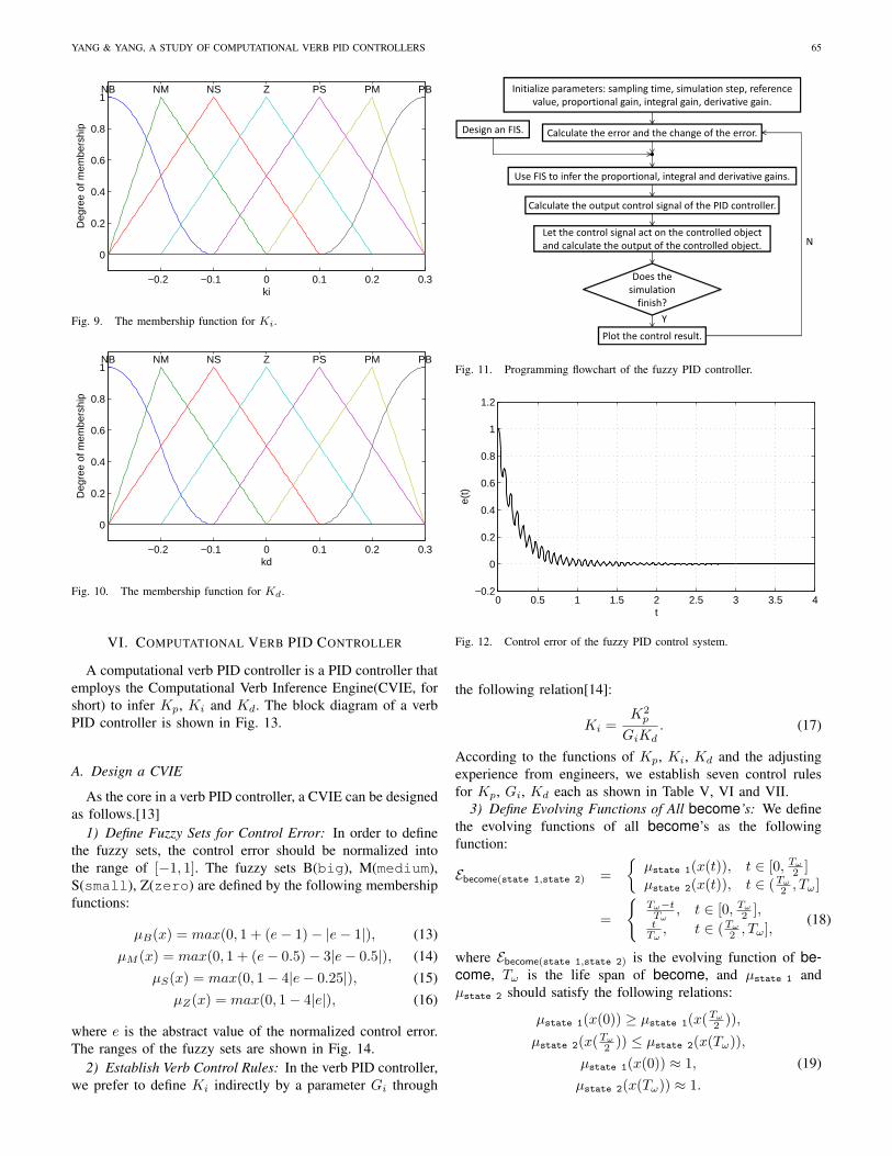
3) Defuzzification: Defuzzification is a process that thefuzzy value is converted into crisp value. There are severalways to implement defuzzification and here we choose theMOM(Mean of Maximum) method. The membership func-tions for Kp, Ki and Kd are shown in Fig. 8, Fig. 9 andFig. 10.

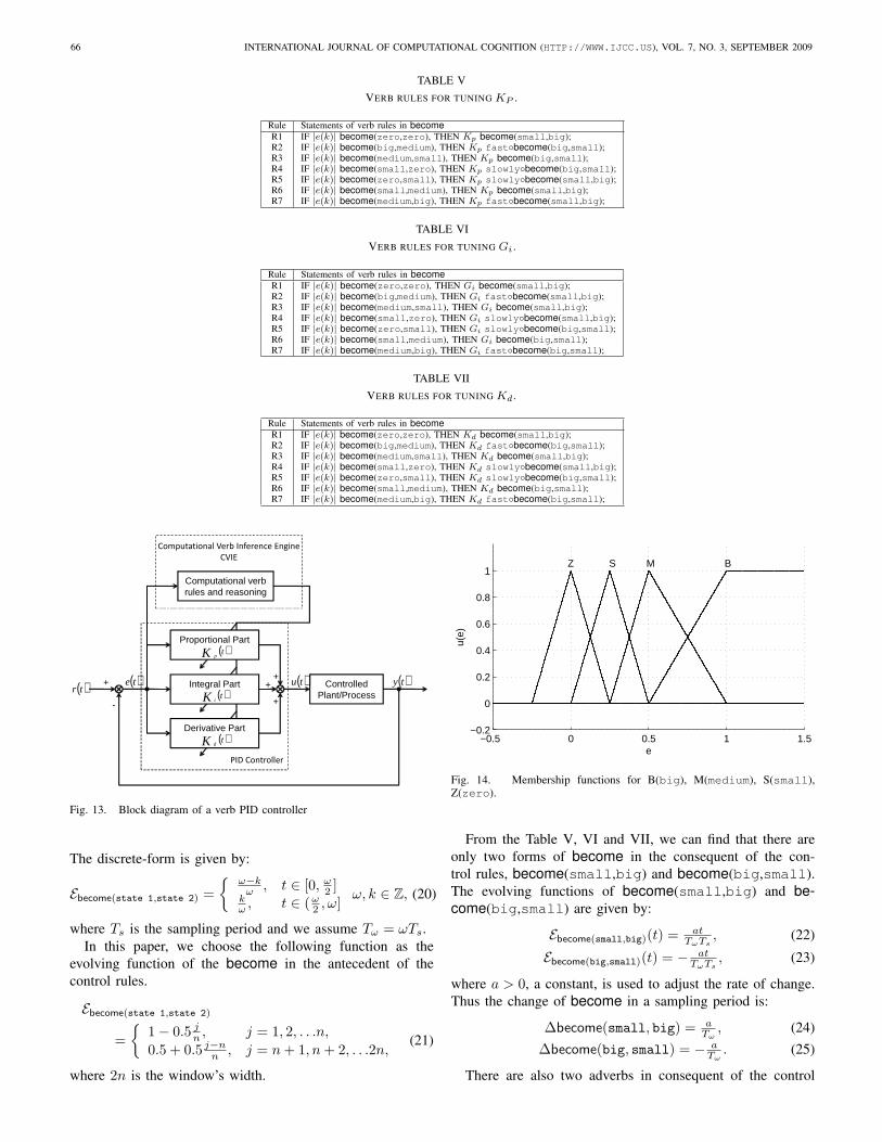
B. Design a Fuzzy PID Controller

There are two methods in MATLAB to realize a fuzzy PIDcontroller. One is to code an M-file totally with MATLABlanguage; the other is to use the Fuzzy Logic Toolbox providedin MATLAB. In this paper, we choose the former one, and theprogramming flowchart of a fuzzy PID controller is given inFig. 11.

TABLE IVFUZZY RULES FOR Kd .

Kdec


e

NB PS NS NB NB NB NM PSNM PS NS NB NM NM NS ZONS ZO NS NM NM NS NS ZOZO ZO NS NS NS NS NS ZOPS ZO ZO ZO ZO ZO ZO ZOPM PB NS PS PS PS PS PBPB PB PM PM PM PS PS PB

−2 −1 0 1 2 3

x 10−4

0

0.2

0.4

0.6

0.8

1

kpD

egre

e of

mem

bers

hip

NB NM NS Z PS PM PB

Fig. 8. The membership function for Kp.

C. Tune the Fuzzy PID Controller

In the conventional PID controller, the three gains Kp, Ki,Kd are initialized to three crisp values, while in a fuzzy PIDcontroller, they will be initialized to three ranges within whichthe FIS will adjust the three gains automatically to achieve thecontrol target. The procedure of tuning is presented as follows:

1) Let Kp = Kp = 0.0301, Kd = Kd = 2.8932 × 10−4,Ki = Ki = 0.7807, where Kp, Kp, Kd, Kd, Ki, Ki

are the upper bounds and lower bounds of Kp, Ki andKd, respectively. That is:

Kp ∈ [Kp , Kp], (10)

Ki ∈ [Ki , Ki], (11)

Kd ∈ [Kd , Kd]. (12)

2) Adjust the six bounds and observe the control result.There is a tip here. Try to change one bound at atime with the other five unchanged. If the control resultis improved, keep on changing in the same direction.Otherwise, restore the changed bound and move on toanother one. But note that some changes that cannotimprove the control result may take effect when otherbounds are changed. So this step should be exercisedrepeatedly till satisfying result.

D. Simulation Result

The final control result is shown in Fig. 12 when Kp =0.0261, Kp = 0.0301, Kd = 2.5932× 10−4, Kd = 4.6932×10−4, Ki = 0.8807, Ki = 1.1707.


−0.2 −0.1 0 0.1 0.2 0.3

0

0.2

0.4

0.6

0.8

1

ki

Deg

ree

of m

embe

rshi

pNB NM NS Z PS PM PB

Fig. 9. The membership function for Ki.

−0.2 −0.1 0 0.1 0.2 0.3

0

0.2

0.4

0.6

0.8

1

kd

Deg

ree

of m

embe

rshi

p

NB NM NS Z PS PM PB

Fig. 10. The membership function for Kd.

VI. COMPUTATIONAL VERB PID CONTROLLER

A computational verb PID controller is a PID controller thatemploys the Computational Verb Inference Engine(CVIE, forshort) to infer Kp, Ki and Kd. The block diagram of a verbPID controller is shown in Fig. 13.

A. Design a CVIE

As the core in a verb PID controller, a CVIE can be designedas follows.[13]

1) Define Fuzzy Sets for Control Error: In order to definethe fuzzy sets, the control error should be normalized intothe range of [−1, 1]. The fuzzy sets B(big), M(medium),S(small), Z(zero) are defined by the following membershipfunctions:

µB(x) = max(0, 1 + (e− 1)− |e− 1|), (13)µM (x) = max(0, 1 + (e− 0.5)− 3|e− 0.5|), (14)

µS(x) = max(0, 1− 4|e− 0.25|), (15)µZ(x) = max(0, 1− 4|e|), (16)

where e is the abstract value of the normalized control error.The ranges of the fuzzy sets are shown in Fig. 14.

2) Establish Verb Control Rules: In the verb PID controller,we prefer to define Ki indirectly by a parameter Gi through


Does the simulation

finish?

Calculate the error and the change of the error.



Plot the control result.

Design an FIS.

Use FIS to infer the proportional, integral and derivative gains.

Y

N

Fig. 11. Programming flowchart of the fuzzy PID controller.

0 0.5 1 1.5 2 2.5 3 3.5 4−0.2

0

0.2

0.4

0.6

0.8

1

1.2

e(t)

t

Fig. 12. Control error of the fuzzy PID control system.

the following relation[14]:

Ki =K2

p

GiKd. (17)

According to the functions of Kp, Ki, Kd and the adjustingexperience from engineers, we establish seven control rulesfor Kp, Gi, Kd each as shown in Table V, VI and VII.

3) Define Evolving Functions of All become’s: We definethe evolving functions of all become’s as the followingfunction:

Ebecome(state 1,state 2) ={

µstate 1(x(t)), t ∈ [0, Tω

2 ]µstate 2(x(t)), t ∈ (Tω

2 , Tω]

=

{Tω−tTω

, t ∈ [0, Tω

2 ],t

Tω, t ∈ (Tω

2 , Tω],(18)

where Ebecome(state 1,state 2) is the evolving function of be-come, Tω is the life span of become, and µstate 1 andµstate 2 should satisfy the following relations:

µstate 1(x(0)) ≥ µstate 1(x(Tω

2 )),

µstate 2(x(Tω

2 )) ≤ µstate 2(x(Tω)),µstate 1(x(0)) ≈ 1, (19)µstate 2(x(Tω)) ≈ 1.


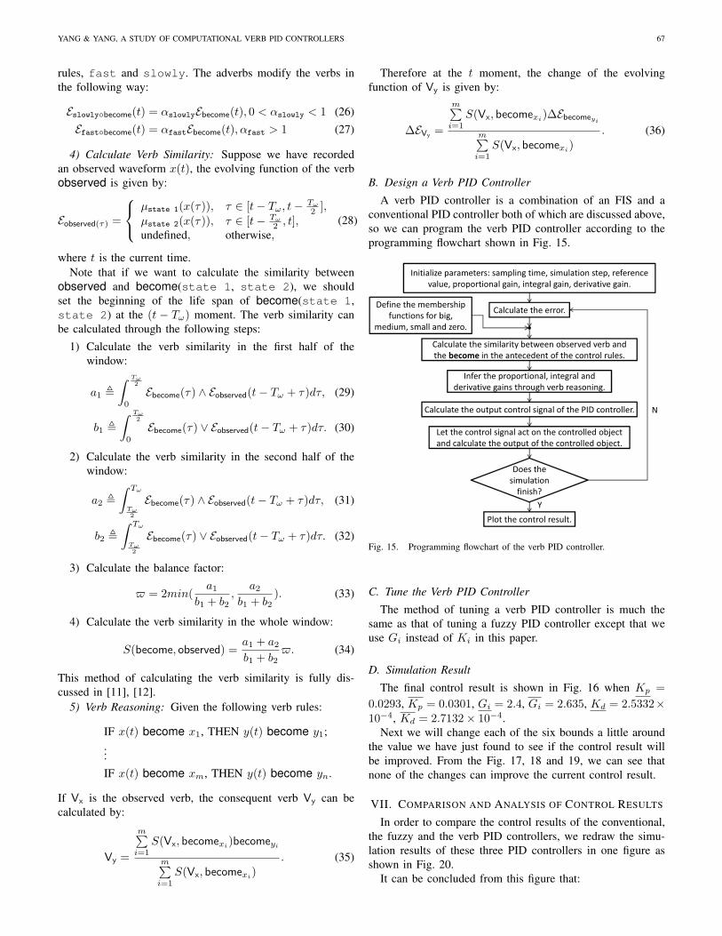
TABLE VVERB RULES FOR TUNING KP .

Rule Statements of verb rules in becomeR1 IF |e(k)| become(zero,zero), THEN Kp become(small,big);R2 IF |e(k)| become(big,medium), THEN Kp fast◦become(big,small);R3 IF |e(k)| become(medium,small), THEN Kp become(big,small);R4 IF |e(k)| become(small,zero), THEN Kp slowly◦become(big,small);R5 IF |e(k)| become(zero,small), THEN Kp slowly◦become(small,big);R6 IF |e(k)| become(small,medium), THEN Kp become(small,big);R7 IF |e(k)| become(medium,big), THEN Kp fast◦become(small,big);

TABLE VIVERB RULES FOR TUNING Gi .

Rule Statements of verb rules in becomeR1 IF |e(k)| become(zero,zero), THEN Gi become(small,big);R2 IF |e(k)| become(big,medium), THEN Gi fast◦become(small,big);R3 IF |e(k)| become(medium,small), THEN Gi become(small,big);R4 IF |e(k)| become(small,zero), THEN Gi slowly◦become(small,big);R5 IF |e(k)| become(zero,small), THEN Gi slowly◦become(big,small);R6 IF |e(k)| become(small,medium), THEN Gi become(big,small);R7 IF |e(k)| become(medium,big), THEN Gi fast◦become(big,small);

TABLE VIIVERB RULES FOR TUNING Kd .

Rule Statements of verb rules in becomeR1 IF |e(k)| become(zero,zero), THEN Kd become(small,big);R2 IF |e(k)| become(big,medium), THEN Kd fast◦become(big,small);R3 IF |e(k)| become(medium,small), THEN Kd become(small,big);R4 IF |e(k)| become(small,zero), THEN Kd slowly◦become(small,big);R5 IF |e(k)| become(zero,small), THEN Kd slowly◦become(big,small);R6 IF |e(k)| become(small,medium), THEN Kd become(big,small);R7 IF |e(k)| become(medium,big), THEN Kd fast◦become(big,small);

Computational verbrules and reasoning

Computational Verb Inference EngineCVIE


Proportional Part

Integral Part

Derivative Part

+

-

PID Controller

+

+

+

( )tK i

( )tK d

( )tK p

( )tr( )te ( )ty( )tu

Fig. 13. Block diagram of a verb PID controller

The discrete-form is given by:

Ebecome(state 1,state 2) ={

ω−kω , t ∈ [0, ω

2 ]kω , t ∈ (ω

2 , ω]ω, k ∈ Z, (20)

where Ts is the sampling period and we assume Tω = ωTs.In this paper, we choose the following function as the

evolving function of the become in the antecedent of thecontrol rules.

Ebecome(state 1,state 2)

={

1− 0.5 jn , j = 1, 2, . . .n,

0.5 + 0.5 j−nn , j = n + 1, n + 2, . . .2n,

(21)

where 2n is the window’s width.

−0.5 0 0.5 1 1.5−0.2

0

0.2

0.4

0.6

0.8

1

e

u(e)

BMSZ

Fig. 14. Membership functions for B(big), M(medium), S(small),Z(zero).

From the Table V, VI and VII, we can find that there areonly two forms of become in the consequent of the con-trol rules, become(small,big) and become(big,small).The evolving functions of become(small,big) and be-come(big,small) are given by:

Ebecome(small,big)(t) = atTωTs

, (22)

Ebecome(big,small)(t) = − atTωTs

, (23)

where a > 0, a constant, is used to adjust the rate of change.Thus the change of become in a sampling period is:

∆become(small, big) = aTω

, (24)∆become(big, small) = − a

Tω. (25)

There are also two adverbs in consequent of the control


rules, fast and slowly. The adverbs modify the verbs inthe following way:

Eslowly◦become(t) = αslowlyEbecome(t), 0 < αslowly < 1 (26)Efast◦become(t) = αfastEbecome(t), αfast > 1 (27)

4) Calculate Verb Similarity: Suppose we have recordedan observed waveform x(t), the evolving function of the verbobserved is given by:

Eobserved(τ) =

µstate 1(x(τ)), τ ∈ [t− Tω, t− Tω

2 ],µstate 2(x(τ)), τ ∈ [t− Tω

2 , t],undefined, otherwise,

(28)

where t is the current time.Note that if we want to calculate the similarity between

observed and become(state 1, state 2), we shouldset the beginning of the life span of become(state 1,state 2) at the (t − Tω) moment. The verb similarity canbe calculated through the following steps:

1) Calculate the verb similarity in the first half of thewindow:

a1 ,∫ Tω

2

0

Ebecome(τ) ∧ Eobserved(t− Tω + τ)dτ, (29)

b1 ,∫ Tω

2

0

Ebecome(τ) ∨ Eobserved(t− Tω + τ)dτ. (30)

2) Calculate the verb similarity in the second half of thewindow:

a2 ,∫ Tω

Tω2

Ebecome(τ) ∧ Eobserved(t− Tω + τ)dτ, (31)

b2 ,∫ Tω

Tω2

Ebecome(τ) ∨ Eobserved(t− Tω + τ)dτ. (32)

3) Calculate the balance factor:

$ = 2min(a1

b1 + b2,

a2

b1 + b2). (33)

4) Calculate the verb similarity in the whole window:

S(become, observed) =a1 + a2

b1 + b2$. (34)

This method of calculating the verb similarity is fully dis-cussed in [11], [12].

5) Verb Reasoning: Given the following verb rules:

IF x(t) become x1, THEN y(t) become y1;...IF x(t) become xm, THEN y(t) become yn.

If Vx is the observed verb, the consequent verb Vy can becalculated by:

Vy =

m∑i=1

S(Vx, becomexi)becomeyi

m∑i=1

S(Vx, becomexi)

. (35)

Therefore at the t moment, the change of the evolvingfunction of Vy is given by:

∆EVy =

m∑i=1

S(Vx, becomexi)∆Ebecomeyi

m∑i=1

S(Vx, becomexi)

. (36)

B. Design a Verb PID Controller

A verb PID controller is a combination of an FIS and aconventional PID controller both of which are discussed above,so we can program the verb PID controller according to theprogramming flowchart shown in Fig. 15.


Does the simulation

finish?

Calculate the error.



Plot the control result.

Define the membership functions for big,

medium, small and zero.

Infer the proportional, integral and derivative gains through verb reasoning.

Calculate the similarity between observed verb and the become in the antecedent of the control rules.

Y

N

Fig. 15. Programming flowchart of the verb PID controller.

C. Tune the Verb PID Controller

The method of tuning a verb PID controller is much thesame as that of tuning a fuzzy PID controller except that weuse Gi instead of Ki in this paper.

D. Simulation Result

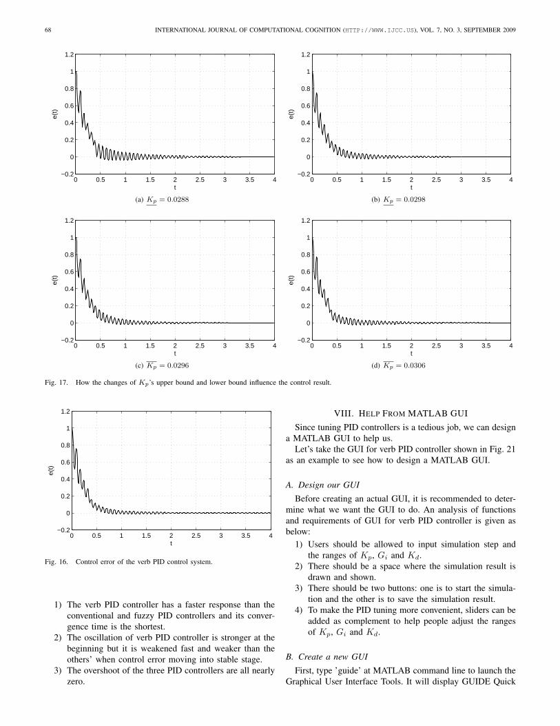
The final control result is shown in Fig. 16 when Kp =0.0293, Kp = 0.0301, Gi = 2.4, Gi = 2.635, Kd = 2.5332×10−4, Kd = 2.7132× 10−4.

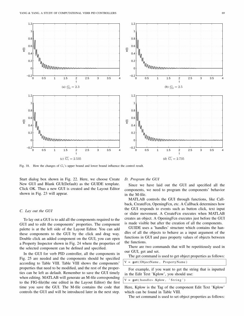
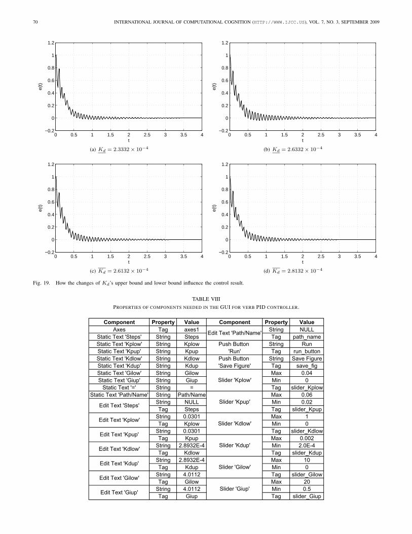
Next we will change each of the six bounds a little aroundthe value we have just found to see if the control result willbe improved. From the Fig. 17, 18 and 19, we can see thatnone of the changes can improve the current control result.

VII. COMPARISON AND ANALYSIS OF CONTROL RESULTS

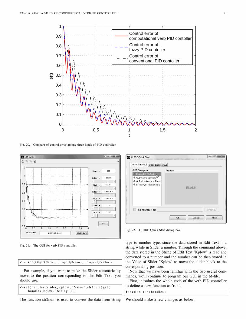
In order to compare the control results of the conventional,the fuzzy and the verb PID controllers, we redraw the simu-lation results of these three PID controllers in one figure asshown in Fig. 20.

It can be concluded from this figure that:


0 0.5 1 1.5 2 2.5 3 3.5 4−0.2

0

0.2

0.4

0.6

0.8

1

1.2e(

t)

t

(a) Kp = 0.0288

0 0.5 1 1.5 2 2.5 3 3.5 4−0.2

0

0.2

0.4

0.6

0.8

1

1.2

e(t)

t

(b) Kp = 0.0298

0 0.5 1 1.5 2 2.5 3 3.5 4−0.2

0

0.2

0.4

0.6

0.8

1

1.2

e(t)

t

(c) Kp = 0.0296

0 0.5 1 1.5 2 2.5 3 3.5 4−0.2

0

0.2

0.4

0.6

0.8

1

1.2

e(t)

t

(d) Kp = 0.0306

Fig. 17. How the changes of Kp’s upper bound and lower bound influence the control result.

0 0.5 1 1.5 2 2.5 3 3.5 4−0.2

0

0.2

0.4

0.6

0.8

1

1.2

e(t)

t

Fig. 16. Control error of the verb PID control system.

1) The verb PID controller has a faster response than theconventional and fuzzy PID controllers and its conver-gence time is the shortest.

2) The oscillation of verb PID controller is stronger at thebeginning but it is weakened fast and weaker than theothers’ when control error moving into stable stage.

3) The overshoot of the three PID controllers are all nearlyzero.

VIII. HELP FROM MATLAB GUI

Since tuning PID controllers is a tedious job, we can designa MATLAB GUI to help us.

Let’s take the GUI for verb PID controller shown in Fig. 21as an example to see how to design a MATLAB GUI.

A. Design our GUI

Before creating an actual GUI, it is recommended to deter-mine what we want the GUI to do. An analysis of functionsand requirements of GUI for verb PID controller is given asbelow:

1) Users should be allowed to input simulation step andthe ranges of Kp, Gi and Kd.

2) There should be a space where the simulation result isdrawn and shown.

3) There should be two buttons: one is to start the simula-tion and the other is to save the simulation result.

4) To make the PID tuning more convenient, sliders can beadded as complement to help people adjust the rangesof Kp, Gi and Kd.

B. Create a new GUI

First, type ’guide’ at MATLAB command line to launch theGraphical User Interface Tools. It will display GUIDE Quick


0 0.5 1 1.5 2 2.5 3 3.5 4−0.2

0

0.2

0.4

0.6

0.8

1

1.2e(

t)

t

(a) Gi = 2.3

0 0.5 1 1.5 2 2.5 3 3.5 4−0.2

0

0.2

0.4

0.6

0.8

1

1.2

e(t)

t

(b) Gi = 2.5

0 0.5 1 1.5 2 2.5 3 3.5 4−0.2

0

0.2

0.4

0.6

0.8

1

1.2

e(t)

t

(c) Gi = 2.535

0 0.5 1 1.5 2 2.5 3 3.5 4−0.2

0

0.2

0.4

0.6

0.8

1

1.2

e(t)

t

(d) Gi = 2.735

Fig. 18. How the changes of Gi’s upper bound and lower bound influence the control result.

Start dialog box shown in Fig. 22. Here, we choose CreateNew GUI and Blank GUI(Default) as the GUIDE template.Click OK. Thus a new GUI is created and the Layout Editorshown in Fig. 23 will appear.

C. Lay out the GUI

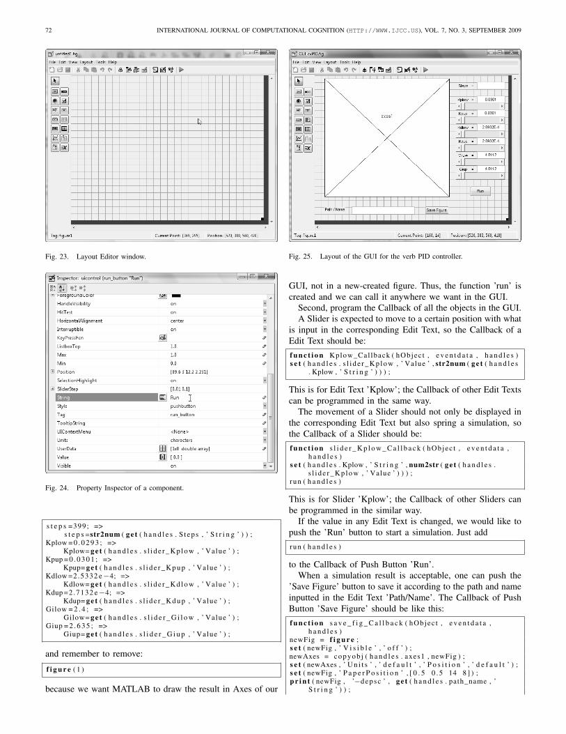
To lay out a GUI is to add all the components required to theGUI and to edit the components’ properties. The componentpalette is at the left side of the Layout Editor. You can addthese components to the GUI by the click and drag way.Double click an added component on the GUI, you can opena Property Inspector shown in Fig. 24 where the properties ofthe selected component can be defined and specified.

In the GUI for verb PID controller, all the components inFig. 25 are needed and the components should be specifiedaccording to Table VIII. Table VIII shows the components’properties that need to be modified, and the rest of the proper-ties can be left as default. Remember to save the GUI timelywhen editing. MATLAB will generate an M-file correspondingto the FIG-file(the one edited in the Layout Editor) the firsttime you save the GUI. The M-file contains the code thatcontrols the GUI and will be introduced later in the next step.

D. Program the GUISince we have laid out the GUI and specified all the

components, we need to program the components’ behaviorin the M-file.

MATLAB controls the GUI through functions, like Call-back, CreateFcn, OpeningFcn, etc. A Callback determines howthe GUI responds to events such as button click, text inputor slider movement. A CreateFcn executes when MATLABcreates an object. A OpeningFcn executes just before the GUIis made visible but after the creation of all the components.

GUIDE uses a ’handles’ structure which contains the han-dles of all the objects to behave as a input argument of thefunctions in GUI and pass property values of objects betweenthe functions.

There are two commands that will be repetitiously used inour GUI, get and set.

The get command is used to get object properties as follows:V = g e t ( ObjectName , Proper tyName )

For example, if you want to get the string that is inputtedin the Edit Text ’Kplow’, you should use:V = g e t ( h a n d l e s . Kplow , ’ S t r i n g ’ )

Here, Kplow is the Tag of the component Edit Text ’Kplow’which can be found in Table VIII.

The set command is used to set object properties as follows:


0 0.5 1 1.5 2 2.5 3 3.5 4−0.2

0

0.2

0.4

0.6

0.8

1

1.2e(

t)

t

(a) Kd = 2.3332× 10−4

0 0.5 1 1.5 2 2.5 3 3.5 4−0.2

0

0.2

0.4

0.6

0.8

1

1.2

e(t)

t

(b) Kd = 2.6332× 10−4

0 0.5 1 1.5 2 2.5 3 3.5 4−0.2

0

0.2

0.4

0.6

0.8

1

1.2

e(t)

t

(c) Kd = 2.6132× 10−4

0 0.5 1 1.5 2 2.5 3 3.5 4−0.2

0

0.2

0.4

0.6

0.8

1

1.2

e(t)

t

(d) Kd = 2.8132× 10−4

Fig. 19. How the changes of Kd’s upper bound and lower bound influence the control result.

TABLE VIIIPROPERTIES OF COMPONENTS NEEDED IN THE GUI FOR VERB PID CONTROLLER.

Component Property Value Component Property Value

Axes Tag axes1 String NULL

Static Text 'Steps' String Steps Tag path_name

Static Text 'Kplow' String Kplow Push Button String Run

Static Text 'Kpup' String Kpup 'Run' Tag run_button

Static Text 'Kdlow' String Kdlow Push Button String Save Figure

Static Text 'Kdup' String Kdup 'Save Figure' Tag save_fig

Static Text 'Gilow' String Gilow Max 0.04

Static Text 'Giup' String Giup Min 0

Static Text '=' String = Tag slider_Kplow

Static Text 'Path/Name' String Path/Name Max 0.06

String NULL Min 0.02

Tag Steps Tag slider_Kpup

String 0.0301 Max 1

Tag Kplow Min 0

String 0.0301 Tag slider_Kdlow

Tag Kpup Max 0.002

String 2.8932E-4 Min 2.0E-4

Tag Kdlow Tag slider_Kdup

String 2.8932E-4 Max 10

Tag Kdup Min 0

String 4.0112 Tag slider_Gilow

Tag Gilow Max 20

String 4.0112 Min 0.5

Tag Giup Tag slider_Giup

Edit Text 'Path/Name'

Slider 'Kplow'

Slider 'Kdlow'

Edit Text 'Giup'

Edit Text 'Kpup'

Edit Text 'Kdlow'

Edit Text 'Kdup'

Edit Text 'Gilow'

Slider 'Kpup'

Slider 'Kdup'

Slider 'Gilow'

Slider 'Giup'

Edit Text 'Steps'

Edit Text 'Kplow'


0 0.5 1 1.5 20

0.1

0.2

0.3

0.4

0.5

0.6

0.7

0.8

0.9

1

e(t)

t

Control error ofcomputational verb PID contoller

Control error offuzzy PID contoller

Control error ofconventional PID contoller

Fig. 20. Compare of control error among three kinds of PID controller.

Fig. 21. The GUI for verb PID controller.

V = s e t ( ObjectName , PropertyName , P r o p e r t y V a l u e )

For example, if you want to make the Slider automaticallymove to the position corresponding to the Edit Text, youshould use:

V= s e t ( h a n d l e s . s l i de r_ Kp l ow , ’ Value ’ , str2num ( g e t (h a n d l e s . Kplow , ’ S t r i n g ’ ) ) )

The function str2num is used to convert the data from string

Fig. 22. GUIDE Quick Start dialog box.

type to number type, since the data stored in Edit Text is astring while in Slider a number. Through the command above,the data stored in the String of Edit Text ’Kplow’ is read andconverted to a number and the number can be then stored inthe Value of Slider ’Kplow’ to move the slider block to thecorresponding position.

Now that we have been familiar with the two useful com-mands, we’ll continue to program our GUI in the M-file.

First, introduce the whole code of the verb PID controllerto define a new function as ’run’.f u n c t i o n run ( h a n d l e s )

We should make a few changes as below:


Fig. 23. Layout Editor window.

Fig. 24. Property Inspector of a component.

s t e p s =399; =>s t e p s =str2num ( g e t ( h a n d l e s . S teps , ’ S t r i n g ’ ) ) ;

Kplow = 0 . 0 2 9 3 ; =>Kplow= g e t ( h a n d l e s . s l i de r_ Kp l ow , ’ Value ’ ) ;

Kpup = 0 . 0 3 0 1 ; =>Kpup= g e t ( h a n d l e s . s l i d e r _ K p u p , ’ Value ’ ) ;

Kdlow =2.5332 e−4; =>Kdlow= g e t ( h a n d l e s . s l i de r_ Kd l ow , ’ Value ’ ) ;

Kdup =2.7132 e−4; =>Kdup= g e t ( h a n d l e s . s l i d e r _ K d u p , ’ Value ’ ) ;

Gilow = 2 . 4 ; =>Gilow= g e t ( h a n d l e s . s l i d e r _ G i l o w , ’ Value ’ ) ;

Giup = 2 . 6 3 5 ; =>Giup= g e t ( h a n d l e s . s l i d e r _ G i u p , ’ Value ’ ) ;

and remember to remove:

f i g u r e ( 1 )

because we want MATLAB to draw the result in Axes of our

Fig. 25. Layout of the GUI for the verb PID controller.

GUI, not in a new-created figure. Thus, the function ’run’ iscreated and we can call it anywhere we want in the GUI.

Second, program the Callback of all the objects in the GUI.A Slider is expected to move to a certain position with what

is input in the corresponding Edit Text, so the Callback of aEdit Text should be:f u n c t i o n Kplow_Cal lback ( hObjec t , e v e n t d a t a , h a n d l e s )s e t ( h a n d l e s . s l i de r_ Kp l ow , ’ Value ’ , str2num ( g e t ( h a n d l e s

. Kplow , ’ S t r i n g ’ ) ) ) ;

This is for Edit Text ’Kplow’; the Callback of other Edit Textscan be programmed in the same way.

The movement of a Slider should not only be displayed inthe corresponding Edit Text but also spring a simulation, sothe Callback of a Slider should be:f u n c t i o n s l i d e r _ K p l o w _ C a l l b a c k ( hObjec t , e v e n t d a t a ,

h a n d l e s )s e t ( h a n d l e s . Kplow , ’ S t r i n g ’ , num2str ( g e t ( h a n d l e s .

s l i de r_ Kp l ow , ’ Value ’ ) ) ) ;run ( h a n d l e s )

This is for Slider ’Kplow’; the Callback of other Sliders canbe programmed in the similar way.

If the value in any Edit Text is changed, we would like topush the ’Run’ button to start a simulation. Just addrun ( h a n d l e s )

to the Callback of Push Button ’Run’.When a simulation result is acceptable, one can push the

’Save Figure’ button to save it according to the path and nameinputted in the Edit Text ’Path/Name’. The Callback of PushButton ’Save Figure’ should be like this:f u n c t i o n s a v e _ f i g _ C a l l b a c k ( hObjec t , e v e n t d a t a ,

h a n d l e s )newFig = f i g u r e ;s e t ( newFig , ’ V i s i b l e ’ , ’ o f f ’ ) ;newAxes = copyob j ( h a n d l e s . axes1 , newFig ) ;s e t ( newAxes , ’ U n i t s ’ , ’ d e f a u l t ’ , ’ P o s i t i o n ’ , ’ d e f a u l t ’ ) ;s e t ( newFig , ’ P a p e r P o s i t i o n ’ , [ 0 . 5 0 . 5 14 8 ] ) ;p r i n t ( newFig , ’−depsc ’ , g e t ( h a n d l e s . path_name , ’

S t r i n g ’ ) ) ;


c l o s e ( newFig ) ;

Third, program some other functions of the GUI.Although the GUI can operate well till now, there are some

details left with the initial part. Since the initial values forthe Edit Texts have been set, the Sliders are expected to gowith them at the start of the GUI, otherwise the slider blockwill stay at the left end by default. The following code shouldtherefore be added to the OpeningFcn of the GUI:

s e t ( h a n d l e s . s l i d e r _ Kp l ow , ’ Value ’ , str2num ( g e t ( h a n d l e s. Kplow , ’ S t r i n g ’ ) ) ) ;

s e t ( h a n d l e s . s l i d e r _ K p u p , ’ Value ’ , str2num ( g e t ( h a n d l e s .Kpup , ’ S t r i n g ’ ) ) ) ;

s e t ( h a n d l e s . s l i d e r _ Kd l ow , ’ Value ’ , str2num ( g e t ( h a n d l e s. Kdlow , ’ S t r i n g ’ ) ) ) ;

s e t ( h a n d l e s . s l i d e r _ K d u p , ’ Value ’ , str2num ( g e t ( h a n d l e s .Kdup , ’ S t r i n g ’ ) ) ) ;

s e t ( h a n d l e s . s l i d e r _ G i l o w , ’ Value ’ , str2num ( g e t ( h a n d l e s. Gilow , ’ S t r i n g ’ ) ) ) ;

s e t ( h a n d l e s . s l i d e r _ G i u p , ’ Value ’ , str2num ( g e t ( h a n d l e s .Giup , ’ S t r i n g ’ ) ) ) ;

Additionally, we may add some buttons in the toolbar. Thereis a Toolbar Editor under the menu of Tools. Pick some usefultools such as Pan, Zoom In, Zoom Out and Data Cursor.

Our GUI is now accomplished. Save it and click ’RunFigure’ in the Layout Editor to enjoy it and it will look likewhat is shown in Fig. 21.[2]

IX. CONCLUSION

Based on the results presented in this paper, we concludethat the method of designing verb PID controllers describedin [13] is feasible. The verb PID controller performs muchbetter than the conventional PID controller and a little bitbetter than the fuzzy PID controller with the model mentionedabove. Moreover, the number of control rules in a verb PIDcontroller is much fewer than that in the fuzzy PID controller.This implies that verb PID controllers consume fewer systemresource in practical applications than fuzzy PID controllersdo.

Although the verb PID controller works nice, its perfor-mance may be improved furthermore if we alter the evolvingfunctions, the method of calculating verb similarities or themethod of verb reasoning. Therefore, how to design a properverb PID controller for a specific plant should be studied inthe future.

REFERENCES

[1] G. R. Chen and T. T. Pham. Introduction to Fuzzy Systems. Chapman& Hall/CRC, Nov. 2005. ISBN:1-58488-531-9.

[2] Jie. Liang Hong. Liang, Yuanyuan. Pu. Signal and Linear System Anal-ysis - Method and Realization Based on MATLAB. Higher EducationPress, Beijing, 2006.

[3] L.-C. Ju. Automatic Control Principle. China Electric Power Press,Beijing, Apr. 2007. ISBN:978-7-5083-5416-3.

[4] J. Li. Research and application of computational verb pid controllerof linear motor. Master’s thesis, Kunming University of Scienceand Technology, Kunming, Feb. 2008. [available online athttp : //www.YangSky.com/researches/computationalverbs/verbfuzctrl/vbPIDMotor.pdf ]. (in Chinese).

[5] Y. Liu S. Zhu, Z.-J. Wang and B.-L. Xia. An improvement of the designof computational verb pid-controllers. System Simulation Technology,2(1):25–30, Jan. 2006. (in Chinese).

[6] Wei. Zhang Shuntian. Lou, Changhua. Hu. System Analysis and DesignBased on MATLAB - Fuzzy System. Xidian University Press, Xi’an,2001.

[7] Z.-L. Wang and Y.-K. Guo. Process Control and Simulink Application.Publishing House of Electronic Industry, Beijing, July 2006. ISBN:7-121-02848-4.

[8] Zhengqing. Hao Xinmin. Shi. Fuzzy Control and MATLAB Simulation.Tsinghua University Press, Beijing Jiaotong University Press, Beijing,2008.

[9] T. Yang. Applications of computational verbs to thedesign of p-controllers. International Journal of Com-putational Cognition, 3(2):52–60, June 2005. [availableonline at http : //www.YangSky.us/ijcc/ijcc32.htm,http : //www.YangSky.com/ijcc/ijcc32.htm].

[10] T. Yang. Architectures of computational verb controllers: To-wards a new paradigm of intelligent control. InternationalJournal of Computational Cognition, 3(2):74–101, June 2005.[available online at http : //www.YangSky.us/ijcc/ijcc32.htm,http : //www.YangSky.com/ijcc/ijcc32.htm].

[11] T. Yang. Computational verb theory: Ten years later. Interna-tional Journal of Computational Cognition, 5(3):63–86, Sep 2007.[available online at http : //www.YangSky.us/ijcc/ijcc52.htm,http : //www.YangSky.com/ijcc/ijcc52.htm].

[12] T. Yang. The Mathematical Principles of Natural Languages: The FirstCourse in Physical Linguistics, volume 6 of YangSky.com Monographsin Information Sciences. Yang’s Scientific Press, Tucson, AZ, Dec. 2007.ISBN:0-9721212-4-2.

[13] T. Yang. Simple computational verb pid controllers. Interna-tional Journal of Computational Cognition, 7(1):74–78, March 2009.[available online at http : //www.YangSky.us/ijcc/ijcc71.htm,http : //www.YangSky.com/ijcc/ijcc71.htm].

[14] M. Tomizuka Zhen-Yu Zhao and S. Isaka. Fuzzy gain scheduling ofpid controllers. IEEE Transactions on Systems, Man and Cybernetics,23(5):1392–1398, 1993.

a study of computational verb pid controllers - citeseerx

Documents