controllers comparison to stabilize a two-wheeled inverted pendulum: pid, lqr and sliding mode...

Controllers Comparison to stabilize a Two-wheeled Inverted Pendulum:

PID, LQR and Sliding Mode Control

JUAN VILLACRÉS1, MICHELLE VISCAINO1, MARCO HERRERA1, OSCAR CAMACHO1, 2 1 Departamento de Automatización y Control Industrial, Facultad de Ingeniería Eléctrica y

Electrónica. Escuela Politécnica Nacional, Quito. ECUADOR

2 Facultad de Ingeniería. Universidad de los Andes. Mérida. VENEZUELA

{juan.villacres01; michelle.viscaino; marco.herrera; oscar.camacho}@epn.edu.ec, [email protected]

Abstract: -This paper compares three control strategies to stabilize a two-wheeled inverted pendulum (TWIP).

The study of TWIP or balancing robot has been extensive because of its unstable and multivariable nature with

highly non-linear dynamics. The mathematical model was derived using Lagrangian approach and was linearized

around the equilibrium point where was considered that the pitch angle tends to zero. The study used a classic

PID control, a Linear-Quadratic Regulator (LQR) and a Slide Mode Control (SMC). The SMC part of state-space

representation of the system and the slide surface was designed from the poles obtained from LQR, therefore

design an Optimal SMC. All the close-loop controllers are in discrete-time; therefore, they were implemented in

a digital way. The results were obtained by simulation using Matlab. The stabilization results were compared in

terms of disturbances rejection capability and the integral square error (ISE) is used to measure their performance.

Key-Words: - Two-Wheeled Inverted Pendulum, Sliding Mode Control, LQR, stabilization, Lagrangian

approach

1 Introduction In the early 60s, several laboratories of prestigious

universities [1] guided and made experiments which

showed a rod mounted on a carriage, if the rod is

placed in an upright position manually, it could

maintain its position autonomously by the action of

the vehicle displacement on which it is stood. This

mechanism would represent an unstable open loop

system with nonlinear dynamics which can be

interpreted by differential equations; therefore,

inverted pendulum control to maintain its vertical

position independently became a classic problem of

nonlinear control. [2] [3]

This platform has been a great help in research to

test the effectiveness of different control techniques

on a nonlinear system with unstable dynamic.

Additionally, it presents feature of an underactuated

system difficult to apply conventional approaches to

robotics [4].

Several works have studied different control

strategies that have been applied to this kind of

systems. In [4], a dynamic model was derived using

a Newtonian approach and presented a comparison of

LQR and PID-PID input in terms of tracking and

disturbances.

In [5], a dynamic model was derived using a

Newtonian approach and two decoupled state-space

controllers around an operating point to design a

system control. In [6] sliding mode control for robust

velocity eliminating the steady velocity tracking error

is designed. In [7], a dynamic model was derived

using Lagrangian approach, two-level velocity

controllers via partial feedback linearization and

stabilizing position were designed.

This paper compares three control strategies to

stabilize a two-wheeled inverted pendulum (TWIP).

As it was mentioned, the study of TWIP or balancing

robot has been extensive because of its unstable

nature with highly non-linear dynamics. The paper

begins with an introduction, the second section

provides an explanation of the model under study, in

the third section basic concepts of control strategies

employed are described and the design of PID, LQR

and SMC are developed, the fourth section presents

the simulation results with a performance analysis

based on ISE criterion for each control technique, and

finally the conclusions are presented.

2 Description of the Two Wheeled

Inverted Pendulum

By rotating the wheels in an appropriate direction

TWIP balance is stable. For stabilization the control

actions are carried out in micro-electromechanical

with a sampling frequency of 100 Hz. The signals

required are obtained from a sensor gyroscope who

measures angular velocity and angular position by

estimating of the pendulum in the vertical plane. The

J. Villacres et al.International Journal of Control Systems and Robotics

http://www.iaras.org/iaras/journals/ijcsr

ISSN: 2367-8917 29 Volume 1, 2016

measure of the angle rotation of each wheel is

obtained by encoders localized at each wheel in the

robot body. The motors DC are controlled by a signal

Pulse Width Modulated (PWM). [15]

The system receives as inputs the voltages of each

spare tire (𝑢𝑙 and 𝑢𝑑) and its outputs are the body

pitch angle 𝜓 [rad], the average angular position of

the wheels 𝜃 [rad] and their velocities �̇� [rad/s], �̇�

[rad/s], in Fig.1 is shown.

Fig. 1 Input/output Scheme of TWIP

In Fig. 2 the variables of the system are shown.

𝜓: Body pitch angle.

𝜃: Average angular position (right and left).

𝜙: Body yaw angle.

Fig. 2 System Views: Frontal, lateral and top

2.1 Model of Two-Wheeled Inverted

Pendulum

The system’s model is taken from [9], TWIP is

described with nonlinear differential equations

obtained by Lagrange method, and the model is

linearized around an equilibrium point where the

body pitch angle tends to zero.

The model is represented in space state:

�̇�1 = 𝐴1𝑥1 + 𝐵1𝑢 (1)

Where:

𝑥1 =

[ 𝜃𝜓

�̇��̇�]

(2)

𝑢 = [𝑢𝑙

𝑢𝑟] (3)

𝐴1 = [

0 00 0

1 00 1

0 𝑎32

0 𝑎42

𝑎33 𝑎34

𝑎43 𝑎44

] (4)

𝐵1 = [

0 00 0

𝑏3 𝑏3

𝑏4 𝑏4

] (5)

Where:

𝑎32 = −𝑔𝑀𝐿𝑒12/det (𝐸) (6)

𝑎42 = 𝑔𝑀𝐿𝑒11/det (𝐸) (7)

𝑎33 = −2(𝜎𝑒22 + 𝛽𝑒12)/det (𝐸) (8)

𝑎43 = 2(𝜎𝑒12 + 𝛽𝑒11)/det (𝐸) (9)

𝑎34 = 2𝛽(𝑒22 + 𝑒12)/det (𝐸) (10)

𝑎44 = −2𝛽(𝑒11 + 𝑒12)/det (𝐸) (11)

𝑏3 = 𝛼(𝑒22 + 𝑒12)/det (𝐸) (12)

𝑏4 = −𝛼(𝑒11 + 𝑒12)/det (𝐸) (13)

𝑒11 = (2𝑚 + 𝑀)𝑅2 + 2𝐽𝑤 + 2𝑛2𝐽𝑚 (14)

𝑒12 = 𝑀𝐿𝑅 − 2𝑛2𝐽𝑚 (15)

𝑒22 = 𝑀𝐿2 + 𝐽𝜓 + 2𝑛2𝐽𝑚 (16)

det(𝐸) = 𝑒11𝑒22 − 𝑒122 (17)

𝛼 = 𝑛𝐾𝑡/𝑅𝑚 (18)

𝛽 = 𝑛𝐾𝑡𝐾𝑏/𝑅𝑚 + 𝑓𝑚 (19)

𝜎 = 𝛽 + 𝑓𝑤 (20)

The parameter values are described in Table 1; they

were taken from [10].

Table 1. Parameter of TWIP

Parameter Unit Description

𝑔 = 9.8 [𝑚/𝑠𝑒𝑐2]

Gravity acceleration

𝑚 = 0.03 [𝑘𝑔] Wheel mass

𝑅 = 0.021 [𝑚] Wheel radius

𝐽𝑤= 𝑚𝑅2/2

[𝑘𝑔𝑚2] Wheel inertia moment

𝑀 = 0.6 [𝑘𝑔] Body mass

𝑊 = 0.09 [𝑚] Body width

𝐷 = 0.05 [𝑚] Body depth

𝐻 = 0.26 [𝑚] Body height

𝐿 = 𝐻/2 [𝑚] Distance of the center

of the mass from the

Wheel axle

𝐽𝜓= 𝑀𝐿2/3

[𝑘𝑔𝑚2] Body pitch inertia

moment

𝐽𝜙 = 𝑀(𝑊2

+𝐷2)/12 [𝑘𝑔𝑚2]

Body yaw inertia

moment

𝐽𝑚= 1𝑥10−5

[𝑘𝑔𝑚2] DC motor inertia

moment



ISSN: 2367-8917 30 Volume 1, 2016

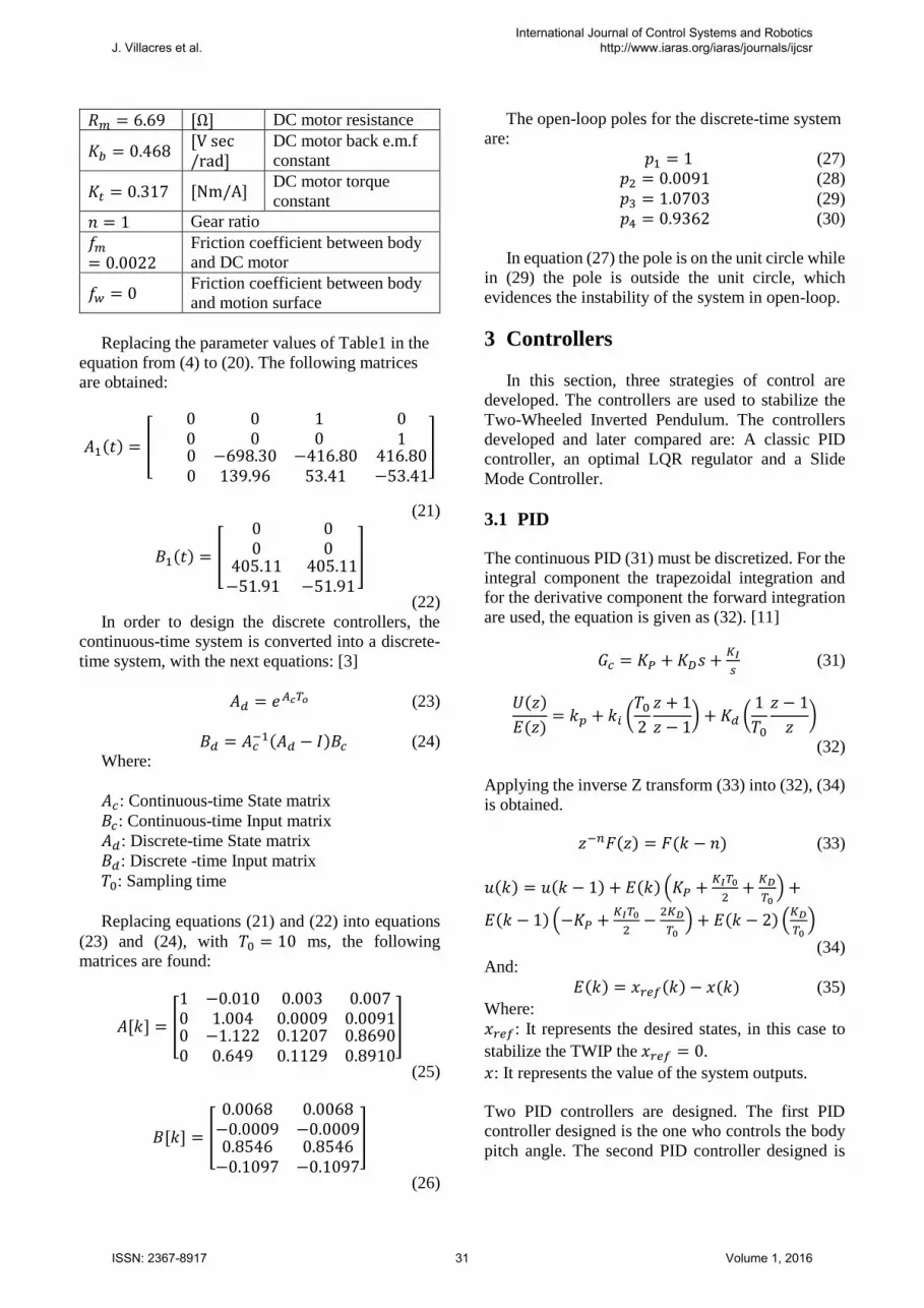
𝑅𝑚 = 6.69 [Ω] DC motor resistance

𝐾𝑏 = 0.468 [V sec/rad]

DC motor back e.m.f

constant

𝐾𝑡 = 0.317 [Nm/A] DC motor torque

constant

𝑛 = 1 Gear ratio

𝑓𝑚= 0.0022

Friction coefficient between body

and DC motor

𝑓𝑤 = 0 Friction coefficient between body

and motion surface

Replacing the parameter values of Table1 in the

equation from (4) to (20). The following matrices

are obtained:

𝐴1(𝑡) = [

0 0 10 0 0

01

0 −698.30 −416.80 0 139.96 53.41

416.80−53.41

]

(21)

𝐵1(𝑡) = [ 0 00 0

405.11 405.11−51.91 −51.91

]

(22)

In order to design the discrete controllers, the

continuous-time system is converted into a discrete-

time system, with the next equations: [3]

𝐴𝑑 = 𝑒𝐴𝑐𝑇𝑜 (23)

𝐵𝑑 = 𝐴𝑐−1(𝐴𝑑 − 𝐼)𝐵𝑐 (24)

Where:

𝐴𝑐: Continuous-time State matrix

𝐵𝑐: Continuous-time Input matrix

𝐴𝑑: Discrete-time State matrix

𝐵𝑑: Discrete -time Input matrix

𝑇0: Sampling time

Replacing equations (21) and (22) into equations

(23) and (24), with 𝑇0 = 10 ms, the following

matrices are found:

𝐴[𝑘] = [

1 −0.010 0.0030 1.004 0.0009

0.0070.0091

0 −1.122 0.12070 0.649 0.1129

0.86900.8910

]

(25)

𝐵[𝑘] = [

0.0068 0.0068−0.0009 −0.00090.8546 0.8546

−0.1097 −0.1097

]

(26)

The open-loop poles for the discrete-time system

are:

𝑝1 = 1 (27)

𝑝2 = 0.0091 (28)

𝑝3 = 1.0703 (29)

𝑝4 = 0.9362 (30)

In equation (27) the pole is on the unit circle while

in (29) the pole is outside the unit circle, which

evidences the instability of the system in open-loop.

3 Controllers

In this section, three strategies of control are

developed. The controllers are used to stabilize the

Two-Wheeled Inverted Pendulum. The controllers

developed and later compared are: A classic PID

controller, an optimal LQR regulator and a Slide

Mode Controller.

3.1 PID

The continuous PID (31) must be discretized. For the

integral component the trapezoidal integration and

for the derivative component the forward integration

are used, the equation is given as (32). [11]

𝐺𝑐 = 𝐾𝑃 + 𝐾𝐷𝑠 +𝐾𝐼

𝑠 (31)

𝑈(𝑧)

𝐸(𝑧)= 𝑘𝑝 + 𝑘𝑖 (

𝑇0

2

𝑧 + 1

𝑧 − 1) + 𝐾𝑑 (

1

𝑇0

𝑧 − 1

𝑧)

(32)

Applying the inverse Z transform (33) into (32), (34)

is obtained.

𝑧−𝑛𝐹(𝑧) = 𝐹(𝑘 − 𝑛) (33)

𝑢(𝑘) = 𝑢(𝑘 − 1) + 𝐸(𝑘) (𝐾𝑃 +𝐾𝐼𝑇0

2+

𝐾𝐷

𝑇0) +

𝐸(𝑘 − 1) (−𝐾𝑃 +𝐾𝐼𝑇0

2−

2𝐾𝐷

𝑇0) + 𝐸(𝑘 − 2) (

𝐾𝐷

𝑇0)

(34)

And:

𝐸(𝑘) = 𝑥𝑟𝑒𝑓(𝑘) − 𝑥(𝑘) (35)

Where:

𝑥𝑟𝑒𝑓: It represents the desired states, in this case to

stabilize the TWIP the 𝑥𝑟𝑒𝑓 = 0.

𝑥: It represents the value of the system outputs.

Two PID controllers are designed. The first PID

controller designed is the one who controls the body

pitch angle. The second PID controller designed is



ISSN: 2367-8917 31 Volume 1, 2016

the one which controls the angular position of the

wheels.

The parameters of the PID controllers are

obtained by trial and error. The tuned parameters are

given as in table 2.

Table 2. PID parameters

KP KI KD

𝜓 -77.97 -0.01 -8.79

𝜃 -1.07 -0.01 -1.36

3.2 LQR

The Linear Quadratic Regulator is a state feedback

control which is useful to handle multivariable

systems.

It is assumed that the system is given by the following

equation:

𝑥(𝑘 + 1) = 𝐴𝑥(𝑘) + 𝐵𝑢(𝑘) (36)

The input for the system will be:

𝑢(𝑘) = −𝐾𝑥(𝑘) (37)

Where K is the gain matrix. The matrix 𝐾 has to bring

the system into a final state 𝑥(𝑘1) = 0 from an initial

state 𝑥(𝑘0).

To determine the matrix 𝐾, the performance index

should be minimized.

𝐽 = ∑ 𝑥𝑇(𝑘 + 1)𝑄𝑥(𝑘 + 1) + 𝑢𝑇(𝑘)𝑅𝑢(𝑘)

𝑘1−1

𝑘=𝑘0

(38)

Where:

𝑄 ∈ ℝ𝑛𝑥𝑛: It is a symmetric matrix, at least positive

semidefinite.

𝑅 ∈ ℝ𝑚𝑥𝑚: It is a symmetric matrix positive

semidefinite.

Replacing (37) into (36):

𝑥(𝑘 + 1) = 𝐴𝑥(𝑘) − 𝐵𝐾𝑥(𝑘) = (𝐴 − 𝐵𝐾)𝑥(𝑘)

(39)

In order to solve the equation (38), the Optimality

Principle [10] is used:

𝐾(𝑖) = [𝑅 + 𝐵𝑇𝑃(𝑖 + 1)𝐵)−1𝐵𝑇𝑃(𝑖 + 1)𝐴 (40)

𝑃(𝑖) = 𝑄 + 𝐾𝑇(𝑖)𝑅𝐾(𝑖) + [𝐴 − 𝐵𝐾(𝑖)𝑇𝑃(𝑖 + 1)[𝐴− 𝐵𝐾(𝑖)]

(41)

The iterative calculation begins with 𝑃(𝑁) = 𝑄 y

𝐾(𝑁) = 0 from 𝑢(𝑁 − 1) until 𝑢(0). This iterative sequence converges when 𝑁 → ∞

The objective is to verify the convergence of the

matrix 𝐾.

‖𝐾𝑁 − 𝐾𝑁−1‖ <𝛾

‖𝐾𝑁‖ (42)

Where:

𝛾: It is a parameter which allows calibrate the

convergence condition.

The matrices 𝑄 and 𝑅 selected are:

𝑄 = [

0.38 00 0.43

0 00 0

0 00 0

0.09 00 0.09

] (43)

𝑅 = [0.00017 0

0 0.00017] (44)

The matrix 𝐾 obtained is:

𝐾 = [−1.099 −81.44 −1.368 −10.860−1.099 −81.44 −1.368 −10.860

]

(45)

3.3 Slide Mode Control (SMC)

It is assumed that the system is given by the following

equation:

𝑥(𝑘 + 1) = 𝐴𝑥(𝑘) + 𝐵𝑢(𝑘) (46)

It is supposed that the pair (𝐴, 𝐵) is controllable,

therefore, there is a non-singular matrix 𝑇 ∈ ℝ𝑛𝑥𝑛 which makes the system in its controllable canonical

form. [12-13]

�̅�(𝑘 + 1) = �̅��̅�(𝑘) + �̅�𝑢(𝑘) (47)

Where:

�̅� = 𝑇1−1𝐴𝑇1 (48)

�̅� = 𝑇−1𝐵 (49)

It is defined a linear function, called sliding surface:

𝑠(𝑥(𝑘)) = 𝑆𝑥(𝑘) = 𝑆̅�̅�(𝑘) 𝑆̅ ∈ ℝ1𝑥𝑛 (50)

Where: 𝑆̅ = 𝑆𝑇1 (51)



ISSN: 2367-8917 32 Volume 1, 2016

𝑆̅ = [�̅�1 �̅�2 … �̅�𝑛−1 1] (52)

Thus, the design of the sliding mode for the reduced

order system defined by (53) is stable. [12-13]

𝑠(𝑥(𝑘)) = 𝑆̅�̅�(𝑘) = 0 (53)

𝑆�̅�(𝑘) = �̅�1𝑦 + �̅�2𝑦𝑘 + ⋯+ �̅�𝑛−1𝑦

𝑘(𝑛−2) + 𝑦𝑘(𝑛−1)

= 0 (54)

The equivalent control must guarantee that:

𝑆𝑥(𝑘 + 1) = 0 (55)

𝑆𝑥(𝑘 + 1) = 𝑆 (𝐴𝑥(𝑘) + 𝐵𝑢𝑒𝑞(𝑘)) = 0

(56)

So,

𝑢𝑒𝑞(𝑘) = −(𝑆𝐵)−1𝑆𝐴𝑥(𝑘) (57)

The control law (58) has two components, a

continuous one 𝑢𝑒𝑞(𝑘) and a discontinuous one 𝑣.

𝑢(𝑘) = 𝑢𝑒𝑞(𝑘) + 𝑣 (58)

In order to achieve steady state equal to zero: [12]

𝑣 = {

𝑐𝑡𝑒, 𝑠(𝑥) < 00, 𝑠(𝑥) = 0

−𝑐𝑡𝑒, 𝑠(𝑥) > 0

(59)

To design the slide surface, the new poles (60), (61)

obtained from feedback the matrix 𝐾 (45) are: [13]

𝑝1,2 = 0.9318 ± 0.0042𝑖 (60)

𝑝3 = 0.9797 (61)

With these poles, the slide surface obtained is given

by:

𝑠(𝑥(𝑘))= [−1.924 −147.918 −1.669 −21.065]

(62)

And the equivalent control law is:

𝑢𝑒𝑞(𝑘) = [1.924 160.270 2.717 21.581] (63)

To reduce the chattering produced by high frequency

switching, a filter for chattering reduction is used

[14], the filter is shown in fig.3 described by (64)

Fig. 3 Filter for chattering reduction

𝑣 = {

𝑐𝑡𝑒, 𝑠(𝑥(𝑘)) < 𝐿

−𝑠

𝐿, |𝑠(𝑥(𝑘))| ≤ 𝐿

−𝑐𝑡𝑒, 𝑠(𝑥(𝑘)) > 𝐿

(64)

4 Simulation Results

In this section, the performance of the three

controllers is compared. The simulations are

performed by using Simulink-Matlab.

The simulation scheme is similar for the

controllers, as shown in fig. 4, where a sampler and

zero-order holder are used in order to simulate a

discrete-time system.

B1s C

A

CONTROL

Saturation

++

Sampler

Zero-Order Holder

Fig. 4 Linear System and Control scheme

As it had been indicated the states of TWIP

are 𝑥 = [𝜃 𝜓 �̇� �̇�]𝑇. The main purpose of the

control is to keep the TWIP in a vertical position.

4.1 Simulations with initial conditions and

without any disturbance

Assuming that the initial states are:

𝑥𝑜 = [0 0.1 0 0]𝑇 (65)

The next figures show the responses, when each

controller is used.



ISSN: 2367-8917 33 Volume 1, 2016

Fig. 5 TWIP, angular wheel position response

Fig. 6 TWIP, body pitch angle response

Fig. 7 TWIP, angular wheel speed response

According with the fig. 6, the SMC presents a smooth

response to stabilize the body pitch angle. The three

controllers have similar settling time as shown in fig.

5. To stabilize the body pitch angle the SMC has the

lowest value of ISE, but to get steady state of the

angular wheel position, the PID has the lowest value

of ISE as shown in table 3.

Fig. 8 TWIP, body pitch angle speed response

Fig. 9 TWIP, input system 𝑢

In fig. 9, it is shown that LQR uses less energy, at the

start than the others.

Fig. 10 TWIP, Phase Portrait body pitch angle

Table 3. ISE Comparison of three controllers without

disturbance

PID LQR SMC

ISE ∗ 10−3

𝜓 0.271 0.393 0.247

𝜃 526.6 810 660.9

-0.04 -0.02 0 0.02 0.04 0.06 0.08 0.1-2.5

-2

-1.5

-1

-0.5

0

0.5

Angula

r S

peed [

rad/s

ec]

Angle [rad]

PID

LQR

SMC



ISSN: 2367-8917 34 Volume 1, 2016

4.2 Simulations with initial conditions and

disturbance on the body pitch angle

Once the TWIP is stabilized, an external force is

applied to the body pitch angle, in order to test the

response to disturbances.

Assuming that the initial states are:

𝑥𝑜 = [0 0.1 0 0]𝑇 (66)

The next figures show the responses, when each

controller is used.

Fig. 11 TWIP, angular wheel position response

Fig. 12 TWIP, body pitch angle response with an

external force applied.

In fig. 12 the SMC response is faster than LQR and it

has a smaller overshoot than PID, when the

controllers are tested with a disturbance.

In figures from 5 to 12, there is no chattering present,

because of the filter.

Table 4. ISE Comparison of three controllers with

disturbance

PID LQR SMC

ISE ∗ 10−3

𝜓 0.666 0.622 0.572

𝜃 653.2 947.9 768.2

5 Conclusion

The three controllers were developed and compared

by simulations.

The SMC presented the best ISE for both cases,

without disturbances and with disturbances.

From implementation point of view, LQR and SMC

are easy to design, and PID does not need a model to

be tuned.

The Two-wheeled Inverted Pendulum is a good

teaching tool for learning conventional and modern

control strategies implementation.

ACKNOWEDGMENTS

Oscar Camacho thanks PROMETEO project of

SENESCYT. Republic of Ecuador, for its

sponsorship in the realization of this work.

References:

[1] K. Lundberg, T. Barton, History of Inverted-

Pendulum Systems, 8th IFAC Symposium on

Advances in Control Education, 2009.

[2] Z. li, C. Yang, L. Fan, Advanced Control of

Wheeled Inverted Pendulum Systems, ©

Springer-Verlag, 2013.

[3] K. Ogata, Modern Control Engineering,

Prentice Hall, 2010.

[4] A. N. K. Nasir, M. A. Ahmad, R. M. T. Raja

Ismail, The Control of a Highly Nonlinear Two-

wheels Balancing Robot: A Comparative

Assessment between LQR and PID-PID Control

Schemes, International Journal of Mechanical,

Aerospace, Industrial, Mechatronic and

Manufacturing Engineering, Vol:4, No.10,

2010.

[5] F. Grasser, A. Arrigo, S. Colombi, A. C. Rufer,

JOE: a mobile inverted pendulum, IEEE Trans.

Industrial Electronics, Vol.49 (1), No.1, 2002,

pp. 107-114.

[6] J. Huang, H. Wang, T. Matsumo, T. Fukuda, K.

Sekiyama, Robust Velocity Sliding Mode

Control of Mobile Wheeled Inverted Pendulum



ISSN: 2367-8917 35 Volume 1, 2016

Systems, International Conference on Robotics

and Automation, 2009.

[7] K. Pathak, J. Franch, K. Agrawal, Velocity and

position control of a wheeled inverted pendulum

by partial feedback linearization, IEEE Trans.

Robotics, Vol.21 (3), No.3, 2005, pp. 505-513.

[8] M. Herrera, W. Chamorro, A. Gómez, O.

Camacho, Two Wheeled Inverted Pendulum

Robot NXT Lego Mindstorms: Mathematical

Modelling and Real Robot Comparisons,

Revista Politécnica, Vol.36, No.1, 2015.

[9] Y. Yamamoto, Nottaway-GS Model Based

Design – Control of self-balancing two-wheeled

robot built with LEGO Mindstorms NXT,

http://www.mathworks.com/matlabcentral/filee

xchange/loadFile.do?objectId=13399&objectT

ype=file, 2008.

[10] M. Herrera, Modelado Discreto y Control

Óptimo de Sistemas No Lineales Multivariables

y su Aplicación a un Péndulo Invertido

utilizando Lego Mindstorms, Master of Science

Thesis, Universidad Politécnica de Madrid,

España 2014.

[11] B. Kuo, Sistemas de Control Automático,

Pearson Education, 1996.

[12] B. M. Al-Hadithi, A. Jiménez, J. D. L. Delgado,

A. J. Barragán, J. M. Andújar, Diseño de un

Controlador Borroso Basado en Estructura

Variable con Modos Deslizantes sin Chattering,

Simposio CEA de Control Inteligente, 2014,

pp.1-4.

[13] Y. Pan, K. Futura, S. Suzuki, S. Hatakeyama,

Design of Variable Structure Controller – From

Sliding Mode to Sliding Sector - , 39th IEEE

Conference on Decision and Control, 2000.

[14] P. Kachroo, M. Tomizuka, Chattering reduction

and error convergence in the sliding-mode

control of a class of nonlinear systems, IEEE

Trans. On Automatic Control, Vol.41, 1996,

pp.1063-1068.

[15] D. Gu, P. Petkov, M. Konstantinov, Robust

Control Design with MATLAB®, chapter 19, ©

Springer-Verlag, 2013.



ISSN: 2367-8917 36 Volume 1, 2016

controllers comparison to stabilize a two-wheeled inverted pendulum: pid, lqr and sliding mode...

Documents