national threshold runoff estimation utilizing gis in support of operational flash flood warning...

National threshold runoff estimation utilizing GIS in support ofoperational flash flood warning systems

T.M. Carpentera, J.A. Sperfslagea, K.P. Georgakakosa,b,* , T. Sweeneyc, D.L. Freadc

aHydrologic Research Center, 12780 High Bluff Drive, Suite 250, San Diego, CA 92130, USAbScripps Institution of Oceanography, University of California, San Diego, La Jolla, CA 92093-0224, USA

cOffice of Hydrology, National Weather Service, NOAA, 1325 East-West Highway, Silver Spring, MD 20910, USA

Received 16 February 1999; received in revised form 9 July 1999; accepted 13 July 1999

Abstract

Threshold runoff is the amount of excess rainfall accumulated during a given time period over a basin that is just enough tocause flooding at the outlet of the draining stream. Threshold runoff estimates are indicators of maximal sustainable surfacerunoff for a given catchment, and are thus an essential component of flash flood warning systems. Used in conjunction with soilmoisture accounting models and areal rainfall data, they form the basis of the US National Weather Service (NWS) flash floodwatch/warning program. As part of their modernization and enhancement effort, the NWS determined that improved flash floodguidance and thus improved threshold runoff estimation is needed across the United States, with spatial resolution commensu-rate to that afforded by the WSR-88D (NEXRAD) radars. In this work, Geographic Information Systems (GIS) and digitalterrain elevation databases have been used to develop a national system for determining threshold runoff. Estimates of thresholdrunoff are presented for several locations in the United States, including large portions of the states of Iowa, Oklahoma, andCalifornia, and using several options in computing threshold runoff. Analysis of the results indicates the importance of channelgeometry in flash flood applications. Larger threshold runoff estimates were computed in Oklahoma (average value of 34 mm)than in Iowa (14 mm) or California (9.5 mm). Comparisons of the threshold runoff estimates produced by the GIS procedurewith those based on manually computed unit hydrographs for the selected catchments are shown as a preliminary measure of theaccuracy of the procedure. Differences of up to about 15 mm for hourly rainfall durations were obtained for basins larger than50 km2. q 1999 Elsevier Science B.V. All rights reserved.

Keywords:Hydrology; Flash floods; Forecasting; Distributed modeling; Geographic information systems; Radar

1. Introduction

Flooding is the worst weather-related hazard, caus-ing loss of life and excessive damage to property.NOAA (1981) and NRC (1996) state that the averagenumber of deaths due to flooding is 140 peopleannually, with nearly $3.6 billion worth of property

damaged or destroyed each year in US. In addition, ithas been reported that flood damages are increasing ata rate of 5% per year (Barrett, 1983). The 1993Mississippi Flood alone caused damages of morethan $15 billion and a loss of 38 lives (Galloway,1994). Flood damage mitigation is provided througha variety of structural and non-structural methods. Asignificant non-structural method is the operation offlood warning systems. Continued improvements inflood warning systems are necessary to further miti-gate flood damages and loss of life.

Journal of Hydrology 224 (1999) 21–44

0022-1694/99/$ - see front matterq 1999 Elsevier Science B.V. All rights reserved.PII: S0022-1694(99)00115-8

* Corresponding author. Hydrologic Research Center, SanDiego, CA, USA. Fax:1 1-858-792-2519.

E-mail address:[email protected] (K.P. Georgakakos)

www.elsevier.com/locate/jhydrol

In the United States, flash flood warnings areprovided by the National Weather Service (NWS).A flash flood is defined as a flood which followsshortly (i.e. within a few hours) after a heavy or exces-sive rainfall event (Georgakakos, 1986; Sweeney,1992). Flash flood warnings and watches are issuedby local NWS Weather Forecast Offices (WFOs),based on the comparison of flash flood guidance(FFG) values with rainfall amounts. FFG refers gener-ally to the volume of rain of a given duration neces-sary to cause minor flooding on small streams.Guidance values are determined by regional RiverForecast Centers (RFCs) and provided to localWFOs for flood forecasting and the issuance of flashflood watches and warnings. The basis of FFG is thecomputation of threshold runoff values, or the amountof effectiverainfall of a given duration that is neces-sary to cause minor flooding. Effective rainfall is theresidual rainfall after losses due to infiltration, deten-tion, and evaporation have been subtracted from theactual rainfall on the catchment level. It is the portionof rainfall that becomes surface runoff on the catch-ment scale. The relationship between FFG and thresh-old runoff is a function of the current soil moistureconditions, which are estimated in real time by opera-tional soil moisture accounting models.

As part of its modernization efforts, the NWS iden-tified several shortcomings with existing FFG proce-dures (Sweeney, 1992). Methods of determiningthreshold runoff estimates varied from one RFC toanother, and in many cases, were not based on gener-ally applicable, objective methods. Computed thresh-old runoff existed with coarse resolution. Forexample, there may have been only four distinctthreshold runoff values within an RFC region (thereare only 13 RFC regions that cover the US), whiletime duration of threshold runoff and flash floodguidance values varied among RFCs. These short-comings lead to inconsistencies in FFG within andacross RFC boundaries. To address these inconsisten-cies, the NWS outlined a plan to generate more accu-rate and consistent FFG, including a uniform andobjective method of computing threshold runoffvalues (Fread, 1992), and a standard algorithm fordetermining FFG (Sweeney, 1992). It is noted thatthe determination of threshold runoff for a given effec-tive rainfall duration is a one-time task. Determinationof flash flood guidance is done frequently using

current soil moisture conditions as estimated byoperational hydrologic models.

The first step, and the focus of this paper, is thedesign and implementation of a consistent procedurefor computing threshold runoff values. It is requiredthat the method of threshold runoff computation beobjective and based on sound hydrologic and hydrau-lic principles with known assumptions and limita-tions. The procedure must be applicable across theUS, with implementation at regional RFCs. With theavailability of high temporal and spatial resolutionprecipitation estimates accompanying the implemen-tation of the national WSR-88D radar network, theenhanced procedure should also make use of thelatest–available technology to produce estimatesdown to small scales. To support areal flash floodguidance, as opposed to basin-specific flash floodguidance, computed threshold runoff values are tobe interpolated to a uniform grid corresponding tothat of the WSR-88D radar rainfall observations(Hydrologic Rainfall Analysis Project, HRAP, grid).The developed procedure utilizes digital terrain data-bases, which are available nationally, and geographicinformation systems (GISs). This paper describes themethodology of threshold runoff computation,comparisons of threshold runoff values for differentcomputation options and for different locations in theUS, and comparisons of procedure-computed valueswith manually computed threshold runoff values.

2. Methodology

For the formulation of a method to compute thresh-old runoff nationally, the following requirements wereidentified:

• the method of threshold runoff determination musthave a sound hydrologic/hydraulic basis;

• the method must be computationally efficient,given the national scale of computations required;

• digital terrain databases with national coverage andGIS should be utilized to facilitate the computa-tions;

• estimates of any free parameters must be compu-table and stable over a region given the availablenational databases.

Threshold runoff has been defined as the amount of

T.M. Carpenter et al. / Journal of Hydrology 224 (1999) 21–4422

rainfall excess of a given duration necessary to causeflooding on small streams. Under the assumption thatcatchments respond linearly to rainfall excess, thresh-old runoff, R, may be found by equating the peakcatchment runoff, determined from the catchmentunit hydrograph of a given duration, to the streamflow at the basin outlet associated with flooding.Mathematically, this is expressed as:

Qp � qpRRA �1�whereQp is the flooding flow (cms or cfs),qpR the unithydrograph peak for a specific durationtR, normalizedby catchment area (cms/km2/cm or cfs/mi2/in), A thecatchment area (km2 or mi2) and R the thresholdrunoff (cm or in.).

Rearranging, one can solve for threshold runoff:

R� Qp=qpRA �2�The solution is found by definingQp, qpR, and A insuch a way that they can be computed given the avail-able data. The approach taken in this work has been toprovide several options for threshold runoff determi-nation suitable for varying data-availability scenarios.A description of these options follows.

2.1. The flooding flow, Qp

This is perhaps the more difficult term to define.Flooding is generally associated with damagingconditions, which may be difficult to quantify interms of flow over a region. One conservative measureof a “flooding flow” is the bankfull discharge. Thisdefinition of “flooding” is physically based, but isconsidered conservative as more than bankfull flowis generally needed to cause damage.

An alternative definition of the flooding flow is theflow of a certain return period. This definition is statis-tically based and carries the notions of risk and uncer-tainty associated with flooding. There is evidence of agood statistical relationship between the bankfull flowand a flow with a return period between 1 and 2 years(Henderson, 1966). This range of flows has been usedas a surrogate for bankfull flow (e.g. Wolman andLeopold, 1957; Nixon, 1959; and also discussion inRiggs, 1990). In this application, the two-year returnperiod flow is used as an alternative to bankfull flowas more than bankfull flow is necessary to produce

flood damage. Each definition requires different setsof field data as described next.

The bankfull discharge is computed from channelgeometry and roughness characteristics usingManning’s steady, uniform flow resistance formula(Chow et al., 1988):

Qp � Qbf � BbD5=3b S0:5

c =n �3�whereBb is the channel top width at bankfull (m),Db

the hydraulic depth at bankfull (m),Sc the local chan-nel slope (dimensionless),n the Manning’s roughnesscoefficient andQbf the bankfull flow (cms).

This formulation makes the approximation of thewetted perimeter by the cross-sectional width (widerectangular channel approximation). Georgakakos etal. (1991) based on data by Jarrett (1984), presentsManning’s roughness coefficient (forn . 0:035) asa function of local channel slope,Sc (dimensionless),and hydraulic depth,Db (m):

n� 0:43S0:37c =D0:15

b �4�Clearly, the computation of bankfull discharge

requires channel cross-sectional data. Measurementsof cross-sectional parameters result from limited localsurveys and are not available nationally on a contin-uous spatial basis. Also, the available remotely senseddata with national coverage do not have the resolutionneeded to reliably estimate small-channel cross-sectional properties. Estimates of these parametersfor unsurveyed streams must be made. This can bedone using regional relationships between the cross-sectional parameters and other catchment and streamcharacteristics, such as catchment area or streamlength, which may be determined through GIS andnationally available digital terrain data.

The two-year return period flow is the flow that isexpected to be equaled or exceeded once every twoyears on average. To implement this option, the flood-ing flow is equated to the two-year return period flow:

Qp � Q2 �5�The two-year return period flow is based on exten-

sive historical discharge records. The US GeologicalSurvey maintains such streamflow records and hasdetermined two-year return period flows with goodnational coverage. In general, though, such recordsare not available for all streams and all locations of

T.M. Carpenter et al. / Journal of Hydrology 224 (1999) 21–44 23

interest. The two-year return period flow at ungaugedlocations may also be estimated using regional rela-tionships with catchment, stream, and other character-istics such as annual precipitation (see USGS, 1994).

2.2. The unit hydrograph peak, qpR

The catchment response is determined from thecatchment unit hydrograph of a given duration. Twooptions are provided for unit hydrograph peak deter-mination. As a first option, Snyder’s empiricalsynthetic unit hydrograph was used to produce magni-tude and time estimates for the unit hydrograph peak.The details of the formulation are reported in Carpen-ter and Georgakakos (1993), and are not included hereas they are available in textbooks (e.g. Chow et al.,1988; Bras, 1990). The empirical coefficients ofSnyder’s formulation should be calibrated with fielddata for basins with similar drainage and storage capa-city. This requires “observed” unit hydrographs forflash flood prone areas (i.e. unit hydrographs derivedfrom observed stream flow and precipitation records).The NWS has determined “observed” unit hydro-graphs for some operational site-specific flow forecastlocations, generally for larger basins. Few “observed”unit hydrographs exist for small to medium sizestreams and the values of the two empirical coeffi-cients may be highly uncertain. Local data and knowl-edge must be used to estimate their values in theregion of application.

The theory of the geomorphologic unit hydrograph(GUH) attempts to eliminate the uncertainty asso-ciated with the empirical coefficients of traditionalsynthetic unit hydrograph approaches. The catchmentresponse is related to catchment and channel charac-teristics, which may be determined with GIS and digi-tal terrain data. For these reasons, the GUH was

selected as an alternative method in determining theunit hydrograph response.

Rodriguez-Iturbe and Valdes (1979) developed thegeomorphologic instantaneous unit hydrograph basedon the geomorphologic structure of basins, usingHorton’s geomorphologic laws (e.g. see Bras, 1990,for a description of Horton’s laws). They began byexpressing the peak magnitude and time to peak ofthe instantaneous unit hydrograph as a function ofHorton’s ratios, stream length and the catchment velo-city. Rodiguez-Iturbe et al. (1982) eliminated thecatchment velocity from the expressions andconverted the peak magnitude and time to peak ofthe instantaneous unit hydrograph to the peak magni-tude and time to peak of a unit hydrograph corre-sponding to a uniform rainfall excess of a givenduration, tR. Their results are reproduced here foreasy reference:

Qp � 2:42iAtR=P0:4�1 2 0:218tR=P

0:4� �6�and

tpR � 0:585P0:4 1 0:75tR �7�where

P � L2:5=�iARLa

1:5� �8�

a � S0:5c =nB2=3 �9�

whereA is the drainage area (km2), tR the duration ofeffective rainfall (h),L the main stream length (km),ithe effective rainfall intensity (cm/h),RL Horton’slength ratio (dimensionless),Sc the local channelslope (dimensionless),n the Manning’s roughnesscoefficient andB the top width (m).

Given that the threshold runoff,R, is equal to therainfall intensity times its duration, [itR], Eq. (6) is


Table 1Options for threshold runoff computation

Flooding flow definition Unit hydrograph options

Options Two-year return periodflow, Q2

Bankfull dischargeQbf Snyder’s syntheticunit hydrograph

Geomorphologic unithydrograph

Data required Regional relationshipfor Q2 (historic flowrecord)

Regional relationship forchannel cross-sectionalparameters (cross-sectional data)

Regional estimatesof empiricalcoefficients

Regional relationship forchannel cross-sectionalparameters (cross-sectionaldata); regional estimates ofRL

reduced to:

Qp � 2:42RA=P0:4�1 2 0:218tR=P0:4� �10�

To computeR, the value ofQp, eitherQbf or Q2, issubstituted into the left hand side of (10) anda iscomputed at bankfull conditions (i.e.B� Bb). Aswith the bankfull flow, regional relationships arenecessary to estimate the channel cross-sectionalparameters involved in computing the GUH (Bb andSc).

The data requirements for each of the options aresummarized in Table 1. The combination of optionsyields four possible methods of computing the thresh-old runoff.

Method 1: Bankfull Flow (Qbf) and Geomorpho-logic Unit Hydrograph (GUH).Method 2: Bankfull Flow and Snyder’s Unit Hydro-graph.Method 3: Two-Year Return Period Flow (Q2) andGeomorphologic Unit Hydrograph.Method 4: Two-Year Return Period Flow andSnyder’s Unit Hydrograph.

2.3. Limitations

In each method, GIS is utilized to process digitalterrain data and compute catchment-scale character-istics, such as drainage area, stream length and aver-age channel slope. Regional relationships are neededto estimate channel cross-sectional and flow para-meters from the catchment-scale characteristics forall locations within the region of application. Thequality of the regional relationships, along with theassumptions of the theory, will indicate the applicabil-ity of various methods within certain regions or forcertain events. For example, the assumption that thecatchment responds linearly to rainfall excess, i.e. unithydrograph theory is applicable, results in limitationson the size of the catchment. Small catchments aremore non-linear than larger ones (Wang et al.,1981), especially during light and moderate rainfall(Caroni et al., 1986). High flows are more favorableto a linear assumption than low flows. The assumptionof uniform rainfall excess over the catchment alsoimplicitly limits the size of the catchment for whicha unit hydrograph approach is reasonable. In manychannels, the channel cross-section varies greatly

over short distances, and may also change in timewith the occurrence of floods. Therefore, bankfulldischarge is difficult to determine in areas withunstable channel cross-sections. In some regions, thetwo-year return period flow significantly underesti-mates a flood flow, even bankfull flow. A longer-return-period flow may be more indicative of a floodflow, and if this is known a priori, may be implemen-ted through the regional relationship for flow. Note,finally, the return period flow depends greatly on thelength of the historical discharge record for streams ina region and on climate variability when climatic vari-ables are included as predictors. The reliability ofthese values may vary from location to location.Knowledge of these limitations is vital in the selectionof the method(s) to compute threshold runoff and ininterpreting the threshold runoff estimates.

3. Implementation

The methodology described has been implementedin the software package,threshR(Kruger et al., 1993).Here, an overview of the system is described.

The procedure is run on a Hydrologic Unit basis (onthe order of several 1000 km2), with threshold runoffcomputations performed on subbasins down toapproximately 5 km2. Hydrologic Units are groupsof stream networks and their associated drainageareas. They have been defined across the UnitedStates through the work of the US Water ResourcesCouncil, the US Soil Conservation Service and anInter-Agency Committee on Water Resources (e.g.USGS, 1974, 1982). For a Hydrologic Unit of interest,four main steps of the procedure are performed:

1. Import and process digital terrain data into the GIS.Digital terrain data includes elevation, stream loca-tion and land use data.

2. Delineate streams and subbasins down to 5 km2 insize and compute geometric properties of thosesubbasins.

3. Compute subbasin threshold runoff, based onmethod(s) selected and regional relationships.

4. Interpolate subbasin threshold runoff to grid-basedthreshold runoff, corresponding to the grid of theWSR-88D radars.

The Geographic Information System selected for this


application was the public domain packagegrass,version 4.0. grass (Geographic Resources AnalysisSupport System) was developed at the US ArmyConstruction Engineering Research Laboratory(USACERL, 1983). In addition to the capabilities toimport and display data from a variety of sources,grass includes a subroutine,r.watershed, whichdelineates streams and catchments based on digitalelevation data.r.watersheddetermines the streamdrainage network based on theAT, or least cost, searchalgorithm and mimics the work of an experiencedcartographer in delineating hydrologic divides(Ehlschlaeger, 1990). The digital elevation datautilized in the program is the Defense MappingAgency (DMA) 1:250,000-scale digital elevationmodel. This data has a 90 m resolution and it is avail-able nationally from the USGS (http://edcwww.cr.usgs.gov/doc/edchome/ndcdb/ndcdb). Based onthe initial sensitivity studies in flat areas, the elevationdata is artificially lowered, or “carved”, at the locationof lakes, streams, and reservoirs to improve ther.watersheddelineation of the streams and basins.EPA river reach files provide digital stream locationsbased on digitization of 1:100,000-scale topographicmaps. The location of lakes and reservoirs, along withthe Hydrologic Units boundary, are derived from200 m resolution, 1:250,000-scale USGS Land Use/Land Cover Composite Thematic Grid files.

The accuracy of ther.watersheddelineation ofwatersheds and streams was examined in Carpenterand Georgakakos (1993) and Sperfslage et al. (1994)for the mild sloping areas of Iowa and Oklahoma.Their estimates may be considered conservative forareas of strong topographic relief. This analysisshowed only a 3% error in area when comparing theGIS-determined Hydrologic Unit areas with the areaof the Units as defined by the USGS. To assess thesub-catchment delineation accuracy, basins with areasin the range (2–80 km2) were manually delineatedfrom 1:24,000-scale topographic maps, and comparedto the GIS-computed sub-catchment areas. A total of15 basins were delineated in Oklahoma and 17 inIowa. When comparing areas without the use ofstream carving, differences were in the range (213to 129%) in Oklahoma, with an average of15.6%,and (243 to 111%) in Iowa, with an average of27.9%. In both regions, smaller sub-catchmentsyield generally higher errors in delineation. The

delineation of streams was examined by the computedlength and by physical location for a limited sample ofeight streams in Oklahoma. The errors in streamlength ranged from27 to 132% with an average of116%. The location of the GIS-computed streamswas compared to that of the EPA river reach streamson a cell-by-cell (90 m on a side) basis. The percen-tage of “matched” cells (both the GIS and EPA iden-tified the cell as “a stream”) for the eight streamsranged from 36 to 76%, with an average of 55%. Incases of a miss, the average distance between the EPAstream and the GIS stream was about 300 m. Therewas significant improvement in delineating streamswhen the location of streams, lakes and reservoirsare “carved” into the elevation data prior tor.watershedprocessing.

A higher resolution (30 m) digital elevation data-base is available from the USGS in the 1:24,000-scaleDigital Elevation Model (DEM) database. In a testcase in Ohio, the improvement in stream delineationwhen using the 30 m data is comparable to theimprovements observed when the location of thestreams are “carved” into the DMA elevation dataas done for Iowa and Oklahoma. Although, theDEM data shows significant improvement in streamdelineation and is desirable for use in operationalthreshold runoff estimation, this database lacksnational coverage. Therefore, the development ofthe procedure and software package continued withthe DMA (90 m) database.

r.watershed output includes basin network orconnectivity information, subbasin areas, lengthsand slopes for both individual subbasins and accumu-lated along the stream network. This information,along with the parameters of the regional regressionrelationships, is used to compute threshold runoff.Depending on the method specified, a varying set ofregression parameters is read. In addition to options inthe method of computing threshold runoff, the proce-dure allows flexibility in defining the time of effectiverainfall, tR, to obtain estimates of threshold runoff forvarious storm durations. Due to limitations in unithydrograph theory, threshold runoff values for sub-catchments with accumulated drainage areas greaterthan 2000 km2 are not computed.

Finally, the subbasin threshold runoff values areinterpolated to a spatial grid. The grid is a user-speci-fied multiple of the HRAP grid, corresponding to the


WSR-88D weather radar. Each grid node is assignedthe subbasin threshold runoff value of the subbasincontaining the node. If a node falls within a subbasinwith a zero threshold runoff value, its value iscomputed from surrounding subbasins based on aninverse-distance weighting. The gridded thresholdrunoff values are produced to support gridded flashflood guidance used with radar precipitation esti-mates.

The r.watershedprocedure to delineate sub-catch-ments is, by far, the most computationally intensivepart of the procedure. For example, it took approxi-mately 100 min of CPU time to process an area ofabout 5000 km2 on an HP/UX 9000 series worksta-tion. The time required forr.watershedprocessingincreases substantially as the size of the analysisarea, a computational region defined as a box aroundthe Hydrologic Unit, increases. In an effort to decreasecomputational time, differences inr.watershedprocessing times were examined for different resolu-tions and for different computing platforms. As higherresolution increases the amount of data to beprocessed for a given analysis area, longer processingtimes are expected for higher resolutions. In fact, forthe area in Ohio, processing time for the 30 m resolu-tion data was nine times longer than the same areawith 90 m resolution data on an HP/UX system. Thesensitivity of the computed threshold runoff to dataresolution was examined. For several areas, thewatershed delineation was performed at a resolutionof 540 m instead of 90 m (one in every six data pointswere used). Threshold runoff was then computedusing the geometric properties of both the 540 and90 m watershed runs. Processing at this coarse resolu-tion substantially decreased the computational proces-sing time for r.watershed. However, uponexamination of the computed threshold runoff values,

non-negligible degradation in the distribution of thevalues was observed for the 540 m runs.

Finally, a number of CPU run-time inter-compari-sons were made for various computational platforms(i.e. CRAY, HP 9000, PC/Linux). The results on PCsrunning under Linux were very encouraging andoutperformed all other cases. The performance ofthe computers was judged by the ratio ofr.watershedexecution times. In limited testing (two HydrologicUnits in California and one in Oklahoma) this perfor-mance ratio for PC/Linux: HP9000: Cray4 was 1:2:5.Processing on a CRAY offered no real advantagesgiven the presentr.watershedsoftware (Sperfslageand Georgakakos, 1998).

4. Application

Threshold runoff has been computed for severallarge regions in the US. This includes essentially thestates of Iowa and Oklahoma, and large areas in Cali-fornia. A summary of the particulars of the applica-tions in each of these regions is provided in Table 2.The procedure has been applied to 80 HydrologicUnits, totaling more than 282,000 km2. Within theseregions, various methods and effective rainfall dura-tions were used. In this section, the application andresults of the threshold runoff procedure aredescribed.

The first step in implementing the procedure is todevelop regional relationships to estimate channelcross-sectional parameters and two-year return periodflows at each of the sub-catchments delineated by ther.watershedroutine. In some cases, such relationshipsmay already be established (e.g. Tortorelli andBergman, 1985; Leopold, 1994). For regions withoutestablished relationships, the data must be available to


Table 2Application regions

California Iowa Oklahoma

No. of hydrologic units processed 11 31 38Total area (km2) of hydrologic units 16,540 110,990 154,740Range in HU area (km2) 88–3805 1810–6370 1790–8260Methods of computation One All four All fourDuration of effective rainfall (h) 1 1 1, 3, and 6

develop such relationships. In Iowa and Oklahoma,sets of channel cross-sectional data were availableand utilized to develop these regional relationships.

4.1. Regional regression relationships

The Iowa City, Iowa Office of the USGS providedsurveyed data for approximately 75 locations in Iowaon distinct streams near stream gauging stations(Eash, 1991). The dataset included estimates of bank-full width, hydraulic depth, and local slope, alongwith a description of potential measurement errors.The discussion of measurement error was used toidentify 43 locations with “well-defined” estimates.The two-year return period flow at the local streamgauge was added to the database. A power-law rela-tionship with the predictor variables of drainage area,A (km2), stream length,L (m), and average channelslope,S (dimensionless) was explored:

X � aAbLgSd �11�whereX represents any of: bankfull top width (Bb inm), hydraulic depth (Db in m), local channel slope(Sc), and two-year return period flow (Q2 in cms). Ateach of the 43 locations, catchment area,A, was givenby the USGS stream gauge description. Stream lengthand average channel slope were manually determinedusing 1:250,000-scale topographic maps. A statisticalsoftware package (Minitab Inc, 1989) was used toevaluate all possible relationships for varying subsetsof predictor variables. Carpenter and Georgakakos(1993) provide a detailed discussion of the statisticalmeasures used to evaluate the relationships. Theselected relationships and their correlation coeffi-cients are given in Table 3. For Iowa, the two-yearflow and top width relationships have fairly strongcorrelation coefficients of 85 and 91%, respectively.The hydraulic depth and local channel slope regressions

show significantly weaker correlation values of 50 and65%, respectively.

A similar dataset was developed for the state ofOklahoma with the assistance of the Oklahoma CityOffice of the USGS. This office provided dischargemeasurements (depth–velocity) and area–slope datareports, which were used to derive estimates of bank-full widths, hydraulic depth and local channel slope.Estimates for 13 streams were derived and used inestablishing the regional relationships. In addition tothe predictors of drainage area, stream length andslope, the average annual precipitation was alsoused. Again at each location, the area was given bythe USGS stream gauge description, and streamlength and channel slope were manually determinedusing 1:250,000-scale topographic maps. A table ofaverage annual precipitation (cm) was digitized basedon data provided in Tortorelli and Bergman (1985). Apower-law type relationship of the form:

X � aAbLgSdPr �12�was fit to the data withX representingBb, Db, or Sc.Similar analysis as with the Iowa data was performedusing the Minitab software (Carpenter and Georgaka-kos, 1995). In Oklahoma, the top width regression hasthe highest correlation coefficient of 82%. For localchannel slope, the correlation coefficient is 66% andfor hydraulic depth, it is 40%. In both Iowa and Okla-homa, the relationship of top width with drainage areashows the highest correlation, followed by local slopeand then hydraulic depth.

Leopold (1994) provides relationships for top widthand hydraulic depth as a function of drainage areabased on stream data in the San Francisco, Californiaarea. These relationships were utilized for the compu-tations in California. No information was available onlocal channel slope in California. The relationship


Table 3Regional relationships for flow and cross-sectional parameters

Parameter California Iowa Oklahoma

Q2 – Q2 � 20:40A0:0607S0:440; R� 85% Q2 � 0:03A0:59P1:84 (Tortorelli and

Bergman, 1985)Bb Bb � 3:29A0:3714 (Leopold, 1994) Bb � 2:80A0:363

; R� 91% Bb � 2:33A0:542; R� 82%

Db Db � 0:3A0:261 (Leopold, 1994) Db � 0:82A0:160; R� 50% Db � 1:03A0:198

; R� 40%Sc Sc � 0:006A20:385 Sc � 0:045A20:203S0:564

; R� 65% Sc � 0:006A20:385; R� 66%

between local channel slope and drainage area devel-oped in semi-arid Oklahoma was used.

4.2. Threshold runoff results

With the regional relationships established, theprocedure to compute threshold runoff can be applied.

In this section, results of the application in Iowa,Oklahoma and California are discussed. The resultsare discussed in terms of (a) the characteristics of thewatershed geometric parameters as computed throughthe GIS, (b) the characteristics of the unit hydrographmethods, and (c) the threshold runoff values.

The output of the GIS-computed catchment


Fig. 1. Relative frequencies of subbasin drainage area.

geometry (r.watershedoutput) includes drainage area,channel average slope, and stream length for (a) indi-vidual subbasins and (b) accumulated along thestream network. Figs. 1–3 show the relativefrequency distributions for the individual subbasinparameters (area, length and slope) for the threeregions. A greater number of Hydrologic Units were

processed in Iowa and Oklahoma than in California,so the frequency is normalized by the number ofsubbasins in each region. The distributions are strik-ingly similar in shape for the three regions, with somevariation for the lower values of drainage area (0–12 km2), stream length (0–6000 m), and in the distri-butions of slope. Note that all distributions display an


Fig. 2. Relative frequencies of subbasin stream length.

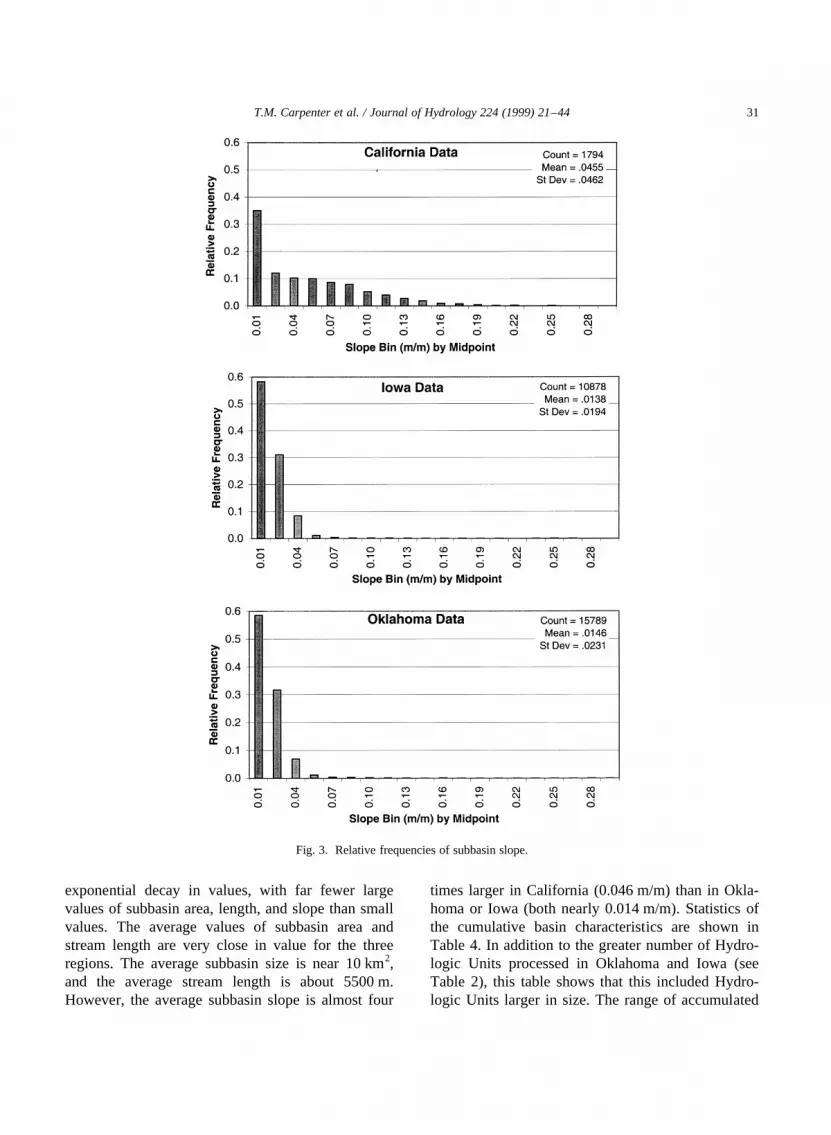
exponential decay in values, with far fewer largevalues of subbasin area, length, and slope than smallvalues. The average values of subbasin area andstream length are very close in value for the threeregions. The average subbasin size is near 10 km2,and the average stream length is about 5500 m.However, the average subbasin slope is almost four

times larger in California (0.046 m/m) than in Okla-homa or Iowa (both nearly 0.014 m/m). Statistics ofthe cumulative basin characteristics are shown inTable 4. In addition to the greater number of Hydro-logic Units processed in Oklahoma and Iowa (seeTable 2), this table shows that this included Hydro-logic Units larger in size. The range of accumulated


Fig. 3. Relative frequencies of subbasin slope.

area and of stream length are larger in these regions,as are the average values. As with the subbasin slope,the average accumulated slope is larger in California(0.05 m/m) than the flatter Central Plains Regions(0.015 m/m). Overall, the similarity among the distri-butions of subbasin area and channel length of thethree regions is remarkable given their very differentphysiographic and climatic regimes.

In computing threshold runoff, the procedurecomputes and stores the unit hydrograph peak andtime to peak. In the geomorphologic unit hydrograph,which depends only on topographic data, a linearapproximation of the unit hydrograph peak is madeand the time to peak is computed from Eq. (7). Rela-tive frequency histograms for these parameters areshown in Figs. 4 and 5. Again, the frequency isnormalized by the number of subbasins for whichthreshold runoff is computed. Average values of theunit hydrograph peak increase from 0.15/h in Califor-nia and Oklahoma to 0.18/h in Iowa. Also, the distri-bution of the unit hydrograph peak exhibits bimodalproperties in California and Iowa. The shapes of thedistributions for the time to peak are very similaramong the three regions. Average time-to-peak valuesdo vary slightly among the regions: California, 5.6 h;Iowa, 5.2 h; Oklahoma, 6.2 h.

The distribution of magnitude and time of the unithydrograph peak with the drainage area is illustratedin Fig. 6 for Oklahoma and for the geormorphologicunit hydrograph with a 1 h effective rainfall duration.Values are plotted for source basins only. Sourcebasins were defined in the procedure as basins withdrainage areas less than 35 km2 which contain thesource of a stream. These are catchments particularly

prone to flash flooding. The unit hydrograph peakmagnitude shows a decreasing trend with increasingdrainage area. For the example shown, the averagepeak is approximately 0.28/h at 5 km2 and decreasesto 0.14/h at 35 km2. The variability of the peak alsodecreases as the drainage area increases. The time topeak tends to increase as drainage area increases.The variability in the time to peak appears lessdependent on drainage area, up to approximately25 km2. The decrease in variability at largerdrainage areas may be due in part to sampling effectswith fewer data points at these larger areas. Similartrends are observed for the other methods andregions.

Turning to the computed threshold runoff esti-mates, Fig. 7 displays the relative frequency of thresh-old runoff of hourly duration for the three regions andfor Method 1 (Qbf/GUH). Significant differences areapparent. Nearly all of the values in California fallbelow 16 mm (approximately 96%). In fact, morethan 80% of the computed values fall in the 8–12 mm range. In Iowa, approximately 95% of thethreshold runoff values are less than 20 mm.However, in Oklahoma, nearly all values are greaterthan this level. The values in Iowa and Oklahoma arelarger and have a wider range than in California.Average threshold runoff values are 9.5 mm in Cali-fornia, 14 mm in Iowa, and 34 mm in Oklahoma. Therange of values in California is 5–22 mm, whereas therange in Iowa is 6–30 and 17–72 mm in Oklahoma.Given the similar distributions of catchment geometrydata in all three regions (i.e. subbasin area and streamlength), these results are believed to be a reflection ofthe channel morphology (e.g. channel width and


Table 4Geometric characteristics for three application regions

California Iowa Oklahoma

Number of subbasins 1794 10,878 15,879Cumulative area(km2)Range 5–3680 5–11,690 5–19,514Average 215 325 566Cumulative slopeRange 0–0.2428 0–0.0644 0–0.0802Average 0.0544 0.0147 0.0145Cumulative length(m)Range 2463–178,210 2090–252,390 2475–434,910Average 24,250 29,250 34,910

depth), which in turn is a reflection of the action ofclimate on terrain.

To illustrate the differences among computationalmethods, Fig. 8 shows the relative frequency histo-grams of 1 h threshold runoff for each of the fourmethods for Oklahoma. The shapes of the distribu-tions are more similar between Methods 1 and 2

(Qbf) and between Methods 3 and 4 (Q2) than betweenMethods 1 and 3 (GUH) or Methods 2 and 4(Snyder’s). This may indicate that the computedthreshold runoff is more sensitive to the definition ofthe flooding flow than the unit hydrograph method.The distributions for Methods 3 and 4 are shifted tothe left (to lower threshold runoff values) when


Fig. 4. Relative frequencies of unit hydrograph peak for geomorphologic unit hydrograph method.

compared to the distributions for Methods 1 and 2.This implies that the bankfull flow methods yieldhigher threshold runoff than the two-year returnperiod flow methods, and thus that the computedbankfull flows are higher than the computed two-year return period flows in Oklahoma.

In Iowa, the distributions (not shown herein) are

more similar among the methods. The similarity indistribution shape between Methods 1 and 2 andbetween Methods 3 and 4 exists. However, there isno shift in the distributions as a function of the flood-ing flow, indicating that the two-year return periodflow is a reasonably good estimate of bankfull flowthere.


Fig. 5. Relative frequencies of time to peak for geomorphologic unit hydrograph method.

Fig. 9 illustrates the effect of increasing the effec-tive rainfall duration,tR. For each method, this figureshows the relative frequency histograms for the 1-, 3-,and 6-h runs in Oklahoma. Clearly, there is a shift tohigher threshold runoff as the effective rainfall dura-tion increases. This effect is most pronounced inMethod 1. To judge the relative magnitude of theshift in distributions, the difference between the 1 hmean threshold runoff value and the 6 h mean value

was computed for each of the four methods. Thedifferences were 30.3, 14.9, 21.4, and 8.5 mm forMethods 1, 2, 3, and 4, respectively. The higher differ-ences in Methods 1 and 3 indicate greater sensitivityto the effective rainfall duration for the geomorpho-logic unit hydrograph method.

In Fig. 10, the threshold runoff values for 3- and 6-heffective rainfall duration are plotted against thecorresponding threshold runoff values for an 1 h


Fig. 6. Distribution of: (a) the unit hydrograph peak; and (b) time to peak for Oklahoma source basins (drainage area between 5 and 35 km2).

effective rainfall duration. This comparison is shownfor source basins only (drainage areas less than35 km2) and for threshold runoff up to 76 mm(3 in.). Again, the increase in threshold runoff witheffective rainfall duration is apparent. Fig. 10 maybe used to estimate threshold runoff for durations of3 and 6 h from the 1 h duration. It is clear from the

greater scatter for the 6 h duration that such estimationwill yield reliable results only for the duration of 3 h.

In the geomorphologic unit hydrograph methods,the above results utilized a constant value of Horton’slength ratio,RL (see Eq. (8)). In the preliminary work,a regional value of 1.9 was established using datafrom Oklahoma. This value of 1.9 was applied for


Fig. 7. Relative frequencies of hourly threshold runoff for method 1.

all Hydrologic Units processed. The effect of thisassumed value was examined by determiningwatershed-specificRL values, running the thresholdrunoff computations with the watershed-specificRL,and, then, comparing these results with the thresholdrunoff values computed with the constantRL. Onlyheadwater Hydrologic Units, that is units containingthe source of a river, were used. This included fourHydrologic Units in California, 13 in Iowa and 13 inOklahoma.

RL is defined as the average stream length of a givenstream order divided by the average stream length ofthe next higher stream order.RL was determined foreach Hydrologic Unit as the best-fit slope from a plotof the logarithm of the average stream length againststream order. These values were, in general, slightly

higher than the constant value of 1.9. The range invalues was 1.9–2.8 in California, 2.0–2.9 in Iowa,and 1.8–2.6 in Oklahoma.

The comparison of threshold runoff valuescomputed with the Hydrologic Unit-specificRL versusthe constantRL is shown in Fig. 11. This plot showsMethod 1 results with a 1 h effective rainfall dura-tion for the three regions, and only for the sourcebasins. Small sensitivity of the results onRL isobserved. Generally lower threshold runoff valueswere obtained with the Hydrologic-Unit-specificRL, especially in Iowa and some regions ofOklahoma. The differences in threshold runoffvalues reach a maximum of 15–20%. Differencesin the time to peak (not shown) were larger, up toabout 30%.


Fig. 8. Relative frequencies of threshold runoff for all four methods of computation in Oklahoma, effective rainfall duration is 1 h.

4.3. Comparison with manually computed thresholdrunoff

In an effort to obtain a preliminary estimate of theaccuracy of the procedure-computed threshold runoffestimates, their values were compared to valuesderived through manually computed methods.Observed precipitation and streamflow records wereused to compute 1 h unit hydrograph peaks forselected streams in Iowa and Oklahoma. The unithydrograph peaks were combined with estimates ofthe two-year return period and bankfull flows, andcatchment area in accordance with Eq. (2).

For this work, only unregulated streams, withdrainage areas less than 1500 km2 were utilized. Intotal, 20 streams in Iowa and 16 streams in Oklahoma

were used. The observed 15 min streamflow data atselected sites was obtained from the Iowa City, Iowaand Oklahoma City, Oklahoma offices of the USGS.Limited data was available, covering only the timeperiod from January 1991 to December 1991 inIowa, and from October 1991 to April 1994 in Okla-homa. With the available data, the first step was toidentify possible rainfall–runoff events that could beused to develop unit hydrographs for the selectedstreams. Events were selected based on satisfying(or nearly satisfying) as many of the following criteriaas possible: (1) uniform rainfall intensity in time, (2)isolated rainfall events, (3) single-peak dischargehydrographs, and (4) high peak discharge (near orgreater than the two-year return period flow). Insome cases, only one criterion may have been met.


Fig. 9. Relative frequencies of threshold runoff for all four methods of computation in Oklahoma and effective rainfall durations of 1, 3, and 6 h.

However, in a few cases, multiple events for a givenstream were identified and used in deriving the unithydrograph.

For each stream and each event, a 1 h unit hydro-graph was derived from the historical data. The deri-vation included separation of baseflow, direct runoffcomputation, and in some cases, transformation fromtheN-hour unit hydrograph to the 1 h unit hydrographusing anS-curve. Details of the unit hydrograph deri-vations are presented in Carpenter and Georgakakos(1993, 1995). The 1 h unit hydrograph peaks wereobtained from the 1 h unit hydrographs, and combinedwith drainage area and estimates of the two-yearreturn period or bankfull flows to arrive at the manu-ally computed threshold runoff values.

Comparisons of the manually computed and proce-dure-computed threshold runoff for Iowa and Okla-homa are presented in Fig. 12. In this figure,

manually computed threshold runoff is shown withfilled symbols, and the procedure-computed valuesare given open symbols. Before discussing the results,we note the high uncertainty associated with derivingunit hydrograph estimates in basins with activesubsurface runoff (as is the case for many basins inIowa and Oklahoma). In Iowa, the manuallycomputed threshold runoff shows greater variabilitythan the procedure-computed values. The range inmanually computed threshold runoff is 2–42 mm,whereas the range in procedure-computed values is8–24 mm. Differences between the procedure- andmanually computed values vary between 2 and25 mm. These differences, if not a result of the uncer-tainties in the manual estimation of unit hydrographsfor historical records, are a result of uncertainties inestimating channel cross-sectional properties. InOklahoma, the procedure yields threshold runoff


Fig. 10. Comparisons of 1-, 3-, and 6-h threshold runoff in Oklahoma.

values with greater variability. The range in theprocedure-computed values is 10–36 mm. The proce-dure-computed values are generally higher than themanually computed values. In Oklahoma, the differ-ences range from 0 to 25 mm. It is noted that thismaximum difference is obtained for the basin with

the lowest drainage area. Excluding this basin, themaximum difference is approximately 15 mm. Themean square error between manually computed andprocedure-computed values for Method 1 (Qbf/GUH)was 8.9 mm in Iowa and 5.8 mm in Oklahoma. Thetwo-year return period flow methods produced


Fig. 11. Comparison of threshold runoff computed with a constant length ratio,RL, over a region versus with a varyingRL. Method 1 is shownwith a 1 h effective rainfall duration.

slightly higher mean square errors than the bankfullflow methods (0.8–1.5 mm higher).

5. Summary, conclusions and recommendations

The US National Weather Service identified a needfor improving flash flood guidance procedures. As a

first step, this paper describes a procedure developedto provide improved estimates of threshold runoff.The procedure has been designed based on objectivehydrologic principles and can be applied consistentlyon a national scale. It includes four methods ofcomputing threshold runoff, to fit varying applicationneeds and data availability scenarios for differentregions within the US. Geographic Information


Fig. 12. Comparison of manually computed (filled symbols) versus procedure-computed (open symbols) hourly threshold runoff.

Systems and nationally available digital databases areused in the determination of watershed geometriccharacteristics, needed to calculate threshold runoff.The procedure has been implemented in the softwarepackage,threshR, and is under operational implemen-tation at regional River Forecast Centers.

The application of the procedure in three differentregions has been demonstrated. These regions includethe state of Iowa, the state of Oklahoma, and severalareas in California. Analysis of the GIS-computedwatershed characteristics showed significant similari-ties in the size of the delineated subbasins and subba-sin stream length. The greatest difference in watershedcharacteristics was observed in channel slope. Theaverage channel slope in California was nearly fourtimes larger than in Iowa or Oklahoma.

Comparisons of the computed threshold runoff andcomputed unit hydrograph characteristics were madeamong the three regions, for the four methods ofcomputations, and for varying effective rainfall dura-tion. These comparisons showed substantially higherthreshold runoff estimates in Oklahoma than in Iowaand California, with the values in Iowa being signifi-cantly higher than those in California. These differ-ences are attributed mainly to differences in channelmorphological properties (most likely a combinationof terrain morphology and structure, and climate). Forthe method compared, Oklahoma had a mean thresh-old runoff value of nearly 34 mm. In Iowa, the meanvalue was 14 mm. California had the lowest meanvalue of 9.5 mm, along with the smallest range invalues. A shift in the frequency distribution of thresh-old runoff for the methods using bankfull flow versusthose using the two-year return period flow wasobserved in Oklahoma. This shift appears to be afunction of the definition of the flooding flow, withbankfull flow producing higher threshold runoff thanthe two-year return period flow. Increasing the dura-tion of effective rainfall produced higher thresholdrunoff values. For Oklahoma, a greater sensitivity toeffective rainfall duration was observed with thegeomorphologic unit hydrograph method than withSnyder’s synthetic unit hydrograph method.

Perhaps one of the greatest sources of uncertaintycomes from estimating channel cross-sectional andflow parameters from regional regression relation-ships. For some regions, these relationships may beestablished. If they are not, the relationships must be

developed from local data within the region. Thisapproach was used in Iowa and Oklahoma. The rela-tionships developed have correlation coefficientsranging from 40 to 91%. The lower correlation coeffi-cients (40%) affect the accuracy of the computedvalues (see theoretical sensitivity study reported inCarpenter and Georgakakos, 1993). Future develop-ments should investigate the possibility of using high-resolution, remotely sensed data along with localsurveys to estimate the channel cross-sectionalgeometry.

In the first implementation of the procedure in theNWS, there is an apparent advantage for usingSnyder’s unit hydrograph approach and the two-yearreturn period flow (Method 4). There are problems inobtaining the necessary data to implement all meth-ods. However, fewer problems are anticipated inobtaining the necessary data to implement Snyder’sunit hydrograph (regional estimates of the empiricalcoefficients). Similarly, the two-year flow is availablefor streamgauge locations with fair national coverage.The cross-sectional data or regional relationships forcross-sectional parameters required to implementbankfull flow and geomorphologic unit hydrographdo not have the same availability on a national scale.

The final section of this paper presented a compar-ison of the procedure-computed threshold runoffvalues with values computed from manually deter-mined unit hydrographs. Given the uncertainty asso-ciated with the manual procedure due to datavariability, the comparison serves to obtain a preli-minary estimate of the possible error in the proce-dure-computed values. Excluding one outlier of25 mm for a small basin, a maximum difference inthe threshold runoff values observed was 15 mm inboth Iowa and Oklahoma. Of course, the ultimatevalidation of this procedure is in monitoring theresults of real-time operation for providing flashflood guidance. Perhaps, newly available high-resolu-tion remotely sensed data can be used to estimateexcessive surface runoff areas for validation.

The next step is the implementation of the proce-dure in an NWS operational setting throughout the USAlthough the undertaking is large, it will generate aset of objective and consistent threshold runoff valuesacross the US. Thus, it will provide excellent oppor-tunities for understanding the spatial properties ofthreshold runoff, for estimating the reliability of the


procedure, and for achieving further improvements inthe methodology.

Acknowledgements

Development of thethreshRsoftware was spon-sored by the Hydrologic Research Laboratory of theNational Weather Service, NOAA, through ContractNo. NA17WH0181. Additional support has beenprovided by the National Science Foundation throughthe Presidential Young Investigator Award to K.P.Georgakakos, and subsequently through Grant no.CMS-9520109, and by the Iowa Institute of HydraulicResearch EPRIa program. Original development wasperformed at the Computation Laboratory for Hydro-meteorology and Water Resources at The Universityof Iowa, with on going development at the HydrologicResearch Center. Special thanks go to the followingpeople for their technical assistance throughout thecourse of this work: Dr George Smith of the Hydro-logic Research Lab; Charles Ehlschlaeger of the USArmy Construction Engineering Research Labora-tory; David Eash of the Iowa City District Office ofthe US Geological Survey; and Hector Bravo, nowwith the University of Wisconsin, Milwaukee. Thesoftware development contributions of Jim Cramerand Anton Kruger of The University of Iowa havebeen invaluable during the course of this project.The views expressed herein are those of the authorsand do not necessarily express those of NSF, NOAA,or any of their sub-agencies.

References

Barrett, C.B., 1983. The NWS flash flood program. Preprints of theFifth Conference on Hydrometeorology, American Meteorolo-gical Society, Boston, MA, 1983, pp. 9–16.

Bras, R.L., 1990. Hydrology an Introduction to Hydrologic Science,Addison-Wesley, Reading, MA, 643 pp.

Caroni, E., Rosso, R., Siccardi, F., 1986. Nonlinearity and time-variance of the hydrologic response of a small mountaincreek. In: Gupta, V.K., Waymire, E., Rodriguez-Iturbe, I.(Eds.), Scale Problems in Hydrology, Reidel, Dordrecht, pp.19–37.

Carpenter, T.M., Georgakakos, K.P., 1993. GIS-based procedures insupport of flash flood guidance. IIHR Report No. 366, IowaInstitute of Hydraulic Research, The University of Iowa, IowaCity, IA, November, 170 pp.

Carpenter, T.M., Georgakakos, K.P., 1995. Verification of threshold

runoff for Oklahoma streams. IIHR Limited Distribution ReportNo. 240, Iowa Institute of Hydraulic Research, The Universityof Iowa, Iowa City, IA, 80 pp.

Chow, V.T., Maidment, D.R., Mays, L.W., 1988. Applied Hydrol-ogy, McGraw-Hill, New York, 572 pp.

Eash, D., 1991. Field measurements and notes on stream parametersfor Iowa streams. Field Notebook (unpublished document), USGeological Survey, Iowa City, IA, 100 pp.

Ehlschlaeger, C.R., 1990. Using the AT search algorithm to develophydrologic models from digital elevation data. Unpublishedpaper, US Army Corps of Engineers Construction EngineeringResearch Laboratory, Champaign, IL, 7 pp.

Fread, D.L., 1992. NWS river mechanics: some recent develop-ments. Proceedings of US/PRC Flood Forecasting Sympo-sium/Workshop, Shanghai, People’s Republic of China, 14–17 April, pp. 81–111.

Galloway, G.E., 1994. Sharing the challenge, flood plain manage-ment into the 21st Century. A Report of the Interagency Flood-plain Management Review Committee, Washington, DC.

Georgakakos, K.P., 1986. On the design of national, real-time warn-ing systems with capability for site-specific, flash-flood fore-casts. Bulletin of the American Meteorological Society 67(10), 1233–1239.

Georgakakos, K.P., Unnikrishna, P.V., Bravo, H.R., Cramer, J.A.,1991. A national system for determining threshold runoff valuesfor flash-flood prediction. Issue Paper, Department of Civil andEnvironmental Engineering and Iowa Institute of HydraulicResearch, The University of Iowa, Iowa City, IA.

Henderson, F.M., 1966. Open Channel Flow, MacMillan, NewYork, 522 pp.

Jarrett, R.D., 1984. Hydraulics of high gradient streams, J.Hydraulic Engng 110 (11), 1519–1539.

Kruger, A., Cramer, J.A., Carpenter, T.M., Sperfslage, J.A., Geor-gakakos, K.P., 1993. threshR: A User’s Manual, Iowa Instituteof Hydraulic Research, Iowa, 29 pp.

Leopold, L.B., 1994. A View of the River, Harvard UniversityPress, Cambridge, MA, 298pp.

Minitab Inc, 1989. MINITAB Reference Manual: Release 7, Mini-tab Inc, State College, Pennsylvania, 342 pp.

National Research Council (NRC), 1996. Assessment of Hydrologicand Hydrometeorological Operations and Services, NationalAcademy Press, Washington, DC, 51 pp.

Nixon, M., 1959. A study of bankfull discharges of rivers inEngland and Wales. Mm. Preo. Instn. Civ. Engrs 6322, 157–174.

NOAA, 1981. Floods, Flash Floods and Warnings, Pamphlet,National Weather Service, NOAA, Washington, DC.

Riggs, H.C., 1990. Estimating flow characteristics at ungaugedsites. In: Beran, M.A., Brilly, M., Becker, A., Bonacci, O.(Eds.), Regionalization in Hydrology, vol. 191. IAHS, pp.150–161.

Rodriguez-Iturbe, I., Valdes, J.B., 1979. The geomorphologic struc-ture of hydrologic response. Water Resources Research 15 (6),1409–1419.

Rodiguez-Iturbe, I., Gonzalez-Sanabria, M., Bras, R.L., 1982. Ageomorphoclimatic theory of the instantaneous unit hydrograph.Water Resources Research 18 (4), 886–887.


Sperfslage, J.A., Carpenter, T.M., Georgakakos, K.P., 1994. GISdetermination of catchment boundaries. IIHR Limited Distribu-tion Report No. 224, Iowa Institute of Hydraulic Research, TheUniversity of Iowa, Iowa City, IA, August, 41 pp.

Sperfslage, J.A., Georgakakos, K.P., 1998. On threshR enhance-ments toward improved computational efficiency. HRC Techni-cal Note No. 8, Hydrologic Research Center, San Diego, CA,July, 36 pp.

Sweeney, T.L., 1992. Modernized areal flash flood guidance.NOAA Technical Report NWS HYDRO 44, HydrologicResearch Laboratory, National Weather Service, NOAA, SilverSpring, MD, October, 21 pp. and an appendix.

Tortorelli, R.L., Bergman, D.L., 1985. Techniques for estimatingflood peak discharges for unregulated streams and streams regu-lated by small floodwater retarding structures in Oklahoma.Water-Resources Investigations Report 84-4358, US GeologicalSurvey, Oklahoma City, OK, 85 pp.

United States Army Corps of Engineers Construction EngineeringResearch Laboratory, 1983. GRASS 4.1 User’s ReferenceManual, USACERL, Champaign, IL, 556 pp.

United States Geological Survey (USGS), 1982. Hydrologic UnitMap-1981 State of Iowa. Scale 1:500.000. USGS, US Depart-ment of Interior, Reston, VA.

United States Geological Survey (USGS), 1974. Hydrologic UnitMap-1974 State of Oklahoma. Scale 1:500.000. USGS, USDepartment of Interior, Reston, VA.

United States Geological Survey (USGS), 1994. Nationwidesummary of US geological survey regional regression equationsfor estimating magnitude and frequency of floods for ungagedsites. USGS Water Resources Investigations Report 94-4002,USGS, US Department of Interior, Reston, VA, 196 pp.

Wang, C.T., Gupta, V.K., Waymire, E., 1981. A geomorphologicsynthesis of nonlinearity in surface runoff. Water ResourcesResearch 17 (3), 545–554.

Wolman, M.G., Leopold, L.B., 1957. River flood plains: someobservations on their formation, US Government PrintingOffice, Washington, DC, US Geological Survey ProfessionalPaper 282-C.


national threshold runoff estimation utilizing gis in support of operational flash flood warning...

Documents