HEALTH ECONOMICS

Health Econ. 15: 65–81 (2006)

Published online 7 September 2005 in Wiley InterScience (www.interscience.wiley.com). DOI:10.1002/hec.1020

National road casualties and economic development

David Bishaia,*, Asma Quresha, Prashant Jamesb and Abdul GhaffarcaDepartment of Population and Family Health Sciences, Johns Hopkins University Bloomberg

School of Public Health, USAbUniversity of California at Irvine, USAcGlobal Forum for Health Research, Geneva, Switzerland

Summary

Objective: This paper explores why traffic fatalities increase with GDP per capita in lower income countries anddecrease with GDP per capita in wealthy countries.Methods: Data from 41 countries for the period 1992–1996 were obtained on road transport crashes, injuries, and

fatalities as well as numbers of vehicles, kilometers of roadway, oil consumption, population, and GDP. Fixedeffects regression was used to control for unobservable heterogeneity among countries.Results: A 10% increase in GDP in a lower income country (GDP/Capita5$1600) is expected to raise the number

of crashes by 7.9%, the number of traffic injuries by 4.7%, and the number of deaths by 3.1% through a mechanismthat is independent of population size, vehicle counts, oil use, and roadway availability. Increases in GDP in richercountries appear to reduce the number of traffic deaths, but do not reduce the number of crashes or injuries, all elseequal. Greater petrol use and alcohol use are related to more traffic fatalities in rich countries, all else equal.Conclusion: In lower income countries a rise in traffic-related crashes, injuries, and deaths accompanies economic

growth. At a threshold of around $1500–$8000 per capita economic growth no longer leads to additional trafficdeaths, although crashes and traffic injuries continue to increase with growth. The negative association betweenGDP and traffic deaths in rich countries may be mediated by lower injury severity and post-injury ambulancetransport and medical care. Copyright # 2005 John Wiley & Sons, Ltd.

JEL classification: O57; R41; I12

Keywords transportation; motor vehicles; traffic safety; cross country studies

Introduction

Expansion of road transport brings opportunityfor wealth and prosperity through increasedcommerce. An unintended side effect of increasingthe contact between people and vehicles through-out the world will be a worsening of the trafficinjury pandemic. With over 1 million killed by carcrashes annually, traffic injuries are projected tobecome the 3rd leading cause of disability adjustedlife years lost by 2020 [1]. The Red Cross has

dubbed the 20th century, ‘The Century of RoadDeath’ [2] and the 21st century may show littleimprovement. Over 30 million people have per-ished in traffic fatalities since the very firstpedestrian casualty in 1898 [2].

Prior studies have recorded a biphasic relation-ship between traffic fatalities and economic devel-opment with fatalities rising for the low incomecountries and falling for the high income countries[3]. Environmental economists finding a similarrelationship between pollution and income notedhomology to Kuznets’s inverted-U relationship

Copyright # 2005 John Wiley & Sons, Ltd.Received 7 October 2003Accepted 17 May 2005

*Correspondence to: Department of Population and Family Health Sciences, Johns Hopkins University Bloomberg School ofPublic Health, 615 N. Wolfe St., Baltimore, MD 21205, USA. E-mail: dbishai@jhu.edu

between income inequality and development. Theydiscuss an ‘environmental Kuznets curve’ [4] inwhich the pollution externalities of mechanizedactivity first rise and then fall with the economicgrowth that attends industrialization. For pollu-tion to decrease while mechanized activity in-creases requires investments in harm reduction.The critical question is whether the investments inharm reduction will be able to keep up withgrowth in the scale and intensity of pollutingactivity.

While environmental economists have beenconcerned with the harms from motorized trans-port, they tend to focus on the exhaust pipe as thesource of harm. To date, few economists have beenas concerned with harms emitted from the bumper.With over 1 million deaths per year due to trafficfatalities, motor vehicles are the most lethal aspectof the modern physical environment, and it is notsurprising that a country’s ability to control theharms in its roadways would be similar to itsability to control other environmental hazards.Motor vehicle fatalities can be considered thegreatest health hazard which rises and falls witheconomic development on the environmentalKuznets curve.

Ceteris paribus, a population that spends moretime exposed to moving vehicles ought to experi-ence more traffic harms. The crudest measure ofexposure to motorized transport, vehicles/popula-tion, always increases with economic growth [5] asdo other measures such as petroleum consumptionper capita and kilometers per capita. Since trafficfatalities can decline at advanced stages ofeconomic growth despite increases in traffic, weneed to understand why higher income countriesare able to mitigate the harm from the increasedpopulation exposure to road traffic. One scenariowould be that investment in harm reduction (saferdrivers, roads, and vehicles) has simply reducedthe numbers of crashes. Another possibility wouldbe that harm reduction policies have reduced thenumber and severity of the injuries that attendcrashes so that even though crashes occur theenergy is channeled away from the occupants andpedestrians. For example, this might occur with atransition away from motorized bicycles tosedans, or through occupant restraints. Finally itmight be the case that improvements in emergencytransport and in the medical treatment of traumahave enabled better survival despite continuingupward trends in the numbers of crashes andinjuries.

The objective of this paper is to identify therelationship between economic growth and trafficfatalities, traffic injuries and crashes. We will showthat although there is an inverted U (an environ-mental Kuznets curve) for fatalities, there is nosuch relationship for injuries and crashes. Asecondary objective of the paper is to identifysome of the mechanisms by which economicgrowth is related to fatalities, injuries, and crashes.Because there are cross country panel data on onlya limited number of variables, the relative con-tribution of various unmeasured determinants oftraffic fatalities such as road quality, enforcementefforts, motorist attitudes, etc. cannot be assessedin this study. We control for the total contributionof time-invariant unmeasured determinants oftraffic fatalities using country fixed and randomeffects models.

Methods

Theoretical framework

Since safety is a normal good, more income oughtto predict more safety, yet the perplexing trend forlow income countries, is that more income leads toless traffic safety and more traffic deaths [3]. Theopposite is true in high income countries wheremore income leads to fewer traffic deaths [3]. Whatcan account for the difference? There are severalpossible explanations: (1) An externalities story inwhich the more advanced stages of economicdevelopment are a prerequisite for the institutionalcapacity to successfully assign liability and toregulate externalities; (2) A competing risks storyin which it is rational for road users to under-invest in road safety and bear a greater exposure tohigh risk transport options in order to generate anincome which can be used to control infectiousand nutritional health risks that are simpler tocontrol early in the epidemiological transition. Inhigher income countries infectious diseases andmalnutrition recede in importance relative totransport injuries and it becomes rational formotorists and governments to spend more re-sources on safety. (3) A vehicle mix story in whichlower traffic fatality rates occur spontaneously aseconomic growth empowers more road users toswitch to driving safer sedans instead of moredangerous transport modalities such as motorized

Copyright # 2005 John Wiley & Sons, Ltd. Health Econ. 15: 65–81 (2006)

D. Bishai et al.66

bicycles and the rooftops of buses; (4) A medicaltechnology story, in which a country’s capacity totransport and resuscitate road trauma victimsmust await the development of a highly capablemedical system. We will review these explanationsone by one.

Externalities

Several have identified the potential for a motor-ist’s insurance policy to increase risk-taking [6,7].Externalities abound in the transportation market,and are not limited to the injuries a single motoristmay inflict on others in the rush from point A topoint B. To the extent that car buyers and localregulators are unconcerned and uninformed aboutvehicle safety, manufacturers can impose safetyexternalities on the market. Purveyors of alcoholmay impose similar safety externalities in theabsence of regulation and enforcement. Roadwayengineers, despite their operation in the publicsector, may experience political incentives tounder-invest in maintaining the safety propertiesof local roadways. In terms of Coase’s theorem, afirst best market solution to any externalitiesproblem can be achieved if rights to injure or tobe spared injury are securely assigned and thencostlessly traded [8]. In Coase’s terms, all extern-ality problems are due to institutional failures tosecurely assign and administer externality rightsand also due to high transaction costs inhibitinginjurers from bearing liability and/or injuryvictims from making claims. Ultimately, both thegenerators and victims of traffic safety externalitiesare distributed widely in the economy. Withformidable transaction barriers separating them,motorists and their victims in a less developedcountry may have to wait for substantial institu-tional development before traffic courts andregulators can successfully assign liability andofficiate over claims.

Competing risks

The competing risks account is familiar to manytransport experts in developing countries whoexplain the low rates of investment in road safetyby pointing to ‘limited resources’. A competingrisks explanation of the connection between

economic growth and traffic casualties assumesthat countries prioritize their investments in publichealth and safety to maximize increments inwelfare per public dollar spent. Under this view,investments in traffic safety are deferred by lowincome countries as they work down a league tableof public investments that are deemed higherpriorities. With development, more of the higheryield (lower cost) public health investments willhave been fully exploited. Thus, with development,investments in safer roads and greater enforcementbecome both more attractive and affordable.These investments would take the form ofregulating and enforcing traffic codes and vehiclesafety standards, as well as controlling thefrequency of alcohol-impaired driving. Prior re-search has shown that excise taxes on alcohol areassociated with lower rates of traffic deaths [9,10].

A recent study of public investment in roadsafety showed that in Pakistan and Uganda ratesof investment in road safety range from $0.07 to$0.09 per capita per year [11]. Yet the wisdom ofdeferring road safety investments in low incomecountries is subject to question since some cost–benefit calculations have shown rates of return oninvestments in road safety in lower incomecountries that approach the returns on manycommonly accepted developing country healthinvestments [12,13].

Vehiclemix

Economic growth can alter the mix of vehicles onthe road. Additional income may lead consumersto upgrade from scooters to sedans, or fromsedans to sport utility vehicles (SUVs). The effectsof income growth on vehicular hazards arecomplex and may not necessarily lead to a positiveeffect of economic development on safety. Perso-nal income growth may also lead individuals topursue convenience by substituting more hazar-dous personal vehicles for safer but less convenientbuses and trains. For instance, bus ridership inBogota, Colombia fell from 69% in 1972 to 52%in 1978 [14]. And more SUVs in a country may notlead to lower fatalities overall. A recent simulationstudy showed that an increasing prevalence ofSUVs in a population of smaller vehicles couldactually increase population level injury and deathrates because of the much higher casualty rateduring crashes between asymmetrically sized ve-

National Road Casualties and Economic Development 67

Copyright # 2005 John Wiley & Sons, Ltd. Health Econ. 15: 65–81 (2006)

hicles [15]. There have been no systematic cross-country studies documenting how vehicle mixchanges with economic development.

Medical technology

The medical technology explanation for thedecline of traffic fatalities is supported by severalstrands of evidence. A case study of urban traumaoutcomes in Ghana, Mexico, and the US identifiedthe importance of investments in prehospital carein determining fatality rate – in Kumasi Ghana51% of severely injured persons died in the field.Corresponding rates in Monterrey, Mexico andSeattle were 40 and 21%, respectively [16].Discrete investments in trauma care and pre-hosptial care have been associated with improvedtrauma survival in a variety of locations [17–19].

An economicmodel

In order to nest these competing hypotheses in acommon economic model let us consider a modelof the choices facing a driver (subscript d), aninnocent bystander (e.g. a walker (subscript w),and a government policy maker (subscript g). Webegin with a traffic fatality production function.

pf ¼ pf jiðad ; aw; agÞ � pijcðad ; aw; agÞ

� pcðad ; aw; agÞ ð1Þ

where pf is the probability of a fatal traffic injury –which can be considered the product of theprobability of a crash (pc) and the probability ofany injury conditional on a crash (pijc) and theprobability of a fatal injury conditional on anyinjury (pf ji). Each of these probabilities is pro-duced by a vector of activities selected by thedriver (ad), the walker (aw) and the government(ag). Activities for each agent, ai (wherei 2 fd;w; gg) are subsets from large but finitechoice sets Si. For instance the choice set for thedriver, Sd includes elements such as vehicle typesand vehicle maintenance, vehicle safety features,driver diligence, and a composite commodityrepresenting the choice to invest in items otherthan safety. The choice set for the walker, Sw

would include proximity to roadway, time of day,etc. The choice set for the government, Sg would

include investments in roadway quality, guard-rails, stoplights, vehicle inspection, trafficcode enforcement, traffic litigation, as well asinvestments in trauma care and emergencytransport. The government choice set alsoincludes a composite commodity, representingthe option of investing in public goods otherthan safety. Associated with each agent’s choiceset is a price vector, pi. We stipulate thatdp=dai50 8i{fd; w; gg. So that the probabilityof injury diminishes with precautionary actions.

The objective of the driver is to minimize his/hertotal expected costs from accidents and accidentprevention

CD ¼ p0dad þX

j{ff ;i;c;g

ljpjðad ; aw; agÞ � ðcjÞ ð2Þ

where CD represents the expected costs of thedriver, pd is a vector of shadow costs for theselected action vector, ad � Sd ; li is the driver’sshare of the joint costs of property loss, health carecosts, and lost life years borne by both the walkerand the driver for each type of event. If lj ¼ 1, thedriver must pay all of both his and the pedestrian’scosts.

The driver therefore chooses the kth element adkof the action vector ad from the opportunity set Sd

as follows:

dpfdadk

lf cf þdpidadk

lici þdpcdadk

lccc þ pdk ¼ 0 ð3Þ

In Equation (3) the sum of the three partialderivatives give the marginal benefit of the driver’skth action choice while pdk gives the action’smarginal cost. The notable point is that with eithercrash or injury insurance or in regimes wheredriver liability is poorly enforced lc and li may bereduced and the driver perceives a marginal benefitthat is distorted below its true level. Thus agovernment’s capacity to assign and adjudicatedisputes over liability for crashes and trafficinjuries can lead to driver choices that can leadto event rates above the social optimum. Therewould also be analogous expressions guiding thepedestrian’s action choices, except these expres-sions would contain (1� l) to depict the pedes-trian’s share of liability for outcome costs. Sincepedestrian injury costs are typically much higherthan motorist costs and since motorist paymentscannot fully indemnify pedestrians against theirpain and suffering, the model predicts thatpedestrians overinvest in safety precautions, e.g.using roadways less than they would like to.

D. Bishai et al.68

Copyright # 2005 John Wiley & Sons, Ltd. Health Econ. 15: 65–81 (2006)

The choice variables for the government are land ag. Some of the elements in the choice set, Sg,will affect how well the liability sharing decision isenforced through the conduct of traffic and civilcourts. With the presence of functioning legalinstitutions the government can meaningfullyestablish the share of liability borne by drivers(l). The government would like to minimize thetotal expected costs to society of both accidentsand accident prevention activities given by thefollowing equation:

CG ¼ p0dad þ p0waw þ p0gag

þX

j{ff ;i;c;g

pjðad ; aw; agÞ � ðcjÞ ð4Þ

Although not depicted by the model, the actionchoices of each party will be best responsereactions to the expected best responses of theother parties. According to Coase theorem, in aneconomy with full information and no transactioncosts between drivers and walkers the choice of ldoes not affect the choices of either party. In asecond best world where information is imperfect,part of the government’s strategy might be todevelop institutions that make it more possible forroadway users to transact trades in injury liabilityby making the assignment of liability moretransparent to all.

The full political economy for the governmentlies unspecified in this model. Various elements ofpg will shift downward with development in thevarious economic sectors. Investments in develop-ing and maintaining judicial systems, and policesystems are seldom justified by their impact ontraffic safety alone. But as judicial institutionsdevelop, they lower the opportunity cost of usinglitigation to improve driver behavior. Similarlyemergency transport and trauma care systems aremade less costly by developments in the healthsystem such as blood banking and the availabilityof trained neurosurgeons as well as heart–lungbypass capabilities that would not transpire solelyfor the benefit of road transport victims. Some ofthe governments’ actions serve to tax roadway usernegligence through fines or to subsidize diligenceby erecting pedestrian byways and maintainingrest areas. In some societies the incidence of thesesanctions falls on politically organized groups whomay resist these measures preferring to have highertraffic speeds, higher legal blood alcohol limits,and looser vehicular safety standards, despite the

likelihood that they themselves may bear a shareof the higher rate of crashes and injuries.

The model helps to organize the four comple-mentary and competing accounts for why trafficcasualties rise then fall with economic develop-ment. Development opens up multiple new optionsfor the players as the prices of the elements in theirchoice sets render various choices more affordable.For walkers and drivers, economic development isaccompanied by development of markets for mass-transit and/or for safer vehicles making thesefeatures of the choice sets, Sw and Sd, moreaffordable. We refer to this possibility as ‘thevehicle mix’ explanation for a reduction in trafficcasualties.

For governments, when economic developmentenhances the quality of legal institutions itencourages governments to select actions from Sg

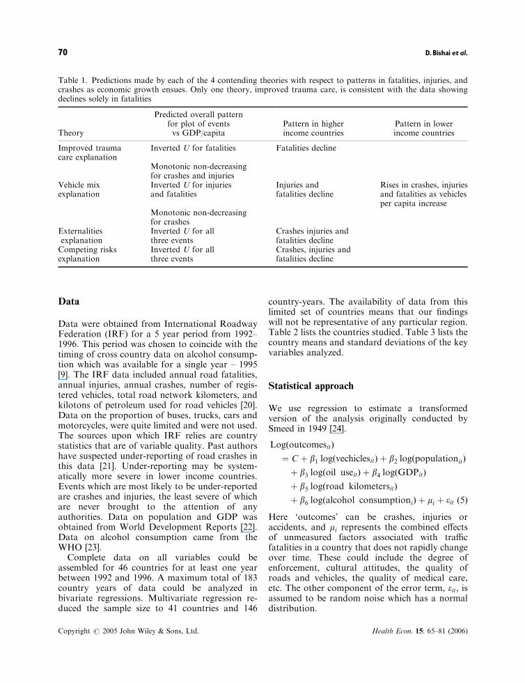
that assign and regulate driver liability. We refer tothis possibility as ‘the externalities’ explanation fora reduction in traffic casualties. Developmentrelated improvements in the capacity of localmedical systems enables governments to selectelements from Sg that enhance emergency care. Wecall this the ‘improved trauma care’ explanation.Finally as returns to scale are increasinglyexploited in the components of Sg that isorthogonal to traffic safety, governments will findit optimal to substitute away from the lessproductive public sector activities towards trafficsafety. We call this the ‘competing risks’ explana-tion. These multiple competing explanations canbe tested, because they lead to different predic-tions. Table 1 summarizes the predictions of themodel.

With all four explanations, small increases inincome in less developed countries simply increaseexposure to road hazards without sufficient devel-opment to predict a reduction in casualties. Thedifferences in the explanations occur further alongin the process of development. Both the external-ities and competing risks explanation involveinvestments in government activities that lead tomore driver diligence and safer roadway environ-ments reducing crashes, and injuries, and fatalities.The vehicle mix explanation does not predict areduction in crashes. It predicts that the vehicleson the roads could potentially be safer, so thatwhen a crash occurs there will be fewer injuriesand fatalities. Finally the improved trauma careexplanation predicts no reductions in crashes orinjuries – ambulances and doctors just do a betterjob saving the lives of all of the victims.

National Road Casualties and Economic Development 69

Copyright # 2005 John Wiley & Sons, Ltd. Health Econ. 15: 65–81 (2006)

Data

Data were obtained from International RoadwayFederation (IRF) for a 5 year period from 1992–1996. This period was chosen to coincide with thetiming of cross country data on alcohol consump-tion which was available for a single year – 1995[9]. The IRF data included annual road fatalities,annual injuries, annual crashes, number of regis-tered vehicles, total road network kilometers, andkilotons of petroleum used for road vehicles [20].Data on the proportion of buses, trucks, cars andmotorcycles, were quite limited and were not used.The sources upon which IRF relies are countrystatistics that are of variable quality. Past authorshave suspected under-reporting of road crashes inthis data [21]. Under-reporting may be system-atically more severe in lower income countries.Events which are most likely to be under-reportedare crashes and injuries, the least severe of whichare never brought to the attention of anyauthorities. Data on population and GDP wasobtained from World Development Reports [22].Data on alcohol consumption came from theWHO [23].

Complete data on all variables could beassembled for 46 countries for at least one yearbetween 1992 and 1996. A maximum total of 183country years of data could be analyzed inbivariate regressions. Multivariate regression re-duced the sample size to 41 countries and 146

country-years. The availability of data from thislimited set of countries means that our findingswill not be representative of any particular region.Table 2 lists the countries studied. Table 3 lists thecountry means and standard deviations of the keyvariables analyzed.

Statistical approach

We use regression to estimate a transformedversion of the analysis originally conducted bySmeed in 1949 [24].

LogðoutcomesitÞ

¼ C þ b1 logðvechiclesitÞ þ b2 logðpopulationitÞ

þ b3 logðoil useitÞ þ b4 logðGDPitÞ

þ b5 logðroad kilometersitÞ

þ b6 logðalcohol consumptioniÞ þ mi þ eit ð5Þ

Here ‘outcomes’ can be crashes, injuries oraccidents, and mi represents the combined effectsof unmeasured factors associated with trafficfatalities in a country that does not rapidly changeover time. These could include the degree ofenforcement, cultural attitudes, the quality ofroads and vehicles, the quality of medical care,etc. The other component of the error term, eit, isassumed to be random noise which has a normaldistribution.

Table 1. Predictions made by each of the 4 contending theories with respect to patterns in fatalities, injuries, andcrashes as economic growth ensues. Only one theory, improved trauma care, is consistent with the data showingdeclines solely in fatalities

Theory

Predicted overall patternfor plot of eventsvs GDP/capita

Pattern in higherincome countries

Pattern in lowerincome countries

Improved traumacare explanation

Inverted U for fatalities Fatalities decline

Monotonic non-decreasingfor crashes and injuries

Vehicle mixexplanation

Inverted U for injuriesand fatalities

Injuries andfatalities decline

Rises in crashes, injuriesand fatalities as vehiclesper capita increase

Monotonic non-decreasingfor crashes

Externalitiesexplanation

Inverted U for allthree events

Crashes injuries andfatalities decline

Competing risksexplanation

Inverted U for allthree events

Crashes, injuries andfatalities decline

D. Bishai et al.70

Copyright # 2005 John Wiley & Sons, Ltd. Health Econ. 15: 65–81 (2006)

Multivariate regression can estimate all of the bparameters. Because inspection of the raw data

showed a biphasic relationship, the sample wasstratified into an upper tertile with GDP/capita

Table 2. Countries studied

CountryDeaths per 100 000vehicles (MEAN) SD Number of years

Austria 33 4.3 5Bahrain 38 8.5 5Brunei 41 7.6 5Bulgaria 74 14.8 5Byelarus 225 48.3 4Cambodia 306 69.3 5Croatia 109 23 5Cyprus 40 4 5Ecuador 296 23 4El Salvador 177 75.7 4Estonia 74 18 5Finland 23 3.4 5France 29 2.2 5Georgia 141 47.8 4Germany 25 4.9 5Greece 69 5.2 5Hong Kong 64 11 5Iceland 12 4.4 5India 1155 30.8 2Israel 40 3.5 5Japan 17 1 3Kazakhstan 232 45 4Korea, Rep. 159 39.4 5Lithuania 100 22.3 5Macedonia 57 2.4 4Malaysia 179 10.4 4Namibia 91 18 4Netherlands 20 0.4 4New Zealand 32 2.5 3Nicaragua 270 72 4Norway 15 1.5 5Pakistan 848 30.6 4Portugal 67 12.5 5Romania 122 16.8 5Saudi Arabia 141 5.7 2Senegal 536 122 4Serbia 79 15 5Slovakia 57 4.1 5Spain 35 2.4 3Sri Lanka 667 88.5 4Sweden 16 2.2 4Switzerland 21 2.6 5Taiwan 70 7 5Turkey 152 17.8 5UK 17 1.6 3US 21 0.1 5Yemen 259 27 5Zimbabwe 328 29.5 5

National Road Casualties and Economic Development 71

Copyright # 2005 John Wiley & Sons, Ltd. Health Econ. 15: 65–81 (2006)

5$1600 and a sample including the lower twotertiles of low income countries with GDP/capita4$1600. Models were run to test the robustness ofthe findings to alternative cut points. Ordinaryleast squares (OLS), fixed effects (FE), andrandom effects (RE) models were estimated. Boththe outcomes and the inputs in the productionmodels are log-transformed to both normalize thevariables and to ease interpretation.

Rather than conduct regressions on outcomesper capita as a function of inputs per capita, weenter both outcomes and inputs unadjusted percapita. Note that if Y and X are completelyuncorrelated, it is elementary to show that Y/Pand X/P can still show a spurious correlation.Consequently, we do not regress events/popula-tion against GDP/population or other factors/population because the regression would be biasedby correlation caused by the common populationdenominator on both sides of the regressionequation. All multivariate models include logpopulation as a separate independent variable,this permits the same ‘per capita’ interpretationwithout creating spurious correlation. In a regres-sion of Y ¼ b0 þ b1X þ b2P, one can interpret b1as the effect of X on Y holding population fixed.Alternatively, after estimation is complete, one candivide through by P to show that ðY=PÞ ¼ ðb0=PÞþðb1ÞðX=PÞ þ b2 and b1 is the effect of per capitaX on per capita Y.

Hausman tests are used to test model specifica-tion [25]. The Hausman test is used to test the nullthat two estimators are consistent where one is aconditional maximum likelihood estimator andtherefore inefficient and the other is efficient underthe null hypothesis. We first test the null that fixed

effects models are consistent relative to OLS, andthen the null that random effects models areconsistent relative to fixed effects models. Becausethe Hausman test relies on an estimate ofVar(b�b) as Var(b)�Var(b) it can sometimes leadto negative Chi squared statistics suggesting thatthe data do not conform to the model assump-tions. Whenever this occurred we used the ‘suest’command in Stata 8.0 [26] to implement a robustHausman test which estimates Var(b�b) asVar(b)�cov(b,b)�cov(b,b)+Var(b) which is al-ways well-defined [27]. We also implemented aBreusch–Pagan test of the null that all randomeffects are zero. Using a combination of theBreusch–Pagan and Hausman tests we were ableto establish preferred statistical models in eachinstance. To enable readers to judge the impor-tance of specification, we present all three modelsand note the preferred specification.

Results

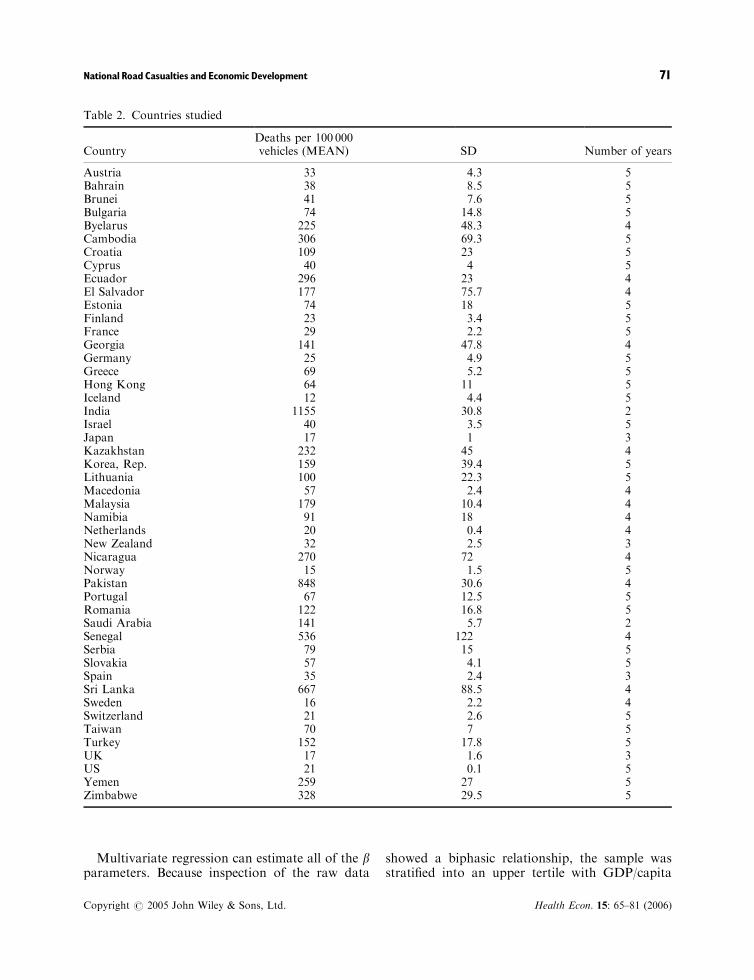
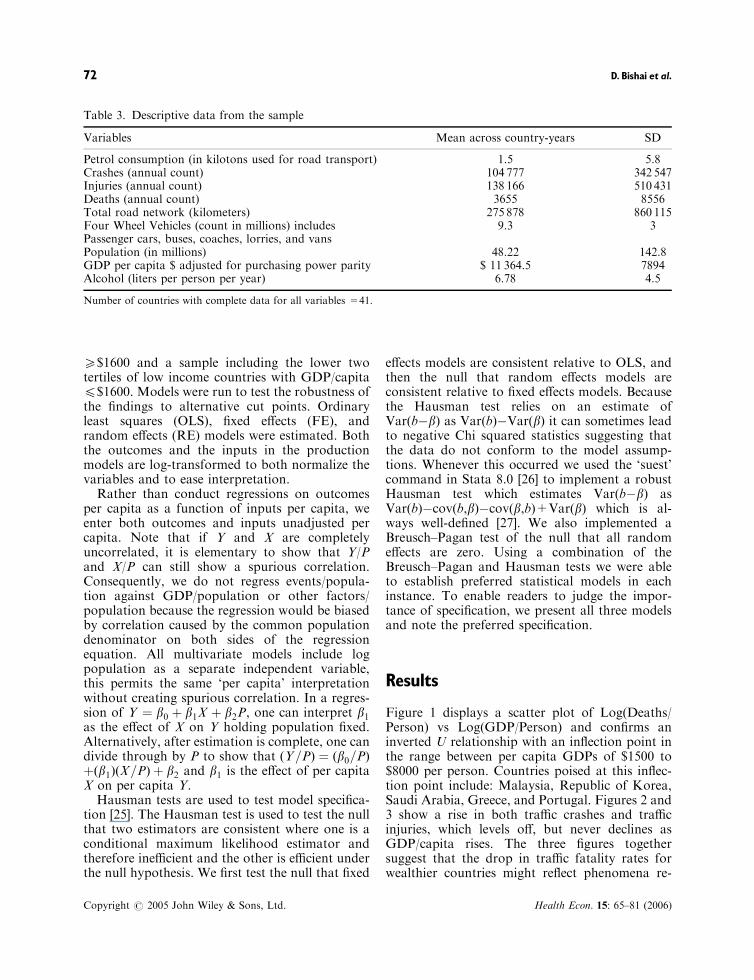
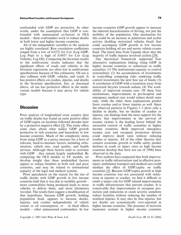
Figure 1 displays a scatter plot of Log(Deaths/Person) vs Log(GDP/Person) and confirms aninverted U relationship with an inflection point inthe range between per capita GDPs of $1500 to$8000 per person. Countries poised at this inflec-tion point include: Malaysia, Republic of Korea,Saudi Arabia, Greece, and Portugal. Figures 2 and3 show a rise in both traffic crashes and trafficinjuries, which levels off, but never declines asGDP/capita rises. The three figures togethersuggest that the drop in traffic fatality rates forwealthier countries might reflect phenomena re-

Table 3. Descriptive data from the sample

Variables Mean across country-years SD

Petrol consumption (in kilotons used for road transport) 1.5 5.8Crashes (annual count) 104 777 342 547Injuries (annual count) 138 166 510 431Deaths (annual count) 3655 8556Total road network (kilometers) 275 878 860 115Four Wheel Vehicles (count in millions) includesPassenger cars, buses, coaches, lorries, and vans

9.3 3

Population (in millions) 48.22 142.8GDP per capita $ adjusted for purchasing power parity $ 11 364.5 7894Alcohol (liters per person per year) 6.78 4.5

Number of countries with complete data for all variables =41.

D. Bishai et al.72

Copyright # 2005 John Wiley & Sons, Ltd. Health Econ. 15: 65–81 (2006)

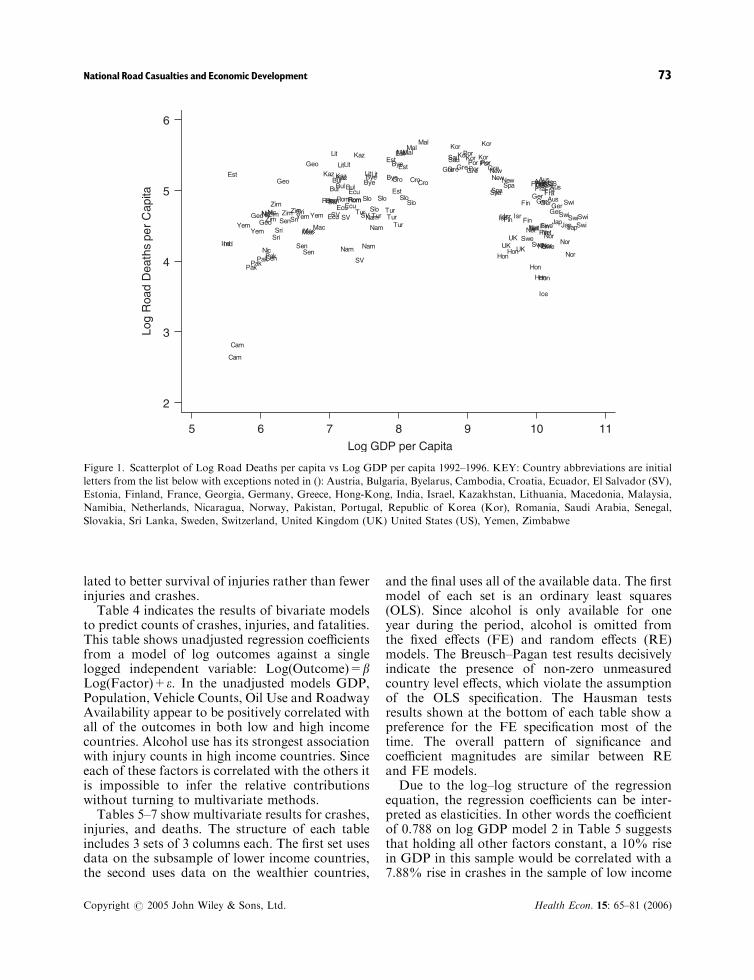
lated to better survival of injuries rather than fewerinjuries and crashes.

Table 4 indicates the results of bivariate modelsto predict counts of crashes, injuries, and fatalities.This table shows unadjusted regression coefficientsfrom a model of log outcomes against a singlelogged independent variable: Log(Outcome)=bLog(Factor)+e. In the unadjusted models GDP,Population, Vehicle Counts, Oil Use and RoadwayAvailability appear to be positively correlated withall of the outcomes in both low and high incomecountries. Alcohol use has its strongest associationwith injury counts in high income countries. Sinceeach of these factors is correlated with the others itis impossible to infer the relative contributionswithout turning to multivariate methods.

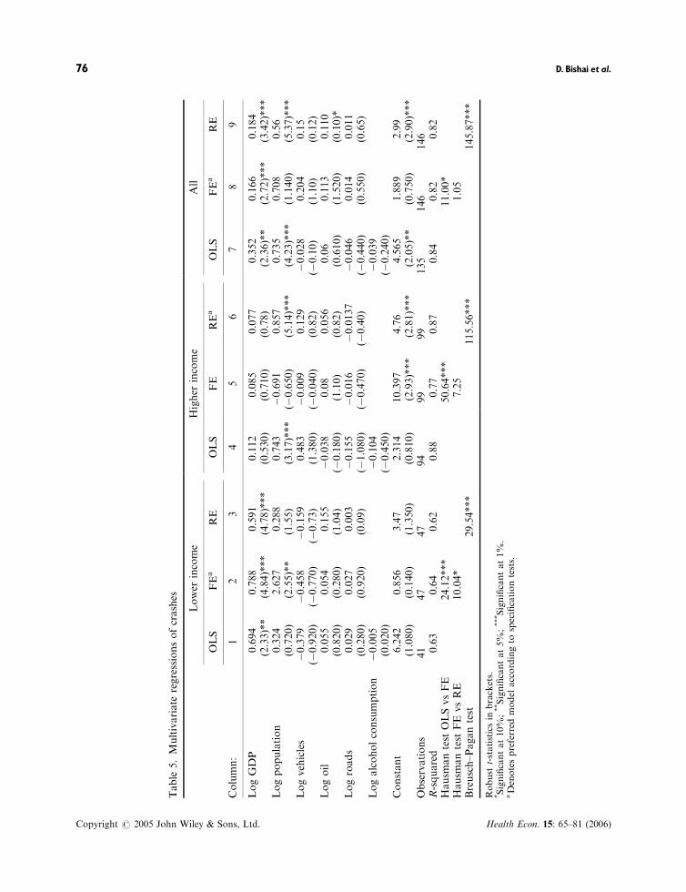
Tables 5–7 show multivariate results for crashes,injuries, and deaths. The structure of each tableincludes 3 sets of 3 columns each. The first set usesdata on the subsample of lower income countries,the second uses data on the wealthier countries,

and the final uses all of the available data. The firstmodel of each set is an ordinary least squares(OLS). Since alcohol is only available for oneyear during the period, alcohol is omitted fromthe fixed effects (FE) and random effects (RE)models. The Breusch–Pagan test results decisivelyindicate the presence of non-zero unmeasuredcountry level effects, which violate the assumptionof the OLS specification. The Hausman testsresults shown at the bottom of each table show apreference for the FE specification most of thetime. The overall pattern of significance andcoefficient magnitudes are similar between REand FE models.

Due to the log–log structure of the regressionequation, the regression coefficients can be inter-preted as elasticities. In other words the coefficientof 0.788 on log GDP model 2 in Table 5 suggeststhat holding all other factors constant, a 10% risein GDP in this sample would be correlated with a7.88% rise in crashes in the sample of low income

Log

Roa

d D

eath

s pe

r C

apita

Log GDP per Capita

5 6 7 8 9 10 11

2

3

4

5

6

AusBul

Bye

EcuSV

Est

Fin

Fra

Geo

Ger

Gre

Hon

Ind

IsrJap

KazKor

Lit

Mal

Net

New

Nic

Nor

Pak

Por

Rom

Sau

Sen

Slo

Spa

Sri

Swe

SwiTur

UK

US

YemZim

AusBul

Bye

EcuSV

Est

Fin

FraGeo

Ger

Gre

HonInd

IsrJap

KorLit

Mac

Mal

Nam

Net

New

NicNor

Pak

Por

Rom

Sen

Slo

Spa

SriSwe

SwiTur

UK

US

YemZim

AusBul Bye Cro

Ecu

Est

Fin

Fra

Geo

Ger

Gre

Hon

Isr

Jap

Kaz

KorLit

Mac

Mal

Nam

Net

New

Nic

Nor

Pak

Por

Rom

Sau

Sen

SloSpa

Sri

Swe

SwiTur

UK

US

Zim

AusBul

Bye

Cam

Cro

Ecu

SV

Est

Fin

Fra

Geo

Ger

Gre

Hon

Isr

Kaz

Kor

Lit

Mac

Mal

Nam

Net

Nic

Nor

Pak

Por

Rom

Sen

Slo

Sri

Swe

SwiTur

US

Yem

Zim

AusBul

Cam

Cro

SV

Est

Fin

Fra

Ger

Gre

Hon

Ice

Kaz

Kor

Lit

Nam

Nor

Por

Rom Slo

SwiTur

US

Yem

Zim

Figure 1. Scatterplot of Log Road Deaths per capita vs Log GDP per capita 1992–1996. KEY: Country abbreviations are initial

letters from the list below with exceptions noted in (): Austria, Bulgaria, Byelarus, Cambodia, Croatia, Ecuador, El Salvador (SV),

Estonia, Finland, France, Georgia, Germany, Greece, Hong-Kong, India, Israel, Kazakhstan, Lithuania, Macedonia, Malaysia,

Namibia, Netherlands, Nicaragua, Norway, Pakistan, Portugal, Republic of Korea (Kor), Romania, Saudi Arabia, Senegal,

Slovakia, Sri Lanka, Sweden, Switzerland, United Kingdom (UK) United States (US), Yemen, Zimbabwe

National Road Casualties and Economic Development 73

Copyright # 2005 John Wiley & Sons, Ltd. Health Econ. 15: 65–81 (2006)

countries. Note that in Table 5 the positiverelationship between crashes and GDP is strongerand more significant in low income countries, and

the results in the full sample are attributable to theeffects in the low income subset. Alcohol useappears to increase traffic deaths (Table 7) with

Log

Acc

iden

ts p

er P

erso

n

Log GDP per Capita5 6 7 8 9 10 11

5

6

7

8

9

Aus

Bul Bye

EcuSV

Est

Fin

Fra

Geo

Ger

GreHon

Ind

Isr

Jap

Kaz

Kor

Lit

Mal

Nam

Net

New

Nic

Nor

Pak

Por

Rom

Sau

SenSlo

SpaSri

Swe

Swi

Tur

UK

US

Yem

Zim

Aus

BulBye

EcuSV

Est

Fin

Fra

Geo

Ger

GreHon

Ind

Isr

JapKor

Lit

Mac

Mal

Nam

Net

New

Nic

Nor

Pak

Por

Rom

Sen Slo

SpaSri

Swe

Swi

Tur

UK

US

Yem

Zim

Aus

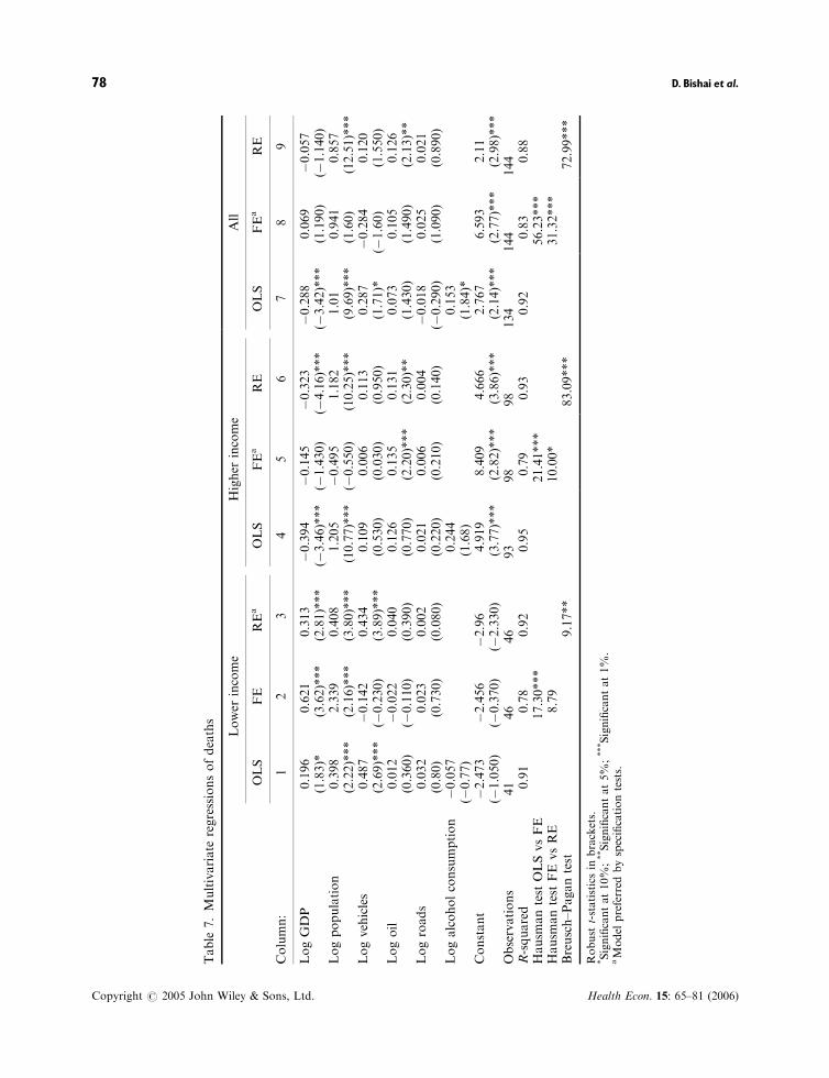
Bul

Bye

Cro

Ecu

Est

Fin

Fra

Geo

Ger

GreHon

Isr

Jap

Kaz

Kor

LitMac

Mal

Nam

Net

New

Nic

Nor

Pak

Por

Rom

SauSen

Slo

Spa

Sri

Swe

Swi

Tur

UK

US

Zim

Aus

Bul

Bye

Cam

Cro

Ecu

SV

Est

Fin

Fra

Geo

Ger

GreHon

Isr

Kaz

Kor

LitMac

Mal

Nam

Net

Nic Nor

Pak

Por

Rom

Sen

Slo

SpaSri

Swe

Swi

Tur

US

Yem

Zim

Aus

Bul

Cam

Cro

SV

Est

Fin

Fra

Ger

Gre Hon

Ice

Kaz

Kor

Lit

Nam

Nor

Por

Rom

Slo

Spa

Swi

Tur

US

Yem

Zim

Figure 2. Scatterplot of Log Traffic Crashes per capita vs Log GDP per capita 1992–1996. Key as per Figure 1

Log

Tra

ffic

Inju

ries

per

Per

son

Log GDP per Capita

5 6 7 8 9 10 11

5

6

7

8

9 Aus

BulBye

Ecu

SV

Est

Fin

Fra

Geo

Ger

GreHon

Ind

IsrJap

Kaz

Kor

Lit

Mal

Net

New

Nic

Nor

Pak

Por

Rom

Sau

Sen

Slo

Spa

Sri

Swe

Swi

Tur

UK

US

Yem

Zim

Aus

Bul

Bye

Ecu

SVEst

Fin

Fra

Geo

Ger

GreHon

Ind

Isr JapKor

LitMac

Mal

Net

New

Nic

Nor

Pak

Por

Rom

Sen

Slo

Spa

Sri

Swe

Swi

Tur

UK

US

Yem

Zim

Aus

Bul

Bye

Cro

Ecu

Est

Fin

Fra

Geo

Ger

GreHon

Isr Jap

Kaz

Kor

Lit

Mac

Mal

Nam

Net

New

Nic

Nor

Pak

Por

Rom

Sau

Sen

Slo

Spa

Sri

Swe

Swi

Tur

UK

US

Zim

Aus

Bul

Bye

Cam

Cro

EcuSV

Est

Fin

Fra

Geo

Ger

GreHon

Isr

Kaz

Kor

Lit

Mac

Mal

Nam

Net

Nic

Nor

Pak

Por

Rom

Sen

Slo

Spa

Sri

Swe

Swi

Tur

US

Yem

Zim

Aus

Bul

Cam

Cro

SV

Est

Fin

Fra

Ger

Gre Hon

Ice

Kaz

Kor

Lit

Nam

Nor

Por

Rom

Slo

Spa

Swi

Tur

US

Yem

Zim

Figure 3. Scatterplot of Log Traffic Injuries per capita vs Log GDP per capita: 1992–1996. Key: as per Figure 1

D. Bishai et al.74

Copyright # 2005 John Wiley & Sons, Ltd. Health Econ. 15: 65–81 (2006)

most of its contribution occurring in rich coun-tries. Note that alcohol use does not predict anincrease in the number of crashes (Table 5) orinjuries (Table 6). It is unusual that alcohol effectsare seen for deaths, but not for crashes andinjuries. This is counterintuitive and may reflectthe inability of ecological models to fully reflectfactors that increase risk on an individual basis[28].

Table 6 suggests that like crashes, injuries aremore strongly positively related to GDP amonglower income than higher income countries. Notefurther that according to the OLS models inTable 6 holding the number of vehicles andpersons constant, low income countries thatconsume more oil have fewer injuries. In the OLSmodel it is likely that oil usage is reflecting factorsrelated to the type of vehicles used in a country. Ifa country used more motor fuel, but held thenumber of vehicles and people constant, onewould suspect that such a country would havelarger vehicles. Fixed effects and random effectsmodels eliminate this type of ‘vehicle mix’ con-founding and in models 2,3,5,6,8, and 9 of Table 6,the protective effect of oil is absent. In wealthiercountries, the preferred models reveal that addi-tional oil use is, all other things equal, associatedwith more injuries (Table 6, Column 5) and deaths(Table 7, Column 5), but not more crashes(Table 5, Column 6). This gives a suggestion thatthe pure effect of additional oil use, e.g. absentfixed effects such as vehicle mix, is to increase the‘energy’ associated with each crash leading tomore injuries and deaths.

Table 7 recovers evidence for the biphasicrelationship between GDP/capita and trafficdeaths per capita with a positive relationship inlow income countries and a negative or zero effectin higher income countries. Table 7 also points outthat for lower income countries holding GDPfixed, growth in the number of vehicles and inpopulation are both stronger contributors totraffic deaths than GDP itself.

The fixed effects models in Table 7 show thatunobservable country effects always bias theeffects of GDP negatively. In lower incomecountries where GDP increases traffic mortalitythese harmful effects are underestimated by OLSmodels, suggesting that the unobservable factorsconfounded with GDP are protective. In higherincome countries where GDP decreases mortality,the protective effects of GDP are overestimated,again suggesting that the unobservable factorsT

able

4.Bivariate

log–logregressionsofaccidents,injuries,anddeaths

Poorcountries

Richcountries

Allcountries

Acc

Inj

Deaths

Acc

Inj

Deaths

Acc

Inj

Deaths

LogGDP

0.724

0.681

0.939

0.775

0.904

0.598

0.629

0.758

0.452

(5.15)***

(4.53)***

(8.66)***

(9.83)***

(11.75)***

(8.81)***

(9.15)***

(11.83)***

(7.63)***

Logpopulation

0.702

0.658

0.889

1.11

1.193

1.034

1.002

1.05

0.996

(9.33)***

(5.05)***

(15.34)***

(13.08)***

(12.20)***

(24.31)***

(8.90)***

(7.45)***

(22.73)***

Logvehicles

0.32

0.49

0.848

0.94

1.043

0.854

0.799

0.945

0.732

(1.310)

(1.97)*

(4.25)***

(17.32)***

(16.62)***

(12.32)***

(10.54)***

(13.41)***

(10.30)***

Logalcoholconsumption

�0.237

�0.107

0.033

0.551

0.958

0.557

0.283

0.585

0.277

(�1.460)

(�0.90)

(0.220)

(1.380)

(2.57)**

(1.79)*

(1.30)

(2.59)**

(1.50)

Logroads

0.557

0.509

0.698

0.818

0.863

0.752

0.781

0.82

0.738

(3.47)***

(2.89)**

(3.84)***

(5.67)***

(6.50)***

(9.45)***

(6.35)***

(6.67)***

(10.46)***

Logoil

0.426

0.327

0.595

0.924

0.994

0.853

0.836

0.922

0.768

(2.68)**

(1.450)

(2.06)*

(14.71)***

(12.48)***

(10.05)***

(11.21)***

(10.25)***

(9.39)***

Poorcountriesdefined

asGDP/capita5

$1600/person.Allregressionsincludeonly

thelogged

annualcountofoutcomes

vsonelogged

independentvariableandaconstant.

Acc=

Log(A

ccidentcount);Inj=

Log(Injury

count);Deaths=

Log(D

eath

count).Robust

t-statisticsin

brackets.

*Significantat10%

;**Significantat5%

;***Significantat1%

.

National Road Casualties and Economic Development 75

Copyright # 2005 John Wiley & Sons, Ltd. Health Econ. 15: 65–81 (2006)

Table

5.Multivariate

regressionsofcrashes

Lower

income

Higher

income

All

OLS

FEa

RE

OLS

FE

REa

OLS

FEa

RE

Column:

12

34

56

78

9

LogGDP

0.694

0.788

0.591

0.112

0.085

0.077

0.352

0.166

0.184

(2.33)**

(4.84)***

(4.78)***

(0.530)

(0.710)

(0.78)

(2.36)**

(2.72)***

(3.42)***

Logpopulation

0.324

2.627

0.288

0.743

�0.691

0.857

0.735

0.708

0.56

(0.720)

(2.55)**

(1.55)

(3.17)***

(�0.650)

(5.14)***

(4.23)***

(1.140)

(5.37)***

Logvehicles

�0.379

�0.458

�0.159

0.483

�0.009

0.129

�0.028

0.204

0.15

(�0.920)

(�0.770)

(�0.73)

(1.380)

(�0.040)

(0.82)

(�0.10)

(1.10)

(0.12)

Logoil

0.055

0.054

0.155

�0.038

0.08

0.056

0.06

0.113

0.110

(0.820)

(0.280)

(1.04)

(�0.180)

(1.10)

(0.82)

(0.610)

(1.520)

(0.10)*

Logroads

0.029

0.027

0.003

�0.155

�0.016

�0.0137

�0.046

0.014

0.011

(0.280)

(0.920)

(0.09)

(�1.080)

(�0.470)

(�0.40)

(�0.440)

(0.550)

(0.65)

Logalcoholconsumption

�0.005

�0.104

�0.039

(0.020)

(�0.450)

(�0.240)

Constant

6.242

0.856

3.47

2.314

10.397

4.76

4.565

1.889

2.99

(1.080)

(0.140)

(1.350)

(0.810)

(2.93)***

(2.81)***

(2.05)**

(0.750)

(2.90)***

Observations

41

47

47

94

99

99

135

146

146

R-squared

0.63

0.64

0.62

0.88

0.77

0.87

0.84

0.82

0.82

Hausm

antest

OLSvsFE

24.12***

50.64***

11.00*

Hausm

antest

FEvsRE

10.04*

7.25

1.05

Breusch–Pagantest

29.54***

115.56***

145.87***

Robust

t-statisticsin

brackets.

*Significantat10%;**Significantat5%

;***Significantat1%

.aDenotespreferred

model

accordingto

specificationtests.

D. Bishai et al.76

Copyright # 2005 John Wiley & Sons, Ltd. Health Econ. 15: 65–81 (2006)

Table

6.Multivariate

regressionsofinjuries

Lower

income

Higher

income

All

OLS

FE

REa

OLS

FEa

RE

OLS

FEa

RE

Column:

12

34

56

78

9

LogGDP

0.63

0.677

0.473

0.175

0.057

0.031

0.386

0.168

0.186

(3.41)***

(2.62)**

(2.78)***

(0.850)

(0.830)

(0.480)

(3.17)***

(2.90)***

(3.55)***

Logpopulation

0.285

2.922

0.302

0.708

�0.755

0.717

0.639

0.821

0.466

(1.070)

(1.79)*

(1.69)*

(3.23)***

(�1.240)

(5.050)***

(4.10)***

(1.390)

(4.93)***

Logvehicles

0.182

�0.758

0.133

0.46

0.214

0.296

0.315

�0.014

0.320

(0.780)

(�0.80)

(0.71)

(1.370)

(1.74)*

(2.70)***

(1.79)*

(�0.080)

(3.50)***

Logoil

�0.201

0.136

�0.027

�0.027

0.078

0.065

�0.14

0.069

0.078

(�3.20)***

(0.440)

(�0.17)

(�0.130)

(1.87)*

(1.540)

(�2.07)**

(0.970)

(1.240)

Logroads

�0.016

0.022

�0.002

�0.146

�0.011

�0.008

�0.07

0.011

0.007

(�0.250)

(0.470)

(�0.04)

(�0.770)

(�0.570)

(�0.380)

(�0.670)

(�0.460)

(0.290)

Logalcoholconsumption�0.056

�0.003

�0.015

(�0.410)

(�0.010)

(�0.120)

Constant

2.756

3.431

2.46

1.777

7.719

3.141

2.279

5.322

1.144

(0.850)

(0.350)

(1.15)

(0.650)

(3.80)***

(2.410)

(1.340)

(2.22)**

(1.210)***

Observations

41

45

45

94

99

99

135

144

146

R-squared

0.77

0.57

0.69

0.88

0.55

0.87

0.89

0.76

0.86

Hausm

antest

OLSvsFE

18.47***

59.68***

42.93***

Hausm

antest

FEvsRE

6.35

29***

13.07**

Breusch–Pagantest

20.72***

139.76***

164.43***

Robust

t-statisticsin

brackets.

*Significantat10%;**Significantat5%

;***Significantat1%

.aPreferred

model

byspecificationtests.

National Road Casualties and Economic Development 77

Copyright # 2005 John Wiley & Sons, Ltd. Health Econ. 15: 65–81 (2006)

Table

7.Multivariate

regressionsofdeaths

Lower

income

Higher

income

All

OLS

FE

REa

OLS

FEa

RE

OLS

FEa

RE

Column:

12

34

56

78

9

LogGDP

0.196

0.621

0.313

�0.394

�0.145

�0.323

�0.288

0.069

�0.057

(1.83)*

(3.62)***

(2.81)***

(�3.46)***

(�1.430)

(�4.16)***

(�3.42)***

(1.190)

(�1.140)

Logpopulation

0.398

2.339

0.408

1.205

�0.495

1.182

1.01

0.941

0.857

(2.22)***

(2.16)***

(3.80)***

(10.77)***

(�0.550)

(10.25)***

(9.69)***

(1.60)

(12.51)***

Logvehicles

0.487

�0.142

0.434

0.109

0.006

0.113

0.287

�0.284

0.120

(2.69)***

(�0.230)

(3.89)***

(0.530)

(0.030)

(0.950)

(1.71)*

(�1.60)

(1.550)

Logoil

0.012

�0.022

0.040

0.126

0.135

0.131

0.073

0.105

0.126

(0.360)

(�0.110)

(0.390)

(0.770)

(2.20)***

(2.30)**

(1.430)

(1.490)

(2.13)**

Logroads

0.032

0.023

0.002

0.021

0.006

0.004

�0.018

0.025

0.021

(0.80)

(0.730)

(0.080)

(0.220)

(0.210)

(0.140)

(�0.290)

(1.090)

(0.890)

Logalcoholconsumption

�0.057

0.244

0.153

(�0.77)

(1.68)

(1.84)*

Constant

�2.473

�2.456

�2.96

4.919

8.409

4.666

2.767

6.593

2.11

(�1.050)

(�0.370)

(�2.330)

(3.77)***

(2.82)***

(3.86)***

(2.14)***

(2.77)***

(2.98)***

Observations

41

46

46

93

98

98

134

144

144

R-squared

0.91

0.78

0.92

0.95

0.79

0.93

0.92

0.83

0.88

Hausm

antest

OLSvsFE

17.30***

21.41***

56.23***

Hausm

antest

FE

vsRE

8.79

10.00*

31.32***

Breusch–Pagantest

9.17**

83.09***

72.99***

Robust

t-statisticsin

brackets.

*Significantat10%;**Significantat5%

;***Significantat1%

.aModel

preferred

byspecificationtests.

D. Bishai et al.78

Copyright # 2005 John Wiley & Sons, Ltd. Health Econ. 15: 65–81 (2006)

confounded with GDP are protective. In otherwords, under the assumption that GDP is con-founded with unmeasured co-factors in OLSmodels – these confounders work to reduce deathsin both lower and higher income countries.

All of the independent variables in the analysisare highly correlated. Raw correlation coefficientsranged from a low of 0.6722 for Cor (Log GDP,Log Pop) to a high of 0.8957 for Cor (LogVehicles, Log Oil). Comparing the bivariate resultsto the multivariate results indicates that thesignificant effects of roads and vehicles in thebivariate regressions are often lost in multivariatespecifications because of this colinearity. Oil use isalso collinear with GDP, vehicles, and roads. Ithas positive effects on crashes, injuries, and deathsin the bivariate specification, but, as discussedabove, oil use has protective effects in the multi-variate models because it may proxy for vehicletype.

Discussion

Prior analysis of longitudinal cross country dataon traffic deaths has found an early positive effectof GDP/capita on fatalities followed decades laterby a protective negative effect [3]. This study offerssome clues about what makes GDP growthprotective in rich countries and hazardous in lowincome countries. Much of the complexity stemsfrom using GDP as a proxy measure for a host ofrelevant, hard-to-measure factors including urba-nization, vehicle mix, road quality, and healthservices. Although these factors tend to correlatewith GDP – they remain largely unidentified. Bycomparing the OLS models to FE models, wedevelop insight that these unidentified factorsappear to reduce fatalities in both rich and poorcountries, and may be related to institutionalcapacity of the legal and medical systems.

Prior speculation on the reason for the rise oftraffic deaths with GDP growth in low incomecountries held that it was due to mobility growth –more commodities being produced leads to morevehicles to deliver them, and more kilometerstraveled. The results here suggest a modification ofthat hypothesis, because GDP growth, holdingpopulation fixed, appears to increase deaths,injuries, and crashes independently of vehiclecounts or oil consumption, or – in fixed effectsmodels – other unmeasured confounders. In low

income countries GDP growth appear to increasethe inherent hazardousness of driving, not just themobility of the population. One mechanism forthis could be an increase in pedestrian and cyclistactivity (holding motorized vehicles fixed) thatcould accompany GDP growth in low incomecountries holding oil use and motor vehicle countsfixed. The latest data from Uganda show that themajority of traffic injuries involved cyclists [29].

Our theoretical framework supported fouralternative explanations linking rising GDP inhigher income countries to reductions in trafficcasualties: (1) The institutional capacity to controlexternalities; (2) An accumulation of investmentsin controlling competing risks rendering trafficcontrol investments the next best use of funds; (3)A correlation of GDP with a transition away frommotorized bicycles towards sedans; (4) The avail-ability of improved trauma care. Of these fourmechanisms, improvements in pre-hospital andemergency medical care would reduce death ratesonly, while the other three explanations predictfewer crashes and/or fewer injuries as well. Sincethe observed patterns in Figures 1–3 show only adecline in deaths, but no decline of crashes orinjuries, our findings lend the most support for thetheory that improvements in the survival oftrauma victims is the leading factor behind thesuccessful control of traffic casualties in higherincome countries. Both improved emergencytrauma care and occupant protection devicescould improve death rates without reducingcrashes or injuries. All of the other theories thatconnect economic growth to traffic safety predictdeclines in crash or injury rates as high incomecountries develop that have not (as of 1996) beenobserved in the data.

Prior authors have suspected that both improve-ments in traffic infrastructure and in effective post-injury ambulance transport and medical care couldmediate the effect of GDP/capita on trafficcasualties [3]. Because GDP/capita growth in highincome countries was not associated with reduc-tions in injuries or crashes, we find it difficult tocredit a major role for GDP related improvementsin traffic infrastructure that prevent crashes. It isconceivable that improvements in occupant pro-tection and reductions in crash severity somehowreduce fatalities without reducing the number ofnonfatal injuries. It may also be that injuries, butnot deaths are systematically over-reported inhigher income countries. The presence of motoristinsurance systems in higher income countries

National Road Casualties and Economic Development 79

Copyright # 2005 John Wiley & Sons, Ltd. Health Econ. 15: 65–81 (2006)

could provide an incentive for growing numbers ofminimally injured motorists to seek medical care inorder to be indemnified. Until injury surveillancesystems improve their tracking of injury severity inmore countries it will be difficult to know whetherthere are cross-country trends towards lowerinjury severity that one would expect if occupantprotection and vehicle design factors were playingan important role.

There were several limitations of this study. Theset of countries with available data are unlikely tobe representative of any particular region or stageof development. Countries with missing years ofdata contribute less than other countries, furtherimpairing any representativeness of the dataset.Where they are measured, data on casualties fromlower income countries could be measured witherror which would bias our results towards zero.Data on crashes may be systematically morecomplete where police resources and GDP arehigher lending an upward reporting bias toestimates of traffic events per change in GDP.One could also conjecture that the very availabilityof traffic casualty data from a low income countrymay be correlated with greater investment ofgovernment resources in traffic issues. Thus sampleselection bias could create a downward bias in ourfindings. A selection bias in government statisticswould allow for the appearance of fewer incre-mental casualties per increment of GDP Despitethese limitations, the major qualitative differencesin the time course of fatalities (inverted-U), vsinjuries and crashes (monotonic growth) (Figures1–3) should be immune to sample selection bias.

Conclusion

According to Red Cross estimates, the costs ofroad transport crashes in developing countries, atmore than $50 billion annually, exceeds the totalworld expenditure on foreign aid [2]. In lowincome countries, it appears that GDP/capitagrowth is associated with a rise in traffic deaths.The mechanism is independent of oil use, popula-tion and vehicle ownership, and may be related toincreases in pedestrian or cyclist activity requiredto transact the exchanges that are necessary forGDP/capita to grow holding vehicle counts and oiluse fixed. In rich countries GDP growth lowerstraffic fatalities. Because GDP does not lower thenumbers of crashes or injuries in rich countries, the

mediating factor there may indeed be occupantprotection as well as post-injury ambulance trans-port and trauma care which can reduce deaths.

Low income countries interested in a develop-ment path that softens the link between GDPgrowth and traffic fatalities, urgently need tocollect basic data on the patterns of traffic fatal-ities. Cost-effective measures to protect pedestriansand cyclists do exist for countries that identifythese groups as having a heightened risk [30–32].

In higher income countries, petroleum andalcohol both appear to contribute to the problemof traffic deaths. Both of these liquids are heavilyregulated and taxed, although seldom with theexpress intent of controlling traffic fatalities. Morecomplete assessment of the economic effects ofhigher fuel prices and higher alcohol prices shouldinclude estimates of the savings due to trafficfatalities that are averted.

Acknowledgements

The authors wish to thank the Johns Hopkins Center forInjury Research and Policy (supported by Centers forDisease Control and Prevention Grant#R49CCR302486) and the Hopkins Population Center(Supported by NIH Grant 5P30AI042855-04). Helpfulcomments were contributed by Maureen Cropper,Adnan Hyder, Eva Jarawan, Mead Over, and anon-ymous referees.

References1. Murray C, Lopez A. The Global Burden of Disease.

Harvard Press: Cambridge, MA, 1996.2. International Federation of Red Cross and Red

Crescent Societies. Must Millions More Die fromTraffic Accidents? In World Disasters Report,Societies IFoRCaRC (ed.). Oxford University Press:New York, 1998.

3. van Beeck EF, Borsboom GJ, Mackenbach JP.Economic development and traffic accident mortal-ity in the industrialized world, 1962–1990. IntJ Epidemiol 2000; 29(3): 503–509.

4. Dasgupta S, Laplante B, Wang H, Wheeler D.Confronting the environmental Kuznets curve.J Econ Perspect 2002; 16(1): 147–168.

5. Kopits E, Cropper M. Traffic fatalities and econom-ic growth. Accid Anal Prev 2005; 37(1): 169–178.

6. Vickrey W. Automobile accidents, Tort law, ex-ternalities, and insurance: an economist’s critique.Law Contemp Problems 1968; 33: 464–487.

D. Bishai et al.80

Copyright # 2005 John Wiley & Sons, Ltd. Health Econ. 15: 65–81 (2006)

7. Calabresi G. The Costs of Accidents: A Legal andEconomic Analysis. Yale University Press: NewHaven, 1970.

8. Coase R. The problem of social cost. J Law Econ1960; 3(October): 1–44.

9. Ruhm CJ. Alcohol policies and highway vehiclefatalities. J Health Econ 1996; 15(4): 435–454.

10. Chaloupka FJ, Grossman M, Saffer H. The effectsof price on the consequences of alcohol use andabuse. Recent Dev Alcohol 1998; 14: 331–346.

11. Bishai D, Hyder AA, Ghaffar A, Morrow RH,Kobusingye O. Rates of public investment for roadsafety in developing countries: case studies ofUganda and Pakistan. Health Policy Plan 2003;18(2): 232–235.

12. Jacobs G. The inclusion of accident savings inhighway cost-benefit analyses. Mimeo. TransportResearch Laboratory: Crowthorne, Berkshire, UK,1989.

13. Norton R, Hyder A, Bishai D, Peden M. Uninten-tional Injuries. In Disease Control Priorities-2,Jamison DT, Musgrove P, Meachem A (eds).National Institutes of Health: Washington, DC,2005.

14. Mohan R. Understanding the Developing MetropolisLessons from the City Study of Bogota and Cali,Colombia. World Bank: Washington, DC, 1994.

15. Tay R. Marginal effects of changing the vehicle mixon fatal crashes. J Transport Econ Policy 2003;37(3): 439–450.

16. Mock CN, Jurkovich GJ, nii-Amon-Kotei D,Arreola-Risa C, Maier RV. Trauma mortalitypatterns in three nations at different economiclevels: implications for global trauma system devel-opment. J Trauma 1998; 44(5): 804–812 (discussion812–4).

17. Adam R, Stedman M, Winn J, Howard M, WilliamsJI, Ali J. Improving trauma care in Trinidad andTobago. West Indian Med J 1994; 43(2): 36–38.

18. Arreola-Risa C, Mock CN, Lojero-Wheatly L et al.Low-cost improvements in prehospital trauma care

in a Latin American city. J Trauma 2000; 48(1):119–124.

19. Husum H, Gilbert M, Wisborg T, Van Heng Y,Murad M. Rural prehospital trauma systemsimprove trauma outcome in low-income countries:a prospective study from North Iraq and Cambodia.J Trauma 2003; 54(6): 1188–1196.

20. International Road Federation. IRF World RoadStatistics – 1998 Edition. International Road Fed-eration: Washington, DC, 1998.

21. Ghaffar A. Measuring the Burden of Injuries inPakistan. Johns Hopkins University: Baltimore,MD; 2000.

22. World Bank. The World Development Report.Oxford University Press: New York, 1993–1997.

23. WHO. Global Status Report on Alcohol. Geneva,1999.

24. Smeed RJ. Some statistical aspects of road safetyresearch. J Roy Stat Soc Ser A 1949; 112: 1–23.

25. Hausman JA. Specification tests in econometrics.Econometrica 1978; 46(6): 1251–1271.

26. Stata Corporation. Stata Reference Manual Release8. Stata Press: College Station, TX, 2003.

27. Weesie J. Seemingly unrelated estimation and thecluster-adjusted sandwich estimator. Stata Tech Bull1999; 52: 34–47.

28. Piantadosi S, Byar DP, Green SB. The ecologicalfallacy. Am J Epidemiol 1988; 127(5): 893–904.

29. Kobusingye O, Guwatudde D, Lett R. Injurypatterns in rural and urban Uganda. Inj Prev2001; 7(1): 46–50.

30. Malek M, Guyer B, Lescohier I. The epidemiologyand prevention of child pedestrian injury. AccidAnal Prev 1990; 22(4): 301–313.

31. Chiu WT, Kuo CY, Hung CC, Chen M. The effectof the Taiwan motorcycle helmet use law on headinjuries. Am J Public Health 2000; 90(5): 793–796.

32. Bishai D, Hyder AA. Modeling the cost effective-ness of injury counter measures in lower and middleincome countries. DCPP Working Paper 2004;http://www.fic.nih.gov/dcpp/wps/WP29.pdf.

National Road Casualties and Economic Development 81

Copyright # 2005 John Wiley & Sons, Ltd. Health Econ. 15: 65–81 (2006)