decoupling of road freight energy use from economic growth in the united kingdom

Energy Policy 41 (2012) 84–97

Contents lists available at ScienceDirect

Energy Policy

0301-42

doi:10.1

n Corr

E-m

journal homepage: www.elsevier.com/locate/enpol

Decoupling of road freight energy use from economic growthin the United Kingdom

Steve Sorrell a,n, Markku Lehtonen a, Lee Stapleton a, Javier Pujol a, Toby Champion b

a Sussex Energy Group, SPRU (Science & Technology Policy Research), Freeman Centre, University of Sussex, Falmer, Brighton, BN1 9QE, UKb Toby Champion Associates, UK

a r t i c l e i n f o

Article history:

Received 12 November 2009

Accepted 2 July 2010Available online 3 August 2010

Keywords:

Freight transport

Energy intensity

Decoupling

15/$ - see front matter & 2010 Elsevier Ltd. A

016/j.enpol.2010.07.007

esponding author. Tel.: +44 1273 877067; fa

ail address: [email protected] (S. Sorrell

a b s t r a c t

Between 1989 and 2004, energy consumption for road freight in the UK is estimated to have increased

by only 6.3%. Over the same period, UK GDP increased by 43.3%, implying that the aggregate energy

intensity of UK road freight fell by 25.8%. During this period, therefore, the UK achieved relative but not

absolute decoupling of road freight energy consumption from GDP. Other measures of road freight

activity, such as tonnes lifted, tonnes moved, loaded distance travelled and total distance travelled also

increased much slower than GDP. The main factor contributing to the observed decoupling was the

declining value of manufactured goods relative to GDP. Reductions in the average payload weight, the

amount of empty running and the fuel use per vehicle kilometre also appear to have made a

contribution, while other factors have acted to increase aggregate energy intensity. The results

demonstrate that the UK has been more successful than most EU countries in decoupling the

environmental impacts of road freight transport from GDP. However, this is largely the unintended

outcome of various economic trends rather than the deliberate result of policy.

& 2010 Elsevier Ltd. All rights reserved.

1. Introduction

The contribution of freight transport to climate change issubstantial and growing. Globally, freight transport accounts forone third of transport energy consumption and around 8% of totalenergy-related carbon dioxide (CO2) emissions. The bulk of theseemissions derive from heavy goods vehicles (HGVs), which inmost countries account for the majority of freight activity. In theUK, for example, HGVs account for more than 68% of goods moved(tonne kilometres), 24% of road fuel use, 22% of transport CO2

emissions and 5% of total CO2 emissions (DfT, 2005b).Despite this, freight transport has been relatively neglected in

terms of both climate policy and the associated policy research.Policy initiatives to restrain the growth in energy use and carbonemissions from this sector (e.g. the UK Sustainable DistributionStrategy and Freight Best Practice programme) have been bothlimited and ineffective, while policy research has focuseddisproportionately upon passenger transport. Both the EuropeanUnion and the UK have the stated goal of decouplingvarious measures of road freight activity from GDP, but this hasgenerally been interpreted as relative rather than absolutedecoupling – implying that energy use and carbon emissionscould continue to increase, even if the objective was met.

ll rights reserved.

x: +44 1273 685865.

).

Freight activity is driven by complex and interlinked trends inproduction, trade, distribution and retail, including incomegrowth, wider sourcing of products, increased specialisation,‘just-in-time’ distribution and increasing concentration of manu-facturing and stockholding (Lehtonen, 2008; McKinnon andWoodburn, 1996; NEI, 1997). The corresponding impact onenergy use and carbon emissions may be either enhanced oroffset by parallel trends in logistics, vehicle technology and themanagement of transport resources, including factors such as thesize, fuel efficiency and average load factor of vehicles. Some ofthese trends have led to greater energy use in this sector overrecent years, while others have encouraged reductions in energyuse. If the growth in carbon emissions from freight transport is tobe halted and reversed, the nature and relative importance ofthese trends needs to be better understood.

This paper contributes to that end by examining trends in tenvariables that have strongly influenced UK road freight energyconsumption over the period 1989–2004. Following McKinnon(2007), we call these variables key ratios since they are each formedfrom the ratio of two other variables which we term key quantities.For example, the ratio of the ‘goods moved’ by freight vehicles(tonne kilometres) to the ‘goods lifted’ by freight vehicles (tonneslifted) represents one such key ratio (the average ‘length of haul’).

This paper shows how UK road freight energy consumptioncan be expressed as the product of these ten key ratios and GDP.Some of these key ratios (e.g. the average length of haul) haveincreased in magnitude since 1989 and thereby led to greater

www.elsevier.com/locate/enpol

dx.doi.org/10.1016/j.enpol.2010.07.007

mailto:[email protected]

dx.doi.org/10.1016/j.enpol.2010.07.007

Table 1Key quantities.

Acronym Definition Measure

GDPt UK gross domestic product £

MANDct Value of domestically produced

manufactured goods in basic prices, broken

down by commodity group

£

MANTct Value of the total supply of manufactured

goods in basic prices, broken down by

commodity group

£

MLIFTct Weight of goods lifted by all modes of

freight transport

Tonnes

S. Sorrell et al. / Energy Policy 41 (2012) 84–97 85

energy consumption, while others (e.g. the amount of emptyrunning) have decreased and led to reduced energy consumption.The paper explores the measurement, meaning and significance ofthese key ratios, together with the key quantities from which theyare formed, and summarises their trends over the period1989–2004. It also examines how these trends vary betweendifferent vehicle types and commodity groups. The analysis ismuch more disaggregated than previous studies in this area(e.g. Kamakate and Schipper, 2009) and provides a nuancedpicture of the factors underlying the aggregate trend in UK roadfreight fuel consumption. This in turn allows the main reasons forthe observed decoupling to be identified.

TLIFTckt Weight of goods lifted by HGVs Tonnes

TKMckt Weight of goods moved by HGVs Tonne-km

VKMckt Distance driven in loaded HGVs Vehicle-km

VKMTckt Distance driven in loaded and unloaded

HGVs

Vehicle-km

FUELckt Estimated energy consumption by HGVs Litres of fuel

Notes:

� All key quantities refer to the UK. All transport key quantities include the

activities of both UK and foreign-registered HGVs.

� Basic prices include taxes (less subsidies) on production, but do not include

taxes/subsidies on the products themselves (e.g. VAT).

2. Method of approach

During the period 1989–2004, energy consumption for roadfreight in the UK is estimated to have increased by only 6.3% whileUK GDP increased by 43.3%, implying that the aggregate energyintensity of UK road freight fell by 25.8% (Fig. 1). During thisperiod, therefore, the UK achieved relative but not absolutedecoupling of road freight energy consumption from GDP. Ourinterest is in exploring the contribution of different variables tothis aggregate trend.

Trends in aggregate quantities such as road freight energyconsumption can be usefully expressed as the product of two ormore variables. For example, the energy consumption of aparticular category of road freight vehicle (k) in year t (FUELkt)could be expressed as the product of the total distance travelledby that category of vehicle (VKMTkt) and the average fuel use perkilometre of that category of vehicle (EINTkt¼FUELkt/VKMTkt). Thetotal energy consumption for all categories of road freight vehiclein year t (FUELt) could then be expressed as

FUELt ¼X

k

FUELkt ¼X

k

VKMTkt�FUELkt

VKMTktð1Þ

FUELt ¼X

k

VKMTkt�EINTkt ð2Þ

Letting Skt¼VKMTkt/VKMTt represent the share of each vehicletype in the total distance travelled by all road freight vehicles inyear t (VKMTt), we can rewrite this as

FUELt ¼X

k

VKMTt�VKMkt

VKMTt

FUELkt

VKMktð3Þ

FUELt ¼X

k

VKMkt�Skt�EINTkt ð4Þ

In the terminology of this paper, Skt and EINTkt are key ratios

while all the other variables are key quantities. The key ratios aredefined for each year and each vehicle type (Skt and EINTkt), butcould also be estimated annually for all vehicle types combined(St and EINTt). Depending upon data availability, the decomposi-tion could be made more complex through the inclusion of

60.0070.0080.0090.00

100.00110.00120.00130.00140.00150.00

199119901989 1994 1998 1999 2000 2004

GDPt FUELt

Inde

x (1

989=

100)

1995 1996 1997 2001 2002 20031992 1993

Fig. 1. Decoupling of UK road freight energy use from GDP.

additional key ratios, or more of the key ratios could be brokendown into additional subcategories – such as different types ofcommodity (c). For example, we could estimate the energyintensity of vehicle type k carrying commodity c in year t – EINTckt.

This study uses ten key ratios to investigate the sources ofchange in UK road freight energy use over the period 1989–2004.1

The analysis is confined to energy use by heavy goods vehicles(HGVs) which account for approximately 80% of goods lifted(tonnes) and 95% of goods moved (tonne kilometres) by road inthe UK. Freight transport by light goods vehicles (o3.5 tonnes) isexcluded owing to inadequate data, although this is acknowl-edged to be an important and growing source of freight transport.

The key ratios and associated key quantities are defined inTables 1 and 2. Key ratios 1–3 are relevant to the supply of goodsin the UK economy while key ratios 4–10 are relevant to thetransport of those goods. The key ratios have been estimated foreach year (t) and several have been disaggregated by fifteencommodity groups (c) and/or six vehicle types (k) (Tables 3and 4). In the graphical presentations that follow, the trends in thekey ratios are presented at the aggregate level (i.e. allcommodities and vehicle types combined), or broken down byeither vehicle type (k) or primary commodity category (p)(Table 3). The aim is to highlight the main trends in thesevariables over the period 1989–2004 and to identify their likelyimportance for road freight energy consumption. In a companionpaper, Sorrell et al. (2009) conduct a formal decompositionanalysis of UK road freight energy consumption, using the fullbreakdown by commodity group (c), vehicle type (k) and year (t).

Using the key quantities, the total energy consumption of trucktype k carrying commodity group c in year t may be expressed as

FUELckt ¼ GDPtMANDt

GDPt

MANDct

MANDt

MANTct

MANDct

MLIFTct

MANTct

TLIFTct

MLIFTct

�TLIFTckt

TLIFTct

TKMckt

TLIFTckt

VKMckt

TKMckt

VKMTckt

VKMckt

FUELckt

VKMTcktð5Þ

1 A longer time series would be desirable, but inconsistencies in the UK Input

Output tables make it difficult to extend the analysis to before 1989. The analysis

may subsequently be updated to include more recent years, but the 2005 changes

in the format of UK freight statistics may create some discontinuities. Also, such

updating is far from straightforward since there are numerous gaps and

inconsistencies in the relevant time series and a great deal of effort is required

to estimate the missing data – see Sorrell et al. (2008).

Table 2Key ratios.

Acronym Definition Interpretation Measure

DOMMANt MANDt

GDPt

Ratio of the value of domestically produced manufactured goods to UK GDP (a measure of the

economic importance of manufactured goods)

Fraction (r1)

CSHAREct MANDct

MANDt

Share of commodity group c in the total value of domestically produced manufactured goods (a

measure of the economic importance of commodity group c)

Fraction (r1)

IDOMSHAREct MANTct

MANDct

Inverse measure of the share of domestic production of commodity group c in the total UK

supply of commodity group c (an inverse measure of the importance of domestic manufacturing

for commodity group c)

Fraction (Z1)

FINTct MLIFTct

MANTct

Ratio of the tonnes lifted of commodity c onto all modes of freight transport to the value of the

UK supply of commodity c (a measure of the ‘freight intensity’ of that commodity)

Tonnes lifted/£

ROADct TLIFTct

MLIFTct

Share of tonnes lifted for commodity group c that are taken by HGV Fraction (r1)

VSIZEckt TLIFTckt

TLIFTct

Share of HGV tonnes lifted for commodity group c that are taken by vehicle type k Fraction (r1)

LOHckt TKMckt

TLIFTckt

Average length of haul for commodity group c in vehicle type k km

ILFckt VKMckt

TKMckt

An inverse measure of the average payload weight for commodity group c in vehicle type k 1/tonnes

ERUNckt VKMTckt

VKMckt

Ratio of total vehicle km to loaded vehicle km for commodity group c in vehicle type k (a

measure of the importance of ‘empty running’ in total vehicle kilometres)

Ratio (Z1)

EINTckt FUELckt

VKMTckt

Energy intensity of vehicle type k carrying commodity group c litres per kilometre

Note: All key ratios refer to the UK. All transport key ratios refer to the activities of both UK and foreign-registered HGVs.

Table 3Primary commodity categories (p) and commodity groups (c).

Primary commodity categories (p) Commodity groups (c)

Food, drink and tobacco Food drink and tobacco

Bulk products Wood timber and cork

Crude minerals

Ores

Crude materials

Coal and coke

Building materials

Iron and steel products

Chemicals, petrol and fertilizer Fertiliser

Petrol and products

Chemicals

Miscellaneous products Other metal products

Machinery and transport equip.

Misc. manufactures

Miscellaneous articles

Table 4Heavy goods vehicle categories (k).

Vehicle type Gross vehicle weight (k)

Rigids Up to 7.5 tonnes

7.5–17 tonnes

17–25 tonnes

Over 25 tonnes

Artics Up to 33 tonnes

Over 33 tonnes

Note: Gross vehicle weight is the maximum permissible weight of the vehicle and

its load.

S. Sorrell et al. / Energy Policy 41 (2012) 84–9786

This can be also written in terms of the key ratios:

FUELckt ¼ GDPt�DOMMANt�CSHAREct�IDOMSHAREct

�FINTct�ROADct�VSIZEckt�LOHckt�ILFckt�ERUNckt�EINTckt

ð6Þ

Total road freight energy consumption in year t is then:

FUELt ¼X

ckFUELckt ð7Þ

If each key ratio remained unchanged over time then theoverall relationship between GDP and road freight energyconsumption would also remain unchanged. But in practice therewill be changes in these ratios, brought about through eitherchange in the relative importance of each commodity and/orvehicle type or changes in the key ratios for each individualcommodity and/or vehicle type. These changes are typicallycomplex, interdependent and frequently uncertain owing to

inadequate data. To provide a comprehensive understanding ofthe driving forces underlying recent changes in UK road freightfuel consumption, the following sections:

�
summarise the relevant sources of data and the associateduncertainties (Section 3); � explain the meaning and significance of each of the
key quantities, together with their trends over the period1989–2004 (Section 4);
� explain the meaning and significance of each of the key ratios,
together with their trends (Section 5); and
� highlight the contribution of both the key quantities and the
key ratios to the aggregate trend in UK road freight fuelconsumption.

3. Data sources

The data required was obtained from several UK and interna-tional sources (Table 5). Inevitably, these form an incompletepicture, with a number of important gaps and omissions whereadditional tabulations and/or estimation is required. Theseadjustments are far from straightforward and uncertaintiesremain for a number of variables, most notably the activity ofgoods vehicles registered outside the UK (Sorrell et al., 2008).

Table 5Primary data sources.

Organisation Document Type of information used

Office of National Statistics Input–output supply and use tables, 1992–2003. The value of UK domestic production, imports and exports,

classified by 123 commodity groups.Input–output supply and use tables 1989–1991, provided separately by

the ONS; not fully comparable with 1992–2003 data.

Department for Transport Continuing survey of road goods transport (CSRGT), plus additional

tabulations requested by the authors

Activity of UK-registered heavy goods vehicles on roads in

the UK

Department for Transport Transport Statistics Great Britain (TSGB) Aggregate data on tonnes lifted by all modes

Department for Transport International Road Haulage Survey (IRHS) International activity of UK-registered HGVs

Department for Transport Roll-on Roll-off enquiry (RoRo) Number of HGVs travelling from GB to mainland Europe,

covering both UK- and foreign-registered vehicles

The Ministry of the

Environment of Northern

Ireland

Northern Ireland Transport Statistics; plus additional tabulations

requested by the authors

Road transport activity in Northern Ireland

Eurostat Eurostat website Road transport activity by foreign-registered vehicles in the

UK; based on sample surveys

8000090000

100000110000120000130000140000150000160000170000180000

1989 1990 1991 1992 1993 1994 1995 1996 1997 1998 1999 2000 2001 2002 2003 2004

GB vehicles in GB All vehicles in UK

Mill

ion

tonn

e km

Fig. 2. Comparing estimates of goods moved (TKMt) by GB-registered vehicles in

GB to goods moved by all vehicles in UK.


Most of the information on freight activity was taken from theContinuing Survey of Road Goods Transport (CSRGT) (DfT, 2005a).This is based upon annual surveys of the activity of a sample ofHGVs registered in the UK. In contrast, the Transport StatisticsGreat Britain (TSGB) reports estimates of vehicle kilometresderived from roadside vehicle counts – which, in principle,include foreign-registered vehicles as well. In 2006, the TSGBestimates of vehicle kilometres were 29% higher than those of theCSRGT, a gap that has been growing since the early 1990s.Possible sources of this discrepancy include the exclusion offoreign-registered vehicles from the CSRGT, the underreporting ofdistance travelled by CSRGT respondents and the misreportingof lorries within the roadside counts (DfT, 2004; McKinnon andPiecyk, 2009).

The TSGB and CSRGT do not contain all of the transport datarequired. In some cases, it was possible to obtain additionaltabulations from the UK Department for Transport (DfT) while inother cases various assumptions needed to be made in order toestimate the missing data. The greatest uncertainty is associatedwith the estimates of tonnes lifted by all modes of freighttransport, broken down by commodity group (MLIFTct), andvehicle kilometres, broken down by commodity group and vehicletype (VKMTckt). The procedure for deriving estimates of these isdescribed in Sorrell et al. (2008).

Data on the supply of goods is obtained primarily from the UKinput–output tables whilst data on the transport of goods isobtained from the CSRGT and the TSGB. Both of the latter areconfined to Great Britain, which means that they excludeNorthern Ireland. Hence, the available data on the supply ofgoods refers to the UK, while that on freight transport refers solelyto Great Britain. The supply and transport of goods withinNorthern Ireland forms a relatively small proportion of the UKtotal, but this proportion has changed over time.2

An additional problem is that the CSRGT data is confined to theactivities of HGVs registered within Great Britain. But some of theactivities of HGVs in the UK may be undertaken by vehiclesregistered in other European countries. The latter may represent asmall part of total UK vehicle activity, but this proportion haschanged over time. Indeed, foreign-registered vehicles appear to

2 We estimate that Northern Ireland accounts for around 3% of tonnes lifted by

HGVs in the UK (Sorrell et al., 2008).

be capturing an increasing proportion of the UK freight market(McKinnon, 2007).

In order to achieve a consistent UK and vehicle coverage weneed to add estimates of the transport of goods within NorthernIreland to the transport data and add estimates of vehicle activityby foreign-registered HGVs to those recorded by the CSRGT.The process for making these adjustments is described in Sorrellet al. (2008). They involve estimating a time series of multipliersthat are used to convert estimates of the activity of GB-registeredHGVs in GB (i.e. CSRGT data) into estimates of the activity of allHGVs within the UK. The adjustment factors vary from year toyear, but are assumed to be identical for each commodity (c) andvehicle (k) category. Also, the same adjustment is applied to thedata on goods lifted, goods moved, loaded vehicle kilometres andtotal vehicle kilometres. This means that, while the key quantitiesTLIFT, TKM, VKM and VKMT are adjusted, the corresponding keyratios (VSIZE, LOH, ILF, ERUN and EINT) remain unaffected (i.e. theytake the same values as implied by the CSRGT for eachcommodity, vehicle type and year – ckt). The process is slightlydifferent for goods lifted by all modes (MLIFT) since only theportion of this which relates to road transport needs to beadjusted. The estimated time series of goods moved by all HGVs inthe UK is illustrated in Fig. 2.

The net result is that the relevant key quantities in Eq. (6)relate to the activities of all HGVs in the UK rather thanGB-registered HGVs in Great Britain. This strongly affects the

80

90

100

110

120

130

140

150

1989

1990

1991

1992

1993

1994

1995

1996

1997

1998

1999

2000

2001

2002

2003

2004

Inde

x (1

989=

100)

GDPt Index MANGDPt Index

Fig. 3. Trends in GDP and gross value-added of manufactured goods.

607080901011121314

150

Year

GDPt MANDt MANTt

Inde

x (1

989=

100)

198 199 199 199 199 199 199 199 199 199 199 200200200 200 200

Fig. 4. Trends in GDP and the value of the supply of manufactured goods.


conclusions regarding the degree to which freight transport hasbeen decoupled from GDP.

4. Trends in key quantities

This section explains the meaning and significance of each ofthe key quantities identified in Table 1 and summarises the trendsin these key quantities over the period 1989–2004.

4.1. GDP and gross value-added for domestic manufacturing

Gross domestic product (GDPt) is the measure from which‘decoupling’ is conventionally measured. Data on UK GDP can beobtained from the UK input–output (I–O) (ONS, 2006). The I–O

tables quote prices in nominal terms and we use a deflator toconvert these to real terms with a base year of 1989. We assumethat the demand for HGV transport depends solely upon thesupply of manufactured goods (i.e. services may reasonably beconsidered as ‘weightless’). A shift towards (away from) manu-facturing within the UK economy should therefore increase(decrease) freight demand relative to GDP. It is therefore usefulto define an additional key quantity – MANGDPt – which is ameasure of the economic importance of manufactured goods forthe UK economy. MANGDPt is calculated in the same way as GDPfor the first 84 of the 123 commodity groups in the I–O tables.Since gross value-added (GVA) tends to be smaller for manufac-tured goods than for services, the contribution of manufacturedgoods to GDP is less than the contribution of manufactured goodsto the total value of goods and services.3 Fig. 3 summarises theindexed trends in GDPt and MANGDPt over the period 1989–2004.GDP increased by 43.3% over this period (from £514 billion to£736 billion in 1989 prices), while the GVA for manufacturedgoods increased by only 5.0%. The share of manufactured goods inGDP fell from 36% to 26% (Fig. 3).

4.2. Value of the supply of manufactured goods

While MANGDPt measures the economic importance ofmanufactured goods, it is not well-suited to estimating the

3 MANGDPt is defined in relation to manufactured goods, which is different

from the output of manufacturing sectors. The input–output tables use the same

classification (s) for both goods and services (rows) and sectors (columns), but

allows for the possibility that a particular commodity or service may be produced

by more than one sector. Hence the contribution of manufactured goods to GDP

(our measure) will not be the same as the contribution of manufacturing sectors to

GDP.

demand for transport for those goods. This is because the wholeproduct is transported, not just the value that is added by theindustry (Kveiborg and Fosgerau, 2007). A better measure of thedriver of freight transport demand is the value of the goods in‘basic prices’4 which represents the price received by themanufacturer and includes the value of all the intermediateinputs. Let MANDst represent the value of the domestic output ofcommodity s in year t, where 1rsr84 in the I–O classification.The total value of domestic output of manufactured goods in aparticular year is then given by MANDt ¼

Ps ¼ 1:84MANDst .

However, imported manufactured goods are also a source oftransport demand. If MANIt represents the value of importedgoods in basic prices, then the sum of MANDt and MANIt

represents the value of the total supply of manufactured goods(MANTt). Total supply is the driver of freight transport demand,since both domestically produced and imported goods requirefreight transport. In principle, we would expect a £ of domes-tically produced goods to generate more freight transport than a £of imported goods because domestic production requires inter-mediate flows of raw materials, components and subassemblies,while imports simply require transport of the final good. The sizeof the difference will depend upon the total distance travelled forall intermediate flows during production, compared to thedistance travelled for final goods; and the distance travelled fordomestically produced final goods compared to that travelled forimported final goods. In practice, the first of these is likely to bemore important than the second and depends in large part on thenumber of links in the supply chain. In general, a shift towardsgreater reliance upon imports should reduce demand for roadfreight in the UK, although the energy use and associated carbonemissions would simply be displaced to other countries.

Fig. 4 shows that the value of the total supply of manufacturedgoods fell by fell by 1.1% over this period. The time series iserratic, however, and influenced by both changes in the productmix and fluctuations in commodity prices and taxes. The value ofdomestic production fell by 14%, while the share of importsincreased from 27.1% to 36.6%.

4.3. Goods lifted by all modes

The conventional measure of the weight of goods carried byfreight vehicles is goods lifted, or tonnes lifted (MLIFTct). This is ameasure of the aggregate weight of goods loaded onto vehicles atthe start of each journey. When the journey of a consignment ofgoods from a producer to a retailer (or from one producer toanother) comprises several discrete journeys, each requiring aseparate reloading operation, the weight of these goods will be

4 Basic prices include taxes (less subsidies) on production, but do not include

taxes/subsidies on the products themselves (e.g. VAT).

40

60

80

100

120

140

160

Inde

x (1

989=

100)

Food, drink and tobacco Bulk products

Chemicals, petrol and fertiliser Miscellaneous products

1989

1990

1991

1992

1993

1994

1995

1996

1997

1998

1999

2000

2001

2002

2003

2004

Fig. 7. Trends in road goods moved by primary commodity category (TKMpt).


recorded several times. Hence, the weight of goods lifted may beseveral times greater than the weight of goods supplied. TheCSRGT gives an estimate of the goods lifted by GB-registeredHGVs in Great Britain for each commodity group (TLIFTct).The TSGB does not provide comparable data for rail, pipelineand water transport, but does provide data on the total tonneslifted by each mode in Great Britain, together with someinformation on the tonnes lifted for individual commodity groupsby rail. Additional tabulations with more detail can be obtainedfrom the Department for Transport (DfT). Sorrell et al. (2008)combine these data sources to estimate the goods lifted by allmodes in Great Britain for each commodity group (MLIFTct)and adjust these to give the corresponding figures for the UK(i.e. allowing for the contribution from Northern Ireland and fromforeign-registered trucks). Since a variety of assumptions neededto be made to arrive at these figures, the estimates should betreated with caution.

As shown in Fig. 5, the total goods lifted by all modes (MLIFTt)are estimated to have increased by 5.3% over the period – from2301 to 2422 million tonnes. However, this reflects a large jumpfrom 2003 to 2004 which derives primarily from freight carried byHGVs. Excluding this, the estimated goods lifted by all modesremained below 1989 levels throughout this period, with anotable fall in the recession years of the early 1990s. In 2003, thetotal goods lifted were still 0.6% below 1989 levels. Closerinvestigation shows that the tonnes lifted of bulk products fellby 16% over this period (with most of the fall occurring between1989 and 1993), while tonnes lifted for the other categoriesincreased. These two trends largely cancelled each other out interms of the overall total.

80859095

100105110115120125

Inde

x (1

989=

100)

MLIFTt Index TLIFTt Index TKMt Index VKMt Index VKMTt Index

1989

1990

1991

1992

1993

1994

1995

1996

1997

1998

1999

2000

2001

2002

2003

2004

Fig. 5. Summary of freight transport trends.

0

50

100

150

200

250

Year

Inde

x (1

989=

100)

Rigids (3.5-7.5) Rigids (7.5-17) Rigids (17-25)Rigids (>25) Artics (3.5-33) Artics (>33)

1989

1990

1991

1992

1993

1994

1995

1996

1997

1998

1999

2000

2001

2002

2003

2004

Fig. 6. Trends in road goods lifted by vehicle type (TLIFTkt).

4.4. Goods lifted by road

Heavy goods vehicles account for the majority of goodstransport, so the trends in goods lifted by HGVs (TLIFTt) arecomparable to those for all modes (MLIFTt) (Fig. 5). The total goodslifted by HGVs are estimated to have increased by 8.4% over theperiod, or marginally more than goods lifted by all modes. Butagain, the figures largely reflect the substantial jump in goodslifted between 2003 and 2004. Excluding this, goods lifted byHGVs remained below 1989 levels until 2002. The 6% jump intotal goods lifted between 2003 and 2004 appears suspicious.However, while changes were made to the CSRGT sampleselection methodology in 2004, this appears insufficient toexplain a change of this size. Instead, much of this increase camefrom bulk products which, because of their weight, exert a majorinfluence on the aggregate figures.

Fig. 6 provides a breakdown of goods lifted by vehiclecategory (k). The share of goods lifted by articulated vehiclesincreased from 40% in 1989 to 53% in 2004. Of particular note isthe increasing importance of 433 tonne vehicles, whichincreased their share of goods lifted from 27% in 1989 to 50% in2004. The general trend is for larger vehicles (both rigid andarticulated) to displace smaller vehicles, which is partly the resultof regulatory changes. In January 1999 the UK governmentincreased the gross weight limit for five axle vehicles from 38 to40 tonnes and set a maximum weight for six axle vehicles of 41tonnes. In February 2001, the weight limit was increased again to44 tonnes. These changes were expected to lead to savings inenergy consumption, by reducing the ratio of vehicle to tonnekilometres (McKinnon, 2005).

4.5. Goods moved by road

The product of the weight carried by HGVs (tonnes) and thedistance driven (kilometres) is termed goods moved and ismeasured in tonne kilometres (TKMt). This may grow faster orslower than goods lifted by HGVs (TLIFTt) depending uponchanges in the pattern of goods distribution – for example,changes in the average length of haul. Fig. 5 shows the total goodsmoved by HGVs which are estimated to have increased by 21.8%over the period – from 138.7 to 168.9 billion tonne kilometres.This compares with an increase of only 8.4% in tonnes lifted. Aselsewhere, these figures include the estimated contribution offoreign-registered trucks to goods moved in the UK. Excludingthis, the goods moved by GB-registered trucks in GB is estimatedto have remained relatively constant since 1998. Hence, if theanalysis was confined to the CSRGT data alone, it would be easy toconclude that goods moved in the UK has been decoupled fromGDP. However, once the estimated contribution from foreign-registered trucks is included, together with the goods moved in

020406080

100120140160180200

Inde

x (1

989=

100)


1989

1990

1991

1992

1993

1994

1995

1996

1997

1998

1999

2000

2001

2002

2003

2004

Fig. 8. Trends in road goods moved by vehicle type (TKMkt).

60

70

80

90

100

110

120

130

1989

Food, drink and tobacco Bulk products

Chemicals, petrol and fertiliser Miscellaneous products

1990 1991 1992 1993 1994 1995 1996 1997 1998 1999 2000 2001 2002 2003 2004

Fig. 9. Trends in fuel consumption by primary commodity category (FUELpt).

FUELkt - index

0

50

100

150

200

250Rigids (3.5-7.5) Rigids (7.5-17) Rigids (17-25)Rigids (>25) Artics (3.5-33) Artics (>33)

1989 1990 1991 1992 1993 1994 1995 1996 1997 1998 1999 2000 2001 2002 2003 2004

Fig. 10. Trends in fuel consumption by vehicle type (FUELkt).


Northern Ireland, the total goods moved in the UK is estimated tohave increased by 3.5% between 1998 and 2004. Hence, whilegoods moved in the UK is increasing slower than GDP, is stillappears to be increasing.

Closer investigation illustrates that tonne kilometres haveincreased significantly for food and drink and miscellaneousproducts but fallen for bulk products and chemicals, petrol andfertilisers (Sorrell et al., 2008) (Fig. 7). Fig. 8 shows that the largestvehicle category (433 tonne artics) accounts for both the largestproportion of goods moved (71% in 2004) and most of the increasein goods moved since 1989. This increase has derived in part fromthe displacement of freight transport by smaller vehicles, notablyo33 tonne artics and 7.5–17 tonne rigids.5

4.6. Loaded distance travelled

Fig. 5 also shows the total distance travelled by loaded HGVs(VKMt). Loaded vehicle kilometres may grow faster or slower thantonne kilometres depending upon the mix of vehicles used andtheir average load factor. The distance travelled by loaded HGVs isestimated to have increased by 15.5% – from 22 680 to 24743million kilometres. This compares with an increase in goodsmoved of 21.4% and an increase in goods lifted of 8.4%. The factthat loaded distance travelled appears to be increasing moreslowly than goods moved suggests that either that the composi-tion of the vehicle fleet has changed (e.g. a greater proportion oflarge vehicles) or that more efficient use is being made of thevehicle fleet. However, loaded distance travelled has stillincreased faster than goods lifted.

4.7. Total distance travelled

Energy use and carbon emissions depend primarily on the totaldistance travelled by HGVs (VKMTt). Total distance travelled maygrow faster or slower than loaded distance travelled dependingupon the extent of ‘empty running’. The total distance travelled byHGVs has increased by 9.1% over the period – from 22 680 to24 743 million kilometres (Fig. 5). This compares with a 15.5%increase in loaded vehicle kilometres. Hence, the proportion ofempty running would appear to have decreased since 1989, withconsequent benefits for freight costs, energy use and emissions.

4.8. Energy consumption

The CSRGT provides estimates of the mean fuel consumptionin litres per kilometre of different categories of vehicle (EINTkt).

5 Oddly, 17–25 tonne rigids appear to have had a steadily declining market

share prior to 1998, after which their market share has steadily increased.

These are derived from the vehicle surveys and represent acomposite of both loaded and unloaded trips. Hence, the totalannual energy consumption for HGVs may be estimated from

FUELt ¼X

k

FUELkt ¼X

k

EINTkt VKMTkt ð8Þ

Using this approach, fuel consumption by HGVs is estimated tohave increased by 6.3% over the period – from 7896 to 8396 millionlitres.6 This compares with a 9.1% increase in total vehiclekilometres. Hence, fleet-average fuel consumption per vehiclekilometre is estimated to have improved since 1989, through acombination of improvements in the on-road fuel efficiency ofindividual vehicles, shifts in the relative importance of differentvehicle types and changes in the manner in which those vehicles areused (e.g. the relative proportion of journeys spent on different typesof road). It is notable that most of this improvement occurredbetween 1992 and 1997 and that the estimated on-road fuelefficiency has been relatively constant since that time. It is possiblethat increasing traffic congestion has had a negative influence onfreight vehicle fuel consumption over the last few years.

The estimated fuel consumption for miscellaneous products istwice that for food and drink products and nearly three times thatfor bulk products – despite the latter accounting for more goodslifted. Fuel consumption for miscellaneous products is estimatedto have increased by 22% since 1989 while that for chemicals,petrol and fertiliser is estimated to have decreased by 36% (Fig. 9).

Fig. 10 illustrates the estimated trends in fuel consumption byvehicle type. Fuel consumption by large articulated vehicles grew by66% over this period while that for the largest category of rigidvehicles more than doubled. Large articulated vehicles now accountfor between four and eight times more fuel consumption than anyother vehicle type. While the smallest rigid vehicles consume

6 McKinnon and Piecyk (2009) compare different approaches to estimating UK

HGV fuel consumption and carbon emissions and find that they lead to widely

different results.

Table 6Summary of aggregate trends in key quantities.

Acronym Definition Total increase(%)

GDPt UK gross domestic product 43.3

MANDt Value of domestically produced manufactured

goods

�14.0

MANTt Value of the total supply of manufactured goods �1.1

MLIFTt Weight of goods lifted by all modes 5.3

TLIFTt Weight of goods lifted by HGVs 8.4

TKMt Weight of goods moved by HGVs 21.8

VKMt Distance driven in loaded HGVs 15.5

VKMTt Distance driven in loaded and unloaded HGVs 9.1

FUELt Energy consumption by HGVs 6.3

5

6

7

8

9

10

11

1989

1990

1991

1992

1993

1994

1995

1996

1997

1998

1999

2000

2001

2002

2003

2004

MANSHAREt Index MANADJt Index DOMMANt Index

Inde

x(19

89=1

00)

Year

Fig. 11. Trends in the contribution of manufactured goods to GDP.


around 40% fewer litres per kilometre than the heaviest articulatedvehicles, the latter carry on average around 8 times more freight ona weight basis. Hence, the shift towards larger vehicles is likely tohave reduced the fleet-average energy use per tonne kilometre.

These figures demonstrate that energy intensity varies widelybetween different commodity groups and vehicle types. Hence,changes in the mix of commodities and/or vehicle types can havea major effect on aggregate fuel consumption.

4.9. Summary of trends in key quantities

Fig. 4 shows that GDP grew faster than the value ofmanufactured goods. Provided that this reduction is not primarilydue to a fall in the mean value density of products (£/tonne), thisshould have contributed towards the observed decoupling of roadfreight energy consumption from GDP.

Fig. 5 shows that goods moved and distance travelled by HGVshave both increased faster than goods lifted by HGVs which inturn has increased slightly faster than goods lifted by all modes.Hence, a modal shift to road appears to have contributed onlymarginally to the increase in road freight. In contrast, loadeddistance travelled has increased more slowly than goods movedand total distance travelled has increased more slowly thanloaded distance travelled. Hence, factors relevant to the composi-tion and use of the vehicle fleet appear to have partly offset thegreater distance over which goods are transported.

Since all these measures have increased slower than GDP,there has been a relative but not absolute decoupling of roadfreight activity (Table 6). In addition, fuel consumption hasincreased by less than all the other measures of road freightactivity. The main factors contributing to the observed decouplingwould appear to be the declining value of manufactured goods

relative to GDP, the improved efficiency in logistics and the shifttowards larger vehicles. In contrast, the main factors preventingdecoupling would appear to be the (small) modal shift towardsroad and the increasing distance over which goods are carried.However, aggregate trends can be misleading if the trends forindividual commodity groups and/or vehicle types are verydifferent since these vary widely in terms of their energyintensity (Sorrell et al., 2009).

5. Trends in key ratios

This section explains the meaning and significance of each ofthe key ratios identified in Table 2 and summarises the trends inthese key quantities over the period 1989–2004.

5.1. Ratio of the value of manufactured goods to GDP

The key ratio DOMMANt is a measure of the economicimportance of domestically produced manufactured goods. Thevalue of domestically manufactured goods as a fraction of GDP fellfrom 0.61 in 1989 to 0.37 in 2004 – a reduction of 40% (Fig. 11).This indicates that services are displacing manufactured goods intheir contribution to GDP which in turn should contribute to arelative decoupling of various measures of freight intensity fromGDP. The factors contributing to this trend may be examinedfurther by decomposing DOMMANt (¼MANDt/GDPt) into theproduct of two additional key ratios:

DOMMANt ¼MANGDPt

GDPt

MANDt

MANGDPtð9Þ

or

DOMMANt ¼MANSHAREt*MANADJt ð10Þ

where MANSHAREt¼MANGDPt/GDPt and MANADJt¼MANDt/MANGDPt.

MANGDPt is measured in the same way as GDPt but formanufactured goods only. MANSHAREt is therefore the ‘correct’measure of the contribution of domestically produced manufac-tured goods to UK GDP. We expect MANSHAREtr1.0; asmanufacturing increases (decreases) in importance relative toservices, MANSHAREt increases (decreases). However, a bettermeasure of the driver of freight transport demand is the value ofthe goods in basic prices (MANDt) which represents the pricereceived by the manufacturer and includes the value of all theintermediate inputs. The relationship between the value ofgoods and the value-added in the manufacture of those goodscan change over time. The ratio MANADJt therefore convertsMANGDPt into MANDt. and we expect MANADJtZ1.0. Changesin MANADJ represent the net effect of both changes in theratio of product prices to manufacturing value-added and changesin the ratio of product prices to product taxes/subsidies.Since gross value-added is approximately eight times largerthan product taxes, changes in the former should have thelarger effect.

This shows that changes in DOMMANt may result from:(a) changes in the relative proportions of manufacturing andservices in total output (in basic prices); (b) changes in grossvalue-added in both manufacturing and service sectors; or(c) changes in taxes/subsidies on both manufactured goods andservices. Fig. 11 shows that importance of manufactured goods tothe UK economy has declined continuously over this period, withthe ratio of the value of domestically manufactured goods to GDPfalling significantly more (40%) than the contribution of domes-tically manufactured goods to GDP (27%). The reason DOMMANt

fell faster than MANSHAREt was that MANADJt fell by 18.1% over

405060708090

100110120130140

1989 1990 1991 1992 1993 1994 1995 1996 1997 1998 1999 2000 2001 2002 2003 2004

Year

Inde

x (1

989=

100)

Food, drink and tobacco Bulk productsChemicals, petrol and fertiliser Miscellaneous products

Fig. 12. Trends in the share of primary commodity categories in the value of

domestically manufactured goods (CSHAREpt).

Table 7Share of commodities in the value of domestically produced manufactured goods

(CSHAREct).

Commodity group Share in 2004(%)

Total change 1989–2004(%)

Food, drink and tobacco 18.8 �7.3

Wood, timber and cork 1.7 3.4

Crude minerals 1.0 9.3

Ores 0.0 �86.5

Crude materials 2.2 �20.5

Coal and coke 4.3 �10.6

Building materials 2.8 �3.9

Iron and steel products 5.6 �27.8

Fertiliser 0.2 14.7

Petrol and products 5.9 58.8

Chemicals 7.7 11.0

Other metal products n.e.s. 3.4 4.9

Machinery and transport

equipment

27.7 4.3

Miscellaneous manufactures 17.0 �0.34

Miscellaneous articles 1.6 43.9

Note: The estimates for Ores are not considered to be robust.

80

85

90

95

100

105

1989 1990 1991 1992 1993 1994 1995 1996 1997 1998 1999 2000 2001 2002 2003 2004


Year

Inde

x (1

989=

100)

Fig. 13. Trends in the share of domestic production in the value of the total supply

of manufactured goods (DOMSHAREpt).


the same period – suggesting that the profitability of manufactur-ing has declined significantly relative to the value of output.

8 A previous analysis of UK road freight activity estimated the weight of goods

transported by road which allowed the calculation of a ‘handling factor’ for road

transport alone (Netherlands Economic Institute, NEI, 1997). It unclear how this

5.2. Share of individual commodities in the value of domestic

manufacturing

Some commodities may be expected to be more transportintensive than others. For example, given the relative complexityof the intermediate supply chains, one tonne of computerequipment may be expected to lead to more tonne kilometresthan one tonne of tomatoes. Shifts in the commodity mix maytherefore affect the overall demand for freight transport. The keyratio CSHAREct captures such shifts. An increase in CSHARE for aparticular commodity c means that this commodity is accountingfor a larger share of the value of domestically manufacturedgoods. Hence, CSHARE is a measure of the ‘economic importance’of individual commodities.7 If the value density (£/tonne) of eachcommodity group remains unchanged, an increase in CSHARE for aparticular commodity c implies an increase in the share of c in thetotal weight of production.

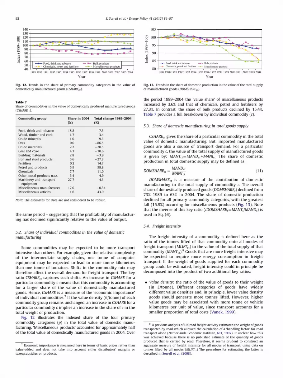
Fig. 12 illustrates the indexed share of the four primarycommodity categories (p) in the total value of domestic manu-facturing. ‘Miscellaneous products’ accounted for approximately halfof the total value of domestically manufactured goods in 2004. Over

7 Economic importance is measured here in terms of basic prices rather than

value-added and does not take into account either distributors’ margins or

taxes/subsidies on products.

the period 1989–2004 the ‘value share’ of miscellaneous productsincreased by 3.6% and that of chemicals, petrol and fertilisers by27.3%. In contrast, the share of bulk products declined by 15.4%.Table 7 provides a full breakdown by individual commodity (c).

5.3. Share of domestic manufacturing in total goods supply

CSHAREct gives the share of a particular commodity in the totalvalue of domestic manufacturing. But, imported manufacturedgoods are also a source of transport demand. For a particularcommodity c, the value of the total supply of manufactured goodsis given by: MANTct¼MANDct+MANIct. The share of domesticproduction in total domestic supply may be defined as

DOMSHAREct ¼MANDct

MANTctð11Þ

DOMSHAREct is a measure of the contribution of domesticmanufacturing to the total supply of commodity c. The overallshare of domestically produced goods (DOMSHAREt) declined from73% 1989 to 63% in 2004. The share of domestic productiondeclined for all primary commodity categories, with the greatestfall (15.9%) occurring for miscellaneous products (Fig. 13). Notethat the inverse of this key ratio (IDOMSHAREt¼MANTt/MANDt) isused in Eq. (6).

5.4. Freight intensity

The freight intensity of a commodity is defined here as theratio of the tonnes lifted of that commodity onto all modes offreight transport (MLIFTct) to the value of the total supply of thatcommodity (MANTct).

8 Goods that are more freight intensive maybe expected to require more energy consumption in freighttransport. If the weight of goods supplied for each commoditygroup could be estimated, freight intensity could in principle bedecomposed into the product of two additional key ratios:

�

was

pro

agg

ton

des

Value density: the ratio of the value of goods to their weight(in £/tonne). Different categories of goods have widelydifferent value densities and, in principle, lower value densitygoods should generate more tonnes lifted. However, highervalue goods may be associated with more tonne or vehiclekilometres per unit of value, since transport accounts for asmaller proportion of total costs (Vanek, 1999).

achieved because there is no published estimate of the quantity of goods

duced that is carried by road. Therefore, it seems prudent to construct an

regate measure of freight intensity for all modes of transport, using data on

nes lifted by all modes (MLIFTct) The procedure for estimating the latter is

cribed in Sorrell et al. (2008).

60708090

100110120130140150160

1989 1990 1991 1992 1993 1994 1995 1996 1997 1998 1999 2000 2001 2002 2003 2004

Year

Inde

x (1

989=

100)


Fig. 15. Trends in freight intensity by primary commodity category (FINTpt).

Table 8Freight intensity of commodity groups (FINTct).

Commodity group Freight intensity in2004, relative toaggregate (%)

Total change1989–2004 (%)

Food, drink and tobacco 111.3 46.9

Wood, timber and cork 136.7 85.6

Crude minerals 1513.3 �9.0

Ores 1646.8 �69.9

Crude materials 49.1 77.9

Coal and coke 70.9 �54.0

Building materials 477.3 15.1

Iron and steel products 50.3 8.6

Fertiliser 184.8 �57.0

Petrol and products 252.1 �14.3

Chemicals 27.0 �29.8

Other metal products n.e.s. 43.3 4.0

Machinery and transport

equipment

10.9 11.0

Miscellaneous manufactures 35.7 42.3

Miscellaneous articles 1505.5 0.2

Note: The estimates for the Ores sector are not considered to be robust.

80

85

90

95

100

105

110

Year

Inde

x (1

989=

100)

FINT ROADt

19891990 1991 1992 1993 1994 1995 1996 1997 1998 1999 2000 2001 2002 2003 2004

Fig. 14. Trends in freight intensity (FINTt) and share of goods lifted by road

(ROADt).

9


�
We used the OECD trade statistics to estimate a time series for the weight of
goods supplied by commodity group (MPRODct), but the results were unreliable

(Sorrell et al., 2008). In addition to inconsistencies within the trade data, there is

no straightforward conversion between the commodity disaggregation used in the

trade statistics and that used in either the input–output tables or the transport

statistics. The time series we obtained frequently suggested that the weight of

goods supplied (MPRODct) exceeded the weight of goods lifted on all transport

modes (MLIFTct) – implying that there was less than one link in the relevant supply

chain (HFct r1:0).

Handling factor: the ratio of the tonnes lifted on to all modes offreight transport to the tonnes supplied. Typically, the journeyof a consignment of goods from a producer to a retailer, orfrom one producer to another, comprises several discretejourneys, each requiring a separate reloading operation. Hence,tonnes lifted may be several times greater than tonnessupplied. The handling factor is often considered to be crudemeasure of the number of links in the supply chain.

Various factors may influence these variables and theimportance of these may vary widely from one commodity toanother. For example, NEI (1997) found that the handling factorfor machinery products increased over the period 1985–1995,partly as a result of the vertical disintegration of the manufactur-ing process and the outsourcing of non-core processes tosubcontractors. At the same time, the handling factor for bulkproducts and textiles declined, partly as a result of a rationalisa-tion of supply chains and increased import penetration.

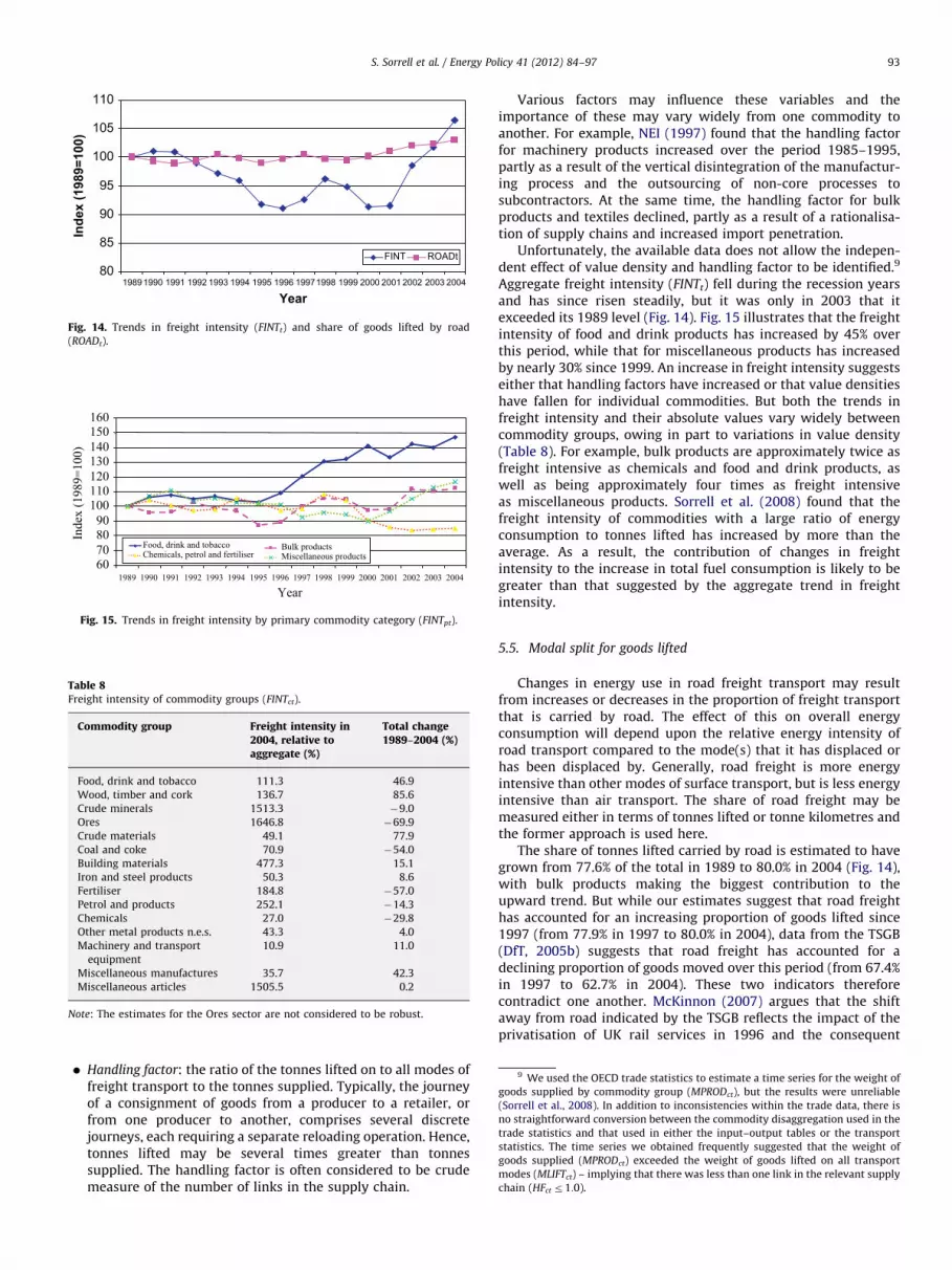
Unfortunately, the available data does not allow the indepen-dent effect of value density and handling factor to be identified.9

Aggregate freight intensity (FINTt) fell during the recession yearsand has since risen steadily, but it was only in 2003 that itexceeded its 1989 level (Fig. 14). Fig. 15 illustrates that the freightintensity of food and drink products has increased by 45% overthis period, while that for miscellaneous products has increasedby nearly 30% since 1999. An increase in freight intensity suggestseither that handling factors have increased or that value densitieshave fallen for individual commodities. But both the trends infreight intensity and their absolute values vary widely betweencommodity groups, owing in part to variations in value density(Table 8). For example, bulk products are approximately twice asfreight intensive as chemicals and food and drink products, aswell as being approximately four times as freight intensiveas miscellaneous products. Sorrell et al. (2008) found that thefreight intensity of commodities with a large ratio of energyconsumption to tonnes lifted has increased by more than theaverage. As a result, the contribution of changes in freightintensity to the increase in total fuel consumption is likely to begreater than that suggested by the aggregate trend in freightintensity.

5.5. Modal split for goods lifted

Changes in energy use in road freight transport may resultfrom increases or decreases in the proportion of freight transportthat is carried by road. The effect of this on overall energyconsumption will depend upon the relative energy intensity ofroad transport compared to the mode(s) that it has displaced orhas been displaced by. Generally, road freight is more energyintensive than other modes of surface transport, but is less energyintensive than air transport. The share of road freight may bemeasured either in terms of tonnes lifted or tonne kilometres andthe former approach is used here.

The share of tonnes lifted carried by road is estimated to havegrown from 77.6% of the total in 1989 to 80.0% in 2004 (Fig. 14),with bulk products making the biggest contribution to theupward trend. But while our estimates suggest that road freighthas accounted for an increasing proportion of goods lifted since1997 (from 77.9% in 1997 to 80.0% in 2004), data from the TSGB(DfT, 2005b) suggests that road freight has accounted for adeclining proportion of goods moved over this period (from 67.4%in 1997 to 62.7% in 2004). These two indicators thereforecontradict one another. McKinnon (2007) argues that the shiftaway from road indicated by the TSGB reflects the impact of theprivatisation of UK rail services in 1996 and the consequent

120125130

00)


expansion of rail freight. But our analysis suggests that, in termsof tonnes lifted, rail has lost market share since that time. Somepossible explanations for these divergent conclusions include:

110115

989=

1

�

Inde

x (1

989=

100)

Inde

x (1

989=

100)

Figload

9095

100105

Inde

x (1


Inaccurate estimates of goods lifted by all modes: Our analysisrelies upon uncertain estimate of goods lifted by commoditygroup for all modes of freight transport. However, ourestimates are consistent with the TSGB data on the total goodslifted by all modes.

1989 1990 1991 1992 1993 1994 1995 1996 1997 1998 1999 2000 2001 2002 2003 2004
�
Year

Fig. 18. Trends in length of haul by primary commodity category (LOHpt).

Shifts in the ratio of goods moved to goods lifted: It is possiblethat the diverging results reflect a real difference in the trendsin goods moved and goods lifted. For example, if the averagelength of haul for rail freight has increased faster than that forroad freight, goods moved by rail (road) would increase faster(slower) than goods lifted by rail (road).
� Inaccurate estimates of the activity of foreign-registered vehicles:
Both our estimates of goods lifted and the TSGB data on goodsmoved should incorporate freight movements by foreign-registered vehicles, which are estimated to have increasedsubstantially since 1997. In our case, the activity of foreign-registered vehicles was estimated from Eurostat and UKsurveys that provided estimates of tonne kilometres byforeign-registered vehicles. In order not to distort ourestimates of key ratios, we simply assumed that the goodslifted by foreign-registered vehicles are proportional to thegoods moved. But the relevant data is sparse, the procedure isfairly crude and our assumptions may be incorrect. Hence, it ispossible that we have overestimated the tonnes lifted byforeign-registered vehicles and thereby the overall road tonneslifted since 1997. This would lead to an upwardly biasedestimate for the modal share of road freight since that date.

020406080

100120140160180200

1989

1990

1991

1992

1993

1994

1995

1996

1997

1998

1999

2000

2001

2002

2003

2004


Fig. 16. Trends in the share of tonnes lifted by vehicle category (VSIZEkt).

70

80

90

100

110

120

130

Year

LOHt LFt ERUNt

1989 1990 1991 1992 1993 1994 1995 19961997 1998 1999 2000 2001 2002 2003 2004

. 17. Trends in length of haul (LOHt), payload weight (LFt) and ratio of total to

ed distanced travelled (ERUNt).

In practice, we suspect that inaccuracies in our estimates of thecontribution of foreign-registered vehicles are the primarycontributor to the diverging results.

5.6. Vehicle split for goods lifted

Energy use for road freight will be strongly influenced by themix of vehicles used. Larger vehicles generally use less energy pertonne kilometre, particularly for long-distance journeys involvingsubstantial motorway travel. Also, the mix of vehicles varieswidely from one commodity group to another. The key ratioVSIZEckt defines the mix of vehicles used in terms of their share ofroad tonnes lifted for each commodity group. Two trends areapparent: first, the displacement of rigid trucks by articulatedtrucks; and second, the displacement of smaller vehicles by largervehicles (Fig. 16). Most of the displacement of rigid by articulatedtrucks occurred before 2000, with the relative share of the twovehicle types remaining relatively constant since then. However,the trend towards large rigids (425 tonnes) and large artics(433 tonnes) is continuing, with the latter now accounting formore than half of tonnes lifted. Since larger vehicles both carrymore weight and are driven longer distances, their contribution togoods moved is proportionally greater.

5.7. Length of haul

Energy use for road freight will also depend upon the distanceover which goods are carried. This is determined by the averagelength of haul for each commodity group and vehicle category(LOHckt). This relates to consignments of goods, rather than thetrip length for individual vehicles, but the two measures areclosely correlated. Increases in the average length of haul wereone of the main drivers of road freight growth during the 1970sand 1980s. During this period, the fleet average length of haulincreased by between 2.0% and 2.5% each year (McKinnon andWoodburn, 1996). This, in turn, was driven by increasing spatialconcentration of economic activity, facilitated by the constructionof the motorway network. However, the process of increasingspatial concentration must have limits and there could becountervailing factors such as increasing congestion on the roadnetwork (McKinnon, 2007).

The average length of haul (LOHt) is estimated to haveincreased by 12.3% between 1989 and 2004 – from 77.7 to87.3 km (Fig. 17). However, the upward trend reversed in 1999and since that time the average length of haul is estimated to havedeclined. As with other variables (e.g. road tonnes lifted), thechange between 2003 and 2004 is quite dramatic (a fall of 6.5%)thereby raising concerns about the compatibility of the 2004 datawith that from previous years.

It is notable that the average length of haul for food and drinkand miscellaneous products is significantly larger than thatfor bulk products and for chemicals, petrol and fertilisers.

80859095

100105110115120125130

Year

Inde

x (1

989=

100)

1989 1990 1991 1992 1993 1994 1995 1996 1997 1998 1999 2000 2001 2002 2003 2004


Fig. 19. Trends in payload weight by primary commodity category (LFpt).

30405060708090

100110

1989

1990

1991

1992

1993

1994

1995

1996

1997

1998

1999

2000

2001

2002

2003

2004

Year

Inde

x - 1

989=

100


Fig. 20. Trends in payload weight by vehicle type (LFkt).


80

85

90

95

100

105

Year

Inde

x (1

989=

100)

1989 1990 1991 1992 1993 1994 1996 1998 1999 2000 2001 2002 2003 20041995 1997

Fig. 21. Trends in ratio of total to loaded vehicle kilometres by primary

commodity category (ERUNpt).

6065707580859095

100105110

Inde

x (1

989=

100)

Rigids (3.5-7.5) Rigids (7.5-17) Rigids (17-25)

Rigids (>25) Artics (3.5-33) Artics (>33)

1989

1990

1991

1992

1993

1994

1995

1996

1997

1998

1999

2000

2001

2002

2003

2004

Fig. 22. Trends in ratio of total to loaded vehicle kilometres by vehicle type

(ERUNkt).


Furthermore the average length of haul for chemicals, petrol andfertilisers declined between 1989 and 2004 while that for theother commodities increased (Fig. 18).10

5.8. Average payload weight

Increases in the average payload weight means that fewervehicle kilometres will be required for each tonne of deliveredgoods. The extent to which this translates into less energy use pertonne of delivered goods will depend upon other variables such asthe energy efficiency of the relevant vehicles.

The fleet average payload weight depends upon both the mixof vehicles (both within and between size categories) and the‘lading factor’ of individual vehicles – defined as the ratio of actualgoods moved to the maximum tonne kilometres achievable ifthe vehicles were loaded to their maximum carrying capacity(DfT, 2005a). The CSRGT publishes estimates of lading factors foreach vehicle category (k), but does not provide enough informa-tion to estimate this variable for commodity group and vehiclecategory (ck). Hence we use the alternative measure of averagepayload weight (LFckt¼TKMckt/VKMckt – note that the inverse ofthis is used in Eq. (6)). Also, the loading of a vehicle may beconstrained by volume as well as by weight. For example, a loadmay fill the available space within a truck before it exceeds themaximum, weight-based carrying capacity. With increasingamounts of packaging per unit weight of some commodities,volume constraints could be becoming increasingly important.

The fleet average payload weight (LFt) increased from 8.84 to9.33 tonnes (+5.5%) over the period (Fig. 17). It is notable that theaverage payload weight continued to increase between 2000 and

10 Note that the reduction in the average length of haul after 1999 has nothing

to do with the increased penetration of foreign-registered vehicles after 1999. This

is because our adjustments to allow for activity by foreign-registered vehicles have

no effect on the estimated key ratios. These are based entirely upon the data

supplied by CSRGT (see Sorrell et al., 2008).

2004, despite a fall from 60% to 57% in the average weight-basedlading factor of all vehicles (DfT, 2005a). This period coincidedwith increases in the maximum allowed vehicle weight, acorresponding increase in the weight-based carrying capacity ofthe UK vehicle fleet and a shift towards larger vehicles. The neteffect was to increase the fleet average payload weight, eventhough the average lading factor fell for both rigid and articulatedvehicles.

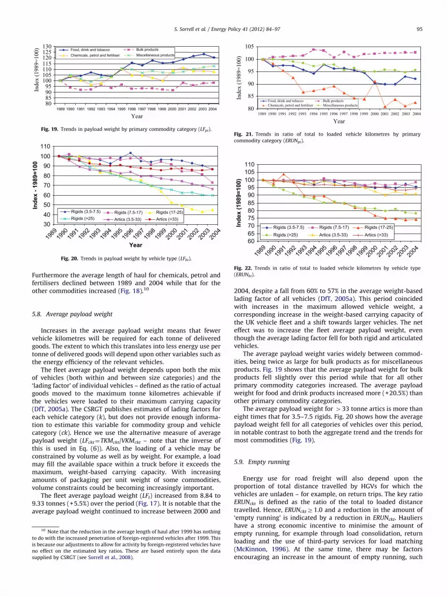
The average payload weight varies widely between commod-ities, being twice as large for bulk products as for miscellaneousproducts. Fig. 19 shows that the average payload weight for bulkproducts fell slightly over this period while that for all otherprimary commodity categories increased. The average payloadweight for food and drink products increased more (+20.5%) thanother primary commodity categories.

The average payload weight for 433 tonne artics is more thaneight times that for 3.5–7.5 rigids. Fig. 20 shows how the averagepayload weight fell for all categories of vehicles over this period,in notable contrast to both the aggregate trend and the trends formost commodities (Fig. 19).

5.9. Empty running

Energy use for road freight will also depend upon theproportion of total distance travelled by HGVs for which thevehicles are unladen – for example, on return trips. The key ratioERUNckt is defined as the ratio of the total to loaded distancetravelled. Hence, ERUNcktZ1.0 and a reduction in the amount of‘empty running’ is indicated by a reduction in ERUNckt. Hauliershave a strong economic incentive to minimise the amount ofempty running, for example through load consolidation, returnloading and the use of third-party services for load matching(McKinnon, 1996). At the same time, there may be factorsencouraging an increase in the amount of empty running, such

60

70

80

90

100

110

120

130

Inde

x (1

989=

100)


1989

1990

1991

1992

1993

1994

1995

1996

1997

1998

1999

2000

2001

2002

2003

2004

Fig. 23. Trends in energy intensity by vehicle type (EINTkt).

60.0

70.0

80.0

90.0

100.0

110.0

120.0

EI_GDPt EI_MANTt EI_MLIFTtEI_TLIFTt EI_TKMt EINTt

Inde

x (1

989=

100)

1989 1990 1991 1992 1993 1994 1996 1998 1999 2000 2001 2002 2003 20041995 1997

Fig. 24. Trends in various measures of UK road freight energy intensity.

Table 9Summary of aggregate trends in key ratios.

Acronym Interpretation Total change (%)

DOMMANt Domestic manufacturing share �40.0

IDOMSHAREt Inverse domestic commodity share 14.9

FINTt Freight intensity 5.3

ROADt Road share 3.0

LOHt Length of haul 12.3

ILFt Inverse payload weight �5.2

ERUNt Empty running �5.5

EINTt Energy intensity �2.5

EI_GDPt Aggregate energy intensity �25.8

Note: The key ratios CSHARE and VSIZE are omitted since they are not meaningful

at the aggregate level.


as increasing time constraints on delivery schedules. There is alsoevidence that the amount of empty running falls as the trip lengthincreases (McKinnon, 1996), implying a negative correlationbetween LOH and ERUN.

The ratio of total to loaded vehicle kilometres is estimated tohave fallen by 5.5% between 1989 and 2004 (Fig. 17), implyingthat the proportion of empty running decreased from 30.8% to26.8%. If the level of empty running had remained at 1989 levels,there would have been an additional 1360 million vehiclekilometres driven on UK roads in 2004. The amount of emptyrunning is largest for food drink and tobacco products, followedby chemicals, petrol and fertilisers. However, these two primarycommodity categories also experienced the greatest reduction inthe amount of empty running between 1989 and 2004 (Fig. 21).

The amount of empty running is greater for rigid vehicles thanfor articulated vehicles, but the trends are converging. Theproportional improvement in the amount of empty running forthe two larger rigid vehicle categories was more than 20%, whilethat for the largest category of articulated vehicles was less than5% (Fig. 22).

5.10. Energy intensity

The estimates of energy intensity by a vehicle type (EINTkt) aretaken from the CSRGT and represent a composite of both loadedand unloaded trips. A proportion of the estimated change in meanenergy intensity for a particular vehicle category will derive fromnewer, more efficient vehicles entering the fleet and older, lessefficient vehicles being replaced. However, the mean energyintensity will also depend upon driving styles, average speeds, therelative use of different types of road, payload weights and otherfactors. There will therefore be some interdependence betweenthis key ratio and others. For example, mean energy consumptionmay be expected to vary with the length of haul, since long-distance trips will involve proportionately more motorway travel.

Fig. 23 illustrates the trends in energy intensity by individualvehicle category. The energy intensity of the smallest category ofrigid vehicle increased over this period, while that of othercategories of vehicle reduced. Even on a vehicle kilometre basis,large articulated vehicles are now less energy intensive than thelargest category of rigid vehicles.

The estimates of the energy intensity of each vehicle categorycan be used to estimate the total fuel consumption for road freighttransport (FUELt) and thus a time series for the overall energyintensity of UK road freight: EINTt¼FUELt/VKMTt. This is estimatedto have fallen by 2.5% between 1989 and 2004, although the trendis rather erratic with a reversal in the downward trend after 1998.Over the same period, a simple average of the energy intensities ofeach vehicle type fell by 10.3%, suggesting that the shift towardslarger vehicles had offset the fall in mean energy use per vehiclekilometre for each category of vehicle. In 2004, the mean energyintensity of the vehicle fleet was 0.32 litres per vehicle kilometre,corresponding to 7.8 miles per gallon.

Energy intensity may also be measured with respect to roadgoods moved (EI_TKM), road tonnes lifted (EI_TLIFT), total tonneslifted (EI_MLIFT), goods supplied (EI_MANT) or GDP (EI_GDP) –with the latter being the measure that is relevant to decoupling(Fig. 24). Energy use per road tonne kilometre is estimated to havefallen by fell by 12.7% over this period, compared to a 2.5% fall inenergy use per vehicle kilometre. This demonstrates that the shifttowards larger vehicles has reduced energy intensity on a tonnekilometre basis. However, energy use per road tonne lifted fell byonly 1.9% and the modal shift towards road led to a 1.0% increasein energy intensity when measured on the basis of tonnes liftedon all modes. On the basis of the total value of goods supplied,energy intensity increased by 7.6%, but when measured on thebasis of GDP, road freight energy intensity fell by 25.8%. Thisdemonstrates that it is the shift from manufacturing to serviceswithin the UK economy, rather than changes in the freighttransport sector, that has played the dominant role in decouplingUK road freight energy consumption from GDP.

5.11. Summary of trends in key ratios

Table 9 summarises the trends in the aggregate measures ofthe key ratios over this period. On the basis of these aggregatemeasures, the main factor contributing to the observeddecoupling would appear to be the declining value ofmanufactured goods relative to GDP. Reductions in the averagepayload weight, the amount of empty running and the fuel useper vehicle kilometre also appear to have made a contribution,while changes in the other key ratios have acted to increaseaggregate energy intensity.


6. Conclusions

This paper has examined the trends in UK road freight activityover the period 1989 to 2004. The results help explain why energyconsumption for road freight appears to have grown much moreslowly than GDP over this period. But to gain a deeper understanding,this data needs to considered alongside the formal decompositionanalysis conducted by Sorrell et al. (2009), together with the broaderqualitative discussion provided by Lehtonen (2008).

It is estimated that, during the period 1989 to 2004, energyconsumption for road freight in the UK increased by only 6.3%, whileUK GDP increased by 43.3%. This suggests that the aggregate energyintensity of UK road freight fell by as much as one quarter over thisperiod. In this respect the UK appears to have been more successfulthan other EU countries in mitigating the environmental impacts ofroad freight, but this is largely the unintended outcome ofvarious economic trends rather than the deliberate result of policy.

The estimates in this paper relate to the energy use for all HGVactivity in the UK, which includes both UK and foreign-registeredHGVs carrying both domestically produced and imported manu-factured goods. Foreign-registered vehicles are accounting for anincreasing proportion of UK road freight activity and importedgoods are accounting for an increasing proportion of the total UKsupply of goods. However, since the data on foreign-registeredvehicle activity is sparse, there is a corresponding uncertainty inour aggregate estimates of road freight energy consumption andother variables – which may be best considered as an upperbound (see Annex 7 of Sorrell et al., 2008). The results demon-strate, however, that the main data source on UK road freight ismisleading, since it only reports the activity by GB-registeredvehicles in Great Britain.

The changes in road freight energy consumption are the result ofa complex interaction of factors affecting the manufacture, supply,distribution and transport of goods, including the geographicallocation of production, the structure of the supply chain, themanagement of transport resources and the size and fuel efficiencyof vehicles. Only a subset of these factors have been influenced byenergy and climate policy (e.g. fuel taxation) and then only to alimited extent. While some factors (e.g. the amount of emptyrunning) have contributed to a decrease in energy consumption perunit of GDP, these have been partly offset by other factors that havecontributed to an increase (e.g. reductions in the average payloadweight). Moreover, these changes are interlinked. For example, long-distance freight movements by large vehicles are very energy-efficient on a tonne-kilometre basis, while short trips by smallvehicles are often energy inefficient. Hence, changes in the averagelength of haul may not have led to a proportionate change in roadfreight energy consumption.

Further reductions in the energy intensity of road freightshould be possible through improvements in the average loadfactor and fuel efficiency of vehicles, together with furtherreductions in the amount of empty running. However, theaggregate potential in each case may be relatively limited. A shifttowards rail and waterborne transport could yield savings insome areas, but the scope for this varies greatly with both thenature of the commodity and the location of the associatedmanufacturing and distribution centres. Also, the energy savingsdepend very much upon the vehicles involved and their loadfactors (e.g. long-distance transport in 433 tonne HGVs isrelatively energy efficient). Given the inherent inflexibility of railtransport and the scale of investment required to achievesignificant modal shifts, it seems more appropriate to focus onthe potential for improving the efficiency of road freight, at leastin the short to medium-term. A reversal of the historic trend ofincreasing length of haul offers considerable potential for energysavings and could potentially be encouraged by increasing traffic

congestion, road pricing, higher fuel prices and growing prefer-ences for locally produced products. But substantial changeswould require a major reorientation of economic activity and areversal of the trends of the last 30 years. The changing coststructure of road freight and the scope for pricing instruments toencourage such trends are priorities for future research.

There are numerous deficiencies in the existing data for UKroad freight that make analyses of this type time-consuming toconduct and which inhibit a better understanding of the relevanttrends. Of particular importance is the lack of data on: (a) loadedand unloaded vehicle kilometres by commodity group and vehicletype; (b) total tonnes lifted (all modes) by commodity group;(c) freight activity in Northern Ireland; (d) the activity of foreignregistered vehicles; and (e) the weight of goods produced.Particular difficulties are created by the incompatibility of thecommodity classification schemes used in the transport, produc-tion and trade statistics (Sorrell et al., 2008). One importantconsequence of these deficiencies is that analysts face consider-able difficulties in constructing an adequate time series of thevalue density and handling factors of different types of goods.This, in turn, precludes a better understanding of the determi-nants of the freight intensity of those goods. Comparableproblems are encountered in other OECD countries.

Acknowledgements

This work has been funded by the UK Research Councils underthe Towards a Sustainable Energy Economy (TSEC) programme.The authors would like to thank the UK Department of Transportfor providing additional tabulations of UK road freight data andAlan McKinnon (Heriot-Watt University, UK) for his extensive andpioneering research in the area of road freight.

References

DfT, 2004. Review of Road Freight Statistics. Department for Transport, London.DfT, 2005a. Transport of Goods by Road in Great Britain: 2004: Annual Report of

the Continuing Survey of Road Goods Transport. Department for Transport,London.

DfT, 2005b. Transport Statistics Great Britain. Department for Transport, London.Kamakate, F., Schipper, L., 2009. Trends in truck freight energy use and carbon

emissions in selected OECD countries from 1973 to 2005. Energy Policy 37(10), 3743–3751.

Kveiborg, O., Fosgerau, M., 2007. Decomposing the decoupling of Danish roadfreight traffic growth and economic growth. Transport Policy 14, 39–48.

Lehtonen, M., 2008. Energy use in UK Road Freight: a Literature Review. SussexEnergy Group, SPRU (Science and Technology Policy Research), University ofSussex, Brighton.

McKinnon, A.C., 1996. The empty running and return loading of road goodsvehicles. Transport Logistics 1 (1), 1–19.

McKinnon, A.C., 2005. The economic and environmental benefits of increasingmaximum truck weight: the British experience. Transportation Research PartD: Transport and Environment 10, 77–95.

McKinnon, A.C., 2007. Decoupling of road freight transport and economic growthtrends in the UK: an exploratory analysis 27 (1), 37–64.

McKinnon, A.C., Piecyk, M.I., 2009. Measurement of CO2 emissions from roadfreight transport: a review of UK experience. Energy Policy 37, 3733–3742.

McKinnon, A.C., Woodburn, A., 1996. Logistical restructuring and freight trafficgrowth: an empirical assessment. Transportation 23 (2), 141–161.

NEI, 1997. REDEFINE: Relationship between Demand for Freight-transport andIndustrial Effects – Work Package 1. Netherlands Economic Institute,Rotterdam.

ONS, 2006. UK Input–Output Analyses 2006 edition Office for National Statistics,London.

Sorrell, S., Lehtonen, M., Stapleton, L., Pujol, J., Champion., T., 2008. Energy use inUK Road Freight: a Decomposition Analysis. Sussex Energy Group, SPRU(Science and Technology Policy Research), University of Sussex, Brighton.

Sorrell, S., Lehtonen, M., Stapleton, L., Pujol, J., Champion., T., 2009. Decomposingroad freight energy use in the United Kingdom. Energy Policy 37 (8),3115–3129.

Vanek, F.M., 1999. UK road freight energy use by product: trends and analysis from1985 to 1995. Transport Policy 6, 237–246.

decoupling of road freight energy use from economic growth in the united kingdom

Documents