multiphoton detachment of a negative ion by an elliptically polarized, monochromatic laser field
TRANSCRIPT
University of Nebraska - LincolnDigitalCommons@University of Nebraska - Lincoln
Anthony F. Starace Publications Research Papers in Physics and Astronomy
1-1-2003
Multiphoton detachment of a negative ion by anelliptically polarized, monochromatic laser fieldN. L. ManakovVoronezh State University, Universitetskaya pl. 1, Voronezh, 394006 Russia, [email protected]
M. V. FrolovVoronezh State University, Russia, [email protected]
Bogdan BorcaUniversity of Nebraska-Lincoln
Anthony F. StaraceUniversity of Nebraska-Lincoln, [email protected]
This Article is brought to you for free and open access by the Research Papers in Physics and Astronomy at DigitalCommons@University of Nebraska -Lincoln. It has been accepted for inclusion in Anthony F. Starace Publications by an authorized administrator of DigitalCommons@University ofNebraska - Lincoln. For more information, please contact [email protected].
Manakov, N. L.; Frolov, M. V.; Borca, Bogdan; and Starace, Anthony F., "Multiphoton detachment of a negative ion by an ellipticallypolarized, monochromatic laser field" (2003). Anthony F. Starace Publications. Paper 175.http://digitalcommons.unl.edu/physicsstarace/175

INSTITUTE OF PHYSICS PUBLISHING JOURNAL OF PHYSICS B: ATOMIC, MOLECULAR AND OPTICAL PHYSICS
J. Phys. B: At. Mol. Opt. Phys. 36 (2003) R49–R124 PII: S0953-4075(03)17644-4
TOPICAL REVIEW
Multiphoton detachment of a negative ion by anelliptically polarized, monochromatic laser field
N L Manakov1, M V Frolov1,2, B Borca2,3,4 and Anthony F Starace2
1 Department of Physics, Voronezh State University, Voronezh 394006, Russia2 Department of Physics and Astronomy, University of Nebraska Lincoln,NE 68588-0111, USA
E-mail: [email protected] and [email protected]
Received 3 July 2002, in final form 20 February 2003Published 22 April 2003Online at stacks.iop.org/JPhysB/36/R49
AbstractThe quasistationary quasienergy state approach (QQES) is applied to theanalysis of partial (n-photon) decay rates and angular distributions (ADs) ofphotoelectrons produced by an elliptically polarized laser field. The problemis formulated for a weakly bound electron with an energy E0 in the three-dimensional δ-model potential (which approximates the short-range potentialof a negative ion) interacting with a strong monochromatic laser field having anelectric vector F (ωt). The results presented cover weak (perturbative), strong(nonperturbative), and superstrong field regimes as well as a wide interval offrequencies ω extending from the tunnelling (hω � |E0|) and multiphoton(hω < |E0|) cases up to the high frequency domain (hω > |E0|).
For a weak laser field, exact equations for the normalization factor and forthe Fourier coefficients of the QQES wavefunction at the origin (|r| → 0) (thatare key elements of the QQES approach for a δ-model potential) as well as for thedetachment amplitudes are analysed analytically using both standard Rayleigh–Schrodinger perturbation theory (PT) in the intensity, I , of the laser field andBrillouin–Wigner PT expansions involving the exact (complex) quasienergy ε.The lowest-order perturbative results for the n-photon ADs are presented inanalytic form, and the parametrization of ADs in terms of polarization- andangular-independent atomic parameters is discussed for the general case ofelliptical polarization. The major emphasis is on the analysis of an ellipticityinduced distortion of three-dimensional ADs and, especially, on the ellipticdichroism (ED) effect, i.e. the dependence of the photoelectron yield in a fixeddirection n on the sign of the ellipticity (or on the helicity) of a laser field.The dominant role of binding potential effects for a correct description of EDand threshold effects is demonstrated, and the intimate relationship betweenatomic ED factors and scattering phases of the detached electron is establishedfor multiphoton detachment, including the above-threshold case.
3 Present address: JILA, University of Colorado and National Institute of Standards and Technology, Boulder,CO 80309-0440, USA.4 On leave from: Institute for Space Sciences, Bucharest-Magurele 76900, Romania.
0953-4075/03/090049+76$30.00 © 2003 IOP Publishing Ltd Printed in the UK R49

R50 Topical Review
For a strong laser field, we present an accurate derivation for the QQESwavefunction and decay rates in the Keldysh approximation (KA) from exactQQES equations, including analytical, first-order (‘rescattering’) correctionsto the KA results. The symmetries of ADs and the existence of ED areestablished using the exact analytical result for the n-photon detachmentamplitude. Accurate numerical results are presented for the variation of thestructure of the ADs as well as of the ED effect with increasing laser intensity.
For the high frequency case, hω > |E0|, a rigorous analytical treatmentof higher-order PT effects is presented for one-photon detachment, taking intoaccount corrections of higher orders in I to the well-known photodetachmentcross section for a short-range potential. Together with the exact numericalanalysis of the total and partial decay rates for hω > |E0|, these resultsdemonstrate the existence of a quasistationary stabilization regime in the decayof a weakly bound electron for any polarization of the laser field. Moreover, thisstabilization occurs only over a limited interval of intensity, up to the closureof the direct photodetachment channel.
In the superstrong field regime, the total decay rate of a weaklybound electron may be described by cycle-averaging the results for aninstantaneous static electric field of strength |F (ωt)| (for any laser frequencyand polarization). All results in this paper are presented in scaled units and areillustrated numerically for the case of the H− negative ion.
Contents
1. Introduction 511.1. Brief survey of dichroic effects in unpolarized atom photoprocesses 511.2. Status of multiphoton detachment of negative ions 551.3. Outline of this review 58
2. Basic results of the QQES approach for the δ-model potential and general equationsfor multiphoton detachment rates 602.1. Definitions and scaled units 602.2. Background results of the QQES approach for a strong laser field 612.3. Basic equations for the QQES solution for a δ-model potential 632.4. Exact result for multiphoton detachment rates 642.5. The QQES wavefunction and detachment rates in the Keldysh approximation 662.6. Analytical PT results for angular distributions and n-photon rates 67
3. Angular distributions and elliptic dichroism in the weak field limit 733.1. Perturbative analysis of angular distributions for elliptically polarized light 733.2. Discussion of dichroic terms in ADs 783.3. Comparisons with recent experiments and multielectron calculations 81
4. Strong field analysis of angular distributions and ED effects 844.1. Symmetry properties of angular distributions and elliptic dichroism 844.2. Total and partial rates of n-photon detachment 854.3. Three-dimensional angular distributions 884.4. Elliptic dichroism in a strong field 91
5. Photodetachment in a strong, high frequency field (ω > 1) 955.1. Higher-order corrections to the one-photon detachment cross section 965.2. The quasistationary stabilization regime 995.3. Angular distributions and ED for ω > 1 101

Topical Review R51
6. Static-electric-field behaviour of decay rates in superstrong fields 1026.1. General remarks 1026.2. ω2 expansion for the complex quasienergy 1036.3. Comparisons with numerical results 105
7. Summary and conclusions 107Acknowledgments 108Appendix A. Normalization of the QQES wavefunction for a δ-model potential 109Appendix B. Perturbative and strong field results for the coefficients φn and fn 109B.1. Brillouin–Wigner expansions 110B.2. Rayleigh–Schrodinger results 111B.3. Exact strong field results 114B.4. ‘Rescattering approximations’ for the coefficients fn 117Appendix C. Details of derivations for the n-photon detachment amplitude 118References 120
1. Introduction
Recent studies of laser–atom interactions have indicated a growing interest in the dependenceof multiphoton processes on the polarization state of a laser field. At present, a considerableellipticity dependence is well documented for a number of strong field processes (e.g. highharmonic generation (HHG), laser-assisted collisions and ionization, including above-threshold ionization) both for single- and multicolour laser fields. Significant differencesin the magnitude of laser–atom interactions for linearly and circularly polarized laser fieldswere predicted first in 1966 for the decay of a weakly bound atomic system in the tunnellingregime [1] (see also [2] for an extension of these results to the case of elliptical polarization).In the multiphoton regime, the differences between multiphoton ionization cross sections werediscussed long ago on the basis of perturbative calculations (see, e.g., [3]). Also, perturbativeresults in this regime for an arbitrary laser ellipticity have been discussed in [4] (for ionization)and in [5] (for harmonic generation). In the past decade a new manifestation of polarizationeffects in laser–atom processes has been discussed: dichroic effects caused by the dependenceof physical observables on the helicity of a laser field, i.e. on the sign of the degree of circularpolarization5, ξ . Moreover, in the multiphoton regime the manifestation of these effects ispossible in two different ways, either as circular dichroism (CD) (which is most pronouncedfor ξ = ±1) or as elliptic dichroism (ED) (which occurs only for the case of an ellipticalpolarization, with 0 < |ξ | < 1, and which is zero for |ξ | = 0, 1). In this review we present adetailed analysis of laser detachment of a weakly bound atomic system (a negative ion) in bothperturbative and nonperturbative regimes (in the laser intensity), including a general analysisof ED effects on the angular distribution of detached electrons and their dependence on thelaser frequency and intensity. Since studies of dichroic effects in photoprocesses involvingfreely oriented (i.e. not oriented or aligned) atoms are relatively new and not commonly known,we give below a brief survey of existing results for these effects.
1.1. Brief survey of dichroic effects in unpolarized atom photoprocesses
The difference between cross sections of a photoprocess for right (ξ = +1) and left (ξ = −1)circular polarization of an incident photon beam, the CD effect, is a widely used tool
5 ξ is defined in (5) below. It takes values in the range −1 � ξ � 1, where ξ = −1, 0, +1 correspond to leftcircularly, linearly and right circularly polarized light, respectively.

R52 Topical Review
to investigate the linear response of magnetic solids and chiral molecular systems to anelectromagnetic field [6]. Asymmetries in the interaction of polarized light with chiralmolecular samples have been known since Pasteur’s experiments on optical activity [7], and thetheory of the effect has been reviewed [8]. Recently, direct measurements have been performedof CD in the photoelectron angular distributions (ADs) resulting from photoionization of free,randomly oriented chiral molecules [9].
The CD effect is also well known in VUV and soft-x-ray photoprocesses(e.g. photoionization) from polarized atomic targets and in photoionization experiments inwhich the spin of the photoelectron is measured [8, 10]. As follows from simple symmetryarguments, the CD for these cases (as well as for magnetic samples) is completely causedby the existence of a time-odd pseudovector inherent to the problem being analysed, sayA (which might represent, e.g., an angular momentum for the case of a polarized atom, aphotoelectron spin for the case of atomic photoionization or a magnetization vector for thecase of a magnetic solid). In general, the existence of a CD effect means that the cross sectionof a particular process involves one or more terms proportional to ξ , the circular polarizationdegree. However, as may be seen from equation (5) below, ξ is proportional to (k · [e × e∗]),where k is the unit vector in the direction of the (time-odd) photon wavevector k and e is the (ingeneral complex) photon polarization vector. One thus sees that ξ is a pseudoscalar (due to itschange of sign upon coordinate inversion). It is also time-even, since k = k/k is time-odd andalso [e × e∗] is time-odd (since e and e∗ get interchanged under time inversion, i.e. e → e∗).Moreover, the parameter ξ can initially enter a cross section only through a combination ofvectors e and e∗ (that enter the problem through the operator for the photon–atom interaction).This combination is unique and has the form i[e×e∗] = ξ k (see (5)), where ξ k is a time-oddpseudovector. Thus the fundamental object of a light beam responsible for dichroic effects isthe ‘CD vector’, ξ k, which is generic to any elliptically polarized photon (i.e. having ξ �= 0).For atomic targets that are polarized (as well as for magnetic solids),a time-odd pseudovector ofthe problem, A, arises naturally. It may represent, e.g., either a spin or an angular momentum.Since all terms contributing to any cross section must be true scalars, one concludes that, forpolarized targets, the CD term arises simply as the scalar product6,
�σCD = αsξ(k · A), (1)
where the dynamical factor αs is a true scalar (that may be represented, e.g., as the real part of aproduct of particular components of the photoprocess amplitudes). Therefore, the existence ofCD for the cases considered above originates from an intrinsic ‘chiral’ vector of the problem,A, that balances the time-oddness and the pseudoscalar property of the ‘CD vector’ ξk.
Dichroic effects in photoprocesses with unpolarized targets have a physical origin thatis different from those mentioned above since in this case the initial atomic system doesnot involve any chiral vectors A. As a general analysis shows [11, 12], these effects originateinstead from the interference between real and imaginary(non-Hermitian or ‘dissipative’) partsof the quantum transition amplitudes (or, alternatively, of the nonlinear susceptibilities [13]).From a general consideration of the simplest possible form of the CD term (i.e. similar toequation (1) for polarized targets), it is clear that in many photoprocesses involving free atomsit is possible to construct a time-even pseudovector as the vector product [a1 × a2] of vectorsof the problem having the same temporal symmetry. Obviously these vectors ai are differentin different processes and their choice depends on the concrete problem studied (e.g. there arethe momenta of incident and scattered electrons in a bremsstrahlung process or the momenta6 When there exist other vectors in the problem, in addition to A, additional CD terms are possible. For example,for the case of photoionization, there appears (in addition to (1)) a CD term with the form α′
sξ(k · p)(A · p), where pis the photoelectron momentum and α′
s is a true scalar coefficient [8].
Topical Review R53
of the two escaping electrons in double photoionization of a target atom). However, the time-odd dynamical (scalar) parameter, βs (that now replaces the time-even αs in (1)), can ariseonly as the result of the interference between real and imaginary parts of some particularcomponents, fi , of the transition amplitudes, i.e. it may be represented as7βs ∼ Im{ fi f ∗
j }.Dichroic effects thus provide the possibility for direct experimental measurements of thisinterference. One important difference between dichroic effects for polarized and unpolarizedtargets is that for the former these effects exist in the total cross sections as well (as is clearfrom (1), where A is a fixed vector), whereas the ‘chiral’ properties of unpolarized targetsarise from the geometry of the particular experimental measurement, i.e. they depend on thedirections of the vectors ai . Thus dichroic effects in processes involving unpolarized targetsare manifested mainly in ADs, and in most cases they vanish in angle-integrated, total crosssections.
CD in photoprocesses involving unpolarized atomic targets was first discussed in 1992 [15]for the case of single-photon, double photoionization of helium. The vector product, [p1 ×p2],of the momenta of the escaping electrons is a time-even pseudovector and the time-odd scalarparameter, βs , involves the non-Hermitian part of the transition amplitude. Thus the CD termin the double photoionization cross section is given by an expression similar to (1), but withthe substitution of the time-even pseudovector [p1 × p2] for A and of the time-odd dynamicalfactor βs for αs [12]. (This process has attracted much attention recently as it provides a verysensitive test of the importance of electron correlations; see reviews [16, 17] on the currentstatus of this problem.) Somewhat later [14], CD in light scattering by unpolarized atomswas predicted. Here the wavevectors of the incident (k1) and scattered (k2) photons form atime-even pseudovector, k1 × k2, and thus the CD for this case occurs only by going beyondthe electric dipole approximation. It leads, in particular, to the production of a circularlypolarized component in the scattered light resulting from the scattering of linearly polarizedoptical radiation by, e.g., a ground state alkali atom. The CD effects in the scattering of x- andγ -rays by heavy atoms and in other bound–bound relativistic two-photon transitions (that alsooriginate from non-dipole processes) have been discussed in [18] and [19].
Besides double photoionization and photon scattering, significant CD effects are possiblein other atomic processes. In laser-assisted electron–atom collisions Fainshtein et al [20]provide perturbative treatments of CD arising from the linear-in-laser-intensity correction to theRutherford formula for elastic e–H+ scattering in the presence of an (elliptically polarized) laserfield. Recent calculations of CD for e–H+ scattering in a strong circularly polarized field havebeen performed in [21]. For bremsstrahlung processes, spontaneous one-photon emission hasbeen treated in [12] and stimulated one-photon emission has been treated in [22]. In scatteringof charged particles from oriented atomic targets (produced, e.g., via optical pumping), the CDeffect leads to the dependence of cross sections on the helicity of the laser pump beam [23].This effect has been observed recently for scattering into the capture channel [24] as well asin cross sections of e–2e impact ionization of atoms assisted by a circularly polarized laserfield resonant with an atomic transition [25, 26]. New aspects of the CD effect appear in thepresence of a static electric field (in addition to a laser field), which induces an anisotropy in aninitially isotropic atomic medium. At present such anisotropy-induced CD was investigated intwo-photon transitions between atomic levels with opposite parities (with a DC-field-inducedresonance) [27], in the total photoelectron yield from a combined two-photon plus secondharmonic (one-photon) ionization of alkali atoms [28], in nonresonant dipole-allowed lightscattering [29] and in (dipole-forbidden) resonant three-photon scattering by ground stateatoms [30].
7 In particular, the width �r of an intermediate resonant level may serve as the parameter βs [14].
R54 Topical Review
It is not so widely known that in multiphoton processes involving two or more identicallaser photons, a new type of dichroic effect is possible that vanishes for the case of completelycircular or linear polarization and that exists only for ‘intermediate’ ellipticity, 0 < |ξ | < 1. Aswas discussed by Manakov [11], these effects have the same interference origin as CD effects.To distinguish them from CD, which is maximum at 100% circular polarization, the term EDwas introduced [13, 31] for those polarization effects that are proportional to the product, lξ ,of the linear (l) and circular (ξ) polarization degrees of a laser beam. In principle, undersuitable conditions (e.g. non-Hermiticity of a transition amplitude, a specialized geometry offields, etc), a more or less considerable ED effect is possible in a majority of single-colour andmulticolour multiphoton processes. Note that in the multicolour case the CD effect (whichis non-vanishing only for ξ = ±1) may be possible in parallel with the ED effect, althoughthe two effects are described by different sets of atomic parameters and may be measuredindependently, thereby providing different information on the atomic states involved. Sucha situation has been analysed for three-photon (dipole-allowed) transitions between boundatomic states [31]; it may also be realized in the ionization of atoms in the presence of a stronglaser field and one of its higher harmonics [32] (see also [33]), as well as in standard two-colourfrequency mixing in gas samples [34].
Measurements of light helicity-dependent interference effects, such as ED, provideeffective tools for polarization control, on the one hand, and for distinguishing betweendifferent theoretical models, on the other hand, in fundamental intense laser–atom processes,such as, e.g., ionization, HHG and laser-assisted collisions. Note that in the latter processthe ED effect is possible only when there is an exchange of two or more photons (e.g. asin stimulated emission or absorption) while in elastic scattering and single-photon scatteringonly the CD effect takes place. All dichroism effects vanish in the Born (or the Born–Volkov)approximation, when only the momentum transfer, pi –p f , of a projectile enters the resultfor the cross section [20, 22]. (For this reason the CD effect was not obtained in a recentanalysis [35] of e–H scattering in a strong circularly polarized field; it appears only in thepresence of an additional, linearly polarized laser beam [36].) In single-colour HHG theED effect is observable only in measurements that determine the polarization state of theharmonics (e.g. by measuring the intensity of the linearly polarized component of the nthharmonic produced by an elliptically polarized pump field [13]). In contrast, the presence ofa static or low-intensity, low frequency laser field in addition to a strong fundamental laserbeam results in a significant ED effect in the total harmonic yield [37]. Other recent results onpolarization effects in HHG can be found in a review [38].
The first analysis of the ionization of atoms by an elliptically polarized field was performedin 1966 [2] (and has been reviewed recently in [39] with an extension to the case of over-barrierionization). In this analysis the well-known Keldysh results [1] for linear and circular laserpolarizations were generalized for the case of a general elliptic polarization. The ellipticity-induced distortion of ADs in the tunnelling regime (by an intense, low frequency field) hasbeen analysed in more detail in [40, 41]. These latter calculations demonstrate considerableellipticity effects in certain situations (in particular, the stretching of ADs along the minoraxis of the polarization ellipse of a laser field). The first experimental measurement of atomicionization by a strong elliptically polarized field was performed in 1988 by Bashkansky et al[42]. Recently, the significant ellipticity dependence of ADs for individual ATI electronpeaks was measured for both low- [43] and high-energy [44] parts of above-thresholdphotoelectron spectra. These effects are explained by the interference of tunnelling electrontrajectories, taking into account rescattering effects [43–46]8.
8 Although the interference exists also for linear polarization, it is most clearly exhibited for nonzero ellipticity.

Topical Review R55
The sensitivity of the ADs to the sign of the ellipticity, i.e. the ED effect, was observed firstin the experiment of Bashkansky et al [42] on the multiphoton ionization of rare gases by anelliptically polarized field: the observed reduction of the symmetry of the ADs in the plane ofthe elliptic laser polarization (as compared to the cases of linear and circular polarizations) isthe result of nonzero ED terms in the angular distribution cross sections. This asymmetry hasattracted much interest because it cannot be explained within the framework of the approximateKeldysh-like theories (e.g. such as the strong field approximation (SFA)) and requires a moredetailed account of the binding potential. Indeed, such more detailed analyses [47, 48] predictthe observed two-fold symmetry of the ADs (instead of a four-fold one, as in the case of linearpolarization). The general treatment of the ED effect in three-dimensional photoelectron ADsfor two-photon ionization of atoms and rather extensive numerical results for the hydrogen|nl〉 states with n � 10 can be found in [49] (see also [32, 50] on dichroic effects in two-colour, two- and three-photon ionization processes). The analysis of the AD asymmetry inthe SFA with inclusion of Coulomb effects is presented in [51]. The entire three-dimensionalAD in two-photon ionization by an elliptically polarized field has been measured first in arecent experiment [52] for the rubidium atom. These results exhibit a clear ED asymmetry.Although this experiment was performed for a fixed sign of the laser ellipticity and the authorsdo not discuss the ED effect as such, they emphasize the efficiency of measurements using anelliptically polarized field for the extraction of information on the radial ionization amplitudesand scattering phases.
As shown by the above brief review, the use of laser fields with an elliptical polarizationadds a new dimension to the analysis of multiphoton interactions. The study of ellipticity-(and, especially, helicity-) dependent effects provides new information on atomic processesthat is inaccessible in measurements employing purely linear or circular polarizations. Inaddition, the high sensitivity of the dichroic parameters to the interaction of a bound electronwith the laser field and to the binding potential provides a sensitive means (because it dependson quantum interference phenomena) for distinguishing between different theoretical modelsin strong laser–atom physics.
1.2. Status of multiphoton detachment of negative ions
The number of existing experimental results on multiphoton detachment of negative ionsis significantly fewer than that for atoms, even though the first experimental measurements(for two-photon detachment of the I− ion) were performed in 1965 [53], simultaneouslywith the first observations of multiphoton ionization of atomic and molecular samples [54].Experimental interest in negative ions burgeoned only at the end of the 1980s, when a numberof measurements (mostly, for negative halide ions) were performed in the perturbative laserintensity regime: in 1987 Trainham et al [55] measured the two-photon detachment crosssection for Cl−, and beginning in 1989, a number of other groups carried out measurementsof two- and three-photon cross sections for other ions [56–60]. In 1990, Blondel et al [61]measured the first multiphoton detachment ADs (for two- and three-photon detachment ofBr−). Subsequently, they presented extensive results for all negative halide ions [62]. In 1991,the first measurements of above-threshold (excess-photon) detachment (ATD) with observationof about two excess photons were performed for F− [63], Au− [64] and Cl− [65] using Nd:YAGlasers with intensities greater than 1012 W cm−2.
The observation of a multiphoton regime in laser detachment of H− requires the use oflonger wavelength laser sources than the Nd:YAG laser. The first observations were reportedin [59] and studied in more detail in [66] for photon energies from 0.15 to 0.39 eV andlaser intensities from 2 to 12 GW cm−2. In particular, characteristic threshold structures andintensity-dependent (ponderomotive)shifts of the detachment threshold energy were observed.

R56 Topical Review
An absorption of excess photons in ATD of H− with Nd:YAG light was observed by Zhao et al[67]: two-photon absorption was measured (with little evidence of three-photon absorption)on top of the background of the open one-photon detachment channel. In more recentexperiments [68, 69], the two-photon detachment of H− was measured near the threshold ofthe one-photon channel (where the latter is suppressed in view of the Wigner threshold law [70](see (B.25) below). However, evidence of ATD spectra similar in clarity to ATI spectra typicalfor atoms at low intensities have been demonstrated only in a very recent experiment [71] inwhich at least three ATD channels for H− have been observed using a short infrared pulse of2.15 µm wavelength (for which the lowest detachment channel is the two-photon one).
All of the experimental studies discussed above were performed using linearly polarizedlight. At first sight, this case seems to be the most interesting one since, e.g., for the case ofcircularly polarized light, the interference of intermediate and final channels having differentangular momenta l for the escaping electron vanishes owing to dipole selection rules; theangular momentum of the detached electron after absorption of n circularly polarized photonsis l = n (for an initial s-electron). Thus, the detachment cross sections are less sensitive todetails of the binding potential. For low photoelectron energies, this fact is especially importantfor negative ions because the scattering phases, δl , for a short-range potential decrease sharplywith increasing l and, in view of the Wigner threshold law, multiphoton cross sections for thecase of circular polarization may be expected to be suppressed. However, as was discussed insection 1.1, the use of an elliptical polarization allows one to obtain new information on theatomic binding potential which in principle cannot be extracted from experiments with purelylinear (or purely circular) polarization. The CD effect in multiphoton detachment was observedby Sturrus et al [72] in two-colour, two-photon detachment of Cl− using a combination of twocounterpropagating laser pulses (in the near-infrared (Nd:YAG) and in the VUV) having eitherthe same or opposite circular polarizations. The relative difference of the two cross sections forthe two measurements (i.e. changing ξir = +1 to −1 for the infrared photon) is 8.5%, with highaccuracy. Obviously, this CD effect is similar to that for chiral systems, since the vector ξvuvkvuv
stands here for the chiral vector A in equation (1). Blondel and Delsart [73] performed the firstmeasurements with elliptically polarized light (using the second harmonic of the Nd:YAG laserto analyse the ADs for two-photon detachment of I− and F−) and emphasized its necessity forperforming a ‘complete’ multiphoton detachment experiment in the perturbative regime [74].A general perturbative analysis of ellipticity effects and in particular the ED asymmetry in thetwo-dimensional AD (namely, in the plane orthogonal to the direction of the laser beam) for thecase of n-photon detachment of negative halide ions was given in [75]. Extensive experimentaldata for the orthogonal plane geometry have been presented in [76] for three- and four-photondetachment of I−, Cl− and F− by a Nd:YAG laser (although the measured ED asymmetry isnot so significant for halide ions). Reference [77] presents perturbative calculations of the EDasymmetry in the photoelectron ADs for two- and three-photon, above-threshold detachmentof the H− ion. These calculations have been performed for an orthogonal plane geometry.They demonstrate a significant variation of the degree of asymmetry with respect to boththe ellipticity parameter and the laser frequency. Recently, a nonperturbative analysis ofellipticity-induced distortion of ADs and ED parameters together with numerical results forATD of H− (modelled by a zero-range potential) have been presented for n = 2–5 in [78].Significant modifications of the three-dimensional ADs as well as sharp variations of the EDparameters near the ATD thresholds were predicted [78]. However, at the present time noexperiments for multiphoton detachment of H− using elliptically polarized photons have yetbeen performed.
Regarding the various theoretical approaches and numerical methods for calculation ofmultiphoton detachment rates and ADs, we mention first that, beginning from the pioneering

Topical Review R57
calculation of two-photon detachment from negative ions in 1967 [79], simple, short-rangepotential models were used in many studies of two- and three-photon detachment of H− (see,e.g., [80–86]), and also for n > 3 [85, 86]. In these works a ‘reduced’ δ-model potentialwas used, in which the scattering phase in the s-wave part of the continuum wavefunctionswas neglected. It was quickly noted that neglect of continuum phase shifts, particularly the s-wave phase shift, was a significant source of error, particularly for the n = 2 detachmentcross section [87, 88]. Meanwhile, since the mid-1980s there have been an increasingnumber of more elaborate theoretical treatments of multiphoton detachment for both H− andheavier negative ions that include, to varying degrees, the effects of electron correlations, bothperturbatively and nonperturbatively [87–121]. Nevertheless, at least for the well-studied H−negative ion, a general conclusion is that use of the zero-range potential model, includingat least the s-wave continuum phase shifts, is sufficient to obtain quantitative agreementwith results of the most elaborate theoretical approaches [87, 88, 105, 117]. At present, foraccurate predictions of multiphoton detachment cross sections different numerically intensiveab initio methods are used, such as the R-matrix Floquet approach [108, 109, 112, 116, 118],various forms of B-spline methods [77, 105, 107, 113] (these methods have been reviewedrecently in [120]) and the direct solution of the time-dependent Schrodinger equation for laserpulse fields [119]. The most detailed results for partial n-photon detachment rates of H−,including results for both weak and strong fields, have been obtained recently by Nicolaideset al [122, 123] using a many-electron version of the Floquet approach. Nonperturbativeresults for ADs in multiphoton detachment of H− for three laser wavelengths, λ = 10.6, 1.908and 1.064 µm can be found in [124–126]. (These authors used the Floquet approach and apseudospectral method for the discretization of the Floquet Hamiltonian, in conjunction witha parametrized one-electron model potential [102].)
Despite the many theoretical studies for multiphoton detachment, only the simplestcases of linear and/or circular polarizations of the laser field have been examined in themany papers cited above (with the exception of the perturbative treatment of [77] for H−)9.The generalization of numerically intensive methods to the case of an arbitrary (elliptical)polarization is not straightforward and leads to much more tedious calculations owing to thelarger number of dimensions that must be treated and to the consequent need for extendedsets of basis functions, inclusion of higher angular momentum states, etc. Furthermore, inpractice, direct numerical analysis may be performed, of course, only for limited sets of fieldparameters (i.e. frequency, intensity and ellipticity). For these reasons, it would be useful tohave a general understanding of the global dependence of multiphoton detachment ADs onthese parameters based on simple analytical models. One possibility is to use the Keldyshapproach results [1], which are most appropriate for weakly bound systems (although onlyfor small frequencies, hω � |E0|, where |E0| is the binding energy). Indeed, following [1],Gribakin and Kuchiev [128] performed a broad and detailed analysis of multiphoton rates andADs within the adiabatic approach (for its generalization to bichromatic fields, see [129]).Their predictions are in reasonable agreement with experimental results for two- and three-photon detachment from negative halide (and some other) ions (see [128, 130]) and also ingood agreement with a recent experiment for H− [71]. However, this development of theKeldysh approach was performed only for the case of linear polarization. Furthermore, for astrong field its accuracy is unclear since, in general, the adiabatic approach is valid only forweak (although nonperturbative) fields, in which the laser field amplitude F is small comparedto the typical ‘internal field’, F0 ∼ √
m|E0|3/|e|h.
9 For a δ-model potential, the analytical perturbative analysis of ellipticity effects was performed for one- and two-photon partial rates [81, 127] and for the two-photon AD including the ED effect [49].

R58 Topical Review
Another possibility to reveal the general features of multiphoton detachment in a stronglaser field is to model the short-range potential of the outer (weakly bound) electron ofa negative ion by a zero-range (δ-model) potential. The δ-model potential allows one toobtain an exact solution for the case of a strong laser field having an arbitrary (elliptical)polarization. The results of this model may be presented in a simple analytical form that isconvenient for a detailed analysis of the frequency,polarization and laser intensity dependencesof multiphoton ADs, including for the case of detachment with absorption of excess photons.In particular, such results may provide a theoretical justification for the extension of existingexperiments on multiphoton detachment for linearly polarized laser fields to the case ofelliptical polarization. Despite its simplicity, the δ-model potential gives a reasonably accuratedescription of photodetachment of negative ions having a ground state outer electron in an s-state, such as, e.g., H− (for photoelectron energies below the H (n = 2) excitation threshold).Moreover, this model potential has already been used successfully to analyse a number ofimportant questions in strong field theories of laser–atom interactions. As examples, wenote that, based upon this model, the first nonperturbative calculation employing the complexquasienergy (or non-Hermitian Floquet) approach was performed [131]; the initial results ofthe adiabatic Keldysh approach [1, 2] were shown to be limiting cases of ab initio results forthe imaginary part of the complex quasienergy for this model in a strong elliptically polarizedfield [127]; the existence of a ‘plateau’ in HHG and ATI spectra was confirmed by quantitativeresults for the δ-model potential [132, 133] and, very recently, the exact solution for this modelhas been used in the analysis of the quasistationary stabilization (QS) problem for a short-rangepotential [134], for the quantum interpretation of resonance-like structures experimentallyobserved in high energy ATI [135] and HHG [136] spectra and for the prediction of plateaueffects in laser-assisted electron–atom scattering [137].
1.3. Outline of this review
In this review we formulate a general approach for the analysis of ADs in a strong ellipticallypolarized field and present both perturbative and nonperturbative treatments of ED effectsin three-dimensional ADs for the case of n-photon detachment of an electron bound in ashort-range (δ-model) potential. The main advantage of this treatment is that, for this modelproblem, an accurate (ab initio) quasistationary quasienergy states (QQES) formulation for astrong laser field may be formulated. It permits simple analytical results for the perturbativeregime and exact numerical results for the strong field limit which together allow one to analysevarious qualitative aspects of the frequency and polarization dependences of multiphoton crosssections for a weakly bound electron. Besides analysing general features of the ADs of detachedelectrons produced by a laser field having photon energy hω smaller than the (unperturbed)binding energy, |E0|, the second question we address in this review is the intensity andpolarization dependence of both total and differential rates of photodetachment in the highfrequency limit, hω > |E0|, when the ordinary photoeffect takes place at low intensities. Thisquestion is closely related to the widely discussed problem of adiabatic (or quasistationary)stabilization of atomic decay rates in the presence of a strong high frequency field. In contrastto the atomic case, where typical laser frequencies (with hω ∼ 1 eV) are much less thanionization potentials, i.e. they correspond to the low frequency limit, hω � |E0|, for negativeions they are of the order of (or even exceed) |E0|, as for H−, where |E0| = 0.7542 eV. Forthis reason, our analysis here focuses on perturbative and strong field results for n-photondetachment with n < 10, including the high frequency domain. We do not analyse here thestrong field, low frequency limit (in which, for neutral targets, the high energy plateau in theATI spectrum occurs), because for negative ions this regime is not of current experimentalinterest.
Topical Review R59
This review is organized as follows. In section 2 we review the theory upon which ouranalysis of multiphoton detachment is based. We first present our notations and the basicdefinitions of the QQES approach. We then survey our prior QQES results for an electron in athree-dimensional δ-model potential subjected to a strong monochromatic laser field having anelliptical polarization. The basic equations for the QQES wavefunction, ε(r, t), and for thecomplex quasienergy, ε, corresponding to an initial bound state electron having the energy E0
are presented in section 2.3. These results are necessary for an accurate derivation of the generalequations (presented in section 2.4) for the differential rates of multiphoton detachment, takingexact account of both strong laser field and binding potential effects. Finally, in sections 2.5and 2.6 we perform an analytical analysis of two important limiting cases:
(i) in section 2.5 we show how both the wavefunctions and the differential rates of the Keldyshapproach follow as limiting cases of our exact QQES results;
(ii) in section 2.6 we present perturbative (in the laser intensity, I ) expansions for the n-photondetachment amplitude and the corresponding differential rates.
Both Rayleigh–Schrodinger (RS) and Brillouin–Wigner (BW) expansions are analysed. Thelatter involves the exact complex quasienergy ε and thus is applicable for higher intensities,far beyond the radius of convergence for the RS perturbation theory (PT) results. We presentanalytical results for the differential rates of n-photon detachment in the lowest order of PT(LOPT), including explicit results for n = 2–5 and a short discussion of the BW expansionfor n = 2. Also, threshold effects in the PT regime are discussed briefly.
Sections 3–6 present detailed analyses of laser ellipticity and ED effects for multiphotonADs and decay rates in various intervals of laser frequencies and intensities. In section 3 theLOPT results of section 2.6 are analysed in more detail: the general analysis of n-photon,three-dimensional ADs for an elliptical polarization is presented (section 3.1), the magnitudeand general properties of ED effects in ADs are discussed (section 3.2) and the good agreementof our numerical results with results of both recent experiments and other calculations for H−is demonstrated. In section 4, after a brief discussion of general symmetry properties of ADsin a strong elliptically polarized field, we present the results of nonperturbative, strong fieldcalculations for both partial (n-photon) and total (summed over n) ADs, including results forthe frequency and intensity dependences of ED parameters. New features of the ADs and theED effect specific to the nonperturbative regime are discussed.
In section 5, photodetachment in a high frequency field, hω > |E0|, is analysed. Itsdependence on ω and on the laser polarization is discussed for a wide interval of intensities,from the LOPT regime up to the strong field limit. More specifically, section 5.1 presentsanalytical results for the electron AD resulting from one-photon detachment, taking intoaccount intensity corrections of orders I and I 2 (in both RS and BW versions of PT) togetherwith a discussion of the onset of stabilization-like behaviour. Numerical results for strongerfields, where above-threshold, n-photon channels contribute and the QS regime is realized,are discussed in sections 5.2 and 5.3. Finally, in section 6 we present analytical estimatesand numerical results for the total decay rate in superstrong fields, when several lowest-order detachment channels are closed; we demonstrate that (for any frequency) the resultsbecome similar to those for decay in a strong static electric field. In section 7, we present ourconclusions.
A number of mathematical details of the QQES theory, upon which our analyses arebased, are presented in the appendices for interested readers. In appendix A we discussthe normalization of the QQES wavefunction ε(r, t), which is divergent for r → ∞. Inappendix B we give a detailed analysis of the Fourier coefficients of ε(r, t) at the origin

R60 Topical Review
(i.e. r → 0). In appendix C we derive the n-photon detachment amplitude from the exactQQES wavefunction.
Note that the Fourier coefficients analysed in appendix B are key elements of the QQESapproach for a δ-model potential, and in particular for the ADs and partial rates of n-photondetachment. They contain complete information on the points of non-analyticity of thedetachment amplitude as a function of the laser field amplitude and frequency. Consequently,they play an essential role for a correct description and proper physical interpretation ofpolarization and threshold effects in ADs for multiphoton detachment. In appendices B.1and B.2 we present both BW and RS perturbative expansions (in the laser intensity) of the exactresults for the normalization factor, for the Fourier coefficients of the QQES wavefunction atthe origin and for the quasienergy ε, all of which are necessary ingredients for accurate BWand RS PT analyses of ADs. The details of numerical calculations in the strong field regime,characteristic plateau features in the strong field behaviour of the Fourier coefficients and theirstrong field ‘rescattering approximations’ are discussed in appendices B.3 and B.4.
2. Basic results of the QQES approach for the δ-model potential and general equationsfor multiphoton detachment rates
2.1. Definitions and scaled units
We use the velocity gauge for the dipole interaction of an electron in the atomic potential U(r)
with a monochromatic laser field (though all our final results are gauge-invariant):
V (r, t) = |e|mc
p · A(t) +e2
2mc2A2(t), (2)
where
F (ωt) = −1
c
∂
∂ tA(t) = F Re(e e−iωt ), (3)
is the electric vector and e is the unit (complex) polarization vector, e ·e∗ = 1. For the generalcase of an elliptic polarization, we use the following invariant parametrization of e:
e = ε + iη[k × ε]√1 + η2
, −1 � η � 1 (4)
where η is the ellipticity and ε and k are the unit vectors in the directions of the major axisof the polarization ellipse and the wavevector of the laser field, k, respectively. Instead of theellipticity, for the description of the polarization state of a laser it is often convenient to usethe degrees of linear (l) and circular (ξ) polarizations (see, e.g., [138])
l = e · e = 1 − η2
1 + η2, ξ = i(k · [e × e∗]) = 2η
1 + η2, (5)
which appear naturally in the theory (see below). Note that l2 + ξ2 = 1 for a completelypolarized laser field. For the analysis of ADs it is convenient to use the geometry presentedin figure 1, where α is the angle between the unit vector n in the direction of the escapingelectron and ε (the major axis of the polarization ellipse) and β is the angle between n and[k × ε] (the minor axis). θ is the polar angle of the vector n in the coordinate frame havingthe z axis along k and the x axis along ε. (The corresponding azimuthal angle of the vector nis ϕ.) In the chosen geometry we have
|e · n|2 = 12 sin2 θ(1 + l cos 2ϕ) = 1
4 sin2 θ∣∣√1 + ξeiϕ +
√1 − ξe−iϕ
∣∣2, (6)
(e · n)2 = 12 sin2 θ(l + cos 2ϕ + iξ sin 2ϕ) = 1
4 sin2 θ(√
1 + ξeiϕ +√
1 − ξe−iϕ)2
. (7)

Topical Review R61
Figure 1. Geometry of a laser field (propagating along k and having the major axis of its polarizationellipse along ε) and the momentum direction, n, of a detached electron.
To describe a weakly bound electron we employ the δ-model potential [139]:
U(r) = 2π h2
mκδ(r)
∂
∂rr, (8)
with the binding energy E0 = −h2κ2/2m, and the bound-state wavefunction
ψ0(r) = Ne−κr
r, (9)
where N = √κ/2π . In order to present our results in the most general form, it is convenient
to use scaled units based on the single parameter κ of the model potential (8): the length unit is1/κ ; the energy and the frequency are measured in units of |E0| and |E0|/h; the field amplitudeF is measured in units of the ‘internal field’, F0 = √
2m|E0|3/|e|h and the corresponding scaledunit of the intensity, I = cF2/8π , is I0 = cF2
0 /8π . As an example, for H − (κ = 0.2356 au)we have F H −
0 = 3.362×10⁷ V cm−1 and I H −0 = 1.498×10¹² W cm−2. Thus, in scaled units,
we have I = F2. The cross section, σ , in our units (κ−2) is connected with that in atomicunits (au), σ (au), by the relation: σ (au) = σ(Eau/2|E0|), where Eau = me4/h2.
We employ in this paper the standard normalization constant N = √κ/2π for the initial
bound state (9), which is self-consistent for the (one-parameter) δ-potential model. However,it is well known that for real negative ions more exact results may be obtained using, insteadof N , a corrected normalization constant, Nc, which may be obtained, e.g., by analysing theasymptotic behaviour of the wavefunction for large r (cf [29, 128, 140] for details). For thiscase, our results for the photodetachment cross sections, σ (n), and/or probabilities should bemultiplied by the renormalization factor Ac = 2π N2
c /κ . For H− the factor Ac has the value2.6551. Thus, e.g.,
σ (n),H− = Acσ(n). (10)
2.2. Background results of the QQES approach for a strong laser field
The simplest way to analyse the laser-field-induced exponential (in time) decay of a boundlevel in the atomic potential U(r) is by use of the QQES approach (see, e.g., [141]), which is
R62 Topical Review
similar to the well-known quasistationary (or resonance) states approach for radiationlessatomic problems with time-independent Hamiltonians. In calculations of the decay rate(e.g. ionization or detachment) of a quantum system subjected to a (periodic in time) strongexternal perturbation, this method allows one to reduce the direct solution of the initial value(Cauchy) problem for the time-dependent Schrodinger equation to a much simpler eigenvalueproblem for the complex quasienergy, ε. In the QQES approach the wavefunction of an initialbound state, ψn(r) exp(iEnt), in the presence of an (adiabatically turned on) strong laserfield (3) has the quasienergy form
�n(r, t) = e−iεn t εn (r, t), (11)
with the periodic QQES wavefunction, εn (r, t) = εn (r, t + 2π/ω), and the complexquasienergy
εn = Re εn − i�n
2. (12)
The quantities Re εn − En and �n determine the Stark shift and the total decay rate of aninitial bound state with the energy En . εn and εn (r, t) satisfy the ‘stationary’ Schrodingerequation, H εn = εn εn , with the Hamiltonian, H = −∇2 + U(r) + V (r, t) − i∂/∂ t and withthe complex boundary condition at r → ∞ (cf [142]).
For a strong laser field, various forms of eigenvalue equations for the complex quasienergymay be used [143]. In particular, ε and ε(r, t) may be obtained as the solution of the integraleigenvalue problem
ε(r, t) =∫
dt ′∫
dr′ eiε(t−t ′)G(+)(r, t, r′, t ′)U(r′) ε(r′, t ′), (13)
where G(+)(r, t, r′, t ′) (or G(−)(r, t, r′, t ′)) is the retarded (or advanced) Green function of afree electron in the potential (2). Note that the integral over t ′ in (13) is formally divergentfor Im ε < 0; it is to be understood as the analytic continuation from the upper half-plane ofcomplex ε, where Im ε > 0. The Green functions G(±) may be presented in the well-knownFeynman form (in scaled units):
G(±)(r, t, r′, t ′) = ∓ i�[±(t − t ′)][4π i(t − t ′)]3/2
eiScl(r,t,r′,t ′), (14)
where �(x) is the Heaviside function, and Scl is the classical action:
Scl(r, t, r′, t ′) = (r − r′)2
4(t − t ′)− (r − r′)
ω2(t − t ′)· (F (ωt) − F (ωt ′)) + Scl(t, t ′), (15)
where
Scl(t, t ′) ≡ Scl(r = 0, t, r′ = 0, t ′) = −u p
ω
[ω(t − t ′)
(1 − 4 sin2(ω(t − t ′)/2)
(ω(t − t ′))2
)
− l cos ω(t + t ′)(
sin ω(t − t ′) − 4 sin2(ω(t − t ′)/2)
ω(t − t ′)
)]. (16)
Here the parameter u p is the ratio of the quiver energy of an electron in a laser field (the‘ponderomotive shift’, Up) to the binding energy |E0|, i.e. the scaled Up shift; it is related tothe well-known Keldysh parameter, γ = ω/F , of strong field theories as:
u p = F2
2ω2= (2γ 2)−1
(= e2 F2
abs
4mωabs2|E0| = Up
|E0| in absolute units
). (17)
As for the case of quasistationary (or resonance) states in radiationless atomic problems,the QQES wavefunctions are non-normalizable by standard procedures because of their

Topical Review R63
asymptotically divergent terms in r (in open ionization channels). The proper normalization isachieved by introducing the ‘dual functions’, ε(r, t), which provide the proper normalizationof ε in accordance with the relation
〈〈 ε(r, t)| ε(r, t)〉〉 = 1
T
∫ T
0dt
∫dr ε(r, t)∗ ε(r, t) = 1. (18)
As discussed in [29, 144], the dual function is defined as follows:
ε(r, t) = [ (r,−t)]∗ξ→−ξ . (19)
Thus, the function 〈 ε | ≡ ∗ε = (r,−t; −ξ) may be considered as a ‘bra-analogue’ of
| ε〉 ≡ (r, t; ξ) and it should be used (instead of 〈 ε |) in calculations of the normalizationfactor and, therefore, of matrix elements of operators acting on ε(r, t).
2.3. Basic equations for the QQES solution for a δ-model potential
The direct numerical solution of the eigenvalue integral equation (13) for a real atomic potentialU(r) is not a simple problem (though it is possible—see, e.g., [91]). However, this equationsimplifies drastically for the δ-model potential, taking into account the known behaviour at theorigin for a solution of the Schrodinger equation involving this short-range potential [139]:
ε(r, t)|r→0 =(
1
r− 1
)fε(t). (20)
The QQES result for this case may be presented in the following form [127]:
ε(r, t) = −4π
∫ ∞
0eiετ G(+)(r, t, 0, t − τ ) fε(t − τ ) dτ, (21)
where ε is the eigenvalue of the one-dimensional integral equation for the periodic in timefunction fε(t)
(√
E − 1) fε(t) = (4π i)−1/2∫ ∞
0
dτ
τ 3/2e−iEτ { fε(t − τ )eiu pτ+iScl (τ,t−τ) − fε(t)}, (22)
where E = u p − ε and Scl(t, t ′) is defined by (16). Obviously, fε(t) is determined only bythe S-wave part of ε(r, t) at the origin, and it tends to N = 1/
√2π (see (9)) at F → 0.
In view of the selection rules for dipole transitions, the Fourier expansion of fε(t) involvesonly harmonics of the same parity, as is evident from the explicit form of Scl(t, t − τ ) in (16).Moreover, analysis of equation (16) shows that (for not too small ω) it is convenient to introducea new function, φε(t), instead of fε(t):
fε(t) =∑
n
fne−2inωt = exp
[ilu p
2ωsin 2ωt
]φε(t) = exp
[ilu p
2ωsin 2ωt
] ∑k
φke−2ikωt . (23)
In fact, this substitution is equivalent to the unitary transformation of the Schrodinger equationthat removes the periodic in time part of the term ∝A2(t) in the photon–atom interaction (2).Obviously, the Fourier coefficients of fε(t), fn , and the φn coefficients are related in generalby simple transformations:
fn =∞∑
k=−∞Jk−n
(lu p
2ω
)φk, φk =
∞∑n=−∞
Jk−n
(lu p
2ω
)fn . (24)
The final eigenvalue equation for ε and φε(t) is [127]
(√
E − 1)φε(t) = (4π i)−1/2∫ ∞
0
dτ
τ 3/2e−iEτ {φε(t − τ )eiz(τ )[1−l cos(ω(2t−τ))] − φε(t)}, (25)
R64 Topical Review
where
z(τ ) = 4u p
ω
sin2 ωτ/2
ωτ. (26)
Equation (25) is equivalent to an infinite system of linear homogeneous equations for theFourier coefficients φn:
(√
E − 2nω − 1)φn =∞∑
n′=−∞Mn,n′(E)φn′, (27)
and a transcendental equation (the Fredholm determinant) for the complex quasienergy:
det∥∥(√
E − 2nω − 1)δn,n′ − Mn,n′(E)
∥∥ = 0, (28)
with the boundary condition ε = E0 = −1 at F = 0. The matrix elements Mn,n′ are integralsof Bessel functions Jm(x):
Mn,n′ (E) = in−n′
√4π i
∫ ∞
0
dτ
τ 3/2e−i(E−(n+n′)ω)τ [eiz(τ ) Jn′−n(l z(τ )) − δn,n′]. (29)
In actual calculations only the matrix elements M0,n(E − 2kω) with n � 0 are necessary inview of the symmetry relations obvious from (29):
Mn,n′(E, ω) = Mn′,n(E, ω) = M−n,−n′ (E,−ω) = Mn+k,n′+k(E + 2kω,ω). (30)
For both perturbative and nonperturbative calculations of the complex quasienergy for not toostrong fields, the ‘BW series’ for ε [127] may be useful:√
E − 1 = M0,0(E) +∑n �=0
M0,n(E)Mn,0(E)√E − 2nω − 1 − Mn,n(E)
+∑n �=0
∑m �=0,m �=n
× M0,n(E)Mn,m(E)Mm,0(E)
(√
E − 2nω − 1 − Mn,n(E))(√
E − 2mω − 1 − Mm,m(E))+ · · · , (31)
which is obtained by an iterative solution of the linear equation (27). Equation (31) is equivalentto the exact equation (28) for ε.
Obviously, the total decay rate, � = −2 Im ε, is independent of an explicit form of theQQES ε(r, t). On the contrary, for calculations of partial n-photon rates and for the ADsof detached electrons (as well as for other applications of the QQES approach) the properlynormalized function ε(r, t) is necessary (see, e.g., [144]). For the δ-model potential, thenormalization of the QQES (21) according to the relation (18) is described in appendix A. Forpractical implementations of the (normalized) QQES solution (21) for the δ-model potentialit is first necessary to calculate the coefficients φn (or fn) and the complex quasienergy ε,e.g., according to (27) and (28). Detailed strong field and perturbative analyses of these keyingredients of the QQES approach for the δ-model potential are presented in appendix B.
2.4. Exact result for multiphoton detachment rates
We will define the n-photon detachment amplitude using the asymptotic form of the normalizedQQES wavefunction at a large distance from an ion. To avoid problems stemming from thelong-range character of the standard representation (2) for the electron–laser dipole interaction,it is convenient for our present purposes to carry out a few unitary transformations for ε(r, t).First, the transformation
ε(1)(r, t) = exp
[i
ω4
∫ t(∂F (ωτ)
∂τ
)2
dτ − iu pt
] ε(r, t) (32)

Topical Review R65
removes the periodic in time part of the term ∼A2(t) from the Hamiltonian H. This isequivalent to using equation (21) for ε
(1)(r, t) with fε(t) → φε(t) (and equation (A.1) for (1)
ε (r, t) with an analogous substitution for fε(t)). Then we transform to the frame oscillatingwith the laser field by introducing a new position vector, R:
r = R +2
ω2F (ωt), (33)
which removes the term ∼A(t) · p from H, so that the entire laser–field dependenceis concentrated in the potential U(R + 2
ω2 F (ωt)). This corresponds to the well-knownKramers–Henneberger transformation [145]. The result is that the QQES wavefunction (21)is transformed to
ψE (R, t) ≡ (1)ε
(R +
2
ω2F (ωt), t
)= 1√
4π i
∞∑k=−∞
φk
×∫ ∞
0
dτ
τ 3/2exp
{i
[2kω(τ − t) − Eτ +
1
4τ
(R +
2
ω2F (ωt − ωτ)
)2]}. (34)
The nth Fourier coefficient of ψE has the following asymptotic behaviour at R = |R| → ∞(see appendix C):
limR→∞
1
T
∫ T
0einωtψE (R, t)dt −→ An
eikn R
R, T = 2π/ω, (35)
where k2n = nω − E = ε + nω − u p is complex because ε is complex. The open n-photon
detachment channels correspond to Re k2n > 0. Obviously, An depends on the direction
n = R/R, but not on R. The explicit form of An is (see appendix C)
An = in∞∑
p=−∞(−1)pφp Jn−2p
(2Fkn
ω2|e · n|
)(e · n
|e · n|)n−2p
. (36)
The lowest, n0th, open channel is determined by the dynamical threshold condition, n0 =1 + [| Re ε| + u p]/ω, where [x] is the largest integer less than x . Thus it depends on both thefrequency and the intensity of the laser field. For open channels, Re kn > 0, whereas for aclosed channel m (i.e. for m < [| Re ε| + u p]/ω) the branch of the square root is defined bythe condition Im km > 0. Finally, taking into account (24), the exact amplitude (36) may bepresented in terms of the coefficients fn :
An = in∞∑
k=−∞fk
∞∑p=−∞
(−1)p Jp−k
(lu p
2ω
)Jn−2p
(2Fkn
ω2|e · n|
)(e · n
|e · n|)n−2p
. (37)
The differential rate for n-photon detachment with detection of the detached electrons inthe direction n may be defined as
d�(n)
d�≡ �(n)(n) = 2|√kn An|2, (38)
where d� ≡ dn. For real kn (neglecting the imaginary part of ε) this definition coincides withthe standard definition for the angular distribution of detached electrons having the asymptoticmomentum, pn = knn, in terms of the electron flux. This formulation, however, cannot beused directly for the quasistationary states. Thus, the definition (38) may be considered as ananalytical continuation of the standard definition for the case of the QQES approach. (Belowin section 2.6.4 we present some arguments to justify our definition (38).) Using in (36) therelations (6) and (7), we can express the dependence of the differential rate (38) in terms ofthe spherical angles of n, θ and ϕ. Then the total detachment rate for absorption of n photons,

R66 Topical Review
�(n), is obtained by simply integrating equation (38) over all solid angles. Summing over allpossible numbers of absorbed photons, one obtains then the total detachment rate:
∞∑n=n0
�(n) = �. (39)
2.5. The QQES wavefunction and detachment rates in the Keldysh approximation
The QQES solution discussed in previous sections provides a rare opportunity to comparerigorously derived results of an exactly solvable problem with results obtained using theKeldysh approximation (KA), which is a limiting case. It is well known that, in general,the KA is applicable for low frequencies, ω � 1, and for sufficiently strong F(ω � F � 1)
such that the Keldysh parameter, γ = ω/F , is small compared to unity. Thus, following theanalysis performed in [127], we consider the low frequency limit of the exact equations forε and ε(r, t). First of all, for small F , it is reasonable to expect that the function fε (t) inthe boundary condition (20) (and therefore in the integral equation (22)) depends only weaklyon the small parameter ω, i.e. it is reasonable to start from the results for ε and ε(r, t) atfε(t) ≈ constant. On the other hand, the time dependence of φε(t) may be significant evenfor small ω in view of the exponential factor in the substitution (23). Thus, for small ω, it isconvenient to use the QQES equations in terms of coefficients fn instead of φn (cf (23)). Itfollows from equations (22), (23) and (25) that the coefficients fn satisfy equations similar tothose satisfied by φn (i.e. equations (27)–(31) as well as the normalization condition (A.3)),provided one makes the substitution Mnn′(E) → Mnn′(E), where the integral for Mnn′(E)
differs from that in (29) by the following substitution in the argument of the Bessel functionin (29):
lz(τ ) → l[z(τ ) − (u p/ω) sin ωτ ]. (40)
As shown in [127], to calculate ε for small ω it is sufficient to approximate the full BWexpansion (obtained by substituting Mnn′(E) → Mnn′(E) in equation (31)) by its leading term:√
E = 1 + M00(E). (41)
In terms of fε (t), the approximation (41) corresponds to the substitution fε (t) ≈ constantin equation (22) with subsequent averaging of the rhs of this equation over the laser periodT = 2π/ω. Equivalently, it corresponds to neglecting coefficients fn with n �= 0 in (22).Putting E = 1 + u p on the rhs of (41) and using the explicit form of M00(1 + u p) in terms of acycle-averaged integral over time of the Volkov Green function, the imaginary part of ε maybe obtained as [127]
� = −2 Im ε = 2 Im(2M00 + M200) ≈ 4 Im M00(1 + u p)
= 8π∑
n
∫dp|Fn(p)|2δ(p2 + 1 + u p − nω), (42)
where Fn(p) is the Fourier coefficient of the Volkov wavefunction at the origin, ϕp(r = 0, t).The result (42) coincides exactly with the initial formula for the decay rates in the KA (see, e.g.,equations (10)–(15) in [1](c)). KA calculations of � for H− based on the direct evaluation ofIm M00 in (42) were carried out in [146]. Many authors have estimated KA decay rates, basedupon the formulation in [1], using a saddle-point analysis for the coefficients Fn(p) (which ingeneral may be expressed in terms of the so-called ‘generalized’ Bessel functions [1](b), [147];see also (45) below). More general results, also using a saddle-point analysis, were obtainedin [128] for the case of linear laser polarization. The results obtained from this latter analysisare in good agreement with experimental measurements and with results of other calculations

Topical Review R67
up to unexpectedly high frequencies of about ω ∼ (0.3–0.5). This is not surprising, since theanalysis in [127] shows that (for not too strong F) the approximation (41) results in a fractionalerror (��/�) in the calculated value for � that is of the order of ω/16.
In summary, the analytic expressions of the Keldysh approach, both for the wavefunctionsand the decay rates, follow from the exact QQES results by approximating ε ≈ E0 = −1,neglecting the Fourier coefficients fk with k �= 0 and by using either of the equivalentapproximations (41) or (42) to calculate the total decay rates. The QQES wavefunction (21)reduces in the KA to
K A(r, t) = −√8π
∫ ∞
0e−iτ G(+)(r, t, 0, t − τ ) dτ, (43)
where we have used f0 = 1/√
2π so that, for F → 0, (43) yields the initial state (9). Finally,as follows from (24), the coefficients φk in the KA reduce to Bessel functions
φk = 1√2π
Jk
(lu p
2ω
). (44)
Note that in the KA (i.e. using (44) and the approximation ε = −1 in kn) the exactresult (36) for An reduces to
AK An = in√
2π
∞∑p=−∞
Jp
(l
u p
2ω
)J2p+n
(2Fkn
ω2|e · n|
)(e · n
|e · n|)2p+n
. (45)
For the cases of linear and circular laser polarizations this result coincides with that obtainedby Reiss [147]. Note that the sum over products of Bessel functions in (45) defines the so-called ‘generalized’ Bessel function, which also has a one-dimensional integral representation(see [1](b), [147]). For an initial S-state and a linearly polarized field, Gribakin andKuchiev [128] obtained an approximation to the integral form of the ‘generalized’ Besselfunction using a saddle-point (adiabatic) analysis. Obviously, the result (45) is equivalent tothat in (37) for fk = δk0/
√2π . Finally, with the use of the approximation I (B.31) for the
coefficients fk (see appendix B.4), equation (37) with fk → f (1)k gives the amplitudeAn taking
account (to first order) of the binding potential (‘rescattering’) correction to the KA result (45).Note that the use of the approximation II for fk (see (B.32)), i.e. fk → f (2)
k , yields the resultfor An equivalent to that in the so-called ‘improved’ KA [133].
2.6. Analytical PT results for angular distributions and n-photon rates
The exact results (36) and (38) permit a simple analytical analysis for weak fields. In contrastto the case of laser ionization of atoms, for the case of multiphoton detachment of negative ions(by Nd:YAG or higher-frequency lasers) the PT regime is relevant to most existing experiments.Indeed, the results of recent many-electron PT calculations [114] are in good agreement withexperimental results for detachment of negative halide ions. Also, existing studies of ellipticityeffects in multiphoton detachment (see [74–77]) employ LOPT. Analytical PT results have theadvantage that they allow one to carry out an exhaustive analysis of ADs over a wide intervalof frequencies.
The analytical PT expressions for �(n)(n) (including higher-order corrections to the LOPTresult) may be derived by an expansion of the Bessel functions and coefficients φk in (36)in a power series in F . Obviously, in order to calculate higher-order (in F) correctionsto ADs, a proper account of intensity-dependent corrections to the normalization factor φ2
0and the coefficients φk with k �= 0 in (36) is required. These corrections are presentedin appendices B.1 and B.2 for both BW and RS versions of PT. In principle, these resultsallow us to investigate analytically both LOPT and higher-order PT effects for the general
R68 Topical Review
case of n-photon detachment, although final results for high-order effects do involve rathercumbersome combinations of the Dm(E + pω) functions (see appendix B.2). As an exampleof the analytical structure of high-order PT corrections for n > 1, we present below only thelinear in I correction for two-photon detachment. (For results for n = 1, see section 5.1.)
2.6.1. Two-photon detachment. The exact strong field result for the differential rate of two-photon detachment is
�(2)(n) = 2|(2ω − E)1/4A2|2, (46)
where A2 is given by (36). Expanding the Bessel function in (36) in a power series in F , theBW result for A2, taking into account terms ∼F2 and F4, is
A2 = −φ0
2
(F
ω2
)2
(2ω − E)(e · n)2
[1 − (2ω − E)
(F
ω2
)2 |e · n|23
]
+ φ1
[1 − (2ω − E)
(F
ω2
)2
|e · n|2], (47)
where φ1 and φ20 are given by (B.5) and (B.8). The two-photon differential rate, including the
linear-in-intensity correction to the lowest-order BW result, follows from (46):
�(2)BW (n) = 1
2|(2ω − E)1/4φ0|2
(F
ω2
)4{|A|2 − 2
(F
ω2
)2
Re(A∗B)
}, (48)
where
A = (2ω − E)(e · n)2 +lD1(E − ω)√
E − 2ω − 1 − M1,1(E),
B = 1
3(2ω − E)2|e · n|2(e · n)2 +
l√E − 2ω − 1 − M1,1(E)
×[(2ω − E)D1(E − ω)|e · n|2 − D2(E − ω) − D1(E − ω)D1(E − 2ω)√
E − 2ω − 1 − M1,1(E)
].
Note that the correction term B involves a more complicated polarization angular factor,|e · n|2(e · n)2, than that in the zero-order term A. Keeping only terms ∼F2 in (47), we havethat E � 1, φ0 � 1/
√2π and φ1 is given by (B.20). Thus the RS LOPT result for �(2)(n) has
a simple form:
�(2)(n) = F4
4πω8
√2ω − 1
∣∣∣∣(2ω − 1)(e · n)2 − li(2ω − 1)3/2 − 2i(ω − 1)3/2 + 1
3(1 + i√
2ω − 1)
∣∣∣∣2
. (49)
This expression coincides with that obtained in [49] by a direct second-order PT calculation fora δ-model potential. Integrating (49) over the directions of n, one obtains the total two-photondecay rate in LOPT:
�(2) = 2
45
F4
ω8
√2ω − 1
{3(2ω − 1)2ξ2 + l2
[2(2ω − 1)2 +
5
ω(ω − 1)2|1 + i
√ω − 1|2
]}, (50)
which coincides with that obtained previously in [81] (see also [80, 88] for the particular casesof linear and circular polarizations (l = 1 and 0)).
In figure 2 we compare the LOPT result for �(2) with both the (more accurate) BW resultand the exact result. Figure 2(a) illustrates the frequency dependence of �(2) for an intensityI = 0.04 in two levels of approximation: (i) the RS LOPT result, (50), and (ii) the BW resultincluding corrections ∼I and I 2 to the LOPT BW result. (Note that we have not presented inthis paper the analytic expression for the BW rate including correction terms ∼I 2; the result

Topical Review R69
0
0.2
0.4
0.6
0.8
1
0.6 0.8 1 1.2 1.4 0.2
0.3
0.4
0.5
0 0.2 0.4 0.6
2
3
4
5
0 0.2 0.4 0.6 0.8 1 1.2 1.4
Figure 2. Total rate of two-photon detachment for H− (divided by I 2 in scaled units) in a linearlypolarized laser field. Short broken curve: the LOPT result, (50); full curve: the BW result, �
(2)BW ,
including the corrections ∼I and I 2; chain curve: exact result. (a) Frequency dependence forF = 0.2 (the exact and BW results are indistinguishable in this figure). (b) Field dependence forthe below-threshold frequency, ω = 0.74. (c) Field dependence for the above-threshold frequency,ω = 1.61.
including the correction ∼I is obtained by integration of (48) over the angles of n.) Theresults for n = 2 shown in figure 2 are qualitatively similar to those for the case of n = 1 (seesection 5 below), although the deviations from LOPT results take place at lower intensitiesthan for n = 1. As shown in figure 2, with increasing F , the percentage reduction of theBW rate, �
(2)
BW , below the LOPT result is much greater for ω < 1 than for above-thresholdfrequencies for a given change in F . Note also the close agreement of the BW results with theexact ones.
2.6.2. Results for n = 3–5. Three-photon detachment can be analysed similarly to the caseof n = 2. Here
A3 = F
ω2
√3ω − E (e · n)
6
[6φ1 − φ0 F2
ω4(3ω − E)(e · n)2
], (51)
and thus we have the following LOPT results for both differential and total rates:
�(3)(n) = 1
36π
(F
ω2
)6
|e · n|2(3ω − 1)3/2
×∣∣∣∣(3ω − 1)(e · n)2 − l
i(2ω − 1)3/2 − 2i(ω − 1)3/2 + 1
1 + i√
2ω − 1
∣∣∣∣2
, (52)

R70 Topical Review
�(3) = 2
315
(F
ω2
)6
(3ω − 1)3/2
[ξ2(3ω − 1)2
+ l2
(2
5(3ω − 1)2 +
35
6
∣∣∣∣ω − 2
5− 2(ω − 1)
1 + i√
ω − 1
1 + i√
2ω − 1
∣∣∣∣2)]
. (53)
We present also the explicit forms of the differential rates for n = 4 and 5:
�(4)(n) =(
F
ω2
)8 √4ω − 1
(4!)2π
∣∣∣∣(4ω − 1)2(e · n)4 − 2l(e · n)2(4ω − 1)g1(ω) +2
3l2g2(ω)
∣∣∣∣2
,
(54)
�(5)(n) =(
F
ω2
)10
|e · n|2 (5ω − 1)3/2
(5!)2π|(5ω − 1)2(e · n)4
− 103 l(e · n)2(5ω − 1)g1(ω) + 10
3 l2g2(ω)|2, (55)
where g1(ω) and g2(ω) enter the LOPT results via the coefficients φ1 and φ2 (cf (B.20)).
2.6.3. The multiphoton case. The general structure of the ADs for higher n can be discernedfrom the results for 2 � n � 5 presented above. The LOPT result for the amplitude An isobtained by expansion of the Bessel functions in (36) in power series in F , and by taking intoaccount the explicit form (B.10) for the coefficients φp in LOPT. The final result for Alopt
n hasa simple form in terms of the LOPT coefficients χk(ω) (see (B.10)):
Aloptn = 1√
2π
(F
ω2
)n [n/2]∑k=0
(−1)n−2k
2 lk (e · n)n−2k
(n − 2k)!(nω − 1)
n−2k2 χk(ω). (56)
Note that, for both even and odd n, n = 2m and 2m +1, the polarization-angular structure of theamplitude involves the same number, m +1, of terms with different polarization-angular factorslk(e · n)n−2k . Note that the term with k = 0 corresponds to the maximal angular momentumL of the detached electron, L = n, and only this term (with χ0(ω) = 1) contributes to theamplitude for the case of circular polarization, l = e · e = 0. The differential rate in LOPT isgiven by (38) with kn = √
nω − 1:
�(n)lopt (n) = 1
π
(F
ω2
)2n√nω − 1
∣∣∣∣[n/2]∑k=0
(−l)k
(n − 2k)!
[(e · n)
√nω − 1
]n−2kχk(ω)
∣∣∣∣2
. (57)
Using the parametrization (7) for e · n in terms of 1 ± ξ , the integration of equation (57) over� is straightforward and yields the total rate:
�(n)lopt = 4
(F
ω2
)2n
(nω − 1)n+1/2
[[n/2]∑k=0
l2k
(n − 2k)!
k∑k′=0
4k′−k(1 − nω)−2k′ |χk′ (ω)|2(2n − 4k ′ + 1)!![(k − k ′)!]2
+ 4[n/2]∑k=1
k−1∑k′=0
n,k,k′ (l2)[(n − k − k ′)!]2(1 − nω)−k−k′
(2(n − k − k ′) + 1)!Re{χk(ω)χ∗
k′(ω)}]. (58)
The polarization-dependent factor n,k,m(l2) is defined by
n,k,k′ (l2) =[n/2]−k∑
s=0
l2(k+s)2 F1
(s + k − n
2 , s + k − n−12 ; 1
2 ; 1 − l2
)s!(s + k − k ′)!(n − 2k − s)!(n − k − k ′ − s)!
+
(n − 1
2−
[n
2
])ln
[(n/2 − k)!(n/2 − k ′)!]2, (59)
Topical Review R71
where the last term contributes only for even n, and where 2 F1 is the hypergeometricpolynomial. The cumbersome factor (59) vanishes for circular polarization (l = 0) andmay be transformed to a simpler form for the case of linear polarization:
n,k,k′ (l = 1) = (2n − 2k − 2k ′)!2[(n − k − k ′)!]2
. (60)
The amplitude (56) depends on n through even or odd powers of e ·n. In agreement withdipole selection rules, this means that for the detached electron only odd values of the angularmomentum L are allowed for odd n and only even values of L are allowed for even n. Ltakes the values L = Lmin, Lmin + 2, . . . , n, where Lmin = n − 2[n/2] is the minimal angularmomentum of the detached electron for even (Lmin = 0) and odd (Lmin = 1) values of n.Partial decay rates into a fixed L channel are useful, in particular, to estimate the quality ofmultielectron wavefunctions in accurate calculations of the multiphoton detachment rate (see,e.g., [105]). Partial amplitudes Alopt
n, L may be obtained by projecting (56) onto the sphericalharmonics, YL M (θ, ϕ), with the use of (6) and (7). For an elliptic polarization the generalexpression for Alopt
n, L is rather cumbersome; thus, we present here only the results for linearpolarization, in which case e·n = ε ·n = cos α and the amplitude (56) involves only Legendrepolynomials PL(cos α):
Aloptn, lin = 1√
4π
(F
ω2
)n n∑L=Lmin ,Lmin +2,...,
√2L + 1aL(ω)PL(cos α). (61)
The function aL(ω) defines the partial amplitude for a given L channel:
aL(ω) = (−1)n/2√
2(2L + 1)
(n−L)/2∑k=0
(−1)k(nω − 1)(n−2k)/2
(n − L − 2k)!! (n + L + 1 − 2k)!!χk(ω). (62)
The sum over k in (62) corresponds to the coherent superposition of amplitudes for thedetachment pathways with various combinations of angular momenta in intermediate statesthat contribute to the fixed-L final state continuum channel. Thus, we obtain the followingpartial expansion for �
(n)
lopt, lin :
�(n)lopt, lin =
n∑L=Lmin
�(n),Llopt, lin , (63)
where the partial decay rate into the Lth channel is
�(n),Llopt, lin = 2
√nω − 1
(F
ω2
)2n
|aL(ω)|2. (64)
2.6.4. Threshold phenomena and connection of partial rates to the imaginary part of thequasienergy. The analytical PT results presented above permit a detailed analysis of all thefrequency, polarization and angular dependences of multiphoton differential cross sections ina weak laser field. The frequency dependence of results for n � 2 with increasing ω abovethe (n − 1)-photon threshold (ω � 1/(n − 1)) exhibits threshold anomalies (TAs) (causedby branch-point non-analyticities of the n-photon amplitudes) at the thresholds for (n − 1),(n − 2), . . . , 2 and 1-photon detachment. Note that these above-threshold peculiarities donot occur in the case of purely circular polarization, ξ = ±1 (owing to the dipole selectionrules for this case). On the contrary, for the case of linear polarization the non-analyticitiesthat arise at the opening of intermediate state thresholds result in frequency dependences oftotal n-photon rates and AD parameters that vary considerably and differently on either sideof each threshold. In particular, for l = 1 the two-photon cross section (50) has quite different

R72 Topical Review
forms for ‘above-threshold frequencies’, ω > 1, (�(2)
ath), and for below-threshold frequencies,12 < ω < 1, (�
(2)bth):
�(2)
ath = 2
45
F4
ω8
√2ω − 1(13ω2 − 18ω + 7), ω > 1, (65)
�(2)
bth = 2
45
F4
ω8
√2ω − 1
{3ω2 + 12ω − 23 +
10
ω[1 − (1 − ω)5/2]
},
1
2< ω < 1. (66)
Despite the non-analyticity, the frequency dependence of the n-photon cross sections iscontinuous at the thresholds; in particular, �(2)(ω → 1) = (2/45)F4(3ξ2 + 2l2), regardless ofwhether ω → 1 from above or belowω = 1. This fact (as well as the very origin of the thresholdpeculiarities) may be seen most clearly from the ‘scattering phase representation’ for the φk(ω)
coefficients that is introduced in appendix B (see, e.g., (B.23) and (B.24)). The continuity atthresholds is a general property of cross sections for a short-range potential. For atomicpotentials with a Coulombic asymptotic behaviour the threshold peculiarities of multiphotoncross sections and nonlinear susceptibilities will be more distinct owing to the condensationof Rydberg resonances below each threshold [148] (see, e.g., [149] for numerical examples).It is important to note that all threshold peculiarities are caused by the Fourier coefficients φk
(given by (B.10)) of the QQES wavefunction at the origin; these peculiarities vanish in theapproximation that χk ∼ δk,0 in (56). Moreover, imaginary parts of these coefficients enter theED terms in ADs, which are proportional to the polarization-angular factor ∼l Im{(e · n)2}.Therefore, in contrast to strong field or low frequency (adiabatic) approximations,when usuallyall but the leading Fourier coefficients of ε(r, t) at r → 0 are neglected, in the perturbativeregime a proper account of these coefficients is essential in order to describe all major featuresof multiphoton ADs.
As has also been mentioned above, the total decay rate, � = −2 Im ε, is independent ofan explicit form of the normalized QQES wavefunction and of a definition of the partial rates,�(n), in terms of wavefunctions (cf (38)). On the other hand, the relation (39) may be used foran independent test of the accuracy of different definitions of the partial rates �(n) for the caseof moderate or strong laser fields, when the LOPT result is insufficient. We illustrate this factbelow by comparison of our results for one- and two-photon detachment obtained by use of RSPT with the imaginary part of the two-term expansion (B.14) for the (complex) quasienergy.For 1/2 < ω < 1 the one-photon channel is closed; thus the polarizability α(ω) is real andIm γ4 in (B.16)–(B.18) determines �(2), which coincides with the results in (50) or (66). Forω > 1, both one- and two-photon channels are open, and thus the self-consistency relation (39)
12 (Im α(ω) + 1
6 Im γ4(ω; l)F2)F2 = �(1) + �(2) (67)
should be fulfilled, where �(2) is defined by equation (50) (or (65), for l = 1) and �(1) is givenby equation (92) below. The explicit expressions for α and γ4 in (B.15)–(B.18) confirm thevalidity of the relation (67). Moreover, we have performed a similar comparison for ω > 1 ofthe analytical result for the imaginary part of ε including terms ∼F6 with the sum of the totalrates (integrated over n) for one-, two- and three-photon detachment. (For n = 2 the correction∼F2 to the result (49) has been calculated analytically.) We have observed the completecoincidence of results for these two independent calculations. These analytical considerationsjustify the self-consistency of both our normalization procedure for the QQES (including thecomplexity of the normalization parameter φ0) and our definition for the differential rates(taking into account the complex ‘momentum’ kn in (38)). Note that the definition (38) is notconventional, i.e. other authors use definitions that differ from (38) (see, e.g., [125, 126, 150]).Note, however, that in these works, firstly, the normalization factor for the QQES wavefunctionappears not to be complex and, secondly, only the real part of the complex quasienergy, Re ε,

Topical Review R73
is used in the definition of the ‘momentum’ kn. Therefore, for example, using these definitionsfor PT calculations of �(1) and �(2) even up to ∼F4, the self-consistency relation (67) will notbe fulfilled.
3. Angular distributions and elliptic dichroism in the weak field limit
Multiphoton detachment with elliptically polarized light produces photoelectron ADs that aresensitive to the sign of the ellipticity and that have lower symmetry than those produced withlinearly or circularly polarized light. Furthermore, the terms in the AD that are sensitive to thephoton helicity result from non-Hermitian components of the multiphoton transition amplitudesor, more precisely, interference between real and imaginary parts of transition amplitudes.Thus, the ED effect provides experimentalists with a means to measure such interference andprovides theorists with a sensitive test of theoretical models. The most straightforward way touncover the origins of these effects is to use the PT approach, which we do here for a generaln-photon detachment process. The ED effect always stems from the interaction of the detachedelectron with the atomic core. In the LOPT limit, this interaction originates, first, from EDterms in n-photon ADs that involve nonzero detached electron phase shifts (which describethe elastic scattering of the detached electron from the atomic core). For the case of ATD, itoriginates also from additional ED terms involving the amplitudes of inelastic electron-corescattering after absorption of m photons ((1/ω) < m < n) by an escaping electron. Wediscuss the quantitative contributions of these alternative ED terms for the case of the δ-modelpotential. We also present explicit AD results for 2 � n � 8 and demonstrate a good agreementof these predictions based upon the δ-model potential with available experimental data andwith results of more elaborate calculations for the H− ion.
3.1. Perturbative analysis of angular distributions for elliptically polarized light
For a circularly polarized laser field, the LOPT results for the differential and total rates havesimple forms for absorption of n photons:
�(n)circ(n) = �
(n)circ
4π
(2n + 1)!!
(2n)!!(sin θ)2n, �
(n)circ = 2n+2
(2n + 1)!
(F
ω2
)2n
(nω − 1)n+ 12 . (68)
These results follow immediately from (57) and (58), where only terms with k = 0 contributefor10 l = 0. Here θ is the angle between n and k. With the use of the Clebsch–Gordanexpansion for the product of Legendre polynomials, one may evaluate the squared modulus ofthe amplitude in (61) to obtain explicit analytic expressions for the AD asymmetry parameters,β2k(ω), for the case of a linearly polarized field11:
�(n)lin (n) = �
(n)
lin
4π
[1 +
n∑k=1
β(n)
2k P2k(cos α)
], (69)
where
β(n)
2k (ω)
( n∑L=Lmin
|aL(ω)|2)
=n∑
L1,L2=Lmin
(C2k 0L10 L20)
2√
(2L1 + 1)(2L2 + 1)aL1(ω)a∗L2
(ω) (70)
and where aL(ω) and �(n)
lin are given by equations (61)–(64).
10 The energy dependence in (68) follows obviously from Wigner’s law (B.25).11 Note that the general form of AD in (69) is valid for any momentumless target (‘Yang’s theorem’) [152].

R74 Topical Review
For an elliptic polarization, the formulae for the ADs are much more involved. Besidesthe loss of axial symmetry (with the symmetry axis being along ε for ξ = 0) or along k forl = 0) a dependence on the sign of ξ appears for 0 < |ξ | < 1. In [11, 49] it was shownthat this dependence is due to the term l Im{(e · n)2} which occurs in both the lowest- andhigher-order PT results for the ADs. General symmetry arguments as well as our explicitresults for 2 � n � 5 in section 2.6 and our general result for arbitrary n in (57) show thatthe polarization-angular dependence of the n-photon AD �(n)(e; n) for an arbitrary ellipticitymay be presented as the sum of combinations of the linear polarization degree, l, and twofundamental vector constructions, |e ·n|2 and l(e ·n)2, whose representations in terms of realvectors (cf the definition (4) and parametrizations (6) and (7) in terms of spherical angles θ
and ϕ) are [49]
2|e · n|2 = (1 + l)(ε · n)2 + (1 − l)(n · [k × ε])2,
2 Re{(e · n)2} = (1 + l)(ε · n)2 − (1 − l)(n · [k × ε])2,
Im{(e · n)2} = ξ(ε · n)(n · [k × ε]).
(71)
An invariant four-parameter representation of the two-photon AD is
1
I 2�(2)(e; n) = l2 A(2)
1 + A(2)
2 |e · n|4 + A(2)
3 l Re{(e · n)2} + A(2)
4 l Im{(e · n)2}, (72)
where the explicit forms for the factors A(2)i are evident by comparison of (72) with (49).
Equation (72) coincides with the general form of the AD for two-photon ionization of atomsfor the case of an initial S-state [49]. The result (52) for n = 3 may be presented in thesame form as (72) with an additional overall factor |e · n|2 on the rhs. In both cases onlyone parameter, A(i)
2 , contributes for l = 0. For l = 1 only the term with the ED parameterA(i)
4 vanishes. Note that for l = 1 the parameters A(i)1−3 are simply related to the asymmetry
parameters β(i)2k in (69). In particular, for n = 2 we have
β(2)
2 = 2
3�(2)
(6
7A(2)
2 + A(2)
3
), β
(2)
4 = 8
35�(2)A(2)
2 , (73)
where �(2) = A(2)
1 + (1/5)A(2)
2 + (1/3)A(2)
3 and �(2)lin = 4π I 2 �(2) is the total two-photon rate
for the case of linear polarization. Similar results for n = 3 in (70) are
�(3) = 13 A(3)
1 + 17 A(3)
2 + 15 A(3)
3 , β(3)2 = 2
3�(3)
(A(3)
1 +5
7A(3)
2 +6
7A(3)
3
),
β(3)
4 = 8
35�(3)
(15
11A(3)
2 + A(3)
3
), β
(3)
6 = 16
231�(3)A(3)
2 ,
(74)
where in this case �(3)lin = 4π I 3 �(3). With increasing n, the number of parameters A(i)
ngrows rapidly. Moreover, the coefficients χk(ω) in (56) are complex (with the exception ofχ0(ω) = 1); thus, for n = 4 and 5 the ADs involve nine parameters including three differentdichroic terms ∼l ξ . Besides l3 Im{(e · n)2} and l2|e · n|2 Im{(e · n)2}, these terms involvea new construction, l2 Im{(e · n)4}. In the general case, the AD �(n)(e; n) with n = 2m andn = 2m + 1 involves (m + 1)2 independent polarization-angular terms, and m(m + 1)/2 amongthem are responsible for the ED effect (i.e. are proportional to the product lξ ).
In the geometry of figure 1 we have (n · ε)2 = cos2 α, (n · [k × ε])2 = cos2 β, and thus
l Im{(e · n)2} = 12ξl sin2 θ sin 2ϕ = ξl cos α cos β. (75)
Therefore, for the case of an elliptical polarization, the ADs are described by two independentangles (e.g. by α and β) and they are symmetric with respect to the inversion n → −n, orequivalently, to the simultaneous change α → α+π and β → β +π . This symmetry originates

Topical Review R75
from conservation of spatial parity and is independent of the polarization state. Note that, ifone neglects the dichroic terms, an additional symmetry appears with respect to a rotation by anangle π around either the major or the minor axes of the polarization ellipse, i.e. for β → β +π
or α → α + π . The ED terms destroy this symmetry. In view of the ED, the ADs for oppositehelicities of a laser beam, i.e. ξ and −ξ , are different and cannot be made to coincide as theresult of spatial rotations. Nevertheless, a symmetry exists with respect to the substitutionξ, k → −ξ, −k (see (71)). In other words, the ADs in two experiments with oppositehelicities and directions of the laser beam will be the same. Equation (75) shows that this lattersymmetry corresponds to a simultaneous change ξ → −ξ and either α → α+π or β → β +π .Obviously, measurements of dichroic terms in ADs would provide information on the laser–atom interaction and on the atomic parameters that is inaccessible to experiments that employlinearly or circularly polarized light sources. As examples of both the variation of ADs whenthe ellipticity varies and the asymmetry caused by the ED terms, we present in figures 3–9(unnormalized) results for three-dimensional ADs for n � 8.
Figures 3(a)–(e) and 4(a)–(d) show ADs for two- and three-photon detachment of H− atthe frequency ω = 0.862 that has been used in a recent experiment on two-photon detachmentof H− by a linearly polarized laser field [68]. Our results in figures 3 and 4 are presented forξ = 0, 0.7,−0.7 and for n = 2, ξ = ±1. For circular polarization (ξ = ±1) the ADs have ahigh symmetry and are similar for any n (see (68)); thus we present results for this case onlyfor n = 2, in figure 3(d). In figures 3(e) and 4(d) we present two-dimensional ADs in the planeof the laser polarization, i.e. in the plane of the vectors ε and [k × ε]. One sees that for bothn = 2 and 3 the ED effects are significant enough to be measured experimentally. Note that forany fixed frequency only four measured data points are sufficient to determine the total set offour invariant atomic parameters A(i) for two- or three-photon detachment in the perturbativeregime. These data points may be, e.g., the total detachment yield or two measurements forsome fixed geometry but for opposite helicities of the laser field,and an additional measurementfor one other value of the angles α and/or β. With these four data points in hand, our analyticalresults allow one to reconstruct the entire (normalized) three-dimensional AD for any geometryand polarization state of the laser field.
Two-dimensional ADs for two- and three-photon detachment of H− in an ellipticallypolarized field have been analysed in [77] using B-spline calculations that treat electroncorrelations. For the case of orthogonal geometry, i.e. θ = π/2, our analytical results fortwo- and three-photon amplitudes coincide with those given in terms of radial matrix elementsthat are presented in the appendix of [77]. We found also good agreement with the B-splinecalculations [77] for the ellipticity dependences of the total rates for n = 2 and 3 (cf ourfigure 12(b) for n = 2 with figure 4 of [77]). Nevertheless our results for ADs in the plane ofthe polarization ellipse disagree with the results of [77], both for n = 2 and 3. For example,in figure 5 we present our planar AD results for n = 3 and for a number of values of η usedin [77]. These results differ substantially from the corresponding results in figure 8 of [77],bothfor below- (figure 5(a)) and above-threshold frequencies (figure 5(b)). Since in accordancewith (73) the parameters A(2)
i with i = 1, 2, 3, are directly connected with the asymmetryparameters and with the total rate, for which our results are in reasonable agreement with otheraccurate calculations (see section 3.3), it may be expected that differences in the values of theED parameter, A(2)
4 , obtained in the δ-model and in the B-spline calculations can explain theobserved disagreement in the ADs for n = 2. Consequently, we varied this arbitrary parameterover a range of ∼(±50)%, but we were still unable to obtain any agreement of these resultswith those of [77]. Thus, the reason for this disagreement is unclear to us. An independentcalculation would thus be very interesting and appears necessary to resolve this contradiction.

R76 Topical Review
Figure 3. The AD of detached electrons for two-photon detachment of H− for ω = 0.862 and(a) ξ = 0, (b) ξ = 0.7, (c) ξ = −0.4 and (d) ξ = ±1. (e) Two-dimensional ADs of detachedelectrons for two-photon detachment of H− in the polarization plane defined by ε and [k × ε] forω = 0.862 and for two different ellipticities, η. Full curve: ξ = 0.7 (η = 0.4); dotted curve:ξ = −0.7 (η = −0.4). The differences of the two curves arise from the ED effect.
Figure 4. The same as figure 3 for three-photon ATD of H−.
Figure 5. Two-dimensional ADs for three-photon detachment of H− for various ellipticities (fullcurve: ξ = 0 (η = 0); broken curve: ξ = 0.64 (η = 0.36); chain curve: ξ = 0.94 (η = 0.7); dottedcurve: ξ = 0.99 (η = 0.9)) and for the same two values of the photoelectron energy, E p = ω − 1,as in figure 8 of [77]. (a) ω = 0.4055 (E p = 0.006 au); (b) ω = 0.76655 (E p = 0.036 au).
The ADs for above-threshold four-photon (ω = 0.31 � 2ωCO2) and five-photon(ω = 0.39) detachment are presented in figures 6(a)–(d) and 7(a)–(d). Because of the small
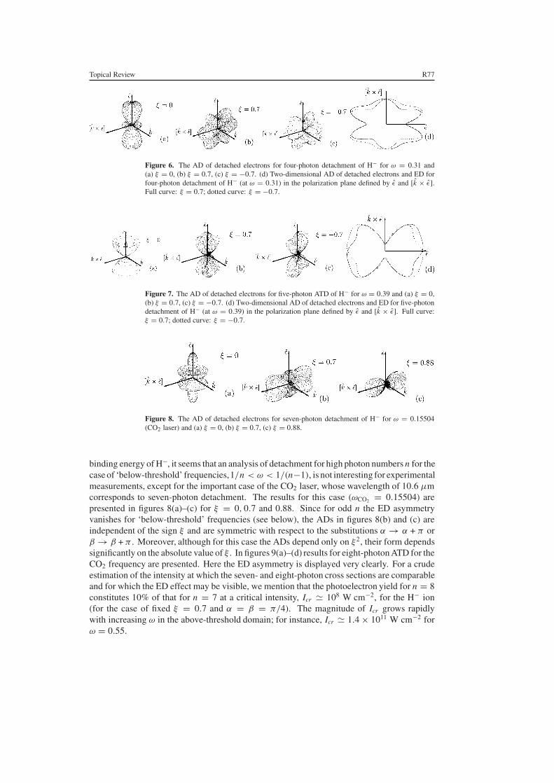
Topical Review R77
Figure 6. The AD of detached electrons for four-photon detachment of H− for ω = 0.31 and(a) ξ = 0, (b) ξ = 0.7, (c) ξ = −0.7. (d) Two-dimensional AD of detached electrons and ED forfour-photon detachment of H− (at ω = 0.31) in the polarization plane defined by ε and [k × ε].Full curve: ξ = 0.7; dotted curve: ξ = −0.7.
Figure 7. The AD of detached electrons for five-photon ATD of H− for ω = 0.39 and (a) ξ = 0,(b) ξ = 0.7, (c) ξ = −0.7. (d) Two-dimensional AD of detached electrons and ED for five-photondetachment of H− (at ω = 0.39) in the polarization plane defined by ε and [k × ε]. Full curve:ξ = 0.7; dotted curve: ξ = −0.7.
Figure 8. The AD of detached electrons for seven-photon detachment of H− for ω = 0.15504(CO2 laser) and (a) ξ = 0, (b) ξ = 0.7, (c) ξ = 0.88.
binding energy of H−, it seems that an analysis of detachment for high photon numbers n for thecase of ‘below-threshold’ frequencies,1/n < ω < 1/(n−1), is not interesting for experimentalmeasurements, except for the important case of the CO2 laser, whose wavelength of 10.6 µmcorresponds to seven-photon detachment. The results for this case (ωCO2 = 0.15504) arepresented in figures 8(a)–(c) for ξ = 0, 0.7 and 0.88. Since for odd n the ED asymmetryvanishes for ‘below-threshold’ frequencies (see below), the ADs in figures 8(b) and (c) areindependent of the sign ξ and are symmetric with respect to the substitutions α → α + π orβ → β + π . Moreover, although for this case the ADs depend only on ξ2, their form dependssignificantly on the absolute value of ξ . In figures 9(a)–(d) results for eight-photon ATD for theCO2 frequency are presented. Here the ED asymmetry is displayed very clearly. For a crudeestimation of the intensity at which the seven- and eight-photon cross sections are comparableand for which the ED effect may be visible, we mention that the photoelectron yield for n = 8constitutes 10% of that for n = 7 at a critical intensity, Icr � 108 W cm−2, for the H− ion(for the case of fixed ξ = 0.7 and α = β = π/4). The magnitude of Icr grows rapidlywith increasing ω in the above-threshold domain; for instance, Icr � 1.4 × 10¹¹ W cm−2 forω = 0.55.

R78 Topical Review
Figure 9. The AD of detached electrons for eight-photon ATD of H− for ω = 0.15504 (CO2 laser)and (a) ξ = 0, (b) ξ = 0.7, (c) ξ = −0.7. (d) Two-dimensional AD in the polarization planedefined by ε and [k × ε]. Full curve: ξ = 0.7; dotted curve: ξ = −0.7.
-0.2
0
0.2
0.4
0.6
0.8
1
0.6 0.8 1 1.2 1.4
-0.4
0
0.4
0.8
0.4 0.8 1.2 1.6 2
-0.8
-0.4
0
0.4
0.8
0.2 0.4 0.6 0.8 1 1.2 1.4
-0.8
-0.4
0
0.4
0.8
0.2 0.4 0.6 0.8 1 1.2 1.4
Figure 10. Frequency dependence of the relative ED parameter, δ(n) (see (77)), for n-photondetachment of H− in the LOPT: (a) δ(2); (b) δ(3); (c) δ(4); (d) δ(5). The geometric parameters are:θ = π/2; α = β = π/4; the polarization parameters are: dotted curve: ξ = 0.2; full curve:ξ = 0.7; chain curve: ξ = 0.94.
3.2. Discussion of dichroic terms in ADs
We discuss now in more detail the magnitude of the ED effect and its frequency dependence.Consider first the cases of n = 2 and 3 based on (49) and (52). For n = 2 the polarization andangular dependence of the ED effect is rather simple:
�(2)ed ≡ �(2)(ξ; n) − �(2)(−ξ; n) = I 2 β
(2)ed lξ cos α cos β. (76)
The kinematical maximum of the ED term corresponds to α = β = π/4, θ = π/2, andξ2 = l2 = 0.5. In figure 10(a) we present the frequency dependence of the dimensionless EDparameter, δ(2), where
δ(n) = �(n)ed [�(n)(ξ; n) + �(n)(−ξ; n)]
−1(77)

Topical Review R79
for H−, θ = π/2 and α = β = π/4. For n = 2 and 3, the ED term �(n)
ed has in general thesame magnitude as other terms in the cross sections, so that δ(n) may attain values of the orderof unity. The angular dependence of �
(3)ed differs from that in (76):
�(3)
ed ≡ �(3)(ξ; n) − �(3)(−ξ; n) = β(3)
ed lξ cos α cos β[(1 + l) cos2 α + (1 − l) cos2 β] I 3.
(78)
In this case the rhs of (78) has a maximum at θ = π/2, ξ = 2/3 and tan(2α) = 2. Thefrequency dependence of δ(3) is presented in figure 10(b).
As shown in figures 10(a) and (b), the parameters δ(n) for n = 2 and 3 vanish at thresholdsand change sign after the opening of the n = 1 channel [78]. The ED effect in two-photondetachment is most significant for below-threshold frequencies; it is small for ω > 1, whenthe one-photon channel is open. On the contrary, for n = 3 the ED effect is nonzero only forabove-threshold frequencies, ω > 1/2; δ(3) achieves considerable values above both the two-photon and the one-photon thresholds. These peculiarities are transparent from the explicitformulae for β
(n)ed which easily follow from (49) and (52). In all cases β
(n)ed originates from
an interference between real and imaginary parts of various terms which enter the detachmentamplitude. In particular,
β(2)ed ≡ A(2)
4 = 1
3πω9(2ω − 1)2(1 − ω)
×[�(1 − ω)
(1 − √
1 − ω)
+ �(ω − 1)
(1 −
√ω − 1
2ω − 1
)], (79)
where the Heaviside function �(x), is unity for x � 0 and is zero for x < 0. The parameterβ
(3)ed is very similar to β
(2)ed :
β(3)
ed ≡ A(3)
4 = 1
9πω13(3ω − 1)5/2
√2ω − 1(1 − ω) �(2ω − 1)
×[�(1 − ω)
(1 − √
1 − ω)
+ �(ω − 1)
(1 −
√ω − 1
2ω − 1
)]. (80)
The first term on the rhs of equation (79) for β(2)ed corresponds to the case ω < 1 while the
second one contributes only when ATD takes place. Moreover, β(3)ed in (80) is zero in the below-
threshold domain, 1/3 < ω < 1/2. The physical meaning of these results becomes more clearby re-writing β
(n)
ed in terms of nth-order PT radial matrix elements, M (n)
L , and scattering phases,δL(E), where L is the angular momentum of the detached electron. In particular, the result (79)in terms of these quantities is [49]
β(2)ed = − 1
24π2ω
√2ω − 1M2[�(1 − ω) sin δ0 M0 + �(ω − 1)
× {sin δ0 Re M0 + cos δ0 Im M0}], (81)
where δ0 ≡ δ0(2ω − 1). Note that, for a δ-model potential, δL>0 = 0 and exp(iδ0) =(1 − i
√2ω − 1)/
√2ω (cf (B.21)) and the matrix elements M (n)
L with L = n are real.Equation (81) shows that for ω < 1 the ED term is proportional to sin δ0 (note that itis this scattering phase which causes the complexity of the coefficient g1(ω) in (B.23) at1/2 < ω < 1), while in the above-threshold case the ED term involves Im M0. The imaginarypart of M0 corresponds to the amplitude of a two-step (cascade) process, namely one-photondetachment followed by subsequent inelastic scattering of the detached electron by the parentatom with the absorption of one additional photon. This two-step process interferes withthe ‘direct’ two-photon detachment in another L channel, whose amplitude is proportional to
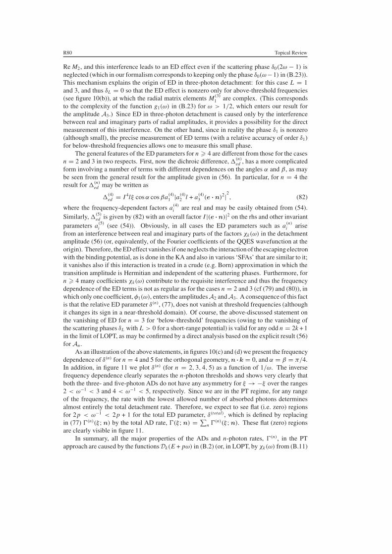
R80 Topical Review
Re M2, and this interference leads to an ED effect even if the scattering phase δ0(2ω − 1) isneglected (which in our formalism corresponds to keeping only the phase δ0(ω−1) in (B.23)).This mechanism explains the origin of ED in three-photon detachment: for this case L = 1and 3, and thus δL = 0 so that the ED effect is nonzero only for above-threshold frequencies(see figure 10(b)), at which the radial matrix elements M (3)
1 are complex. (This correspondsto the complexity of the function g1(ω) in (B.23) for ω > 1/2, which enters our result forthe amplitude A3.) Since ED in three-photon detachment is caused only by the interferencebetween real and imaginary parts of radial amplitudes, it provides a possibility for the directmeasurement of this interference. On the other hand, since in reality the phase δ1 is nonzero(although small), the precise measurement of ED terms (with a relative accuracy of order δ1)for below-threshold frequencies allows one to measure this small phase.
The general features of the ED parameters for n � 4 are different from those for the casesn = 2 and 3 in two respects. First, now the dichroic difference, �(n)
ed , has a more complicatedform involving a number of terms with different dependences on the angles α and β, as maybe seen from the general result for the amplitude given in (56). In particular, for n = 4 theresult for �
(n)ed may be written as
�(4)ed = I 4lξ cos α cos βa(4)
1 |a(4)
2 l + a(4)
3 (e · n)2|2, (82)
where the frequency-dependent factors a(4)
i are real and may be easily obtained from (54).Similarly, �(5)
ed is given by (82) with an overall factor I |(e · n)|2 on the rhs and other invariantparameters a(5)
i (see (54)). Obviously, in all cases the ED parameters such as a(n)
i arisefrom an interference between real and imaginary parts of the factors χk(ω) in the detachmentamplitude (56) (or, equivalently, of the Fourier coefficients of the QQES wavefunction at theorigin). Therefore, the ED effect vanishes if one neglects the interaction of the escaping electronwith the binding potential, as is done in the KA and also in various ‘SFAs’ that are similar to it;it vanishes also if this interaction is treated in a crude (e.g. Born) approximation in which thetransition amplitude is Hermitian and independent of the scattering phases. Furthermore, forn � 4 many coefficients χk(ω) contribute to the requisite interference and thus the frequencydependence of the ED terms is not as regular as for the cases n = 2 and 3 (cf (79) and (80)), inwhich only one coefficient, φ1(ω), enters the amplitudesA2 andA3. A consequence of this factis that the relative ED parameter δ(n), (77), does not vanish at threshold frequencies (althoughit changes its sign in a near-threshold domain). Of course, the above-discussed statement onthe vanishing of ED for n = 3 for ‘below-threshold’ frequencies (owing to the vanishing ofthe scattering phases δL with L > 0 for a short-range potential) is valid for any odd n = 2k + 1in the limit of LOPT, as may be confirmed by a direct analysis based on the explicit result (56)for An.
As an illustration of the above statements, in figures 10(c) and (d) we present the frequencydependence of δ(n) for n = 4 and 5 for the orthogonal geometry, n ·k = 0, and α = β = π/4.In addition, in figure 11 we plot δ(n) (for n = 2, 3, 4, 5) as a function of 1/ω. The inversefrequency dependence clearly separates the n-photon thresholds and shows very clearly thatboth the three- and five-photon ADs do not have any asymmetry for ξ → −ξ over the ranges2 < ω−1 < 3 and 4 < ω−1 < 5, respectively. Since we are in the PT regime, for any rangeof the frequency, the rate with the lowest allowed number of absorbed photons determinesalmost entirely the total detachment rate. Therefore, we expect to see flat (i.e. zero) regionsfor 2 p < ω−1 < 2 p + 1 for the total ED parameter, δ(total), which is defined by replacingin (77) �(n)(ξ; n) by the total AD rate, �(ξ; n) = ∑
n �(n)(ξ; n). These flat (zero) regionsare clearly visible in figure 11.
In summary, all the major properties of the ADs and n-photon rates, �(n), in the PTapproach are caused by the functions Dk(E + pω) in (B.2) (or, in LOPT, by χk(ω) from (B.11)
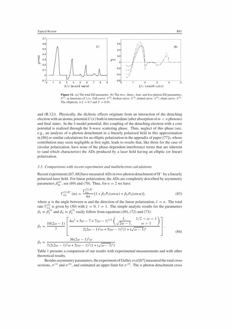
Topical Review R81
-0.1
0
0.1
0.2
0.3
0.4
0.5
0.6
0.7
0 1 2 3 4 5 6 7 8 9-0.6
-0.4
-0.2
0
0.2
0.4
0.6
0 1 2 3 4 5
Figure 11. (a) The total ED parameter. (b) The two-, three-, four- and five-photon ED parameters,δ(n), as functions of 1/ω. Full curve: δ(2); broken curve: δ(3); dotted curve: δ(4); chain curve: δ(5).The ellipticity is ξ = 0.7 and F = 0.01.
and (B.12)). Physically, the dichroic effects originate from an interaction of the detachingelectron with an atomic potential U(r)both in intermediate (after absorption of m < n photons)and final states. In the δ-model potential, this coupling of the detaching electron with a corepotential is realized through the S-wave scattering phase. Thus, neglect of this phase (see,e.g., an analysis of n-photon detachment in a linearly polarized field in this approximationin [86] or similar calculations for an elliptic polarization in the appendix of paper [77]), whosecontribution may seem negligible at first sight, leads to results that, like those for the case ofcircular polarization, have none of the phase-dependent interference terms that are inherentto (and which characterize) the ADs produced by a laser field having an elliptic (or linear)polarization.
3.3. Comparisons with recent experiments and multielectron calculations
Recent experiments [67, 68] have measured ADs in two-photon detachment of H− by a linearlypolarized laser field. For linear polarization, the ADs are completely described by asymmetryparameters β
(n)
2k , see (69) and (70). Thus, for n = 2 we have
�(2),H−lin (n) = �
(2),H−lin
4π[1 + β2 P2(cos α) + β4 P4(cos α)], (83)
where α is the angle between n and the direction of the linear polarization, ε = e. The totalrate �
(2)lin is given by (50) with ξ = 0, l = 1. The simple analytic results for the parameters
β2 ≡ β(2)
2 and β4 ≡ β(2)
4 easily follow from equations (49), (72) and (73):
β2 = 10(2ω − 1)
7
4ω2 + 5ω − 7 + 7|ω − 1|3/2
(1, 1/2 < ω < 1√
2ω − 1, ω > 1
)2(2ω − 1)2ω + 5(ω − 1)2|1 + i
√ω − 1|2
,
β4 = 36(2ω − 1)2ω
7(2(2ω − 1)2ω + 5(ω − 1)2|1 + i√
ω − 1|2) .
(84)
Table 1 presents a comparison of our results with experimental measurements and with othertheoretical results.
Besides asymmetry parameters, the experiment of Gulley et al[67] measured the total crosssections, σ (1) and σ (2), and estimated an upper limit for σ (3). The n-photon detachment cross

R82 Topical Review
-2
-1
0
1
2
3
0.01 0.02 0.03 0.04 0.05 0.06 0.07 0 0.2 0.4 0.6 0.8 1
Figure 12. (a) Asymmetry parameters β2 (thick broken curve) and β4 (thick full curve) for H−in the δ-model approach (cf (84)) as functions of photon energy. Thin broken and thin full curvesare the results of Sanchez et al (1998) [107]. (b) Ellipticity dependence of the total generalizedcross section for two-photon detachment of H− for four photoelectron energies, E p = ω − 2|E0|,chosen to be the same as in figure 4 of [77]. Full curve: ω = 0.0157 au (= 0.566 in sc. units); longbroken curve: ω = 0.0182 au (= 0.655 in sc. units); short broken curve: ω = 0.0284 au (= 1.025in sc. units); chain curve: ω = 0.043 au (= 1.55 in sc. units).
Table 1. Photoelectron angular distribution asymmetry parameters β2 and β4 for two-photondetachment of H−.
ω (in sc. units) β2 β4 References
0.8620 0.7 ± 0.2 2.0+0.4−0.2 Expt. [68]
0.70 2.47 This work (cf (84))0.65 2.31 Theory [107]
1.0027 1.3 ± 0.2 2.4+0.17−0.2 Expt. [68]1.44 2.57 This work (cf (84))1.10 2.47 Theory [125]1.22 2.52 Theory [107]
1.5468 2.54+0.44−0.6 2.29+0.07−0.31 Expt. [67]
2.71 2.20 This work (cf (84))
Table 2. Generalized cross sections for one-, two- and three-photon detachment of H− forω = 1.5468.
σ (1),H−σ (2),H−
σ (3),H−
(10−17 cm2) (10−48 cm4 s) (10−79 cm6 s2) References
3.6 ± 1.7 1.3 ± 0.5 �4.4 Expt. [67]3.65 0.96 0.13 This work (cf (85))3.58 Theory [151]
section, σ (n), is connected with the partial decay rate, �(n), in the standard way, σ (n) = �(n)/J ,where J = F2/(8πωα) is the photon flux (in scaled units) and α is the fine-structure constant.For n > 1 the ‘generalized cross sections’, σ (n),
σ (n) =[
8πωα
F2
]n−1
σ (n), (85)
are convenient for analysing n-photon detachment. (In absolute units, the dimension ofσ (n) is cm2(cm2 s)(n−1).) In table 2 we present theoretically calculated and experimentallymeasured [67] cross sections of H− photodetachment for n = 1, 2, 3 at ω = 1.5468. Tables 1

Topical Review R83
0
2
4
6
8
1500 1600 1700 1800 1900 20000
0.5
1
1.5
1000 1050 1100 1150 1200
Figure 13. Partial and total detachment rates for H− in a linearly polarized field for n = 4 (a)and n = 6 (b). Full curve: total rate; long broken curve: partial rate to the S-channel; shortbroken curve: D-channel partial rate; chain curve: G-channel partial rate. The contribution of theI -continuum channel (for L = 6) is negligible for the frequencies considered and is therefore notshown.
0
2
4
6
8
0.25 0.3 0.35 0.4 0.45 0.50
2
4
6
8
0.2 0.25 0.3 0.35 0.4
0
2
4
6
8
0.16 0.18 0.2 0.22 0.24 0.26 0.28 0.3
Figure 14. Frequency dependence of the total detachment rates for H− (divided by I n ; in scaledunits) in linearly polarized (full curve) and circularly polarized (short broken curve) fields for(a) n = 4, (b) n = 5 and (c) n = 6. Results for l = 0 correspond to G-, H - and I -continuumchannels, respectively.
and 2 demonstrate good agreement of our simple analytical results with both experimentalmeasurements and more sophisticated calculations.
For a more detailed analysis of the accuracy of the δ-model potential in multiphotoncalculations for H−, in figure 12 we present the asymmetry parameters β2 and β4 (where β2 isphase-sensitive), and also the ellipticity dependence of the total detachment rate for n = 2. Our

R84 Topical Review
results for β2,4 are in good agreement with the results in figure 2 of Sanchez et al (1998) [107];the maximum difference between our results and theirs does not exceed 10%. There is similarlygood agreement of our results and theirs for the total two-photon rate for l = 1. Finally, oneobserves similar agreement between our results for the ellipticity dependence of the total two-photon detachment rate for H− shown in figure 12(b) and those in figure 4 of Nikolopoulosand Lambropoulos [77].
In figure 13(a) we present the total rate for four-photon detachment of H− for l = 1,calculated using equation (63). Comparison with the B-spline multielectron calculations ofvan der Hart [105] demonstrates the same good agreement and level of accuracy of our resultsas for the two-photon asymmetry parameters β2 and β4 discussed above. Our results evenconfirm a small dip just above the first minimum (that arises from the interference of S- andD-wave final state channels), which is slightly more pronounced in figure 13(a) than in figure 5of [105]. This result disproves an assertion that ‘... the difference between model potentialapproaches and descriptions with electron correlations included will be more pronounced inthe four-photon detachment spectrum than for lower order detachment’ [105]. Moreover, asimilarly good agreement (with only about 10% differences in the positions and heights ofthe maxima corresponding to the S- and D-wave continuum channels) may be observed bycomparing the results for n = 6 in our figure 13(b) with those in figure 7 of [105].
The total rates �(n) for n = 4, 5 and 6 are presented in figure 14 over an extended frequencyinterval (compared with that in [105]) for two polarization states of the laser, l = 0 and 1.These results demonstrate the interesting fact that, for high enough above-threshold frequencies(corresponding to the absorption of a few excess photons), the efficiency of detachment by acircularly polarized field becomes higher than that for the case of linear polarization (thoughboth efficiencies are very small). It means that the continuum channel with maximum orbitalmomentum, L = n, is the dominant one for these frequencies. Meanwhile, for smaller ω,the population of this channel is negligible and it is not even visible in figure 14 for n = 6.This statement may be regarded as a general one for the PT region; we have found it to holdfor n > 6 as well. Finally, our results in figures 13 and 14 are in good agreement (with anaccuracy of about 2%) with results [102] of one-electron PT calculations of �(n) for H− (for2 � n � 8 and ‘below-threshold’ frequencies, 1/n � ω � 1/(n − 1)).
In summary, the above comparisons demonstrate a reasonable agreement of our analyticalresults with more detailed (and time-consuming) calculations. (See, however, the discussionof figure 5 above.) We are inclined to consider such agreement for multiphoton calculations asexcellent, taking into consideration that an accuracy of 10% or better is beyond the capabilitiesof recent multiphoton experiments.
4. Strong field analysis of angular distributions and ED effects
4.1. Symmetry properties of angular distributions and elliptic dichroism
In a strong field, the symmetry properties of ADs (including the ED effect) are essentiallythe same as in the PT analysis of the previous section since they follow from rather generalarguments [11, 49]. In the dipole approximation, e and n are the only vector parameters ofthe problem for the case of an unpolarized target atom. Thus, in any PT order (and hencein the nonperturbative regime as well) the n-photon amplitude may involve only even (foreven n) or odd (for odd n) powers of scalar products e · n and e∗ · n. Hence, the ADis invariant to n → −n. This inversion symmetry stems from parity conservation in theproblem considered. Also, the AD is invariant to a rotation by an angle π around the directionof k (which corresponds to the invariance of results with respect to inversion of the directions

Topical Review R85
of the polarization unit vectors ε and [k × ε], i.e. to the substitutions e → −e, e∗ → −e∗in the cross section). This symmetry is equivalent to a rotation by π around ε followed by arotation by π around [k × ε]. Besides the two mentioned above, no other symmetries exist forADs produced by an elliptically polarized laser. Moreover, there is a significant asymmetryresulting from the change ξ → −ξ that originates from odd powers of the ED factor (cf (71)or (75) and the discussion following equations (69) and (70)). For the δ-model potential, allthese general observations follow straightforwardly from the exact results (36) and (38), wherethe coefficients φ±p depend only on l and the Bessel functions depend only on the modulus|e · n|.
As mentioned above, the AD is invariant to a simultaneous rotation by an angle π
around the directions of ε and [k × ε]. Neglecting the ED terms, ADs exhibit an additionalsymmetry with respect to separate rotations by an angle π around either ε or [k × ε]. TheED terms, however, destroy this symmetry and cause the well-known asymmetry of the ADs.Thus, this asymmetry illustrates an interesting physical phenomenon specific to an ellipticallypolarized field: the light-helicity dependence of multiphoton ADs. Note that if one neglectsthe coefficients fn with n �= 0 (as is done to reduce the exact results for a δ-model potentialto those for the KA), the ED effect (i.e. the asymmetry with respect to ξ ) of the AD vanishes.Finally, we note the general symmetry of ADs with respect to the substitution ξ, k → −ξ, −k(which is equivalent to the change ξ → −ξ and a rotation by π around either ε or [k × ε]),i.e. the equivalence of ADs in two experiments with opposite helicities and directions of thelaser beam (cf (71)).
4.2. Total and partial rates of n-photon detachment
We analyse here the dependence of the n-photon detachment rates, �(n), on intensityand frequency in the nonperturbative domain of these parameters. For a given n, thisnonperturbative domain is bordered by the PT regime (for low intensities and/or highfrequencies) and the region of the intensity-induced closing of the n-photon detachmentthreshold. We give here examples of the behaviour of the rates between these two extremecases. Numerical results are obtained using (36) and (38) as well as the angular integral overthe differential rate (38), in which ε and φn are numerical solutions of equations (27) and (28).Expansion of the amplitude (36) in partial waves allows us to calculate numerically the fixedangular momentum L components of �(n)(n) (i.e. partial n-photon rates). The amplitude An
in (36) involves an infinite summation over p, allowing in general any value of L permittedby dipole selection rules. This reflects the possibility that virtual absorption and emissionof photons may lead to a final-state angular momentum value that is larger than n. Thispossibility is specific to the nonperturbative regime since the LOPT analysis predicts only amaximum of n quanta of angular momenta absorbed by the ejected electrons. However, ournumerical calculations show that for all the values of the parameters in the nonperturbativeregime considered by us, the contribution of the continuum channels with L higher than n isextremely small.
In figure 15 we show the two-photon detachment dependence on frequency for the case oflinear and elliptic polarization and two (perturbative and strong) laser intensities. We prefer toplot the dependence on the inverse frequency 1/ω (i.e. wavelength in our scaled units) since itallows a better visualization of the low frequency region, ω < 1. As the intensity increases, theponderomotive shift Up moves the position of the threshold towards larger frequencies. Thecurves representing the S and D rates allow us to understand the modification of the summedtwo-photon rate. Qualitatively, the S and D rates have the same behaviour at all intensities:a fixed number of maxima and minima covering the region from the threshold to the high

R86 Topical Review
Figure 15. Two-photon detachment rate for the case of linearly polarized (ξ = 0; (a,b)) andelliptically polarized (ξ = 0.7; (c, d)) light as a function of 1/ω for two intensities: (a, c) F = 0.01,(b, d) F = 1.0. Thin full curve: S-wave continuum channel; thin broken curve: D-wave continuumchannel; thick full curve: total two-photon rate (sum of S and D channels).
frequency limit. These maxima and minima are related to the oscillatory nature of the Besselfunctions appearing in (36). In general, for any fixed n, the number of maxima of the partialwaves when going from the high frequency, low intensity limit to the threshold ranges fromonly one maximum for L = n up to [n/2] + 1 for the lowest value of L allowed by the dipoleselection rules (0 for even n and 1 for odd n). This can be observed in figure 15 where theD-wave channel rate has only one maximum and the S-wave channel rate has two maxima andone minimum. Changing the intensity results in the same number of maxima and minima butchanges their frequency location and the magnitude of the rates at the maxima. As the intensityincreases, the magnitudes of the maxima of both the total and partial rates increase. Also, themaximum of the D-wave partial rate increases relative to that of the S-wave partial rate so thatthe total rate changes its shape (versus 1/ω) from having a single maximum at low intensityto having a double maximum at high intensities. All these features reflect a complicated,intensity-dependent interference of the different detachment pathways leading to a particularfinal state of the escaping electron, such as between different L-wave channels contributing toa particular final momentum state, or between LOPT and higher-order processes contributingto a particular electron channel. Since for circular polarization only electrons with L = ncan be ejected, as we vary the ellipticity from linear to circular the relative importance of theL = n partial rate must increase. This can be observed by comparing figures 15(a), (b) forξ = 0 to figures 15(c), (d) for ξ = 0.7. For circular polarization the structure of the n photonrate is very simple: L = n is the only allowed angular momentum and the corresponding rate
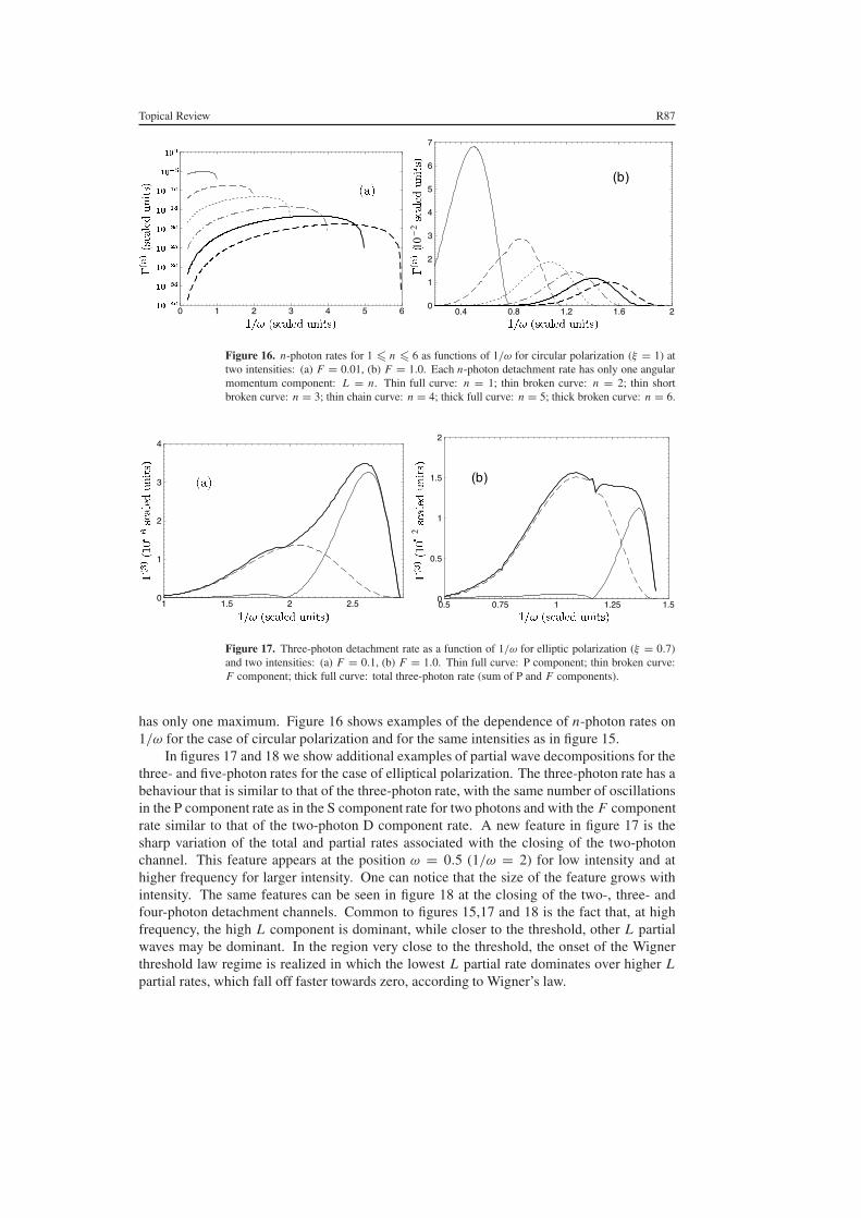
Topical Review R87
0 1 2 3 4 5 60
1
2
3
4
5
6
7
0.4 0.8 1.2 1.6 2
(b)
10−
2
Figure 16. n-photon rates for 1 � n � 6 as functions of 1/ω for circular polarization (ξ = 1) attwo intensities: (a) F = 0.01, (b) F = 1.0. Each n-photon detachment rate has only one angularmomentum component: L = n. Thin full curve: n = 1; thin broken curve: n = 2; thin shortbroken curve: n = 3; thin chain curve: n = 4; thick full curve: n = 5; thick broken curve: n = 6.
0
1
2
3
4
1 1.5 2 2.5 0
0.5
1
1.5
2
0.5 0.75 1 1.25 1.5
(b)
2
Figure 17. Three-photon detachment rate as a function of 1/ω for elliptic polarization (ξ = 0.7)and two intensities: (a) F = 0.1, (b) F = 1.0. Thin full curve: P component; thin broken curve:F component; thick full curve: total three-photon rate (sum of P and F components).
has only one maximum. Figure 16 shows examples of the dependence of n-photon rates on1/ω for the case of circular polarization and for the same intensities as in figure 15.
In figures 17 and 18 we show additional examples of partial wave decompositions for thethree- and five-photon rates for the case of elliptical polarization. The three-photon rate has abehaviour that is similar to that of the three-photon rate, with the same number of oscillationsin the P component rate as in the S component rate for two photons and with the F componentrate similar to that of the two-photon D component rate. A new feature in figure 17 is thesharp variation of the total and partial rates associated with the closing of the two-photonchannel. This feature appears at the position ω = 0.5 (1/ω = 2) for low intensity and athigher frequency for larger intensity. One can notice that the size of the feature grows withintensity. The same features can be seen in figure 18 at the closing of the two-, three- andfour-photon detachment channels. Common to figures 15,17 and 18 is the fact that, at highfrequency, the high L component is dominant, while closer to the threshold, other L partialwaves may be dominant. In the region very close to the threshold, the onset of the Wignerthreshold law regime is realized in which the lowest L partial rate dominates over higher Lpartial rates, which fall off faster towards zero, according to Wigner’s law.

R88 Topical Review
0
0.5
1
1.5
2
2.5
3
2 2.5 3 3.5 4 4.5 0
0.2
0.4
0.6
0.8
1
0.6 0.8 1 1.2 1.4 1.6 1.8 2
(b)
2
Figure 18. Same as figure 17 but for five-photon detachment, where now the chain curve denotesthe H-wave partial rate and the full curve is the sum of the P-, F- and H-wave partial rates.
The intensity dependence of the n-photon rates as well as that of the partial rates looksvery similar to their dependence on the inverse frequency. The reason is that, as may be seenin (B.1), the matrix elements in the system of equations (27) that determine the coefficientsφn depend on F and 1/ω in a similar way. There is an additional dependence on ω in thecoefficients of the series but, for the parameters considered, this dependence is very weak. Wehave the situation of a quasiscaling with the parameter F/ω2; therefore the dependence on F issimilar to that on 1/ω2. In figure 19 we present the dependence of �(n) (and of its partial ratesfor particular values of L) on the laser amplitude F for n = 2, 3 and 5, respectively, for thesame ellipticity (ξ = 0.7) and for two frequencies: ω = 0.8 and 1.5. The intensity is variedfrom small, perturbative values up to the value for which the Up shift closes the particularn-photon channel. Near the two- and three-photon thresholds, we see the much faster increaseof the low L rates, S and P, followed by a region where the D and F rates dominate. In thelow intensity part (not visible in the figures), which of the partial rates is dominant dependson the value of ω; this information can be extracted from the previous figures showing the ω
dependence for low intensities. From figures 19(e), (f) one can see that, for higher numbersof photons, the lower L components have increasingly more oscillations while the componentwith L = n has the least rapid variation and, except for threshold-induced anomalies, only onebroad maximum. One can notice these distinct TAs in both the partial rates and the total rate.They are associated with the closing of the lower-order detachment channels [135].
4.3. Three-dimensional angular distributions
As in the PT analysis, we find it more instructive to show 3D plots of the differential rates�(n)(n). These rates are obtained using the exact result given by equations (37) and (38).Since we are interested in the change of the AD as the intensity is varied over a large range,thus leading to large variations of the rates, we rescale our results such that all of the 3Dfigures have approximately the same size. Figure 20 shows the ADs for two- and three-photondetachment as the intensity is increased from low intensity up to that which closes, respectively,the two- and three-photon detachment channels. For low perturbative intensities, the electronsare ejected mainly along the major polarization axis. However, as the intensity increases, theinterplay between the various L components can lead to significantly different ADs. In thesimplest cases of two- and three-photon detachment, the interplay between the S and D (or Pand F) components in the region preceding the onset of the Wigner threshold law regime can

Topical Review R89
Figure 19. n-photon detachment rate as a function of laser amplitude, F , for the case of ellipticpolarization (ξ = 0.7) for two frequencies, ω = 0.8 (left panels) and ω = 1.5 (right panels).Thick full curves represent total n-photon rates. (a, b) Thin full curve—S-wave component; thinbroken curve—D-wave component. (c, d) Thin full curve—P component; thin broken curve— Fcomponent. (e, f) Thin full curve—P component; thin broken curve— F component; thin chaincurve—H component.
lead to a cancellation of the detachment amplitude along the major polarization axis for certainvalues of the intensity and the frequency [78]. This effect is illustrated in figure 20 where onesees that, in the region of intensities shown in the third and fourth rows, the probability fortwo- and three-photon detachment along the ε axis passes though zero. This situation can berealized for any polarization that allows the existence of several angular momenta in the finalstate, i.e. for any polarization except circular. For circular polarization, the AD is always thatcorresponding to an L = n partial wave and does not change its shape as either the frequency

R90 Topical Review
Figure 20. Two- and three-photon detachment ADs (i.e. n = 2, 3) as functions of the laseramplitude F for the fixed frequency, ω = 0.8, and two different polarizations. First column:n = 2, ξ = 0.0 (linear polarization); second column: n = 3, ξ = 0.0; third column: n = 2,ξ = 0.7; fourth column: n = 3, ξ = 0.7. For each case, five values of F are given, in which thelowest, F = 0.01, corresponds to the perturbative regime and the highest is just at the intensity-induced closing of the n-photon channel. The different figures have been scaled in order to havethe same size.
or the intensity is varied. The unusual ADs obtained for linear and elliptic polarization can beunderstood as resulting from quantum interference between the different angular momentumstates in the intermediate region between the perturbative regime and the Wigner thresholdlaw regime. For the highest value of the intensity shown in each figure, which in each case isclose to the corresponding threshold, we see that the S and P waves are dominant for two- andthree-photon processes, respectively, in agreement with Wigner’s threshold law (cf the bottomrow of figure 20).
The oscillation pattern of the ADs for the case of linear polarization was mentionedin earlier quasiclassical (saddle point) calculations (see equation (53) in [1](c) and thediscussion after equation (23) in [1](b)) and was analysed later in more detail by Gribakinand Kuchiev [128] using the Keldysh approach. In these analyses the angular momentumcomponents of the escaping electron were not resolved; instead, the oscillation pattern is

Topical Review R91
Table 3. Photoelectron AD asymmetry parameters β2k for two-photon detachment of H− by thelinearly polarized field of frequency ω = 0.758 (λ = 2.15 µm). 10n ≡ (n).
I (W cm−2) β2 β4 β6 β8 References
1.3(11) −5.49(−1) 1.97 −4.55(−2) 4.37(−4) Equations (38), (37)−3.62(−1) 1.84 −4.18(−2) 3.95(−4) [153]
2.35(−1) 2.41 0.34(−2) 58.9(−4) [128] a
2.22(−1) 2.39 −5.59(−2) 5.41(−4) Equations (38), (45)
6.5(11) −1.32 3.63(−1) −1.20(−2) 1.75(−4) Equations (38), (37)−1.19 2.87(−1) −0.77(−2) 0.91(−4) [153]−1.37 3.92(−1) −1.08(−2) 2.67(−4) [128] a
−1.42 4.34(−1) −1.58(−2) 2.52(−4) Equations (38), (45)
a Entries for [128] are taken from table II of [153].
interpreted as stemming from the interference between contributions of two saddle pointscorresponding to two peak values of the field amplitude over the laser period. Recently thesuppression of electron yield along the direction of linear laser polarization has been measuredby Reichle et al [71] in two-photon detachment of H− at ω = 0.758, and their experimentalresults (for two laser intensities, 1.3 × 10¹¹ and 6.5 × 10¹¹ W cm−2) were found to be inagreement with the KA results [128]. Very recently, more sophisticated calculations havebeen performed [153] (based on the numerically intensive methods described in [126]) withresults that differ only slightly from those in [128], primarily for the lower intensity. In table 3we compare the above-mentioned results for the AD asymmetry parameters with our resultsobtained using the exact equations (38) and (37) and also our results using the ‘exact’ KAamplitude (45) (i.e. beyond the adiabatic approach used in [128]). For the lower intensity, onesees that our exact results are in reasonable agreement with those in [153], while for the higherintensity all results are in reasonable agreement.
Figure 21 shows the AD of all the ejected electrons, �(n) = ∑n �(n)(n), regardless of
their energy. For low intensities, the two-photon channel is the dominant process and the totalAD �(n) is very similar to that for two-photon detachment. For higher intensities, the ATDrates become increasingly more important. Several partial rates contribute equally to �(n). Asthe intensity increases, �(n) has a very different form from those of the individual n-photonrates �(n)(n) shown in figure 20. We see in particular that in the region of intensities for whichthe two- or three-photon rates have close to zero electrons ejected along the major polarizationaxis, �(n) does not preserve this property. Higher-order processes are more important andcompletely mask the effect. Indeed, as the intensity increases, �(n) is increasingly localizedalong the major polarization axis ε.
4.4. Elliptic dichroism in a strong field
To analyse the frequency and intensity dependence of ED in the nonperturbative regime, we usethe same ED parameter, δ(n), as in the LOPT case, (77), where the differential rates are measuredin the direction of the geometrical maximum of the effect (cf figure (1) and equation (71)):θ = π/2 (i.e. in the polarization plane) and α = β = π/4 (i.e. halfway between the major andminor axes of the polarization ellipse). We also define the total ED parameter for the total AD�(n), δ(total), by replacing the n-photon AD �(n)(ξ; n) in (77) by �(ξ; n) = ∑
n �(n)(ξ; n).
4.4.1. Frequency dependence. In figure 22 we present the frequency dependence of δ(n) withn = 2, 3, 4, 5 for three nonperturbative intensities. Similar results for the PT regime werediscussed in section 3.2 (figure 10). Aside from the frequency shift of the entire structure of

R92 Topical Review
Figure 21. Total detachment ADs (summed over n) at ω = 0.8 and ξ = 0.7 for ten values of thelaser amplitude, F , as indicated in the figure. The different figures have been scaled in order tohave the same size.
the curves due to the Up shift, one also sees that the ED in the three- and five-photon detachmentcases is nonzero even in the region 1/3 < ω < 1/2 and 1/5 < ω < 1/4, respectively, whichcontrasts with the perturbative case. The ED in these frequency regions increases with thelaser intensity owing to higher-order processes which, by interference with the lowest-orderones, produce the ED effect. The oscillations of δ(n) can be traced to the oscillatory nature ofthe Bessel functions that determine the ADs, as discussed in section 3.2. Note that, in the limitof the Wigner law regime, in which one L component is dominant, the ED tends to zero sincethe AD in this region is that of a pure S or P distribution and all interference effects disappear.

Topical Review R93
-0.2
0
0.2
0.4
0.6
0.6 0.8 1 1.2 1.4-0.2
0
0.2
0.4
0.6
0.5 0.75 1 1.25 1.5
-0.4
-0.2
0
0.2
0.4
0.6
0.25 0.5 0.75 1 1.25 1.5-0.4
-0.2
0
0.2
0.4
0.6
0.25 0.5 0.75 1 1.25 1.5
Figure 22. Frequency dependence of the ED parameter δ(n) for elliptically polarized light(|ξ | = 0.7) and for three nonperturbative intensities. Full curve: F = 0.1; broken curve: F = 0.5;chain curve: F = 1.0. (a) n = 2; (b) n = 3; (c) n = 4; (d) n = 5.
-0.1
0
0.1
0.2
0.3
0.4
0.5
0.6
0 1 2 3 4 5 6
Figure 23. The total ED parameter for |ξ | = 0.7 plotted versus 1/ω, for three intensities. Fullcurve: F = 0.1; broken curve: F = 0.5; chain curve: F = 1.0.
Figure 23 shows the total ED parameter as a function of 1/ω for three intensities. The largemaxima can be identified as arising from the large ED effect in a single n-photon channel. Forlow frequency the contributions of a large number of channels, each having a large number ofoscillations, tends to reduce the ED effect in �(n). However, for higher intensity (F = 1) wenote an interesting effect: towards low frequencies the ED parameter shows a decreasing trendwhich does not stop at zero but continues increasing in absolute value towards negative values.This region corresponds to large maxima (in absolute value) in the n-photon ED parameters
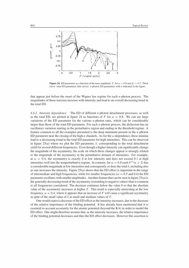
R94 Topical Review
Figure 24. ED parameter as a function of the laser amplitude, F , for ω = 0.8 and |ξ | = 0.7. Thickcurve: total ED parameter; thin curves: n-photon ED parameters with n indicated in the figure.
that appear just before the onset of the Wigner law regime for each n-photon process. Themagnitudes of these maxima increase with intensity and lead to an overall decreasing trend inthe total ED.
4.4.2. Intensity dependence. The ED of different n-photon detachment processes, as wellas the total ED, are plotted in figure 24 as functions of F for ω = 0.8. We can see largevariations of the ED parameter for the various n-photon rates, which can be considerablylarger than those of the total ED parameter. For each n-photon process, the dichroism has anoscillatory variation starting in the perturbative region and ending in the threshold regime. Afeature common to all the examples presented is the deep minimum present in the n-photonED parameter near the closing of the high n channels. As for the ω dependence, these minimalead to a decreasing trend in the total ED parameter for high intensities. This can be observedin figure 25(a) where we plot the ED parameter, δ, corresponding to the total detachmentyield for several different frequencies. Even though a higher intensity can significantly changethe magnitude of the asymmetry, the scale on which these changes appear is strongly relatedto the magnitude of the asymmetry in the perturbative domain of intensities. For example,at ω = 0.4, the asymmetry is exactly 0 at low intensity and does not exceed 0.1 at highintensities well into the nonperturbative regime. In contrast, for ω = 0.8 each δ(n)(n � 2) hasa considerable magnitude at low intensities and consequently so does the total δ, including alsoas one increases the intensity. Figure 25(a) shows that the ED effect is important in the rangeof intermediate and high frequencies, while for smaller frequencies (ω = 0.5 and 0.4) the EDparameter oscillates with smaller amplitudes. Another feature that can be seen in figure 25(a) isthe generally decreasing trend of the asymmetry (extending to negative values) that is commonto all frequencies considered. The decrease continues below the value 0 so that the absolutevalue of the asymmetry increases at higher F . This trend is especially interesting at the lowfrequency, ω = 0.4, where it appears that an increase of F will cause a significant asymmetryin spite of the small value of δ at small and medium values of F .
One would expect a decrease of the ED effect as the intensity increases, due to the decreaseof the relative importance of the binding potential. It has already been mentioned that it isessential to account accurately for the atomic potential (beyond the KA) in order to model theED effect. One might therefore assume that, as the intensity increases, the relative importanceof the binding potential decreases and thus the ED effect decreases. However this assertion is

Topical Review R95
Figure 25. Total ED parameter as a function of the laser amplitude, F , for |ξ | = 0.7. (a) The resultsfor different frequencies (full curve: ω = 0.4; broken curve: ω = 0.5; chain curve: ω = 0.8;dotted curve: ω = 1.0). (b) The result for ω = 0.8 including (full curve) and neglecting (brokencurve) the imaginary part of the quasienergy.
contradicted by our results shown in figure 25(a), and therefore a different mechanism mustbe responsible for the nonzero dichroism observed at high intensities. Aside from the factthat the binding potential leads to nonzero coefficients φn having imaginary parts, there is anadditional reason for the origin of the ED effect. The imaginary part of the ATD amplitudewhich multiplies the kinematic factor (71) to produce the ED terms in �(n)(n) can appear due tothe complex part of the quasienergy, as measured by � = −2 Im ε. � is small at low intensitiesand cannot affect the ED significantly. However, for high intensities, � increases very sharplyand its contribution to the ED parameter increases correspondingly. We show the importanceof this contribution in figure 25(b), where we plot the total ED parameter calculated with theexact quasienergy and with the approximation Im ε = 0. (Note that the latter approximatecalculation is done using the exact values of the complex coefficients φn , and therefore thepotential is taken into account beyond the KA.) The two results are very close to each otherfor low intensities, but differ significantly for high intensities, where Im ε is large. While theexact calculation shows the decreasing trend, the one that neglects Im ε decreases and thenstays approximately constant as I increases. We can conclude that the increasing trend (inabsolute value) as intensity increases relates to the direct contribution of Im ε.
5. Photodetachment in a strong, high frequency field (ω > 1)
In many cases the photon energy of the fundamental or lower harmonics of existing intenselasers exceeds the binding energy of a weakly bound electron in a negative ion. In such casesthe ‘high frequency’ regime of their decay is realized when the direct laser detachment channelis open, i.e. ω > 1. Although we have already mentioned in section 4 some peculiarities ofthe ω and F dependences of the total rates and ADs for the case of ω > 1, in the presentsection we analyse this important case in more detail. This question is closely related to thewidely discussed general problem of strong field atomic stabilization, i.e. to the somewhatcounterintuitive regime of atomic ionization in a high frequency field in which the decayprobability appears to be a decreasing function of laser intensity. Although theoretical modelsof such stabilization were suggested more than 10 years ago [154, 155] (see also [156, 157] aswell as recent reviews [158, 159]), there still does not exist an exact solution of this problemfor an electron bound by Coulomb forces in a superstrong laser field. Thus there does not
R96 Topical Review
exist a complete understanding of the dependence of this interesting nonlinear phenomenonon the atomic and field parameters in the ultrastrong field limit. In particular, the theoreticalmodels predict an unlimited (possibly oscillatory) decrease of the ionization rate � as the fieldamplitude increases (see [159]). On the other hand, the results of numerical calculationshave demonstrated that the decrease of decay rates for a Coulomb potential [157, 160]covers only a limited interval of laser intensities. Moreover, existing experiments on atomicstabilization [161] provide only limited information on its intensity dependence. Althoughstabilization was originally identified as a property of decay rates (quasistationary stabilization,QS), in recent years the wavepacket version of stabilization (or ‘dynamic stabilization’,DS) [156, 162] has attracted interest. DS originates from the pulse form of a laser fieldrather than from any intrinsic property of the atom in a strong monochromatic field. ThusDS means that the total ionization probability at the end of a fixed-duration laser pulse doesnot approach unity with increasing peak intensity. However, a detailed analysis [163] (seealso [160]), which uses the QQES as an adiabatic basis for the laser pulse, has shown that DShas essentially the same (quasistationary) origin as QS.
Though short-range potential models are deemed to be appropriate for the study of QS,analyses employing them sometimes show contradictory results. In particular, for the one-dimensional δ model, there have been claims both for the existence of QS [164] and for itsnon-existence [165]. The absence of QS for the three-dimensional δ-model potential in acircularly polarized field is claimed in [166]. The more exact analysis in [167] does not givea definitive result for the high intensity limit. Finally, a number of authors deny the existenceof stabilization based on formal mathematical arguments, in particular, of QS for ionizationfrom a δ potential [168] and of DS in pulsed fields [169]. However, these arguments take theform of existence theorems valid for I → ∞ and do not restrict the existence of a decreasing(stabilization-like) trend of �(I ) in a limited interval of intensities. A recent exact analysis ofthe QS problem for an electron in a δ-model potential [134] shows that precisely this situationis realized in the nonperturbative regime (up to the closure of the one-photon channel) forabove-threshold frequencies (ω > 1) for any polarization state of the laser field. The lackof QS in an asymptotically strong field follows from a more general statement [170] on theequivalence of the effect of a superstrong monochromatic field on a weakly bound electron tothat of a strong static electric field (in which case QS is clearly absent).
In what follows, we examine the frequency and intensity dependence of the detachmentrates in the high frequency regime. We first examine the perturbative (in intensity) behaviourof the one-photon detachment cross section, showing that a decrease with increasing intensityoccurs even in the perturbative region. This decrease (or stabilization) breaks down at theclosing of the one-photon threshold. Our exact results show in fact that stabilization-typebehaviour occurs in the vicinity of each n-photon threshold. We also present exact results forthe ADs in the high frequency regime.
5.1. Higher-order corrections to the one-photon detachment cross section
For a high frequency field, the PT expansion of the decay rate may be applicable up to highintensity, I � 1. Therefore, we first present analytical results for the intensity-dependentcorrections, ∼I and ∼I 2, to the well-known photodetachment cross section, σ0, for a short-range potential:
dσ0
d�= 3
4πσ0|e · n|2, σ0 = 32πα
3ω3(ω − 1)3/2. (86)
Since the PT expansion for the complex quasienergy ε (and, therefore, for decay rates ina monochromatic laser field) is convergent [143, 171], it means that an exact, strong laser

Topical Review R97
field generalization of (86), dσ (1)/d�, has a regular, convergent RS expansion in the (scaled)intensity, I = F2, for not too high I :
dσ (1)
d�= dσ0
d�+ I �σ1 + I 2 �σ2 + · · · . (87)
Moreover, in the BW version of an expansion like (87) (see (89) below), the parameters�σi = �σi (ε) are I -dependent (owing to their dependence on ε = ε(I )). Thus, in the sameorder, ∼I n , the accuracy of the BW expansion may be substantially higher than that of the RSexpansion since the nth-order BW result includes summations of many infinite subsequencesof the RS expansion, which originate from the RS expansions of the parameters �σi (ε) in I .
The standard PT calculation of even the first RS correction, �σ(1), is not a simpleproblem since in such an analysis in addition to the calculation of third-order Feynmandiagrams (which correspond to the re-emission of a photon) one must also take properaccount of the so-called ‘secular’ and normalization terms, which occur in higher ordersof PT (see, e.g., [172]). Moreover, the contributions of separate Feynman diagrams involve(non-regularizable) singularities that cancel only in the total amplitude [173]. In our analysisthe problem is simplified because we start from the result (38) for n = 1, i.e. we deal directlywith the exact amplitude A1, thereby avoiding PT calculations of separate Feynman diagrams,etc. To obtain the BW PT expansion of dσ (1)/d� up to terms ∼I 2, we expand the Besselfunctions in the amplitude A1 in (36) up to terms ∼F5. Note that only the coefficients φn withn = 0 and ±1 contribute for this case. The final BW result is
A1(E) = iF
ω2
√E − ω
{φ0
[1 − F2
2ω4(ω − E)|e · n|2 +
F4
12ω8(ω − E)2|e · n|4
](e · n)
+ φ1
[1 − F2
2ω4(ω − E)|e · n|2
](e∗ · n) − φ−1
F2
6ω4(ω − E)(e · n)3
}, (88)
where φ±1 and φ0 are given by (B.5) and (B.6) and their expansions up to ∼F4 contribute toA1(E). The resulting three-term BW expansion for the one-photon detachment cross sectionmay be written as follows:
dσ(1)
BW
d�= 16πα|φ0|2 |ω − E |3/2
ω3
{|e · n|2 − F2
ω4Re
[(ω − E)|e · n|4 + l
D1(E − ω)(e∗ · n)2
√E − 2ω − 1
]
+F4
ω8
[l2
4|e · n|2
∣∣∣∣ D1(E − ω)√E − 2ω − 1
∣∣∣∣2
+|e · n|6
4
(|ω − E |2 +
2
3Re(ω − E)2
)
+ l|e · n|2[(ω − Re E) Re
(D1(E − ω)(e∗ · n)2
√E − 2ω − 1
)
+ Re
(D1(E + ω)√E + 2ω − 1
ω − E
6(e · n)2
)]
− l Re
(D2(E − ω)√E − 2ω − 1
(e∗ · n)2 +D1(E − ω)D1(E − 2ω)(e∗ · n)2
(√
E − 2ω − 1)2
)]}.
(89)
Despite its apparent complexity, dσ(1)
BW /d� is only a combination of simple functions D1 andD2, which are defined in (B.2). Thus, it is even somewhat unexpected that the summed resultof high-order PT corrections to the (linear in F) LOPT photodetachment amplitude up to terms∼F5 can be presented in an accessible analytical form (89). Integrating (89) over �, we findthe total cross section in the BW approach. Including terms up to order F2, the result is

R98 Topical Review
σ(1)BW = 64
3π2α|φ0(E)|2 |ω − E |3/2
ω3
×{
1 − F2
ω4
[2 + l2
5(ω − Re E) + l2 Re
(D1(E − ω)√E − 2ω − 1
)]}. (90)
To obtain the RS results, the (complex) parameter E = γ 2 − ε in (89) and (90) shouldbe expanded in powers of F2 (see (B.14) and (B.15)–(B.18)) taking into account also the Edependence of the normalization factor φ0 (see (B.6)–(B.8)). Then the resulting terms up toorder F4 on the rhs of (89) should be collected. Since the final results are too cumbersometo present here (as they correspond to the fifth order of standard (RS) PT), we present here anexplicit form only for the linear in I RS correction to (87):
�σ RS1 = 8α
3ω7
√ω − 1
{|e · n|2[√ω + 1(ω2 − 7) + 14 − 8ω
] − 3|e · n|4(ω − 1)2
+ l Re{(e · n)2} (ω − 1)
ω
[1 + 2ω(ω − 1) − (ω − 1)3/2
√2ω − 1
]+ l Im{(e · n)2} (ω − 1)2
ω
[√2ω − 1 − √
ω − 1]}
. (91)
The total photodetachment rate including the lowest two orders of RS PT is
�(1)
RS = 4F2
3ω4(ω − 1)3/2 +
4F4
9ω8
√ω − 1
{√ω + 1(ω2 − 7) − 2
5(3ω2 + 14ω − 32)
+ l2 ω − 1
ω
[1 +
7
5ω(ω − 1) − (ω − 1)3/2
√2ω − 1
]}. (92)
Note the smoother threshold behaviour, ∼√ω − E , where E = 1, of �σ RS
1 comparedto that of σ0, which originates from the S-wave part of the detached electron’s final-statewavefunction in the third PT order12. Thus, the strong field corrections are most important fornear-threshold frequencies. The term ∼l Im{(e ·n)2} in (89) and (91) describes the ED effect,see (71). We note the considerable threshold suppression of the ED term, ∼(ω − 1)2, as wellas its smallness at high frequencies (by a factor ∼ω−1) compared to the leading terms in (91).This is the reason that the numerical value of the ED parameter in the AD �(1)(n) is small(although nonzero) and does not exceed a fraction of one per cent for any frequency ω > 1.
Although the field amplitude F is a formally small parameter of the PT analysis, the actualparameter of the PT expansion (87) is I/ω4 (see (89) and (92)). Thus, for ω > 1 a few ordersof RS or BW PT expansions give a reasonable result for dσ (1)/d� for even high intensities upto I = F2 � 1. In figure 26(a) we present the frequency dependence of the total rates σ
(1)RS
and σ(1)BW for F = 0.5(I = 0.25) taking into account the terms of order I and I 2. The BW
result is obtained from (89) with the quasienergy ε calculated from equations (B.7) and (B.9).As mentioned above, the intensity corrections are most important near the threshold, wherethe BW result is more accurate than the RS one. The curve for σ
(1)BW in figure 26(a) starts from
the dynamical threshold, ωth(F) = − Re ε, which is shifted from ωth(0) = 1 because of the(negative) Stark shift. Generally, the RS curve for σ (1) starts from the unshifted threshold,ωth(0), although the result (92) gives a negative value of �(1) for 1 < ω < ωth(F). (Thesephysically senseless results for the decay rate are not presented in figure 26(a).) This factindicates the breakdown of high-order RS results in the near-threshold domain. Formally, thisinaccuracy is caused by the use of power expansions (in F) of threshold factors reducing (90)
12 The terms of order F2 in the BW results (89) and (90) also have a threshold behaviour ∼|√ω − E |, as may beverified from the threshold behaviour of the φ0(E) and D1(E − ω) functions.

Topical Review R99
0
2
4
6
8
1.2 1.6 2 2.4 2.80
2
4
6
8
0 0.2 0.4 0.6 0.8 1 1.2 1.4
Figure 26. One-photon detachment cross section of H− in a linearly polarized laser field. Shortbroken curve: the LOPT result, σ0; full curve: the BW result, σ
(1)BW , taking into account corrections
∼I and I 2; long broken curve: the RS result, σ(1)RS , taking into account corrections ∼I and I 2.
(a) Frequency dependence for F = 0.5. (b) Field dependence for ω = 1.61.
to (92). With increasing ω, the intensity corrections become negligible up to I ∼ 1. The generalresult of high-order PT corrections is the lowering of the one-photon cross section in a strongfield compared with σ0. This suppression increases with increasing F , as is demonstrated infigure 26(b) for a fixed frequency ω. The RS PT breaks down for F > 1 while the three-termBW result is correct. Comparison with the exact numerical results shows that terms of order∼I 3 and higher change the BW result by less than 2% up to F � 1.5.
5.2. The quasistationary stabilization regime
The results of the previous section show that, as F increases, for a high frequency field, thePT regime, in which �(1) ∼ F2, evolves smoothly into a ‘stabilization-like’ behaviour (i.e. thedetachment rate decreases). The PT analysis demonstrates clearly the onset of this stabilizationbehaviour. Moreover, in strong fields, even for high frequencies, ω > 1, the contributions oftwo- (and more) photon detachment channels become important. Thus, in this case the Fdependence of the total rate � should be analysed. In figure 27 we present the results of exactnumerical calculations for �(F) [170] (see also [134, 174]) for different values of l and forω = 1.5, which corresponds to the case of H− irradiated by a Nd:YAG laser. One sees that thestabilization behaviour breaks down at the closure of the one-photon ionization channel, i.e. atF = F (1)
th . One sees also that the threshold structure of �(F) at higher thresholds F = F (n)
th(corresponding to the closure of higher-n ATD channels with n � 2) is significantly differentfrom that for n = 1 and depends sensitively on the laser polarization. Note that the finite valueof � at F = F (1)
th (where �(1) vanishes) results from the contributions of partial rates �(n) forn-photon ATD with n = 2, 3, . . ., whose F dependence (for n > 2) is essentially perturbativefor F ∼ F (1)
th . This feature is rather clear in figure 28, where the partial rate contributions to �
are presented separately. With increasing F in the superstrong field limit, F � 1, the decayrate increases with no limit (see section 7).
One general comment is necessary concerning the physical interpretation of � = −2 Im ε
in strong and superstrong field regions (see section 6) when the magnitude of � can be oforder unity, � ≈ 1 (see, e.g., figures 27 and 35). Obviously, in such cases the concept of thedecay rate becomes inapplicable both formally (since the exponential decay law only appliesfor � � |Re ε|; see, e.g., [81, 175] for details) and physically (since the idealization of a long

R100 Topical Review
0
0.1
0.2
0.3
0.4
0.5
0 1 2 3 4
Figure 27. F dependence of the total detachment rate � for ω = 1.5. Thick full curve: l = 0; thinbroken curve: l = 0.22; thin chain curve: l = 0.47; thin dotted curve: l = 0.72; thin full curve:l = 1. Open circles: the LOPT result for �(1) ∼ F2. Full circles: PT result for �(1)+�(2)(includingterms up to order F4) for l = 0.72.
0
0.05
0.1
0.15
0.2
0 0.5 1 1.5 2 2.5
Figure 28. Partial rate contributions �(n) to the F dependence of � for ω = 1.5 and ξ = 0. Thinfull curve: �(1); broken curve: �(2); chain curve: �(3); dotted curve: �(4); full curve with fullcircles: �(5); thick full curve: �.
monochromatic laser pulse fails if the ionization time is of the order of the atomic period).Moreover, in reality superstrong fields are produced in the form of short pulses; thus the constantlaser amplitude F is changed to that of a pulse envelope, F → Fmax f (t) (with Fmax its peakvalue and f (t) its temporal shape function), and the total ionization probability at the end of apulse, Wtot , measures the experimental ionization or detachment yield. Although the correctcalculation of Wtot requires a numerical solution of the TDSE, a reasonable approximation forWtot gives an adiabatic result
W (ad)tot = 1 − exp
[−
∫ ∞
−∞�(Fmax f (t)) dt
], (93)
based on the instantaneous decay rates �(Fmax f (t)). As shown in [160, 163, 176], the closeagreement of exact results for Wtot with W (ad)
tot extends well into the DS regime, e.g. for H(1s)up to 5 cycle pulses with Fmax � 10 au [160]. This means that DS originates from QS ofdecay rates �, and that even for strong, short pulse fields, the QQES approach does not loseits significance, thereby providing a convenient adiabatic basis.

Topical Review R101
Figure 29. Ellipticity dependence of the total AD, �(n), at ω = 1.5 and F = 1.35 (in the planeof laser polarization). Dotted curves: LOPT result for n = 1.
-1
-0.75
-0.5
-0.25
0
0.25
0.5
0 1 2 3 4 5 6
2
34
5
6
Figure 30. Same as figure 24 but for ω = 1.5.
5.3. Angular distributions and ED for ω > 1
The total (summed over n) AD, �(n), in the stabilization and ‘post-stabilization’ regions israther simple. In figure 29 we present �(n) for ω = 1.5 and for F = 1.35 that lies in thestabilization interval, F < F (1)
th , close to F (1)
th . For linear polarization, strong field effectsresult in a narrowing of the ADs as compared to the LOPT result for n = 1. Similarly, forF (1)
th < F < F (2)th , the dependence of �(n) on F (not shown) is largely due to �
(2)lopt (n), both for
ξ = 0 and for ±0.69. Consequently, the AD in this region is similar to that shown in figure 29,since there also �(n) is dominated by the contribution of �(2)(n) since the n = 1 threshold isclosing. Note the signature of ED in figure 29: although for �(1)(n) the ED parameter is smallup to F ≈ F (1)
th , in figure 29 the ED originates primarily from the two-photon ATD channel,�(2)(n), whose contribution, as just noted, is dominant at F ≈ F (1)
th . The ED parameters δ(n)
and δ(total) for ω = 1.5 are presented in figure 30 over a wide interval of intensities. Concerningthe strong field behaviour of the ED parameters (when a few of the ATD channels are closed),the same arguments as for the results in figure 25(b) for ω = 0.8 are valid: the increasing trend(in absolute value) of δ(n) and δ(total) with increasing F is caused completely by the increase ofIm ε (or, equivalently, by the total rate �) in the superstrong field limit. As will be discussedin the next section, in this limit the dependence of � on F exhibits a universal behaviour thatis largely independent of the frequency.

R102 Topical Review
6. Static-electric-field behaviour of decay rates in superstrong fields
6.1. General remarks
The accurate description of the intensity dependence of the decay rate of a bound level over abroad interval of laser frequencies is one of the challenging problems of strong field laser–atomphysics. Existing qualitative results obtained from nonperturbative (in the intensity) analysesof atomic decay rates depend significantly on the relation between the laser frequency ω andω0 = 1 (=|E0|/h in absolute units), as well as on the relation between the laser amplitudeF and F0 = 1 (=√
2m|E0|3/|e|h in absolute units). For small frequencies, ω � 1, and fieldstrengths F � ω, or equivalently for γ < 1, the tunnelling regime for the decay is realized,which is applicable only for weak (although nonperturbative) fields, F � 1. For the caseof ground-state atomic hydrogen, H(1s), Pont et al [177, 178] performed a low frequencyanalysis of the decay rate � beyond the KA (up to F � 0.2) using the ω2 expansion ofthe complex quasienergy within a basis of quasistationary states of the hydrogen atom in astatic electric field (whose magnitude was equal to that of the instantaneous laser field, seebelow). For ω = 0.134 (λ = 616 nm), the comparison of the F dependence of these ‘static-field-based’ results with the exact ones shows a reasonable agreement (which becomes betterfor stronger F) except for the structure seen in the exact �(F), which is due to Rydberglevels shifting in and out of resonance as the intensity varies. With increasing F (e.g. forF � 0.2 in the case of H(1s)), over-barrier ionization becomes important. Recently, the over-barrier decay rate � in the low frequency limit, ω � 1, has been obtained by Popov [39]by an adiabatic cycle-averaging of the Stark width �stat for a strong static electric field.It demonstrates a surprisingly linear dependence of � on F (the ‘intermediate’ asymptoticregime [39]):
� ≈ k(F − Fcr ), (94)
where the fitting parameters k and Fcr do not depend on F over a wide fitting interval(e.g. 0.6 < F < 2 for H(1s)) and are smooth functions of the laser ellipticity. For above-threshold frequencies, ω > 1, and in the strongly nonperturbative regime, the concept ofQS of atomic decay rates is conventionally understood to be applicable, in which case �(F)
has a decreasing trend with increasing F (see section 5). However, for a Coulomb potentialthe existence of a stabilization regime for decay rates in the ultrastrong field limit is still anopen question. Moreover, for a short-range potential, as discussed previously in section 5.2,a stabilization-like behaviour exists only over a limited interval of intensity, after which� tends to increase without limit with increasing F (on average, with fluctuations due toTAs).
In order to show the general features of�(F, ω)over broad intervals of F and ω, in figure 31we present exact numerical results for �(F, ω) for the case that l = 0.72 for frequencies inthe interval 0.15 < ω < 2 and for four different values of F between F = 0.01 (PT region)and F = 1.0 (strong field regime) [170]. For weak F , �(ω) exhibits typical perturbativebehaviour, i.e. a step-like increase as ω increases that results from the sequential contributionsof the n-photon partial rates, �(n) ∼ F2n , with n0 (the minimum number of photons necessaryfor ionization) becoming smaller as ω increases. As F increases, the stair-step behaviourgradually disappears as �(ω) becomes nearly insensitive to ω for essentially nonperturbativevalues of F . This unusual behaviour of �(ω) at high F allows us to assume that, in the strongfield limit, the decay mechanism itself becomes essentially independent of the frequency, evenin the ω > 1 domain. In the next section we present the analytical basis for this result.

Topical Review R103
0 1 2 3 4 5 6 7
Figure 31. 1/ω dependence of the total detachment rate � for four values of F , as indicated in thefigure, and for l = 0.72.
6.2. ω2 expansion for the complex quasienergy
To analyse the strong field regime in more detail, instead of the conventional representation (11)for a quasienergy state, we use the following one:
�ε(r, t) = χ(r, t) exp
(−i
∫ t
E(t ′) dt ′)
, (95)
where �ε(r, t) is the solution of the Schrodinger equation for a Hamiltonian H (r, t) =Hat(r) + V (r, t), where Hat(r) describes the atom and V (r, t) = r · F (ωt). The periodicfunctions χ(r, t) and E(t) satisfy the following equation:(
Hat(r) + r · F (ωt) − E(t) − i∂
∂ t
)χ(r, t) = 0. (96)
Since ε , χ and E(t) are periodic in time, the quasienergy ε is the cycle average of E(t):
ε = 1
T
∫ T
0E(t) dt, where T = 2π/ω. (97)
Equations (95)–(97) are very general and were used by Langhoff et al [172] in their analysesof so-called ‘secular terms’ in higher orders of PT (in V ) and by Pont et al [178] in the lowfrequency analysis of the ionization of H(1s). In [178] the formal development of a PT inW = −i ω ∂/∂τ , where τ = ωt , is presented for calculations of χ(r, t) and E(t) based onthe instantaneous state, χ(0)(r, t), with energy E (0)(t), of an atom in a static electric field ofstrength F = |F (ωt)|. In what follows, we employ such an approach to analyse the frequencydependence of ε for the δ-model potential in the strong field limit [170]. Since we do notassume that ω is small compared to the binding energy |E0|, the key issue is to calculate thenext order correction, E (2)(t) ∼ ω2, to E (0)(t) in order to estimate the accuracy of the expansionof ε in a power series in ω2, which generally is an asymptotic expansion in F [178]. Note thatin [178] it is shown that E (1)(t) = 0. Also, corresponding to E (n)(t), we define ε(n) accordingto equation (97).
The general result for E (2)(t) is [178]
E (2)(t) = ω2
⟨∂χ (0)(r, t)
∂τ
∣∣∣∣G′E(0)(t)(r, r′)
∣∣∣∣∂χ(0)(r′, t)
∂τ
⟩, (98)
where G′E(0)(t)(r, r′) is the reduced Green function of an atom in a static electric field and
χ (0)(r, t) is the ‘dual’ function, χ (0)(r, t) = χ(0) ∗(r,−t; −ξ), which is necessary to provide

R104 Topical Review
-6
-4
-2
0
2
0 20 40 60 80 1000
1
2
3
4
0 20 40 60 80 100
Figure 32. Dependence on F and l of the real (a) and imaginary (b) parts of the ratio ε(2)/ε(0) forω = 1. Full curve: l = 0. Long broken curve: l = 0.5. Chain curve: l = 0.7. Short broken curve:l = 0.9.
a proper normalization of the quasistationary (resonance) state χ(0)(r, t), see (19). In theδ-model potential (see the review [29] for details), E (0)(t) at any fixed t can be obtained as theroot of the transcendental equation:
1 + πF1/3 J (ξ) = 0, (99)
where ξ = −E (0)(t)F−2/3, F ≡ |F (ωt)| = F√
(1 + l cos 2ωt)/2, and J (ξ) is a combinationof regular (Ai) and irregular (Bi) Airy functions and their derivatives:
J (ξ) = Ai′(ξ)Bi′(ξ) − ξAi(ξ)Bi(ξ) + i[Ai′2(ξ) − ξAi2(ξ)].
Using the explicit forms of χ0(r, t) and G′E(0)(t)(r, r′), the matrix element in (98) can be
calculated analytically in terms of Airy functions and their derivatives [170]. The generalresult simplifies for the case of a circularly polarized laser field (l = 0). In this case E(t) istime-independent, ε(0)
circ = E (0) and the correction ε(2)circ ≡ E (2) is [134, 170]
ε(2)circ = ω2
360(F/√
2)2/3
J (5)(ξ0)
J (1)(ξ0), (100)
where ξ0 = ε(0)
circ(F/√
2)−2/3 and J (n)(x) = dn J (x)/dxn. In the weak field limit (F � 1),neglecting exponentially small (tunnelling) terms, the following result for ε = ε(0) + ε(2) foran elliptic polarization is valid [170]:
ε = −1 − F2
32
{1 +
3F2
4
(1 +
l2
2
)+
7
24ω2
[1 +
13
2F2
(1 +
25
28l2
)]}. (101)
This result coincides exactly with the first two terms in the ω expansion of the PT result (B.14)for ε taking into account the explicit forms (B.15) and (B.16) for the dynamic polarizabilityand hyperpolarizability. Thus, for weak fields, the ‘zero approximation’, ε � ε(0), is valid onlyin the low frequency limit, ω � 1. The asymptotic analysis of ε
(2)circ shows that, in ultrastrong
fields, F � 1, the ratio of ε(2)
circ to ε(0)
circ is of order (ω/F5/3)2 [134]. Thus the correction ε(2)
circis negligibly small at any (finite) frequency. To establish the accuracy of the term ε(0) in thestrong field regime for an arbitrary polarization, in figure 32 we present numerical results forreal and imaginary parts of the ratio of ε(2) to ε(0) for a number of values of l at fixed ω = 1.(Obviously, for other ω the results scale as ω2.) One observes that, with increasing F , thetwo-term approximation, ε(0) + ε(2) (which we call the adiabatic approximation (AA) result),is applicable over a wide interval of ω, including the above-threshold region, ω > 1.

Topical Review R105
-1.02
-1.016
-1.012
-1.008
-1.004
-1
0 0.1 0.2 0.3 0.4 0.5 0.6 0.7 0.8 0 0.1 0.2 0.3 0.4 0.5 0.6 0.7 0.8
0
0.5
1
1.5
2
2.5
0.4 0.5 0.6 0.7 0.8
Figure 33. F dependence of the real (a) and imaginary (b) parts of the complex quasienergy forω = 0.36 and l = 1. Full curve: the exact QQES result. Broken curve: the AA result.
-1.1
-1.08
-1.06
-1.04
-1.02
-1
0 1 2 3 4 5 6-1.16
-1.12
-1.08
-1.04
-1
-0.96
-0.92
0 1 2 3 4 5 6
Figure 34. F dependence of Re ε for ω = 1.5: (a) l = 0 and (b) l = 1. Full curve: the exactQQES result. Broken curve: the AA result.
6.3. Comparisons with numerical results
To check both the relation between the AA results and exact numerical results for ε and alsothe applicability of the δ-potential model for real negative ions in a strong laser field, in table 4we compare our numerical (QQES) and approximate (AA) results for the detachment of H−by linearly polarized CO2 laser radiation (for which ω = 0.155) with existing theoreticalpredictions [97, 123, 124, 128]. As noted below equation (9), our scaled unit of intensity forH− is I0 = 1.498 × 10¹² W cm−2. The comparisons in table 4 show the excellent agreementof our exact QQES results with more refined (and time-consuming) calculations and also thehigh accuracy of the AA results for nonperturbative intensities I � 5 × 10¹⁰ W cm−2, whenγ � 1.
Comparisons of εQQE S and εAA as functions of F are presented in figure 33 for ω < 1and in figures 34 and 35 for ω > 1. The AA and QQES results for l = 0 and ω < 1 arealmost indistinguishable: for ω = 0.36 and F > 0.3 the difference between εQQE S andεAA is less than 3%; for ω = 0.56 and F > 0.4 it is less than 2%; and for ω = 0.77 andF > 0.5 the difference is less than 4%. Generally, the AA results describe accurately thetrends of the position and the width of a quasistationary level but fail to describe the threshold-related peculiarities, which are lost by using the ω2 expansion for the iterative solution ofequation (96). These peculiarities are most pronounced for the case of linear polarizationand they are exhibited at the points of non-analyticity of the function ε(F), which correspond
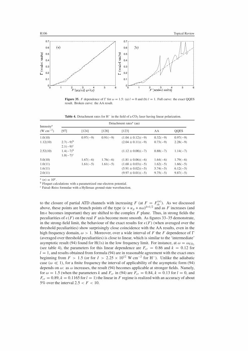
R106 Topical Review
0
0.1
0.2
0.3
0.4
0.5
0.6
0.7
0 1 2 3 4 5 60
0.1
0.2
0.3
0.4
0.5
0.6
0.7
0 1 2 3 4 5 6
Figure 35. F dependence of � for ω = 1.5: (a) l = 0 and (b) l = 1. Full curve: the exact QQESresult. Broken curve: the AA result.
Table 4. Detachment rates for H− in the field of a CO2 laser having linear polarization.
Detachment ratesa (au)Intensitya
(W cm−2) [97] [124] [128] [123] AA QQES
1.0(10) 0.97(−9) 0.91(−9) (1.04 ± 0.12)(−9) 0.32(−9) 0.97(−9)
1.12(10) 2.7(−9)b (2.04 ± 0.11)(−9) 0.73(−9) 2.28(−9)
2.1(−9)c
2.52(10) 1.4(−7)b (1.12 ± 0.08)(−7) 0.88(−7) 1.14(−7)
1.0(−7)c
5.0(10) 1.67(−6) 1.76(−6) (1.81 ± 0.06)(−6) 1.64(−6) 1.79(−6)
1.0(11) 1.61(−5) 1.61(−5) (1.68 ± 0.03)(−5) 1.62(−5) 1.66(−5)
1.6(11) (5.91 ± 0.02)(−5) 5.74(−5) 6.12(−5)
2.0(11) (9.97 ± 0.01)(−5) 9.75(−5) 9.87(−5)
a (n) ≡ 10n .b Floquet calculations with a parametrized one-electron potential.c Faisal–Reiss formulae with a Hylleraas ground-state wavefunction.
to the closure of partial ATD channels with increasing F (at F = F (n)th ). As we discussed
above, these points are branch points of the type (ε + u p + nω)k+1/2 and as F increases (andIm ε becomes important) they are shifted to the complex F plane. Thus, in strong fields thepeculiarities of ε(F) on the real F axis become more smooth. As figures 33–35 demonstrate,in the strong-field limit, the behaviour of the exact results for ε(F) (when averaged over thethreshold peculiarities) show surprisingly close coincidence with the AA results, even in thehigh frequency domain, ω > 1. Moreover, over a wide interval of F the F dependence of �
(averaged over threshold peculiarities) is close to linear, which is similar to the ‘intermediate’asymptotic result (94) found for H(1s) in the low frequency limit. For instance, at ω = ωCO2
(see table 4), the parameters for this linear dependence are Fcr = 0.86 and k = 0.12 forl = 1, and results obtained from formula (94) are in reasonable agreement with the exact onesbeginning from F > 1.5 (or for I > 2.25 × 10¹² W cm−2 for H−). Unlike the adiabaticcase (ω � 1), for a finite frequency the interval of applicability of the asymptotic form (94)depends on ω: as ω increases, the result (94) becomes applicable at stronger fields. Namely,for ω = 1.5 (when the parameters k and Fcr in (94) are Fcr = 0.84, k = 0.13 for l = 0, andFcr = 0.89, k = 0.1165 for l = 1) the linear in F regime is realized with an accuracy of about5% over the interval 2.5 < F < 10.

Topical Review R107
The results presented in this section justify the conceptual statement, namely that thedecay of a weakly bound atomic system in a strong laser field F (ωt) with any frequency andpolarization state may be described by cycle-averaging the results for an instantaneous staticelectric field of strength |F (ωt)|.
7. Summary and conclusions
Even for long (monochromatic) laser pulses with a shaped focus, the output of a laser–atom interaction depends on many parameters, e.g. for multiphoton detachment there are thefrequency, intensity and polarization state of a laser as well as the momentum direction of theescaping electron. Since time-consuming, completely numerical ab initio calculations maybe performed only for limited sets of such control parameters, simple, analytically solvablemodels that cover the entire parameter space are particularly useful for determining the best wayto control laser–atom processes. For strong laser–atom problems (where ionization stronglyaffects the features of any laser–atom process), the most important requirement for such modelsis the existence of both discrete and continuum spectra for the model system in the absence of thelaser field. One of the most basic models for laser–atom physics was suggested by Keldysh,namely a single-electron bound state that does not interact with a free-electron continuum(which evolves to a ‘Volkov continuum’ for nonzero laser field). Thus, in the KA, the couplingbetween bound and continuum states is provided only by the initial laser excitation of theelectron out of the bound state (to which it never returns). It is somewhat surprising thatthis simplest model allows one to predict qualitative features for a number of laser–atomeffects. The major deficiency of the KA is its complete neglect of coupling between boundand continuum states, i.e. of atomic dynamics, since these states are eigenstates of differentHamiltonians.
In this paper we have reviewed (and extended) existing results for a next-level model(compared to the Keldysh one), i.e. the zero-range (or δ-function) potential model system.In the absence of the laser field, this model again involves only a single-electron boundstate; however, this state is ‘minimally’ related to the three-dimensional continuum throughthe S-wave scattering phase. Nevertheless, for a nonzero laser field, even this ‘minimalcoupling’ allows an accurate, self-consistent account for some major corrections to the Keldyshmodel, as it includes ‘multiple interactions’ of the escaping (or quasibound) electron with thebinding potential. The (single) bound and continuum states of the δ-model potential form acomplete set of eigenfunctions of the unperturbed Hamiltonian,as required for a self-consistentdynamical model. Owing to the fact that a zero-range potential acts only at r = 0, and thusamounts to a boundary condition on the wavefunction of the system, this model provides thepossibility for an accurate quantum treatment of strong laser and binding potential effectson an equal footing. In this review, we have solved this model problem using the QQESapproach.
We have formulated the basic results of the QQES approach for a δ-model potential andpresented general equations for the multiphoton detachment amplitude in sections 2.3–2.5and appendices A–C. In particular, we have analysed the key ingredients of this approach,the Fourier coefficients of the QQES wavefunction at the origin, which provide informationon binding potential effects in the presence of a laser field. These results may be useful indifferent applications of this model to describe the behaviour of a shallow bound level subjectedto a strong monochromatic perturbation. In this review they have been used in our generalanalysis of ADs and photon polarization effects in multiphoton detachment of a weakly boundelectron. Based on analytical results for n-photon ADs of detached electrons obtained bothin BW (i.e. using the exact complex quasienergy) and RS versions of PT expansions, the
R108 Topical Review
ellipticity dependence of ADs and ED effects have been analysed in detail and illustrativeexamples were presented for photon numbers up to n = 8. For the nonperturbative regime,numerical results were presented which show the strong field modifications of ADs and dichroiceffects. These modifications are most important near the closure of open photodetachmentchannels.
We have also performed a detailed analysis of the case when the laser frequency exceeds theelectron binding energy |E0|, which is important for the description of negative ions in opticaland VUV laser fields. In applying our results to multiphoton detachment of H−, satisfactoryagreement with existing experiments as well as with more sophisticated calculations thatinclude correlation effects has been found both in the perturbative and in the nonperturbativeregimes. A most interesting feature shown in our general analysis is the existence of astabilization-like behaviour of the total rate � with increasing F up to the closure of the one-photon photodetachment channel at F = F (1)
th . A general analysis for the F dependence of thecomplex quasienergy ε and the total rate � in the superstrong field limit (when a number of thelowest ATD channels are closed) shows that the exact results for ε are fairly well approximatedby the cycle-averaged complex energy of the quasistationary state in an instantaneous staticelectric field of strength |F (ωt)|. Furthermore, in the superstrong field regime, F � ω, thisresult is valid not only for ω � 1 (as may be expected from adiabaticity arguments) but also forany ω, including the ‘post-stabilization’ regime F � F (1)
th for ω > 1. Of course, our proof ofthis conceptual result is valid only for a short-range potential; its verification for Coulomb-likepotentials remains a challenging problem.
Finally, we conclude by noting the efficacy of using the QQES approach for a δ-modelpotential to provide a qualitative description of recently observed strong laser field effects inreal atoms, namely the plateau structures and threshold phenomena in both ATI and HHGprocesses. For example, an approximate account of binding potential effects (equivalentto the use of approximation (B.32) for the coefficients fn) has permitted the estimation ofthe cut-off energy, ∼10Up, of the ATI plateau [133] (see also [179]). Also, a resonance-like enhancement of ATI peak intensities has been discovered experimentally [180, 181]and confirmed by direct numerical integration of the TDSE [182]. Most recently, the roleof channel closings, i.e. threshold effects, have been identified as important for describingthe observed enhancement of ATI peaks [183]. The improved KA [133] reproduces theresonant-like behaviour of peaks along the high energy plateau near multiphoton channelclosings [183, 184] (see also the quasiclassical analysis in [185]). A rigorous analytical andnumerical analysis employing the exact QQES results (36) and (38) [135] has shown thatthe enhancements mentioned above have a purely quantum origin that stems from well-knownthreshold phenomena (TAs) in multichannel problems (see, e.g., [142, 148, 186, 187]). SimilarTAs in the region of the HHG plateau have been shown to induce significant enhancements ofthe HHG spectrum, as discussed in [136]. Based upon these past successes, we conclude thatthe application of this model to the description of laser–atom and laser–negative ion processesholds great promise for elucidating known phenomena and for predicting new phenomena (see,e.g., [137]). In particular, the plateau structures and threshold phenomena predicted by oursimple short-range potential model may be expected to be observable in negative ions as well,using strong infrared laser radiation.
Acknowledgments
This work has been supported in part by the CRDF and the RF Ministry of Education undergrant no VZ-010-0, by grant E02-3.1-115 of the RF Ministry of Education (NLM), and by theUS National Science Foundation under grant no PHY-0070980.

Topical Review R109
Appendix A. Normalization of the QQES wavefunction for a δ-model potential
For the δ-model potential, the definition of the dual function in (19) is equivalent to the followingalternative definition (cf (21)):
ε(r, t) = −4π
∫ 0
−∞eiε∗τ G(−)(r, t, 0, t − τ ) fε (t − τ ) dτ, (A.1)
where G(−)(r, t, 0, t − τ ) is the advanced Green function (14) and the integral over τ isconsidered as analytically continued from the lower half-plane of complex ε. Taking intoaccount (23) and integrating over r and t , the relation (18) gives
2√
π i∑n,k
in−k φ∗nφk
∫ ∞
0
dτ
τ 1/2exp[−i((E − nω − kω)τ − z(τ ))]Jk−n(z(τ )) = 1, (A.2)
where the integral over τ is calculated by differentiating M0,k(E) in (29) with respect to E .As a result, the normalization condition (18) may be expressed in terms of the same matrixelements that enter the basic equations (27) and (28) for φn and ε:
4π
∞∑n,k=−∞
φ∗nφk
∂
∂E[√
E − 2nω δn,k − Mn,k(E)]∣∣
E=E= 1. (A.3)
In fact, for the case considered, the normalization procedure serves to define the coefficientφ0, since φn �=0 can be expressed in terms of φ0 by means of the homogeneous equations (27).Thus, the identity (A.3) may be considered as an equation for the product φ∗
0φ0. The symmetryproperties for the coefficients φn and φn may be deduced from the following considerations: thematrix elements (29) are independent of the sign of ξ , and the relation (A.3) is an even functionof ω. Also, the system of linear equations for φ∗
n , is similar to (27) (with complex-conjugatedmatrix elements). Thus, one determines that
φn(ω, F) = φ∗n (ω, F), φn(ω, F) = φ∗
−n(−ω, F). (A.4)
Since the phases of the coefficients φ0 and φ∗0 are not important, we can set φ∗
0 = φ0, andthus φ∗
0φ0 = φ02. Note that the normalization factor for the QQES has an especially simple
and transparent form for the case of circular polarization (l = 0), when only the coefficientφ0 = f0 is nonzero:
4πφ20
∂
∂E[√
E − Mcirc(E)]|E=E = 1. (A.5)
Mcirc(E) is the matrix element M0,0(E) with l = 0, which enters a transcendental equationfor the quasienergy in this case [131] (see also the discussion of (B.6) below):√
E − Mcirc(E) = 1. (A.6)
Appendix B. Perturbative and strong field results for the coefficients φn and fn
The formal procedures for the correct numerical evaluation of the complex quasienergy andthe Fourier coefficients of the QQES wavefunction at the origin (r → 0) are described insection 2.3. An exact numerical solution of the eigenvalue problem for ε and φn in (28)and (27) is a formidable task. Below, in sections B.3 and B.4 we present some details of suchcalculations and examples of exact numerical results for the coefficients φn and fn as well asanalytical approximations for fn in the strong field regime. Simple analytical expressions maybe derived in the PT approach (including higher-order corrections to the LOPT result). Wepresent below these perturbative expansions in two forms:
R110 Topical Review
(i) in terms of the BW PT expansion, which involves the exact quasienergy ε, i.e. assumingthe complex parameter E = u p − ε is exactly known;
(ii) in terms of the standard RS PT expansion, which involves the real, zero-order quasienergyε0 = E0, i.e. E = −E0 = 1. Of course, the BW results are more accurate than the RSresults, especially for frequencies near thresholds. Using the PT expansion for ε, the BWresults may be easily transformed to the standard RS form.
B.1. Brillouin–Wigner expansions
To obtain the power expansion (in F2) for the coefficients φn in (27), we use the expansionof the matrix elements M0k(E) in (29) in an absolutely convergent series in u p [127]. Thisexpansion may be written as
M0k(E) = (−l)k
2kk!
∞∑n=δk,0
1
n!
(F2
ω4
)(n+k)
2 F1
(−n
2,
1 − n
2; k + 1; l2
)Dn+k(E − kω), (B.1)
where 2 F1 is the hypergeometric polynomial of l2 having the same order, m, for both n = 2mand n = 2m + 1. The important function D in (B.1) is defined by
Dn(E − pω) = (2n)!!
2n + 1
n∑m=−n
(−1)(m+1) (E − pω + mω)n+ 12
(n + m)!(n − m)!. (B.2)
In accordance with the boundary conditions for the QQES wavefunctions, the square root,√E − kω, is defined as
Re√
E − kω > 0, for k < Re E/ω,
Im√
E − kω < 0, for k > Re E/ω.(B.3)
Note that for small ω the function Dn(E − pω) vanishes as ∼ω2n :
limω→0
Dn(E − pω) � (|2n − 3|)!!√E
(ω2
4E
)n
.
We present below results for M0,k(E) up to terms of orders F2 and F4. Only the followingmatrix elements are nonzero for this case:
M0,0(E) = F2
ω4
[D1(E) +
F2
2ω4
(1 +
l2
2
)D2(E)
],
M0,1(E) = − l
2
F2
ω4
[D1(E − ω) +
F2
ω4D2(E − ω)
],
M0,2(E) = l2 F4
8ω8D2(E − 2ω).
(B.4)
The above equations allow us obtain the ‘BW’ results for the coefficients φ±k with anaccuracy up to ∼F4:
φ1 = − l
2
F2
ω4
φ0√E − 2ω − 1
[D1(E − ω) +
F2
ω4
(D2(E − ω) +
D1(E − ω)D1(E − 2ω)√E − 2ω − 1
)],
φ2 = l2
8
(F2
ω4
)2φ0√
E − 4ω − 1
[D2(E − 2ω) + 2
D1(E − 3ω)D1(E − ω)√E − 2ω − 1
]. (B.5)
The coefficients φn with negative indices are given by φ−n(ω) = φn(−ω).
Topical Review R111
The result for the normalization factor φ20 up to terms ∼F4 and involving the exact E can
be obtained from (A.3), taking into account the above BW expansions for M0,k(E) and φn :
φ20 =
[4π
∂ F(E, ω, F)
∂ E
]−1
, (B.6)
where the result for F(E, ω, F) is
F(E, ω, F) = √E − F2
ω4D1(E)
− 1
4
(F2
ω4
)2[(2 + l2)D2(E) + l2
{D2
1(E + ω)√E + 2ω − 1
+D2
1(E − ω)√E − 2ω − 1
}]. (B.7)
Taking into account only the term ∼F2, one obtains for φ20
φ20 =
√E
2π
[1 +
F2
ω4
(√E(E + ω) +
√E(E − ω) − 2E
)]. (B.8)
It is an interesting fact that the equation,
F(E, ω, F) = 1, (B.9)
coincides with the transcendental equation for ε (or for E), which follows from theexpansion (31), taking into account only terms up to ∼F4 on the rhs of (31). Straightforwardcalculations show that the results in (B.6) and (B.9) for a general elliptic polarizationare valid to an arbitrary order F2n (taking into account, of course, terms ∼F2n in theexpression for F(E, ω, F)), which is equivalent to the result in (A.5) and (A.6) for the caseof circular polarization. Generally speaking, calculating the parameter E = E(F) as the(nonperturbative) solution of the transcendental equation (B.9) with the boundary conditionE → 1 as F → 0, we obtain a complicated,non-polynomial dependence of the BW expansionsfor φn and φ2
0 on the field amplitude F . Thus these results are much more accurate than standard(polynomial in F) RS expansions.
B.2. Rayleigh–Schrodinger results
In the LOPT, the coefficients φ±k with k > 0 are proportional to F2k and φ0 � N = 1/√
2π
(see (9)). The perturbative solution of equation (27) in the LOPT gives a simple result for φ±k
for any k:
φ±k = 1√2π
(l F2
ω4
)k
χk(±ω), (B.10)
where χk(ω) is determined by the recurrence relation
χk(ω) = − i
1 + i√
2kω − 1
k∑j=1
ϕ j,k(ω)χk− j (ω), (B.11)
with the initial value χ0 = 1. The function ϕ j,k(ω) in (B.11) is given by
ϕ j,k(ω) = 1
(2 j + 1)!
2 j∑m=0
(−1)m+ j Cm2 j [(2k − m)ω − 1] j+ 1
2 , (B.12)
where Cmn is a binomial coefficient. ϕ j,k is simply related to the function D in (B.2):
ϕ j,k(ω) = i(−1) j
(2 j)!!D j (1 − (2k − j)ω). (B.13)

R112 Topical Review
To obtain higher-order corrections to the LOPT result (B.10), the RS expansion of thequasienergy ε is necessary. Taking into account only the corrections ∼F2 and F4, ε maybe written in terms of the (polarization-independent) dynamic polarizability, α(ω), and thehyperpolarizability, γ4(ω; l), which depends on both the frequency and the polarization stateof a laser field:
ε = −1 − α(ω)
4F2 − γ4(ω; l)
24F4, (B.14)
where the iterative in F solution of equation (B.9) using F(E, ω, F) in (B.7) gives expressionsfor the polarizability and hyperpolarizability in terms of D1(1) and D2(1) functions. Takinginto account the explicit form of these functions, final results coincide with those obtainedpreviously in [81] by direct perturbative calculations (see also [188] on an alternative way tocalculate α(ω)):
α(ω) = − 2
ω2+
8
3ω4[(ω + 1)3/2 − 2 + i(ω − 1)3/2], (B.15)
γ4(ω; l) = 8
15ω8[( fξ (ω) + fξ (−ω))ξ2 + ( fl(ω) + fl(−ω))l2], (B.16)
where the functions fξ (ω) and fl(ω) are defined by
fξ (ω) = 45ω2 + 96 + 5i(ω2 − 1)1/2(ω2 − 7)
− 4i(ω − 1)1/2(3ω2 + 14ω − 32) + 3i(2ω − 1)5/2, (B.17)
fl(ω) = 60ω2 + 124 + 5i√
ω2 − 1(ω2 − 7) − 1
ω[10(ω − 1)5/2(2ω − 1)1/2 − i(2ω − 1)1/2
× (3ω3 + 12ω2 − 23ω + 10) − 2i(ω − 1)1/2(ω3 − 42ω2 + 76ω − 5)]. (B.18)
Note that we define√−a as i
√a for a > 0. The hyperpolarizability γ4(ω; l) is an important
atomic parameter and involves a complicated combination of fourth-order PT matrix elements(see, e.g., [141]). For H−, γ4(ω; l) (for the case of linear polarization) was calculated, takinginto account electron correlations, perturbatively (in F) in [189] (in the static limit ω = 0) aswell as nonperturbatively (in F) [108, 190]. It is somewhat surprising that the simple δ-modelresult in (B.16)–(B.18) is in close agreement with results of these sophisticated calculations(see comparisons in [191], where the δ-model result for the dynamical hyperpolarizability ofH− in the presence of a strong static electric field is also presented).
To calculate the F-dependent RS corrections to the normalization parameter, φ0 =1/
√2π + φ0
(1) + · · ·, the relations (B.6) and (B.7) may be used, taking into account theexpansion (B.14) for the quasienergy. One obtains for the lowest order in F correction:
φ0(1) = 1√
2π
F2
2ω4
{√ω + 1 − 2 − i
√ω − 1 +
1
3[(ω + 1)3/2 − 2 + i(ω − 1)3/2]
}. (B.19)
Note that the normalization factor for the QQES solution is unconventional because it iscomplex; see (A.3) or (B.6) (in LOPT the complexity appears only for above-thresholdfrequencies, ω > 1). Nevertheless, this complexity is not surprising in the theory ofquasistationary states for radiationless problems (see, e.g., [192]); it originates from an analyticcontinuation of the standard normalization convention to the case of the QQES.
B.2.1. Analytical properties of φ±k(ω) and threshold phenomena. We discuss now in moredetail the analytical structures of the coefficients φ±k , which are essential for the analysis ofADs. For clarity, we present here an explicit RS form of the coefficients φ1 and φ2, whichenter the LOPT result for the ADs for n � 5:
φ1 = l F2
√2π6ω4
g1(ω), φ2 = l2 F4
√2π36ω8
g2(ω), (B.20)
Topical Review R113
where
g1(ω) ≡ 3χ1(ω) = i(2ω − 1)3/2 − 2i(ω − 1)3/2 + 1
1 + i√
2ω − 1,
g2(ω) ≡ 9χ2(ω) = ig1(ω)
[(4ω − 1)3/2 − 2(3ω − 1)3/2 + (2ω − 1)3/2
1 + i√
4ω − 1
]
− 3
10
i(4ω − 1)5/2 − 4i(3ω − 1)5/2 + 6i(2ω − 1)5/2 − 4i(ω − 1)5/2 − 1
1 + i√
4ω − 1.
Most important is the complexity of φk , whose imaginary part, Im φk , is different in eachfrequency interval 1/p < ω < 1/(p − 1), for p = 1, 2, . . .. This fact becomes rather clear byintroducing the ‘phase function’, δ0(E), of E (which is in general complex) as follows:
eiδ0(E) = 1 − i√
E√1 + E
. (B.21)
For positive E , δ0(E) is the well-known phase shift of the continuum S-state for a short-range potential. (Other scattering phases, δL(E), are zero in the δ-model potential.) Thuseiδ0(E) = cos δ0(E) + i sin δ0(E). On the contrary, for negative arguments, E = −E ′, in theinterval −1 < E � 0 the exponential (B.21) is real:
e±iδ0(−E ′) = 1 ∓ √E ′
√1 − E ′ . (B.22)
Thus, equation (B.21) gives an analytical continuation of the scattering phase to the region ofnegative E . Note that at E = E0 = −1 we obtain the well-known result, cot δ0(E0) = i ,which determines the poles of the S matrix at the bound state energies. A detailed analysisshows that φ±k in any PT order may be presented as a combination of exponentials (havingthe form (B.21), with different E = pω ∓ 1, where p is an integer) and regular functions of ω
(having the form (mω ∓ 1)n, where m and n are integers). For instance, the functions g1 andg2 in (B.20) may be re-written in terms of δ0 as follows:
g1(ω) = 2ω − 1 − √2(ω − 1)ei[δ0(2ω−1)−δ0(ω−1)], (B.23)
g2(ω) = g1(ω)
[4ω − 1 − eiδ0(4ω−1)
(√3(3ω − 1)e−iδ0(3ω−1) +
1√2(2ω − 1)e−iδ0(2ω−1)
)]
+3
5eiδ0(4ω−1)
[√3(3ω − 1)2e−iδ0(3ω−1) − 3√
2(2ω − 1)2e−iδ0(2ω−1)
+ (ω − 1)2e−iδ0(ω−1)
]− 3
10(4ω − 1)2. (B.24)
These equations (together with (B.20)) demonstrate that φk is complex entirely because of thescattering phases: a new phase (say, δ0(2mω − 1) with m < k) contributes to φk when thefrequency ω increases from ω < 1/2m to ω > 1/2m and, thus, a new detachment channel(with the absorption of two additional photons) is opened. For instance, the function g1(ω) isreal for ω < 1/2; for 1/2 < ω < 1, g1(ω) is complex because of the phase δ0(2ω − 1); andfor ω > 1 an additional contribution to the imaginary part of g1 appears because of the phaseδ0(ω − 1). Similarly, g2(ω) is real only for ω < 1/4. Therefore, the entire set of coefficientsφ±k is real if the phases φk are neglected, i.e. if the interactions of the escaping electron withthe parent atom in the final state as well as in intermediate states (i.e. after absorption of m < kphotons) are neglected. Note that the phase dependence (and the complexity) of the coefficientsφk may be established also by direct PT calculations of Fourier harmonics of the S-wave partof the QQES wavefunction ε(r, t) (which is given at r → 0 in terms of the coefficients
R114 Topical Review
φ±k), using the known Green function for an electron in a δ-model potential. However, sucha calculation is much more tedious than the PT expansions of the exact results presented insection 2.
The general features of the frequency dependence of the φk coefficients discussed aboveprovide an instructive illustration of the so-called threshold phenomena that are predicted bythe general theory of multichannel reactions involving a short-range binding potential (see,e.g., [186]). For this kind of potential, in a classic paper [70] Wigner showed that the branch-point singularity of the reaction amplitude at the threshold energy (E = 0) of a given breakupchannel having an orbital angular momentum L causes a universal threshold behaviour of thecorresponding breakup cross section:
σL ∝ E L+1/2, (B.25)
above the opening of this channel. Extending Wigner’s analysis, Baz’ [187] showed thatgenerally in a multichannel problem the branch-point non-analyticity of the multichannelamplitude at the mth-channel threshold, Em = 0, causes a particular, non-analytic behaviour,or TA, in the partial cross sections of all other open channels, in general. These TAs are wellknown and described in textbooks (see, e.g., [148] and section 147 in [142]). Laser detachmentof a negative ion provides a good example of a multichannel problem where TA effects canhave a great influence on partial cross sections at the opening or closure of a multiphotondetachment channel owing to a variation of either the laser frequency or intensity. (In thelatter case, the closure originates from ponderomotive shift effects.) In the QQES problemfor a zero-range potential (in which case only the S-wave scattering phases δ0(E) provide theinterchannel couplings), all the non-analyticities are concentrated exclusively in the S-wavepart of the QQES solution, i.e. in the coefficients φk , as is obvious from equations (21) and (23).The threshold branch-point singularities of φk are evident from the explicit form (B.1) for thematrix elements M0k , which enter the exact equation (27) satisfied by φk . Of course, for anarbitrary F , the position of the branch point for the mth threshold:
mω − E ≡ mω + ε − u p = 0, (B.26)
is shifted to the complex plane of F and ω. However, in the RS PT approach, the TAs occurat real frequencies, mω − 1 = 0, and cause the specific frequency dependence of the φk
coefficients discussed above.
B.3. Exact strong field results
In the strongly nonperturbative regime, the use of the expansion (B.1) for numerical calculationsof the matrix elements M0k(E) becomes ineffective because of the slow convergence of theseries in (F/ω2)2 for ω < 1. Moreover, as discussed below, for strong F the direct numericalcalculation of the coefficients fn using the matrix elements Mnn′(E) is preferable to use of therelation (24) for their calculation in terms of φn. Note that the integral (29) (as well as the similarintegral for Mnn′(E)) is formally divergent for τ → ∞ because of the negative imaginary partof the quasienergy ε (see the above discussion of equation (13)). The numerical calculation ofsuch integrals is possible by using the following analytic continuation procedure [134]:∫ ∞
0
dτ
τ 1/2e−iατ f (τ ) =
∫ ∞
0
dτ
τ 1/2e−iατ
∫ ∞
−∞dτ ′δ(τ ′ − τ ) f (τ ′)
=∫ ∞
−∞dτ ′
∫ ∞
0
dτ
τ 1/2e−iατ
∫ ∞
−∞dk
2πeik(τ ′−τ) f (τ ′)
= 1√4π i
∫ ∞
−∞dk√α + k
∫ ∞
−∞dτeikτ f (τ ). (B.27)

Topical Review R115
Figure B.1. n dependence of the Fourier coefficients fn for linear laser polarization. (a) Exactvalues of | fn/ f0| for different F and ω = 0.155. Full squares: F = 0.1; full circles: F = 0.2;triangles: F = 0.3; empty circles: F = 0.4. Arrows mark the cut-offs in units of the energy(see (B.29)). Full curves serve to guide the eye. (b) Exact values of | fn/ f0| for different ω andF = 0.4. Full squares: ω = 0.138; empty squares: ω = 0.178; full circles: ω = 0.218; emptycircles: ω = 0.298; full triangles: ω = 0.458.
The above formula involves a Fourier transform (that can be calculated very efficiently usinga Fast Fourier Transform algorithm) followed by a second integration, which can also beperformed numerically with high accuracy. The finite system of equations, obtained from (27)(or from a similar system for fn) after truncating the ranges of n and n′ to an appropriate finitenumber of values, can then be solved numerically. One obtains thereby the eigenvalues ε aswell as the Fourier coefficients φn (or fn) of the QQES state at the origin. Note that Mur et al[193] suggest using the Zel’dovich regularization for singular integrals like the first one inequation (B.27), i.e. introducing a regularization factor exp(−στ 2) with σ → + 0 [148, 194].They demonstrate a reasonable convergence (with decreasing σ ) of this method in calculationsof ε for a circularly polarized field (where only one matrix element, M00, is necessary).However, the applicability of this regularization method for the cases of linear or ellipticpolarization is questionable since in these cases a large number of matrix elements Mnn′ (29)calculated with high precision are necessary for the solution of the determinantal equation (28).In addition, as shown in [193], the proposed method of regularization in [193] is inapplicablefor calculations of ‘near-threshold’ matrix elements, when Im ε is of the order of (or largerthan) | Re ε + kω|.
In figure B.1 we present the dependence of the exactly calculated coefficients fn asfunctions of F (in figure B.1(a)) and ω (in figure B.1(b)) in the nonperturbative regime. Recallthat, in the KA limit, f K A
n = δn0/√
2π . As we have noted after equation (B.19), in generalthe normalization factor of a QQES wavefunction (i.e. φ0 or f0) is complex. However, themagnitude of the imaginary part of f0 is very small for the values F and ω considered infigure B.1 and, actually, it has the same magnitude as the imaginary part of the quasienergy:∼(10−4 −10−3). Moreover, the modulus of the normalization factor f0 for this case is close tothe zero-field value 1/
√2π , decreasing only by about 2% at F ≈ 0.5. With increasing F , the
negative-n and a few of the lowest positive-n coefficients exhibit typical (smoothly decreasing)perturbative behaviour. However, even for weak intensities (e.g. for I = F2 = 10−2 infigure B.1(a)), the plateau signature characterizing the dependence of f n on n appears starting atsome n ≈ nth , and a well-developed plateau structure is formed in the strongly nonperturbativeregime, γ < 1, having a cut-off at some n ≈ nc.
To explain the behaviour of the coefficients fn described above and to estimate nth andnc, we emphasize that the coefficients fn �=0 vanish in the KA limit and that these coefficients

R116 Topical Review
originate from the simultaneous interaction of the electron with both the laser field and thebinding potential. Concerning the onset of the plateau, we note that (in weak fields) the PTresult for fn may be presented as: fn = cn(ω)F2|n| (cf the similar results (B.10)–(B.12) forthe φn coefficients). Thus, for fixed F and ω, the breakdown of a smooth decrease of fn
with increasing n, fn ∼ F2|n|, originates only from the appearance of an irregularity (non-analyticity) in the behaviour of the factor cn(ω) starting from n = nth . One may observe theeffects of this singularity in figure B.1(a), where the F = 0.1 curve shows a sudden rise aboven = 3 and where the F = 0.2 curve shows a similar rise, again above n = 3. Note that, withincreasing F , the location of these singularities does not necessarily occur at integer valuesof n, so that not every curve in figure B.1(a) shows the singularity clearly. Nevertheless, thecalculations with smaller steps in F (as in figure B.1(a)) show that the position of nth is largelyintensity-independent up to high values of F , i.e. it has a PT origin. In the PT limit, the valueof nth may be estimated owing to the analytical structure of the perturbative results for thecoefficients fn that involve characteristic branch-point terms
√pω + 1 with p = ±1, . . . ,±2n
(see (B.10)–(B.12) and the explicit expressions (B.20) for the φn coefficients having n = ±1and ±2). It is clear that, at fixed ω, the first irregularity in the dependence of fn on n withincreasing n should appear for n = nth , which is defined by (1 − 2nthω) � 0, i.e. 2nth issimply the lowest even (open) Up-unshifted photodetachment channel for a given value of ω.Thus, one obtains the following estimate for nth :
2nthω ≈ 1 (or E0 + 2nthhω � 0 in absolute units). (B.28)
This estimate is in good agreement with numerical values of nth , both for different F (infigure B.1(a)) and ω (in figure B.1(b)) and shows that in a rigorous treatment the onset of theplateau feature in the spectrum of fn originates from purely quantum (zero-field threshold)effects. In contrast, the position of the cut-offs in the spectra for fn in figure B.1 may beexplained using classical considerations in terms of rescattering effects. Indeed, the coefficientsfn are proportional to the amplitudes for the electron (having the energy EN = Re ε + 2nω)at the origin (see (20) and (23)). The number N = 2n is even since the probability density atthe origin is determined by the S-wave component of ε(r, t), i.e. in view of electric dipoleselection rules, the electron can return to the parent atom only after absorption or emission ofan even number of photons, when the S-wave component of angular momentum is nonzero(see the discussion above equation (23)). Figure B.1 shows that only electrons with positiveenergies up to E2nc = Re ε + 2ncω have a significant probability density to be at the origin.To estimate nc, it is reasonable to equate E2nc with the maximum energy of the ‘rescattered’electrons at the origin, which is well known from numerical quantum calculations [195] aswell as from a simple classical analysis [132]: Ec ≈ 3.17Up. Thus, we obtain the followingestimation for nc:
2ncω ≈ 1 + 3.17u p, (B.29)
which agrees very well with our numerical results for nc in figure B.1 for strong F and/orsmall ω, i.e. for small values of the Keldysh parameter γ .
The behaviour of the φn coefficients is significantly different from that for fn . Numericalevaluations demonstrate that, with increasing F , the coefficients φn undergo large variationsand grow rapidly with increasing |n| for both n > 0 and n < 0. For example, we present infigure B.2 the F dependence of the normalization constant φ0 and the coefficients φn for theparticular frequency ω = 0.155 and for linear laser polarization. For circular polarization,φcirc
0
coincides with f circ0 and differs only slightly from 1/
√2π . In contrast, for linear polarization
we have a large number of contributing coefficients φn , which vanish at F = 0 but which haveincreasing contributions as the intensity increases. Therefore,
√2π |φ0| needs to be decreasing

Topical Review R117
Figure B.2. (a) F dependence of the normalization factor φ0 for the case of linear laser polarization(l = 1) at ω = 0.155 (full curve) and ω = 0.202 (broken curve). (b) Dependence of the ratio,|φn/φ0|, on n (at ω = 0.155 and l = 1) for three values of the laser amplitude: F = 0.05 (dottedcurve); F = 0.20 (thick full curve); F = 0.49 (thin full curve). Squares, circles and triangles areresults of the KA (equation (44)) for F = 0.05, 0.20 and 0.49, respectively.
in order to maintain the unit normalization of ε(r, t). Although the imaginary part of φ0 isvery small, ∼(10−4 − 10−3), its real part reveals big variations. It is interesting that the exactresults for
√2π Re φ0 in figure B.2(a) are in excellent agreement with those of the KA (44):
the difference between the exact and the KA results is less than 1%.For coefficients φn with n �= 0, the coincidence of the exact and the KA results takes
place only in the weak field domain, γ > 1 (see figure B.2(b) where γ = 3.1 for F = 0.05).At γ ∼ 1 (γ = 0.775 for F = 0.2 in figure B.2(b)) the exact coefficients for positive nstart to increase above those of the KA beginning from some n. For high enough F , a two-plateau structure for |φn/φ0| for positive n develops: the higher plateau for smaller values ofn represents the ‘Keldysh regime’; the lower (beyond KA) plateau for larger values of n iscaused by binding potential (rescattering) effects. Numerical values of the cut-off number, nc,for the second plateau are well approximated by the same estimate (B.29) as for the coefficientsfn . Since the KA reproduces φn well, except for those n values in the second plateau domain,the origin of the first plateau is clearly independent of the binding potential and, therefore,can be explained in terms of the KA. The curve for F = 0.49 in figure B.2(b) and numericalcalculations for other values of F and ω show that, with reasonable accuracy, the critical valueof n, ncr , at which the non-KA plateau begins can be obtained from the relation
ncrω ≈ u p (or 2ncr hω ≡ Ecr ≈ 2Up in absolute units). (B.30)
Mathematically, the value ncr corresponds to the value of the index n in√
2πφK An = Jn(u p/2ω)
at which the oscillatory behaviour of the Bessel function Jm(x) with increasing m changes to adecreasing behaviour (this happens for indices m much larger than the argument x , and m ∼ 2xcorresponds to the transition domain). The estimate in (B.30) for ncr agrees with the knownquasiclassical results on the size of the ‘Keldysh plateau’ in ATI processes [196]: neglectingrescattering by the binding potential, the ‘Keldysh part’ of the ATI plateau corresponds to anelectron energy Ecr of order 2Up .
B.4. ‘Rescattering approximations’ for the coefficients fn
An exact calculation of the coefficients fn is time-consuming since it requires the preliminarycalculation of the complex quasienergy according to (28). A simple way to obtain fn
approximately in the nonperturbative regime is the iterative solution of equation (27) with the

R118 Topical Review
Figure B.3. Comparison of exact and approximate Fourier coefficients fn for the case of linearlaser polarization, ω = 0.155, and F = 0.25. Squares: exact results; triangles: approximationI results using (B.31); circles: approximation II results using (B.32). Note that the squares andtriangles are indistinguishable on the scale of this figure.
substitution Mnn′(E) → Mnn′(E) (where Mn,n′(E) is defined in the text above (40)) startingfrom the KA results: f K A
n = δn0/√
2π , E = 1 + u p. The first iteration gives the followingapproximation for fn �=0:
f (1)n = Mn,0(1 + u p)√
1 + u p + 2nω − 1 − Mn,n(1 + u p)f K A0 . (B.31)
We shall call this method ‘approximation I’. Obviously, approximation I is equivalent toa perturbative (first-order) account of the binding potential (or rescattering) effects withrespect to the KA results. Figure B.3 demonstrates an unexpectedly precise agreement ofthe approximation I coefficients f (1)
n with the exact results.A simplified version of approximation I (denoted approximation II) consists in replacing
the entire denominator of (B.31) by −1:
f (2)n = −Mn,0(1 + u p) f K A
0 . (B.32)
Although this approximation has no proper theoretical justification, the results ofapproximations I and II are in good qualitative agreement, as may be seen in figure B.3(although, compared to approximation I, approximation II gives a less accurate estimate forthe coefficients fn , both on the plateau and beyond the plateau). Using the approximateanalytical result (B.31) for f (1)
n instead of the exact numerical Fourier coefficients of f (t − τ )
in (21) (see also (23)), we obtain an analytical expression for the QQES wavefunction. Thismay be useful in different applications that take into account the first-order binding potentialcorrections to the KA result (43). Similarly, the use of f (1)
n or f (2)n in (37) gives the rescattering
corrections to the KA amplitude (45). Note that the final result for the differential rate �(n)(n)
in (38) with ε = E0 = −1, f0 → f K A0 and fn �=0 → f (2)
n coincides with that obtained byLohr et al [133] using a different approach for the generalization of the Keldysh amplitude toaccount for rescattering.
Appendix C. Details of derivations for the n-photon detachment amplitude
To derive the result (36) for the amplitudeAn , we consider first the following singular integral:
g(n)ε (r) = i
2n
∫ ∞
0
dτ exp[iετ + i r2
4τ]
(4π iτ )3/2τ n, n = 0, 1, 2, 3 . . . . (C.1)
Topical Review R119
For n = 0 we have the known identity
g(0)ε (r) = i
∫ ∞
0dτ
exp[i r2
4τ+ iετ ]
(4π iτ )3/2= ei
√εr
4πr, (C.2)
which in fact is equivalent to the Fourier transform of the time-dependent (retarded) Greenfunction for a free electron. The identity (C.2) allows us to verify the following recurrencerelation for evaluation of g(n)
ε (r) for n > 0:
g(n)ε (r) = −i
r
r2·
∂
∂rg(n−1)
ε (r), n = 1, 2, 3 . . . . (C.3)
The direct calculation of derivatives gives the major asymptotic term, ∼r−n−1:
g(n)ε (r) = i
2n
∫ ∞
0
dτ exp[iετ + i r2
4τ]
(4π iτ )3/2τ n= ei
√εr
4πr
(√ε
r
)n
+ · · · . (C.4)
The Taylor expansion of the exponential factor exp( iω2τ
R · F (ωt − ωτ)) in (34) leads tothe following asymptotic form of ψE (R, t) at R → ∞:
ψE (R, t)|R→∞ � 1√4π i
∞∑k=−∞
∞∑p=0
p∑l=0
φkei(p−2l−2k)ωt (e · n)l(e∗ · n)p−l
l!(p − l)!
(iRF
2ω2
)p
×∫ ∞
0
dτ
τ p+3/2exp
[i
{R2
4τ+ (2kω + 2lω − pω − E)τ
}], (C.5)
where n = R/R. The integral over τ is approximated by the first term on the right of (C.4).Finally, extracting from ψE (R, t)|R→∞ the harmonic of frequency nω, we obtain (cf (35))
limR→∞ ψE (R, t) =
∑n
Aneikn R
Re−inωt + · · · , (C.6)
where kn = √nω − E and the n-photon detachment amplitude is given by
An =∞∑
k=−∞
∞∑p=0
p∑l=0
φkδn,2l+2k−p(e · n)l(e∗ · n)p−l
l!(p − l)!
(iF
ω2kn
)p
. (C.7)
Taking into account the Kronecker symbol δi, j and replacing the summation index p by maccording to p = 2m + s, where s = n − 2[ n
2 ], equation (C.7) can be presented as follows:
An = is∞∑
k=−∞φk
∞∑m=m0(k)
(−1)m (e · n)[ n2 ]+m−k+s (e∗ · n)m+k−[ n
2 ]
(m + [ n2 ] − k + s)!(m + k − [ n
2 ])!
(F
ω2kn
)2m+s
, (C.8)
where m0(k) = k − [ n2 ] − s at k � ([ n
2 ] + 1) and m0(k) = [ n2 ] − k at k � [ n
2 ]. Using thefollowing relation:
(e · n)m+[ n2 ]−k+s (e∗ · n)m+k−[ n
2 ] = |e · n|2m+s
(e · n
|e · n|)n−2k
,
and taking into account that the sum over m in (C.8) gives the series representation for theBessel function Jl(x) with an integer index l:
∞∑m=m0(k)
(−1)mz2m+s
(m + [ n2 ] − k + s)!(m + k − [ n
2 ])!= (−1)[ n
2 ]−k Jn−2k(2z),
we obtain the final result (36) for An.
R120 Topical Review
References
[1] (a) Keldysh L V 1964 Zh. Eksp. Teor. Fiz. 47 1945 (Engl. transl. 1965 Sov. Phys.–JETP 20 1307)(b) Nikishov A I and Ritus V I 1966 Zh. Eksp. Teor. Fiz. 50 255 (Engl. transl. 1966 Sov. Phys.–JETP 23 168)(c) Perelomov A M, Popov V S and Terent’ev M V 1966 Zh. Eksp. Teor. Fiz. 50 1393 (Engl. transl. 1966 Sov.
Phys.–JETP 23 924)[2] Perelomov A M, Popov V S and Terent’ev M V 1966 Zh. Eksp. Teor. Fiz. 51 309 (Engl. transl. 1967 Sov.
Phys.–JETP 24 207)Perelomov A M and Popov V S 1967 Zh. Eksp. Teor. Fiz. 52 514 (Engl. transl. 1967 Sov. Phys.–JETP 25 336)Popov V S, Kuznetsov V P and Perelomov A M 1967 Zh. Eksp. Teor. Fiz. 53 331 (Engl. transl. 1968 Sov.
Phys.–JETP 26 222)[3] Zon B A, Manakov N L and Rapoport L P 1971 Zh. Eksp. Teor. Fiz. 61 968 (Engl. transl. 1972 Sov. Phys.–JETP
34 515)Lambropoulos P 1972 Phys. Rev. Lett. 28 585Klarsfeld S and Maquet A 1972 Phys. Rev. Lett. 29 79Lambropoulos P 1972 Phys. Rev. Lett. 29 453
[4] Delone G A, Manakov N L, Preobrazhenskii M A and Rapoport L P 1976 Zh. Eksp. Teor. Fiz. 70 1234 (Engl.transl. 1976 Sov. Phys.–JETP 43 642)
[5] Manakov N L and Ovsiannikov V D 1980 Zh. Eksp. Teor. Fiz. 79 1769 (Engl. transl. 1980 Sov. Phys.–JETP 52895)
[6] Nakanishi K, Berova N and Woody R W (ed) 1994 Circular Dichroism: Principles and Applications (NewYork: VCH)
[7] Pasteur L 1848 Ann. Chim. Phys. III 24 442[8] Cherepkov N A 1983 Adv. At. Mol. Phys. 19 395[9] Bowering N, Lischke T, Muller N, Khalil T and Heinzman U 2001 Phys. Rev. Lett. 86 1187
[10] Schonhense G and Hornes J 1996 VUV and Soft-X-ray Photoionization ed U Becker and D A Shirley (NewYork: Plenum) p 607
[11] Manakov N L 1996 Super-Intense Laser–Atom Physics IV (NATO ASI Series: Series 3 vol 313) ed H GMuller and M V Fedorov (Dordrecht: Kluwer) p 153
[12] Manakov N L, Marmo S I and Meremianin A V 1996 J. Phys. B: At. Mol. Opt. Phys. 29 2711[13] Manakov N L 1996 Zh. Eksp. Teor. Fiz. 110 1244 (Engl. transl. 1996 Sov. Phys.–JETP 83 685)[14] Manakov N L 1994 Zh. Eksp. Teor. Fiz. 106 1286 (Engl. transl. 1994 Sov. Phys.–JETP 79 696)[15] Berakdar J and Klar H 1992 Phys. Rev. Lett. 69 1175[16] Briggs J S and Schmidt V 2000 J. Phys. B: At. Mol. Opt. Phys. 33 R1[17] Berakdar J and Klar H 2001 Phys. Rep. 340 473[18] Manakov N L, Marmo S I and Meremianin A V 1996 J. Electron. Spectrosc. Relat. Phenom. 79 331
Manakov N L, Meremianin A V, Carney J P J and Pratt R H 2000 Phys. Rev. A 61 032711[19] Manakov N L, Meremianin A V, Maquet A and Carney J P J 2000 J. Phys. B: At. Mol. Opt. Phys. 33 4425[20] Fainshtein A G, Manakov N L and Marmo S I 1994 Phys. Lett. A 195 358
Manakov N L, Marmo S I and Fainshtein A G 1995 Zh. Eksp. Teor. Fiz. 108 1569 (Engl. transl. 1995 Sov.Phys.–JETP 81 860)
[21] Rapoport L P and Kornev A S 2000 J. Phys. B: At. Mol. Opt. Phys. 33 87[22] Manakov N L, Marmo S I and Volovich V V 1995 Phys. Lett. A 204 42
Manakov N L, Marmo S I and Volovich V V 1996 J. Electron. Spectrosc. Relat. Phenom. 79 327[23] Fehr M, Berakdar J and Klar H 1994 J. Phys. B: At. Mol. Opt. Phys. 27 L401
Berakdar J, Engelns A and Klar H 1996 J. Phys. B: At. Mol. Opt. Phys. 29 1109[24] Roller-Lutz Z, Wang Y, Lutz H O, Bastug T, Mukoyama T and Frike B 1999 Phys. Lett. A 262 66[25] Dorn A, Elliot A, Lower J, Weigold E, Berakdar J, Engelns A and Klar H 1998 Phys. Rev. Lett. 80 257[26] Lower J, Elliott A, Weigold E, Mazevet S and Berakdar J 2000 Phys. Rev. A 62 012706[27] Manakov N L and Ovsiannikov V D 1997 J. Phys. B: At. Mol. Opt. Phys. 30 2109[28] Manakov N L, Ovsiannikov V D and Starace A F 1999 Phys. Rev. Lett. 82 4791[29] Manakov N L, Frolov M V, Starace A F and Fabrikant I I 2000 J. Phys. B: At. Mol. Opt. Phys. 33 R141[30] Manakov N L and Ovsiannikov V D 2000 J. Phys. B: At. Mol. Opt. Phys. 33 2466[31] Manakov N L and Meremianin A V 1997 Zh. Eksp. Teor. Fiz. 112 1984 (Engl. transl. 1997 Sov. Phys.–JETP
84 1080)[32] Taieb R, Veniard V, Maquet A, Manakov N L and Marmo S I 2000 Phys. Rev. A 62 013402[33] Fifirig M and Florescu V 1998 Eur. Phys. J. D 2 143[34] Manakov N L and Ovsiannikov V D 2000 Laser Phys. 10 1251

Topical Review R121
[35] Cionga A, Ehlotzky F and Zloh G 2000 Phys. Rev. A 61 063417[36] Cionga A, Ehlotzky F and Zloh G 2000 Phys. Rev. A 62 063406[37] Borca B, Flegel A V, Frolov M V, Manakov N L, Milosevic D B and Starace A F 2000 Phys. Rev. Lett. 85 732[38] Salieres P, L’Huillier A, Antoine P and Lewenstein M 1999 Adv. At. Mol. Opt. Phys. 41 83[39] Popov V S 2000 Zh. Eksp. Teor. Fiz. 118 56 (Engl. transl. 2000 Sov. Phys.–JETP 91 48)[40] Goreslavskii S P and Popruzhenko S V 1996 Zh. Eksp. Teor. Fiz. 110 1200 (Engl. transl. 1996 Sov. Phys.–JETP
83 663)Goreslavskii S P and Popruzhenko S V 1996 Laser Phys. 6 780
[41] Mur V D, Popruzhenko S V and Popov V S 2001 Zh. Eksp. Teor. Fiz. 119 893 (Engl. transl. 2001 Sov. Phys.–JETP 92 777)
[42] Bashkansky M, Bucksbaum P H and Schumacher D W 1988 Phys. Rev. Lett. 60 2458[43] Paulus G G, Zacher F, Walter H, Lohr A, Becker W and Kleber M 1998 Phys. Rev. Lett. 80 484[44] Paulus G G, Grasbon F, Dreischuh A, Walter H, Kopold R and Becker W 2000 Phys. Rev. Lett. 84 3791[45] Goreslavskii S P, Popruzhenko S V and Shvetsov-Shilovski N I 2003 Laser Phys. at press[46] Kopold R, Milosevic D B and Becker W 2000 Phys. Rev. Lett. 84 3831[47] Basile S, Trombetta F and Ferrante G 1988 Phys. Rev. Lett. 61 2435
Lambropoulos P and Tang X 1988 Phys. Rev. Lett. 61 2506Muller H G, Petite G and Agostini P 1988 Phys. Rev. Lett. 61 2507
[48] Krstic P and Mittleman M H 1991 Phys. Rev. A 44 5938[49] Manakov N L, Maquet A, Marmo S I, Veniard V and Ferrante G 1999 J. Phys. B: At. Mol. Opt. Phys. 32 3747[50] Fifirig M and Cionga A 2002 J. Phys. B: At. Mol. Opt. Phys. 35 821
Cionga A, Fifirig M and Ehlotzky F 2002 J. Phys. B: At. Mol. Opt. Phys. 35 4875Fifirig M 2002 Phys. Scr. 65 213
[51] Jaron A, Kaminski J Z and Ehlotzky F 1999 Opt. Commun. 163 115[52] Wang Z M and Elliot D S 2000 Phys. Rev. Lett. 84 3795
Wang Z M and Elliot D S 2000 Phys. Rev. A 62 053404[53] Hall J, Robinson E and Branscomb L 1965 Phys. Rev. Lett. 14 1013[54] Voronov G S, Delone G A, Delone N B and Kudrevatova O V 1965 Zh. Eksp. Teor. Fiz. Pis. Red. 2 377 (Engl.
transl. 1965 JETP Lett. 2 237)Voronov G S and Delone N B 1966 Zh. Exp. Teor. Fiz. 50 78 (Engl. transl. 1966 Sov. Phys.–JETP 23 54)
[55] Trainham R, Fletcher G D and Larson D J 1987 J. Phys. B: At. Mol. Phys. 20 L777[56] Kwon N, Armstrong P S, Olsson T, Trainham R and Larson D J 1989 Phys. Rev. A 40 676[57] Blondel C, Champeau R-J, Crance M, Crubellier A, Delsart C and Marinescu D 1989 J. Phys. B: At. Mol. Opt.
Phys. 22 1335[58] Blondel C and Trainham R 1989 J. Opt. Soc. Am. B 6 1774[59] Tang C Y, Harris P G, Mohagheghi A H, Bryant H C, Quick C R, Donahue J B, Reeder R A, Cohen S,
Smith W W and Stewart J E 1989 Phys. Rev. A 39 6068[60] Stapelfeldt H, Brink C and Haugen H K 1991 J. Phys. B: At. Mol. Opt. Phys. 24 L437[61] Blondel C, Crance M, Delsart C, Giraud A and Trainham R 1990 J. Phys. B: At. Mol. Opt. Phys. 23 L685[62] Blondel C, Crance M, Delsart C and Giraud A 1992 J. Physique 2 839[63] Blondel C, Crance M, Delsart C and Giraud A 1991 J. Phys. B: At. Mol. Opt. Phys. 24 3575[64] Stapelfeldt H, Balling P, Brink C and Haugen H K 1991 Phys. Rev. Lett. 67 1731[65] Davidson M D, Muller H G and van Linden van den Heuvell H B 1991 Phys. Rev. Lett. 67 1712
Davidson M D, Schumacher D V, Bucksbaum P H, Muller H G and van Linden van den Heuvell H B 1992Phys. Rev. Lett. 69 3459
Davidson M D, Broers D, Muller H G and van Linden van den Heuvell H B 1992 J. Phys. B: At. Mol. Opt.Phys. 25 3093
[66] Tang C Y, Bryant H C, Harris P G, Mohagheghi A H, Reeder R A, Sharifian H, Toutounchi H, Quick C R,Donahue J B, Cohen S and Smith W W 1991 Phys. Rev. Lett. 66 3124
[67] Zhao X M, Gulley M S, Bryant H C, Strauss C E M, Funk D J, Stintz A, Rislove D C, Kyrala G A, Ingalis W B andMiller W A 1997 Phys. Rev. Lett. 78 1656
Gulley M S, Zhao X M, Bryant H C, Strauss C E M, Funk D J, Stintz A, Rislove D C, Kyrala G A, Ingalis W B andMiller W A 1999 Phys. Rev. A 60 4753
[68] Praestegaard L, Andersen T and Balling P 1999 Phys. Rev. A 59 3154[69] Balling P, Andersen H H, Brodie C A, Pedersen U V, Petrunin V V, Raarup M K, Steiner P and Andersen T 2000
Phys. Rev. A 61 022702[70] Wigner E P 1948 Phys. Rev. 73 1002

R122 Topical Review
[71] Reichle R, Helm H and Kiyan I Yu 2001 Phys. Rev. Lett. 87 243001[72] Sturrus W G, Ratliff L P and Larson D J 1992 J. Phys. B: At. Mol. Opt. Phys. 25 L359[73] Blondel C and Delsart C 1993 Nucl. Instrum. Methods Phys. Res. B 79 156[74] Blondel C and Delsart C 1993 Laser Phys. 3 3[75] Duleu F, Blondel C and Delsart C 1995 J. Phys. B: At. Mol. Opt. Phys. 28 3845[76] Duleu F, Blondel C and Delsart C 1995 J. Phys. B: At. Mol. Opt. Phys. 28 3861[77] Nikolopoulos L A A and Lambropoulos P 1997 Phys. Rev. A 56 3106[78] Borca B, Frolov M V, Manakov N L and Starace A F 2001 Phys. Rev. Lett. 87 133001[79] Robinson E J and Geltman S 1967 Phys. Rev. 153 4[80] Adelman S A 1973 J. Phys. B: At. Mol. Phys. 6 1986[81] Manakov N L, Preobrazhenskii M A, Rapoport L P and Fainshtein A G 1978 Zh. Eksp. Teor. Fiz. 75 1243 (Engl.
transl. 1978 Sov. Phys.–JETP 48 626)[82] Golovinskii P A and Zon B A 1981 Bull. Acad. Sci. USSR Phys. Ser. 45 12[83] Delone N B, Kiyan I Yu, Krainov V P and Tugushev V I 1985 Opt. Spektrosk. 58 262 (Engl. transl. 1985 Opt.
Spectrosc. (USSR) 58 157)[84] Arrighini G P, Guidotti C and Durante N 1987 Phys. Rev. A 35 1528[85] Gao B and Starace A F 1990 Phys. Rev. A 42 5580[86] Geltman S 1990 Phys. Rev. A 42 6958[87] Geltman S 1991 Phys. Rev. A 43 4930[88] Liu C R, Gao B and Starace A F 1992 Phys. Rev. A 46 5985[89] Fink M G J and Zoller P 1985 J. Phys. B: At. Mol. Phys. 18 L373[90] Crance M and Aymar M 1985 J. Phys. B: At. Mol. Phys. 18 3529
Crance M 1988 J. Phys. B: At. Mol. Opt. Phys. 21 3559Crance M 1990 J. Phys. B: At. Mol. Opt. Phys. 23 L285
[91] Shakeshaft R and Tang X 1987 Phys. Rev. A 36 3193[92] Mercouris Th and Nicolaides C A 1988 J. Phys. B: At. Mol. Opt. Phys. 21 L285
Mercouris Th and Nicolaides C A 1991 J. Phys. B: At. Mol. Opt. Phys. 24 L557[93] Jiang T F and Starace A F 1988 Phys. Rev. A 38 2347[94] Pan C, Gao B and Starace A F 1990 Phys. Rev. A 41 6271[95] Golovinski P A and Kiyan I Yu 1990 Usp. Fiz. Nauk 160 97 (Engl. transl. 1990 Sov. Phys.–Usp. 33 453)[96] Mu X 1990 Phys. Rev. A 42 2944
Mu X, Ruscheinski J and Graseman B 1990 Phys. Rev. A 42 2949[97] Dorr M, Potvliege R M, Proulx D and Shakeshaft R 1990 Phys. Rev. A 42 4138[98] Pan C and Starace A F 1991 Phys. Rev. A 44 324[99] Mercouris Th and Nicolaides C A 1992 Phys. Rev. A 45 2116
[100] Proulx D and Shakeshaft R 1992 Phys. Rev. A 46 R2221[101] Collins L A and Merts A L 1992 Phys. Rev. A 45 6615[102] Laughlin C and Chu S I 1993 Phys. Rev. A 48 4654[103] Proulx D, Pont M and Shakeshaft R 1994 Phys. Rev. A 49 1208[104] Dimou L and Faisal F H M 1994 J. Phys. B: At. Mol. Opt. Phys. 27 L333[105] Van der Hart H W 1994 Phys. Rev. A 50 2508[106] Wang J, Chu S I and Laughlin C 1994 Phys. Rev. A 50 3208[107] Sanchez I, Bachau H and Martin F 1995 J. Phys. B: At. Mol. Opt. Phys. 28 2863
Sanchez I, Bachau H and Martin F 1997 J. Phys. B: At. Mol. Opt. Phys. 30 2417Sanchez I, Bachau H and Martin F 1998 J. Phys. B: At. Mol. Opt. Phys. 31 L801
[108] Dorr M, Purvis J, Terao-Dunseath M, Burke P G, Joachain C J and Noble C J 1995 J. Phys. B: At. Mol. Opt.Phys. 28 4481
[109] Van der Hart H W 1996 J. Phys. B: At. Mol. Opt. Phys. 29 3059[110] Yang B, Pont M, Shakeshaft R, Van Duijn E and Piraux B 1997 Phys. Rev. A 56 4946[111] Scrinzi A and Piraux B 1998 Phys. Rev. A 58 1310[112] Glass D H, Burke P G, Noble C J and Woste G B 1998 J. Phys. B: At. Mol. Opt. Phys. 31 L667[113] Nikolopoulos L A A and Lambropoulos P 1999 Phys. Rev. Lett. 82 3771[114] Gribakin G F, Ivanov V K, Korol A V and Kuchiev M Yu 1999 J. Phys. B: At. Mol. Opt. Phys. 32 5463
Gribakin G F, Ivanov V K, Korol A V and Kuchiev M Yu 2000 J. Phys. B: At. Mol. Opt. Phys. 33 821[115] Pazdzersky V A, Usachenko V I and Ushnurtsev A V 2000 J. Phys. B: At. Mol. Opt. Phys. 33 1135[116] Van der Hart H W 2000 J. Phys. B: At. Mol. Opt. Phys. 33 1789[117] Masili M and Starace A F 2000 Phys. Rev. A 62 033403[118] Vinci N, Glass D H, Taylor K T and Burke P G 2000 J. Phys. B: At. Mol. Opt. Phys. 33 4799

Topical Review R123
[119] Lagmago Kampta G, Grosges T, Piraux B, Hasbani R, Cormier E and Bachau H 2001 J. Phys. B: At. Mol. Opt.Phys. 34 857
[120] Bachau H, Cormier E, Decleva P, Hansen J E and Martin F 2001 Rep. Prog. Phys. 64 1815[121] Telnov D A and Chu S I 2002 Phys. Rev. A 66 043417[122] Nicolaides C A, Haritos C and Mercouris Th 2000 J. Phys. B: At. Mol. Opt. Phys. 33 2733[123] Haritos C, Mercouris Th and Nicolaides C A 2001 Phys. Rev. A 63 013410[124] Telnov D A and Chu S I 1994 Phys. Rev. A 50 4099[125] Telnov D A and Chu S I 1996 J. Phys. B: At. Mol. Opt. Phys. 29 4401[126] Telnov D A and Chu S I 1999 Phys. Rev. A 59 2864
Telnov D A and Chu S I 2000 Phys. Rev. A 61 013408[127] Manakov N L and Fainshtein A G 1979 Dokl. Akad. Nauk. SSSR 244 567 (Engl. transl. 1979 Sov. Phys.–Dokl.
24 41)Manakov N L and Fainshtein A G 1980 Zh. Eksp. Teor. Fiz. 79 751 (Engl. transl. 1980 Sov. Phys.–JETP 52
382)[128] Gribakin G F and Kuchiev M Yu 1997 Phys. Rev. A 55 3760[129] Kuchiev M Yu and Ostrovsky V N 1998 J. Phys. B: At. Mol. Opt. Phys. 31 2525[130] Gribakin G F and Kuchiev M Yu 1997 J. Phys. B: At. Mol. Opt. Phys. 30 L657[131] Manakov N L and Rapoport L P 1975 Zh. Eksp. Teor. Fiz. 69 842 (Engl. transl.1975 Sov. Phys.–JETP 42 430)
Berson I J 1975 J. Phys. B: At. Mol. Phys. 8 3078[132] Becker W, Long S and McIver J K 1994 Phys. Rev. A 30 1540[133] Lohr A, Kleber M, Kopold R and Becker W 1997 Phys. Rev. A 55 R4003[134] Manakov N L, Frolov M V, Borca B and Starace A F 2000 Zh. Eksp. Teor. Fiz. Pis. Red. 72 426 (Engl. transl.
2000 JETP Lett. 72 294)[135] Borca B, Frolov M V, Manakov N L and Starace A F 2002 Phys. Rev. Lett. 88 193001[136] Borca B, Starace A F, Flegel A V, Frolov M V and Manakov N L 2002 Phys. Rev. A 65 051402(R)[137] Manakov N L, Starace A F, Flegel A V and Frolov M V 2002 Zh. Eksp. Teor. Fiz. Pis. Red. 76 316 (Engl.
transl. 2002 JETP Lett. 76 258)[138] Berestetskii V B, Lifshitz E M and Pitaevskii L P 1982 Quantum Electrodynamics 2nd edn (Oxford: Pergamon)
section 8[139] Demkov Yu N and Ostrovsky V N 1988 Zero-Range Potentials and Their Applications in Atomic Physics (New
York: Plenum)[140] Du M L and Delos J B 1988 Phys. Rev. A 38 5609[141] Manakov N L, Ovsiannikov V D and Rapoport L P 1986 Phys. Rep. 141 319[142] Landau L D and Lifshitz E M 1992 Quantum Mechanics 4th edn (Oxford: Pergamon)[143] Manakov N L and Fainshtein A G 1981 Teor. Mat. Fiz. 48 375 (Engl. transl. 1982 Theor. Math. Phys. 48 815)[144] Potvliege R M and Shakeshaft R 1992 Atoms in Intense Laser Fields: Adv. At. Mol. Opt. Phys. (Suppl.) 1 373[145] Kramers H A 1956 Collected Scientific Papers (Amsterdam: North-Holland)
Henneberger W C 1968 Phys. Rev. Lett. 21 838[146] Becker W, Long S and McIver J K 1990 Phys. Rev. A 42 4416[147] Reiss H R 1980 Phys. Rev. A 22 1786[148] Baz’ A I, Zel’dovich Ya B and Perelomov A M 1971 Scattering, Reactions and Decays in Nonrelativistic
Quantum Mechanics 2nd edn (Moscow: Nauka)[149] Manakov N L, Marmo S I and Fainshtein A G 1986 Zh. Eksp. Teor. Fiz. 91 51 (Engl. transl. 1986 Sov. Phys.–
JETP 64 29)[150] Telnov D A 1991 J. Phys. B: At. Mol. Opt. Phys. 24 2967[151] Broad J T and Reinhardt W P 1976 Phys. Rev. A 14 2159[152] Yang C N 1948 Phys. Rev. 74 764[153] Telnov D A and Chu S I 2002 Phys. Rev. A 66 063409[154] Fedorov M V and Movsesian A M 1988 J. Phys. B: At. Mol. Opt. Phys. 21 L155[155] Pont M and Gavrila M 1990 Phys. Rev. Lett. 65 2362[156] Su Q, Eberly J H and Javananien J 1990 Phys. Rev. Lett. 64 862[157] Dorr M, Potvliege R and Shakeshaft R 1990 Phys. Rev. Lett. 64 2003[158] Fedorov M V 1999 Laser Phys. 9 209[159] Gavrila M 2002 J. Phys. B: At. Mol. Opt. Phys. 35 R147[160] Dondera M, Muller H G and Gavrila M 2002 Phys. Rev. A 65 031405(R)[161] de Boer M P, Hoogenraad J H, Vrijen R B, Constantinescu R C, Noordam L D and Muller H G 1993 Phys.
Rev. Lett. 71 3263van Druten N J, Constantinescu R C, Schins J M, Nieuwenhuize H and Muller H G 1997 Phys. Rev. A 55 622

R124 Topical Review
[162] Eberly J H, Grobe R, Law C K and Su Q 1992 Atoms in Intense Laser Fields ed M Gavrila (New York:Academic) p 301
Su Q 1993 Laser Phys. 2 241[163] Dorr M and Potvliege R M 2000 J. Phys. B: At. Mol. Opt. Phys. 33 L233[164] Grozdanov T, Krstic P S and Mittelman M H 1990 Phys. Lett. A 149 144[165] Geltman S 1992 Phys. Rev. A 45 5293[166] Krainov V P and Preobrazhenskii M A 1993 Zh. Exp. Teor. Fiz. 103 1142 (Engl. transl. 1993 Sov. Phys.–JETP
76 559)[167] LaGattuta K J 1994 Phys. Rev. A 49 1745[168] Kaminski J Z 1995 Phys. Rev. A 52 4976[169] Figueira C, Fring A and Schrader R 1999 Laser Phys. 9 379[170] Frolov M V, Manakov N L, Borca B and Starace A F 2001 J. Phys. B: At. Mol. Opt. Phys. 34 L579[171] Potvliege R M and Shakeshaft R 1990 Phys. Rev. A 41 1609[172] Langhoff P W, Epstein S T and Karplus M 1972 Rev. Mod. Phys. 44 602[173] Edwards M and Shakeshaft R 1988 Z. Phys. D 8 51[174] Manakov N L, Frolov M V, Borca B and Starace A F 2001 Super-Intense Laser–Atom Physics (NATO Sci. Ser.
II: Math., Phys. and Chemistry vol 12) ed B Piraux and K Rzazewski (Dordrecht: Kluwer) p 295[175] Goldberger M L and Watson K M 1964 Collision Theory (New York: Wiley) section 8.2[176] Piraux B and Potvliege R M 1998 Phys. Rev. A 57 5009[177] Pont M, Shakeshaft R and Potvliege R M 1990 Phys. Rev. A 42 6969[178] Pont M, Potvliege R M, Shakeshaft R and Teng Z-J 1992 Phys. Rev. A 45 8235[179] Paulus G G, Nicklich W, Xu H, Lambropoulos P and Walther H 1994 Phys. Rev. Lett. 72 2851[180] Hansch P, Walker M A and Van Woerkom L D 1997 Phys. Rev. A 55 R2535[181] Hertlein M P, Bucksbaum P H and Muller H G 1997 J. Phys. B: At. Mol. Opt. Phys. 30 L197[182] Muller H G and Kooiman F C 1998 Phys. Rev. Lett. 81 1207[183] Paulus G G, Grasbon F, Walther H, Kopold R and Becker W 2001 Phys. Rev. A 64 021401(R)[184] Kopold R, Becker W, Kleber M and Paulus G G 2002 J. Phys. B: At. Mol. Opt. Phys. 35 217[185] Popruzhenko S V, Korneev Ph A, Goreslavski S P and Becker W 2002 Phys. Rev. Lett. 89 023001[186] Newton R G 1982 Scattering Theory of Waves and Particles 2nd edn (New York: Springer)[187] Baz’ A I 1957 Zh. Eksp. Teor. Fiz. 33 923 (Engl. transl. 1958 Sov. Phys.–JETP 6 709)[188] Adelman S A 1972 Phys. Rev. A 5 508[189] Pipin J and Bishop D M 1992 J. Phys. B: At. Mol. Opt. Phys. 25 17[190] Nicolaides C A, Mercouris Th and Piangos N A 1990 J. Phys. B: At. Mol. Opt. Phys. 23 L669[191] Frolov M V, Manakov N L and Starace A F 2001 Phys. Rev. A 64 023417[192] Watson D K 1986 Phys. Rev. A 34 1016
Rescigno T N and McCurdy C W 1986 Phys. Rev. A 34 1882[193] Mur V D, Pozdnyakov S G, Popov V S and Popruzhenko S V 2002 Zh. Eksp. Teor. Fiz. Pis. Red. 75 294 (Engl.
transl. 2002 JETP Lett. 75 249)[194] Zel’dovich Ya B 1961 Zh. Eksp. Teor. Fiz. 39 776 (Engl. transl. 1961 Sov. Phys.–JETP 12 542)[195] Krause J L, Schaffer K J and Kulander K C 1992 Phys. Rev. Lett. 68 3535[196] van Linden van den Heuvell H B and Muller H G 1988 Multiphoton Processes (Studies in Modern Optics vol
8) ed S J Smith and P L Knight (Cambridge: Cambridge University Press) p 25