multi-physics for integrated analysis of flexible body dynamics
TRANSCRIPT
This item was submitted to Loughborough's Research Repository by the author. Items in Figshare are protected by copyright, with all rights reserved, unless otherwise indicated.
Multi-physics for integrated analysis of flexible body dynamics withMulti-physics for integrated analysis of flexible body dynamics withtribological conjunction in IC enginestribological conjunction in IC engines
PLEASE CITE THE PUBLISHED VERSION
PUBLISHER
© M.S. Malika Perera
PUBLISHER STATEMENT
This work is made available according to the conditions of the Creative Commons Attribution-NonCommercial-NoDerivatives 4.0 International (CC BY-NC-ND 4.0) licence. Full details of this licence are available at:https://creativecommons.org/licenses/by-nc-nd/4.0/
LICENCE
CC BY-NC-ND 4.0
REPOSITORY RECORD
Perera, M.S. Malika. 2019. “Multi-physics for Integrated Analysis of Flexible Body Dynamics with TribologicalConjunction in IC Engines”. figshare. https://hdl.handle.net/2134/33601.

"
University Library · 1_- Lo,:,gh~orough .UmversJty
AuthorlFiling Title ..... p..~.~~ .. f ....•. .tt:.5.., ............ . ........................................................................................
Class Mark ............ 1 ....................................................... .
Please note that fines are charged on ALL overdue items.
FO REFERENC ONl't
~----
r------ "
, 11i1~I[!ijilmi 11111111111111111 ~III
!
Multi-Physics for Integrated Analysis of
Flexible Body Dynamics with Tribological
Conjunction in IC Engines
By
M.S.Malika Perera B.Sc (Hons.)
Thesis submitted in partial fulfilment of the
requirements for the Degree of Doctor of
Philosophy
Loughborough University
I"'" "
Wolfso~ School of Mechanical & Manufacturing , Engineering
December 2006
•• Loughborough • University

Q8 Loughborough ;;. ." Univel'~ity
I'ilkington Library
Date b\1-o0'i Class -( Ace 04-034-'1, \ bO 0 No.
ABSTRACT
Since the inception of internal combustion engine, there has been a continual strive to improve its efficiency and refinement. Until very recently, the developments in this regard have been largely based on an experiential basis, or backed by analytical investigations, confined to particular features of the engines. This has been due to lack of computational power, and analysis tools of an integrative nature. In recent years enhanced computing power has meant that complex models, chiefly based on multi-body dynamics could be developed, and further enhanced by the inclusion of component flexibility in the form of structural modes, obtained through finite element analysis. This approach has enabled study of dynamics/vibration response of engines in a more quantitative manner than hitherto possible. Structural integrity issues, as well as noise and vibration (refinement) can then be studied in an integrated manner. However, earlier models still lack sufficient detail to include, within the same analysis, issues related to efficiency, chiefly prediction of parasitic losses due to mechanical imbalance and friction.
It is clear that a more integrative approach, comprtsmg inertial dynamics, component flexibility and frictional behaviour of load bearing and transmitting conjunctions is required. Although specific and detailed analysis of such conjunctions has been carried out, their integrated inclusion in an overall efficient model has been lacking. The main aim of this thesis is to introduce and apply such an integrative model, dealing with small-scale dynamics/tribology of such conjunctions, together with flexible-multi-body dynamics of IC engines, within a single analysis. This approach is, therefore, termed multi-scale multiphysics approach, which forms the main overall contribution of this thesis to knowledge.
Additionally, the inclusion of the 4-stroke combustion cycle within the analysis provides the variation of all the included physical phenomena during representative engine cycles, which has not been reported hitherto, even in detailed analysis of very confined sub-systems, such as engine bearings or piston systems. Inclusion of thermal effects in some of the conjunctions in an efficient analytical manner makes the model predictions more representative of the actual prevailing fired conditions, than many reported research carried out mainly under isothermal conditions.
The measured flywheel rotational as well as nodding motions are closely correlated with numerically predicted values both in magnitude and frequency spectrum. The main bearing, piston-to-cylinder wall and piston ring-to-cylinder wall lubricated contacts are represented by analytical solutions of the Reynolds equation. Temperature rise at the piston ring-to-cylinder wall contact is sought by the energy equation. Experimentally verified modal properties of connecting rod, crankshaft and flywheel are included in the analytical model. Analytically predicted frictional variations and dynamic behaviour of contact conjunctions are closely correlated with each other. Such that the main findings of the thesis are chiefly in line with measured, observed or surmised behaviour of IC engines, and verified analytically for the case of inertial dynamics, as well as through experimental measurements.
Keywords: Multi-scale multi-physics modelling, multi-body dynamics, structural vibration, piston skirt and ring-pack to cylinder friction/lubrication, tribo-dynamics of engine bearings
ii

ACKNOWLEDGEMENTS
Firstly I would like to express profound gratitude to my supervisors, Dr. Stephanos
Theodossiades and Professor Homer Rahnejat for their invaluable support, advice,
supervision, and encouragement throughout the course of my research.
I would also acknowledge Wolfson School of Mechanical and Manufacturing Engineering in
Loughborough University for funding me with a departmental studentship and supporting my
work with all available resources.
I would also acknowledge Department of Mechanical Engineering, University of Moratuwa,
Sri Lanka for its support both in administrative and financial aspects throughout my research.
I really appreciate the kindness and advice by its staff and colleagues during my research.
I wish to express my gratitude to all my friends and colleagues who made the whole PhD
experience much more interesting and rewarding.
I am as ever, especially indebted to my parents, Mr. John and Mrs, Evelyn Perera for their
love and support throughout my life including my years in school. I also wish to thank my
brother and my sister for their support and understanding during my study.
iii
TABLE OF CONTENTS
Abstract ..................................................................................................................................... ii
Acknowledgements .................................................................................................................. iii
Table of Contents ..................................................................................................................... .iv
Glossary OfTenns ................................................................................................................. viii
List Of Figures ......................................................................................................................... .ix
List Of Table .......................................................................................................................... xiii
Nomenclature .......................................................................................................................... xiv
1 Introduction ........................................................................................................................ 1
1.1 Basic Engine Types .................................................................................................... 1
1.2 Historical Evolution of Engines ................................................................................. 3
1.3 Noise, Vibration and Harshness ................................................................................. 4
1.4 Sources of vibration in an Engine .............................................................................. 5
1.5 Crankshaft Vibrations ................................................................................................ 9
1.6 Engine perfonnance ................................................................................................. 1 0
1.7 Aims and Objectives ................................................................................................ 11
1.8 Structure of the Thesis ............................................................................................. 14
2 Literature Review ............................................................................................................. 16
2.1 Introduction .............................................................................................................. 16
2.2 Lubrication Analysis ................................................................................................ 18
2.2.1 Principle of Lubrication ................................................................................... 20
2.2.2 Lubrication of Crankshaft Support Journal Bearings ...................................... 22
2.2.3 Piston Secondary Motion ................................................................................. 28
2.2.4 Piston Ring Analysis ........................................................................................ 32
2.3 Dynamic behaviour of the Crankshaft ..................................................................... 37
2.3.1 Torsional Vibrations ........................................................................................ 39
2.3.2 Engine Noise Emission .................................................................................... 41
2.4 Vibration Analysis with FEM .................................................................................. 43
2.5 Crankshaft Offset ..................................................................................................... 44
3 Multi-Physics Modelling ................................................................................................. 46
3.1 Introduction to Multi-Physics Modelling ................................................................ .46
3.2 Mathematical Model For Multi-Body Dynamic System ......................................... 50
3.2.1 Multi-Degree of Freedom System ................................................................... 50
iv
3.2.2 Lagrange's equation for multi body dynamics system .................................... 51
3.2.3 Generalized Forces ........................................................................................... 54
3.2.4 Constraining Reaction Forces .......................................................................... 56
3.2.5 Kinematic System Development ...................................................................... 56
3.2.6 Equations of Motion ........................................................................................ 57
3.3 Component Flexibility ............................................................................................. 58
3.3.1 Finite Element Analysis ................................................................................... 60
3.3.2 Boundary Conditions ....................................................................................... 61
3.3.3 Modal Transformation ..................................................................................... 62
3.3.4 Component Mode Synthesis ............................................................................ 62
3.3.5 Creation of Flexible Bodies ............................................................................. 64
3.4 Method of Formulation and Solution ....................................................................... 66
3.4.1 LV Decomposition (Cholesky Factorisation) .................................................. 67
3.5 Engine Dynamics ..................................................................................................... 70
3.5.1 Translational Inertial Imbalance ...................................................................... 71
3.5.2 Power Torque Fluctuations .............................................................................. 73
3.5.3 Rotational Imbalance ....................................................................................... 74
4 Tribological contacts ........................................................................................................ 76
4.1 Introduction .............................................................................................................. 76
4.2 Lubrication Regimes ................................................................................................ 77
4.2.1 Boundary Lubrication ...................................................................................... 78
4.2.2 Mixed Lubrication ........................................................................................... 78
4.2.3 Hydrodynamic and Elastoydrodynamic Lubrication ....................................... 78
4.3 Reynolds Equation - General Development ............................................................ 79
4.3.1 Short Bearing Approximation .......................................................................... 81
4.3.2 Stiffness of Journal Bearing ............................................................................. 87
4.3.3 One dimensional solution for piston skirt and ring contacts ............................ 89
4.4 Analysis of Friction .................................................................................................. 95
4.4.1 Boundary Friction Force .................................................................................. 96
4.4.2 Viscous Friction Force ..................................................................................... 99
4.5 Temperature Effects in Lubricated Contacts ......................................................... 100
5 Numerical Model Development. .................................................................................... 1 06
5.1 Introduction ............................................................................................................ 106
v
5.2 Rigid Single Cylinder Model ................................................................................. 107
5.2.1 The ADAMS Multi-body System Software .................................................. 107
5.2.2 Modelling Procedure in ADAMS .................................................................. 108
5.3 Basic Components in the Engine ........................................................................... 110
5.3.1 Flywheel ......................................................................................................... 111
5.3.2 Crankshaft ...................................................................................................... 111
5.3.3 Connecting Rod .............................................. ; .............................................. 112
5.3.4 Piston .............................................................................................................. 112
5.4 Flexible Engine Components in ADAMS ............................................................. 113
5.4.1 Modelling Procedure ...................................................................................... 114
5.5 Applied Forces ....................................................................................................... 120
5.5.1 Combustion Gas Force ................................................................................... 120
5.5.2 Engine Load Torque ...................................................................................... 122
5.5.3 Main Bearing Reaction Force ........................................................................ 124
5.5.4 Main Bearing Friction Torque ....................................................................... 125
5.5.5 Piston Skirt Interaction with Cylinder Wall ................................................... 127
5.5.6 Friction Between the Piston Skirt and the Cylinder Wall .............................. 134
5.5.7 Friction Between The Ring and The Cylinder Wall ...................................... 135
6 Experimentatal investigation ......................................................................................... 142
6.1 Introduction ............................................................................................................ 142
6.2 Engine Testing ....................................................................................................... 144
6.2.1 Description of Test Rig .................................................................................. 144
6.3
6.3.1
6.3.2
6.3.3
6.3.4
6.4
6.4.1
6.4.2
6.5
Measurement Hardware ......................................................................................... 146
Controlled Impact Excitation ......................................................................... 148
Acceleration Response Measurement ............................................................ 150
Velocity Measurement at Flywheel End ........................................................ 151
Combustion Gas Pressure Measurement ....................................................... 154
Signal Processing and Data Acquisition ................................................................ 155
Briefbackground in Digital Signal Processing .............................................. 155
Signal Analysis .............................................................................................. 156
Testing Procedure .................................................................................................. 161
7 Results and Discussion .................................................................................................. 167
7.1 Single cylinder engine dynamics ........................................................................... 167
vi
7.2 The single cylinder engine model .......................................................................... 172
7.2.1 Experimental verification ............................................................................... 172
7.2.2 Piston secondary motion ................................................................................ 185
7.2.3 Piston ring analysis ........................................................................................ 189
7.3 Effect of offsetting the crankshaft .......................................................................... 200
8 Conclusions and Suggestions for Future work .............................................................. 205
8.1 Overall Conclusions ............... " ................................................................................ 205
8.2 Contributions to Knowledge .................................................................................. 207
8.3 Critical Assessment of the approach.:.~ .................................................................. 207
8.4 Suggestions for Future Work ................................................................................. 208
9 References ...................................................................................................................... 210
vii
ADAMS
BDC
BDF
BEM
CAE
CMS
CRDI
DOF
EHD
FE
FEA
FEM
FFT
FRF
GUI
LDV
MBS
MNF
MOFT
NVH
OFT
PVD
RBE
RIM
TDC
TMM
GLOSSARY OF TERMS
Automatic Dynamic Analysis of Mechanical Systems
Bottom Dead Centre
Backward Differential Methods
Boundary Element Method
Computer Aided Engineering
Component Mode Synthesis
Common Rail Direct Injection
Degrees Of Freedom
Elastohydrodynamic Lubrication
Finite Element
Finite Element Analysis
Finite Element Method
Fast Fourier Transformation
Frequency Response Function
Graphical User Interface
Laser Doppler Vibrometer
Multi-body Dynamic System
Modal Neutral File
Minimum Oil Film Thickness
Noise, Vibration and Harshness
Oil Film Thickness
Physical Vapour Deposition
Rigid Body Element
Reduced Impedance Method
Top Dead Centre
Transfer Matrix Method
viii
LIST OF FIGURES
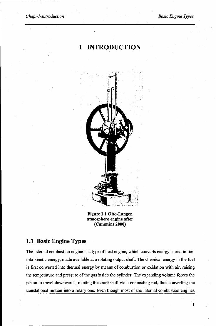
Figure 1.1 Otto-Langen atmosphere engine after (Cummins 2000) .......................................... 1
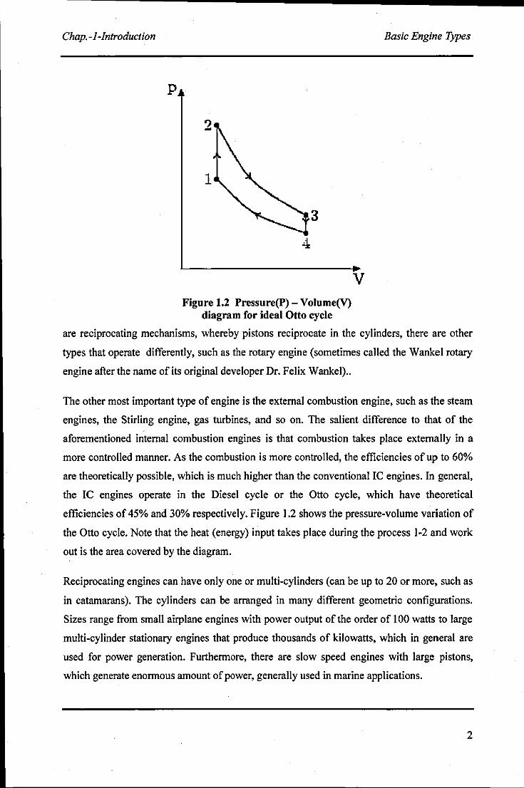
Figure 1.2 Pressure(p) - Volume(V) diagram for ideal Otto cycle .......................................... 2
Figure 1.3 Forces acting on the piston during the power stroke ................................................ 5
Figure 1.4 whirl of journal bearings .......................................................................................... 7
Figure 1.5 Piston crankshaft assembly ....................................................................................... 9
Figure 1.6 Energy consumption in an internal combustion engine after (Anderson 199 I) ..... 11
Figure 1.7: Model development flow diagram ........................................................................ 13
Figure 2.1 Percentage noise emission from various noise sources in an engine, after (Spessert
and Ponsa 1990) ............................................................................................................. 17
Figure 2.2 Sensitivity of the engine component friction to various lubricants after (Taylor
2002) ............................................................................................................................... 19
Figure 2.3 Journal instability motion ....................................................................................... 24
Figure 2.4 Shaft centre movement ........................................................................................... 24
Figure 2.5 Formation of cavitation under EHL conditions after (Aoyama et al. 2003) .......... 25
Figure 2.6 Full Sommerfeld pressure variation in a journal ................................................... 26
Figure 2.7 Pressure variation with Reynolds boundary conditions ......................................... 27
Figure 2.8 Comparison of finite length and short bearing solutions after (Mourelatos 200 1 b)
........................................................................................................................................ 28
Figure 2.9 Conventional and ArticuIIated piston configuration .............................................. 29
Figure 2.10 Gudgeon pin offset ............................................................................................... 31
Figure 2.11 Forces acting on piston ring ................................................................................. 33
Figure 3.1 Euler Beam ............................................................................................................. 47
Figure 3.2 A cantilever beam under Static(a) and Dynamic(b) loading .................................. 47
Figure 3.3 Multi Body system of Piston Crankshaft assembly ................................................ 49
Figure 3.4 Two Degree Of Freedom system ............................................................................ 50
Figure 3.5 Generalized forces acting on a rigid body .............................................................. 55
Figure 3.6 Deformable body coordinates ................................ : ................................................ 59
Figure 3.7 Super-element Crankshaft - Mode shape for the frequency of 2704Hz (created
using MSCINastran) ....................................................................................................... 65
Figure 3.8 FFT of Crank Angular Velocity for Rigid Engine ModeL .................................... 68
Figure 3.9 FFT of Crank Angular Velocity for Flexible Engine Model.. ................................ 69
Figure 3.10 Round-off and Truncation error (after (Rao 2002» ............................................ 70
ix
------------------......... Figure 3.11 Geometrical configuration of a single cylinder engine ........................................ 72
Figure 4.1 Stribeck curve ......................................................................................................... 79
Figure 4.2 Physical representation of Reynolds equation ........................................................ 80
Figure 4.3 Pressure distribution in ajournal bearing .............................................................. 85
Figure 4.4 Variation of Sommerfeld number with minimum film thickness (LID = 0.5) ....... 88
Figure 4.5 Shaft whirling stability map ................................................................................... 89
Figure 4.6 Ring Lubrication ..................................................................................................... 90
Figure 4.7 Pressure distributions with Sommerfeld condition ................................................. 94
Figure 4.8 Lubricated contact .................................................................................................. 97
Figure 4.9 Temperature variation along the contact. ............................................................ 10 I
Figure 4.1 0 Heat flow within a lubricated contact. ................................................................ 102
Figure 5.1 Rigid body Engine Model ................................................•..................•................ 109
Figure 5.2 Single cylinder engine crankshaft ........................................................................ 112
Figure 5.3 Connecting rod and Piston .................................................................................... 113
Figure 5.4 Enlarged view of the journal bearing in the crankshaft ........................................ 115
Figure 5.5 Meshed crankshaft with boundary conditions ...................................................... 116
Figure 5.6 Flexible engine model in ADAMS ..................................................................•...• 119
Figure 5.7 A cycle of combustion gas force .......................................................................... 121
Figure 5.8 Combustion gas force variation for 74 engine cycles ......................................... 122
Figure 5.9 Engine load torque and crank speed variation ...................................................... 123
Figure 5.10 Spline fitted engine load torque variation with angluar velocity ....................... 123
Figure 5.11 Bearing and journal centre configuration ........................................................... 125
Figure 5.12 General force vector at main bearing ................................................................. 125
Figure 5.13 Main bearing friction torque .•.......•................................ : ..............•..................... 127
Figure 5.14 Posible piston modes inside the cylinder ............................................................ 128
Figure 5.15 Minimum film thickness variation at piston edge .............................................. 128
Figure 5.16 Forces acting on the piston skirt .............................................•........................... 129
Figure 5.17 Pressure variation along the contact at piston edge ............................................ 130
Figure 5.18 Piston kinematical and geometrical parameters for minimum film thickness
calculation ..................................................................................................................... 131
Figure 5.19 Spline fitted temperature variation along the cylinder wall (Heywood 1988) ... 131
Figure 5.20 Piston friction force during one combustion cycle ............................................. 132
Figure 5.21 Flow chart for friction force calculation ............................................................. 133
x
Figure 5.22 Forces acting on piston ring ............................................................................... 136
Figure 5.23 Flow diagram for piston-ring friction calculation .............................................. 138
Figure 5.24 Lubricant temperature variation at piston ring-cylinder wall interaction ........... 139
Figure 5.25 Schematic diagram of multi-physics model ....................................................... 140
Figure 6.1 The E6 Engine Test Rig ....................................................................................... 145
Figure 6.2 E6 Engine front end .............................................................................................. 146
Figure 6.3 Schematic of hardware used in impact test .......................................................... 147
Figure 6.4 Time and frequency domain response of an impact excitation ............................ 149
Figure 6.5 Schematic diagram of an accelerometer ............................................................... 150
Figure 6.6 The laser torsional vibrometer optical geometry .................................................. 152
Figure 6.7 Flywheel vibration measurements ........................................................................ 153
Figure 6.8 Pressure sensor and calibration ............................................................................ 154
Figure 6.9 FRF with the corresponding phase angle and coherence function •..........•........... 159
Figure 6.10 Enlarged FRF magnitude corresponding to 2nd peak of Figure 6.9 .................. 160
Figure 6.11 Impact test apparatus set up for the crankshaft .................................................. 161
Figure 6.12 Impact test positions on engine components ...................................................... 162
Figure 6.13 Bruel & Kjaer Conditioning Amplifier and DAC system .................................. 164
Figure 6.14 Front end of the PULSE software ...................................................................... 165
Figure 6.15 CAD model and the actual model of the Connecting Rod ................................• 166
Figure 7.1 Fourier frequency spectrum for combustion gas force ......................................... 168
Figure 7.2 Major modes of the crankshaft and the connecting rod ....................................... 169
Figure 7.3 Forces acting on the connecting rod ..................................................................... 170
Figure 7.4 Frequency spectrum for Flywheel rotational speed from multi physics numerical
model ............................................................................................................................ 173
Figure 7.5 Frequency spectrum for experimentally measured flywheel rotational velocity .173
Figure 7.6 Experimentally measured Flywheel nodding velocity ......................................... 174
Figure 7.7 Numerically obtained Flywheel nodding velocity ............................................... 174
Figure 7.8 Frequency spectrum for experimentally measured flywheel nodding motion ..... 175
Figure 7.9 Frequency spectrum for numerically obtained flywheel nodding velocity .......... 175
Figure 7.10 Bearing eccentricity and Sommerfeld number variation during a combustion
cylcle (for crankshaft front bearing) ............................................................................. 178
Figure 7.11 Bearing centre eccentricity ratio during a combustion cycle ............................. 178
Figure 7.12 Bearing load at 4 stroke combustion cycle ......................................................... 180
xi
Figure 7.13 Bearing center velocity (in radial direction) during a 4 stroke cycle ................ 181
Figure 7.14 Variation offriction coefficient at bearing during a 4 stroke cycle ................... 181
Figure 7.15 Crankshaft bearing centre loci during a combustion cycle ................................ 183
Figure 7.16 Fourier frequency spectrum of the bearing froce at front end oftbe crankshaft 184
Figure 7.17 Piston secondary motion ..................................................................................... 185
Figure 7.18 Piston thrust force variation at positions 1 and 2 ................ : .............................. 186
Figure 7.19 Film thickness and squeeze velocity variation at thrust side (at piston position 2)
...................................................................................................................................... 187
Figure 7.20 Coefficient offriction for the piston skirt-to-cylinder wall contact ................... 188
Figure 7.21 Fourier spectrum for angular acceleration of piston tilting motion ................... 189
Figure 7.22 Reaction force variation at piston ring cylinder wall contact ............................. 190
Figure 7.23 Variation of film thickness and friction force at piston ring cylinder wall contact
...................................................................................................................................... 191
Figure 7.24 Piston ring friction forces ................................................................................... 192
Figure 7.25 Maximum lubricant pressure at piston ring to cylinder wall contact during a
combustion cycle .......................................................................................................... 193
Figure 7.26 Heat dessipation in the piston ring· cylinder wall contact ................................ 194
Figure 7.27 Variation of Peclet number in the piston ring-cylinder wall contact during a
combustion cycle .......................................................................................................... 195
Figure 7.28 Variation of viscosity in the piston ring-to-cylinder wall contact during the
engine cycle .................................................................................................................. 196
Figure 7.29 Percentage energy loss in the E6 engine model ................................................. 197
Figure 7.30 Temperature rise at piston ring to cylinder wall contact for different ring
thickness ....................................................................................................................... 198
Figure 7.31 Piston orientation and forces acting before and after TDC ................................ 20 1
Figure 7.32 Major thrust side force variation with crankshaft offset towards thrust side ..... 202
Figure 7.33 Minor thrust side force variation with respect to the crankshaft offset towards the
major thrust side ........................................................................................................... 203
Figure 7.34 Variation of piston translation with respect to crankshaft offset ........................ 204
xii
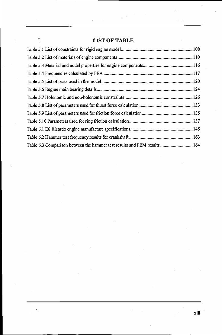
LIST OF TABLE
Table 5.1 List of constraints for rigid engine model... ........................................................... 108
Table 5.2 List of materials of engine components ................................................................. !10
Table 5.3 Material and nodel properties for engine components ........................................... ! 16
Table 5.4 Frequencies calculated by FEA ............................................................................. 1 17
Table 5.5 List of parts used in the model.. ............................................................................. 120
Table 5.6 Engine main bearing details ................................................................................... 124
Table 5.7 Holonomic and non-holonomic constraints ........................................................... 126
Table 5.8 List of parameters used for thrust force calculation .............................................. 133
Table 5.9 List of parameters used for friction force calculation ............................................ 135
Table 5.1 0 Parameters used for ring friction calculation ....................................................... 137
Table 6.1 E6 Ricardo engine manufacture specifications ...................................................... 145
Table 6.2 Hammer test frequency results for crankshaft ....................................................... 163
Table 6.3 Comparison between the hammer test results and FEM results ............................ 164
xiii
B
c
c -p
c -q
D
e
iD
F;, -
F -... F -"
F" g
h
k
K
k,
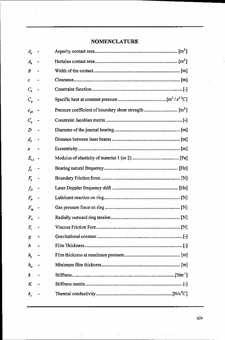
NOMENCLATURE
Asperity contact area ....................................................................... [m2]
Hertzian contact area ....................................................................... [m2]
Width of the contact .......................................................................... [m]
Clearance ........................................................................................... [m]
Constraint function .............................................................................. [-]
Specific heat at constant pressure ......................................... [m2 / S2 °C]
Pressure coefficient of boundary shear strength ............................. [m2]
Constraint Jacobian matrix ................................................................. [-]
Diameter of the joumal bearing ........................................................ [m]
Distance between laser beams .......................................................... [m]
Eccentricity ....................................................................................... [m]
Modulus of elasticity of material 1 (or 2) ........................................ [Pal
Bearing natural frequency ............................................................... [Hz]
Boundary Friction force .................................................................... [N]
Laser Doppler frequency shift ........................................................ [Hz]
Lubricant reaction on ring ................................................................. [N]
Gas pressure force on ring ................................................................ [N]
Radially outward ring tension ........................................................... [N]
Viscous Friction Fore ........................................................................ [N]
Gravitational constant ......................................................................... [-]
Film Thickness .................................................................................... [-]
Film thickness at maximum pressure ................................................ [m]
Minimum film thickness ................................................................... [m]
Stiffness ..........................................................•..........•.................• [Nm·l]
Stiffness matrix ................................................................................... [-]
Thermal conductivity ................................................................. [N/s °C]
xiv
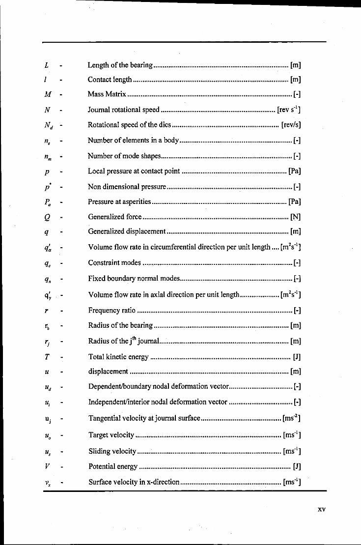
~--------~--------------------.......... . L
1
M
N
n,
n -m
p
• p
Q
q
q~
q~
r
T
u
u,
u,
v
Length of the bearing ........................................................................ [m]
Contact length ................................................................................... [m]
Mass Matrix ........................................................................................ [-]
Journal rotational speed •............................................................ [rev s·']
Rotational speed of the dics ......................................................... [rev/s]
Number of elements in a body ............................................................ [-]
Number of mode shapes ...................................................................... [-]
Local pressure at contact point ........................................................ [Pal
Non dimensional pressure ................................................................... [-]
Pressure at asperities ........................................................................ [Pal
Generalized force .............................................................................. [N]
Generalized displacement ................................................................. [m]
Volume flow rate in circumferential direction per unit length .... [m2s·']
Constraint modes ................................................................................ [-]
Fixed boundary normal modes ............................................................ [-]
Volume flow rate in axial direction per unit length ..................... [m2s·']
Frequency ratio ................................................................................... [-]
Radius of the bearing ..............•...............•.....•........•...............••...•...•• [m]
Radius of the jth journaL .........•...............•......................................... [m]
Total kinetic energy ........................................................................... [J]
displacement ..................................................................................... [m]
Dependentlboundary nodal deformation vector .................................. [-]
Independent/interior nodal deformation vector .................................. [-]
Tangential velocity at journal surface ........................................... [ms·2]
Target velocity .............................................................................. [ms·']
Sliding velocity ............................................................................. [ms·']
Potential energy........ .............. .... ............. ..... ......... ......... ... .... ............ [J]
Surface velocity in x-direction ...................................................... [ms·']
xv
Vy
w
w
w,
• w,
w -x
w -y
y
a
r r, e
710
8
A
A
p
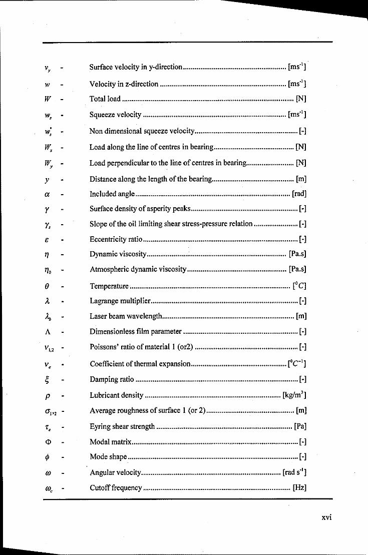
Surface velocity in y-direction ...................................................... [ms·l]
V I . . d' . [ .1] e OClty In z- lrectlOn .................................................................. ms
Total load .......................................................................................... [N]
Squeeze velocity ........................................................................... [ms·l]
Non dimensional squeeze velocity .•.................................................... [-]
Load along the line of centres in bearing .......................................... [N]
Load perpendicular to the line of centres in bearing ......................... [N]
Distance along the length of the bearing ....................................•...... [m]
Included angle .........................•....................................................... [rad]
Surface density of asperity peaks ........................................................ [-]
Slope of the oil limiting shear stress-pressure relation ...........•.•......... [-]
Eccentricity ratio ................................................................................. [-]
Dynamic viscosity ...................•..................................................... [Pa.s]
Atmospheric dynamic viscosity .................................................... [Pa.s]
Temperature .... .... ............. .......•................................ ...... ................. [0 C]
Lagrange multiplier ............................................................................. [-]
Laser beam wavelength ..................................................................... [m]
Dimensionless film parameter ............................................................ [-]
Poissons' ratio of material I (or2) ...................................................... [-]
Coefficient of thermal expansion .................................................. [oC-I]
Damping ratio .....................•...•........................................................... [-]
Lubricant density ....................................................................... [kg/m3]
Average roughness of surface I (or 2) .............................................. [m]
Eyring shear strength .............••........................................................ [Pal
Modal matrix ....................................................................................... [-]
Mode shape ......................................................................................... [-]
Angular velocity ......................................................................... [rad S·I]
Cutoff frequency ............................................................................. [Hz]
xvi

Angular velocity of accelerometer base ..................................... [rad s"l
Journal angular velocity ............................................................. [rad s"l
ID -n Natural frequency of the accelerometer ..................................... [rad s"l
xvii
Chap.-l-Introduction Basic Engine Types
1 INTRODUCTION
1.1 Basic Engine Types
Figure 1.1 Otto-Langen atmosphere engine after
(Cummins 2000)
The internal combustion engine is a type of heat engine, which converts energy stored in fuel
into kinetic energy, made available at a rotating output shaft. The chemical energy in the fuel
is first converted into thermal energy by means of combustion or oxidation with air, raising
the temperature and pressure of the gas inside the cylinder. The expanding volume forces the
piston to travel downwards, rotating the crankshaft via a connecting rod, thus converting the
translational motion into a rotary one. Even though most of the internal combustion engines
I
Chap. -I-Introduction Basic Engine Types
p
2
1
3
4:
v Figure 1.2 Pressure(p) - Volume(V)
diagram for ideal Otto cycle
are reciprocating mechanisms, whereby pistons reciprocate in the cylinders, there are other
types that operate differently, such as the rotary engine (sometimes called the Wankel rotary
engine after the name of its original developer Dr. Felix Wankel) ..
The other most important type of engine is the external combustion engine, such as the steam
engines, the Stirling engine, gas turbines, and so on. The salient difference to that of the
aforementioned internal combustion engines is that combustion takes place externally in a
more controlled manner. As the combustion is more controlled, the efficiencies of up to 60%
are theoretically possible, which is much higher than the conventional IC engines. In general,
the IC engines operate in the Diesel cycle or the Otto cycle, which have theoretical
efficiencies of 45% and 30% respectively. Figure 1.2 shows the pressure-volume variation of
the Otto cycle. Note that the heat (energy) input takes place during the process 1-2 and work
out is the area covered by the diagram.
Reciprocating engines can have only one or multi-cylinders (can be up to 20 or more, such as
in catamarans). The cylinders can be arranged in many different geometric configurations.
Sizes range from small airplane engines with power output of the order of 100 watts to large
multi-cylinder stationary engines that produce thousands of kilowatts, which in general are
used for power generation. Furthermore, there are slow speed engines with large pistons,
which generate enormous amount of power, generally used in marine applications.
2
Chap. -1-Introduction Historical Evolution of Engines
1.2 Historical Evolution of Engines
The year 2001 marks the 125th anniversary of the modern internal combustion engine
(Cummins 2000). Virtually all of the basic elements in the present reciprocating four-stroke
cycle engine were present in Nicolaus Otto's creation more than a century ago. Since then
minor improvements have been made to the original concept to improve efficiency and power
output.
During the second half of the 19th century many different styles of internal combustion
engines were built and tested. The first fairly practical engine was invented by J.J.E. Lenoir
(1822-1900) and appeared on the scene about 1860, even though it was a non- compression
engine with mechanical efficiency of 5%. In 1867 the Otto-Langen engine with improved
efficiency of 11 % was introduced. It was an important stepping-stone for the introduction of
the 4-stroke cycle engine, later developed by Otto in 1876. During this time engines operating
on the same basic four-stroke cycle as the modern automobile engine began to evolve as the
. best design (Gas Engine Magazine, Feb 1991). Although many people were working on the
four-stroke cycle design, Otto was given the credit for his prototype engine in 1876.
In the 1880s the internal combustion engine first appeared in automobiles (Givens 1990). In
this decade the two-stroke cycle engine became practical and was manufactured in large
numbers. By 1892, RudolfDiesel (1858-1913) had perfected his compression ignition engine
into basically the same diesel engine known today. This was after years of development
work, which included the use of solid fuels in his early experimental engines. Early
compression ignition engines were noisy, large, slow, single-cylinder engines. They were,
however, more efficient than the spark ignition engines, even though some drawbacks like
high noise, harshness and dark fume existed. Modern engines use technologies like Common
Rail Direct Injection (CRDI), which controls the amount of fuel into the combustion chamber
precisely with accurate timing in order to maximise combustion efficiency. Whereby in the
past, diesel engines were unrefined, sluggish and environmentally unfriendly, this is no
longer true in modern diesel engines due to the above-mentioned advancements in
combustion strategy, material and manufacturing technology. They are now powerful, smooth
and very refined, so much so that they have been introduced as alternative engines in the line
up of flagship models.
3
Chap.-l-lntroduction Noise, Vibration and Harshness
1.3 Noise, Vibration and Harshness
The improved performance and compactness of modem internal combustion engines makes
them a suitable power plant for automobiles. Even though, in the early stages, they were
mainly used for applications like lifting elevators, water pumping and so on. Nowadays the
automobile industry accounts for the main application area. There are some basic customer
concerns in a modem vehicle. Outer appearance, vehicle handling, reliability and fuel
efficiency are the most important among them. However, noise, vibration and harshness play
an increasingly major role in the context of customer expectations.
The suspension system in most modem vehicles is sufficiently refined to counteract the effect
of vibration transmitted due to the unevenness of the road surface. Imbalances of rotating
parts, clearance between gear teeth, road noise from tyres and cyclic combustion force in the
combustion chamber can be regarded as critical Noise, Vibration and Harshness (NVH)
sources. In (Morita et aI, 2001) combustion force is attributed to be the prominent source of
noise. However, the non-uniform character of the torque generated in reciprocating engines
arises due to the application of periodic combustion forces and the associated inertial forces
of rotating and articulated members. Fuel injector pumps, timing gear rattle, bearing
reactions, camshafts, crankshafts, etc also contribute in different ways to engine noise
(Haddad and Tjan 1995).
Although most excitations from the ground are counteracted reasonably effectively through
the suspension, the power plant itself is the source of noise and vibration so the dynamic
analysis of the engine mechanism is required (Suh et aI, 2000). Understanding the origins and
parametric dependencies of noise and vibration is the first step in a reduction (i.e. refinement)
strategy. Such concerns extend to piston-driven internal combustion engines, which may
often be the major source of vehicle noise and vibration (Hoffman and Dowling 1999). The
engine noise is dominant in the middle to high frequency range (0.5 to 2.5KHz). The impact
ofIC engine vibration on vehicle performance or customer perceived quality is typically less
serious at higher frequencies, because reliable isolation strategies exist for eliminating
vibration transmission from the engine to the vehicle structure.
In recent years the specific output of the engine has been increased, while the rigidity of the
structure has been reduced in high-speed automobile diesel engines.
4
Chap. -I-Introduction
Anti-thrust side
Combustion Pressure
j j t! j Thrust side
Sources o/vibration in an Engine
I Piston Motion
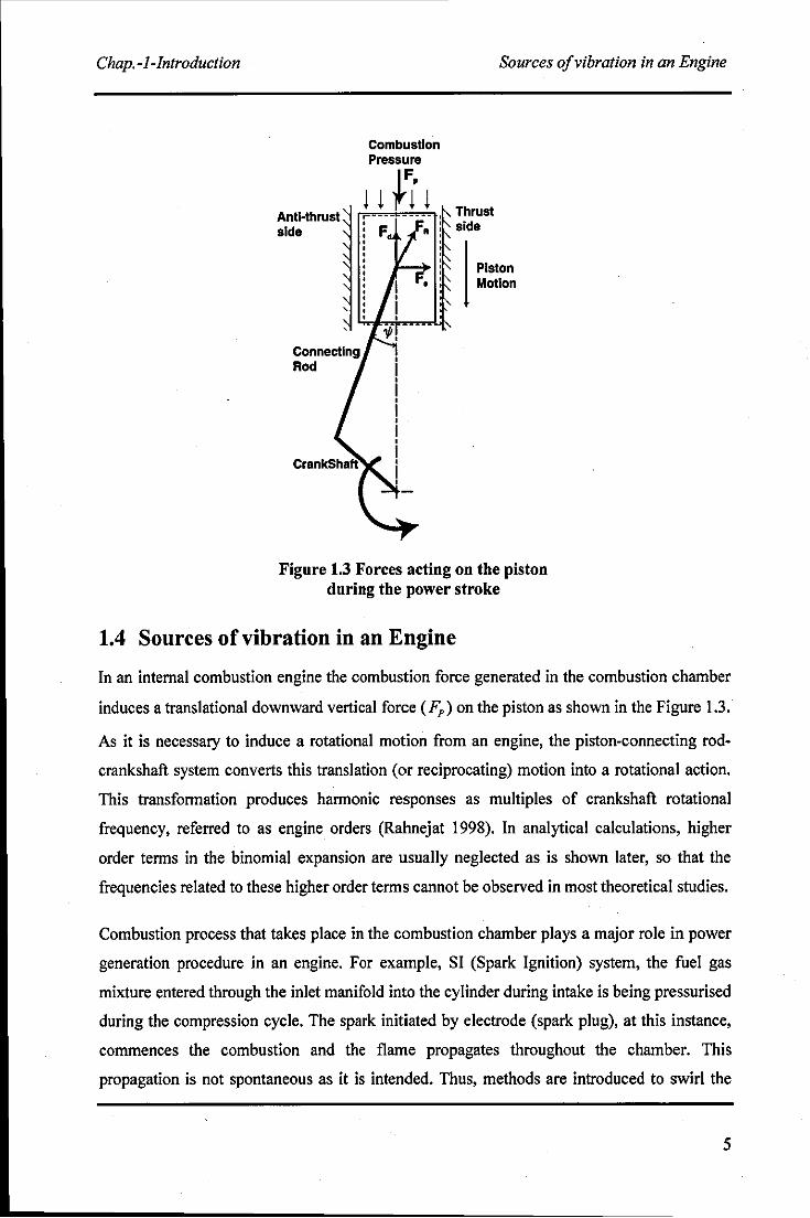
Figure 1.3 Forces acting on the piston during the power stroke
1.4 Sources of vibration in an Engine
In an internal combustion engine the combustion force generated in the combustion chamber
induces a translational downward vertical force (Fp) on the piston as shown in the Figure 1.3.
As it is necessary to induce a rotational motion from an engine, the piston-connecting rod
crankshaft system converts this translation (or reciprocating) motion into a rotational action.
This transformation produces harmonic responses as multiples of crankshaft rotational
frequency, referred to as engine orders (Rahnejat 1998). In analytical calculations, higher
order terms in the binomial expansion are usually neglected as is shown later, so that the
frequencies related to these higher order terms cannot be observed in most theoretical studies.
Combustion process that takes place in the combustion chamber plays a major role in power
generation procedure in an engine. For example, SI (Spark Ignition) system, the fuel gas
mixture entered through the inlet manifold into the cylinder during intake is being pressurised
during the compression cycle. The spark initiated by electrode (spark plug), at this instance,
commences the combustion and the flame propagates throughout the chamber. This
propagation is not spontaneous as it is intended. Thus, methods are introduced to swirl the
5
Chap. -I-Introduction Sources o/vibration in an Engine
mixture and make it turbulent to enhance flame propagation. However, this non-uniform
behaviour of the combustion gives rise to pressure force fluctuations, which manifests as
harmonics in the combustion pressure force (Fp in Figure 1.3). The reaction force, Fd , acting
on the piston from the connecting rod balances the gas pressure force Fp. As the connecting
rod is at an angle ljI to the vertical, and is hinged to the piston, there is a horizontal
component F" due to the resultant force FR , at the connecting rod. This horizontal
component forces the piston towards the right side of the cylinder wall, shown in the Figure
1.3. This side of the cylinder, where the impact often occurs is known as the Thrust Side.
During the compression stroke, connecting rod is arranged such that the thrust force
Fd reverses its direction. This action pushes the piston against the other side of the cylinder,
which is known as the anti-thrust Side. This side force reversals during the engine cycle
moves the piston horizontally and this is know as Piston Slap motion or Piston Secondary
motion. At the TDC (Top Dead Centre) and BDC (Bottom Dead Centre) these force reversals
are most significant.
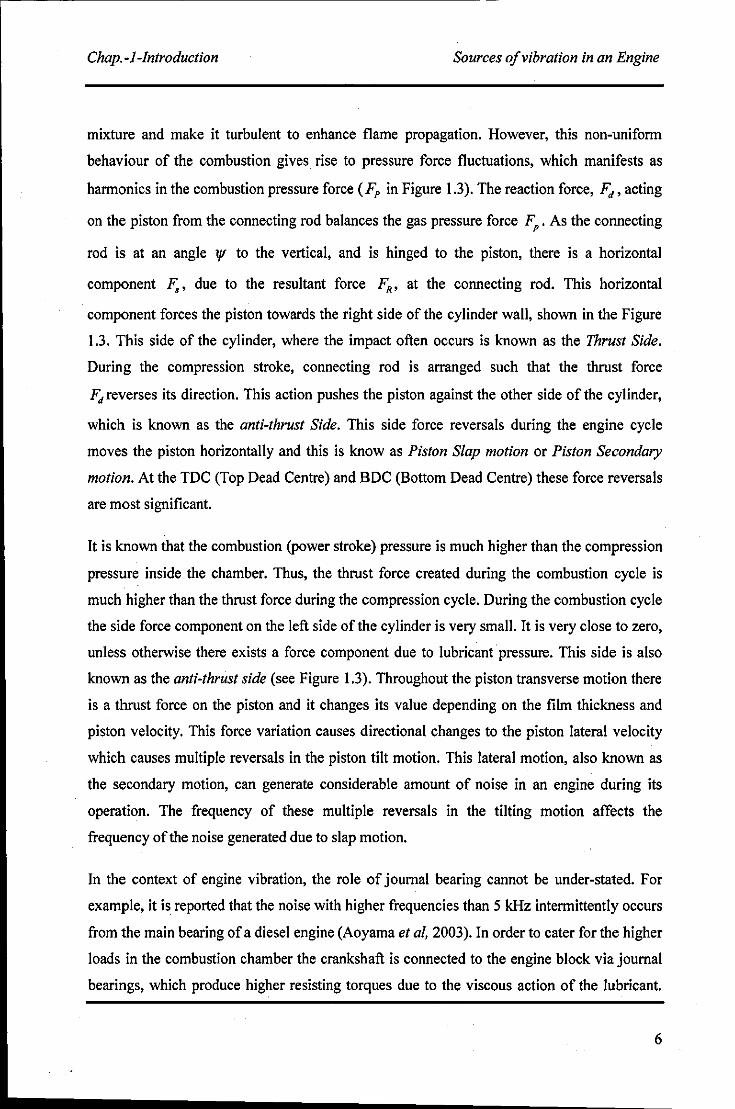
It is known that the combustion (power stroke) pressure is much higher than the compression
pressure inside the chamber. Thus, the thrust force created during the combustion cycle is
much higher than the thrust force during the compression cycle. During the combustion cycle
the side force component on the left side of the cylinder is very small. It is very close to zero,
unless otherwise there exists a force component due to lubricant· pressure. This side is also
known as the anti-thrust side (see Figure 1.3). Throughout the piston transverse motion there
is a thrust force on the piston and it changes its value depending on the film thickness and
piston velocity. This force variation causes directional changes to the piston lateral velocity
which causes multiple reversals in the piston tilt motion. This lateral motion, also known as
the secondary motion, can generate considerable amount of noise in an engine during its
operation. The frequency of these multiple reversals in the tilting motion affects the
frequency of the noise generated due to slap motion.
In the context of engine vibration, the role of journal bearing cannot be under-stated. For
example, it is reported that the noise with higher frequencies than 5 kHz intermittently occurs
from the main bearing of a diesel engine (Aoyama et aI, 2003). In order to cater for the higher
loads in the combustion chamber the crankshaft is connected to the engine block via journal
bearings, which produce higher resisting torques due to the viscous action of the lubricant.
6
Chap. -1-Introduction
Bearing (shell)
Shaft (journal)
w < __ _
Sources a/vibration in an Engine
t
Line of Centres
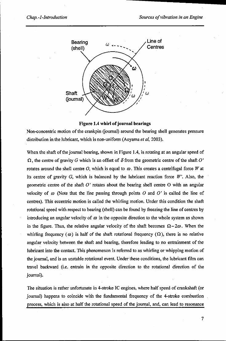
Figure 1.4 whirl of journal bearings
Non-concentric motion of the crankpin Gournal) around the bearing shell generates pressure
distribution in the lubricant, which is non-uniform (Aoyama et aI, 2003).
When the shaft of the journal bearing, shown in Figure 1.4, is rotating at an angular speed of
n, the centre of gravity G which is an offset of 8 from the geometric centre of the shaft 0'
rotates around the shell centre 0, which is equal to 0). This creates a centrifugal force Wat
its centre of gravity G, which is balanced by the lubricant reaction force W'. Also, the
geometric centre of the shaft 0' rotates about the bearing shell centre 0 with an angular
velocity of 0) (Note that the line passing through points 0 and 0' is called the line of
centres). This eccentric motion is called the whirling motion. Under this condition the shaft
rotational speed with respect to bearing (shell) can be found by freezing the line of centres by
introducing an angular velocity of 0) in the opposite direction to the whole system as shown
in the figure. Thus, the relative angular velocity of the shaft becomes n - 20). When the
whirling frequency (0) is half of the shaft rotational frequency (n), there is no relative
angular velocity between the shaft and bearing, therefore leading to no entrainment of the
lubricant into the contact. This phenomenon is referred to as whirling or Whipping motion of
the journal, and is an unstable rotational event. Under these conditions, the lubricant film can
travel backward (i.e. entrain in the opposite direction to the rotational direction of the
journal).
The situation is rather unfortunate in 4-stroke le engines, where half speed of crankshaft (or
journal) happens to coincide with the fundamental frequency of the 4-stroke combustion
process, which is also at half the rotational speed of the journal, and, can lead to resonance
7
Chap.-l-Introduction Sources o/vibration in an Engine
conditions. This is a non-linear event, known as the jump phenomenon, where at a given
speed of rotation the journal motion can jump from a seemingly stable orbit to another orbit
with different amplitude instantaneously. To investigate such conditions and guard against
their occurrence, it is necessary to carry out an analysis that includes inertial dynamics,
flexural motion of elastic components and reaction forces from the lubricant pressure.
In compression ignition engines, the noise induced from the injector pump is an equally
important source, as described earlier. For each combustion cycle, the fuel is pumped at the
appropriate instant of time to the combustion chamber via the injector pump. It creates a
pressure wave, which travels from the pump to the combustion chamber through a steel tube.
This excitation is half the engine order in a four-stroke internal combustion engine (Spessert
and Ponsa 1990) also it is more of a problem now as the injector pressures are significantly
higher (around 400-450 bar)
Basically the engine imbalance occurs due to translational masses and rotating eccentric
masses. There exists primary and secondary out of balance excitation from these translational
masses as it is explained in section 3.5.1. These primary excitations can be balanced by
adding masses where as secondary excitations can be minimised by proper phasing of
adjacent crank-throws. Thus, the inertial imbalance due to the reciprocating mass of the
piston and articulated connecting rod is minimised in multi-cylinder engines. Axial, torsional
and lateral vibrations, which induce stresses occur simultaneously in the crankshaft of a
multi-cylinder engine (Wakabayashi et aI, 1995). The crankshaft of the multi-cylinder engine
has a phase difference between the adjacent crank-throw planes, so, the four kinds of
vibrations are all coupled in the crankshaft rotation.
All these noise sources, which were discussed in this section and not described fully, such as
timing gear rattle, valve train excitation etc., can induce air born noise in an automobile. All
cyclic excitations generated by aforementioned causes deform the body, which is adjacent to
it. This will cause vibrations of structural elements. In this case, the structure deforms
according to a specific mode shape or a combination of mode shapes, depending on the
excitation frequency. Then, the physical boundary of the body (structure) excites the adjacent
environment, which is air and creates structure-borne noise. This is the main form of energy
transfer from the source of excitation to the environment. Therefore, reduction in system level
vibration translates to reduction of noise emitted from the system, thereby reducing the loss
8
Chap. -I-Introduction
I / Combustion gas I pressure
U!U!
I
/-f-. ..... /,Fr " I
I I \\. Ft _---1-__ ---r--
\ I I
\ I / "~_I_/"
I
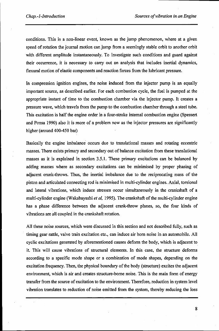
Figure 1.5 Piston crankshaft assembly
Crankshaft Vibrations
of energy. This means reduction in vibration can be regarded as an attempt to increase the
efficiency of a system.
1.5 Crankshaft Vibrations
As discussed in earlier sections, there are various sources of vibration in an engine, some of
which are well understood. However, it is difficult to usually take all these factors into
account in a single model. Therefore, in this study, the piston-connecting rod-crankshaft sub
system is investigated.
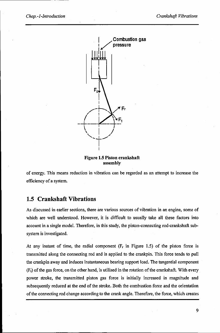
At any instant of time, the radial component (Fr in Figure 1.5) of the piston force is
transmitted along the connecting rod and is applied to the crankpin. This force tends to pull
the crankpin away and induces instantaneous bearing support load. The tangential component
(Ft) of the gas force, on the other hand, is utilised in the rotation of the crankshaft. With every
power stroke, the transmitted piston gas force is initially increased in magnitude and
subsequently reduced at the end of the stroke. Both the combustion force and the orientation
of the connecting rod change according to the crank angle. Therefore, the force, which creates
9
Chap. -I-Introduction Engine performance
torque vary with the crank angle. This action imparts a "twist-untwist" action of the
crankshaft (known· as crankshaft wind-up or wind-down), causing torsional vibrations to
occur.
The tangential force component of the piston acting on the crankshaft also induces a bending
moment on the crankshaft other than the torsional moment, known as the coupled torsional
bending moment. As the force, which causes this bending moment, is indeed fluctuates due to
aforementioned reasons, this will create bending vibrations, which could excite the bending
modes of the crankshaft.
In a four-stroke single cylinder internal combustion engine, the fundamental frequency of the
applied torque coincides with half speed of the crankshaft, and its harmonics, are, whole or
half orders of the instantaneous engine speed. Therefore, there is almost an infinite number of
critical speeds, and in principle, high vibratory torques may be induced at each one of these
frequencies. The generated vibration amplitudes can be high enough in extreme cases to
cause crankshaft or other engine component failure. However, only a few critical speeds
induce seriously high vibratory torque amplitudes (80ysal and Rahnejat 1997).
Despite this, the excitations induced by the bearing cannot be neglected as discussed earlier.
Due to the off-centre motion of the crankshaft on the bearing bushing, high vibration
excitations can occur. This can be exaggerated by the excitations produced by piston lateral
motion. Even though there is a relationship between engine speed and the excitation
frequency of the combustion force, it is difficult to figure out a relationship between the
crankshaft rotational speed and the slap excitation frequency (Cho et ai, 2002).
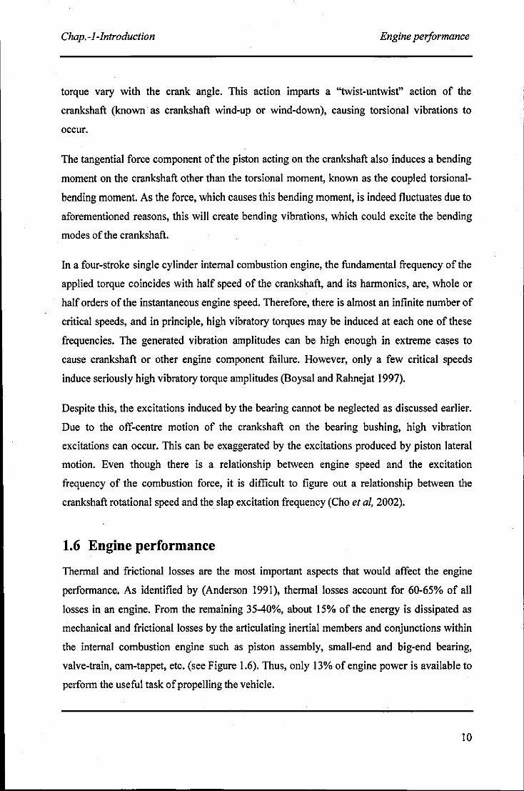
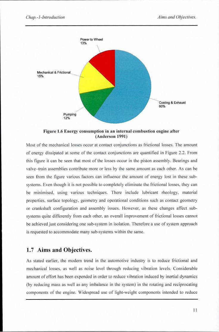
1.6 Engine performance
Thermal and frictional losses are the most important aspects that would affect the engine
performance. As identified by (Anderson 1991), thermal losses account for 60-65% of all
losses in an engine. From the remaining 35-40%, about 15% of the energy is dissipated as
mechanical and frictional losses by the articulating inertial members and conjunctions within
the internal combustion engine such as piston assembly, small-end and big-end bearing,
valve-train, cam-tappet, etc. (see Figure 1.6). Thus, only 13% of engine power is available to
perform the useful task of propelling the vehicle.
10
Chap. -l-lntroduct ion Aims and Objectives.
Mechanical & Frictional 15%
Pumping 12%
Power to Wheel 13%
-~-.-" •• - & Exhaust 60%
Figure 1.6 Energy consumption in an interna l combustion eng in e after (A nderson 199 1)
Most of the mechanica l losses occur at contact conjunct ions as frictiona l losses. The amount
of energy di ss ipated at some of the contact conjunctions are quant ified in Figure 2.2 . From
thi s figure it can be seen that most of the losses occur in the p iston assembly. Bearings and
va lve- train assemblies contribute more or less by the same amount as each other. As can be
seen from the figure various factors can influence the amount of energy lost in these sub
systems. Even tho ugh it is not possib le to completely eliminate the fr ictio nal losses, they can
be minimised, using vario us techniques. There include lubricant rheo logy, materia l
properties, surface topology, geometry and o perat ional condit ions such as contact geometry
or crankshaft configuration and assemb ly issues . However, as these changes affect sub
systems quite diffe rently from each other, an overa ll improvement of fr ictional losses cannot
be ach ieved just considering one sub-system in iso lation. Therefore a use of system approach
is requested to accommodate man y sub-systems withi n the same.
1.7 Aims and Objectives.
As stated earl ier, the modern trend in the a utomotive industry is to red uce fr ict iona l and
mechanical losses, as we ll as noise level through reducing vibration leve ls. Considerable
amount of effort has been expended in order to reduce vibration induced by inert ial dynamics
(by reducing mass as we ll as any imbalance in the system) in the rotating and reciprocat ing
components of the engine. Widespread use o f light-weight components intended to reduce
11
Chap. -I-introduction Aims and Objeclives.
inert ial imbalances (thus mechanical losses a nd ineffi ciency), unfortunately has to a large
extent led to increased structura l vibration. Therefore, an optimum balance between inertia l
dynamics and structura l vibration has to be struck. The main design questi on becomes one of
fl ex ibi lity and we ight versus noise and vibration.
It has been found that finite e lement so lutions show differences between test results wi th
dynamica ll y loaded structures that undergo large ri gid body motions. So luti on through the
use of non- linear Finite Element Ana lysis (FEA) has improved the accuracy of resu lts, yet
fai ls to prov ide a complete descr ipti on of complex mechanical systems, including
hydrodynamics and large rig id body motions (Du 1999).
A rigid body mode l is not suffi cient to provide a realist ic assessment of the system, as the
reduced flexibility, g ives unexpected amp li tudes in some operating conditi ons. There fore, a
model should, have component fle xib ility. As a response to the high lighted short-comings,
commercial mult i-body dynamics software (ADAMS - Automatic Dynam ic Ana lysis of
Mechanica l Systems) is used in this report to model the inertial properties of the system and
the component flexib ility is incorporated into the model, using an FEA software.
The hyd rodynamic forces actin g on the bearings, piston slap (secondary motion) motion,
inc luding the skirt lubrication and e lastic propelties, ring lubrication includ ing thermal
analys is and the combusti on force acting on the piston top surface are a lso to be included in
the mode l, as given analytical fu nctions or splines fitted to measured data. Most of these
forc ing function s have been va lidated using a n E6 test engine. Particularly, the variat ions in
the combustion gas fo rce and crankshaft angu lar velocity been measured with an acceptable
degree of accuracy.
The main a im of th is report is to present a deta iled eng ine modelling method, referred to as a
multi-physics approach, in which, combined r igid body inertia l dynamics, structural moda l
characteristics o f e lastic components and tribologica l behaviour of load bearing surfaces have
been inc luded into a s ingle model. When such a model is made, the validi ty of model
predictions must be ascerta ined aga inst exper imenta l fi nd ings to enhance confidence in the
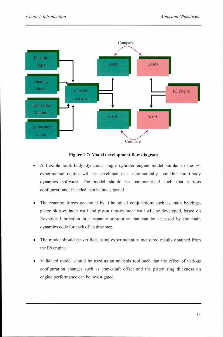
use of this methodology. Figure 1.7 shows the basic flow chart for the entire process of model
development and va lidat ion.
In order to achieve the above object ives the fo llowing steps are undertaken in th is thes is:
12
Chap. -I-Introduction Aims and Objectives.
Compare
~ ....... --. Loads
E6 Engine
NVH
~ Compare
Figure 1.7: Model development flow diagram
• A fl ex ible multi-body dynamics single cylinder engine model simi lar to the E6
experimental engine wi ll be developed in a commercia ll y ava ilab le multi-body
dynamics software. The model should be parameteri zed such that va rious
configurations, if needed, can be in vestigated.
• The reaction forces generated by tribological conjunct ions such as mall1 bearings,
piston skirt-cy li nder wa ll and piston ring-cylinder wa ll will be developed, based on
Reynolds lubrication in a separate subroutine that can be accessed by the main
dynamics code fo r each of its time step.
• The model should be verifi ed, using experimentally measured results obtained from
the E6 engine.
• Validated mode l should be used as an analysis tool such that the effect of vari ous
configuration changes such as crankshaft offset and the piston ring thickness on
engine performance can be investigated.
13
Chap. -/-Jntroduct ion Structure of the Thesis
1.8 Structure ofthe Thesis
Througho ut this chapter the genera l trend and concerns of automotive industry in re lat ion to
vibrations of IC engines, and frictiona l and mechani cal losses were di scussed. Its current
devel opments and interests were a lso highli ghted, thereby providing necessary motivation for
undel1aking th is research. The thesis is di vided into e ight chapters including the current
chapter.
Chapter 2 reviews the research work carri ed o ut in thi s fi e ld stal1ing from the basic hi stori cal
develo pments and theoretica l findin gs, to the latest experimental and research wo rk releva nt
to engine vibrati ons. Particular attention has been paid to the use of multi-body dynamics and
tribologica l aspects o f engine components.
In Chapter 3 a comprehensive mu lti-body dyna mic anal ysis is presented for single cy linder
eng ines, including kinematic and dynamics of rigid and defo rmab le bodi es . Analytical
techniques for deri ving the system di fferential and a lgebraic eq uations of motion of a mu lti -
body system are di scussed wi th re lation to Lagrang ian dynamics. Sub-structure couplin g
technique is used to coup le rigid body motions with elastic defo rm atio n.
In Chapter 4 hyd rodynam ic lubricatio n analys is rela ted to certa in contact conjunctio ns In
single cy linder eng ine is presented. Analytica l equat ions for lubricated conjuncti ons are
obtained, using class ica l analyt ica l approaches. Temperature va ri at ions are a lso obta in ed fo r
these contact conjunctio ns, wh ich affect the rheo logica l characterist ics of the lubricant, using
the energy equati on. Considering these reaction forces from the lubricated contacts, the s ing le
cylinder engine model is deve loped in a commerciall y ava ilable dynam ics code, ADAMS.
The construct ion of th is numerical mode l with the integrated tr ibo logical subroutines is
described in Chapter 5. The basic methodo logy used to obta in the component mode shapes,
using commercia ll y ava ilab le FE package, Nastran , is also presented in the same chapter.
Chapter 6 is basica ll y devoted to descriptio n of ex perimental measurements, as we ll as
techniques used to va lidate the developed nu meri ca l mode l. The use of measuring transducers
such as acce lerometers, vibrometers and impact hammers are detailed and the ir
measuremen ts a re quantified w ithin the chapter. Compari sons are made between the
measured and nume rica l data, presented in Chapter 7. C ritica l assessment of numeri cal resu lts
wi th respect to the deve loped mUlti -phys ics environment and its inte r-discip linary
14

Chap. -i -Introduction Structure of the Thesis
characteri stics is made. Also the benefits of such a holi stic mu lti-disciplinary approach in
engine design process and its usefulness in refining engine performance criteria are discussed.
Finall y, chapter 8 highlights the main conc lusions of the research and proposes suggestions
fo r future work to be carried out to extend the research and development fi ndings contained
in this thesis.
15
Chap 2 - Literature Review Introduction
2 LITERATURE REVIEW
2.1 Introduction
With improved ride and handling performance of a veh icle, power tra in no ise and vibration
characteristics have become progress ively more important. In the modern soc iety, the
lifestyle of many people involves the use of motor veh icles, and a significa nt proportion of
drivers' t ime is spent under idling conditions or in slow moving traffics in congestio n. As a
result, a ll road users are subjected to noise sources, part icularl y contributed by the power
train system. In contrast, noises induced from road-tyre interactions and by aerodynamics are
dominant at high speeds. However, recent surveys show that drivers are more annoyed by
structure-borne no ise and vibration than ai rborne no ise, the former be ing at a lower freq uency
and almost entirely induced by the power tra in system as reported in (Gupta 2002) .
Internal combustion engine can be broadly categori sed into several sub-systems concerning
no ise and vibration such as fue l pump system, timing belt gears, cam-tappet (va lve train)
system and crankshaft piston assembly. Exc itations frol11 fuel pUI11P system are dOl11inant
particularly in C l (Com press ion Ignition) engines as it incorporates high injection pressures.
Although the combustion pressure exc itation is more domi nant in naturall y aspi rated eng ines,
it is great ly reduced in turbo-charged engines as reported in (Spessert and Ponsa 1990) .
However, noise contribution from piston assembly is reta ined, demonstrating its significance
as an engine noise concern. Percentage no ise contributions from va ri ous sources in an engine
are shown in Figure 2. 1.
Pi ston crankshaft assembl y IS inherentl y unbalanced, because the translationa l inertial
imba lance of the reciprocating elements, such as the pi ston and connecting rod cannot be
represented by a rotating element with a constant rotating inertia as shown in (Rahnej at
1998), using a lumped mass model. Due to th is trans lati onal im balance there ex ists a
vibration spectrum that contains a ll the multip les of engine order v ibration. However, it is
poss ible to reduce or el iminate the horizontal latera l inertial force by employi ng
counterbal anced masses a long the crankshaft, whereas its verti ca l component can onl y be
attenuated by proper angular positioning of the crank or introd ucing a proper fi ring order
between the cylinders. However, a ll multiple frequency o rders a lways ex ist in single cylinder
16
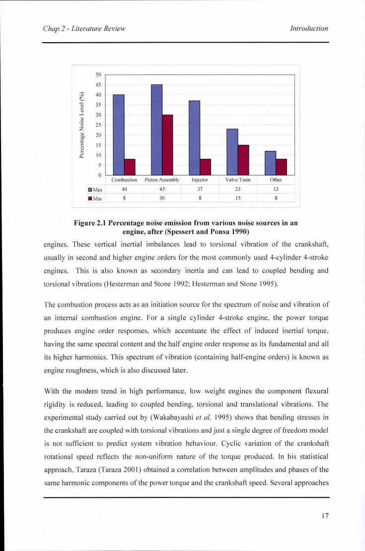
Chap 2 - Literature Review
50
45
~ ~
40
U >
35
" ...J 30 " ~ '0 z 25
" 20 en -'" 5 15 ~
" 10 0-
5
0 Combustion
ClI Max 40
_ Min 8
Piston Asse mbly Injector
45 37
)0 8
Valve T rain
2)
15
Other
12
8
Introduction
Figure 2.1 Percentage noise emission from various noise sources in an engine, after (S pessert and Ponsa 1990)
engines. These vert ica l inert ial imba lances lead to torsional vibration of the crankshaft,
usua lly in second and higher engine orders for the most commonly used 4-cylinder 4-stroke
engines. This is also known as secondary inert ia and can lead to coupled bending and
torsional vibrations (Hesterman and Stone 1992; Heste rm an and Stone 1995).
The combustion process acts as an initiation source for the spectrum of noise and vibration of
an internal combustion engine. For a single cylinder 4-stroke engine, the power torque
produces engine order responses, which accentuate the effect of induced inel1 ial torque,
having the same spectral content and the half engine order response as its fundamenta l and all
its higher harmonics. This spectrum of vibrat ion (containing half-engi ne orders) is known as
engine roughness, which is also di scussed later.
With the modern trend in high performance, low we ight engines the component fl exural
rigidity is reduced, lead ing to coup led bend ing, torsional and trans lational vibrations. The
experimenta l study carried out by (Wakabayashi et ai, 1995) shows that bending stresses in
the crankshaft are coupled with torsional vibrations and just a single degree of freedom model
is not sufficient to predict system vibration behaviour. Cyclic variation of the crankshaft
rotat ional speed reflects the non-uniform nature of the torque produced. In his stati stical
approach, Taraza (Taraza 200 I) obtained a corre lation between amplitudes and phases of the
same harmonic components of the power torque and the crankshaft speed. Severa l approaches
17
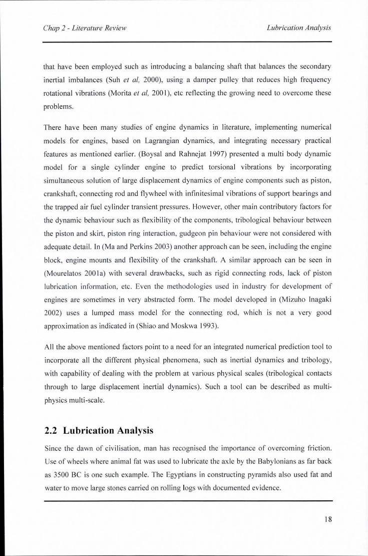
Chap 2 - LileralUl'e Review Lubricalion Analysis
that have been employed such as introducing a ba lancing shaft that ba lances the secondary
inertia l imba lances (Suh el 01, 2000), us ing a damper pulley that reduces hi gh frequency
rotat iona l vibrations (Morita el 01, 200 I), etc reflecting the g rowing need to overcome these
prob lems.
There have been many stud ies of engine dynam ics in literature, implementi ng numerica l
models for eng ines, based on Lagrangian d ynamics, and integrating necessa ry practica l
featu res as mentioned earl ier. (Boysal and Ra hnejat 1997) prese nted a mul ti body dynam ic
model for a s ingle cy linder engine to predict torsiona l v ibrat ions by incorporating
simultaneo us so lution of large d isplacement dynam ics of eng ine components such as pi ston,
crankshaft, connecting rod and fl ywheel with infinitesimal vibrations of support beari ngs and
the trapped air fuel cyl inder transient pressures. However, oth er ma in contributory factors for
the dynamic behav io ur such as flexibi lity of the components, tr ibologica l behav iour between
the pi ston and skirt, pi ston ring interaction, gudgeon pin behaviour were not considered with
adequate detail. In (Ma and Perkins 2003) another approach can be seen, includ ing the engine
block, eng ine mounts and fl exi bi li ty o f the c rankshaft. A simi la r approach can be seen in
(MoUl·e latos 200 I a) wi th severa l drawbacks, such as rig id connecting rods, lack of piston
lubrication in formation, etc. Even the methodologies used in industry for development of
engines are sometimes in very abstracted form . The model deve loped in (M izuho Inagaki
2002) uses a lumped mass model for the connect ing rod, which is not a ve ry good
approx imatio n as ind icated in (Shiao and Moskwa 1993) .
All the above mentio ned factors point to a need for an integrated numerical pred iction tool to
incorporate a ll the d ifferent ph ys ica l phenomena, such as inertia l dynam ics and tribo logy,
with capabi lity of dea ling with the problem at va rious phys ica l sca les (t ri bo logica l contacts
through to large displacement ineltial dynam ics) . Such a tool can be described as mu lti
physics multi -scale.
2.2 Lubrication Analysis
Since the dawn of civ ilisation, man has recogni sed the impo rtance of ove rcom ing friction.
Use o f whee ls where an ima l fat was used to lubricate the ax le by the Babylonians as far back
as 3500 BC is one such examp le. The Egyptians in constructing pyramids a lso used fat and
water to move la rge stones carried on rolling logs with documented ev idence.
18
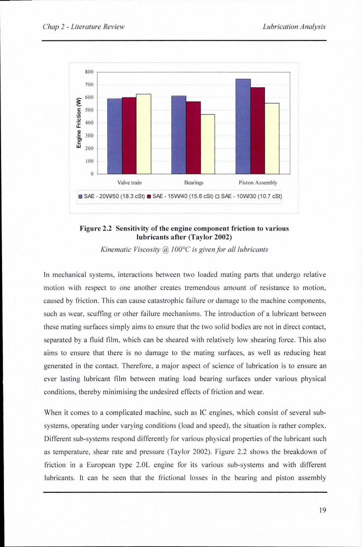
Chap 2 - Lileralllre Review LlIbricalion Analysis
800 r--------------------------------------------, 700
~ 600
c 500 .12 .~ 400 "-
" .!; 300 Cl c: w 200
100
o Valve train Bearing') Piston Assembly
11 SAE - 20W/50 (18.3 eSt) 11 SAE -15W/40 (15.6 eSt) 0 SAE -10W/30 (10.7 eSt)
Figure 2.2 Sensitivity of the engine component friction to various lubricants after (Taylor 2002)
Kinemalic Viscosily @ !OO°C i ' given/or alllllbricanls
In mechanical systems, interactions between two loaded mating parts that undergo relative
motion with respect to one another creates tremendous amount of resistance to motion,
caused by fri cti on. This can cause catastrophic fai lure or damage to the machine components,
such as wear, scuffing or other fa ilure mechanisms. The introduction of a lubricant between
these mating surfaces sim ply aims to ensure that the two so li d bodies are not in direct contact,
separated by a nuid film , which can be sheared with relative ly low shearing force. This also
aims to ensure that there is no damage to the mating surfaces, as we ll as reducing heat
generated in the contact. Therefore, a major aspect of sc ience of lubrication is to ensure an
ever lasting lubricant film between mating load bea ring surfaces under various physical
conditions, thereby minimising the undesired effects of friction and wear.
When it comes to a complicated machine, such as le engines, which consist of severa l sub
systems, operating under vary ing conditions (load and speed), the situat ion is rather complex.
Different sub-systems respond differently fo r various ph ysical properties or the lubricant such
as temperature, shear rate and pressure (Taylor 2002). Figure 2.2 shows the breakdown of
fricti on in a European type 2.0L engine for its various sub-systems and with different
lubricants. It can be seen that the frictional losses in the bearing and piston assembly
19
Chap 2 - Literature Review Lubrication Analysis
decrease, while the viscosity is increased, whereas the friction increases in the valve train
assembly. This is the case for piston as the proportion of viscous to boundary contribution
becomes more significant with increased viscosity, at least as one effect. Already some
research on the total engine frictional losses have been carried out, but more details have to
be made clearer. Furthermore, the effects of lubricant viscosity on friction and wear of an
engine with specific lubricated contacts have not been clearly understood. Thus, it is very
complex to determine an optimised viscosity value. In fact reducing oil viscosity not only
deteriorates the reliability of engine parts, but also can increase friction in some other
conjunctions. Therefore, it is necessary to understand quantitatively the effects of different
lubricant properties on different lubricated conjunctions under real varying operating
conditions.
2.2.1 Principle of Lubrication
When one surface moves relative to a counter-face, the lubricant is dragged into the contact
conjunction (Cameron 1966). As the passage converges and the lubricant volume entering
into the contact remains constant, the almost incompressible fluid generates pressure to make
its path through the conjunction. This pressure force moves the two surfaces apart, preventing
a solid-to-solid contact. Even though many attempts reported in the literature about the use of
animal fat as an agent of reducing friction force, a proper study about lubrication from an
engineering science standpoint commenced in the 1850's with the studies carried out by Von
Pauli in 1849 and Him in 1854 as reported in (Rahnejat 1984). They studied lubricated shafts
and bearings operating under fully hydrodynamic conditions. (Petroff 1883) analysed Him's
work in some detail in 1883. Petroffwas studying the variation offrictional characteristics in
a journal bearing with different types of oil, assuming that the lubricant was sheared between
the shaft and the bearing. Tower (Tower 1883) showed that there were considerable pressures
generated in rolling element bearings under fully hydrodynamic contact conditions. During
this period (Reynolds 1886) showed, using an analytical model, that a converging wedge
shaped film generated an oil pressure distribution based on the Newton's model for slow
viscous action and the well known Navier's - Stokes equation. All the subsequent lubrication
investigations by many authors are founded on the fundamental work ofReynolds.
In recent years it has been recognized that the lubricated contacts with low geometrical
conformity such as gears, cams, rolling element bearings behave rather differently to the
20
Chap 2 - Literature Review Lubrication Analysis
classical hydrodynamic lubrication (Dowson and Higginson 1977). High pressures generated
within this type of contact affect the viscosity of the lubricant dramatically as shown by Barus
and Roelands (Gohar 1988) and the lubricant becomes semi-amorphous. Furthermore, the
application of high contact loads and the change in viscosity can lead to substantial local
deformation of elastic solids. In contrast this local deformation changes the shape of the fluid
film and concurrently the pressure distribution in the contact. Ultimately, the metal to metal
contact is prevented. The formation of lubrication film due to such action is known as
elastohydrodynamic lubrication (EHL).
Only in the past 3 decades a complete theoretical solution for an isothermal EHL of point
contacts has successfully been analyzed, using simultaneous solution of the elasticity and
Reynolds equation. In (Hamrock and Dowson 1976) the conjunction is divided into equal
rectangular areas with a uniform pressure element over each area and pressure at each grid
point is calculated using Reynolds' equation. Again (Hamrock and Dowson 1 977a) presented
a similar approach for a point contact under fully flooded condition. A fully flooded condition
is said to exist, when the inlet distance of the conjunction ceases to influence in any
significant way the minimum film thickness. The inlet distance of the conjunction is defined
as the distance from the centre of the contact to the edge of the computing area. In (Hamrock
and Jacobson 1983) a procedure for the numerical solution of the complete isothermal EHL
for a line contact is presented, assuming that there is no side leakage. This analysis may thus
be used as the foundation for more complicated analysis, incorporating surface roughness,
non-Newtonian effects, and temperature effects (Balakrishnan and Rahnejat 2005;
Dursunkaya et aI, 1994; Keribar and Dursunkaya 1992; Mihailidis et aI, 1999; Priest et aI,
2000). Furthermore, Hamrock has formulated a relationship between minimum film thickness
and physical properties such as contact load, sliding speed and material parameters. Such
relationships are obtained by regression of numerical predictions over a range of these
parameters or by experimentation under similar conditions. These relationships are referred to
as extrapolated oil film thickness formulae. It is found that the sliding velocity is the most
influential parameter on the minimum film thickness.
It was not until the late 1960s and early 1970s that the influence of lubricant starvation upon
elastohydrodynamic behaviour received serious consideration (Chevalier et aI, 1996; Messe
and Lubrecht 2000), which can influence the minimum film thickness by deviating from fully
flooded condition. Prior to this time it was assumed that the inlets were fully flooded.
21
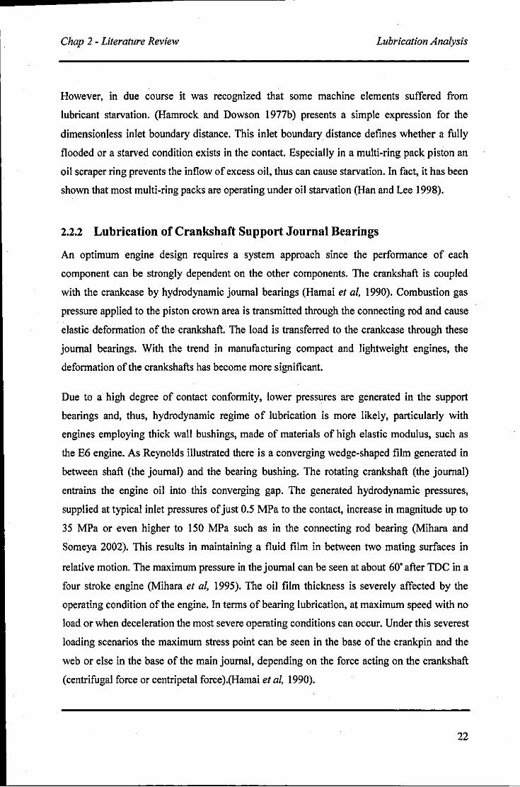
Chap 2 - Literature Review Lubrication Analysis
However, in due course it was recognized that some machine elements suffered from
lubricant starvation. (Hamrock and Dowson 1977b) presents a simple expression for the
dimension less inlet boundary distance. This inlet boundary distance defines whether a fully
flooded or a starved condition exists in the contact. Especially in a multi-ring pack piston an
oil scraper ring prevents the inflow of excess oil, thus can cause starvation. In fact, it has been
shown that most multi-ring packs are operating under oil starvation (Han and Lee 1998).
2.2.2 Lubrication of Crankshaft Support Journal Bearings
An optimum engine design requires a system approach since the performance of each
component can be strongly dependent on the other components. The crankshaft is coupled
with the crankcase by hydrodynamic journal bearings (Hamai et ai, 1990). Combustion gas
pressure applied to the piston crown area is transmitted through the connecting rod and cause
elastic deformation of the crankshaft. The load is transferred to the crankcase through these
journal bearings. With the trend in manufacturing compact and lightweight engines, the
deformation of the crankshafts has become more significant.
Due to a high degree of contact conformity, lower pressures are generated in the support
bearings and, thus, hydrodynamic regime of lubrication is more likely, particularly with
engines employing thick wall bushings, made of materials of high elastic modulus, such as
the E6 engine. As Reynolds illustrated there is a converging wedge-shaped film generated in
between shaft (the journal) and the bearing bushing. The rotating crankshaft (the journal)
entrains the engine oil into this converging gap. The generated hydrodynamic pressures,
supplied at typical inlet pressures of just 0.5 MPa to the contact, increase in magnitude up to
35 MPa or even higher to 150 MPa such as in the connecting rod bearing (Mihara and
Someya 2002). This results in maintaining a fluid film in between two mating surfaces in
relative motion. The maximum pressure in the journal can be seen at about 60' after TDC in a
four stroke engine (Mihara et ai, 1995). The oil film thickness is severely affected by the
operating condition of the engine. In terms of bearing lubrication, at maximum speed with no
load or when deceleration the most severe operating conditions can occur. Under this severest
loading scenarios the maximum stress point can be seen in the base of the crankpin and the
web or else in the base of the main journal, depending on the force acting on the crankshaft
(centrifugal force or centripetal force).(Hamai et ai, 1990).
22
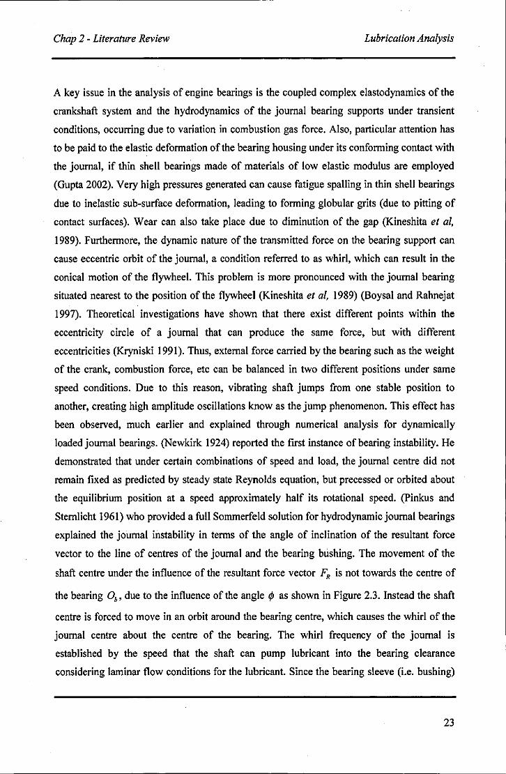
Chap 2 - Literature Review Lubrication Analysis
A key issue in the analysis of engine bearings is the coupled complex elastodynamics of the
crankshaft system and the hydrodynamics of the journal bearing supports under transient
conditions, occurring due to variation in combustion gas force. Also, particular attention has
to be paid to the elastic deformation of the bearing housing under its conforming contact with
the journal, if thin shell bearings made of materials of low elastic modulus are employed
(Gupta 2002). Very high pressures generated can cause fatigue spalling in thin shell bearings
due to inelastic sub-surface deformation, leading to forming globular grits (due to pitting of
contact surfaces). Wear can also take place due to diminution of the gap (Kineshita et ai,
1989). Furthermore, the dynamic nature of the transmitted force on the bearing support can
cause eccentric orbit of the journal, a condition referred to as whirl, which can result in the
conical motion of the flywheel. This problem is more pronounced with the journal bearing
situated nearest to the position of the flywheel (Kineshita et ai, 1989) (Boysal and Rahnejat
1997). Theoretical investigations have shown that there exist different points within the
eccentricity circle of a journal that can produce the same force, but with different
eccentricities (Kryniski 1991). Thus, external force carried by the bearing such as the weight
of the crank, combustion force, etc can be balanced in two different positions under same
speed conditions. Due to this reason, vibrating shaft jumps from one stable position to
another, creating high amplitude oscillations know as the jump phenomenon. This effect has
been observed, much earlier and explained through numerical analysis for dynamically
loadedjoumal bearings. (Newkirk 1924) reported the first instance of bearing instability. He
demonstrated that under certain combinations of speed and load, the journal centre did not
remain fixed as predicted by steady state Reynolds equation, but precessed or orbited about
the equilibrium position at a speed approximately half its rotational speed. (pinkus and
Sternlicht 1961) who provided a full Sommerfeld solution for hydrodynamic journal bearings
explained the journal instability in terms of the angle of inclination of the resultant force
vector to the line of centres of the journal and the bearing bushing. The movement of the
shaft centre under the influence of the resultant force vector FR is not towards the centre of
the bearing 0., due to the influence of the angle I/> as shown in Figure 2.3. Instead the shaft
centre is forced to move in an orbit around the bearing centre, which causes the whirl of the
journal centre about the centre of the bearing. The whirl frequency of the journal is
established by the speed that the shaft can pump lubricant into the bearing clearance
considering laminar flow conditions for the lubricant. Since the bearing sleeve (Le. bushing)
23
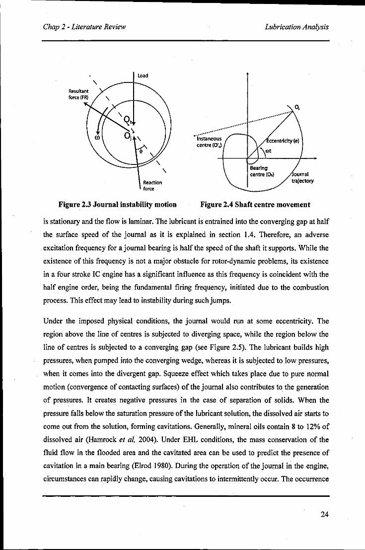
Chap 2 - Literature Review
\ Resultant force (FR) \
Load
Reaction force
Figure 2.3 Journal instability motion
Lubrication Analysis
··I~;~~:~:·············· ~ .. -................... .
centre (O'J
Figure 2.4 Shaft centre movement
is stationary and the flow is laminar, The lubricant is entrained into the converging gap at half
the surface speed of the journal as it is explained in section lA, Therefore, an adverse
excitation frequency for a journal bearing is half the speed of the shaft it supports, While the
existence of this frequency is not a major obstacle for rotor-dynamic problems, its existence
in a four stroke le engine has a significant influence as this frequency is coincident with the
half engine order, being the fundamental firing frequency, initiated due to the combustion
process, This effect may lead to instability during such jumps,
Under the imposed physical conditions, the journal would run at some eccentricity, The
region above the line of centres is subjected to diverging space, while the region below the
line of centres is subjected to a converging gap (see Figure 2,5). The lubricant builds high
pressures, when pumped into the converging wedge, whereas it is subjected to low pressures,
when it comes into the divergent gap. Squeeze effect which takes place due to pure normal
motion (convergence of contacting surfaces) of the journal also contributes to the generation
of pressures. It creates negative pressures in the case of separation of solids. When the
pressure falls below the saturation pressure of the lubricant solution, the dissolved air starts to
come out from the solution, forming cavitations. Generally, mineral oils contain 8 to 12% of
dissolved air (Hamrock et aI, 2004). Under EHL conditions, the mass conservation of the
fluid flow in the flooded area and the cavitated area can be used to predict the presence of
cavitation in a main bearing (Elrod 1980). During the operation of the journal in the engine,
circumstances can rapidly change, causing cavitations to intermittently occur. The occurrence
24
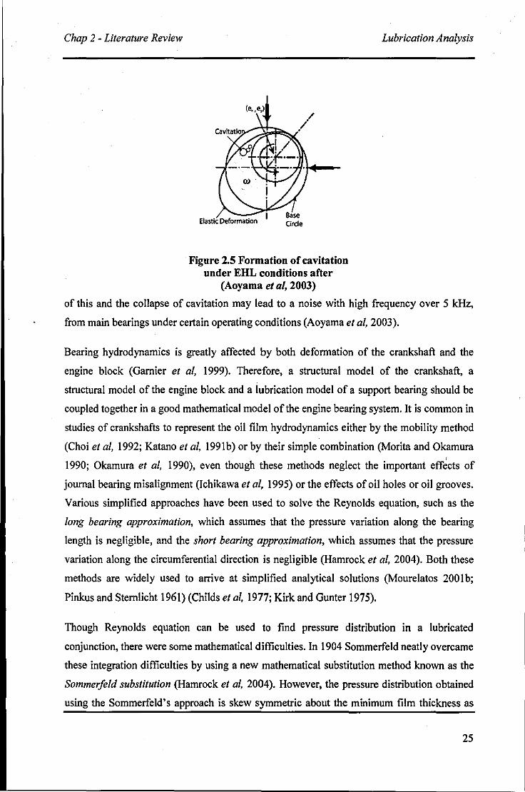
Chap 2 - Literature Review
(e.,e,)
Elastic Deformation
Figure 2.5 Formation of cavitation under EHL conditions after
(Aoyama et ai, 2003)
Lubrication Analysis
of this and the collapse of cavitation may lead to a noise with high frequency over 5 kHz,
from main bearings under certain operating conditions (Aoyama et ai, 2003).
Bearing hydrodynamics is greatly affected by both deformation of the crankshaft and the
engine block (Gamier et ai, 1999). Therefore, a structural model of the crankshaft, a
structural model of the engine block and a lubrication model of a support bearing should be
coupled together in a good mathematical model of the engine bearing system. It is common in
studies of crankshafts to represent the oil film hydrodynamics either by the mobility method
(Choi et ai, 1992; Katano et ai, 1991b) or by their simple combination (Morita and Okamura ,
1990; Okamura et ai, 1990), even though these methods neglect the important effects of
journal bearing misalignment (Ichikawa et ai, 1995) or the effects of oil holes or oil grooves.
Various simplified approaches have been used to solve the Reynolds equation, such as the
long bearing approximation, which assumes that the pressure variation along the bearing
length is negligible, and the short bearing approximation, which assumes that the pressure
variation along the circumferential direction is negligible (Hamrock et ai, 2004). Both these
methods are widely used to arrive at simplified analytical solutions (Mourelatos 2001b;
Pinkus and Stemlicht I 961)(Childs et ai, 1977; Kirk and Gunter 1975).
Though Reynolds equation can be used to find pressure distribution in a lubricated
conjunction, there were some mathematical difficulties. In 1904 Sommerfeld neatly overcame
these integration difficulties by using a new mathematical substitution method known as the
Sommerfeld substitution (Hamrock et ai, 2004). However, the pressure distribution obtained
using the Sommerfeld's approach is skew symmetric about the minimum film thickness as
25
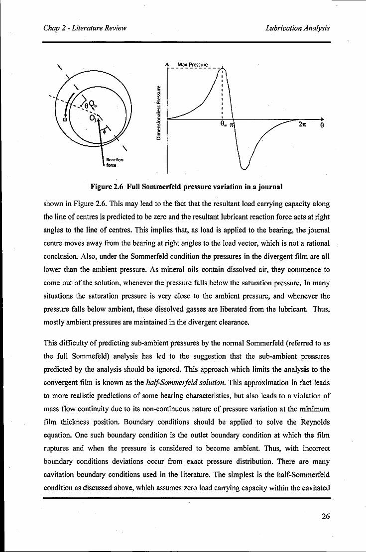
Chap 2 - Literature Review
Reaction force
Max. Pressure
Lubrication Analysis
9m It 9
Figure 2.6 Full Sommerfeld pressure variation in a journal
shown in Figure 2.6. This may lead to the fact that the resultant load carrying capacity along
the line of centres is predicted to be zero and the resultant lubricant reaction force acts at right
angles to the line of centres. This implies that, as load is applied to the bearing, the journal
centre moves away from the bearing at right angles to the load vector, which is not a rational
conclusion. Also, under the Sommerfeld condition the pressures in the divergent film are all
lower than the ambient pressure. As mineral oils contain dissolved air, they commence to
come out of the solution, whenever the pressure falls below the saturation pressure. In many
situations the saturation pressure is very close to the ambient pressure, and whenever the
pressure falls below ambient, these dissolved gasses are liberated from the lubricant. Thus,
mostly ambient pressures are maintained in the divergent clearance.
This difficulty of predicting sub-ambient pressures by the normal Sommerfeld (referred to as
the full Sommefeld) analysis has led to the suggestion that the sub-ambient pressures
predicted by the analysis should be ignored. This approach which limits the analysis to the
convergent film is known as the half-Sommerfold solution. This approximation in fact leads
to more realistic predictions of some bearing characteristics, but also leads to a violation of
mass flow continuity due to its non-continuous nature of pressure variation at the minimum
film thickness position. Boundary conditions should be applied to solve the Reynolds
equation. One such boundary condition is the outlet boundary condition at which the film
ruptures and when the pressure is considered to become ambient. Thus, with incorrect
boundary conditions deviations occur from exact pressure distribution. There are many
cavitation boundary conditions used in the literature. The simplest is the half-Sommerfeld
condition as discussed above, which assumes zero load carrying capacity within the cavitated
26
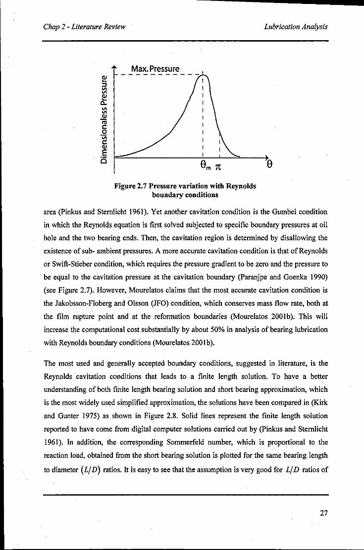
Chap 2 - Literature Review
!!! ::I ~ !!!
0... VI VI Q)
ca c o 'iij c Q)
E 15
Max. Pressure
Figure 2.7 Pressure variation with Reynolds boundary conditions
Lubrication Analysis
e
area (Pinkus and Stemlicht 1961 ). Yet another cavitation condition is the Gumbel condition
in which the Reynolds equation is first solved subjected to specific boundary pressures at oil
hole and the two bearing ends. Then, the cavitation region is determined by disallowing the
existence of sub- ambient pressures. A more accurate cavitation condition is that of Reynolds
or Swift-Stieber condition, which requires the pressure gradient to be zero and the pressure to
be equal to the cavitation pressure at the cavitation boundary (Paranjpe and Goenka 1990)
(see Figure 2.7). However, Mourelatos claims that the most accurate cavitation condition is
the Jakobsson-Floberg and Olsson (JFO) condition, which conserves mass flow rate, both at
the film rupture point and at the reformation boundaries (Mourelatos 2001 b). This will
increase the computational cost substantially by about 50% in analysis of bearing lubrication
with Reynolds boundary conditions (Mourelatos 2001 b).
The most used and generally accepted boundary conditions, suggested in literature, is the
Reynolds cavitation conditions that leads to a finite length solution. To have a better
understanding of both finite length bearing solution and short bearing approximation, which
is the most widely used simplified approximation, the solutions have been compared in (Kirk
and Gunter 1975) as shown in Figure 2.8. Solid lines represent the finite length solution
reported to have come from digital computer solutions carried out by (Pinkus and Stemlicht
1961). In addition, the corresponding Sommerfeld number, which is proportional to the
reaction load, obtained from the short bearing solution is plotted for the same bearing length
to diameter (Lf D) ratios. It is easy to see that the assumption is very good for Lf D ratios of
27
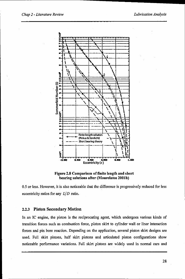
Chap 2 - Literature Review
o -.8
E
" z .., ~ .. E
~
• i • • .. • .. " .. .. • i • • .. • .. " .. N
t. i • • .. • .. " .. .. ~
\ ~ " I Ir '\. \
' .~ '\. ~~ , ~ \. \ \~ " '\ ~ ~-
• _ A\ -\---.'\. -,,1- '1I.
'\ "" --.-~~ ~\ " '" -- --- --N
~~ \ ! ~ \ I ~
~~ -1--r-1-.----:
f:=~~ .. - I--- -1---- f------ , . \ -- ------ ~-\ ---- , \
!\ \ Anite length solution -\ l\~' \ • • (Pinku. & Stmlicht)
- - - - Short bearing theory \ \ \1, .---1-------
'- \' I
\ \ ~~ 0.211 0.'I0Il 0.Il00 0.l1li I.DID
Eccentricity (t:)
Figure 2.8 Comparison of finite length and short bearing solutions after (Mourelatos 2001b)
Lubrication Analysis
0.5 or less. However, it is also noticeable that the difference is progressively reduced for less
eccentricity ratios for any L/ D ratio.
2.2.3 Piston Secondary Motion
In an le engine, the piston is the reciprocating agent, which undergoes various kinds of
transition forces such as combustion force, piston skirt to cylinder wall or liner interaction
forces and pin bore reaction. Depending on the application, several piston skirt designs are
used. Full skirt pistons, half skirt pistons and articulated piston configurations show
noticeable performance variations. Full skirt pistons are widely used in normal cars and
28
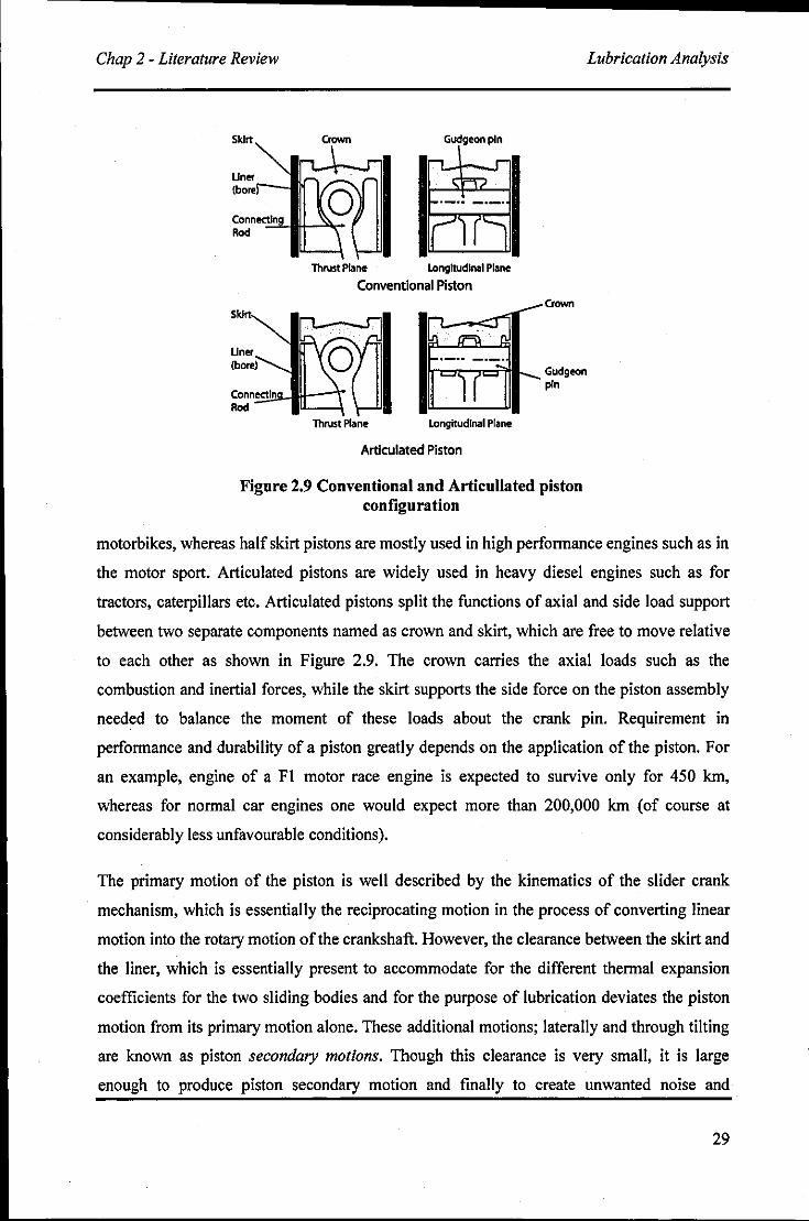
Chap 2 - Literature Review
Skirt
Un .. (bore,r--.lIN
Gudgeon pin
Connectl""""'-III+-....>o\,c> Rod
Skirt
Uner (bore)
Connectln Rod
Thrust Plane longitudinal Plane
Conventional Piston
Thrust Plane longitudinal Plane
Articulated Piston
Crown
Gudgeon pin
Figure 2.9 Conventional and Articullated piston configuration
Lubrication Analysis
motorbikes, whereas half skirt pistons are mostly used in high performance engines such as in
the motor sport. Articulated pistons are widely used in heavy diesel engines such as for
tractors, caterpillars etc. Articulated pistons split the functions of axial and side load support
between two separate components named as crown and skirt, which are free to move relative
to each other as shown in Figure 2.9. The crown carries the axial loads such as the
combustion and inertial forces, while the skirt supports the side force on the piston assembly
needed to balance the moment of these loads about the crank pin. Requirement in
performance and durability of a piston greatly depends on the application of the piston. For
an example, engine of a FI motor race engine is expected to survive only for 450 km,
whereas for normal car engines one would expect more than 200,000 km (of course at
considerably less unfavourable conditions).
The primary motion of the piston is well described by the kinematics of the slider crank
mechanism, which is essentially the reciprocating motion in the process of converting linear
motion into the rotary motion of the crankshaft. However, the clearance between the skirt and
the liner, which is essentially present to accommodate for the different thermal expansion
coefficients for the two sliding bodies and for the purpose of lubrication deviates the piston
motion from its primary motion alone. These additional motions; laterally and through tilting
are known as piston secondary motions. Though this clearance is very small, it is large
enough to produce piston secondary motion and finally to create unwanted noise and
29
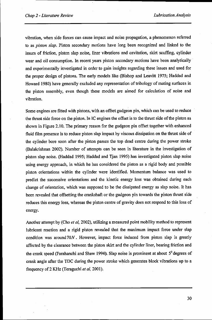
Chap 2 - Literature Review Lubrication Analysis
vibration, when side forces can cause impact and noise propagation, a phenomenon referred
to as piston slap. Piston secondary motions have long been recognized and linked to the
issues of friction, piston slap noise, liner vibrations and cavitation, skirt scuffing, cylinder
wear and oil consumption. In recent years piston secondary motions have been analytically
and experimentally investigated in order to gain insights regarding these issues and used for
the proper design of pistons. The early models like (Bishop and Leavitt 1975; Haddad and
Howard 1980) have generally excluded any representation of tribology of mating surfaces in
the piston assembly, even though these models are aimed for calculation of noise and
vibration.
Some engines are fitted with pistons, with an offset gudgeon pin, which can be used to reduce
the thrust side force on the piston. In IC engines the offset is to the thrust side of the piston as
shown in Figure 2.10. The primary reason for the gudgeon pin offset together with enhanced
fluid film presence is to reduce piston slap impact by viscous dissipation on the thrust side of
the cylinder bore soon after the piston passes the top dead centre during the power stroke
(Balakrishnan 2002). Number of attempts can be seen in literature in the investigation of
piston slap noise. (Haddad 1995; Haddad and Tjan 1995) has investigated piston slap noise
using energy approach, in which he has considered the piston as a rigid body and possible
piston orientations within the cylinder were identified. Momentum balance was used to
predict the successive orientations and the kinetic energy loss was obtained during each
change of orientation, which was supposed to be the dissipated energy as slap noise. It has
been revealed that offsetting the crankshaft or the gudgeon pin towards the piston thrust side
reduces this energy loss, whereas the piston centre of gravity does not respond to this loss of
energy.
Another attempt by (Cho et ai, 2002), utilizing a measured point mobility method to represent
lubricant reaction and a rigid piston revealed that the maximum impact force under slap
condition was around 70N. However, impact force induced from piston slap is greatly
affected by the clearance between the piston skirt and the cylinder liner, bearing friction and
the crank speed (Farahanchi and Shaw 1994). Slap noise is prominent at about 50 degrees of
crank angle after the TDC during the power stroke which generates block vibrations up to a
frequency of 2 KHz (Teraguchi et ai, 2001).
30
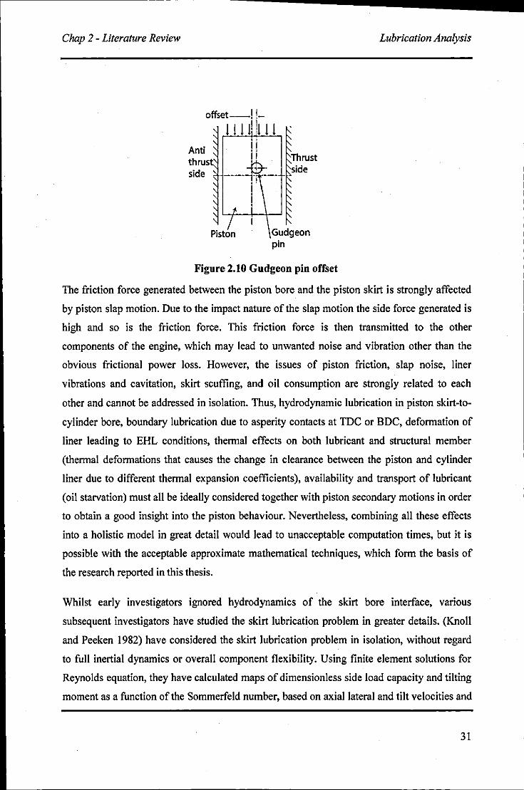
Chap 2 - Literature Review
offset--! !-
I I I I!!I I I Anti thrus side side
Gudgeon pin
Figure 2.10 Gudgeon pin offset
Lubrication Analysis
The friction force generated between the piston bore and the piston skirt is strongly affected
by piston slap motion. Oue to the impact nature of the slap motion the side force generated is
high and so is the friction force. This friction force is then transmitted to the other
components of the engine, which may lead to unwanted noise and vibration other than the
obvious frictional power loss. However, the issues of piston friction, slap noise, liner
vibrations and cavitation, skirt scuffing, and oil consumption are strongly related to each
other and cannot be addressed in isolation. Thus, hydrodynamic lubrication in piston skirt-to
cylinder bore, boundary lubrication due to asperity contacts at TOC or BOC, deformation of
liner leading to EHL conditions, thermal effects on both lubricant and structural member
(thermal deformations that causes the change in clearance between the piston and cylinder
liner due to different thermal expansion coefficients), availability and transport of lubricant
(oil starvation) must all be ideally considered together with piston secondary motions in order
to obtain a good insight into the piston behaviour. Nevertheless, combining all these effects
into a holistic model in great detail would lead to unacceptable computation times, but it is
possible with the acceptable approximate mathematical techniques, which form the basis of
the research reported in this thesis.
Whilst early investigators ignored hydrodynamics of the skirt bore interface, various
subsequent investigators have studied the skirt lubrication problem in greater details. (Knoll
and Peeken 1982) have considered the skirt lubrication problem in isolation, without regard
to full inertial dynamics or overall component flexibility. Using finite element solutions for
Reynolds equation, they have calculated maps of dimensionless side load capacity and tilting
moment as a function of the Sommerfeld number, based on axial lateral and tilt velocities and
31
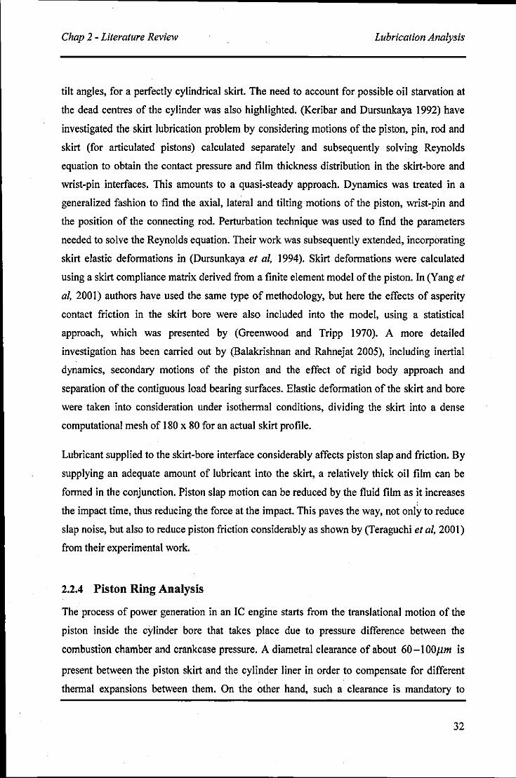
Chap 2 - Literature Review Lubrication Analysis
tilt angles, for a perfectly cylindrical skirt. The need to account for possible oil starvation at
the dead centres of the cylinder was also highlighted. (Keribar and Dursunkaya 1992) have
investigated the skirt lubrication problem by considering motions of the piston, pin, rod and
skirt (for articulated pistons) calculated separately and subsequently solving Reynolds
equation to obtain the contact pressure and film thickness distribution in the skirt-bore and
wrist-pin interfaces. This amounts to a quasi-steady approach. Dynamics was treated in a
generalized fashion to find the axial, lateral and tilting motions of the piston, wrist-pin and
the position of the connecting rod. Perturbation technique was used to find the parameters
needed to solve the Reynolds equation. Their work was subsequently extended, incorporating
skirt elastic deformations in (Dursunkaya et aI, 1994). Skirt deformations were calculated
using a skirt compliance matrix derived from a finite element model of the piston. In (Yang et
aI, 2001) authors have used the same type of methodology, but here the effects of asperity
contact friction in the skirt bore were also included into the model, using a statistical
approach, which was presented by (Greenwood and Tripp 1970). A more detailed
investigation has been carried out by (Balakrishnan and Rahnejat 2005), including inertial
dynamics, secondary motions of the piston and the effect of rigid body approach and
separation of the contiguous load bearing surfaces. Elastic deformation of the skirt and bore
were taken into consideration under isothermal conditions, dividing the skirt into a dense
computational mesh of 180 x 80 for an actual skirt profile.
Lubricant supplied to the skirt-bore interface considerably affects piston slap and friction. By
supplying an adequate amount of lubricant into the skirt, a relatively thick oil film can be
formed in the conjunction. Piston slap motion can be reduced by the fluid film as it increases l
the impact time, thus reducing the force at the impact. This paves the way, not only to reduce
slap noise, but also to reduce piston friction considerably as shown by (Teraguchi et aI, 2001)
from their experimental work.
2.2.4 Piston Ring Analysis
The process of power generation in an le engine starts from the translational motion of the
piston inside the cylinder bore that takes place due to pressure difference between the
combustion chamber and crankcase pressure. A diametral clearance of about 60 - I OOpm is
present between the piston skirt and the cylinder liner in order to compensate for different
thermal expansions between them. On the other hand, such a clearance is mandatory to
32
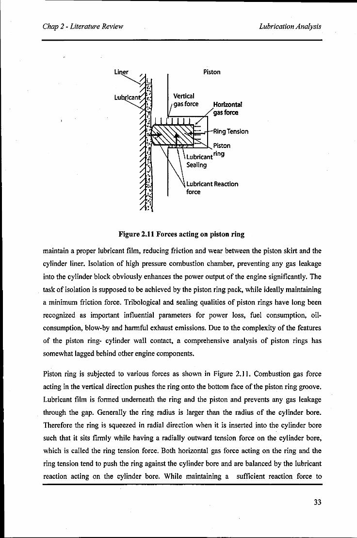
Chap 2 - Literature Review
Lu Vertical gas force
Piston
Horizontal gas force
~-#~'IRingTension
~~~~d:::::::~Piston
Figure 2.11 Forces acting on piston ring
Lubrication Analysis
maintain a proper lubricant film, reducing friction and wear between the piston skirt and the
cylinder liner. Isolation of high pressure combustion chamber, preventing any gas leakage
into the cylinder block obviously enhances the power output of the engine significantly. The
task of isolation is supposed to be achieved by the piston ring pack, while ideally maintaining
a minimum friction force. Tribological and sealing qualities of piston rings have long been
recognized as important influential parameters for power loss, fuel consumption, oil
consumption, blow-by and harmful exhaust emissions. Due to the complexity of the features
of the piston ring- cylinder wall contact, a comprehensive analysis of piston rings has
somewhat lagged behind other engine components.
Piston ring is subjected to various forces as shown in Figure 2.11. Combustion gas force
acting in the vertical direction pushes the ring onto the bottom face of the piston ring groove.
Lubricant film is formed underneath the ring and the piston and prevents any gas leakage
through the gap. Generally the ring radius is larger than the radius of the cylinder bore.
Therefore the ring is squeezed in radial direction when it is inserted into the cylinder bore
such that it sits firmly while having a radially outward tension force on the cylinder bore,
which is called the ring tension force. Both horizontal gas force acting on the ring and the
ring tension tend to push the ring against the cylinder bore and are balanced by the lubricant
reaction acting on the cylinder bore. While maintaining a sufficient reaction force to
33
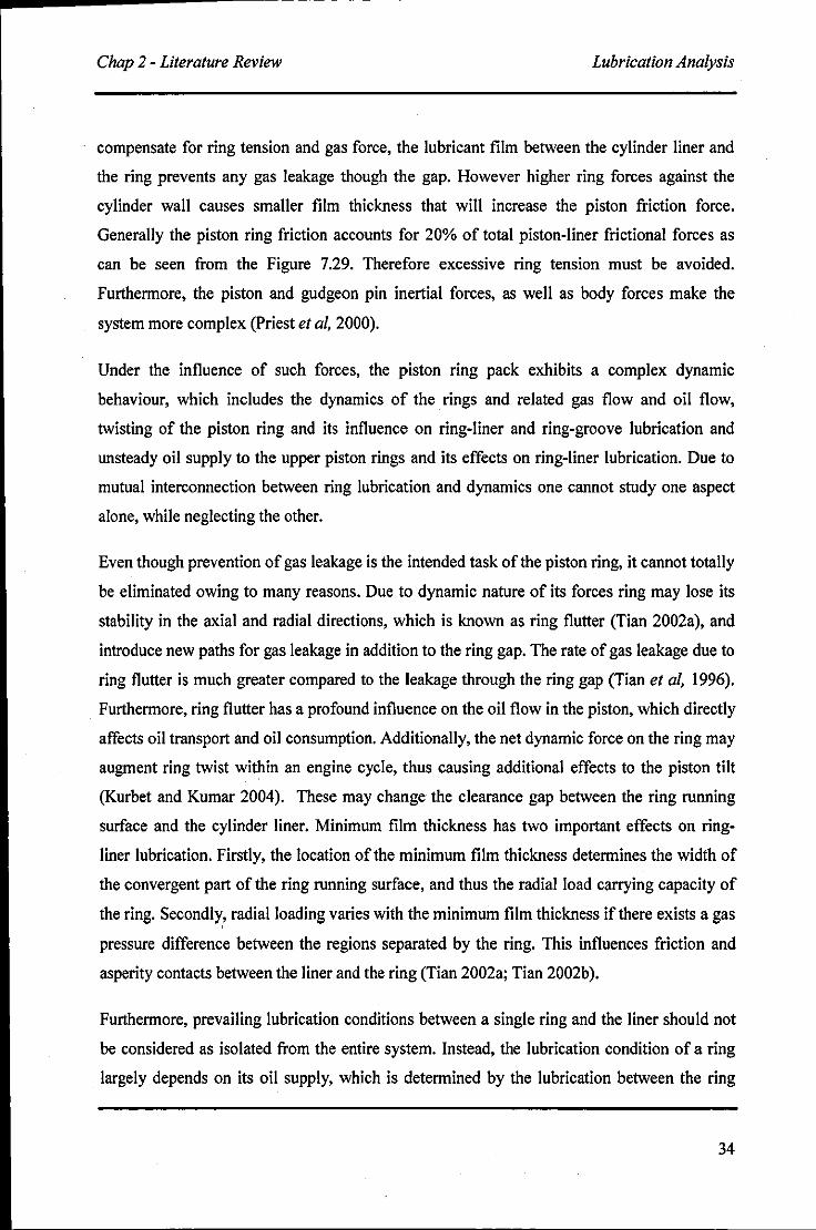
Chap 2 - Literature Review Lubrication Analysis
compensate for ring tension and gas force, the lubricant film between the cylinder liner and
the ring prevents any gas leakage though the gap. However higher ring forces against the
cylinder wall causes smaller film thickness that will increase the piston friction force.
Generally the piston ring friction accounts for 20% of total piston-liner frictional forces as
can be seen from the Figure 7.29. Therefore excessive ring tension must be avoided.
Furthermore, the piston and gudgeon pin inertial forces, as well as body forces make the
system more complex (Priest et ai, 2000).
Under the influence of such forces, the piston ring pack exhibits a complex dynamic
behaviour, which includes the dynamics of the rings and related gas flow and oil flow,
twisting of the piston ring and its influence on ring-liner and ring-groove lubrication and
unsteady oil supply to the upper piston rings and its effects on ring-liner lubrication. Due to
mutual interconnection between ring lubrication and dynamics one cannot study one aspect
alone, while neglecting the other.
Even though prevention of gas leakage is the intended task of the piston ring, it cannot totally
be eliminated owing to many reasons. Due to dynamic nature of its forces ring may lose its
stability in the axial and radial directions, which is known as ring flutter (Tian 2002a), and
introduce new paths for gas leakage in addition to the ring gap. The rate of gas leakage due to
ring flutter is much greater compared to the leakage through the ring gap (Tian et ai, 1996).
Furthermore, ring flutter has a profound influence on the oil flow in the piston, which directly
affects oil transport and oil consumption. Additionally, the net dynamic force on the ring may
augment ring twist within an engine cycle, thus causing additional effects to the piston tilt
(Kurbet and Kumar 2004). These may change the clearance gap between the ring running
surface and the cylinder liner. Minimum film thickness has two important effects on ring
liner lubrication. Firstly, the location of the minimum film thickness determines the width of
the convergent part of the ring running surface, and thus the radial load carrying capacity of
the ring. Secondly, radial loading varies with the minimum film thickness if there exists a gas
pressure difference between the regions separated by the ring. This influences friction and
asperity contacts between the liner and the ring (Tian 2002a; Tian 2002b).
Furthermore, prevailing lubrication conditions between a single ring and the liner should not
be considered as isolated from the entire system. Instead, the lubrication condition of a ring
largely depends on its oil supply, which is determined by the lubrication between the ring
34
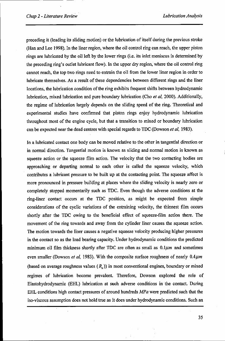
Chap 2 - Literature Review Lubrication Analysis
preceding it (leading its sliding motion) or the lubrication of itself during the previous stroke
(Han and Lee 1998). In the liner region, where the oil control ring can reach, the upper piston
rings are lubricated by the oil left by the lower rings (i.e. its inlet meniscus is determined by
the preceding ring's outlet lubricant flow). In the upper dry region, where the oil control ring
cannot reach, the top two rings need to entrain the oil from the lower liner region in order to
lubricate themselves. As a result of these dependencies between different rings and the liner
locations, the lubrication condition of the ring exhibits frequent shifts between hydrodynamic
lubrication, mixed lubrication and pure boundary lubrication (Cho et ai, 2000). Additionally,
the regime of lubrication largely depends on the sliding speed of the ring. Theoretical and
experimental studies have confirmed that piston rings enjoy hydrodynamic lubrication
throughout most of the engine cycle, but that a transition to mixed or boundary lubrication
can be expected near the dead centres with special regards to TDC (Dowson et ai, 1983).
In a lubricated contact one body can be moved relative to the other in tangential direction or
in normal direction. Tangential motion is known as sliding and normal motion is known as
squeeze action or the squeeze film action. The velocity that the two contacting bodies are
approaching or departing normal to each other is called the squeeze velocity, which
contributes a lubricant pressure to be built up at the contacting point. The squeeze affect is
more pronounced in pressure building at places where the sliding velocity is nearly zero or
completely stopped momentarily such as TDC. Even though the adverse conditions at the
ring-liner contact occurs at the TDC position, as might be expected from simple
considerations of the cyclic variations of the entraining velocity, the thinnest film occurs
shortly after the TDC owing to the beneficial effect of squeeze-film action there. The
movement of the ring towards and away from the cylinder liner causes the squeeze action.
The motion towards the liner causes a negative squeeze velocity producing higher pressures
in the contact so as the load bearing capacity. Under hydrodynamic conditions the predicted
minimum oil film thickness shortly after TDC are often as small as O.lllm and sometimes
even smaller (Dowson et ai, 1983). With the composite surface roughness of nearly O.4llm
(based on average roughness values (Ra)) in most conventional engines, boundary or mixed
regimes of lubrication become prevalent. Therefore, Dowson explored the role of
Elastohydrodynamic (EHL) lubrication at such adverse conditions in the contact. During
EHL conditions high contact pressures of around hundreds MPa were predicted such that the
iso-viscous assumption does not hold true as it does under hydrodynamic conditions. Such an
35
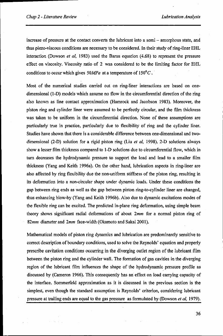
Chap 2 - Literature Review Lubrication Analysis
increase of pressure at the contact converts the lubricant into a semi - amorphous state, and
thus piezo-viscous conditions are necessary to be considered. In their study of ring-liner EHL
interaction (Dowson et ai, 1983) used the Barus equation (4.68) to represent the pressure
effect on viscosity. Viscosity ratio of 2 was considered to be the limiting factor for EHL
conditions to occur which gives 50MPa at a temperature of 1500 C .
Most of the numerical studies carried out on ring-liner interactions are based on one
dimensional (I-D) models which assume no flow in the circumferential direction of the ring
also known as line contact approximation (Hamrock and Jacobson 1983). Moreover, the
piston ring and cylinder liner were assumed to be perfectly circular, and the film thickness
was taken to be uniform in the circumferential direction. None of these assumptions are
particularly true in practice, particularly due to flexibility of ring and the cylinder liner.
Studies have shown that there is a considerable difference between one-dimensional and two
dimensional (2-D) solution for a rigid piston ring (Liu et ai, 1998). 2-D solutions always
show a lesser film thickness compared to 1-0 solutions due to circumferential flow, which in
turn decreases the hydrodynamic pressure to support the load and lead to a smaller film
thickness (Yang and Keith 1996a). On the other hand, lubrication aspects in ring-liner are
also affected by ring flexibility due the non-uniform stiffness of the piston ring, resulting in
its deformation into a non-circular shape under dynamic loads. Under these conditions the
gap between ring ends as well as the gap between piston ring-to-cylinder liner are changed,
thus enhancing blow-by (Yang and Keith 1996b). Also due to dynamic excitations modes of
the flexible ring can be excited. The predicted in-plane ring deformation, using simple beam
theory shows significant radial deformations of about 2mm for a normal piston ring of
82mm diameter and 2mm face-width (Okamoto and SakaI2001).
Mathematical models of piston ring dynamics and lubrication are predominantly sensitive to
correct description of boundary conditions, used to solve the Reynolds' equation and properly
prescribe cavitation conditions occurring in the diverging outlet region of the lubricant film
between the piston ring and the cylinder wall. The formation of gas cavities in the diverging
region of the lubricant film influences the shape of the hydrodynamic pressure profile as
discussed by (Cameron 1966). This consequently has an effect on load carrying capacity of
the interface. Sommerfeld approximation as it is discussed in the previous section is the
simplest, even though the standard assumption is Reynolds' criterion, considering lubricant
pressure at trailing ends are equal to the gas pressure as formulated by (Dowson et ai, 1979).
36
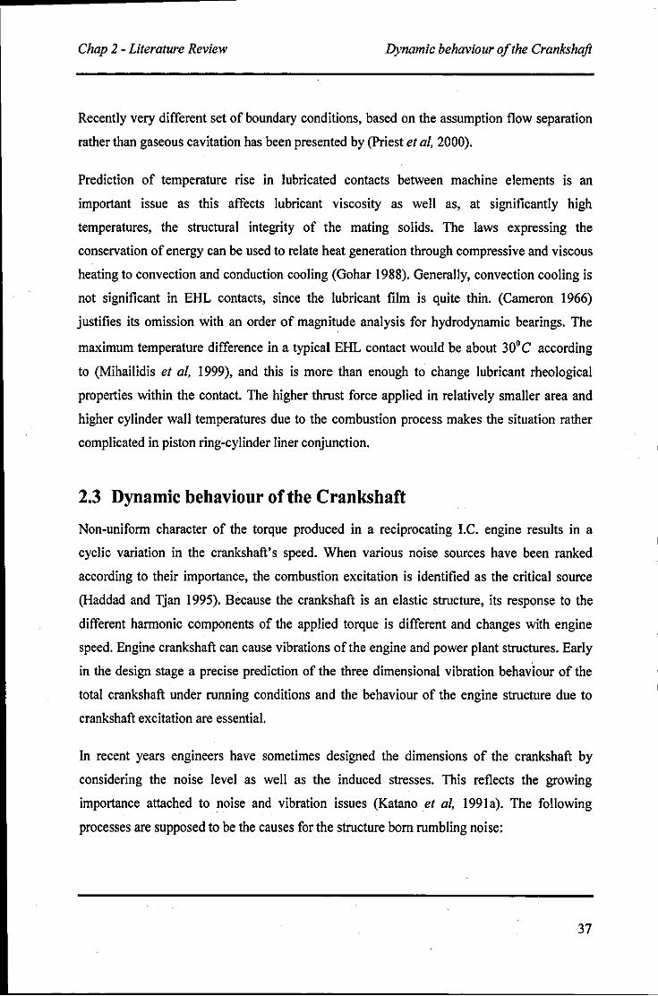
Chap 2 - Literature Review Dynamic behaviour of the Crankshaft
Recently very different set of boundary conditions, based on the assumption flow separation
rather than gaseous cavitation has been presented by (Priest et aI, 2000).
Prediction of temperature rise in lubricated contacts between machine elements is an
important issue as this affects lubricant viscosity as well as, at significantly high
temperatures, the structural integrity of the mating solids. The laws expressing the
conservation of energy can be used to relate heat generation through compressive and viscous
heating to convection and conduction cooling (Gohar 1988). Generally, convection cooling is
not significant in EHL contacts, since the lubricant film is quite thin. (Cameron 1966)
justifies its omission with an order of magnitude analysis for hydrodynamic bearings. The
maximum temperature difference in a typical EHL contact would be about 30° C according
to (Mihailidis et aI, 1999), and this is more than enough to change lubricant rheological
properties within the contact. The higher thrust force applied in relatively smaller area and
higher cylinder wall temperatures due to the combustion process makes the situation rather
complicated in piston ring-cylinder liner conjunction.
2.3 Dynamic behaviour of the Crankshaft
Non-uniform character of the torque produced in a reciprocating I.C. engine results in a
cyclic variation in the crankshaft's speed. When various noise sources have been ranked
according to their importance, the combustion excitation is identified as the critical source
(Haddad and Tjan 1995). Because the crankshaft is an elastic structure, its response to the
different harmonic components of the applied torque is different and changes with engine
speed. Engine crankshaft can cause vibrations of the engine and power plant structures. Early
in the design stage a precise prediction of the three dimensional vibration behaviour of the
total crankshaft under running conditions and the behaviour of the engine structure due to
crankshaft excitation are essential.
In recent years engineers have sometimes designed the dimensions of the crankshaft by
considering the noise level as well as the induced stresses. This reflects the growing
importance attached to noise and vibration issues (Katano et aI, 1991a). The following
processes are supposed to be the causes for the structure born rumbling noise:
37
Chap 2 - Literature Review Dynamic behaviour of the Crankshaft
I. The inertial force by the reciprocating mass of the piston and the connecting rod
system pushes· and pulls the crank pin, resulting in torsional vibrations of the
crankshaft.
2. In this state, the combustion gas pressure in the combustion chamber causes the piston
and connecting rod to induce inertial torque variations in the crankpin attached to each
cylinder.
3. Both combustion gas force and the connecting rod forces on the piston create a side
thrust force that pushes the piston against the cylinder wall, creating an impact force.
4. The crankshaft, accelerated by the exciting force, rotates and gives rise to varying
journals' reactions.
5. The shock, thus generated, vibrates the cylinder block through the main bearings as
well as the cylinder wall, and causes noise to be radiated from the cylinder block
surface. Vibration is subsequently propagated to the cabin through the engine mounts.
6. The cabin panels vibrate in response to the rumbling noise.
7. The cabin air cavity resonates under the engine excitation.
Since this process involves a large chain reaction, it is not sensible to analyse given sub
systems in isolation. Thus, several system approaches have been made to study the dynamic
behaviour of the crankshaft system.
In (Katano et ai, 1991a) the crankshaft behaviour and the source of the rumbling noise was
simulated in order to clarify the effect of crankshaft vibration on its support bearings after it
is accelerated by the induced inertial imbalance. This study was based on the non-linearity of
the oil film, dynamic characteristics of the crankshaft and the flexibility of the cylinder block.
The mobility method was used to relate the rate of change of eccentricity to the loading and
the current state of the bearings. Components' mass, inertial properties, stiffuess and damping
matrices were partitioned to distinguish between the degrees of freedom under several
loading conditions.
(Boysal and Rahnejat 1997) presented a multi-body numerical non-linear dynamic model of a
single cylinder internal combustion engine. The model comprises all rigid body inertial
members, support bearings, joints, couplers and connections between various engine
components, as well as means of vibration damping, such as the crankshaft torsional damper.
The detailed model is parameterised, thus enabling virtual prototype testing of various engine
38
------------------------------........... .. Chap 2 - Literature Review Dynamic behaviour of the Crankshaft
designs, as well as allowing the engine designer to carry out a comprehensive noise, vibration
and harshness investigation of engine performance. This new approach was basically
concentrated on engine design. It incorporated large displacement dynamics of engine
components, combustion pressure and infinitesimal vibrations of support bearings.
Combination of multi-body dynamics with flexible bodies is an advantage for geometric non
linear FEA and rigid body dynamics. (Du 1999) investigated a V6 engine, which had been
modelled with multi-body dynamics and flexible bodies. Impedance method and a full FE
method to model the oil film bearing were used to represent hydrodynamic bearings as two
alternative approaches. Model synthesis technique was used to reduce the size and number of
resulting equations, representing the stiffuess and mass of the crankshaft and the engine
block. It was concluded that the vibration behaviour was largely different with a flexible
engine block, when compared to a rigid block.
(Piraner et aI, 2002) used a simplified approach, developed in the industry. It first combines a
"quasi-static" crankshaft model and a rigid hydrodynamic bearing model to address
crankshaft fillet bending stress and bearing performance characteristics. Then, the cmnkshaft
bending loads are combined with the torsional loads to simulate stress at any location in a
crankshaft FE model. ADAMS and ANSYS were the main software tools used.
2.3.1 Torsional Vibrations
At any instant of time the mdial component of the piston force is transmitted along the
connecting rod and is applied to the crank pin. This force tends to pull the crankpin away and
induces an instantaneous bearing support load. The tangential component of the piston force
is utilised for crankshaft rotation. During piston motion inside the cylinder the inertial piston
imbalance increases in magnitude and subsequently reduces at the end of the stroke. This
action results in an imparted twist-untwist action on the crankshaft, inducing torsional
vibrations. Owing to the combustion cycle, the gas pressure inside the combustion chamber
varies with a maximum pressure force at the power stroke, a few degrees after the TDC. In a
four stroke internal combustion engine the applied torque's fundamental frequency coincides
with half the crankshaft speed and its harmonics are at whole or half orders of the same speed
(Rahnejat 1998). Half order harmonics of the engine torque are only contributed by the gas
pressure and integer harmonics orders up to sixth order are mainly contributed by the
39
Chap 2 - Literature Review Dynamic behaviour of the Crankshaft
reciprocating inertia (Taraza 200 I). Due to small, but inherent variations in cylinder
operation, the pressure varies from cycle to cycle and cylinder to cylinder, causing
fluctuations of the mean value of the cylinder torque (Taraza 200 I). Therefore, there are an
infinite number of critical frequencies, and in principle high vibratory torques can be
expected at each of these frequencies, which are referred to as unexpected rotational
frequencies. This phenomenon was first observed by Draminsky (see (Draminsky 1965)).
(Hesterman and Stone 1992) pointed out that this is due to variations in inertia of large
reciprocating mass and, thus a constant inertial assumption is not particularly valid for
reciprocating masses. It has been known for some time that the torsional vibration of
reciprocating engines and pumps cannot be modelled accurately by representing the
reciprocating mechanism by a constant inertia. It further varies with the angular position. The
major component of this variation is a twice per revolution cyclic effect and hence termed as
secondary inertia. The consequences of this secondary inertia effect can be serious for
torsional vibrations, causing secondary resonance and even instability.
(Goldsbrough and Baker 1926) used the linearized Floquet model (a non-homogeneous
differential equation with periodic coefficients) for low speed multi-cylinder engines with
certain assumptions such as, no relative twist between neighbouring crank assemblies, the
flexible connecting rods are massless, connecting rod is infinitely long and higher order terms
in the resulting equations were considered as not significant. He made an experimental rig
and consequent correlations between the predicted and measured results were deemed as
being very good, although deviations were noticed as the piston weight was increased. Based
on his experimental work, Goldsborugh concluded that the flexible shaft was subjected to
vibrations at all speeds, and within a certain defined range these vibrations were unstable
(Hesterman and Stone 1995). However, revealed induced cyclic stresses at the service speeds
were found to be well in excess of those predicted. In order to explain these unusually high
stresses, Draminsky developed a theory based on non-linear analysis (Draminsky 1965).
Balancing of reciprocating inertia has become a severe problem for three cylinder engines of
180· phase difference configuration as only 50% of the unbalanced primary reciprocating
moments are eliminated by adding counterweights to the crankshaft system. This enhances
primary pitching moment on the engine. (Suh et ai, 2000) investigated the effects of balance
shaft on this pitching moment with the aid of DADS and MSClNastran, taking into account
dynamic and inertia properties respectively. It has been observed that the rigid body motions
40
Chap 2 - Literature Review Dynamic behaviour of the Crankshaft
of the engine with the primary balance shaft are largely reduced due to the transformation of
50% of the unbalanced pitching moment into the yaw moment in a three cylinder
configuration. In engines with large reciprocating masses the effect of inertia variation is
significantly more pronounced
The variation of torsional inertia with time, which results in a secondary resonance, affects
crankshaft failures. The induced inertial torque may have components at any integer multiples
of engine speed. If any of these contributions coincide with component frequency an
unexpected resonance may occur. If the oscillation occurs at resonance condition (multiples
(n) of the engine speed coincident with undamped natural frequency), then there is a
consequential oscillation at n-2 and n+2 as well (Hesterman and Stone 1992). Until recent
times, one-degree of freedom analysis was predominant in the process of crankshaft vibration
analysis. which is not able to capture the coupled bending and torsional vibrations. However,
the later use of Transfer Matrix Method (TMM) has allowed investigation of coupled
vibrations in crankshafts (Wakabayashi et aI, 1995).
2.3.2 Engine Noise Emission
The main energy source for the engine as the power plant is the combustion process from
which a certain amount is utilized for coupled axial, bending and torsional vibrations of the
crankshaft. Some of the energy is dissipated from the crankshaft itself due to its internal
damping and in the form of acoustic energy. However, another significant amount of
vibration energy is transferred to the engine block through the main crankshaft support
journal bearings. The piston secondary motion also creates significant amount of excitations
on the engine block (Spessert and Ponsa 1990). These excitations with various frequencies
are absorbed by the engine block and dissipated through them to the environment as acoustic
(air born) energy (or noise), and to lesser extent as heat It is known that the engine noise is
dominant in the middle to high frequency range (0.5 to 2.5 KHz) (Athavale and P.R. 1999). It
has been determined that this noise is mainly caused by the fundamental natural vibrations of
the cylinder block.
Parallel to the development of light weight, high output power engines, made of materials
with significant elasticity and thermal expansion the attention towards noise emission has
become significant as a perceived quality issue. Thus, the need for more detailed analysis has
41
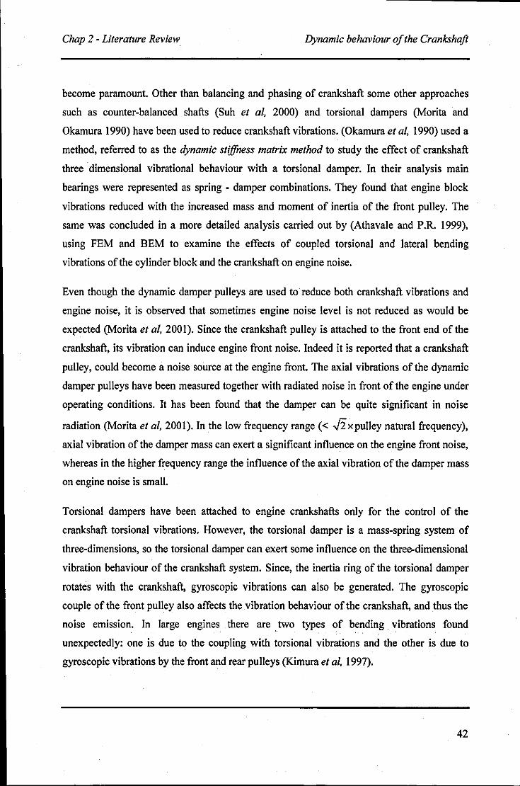
Chap 2 - Literature Review Dynamic behaviour of the Crankshaft
become paramount. Other than balancing and phasing of crankshaft some other approaches
such as counter-balanced shafts (Suh et al, 2000) and torsional dampers (Morita and
Okamura 1990) have been used to reduce crankshaft vibrations. (Okamura et al, 1990) used a
method, referred to as the dynamic stiffness matrix method to study the effect of crankshaft
three dimensional vibrational behaviour with a torsional damper. In their analysis main
bearings were represented as spring - damper combinations. They found that engine block
vibrations reduced with the increased mass and moment of inertia of the front pulley. The
same was concluded in a more detailed analysis carried out by (Athavale and P.R. 1999),
using FEM and BEM to examine the effects of coupled torsional and lateral bending
vibrations of the cylinder block and the crankshaft on engine noise.
Even though the dynamic damper pulleys are used to reduce both crankshaft vibrations and
engine noise, it is observed that sometimes engine noise level is not reduced as would be
expected (Morita et al, 2001). Since the crankshaft pulley is attached to the front end of the
crankshaft, its vibration can induce engine front noise. Indeed it is reported that a crankshaft
pulley, could become a noise source at the engine front. The axial vibrations of the dynamic
damper pulleys have been measured together with radiated noise in front of the engine under
operating conditions. It has been found that the damper can be quite significant in noise
radiation (Morita et al, 200 I). In the low frequency range « .,fi x pulley natural frequency),
axial vibration of the damper mass can exert a significant influence on the engine front noise,
whereas in the higher frequency range the influence of the axial vibration of the damper mass
on engine noise is small.
Torsional dampers have been attached to engine crankshafts only for the control of the
crankshaft torsional vibrations. However, the torsional damper is a mass-spring system of
three-dimensions, so the torsional damper can exert some influence on the three-dimensional
vibration behaviour of the crankshaft system. Since, the inertia ring of the torsional damper
rotates with the crankshaft, gyroscopic vibrations can also be generated. The gyroscopic
couple of the front pulley also affects the vibration behaviour of the crankshaft, and thus the
noise emission. In large engines there are two types of bending vibrations found
unexpectedly: one is due to the coupling with torsional vibrations and the other is due to
gyroscopic vibrations by the front and rear pulleys (Kimura et al, 1997).
42
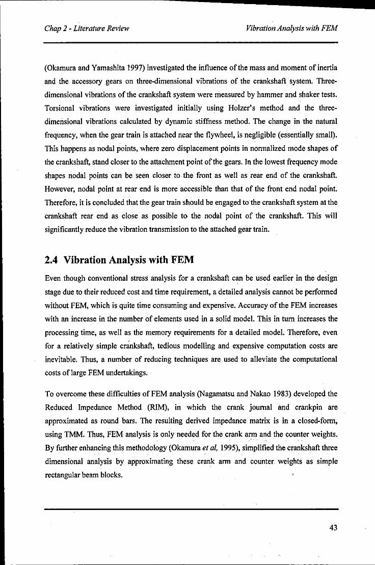
Chap 2 - Literature Review Vibration Analysis with FEM
(Okamura and Yamashita 1997) investigated the influence of the mass and moment of inertia
and the accessory gears on three-dimensional vibrations of the crankshaft system. Three
dimensional vibrations of the crankshaft system were measured by hammer and shaker tests.
Torsional vibrations were investigated initially using Holzer's method and the three
dimensional vibrations calculated by dynamic stiffness method. The change in the natural
frequency, when the gear train is attached near the flywheel, is negligible (essentially small).
This happens as nodal points, where zero displacement points in normalized mode shapes of
the crankshaft, stand closer to the attachment point of the gears. In the lowest frequency mode
shapes nodal points can be seen closer to the front as well as rear end of the crankshaft.
However, nodal point at rear end is more accessible than that of the front end nodal point.
Therefore, it is concluded that the gear train should be engaged to the crankshaft system at the
crankshaft rear end as close as possible to the nodal point of the crankshaft. This will
significantly reduce the vibration transmission to the attached gear train.
2.4 Vibration Analysis with FEM
Even though conventional stress analysis for a crankshaft can be used earlier in the design
stage due to their reduced cost and time requirement, a detailed analysis cannot be performed
without FEM, which is quite time consuming and expensive. Accuracy of the FEM increases
with an increase in the number of elements used in a solid model. This in turn increases the
processing time, as well as the memory requirements for a detailed model. Therefore, even
for a relatively simple crankshaft, tedious modelling and expensive computation costs are
inevitable. Thus, a number of reducing techniques are used to alleviate the computational
costs of large FEM undertakings.
To overcome these difficulties of FEM analysis (Nagamatsu and Nakao 1983) developed the
Reduced Impedance Method (RIM), in which the crank journal and crankpin are
approximated as round bars. The resulting derived impedance matrix is in a closed-form,
using TMM. Thus, FEM analysis is only needed for the crank arm and the counter weights.
By further enhancing this methodology (Okamura et ai, 1995), simplified the crankshaft three
dimensional analysis by approximating these crank arm and counter weights as simple
rectangular beam blocks.
43
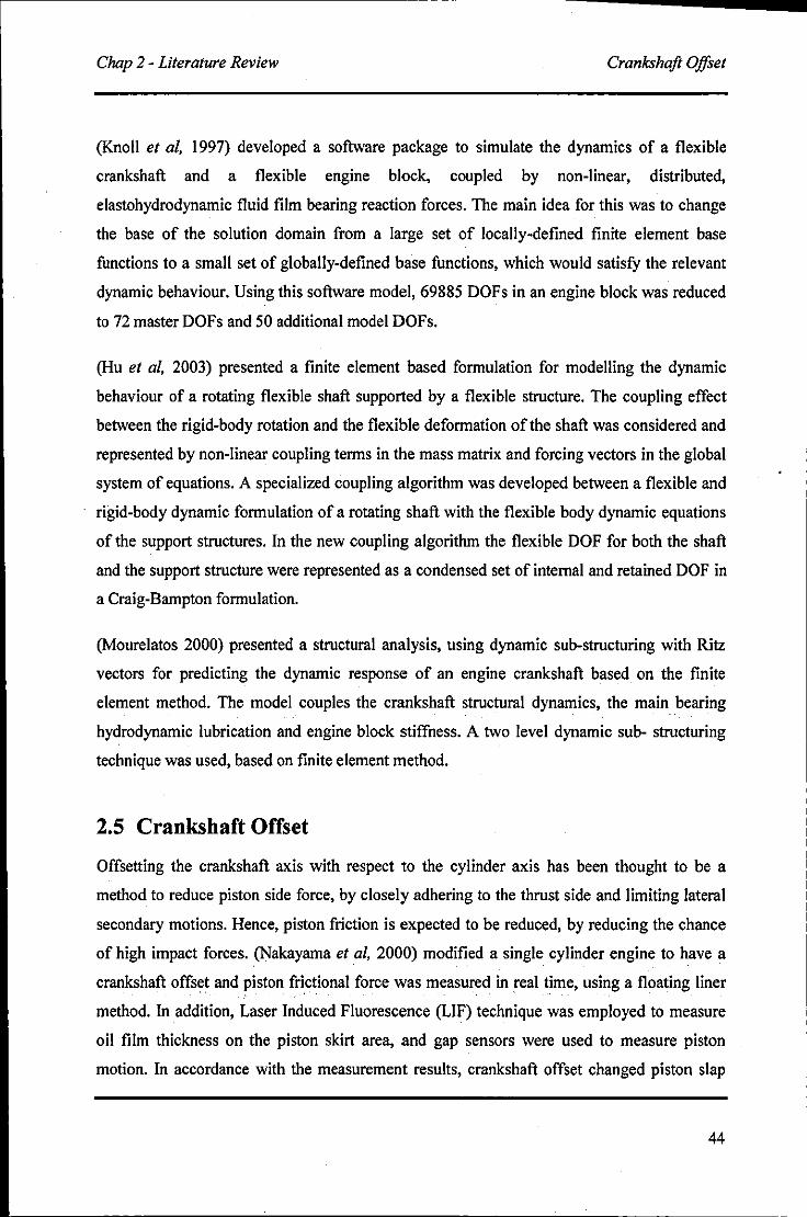
Chap 2 - Literature Review Crankshaft Offset
(Knoll et aI, 1997) developed a software package to simulate the dynamics of a flexible
crankshaft and a flexible engine block, coupled by non-linear, distributed,
elastohydrodynamic fluid film bearing reaction forces. The main idea for this was to change
the base of the solution domain from a large set of locally-defined finite element base
functions to a small set of globally-defined base functions, which would satisfY the relevant
dynamic behaviour. Using this software model, 69885 OOFs in an engine block was reduced
to 72 master OOFs and 50 additional model OOFs.
(Hu et aI, 2003) presented a finite element based formulation for modelling the dynamic
behaviour of a rotating flexible shaft supported by a flexible structure. The coupling effect
between the rigid-body rotation and the flexible deformation of the shaft was considered and
represented by non-linear coupling terms in the mass matrix and forcing vectors in the global
system of equations. A specialized coupling algorithm was developed between a flexible and
rigid-body dynamic formulation of a rotating shaft with the flexible body dynamic equations
of the support structures. In the new coupling algorithm the flexible OOF for both the shaft
and the support structure were represented as a condensed set of internal and retained OOF in
a Craig-Bampton formulation.
(Mourelatos 2000) presented a structural analysis, using dynamic sub-structuring with Ritz
vectors for predicting the dynamic response of an engine crankshaft based on the finite
element method. The model couples the crankshaft structural dynamics, the main bearing
hydrodynamic lubrication and engine block stiffness. A two level dynamic sub- structuring
technique was used, based on finite element method.
2.5 Crankshaft Offset
Offsetting the crankshaft axis with respect to the cylinder axis has been thought to be a
method to reduce piston side force, by closely adhering to the thrust side and limiting lateral
secondary motions. Hence, piston friction is expected to be reduced, by reducing the chance
of high impact forces. (Nakayama et aI, 2000) modified a single cylinder engine to have a
crankshaft offset and piston frictional force was measured in real time, using a floating liner
method. In addition, Laser Induced Fluorescence (LIF) technique was employed to measure
oil film thickness on the piston skirt area, and gap sensors were used to measure piston
motion. In accordance with the measurement results, crankshaft offset changed piston slap
44
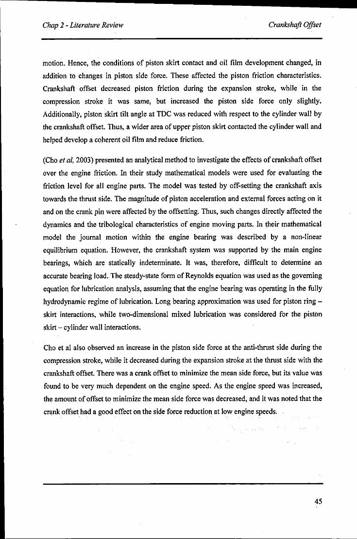
~------------------------............... Chap 2 - Literature Review Crankshaft Offset
motion. Hence, the conditions of piston skirt contact and oil film development changed, in
addition to changes in piston side force. These affected the piston friction characteristics.
Crankshaft offset decreased piston friction during the expansion stroke, while in the
compression stroke it was same, but increased the piston side force only slightly.
Additionally, piston skirt tilt angle at TDC was reduced with respect to the cylinder wall by
the crankshaft offset. Thus, a wider area of upper piston skirt contacted the cylinder wall and
helped develop a coherent oil film and reduce friction.
(Cho et al. 2003) presented an analytical method to investigate the effects of crankshaft offset
over the engine friction. In their study mathematical models were used for evaluating the
friction level for all engine parts. The model was tested by off-setting the crankshaft axis
towards the thrust side. The magnitude of piston acceleration and external forces acting on it
and on the crank pin were affected by the offsetting. Thus, such changes directly affected the
dynamics and the tribological characteristics of engine moving parts. In their mathematical
model the journal motion within the engine bearing was described by a non-linear
equilibrium equation. However, the crankshaft system was supported by the main engine
bearings, which are statically indeterminate. It was, therefore, difficult to determine an
accurate bearing load. The steady-state form of Reynolds equation was used as the governing
equation for lubrication analysis, assuming that the engine bearing was operating in the fully
hydrodynamic regime of lubrication. Long bearing approximation was used for piston ring -
skirt interactions, while two~dimensional mixed lubrication was considered for the piston
skirt - cylinder wall interactions.
Cho et al also observed an increase in the piston side force at the anti-thrust side during the
compression stroke, while it decreased during the expansion stroke at the thrust side with the
crankshaft offset. There was a crank offset to minimize the mean side force, but its value was
found to be very much dependent on the engine speed. As the engine speed was increased,
the amount of offset to minimize the mean side force was decreased, and it was noted that the
crank offset had a good effect on the side force reduction at low engine speeds.
45
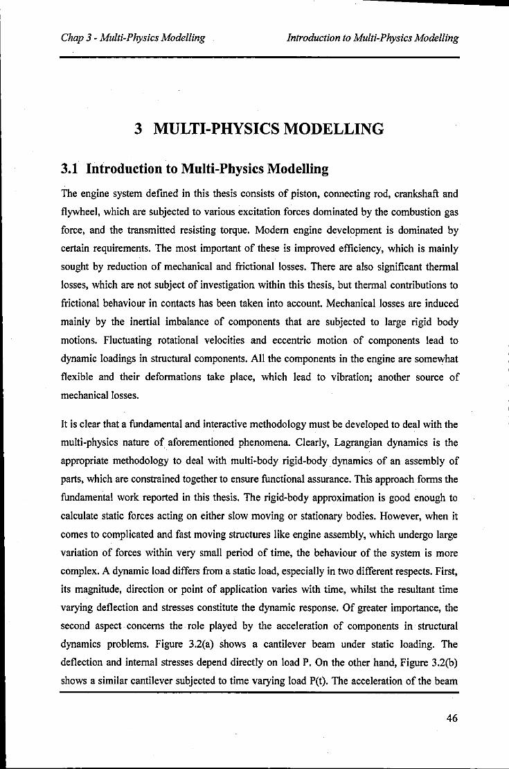
Chap 3 - Multi-Physics Modelling Introduction to Multi-Physics Modelling
3 MULTI-PHYSICS MODELLING
3.1 Introduction to Multi-Physics Modelling
The engine system defined in this thesis consists of piston, connecting rod, crankshaft and
flywheel, which are subjected to various excitation forces dominated by the combustion gas
force, and the transmitted resisting torque. Modem engine development is dominated by
certain requirements. The most important of these is improved efficiency, which is mainly
sought by reduction of mechanical and frictional losses. There are also significant thermal
losses, which are not subject of investigation within this thesis, but thermal contributions to
frictional behaviour in contacts has been taken into account. Mechanical losses are induced
mainly by the inertial imbalance of components that are subjected to large rigid body
motions. Fluctuating rotational velocities and eccentric motion of components lead to
dynamic loadings in structural components. All the components in the engine are somewhat
flexible and their deformations take place, which lead to vibration; another source of
mechanical losses.
It is clear that a fundamental and interactive methodology must be developed to deal with the
multi-physics nature of aforementioned phenomena. Clearly, Lagrangian dynamics is the
appropriate methodology to deal with multi-body rigid-body dynamics of an assembly of
parts, which are constrained together to ensure functional assurance. This approach forms the
fundamental work reported in this thesis. The rigid-body approximation is good enough to
calculate static forces acting on either slow moving or stationary bodies. However, when it
comes to complicated and fast moving structures like engine assembly, which undergo large
variation of forces within very small period of time, the behaviour of the system is more
complex. A dynamic load differs from a static load, especially in two different respects. First,
its magnitude, direction or point of application varies with time, whilst the resultant time
varying deflection and stresses constitute the dynamic response. Of greater importance, the
second aspect concerns the role played by the acceleration of components in structural
dynamics problems. Figure 3.2(a) shows a cantilever beam under static loading. The
deflection and internal stresses depend directly on load P. On the other hand, Figure 3.2(b)
shows a similar cantilever subjected to time varying load P(t). The acceleration of the beam
46
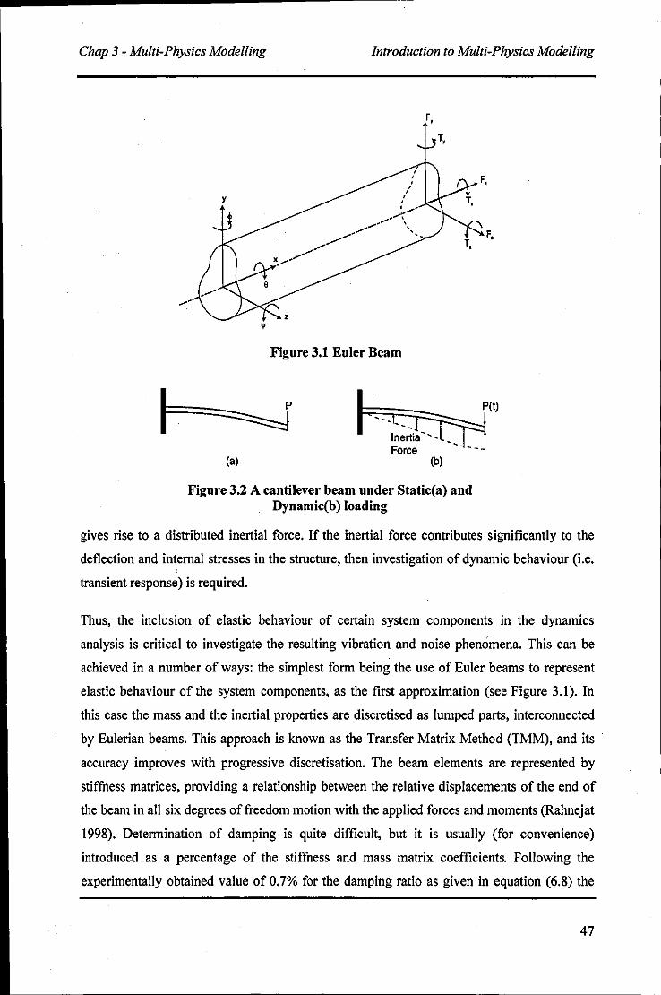
Chap 3 - Multi-Physics Modelling Introduction to Multi-Physics Modelling
I
y
(a)
......... ....x ................
/' /'
/'
• . · • • .
• ...... ,,~--\
/' ,
F,
F.
T.
F, T,
Figure 3.1 Euler Beam
1--cl :fJ'1" Inertia - - - __ Force --
(b)
Figure 3.2 A cantilever beam under Static(a) and Dynamic(b) loading
gives rise to a distributed inertial force. If the inertial force contributes significantly to the
deflection and internal stresses in the structure, then investigation of dynamic behaviour (Le.
transient response) is required.
Thus, the inclusion of elastic behaviour of certain system components in the dynamics
analysis is critical to investigate the resulting vibration and noise phenomena. This can be
achieved in a number of ways: the simplest form being the use of Euler beams to represent
elastic behaviour of the system components, as the first approximation (see Figure 3.1). In
this case the mass and the inertial properties are discretised as lumped parts, interconnected
by Eulerian beams. This approach is known as the Transfer Matrix Method (TMM), and its
accuracy improves with progressive discretisation. The beam elements are represented by
stiffness matrices, providing a relationship between the relative displacements of the end of
the beam in all six degrees offreedom motion with the applied forces and moments (Rahnejat
1998). Determination of damping is quite difficult, but it is usually (for convenience)
introduced as a percentage of the stiffness and mass matrix coefficients. Following the
experimentaIly obtained value of 0.7% for the damping ratio as given in equation (6.8) the
47
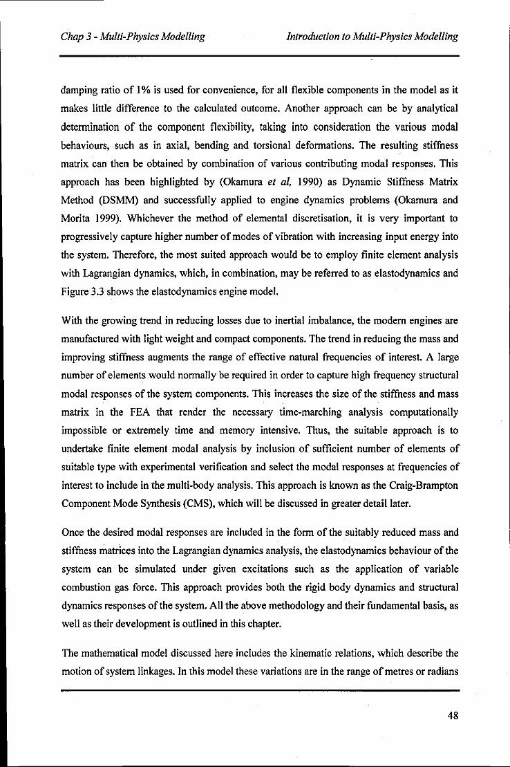
Chap 3 - Multi-Physics Modelling Introduction to Multi-Physics Modelling
damping ratio of 1 % is used for convenience, for all flexible components in the model as it
makes little difference to the calculated outcome. Another approach can be by analytical
determination of the component flexibility, taking into consideration the various modal
behaviours, such as in axial, bending and torsional deformations. The resulting stiffness
matrix can then be obtained by combination of various contributing modal responses. This
approach has been highlighted by (Okamura et ai, 1990) as Dynamic Stiffness Matrix
Method (DSMM) and successfully applied to engine dynamics problems (Okamura and
Morita 1999). Whichever the method of elemental discretisation, it is very important to
progressively capture higher number of modes of vibration with increasing input energy into
the system. Therefore, the most suited approach would be to employ finite element analysis
with Lagrangian dynamics, which, in combination, may be referred to as elastodynamics and
Figure 3.3 shows the elastodynamics engine model.
With the growing trend in reducing losses due to inertial imbalance, the modem engines are
manufactured with light weight and compact components. The trend in reducing the mass and
improving stiffness augments the range of effective natural frequencies of interest. A large
number of elements would normally be required in order to capture high frequency structural
modal responses of the system components. This increases the size of the stiffness and mass
matrix in the FEA that render the necessary time-marching analysis computationally
impossible or extremely time and memory intensive. Thus, the suitable approach is to
undertake finite element modal analysis by inclusion of sufficient number of elements of
suitable type with experimental verification and select the modal responses at frequencies of
interest to include in the multi-body analysis. This approach is known as the Craig-Brampton
Component Mode Synthesis (CMS), which will be discussed in greater detail later.
Once the desired modal responses are included in the form of the suitably reduced mass and
stiffness matrices into the Lagrangian dynamics analysis, the elastodynamics behaviour of the
system can be simulated under given excitations such as the application of variable
combustion gas force. This approach provides both the rigid body dynamics and structural
dynamics responses of the system. All the above methodology and their fundamental basis, as
well as their development is outlined in this chapter.
The mathematical model discussed here includes the kinematic relations, which describe the
motion of system linkages. In this model these variations are in the range of metres or radians
48
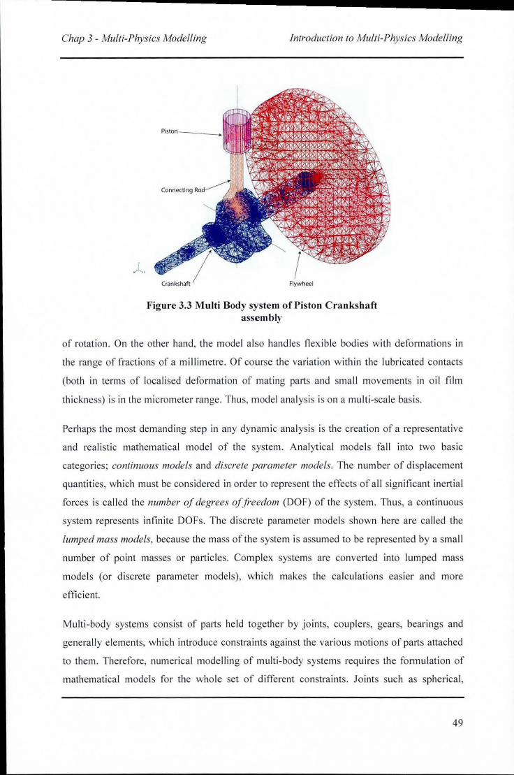
----------------------------........... . Chap 3 - Multi-Physics Modelling Introduction to Multi-Physics Modelling
J.. Crankshaft Flywheel
Figure 3.3 Multi Body system of Piston C rankshaft assembly
of rotation. On the other hand, the mode l a lso handles fl exib le bodies with deformati ons in
the range of fract ions of a mill imetre. Of course the variati on within the lubricated contacts
(both in terms of locali sed deformation of mati ng pans and small movements in oil film
th ickness) is in the mi crometer range. Th us, model analys is is on a mult i-scale bas is.
Perhaps the most demandi ng step in any dynamic analys is is the creation of a repre entative
and real istic mathematica l model of the system. Analytical models fa ll into two bas ic
categori es; continuous models and discrete parameter models. The number of d isplacement
quant iti es, which must be considered in order to represent the effects of all significant inenial
forces is ca lled the number of degrees of freedom (DOF) of the system. Thus, a continuous
system represents infinite DOFs. The discrete parameter models shown here are ca lled the
lumped mass models, because the mass of the system is assumed to be represented by a small
number of po int masses or panic les. Complex systems are converted into lum ped mass
model s (or di screte parameter mode ls), whi ch makes the ca lcul ations easier and more
effic ient.
Multi-body systems consist of parts held together by jo in ts, couplers, gea rs, bearings and
genera lly e lements, whi ch introduce constra ints aga inst the various motions of pans attached
to them. Therefore, numerica l mode lli ng of mult i-body systems requires the formulati on of
mathemati ca l model s for the whole set of d ifferent constraints. Jo ints such as spherical,
49
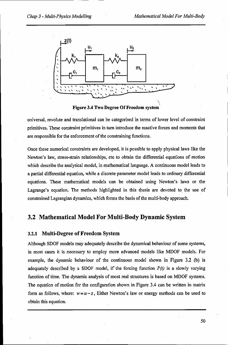
Chap 3 - Multi-Physics Modelling Mathematical Model For Multi-Body
12-(t)
~ k, ,
, , , rn, , c, c.
rn.
, ~~~~~~==~~~
""", .. " "'" " .. ,",' .... " .. " .... " .... " .... " .. " .. " .. .. .. " .. .. "",',
\. Figure 3.4 Two Degree Of Freedom system
universal, revolute and translational can be categorised in terms of lower level of constraint
primitives. These constraint primitives in turn introduce the reactive forces and moments that
are responsible for the enforcement of the constraining functions.
Once these numerical constraints are developed, it is possible to apply physical laws like the
Newton's law, stress-strain relationships, etc to obtain the differential equations of motion
which describe the analytical model, in mathematical language. A continuous model leads to
a partial differential equation, while a discrete parameter model leads to ordinary differential
equations. These mathematical models can be obtained using Newton's laws or the
Lagrange's equation. The methods highlighted in this thesis are devoted to the use of
constrained Lagrangian dynamics, which forms the basis of the multi-body approach.
3.2 Mathematical Model For Multi-Body Dynamic System
3.2.1 Multi-Degree of Freedom System
Although SDOF models may adequately describe the dynamical behaviour of some systems,
in most cases it is necessary to employ more advanced models like MDOF models. For
example, the dynamic behaviour of the continuous model shown in Figure 3.2 (b) is
adequately described by a SDOF model, if' the forcing function P(t) is a slowly varying
function of time. The dynamic analysis of most real structures is based on MDOF systems.
The equation of motion for the configuration shown in Figure 3.4 can be written in matrix
form as foHows, where: w = u - Z , Either Newton's law or energy methods can be used to
obtain this equation.
50
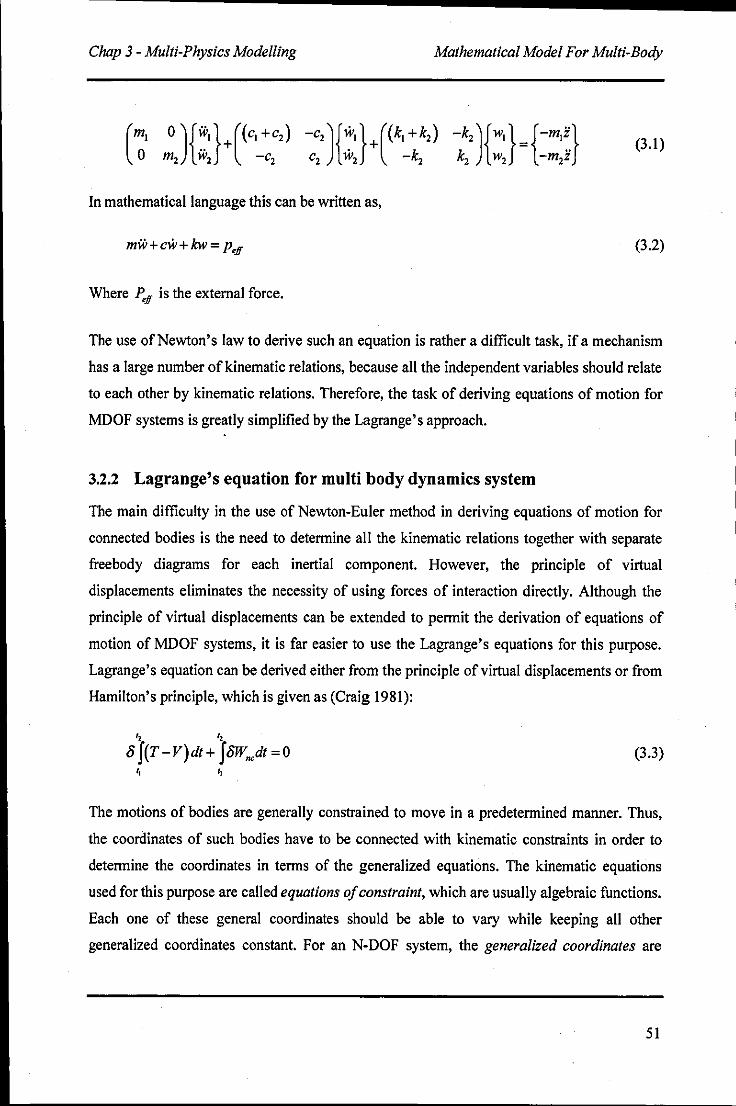
Chap 3 - Multi-Physics Modelling Mathematical Model For Multi-Body
(m! 0 ){~!}+((C~+C2) -C2){~!}+((k~+k2) -k2}{W!}={=ml~.} (3.1) o m2 w2 c2 c2 w2 k2 k2 w2 m2z
In mathematical language this can be written as,
mw+cW+kw= PeJf (3.2)
Where P.Jf is the external force.
The use of Newton's law to derive such an equation is rather a difficult task, if a mechanism
has a large number of kinematic relations, because all the independent variables should relate
to each other by kinematic relations. Therefore, the task of deriving equations of motion for
MDOF systems is greatly simplified by the Lagrange's approach.
3.2.2 Lagrange's equation for multi body dynamics system
The main difficulty in the use of Newton-Euler method in deriving equations of motion for
connected bodies is the need to determine all the kinematic relations together with separate
freebody diagrams for each inertial component. However, the principle of virtual
displacements eliminates the necessity of using forces of interaction directly. Although the
principle of virtual displacements can be extended to permit the derivation of equations of
motion of MDOF systems, it is far easier to use the Lagrange's equations for this purpose.
Lagrange's equation can be derived either from the principle of virtual displacements or from
Hamilton's principle, which is given as (Craig 1981):
'2 '2 of(r-V)dt+ JoWn,dt=O (3.3)
I, I,
The motions of bodies are generally constrained to move in a predetermined manner. Thus,
the coordinates of such bodies have to be connected with kinematic constraints in order to
determine the coordinates in terms of the generalized equations. The kinematic equations
used for this purpose are called equations of constraint, which are usually algebraic functions.
Each one of these general coordinates should be able to vary while keeping all other
generalized coordinates constant. For an N-DOF system, the generalized coordinates are
SI
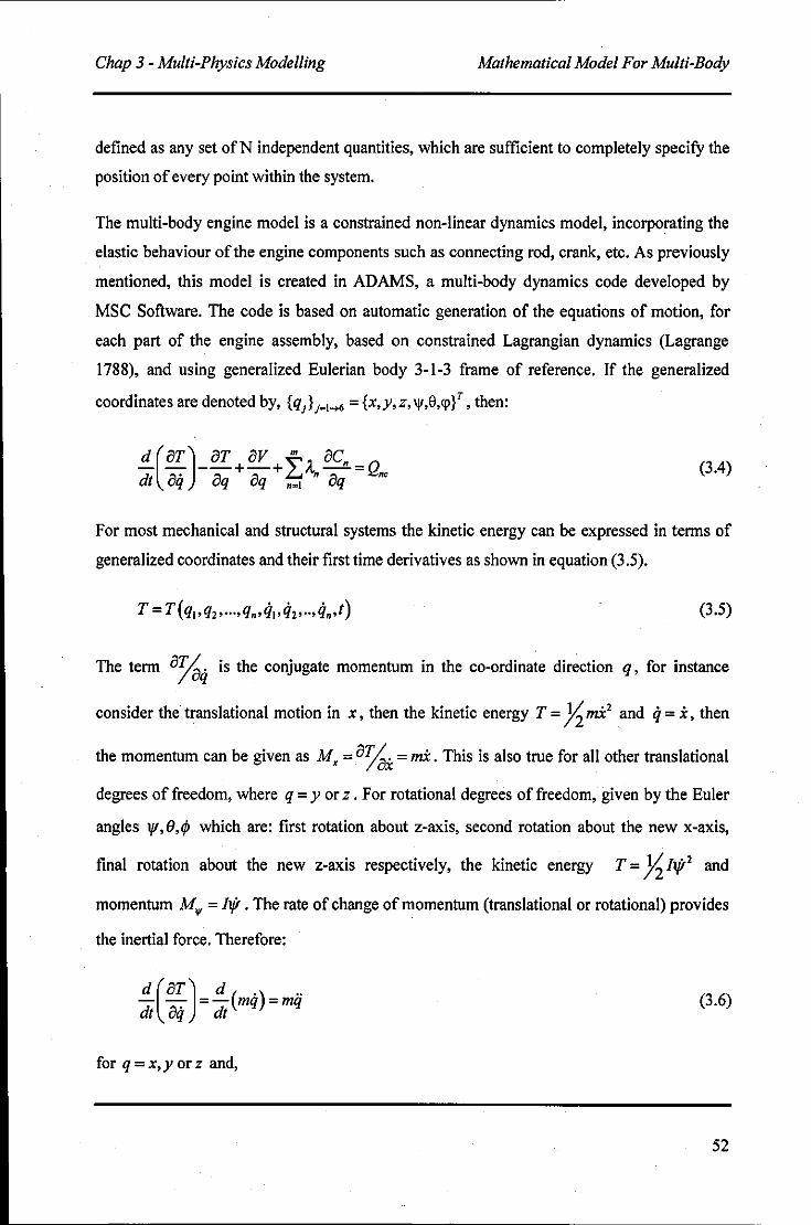
Chap 3 - Multi-Physics Modelling Mathematical Model For Multi-Body
defined as any set of N independent quantities, which are sufficient to completely specify the
position of every point within the system.
The multi-body engine model is a constrained non-linear dynamics model, incorporating the
elastic behaviour of the engine components such as connecting rod, crank, etc. As previously
mentioned, this model is created in ADAMS, a multi-body dynamics code developed by
MSC Software. The code is based on automatic generation of the equations of motion, for
each part of the engine assembly, based on constrained Lagrangian dynamics (Lagrange
1788), and using generali:z;ed Eulerian body 3-1-3 frame of reference. If the generalized
coordinates are denoted by, {qj}j=, .... = {x,y,z, ,!"e,cp}" then:
(3.4)
For most mechanical and structural systems the kinetic energy can be expressed in terms of
generalized coordinates and their first time derivatives as shown in equation (3.5).
(3.5)
The term B;latj is the conjugate momentum in the co-ordinate direction q, for instance
consider the translational motion in x, then the kinetic energy T = ~ mic' and tj = x, then
the momentum can be given as M, = B%x = mic. This is also true for all other translational
degrees of freedom, where q = y or z . For rotational degrees of freedom, given by the Euler
angles If/,e,rp which are: first rotation about z-axis, second rotation about the new x-axis,
final rotation about the new z-axis respectively, the kinetic energy T = ~ Iljt' and
momentum M", = Iljt . The rate of change of momentum (translational or rotational) provides
the inertial force. Therefore:
d (BT) d (.) .. dt Btj = dt mq =mq
for q = x,y or z and,
(3.6)
52
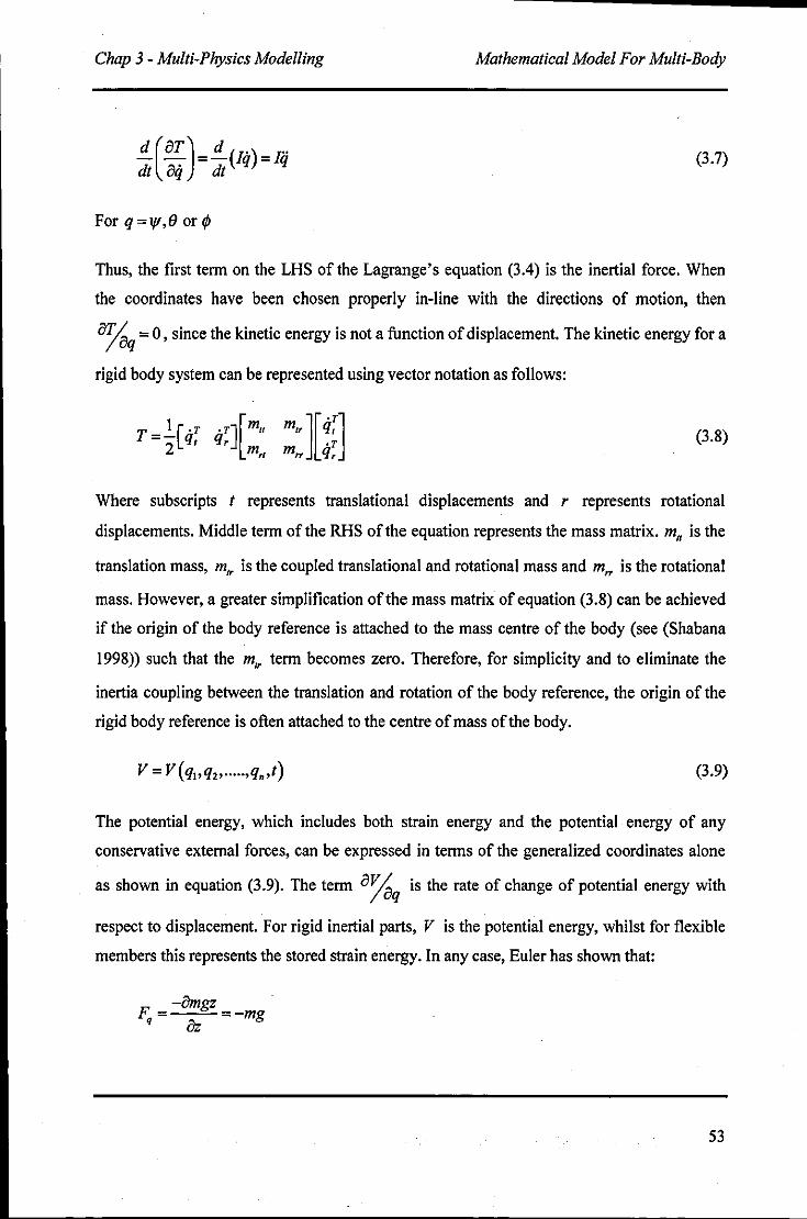
Chap 3 - Multi-Physics Modelling Mathematical Model For Multi-Body
(3.7)
For q=l/f,e or4J
Thus, the first term on the LHS of the Lagrange's equation (3.4) is the inertial force. When
the coordinates have been chosen properly in-line with the directions of motion, then
8%q = 0 , since the kinetic energy is not a function of displacement. The kinetic energy for a
rigid body system can be represented using vector notation as follows:
T=.!.[.r .rJ[mll m,,][q;] 2
q, q, ·r mrl m" q,
(3.8)
Where subscripts t represents translational displacements and r represents rotational
displacements. Middle term of the RHS of the equation represents the mass matrix. m" is the
translation mass, m" is the coupled translational and rotational mass and m" is the rotational
mass. However, a greater simplification of the mass matrix of equation (3.8) can be achieved
if the origin of the body reference is attached to the mass centre of the body (see (Shabana
1998» such that the m" term becomes zero. Therefore, for simplicity and to eliminate the
inertia coupling between the translation and rotation of the body reference, the origin of the
rigid body reference is often attached to the centre of mass of the body.
(3.9)
The potential energy, which includes both strain energy and the potential energy of any
conservative external forces, can be expressed in terms of the generalized coordinates alone
as shown in equation (3.9). The term 81aq is the rate of change of potential energy with
respect to displacement. For rigid inertial parts, V is the potential energy, whilst for flexible
members this represents the stored strain energy. In any case, Euler has shown that:
F __ -8mgz
-mg q az
53
Chap 3 - Multi-Physics Modelling Mathematical Model For Multi-Body
And the negative sign indicates the direction of gravity. In case of a flexible member such as
a spring the stored strain energy is Yz la2 , then:
-la
Which is the restoring force.
3.2.3 Generalized Forces
The virtual work of generalized forces, Q"Q2' ...... ,Q. as they act through virtual
displacements caused by arbitrary variations in the generalized coordinates, can be expressed
as a linear function of those variations as shown in (3.10).
(3.10)
The forces acting on a system are twofold: the elastic restoring forces and other external
forces. Elastic forces can be restored by reversing the motion and thus they are considered as
conservative forces. External forces are non-conservative. Therefore, the total work done on a
system can be represented as:
oW = off'" + oW" (3.11)
It is important to mention that these conservative forces give rise to potential energy and if
the potential energy is taken into consideration for Lagrange's equation, then the virtual work
component due to conservative forces is neglected in the calculation of the generalized
forces. Even though the development of virtual work is essential for particles, it can easily be
extended to the case of rigid bodies. Thus, these elastic restoring forces and other applied
forces can be transformed to the Euler's generalized coordinates by the application of the
principle of virtual work that can be written as:
(3.12)
54
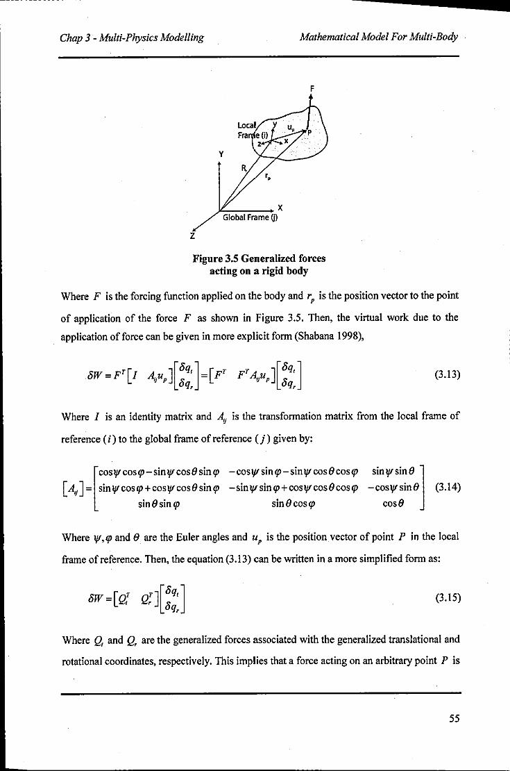
----------------------------------...... Chap 3 - Multi-Physics Modelling Mathematical Model For Multi-Body
z
y
r,
)L-,...,-- X Global Frame Q)
F
Figure 3.5 Generalized forces acting on a rigid body
Where F is the forcing function applied on the body and rp is the position vector to the point
of application of the force F as shown in Figure 3.5. Then, the virtual work due to the
application of force can be given in more explicit form (Shabana 1998),
(3.13)
Where I is an identity matrix and A.t is the transformation matrix from the local frame of
reference (i) to the global frame of reference (j) given by:
[
COSlJl cosq>- sinlJl cos6 sin q> -coslJl sin q>-sinlJl cos6 cosq>
[ Aij ] = sin lJI cos q> + cos lJI cos 6 sin q> - sin lJI sin q> + cos lJI cos 6 cos q> sin 6 sin q> sin 6 cos q>
sin lJI sin 6] -coslJlsin6 (3.14)
cos6
Where lJI,q> and 6 are the Euler angles and up is the position vector of point P in the local
frame of reference. Then, the equation (3.13) can be written in a more simplified form as:
(3.15)
Where Q, and Q, are the generalized forces associated with the generalized translational and
rotational coordinates, respectively. This implies that a force acting on an arbitrary point P is
55
Chap 3 - Multi-Physics Modelling Mathematical Model For Multi-Body
equivalent to a force that has the same magnitude acting at the origin of the body frame of
reference and a moment acting on the same body.
3.2.4 Constraining Reaction Forces
The first three terms on the LHS of the equation (3.4) deal with inertial, body and restoring or
restraining forces, respectively. The last term gives the reaction forces caused by the
constraining elements. The RHS of the equation represents all the non-conservative forces.
The n constraint functions for the different joints in the engine model are represented by
holonomic and non-holonomic functions. Holonomic functions are displacement dependent
constraints, such as the restriction of motion in a given direction; a revolute joint, which is
time independent or a coupling joint of the crankshaft and camshaft according to a set ratio.
These functions can be used to eliminate dependent coordinates of the system. Non
holonomic constraints restrict the kinematically possible values of velocities of the bodies of
the system such as constant velocity motion. In a non-holonomic system, some coordinates
may be independent, but their variations are dependent. These constraint functions can be
represented in matrix form as follows (Rahnejat 1998):
(3.\6)
For instance, for a revolute joint there are 5 constraining functions (such that Cn in equation
(3.4) gives 5 equations, n=5). The term aC/aq provides the effect of the constraint in
direction q. The reaction force in the direction q is given by An aC/aq, where An is the
Lagrange multiplier. However, there may be many contributing reactions in a given direction,
thus the summation mark in Lagrange's equation.
3.2.5 Kinematic System Development
In multi-body systems, kinematic constraint equations may exist because of mechanical joints
or specified motion trajectories. The constraint equations of the multi-body system for a
virtual displacement can be written as:
56
Chap 3 - Multi-Physics Modelling Mathematical Model For Multi-Body
(3.17)
Where Cq represents the constraint Jacobian matrix. For holonomic systems, all system
coordinates can be divided into a set of dependent coordinate qd and a set of independent
coordinates q,. For instance, for the engine system shown above either (}2 or R: can be
considered as the independent coordinates and the rest of coordinates can be considered as
the dependent coordinates. Thus, the vector q of generalized coordinates can be partitioned
and constraint equation can be written as:
(3.18)
Where Cqd and Cq, are the constraint Jacobian matrices associated with the dependent and
independent coordinates respectively. If the constraints of equation (3.17) are linearly
independent and Cqd is non-singular, (where its inverse exists), the dependent coordinates
can be written as:
(3.19)
The whole set of generalized coordinates can then be written in terms of independent
coordinates as follows:
[Oq,] [ I] oq= 0 = -C'C. oq, =Bq,
qd qd ql
(3.20)
Thus, the configuration or the state of a multi-body system, consisting of interconnected rigid
bodies, for a given virtual displacement of independent variables can be obtained using
equation (3.20).
3.2.6 Equations of Motion
The formulated kinetic energy for each body using equation (3.8) provides the inertial forces
of the system. The virtual work formulated in equation (3.15) provides all conservative and
non-conservative (body forces and external forces) generalized forces including damping
forces in the system. The vector of non-linear algebraic constraints, describing mechanical
57
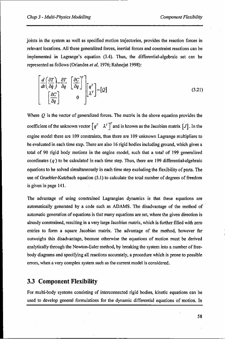
Chap 3 - Multi-Physics Modelling Component Flexibility
joints in the system as well as specified motion trajectories, provides the reaction forces in
relevant locations. All these generalized forces, inertial forces and constraint reactions can be
implemented in Lagrange's equation (3.4). Thus, the differential-algebraic set can be
represented as follows (Orlandea et ai, 1976; Rahnejat 1998):
d (aT) aT -- --dt aq aq
[~~] (3.21)
Where Q is the vector of generalized forces. The matrix in the above equation provides the
coefficient of the unknown vector [qT AT J and is known as the Jacobian matrix [Jj. In the
engine model there are 109 constraints, thus there are 109 unknown Lagrange multipliers to
be evaluated in each time step. There are also 16 rigid bodies including ground, which gives a
total of 90 rigid body motions in the engine model, such that a total of 199 generalized
coordinates (q) to be calculated in each time step. Thus, there are 199 differential-algebraic
equations to be solved simultaneously in each time step excluding the flexibility of parts. The
use of Gruebler-Kutzbach equation (5.1) to calculate the total number of degrees of freedom
is given in page 141.
The advantage of using constrained Lagrangian dynamics is that these equations are
automatically generated by a code such as ADAMS. The disadvantage of the method of
automatic generation of equations is that many equations are set, where the given direction is
already constrained, resulting in a very large Jacobian matrix, which is further filled with zero
entries to form a square Jacobian matrix. The advantage of the method, however far
outweighs this disadvantage, because otherwise the equations of motion must be derived
analytically through the Newton-Euler method, by breaking the system into a number of free
body diagrams and specifying all reactions accurately, a procedure which is prone to possible
errors, when a very complex system such as the current model is considered.
3.3 Component Flexibility
For multi-body systems consisting of interconnected rigid bodies, kinetic equations can be
used to develop general formulations for the dynamic differential equations of motion. In
58
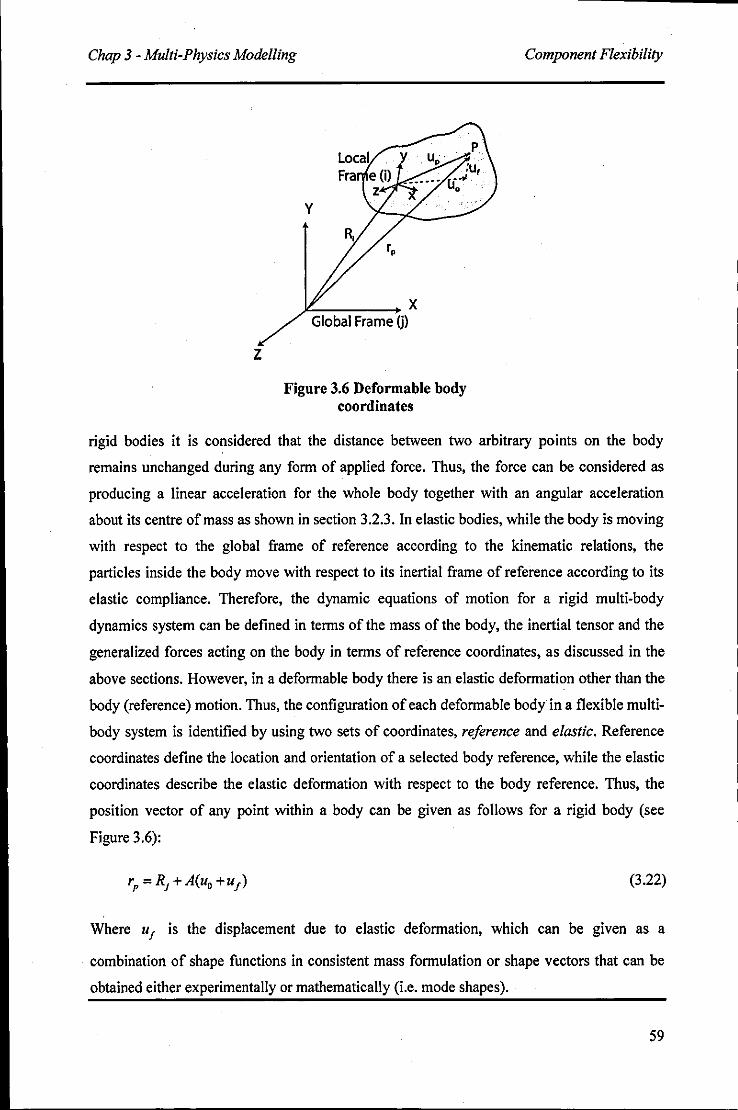
Chap 3 - Multi-Physics Modelling
z
y
J£-____ x Global Frame 0)
Figure 3.6 Deformable body coordinates
Component Flexibility
rigid bodies it is considered that the distance between two arbitrary points on the body
remains unchanged during any form of applied force. Thus, the force can be considered as
producing a linear acceleration for the whole body together with an angular acceleration
about its centre of mass as shown in section 3.2.3. In elastic bodies, while the body is moving
with respect to the global frame of reference according to the kinematic relations, the
particles inside the body move with respect to its inertial frame of reference according to its
elastic compliance. Therefore, the dynamic equations of motion for a rigid multi-body
dynamics system can be defined in terms of the mass of the body, the inertial tensor and the
generalized forces acting on the body in terms of reference coordinates, as discussed in the
above sections. However, in a deformable body there is an elastic deformation other than the
body (reference) motion. Thus, the configuration of each deformable body in a flexible multi
body system is identified by using two sets of coordinates, reference and elastic. Reference
coordinates define the location and orientation of a selected body reference, while the elastic
coordinates describe the elastic deformation with respect to the body reference. Thus, the
position vector of any point within a body can be given as follows for a rigid body (see
Figure 3.6):
(3.22)
Where U f is the displacement due to elastic deformation, which can be given as a
combination of shape functions in consistent mass formulation or shape vectors that can be
obtained either experimentally or mathematically (Le. mode shapes).
59
~----------------------------------....... Chap 3 - Multi-Physics Modelling Component Flexibility
3.3.1 Finite Element Analysis
In Finite element analysis a continuous flexible body is represented by a collection of
interconnected beams or elemental regions, with specified constitutive relations. A 3-
dimensional Bemoulli-Euler beam element in the body can be subjected to transverse,
bending and torsional motions, according to the forces applied on the body. The stiffness and
mass matrices for the beam element can be obtained using the beam theory considering
assumed shape functions as described in (Craig 1981). This mass matrix is called the
consistent mass matrix, as the same shape functions are used to obtain both the mass and
stiffness matrices. This leads to a coupling between translational coordinates and rotational
coordinates in the mass matrix, which creates difficulties in solving the mesh for mode
shapes. This problem can be eliminated by using the lumped mass model, which simply
assumes that the mass of the beam element is purely concentrated on its two end points,
which are nodal points of the mesh and these mesh points are connected by a spring, which
has a spring constant depending on the material parameters. These nodal displacements can
be transformed from the local coordinate system to the global coordinate system using the
transformation matrix T. Then, the forces associated with nodes can easily be transformed
into the global system using the virtual work approach, thus:
(3.23)
Where Fg,F; represent forces in the global and the local coordinate systems respectively. In a
similar manner using the potential energy, the stiffness matrix in global coordinates can be
obtained as:
(3.24)
where: subscripts g and I represent the global and local systems. Transformation for the mass
matrix can be obtained using the kinetic energy as:
(3.25)
These matrices can be assembled in such a way that system force, stiffness and mass matrices
can be formed. Then, the component stiffness and mass matrix becomes:
60
Chap 3 - Multi-Physics Modelling Component Flexibility
(3.26)
And:
(3.27)
Where ne and L, are the number of elements in the component and locater matrix as
described in (Craig 1981), respectively.
3.3.2 Boundary Conditions
Dynamic analysis requires boundary conditions to be stated, so that components can be
connected to each other applying an appropriate synthesis technique. When a flexible body is
constrained certain displacements are inhibited, the most straight-forward procedure for
enforcing such a condition is to partition the system into independent or active degrees-of
freedom (u, ) and dependent or constrained degrees-of-freedom (ud ), as shown below;
(3.28)
These can be obtained by partitioning component stiffness matrix (3.26) and mass matrix
(3.27) and the force vector (3.23). For instance, if ud = 0 due to imposed constraint
conditions, then the equation (3.28) can be written as:
(3.29)
Then, this equation can be solved for the eigenvalues and the corresponding eigenvectors,
giving the natural frequencies and mode shapes of the component (flexible body) under the
specified boundary conditions. Free-free normal modes can be obtained by equation (3.28),
simply putting the external force vector as zero, where no coordinates are constrained to the
body.
61
;---------------------------------......... Chap 3 - Multi-Physics Modelling Component Flexibility
3.3.3 Modal Transformation
The discretisation of a component into a finite element (FE) model represents an infinite
number of degrees of freedom with a finite, but very large number of finite element degrees
offreedom. The most important aspect of the FE analysis in dynamics problem, as outlined in
section 3.3.1, is that it can take into consideration small linear elastic deformations of the
flexible body relative to the local frame of reference. These elastic deformations or shape
vectors are the eigen-vectors of the body obtained, using equation (3.28). So that the linear
elastic deformations of the nodes can be given as a linear combination of shape vectors as:
n.
uj = "L,I/I,qm' =<tJqm (3.30) i=l
Where nm is the number of mode shapes, and the scalar factors of amplitudes qm are the
modal coordinates and modes 1/1, are included in the columns of the modal matrix, <tJ. A
reduced order model can be achieved by solving only for nm mode shapes, where nm < ne'
This concept is called modal super position which means that the behaviour of a component
with a very large number of nodal OOFs can be captured with a much smaller number of
modal OOFs. The nm mode shapes should be selected such that a good approximation of a
pre-determined frequency area of mode shapes is included.
3.3.4 Component Mode Synthesis
The modal transformation method described above can be used to transform a larger set of
physical coordinates uj to a smaller set of modal coordinates qm' In large scale multi-body
dynamics problems it is necessary to reduce the number of coordinates in this manner, if a
solution is to be obtained within a reasonable time. The Component Mode Synthesis is used
to couple all the sub-structures in the multi-body system in order to obtain a dynamic
response. The determination of the modal mass matrix M can be achieved according to the
Craig-Brampton (Craig and Brampton 1968) reduction method, which is one of the most
general methods for Component Mode Synthesis technique.
In this technique the component is basically divided into two sets ofOOFs. First, there are the
boundary OOFs (ud ), which are not subjected to modal superposition. These are the nodes
62
Chap 3 - Multi-Physics Modelling Component Flexibility
which are used to connect one body to another in structural coupling. Thus, these are
dependent on the other member of the assembled system. Second set of DOFs are the interior
DOFs (u,) which are subjected to modal superposition. These are the independent DOFs.
Additionany, two sets of mode shapes are defined as fonows:
I. The Constrained Modes (qJ are static shapes that are obtained by giving each of the
boundary degrees of freedom a unit displacement, while holding an other boundary
degrees of freedom fixed. There is a one-to-one correspondence between the modal
coordinates of the constrained modes and the displacement in the corresponding
boundary degrees of freedom, q, = ud • These modes can be obtained by setting /, to
zero and ud as an identity matrix of an order equivalent to the number of boundary
DOFs in equation (3.28).
2. The Fixed Boundary Normal Modes (q.), which are obtained by fixing the
boundary degrees of freedom and computing a solution for the eigen-value problem.
These modes can be obtained by setting /, to zero and ud to a zero matrix, as an the
boundary DOFs are fixed in equation (3.28). These modes define the modal expansion
of the interior degrees of freedom.
The relationship between the physical degrees of freedom, the Craig Brampton modes and
their modal coordinates is expressed as:
(3.3\)
where: I/!,c are the physical displacements of the interior degrees of freedom in the.
constrained modes, and I/!'n are the physical displacements of the interior degrees of freedom
in the normal modes. The first column of the matrix 1jI represents the constrained modes and
the second column represents the fixed normal modes. The modal superposition, as described
in section 3.3.3, can be used in matrix I/!,. to reduce the number of modal coordinates
accordingly.
63
Chap 3 - Multi-Physics Modelling Component Flexibility
The component generalized stiffness (keg) and mass (meg ) matrices are obtained through the
following transformations:
(3.32)
(3.33)
where the superscript I represents the component number. It is shown that the use of
constrained modes leads to an uncoupled stiffness matrix k~ in the component generalized
coordinates (Craig 1981). Constraint compatibility as discussed in section 3.2.5 in equation
(3.20) for a rigid multi-body system is used to synthesize the system stiffness matrix (K) and
the mass matrix (M), which are used in the Lagrange's equation of motion such as:
(3.34)
Where: keg is the component generalized stiffness for all components in the system, and:
(3.35)
Where: meg is the component generalized mass for all the components in the system and B is
the transformation matrix (see (Craig 1981)).
3.3.5 Creation of Flexible Bodies
In the engine model the crankshaft, connecting rod and flywheel are modelled as flexible
bodies. As it is explained in section 5.4.1, the experimental results show that the first natural
frequency of the piston is 9000Hz. However significant engine order excitations are starting
from 15Hz which is the half engine order and goes up to about 500Hz. Therefore with such
low excitation frequencies it is difficult to excite modes of natural frequencies of 9000Hz and
thus components with higher first natural frequencies such as piston are included into the
model as rigid bodies. Four nodded, three-dimensional tetrahedral elements have been used in
the super-element creation. The number of elements and their size has been kept large enough
64
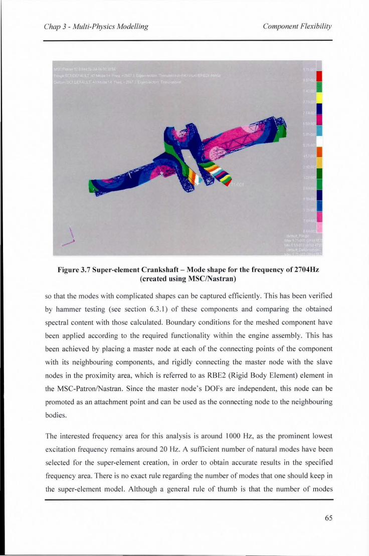
Chap 3 - Multi-Physics Modelling Component Flexibility
\ .....,
Figure 3.7 Super-element C ranks haft - Mode sha pe for the frequency of 2704Hz (c reated using MSClNastra n)
so that the modes with complicated shapes can be captured effic ient ly. Th is has been verified
by hammer testing (see section 6.3.1 ) of these components and comparing the obtained
spectra l content with those calculated. Boundary conditions for the meshed component have
been applied according to the requ ired functionality within the engine assembl y. This has
been ach ieved by placi ng a master node at each o f the connecting po ints of the component
with its neighbouring components, and rigidly connecting the master node with the slave
nodes in the proximi ty area , whi ch is referred to as RBE2 (Rigid Body Element) e lement in
the MSC-PatroniNastran. Since the master node's OOFs are independent, th is node can be
promoted as an attachment point and can be used as the connecting node to the neighbo uri ng
bodies.
The interested freque ncy area for this ana lysi s is a round 1000 Hz, as the prom inent lowest
exc itation frequency remains around 20 Hz. A sufficient number of natural modes have been
selected fo r the supe r-e lement creation, in order to obta in accurate resu lts in the spec ified
frequency area. There is no exact rul e regardi ng the number of modes that one shou ld keep in
the super-e lement model. A lthough a genera l rul e of thu mb is that the num ber of modes
65
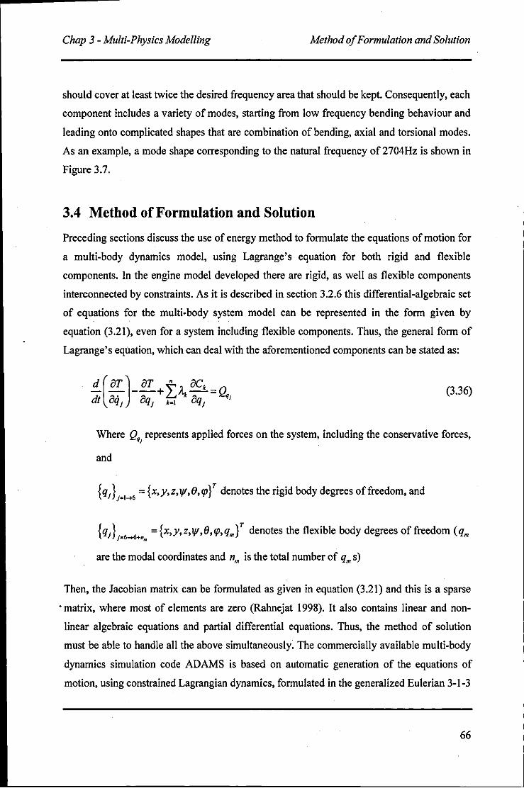
Chap 3 - Multi-Physics Modelling Method of Formulation and Solution
should cover at least twice the desired frequency area that should be kept. Consequently, each
component includes a variety of modes, starting from low frequency bending behaviour and
leading onto complicated shapes that are combination of bending, axial and torsional modes.
As an example, a mode shape corresponding to the natural frequency of 2704Hz is shown in
Figure 3.7.
3.4 Method of Formulation and Solution
Preceding sections discuss the use of energy method to formulate the equations of motion for
a multi-body dynamics model, using Lagrange's equation for both rigid and flexible
components. In the engine model developed there are rigid, as well as flexible components
interconnected by constraints. As it is described in section 3.2.6 this differential-algebraic set
of equations for the multi-body system model can be represented in the form given by
equation (3.21), even for a system including flexible components. Thus, the general form of
Lagrange's equation, which can deal with the aforementioned components can be stated as:
(3.36)
Where Qql represents applied forces on the system, including the conservative forces,
and
{qJ} = {x,y,z,lf/,(J,cp}T denotes the rigid body degrees of freedom, and 1=1-+6
{qJ}. ={x,y,z,lf/,(J,cp,qm}T denotes the flexible body degrees of freedom (qm 1' .. 6 .... 6+nm
are the modal coordinates and nm is the total number of qm s)
Then, the Jacobian matrix can be formulated as given in equation (3.21) and this is a sparse
• matrix, where most of elements are zero (Rahnejat 1998). It also contains linear and non
linear algebraic equations and partial differential equations. Thus, the method of solution
must be able to handle all the above simultaneously. The commercially available multi-body
dynamics simulation code ADAMS is based on automatic generation of the equations of
motion, using constrained Lagrangian dynamics, formulated in the generalized Eulerian 3-1-3
66
Chap 3 - Multi-Physics Modelling Method of Formulation and Solution
frame of reference. The compliance of flexible members is given by stiffness and damping
matrices obtained during the super-element modal analysis outlined in section 3.3.4.
3.4.1 LV Decomposition (Cholesky Factorisation)
For a set of linear equations which has to be repeatedly solved with different homogenous
terms, the LV decomposition is recommended (Orlandea et al. 1976; Rahnejat 1998). The LV
decomposition represents the replacement of the Jacobian matrix given in equation (3.21) by
a product of two triangular matrices, known as the lower and upper triangular matrices. In the
lower triangular matrix all the non-zero elements occupy the diagnol elements or below it,
whilst in the upper triangular matrix all such terms reside on or above the diagonal. Then:
[L].[U] = [J] (3.37)
Where [J] is the Jacobian matrix. Thus, equation (3.21) can be written as:
[J].{q A}' = {Q} (3.38)
The LV decomposition can be used to solve equation (3.38) as follows:
[J].{q A}T = ([L][U]).{q .?cl' =[L].([u].{q Af)={Q} (3.39)
The above equation can be represented by a pair of equations. The first step is to solve for
vector {V}, which can be found by:
[L].{V} ={Q} (3.40)
Then, the second step is to solve:
[U]{q,A}' ={V} (3.41)
These matrices are sufficient for the solution of a linear system. However, the set of equations
in the multi-body system presented here have non-linear equations as well. These non-linear
equations are solved using the Newton-Raphson method with Backward Differencing Method
(BDF).
67
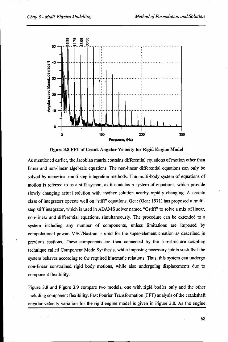
Chap 3 - Multi-Physics Modelling
50
o
Cl> ..,
100
Method of Formulation and Solution
200 300 Frequency (Hz)
Figure 3.8 FFT of Crank Angular Velocity for Rigid Engine Model
As mentioned earlier, the Jacobian matrix contains differential equations of motion other than
linear and non-linear algebraic equations. The non-linear differential equations can only be
solved by numerical multi-step integration methods. The multi-body system of equations of
motion is referred to as a stiff system, as it contains a system of equations, which provide
slowly changing actual solution with another solution nearby rapidly changing. A certain
class of integrators operate well on "stiff' equations. Gear (Gear 1971) has proposed a multi
step stiff integrator, which is used in ADAMS solver named "Gstiff' to solve a mix of linear,
non-linear and differential equations, simultaneously. The procedure can be extended to a
system including any number of components, unless limitations are imposed by
computational power. MSCINastran is used for the super-element creation as described in
previous sections. These components are then connected by the sub-structure coupling
technique called Component Mode Synthesis, while imposing necessary joints such that the
system behaves according to the required kinematic relations. Thus, this system can undergo
non-linear constrained rigid body motions, while also undergoing displacements due to
component flexibility.
Figure 3.8 and Figure 3.9 compare two models, one with rigid bodies only and the other
including component flexibility. Fast Fourier Transformation (FFD analysis of the crankshaft
angular velocity variation for the rigid engine model is given in Figure 3.8. As the engine
68
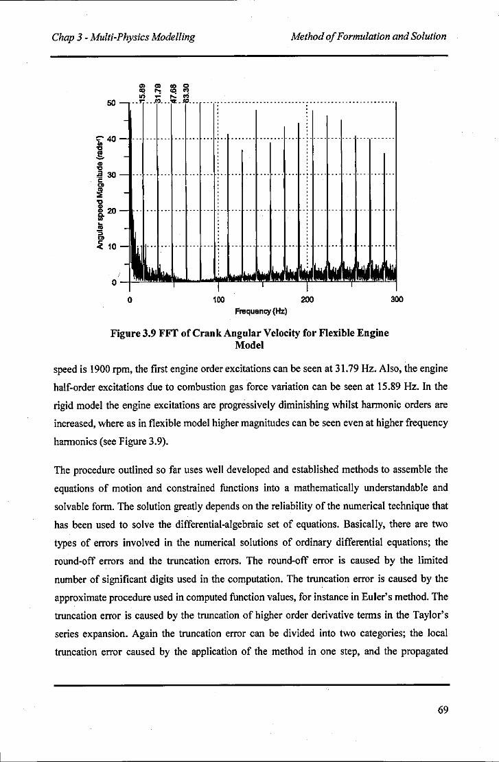
Chap 3 - Multi-Physics Modelling Method of Formulation and Solution
50
/
o o
'" ...
100 200 Frequency (Hz)
Figure 3.9 FFf of Crank Angular Velocity for Flexible Engine Model
300
speed is 1900 rpm, the first engine order excitations can be seen at 31.79 Hz. Also, the engine
half-order excitations due to combustion gas force variation can be seen at 15.89 Hz. In the
rigid model the engine excitations are progressively diminishing whilst harmonic orders are
increased, where as in flexible model higher magnitudes can be seen even at higher frequency
harmonics (see Figure 3.9).
The procedure outlined so far uses well developed and established methods to assemble the
equations of motion and constrained functions into a mathematically understandable and
solvable form. The solution greatly depends on the reliability of the numerical technique that
has been used to solve the differential-algebraic set of equations. Basically, there are two
types of errors involved in the numerical solutions of ordinary differential equations; the
round-off errors and the truncation errors. The round-off error is caused by the limited
number of significant digits used in the computation. The truncation error is caused by the
approximate procedure used in computed function values, for instance in Euler's method. The
truncation error is caused by the truncation of higher order derivative terms in the Taylor's
series expansion. Again the truncation error can be divided into two categories; the local
truncation error caused by the application of the method in one step, and the propagated
69
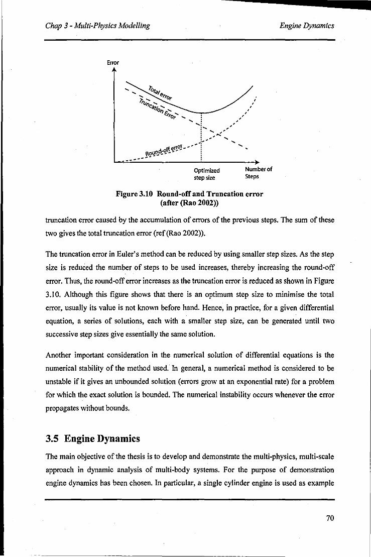
Chap 3 - Multi-Physics Modelling
Error
Optimized step size
Number of Steps
Figure 3.10 Round-off and Truncation error (after (Rao 2002»
Engine Dynamics
truncation error caused by the accumulation of errors of the previous steps. The sum of these
two gives the total truncation error (ref (Rao 2002».
-
The truncation error in Euler's method can be reduced by using smaller step sizes. As the step
size is reduced the number of steps to be used increases, thereby increasing the round-off
error. Thus, the round-off error increases as the truncation error is reduced as shown in Figure
3.1 O. Although this figure shows that there is an optimum step size to minimise the total
error, usualIy its value is not known before hand. Hence, in practice, for a given differential
equation, a series of solutions, each with a smalIer step size, can be generated until two
successive step sizes give essentially the same solution.
Another important consideration in the numerical solution of differential equations is the
numerical stability of the method used. In general, a numerical method is considered to be
unstable if it gives an unbounded solution (errors grow at an exponential rate) for a problem
for which the exact solution is bounded. The numerical instability occurs whenever the error
propagates without bounds.
3.5 Engine Dynamics
The main objective of the thesis is to develop and demonstrate the multi-physics, multi-scale
approach in dynamic analysis of multi-body systems. For the purpose of demonstration
engine dynamics has been chosen. In particular, a single cylinder engine is used as example
70
Chap 3 - Multi-Physics Modelling Engine Dynamics
for the investigations. Single cylinder engines are often used for developments and proof of
concepts, such as the introduction of new technologies and analysis techniques, therefore the
same approach is employed here. In dynamic analysis one objective is to understand the NVH
characteristics of the engine, and the other is its efficiency with regard to minimization of the
frictional and mechanical losses. Validation of any modelling method used in respect ofNVH
characteristics can be carried by comparing the results with closed form analytical solutions,
as highlighted by (Rahnejat 1998). This approach is undertaken, and complemented later with
experimental studies (see chapter 6).
3.5.1 Translational Inertial Imbalance
Among most of the engine parts the piston-connecting rod-crank sub-system can be regarded
as the most important system in terms of dynamics. The basic function of this sub-system is
to convert the reciprocating applied gas force into a rotational moment (torque) applied to the
crankshaft. This system can be considered as one, having two degrees of freedom: rotation of
the crankshaft and the reciprocating motion of the piston. The rotation of the crank is pre
determined by geometric constraints, thus is kinematic. Figure 3.11 shows a simple model of
a single cylinder engine.
In order to yield a realistic solution from this simplified model the articulating mass of the
connecting rod must be divided into two concentrated masses, one at the piston, which is
purely translating, and the other at the crankshaft, which is purely rotating. Thus, the
translating mass of the connected rod and the piston is given by m, and the rotating mass of
the connecting rod and crankshaft pin is given by m2 as shown in Figure 3.11.
The combustion force represented by F;, induces a torque on the crankshaft equivalent to:
T = F;d P CosrfJ
d can be replaced by le and re' which are engine design parameters, and:
d = (le + re)SinrfJe
(3.42)
(3.43)
71
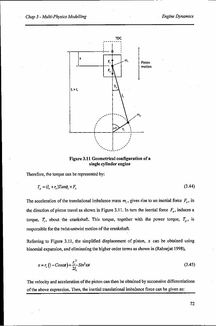
Chap 3 - Multi-Physics Modelling
Ix
, , , • ,
Toe ,a. _______ , , I , , , , , ,
~ :
F. m,
F,
,'---t-··.. /m, ", I ..... , , ,
----------~-------• , • • •
", "
i ' , i ,,/
.... -'-_ ...... '
Piston motion
Figure 3.11 Geometrical configuration of a single cylinder engine
Therefore, the torque can be represented by:
Engine Dynamics
(3.44)
The acceleration of the translational imbalance mass m" gives rise to an inertial force F., in
the direction of piston travel as shown in Figure 3.11. In turn the inertial force F., induces a
torque, T" about, the crankshaft. This torque, together with the power torque, Tp ' is
responsible for the twist-untwist motion of the crankshaft.
Referring to Figure 3.11, the simplified displacement of piston, x can be obtained using
binomial expansion, and eliminating the higher order terms as shown in (Rahnejat 1998),
r2 x = r, (\- Coscat) + -'-Sin2 cat
21, (3.45)
The velocity and acceleration of the piston can then be obtained by successive differentiations
of the above expression. Then, the inertial translational imbalance force can be given as:
72
Chap 3 - Multi-Physics Modelling Engine Dynamics
(3.46)
Substituting the moment arm d (equation (3.43)) in terms of vertical distance between the
instantaneous piston position and the crank centre, and assuming that rfJc is small, and
ignoring higher order terms, the induced inertial torque can be represented as:
(3.47)
The practical implications of the above simplified analysis is that due to the translational
imbalance introduced by the piston acceleration and the connecting rod articulation, there
exists a vibration spectrum that contains all the multiples of engine orders (co,2co,3co, .... ).
The fact that the higher order terms do not appear in the final results here is due to the limited
binomial expansion in the derivation process. These frequencies can easily be seen in the FFT
of crank angular speeds shown in Figure 3.8 and Figure 3.9. However, it is clear that the
influence from higher order terms is quite small compared with the effects from the first few
engine order harmonics for a rigid body system. However, one should not ignore the higher
order terms when considering flexible bodies, as a small excitation can be significant at
resonant conditions.
3.5.2 Power Torque Fluctuations
The power torque fluctuations can be expressed as a Fourier series, based upon a complete
engine cycle, which corresponds to a 720° degree crank angle rotation for a four-stroke
engine. Therefore, the power torque Tp in equation (3.44) can be represented in the form of
the kth harmonic of the engine cycle frequency as in (Rahnejat 1998), thus:
T - Fik ;k("-</I)/2 jlr. - c e (3.48)
Where j denotes the cylinder identity number. When the equation is simplified for a single
cylinder engine by letting j = I and 1JI = 0 (the phase shift), it can be written as:
(3.49)
73
Chap 3 - Multi-Physics Modelling Engine Dynamics
It can be observed that the power torque for a single cylinder engine is a function of the
varying combustion force power series, with contributions at all multiples of m. Clearly odd
values of k give rise to half-order contributions, whilst the even values of k yield whole
multiples of engine order. Thus, the effect of the engine whole order multiples clearly
coincides with the inertial imbalance. The half-engine order responses are quite clear in
Figure 3.8 and Figure 3.9, especially in the lower engine orders. As frequency increases, the
effect is attenuated.
3.5.3 Rotational Imbalance
Rotational imbalance is caused by mass m2 , with the mass of the crankpin rotating at a
distance to the centre of rotation of the crankshaft. This rotational imbalance induces a
horizontal inertial force in the y-direction as:
F" = -m2rm2 SinOJt (3.50)
It is possible to reduce or eliminate this horizontal inertial force by employing
counterbalancing masses along the crankshaft. The vertical imbalance component will always
remain in a single cylinder engine, although it can be reduced in multi-cylinder engines by
properly adjusted phase angles.
The simple analysis highlighted above is particularly useful in the identification of the
spectral contents of the both experimentally and numerically obtained frequency domain
responses, as they are the most prominent excitations in a single cylinder engine. The
experimentally obtained vibration spectrum is very complex, and contains not only whole and
half-order multiples of engine order, but also other contributions that often appear at rather
strange multiples of engine order.
It is obvious that analytical methods employ various simplifications in order to obtain a
simple solution. For instance, the elimination of higher order terms in the binomial expansion
is already shown to lead to omission of certain higher engine order contributions. Thus, one
cannot completely rely on analytical results. Therefore a numerical model must be validated
against experimental findings as far as possible, that increases the level of confidence of the
model. On the other hand, there are also some limitations in experimentation as it depends on
various factors such as accuracy of instrumentation, environmental effects and physical
74
Chap 3 - Multi-Physics Modelling Engine Dynamics
limitations like accessibility, which are discussed later in Chapter 06. Therefore, special care
must be taken when selecting experimental measurements during a model validation.
Conversely, such a validated numerical model can be used to predict the system behaviour,
which otherwise cannot be measured (forces at gudgeon pin) or expensive measuring
techniques (cylinder liner force) has to be utilized.
In this mUlti-physics numerical model development, so far the emphasis is put on the
development of a rigid body system, incorporating component flexibility. It is also important
to note that the basic joint primitives are used for all constraint formulations, which is not
exactly the physical situation in actual systems. In particular in IC engines, lubricated
contacts, such as crankshaft support engine journal bearings, piston-cylinder interactions are
quite complicated than simple kinematic constraints often used in traditional multi-body
analyses. Proper use of tribological contacts must be made instead of merely introducing
constraints. These provide frictional and contact forces, which may be regarded as forms of
restraint rather than rigid constraints. The next chapter is devoted to basic physical
approaches for development and use of lubricated contacts within the multi-physics analysis
framework.
75
Chap 4 - Tribological contacts Introduction
4 TRIBOLOGICAL CONTACTS
4.1 Introduction
This chapter provides the theoretical basis for lubricated contacts included in the multi
physics model of le engines. The model comprises a number of such load bearing
conjunctions. These include the sliding contact of piston skirt-to-cylinder bore, which is a
partially conforming contact, with a fairly large contact area. The contact of piston
compression ring against the cylinder wall is also considered, which has a much smaller
contact area than that of the piston skirt, as well as a lower degree of conformity and smaller
clearance. Thus, the piston ring-to-cylinder wall contact is subjected to a more severe
lubrication condition. The model also includes the closely conforming contacts in the main
crankshaft engine journal bearings (for three such conjunctions). In a real engine there are
clearly other lubricated contacts, such as the highly loaded non-conforming cam-tappet
conjunction, their higher loaded (than the support journal bearings) contacts of the big-end
and small end connecting rod bearings. The model, as described in the previous chapter
pertains to the piston-connecting rod-crank sub-system, thus it does not take into account the
camshaft and valve train system. Furthermore, the connecting rod bearings are represented by
kinematic constraints in order to reduce the model complexity. However, the integrated
methodology reported here can easily be expanded to take these into account (see suggestions
for future work in chapter 8).
In the engine model, the crankshaft is connected to the engine block via the main engine
bearings, which in the case of the test engine used in this thesis (a Ricardo E6 single cylinder
engine) can be treated as a hydrodynamic journal bearing. Main bearing has to withstand
against the transmitted effect of high combustion gas forces and the reciprocating inertia of
the articulated mass of the connecting rod and the piston assembly. In general, the maximum
number of such main support bearings would be the number of cylinders plus one. One
bearing can be placed in between each set of pistons and two at each end of the crankshaft. In
low power engines the number of bearings could be less than its maximum number. Most of
modem engines are fitted with journal bearings. As the surface area between the two contacts
is large (i.e. a closely conforming contact) it can withstand very high loads. The frictional
76
Chap 4 - Tribological contacts Lubrication Regimes
loss in journal bearings is comparatively high and as a consequence high perfonnance
engines such as those in motorsports are fitted with roller or needle bearings, which are very
expensive and .less durable. A coherent lubricating film must be present to keep the two
contacting surfaces apart and guard against incidence of wear. Therefore, there is a designed
gap between the mating surfaces, referred to as the clearance gap. This clearance gap is filled
with the lubricant due to a combination of entraining motion of the lubricant into the resulting
wedge shape and by squeeze film retention due to load. As a result the crankshaft "floats" on
this film of fluid. Journal bearings are designed to support shafts and to carry radial loads
with minimum power loss and wear.
Fluid film lubrication can broadly be categorized into two regimes, namely hydrodynamics
and elastohydrodynamic. Hydrodynamic regime of lubrication occurs mostly at low to
medium loads and moderate to high speeds of entraining motion. Thus, the generated
pressures are insufficient to cause local defonnation of contacting elastic solids. Such
conditions are prevalent in closely or partially confonning contacts with relatively large load
bearing surface areas, such as in journal bearings. Under elastohydrodynamic regime of
lubrication the contact area is usually very small, mostly as a result of non-confonning
mating surfaces, and the forces acting are sufficiently high to cause local defonnation in the
contact zone. Frictional losses in fluid film lubrication are due to viscous shearing effect in
the lubricant film under sliding conditions. Thus, the viscosity of the lubricant and the film
thickness play crucial roles. If the film thickness is bridged, asperity interactions also play an
important role, and a mixed regime oflubrication results.
4.2 Lubrication Regimes
With regard to the contacts considered in this thesis, three regimes of lubrication must be
considered. These are mixed lubrication, hydrodynamic and fluid film lubrication. The fluid
film lubrication can be divided into hydrodynamic and elastohydrodynamic lubrication
depending on the pressures involved. In the multi-body dynamics model, hydrodynamic
regime of lubrication is considered for the engine bearings. This is true for the particular
engine under consideration (i.e. the Ricardo E6 engine). The bearing bushing is considered
thick, and made of steel, thus not subject to defonnation. In some modem engines, the
bearing bushing is a shell, made of materials of low elastic modulus such as tin-based alloys.
77
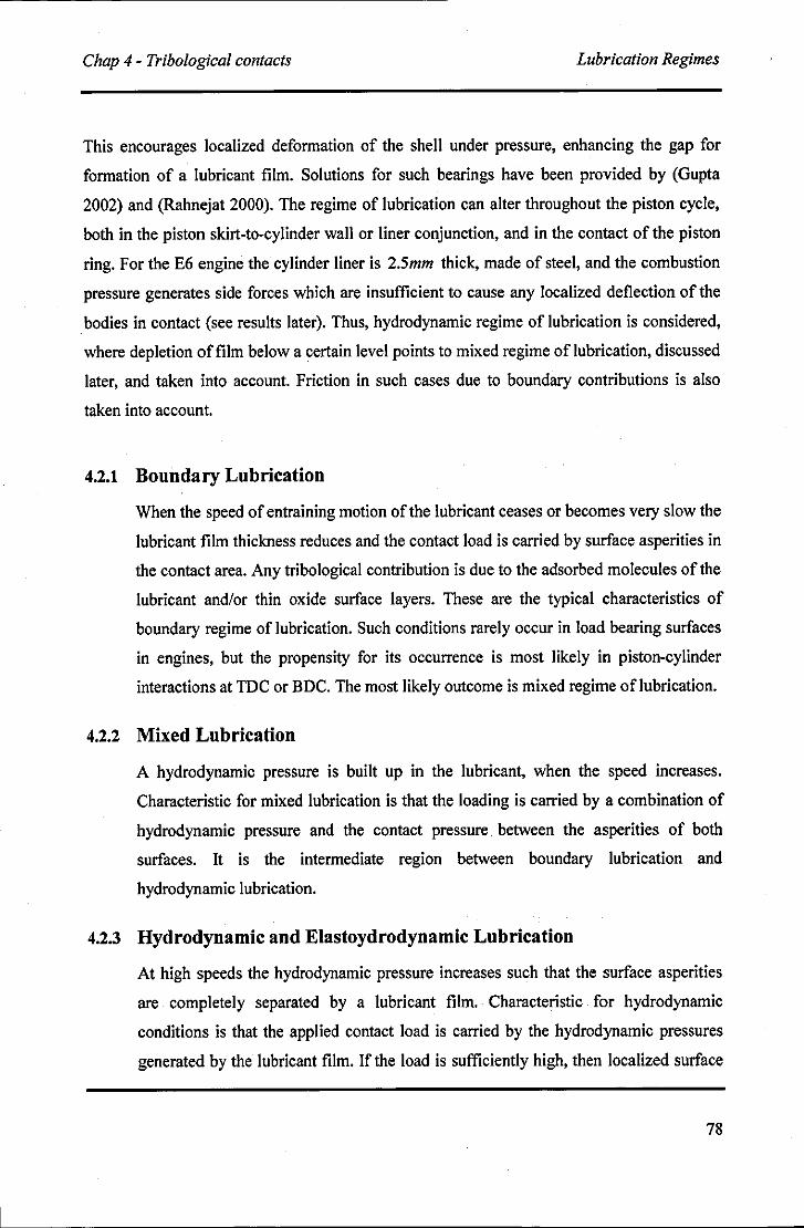
Chap 4 - Tribological contacts Lubrication Regimes
This encourages localized deformation of the shell under pressure, enhancing the gap for
formation of a lubricant film. Solutions for such bearings have been provided by (Gupta
2002) and (Rahnejat 2000). The regime of lubrication can alter throughout the piston cycle,
both in the piston skirt-to-cylinder wall or liner conjunction, and in the contact of the piston
ring. For the E6 engine the cylinder liner is 2.5mm thick, made of steel, and the combustion
pressure generates side forces which are insufficient to cause any localized deflection of the
bodies in contact (see results later). Thus, hydrodynamic regime of lubrication is considered,
where depletion of film below a certain level points to mixed regime of lubrication, discussed
later, and taken into account. Friction in such cases due to boundary contributions is also
taken into account.
4.2.1 Boundary Lubrication
When the speed of entraining motion of the lubricant ceases or becomes very slow the
lubricant film thickness reduces and the contact load is carried by surface asperities in
the contact area. Any tribological contribution is due to the adsorbed molecules of the
lubricant and/or thin oxide surface layers. These are the typical characteristics of
boundary regime of lubrication. Such conditions rarely occur in load bearing surfaces
in engines, but the propensity for its occurrence is most likely in piston-cylinder
interactions at TDC or BDC. The most likely outcome is mixed regime of lubrication.
4.2.2 Mixed Lubrication
A hydrodynamic pressure is built up in the lubricant, when the speed increases.
Characteristic for mixed lubrication is that the loading is carried by a combination of
hydrodynamic pressure and the contact pressure between the asperities of both
surfaces. It is the intermediate region between boundary lubrication and
hydrodynamic lubrication.
4.2.3 Hydrodynamic and Elastoydrodynamic Lubrication
At high speeds the hydrodynamic pressure increases such that the surface asperities
are completely separated by a lubricant film .. · Characteristic for hydrodynamic
conditions is that the applied contact load is carried by the hydrodynamic pressures
generated by the lubricant film. If the load is sufficiently high, then localized surface
78
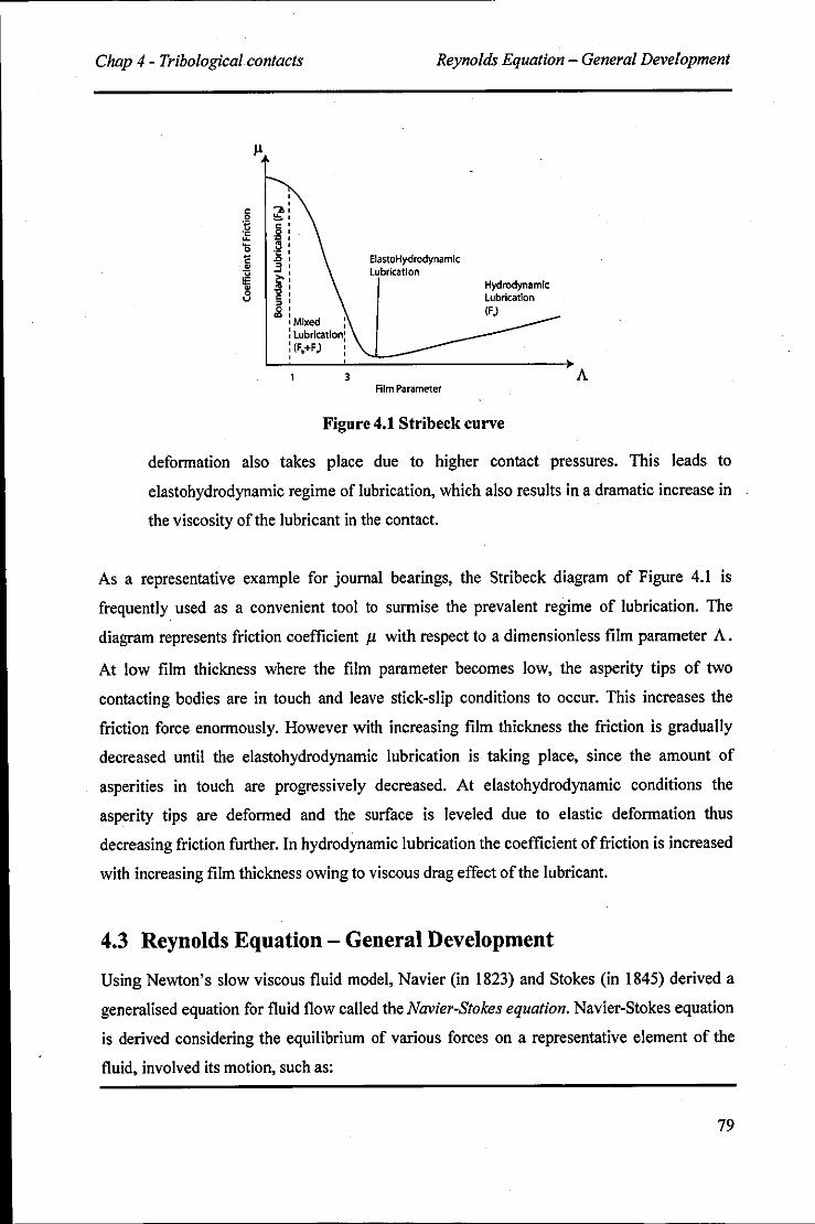
Chap 4 - Tribological contacts Reynolds Equation - General Development
J.I
, , ." , ~,
0' 0'
; I
3' .;: , .0 ,
3' ~: ~,
"0,
~: -Mixed : : lubrication: : (Ft+F) ,
3
ElastoHydrodynamlc Lubrication
Film Parameter
Hydrodynamic Lubrication (F)
Figure 4.1 Stribeck curve
A
deformation also takes place due to higher contact pressures. This leads to
elastohydrodynamic regime of lubrication, which also results in a dramatic increase in
the viscosity of the lubricant in the contact.
As a representative example for journal bearings, the Stribeck diagram of Figure 4.1 is
frequently used as a convenient tool to surmise the prevalent regime of lubrication. The
diagram represents friction coefficient 11 with respect to a dimensionless film parameter A.
At low film thickness where the film parameter becomes low, the asperity tips of two
contacting bodies are in touch and leave stick-slip conditions to occur. This increases the
friction force enormously. However with increasing film thickness the friction is gradually
decreased until the elastohydrodynamic lubrication is taking place, since the amount of
asperities in touch are progressively decreased. At elastohydrodynamic conditions the
asperity tips are deformed and the surface is leveled due to elastic deformation thus
decreasing friction further. In hydrodynamic lubrication the coefficient of friction is increased
with increasing film thickness owing to viscous drag effect of the lubricant.
4.3 Reynolds Equation - General Development
Using Newton's slow viscous fluid model, Navier (in 1823) and Stokes (in 1845) derived a
generalised equation for fluid flow called the Navier-Stokes equation. Navier-Stokes equation
is derived considering the equilibrium of various forces on a representative element of the
fluid, involved its motion, such as:
79
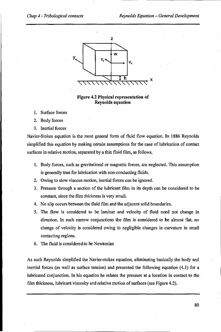
Chap 4 - Tribological contacts Reynolds Equation - General Development
y
I. Surface forces
2. Body forces
3. Inertial forces
z
w
Figure 4.2 Physical representation of Reynolds equation
Navier-Stokes equation is the most general fonn of fluid flow equation. In 1886 Reynolds
simplified this equation by making certain assumptions for the case of lubrication of contact
surfaces in relative motion, separated by a thin fluid film, as follows.
I. Body forces, such as gravitational or magnetic forces, are neglected. This assumption
is generally true for lubrication with non-conducting fluids.
2. Owing to slow viscous motion, inertial forces can be ignored.
3. Pressure through a section of the lubricant film in its depth can be considered to be
constant, since the film thickness is very small.
4. No slip occurs between the fluid film and the adjacent solid boundaries.
5. The flow is considered to be laminar and velocity of fluid need not change in
direction. In such narrow conjunctions the film is considered to be almost flat, no
change of velocity is considered owing to negligible changes in curvature in small
contacting regions.
6. The fluid is considered to be Newtonian
As such Reynolds simplified the Navier-stokes equation, eliminating basically the body and
inertial forces (as well as surface tension) and presented the following equation (4.1) for a
lubricated conjunction. In his equation he relates the pressure at a location in contact to the
film thickness, lubricant viscosity and relative motion of surfaces (see Figure 4.2).
80
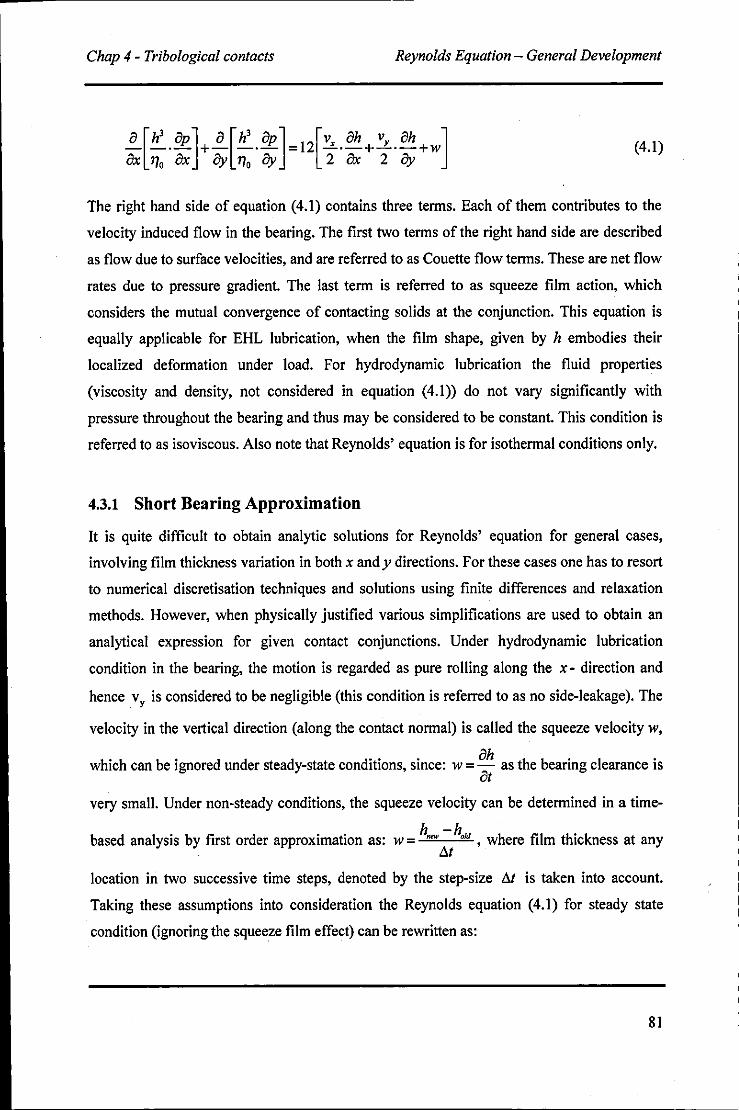
Chap 4 - Tribological contacts Reynolds Equation - General Development
(4.1)
The right hand side of equation (4.1) contains three terms. Each of them contributes to the
velocity induced flow in the bearing. The first two terms of the right hand side are described
as flow due to surface velocities, and are referred to as Couette flow terms. These are net flow
rates due to pressure gradient. The last term is referred to as squeeze film action, which
considers the mutual convergence of contacting solids at the conjunction. This equation is
equally applicable for EHL lubrication, when the film shape, given by h embodies their
localized deformation under load. For hydrodynamic lubrication the fluid properties
(viscosity and density, not considered in equation (4.1» do not vary significantly with
pressure throughout the bearing and thus may be considered to be constant. This condition is
referred to as isoviscous. Also note that Reynolds' equation is for isothermal conditions only.
4.3.1 Short Bearing Approximation
It is quite difficult to obtain analytic solutions for Reynolds' equation for general cases,
involving film thickness variation in both x and y directions. For these cases one has to resort
to numerical discretisation techniques and solutions using finite differences and relaxation
methods. However, when physically justified various simplifications are used to obtain an
analytical expression for given contact conjunctions. Under hydrodynamic lubrication
condition in the bearing, the motion is regarded as pure rolling along the x - direction and
hence Vy is considered to be negligible (this condition is referred to as no side-leakage). The
velocity in the vertical direction (along the contact normal) is called the squeeze velocity w,
which can be ignored under steady-state conditions, since: w = ah as the bearing clearance is at very small. Under non-steady conditions, the squeeze velocity can be determined in a time
based analysis by first order approximation as: w = h_ - h"d , where film thickness at any M
location in two successive time steps, denoted by the step-size M is taken into account.
Taking these assumptions into consideration the Reynolds equation (4.1) for steady state
condition (ignoring the squeeze film effect) can be rewritten as:
81
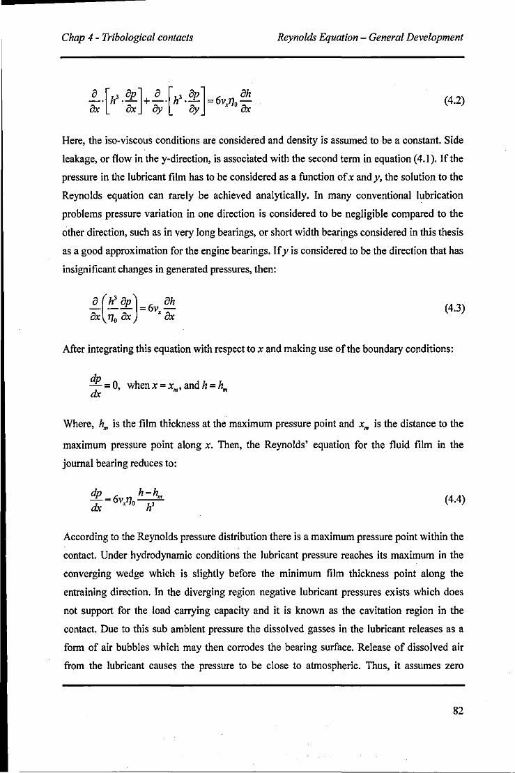
Chap 4 - Tribological contacts Reynolds Equation - General Development
(4.2)
Here, the iso-viscous conditions are considered and density is assumed to be a constant. Side
leakage, or flow in the y-direction, is associated with the second term in equation (4.1). If the
pressure in the lubricant film has to be considered as a function of x and y, the solution to the
Reynolds equation can rarely be achieved analytically. In many conventional lubrication
problems pressure variation in one direction is considered to be negligible compared to the
other direction, such as in very long bearings, or short width bearings considered in this thesis
as a good approximation for the engine bearings. If y is considered to be the direction that has
insignificant changes in generated pressures, then:
~(h3 BP)=6V Bh Bx 110 Bx x ax (4.3)
After integrating this equation with respect to x and making use of the boundary conditions:
dp -0 h dh h - , wenx=xm,an = m dx
Where, hm is the film thickness at the maximum pressure point and xm is the distance to the
maximum pressure point along x. Then, the Reynolds' equation for the fluid film in the
journal bearing reduces to:
(4.4)
According to the Reynolds pressure distribution there is a maximum pressure point within the
contact. Under hydrodynamic conditions the lubricant pressure reaches its maximum in the
converging wedge which is slightly before the minimum film thickness point along the
entraining direction. In the diverging region negative lubricant pressures exists which does
not support for the load carrying capacity and it is known as the cavitation region in the
contact. Due to this sub ambient pressure the dissolved gasses in the lubricant releases as a
form of air bubbles which may then corrodes the bearing surface. Release of dissolved air
from the lubricant causes the pressure to be close to atmospheric. Thus, it assumes zero
82
Chap 4 - Tribological contacts Reynolds Equation - General Development
pressure in the cavitated region. With contact geometry, kinematics and lubricant rheology
solutions to Reynolds equation can be sought. Solutions can be obtained by direct integration
of Reynolds equation analytically, if for the prevailing conditions it can be reduced to a one
dimensional problem. This means the variatiori along the other contact dimension can be
considered as negligible. For example, if one of the contact dimensions x or y is considered
to be infinitely long, its effects upon variation of generated pressure distribution is negligible,
or in other words the pressure remains constant in that direction. This condition is known as
Long Bearing Approximation. If this condition persists, then there is negligible side leakage
as assumed earlier. Long bearing approximation is an applicable assumption for bearings with
the diameter to length (some times referred to as width) ratio: (2%), being less than 0.5 as
highlighted by Sommerfeld and detailed by Cameron (Cameron 1966). Solutions for all
tribological contacts pertaining to long or short bearing assumptions can be found analytically
if the film shape is described geometrically. The same, of course, is true for engine journal
bearings (Hamrock et ai, 2004). Yet the expression is not particularly useful as an analytical
solution, since it is difficult to obtain the load components by further integration. In 1904
Sommerfeld neatly overcome this integration problem by introducing a mathematical
relationship called the "Sommerfeld substitution" as it is discussed in Chapter 2. The use of
Sommerfeld substitution leads to evaluation of pressure distribution for the complete journal.
However, the pressure distribution is skew symmetric, generating positive pressures in the
converging film (0 ~ a ~ n) and negative pressures in the diverging gap (n ~ a ~ 2n), the
integration of which leads to no load carrying capacity. Thus, half-Sommerfeld condition is
used, where the negative pressures are ignored. Once the pressure is known the load
components can be calculated. It is convenient to determine the components of the resultant
load along and perpendicular to the line of centres (this is the line joining the centre of the
journal to the geometric centre of the bushing).
Then, the force along the line of centres becomes zero due to the symmetry of the pressure
distribution with use of full-Sommerfeld condition, which is not practical. This demonstrates
that for a full-Sommerfeld solution the resultant normal load acts at right angles to the line of
centres, that is the attitude angle is 900• So that as the load is applied the shaft centre moves
away from the bearing centre at right angles to the load vector. To overcome these difficulties
the half-Sommerfeld solution, which neglects the negative pressures inside the contact
83
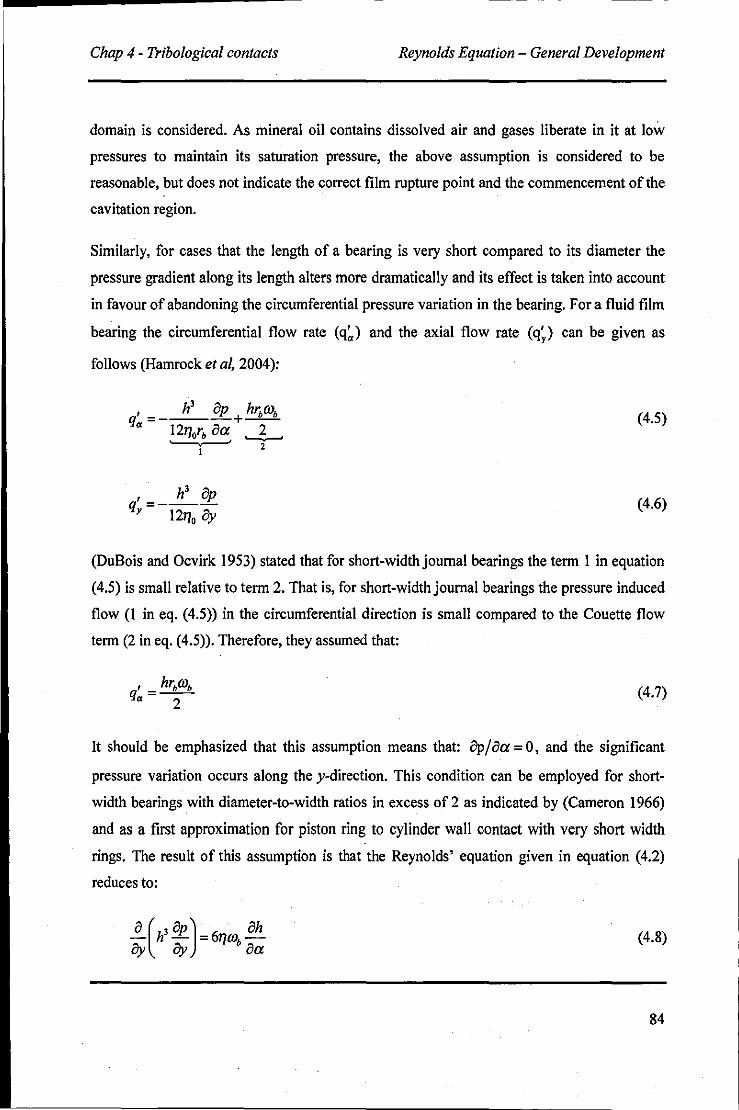
Chap 4 - Tribological contacts Reynolds Equation - General Development
domain is considered. As mineral oil contains dissolved air and gases liberate in it at low
pressures to maintain its saturation pressure, the above assumption is considered to be
reasonable, but does not indicate the correct film rupture point and the commencement of the
cavitation region.
Similarly, for cases that the length of a bearing is very short compared to its diameter the
pressure gradient along its length alters more dramaticaIly and its effect is taken into account
in favour of abandoning the circumferential pressure variation in the bearing. For a fluid film
bearing the circumferential flow rate (q~) and the axial flow rate (q~) can be given as
fo\1ows (Hamrock et aI, 2004):
(4.5)
(4.6)
(DuBois and Ocvirk 1953) stated that for short-width journal bearings the term 1 in equation
(4.5) is sma\1 relative to term 2. That is, for short-width journal bearings the pressure induced
flow (1 in eq. (4.5)) in the circumferential direction is sma\1 compared to the Couette flow
term (2 in eq. (4.5)). Therefore, they assumed that:
(4.7)
It should be emphasized that this assumption means that: Op/8a = 0, and the significant
pressure variation occurs along the y-direction. This condition can be employed for short
width bearings with diameter-to-width ratios in excess of 2 as indicated by (Cameron 1966)
and as a first approximation for piston ring to cylinder waIl contact with very short width
rings. The result of this assumption is that the Reynolds' equation given in equation (4.2)
reduces to:
8 (h38P)_6 8h - - - 1]OJb -ay ay 8a (4.8)
84
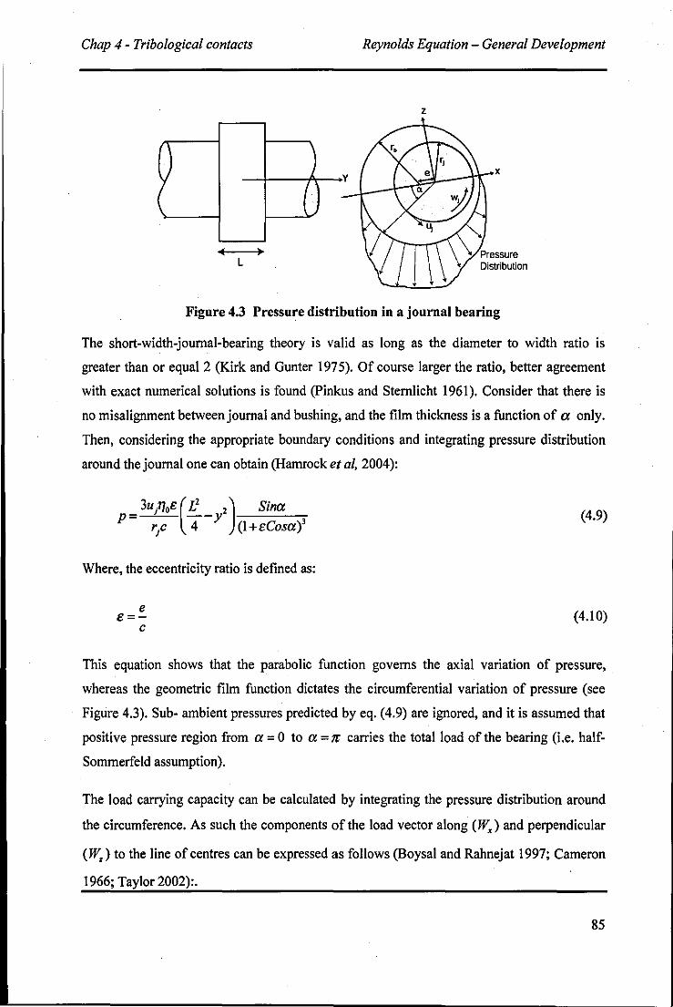
Chap 4 - Tribological contacts Reynolds Equation - General Development
z
, .. L
Figure 4.3 Pressure distribution in a journal bearing
The short-width-journal-bearing theory is valid as long as the diameter to width ratio is
greater than or equal 2 (Kirk and Gunter 1975). Of course larger the ratio, better agreement
with exact numerical solutions is found (Pinkus and Sternlicht 1961). Consider that there is
no misalignment between journal and bushing, and the film thickness is a function of a only.
Then, considering the appropriate boundary conditions and integrating pressure distribution
around the journal one can obtain (Hamrock et al. 2004):
3u/1oe(L2 2) Sina p --y rp 4 (l+eCosa)3
Where, the eccentricity ratio is defined as:
e e=
c
(4.9)
(4.10)
This equation shows that the parabolic function governs the axial variation of pressure,
whereas the geometric film function dictates the circumferential variation of pressure (see
Figure 4.3). Sub- ambient pressures predicted by eq. (4.9) are ignored, and it is assumed that
positive pressure region from a = 0 to a = 7r carries the total load of the bearing (Le. half
Sommerfeld assumption).
The load carrying capacity can be calculated by integrating the pressure distribution around
the circumference. As such the components of the load vector along (W,) and perpendicular
(W,) to the line of centres can be expressed as follows (Boysal and Rahnejat 1997; Cameron
1966; Taylor 2002):.
85
Chap 4 - Tribological contacts Reynolds Equation - General Development
w, Ub7JOE ne 4c' (l-e')%
(4.11)
(4.12)
The altitude angle lI' , which is the angle between line of centres and the resultant force can
be given as,
n.Jl-e' tanll'=~::""""::
e (4.13)
The friction or the traction force in a lubricated conjunction is generated due to the relative
sliding motion of the two contacting surfaces. Here U j refers to the surface velocity of the
journal, whereas ub is the surface velocity of the bearing bushing.
LI2~hap 7J(Uj -Ub)r F= f --+ dy
-LI2 0 2 ax h (4.14)
With the short bearing approximation, : = 0 (as already explained above), thus after
integration:
(4.15)
The first quotient is known as the "Petroff friction", which would be present where the
journal and the bearing shell are concentric (i.e. rotating cylinder friction). The second
quotient is termed the "PetroffMultiplier". Note also the higher the e, the greater the friction
and hence more heat is generated. The negative sign indicates opposition to the direction of
entraining motion. Thus, an estimate of coefficient of friction can be obtained as:
(4.16)
86
~~~~~~~--~----------------......... Chap 4 - Tribological contacts Reynolds Equation - General Development
4.3.2 Stiffness of Journal Bearing
The total bearing load (W) can be obtained as:
(4.17)
Thus:
(4.18)
Equation (4.18) provides the relationship between load and eccentricity. A more common
way of expressing this relationship is in terms of the dimension less group called the
Sommerfeld number (S) such as:
W c' S=--- (4.19)
NDLT/ rf
Note that r, '" rh = % and N is in rev/so In terms of S, equation (4.18) for a short width
bearing, can be represented:
(4.20)
From this equation it is clear that s=f{e,Yv). It can be seen from the definition of Sin
equation (4.19), that SocW. Also by definition hm =c(l-e). Taking these relations into
consideration the variation of S with the minimum film thickness hm for a given Yv ratio
can be obtained, which is effectively the load-deflection curve as shown in Figure 4.4. The
figure shows that the bearing is stiffest in the vicinity of the minimum film thickness and
softer at both ends.
As mentioned in (Gohar 1988) a bearing can simplifY into a simple mass spring arrangement.
Then, the natural frequency of the system can be given as:
87
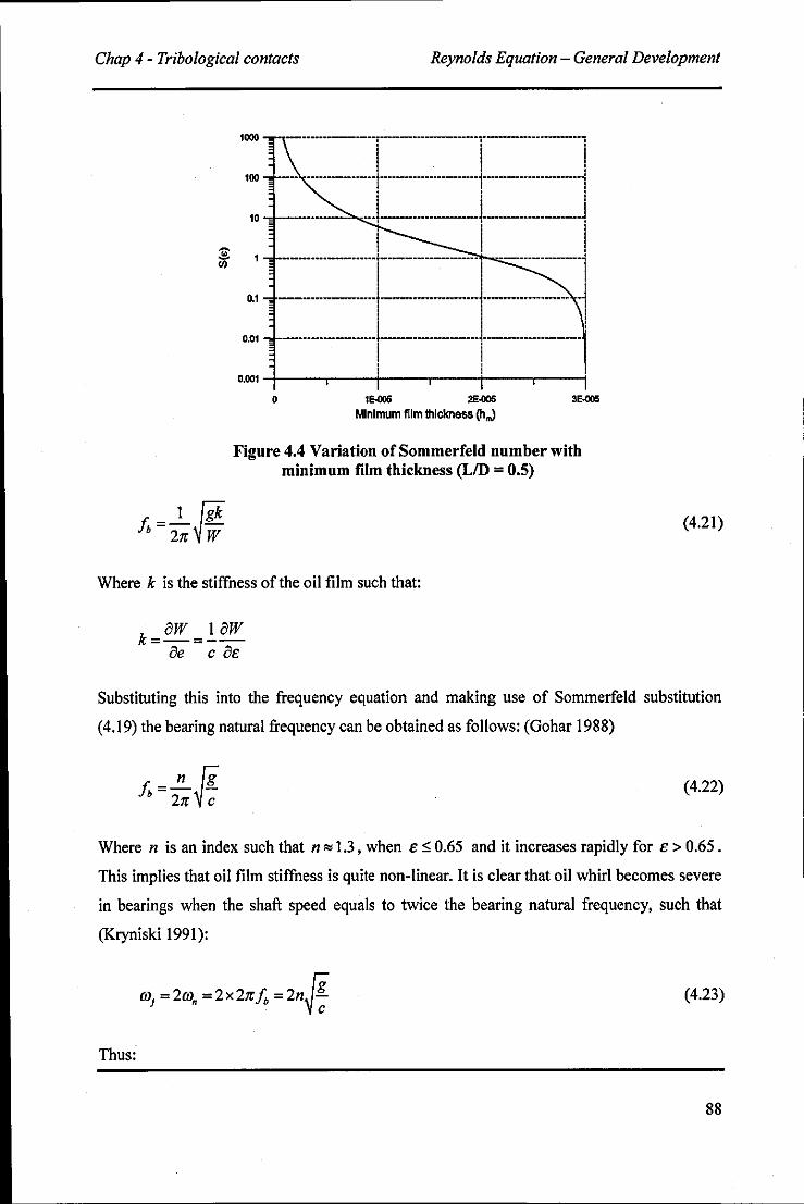
Chap 4 - Tribological contacts Reynolds Equation - General Development
~ III
f, =_1 {gk b 2n~W
1000 _ .. _-----j-----------,------------, I I I
100
10
---- ----------------1-------------------1--------------]
------ ·-J-----------1-----------: I I !
0.1 ~=:::~=~::I~~~:::::~~::: --~~~::::::=~:~ 0.01
i j' i ------------------1--------------- ___________ i I i
0.001 ! !
0 1E-005 2E.()Q6 3E.(J()5
Minimum film thickness (h.)
Figure 4.4 Variation of Sommerfeld number with minimum film thickness (LID = 0_5)
Where k is the stiffness of the oil film such that:
(4.21)
Substituting this into the frequency equation and making use of Sommerfeld substitution
(4.19) the bearing natural frequency can be obtained as follows: (Gohar 1988)
f.=~ [i 2n~;
(4.22)
Where n is an index such that n '" 1.3, when e ~ 0.65 and it increases rapidly for e > 0.65 .
This implies that oil film stiffness is quite non-linear. It is clear that oil whirl becomes severe
in bearings when the shaft speed equals to twice the bearing natural frequency, such that
(Kryniski 1991):
(4.23)
Thus:
88
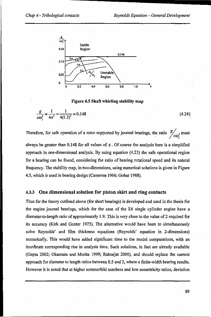
Chap 4 - Tribological contacts Reynolds Equation - General Development
...L=_I_ cal 4n2
)
.JL cro; Stable
0.20 Region
0.148 05 .45 _~-
0.10 ••..••..•.. _ ••....• O~~~, _,
o . .. ---. ~ Unstable 0.05 (J)J Region
0 0 0.2 0.4 0.6 0.8 1.0
Figure 4.5 Shaft whirling stability map
I 0.148
4(1.3)2 (4.24).
Therefore, for safe operation of a rotor supported by journal bearings, the ratio g/ 2 must / cm)
always be greater than 0.148 for all values of e . Of course the analysis here is a simplified
approach in one-dimensional analysis. By using equation (4.23) the safe operational region
for a bearing can be found, considering the ratio of bearing rotational speed and its natural
frequency. The stability map, in two-dimensions, using numerical solutions is given in Figure
4.5, which is used in bearing design (Cameron 1966; Gohar 1988).
4.3.3 One dimensional solution for piston skirt and ring contacts
Thus far the theory outlined above (for short bearings) is developed and used in the thesis for
the engine journal bearings, which for the case of the E6 single cylinder engine have a
diameter-to-Iength ratio of approximately 1.9. This is very close to the value of2 required for
its accuracy (Kirk and Gunter 1975). The alternative would have been to simultaneously
solve Reynolds' and film thickness. equations (Reynolds' equation in 2-dimensions)
numerically. This would have added significant time to the model computations, with an
inordinate corresponding rise in analysis time. Such solutions, in fact are already available
(Gupta 2002; Okamura and Morita 1999; Rahnejat 2000), and should replace the current
approach for diameter to length ratios between 0.5 and 2, where a finite-width bearing results.
However it is noted that at higher sommerfeld numbers and low eccentricity ratios, deviation
89
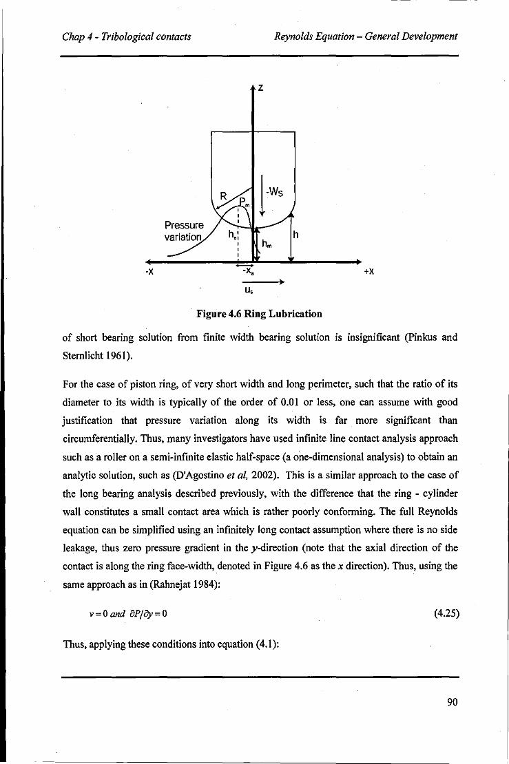
Chap 4 - Tribological contacts Reynolds Equation - General Development
-x
Pressure variation he:
+--+ -x,
u,
z
l-ws
h hm
Figure 4.6 Ring Lubrication
+x
of short bearing solution from finite width bearing solution is insignificant (Pinkus and
Stemlicht 1961).
For the case of piston ring, of very short width and long perimeter, such that the ratio of its
diameter to its width is typically of the order of 0.0 I or less, one can assume with good
justification that pressure variation along its width is far more significant than
circumferentially. Thus, many investigators have used infinite line contact analysis approach
such as a roller on a semi-infinite elastic half-space (a one-dimensional analysis) to obtain an
analytic solution, such as (D'Agostino et ai, 2002). This is a similar approach to the case of
the long bearing analysis described previously, with the difference that the ring - cylinder
wall constitutes a small contact area which is rather poorly conforming. The full Reynolds
equation can be simplified using an infinitely long contact assumption where there is no side
leakage, thus zero pressure gradient in the y-direction (note that the axial direction of the
contact is along the ring face-width, denoted in Figure 4.6 as the x direction). Thus, using the
same approach as in (Rahnejat 1984):
(4.25)
Thus, applying these conditions into equation (4.1):
90
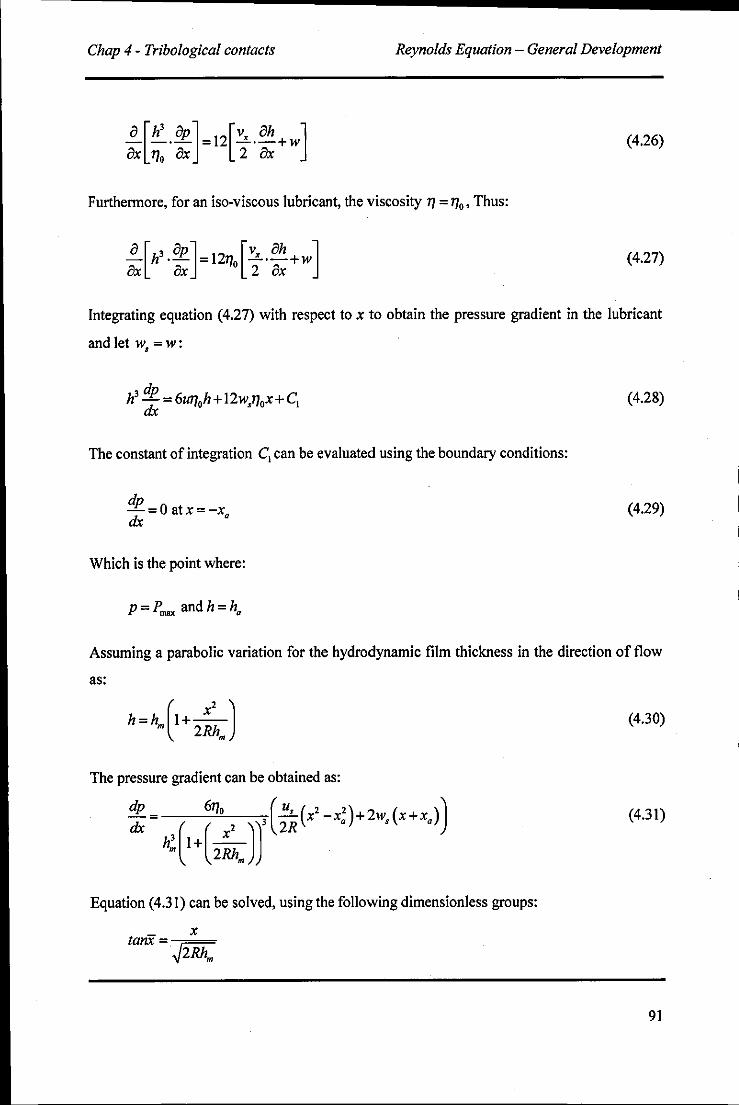
Chap 4 - Tribological contacts Reynolds Equation - General Development
(4.26)
Furthennore, for an iso-viscous lubricant, the viscosity 11 = 110, Thus:
a [ 3 ap ] [Vx ah ] - h .- =12110 -·-+w ax ax 2ax
(4.27)
Integrating equation (4.27) with respect to x to obtain the pressure gradient in the lubricant
and let w, = w :
The constant of integration Cl can be evaluated using the boundary conditions:
dp=Oatx=-x dx Q
Which is the point where:
P =p andh=h """' Q
(4.28)
(4.29)
Assuming a parabolic variation for the hydrodynamic film thickness in the direction of flow
as:
h=h (1+~) m 2Rh
m
The pressure gradient can be obtained as:
: -h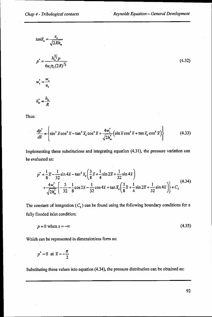
Chap 4 - Tribological contacts Reynolds Equation - General Development
Thus:
_ xa tanx =~dk.=
a ~2Rhm
, p
6u,7]o (2R)~
, w, w =,
u,
h' = hm m R
(4.32)
;;;: ={sin2xcos2x-tan2xacos4x+ J~: (sin X cos3 X +tan xa cos
4 X)} (4.33)
Implementing these substitutions and integrating equation (4.31), the pressure variation can
be evaluated as:
p =gX- 32sm x-tan xa gX+4"sm x+ 32sm x , 1 - 1 . 4- 2 - (L I . T 1 . 4-)
, { ( )} (4.34) + 4w, -~-.!.cos2x __ 1 cos4x +tanx ~x +.!.sin2x + J... sin 4x +C ~2h: 32 8 32 a 8 4 32 2
The constant of integration (C2 ) can be found using the following boundary conditions for a
fully flooded inlet condition:
p =0 when x =-00
Which can be represented in dimensionless form as:
'0 - re p = at X=--2
(4.35)
Substituting these values into equation (4.34), the pressure distribution can be obtained as:
92
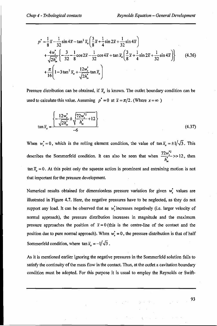
Chap 4 - Tribological contacts Reynolds Equation - General Development
, L I . 4- ,- (L I . 2- I . 4-) p =-x--sm x-tan x -x+-sm x+-sm x 8 32 a 8 4 32
+-- ----cos x--cos x+tanx -x+-sm x+-sm x 4w; { 3 I 2- I 4- - (L I . 2- I . 4-)} ~2h: 32 8 32 a 8 4 32
+l:.[1-3tan'xa + g12W; tanxa ]
16 2h' m
(4.36)
Pressure distribution can be obtained, if xa is known. The outlet boundary condition can be
used to calculate this value. Assuming p' = 0 at x = 7t /2. (Where x = 00 )
{_ 12w; ± 72v.::' + 12}
_ ~2h: hm tan xa = -'---'----""----6----""- (4.37)
When w: = 0, which is the rolling element condition, the value of tan xa = ± 1/ J3. This
describes the Sommerfeld condition. It can also be 72w" seen that when --:-»12, then
hm
tan xa = O. At this point only the squeeze action is prominent and entraining motion is not
that important for the pressure development.
Numerical results obtained for dimensionless pressure variation for given w; values are
illustrated in Figure 4.7. Here, the negative pressures have to be neglected, as they do not
support any load. It can be observed that as w; increases negatively (Le. larger velocity of
normal approach), the pressure distribution increases in magnitude and the maximum
pressure approaches the position of x = 0 (this is the centre-line of the contact and the
position due to pure normal approach). When w; = 0, the pressure distribution is that of half
Sommerfeld condition, where tan xa = -1/ J3 .
As it is mentioned earlier ignoring the negative pressures in the Sommerfeld solution fails to
satisfy the continuity of the mass flow in the contact. Thus, at the outlet a cavitation boundary
condition must be adopted. For this purpose it is usual to employ the Reynolds or Swift-
93
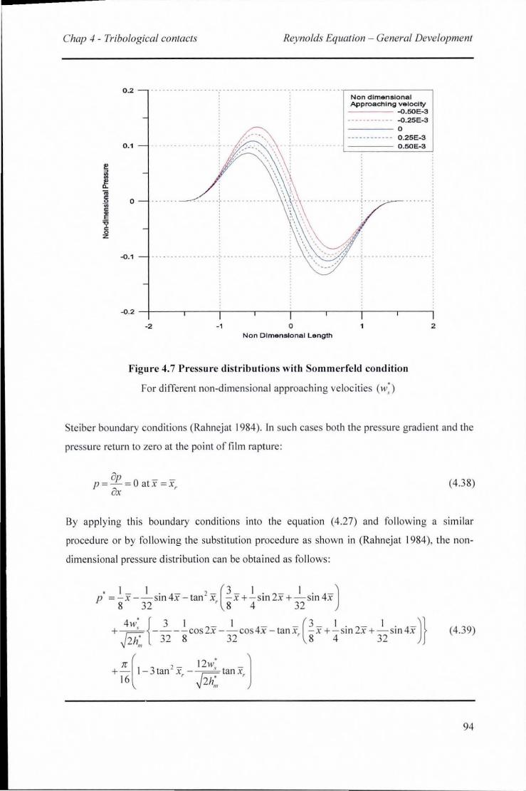
Chap -I - Tribological comacts Reynolds Eqllation - General Development
I!! ~ ~ n;
~ i ~ z
0.2 ............ --_ ... . -_ ......... ........... .
0.1 -
Non dimensional ApproaChing velodty -...:.~-.......; "'.60E-3 _._ •..•.•. _. "'.25E-3 ---- 0 - - - - . - --._ - . O.25E-3
O.50E-3
0 _ . .. -.. :
"'.1 .- ........... ;. ..
"'.2 -1---r---r---r---T---'---;---'---~
-2 -1 o Non Dimensional Length
Figure 4.7 Pressure distributions with Sommerfeld condition
For differenr non-d imensiona l approaching veloc iti es (11';)
2
Steiber boundary conditions (Rahnejat 1984). In such cases both the pressure grad ient and the
pressure return 10 zero at the point offilm rapture:
8p 0 - -p =-= at x =X 8x '
(4.38)
By applying thi s boundary conditions into the equation (4.27) and following a similar
procedure or by fo llowing the substitution procedure as shown in (Rahnejat 1984), the non
dimensional pressure di stribution can be obta ined as follows:
. 1 - 1 . 4- , -(L 1 . 2- 1 . 4-) P =-x--sm x-tan' x - X+ - SIl1 X+ - Slll x 8 32 ' 8 4 32
411': { 3 1 2- 1 4- -(L I '?- 1 . 4-)} +-- - ---cos x- - co x- talLY -X+-SII1_x+ - sm x rv; 32 8 32 ' 8 4 32 " 1. 17/11
(4 .39)
+.!:.. ( 1-3 tan 2 x - 12w: tan x ] 16 ' rv; ,
" 1. 17",
94
Chap 4 - Tribological contacts Analysis of Friction
Note that equation (4.39) can simply be obtained by just replacing xa in (4.36) by -x" Now
the pressure distribution can be found, if the film rapture point is known. x, can be
determined by utilizing the other half of the boundary conditions (4.38). Thus, equation
(4.39) becomes:
-x --sm x -tan x -x +-sm x +-sm x L 1. 4- 2 - (L I. 2- 1. 4-) 8 '32 ' , 8' 4 '32 '
4w: { 3 1 2- 1 4-· - (L I. 2- 1 . 4-)} +-- ----cos X --cos x -tanx -x +-sm x +-sm x ~ 32 8 '32 ' , 8 '4 '32 '
V2hm
(4.40)
+!E..(1-3tan2 x'-fo[I2W: tanx,)=o 16 2h'
m
Even in the contact between piston and bore the pressure variation along the circumferential
direction can be considered negligible compared to the high pressures along the axial
direction. This leads to insignificant fluid flow in the circumferential direction as it is given in
equation (4.25). Moreover, higher stiffness of the piston material which leads to very high
natural frequencies implies that the piston behaves more like a rigid component within the
domain of excitation. Even though there are many studies available in literature considering
the elastic deformations of the piston-bore lubrication (Balakrishnan and Rahnejat 2005;
Dursunkaya and Keribar 1992; Dursunkaya et aI, 1994), it is found that these elastic
behaviour prevails only at the peak combustion pressure. However, even in such a location
the pressures are usually insufficient to significantly alter the lubricant viscosity. Thus, as
(Balakrishnan and Rahnejat 2005) have found only isoviscous elastic conditions are
encountered in very small parts of the cycle. Thus, the engine operating conditions
demonstrate that EHL conditions may hardly be present other than possibly at engine start
up. Taking these facts into consideration the methodology developed so far can be used
reasonably to predict the lubrication characteristics of the contact between the piston and the
bore.
4.4 Analysis of Friction
If a machine element is adequately designed, with proper fluid film lubrication the contacting
surfaces are completely separated. Conversely, when the film thickness is insufficient
asperity interactions take place and this can lead to excessive wear and friction. The theory of
95
Chap 4 - Tribological contacts Analysis of Friction
friction expounded initially for static case by Amontons in 1699 and extended to kinetic
friction by Coulomb in the 18th century is based on the supposition that it (friction) arises
from asperity interactions, thus dependent on the surface quality (topography). Of course
friction also arises in lubricated contacts, even with full separation of surfaces due to shearing
between layers of the fluid. This viscous action causes friction, which is not only present in
relative sliding of surfaces but also under pure rolling conditions, but to a much lesser extent.
Therefore, for fluid film lubrication viscous friction is the dominant source, whilst Coulomb
friction acts under boundary regime of lubrication. These two phenomena contribute to the
total friction in mixed regime oflubrication.
In order to identify the lubrication regime a dimensionless parameter can be defined as
follows:
A ~u' +u' I ,
(4.41)
Smaller A results more frequent random contacts between asperities. Under such conditions
boundary lubrication occurs. Larger film parameters result in more coherent lubricant films,
which lead to hydrodynamic lubrication. However, great differences in geometric conformity
from hydrodynamically lubricated conjunctions to elastohydrodynamically lubricated
conjunctions make it difficult for clear distinctions to be made. Therefore, rough estimates are
used to distinguish between regimes of lubrication as shown in Figure 4.1. Thus, it is
reasonable to consider friction force between two surfaces to be made up of two
contributions: a boundary friction Fb and a viscous friction Fv. Film parameter is used to
identify the prominent friction component as shown in Figure 4.1.
(4.42)
4.4.1 Boundary Friction Force
Boundary lubrication occurs when the asperities are in contact. The lubrication conditions can·
still prevail on asperity tips and in the oil film trapped between the asperities (see Figure 4.8),
but friction arising from these are quite different. The distribution of peaks and valleys on a
surface cannot be calculated precisely due to its random nature. Thus, a statistical approach
96
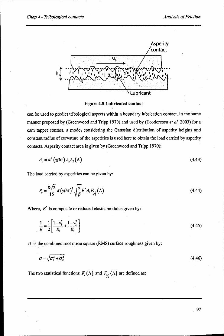
Chap 4 - Tribological contacts Analysis of Friction
Lubricant
Figure 4.8 Lubricated contact
can be used to predict tribological aspects within a boundary lubrication contact. In the same
manner proposed by (Greenwood and Tripp 1970) and used by (Teodorescu et aI, 2003) for a
cam tappet contact, a model considering the Gaussian distribution of asperity heights and
constant radius of curvature of the asperities is used here to obtain the load carried by asperity
contacts. Asperity contact area is given by (Greenwood and Tripp 1970):
(4.43)
The load carried by asperities can be given by:
(4.44)
Where, E' is composite or reduced elastic modulus given by:
(4.45)
(J is the combined root mean square (RMS) surface roughness given by:
(4.46)
The two statistical functions F; (A) and FX (A) are defined as:
97
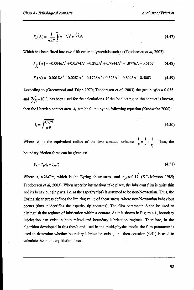
Chap 4 - Tribological contacts Analysis of Friction
(4.47)
Which has been fitted into two fifth order polynomials such as (Teodorescu et ai, 2003):
F% (A) = -0.0046A' +0.0574A' -0.295A' +0.7844A' -1.0776A+0.6167 (4.48)
F,(A) =-0.0018A' + 0.028 lA' -0.1728A' +0.525A' -0.8043A + 0.5003 (4.49)
According to (Greenwood and Tripp 1970; Teodorescu et ai, 2003) the group rf3a = 0.055
and c;;P = I 0-' , has been used for the calculations. If the load acting on the contact is known,
then the Hertzian contact area Ah can be found by the following equation (Kushwaha 2000):
Ah=tWRI
nE
Where R is the equivalent radius of the two contact surfaces:
boundary friction force can be given as:
(4.50)
I I I -=-+-. Thus, the R r. r,
(4.51)
Where 'f, "" 2MPa, which is the Eyring shear stress and cpb "" 0.17 (K.L.Johnson 1985;
Teodorescu et ai, 2003). When asperity interactions take place, the lubricant film is quite thin
and its behaviour (in parts, i.e. at the asperity tips) is assumed to be non-Newtonian. Thus, the
Eyring shear stress defines the limiting value of shear stress, where non-Newtonian behaviour
occurs (thus it identifies the asperity tip contacts). The film parameter A can be used to
distinguish the regimes of lubrication within a contact. As it is shown in Figure 4.1, boundary
lubrication can exist in both mixed and boundary lubrication regimes. Therefore, in the
algorithm developed in this thesis and used in the multi-physics model the film parameter is
used to determine whether boundary lubrication exists, and then equation (4.51) is used to
calculate the boundary friction force.
98
------------ - -- - --------------........ Chap 4 - Tribological contacts Analysis of Friction
4.4.2 . Viscous Friction Force
Viscous friction force is produced by shearing of the oil film trapped between the two
contacting surfaces. Depending on the oil film thickness, the lubricant can behaves as a
Newtonian liquid such that the shear stress is linearly related to the shear strain or it may
behave in a Non-Newtonian manner. (Eyring 1936) has proposed a model, which
incorporates the non-linear viscous behaviour. According to this model the shear stress is
linearly varying with shear strain until it reaches the Eyring shear strength (",) , which is
about 2MPa for most lubricants. Subsequently, it starts to deviate from linearity. Taking this
behaviour into consideration the shear stress can be used to identify the lubricant behaviour
as previously pointed out. Thus:
(4.52)
Then, the Newtonian behaviour prevails within the contact and the shear stress becomes:
(4.53)
However, if the inequality (4.52) is not satisfied, then the Non-Newtonian behaviour prevails
and the shear stress is determined by the rheological properties of the oil such as:
(4.54)
Where r, is the slope of oil limiting shear stress-pressure relationship and this could be
approximated to a mean sliding velocity (u;{) of the contact. Thus, depending on the
situation the viscous induced stress can be calculated either by (4.53) or (4.54).
During the piston motion inside the cylinder bore any of lubrication regimes can dominate. In
piston mid-stroke the hydrodynamic lubrication condition is predominant due to high sliding
velocities and relatively low side forces. At dead centres the velocity instantaneously
becomes zero, thus producing no lubricant entrainment, especially when this happens at the
TDe during the power stroke of the engine. Here the situation becomes more severe due to a
99
Chap 4 - Tribological contacts Temperature Effects in Lubricated Contacts
high side force. Under these conditions there is a better chance of boundary lubrication
conditions to occur at top dead centre, which can be represented by the described procedure.
4.5 Temperature Effects in Lubricated Contacts
Thus far all the analytical methods described are based on the assumption that isothermal
solutions to tribological contacts suffice as first reasonable approximation. This also happens
to be the approach by many other investigators, such as those cited in this chapter. However,
in all contacts the temperature of the lubricant rises from that of the bulk oil temperature, and
this reduces its viscosity, which in turn reduces the film thickness. In conjunctions with lower
pressures and larger gaps, and particularly at lower shear rates the temperature rise is less
pronounced, and one may ignore the temperature effect, at least as a first approximation.
However, in less conforming conjunctions and at high shearing rates, such as the case of
piston ring to cylinder liner contact temperature rise and its effect of viscous behaviour of the
lubricant should not be neglected. Thus, Reynolds pressure variation at the contact changes
whist altering the reaction force. In fact, prediction of temperature rise in such lubricated
contacts of a machine element is an important contribution to the engineering design process.
The conservation of energy at a point in the lubricant film is the fundamental equation that is
necessary for this prediction. Assuming that there is no other external source of heating
present, the pressure along the thickness of the film is constant under steady state condition.
Considering the fluid flow is only in the x-direction the 2-dimentional energy equation for a
contact is given by (Gohar 1988)as:
~'Vx8.(: )+: (~ J = :VxCp.(~)-~, (~;~) compressivc . viscous convection conduction heating heating cooling cooling
(4.55)
Where 8 (x) is the temperature rise of the oil from the inlet, v, is its coefficient of thermal
expansion, Cp is the specific heat at constant temperature and k, is the thermal conductivity.
As it can be seen from the equation (4.55), the heat is generated due to compressive action as
well as viscous action in a contact and this heat is dissipated to the environment by
convection or by conduction cooling. Lubricants behave as incompressible (volume does not
change with pressure) fluids in low pressures but it undergoes compression at high pressures
lOO
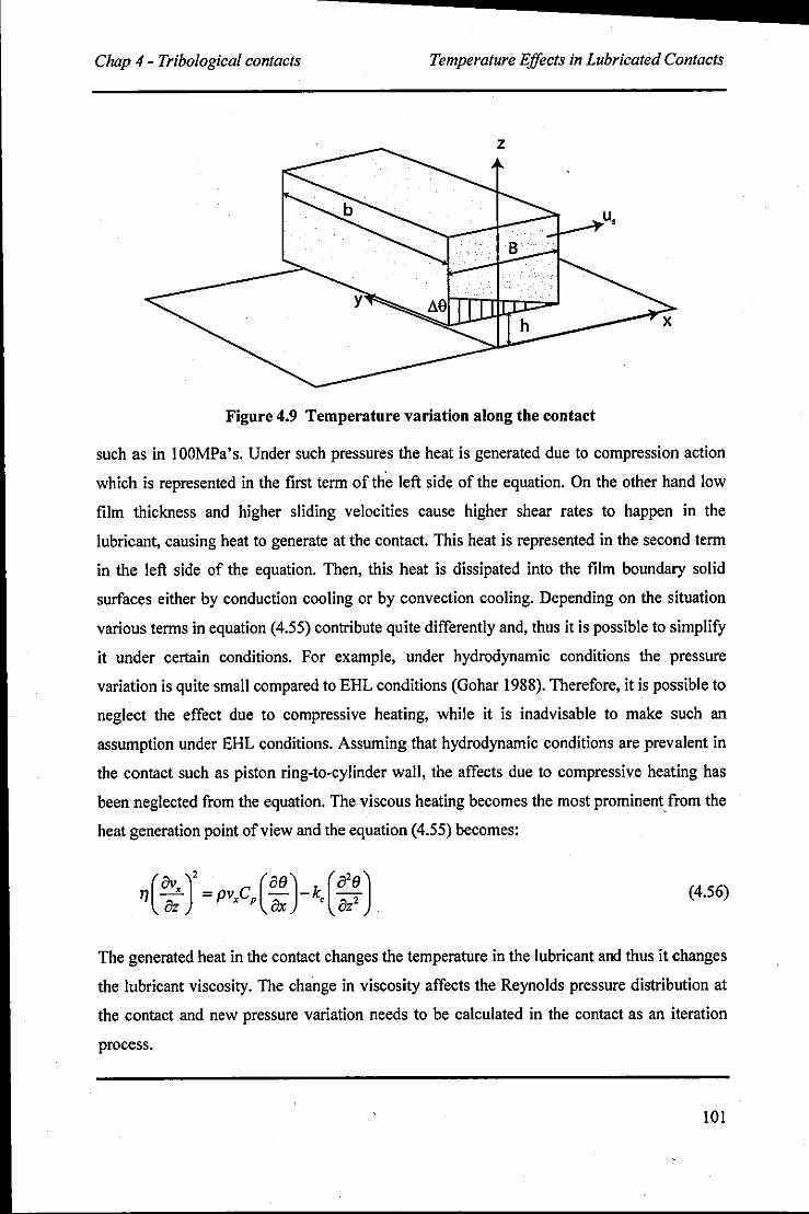
,--------- - - - -
Chap 4 - Tribological contacts Temperature Effects in Lubricated Contacts
u,
Figure 4.9 Temperature variation along the contact
such as in 100MPa's. Under such pressures the heat is generated due to compression action
which is represented in the first term of the left side of the equation. On the other hand low
film thickness and higher sliding velocities cause higher shear rates to happen in the
lubricant, causing heat to generate at the contact. This heat is represented in the second term
in the left side of the equation. Then, this heat is dissipated into the film boundary solid
surfaces either by conduction cooling or by convection cooling. Depending on the situation
various terms in equation (4.55) contribute quite differently and, thus it is possible to simplify
it under certain conditions. For example, under hydrodynamic conditions the pressure
variation is quite small compared to EHL conditions (Gohar 1988). Therefore, it is possible to
neglect the effect due to compressive heating, while it is inadvisable to make such an
assumption under EHL conditions. Assuming that hydrodynamic conditions are prevalent in
the contact such as piston ring-to-cylinder wall, the affects due to compressive heating has
been neglected from the equation. The viscous heating becomes the most prominent from the
heat generation point of view and the equation (4.55) becomes:
(4.56)
The generated heat in the contact changes the temperature in the lubricant and thus it changes
the lubricant viscosity. The change in viscosity affects the Reynolds pressure distribution at
the contact and new pressure variation needs to be calculated in the contact as an iteration
process.
101
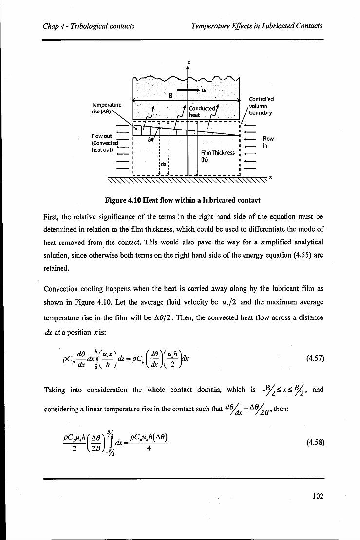
Chap 4 - Tribological contacts Temperature Effects in Lubricated Contacts
Temperature rlse(ll.a)
z
-~tb=~~ Flowout - ~ '-(Convecteer- ,
heat out) = : , -,
• • • • • • • • :dx: _I 1I , ..
------.-~--- -
,-,-
Film Thickness , ,-
(h) '-,
Figure 4.10 Heat flow within a lubricated contact
Flow In
x
First, the relative significance of the terms in the right hand side of the equation must be
determined in relation to the film thickness, which could be used to differentiate the mode of
heat removed from. the contact. This would also pave the way for a simplified analytical
solution, since otherwise both terms on the right hand side of the energy equation (4.55) are
retained.
Convection cooling happens when the heat is carried away along by the lubricant film as
shown in Figure 4.1 O. Let the average fluid velocity be u,/2 and the maximum average
temperature rise in the film will be "'6/2. Then, the convected heat flow across a distance
dx at a position x is:
(4.57)
Taking into consideration the whole contact domain, which is -%::; x::; ~, and
considering a linear temperature rise in the contact such that d% = "'%B' then:
(4.58)
102
Chap 4 - Tribological contacts Temperature Effects in Lubricated Contacts
Therefore, the total convected heat through the contact can be given by equation (4.58). Heat
within the film can also be removed away by conduction as shown in Figure 4.1 O. When the
heat is carried away by conduction, then the solution assumes that the temperature gradient
across the film varies linearly for each value of x rising from zero at its bottom surface to a
value of 0% at the top as shown in (Gohar 1988). This gives a parabolic temperature
distribution across the film. Thus, the heat flow rate into the top surface through a column of
width dx and height his:
(4.59)
Substituting: 00 = x!J.% as the temperature rises linear across the contact, into equation
(4.59) the total conducted heat flow can be calculated as:
k,!J.O Bfxdx
= k,M B
Bh 0 2h (4.60)
This equation provides the heat removed by conduction. Substituting values from equations
(4.58) and (4.60) into the energy equation (4.56), considering the whole contact domain:
f f~(Ov.)2 dzdx= pU,Cph!J.O + k,{M)B _y, 0 oz 4 2h
(4.61)
Assuming that a linear velocity variation across the fluid film:
011. u, -=-OZ h
(4.62)
Thus, equation (4.61) becomes:
~u;B = pU,Cph!J.O + k,(M)B h 4 2h
(4.63)
The temperature rise within the contact can be obtained from equation (4.63). However, it is
known that when the film is thick such as in hydrodynamic lubrication the most dominant
103
Chap 4 - Tribological contacts Temperature Effects in Lubricated Contacts
heat removing mechanism is convection, where as under EHL conditions conduction is most
prominent (Cameron 1966; Gohar 1988; Rahnejat and Gohar). If a condition can be imposed
to distinguish the effective cooling method under prevailing circumstances, then the amount
of calculations can be reduced, and an analytical solution can be established. The Peelet
number, which is a dimensionless number, defined as the ratio of convected heat energy by
the fluid to the thermal energy conducted by the adjacent solid surfaces can be used to
ascertain the validity of the simplification made. By definition:
Convected heat Peclet Number (Pe) =
Conducted heat
Thus, from the above derivations:
(4.64)
(4.65)
The denominator of the right side of equation (4.65) is called diffusivity, which is a constant
for a specific fluid. Diffusivity has the units m% and for the lubricant oil of SAE 15W -40
used in the engine the diffusivity is 7.38xlO-8 m2 / s at 100°C (Shell). Contact width (B) for
the piston ring - cylinder wall interaction is given by the ring width of 2mm. Such "that, the
Peclet number variation during an engine combustion cycle is given in Figure 7.27.
Therefore, both convection and conduction cooling are taken into consideration for the
calculation of temperature rise within the contact.
Once the temperature rise (1';8) is obtained by equation (4.63), the final temperature (9,) at
contact is calculated using a relaxation method such as:
(4.66)
Where 9, is the inlet temperature and k, = 0.5 (relaxation factor) for this case. Then the new
viscosity corresponding to temperature 9, can be calculated using Vogel equation which is
given by (Hamrock et ai, 2004) as:
104
Chap 4 - Tribological contacts
In(17) = -1.845+( 700.81) 9-203
Temperature Effects in Lubricated Contacts
(4.67)
where 9 is the temperature in Kelvin and 1) is the viscosity in centi-poise, or by Barus
equation as:
(4.68)
Where a is the viscosity-pressure coefficient and p is the pressure. Then the minimum film
thickness for the corresponding viscosity under these conditions can be found, if the total
force acting on the contact is known. The detailed implementation of temperature effects at
piston ring - cylinder wall interaction, using the above analysis is presented in section 5.5.7.
Even though almost all lubrication contacts are established based on Reynolds equation, it
can be simplified according to the circumstances of the contact that will reduce the intensity
of numerical techniques needed to solve them, as it has been discussed. This will enable
modem computers to solve such an immense multi-physics numerical model within
reasonable duration of time. The following Chapter is devoted to a discussion of
incorporating these lubricated contacts to a commercially available multi-body dynamics
software tool in an efficient and methodical manner which can be extended to any system that
include kinematic relations and constraint reactions.
105
Chap 5 - Numerical Model Development Introduction
5 NUMERICAL MODEL DEVELOPMENT
5.1 Introdnction
In the fonner chapters, theoretical basis used for multi-body dynamics, component flexibility
and tribology within this thesis have been discussed, with particular reference to internal
combustion engines. In this chapter these methods are combined to develop a multi-physics
numerical methodology with a single cylinder engine model. Firstly, multi-body dynamics is
used to develop the constrained rigid body inertial dynamics of the engine. This base model
includes rigid body motions only, such as the translation of the piston, its secondary motions,
angulations of the connecting rod, and rotation of the crankshaft. Then, selected rigid bodies
are replaced with flexible components. These are the elements of the system that in practice
are more prone to structural defonnation, when subjected to the applied combustion gas
force. The introduction of component flexibility lessens the stiffness of the model, while it
makes it more realistic. Idealized primary joints used in the usual multi-body models such as
revolute, translational, etc with well-defined motion trajectories and OOFs do not exist in real
physical systems, which are subject to compliances offered by system flexibility and
clearance. This also includes the reaction forces offered by the load bearing systems, which
should be modelled in realistic tribological tenns. Current multi-body dynamic analysis codes
such as AOAMS, used in this thesis and widely in industry, do not possess these very
important features, thus the analyses reported in literature using such approaches are usually
devoid of practical significance, particular with regard to an in-depth scientific investigation.
Almost all contacts of an engine are ideally regarded as lubricated. The purpose, of course, is
to minimize friction, wear and thus better efficient engines. One should also not under
estimate the contributions made by the lubricant by removing the generated heat away from
load bearing conjunctions, and thus enhance the thennal stability of engines.
Whilst the multi-physics approach expounded here includes a number of key disciplines in
the same analysis, it must be noted that there are many other aspects of an IC engine that are
not considered in depth during this analysis such as the behaviour of big-end bearing and the
gudgeon pin interaction with piston, which also behaves in a complicated manner
(Balakrishnan and Rahnejat 2005; Cho et ai, 2003; Koizumi et ai, 2000). Also, engine
106
Chap 5 - Numerical Model Development Rigid Single Cylinder Model
housing flexibility can be quite influential in investigation of overall NVH performance in an
IC engine (Gamier et ai, 1999). This aspect is also not considered here. However, it is not
possible to include all these effects into a single model with the available computational
capabilities, and within sensible analysis times. Furthermore, very large and complicated
models with many interactions are often not the most useful. Thus, those aspects included in
the multi-physics analysis are deemed as the most influential from a combined dynamics,
NVH and triboloy viewpoint. The method employed also provides structural deformation
data (within the elastic limit), which can be used for durability analysis (not discussed in this
thesis), aside from its contributions to structural vibrations. Furthermore, within the NVH
spectra, the thesis focuses on two key aspects: firstly, the engine order vibration that
contribute to vehicle harshness at low frequencies, and secondly on vibrations of the piston
connecting rod-crankshaft sub-system, which are structure-borne. Thus, airborne noise is not
considered, which may arise from inclusion of other attachments such as casing, covers,
manifolds or other components of lighter construction. This, however, can readily be
achieved by simple additions to the model.
5.2 Rigid Single Cylinder Model
S.2.1 The ADAMS Multi-body System Software
ADAMS (an acronym for Automatic Qynamic Analysis of Mechanical .systems) is a general
purpose dynamic system simulation code and is a product of MSC Software. It automatically
generates equations of motion of a mechanical model, based on constrained Lagrangian
dynamics, described in Chapter 3. Thus, ADAMS is used to analyse a wide range of multi
body dynamic systems. It has become an industry-standard analysis code, and is used in all
kind of industries such as automotive, aerospace, machinery and construction as reported by
(Blundell 1991). It has an open architecture that allows users to create their own extension
data set, features or subroutines (ADAMS/Solver).
In ADAMS a "marker" defines a position to which an orthogonal triad of unit vectors is
attached. It identifies a location and its orientation with respect to a reference frame that can
simply define geometry or a point of attachment, or centre of mass and inertial properties of a
body (referred as a part in ADAMS). Orientation of any marker with respect to the global
107
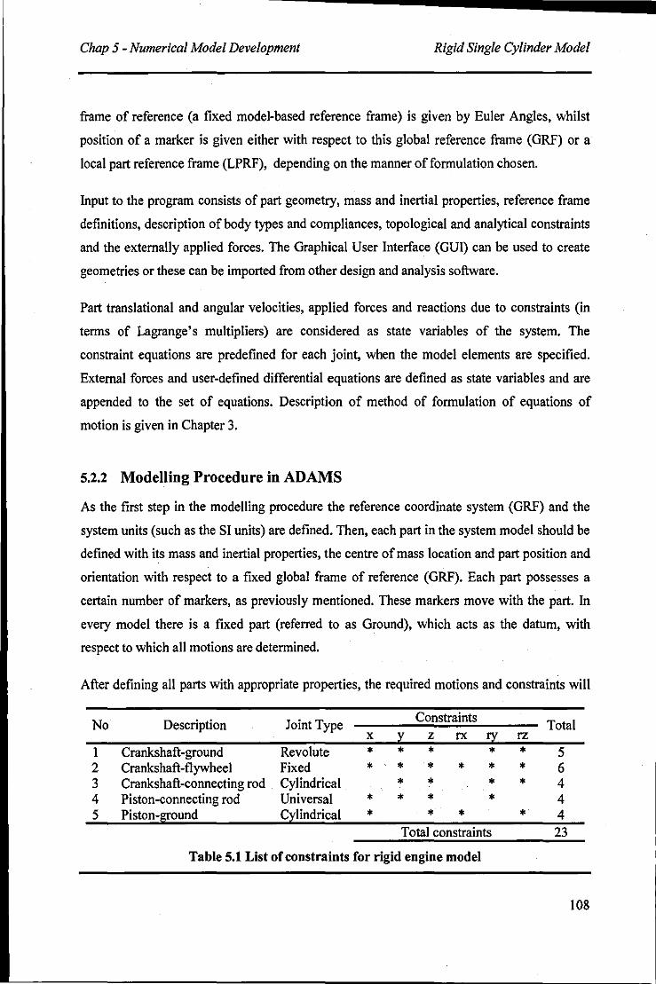
------------------........ Chap 5 - Numerical Model Development Rigid Single Cylinder Model
frame of reference (a fixed model-based reference frame) is given by Euler Angles, whilst
position of a marker is given either with respect to this global reference frame (GRF) or a
local part reference frame (LPRF), depending on the manner of formulation chosen.
Input to the program consists of part geometry, mass and inertial properties, reference frame
definitions, description of body types and compliances, topological and analytical constraints
and the externally applied forces. The Graphical User Interface (GUI) can be used to create
geometries or these can be imported from other design and analysis software.
Part translational and angular velocities, applied forces and reactions due to constraints (in
terms of Lagrange's multipliers) are considered as state variables of the system. The
constraint equations are predefined for each joint, when the model elements are specified.
External forces and user-defined differential equations are defined as state variables and are
appended to the set of equations. Description of method of formulation of equations of
motion is given in Chapter 3.
5.2.2 Modelling Procedure in ADAMS
As the first step in the mode\ling procedure the reference coordinate system (GRF) and the
system units (such as the SI units) are defined. Then, each part in the system model should be
defined with its mass and inertial properties, the centre of mass location and part position and
orientation with respect to a fixed global frame of reference (GRF). Each part possesses a
certain number of markers, as previously mentioned. These markers move with the part. In
every model there is a fixed part (referred to as Ground), which acts as the datum, with
respect to which all motions are determined.
After defining all parts with appropriate properties, the required motions and constraints will
No Description Joint Type Constraints
Total x ~ z rx !I rz
1 Crankshaft-ground Revolute • * • * • 5 2 Crankshaft-flywheel Fixed • * * * * * 6 3 Crankshaft-connecting rod Cylindrical * * * * 4 4 Piston-connecting rod Universal * * * * 4 5 Piston-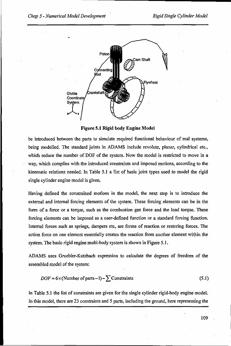
Chap 5 - Numerical Model Development Rigid Single Cylinder Model
Figure 5.1 Rigid body Engine Model
be introduced between the parts to simulate required functional behaviour of real systems,
being modelled. The standard joints in ADAMS include revolute, planar, cylindrical etc.,
which reduce the number of DOF of the system. Now the model is restricted to move in a
way, which complies with the introduced constraints and imposed motions, according to the
kinematic relations needed. In Table 5.1 a list of basic joint types used to model the rigid
single cylinder engine model is given.
Having defined the constrained motions in the model, the next step is to introduce the
external and internal forcing elements of the system. These forcing elements can be in the
form of a force or a torque, such as the combustion gas force and the load torque. These
forcing elements can be imposed as a user-defined function or a standard forcing function.
Internal forces such as springs, dampers etc, are forms of reaction or restoring forces. The
action force on one element essentially creates the reaction from another element within the
system. The basic rigid engine multi-body system is shown in Figure 5.1.
ADAMS uses Gruebler-Kutzbach expression to calculate the degrees of freedom of the
assembled model of the system:
DOF = 6 x (Number of parts -I) - L Constraints (5.1)
In Table 5.1 the list of constraints are given for the single cylinder rigid-body engine model.
In this model, there are 23 constraints and 5 parts, including the ground, here representing the
109
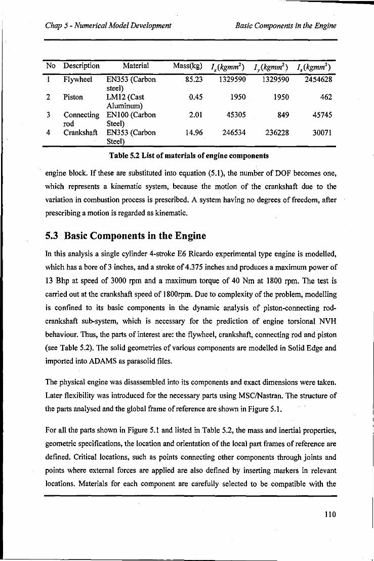
Chap 5 - Numerical Model Development Basic Components in the Engine
No Description Material Mass(kg) Ix (kgmm') I/kgmm') I,(kgmm') I Flywheel EN353 (Carbon 85.23 1329590 1329590 2454628
steel) 2 Piston LMI2 (Cast 0.45 1950 1950 462
Aluminum) 3 Connecting ENIOO (Carbon 2.01 45305 849 45745
rod Steel) 4 Crankshaft EN353 (Carbon 14.96 246534 236228 30071
Steel)
Table 5.2 List of materials of engine components
engine block. If these are substituted into equation (5.1), the number of DOF becomes one,
which represents a kinematic system, because the motion of the crankshaft due to the
variation in combustion process is prescribed. A system having no degrees of freedom, after
prescribing a motion is regarded as kinematic.
5.3 Basic Components in the Engine
In this analysis a single cylinder 4-stroke E6 Ricardo experimental type engine is modelled,
which has a bore of 3 inches, and a stroke of 4.375 inches and produces a maximum power of
13 Bhp at speed of 3000 rpm and a maximum torque of 40 Nm at 1800 rpm. The test is
carried out at the crankshaft speed of 1800rpm. Due to complexity of the problem, modelling
is confined to its basic components in the dynamic analysis of piston-connecting rod
crankshaft sub-system, which is necessary for the prediction of engine torsional NVH
behaviour. Thus, the parts of interest are: the flywheel, crankshaft, connecting rod and piston
(see Table 5.2). The solid geometries of various components are modelled in Solid Edge and
imported into ADAMS as parasolid files.
The physical engine was disassembled into its components and exact dimensions were taken.
Later flexibility was introduced for the necessary parts using MSClNastran. The structure of
the parts analysed and the global frame of reference are shown in Figure 5.1.
For all the parts shown in Figure 5.1 and listed in Table 5.2, the mass and inertial properties,
geometric specifications, the location and orientation of the local part frames of reference are
defined. Critical locations, such as points connecting other components through joints and
points where external forces are applied are also defined by inserting markers in relevant
locations. Materials for each component are carefully selected to be compatible with the
110
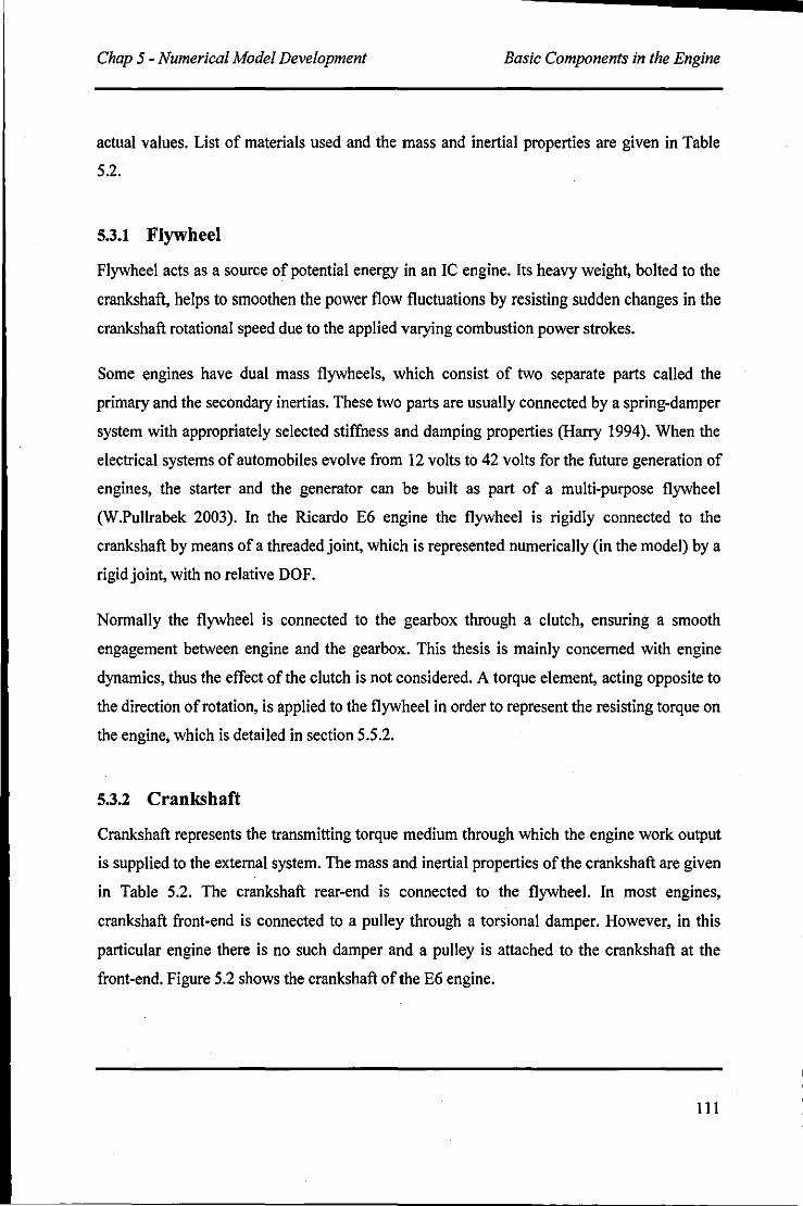
Chap 5 - Numerical Model Development Basic Components in the Engine
actual values. List of materials used and the mass and inertial properties are given in Table
5.2.
5.3.1 Flywheel
Flywheel acts as a source of potential energy in an IC engine. Its heavy weight, bolted to the
crankshaft, helps to smoothen the power flow fluctuations by resisting sudden changes in the
crankshaft rotational speed due to the applied varying combustion power strokes.
Some engines have dual mass flywheels, which consist of two separate parts called the
primary and the secondary inertias. These two parts are usually connected by a spring-damper
system with appropriately selected stiffness and damping properties (Harry 1994). When the
electrical systems of automobiles evolve from 12 volts to 42 volts for the future generation of
engines, the starter and the generator can be built as part of a multi-purpose flywheel
(W.Pullrabek 2003). In the Ricardo E6 engine the flywheel is rigidly connected to the
crankshaft by means of a threaded joint, which is represented numerically (in the model) by a
rigid joint, with no relative DOF.
Normally the flywheel is connected to the gearbox through a clutch, ensuring a smooth
engagement between engine and the gearbox. This thesis is mainly concerned with engine
dynamics, thus the effect of the clutch is not considered. A torque element, acting opposite to
the direction of rotation, is applied to the flywheel in order to represent the resisting torque on
the engine, which is detailed in section 5.5.2.
5.3.2 Crankshaft
Crankshaft represents the transmitting torque medium through which the engine work output
is supplied to the external system. The mass and inertial properties of the crankshaft are given
in Table 5.2. The crankshaft rear-end is connected to the flywheel. In most engines,
crankshaft front-end is connected to a pulley through a torsional damper. However, in this
particular engine there is no such damper and a pulley is attached to the crankshaft at the
front·end. Figure 5.2 shows the crankshaft of the E6 engine.
111
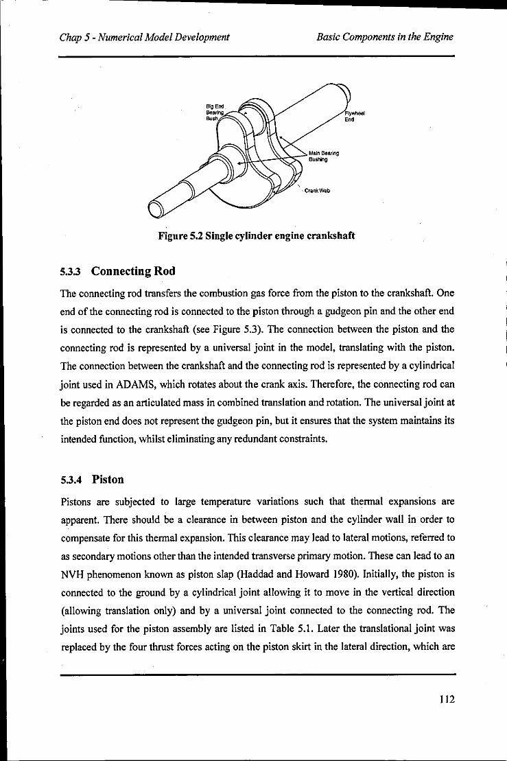
Chap 5 - Numerical Model Development Basic Components in the Engine
\'1~~~;;)~ Main Bearing .... Bushing
Flywheel End
Figure 5.2 Single cylinder engine crankshaft
5.3.3 Connecting Rod
The connecting rod transfers the combustion gas force from the piston to the crankshaft. One
end of the connecting rod is connected to the piston through a gudgeon pin and the other end
is connected to the crankshaft (see Figure 5.3). The connection between the piston and the
connecting rod is represented by a universal joint in the model, translating with the piston.
The connection between the crankshaft and the connecting rod is represented by a cylindrical
joint used in ADAMS, which rotates about the crank axis. Therefore, the connecting rod can
be regarded as an articulated mass in combined translation and rotation. The universal joint at
the piston end does not represent the gudgeon pin, but it ensures that the system maintains its
intended function, whilst eliminating any redundant constraints.
5.3.4 Piston
Pistons are subjected to large temperature variations such that thermal expansions are
apparent. There should be a clearance in between piston and the cylinder wal1 in order to
compensate for this thermal expansion. This clearance may lead to lateral motions, referred to
as secondary motions other than the intended transverse primary motion. These can lead to an
NVH phenomenon known as piston slap (Haddad and Howard 1980). Initial1y, the piston is
connected to the ground by a cylindrical joint al10wing it to move in the vertical direction
(al1owing translation only) and by a universal joint connected to the connecting rod. The
joints used for the piston assembly are listed in Table 5.1. Later the translational joint was
replaced by the four thrust forces acting on the piston skirt in the lateral direction, which are
112
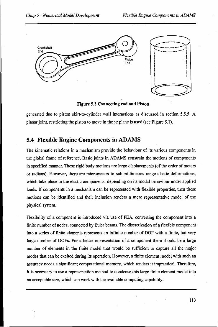
Chap 5 - Numerical Model Development Flexible Engine Components in ADAMS
Piston End
Figure 5.3 Connecting rod and Piston
.... --------- .... ."
~- -_ .... '"( ~ ------- ~ 1 ........ - ___ ---_ ...... I I I I I I I I I I I I
C-==~::::--L
generated due to piston skirt-to-cylinder wall interactions as discussed in section 5.5.5. A
planar joint, restricting the piston to move in the yz plane is used (see Figure 5.1).
5.4 Flexible Engine Components in ADAMS
The kinematic relations in a mechanism provide the behaviour of its various components in
the global frame of reference. Basic joints in ADAMS constrain the motions of components
in specified manner. These rigid body motions are large displacements (of the order of meters
or radians). However, there are micrometers to sub-millimetres range elastic deformations,
which take place in the elastic components, depending on its modal behaviour under applied
loads. If components in a mechanism can be represented with flexible properties, then these
motions can be identified and their inclusion renders a more representative model of the
physical system.
Flexibility of a component is introduced via use of FEA, converting the component into a
finite number of nodes, connected by Euler beams. The discretization of a flexible component
into a series of finite elements represents an infinite number of DOF with a finite, but very
large number of DOFs. For a better representation of a component there should be a large
number of elements in the finite model that would be sufficient to capture all the major
modes that can be excited during its operation. However, a finite element model with such an
accuracy needs a significant computational memory, which renders it impractical. Therefore,
it is necessary to use a representation method to condense this large finite element model into
an acceptable size, which can work with the available computing capability.
113
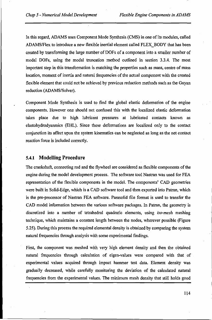
Chap 5 - Numerical Model Development Flexible Engine Components in ADAMS
In this regard, ADAMS uses Component Mode Synthesis (CMS) in one of its modules, called
ADAMSlFlex to introduce a new flexible inertial element called FLEX_BODY that has been
created by transforming the large number of DOFs of a component into a smaller number of
modal DOFs, using the modal truncation method outlined in section 3.3.4. The most
important step in this transformation is matching the properties such as mass, centre of mass
location, moment of inertia and natural frequencies of the actual component with the created
flexible element that could not be achieved by previous reduction methods such as the Guyan
reduction (ADAMS/Solver).
Component Mode Synthesis is used to find the global elastic deformation of the engine
components. However one should not confused this with the localized elastic deformation
takes place due to high lubricant pressures at lubricated contacts known as
elastohydrodyanmics (EHL). Since these deformations are localized only to the contact
conjunction its affect upon the system kinematics can be neglected as long as the net contact
reaction force is included correctly.
5.4.1 Modelling Procedure
The crankshaft, connecting rod and the flywheel are considered as flexible components of the
engine during the model development process. The software tool Nastran was used for FEA
representation of the flexible components in the model. The components' CAD geometries
were built in Solid-Edge, which is a CAD software tool and then exported into Patran, which
is the pre-processor of Nastran FEA software. Parasolid file format is used to transfer the
CAD model information between the various software packages. In Patran, the geometry is
discretized into a number of tetrahedral quadratic elements, using iso-mesh meshing
technique, which maintains a constant length between the nodes, wherever possible (Figure
5.25). During this process the required elemental density is obtained by comparing the system
natural frequencies through analysis with some experimental findings.
First, the component was meshed with very high element density and then the obtained
natural frequencies through calculation of eigen-values were compared with that of
experimental values acquired through impact hammer test data. Element density was
gradually decreased, while carefully monitoring the deviation of the calculated natural
frequencies from the experimental values. The minimum mesh density that still holds good
114
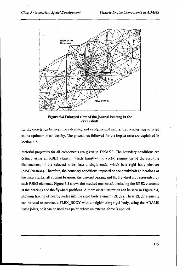
Chap 5 - Numerical Model Development Flexible Engine Components in ADAMS
Figure 5.4 Enlarged view of the journal bearing in the crankshaft
for the correlation between the calculated and experimented natural frequencies was selected
as the optimum mesh density. The procedures followed for the impact tests are explained in
section 6.5.
Material properties for all components are given in Table 5.3. The boundary conditions are
defined using an RBE2 element, which transfers the vector summation of the resulting
displacement of the selected nodes into a single node, which is a rigid body element
(MSClNastran). Therefore, the boundary conditions imposed on the crankshaft at locations of
the main crankshaft support bearings, the big-end bearing and the flywheel are represented by
such RBE2 elements. Figure 5.5 shows the meshed crankshaft, including the RBE2 elements
at the bearings and the flywheel positions. A more clear illustration can be seen in Figure 5.4,
showing linking of nearby nodes into the rigid body element (RBE2). These RBE2 elements
can be used to connect a FLEX_BODY with a neighbouring rigid body, using the ADAMS
basic joints, or it can be used as a point, where an external force is applied.
lIS
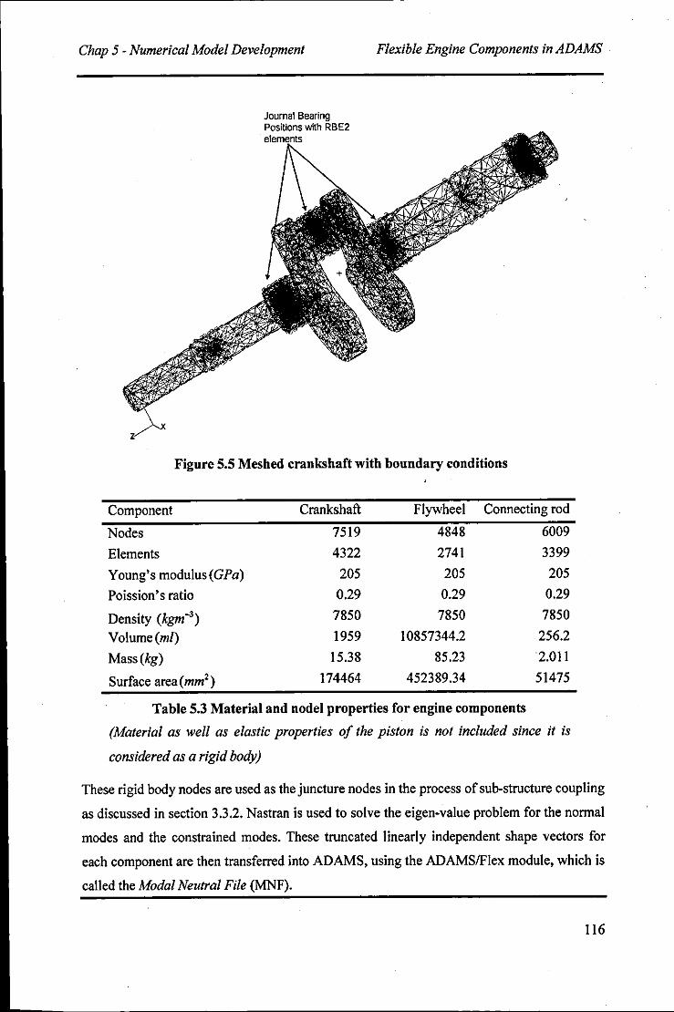
Chap 5 - Numerical Model Development Flexible Engine Components in ADAMS
Journal Bearing Positions with RBE2
Figure 5.5 Meshed crankshaft with boundary conditions
Component Crankshaft Flywheel Connecting rod
Nodes 7519 4848 6009
Elements 4322 2741 3399
Young's modulus (GPa) 205 205 205
Poission's ratio 0.29 0.29 0.29
Density (kgm-3) 7850 7850 7850
Volume (ml) 1959 10857344.2 256.2
Mass (kg) 15.38 85.23 2.011
Surface area(mm2) 174464 452389.34 51475
Table 5.3 Material and nodel properties for engine components
(Material as well as elastic properties of the piston is not included since it is
considered as a rigid body)
These rigid body nodes are used as the juncture nodes in the process of sub-structure coupling
as discussed in section 3.3.2. Nastran is used to solve the eigen-value problem for the normal
modes and the constrained modes. These truncated linearly independent shape vectors for
each component are then transferred into ADAMS, using the ADAMSlFlex module, which is
called the Modal Neutral File (MNF).
116
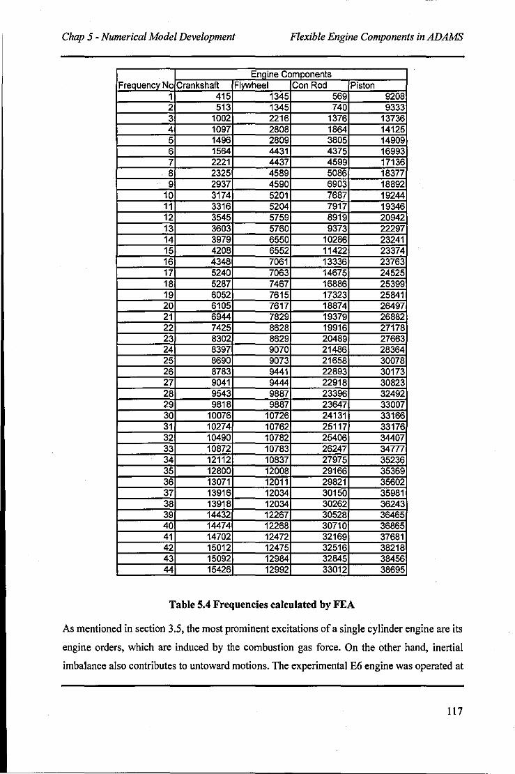
Chap 5 - Numerical Model Development Flexible Engine Components in ADAMS
~on Rod 1 415 1345 569 9208
513 1l4~ 74 02
~--~~--~~r---~~--~~--~~ :64 4431 '5 16993
1 1
1
2: 2:
2221 4437 459 7136 458 8377 459 8892 520 9244
1979 1208 1348 i240 ~87
520' 575! 576( 6 6
7063
7~ 117 8~l19
9:l73 10281 11'12:
14(i7! i8f
7425 8628 1991' 02 8629 i97 9070 i9C 9073
24525
!6 8783 9441 30173
r-____ ~2~----~J~4·----~~~44~--~2~2911~8--~0~823 ~~~~r-~9~887~~~ ~
3
4
1
1901 172
12' 12 2800 3071 3916
13918 14432
151 15426
~ 31 33166
10837 120C 1201 1203 12034
!21
175 12984 12992
2511 2
'"
@1
16
3301<!
i61 35981
,243
3 38456 38695
Table 5.4 Frequencies calculated by FEA
As mentioned in section 3.5, the most prominent excitations of a single cylinder engine are its
engine orders, which are induced by the combustion gas force. On the other hand, inertial
imbalance also contributes to untoward motions. The experimental E6 engine was operated at
117
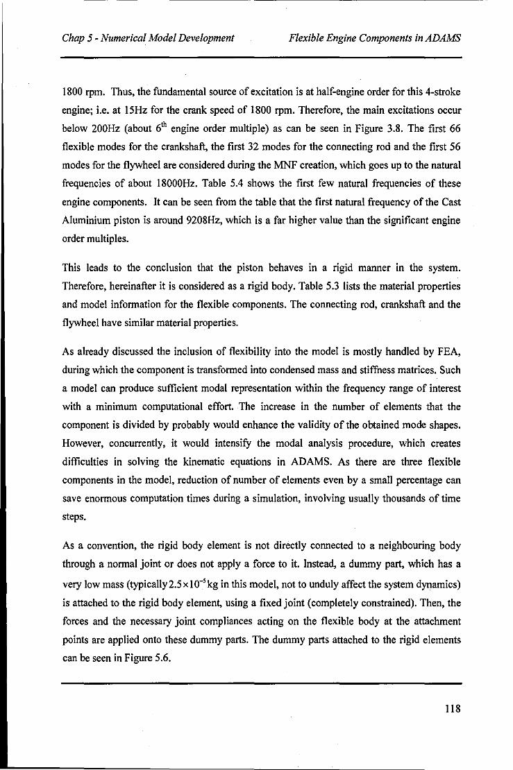
Chap 5 - Numerical Model Development Flexible Engine Components in ADAMS
1800 rpm. Thus, the fundamental source of excitation is at half-engine order for this 4-stroke
engine; i.e. at 15Hz for the crank speed of 1800 rpm. Therefore, the main excitations occur
below 200Hz (about 6th engine order multiple) as can be seen in Figure 3.8. The first 66
flexible modes for the crankshaft, the first 32 modes for the connecting rod and the first 56
modes for the flywheel are considered during the MNF creation, which goes up to the natural
frequencies of about 18000Hz. Table 5.4 shows the first few natural frequencies of these
engine components. It can be seen from the table that the first natural frequency of the Cast
Aluminium piston is around 9208Hz, which is a far higher value than the significant engine
order multiples.
This leads to the conclusion that the piston behaves in a rigid manner in the system.
Therefore, hereinafter it is considered as a rigid body. Table 5.3 lists the material properties
and model information for the flexible components. The connecting rod, crankshaft and the
flywheel have similar material properties.
As already discussed the inclusion of flexibility into the model is mostly handled by FEA,
during which the component is transformed into condensed mass and stiffness matrices. Such
a model can produce sufficient modal representation within the frequency range of interest
with a minimum computational effort. The increase in the number of elements that the
component is divided by probably would enhance the validity of the obtained mode shapes.
However, concurrently, it would intensifY the modal analysis procedure, which creates
difficulties in solving the kinematic equations in ADAMS. As there are three flexible
components in the model, reduction of number of elements even by a small percentage can
save enormous computation times during a simulation, involving usually thousands of time
steps.
As a convention, the rigid body element is not directly connected to a neighbouring body
through a normal joint or does not apply a force to it. Instead, a dummy part, which has a
very low mass (typically 2.5 x 10·' kg in this model, not to unduly affect the system dynamics)
is attached to the rigid body element, using a fixed joint (completely constrained). Then, the
forces and the necessary joint compliances acting on the flexible body at the attachment
points are applied onto these dummy parts. The dummy parts attached to the rigid elements
can be seen in Figure 5.6.
118
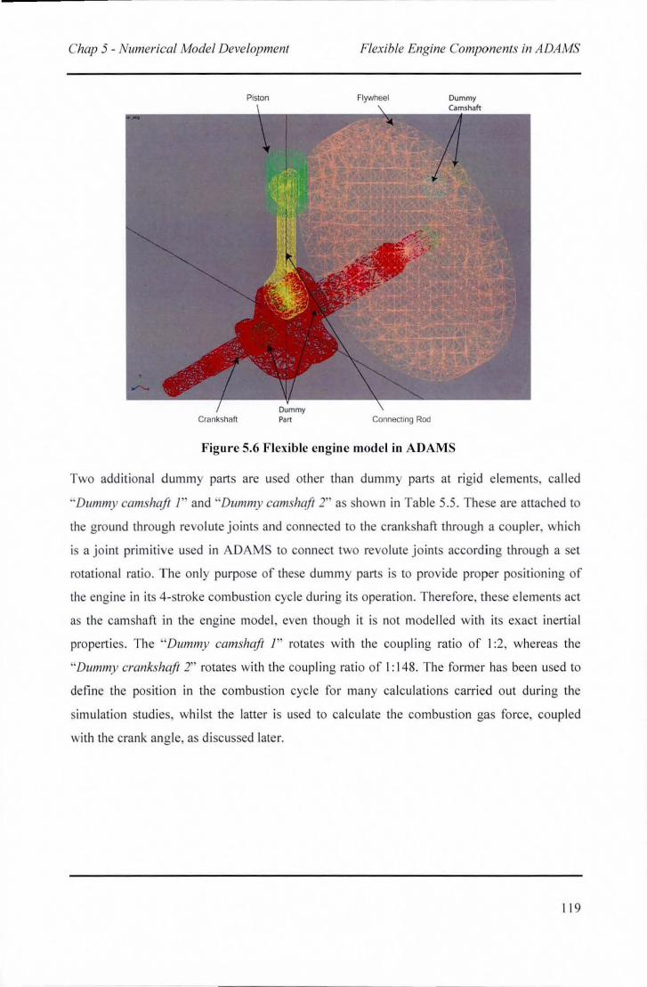
Chap 5 - Numerical Model Development Flexible Engine Components in A DAMS
Piston Flywheel
Crankshaft ConnectIng Rod
Figure 5.6 Flex ible eng in e model in ADAMS
Two add itional dummy pans are used other than dummy pans at rig id e lements, ca ll ed
"Dummy camshaft I" and "Dummy camshaft 2" as hown in Table 5.5. These are attached to
the ground through revolute joints and connected to the crankshafl thro ugh a coup ler, which
is a joi nt primitive used in ADAMS to connect two revo lute joints according through a set
rotational ratio. The only purpose of these dummy pans is to prov ide proper posit ioning of
the engi ne in its 4-stroke combustion cycle during its operation. Therefo re, these elements act
as the camshaft in the engine mode l, even though it is not mode lled with its exact inertia l
properties . The " Dummy camshaft I" rotates w ith the co upli ng rat io of I :2, whereas the
"Dummy crankshaft 2" rotates with the coup li ng ratio of I : 148. The former has been used to
define the pos ition in the combustio n cycle for many ca lculations carri ed out during the
simulati on studi es, whil st the latter is used to calculate the combustion gas force, coupled
with the crank ang le, as discussed later.
11 9
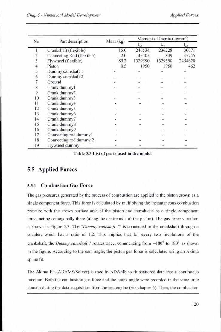
Chap 5 - Numerical Model Development Applied Forces
No Pan description Mass (kg) Moment of Inenia (kllmml)
Ixx Iyv Izz I Crankshaft (flexi ble) 15.0 246534 236228 3007 1 2 Connecting Rod (flex ible) 2.0 45305 849 45745 3 Flywheel (flexib le) 85.2 1329590 1329590 2454628 4 Pi ston 0.5 1950 1950 462 5 Dummy camshaft I 6 Dummy camshaft 2 7 Ground 8 Crank dummy I 9 Crank dummy2 10 Crank dummy3 11 Crank dummy4 12 Crank dummy5 13 Crank dummy6 14 Crank dummy7 15 Crank dummy8 16 Crank dummy9 17 Connecting rod dummy 1 18 Connecting rod dummy 2 19 Flywheel dummy
Table 5.5 List of pa rts used in the model
5.5 Applied Forces
5.5.1 Combustion Gas Fo rce
The gas pressures generated by the process of combustion a re applied to the piston crown as a
ingle component force. This force is calculated by multiplying the instantaneous combustion
pressure with the crown surface area of the piston and introduced as a si ngle component
fo rce, act ing orthogona lly there (a long the centre axis of the pi ston). The gas force variation
is shown in Figure 5.7. The "Dummy camshaft I " is connected to the crankshaft through a
coupler, which has a ratio of I :2 . This implies that for every two revolutions of the
crankshaft, the Dummy camshaft I rotates once, commencing from - 1800 to 1800 as shown
in the figure. According to the cam angle, the piston gas force is calculated using an Akima
spline fit.
The Akima Fit (ADAMS/Solver) is used in ADAMS to fit scattered data into a continuous
function . Both the combustion gas force and the c rank angle were recorded in the same time
domain during the data acqu isitio n from the test engine (see chapter 6). Then, the combustion
120
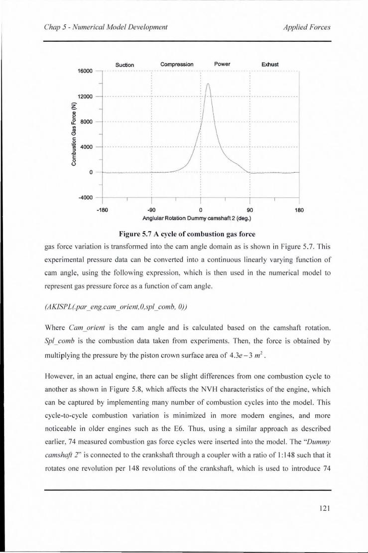
Chap 5 - Numerical Model Development
16000
12000
" ~ 4000 " ~ o t>
Suction Compression
Applied Forces
Power Exhus1
~ooo -t----,,----r----,-----r----.-----r----,----~
-180 -90 o 90 180
Anglular Rolation Dummy camshafl 2 (deg.)
Figure 5.7 A cycle of combustion gas force
gas force variat ion is transformed into Ihe cam angle domain as is shown in Figure 5.7. This
experimental pressure data can be converted into a continuous linearl y vary ing function of
cam angle. using the following expression, which is then used in the numerical model to
represent gas pressure force as a functi on of cam angle.
(A KlSP L(pcl/·_eng.cam_ orient, O" pl_comb, 0))
Where Cam_orient is the cam ang le and is ca lcu lated based on the camshaft rotat ion.
SplJomb is the combustion data taken from experiments. Then, the force is obtained by
mUltiplying the pressure by the pi ston crown s urface a rea of 4.3e-3 m' .
However, in an actual engi ne, there can be sli ght differences from one combustio n cycle to
anoth er as shown in Figure 5.8, which affects the VH characte ristics of the engi ne, which
can be captured by implementing many number of combusti on cycles into the model. Th is
cyc le-to-cyc le combust io n variati on is minimized in more modern engines, and more
noticeable in older engi nes such as the E6. Thus, usi ng a s imilar approach as described
earlier, 74 measured combustion gas force cycles were inse lted into the model. The ··Dummy
camshaft 2'" is connected to the cra nkshaft through a co upl er w ith a ratio of I : 148 such that it
rotates one revo lution per 148 revo lutions of the crankshaft, whi ch is used to introduce 74
12 1
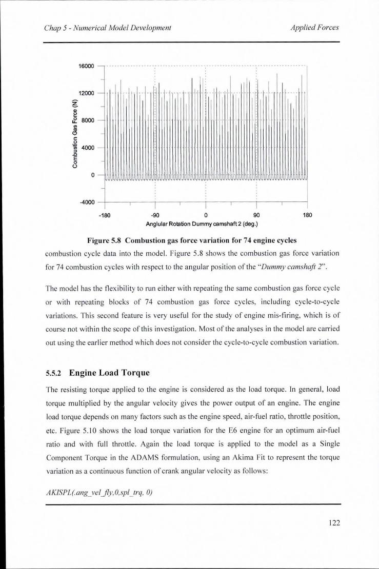
Chap 5 - Numerical Model Development Applied Forces
16000 - . .• .. .. . .. .....•....•..•• . ..... . .... . ... . . • • . ...... . . .. . .. . .. .. ...• .. ...
-
12000 -
g -~ .£ 8000 -
" ~ " 0
11\
11 ~
" 4000 -
.0 E 0 ()
0 - 'VVVVVVVUV\~ JVVVVIJUUVUJ'U! . UUUtll JtmtlUUU~J\JUtmUUUUlJVUUUlJlJlft ~
·4000 -+--.---t-I--.---
lr----.----i
I---.-----1
-180 ·90 0 90 180
Mglular Rotation Dummy ca mshaft 2 (deg.)
Figure 5.8 Combustion gas force variation for 74 engine cycles
combustion cyc le data into the model. Figure 5.8 shows the combustion gas force va ri at ion
for 74 combusti on cyc les with respect to the angular pos ition of the ·'Dummy camshaft 2".
The model has the fl exib ility to run e ither with repeating the same combustion gas force cyc le
or with repeating blocks of 74 combusti o n gas fo rce cyc les, includ ing cyc le-to-cyc le
va ri ations. Thi s second feature is very usefu l for the study of engine mis-firing, which is o f
course not wi thin the scope of this investigatio n. Most of the ana lyses in the model a re carried
out usi ng the earl ier meth od which does not consider the cycle-to-cycle combustion variati on.
5.5.2 Engine Load Torque
The res isting torque appl ied to the engine is considered as the load torque. In general, load
torque multipli ed by the angu lar velocity gives the power o utput of an engine. The engine
load torque depends on many factors such as the engine speed, a ir-fuel rati o, throttle pos ition,
etc. Figure 5. 10 shows the load torque variation for the E6 eng ine for an optimum a ir- fuel
ratio and with fu ll throttl e. Again the load torque is app lied to the model as a S ing le
Component Torque in the ADAMS formulati o n, using an Ak ima Fit to represent the torque
variation as a continuous funct ion of crank angu lar ve locity as fo ll ows:
AKISPL(ang_veljly,O,spUrq, O)
122
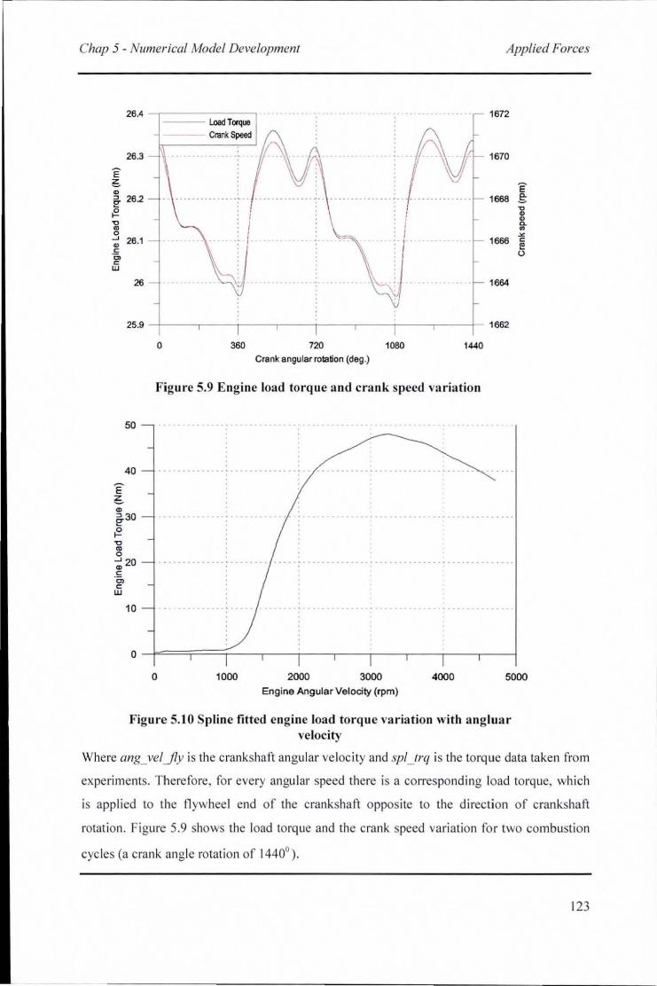
Chap j - Numerical Model Development Applied Forces
26.4
26.3
E ~
" ~ 26.2 {3.
" " 0 ~
" c 0. c w
E e .,
26.1
26
25.9
50
40
e- 30
{3.
" '" o a! 20 c .c, c W
10
1672
1670
1664
-+-----r----~---,----~----,_----r_--_,----~ 1 ~2
0 360 720 1060 1440 Crank angular rotation (deg.)
Figure 5.9 Engine load torque and crank speed variation
o 1000 2000 3000 4000 5000 Engine Angular Velocity (rpm)
Figure 5.10 Spline fi tted engine load torque va ria tion with angluar velocity
Where ang_velJy is the crankshaft angu lar ve loc ity and spl_trq is the torque data taken from
experiments . Therefore, for every angular speed there is a corresponding load torque, which
is appli ed to the flywheel end of the crankshaft opposite to the direction of cranksha ft
rotati on. Figure 5.9 shows the load torque and the crank speed variation for two combustion
cycles (a crank ang le rotation of 1440° ).
123
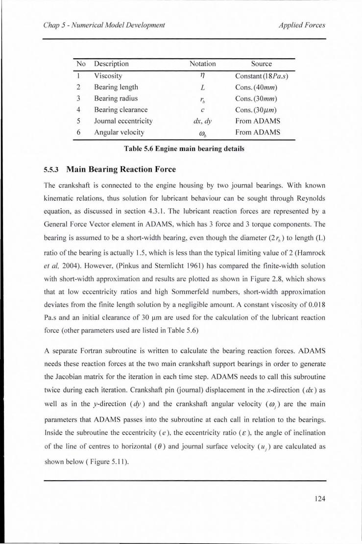
Chap 5 - Numerical Model Developmenl Applied Forces
No Descri ption Notation Source
I Viscos ity 1) Constant (18Pa.s)
2 Bearing length L Cons. (40Il1m)
3 Bearing radius r b Cons. (30/11/11)
4 Bearing clearance c Cons. (30)1/11)
5 Journa l eccentri city dx, dy From ADAMS
6 Angular veloc ity Wb From ADAMS
Table 5.6 Engine main bcaring dcta ils
5.5.3 Main Bea ring Reaction Force
The crankshaft is connected to the engine housing by two journal bearings. With known
ki nematic relations, thus so lution for lubricant behaviour can be sought through Reynolds
equation, as di scussed in section 4.3. 1. The lubri cant reaction forces are represented by a
Genera l Force Vector element in ADAM , which has 3 fo rce and 3 IOrque components. The
bearing is assumed to be a short-width bearing, even though the diameter (2 1. ) to length (L)
ratio of the bearing is actuall y 1.5. which is less than the typical limiting value of 2 (Ham rock
el ai, 2004). However, (Pinkus and Sternlicht 196 1) has compared the finite-width so lution
with short-width approx imation and results are ploned as shown in Figure 2.8, which shows
that at low eccentricity ratios and high Sommerfeld numbers, short-width approx imation
deviates from the fin ite length so lut ion by a negli gible amount. A constant viscos ity of 0.0 18
Pa.s and an initial clearance of 30 ~lIn are used for the ca lculat ion of the lu bricant reaction
force (other parameters used are li sted in Table 5.6)
A separate Fortran subrout ine is written to ca lculate the bearing reaction forces. ADAMS
needs these reaction forces at the two main crankshaft support bearings in order to generate
the Jacobian matrix for the iteration in each time step . ADAMS needs to cal l thi s subroutine
twice during each iteration. Crankshaft pin Gournal) di splacement in the x-direction (dx) as
wel l as in the y-direction ( dy) and the crankshaft angular ve locity (w) ) are the main
parameters that ADAMS passes into the subrout ine at each call in relation to the bearings.
Inside the subroutine the eccentricity (e), the eccentric ity ratio (e) , the angle of inclination
of the line of cent res 10 horizontal ( e ) and journal surface velocity ( 11) are ca lculated as
shown be low ( Figure 5. I I).
124
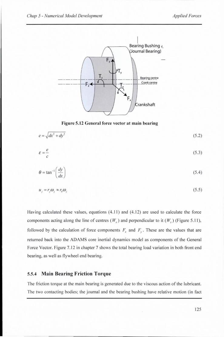
Chap j - Numerical Model Developmenl
I ~------... Bearing Bushing v.
Journal Bearing)
T, T,
F ,;+t-'--+--";,~ -'f - --, _ Bear~n.9.£.e~~e _ Cra.!!k (erur.~
F, rankshaft
Figure 5.12 General force vector at main bearing
e = Jdx' +dy'
e £=
C
e _,(dY) = tan -dx
Applied Forces
(5.2)
(5.3)
(5 .4)
(5.5)
Having calculated these va lues, equations (4 . I I) and (4 .1 2) are used to calculate the force
components acting along the li ne of centres (W,) and perpend icular to it (W,) (F igure 5. 11 ),
followed by the ca lculat ion of force components F: and F,. These are the va lues that are
returned back into the ADAMS core inertial dynam ics model as components of the Genera l
Force Vector. Figure 7.12 in chapter 7 shows th e total bearing load variati on in both front end
bearing, as we ll as fl ywheel end bearing.
5.5.4 Main Bearing Friction Torque
The fr iction torque at the main bearing is generated due to the viscous acti on of the lubricant.
The two contacting bod ies; the journa l and the bearing bu hing have re lative moti on (in fact
125
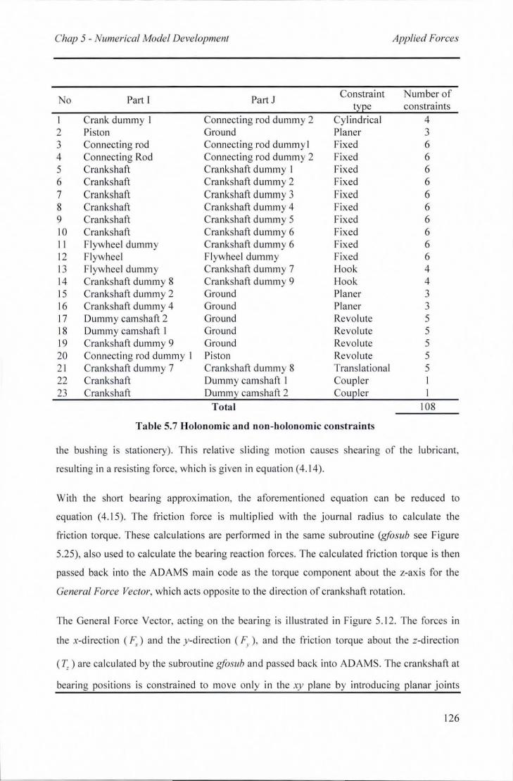
Chap j - Numerical Model Development Applied Forces
No Pan I Part J Constraint umber of
t~~e constra i nts Crank dummy I Connecting rod dummy 2 Cylindrical 4
2 Piston Ground Planer 3 ,
Connect ing rod Connecting rod dummy I Fixed 6 )
4 Connect ing Rod Connecting rod dumm y 2 Fixed 6 5 Crankshaft Crankshaft dummy I Fixed 6 6 Crankshaft Crankshaft dummy 2 Fixed 6 7 Crankshaft Crankshaft dummy 3 Fixed 6 8 Crankshaft Crankshaft dummy 4 Fixed 6 9 Crankshaft Crankshaft dummy 5 Fixed 6 10 Crankshaft Crankshaft dummy 6 Fixed 6 11 Flywheel dummy Crankshaft dummy 6 Fixed 6 12 Flywheel Flywheel dummy Fixed 6 13 Fl ywheel dummy Crankshaft dummy 7 Hook 4 14 Crankshaft dummy 8 Crankshaft dummy 9 Hook 4 15 Crankshaft dummy 2 Ground Planer 3 16 Crankshaft dummy 4 Ground Planer
, )
17 Dummy camshaft 2 Ground Revolute 5 18 Dummy camshaft I Ground Revolute 5 19 Crankshaft dummy 9 Ground Revolute 5 20 Connecting rod dummy I Piston Revolute 5 21 Crankshaft dummy 7 Crankshaft dummy 8 Translational 5 22 Crankshaft Dummy camshaft I Coupler I 23 Crankshaft Dumm~ camshaft 2 Cou~l er I
Total 108
Table 5.7 Holonomic and non-holonom ic constraints
the bushing is stati onery). This relati ve sliding motion causes shearing of the lubricant,
resulting in a resisting force, which is given in equation (4.14).
With the short bearing approximation, the aforementioned equation can be reduced to
equation (4.15). The friction force is multip li ed with the journal radius to calculate the
friction torque . These calculations are performed in the same subroutine (g(osub see Figure
5.25), also used to calculate the bearing reaction forces. The calculated friction torque is then
passed back into the ADAMS main code as the torque component about the z-axis for the
General Force Vector, which acts opposite to the direction of crankshaft rotation.
The General Force Vector, acting on the bearing is illustrated in Figure 5. 12. The fo rces in
the x-direction (F.) and the y-direction (F, ). and the fri ction torque about the z-direction
(T,) are calculated by the subroutine g(osub and passed back into ADAMS. The crankshaft at
bearing pos itions is constrained to move only in the xy plane by introducing planar joints
126
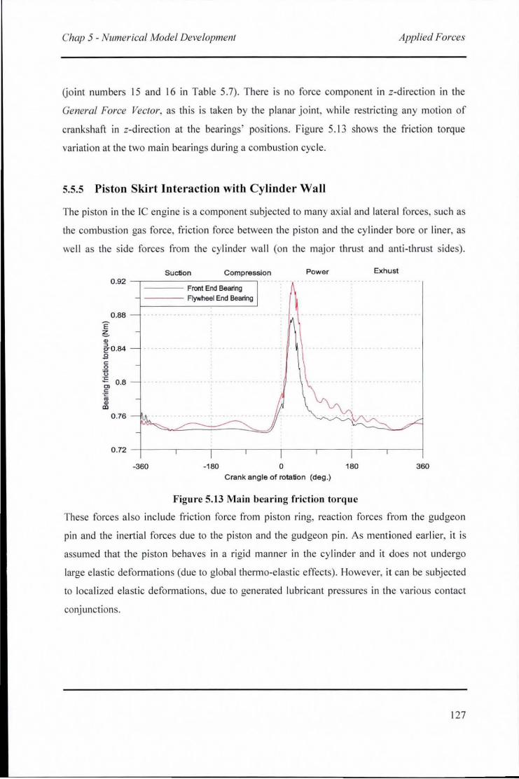
Chap 5 - Numerical Model Development Applied Forces
Goint numbers 15 and 16 in Table 5.7) . There is no force component in z-direction in the
General Force Vector, as thi s is taken by the planar joint, while restricting any motio n of
crank haft in z-d irecti on at the bearings ' posi tion . Figure 5.1 3 shows the friction torque
variati on at the two main bearings during a combustion cyc le.
S.S.S Piston Skirt Interaction with Cylinder Wall
The pi ston in the le engine is a component subj ected to many axial and latera l forces, such as
the combustion gas force , friction force between the pi ston and the cylinder bore or liner, as
wel l as the side forces from the cylinder wall (on the major thrust and anti-thrust sides) .
E ~
"
0 .92
0.88
2-0.84 B
" o il :E 0.8 CD
" ." .. " Cl>
0 .76
Suction Compression
Front End Bearing - --- Flywheel End Bearing
Power Exhust
0 .72 --j---r---r---,---.,---,----,----,----j
-360 -180 o 180 360
Crank angle of rotation (deg.)
Figure S. \3 Main bearing friction torque
These forces al so include fr iction force from piston ring, reaction forces from the gudgeon
pin and the ineltia l forces due to the piston and the gudgeon pin. As mentioned earl ier, it is
assumed that the pi ston behaves in a ri gid manner in the cylinder and it does not undergo
large elastic deformations (due to global thermo-e lastic effects) . However, it can be subjected
to loca li zed e lastic deformations. due to generated lubricant pressures in the various contact
conjunctions.
127
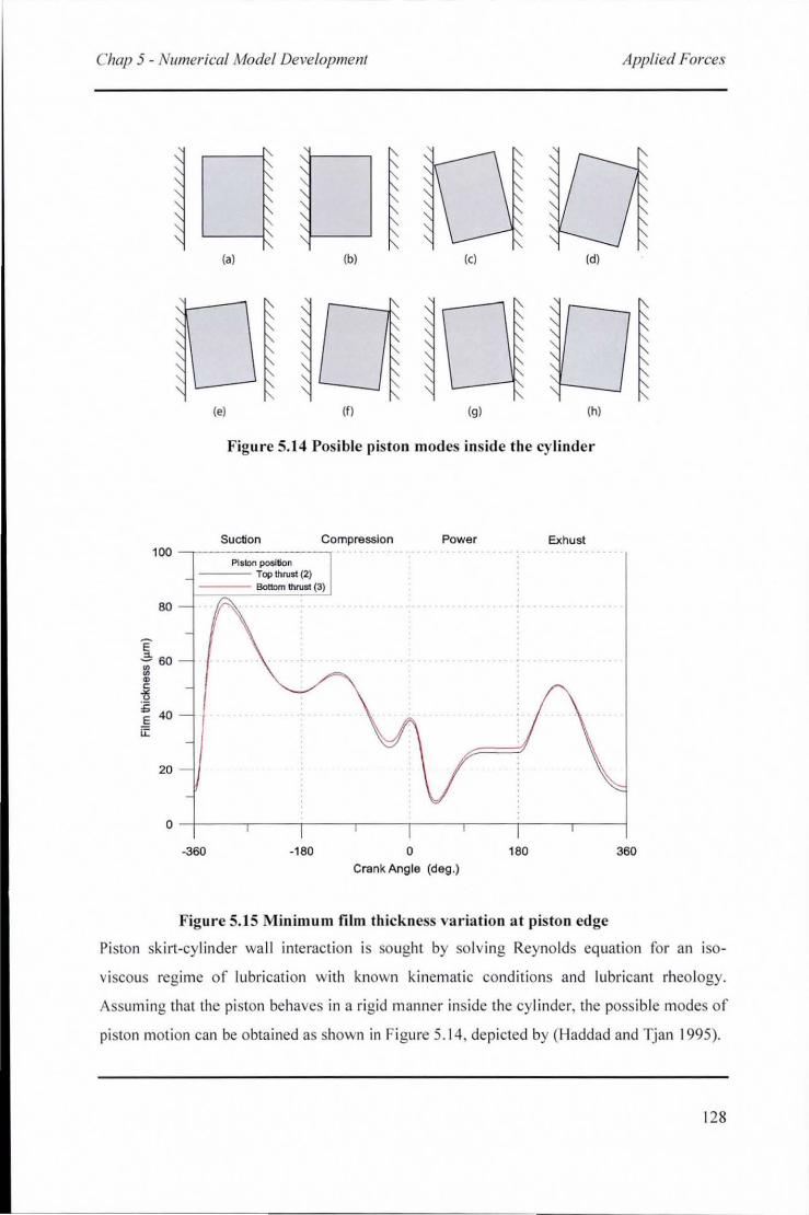
Chap 5 - Numerical Model Developmenl
(a) (b) (c) (d)
(e) (I) (g) (h)
Figure 5.14 Posible piston modes inside the cylinder
Suction CompressIon 100 -,---- ---,
80
E .a 60 ::l .. ~ :6 40 E il:
20
Piston posi tion Top thrust (2) Bottom thrus1 (3)
Power Exhust
Applied Forces
0 -+----,----,----,-----,----.----T----,----4 ·360 -180 o 180 360
Crank Angle (deg.)
Figure 5.15 Minimum film thickness variation at piston edge
Piston skirt-cylinder wall interact ion is so ught by so lving Reyno lds eq uati on for an iso
viscous regime of lubrication with known kinemati c conditi ons and lu bricant rheo logy.
Assuming that the pi ston behaves in a rigid manner inside the cylinder, the poss ible modes o f
pi ston motion can be obtained as shown in Figure 5. 14, dep icted by (Haddad and Tjan 1995).
128
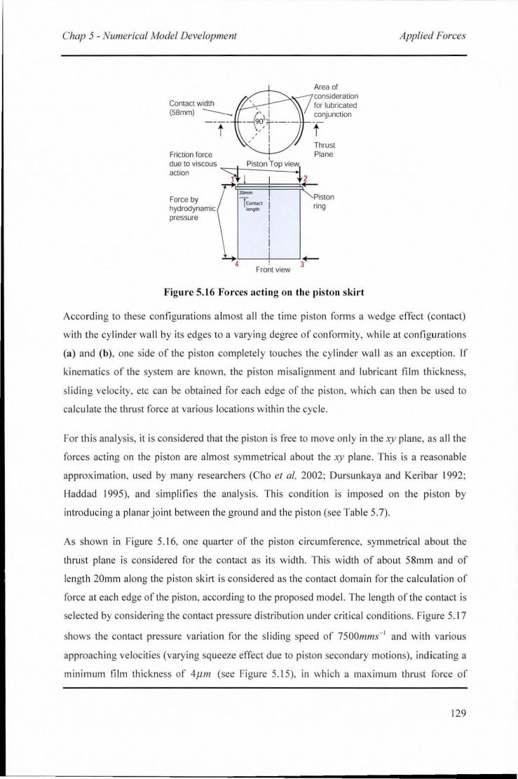
Chap 5 - Numerical Model Development
Contact width (58mm) __
Area of ---T:::::'~-J COnSideration
for lubricated conjunction
t f Thrust
Friction force I Plane
due (0 viscous ~, IPiSIOn IT op Vie~, 2 action ?t ~~
Force by / "'"""I ! Piston ""'~, I . hydrodynamic let'ogm I nng
pressure 1
i , I
.l i ~~4-----+!----~'~ Front view
Figure 5.16 Forces acting 011 the pistoll skirt
Applied Forces
Accord ing to these confi gurati ons a lmost a ll the t ime piston forms a wedge effect (contact)
with the cylinder wa ll by its edges to a vary ing degree of confo rmity, wh il e at configurations
(a) and (b), one side of the pi ston completely touches th e cy linder wall as an exception. If
kinematics of the system are known, the pi ston misa lignment and lubricant film thickness,
sliding veloc ity, etc can be obtained fo r each edge of the pi ston, wh ich can then be used to
ca lcul ate the thrust force at various locations with in the cycle .
For thi s analysis, it is considered that the pi sto n is free to move onl y in the .\y plane, as a ll the
forces act ing on the piston are almost symmetrical about the xy plane. Th is is a reasonable
approxi mation, used by many researchers (Cho et ai, 2002; Dursunkaya and Keribar 1992;
Haddad 1995), and simplifies the analysis. Th is condition is imposed on the p iston by
introducin g a planar joint between th e ground and the pi ston (see Table 5.7).
As shown in Figure 5.1 6, one quarter of th e pi ston c ircumference, symmetrica l about the
thrust plane is considered for the contact as its w idth . This width o f about 58mm and of
length 20mm along the pi sto n skirt is considered as the contact doma in for the ca lcu lation of
fo rce at each edge o f the piston, according to the proposed model. The length of the contact is
se lected by considering the contact pressure di stribut io n under critica l conditions. Figure 5.1 7
shows the contact pressure variation for the s li ding speed of 7500111l11S- ' and with various
approaching ve loc iti e (varyin g squeeze effect due to piston secondary motions), indicating a
mi ni mum film thickness of 411m (see Figure 5.15), in whi ch a maximum thrust force of
129
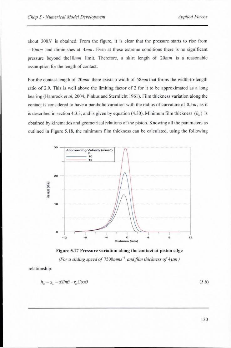
Chap 5 - Numerical Model Development Applied Forces
about 300N is obta ined. From the figure, it is c lear th at the pressure starts to rise from
-10111111 and diminishes at 4mm . Even at these extreme cond itions there is no sign ificant
pressure beyond the I Oll1m limit. Therefore, a skirt length of 20111111 is a reasonab le
assumption for the length of contact.
For the contact length of 20117111 there exists a width of 58111 111 that fo rms the width-to- Iength
ratio of 2.9. This is we ll above the limiti ng facto r of 2 for it to be approx imated as a long
bearing (Hamrock et ai, 2004; Pinkus and Stern li cht 196 1). Film thi ckness vari ation along the
contact is considered to have a parabo lic varia tion w ith the rad ius of curvature of 0.5 111 , as it
is described in sect ion 4.3.3 , and is g iven by equatio n (4.30). Minimum film th ickness (h",) is
obtained by kinematics and geometri ca l re latio ns of the piston. Knowing a ll the parameters as
outl ined in Figure 5.1 8, the min im um fi lm thickness can be ca lcu lated, using the fo llowing
.. ~
6 " i1l ~
re la tio nshi p:
30 -,-------------------,
20
10
Approaching Ve locity (mm s-1) 5
-------- 1 0 1 5
- 1 2 -8 ... o Distance (mm )
4 •
Figure 5.1 7 Pressure variatio n along the contact at pis ton edge
(For a sliding speed of 7500111ll1S - I and film thickness of 4tJ.m)
h", = x, -aSim'}- I;"Cost}
1 2
(5.6)
130
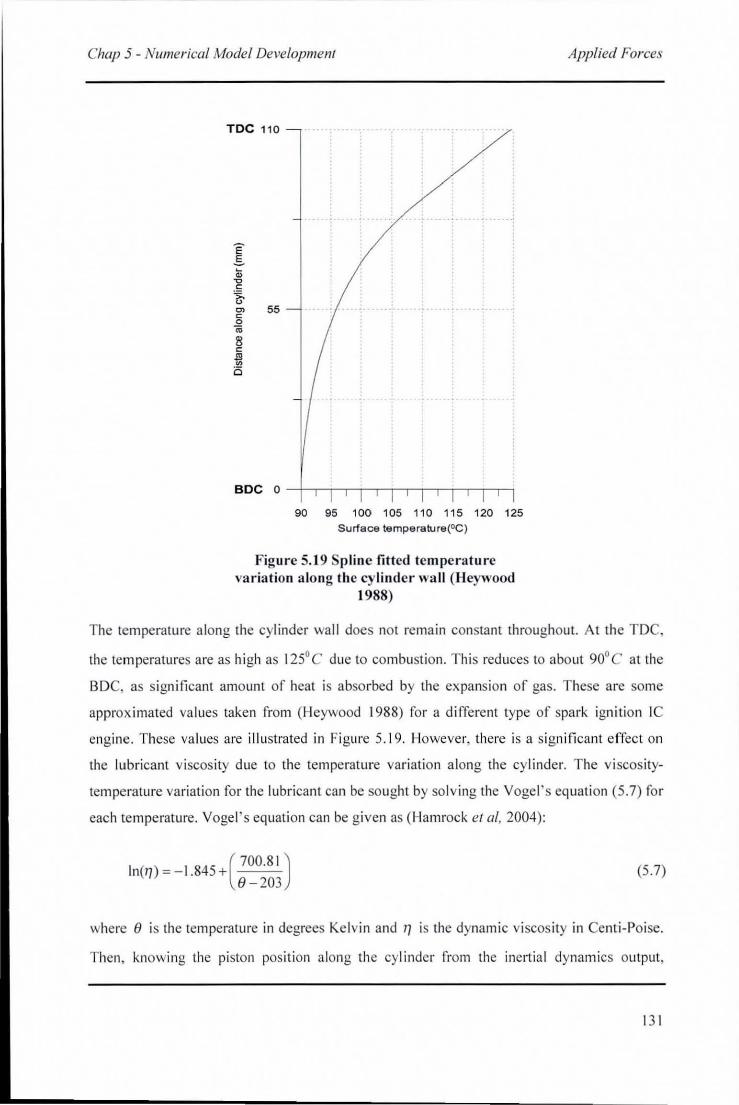
Chap 5 - Numerical Model Development
Toe 110
E .§. 0;
"0 C
~ '" 55 c 0 Oi 1l c .!!l ~
Ci
90 95 100 105 110 115 120 125 Surlace temperatu re(OC )
Figure 5.19 Spline fitted temperature va riation a long th e cylinder wall (Heywood
1988)
Applied Forces
The temperature along the cylinder wall does not remain constant throughout. At the TDC,
the temperatures are as hi gh as 125' C due to combustion. This reduces to about 90' C a t the
BDC, as s ignificant amount of heat is absorbed by the expansion of gas . These are some
approximated values taken fro m (Heywood 1988) for a d iffe rent type of spark ignition IC
eng ine. These va lues are illustrated in Figure 5. 19. However, there is a significant effect on
the lu bricant viscosity d ue to the temperature variation along the cylinder. The viscosity
temperature variation for the lubricant can be sough t by so lving the Vogel's equation (5.7) for
each temperature. Vogel 's eq uation can be given as (Hamrock et ai, 2004):
In(T]) = - 1.845 +( 700.81 ) 8-203
(5 .7)
where 8 is the temperature in degrees Kelvin and I) is the dynamic visco ity in Centi-Po ise.
Then , knowing the piston posit ion a long the cyl inder frol11 the inertia l dynamics output,
13 1
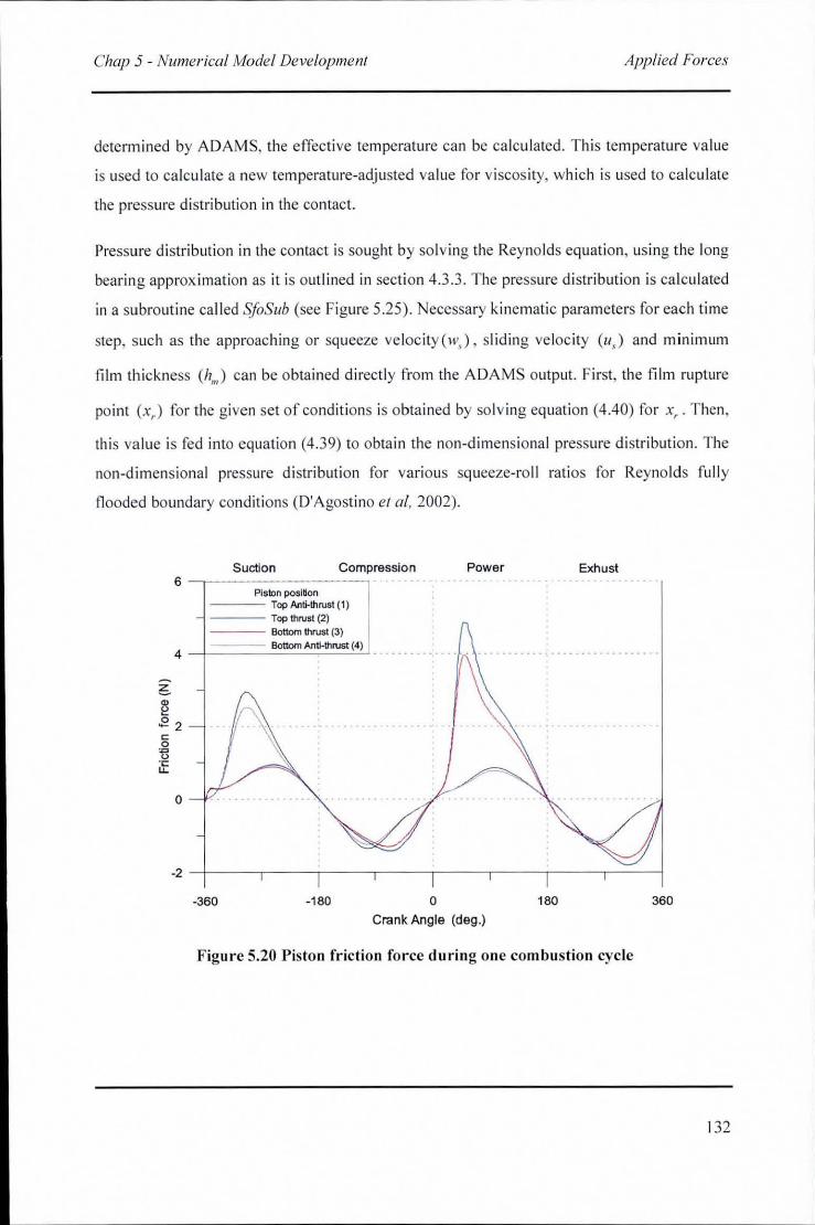
Chap 5 - Numerical Model Development Applied Forces
determined by ADAMS, the effecti ve temperature can be ca lcu lated . This temperature va lue
is used to ca lcul ate a new temperature-adjusted va lue for viscos ity, which is used to ca lculate
the pressure distributio n in the contact.
Pressure distribution in the co ntact is sought by solving the Reyno lds equation, using the long
bearing approximation as it is outlined in secti on 4.3.3. The pressure d istribution is ca lcu lated
in a subroutine ca lled SfoSlIb (see Figure 5.25). Necessary kinematic parameters for each time
step, such as the approaching or squeeze ve locity(wJ , sliding velocity (1I, ) and minimum
film thickness (h., ) can be obtained directl y from the ADAMS output. First, the film rupture
point (x,) for the given set of conditions is o bta ined by so lving equation (4.40) for x" Then,
this val ue is fed into equation (4.39) to obtain the non-dimensio nal pressure di stribution. The
non-dimensional pressure di stribution fo r various squeeze-ro ll rat ios for Reynolds ful ly
flooded boundary conditi ons (D'Agostino et aI, 2002).
Suction Compression 6 ---r----------.,
Piston position --- Top Anti-thrust (1) - -- Top thrust (2) --- Bottom thrust (3)
Power Exhust
4 -+-===:....":Bo~ttom""".:An~'.~th~rus~t~(4!J) _ ...• .•• •. . .• • •• • •.•••• l •• _ • • ••• _ ..••••••
o
-2 -+--.---r---.---,--,-----.,---,-=-~
-360 -180 o 180 360
Crank Angle (deg .)
Figure 5.20 Piston friction force during one combustion cycle
132
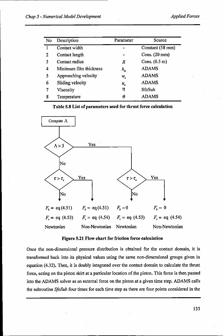
Chap 5 - Numerical Model Development Applied Forces
No Description Parameter Source
1 Contact width Constant (58 mm)
2 Contact length Cons. (20 mm)
3 Contact radius R Cons. (0.5 m)
4 Minimum film thickness hm ADAMS
5 Approaching velocity w, ADAMS
6 Sliding velocity u, ADAMS
7 Viscosity 1) SfoSub
8 Temperature (J ADAMS
Table 5.8 List of parameters used for thrust force calculation
Compute A
A>3 Yes
T>T, Yes T>T, Yes
No No
F" = eq (4.51) F" = eq (4.51) F" = 0 F" = 0
F., = eq (4.53) F., = eq (4.54) F., = eq (4.53) F., = eq (4.54)
Newtonian Non-Newtonian Newtonian Non-Newtonian
Figure 5.21 Flow chart for friction force calculation
Once the non-dimensional pressure distribution is obtained for the contact domain, it is
transformed back into its physical values using the same non-dimensional groups given in
equation (4.32). Then, it is doubly integrated over the contact domain to calculate the thrust
force, acting on the piston skirt at a particular location of the piston. This force is then passed
into the ADAMS solver as an external force on the piston at a given time step. ADAMS calls
the subroutine SfoSub four times for each time step as there are four points considered in the
133
----------------------------------...... Chap 5 - Numerical Model Development Applied Forces
particular piston skirt location as shown in Figure 5.18. Thrust force variation at four corners
of the piston during one combustion cycle is illustrated in Figure 7.18, chapter 7. The list of
parameters and their values used for force calculation is given in Table 5.8.
5.5.6 Friction Between the Piston Skirt and the Cylinder Wall
Friction force acting at each point of consideration on the piston skirt is calculated using the
boundary and viscous force contributions as outlined in section 4.4. Boundary friction is
calculated using the statistical approach described in section 4.4.1. The parameters used for
boundary friction calculation and their values are given in Table 5.9.
Sliding velocity (u,) , minimum film thickness (hm) , maximum pressure and thrust force at
the contact are the main values necessary for calculation of friction. Sliding velocity and
minimum film thickness can be obtained from ADAMS. Maximum pressure and the thrust
load at the contact can be obtained from load calculation as described in the previous section
5.5.5. Knowing these basic values other parameters such as, the Hertzian contact area (A.),
the non-dimensional film parameter (A) and the shear stress (r) can be calculated, using
equations (4.50), (4.41) and (4.53) respectively. Then, non-dimensional film parameter is
used to calculate values of statistical functions given by equations (4.48) and (4.49). Then,
the asperity contact area (Aa) and the asperity load (P,,) are calculated, using equations (4.43)
and (4.44) respectively.
Then mode of friction is obtained by examining the film parameter. If it is greater than 3, then
viscous frictional conditions are regarded as prevalent and the friction force is calculated
using equation (4.53). Non-Newtonian conditions may be prevalent for whatever the film
thickness and this must be tested by examining the shear stress against the critical value of
the Eyring stress (Cameron 1966). Ifit is greater than this limit, then the equation (4.54) must
be used for calculation of friction. However, if the film parameter is less than 3, then both
boundary friction and viscous friction may be present. Boundary friction is calculated using
equation (4.51) and it is added to the viscous friction contribution, calculated using the same
method as already described. Flow chart for friction force calculation is given in Figure 5.21.
The friction force variation at four piston edges for a one combustion cycle is shown in
Figure 5.20.
134
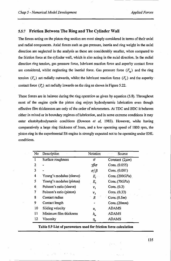
Chap 5 - Numerical Model Development Applied Forces
5.5.7 Friction Between The Ring and The Cylinder Wall
The forces acting on the piston ring section are most simply considered in terms of their axial
and radial components. Axial forces such as gas pressure, inertia and ring weight in the axial
direction are neglected in the analysis as these are considerably smaller, when compared to
the friction force at the cylinder wall, which is also acting in the axial direction. In the radial
direction ring tension, gas pressure force, lubricant reaction force and asperity contact force
are considered, whilst neglecting the inertial force. Gas pressure force (F,.) and the ring
tension (F,,) act radially outwards, whilst the lubricant reaction force (F;,) and the asperity·
contact force (p.) act radially inwards on the ring as shown in Figure 5.22.
These forces are in balance during the ring operation as given by equation (5.8). Throughout
most of the engine cycle the piston ring enjoys hydrodynamic lubrication even though
effective film thicknesses are only of the order of micrometers. At TDC and BDC it behaves
either in mixed or in boundary regimes of lubrication, and in some extreme conditions it may
enter elastohydrodynamic conditions (Dowson et ai, 1983). However, while having
comparatively a large ring thickness of 3mm, and a low operating speed of 1800 rpm, the
piston ring in the experimental E6 engine is strongly expected not to be operating under EHL
conditions.
No Description Notation Source
1 Surface roughness a Constant (2Jlm)
2 y{Ja Cons. (0.055)
3 alP Cons. (0.001)
4 Young's modulus (sleeve) El Cons. (200GPa)
5 Young's modulus (piston) E, Cons. (70GPa)
6 Poisson's ratio (sleeve) VI Cons. (0.3)
7 Poisson's ratio (piston) v, Cons. (0.33)
8 Contact radius R Cons. (0.5m)
9 Contact length Cons. (20mm)
10 Sliding velocity u, ADAMS
11 Minimum film thickness hm ADAMS
12 Viscosity 11. ADAMS
Table 5.9 List of parameters used for friction force calculation
135
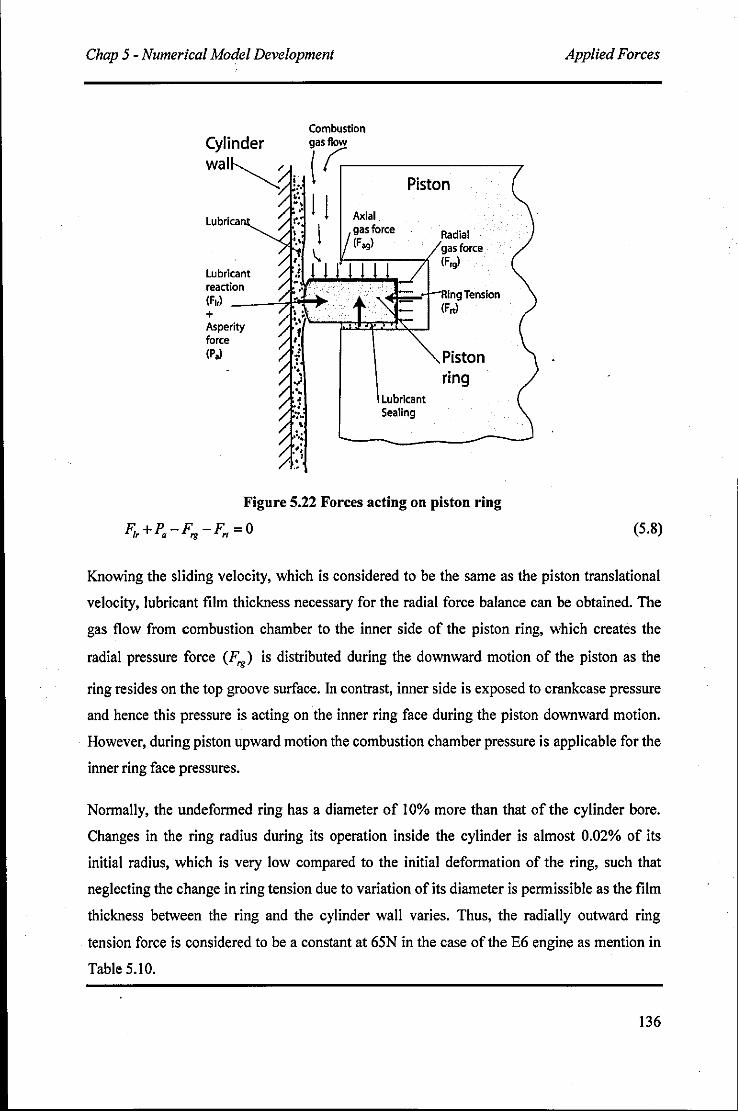
Chap 5 - Numerical Model Development
Lubrica
lubricant reaction (F,,) --~7I?"t-~ + Asperity force (Pal
Piston
Radial gas force (F",)
" ... fliO~l"ilng Tension
Lubricant Sealing
(F.,)
Piston ring
Figure 5.22 Forces acting on piston ring
F" +Pa -F" -F" = 0
Applied Forces
(5.8)
Knowing the sliding velocity, which is considered to be the same as the piston translational
velocity, lubricant film thickness necessary for the radial force balance can be obtained. The
gas flow from combustion chamber to the inner side of the piston ring, which creates the
radial pressure force (F",) is distributed during the downward motion of the piston as the
ring resides on the top groove surface. In contrast, inner side is exposed to crankcase pressure
and hence this pressure is acting on the inner ring face during the piston downward motion.
However, during piston upward motion the combustion chamber pressure is applicable for the
inner ring face pressures.
Normally, the undeformed ring has a diameter of 10% more than that of the cylinder bore.
Changes in the ring radius during its operation inside the cylinder is almost 0.02% of its
initial radius, which is very low compared to the initial deformation of the ring, such that
neglecting the change in ring tension due to variation of its diameter is permissible as the film
thickness between the ring and the cylinder wall varies. Thus, the radially outward ring
tension force is considered to be a constant at 65N in the case of the E6 engine as mention in
Table 5.10.
136
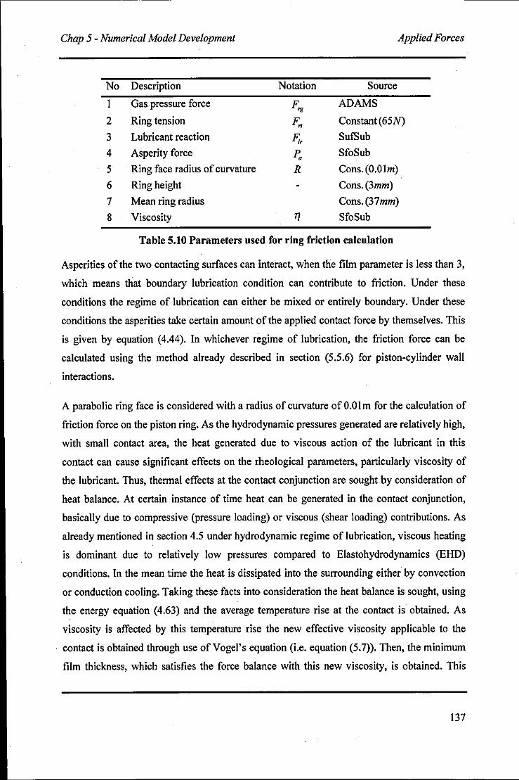
Chap 5 - Numerical Model Development Applied Forces
No Description Notation Source
I Gas pressure force F,. ADAMS
2 Ring tension F" Constant (65 N)
3 Lubricant reaction F;, SufSub
4 Asperity force 1'. SfoSub
5 Ring face radius of curvature R Cons. (O.Olm)
6 Ring height Cons. (3mm)
7 Mean ring radius Cons. (37mm)
8 Viscosity T/ SfoSub
Table 5.10 Parameters used for ring friction calculation
Asperities of the two contacting surfaces can interact, when the film parameter is less than 3,
which means that boundary lubrication condition can contribute to friction. Under these
conditions the regime of lubrication can either be mixed or entirely boundary. Under these
conditions the asperities take certain amount of the applied contact force by themselves. This
is given by equation (4.44). In whichever regime of lubrication, the friction force can be
calculated using the method already described in section (5.5.6) for piston-cylinder wall
interactions.
A parabolic ring face is considered with a radius of curvature of O.Olm for the calculation of
friction force on the piston ring. As the hydrodynamic pressures generated are relatively high,
with small contact area, the heat generated due to viscous action of the lubricant in this
contact can cause significant effects on the rheological parameters, particularly viscosity of
the lubricant. Thus, thermal effects at the contact conjunction are sought by consideration of
heat balance. At certain instance of time heat can be generated in the contact conjunction,
basically due to compressive (pressure loading) or viscous (shear loading) contributions. As
already mentioned in section 4.5 under hydrodynamic regime of lubrication, viscous heating
is dominant due to relatively Iow pressures compared to Elastohydrodynamics (EHD)
conditions. In the mean time the heat is dissipated into the surrounding either by convection
or conduction cooling. Taking these facts into consideration the heat balance is sought, using
the energy equation (4.63) and the average temperature rise at the contact is obtained. As
viscosity is affected by this temperature rise the new effective viscosity applicable to the
contact is obtained through use ofVogel's equation (Le. equation (5.7». Then, the minimum
film thickness, which satisfies the force balance with this new viscosity, is obtained. This
137
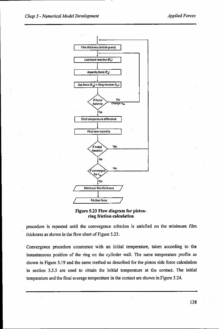
Chap 5 - Numerical Model Development
1-------. Film thickness (initial guess)
lubricant reaction (Fir)
Asperity force (P,)
J Gas force (Frg) + Ring tension (Frt)
No c ange m
Find temperature difference
Find new viscosity
Yes iteration
No
(converged No
forh
Yes
Minimum film thickness
L friction force 7 Figure 5.23 Flow diagram for pistou
ring friction calculation
Applied Forces
procedure is repeated until the convergence criterion is satisfied on the minimum film
thickness as shown in the flow chart of Figure 5.23.
Convergence procedure commence with an initial temperature, taken according to the
instantaneous position of the ring on the cylinder wall. The same temperature profile as
shown in Figure 5.19 and the same method as described for the piston side force calculation
in section 5.5.5 are used to obtain the initial temperature at the contact. The initial
temperature and the final average temperature in the contact are shown in Figure 5.24.
138
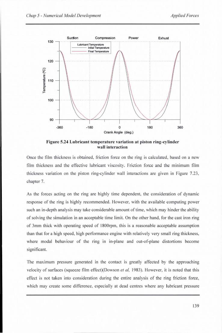
Chap 5 - Numerical Model Development Applied Forces
130
120
I!! ~ 110 8. E ~
-360
Suction Compression
lubricant Temperature Initial Temperature Final Temperature
-180
Power
o Crank Angle (deg.)
ExhuSl
180 380
Figure 5.24 Lubrica nt temperature va riation a t piston r ing-cylinder wa ll in teraction
Once the film thickness is obtained, fr ict ion fo rce on the ring is calculated, based on a new
film thicknes and the effecti ve lubricant viscosity. Friction force and the minimum film
th ickness variation on the piston ring-cylinder wall interactions are given in Figure 7.23,
chapter 7.
As the forces acting on the ring are highl y time dependent, the consideration of dynamic
response of the ring is highl y recommended. However, with the ava il ab le comput ing power
such an in-depth analysis may take considerable amount of time, which may hinder the ab il ity
of so lving the sim ulation in an acceptable time lim it. On the other hand, for the cast iron ring
of 3mm th ick with operating speed of 1800rpm, thi s is a reasonable acceptable assum ption
than that for a high speed, high performance engine with relatively very small ring th ickness,
where modal behaviour of the ring in in-plane and out-of-plane distortions become
significant.
The maxi mum pressure generated in the contact is greatl y affected by the approaching
velocity of surfaces (squeeze fi lm effect)(Dowson et ai, 1983). However, it is noted that this
effect is not taken into considerati on during the entire anal ys is of the ring friction force,
which may create some difference, e pecia ll y at dead centres where any lubricant pressure
139
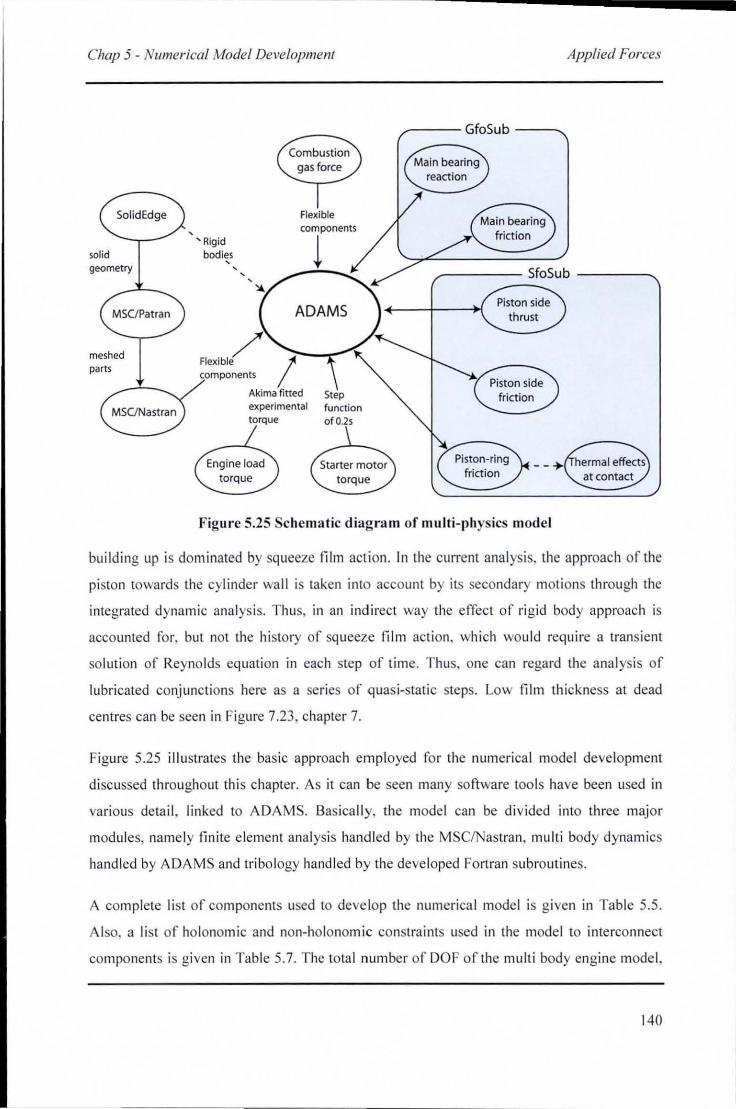
Chap 5 - Numerical Model Development
solid geometry
meshed parts
, 'Rigid
bodies ,
Flexible
,
Step experimental function torque of 0.25
Applied Forces
~-- GfoSub ---..
,----- SfoSub ------....
Figure 5.25 Schematic diagram of multi-physics model
building up is dominated by squeeze film action. In the current anal ysis, the approach of the
piston towards the cylinder wall is taken into account by its secondary motions through the
integrated dynamic analysis. Thus, in an ind irect way the effect of ri gid body approach is
accounted for, but not the hi sto ry of squeeze fi lm action, which would require a transient
solution of Reynolds equation in each step of time. Thus, one can regard the analys is of
lubricated conjunctions here as a series of quasi-stati c steps. Low film thickness at dead
centres can be seen in Figure 7.23, chapter 7.
Figure 5.25 ill ustrates the basic approach employed for the numerical model development
discussed throughout th is chapter. As it can be seen many software tools have been used in
various detail, linked to ADAMS. Basica lly, the model can be divided into three major
modules, namely finite element analysis hand led by the MSClNastran, mu lti body dynamics
ha ndled by ADAMS and tribology hand led by the deve loped Fortran subroutines.
A complete li st of components used to develop the numerical model is given in Table 5.5.
Also, a list of holonomic and non-holonomic constraints used in the model to interconnect
components is given in Table 5.7. The total number of DOF of the multi body engine model ,
140
Chap 5 - Numerical Model Development Applied Forces
including the elastic DOFs due to component fl ex ib il ity can be obta ined using the Gurebler
Kutzbach expression as:
umber of OOF = flexible body modes (flywheel + crank + conrod) +
6 (number of rigid parts - I) - I (Contraints)
= (56+66+ 32)+ 6 x (16-1)-1 08
= 154 +90 - 108
= 136
Thus, the model comprises 136 OOF, including 90 ri gid body motions and 154 structural
modes, which leads to a total of 362 algebra ic and differential equations to be so lved in the
AOAM solver as di scussed in chapter 3.
Whatever the method used for the development of the numerical model , its va lidity must be
ascerta ined as the derivations are based on certa in assumptions and use of certa in numerical
methods. The fo llowing chapter is devoted to measu rements carri ed out on the E6 engine in
the process of va lidation of the multi-physics numerica l model developed thus far.
141
Chap 6 - Experimentatal investigation Inlroduction
6 EXPERIMENTATAL INVESTIGATION
6.1 Introduction
This chapter describes the experimental measurements of vibration from the E6 Ricardo
single cylinder engine. The numerica l prototype descri bed in the previous chapter is
developed, based on the appl ication of the multi-physics multi-scale modelling method to the
same engi ne. Therefore, the mai n purpose of the experimenta l work is to obtain results, which
can be used to gauge the practical use and degree of conformity of the proposed ana lyt ical
approach to a real life app lication.
There are a number of key parameters involved in any experimen tal verification of a
numerica l method. For the current study it was important to determine parameters that can be
pred icted and also easil y measured fo r the purpose of model va li dation. Of course many
pred icted parameters can also be measured. However, the task can become very arduous, if
micro-scale parameters are to be measured , such as lubricant film thickness in the various
modelled conjunct ions. Thi would usually require use of optical engines, runn ing under
motorised (rather than real fired) conditions. This approach, however, is not useful fo r
practical applications. With optical engines, it is possib le to use UF, as pointed out in the
literature review to obtain a measure of film thickness in the piston-cyli nder conjunction
(Se ki et 01, 2000). Another approach may be the use of newly deve loped ul trason ic sensors
attached to the outside wa ll of the cylinder liner, and usable under engi ne fir ing condition
(Dwyer-Joyce et al, 2005). Alternati ve ly, indirect measurements may be taken, for example, a
measure of cyl inder fr ict ion, using a floatin g li ner (Cho et al, 2000). Al l these approaches are
rather time consuming and require a fair amount of development. They are deemed as rather
beyond the main scope of thi s research, with its focus on the development of mUlti-phys ics
method and app lication to prediction of engine conditions. Thus, the approach undertaken in
this chapter uses remote, non-contact measurements of vibration, the philosophy being that
the degree of conform ity of pred ictions with these measurements would indirectly indicate
the re levance of the underlying methods used to practical applications.
Thus, the following measurements are undertaken here:
142
Chap 6 - Experimentatal investigation Introduction
1. Flywhee l nodding motion (being due to its con ical whirl) i measured usi ng state-of
the-art laser torsional vibrometers .
2. Engine angular velocity variation at the fl ywhee l end
Additionall y, frequency responses of engine components are also determined by impact
hammer excitation. These are compared with those emp loyed in the model.
Combined eccentric motion of crankshaft-flywheel assemb ly, gives rise to a conical whirl ing
action, especia ll y at the fl ywhee l end due to eccentricity of the heavy mass of fl ywheel. This
moti on of the fl ywhee l is commonly referred to as fl ywheel nodd ing action in industry. Due
to this motion, po ints on the surface of the fl ywhee l move in the ax ial direction, as we ll as
undergoing torsiona l oscillations about the crankshaft axis. Some relations and details of this
motion have been outlined by (Kelly 1999) with relation to an impact noi se and vibration
phenomenon resu lting in the c lutch system, referred to as whoop.
Vibration measurements are equally important in many areas such as design of structures,
durab ility testing, machine d iagnostics, etc, other than for the purpose of val idation of
analytical mode ls. Natural frequencies of a machine or a structure play an extremely
important role in predicting and understanding the dynamic behav iour of a system. Hence, the
major reason for perform ing vibration test of a system is to determ ine its natura l frequencies
and mode shapes under dynamic exci tati ons. Detailed description of such an experimenta l
modal analysis, used with Component Mode Synthesis (CMS), which can be used to
determine natura l freq uencies, mode shapes and damping ratios are g iven in this chapter.
As previously ex plained , engine rotati onal speed is affected by man y factors uch as, the
combustion gas force, rotational and translati ona l imbalances. Even though certain
precautionary measures can be undertaken, such as balancing of parts, critically adjusting
bearing clearances, employing ene rgy reservoirs (fl ywheel), balance shafts, dual mass
fl ywheels, in order to minimize angular ve loc ity fluctuati ons, it is not poss ible to entirel y
eliminate these ources of excitati on, which are usually inherent to system dynamics.
Therefore, these exc itations are embedded in engine rotational speed to a certain degree and
can be captu red by measu ring the crankshaft angular ve locity response with a required level
of accuracy. Many types of sensors and transducers have been used fo r monitoring engine
conditions . These include: eddy current ga p senso rs for measuring bearing loads (Moreau et
143
Chap 6 - Experimentalal invesligalion Engine Tesling
ai, 2002), stra in gauges for measunng stresses at van ous points, including in bearings
(M ihara and Someya 1995), phys ica l vapour depos ited pressure transducers (M ihara el ai,
1995; Mihara el ai, 1996; Mihara and Someya 2002)and most commonly acce lerometers .
Although a ll these measuring devices have re ported to have certain degrees of success, and
can be regarded as d irect measurement of events, there ex ists a number of major problems.
Firstly, those used in contact conjuncti ons are often subjected to wear o r separation from
surfaces. econdl y, those used to moni tor these conjuncti ons as non-contact dev ices, such as
the eddy current probes or ultrasoni c sensors have insuffic ient reso lution (sensing head be ing
larger or of the same order as the contact d imensions), thus provide an average va lue at best.
Fina ll y, the respon e time of some of these dev ices are insuffic ient to obtain adeq uate data,
showing va riati on of events. The advantage of using lasers is operation at speed of light, as
we ll as the precise nature of measurements in a non-contact manner. thus not interfering with
the process itse lf. The current study employs laser Doppler vibrometry (Be ll and Rothberg
2000a; Bell and Rothberg 2000b), as we ll as piezoe lectric c rystal acce lerometers and pressure
se nsors for measurement of vibrations and combustion pressure .
6.2 Engine Testing
6.2.1 Description of Test Rig
A si ngle cylinder poppet va lve 4-stroke E6 Ricardo experimenta l-type engll1e was first
manufactured in 1958 by Ri cardo Consulting Engineers. This engine has the flexibility to
operate e ither with d iese l fuel or gaso line at different compression rati os. Cylinder head can
move relative to the cy linder, pi ston and crankshaft assembly, in th e vertica l d irection, thus
changing the com pression ratio . Experimenls were performed selling the compression ratio of
1:8 and with gaso line fuel. Acco rding to the manufacturer' s specification, the engine can
produce a maxim um power of 13 Bhp at the speed of 3000 rpm and a maximum torque of 40
m at the speed of 1800rpm. The engine has a cylinder bore of 3 inches and a stroke of 4.375
inches as listed in Table 6.1 . This is an undersqure or longstroke engine whi ch has a higher
stroke compared to bore of the piston. Such a configurat ion creates hi gher fr iction fo rce as
we ll as the wear rate since its higher transve rse ve loc ities. However due to higher crank
radius it can create considerably hi gher torques compared to shortstroke engines.
144
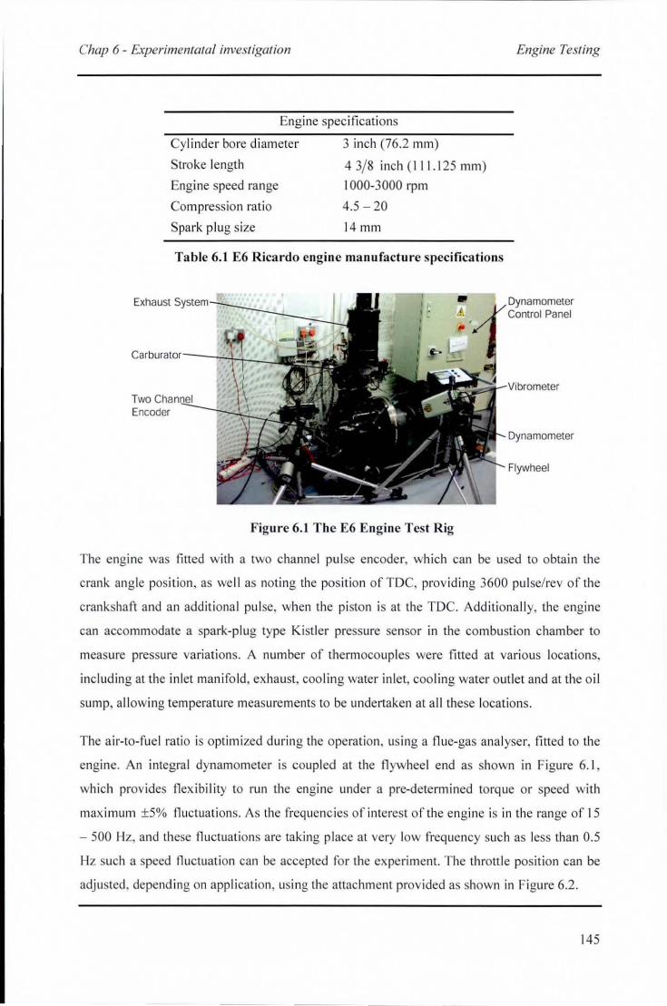
Chap 6 - £rperimenlarai invesligalion
Engine spec ifications
Cylinder bore di ameter 3 inch (76.2 mm)
troke length 4 3/ 8 inch (I I 1.125 mm)
Engine speed range 1000-3000 rpm
Compress ion rati o 4.5 - 20
Spark plug size 14 mm
Table 6.1 E6 Ricardo engine ma nufacture specifications
Exhaust SY5;tenn-!_-;~~~_-:",-J~
TWOC~anQ~_~L\~~ Encoder
Figure 6.1 The E6 Engi ne Test Rig
Engine Tesling
Dynamometer Control Panel
Dynamometer
Flywheel
The engine was fitted with a two channel pulse encoder, which can be used to obtain the
crank angle position, as we ll as noting the position of TOC, providing 3600 pulse/rev of the
crankshaft and an additiona l pulse, when the pi sto n is at the TOe. Additionall y, the engine
can accommodate a spark-plug type Ki stler pressure sensor in the combustion chamber to
measure pressure variations. A number of therm oco uples were fitted at various locations,
including at the inlet manifo ld, ex haust, cooling water inlet cooli ng water outlet and at the o il
sump, allowing temperature measurements to be undertaken at all these locations.
The air-to-fue l ratio is optimized during the operation, using a flue-gas ana lyser, fitted to the
engine. An integral dynamometer is coupled at the flywheel end as shown in Figure 6. 1,
which prov ides flex ibility to run the engine under a pre-determined torque or speed with
maximu m ±5% fluct uations. As the frequenc ies of interest of the engine is in the range of 15
- 500 Hz, and these fluctuati ons are taking place at very low frequency such as less than 0.5
Hz such a speed fluctuati on can be accepted fo r the experiment. The throttle position can be
adjusted , depending on appl icat ion, using the attachment prov ided as shown in Figure 6.2 .
145
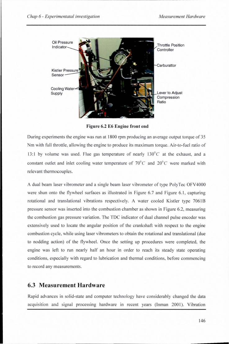
Chap 6 - £rperimentalai investigatian
Oil Pressure
Kistler ;~~~ Sensor
Cooling Water-"! Supply
Figure 6.2 E6 Engine front cnd
Measurement Hardware
Throttle Position Conlrolier
During experiments the engine was run at 1800 rpm producing an average output torq ue of 35
m with full throttle, a ll owing the engine to produce its maximum torque. Ai r- to-fuel ratio of
13: 1 by vo lume was used. Flue gas temperature of nearl y 130°C at the exhaust, and a
constant outlet and inlet cooling water temperat ure of 70° C and 20°C were marked wi th
relevant thermocouples.
A dual beam laser vibrometer and a single beam laser vibrometer of type PolyTec OFV4000
were shun onto the fl ywheel surfaces as illustrated in Figure 6.7 and Figure 6. 1, capturing
rotational and trans lational vibrations respecti ve ly. A water cooled Kist ler type 706 1 B
pressure sensor was inserted into the combustion chamber as shown in Figure 6.2, measuring
the combustion gas pressure vari ation. The TDC indicator of dua l channel pulse encoder was
extensive ly used to locate the angular pos ition of the crankshaft with respect to the engi ne
combust ion cycle, while using laser vibrometers to obtain the rotational and translational (due
to nodding action) of the fl ywhee l. Once the setting up procedures were completed, the
engine was left to run nearly ha lf an hour in order to reach its steady state operating
conditions, especiall y with regard to lubri cation and thermal conditions, before commencing
to record any measurements.
6.3 Measurement Hardware
Rapid advances in so lid-state and computer technology have considerably changed the data
acqu isi ti on and signal process ing hardware in recent years (l nman 200 I). Vibration
146
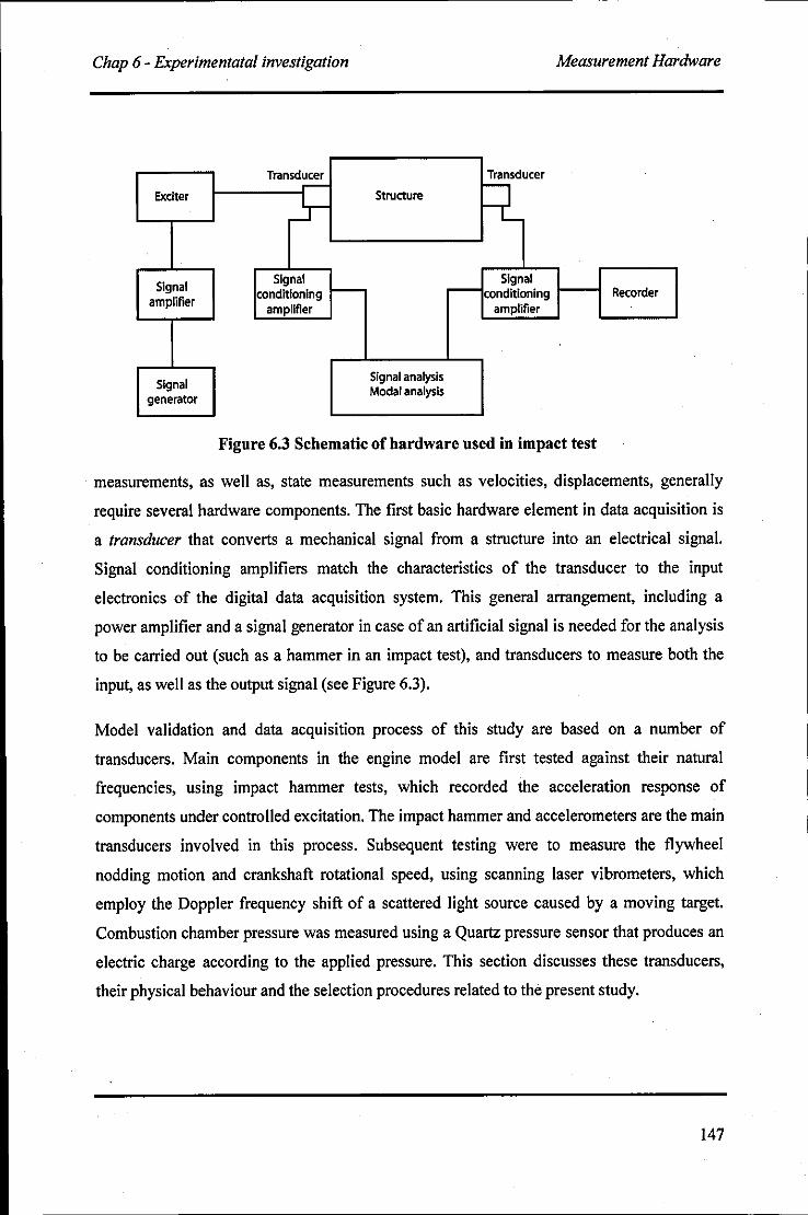
Chap 6 - Experimentatal investigation Measurement Hardware
Transducer Transducer ~
=L Exciter ,J- Structure
Signal Signal - r--Signal
amplifier conditioning conditioning Recorder
amplifier amplifier
Signal Signal analysis
generator Modal analysis
Figure 6.3 Schematic of hardware used in impact test
measurements, as well as, state measurements such as velocities, displacements, generally
require several hardware components. The first basic hardware element in data acquisition is
a transducer that converts a mechanical signal from a structure into an electrical signal.
Signal conditioning amplifiers match the characteristics of the transducer to the input
electronics of the digital data acquisition system. This general arrangement, including a
power amplifier and a signal generator in case of an artificial signal is needed for the analysis
to be carried out (such as a hammer in an impact test), and transducers to measure both the
input, as well as the output signal (see Figure 6.3).
Model validation and data acquisition process of this study are based on a number of
transducers. Main components in the engine model are first tested against their natural
frequencies, using impact hammer tests, which recorded the acceleration response of
components under controlled excitation. The impact hammer and accelerometers are the main
transducers involved in this process. Subsequent testing were to measure the flywheel
nodding motion and crankshaft rotational speed, using scanning laser vibrometers, which
employ the Doppler frequency shift of a scattered light source caused by a moving target.
Combustion chamber pressure was measured using a Quartz pressure sensor that produces an
electric charge according to the applied pressure. This section discusses these transducers,
their physical behaviour and the selection procedures related to the present study.
147
Chap 6 - Experimentatai investigation Measurement Hardware
6.3.1 Controlled Impact Excitation
Vibration test methods are based on several assumptions. The main assumption is that
lumped parameter models adequately represent the test structure and its linearity during
excitations is considered to be most important. During vibration tests that mostly rely on
controlled excitations imposed on the system such as impact test, shakers (electromagnetic or
electrohydraulic) or impact hammers are the most widely used devices.
Shakers are capable of producing a predetermined waveform within a required frequency
range, resulting easily in measurable outputs. Shakers are attached onto the test structures,
while carefully selecting the size and method of attachment, minimising the mass loading
effect that could lower the measured frequency. Even though the use of a stringer can
minimize this effect, while controlling the direction of excitation more precisely, impact
hammer has become a more popular device due to its simplicity and comparatively low cost.
Impact hammer is intended to apply an impUlse excitation onto the structure that can excite
system's natural frequencies. This is possible to achieve by an ideal impact excitation as it
can be shown by decoupling the equation of motion of the lumped parameter model to its
modal degrees offreedom (Craig 1981; Inman 2001). The peak impact load on the structure
is proportional to the head mass and velocity. The load cell at the head measures the impact
force.
Figure 6.4 illustrates the time history and corresponding frequency response of a hammer hit
involved in a crankshaft natural frequency test. Generally, an excitation is considered to be
impulsive, if its duration (~t) is small compared to the period associated with component's
maximum undamped natural frequency of interest. However, the Frequency Response
Function (FRF) of the particular impulse shows consistence of its frequencies up to nearly
6000Hz, and it has sufficient energy to excite frequencies up to 3200Hz, which is the cut
off frequency in this case.
The time history of the impulse, shown in the figure, does not represent an ideal impulse, but
rather one of a finite time duration of 230,us. Hence, the frequency response is not a flat
straight line as it should ideally and theoretically be, but has a periodic form. This periodic
form can be seen from the frequency response function (FRF). The duration of impulse and
hence the shape of the frequency response is controlled by the mass and stiffness of both the
148
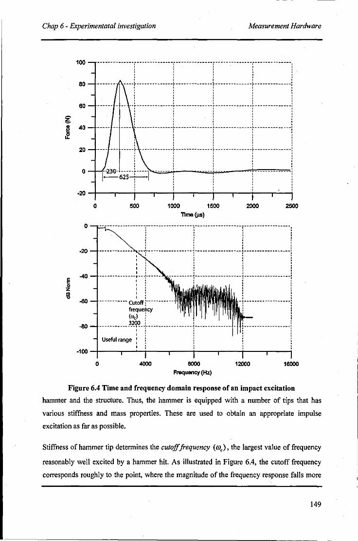
Chap 6 - Experimentatal investigation Measurement Hardware
-~ § {l
100
80
60
40
20
0
-20
0
0
.-------------j--------------j-------------- --------------i--------------" , :: : , , , , " " ----r--------------r-------------- --------------r--------------: " " , , , , , , , , , , " " -~--------------~-------------- --------------r--------------I I I I I " I I " I I I I I I , " : I ::
----- -- ---- ~--------------~-------------- --------------~-------- ______ I , " , " , " , " " " " I I " I I
---- --- -----r ------------r-------------- --------------r--------------t I I " I I I I I I I I I I " I I I I
l~ 625--~ ----j ...... ==+-' ---~-'"---=-.=.-F----~-----~--1[""--'"'-",-'"'--"'-"'--"-,,,-=---[ , " , " , , , ,
500 1000 1500 2000 2500 TIme{jls)
-- --- ;--. - •.. -- .. --------- r-- -- -.-- -- --- ---- -, , , : : , ,
, , -20 -+----·---··-----'>,.c-+·-------------·-·~-------·---··------.,-------.--- .. -- .. ---;
-40 , I I I
--------- Cutoff
(00,)
--- •. -~- .• ------------.--.
- _ •• --_. -- }-~qq: --:- ..•••.. _ •• --- --- _.-
Useful range
, , , , : ,
--- ---- -------: , : , : , --- ------ ---_.' : , , , , : , --- ----- --- -- -_., , , , , , : ,
-100 -1!---T""---i---...,----i---T""---i-----r----i'
o 4000 8000 Frequency (Hz)
12000 16000
Figure 6.4 Time and frequency domain response of an impact excitation
hammer and the structure. Thus, the hammer is equipped with a number of tips that has
various stiffness and mass properties. These are used to obtain an appropriate impulse
excitation as far as possible.
Stiffness of hammer tip determines the cutoff frequency (CO,), the largest value of frequency
reasonably well excited by a hammer hit. As illustrated in Figure 6.4, the cutoff frequency
corresponds roughly to the point, where the magnitude of the frequency response falls more
149
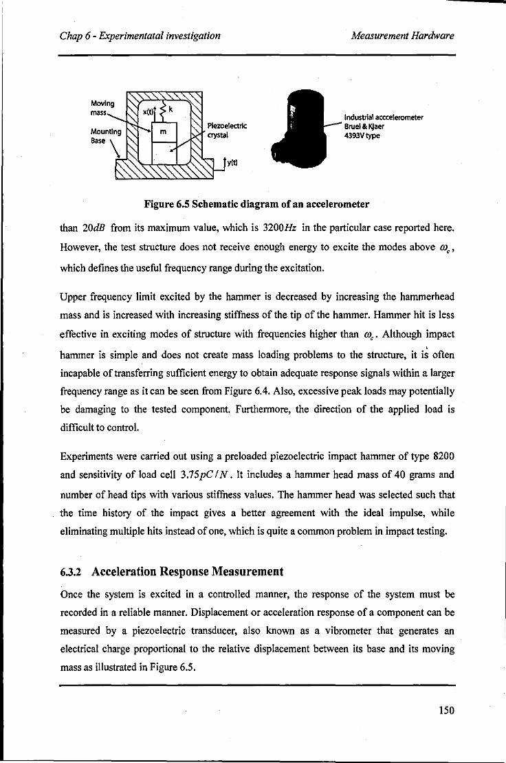
Chap 6 - Experimentatal investigation Measurement Hardware
Industrial acccelerometer Bruel & KJaer 4393Vtype
Figure 6.S Schematic diagram of au accelerometer
than 20dE from its maximum value, which is 3200Hz in the particular case reported here.
However, the test structure does not receive enough energy to excite the modes above me'
which defines the useful frequency range during the excitation.
Upper frequency limit excited by the hammer is decreased by increasing the hammerhead
mass and is increased with increasing stiffness of the tip of the hammer. Hammer hit is less
effective in exciting modes of structure with frequencies higher than me' Although impact
hammer is simple and does not create mass loading problems to the structure, it i~ often
incapable of transferring sufficient energy to obtain adequate response signals within a larger
frequency range as it can be seen from Figure 6.4. Also, excessive peak loads may potentially
be damaging to the tested component. Furthermore, the direction of the applied load is
difficult to control.
Experiments were carried out using a preloaded piezoelectric impact hammer of type 8200
and sensitivity of load cell 3.75pC IN. It includes a hammer head mass of 40 grams and
number of head tips with various stiffness values. The hammer head was selected such that
the time history of the impact gives a better agreement with the ideal impulse, while
eliminating multiple hits instead of one, which is quite a common problem in impact testing.
6.3.2 Acceleration Response Measurement
Once the system is excited in a controlled manner, the response of the system must be
recorded in a reliable manner. Displacement or acceleration response of a component can be
measured by a piezoelectric transducer, also known as a vibrometer that generates an
electrical charge proportional to the relative displacement between its base and its moving
mass as illustrated in Figure 6.5.
150
Chap 6 - Experimentatal investigation Measurement Hardware
Piezoelectric Bruel & Kjaer type 4393V accelerometers were used during this study. These
have a resonant frequency of 55kHz. When the ratio between the measuring frequency over
resonance frequency (r) is small, the measured acceleration deviates only by a small amount
from the actual acceleration of the measuring body. Generally, the range of frequency ratio
(r) of 0 - 0.2 is considered as the efficient range after experimental validation (Inman 2001).
The accelerometers are suitable for measuring responses up to 11kHz. However, according to
manufacturer's specifications those chosen can reliably measure up to 15kHz, even though
experiments carried out needed a maximum of 8kHz response only.
Mounting the accelerometer at the measuring sites is one of the most critical factors for
obtaining accurate results from practical vibration measurement. Sloppy mounting results in a
reduction in the mounted resonant frequency, which can severely limit the useful frequency
range of the accelerometer. The ideal mounting is by a threaded stud to a flat smooth surface
with a thin layer of grease between surfaces to improve the stiffness of the mounting by
which a resonance frequency of 32kHz can be attained (Kjaer 1982). However, as this
method needs much preparation work, as well as machining on the measured component, the
most commonly used alternative mounting method is a thin layer of Bees-wax sticking the
accelerometer onto the component's surface. From this method a maximum resonant
frequency of 29kHz could be achieved with the maximum usable acceleration of 100ms-2 as
the accelerometer weight used was 2.9 g .
6.3.3 Velocity Measurement at Flywheel End
Successful measurement of vibration, using accelerometers mostly relies on firm contacts
between the transducer and the measurement surface, as described above. Nevertheless,
torsional, as well as translational vibration of a moving body such as the flywheel nodding
motion, is not possible using an attached type transducer, especially due difficulties in rooting
the connecting leads out of the crankcase. Thus, a non-contacting type vibrometer such as the
scanning Laser Doppler Vibrometer (LDV) was used for this aspect. The physical principle
behind LDV relies upon the detection of a Doppler frequency shift in the coherent light
source scattered by a moving target. The measured frequency shift iD' relates to object
surface velocity component Uo in the direction of the incident beam as given by following
equation (Halliwell 1996):
151
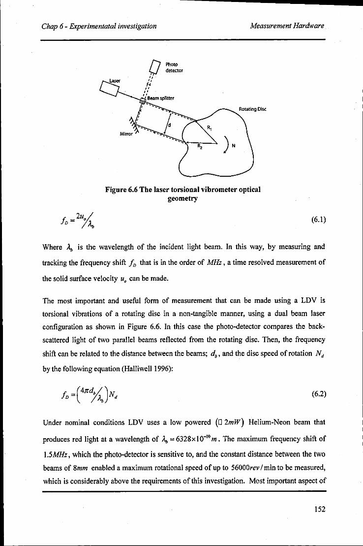
Chap 6 - Experimentatal investigation Measurement Hardware
O Photo I detector
" " I' " " , , I Beam splitter
Rotating Disc
Figure 6.6 The laser torsioual vibrometer optical geometry
(6.1)
Where A" is the wavelength of the incident light beam. In this way, by measuring and
tracking the frequency shift In that is in the order of MHz, a time resolved measurement of
the solid surface velocity Uo can be made.
The most important and useful form of measurement that can be made using a LDV is
torsional vibrations of a rotating disc in a non-tangible manner, using a dual beam laser
configuration as shown in Figure 6.6. In this case the photo-detector compares the back
scattered light of two parallel beams reflected from the rotating disc. Then, the frequency
shift can be related to the distance between the beams; db' and the disc speed of rotation Nd
by the following equation (Halliwell 1996):
(6.2)
Under nominal conditions LDV uses a low powered (02mW) Helium-Neon beam that
produces red light at a wavelength of ;." = 6328 x 1 0-10 m. The maximum frequency shift of
1.5MHz, which the photo-detector is sensitive to, and the constant distance between the two
beams of 8mm enabled a maximum rotational speed of up to 56000rev / min to be measured,
which is considerably above the requirements of this investigation. Most important aspect of
152
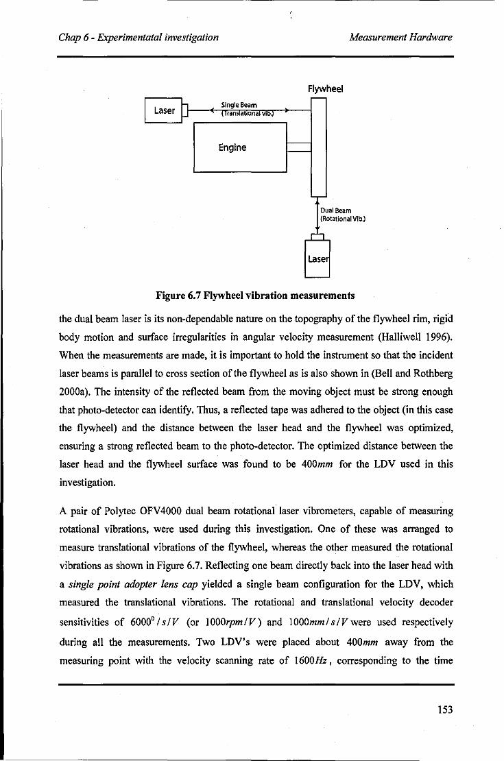
Chap 6 - Experimentatal investigation Measurement Hardware
Flywheel
Single Beam Laser -It--'',lT.llr'''an''''''''''at'''lon,,,,,:r:v'''IID :T .. } -0---;
Engine
Dual Beam (Rotational Vlb.)
Lase
-Figure 6.7 Flywheel vibration measurements
the dual beam laser is its non-dependable nature on the topography of the flywheel rim, rigid
body motion and surface irregularities in angular velocity measurement (Halliwell 1996).
When the measurements are made, it is important to hold the instrument so that the incident
laser beams is parallel to cross section of the flywheel as is also shown in (Bell and Rothberg
2000a). The intensity of the reflected beam from the moving object must be strong enough
that photo-detector can identify. Thus, a reflected tape was adhered to the object (in this case
the flywheel) and the distance between the laser head and the flywheel was optimized,
ensuring a strong reflected beam to the photo-detector. The optimized distance between the
laser head and the flywheel surface was found to be 400mm for the LDV used in this
investigation.
A pair of Polytec OFV 4000 dual beam rotational laser vibrometers, capable of measuring
rotational vibrations, were used during this investigation. One of these was arranged to
measure translational vibrations of the flywheel, whereas the other measured the rotational
vibrations as shown in Figure 6.7. Reflecting one beam directly back into the laser head with
a single point adopter lens cap yielded a single beam configuration for the LDV, which
measured the translational vibrations. The rotational and translational velocity decoder
sensitivities of 6000° I s I V (or I OOOrpm I V) and I OOOmm I s I V were used respectively
during all the measurements. Two LDV's were placed about 400mm away from the
measuring point with the velocity scanning rate of 1600Hz, corresponding to the time
153
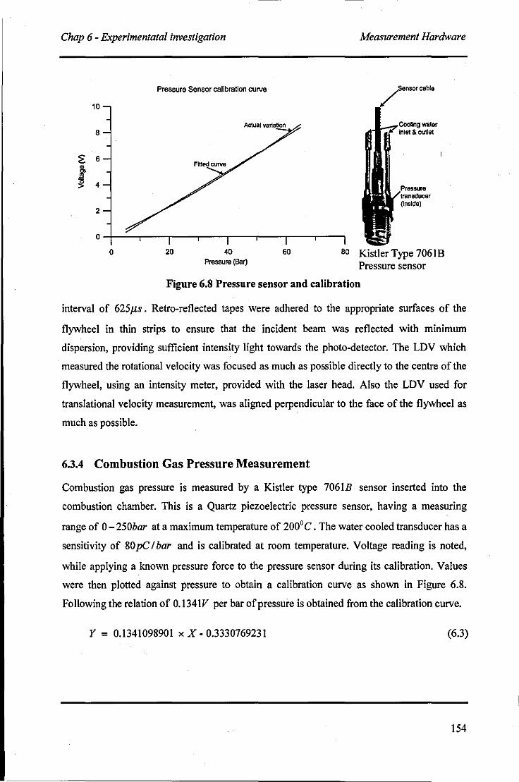
Chap 6 - Experimentatal investigation
o
Pressure Sensor calibration curve
20 40 Pressure (Bar)
60
Measurement Hardware
JI-.i" ~~"~~ water ~ Inlet & outlet
80 Kistler Type 7061B Pressure sensor
Figure 6.S Pressure sensor and calibration
interval of 625f.ls. Retro-reflected tapes were adhered to the appropriate surfaces of the
flywheel in thin strips to ensure that the incident beam was reflected with minimum
dispersion, providing sufficient intensity light towards the photo-detector. The LDV which
measured the rotational velocity was focused as much as possible directly to the centre of the
flywheel, using an intensity meter, provided with the laser head. Also the LDV used for
translational velocity measurement, was aligned perpendicular to the face of the flywheel as
much as possible.
6.3.4 Combustion Gas Pressure Measurement
Combustion gas pressure is measured by a Kistler type 706lB sensor inserted into the
combustion chamber. This is a Quartz piezoelectric pressure sensor, having a measuring
range of 0 - 250bar at a maximum temperature of 2000 C . The water cooled transducer has a
sensitivity of 80 pC / bar and is calibrated at room temperature. Voltage reading is noted,
while applying a known pressure force to the pressure sensor during its calibration. Values
were then plotted against pressure to obtain a calibration curve as shown in Figure 6.8.
Following the relation of 0.1341V per bar of pressure is obtained from the calibration curve.
Y = 0.1341098901 x X - 0.3330769231 (6.3)
154
Chap 6 - Experimentatal investigation Signal Processing and Data Acquisition
During experiments the observed voltage reading from the transducer was converted back
into a pressure reading. Cool water was circulated to the transducer to protect it from possible
damage that may be caused due to higher temperatures.
Output impedance of most transducers is not well suited for direct input into the signal
analysis equipment. Hence, signal conditioners, which may be charge amplifiers or voltage
amplifiers are often used to amplify signals prior to their analysis, and must be properly
calibrated along with the transducers in terms of both magnitude and phase over the
frequency range of interest.
Once the response signal has been properly conditioned, it is routed to an analyser for signal
processing. The analyser type that has become the standard is called the digital Fourier
analyzer, also called Fast Fourier Transform (FFT) analyser. Basically, the analyser accepts
an analogue voltage signal that represents acceleration, velocity, pressure, etc. which is then
filtered and digitized for computation. The analysed signal can then be manipulated in a
variety of ways to produce such information as natural frequencies, damping ratios, etc.
which forms the topic for the following section.
6.4 Signal Processing and Data Acquisition
6.4.1 Brief background in Digital Signal Processing
Much of the analysis, especially in modal impact testing and engine responses is of a periodic
nature and needs to perform an analysis in the frequency domain. Therefore, it is required to
convert the analogue time domain signals into digital frequency domain information. The
method used to perform a transformation of this nature is called the Fourier transformation
from which, a periodic signal oftime period T is represented by the Fourier coefficients or
spectral coefficients at various frequencies.
Basically, this process is started by an Analogue-to-Digital (AID) conversion that multiplies
the signal by a square wave function, which is zero over alternate values of !:J.t and has the
value of unity at each I'J.t for a small time. Here !:J.t is called the sampling time and special
care must be taken when choosing its value as this can lead to a wrong interpretation of the
analogue signal. A common error incorporating with improper sampling is called aliasing,
which can cause high frequencies to appear as low frequencies (Inman 2001). Aliasing results
155
Chap 6 - Experimentatal investigation Signal Processing and Data Acquisition
from Analog to Digital (AID) conversation and refers to the misrepresentation of the analog
signal by the digital record. Basically, if the sampling rate is too slow to catch the details of
the analog signal, the digital representation will cause high frequencies to appear as low
frequencies.
Aliasing is avoided by choosing a sampling time small enough to provide at least two
samples per cycle of the highest frequency of interest. In fact, experience indicates that 2.5
samples per cycle is a better choice, which is referred to as the sampling theorem (Otnes and
Encochson 1972). It is also possible to avoid aliasing by using an anti-aliasing low pass filter,
which only allows low frequencies to pass through. Accordingly, the engine tests using LDV
used a sampling time of 6251ls, which is equivalent to a frequency of 1600Hz, whereas the
frequencies of interest of engine excitations are up to 500Hz with a cycle time of 2000lls .
Once the digital record of signal is available, the discrete version of the Fourier transform is
performed. The task of the analyser is to compute the Fourier coefficients, using Fast Fourier
Transform which is developed by (Cooley and Tukey 1965). To make the digital analysis
feasible, the periodic signal must be sampled over a finite time. This can give rise to another
problem referred to as leakage (Inman 2001), which can simply occur due to not cutting the
signal at any integral multiple of its period. This causes erroneous frequencies to appear in
the digital representation, as a Fourier Transforms assumes that a signal is periodic within the
sample record length, which is not actually the case. However, this can be minimized either
by using a window function that forces the signal to be zero outside the sampling period or by
collecting data for a longer time period that takes into consideration many number of cycles.
The most commonly used window function is the Hanning Window.
6.4.2 Signal Analysis
Most of the signals processed during the experiments were non-deterministic or random with
a collection of time histories resulting from various excitations, which could have been
severely affected by disturbances (noise) of various form. Such a random signal with an
assembly of information of data can only be treated in a statistical manner in order to
distinguish its spectral contents and separate these into spectral contributions. This process
can effectively be simplified by transforming the signal from its time domain to frequency
domain, employing well developed techniques as it is discussed in the previous section. Once
156
Chap 6 - Experimentatal investigation Signal Processing and Data Acquisition
the obtained signals were transformed, clear spectra could be seen such as in the engine
output response, which is dominated by engine orders and half orders that are due to
translating mass and combustion force respectively. Impact testing accomplished to capture
natural frequencies of components associated with its modal deformation, the situation was
rather complicated as some of the frequencies resided very much closely to each other within
the spectrum. In such a scenario it is important to eliminate other excitations as much as
possible, which is also known as noise of the signal that would be mistaken with natural
frequencies. As such, confidence in a measured quantity is increased by performing a number
of identical tests and averaging the results.
If the signal is deterministic, then the Frequency Response Function (FRF), which describes
the relationship between the input and the output, for the system can be derived by
mathematical relations. However, when the input and output behaviour is available in the
form of statistical data in time domain, a rather different approach is used to determine the
FRF of the system. As such the Power Spectral Density (PSD) of autocorrelation of the
excitation spectra S jJ(m) and PSD of cross correlation between the excitation and response
Sfx (m) can be related to FRF HUm) as follows:
(6.4)
In the same manner PSD of autocorrelation of response spectra Sxx(m) and PSD of cross
correlation between the excitation and response Sx/(m) can be related to FRF HUm) as
follows:
(6.5)
Such that FRF for the same system can be calculated employing two completely different
approaches as given by equations (6.4) and (6.5) that underlie the complexity of the process
behind the coherence function, which is widely used to identify whether a signal is
contaminated with noise (more rigorous derivation can be found in (Newland 1993)).
Whatever the method used to calculate FRF, it must produce the same function as it is for the
same system. Therefore, the coherence jitnction denoted by r2, which is the ratio between
157
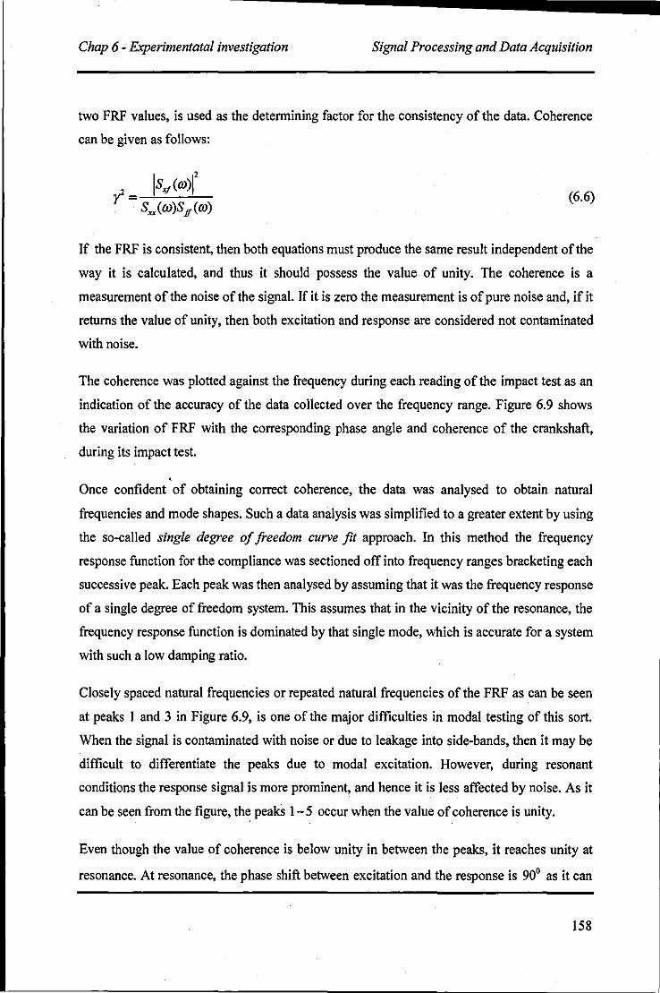
----------------......... .. Chap 6 - Experimentatal investigation Signal Processing and Data Acquisition
two FRF values, is used as the determining factor for the consistency of the data. Coherence
can be given as follows:
, ISx,(m)I' r = Sxx(ro)S jf(m)
(6.6)
If the FRF is consistent, then both equations must produce the same result independent of the
way it is calculated, and thus it should possess the value of unity. The coherence is a
measurement of the noise of the signal. If it is zero the measurement is of pure noise and, if it
returns the value of unity, then both excitation and response are considered not contaminated
with noise.
The coherence was plotted against the frequency during each reading of the impact test as an
indication of the accuracy of the data collected over the frequency range. Figure 6.9 shows
the variation of FRF with the corresponding phase angle and coherence of the crankshaft,
during its impact test.
, Once confident of obtaining correct coherence, the data was analysed to obtain natural
frequencies and mode shapes. Such a data analysis was simplified to a greater extent by using
the so-called single degree of freedom curve fit approach. In this method the frequency
response function for the compliance was sectioned off into frequency ranges bracketing each
successive peak. Each peak was then analysed by assuming that it was the frequency response
of a single degree of freedom system. This assumes that in the vicinity of the resonance, the
frequency response function is dominated by that single mode, which is accurate for a system
with such a low damping ratio.
Closely spaced natural frequencies or repeated natural frequencies of the FRF as can be seen
at peaks \ and 3 in Figure 6.9, is one of the major difficulties in modal testing of this sort.
When the signal is contaminated with noise or due to leakage into side-bands, then it may be
difficult to differentiate the peaks due to modal excitation. However, during resonant
conditions the response signal is more prominent, and hence it is less affected by noise. As it
can be seen from the figure, the peaks \-5 occur when the value of coherence is unity.
Even though the value of coherence is below unity in between the peaks, it reaches unity at
resonance. At resonance, the phase shift between excitation and the response is 90° as it can
158
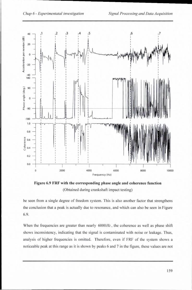
--------------------------........... . Chap 6 - Experimentatal investigation Signal Processing and Data Acquisition
40
<0 :!! c
20 S • ~ c
~ 0 0-c 0
'Q
~
" ·20 ~ u u <:
-40 180
--, 90 co
~
:!! ~
Co 0 c • ~ · • ~ ·90 ~
·180
1.0
0.8
~
~ 0.6 ~ ~ ~
o 004 u
0.2
0.0
,1 ,2 ,3 ,4 ,5 ,6 ,7
,
~,J;,~ , ,
0 2000 4000 6000 8000
Frequency (Hz)
Figure 6.9 FRF with the corresponding phase angle a nd coherence function
(Obtained during crankshaft impact testing)
10000
be seen from a single degree of freedom system. This is also another factor that strengthens
the conclusion that a peak is actuall y due to resonance, and which can also be seen in Figure
6.9.
When the frequencies are greater than nearl y 6000 Hz, the coherence as we ll as phase shift
shows inconsistency, indicating that the signa l is conta minated with no ise or leakage. Thus,
analysis of higher frequencies is omined. Therefore, even if FRF of the system shows a
noticeable peak at th is range as it is hown by peaks 6 and 7 in the fi gure, these values are not
159
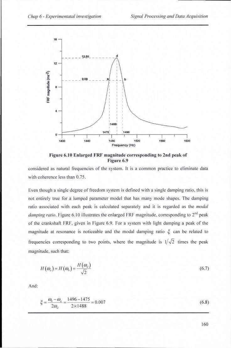
Chap 6 - Experimentatal investigation Signal Processing and Data Acquisition
16
12
if ~ s m -g
8 ~ c :5' E u. a: u.
~
o
__ ___ !2~ ________ d
_____ ~.o~ ______ a _.1._ b I I
I 114881 I
_f:==~~ __ ,-__ -,~1~47~6~' r-~~'~4~~-, ____ ,-__ -. ____ .-__ -,
1400 ,4<0 1480 1520 ' 560 ' 600 Frequency (Hz)
Figure 6. to Enlarged FRF mag nitude cor respondi ng to 2nd peak of Figure 6.9
considered as natu ra l frequencies of the system. It is a common practice to e li mi nate data
with coherence less than 0.75.
Even though a ingle degree o f freedom system is de fined with a s ing le da mping rat io, thi s is
not entire ly true fo r a lum ped pa ramete r mode l that ha many mode shapes. T he dam ping
ratio assoc iated with each peak is calcu lated separately and it i regarded as the modal
damping ratio. Figure 6. 10 ill ustrates the enla rged FRF magnitude, corres ponding to 2nd peak
of the crankshaft FRF, g iven in Figure 6.9. For a system with li ght dampi ng a peak of the
magnitude at resonance is noticeable and the moda l damp ing rat io ~ can be re lated to
frequencies corresponding to two poi nts, where the magnitude is 1/ J2 times the peak
magnitude, such that:
And:
H(W) H (w ) = H (w ) = "
" h J2
1496- 1475
2 x 1488
(6.7)
0.007 (6.8)
160
Chap 6 - Experimentatal investigation
D --t---j-< Ill! !I I! I 11
Hammer
Charge Amplifier
Data Acqu isition Card
Testing Procedure
D 00 I i
Computer
Figure 6. 11 1 mpact test apparatus set up for the crankshaft
Here, w" refers to the damped natura l frequency and thi s re lation is known as 3-dB down
point (lnman 200 I). As it can be seen fro m the ca lcul at ions, the damping ratio is very low:
0.007 (equation (6.8» , corresponding to th e second peak. As such damped natu ral freq uency
is considered as the undamped natura l frequency of the system, as there is very linle
difference between them.
6.5 Testing Procedure
This ecti on dea ls with the testing procedures undertaken for the impact tests. The impact
tests we re performed to va lidate the natural frequenc ies that have been obtained during FEA .
The engi ne was dismant led and components such as crankshaft, flywheel and connecting rod
were tested for thei r natural frequencies separate ly.
Figure 6. 11 outlines the experimenta l setup during impact testing on the crankshaft. The
crankshaft was hung by two strings, each I m long. Th is may damp out some mode shapes
as strings impose a restri cted moti on along their directio n. The most suitable method is to
have a free-free boundary condition, while the response is measured . However, such an idea l
condition cannot be obtained as there must be some means to ho ld the test piece during the
test. The strings remove onl y the translat ional degree of freedom (DO F), al lowing a ll the
other possib le movements to take place.
The ult imate objective of the impact testing o n components was to capture a ll the ir natural
frequencies, unlike the mode shape estimatio n, where im pact test is mostly used. In mode
shape estimation, it is necessa ry to calculate the magnitude of the respo nse, as we ll as the
161
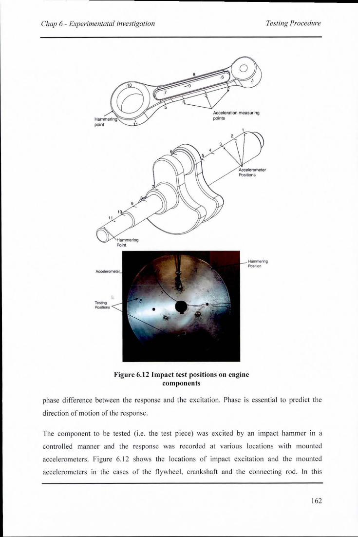
Chap 6 - Experimentata! investigation Testing Procedure
Testing
",.,,','"
B
4
6
AcceleraUon measuring poinlS
Accelerometer Posilions
Hammering Position
Figure 6. 12 Impact test pos itions on engine components
phase difference between the response and the exc itation. Phase is essent ia l to predict the
di rection of mot ion of the response.
The compo nent to be tested (i.e. the test piece) was exc ited by an impact hammer in a
contro ll ed manner and the response was recorded at various locati ons w ith mounted
accelerometers. Figure 6. 12 shows the locations of impact exc itation and the mounted
acce lerometers in the cases of the fl ywhee l, cranksha ft and the connecting rod . In thi s
162
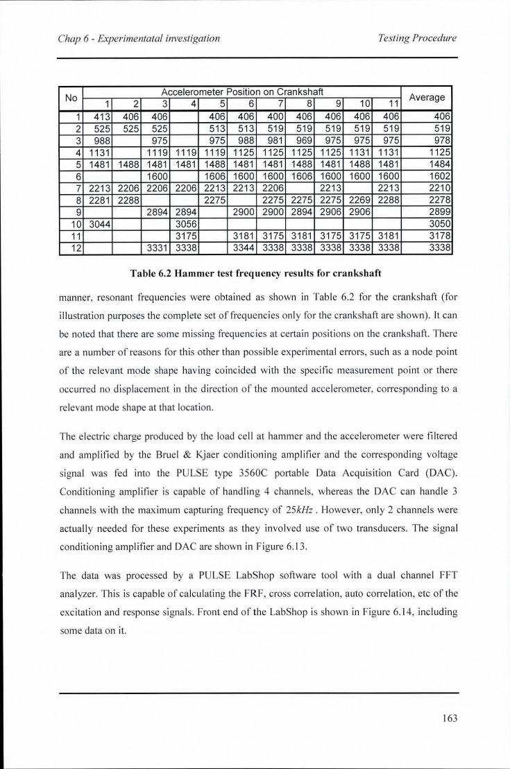
Chap 6 - Experill7entatal investigation Testing Procedure
No Accelerometer Position on Crankshaft Average
1 2 3 4 5 6 7 8 9 10 11 1 41 3 406 406 406 406 400 406 406 406 406 406 2 525 525 525 513 513 519 519 519 519 519 519 3 988 975 975 988 981 969 975 975 975 978 4 1131 1119 1119 1119 1125 1125 1125 1125 1131 1131 1125 5 1481 1488 1481 1481 1488 1481 1481 1488 1481 1488 1481 1484 6 1600 1606 1600 1600 1606 1600 1600 1600 1602 7 221 3 2206 2206 2206 2213 221 3 2206 221 3 2213 2210 8 2281 2288 2275 2275 2275 2275 2269 2288 2278 9 2894 2894 2900 2900 2894 2906 2906 2899
10 3044 3056 3050 11 3175 3181 3175 3181 3175 3175 3181 3178 12 3331 3338 3344 3338 3338 3338 3338 3338 3338
Table 6.2 Hammer test frequency results for crankshaft
manner, resonant frequencies were obtained as shown in Tab le 6.2 for the crankshaft (for
illustrati on purposes the complete set of frequencies onl y for the crankshaft are shown). It can
be noted that there are some missing frequencies at certa in positions on the crankshaft. There
are a nu mber of reasons fo r this other than possi ble ex perimenta l errors, such as a node point
of the re levant mode shape hav ing co incided with the spec ifi c measurement point or th ere
occurred no d isp lacement in the di rection of the mounted accelerometer, corresponding to a
relevant mode shape at that location.
The electric charge prod uced by the load cell at hammer and the acce lerometer were fil tered
and amplifi ed by the Bruel & Kjaer conditioning amplifi er and the corresponding vo ltage
signal was fed into the PULSE type 3560C portab le Data Acqu is ition Ca rd (DAC).
Conditioning ampli fier is capable of handling 4 channels, whereas the DAC can hand le 3
channels with the max imum capturing frequency of 25kHz. However, onl y 2 channels were
actuall y needed for these ex periments as they in vo lved use of two transducers. The signal
cond itioning amplifier and DAC are shown in Figure 6. 13.
The data was processed by a PULSE LabShop software too l with a dual channel FFT
analyzer. Thi s is capab le of ca lculating the FRF, cross co rre lation, auto correlation, etc of the
exc itation and response signa ls. Front end of the LabShop is shown in Figure 6. 14, including
some data on it.
163

Chap 6 - Experimentatai investigation Testing Procedure
Signal Conditioning Ampl ifier
InpUVOutput Module
PULSE Type 3560C ponable Data Acquisition Card
Figure 6.13 Bruel & Kjaer Conditioning Amplifier and DAC system
The FRF obtained by im pact testing on the piston does not show any peak within the
frequency range of 0 - 6000Hz, which the data acquisition system is capable of capturing.
This underpins the fact that higher natural frequencies of about 9000Hz, which have been
Crankshaft Connecting Rod Flywheel FEM Hammer Error FEM Hammer Error FEM Hammer Error
results results results results results results 415 406 -2% 569 636 -12% 1345 1330 1% 51 3 519 1% 740 1345
1002 978 -3% 1376 1206 12% 2216 2138 4% 1097 1125 3% 1864 2030 -9% 2808 2938 -5% 1496 1484 ·1 % 3805 3291 13% 2809 1564 1651 5% 4375 4431 4424 0% 2221 2210 ·1 % 4599 4600 0% 4437 2325 2278 ·2% 4589 4780 -4% 2937 2899 ·1 % 3174 3178 0% 3316 3338 1%
Table 6.3 Comparison between the hamme,' test results and FEM results
164
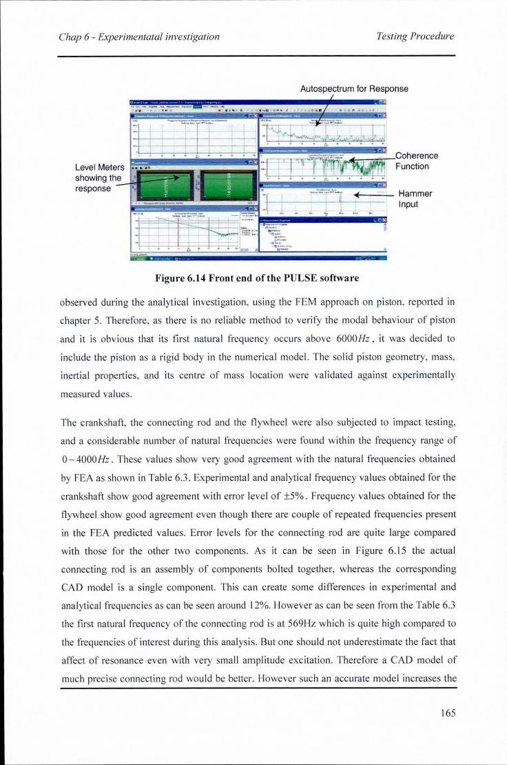
Chap 6 - I:-xperill1entalai investigation
Level Meters showing the response
-:<_, _____ '_
Testing Procedure
Autospectrum for Response
Function
~:::~~~f~~~~ Hammer "~ Input
Figure 6. 14 Front end of the PULSE software
observed during the analytica l invest igati on, using the FEM approach on piston, reported in
chapter 5. Therefore, as th ere is no rel iab le method to ve rify the moda l behav io ur of piston
and it is obvious that its first natural frequency occurs above 6000Hz, it was decided to
inc lude the piston as a rigid body in the num eri ca l mode l. The so lid pi ston geometry, mass,
inertial properties, and its centre of mass location were val idated aga inst experimenta ll y
measured va lues.
The crankshaft, the connect ing rod and the flywheel were al so subjected to impact testin g,
and a considerable number of natural frequenc ies were fo und with in the frequency range of
0-4000Hz . These values show ve ry good agreement with the natura l frequencies obta ined
by FEA as shown in Table 6.3 . Experimental and analytica l freq uency va lues obta ined for the
cra nkshaft show good agreement with error leve l of ±5%. Frequency va lues o bta ined for the
fl ywheel show good agreement even though there are couple of repeated frequenci es present
in the FEA pred icted values. Error leve ls for the connecting rod are quite large compared
with those for the other two components. As it can be seen in Figure 6.15 the actua l
connecting rod is an assemb ly of components bolted together, whereas the corresponding
CA D model is a s ing le component. This can create some d iffere nces in experimenta l and
ana lyt ical frequenc ies as can be seen around 12%. However as can be seen from the Tab le 6.3
the first nalUra l frequency of the connecting rod is at 569Hz which is quite high compared to
the frequencies of interest during th is ana lys is. But o ne should not underestimate the fact that
affect of resonance even w ith very sma ll amp litude excitation. Therefore a CAD model of
much precise connecting rod wou ld be better. However such an accurate model increases the
165

Chap 6 - Experimenlatal investigation
Actual Mooel CAO Model
Figure 6. 15 CAD model and the actual model of the Connecting Rod
Testing Procedure
number of element in the model qu ite considerab ly and bo lted connection between lower half
and upper half of the bigend bearing is onl y possib le with fi xed joint prim itive in ADAMS.
Such an addition increases the num ber of degrees of freedom considerably thus increas ing
thus increasing the simulat ion time.
166
Chap 7 - Results and Discussion Single cylinder engine dy namics
7 RESULTS AND DISCUSSION
7.1 Single cylinder engine dynamics
As highlighted in Chapter 2, modern engine development is dominated by reduction o f noise
and fricti onal losses wh il e enhancing the system efficiency. This became further cha llenging
with the introduction of high powered low we ight (high power to we ight ratio) engines that
use light and low stiffness material , thus reflecting the need for a deta il ed investigation o f
dynamic behaviour of an engine, w ith specia l rega rds to emiss ion of no ise and frictional
losses. Internal combustion engine is a compl icated system that inc ludes many other sub
systems such as, fuel deli very system, cam-tappet, accessory gears, pisto n rings, pistons,
crankshaft and main bearings that exhibit d ifferent dynamic behaviours. It is not poss ible to
develop a numeri ca l o r an anal yt ica l mode l that wo uld be capa ble o f address in g a ll these sub
systems including their dynamics, e lastic ity, lubricat ion and thermodynamic behavio urs with
a reliable degree o f accuracy. Therefore, many authors studying N VH characteristics of the
engine have paid the ir utmost attention only to a sub-system or a part o f the ub-system.
The freq uency spectrum of the measured combust ion gas force (see Figure 7. 1) shows man y
excitati ons belong ing to eng ine order multip les and half eng ine order multipl es (Note that
engine is running at nearl y 1800rpm, which g ives a first engi ne o rder of 30Hz). In IC
eng in es the gas pressure force acting on the pi ston is co nverted into a dri ving torque at the
crankshaft end through a slider crank mechanism. During thi s process of convers ion, many
exc itations are developed, whi ch are al so shown in the ana lytica l equation (3.47).
Particularly, these integer mUlti ples o f engi ne order excitat ions are due to vari able inertia l
effect of the translat ing mass of the pi ston and the connecting rod. Even though the equati on
shows only up to three eng ine orders, there a re many exc itat ions in it, wh ich were omitted
during the binomial expansion of equation (3.45), owing to the ir neg li gible amplitude.
Howeve r, it must be noted that under resonant conditio ns even very low ampl itude
exc itations can cause vibratio ns with hi gher amplitudes. In fact , these exc itati o ns a re
responsible for the twist-untwist action of the cranksha ft, which leads to to rsional v ibrations
of the crankshaft.
167
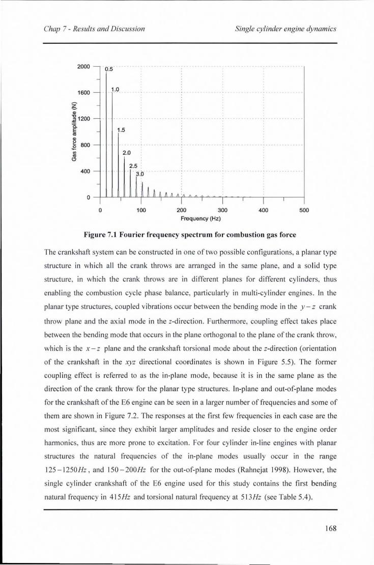
Chap 7 - Results and Discussion
2000 - 0.5
1600 -
~ -" ] 1200 -a ~ -
~ ~ 800 -~
c3 -
400 -
1.0
1.5
2.0
2.5 3.b
Single cylinder engine dynamics
Frequency (Hz)
Figure 7.1 Fourier frequency spectrum for combustion gas force
The crankshaft system can be constructed in o ne of two poss ible configurations, a planar type
structure in whi ch all the crank throws are arranged in the same plane, and a so lid type
structure, in whi ch the crank throws are in different planes for different cy linders, thus
enabling the combustion cycle phase balance, particularly in multi-cylinder engines . In the
planar type structu res, coupled vibratio ns occur between the bending mode in the y - z crank
throw plane and the axia l mode in the z-directio n. Furthermore, coupling effect takes place
between the bending mode that occurs in the plane orthogona l to the plane of the crank throw,
which is the x-z plane and the c rankshaft torsional mode about the z-directio n (orientati on
of the crankshaft in the xyz directi onal coo rdinates is shown in Figure 5.5). The former
coupling effect is referred to as the in-plane mode, because it is in the same plane as the
di rection of the crank throw for the planar type structures. In-plane and out-oF-plane modes
for the crankshaft of the E6 engine can be seen in a larger number of frequencies and some of
them are shown in Figure 7.2. The responses at the first few frequencies in each case are the
most s ignificant, s ince they ex hibit la rge r amplitudes and reside closer to the engine order
harmonics, thus are more prone to excitation. For four cylinder in-l ine engines with planar
structures the natura l frequencies of the in-plane modes usuall y occur in the range
125 - 1250 Hz , and 150 - 200 Hz for the out-of-plane modes (Rahnejat 1998). However, the
s ingle cylinder crankshaft of the E6 eng ine used for thi s study conta ins the first bending
natura l freque ncy in 415Hz and torsional natura l frequency at 5 13Hz (see Tab le 5.4) .
168
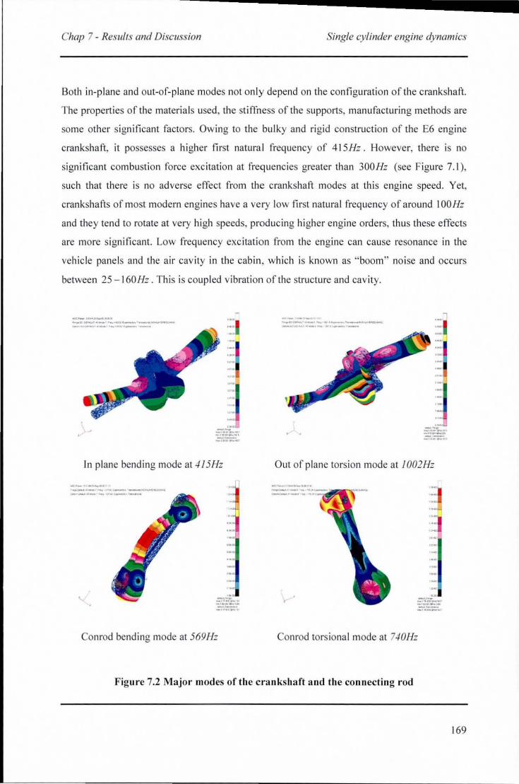
Chap 7 - Resulls and Discussion Single cylinder engine dynamics
Both in-plane and out-of-plane modes not on ly depend on the configuration of the crankshaft.
The propel1ies of the materials used, the stiffness of the supports, manufacturing methods are
some other significant factors. Owing to the bu lky and ri gid construction of the E6 engine
crankshaft, it possesses a hi gher first natural frequency of 415Hz . However, there is no
significant combustion force exc itation at frequenc ies greater than 300 Hz (see Figu re 7.1 ),
such that there is no adverse effect from the crankshaft modes at thi s engine speed. Yet,
crankshafts of most modern engines have a very low first natural freque ncy of around 100/-lz
and they tend to rotate at very high peeds, producing hi ghe r engine orders, thus these effects
are more significant. Low frequency excitat ion from the engi ne can cause resonance in the
vehicle panels and the ai r cav ity in the cab in , whi ch is known as "boom" noi se and occurs
between 25 - 160Hz . This is coup led vibration of the structure and cav ity.
--" ... _--................. _ ........ "._. __ -..-
In plane bending mode at ./15/-1z
__ ... _ ... or
--"--.""'------ .. _,_ ..... _-
Con rod bend ing mode at 569/-1z
_ ... ,_ ... _ ........ _---- ...... _., ...... ,._.-
Out of plane torsion mode at 1002Hz
Con rod torsional mode at ?-10Hz
Figure 7.2 Major modes of the crankshaft and the connecting rod
169
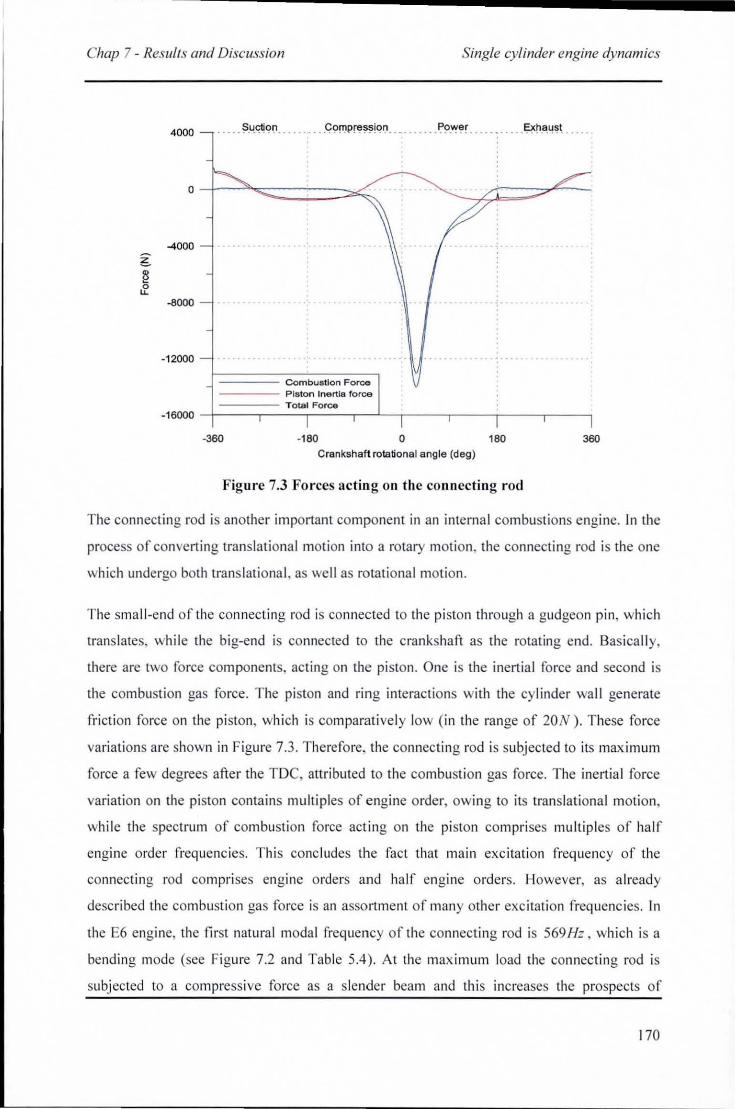
Chap 7 - Resulls and Discussion Single cylinder engine dynamics
~ ~ &
4000
-4000
-8000
-12000
Combustion Force ---- Piston Ine rtia force
_~====~~~T~O~~I~F~O~'~~-r_~-r __ -. __ ~ __ -'r-_-. -16000
-360 -180 o 180 360
Crankshaft rotational angle (deg)
Figure 7.3 Forces acting on the connecting rod
The connecting rod is another im portant component in an internal combustions engine. In the
process of convert ing translational moti on into a rotary motion. the connect ing rod is the one
which undergo both translationa l, as well as rotational motion.
The small-end of the connect ing rod is connected to th e piston through a gudgeon pin, which
translates, while the big-end is connected to the crankshaft as the rotating end. Basical ly,
there are two force components, acting on the pi ston. One is the inertial force and second i
the combustion gas force. The piston and ring interactions with the cylinder wal l ge nerate
fr iction force on the pi ston , which is comparati vely low (i n the range of 20N). These force
variat ions are shown in Figure 7.3 . Therefore, the connecting rod is subj ected to its maxi mum
force a few degrees after the TDe, att ri buted to the combusti on gas force. The inertia l force
variation on the piston contains multiples of engine o rder, owing to its translati ona l motion,
whi le the spectrum of combustion force act ing on the pi ston comprises multiples of ha lf
engine ord er frequencies. This concludes the fact that main excitat ion frequenc y of the
connecting rod compri ses engi ne orders and half engi ne o rders. However, as alread y
described the combustion gas force is an asso rtment of many oth er exc itat ion freque ncies . In
the E6 eng ine, the first natu ral modal frequency of the connect ing rod is 569Hz , which is a
bending mode (see Figure 7.2 and Table 5.4). At the maximum load the connectin g rod is
subj ected to a compressive force as a slender beam and thi s increases the prospects of
170
Chap 7 - Results and Discussion Single cylinder engine dynamics
exciting the bending mode. However, as the exc itat ion frequenc ies are much lower than this
first natura l frequency, th e tendency of exciting the bending mode is quite slim. Nevertheless,
thi s is considered to be a vita l aspect during the engine design process (Fantino et al, 1983;
Goudas and Natsiavas 2004).
Eccentric orbit of the main journal bearing can take place due to the dynam ic nature of the
transmitted fo rce onto the bearing supports as descri bed in secti on 2.2 .2. Th is problem is
more pronounced w ith the bearing at the fl ywhee l end. Jump phenomenon, which takes place
due to the existence o f different equ il ibrium pos itions within the orbit for the same operating
condit ions, can produce exc itat ions in many frequencies . The whirling motion that happens at
tw ice the speed of rotatio n creates another exc itatio n at second engine order as di scussed in
section 2.2 .2. Even though primary motion of the pi ston is we ll-defined by the slider crank
mechanism, there exists a secondary motion owing to c learance between the pi ston skirt and
the cyli nder liner. Tho ugh this c learance is small , it is large enough to produce secondary
tilting and translational lateral motions that may create un wanted noise and vibrat ion as
disc ussed in secti on 2.2.3 .
These observations highl ight the com plexity of the combined effects of the inertial force and
torque ex c itat ions upon the fo rmation of coupled out-o f-plane and in-plane deflection modes
of the flex ible bodies sllch as the c rankshaft and the connecting rod. There are man y
anal ytica l approaches for so lutio n o f va rious eng ine dyn amic phenomena that are use fu l in
the understandi ng of complex eng ine dynamics spectra . A simple ana lysis fo r a single
cy linder engine, inc luding inertial forces and combusti on force has been presented in section
3.5 and some other complex analysis can be found in li terature (Cho et al, 2003 ; S.H et aI,
2002). Nevertheless, many of these analytica l approaches do not include the effect of other
sources of non-linearity o r these are inc luded in very abstracted forms. Most prominently,
these sources of non-linearity inc lude journa l bearing hydrodynam ics, piston skirt - cylinder
wa ll lu brication and frict ion, its secondary ti lting moti on and pi ston ring-to-cylinder wa ll
interactions.
Furthermore, the assemb ly of parts in the engi ne model incorporates constraints, representing
the attachment of parts that describe certa in motions, such as translations and rotat ions.
Analytica l so lutions can be obtained by lineari z ing these non-linear equatio ns. However, the ir
omiss ion from the system dynamics equati on can lead to erroneous inte rpretat ions or
171
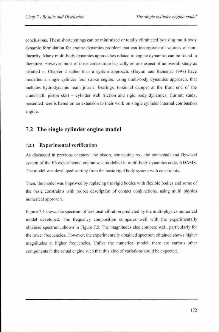
Chap 7 - Results and Discussion The single cylinder engine model
conclusions. These shortcomings can be minimized or totally eliminated by using multi-body
dynamic formu lation fo r engine dynamics problem that can incorporate all sources of non
linearity. Many multi -body dynamics approaches related to engine dynamics can be fo und in
literature. However, most of these concentrate basica ll y on one aspect of an overall study as
deta iled in Chapter 2 rather than a system approach. (80ysa l and Rahnejat 1997) have
modelled a single cylinder four stroke engine, using mul ti-body dynamics approach, that
includes hyd rodynamic main journal bearings, torsional damper at the front end of the
crankshaft, piston sk irt - cylinder wa ll fr ict ion and rigid body dynamics. Current study,
presented here is based on an extension to thei r work on single cylinder internal combustion
engine.
7.2 The single cylinder engine model
7.2.1 Experimental verification
As discussed in previous chapters, the piston, connecting rod , the crankshaft and fl ywheel
system of the E6 experimental engine was modelled in multi-body dynamics code, ADAMS.
The model was developed starting from the basic rigid body system with constraints.
Then, the model was improved by replac ing the rigid bodies with flexib le bodies and some of
the basic constraints with proper description of contact conj unct ions, using multi phys ics
numerica l ap proach.
Figure 7.4 shows the spectrum of torsional vibration pred icted by the mu lti-phys ics numerica l
model deve loped. The frequency compos ition compares we ll wi th the experimentally
obtained spectrum, shown in Figure 7.5. The magnitudes also compare well , particularl y for
the lower frequencies. However, the experimentally obtained spectrum obtained shows higher
magnitudes at hi gher frequencies. Unlike the numerical model , there are various other
components in the actual engine such that this kind of variat ions cou ld be expected.
172
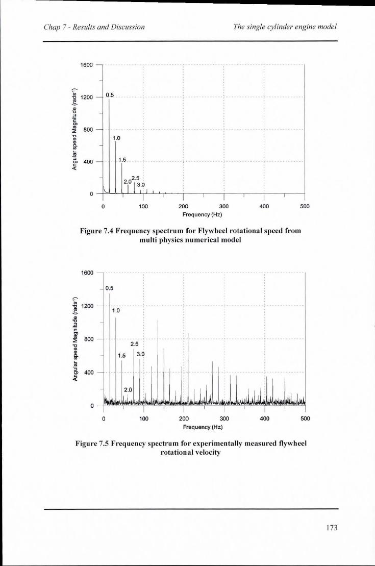
Chap 7 - Results and Discussion The single cylinder engine model
1600
" a .5 . U> 1200 u
~
" u .a '" '" .. 800 ' , , .. ::;; u 1.0 " " 0. U>
a; "3
400 . 1.5 ... '"
., ~
o 100 200 300 400 500 Frequency (Hz)
Figure 7.4 Freq uency spectrum for Flywheel rotational speed from multi physics numerical model
1600 -
0.5
" u 1200 - . ,g 1.0
" "C .a c '" .. 600 -::;;
"C 2 .5
" " - 1.5 3.Q 0. U>
a; "3
400 -'" ~
o I I o 100
,
200 I
300
Frequency (Hz)
I 400 500
Figure 7.5 Frequency spectrum for experimentally measured flywheel rotational velocity
173
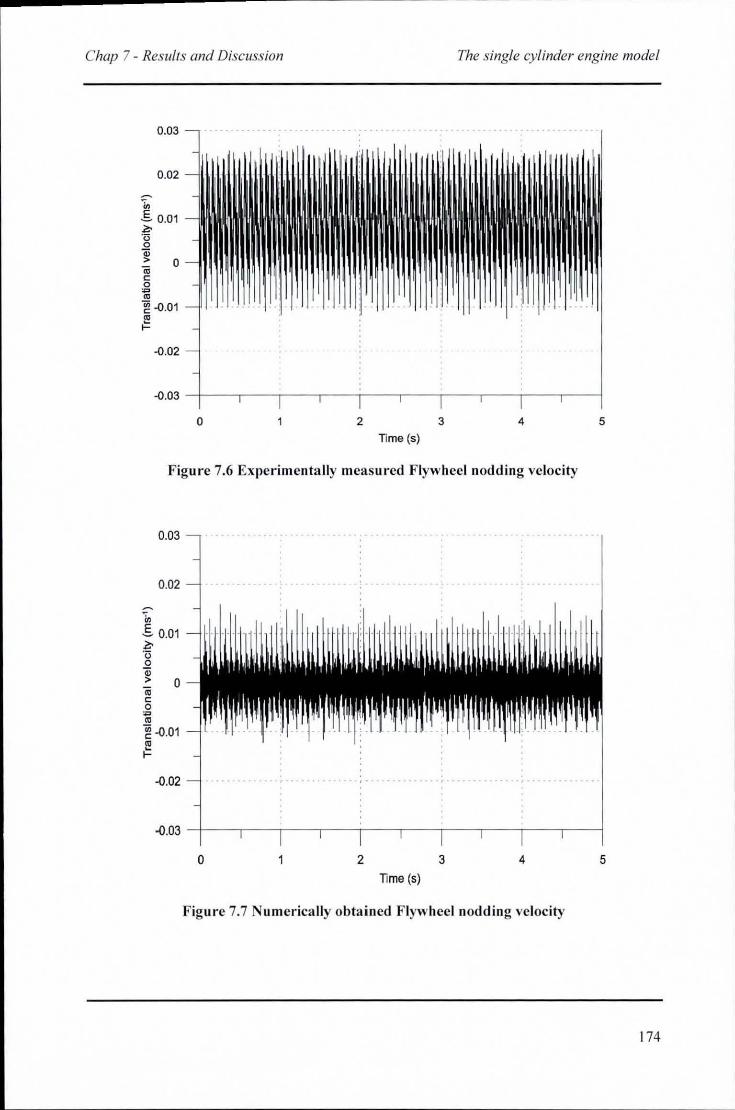
Chap 7 - Resulls and Discussion The single cylinder engine model
0.03 .. . . ..
0.02
~ £ 0.01 ;?> ·0 0 0; > 0 0; c: 0 ~
'" ~ -0.01 11 I-
-0.02
-0.03
0 2 3 4
Time (s)
Figure 7.6 Experimentally measured Flywheel nodding velocity
0.03
0.02
~ .s 0.01 ;?> ·0 o ~ iii co o ~
'"
o
~ -0.01
~
-0.02
5
-0.03 -+--.---,--,---,-----r---,---,----.--.---1
o 2 3 4 5
Time (5)
Figure 7.7 Numerically obtained Flywheel nodding velocity
174
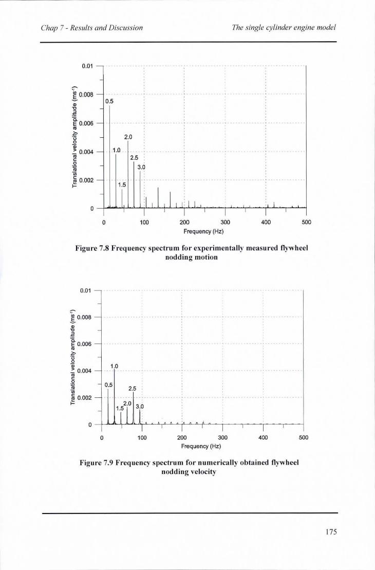
Chap 7 - Results and Discussion The single cylinder engine model
0.Q1 -
~
~ 0.008 - . ~ 0.5 " -~ a. E 0.006 - . ., ~ ·0 -o
Q) ? 0.004 - 1.0 . .. c g -.. u; e 0.002 -f-
-
o
2.0
2.5
3.0
Figure 7.8 Frequency s pectrum for experimentally measured flywheel nodding motion
0.Q1
k 0.008
'" " ~ a. E 0.006 .. ~ ." o Q)
? 0.004 '" c o ~ .. u; E 0.002 f-
o
1.0
0.5 2.5 :
100 200 300 400
Frequency (Hz)
Figure 7.9 Frequency spectrum for numerically obtained flywheel nodding velocity
500
175
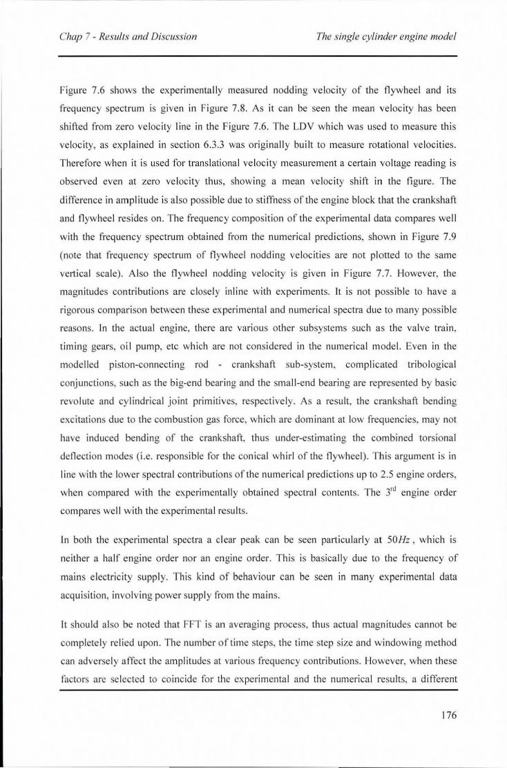
Chap 7 - Resulls and Discussion The single cylinder engine model
Figure 7.6 shows the experimenta lly measured nodding veloc ity of the fl ywheel and its
frequency spectrum is given in Figure 7.8. As it can be seen the mean ve loc ity has been
shifted from ze ro ve loc ity line in the Figure 7.6. The LDV which was used to measure th is
ve loc ity, as exp lained in sect ion 6.3.3 was origina ll y built to measure rotational ve loc it ies.
Therefore when it is used for translati o na l veloc ity measurement a certain vo ltage readi ng is
observed even at zero veloc ity thus, showing a mean ve loc ity shift in the figure. The
difference in amplitude is also poss ibl e due to st iffness of the engine block that the crankshaft
and fl ywheel resides on. The frequency composi tion o f the experim enta l data compares we ll
with the frequency spectrum o bta ined fro m the numerica l pred ictions, shown in Figure 7.9
(note that frequency spectrum of fl ywhee l nodd ing ve lociti es a re not plotted to the same
verti ca l scale). Al so the fl ywheel nodding veloc ity is given in Figure 7.7 . However, the
magnitudes con tributions are close ly inl ine with ex periments. It is not poss ible to have a
ri gorous comparison between these experimental and numerica l spectra due to many poss ible
reasons. In the actual engine, there a re various other subsystems such as the va lve train ,
tim ing gears, o il pump, etc which are not considered in the numerical mode l. Even in the
modelled pi sto n-co nnecting rod - crankshaft sub-system, complicated tribo logica l
conjunctions, such as the big-end bearing and the small-end bearin g are represented by basic
revo lute and cylindri ca l jo int primitives, respectively. As a resu lt , the c rankshaft bending
exc itations d ue to the combustion gas force , wh ich are dominant at low freque ncies, may not
have induced bending of the crankshaft, thus under-estimating the combined torsional
deflecti on modes (i.e . responsible for the con ica l whirl of the fl ywheel). Thi s argum ent is in
line with the lower spectral contributions o f the numerica l predictions up to 2.5 eng ine o rders,
when compared with the experimentall y obtained spectral contents. The 3rd engll1e order
compares well w ith the experimental results.
In both the ex perimental spectra a clear peak can be seen particularly at 50Hz , which is
neith er a ha lf engine order nor an engi ne order. This is basically due to th e frequency of
mains e lectric ity suppl y. This kind o f behaviour can be seen in many ex perimenta l data
acquisition, invo lving power suppl y from the mains.
It should a lso be noted that FFT is an averaging process, thus actual magnitudes cannot be
com pletel y relied upon. The number o f time ste ps, the time step s ize and w indowing method
can adverse ly affect the amplitudes at vari ous freq uency contributions. However, when these
factors a re se lected to co incide fo r the ex perimental and the numerical results, a different
176
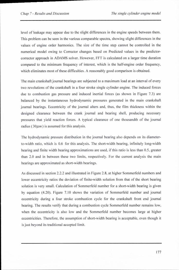
Chap 7 - Results and Discussion The single cylinder engine model
level of leakage may appear due to the slight differences in the engine speeds between them.
This problem can be seen in the vari ous comparable spectra, showing slight differences in the
va lues of engine order hannonics. The size of the time step cannot be contro lled in the
numeri ca l model owing to Corrector changes based on Predicted va lues in the predictor
corrector approach in ADAMS solver. However, FFT is calculated on a larger time duration
compared to the minimum frequency of inte rest, which is the half-engine order frequency,
which eliminates most of these difficulties. A reasonably good compari son is obtained.
The main crankshaft journal bearings are subjected to a max imum load at an interva l of every
two revolutions of the crankshaft in a four stroke single cyli nder engine. The induced forces
due to combustion gas pressure and induced inert ial forces (as shown in Figure 7.3) are
ba lanced by the instantaneous hyd rodynami c pressures generated in the main crankshaft
journal bearings. Eccentricity of the journal alte rs and, thus, the film th ickness withi n the
designed clearance between the crank journal and bearing she ll , producing necessary
pressures that yield reacti on forces. A typica l clearance of one thousandth of the journal
rad ius (30).1.111) is assum ed for this ana lys is.
The hydrodynamic pressure distribution in the journal bearing also depends on its diameter
to-width ratio, which is 0.6 fo r this analysis. The short-width bearing, infinitely long-width
bearing and fin ite width bearing app rox imations are used, if th is ratio is less than 0.5, greater
than 2.0 and in between these two li mits, respectively. Fo r the current ana lys is the main
bearings are approx imated as short-width bearings.
As discussed in section 2.2.2 and illustrated in Figu re 2.8, at higher Sommerfeld num bers and
lower eccentricity rat ios the deviation of fi nite-width so lution fro m that of the short bearing
so lution is ve ry small. Ca lcu lation of Sommerfe ld number fo r a short-width bearing is given
by equation (4.20). Figure 7.10 shows the va ri ation of Sommerfe ld num ber and journal
eccentricity during a fo ur stroke combustion cycle for the crankshaft front end journal
bearing. The results verify that during a combustion cycle Sommerfeld number remains low,
when the eccentri c ity is also low and the Sommerfe ld number becomes large at higher
eccentric ities. Therefore, the assumpt ion of sholt -width bea ring is acceptab le, even though it
is just beyond its tradi ti onal accepted limi t.
177
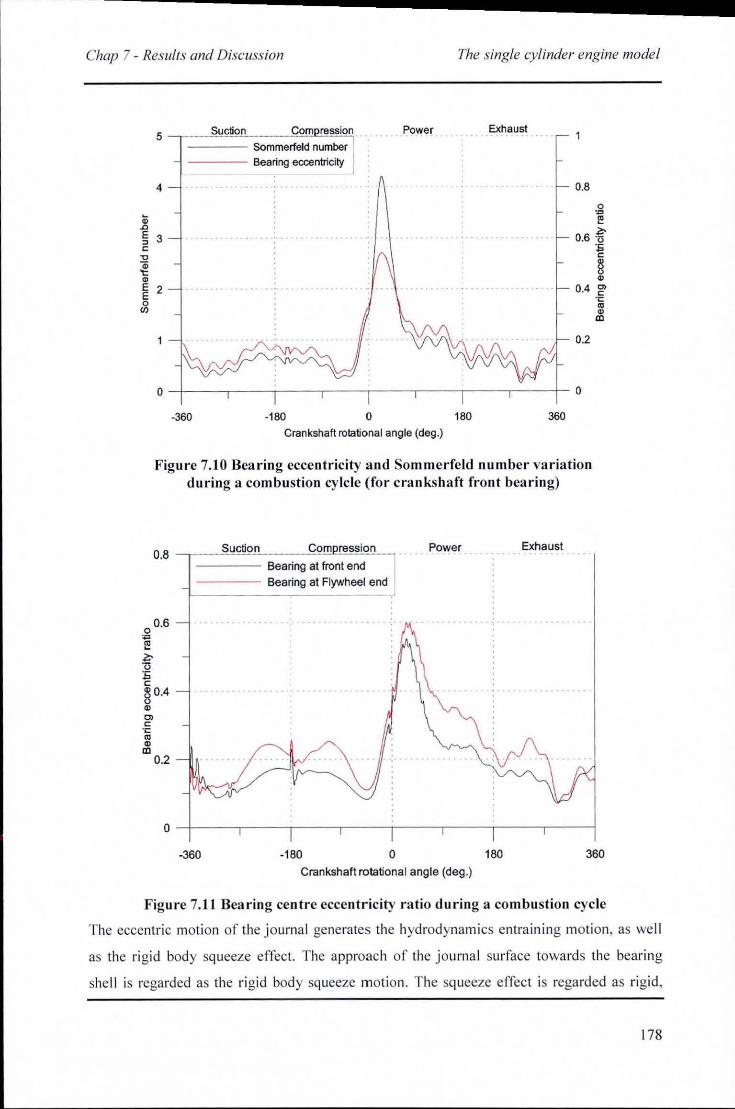
------------------------........... Chap 7 - Results and Discussion The single cylinder engine model
5 _~==~S~U~c~tio~n~~~~c~o~m~re~~~io~n Sommerfeld number
4
;; .0
§ 3 c "0
~ ~
E 2 E o
'"
---- Bearing eccentricity
Power Exhaust
0.8
,g E
0.6 .~ :E c § ..
0.4 ~
0.2
'c
'" ~ "'
o -+----.-----.----.-----.----.-----,----.-----+- o
-360 -180 o 180 360
Crankshaft rotational angle (deg .)
Figure 7.10 Bearing eccentricity and Sommerfeld number variation during a combustion cylcle (for crankshaft front bearing)
Suction Corn ression 0.8 -,- -"'="'-'----""''''''''-=''''"'----, . POY'~r
o 0.6
'" ~ ~ '0 :E c 80.4 .. Cl c
'c
'" ~ "' 0.2
o
---- Bearing al front end
---- Bearing at Flywheel end
-360 ·180 o Crankshaft rotationa l angle (deg .)
Exhaust
180 360
Figure 7.11 Bearing centre eccentricity ratio during a combustion cycle
The eccentric motion of the journal generates the hydrodynamics entraining motion, as we ll
as the ri gid body squeeze effect. The approach of the journal surface towards the bearing
shell is rega rded as the ri gid body sq ueeze mOlion. The squeeze effect is regarded as rig id,
178
Chap 7 - Results and Discussion The single cylinder engine model
when the elastic deformations are ignored during hyd rodynamic analysis of journal bearings.
However, modern bearings are signi fica ntl y li ght in construct ion (i.e. made of material s of
low elastic modulus, such as Tin-based alloys). Thus, under extreme operat ing conditions the
bearing shell would be elastically deformed due to hi gh pressures. In fact, this will generate
sufficie nt lubricant film to separate the two contiguous bodies apart, a mechanism which is
referred to as elastohydrodyanmic lubrication. However, during these conditions viscosity of
the lubricant substantia lly increases and pressures are as much as hundreds of MPa that are
capable of deforming the adjacent elast ic bodies. This is not the case for the E6 engine.
However, the so lution of thin shell elastohydrodynamic problem is computat ionall y
compl icated and difficu lt to include in the same multi-body ana lys is. The E6 experimental
engine is fined with a thi ck journal bearing bushing of 5111111 thickness, made of steel and
subjected to low combustion pressures of nea rl y 35bar, compared to modern engines with a
shell thickness of 1.5111111 and combustion pressure of ISObar. During a fo ur stroke cycle,
shown in Figure 7. 1 I, the max imum eccentricity ra ti o is close to 0.6 , which means a flu id
film is maintained throughout the cycle. Therefore, it is concluded that hyd rodynamic
lu brication exists th roughout the cycle as assumed.
During the engine operation the planar-type single cylinder crankshaft is subjected to coupled
bending and torsional vibrations. Therefore, thi s can act as a source of exc itation for the
crankshaft and the flywheel bend ing and axia l float , which is known as fl ywheel nodd ing
act ion. The bearing closest to the flywheel end is subjected to higher loads during the engine
cycle. This effect is particularly pronounced during the peak combustion force. The bearing
force variation is shown in Figure 7. 12, which confirms this supposition. Whilst a maximum
load of nearl y 6000N is obtained for the front end bearing, that for the fl ywheel-end bearing
is 7500N. Higher the reaction force, the eccentric ity of the bearing becomes larger in order
to produce the necessary hydrodynamic reaction. During a 4 stroke engine cycle most
pronounced force component is the combustion gas force as can be seen from Figure 7.3 ,
other than the inertial forces due to the various mov ing components. This force must be
balanced by the bearing reaction force. Therefore, the bearing reaction al so exhibits a similar
force variat ion (or pattern) (see Figure 7.3 and Figure 7. 12). It must be noted that other
inert ial forces , such as the crankshaft are not taken into consideration during this total force
calculati on in Figure 7.3, as it conta ins almost a constant inertial contribution due to its rota ry
motion.
179
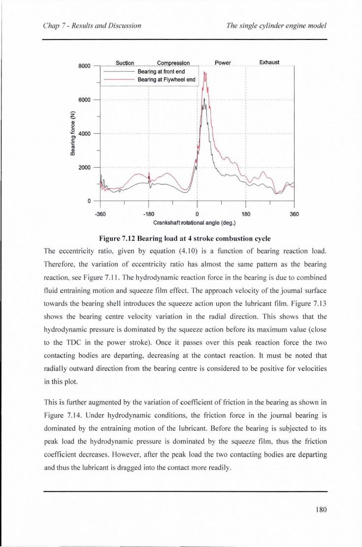
Chap 7 - Resulls and Discussion The single cylinder engine model
~
~
8000 -, __ ~S~u~~~'o~n~ ____ ~C~om~~~s~s~io~n~
------ Bearing at front end - ----- Bearing at Flywheel end
6000 .'
Power Exhaust
.E 4000 Cl c ·c Cl>
" '" 2000
o -+----,-----r----,-----r----.----,-----r--~
-360 ,180 o 180 360
Crankshaft rolational angle (deg.)
Figure 7.12 Bearing load at 4 stroke combustion cycle
The eccentricity ratio, given by equat ion (4. 10) is a function of bearing reaction load.
Therefore, the variation of eccent ricity ratio has almost the same pattern a the bearing
react ion. see Figure 7.11 . The hydrodynamic reaction force in the bearing is due to combined
flu id entraining moti on and squeeze film effect. The approach ve locity of the joumal surface
towards the bearing shell introduces the squeeze action upon the lubricant film . Figure 7.1 3
shows the bearing centre velocity variation in the radia l direction. Thi s shows that the
hydrodynamic pressure is dominated by the squeeze action before its max imum value (close
to the TDe in the power stroke). Once it passes over this peak reaction fo rce the two
contacti ng bod ies are depa rting, decreasing at the contact reaction. It must be noted that
radiall y outward direction from the bearing centre is considered to be positive for ve loc ities
in thi s plot.
This is fu rther augmented by the variation of coefficient of fr iction in the bearing as shown in
Figure 7. 14. Under hydrodynamic condit ions, the fr ict ion force in the journal bearing is
dominated by the entraining motion of the lubricant. Before the bearing is subjected to its
peak load the hydrodynamic pressure is dominated by the squeeze film , thus the friction
coeffic ient decreases. However, after the peak load the tWO contacting bodies are departing
and thus the lu bricant is dragged into the contact more readily.
180
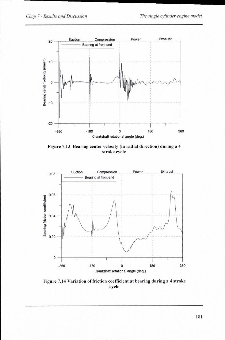
--------------------------.......... ..... Chap 7 - Results and Discussion The single cylinder engine model
~ E .s Z-'0 0 0; > .Si c 1l Cl> c ·c .. " CD
Po~er Exhaust
Bearing at front end
10
0
-10
-20 -+-----,----T-----,----,-----,----T----,,---~
-360 -180 o 180 360 Crankshaft rotational angle (deg .)
Figure 7.13 Bearing center velocity (in radial direction) during a 4 stroke cycle
Suction Corn ression 0.08 -.-----'==----~===;' Power Exhaust
---- Bearing at front end
C 0.06 .. ,
" '0
1 c ~ 0.04
:E Cl c ·c .. " aJ 0.02
O -+----,----r---,,----r---.----,----,--~
-360 -180 o 180 360
Crankshaft rotational angle (deg.)
Figure 7. 14 Va riation of friction coefficient at bea ring during a 4 stroke cycle
181
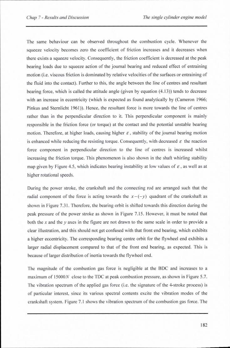
Chap 7 - Results and Discussion The single cylinder engine model
The same behav iour can be observed throughout the combustion cyc le. Whenever the
squeeze veloci ty becomes zero th e coefficient of fr icti on increases and it decreases when
there exists a squeeze velocity. Consequentl y, the fr iction coeffic ient is decreased at the peak
bearing loads due to sq ueeze action of th e journa l bearing and red uced effect of entrai ni ng
motiol1 (i.e . viscous friction is dominated by relati ve velocities of the surfaces or entra ining of
the fluid into the contact). Further to this, the angle between the line of centres and resu ltant
bearing force, which is called the attitude angle (given by eq uation (4.13» tends to decrease
with an increase in eccentric ity (which is expected as found analyticall y by (Cameron 1966;
Pinkus and Sternlicht 1961 )). Hence, the resultant force is more towards the line of centres
rather than in the perpendicular direction to it. Th is perpendicu lar component is ma inl y
responsib le in the fr ict ion force (or torque) at the contact and the potent ial unstab le bearing
motion. Therefore, at hi gher loads, causing hi gher 1:, stabi lity of the j ournal bearing motion
is enhanced whil e reducing the res isting torque. Consequently, with decreased I: the reaction
force component in pe rpendicu lar direct ion to the line of centres is increased wh il st
increasing th e frict ion torque. Thi s phenomenon is a lso shown in the shaft whirling stab ility
map given by Figure 4.5 , whi ch indicates bea rin g instab il ity at low va lues of 1: , as we ll as at
hi gher rotati onal speeds.
During the power stroke, the crankshaft and the connectin g rod are arranged such that the
radia l component of the force is acting towa rds the x-(-y) quadrant of th e crankshaft as
shown in Figure 7.3 1. Therefo re, the bea ring orb it is shi fted towards this direction during th e
peak pressure of the power stroke as shown in Figure 7. 15. However, it must be noted that
both the x and the y axes in the fi gure are no t drawn to the same scale in order to prov ide a
clear illustrat ion, and thi s should not get confused with that front end bearing, whi ch exhibits
a higher eccentri city. The correspond ing bearing centre o rbit fo r the fl ywheel end exhibits a
larger rad ia l d isplacement compared to that of the front end bearing, as expected. Thi s is
because of larger d istribution of inertia towards th e fl ywheel end.
The magnitude of the combusti on gas force is neg li gi ble at the BDC and increases to a
max imum of ISOOON close to the TDC at peak combusti on pressure, as shown in Figure S.7.
The vibration spectrum of the app lied gas force (i.e. the signature of the 4-stroke process) is
of particular interest, s ince its va rious spectral contents exc ite the vibration modes of the
crankshaft syste m. Figure 7. 1 shows the vibration spectrum of the combustion gas force. The
182
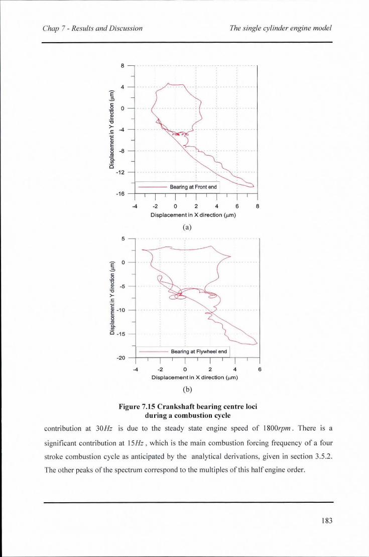
Chap 7 - Resulls and Discussion The single cylinder engine model
8 ._ ... .
4 E 2.
" 0 0 = " ~ 'C >- -4 .s C Q)
E 1l -8 '" a. '" is
-12
Bearing at Front end -16
-4 -2 0 2 4 6 8
5
E 0 2. " o = " ~ -5 '0 >-.s C ~ -10
1l '" g. is -15
Displacement in X direction ()lm)
(a)
---- Bearing at Flywheel end -20 -+-.--,--,--,--.--.--,-,---,-1
-4 -2 o 2 4
Displacement in X direction ()lm)
(b)
Figure 7. 15 Crankshaft bearing centre loci during a combustion cycle
6
contribution at 30Hz is due to the stead y state eng ine speed of 1800'1)m . There is a
signi fica nt contribution at 15Hz , w hi ch is th e main combusti on forcing frequency o f a four
stroke combusti on cycle as anticipated by the analyt ica l derivations, given in sectio n 3.5.2 .
The other peaks of the spectrum correspond to the multipl es of thi s ha lf eng ine o rder.
183
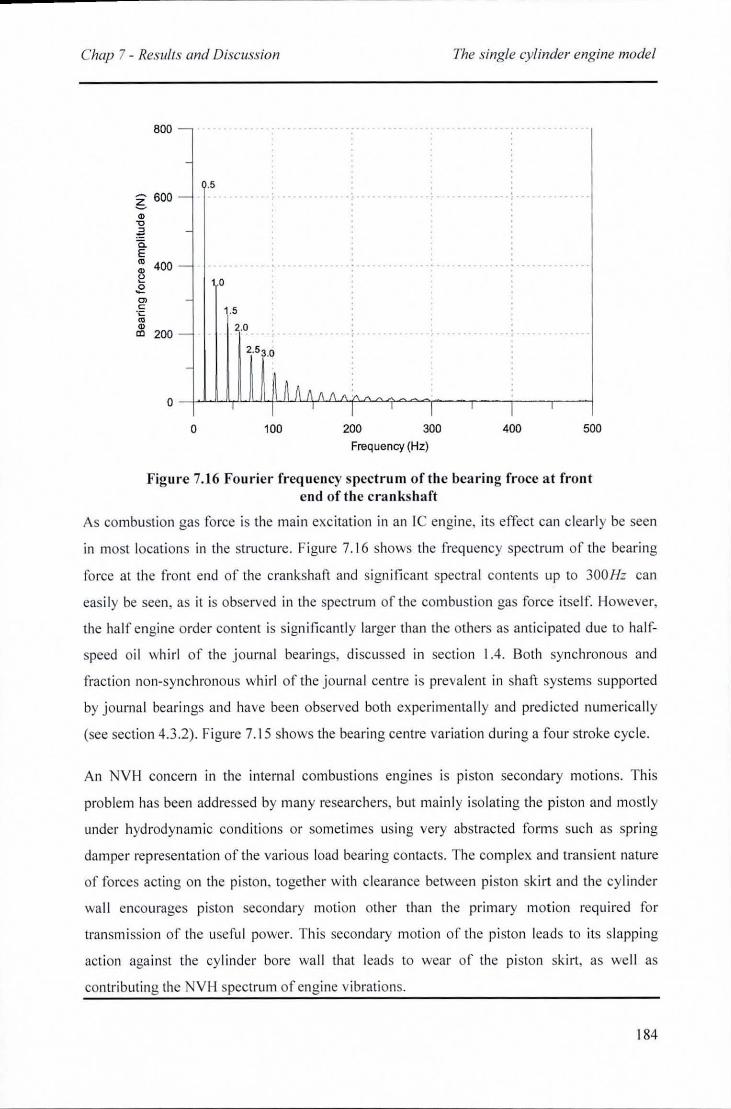
Chap 7 - Results and Discussion
800
- 600 6 <I)
" ~ Q. E '" 400 ~ .2 '" c ·c
'" ~ 200
.5
1.0
o
.5
2.0
100
The single cylinder engine model
200 300 400 500
Frequency (Hz)
Figure 7.16 Fouricr frequency spectrum of the bearing froce at front end of the crankshaft
As combusti on gas force is the main excitation in an le engine, its effect can clearly be seen
in most locations in the structure. Figure 7. I 6 shows the frequency spectrum of the bearing
force at the front end of the crankshaft and significant spectral contents up to 300 Hz can
eas il y be seen, as it is observed in the spectrum of the combustion gas force itself. However,
the half engine order content is significantly larger than the others as anti cipated due to half
speed oil whirl of the journal bearings, di scussed in section 1.4. Both synchronous and
fracti on non-synchronous whirl of the journal centre is preva lent in shaft systems supported
by journal bearings and have been observed both experimentally and predicted numerically
(see section 4.3 .2). Figure 7. I 5 shows the bearing centre va riation during a four stroke cycle.
An NVH concern in the internal combustions engines is piston secondary motions. This
problem has been addressed by many researchers, but mainly iso lating the piston and mostly
under hydrodynamic conditions or sometimes using very abstracted forms such as spring
damper representation of the various load bearing contacts. The complex and transient nature
of forces acti ng on the piston, together with clearance between piston skirt and the cylinder
wa ll encourages piston secondary motion other than the primary motion required for
transmission of the useful power. This secondary moti on of the piston leads to its slapping
action against the cylinder bore wa ll that leads to wear of the piston skirt, as weJI as
contributing the NVH spectrum of engine vibrations.
184
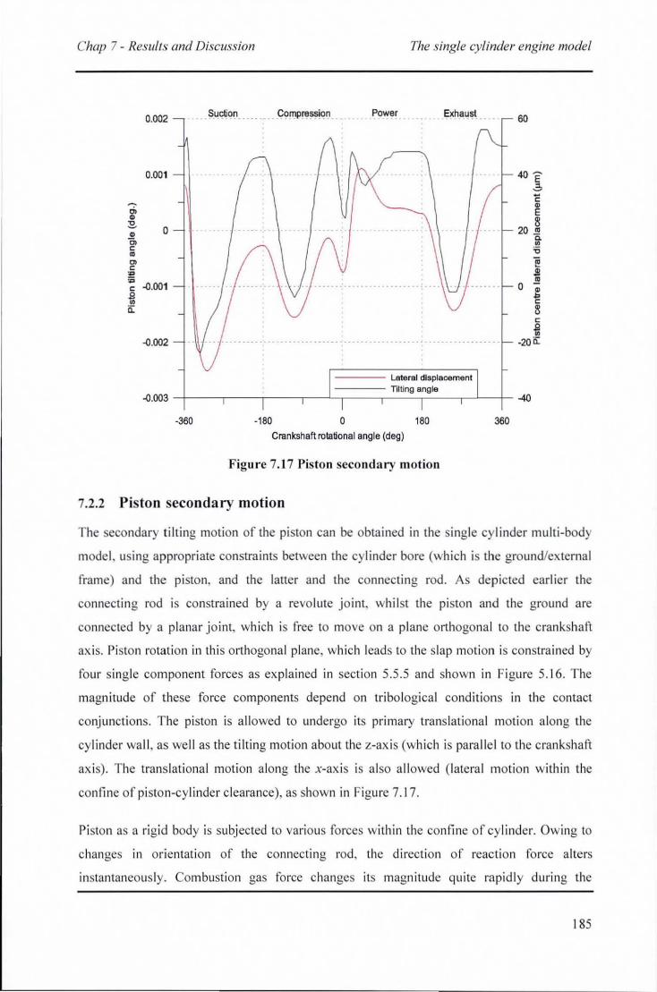
Chap 7 - Results and Discussion The single cylinder engine model
0.002
0.001
.;, 4> ~
0 4> C> C ~
CD C ., ;;;
·0.001 c Jl ~
0:
-<l.OO2
·360
Suction Compressi~n Power Exhaust 60
40~
], c ~ B
20 ~ C. o 'C e S
o !! g c B c ~
...... _ .. --............ . . . -. _ ... -,........... . ...... .200:
·180 o 180 360 Crankshaft rotational angle (deg)
F igure 7. 17 Piston secondary motion
7.2.2 Piston secondary motion
The econdary tilting motion of the piston can be obta ined in the s ingle cylinder multi-body
mode l, us ing appropri ate constraints between the cy linder bore (which is the ground/ex ternal
frame) and the piston, and the laner and the connect ing rod . As depicted earli er the
connecting rod is constrained by a revo lute j oint, whilst the piston and the ground are
connected by a planar joint, wh ich is free to move on a plane orthogona l to the c rankshaft
ax is. Pi ston rotation in thi s orthogonal plane, which leads to the slap motion is constra ined by
four s ingle component forces as explained in section 5.5 .5 and shown in Figure 5. 16. The
magnitude of these force components depend on tribo logical conditions in the contact
conjunct ions. The piston is allowed to undergo its primary translational moti on a long the
cylinder wa ll , as well as the tilti ng motion about the z-ax is (which is para lle l to the crankshaft
ax is). The trans lat ional motion along the x-ax is is a lso allowed (latera l motio n w ithin the
confine o f pi sto n-cy linder c learance), as shown in Figure 7.17.
Pi ston as a ri gid body is subjected to various forces with in the confine of cylinder. Owing to
changes in orientation of the connecting rod, the direction of reac tion force a lters
instantaneous ly. Combustion gas force changes its magnitude quite rapidly during the
185
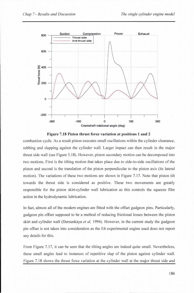
Chap 7 - Resulls and Discussion The single cylinder engine model
BOO
600
g400
~ ;; 2 F200
o
Suction Corn ression Power Exhaust Thrust side Anti-thrust side
-200 -+-----,----,-----,----,-----,----,-----,----,
-360 -1BO o 180 360 Crankshaft rotational angle (deg)
Figure 7. 18 Piston thrust force v'lriation at positions 1 and 2
combustion cycle. As a result pi ston executes small osc ill ations w ith in the cyl inder c learance,
rubbing and slapping agai nst the cylinder wa ll. Larger impact can then result in the major
thrust s ide wall (see Figu re 5.1 8). However, pi ston secondary motion can be decomposed into
two moti ons. First is the tilting moti on that takes place due to side-to-side osc ill atio ns of the
pi ston and seco nd is the trans lation o f the piston perpendicular to the piston ax is (its latera l
motion). The va riati ons of these two motions are shown in Figure 7. 17. Ole that pi ston tilt
towards the thrust side is considered as pos iti ve . These two movements are greatl y
responsible for the piston sk irt-cylinder wa ll lubrication as thi s contro ls the squeeze fi lm
action in the hyd rodynamic lu brication.
In fact , almost a ll of the modern engi nes are fitted wi th the offset gudgeon pins. Particula rl y,
gudgeon pin offset supposed to be a method of reduc in g fri ctiona l losses between the pi ston
skirt and cy linder wa ll (Dursunkaya el ai, 1994). Howeve r, in the current s tudy the gudgeon
pin offset is not taken into consideration as the E6 ex perimenta l engine used does not report
any deta ils for thi s.
From Figure 7.17, it can be seen that the tilt ing angles are indeed quite small . Nevertheless,
these small ang les lead to instances o f repetiti ve s lap o f the piston aga inst cy linder wa ll.
Figure 7. 18 shows the thrust force va riatio n at the cy linder wa ll at the maj or thrust ide and
186
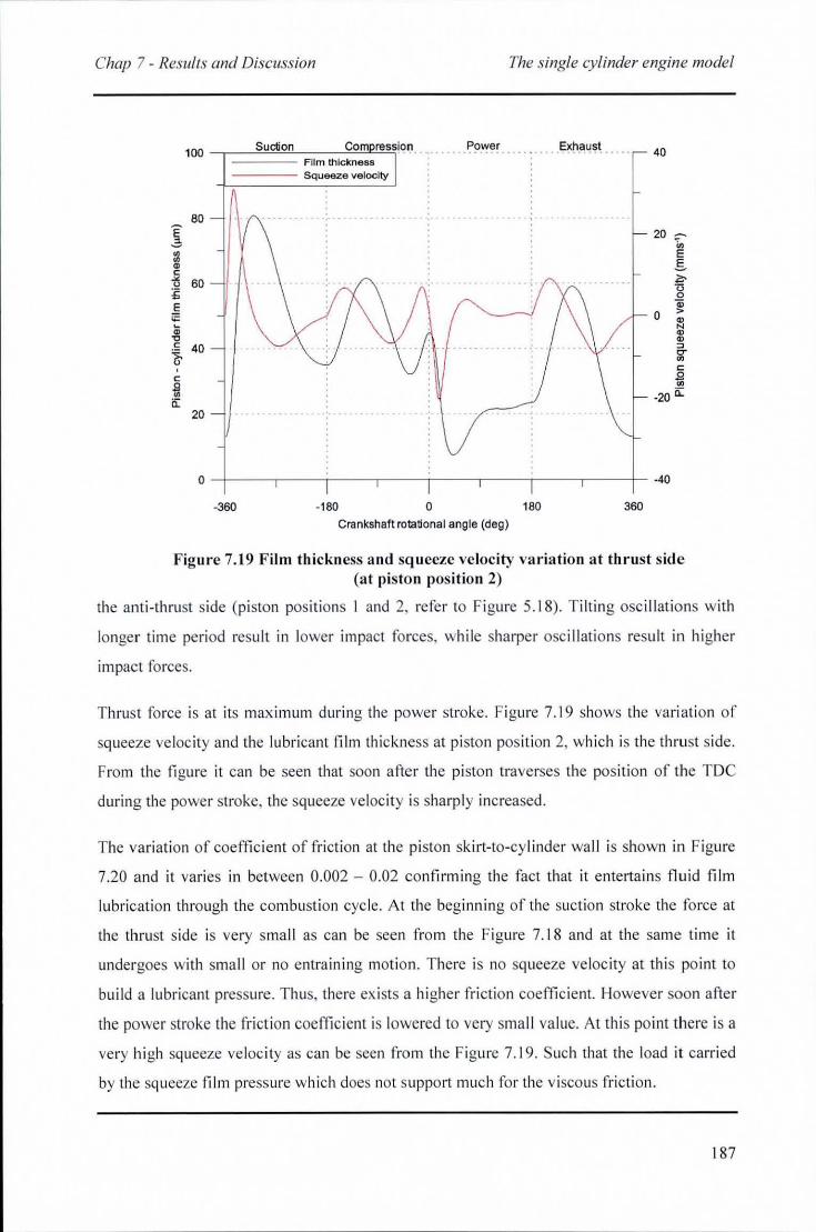
Chap 7 - Results and Discussion The single cylinder engine model
, c
i!i 0:
100 Suction
20
Corn ress[c?I) .. Film thIckness Squeeze velocIty
.~.~I.:!~~ ... -- 40
o -+--~---T--~--~--~--~--~---+- -40
-360 -160 o 180 360
Crankshaft ro1ational angle (deg )
Figure 7, 19 Film thickness and squeeze velocity variation at thrust side (at piston position 2)
the anti-thrust s ide (piston pos it ions I and 2, refer to Figure 5. 18). Tilting osc ill atio ns w ith
longer ti me period result in lower impact forces, whi le sharper osci llati ons result in hi gher
impact fo rces .
Thrust fo rce is at its max imum during the power stroke. Figure 7. 19 shows the vari ation o f
squeeze ve loc ity and the lubricant fi Im thickness at piston pos ition 2, which is the thrust side.
From the fi gure it can be seen that soon a fter the pi ston traverses the position of the TOe
during the power stroke, the squeeze velocity is sharply increased.
The vari ati on of coe ffi c ient of friction at the pi ston sk iI1-to-cyli nder wa ll is shown in Figure
7.20 and it varies in between 0.002 - 0.02 confirming the fact that it entertain s fluid film
lubrication through the combustion cyc le. At the beginning of the suct ion stroke the force at
the thrust side is very small as can be seen from the Figure 7. 18 and at the same time it
undergoes with sma ll or no entrai ning moti on. There is no sq ueeze velocity at this po int to
bu ild a lubricant pressure. Thus, there ex ists a hi gher fr iction coeffic ient. However soon afte r
the power stroke the fricti on coeffic ient is lowered to very small va lue. At th is point there is a
very hi gh squeeze veloc ity as can be seen from the Figure 7.19. Such that the load it carried
by the squeeze film press ure whi ch does not support much for the viscous fr iction.
187
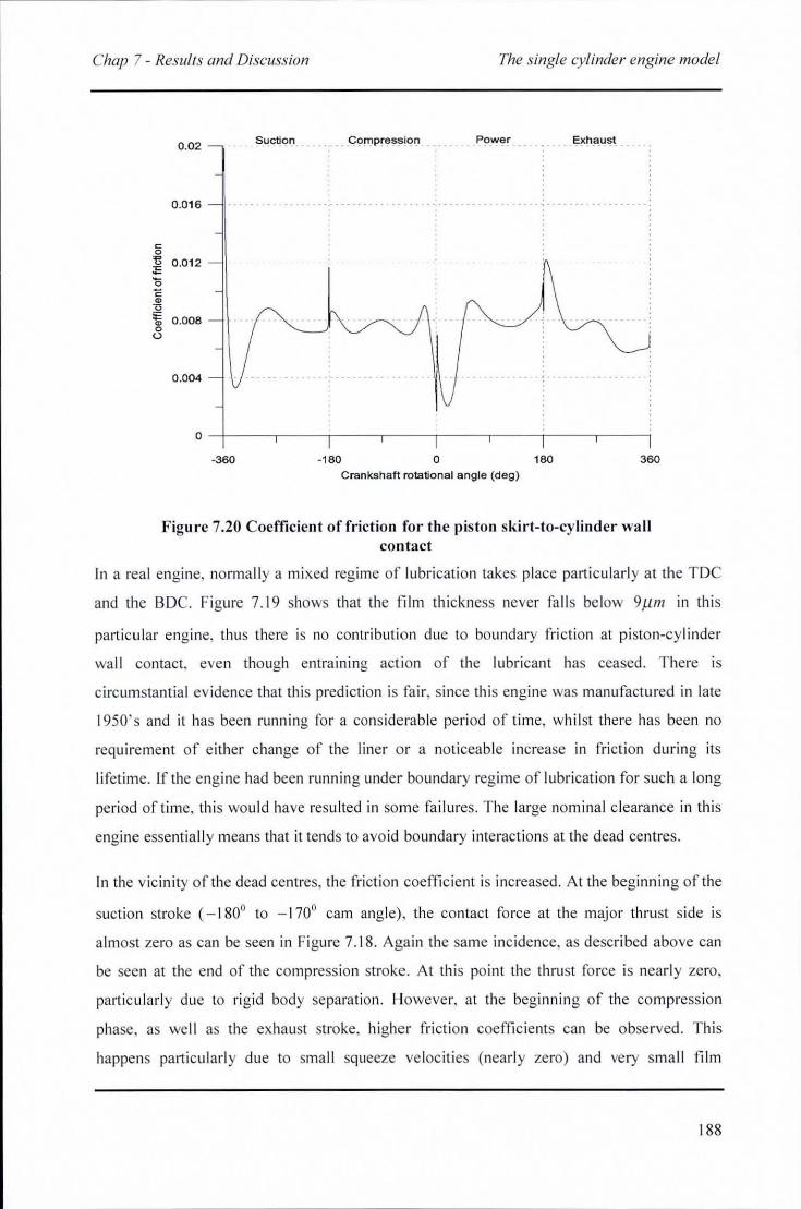
Chap 7 - Results and Discussion The single cylinder engine lI10del
c 0 '!l :E '0 c " ."
'" " 0 u
0 .02 Power Exh.aust .
0.016
0 .012
0 .008
0.004
o -+----,-----,----,-----r----,---~----_,--~
-360 -180 o 180 360 Crankshaft rotational angle (deg)
Figure 7.20 Coefficient of frict ion fo r the piston skirt-to-cy li nder wa ll contact
In a rea l engine, normally a mi xed regime of lubrication takes place pa rti cularl y at the TOC
and the BOC. Figure 7.19 shows that the fi lm thickness never fa ll s be low 911111 in th is
p3l1icular engi ne, thus there is no contribution due to boundary friction at piston-cyli nder
wa ll contact, even though entraining action of the lubricant has ceased. There is
circumstantia l evidence that th is prediction is fair, since th is engine was manufactured in late
1950 's and it has been running for a considerable period of time, whil st there has been no
req uil'ement of either change of the liner or a noticeable increase in friction dur ing its
lifetime. If the engine had been running under boundary reg ime of lubrication for such a long
period of time, this would have resulted in some fa il ures. The large nomina l clearance in this
engine essent iall y means that it tends to avo id boundary interactions at the dead centres.
In the vic inity of the dead centres, the friction coefficient is increased. At the beginning of the
suction stroke (- 180· to - 170· cam ang le), the contact force at the major thrust side is
al most zero as can be seen in Figure 7. 18. Again the same incidence, as described above can
be seen at the end of the compression stroke. At thi s point the thrust fo rce is nearl y zero,
particularl y due to rigid body separation. However, at the beginning of the compress ion
phase , as we ll as the exhaust stroke, higher frict ion coefficients can be observed. This
happens pal1i cul arl y due to small squeeze veloc ities (nea rl y zero) and very small fi lm
188
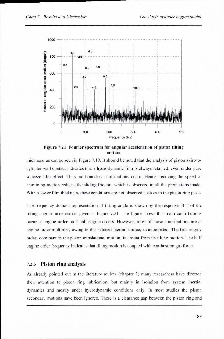
Chap 7 - Results and Discussion The single cylinder engine model
1000 . ................ . . . . .. .. . ............ . ........ . ............ . ... . .. . .
'1.;' 800 Cl
4.0
Q)
:!:!. c:: 0 ., .5 e 600 " @ '" :;; :; 400 Cl c::
'" ~ ;; c:: .9 200 '" 0:
o 100 200 300 400 500
Frequency (Hz)
Figure 7.21 Fou rier spectrum for angu lar acceleration of piston tilting motion
thi ckness, as can be seen in Figure 7. 19. It should be noted that the analysis of piston sk irt-to
cy linder wall contact indicates that a hyd rodynamic film is always reta ined, even under pure
squeeze film effect. Thus, no boundary contributions occur. Hence, reduc ing the speed of
entra ining motion reduces the slid ing fr iction, whi ch is observed in al l the pred ictions made.
With a lower film thickness, these conditions are not observed such as in the piston ring pack.
The frequency doma in representation of ti lting angle is shown by the response FFT of the
ti lti ng angular acceleration given in Figure 7 .2 1. The figure shows that main contri butions
occur at engine orders and half engine orders. However, most of these contributions are at
engi ne order multiples, owing to the induced inertia l torque, as anti cipated. The first engine
order, domi nant in the piston translationa l moti on, is absent from its tilting motion. The half
engine order frequency indicates that tilting motion is coupled with combustion gas force.
7.2.3 Piston ring analys is
As already pointed out in the literature rev iew (chapter 2) many researchers have d irected
their attention to piston ring lubrication, but mainly 111 iso lation from system inertial
dynamics and mostly under hydrodynamic cond it ions onl y. In most studies the piston
secondary moti ons have been ignored. There is a c learance gap between the pi ston ring and
189
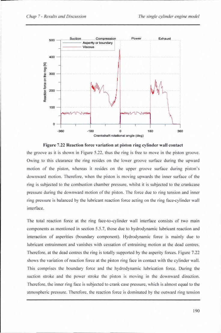
Chap 7 - Results and Discussion The single cylinder engine model
500 Q Power Exhaus~
Aspertty or boundary
Viscous
400
~ '" c ·c ., 300 = c 0
1! .2 c 0
200 tl .. ., '"
100
~,.
0
-360 -180 0 180 360 Crankshaft rotati onal angle (deg)
Figure 7_22 Reaction fo rce va riatio n a t p isto n ring cy linder wa ll contact
the groove as it is shown in Figure 5 .22, thus the ring is free to move in the pi ston groove.
Owing to th is c lea rance the ring resides on the lower groove surface during the upward
moti on of the pi ston, whereas it resides o n the upper groove surface during pi sto n's
downwa rd motion. Therefore, when the pi sto n is mov ing upwards the inner surface of the
ring is subjected to the combusti on chamber pressure, wh il st it is subjected to the crankcase
pressure during the downward motion of the pi ston. The fo rce due to ring tension and inner
ring pressure is balanced by the lubricant react ion fo rce act ing on the ring face-cylinder wa ll
interface .
The total reaction force at the ring face-to-cylinder wa ll interface consists of two main
components as mentioned in section 5.5.7, those due to hydrodynamic lubricant reaction and
interaction of asperities (boundary component) . Hydrodynam ic force is mainl y due to
lubricant entrainment and van ishes with cessation of entra ining motion at the dead centres.
Therefore, at the dead centres the ring is totall y supported by the asperity forces. Figure 7.22
shows the variat ion of reaction force at the piston ring face in contact with the cyli nder wa ll.
This compri ses the bo undary fo rce and the hydrodyna mic lubricat ion force . During the
suct io n stroke and the power stroke the piston is mov ing in the downwa rd direction.
Therefore, th e inner ring face is subjected to c rank case pressure, which is a lmo t equal to the
atmospheric pressure. Therefore, the reaction force is dominated by the outwa rd rin g tension
190
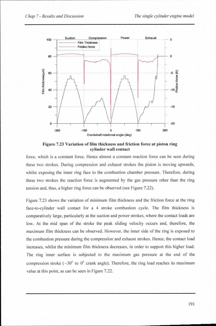
Chap 7 - Results and Discussion The single cylinder engine model
100
80
20
Suction Corn re~ion
Film Thickness
---- Friction force
Power Exhaust. 5
-15
0 ~---.---4~--.--~---.---4---.---4- ·20
·360 -180 o 180 360
Crankshaft rotational angle (deg)
Figure 7.23 Variation of film thickness and friction force at piston ring cylinder wall contact
force , which is a constant force. Hence almost a constant reaction force can be seen during
these two strokes. During compression and ex haust strokes the piston is movi ng upwards,
whil st ex posing the inner ring face to the combusti on chamber pressure. Therefo re, during
these two strokes the reaction force is augmented by the gas pressure other than the ring
tension and, thus, a higher ring fo rce can be obse rved (see Figure 7.22).
Figure 7.23 shows the variati on of minimum film thickness and the frict ion fo rce at the ring
face-to-cy linder wal l contact for a 4 stroke combusti on cycle. The fi lm th ickness is
comparative ly large, palt icul arly at the suct ion and power strokes, where the contact loads are
low. At the mid span of the stroke the peak sliding ve loc ity occurs and, therefore, the
maximum fi lm thickness can be observed . However, the inner side of the ring is exposed to
the combusti on pressure during the compression and exhaust strokes. Hence, the contact load
increases, whil st the min imum fi lm thi ckness decreases, in order to support th is hi gher load.
The ring inner surface is subj ected to th e max imum gas press ure at the end of the
compression stroke (_300 to 00 crank angle). There fore, the ring load reaches its max imum
va lue at this point , as can be seen in Figure 7.22.
19 1
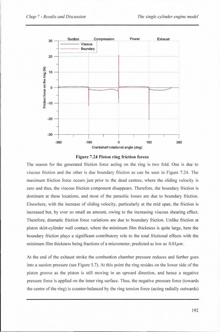
~------------------------------~--- ---
Chap 7 - Resulls and Discussion The single cylinder engine model
30 _T=::,s~U~cti~·o~n~;;;;;;;;;-,compreSSion Viscous
-------- Boundary
20 - ·~~
-
b '" 10 -c
-.- .... ~c
" ,s
Power Exhaust
g 0 ~=====t==~~======F=~~ ~ 1 .2 c o '!l -10 -·c u.
-20 -
·30 -+--'--'-'Ir-- ,,--,-1--'--'--'--1 - "--'1 -360 -180 0 180 360
Crankshaft rotational angle (deg)
Figure 7.24 Pis ton ring friction forces
The reason fo r the generated fri cti on fo rce act ing on th e ri ng is two fo ld . One is due to
viscous friction and the other is due boundary friction as can be seen in Figure 7.24. The
max imum friction force occurs j ust prior to the dead centres, where the s liding veloc ity is
zero and thus, the viscous fricti on component di sappears . Therefore, the boundary fr iction i
dom inant at these locations, and most of the pa rasitic losses are d ue to bo undary friction.
Elsewhe re, wi th the increase of slid ing ve loc ity, pmticula rl y at the mid span, the fr icti on is
increased but, by ever so small an amou nt, owing to the increas ing viscous shearing effect.
There fore, dramatic fri ction fo rce variati ons a re due to bo undary fr ictio n. Unlike fr iction at
pi ston sk irt-cylinder wa ll contact, where the minimum film thi ckness is quite large, here the
boundary friction plays a s igni fica nt contri buto ry ro le to the tota l fri cti onal effects with the
m ini mum fil m thickness be ing fractions of a micrometer, pred icted as low as 0.0 Ipm.
At the end o f the ex haust stroke the combustion chamber pressure reduces and further goe
into a suct ion pressure (see Figure 5.7). At thi s point the ring resides on the lower side of the
piston groove as the piston is still moving in an upward d irecti on. and hence a negati ve
pressure force is appl ied on the inner ring sur face . Thus, the negati ve pressure force (towards
the centre o f the rin g) is counter-ba lanced by the ring tension fo rce (actin g radia ll y outwards)
192
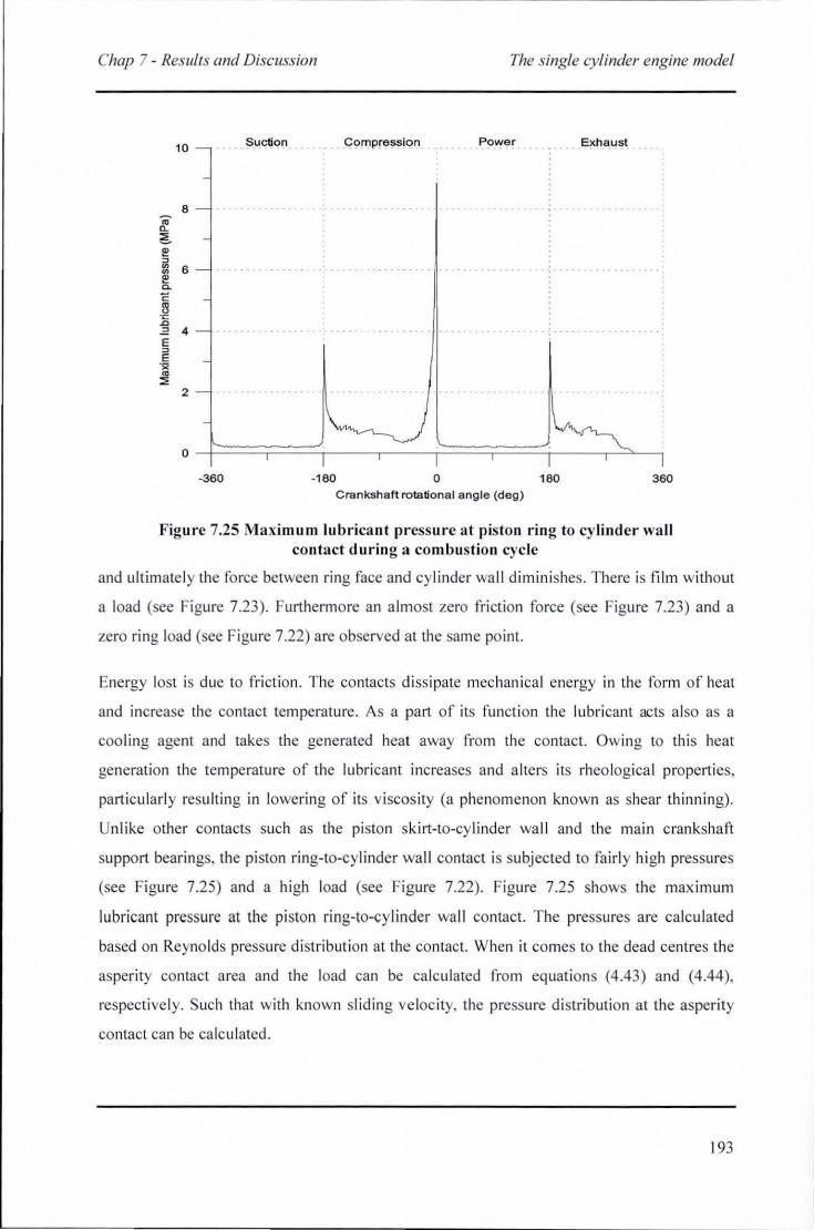
Chap 7 - Results and DisclIssion The single cylinder engine model
10 Su~on Power Exhaust
8
2
-360 -180 o 180 360 Crankshaft rota tional angle (deg)
Figure 7.25 Maximum lubricant pressure at piston ring to cylinder wall conhlct during a combustion cycle
and ultimately the force between ring Face and cylinder wa ll diminishes. There is film without
a load (see Figure 7.23). Furthermore an almost zero fri ction force (see Figure 7.23) and a
zero ring load (see Figure 7.22) are observed at the same point.
Energy lost is due to Friction. The contacts d issipate mechanical energy in the form of heat
and increase the contact temperature. As a part of its functi on the lubricant acts a lso as a
cooling agent and takes the generated heat away From the contact. Owing to thi s heat
generation the temperature of the lubricant increases and alters its rheologica l properties,
palticularl y resulting in lowering of its vi scos ity (a phenomenon known as shear thinning).
Unlike other contacts such as the piston skirt-to-cylinder wa ll and the main crankshaft
support bearings, the piston ring-to-cylinder wall contact is subjected to fairl y high pressures
(see Figure 7.25) and a high load (see Figure 7.22). Figure 7.25 shows the maximum
lubricant pressure at the piston ring-to-cylinder wall contact. The pres ure are calculated
based on Reynolds pressure di stribution at the contact. When it comes to the dead centres the
asperity contact area and the load can be calculated from equations (4.43) and (4.44),
respectivel y. Such that with known sliding ve loc ity. the pressure di stribution at the asperity
contact can be calculated.
193
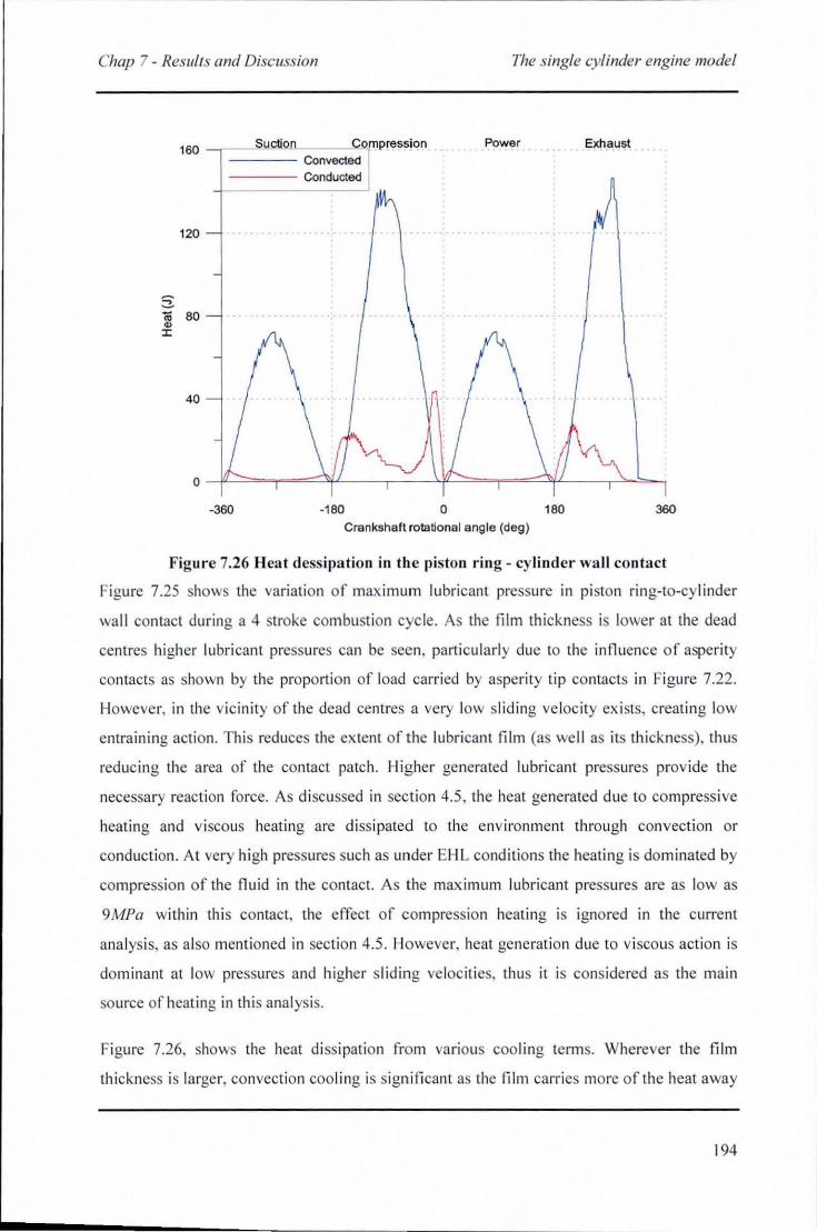
Chap 7 - Reslllrs and DisclIssian The single cylinder engine model
160 -T======~C;;;~;,;;"(mpr~ss~on . Convected
Power
---- Conducted
120
-360 -180 o 180 360
Crankshaft rotationa l angle (deg)
Figure 7.26 Heat dessipation in the piston ring - cylinder wall contact
Figure 7.25 shows the variati on of max imum lubricant pressure in piston ring-to-cylinder
wa ll contact during a 4 stroke combustion cycle. As the fi lm thickness is lower at the dead
centres higher lu bricant pressures can be seen, part icularly due to the influence of asperity
contacts as shown by the proport ion of load carri ed by asperity tip contacts in Figure 7.22.
However, in the vici nity of the dead centres a very low sliding ve loc ity ex ists, creating low
entraining action. This reduces the extent of the lubricant film (as well as its th ickness), thus
reducing the area of the contact patch. Higher generated lubricant pressures provide the
necessary reaction force. As discussed in section 4.5, the heat generated due to compress ive
heating and viscous heating are diss ipated to the environment through convection or
conduction. At very high pressures such as under EHL conditions the heating is domi nated by
compression of the fluid in the contact. As the maximum lubricant pressures are as low as
9MPa within thi s contact, the effect of compression heating is ignored in the current
ana lysis, as al 0 mentioned in section 4.5 . However, heat generation due to viscolls action is
dominant at low pressures and higher sliding veloc ities, thus it is considered as the main
source of healing in this analysis.
Figure 7.26, shows the heat di ssipation from va rioll s cool ing terms. Wherever the film
thi ckness is larger, convection cooling is sign ificant as the fi lm carries more of the heat away
194
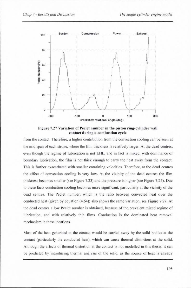
Chap 7 - Results and Discussion The single cylinder engine model
100
80
" e::.. 60
.8 E " z -.; "ll 40 ~
Suction
-360 -180
Compres;;ion Power Exhaust
o 180 360 Crankshaft rotational angle (deg)
Figure 7.27 Variation of Peel et number in the pis ton ring-cy linder wall contact during a combustion cycle
from the contact. Therefore, a hi gher contribution from the convection cooling can be seen at
the mid span of each stroke, where the film thickness is rel atively larger. At the dead centres,
even though the regime of lubrication is not EHL, and in fact is mixed , with dom inance of
boundary lubrication, the film is not thi ck enough to carry the heat away from the contact.
Th is is further exacerbated wit h smaller entrain ing velocities. Therefore, at the dead centres
the effect of convection cooling is very low. At the vicinity of the dead centres the film
thickness becomes smaller (see Figure 7.23) and the pressure is higher (see Figure 7.25). Due
to these facts conduct ion coo li ng becomes more signifi cant, particularl y at the vicinity of the
dead centres. The Peel et number, which is the rati o between convected heat over th e
conducted heat (given by equation (4.64)) also shows the same variation , see Figure 7.27. At
the dead centres a low Peel et number is obtained , because of the prevalent mixed regime of
lubrication, and with relatively thin films. Conduction is the dominated heat remova l
mechanism in these locati ons.
Most of the heat generated at the contact wo uld be carried away by the so lid bodies at the
contact (part icula rl y the conducted heat), which can cause thermal d istorti ons at the so lid.
Although the affects of thennal di storti on at the contact is not modell ed in thi s thesis, it can
be predicted by introducing thermal analysis of the so lid , as the source of heat is alread y
195
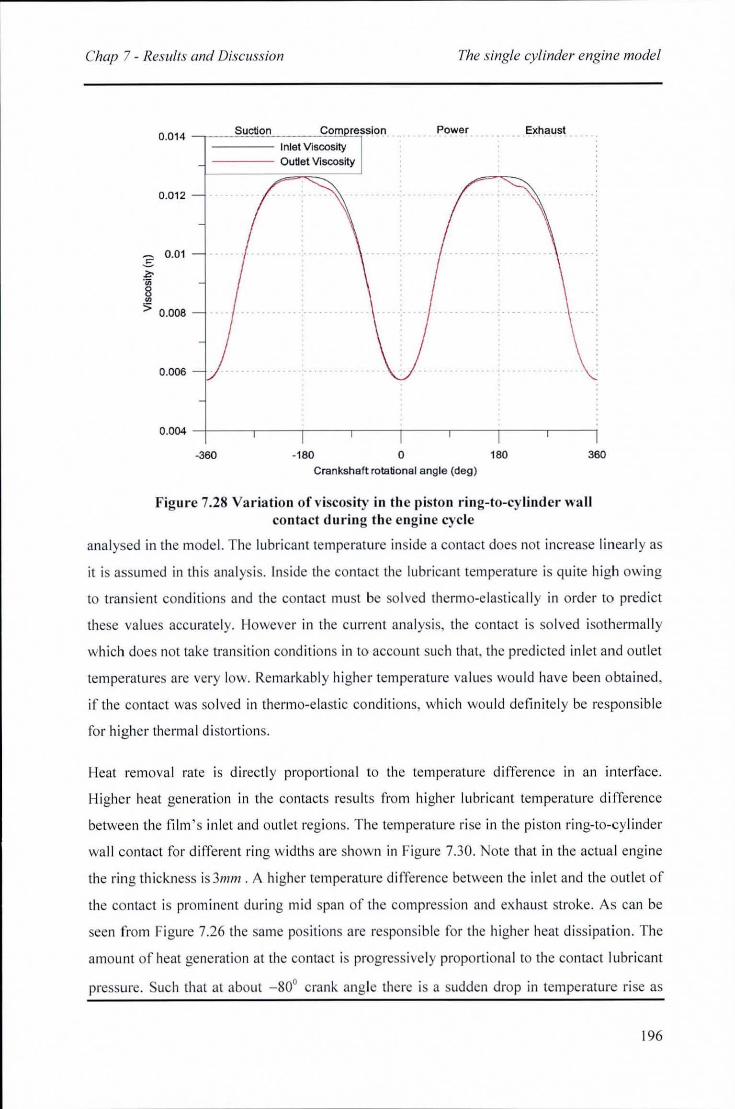
Chap 7 - Results and Discussion The single cylinder engine model
0.014
0.012
_ 0 .01 5 ;,. ';; 8 o
5 0.008
0.006
Suction Corn ression
Inlet Viscosity ---- Outlet Viscosity
Power Exhaust
0.004 -/----,---,---,---,----,----r---,----i
-360 -180 o 160 360
Crankshaft rotational angle (deg)
Figure 7.28 Variation of viscos ity in the piston ring-to-cylinder wall contact during the engine cycle
analysed in the model. The lubricant temperature inside a contact does not increase linearly as
it is assumed in this ana lys is. Inside the contact the lubricant temperature is qu ite high owi ng
to transient conditions and the contact must be so lved thermo-elastica ll y in order to predict
these va lues accurately. However in the current analys is, the contact is solved isothermally
which does not take tra nsition conditions in to accoun t such that, the predicted in let and outl et
temperatures are very low. Remarkably higher temperature va lues woul d have been obtained,
if the contact was solved in thermo-elastic conditions, which would defi ni te ly be responsib le
for higher thermal distortions.
Heat remova l rate is direct ly proportional to the temperature difference in an interface.
Higher heat generation in the contacts resul ts from higher lubricant temperature difference
between the film 's in let and outl et reg ions. The temperature ri se in the piston ring-to-cy linder
wa ll contact for di ffe rent ring widths are shown in Figure 7.30. Note that in the actual engi ne
the ring thickness is 3mm . A higher temperature difference between the inlet and the outlet of
the contact is prominent during mid span of the compress ion and exhaust stroke. As can be
seen from Figu re 7.26 the same positions are responsible for the higher heat dissipation. The
amount of heat generat ion at the contact is progressive ly proportional to the contact lubricant
pressure. Such that at about - 800 crank angle there is a sudden drop in temperature ri se as
196
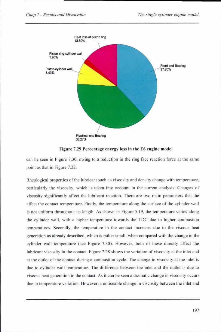
Chap 7 - Resulls and Disc1Ission
Heat loss at piston ring 13.69%
Piston I1ng-cyllnder wall 1.95%
PislorH:ylinder 8.400/0
Flywheel end Beanng 3827%
The single cylinder engine model
Figure 7.29 Percentage energy loss in th e E6 engi ne model
can be seen in Figure 7.30, owing to a reduction in the ring face reaction force at the same
po int as that in Figure 7.22.
Rheo logica l pro perties of the lubricant such as viscos ity and density change with temperature,
palt icul arl y the viscosity, whi ch is taken into account in the current ana lysis. Changes of
vi scos ity significant ly affect the lu bricant reaction. There are two main parameters that the
affect the contact temperature. Firstl y, the temperature a long the surface of the cy li nder wa ll
is not uniform throughout its length . As shown in Figure 5. 19, the temperature varies a long
the cy li nder wa ll , wi th a higher temperature towards the TDC due to hi gher combustion
tem peratures. Secondly, the temperature in the contact increases due to the v iscous heat
generation as a lready described, which is rath er small , when compared with the change in the
cylinder wa ll temperature (see Figure 7.30). However, both of these d irectly affect the
lubri cant viscosity in the contact. Figure 7.28 shows the va ri ation o f viscos ity at the inlet and
at the outlet of the contact during a combusti on cyc le. The change in viscosity at the inlet is
due to cylinder wa ll temperature. The d iffe re nce between the in let and the o utlet is du e to
viscous heat generati on in the contact. As it can be seen a dramatic change in viscos ity occurs
due to temperature variati on. Howeve r, a noticeab le change in v iscosity between the in let and
197
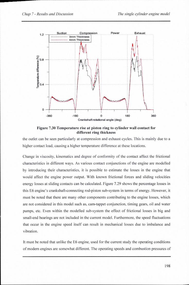
Chap 7 - Results and Discussion The single cylinder engine model
Suction 1.2 T==:=-;;;;;;:;;-~~;"f
Power
o -4-----,-----*-----,----~----_,----~----,_~~
-360 -180 o 180 360 Crankshaft rotational angle (deg )
Figure 7.30 Temperature rise at pis ton ring to cylinder wall contact for different ring thickness
the outlet can be seen parti cula rl y at compress ion and exhaust cyc les. Thi s is mainl y due to a
hi gher contact load , causing a higher temperatu re difference at these locations.
Change in viscos ity, kinematics and degree of conformity of the contact affect the frictiona l
characteristi cs in di ffe rent ways. As various contact conj unctions of the engi ne are modelled
by introducing their characteri sti cs, it is possi ble to estimate th e losses in the engi ne that
would affect the engine power output. With known fri ctiona l fo rces and sliding ve loc iti es
energy losses at sliding contacts can be ca lcul ated. Figure 7.29 shows the percentage losses in
thi s E6 engi ne's crankshaft-co nnecting rod-pi ston sub-system in terms of energy. However, it
must be noted that there are many other components contributing to the eng ine losses, which
are not considered in this model such as, cam-tappet conjunction, timing gears, o il and water
pumps, etc. Even within the modell ed sub-system the effect of fri ctional losses in big and
small-end bearings are not included in the current model. Furthermore, the speed fluctuations
that occur in the engine speed itse lf can res ult in mechani ca l losses due to im ba lance and
vibration.
It must be noted that unlike th e E6 engine, used fo r the current study the operating conditions
of modern engi nes are somewhat d iffe rent. The operating speeds and combustion pressures of
198
Chap 7 - Results and Discussion The single cylinder engine model
modern engines are significantly hi gher compared to speeds and pressure considered in th is
study. On the other hand, in most modern eng ines the inner ring face is ex posed into the
combustion cham ber through drill ed ho les between the ring groove and the piston top
surface. This would a ll ow high pressure combustion gasses to penetrate into the pi ston ring
groove and increase the ring groove pressure, wh ich is act ing on inner ring face . This would
increase the ring face force particu larl y during the power stroke, where a better sealing
becomes mandato ry. This paves the way fo r reduced initial ring tens ion needed to ensure
better seal ing at lower inner ring pressures and hence the size of the ring can be reduced .
Owing to low st iffness and softer ring constructions the natura l frequencies of the pi ston ring
are reduced and enhance the chance of the ir co inciding wi th engine order mu ltiples, pa rticular
in hi gh performance high speed eng ines. In such cases the dynam ic analys is of the pi ston rin g
is crucial in order to obta in a better representa ti on of the piston ring physica l behav iour.
Owing to the rather ri g id (stiffer) constructio n of the E6 engi ne piston ring, when compared
to the more modern eng ines, hi gher fundamental natural frequencies can be observed, whi ch
are far higher than the major engine order excitations. Also, the nex ibility of the piston ring is
not included in the current numeri ca l model. In thi s series of quasi-static analyses, the effect
of squeeze film action cannot be considered. However, for a fu ll transient ana lysis, thi s effect
must be considered, which would have to also in cl ude the modal excitation of the ring.
Moreover, many papers in the literature repo rt that in modern engines the contact between the
pi ston ring and the cy linder wa ll undergoes EHL cond itions, owing to its nex ibili ty and
hi gher contact forces act ing on the small contact area .
Due to dynamic nature of the forces on the piston ring, the ring modes are eas ily get excited
and in-plane and out-plane ring deformation takes place. Thi s would result a hi gher radial
clearance between the ring face and cylinder liner at some points on the ring circumference
allowing hi gh pressure gasses to pass through. When the out-pl ane modes are exc ited the
clearance between the ring and the piston-ring-groove at ring top and bottom surface is
affected at some points. These clearances create paths all around the piston ring a ll owing hi gh
pressure combustion chamber gasses to pass through to the low pressure crankcase which is
known as blow-by. The effect o f blow-by is fu rther enhanced by ring wear and ring n attering
that causes ring to osci llate within the piston groove. In mu lti-ring pack systems, the inter
ring gas pressure is mostly dependent on the extent of blow-by. Most of these effects are not
included in the current model as these are no t applicab le to the E6 experimental engine. In
199
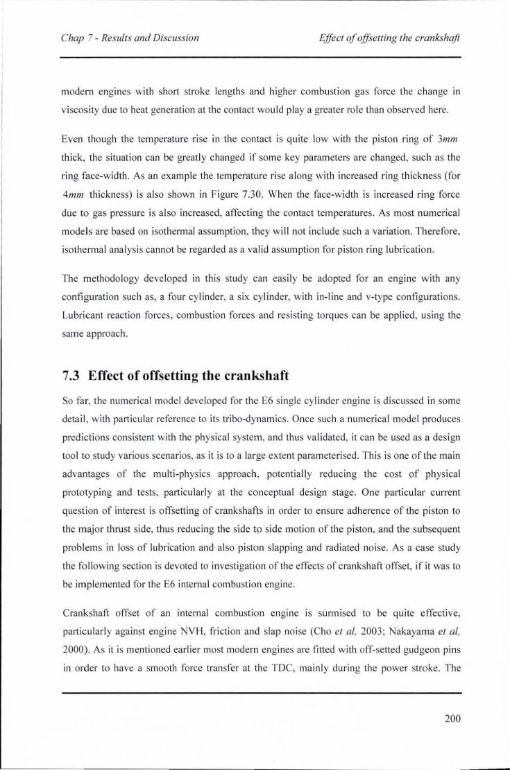
Chap 7 - Resulrs and Discussion EJJecr %jJseffing rhe crankshaft
modern engines with short stroke lengths and higher combustion gas force the change in
viscos ity due to heat generation at the contact would play a greater ro le than observed here.
Even though the temperature ri e in the contact is quite low with the pi ston ring of 3mm
thick, the situation can be greatl y changed if some key parameters are changed, such as the
ri ng face-width . As an example the temperature ri se a long with increased ring thickness (for
4mm thickness) is also shown in Figure 7.30. When the face-width is increased ring force
due to gas pressure is a lso increased, affecting the contact temperatures. As most numerical
model s are based on isothermal assumption, they will not include such a variation. Therefore,
isothermal anal ysis cannot be rega rded as a val id assumption fo r pi ston ring lubricatio n.
The methodology deve loped in thi s study can easily be adopted fo r an engine with any
configuration such as, a four cylinder, a six cyl inder, with in-line and v-type configurations.
Lubricant reacti on fo rces, combustion fo rces and res isting torques can be app lied, us ing the
same approach.
7.3 Effect of offsetting the crankshaft
So fa r, the numerica l model deve loped fo r the E6 single cy linder engine is discussed in some
deta il, wit h particular reference to its tri bo-dynamics. Once such a numeri ca l model produces
predictions consistent with the ph ysical system, and thus va lidated. it can be used as a des ign
too l to study va rious scenarios, as it is to a large extent pa rameterised. Thi s is one of the main
advantages of the mUlti-physics approach, potenti all y reducing the cost of physical
prototyping and tests, particul arl y at the conceptual design stage. One particular current
question of interest is offsett ing of crankshafts in order to ensure adherence of the piston to
the major thru t side, thus reducin g the side to side motion of the pi ston, and the subsequent
problems in loss of lubrication and also pi ston slapping and radiated no ise. As a case study
the fo llowing secti on is devoted to invest igati on of the effects of crankshaft offset, if it was to
be implemented for the E6 internal combustion eng ine.
Crankshaft offset of an internal combusti on engine is surmised to be quite effecti ve,
panicularly aga inst engi ne VH. fricti on and slap no ise (Cho et 01, 2003; akayama et ai,
2000). As it is mentioned earl ier most modern engi nes are fitted with off-sel1ed gudgeon pins
in order to have a smooth force transfer at the TO , mainl y during the power stroke. The
200
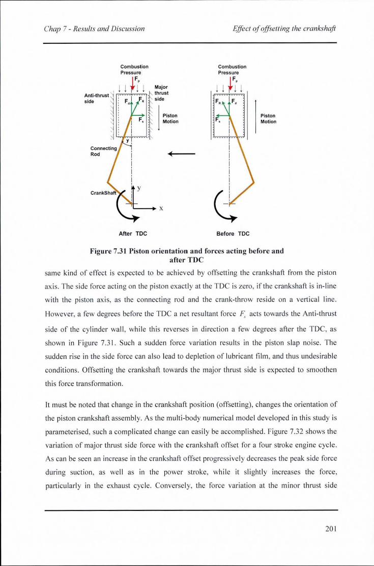
Chap 7 - Results and Discussion
Anti·thrust side
Combustion Pressure
IF, ! ! t ! !
y
Major thrust
Piston Motion
'L--. x
After TDe
E;/j"ect of ojJse/ling the crankshafl
Combustion Pressure
IF, ! ! t ! ! F,
Before TDe
Piston Motion
Figure 7.3\ Piston orientation a nd forces acting before and after TOe
same kind of effect is expected to be achieved by offsetting the crankshaft from the pi ston
axis. The side force acting on the piston exactly at the TOC is zero, if the crankshaft is in-line
with the piston axis, as the co nnecting rod and the crank-throw res ide on a vert ical line.
However, a few degrees before the TDe a net resultant force F, acts toward s the Anti-thrust
side of the cy linder wa ll , while this reverse in di rect ion a few degrees after the TOC, as
shown in Figure 7.31. Such a sudden fo rce vari at ion results in the piston slap noise. The
sudden ri se in the side force can also lead to depleti on of lu bricant film , and thus undesirab le
conditions. Offsetting the crankshaft towards the major thrust side is expected to smoothen
th is force transformat ion.
It must be noted that change in the crankshaft pos ition (offsetting), changes th e orientation of
the piston crankshaft assembly. As the multi-body numerica l model developed in this study is
parameterised, such a complicated change can easil y be accompli shed. Figu re 7.32 shows th e
va ri at ion of major thrust side force with the crankshaft offset fo r a fOllr stroke eng ine cycle.
As can be seen an increase in the crankshaft offset progressively decreases the peak side fo rce
dur in g suction , as we ll as in the power stroke, while it sli ghtl y increases the fo rce,
part icu larly in the exhaust cyc le. Converse ly, the force variation at the minor thrust side
20 1
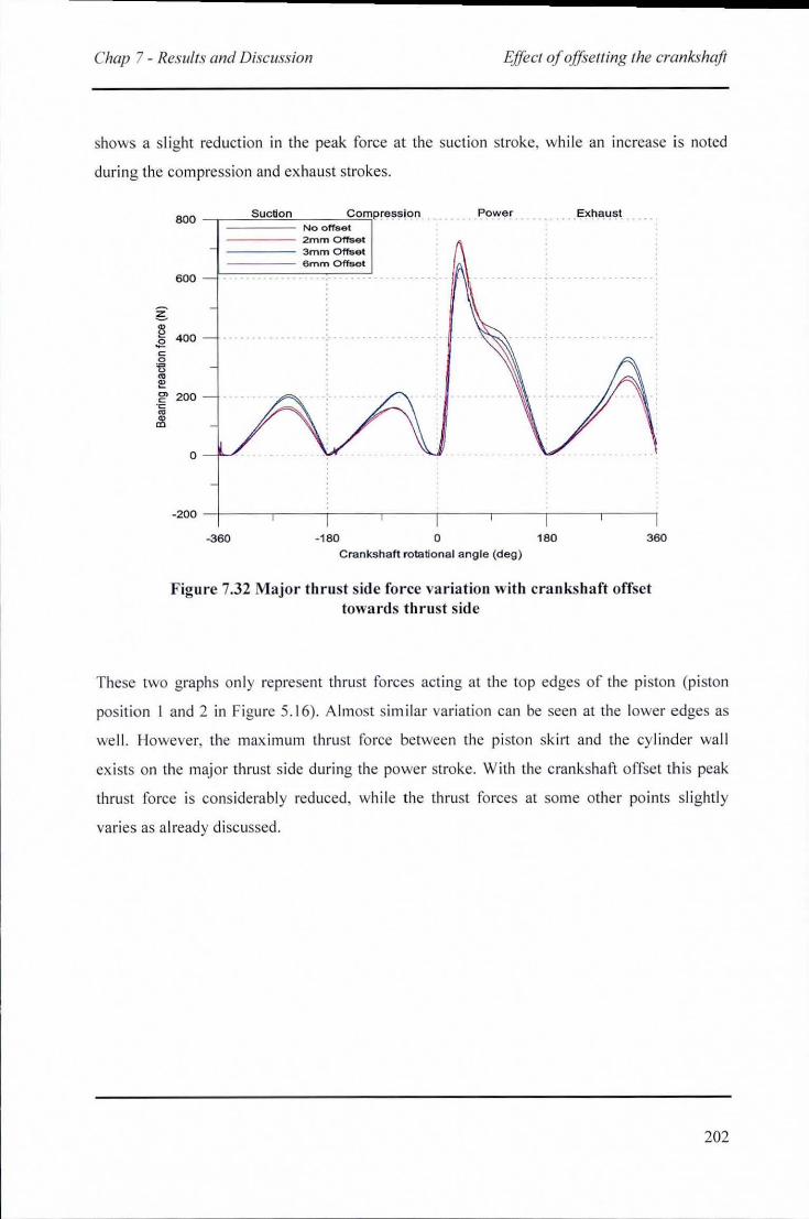
Chap 7 - Results and Discussion Effect of ojJsell ing the crankshaji
shows a slight reduction in the peak force at the suction stroke, while an increase is noted
during the compress ion and exhaust strokes.
800 -T = =s="=c:,ti:::on::-Noclf.;;;co<°4mpress,<?o_ .. No offset
_jl~~~~_2~m;m~~~;etu 3mm Offset 6 mm Offset
600 ... .... . ..
g 1l .E 400 ~ o tl i! g> 200
.~
~
o
-200 -4-----,----~------r-----r-----r-----r-----,-----,
-360 -180 o 180 360 Cranksha ft rota tiona l angle (deg )
Figure 7.32 Major thrust side fo rce variation with crankshaft offset towards thrust side
These two graphs only represent thrust fo rces acting at the top edges of the piston (p iston
pos ition I and 2 in Figure 5. 16) . A lmost similar vari ati on can be seen at the lower edges as
we ll . However, the max imum thrust force betwee n the pi ston skirt and the cy linder wall
ex ists on the major thrust side during the power stroke. With the crankshaft o ffse t th is peak
thrust force is considerably reduced, whi le the thrust fo rces at some other po ints slightl y
va ri es as a lread y di scussed.
202
Chap 7 - Results and Discuss ion F;/fect of oJJselling the crankshaji
400 _T==S=U~cli~.o~n~~~!c:om~PfeSSiqn No offse t 2mrn Offset
_]l~~~~~3m~m~~~~tU 6mm orrset
300
g 1! 200 ,g c 0
13 ~
~ C» 100 c ·c ~
~
o
-100 -4-----,-----,-----,------,-----,-----.-----.-----,
-360 -180 o 180 360 Crankshaft rotationa l angle (deg)
Figu re 7.33 Minor thrust side force variation with respect to the crankshaft offset towards the major th rust side
The pi ston lateral moti on becomes max imum in the negati ve x -directi on during the suction
stroke (at crank angle o f -320°) and in the pos iti ve x - di recti on at the power stroke (at c rank
angle of 40° ) fo r a 3mm offset towards maj or thrust s ide. The pi ston is translated w ithin
these two limits during th e four stroke eng ine cyc le as shown in Figure 7.34. Along with the
crankshaft o ffset these max imum limits have been reduced as can be seen in the fi gure. On
the other hand , the di splacements at other places such as at compression and ex haust strokes
have been increased. The crankshaft offset can be regarded as a process that smoothen the
dynamic behav iour of the pi sto n. However, excess ive inc rease in crankshaft o ffse t would not
be supported by the numeri ca l model and results shows a maximum of about 4mm is
poss ible with the current model. Excessive o ffset creates mass ive forces on the thrust side
thus EHL would need to support such a load whi ch is not modelled.
Crankshaft offset is a lso regarded as a process to change fri ction fo rces, acting on the piston
skirt-to-cylinder wa ll. However, it is a lso repo lted that these variati ons are mostly dependent
on the engine operati ng speed (Cho et 01, 2003). Addi ti ona ll y, the change in vi scosity of the
lubri cant changes the fri ctional force characte ri sti cs o f the engine. However, the behavi our of
an internal combustion eng ine can be changed due to various reasons.
203
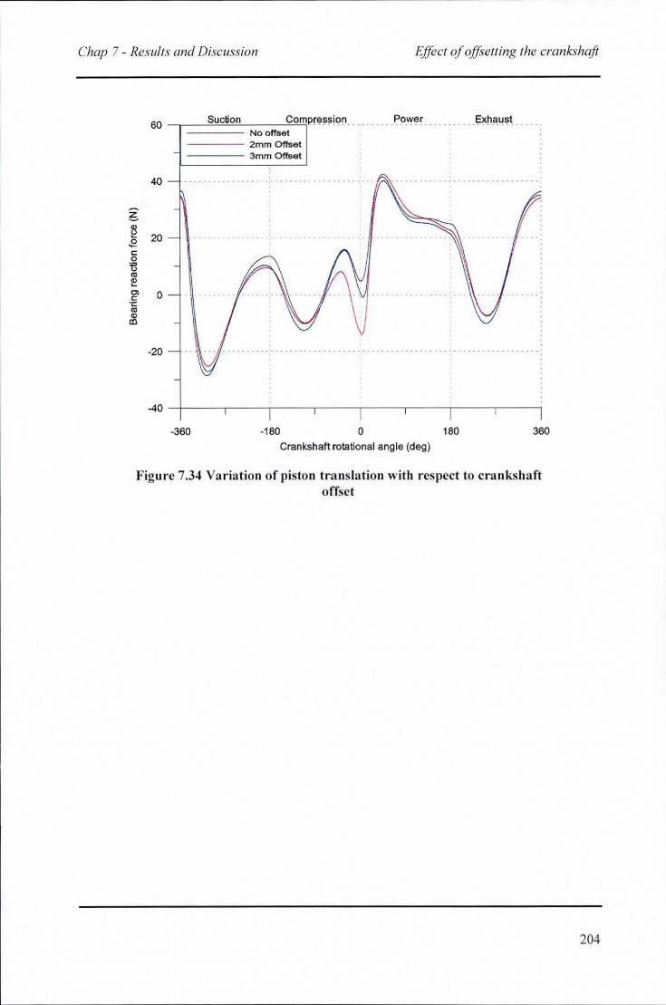
Chap 7 - Results and Discussion Effect of offsetting the crankshaft
60 _T==s=u=c=ti=on=-No"-;;;;;~c",olmprEit~lqf! .. _, ____ . _ . ~ower No offset
---- 2mm Offset 3mm Offset
40
20
o
-20
40 -+----,-----r----,-----r----,-----r----,----~
-360 -180 o 180 360 Crankshaft rotationa l angle (deg)
Figure 7.34 Va riation of piston tra nsla tion with respect to crankshaft offset
204
Chap 8 - Conclusions and Suggestions for Overall Conclusions
8 CONCLUSIONS AND SUGGESTIONS FOR FUTURE
WORK
8.1 Overall Conclusions
The investigations in this thesis highlight the complexity of the piston, connecting rod,
crankshaft and flywheel multi-body dynamics. The problem is multi-disciplinary in nature
drawing the attention towards a multi-physics approach. It involves rigid inertial body
motions, component flexibility, tribological contacts and their thermal considerations.
Although the motion of the engine is largely prescribed, based on kinematics, induced by
combustion gas force, it is greatly affected by inertial dynamics, elastic distortion of the
flexible components and the complex nature of the power torque, comprising many
harmonics. Furthermore, the piston is subjected to small amplitude lateral and tilting motions,
which are induced by interactions between the piston and the cylinder bore, referred to as
piston secondary motion. Kinetics in the contact of the mating surfaces is affected by these
interactions, other than primary engine kinematics. Clearance between the piston ring and the
groove allows it to move relatively freely within its confinement. Higher lubricant pressures
are generated within the piston ring cylinder wall contact, which are highly transient in
nature. Generated pressures and viscous friction cause a temperature rise within the contact
that affects the rheological parameters of the lubricant. Therefore, the analysis includes
physical disciplines, such as tribology, heat transfer, flexibility, constrained multi-body
dynamics and small amplitude vibrations.
The regime of lubrication in crankshaft main bearings is considered to be hydrodynamic,
even though the more modern main bearing lubrication problems with thin shells are solved
based on EHL conditions. The results obtained for these bearings illustrate that the
assumption is valid, with relatively large minimum film thickness existing in the case
considered, giving an eccentricity ratio in the range: 0.09-0.6. The complexity of the problem
is in combined solution of all the involved phenomena, all of which are non-linear in nature.
The solution is obtained quasi-statically such that the contribution of both lubricant
205
Chap 8 - Conclusions and Suggestions/or Overall Conclusions
entrainment and squeeze film effects can be seen. Particularly, at power stroke, the squeeze
film action is significant in these bearings.
All the results obtained for piston - cylinder wall interactions point to the dominance of the
hydrodynamic regime of lubrication, with relatively large minimum oil film thickness in the
range: 8 -1 Opm, and with relatively low generated pressures in the range offew MPa, even
at the thrust side under critical operating conditions. With the aforementioned pressure
distribution and the contact conformity, iso-viscous regime of fluid film lubrication prevails.
This is certainly the case in more unloaded parts of the piston cycle. When the speed of
entraining motion is significant such as in the mid-stroke of piston motion a lubricant film
can be retained and the coefficient of friction is quite low. At the TOC and the BOC, with
diminished entraining motion, the lubricant film thickness is sufficient in the case of the E6
engine to ensure fluid film lubrication. The approaching velocities of the contiguous bodies
are large enough to create necessary pressures or gaps through separation of solids, in order
to keep the two bodies apart. The results of this thesis, with particular regard to film thickness
have indicated that during the whole piston cycle the hydrodynamic conditions prevail in the
piston to cylinder wall contact, for the particular engine under investigation, although
boundary contributions have been noted at the dead centres on the case of piston ring to
cylinder wall contact.
The dynamic behaviour of the engine is greatly influenced by the inclusion of flexibility of
engine components. The difference in amplitude contributions at higher frequencies in the
spectrum (at higher engine orders, particular half-engine order multiples) between rigid and
flexible engine models provide the justification for their inclusion in the model. These
frequencies are found to be well below the modal response of flexible parts for the
investigated engine. This may not be the case for more modem engines using lighter
constructions. Adverse effects would have been observed if the lower natural frequencies of
flexible components would be closer to engine excitation frequencies, which can be the case
in some modem engines.
The thesis has achieved its primary aims and objectives with good correlation between its
analytical predictions and experimental measurements, for the case of engine dynamics.
Clearly, it is important to include details of the system up to a certain level that can represent
prevailing conditions quite accurately. However, this can lead to a very complex, as well as
206
--------------............. Chap 8 - Conclusions and Suggestions/or Contributions to Knowledge
computationally inefficient numerical model that would tend to become impractical with
regard to analysis times from an industrial perspective. Thus, the inclusion of component
flexibility was confined only to the connecting rod, crankshaft and the flywheel. This can be
regarded as a simplifying assumption.
8.2 Contributions to Knowledge
The development of mUlti-physics multi-scale model of a single cylinder, 4-stroke internal
combustion engine model, which is verified to a certain extent against experimental findings
constitutes the main contribution of this thesis. Development of such an integrative model,
which is able to predict structural integrity issues, tribological aspects and vibration concerns
in a simultaneous manner would yield to a better platform for design engineers. The "
traditional approach of detailing one tribological conjunction at a time may not represent
better overall reliable results due to lack of proper inclusion of excitation and interplay
between various conjunctions, through inertial dynamics. Particularly, piston skirt-to-cylinder
wall interaction cannot be considered in isolation from piston primary, as well as secondary
motions. Such a conjunction may easily be affected by not only large rigid body kinematics,
but also from structural deformation, as well as tribological behaviour of crankshaft main
bearings. Therefore, development of such an integrated model can provide the necessary
information within a reasonable time limit.
8.3 Critical Assessment of the approach
Construction of an accurate numerical model depends on many aspects, since the model is
aimed towards examining system dynamic behaviour. Deformation of elastic members under
dynamic loads depends on mode shapes for various modal frequencies. Even though the
accuracy of these modal deformations is paramount, its accuracy is progressively increased
with an increasing number of elements. However, an increasing computing power is needed
to solve such a model and thus, the number of elements used were based on experimentation,
which indeed neglects the higher frequency modes. The influence of higher frequency modes
during a low frequency excitation should not be under-estimated.
I-D analysis for the crankshaft bearing lubrication resolves the bearing reaction force into a
single component force acting at the journal bearing position. Even though the bearing width
207
Chap 8 - Conclusions and Suggestions for Suggestionsfor Future Work
is considered for this analysis, the lubricant pressure reaction force variation along the
bearing axis within the confinement of the bearing width is not considered. This force
variation may lead to an in-plane and out-of-plane bending moments. Only a 2-D analysis of
the journal bearing can possibly be taken into consideration for these bending moments. Even
in such an analysis the accuracy is increased along with increased number of grid points,
which would dramatically add to the computation times. Extensive use of \-0 solution for
journal bearings in literature, in engine applications shows the general acceptance of the
method, even though, bending moments are not taken into consideration.
The piston-to-cylinder wall interaction is approximated to a line contact, even though a
conformal contact is prevalent at this conjunction. With the available kinematics and
geometry the film thickness varies along the circumferential direction, whereas the current
model considers this to be uniform within quarter of the circumference at the major and the
minor thrust sides. However, in reality the film thickness varies along the circumferential
direction.
In piston ring-cylinder wall interaction it is assumed that the film thickness is uniform
throughout the circumferential direction, which is not the actual case. The ring stiffness varies
along the circumference presenting less stiffness at ring edges. Such that the in-plane as well
as out-plane ring modes will be excited causing different film thickness along the ring
circumference and in worst cases collapse of film and blow-by to occur.
8.4 Suggestions for Future Work
As already highlighted above, some of the salient features of piston-connecting rod
crankshaft-flywheel sub-system need further developments. Inclusion of 2-D solution for
piston skirt and the crankshaft bearings, but with fast convergence would be required. Other
improvements of note that may be undertaken can include:
• The big-end and small-end bearings are not included in the current model. There are
only described by holonomic joints. The big-end bearing is subjected to global
motion other than the sliding motion inside the contact. Even the small-end bearing
undergoes global motion and it is subjected to heavy loads, while experiencing
relatively small entraining speed with high frequency reversals in the entraining
208
Chap 8 - Conclusions and Suggestions for Suggestionsfor Future Work
direction. This makes the contact more complicated. Inclusion of such behaviours can
be quite important.
• Piston ring flexibility in terms of its global modal behaviour has not been included in
the current numerical model. Quite complicated mode shapes can be seen in piston
rings particularly due to geometry and material properties. However inclusion of at
least in-plane mode shapes that would directly influence the lubrication problem
would be quite important.
• Even though thermal effects in some of the contact conjunctions have been
considered, as well as its thermal effects on shear thinning of the lubricant, the global
thermal distortions of solids were ignored. Such an addition would be the most
important addition, particularly in cylinder liner behaviour.
• The flexibility of the engine block can easily be introduced in to the model using the
finite element methods and its noise emission to the environment can be subsequently
calculated by employing the Boundary Element Method from the engine block to the
external environment.
209
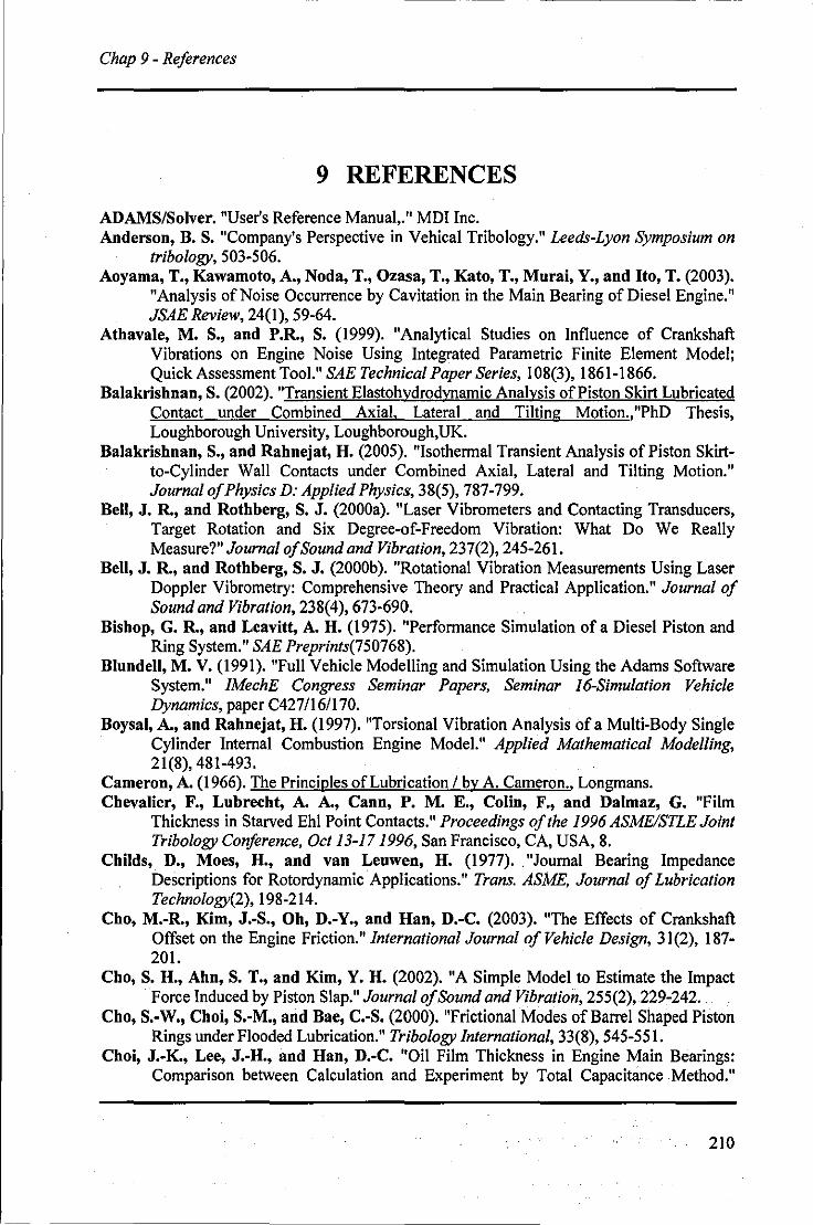
Chap 9 - References
9 REFERENCES
ADAMS/Solver. "User's Reference Manual,." MOl Inc. Anderson, B. S. "Company's Perspective in Vehical Tribology." Leeds-Lyon Symposium on
tribology, 503-506. Aoyama, T., Kawamoto, A., Noda, T., Ozasa, T., Kato, T., Murai, Y., and Ito, T. (2003).
"Analysis of Noise Occurrence by Cavitation in the Main Bearing of Diesel Engine." JSAE Review, 24(1), 59-64.
Athavale, M. S., and P.R., S. (1999). "Analytical Studies on Influence of Crankshaft Vibrations on Engine Noise Using Integrated Parametric Finite Element Model; Quick Assessment Too!." SAE Technical Paper Series, 108(3), 1861-1866.
Balakrishnan, S. (2002). "Transient Elastohydrodynamic Analysis of Piston Skirt Lubricated Contact under Combined Axial, Lateral and Tilting Motion., "PhD Thesis, Loughborough University, Loughborough,UK.
Balakrishnan, S., and Rahnejat, H. (2005). "Isothermal Transient Analysis of Piston Skirtto-Cylinder Wall Contacts under Combined Axial, Lateral and Tilting Motion." Journal of Physics D: Applied Physics, 38(5), 787-799.
Bell, J. R., and Rothberg, S. J. (2000a). "Laser Vibrometers and Contacting Transducers, Target Rotation and Six Degree-of-Freedom Vibration: What Do We Really Measure?" Journal of Sound and Vibration, 237(2), 245-261.
Bell, J. R., and Rothberg, S. J. (2000b). "Rotational Vibration Measurements Using Laser Doppler Vibrometry: Comprehensive Theory and Practical Application." Journal of Sound and Vibration, 238(4), 673-690.
Bishop, G. R., and Leavitt, A. H. (1975). "Performance Simulation of a Diesel Piston and Ring System." SAE Preprints(750768).
Blundell, M. V. (1991). "Full Vehicle Modelling and Simulation Using the Adams Software System." IMechE Congress Seminar Papers, Seminar 16-Simulation Vehicle Dynamics, paper C427/16/170.
Boysal, A., and Rahnejat, H. (1997). "Torsional Vibration Analysis of a Multi-Body Single Cylinder Internal Combustion Engine Mode!." Applied Mathematical Modelling, 21(8),481-493.
Cameron, A. (1966). The Principles of Lubrication I by A. Cameron., Longmans. Chevalier, F., Lubrecht, A. A., Cann, P. M. E., Colin, F., and Dalmaz, G. "Film
Thickness in Starved Ehl Point Contacts." Proceedings of the 1996 ASMEISTLE Joint Tribology Conference, Oct 13-17 1996, San Francisco, CA, USA, 8.
Childs, D., Moes, H., and van Leuwen, H. (1977) .. "Journal Bearing Impedance Descriptions for Rotordynamic Applications." Trans. ASME, Journal of Lubrication Technology(2), 198-214.
Cho, M.-R., Kim, J.-S., Oh, D.-Y., and Han, D.-C. (2003). "The Effects of Crankshaft Offset on the Engine Friction." International Journal of Vehicle Design, 31(2),187-201.
Cho, S. H., Ahn, S. T., and Kim, Y. H. (2002). "A Simple Model to Estimate the Impact Force Induced by Piston Slap." Journal of Sound and Vibration, 255(2), 229-242.
Cho, S.-W., Choi, S.-M., and Bae, c.-S. (2000). "Frictional Modes of Barrel Shaped Piston Rings under Flooded Lubrication." Tribology International, 33(8), 545-551.
Choi, J.-K., Lee, J.-H., and Han, D.-C. "Oil Film Thickness in Engine Main Bearings: Comparison between Calculation and Experiment by Total Capacitance Method."
210
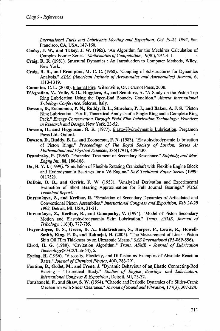
Chap 9 - References
International Fuels and Lubricants Meeting and Exposition, Qct 19-22 1992, San Francisco, CA, USA, 147-160.
Cooley, J. W., and Tukey, J. W. (1965). "An Algorithm for the Mechines Calculation of Complex Fourier Series." Mathematics of Computation, 19(90}, 297-311.
Craig, R. R. (1981). Structural Dynamics: An Introduction to Computer Methods, Wiley, New York.
Craig, R. R., and Brampton, M. C. C. (1968). "Coupling of Substructures for Dynamics Analysis." AIAA (American Institute of Aeromautics and Astronautics) Journal, 6, 1313-1319.
Cummins, C. L. (2000). Internal Fire, Wilsonville, Or. : Carnot Press, 2000. D'Agostino, V., Valle, S. D., Ruggiero, A., and Senatore, A. "A Study on the Piston Top
Ring Lubrication Using the Open-End Boundry Condition." Aimeta International Tribology Conference, Salerno, Italy.
Dowson, D., Economou, P. N., Ruddy, B. L., Strachan, P. J., and Baker, A. J. S. "Piston Ring Lubrication - Part n, Theoretical Analysis of a Single Ring and a Complete Ring Pack." Energy Conservation Through Fluid Film Lubrication Technology: Frontiers in Research and Design, New York, 23-52.
Dowson, D., and Higginson, G. R. (1977). Elasto-Hydrodynamic Lubrication, Pergamon Press Ltd., Oxford.
Dowson, D., Ruddy, B. L., and Economou, P. N. (1983). "Elastohydrodynamic Lubrication of Piston Rings." Proceedings of The Royal Society of London, Series A: Mathematical and Physical Sciences, 386(1791}, 409-430.
Draminsky, P. (1965). "Extended Treatment of Secondary Resonance." Shipbldg and Mar. Engng Int., 88, 180-186.
Du, H. Y. I. (1999). "Simulation of Flexible Rotating Crankshaft with Flexible Engine Block and Hydrodynamic Bearings for a V6 Engine." SAE Techincal Paper Series (1999-011752).
DuBois, O. B., and Ocvirk, F. W. (1953). "Analytical Derivation and Experimental Evaluation of Short Bearing Approximation for Full Journal Bearings." NASA Technical Report.
Dursunkaya, Z., and Keribar, R. "Simulation of Secondary Dynamics of Articulated and Conventional Piston Assemblies." International Congress and Exposition, Feb 24-28 1992, Detroit, MI, USA, 21-31.
Dursunkaya, Z., Keribar, R., and Ganapathy, V. (1994). "Model of Piston Secondary Motion and Elastohydrodynamic Skirt Lubrication." Trans. ASME, Journal of Tribology, 116(4}, 777-785.
Dwyer-Joyce, D. S., Green, D. A., Balakrishnan, S., Harper, P., Lewis, R., HowellSmith, King, P. D., and Rahnejat, H. (2005). "The Measurement of Liner - Piston Skirt Oil Film Thickness by an Ultrasonic Means." SAE International (P5-06P-596).
Elrod, H. G. (1980). "Cavitation Algorithm." Trans. ASME - Journal of Lubrication Technology(80-C2ILub-54}, 5.
Eyring, H. (1936). "Viscosity, Plasticity, and Diffusion as Examples of Absolute Reaction Rates." Journal of Chemical Physics, 4(4}, 283-291.
Fantino, B., Godet, M., and Frene, J. "Dynamic Behaviour of an Elastic Connecting-Rod Bearing - Theoretical Study." Studies of Engine. Bearings and Lubrication, International Congress & Exposition., Detroit, MI, 23-32.
Farahanchi, F., and Shaw, S. W. (1994). "Chaotic and Periodic Dynamics ofa Slider-Crank Mechanism with Slider Clearance." Journal of Sound and Vibration, 177(3}, 307-324.
211
----------------........ Chap 9 - References
Garnier, T., Bonneau, D., and Grente, C. (1999). "Three-Dimensional Ehd Behavior of the Engine Block/Crankshaft Assembly for a Four Cylinder Inline Automotive Engine." Trans. ASME, JournalofTribology, 121(4),721-730.
Gear, C. W. (1971). "Simultaneous Numerical Soution of Differential Algebraic Equations." Circuits and Systems, IEEE Transactions on [legacy, pre -1988J, 18(1),89-95.
Givens, L. (1990). "Technical History of the Automobile." Automotive Engineering (Warrendale, Pennsylvania), 98(6), 61-67.
Gohar, R. (1988). Elastohydrodvnamics, Ellis Horwood Ltd., Chichester. Goldsbrougb, G. R., and Baker, H. (1926). "The Properties of Torsional Vibrations in
Reciprocating Engine Shafts." Proc. R. Soc., 1l3, 259-281. Goudas, I., and Natsiavas, S. (2004). "Non-Linear Dynamics of Engine Mechanisms with a
Flexible Connecting Rod." Proceedings of the Institution of Mechanical Engineers, Part K: Journal of Multi-body Dynamics, 218(2), 67-80.
Greenwood, J. A., and Tripp, J. H. (1970). "The Contact of Two Nominally Flat Rough Surfaces." Proc. Instn. Mech. Engrs., 185,625-633.
Gupta, S. (2002). "Elasto-Multi-Body Dynamics of Internal Combustion Engines with Thin Shell Elastohydrodvnamic Journal Bearings,"PhD Thesis, Loughborough, Loughborough, UK.
Haddad, S. D. (1995). "Theoretical Treatment of Piston Motion in I.C. Piston Engine for the Prediction of Piston Slap Excitation." Mechanism & Machine Theory, 30(2), 253-269.
Haddad, S. D., and Howard, D. A. (1980). "Analysis of Piston Slap-Induced Noise and Assessment of Some Methods of Control in Diesel Engines." SAE Preprints, 800517-25.
Haddad, S. D., and Tjan, K.-t. (1995). "Analytical Study of Offset Piston and Crankshaft Designs and the Effect of Oil Film on Piston Slap Excitation in a Diesel Engine." Mechanism & Machine Theory, 30(2), 271-284.
Halliwell, N. A. (1996). "Laser Torsional Vibrometer: A Step Forward in Rotating Machinery Diagnostics." Journal of Sound and Vibration, 190(3),399-418.
Hamai, K., Masuda, T., and Goto, T. (1990). "Structural Analysis on Crankshaft Considering Oil Film Pressure Distribution around Sliding Bearings." Tribology Transactions, 33(2),179-184.
Hamrock, B. J., and Dowson, D. (1976). "Isothermal Elastohydrodynamic Lubrication of Point Contacts Em Dash 2. Ellipticity Parameter Results." Trans. ASME, Journal of Lubrication Technology, 98 Ser F(3), 375-383.
Hamrock, B. J., and Dowson, D. (1977a). "Isothermal Elastohydrodynamic Lubrication of Point Contacts." Trans. ASME, Journal of Lubrication Technology, 99 Ser F(1), 15-23.
Hamrocl<, B. J., and Dowson, D. (1977b). "Isothermal Elastohydrodynamic Lubrication of Point Contacts." Trans. ASME, Journal of Lubrication Technology, 99 Ser F(2), 264-276.
Hamrocl<, B. J., and Jacobson, B. O. "Elastohydrodynamic Lubrication of Line Contacts." ASLE Preprints presented at the ASLElASME Lubrication Conference., Hartford, CT, USA, 12.
Hamrock, B. J., Scbmid, S. R., and Jacobson, B. O. (2004). Fundamentals of Fluid Film Lubrication, Marcel Dekker, Inc., New York, USA.
Han, D.-C., and Lee, J.-S. (1998). "Analysis of the Piston Ring Lubrication with a New Boundary Condition." Tribology International, 31(12), 753-760.
Harry, W. (1994). Automotive Engines, Gregg Division, McGraw-HiII, New York; London :.
212
Chap 9 - References
Hesterman, D. C., and Stone, B. J. (1992). "The Causes of Torsional Resonance in Reciprocating Engines and Pumps at Other Than Interger Multiples of the Fundamental Excitation Frequency." IMechE.
Hesterman, D. C., and Stone, B. J. (1995). "Secondary Inertia Effects in the Torsional Vibration of Reciprocating Engines - a Literature Review." Proceedings of the Institution of Mechanical Engineers, Part C: Journal of Mechanical Engineering Science, 209(1),11-15.
Heywood, J. B. (1988). Internal Combustion Engine Fundamentals, McGrew-Hill, New York.
Hoffman, M. W. D., and Dowling, R. D. (1999). "Modeling Fully-Coupled Rigid Engine Dynamics and Vibrations." Society of Automotive Engineers.
Hu, K., Mourelatos, Z. P., and Vlahopoulos, N. (2003). "Computational Analysis for Dynamic Response of a Rotating Shaft on Flexible Support Structure with Clearances." Journal of Sound and Vibration, 267(1), 1-28.
Ichikawa, S., Mihara, Y., and Someya, T. (1995). "Study on Main Bearing Load and Deformation of Multi-Cylinder Internal Combustion Engine: Relative Inclination between Main Shaft and Bearing." JSAE Review, 16(4),383-386.
Inman, D. J. (2001). Engineering Vibration, Prentice-Hall,Inc., London. K.L.Johnson. (1985). Contact Mechanics, Cambridge University Press, Cambridge. Katano, H., Iwamoto, A., and Saitoh, T. (199Ia). "Dynamic Behaviour Analysis ofInternal
Combustion Engine Crankshafts under Operating Conditions." International Conference on Computers in Engine Technology, Sep 10-12 1991, Procs. Inst. Mech. Engrs., Part C: Journal of Mechanical Engineering Science, 205 BN - 0-85298-765-x.
Katano, H., Iwamoto, A., and Saitoh, T. (199Ib). "Dynamic Behaviour Analysis ofInternal Combustion Engine Crankshafts under Operating Conditions." International Conference on Computers in Engine Technology, Sep 10-12 1991, Proceedings of the Institution of Mechanical Engineers, 205 BN - 0-85298-765-x.
Kelly, P. (1999). "Multi-Body Dvnamic Analysis of Engine Induced Automotive Clutch Pedal Vibration,"PhD Thesis, University of Bradford.
Keribar, R., and Dursunkaya, Z. "Modeling of Piston Secondary Dynamics and Tribology." Proceedings of the Annual Automotive Technology Development Contractors' Coordination Meeting, Dct 28-31 1991, Dearborn, MI, USA, 657-677.
Kimura, J., Shiono, K., Okamura, H., and Sogabe, K. (1997). "Experiments and Analysis of Crankshaft Three Dimensional Vibrations and Bending Stresses in a V-Type TenCylinder Engine: Influence of Crankshaft Gyroscopic Motions." Society of Automotive Engineers.
Kineshita, M., Sakamoto, T., and Okamura, H. (1989). "An Experimental Study of a Torsional-Bending Damper Pulley for an Engine Crankshaft." SAE (Society of Automotive Engineers) Transactions (891127), 23-33.
Kirk, R. G., and Gunter, E. J. (1975). "Short Bearing Analysis Applied to Rotor Dynamics." Journal of Lubrication Technology, Transactions ASME, 98 Ser F(I), 47-56.
Kjaer, B. (1982). "Measuring Vibrations." Bruel & Kjaer Co. Knoll, G., Schoenen, R., and Wilhelm, K. "Full. Dynamic Analysis of Crankshaft and
Engine Block with Special Respect to Elastohydrodynamic Bearing Coupling." Proceedings of the 1997 Spring Technical Conference of the ASME Internal Combustion Engine Division, Apr 27-301997, Fort Collins, CO, USA, 1-8.
213
Chap 9 - References
Knoll, G. D., and Peeken, H. J. (1982). "Hydrodynamic Lubrication of Piston Skirts." Trans ASME, Journal of Lubrication Technology, 104(4),504-509.
Koizumi, T., Tsujiuchi, N., Okamura, M., Kubomoto, I., and Ishida, E. (2000). "Reduction of Piston Slap Excitation with Small Gasoline Engine." Proceedings of the International Modal Analysis Conference - IMAC, 2, 1731-1736.
Kryniski, K. (1991). "Jumping Phenomenon in Journal Bearings." Transactions of ASME, Journal of Rotating Machinery and Vehicle Dynamics., DE-Vol 35, 169·173.
Kurbet, S. N., and Kumar, R. K. (2004). "A Finite Element Study of Piston Tilt Effects on Piston Ring Dynamics in Internal Combustion Engines." Proceedings of the Institution of Mechanical Engineers, Part K: Journal of Multi-body Dynamics, 218(2),107·117.
Kushwaha, M. (2000). "Elasto-Multi·Body Dynamics of Valve Train Systems with Transient Elastohydrodynamic Contact Conditions.,"PhD Thesis, University of Bradford, Bradford.
Lagrange. (1788). "Mecanique Analytique." L' Academie de Sciences, Paris. Liu, K., Xie, Y. B., and Gui, C. L. (1998). "Two·Dimensional Lubrication Study of the
Piston Ring Pack." Proceedings of the Institution of Mechanical Engineers, Part J: Journal of Engineering Tribology, 212(3), 215-220.
Ma, Z.-D., and Perkins, N. C. (2003). "An Efficient Multibody Dynamics Model for Internal Combustion Engine Systems." Multibody System Dynamics, 10(4),363-391.
Messe, S., and Lubrecht, A. A. (2000). "Transient Elastohydrodynamic Analysis of an Overhead Cam/Tappet Contact." Proceedings of the Institution of Mechanical Engineers, Part J: Journal of Engineering Tribology, 214(5), 415·425.
Mihailidis, A., Retzepis, J., Salpistis, C., and Panajiotidis, K. (1999). "Calculation of Friction Coefficient and Temperature Field of Line Contacts Lubricated with a NonNewtonian Fluid." Proceedings of the NORDTRIP'98 Conference, 232(2), 213-220.
Mihara, Y., Hayashi, T., Nakamura, M., and Someya, T. (1995). "Development of Measuring Method for Oil Film Pressure of Engine Main Bearing by Thin Film Sensor." JSAE Review, 16(2), 125·130.
Mihara, Y., Kajiwara, M., Fukamatsu, T., and Someya, T. (1996). "Study on the Measurement of Oil· Film Pressure of Engine Main Bearing by Thin·Film Sensor - the Influence of Bearing Deformation on Pressure Sensor Output under Engine Operation." JSAE Review, 17(3),281.286.
Mihara, Y., and Someya, T. (1995). "Study of Main Bearing Load and Deformation in a Multi·Cylinder Internal Combustion Engine." JSAE Review, 16(2), 188·189.
Mihara, Y., and Someya, T. (2002). "Measurement of Oil·Film Pressure in Engine Bearings Using a Thin-Film Sensor." Lubrication Engineering, 58(5), 10-19.
Mizuho Inagaki, A. K., Takayuki Aoyama, Ken·ichi Yamamoto. (2002). "Prediction of Structural and Kinematic Coupled Vibration on Internal Combustion Engine." R&D Review of Toyota CRDL.
Moreau, H., Maspeyrot, P., Chomat·Delalex, A. M., Bonneau, D., and Frene, J. (2002). "Dynamic Behaviour of Elastic Engine Main Bearings: Theory and Measurements." Proceedings of the Institution of Mechanical Engineers, Part J: Journal of Engineering Tribology, 216(4),179·193.. ..•. .. • ....•
Morita, T., and Okamura, H. "Dynamic Stiffness Matrix Approach to the Analysis of Three·Dimensional Vibrations of Automobile Engine Crankshafts. Part 2. Application to Firing Conditions." Winter Annual Meeting of the American Society of Mechanical Engineers, Nov 25-301990, Dallas, TX, USA, 59-66.
214
Chap 9 - References
Morita, T., Tsuna, Y., and Okada, A. (2001). "Influence of Dynamic Damper Pulley Design on Engine Front Noise." SAE transactions (SAE transact.), 11 0(6) (ISSN 0096-736X),1547-1552.
Mourelatos, Z. P. (2000). "Efficient Crankshaft Dynamic Analysis Using SubstructUring with Ritz Vectors." Journal of Sound and Vibration, 238(3), 495-527.
Mourelatos, Z. P. (200Ia). "A Crankshaft System Model for Structural Dynamic Analysis of Internal Combustion Engines." Computers and Structures, 79(20-21), 2009-2027.
Mourelatos, Z.' P. (200Ib). "An Efficient Journal Bearing Lubrication Analysis for Engine Crankshafts." Tribology Transactions, 44(3),351-358.
MSClNastran. "Encyclopedia." Nagamatsu, A., and Nakao, A. (1983). "Analysis of Forced Vibration by Reduced
Impedance Method (Part 3 Damped Vibration)." Bulletin of the JSME, 26(214), 592-597.
Nakayama, K., Tamaki, S., Hiroyuki, M., and Takiguchi, M. (2000). "The Effect of Crankshaft Offset on Piston Friction Force in a Gasoline Engine." SAE transactions (SAE transact.), 109(3), 885-892.
Newkirk, B. L. (1924). "Shaft Whipping." General Electric Review, 27,169. Newland, D. E. (1993). Randon Vibration and Spectral Analysis, Longman, New York. Okamoto, M., and Sakal, I. (2001). "Contact Pressure Distribution of Piston Rings -
Calculation Based on Piston Ring Contour." Society of Automitive Engineers. Okamura, H., and Morita, T. (1999). "Efficient Modelling and Analysis for Crankshaft
Three-Dimensional Vibrations under Firing Conditions." Proceeding of the Instittion of Mechanical Engineers - K, 213(1), 33-44.
Okamura, H., Shinno, A., Yamanaka, T., Suzuki, A., and Sogabe, K. "Dynamic Stiffuess Matrix Approach to the Analysis of Three-Dimensional Vibrations of Automobile Engine Crankshafts. Part I. Background and Application to Free Vibrations." Winter Annual Meeting of the American Society of Mechanical Engineers, Nov 25-30 1990, Dallas, TX, USA, 47-58.
Okamura, H., Shinno, A., Yamanaka, T., Suzuki, A., and Sogabe, K. (1995). "Simple Modeling and Analysis for Crankshaft Three-Dimensional ,Vibrations, ,Part 1: Background and Application to Free Vibrations." Journal of Vibration and Acoustics, Transactions of the ASME, 117(1),70-79.
Okamura, H., and Yamashita, K. "Influence of the Valve and Accessory Gear Train on the Crankshaft Three-Dimensional Vibrations in High Speed Engines." SAE Conference Proceedings.
Orlandea, N., Chace, M. A., and Calahan, D. A. (1976). "Sparsity-Oriented Approach to the Dynamic Analysis and Design of Mechanical Systems Em Dash I." American Society of Mechanical Engineers (Paper}(76-DET-19), 7.
Otnes, R. K., and Encochson, L. (1972). Digital Time Serier Analysis, WHey, New York. Paranjpe, R. S., and Goenka, P. K. (1990). "Analysis of Crankshaft Bearings Using a Mass
Conserving Algorithm." Tribology Transactions, 33(3), 333-344. Petroff, N. P. (1883). "Friction in Machines and the Effect of the Lubricant." Inzh. Zh. St.
Petersburg, 1,71-140., ' "" Pinkus, 0., and Stemlicht, B. (1961). Theorv of Hydrodynamic Lubrication, McGraw-HiIl. Piraner, I.; Pflueger, C., and Bouthier, O. (2002). "Cummins Crankshaft and Bearing
Analysis Process." North American MD! User Conference. Priest, M., Dowson, D., and Taylor, C. M. (2000). "Theoritical Modelling of Cavitation in
Piston Ring Lubrication." proceeding of the Instittion of Mechanical Engineers - C, 214,435.
215
Chap 9 - References
Rahnejat, H. (1984). "Influence of Vibration on the Oil Film in Concentrated Contacts,"PhD Thesis, University of London, London.
Rahnejat, H. (1998). Multi-Body Dvnamics: Vehicle. Machines. and Mechanisms, Society of Automotive Engineers, Inc., Warrendale, USA.
Rahnejat, H. (2000). "Multi-Body Dynamics: Historical Evolution and Application." Proceedings of the Institution of Mechanical Engineers, Part D: Journal of Automobile Engineering, 214(1), 149.
Rahnejat, H., and Gohar, R. Icp Press, in Review Process. Rao, S. S. (2002). Applied Numerical Methods for Engineers and Scientists, Prentice Hall,
New Jersey. Reynolds, O. (1886). "On the Theory of Lubrication and Its Application to Mr. Beauchamp
Tower's Experiments, Including an Experimental Determination of the Viscosity of Olive Oil." Phil. Transaction of Royal Society, London, 177, 157-234.
S.H, C., S.T, A., and Y.H, K. (2002). "A Simple Model to Estimate the Impact Force Induced by Piston Slap." Journal of Sound and Vibrations, 255.
Seki, T., Nakayama, K., Yamada, T., Yoshida, A., and Takiguchi, M. (2000). "Study on Variation in Oil Film Thickness of a Piston Ring Package: Variation of Oil Film Thickness in Piston Sliding Direction." JSAE Review, 21(3), 315-320.
Shabana, A. A. (1998). Dvnamics of Multibody System, University of Cambridge Press. Shell. "Shell Bearings Help Desk." Shiao, Y.-j., and Moskwa, J. J. "Investigation of Load Force and Dynamic Error Magnitude
Using the Lumped Mass Connecting Rod Model." International Congress and Exposition, Mar 1-5 1993, Detroit, MI, USA, 1-10.
Spessert, B., and Ponsa, R. (1990). "Investigation in the Noise from Main Running Gear, Timing Gears and Injection Pump of Di Diesel Engines." SAE (Society of Automotive Engineers) Transactions, 99(Sect 3), 14-33.
Suh, K.-H., Lee, Y,-K., and Yoon, H.-S. (2000). "A Study on the Balancing of the ThreeCylinder Engine with Balance Shaft." SAE Techincal Paper Series.
Taraza, D. (200 I). "Quantifying Relationaship between the Crankshaft's Speed Variation and the Gas Pressure Torque." SAE Technical paper series.
Taylor, R. I. (2002). "Lubrication, Tribology & Motorsport." SAE Techincal Paper Series(2002-0 I -3355).
Teodorescu, M., Taraza, D., Henein, N. A., and Bryzik, W. (2003). "Simplified Elasto Hydrodynamic Friction Model of the Cam-Tappet Contact." SAE transactions (SAE transact.), 112(3), 1271 -1282.
Teraguchi, S., Suzuki, W., and Takiguchi, M. (2001). "Effects of Lubricating Oil Supply on Reductions of Piston Slap Vibration and Piston Friction." Society of Automitive Engineers(200 I -0 I -0566).
Tian, T. (2002a). "Dynamic Behaviours of Piston Rings and Their Practical Impact. Part I: Ring Flutter and Ring Collapse and Their Effects on Gas Flow and Oil Transport." Proceedings of the Institution of Mechanical Engineers, Part J: Journal of Engineering Tribology, 216(4), 209-228.
Tian, T. (2002b). "Dynamic Behaviours of Piston Rings and Their Practical Impact. Part 2: Oil Transport, Friction and Wear of RinglLiner Interface and the Effects of Piston and Ring Dynamics." Proceedings of the Institution of Mechanical Engineers, Part J: Journal of Engineering Tribology, 216(4),229-247.
Tian, T" Noordzij, L. B., Wong, V. W., and Heywood, J, B. "Mode ling Piston-Ring Dynamics, B1owby, and Ring-Twist Effects." Proceedings of the 1996 18th Annual
216
Chap 9 - References
Fall Technical Conference of the ASME Internal Combustion Engine Division. Part 2 (of 5), Oct 20-231996, Fairborn, OH, USA, 67-80.
Tower, B. (1883). "First Report on Friction Experiments (Friction of Lubricated Bearings)." Institution of Mechanical Engineers Part J, 632-659.
W.PuIlrabek, W. (2003). Engineering Fundamentals of the Internal Combustion Engine, Prentice Hall Upper Saddle River, NJ, USA.
Wakabayashi, K., Honda, Y., Kodama, T., and Iwamoto, S. (1995). "The Charactersitics of the Bending Vibration Stress Coupled with Torsional Vibration of Automobile Diesel Engine Shaftings." SAE Technical Paper Series.
Yang, J., Yang, W., Yu, X., and Wang, C. (2001). "Design of Internal Combustion Engine Piston Based on Skirt Lubrication Analysis." Society of Automitive Engineers(200 1-01-2486).
Yang, Q., and Keith, T. G., Jr. (1996a). "Two-Dimensional Piston Ring Lubrication - Part I: Rigid Ring and Liner Solution." Tribology Transactions, 39(4), 757-768.
Yang, Q., and Keith, T. G., Jr. (1996b). "Two-Dimensional Piston Ring Lubrication - Part Ii: Elastic Ring Consideration." Tribology Transactions, 39(4), 870-880.
217