molecular dynamics studies of peptide-membrane interactions: insights from coarse-grained models
TRANSCRIPT
Molecular dynamics studies ofpeptide-membrane interactions: Insights
from coarse-grained models
Paraskevi GkekaT
HE
U N I V E R S
I TY
OF
ED I N B U
RG
H
A thesis submitted for the degree of Doctor of PhilosophyThe University of Edinburgh
April 16, 2010
Abstract
Peptide-membrane interactions play an important role in a number of biological pro-
cesses, such as antimicrobial defence mechanisms, viral translocation, membrane fu-
sion and functions of membrane proteins. In particular, amphipathic α-helical peptides
comprise a large family of membrane-active peptides that could exhibit a broad range
of biological activities. A membrane, interacting with an amphipathic α-helical pep-
tide, may experience a number of possible structural transitions, including stretching,
reorganization of lipid molecules, formation of defects, transient and stable pores, for-
mation of vesicles, endo- and pinocytosis and other phenomena. Naturally, theoretical
and experimental studies of these interactions have been an intense on-going area of
research. However, complete understanding of the relationship between the structure
of the peptide and the mechanism of interaction it induces, as well as molecular details
of this process, still remain elusive. Lack of this knowledge is a key challenge in our
efforts to elucidate some of the biological functions of membrane active peptides or to
design peptides with tailored functionalities that can be exploited in drug delivery or
antimicrobial strategies.
iii
In principle, molecular dynamics is a powerful research tool to study peptide-membrane
interactions, which can provide a detailed description of these processes on molecular
level. However, a model operating on the appropriate time and length scale is imper-
ative in this description. In this study, we adopt a coarse-grained approach where the
accessible simulation time and length scales reach microseconds and tens of nanome-
ters, respectively. Thus, the two key objectives of this study are to validate the ap-
plicability of the adopted coarse-grained approach to the study of peptide-membrane
interactions and to provide a systematic description of these interactions as a function
of peptide structure and surface chemistry.
We applied the adopted strategy to a range of peptide systems, whose behaviour has
been well established in either experiments or detailed atomistic simulations and out-
lined the scope and applicability of the coarse-grained model. We generated some
useful insights on the relationship between the structure of the peptides and the mech-
anism of peptide-membrane interactions. Particularly interesting results have been
obtained for LS3, a membrane spanning peptide, with a propensity to self-assembly
into ion-conducting channels. Firstly, we captured, for the first time, the complete
process of self-assembly of LS3 into a hexameric ion-conducting channel and explored
its properties. The channel has structure of a barrel-stave pore with peptides aligned
along the lipid tails. However, we discovered that a shorter version of the peptide
leads to a more disordered, less stable structure often classified as a toroidal pore.
This link between two types of pores has been established for the first time and opens
interesting opportunities in tuning peptide structures for a particular pore-inducing
mechanism. We also established that different classes of peptides can be uniquely
characterized by the distinct energy profile as they cross the membrane. Finally, we
extended this investigation to the internalization mechanisms of more complex enti-
ties such as peptide complexes and nanoparticles. Coarse-grained steered molecular
dynamics simulations of these model systems are performed and some preliminary
results are presented in this thesis.
To summarize, in this thesis, we demonstrate that coarse-grained models can be suc-
cessfully used to underpin peptide interaction and self-assembly processes in the pres-
ence of membranes in their full complexity. We believe that these simulations can
be used to guide the design of peptides with tailored functionalities for applications
iv
such as drug delivery vectors and antimicrobial systems. This study also suggests that
coarse-grained simulations can be used as an efficient way to generate initial configu-
rations for more detailed atomistic simulations. These multiscale simulation ideas will
be a natural future extension of this work.
Declaration of originality
I hereby declare that the research recorded in this thesis and the thesis itself was com-
posed and originated entirely by myself in the School of Engineering, The University
of Edinburgh.
Paraskevi Gkeka
v

Declaration of originality vi
”By chance, like people say, I suddenly found a strange refuge. However, this kind of luck does
not exist. When someone needs something and tries to have it, it is not the luck that gives it to
him, but his own will and effort that makes him look for it.”
Herman Hesse (Demian)

Dedication
Στην oικoγǫνǫια µoυ.
Σας ǫυχαριστω για oλα.
To my teachers.
Through simple luck, divine intervention or both, I have been fortunate to have had
exceptional teachers during my educational years.
vii

Acknowledgements
I would like to take this opportunity to acknowledge those who have helped me com-
plete this thesis. First and foremost, I would like to express my gratitude to my su-
pervisor, Dr. Lev Sarkisov - his encouragement, support, and thoughtful advice have
been immensely valuable for me. I am particularly grateful to him for his elegant and
interesting research ideas, which were the best motivations for me to work. Lev, I truly
enjoyed working with you.
I would like to thank my second supervisor, Dr. Tina Duren, for her helpful advice
during these years of my PhD. I also wish to thank my examiners Prof. Mark Sansom
and Dr. Perdita Barran for their comments on my thesis and the interesting discussion
during my viva.
Finally, I would like to thank the Institute of Materials and Sciences of the University
of Edinburgh for the financial support.
viii
Contents
Declaration of originality . . . . . . . . . . . . . . . . . . . . . . . . . . . vDedication . . . . . . . . . . . . . . . . . . . . . . . . . . . . . . . . . . . viiAcknowledgements . . . . . . . . . . . . . . . . . . . . . . . . . . . . . . viiiContents . . . . . . . . . . . . . . . . . . . . . . . . . . . . . . . . . . . . ixList of figures . . . . . . . . . . . . . . . . . . . . . . . . . . . . . . . . . xiiList of tables . . . . . . . . . . . . . . . . . . . . . . . . . . . . . . . . . . xv
1 Introduction 11.1 Biological background . . . . . . . . . . . . . . . . . . . . . . . . . . . . . 2
1.1.1 The biological membranes and lipid bilayers . . . . . . . . . . . . . 21.1.2 Peptides . . . . . . . . . . . . . . . . . . . . . . . . . . . . . . . . 4
1.2 Peptide-membrane interactions . . . . . . . . . . . . . . . . . . . . . . . . 61.3 Experimental techniques and limitations . . . . . . . . . . . . . . . . . . . 111.4 Molecular modelling and computer simulations of peptide-membrane inter-
actions . . . . . . . . . . . . . . . . . . . . . . . . . . . . . . . . . . . . . 131.5 Nanoparticle membrane interactions . . . . . . . . . . . . . . . . . . . . . 211.6 Objectives and scope of the thesis . . . . . . . . . . . . . . . . . . . . . . 241.7 Publications and presentations . . . . . . . . . . . . . . . . . . . . . . . . 26
2 Methodology 272.1 Fundamentals of molecular dynamics . . . . . . . . . . . . . . . . . . . . . 28
2.1.1 Statistical mechanics of the microcanonical ensemble . . . . . . . . 282.1.2 Molecular dynamics in the microcanonical ensemble . . . . . . . . . 302.1.3 Determination of properties in MD . . . . . . . . . . . . . . . . . . 332.1.4 Molecular dynamics in other ensembles . . . . . . . . . . . . . . . . 38
2.2 Pressure and temperature control in MD simulations . . . . . . . . . . . . 412.2.1 Baro- and thermostats using the extended Hamiltonian approach . . 412.2.2 Other methods to control pressure and temperature . . . . . . . . . 46
2.3 Implementation issues . . . . . . . . . . . . . . . . . . . . . . . . . . . . . 48
ix
Contents x
2.3.1 Time integration algorithm . . . . . . . . . . . . . . . . . . . . . . 482.3.2 Periodic boundary conditions . . . . . . . . . . . . . . . . . . . . . 492.3.3 Neighbour list . . . . . . . . . . . . . . . . . . . . . . . . . . . . . 512.3.4 Pressure coupling protocols . . . . . . . . . . . . . . . . . . . . . . 51
2.4 Potential of mean force . . . . . . . . . . . . . . . . . . . . . . . . . . . . 522.5 Molecular force field . . . . . . . . . . . . . . . . . . . . . . . . . . . . . . 55
2.5.1 Non-bonded interactions . . . . . . . . . . . . . . . . . . . . . . . 562.5.2 Bonded interactions . . . . . . . . . . . . . . . . . . . . . . . . . . 60
2.6 The molecular model . . . . . . . . . . . . . . . . . . . . . . . . . . . . . 612.6.1 Molecular mapping and interaction sites . . . . . . . . . . . . . . . 612.6.2 The molecular force field . . . . . . . . . . . . . . . . . . . . . . . 612.6.3 Coarse-grained description of a peptide-membrane system . . . . . 64
2.7 Data analysis tools . . . . . . . . . . . . . . . . . . . . . . . . . . . . . . 672.7.1 Density profiles . . . . . . . . . . . . . . . . . . . . . . . . . . . . 682.7.2 Angle distribution . . . . . . . . . . . . . . . . . . . . . . . . . . . 682.7.3 Geometrical features of supramolecular assemblies . . . . . . . . . . 69
3 Coarse-grained model validation: Application to different classes of amphi-pathic α-helical peptides 713.1 Introduction . . . . . . . . . . . . . . . . . . . . . . . . . . . . . . . . . . 723.2 Simulation parameters . . . . . . . . . . . . . . . . . . . . . . . . . . . . . 76
3.2.1 Atomistic simulations . . . . . . . . . . . . . . . . . . . . . . . . . 773.2.2 Potential of mean force calculations . . . . . . . . . . . . . . . . . 77
3.3 Results . . . . . . . . . . . . . . . . . . . . . . . . . . . . . . . . . . . . . 783.3.1 Pore forming peptides . . . . . . . . . . . . . . . . . . . . . . . . . 783.3.2 Amphipathic non-spanning helices . . . . . . . . . . . . . . . . . . 803.3.3 Fusion peptides . . . . . . . . . . . . . . . . . . . . . . . . . . . . 833.3.4 Transmembrane helices . . . . . . . . . . . . . . . . . . . . . . . . 89
3.4 Discussion . . . . . . . . . . . . . . . . . . . . . . . . . . . . . . . . . . . 93
4 Pore-formation by α-helical peptides 954.1 Pore-forming peptides . . . . . . . . . . . . . . . . . . . . . . . . . . . . . 964.2 Summary of simulations . . . . . . . . . . . . . . . . . . . . . . . . . . . . 984.3 Results . . . . . . . . . . . . . . . . . . . . . . . . . . . . . . . . . . . . . 101
4.3.1 LS3 complexes . . . . . . . . . . . . . . . . . . . . . . . . . . . . . 1014.3.2 Hexameric barrel-stave pore . . . . . . . . . . . . . . . . . . . . . . 1034.3.3 The toroidal pore . . . . . . . . . . . . . . . . . . . . . . . . . . . 107
4.4 Barrel-stave versus toroidal pore . . . . . . . . . . . . . . . . . . . . . . . 1114.5 Conclusions . . . . . . . . . . . . . . . . . . . . . . . . . . . . . . . . . . 114
5 Cell-penetrating peptides 1185.1 Introduction . . . . . . . . . . . . . . . . . . . . . . . . . . . . . . . . . . 1195.2 Methodology . . . . . . . . . . . . . . . . . . . . . . . . . . . . . . . . . . 1245.3 pHLIP peptide . . . . . . . . . . . . . . . . . . . . . . . . . . . . . . . . . 1255.4 Pep-1 peptide . . . . . . . . . . . . . . . . . . . . . . . . . . . . . . . . . 1325.5 Conclusions . . . . . . . . . . . . . . . . . . . . . . . . . . . . . . . . . . 142
Contents xi
6 Nanoparticles 1456.1 Methodology . . . . . . . . . . . . . . . . . . . . . . . . . . . . . . . . . . 1466.2 Results . . . . . . . . . . . . . . . . . . . . . . . . . . . . . . . . . . . . . 150
6.2.1 1 nm nanoparticles . . . . . . . . . . . . . . . . . . . . . . . . . . 1506.2.2 3 nm nanoparticles . . . . . . . . . . . . . . . . . . . . . . . . . . 1526.2.3 Charged nanoparticles . . . . . . . . . . . . . . . . . . . . . . . . . 1566.2.4 The effect of membrane size . . . . . . . . . . . . . . . . . . . . . 157
6.3 Discussion . . . . . . . . . . . . . . . . . . . . . . . . . . . . . . . . . . . 159
7 Summary and Conclusions 1617.1 Summary of dissertation . . . . . . . . . . . . . . . . . . . . . . . . . . . . 1617.2 Final thoughts and future directions . . . . . . . . . . . . . . . . . . . . . 164
A Appendix A 168
B Appendix B 171
C Appendix C 176
References 178

List of figures
1.1 The fluid mosaic model . . . . . . . . . . . . . . . . . . . . . . . . . . . . 21.2 Lipid phase diagram . . . . . . . . . . . . . . . . . . . . . . . . . . . . . . 41.3 The α-helix . . . . . . . . . . . . . . . . . . . . . . . . . . . . . . . . . . 61.4 Schematic of possible peptide-membrane interactions . . . . . . . . . . . . 101.5 Mean-field model . . . . . . . . . . . . . . . . . . . . . . . . . . . . . . . 141.6 Coarse-grained models . . . . . . . . . . . . . . . . . . . . . . . . . . . . . 171.7 Different uptake mechanisms of nanoparticles with different coatings . . . . 211.8 Lipid bilayer fusion on rough surfaces . . . . . . . . . . . . . . . . . . . . . 23
2.1 Nose-Hoover negative feedback mechanism . . . . . . . . . . . . . . . . . 452.2 Average pressure versus number of time steps for the NPT ensemble, using
the Nose-Hoover baro- thermostat . . . . . . . . . . . . . . . . . . . . . . 462.3 Periodic boundary conditions . . . . . . . . . . . . . . . . . . . . . . . . . 502.4 Pressure coupling protocols . . . . . . . . . . . . . . . . . . . . . . . . . . 522.5 Examples of interactions in a force field . . . . . . . . . . . . . . . . . . . 552.6 Lennard-Jones (12,6) pair potential and pair force . . . . . . . . . . . . . . 572.7 Ewald summation . . . . . . . . . . . . . . . . . . . . . . . . . . . . . . . 592.8 Atomistic and coarse-grained representations for a DPPC lipid . . . . . . . 642.9 Coarse-grained representation of a lipid bilayer . . . . . . . . . . . . . . . . 652.10 Atomistic and coarse-grained representations for LS3 synthetic peptide . . . 672.11 Angle calculation . . . . . . . . . . . . . . . . . . . . . . . . . . . . . . . 69
3.1 Schematic view of the different classes of α-helical peptides . . . . . . . . . 723.2 Peptides under study . . . . . . . . . . . . . . . . . . . . . . . . . . . . . 753.3 Formation of a barrel-stave pore by six LS3 peptides . . . . . . . . . . . . 803.4 Potential of mean force for the transfer of the LS3 synthetic peptide from
the water phase across a DPPC lipid bilayer . . . . . . . . . . . . . . . . . 813.5 Final snapshot from the simulation of the LAP20 synthetic peptide . . . . . 823.6 Angle distribution for the LAP-20 peptide . . . . . . . . . . . . . . . . . . 82
xii
List of figures xiii
3.7 Potential of mean force for the transfer of LAP20 synthetic peptide from thewater phase across the DOPC lipid bilayer . . . . . . . . . . . . . . . . . . 83
3.8 Angle distribution for the SIV peptide . . . . . . . . . . . . . . . . . . . . 853.9 Snapshots from atomistic and coarse-grained simulations of SIV fusion peptide 853.10 Neutron scattering length density profiles for Val2, Leu8 and Leu11 residues
of SIV peptide . . . . . . . . . . . . . . . . . . . . . . . . . . . . . . . . . 863.11 Density profiles of leucine 8 as a function of the distance from the centre of
the bilayer . . . . . . . . . . . . . . . . . . . . . . . . . . . . . . . . . . . 873.12 Radial distribution function for DOPC bilayer in the presence of SIV fusion
peptide . . . . . . . . . . . . . . . . . . . . . . . . . . . . . . . . . . . . . 883.13 Potential of mean force for the transfer of the SIV fusion peptide from the
water phase across a DOPC lipid bilayer . . . . . . . . . . . . . . . . . . . 883.14 Snapshots from the pHLIP simulation . . . . . . . . . . . . . . . . . . . . 903.15 Final snapshot from the TMX-1 simulation . . . . . . . . . . . . . . . . . . 913.16 Potential of mean force for the transfer of pHLIP and TMX-1 transmembrane
helices across a lipid bilayer . . . . . . . . . . . . . . . . . . . . . . . . . . 923.17 Map of PMF types for the different classes of α-helical peptides. . . . . . . 94
4.1 Escherichia coli treated with an antimicrobial peptide . . . . . . . . . . . . 964.2 Schematic of the barrel-stave and toroidal pore . . . . . . . . . . . . . . . 974.3 Representative snapshots of different types of complexes observed in LS3
simulations . . . . . . . . . . . . . . . . . . . . . . . . . . . . . . . . . . . 1024.4 Snapshots from the formation of a hexameric complex from two trimers . . 1024.5 Top view of the hexameric pore . . . . . . . . . . . . . . . . . . . . . . . . 1034.6 Hexameric pore filled with water . . . . . . . . . . . . . . . . . . . . . . . 1044.7 The density of water in a LS3 barrel-stave pore . . . . . . . . . . . . . . . 1054.8 Mean square displacement versus time for the LS3 bundle . . . . . . . . . . 1064.9 Tilt angle of the hexameric peptide bundle . . . . . . . . . . . . . . . . . . 1074.10 Characteristic snapshots of a simulation with typical (LSSLLSL)2 complex
formation . . . . . . . . . . . . . . . . . . . . . . . . . . . . . . . . . . . 1094.11 Characteristic snapshots from the simulations with magainin and (LSSLLSL)2
peptides . . . . . . . . . . . . . . . . . . . . . . . . . . . . . . . . . . . . 1104.12 Comparative plot of the PMF patterns of LS3 and (LSSLLSL)2 . . . . . . . 1104.13 P2 order parameter of consecutive bonds with respect to the bilayer normal 1114.14 P2 order parameter of consecutive bonds with respect to the bilayer normal
in the vicinity of the pores . . . . . . . . . . . . . . . . . . . . . . . . . . 1124.15 Water density in the barrel-stave and the toroidal pore . . . . . . . . . . . 113
5.1 Proposed pHLIP translocation mechanism across a lipid bilayer . . . . . . . 1215.2 Proposed Pep-1 translocation mechanism across a lipid bilayer I: Endocytosis 1225.3 Proposed Pep-1 translocation mechanism across a lipid bilayer II: Pore for-
mation . . . . . . . . . . . . . . . . . . . . . . . . . . . . . . . . . . . . . 1235.4 Proposed features of Pep-1/cargo complexes . . . . . . . . . . . . . . . . . 1235.5 pHLIP peptide: A short summary . . . . . . . . . . . . . . . . . . . . . . . 1255.6 Strong membrane undulations induced by a pentameric pHLIP complex . . 1275.7 Snapshots from pHLIP simulations . . . . . . . . . . . . . . . . . . . . . . 130

List of figures xiv
5.8 Top view of the defect created by the pHLIP complex on the surface of thelipid bilayer . . . . . . . . . . . . . . . . . . . . . . . . . . . . . . . . . . . 130
5.9 Schematic of the defect caused at the surface of the lipid bilayer by a pHLIPcomplex . . . . . . . . . . . . . . . . . . . . . . . . . . . . . . . . . . . . 131
5.10 P2 order parameter of consecutive bonds with respect to the bilayer normalin the vicinity of pHLIP tetrameric complex . . . . . . . . . . . . . . . . . 131
5.11 Pep-1 peptide: A short summary . . . . . . . . . . . . . . . . . . . . . . . 1325.12 Density profile of tryptophan and valine residues of Pep-1 . . . . . . . . . . 1345.13 Snapshots from Pep-1 simulations . . . . . . . . . . . . . . . . . . . . . . 1375.14 The effect of tryptophan in Pep-1/membrane interaction . . . . . . . . . . 1385.15 Snapshots from the MD simulations of Pep-1 complex . . . . . . . . . . . 1395.16 Transient water pore formed by Pep-1 complex . . . . . . . . . . . . . . . 1405.17 Snapshots from the Steered MD simulations with Pep-1 complex . . . . . . 1415.18 Area per lipid from the Steered MD simulations of Pep-1 complex . . . . . 142
6.1 Nomenclature for the 1 nm nanoparticles . . . . . . . . . . . . . . . . . . . 1476.2 Nomenclature for the 3 nm nanoparticles . . . . . . . . . . . . . . . . . . . 1486.3 P2 order parameter of consecutive bonds with respect to the bilayer normal
in the vicinity of the nanoparticles . . . . . . . . . . . . . . . . . . . . . . 1516.4 Area per lipid for the 1-nm nanoparticle . . . . . . . . . . . . . . . . . . . 1526.5 Detail of the interdigitated state of a lipid bilayer . . . . . . . . . . . . . . 1536.6 Interdigitated state and transient pore formation from the polar nanoparticle 1546.7 Mixed nanoparticle insertion in the lipid bilayer . . . . . . . . . . . . . . . 1556.8 Final snapshots from the MD simulations of the charged nanoparticles . . . 1576.9 Pulling in a small membrane . . . . . . . . . . . . . . . . . . . . . . . . . 158
A.1 The 20 common amino acids . . . . . . . . . . . . . . . . . . . . . . . . . 169A.2 Different levels of structure in proteins. . . . . . . . . . . . . . . . . . . . . 170
B.1 Evolution of ξ and ξ . . . . . . . . . . . . . . . . . . . . . . . . . . . . . . 173B.2 U/N versus time . . . . . . . . . . . . . . . . . . . . . . . . . . . . . . . . 174B.3 Evolution of average pressure . . . . . . . . . . . . . . . . . . . . . . . . . 175B.4 Evolution of average temperature . . . . . . . . . . . . . . . . . . . . . . . 175
C.1 Potential of mean force for the transfer of SIV peptide from the water phaseacross a DOPC lipid bilayer . . . . . . . . . . . . . . . . . . . . . . . . . . 177
List of tables
2.1 Force field levels of interaction . . . . . . . . . . . . . . . . . . . . . . . . 622.2 CG bead interaction matrix . . . . . . . . . . . . . . . . . . . . . . . . . . 632.3 CG representation of the amino acids . . . . . . . . . . . . . . . . . . . . . 662.4 CG representation of the backbone structure of a peptide . . . . . . . . . . 66
3.1 Summary of the peptides under study and their primary sequences . . . . . 74
4.1 Summary of simulations for LS3 peptide . . . . . . . . . . . . . . . . . . . 994.2 Summary of simulations for (LSSLLSL)2 peptide . . . . . . . . . . . . . . . 1004.3 Apparent area and volume per lipid in the presence of barrel-stave and
toroidal pore . . . . . . . . . . . . . . . . . . . . . . . . . . . . . . . . . . 1144.4 Summary of the differences between the barrel-stave pore formed by LS3
peptides and the toroidal pore formed by (LSSLLSL)2 peptides . . . . . . . 114
5.1 Systems of lipid bilayers used in pHLIP and Pep-1 simulations . . . . . . . 1245.2 Summary of simulations for pHLIP peptide Set I . . . . . . . . . . . . . . . 1265.3 Summary of simulations for pHLIP peptide Set II . . . . . . . . . . . . . . 1285.4 Summary of simulations for pHLIP peptide Set III . . . . . . . . . . . . . . 1295.5 Summary of simulations for Pep-1 peptide Set I . . . . . . . . . . . . . . . 1335.6 Summary of simulations for Pep-1 peptide Set II . . . . . . . . . . . . . . . 1355.7 Summary of simulations for Pep-1 peptide Set III . . . . . . . . . . . . . . 136
6.1 Types of nanoparticles . . . . . . . . . . . . . . . . . . . . . . . . . . . . . 1476.2 Systems used for the steered MD simulations . . . . . . . . . . . . . . . . 1486.3 Summary of simulations for the 1 nm nanoparticles . . . . . . . . . . . . . 1506.4 Summary of simulations for the nanoparticles of 3-nm diameter . . . . . . . 1536.5 Summary of simulations for a big polar nanoparticle in a small lipid bilayer . 158
A.1 History of classical molecular dynamics simulations of biomolecular systems 168
xv
List of tables xvi
B.1 NVE with leap-frog integrator vs equation of state . . . . . . . . . . . . . 172B.2 Leap Frog vs Gear Predictor-Corrector . . . . . . . . . . . . . . . . . . . . 172B.3 NVE gear predictor-corrector . . . . . . . . . . . . . . . . . . . . . . . . . 173B.4 Average quantities in the NVT ensemble . . . . . . . . . . . . . . . . . . . 173B.5 Comparative table . . . . . . . . . . . . . . . . . . . . . . . . . . . . . . . 174

CHAPTER 1
Introduction
In this thesis, I apply coarse-grained molecular models to elucidate mechanisms of
peptide-membrane interactions. The objective of this chapter is to introduce the com-
ponents of the system (peptides, lipid membranes and bilayers), and their key char-
acteristics. I will elaborate on why it is important to study and understand peptide-
membrane interactions, how computer simulations and molecular modelling can be
instrumental in gaining this knowledge and review the state of the art in this field.
Finally, I will formulate the scope and objectives of this thesis and provide an outline
of its structure.
1
1.1. Biological background 2
1.1 Biological background
1.1.1 The biological membranes and lipid bilayers
The cell membrane is the basic structural part of the cell that encapsulates its contents
and defines the intra- and extra- cellular space. It provides the integrity of the cell
structure, preventing contents of the cell from leaking out, it regulates the transport
of molecules across the cell (ions, nutrients etc.) and maintains the cell potential. Fur-
thermore, the cell membrane serves as a protective barrier, which prevents transport
of undesired molecules and pathogens into the cell. Molecular recognition mecha-
nisms at the membrane surface, which allow the cell to detect a pathogen, also play an
important role in cell signalling, and other forms of cell-cell interactions.
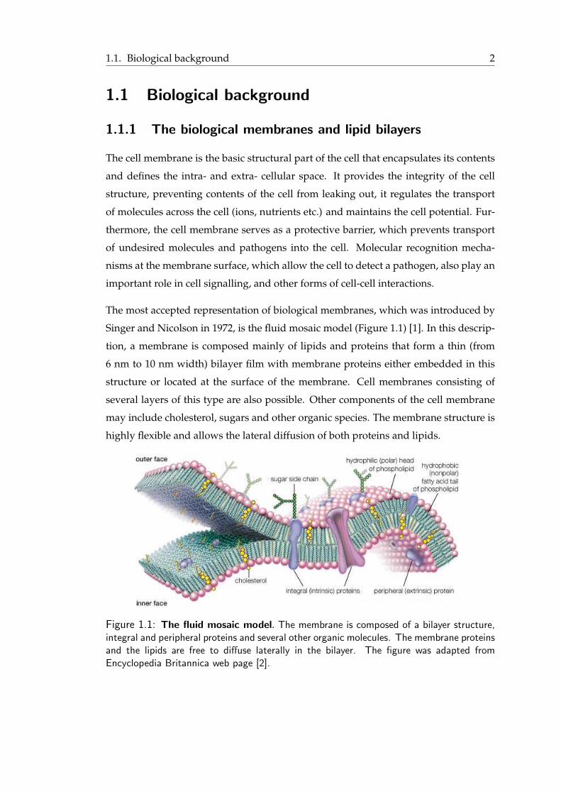
The most accepted representation of biological membranes, which was introduced by
Singer and Nicolson in 1972, is the fluid mosaic model (Figure 1.1) [1]. In this descrip-
tion, a membrane is composed mainly of lipids and proteins that form a thin (from
6 nm to 10 nm width) bilayer film with membrane proteins either embedded in this
structure or located at the surface of the membrane. Cell membranes consisting of
several layers of this type are also possible. Other components of the cell membrane
may include cholesterol, sugars and other organic species. The membrane structure is
highly flexible and allows the lateral diffusion of both proteins and lipids.
Figure 1.1: The fluid mosaic model. The membrane is composed of a bilayer structure,integral and peripheral proteins and several other organic molecules. The membrane proteinsand the lipids are free to diffuse laterally in the bilayer. The figure was adapted fromEncyclopedia Britannica web page [2].
1.1. Biological background 3
Although most of the specific membrane functions (such as regulated ion conduction,
molecular recognition, signalling etc.) are performed by membrane proteins, a num-
ber of membrane properties (such as mechanical elasticity, defects formation, phase
behaviour and passive transport) are defined by the lipid bilayer. As a cell membrane
is difficult to obtain in its full complexity in vitro, a lipid bilayer often serves as a model
cell membrane in the studies of various membrane properties and functions.
Let us review the key characteristics of lipid bilayers, which one can view as cell mem-
branes, with membrane proteins and other biomolecules that are usually incorporated
in them removed. Even in this reduced form the lipid bilayer is a complex structure.
Membrane lipids are small amphipathic molecules, made of two major components:
fatty acids and a phosphate group. The fatty acids are the hydrophobic tails and the
phosphates are the polar head-groups of the lipids. There are several different types of
lipids including phosphatidyleserine (PS), phosphatidylglycerol (PG), phosphatidyl-
choline (PC) and phosphatidylethanolamine (PE). In the case of PS and PG lipids the
head-group is negatively charged.
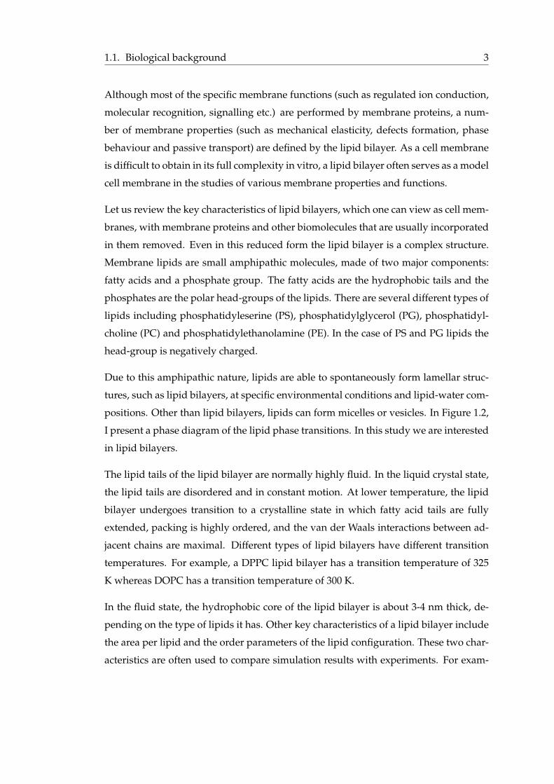
Due to this amphipathic nature, lipids are able to spontaneously form lamellar struc-
tures, such as lipid bilayers, at specific environmental conditions and lipid-water com-
positions. Other than lipid bilayers, lipids can form micelles or vesicles. In Figure 1.2,
I present a phase diagram of the lipid phase transitions. In this study we are interested
in lipid bilayers.
The lipid tails of the lipid bilayer are normally highly fluid. In the liquid crystal state,
the lipid tails are disordered and in constant motion. At lower temperature, the lipid
bilayer undergoes transition to a crystalline state in which fatty acid tails are fully
extended, packing is highly ordered, and the van der Waals interactions between ad-
jacent chains are maximal. Different types of lipid bilayers have different transition
temperatures. For example, a DPPC lipid bilayer has a transition temperature of 325
K whereas DOPC has a transition temperature of 300 K.
In the fluid state, the hydrophobic core of the lipid bilayer is about 3-4 nm thick, de-
pending on the type of lipids it has. Other key characteristics of a lipid bilayer include
the area per lipid and the order parameters of the lipid configuration. These two char-
acteristics are often used to compare simulation results with experiments. For exam-
1.1. Biological background 4
Figure 1.2: Lipid phase diagram. The figure was adapted from [3].
ple, a DOPC lipid bilayer has an area per lipid of 72.2 A2 [4] and this value can be used
to validate a force field or as a point of reference for a simulation result. The order
parameter is a measure of ordering of the lipids. It can indicate possible structural
deformations of a lipid bilayer and thus it constitutes an important characteristic.
The composition of real cell membranes is complex, but quite often, at least as a start-
ing point, in membrane studies and membrane-protein studies, a model system of a
bilayer consisting of one specific lipid (usually DOPC and DPPC) is employed. A sim-
ilar approach will be adopted here.
1.1.2 Peptides
A peptide is composed of amino acids. In general, there are 20 different amino acids
commonly found in peptides and proteins. Each of them is formed by an amino group,
a carboxyl group, a central CH group (the carbon of this central CH group is usu-
ally called α-carbon or Cα) and a specific side chain (Figure A.1, Appendix A). The
sequence of Cα atoms connected through covalent peptide bonds, including the N-
terminus (free NH2 initial group) and C-terminus (free COOH final group) is called
the peptide backbone. It is the main structural part of the peptide that determines
its overall geometric properties. The side-chains of a peptide define its physical and

1.1. Biological background 5
chemical properties.
The structure of a peptide or a protein can be described at different levels (Figure A.2,
Appendix A). The primary structure of the peptide describes the actual sequence of
amino acids, or residues, within the peptide. The term secondary structure refers to the
geometry or conformational behaviour of this primary sequence. A disordered pep-
tide chain is often called a random coil. However, many peptides have well-defined
three-dimensional secondary structure. Three of the most frequently occurring struc-
tures are the α-helix, the β-sheet and β-turns. In a larger protein, the three dimensional
arrangement, or packing of secondary units, is characterized by the tertiary structure,
whereas assemblies of several proteins are classified as quaternary structures.
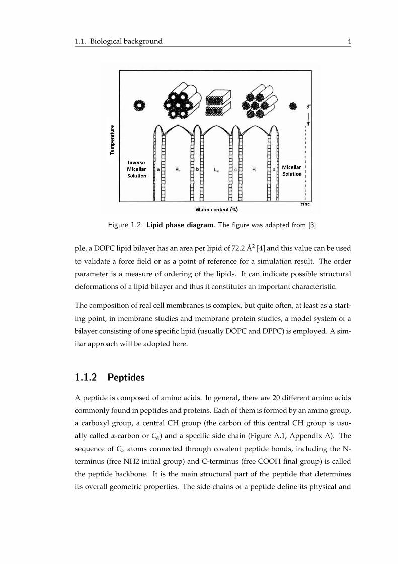
A common secondary structural motif in biologically active peptides is the amphi-
pathic α-helix. An α-helix is formed when a chain of amino acids twists around itself
in a well-ordered way (Figure 1.3(a)). This helical structure is stabilized by a network
of backbone hydrogen bonds between the backbone carbonyl oxygen of residue i and
the amide proton of residue i+4, with the side groups of the amino acid residues pro-
truding outward from the helical backbone. The rise along the helical axis for every
two successive α-carbons is 1.5 A and the respective rotation is about 100 degrees.
Moreover, each helical turn extends for about 5.4 A along the long axis of the helix,
resulting in 3.6 residues per turn (Figure 1.3(a)). Another important feature of an α-
helical peptide is the inherent net dipole that exists along its axis due to the synergy
of each of the small dipoles that exist in each peptide bond (Figure 1.3(b)). The helical
dipole plays an important role in pore formation and stabilization and ion transport
across membranes.
An α-helix is called amphipathic when it has both hydrophobic and hydrophilic residues
positioned along its axis. This distribution of hydrophobicity has been shown to play
an important role in the way with which the amphipathic α-helical peptides interact
with the biological membranes [6]. Amphipathic α-helices are the peptides of interest
in this study and more details about their function will be given in the next chapters.
1.2. Peptide-membrane interactions 6
(a) Ball-and-stick representation of an α-helix. (b) Helix dipole.
Figure 1.3: The α-helix. (a) Ball-and-stick representation of an α-helix, showing thehydrogen bonds between the ith and ith + 4 residues. (b) A helical dipole is created by thetransmission of the electric dipole of the peptide bonds along the helical axis. The figurehas been adapted from [5].
1.2 Peptide-membrane interactions
Peptide-membrane interactions are at the heart of a number of important biological
processes. For example, antimicrobial peptides are a family of peptides with a partic-
ular propensity to recognize and disintegrate bacterial pathogens. A number of these
peptides have been identified as key components of the natural immune defence sys-
tem [7]. A related family of peptides is the so-called cell-penetrating peptides (CPPs)
capable of efficient translocation through the cell membrane, either by themselves or
together with a molecular cargo [8]. These peptides are being explored as potential
programmable drug delivery vectors. As a part of larger proteins, ion-conducting
channel peptides form well-organized transmembrane bundles capable of selective
transport of ions. Other peptides are believed to play a key role in mediation of various

1.2. Peptide-membrane interactions 7
complex cellular processes, such as membrane fusion. It is clear that a better under-
standing of peptide-membrane interactions on molecular level not only is important
in the elucidation of various biological processes, but also could be instrumental in
designing peptides with tailored functionalities, for example, for antibiotic and drug
delivery applications.
Peptide-membrane interactions are complex and beautifully diverse phenomena. De-
pending on their composition, charge, and structure different peptides evoke different
interaction mechanisms with the membrane. Here, I present some of the most com-
monly seen scenarios in the studies of peptide-membrane interactions. In this analysis,
I exclusively focus on α-helical peptides. There are two reasons for this. First, α-helical
secondary structure is abundant among membrane active peptides. Second, develop-
ment of a fully comprehensive description of peptide-membrane interactions is a chal-
lenging task. Having the peptide in a well-defined structure eliminates at least one
additional degree of complexity associated with the conformational behaviour of the
peptide itself. Thus, α-helical peptides are a natural starting point in the construction
of this description.
Let us first consider different peptide internalization mechanisms. These mechanisms
can be categorized into endocytosis mediated entry and direct penetration in the mem-
brane. Endocytosis is an important biological process, used by the cell for transport of
various molecular species across the cell membrane. In the case of peptide transport,
its mechanism can be described as follows; first, several peptides form an aggregate in
the aqueous phase, then the cell absorbs the aggregate from the outside environment
by engulfing it with its cell membrane and finally, a vesicle (endosome) is formed
and released on the inner side of the membrane (Figure 1.4(a)). In principle, sponta-
neous formation of an endosome is possible as a result of membrane fluctuation and
budding. However, more commonly, endocytosis is a receptor mediated and energy
dependent process. Several classes of cell-penetrating peptides are believed to induce
this mechanism.
Direct penetration mechanisms, on the other hand, are receptor and energy indepen-
dent, and may also be classified in several distinct scenarios. One of these mechanisms
is the sinking raft model. In this model, the peptides form aggregates of limited size
and associate with one of the faces of the membrane. The mass imbalance of the lipid
1.2. Peptide-membrane interactions 8
bilayer due to this association induces curvature that provides the driving force for
the translocation of peptides across the bilayer [14] (Figure 1.4(b)). This mechanism
has been proposed for several antimicrobial peptides, for example delta-Lysin [10] .
Another scenario of direct penetration is the formation of an inverted micelle. In this
case, a peptide interacts with the negatively charged phospholipids, inducing the for-
mation of an inverted micelle inside the lipid bilayer (Figure 1.4(c)). Then, either the
peptide is entrapped within the micelle and then released into the cell, or the forma-
tion of the micelle perturbs locally the membrane and induces a new peptide insertion
event.
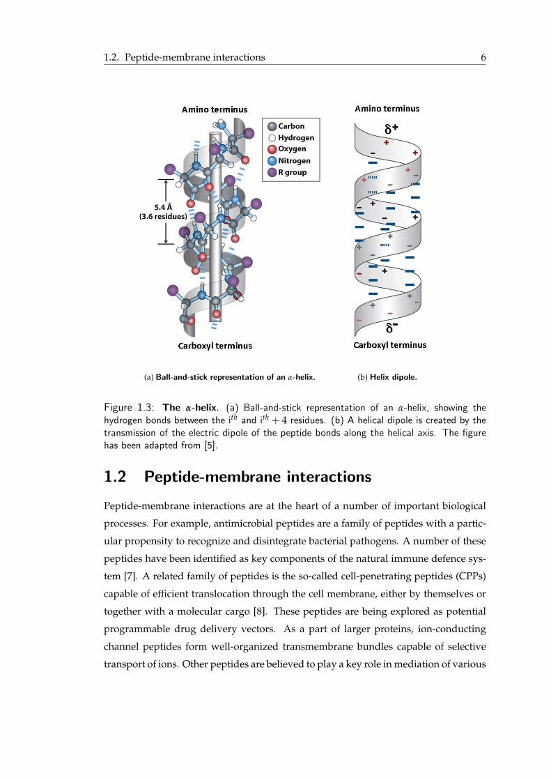
The formation of transmembrane pores is another way of interaction between α-helical
peptides and membranes. Three different pore structures, the barrel-stave, the carpet
and the toroidal pore model, have been proposed and investigated. The main differ-
ences between these models lie in the lipid structure around the pores and the pore
stability. In the barrel-stave model, the lipids are parallel to each other and the pep-
tides form a well-defined, very stable bundle, which, if it is of a sufficient diameter, can
serve as a pore. This is believed to be the structure of the peptides in ion-conducting
channels, either as a part of a larger protein, or formed through a self-assembly pro-
cess. In the case of the toroidal model, the lipids create a toroidal-shaped (or donut-
shaped) opening covered with the peptides in different orientations. Toroidal pores
are generally less stable (i.e. they are transient) than the barrel-stave pores. Some stud-
ies suggest that this mechanism is involved in membrane disruption action of some
antimicrobial peptides, leading to cell leaking out its contents [15].
In the carpet model, peptides accumulate on the membrane until its integrity is breached
and transient holes are formed. These holes, when the peptides are in high concentra-
tions, may result into the complete collapse of the membrane. Again, this mechanism
has been proposed, among others, as permeabilization mechanism of α-helical antimi-
crobial peptides (AMPs) (Figure 1.4(d)).
Several peptide-membrane interaction mechanisms involve a peptide inserted in the
membrane. In membrane fusion, the fusion peptides, short hydrophobic parts of fu-
sion proteins, destabilize the lipid bilayer structure by adopting an oblique orienta-
tion within the membrane [6]. This orientation has been linked to the gradient of
hydrophobicity along the helical axis of the peptides. In Figure 1.4(e), I show one of
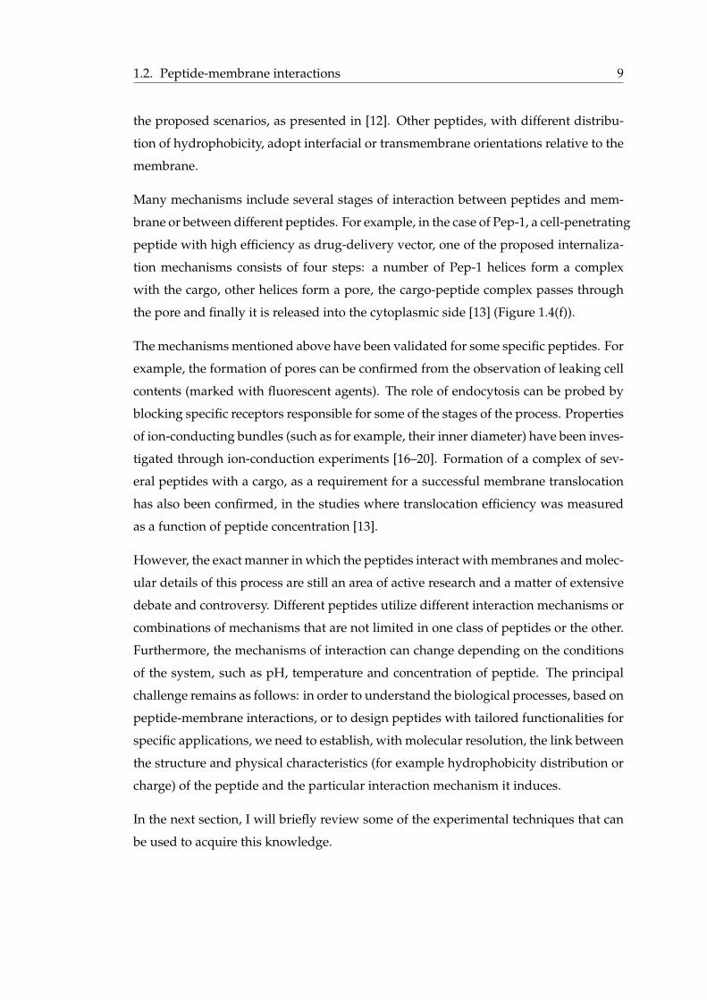
1.2. Peptide-membrane interactions 9
the proposed scenarios, as presented in [12]. Other peptides, with different distribu-
tion of hydrophobicity, adopt interfacial or transmembrane orientations relative to the
membrane.
Many mechanisms include several stages of interaction between peptides and mem-
brane or between different peptides. For example, in the case of Pep-1, a cell-penetrating
peptide with high efficiency as drug-delivery vector, one of the proposed internaliza-
tion mechanisms consists of four steps: a number of Pep-1 helices form a complex
with the cargo, other helices form a pore, the cargo-peptide complex passes through
the pore and finally it is released into the cytoplasmic side [13] (Figure 1.4(f)).
The mechanisms mentioned above have been validated for some specific peptides. For
example, the formation of pores can be confirmed from the observation of leaking cell
contents (marked with fluorescent agents). The role of endocytosis can be probed by
blocking specific receptors responsible for some of the stages of the process. Properties
of ion-conducting bundles (such as for example, their inner diameter) have been inves-
tigated through ion-conduction experiments [16–20]. Formation of a complex of sev-
eral peptides with a cargo, as a requirement for a successful membrane translocation
has also been confirmed, in the studies where translocation efficiency was measured
as a function of peptide concentration [13].
However, the exact manner in which the peptides interact with membranes and molec-
ular details of this process are still an area of active research and a matter of extensive
debate and controversy. Different peptides utilize different interaction mechanisms or
combinations of mechanisms that are not limited in one class of peptides or the other.
Furthermore, the mechanisms of interaction can change depending on the conditions
of the system, such as pH, temperature and concentration of peptide. The principal
challenge remains as follows: in order to understand the biological processes, based on
peptide-membrane interactions, or to design peptides with tailored functionalities for
specific applications, we need to establish, with molecular resolution, the link between
the structure and physical characteristics (for example hydrophobicity distribution or
charge) of the peptide and the particular interaction mechanism it induces.
In the next section, I will briefly review some of the experimental techniques that can
be used to acquire this knowledge.
1.2. Peptide-membrane interactions 10
Figure 1.4: Schematic of possible peptide-membrane interactions. (a) Endocytosis.Figure adapted from [9] (b) The sinking-raft model, adapted from [10]. (c)The invertedmicelle model. Figure adapted from [9]. (d) Different pore formations proposed for α-helicalantimicrobial peptides, adapted from [11]. (e) One of the proposed mechanisms for fusion,adapted from [12]. (f) Proposed schematic model for the internalization of the Pep-1/cargocomplex through the membrane, adapted from [13].

1.3. Experimental techniques and limitations 11
1.3 Experimental techniques and limitations
During the last decades, several experimental techniques have been developed and
applied to biological systems. These techniques differ in the nature (alive, preserved
or sectioned) and the size of the sample they can be used for, their sensitivity and the
type and resolution of information they can provide. In this section, I will present some
of the most recent and the most significant methods and studies and I will discuss their
limitations.
The location and orientation of a peptide relative to a lipid bilayer as well as lipids
rearrangement in the presence of a peptide are two important structural characteris-
tics of peptide-membrane interactions. Experimental techniques that have been used
to get structural information include Fourier Transform Infrared Spectroscopy (FTIR)
[21–27], X-ray and Neutron Diffraction methods [28, 29] as well as Nuclear Magnetic
Resonance (NMR) [30–38]. However, the possibilities of using for example X-ray or
neutron diffraction to gain detailed insights into peptide-membrane systems are lim-
ited, since these systems lack long-range crystalline order. NMR and specifically solid-
state NMR has numerous applications in peptide systems over the last years [33–39].
A series of NMR studies by Opella and co-workers has provided important insights in
peptide orientation [40–42]. Atomic Force Microscopy (AFM) has also been used for
the structural characterization of peptide-membrane systems. Ripple phases in lipid
bilayers induced by lipopeptides, destabilization of a bilayer due to fusion peptides,
and restructuring of the membrane in the presence of specific peptides are some of
the examples where AFM has been used to get information about peptide-membrane
interactions [43–45]. On the other hand, however detailed are the structural charac-
teristics captured by AFM, the method generally does not provide any chemical in-
formation of the system under study. A recent improvement in this area is the use of
functionalized AFM tip [46].
There are also experimental techniques that can be used in order to map the position
of different molecules in a peptide-lipid bilayer system. Imaging Mass Spectrometry
(IMS), like MALDI1 imaging and secondary ion mass spectrometry (SIMS), is one of
the latest techniques to be developed and among the most powerful ones [47–49]. An-
1MALDI: matrix-assisted laser desorption ionization
1.3. Experimental techniques and limitations 12
other promising imaging technique is Surface Plasma Resonance (SPR) spectroscopy,
that allows for the real-time observation of peptide binding to phospholipid bilayers
[50, 51] and membrane-mediated cell signalling [52]. Other imaging techniques used
in peptide-lipid studies are Light Scattering Spectroscopy (SLS (static) or DLS (dy-
namic)) [53], Fluorescence Spectroscopy [54].
Even with this broad arsenal of experimental techniques it is still difficult to obtain
complete and detailed information about the modes of peptide-membrane interac-
tions. Let us illustrate the challenges in some of the experimental techniques using
an example of a direct relevance to the current study. Bradshaw and co-workers
have performed a series of important experimental studies on the SIV fusion peptide
[29, 55, 56]. In one of them, the authors carried out neutron diffraction measurements
from stacked multilayers of DOPC and determined the location and orientation of
specifically deuterated SIV fusion peptides within the bilayer. The results from this
study showed that there are two different populations of peptides. One major popula-
tion close to the bilayer surface, and a smaller population hidden in the hydrophobic
core. Two equally plausible orientations at 55o and 78o with respect to the bilayer
normal, were found consistent with the experimental observations. However, based
on the additional FTIR data from previous studies, the oblique orientation at 55o was
accepted as the most probable one.
This illustration also highlights several issues, characteristic for most of the experimen-
tal techniques. First and foremost, the obtained data corresponds to an equilibrium
average over multiple peptide-membrane configurations (in this specific case, average
over various angle and location distributions). Thus, detailed information about a par-
ticular configuration of interest or the detailed information about dynamics of peptide-
membrane assembly is beyond the scope of this approach. Furthermore, to interpret
the obtained data, a model is required, construction or contemplation of which may
be a challenge in itself. Unambiguous behaviour, quite often, can be derived only us-
ing several complementary experimental techniques (in this case, additional data from
FTIR were required). Finally, although as I have already mentioned, some of the exper-
imental methods are now able to provide a more detailed and dynamic information, it
is also important to remember that in general experimental studies are expensive and
time consuming.

1.4. Molecular modelling and computer simulations of peptide-membraneinteractions 13
Thus, we still need a description of peptide-membrane interactions which would con-
sider behaviour of an individual or several peptide molecules, elucidate the dynam-
ics of the peptide-membrane assembly process, provide a link between the observed
behaviour and the data measured in experiments and be sufficiently modest in the re-
sources required to systematically explore a large number of systems. I believe these
issues can be addressed within computer simulations, and specifically molecular dy-
namics. I will review recent progress in the area with a focus on peptide-membrane
interactions in the next section.
1.4 Molecular modelling and computer simulations
of peptide-membrane interactions
Over the years, a number of theoretical and computer simulation approaches have
been developed to describe membrane behaviour and peptide-membrane interactions.
These approaches vary in the way the peptide-membrane system is modelled and
what type of information can be obtained from this model. For example, a lipid bi-
layer can be modelled as essentially an infinite hydrophobic slab (with varying degree
of complexity) through some effective field function. This approach is usually adopted
in various mean-field models developed over the years. Quite often, to reduce the
computational load, solvent is not included in the model explicitly, and its presence is
accounted for through some effective interactions between the remaining components.
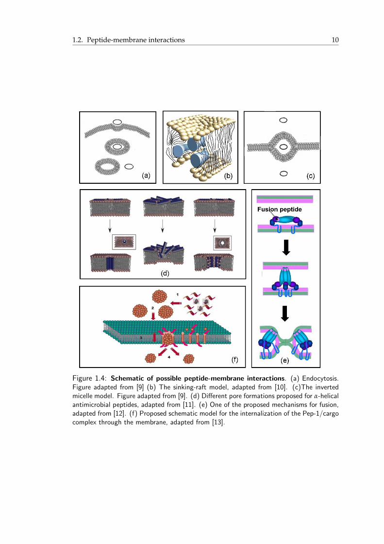
In its general form, a mean-field method indicates that the lipid bilayer and the sur-
rounding water are described by an empirical energy function. In Figure 1.5 there
is a schematic of the lipid bilayer and the water phase and one of the possible en-
ergy functions f (z) used in the mean-field methods to define the different levels of
hydrophobicity in the system. When a peptide or protein is considered (represented
by a cylinder in the schematic), a hydrophobic term is included in the potential en-
ergy function. This term shows the contribution of each residue of the peptide in the
peptide-membrane interactions.
An approach based on the mean-field theory is the self-consistent field (SCF) theory.
In SCF theory the van der Waals-type interactions are used for the different types of
1.4. Molecular modelling and computer simulations of peptide-membraneinteractions 14
Figure 1.5: Mean-field model for the treatment of peptide-membrane interactions.The lipid bilayer is represented by a hydrophobic slab.
particles as well as the configurational entropy of the lipid tails. Leermakers and co-
workers have applied SCF theory in a series of membrane and membrane-peptide
studies [57–59]. In a recent study, SCF theory was also used by Liang and Ma to study
the effects of inclusions in supported mixed lipid bilayers [60]. In [61] and [62], the
same authors combined SCF theory and density functional theory to investigate the
structural organization of membrane proteins in lipid bilayers as well as the effect of
nanosized hydrophobic inclusions in lipid bilayers. Mean-field theory was also used
by Lague and co-workers [63–65]. The authors employed a mean-field approach based
on results from fully detailed atomistic simulations, to develop a theory for defining
the structure of the lipid chains around a model membrane protein and to study the
lipid-mediated protein-protein interactions. Also, La Rocca et al. used mean-field
theory to determine the optimal orientation of a helical peptide in a lipid bilayer [66,
67].
Another implicit-solvent approach is the generalized Born/surface area (GB/SA) mod-
els [68]. Im et al. in a series of studies have used the GB/SA approach to study mem-
brane peptides [69, 70]. Also, Ulmschneider and co-workers developed an implicit-
membrane representation and applied it in influenza M2 peptide and glycophorin A
dimer [71, 72].
One of the most important limitations of mean-field based approaches are the sim-
1.4. Molecular modelling and computer simulations of peptide-membraneinteractions 15
plifications that need to be made in order to develop feasible analytical theories. The
description of the lipid bilayer by a free energy functional cannot capture the complex-
ity that lies at the molecular level of the membrane. Moreover, the difficulty in linking
the parameters used in these models with physical properties constitutes an important
disadvantage.
In order to select an appropriate approach from a huge number of models and methods
developed over the last 40-50 years, it is important to formulate the long term goals of
this study. I would like to develop a capability to describe peptide-membrane interac-
tion processes in their entire complexity, from the dynamics of the self-assembly pro-
cesses to equilibrium properties of peptide-membrane systems. This objective imposes
several key restrictions on our choice of methods. It is evident, that peptide-membrane
self-assembly processes, such as formation of trans-membrane pores, requires signifi-
cant structural rearrangement of both peptides and the membrane. This process also
seems to be mediated (at least to some extent) by the solvent. Thus, our description
must be based on a reasonably detailed model of all the components of the system, i.e.
solvent, peptides, lipid bilayer. This restriction excludes the models based on mem-
brane as an effective hydrophobic medium and implicit solvent models. Next, I am
interested not only in the final equilibrium properties of the system, but in the actual
process of self-assembly. Therefore, it seems that most of the conventional Monte Carlo
approaches would not be appropriate here. On the other hand, Molecular Dynamics
seems to satisfy all the required conditions and, therefore, in the review of the recent
studies of peptide-membrane interactions I will mostly focus on this approach, with
occasional diversion into other methods.
There has been significant progress in the field of molecular dynamics simulations
of biomolecular systems since the first simulation of a protein in vacuum, reported
33 years ago [73] (see Table A, Appendix A). Some of the first studies of membrane-
peptide interactions employing molecular dynamics simulations on a sub-nanosecond
timescale include the study of a model peptide designed to anchor to bilayer surfaces
[74], amphipathic α-helices [75] and the bee venom peptide melittin [76].
Recently, several atomistic molecular simulation studies attempted to address long-
scale peptide-membrane phenomena in their full complexity. In one of these studies,
Leontiadou and co-workers captured toroidal pore formation in simulations of an-
1.4. Molecular modelling and computer simulations of peptide-membraneinteractions 16
timicrobial peptide magainin-H2 and a model phospholipid membrane [77]. Studies
of toroidal pore formation and its structural characteristics have been further extended
by Sengupta and co-workers [78]. In another example, Herce and Garcia applied
fully atomistic simulations to propose a complex multistage mechanism of HIV-1 TAT
peptide translocation across the membrane [79]. Formation of a transient pore was
observed, with the peptides diffusing on the surface of the pore to cross the mem-
brane. An alternative mechanism, based on micropinocytosis, has been suggested for
TAT translocation in fully atomistic studies by Yesylevskyy and co-workers. In mi-
cropinocytosis a cluster of peptides wraps the membrane around itself to form a small
vesicle [80]. A similar mechanism of translocation was reported by the same group
for another cell-penetrating peptide, Penetratin. None of these simulations however
spanned timescale beyond several hundred of nanoseconds, and in many cases the
simulations were limited to tens of nanoseconds. Routine operation on longer time
scale still remains prohibitively expensive in atomistic simulations. This limitation im-
posed by atomistic simulations led to the development of coarse-grained approaches
to study complex biomolecular phenomena.
Coarse-grained approaches are based on the idea of systematically reducing the level
of detail in the way the system is represented, and thus increasing the time/length
scale of the simulation. One way of doing this is by modelling the system as a group
of effective particles (‘beads’). Each of these beads represents an ensemble of atoms
whose atomistic degrees of freedom do not play an important role in the process under
consideration and are integrated out. This leads to several implications. First of all, it
results in the expected improvement in computational efficiency of the model due to
the reduced number of degrees of freedom (depending on the level of coarse-graining).
Furthermore, as has been noted in a number of studies, smoothing out of fine-grained
degrees of freedom in CG models reduces the effective friction between the molecules.
As a result, many complex processes such as biomolecular self-assembly occur on a
shorter effective time scale.
Several strategies to construct CG models have been offered over the years. For exam-
ple, the interactions between coarse-grained beads can be calibrated to reproduce the
forces between the corresponding groups of atoms in atomistic simulations [81]. Al-
ternatively, the coarse-grained model can be calibrated to reproduce certain physical

1.4. Molecular modelling and computer simulations of peptide-membraneinteractions 17
characteristics of the system of interest, such as density, phase transitions and structure
[82]. In Figure 1.6, some representative coarse-grained models for lipids are shown. he
article by Venturoli and co-workers is an excellent review of the current developments
and achievements in this field [83]. State-of-the-art in atomistic and CG simulation
studies of lipid membranes, including peptide-membrane interactions, has also been
recently reviewed by [84]. Another recent review on the advances in the area of multi-
scale modelling is the one by Murtola et al. [85].
Figure 1.6: Coarse-grained models for lipids. (a) Atomistic representation. (b) Groupof ∼4-5 atoms is represented as a ’bead’ [82]. (c) Every lipid is represented as a Gay-Berneparticle [86].
Using coarse-grained models, it has been possible to investigate a number of processes
related to biomembrane physics, which have been difficult to study by MD simulation
methods on all-atom models. In the early 90’s, Smit and co-workers developed a CG
model of oil/water/surfactant system. Two types of particles are defined, labeled with
the letters o and w. In this model, oil molecules are represented by a single o particle,
water molecules by a single w particle and surfactant molecules are represented by
a chain of two w particles followed by five o particles, each bound to its neighbour
by a strong harmonic force. Simulations showed for the first time the spontaneous
formation of micelles [87, 88].
1.4. Molecular modelling and computer simulations of peptide-membraneinteractions 18
Some years later, Groot and Warren introduced the Dissipative Particle Dynamics
(DPD) technique into the field of biological systems [89]. In this technique, the forces
are grouped together to yield an effective friction and a fluctuating force between the
interacting sites. Kranenburg et al. employed DPD combined with a Monte Carlo
scheme to achieve the natural state of a tensionless bilayer and managed to describe
the phase behaviour of phospholipid bilayers [90]. Smit model has also been extended
to study the structural changes resulting from the inclusion of a rod-like objects serv-
ing as an idealized protein [91]. Recently, this approach was used to systematically
compute the potential of mean force (PMF) between two proteins as a function of the
hydrophobic mismatch of the proteins [92, 93].
In the late 90’s, a different kind of coarse-grained model was proposed. Goetz and
Lipowsky, introduced an even simpler, idealised CG bilayer model, capable of qual-
itatively describing some fundamental membrane characteristics [94]. In this model,
only two types of Lennard-Jones sites are included: hydrophilic sites, used to describe
both solvent and lipid-head particles, and hydrophobic sites to model lipid-tail seg-
ments. Some of the phenomena captured by this model were bilayer self-aggregation,
diffusion, and area compressibility.
Klein and co-workers developed a different coarse-grained model for simulating hy-
drated DMPC lipid bilayers which was one of the first attempts to include an explicit,
but simplified, treatment of electrostatic interactions in a CG model. In this model, 118
atoms of a DMPC lipid are represented by a 13 CG sites. The two choline and phos-
phate head-groups were assigned +e and -e charges, respectively, and the potentials
were parameterised in order to mimic structural properties obtained from atomistic
simulations and experimental data. Water was modelled as spherically symmetric
sites each representing a group of three water molecules. In 2001, Shelley et. al, using
this model, studied the self-assembly of phospholipids into various phases, both in the
absence and in the presence of biomolecules such as anaesthetics and alkanes [95, 96].
In 2004, Marrink et al. introduced a very simple, flexible and efficient CG model for
lipid simulations [82], to describe properties of lipid-water systems. In their model, ev-
ery four heavy atoms (i.e. not hydrogens) are represented by one effective bead. Four
major types of beads and several variants were introduced to describe different levels
of polarity and charge. The parameters used in this model were optimized using a trial
1.4. Molecular modelling and computer simulations of peptide-membraneinteractions 19
and error procedure, in order to satisfactorily reproduce the experimental densities of
pure water and alkane at room temperature and other experimentally obtained phys-
ical parameters. The model has been validated against several processes, such as lipid
phase transitions, micellar and vesicle behaviour as well as lipid bilayer formation,
clearly demonstrating that such complex processes are within its scope [97–99].
In the following years several attempts have been made to extend the original model
of Marrink and co-workers to proteins, peptides and other biological entities. One of
these extended models was recently proposed by Bond and Sansom [100, 101]. They
introduced a model of proteins, where a representation for each amino acid was based
on its properties (tendency to form hydrogen bonds, hydrophobicity/hydrophilicity
and charge). The same idea of a four-to-one mapping was followed, with the amino
acids modelled by one, two or three beads, one representing the backbone of the amino
acid and the others the side chain. More information about the model can be found
in the original publication [100]. With this protocol, the authors investigated different
peptides in membranes, capturing, among other effects, the insertion and dimeriza-
tion of Glycophorin A (GpA) [100], the insertion of OmpA protein and WALPs into
a lipid bilayer [100] and the interfacial orientation of LS3 peptide in monomeric form
[101]. The model has also been used for the prediction of several processes such as
the insertion of DNA in a lipid bilayer [102], the interaction of membrane enzymes
with lipid bilayers [103] and the dependence of peptide-membrane interactions on the
initial structure of the peptide in different lipid environments [104].
Recently, a new version of the force field proposed by Marrink and co-workers has
been developed, with an extension to proteins [105, 106]. The proposed model, MAR-
TINI, features a larger number of bead types and interactions, and has been optimized
to reproduce some key properties of amino acids, such as oil/water partition coeffi-
cients and association constants between different amino acids. Moreover, the model
has been shown to accurately capture peptide-membrane interactions for several he-
lical peptides [105], and to correctly reproduce the formation of a toroidal pore by
magainin-H2, confirming earlier atomistic simulations [77]. Other applications of the
MARTINI include the effect of temperature and membrane composition on the prop-
erties of liposomes in the limit of high curvature [107], the self assembly of cyclic pep-
tides near or within membranes [108] and the formation of a barrel-stave pore by LS3
1.4. Molecular modelling and computer simulations of peptide-membraneinteractions 20
synthetic peptide [109].
Several other studies and approaches should also be mentioned. An innovative mul-
tiscale approach was followed by Izvekov and Voth in [110]. The authors developed a
CG model for hydrated DMPC bilayers using a multiscale approach in which explicit
atomistic forces are propagated in scale to the coarse-grained level. This method is not
dependent on the matching of selected thermodynamic data, but it makes use of the
calculated atomic forces from an underlying atomic level (AL) model. An improved
version of this model was recently introduced and applied to studies of two peptides,
Ala-15 and V5PGV5, and it exhibited good agreement with the structural properties of
the peptides [111].
Another promising approach is the introduction of a new, very simple CG model
for lipids proposed by Michel and Cleaver (Figure 1.6(c)). The model is a combina-
tion of spherical Lennard-Jones beads (for the choline and phosphate moieties) with
Gay-Berne soft uniaxial ellipsoids (for the glycerol and hydrocarbon tails). In [86],
the authors examined the ability of the model to exhibit amphiphilicity by studying
the behaviour of appropriately tuned Gay-Berne particles immersed in a solvent of
Lennard-Jones particles. The model is proved to be suitable for studying the effects
of molecular interaction parameters on a range of self-assembly processes. A similar
approach has been employed by Essex and co-workers in an effort to include different
levels of detail in the system [112–114]. For example, in [114], the authors have studied
the permeability of small molecules in atomistic representation across a lipid bilayer
represented by Gay-Berne and LJ potentials.
Taken together, the aforementioned simulation studies demonstrate the power of molec-
ular simulations in investigating the membrane-peptide interactions. In particular,
molecular dynamics simulations have provided us with important information about
the different interaction mechanisms at a molecular level. The overall strategy of this
study is based on coarse-grained MD simulations combined, when necessary, with
more detailed information taken from atomistic simulations as well as free energy cal-
culations by means of umbrella sampling.

1.5. Nanoparticle membrane interactions 21
1.5 Nanoparticle membrane interactions
Because of the wide use of nanoparticles in a variety of products, varying from drug
and gene delivery materials to consumer products like paints, it is important to un-
derstand how these materials interact with cell membranes [115–117]. In particular,
the cytoxicity of these materials is one of the parameters that needs to be further stud-
ied, as it can either lead to a hazardous event or be used as targeted drug delivery, for
example in cancer therapy.
There are numerous studies about the membrane internalization mechanisms and the
cytoxicity of different types of nanoparticles [118]. In a recent study, Verma et al. used
gold nanoparticles, coated with anionic and hydrophobic groups either at random
positions or at striations of alternating groups [119]. The radius of the nanoparticles
was approximately 6 nm. This study showed that the ‘striped’ nanoparticles were able
to cross the cell membrane without bilayer disruption, whereas the other nanoparticles
followed an endocytic pathway and were trapped in endosomes (Figure 1.7).
Figure 1.7: Different uptake mechanisms of nanoparticles with different coatings.The ‘striped’ nanoparticles are able to cross the cell membrane either directly withoutbilayer disruption (left) or by endocytosis (centre), whereas the other nanoparticles followan endocytic pathway and are mostly trapped in endosomes (right). Figure adapted from[120].

1.5. Nanoparticle membrane interactions 22
In another study, Leroueil et al. used nanoparticles of different sizes injected onto sup-
ported lipid bilayers [121]. They found that cationic nanoparticles with a diameter of
about 5-6 nm induced membrane disruption. Nanoparticles of a 50 nm size led to the
formation of holes in the lipid bilayers.
Recently, a study with nanoparticles with sizes ranging from 1 nm to 140 nm was car-
ried out by Roiter and co-workers [122]. In this work, the authors used AFM to capture
the structural differences of a lipid bilayer after interacting with silica nanoparticles of
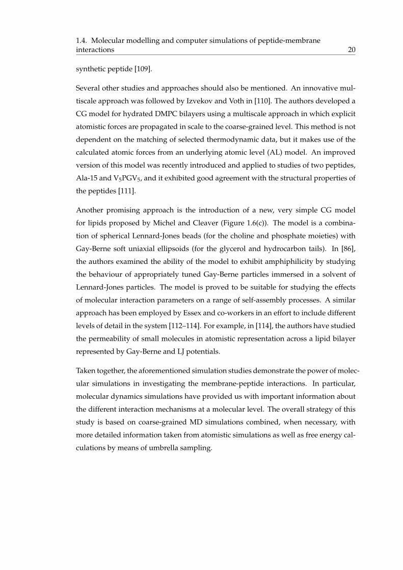
different sizes. The results are shown in Figure 1.8. The lipid bilayer forms uniformly
in the case of nanoparticles with diameter less than 1.2 nm. For nanoparticles larger
than 1.2 nm or smaller than 22 nm thinning of the bilayer and formation of pores are
observed. For nanoparticles larger than 22 nm, with and without bumps, coverage or
incomplete coverage due to the bumps is observed. A similar study was performed
by Ahmed and Wunder [123]. In this work, nanoparticles with a diameter of 5 nm
induced the transition of the lipid bilayer from the lamellar to an interdigitated state.
Simulation studies have also been performed in the area of nanoparticle-membrane
interactions. In [124], the authors captured the formation of holes in lipid bilayers
induced by clusters of dendrimers at their surface. They used coarse-grained MD
simulations, and in particular the MARTINI force field. Water and ions could pass
through the pores which had diameters of 1-5 nm. In another study, the authors used
DPD method in a stretched bilayer and observed the formation of holes under the
dendrimer cluster as well as at other points of the bilayer [125]. In the case where
a ‘not stretched’ bilayer was used, the dendrimers seemed to diffuse in the lipid bi-
layer and the clusters were deformed. Also, D’Rozario et al. performed coarse-grained
MD simulations with particles of a diameter about 1.1 nm to study the interactions of
pristine C60 and its derivatives with lipid bilayers [126]. The nanoparticles were repre-
sented as spheres with 20 evenly spaced coarse-grained particles of different types on
their surfaces. Pristine was represented only by hydrophobic coarse-grained beads.
Its derivatives C60(OH)N , with N = 5, 10, 15 or 20, were constructed by replacing N
number of hydrophobic beads with polar ones. This replacement was either done
at a patch of the nanoparticle, or at random positions. The authors performed MD
simulations and they showed that the apolar and amphipathic fullerenes are mainly
within the lipid bilayer, with the amphipathic nanoparticles being closer to the lipid
1.5. Nanoparticle membrane interactions 23
Figure 1.8: Lipid bilayer fusion on rough surfaces. For nanoparticles larger than 1.2nm or smaller than 22 nm the formation of pores is observed (top). The lipid bilayer hasthe same topography with the nanoparticles with diameter less than 1.2 nm (centre, left).For nanoparticles larger than 22 nm, with and without bumps, coverage (centre, right) orincomplete coverage (bottom) due to the bumps is observed. Figure adapted from [122].
heads. PMF calculations were also carried out and were in good agreement with the
simulation observations. Recently, Li and Gu presented a simulation study of inter-
actions between charged nanoparticles and charge-neutral phospholipid membranes
[127]. They employed the MARTINI force field and showed that due to the increase
of the electrostatic energy, the charged nanoparticle can be partially wrapped by the
membrane.
In this study, an effort to get insights of the interaction of nanoparticles of different
sizes and surface chemistry with lipid bilayer has been made.
1.6. Objectives and scope of the thesis 24
1.6 Objectives and scope of the thesis
The main objective of this work is to test the scope and applicability of coarse-grained
models to capture peptide interaction and self-assembly processes in the presence of
membranes as well as to provide a systematic description of these interactions as a
function of peptide structure and surface chemistry. The bulk of this thesis is devoted
to the interactions of α-helical peptides with lipid bilayers. In the last part of the the-
sis, I employed CG MD simulations to study the interactions of nanoparticles with
membranes. Short chapter summaries are given below.
Chapter 2 / Methodology: Description of the methods used in this work. An introduc-
tion to statistical mechanics and the link to molecular dynamics simulations is given.
This introduction includes potential of mean force calculations, implementation issues,
pressure and temperature control methods and other concepts needed in MD simula-
tions. In the second part of the chapter, a description of the model used is provided.
I close the chapter with the simulation parameters used in this work and the analysis
tools developed for the analysis of our results.
Chapter 3 / Coarse-grained model validation in application to different classes of
amphipatic peptides: MD simulations of different α-helical peptides in a lipid bilayer
are performed. The MARTINI CG force field is employed and the results are compared
with the available experimental or atomistic simulation data. Potential of mean force
calculations are also performed by means of the umbrella sampling method. Different
PMF patterns are calculated for the peptides, leading to a possible classification linked
to their hydrophobicity.
Chapter 4 / Pore formation by synthetic peptides: MD simulations of LS3 pore form-
ing peptide are carried out. The MARTINI CG force field is employed in extensive
MD simulations with different concentrations of peptides in lipid bilayers. Different
complexes are observed, including the formation of a hexameric barrel-stave pore.
Structural and dynamical details of the pore are calculated. Simulations are also per-
formed for a shorter version of LS3 peptide. This peptide seems to form complexes
of different shape, toroidal-like bundles, smaller in size and unstable. A link between
the length of the peptides and their ability to induce the formation of different types
of pore is established.
1.6. Objectives and scope of the thesis 25
Chapter 6 / Cell-penetrating peptides: A study on the interaction of two cell-penetrating
peptides with a lipid bilayer. Coarse-grained molecular dynamics simulations are per-
formed. Formation of complexes of different sizes and membrane perturbation are
two of the main results in this chapter. Steered MD simulations are also performed in
an effort to capture early stages of an endocytic pathway.
Chapter 7 / Interactions between nanoparticles and lipid membranes: MD and Steered
MD simulations of nanoparticles of different size and nature in a lipid bilayer system
are used to study the effect of nanoparticle size, hydrophobicity and charged is exam-
ined. Deformation of the lipid bilayer and interdigitated state have been observed.
Chapter 8: Conclusion and summary.
1.7. Publications and presentations 26
1.7 Publications and presentations
Publications
• P. Gkeka and L. Sarkisov, J. PHYS. CHEM. B., 113 (1), pp. 6-8 .
Spontaneous formation of a barrel-stave pore in a coarse-grained model of the synthetic
LS3 peptide and a DPPC lipid bilayer. (Jan. 2009)
• P. Gkeka and L. Sarkisov, J. PHYS. CHEM. B.,114 (2), pp. 826-839 .
Interactions of phospholipid bilayers with several classes of amphiphilic α-helical pep-
tides: insights from coarse-grained molecular dynamics simulations. (Jan. 2010)
Presentations
• 2009 AICHE ANNUAL MEETING.
Linking Atomistic and Mesoscales: Atomistic and Simple Coarse-Grained Models in
Application to Biomolecular Problems. (Nov. 2009)
• PSI-K SUMMER SCHOOL ON ‘SIMULATION APPROACHES TO PROBLEMS IN MOLEC-
ULAR AND CELLULAR BIOLOGY’.
Coarse-grained simulations and free energy calculations of α-helical peptides. (Sept.
2009)
• FARADAY DISCUSSION 144: MULTISCALE MODELLING OF SOFT MATTER.
Coarse-grained simulations of α-helical peptides. (July 2009)
• CCP5 ANNUAL MEETING: SURFACES AND INTERFACES.
Coarse-grained modelling of membrane-peptide interactions. (Sept. 2008)
• CONFERENCE ON MOLECULAR SIMULATIONS IN BIOSYSTEMS AND MATERIAL
SCIENCE (SIMBIOMA) .
Coarse-grained modelling of membrane translocation mechanisms of α-helical cell-penetrating
peptides. (April 2008)
CHAPTER 2
Methodology
This chapter is a short description of the methodology used in this work. In this the-
sis, molecular dynamics (MD) is a primary tool. The roots of MD and other molecular
modelling approaches employed in this study lie in statistical mechanics, an area of
science, which aims to construct macroscopic properties of a system from basic in-
formation about intermolecular interactions. Thus, before I address the specific area
of peptide-membrane interactions, I will introduce some basic ideas of statistical me-
chanics, and building on these ideas, review the principles of molecular dynamics, free
energy calculations and other methods employed in this work.
In the second part of this chapter, I will provide a more detailed description of the
model used in this study. Specifically, a short description of the MARTINI coarse-
grained model, the molecular mapping and in particular the representation of lipids,
lipid bilayers and peptides will be presented. Finally, at the end of the chapter, there is
a presentation of the tools developed during this work for the calculation of different
parameters and the description of the systems under study.
27
2.1. Fundamentals of molecular dynamics 28
2.1 Fundamentals of molecular dynamics
Molecular dynamics (MD) is a computer simulation technique, where the classical
equations of motion of atoms or molecules are used to calculate the time evolution
of the system. In the following sections, I will derive the principles of molecular dy-
namics starting from a fundamental statistical mechanics description of a system with
constant number of particles, volume and energy. I will discuss how the properties
of the system can be extracted from MD simulations. I will then focus on several key
issues associated with the implementation of MD, such as integration algorithms. Fi-
nally, I will extend our review to advanced MD in systems with constant temperature
and pressure.
2.1.1 Statistical mechanics of the microcanonical ensemble
Let us consider a system of N particles in volume V. If the system is isolated, its energy
E is constant. In statistical mechanics this system corresponds to the microcanonical
ensemble (NVE). A microcanonical MD trajectory may be seen as an exchange of
potential and kinetic energy, with the total energy being conserved.
In the NVE ensemble, the probability density is proportional to the factor
δ(H(rN , pN) − E), (2.1)
where H is the Hamiltonian of the system and rN and pN are the positions and the
momenta of the N particles of the system respectively, with
rN = (r1, r2, . . . , rN), (2.2)
pN = (p1, p2, . . . , pN) (2.3)
and
2.1. Fundamentals of molecular dynamics 29
pi = mi ri. (2.4)
The microcanonical partition function can be written as:
QNVE =1
h3N N!
∫ ∫
δ(H(rN, pN) − E)drNdpN , (2.5)
where the factor1
h3N N!is a measure of the volume of the phase space, h is the Planck
constant and the indistinguishable nature of the particles is accounted through N!.
According to the principles of statistical mechanics, any property A(rN , pN) of the
system can be calculated as an ensemble average
〈A〉 =1
QNVE
1
h3N N!
∫ ∫
A(rN , pN)δ(H(rN, pN) − E)drNdpN . (2.6)
Moreover, knowledge of the partition function defines all thermodynamic properties
of the system. Specifically, in the microcanonical ensemble, the link between the parti-
tion function and the entropy is given by the following formula:
S = kB ln QNVE, (2.7)
where kB is the Boltzman constant.
In practice, direct evaluation of the partition function or integrals like the one in Equa-
tion (2.6) is possible only for a few special cases. For other cases, we must resort to
simulation methods to recover properties of the system in each specific ensemble. The
main idea of any simulation method is to generate a series of states of the system with
the probability density corresponding to a particular ensemble. In this case, any prop-
erty of the system will be the average of this property, observed in a series of gener-
ated states of the system. In principle, two types of simulation methods exist, based on
stochastic approaches (Monte Carlo) and based on deterministic approaches (Molecu-
lar Dynamics), with several hybrid variations spanning the range between them.
2.1. Fundamentals of molecular dynamics 30
In this thesis, I am interested in a range of dynamic properties of the systems of interest,
such as self-diffusion, and the evolution of the system from non-equilibrium states
towards equilibrium. Thus, molecular dynamics is the method of choice throughout
this study. Let us outline the principles of this method, by examining how it is applied
to the microcanonical ensemble.
2.1.2 Molecular dynamics in the microcanonical ensemble
The basic idea of molecular dynamics is to solve numerically the equations of motion
of N interacting atoms or molecules. Thus, the next step in our review of molecular
dynamics is to derive these equations.
In the microcanonical ensemble, as the positions rN and the momenta pN change with
time, the system as a whole evolves in the (rN , pN) phase space along an isoenergetic
surface H(rN , pN) = E, and therefore the Hamiltonian is a conserved property:
dH(rN , pN)
dt= 0. (2.8)
Thus,
dH(rN , pN)
dt=
N
∑i=1
∂H(rN , pN)
∂pi· pi +
N
∑i=1
∂H(rN , pN)
∂ri· ri = 0. (2.9)
The Hamiltonian H of the system in the microcanonical ensemble can be written as
the sum of kinetic and potential energy functions,
H(rN , pN) = K(pN) + V(rN) (2.10)
where K and V are the kinetic and potential energy functions respectively. The kinetic
energy K can be expressed as
K(pN) =N
∑i=1
p2i
2mi. (2.11)
2.1. Fundamentals of molecular dynamics 31
Then, by replacing Equation (2.11) in Equation (2.10), we obtain
H(rN , pN) =N
∑i=1
p2i
2mi+ V(rN), (2.12)
and the time derivative of this Hamiltonian will be
dH(rN , pN)
dt=
N
∑i=1
pi
mi· pi +
N
∑i=1
∂V(rN)
∂ri· ri. (2.13)
Again, from Equations (2.8) and (2.13), it holds that
N
∑i=1
pi
mi· pi +
N
∑i=1
∂V(rN)
∂ri· ri = 0. (2.14)
From Equations (2.9) and (2.14), we get
N
∑i=1
∂H(rN , pN)
∂pi· pi +
N
∑i=1
∂H(rN , pN)
∂ri· ri =
N
∑i=1
pi
mi· pi +
N
∑i=1
∂V(rN)
∂ri· ri (2.15)
and thus, for every particle i with i ∈ {1, 2, · · · , N}, it holds that
∂H(rN , pN)
∂pi=
pi
mi(2.16)
and
∂H(rN , pN)
∂ri=
∂V(rN)
∂ri. (2.17)
If we substitute Equation (2.4) into Equation (2.16), we get
∂H(rN , pN)
∂pi= ri, ∀ i ∈ {1, 2, · · · , N} (2.18)
Equation (2.9), after substituting Equation (2.18), becomes
2.1. Fundamentals of molecular dynamics 32
N
∑i=1
ri · pi +N
∑i=1
∂H(rN , pN)
∂ri· ri = 0 =⇒
N
∑i=1
(
pi +∂H(rN , pN)
∂ri
)
· ri = 0 (2.19)
As the vectors of velocities ri are independent, Equation (2.18) holds if and only if
∂H(rN , pN)
∂ri= −pi, ∀ i ∈ {1, 2, · · · , N} (2.20)
Equations (2.18) and (2.20) are also known as Hamilton equations of motion and are
equivalent to Newton’s second law,
Fi = mi ri. (2.21)
Indeed, from Equation (2.4) we have
pi = mi ri. (2.22)
If we now substitute Equation (2.22) into Equation (2.20), we get
∂H(rN , pN)
∂ri= −mi ri, ∀ i ∈ {1, 2, · · · , N}. (2.23)
From Equations (2.17) and (2.23) it follows that
Fi = −∂H(rN , pN)
∂ri= −∂V(rN)
∂ri, ∀ i ∈ {1, 2, · · · , N}. (2.24)
which combined with Equation (2.23) yields Newton’s second law (Equation (2.21)).
Numerical integration of Equations (2.18) and (2.20) in time constitutes the molecular
dynamics simulation.
2.1. Fundamentals of molecular dynamics 33
2.1.3 Determination of properties in MD
As mentioned in the previous section, during a molecular dynamics simulation in the
NVE ensemble, the system moves in the (rN , pN) phase space along the larger surface
of constant energy E. A generic physical property A of the system that is a function of
either positions, momenta or both will also evolve along this trajectory,
A(t) = f (rN(t), pN(t)). (2.25)
The central idea of molecular dynamics is that the average of A over time
〈A〉 = limt→∞
1
t
∫ t0+t
t0
A(τ)dτ (2.26)
is equal to the equilibrium ensemble average (Equation (2.6)). In order for this to be
true, the system of interest must satisfy several conditions. Omitting detailed dis-
cussion, at least in principle, the system should be able to visit all the states of the
ensemble during the simulation.
As an MD simulation progresses, the system reaches equilibrium, where various prop-
erties (as estimated from time averages) do not change with the time of the simulation.
Below, I discuss some of the key properties measured in a molecular dynamics simu-
lation.
Temperature
The temperature of the system is related to its kinetic energy. For a system of N
monoatomic molecules this relation is expressed by the equipartition function
〈K〉 = limt→∞
1
t
∫ t0+t
t0
K(pN)dτ =3
2NkBT, (2.27)
where kB is the Boltzmann constant.
Alternatively, as the simulation progresses, the temperature of the system can be ex-
pressed as a function of time (by substituting Equation (2.11) into Equation (2.27))
2.1. Fundamentals of molecular dynamics 34
T(t) =2
3
K
NkB=
1
3NkB
N
∑i=1
p2i
mi=
N
∑i=1
miv2i (t)
kBN. (2.28)
Finally, although it is more convenient to show this in canonical (NVT) ensemble, the
distribution of kinetic energies of molecules must follow the Maxwell-Boltzman dis-
tribution in the microcanonical ensemble as well.
Pressure
For the calculation of the average pressure the Clausius virial function is usually used
W(rN) =N
∑i=1
ri · Ftotali , (2.29)
where Ftotali is the total force exerted on atom i. From Equation (2.29) and Newton’s
second law, the average of W is given by
〈W〉 = limt→∞
1
t
∫ t0+t
t0
N
∑t=1
ri(τ) · mi ri(τ)dτ. (2.30)
Integrating by parts, results:
〈W〉 = − limt→∞
1
t
∫ t0+t
t0
N
∑t=1
mi |ri(τ)|2 dτ. (2.31)
From Equations (2.27) and (2.31),
〈W〉 = −3NkBT, (2.32)
with N the total number of particles and kB the Boltzmann constant.
The total force exerted on a particle is composed of the interatomic interactions and
the external force from the walls of the system,
2.1. Fundamentals of molecular dynamics 35
Ftotali = Finter
i + Fexti , ∀ i ∈ {1, 2, · · · , N}. (2.33)
Equation (2.29), after substituting Equation (2.33), becomes
W(rN) =N
∑i=1
ri · Finti +
N
∑i=1
ri · Fexti . (2.34)
If we now assume that the system is enclosed in a parallelepipedic container with
dimensions Lx, Ly and Lz, from Equation (2.29) we get
⟨
Wext⟩
= Lx(−PLyLz) + Ly(−PLxLz) + Lz(−PLxLy) = −3PV. (2.35)
Then, Equation (2.34) becomes
〈W〉 =
⟨
N
∑i=1
ri · Finti
⟩
− 3PV. (2.36)
From Equations (2.32) and (2.36), we get
⟨
N
∑i=1
ri · Finti
⟩
− 3PV = −3NkBT, (2.37)
or,
P =1
V
[
NkBT − 1
3
⟨
N
∑i=1
ri · Finti
⟩]
. (2.38)
Finally, in the case that the interatomic interactions are described by a potential V we
have
P =1
V
[
NkBT − 1
3
⟨
N
∑i=1
∑j=i+1
rij ·dVdr
|rij
⟩]
, (2.39)
where rij is the distance between particles i and j.
2.1. Fundamentals of molecular dynamics 36
Mean square displacement and self-diffusion coefficient
According to Fick’s first law of diffusion, the flux of matter J is equal to the diffusion
coefficient (D) multiplied by the concentration gradient. For one-dimensional diffu-
sion, this is
J = −DdC
dx, (2.40)
where C is the concentration. From Equation (2.40) and the mass balance, we get
∂C
dt= −∂J
∂x=
∂
∂x
(
DdC
dx
)
= D∂2C
∂x2, (2.41)
which is Fick’s second law. The solution of Equation (2.41) with N0 particles at t = 0
having x = 0 is given by
C =N0
2√
πDtexp
[
− x2
4Dt
]
, (2.42)
Equation (2.42) is a Gaussian function with a peak at x = 0. In other words, as time
evolves, particles diffuse away from the origin. The mean square displacement of a
group of particles A is defined as
msd =⟨
‖ri(t)− ri(0)‖2⟩
, (2.43)
which for any time with t > 0, will be given by the second moment of the distribution
⟨
‖ri(t)− ri(0)‖2⟩
=1
N0
∫
x2Cdx(2.42)= 2Dt, (2.44)
which is valid for t larger than the average time between collisions of atoms. Finally,
in three dimensions
limt→∞
⟨
‖ri(t) − ri(0)‖2⟩
= 6Dt. (2.45)
2.1. Fundamentals of molecular dynamics 37
Equations (2.44) and (2.45) are known as the Einstein relations for the self-diffusion
coefficient in one and three dimensions respectively.
Structural parameters of lipid bilayers
Radial distribution function (RDF) is a very useful way to get details about the struc-
ture of a system. The radial distribution function, g(r), is the probability of finding a
pair of particles at a distance r, relative to what is expected for an ideal gas at the same
density (i.e. uniform random distribution),
ρg(r) =1
N
⟨
N
∑i=1
N
∑j 6=i
δ(r − rij)
⟩
, (2.46)
where N is the total number of atoms, ρ = N/V is the number density and rij is the
distance between two particles i and j. The radial distribution function can be used
to distinguish between different lipid bilayer phases, as it gives information about its
structure and can be directly compared with available experimental data [128].
Another important measure of the structure of a lipid bilayer is their order parameters.
The P2 or second-rank order parameter is given by
P2 =1
2
(
3 cos2 θ − 1)
(2.47)
and is calculated for consecutive bonds, with θ the angle between the direction of the
bond and the bilayer normal. P2 = 1 indicates perfect alignment, P2 = −0.5 perfect
antialignment and P2 = 0 a random orientation.
The area per lipid and the volume per lipid molecule are also two characteristics of
a lipid bilayer. The area per lipid molecule can be easily calculated by dividing the
surface area of the lipid bilayer by the number of lipids that are present in each leaflet.
For the volume per lipid the following formula can be used
VL =ALLz
2− NwVw, (2.48)
2.1. Fundamentals of molecular dynamics 38
where AL is the area per lipid, Lz is the length of the simulation box in the direction
of the bilayer normal, Nw is the number of waters per lipid molecule and Vw is the
volume per water.
2.1.4 Molecular dynamics in other ensembles
A system simulated in a microcanonical ensemble will evolve towards equilibrium
T and P. However, it is difficult to a priori estimate what these equilibrium values
will be. A more convenient and realistic approach is to study a system with defined
temperature, pressure or both. In the next section, I will introduce the statistical me-
chanics principles of canonical (NVT) and isothermal-isobaric (NPT) ensembles and
then review the methods available to control the pressure and the temperature in MD
simulations.
The canonical ensemble
In the canonical or NVT ensemble, the number of particles N, the volume of the system
V and the temperature T are kept fixed. In this ensemble the probability density of the
system is proportional to
exp
(
−H(rN , pN)
kBT
)
, (2.49)
and the partition function is given by
QNVT =1
h3N N!
∫ ∫
exp
(
−H(rN , pN)
kBT
)
drNdpN . (2.50)
The factor1
h3N N!is a measure of the volume of the phase space where h is the Planck
constant and N! accounts for the indistinguishable nature of the particles.
The Hamiltonian of the system can be written as the sum of kinetic and potential en-
ergy, thus Equation (2.50) gives

2.1. Fundamentals of molecular dynamics 39
QNVT =1
h3N N!
∫
exp
(
−K(pN)
kBT
)
dpN∫
exp
(
−V(rN)
kBT
)
drN = QkinNVTQ
potNVT. (2.51)
For an ideal gas (V = 0)
QkinNVT =
VN
N!Λ3N, (2.52)
where Λ is the thermal de Broglie wavelength
Λ =
(
h2
2πmikBT
)1/2
. (2.53)
For the contribution of potential energy we have
QpotNVT =
1
VN
∫
exp
(
−V(rN)
kBT
)
drN (2.54)
or
ZNVT =∫
exp
(
−V(rN)
kBT
)
drN (2.55)
where ZNVT is the configurational integral.
Finally, for the canonical ensemble we have
QNVT =1
Λ3N N!
∫
exp
(
−V(rN)
kBT
)
drN =1
Λ3N N!ZNVT. (2.56)
2.1. Fundamentals of molecular dynamics 40
The link between canonical ensemble and macroscopic thermodynamic functions is
provided by the following relation
A = −kBT ln QNVT, (2.57)
where A is the Helmholtz free energy.
The isobaric-isothermal ensemble
In the isothermal-isobaric ensemble (NPT), the number of molecules (N), the pressure
(P) and the temperature (T) are kept fixed. For this ensemble, the probability density
is proportional to
exp
(
−H(rN , pN) + PV
kBT
)
. (2.58)
In this ensemble the volume plays an important role, as it is the parameter that deter-
mines the pressure and must vary in order to keep pressure constant. The partition
function in this case is given by
∆NPT =1
N!h3NV0
∫ ∫ ∫
exp
(
−H(rN , pN) + PV
kBT
)
drNdpNdV, (2.59)
where V0 is the basic unit of volume.
The configurational integral in the NPT ensemble is
ZNPT =∫
exp
(
− PV
kBT
)
dV∫
exp
(
−V(rN)
kBT
)
drN . (2.60)
Moreover, the Gibbs free energy G can be defined as
G = −kBT ln ∆NPT. (2.61)

2.2. Pressure and temperature control in MD simulations 41
2.2 Pressure and temperature control in MD simu-
lations
Over the years, a number of schemes have been proposed in order to maintain con-
stant temperature and pressure conditions in MD simulations. The most rigorous
approaches satisfy two main constraints: the Hamiltonian of the system must be con-
served and the distribution must correspond to the appropriate ensemble. These meth-
ods have been developed within the extended Hamiltonian framework. Thus, I will
first focus on them and then briefly review less rigorous approaches.
2.2.1 Baro- and thermostats using the extended Hamiltonian
approach
Barostat control of MD simulation by means of an extended system method was origi-
nally proposed by Andersen [129], and then extended and generalized to temperature
control by Nose [130] and Hoover [131, 132]. As it is intuitively easier to understand
the principles of the barostat, this will be the starting point of our analysis.
The main idea of this method is that the physical system is extended to a composite
system consisting of the system of interest and an external one [130]. In order to control
the pressure, the volume of the simulation cell must be free to fluctuate. As proposed
by Andersen, the volume should be treated as a dynamic variable just like particle
positions and velocities.
Consider a simulation box which is a cube with an edge length L. Two sets of variables
are considered: real {ri, vi, pi} and virtual {ρi, νi, πi} ones. The positions, velocities
and momenta are scaled by L as
ri = Lρi
vi = Lρi = Lνi
pi = πi,
(2.62)
2.2. Pressure and temperature control in MD simulations 42
where L = V1/3. Moreover, a piston is imposed on the system in order to control the
volume. This piston can be seen as the external system mentioned before that will
be used to maintain the pressure constant. The Hamiltonian of the extended system,
expressed in terms of virtual variables is given by
H∗ =N
∑i=1
V−2/3π2i
2mi+ V(V1/3ρN
i ) +p2
ǫ
2W+ PextV, (2.63)
where ρi and πi are the scaled position and momentum of the ith particle, V is the
volume of the system, pǫ is the barostat momentum (or conjugate momentum of the
volume), W is the barostat inertia parameter corresponding to the piston mass and Pext
is the external pressure. The term PextV corresponds to the potential energy associated
with the volume change whereas the necessary work is Pext∆V.
The equation of motion for the volume is
Wd2V
dt2= −∂H∗
∂V=
1
3V
(
N
∑i=1
V−2/3π2i
mi−
N
∑i=1
∑j=i+1
V1/3ρij ·∂V∂rij
)
− Pext
=1
3V
[
N
∑i=1
p2i
mi−
N
∑i=1
∑j=i+1
rij ·∂V∂rij
]
− Pext = Pint − Pext,
(2.64)
where we made use of the virial theorem. From Equation (2.64) it follows that the
change of the volume is governed by the fluctuations between the internal and external
pressure.
A similar idea was followed by Nose for the formulation of a thermostat based on
one extended system [133, 134]. The idea of this method is to capture the effect of
one external system, acting as heat reservoir, through an additional degree of freedom
s. This heat reservoir controls the temperature of the given system, causing small
fluctuations around a set value.
In a similar manner as for the barostat, two sets of variables, real {ri, pi} and virtual
{ρi, πi}, are defined. The effect of the heat reservoir to the system is expressed by
scaling the velocity by the new variable s, which is also treated as a dynamical variable

2.2. Pressure and temperature control in MD simulations 43
in the extended system. s is defined as s =dτ
dtwith τ and t being the virtual and real
time respectively.
The Hamiltonian of the new extended system, in virtual coordinates, is
H∗ =N
∑i=1
π2i
2mis2+ V(ρN) +
π2s
2Q+ gkBT ln(s), (2.65)
where g = 3N + 1 is the number degrees of freedom of the extended system (N parti-
cles + 1 the new degree of freedom) and Q is the effective ‘mass’ associated with s1. ps
is defined as ps = Qs. The transformation from the real variables {ri, pi} to the virtual
ones {ρi, πi} is performed according to ρi = ri and πi = pi/s.
From Equation (2.65), we get the following equations of motion
ρi =∂H∗
∂πi=
πi
mis2
πi = −∂H∗
∂ρi
= − ∂V∂ρi
s =∂H∗
∂πs=
πs
Q
πs = −∂H∗
∂s=
N
∑i=1
π2i
mis3− gkBT
s
(2.66)
Hoover simplified the system (2.66), by introducing a new variable ξ (friction constant )
[131],
ξ = sds
dt= s
ds
dτ
dτ
dt= s
∂H∗
dπs
dτ
dt= s2 πs
Q. (2.67)
1The parameter Q is a thermal inertia parameter, which determines the rate of the heat transfer. Thevalue of this parameter must be set carefully, because if it is chosen to be too small the phase space ofthe system will not be canonical, and if it is chosen to be too large the temperature control will not beefficient.
2.2. Pressure and temperature control in MD simulations 44
By transforming the system (2.66) back into the real variables {ri, pi}, we get:
ri =pi
mi
pi = − ∂V∂ri
− ξpi
d ln(s)
dt=ξ
ξ =1
Q
(
N
∑i=1
p2i
2mi− gkBT
)
(2.68)
The system (2.68) describes the Nose-Hoover thermostat.
In Appendix B, Figure B.1, I show the evolution of ξ and dξ/dt with time. This simula-
tion was performed with our NVT program with a thermal inertia parameter Q = 10,
125 particles and the Gear Predictor-Corrector algorithm (for more information about
the MD program see Appendix B). From the figure, we can see that the friction coef-
ficient ξ is not constant. It depends on the fluctuations of kinetic energy around the
average value (g/2)kBT. For example, when the kinetic energy is larger than the aver-
age, dξ/dt will be positive, followed by an increase in the value of ξ. This is a negative
feedback mechanism as the friction coefficient changes opposite to the energy fluctua-
tions.
It can be shown that equations (2.68) sample a canonical ensemble [131] and have the
following conserved quantity
H′=
N
∑i=1
p2i
2mi+ V(rN) +
s2 p2s
2Q+ gkBT ln(s). (2.69)
If we now combine the different contributions from the barostat and the thermostat
the Hamiltonian of the system will be
H′=
N
∑i=1
p2i
2mi+ V(rN) +
s2 p2s
2Q+ gkBT ln(s)
p2ǫ
2W+ PextV. (2.70)
and the corresponding equations of motion are:
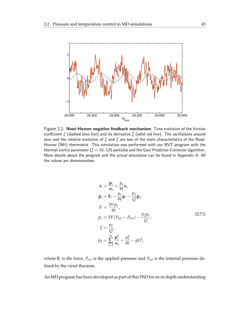
2.2. Pressure and temperature control in MD simulations 45
28,000 28,400 28,800 29,200 29,600 30,000
−1
0
1
Ntime
Figure 2.1: Nose-Hoover negative feedback mechanism. Time evolution of the frictioncoefficient ξ (dashed blue line) and its derivative ξ (solid red line). The oscillations aroundzero and the relative evolution of ξ and ξ are two of the main characteristics of the Nose-Hoover (NH) thermostat. This simulation was performed with our NVT program with thethermal inertia parameter Q = 10, 125 particles and the Gear Predictor-Corrector algorithm.More details about the program and the actual simulation can be found in Appendix A. Allthe values are dimensionless.
ri =pi
mi+
pǫ
Wri,
pi = Fi −pǫ
Wpi −
pξ
Qpi,
V =3Vpǫ
W,
pǫ = 3V(Pint − Pext) −pξ pǫ
Q,
ξ =pξ
Q,
pξ =N
∑i=1
p2i
mi+
p2ǫ
W− gkT,
(2.71)
where Fi is the force, Pext is the applied pressure and Pint is the internal pressure de-
fined by the virial theorem.
An MD program has been developed as part of this PhD for an in-depth understanding
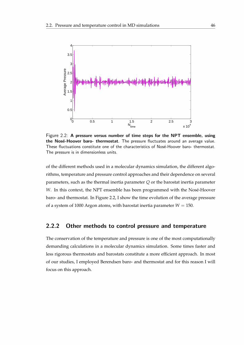
2.2. Pressure and temperature control in MD simulations 46
0 0.5 1 1.5 2 2.5 3
x 104
0
0.5
1
1.5
2
2.5
3
3.5
4
Ntime
Ave
rage
Pre
ssur
e
Figure 2.2: A pressure versus number of time steps for the NPT ensemble, usingthe Nose-Hoover baro- thermostat. The pressure fluctuates around an average value.These fluctuations constitute one of the characteristics of Nose-Hoover baro- thermostat.The pressure is in dimensionless units.
of the different methods used in a molecular dynamics simulation, the different algo-
rithms, temperature and pressure control approaches and their dependence on several
parameters, such as the thermal inertia parameter Q or the barostat inertia parameter
W. In this context, the NPT ensemble has been programmed with the Nose-Hoover
baro- and thermostat. In Figure 2.2, I show the time evolution of the average pressure
of a system of 1000 Argon atoms, with barostat inertia parameter W = 150.
2.2.2 Other methods to control pressure and temperature
The conservation of the temperature and pressure is one of the most computationally
demanding calculations in a molecular dynamics simulation. Some times faster and
less rigorous thermostats and barostats constitute a more efficient approach. In most
of our studies, I employed Berendsen baro- and thermostat and for this reason I will
focus on this approach.
2.2. Pressure and temperature control in MD simulations 47
Berendsen barostat: In this approach, the volume of the system is scaled by a factor
µ3 at each time step2. The parameter µ is given by:
µ =
[
1 − ∆t
τP(P − P0)
]1/3
, (2.72)
where P is the instantaneous pressure, P0 is the desired pressure, ∆t is the time step
and τP is a user defined time constant, with which user can adjust the strength of
pressure coupling.
One of the main advantages of Berendsen barostat, apart from its simplicity, is the
choice of having either isotropic or anisotropic coupling by just using different scaling
factors for every dimension of the system.
Berendsen thermostat: Berendsen thermostat [135] is a proportional type of thermo-
stat, that follows the same general idea; the velocities of all particles are scaled at each
step by a factor λ,
λ =
[
1 +∆t
τT
(
T0
Ti− 1
)]1/2
, (2.73)
where Ti is the instantaneous temperature, T0 is the desired temperature, ∆t is the time
step and τT is a user defined time constant. τT is a parameter that is used to adjust the
strength of the coupling of the system to a hypothetical heat bath.
The equation of motion corresponding to the Berendsen thermostat is:
mi ri = Fi(t) − 1
2τ−1
T
[
T0
T(t)− 1
]
ri. (2.74)
A system coupled with a heating bath using the Berendsen thermostat does not strictly
follow the canonical ensemble [136]. However, in practice, the deviation from canoni-
cal is usually small.
To close this section, I need to mention that there are several other approaches for
thermostats and barostats. More information can be found in [137–139].
2In the case of non-cubic systems, each coordinate is scaled by a factor of µ.
2.3. Implementation issues 48
2.3 Implementation issues
2.3.1 Time integration algorithm
Now that I have formulated the equations of motion for a system of N particles in
various ensembles, I can introduce the main idea behind molecular dynamics. From
Equation (2.21), one can calculate the forces on each of the particles of the system at a
particular time. Once the forces are computed, Equation (2.21) is integrated numeri-
cally in order to produce the new positions and new velocities of each particle of the
system. Then, the new coordinates are used to calculate the potential energy again.
For this procedure a time integration algorithm is needed.
The time integration algorithms are based on finite difference methods. The idea be-
hind these methods is that the time is broken down into smaller stages, separated by
a time step dt, creating a finite grid. At a point of this grid, corresponding to time
t, the positions and a number of their derivatives are known (or can be calculated),
and are used in order to estimate the same quantities at a time t + dt as Taylor series
expansions,
r(t + dt) = r(t) + dtv(t) +1
2dt2a(t) +
1
6dt3b(t) +
1
24dt4c(t) + · · · (2.75)
v(t + dt) = v(t) + dta(t) +1
2dt2b(t) +
1
6dt3c(t) + · · · (2.76)
a(t + dt) = a(t) + dtb(t) +1
2dt2c(t) + · · · (2.77)
b(t + dt) = b(t) + dtc(t) + · · · (2.78)
where v is the first derivative of the positions with respect to time (velocity), a is the
second derivative of the positions (acceleration), b is the third derivative and so on.
There are several different algorithms used in molecular dynamics with the Verlet al-
gorithm [140] and its variations being the most widely used. In the majority of our
studies, one of these variations, the so-called leap-frog algorithm is used for the inte-
gration of the equations of motion [141]. The relationships used in leap-frog algorithm
are

2.3. Implementation issues 49
r (t + dt) = r (t) + dtv
(
t +1
2dt
)
(2.79)
v
(
t +1
2dt
)
= v
(
t − 1
2dt
)
+ dta (t) (2.80)
and it can be easily shown that the velocity is calculated by making use of the half
intervals,
v (t) =
v
(
t +1
2dt
)
+ v
(
t − 1
2dt
)
2. (2.81)
Overall, in the leap-frog algorithm, the velocities at t +1
2dt are calculated from the
velocities at t − 1
2dt and the accelerations at t. From the calculated velocities and the
position at time t, the new positions at t + dt are estimated.
2.3.2 Periodic boundary conditions
In the majority of the applications of MD simulations, in order to get a realistic view
of a phenomenon, one would like to be able to treat the system in a bulk environment,
and not in a simulation cell of limited dimensions. In order to achieve this ‘bulk’
behaviour of the system, a technique known as periodic boundary conditions (PBC)
is used. In this technique, the single simulation cell is infinitely replicated in the three
Cartesian dimensions3. So, if one particle is located at position r, then this particle
represents an infinite number of particles at the following positions,
r + kα + lβ + mγ, k, l and m ∈ Z (2.82)
where α, β and γ the three vectors representing the dimensions of the simulation cell.
The most important feature of PBC is that every particle can interact not only with the
3There are cases where, depending on the system and the phenomenon under study, this replicationis done in one or two dimensions.

2.3. Implementation issues 50
Figure 2.3: Periodic boundary conditions. A two dimensional representation of theperiodic boundary conditions. The simulation cell, which is coloured grey, is infinitelyreplicated in three dimensions. Once a particle ‘leaves’ the simulation cell, it reenters to itfrom the opposite side and the total number of particles in each cell is constant.
particles that are already in the simulation cell, but also with the ones located in the
neighbouring cells. This way, any surface effects due to the finite dimensions of the
cell are eliminated. However, with the PBC there could be effects associated with the
artificial periodicity of the system. Also, any movement of a particle outside the cell
does not affect its interaction with the particles close to it, as the particle ‘leaves’ the
cell and re-enters to it from the opposite side (Figure 2.3).
Another technique used in combination with the PBC is the minimum image conven-
tion.
The minimum image convention
In the minimum image convention, every particle i interacts only with the closest im-
age of particle j. There are some assumptions to be made so that this condition holds.
As described before, a usual treatment for a potential is to neglect all the interactions
after a cut-off distance rc between two particles. If now we assume that the simulation

2.3. Implementation issues 51
cell is larger than 2rc, it is clear that under these conditions there is at most one pair
formed by particle i in the cell and all the images of a particle j.
2.3.3 Neighbour list
Neighbour list is a method used in combination with cut-off for the calculation of in-
teractions between particles. In addition to a cut-off radius rc, another radius rn, larger
than rc, is defined. This radius is used in the creation of a ‘neighbour list’ that includes
the atoms that are located at a distance smaller than rn. In the calculation of short-
range interactions, only the particles in each particle’s neighbour list are considered.
While the simulation proceeds, particles move in or out of the boundaries of rn. It is
thus necessary that the neighbour list is updated regularly throughout the simulation.
In order for this to be done periodically and not at each step, rn should be chosen so
that the difference rn − rc is large enough.
It is also important to note here, that the neighbour list method leads to a noticeable
speedup in the calculation of the forces, as the time to examine all pair separations in
a system of N particles is proportional to N2 and this calculation is avoided between
the updates of the list.
2.3.4 Pressure coupling protocols
Apart from the different barostats, there are three different ways to implement pres-
sure coupling, as illustrated in Figure 2.4:
• isotropic : in this case all three pressure contributions are coupled, i.e. a change
in volume is implemented by changing the length of the box edges by the same
increment.
• semiisotropic : with this option, only the pressure contributions in x and y direc-
tions are coupled.
• anisotropic : there is no coupling between any of the pressure contributions.
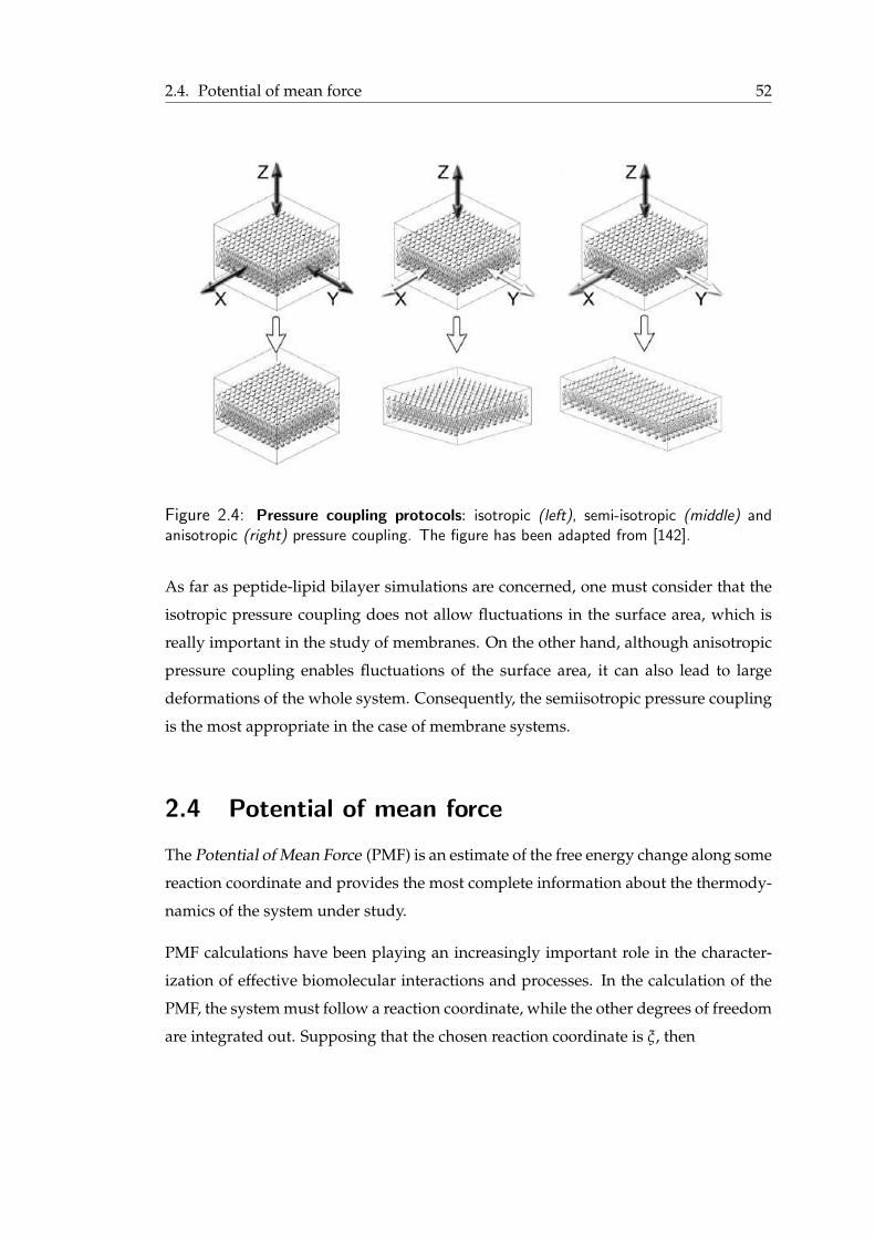
2.4. Potential of mean force 52
Figure 2.4: Pressure coupling protocols: isotropic (left), semi-isotropic (middle) andanisotropic (right) pressure coupling. The figure has been adapted from [142].
As far as peptide-lipid bilayer simulations are concerned, one must consider that the
isotropic pressure coupling does not allow fluctuations in the surface area, which is
really important in the study of membranes. On the other hand, although anisotropic
pressure coupling enables fluctuations of the surface area, it can also lead to large
deformations of the whole system. Consequently, the semiisotropic pressure coupling
is the most appropriate in the case of membrane systems.
2.4 Potential of mean force
The Potential of Mean Force (PMF) is an estimate of the free energy change along some
reaction coordinate and provides the most complete information about the thermody-
namics of the system under study.
PMF calculations have been playing an increasingly important role in the character-
ization of effective biomolecular interactions and processes. In the calculation of the
PMF, the system must follow a reaction coordinate, while the other degrees of freedom
are integrated out. Supposing that the chosen reaction coordinate is ξ, then
2.4. Potential of mean force 53
A(ξ) = −kBT lnP(ξ), (2.83)
where A is the free energy of the system and P is the probability distribution to find
the system at a specific value of the reaction coordinate.
Ideally, one would be able to calculate the free energy difference by counting how
often the system samples the different values of the reaction coordinate ξ. However,
with simple MD simulations it is not possible to sample two states separated by a high
energy barrier, and it is thus an inefficient method for this type of calculations. In
these studies, I choose one of the most used and validated methods for the calculation
of PMF, the umbrella sampling method [143].
In umbrella sampling, the potential function of the system is modified so that the all
the possible states are sampled sufficiently. Considering a reaction coordinate ξ, the
modified potential is given by
V ′(ξ) = V(ξ) + W(ξ), (2.84)
where W is a weighting function, also referred as the biasing potential 4. Usually, the
weighting function has the following form
W(ξ) = k(ξ − ξ0)2, (2.85)
and acts as a spring that encourages barrier crossing. The furthest the system is from
the equilibrium state ξ0, the largest the value of the weighting function, leading to a
non-Boltzmann distribution.
A range of values for the reaction coordinate ξ is chosen, (ξmin, ξmax), and is divided
into N windows centered around chosen values of ξi, with i = 1, . . . , N. In each win-
dow, the reference system is under the influence of the weighting function Wi and the
reaction coordinate is sampled. The biased probability function is given by
4It is important to note that since the potential has changed, the probability function will be deter-mined using this potential.

2.4. Potential of mean force 54
P ′i (ξ) =
Z0
Ziexp−Wi(ξ) P0(ξ), (2.86)
where 0 denotes the reference position and i the window.
It can be shown that the unbiased free energy is given by,
A(ξ) = −kBT lnP ′(ξ) −W(ξ) + K, (2.87)
where K is a free energy constant and depends on W(ξ). An efficient way of estimating
this constant is by using the weighted histogram analysis method (WHAM).
Weighted histogram analysis method
The weighted histogram analysis method is an optimization procedure to calculate the
constants Ki, so that the estimate for the unbiased distribution function is the weighted
sum over the individual unbiased distribution functions of all the N windows used
[144]
P0(ξ) =∑
Ni=1 niP
′i (ξ)
∑Ni=1 ni exp[−(W i(ξ) − Ki)/kBT]
(2.88)
where ni is the number of observations used to construct the biased distribution func-
tion. Also,
Ki = −kBT lnN
∑i=1
P ′(ξ) exp[−W i(ξ)/kBT]. (2.89)
Finally, Equations (2.88) and (2.89) are solved via iterative procedures.
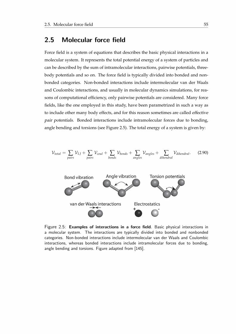
2.5. Molecular force field 55
2.5 Molecular force field
Force field is a system of equations that describes the basic physical interactions in a
molecular system. It represents the total potential energy of a system of particles and
can be described by the sum of intramolecular interactions, pairwise potentials, three-
body potentials and so on. The force field is typically divided into bonded and non-
bonded categories. Non-bonded interactions include intermolecular van der Waals
and Coulombic interactions, and usually in molecular dynamics simulations, for rea-
sons of computational efficiency, only pairwise potentials are considered. Many force
fields, like the one employed in this study, have been parametrized in such a way as
to include other many body effects, and for this reason sometimes are called effective
pair potentials. Bonded interactions include intramolecular forces due to bonding,
angle bending and torsions (see Figure 2.5). The total energy of a system is given by:
Vtotal = ∑pairs
VLJ + ∑pairs
Vcoul + ∑bonds
Vbonds + ∑angles
Vangles + ∑dihendral
Vdihendral . (2.90)
Figure 2.5: Examples of interactions in a force field. Basic physical interactions ina molecular system. The interactions are typically divided into bonded and nonbondedcategories. Non-bonded interactions include intermolecular van der Waals and Coulombicinteractions, whereas bonded interactions include intramolecular forces due to bonding,angle bending and torsions. Figure adapted from [145].
2.5. Molecular force field 56
2.5.1 Non-bonded interactions
van der Waals Interactions
In order to calculate the forces on each particle of a system, one needs a description of
interparticle interactions, or potentials. One of the simplest and most used potentials
to describe the van der Waals interactions is the Lennard-Jones (LJ) 12-6 potential. For
a pair of atoms i and j located at ri and rj the LJ 12-6 potential energy is
VLJ(rij) = 4ǫ
[
(
σ
rij
)12
−(
σ
rij
)6]
, (2.91)
where rij = ri − rj and rij = ‖rij‖, ǫ is the depth of the potential and σ is the collision
diameter. The potential described by Equation (2.91) includes both a short-range, re-
pulsive component due to electronic clouds overlap, and an attractive component due
to dispersion forces.
Since intermolecular forces are necessarily conservative, the force that atom j exerts on
atom i is given by
Fij =
(
48ǫ
σ2
)
[
(
σ
rij
)14
− 1
2
(
σ
rij
)8]
rij. (2.92)
As depicted in Figure 2.6, the contribution of remote particles to the total LJ-potential
can be considered insignificant. We can thus neglect pair interactions beyond some cut
off radius rc in order to save computational time.
A common choice for rc is 2.5σ as for rij = rc, Fij has a comparatively small value.
Usually in practice, in order to avoid large errors and the noise induced by the cut-off
effects, the truncated forces are replaced by forces that are continuous with continuous
derivatives at the cut-off radius. This method is called shift.
The shifted force Fs will be given by
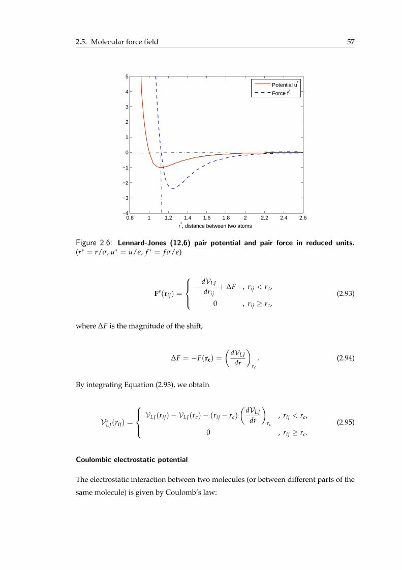
2.5. Molecular force field 57
0.8 1 1.2 1.4 1.6 1.8 2 2.2 2.4 2.6−4
−3
−2
−1
0
1
2
3
4
5
r*, distance between two atoms
Potential u*
Force f*
Figure 2.6: Lennard-Jones (12,6) pair potential and pair force in reduced units.(r∗ = r/σ, u∗ = u/ǫ, f ∗ = f σ/ǫ)
Fs(rij) =
−dVLJ
drij+ ∆F , rij < rc,
0 , rij ≥ rc,
(2.93)
where ∆F is the magnitude of the shift,
∆F = −F(rc) =
(
dVLJ
dr
)
rc
. (2.94)
By integrating Equation (2.93), we obtain
V sLJ(rij) =
VLJ(rij) − VLJ(rc) − (rij − rc)
(
dVLJ
dr
)
rc
, rij < rc,
0 , rij ≥ rc.
(2.95)
Coulombic electrostatic potential
The electrostatic interaction between two molecules (or between different parts of the
same molecule) is given by Coulomb’s law:
2.5. Molecular force field 58
Vcoul(rij) =qiqj
4πǫ0rij, (2.96)
where ǫ0 is the permittivity in vacuum, qi and qj represent the charges on particles i
and j respectively, and rij is the distance between particles i and j.
The Coulombic force that atom j exerts on atom i is
Fcoulij =
qiqj
4πǫ0r2ij
. (2.97)
The treatment of electrostatic interactions has become a subject of controversy in the
area of molecular dynamics simulations. The use of a cut-off is reasonably efficient
for van der Waals interactions with r−6 radial dependence, such as the Lennard-Jones
potential. However, this treatment may lead to artefacts in the case of electrostatic
interactions, since they have considerably longer range (they decay as a function of
r−1). A more efficient approach is the Ewald summation technique.
In Ewald summation method, the slowly converging charge distribution is treated as
the sum of two reciprocal space distributions, which converges much faster. Suppos-
ing that we have a system of N particles, treated with periodic boundary conditions
and with a dielectric constant ǫ0, we have
Vcoul =1
2 ∑n
N
∑i=1
N
∑j=1
qiqj
4πǫ0|rij + n| , (2.98)
where n = (nxLx, nyLy, nzLz), with Lx, Ly, Lz the dimensions of the simulation box and
nx, ny, nz integer indicating the position at the cubic lattice created from the periodic
boundary conditions. In the case that |n| = 0, i.e. we are in the central box, the first
sum is for all the i and j with i 6= j.
Equation (2.98) converges very slowly. The key to this method is that instead of wait-
ing for Equation (2.98) to converge, the summation is broken into two series that con-
verge much faster. Each point charge is surrounded by a Gaussian charge distribution,

2.5. Molecular force field 59
Figure 2.7: Ewald summation. The initial set of charges (left) are surrounded bya Gaussian distribution calculated in the real space (top right) and then cancelled by aGaussian distribution calculated in the reciprocal space (bottom right).
ρi(r) =qiα
3
π3/2exp(−α2r2), ∀ i ∈ 1, . . . , N, (2.99)
where α is a positive parameter that determines the width of distribution. These Gaus-
sians are cancelled with the corresponding Gaussians of negative sign in reciprocal
space, in order to determine the original coulombic potential (Figure 2.7).
There are several variations of Ewald summation method, with the particle mesh
Ewald (PME) being one of the most widely used in molecular dynamics simulations.
Briefly, in PME, only the 27 nearest points in the three dimensions are used in the cal-
culation of potential. From this 27-point mesh of charge density, through the use of fast
Fourier transform, and interpolation, the potential at each of the particles is calculated.
Apart from the cut-off and the lattice-sum techniques, like the PME, there are the reac-
tion field approaches (RF). In these methods, a correction term is added to the cut-off
result based on a continuum electrostatics description of the solvent outside the cut-
off sphere [142]. This way the effect of long-range electrostatic interactions is also in-
cluded. However, due the structure of lipid bilayers, this approach is not appropriate
for the description of electrostatic interactions for peptide-membrane systems.
More detailed description of the different approaches for the treatement of the elec-
trostatics can be found in Allen and Tildesley [139], Leach [137] and Frenkel and Smit
2.5. Molecular force field 60
[138].
2.5.2 Bonded interactions
In order to describe the structure of a molecule, one uses the interatomic distances
constrained by chemical bond lengths between two particles, the bond angles between
three particles and dihedral angles between three consecutive bond vectors. I will
shortly present the most common approaches for the treatment of bonded interactions.
Bond length
The bond length (stretching) between two particles is often modelled using a harmonic
spring potential:
Vbond(r) =1
2kb(r − rb)
2, (2.100)
where kb is the bond force constant representing the stiffness of the bond, rb is the
equilibrium bond length and r is the distance between the two bonded atoms.
Angle bending
Angle bending, like the bond length interaction, can be represented by a harmonic
potential as a function of θ, which is the angle formed by three particles:
Vangle(θ) = kθ(θ − θ0)2, (2.101)
where kθ is the angle force constant and θ0 is the optimal equilibrium angle.
Torsions
The dihedral angle potentials describe the interaction arising from torsional forces be-
tween particles and they require the specification of four atomic positions. One of the
mainly used expressions for the dihedral angle potential is:
2.6. The molecular model 61
Vdihendral(φ) = kφ(1 + cos(nφ − δ)), (2.102)
where φ is the dihedral angle, kφ is the dihendral force constant, n is the multiplicity,
and δ is the phase of the potential.
2.6 The molecular model
2.6.1 Molecular mapping and interaction sites
In the studies presented in this thesis, the species are described using the model of
lipids and peptides recently proposed by Marrink and co-workers (MARTINI) [105,
106]. The MARTINI was developed in an effort to expand an already successful coarse-
grained protocol for membranes to proteins. In the following sections, I will present
a general description of the model and force field parameters, and I will focus on the
representations and parameters used for the modelling of membranes and peptides.
In the MARTINI, every four heavy atoms (i.e. not hydrogens) are represented by one
effective bead, with an exception made for ring structures. There are four main types
of beads representing different levels of interaction: polar (P), apolar (C), nonpolar
(N), and charged (Q). Apart from these main types, each bead is assigned a further
subtype, in order to describe more accurately the overall chemical nature of the rep-
resented group of atoms. In this description, hydrogen-bonding capability (d=donor,
a=acceptor, da=both and 0=none) and different levels of polarity (from 1=low polarity,
to 5=high polarity) are included. All the beads are assigned a mass of m=72 amu (four
water molecules) for reasons of computational efficiency (for the beads that take part
in ring structures this value is equal to 45 amu).
2.6.2 The molecular force field
In the MARTINI, the van der Waals interactions are described using a shifted Lennard-
Jones 12-6 potential. An effective size of σ=0.47 nm is used (this value is slightly
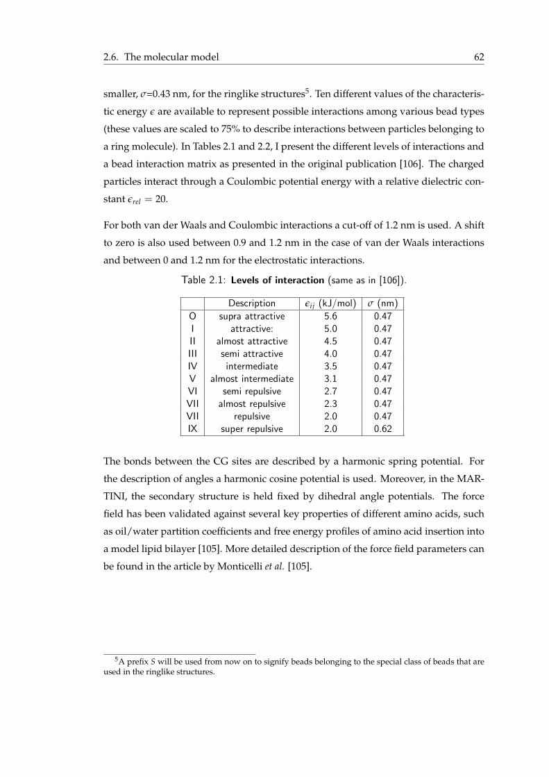
2.6. The molecular model 62
smaller, σ=0.43 nm, for the ringlike structures5. Ten different values of the characteris-
tic energy ǫ are available to represent possible interactions among various bead types
(these values are scaled to 75% to describe interactions between particles belonging to
a ring molecule). In Tables 2.1 and 2.2, I present the different levels of interactions and
a bead interaction matrix as presented in the original publication [106]. The charged
particles interact through a Coulombic potential energy with a relative dielectric con-
stant ǫrel = 20.
For both van der Waals and Coulombic interactions a cut-off of 1.2 nm is used. A shift
to zero is also used between 0.9 and 1.2 nm in the case of van der Waals interactions
and between 0 and 1.2 nm for the electrostatic interactions.
Table 2.1: Levels of interaction (same as in [106]).
Description ǫij (kJ/mol) σ (nm)
O supra attractive 5.6 0.47I attractive: 5.0 0.47II almost attractive 4.5 0.47III semi attractive 4.0 0.47IV intermediate 3.5 0.47V almost intermediate 3.1 0.47VI semi repulsive 2.7 0.47VII almost repulsive 2.3 0.47VII repulsive 2.0 0.47IX super repulsive 2.0 0.62
The bonds between the CG sites are described by a harmonic spring potential. For
the description of angles a harmonic cosine potential is used. Moreover, in the MAR-
TINI, the secondary structure is held fixed by dihedral angle potentials. The force
field has been validated against several key properties of different amino acids, such
as oil/water partition coefficients and free energy profiles of amino acid insertion into
a model lipid bilayer [105]. More detailed description of the force field parameters can
be found in the article by Monticelli et al. [105].
5A prefix S will be used from now on to signify beads belonging to the special class of beads that areused in the ringlike structures.

2.6.T
he
mo
lecular
mo
del
63
Table 2.2: Interaction matrix (same as in [106]).
Q P N Cda d a 0 5 4 3 2 1 da d a 0 5 4 3 2 1
Q da O O O II O O O I I I I I IV V VI VII IX IXd O I O II O O O I I I III I IV V VI VII IX IXa O O I II O O O I I I I III IV V VI VII IX IX0 II II II IV I O I II III III III III IV V VI VII IX IX
P 5 O O O I O O O O O I I I IV V VI VI VII VIII4 O O O O O I I II II III III III IV V VI VI VII VIII3 O O O I O I I II II II II II IV IV V V VI VII2 I I I II O II II II II II II II III IV IV V VI VII1 I I I III O II II II II II II II III IV IV IV V VI
N da I I I III I III II II II II II II IV IV V VI VI VId I III I III I III II II II II III II IV IV V VI VI VIa I I III III I III II II II II II III IV IV V VI VI VI0 IV IV IV IV IV IV IV III III IV IV IV IV IV IV IV V VI
C 5 V V V V V V IV IV IV IV IV IV IV IV IV IV V V4 VI VI VI VI VI VI V IV IV V V V IV IV IV IV V V3 VII VII VII VII VI VI V V IV VI VI VI IV IV IV IV IV IV2 IX IX IX IX VII VII VI VI V VI VI VI V V V IV IV IV1 IX IX IX IX VIII VIII VII VII VI VI VI VI VI V V IV IV IV

2.6. The molecular model 64
2.6.3 Coarse-grained description of a peptide-membrane sys-
tem
The membrane
The membranes used in the coarse-grained simulations of this thesis have been repre-
sented with the MARTINI force field. As described in the Introduction, a membrane
is composed mainly of lipids and proteins. For reasons of simplicity, I will represent
the membrane as a lipid bilayer, without undervaluing the importance of membrane
proteins in the overall functionality of a cell membrane.
Figure 2.8: Atomistic and coarse-grained representations for a DPPC lipid.Atomistic (left) and coarse-grained (right) representations for a DPPC lipid. We can notethe dramatic reduction in system size from the AL to the CG representation. This reducessignificantly the time and memory requirements of the simulation. Colours: a) for the atom-istic representation: carbon=light blue, oxygen=red, nitrogen=dark blue, hydrogen=white,b) for the coarse-grained representation: lipid tails (C1 type)=yellow, glycerol moiety (Na-type)=orange, phosphate moiety (Qa-type)=purple and choline group (Q0-type)=pink.
In Figure 2.8, there are the atomistic and coarse-grained representations of a DPPC
lipid. The lipid tails are represented as C1-type beads, the glycerol moiety as Na-type,
the phosphate moiety as Qa-type and the choline group as Q0-type beads. Moreover,
in the MARTINI, four water molecules are represented by a P4-type bead. A lipid
bilayer described by the MARTINI force field is depicted in Figure 2.9.

2.6. The molecular model 65
Figure 2.9: Coarse-grained representation of a lipid bilayer. Colours: lipid tails(C1 type)=yellow, glycerol moiety (Na-type)=orange, phosphate moiety (Qa-type)=purple,choline group (Q0-type)=pink and water beads (P4-type)=light blue.
The peptides
The coarse-grained representation of the different natural amino acids is done in the
same way described above. The side chains of the amino acids are mapped to the
coarse-grained beads that describe appropriately their properties. The hydrophobic
amino acids are mapped to C-type beads, the hydrophilic to P-type beads and for
the representation of the charged amino acids Q-type beads are used. The ring-like
side chains of the bulkier amino acids are represented by three or four beads of ring
particles 6. In Table 2.3, I summarize this mapping. The beads that are shown in
brackets correspond to the protonated state of the amino acids. Alanine and glysine
are represented only by the backbone bead. The backbone bead types depend on the
secondary structure of the peptide or protein that they describe. For example, in the
case of α-helices the backbone structure is mapped into N0-type beads apart from the
termini. For a capped α-helix the termini are represented by Nd-type and Na-type
beads for the N-terminus and C-terminus respectively. In the case where an uncapped
helix is considered, charged beads (Qd and Qa) are used to represent the termini. Also,
the three closest to the termini backbone beads are represented by Nd and Na types for
the N- and C-terminus respectively. The overall mapping of the backbone of a capped
peptide is shown in Table 2.4. In Figure 2.10, I show the atomistic and coarse-grained
representations of LS3 synthetic peptide. From the figure, we can see the dramatic
6These particles are slightly smaller, σ=0.43 nm, and for their description an S is put before the nameof the assigned bead.
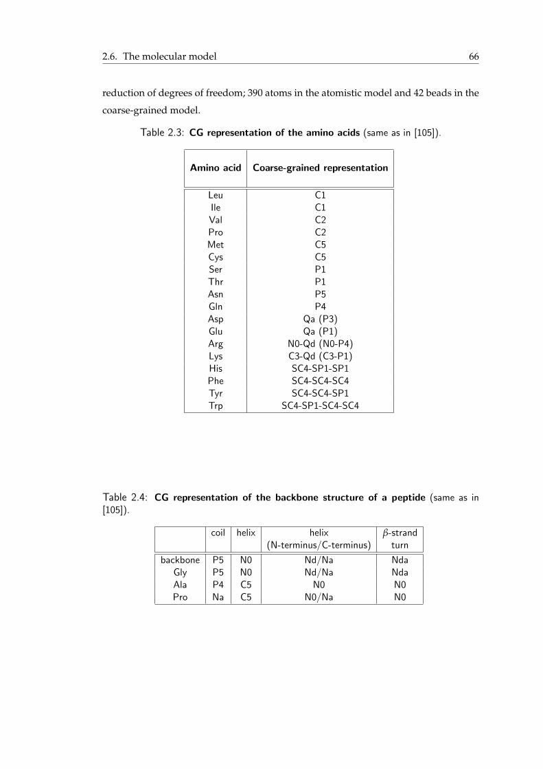
2.6. The molecular model 66
reduction of degrees of freedom; 390 atoms in the atomistic model and 42 beads in the
coarse-grained model.
Table 2.3: CG representation of the amino acids (same as in [105]).
Amino acid Coarse-grained representation
Leu C1Ile C1Val C2Pro C2Met C5Cys C5Ser P1Thr P1Asn P5Gln P4Asp Qa (P3)Glu Qa (P1)Arg N0-Qd (N0-P4)Lys C3-Qd (C3-P1)His SC4-SP1-SP1Phe SC4-SC4-SC4Tyr SC4-SC4-SP1Trp SC4-SP1-SC4-SC4
Table 2.4: CG representation of the backbone structure of a peptide (same as in[105]).
coil helix helix β-strand(N-terminus/C-terminus) turn
backbone P5 N0 Nd/Na NdaGly P5 N0 Nd/Na NdaAla P4 C5 N0 N0Pro Na C5 N0/Na N0

2.7. Data analysis tools 67
Figure 2.10: Atomistic and coarse-grained representations for LS3 synthetic peptide.Colours: a) for the atomistic representation: cyan=carbon, red=oxygen, blue=nitrogen,white=hydrogen, b) for the coarse-grained representation: blue=hydrophobic beads, lightblue=hydrophilic beads and orange= backbone beads. The beads are not shown to scale.
2.7 Data analysis tools
In the current study I am interested in getting information about the dynamics and
structural features and rearrangements of a peptide-membrane system. VMD software
is used throughout this investigation for the direct visualization of the systems under
study [146]. There are however features that cannot be identified simply by viewing
the evolution of a system through time. For this reason, density profiles, peptide angle
distributions, the radii of formatted pores as well as their self-diffusion coefficient are
calculated in this study. For the later, GROMACS software was used to get the mean
squared displacement and by using the Einstein relation and weighted least squares
I estimated the self-diffusion coefficient [147]. More details about these calculations
will be given in the relevant chapter. For the other features I developed a range of
programs which will be described in the following sections.
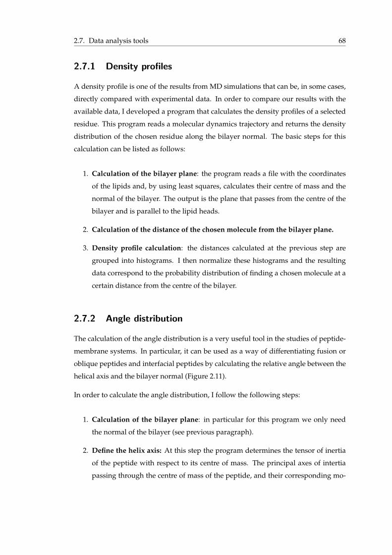
2.7. Data analysis tools 68
2.7.1 Density profiles
A density profile is one of the results from MD simulations that can be, in some cases,
directly compared with experimental data. In order to compare our results with the
available data, I developed a program that calculates the density profiles of a selected
residue. This program reads a molecular dynamics trajectory and returns the density
distribution of the chosen residue along the bilayer normal. The basic steps for this
calculation can be listed as follows:
1. Calculation of the bilayer plane: the program reads a file with the coordinates
of the lipids and, by using least squares, calculates their centre of mass and the
normal of the bilayer. The output is the plane that passes from the centre of the
bilayer and is parallel to the lipid heads.
2. Calculation of the distance of the chosen molecule from the bilayer plane.
3. Density profile calculation: the distances calculated at the previous step are
grouped into histograms. I then normalize these histograms and the resulting
data correspond to the probability distribution of finding a chosen molecule at a
certain distance from the centre of the bilayer.
2.7.2 Angle distribution
The calculation of the angle distribution is a very useful tool in the studies of peptide-
membrane systems. In particular, it can be used as a way of differentiating fusion or
oblique peptides and interfacial peptides by calculating the relative angle between the
helical axis and the bilayer normal (Figure 2.11).
In order to calculate the angle distribution, I follow the following steps:
1. Calculation of the bilayer plane: in particular for this program we only need
the normal of the bilayer (see previous paragraph).
2. Define the helix axis: At this step the program determines the tensor of inertia
of the peptide with respect to its centre of mass. The principal axes of intertia
passing through the centre of mass of the peptide, and their corresponding mo-
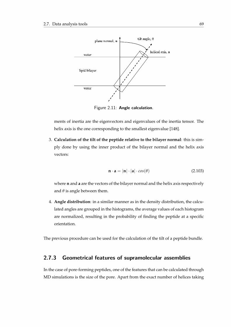
2.7. Data analysis tools 69
Figure 2.11: Angle calculation.
ments of inertia are the eigenvectors and eigenvalues of the inertia tensor. The
helix axis is the one corresponding to the smallest eigenvalue [148].
3. Calculation of the tilt of the peptide relative to the bilayer normal: this is sim-
ply done by using the inner product of the bilayer normal and the helix axis
vectors:
n · a = |n| · |a| · cos(θ) (2.103)
where n and a are the vectors of the bilayer normal and the helix axis respectively
and θ is angle between them.
4. Angle distribution: in a similar manner as in the density distribution, the calcu-
lated angles are grouped in the histograms, the average values of each histogram
are normalized, resulting in the probability of finding the peptide at a specific
orientation.
The previous procedure can be used for the calculation of the tilt of a peptide bundle.
2.7.3 Geometrical features of supramolecular assemblies
In the case of pore-forming peptides, one of the features that can be calculated through
MD simulations is the size of the pore. Apart from the exact number of helices taking
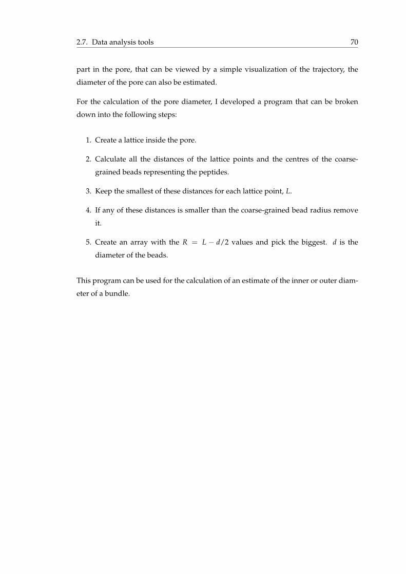
2.7. Data analysis tools 70
part in the pore, that can be viewed by a simple visualization of the trajectory, the
diameter of the pore can also be estimated.
For the calculation of the pore diameter, I developed a program that can be broken
down into the following steps:
1. Create a lattice inside the pore.
2. Calculate all the distances of the lattice points and the centres of the coarse-
grained beads representing the peptides.
3. Keep the smallest of these distances for each lattice point, L.
4. If any of these distances is smaller than the coarse-grained bead radius remove
it.
5. Create an array with the R = L − d/2 values and pick the biggest. d is the
diameter of the beads.
This program can be used for the calculation of an estimate of the inner or outer diam-
eter of a bundle.
CHAPTER 3
Coarse-grained model validation:
Application to different classes of
amphipathic α-helical peptides
Until now, I have introduced the biological and modelling background on peptide-
membrane interactions. In this chapter, I focus on several types of interactions between
lipid membranes and α-helical peptides, based on the distribution of hydrophobic and
hydrophilic residues along the helix. I employed the MARTINI force field and tested
its ability to capture diverse types of behaviour. For example, the simulations provided
us with useful insights on the formation of a barrel-stave pore. Amphipathic nonspan-
ning peptides were also described with sufficient accuracy. However, the picture was
not as clear for fusion and transmembrane peptides. For each class of peptides, I cal-
culated the potential of mean force (PMF) for peptide translocation across the lipid
bilayer and demonstrated that each class has a distinct shape of PMF. The reliability of
71

3.1. Introduction 72
these calculations, as well as wider implications of the results, are discussed.
3.1 Introduction
In the effort to test the validity and scope of the MARTINI coarse-grained model, I
was guided by a general classification of possible modes of peptide-membrane inter-
actions for α-helices employed in a series of publications by Brasseur and co-workers
[6, 149, 150]. This classification is based on a view of α-helical peptides as amphiphilic
entities with a well-defined geometry. The idea is that the distribution of hydrophobic
and hydrophilic residues along the α-helix plays a central role in the partition of the
peptide between the hydrophilic aqueous media and the hydrophobic core of the lipid
membrane. Thus, depending on this distribution, several possible scenarios can be
identified and are schematically depicted in Figure 3.1. In these schematics α-helices
are represented as cylinders with their hydrophobic regions shaded yellow. The top
part of each subfigure provides a side-view of the cylinders. From this side-view, one
can observe the difference in the hydrophobicity distribution among various classes of
peptides. At the bottom of each subfigure, I present the proposed interaction mech-
anism for each class. The helices are represented as cylinders coloured orange. Al-
though this is a simplified description, and not all of the α-helical peptides feature
a well-defined distribution of hydrophobic groups, there are many of them whose
structure and behaviour does indeed fall in one of these general classes. Let us briefly
review some of the examples here.
Figure 3.1: Schematic view of the different classes of α-helical peptides accordingto their hydrophobicity distribution along the axis. Top of subfigures: side-view of theα-helices. The helices are represented as cylinders with their hydrophobic regions yellow.Bottom of subfigures: proposed interaction mechanism for each class. The helices arerepresented as cylinders coloured orange. (Adapted from figures 3, 4 and 5 in reference[6].)
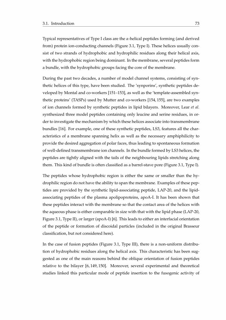
3.1. Introduction 73
Typical representatives of Type I class are the α-helical peptides forming (and derived
from) protein ion-conducting channels (Figure 3.1, Type I). These helices usually con-
sist of two strands of hydrophobic and hydrophilic residues along their helical axis,
with the hydrophobic region being dominant. In the membrane, several peptides form
a bundle, with the hydrophobic groups facing the core of the membrane.
During the past two decades, a number of model channel systems, consisting of syn-
thetic helices of this type, have been studied. The ‘synporins’, synthetic peptides de-
veloped by Montal and co-workers [151–153], as well as the ‘template-assembled syn-
thetic proteins’ (TASPs) used by Mutter and co-workers [154, 155], are two examples
of ion channels formed by synthetic peptides in lipid bilayers. Moreover, Lear et al.
synthesized three model peptides containing only leucine and serine residues, in or-
der to investigate the mechanism by which these helices associate into transmembrane
bundles [16]. For example, one of these synthetic peptides, LS3, features all the char-
acteristics of a membrane spanning helix as well as the necessary amphiphilicity to
provide the desired aggregation of polar faces, thus leading to spontaneous formation
of well-defined transmembrane ion channels. In the bundle formed by LS3 helices, the
peptides are tightly aligned with the tails of the neighbouring lipids stretching along
them. This kind of bundle is often classified as a barrel-stave pore (Figure 3.1, Type I).
The peptides whose hydrophobic region is either the same or smaller than the hy-
drophilic region do not have the ability to span the membrane. Examples of these pep-
tides are provided by the synthetic lipid-associating peptide, LAP-20, and the lipid-
associating peptides of the plasma apolipoproteins, apoA-I. It has been shown that
these peptides interact with the membrane so that the contact area of the helices with
the aqueous phase is either comparable in size with that with the lipid phase (LAP-20,
Figure 3.1, Type II), or larger (apoA-I) [6]. This leads to either an interfacial orientation
of the peptide or formation of discoidal particles (included in the original Brasseur
classification, but not considered here).
In the case of fusion peptides (Figure 3.1, Type III), there is a non-uniform distribu-
tion of hydrophobic residues along the helical axis. This characteristic has been sug-
gested as one of the main reasons behind the oblique orientation of fusion peptides
relative to the bilayer [6, 149, 150]. Moreover, several experimental and theoretical
studies linked this particular mode of peptide insertion to the fusogenic activity of

3.1. Introduction 74
these peptides [149, 156–158]. The fusion peptides of Simian Immunodeficiency Virus
(SIV) [149, 159, 160], Newcastle Disease Virus (NDV) [161] and Human Immunodefi-
ciency Virus (HIV) [159, 162] were some of the first representatives of this class to be
identified.
Those helices that are long enough to span the hydrophobic medium of the membrane,
with most or all of their residues being hydrophobic, tend to adopt a transmembrane
position in a lipid bilayer (Figure 3.1, Type IV). These transmembrane helices have a
uniform distribution of hydrophobic residues both around and along their helical axis.
Among this kind of helices are the Glycophorin A (GpA) [100, 163], the pHLIP peptide
[164–167] as well as the TMX-1 synthetic peptide [54].
Selected representative peptides from each class were chosen in order to probe the
ability of a coarse-grained protocol to capture these diverse scenarios. The selected
peptides satisfy one or more of the following criteria: there should be well-reported
experimental data on their behaviour, they should be sufficiently simple (short), have
a confirmed α-helical structure in the presence of the membranes and be of a certain
technological importance. In Table 3.1, I summarize the peptides considered in this
work and the class of behaviour they belong to.
Table 3.1: Summary of the peptides under study and their primary sequences.
Peptide Sequence Type Ref.
LS3 (LSSLLSL)3 I [16]
LAP20 VSSLLSSLKEYWSSLKESFS II [168]
SIV GVFVLGFLGFLA III [29]
TMX-1 WNALAAVAAALAAVAAALAAVAASKSKSKSK IV [54]
pHLIP ACEQNPIYWARYANWLFTTPLLLLNLALLVDADEGTG IV [164]
In Figure 3.2, I present the side and top view of the peptides under study. For simplic-
ity, I represent the backbone beads of the helices with orange, the side chain beads of all
the hydrophilic residues with light blue and all the side chain beads of the hydropho-
bic residues with yellow. Alanine is represented by one bead coloured yellow as an
3.1. Introduction 75
indication of its hydrophobic nature. In the top view of the helices, the hydrophilic
beads have been removed in order to show the distribution of the hydrophobic beads
around the helical axis.
Figure 3.2: Side and top views of LS3, LAP20, SIV, TMX-1 and pHLIP peptides.Their backbone beads are shown in orange, their hydrophobic residues in yellow and theirhydrophilic residues in light blue. Alanine is represented by one yellow bead.
3.2. Simulation parameters 76
3.2 Simulation parameters
The simulations presented in this study were performed with GROMACS simulation
package, version 3.3.2 [169]. Initially, I employed molecular dynamics simulations of
lipid and water components, in order to obtain the initial bilayer structures that were
used in our studies. These preliminary simulations were up to 200 ns long depending
on the size of the bilayer. The protocol and the simulation parameters used for these
assembly simulations have previously been employed by Marrink and co-workers
[82]. Three different types of lipid bilayer systems were considered: 1,2-Dipalmitoyl-
sn-Glycero-3-phosphocholine or DPPC, 1,2-Dioleoyl-sn-Glycero-3-phosphocholine or
DOPC and 1-Palmitoyl,2-oleoyl-sn-Glycero-3-phosphocholine or POPC. I chose differ-
ent lipid systems in order to have a direct comparison with the corresponding experi-
mental studies for each peptide.
The atomistic structures of the peptides were generated using HyperChem 8.0 soft-
ware [170]. To coarse-grain these structures, I applied the script provided on the MAR-
TINI force field web page [171]. All peptides of interest were considered to be in the
α-helical secondary structure1. In the coarse-grained description their α-helical struc-
ture was maintained via the constraints imposed by the MARTINI force field. All the
peptides were capped at their termini apart from the LS3 peptide. After minimizing
the energy of individual peptide molecules, I randomly inserted them in the system of
interest. In the cases where the peptides under study were charged, ions were inserted
in the system to maintain the overall system electroneutrality. For each system, I then
performed energy minimization using the steepest descent method. Finally, molecular
dynamics (MD) simulations with constant pressure, temperature and number of par-
ticles (NPT ensemble) were performed. The temperature was kept constant for each
group, at 323 K for the DPPC/peptides systems and 300 K for the DOPC/peptide and
POPC/peptide systems, using the Berendsen thermostat with a relaxation time of 1 ps
[135]. The pressure of the system was semi-isotropically coupled and maintained at
1 bar using the Berendsen algorithm with a time constant of 5 ps and a compressibil-
ity of 4.5 × 10⁻⁵ bar−1 [135]. The non-bonded potential energy functions were cut-off
and shifted at 12 A, with forces smoothly decaying between 9 A and 12 A for van
der Waals forces and throughout the whole interaction range for the treatment of elec-
1In the case of SIV fusion peptide the C-terminus is left flexible. See also section 3.2.1.
3.2. Simulation parameters 77
trostatic forces. The simulations were performed using a 25 fs integration time step.
The simulation parameters applied in our membrane-peptide studies have previously
been proposed and used by other groups [100, 105].
3.2.1 Atomistic simulations
For the specific case of the SIV fusion peptide, I also performed atomistic molecu-
lar dynamics simulations in a DOPC bilayer. I used the united atom lipid parame-
ters initially developed by Berger et al. [172], and modified for DOPC lipids by Siu
et al. [173, 174], combined with the GROMOS96 force field and Simple Point Charge
(SPC) model for water proposed by Berendsen [175]. I assumed that the peptide is
in an α-helical secondary structure, apart from its C-terminus which is left flexible, in
agreement with previous observations [29]. To maintain the secondary structure, I put
restraints between the ith- (ith + 4) α-carbons, starting from the third residue of the pep-
tide. I performed a number of self-assembly molecular dynamics simulations, up to
100 ns long, initially with the lipids and water randomly mixed and allowed to spon-
taneously form a lipid bilayer. From the formed lipid bilayers, I chose a system of 97
DOPC molecules and 4947 water molecules. I then randomly inserted the SIV fusion
peptide in the water phase of the system, and performed NPT molecular dynamics
simulations. All simulations were carried out using the GROMACS simulation pack-
age [169], following the approach proposed by de Vries et al. [176], at T = 300 K, P = 1
bar, with a time step of 2.5 fs, using the Berendsen thermostat and barostat [135].
3.2.2 Potential of mean force calculations
I am interested in the potential of mean force (PMF) as a function of the distance be-
tween the peptide and the lipid bilayer. In this study, the PMF was calculated using the
umbrella sampling protocol [143]. This calculation was performed for coarse-grained
models of peptides only. All PMF calculations were carried out for a single peptide
interacting with a bilayer. The total separation distance between the peptide and the
centre of the bilayer was 5 nm and was divided into 50 small windows of 0.1 nm each.
For each peptide, three sets of umbrella sampling simulations with 50 windows were
performed. In each set and in each window, I used different independent initial con-

3.3. Results 78
figurations, with the peptide placed at the corresponding distance from the centre of
the bilayer. The system was then left to equilibrate for several nanoseconds. After-
wards, a 100 ns long simulation was performed, with the biasing potential applied to
restrain the centre of mass of the peptide at a required distance from the centre of the
bilayer. Thus, a single PMF profile required 50 simulations, covering the whole sepa-
ration range of interest, with a total simulation time of 5 µs. A force constant of 1000
kJ mol−1 nm−2 was applied, following the approach by Monticelli et al. [105]. The
system used in the case of the longer peptides featured a large enough water phase to
avoid possible effects associated with the system size and peptide-peptide interactions
over periodic boundaries. The peptides were left free to rotate around their restrained
centre of mass. In order to obtain the unbiased PMFs, I used the weighted histogram
analysis method (WHAM) [144], with 50 bins and a tolerance of 10−5 kT for the con-
vergence of WHAM equations. The final PMF profile for each peptide and its errors
were calculated as the average and standard deviation of the three independent sets
of simulations and were symmetrized with respect to the center of the bilayer.
3.3 Results
3.3.1 Pore forming peptides
The conduction of ions across a membrane is an important biological process per-
formed by ion channel proteins. It is therefore of great interest to understand how
these structures form and function. The synthetic peptides suggested by Lear et al. are
an excellent model system for this study, since they are simple, and there is experimen-
tal evidence that they form bundles with properties similar to that of the ion channel
proteins [16]. One of these model peptides, LS3, is a 21-residue amphiphilic peptide
with a repeating motif (LSSLLSL)3 (Figure 3.2). Its hydrophobic residues (leucine, L)
and its hydrophilic residues (serine, S) form two parallel bands on the surface of the he-
lix, as shown in Figure 3.2. Due to its amphiphilic nature, LS3 shows a tendency to hide
its hydrophobic residues either by adopting an interfacial orientation as a monomer, or
by taking part in the formation of pores. The formation of ion conducting bundles by
approximately six LS3 helices has been confirmed in a number of experimental [16–
18, 177] and theoretical [178] studies. Thus, LS3 can be classified as a pore-forming
3.3. Results 79
peptide (Figure 3.1, Type I). It has also been reported that the application of trans-
membrane voltage significantly enhances the pore formation, due to the asymmetric
charge distribution within the helix (the N-terminus is positive and the C-terminus is
negative) [179].
I performed molecular dynamics simulations with different peptide/lipid ratios in a
DPPC membrane. I randomly placed the peptides in a system with a preassembled
DPPC lipid bilayer of 256 lipids and 3228 waters (some of them happened to be at
the membrane-water interface and some in the bulk), and ran MD simulations for
several microseconds. I observed the formation of different complexes, including the
formation of a barrel-stave pore, as well as the interfacial orientation of some peptides.
Figure 3.3 shows a number of system configurations from the simulation with the
barrel-stave pore formation. During the formation, several peptide complexes were
observed, including dimers and trimers with some of the peptides at the surface of the
bilayer and others inside the bilayer at an oblique angle. The actual pore formation
seemed to be initiated when two or more peptides adopted a proper transmembrane
orientation. More specifically, in the first snapshot taken at the 5th nanosecond of sim-
ulation, a peptide is at a transmembrane position whereas three more are close to it.
After about 100 nanoseconds, two more peptides adopt a transmembrane position.
The third snapshot shows a configuration where three peptides are inside the lipid
bilayer and three more are close to the trimer at the interface, having adopted a tilt
orientation. Finally, at the last snapshot a pore is formed by six peptides and is stable
for the rest of the simulation time (about 14 µs). From the configurations of the lipid
molecules in the vicinity of the bundle, this structure can be classified as a barrel-stave
pore.
Simulations of several microseconds with a single LS3 peptide placed in the water
phase of a lipid bilayer have also been performed. The peptide adopted an interfacial
positioning in all three simulations. No transmembrane orientation has been observed.
It is of great importance that, by using a simple coarse-grained model like the MAR-
TINI, I managed to capture the spontaneous formation of a barrel-stave pore by LS3
peptide as well as its interfacial positioning as a monomer. To add further significance
to these results, the formed pore features similar characteristics to the one predicted
from the experiments: it is formed by six helices and has an internal diameter of about
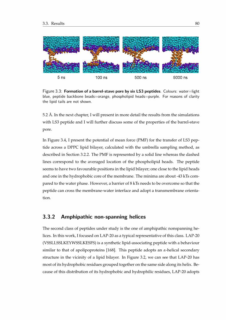
3.3. Results 80
Figure 3.3: Formation of a barrel-stave pore by six LS3 peptides. Colours: water=lightblue, peptide backbone beads=orange, phospholipid heads=purple. For reasons of claritythe lipid tails are not shown.
5.2 A. In the next chapter, I will present in more detail the results from the simulations
with LS3 peptide and I will further discuss some of the properties of the barrel-stave
pore.
In Figure 3.4, I present the potential of mean force (PMF) for the transfer of LS3 pep-
tide across a DPPC lipid bilayer, calculated with the umbrella sampling method, as
described in Section 3.2.2. The PMF is represented by a solid line whereas the dashed
lines correspond to the averaged location of the phospholipid heads. The peptide
seems to have two favourable positions in the lipid bilayer; one close to the lipid heads
and one in the hydrophobic core of the membrane. The minima are about -43 kTs com-
pared to the water phase. However, a barrier of 8 kTs needs to be overcome so that the
peptide can cross the membrane-water interface and adopt a transmembrane orienta-
tion.
3.3.2 Amphipathic non-spanning helices
The second class of peptides under study is the one of amphipathic nonspanning he-
lices. In this work, I focused on LAP-20 as a typical representative of this class. LAP-20
(VSSLLSSLKEYWSSLKESFS) is a synthetic lipid-associating peptide with a behaviour
similar to that of apolipoproteins [168]. This peptide adopts an α-helical secondary
structure in the vicinity of a lipid bilayer. In Figure 3.2, we can see that LAP-20 has
most of its hydrophobic residues grouped together on the same side along its helix. Be-
cause of this distribution of its hydrophobic and hydrophilic residues, LAP-20 adopts
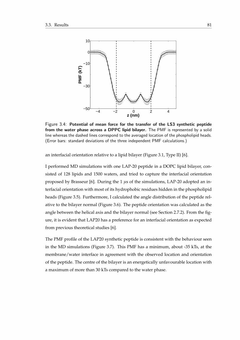
3.3. Results 81
−4 −2 0 2 4−50
−30
−10
0
10
z (nm)
PM
F (
kT)
Figure 3.4: Potential of mean force for the transfer of the LS3 synthetic peptidefrom the water phase across a DPPC lipid bilayer. The PMF is represented by a solidline whereas the dashed lines correspond to the averaged location of the phospholipid heads.(Error bars: standard deviations of the three independent PMF calculations.)
an interfacial orientation relative to a lipid bilayer (Figure 3.1, Type II) [6].
I performed MD simulations with one LAP-20 peptide in a DOPC lipid bilayer, con-
sisted of 128 lipids and 1500 waters, and tried to capture the interfacial orientation
proposed by Brasseur [6]. During the 1 µs of the simulations, LAP-20 adopted an in-
terfacial orientation with most of its hydrophobic residues hidden in the phospholipid
heads (Figure 3.5). Furthermore, I calculated the angle distribution of the peptide rel-
ative to the bilayer normal (Figure 3.6). The peptide orientation was calculated as the
angle between the helical axis and the bilayer normal (see Section 2.7.2). From the fig-
ure, it is evident that LAP20 has a preference for an interfacial orientation as expected
from previous theoretical studies [6].
The PMF profile of the LAP20 synthetic peptide is consistent with the behaviour seen
in the MD simulations (Figure 3.7). This PMF has a minimum, about -35 kTs, at the
membrane/water interface in agreement with the observed location and orientation
of the peptide. The centre of the bilayer is an energetically unfavourable location with
a maximum of more than 30 kTs compared to the water phase.
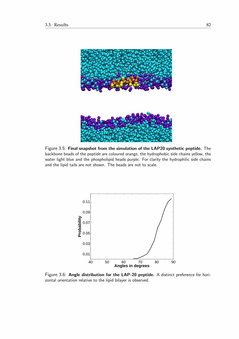
3.3. Results 82
Figure 3.5: Final snapshot from the simulation of the LAP20 synthetic peptide. Thebackbone beads of the peptide are coloured orange, the hydrophobic side chains yellow, thewater light blue and the phospholipid heads purple. For clarity the hydrophilic side chainsand the lipid tails are not shown. The beads are not to scale.
40 50 60 70 80 90
0.01
0.03
0.05
0.07
0.09
0.11
Angles in degrees
Pro
bab
ility
Figure 3.6: Angle distribution for the LAP-20 peptide. A distinct preference for hori-zontal orientation relative to the lipid bilayer is observed.
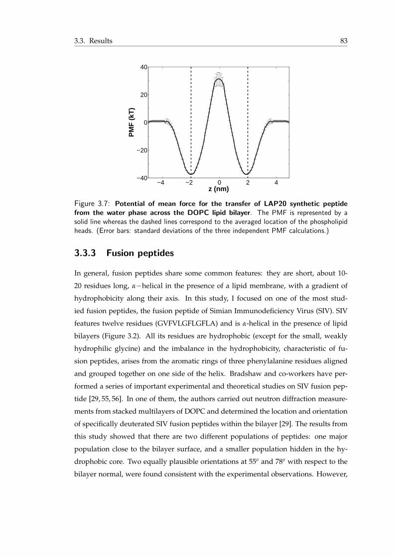
3.3. Results 83
−4 −2 0 2 4−40
−20
0
20
40
z (nm)
PM
F (
kT)
Figure 3.7: Potential of mean force for the transfer of LAP20 synthetic peptidefrom the water phase across the DOPC lipid bilayer. The PMF is represented by asolid line whereas the dashed lines correspond to the averaged location of the phospholipidheads. (Error bars: standard deviations of the three independent PMF calculations.)
3.3.3 Fusion peptides
In general, fusion peptides share some common features: they are short, about 10-
20 residues long, α−helical in the presence of a lipid membrane, with a gradient of
hydrophobicity along their axis. In this study, I focused on one of the most stud-
ied fusion peptides, the fusion peptide of Simian Immunodeficiency Virus (SIV). SIV
features twelve residues (GVFVLGFLGFLA) and is α-helical in the presence of lipid
bilayers (Figure 3.2). All its residues are hydrophobic (except for the small, weakly
hydrophilic glycine) and the imbalance in the hydrophobicity, characteristic of fu-
sion peptides, arises from the aromatic rings of three phenylalanine residues aligned
and grouped together on one side of the helix. Bradshaw and co-workers have per-
formed a series of important experimental and theoretical studies on SIV fusion pep-
tide [29, 55, 56]. In one of them, the authors carried out neutron diffraction measure-
ments from stacked multilayers of DOPC and determined the location and orientation
of specifically deuterated SIV fusion peptides within the bilayer [29]. The results from
this study showed that there are two different populations of peptides: one major
population close to the bilayer surface, and a smaller population hidden in the hy-
drophobic core. Two equally plausible orientations at 55o and 78o with respect to the
bilayer normal, were found consistent with the experimental observations. However,
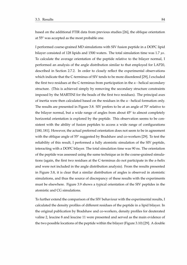
3.3. Results 84
based on the additional FTIR data from previous studies [26], the oblique orientation
at 55o was accepted as the most probable one.
I performed coarse-grained MD simulations with SIV fusion peptide in a DOPC lipid
bilayer consisted of 128 lipids and 1500 waters. The total simulation time was 1.7 µs.
To calculate the average orientation of the peptide relative to the bilayer normal, I
performed an analysis of the angle distribution similar to that employed for LAP20,
described in Section 2.7.2. In order to closely reflect the experimental observations
which indicate that the C-terminus of SIV tends to be more disordered [29], I excluded
the first two residues at the C-terminus from participation in the α−helical secondary
structure. (This is achieved simply by removing the secondary structure constraints
imposed by the MARTINI for the beads of the first two residues). The principal axes
of inertia were then calculated based on the residues in the α−helical formation only.
The results are presented in Figure 3.8. SIV prefers to be at an angle of 70o relative to
the bilayer normal, but a wide range of angles from about 45o to almost completely
horizontal orientation is explored by the peptide. This observation seems to be con-
sistent with the ability of fusion peptides to access a wide range of configurations
[180, 181]. However, the actual preferred orientation does not seem to be in agreement
with the oblique angle of 55o suggested by Bradshaw and co-workers [29]. To test the
reliability of this result, I performed a fully atomistic simulation of the SIV peptide,
interacting with a DOPC bilayer. The total simulation time was 90 ns. The orientation
of the peptide was assessed using the same technique as in the coarse-grained simula-
tions (again, the first two residues at the C-terminus do not participate in the α-helix
and were not included in the angle distribution analysis). From the results presented
in Figure 3.8, it is clear that a similar distribution of angles is observed in atomistic
simulations, and thus the source of discrepancy of these results with the experiments
must be elsewhere. Figure 3.9 shows a typical orientation of the SIV peptides in the
atomistic and CG simulations.
To further extend the comparison of the SIV behaviour with the experimental results, I
calculated the density profiles of different residues of the peptide in a lipid bilayer. In
the original publication by Bradshaw and co-workers, density profiles for deuterated
valine 2, leucine 8 and leucine 11 were presented and served as the main evidence of
the two possible locations of the peptide within the bilayer (Figure 3.10) [29]. A double
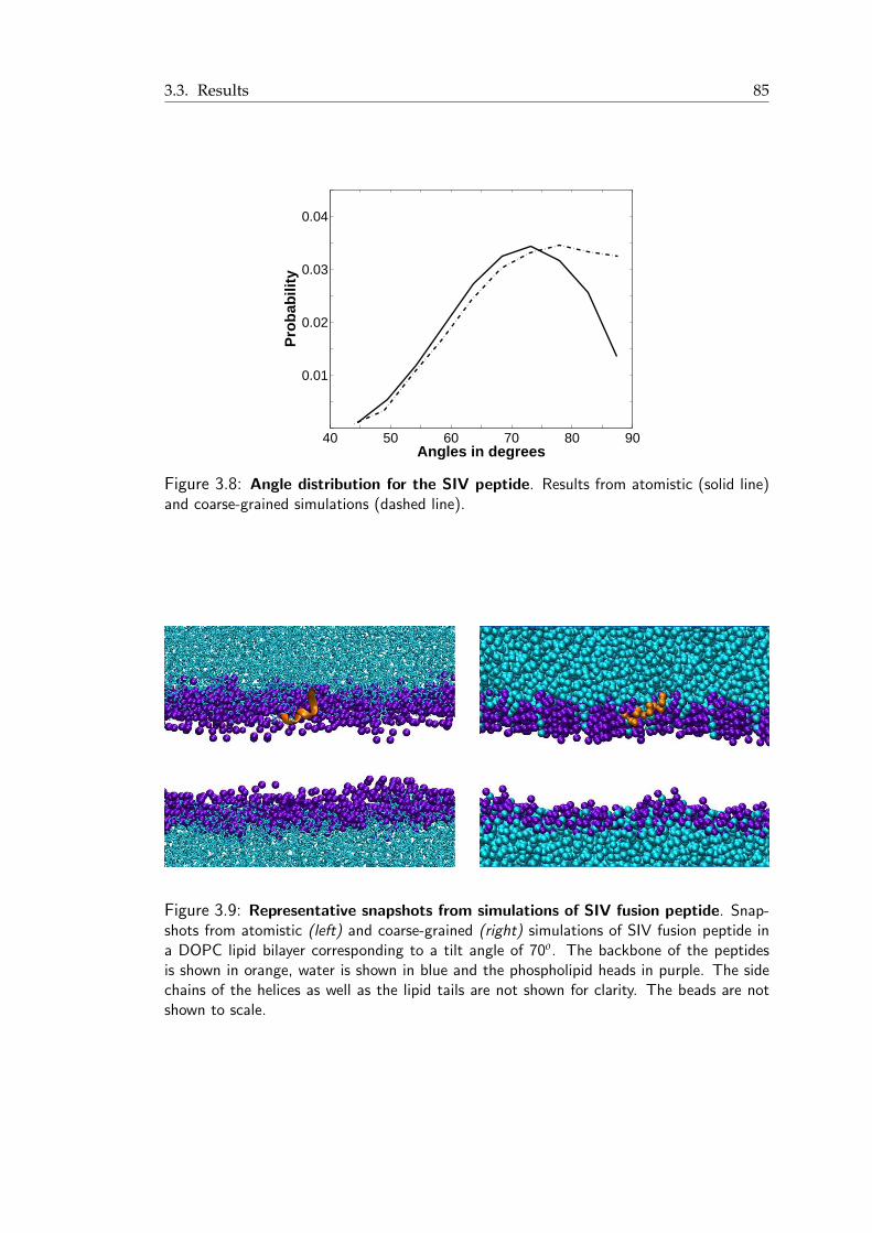
3.3. Results 85
40 50 60 70 80 90
0.01
0.02
0.03
0.04
Angles in degrees
Pro
bab
ility
Figure 3.8: Angle distribution for the SIV peptide. Results from atomistic (solid line)and coarse-grained simulations (dashed line).
Figure 3.9: Representative snapshots from simulations of SIV fusion peptide. Snap-shots from atomistic (left) and coarse-grained (right) simulations of SIV fusion peptide ina DOPC lipid bilayer corresponding to a tilt angle of 70o. The backbone of the peptidesis shown in orange, water is shown in blue and the phospholipid heads in purple. The sidechains of the helices as well as the lipid tails are not shown for clarity. The beads are notshown to scale.

3.3. Results 86
peak is evident for leucine 8 and therefore I focused on this residue.
Figure 3.10: Neutron scattering length density profiles for Val2, Leu8 and Leu11 ofSIV peptide. (- -) minor population , (-.-) major population, and (solid line) sum of majorand minor populations. Figure adapted from [29].
In Figure 3.11, I present the density profile for leucine 8 of the SIV fusion peptide from
both the atomistic and the coarse-grained simulations. Since the thickness of the bi-
layer is somewhat different in the atomistic and coarse-grained representations, the z-
axis is given in dimensionless units with the lipid length in a particular representation
being the scaling parameter. The atomistic simulations predict a deeper positioning of
leucine 8 in the bilayer, whereas in the CG simulations the peptide lies closer to the
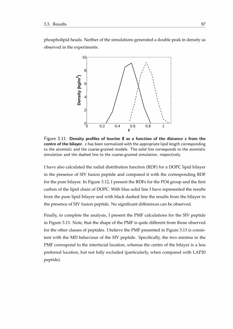
3.3. Results 87
phospholipid heads. Neither of the simulations generated a double peak in density as
observed in the experiments.
0 0.2 0.4 0.6 0.8 10
2
4
6
8
10
z
Den
sity
(kg
/m2 )
Figure 3.11: Density profiles of leucine 8 as a function of the distance z from thecentre of the bilayer. z has been normalized with the appropriate lipid length correspondingto the atomistic and the coarse-grained models. The solid line corresponds to the atomisticsimulation and the dashed line to the coarse-grained simulation, respectively.
I have also calculated the radial distribution function (RDF) for a DOPC lipid bilayer
in the presence of SIV fusion peptide and compared it with the corresponding RDF
for the pure bilayer. In Figure 3.12, I present the RDFs for the PO4 group and the first
carbon of the lipid chain of DOPC. With blue solid line I have represented the results
from the pure lipid bilayer and with black dashed line the results from the bilayer in
the presence of SIV fusion peptide. No significant differences can be observed.
Finally, to complete the analysis, I present the PMF calculations for the SIV peptide
in Figure 3.13. Note, that the shape of the PMF is quite different from those observed
for the other classes of peptides. I believe the PMF presented in Figure 3.13 is consis-
tent with the MD behaviour of the SIV peptide. Specifically, the two minima in the
PMF correspond to the interfacial location, whereas the centre of the bilayer is a less
preferred location, but not fully excluded (particularly, when compared with LAP20
peptide).

3.3. Results 88
0 1 2 3 40
1
2
3
4
5
r (nm)
g(r
)
(a)
0 1 2 3 40
2
4
6
8
10
12
r (nm)
g(r
)
(b)
Figure 3.12: Radial distribution function for DOPC bilayer in the presence of SIVfusion peptide. RDFs for the PO4 group (a) and the first carbon of the lipid chain ofDOPC (b) are shown. With blue solid line I have represented the results from the pure lipidbilayer and with black dashed line the results from the bilayer in the presence of SIV fusionpeptide.
−4 −2 0 2 4
−30
−20
−10
0
z (nm)
PM
F (
kT)
Figure 3.13: Potential of mean force for the transfer of the SIV fusion peptide fromthe water phase across a DOPC lipid bilayer. The PMF is represented by a continuousline whereas the dashed lines correspond to the averaged location of the phospholipid heads.(Error bars: standard deviations of the three independent PMF calculations.)

3.3. Results 89
3.3.4 Transmembrane helices
In the original description of various classes of peptides provided in Figure 3.1, the
transmembrane helices span the lipid bilayer due to the match between the hydropho-
bic region of the α-helix and the width of the hydrophobic core of the lipid bilayer.
Alternatively, one could employ a functional definition of transmembrane peptides
as structures capable of spontaneous insertion in the bilayer, leading to a characteris-
tic transmembrane orientation. This ability of transmembrane peptides to cross lipid
bilayers is of great interest in the development of novel drug vectors and other ap-
plications. However, the details of the translocation mechanisms are not yet under-
stood. Studies of these peptides have been carried out both through experiments
and simulations. For example, Bond and Sansom captured the spontaneous inser-
tion of GpA helix by means of CG simulations [100]. Another peptide, that has been
studied in a series of experiments by the group of Engelman, is pH (low) insertion
peptide, known as pHLIP [164–167]. pHLIP (ACEQNPIYWARYADWLFTTPLLLLD-
LALLVDADEGTG) is a peptide derived from the integral membrane protein bacte-
riorhodopsin C. It exhibits high solubility at neutral pH in a non helical conforma-
tion, however, at lower pH (pKa of 6.0), the peptide adopts a transmembrane position
in an α-helical conformation. It has been proposed that this pH-dependent mecha-
nism of translocation can be exploited in the early detection of pathological conditions
in cells. In one of their studies, Engleman and co-workers, designed two variants
of pHLIP in order to check the specificity of the function of the peptide in tumours
and test its mechanism of insertion. In one of the variants, N-pHLIP (ACEQNPIY-
WARYANWLFTTPLLLLNLALLVDADEGTG), the aspartic acid (Asp, D) residues are
replaced by asparagine (Asn, N). This peptide remains an α-helical structure in the
presence of liposomes over a wide pH range and adopts a transmembrane position
in a lipid bilayer. I have chosen this pHLIP version for the studies of transmembrane
helices.
I carried out a series of MD simulations with pHLIP in a DOPC (512 lipids and 6000
waters) and in a POPC (512 lipids 6000 waters) bilayer. I did not observe the pHLIP
insertion in any of our simulations unless the peptide was initially half-inserted in the
lipid bilayer (Figure 3.14). In Figure 3.14, water is represented by blue beads, lipid
heads by purple beads and the backbone of the peptide is coloured orange. The hy-
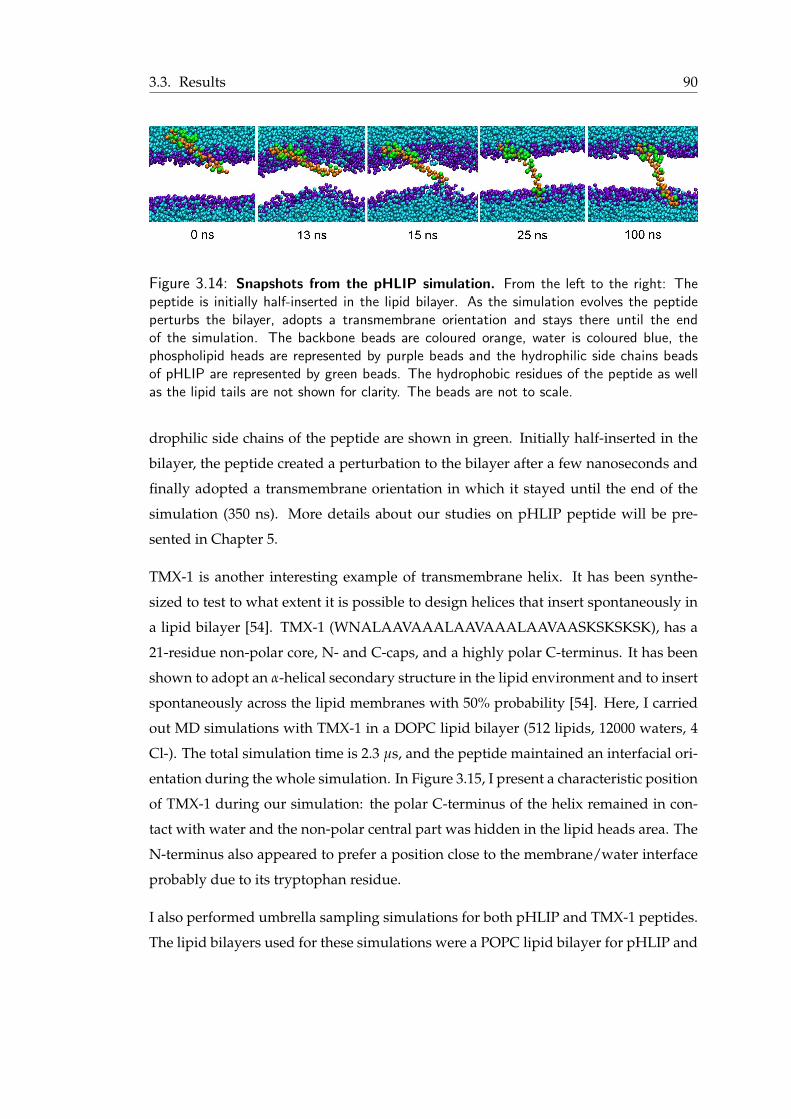
3.3. Results 90
Figure 3.14: Snapshots from the pHLIP simulation. From the left to the right: Thepeptide is initially half-inserted in the lipid bilayer. As the simulation evolves the peptideperturbs the bilayer, adopts a transmembrane orientation and stays there until the endof the simulation. The backbone beads are coloured orange, water is coloured blue, thephospholipid heads are represented by purple beads and the hydrophilic side chains beadsof pHLIP are represented by green beads. The hydrophobic residues of the peptide as wellas the lipid tails are not shown for clarity. The beads are not to scale.
drophilic side chains of the peptide are shown in green. Initially half-inserted in the
bilayer, the peptide created a perturbation to the bilayer after a few nanoseconds and
finally adopted a transmembrane orientation in which it stayed until the end of the
simulation (350 ns). More details about our studies on pHLIP peptide will be pre-
sented in Chapter 5.
TMX-1 is another interesting example of transmembrane helix. It has been synthe-
sized to test to what extent it is possible to design helices that insert spontaneously in
a lipid bilayer [54]. TMX-1 (WNALAAVAAALAAVAAALAAVAASKSKSKSK), has a
21-residue non-polar core, N- and C-caps, and a highly polar C-terminus. It has been
shown to adopt an α-helical secondary structure in the lipid environment and to insert
spontaneously across the lipid membranes with 50% probability [54]. Here, I carried
out MD simulations with TMX-1 in a DOPC lipid bilayer (512 lipids, 12000 waters, 4
Cl-). The total simulation time is 2.3 µs, and the peptide maintained an interfacial ori-
entation during the whole simulation. In Figure 3.15, I present a characteristic position
of TMX-1 during our simulation: the polar C-terminus of the helix remained in con-
tact with water and the non-polar central part was hidden in the lipid heads area. The
N-terminus also appeared to prefer a position close to the membrane/water interface
probably due to its tryptophan residue.
I also performed umbrella sampling simulations for both pHLIP and TMX-1 peptides.
The lipid bilayers used for these simulations were a POPC lipid bilayer for pHLIP and
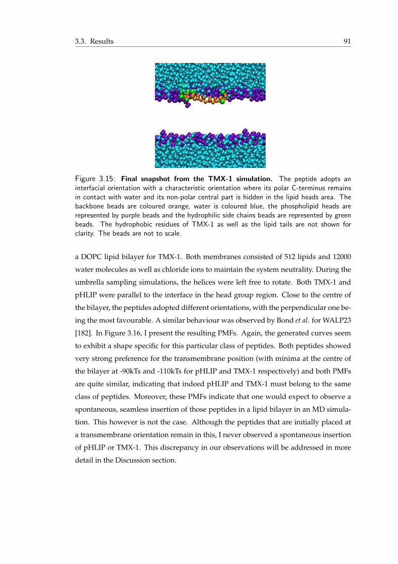
3.3. Results 91
Figure 3.15: Final snapshot from the TMX-1 simulation. The peptide adopts aninterfacial orientation with a characteristic orientation where its polar C-terminus remainsin contact with water and its non-polar central part is hidden in the lipid heads area. Thebackbone beads are coloured orange, water is coloured blue, the phospholipid heads arerepresented by purple beads and the hydrophilic side chains beads are represented by greenbeads. The hydrophobic residues of TMX-1 as well as the lipid tails are not shown forclarity. The beads are not to scale.
a DOPC lipid bilayer for TMX-1. Both membranes consisted of 512 lipids and 12000
water molecules as well as chloride ions to maintain the system neutrality. During the
umbrella sampling simulations, the helices were left free to rotate. Both TMX-1 and
pHLIP were parallel to the interface in the head group region. Close to the centre of
the bilayer, the peptides adopted different orientations, with the perpendicular one be-
ing the most favourable. A similar behaviour was observed by Bond et al. for WALP23
[182]. In Figure 3.16, I present the resulting PMFs. Again, the generated curves seem
to exhibit a shape specific for this particular class of peptides. Both peptides showed
very strong preference for the transmembrane position (with minima at the centre of
the bilayer at -90kTs and -110kTs for pHLIP and TMX-1 respectively) and both PMFs
are quite similar, indicating that indeed pHLIP and TMX-1 must belong to the same
class of peptides. Moreover, these PMFs indicate that one would expect to observe a
spontaneous, seamless insertion of those peptides in a lipid bilayer in an MD simula-
tion. This however is not the case. Although the peptides that are initially placed at
a transmembrane orientation remain in this, I never observed a spontaneous insertion
of pHLIP or TMX-1. This discrepancy in our observations will be addressed in more
detail in the Discussion section.
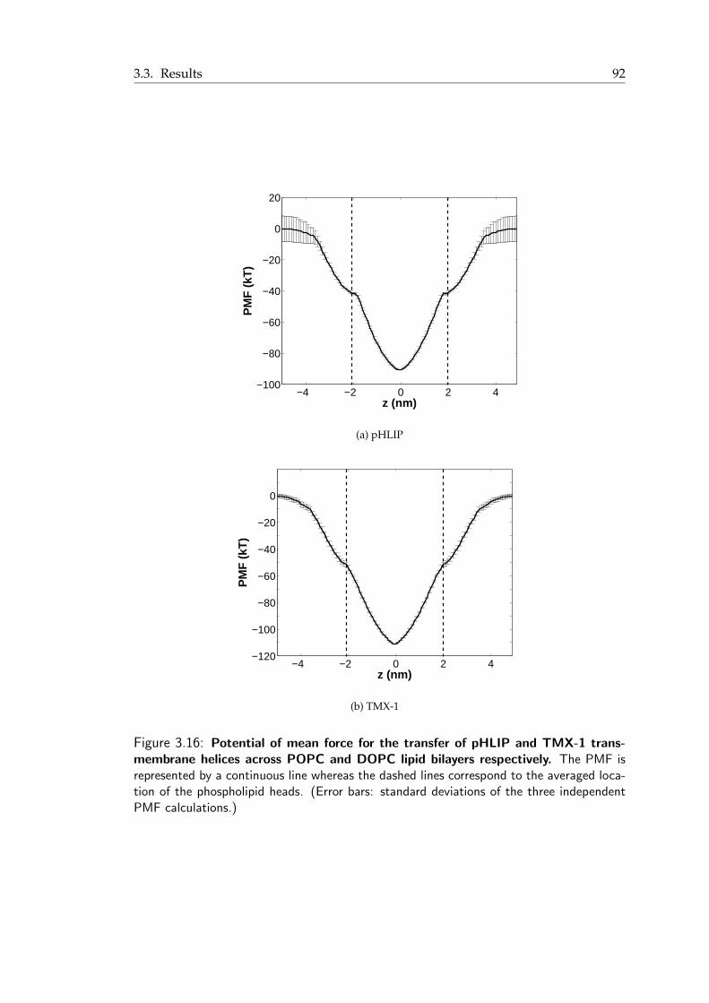
3.3. Results 92
−4 −2 0 2 4−100
−80
−60
−40
−20
0
20
z (nm)
PM
F (
kT)
(a) pHLIP
−4 −2 0 2 4−120
−100
−80
−60
−40
−20
0
z (nm)
PM
F (
kT)
(b) TMX-1
Figure 3.16: Potential of mean force for the transfer of pHLIP and TMX-1 trans-membrane helices across POPC and DOPC lipid bilayers respectively. The PMF isrepresented by a continuous line whereas the dashed lines correspond to the averaged loca-tion of the phospholipid heads. (Error bars: standard deviations of the three independentPMF calculations.)
3.4. Discussion 93
3.4 Discussion
The results reported in this chapter suggest that the MARTINI coarse-grained model
is able to describe several classes of interactions between α-helical peptides and lipid
bilayers. The self-assembly of a barrel-stave pore and the behaviour of interfacial non-
spanning peptides are within the scope of the MARTINI. Furthermore, the model is
able to provide new important insights regarding the details of peptide self-assembly
in the vicinity of a lipid bilayer. The number of helices constituting the pore as well as
its effective diameter predicted from our simulations are in agreement with previous
experimental studies [16, 17].
I performed potential of mean force (PMF) calculations for each peptide considered
in this study. In Figure 3.17, I present a summary of the different PMFs. The PMF
provides an estimate of the free energy profile as the peptide crosses the bilayer, and
can be used directly to calculate the partition of the peptide between the water phase
and the lipid phase. I showed that each class of peptide-bilayer interaction has a very
distinct form of PMF (Figure 3.17). For example, the PMF for LS3 features three energy
minima of comparable depth, one at the centre of the bilayer and two additional min-
ima at the interfaces of the bilayer. A very distinct PMF is observed for the fusion SIV
peptide, with the energy minimum corresponding to the lipid interface and the ener-
getic penalty for SIV’s location in the centre of the bilayer of about 15 kT. pHLIP and
TMX-1 peptides exhibit barrier-less PMFs with -90 kT and -110 kT minima respectively
at the centre of the bilayer, signifying a very strong preference for the transmembrane
orientation. Although this result agrees with our expectations and experimental ob-
servations [54, 165], it contradicts our MD studies, where no spontaneous insertion of
the peptides in the bilayer is observed. Let us briefly explore possible sources of the
discrepancy.
First, I would like to ensure that the observed PMF is not an artefact resulting from
the technical limitations of the applied methods. Specifically, the system features large
enough water phase to eliminate possible periodic boundary condition effects. In the
original setup, I used the Berendsen thermostat to control the temperature of the sys-
tem and this method has been criticized for not being able to provide correct distribu-
tion of velocities. For one of the smaller peptides, I repeated the simulations with the
Nose-Hoover thermostat and, not surprisingly, observed marginal differences. Also,
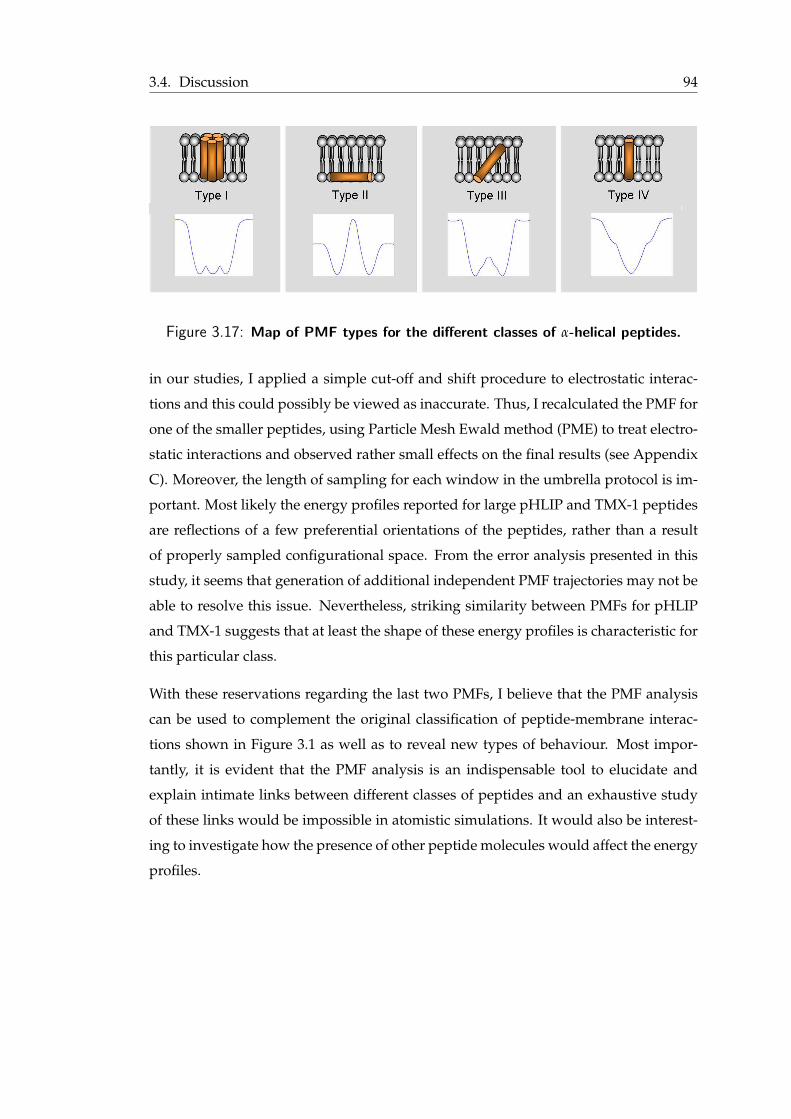
3.4. Discussion 94
Figure 3.17: Map of PMF types for the different classes of α-helical peptides.
in our studies, I applied a simple cut-off and shift procedure to electrostatic interac-
tions and this could possibly be viewed as inaccurate. Thus, I recalculated the PMF for
one of the smaller peptides, using Particle Mesh Ewald method (PME) to treat electro-
static interactions and observed rather small effects on the final results (see Appendix
C). Moreover, the length of sampling for each window in the umbrella protocol is im-
portant. Most likely the energy profiles reported for large pHLIP and TMX-1 peptides
are reflections of a few preferential orientations of the peptides, rather than a result
of properly sampled configurational space. From the error analysis presented in this
study, it seems that generation of additional independent PMF trajectories may not be
able to resolve this issue. Nevertheless, striking similarity between PMFs for pHLIP
and TMX-1 suggests that at least the shape of these energy profiles is characteristic for
this particular class.
With these reservations regarding the last two PMFs, I believe that the PMF analysis
can be used to complement the original classification of peptide-membrane interac-
tions shown in Figure 3.1 as well as to reveal new types of behaviour. Most impor-
tantly, it is evident that the PMF analysis is an indispensable tool to elucidate and
explain intimate links between different classes of peptides and an exhaustive study
of these links would be impossible in atomistic simulations. It would also be interest-
ing to investigate how the presence of other peptide molecules would affect the energy
profiles.
CHAPTER 4
Pore-formation by α-helical peptides
This chapter is a presentation of more in-depth studies on pore formation mechanisms.
These mechanisms play an important role in many biological processes, from ion-
conduction across cell membranes to antimicrobial defence mechanisms and many
more. For this study, I chose LS3 synthetic peptide, because of its simplicity (it has
only two types of amino acids) and its potential to form pores. I have already shown
that the spontaneous formation of a LS3 barrel-stave pore can be successfully captured
by means of coarse-grained molecular dynamics simulations. In this chapter, I present
a series of simulations that provide further evidence of the propensity of LS3 to form
pores as well as structural and dynamical information about them. I also investigate
how pore formation mechanisms depend on the structural modifications of LS3.
95
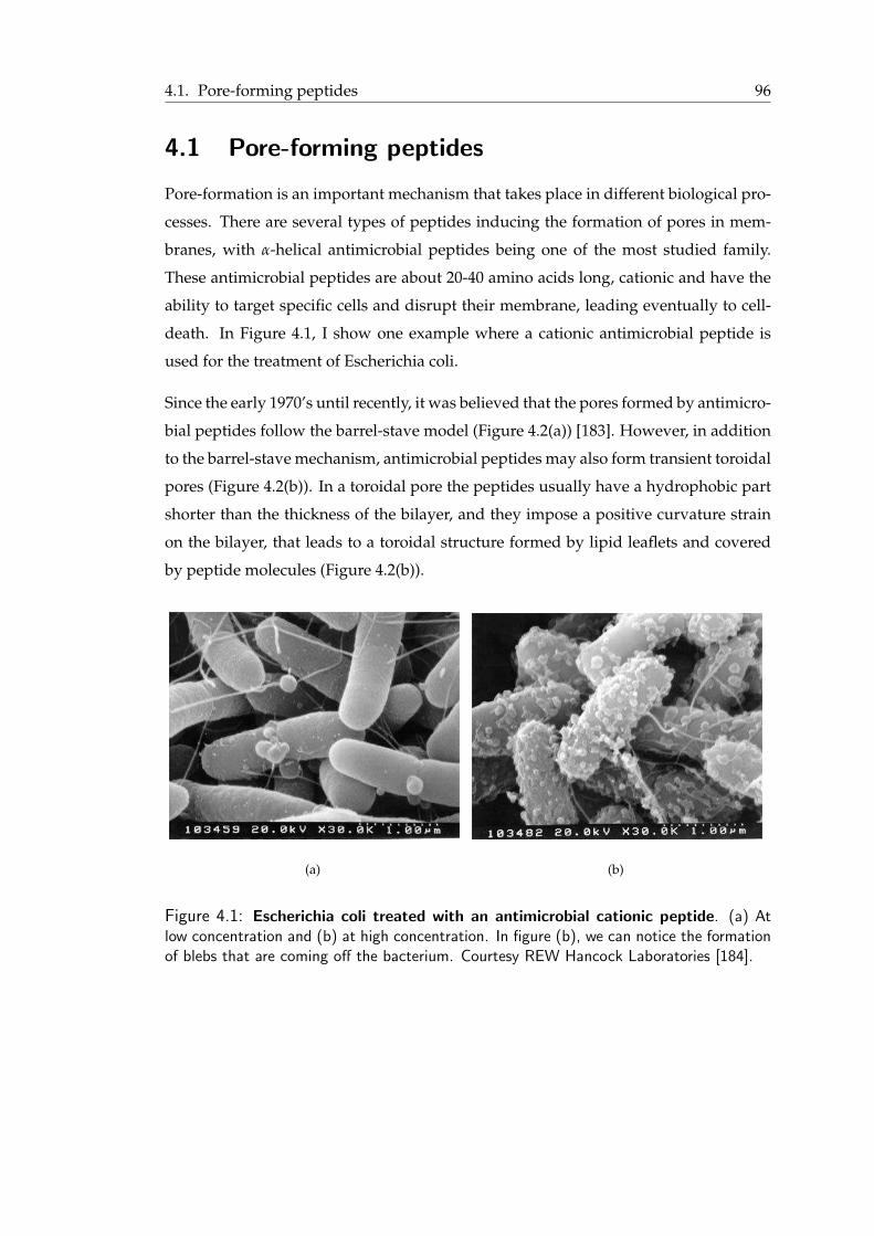
4.1. Pore-forming peptides 96
4.1 Pore-forming peptides
Pore-formation is an important mechanism that takes place in different biological pro-
cesses. There are several types of peptides inducing the formation of pores in mem-
branes, with α-helical antimicrobial peptides being one of the most studied family.
These antimicrobial peptides are about 20-40 amino acids long, cationic and have the
ability to target specific cells and disrupt their membrane, leading eventually to cell-
death. In Figure 4.1, I show one example where a cationic antimicrobial peptide is
used for the treatment of Escherichia coli.
Since the early 1970’s until recently, it was believed that the pores formed by antimicro-
bial peptides follow the barrel-stave model (Figure 4.2(a)) [183]. However, in addition
to the barrel-stave mechanism, antimicrobial peptides may also form transient toroidal
pores (Figure 4.2(b)). In a toroidal pore the peptides usually have a hydrophobic part
shorter than the thickness of the bilayer, and they impose a positive curvature strain
on the bilayer, that leads to a toroidal structure formed by lipid leaflets and covered
by peptide molecules (Figure 4.2(b)).
(a) (b)
Figure 4.1: Escherichia coli treated with an antimicrobial cationic peptide. (a) Atlow concentration and (b) at high concentration. In figure (b), we can notice the formationof blebs that are coming off the bacterium. Courtesy REW Hancock Laboratories [184].

4.1. Pore-forming peptides 97
Figure 4.2: Schematic of the barrel-stave (a) and toroidal (b) pore. The structure oflipids in the vicinity of the pores is one of their main differences.
Another type of peptides of interest here is the family of pore-forming toxins (PFT).
PFTs are soluble and act on cell membranes by forming transmembrane channels, for
example β-barrels (in the case of α-toxin from Staphylococcus aureus) [185]. There are
a few cases of PFTs with α-helical secondary structure that form unstable pores.
α-helical peptides forming (and derived from) protein ion-conducting channels are
another family of pore-forming peptides. In the membrane, several helices form a
bundle, that can be classified as a barrel-stave pore (Figure 4.2(a)). There is a number
of model channel systems, consisting of synthetic helices of this type, with ‘synporins’
[151–153] and ‘template-assembled synthetic proteins’ (TASPs) [154, 155], being two
representative examples.
There are several simulation studies on pore-forming peptides, and in particular the
ones with α-helical structure. I will briefly mention a few representative works. Nielsen
and co-workers have recently combined NMR and molecular dynamics simulation
studies to study alamethicin antimicrobial peptide [186, 187]. One of the first simu-
lation studies of antimicrobial peptides and toroidal pore formation mechanisms was
presented by Leontiadou et al. in [188]. In this publication the authors showed that
magainin-H2, above a certain concentration, induced the formation of a toroidal pore.
A series of simulation studies performed by the same group showed among others
that the shape of a toroidal pore may be very disordered, with peptides and lipids at
oblique orientations lining the pore [77, 78]. Moreover, the MARTINI coarse-grained
model has been shown to be able to capture both the barrel-stave pore formation (for
LS3 synthetic peptide) [109] and toroidal mechanisms (for magainin-H2 and melittin

4.2. Summary of simulations 98
antimicrobial peptides) [78, 105] of pore formation.
In the previous chapter, I presented the formation of a barrel-stave pore from LS3 pep-
tide. Here, I will discuss in more detail the characteristics of the pore and present a
series of simulations I performed with LS3 at different concentrations.
In an effort to examine the characteristics of LS3 that lead to the formation of a pore, I
performed simulations with a 14-residue version of LS3, (LSSLLSL)2, that as has been
experimentally shown does not form discrete, stable channels [16]. To our surprise
this peptide at relatively high concentrations formed complexes in the lipid bilayer, re-
sembling toroidal pores. These pores were transient, disordered and with a very small
radius. I carried out a series of simulations to examine the link between the formation
of these pores and the concentration of the peptide. I also performed simulations with
magainin-H2 peptide in order to be able to compare the structures of the pores formed
by magainin and the short version of LS3. Finally, I performed PMF calculations that
showed a different profile for (LSSLLSL)2 compared to (LSSLLSL)3.
4.2 Summary of simulations
I have performed a range of NPT molecular dynamics simulations for LS3 and (LSSLLSL)2
in a DPPC membrane, at 323 K and 1 bar, and with peptide/lipid ratios varying from
6/256 to 12/256. The MARTINI force field was used. First, I randomly put the pep-
tides in a system with a preassembled DPPC lipid bilayer (some of them happened to
be at the membrane-water interface and some in the bulk), and, after energy minimiza-
tion of the system, I carried out MD simulations for several microseconds. The rest of
the simulation parameters are the same as described in Section 3.2. Summaries of the
simulations for the two peptides are presented in Tables 4.1 and 4.2. There seems to be
no connection between the orientation of the termini in the oligomers.
I also performed two simulations for magainin-H2 peptide. The MARTINI force field
was used with simulation parameters as described in Section 3.2. The system had 128
DPPC lipids, 2000 waters and 7 peptides. The peptides were randomly placed in a
system with a preassembled DPPC lipid bilayer. An energy minimization run was
performed, followed by an equilibration run. MD simulations in the NPT ensemble at
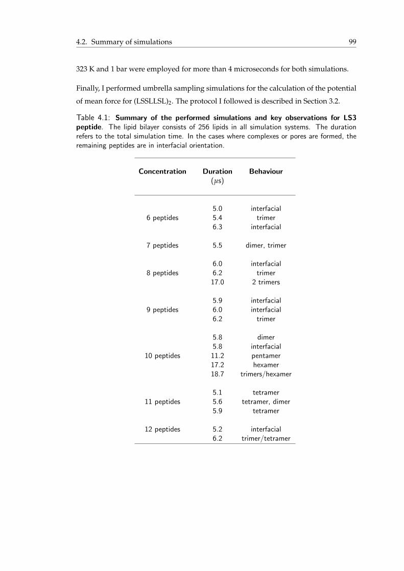
4.2. Summary of simulations 99
323 K and 1 bar were employed for more than 4 microseconds for both simulations.
Finally, I performed umbrella sampling simulations for the calculation of the potential
of mean force for (LSSLLSL)2. The protocol I followed is described in Section 3.2.
Table 4.1: Summary of the performed simulations and key observations for LS3peptide. The lipid bilayer consists of 256 lipids in all simulation systems. The durationrefers to the total simulation time. In the cases where complexes or pores are formed, theremaining peptides are in interfacial orientation.
Concentration Duration Behaviour(µs)
5.0 interfacial6 peptides 5.4 trimer
6.3 interfacial
7 peptides 5.5 dimer, trimer
6.0 interfacial8 peptides 6.2 trimer
17.0 2 trimers
5.9 interfacial9 peptides 6.0 interfacial
6.2 trimer
5.8 dimer5.8 interfacial
10 peptides 11.2 pentamer17.2 hexamer18.7 trimers/hexamer
5.1 tetramer11 peptides 5.6 tetramer, dimer
5.9 tetramer
12 peptides 5.2 interfacial6.2 trimer/tetramer
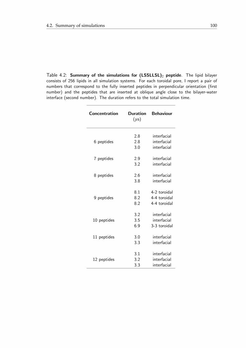
4.2. Summary of simulations 100
Table 4.2: Summary of the simulations for (LSSLLSL)2 peptide. The lipid bilayerconsists of 256 lipids in all simulation systems. For each toroidal pore, I report a pair ofnumbers that correspond to the fully inserted peptides in perpendicular orientation (firstnumber) and the peptides that are inserted at oblique angle close to the bilayer-waterinterface (second number). The duration refers to the total simulation time.
Concentration Duration Behaviour(µs)
2.8 interfacial6 peptides 2.8 interfacial
3.0 interfacial
7 peptides 2.9 interfacial3.2 interfacial
8 peptides 2.6 interfacial3.8 interfacial
8.1 4-2 toroidal9 peptides 8.2 4-4 toroidal
8.2 4-4 toroidal
3.2 interfacial10 peptides 3.5 interfacial
6.9 3-3 toroidal
11 peptides 3.0 interfacial3.3 interfacial
3.1 interfacial12 peptides 3.2 interfacial
3.3 interfacial
4.3. Results 101
4.3 Results
4.3.1 LS3 complexes
From the simulations of LS3 at different peptide/lipid ratios, I observed the formation
of different complexes as well as the interfacial orientation of peptides. Regarding
the orientation of the termini of the helices within the bilayer, there seemed to be no
particular preference in the absence of the transmembrane potential. It is also worth
mentioning that at higher concentrations of the peptide, the propensity to form large
complexes and pores was higher, while at smaller concentrations dimers and trimers
were more common. However, a high concentration of peptides did not necessarily
lead to a pore formation (Table 4.1).
From the observed complexes, the dimers and trimers were formed at different con-
centrations and were stable for several microseconds. The tetramers were also very
stable (for more than 10 microseconds in some cases) with some of them having the
shape of a pore. Also, a complex of five helices has been observed once (Figure 4.3,
bottom left). The hexameric bundle observed in one of our simulations can be classi-
fied as a barrel-stave pore, both by its shape and by the configuration of the lipids
around it (Figure 4.3, bottom right) [109]. Complexes consisted of six helices, without
the formation of an open pore have also been observed. For example, the formation
of a hexameric complex was captured when two trimers approached each other and
merged into one structure. In Figure 4.4, I present top view snapshots from the forma-
tion of the hexamer. In the figure, the backbone beads are coloured orange and water
is coloured blue.
In Figure 4.3, I present the top view of complexes of different sizes. I have chosen rep-
resentative complexes where their structure and the distribution of their hydrophilic
residues are easy to observe. There are cases where these structures are more dis-
ordered. As shown in the figure, most of the hydrophilic residues of the peptides
(coloured blue) are lying at the inner surface of the complexes. The hydrophobic
residues are not shown in the figure.
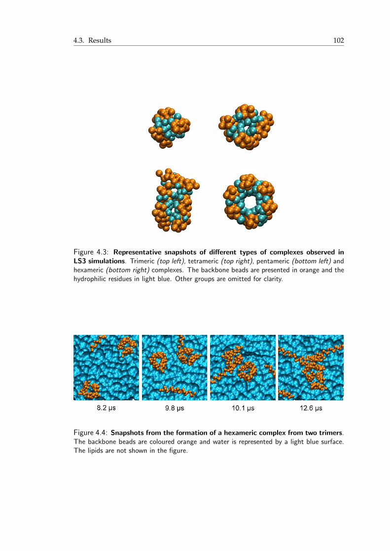
4.3. Results 102
Figure 4.3: Representative snapshots of different types of complexes observed inLS3 simulations. Trimeric (top left), tetrameric (top right), pentameric (bottom left) andhexameric (bottom right) complexes. The backbone beads are presented in orange and thehydrophilic residues in light blue. Other groups are omitted for clarity.
Figure 4.4: Snapshots from the formation of a hexameric complex from two trimers.The backbone beads are coloured orange and water is represented by a light blue surface.The lipids are not shown in the figure.
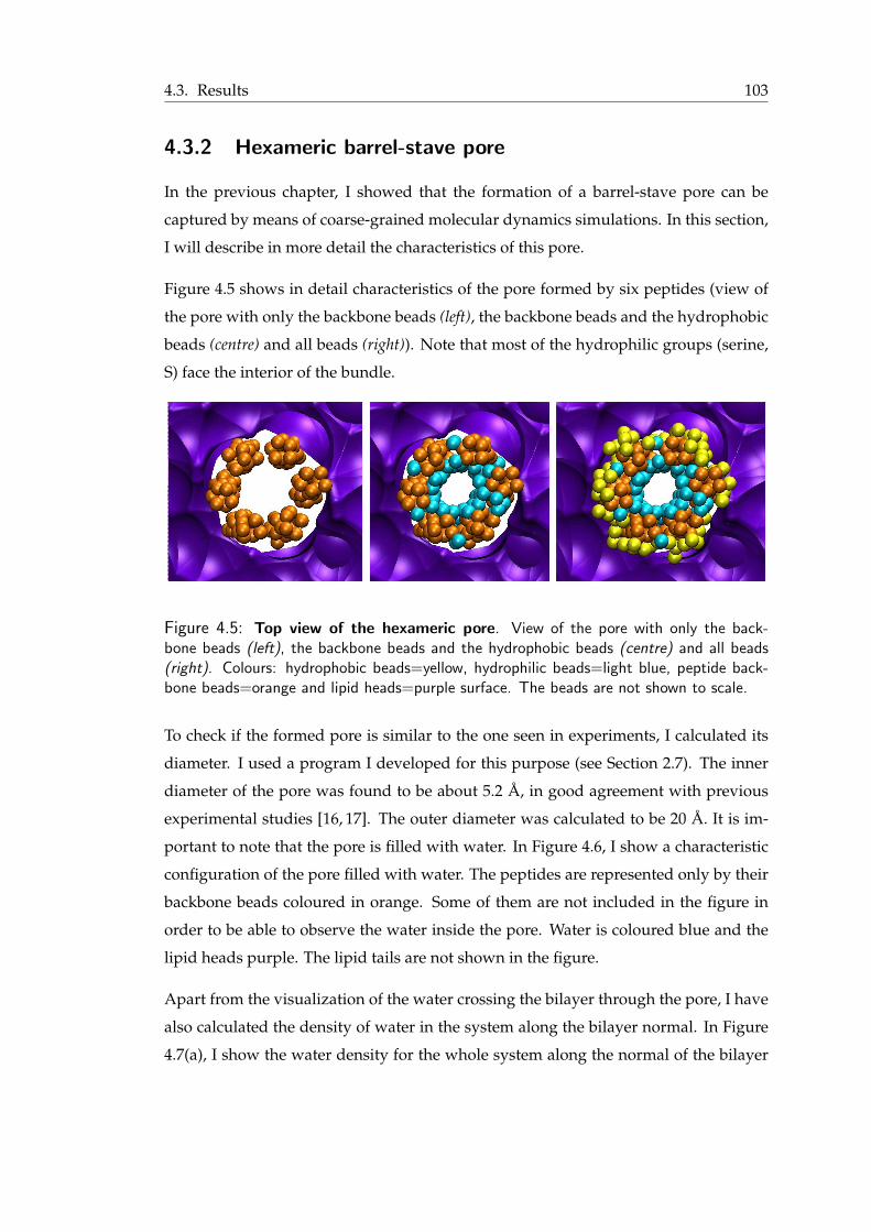
4.3. Results 103
4.3.2 Hexameric barrel-stave pore
In the previous chapter, I showed that the formation of a barrel-stave pore can be
captured by means of coarse-grained molecular dynamics simulations. In this section,
I will describe in more detail the characteristics of this pore.
Figure 4.5 shows in detail characteristics of the pore formed by six peptides (view of
the pore with only the backbone beads (left), the backbone beads and the hydrophobic
beads (centre) and all beads (right)). Note that most of the hydrophilic groups (serine,
S) face the interior of the bundle.
Figure 4.5: Top view of the hexameric pore. View of the pore with only the back-bone beads (left), the backbone beads and the hydrophobic beads (centre) and all beads(right). Colours: hydrophobic beads=yellow, hydrophilic beads=light blue, peptide back-bone beads=orange and lipid heads=purple surface. The beads are not shown to scale.
To check if the formed pore is similar to the one seen in experiments, I calculated its
diameter. I used a program I developed for this purpose (see Section 2.7). The inner
diameter of the pore was found to be about 5.2 A, in good agreement with previous
experimental studies [16, 17]. The outer diameter was calculated to be 20 A. It is im-
portant to note that the pore is filled with water. In Figure 4.6, I show a characteristic
configuration of the pore filled with water. The peptides are represented only by their
backbone beads coloured in orange. Some of them are not included in the figure in
order to be able to observe the water inside the pore. Water is coloured blue and the
lipid heads purple. The lipid tails are not shown in the figure.
Apart from the visualization of the water crossing the bilayer through the pore, I have
also calculated the density of water in the system along the bilayer normal. In Figure
4.7(a), I show the water density for the whole system along the normal of the bilayer
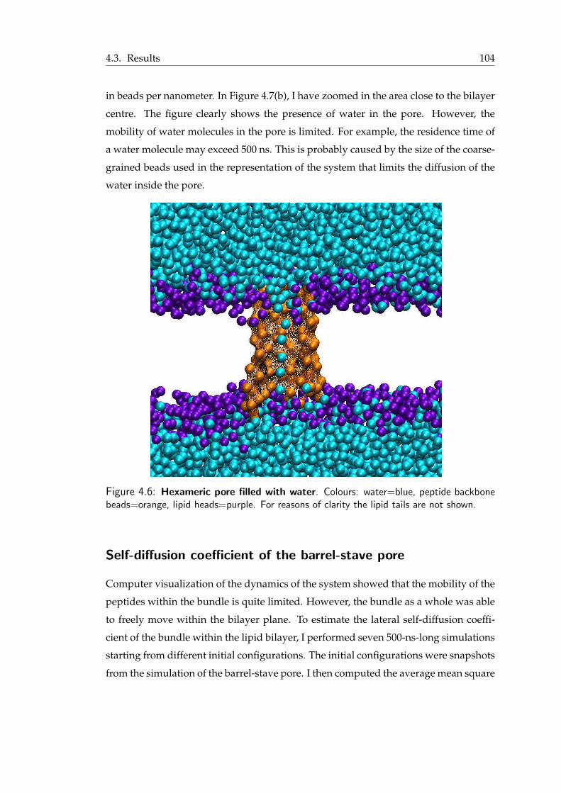
4.3. Results 104
in beads per nanometer. In Figure 4.7(b), I have zoomed in the area close to the bilayer
centre. The figure clearly shows the presence of water in the pore. However, the
mobility of water molecules in the pore is limited. For example, the residence time of
a water molecule may exceed 500 ns. This is probably caused by the size of the coarse-
grained beads used in the representation of the system that limits the diffusion of the
water inside the pore.
Figure 4.6: Hexameric pore filled with water. Colours: water=blue, peptide backbonebeads=orange, lipid heads=purple. For reasons of clarity the lipid tails are not shown.
Self-diffusion coefficient of the barrel-stave pore
Computer visualization of the dynamics of the system showed that the mobility of the
peptides within the bundle is quite limited. However, the bundle as a whole was able
to freely move within the bilayer plane. To estimate the lateral self-diffusion coeffi-
cient of the bundle within the lipid bilayer, I performed seven 500-ns-long simulations
starting from different initial configurations. The initial configurations were snapshots
from the simulation of the barrel-stave pore. I then computed the average mean square
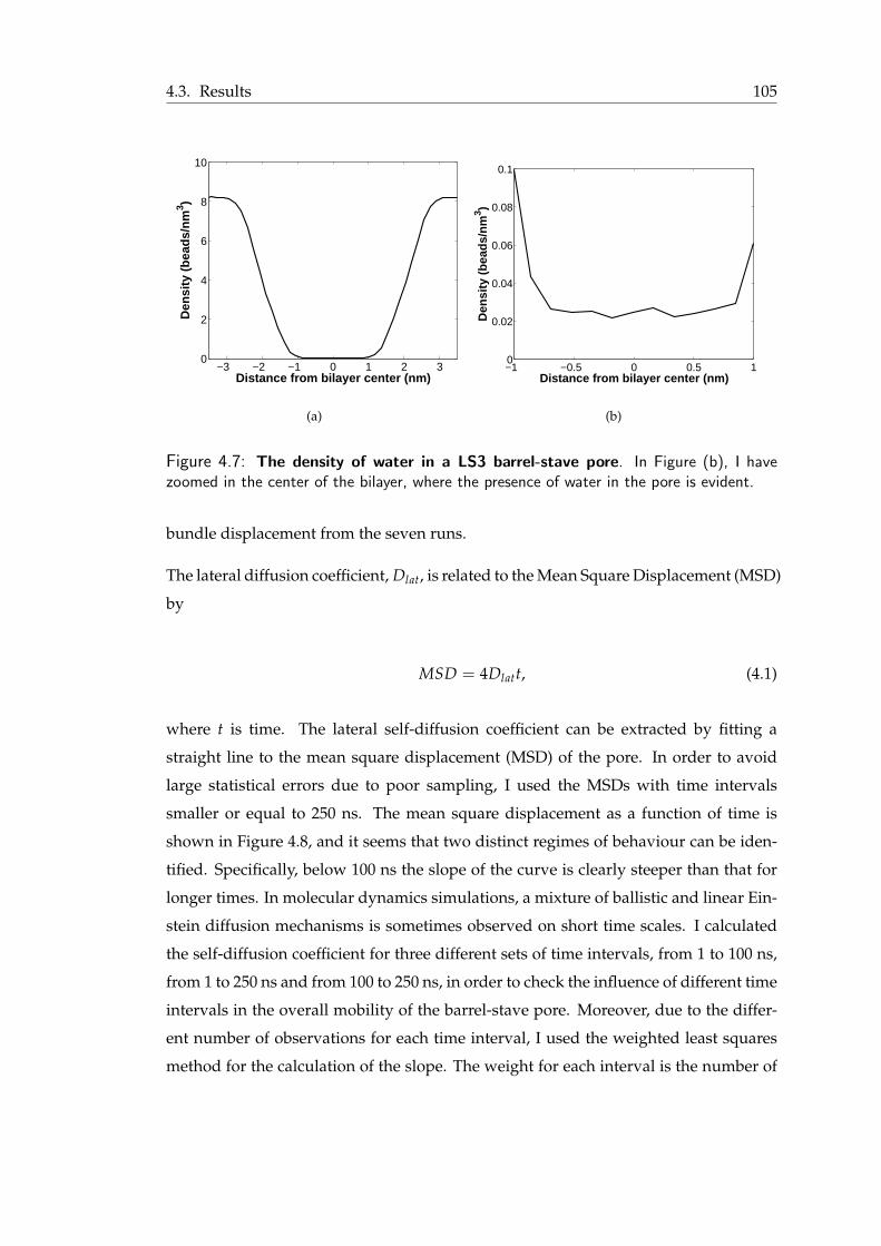
4.3. Results 105
−3 −2 −1 0 1 2 30
2
4
6
8
10
Distance from bilayer center (nm)
Den
sity
(b
ead
s/n
m3 )
(a)
−1 −0.5 0 0.5 10
0.02
0.04
0.06
0.08
0.1
Distance from bilayer center (nm)
Den
sity
(b
ead
s/n
m3 )
(b)
Figure 4.7: The density of water in a LS3 barrel-stave pore. In Figure (b), I havezoomed in the center of the bilayer, where the presence of water in the pore is evident.
bundle displacement from the seven runs.
The lateral diffusion coefficient, Dlat, is related to the Mean Square Displacement (MSD)
by
MSD = 4Dlatt, (4.1)
where t is time. The lateral self-diffusion coefficient can be extracted by fitting a
straight line to the mean square displacement (MSD) of the pore. In order to avoid
large statistical errors due to poor sampling, I used the MSDs with time intervals
smaller or equal to 250 ns. The mean square displacement as a function of time is
shown in Figure 4.8, and it seems that two distinct regimes of behaviour can be iden-
tified. Specifically, below 100 ns the slope of the curve is clearly steeper than that for
longer times. In molecular dynamics simulations, a mixture of ballistic and linear Ein-
stein diffusion mechanisms is sometimes observed on short time scales. I calculated
the self-diffusion coefficient for three different sets of time intervals, from 1 to 100 ns,
from 1 to 250 ns and from 100 to 250 ns, in order to check the influence of different time
intervals in the overall mobility of the barrel-stave pore. Moreover, due to the differ-
ent number of observations for each time interval, I used the weighted least squares
method for the calculation of the slope. The weight for each interval is the number of
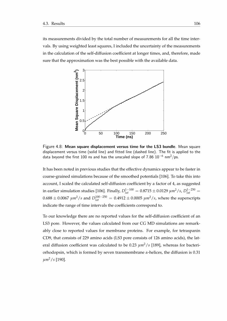
4.3. Results 106
its measurements divided by the total number of measurements for all the time inter-
vals. By using weighted least squares, I included the uncertainty of the measurements
in the calculation of the self-diffusion coefficient at longer times, and, therefore, made
sure that the approximation was the best possible with the available data.
0 50 100 150 200 2500
0.5
1
1.5
2
2.5
3
Time (ns)
Mea
n S
qu
are
Dis
pla
cem
ent
(nm
2 )
Figure 4.8: Mean square displacement versus time for the LS3 bundle. Mean squaredisplacement versus time (solid line) and fitted line (dashed line). The fit is applied to thedata beyond the first 100 ns and has the unscaled slope of 7.86 10−6 nm2/ps.
It has been noted in previous studies that the effective dynamics appear to be faster in
coarse-grained simulations because of the smoothed potentials [106]. To take this into
account, I scaled the calculated self-diffusion coefficient by a factor of 4, as suggested
in earlier simulation studies [106]. Finally, D1−100lat = 0.8715 ± 0.0129 µm2/s, D1−250
lat =
0.688 ± 0.0067 µm2/s and D100−250lat = 0.4912 ± 0.0005 µm2/s, where the superscripts
indicate the range of time intervals the coefficients correspond to.
To our knowledge there are no reported values for the self-diffusion coefficient of an
LS3 pore. However, the values calculated from our CG MD simulations are remark-
ably close to reported values for membrane proteins. For example, for tetraspanin
CD9, that consists of 229 amino acids (LS3 pore consists of 126 amino acids), the lat-
eral diffusion coefficient was calculated to be 0.23 µm2/s [189], whereas for bacteri-
orhodopsin, which is formed by seven transmembrane α-helices, the diffusion is 0.31
µm2/s [190].

4.3. Results 107
Tilt of the pore
It is also worth mentioning that, during the simulation, the relative angles between
the helices were very small (a few degrees), as the peptides were strongly aligned,
whereas each of the helices adopted an orientation of around 20o relative to the bilayer
normal, resulting in an similar orientation (of about 20o) of the bundle as a whole. This
is in good agreement with previous simulation studies [191]. The distribution of the
tilt angle for the hexameric pore is shown in Figure 4.9.
60 70 80 90 100 110
0.01
0.02
0.03
0.04
0.05
Angles in degrees
Pro
bab
ility
Figure 4.9: Tilt angle of the hexameric peptide bundle.
4.3.3 The toroidal pore
In our efforts to define the characteristics of a pore-forming peptide, I used a shortened
version of LS3 that has been experimentally shown to fail to form discrete, stable pores
[16]. (LSSLLSL)2 has the same proportion of hydrophobic and hydrophilic residues
and the same distribution as LS3. Thus, one would expect this peptide to show a
similar behaviour to that of LS3. However, in our simulations, (LSSLLSL)2 preferred
either an interfacial positioning or the formation of complexes. This kind of interaction
could be explained by the hydrophobic mismatch between the peptide and bilayer
thickness. (LSSLLSL)2, in order to position its hydrophilic residues away from the
hydrophobic lipid tails, creates complexes involving several peptides, some of them
inserted in the bilayer and the others located at the bilayer interface.
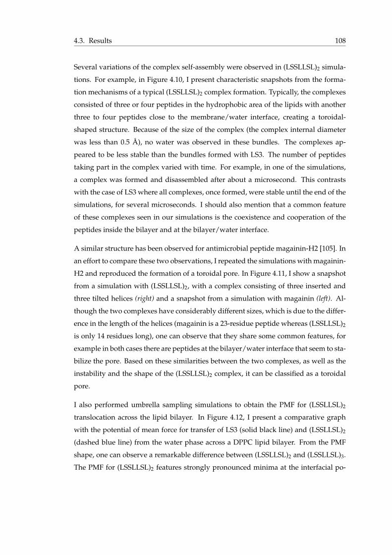
4.3. Results 108
Several variations of the complex self-assembly were observed in (LSSLLSL)2 simula-
tions. For example, in Figure 4.10, I present characteristic snapshots from the forma-
tion mechanisms of a typical (LSSLLSL)2 complex formation. Typically, the complexes
consisted of three or four peptides in the hydrophobic area of the lipids with another
three to four peptides close to the membrane/water interface, creating a toroidal-
shaped structure. Because of the size of the complex (the complex internal diameter
was less than 0.5 A), no water was observed in these bundles. The complexes ap-
peared to be less stable than the bundles formed with LS3. The number of peptides
taking part in the complex varied with time. For example, in one of the simulations,
a complex was formed and disassembled after about a microsecond. This contrasts
with the case of LS3 where all complexes, once formed, were stable until the end of the
simulations, for several microseconds. I should also mention that a common feature
of these complexes seen in our simulations is the coexistence and cooperation of the
peptides inside the bilayer and at the bilayer/water interface.
A similar structure has been observed for antimicrobial peptide magainin-H2 [105]. In
an effort to compare these two observations, I repeated the simulations with magainin-
H2 and reproduced the formation of a toroidal pore. In Figure 4.11, I show a snapshot
from a simulation with (LSSLLSL)2, with a complex consisting of three inserted and
three tilted helices (right) and a snapshot from a simulation with magainin (left). Al-
though the two complexes have considerably different sizes, which is due to the differ-
ence in the length of the helices (magainin is a 23-residue peptide whereas (LSSLLSL)2
is only 14 residues long), one can observe that they share some common features, for
example in both cases there are peptides at the bilayer/water interface that seem to sta-
bilize the pore. Based on these similarities between the two complexes, as well as the
instability and the shape of the (LSSLLSL)2 complex, it can be classified as a toroidal
pore.
I also performed umbrella sampling simulations to obtain the PMF for (LSSLLSL)2
translocation across the lipid bilayer. In Figure 4.12, I present a comparative graph
with the potential of mean force for transfer of LS3 (solid black line) and (LSSLLSL)2
(dashed blue line) from the water phase across a DPPC lipid bilayer. From the PMF
shape, one can observe a remarkable difference between (LSSLLSL)2 and (LSSLLSL)3.
The PMF for (LSSLLSL)2 features strongly pronounced minima at the interfacial po-
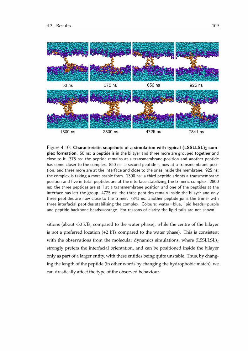
4.3. Results 109
Figure 4.10: Characteristic snapshots of a simulation with typical (LSSLLSL)2 com-plex formation. 50 ns: a peptide is in the bilayer and three more are grouped together andclose to it. 375 ns: the peptide remains at a transmembrane position and another peptidehas come closer to the complex. 850 ns: a second peptide is now at a transmembrane posi-tion, and three more are at the interface and close to the ones inside the membrane. 925 ns:the complex is taking a more stable form. 1300 ns: a third peptide adopts a transmembraneposition and five in total peptides are at the interface stabilizing the trimeric complex. 2800ns: the three peptides are still at a transmembrane position and one of the peptides at theinterface has left the group. 4725 ns: the three peptides remain inside the bilayer and onlythree peptides are now close to the trimer. 7841 ns: another peptide joins the trimer withthree interfacial peptides stabilising the complex. Colours: water=blue, lipid heads=purpleand peptide backbone beads=orange. For reasons of clarity the lipid tails are not shown.
sitions (about -30 kTs, compared to the water phase), while the centre of the bilayer
is not a preferred location (+2 kTs compared to the water phase). This is consistent
with the observations from the molecular dynamics simulations, where (LSSLLSL)2
strongly prefers the interfacial orientation, and can be positioned inside the bilayer
only as part of a larger entity, with these entities being quite unstable. Thus, by chang-
ing the length of the peptide (in other words by changing the hydrophobic match), we
can drastically affect the type of the observed behaviour.
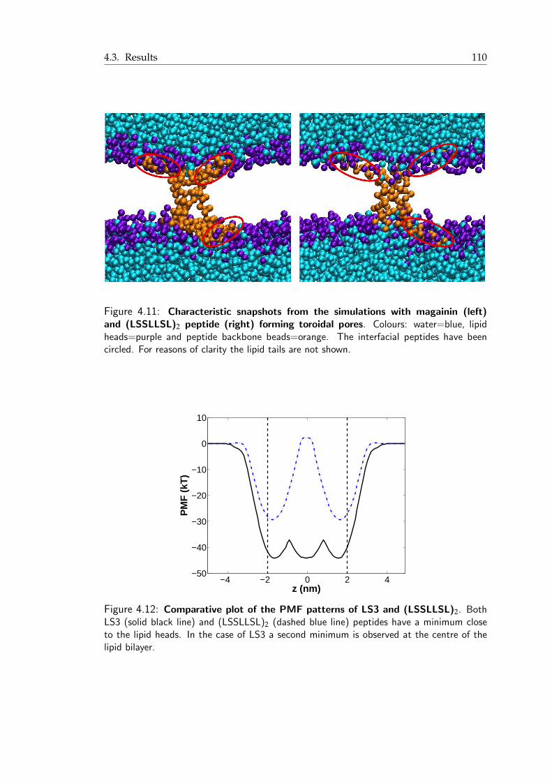
4.3. Results 110
Figure 4.11: Characteristic snapshots from the simulations with magainin (left)and (LSSLLSL)2 peptide (right) forming toroidal pores. Colours: water=blue, lipidheads=purple and peptide backbone beads=orange. The interfacial peptides have beencircled. For reasons of clarity the lipid tails are not shown.
−4 −2 0 2 4−50
−40
−30
−20
−10
0
10
z (nm)
PM
F (
kT)
Figure 4.12: Comparative plot of the PMF patterns of LS3 and (LSSLLSL)2. BothLS3 (solid black line) and (LSSLLSL)2 (dashed blue line) peptides have a minimum closeto the lipid heads. In the case of LS3 a second minimum is observed at the centre of thelipid bilayer.
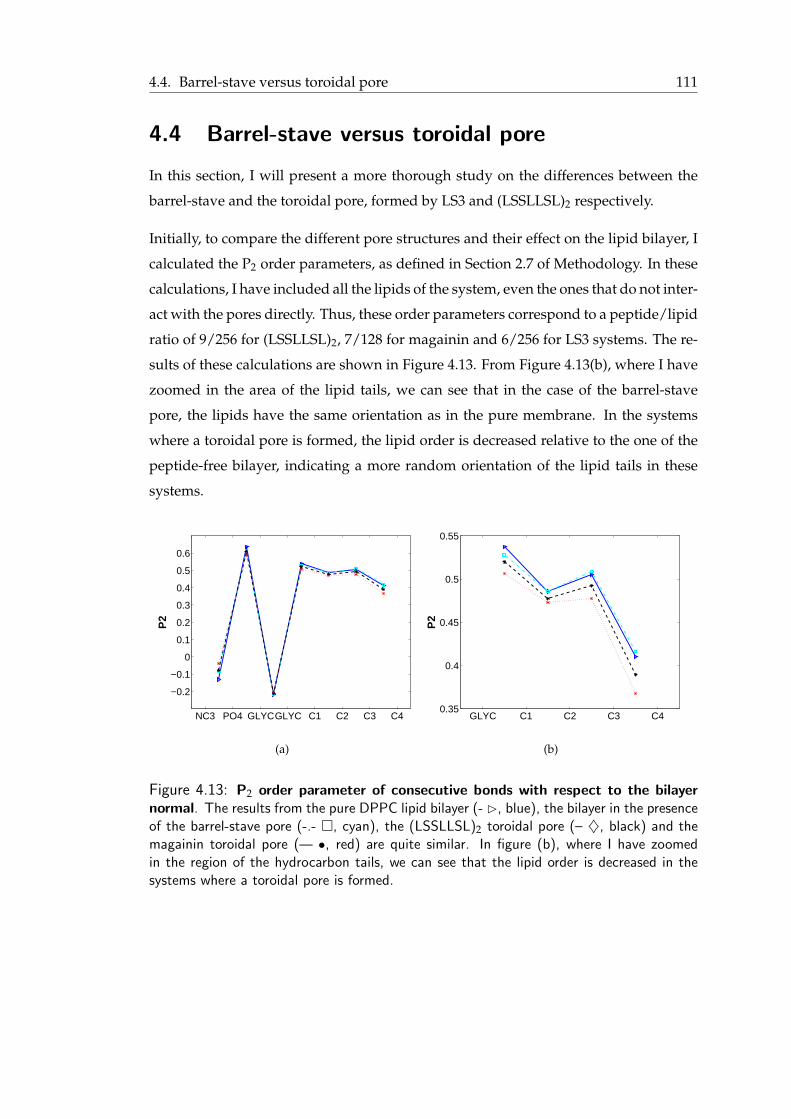
4.4. Barrel-stave versus toroidal pore 111
4.4 Barrel-stave versus toroidal pore
In this section, I will present a more thorough study on the differences between the
barrel-stave and the toroidal pore, formed by LS3 and (LSSLLSL)2 respectively.
Initially, to compare the different pore structures and their effect on the lipid bilayer, I
calculated the P2 order parameters, as defined in Section 2.7 of Methodology. In these
calculations, I have included all the lipids of the system, even the ones that do not inter-
act with the pores directly. Thus, these order parameters correspond to a peptide/lipid
ratio of 9/256 for (LSSLLSL)2, 7/128 for magainin and 6/256 for LS3 systems. The re-
sults of these calculations are shown in Figure 4.13. From Figure 4.13(b), where I have
zoomed in the area of the lipid tails, we can see that in the case of the barrel-stave
pore, the lipids have the same orientation as in the pure membrane. In the systems
where a toroidal pore is formed, the lipid order is decreased relative to the one of the
peptide-free bilayer, indicating a more random orientation of the lipid tails in these
systems.
NC3 PO4 GLYCGLYC C1 C2 C3 C4
−0.2
−0.1
0
0.1
0.2
0.3
0.4
0.5
0.6
P2
(a)
GLYC C1 C2 C3 C40.35
0.4
0.45
0.5
0.55
P2
(b)
Figure 4.13: P2 order parameter of consecutive bonds with respect to the bilayernormal. The results from the pure DPPC lipid bilayer (- ⊲, blue), the bilayer in the presenceof the barrel-stave pore (-.- �, cyan), the (LSSLLSL)2 toroidal pore (– ♦, black) and themagainin toroidal pore (— •, red) are quite similar. In figure (b), where I have zoomedin the region of the hydrocarbon tails, we can see that the lipid order is decreased in thesystems where a toroidal pore is formed.
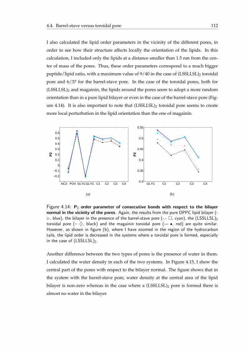
4.4. Barrel-stave versus toroidal pore 112
I also calculated the lipid order parameters in the vicinity of the different pores, in
order to see how their structure affects locally the orientation of the lipids. In this
calculation, I included only the lipids at a distance smaller than 1.5 nm from the cen-
ter of mass of the pores. Thus, these order parameters correspond to a much bigger
peptide/lipid ratio, with a maximum value of 9/40 in the case of (LSSLLSL)2 toroidal
pore and 6/37 for the barrel-stave pore. In the case of the toroidal pores, both for
(LSSLLSL)2 and magainin, the lipids around the pores seem to adopt a more random
orientation than in a pure lipid bilayer or even in the case of the barrel-stave pore (Fig-
ure 4.14). It is also important to note that (LSSLLSL)2 toroidal pore seems to create
more local perturbation in the lipid orientation than the one of magainin.
NC3 PO4 GLYCGLYC C1 C2 C3 C4
−0.2
−0.1
0
0.1
0.2
0.3
0.4
0.5
0.6
P2
(a)
GLYC C1 C2 C3 C40.3
0.35
0.4
0.45
0.5
0.55
P2
(b)
Figure 4.14: P2 order parameter of consecutive bonds with respect to the bilayernormal in the vicinity of the pores. Again, the results from the pure DPPC lipid bilayer (-⊲, blue), the bilayer in the presence of the barrel-stave pore (-.- �, cyan), the (LSSLLSL)2
toroidal pore (– ♦, black) and the magainin toroidal pore (— •, red) are quite similar.However, as shown in figure (b), where I have zoomed in the region of the hydrocarbontails, the lipid order is decreased in the systems where a toroidal pore is formed, especiallyin the case of (LSSLLSL)2.
Another difference between the two types of pores is the presence of water in them.
I calculated the water density in each of the two systems. In Figure 4.15, I show the
central part of the pores with respect to the bilayer normal. The figure shows that in
the system with the barrel-stave pore, water density at the central area of the lipid
bilayer is non-zero whereas in the case where a (LSSLLSL)2 pore is formed there is
almost no water in the bilayer.

4.4. Barrel-stave versus toroidal pore 113
−1 −0.5 0 0.5 10
0.01
0.02
0.03
0.04
0.05
0.06
0.07
Distance from bilayer center (nm)
Den
sity
(b
ead
s/n
m3 )
Figure 4.15: Water density in the barrel-stave and the toroidal pore. The plotcorresponds to the central part of the pores and the distance is with respect to the bilayernormal. In the case of the barrel-stave pore (black solid line, x) we can see that there iswater at the central part of the bilayer whereas in the case of (LSSLLSL)2 pore (blue dashedline, ∗) the density of water is close to zero.
I have also calculated the apparent area per lipid and volume per lipid in the presence
of the two different kinds of pores. The systems under study have 256 DPPC lipids
and 3228 waters. The area per lipid was obtained by dividing the area of the plane of
the lipid bilayer by the number of lipids present in each leaflet. For the calculation of
the volume per lipid the following formula was used:
VL =ALLz
2− NwVw, (4.2)
where AL is the area per lipid, Lz is the length of the simulation box in the direction
of the bilayer normal, Nw is the number of waters per lipid molecule and Vw1 is the
volume per water. In Table 4.3, we summarize the results. The apparent area per lipid
is increased in the presence of the pores, as expected. In the case of the toroidal pore
this increment is slightly bigger. The value for the volume per lipid is very similar in
all three systems.
1Vw was calculated by a simulation with bulk water at the same conditions.
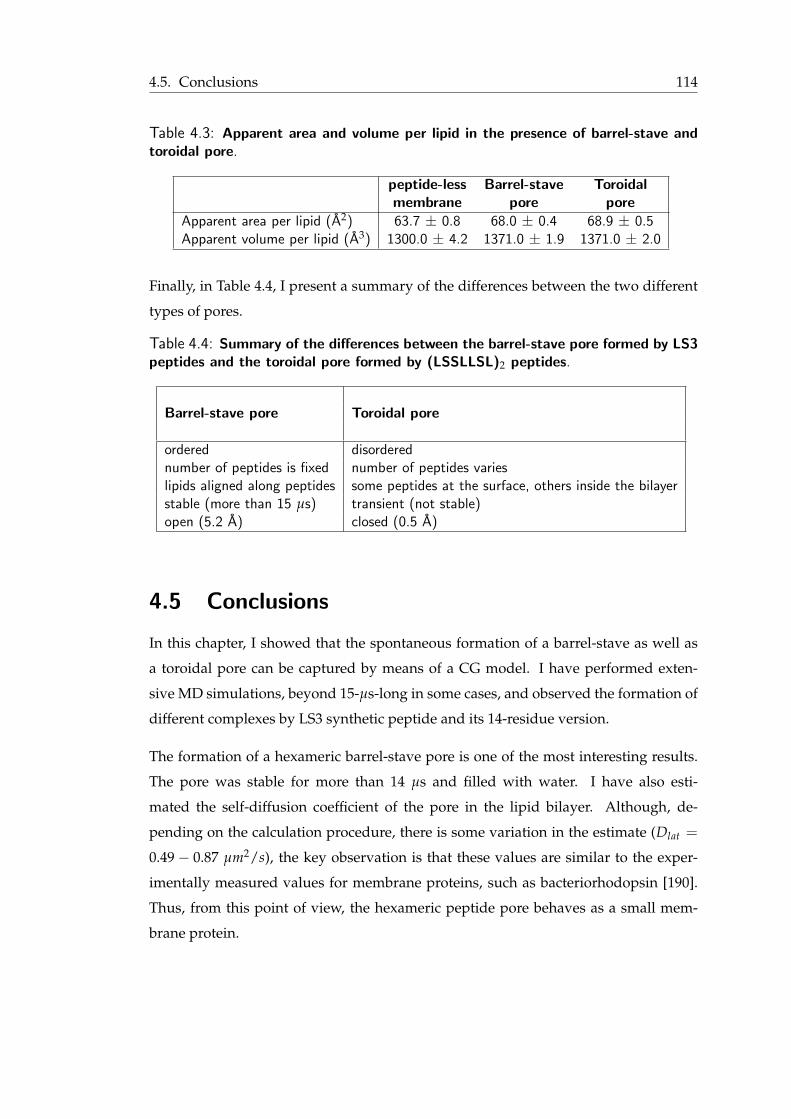
4.5. Conclusions 114
Table 4.3: Apparent area and volume per lipid in the presence of barrel-stave andtoroidal pore.
peptide-less Barrel-stave Toroidalmembrane pore pore
Apparent area per lipid (A2) 63.7 ± 0.8 68.0 ± 0.4 68.9 ± 0.5Apparent volume per lipid (A3) 1300.0 ± 4.2 1371.0 ± 1.9 1371.0 ± 2.0
Finally, in Table 4.4, I present a summary of the differences between the two different
types of pores.
Table 4.4: Summary of the differences between the barrel-stave pore formed by LS3peptides and the toroidal pore formed by (LSSLLSL)2 peptides.
Barrel-stave pore Toroidal pore
ordered disorderednumber of peptides is fixed number of peptides varieslipids aligned along peptides some peptides at the surface, others inside the bilayerstable (more than 15 µs) transient (not stable)open (5.2 A) closed (0.5 A)
4.5 Conclusions
In this chapter, I showed that the spontaneous formation of a barrel-stave as well as
a toroidal pore can be captured by means of a CG model. I have performed exten-
sive MD simulations, beyond 15-µs-long in some cases, and observed the formation of
different complexes by LS3 synthetic peptide and its 14-residue version.
The formation of a hexameric barrel-stave pore is one of the most interesting results.
The pore was stable for more than 14 µs and filled with water. I have also esti-
mated the self-diffusion coefficient of the pore in the lipid bilayer. Although, de-
pending on the calculation procedure, there is some variation in the estimate (Dlat =
0.49 − 0.87 µm2/s), the key observation is that these values are similar to the exper-
imentally measured values for membrane proteins, such as bacteriorhodopsin [190].
Thus, from this point of view, the hexameric peptide pore behaves as a small mem-
brane protein.
4.5. Conclusions 115
Interestingly, the barrel-stave pore forms in the absence of a transmembrane poten-
tial, and naturally, there is no preferred orientation of the peptides within the bilayer.
However, the impact of the applied electrostatic field will be investigated in future
work.
Remarkably, the simulations of a shorter version of this peptide, (LSSLLSL)2, showed
that this peptide has a much lower propensity for poration and, when a complex does
form, it has a toroidal structure. These complexes were different to the barrel-stave
pore or the other complexes formed by LS3. They had a small diameter that does not
allow for water to pass through it. Also, they were unstable, with the number of pep-
tides taking part in them varying during the simulation. Another difference between
the two observed pores was the structure of lipids in their vicinity. I calculated the
order parameters of the lipids around the pores, and I showed that in the case of the
toroidal pore the lipids have a decreased order relative to those close to the barrel stave
pore.
I also calculated the apparent area and volume per lipid in the systems with the two
different pores. The values were higher for the toroidal pore although its size was
smaller. This is another indication of the disordered structure of the toroidal pore. It
is important to note here that the values calculated by our simulations can be directly
compared to measurements by Langmuir balance or diffraction techniques and thus,
give information about the possible formation of a pore.
Also, the PMF for (LSSLLSL)2 is dramatically different from that of LS3, with the en-
ergy minima at the bilayer interfaces and the core of the bilayer being an unfavourable
location of the peptide. In the light of this PMF, the strong propensity of (LSSLLSL)2
for the interfacial orientation in MD simulations is not surprising. Furthermore, there
are clear similarities between the PMF of LAP20 peptide, presented in Chapter 3 and
the PMF calculated for (LSSLLSL)2, with the features of the (LSSLLSL)2 PMF magni-
fied in the LAP20 case. Thus, it seems that from this point of view the two peptides
belong to the same class of nonspanning peptides. Whether or not under certain cir-
cumstances LAP20 exhibits self-assembly behaviour similar to the toroidal structures
of (LSSLLSL)2 remains an open question.
4.5. Conclusions 116
To close this chapter, I would like to draw the attention of the reader to what I believe
is a very important conclusion from this study. Our extensive simulation studies show
a potential link between the length of a peptide and its ability to form either stable,
ordered and open pores or transient, disordered and closed pores. The formation of a
toroidal-like pore by an uncharged and short peptide seems contradictory to the typ-
ical toroidal-pore forming peptides, the antimicrobial peptides (AMPs). The AMPs
are 20-40 amino acids long and usually cationic. Their positive charge is often used
as an explanation for their interaction with bacterial membranes that are usually an-
ionic. However, an explanation for the pore-forming abilities of (LSSLLSL)2 lies in the
hydrophobic mismatch between the length of the peptide and the thickness of the bi-
layer. Also, the formation of the toroidal pore in our simulations seems to be initiated
when at least one peptide is initially half-inserted in the lipid head area. Moreover, in
some AMPs the hydrophobic region along the helical axis is shorter than the bilayer
thickness that could also be another reason for the shape of the pore. Thus, a possi-
ble conclusion could be that the formation of a toroidal pore may be initiated by the
electrostatic interactions between the peptide and the membrane, however, the shape
of the pore seems to be linked to the distribution of hydrophobic residues along the
helical axis.

CHAPTER 5
Cell-penetrating peptides
In this chapter, we will extend our studies to the self-assembly and membrane inter-
nalization mechanisms of cell-penetrating peptides, which have the ability to transfer
large macromolecules across cellular membranes. We have chosen two particularly
interesting cases, pHLIP and Pep-1 peptides. It has been experimentally shown that
pHLIP serves as an efficient drug carrier without poration or self-assembly process.
On the other hand, the translocation mechanism of Pep-1 has been a subject of contro-
versy over the last years and is not yet established.
We will start the chapter with a short introduction to the area of cell-penetrating pep-
tides, emphasising in their importance and possible applications, and focusing on the
two chosen peptides. We will follow with the methodology and the results. The chap-
ter closes with a discussion on the main outcomes of our study.
117
5.1. Introduction 118
5.1 Introduction
High molecular weight biomolecules have been playing an increasingly important role
as new, more effective therapeutic drugs. The bioavailability of drugs depends signifi-
cantly on their solubility properties; they must be polar enough to dissolve in biologi-
cal fluids, but not so polar that the drug cannot enter the cell. As a consequence, many
drug candidates, being out of this polarity range, fail to advance clinically. One of
the most promising approaches to resolve this problem is the use of peptide-carriers,
commonly known as cell-penetrating peptides (CPPs).
Cell-penetrating peptides (CPPs) are a family of short, highly basic and amphipathic
peptides. They have been successfully used to transport large macromolecules, such as
proteins, peptides, antisense oligonucleotide (ON), siRNAs, plasmids and other large
particles, like liposomes, across cellular membranes both in vitro and in vivo. The ini-
tial discovery of CPPs originated from the observation that some intracellular pro-
teins, when added to an extracellular medium, had the ability to translocate across the
membrane. Tat transactivator of HIV virus type 1 [192] and pAntp, Drosophila anten-
napedia transcription protein [193], were the first peptides to be identified with this
ability.
A number of studies have been made on the ability of cell-penetrating peptides to in-
hibit tumour growth in vivo [194–196]. They can be used as delivery vectors of tumour
suppressors, such as human p53 or lac tumour suppressor, or other proapoptotic pro-
teins. In another example, it has been shown that, using a cell-penetrating peptide,
nitric oxide synthesis could be inhibited and inflammation could be reduced in an an-
imal model [197]. Furthermore, the incorporation of CPPs into vaccines is currently
being studied as there are indications that they could constitute a useful ingredient
that would ensure an effective T-cell response. These are just a few from numerous
examples of successful applications of cell-penetrating peptides as drug-delivery vec-
tors.
Despite the extensive research on how CPPs traverse cell membranes and promote the
intracellular uptake of various cargo molecules, the underlying mechanism remains
unclear. Depending on their charge, size, and structure, different CPPs utilize dif-
ferent internalization mechanisms. It is also possible that after cargos are linked to
5.1. Introduction 119
the peptides, this internalization mechanism changes. Possible mechanisms include
endocytosis-mediated entry, translocation by means of the sinking-raft model, the for-
mation of pores or translocation through formation of an inverted micelle. Some of
the possible mechanisms have already been introduced in Chapter 1 (Figure 1.4). The
molecular details of the various translocation processes are not well understood. It is
thus important to (i) elucidate these details and (ii) link the properties of the peptides
to the various mechanisms of peptide-membrane interaction they induce. This would
be an important step towards the rational design of peptides with tailored functional-
ities.
Molecular dynamics simulations can play an important role in the overall process of
understanding and elucidating the mechanisms of interactions of CPPs with lipid bi-
layers. In this study, we chose two particularly interesting cell-penetrating peptides,
pHLIP and Pep-1. We have already introduced pHLIP in Chapter 3, however for the
purposes of this chapter, we will provide further information about its translocation
mechanism.
pHLIP is an amphipathic peptide that has been shown to accumulate in the mem-
branes of cells in acidic environments and to have the ability to transfer attached
molecules across them. In other words, pHLIP can act as a nanosyringe [164, 167].
Some of its possible applications include diagnostic imaging, drug therapy or genetic
control. These potential uses of pHLIP are based on the fact that in many diseases there
are naturally occurring acidic environments, ranging from 5.5 to 6.5 pH (e.g. tumours,
sites of inflammation or stroke-afficted tissues). There is a generally accepted mecha-
nism of pHLIP translocation which is shown in Figure 5.1. At pH=7, pHLIP is solu-
ble in water in a random conformation, and at lipid/peptide ratios larger than 100, it
binds to the membrane/water interface where conformational changes happen. When
pH<6, it adopts a transmembrane position in a α-helical structure [164, 167, 198]. We
should also note that for low lipid/peptide ratios, no translocation across the mem-
brane has been observed [166]. Moreover, in the same publication, the authors suggest
that the hydrophobic C-terminus of pHLIP seems to be the one adsorbed first, when
the peptide is bound to the membrane.
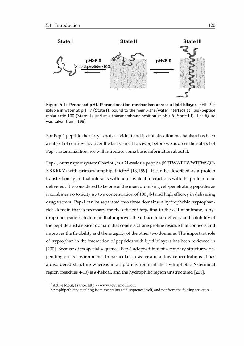
5.1. Introduction 120
Figure 5.1: Proposed pHLIP translocation mechanism across a lipid bilayer. pHLIP issoluble in water at pH=7 (State I), bound to the membrane/water interface at lipid/peptidemolar ratio 100 (State II), and at a transmembrane position at pH<6 (State III). The figurewas taken from [198].
For Pep-1 peptide the story is not as evident and its translocation mechanism has been
a subject of controversy over the last years. However, before we address the subject of
Pep-1 internalization, we will introduce some basic information about it.
Pep-1, or transport system Chariot1, is a 21-residue peptide (KETWWETWWTEWSQP-
KKKRKV) with primary amphipathicity2 [13, 199]. It can be described as a protein
transfection agent that interacts with non-covalent interactions with the protein to be
delivered. It is considered to be one of the most promising cell-penetrating peptides as
it combines no toxicity up to a concentration of 100 µM and high efficacy in delivering
drug vectors. Pep-1 can be separated into three domains; a hydrophobic tryptophan-
rich domain that is necessary for the efficient targeting to the cell membrane, a hy-
drophilic lysine-rich domain that improves the intracellular delivery and solubility of
the peptide and a spacer domain that consists of one proline residue that connects and
improves the flexibility and the integrity of the other two domains. The important role
of tryptophan in the interaction of peptides with lipid bilayers has been reviewed in
[200]. Because of its special sequence, Pep-1 adopts different secondary structures, de-
pending on its environment. In particular, in water and at low concentrations, it has
a disordered structure whereas in a lipid environment the hydrophobic N-terminal
region (residues 4-13) is α-helical, and the hydrophilic region unstructured [201].
1Active Motif, France, http://www.activemotif.com2Amphipathicity resulting from the amino acid sequence itself, and not from the folding structure.
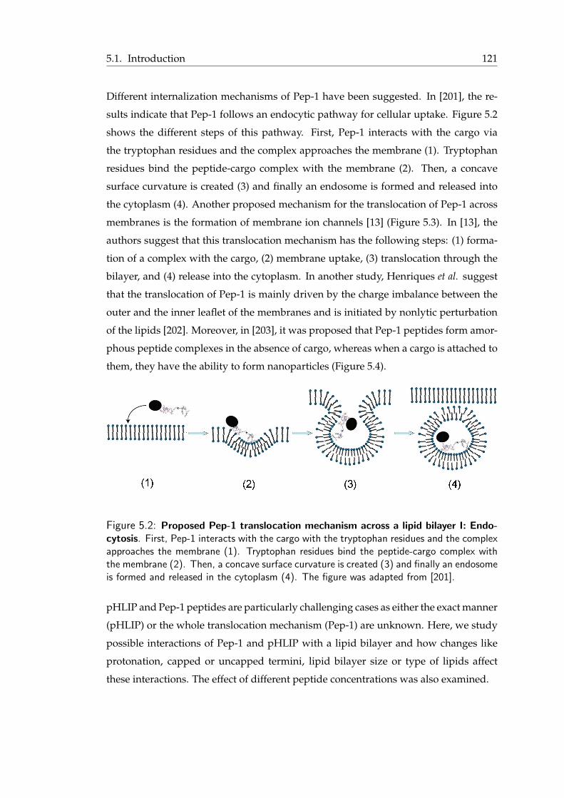
5.1. Introduction 121
Different internalization mechanisms of Pep-1 have been suggested. In [201], the re-
sults indicate that Pep-1 follows an endocytic pathway for cellular uptake. Figure 5.2
shows the different steps of this pathway. First, Pep-1 interacts with the cargo via
the tryptophan residues and the complex approaches the membrane (1). Tryptophan
residues bind the peptide-cargo complex with the membrane (2). Then, a concave
surface curvature is created (3) and finally an endosome is formed and released into
the cytoplasm (4). Another proposed mechanism for the translocation of Pep-1 across
membranes is the formation of membrane ion channels [13] (Figure 5.3). In [13], the
authors suggest that this translocation mechanism has the following steps: (1) forma-
tion of a complex with the cargo, (2) membrane uptake, (3) translocation through the
bilayer, and (4) release into the cytoplasm. In another study, Henriques et al. suggest
that the translocation of Pep-1 is mainly driven by the charge imbalance between the
outer and the inner leaflet of the membranes and is initiated by nonlytic perturbation
of the lipids [202]. Moreover, in [203], it was proposed that Pep-1 peptides form amor-
phous peptide complexes in the absence of cargo, whereas when a cargo is attached to
them, they have the ability to form nanoparticles (Figure 5.4).
Figure 5.2: Proposed Pep-1 translocation mechanism across a lipid bilayer I: Endo-cytosis. First, Pep-1 interacts with the cargo with the tryptophan residues and the complexapproaches the membrane (1). Tryptophan residues bind the peptide-cargo complex withthe membrane (2). Then, a concave surface curvature is created (3) and finally an endosomeis formed and released in the cytoplasm (4). The figure was adapted from [201].
pHLIP and Pep-1 peptides are particularly challenging cases as either the exact manner
(pHLIP) or the whole translocation mechanism (Pep-1) are unknown. Here, we study
possible interactions of Pep-1 and pHLIP with a lipid bilayer and how changes like
protonation, capped or uncapped termini, lipid bilayer size or type of lipids affect
these interactions. The effect of different peptide concentrations was also examined.
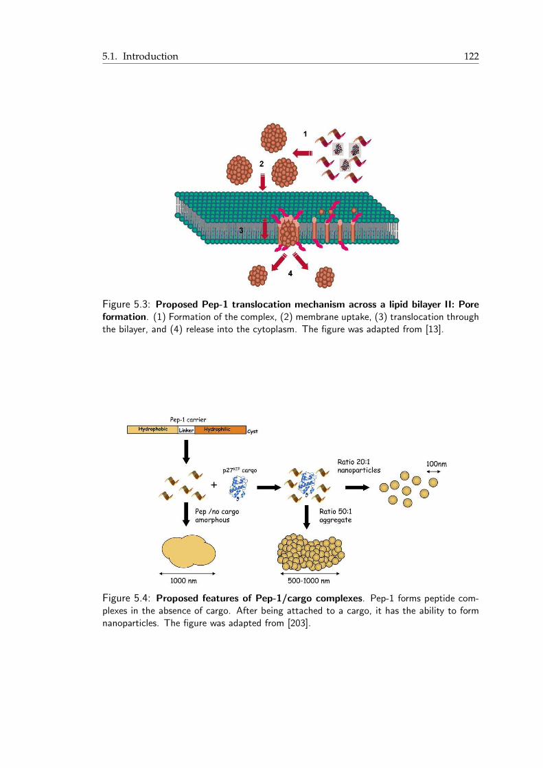
5.1. Introduction 122
Figure 5.3: Proposed Pep-1 translocation mechanism across a lipid bilayer II: Poreformation. (1) Formation of the complex, (2) membrane uptake, (3) translocation throughthe bilayer, and (4) release into the cytoplasm. The figure was adapted from [13].
Figure 5.4: Proposed features of Pep-1/cargo complexes. Pep-1 forms peptide com-plexes in the absence of cargo. After being attached to a cargo, it has the ability to formnanoparticles. The figure was adapted from [203].
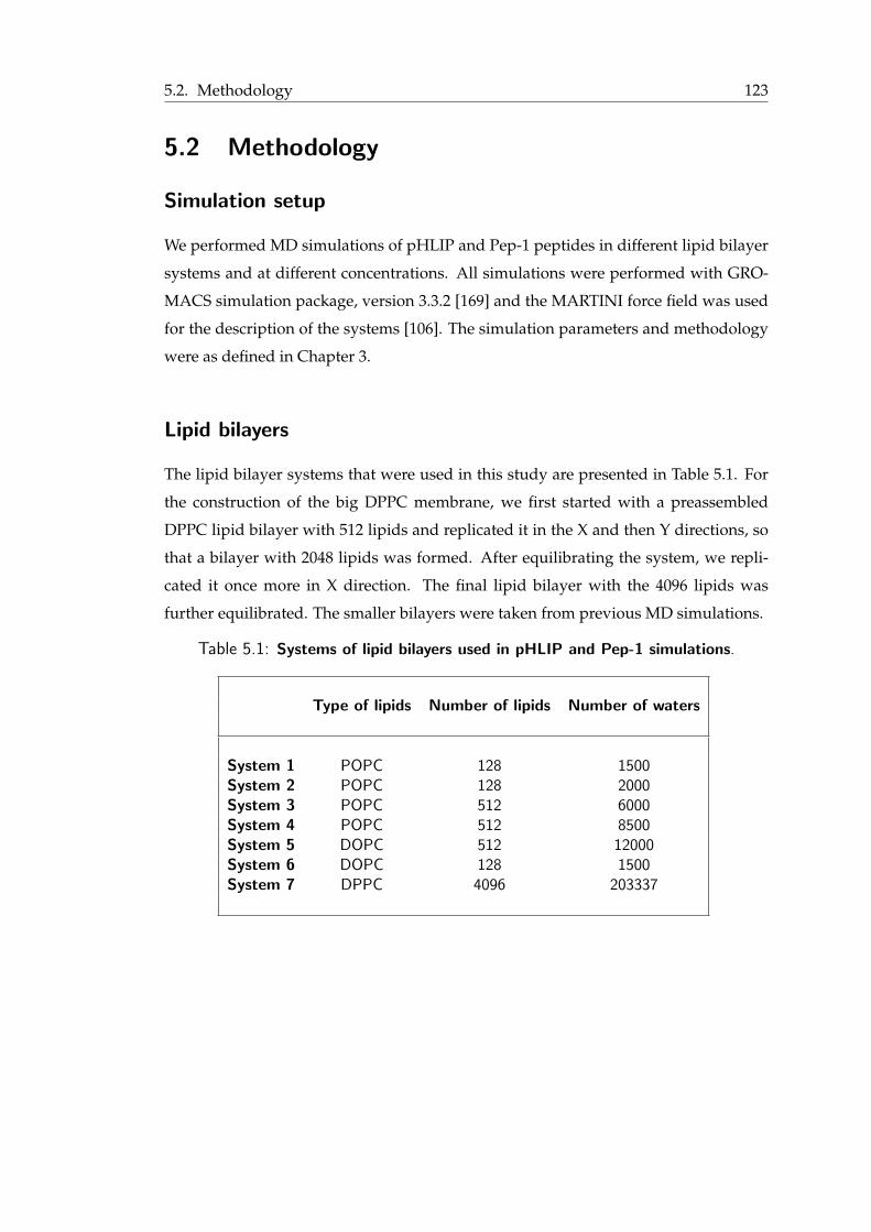
5.2. Methodology 123
5.2 Methodology
Simulation setup
We performed MD simulations of pHLIP and Pep-1 peptides in different lipid bilayer
systems and at different concentrations. All simulations were performed with GRO-
MACS simulation package, version 3.3.2 [169] and the MARTINI force field was used
for the description of the systems [106]. The simulation parameters and methodology
were as defined in Chapter 3.
Lipid bilayers
The lipid bilayer systems that were used in this study are presented in Table 5.1. For
the construction of the big DPPC membrane, we first started with a preassembled
DPPC lipid bilayer with 512 lipids and replicated it in the X and then Y directions, so
that a bilayer with 2048 lipids was formed. After equilibrating the system, we repli-
cated it once more in X direction. The final lipid bilayer with the 4096 lipids was
further equilibrated. The smaller bilayers were taken from previous MD simulations.
Table 5.1: Systems of lipid bilayers used in pHLIP and Pep-1 simulations.
Type of lipids Number of lipids Number of waters
System 1 POPC 128 1500System 2 POPC 128 2000System 3 POPC 512 6000System 4 POPC 512 8500System 5 DOPC 512 12000System 6 DOPC 128 1500System 7 DPPC 4096 203337

5.3. pHLIP peptide 124
Steered MD simulations
Steered MD simulations were performed for Pep-1 peptide, in an effort to capture
a potential endocytic pathway, which is a large scale and slow process. We used a
preassembled peptide complex, a pentamer formed in one of the MD simulations. We
used a harmonic potential with a force constant of 5000 kJ/(mol·nm2) applied to the
centre of the complex with the direction of the normal of the bilayer towards its centre.
The pulling rate was 0.0005 nm/ps. The complex’ motion in the XY plane was not
restrained.
5.3 pHLIP peptide
In Figure 5.5, we present the amino acid sequence of pHLIP and a summary of its
observed or proposed behaviour. In our studies, pHLIP is treated as an α-helix in the
whole system (even when it is in water). We believe that for the purposes of our study,
this representation is adequate.
Figure 5.5: pHLIP peptide: A short summary.
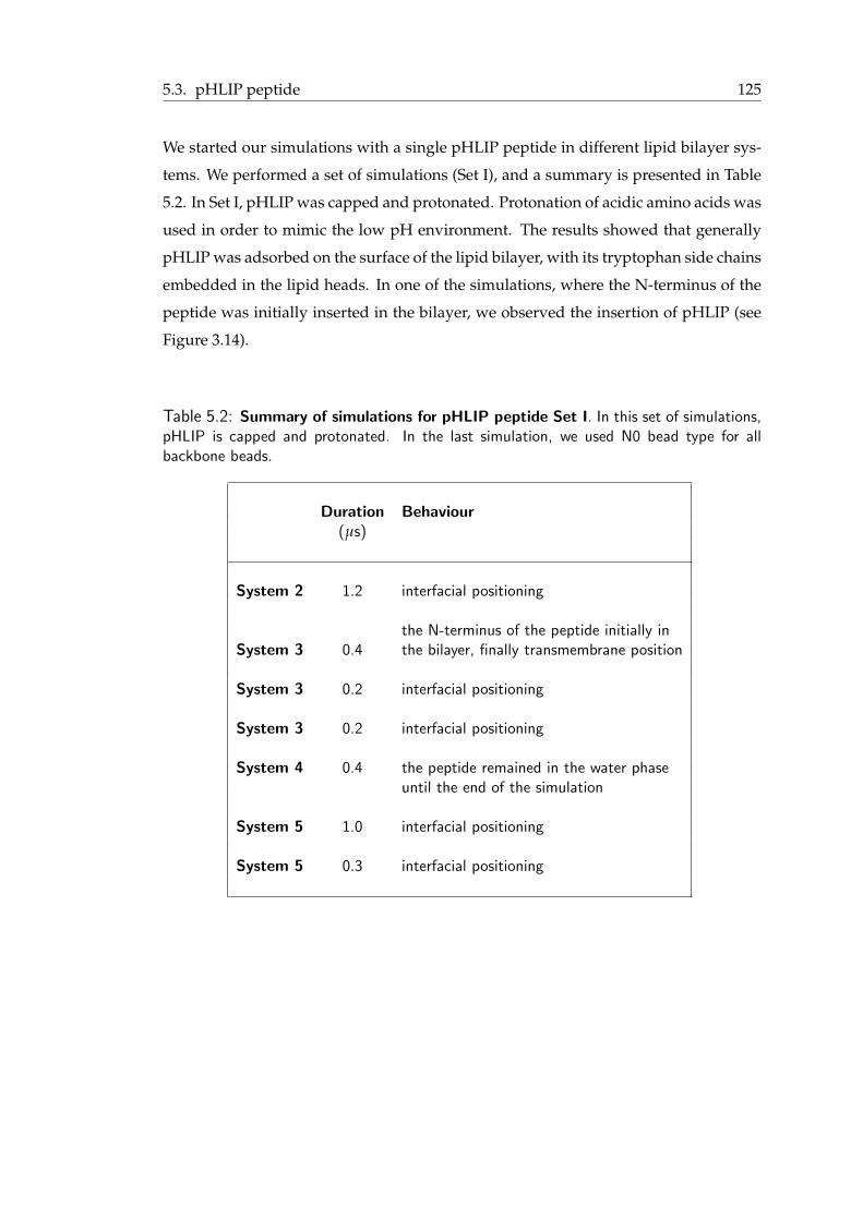
5.3. pHLIP peptide 125
We started our simulations with a single pHLIP peptide in different lipid bilayer sys-
tems. We performed a set of simulations (Set I), and a summary is presented in Table
5.2. In Set I, pHLIP was capped and protonated. Protonation of acidic amino acids was
used in order to mimic the low pH environment. The results showed that generally
pHLIP was adsorbed on the surface of the lipid bilayer, with its tryptophan side chains
embedded in the lipid heads. In one of the simulations, where the N-terminus of the
peptide was initially inserted in the bilayer, we observed the insertion of pHLIP (see
Figure 3.14).
Table 5.2: Summary of simulations for pHLIP peptide Set I. In this set of simulations,pHLIP is capped and protonated. In the last simulation, we used N0 bead type for allbackbone beads.
Duration Behaviour(µs)
System 2 1.2 interfacial positioning
the N-terminus of the peptide initially inSystem 3 0.4 the bilayer, finally transmembrane position
System 3 0.2 interfacial positioning
System 3 0.2 interfacial positioning
System 4 0.4 the peptide remained in the water phaseuntil the end of the simulation
System 5 1.0 interfacial positioning
System 5 0.3 interfacial positioning
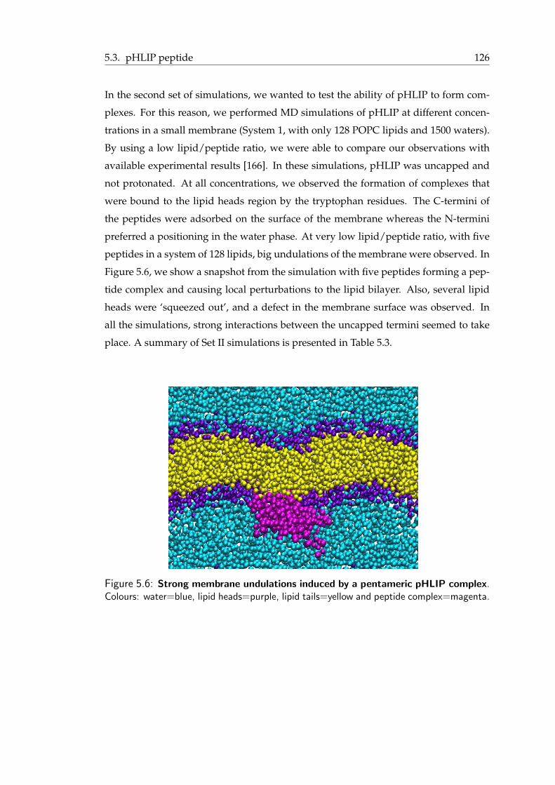
5.3. pHLIP peptide 126
In the second set of simulations, we wanted to test the ability of pHLIP to form com-
plexes. For this reason, we performed MD simulations of pHLIP at different concen-
trations in a small membrane (System 1, with only 128 POPC lipids and 1500 waters).
By using a low lipid/peptide ratio, we were able to compare our observations with
available experimental results [166]. In these simulations, pHLIP was uncapped and
not protonated. At all concentrations, we observed the formation of complexes that
were bound to the lipid heads region by the tryptophan residues. The C-termini of
the peptides were adsorbed on the surface of the membrane whereas the N-termini
preferred a positioning in the water phase. At very low lipid/peptide ratio, with five
peptides in a system of 128 lipids, big undulations of the membrane were observed. In
Figure 5.6, we show a snapshot from the simulation with five peptides forming a pep-
tide complex and causing local perturbations to the lipid bilayer. Also, several lipid
heads were ‘squeezed out’, and a defect in the membrane surface was observed. In
all the simulations, strong interactions between the uncapped termini seemed to take
place. A summary of Set II simulations is presented in Table 5.3.
Figure 5.6: Strong membrane undulations induced by a pentameric pHLIP complex.Colours: water=blue, lipid heads=purple, lipid tails=yellow and peptide complex=magenta.
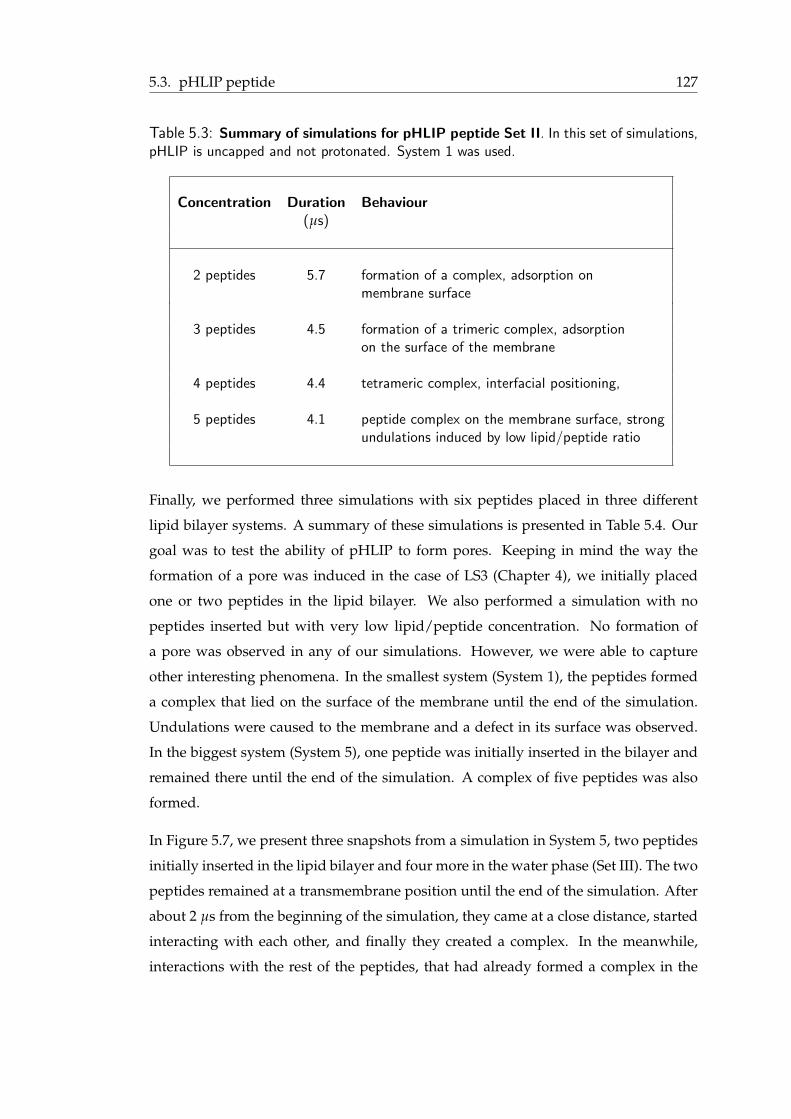
5.3. pHLIP peptide 127
Table 5.3: Summary of simulations for pHLIP peptide Set II. In this set of simulations,pHLIP is uncapped and not protonated. System 1 was used.
Concentration Duration Behaviour(µs)
2 peptides 5.7 formation of a complex, adsorption onmembrane surface
3 peptides 4.5 formation of a trimeric complex, adsorptionon the surface of the membrane
4 peptides 4.4 tetrameric complex, interfacial positioning,
5 peptides 4.1 peptide complex on the membrane surface, strongundulations induced by low lipid/peptide ratio
Finally, we performed three simulations with six peptides placed in three different
lipid bilayer systems. A summary of these simulations is presented in Table 5.4. Our
goal was to test the ability of pHLIP to form pores. Keeping in mind the way the
formation of a pore was induced in the case of LS3 (Chapter 4), we initially placed
one or two peptides in the lipid bilayer. We also performed a simulation with no
peptides inserted but with very low lipid/peptide concentration. No formation of
a pore was observed in any of our simulations. However, we were able to capture
other interesting phenomena. In the smallest system (System 1), the peptides formed
a complex that lied on the surface of the membrane until the end of the simulation.
Undulations were caused to the membrane and a defect in its surface was observed.
In the biggest system (System 5), one peptide was initially inserted in the bilayer and
remained there until the end of the simulation. A complex of five peptides was also
formed.
In Figure 5.7, we present three snapshots from a simulation in System 5, two peptides
initially inserted in the lipid bilayer and four more in the water phase (Set III). The two
peptides remained at a transmembrane position until the end of the simulation. After
about 2 µs from the beginning of the simulation, they came at a close distance, started
interacting with each other, and finally they created a complex. In the meanwhile,
interactions with the rest of the peptides, that had already formed a complex in the
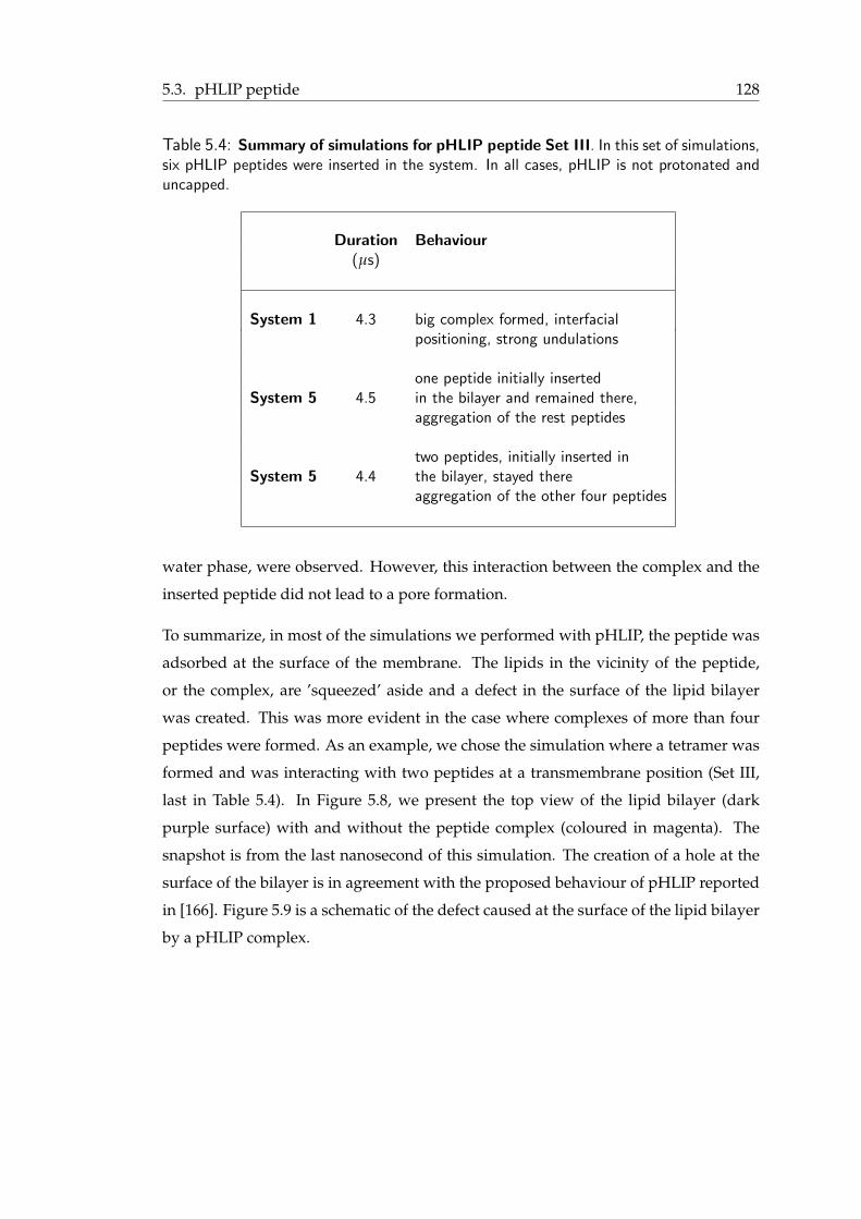
5.3. pHLIP peptide 128
Table 5.4: Summary of simulations for pHLIP peptide Set III. In this set of simulations,six pHLIP peptides were inserted in the system. In all cases, pHLIP is not protonated anduncapped.
Duration Behaviour(µs)
System 1 4.3 big complex formed, interfacialpositioning, strong undulations
one peptide initially insertedSystem 5 4.5 in the bilayer and remained there,
aggregation of the rest peptides
two peptides, initially inserted inSystem 5 4.4 the bilayer, stayed there
aggregation of the other four peptides
water phase, were observed. However, this interaction between the complex and the
inserted peptide did not lead to a pore formation.
To summarize, in most of the simulations we performed with pHLIP, the peptide was
adsorbed at the surface of the membrane. The lipids in the vicinity of the peptide,
or the complex, are ’squeezed’ aside and a defect in the surface of the lipid bilayer
was created. This was more evident in the case where complexes of more than four
peptides were formed. As an example, we chose the simulation where a tetramer was
formed and was interacting with two peptides at a transmembrane position (Set III,
last in Table 5.4). In Figure 5.8, we present the top view of the lipid bilayer (dark
purple surface) with and without the peptide complex (coloured in magenta). The
snapshot is from the last nanosecond of this simulation. The creation of a hole at the
surface of the bilayer is in agreement with the proposed behaviour of pHLIP reported
in [166]. Figure 5.9 is a schematic of the defect caused at the surface of the lipid bilayer
by a pHLIP complex.
5.3. pHLIP peptide 129
Figure 5.7: Snapshots from pHLIP simulations. Two peptides are initially placed at atransmembrane position and remain there until the end of the simulation. After about 2 µsfrom the beginning of the simulation, they come at a close distance and start interactingwith each other, and finally they create a complex. In the meanwhile, interactions with therest of the peptides, that have already formed a complex in the water phase, are observed.However, this interaction between the complex and the inserted peptide does not lead toa pore formation. Colours: lipid heads=purple and peptide backbone beads=orange. Thewater and lipid tails have been removed for reasons of clarity.
Figure 5.8: Top view of the defect created by the pHLIP complex on the surface ofthe lipid bilayer. (a) Snapshot of the defect with only the surface of the bilayer shown as asurface coloured purple. (b) Snapshot with the lipid tails shown as green and yellow beadscorresponding to the top and bottom leaflet respectively. (c) Snapshot where the peptidecomplex is also included and coloured in magenta.
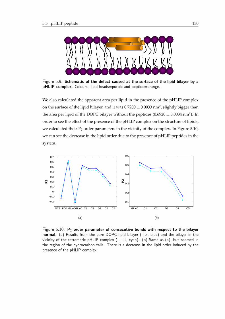
5.3. pHLIP peptide 130
Figure 5.9: Schematic of the defect caused at the surface of the lipid bilayer by apHLIP complex. Colours: lipid heads=purple and peptide=orange.
We also calculated the apparent area per lipid in the presence of the pHLIP complex
on the surface of the lipid bilayer, and it was 0.7200 ± 0.0033 nm2, slightly bigger than
the area per lipid of the DOPC bilayer without the peptides (0.6920 ± 0.0034 nm2). In
order to see the effect of the presence of the pHLIP complex on the structure of lipids,
we calculated their P2 order parameters in the vicinity of the complex. In Figure 5.10,
we can see the decrease in the lipid order due to the presence of pHLIP peptides in the
system.
NC3 PO4 GLYCGLYC C1 C2 D3 C4 C5
−0.2
−0.1
0
0.1
0.2
0.3
0.4
0.5
0.6
0.7
P2
(a)
GLYC C1 C2 D3 C4 C5
0.1
0.2
0.3
0.4
0.5
0.6
P2
(b)
Figure 5.10: P2 order parameter of consecutive bonds with respect to the bilayernormal. (a) Results from the pure DOPC lipid bilayer (- ⊲, blue) and the bilayer in thevicinity of the tetrameric pHLIP complex (-.- �, cyan). (b) Same as (a), but zoomed inthe region of the hydrocarbon tails. There is a decrease in the lipid order induced by thepresence of the pHLIP complex.
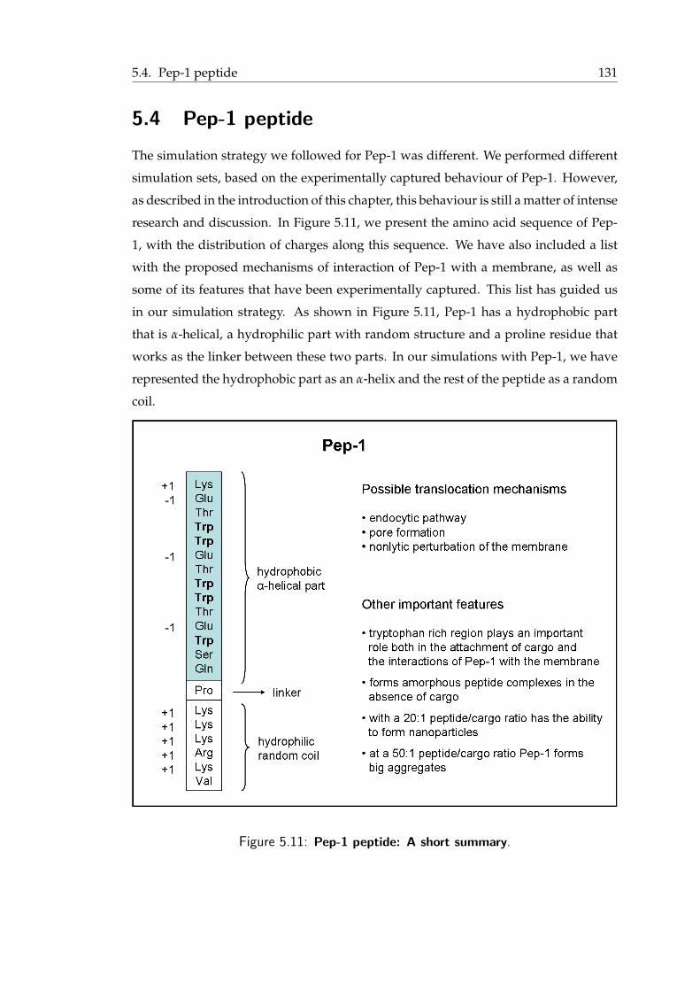
5.4. Pep-1 peptide 131
5.4 Pep-1 peptide
The simulation strategy we followed for Pep-1 was different. We performed different
simulation sets, based on the experimentally captured behaviour of Pep-1. However,
as described in the introduction of this chapter, this behaviour is still a matter of intense
research and discussion. In Figure 5.11, we present the amino acid sequence of Pep-
1, with the distribution of charges along this sequence. We have also included a list
with the proposed mechanisms of interaction of Pep-1 with a membrane, as well as
some of its features that have been experimentally captured. This list has guided us
in our simulation strategy. As shown in Figure 5.11, Pep-1 has a hydrophobic part
that is α-helical, a hydrophilic part with random structure and a proline residue that
works as the linker between these two parts. In our simulations with Pep-1, we have
represented the hydrophobic part as an α-helix and the rest of the peptide as a random
coil.
Figure 5.11: Pep-1 peptide: A short summary.
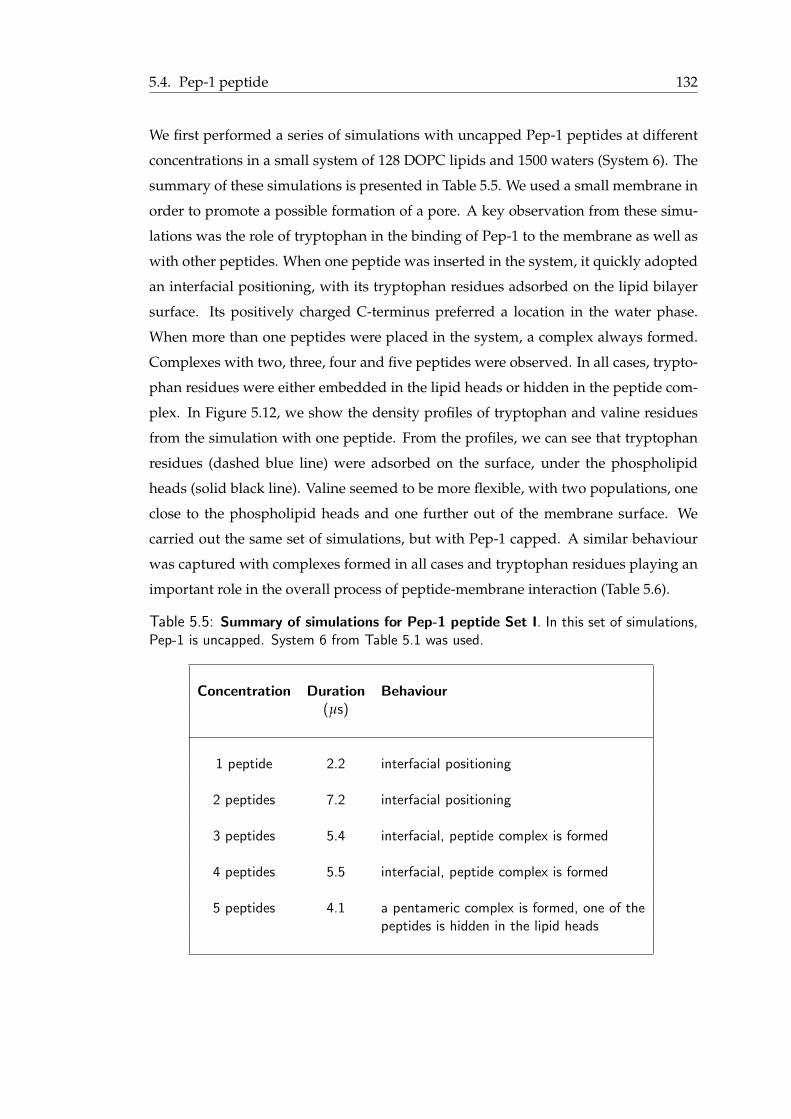
5.4. Pep-1 peptide 132
We first performed a series of simulations with uncapped Pep-1 peptides at different
concentrations in a small system of 128 DOPC lipids and 1500 waters (System 6). The
summary of these simulations is presented in Table 5.5. We used a small membrane in
order to promote a possible formation of a pore. A key observation from these simu-
lations was the role of tryptophan in the binding of Pep-1 to the membrane as well as
with other peptides. When one peptide was inserted in the system, it quickly adopted
an interfacial positioning, with its tryptophan residues adsorbed on the lipid bilayer
surface. Its positively charged C-terminus preferred a location in the water phase.
When more than one peptides were placed in the system, a complex always formed.
Complexes with two, three, four and five peptides were observed. In all cases, trypto-
phan residues were either embedded in the lipid heads or hidden in the peptide com-
plex. In Figure 5.12, we show the density profiles of tryptophan and valine residues
from the simulation with one peptide. From the profiles, we can see that tryptophan
residues (dashed blue line) were adsorbed on the surface, under the phospholipid
heads (solid black line). Valine seemed to be more flexible, with two populations, one
close to the phospholipid heads and one further out of the membrane surface. We
carried out the same set of simulations, but with Pep-1 capped. A similar behaviour
was captured with complexes formed in all cases and tryptophan residues playing an
important role in the overall process of peptide-membrane interaction (Table 5.6).
Table 5.5: Summary of simulations for Pep-1 peptide Set I. In this set of simulations,Pep-1 is uncapped. System 6 from Table 5.1 was used.
Concentration Duration Behaviour(µs)
1 peptide 2.2 interfacial positioning
2 peptides 7.2 interfacial positioning
3 peptides 5.4 interfacial, peptide complex is formed
4 peptides 5.5 interfacial, peptide complex is formed
5 peptides 4.1 a pentameric complex is formed, one of thepeptides is hidden in the lipid heads
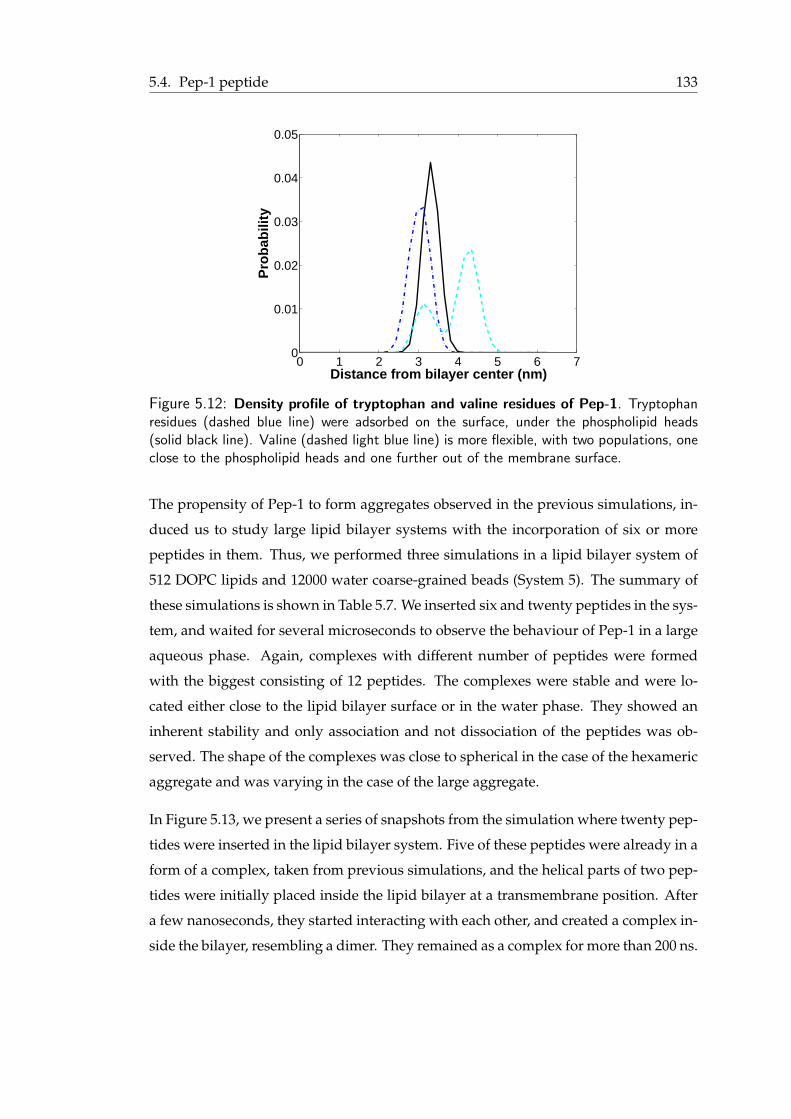
5.4. Pep-1 peptide 133
0 1 2 3 4 5 6 70
0.01
0.02
0.03
0.04
0.05
Distance from bilayer center (nm)
Pro
bab
ility
Figure 5.12: Density profile of tryptophan and valine residues of Pep-1. Tryptophanresidues (dashed blue line) were adsorbed on the surface, under the phospholipid heads(solid black line). Valine (dashed light blue line) is more flexible, with two populations, oneclose to the phospholipid heads and one further out of the membrane surface.
The propensity of Pep-1 to form aggregates observed in the previous simulations, in-
duced us to study large lipid bilayer systems with the incorporation of six or more
peptides in them. Thus, we performed three simulations in a lipid bilayer system of
512 DOPC lipids and 12000 water coarse-grained beads (System 5). The summary of
these simulations is shown in Table 5.7. We inserted six and twenty peptides in the sys-
tem, and waited for several microseconds to observe the behaviour of Pep-1 in a large
aqueous phase. Again, complexes with different number of peptides were formed
with the biggest consisting of 12 peptides. The complexes were stable and were lo-
cated either close to the lipid bilayer surface or in the water phase. They showed an
inherent stability and only association and not dissociation of the peptides was ob-
served. The shape of the complexes was close to spherical in the case of the hexameric
aggregate and was varying in the case of the large aggregate.
In Figure 5.13, we present a series of snapshots from the simulation where twenty pep-
tides were inserted in the lipid bilayer system. Five of these peptides were already in a
form of a complex, taken from previous simulations, and the helical parts of two pep-
tides were initially placed inside the lipid bilayer at a transmembrane position. After
a few nanoseconds, they started interacting with each other, and created a complex in-
side the bilayer, resembling a dimer. They remained as a complex for more than 200 ns.
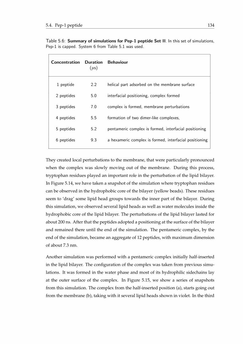
5.4. Pep-1 peptide 134
Table 5.6: Summary of simulations for Pep-1 peptide Set II. In this set of simulations,Pep-1 is capped. System 6 from Table 5.1 was used.
Concentration Duration Behaviour(µs)
1 peptide 2.2 helical part adsorbed on the membrane surface
2 peptides 5.0 interfacial positioning, complex formed
3 peptides 7.0 complex is formed, membrane perturbations
4 peptides 5.5 formation of two dimer-like complexes,
5 peptides 5.2 pentameric complex is formed, interfacial positioning
6 peptides 9.3 a hexameric complex is formed, interfacial positioning
They created local perturbations to the membrane, that were particularly pronounced
when the complex was slowly moving out of the membrane. During this process,
tryptophan residues played an important role in the perturbation of the lipid bilayer.
In Figure 5.14, we have taken a snapshot of the simulation where tryptophan residues
can be observed in the hydrophobic core of the bilayer (yellow beads). These residues
seem to ‘drag’ some lipid head groups towards the inner part of the bilayer. During
this simulation, we observed several lipid heads as well as water molecules inside the
hydrophobic core of the lipid bilayer. The perturbations of the lipid bilayer lasted for
about 200 ns. After that the peptides adopted a positioning at the surface of the bilayer
and remained there until the end of the simulation. The pentameric complex, by the
end of the simulation, became an aggregate of 12 peptides, with maximum dimension
of about 7.3 nm.
Another simulation was performed with a pentameric complex initially half-inserted
in the lipid bilayer. The configuration of the complex was taken from previous simu-
lations. It was formed in the water phase and most of its hydrophilic sidechains lay
at the outer surface of the complex. In Figure 5.15, we show a series of snapshots
from this simulation. The complex from the half-inserted position (a), starts going out
from the membrane (b), taking with it several lipid heads shown in violet. In the third
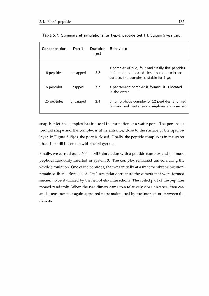
5.4. Pep-1 peptide 135
Table 5.7: Summary of simulations for Pep-1 peptide Set III. System 5 was used.
Concentration Pep-1 Duration Behaviour(µs)
a complex of two, four and finally five peptides6 peptides uncapped 3.8 is formed and located close to the membrane
surface, the complex is stable for 1 µs
6 peptides capped 3.7 a pentameric complex is formed, it is locatedin the water
20 peptides uncapped 2.4 an amorphous complex of 12 peptides is formedtrimeric and pentameric complexes are observed
snapshot (c), the complex has induced the formation of a water pore. The pore has a
toroidal shape and the complex is at its entrance, close to the surface of the lipid bi-
layer. In Figure 5.15(d), the pore is closed. Finally, the peptide complex is in the water
phase but still in contact with the bilayer (e).
Finally, we carried out a 500 ns MD simulation with a peptide complex and ten more
peptides randomly inserted in System 3. The complex remained united during the
whole simulation. One of the peptides, that was initially at a transmembrane position,
remained there. Because of Pep-1 secondary structure the dimers that were formed
seemed to be stabilized by the helix-helix interactions. The coiled part of the peptides
moved randomly. When the two dimers came to a relatively close distance, they cre-
ated a tetramer that again appeared to be maintained by the interactions between the
helices.
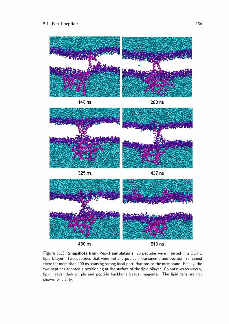
5.4. Pep-1 peptide 136
Figure 5.13: Snapshots from Pep-1 simulations. 20 peptides were inserted in a DOPClipid bilayer. Two peptides that were initially put at a transmembrane position, remainedthere for more than 400 ns, causing strong local perturbations to the membrane. Finally, thetwo peptides adopted a positioning at the surface of the lipid bilayer. Colours: water=cyan,lipid heads=dark purple and peptide backbone beads=magenta. The lipid tails are notshown for clarity.

5.4. Pep-1 peptide 137
Figure 5.14: The effect of tryptophan in Pep-1/membrane interaction. Colours: wa-ter=blue, lipid heads=purple and peptide backbone beads=magenta. Tryptophan residuesthat are inside the lipid bilayer are coloured yellow.

5.4. Pep-1 peptide 138
(a) 1 ns (b) 2 ns
(c) 30 ns (d) 40 ns
(e) 88 ns
Figure 5.15: Snapshots from the MD simulations of Pep-1 complex. Colours: wa-ter=blue, lipid heads=purple, lipid tails=yellow and peptide complex=magenta.
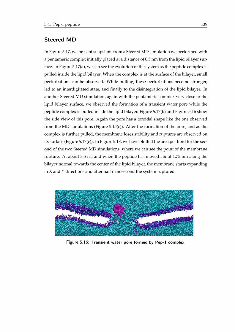
5.4. Pep-1 peptide 139
Steered MD
In Figure 5.17, we present snapshots from a Steered MD simulation we performed with
a pentameric complex initially placed at a distance of 0.5 nm from the lipid bilayer sur-
face. In Figure 5.17(a), we can see the evolution of the system as the peptide complex is
pulled inside the lipid bilayer. When the complex is at the surface of the bilayer, small
perturbations can be observed. While pulling, these perturbations become stronger,
led to an interdigitated state, and finally to the disintegration of the lipid bilayer. In
another Steered MD simulation, again with the pentameric complex very close to the
lipid bilayer surface, we observed the formation of a transient water pore while the
peptide complex is pulled inside the lipid bilayer. Figure 5.17(b) and Figure 5.16 show
the side view of this pore. Again the pore has a toroidal shape like the one observed
from the MD simulations (Figure 5.15(c)). After the formation of the pore, and as the
complex is further pulled, the membrane loses stability and ruptures are observed on
its surface (Figure 5.17(c)). In Figure 5.18, we have plotted the area per lipid for the sec-
ond of the two Steered MD simulations, where we can see the point of the membrane
rupture. At about 3.5 ns, and when the peptide has moved about 1.75 nm along the
bilayer normal towards the center of the lipid bilayer, the membrane starts expanding
in X and Y directions and after half nanosecond the system ruptured.
Figure 5.16: Transient water pore formed by Pep-1 complex.
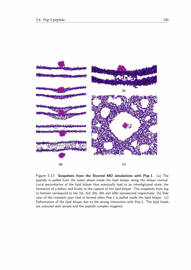
5.4. Pep-1 peptide 140
Figure 5.17: Snapshots from the Steered MD simulations with Pep-1. (a) Thepeptide is pulled from the water phase inside the lipid bilayer along the bilayer normal.Local perturbation of the lipid bilayer that eventually lead to an interdigitated state, theformation of a defect and finally to the rupture of the lipid bilayer. The snapshots from topto bottom correspond to the 1st, 3rd, 6th, 8th and 10th nanosecond respectively. (b) Sideview of the transient pore that is formed when Pep-1 is pulled inside the lipid bilayer. (c)Deformation of the lipid bilayer due to the strong interaction with Pep-1. The lipid headsare coloured dark purple and the peptide complex magenta.
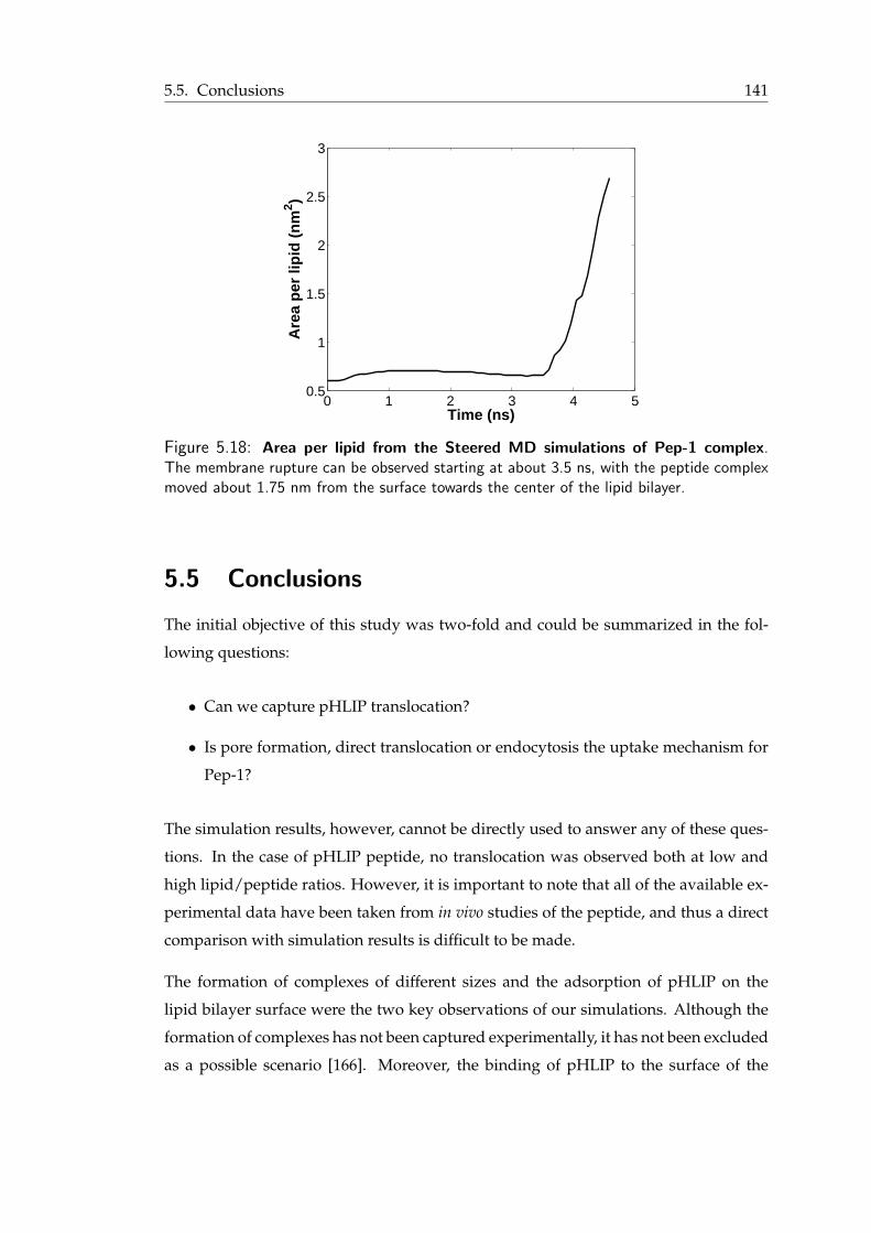
5.5. Conclusions 141
0 1 2 3 4 50.5
1
1.5
2
2.5
3
Time (ns)
Are
a p
er li
pid
(n
m2 )
Figure 5.18: Area per lipid from the Steered MD simulations of Pep-1 complex.The membrane rupture can be observed starting at about 3.5 ns, with the peptide complexmoved about 1.75 nm from the surface towards the center of the lipid bilayer.
5.5 Conclusions
The initial objective of this study was two-fold and could be summarized in the fol-
lowing questions:
• Can we capture pHLIP translocation?
• Is pore formation, direct translocation or endocytosis the uptake mechanism for
Pep-1?
The simulation results, however, cannot be directly used to answer any of these ques-
tions. In the case of pHLIP peptide, no translocation was observed both at low and
high lipid/peptide ratios. However, it is important to note that all of the available ex-
perimental data have been taken from in vivo studies of the peptide, and thus a direct
comparison with simulation results is difficult to be made.
The formation of complexes of different sizes and the adsorption of pHLIP on the
lipid bilayer surface were the two key observations of our simulations. Although the
formation of complexes has not been captured experimentally, it has not been excluded
as a possible scenario [166]. Moreover, the binding of pHLIP to the surface of the
5.5. Conclusions 142
membrane has been proposed in several studies [164, 166, 167, 198]. pHLIP tends to
‘squeeze out’ the lipid heads, and lead to the formation of defects in the surface of
the bilayer. Also, from the calculation of the order parameters of the lipids close to
a tetrameric peptide complex, we observed a decrease in the ordering of lipid chains
that is probably caused by the interactions of pHLIP with the lipid heads.
Another key observation from our simulations is the positioning of the C-terminus of
pHLIP in the lipid heads region when a single peptide was considered. This obser-
vation is in agreement with previous experimental studies [166]. In the case where
the N-terminus of the peptide was half-inserted in the lipid bilayer, we observed its
insertion in the hydrophobic core. The initiation of the insertion only when one termi-
nus was inside in the bilayer, may signify that there is probably something missing in
the description of pHLIP-membrane interactions in our studies. A better treatment of
the electrostatic interactions or even a more realistic representation of the membrane
could be possible improvements of the description of the system.
In the case of Pep-1, we observed the formation of complexes of different sizes. In
particular, an interesting result was the formation of a peptide complex consisting of 12
peptides. The complex, once formed, remained stable until the end of the simulation.
This was the case for all the different complexes we observed. The complexes were
stable, with a constant number of peptides unless another free peptide approached
and joined the aggregate. The formation of complexes is in agreement with available
experimental observations, where the peptide formed large aggregates in the absence
of cargo [203].
Also, tryptophan seems to play and important part in the interaction of Pep-1 with
the lipid bilayer as well as in peptide-peptide interactions. We showed by plotting
the density profiles of tryptophan and valine residues that tryptophan was under the
layer of phospholipid heads during the whole simulation, whereas valine seemed to
be more flexible and covered a bigger area close to the surface of the lipid bilayer. This
observation is also in agreement with experimental results [201].
Another notable result is the formation of transient pore-like structures, once the pep-
tide or the peptide complex is slightly inside the lipid bilayer, close to the lipid head
region. This was captured both by MD and Steered MD simulations. These structures

5.5. Conclusions 143
had a toroidal shape and in two cases they were filled with water. As in the case of
pHLIP with the insertion, this initial driving force that is needed in order for these
pores to form seems to be missing from our description of the system. Probably the
absence of cargo or a different treatment of electrostatic interactions are the missing
parameters that should be included in order to have a more realistic representation of
the system. However, many key features of Pep-1 interactions are captured in our re-
sults and show that further investigations and improvement in the description of the
system could provide us with a better understanding of these interactions.
CHAPTER 6
Interactions between nanoparticles and
lipid membranes
The wide use of nanoparticles in a variety of products, such as drug and gene delivery
materials, and the results from our simulation studies on cell-penetrating peptides,
with the formation of nanosized complexes, were two of the reasons that inspired
this study. Nanoparticles of two sizes (1 nm and 3 nm diameter) with different surface
chemistry were constructed, with different types and distribution of CG beads on their
surface. MD and Steered MD simulations were then performed in order to obtain
insights about the nanoparticle-membrane interactions. Some qualitative results will
be presented mainly by means of visualization and some first observations will be
discussed.
144
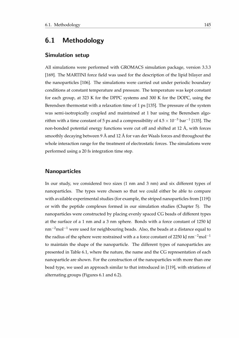
6.1. Methodology 145
6.1 Methodology
Simulation setup
All simulations were performed with GROMACS simulation package, version 3.3.3
[169]. The MARTINI force field was used for the description of the lipid bilayer and
the nanoparticles [106]. The simulations were carried out under periodic boundary
conditions at constant temperature and pressure. The temperature was kept constant
for each group, at 323 K for the DPPC systems and 300 K for the DOPC, using the
Berendsen thermostat with a relaxation time of 1 ps [135]. The pressure of the system
was semi-isotropically coupled and maintained at 1 bar using the Berendsen algo-
rithm with a time constant of 5 ps and a compressibility of 4.5 × 10⁻⁵ bar−1 [135]. The
non-bonded potential energy functions were cut off and shifted at 12 A, with forces
smoothly decaying between 9 A and 12 A for van der Waals forces and throughout the
whole interaction range for the treatment of electrostatic forces. The simulations were
performed using a 20 fs integration time step.
Nanoparticles
In our study, we considered two sizes (1 nm and 3 nm) and six different types of
nanoparticles. The types were chosen so that we could either be able to compare
with available experimental studies (for example, the striped nanoparticles from [119])
or with the peptide complexes formed in our simulation studies (Chapter 5). The
nanoparticles were constructed by placing evenly spaced CG beads of different types
at the surface of a 1 nm and a 3 nm sphere. Bonds with a force constant of 1250 kJ
nm−2mol−1 were used for neighbouring beads. Also, the beads at a distance equal to
the radius of the sphere were restrained with a a force constant of 2250 kJ nm−2mol−1
to maintain the shape of the nanoparticle. The different types of nanoparticles are
presented in Table 6.1, where the nature, the name and the CG representation of each
nanoparticle are shown. For the construction of the nanoparticles with more than one
bead type, we used an approach similar to that introduced in [119], with striations of
alternating groups (Figures 6.1 and 6.2).
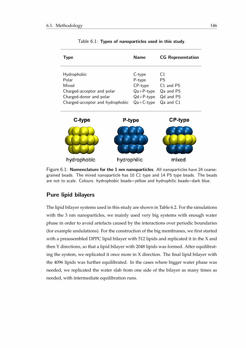
6.1. Methodology 146
Table 6.1: Types of nanoparticles used in this study.
Type Name CG Representation
Hydrophobic C-type C1Polar P-type P5Mixed CP-type C1 and P5Charged-acceptor and polar Qa+P-type Qa and P5Charged-donor and polar Qd+P-type Qd and P5Charged-acceptor and hydrophobic Qa+C-type Qa and C1
Figure 6.1: Nomenclature for the 1 nm nanoparticles. All nanoparticles have 24 coarse-grained beads. The mixed nanoparticle has 10 C1 type and 14 P5 type beads. The beadsare not to scale. Colours: hydrophobic beads=yellow and hydrophilic beads=dark blue.
Pure lipid bilayers
The lipid bilayer systems used in this study are shown in Table 6.2. For the simulations
with the 3 nm nanoparticles, we mainly used very big systems with enough water
phase in order to avoid artefacts caused by the interactions over periodic boundaries
(for example undulations). For the construction of the big membranes, we first started
with a preassembled DPPC lipid bilayer with 512 lipids and replicated it in the X and
then Y directions, so that a lipid bilayer with 2048 lipids was formed. After equilibrat-
ing the system, we replicated it once more in X direction. The final lipid bilayer with
the 4096 lipids was further equilibrated. In the cases where bigger water phase was
needed, we replicated the water slab from one side of the bilayer as many times as
needed, with intermediate equilibration runs.
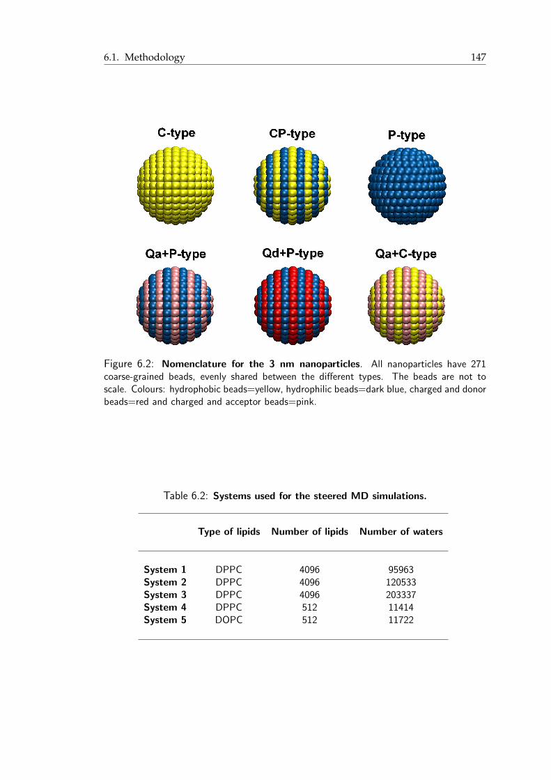
6.1. Methodology 147
Figure 6.2: Nomenclature for the 3 nm nanoparticles. All nanoparticles have 271coarse-grained beads, evenly shared between the different types. The beads are not toscale. Colours: hydrophobic beads=yellow, hydrophilic beads=dark blue, charged and donorbeads=red and charged and acceptor beads=pink.
Table 6.2: Systems used for the steered MD simulations.
Type of lipids Number of lipids Number of waters
System 1 DPPC 4096 95963System 2 DPPC 4096 120533System 3 DPPC 4096 203337System 4 DPPC 512 11414System 5 DOPC 512 11722
6.1. Methodology 148
Nanoparticle-bilayer systems
After the preparation of the lipid bilayers, we performed a series of Steered MD simu-
lations. The initial configurations for these simulations were prepared as follows: first,
we created an empty sphere in the water phase of each lipid bilayer system, by re-
moving the corresponding water beads. To avoid overlaps, the diameter of this sphere
was 1 nm bigger than the diameter of the nanoparticle to be inserted. For the systems
where charged particles were used, we added ions to maintain the overall neutrality of
the system. An equilibration simulation of about 50-100 ns, depending on the system
size, was then performed.
Steered MD
In order to speed up the process of interaction of a nanoparticle with a lipid bilayer,
which in the case of the pore formation or the interdigitated state seen in experiments
may be a very slow event, we applied an external force to the nanoparticle. We used
a harmonic potential with a force constant of 5000 kJ/(mol·nm2) applied to the centre
of the nanoparticle with the direction of the normal of the bilayer. The pulling rate
was 0.0005 nm/ps. Due to the size of the lipid bilayers we used in this study, it is
possible that their response to the pulling of the nanoparticles through them will not
be fast enough and could cause mechanical instability to the system. Thus, in some
cases that will be specified in the results section, we used a pulling rate of 0.00005
nm/ps and a force constant equal to 1000 kJ/(mol·nm2), in order to examine if indeed
the response of the big lipid bilayers may lead to artefacts depending on the pulling
rate and force constant. The nanoparticle motion in the XY plane was not restrained
and the nanoparticle is free to rotate. The simulation parameters were as described
before in this section, apart from the pressure coupling that for the Steered MD was
anisotropic.

6.2. Results 149
6.2 Results
6.2.1 1 nm nanoparticles
We performed steered molecular dynamics simulations for each of the nanoparticle
types introduced in the Methodology. The summary of these simulations is presented
in Table 6.3. System 1 from Table 6.2.
Table 6.3: Summary of simulations for the 1 nm nanoparticles.
Nanoparticle Steered MD Simple MD
C-type insertion
P-type bilayer thinning, holes formation positioning at the bilayer surface
CP-type insertion under the phospholipid heads
From the pulling simulations, the C- and CP-type nanoparticles inserted into the lipid
bilayer. The hydrophobic nanoparticle passed very smoothly in the hydrophobic core
of the bilayer, whereas the mixed nanoparticle induced a curvature to the membrane,
by dragging several lipid heads with it. The polar nanoparticle, although of a small
size, induced thinning and high curvature to the lipid bilayer. If we compare our
observations with that reported in [122], we will see that they are not contradictory.
Actually, in our simulations, both the polar and the mixed nanoparticle induced really
high curvature to the membrane without disrupting it (Figure 6.3(a)). Thus, using the
same terminology as in [122], ‘the lipid bilayer followed the topographical features of
the nanoparticle’.
Thinning of the bilayer was also observed for the C- and CP-type nanoparticles. The
thinning of the bilayer happened while pulling the nanoparticles out of the hydropho-
bic core of the bilayer. In all the cases where this thinning was captured, after a few
nanoseconds the membrane returned to its original state.
We have calculated the order parameters of the lipids in the vicinity of the nanopar-
ticles (Figure 6.3(b)). We used only one snapshot for each type (shown next to the
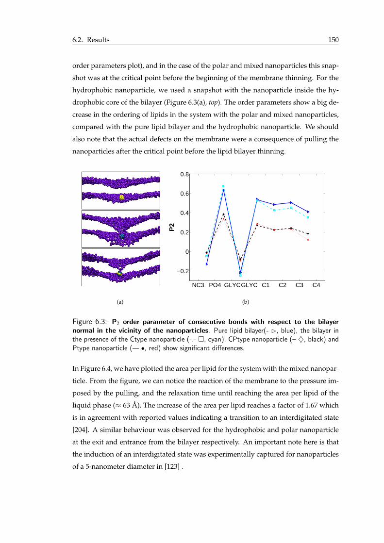
6.2. Results 150
order parameters plot), and in the case of the polar and mixed nanoparticles this snap-
shot was at the critical point before the beginning of the membrane thinning. For the
hydrophobic nanoparticle, we used a snapshot with the nanoparticle inside the hy-
drophobic core of the bilayer (Figure 6.3(a), top). The order parameters show a big de-
crease in the ordering of lipids in the system with the polar and mixed nanoparticles,
compared with the pure lipid bilayer and the hydrophobic nanoparticle. We should
also note that the actual defects on the membrane were a consequence of pulling the
nanoparticles after the critical point before the lipid bilayer thinning.
(a)
NC3 PO4 GLYCGLYC C1 C2 C3 C4
−0.2
0
0.2
0.4
0.6
0.8P
2
(b)
Figure 6.3: P2 order parameter of consecutive bonds with respect to the bilayernormal in the vicinity of the nanoparticles. Pure lipid bilayer(- ⊲, blue), the bilayer inthe presence of the Ctype nanoparticle (-.- �, cyan), CPtype nanoparticle (– ♦, black) andPtype nanoparticle (— •, red) show significant differences.
In Figure 6.4, we have plotted the area per lipid for the system with the mixed nanopar-
ticle. From the figure, we can notice the reaction of the membrane to the pressure im-
posed by the pulling, and the relaxation time until reaching the area per lipid of the
liquid phase (≈ 63 A). The increase of the area per lipid reaches a factor of 1.67 which
is in agreement with reported values indicating a transition to an interdigitated state
[204]. A similar behaviour was observed for the hydrophobic and polar nanoparticle
at the exit and entrance from the bilayer respectively. An important note here is that
the induction of an interdigitated state was experimentally captured for nanoparticles
of a 5-nanometer diameter in [123] .
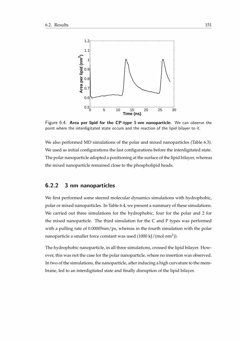
6.2. Results 151
0 5 10 15 20 25 300.5
0.6
0.7
0.8
0.9
1
1.1
1.2
Time (ns)
Are
a p
er li
pid
(n
m2 )
Figure 6.4: Area per lipid for the CP-type 1-nm nanoparticle. We can observe thepoint where the interdigitated state occurs and the reaction of the lipid bilayer to it.
We also performed MD simulations of the polar and mixed nanoparticles (Table 6.3).
We used as initial configurations the last configurations before the interdigitated state.
The polar nanoparticle adopted a positioning at the surface of the lipid bilayer, whereas
the mixed nanoparticle remained close to the phospholipid heads.
6.2.2 3 nm nanoparticles
We first performed some steered molecular dynamics simulations with hydrophobic,
polar or mixed nanoparticles. In Table 6.4, we present a summary of these simulations.
We carried out three simulations for the hydrophobic, four for the polar and 2 for
the mixed nanoparticle. The third simulation for the C and P types was performed
with a pulling rate of 0.00005nm/ps, whereas in the fourth simulation with the polar
nanoparticle a smaller force constant was used (1000 kJ/(mol·nm2)).
The hydrophobic nanoparticle, in all three simulations, crossed the lipid bilayer. How-
ever, this was not the case for the polar nanoparticle, where no insertion was observed.
In two of the simulations, the nanoparticle, after inducing a high curvature to the mem-
brane, led to an interdigitated state and finally disruption of the lipid bilayer.
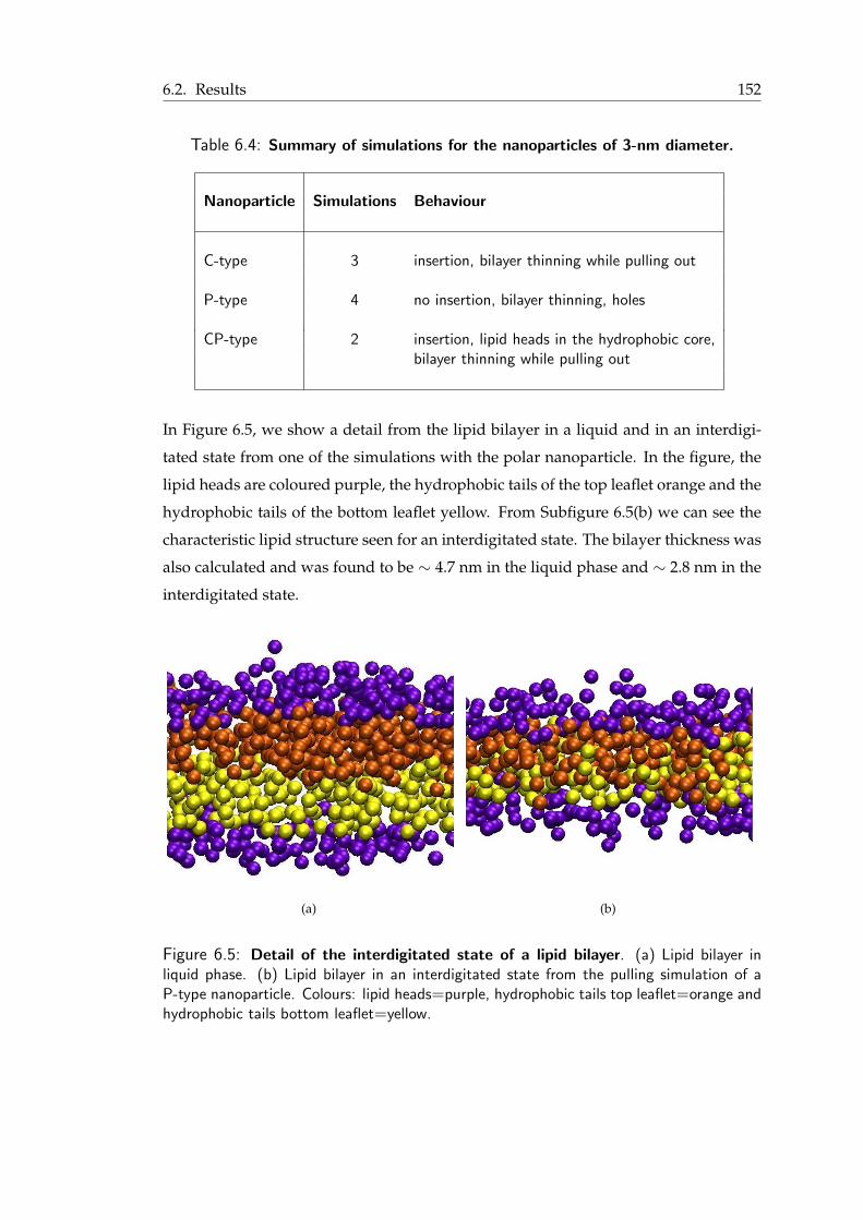
6.2. Results 152
Table 6.4: Summary of simulations for the nanoparticles of 3-nm diameter.
Nanoparticle Simulations Behaviour
C-type 3 insertion, bilayer thinning while pulling out
P-type 4 no insertion, bilayer thinning, holes
CP-type 2 insertion, lipid heads in the hydrophobic core,bilayer thinning while pulling out
In Figure 6.5, we show a detail from the lipid bilayer in a liquid and in an interdigi-
tated state from one of the simulations with the polar nanoparticle. In the figure, the
lipid heads are coloured purple, the hydrophobic tails of the top leaflet orange and the
hydrophobic tails of the bottom leaflet yellow. From Subfigure 6.5(b) we can see the
characteristic lipid structure seen for an interdigitated state. The bilayer thickness was
also calculated and was found to be ∼ 4.7 nm in the liquid phase and ∼ 2.8 nm in the
interdigitated state.
(a) (b)
Figure 6.5: Detail of the interdigitated state of a lipid bilayer. (a) Lipid bilayer inliquid phase. (b) Lipid bilayer in an interdigitated state from the pulling simulation of aP-type nanoparticle. Colours: lipid heads=purple, hydrophobic tails top leaflet=orange andhydrophobic tails bottom leaflet=yellow.
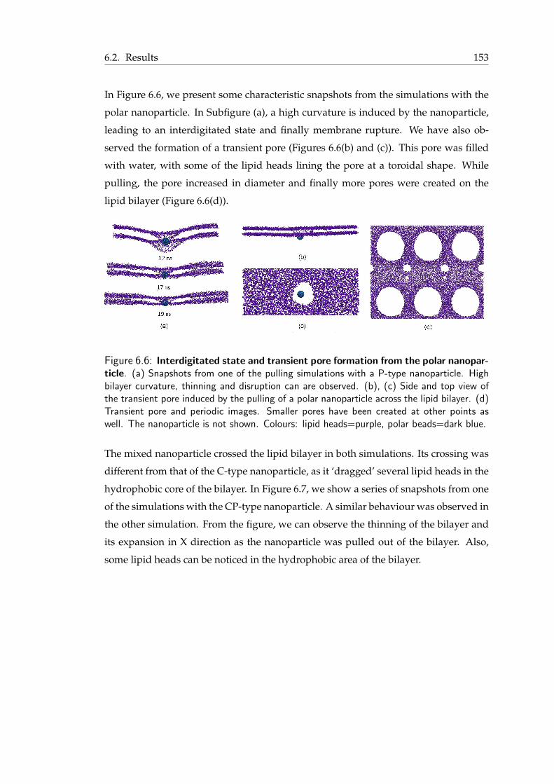
6.2. Results 153
In Figure 6.6, we present some characteristic snapshots from the simulations with the
polar nanoparticle. In Subfigure (a), a high curvature is induced by the nanoparticle,
leading to an interdigitated state and finally membrane rupture. We have also ob-
served the formation of a transient pore (Figures 6.6(b) and (c)). This pore was filled
with water, with some of the lipid heads lining the pore at a toroidal shape. While
pulling, the pore increased in diameter and finally more pores were created on the
lipid bilayer (Figure 6.6(d)).
Figure 6.6: Interdigitated state and transient pore formation from the polar nanopar-ticle. (a) Snapshots from one of the pulling simulations with a P-type nanoparticle. Highbilayer curvature, thinning and disruption can are observed. (b), (c) Side and top view ofthe transient pore induced by the pulling of a polar nanoparticle across the lipid bilayer. (d)Transient pore and periodic images. Smaller pores have been created at other points aswell. The nanoparticle is not shown. Colours: lipid heads=purple, polar beads=dark blue.
The mixed nanoparticle crossed the lipid bilayer in both simulations. Its crossing was
different from that of the C-type nanoparticle, as it ‘dragged’ several lipid heads in the
hydrophobic core of the bilayer. In Figure 6.7, we show a series of snapshots from one
of the simulations with the CP-type nanoparticle. A similar behaviour was observed in
the other simulation. From the figure, we can observe the thinning of the bilayer and
its expansion in X direction as the nanoparticle was pulled out of the bilayer. Also,
some lipid heads can be noticed in the hydrophobic area of the bilayer.

6.2. Results 154
Figure 6.7: Mixed nanoparticle insertion in the lipid bilayer. Snapshots from the pullingsimulation with CP-type nanoparticle. The nanoparticle enters the bilayer and drags severallipid heads into its hydrophobic core. A thinning of the bilayer is observed while pulling thenanoparticle out of the bilayer. Colours: lipid heads=purple, polar beads=dark blue.
6.2. Results 155
It is important to note that we observed thinning of the bilayer in all of the performed
simulations. In the cases of the hydrophobic and mixed nanoparticles, this happened
while pulling the nanoparticles out of the lipid bilayer. For the hydrophilic nanopar-
ticle this thinning and disruption of the membrane occurred while pulling it inside
the bilayer. As in the case of the small nanoparticles, we calculated the area per lipid
for the different types and the different simulations. We found an increase of the area
per lipid by a factor of about 2.6. The value of this factor is similar for all types of
nanoparticles and is probably indicative of their and lipid bilayer relative sizes. The
configurations of the membranes resemble the ones observed in the simulations with
the small nanoparticles. The main difference is that due to the expansion of the bi-
layer in X and Y directions, and consequently the ‘shrinking’ in Z direction, the bilayer
interacted with its periodic images and eventually the system collapsed.
6.2.3 Charged nanoparticles
In this study, we considered three types of charged nanoparticles, positively charged
and polar (Qd+P-type), negatively charged and hydrophobic (Qa+C-type) and neg-
atively charged and polar (Qa+P-type). We have performed MD simulations with
Qa+C- and Qa+P-type nanoparticles. Typical snapshots from these simulations are
shown in Figure 6.8. Both nanoparticles adopted a positioning close to the surface of
the lipid bilayer. In the case of the Qa+P-type nanoparticle, molecules of water lied be-
tween the nanoparticle and the phospholipid heads, whereas the Qa+C-type nanopar-
ticle seemed to directly interact with the lipid bilayer. During the 30 nanoseconds of
the simulations, we did not observe any distinct curvature of the membrane induced
by the interaction with the nanoparticles.
We also performed Steered MD simulations for the three different charged nanoparti-
cles. In all three simulations, we observed a high curvature and thinning of the bilayer
until the systems collapsed due to the interactions with the periodic images of the
bilayers and the nanoparticles.

6.2. Results 156
(a)
(b)
Figure 6.8: Final snapshots from the MD simulations of the charged nanoparticles.Colours: water=cyan, lipid heads=violet, Qa=pink, hydrophobic particles=yellow, polarparticles=blue .
6.2.4 The effect of membrane size
We also tried to examine the effect that a smaller lipid bilayer may have to our results.
We used a 3 nm polar nanoparticle with two different types of membranes DPPC and
DOPC (Systems 4 and 5 respectively). The summary of these simulations is shown in
Table 6.5. A similar behaviour to that for the big lipid bilayer was observed. However,
in one of our simulations, we captured the formation of a transient water pore. Then,
strong undulations of the lipid bilayer and partial engulfment of the nanoparticle were
observed. Snapshots of this simulation are shown in Figure 6.9.
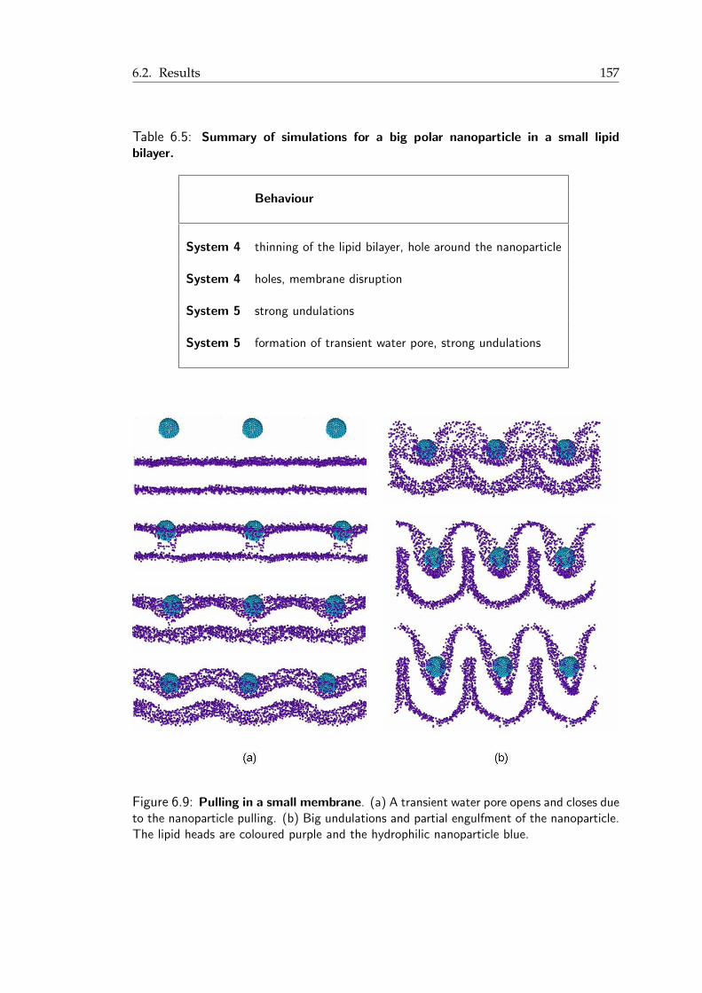
6.2. Results 157
Table 6.5: Summary of simulations for a big polar nanoparticle in a small lipidbilayer.
Behaviour
System 4 thinning of the lipid bilayer, hole around the nanoparticle
System 4 holes, membrane disruption
System 5 strong undulations
System 5 formation of transient water pore, strong undulations
Figure 6.9: Pulling in a small membrane. (a) A transient water pore opens and closes dueto the nanoparticle pulling. (b) Big undulations and partial engulfment of the nanoparticle.The lipid heads are coloured purple and the hydrophilic nanoparticle blue.
6.3. Discussion 158
6.3 Discussion
We performed simple and steered molecular dynamics simulations with nanoparticles
of different sizes and nature. From the small nanoparticles, with a diameter of 1 nm,
we observed the insertion of the hydrophobic and mixed nanoparticle in the bilayer.
The mixed nanoparticle, however, seemed to ‘drag’ several phospholipid heads inside
the lipid bilayer. The hydrophilic nanoparticle induces high curvature to the bilayer
that eventually leads to the bilayer thinning and the creation of holes. From the calcu-
lation of the area per lipid and the configuration of the lipid bilayer, we could classify
this thinning as an interdigitated state. The interdigitated state was also observed in
the study by Ahmed and Wunder [123] with 5 nm diameter nanoparticles, and could
be also linked to the thinning of the membrane reported in [122]. A thinning of the
bilayer was also observed for our simulations with the C- and CP-type nanoparticles,
only this time, it was induced by the pulling of the nanoparticles out of the bilayer.
Another important observation from our simulations with the small nanoparticles is
that, in the case of the P- and CP-type, a disorder in the structure of the lipids can be
captured by visualization and order parameter calculations. The order parameters in
these two cases are significantly different to that of a pure lipid bilayer, indicating the
level of interaction between the nanoparticles and the lipids.
A similar behaviour was captured in our simulations with the big nanoparticles. The
C- and CP-type nanoparticles inserted into the bilayer, whereas the polar nanoparticle
caused significant deformation to the lipid bilayer, including thinning and formation
of holes. Thinning of the bilayer was also observed for the hydrophobic and mixed
nanoparticles while pulling them out of the bilayer.
Sensitivity analysis has also been performed. We carried out two simulations, one for
polar and one for hydrophobic nanoparticle, with a very small pulling rate in order to
allow enough time for the membrane to react to the interaction with it. These simu-
lations gave similar results to those from the simulations with the higher pulling rate.
We also performed one simulation with a polar nanoparticle and a ten times smaller
force constant. The results did not present differences to the previous ones.
From the MD simulations with the Qa+C and Qa+P nanoparticles, we observed an
interfacial positioning. For the first case, a positioning very close to the lipid heads

6.3. Discussion 159
was captured. In the case of the Qa+P-type nanoparticle, we observed some water
molecules between the nanoparticle and the lipid bilayer. We also performed Steered
MD simulations with three types of charged nanoparticles. In all cases thinning of the
bilayer was observed. I should mention here that better treatment of the electrostatic
interactions, for example use of PME instead of the shift method, could give a more
realistic description of the system and improve the accuracy of the results.
We need to keep in mind that the non-equilibrium simulations may provide some
insight of otherwise difficult to capture events, however they should always be con-
sidered with caution. Future studies could be combined with more MD simulations.
Also, nanoparticles with random distribution of hydrophobicity or charges could also
constitute an interesting case study and could be compared with our ‘striped’ nanopar-
ticles. An improvement in the description of our system would be to use a bigger wa-
ter phase in order to avoid possible interaction between the bilayer and its periodic
images due to the thinning effect.
We should mention again that this work is at a preliminary stage and it could only be
used as a starting point for a more detailed study of the interaction of nanoparticles
with lipid bilayers.
CHAPTER 7
Summary and conclusions
7.1 Summary of dissertation
Peptide-membrane interactions play an essential role in cells. A few of their func-
tions include antimicrobial defence mechanisms, viral translocation, signal transduc-
tion and membrane fusion. Because of their importance in these processes, peptide-
membrane interactions have been extensively investigated, both through theoretical,
computational and experimental studies.
In this work, molecular dynamics simulations have been employed in the studies of
peptide-membrane interactions. I am particularly interested in α-helical peptides, that
constitute a potentially vast family of membrane-active peptides. The processes of
interest, such as pore formation or self-assembly processes, run over long time and
length scales. On the other hand, atomistic simulations are limited to several hundreds
of nanoseconds and tens of nanometers. To overcome these limitations, in this study,
160

7.1. Summary of dissertation 161
a coarse-grained approach was adopted.
In the first chapter, I introduced the biological background of the system of interest
(peptides and membranes). I elaborated on importance of peptide-membrane inter-
actions, how computer simulations and molecular modelling can be instrumental in
gaining information about them and reviewed the state of the art in this field.
A short description of the methodology used in this work followed in Chapter 2. Some
basic ideas of statistical mechanics were presented, and the principles of molecular
dynamics, free energy calculations and other methods employed in this work were re-
viewed. I then introduced the model used in this study. Specifically, a short description
of the MARTINI coarse-grained model, the molecular mapping and the representation
of lipids, lipid bilayers and peptides were presented.
In Chapter 3, I focused on several types of interactions between lipid membranes and
α-helical peptides, based on the distribution of hydrophobicity along the helix. I em-
ployed the MARTINI coarse-grained force field and tested its ability to capture di-
verse types of behaviour. Four different classes of amphipathic α-helical peptides were
considered: pore-forming, non-membrane-spanning, fusion and transmembrane pep-
tides. The simulations provided us with useful insights on the formation of a barrel-
stave pore. Also, amphipathic nonspanning peptides were described with sufficient
accuracy. However, the picture was not as clear for fusion and transmembrane pep-
tides. For SIV fusion peptides, our results both from atomistic and coarse-grained
simulations seemed to underestimate the oblique insertion of the peptide that has been
captured through experiments. In the case of transmembrane peptides, I did not man-
age to capture the spontaneous insertion. However, once a peptide was half-inserted
in the lipid bilayer, it adopted a transmembrane position and remained there until the
end of our simulations (a few microseconds). For each class of peptides, I also cal-
culated the potential of mean force (PMF) for peptide translocation across the lipid
bilayer and demonstrated that each class has a distinct shape of PMF.
Pore formation mechanisms play an important role in many biological processes, from
ion-conduction across cell membranes to antimicrobial defence mechanisms and many
more. I chose a synthetic peptide, LS3, which is simple (it has only two types of amino
acids) and has the potential to form pores. I showed that the spontaneous formation of
7.1. Summary of dissertation 162
a barrel-stave pore formed by LS3 is within the limits of the employed coarse-grained
protocol. In Chapter 4, I presented a series of simulations that provide further evidence
of the propensity of LS3 to form pores as well as structural and dynamical information
about them. For example, the barrel-stave pore captured in our studies was open for
more than 14 µs and filled with water. Moreover, the calculated self-diffusion coeffi-
cient (Dlat = 0.49 − 0.87 µm2/s) is similar to the experimentally measured values for
membrane proteins. I also investigated how pore formation mechanism depends on
the structural modifications of LS3. Remarkably, the simulations of a shorter version
of this peptide, (LSSLLSL)2, showed that this peptide has a much lower propensity for
poration and, when a complex does form, it has a toroidal structure. These complexes
were different to the barrel-stave pore or the other complexes formed by LS3. They
had a small diameter that does not allow for water to pass through it. Also, they were
unstable, with the number of peptides taking part in them varying during the simula-
tion. Another difference between the two observed pores was the structure of lipids in
their vicinity, as shown by order parameters calculations. The PMF for (LSSLLSL)2 was
dramatically different to that of LS3, with the energy minima at the bilayer interfaces
and the core of the bilayer being an unfavourable location of the peptide.
In Chapter 5, I extended our studies to the self-assembly and membrane internaliza-
tion mechanisms of cell-penetrating peptides. In particular, I chose two peptides of
significant technological importance, pHLIP and Pep-1. The formation of complexes
of different sizes and the adsorption of pHLIP on the lipid bilayer surface were the two
key observations of our simulations. These complexes were bound to the membrane
surface and ‘squeezed out’ the lipid heads, resulting in the formation of defects on the
surface of the bilayer. In the case of Pep-1, formation of complexes of different sizes
was observed. The complexes were stable, with a constant number of peptides unless
another free peptide approached and joined the aggregate. An interesting observation
was that tryptophan seems to play and important role in the interaction of Pep-1 with
the lipid bilayer as well as in peptide-peptide interactions. Another notable result was
the formation of transient pore-like structures, once the peptide or the peptide ‘lump’
was slightly inside the lipid bilayer, close to the lipid head region. This was captured
both by MD and Steered MD simulations. These structures had a toroidal shape and
in two cases they were filled with water.
7.2. Final thoughts and future directions 163
Finally, in Chapter 6, I presented some preliminary qualitative results from our simu-
lation studies on interactions between nanoparticles and lipid membranes. Molecular
dynamics simulations as well as Steered MD simulations were performed. Two dif-
ferent sizes, with 1 and 3 nm diameter, as well as different surface chemistry ranging
from fully hydrophobic to charged nanoparticles were considered. An important ob-
servation from our simulations is the induction of an interdigitated state of the mem-
brane when small hydrophilic or larger nanoparticles with some degree of polarity
were pulled inside the lipid bilayer. From the molecular dynamics simulations of the
charged nanoparticles an interfacial positioning was observed in all cases.
In summary, it has been shown that the formation and evolution of pores in mem-
branes, the interfacial positioning of non-membrane-spanning peptides as well as other
self-assembly processes are within the limits of coarse-grained molecular dynamics
simulations. An important link between the barrel-stave and the toroidal mechanism
and the length of the peptides was also established. Overall, this work has demon-
strated that coarse-grained simulation models can be used to address biologically rel-
evant processes.
7.2 Final thoughts and future directions
Some of the conclusions and future directions of this study could be summarized in
five main subjects: free energy calculations, implications of coarse-grained approaches
and multiscale modelling, representation of the membrane, nanoparticles studies and
other peptide systems and treatment of electrostatic interactions. Here, I present some
of our ideas and possible future directions in these five subjects.
Potential of mean force calculations
Potential of mean force (PMF) is a very useful tool in the studies of peptide-membrane
interactions. I calculated the PMF for peptide translocation across the lipid bilayer
and demonstrated that each class of the studied peptides has a distinct shape of PMF.
A natural step forward in this study would be the calculation of PMF for more pep-
tides belonging to each of the different classes in order to establish a general map of

7.2. Final thoughts and future directions 164
interactions. In addition to this, the effect of the presence of peptides, proteins or other
biological entities in the lipid bilayer on the PMF profile could add further information
in this map of behaviours. Also, calculation of the PMF with two reaction coordinates,
the distance along the normal of the bilayer as well as the orientation of the peptide
relative to it, could lead to a better understanding of the translocation mechanisms of
α-helical peptides and in particular transmembrane helices.
The representation of the membrane
In our studies, the membrane is treated as a lipid bilayer with only one component.
This could be one of the reasons for not being able to capture the direct translocation
of a peptide unless an initial perturbation of the membrane was imposed. A more
realistic approach would be the incorporation of membrane proteins, cholesterol or
more than one lipid types in the description of the membrane. For example, incorpo-
rating membrane proteins in the membrane could apply a stress to the lipid bilayer
important for several of its functions, such as peptide translocation across it. Also, the
presence of cholesterol in the lipid bilayer would make it stiffer and more difficult to
pass. PMF calculations under these two different conditions, the presence of mem-
brane proteins or cholesterol, could give important insights in the peptide-membrane
interactions and the factors that influence them.
Treatment of electrostatic interactions
The use of cut-off and shift techniques for the treatment of electrostatic interactions is
a matter of extensive discussion and controversy in the area of molecular modelling.
In the present study, I adopted the most widely used approach for MARTINI force
field, the shift method. However, the use of PME method could be the next step to a
more realistic representation of the system. For example, in the case of pHLIP or Pep-1
peptides the electrostatic interactions with the membrane may play an important role
in the translocation mechanism. Moreover, in the studies of nanoparticles, where most
of the available experimental data and applications are related to cationic particles,
PME could possibly be a better treatment for the description of the system. Some
simulations have already been performed with the charged nanoparticles and PME
7.2. Final thoughts and future directions 165
without however giving significantly different results. More investigation in the area
is necessary.
Nanoparticles studies
The importance of nanoparticles in everyday life is indisputable. The studies pre-
sented in this dissertation are preliminary and limited to qualitative observations. Fur-
ther more detailed information on the systems could offer a better understanding of
the mechanisms of interactions of the nanoparticles with the lipid membranes. Also,
simulations with the charges randomly placed at the surface of the nanoparticles could
offer direct comparison with the available experimental data. Larger nanoparticles and
systems could also be considered.
Coarse-grained approaches and multiscale modelling
Despite the overall success of the MARTINI force field to capture the behaviour of
several types of α-helical peptides, there are still some reservations regarding its use in
new systems. To start with, the MARTINI protocol implies that the secondary struc-
ture of the peptides is known and does not change in the process of interest. However,
for several cases, like pHLIP peptide, this description is not adequate, as complex con-
formational evolution of a peptide is often an integral part of the peptide-membrane
interaction mechanism. Furthermore, the CG treatment of water where several dis-
joint degrees of freedom are fused together in a single Lennard-Jones site also presents
a well recognized issue. ‘Structureless’ and chargeless water is unable to describe wa-
ter ordering in the vicinity of hydrophobic surfaces or orientation of water molecules
in electric fields. This leaves a number of important peptide-membrane processes be-
yond the scope of the MARTINI. For example, the higher propensity of LS3 to form
barrel-stave pores in the presence of a weak transmembrane potential most likely will
not be adequately described by the MARTINI. Translocation of cationic peptides, such
as many examples from the family of cell-penetrating peptides, also requires accurate
description of water properties.
Even with these limitations, the MARTINI and other CG approaches provide a compu-
tationally powerful tool to identify and elucidate mechanisms of peptide-membrane
7.2. Final thoughts and future directions 166
interactions and self-assembly processes. The potential structures identified in the CG
simulations can then serve as a starting point and be refined in more detailed atomistic
studies. A further step in the peptide-membrane studies could be to adopt a multiscale
approach and develop it as necessary in order to capture the different phenomena at
the desired resolution. This approach may include sequential inverse mapping, hy-
brid simulations with different levels of resolution used simultaneously or an adap-
tive method which will allow for individual molecules to switch between different
resolution levels.
Direct extension of the MARTINI (or any other CG approach) to new classes of pep-
tides should be approached with caution. It seems that application of a CG approach
to a new class of peptide-membrane interaction should involve careful validation (and
if necessary re-calibration) of the approach against known experimental observations
for several reference systems within the class. Once the applicability of the CG model
is established, the CG approach can indeed provide a number of valuable insights on
the behaviour of the system as a function of various system parameters.
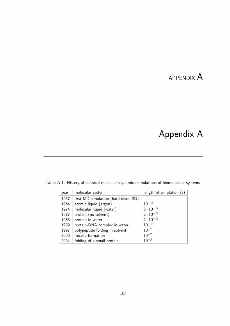
APPENDIX A
Appendix A
Table A.1: History of classical molecular dynamics simulations of biomolecular systems.
year molecular system length of simulation (s)
1957 first MD simulation (hard discs, 2D)1964 atomic liquid (argon) 10−11
1974 molecular liquid (water) 5 · 10−12
1977 protein (no solvent) 2 · 10−11
1983 protein in water 2 · 10−11
1989 protein-DNA complex in water 10−10
1997 polypeptide folding in solvent 10−7
2000 micelle formation 10−7
200x folding of a small protein 10−3
167

168
Figure A.1: The 20 common amino acids. The pink shaded parts represent the R groupof each amino acid. In the case of histidine the R group is shown as uncharged, however atpH 7.0 a fraction of the group is positively charged. The figure has been adapted from [5].
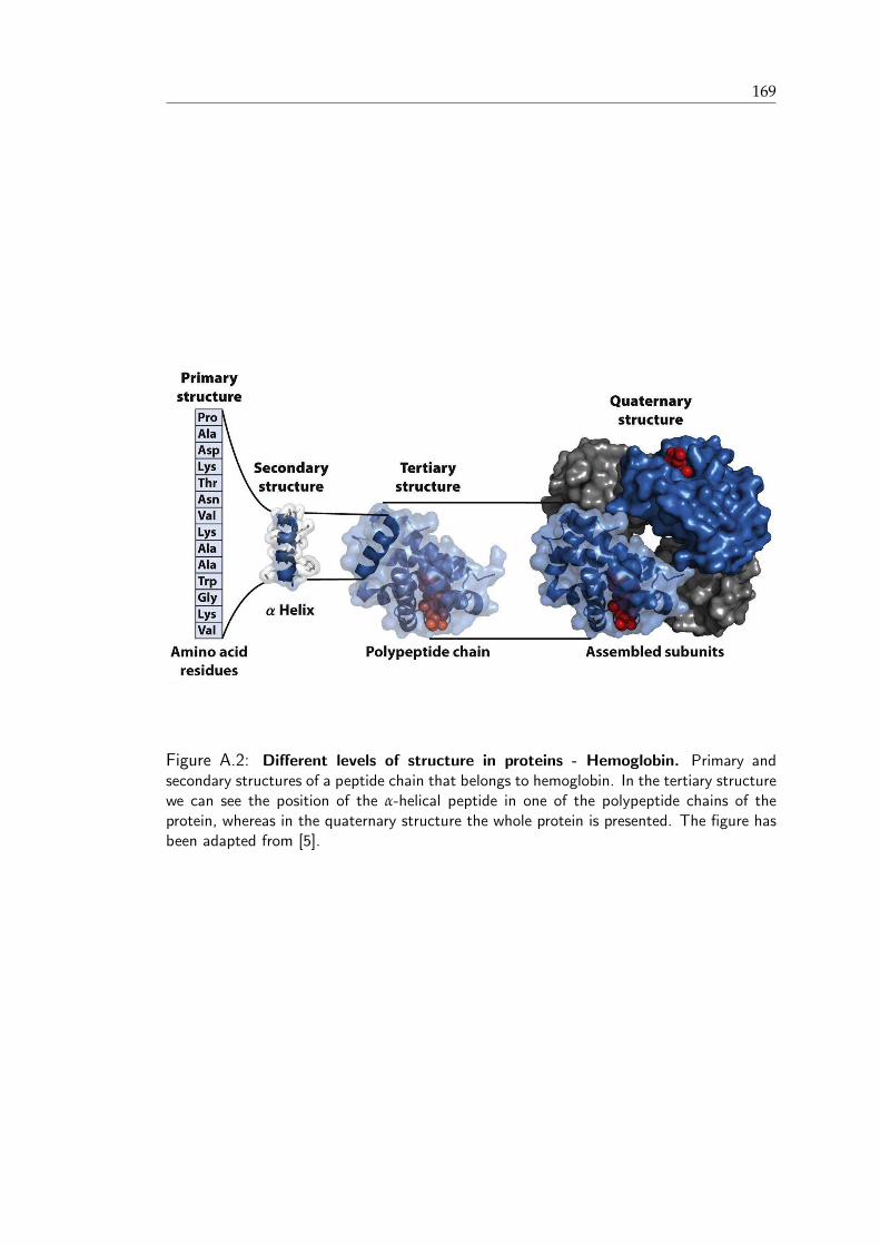
169
Figure A.2: Different levels of structure in proteins - Hemoglobin. Primary andsecondary structures of a peptide chain that belongs to hemoglobin. In the tertiary structurewe can see the position of the α-helical peptide in one of the polypeptide chains of theprotein, whereas in the quaternary structure the whole protein is presented. The figure hasbeen adapted from [5].
APPENDIX B
Appendix B
In this section, we will shortly describe the molecular dynamics program we have
developed as part of this PhD.
1. The NVE ensemble:
(a) NVE with the leap-frog integrator scheme:
Firstly, we developed a code for the NVE ensemble using the leap-frog integrator
scheme. In table B.1, we present the comparative results from the house code and
a code that calculates the pressure and the potential energy based on the LJ equation
of state. We can see that our results are in good agreement with those predicted by the
equation of state1.
1From now on all the quantities are in reduced units
170
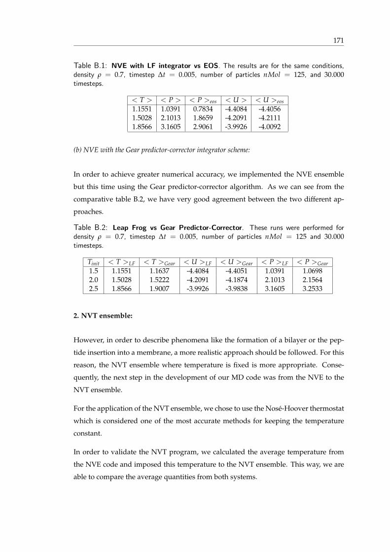
171
Table B.1: NVE with LF integrator vs EOS. The results are for the same conditions,density ρ = 0.7, timestep ∆t = 0.005, number of particles nMol = 125, and 30.000timesteps.
< T > < P > < P >eos < U > < U >eos
1.1551 1.0391 0.7834 -4.4084 -4.40561.5028 2.1013 1.8659 -4.2091 -4.21111.8566 3.1605 2.9061 -3.9926 -4.0092
(b) NVE with the Gear predictor-corrector integrator scheme:
In order to achieve greater numerical accuracy, we implemented the NVE ensemble
but this time using the Gear predictor-corrector algorithm. As we can see from the
comparative table B.2, we have very good agreement between the two different ap-
proaches.
Table B.2: Leap Frog vs Gear Predictor-Corrector. These runs were performed fordensity ρ = 0.7, timestep ∆t = 0.005, number of particles nMol = 125 and 30.000timesteps.
Tinit < T >LF < T >Gear < U >LF < U >Gear < P >LF < P >Gear
1.5 1.1551 1.1637 -4.4084 -4.4051 1.0391 1.06982.0 1.5028 1.5222 -4.2091 -4.1874 2.1013 2.15642.5 1.8566 1.9007 -3.9926 -3.9838 3.1605 3.2533
2. NVT ensemble:
However, in order to describe phenomena like the formation of a bilayer or the pep-
tide insertion into a membrane, a more realistic approach should be followed. For this
reason, the NVT ensemble where temperature is fixed is more appropriate. Conse-
quently, the next step in the development of our MD code was from the NVE to the
NVT ensemble.
For the application of the NVT ensemble, we chose to use the Nose-Hoover thermostat
which is considered one of the most accurate methods for keeping the temperature
constant.
In order to validate the NVT program, we calculated the average temperature from
the NVE code and imposed this temperature to the NVT ensemble. This way, we are
able to compare the average quantities from both systems.
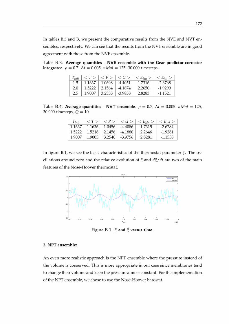
172
In tables B.3 and B, we present the comparative results from the NVE and NVT en-
sembles, respectively. We can see that the results from the NVT ensemble are in good
agreement with those from the NVE ensemble.
Table B.3: Average quantities - NVE ensemble with the Gear predictor-correctorintegrator. ρ = 0.7, ∆t = 0.005, nMol = 125, 30.000 timesteps.
Tinit < T > < P > < U > < Ekin > < Etot >
1.5 1.1637 1.0698 -4.4051 1.7316 -2.67682.0 1.5222 2.1564 -4.1874 2.2650 -1.92992.5 1.9007 3.2533 -3.9838 2.8283 -1.1521
Table B.4: Average quantities - NVT ensemble. ρ = 0.7, ∆t = 0.005, nMol = 125,30.000 timesteps, Q = 10.
Tinit < T > < P > < U > < Ekin > < Etot >
1.1637 1.1636 1.0456 -4.4086 1.7315 -2.67841.5222 1.5218 2.1456 -4.1880 2.2646 -1.92811.9007 1.9005 3.2540 -3.9756 2.8281 -1.1558
In figure B.1, we see the basic characteristics of the thermostat parameter ξ. The os-
cillations around zero and the relative evolution of ξ and dξ/dt are two of the main
features of the Nose-Hoover thermostat.
2.8 2.82 2.84 2.86 2.88 2.9 2.92 2.94 2.96 2.98 3
x 104
−1.5
−1
−0.5
0
0.5
1
1.5Q=100
Ntime
ksidksi/dt
Figure B.1: ξ and ξ versus time.
3. NPT ensemble:
An even more realistic approach is the NPT ensemble where the pressure instead of
the volume is conserved. This is more appropriate in our case since membranes tend
to change their volume and keep the pressure almost constant. For the implementation
of the NPT ensemble, we chose to use the Nose-Hoover barostat.
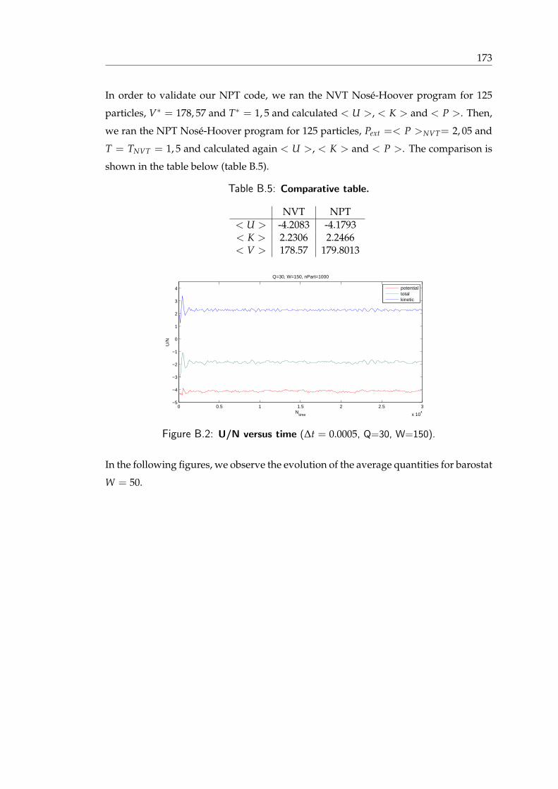
173
In order to validate our NPT code, we ran the NVT Nose-Hoover program for 125
particles, V∗ = 178, 57 and T∗ = 1, 5 and calculated < U >, < K > and < P >. Then,
we ran the NPT Nose-Hoover program for 125 particles, Pext =< P >NVT= 2, 05 and
T = TNVT = 1, 5 and calculated again < U >, < K > and < P >. The comparison is
shown in the table below (table B.5).
Table B.5: Comparative table.
NVT NPT
< U > -4.2083 -4.1793< K > 2.2306 2.2466< V > 178.57 179.8013
0 0.5 1 1.5 2 2.5 3
x 104
−5
−4
−3
−2
−1
0
1
2
3
4
Q=30, W=150, nPart=1000
Ntime
U/N
potentialtotalkinetic
Figure B.2: U/N versus time (∆t = 0.0005, Q=30, W=150).
In the following figures, we observe the evolution of the average quantities for barostat
W = 50.
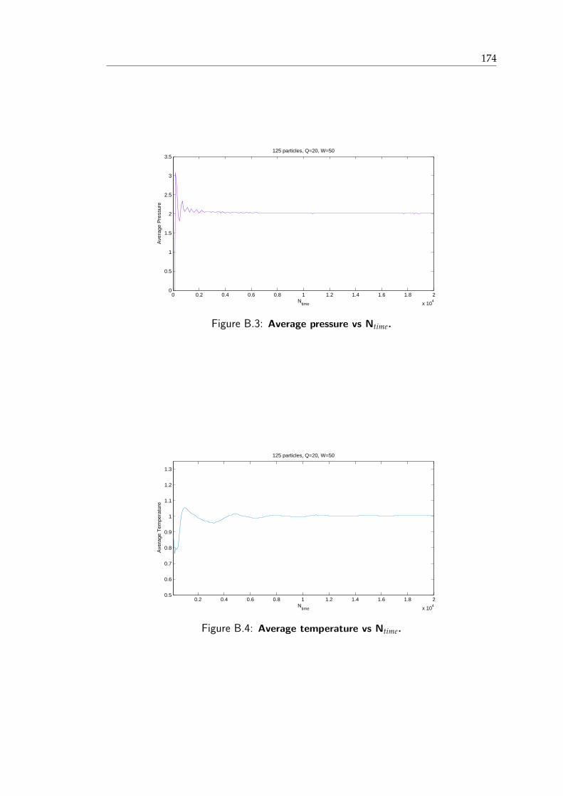
174
0 0.2 0.4 0.6 0.8 1 1.2 1.4 1.6 1.8 2
x 104
0
0.5
1
1.5
2
2.5
3
3.5125 particles, Q=20, W=50
Ntime
Ave
rage
Pre
ssur
e
Figure B.3: Average pressure vs Ntime.
0.2 0.4 0.6 0.8 1 1.2 1.4 1.6 1.8 2
x 104
0.5
0.6
0.7
0.8
0.9
1
1.1
1.2
1.3
125 particles, Q=20, W=50
Ntime
Ave
rage
Tem
pera
ture
Figure B.4: Average temperature vs Ntime.
APPENDIX C
Appendix C
In the figure below, we present the free energy profiles for the translocation of SIV fu-
sion peptide across a DOPC bilayer, calculated by using different methods for the treat-
ment of electrostatics and pressure coupling. In particular, we perform an umbrella
sampling simulation with the Nose-Hoover thermostat and one with the Particle-mesh
Ewald (PME) for the treatment of electrostatic interactions. For the PME scheme, we
use a grid spacing of 0.12 nm and quadratic interpolation. The rest of the parameters
in the two simulations are as in the original.
175
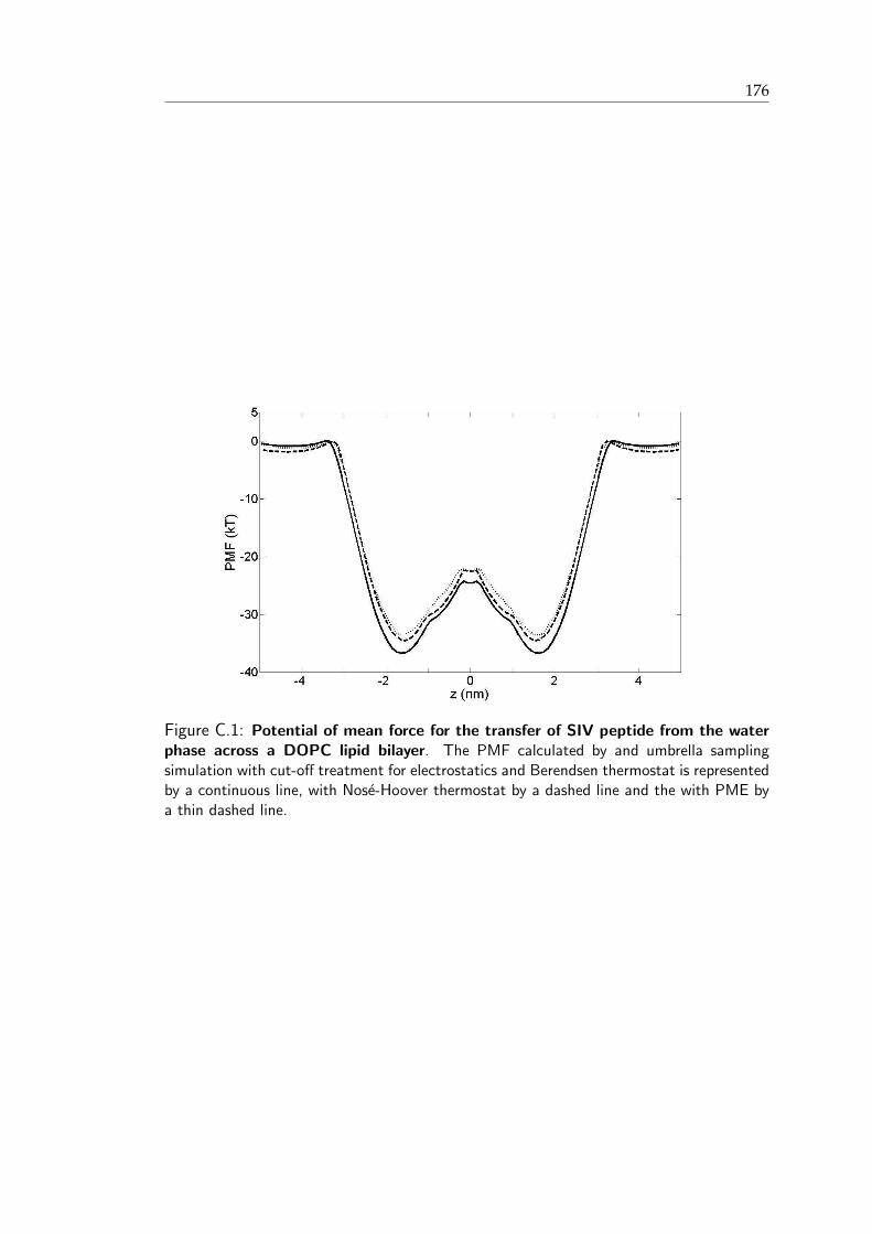
176
Figure C.1: Potential of mean force for the transfer of SIV peptide from the waterphase across a DOPC lipid bilayer. The PMF calculated by and umbrella samplingsimulation with cut-off treatment for electrostatics and Berendsen thermostat is representedby a continuous line, with Nose-Hoover thermostat by a dashed line and the with PME bya thin dashed line.
References
[1] S. J. Singer and G. L. Nicolson, “Fluid mosaic model of structure of cell-membranes,” Science, vol. 175, no. 4023, pp. 720–731, 1972.
[2] Encyclopedia Britannica, Inc. http://www.britannica.com (accessed Nov. 21,2009).
[3] J. Seddon, “Structure of the inverted hexagonal (HII) phase, and non-lamellarphase-transitions of lipids,” Biochimica et Biophysica Acta, vol. 1031, no. 1, pp. 1–69, 1990.
[4] K. Balali-Mood, T. Harroun, and J. Bradshaw, “Molecular dynamics simulationsof a mixed DOPC/DOPG bilayer,” European Physical Journal E, vol. 12, no. Suppl.1, pp. S135–S140, 2003.
[5] D. L. Nelson and M. M. Cox, Principles of Biochemistry. W. H. Freeman and Com-pany, fifth ed., 2008.
[6] R. Brasseur, “Differentiation of lipid-associating helices by use of three-dimensional molecular hydrophobicity potential calculations,” Journal of Biolog-ical Chemistry, vol. 266, no. 24, pp. 16120–16127, 1991.
[7] M. Yeaman and N. Yount, “Mechanisms of antimicrobial peptide action and re-sistance,” Pharmacological Reviews, vol. 55, no. 1, pp. 27–55, 2003.
[8] U. Langel, Handbook of cell-penetrating peptides. Taylor & Francis, 2nd ed., 2007.
[9] S. El-Andaloussi, T. Holm, and U. Langel, “Cell-penetrating peptides: Mecha-nisms and applications,” Current Pharmaceutical Design, vol. 11, pp. 3597–3611,2005.
[10] A. Pokorny, T. Birkbeck, and P. Almeida, “Mechanism and kinetics of delta-Lysininteraction with phospholipid vesicles,” Biochemistry, vol. 41, no. 36, pp. 11044–11056, 2002.
177
References 178
[11] O. Toke, “Antimicrobial peptides: New candidates in the fight against bacterialinfections,” Biopolymers, vol. 80, no. 6, pp. 717–735, 2005.
[12] G. B. Melikyan, “Common principles and intermediates of viral protein-mediated fusion: the HIV-1 paradigm,” Retrovirology, vol. 5, 2008.
[13] S. Deshayes, A. Heitz, M. C. Morris, P. Charnet, G. Divita, and F. Heitz, “In-sight into the mechanism of internalization of the cell-penetrating carrier peptidePep–1 through conformational analysis,” Biochemistry, vol. 43, pp. 1449–1457,2004.
[14] R. Fischer, M. Fotin-Mleczek, H. Hufnagel, and R. Brock, “Break on through tothe other side - biophysics and cell biology shed light on cell-penetrating pep-tides,” ChemBioChem, vol. 6, pp. 2126–2142, 2005.
[15] D. Allende, S. Simon, and T. J. McIntosh, “Melittin-induced bilayer leakage de-pends on lipid material properties: Evidence for toroidal pores,” Biophysical Jour-nal, vol. 88, no. 3, pp. 1828 – 1837, 2005.
[16] J. D. Lear, Z. R. Wasserman, and W. F. Degrado, “Synthetic amphiphilic peptidemodels for protein ion channels,” Science, vol. 240, no. 4856, pp. 1177–1181, 1988.
[17] K. S. Akerfeldt, J. D. Lear, Z. R. Wasserman, L. A. Chung, and W. F. Degrado,“Synthetic peptides as models for ion channel proteins,” Accounts of ChemicalResearch, vol. 26, pp. 191–197, 1993.
[18] J. D. Lear, J. P. Schneider, P. K. Kienker, and W. F. DeGrado, “Electrostatic effectson ion selectivity and rectification in designed ion channel peptides,” Journal ofAmerican Chemical Society, vol. 119, pp. 3212–3217, 1997.
[19] L. Chaloin, E. De, P. Charnet, G. Molle, and F. Heitz, “Ionic channels formed bya primary amphipathic peptide containing a signal peptide and a nuclear local-ization sequence,” Biochimica et Biophysica Acta-Biomembranes, vol. 1375, no. 1-2,pp. 52–60, 1998.
[20] E. De, L. Chaloin, A. Heitz, J. Mery, G. Molle, and F. Heitz, “Conformation andion channel properties of a five-helix bundle protein,” Journal of Peptide Science,vol. 7, no. 1, pp. 41–49, 2001.
[21] P. Haris and D. Chapman, “The conformational-analysis of peptides usingFourier-Transform IR spectroscopy,” Biopolymers, vol. 37, no. 4, pp. 251–263,1995.
[22] L. Tamm and S. Tatulian, “Infrared spectroscopy of proteins and peptides in lipidbilayers,” Quarterly Reviews of Biophysics, vol. 30, no. 4, pp. 365–429, 1997.
[23] E. Goormaghtigh, V. Raussens, and J. Ruysschaert, “Attenuated total reflectioninfrared spectroscopy of proteins and lipids in biological membranes,” Biochim-ica et Biophysica Acta-Reviews on Biomembranes, vol. 1422, no. 2, pp. 105–185, 1999.
References 179
[24] V. Vie, N. Van Mau, L. Chaloin, E. Lesniewska, C. Le Grimellec, and F. Heitz,“Detection of peptide-lipid interactions in mixed monolayers, using isotherms,atomic force microscopy, and Fourier transform infrared analyses,” BiophysicalJournal, vol. 78, no. 2, pp. 846–856, 2000.
[25] S. Frey and L. Tamm, “Orientation of melittin in phospholipid-bilayers - A polar-ized attenuated total reflection infrared study,” Biophysical Journal, vol. 60, no. 4,pp. 922–930, 1991.
[26] I. Martin, M. Dubois, F. Defrisequertain, T. Saernark, A. Burny, R. Brasseur, andJ. Ruysschaert, “Correlation between fusogenicity of synthetic modified pep-tides corresponding to the NH2-terminal extremity of Simian ImmunodeficiencyVirus GP32 and their mode of insertion into the lipid bilayer - An infrared-spectroscopy study,” Journal of Virology, vol. 68, no. 2, pp. 1139–1148, 1994.
[27] Wang, J and Lee, S-H and Chen, Z, “Quantifying the ordering of adsorbed pro-teins in situ,” Journal of Physical Chemistry B, vol. 112, no. 7, pp. 2281–2290, 2008.
[28] I. de la Arada, J.-P. Julien, B. G. de la Torre, N. Huarte, D. Andreu, E. F. Pai, J. L. R.Arrondo, and J. L. Nieva, “Structural constraints imposed by the conserved fu-sion peptide on the HIV-1 gp41 epitope recognized by the broadly neutralizingantibody 2F5,” Journal of Physical Chemistry B, vol. 113, no. 41, pp. 13626–13637,2009.
[29] J. P. Bradshaw, M. J. M. Darkes, T. A. Haroun, J. Katsaras, and R. M. Epand,“Oblique membrane insertion of viral fusion peptide probed by neutron diffrac-tion,” Biochemistry, vol. 39, no. 22, pp. 6581–6585, 2000.
[30] L. Chaloin, P. Vidal, A. Heitz, N. VanMau, J. Mery, G. Divita, and F. Heitz, “Con-formations of primary amphipathic carrier peptides in membrane mimickingenvironments,” Biochemistry, vol. 36, no. 37, pp. 11179–11187, 1997.
[31] M. Lindberg, J. Jarvet, U. Langel, and A. Graslund, “Secondary structure and po-sition of the cell-penetrating peptide transportan in SDS micelles as determinedby NMR,” Biochemistry, vol. 40, no. 10, pp. 3141–3149, 2001.
[32] M. Magzoub, K. Kilk, L. Eriksson, U. Langel, and A. Graslund, “Interaction andstructure induction of cell-penetrating peptides in the presence of phospholipidvesicles,” Biochimica et Biophysica Acta-Biomembranes, vol. 1512, no. 1, pp. 77–89,2001.
[33] R. Ketchem, W. Hu, and T. Cross, “High-resolution conformation of Gramicidin-A in a lipid bilayer by solid-state NMR,” Science, vol. 261, no. 5127, pp. 1457–1460, 1993.
[34] B. Bechinger, “The structure, dynamics and orientation of antimicrobial peptidesin membranes by multidimensional solid-state NMR spectroscopy,” Biochimicaet Biophysica Acta-Biomembranes, vol. 1462, no. 1-2, pp. 157–183, 1999.
[35] J. Yang, C. Gabrys, and D. Weliky, “Solid-state nuclear magnetic resonance evi-dence for an extended beta strand conformation of the membrane-bound HIV-1fusion peptide,” Biochemistry, vol. 40, no. 27, pp. 8126–8137, 2001.
References 180
[36] S. Yamaguchi, T. Hong, A. Waring, R. Lehrer, and M. Hong, “Solid-state NMRinvestigations of peptide-lipid interaction and orientation of a β-sheet antimi-crobial peptide, protegrin,” Biochemistry, vol. 41, no. 31, pp. 9852–9862, 2002.
[37] F. Porcelli, B. Buck, D. Lee, K. Hallock, A. Ramamoorthy, and G. Veglia, “Struc-ture and orientation of pardaxin determined by NMR experiments in modelmembranes,” Journal of Biological Chemistry, vol. 279, no. 44, pp. 45815–45823,2004.
[38] A. Ramamoorthy, S. Thennarasu, D. Lee, A. Tan, and L. Maloy, “Solid-state NMRinvestigation of the membrane-disrupting mechanism of antimicrobial peptidesMSI-78 and MSI-594 derived from magainin 2 and melittin,” Biophysical Journal,vol. 91, no. 1, pp. 206–216, 2006.
[39] S. Bhattacharjya and A. Ramamoorthy, “Multifunctional host defense peptides:functional and mechanistic insights from NMR structures of potent antimicro-bial peptides,” FEBS Journal, vol. 276, no. 22, pp. 6465–6473, 2009.
[40] B. Bechinger, M. Zasloff, and S. Opella, “Structure and orientation of the antibi-otic peptide magainin in membranes by solid-state nuclear-magnetic-resonancespectroscopy,” Protein Science, vol. 2, pp. 2077–2084, DEC 1993.
[41] S. Opella, F. Marassi, J. Gesell, A. Valente, Y. Kim, M. Oblatt-Montal, andM. Montal, “Structures of the M2 channel-lining segments from nicotinic acetyl-choline and NMDA receptors by NMR spectroscopy,” Nature Structural Biology,vol. 6, pp. 374–379, APR 1999.
[42] S. J. Opella, A. C. Zeri, and S. H. Park, “Structure, dynamics, and assembly of fil-amentous bacteriophages by nuclear magnetic resonance spectroscopy,” AnnualReview of Physical Chemistry, vol. 59, pp. 635–657, 2008.
[43] Brasseur, R and Deleu, M and Mingeot-Leclercq, M-P and Francius, G andDufrene, Y F., “Probing peptide-membrane interactions using AFM,” Surface andInterface Analysis, vol. 40, no. 3-4, pp. 151–156, 2008.
[44] H. You, X. Qi, G. Grabowski, and L. Yu, “Phospholipid membrane interactionsof saposin C: In situ atomic force microscopic study,” Biophysical Journal, vol. 84,no. 3, pp. 2043–2057, 2003.
[45] S. Morandat and K. El Kirat, “Real-time atomic force microscopy reveals cy-tochrome C-induced alterations in neutral lipid bilayers,” Langmuir, vol. 23,no. 22, pp. 10929–10932, 2007.
[46] Wang, H and Obenauer-Kutner, L and Lin, M and Huang, Y and Grace, M. J.and Lindsay, S. M., “Imaging glycosylation,” Journal of American Chemical Society,vol. 130, no. 26, pp. 8154–8155, 2008.
[47] M. L. Kraft, P. K. Weber, M. L. Longo, I. D. Hutcheon, and S. G. Boxer, “Phase sep-aration of lipid membranes analyzed with high-resolution secondary ion massspectrometry,” Science, vol. 313, no. 5795, pp. 1948–1951, 2006.
References 181
[48] P. D. Veith, S. G. Dashper, N. M. O’Brien-Simpson, R. A. Paolini, R. Orth, K. A.Walsh, and E. C. Reynolds, “Major proteins and antigens of Treponema den-ticola,” Biochimica et Biophysica Acta-Proteins and Proteomics, vol. 1794, no. 10,pp. 1421–1432, 2009.
[49] S. G. Boxer, M. L. Kraft, and P. K. Weber, “Advances in imaging secondary ionmass spectrometry for biological samples,” Annual Review of Biophysics, vol. 38,pp. 53–74, 2009.
[50] H. Mozsolits, H. Wirth, J. Werkmeister, and M. Aguilar, “Analysis of antimicro-bial peptide interactions with hybrid bilayer membrane systems using surfaceplasmon resonance,” Biochimica et Biophysica Acta-Biomembranes, vol. 1512, no. 1,pp. 64–76, 2001.
[51] H. Mozsolits and M. Aguilar, “Surface plasmon resonance spectroscopy: Anemerging tool for the study of peptide-membrane interactions,” Biopolymers,vol. 66, no. 1, pp. 3–18, 2002.
[52] H. Mozsolits, W. Thomas, and M. Aguilar, “Surface plasmon resonance spec-troscopy in the study of membrane-mediated cell signalling,” Journal of PeptideScience, vol. 9, no. 2, pp. 77–89, 2003.
[53] M. M. Domingues, P. S. Santiago, M. A. R. B. Castanho, and N. C. Santos, “Whatcan light scattering spectroscopy do for membrane-active peptide studies,” Jour-nal of Peptide Science, vol. 14, no. 4, pp. 394–400, 2008.
[54] W. Wimley and S. White, “Designing transmembrane alpha-helices that insertspontaneously,” Biochemistry, vol. 39, no. 15, pp. 4432–4442, 2000.
[55] J. Bradshaw, M. Darkes, J. Katsaras, and R. Epand, “Neutron diffraction studiesof viral fusion peptides,” Physica B, vol. 276, pp. 495–498, 2000.
[56] T. Harroun, K. Balali-Mood, I. Gourlay, and J. Bradshaw, “The fusion peptideof simian immunodeficiency virus and the phase behaviour of N-methylateddioleoylphosphatidylethanolamine,” Biochimica et Biophysica Acta-Biomembranes,vol. 1617, no. 1-2, pp. 62–68, 2003.
[57] F. Leemakers and J. Scheutjens, “Statistical thermodynamics of association col-loids .1. Lipid bilayer-membranes,” Journal of Chemical Physics, vol. 89, no. 5,pp. 3264–3274, 1988.
[58] L. Meijer, F. Leermakers, and J. Lyklema, “Self-consistent-field modeling of com-plex molecules with united atom detail in inhomogeneous systems. Cyclic andbranched foreign molecules in dimyristoylphosphatidylcholine membranes,”Journal of Chemical Physics, vol. 110, no. 13, pp. 6560–6579, 1999.
[59] R. Kik, F. Leermakers, and J. Kleijn, “Molecular modeling of lipid bilayers andthe effect of protein-like inclusions,” Physical Chemistry Chemical Physics, vol. 7,no. 9, pp. 1996–2005, 2005.
References 182
[60] Q. Liang and Y.-Q. Ma, “Inclusion-mediated lipid organization in supportedmembranes on a patterned substrate,” Journal of Physical Chemistry B, vol. 112,no. 7, pp. 1963–1967, 2008.
[61] Q. Liang and Y. Q. Ma, “Organization of membrane-associated proteins in lipidbilayers,” European Physical Journal E, vol. 25, no. 2, pp. 129–138, 2008.
[62] C.-l. Ren and Y.-q. Ma, “Structure and organization of nanosized-inclusion-containing bilayer membranes,” Physical Review E, vol. 80, no. 1, Part 1, 2009.
[63] P. Lague, M. Zuckermann, and B. Roux, “Protein inclusion in lipid membranes:A theory based on the hypernetted chain integral equation,” Faraday Discussions,vol. 111, pp. 165–172, 1998.
[64] P. Lague, M. Zuckermann, and B. Roux, “Lipid-mediated interactions betweenintrinsic membrane proteins: A theoretical study based on integral equations,”Biophysical Journal, vol. 79, no. 6, pp. 2867–2879, 2000.
[65] P. Lague, M. Zuckermann, and B. Roux, “Lipid-mediated interactions betweenintrinsic membrane proteins: Dependence on protein size and lipid composi-tion,” Biophysical Journal, vol. 81, no. 1, pp. 276–284, 2001.
[66] P. La Rocca, Y. Shai, and M. Sansom, “Peptide-bilayer interactions: simulationsof dermaseptin B, an antimicrobial peptide,” Biophysical Chemistry, vol. 76, no. 2,pp. 145–159, 1999.
[67] P. La Rocca, P. Biggin, D. Tieleman, and M. Sansom, “Simulation studies of theinteraction of antimicrobial peptides and lipid bilayers,” Biochimica et BiophysicaActa-Biomembranes, vol. 1462, no. 1-2, pp. 185–200, 1999.
[68] W. Still, A. Tempczyk, R. Hawley, and T. Hendrickson, “Semianalytical treat-ment of solvation for molecular mechanics and dynamics,” Journal of AmericanChemical Society, vol. 112, no. 16, pp. 6127–6129, 1990.
[69] W. Im, M. Feig, and C. Brooks, “An implicit membrane generalized born the-ory for the study of structure, stability, and interactions of membrane proteins,”Biophysical Journal, vol. 85, pp. 2900–2918, NOV 1 2003.
[70] W. Im, M. Lee, and C. Brooks, “Generalized born model with a simple smoothingfunction,” Journal of Computational Chemistry, vol. 24, pp. 1691–1702, NOV 152003.
[71] M. Ulmschneider, M. Sansom, and A. Di Nola, “Properties of integral membraneprotein structures: Derivation of an implicit membrane potential,” Proteins-Structure function and bioinformatics, vol. 59, no. 2, pp. 252–265, 2005.
[72] M. B. Ulmschneider, J. P. Ulmschneider, M. S. P. Sansom, and A. Di Nola, “Ageneralized Born implicit-membrane representation compared to experimentalinsertion free energies,” Biophysical Journal, vol. 92, pp. 2338–2349, APR 1 2007.
[73] J. McCammon, B. Gelin, and M. Karplus, “Dynamics of folded proteins,” Nature,vol. 267, no. 5612, pp. 585–590, 1977.
References 183
[74] K. Damodaran, K. Merz, and B. Gaber, “Interaction od small peptides with lipidbilayers,” Biophysical Journal, vol. 69, no. 4, pp. 1299–1308, 1995.
[75] K. Belohorcova, J. Davis, T. Woolf, and B. Roux, “Structure and dynamics of anamphiphilic peptide in a lipid bilayer: A molecular dynamics study,” BiophysicalJournal, vol. 73, no. 6, pp. 3039–3055, 1997.
[76] S. Berneche, M. Nina, and B. Roux, “Molecular dynamics simulation of melit-tin in a dimyristoylphosphatidylcholine bilayer membrane,” Biophysical Journal,vol. 75, no. 4, pp. 1603–1618, 1998.
[77] H. Leontiadou, A. E. Mark, and S. J. Marrink, “Antimicrobial peptides in action,”Journal of American Chemical Society, vol. 128, pp. 12156–12161, 2006.
[78] D. Sengupta, H. Leontiadou, A. E. Mark, and S. J. Marrink, “Toroidal poresformed by antimicrobial peptides show significant disorder,” Biochimica et Bio-physica Acta-Biomembranes, vol. 1778, no. 10, pp. 2308–2317, 2008.
[79] H. D. Herce and A. E. Garcia, “Molecular dynamics simulations suggest a mech-anism for translocation of the HIV-1 TAT peptide across lipid membranes,” Pro-ceedings of the National Academy of Sciences of the United States of America, vol. 104,no. 52, pp. 20805–20810, 2007.
[80] S. Yesylevskyy, S. J. Marrink, and A. E. Mark, “Alternative mechanisms for theinteraction of the cell-penetrating peptides Penetratin and the TAT peptide withlipid bilayers,” Biophysical Journal, vol. 97, no. 1, pp. 40–49, 2009.
[81] S. Izvekov and G. Voth, “Multiscale coarse-graining of mixed phospho-lipid/cholesterol bilayers,” Journal of Chemical Theory and Computation, vol. 2,no. 3, pp. 637–648, 2006.
[82] S. J. Marrink, A. H. de Vries, and A. E. Mark, “Coarse grained model for semi-quantitative lipid simulations,” Journal of Physical Chemistry B, vol. 108, pp. 750–760, 2004.
[83] M. Venturoli, M. M. Sperotto, M. Kranenburg, and B. Smit, “Mesoscopic modelsof biological membranes,” Physics Reports, vol. 437, pp. 1–54, 2006.
[84] S. J. Marrink, A. H. de Vries, and D. P. Tieleman, “Lipids on the move: Simula-tions of membrane pores, domains, stalks and curves,” Biochimica et BiophysicaActa-Biomembranes, vol. 1788, no. 1, Sp. Iss. SI, pp. 149–168, 2009.
[85] T. Murtola, A. Bunker, I. Vattulainen, M. Deserno, and M. Karttunen, “Multiscalemodeling of emergent materials: biological and soft matter,” Physical ChemistryChemical Physics, vol. 11, no. 12, pp. 1869–1892, 2009.
[86] D. J. Michel and D. J. Cleaver, “Coarse-grained simulation of amphiphilic self-assembly,” Journal of Chemical Physics, vol. 126, no. 3, p. 34506, 2007.
[87] Smit, Berend and Hilbers, P. A. J. and Esselink, K. and Rupert, N. M. and vanOs, N. M. and Schlijper, A. G., “Computer simulations of a water/oil interfacein the presence of micelles,” Nature, vol. 348, pp. 624–625, 1990.
References 184
[88] Smit, Berend and Hilbers, P. A. J. and Esselink, K. and Rupert, N. M. and vanOs, N. M. and Schlijper, A. G., “Structure of a water/oil interface in the presenceof micelles: a computer simulation study,” Journal of Physical Chemistry, vol. 95,pp. 6361–6368, 1991.
[89] R. D. Groot and P. B. Warren, “Dissipative particle dynamics: Bridging thegap between atomistic and mesoscopic simulation,” Journal of Chemical Physics,vol. 107, pp. 4423–4435, 1997.
[90] M. Kranenburg, M. Venturoli, and B. Smit, “Phase behaviour and induced inter-digitation in bilayers studied with dissipative particle dynamics,” Journal Physi-cal Chemistry B, vol. 107, pp. 11491–11501, 2003.
[91] M. Venturoli, B. Smit, and M. Sperotto, “Simulation studies of protein-inducedbilayer deformations, and lipid-induced protein tilting, on a mesoscopic modelfor lipid bilayers with embedded proteins,” Biophysical Journal, vol. 88, no. 3,pp. 1778–1798, 2005.
[92] U. Schmidt, G. Guigas, and M. Weiss, “Cluster formation of transmembrane pro-teins due to hydrophobic mismatching,” Physical Review Letters, vol. 101, no. 12,2008.
[93] F. J.-M. de Meyer, M. Venturoli, and B. Smit, “Molecular simulations oflipid-mediated protein-protein interactions,” Biophysical Journal, vol. 95, no. 4,pp. 1851–1865, 2008.
[94] R. Goetz and R. Lipowsky, “Computer simulations of bilayer membranes: Self-assembly and interfacial tension,” Journal of Chemical Physics, vol. 108, no. 17,pp. 7397–7409, 1998.
[95] J. C. Shelley, M. Y. Shelley, R. C. Reeder, S. Bandyopadhyay, and M. L. Klein, “Acoarse grained model for phospholipid simulations,” Journal of Physical Chem-istry B, vol. 105, pp. 4464–4470, 2001.
[96] J. C. Shelley, M. Y. Shelley, R. C. Reeder, S. Bandyopadhyay, P. B. Moore, andM. L. Klein, “Simulations of phospholipids using a coarse grain model,” Journalof Physical Chemistry B, vol. 105, pp. 9785–9792, 2001.
[97] S. J. Marrink and A. E. Mark, “Molecular view of hexagonal phase formation inphospholipid membranes,” Biophysical Journal, vol. 84, pp. 3894–3900, 2004.
[98] S. J. Marrink, J. Risselada, and A. E. Mark, “Simulation of gel phase forma-tion and melting in lipid bilayers using a coarse grained model,” Chemistry andPhysics of Lipids, vol. 135, pp. 223–244, 2005.
[99] V. Knecht and S. J. Marrink, “Molecular dynamics simulations of lipid vesiclefusion in atomic detail,” Biophysical Journal, vol. 92, pp. 4254–4261, 2007.
[100] P. J. Bond and M. S. P. Sansom, “Insertion and assembly of membrane proteinsvia simulation,” Journal of Americal Chemical Society, vol. 128, pp. 2697–2704, 2006.
References 185
[101] P. J. Bond, J. Holyoake, A. Ivetac, S. Khalid, and M. S. P. Sansom, “Coarse-grainedmolecular dynamics simulations of membrane proteins and peptides,” Journal ofStructural Biology, vol. 157, pp. 593–605, 2007.
[102] S. Khalid, P. J. Bond, J. Holyoake, R. W. Hawtin, and M. S. P. Sansom, “DNA andlipid bilayers: self-assembly and insertion,” Journal of the Royal Society Interface,vol. 5, no. Suppl. 3, pp. S241–S250, 2008.
[103] K. Balali-Mood, P. J. Bond, and M. S. P. Sansom, “Interaction of monotopic mem-brane enzymes with a lipid bilayer: A coarse-grained MD simulation study,”Biochemistry, vol. 48, no. 10, pp. 2135–2145, 2009.
[104] K. Cox and M. S. P. Sansom, “One membrane protein, two structures and sixenvironments: a comparative molecular dynamics simulation study of the bac-terial outer membrane protein PagP,” Molecular Membrane Biology, vol. 26, no. 4,pp. 205–214, 2009.
[105] L. Monticelli, S. K. Kandasamy, X. Periole, D. P. Tieleman, and S. J. Marrink,“The MARTINI Coarse-Grained Force Field: Extension to Proteins,” Journal ofChemical Theory and Computation, vol. 4, pp. 819–834, 2008.
[106] S. J. Marrink, H. J. Risselada, S. Yefimov, D. P. Tieleman, and A. H. de Vries,“The MARTINI force field: coarse grained model for biomolecular simulations,”Journal of Physical Chemistry B, vol. 111, pp. 7812–7824, 2007.
[107] H. J. Risselada and S. J. Marrink, “Curvature effects on lipid packing and dynam-ics in liposomes revealed by coarse grained molecular dynamics simulations,”Physical Chemistry Chemical Physics, vol. 11, no. 12, pp. 2056–2067, 2009.
[108] A. Khalfa, W. Treptow, B. Maigret, and M. Tarek, “Self-assembly of peptides nearor within membranes using coarse grained MD simulations,” Chemical Physics,vol. 358, no. 1-2, pp. 161–170, 2009.
[109] P. Gkeka and L. Sarkisov, “Spontaneous formation of a barrel-stave pore in acoarse-grained model of the synthetic LS3 peptide and a DPPC lipid bilayer,”Journal of Physical Chemistry B, vol. 113, no. 1, pp. 6–8, 2009.
[110] S. Izvekov and A. G. Voth, “A multiscale coarse-graining method for biolmolec-ular systems,” Journal of Physical Chemistry B, vol. 109, pp. 2469–2473, 2005.
[111] J. Zhou, F. I. Thorpe, S. Izvekov, and A. G. Voth, “Coarse-grained peptidemodeling using a systematic multiscale approach,” Biophysical journal, vol. 92,pp. 4289–4303, 2007.
[112] J. Michel, M. Orsi, and J. W. Essex, “Prediction of partition coefficients by mul-tiscale hybrid atomic-level/coarse-grain simulations,” Journal of Physical Chem-istry B, vol. 112, no. 3, pp. 657–660, 2008.
[113] M. Orsi, D. Y. Haubertin, W. E. Sanderson, and J. W. Essex, “A quantitativecoarse-grain model for lipid bilayers,” Journal of Physical Chemistry B, vol. 112,no. 3, pp. 802–815, 2008.
References 186
[114] M. Orsi, W. E. Sanderson, and J. W. Essex, “Permeability of Small Moleculesthrough a Lipid Bilayer: A Multiscale Simulation Study,” Journal of PhysicalChemistry B, vol. 113, no. 35, pp. 12019–12029, 2009.
[115] S. Popielarski, S. Pun, and M. Davis, “A nanoparticle-based model delivery sys-tem to guide the rational design of gene delivery to the liver. 1. Synthesis andcharacterization,” Bioconjugate Chemistry, vol. 16, no. 5, pp. 1063–1070, 2005.
[116] Y. B. Patil, S. K. Swaminathan, T. Sadhukha, L. Ma, and J. Panyam, “The use ofnanoparticle-mediated targeted gene silencing and drug delivery to overcometumor drug resistance,” Biomaterials, vol. 31, no. 2, pp. 358–365, 2010.
[117] S. K. Dhoke and A. S. Khanna, “Electrochemical behavior of nano-iron oxidemodified alkyd based waterborne coatings,” Materials Chemistry and Physics,vol. 117, no. 2-3, pp. 550–556, 2009.
[118] A. E. Nel, L. Maedler, D. Velegol, T. Xia, E. M. V. Hoek, P. Somasundaran,F. Klaessig, V. Castranova, and M. Thompson, “Understanding biophysicochem-ical interactions at the nano-bio interface,” Nature Materials, vol. 8, no. 7, pp. 543–557, 2009.
[119] A. Verma, O. Uzun, Y. Hu, Y. Hu, H.-S. Han, N. Watson, S. Chen, D. J.Irvine, and F. Stellacci, “Surface-structure-regulated cell-membrane penetrationby monolayer-protected nanoparticles,” Nature Materials, vol. 7, no. 7, pp. 588–595, 2008.
[120] T. Xia, L. Rome, and A. Nel, “Nanobiology - Particles slip cell security,” NatureMaterials, vol. 7, no. 7, pp. 519–520, 2008.
[121] P. R. Leroueil, S. A. Berry, K. Duthie, G. Han, V. M. Rotello, D. Q. McNerny, J. R.Baker, Jr., B. G. Orr, and M. M. B. Holl, “Wide varieties of cationic nanoparticlesinduce defects in supported lipid bilayers,” Nano Letters, vol. 8, no. 2, pp. 420–424, 2008.
[122] Y. Roiter, M. Ornatska, A. R. Rammohan, J. Balakrishnan, D. R. Heine, andS. Minko, “Interaction of lipid membrane with nanostructured surfaces,” Lang-muir, vol. 25, no. 11, pp. 6287–6299, 2009.
[123] S. Ahmed and S. L. Wunder, “Effect of high surface curvature on the main phasetransition of supported phospholipid bilayers on SiO2 nanoparticles,” Langmuir,vol. 25, no. 6, pp. 3682–3691, 2009.
[124] H. Lee and R. G. Larson, “Coarse-grained molecular dynamics studies of theconcentration and size dependence of fifth- and seventh-generation PAMAMdendrimers on pore formation in DMPC bilayer,” Journal of Physical Chemistry B,vol. 112, no. 26, pp. 7778–7784, 2008.
[125] L.-T. Yan and X. Yu, “Enhanced permeability of charged dendrimers across tenselipid bilayer membranes,” ACS NANO, vol. 3, no. 8, pp. 2171–2176, 2009.

References 187
[126] R. S. G. D’Rozario, C. L. Wee, E. J. Wallace, and M. S. P. Sansom, “The inter-action of C-60 and its derivatives with a lipid bilayer via molecular dynamicssimulations,” Nanotechnology, vol. 20, no. 11, 2009.
[127] Y. Li and N. Gu, “Thermodynamics of charged nanoparticle adsorption oncharge-neutral membranes: A simulation study,” Journal of Physical ChemistryB, 2010.
[128] E. Egberts, S. Marrink, and H. Berendsen, “Molecular-dynamics simulation ofa phospholipid membrane,” European Biophysics Journal with Biophysics Letters,vol. 22, no. 6, pp. 423–436, 1994.
[129] H. C. Andersen, “Molecular dynamics simulations at constant pressure and/ortemperature,” Journal of Chemical Physics, vol. 72, no. 4, p. 2384, 1980.
[130] S. Nose, “Constant temperature molecular dynamics methods,” Progress of The-oretical Physics Supplement, vol. 103, 1991.
[131] W. G. Hoover, “Canonical dynamics: Equilibrium phase-space distributions,”Physical Review A, vol. 31, no. 3, 1985.
[132] W. G. Hoover, “Constant-pressure equations of motion,” Physical Review A,vol. 34, no. 3, p. 2499, 1986.
[133] S. Nose, “A molecular-dynamics method for simulations in the canonical ensem-ble,” Molecular Physics, vol. 52, no. 2, pp. 255–268, 1984.
[134] S. Nose, “A unified formulation of the constant temperature molecular-dynamics methods,” Journal of Chemical Physics, vol. 81, no. 1, pp. 511–519, 1984.
[135] H. J. C. Berendsen, J. P. M. Postma, W. F. Vangunsteren, A. Dinola, and J. R.Haak, “Molecular dynamics with coupling to an external bath,” Journal of Chem-ical Physics, vol. 81, no. 8, pp. 3684–3690, 1984.
[136] P. Hunenberger H., “Thermostat algorithms for molecular dynamics simula-tions,” Advances in Polymer Science, vol. 173, 2005.
[137] Leach, A. R., Molecular Modelling, Principles and Applications. Pearson EducationLimited, 2nd ed., 2001.
[138] D. Frenkel and B. Smit, Understanding Molecular Simulation. Academic Press,2006.
[139] M. P. Allen and D. J. Tildesley, Computer Simulation of Liquids. Oxford UniversityPress, 1991.
[140] L. Verlet, “Computer experiments on classical fluids: I. Thermodynamical prop-erties of Lennard-Jones molecules,” Physical Review, vol. 159, no. 1, pp. 98–&,1967.
[141] R. Hochney, S. Goel, and J. Eastwood, “Quiet high-resolution computer modelsof a plasma,” Journal of Computational Physics, vol. 14, no. 2, pp. 148–158, 1974.

References 188
[142] C. Kandt, W. Ash L., and P. Tieleman D., “Setting up and running moleculardynamics simulations of membrane proteins,” Methods, vol. 41, 2007.
[143] G. Torrie and J. Valleau, “Non-physical sampling distributions in Monte-Carlofree-energy estimation - umbrella sampling,” Journal of Computational Physics,vol. 23, no. 2, pp. 187–199, 1977.
[144] S. Kumar, D. Bouzida, R. Swendsen, P. Kollman, and J. Rosenberg,“The weighted histogram analysis method for free-energy calculations onbiomolecules .1. The method,” Journal of Computational Chemistry, vol. 13, no. 8,pp. 1011–1021, 1992.
[145] A. Kukol, Molecular Modeling of Proteins. Humana Press, 2008.
[146] Humphrey, W. and Dalke, A. and Schulten, K., “VMD: Visual molecular dynam-ics,” Journal of Molecular Graphics, vol. 14, pp. 33–38, 1996.
[147] D. van der Spoel, E. Lindahl, B. Hess, G. Groenhof, A. E. Mark, and H. Berend-sen, “Gromacs: Fast, flexible, and free,” Journal of Computational Chemistry,vol. 26, 2005.
[148] A. J. Kaats, H. L. Galiana, and J. L. Nadeau, “Standardizing the atomic descrip-tion, axis and centre of biological ion channels,” Journal of Neuroscience Methods,vol. 165, pp. 135–143, 2007.
[149] M. Horth, B. Lambrecht, M. Chuah Lay Kim, F. Bex, C. Thiriart, J.-M. Ruyss-chaert, A. Burny, and R. Brasseur, “Theoretical and functional analysis of theSIV fusion peptide,” The EMBO Journal, vol. 10, no. 10, pp. 2747–2755, 1991.
[150] A. Schanck, J. Peuvot, and R. Brasseur, “Influence of the mode of insertion ofSIV peptides into membranes on the structure of model membrane as stud-ied by 31P NMR,” Biochemical and Biophysical Research Communications, vol. 250,no. RC989001, pp. 12–14, 1998.
[151] M. Oblatt-Montal, L. Buhler, T. Iwamoto, J. Tomich, and M. Montal, “Syntheticpeptides and 4-helix bundle proteins as model systems for the pore-formingstructure of channel proteins .1. Transmembrane segment M2 of the nicotiniccholinergic receptor-channel is a key pore-lining structure,” The Journal of Biolog-ical Chemistry, vol. 268, no. 20, pp. 14601–14607, 1993.
[152] G. Reddy, T. Iwamoto, J. Tomich, and M. Montal, “Synthetic peptides and 4-helixbundle proteins as model systems for the pore-forming structure of channel pro-teins 2. Transmembrane segment M2 of the brain glycine receptor is a plausi-ble candidate for the pore-lining structure,” The Journal of Biological Chemistry,vol. 268, no. 20, pp. 14608–14615, 1993.
[153] C. Becker, M. Oblatt-Montal, G. Kochendoerfer, and M. Montal, “Chemicalsynthesis and single channel properties of tetrameric and pentameric TASPs(template-assembled synthetic proteins) derived from the transmembrane do-main of HIV virus protein u (Vpu),” The Journal of Biological Chemistry, vol. 279,no. 17, pp. 17483–17489, 2004.
References 189
[154] M. Mutter, G. Tuchscerer, C. Miller, K. Altmann, R. Carey, D. Wyss, A. Labhartdt,and J. Rivier, “Template-assembled synthetic proteins with 4-helix-bundle topol-ogy - Total chemical synthesis and conformational studies,” Journal of AmericanChemical Society, vol. 114, no. 4, pp. 1463–1470, 1992.
[155] A. Grove, M. Mutter, J. Rivier, and M. Montal, “Template-assembled syntheticproteins designed to adopt a globular, 4-helix bundle conformation form ionicchannels in lipid bilayers,” Journal of American Chemical Society, vol. 115, no. 14,pp. 5919–5924, 1993.
[156] R. F. Epand, I. Martin, J.-M. Ruysschaert, and R. Epand, “Membrane orientationof the SIV fusion peptide determines its effect on bilayer stability and ability topromote membrane fusion,” Biochemical and Biophysical Research Communications,vol. 205, no. 3, pp. 1938–1943, 1994.
[157] A. Colotto, J. Martin, J.-M. Ruysschaert, A. Sen, and R. M. Epand, “Structuralstudy of the interaction between the siv fusion peptide and model membranes,”Biochemistry, vol. 35, no. 3, pp. 980–989, 1996.
[158] S. Kamath and T. C. Wong, “Membrane structure of the human immunodefi-ciency virus gp41 fusion domain by molecular dynamics simulation,” BiophysicalJournal, vol. 83, no. 1, pp. 135–143, 2002.
[159] M. Bosch, K. Fargnoli, S. Picciafuoco, F. Giombini, F. Wong-Staal, and G. Fran-chini, “Identification of the fusion peptide of primate immunodeficiencyviruses,” Science, vol. 244, no. 4905, pp. 694–697, 1989.
[160] I. Martin, F. Defrise-Quertain, V. Mandieau, and N. M. Nielsen, “Fusogenic ac-tivity of SIV Simian Immunodeficiency Virus peptides located in the gp32 aminoterminal domain,” Biochemistry, vol. 39, no. 22, pp. 6581–6585, 1991.
[161] Brasseur, R. and Lorge, P. and Goormaghtigh, E. and Ruysschaert, J.-M. andEspion, D. and Burny, A., “The mode of insertion of the paramyxovirus F1 N-terminus into lipid matrix, an initial step in host cell/virus fusion.,” Virus Genes,vol. 1, no. 4, pp. 325–332, 1988.
[162] W. R. Gallaher, “Detection of a fusion peptide sequence in the transmembraneprotein of human immunodeficiency virus,” Cell, vol. 50, no. 3, pp. 327–328,1987.
[163] S. Smith, D. Song, S. Shekar, M. Groesbeek, M. Ziliox, and S. Aimoto, “Structureof the transmembrane dimer interface of glycophorin A in membrane bilayers,”Biochemistry, vol. 40, no. 22, pp. 6553–6558, 2001.
[164] Y. Reshetnyak, O. Andreev, U. Lehnert, and D. Engelman, “Translocation ofmolecules into cells by pH-dependent insertion of a transmembrane helix,” Pro-ceedings of the National Academy of Sciences of the United States of America, vol. 103,no. 17, pp. 6460–6465, 2006.
References 190
[165] O. A. Andreev, A. D. Dupuy, M. Segala, S. Sandugu, D. A. Serra, C. O. Chich-ester, D. M. Engelman, and Y. K. Reshetnyak, “Mechanism and uses of a mem-brane peptide that targets tumors and other acidic tissues in vivo,” Proceedingsof the National Academy of Sciences of the United States of America, vol. 104, no. 19,pp. 7893–7898, 2007.
[166] Y. K. Reshetnyak, O. A. Andreev, M. Segala, V. S. Markin, and D. M. Engel-man, “Energetics of peptide (pHLIP) binding to and folding across a lipid bilayermembrane,” Proceedings of the National Academy of Sciences of the United States ofAmerica, vol. 105, no. 40, pp. 15340–15345, 2008.
[167] M. Zoonens, Y. K. Reshetnyak, and D. M. Engelman, “Bilayer interactions ofpHLIP, a peptide that can deliver drugs and target tumors,” Biophysical Journal,vol. 95, no. 1, pp. 225–235, 2008.
[168] H. J. Pownall, A. M. J. Hu A. amd Gotto, J. J. Albers, and J. T. Sparrow, “Activa-tion of lecithin: cholesterol acyltransferase by a synthetic model lipid-associatingpeptide,” Proceedings of the National Academy of Sciences of the United States ofAmerica, vol. 77, no. 6, pp. 3154–3158, 1980.
[169] Berendsen, H. J. C. and van der Spoel, D. and van Drunen, R. , “Gromacs:A message-passing parallel molecular dynamics implementation,” ComputerPhysics Communications, vol. 91, pp. 43–56, 1995.
[170] Hypercube, Inc. Home Page. http://www.hyper.com (accessed Nov. 21, 2009).
[171] MARTINI. http://md.chem.rug.nl/˜marrink/MARTINI/Parameters.html (ac-cessed Nov. 21, 2009).
[172] O. Berger, O. Edholm, and F. Jahnig, “Molecular dynamics simulations of a fluidbilayer of dipalmitoylphosphatidylcholine at full hydration, constant pressure,and constant temperature,” Biophysical Journal, vol. 72, no. 5, pp. 2002–2013, 1997.
[173] S. W. I. Siu, R. Vacha, P. Jungwirth, and R. A. Bockmann, “Biomolecular simu-lations of membranes: Physical properties from different force fields,” Journal ofChemical Physics, vol. 128, no. 12, 2008.
[174] Theoretical & Computational Membrane Biology Home Page, Saarland Univer-sity. http://www.bioinf.uni-sb.de/RB (accessed Nov. 21, 2009).
[175] Berendsen, H. J. C. and Postma, J. P. M. and van Gunsteren, W. F. and Hermans,J., Intermolecular forces, pp. 331–342. D. Reidel; Dordrecht, Holland, 1981.
[176] A. H. de Vries, A. E. Mark, and S. J. Marrink, “The binary mixing behavior ofphospholipids in a bilayer: A molecular dynamics study,” Journal of PhysicalChemistry B, vol. 108, no. 7, pp. 2454–2463, 2004.
[177] P. K. Kienker, W. F. DeGrado, and J. D. Lear, “A helical-dipole model describesthe single-channel current rectification of an uncharged peptide ion channel,”Proceedings of the National Academy of Sciences of the United States of America,vol. 91, pp. 4859–4863, 1994.
References 191
[178] G. R. Dieckmann, J. D. Lear, Q. F. Zhong, M. L. Klein, W. F. DeGrado, and K. A.Sharp, “Exploration of the structural features defining ion channel conduction,”Biophysical Journal, vol. 76, no. 2, pp. 618–630, 1999.
[179] L. Chung, J. Lear, and W. Degrado, “Fluorescence studies of the secondary struc-ture and orientation of a model ion channel peptide in phospholipid-vesicles,”Biochemistry, vol. 31, no. 28, pp. 6608–6616, 1992.
[180] L. Lins, B. Charloteaux, A. Thomas, and R. Brasseur, “Computational study oflipid-destabilizing protein fragments: Towards a comprehensive view of tiltedpeptides,” Proteins, vol. 44, no. 4, pp. 435–447, 2001.
[181] R. Efremov, D. Nolde, A. Konshina, N. Syrtcev, and A. Arseniev, “Peptides andproteins in membranes: What can we learn via computer simulations?,” CurrentMedicinal Chemistry, vol. 11, no. 18, pp. 2421–2442, 2004.
[182] P. J. Bond, C. L. Wee, and M. S. P. Sansom, “Coarse-grained molecular dynamicssimulations of the energetics of helix insertion into a lipid bilayer,” Biochemistry,vol. 47, no. 43, pp. 11321–11331, 2008.
[183] G. Baumann and P. Mueller, “A molecular model of membrane excitability,”Journal of Supramolecular Structure, vol. 2, no. 5/6, pp. 538–557, 1974.
[184] The R.E.W. Hancock Laboratory. http://cmdr.ubc.ca/bobh/ (accessed April 12,2010).
[185] P. Malovrh, G. Viero, M. D. Serra, Z. Podlesek, J. H. Lakey, P. Maek, G. Men-estrina, and G. Anderluh, “A novel mechanism of pore formation,” Journal ofBiological Chemistry, vol. 278, no. 25, pp. 22678–22685, 2003.
[186] L. Thogersen, B. Schiott, T. Vosegaard, N. C. Nielsen, and E. Tajkhorshid, “Pep-tide Aggregation and Pore Formation in a Lipid Bilayer: A Combined Coarse-Grained and All Atom Molecular Dynamics Study,” Biophysical Journal, vol. 95,no. 9, pp. 4337–4347, 2008.
[187] J. Dittmer, L. Thogersen, J. Underhaug, K. Bertelsen, T. Vosegaard, J. M. Peder-sen, B. Schiott, E. Tajkhorshid, T. Skrydstrup, and N. C. Nielsen, “Incorporationof Antimicrobial Peptides into Membranes: A Combined Liquid-State NMR andMolecular Dynamics Study of Alamethicin in DMPC/DHPC Bicelles,” Journal ofPhysical Chemistry B, vol. 113, no. 19, pp. 6928–6937, 2009.
[188] H. Leontiadou, A. E. Mark, and S. J. Marrink, “Molecular dynamics simulationsof hydrophilic pores in lipid bilayers,” Biophysical journal, vol. 86, 2004.
[189] C. Espenel, E. Margeat, P. Dosset, C. Arduise, C. Le Grimellec, C. A. Royer,C. Boucheix, E. Rubinstein, and P.-E. Milhiet, “Single-molecule analysis ofCD9 dynamics and partitioning reveals multiple modes of interaction in thetetraspanin web,” The Journal of Cell Biology, vol. 182, no. 4, pp. 765–776, 2008.
[190] Y. Gambin, R. Lopez-Esparza, M. Reffay, E. Sierecki, N. Gov, M. Genest,R. Hodges, and W. Urbach, “Lateral mobility of proteins in liquid membranes

References 192
revisited,” Proceedings of the National Academy of Sciences of the United States ofAmerica, vol. 103, no. 7, pp. 2098–2102, 2006.
[191] H. Randa, L. Forrest, G. Voth, and M. Sansom, “Molecular dynamics of syntheticleucine-serine ion channels in a phospholipid membrane,” Biophysical Journal,vol. 77, no. 5, pp. 2400–2410, 1999.
[192] A. D. Frankel and C. O. Pado, “Cellular Uptake of the Tat Protein from HumanImmunodeficiency Virus,” Cell, vol. 55, pp. 1189–1193, 1988.
[193] A. H. Joliot, C. Pernelle, H. Deangostini-Bazin, and A. Prochiantz, “Antennape-dia homeobox peptide regulates neural morphogenesis,” Proceedings of the Na-tional Academy of Sciences of the United States of America, vol. 88, pp. 1864–1868,1991.
[194] Y. Li, Y. Mao, R. V. Rosal, R. D. Dinnen, A. C. Williams, P. W. Brandt-Rauf, andR. L. Fine, “Selective induction of apoptosis through the FADD/Caspase-8 path-way by a p53 C-terminal peptide in human pre-malignant and malignant cells,”International Journal of Cancer, vol. 115, pp. 55–64, 2005.
[195] M. Jain, S. C. Chauhan, A. P. Singh, G. Venkatraman, D. Colcher, and S. K. Batra,“Penetratin improves tumor retention of single-chain antibodies: A novel steptoward optimization of radioimmunotherapy of solid tumors,” Cancer Research,vol. 65, no. 17, pp. 7840–7846, 2005.
[196] S. E. Perea, O. Reyes, Y. Puchades, O. Mendoza, N. S. Vispo, I. Torrens, A. Santos,R. Silva, B. Acevedo, E. Lopez, V. Falcon, and D. F. Alonso, “Antitumor effect ofa novel proapoptotic peptide that impairs the phosphorylation by the proteinkinase 2,” Cancer Research, vol. 64, pp. 7127–7129, 2004.
[197] M. Bucci, J.-P. Gratton, R. D. Rudic, L. Acevedo, F. Roviezzo, G. Cirino, and W. C.Sessa, “In vivo delivery of the caveolin-1 scaffolding domain inhibits nitric oxidesynthesis and reduces inflammation,” Nature Medicine, vol. 6, no. 12, pp. 1362–1367, 2000.
[198] Y. Reshetnyak, M. Segala, O. Andreev, and D. Engelman, “A monomeric mem-brane peptide that lives in three worlds: In solution, attached to, and insertedacross lipid bilayers,” Biophysical Journal, vol. 93, no. 7, pp. 2363–2372, 2007.
[199] M. Morris, J. Depollier, J. Mery, F. Heitz, and G. Divita, “A peptide carrier for thedelivery of biologically active proteins into mammalian cells,” Nature Biotechnol-ogy, vol. 19, no. 12, pp. 1173–1176, 2001.
[200] J. Killian and G. von Heijne, “How proteins adapt to a membrane-water inter-face,” Trends in Biochemical Sciences, vol. 25, no. 9, pp. 429–434, 2000.
[201] K. Weller, S. Lauber, M. Lerch, A. Renaud, H. Merkle, and O. Zerbe, “Biophysi-cal and biological studies of end-group-modified derivatives of Pep-1,” Biochem-istry, vol. 44, no. 48, pp. 15799–15811, 2005.
References 193
[202] S. Henriques and M. Castanho, “Consequences of nonlytic membrane perturba-tion to the translocation of the cell penetrating peptide Pep-1 in lipidic vesicles,”Biochemistry, vol. 43, no. 30, pp. 9716–9724, 2004.
[203] M. A. Munoz-Morris, F. Heitz, G. Divita, and M. C. Morris, “The peptide car-rier Pep-1 forms biologically efficient nanoparticle complexes,” Biochemical andBiophysical Research Communications, vol. 355, no. 4, pp. 877–882, 2007.
[204] R. McClain and J. Breen, “The image-based observation of the L beta I-to-L-betaphase transition in solid-supported lipid bilayers,” Langmuir, vol. 17, no. 16,pp. 5121–5124, 2001.
Epilogos
This is the point where I realize that I have reached the end of this PhD. It has been
a great experience that made me stronger and more complete. It would not be like
this if I did not have good friends with me to support me and give me a smile when
difficulties arose.
Πανo, σ’ ǫυχαριστω πoυ ησoυν παντα διπλα µoυ.
Zωη, αν και γνωριζ oµαστǫ λιγo καιρo, σǫ αισθανoµαι δικo µoυ ανθρωπo. Σ’ ǫυχαριστω.
Mǫρoπακι, Mιλλυ ǫυχαριστω.
Thanks to all my friends from the university.
Eduardo, espero que saibas que tu es uma das pessoas que eu mais gosto e que a
tua amizade durante estes ultimos anos foi realmente importante para mim. Nao te
esquecas de mim.
Jose, obrigada por me fazeres sorrir. Tu das significado aquilo que eu faco...