structure and pair correlations of a simple coarse grained model for supercritical carbon dioxide

For Peer Review O

nly

(SI)Structure and pair correlations of a simple Coarse

Grained model for supercritical Carbon Dioxide

Journal: Molecular Physics

Manuscript ID: TMPH-2008-0443

Manuscript Type: Special Issue Paper - Dr. Jean-Jacques Weis

Date Submitted by the Author:

30-Dec-2008

Complete List of Authors: Mognetti, Bortolo; Mainz University, Institut für Physik Oettel, Martin; Mainz University, Institut für Physik

Virnau, Peter; Mainz University, Institut für Physik Yelash, Leonid; Mainz University, Institut für Physik Binder, Kurt; Mainz University, Institut für Physik

Keywords: Carbon Dioxide, Coarse Grained models, Supercritical Fluids

Note: The following files were submitted by the author for peer review, but cannot be converted to PDF. You must view these files (e.g. movies) online.

manuscript.tar

URL: http://mc.manuscriptcentral.com/tandf/tmph

Molecular Physics

For Peer Review O

nly

Structure and pair correlations of a simple Coarse Grained model

for supercritical Carbon Dioxide

B. M. Mognetti(a), M. Oettel, P. Virnau, L. Yelash, K. Binder(a)

Institut fur Physik, Johannes Gutenberg Universitat Mainz,

Staudinger Weg 7, 55099 Mainz, Germany

A recently introduced coarse-grained pair potential for carbon dioxide molecules

is used to compute structural properties in the supercritical region near the critical

point, applying Monte Carlo simulations. In this model, molecules are described

as point particles, interacting with Lennard-Jones (LJ) forces and an (isotropically

averaged) quadrupole-quadrupole potential, the LJ parameters being chosen such

that gratifying agreement with the experimental phase diagram near the critical

point is obtained. It is shown that the model gives also a reasonable account of

the pair correlation function, although in the nearest neighbor shell some systematic

discrepancies between the model predictions and results from simulations of fully

atomistic models and experiments are found. By comparison with results from an

equivalent model but with the full angle-dependent quadrupolar interaction these

discrepancies are traced back to the effect of orientational correlations and of the in-

sufficient representation of molecular packing. Furthermore, the correlation length of

density fluctuations is obtained from Ornstein-Zernike plots of the inverse structure

factor, and shown to be in rough agreement with corresponding experimental results.

Finally possible refinements of this coarse-grained model are briefly discussed.

(a) Electronic mail: [email protected], [email protected]

I. INTRODUCTION

From the point of view of modern chemical engineering and processing supercritical flu-

ids deserve a particular interest. Due to their peculiar properties [1] (e.g. strong density

fluctuations) they are frequently used as plasticizer, solvent for polymers, blowing agents

in foam forming etc. Among supercritical fluids, carbon dioxide (CO2) is particularly in-

Page 1 of 24


Molecular Physics

123456789101112131415161718192021222324252627282930313233343536373839404142434445464748495051525354555657585960

For Peer Review O

nly

2

teresting because it is considered a green solvent [2] and its critical point (Tc ≈ 304 K)

is easily accessible. Its widespread use in the chemical industry is also a driving force for

theoretical efforts aiming at the understanding of structural and bulk properties of pure CO2

and mixtures containing it. Computer simulation techniques [3] such as the grand canonical

Monte Carlo method [4, 5] naturally offer themselves as tools to obtain quantitative infor-

mation in that direction. However, considering for instance the specific case of polymers

dissolved in CO2, severe practical difficulties appear related to the complicate topology of

the phase diagrams [6, 7], the large number of degrees of freedom to sample (as, e.g., in

an atomistic approach [8]), and the substantial number of control parameters (temperature,

pressure, solvent concentration and chain length). These difficulties clearly set limitations

in the practical determination of a precise mixture phase diagram which is required, e.g.,

in order to optimize the process of foam formation [9]. For this reason, the pursuit of a

coarse grained description of the system in terms of only a few degrees of freedom appears

to be an attractive way to proceed in the investigation of complex fluid mixtures [10, 11].

Coarse graining is well–established for polymers [11], naturally it should also be considered

for solvent particles.

Recently [12, 13] we have proposed such a simple coarse–grained model for quadrupolar

solvents (of which CO2 is an example) which is able to reproduce nicely the corresponding

experimental phase diagrams, as has been shown in particular for CO2 and benzene (C6H6).

Within this approach, the solvent molecules are modelled as Lennard–Jones (LJ) particles

interacting with an additional electric quadrupole–quadrupole potential. The latter can

either be considered in its full anisotropic form or in a spherically averaged form (thus

adding a temperature–dependent, isotropic part to the LJ potential). The model possesses

three parameters: the LJ particle radius, the LJ energy scale, and the quadrupole moment.

The latter can be taken directly from experiment whereas the LJ radius and energy scale

are determined by matching the critical point of the model to the experimental values of

the solvent under consideration. (Note that this is different from previous attempts to

fix the scale parameters in spherically averaged models [14].) Thus the model setup is

suitably general and can be applied with modest effort to other quadrupolar solvents. The

improvement with respect to previous attempts [15], which neglect explicit quadrupolar

interactions, is significant not only in the quality of the phase diagram of the pure solvent

but also in the calculation of the equation of state in mixtures with alkanes [16]. In the

Page 2 of 24


Molecular Physics

123456789101112131415161718192021222324252627282930313233343536373839404142434445464748495051525354555657585960

For Peer Review O

nly

3

latter case, no expensive experimental data for the mixture are necessary to fix the model

since the polymer–solvent interaction parameters are determined by the Lorenz–Berthelot

rule [3, 17].

The main investigation in [12, 13, 16, 18] was devoted to the equation of state of pure

solvents and mixtures and shows that a good description of the phase diagram is achieved

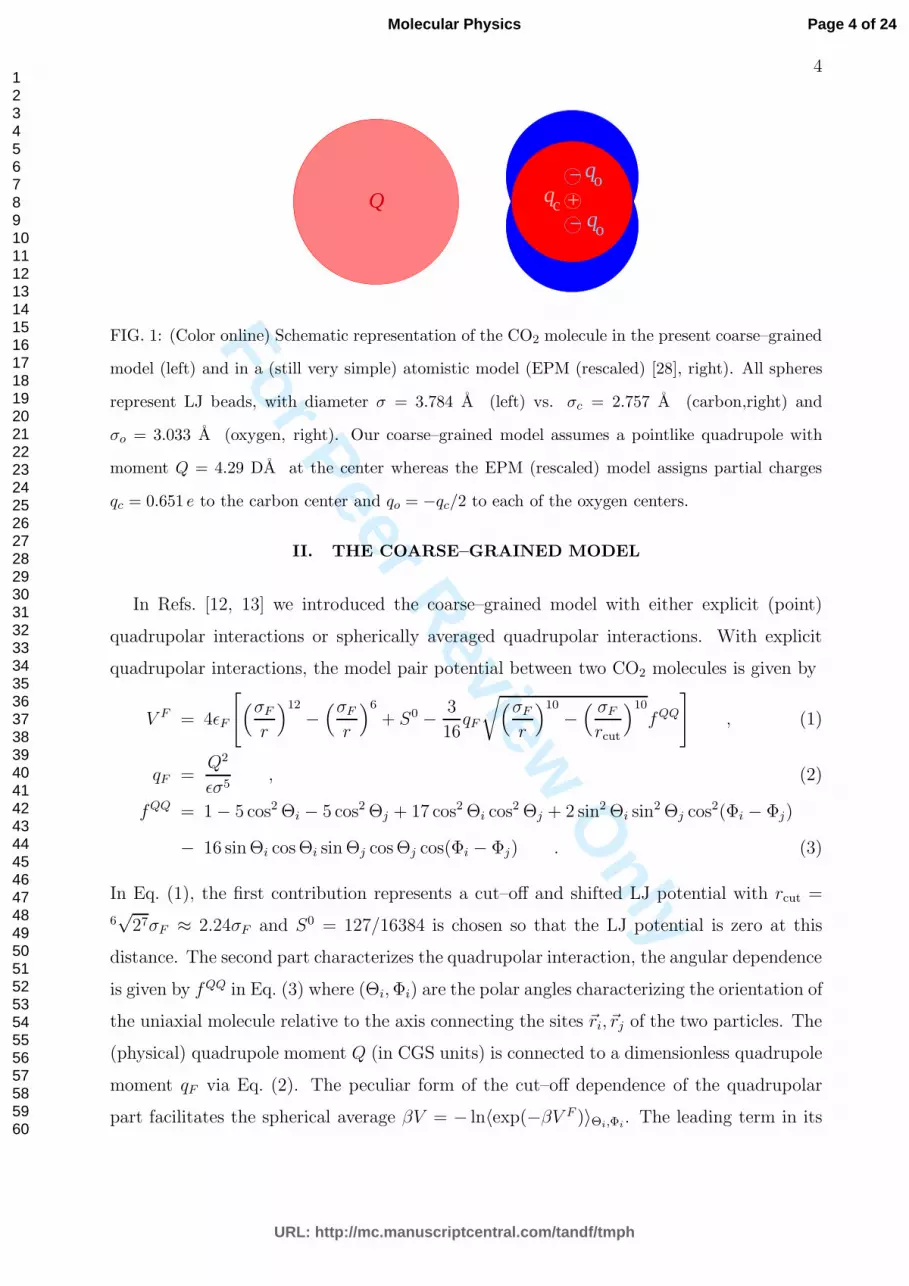
with a simple, single–bead representation of the solvent molecule. Considering the crude

nature of this approximation (see Fig. 1), this is indeed surprising and may be viewed

as the manifestation of a generalized “rule of corresponding states”. However, away from

coexistence, for high densities, deviations between the model and experimental equation of

state for CO2 could be observed [13] and can be related to an oversimplified treatment of the

packing of the solvent molecules which is governed by the repulsive core of the intermolecular

potential. In order to understand further the inevitable limitations of our modeling but also

to obtain more insight as to the high quality of the equation of state near coexistence, we

investigate in this work pair correlation functions and structure factors in the supercritical

region. A second motivation is the already mentioned property of supercritical CO2 as being

a good solvent for other substances. This is related to strong density fluctuations, leading

to cluster formation and encapsulation of solute molecules. Partly due to this engineering

interest, there are a number of experimental and atomistic simulation studies available which

offer rich possibilities for comparison.

We briefly outline the content of this work: In Sec. II we introduce the coarse–grained

model and recall its equation of state. In Sec. III we present our main results for the

structure in the supercritical region, using the spherically averaged model. This section is

divided into two parts. In the first part the correlation length (governing the long-range

behavior of the correlation functions) is discussed by comparing experimental data with

a scaling analysis and simulations. In the second part, site–site and neutron–weighted

correlation functions are compared to experiment and atomistic simulations. In Sec. IV

we investigate the orientational correlations using the coarse–grained model with explicit

quadrupolar interactions. Finally, in Sec. V we present our conclusions.

Page 3 of 24


Molecular Physics

123456789101112131415161718192021222324252627282930313233343536373839404142434445464748495051525354555657585960

For Peer Review O

nly

4

qQ−+− qo

qo

c

FIG. 1: (Color online) Schematic representation of the CO2 molecule in the present coarse–grained

model (left) and in a (still very simple) atomistic model (EPM (rescaled) [28], right). All spheres

represent LJ beads, with diameter σ = 3.784 A (left) vs. σc = 2.757 A (carbon,right) and

σo = 3.033 A (oxygen, right). Our coarse–grained model assumes a pointlike quadrupole with

moment Q = 4.29 DA at the center whereas the EPM (rescaled) model assigns partial charges

qc = 0.651 e to the carbon center and qo = −qc/2 to each of the oxygen centers.

II. THE COARSE–GRAINED MODEL

In Refs. [12, 13] we introduced the coarse–grained model with either explicit (point)

quadrupolar interactions or spherically averaged quadrupolar interactions. With explicit

quadrupolar interactions, the model pair potential between two CO2 molecules is given by

V F = 4ǫF

[(σF

r

)12

−(σF

r

)6

+ S0 − 3

16qF

√(σF

r

)10

−( σF

rcut

)10

fQQ

], (1)

qF =Q2

ǫσ5, (2)

fQQ = 1 − 5 cos2 Θi − 5 cos2 Θj + 17 cos2 Θi cos2 Θj + 2 sin2 Θi sin2 Θj cos2(Φi − Φj)

− 16 sin Θi cos Θi sin Θj cos Θj cos(Φi − Φj) . (3)

In Eq. (1), the first contribution represents a cut–off and shifted LJ potential with rcut =

6√

27σF ≈ 2.24σF and S0 = 127/16384 is chosen so that the LJ potential is zero at this

distance. The second part characterizes the quadrupolar interaction, the angular dependence

is given by fQQ in Eq. (3) where (Θi, Φi) are the polar angles characterizing the orientation of

the uniaxial molecule relative to the axis connecting the sites ~ri, ~rj of the two particles. The

(physical) quadrupole moment Q (in CGS units) is connected to a dimensionless quadrupole

moment qF via Eq. (2). The peculiar form of the cut–off dependence of the quadrupolar

part facilitates the spherical average βV = − ln〈exp(−βV F )〉Θi,Φi. The leading term in its

Page 4 of 24


Molecular Physics

123456789101112131415161718192021222324252627282930313233343536373839404142434445464748495051525354555657585960

For Peer Review O

nly

5

0 0.2 0.8 1Density [g/cm3]

240

260

280

300T

empe

ratu

re [K

]

EXP. (NIST)EPM (rescaled)qc=0.387

qc=0

240 260 280 300Temperature [K]

0

20

40

60

80

Pre

ssur

e [b

ar]

qc=0.387

EXP. (NIST)EPM (rescaled)qc=0

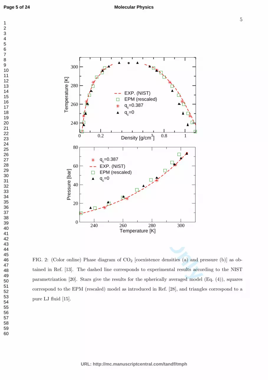
FIG. 2: (Color online) Phase diagram of CO2 [coexistence densities (a) and pressure (b)] as ob-

tained in Ref. [13]. The dashed line corresponds to experimental results according to the NIST

parametrization [20]. Stars give the results for the spherically averaged model (Eq. (4)), squares

correspond to the EPM (rescaled) model as introduced in Ref. [28], and triangles correspond to a

pure LJ fluid [15].

Page 5 of 24


Molecular Physics

123456789101112131415161718192021222324252627282930313233343536373839404142434445464748495051525354555657585960

For Peer Review O

nly

6

high temperature expansion results in an attractive contribution ∝ r−10 (see also [14, 19]).

Using this result, the pair potential of the spherically averaged model is given by:

V A = 4ǫ

[(σ

r

)12

−(σ

r

)6

− 7

20qc

Tc

T

[(σ

r

)10

−( σ

rcut

)10]

+ S0

]

, (4)

qc =Q4

ǫkBTcσ10, (5)

The central idea in our approach is to fix the free parameters of the two models defined above

by the experimental values of the critical point of CO2 (Tc = 304.13 K, ρc = 10.62 mol/ℓ)

[12, 13]. For a given value of the quadrupole moment Q (fixed by experiment), this results

in different values for the energy and length scales ǫF , σF (model with explicit quadrupolar

interactions) and ǫA, σA (spherically averaged model). Explictly, we obtain for Q = 4.292

DA (experimental value Q = 4.3 ± 0.4 DA [20]) the following set of parameters for the

explicit quadrupolar model defined by Eq. (3)

ǫF = 3.598 × 10−21 J σF = 3.760 A qF = 0.689 . (6)

Using the same value for Q, we obtain for the spherically averaged model defined by Eq. (4)

ǫA = 3.494 × 10−21 J σA = 3.784 A qc = 0.385 . (7)

(For the non–trivial numerical procedure to fix these parameters, see Refs. [12, 13].)

In Fig. 2 we recall results for the phase diagram of CO2 [13]. The binodal of the spherically

averaged model is almost indistinguishable from the experimental one. The binodal of a

particular example of an atomistic model (EPM rescaled, see Ref. [28] and Fig. 1) is of

similar quality, however, the coexistence pressure is slightly less well described by the latter.

For comparison, we also show the binodal of a pure LJ model with energy and length scale

again adjusted to the critical point of CO2 (ǫLJ = 4.206×10−21 J, σLJ = 3.695 A [15]) which

clearly deviates from the experimental curve. Since all models whose binodals are shown

here have been adjusted to the experimental critical point, one can draw the conclusion that

for a correct description of phase coexistence the use of a spherically averaged model with a

temperature dependent part (corresponding to the physical quadrupole) in the effective two–

particle potential is sufficient. It does not seem to be necessary to insist on atomistic details,

note furthermore that such a temperature dependent interaction would also be obtained if

one averages over the pair potential of the atomistic model. Note that due to the presence of

Page 6 of 24


Molecular Physics

123456789101112131415161718192021222324252627282930313233343536373839404142434445464748495051525354555657585960

For Peer Review O

nly

7

explicit (partial) charges in the atomistic model, the use of the latter would be inconvenient

for a study of the critical behavior (see Sec. III) or when one considers the phase behavior

of mixture of CO2 with alkanes (see Ref. [16]).

III. CO2 IN THE SUPERCRITICAL REGION

In this section we investigate the correlation length and site–site pair correlation functions

of carbon dioxide in the supercritical region. We will compare to experimental data for the

correlation length [21, 22] obtained for supercritical temperatures in the range T/Tc − 1 =

2.3 · 10−3 . . . 3.7 · 10−2 (Subsec. IIIA). Experimental and atomistic simulation data for the

site–site correlation functions have been obtained in Refs. [23, 24] for two temperatures

T = 307 K (T/Tc = 1.01) and T = 310 K (T/Tc = 1.02) and several densities. The

corresponding comparison with our model will be discussed in Subsec. III B.

A. Correlation length

The correlation length ξ reflects the range of the asymptotic decay of the pair correlation

function g(r). For a fluid with short–ranged interactions, its practical determination is

almost exclusively facilitated through the analysis of the small–q behaviour of the structure

factor (Ornstein–Zernike plots):

S(q)q→0=

S(0)

1 + ξ2q2S(q) = 1 + ρ

∫dr exp(irq)

[g(r) − 1

]. (8)

This assumed form of S(q) corresponds to a long–ranged decay of the pair correlation func-

tion g(r) → 1+exp(−r/ξ)/r [25]. Although the critical behaviour of the Ising model (defin-

ing the universality class under which also fluids with short–ranged interactions are assumed

to fall) is slightly different (g(r) → 1 + exp(−r/ξ)/r1+η with η ≈ 0.036), the deviations of

the corresponding S(q) from the form in Eq. (8) are small for practical purposes.

First we consider the results presented in Ref. [21], where experimental results for the

structure factor, obtained using small-angle neutron scattering (SANS), have been given

for five supercritical states very near the critical point (T/Tc − 1 = 0.0023 . . . 0.0033). In

Ref. [21] a reverse Monte Carlo method was used to fit SANS intensities, from which the

correlation length ξ was obtained using Eq. (8).

Page 7 of 24


Molecular Physics

123456789101112131415161718192021222324252627282930313233343536373839404142434445464748495051525354555657585960

For Peer Review O

nly

8

5 10 15 20 25r [A]

0.9

1

1.1

1.2

g(r)

A1A2A3A4A5

0 0.1 0.2 0.3 0.4 0.5q

2

0

0.1

0.2

0.3

0.4

0.5

0.6

1/S

(q)

A1A2A3A4A5

FIG. 3: (Color online) Pair correlation functions g(r) and inverse structure factors S(q2)−1 at low

q2 (in σ−2A unit) for the five state points A1. . . A5 investigated in Ref. [21], see also Table I.

At the five thermodynamic points reported in Ref. [21], we have performed massive NVT

Monte Carlo Simulations [4] of the spherically averaged model (Eq. (4)). We use cubic

boxes of size (121·A)3 with the number of particles being between 6,780 and 15,673. Monte

Carlo moves consist in simple local rearrangement of particle positions, and near criticality

“critical slowing down” limits the accuracy that can be reached. In a run equivalent of

4,800 h per AMD Opteron DualCore 2.6 GHz processor, and estimating the autocorrelation

length using the binning methods, we are confident, however, that a reasonable number of

uncorrelated configurations have been generated. Results for the pair correlation functions

g(r) and inverse structure factors S(q2)−1 at low q2 for the five points investigated in Ref. [21]

are shown in Fig. 3. As can be seen, our data for S(q2)−1 can be fit very well with a straight

line, permitting the extraction of the correlation length ξ. The results for ξ in comparison

Page 8 of 24


Molecular Physics

123456789101112131415161718192021222324252627282930313233343536373839404142434445464748495051525354555657585960

For Peer Review O

nly

9

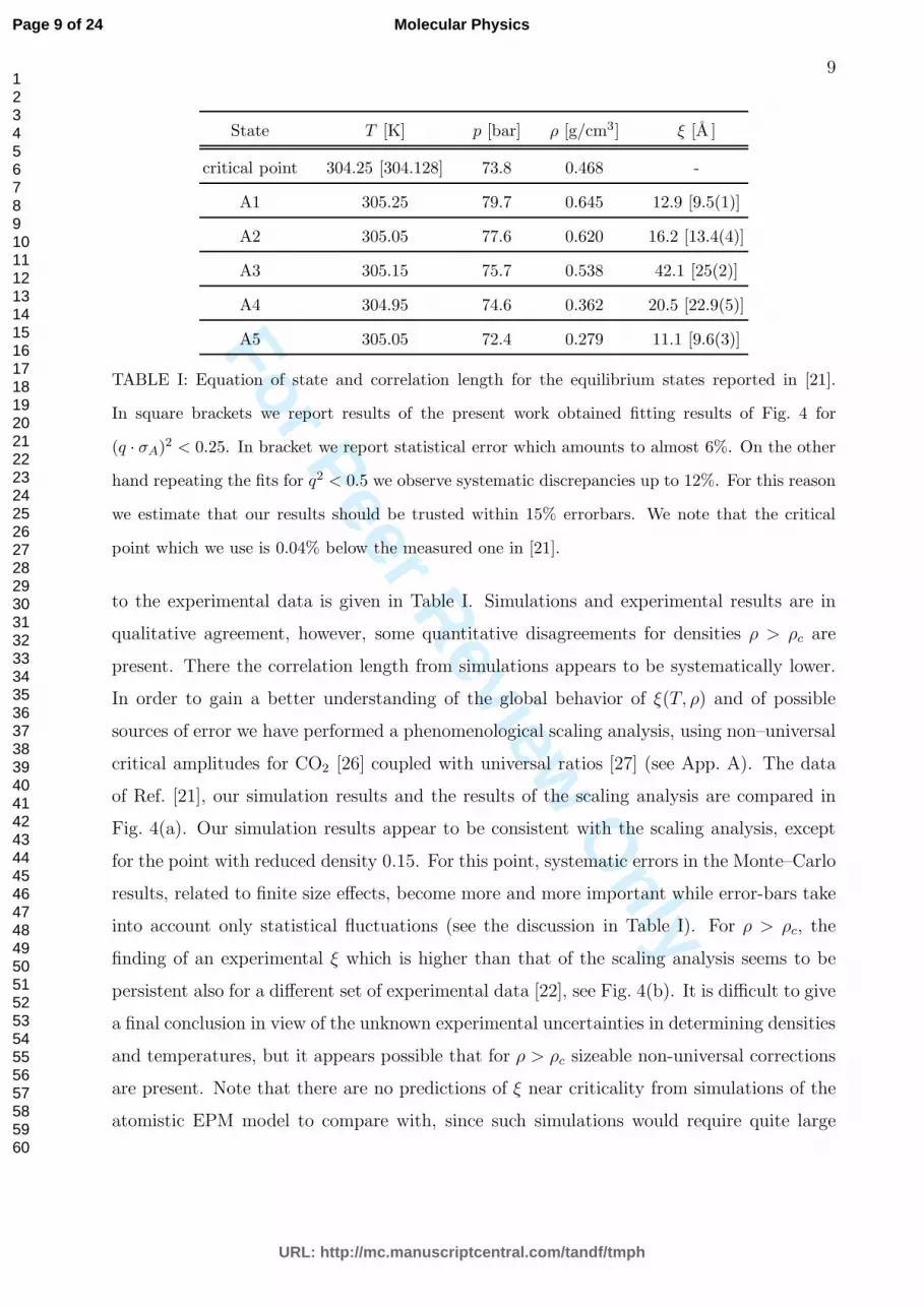
State T [K] p [bar] ρ [g/cm3] ξ [A ]

critical point 304.25 [304.128] 73.8 0.468 -

A1 305.25 79.7 0.645 12.9 [9.5(1)]

A2 305.05 77.6 0.620 16.2 [13.4(4)]

A3 305.15 75.7 0.538 42.1 [25(2)]

A4 304.95 74.6 0.362 20.5 [22.9(5)]

A5 305.05 72.4 0.279 11.1 [9.6(3)]

TABLE I: Equation of state and correlation length for the equilibrium states reported in [21].

In square brackets we report results of the present work obtained fitting results of Fig. 4 for

(q · σA)2 < 0.25. In bracket we report statistical error which amounts to almost 6%. On the other

hand repeating the fits for q2 < 0.5 we observe systematic discrepancies up to 12%. For this reason

we estimate that our results should be trusted within 15% errorbars. We note that the critical

point which we use is 0.04% below the measured one in [21].

to the experimental data is given in Table I. Simulations and experimental results are in

qualitative agreement, however, some quantitative disagreements for densities ρ > ρc are

present. There the correlation length from simulations appears to be systematically lower.

In order to gain a better understanding of the global behavior of ξ(T, ρ) and of possible

sources of error we have performed a phenomenological scaling analysis, using non–universal

critical amplitudes for CO2 [26] coupled with universal ratios [27] (see App. A). The data

of Ref. [21], our simulation results and the results of the scaling analysis are compared in

Fig. 4(a). Our simulation results appear to be consistent with the scaling analysis, except

for the point with reduced density 0.15. For this point, systematic errors in the Monte–Carlo

results, related to finite size effects, become more and more important while error-bars take

into account only statistical fluctuations (see the discussion in Table I). For ρ > ρc, the

finding of an experimental ξ which is higher than that of the scaling analysis seems to be

persistent also for a different set of experimental data [22], see Fig. 4(b). It is difficult to give

a final conclusion in view of the unknown experimental uncertainties in determining densities

and temperatures, but it appears possible that for ρ > ρc sizeable non-universal corrections

are present. Note that there are no predictions of ξ near criticality from simulations of the

atomistic EPM model to compare with, since such simulations would require quite large

Page 9 of 24


Molecular Physics

123456789101112131415161718192021222324252627282930313233343536373839404142434445464748495051525354555657585960

For Peer Review O

nly

10

-0.4 -0.2 0 0.2 0.4(ρ-ρc)/ρc

0

10

20

30

40

50

60

70

ξ [A

]

MCExp

t=(2.3-3.3)10-3

t=(2.7-3.7)10-3

-0.4 -0.2 0 0.2 0.4(ρ-ρc)/ρc

0

5

10

15

20

25

30

ξ [A

]

t=0.023 t=0.037 t=0.0095

FIG. 4: (Color online) (a) Experimental results for ξ [21] compared with our simulations and

the scaling analysis of App. A Simulations and experiments have been done at the same physical

temperature T . However, Ref. [21] uses a critical temperature which is slightly different from

the value which we use. Therefore, broken (Tc = 304.128 from our simulation) and full lines

(Tc = 304.25 K from experiment) [21]) give results according to the scaling analysis with t =

(T − Tc)/Tc calculated accordingly. The MC errorbars reported are statistical ones, while we

expect (as discussed in Table I) systematic error which validate our results within a 15% level

of confidence. (b) Experimental results for ξ according to Ref. [22] compared with the scaling

analysis.

Page 10 of 24


Molecular Physics

123456789101112131415161718192021222324252627282930313233343536373839404142434445464748495051525354555657585960

For Peer Review O

nly

11

B1 B2 B3 C1 C2 C3 C4 D1 D2 D3

T [K] 307 307 307 310 310 310 310 313 373 373

ρ [g/cm3] 0.2 0.468 0.6 0.15912 0.36036 0.5616 0.702 1.023 0.943 0.833

TABLE II: State points investigated in Ref. [24] (for T=307 K, named B1-B3), in Ref. [23] (for

T=310 K, named C1-C4) and in Ref. [30] (D1-D3).

computational efforts.

B. Site–site correlation functions

In a second comparison, we will focus on the short–ranged correlations as seen in the

peak structure of site–site correlation functions [where the sites can be either carbon (C) or

oxygen (O)]. We consider the results reported in [23, 24] for two isotherms (see Table II).

In [24] neutron weighted radial distribution functions and corresponding molecular dynamic

simulations (using the EPM (rescaled) model [28]) of three state points (B1. . . B3 in Table

II) have been reported. In ref. [23] neutron weight radial distribution functions are also

given (for the four states C1. . . C4 in Table II) along with simulations results obtained using

the model of Murthy et al. [29]. In both cases, the atomistic models gave a good account of

the experimentally determined neutron weighted g(r).

For the states investigated in [23, 24], we have done NVT simulations using the averaged

model (4). In Fig. 5 (full lines) we report pair correlation function g(r) of the spherically

averaged model (4) compared with (dot lines) C–C pair correlation functions numerically

obtained in [24] (state points B1. . . B3 , T=307 K) and [23] (state points C1. . . C4 , T=310

K). Compared to the atomistic models, we find that the position of the first and the (weak)

second peak are reproduced whereas the first peak is too narrow and high in our averaged

model. Here, the assumption of a single LJ bead of the averaged model is too rigid and

does not account properly for the side–to–side configuration of two CO2 molecules. The

inadequacy of the repulsive part of the single–bead LJ potential can also be seen if one

does a spherical average of the atomistic potential of the EPM (rescaled) model (for its

definition, see Fig. 1). Whereas the potential minimum coincides with the one in our model,

the repulsive part of the EPM (rescaled) averaged potential is much softer.

In [23], atomistic simulation results for the carbon-oxygen [gCO(r)] and oxygen-oxygen

Page 11 of 24


Molecular Physics

123456789101112131415161718192021222324252627282930313233343536373839404142434445464748495051525354555657585960

For Peer Review O

nly

12

0 5 10 15 20r [A]

0

1

2

3

4

5g cc

(r)

and

g(r)

B1, B2, B3

C1, C2, C3, C4

FIG. 5: (Color online) Full lines: pair correlation functions of the model investigated in this paper,

for the two isotherm of Table II. Dotted lines: results for the carbon-carbon correlation functions

for the two isotherms of the Table II obtained in [23, 24] (see the text for more detail). Curves

with higher first peak correspond to states with lower density.

[gOO(r)] correlation functions have also been reported (dotted lines in Fig. 6). Of course the

latter cannot be measured in our simple model which neglects all atomistic details. However,

a simple reconstruction procedure for these correlation functions is suggested as follows.

Compared to gCC (Fig. 5), we can observe that gCO(r) and gOO(r) exhibit the same position

for the peaks which are however less prominent and more dispersed. This spatial dispersion

is due to the spatial fluctuations of the oxygen atoms near the carbon center of mass. We

assume a rigid, linear model for the CO2 molecule, with the distance between carbon and

oxygen atoms given by the experimental value dCO = 1.19A. Correspondingly, the distance

between the two oxygen atoms is given by dOO = 2dCO. Furthermore, we identify gCC(r) with

our g(r) and obtain gCO(r) and gOO(r) by averaging over the orientations of the molecules,

Page 12 of 24


Molecular Physics

123456789101112131415161718192021222324252627282930313233343536373839404142434445464748495051525354555657585960

For Peer Review O

nly

13

0 5 10 15 20r [A]

0

1

2

3

4g C

O(r

)

B1, B2, B3

C1, C2, C3, C4

0 5 10 15 20r [A]

0

0.5

1

1.5

2

2.5

3

3.5

g OO(r

)

B1, B2, B3

C1, C2, C3, C4

FIG. 6: (Color online) a) Full lines: carbon-oxygen pair correlation functions of the model investi-

gated in this paper, for the two isotherms of Table II. Dotted lines: results for the carbon-oxygen

correlation functions for the T = 310 K isotherm obtained in [23]. Curves with higher first peak cor-

respond to states with lower density. b) The same as in Fig. 6b) for the oxygen-oxygen correlation

functions.

weighted properly by g(r):

gCO(r) =

∫dw1dw2dr

′

4πr2g(r′)δ(dC1O2

− r) gOO(r) =

∫dw1dw2dr

′

4πr2g(r′)δ(dO1O2

− r) .

(9)

In Eq. (9), w1 and w2 are the unit vectors pointing from C to O on each molecule, dC1O2

is the distance between the carbon atom of the first molecule and one oxygen atom of the

second molecule which can be obtained as a function of wi, r′ (the distance between the

carbon atoms) and dCO using simple trigonometric relations. dO1O2is the distance between

two oxygen atoms on different molecules and is computed similar to dC1O2. w1 and w2 are

sampled uniformly (and independently) on the unit spheres.

In Fig. 6 we report our approximation for gCO and gCC (full lines), compared with the

results of ref. [23] (dotted lines). The qualitative shape of the results of the atomistic

simulations [23] is reproduced (such as the height of the peaks), but rather big discrepancies

in gOO remain. At short distances, in the case of gOO(r), the results from the atomistic

simulations go to zero faster than our predictions, oppositely to what happens in gCC (5).

For this reason we argue that the rather good agreement in gCO(r) is merely a fortunate

cancellation of errors. For gOO(r) (Fig. 6b), the atomistic models predict a double peak

structure that our approach ignores. This effect is due to orientational correlations which

Page 13 of 24


Molecular Physics

123456789101112131415161718192021222324252627282930313233343536373839404142434445464748495051525354555657585960

For Peer Review O

nly

14

0 5 10 15 20r [A]

0

1

2

3

4

5g nw

(r)

B1, B2, B3

C1, C2, C3, C4

FIG. 7: (Color online) Dotted line: experimental neutron weighted pair correlation functions of refs.

[23, 24], for the seven thermodynamic states reported in Table II. Full lines: simulation estimate

of the neutron weighted pair correlation function using formula (10) (see ref. [30]). Curves with

higher first peak (i.e. from the top to bottom) correspond to states with lower density.

are neglected in our approach. The orientational correlations imply that CO2 molecules

at small distances (in the first solvation shell) prefer to stay in a T-shape configuration

(i.e. with the two molecules axes orthogonal w1 · w2=0), which minimizes the quadrupolar

quadrupolar interaction (1). If we put two molecules in a T-shape configuration with the

distance between carbon atoms equal to 5A (as suggested by the position of the first peak

in Fig. 5) and we measure the two intermolecular distances between oxygen atoms we obtain

3A, and 6A corresponding approximately to the position of the two peaks in Fig. 6.

Finally we can compare our results with correlation functions obtained using neutron

weighted experiments. For such a comparison, the neutron weighted pair correlation function

must be compared with the following combination of atomistic pair correlation function [30]

gnw = 0.133gCC + 0.464gCO + 0.403gOO . (10)

Page 14 of 24


Molecular Physics

123456789101112131415161718192021222324252627282930313233343536373839404142434445464748495051525354555657585960

For Peer Review O

nly

15

Using our results (Figs. 5, 6) (keeping in mind the limitation of our approach that we have

just pointed out), the results for gnw together with the experimental results reported in Refs.

[23, 24] is shown in Fig. 10. We observe that the simulation results (full lines) systematically

overestimate the experimental peak, due to the overestimated peak in gCC(r) ≡ g(r). We

observe also that the core region is reached more steeply in the experimental results than

in our simulation data. This is related to the deficiencies of our gOO(r) for 1.5A≤ r ≤4A,

which has been discussed before. Our results imply that an excellent fit of the equation of

state, as achieved by our model potential [12, 13], does not guarantee a similarly accurate

prediction of the local structure of the fluid.

IV. ORIENTATIONAL STRUCTURE

In the previous section we have pointed out the importance of considering orientational

correlations in describing the structure of carbon dioxide at small distances (r ≤ 7A).

These were for instance responsible for the double peak structure in the oxygen-oxygen pair

correlation function (Fig. 6) which was not properly reproduced by the averaged model

V A (Eq. (4)). In this section we present results for the model with explicit quadrupolar

interactions [Eq. (1)] with parameters given in Eq. (6). This model with explicit angular

dependency was already considered in Ref. [13] where, among other things, we compared

the phase diagram of CO2 as obtained using VF or VA. Both phase diagrams turned out

to be very similar, with the spherically averaged model showing even better agreement with

experiment than the explicit model.

Lennard-Jones potentials plus point-like quadrupolar interactions have been a long-time

subject of investigation (see eg. [31]), both by simulation and using equation of states. In

such investigations the full (angular-dependent) pair correlation function g(r,w1,w2) (where

r is the intermolecular vector, w1 and w2 are the orientations of the linear molecules) is

projected onto spherical harmonics in a proper reference systems (usually the laboratory

frame or the molecular frame in which the orientation of a molecule is fixed). Following

Ref. [31], in the laboratory reference frame (i.e. with the orientations of the two molecules

Page 15 of 24


Molecular Physics

123456789101112131415161718192021222324252627282930313233343536373839404142434445464748495051525354555657585960

For Peer Review O

nly

16

0 5 10 15 20r [A]

0

1

2

3

4

5

g(r)

VA

VF

D1

D2

D3

4 6 8 10r [A]

-25

-20

-15

-10

-5

0

5

g(l 1, l

2, l3; r

)

g(2,2,4;r)g(2,2,2;r)g(2,2,0;r)g(2,0,2;r)

FIG. 8: (Color online) (a) Pair correlation functions using the averaged V A (full lines) and the

full V F (broken lines) model for the state points D1, D2 and D3 (see Table II). In the statistical

errors the two models predict the same results. (b) Harmonic decomposition of the pair correlation

function for the full model V F in the laboratory reference frame [see Eq. (11)]. Angular correlations

are well visible in the first and second solvation shell [see Fig. 8(a)], while for r > 8A g(l1, l2, l; r)

is almost zero.

free) g(l1, l2, l; r) are defined in the following manner

g(r,w1,w2) =∑

l1l2l

g(l1, l2, l; r)∑

m1m2m

C(l1, l2, l; m1, m2, m) (11)

Yl1,m1(w1)Yl2,m2

(w2)Y∗

l,m(w) , (12)

where C(l1, l2, l; m1, m2, m) are Clebsch–Gordan coefficients, r = rw, and Yl,m(w) spheri-

cal harmonics. For isotropic potentials (like V A), g(l1, l2, l; r) are strictly zero apart from

g(0, 0, 0; r) which corresponds to the standard pair correlation function (up to a normaliza-

Page 16 of 24


Molecular Physics

123456789101112131415161718192021222324252627282930313233343536373839404142434445464748495051525354555657585960

For Peer Review O

nly

17

tion factor related to the chosen reference frame).

Monte Carlo results for the model with explicit quadrupolar interactions have been ob-

tained for the three state points D1. . . D3 (see Table II) which have been investigated in

Ref. [30] experimentally and by atomistic simulations using an EPM–like model. In Fig.

8(b) we report several g(l1, l2, l; r) for the state point D1 for which T ≈ Tc and ρ ≈ 2.2ρc.

We can see that orientational correlations are well visible at this rather high density, espe-

cially in the first solvation shell (while they are much weaker in the second shell). On the

other hand it is interesting to observe how concerning the pair correlation function [Fig.

8(a)] the full model (1) and the averaged model (4) predict almost the same results for

all the three state points D1. . . D3. Incidentally, the same result holds for state points at

coexistence. Indeed we have verified that the pair correlation functions in the coexistence

liquid branch are almost equal for the explicit (V F ) and averaged (V A) model (in this case

minimal differences are visible only in the height of the first peak).

Angular anisotropies in the pair correlation function can be conveniently monitored using

the partially averaged pair correlation function

g(r, θ) =

∫dw2g(r,w1,w2)

where cos θ = w ·w1. It describes the probability to find a second molecule at distance r and

angle θ with the z–axis provided the first molecule is fixed at the origin with orientation along

the z–axis. For the state point D1 our result for g(r, θ) is shown in Fig. 9 and clearly shows

the presence of angular anisotropies (preferential arrangement of the second molecule near

the “poles” and the “equator” of the sphere defined by w1). Thus we reproduce qualitatively

the same phenomena observed in atomistic models (see also Refs. [32, 33]). Quantitative

differences remain however: the atomistic simulation in Ref. [30] (see Fig. 6(a) in the third

work) predict a more pronounced peak around the equator (cos θ = 0), similar to other

investigations [32, 33]. At this point we should also mention that at high pressure and high

density (as considered in states D in Table II), the deficiency of our coarse–grained models

related to the inadequate repulsive part of the potential reaches up to 5% in the equation of

state. Further systematic improvements of our coarse–grained model aiming at quantitative

reproduction of anisotropic structure data should therefore include a more systematic partial

angular averaging of more realistic, atomistic potentials.

Page 17 of 24


Molecular Physics

123456789101112131415161718192021222324252627282930313233343536373839404142434445464748495051525354555657585960

For Peer Review O

nly

18

0

0.5

1

1.5

2

2.5

3

-1-0.5

00.5

1cos(theta)

05

1015

20

r [A]

0

0.5

1

1.5

2

2.5

3

g(r,theta)

FIG. 9: (Color online) Pair correlation function g(r, θ) as a function of the intermolecular distance

r and the angle θ between the molecular axis and the intermolecular direction (cos θ = w · w1).

The plot refers to state D1 of Table II.

V. CONCLUSION

In this paper we have investigated the correlation length and correlation functions

(site–site and angular–resolved) of carbon dioxide (CO2) in the supercritical region for

an efficient coarse–grained model defined by single Lennard–Jones beads with additional

point quadrupolar interactions (taken into account explicit or spherically averaged). This

model gives good results for pure component phase diagrams (e.g. CO2 and C6H6) [12]

and in the phase diagrams of mixture with alkanes [16]. Its performance for structural

properties gives a more differentiated picture. At small distances (r < 8A) the pair

correlations of CO2 are mainly given by packing effects. These are not correctly taken

Page 18 of 24


Molecular Physics

123456789101112131415161718192021222324252627282930313233343536373839404142434445464748495051525354555657585960

For Peer Review O

nly

19

into account by our coarse–grained model which neglects atomistic details and maps the

CO2 molecule insufficiently onto a spherically symmetric, single bead. Indeed looking at

the first solvation shell of the center of mass pair correlation function (see Fig. 5), our

model predicts a too narrow and too high peak in comparison with the predictions of

atomistic models [23, 24], while the position of the peak is properly reproduced. On the

other hand in the long distances regime (and near the critical point) physics is driven by

long range fluctuations which happen at the scale of the correlation length ξ. Using an

Ornstein-Zernike fit, we have computed the correlation length for several states near the

critical point. Results are in qualitative agreement with experiment and scaling predictions

(see App. A). Possible explanations of quantitative discrepancies have been discussed. Note

that correlation lengths near criticality are notoriously difficult to estimate by simulations,

and no such simulation estimates from more realistic atomistic models of CO2 are available.

We have also investigated explicit angular correlations in the coarse-grained model. For

the phase diagram, there is substantial agreement between the spherically symmetric

model and the model with explicit quadrupolar interactions [13]. This agreement is

also reflected in the pair correlation functions: g(r) from the spherically averaged model

and the isotropic component of g(r,w1,w2) from the model with explicit quadrupolar

interactions are the same within statistical errors for the state points investigated here..

We have found that the explicit model is able to qualitatively reproduce anisotropies in the

first solvation shell which are usually discussed in the literature employing atomistic models.

ACKNOWLEDGEMENTS

B.M.M. thanks the BASF AG (Ludwigshafen) for financial support, while M.O. was

supported by the Deutsche Forschungsgemeinschaft via the Collaborative Research Centre

(Sonderforschungsbereich) SFB-TR6 ”Colloids in External Fields” (project section N01).

CPU times was provided by the NIC Julich and the ZDV Mainz. Useful and stimulating

discussion with F.Heilmann, L.G.MacDowell, M.Muller, W.Paul, H.Weiss and J.Zausch are

gratefully acknowledged.

Page 19 of 24


Molecular Physics

123456789101112131415161718192021222324252627282930313233343536373839404142434445464748495051525354555657585960

For Peer Review O

nly

20

APPENDIX A: SCALING PREDICTION FOR THE CORRELATION LENGTH

IN THE SUPERCRITICAL REGION

In this appendix we report the procedure that has been used to obtain the scaling pre-

dictions for the correlation length ξ near the critical point. Renormalization group theories

[34] predict that the scaling laws of thermodynamic quantities (specific heats, correlation

length, etc.) do not depend on atomistic details of the system but are the same within

certain universality classes (the Ising one for the gas-liquid transition) [35]. We define the

reduced density ρ and temperature t [35]

ρ =ρ − ρd(t)

ρct =

T − Tc

Tc, (A1)

where ρd is the coexistence diameter ρd(t) = (ρcl +ρc

g)/2 (ρcl and ρc

g liquid and gas coexistence

densities) extrapolated also into the supercritical region. Standard scaling relations are

written as (for ρ = 0)

ξ = f+ t−ν (t → 0+) (A2)

ξ = f− (−t)−ν (t → 0−) (A3)

ρl/g = ±B(−t)β (A4)

and (for t = 0)

ξ = ξc|µ|−νc (A5)

|µ| = Dc|ρ|δ (A6)

ξ = ξcD−

νβδ

c |ρ|− νβ , (A7)

where (A7) has been obtained using Eqs. (A5) and (A6) and known relations on critical

exponents [27], while µ is the reduced chemical potential. In Eqs. (A2)-(A7) the exponents

are universal quantities, proper of the Ising universality class, while the amplitudes are

system dependent. On the other hand renormalization group also predicts that certain

adimensional ratios of amplitudes are also universal. This is a big simplification because it

reduces the set of experimental input required for the scaling analysis. Ref. [27] reports the

following best estimates for critical exponents

δ = 4.789(2) η = 0.0364(5) β = 0.3265(3) ν = 0.6301(4) , (A8)

Page 20 of 24


Molecular Physics

123456789101112131415161718192021222324252627282930313233343536373839404142434445464748495051525354555657585960

For Peer Review O

nly

21

-0.4 -0.2 0 0.2 0.4(ρ - ρc)/ρc

-0.02

0

0.02

0.04

0.06

(T-T

c)/T

c

ξ=10 Aξ=15 Aξ=20 Aξ=25 Aξ=30 Aξ=35 Aξ=40 Aξ=45 Aξ=50 A

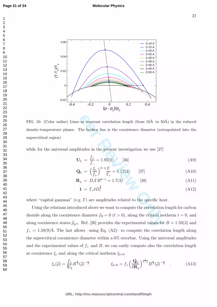
FIG. 10: (Color online) Lines at constant correlation length (from 10A to 50A) in the reduced

density-temperature planes. The broken line is the coexistence diameter (extrapolated into the

supercritical region)

while for the universal amplitudes in the present investigation we use [27]

Uξ =f+

f−= 1.95(2) [36] (A9)

Q2 =( ξc

f+

)2−η Γ

Γc= 1.17(2) [37] (A10)

Rχ = DcΓBδ−1 = 1.7(3) [38] (A11)

1 = ΓcδD1

δc (A12)

where “capital gammas” (e.g. Γ) are amplitudes related to the specific heat.

Using the relations introduced above we want to compute the correlation length for carbon

dioxide along the coexistence diameter ρd = 0 (t > 0), along the critical isotherm t = 0, and

along coexistence states ρg/l. Ref. [26] provides the experimental values for B = 1.59(3) and

f+ = 1.50(9)A. The last allows –using Eq. (A2)– to compute the correlation length along

the supercritical coexistence diameter within a 6% errorbar. Using the universal amplitudes

and the experimental values of f+ and B, we can easily compute also the correlation length

at coexistence ξc and along the critical isotherm ξt=0

ξc(ρ) =f+

UξB

νβ (ρ)−

νβ ξt=0 = f+

( Q2

δRχ

) 1

2−η

Bνβ (ρ)−

νβ . (A13)

Page 21 of 24


Molecular Physics

123456789101112131415161718192021222324252627282930313233343536373839404142434445464748495051525354555657585960

For Peer Review O

nly

22

Notice that at fixed ρ the ratio between the correlation length along the critical isotherm

and along the coexistence states is universal and given by Uξ

(Q2

δRχ

) 1

2−η ≈ 0.73.

Using Eq. (A13) and (A2) in Fig. 10 we sketch lines at constant correlation length.

Starting from previous obtained results along the coexistence diameter, the critical isotherm

and the coexistence densities we interpolate these points using simple quadratic functions

(hyperbola). This is an approximation, indeed the correct way to proceed would require the

knowledge of an universal crossover function fξ(x) which interpolates the correlation length

in the full (ρ, t) plane [27].

[1] Kiran, E., and Brennecke, J. F., eds., 1993, Supercritical Fluid Engineering Science. ACS Sym-

posium Series 514 (Washington D.C: American Chem. Soc.). Kiran, E., and Levelt-Sengers,

J. M. H., eds., 1994, Supercritical Fluids (Dordrecht: Kluwer).

[2] Kemmere, M. F., and Meyer, Th., eds., 2005, Supercritical Carbon Dioxide in Polymer Reac-

tion Engineering (Weinheim: Wiley-VCH).

[3] Levesque, D., Weis, J. J., and Hansen, J. P., 1979, in Monte Carlo Methods in Statistical

Physics, edited by K. Binder, 7, 47.

[4] Frenkel, D., Smit, B., 2002, Understanding Molecular Simulation: From Algorithms to Appli-

cations (San Diego: Academic Press)

[5] Landau, D. P., and Binder, K., 2005, A Guide to Monte Carlo Simulations in Statistical

Physics (Cambridge: University Press).

[6] Scott, R. L., and van Konynenburg, P. H., 1970, Discuss. Faraday Soc., 49, 87; van Konynen-

burg, P. H., and Scott, R. L., 1980, Philos. Trans. R. Soc. London Ser. A, 298, 495; Rowlinson,

J. S., and Swinton, F. L., 1982, Liquids and Liquid Mixtures, (London: Butterworths).

[7] Bolz, A., Deiters, U. K., Peters, C. J., and de Loos, T. W., 1998, Pur. Appl. Chem., 70, 2233.

[8] Levesque, D. and Weis, J. J., 1991, in The Monte Carlo Method in Condensed Matter Physics,

edited by K. Binder, 71, 121.

[9] Krause, B., Sijbesme, H. J. P., Munuklu, P., van der Vegt, N. F. A., and Wessling, M., 2001

Macromolecules, 34, 8792.

[10] Yip, S., ed., 2005, Handbook of Material Modeling (Berlin: Springer).

[11] Kotelyanskii, M. J., Theodorou, D. Y., eds., 2004, Simulation Method for Polymers (New

Page 22 of 24


Molecular Physics

123456789101112131415161718192021222324252627282930313233343536373839404142434445464748495051525354555657585960

For Peer Review O

nly

23

York: Marcel Dekker).

[12] Mognetti, B. M., Yelash, L., Virnau, P., Paul, W., Binder, K., Muller, M., and MacDowell,

L. G., 2008, J. chem. Phys., 128, 104501.

[13] Mognetti, B. M., Oettel, M., Yelash, L., Virnau, P., Paul, W., and Binder, K., 2008, Phys.

Rev. E, 77, 041506.

[14] Gelb, L. D., Muller, E. A., 2002, Fluid Phase Equilib., 203, 1; Albo, S., Muller, E. A., 2003,

J. Phys. Chem. B, 107, 1672; Muller, E. A., Gelb, L. D., 2003, Ind. Eng. Chem. Res., 42,

4123.

[15] Virnau, P., Muller, M., MacDowell, L. G., and Binder, K., 2004, J. chem. Phys., 121, 2169.

[16] Mognetti, B. M., Yelash, L., Virnau, P., Paul, W., Binder, K., Muller, M., and MacDowell, L.

G., 2008, J. chem. Phys., to appear; Binder, K., Mognetti, B. M., Macdowell, L. G., Oettel,

M., Paul, W., Virnau, P., and Yelash, L., Macromol. Symposia, submitted.

[17] Levesque, D., Weis, J. J., and Hansen, J. P., 1984, in Application of the Monte Carlo Method

in Statistical Physics, edited by K. Binder, 36, 37.

[18] Mognetti, B. M., Virnau, P., Yelash, L., Paul, W., Binder, K., Muller, M., and MacDowell,

L. G., 2009, Phys. Chem. Chem. Phys., DOI:10.1039/b818020m

[19] Stell, G., Rasiaiah, J. C., and Narang, H., 1974, Mol. Phys., 27, 1392.

[20] NIST website: http://webbook.nist.gov/chemistry/

[21] Sato, T., Sugiyama, M., Misawa, M., Takata, S., Otomo, T., Itoh, K., Mori, K., and Fukunaga,

T., 2008, J. Phys.: Condens. Matter, 20, 104203.

[22] Nishikawa, K., Tanaka, I., Amemiya, Y., 1996, J. Phys. Chem., 100, 418.

[23] Ishii, R., Okazaki, S., Okada, I., Furusaka, M., Watanabe, N., Misawa, M., and Fukunaga, T.,

1996, J. chem. Phys., 105, 7011.

[24] Adams, J. E., and Siavosh-Haghighi, A., 2002, J. Phys. Chem. B, 106, 7973.

[25] Hansen, J. P., and McDonald, I. R., 1986, Theory of Simple Liquids (New York: Academic).

[26] Sengers, J. V., Moldover, M. R., 1978, Phys. Lett. A, 66, 44.

[27] Pelissetto, A., Vicari, E., 2002, Phys. Rep., 368, 549.

[28] Harris, J. G., and Yung, K. H., 1995, J. Phys. Chem., 99, 12021.

[29] Murthy, C. S., Singer, K., and McDonald, I. R., 1981, Mol. Phys., 44, 135.

[30] Chiappini, s., Nardone, M., Ricci, F. P., and Bellissent-Funel, M. C., 1996, Mol. Phys., 89,

975; Cipriani, P., Nardone, M., and Ricci, F. P., 1998, Physica B 241-243, 940; Cipriani, P.,

Page 23 of 24


Molecular Physics

123456789101112131415161718192021222324252627282930313233343536373839404142434445464748495051525354555657585960

For Peer Review O

nly

24

Nardone, M., Ricci, F. P., and Ricci, M. A., 2001, Mol. Phys., 99, 301.

[31] Murad, S., Gubbins, K. E., and Gray, C. G., 1979, Chem. Phys. Lett., 65, 187; Lee, L. L.,

Assad, E., Kwong, H. A., Chung, T. H., and Haile, J. M., 1982, Physica, 110A, 235; Murad,

S., Gubbins, K. E., and Gray, C. G., 1983, Chem. Phys., 81, 87.

[32] Temleitner, L., and Pusztai, L., 2007, J. Phys.: Cond. Mat., 19, 335203.

[33] Shukla, C. L., Hallett, J. P., Popov, A. V., Hernandez, R., Liotta, C. L., and Eckert, C. A.,

2006, J. Phys. Chem. B, 110, 24101

[34] Fisher, M. E., 1974, Rev. Mod. Phys., 46, 597.

[35] Privman, V., Hohenberg, P. C., Aharony,A. in Phase Transitions and Critical Phenomena,

vol. 14, Domb, C., Lebowitz, J. L., eds., 1991 (Academic Press).

[36] Caselle, M., Hasenbusch, M., 1997, J. Phys. A, 30, 4963.

[37] Fisher, M. E., Zinn, S.-Y., 1998, J. Phys. A, 31, L629.

[38] Zalczer, G., Bourgou, A., Beysens, D., 1983, Phys. Rev. A, 28, 440.

Page 24 of 24


Molecular Physics

123456789101112131415161718192021222324252627282930313233343536373839404142434445464748495051525354555657585960

structure and pair correlations of a simple coarse grained model for supercritical carbon dioxide

Documents