modelling the rheological properties of bituminous binders using mathematical equations

Construction and Building Materials 40 (2013) 174–188

Contents lists available at SciVerse ScienceDirect

Construction and Building Materials

journal homepage: www.elsevier .com/locate /conbui ldmat

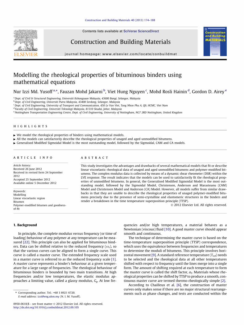
Modelling the rheological properties of bituminous binders usingmathematical equations

Nur Izzi Md. Yusoff a,⇑, Fauzan Mohd Jakarni b, Viet Hung Nguyen c, Mohd Rosli Hainin d, Gordon D. Airey e

a Dept. of Civil & Structural Engineering, Universiti Kebangsaan Malaysia, 43600 Bangi, Selangor, Malaysiab Dept. of Civil Engineering, Universiti Putra Malaysia, 43400 Serdang, Selangor, Malaysiac Dept. of Civil Engineering, University of Transport and Communication, 450 Le Van Viet, Tang Nhon Phu A, Q9, HCMC, Viet Namd Faculty of Civil Engineering, Universiti Teknologi Malaysia, 81310 Skudai, Johor, Malaysiae Nottingham Transportation Engineering Centre, Dept. of Civil Engineering, University of Nottingham, NG7 2RD Nottingham, United Kingdom

h i g h l i g h t s

" We model the rheological properties of binders using mathematical models." All the models can satisfactorily describe the rheological properties of unaged and aged unmodified bitumens." Generalised Modified Sigmoidal Model is the most outstanding model, followed by the Sigmoidal, CAM and CA models.

a r t i c l e i n f o

Article history:Received 26 June 2012Received in revised form 24 September2012Accepted 25 September 2012Available online 5 December 2012

Keywords:ModellingLinear viscoelastic regionBitumenPolymer-modified bitumen and goodness-of-fit

0950-0618/$ - see front matter � 2012 Elsevier Ltd. Ahttp://dx.doi.org/10.1016/j.conbuildmat.2012.09.105

⇑ Corresponding author. Tel.: +60 3 8921 6720.E-mail address: [email protected] (N. I. M. Yusoff)

a b s t r a c t

This study investigates the advantages and drawbacks of several mathematical models that fit or describelinear viscoelastic rheological data of unaged and aged unmodified bitumens and polymer-modified bit-umens. The complex modulus data is collected by means of a dynamic shear rheometer (DSR) within theLVE response. The result indicates that the models can be used to satisfactorily fit the rheological prop-erties of unmodified bitumens. In general, the Generalised Modified Sigmoidal Model is the most out-standing model, followed by the Sigmoidal Model, Christensen, Anderson and Marasteanu (CAM)Model and Christensen Model and Anderson (CA) Model. However, all models suffer from similar draw-backs in that they are unable to describe the rheological properties of unaged polymer-modified bitu-mens precisely due to the presence of semi-crystalline and elastomeric structures in the binders andrender a breakdown in the time temperature superposition principle (TTSP).

� 2012 Elsevier Ltd. All rights reserved.

1. Background

In principle, the complete modulus versus frequency (or time ofloading) behaviour of any polymer at any temperature can be mea-sured [22]. This principle can also be applied for bituminous bind-ers. Data can be shifted relative to the reduced frequency (xr), sothat the various curves can be aligned to form a single curve. Thiscurve is called a master curve. The extended frequency scale usedin a master curve is referred to as the reduced frequency scale [1].A master curve represents a binder’s behaviour at a given temper-ature for a large range of frequencies. The rheological behaviour ofbituminous binders is bounded by two main transitions. At highfrequencies and/or low temperatures, the elastic modulus ap-proaches a limiting value, called a glassy modulus, Gg. At low fre-

ll rights reserved.

.

quencies and/or high temperatures, a material behaves as aNewtonian (viscous) fluid [10]. A good master curve should appearsmooth and continuous.

The technique of determining the master curve is based on thetime-temperature superposition principle (TTSP) correspondence,which uses the equivalence between frequencies and temperaturesto determine the moduli of bitumens. This principle involves hori-zontal movement [9]. A standard reference temperature (Tref) needsto be selected and the rheological data at all other temperaturesshifted with respect to frequency until the lines merge into a singleform. The amount of shifting required at each temperature to formthe master curve is called the shift factor, aT. Materials whose rhe-ological properties can be shifted by TTSP to produce a smooth, con-tinuous master curve are termed thermo-rheologically simple [2].

According to Chailleux et al. [6], the construction of mastercurves only makes sense if there are no major structural rearrange-ments such as phase changes, and tests are conducted within the

http://dx.doi.org/10.1016/j.conbuildmat.2012.09.105

mailto:[email protected]

http://dx.doi.org/10.1016/j.conbuildmat.2012.09.105

http://www.sciencedirect.com/science/journal/09500618

http://www.elsevier.com/locate/conbuildmat

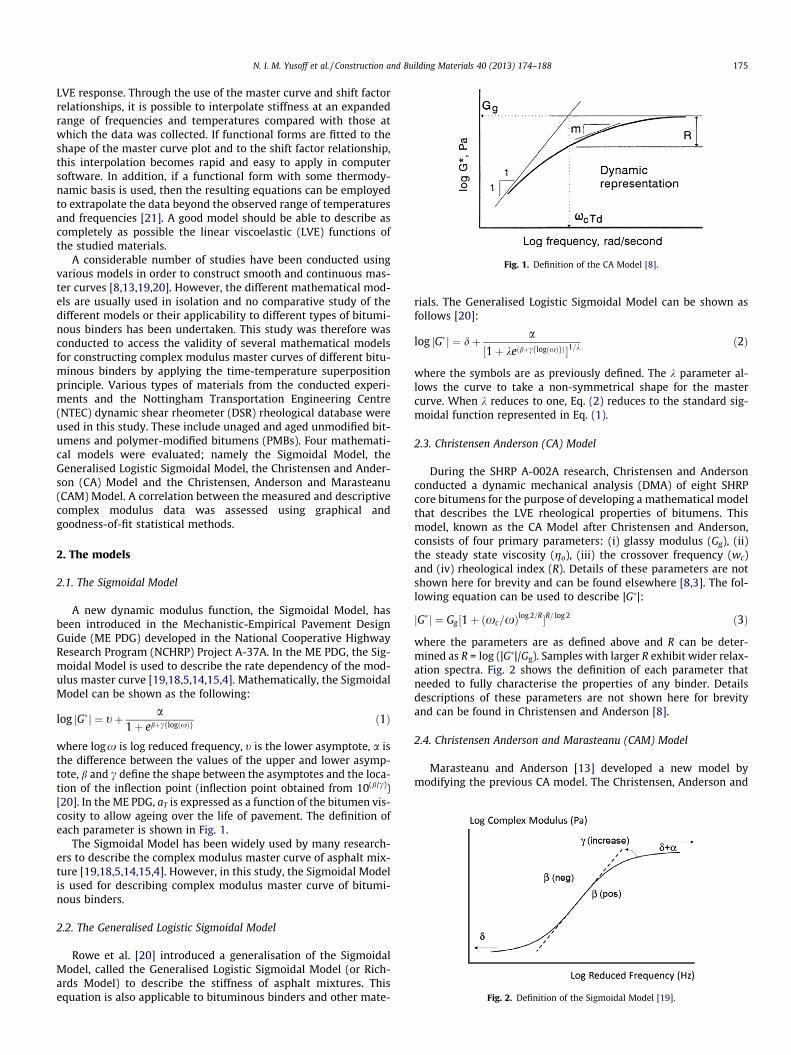
Fig. 1. Definition of the CA Model [8].

Fig. 2. Definition of the Sigmoidal Model [19].

N. I. M. Yusoff et al. / Construction and Building Materials 40 (2013) 174–188 175

LVE response. Through the use of the master curve and shift factorrelationships, it is possible to interpolate stiffness at an expandedrange of frequencies and temperatures compared with those atwhich the data was collected. If functional forms are fitted to theshape of the master curve plot and to the shift factor relationship,this interpolation becomes rapid and easy to apply in computersoftware. In addition, if a functional form with some thermody-namic basis is used, then the resulting equations can be employedto extrapolate the data beyond the observed range of temperaturesand frequencies [21]. A good model should be able to describe ascompletely as possible the linear viscoelastic (LVE) functions ofthe studied materials.

A considerable number of studies have been conducted usingvarious models in order to construct smooth and continuous mas-ter curves [8,13,19,20]. However, the different mathematical mod-els are usually used in isolation and no comparative study of thedifferent models or their applicability to different types of bitumi-nous binders has been undertaken. This study was therefore wasconducted to access the validity of several mathematical modelsfor constructing complex modulus master curves of different bitu-minous binders by applying the time-temperature superpositionprinciple. Various types of materials from the conducted experi-ments and the Nottingham Transportation Engineering Centre(NTEC) dynamic shear rheometer (DSR) rheological database wereused in this study. These include unaged and aged unmodified bit-umens and polymer-modified bitumens (PMBs). Four mathemati-cal models were evaluated; namely the Sigmoidal Model, theGeneralised Logistic Sigmoidal Model, the Christensen and Ander-son (CA) Model and the Christensen, Anderson and Marasteanu(CAM) Model. A correlation between the measured and descriptivecomplex modulus data was assessed using graphical andgoodness-of-fit statistical methods.

2. The models

2.1. The Sigmoidal Model

A new dynamic modulus function, the Sigmoidal Model, hasbeen introduced in the Mechanistic-Empirical Pavement DesignGuide (ME PDG) developed in the National Cooperative HighwayResearch Program (NCHRP) Project A-37A. In the ME PDG, the Sig-moidal Model is used to describe the rate dependency of the mod-ulus master curve [19,18,5,14,15,4]. Mathematically, the SigmoidalModel can be shown as the following:

log jG�j ¼ tþ a1þ ebþcflogðxÞg ð1Þ

where logx is log reduced frequency, t is the lower asymptote, a isthe difference between the values of the upper and lower asymp-tote, b and c define the shape between the asymptotes and the loca-tion of the inflection point (inflection point obtained from 10(b/c))[20]. In the ME PDG, aT is expressed as a function of the bitumen vis-cosity to allow ageing over the life of pavement. The definition ofeach parameter is shown in Fig. 1.

The Sigmoidal Model has been widely used by many research-ers to describe the complex modulus master curve of asphalt mix-ture [19,18,5,14,15,4]. However, in this study, the Sigmoidal Modelis used for describing complex modulus master curve of bitumi-nous binders.

2.2. The Generalised Logistic Sigmoidal Model

Rowe et al. [20] introduced a generalisation of the SigmoidalModel, called the Generalised Logistic Sigmoidal Model (or Rich-ards Model) to describe the stiffness of asphalt mixtures. Thisequation is also applicable to bituminous binders and other mate-

rials. The Generalised Logistic Sigmoidal Model can be shown asfollows [20]:

log jG�j ¼ dþ a½1þ keðbþcflogðxÞgÞ�1=k

ð2Þ

where the symbols are as previously defined. The k parameter al-lows the curve to take a non-symmetrical shape for the mastercurve. When k reduces to one, Eq. (2) reduces to the standard sig-moidal function represented in Eq. (1).

2.3. Christensen Anderson (CA) Model

During the SHRP A-002A research, Christensen and Andersonconducted a dynamic mechanical analysis (DMA) of eight SHRPcore bitumens for the purpose of developing a mathematical modelthat describes the LVE rheological properties of bitumens. Thismodel, known as the CA Model after Christensen and Anderson,consists of four primary parameters: (i) glassy modulus (Gg), (ii)the steady state viscosity (go), (iii) the crossover frequency (wc)and (iv) rheological index (R). Details of these parameters are notshown here for brevity and can be found elsewhere [8,3]. The fol-lowing equation can be used to describe |G�|:

jG�j ¼ Gg ½1þ ðxc=xÞlog 2=R�R= log 2 ð3Þ

where the parameters are as defined above and R can be deter-mined as R = log (|G�|/Gg). Samples with larger R exhibit wider relax-ation spectra. Fig. 2 shows the definition of each parameter thatneeded to fully characterise the properties of any binder. Detailsdescriptions of these parameters are not shown here for brevityand can be found in Christensen and Anderson [8].

2.4. Christensen Anderson and Marasteanu (CAM) Model

Marasteanu and Anderson [13] developed a new model bymodifying the previous CA model. The Christensen, Anderson and

176 N. I. M. Yusoff et al. / Construction and Building Materials 40 (2013) 174–188

Marasteanu (CAM) model attempts to improve the descriptions ofunmodified and polymer-modified bitumens, especially at low andhigh frequencies. By applying the Havriliak and Nagami model tothe initial CA model, the following equations for |G�| is introduced[12,13]:

jG�j ¼ Gg ½1þ ðxc=xÞv �wv ð4Þ

The introduction of the w parameter addresses the issue of howfast or how slow the complex moduli data converge into the twoasymptotes (the 45� asymptote and the Gg asymptote) as the fre-quency goes to zero or infinity [12].

2.5. Detailed procedure

The construction of the |G�| master curve was done with the aidof the Solver function in MS Excel. This function is used to performoptimisation of data with non-linear least squares regression tech-niques. The procedure consisted of minimising the sum of squareerror (SSE) between measured data |G�| (hereafter called mea-sured) and modelled data (hereafter called descriptive), as shownin the following equation:

SSE ¼X ðlog jG�expðf ; TÞj � log jG�desðaTðT; TrefÞ � f ; TrefÞjÞ

ðlog jG�expðf ; TÞjÞ2

2

ð5Þ

where jG�expðf ; TÞj is the measured complex modulus, jG�desðf ; TÞj isthe descriptive complex modulus, T is temperature (�C), Tref is thereference temperature, f is frequency (Hz) and aT (T,Tref) is the shiftfactor. In this study, the Tref was arbitrarily taken as 10 �C. Forexample (in the case of the Generalised Logistic Sigmoidal Model),by combining the model and Eq. (5), the following equation isobtained:

SSE ¼X log jG�expðf ; TÞj � ðdþ Max�d

½1þkebþc logðaT ðT;Tref Þ�f Þ �1=kÞ

� �ðlog jG�expðf ; TÞjÞ

2

2

ð6Þ

The coefficients a, d, b, k, and aT (T,Tref) are fitted in the minimi-sation procedure between the measured and modelled data. Theshift factor functions were used together with the master curvemodel. For example, when the lines are shifted manually, Eq. (6)becomes:

SSE ¼X log jG�expðf ; TÞj � ðdþ Max�d

½1þkebþc log aTþlog f �1=kÞ

� �ðlog jG�expðf ; TÞjÞ

2

2

ð7Þ

The coefficients that need to be determined are now a, d, b, k,and logaT. The Solver function, together with initial seed valuesfor the coefficients, is used to obtain the optimum values of thecoefficients using a number of minimisation runs (Morrison,2005). When no further changes are observed, the iteration processis terminated and the final values quoted for the coefficients.

Table 1Criteria of the goodness-of-fit statistics [25].

Criteria R2 Se/Sy

Excellent P0.90 60.35Good 0.70–0.89 0.36–0.55Fair 0.40–0.69 0.56–0.75Poor 0.20–0.39 0.76–0.89Very poor 60.19 P0.90

3. Statistical analysis

The overall reliability of a model compared to the measurementcan be evaluated by means of a graphical method and goodness-of-fit statistics. Several goodness-of-fit statistic methods, namely thecorrelation of determination, R2, standard error ratio, Se/Sy, discrep-ancy ratio, ri, mean normalised error (MNE) and average geometricdeviation (AGD), were used in this study. However, it is worthmentioning that there are many possible solutions that have beenused to find the goodness-of-fit statistical parameters. All of therheological data will be assessed using both a graphical methodand goodness-of-fit statistics.

3.1. Graphical method

A graphical method is intended to visually and qualitativelyshow an agreement between the model and measured valuesand to display the distribution error [26]. A graph of measured(x-axis) and model (y-axis) is plotted and an observation is madeto see the data distribution from the equality line. It shows thatthe model is in good agreement with the measured data if thepoints are distributed nicely on the equality line. On the otherhand, if the points are scattered from the equality line, the modelis not in good agreement with the measurements.

3.2. Standard error ratio, Se/Sy

The standard error of estimation, Se, and standard error of devi-ation, Sy, can be defined as follows:

Se ¼

ffiffiffiffiffiffiffiffiffiffiffiffiffiffiffiffiffiffiffiffiffiffiffiffiPðY � bY Þ2ðn� kÞ

sð8Þ

and

Sy ¼

ffiffiffiffiffiffiffiffiffiffiffiffiffiffiffiffiffiffiffiffiffiffiffiPðY � YÞ2

ðn� 1Þ

sð9Þ

where n is sample size, k is number of independent variables in themodel, Y is tested complex modulus, bY is descriptive complex mod-ulus and Y is mean value of tested complex modulus. Therefore, theratio Se/Sy is a measure of the improvement in the accuracy of mod-elling due to the descriptive equation. When the ratio is small, e.g.near zero, more variation in the dynamic data about their mean canbe explained by the equation. A small value indicates a betterdescription [25].

3.3. Coefficient of determination, R2

The coefficient of determination, R2, is a measure of the modelaccuracy. R2 is expressed as follows:

R2 ¼ 1� ðn� kÞðn� 1Þ �

Se

Sy

� �2

ð10Þ

where the symbols are as previously defined. For the perfect fit,R2 = 1. Subjective criteria, which were used in the NCHRP project9-19 Task C, were used to evaluate the performance of the modelin this study, as shown in Table 1 [25].

3.4. The discrepancy ratio (ri)

The discrepancy ratio, ri, indicates the accuracy of the goodness-of-fit between the measured and modelled data. For example, ri forthe measured and descriptive dynamic function can be expressedas:

ri ¼YTpi

YTmi

ð11Þ

where YTpiand YTmi

are the descriptive and measured complex mod-uli respectively. The subscript i denotes the data set number. The

Spindle

Bitumen

DSR bodyDSR base plate

Water level

Water chamber cover

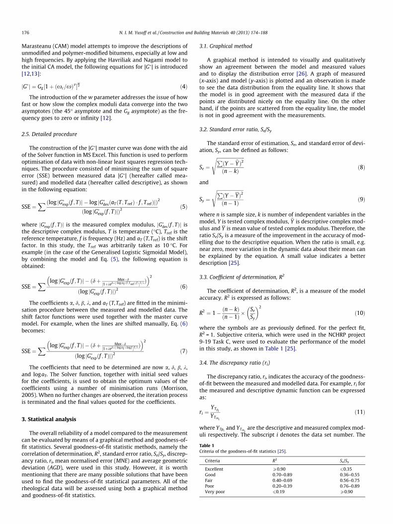
Fig. 3. Schematic of dynamic shear rheometer testing configuration.

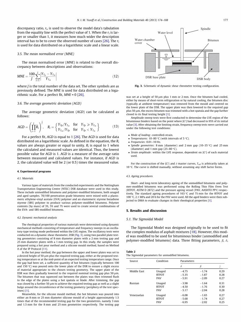
Table 2The Sigmoidal parameters for unmodified bitumens.

Source Condition Parameters

d b c

Middle East Unaged �4.75 �1.74 0.29RTFOT �5.35 �1.87 0.28PAV �5.91 �2.09 0.27

Russian Unaged �3.98 �1.64 0.31RTFOT �4.50 �1.76 0.30PAV �5.17 �2.04 0.28

Venezuelan Unaged �6.08 �1.65 0.27RTFOT �5.68 �1.74 0.27PAV �6.95 �2.02 0.25


discrepancy ratio, ri, is used to observe the model data’s tabulationfrom the equality line with the perfect value of 1. When the ri is lar-ger or smaller than 1, it measures how much wider the descriptioninterval has to be to cover the observed number of cases [26]. The ri

is used for data distributed on a logarithmic scale and a linear scale.

3.5. The mean normalised error (MNE)

The mean normalised error (MNE) is related to the overall dis-crepancy between descriptions and observations:

MNE ¼ 100J

XJ

i¼1

YTp � YTm

YTm

�� ð12Þ

where J is the total number of the data set. The other symbols are aspreviously defined. The MNE is used for data distributed on a loga-rithmic scale. For a perfect fit, MNE = 0 [26].

3.6. The average geometric deviation (AGD)

The average geometric deviation (AGD) can be calculated asfollows:

AGD ¼YJ

i¼1

eRi

!1J

; Ri ¼YTp=YTm for YTp P YTm

YTm=YTp for YTp < YTm

� ð13Þ

For a perfect fit, AGD is equal to 1 [26]. The AGD is used for datadistributed on a logarithmic scale. As defined in the equation, the Ri

values are always greater or equal to unity. Ri is equal to 1 whenthe calculated and measured values are identical. Thus, the lowestpossible value for AGD is 1. AGD is a measure of the average ratiobetween measured and calculated values. For instance, if AGD is2, the calculated value will be 2 (or 0.5) times the measured value.

4. Experimental programs

4.1. Materials

Various types of materials from the conducted experiments and the NottinghamTransportation Engineering Centre (NTEC) DSR database were used in this study.These include unmodified bitumens and polymer-modified bitumens, both unagedand aged samples. 70/100 penetration grade bitumens were mixed with a plasto-meric ethylene-vinyl acetate (EVA) polymer and an elastomeric styrene butadienestyrene (SBS) polymer to produce various polymer-modified bitumens. Polymercontents (by mass) of 3%, 5% and 7% were used to create several combinations ofthe EVA- and SBS-modified bitumens.

4.2. Dynamic mechanical analysis

The rheological properties of various materials were determined using dynamicmechanical methods consisting of temperature and frequency sweeps in an oscilla-tory-type testing mode performed within the LVE region. The oscillatory tests wereconducted on a dynamic shear rheometer, DSR (Fig. 3), using two parallel plate test-ing geometries consisting of 8 mm diameter plates with a 2 mm testing gap and25 mm diameter plates with a 1 mm testing gap. In this study, the samples wereprepared using a hot pour method and a silicone mould method, based on MethodA of the IP Protocol [11].

In the hot pour method, the gap between the upper and lower plates was set toa desired height of 50 lm plus the required testing gap, either at the proposed test-ing temperature or at the mid-point of an expected testing temperature range. Oncethe gap had been set, a sufficient quantity of hot bitumen (typically between 100and 150 �C) was poured onto the lower plate of the DSR to ensure a slight excessof material appropriate to the chosen testing geometry. The upper plate of theDSR was then gradually lowered to the required nominal testing gap plus 50 lm.The bitumen that was squeezed out between the plates was then trimmed flushto the edge of the plates using a hot spatula or blade. After trimming, the gapwas closed by a further 50 lm to achieve the required testing gap as well as a slightbulge around the circumference of the testing geometry (periphery of the test spec-imen) [1].

Meanwhile, for the silicone mould method, the hot bitumen was poured intoeither an 8 mm or 25 mm diameter silicone mould of a height approximately 1.5times that of the recommended testing gap for the two geometries, namely 3 mmand 1.5 mm for the 8 mm and 25 mm geometries respectively. The testing gap

was set at a height of 50 lm plus 1 mm or 2 mm. Once the bitumen had cooled,either by means of short-term refrigeration or by natural cooling, the bitumen disc(typically at ambient temperature) was removed from the mould and centred onthe lower plate of the DSR. The upper plate was then lowered to the required gapplus 50 lm, the excess bitumen was trimmed with a hot spatula and the gap furtherclosed to its final testing height [1].

Amplitude sweep tests were first conducted to determine the LVE region of thebituminous binders based on the point where |G�| had decreased to 95% of its initialvalue [3]. After obtaining the limiting strain, frequency sweep tests were carried outunder the following test conditions:

� Mode of loading: controlled-strain.� Temperatures: 10–80 �C (with intervals of 5 �C).� Frequencies: 0.01–10 Hz.� Spindle geometries: 8 mm (diameter) and 2 mm gap (10–35 �C) and 25 mm

(diameter) and 1 mm gap (25–80 �C).� Strain amplitude: within the LVE response, dependent on |G�| of each material

used.

For the construction of the |G�| and d master curves, Tref is arbitrarily taken at10 �C. The curve is shifted manually, without assuming any shift factor forms.

4.3. Ageing procedures

Short- and long-term laboratory ageing of the unmodified bitumens and poly-mer-modified bitumens was performed using the Rolling Thin Film Oven Test(RTFOT, ASTM D 2872) and the pressure ageing vessel (PAV, AASHTO PP1) respec-tively. The standard ageing procedures of 163 �C and 75 min for the RTFOT and100 �C, 2.1 MPa and 20 h for the PAV were used. All the aged binders were then sub-jected to DMA to evaluate changes in their rheological properties [1].

5. Results and discussion

5.1. The Sigmoidal Model

The Sigmoidal Model was designed originally to be used to fitthe complex modulus of asphalt mixtures [18]. However, this mod-el was modified to be used for bituminous binder (unmodified andpolymer-modified bitumens) data. Three fitting parameters, b, d,

-10 -5 0 5 10-2

0

2

4

6

8

10

Log Reduced Frequency (Hz)

Log

Com

plex

Mod

ulus

(Pa)

Unmodified Bitumens (Venezuelan)

Unaged (exp)Unaged (model)RTFOT (exp)RTFOT (model)PAV (exp)PAV (model)

-10 -5 0 5 10-2

0

2

4

6

8

10


Log

Com

plex

Mod

ulus

(Pa)

Unmodified Bitumens (Middle East)


-10 -5 0 5 10-2

0

2

4

6

8

10


Log

Com

plex

Mod

ulus

(Pa)

Unmodified Bitumen (Russian)


Tref = 10oC

Tref = 10oC

Tref = 10oC

Fig. 4. Comparisons between measured and model of unaged and aged unmodifiedbitumen data using the Sigmoidal Model (Tref = 10 �C).


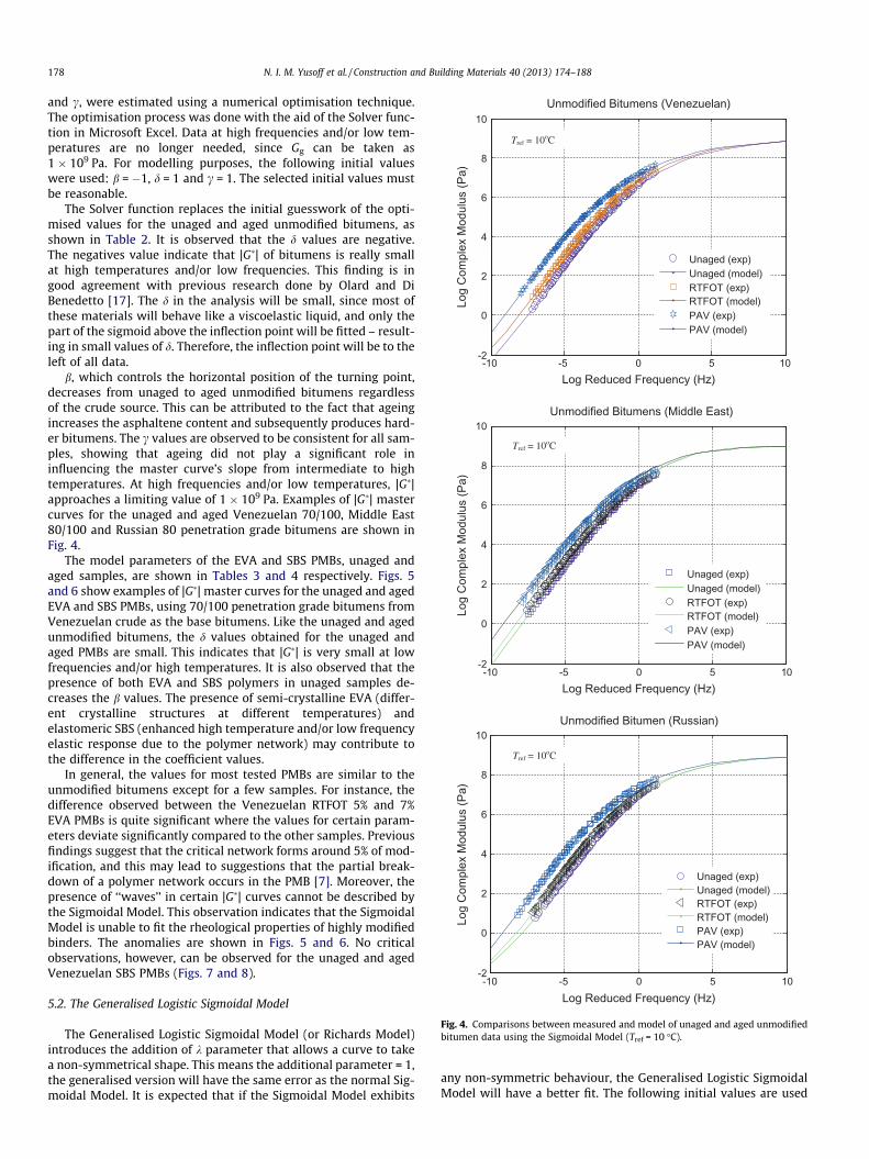
and c, were estimated using a numerical optimisation technique.The optimisation process was done with the aid of the Solver func-tion in Microsoft Excel. Data at high frequencies and/or low tem-peratures are no longer needed, since Gg can be taken as1 � 109 Pa. For modelling purposes, the following initial valueswere used: b = �1, d = 1 and c = 1. The selected initial values mustbe reasonable.

The Solver function replaces the initial guesswork of the opti-mised values for the unaged and aged unmodified bitumens, asshown in Table 2. It is observed that the d values are negative.The negatives value indicate that |G�| of bitumens is really smallat high temperatures and/or low frequencies. This finding is ingood agreement with previous research done by Olard and DiBenedetto [17]. The d in the analysis will be small, since most ofthese materials will behave like a viscoelastic liquid, and only thepart of the sigmoid above the inflection point will be fitted – result-ing in small values of d. Therefore, the inflection point will be to theleft of all data.

b, which controls the horizontal position of the turning point,decreases from unaged to aged unmodified bitumens regardlessof the crude source. This can be attributed to the fact that ageingincreases the asphaltene content and subsequently produces hard-er bitumens. The c values are observed to be consistent for all sam-ples, showing that ageing did not play a significant role ininfluencing the master curve’s slope from intermediate to hightemperatures. At high frequencies and/or low temperatures, |G�|approaches a limiting value of 1 � 109 Pa. Examples of |G�| mastercurves for the unaged and aged Venezuelan 70/100, Middle East80/100 and Russian 80 penetration grade bitumens are shown inFig. 4.

The model parameters of the EVA and SBS PMBs, unaged andaged samples, are shown in Tables 3 and 4 respectively. Figs. 5and 6 show examples of |G�| master curves for the unaged and agedEVA and SBS PMBs, using 70/100 penetration grade bitumens fromVenezuelan crude as the base bitumens. Like the unaged and agedunmodified bitumens, the d values obtained for the unaged andaged PMBs are small. This indicates that |G�| is very small at lowfrequencies and/or high temperatures. It is also observed that thepresence of both EVA and SBS polymers in unaged samples de-creases the b values. The presence of semi-crystalline EVA (differ-ent crystalline structures at different temperatures) andelastomeric SBS (enhanced high temperature and/or low frequencyelastic response due to the polymer network) may contribute tothe difference in the coefficient values.

In general, the values for most tested PMBs are similar to theunmodified bitumens except for a few samples. For instance, thedifference observed between the Venezuelan RTFOT 5% and 7%EVA PMBs is quite significant where the values for certain param-eters deviate significantly compared to the other samples. Previousfindings suggest that the critical network forms around 5% of mod-ification, and this may lead to suggestions that the partial break-down of a polymer network occurs in the PMB [7]. Moreover, thepresence of ‘‘waves’’ in certain |G�| curves cannot be described bythe Sigmoidal Model. This observation indicates that the SigmoidalModel is unable to fit the rheological properties of highly modifiedbinders. The anomalies are shown in Figs. 5 and 6. No criticalobservations, however, can be observed for the unaged and agedVenezuelan SBS PMBs (Figs. 7 and 8).

5.2. The Generalised Logistic Sigmoidal Model

The Generalised Logistic Sigmoidal Model (or Richards Model)introduces the addition of k parameter that allows a curve to takea non-symmetrical shape. This means the additional parameter = 1,the generalised version will have the same error as the normal Sig-moidal Model. It is expected that if the Sigmoidal Model exhibits

any non-symmetric behaviour, the Generalised Logistic SigmoidalModel will have a better fit. The following initial values are used

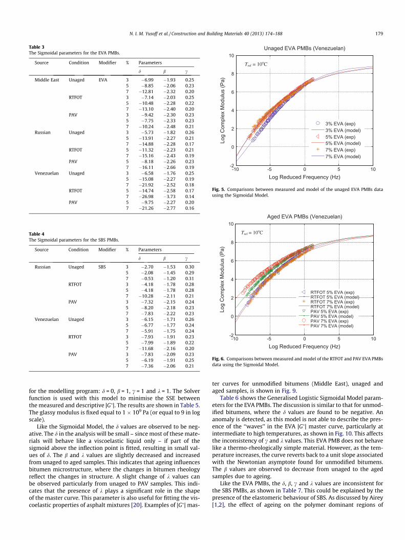
Table 3The Sigmoidal parameters for the EVA PMBs.

Source Condition Modifier % Parameters

d b c

Middle East Unaged EVA 3 �6.99 �1.93 0.255 �8.85 �2.06 0.237 �12.81 �2.32 0.20

RTFOT 3 �7.14 �2.03 0.255 �10.48 �2.28 0.227 �13.10 �2.40 0.20

PAV 3 �9.42 �2.30 0.235 �7.75 �2.33 0.237 �10.24 �2.48 0.21

Russian Unaged 3 �5.73 �1.82 0.265 �13.91 �2.27 0.217 �14.88 �2.28 0.17

RTFOT 5 �11.32 �2.23 0.217 �15.16 �2.43 0.19

PAV 5 �8.18 �2.26 0.237 �16.11 �2.66 0.19

Venezuelan Unaged 3 �6.58 �1.76 0.255 �15.08 �2.27 0.197 �21.92 �2.52 0.18

RTFOT 5 �14.74 �2.58 0.177 �26.98 �3.73 0.14

PAV 5 �9.75 �2.27 0.207 �21.26 �2.77 0.16

-10 -5 0 5 10-2

0

2

4

6

8

10


Log

Com

plex

Mod

ulus

(Pa)

Aged EVA PMBs (Venezuelan)

RTFOT 5% EVA (exp)RTFOT 5% EVA (model)RTFOT 7% EVA (exp)RTFOT 7% EVA (model)PAV 5% EVA (exp)PAV 5% EVA (model)PAV 7% EVA (exp)PAV 7% EVA (model)

(b)Tref = 10oC

Fig. 6. Comparisons between measured and model of the RTFOT and PAV EVA PMBsdata using the Sigmoidal Model.

-10 -5 0 5 10-2

0

2

4

6

8

10


Log

Com

plex

Mod

ulus

(Pa)

Unaged EVA PMBs (Venezuelan)

3% EVA (exp)3% EVA (model)5% EVA (exp)5% EVA (model)7% EVA (exp)7% EVA (model)

(a)Tref = 10oC

Fig. 5. Comparisons between measured and model of the unaged EVA PMBs datausing the Sigmoidal Model.

Table 4The Sigmoidal parameters for the SBS PMBs.


d b c

Russian Unaged SBS 3 �2.70 �1.53 0.305 �2.08 �1.45 0.297 �0.53 �1.20 0.31

RTFOT 3 �4.18 �1.78 0.285 �4.18 �1.78 0.287 �10.28 �2.11 0.21

PAV 3 �7.32 �2.15 0.245 �8.20 �2.18 0.237 �7.83 �2.22 0.23

Venezuelan Unaged 3 �6.15 �1.71 0.265 �6.77 �1.77 0.247 �5.91 �1.75 0.24

RTFOT 3 �7.93 �1.91 0.235 �7.99 �1.89 0.227 �11.68 �2.16 0.20

PAV 3 �7.83 �2.09 0.235 �6.19 �1.91 0.257 �7.36 �2.06 0.21


for the modelling program: d = 0, b = 1, c = 1 and k = 1. The Solverfunction is used with this model to minimise the SSE betweenthe measured and descriptive |G�|. The results are shown in Table 5.The glassy modulus is fixed equal to 1 � 109 Pa (or equal to 9 in logscale).

Like the Sigmoidal Model, the d values are observed to be neg-ative. The d in the analysis will be small – since most of these mate-rials will behave like a viscoelastic liquid only – if part of thesigmoid above the inflection point is fitted, resulting in small val-ues of d. The b and k values are slightly decreased and increasedfrom unaged to aged samples. This indicates that ageing influencesbitumen microstructure, where the changes in bitumen rheologyreflect the changes in structure. A slight change of k values canbe observed particularly from unaged to PAV samples. This indi-cates that the presence of k plays a significant role in the shapeof the master curve. This parameter is also useful for fitting the vis-coelastic properties of asphalt mixtures [20]. Examples of |G�| mas-

ter curves for unmodified bitumens (Middle East), unaged andaged samples, is shown in Fig. 9.

Table 6 shows the Generalised Logistic Sigmoidal Model param-eters for the EVA PMBs. The discussion is similar to that for unmod-ified bitumens, where the d values are found to be negative. Ananomaly is detected, as this model is not able to describe the pres-ence of the ‘‘waves’’ in the EVA |G�| master curve, particularly atintermediate to high temperatures, as shown in Fig. 10. This affectsthe inconsistency of c and k values. This EVA PMB does not behavelike a thermo-rheologically simple material. However, as the tem-perature increases, the curve reverts back to a unit slope associatedwith the Newtonian asymptote found for unmodified bitumens.The b values are observed to decrease from unaged to the agedsamples due to ageing.

Like the EVA PMBs, the d, b, c and k values are inconsistent forthe SBS PMBs, as shown in Table 7. This could be explained by thepresence of the elastomeric behaviour of SBS. As discussed by Airey[1,2], the effect of ageing on the polymer dominant regions of

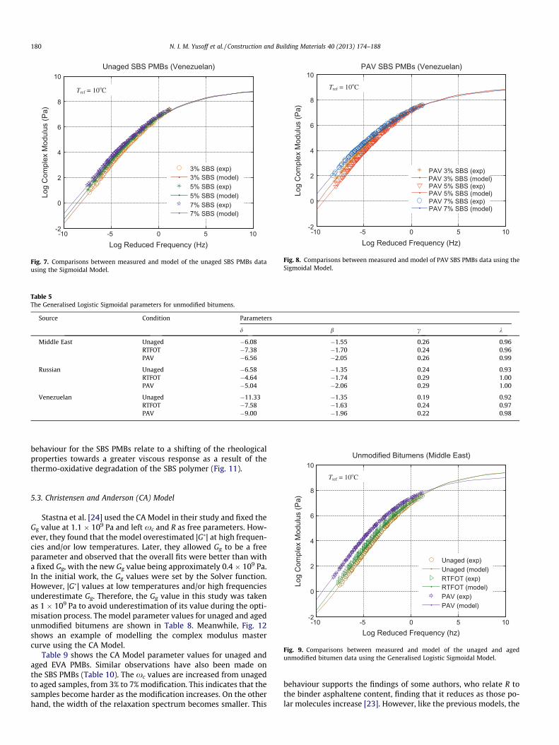
Table 5The Generalised Logistic Sigmoidal parameters for unmodified bitumens.


d b c k

Middle East Unaged �6.08 �1.55 0.26 0.96RTFOT �7.38 �1.70 0.24 0.96PAV �6.56 �2.05 0.26 0.99

Russian Unaged �6.58 �1.35 0.24 0.93RTFOT �4.64 �1.74 0.29 1.00PAV �5.04 �2.06 0.29 1.00

Venezuelan Unaged �11.33 �1.35 0.19 0.92RTFOT �7.58 �1.63 0.24 0.97PAV �9.00 �1.96 0.22 0.98

-10 -5 0 5 10-2

0

2

4

6

8

10

Log

Com

plex

Mod

ulus

(Pa)

Unaged SBS PMBs (Venezuelan)

3% SBS (exp)3% SBS (model)5% SBS (exp)5% SBS (model)7% SBS (exp)7% SBS (model)

(a)Tref = 10oC


Fig. 7. Comparisons between measured and model of the unaged SBS PMBs datausing the Sigmoidal Model.

10Unmodified Bitumens (Middle East)

o

-10 -5 0 5 10-2

0

2

4

6

8

10


Log

Com

plex

Mod

ulus

(Pa)

PAV SBS PMBs (Venezuelan)

PAV 3% SBS (exp)PAV 3% SBS (model)PAV 5% SBS (exp)PAV 5% SBS (model)PAV 7% SBS (exp)PAV 7% SBS (model)

Tref = 10oC

Fig. 8. Comparisons between measured and model of PAV SBS PMBs data using theSigmoidal Model.


behaviour for the SBS PMBs relate to a shifting of the rheologicalproperties towards a greater viscous response as a result of thethermo-oxidative degradation of the SBS polymer (Fig. 11).

-10 -5 0 5 10-2

0

2

4

6

8

Log Reduced Frequency (hz)

Log

Com

plex

Mod

ulus

(Pa)


Tref = 10 C

Fig. 9. Comparisons between measured and model of the unaged and agedunmodified bitumen data using the Generalised Logistic Sigmoidal Model.

5.3. Christensen and Anderson (CA) Model

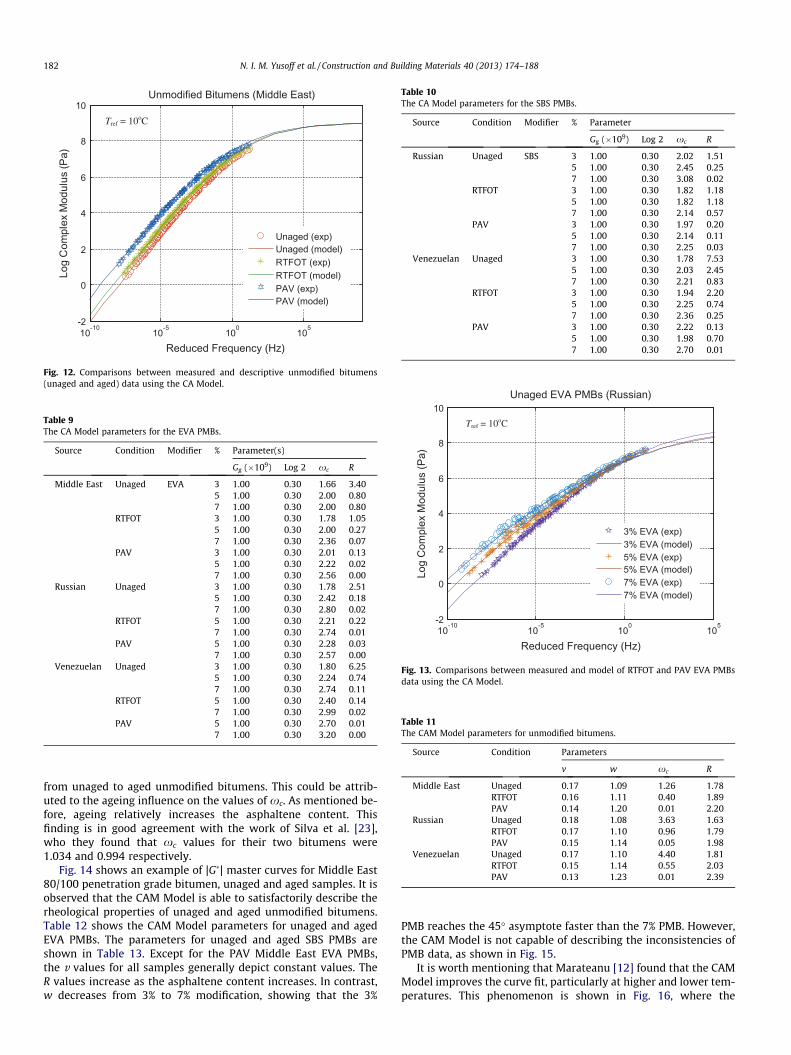
Stastna et al. [24] used the CA Model in their study and fixed theGg value at 1.1 � 109 Pa and left xc and R as free parameters. How-ever, they found that the model overestimated |G�| at high frequen-cies and/or low temperatures. Later, they allowed Gg to be a freeparameter and observed that the overall fits were better than witha fixed Gg, with the new Gg value being approximately 0.4 � 109 Pa.In the initial work, the Gg values were set by the Solver function.However, |G�| values at low temperatures and/or high frequenciesunderestimate Gg. Therefore, the Gg value in this study was takenas 1 � 109 Pa to avoid underestimation of its value during the opti-misation process. The model parameter values for unaged and agedunmodified bitumens are shown in Table 8. Meanwhile, Fig. 12shows an example of modelling the complex modulus mastercurve using the CA Model.

Table 9 shows the CA Model parameter values for unaged andaged EVA PMBs. Similar observations have also been made onthe SBS PMBs (Table 10). The xc values are increased from unagedto aged samples, from 3% to 7% modification. This indicates that thesamples become harder as the modification increases. On the otherhand, the width of the relaxation spectrum becomes smaller. This

behaviour supports the findings of some authors, who relate R tothe binder asphaltene content, finding that it reduces as those po-lar molecules increase [23]. However, like the previous models, the

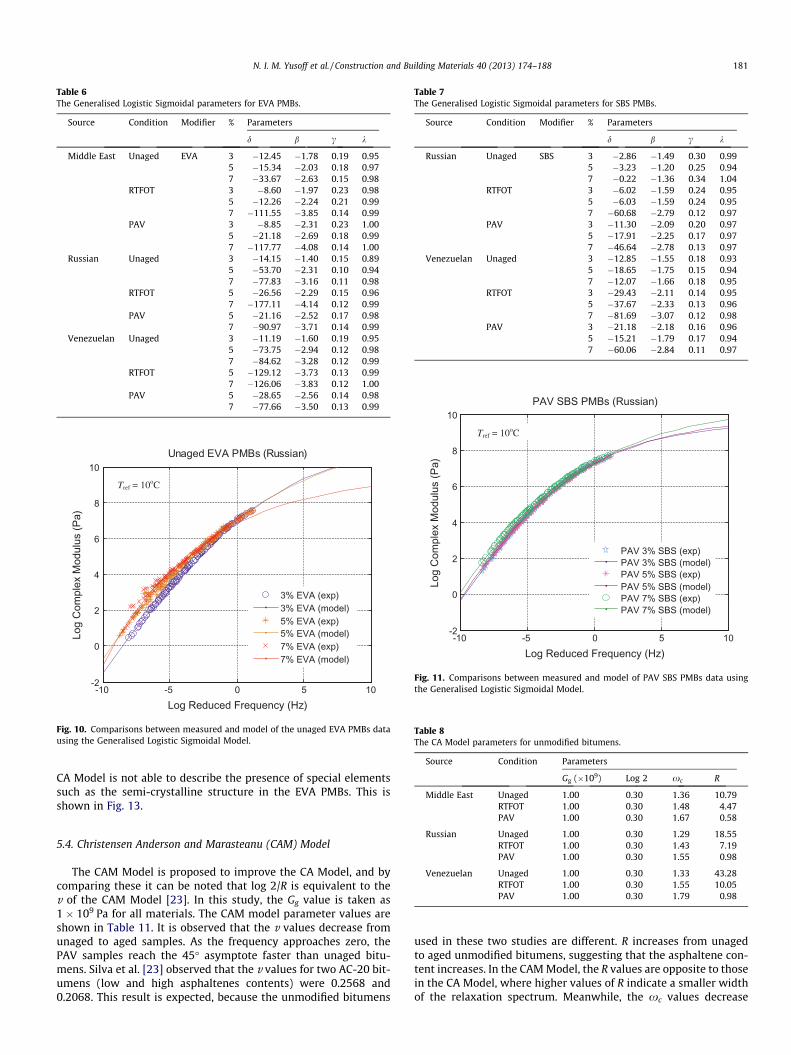
Table 6The Generalised Logistic Sigmoidal parameters for EVA PMBs.


d b c k

Middle East Unaged EVA 3 �12.45 �1.78 0.19 0.955 �15.34 �2.03 0.18 0.977 �33.67 �2.63 0.15 0.98

RTFOT 3 �8.60 �1.97 0.23 0.985 �12.26 �2.24 0.21 0.997 �111.55 �3.85 0.14 0.99

PAV 3 �8.85 �2.31 0.23 1.005 �21.18 �2.69 0.18 0.997 �117.77 �4.08 0.14 1.00

Russian Unaged 3 �14.15 �1.40 0.15 0.895 �53.70 �2.31 0.10 0.947 �77.83 �3.16 0.11 0.98

RTFOT 5 �26.56 �2.29 0.15 0.967 �177.11 �4.14 0.12 0.99

PAV 5 �21.16 �2.52 0.17 0.987 �90.97 �3.71 0.14 0.99

Venezuelan Unaged 3 �11.19 �1.60 0.19 0.955 �73.75 �2.94 0.12 0.987 �84.62 �3.28 0.12 0.99

RTFOT 5 �129.12 �3.73 0.13 0.997 �126.06 �3.83 0.12 1.00

PAV 5 �28.65 �2.56 0.14 0.987 �77.66 �3.50 0.13 0.99

-10 -5 0 5 10-2

0

2

4

6

8

10


Log

Com

plex

Mod

ulus

(Pa)

Unaged EVA PMBs (Russian)


(a)Tref = 10oC

Fig. 10. Comparisons between measured and model of the unaged EVA PMBs datausing the Generalised Logistic Sigmoidal Model.

Table 7The Generalised Logistic Sigmoidal parameters for SBS PMBs.


d b c k

Russian Unaged SBS 3 �2.86 �1.49 0.30 0.995 �3.23 �1.20 0.25 0.947 �0.22 �1.36 0.34 1.04

RTFOT 3 �6.02 �1.59 0.24 0.955 �6.03 �1.59 0.24 0.957 �60.68 �2.79 0.12 0.97

PAV 3 �11.30 �2.09 0.20 0.975 �17.91 �2.25 0.17 0.977 �46.64 �2.78 0.13 0.97

Venezuelan Unaged 3 �12.85 �1.55 0.18 0.935 �18.65 �1.75 0.15 0.947 �12.07 �1.66 0.18 0.95

RTFOT 3 �29.43 �2.11 0.14 0.955 �37.67 �2.33 0.13 0.967 �81.69 �3.07 0.12 0.98

PAV 3 �21.18 �2.18 0.16 0.965 �15.21 �1.79 0.17 0.947 �60.06 �2.84 0.11 0.97

-10 -5 0 5 10-2

0

2

4

6

8

10


Log

Com

plex

Mod

ulus

(Pa)

PAV SBS PMBs (Russian)


Tref = 10oC

Fig. 11. Comparisons between measured and model of PAV SBS PMBs data usingthe Generalised Logistic Sigmoidal Model.

Table 8The CA Model parameters for unmodified bitumens.


Gg (�109) Log 2 xc R

Middle East Unaged 1.00 0.30 1.36 10.79RTFOT 1.00 0.30 1.48 4.47


CA Model is not able to describe the presence of special elementssuch as the semi-crystalline structure in the EVA PMBs. This isshown in Fig. 13.

PAV 1.00 0.30 1.67 0.58

Russian Unaged 1.00 0.30 1.29 18.55RTFOT 1.00 0.30 1.43 7.19PAV 1.00 0.30 1.55 0.98

Venezuelan Unaged 1.00 0.30 1.33 43.28RTFOT 1.00 0.30 1.55 10.05PAV 1.00 0.30 1.79 0.98

5.4. Christensen Anderson and Marasteanu (CAM) Model

The CAM Model is proposed to improve the CA Model, and bycomparing these it can be noted that log 2/R is equivalent to thev of the CAM Model [23]. In this study, the Gg value is taken as1 � 109 Pa for all materials. The CAM model parameter values areshown in Table 11. It is observed that the v values decrease fromunaged to aged samples. As the frequency approaches zero, thePAV samples reach the 45� asymptote faster than unaged bitu-mens. Silva et al. [23] observed that the v values for two AC-20 bit-umens (low and high asphaltenes contents) were 0.2568 and0.2068. This result is expected, because the unmodified bitumens

used in these two studies are different. R increases from unagedto aged unmodified bitumens, suggesting that the asphaltene con-tent increases. In the CAM Model, the R values are opposite to thosein the CA Model, where higher values of R indicate a smaller widthof the relaxation spectrum. Meanwhile, the xc values decrease

10-10

10-5

100

105

-2

0

2

4

6

8

10

Reduced Frequency (Hz)

Log

Com

plex

Mod

ulus

(Pa)



Tref = 10oC

Fig. 12. Comparisons between measured and descriptive unmodified bitumens(unaged and aged) data using the CA Model.

Table 9The CA Model parameters for the EVA PMBs.

Source Condition Modifier % Parameter(s)


Middle East Unaged EVA 3 1.00 0.30 1.66 3.405 1.00 0.30 2.00 0.807 1.00 0.30 2.00 0.80

RTFOT 3 1.00 0.30 1.78 1.055 1.00 0.30 2.00 0.277 1.00 0.30 2.36 0.07

PAV 3 1.00 0.30 2.01 0.135 1.00 0.30 2.22 0.027 1.00 0.30 2.56 0.00

Russian Unaged 3 1.00 0.30 1.78 2.515 1.00 0.30 2.42 0.187 1.00 0.30 2.80 0.02

RTFOT 5 1.00 0.30 2.21 0.227 1.00 0.30 2.74 0.01

PAV 5 1.00 0.30 2.28 0.037 1.00 0.30 2.57 0.00

Venezuelan Unaged 3 1.00 0.30 1.80 6.255 1.00 0.30 2.24 0.747 1.00 0.30 2.74 0.11

RTFOT 5 1.00 0.30 2.40 0.147 1.00 0.30 2.99 0.02

PAV 5 1.00 0.30 2.70 0.017 1.00 0.30 3.20 0.00

Table 10The CA Model parameters for the SBS PMBs.

Source Condition Modifier % Parameter


Russian Unaged SBS 3 1.00 0.30 2.02 1.515 1.00 0.30 2.45 0.257 1.00 0.30 3.08 0.02

RTFOT 3 1.00 0.30 1.82 1.185 1.00 0.30 1.82 1.187 1.00 0.30 2.14 0.57

PAV 3 1.00 0.30 1.97 0.205 1.00 0.30 2.14 0.117 1.00 0.30 2.25 0.03


RTFOT 3 1.00 0.30 1.94 2.205 1.00 0.30 2.25 0.747 1.00 0.30 2.36 0.25

PAV 3 1.00 0.30 2.22 0.135 1.00 0.30 1.98 0.707 1.00 0.30 2.70 0.01

10-10

10-5

100

105

-2

0

2

4

6

8

10


Log

Com

plex

Mod

ulus

(Pa)



Tref = 10oC

Fig. 13. Comparisons between measured and model of RTFOT and PAV EVA PMBsdata using the CA Model.

Table 11The CAM Model parameters for unmodified bitumens.


v w xc R

Middle East Unaged 0.17 1.09 1.26 1.78RTFOT 0.16 1.11 0.40 1.89PAV 0.14 1.20 0.01 2.20

Russian Unaged 0.18 1.08 3.63 1.63RTFOT 0.17 1.10 0.96 1.79PAV 0.15 1.14 0.05 1.98

Venezuelan Unaged 0.17 1.10 4.40 1.81RTFOT 0.15 1.14 0.55 2.03PAV 0.13 1.23 0.01 2.39


from unaged to aged unmodified bitumens. This could be attrib-uted to the ageing influence on the values of xc. As mentioned be-fore, ageing relatively increases the asphaltene content. Thisfinding is in good agreement with the work of Silva et al. [23],who they found that xc values for their two bitumens were1.034 and 0.994 respectively.

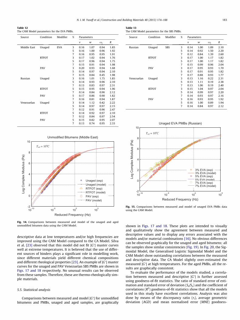
Fig. 14 shows an example of |G�| master curves for Middle East80/100 penetration grade bitumen, unaged and aged samples. It isobserved that the CAM Model is able to satisfactorily describe therheological properties of unaged and aged unmodified bitumens.Table 12 shows the CAM Model parameters for unaged and agedEVA PMBs. The parameters for unaged and aged SBS PMBs areshown in Table 13. Except for the PAV Middle East EVA PMBs,the v values for all samples generally depict constant values. TheR values increase as the asphaltene content increases. In contrast,w decreases from 3% to 7% modification, showing that the 3%

PMB reaches the 45� asymptote faster than the 7% PMB. However,the CAM Model is not capable of describing the inconsistencies ofPMB data, as shown in Fig. 15.

It is worth mentioning that Marateanu [12] found that the CAMModel improves the curve fit, particularly at higher and lower tem-peratures. This phenomenon is shown in Fig. 16, where the

10-10

10-5

100

105

-2

0

2

4

6

8

10


Log

Com

plex

Mod

ulus

(Pa)



Tref = 10oC

Fig. 14. Comparisons between measured and model of the unaged and agedunmodified bitumen data using the CAM Model.

Table 12The CAM Model parameters for the EVA PMBs.


v w xc R

Middle East Unaged EVA 3 0.16 1.07 0.94 1.855 0.16 1.00 0.96 1.927 0.16 0.95 0.95 1.91

RTFOT 3 0.17 1.02 0.94 1.765 0.17 0.96 0.94 1.757 0.15 0.91 0.94 1.98

PAV 3 0.20 0.93 0.94 1.685 0.14 0.97 0.94 2.107 0.15 0.84 0.45 1.98

Russian Unaged 3 0.16 1.01 1.75 1.855 0.14 0.93 0.96 2.107 0.13 0.83 0.97 2.31

RTFOT 5 0.15 0.95 0.94 1.967 0.14 0.84 0.96 2.12

PAV 5 0.17 0.86 0.90 1.827 0.16 0.81 0.94 1.87


RTFOT 5 0.14 0.92 0.97 2.107 0.12 0.84 0.97 2.54

PAV 5 0.15 0.82 0.95 2.077 0.13 0.74 0.95 2.33

Table 13The CAM Model parameters for the SBS PMBs.


v w xc R

Russian Unaged SBS 3 0.14 1.00 1.09 2.105 0.14 0.92 1.50 2.207 0.12 0.84 1.39 2.60

RTFOT 3 0.17 1.00 1.17 1.825 0.17 1.00 1.17 1.827 0.15 0.99 0.96 2.04

PAV 3 0.17 0.95 0.93 1.705 0.17 0.91 0.95 1.827 0.17 0.88 0.93 1.77


RTFOT 3 0.15 1.04 0.97 2.045 0.14 0.99 0.97 2.207 0.14 0.93 0.97 2.16

PAV 3 0.16 0.93 0.95 1.925 0.16 1.00 0.89 1.947 0.14 0.84 0.97 2.12

10-10

10-5

100

105

-2

0

2

4

6

8

10


Log

Com

plex

Mod

ulus

(Pa)



Tref = 10oC

Fig. 15. Comparisons between measured and model of unaged EVA PMBs datausing the CAM Model.


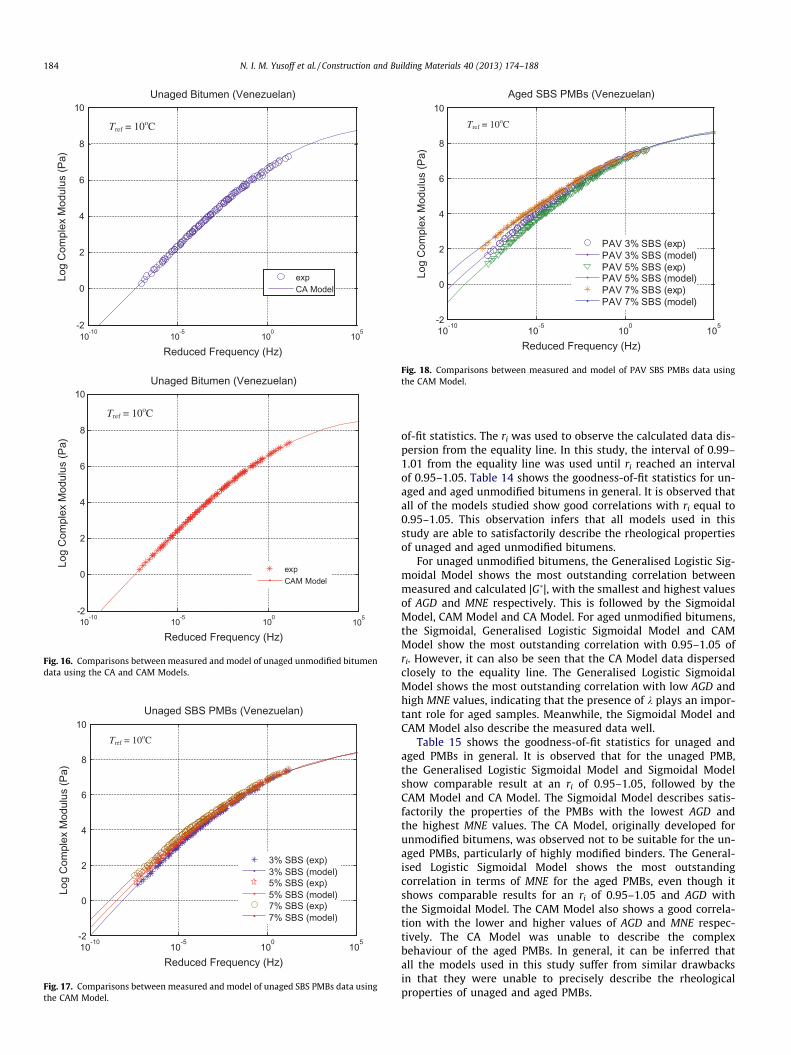
descriptive data at low temperatures and/or high frequencies areimproved using the CAM Model compared to the CA Model. Silvaet al. [23] observed that this model did not fit |G�| master curveswell at extreme temperatures. It is believed that the use of differ-ent sources of binders plays a significant role in modelling work,since different materials yield different chemical compositionsand different rheological properties [23]. An example of |G�| mastercurves for the unaged and PAV Venezuelan SBS PMBs are shown inFigs. 17 and 18 respectively. No unusual results can be observedfrom these samples. Therefore, these are thermo-rheologically sim-ple materials.

5.5. Statistical analysis

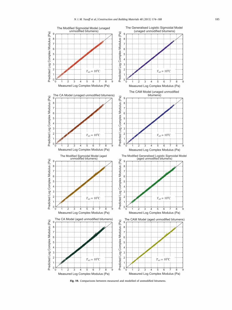
Comparisons between measured and model |G�| for unmodifiedbitumens and PMBs, unaged and aged samples, are graphically

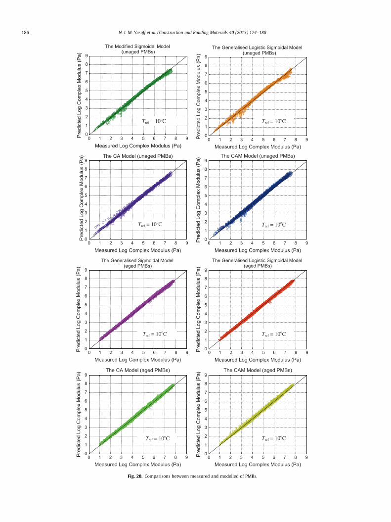
shown in Figs. 17 and 18. These plots are intended to visuallyand qualitatively show the agreement between measured anddescriptive values and to display any errors associated with themodels and/or material combinations [16]. No obvious differencescan be observed graphically for the unaged and aged bitumens; allthe samples show similar consistencies (Fig. 19). In Fig. 20, the Sig-moidal Model, the Generalised Logistic Sigmoidal Model and theCAM Model show outstanding correlations between the measuredand descriptive data. The CA Model slightly over-estimated themeasured |G�| at high temperatures. For the aged PMBs, all the re-sults are graphically consistent.

To evaluate the performance of the models studied, a correla-tion between measured and descriptive |G�| is further assessedusing goodness-of-fit statistics. The ratio of standard error of esti-mation and standard error of deviation (Se/Sy) and the coefficient ofcorrelations (R2) goodness-of-fit statistics show that all the modelsused in this study have excellent correlations. Analysis was alsodone by means of the discrepancy ratio (ri), average geometricdeviation (AGD) and mean normalised error (MNE) goodness-

10-10

10-5

100

105

-2

0

2

4

6

8

10


Log

Com

plex

Mod

ulus

(Pa)

Unaged Bitumen (Venezuelan)

expCA Model

10-10

10-5

100

105

-2

0

2

4

6

8

10


Log

Com

plex

Mod

ulus

(Pa)

Unaged Bitumen (Venezuelan)

expCAM Model

Tref = 10oC

Tref = 10oC

Fig. 16. Comparisons between measured and model of unaged unmodified bitumendata using the CA and CAM Models.

10-10

10-5

100

105

-2

0

2

4

6

8

10


Log

Com

plex

Mod

ulus

(Pa)

Aged SBS PMBs (Venezuelan)


Tref = 10oC

Fig. 18. Comparisons between measured and model of PAV SBS PMBs data usingthe CAM Model.

10-10

10-5

100

105

-2

0

2

4

6

8

10


Log

Com

plex

Mod

ulus

(Pa)

Unaged SBS PMBs (Venezuelan)

3% SBS (exp)3% SBS (model)5% SBS (exp)5% SBS (model)7% SBS (exp)7% SBS (model)

Tref = 10oC

Fig. 17. Comparisons between measured and model of unaged SBS PMBs data usingthe CAM Model.


of-fit statistics. The ri was used to observe the calculated data dis-persion from the equality line. In this study, the interval of 0.99–1.01 from the equality line was used until ri reached an intervalof 0.95–1.05. Table 14 shows the goodness-of-fit statistics for un-aged and aged unmodified bitumens in general. It is observed thatall of the models studied show good correlations with ri equal to0.95–1.05. This observation infers that all models used in thisstudy are able to satisfactorily describe the rheological propertiesof unaged and aged unmodified bitumens.

For unaged unmodified bitumens, the Generalised Logistic Sig-moidal Model shows the most outstanding correlation betweenmeasured and calculated |G�|, with the smallest and highest valuesof AGD and MNE respectively. This is followed by the SigmoidalModel, CAM Model and CA Model. For aged unmodified bitumens,the Sigmoidal, Generalised Logistic Sigmoidal Model and CAMModel show the most outstanding correlation with 0.95–1.05 ofri. However, it can also be seen that the CA Model data dispersedclosely to the equality line. The Generalised Logistic SigmoidalModel shows the most outstanding correlation with low AGD andhigh MNE values, indicating that the presence of k plays an impor-tant role for aged samples. Meanwhile, the Sigmoidal Model andCAM Model also describe the measured data well.

Table 15 shows the goodness-of-fit statistics for unaged andaged PMBs in general. It is observed that for the unaged PMB,the Generalised Logistic Sigmoidal Model and Sigmoidal Modelshow comparable result at an ri of 0.95–1.05, followed by theCAM Model and CA Model. The Sigmoidal Model describes satis-factorily the properties of the PMBs with the lowest AGD andthe highest MNE values. The CA Model, originally developed forunmodified bitumens, was observed not to be suitable for the un-aged PMBs, particularly of highly modified binders. The General-ised Logistic Sigmoidal Model shows the most outstandingcorrelation in terms of MNE for the aged PMBs, even though itshows comparable results for an ri of 0.95–1.05 and AGD withthe Sigmoidal Model. The CAM Model also shows a good correla-tion with the lower and higher values of AGD and MNE respec-tively. The CA Model was unable to describe the complexbehaviour of the aged PMBs. In general, it can be inferred thatall the models used in this study suffer from similar drawbacksin that they were unable to precisely describe the rheologicalproperties of unaged and aged PMBs.

0 1 2 3 4 5 6 7 8 90

1

2

3

4

5

6

7

8

9

Measured Log Complex Modulus (Pa)

Pred

icte

d Lo

g C

ompl

ex M

odul

us (P

a)

0 1 2 3 4 5 6 7 8 90

1

2

3

4

5

6

7

8

9


Pred

icte

d Lo

g C

ompl

ex M

odul

us (P

a)

The CA Model (aged unmodified bitumens)

0 1 2 3 4 5 6 7 8 90

1

2

3

4

5

6

7

8

9


Pred

icte

d Lo

g C

ompl

ex M

odul

us (P

a)

The Generalised Logistic Sigmoidal Model

0 1 2 3 4 5 6 7 8 90

1

2

3

4

5

6

7

8

9


Pred

icte

d Lo

g C

ompl

ex M

odul

us (P

a) The CA Model (unaged unmodified bitumens)

0 1 2 3 4 5 6 7 8 90

1

2

3

4

5

6

7

8

9


Pred

icte

d Lo

g C

ompl

ex M

odul

us (P

a)

The CAM Model (unaged unmodified bitumens)

0 1 2 3 4 5 6 7 8 90

1

2

3

4

5

6

7

8

9


Pred

icte

d Lo

g C

ompl

ex M

odul

us (P

a)

0 1 2 3 4 5 6 7 8 90

1

2

3

4

5

6

7

8

9


Pred

icte

d Lo

g C

ompl

ex M

odul

us (P

a)

0 1 2 3 4 5 6 7 8 90

1

2

3

4

5

6

7

8

9


Pred

icte

d Lo

g C

ompl

ex M

odul

us (P

a) The CAM Model (aged unmodified bitumens)

Tref = 10oC Tref = 10oC




The Modified Generalised Logistic Sigmoidal Model (aged unmodified bitumens)

The Modified Sigmoidal Model (aged unmodified bitumens)

The Modified Sigmoidal Model (unaged unmodified bitumens) (unaged unmodified bitumens)

Fig. 19. Comparisons between measured and modelled of unmodified bitumens.


0 1 2 3 4 5 6 7 8 90

1

2

3

4

5

6

7

8

9


Pre

dict

ed L

og C

ompl

ex M

odul

us (P

a) The CA Model (unaged PMBs)

0 1 2 3 4 5 6 7 8 90

1

2

3

4

5

6

7

8

9


Pred

icte

d Lo

g C

ompl

ex M

odul

us (P

a)

The Generalised Sigmoidal Model

0 1 2 3 4 5 6 7 8 90

1

2

3

4

5

6

7

8

9


Pred

icte

d Lo

g C

ompl

ex M

odul

us (P

a)

The CA Model (aged PMBs)

0 1 2 3 4 5 6 7 8 90

1

2

3

4

5

6

7

8

9


Pred

icte

d Lo

g C

ompl

ex M

odul

us (P

a)

0 1 2 3 4 5 6 7 8 90

1

2

3

4

5

6

7

8

9


Pred

icte

d Lo

g C

ompl

ex M

odul

us (P

a)

The Modified Sigmoidal Model

0 1 2 3 4 5 6 7 8 90

1

2

3

4

5

6

7

8

9


Pred

icte

d Lo

g C

ompl

ex M

odul

us (P

a)

The CAM Model (unaged PMBs)

0 1 2 3 4 5 6 7 8 90

1

2

3

4

5

6

7

8

9


Pred

icte

d Lo

g C

ompl

ex M

odul

us (P

a)

0 1 2 3 4 5 6 7 8 90

1

2

3

4

5

6

7

8

9


Pred

icte

d Lo

g C

ompl

ex M

odul

us (P

a)

The CAM Model (aged PMBs)

Tref = 10oC

Tref = 10oC

Tref = 10oC

Tref = 10oC

(unaged PMBs)The Generalised Logistic Sigmoidal Model

(unaged PMBs)

(aged PMBs)The Generalised Logistic Sigmoidal Model

(aged PMBs)

Tref = 10oC

Tref = 10oC

Tref = 10oC

Tref = 10oC

Fig. 20. Comparisons between measured and modelled of PMBs.


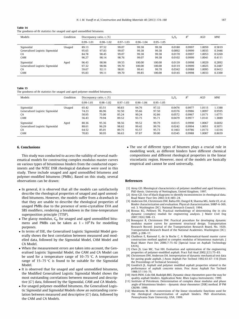
Table 14The goodness-of-fit statistics for unaged and aged unmodified bitumens.

Models Condition Discrepancy ratio, ri (%) Se/Sy R2 AGD MNE

0.99–1.01 0.98–1.02 0.97–1.03 0.96–1.04 0.95–1.05

Sigmoidal Unaged 89.13 97.52 99.07 99.38 99.38 0.0180 0.9997 1.0059 0.5819Generalised Logistic Sigmoidal 95.65 97.83 99.07 99.38 99.38 0.0092 0.9999 1.0035 0.3446CA 84.78 98.45 99.07 99.38 99.38 0.0170 0.9997 1.0053 0.5269CAM 96.27 98.14 98.76 99.07 99.38 0.0102 0.9999 1.0041 0.4111

Sigmoidal Aged 96.43 98.96 99.55 100.00 100.00 0.0139 0.9998 1.0029 0.2892Generalised Logistic Sigmoidal 97.32 98.96 99.70 100.00 100.00 0.0119 0.9999 1.0025 0.2487CA 59.67 92.11 98.81 99.41 99.70 0.0342 0.9988 1.0095 0.9412CAM 95.83 99.11 99.70 99.85 100.00 0.0145 0.9998 1.0033 0.3300

Table 15The goodness-of-fit statistics for unaged and aged polymer-modified bitumens.

Models Condition Discrepancy ratio, ri (%) Se/Sy R2 AGD MNE

0.99-1.01 0.98–1.02 0.97–1.03 0.96–1.04 0.95–1.05

Sigmoidal Unaged 65.42 83.51 90.83 94.76 97.32 0.0476 0.9977 1.0115 1.1388Generalised Logistic Sigmoidal 74.23 86.96 92.50 95.66 97.50 0.0376 0.9986 1.0097 0.9595CA 50.95 75.00 85.24 90.24 92.86 0.0572 0.9967 1.0171 1.6771CAM 56.43 79.94 89.52 93.75 95.71 0.0479 0.9977 1.0141 1.3889

Sigmoidal Aged 80.36 95.36 98.56 99.52 99.79 0.0315 0.9990 1.0067 0.6692Generalised Logistic Sigmoidal 88.61 96.29 98.62 99.42 99.76 0.0242 0.9994 1.0051 0.5071CA 64.52 85.01 89.75 93.57 95.73 0.1463 0.9786 1.0173 1.6316CAM 70.83 90.95 96.63 97.87 99.00 0.0345 0.9988 1.0087 0.8659


6. Conclusions

This study was conducted to access the validity of several math-ematical models for constructing complex modulus master curveson various types of bituminous binders from the conducted exper-iments and the NTEC DSR rheological database were used in thisstudy. These include unaged and aged unmodified bitumens andpolymer-modified bitumens (PMBs). Based on this study, severalobservations can be drawn:

� In general, it is observed that all the models can satisfactorilydescribe the rheological properties of unaged and aged unmod-ified bitumens. However, the models suffer from a drawback inthat they are unable to describe the rheological properties ofunaged PMBs due to the presence of semi-crystalline EVA andSBS modifiers, rendering a breakdown in the time-temperaturesuperposition principle (TTSP).� The glassy modulus, Gg, for unaged and aged unmodified bitu-

mens and PMBs can be taken as 1 � 109 Pa for modellingpurposes.� In terms of SSE, the Generalised Logistic Sigmoidal Model gen-

erally shows the best correlation between measured and mod-elled data, followed by the Sigmoidal Model, CAM Model andCA Model.� When the measurement errors are taken into account, the Gen-

eralised Logistic Sigmoidal Model, the CAM and CA Model canbe used for a temperature range of 10–75 �C. A temperaturerange of 15–75 �C is found to be suitable for the SigmoidalModel.� It is observed that for unaged and aged unmodified bitumens,

the Modified Generalised Logistic Sigmoidal Model shows themost outstanding correlations between measured and descrip-tive |G�| data, followed by the Sigmoidal, CAM and CA Models.� For unaged polymer-modified bitumens, the Generalised Logis-

tic Sigmoidal and Sigmoidal Models show an outstanding corre-lation between measured and descriptive |G�| data, followed bythe CAM and CA Models.

� The use of different types of bitumen plays a crucial rule inmodelling work, as different binders have different chemicalcompositions and different rheological properties in the linearviscoelastic region. However, most of the models are basicallyempirical and cannot be used universally.

References

[1] Airey GD. Rheological characteristics of polymer modified and aged bitumens.PhD thesis. University of Nottingham, United Kingdom; 1997.

[2] Airey GD. Use of black diagrams to identify inconsistencies in rheological data.Road Mater Pave Des 2002;3(4):403–24.

[3] Anderson DA, Christensen DW, Bahia HU, Dongré R, Sharma MG, Antle CE, et al.Binder characterization and evaluation. Physical characterization. SHRP-A-369,vol. 3. Washington (DC): National Research Council; 1994.

[4] Biswas KG, Pellinen TK. Practical methodology of determining the in situdynamic (complex) moduli for engineering analysis. J Mater Civil Eng2007;19(6):508–13.

[5] Bonaquist R, Christensen DW. Practical procedure for developing dynamicmodulus master curves for pavement structural design. TransportationResearch Record: Journal of the Transportation Research Board, No. 1929,Transportation Research Board of the National Academies, Washington (DC);2005. p 208–17.

[6] Chailleux E, Ramond G, de la Roche C. A Mathematical-based master curveconstruction method applied to complex modulus of bituminous materials. JRoad Mater Pave Des 2006;7:75–92 [Special Issue on Asphalt TechnologyEATA].

[7] Chen JS, Liao MC, Tsai HH. Evaluation and optimization of the engineeringproperties of polymer-modified asphalt. Pract Fail Anal 2002;2(3):75–83.

[8] Christensen DW, Anderson DA. Interpretation of dynamic mechanical test datafor paving grade asphalt. J Assoc Asphalt Pav Technol 1992;61:67–116 [fromthe Proceedings of Technical Sessions].

[9] Goodrich JL. Asphalt and polymer modified asphalt properties related to theperformance of asphalt concrete mixes. Proc Assoc Asphalt Pav Technol1988;57:116–75.

[10] Herh PKW, Colo SM, Rudolph BKS. Dynamic shear rheometers pave the way forquality asphalt binders. Application Note. Rheo Logica Instruments; 1999.

[11] Institute of Petroleum. Determination of complex shear modulus and phaseangle of bituminous binders – dynamic shear rheometer (DSR) method. IP PMCM/99; 1999.

[12] Marateanu M. Inter-conversions of the linear viscoelastic functions used forthe rheological characterization of asphalt binders. PhD dissertation,Pennsylvania State University, USA; 1999.


[13] Marasteanu O, Anderson DA. Improved model for bitumen rheologicalcharacterization. In: Eurobitume workshop on performance relatedproperties for bitumens binder, Luxembourg, paper no. 133; 1999.

[14] Medani TO, Huurman M. Constructing the stiffness master curves for asphalticmixes. Report 7-01-127-3. Delft University and Technology, Netherlands;2003.

[15] Medani TO, Huurman M, Molenaar AAA. On the computation of master curvesfor bituminous mixes. In: Proceedings 3rd eurobitume congress, Vienna,Austria, vol. 2; 2004, p. 1909–1917.

[16] Molinas A, Wu B. Comparison of fractional bed-material load computationmethods in sand-bed channels. Earth Surf Process Landf 2000;25:1045–68.

[17] Olard F, Di Benedetto H. General ‘‘2S2P1D’’ model and relation between thelinear viscoelastic behaviours of bituminous binders and mixes. Road MaterPave Des 2003;4(2):185–224.

[18] Pellinen TK, Witczak MW. Stress dependent master curve construction fordynamic (complex) modulus. J Assoc Asphalt Pav 2002;71:281–309.

[19] Pellinen TK, Witczak MW, Bonaquist RF. Asphalt mix master curveconstruction using sigmoidal fitting function with non-linear least squaresoptimization technique. In: Proceedings of 15th ASCE engineering mechanicsconference, June 2–5, 2002, Columbia University, New York, NY; 2002.

[20] Rowe G, Baumgardner G, Sharrock M. Functional forms for master curveanalysis of bituminous materials. In: Paper submitted to the RILEMconference; 2009.

[21] Rowe GM, Sharrock MJ. Alternate shift factor relationship for describing thetemperature dependency of the visco-elastic behaviour of asphalt materials.In: Transportation research board annual meeting, Washington, DC; 2011.

[22] Shaw M, McKnight WJ. Introduction to polymer viscoelasticity. John Wiley &Sons, Inc.; 2005.

[23] Silva LSD, Forte MMDC, Vignol LDA, Cardozo NSM. Study of rheologicalproperties of pure and polymer modified Brazilian asphalt binders. J Mater Sci2004;39:539–46.

[24] Stastna J, Zanzotto L, Berti J. How good are some rheological models ofdynamic material functions of asphalt? J Assoc Asphalt Pav Technol1997;66:458–79.

[25] Tran NH, Hall KD. Evaluating the predictive equation in determining dynamic(complex) modulus of asphalt mixtures. J Assoc Asphalt Pav Technol 2005;74[CD ROM].

[26] Wu B, Molinas A, Juliean PY. Predictability of sediment transport in the yellowriver using selected transport formulas. Int J Sed Res 2008;23:283–98.

modelling the rheological properties of bituminous binders using mathematical equations

Documents