Modelling Compound Leaves Using Implicit Contours

Mark S. Hammel, Przemyslaw Prusinkiewicz, and Brian Wyvill

ABSTRACT

This pa.per proposes a. method for modelling compound leaves in plants. The layout of leaf lobes is captured by a. branching skeleton generated using a.n L-system. The leaf margin is then traced around the skeleton. Finally, the surface bounded by the margin can be bent and complemented with a relief, if these features are found in the real leaf.

The paper focuses on the specification and tracing of the margin, and includes references to the techniques described in the literature for performing the other tasks. The margin is defined as an implicit contour - a one-dimensional counterpart of implicit surfaces used previously in computer graphics. Techniques for specifying and tracing the contour are discussed in detail.

Keywords: modelling of natural phenomena, leaf, implicit surface, implicit contour, contour tracing.

1 INTRODUCTION

One of the challenges in the modelling of natural phenomena is the synthesis of realistic images of plants. In recent years, several methods, including L-systems (Lindenmayer 1968), were suc­cessfully applied to model branching plant structures (Prusinkiewicz, Lindenmayer, Hanan 1988; Prusinkiewicz, Hanan 1990). Subsequently, timed L-systems were.introduced to animate the de­velopment of these structures over continuous time (Prusinkiewicz, Lindenmayer 1990, Chapter 6). Nevertheless, the animation of the development of plant organs presents a challenge to the modelling method, for in this case, the model must capture the changes in surfaces over time.

A simple instance of this problem occurs while displaying leaves or petals that emerge from buds. This process can be compared to the unfolding of a two-dimensional figure, cut from a sheet of paper. Its embedding in the three-dimensional space changes, but the intrinsic geometry (Faux, Pratt 1979, Page 40), which specifies the shape of the margin within the sheet, remains the same (Bell 1991, Page 37). If the organ is modelled using parametric surfaces, its unfolding can be captured by global shape deformation techniques (Farin 1990, Page 292). In this case, the control points of the modelled surface are embedded in a three-dimensional object that undergoes deformations such a.s twisting, bending, or tapering (Barr 1984). Another possibility is to assume that the control points are positioned at the endpoints of a branching structure, evolving over time (Figure 1 ). This approach, with the branches specified using an L-system, has been applied to animate the development of leaves and flowers in Lychnis coronaria (Prusinkiewicz, Hammel 1991).

After the leaves or petals have unfolded, they continue to develop until they reach their mature form. In the case of homoblastic development, the shape of the organs remains the same, and

199

200

Figure 1: Development of a petal modelled using a parametric surface. Control points are placed at the endpoints of a branching structure that changes its geometry over time.

Figure 2: Development of a leaf margin expressed using an L-system (Herman, Rozenberg 1975). The string symbols capture the sequence of lobes and notches, but no strict geometric interpreta­tion guides the drawing.

•

only their size changes. Many organs, however, follow the path of heteroblastic development (Bell 1991, Page 28), with the younger. and older forms assuming significantly different shapes. The differences may include the generation of new lobes and notches. The magnitude of these changes is particularly pronounced in compound leaves, such as divided fern fronds (Jones 1987), where new lobes are often formed in a recursive fashion. The organs pursuing a heteroblastic developmental path are the focus of attention in this paper.

The first formal description of the development of a compound leaf was proposed by Rozenberg and Lindenmayer (Rozenberg, Lindenmayer 1973; Herman, Rozenberg 1975), who applied the formalism of context-free L-systems to describe the sequence of lobes and notches around the leaf margin (Figure 2). No automatic graphical interpretation was proposed, and the corresponding images were band-drawn. Pursuing an alternative approach, Lindenmayer (1977) applied brack­eted L-systems to describe the branching structure of the lobe arrangement in a leaf (Figure 3). This type of description is readily amenable to the automatic visualisation of leaf skeletons rep­resenting the axes of symmetry of the lobes (Prusinkiewicz, Lindenmayer 1990, Chapter 5). The automatic visualisation of the leaf margin, lying at a certain distance from the skeleton, was ad­dressed by Lienhardt (1987), Lienhardt and Fran<;on (1987), Prusinkiewicz, Lindenmayer, and Hanan (1988), and Viennot et al. (1989).

In principle, two approaches to the construction of a leaf margin, given its skeleton, can be followed. One is to use the skeleton to position a set of control points that will define a parametric curve. Problems occur when new control points are inserted to specify the emerging lobes. The sudden change of the skeleton topology (Figure 4) requires that all control points be repositioned

201

Figure 3: Development of a branching leaf structure expressed using an L-system {Lindenmayer 1977). The terminal edges represent axes of the lobes, but no rules for tracing leaf margins have been specified.

..,, ..•

Figure 4: Drastic change of skeleton topology related to the formation of new lobes

to maintain the continuity of leaf shape over time (Foley et al. 1990, Pages 507-510). Such a global change is difficult to express using L-systems.

In this paper, we propose to generate leaf margins around skeletons automatically, using implicit contours, which can be viewed as a one-dimensional analogue of implicit surfaces (Wyvill et al. 1986; Bloomenthal, Wyvill 1990). Intuitively, the method creates a planar scalar field in the proximity of the skeleton. The margin is represented by a contour, defined as the locus of points with a given field value. The area bounded by this contour forms the surface of the leaf (Figure 5).

The relation of an implicit contour to a scalar field is illustrated in Figure 6. The skeleton is a simple branching structure. The field function J(x, y) defines the field by capturing the Euclideandistances of sample points from the skeleton, and is represented if Figure 6 as a height field. The contour corresponds to a horizontal section of this field.

The definition of the function f(x, y) in terms of the Euclidean distance between sample points and the contour does not provide sufficient flexibility to control details of the contour shape. For

Figure 5: Margin definition using implicit contours. The margin is drawn in the proximity of the skeleton as a locus of points for which the field function assumes a constant value.

202

Figure 6: A planar scalar field represented using height values. The intersection of a horizontal plane with the height field represents the implicit contour.

example, all notches are sharp, and no possibility for specifying gradually curving notches exists. In the next section, we introduce a more general definition of the field function, providing greater control of the contour shape.

2 IMPLICIT CONTOURS

Consider the field function f: !R2 -> �, defined for each point in a plane rr. An implicit contour is the set of all points in rr such that f(x,y) = c, where c is a constant threshold value. 1 Points (x,y) that evaluate to a number less than care considered to lie outside of the contour, and points that evaluate to a number greater than c are considered to be inside of it. We are interested in field functions defined in relation to skeletons made up of primitive skeletal elements (Bloomenthal, Wyvill 1990) embedded in rr. In our case, these elements are line segments forming a branching structure. The value of the field function at any point on the plane 1r is equal to the sum of the contributions from all skeletal elements. Each line segment has a radius of influence, within which it affects the value of the field function. The contribution from an individual element is the greatest on the line itself and decreases as the distance to the line increases, dropping to zero at the radius.

We assume that each line's contribution is defined by the following function, originally proposed for implicit surfaces by Wyvill et al. (1986):

F(d)={2�-3�+1 if 0�d�r,0.0 if d > r.

(1)

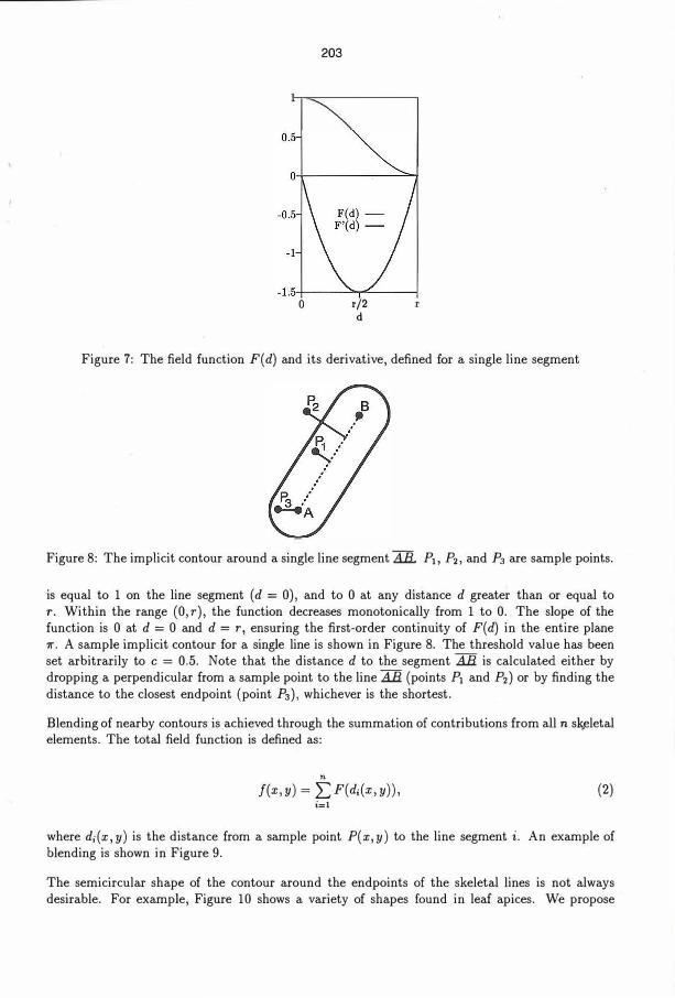
In this equation, d is the distance from a point in space to the line under consideration, and r is the radius of influence of this line. Figure 7 shows plots of F(d) and its derivative. The function

1 We extend the usual definition of an implicitly defined curve, which sets the threshold value c to 0.

203

0 r/2 d

Figure 7: The field function F(d) and its derivative, defined for a single line segment

Figure 8: The implicit contour around a single line segment AB. Pi, P2 , and P3 are sample points.

is equal to 1 on the line segment (d = 0), and to 0 at any distance d greater than or equal tor. Within the range (0, r), the function decreases monotonically from 1 to 0. The slope of thefunction is 0 at d = 0 and d = r, ensuring the first-order continuity of F(d) in the entire plane1r. A sample implicit contour for a single line is shown in Figure 8. The threshold value has been set arbitrarily to c = 0.5. Note that the distance d to the segment AB is calculated either bydropping a perpendicular from a sample point to the line AB (points Pi and P2) or by finding the distance to the closest endpoint (point Pa), whichever is the shortest.

Blending of nearby contours is achieved through the summation of contributions from all n s�eletal elements. The total field function is defined as:

n

f(x,y) = EF(d;(x,y)), (2) i=l

where d;(x,y) is the distance from a sample point P(x,y) to the line segment i. An example ofblending is shown in Figure 9.

The semicircular shape of the contour around the endpoints of the skeletal lines is not always desirable. For example, Figure 10 shows a variety of shapes found in leaf apices. We propose

204

Figure 9: An example of an implicit contour around a single line segment, and contour blending of two line segments with soft, U-shaped notches

acute subacute obtuse rounded cuspidate

acuminate mucronate aristate retuse emarginate

Figure 10: Variety of shapes of leaf apices, hand-drawn (Sugden 1984)

to model such shapes by varying the radius of influence along line segments. Consequently, the specification of a line segment will include four components: a length, two radii of influence ( one at each end of the line), and a method of interpolation between these radii. A variety of functions can then be used for interpolation. Three examples are shown if Figure 11.

3 TRACING THE CONTOUR

The drawing of a contour does not require the evaluation of the field function at each. point of the plane 1r. Instead, we can examine the neighbourhood of the contour, tracing it until a closed curve is found. Naturally, care must be taken to consider all components if the contour consists of disconnected curves.

To trace the contour, we impose a discrete grid on the plane including the field function. Although several methods for contour tracing in a discrete space are utilised in image processing (Pavlidis 1982, Pages 142-148), we propose here another algorithm, analogous to the surface tracing method developed by Wyvill et al. (1986). The algorithm consists of two phases: finding an initial point on the contour, and following the contour.

To find a .starting point, we first consider a grid location closest to the middle of some skeletal line segment. If the grid is fine enough, this point will be inside the contour. A scanning direction is then chosen, and successive points of the grid are examined until a point outside the contour is found. If two adjacent grid points straddle the contour (one is inside, the other outside) then a point on the contour is guaranteed to exist between these two locations. The position of this point

205

a b C

Figure 11: Controlling the shape of the radius of influence along a skeletal line using: a) a linear interpolation function, b) a sigmoidal function (as shown in Figure 7), and c) an exponential function. In all three cases, the radius of influence is equal to 1.0 at the bottom, and to 0.0 at the top of the skeletal line

Figure 12: Traversing the contour of an isolated line segment

can be approximated by interpolation, binary subdivision, or any other root finding method.

Now that a point on the contour has been found, a grid cell can be associated with it, and the tracing can begin. Figure 12 illustrates this process. A direction, clockwise or counter-clockwise, is chosen. The traversal progresses from the initial cell through consecutive, adjacent cells. In each cell, a new point on the contour is found and connected to the previous point. The traversal halts when a new contour point overlaps an existing one - this will occur at the starting point.

The process of moving from one cell to the next involves calculating the value of the field function at each vertex of the current cell. The value at a vertex can be greater than or equal to the threshold c (the vertex is in state 1), or it can be less than the threshold c (state 0). Assuming that the radius of curvature is large enough (the contour does not loop inside a single cell), each combination of vertex states determines a partition of the cell into an inside and outside region. All possible combinations are shown in Figure 13. Two cells, numbered 22 and 25 in Figure 13, have the same configurations of vertex states as cells 6 and 9, but correspond to different distributions of the inside and outside regions. The diagonally placed vertices in state 1 can be viewed as included in two separate interior regions or as belonging to a single interior region that runs diagonally down the cell. These ambiguous cases are distinguished by evaluating the field function in the centre of the cell.

For a given direction of contour traversal, the configuration of the current cell determines the position of the next cell along the contour. Since the total number of cell configurations is small

206

Figure 13: Possible configurations of a cell with respect to a contour. A black dot represents a grid point inside the contour, and a clear dot represents a point outside the contour. The grey areas suggest the cell regions that are inside the contour. The labels represent dot configurations, viewed as binary numbers.

(18), the position of the next cell can be conveniently found using a look-up table, indexed by the cell number. For example, if the current cell is of type 1, the next cell must be situated below. The contour will cross the edge between vertices O and 1; the position of the intercept can be approximated using any root finding method, as was done for the initial point on the contour.

4 SAMPLE RESULTS

Figure 14 shows a pinnate (Jones 1987, Page 29) fern leaf at three stages of development. The branching structures were generated using an L-system reaching three different derivation lengths. The implicit contours were then drawn using the technique described in the previous sections.

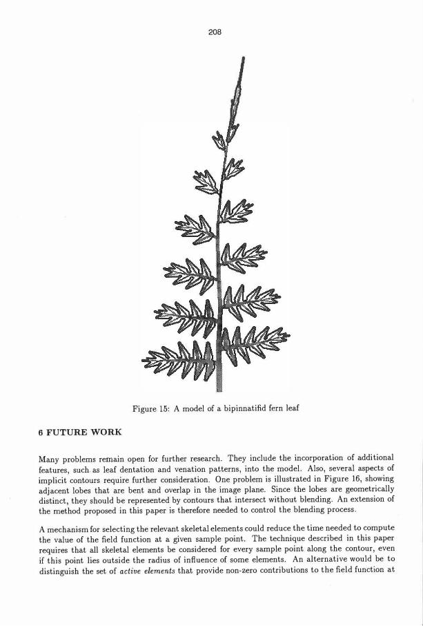
Figure 15 shows a more complex bipinnatifid leaf (Jones 1987, Page 29). In this case, each branch stemming from the axis is surrounded by a separate contour, which does not blend with this axis.

207

Figure 14: Simulated development of a pinnate fern leaf

5 CONCLUSIONS

We have presented a method for generating the margin of compound leaves. The idea is to first specify a skeletal branching structure that captures the layout of the lobes, then trace the contour around it. The margin is defined as the set of points for which a field function, characterised with respect to the elements of the branching structure, evaluates to a given constant value. Thus, the contour can be viewed as a one-dimensional analogue of an implicitly defined surface. The proposed method offers the following advantages:

• the generation of the contour is a separate task from the development of the skeleton, so itis independent of the branch-generating system used,

• the method requires only a small set of parameters, which implies that a margin for a givenskeleton can be specified easily,

• the simulation of leaf development can be accomplished using known techniques for animat­ing the development of a branching structure (Prusinkiewicz, Lindenmayer 1990, Chapter6), and generating the contour automatically,

• the resulting margin shapes correspond well with those observed in nature.

The contour bounds an area that represents the surface of a leaf. Once this surface has been defined, it can be bent or complemented with a relief for increased realism. Techniques for con­trolling the shape of a surface given by its contour were described by Fracchia and Prusinkiewicz (1991), Fracchia (1991), and Celniker and Gossard (1991).

208

Figure 15: A model of a bipinnatifid fern leaf

6 FUTURE WORK

Many problems remain open for further research. They include the incorporation of additional

features, such. as leaf dentation and venation patterns, into the model. Also, several aspects of

implicit contours require further consideration. One problem is illustrated in Figure 16, showing adjacent lobes that are bent and overlap in the image plane. Since the lobes are geometrically distinct, they should be represented by contours that intersect without blending. An extension of the method proposed in this paper is therefore needed to control the blending process.

A mechanism for selecting the relevant skeletal elements could reduce the time needed to compute the value of the field function at a given sample point. The technique described in this paper requires that all skeletal elements be considered for every sample point along the contour, even

if this point lies outside the radius of influence of some elements. An alternative would be to

distinguish the set of active elements that provide non-zero contributions to the field function at

209

Figure 16: Overlapping lobes should not blend.

a given point. This set could be determined using a presorting technique such as that described by Wyvill et al. (1986).

Throughout this paper, we view leaves as two-dimensional surfaces. In reality, they are three­dimensional objects, and at least at the veins, their thickness is not negligible. Modelling very thin objects using implicit surfaces is an open problem, although some results in this direction have been obtained (Bloomenthal 1989).

ACKNOWLEDGEMENTS

We would like to thank Jules Bloomenthal for many discussions that clarified concepts presented in this paper. Jim Hanan developed the version of the L-system-based modelling program that we used to generate the skeletons. Dietmar Saupe wrote the program for displaying height fields, which we employed to create Figure 6. Also, we would like to thank the anonymous referees for indicating some open problems and missing citations. This research was performed using the GraphicsJungle environment at the University of Calgary and was supported by operating grants, equipment grants, and a scholarship from the Natural Sciences and Engineering Research Council of Canada.

REFERENCES

Barr AH (1988) Global and local deformations of solid primitives. Proceedjngs of SIGGRAPH '84 (Minneapolis, Minnesota, July 23-27, 1984), in Computer Graphics 18,3, pages 21-30, ACM SIGGRAPH, New York.

Bell AD (1991) Plant Form, An Illustrated Guide to Flowering Plant Morphology. Oxford Uni­versity Press.

Bloomenthal J, Wyvill B (1990) Interactive techniques for implicit modeling. Computer Graphics,

24(2):109-116.

Bloomenthal J (1989) Techniques for implicit modeling. Technical Report P89-00106, Xerox PARC.

Celniker G, Gossard D (1991) Deformable curve and surface finite-elements for free-form shape design. Proceedings of SIGGRAPH '91 (Las Vegas, Nevada, July 28 - August 2, 1991), in Computer Graphics 25,4, pages 257-266, ACM SIGGRAPH, New York.

210

Farin G (1990) Curves and Surfaces for Computer Aided Geometric Design. Second Edition. Academic Press, Boston.

Faux ID, Pratt MJ (1979) Computational Geometry for Design and Manufacture. Ellis Horwood Limited, Chichester.

Foley JD, Van Dam A, Feiner SK, Hughes JF (1990) Computer Graphics: Principles and Practice. Addison-Wesley, Reading, MA.

Fracchia FD (1991) Visualization of the Development of Multicellular Structures. PhD thesis, University of Regina, Regina, SK.

Fracchia FD, Prusinkiewicz P (1991) A physically-based finite element approach to modeling patches with n-sided polygonal domains. Proceeding of the Third Annual Western Computer Graphics Symposium, pages 21-25, Silver Star, BC.

Herman GT, Rozenberg G (1975) Developmental systems and languages. North-Holland, Amster­dam. With Lindenmayer A.

Jones DL (1987) Encyclopaedia of Ferns. Timber Press, Portland, OR.

Lienhardt P (1987) Modelisation et evolution de surfaces libres. PhD thesis, Universite Louis Pasteur, Strasbourg.

Lienhardt P, Fran<;on J (1987) Synthese d'images de feuilles vegetales. Technical Report R-87-1, Departement d'informatique, Universite Louis Pasteur, Strasbourg.

Lindenmayer A (1968) Mathematical models for cellular interaction in development, Parts I and II. Journal of Theoretical Biology, 18:280-315.

Lindenmayer A (1977) Paracladial relationships in leaves. Ber. Deutsch Bot. Ges. Bd., 90:287-301.

Pavlidis T (1982) Algorithms for Graphics and Image Processing. Computer Science Press, Rockville, Maryland.

Prusinkiewicz P, Hammel MS (1991) Continuous animation using L-systems. Video tape.

Prusinkiewicz P, Hanan J (1990) Visualization of botanical structures and processes. In D. Thal­mann, editor, Scientific Visualization and Graphics Simulation, pages 183-201. J. Wiley & Sons, Chichester.

Prusinkiewicz P, Lindenmayer A (1990) The Algorithmic Beauty of Plants. Springer-Verlag, New York. With Hanan J, Fracchia FD, Fowler DR, de Boer MJM, and Mercer L.

Prusinkiewicz P, Lindenmayer A, Hanan J (1988) Developmental models of herbaceous plants for computer imagery purposes. Proceedings of SIGGRAPH '88 (Atlanta, Georgia, August 1-5, 1988), in Computer Graphics 22,4, pages 141-150, ACM SIGGRAPH, New York.

Rozenberg G, Lindenmayer A (1973) Developmental systems with locally catenative formulas. Acta Informatica, 2:214-248.

Sugden A (1984) Longman Illustrated Dictionary of Botany. Longman Group Limited, Burnt Mill, Harlow, Essex.

(I

211

Viennot XG, Eyrolles G, Janey N, Arques D (1989) Combinatorial analysis of ramified patterns and computer imagery of trees. Proceedings of SIGGRAPH '89 (Boston, Massachusetts, July 31 - August 4, 1989), in Computer Graphics 23,3, pages 31-40, ACM SIGGRAPH, New York.

Wyvill G, McPheeters C, Wyvill B (1986) Data structure for soft objects. The Visual Computer, 2( 4):227-234.

Mark S. Hammel received his B.Sc. from the University of Saskatchewan, Canada in 1991. He is currently pursuing a M.Sc. degree at the University of Calgary, Canada. His research interests lie in the area of computer graphics, computer animation, the modelling of natural phenomena, and scientific visualisation.

Address: Department of Computer Science, University of Calgary, Calgary, Alberta, Canada T2N 1N4.

Przemyslaw Prusinkiewicz is a professor of Computer Science at the University of Calgary, Canada. His research interests include computer graphics, interactive techniques, and computer music. Dr. Prusinkiewicz received his M.S. in 1974 and Ph.D. in 1978, both in computer science, from the Technical University of Warsaw. He is a member of the ACM and IEEE CS.

Address: Department of Computer Science, University of Calgary, Calgary, Alberta, Canada T2N IN4.

212

Brian Wyvill is a professor in the Department of Computer Science at the University of Calgary. After gaining his PhD in the UK in 1975, he worked both in academia (Royal College of Art) and in industry on projects such as some animation sequences for the film, Alien. He emigrated to Canada in 1981 where his research has centred around the GraphicsLand (now GraphicsJungle) Graphics Environment project. Brian has recently returned from sabbatical at Hewlett Packard Company laboratories in California.

Address: Department of Computer Science, University of Calgary, Calgary, Alberta, Canada T2N 1N4.