Int J Comput Vis (2008) 79: 31–43DOI 10.1007/s11263-007-0088-2

From Inpainting to Active Contours

François Lauze · Mads Nielsen

Received: 17 February 2007 / Accepted: 11 September 2007 / Published online: 17 November 2007© Springer Science+Business Media, LLC 2007

Abstract Background subtraction is an elementary methodfor detection of foreground objects and their segmentations.Obviously it requires an observation image as well as abackground one. In this work we attempt to remove the lastrequirement by reconstructing the background from the ob-servation image and a guess on the location of the objectto be segmented via variational inpainting method. A nu-merical evaluation of this reconstruction provides a “disoc-clusion measure” and the correct foreground segmentationregion is expected to maximize this measure. This formula-tion is in fact an optimal control problem, where controls areshapes/regions and states are the corresponding inpaintings.Optimization of the disocclusion measure leads formally toa coupled contour evolution equation, an inpainting equation(the state equation) as well as a linear PDE depending on theinpainting (the adjoint state equation). The contour evolu-tion is implemented in the framework of level sets. Finally,the proposed method is validated on various examples. Wefocus among others in the segmentation of calcified plaquesobserved in radiographs from human lumbar aortic regions.

Keywords Segmentation · Inpainting · Active contours ·Disocclusion · Adjoint methods · Variational methods

F. Lauze (�) · M. NielsenNordic Bioscience A/S, Herlev Hovedgade 207, 2370 Herlev,Denmarke-mail: francois@nordicbioscience.com

M. NielsenDIKU, University of Copenhagen, Universitetsparken 1,2100 Copenhagen, Denmarke-mail: madsn@diku.dk

1 Introduction: Some Challenging Problems

The three pictures in Fig. 1 represent first: the flag of theGreenland territory; second: an object added on a smoothbackground via addition of the intensities, similar to thepresence of transparent layers, that we will call “pseudo cal-cification” in the sequel—a typical case would indeed bethe one of an X-ray showing a calcific deposit on some softtissue; and third, a true aortic calcification from a lateralX-ray, with inverted intensities. Contour based active con-tour methods can provide a segmentation of the circle, al-though sensitive to the initialization, region based activecontours using statistical parameters of intensity/color dis-tributions for each regions, will fail to isolate the circle inthe Greenland’s flag from the rest of the image, since thetwo regions have the same statistics! In the pseudocalcifi-cation image the difficulty comes also from hardly visibleedge information, and the reality is often much worse thanthis artificial image, while finding discriminating statisticalinvariants may also prove very difficult. In the case of thetrue calcification, the bottom of the calcific deposit is onlyvisible by transparency under a dark anatomical structure(hip).

In an attempt to overcome these problems, we introducea novel methodology, within the framework of active con-tours. This belongs to the region based family of active con-tours, but instead of considering that the image domain ispartitioned in two (or several regions), our approach con-sists in considering the following problem: if the region �

containing the object of interest is known, and if we haveenough prior information on the type of background, can wereconstruct the occluded background image? If we assumea positive answer to that question, then we ask whether agiven region � contains an object occluding the background

32 Int J Comput Vis (2008) 79: 31–43

Fig. 1 Challenging inputs for region based active contours. From left to right: The Greenland’s Flag, a pseudo-calcification and a true, invertedX-ray of a aortic calcification

in the following way: if � delimits indeed the area occu-pied by a foreground object, then there should be sufficientlylarge difference between the observed image and the recon-structed one within this region. This leads naturally to a vari-ational problem: if � is a given region of the image plane D,u0 the observed image, u(�) = I(u0,�) the reconstructedbackground and if we call J (�) this background/foregrounddifference, we may look for the true region � as an ex-tremum for J (�). The goal of this work is to propose such ameasure, first in general terms, and then a specific instan-tiation based on a relatively simple variational inpaintingformulation, which essentially corresponds to the TV in-painting of Chan and Shen (Chan and Shen 2002) and asimple measure for discrepancy between two images, basedon pixel value differences. The corresponding optimizationproblem belongs to the class of optimal control problems,where the control space is a space of admissible shapes, inour cases, some admissible open sets of the image plane.Then given such an admissible open set or control �, itsassociated state will be the inpainting-denoising of u0 in-side �.

We use the shape derivatives tools developed by Delfourand Zolésio (2001) (see also Aubert et al. 2003) in orderto derive optimality conditions. In particular, when comput-ing the Gâteaux derivative of our disocclusion criterion withrespect to a shape deformation, we retrieve the shape ad-joint state. From the (informal) computation of the Gâteauxderivative, we deduce, by gradient descent, a curve evolutionequation which is then implemented within the frameworkof level sets.

The paper is organized as follows. In Sect. 2, we givea short review of active contour algorithms. In Sect. 3,we introduce an “disocclusion quality measure”, computeits Gâteaux derivative and deduce our inpainting based ac-tive contour algorithm from it. Several experiments are pre-sented in Sect. 5 and we conclude in Sect. 6.

This work extends a previous workshop article (Lauzeand Nielsen 2005) and the ideas presented here have alsobeen used in a conference paper (Lauze and de Bruijne2007).

2 Background

Since the seminal paper of Kass, Witkin and Terzopoulos(Kass et al. 1987), active contours have been used rather ex-tensively in computer vision and medical imaging, for thepurpose of detection and segmentation, in order to over-come the locality problem of edge detectors. In their originalformulation, they are curves with built in regularity proper-ties and preferences for edges in an image. These propertiesare enforced via an energy minimization. Given an imageu(x, y) defined on a domain D, a edge detector, for instancethe gradient magnitude image |∇I | and a decreasing func-tion g : [0,∞] → R, and a curve C : [0,1] → D, they definethe snake energy

E(C) =∫ 1

0(α|Ct |2 + β|Ctt |2) dt

+∫ 1

0g(|∇I (C(t)|)) dt

and snakes are minimizers of E. The first part of this en-ergy, the so-called internal energy controls the size and thesmoothness of the contour, while the second term, the exter-nal energy, attracts the snake towards the edges of the ob-ject in the image. Although very simple to implement, thesesnakes suffer among other of initialization problems and ne-cessitates reparameterization. In order to overcome initial-ization problems several solutions were proposed, includ-ing balloon forces (Cohen and Cohen 1993), gradient vectorflows (Xu and Prince 1997). Geodesic active contours, pro-posed independently by Caselles et al. (1995) and Kichenas-samy et al. (1995) introduced a parametrization independentformulation based on a energy formulation for a candidatecontour �

J(�) =∫

�

k(b) ds

where k(b) is a function that should be small at object bound-ary and s is the arclength parameterization of �. Whenkb ≡ 1, J (�) is thus simply the length of � and the associ-

Int J Comput Vis (2008) 79: 31–43 33

ated steepest descent equation is the well known Euclideanshortening flow:

∂�

∂t= −dJ (�) = κ �n

where κ is the curvature of � and �n is the exterior normal.The effect of kb is the replace the usual metric on the im-age plane by one which is image dependent. The resultingsteepest descent equation is

∂�

∂t= (kbκ − ∇kb · �n)�n.

The first term allows shortening to slow down or stop atedges while the second tends to move the contour orthog-onally in the direction of an edge.

All these models deal only with contours, not with theregions they separate. A fundamental landmark in imagesegmentation is the variational formulation of Mumford andShah (1989)

E(u,C) = 1

2

∫D

(u − u0)2 dx

+ λ

2

∫D\C

|∇u|2 + ν(C).

A minimizing pair (u,C) represents a piecewise smooth ap-proximation of the input image u0 on the image plane D,which may have discontinuities along a boundary C, whoselength is denoted by (C). Inspired by this approach, Co-hen et al. proposed a region based algorithm in Cohen et al.(1993) and some region based strategies were discussed byRonfard (1994).

Based on a simplification of the Mumford-Shah segmen-tation functional, Chan and Vese proposed a region basedformulation in Chan and Vese (2001). Roughly speakingthe image domain should be decomposed as an open “innerpart” �i , an open “outer” part �o = D\�i , where �i is theclosure of �i and the boundary � = ∂�i and � is recoveredas a minimizer of the following cost function

J (�,ai, ao) = λ1

∫�i

(u0 − ai)2 dx

+ λ2

∫�o

(u0 − ao)2 dx

+ α(�) + μ|�i | (1)

where ai and ao are reals λ1, λ2, α and μ are fixed positiveparameters and |�i | is the area of �i . A trivial computationshows that the optimal ai and ao are the average values ofu0 in the inner and outer regions respectively, and a levelsetoptimization coupled with the estimation of the mean valuesis performed that attempts to recover two regions such that|ai − ao| is as large as possible while enforcing regularity

properties for these regions. We will often refer to it as the“Chan-Vese” approach in the sequel.

More complex statistical descriptors have been proposedinstead of the mean, as histogram matching in (Aubert et al.2003). In a series of papers, Paragios and Deriche proposeda paradigm called Geodesic Active Regions where both con-tour based and region based terms are used (see for in-stance Paragios and Deriche 2002). General forms for regionbased energy functionals were studied by Jehan-Besson etal. (2003) with general energy formulation of the form:

J (�i,�o,�) =∫

�i

ki(x,�i) dx

+∫

�o

ko(x,�o)dx

+∫

�

k(b) ds.

The algorithms mentioned above either use a parametric for-mulation of the different densities in regions and boundaries,such as Gaussian, mixture of Gaussian, parametric descrip-tion for the distributions of responses of some linear filters asin Heiler and Schnörr (2005) or use a supervised approach:distributions are learned from examples. A non parametricand unsupervised approach has been proposed by Kim et al.(2005), and is based on the mutual information between thedistribution of intensities and the regions labeling, seen alsoas a random variable.

A extensive review and discussion of statistical methodsfor actives contours and discussion can be found in the workof Cremers et al. (2007). Another excellent reference is Os-her and Paragios (2003).

We note nevertheless that in region based active contours,the different regions one want to recover form, together withtheir boundaries, a partition of the image domain, and thatthe respective contents of these regions are usually assumedto be independent of each others. While this assumption issufficient in many applications, the images shown in the pre-vious section show that it may fail.

3 Inpainting Based Segmentation

In this section we introduce background disocclusion ideasand a corresponding variational formulation that will leadto an active contour evolution equation for the segmenta-tion task. We start by the well known background subtrac-tion and discuss elementary ways to recover the support of aforeground object from it. Then inpainting is introduced viastatistical inference leading to variational formulations andcombining it with support recovery from background sub-traction we derive the background disocclusion criterion.

34 Int J Comput Vis (2008) 79: 31–43

3.1 Background Subtraction and Active Region

A standard approach in detection and tracking is backgroundsubtraction. Let us assume that a reference background im-age ub is known. If u0 is now an image of the same scene,with an added object, then a way to detect this object is tocompute the pixelwise difference d(x) = u0(x) − ub(x) ora function x �→ L(ub(x),u0(x)) measuring the discrepancybetween ub(x) and u0(x) where the map (c, d) �→ L(c, d)

is tailored to the problem at hand (when comparing refer-ence and input images, one might expect for instance noiseand illumination changes, see Ohta 2001 for an example, butthis is a situation that we will not consider here). The region� where these discrepancies are large enough is expected tocorrespond to the location of this object. Depending on thetask at hand, a simple thresholding may provide the result,or a more elaborated extraction can be proposed, that will beable to group pixels in a more coherent way. Among these,when considering pixelwise difference u0 − ub , a good can-didate might be the algorithm of Chan and Vese describedin the previous section in (1). If we assume only white noisecontamination for the background and observations, thendifference image should have zero mean in the complementof the foreground region. This means in fact that the para-meter ao describing the average intensity value in this outerregion in (1) is expected to be 0 and the algorithm will at-tempt to evolve the contour in order to maximize (in absolutevalue) the parameter ai attached to the foreground or innerregion in (1):

|ai(�)| = 1

|�|∣∣∣∣∫

�

(u0 − ub) dx

∣∣∣∣while imposing regularity on the boundary via a length termand potentially on the region size via the area term.

Following this rationale, we propose, for a given r > 0,to maximize the following criterion

K(�;ub,u0) = 1

|�|r∣∣∣∣∫

�

L(ub,u0) dx

∣∣∣∣ (2)

that can be interpreted as a generalized moment of the dis-crepancy between ub and u0. We could add some regularityconstraint to K such as a term of the form −α(�) where� = ∂� is the boundary of � and α a positive weight,we have not included it, since in practice we did not en-counter regularity problems. The introduction of the expo-nent r in the criterion above allows to control the regionsize and helps improving “concavity” of our functional. Thefollowing sketchy situation, illustrated in Fig. 2 shows itsrole. The background is a constant image, with value ar-bitrarily set to 0, and two identical foreground regions �1

and �2 are superimposed to it, say that each object is a unitsquare with intensity 1. The local pixel discrepancy function

Fig. 2 Role of the areaexponent

L(c, d) is chosen as the difference c − d . Then for r = 1,K(�1) = K(�2) = K(�1 ∪ �2) = 1 and in fact any � ⊂�1 ∪�2 is a maximizer for K! In the case r < 1 then clearlyK(�1) = K(�2) = 1, while K(�1 ∪ �2) = 21−r > 1, �1

and �2 are local maximizers for K while �1 ∪�2 is a globalmaximizer.

3.2 Background Estimation via Inpainting

Let us now consider the situation where a reference back-ground is not known, but we know instead a distribution forthe background images, generally in the form of a distrib-ution of the responses of some local filters over the imagesites, say D = {s1, . . . , sN } ⊂ R

2 and u : D �→ R,

p(u) = p([f (u, s)]s∈D) =∏s∈D

p(f (u, s))

where we have assumed independence of the local filterresponses, an assumption used frequently for its computa-tional tractability. In the sequel we assume f (u, s) to be adiscrete counterpart of |∇u| at location s, for instance

f (u, s) =⎧⎨⎩

∑r∈V(s) α(|r − s|)|ur − us | or√∑

r∈V(s) α(|r − s|)(ur − us)2

where V(s) denote the spatial 4- or 8-points neighborhoodof pixel location s. For consistency with the continuous set-ting, α is chosen proportional to 1/|r − s| in the first caseand 1/|r − s|2 is the second. The p.d.f. p is taken as a gen-eralized Laplacian

p(x) = q

2r�(1/q)e−| x

r|q

where q, r > 0 and �(x) is the Euler-Legendre Gammafunction.

We now assume that we are given an observed image u0

from our unknown background image ub with an added ob-ject corresponding to an image uf supported on a subset �

of D and some white noise η:

u0 = C(ub,uf , η)

Int J Comput Vis (2008) 79: 31–43 35

where C is a combination operation of additive/multi-plicative type in the case of a transparent object added onthe background, or an XOR-like operation when foregroundoccludes background, for instance. Our main problem isthe determination of �, but let us assume we know it. ByBayes’s rule of retrodiction, the probability p(u|u0,�) of u

being the background image knowing u0 and � is given by

p(u|u0,�) = p(u0|u,�)p(u|�)

p(u0|�). (3)

We will assume, for sake of simplicity, that occlusion lo-cation is independent of the background, so that p(u|�) =p(u) (although in many situations this assumption seemsvery natural, in one of the situations we have in mind in thisarticle, segmentation of calcifications in radiographs of thelumbar aortic region, the partial occlusion due to the pres-ence of calcification has a tendency to occur along a specificregion, the aorta walls, but we won’t use it here). We assumethat observations are contaminated by Gaussian white noiseof variance σ 2. The resulting likelihood term is

p(u0|u,�) =∏

s∈D\�

1√2πσ 2

e(us−u0s )2

2σ2 .

Then an estimate of the background image can be ob-tained via a maximum a posteriori (MAP) from (3), or,equivalently, neglecting the evidence p(u0|�) which is con-stant for a given observed image u0 and occlusion locus �,we obtain u as a minimizing element for the energy

E(u;�) := E(u;�,u0)

= − log p(u0|u,�) − log p(u)

(we will mostly omit u0 in E in order to increase legibility).With the previous assumptions on the different probabili-ties and omitting constants, the MAP estimate becomes, ina continuous setting

u := u(�) = argminu

E(u,�)

=∫

D

(λ

2χD\�(u − u0)

2 + |∇u|q)

dx

where λ = rq/(2σ 2), D denotes from now an open set ofR

2, the image plane, � an open included in D and χD\�is the characteristic function of D\�. For q = 1 this is pre-cisely the Total Variation simultaneous inpainting and de-noising model of Chan and Shen (2002). In the sequel, weuse a slightly modified version of the above inpainting en-ergy

E(u;�) =∫

D

(λ

2χD\�(u − u0)

2 + ϕ(|∇u|))

dx (4)

where ϕ : R → R+ is a strictly convex function, increasingfor x > 0 with ϕ(x) ≈ c|x|q when x becomes large. It iseasily seen that q must be at least 1.

With the assumptions we made on q and ϕ the mini-mizing element of energy (4) can be shown to exist and beunique in the Sobolev space W 1,q (D) when q > 1 and inthe space of functions of bounded variations BV (D) whenq = 1 (where there, ∇u replaced by the Radon measure Du,see Aubert and Kornprobst 2006 for details). Boundary con-ditions (BCs) will be necessary when we have to integrate bypart, we choose the very natural zero Neumann ones, i.e. weconsider only the functions u that satisfy ∂u/∂ �n = 0 where�n is the exterior normal to D. In practice, the function ϕ weused is ϕ(x) = 1

q(√

x2 + ε2 )q where ε is a strictly positivereal number.

A straightforward application of the Calculus of Varia-tions provides the following well known characterization ofthe minimizer or the inpainting energy: for every function ξ

satisfying null Neumann BCs on ∂D and with enough regu-larity, we set to 0 the directional derivative:

d

dτE(u + τξ ;u0,�)|τ=0 = 0

from which we obtain the variational form for the Euler-Lagrange equation which results from the inpainting en-ergy (4) (we will omit the u0 in the directional derivativeexpression in order to alleviate notations)

∂E(u;�)

∂u= 0

where ∂E(u;�)∂u

is the linear map

ξ �→ ∂E(u;�)

∂u(ξ) =

∫D

[λχD\�(u − u0)ξ

+ ϕ′(|∇u|)|∇u| ∇uT ∇ξ

]dx. (5)

An integration by part, using the Neumann BCs on u pro-vides a formal representation of ∂E(u;�)

∂uand the associated

PDE form of the Euler-Lagrange equation

∂E(u;�)

∂u= 0, where

(6)∂E(u;�)

∂u= λχD\�(u − u0) − ∇ ·

(ϕ′(|∇u|)

|∇u| ∇u

).

3.3 Disocclusion Measure

We finally introduce in this paragraph our variational for-mulation which will lead to the detection and segmentationalgorithm via the formalism of optimal control. As discussedin Sect. 3.1, the knowledge of a background image ub and

36 Int J Comput Vis (2008) 79: 31–43

the observation image u0 allows for defining a numericalcriterion measuring the goodness of a candidate detectionand we have proposed such a criterion K(�;ub,u0) in (2).In the previous paragraph, we argued that, under assumptionof the intensity distributions of the background images, theknowledge of the occluding object location � allows us toestimate the current background image by minimizing theinpainting energy (4) or solving for the inpainting PDE (6).Combining these ideas, we propose to recover the region �

and the disoccluded background estimate ub by solving theconstrained problem

(�, ub) = argmax(�,ub)

K(�;ub,u0) (7)

under the constraint ∂E(ub;�)∂u

= 0.The simultaneous estimation of inpainting and segmen-

tation may well seem a hen/egg problem: segmentation via(2) requires the background which in turn can be estimatedvia inpainting as soon as the segmentation is known. Theformulation (7) tackles this apparently paradoxical situationby solving for the segmentation and the inpainting simulta-neously.

With the assumptions on the inpainting functional madein the previous paragraph, the inpainting energy has a uniquesolution ub(�;u0) for each (admissible) � and we can de-fine a numerical criterion that we call disocclusion measure

J (�) = K(�; u(�;u0), u0)

=∣∣∣∣∫

�

L(u(�;u0), u0) dx

|�|r∣∣∣∣. (8)

It is thus clear that solving the constrained maximizationproblem (7) defined above is the same as finding a max-imizer � of � → J (�) and the corresponding inpaintingu(�;u0).

If a reasonable definition of differentiation with respectto a shape exists, a necessary condition for optimality is torequest the shape gradient of J to be null when computedat an optimal shape �. In the next section we will proposesuch an optimization.

4 Optimization via Adjoint Based Method

Given a space of admissible shapes Uad , we propose tofind an element � ∈ Uad which maximizes this disocclu-sion measure. In order perform the optimization, we will usemethods from optimal control theory of systems governedby partial differential equations, their use will transform theoptimization problem into a contour evolution equation.

A source of difficulty is the fact that the set of open sub-sets � ⊂ D has not the structure of a vector space and differ-ential methods cannot be used directly in order to search for

an optimal shape. Instead, we consider variations of � ac-cording to a flow field dx

dt= �v(x, t). This will allow us to de-

fine the directional derivative 〈J ′(�), �v(−,0)〉 at time t = 0.This theoretical framework has been used in Computer Vi-sion, especially by Jehan-Besson et al. (2003) as well asAubert et al. (2003) and recently by Roy et al. (2006).

Adjoint state methods are widely used in control theory,and especially in shape design and control of systems gov-erned by PDEs. We refer the reader to the classical book ofJ.L. Lions (1971). Some generic presentation can be foundin the paper of Ta’asan (1997) or Gunzburger (2001). In thenext paragraph we recall some elementary facts from shapeanalysis and shape differentiation, following Delfour andZolésio (2001), Aubert et al. (2003) and the actual deriva-tion of optimality conditions for the disocclusion measurewill be presented in Sect. 4.2

4.1 Shape Gradients and Shape Derivatives

In the sequel we will assume that � is a “sufficiently regu-lar” open set so that we can apply the machinery of shapederivatives as exposed in Delfour and Zolésio (2001). Underthe action of a vector field �v(x, t) =: �v defined on R

2 fort ≥ 0, a point x(t) will move through the evolution equationx := dx

dt= �v(x(t), t), from which one defines the transfor-

mation Tt = Tt (�v) : R2 → R

2. When �v is smooth enoughand t sufficiently small, Tt will be a diffeomorphism of R

2

and the image Tt (�) of an open set � will be an open set�(t), with � = �(0). Given a function J (�) and �v one de-fines the directional derivative of J in the direction of �v(·,0)

(more simply �v) as the semi-derivative of J (t) := J (�(t))

at time 0

dJ (�; �v) := 〈J ′(�), �v〉 := limt→0+

J (�(t)) − J (�)

t.

Under sufficient regularity conditions, that we assume tohold, the map which associates to each vector field �v thequantity 〈J ′(�), �v〉 is linear and is called the shape gradientof J at �. When J (�) has the integral form

∫�

F(x,�)dx,

it is proved in (Delfour and Zolésio 1989; Delfour and Zolé-sio 2001) that

〈J ′(�), �v〉 =∫

�

Fs(x,�; �v)dx +∫

�

F(x,�)�v · �nda (9)

where � = ∂� is the (oriented) boundary of �, �n the out-ward normal to it and a is the arc-length on it and

Int J Comput Vis (2008) 79: 31–43 37

Fs(x,�; �v) :=⟨∂F

∂�, �v

⟩

:= limt→0+

F(x,�(t)) − F(x,�)

t

is the shape semi-derivative or simply shape derivative ofF(x,�) in the direction of the vector field �v. Standard dif-ferentiation rules are valid for shape derivatives and shapegradients.

4.2 The Shape Gradient of the Disocclusion Measure

We now compute the shape gradient for the disocclusionmeasure (8). Using control terminology, � is the control, thecorresponding inpainting u(�) is the associated state andthe variational form (5) of the Euler-Lagrange equation as-sociated to the inpainting energy is the state equation linkingu(�) and �.

By shape as well as standard differentiation rules, oneobtains

〈J ′(�), �v〉 = − r

|�|r+1〈|�|′, �v〉

∣∣∣∣∫

�

L(u(�),u0) dx

∣∣∣∣ (10)

+ S

|�|r∫

�

Ls(u(�),u0; �v)dx (11)

+ S

|�|r∫

�

L(u(�),u0)�v · �nda (12)

where S := sign(∫�

L(u(�),u0) dx) comes from the deriv-ative of the absolute value function. The chain rule appliesalso to the shape derivative of the term (11):

Ls(u(�),u0; �v) = Lc(u(�),u0)

⟨∂u(�)

∂�, �v

⟩

where Lc is the derivative of (c, d) �→ L(c, d) w.r.t. its firstvariable. The shape gradient of � �→ |�| = ∫

�dx is given

by

〈|�|′, �v〉 =∫

�

�v · �nda

(when � is smooth, this can be directly obtained fromStokes’s theorem) and the term (10) is

− rJ (�)

|�|∫

�

�v · �nda.

Denoting by u the shape derivative 〈 ∂u∂�

, �v〉,

〈J ′(�), �v〉 =∫

�

(− rJ (�)

|�| + S

|�|r L(u(�),u0)

)�v · �nda

+ S

|�|r∫

�

Lc(u(�),u0)u dx. (13)

The last integral in (13) has to be replaced by an integralon �. It includes the shape derivative of the inpainting w.r.t.�, which is expressed via the sensibility equation, obtainedby differentiating the state equation which we recall for thereader’s convenience,

∀ξ, ξ �→ ∂E(u;�)

∂u(ξ)

=∫

D

[λχD\�(u − u0)ξ + ϕ′(|∇u|)

|∇u| ∇uT ∇ξ

]dx

= 0.

We get, via the chain rule:

⟨d

d�

∂E(u(�),�)

∂u, �v

⟩=

⟨∂2E(u(�),�)

∂u2, u

⟩

+⟨∂2E(u(�),�)

∂�∂u, �v

⟩= 0.

More precisely, if one defines (τ) = ∂E(u+τ u,�)∂u

, the sensi-bility equation asserts that for all ξ with zero Neumann BCson ∂D,

′(0)(ξ) +⟨

∂

∂�

∂E(u,�)

∂u(ξ), �v

⟩= 0.

Note that u must satisfy zero Neumann BCs on ∂D other-wise u + τ u would not, a fact that we will use below. Thequantity ′(0)(ξ) is, by a straightforward computation

′(0)(ξ) =∫

D

(λχD\�ξu + ∇ξ tA(∇u)∇u

)dx, (14)

A(∇u) = Hf (ux,uy) f (c, d) = ϕ(√

c2 + d2) (15)

where H denotes the Hessian operator. With the assump-tions made on ϕ in the previous section and the convexityof the Euclidean norm, it follows that A(∇u) is (at least for-mally) positive definite for each (x, y) ∈ D.

On the other hand, a straightforward computation gives

⟨∂

∂�

∂E(u,�)

∂u(ξ), �v

⟩= −λ

∫�

(u − u0)ξ �v · �nda

and we obtain the sensitivity equation

∀ξ,

∫D

(λχD\�ξu + ∇ξ tA(∇u)∇u

)dx (16)

− λ

∫�

(u − u0)ξ �v · �nda = 0.

Add it to (13) to obtain, after re-arranging the terms byboundary integral along � and area integral on D,

38 Int J Comput Vis (2008) 79: 31–43

〈J ′(�), �v〉 =∫

�

(− rJ (�)

|�| + S

|�|r L(u(�),u0)

− λ(u − u0)ξ

)�v · �nda

+∫

D

(S

|�|r χ�Lc(u(�),u0)u

+ λχD\�ξu + ∇ξ tA(∇u)∇u

)dx. (17)

The second integral in the equation above can be rewrittenafter integration by part in order to eliminate ∇u, using u’szero Neumann BCs, as∫

D

(λχD\�ξ − ∇ · (A(∇u)∇ξ)

+ S

|�|r χ�Lc(u(�),u0)

)u dx. (18)

Being free to choose ξ , we choose it as solution of the ad-joint state equation, a linear elliptic equation in ξ

λχD\�ξ − ∇ · (A(∇u)∇ξ) = − S

|�|r χ�Lc(u(�),u0) (19)

so that the term (18), or equivalently the second term of (17)vanishes. This particular value is called adjoint state vari-able or costate. With that choice, the shape gradient be-comes

�v �→ 〈J ′(�), �v〉

=∫

�

(− rJ (�)

|�| + S

|�|r L(u(�),u0) − λ(u − u0)ξ

)

× �v · �nda.

In the following we denote by F the quantity

F = − rJ (�)

|�| + S

|�|r L(u(�),u0) − λ(u − u0)ξ (20)

so that 〈J ′(�), �v〉 = ∫�F �n · �v da.

4.3 Curve Evolution, Level Set Formulation and Numerics

Since our goal is to maximize the “disocclusion criterion”J (�), we want at each iteration to find the contour evolution�v that maximizes the gradient of the criterion. The optimal �vmust be, by Cauchy-Schwarz theorem, a positive scalar mul-tiple of F �n where F is defined by (20) and �n is the outwardnormal to �. The gradient ascent algorithm can be written ina continuous setting as equation ∂�

∂t= F �n. This curve evo-

lution is rewritten into the Osher-Sethian framework of levelsets (Sethian 1999) as

ψt +F |∇ψ | = 0

where ψ represents implicitly the evolving contour �(t)

and region �(t) via �(t) = {ψ(x, t) = 0} and �(t) ={ψ(x, t) < 0}. A first order space convex scheme is usedto solve this level sets evolution equation, we follow verba-tim the numerical techniques discussed by Sethian (1999),Chaps. 5 and 6 (with the obvious adaptation from dimen-sion 3 to dimension 2 in Sethian (1999 , p. 65).

This leads to the following algorithm:

1. Choose an original contour �0, compute ψ0 as thesigned distance function ψ0(x) = dist�0(x), and �0 ={x,H(−ψ0(x)) = 1}, where H is the 1-dimensionalHeaviside function

2. For i = 0 to N − 1 or a convergence condition has beenfulfilled(a) compute the inpainting un from the partial dif-

ferential equation form (6) of the state equation∂E(un,�n)

∂u= 0,

(b) compute the adjoint state ξn corresponding to(�n,un) via (19),

(c) compute disocclusion measure J (�n),(d) compute Fn from the previous calculations,(e) compute ψn+1 withe the above scheme,(f) extract �n+1 and �n+1 from it,(g) reinitialize ψn+1 as a signed distance ψn+1(x) =

dist�n+1(x)

3. Return the optimal pair (�N,uN).

For stability reasons, the time step �t is chosen at each it-erations as 1/‖Fn‖∞ (see Sethian 1999, p. 67). The dis-cretization of the divergence term in the inpainting equation∂E(un,�n)

∂u= 0 follows closely the discretization proposed by

Chan and Shen (2002). Using this discretization, we obtaina non linear algebraic system of the form Q(u) = v, whichwe have both solved using a standard fixed point scheme anda linear Gauss-Seidel solver at each fixed point iteration, oras we have also used here, a multigrid solver, implementinga full multigrid (FMG). In this multigrid setting, the down-sampling of the discretized characteristic function χD\� isperformed by a simple nearest neighborhood downsampler,while all the other grid transfer operations use the same op-erations as in Bruhn et al. (2005). At each level, the errorsmoother used is a simple non linear Gauss–Seidel with ared-black ordering.

The computation of the adjoint state can be done essen-tially in two ways: using the discrete adjoint that comesfrom the numerical gradient of Q(u), a method often usedin complex problems, usually associated with automatic dif-ferentiators like Odyssée (Rostaing et al. 1993) or ADOL-C(Griewank et al. 1996), or, as we used here, by discretiz-ing directly (19), which is reasonably simple here. It nev-ertheless requires some care. Indeed, apart from the trivialcase, where the matrix A defined in (14) is diagonal, in thecase or the quadratic regularizer ϕ(|∇u|) = |∇u|2, where

Int J Comput Vis (2008) 79: 31–43 39

A = Id , the divergence term will normally contain spatialcross-derivatives and thus needs special attention for the dis-cretization. For that purpose we have used the scheme pro-posed by Rybak (2004), keeping Chan and Shen discretiza-tion for the derivatives of un. With this, the linear systemresulting from (19) is solved using a Gauss–Seidel solver.

Finally, an important point to mention is that the Heav-iside function used is implemented with almost no regular-ization, as opposed to way it is handled in the level set imple-mentation of most region based algorithms. Too much regu-larization would bias the inpainting.

5 Experiments

We perform a series of experimentations both on synthetic aswell as real data in order to check our approach. A first seriesis concerned with simple images where contours seem welldefined, and because of this simplicity, they allow for an in-tuitive understanding of the parameters, especially the areaweight, and we gradually propose more complex ones. Mostof the more complex ones will present (partially) transparentforeground objects over spatially varying backgrounds. Weuse both some synthetic images as well as real data, X-rayshere. We finish with an attempt to use the method with aninput that violates largely some of the problem settings.

We have used two choices for the discrepancy functionL(c, d). The first choice L(c, d) = ±(c − d) corresponds tothe assumption that the object to be segmented is globallyeither lighter or darker that the background, and the noisecontribution is expected to vanish in the disocclusion crite-rion: if the observed image u0 is contaminated by Gaussian

white noise u0 = u0 +η, u0 being an hypothetical noise-freeobservation, then

∫�

L(ub,u0) dx =∫

�

(ub − u0) dx

=∫

�

(ub − u0) dx −∫

�

η dx

=∫

�

(ub − u0) dx

since η is white noise.Because the previous assumption on intensity compar-

isons between background and foreground is very restric-tive, it would for instance not hold for the Greenland’s flagexample given at the beginning of this paper, we have mostlyused the discrepancy function L(c, d) = |c − d|.

The inpainting used has normally been the regularizedTotal Variation one, i.e. ϕ(s) = √

s2 + ε2 in the energy (4),but quadratic penalizer (ϕ(s) = s2) have also been used.

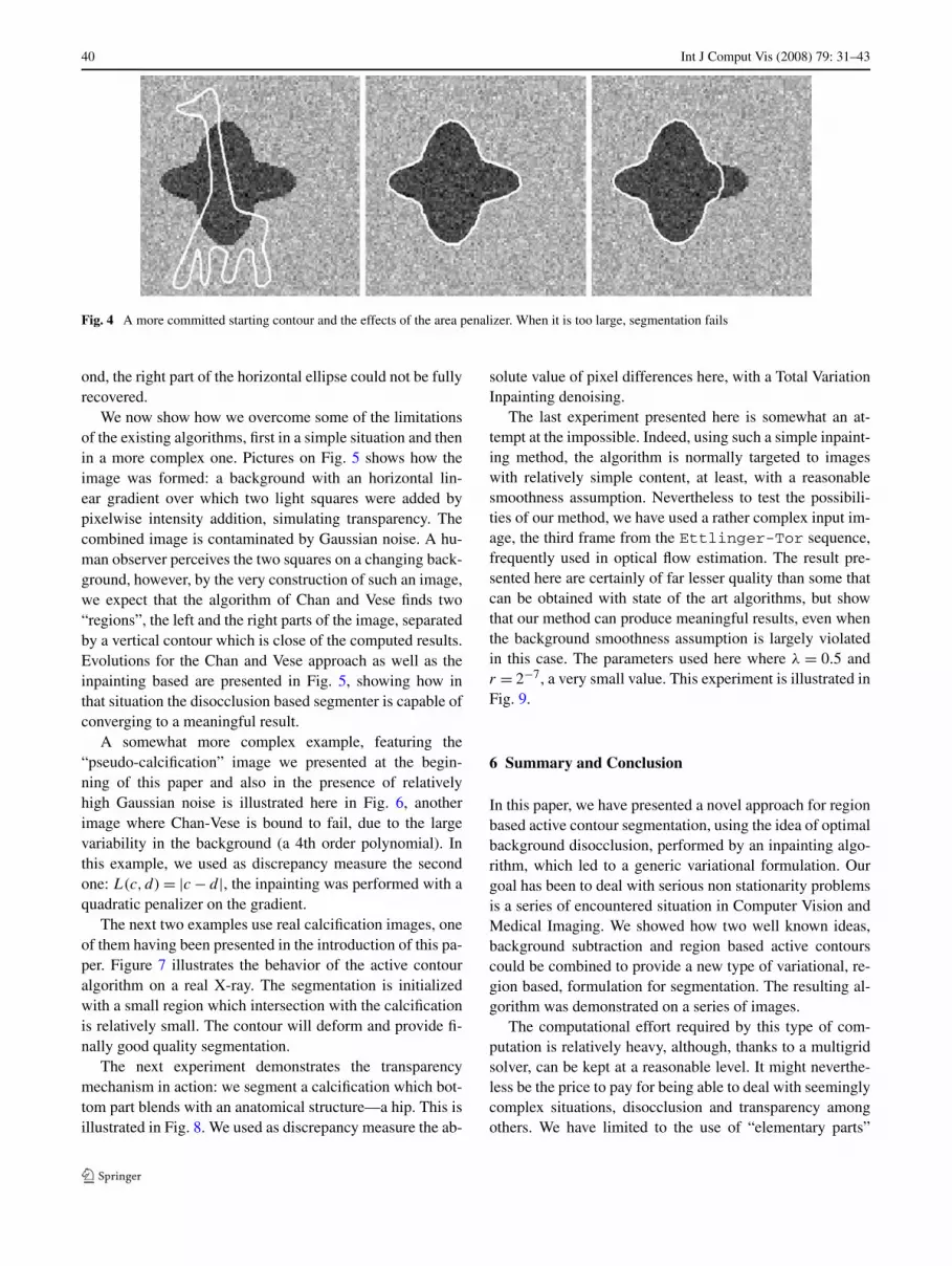
Figure 3 shows a dark non convex object on a light back-ground with 30% added Gaussian noise. In this experiment,λ = 0.1, r = 0.55. The first row shows a snapshot of thecontour evolution at iterations 1, 10, 20 and 30, the secondrow shows the corresponding domains. We re-did the pre-vious experiment with a more “committed” initialization. Itillustrates some stability with respect to the initial contour,as well as the role of the area penalizer exponent r in |�|rand is illustrated in Fig. 4. We ran two experiments, the firstwith a value of r = 0.55, as in the previous case and the sec-ond with a value of r = 0.60. In both cases, the λ weight inthe data versus inpainting was set to 0.1. In the first case,a correct segmentation has been achieved, while in the sec-

Fig. 3 Segmenting a non convex object, starting from an uncommitted guess

40 Int J Comput Vis (2008) 79: 31–43

Fig. 4 A more committed starting contour and the effects of the area penalizer. When it is too large, segmentation fails

ond, the right part of the horizontal ellipse could not be fullyrecovered.

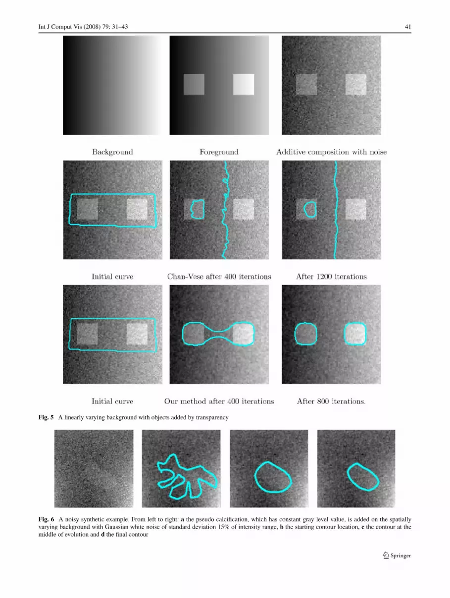
We now show how we overcome some of the limitationsof the existing algorithms, first in a simple situation and thenin a more complex one. Pictures on Fig. 5 shows how theimage was formed: a background with an horizontal lin-ear gradient over which two light squares were added bypixelwise intensity addition, simulating transparency. Thecombined image is contaminated by Gaussian noise. A hu-man observer perceives the two squares on a changing back-ground, however, by the very construction of such an image,we expect that the algorithm of Chan and Vese finds two“regions”, the left and the right parts of the image, separatedby a vertical contour which is close of the computed results.Evolutions for the Chan and Vese approach as well as theinpainting based are presented in Fig. 5, showing how inthat situation the disocclusion based segmenter is capable ofconverging to a meaningful result.

A somewhat more complex example, featuring the“pseudo-calcification” image we presented at the begin-ning of this paper and also in the presence of relativelyhigh Gaussian noise is illustrated here in Fig. 6, anotherimage where Chan-Vese is bound to fail, due to the largevariability in the background (a 4th order polynomial). Inthis example, we used as discrepancy measure the secondone: L(c, d) = |c − d|, the inpainting was performed with aquadratic penalizer on the gradient.

The next two examples use real calcification images, oneof them having been presented in the introduction of this pa-per. Figure 7 illustrates the behavior of the active contouralgorithm on a real X-ray. The segmentation is initializedwith a small region which intersection with the calcificationis relatively small. The contour will deform and provide fi-nally good quality segmentation.

The next experiment demonstrates the transparencymechanism in action: we segment a calcification which bot-tom part blends with an anatomical structure—a hip. This isillustrated in Fig. 8. We used as discrepancy measure the ab-

solute value of pixel differences here, with a Total VariationInpainting denoising.

The last experiment presented here is somewhat an at-tempt at the impossible. Indeed, using such a simple inpaint-ing method, the algorithm is normally targeted to imageswith relatively simple content, at least, with a reasonablesmoothness assumption. Nevertheless to test the possibili-ties of our method, we have used a rather complex input im-age, the third frame from the Ettlinger-Tor sequence,frequently used in optical flow estimation. The result pre-sented here are certainly of far lesser quality than some thatcan be obtained with state of the art algorithms, but showthat our method can produce meaningful results, even whenthe background smoothness assumption is largely violatedin this case. The parameters used here where λ = 0.5 andr = 2−7, a very small value. This experiment is illustrated inFig. 9.

6 Summary and Conclusion

In this paper, we have presented a novel approach for regionbased active contour segmentation, using the idea of optimalbackground disocclusion, performed by an inpainting algo-rithm, which led to a generic variational formulation. Ourgoal has been to deal with serious non stationarity problemsis a series of encountered situation in Computer Vision andMedical Imaging. We showed how two well known ideas,background subtraction and region based active contourscould be combined to provide a new type of variational, re-gion based, formulation for segmentation. The resulting al-gorithm was demonstrated on a series of images.

The computational effort required by this type of com-putation is relatively heavy, although, thanks to a multigridsolver, can be kept at a reasonable level. It might neverthe-less be the price to pay for being able to deal with seeminglycomplex situations, disocclusion and transparency amongothers. We have limited to the use of “elementary parts”

Int J Comput Vis (2008) 79: 31–43 41

Fig. 5 A linearly varying background with objects added by transparency

Fig. 6 A noisy synthetic example. From left to right: a the pseudo calcification, which has constant gray level value, is added on the spatiallyvarying background with Gaussian white noise of standard deviation 15% of intensity range, b the starting contour location, c the contour at themiddle of evolution and d the final contour

42 Int J Comput Vis (2008) 79: 31–43

Fig. 7 Evolution of the active contour in a real X-ray. a A subimage of the original X-ray (inverted), b the starting contour, with only small overlapwith the calcific deposit. c The contour has “entered” the calcific deposit and start growing, d the final segmentation

Fig. 8 Evolution of the active contour in a real X-ray: the use of TV inpainting in the background subtraction allows for reconstruction of thehip with in turns provides a subimage of the original X-ray (inverted), b the starting contour, with only small overlap over the hip. c The contour“progresses” on both parts of the hip and d the final segmentation

Fig. 9 Can we segment Ettlinger Tor’s bus? Using the total variation inpainting. Many difficulties are due to the presence of 1D structures, whichare arguably not compatible with the bounded variation assumption on the background image

in constructing our disocclusion measure, we could con-sider more advanced region based segmentations instead ofthe Chan-Vese model, as well as more complex inpaint-ing procedures. One could use more sophisticated inpaint-ings such as Elastica based ones (Ballester et al. 2001;Chan and Shen 2002), but the resulting Euler-Lagrange andAdjoint State equations become much more complex andtime consuming to solve.

We are currently working on specializing this approachwhere either more prior knowledge is available on the ob-jects to be segmented or more on the data is known.

Acknowledgements The Ettlinger-Tor sequence is copyright(C) 1998 by H.H. Nagel, KOGS/IAKS Universität Karlsruhe. The cal-

cification images presented here are courtesy of the Center For Clinicaland Basic Research (CCBR) A/S, Ballerup, Denmark.

References

Aubert, G., & Kornprobst, P. (2006). Applied mathematical sciences:Vol. 147, Mathematical problems in image processing: partial dif-ferential equations and the calculus of variations, 2nd edn. NewYork: Springer.

Aubert, G., Barlaud, M., Jehan-Besson, S., & Faugeras, O. (2003). Im-age segmentation using active contours: calculus of variations orshape gradients? SIAM Journal of Applied Mathematics, 63(6),2128–2154.

Ballester, C., Bertalmio, M., Caselles, V., Sapiro, G., & Verdera, J.(2001). Filling-in by joint interpolation of vector fields and gray

Int J Comput Vis (2008) 79: 31–43 43

levels. IEEE Transactions on Image Processing, 10(8), 1200–1211.

Bruhn, A., Weickert, J., Feddern, C., Kohlberger, T., & Schnörr, C.(2005). Variational optical flow computation in real time. IEEETransactions on Image Processing, 14(5), 608–615.

Caselles, V., Kimmel, R., & Sapiro, G. (1995). Geodesic active con-tours. In Proceedings of the 5th international conference on com-puter vision (pp. 694–699). Boston, MA, June 1995. Los Alami-tos: IEEE Computer Society Press.

Chan, T., & Shen, J. (2002). Mathematical models for local nontextureinpainting. SIAM Journal of Applied Mathematics, 62(3), 1019–1043.

Chan, T., & Vese, L. (2001). Active contours without edges. IEEETransactions on Image Processing, 10(2), 266–277.

Cohen, L. D., & Cohen, I. (1993). Finite-element methods for ac-tive contour models and balloons for 2-D and 3-D images.IEEE Transactions on Pattern Analysis and Machine Intelligence,15(11), 1131–1147.

Cohen, L. D., Bardinet, E., & Ayache, N. (1993). Surface reconstruc-tion using active contour models. In SPIE conference on geomet-ric methods in computer vision, San Diego, CA, USA.

Cremers, D., Rousson, M., & Deriche, R. (2007). A review of statisticalapproaches to level set segmentation: integrating color, texture,motion and shape. The International Journal of Computer Vision,72(2), April.

Delfour, M. C., & Zolésio, J. P. (1989). Analyse des problèmes deforme par la dérivation des minimax. Annales de l’Institut HenriPoincaré, Section C, S6, 211–227.

Delfour, M. C., & Zolésio, J.-P. (2001). Shapes and geometries. Ad-vances in design and control. Philadelphia: SIAM.

Griewank, A., Juedes, D., & Utke, J. (1996). ADOL–C, a packagefor the automatic differentiation of algorithms written in C/C++.ACM Transactions on Mathematical Software, 22(2), 131–167.

Gunzburger, M. (2001). Adjoint equation-based methods for controlproblems in incompressible, viscous flows. Flow, Turbulence andCombustion, 65, 249–272.

Heiler, M., & Schnörr, C. (2005). Natural image statistics for naturalimage segmentation. The International Journal of Computer Vi-sion, 63(1), 5–19.

Jehan-Besson, S., Barlaud, M., & Aubert, G. (2003). DREAM2S: de-formable regions driven by an Eulerian accurate minimizationmethod for image and video segmentation. The InternationalJournal of Computer Vision, 53(1), 45–70.

Kass, M., Witkin, A., & Terzopoulos, D. (1987). Snakes: active con-tour models. In First international conference on computer vision(pp. 259–268), London, June 1987.

Kichenassamy, S., Kumar, A., Olver, P., Tannenbaum, A., & Yezzi, A.(1995). Gradient flows and geometric active contour models. InProceedings of the 5th international conference on computer vi-sion (pp. 810–815). Boston, MA, June 1995. Los Alamitos: IEEEComputer Society Press.

Kim, J., Fisher III, J. W., Yezzi, A., Çetin, M., & Willsky, A. S. (2005).A nonparametric statistical method for image segmentation us-ing information theory and curve evolution. IEEE Transactionson Image Processing, 14(10), 1486–1502.

Lauze, F., & de Bruijne, M. (2007). Toward automated detectionand segmentation of aortic calcifications from radiographs. InJ. Pluim & J.M. Reinhardt (Eds.), Medical imaging—SPIE proc-SPIE (Vol. 6512), SPIE press.

Lauze, F., & Nielsen, M. (2005). From inpainting to active contours. InN. Paragios et al. (Eds.) LNCS: Vol. 3752. Proceedings of the thirdIEEE workshop on variational, geometric and level set methodsin computer vision, Bejing, China, October 2005 (pp. 97–108).New York: Springer.

Lions, J. L. (1971). Optimal control of systems governed by partialdifferential equations (trans: Mitter, S. K.). New York: Springer.

Mumford, D., & Shah, J. (1989). Optimal approximations by piecewisesmooth functions and associated variational problems. Communi-cations on Pure and Applied Mathematics, 42, 577–684.

Ohta, N. (2001). A statistical approach to background substraction forsurveillance systems. In International conference on computer vi-sion (Vol. 2, pp. 481–486). Vancouver, BC, CA, July 2001.

Osher, S., & Paragios, N. (2003). Geometric level set methods in imag-ing, vision and graphics. New York: Springer.

Paragios, N., & Deriche, R. (2002). Geodesic active regions: a new par-adigm to deal with frame partition problems in computer vision.Journal of Visual Communication and Image Representation, Spe-cial Issue on Partial Differential Equations in Image Processing,Computer Vision and Computer Graphics, 13(1/2), 249–268.

Ronfard, R. (1994). Region based strategies for active contour models.The International Journal of Computer Vision, 13(2), 229–251.

Rostaing, N., Dalmas, S., & Galligo, A. (1993). Automatic differentia-tion in Odyssée. Tellus, 45(5), 558–568.

Roy, T., Debreuve, E., Barlaud, M., & Aubert, G. (2006). Segmenta-tion of a vector field: dominant parameter and shape optimization.Journal of Mathematical Imaging and Vision, 24(2), 259–276.

Rybak, I. V. (2004). Monotone and conservative difference schemesfor elliptic equations with mixed derivatives. Mathematical Mod-elling and Analysis, 9(2), 169–178.

Sethian, J. A. (1999). Level set methods and fast marching methods:evolving interfaces in computational geometry, fluid mechanics,computer vision, and materials sciences. Cambridge monographon applied and computational mathematics. Cambridge: Cam-bridge University Press.

Ta’asan, S. (1997). Lecture notes on optimization. 1. Introduction toshape design and control (Technical report). Von Karman In-stitue.

Xu, C., & Prince, J. L. (1997). Gradient vector flow: a new externalforce for snakes. In International conference on computer visionand pattern recognition (p. 66).