modeling oil and petroleum evaporation

www.jpsr.org Journal of Petroleum Science Research (JPSR) Volume 2 Issue 3, July 2013

104

Modeling Oil and Petroleum Evaporation Merv F. Fingas

Spill Science

1717 Rutherford Point, S.W., Edmonton, AB, Canada T6W 1J6

*[email protected]

Abstract

Evaporation is an important component in oil spill models.

Various approaches for oil evaporation prediction are

summarized. Models can be divided into those models that

use the basis of air‐boundary‐regulation or those that use

liquid diffusion‐regulated evaporation physics. Studies

show that oil is not air boundary‐layer regulated such as it is

for water evaporation, which implies that a simplistic

evaporation equation suffices to accurately describe the

process. The following processes do not require

consideration: wind velocity, turbulence level, area and scale

size. The factors important to evaporation are time and

temperature. Oil evaporation does show a thickness effect,

although not as pronounced as that for air‐boundary‐layer

regulated models. A thickness adjustment calculation is

presented for diffusion‐regulated models. This new model is

applicable to thicknesses greater than about 1.5 mm. In the

case of thin slicks, this adjustment is not relevant as oils

typically spread to less than that in a short time.

The use of air‐boundary‐models results in three types of

errors: air‐boundary‐layer models cannot accurately deal

with long term evaporation; second, the wind factor results

in unrealistic values and finally, they have not been adjusted

for the different curvature for diesel‐like evaporation.

Further, these semi‐empirical equations require inputs such

as area, etc., that are unknown at the time of the spills. There

has been some effort on the part of modellers to adjust air‐

boundary‐layer models to be more realistic on the long‐term,

but these may be artificial and result in other errors such as

under‐estimation for long‐term prediction. A comparison of

models shows that on a very short term, such as a few hours,

most models yield similar results. However, as time

increases past a few days, the errors with air‐boundary‐layer

regulated models are unacceptable. Examples are given

where errors are as large as 100% over a few days.

Keywords

Oil Spill Evaporation; Hydrocarbon Evaporation; Evaporation

Modeling

Introduction

Evaporation is an important process for most oil spills.

Almost all oil spill models include evaporation as a

process and output of the model. Evaporation plays a

prime role in the fate of most oils. In a few days,

typical crude oils can lose up to 45% of their volume

(Fingas 2011). The Deepwater Horizon oil lost up to

55% in a short time when released under water at high

pressure. Many crude oils must undergo evaporation

before the formation of water‐in‐oil emulsions. Light

oils will change very dramatically from fluid to

viscous; while heavy oils will become solid‐like. Many

oils after long evaporative exposure, form tar balls or

heavy tar mats. Despite the importance of the process,

only some work has been conducted on the basic

physics and chemistry of oil spill evaporation (Fingas

1995). The difficulty in studying oil evaporation is that

oil is a mixture of hundreds of compounds and oil

composition varies from source to source and even

over time. Much of the work described in the previous

literature focused on calibrating equations developed

for water evaporation (Fingas 1995).

The mechanisms that regulate evaporation are

important (Brutsaert 1995; Jones 1992). Evaporation of

a liquid can be considered as the movement of

molecules from the surface into the vapour phase

above it. The immediate layer of air above the

evaporation surface is known as the air boundary

layer5 which is the intermediate interface between the

air and the liquid and might be viewed as very thin e.g.

as less than 1 mm. The characteristics of this air

boundary layer can influence evaporation. In the case

of water, the boundary layer regulates the evaporation

rate. Air can hold a variable amount of water,

depending on temperature, as expressed by the

relative humidity. Under conditions where the air

boundary layer doesn’t move (no wind) or has low

turbulence, the air immediately above the water

quickly becomes saturated and evaporation slows. The

actual evaporation of water proceeds at a small

fraction of the possible evaporation rate because of the

saturation of the boundary layer. The air‐boundary‐

layer physics is then said to regulate the evaporation

of water. This regulation manifests the increase of

evaporation with wind or turbulence. When

Journal of Petroleum Science Research (JPSR) Volume 2 Issue 3, July 2013 www.jpsr.org

105

turbulence is weak, evaporation can slow down by

orders‐of‐magnitude. The molecular diffusion of water

molecules through air is at least 103 times slower than

turbulent diffusion (Monteith and Unsworth 2008).

Some liquids are not air‐boundary‐layer regulated

primarily because they evaporate too slowly to make

the vapours saturate the air boundary layer above

them (Fingas 2011). Many mixtures are regulated by

the diffusion of molecules inside the liquid to the

surface of the liquid. Such a mechanism is true for

many slowly‐evaporating mixtures of compounds

such as oils and fuels. Some of the outcomes of this

mechanism may seem counterintuitive to some people

such as that increasing area may not necessarily

increase evaporation rate. More importantly,

increasing wind speed does not increase evaporation.

Scientific work on water evaporation dates back

decades and thus the basis for early oil evaporation

work has been established (Fingas 2011). There are

several fundamental differences between the

evaporation of a pure liquid such as water and that of

a multi‐component system such as crude oil. The

evaporation rate for a single liquid such as water is a

constant with respect to time. Evaporative loss, either

by weight or volume, is not linear with time for crude

oils, and other multi‐component fuel mixtures (Fingas

1997).

Review of Historical Developments

For air‐boundary‐layer regulated liquids, one can

write the mass transfer rate in semi‐empirical form as

(Fingas 2011):

E = K C Tu S (1)

where E is the evaporation rate in mass per unit area,

K is the mass transfer rate of the evaporating liquid,

sometimes denoted as kg (gas phase mass transfer

coefficient, which may incorporate some of other

parameters noted here), C is the concentration (mass)

of the evaporating fluid as a mass per volume, Tu is a

factor characterizing the relative intensity of

turbulence, and S is a factor related to the saturation of

the boundary layer above the evaporating liquid. The

saturation parameter, S, represents the effects of local

advection on saturation dynamics. If the air has

already been saturated with the compound in question,

the evaporation rate approaches zero. This also relates

to the scale length of an evaporating pool. If one views

a large pool over which a wind is blowing, there is a

high probability that the air is saturated downwind

and the evaporation rate per unit area is lower than

that for a smaller pool. It is noted that there are many

equivalent ways to express this fundamental

evaporation equation. These will be seen in the

equations below.

Sutton proposed the following equation based on

empirical work (Brutsaert 1982):

E = K Cs

U7/9 d - 1/9 Sc- r (2)

where Cs is the concentration of the evaporating fluid

(mass/volume), U is the wind speed, d is the area of

the pool, Sc is the Schmidt number and r is the

empirical exponent assigned values from 0 to 2/3.

Other parameters are defined as above. The terms in

this equation are analogous to the very generic

equation, (1), proposed above. The turbulence is

expressed by a combination of the wind speed, U, and

the Schmidt number, Sc that is the ratio of kinematic

viscosity of air (ν) to the molecular diffusivity (D) of

the diffusing gas in air, i.e., a dimensionless expression

of the molecular diffusivity of the evaporating

substance in air.7 The coefficient of the wind power

typifies the turbulence level. The value of 0.78 (7/9) as

chosen by Sutton, represents a turbulent wind

whereas a coefficient of 0.5 would represent a wind

flow that is more laminar. The scale length

represented by d has been given an empirical

exponent of ‐1/9. This represents for water, a weak

dependence on size. The exponent of the Schmidt

number, r, represents the effect of the diffusivity of the

particular chemical, and historically was assigned

values between 0 and 2/3 (Sutton 1934).

Blokker was the first to develop oil evaporation

equations for oil evaporation at sea, with his partially

theoretical starting basis (Blokker, 1964). Oil was

presumed to be a one‐component liquid. The

distillation data and the average boiling points of

successive fractions were used as the starting point to

predict an overall vapour pressure. The average

vapour pressure of these fractions was then calculated

from the Clausius‐Clapeyron equation to yield:

logp

s

p=

qM

4.57

1

T-

1

Ts

(3)

where p is the vapour pressure at the absolute tem‐

perature, T; ps is the vapour pressure at the boiling

point, Ts (for ps, 760 mm Hg was used); q is the heat of

evaporation in cal/g and M is the molecular weight.

The term qM/(4.57 Ts) was taken to be nearly constant


106

for hydrocarbons (=5.0 +/‐ 0.2) and thus the expression

was simplified to

log ps /p = 5.0 [ (Ts ‐ T)/T] (4)

From the empirical data and equation (4), the

weathering curve was calculated, assuming that

Raoultʹs law is valid for this situation giving qM as a

function of the percentage evaporated. Pasquillʹs

equation was applied stepwise, and the total

evaporation time was obtained by summation:

where t is the total evaporation time in hours, Δh is the

decrease in layer thickness in m, D is the diameter of

the oil spill, β is a meteorological constant (assigned a

value of 0.11), Kev is a constant for atmospheric

stability (taken to be 1.2 x 10‐8), α is a meteorological

constant (assigned a value of 0.78), P is the vapour

pressure at the absolute temperature, T; and M is the

molecular weight of the component or oil mass. Tests

of this equation by experimental evaporation using a

small wind tunnel did not yield good correspondence

to test data.

Mackay and Matsugu (1973) approached evaporation

by using the classical water evaporation and

experimental work. The water evaporation equation

was corrected to hydrocarbons using the evaporation

rate of cumene. Data on the evaporation of water and

cumene have been used to correlate the gas phase

mass transfer coefficient as a function of wind‐speed

and pool size by the equation,

K m = 0.0292 U 0.78 X ‐0.11 Sc ‐0.67 (6)

Where Km is the mass transfer coefficient in units of

mass per unit time and X is the pool diameter or the

scale size of evaporating area. Note that the exponent

of the wind speed, U, is 0.78 equal to the classical

water evaporation‐derived coefficient. Mackay and

Matsugu noted that for hydrocarbon mixtures the

evaporation process is more complex, dependent on

the liquid diffusion resistance being present.9

Experimental data on gasoline evaporation were

compared with computed rates which showed some

deviations from the experimental values and

suggested the presence of a liquid‐phase mass‐transfer

resistance. The same group showed that the

evaporative loss of a mass of oil spilled can be

estimated using a mass transfer coefficient, Km, as

shown above (Goodwin et al. 1976). This approach

was investigated with some laboratory data and tested

against some known mass transfer conditions on the

sea Butler (1976) developed a model to examine

evaporation of specific hydrocarbon components. The

weathering rate was taken as proportional to the

equilibrium vapour pressure, P, of the compound and

to the fraction remaining:

dx/dt = ‐kP(x/xo) (7)

where x is the amount of a particular component of a

crude oil at time, t, xo is the amount of that same com‐

ponent present at the beginning of weathering (t = 0), k

is an empirical rate coefficient and P is the vapour

pressure of the chosen oil component.

Butler assumed that petroleum is a complicated

mixture of compounds, therefore P is not equal to the

vapour pressure of the pure compound, but neither

would there be large variation in the activity

coefficient as the weathering process occurs (Butler

1976). For this reason, the activity coefficients were

subsumed in the empirical rate coefficient k. P and k

were taken as independent of the amount, x, for a

fairly wide range of oils. The equation was then

directly integrated to give the fraction of the original

compound remaining after weathering as:

x/xo = exp(‐ktP/xo) (8)

The vapour pressure of individual components was fit

using a regression line to yield a predictor equation for

vapour pressure:

P = exp(10.94 ‐ 1.06 N) (9)

where P is the vapour pressure in Torr and N is the

carbon number of the compound in question. This

combined with equation (8) and yielded the following

expression:

x/xo = exp [‐(kt/xo)exp(10.94 ‐ 1.06 N)] (10)

Where x/xo is the fraction of the component left after

weathering, k is an empirical constant, xo is the

original quantity of the component and N is the

carbon number of the component in question.

Equation (10) predicts that the fraction weathered is a

function of the carbon number and decreases at a rate

that is faster than predicted from simple exponential

decay.12 If the initial distribution of compounds is

essentially uniform (xo independent of N), then the

above equation predicts that the carbon number where

a constant fraction (e.g. half) of the initial amount has

been lost (x = 0.5 xo) is a logarithmic function of the

time of weathering:

N1/2 = 10.66 + 2.17 log (kt/xo) (11)


107

where N1/2 is half of the volume fraction of the oil. The

equation was tested using evaporation data from some

patches of oil on shoreline, whose age was known. The

equation was capable of predicting the age of the

samples relatively well. It was suggested that the

equation was applicable to open water spills; however,

this was never subsequently applied in models.

Yang and Wang (1977) developed an equation using

the Mackay and Matsugu molecular diffusion

process.2 The vapour phase mass transfer process was

expressed as:

where Die is the vapour phase mass transfer rate, km is

a coefficient that lumps all the unknown factors

affecting the value of Die, pi is the hydrocarbon vapour

pressure of fraction, I, at the interface, pi∞ is the

hydrocarbon vapour pressure of fraction, I, at infinite

altitude of the atmosphere, R is the universal gas

constant and Ts is the absolute temperature of the oil

slick. The following functional relationship was

proposed (Yang and Wang 1977):

where A is the slick area, U is the over‐water wind

speed, and a, q and γ are empirical coefficients. This

relationship was based on the results of previous

studies, including, for instance, those of MacKay and

Matsugu who suggested the value of γ to be in the

range from ‐0.025 to ‐0.055.9 Further experiments were

performed by Yang and Wang to determine the values

of ‘a’ and ‘q’. Experiments showed that a film formed

on evaporating oils and this film severely retarded

evaporation. Before the surface film has developed

(ρt/ρo < 1.0078):

where Kmb is the coefficient that groups all factors

affecting evaporation before the surface film has

formed and A is the area. After the surface film has

developed (ρt/ρo > 1.0078)

Kma = 1/5 kmb (15)

where ρo is initial oil density, ρt is weathered oil

density at time t, and Kma is the coefficient that groups

all factors affecting evaporation after the surface film

has formed.12 The evaporation rate was found to be

reduced fivefold after the formation of the surface film.

Drivas (1982) compared the Mackay and Matsugu

equation with data found in the literature and noted

that the equations yielded predictions that were close

to the experimental data. Rheijnhart and Rose (1982)

developed a simple predictor model for the

evaporation of oil at sea and proposed the following

simple relationship:

Qei = αCo (16)

where Qei is the evaporation rate of the component of

interest, α is a constant incorporating wind velocity

and other factors (taken as 0.0009 m s‐1) and Co is the

equilibrium concentration of the vapour at the oil

surface. Several pan experiments were run to simulate

evaporation at sea and the data used to test the

equation. No method was given to calculate the

essential value, Co.

Brighton (1985,1990) proposed that the standard

formulation used by many workers required refining.

His starting point for water evaporation was similar to

that proposed by Sutton:

E = Km

Cs

U7/9 d1/9 Sc- r (17)

where E is the mean evaporation rate per unit area, Km

is an empirically‐determined constant, presumably

related to the foregoing mass transfer constant, Cs is

the concentration of the evaporation fluid

(mass/volume), d is the area of the pool and r is an

empirical exponent assigned values from 0 to 2/3.

Brighton suggested that this equation should conform

to the basic dimensionless form involving the

parameters U and Zo (wind speed and roughness

length, respectively) which define the boundary layer

conditions. The key factor in Brighton’s analysis was

to use a linear eddy‐diffusivity profile. This feature

implied that concentration profiles become

logarithmic near the surface, which is suspected to be

more realistic compared to the more finite values

previously used. Using a power profile to provide an

estimation of the turbulence, Brighton was able to

substitute the following identities into the classical

relationship:

Where: u* is the friction velocity, z1 is the reference

height above the surface, z0 is the roughness length

and n is the power law dimensionless term. The

evaporation equation now became:


108

where z is the height above the surface, Χ is the

concentration of the evaporating compounds, x is the

dimension of the evaporating pool, k given by K/u*z, is

the von Karman constant and σ is the turbulent

Schmidt number (taken as 0.85). Brighton

subsequently compared his model with experimental

evaporation data in the field and in the laboratory,

including laboratory oil evaporation data (Brighton

1985, 1990). The model only correlated well with

laboratory water evaporation data and the reason

given was other data sets were ‘noisy’.

Tkalin (1986) proposed a series of equations to predict

evaporation at sea:

Ei=

KaM

iP

oix

t

RT(21)

where Ei is the evaporation rate of component I (or the

sum of all components) (kg/m2s), Ka is the mass

transfer coefficient (m/s), Mi is the molecular weight,

Poi is the vapour pressure of the component I, and xt is

the amount of component I at time, t. Using empirical

data, relationships were developed for some of the

factors in the equation:

Poi = 103eA (22)

where A = ‐(4.4 + logTb)[1.803{Tb/T ‐ 1} ‐ 0.803 ln(Tb/T)]

(23)

and where Tb is the boiling point of the hydrocarbon,

given as

Ka = 1.25U10‐3 (24)

The equations were verified using empirical data from

the literature.

A frequently used work in older spill modelling is that

of Stiver and Mackay (1984)based on some of the

earlier work of Mackay and Matsugu (1973). The

formulation was initiated with assumptions on the

evaporation of a liquid. If a liquid is spilled, the rate of

evaporation is given as:

N = KAP/(RT) (25)

where N is the evaporative molar flux (mol/s), K is the

mass transfer coefficient under the prevailing wind

(ms‐1) and A is the area (m2), P is the vapour pressure

of the bulk liquid. This equation was arranged to give:

dFv/dt = KAPν/(VoRT) (26)

where Fv is the volume fraction evaporated, v is the

liquidʹs molar volume (m3/mol) and Vo is the initial

volume of spilled liquid (m3). By rearranging:

dFv = [Pν/(RT)](KAdt/Vo) (27)

or dFv = Hdθ (28)

where H is Henryʹs law constant and θ is the

evaporative exposure (defined below).

The right‐hand side of the second last equation has

been separated into two dimensionless groups (Stiver

and MacKay 1984). The group, KAdt/Vo, represents

the time‐rate of what has been termed as the

“evaporative exposure” and was denoted as dθ. The

evaporative exposure is a function of time, the spill

area and volume (or thickness), and the mass transfer

coefficient (which is dependent on the wind speed).

The evaporative exposure can be viewed as the ratio of

exposed vapour volume to the initial liquid volume.18

The group Pν/(RT) or H is a dimensionless

Henryʹs law constant or ratio of the equilibrium

concentration of the substance in the vapour phase

[P/(RT)] to that in the liquid (l/ν). H is a function of

temperature. The product θH is thus the ratio of the

amount which has evaporated (oil concentration in

vapour times vapour volume) to the amount originally

present. For a pure liquid, H is independent of Fv and

equation 26 was integrated directly to give:

Fv = H θ (29)

If K, A, and temperature are constant, the evaporation

rate is constant and evaporation is complete (Fv is

unity) when θ achieves a value of 1/H.

If the liquid is a mixture, H depends on Fv and the

basic equation can only be integrated if H is expressed

as a function of Fv; i.e., the principal variable of vapour

pressure is expressed as a function of composition.

The evaporation rate slows as evaporation proceeds in

such cases. Equation (27) was replaced with a new

equation developed using laboratory empirical data:

Fv = (T/K1) ln (1 + K1θ/T) exp(K2 ‐ K3/T) (30)

where Fv is the volume fraction evaporated and K1,2,3

are empirical constants.18 A value for K1 was obtained

from the slope of the Fv vs. log θ curve from pan or

bubble evaporation experiments. For θ greater than

104, K1 was found to be approximately 2.3T divided by

the slope. The expression exp(K2 ‐ K3/T) was then

calculated, and K2 and K3 were determined

individually from evaporation curves at two different

temperatures.

Hamoda and co‐workers (1989) performed theoretical

and experimental work on evaporation. An equation


109

was developed to express the effects of APIo

(American Petroleum Institute gravity‐a unit of

density) of the crude oil, temperature, and salinity on

the mass transfer coefficient K:

K = 1.68 x 10‐5 (APIo)1.253 (T)1.80 e0.1441 (31)

where K is the mass transfer coefficient, cm h‐1, APIo is

the density in API units, unitless, and e is the water

salinity in degrees salinity or parts‐per‐thousand. The

exponents of the equation were determined by

multiple linear regression on experimental data.

Quinn and co‐workers (1990) weathered oils in a

controlled environment and correlated the data with

equations developed starting with Fickʹs diffusion law

and the Clausius‐Clapeyron equation. Crude oil was

divided into a series of pseudo fractions by boiling

point. Each fraction was taken to be equivalent to an n‐

paraffin. The n‐paraffin distributions of a number of

naturally weathered crude oils were determined by

capillary gas‐liquid chromatography. The actual

measured evaporation was compared with those

generated by computer simulation of weathering.

Bobra (1992) conducted laboratory studies on the

evaporation of crude oils. The evaporation curves for

several crude oils and petroleum products were

measured under several different environmental

conditions. These data were compared to the equation

developed by Stiver and Mackay (1984). The equation

used was:

FV = ln[1 + B(TG/T) θ exp(A ‐ B To/T)] {T/BTG} (32)

where FV is the fraction evaporated, TG is the gradient

of the modified distillation curve, A and B are

dimensionless constants, To is initial boiling point of

the oil and θ is the evaporative exposure as previously

defined. The constants for the above equation and the

results from several comparison runs were carried

out.21 The agreement between the experimental data

and the equation results were poor in most cases. This

comparison showed that the Stiver and Mackay

equation predicts the evaporation of most oils

relatively well until time approaches 8 hours, after that

it over‐predicted the evaporation. The ʹovershootʹ

could be as much as 10% evaporative loss at the 24‐

hour mark. This is especially true for very light oils.

The Stiver and Mackay equation was also found to

under‐predict or over‐predict the evaporation of oils

in the initial phases. Bobra also noted that most oil

evaporation follows a logarithmic curve with time and

that a simple approach to this was much more

accurate than using equation (30).

In summary, it is difficult to develop a theoretical

approach to oil evaporation for several reasons. First,

oil consists of many components and thus there is no

constant boiling point, vapor pressure or other

essential properties used in typical evaporation

models. Further, oil evaporation proceeds by diffusion

regulation but not by air‐boundary‐layer regulation.

Water evaporation models cannot be accurately

modified to oil evaporation for these reasons.

Development of Diffusion-Rgulated Models

The review of the predictive and theoretical work in

section 2 above reveals those air‐boundary‐layer

concepts that are limited and cannot accurately

explain long‐term evaporation. Fingas conducted a

series of experiments over several years to examine the

concepts (Fingas 1998, 2011).

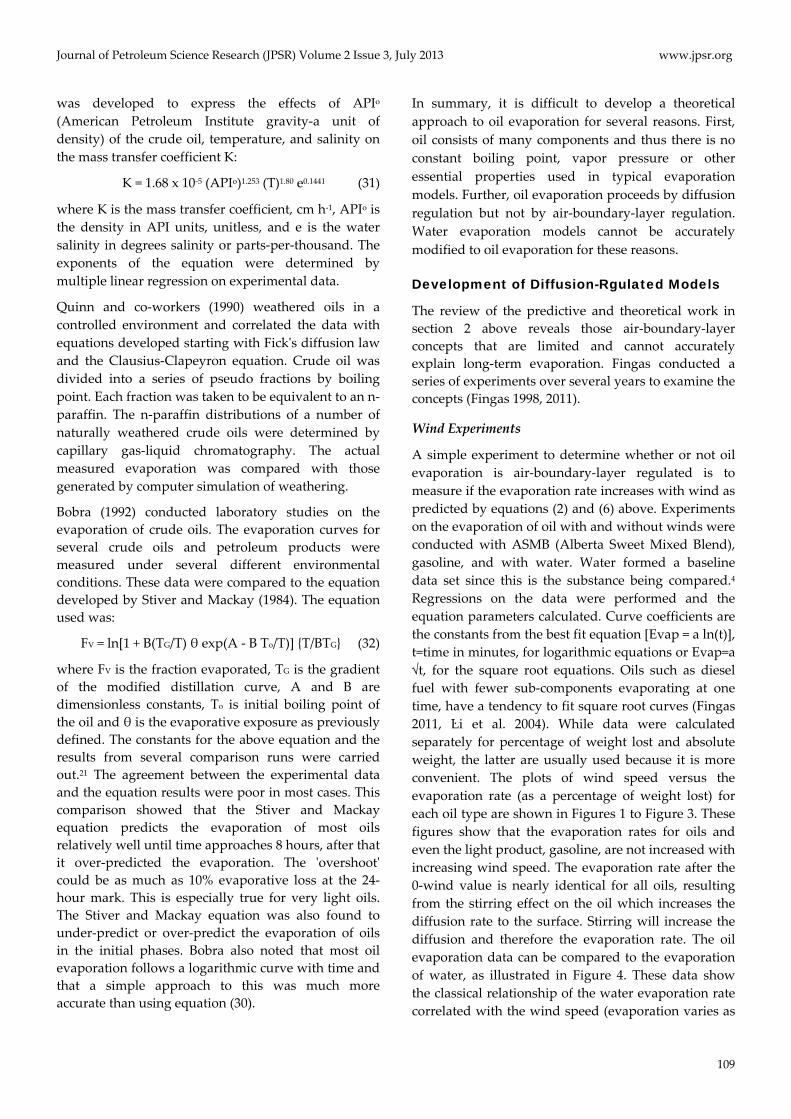
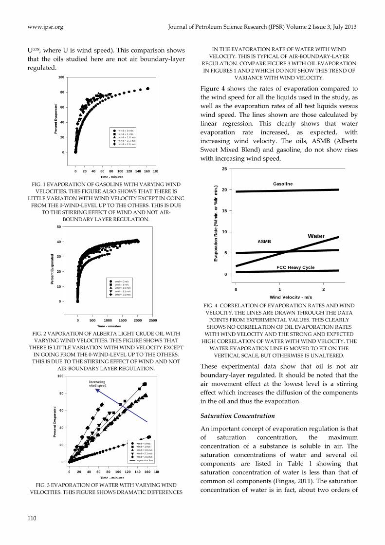
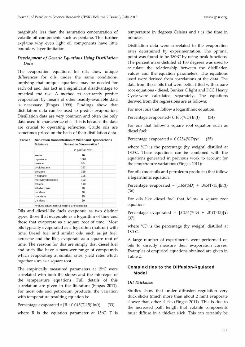
Wind Experiments

A simple experiment to determine whether or not oil

evaporation is air‐boundary‐layer regulated is to

measure if the evaporation rate increases with wind as

predicted by equations (2) and (6) above. Experiments

on the evaporation of oil with and without winds were

conducted with ASMB (Alberta Sweet Mixed Blend),

gasoline, and with water. Water formed a baseline

data set since this is the substance being compared.4

Regressions on the data were performed and the

equation parameters calculated. Curve coefficients are

the constants from the best fit equation [Evap = a ln(t)],

t=time in minutes, for logarithmic equations or Evap=a

√t, for the square root equations. Oils such as diesel

fuel with fewer sub‐components evaporating at one

time, have a tendency to fit square root curves (Fingas

2011, Ŀi et al. 2004). While data were calculated

separately for percentage of weight lost and absolute

weight, the latter are usually used because it is more

convenient. The plots of wind speed versus the

evaporation rate (as a percentage of weight lost) for

each oil type are shown in Figures 1 to Figure 3. These

figures show that the evaporation rates for oils and

even the light product, gasoline, are not increased with

increasing wind speed. The evaporation rate after the

0‐wind value is nearly identical for all oils, resulting

from the stirring effect on the oil which increases the

diffusion rate to the surface. Stirring will increase the

diffusion and therefore the evaporation rate. The oil

evaporation data can be compared to the evaporation

of water, as illustrated in Figure 4. These data show

the classical relationship of the water evaporation rate

correlated with the wind speed (evaporation varies as


110

U0.78, where U is wind speed). This comparison shows

that the oils studied here are not air boundary‐layer

regulated.

Time - minutes

0 20 40 60 80 100 120 140 160 180

Pe

rce

ntE

vap

ora

ted

0

20

40

60

80

100

wind = 0 m/s

wind = 1 m/swind = 1 .6 m/s

wind = 2 .1 m/s

wind = 2 .6 m/s

FIG. 1 EVAPORATION OF GASOLINE WITH VARYING WIND

VELOCITIES. THIS FIGURE ALSO SHOWS THAT THERE IS

LITTLE VARIATION WITH WIND VELOCITY EXCEPT IN GOING

FROM THE 0‐WIND‐LEVEL UP TO THE OTHERS. THIS IS DUE

TO THE STIRRING EFFECT OF WIND AND NOT AIR‐

BOUNDARY LAYER REGULATION.

Time - minutes

0 500 1000 1500 2000 2500

Perc

entE

vap

orat

ed

0

10

20

30

40

50

wind = 0 m/swind = 1 m/swind = 1.6 m/s

wind = 2.1 m/swind = 2.6 m/s

FIG. 2 VAPORATION OF ALBERTA LIGHT CRUDE OIL WITH

VARYING WIND VELOCITIES. THIS FIGURE SHOWS THAT

THERE IS LITTLE VARIATION WITH WIND VELOCITY EXCEPT

IN GOING FROM THE 0‐WIND‐LEVEL UP TO THE OTHERS.

THIS IS DUE TO THE STIRRING EFFECT OF WIND AND NOT

AIR‐BOUNDARY LAYER REGULATION.

Time - minutes

0 20 40 60 80 100 120 140 160 180

Pe

rce

ntE

vap

orat

ed

0

20

40

60

80

100

wind = 0 m/swind = 1 m/s

wind = 1.6 m/s

wind = 2.1 m/s

wind = 2.6 m/s

regression line

Increasingwind speed

FIG. 3 EVAPORATION OF WATER WITH VARYING WIND

VELOCITIES. THIS FIGURE SHOWS DRAMATIC DIFFERENCES

IN THE EVAPORATION RATE OF WATER WITH WIND

VELOCITY. THIS IS TYPICAL OF AIR‐BOUNDARY‐LAYER

REGULATION. COMPARE FIGURE 3 WITH OIL EVAPORATION

IN FIGURES 1 AND 2 WHICH DO NOT SHOW THIS TREND OF

VARIANCE WITH WIND VELOCITY.

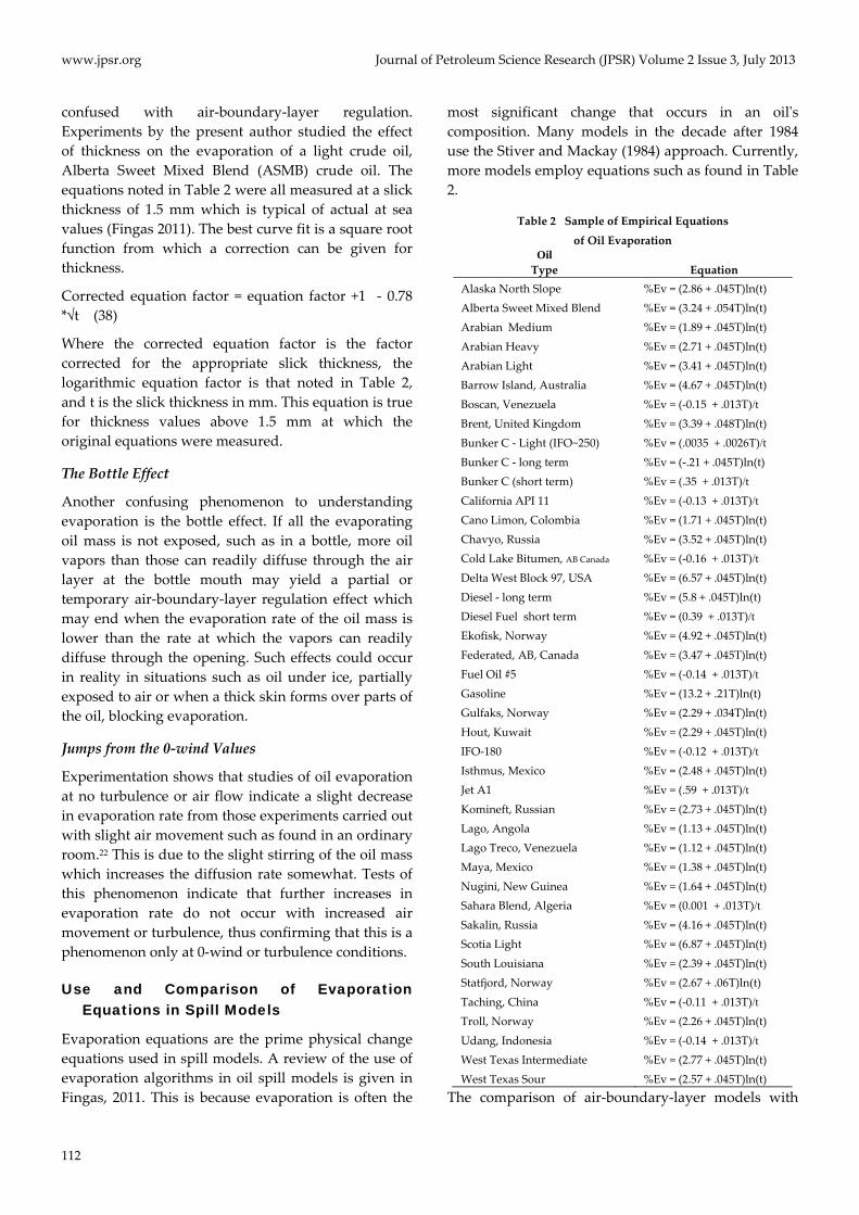
Figure 4 shows the rates of evaporation compared to

the wind speed for all the liquids used in the study, as

well as the evaporation rates of all test liquids versus

wind speed. The lines shown are those calculated by

linear regression. This clearly shows that water

evaporation rate increased, as expected, with

increasing wind velocity. The oils, ASMB (Alberta

Sweet Mixed Blend) and gasoline, do not show rises

with increasing wind speed.

Wind Velocity - m/s

0 1 2

Eva

pora

tion

Rat

e(%

/min

.or

%/ln

min

.)

0

5

10

15

20

25

Water

Gasoline

FCC Heavy Cycle

ASMB

FIG. 4 CORRELATION OF EVAPORATION RATES AND WIND

VELOCITY. THE LINES ARE DRAWN THROUGH THE DATA

POINTS FROM EXPERIMENTAL VALUES. THIS CLEARLY

SHOWS NO CORRELATION OF OIL EVAPORATION RATES

WITH WIND VELOCITY AND THE STRONG AND EXPECTED

HIGH CORRELATION OF WATER WITH WIND VELOCITY. THE

WATER EVAPORATION LINE IS MOVED TO FIT ON THE

VERTICAL SCALE, BUT OTHERWISE IS UNALTERED.

These experimental data show that oil is not air

boundary‐layer regulated. It should be noted that the

air movement effect at the lowest level is a stirring

effect which increases the diffusion of the components

in the oil and thus the evaporation.

Saturation Concentration

An important concept of evaporation regulation is that

of saturation concentration, the maximum

concentration of a substance is soluble in air. The

saturation concentrations of water and several oil

components are listed in Table 1 showing that

saturation concentration of water is less than that of

common oil components (Fingas, 2011). The saturation

concentration of water is in fact, about two orders of


111

magnitude less than the saturation concentration of

volatile oil components such as pentane. This further

explains why even light oil components have little

boundary layer limitation.

Development of Generic Equations Using Distillation

Data

The evaporation equations for oils show unique

differences for oils under the same conditions,

implying that unique equations may be needed for

each oil and this fact is a significant disadvantage to

practical end use. A method to accurately predict

evaporation by means of other readily‐available data

is necessary (Fingas 1999). Findings show that

distillation data can be used to predict evaporation.

Distillation data are very common and often the only

data used to characterize oils. This is because the data

are crucial to operating refineries. Crude oils are

sometimes priced on the basis of their distillation data.

Table 1 Saturation Concentration of Water and HydrocarbonsSubstance Saturation Concentration *

in g/m3 at 25oC

water 20

n-pentane 1689

hexane 564

cyclohexane 357

benzene 319

n-heptane 196

methylcyclohexane 192

toluene 110

ethybenzene 40

p-xylene 38

m-xylene 35

o-xylene 29

*Values taken from Ullmann's Encyclopedia Oils and diesel‐like fuels evaporate as two distinct

types, those that evaporate as a logarithm of time and

those that evaporate as a square root of time.1 Most

oils typically evaporated as a logarithm (natural) with

time. Diesel fuel and similar oils, such as jet fuel,

kerosene and the like, evaporate as a square root of

time. The reasons for this are simply that diesel fuel

and such like have a narrower range of compounds

which evaporating at similar rates, yield rates which

together sum as a square root.

The empirically measured parameters at 15oC were

correlated with both the slopes and the intercepts of

the temperature equations. Full details of this

correlation are given in the literature (Fingas 2011).

For most oils and petroleum products, the variation

with temperature resulting equation is:

Percentage evaporated = [B + 0.045(T‐15)]ln(t) (33)

where B is the equation parameter at 15oC, T is

temperature in degrees Celsius and t is the time in

minutes.

Distillation data were correlated to the evaporation

rates determined by experimentation. The optimal

point was found to be 180oC by using peak functions.

The percent mass distilled at 180 degrees was used to

calculate the relationship between the distillation

values and the equation parameters. The equations

used were derived from correlations of the data. The

data from those oils that were better fitted with square

root equations ‐ diesel, Bunker C light and FCC Heavy

Cycle‐were calculated separately. The equations

derived from the regressions are as follows:

For most oils that follow a logarithmic equation:

Percentage evaporated= 0.165(%D) ln(t) (34)

For oils that follow a square root equation such as

diesel fuel:

Percentage evaporated = 0.0254(%D)√t (35)

where %D is the percentage (by weight) distilled at

180oC. These equations can be combined with the

equations generated in previous work to account for

the temperature variations (Fingas 2011):

For oils (most oils and petroleum products) that follow

a logarithmic equation:

Percentage evaporated = [.165(%D) + .045(T‐15)]ln(t)

(36)

For oils like diesel fuel that follow a square root

equation:

Percentage evaporated = [.0254(%D) + .01(T‐15)]√t

(37)

where %D is the percentage (by weight) distilled at

180oC.

A large number of experiments were performed on

oils to directly measure their evaporation curves.

Examples of empirical equations obtained are given in

Table 2.

Complexities to the Diffusion-Rgulated Model

Oil Thickness

Studies show that under diffusion regulation very

thick slicks (much more than about 2 mm) evaporate

slower than other slicks (Fingas 2011). This is due to

the increased path length that volatile components

must diffuse in a thicker slick. This can certainly be


112

confused with air‐boundary‐layer regulation.

Experiments by the present author studied the effect

of thickness on the evaporation of a light crude oil,

Alberta Sweet Mixed Blend (ASMB) crude oil. The

equations noted in Table 2 were all measured at a slick

thickness of 1.5 mm which is typical of actual at sea

values (Fingas 2011). The best curve fit is a square root

function from which a correction can be given for

thickness.

Corrected equation factor = equation factor +1 ‐ 0.78

*√t (38)

Where the corrected equation factor is the factor

corrected for the appropriate slick thickness, the

logarithmic equation factor is that noted in Table 2,

and t is the slick thickness in mm. This equation is true

for thickness values above 1.5 mm at which the

original equations were measured.

The Bottle Effect

Another confusing phenomenon to understanding

evaporation is the bottle effect. If all the evaporating

oil mass is not exposed, such as in a bottle, more oil

vapors than those can readily diffuse through the air

layer at the bottle mouth may yield a partial or

temporary air‐boundary‐layer regulation effect which

may end when the evaporation rate of the oil mass is

lower than the rate at which the vapors can readily

diffuse through the opening. Such effects could occur

in reality in situations such as oil under ice, partially

exposed to air or when a thick skin forms over parts of

the oil, blocking evaporation.

Jumps from the 0‐wind Values

Experimentation shows that studies of oil evaporation

at no turbulence or air flow indicate a slight decrease

in evaporation rate from those experiments carried out

with slight air movement such as found in an ordinary

room.22 This is due to the slight stirring of the oil mass

which increases the diffusion rate somewhat. Tests of

this phenomenon indicate that further increases in

evaporation rate do not occur with increased air

movement or turbulence, thus confirming that this is a

phenomenon only at 0‐wind or turbulence conditions.

Use and Comparison of Evaporation Equations in Spill Models

Evaporation equations are the prime physical change

equations used in spill models. A review of the use of

evaporation algorithms in oil spill models is given in

Fingas, 2011. This is because evaporation is often the

most significant change that occurs in an oilʹs

composition. Many models in the decade after 1984

use the Stiver and Mackay (1984) approach. Currently,

more models employ equations such as found in Table

2.

Table 2 Sample of Empirical Equations

of Oil Evaporation Oil Type Equation

Alaska North Slope %Ev = (2.86 + .045T)ln(t)

Alberta Sweet Mixed Blend %Ev = (3.24 + .054T)ln(t)

Arabian Medium %Ev = (1.89 + .045T)ln(t)

Arabian Heavy %Ev = (2.71 + .045T)ln(t)

Arabian Light %Ev = (3.41 + .045T)ln(t)

Barrow Island, Australia %Ev = (4.67 + .045T)ln(t)

Boscan, Venezuela %Ev = (‐0.15 + .013T)t

Brent, United Kingdom %Ev = (3.39 + .048T)ln(t)

Bunker C ‐ Light (IFO~250) %Ev = (.0035 + .0026T)t

Bunker C ‐ long term %Ev = (‐.21 + .045T)ln(t)

Bunker C (short term) %Ev = (.35 + .013T)t

California API 11 %Ev = (‐0.13 + .013T)t

Cano Limon, Colombia %Ev = (1.71 + .045T)ln(t)

Chavyo, Russia %Ev = (3.52 + .045T)ln(t)

Cold Lake Bitumen, AB Canada %Ev = (‐0.16 + .013T)t

Delta West Block 97, USA %Ev = (6.57 + .045T)ln(t)

Diesel ‐ long term %Ev = (5.8 + .045T)ln(t)

Diesel Fuel short term %Ev = (0.39 + .013T)t

Ekofisk, Norway %Ev = (4.92 + .045T)ln(t)

Federated, AB, Canada %Ev = (3.47 + .045T)ln(t)

Fuel Oil #5 %Ev = (‐0.14 + .013T)t

Gasoline %Ev = (13.2 + .21T)ln(t)

Gulfaks, Norway %Ev = (2.29 + .034T)ln(t)

Hout, Kuwait %Ev = (2.29 + .045T)ln(t)

IFO‐180 %Ev = (‐0.12 + .013T)t

Isthmus, Mexico %Ev = (2.48 + .045T)ln(t)

Jet A1 %Ev = (.59 + .013T)t

Komineft, Russian %Ev = (2.73 + .045T)ln(t)

Lago, Angola %Ev = (1.13 + .045T)ln(t)

Lago Treco, Venezuela %Ev = (1.12 + .045T)ln(t)

Maya, Mexico %Ev = (1.38 + .045T)ln(t)

Nugini, New Guinea %Ev = (1.64 + .045T)ln(t)

Sahara Blend, Algeria %Ev = (0.001 + .013T)t

Sakalin, Russia %Ev = (4.16 + .045T)ln(t)

Scotia Light %Ev = (6.87 + .045T)ln(t)

South Louisiana %Ev = (2.39 + .045T)ln(t)

Statfjord, Norway %Ev = (2.67 + .06T)ln(t)

Taching, China %Ev = (‐0.11 + .013T)t

Troll, Norway %Ev = (2.26 + .045T)ln(t)

Udang, Indonesia %Ev = (‐0.14 + .013T)t

West Texas Intermediate %Ev = (2.77 + .045T)ln(t)

West Texas Sour %Ev = (2.57 + .045T)ln(t)

The comparison of air‐boundary‐layer models with


113

the empirical equations leads to some interesting

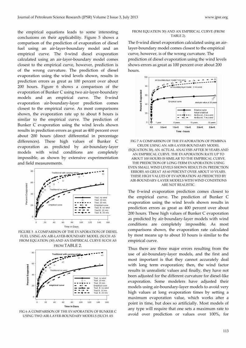
conclusions on their applicability. Figure 5 shows a

comparison of the prediction of evaporation of diesel

fuel using an air‐layer‐boundary model and an

empirical curve. The 0‐wind diesel evaporation

calculated using an air‐layer‐boundary model comes

closest to the empirical curve, however, prediction is

of the wrong curvature. The prediction of diesel

evaporation using the wind levels shown, results in

prediction errors as great as 100 percent over about

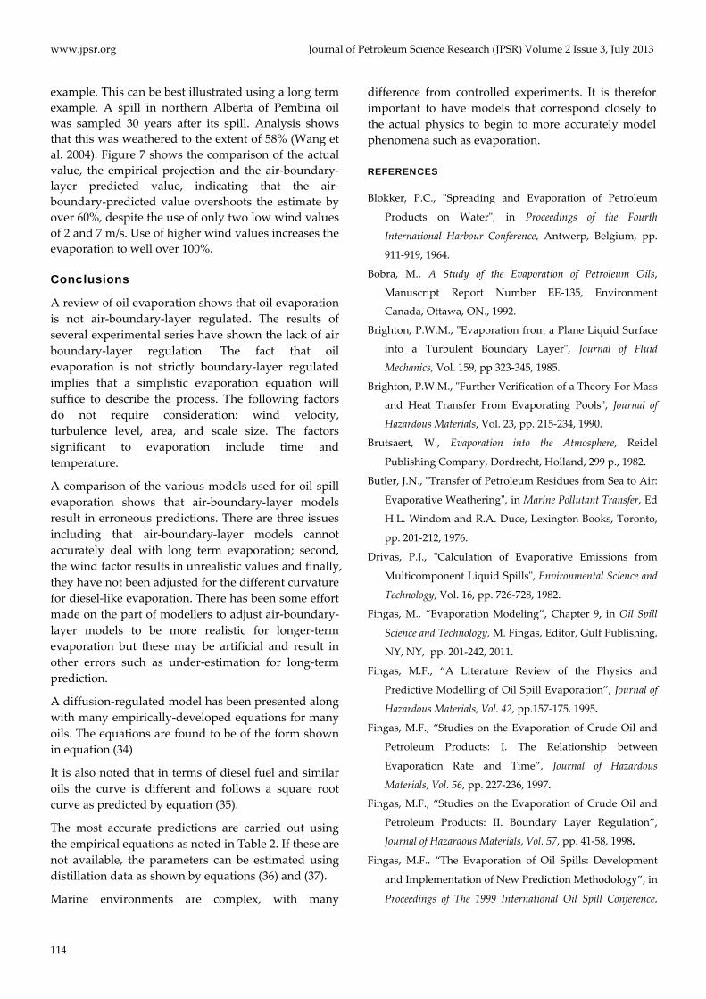
200 hours. Figure 6 shows a comparison of the

evaporation of Bunker C using two air‐layer‐boundary

models and an empirical curve. The 0‐wind

evaporation air‐boundary‐layer prediction comes

closest to the empirical curve. As most comparisons

shown, the evaporation rate up to about 8 hours is

similar to the empirical curve. The prediction of

Bunker C evaporation using the wind levels shown

results in prediction errors as great as 400 percent over

about 200 hours (direct differential in percentage

differences). These high values of Bunker C

evaporation as predicted by air‐boundary‐layer

models with wind conditions are completely

impossible, as shown by extensive experimentation

and field measurements.

Time in Days

0 20 40 60 80 100 120 140 160

Per

cen

tE

vapo

rate

d

0

20

40

60

80

Trad. no windTrad. 10 m/sTrad. 20 m/sEmpirical curveTrad. B. no windTrad B. 10 m/sTrad. B. 20 m/s

empirical curve

Traditional no wind

Traditional with varying winds

FIGURE 5 A COMPARISON OF THE EVAPORATION OF DIESEL

FUEL USING AN AIR‐LAYER‐BOUNDARY MODEL (SUCH AS

FROM EQUATION (30) AND AN EMPIRICAL CURVE SUCH AS

FROM TABLE 2.

Time in Days

0 20 40 60 80 100 120 140 160

Per

cen

tE

vapo

rate

d

0

20

40

60

80

Trad. no windTrad. 10 m/sTrad. 20 m/sEmpirical curveTrad. B. no windTrad B. 10 m/sTrad. B. 20 m/s

empirical curve

Traditional no wind

Traditional with varying winds

FIG 6 A COMPARISON OF THE EVAPORATION OF BUNKER C

USING TWO AIR‐LAYER‐BOUNDARY MODELS (SUCH AS

FROM EQUATION 30) AND AN EMPIRICAL CURVE (FROM

TABLE 2).

The 0‐wind diesel evaporation calculated using an air‐

layer‐boundary model comes closest to the empirical

curve, however, is of the wrong curvature. The

prediction of diesel evaporation using the wind levels

shows errors as great as 100 percent over about 200

hours.

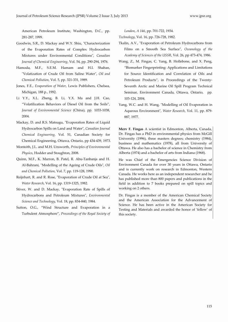
FIG 7 A COMPARISON OF THE EVAPORATION OF PEMBINA

CRUDE USING AN AIR‐LAYER‐BOUNDARY MODEL

(EQUATION 30), AN ACTUAL ANALYSIS AFTER 30 YEARS AND

AN EMPIRICAL CURVE. THE EVAPORATION RATE UP TO

ABOUT 100 HOURS IS SIMILAR TO THE EMPIRICAL CURVE.

THE PREDICTION OF LONG‐TERM EVAPORATION USING

EVEN SMALL WIND LEVELS SHOWN RESULTS IN PREDICTION

ERRORS AS GREAT AS 60 PERCENT OVER ABOUT 10 YEARS.

THESE HIGH VALUES OF EVAPORATION AS PREDICTED BY

AIR‐BOUNDARY‐LAYER MODELS WITH WIND CONDITIONS

ARE NOT REALISTIC.

The 0‐wind evaporation prediction comes closest to

the empirical curve. The prediction of Bunker C

evaporation using the wind levels shown results in

prediction errors as great as 400 percent over about

200 hours. These high values of Bunker C evaporation

as predicted by air‐boundary‐layer models with wind

conditions are completely impossible. As most

comparisons shown, the evaporation rate calculated

by most means up to about 10 hours is similar to the

empirical curve.

Thus there are three major errors resulting from the

use of air‐boundary‐layer models, and the first and

most important is that they cannot accurately deal

with long term evaporation; then, the wind factor

results in unrealistic values and finally, they have not

been adjusted for the different curvature for diesel‐like

evaporation. Some modelers have adjusted their

models using air‐boundary‐layer models to avoid very

high values at long evaporation times by setting a

maximum evaporation value, which works after a

point in time, but does so artificially. Most models of

any type will require that one sets a maximum rate to

avoid over prediction or values over 100%, for


114

example. This can be best illustrated using a long term

example. A spill in northern Alberta of Pembina oil

was sampled 30 years after its spill. Analysis shows

that this was weathered to the extent of 58% (Wang et

al. 2004). Figure 7 shows the comparison of the actual

value, the empirical projection and the air‐boundary‐

layer predicted value, indicating that the air‐

boundary‐predicted value overshoots the estimate by

over 60%, despite the use of only two low wind values

of 2 and 7 m/s. Use of higher wind values increases the

evaporation to well over 100%.

Conclusions

A review of oil evaporation shows that oil evaporation

is not air‐boundary‐layer regulated. The results of

several experimental series have shown the lack of air

boundary‐layer regulation. The fact that oil

evaporation is not strictly boundary‐layer regulated

implies that a simplistic evaporation equation will

suffice to describe the process. The following factors

do not require consideration: wind velocity,

turbulence level, area, and scale size. The factors

significant to evaporation include time and

temperature.

A comparison of the various models used for oil spill

evaporation shows that air‐boundary‐layer models

result in erroneous predictions. There are three issues

including that air‐boundary‐layer models cannot

accurately deal with long term evaporation; second,

the wind factor results in unrealistic values and finally,

they have not been adjusted for the different curvature

for diesel‐like evaporation. There has been some effort

made on the part of modellers to adjust air‐boundary‐

layer models to be more realistic for longer‐term

evaporation but these may be artificial and result in

other errors such as under‐estimation for long‐term

prediction.

A diffusion‐regulated model has been presented along

with many empirically‐developed equations for many

oils. The equations are found to be of the form shown

in equation (34)

It is also noted that in terms of diesel fuel and similar

oils the curve is different and follows a square root

curve as predicted by equation (35).

The most accurate predictions are carried out using

the empirical equations as noted in Table 2. If these are

not available, the parameters can be estimated using

distillation data as shown by equations (36) and (37).

Marine environments are complex, with many

difference from controlled experiments. It is therefor

important to have models that correspond closely to

the actual physics to begin to more accurately model

phenomena such as evaporation.

REFERENCES

Blokker, P.C., ʺSpreading and Evaporation of Petroleum

Products on Waterʺ, in Proceedings of the Fourth

International Harbour Conference, Antwerp, Belgium, pp.

911‐919, 1964.

Bobra, M., A Study of the Evaporation of Petroleum Oils,

Manuscript Report Number EE‐135, Environment

Canada, Ottawa, ON., 1992.

Brighton, P.W.M., ʺEvaporation from a Plane Liquid Surface

into a Turbulent Boundary Layerʺ, Journal of Fluid

Mechanics, Vol. 159, pp 323‐345, 1985.

Brighton, P.W.M., ʺFurther Verification of a Theory For Mass

and Heat Transfer From Evaporating Poolsʺ, Journal of

Hazardous Materials, Vol. 23, pp. 215‐234, 1990.

Brutsaert, W., Evaporation into the Atmosphere, Reidel

Publishing Company, Dordrecht, Holland, 299 p., 1982.

Butler, J.N., ʺTransfer of Petroleum Residues from Sea to Air:

Evaporative Weatheringʺ, in Marine Pollutant Transfer, Ed

H.L. Windom and R.A. Duce, Lexington Books, Toronto,

pp. 201‐212, 1976.

Drivas, P.J., ʺCalculation of Evaporative Emissions from

Multicomponent Liquid Spillsʺ, Environmental Science and

Technology, Vol. 16, pp. 726‐728, 1982.

Fingas, M., “Evaporation Modeling”, Chapter 9, in Oil Spill

Science and Technology, M. Fingas, Editor, Gulf Publishing,

NY, NY, pp. 201‐242, 2011.

Fingas, M.F., “A Literature Review of the Physics and

Predictive Modelling of Oil Spill Evaporation”, Journal of

Hazardous Materials, Vol. 42, pp.157‐175, 1995.

Fingas, M.F., “Studies on the Evaporation of Crude Oil and

Petroleum Products: I. The Relationship between

Evaporation Rate and Time”, Journal of Hazardous

Materials, Vol. 56, pp. 227‐236, 1997.

Fingas, M.F., “Studies on the Evaporation of Crude Oil and

Petroleum Products: II. Boundary Layer Regulation”,

Journal of Hazardous Materials, Vol. 57, pp. 41‐58, 1998.

Fingas, M.F., “The Evaporation of Oil Spills: Development

and Implementation of New Prediction Methodology”, in

Proceedings of The 1999 International Oil Spill Conference,


115

American Petroleum Institute, Washington, D.C., pp.

281‐287, 1999.

Goodwin, S.R., D. Mackay and W.Y. Shiu, ʺCharacterization

of the Evaporation Rates of Complex Hydrocarbon

Mixtures under Environmental Conditionsʺ, Canadian

Journal of Chemical Engineering, Vol. 54, pp. 290‐294, 1976.

Hamoda, M.F., S.E.M. Hamam and H.I. Shaban,

ʺVolatization of Crude Oil from Saline Waterʺ, Oil and

Chemical Pollution, Vol. 5, pp. 321‐331, 1989.

Jones, F.E., Evaporation of Water, Lewis Publishers, Chelsea,

Michigan, 188 p., 1992.

Li Y.Y., X.L. Zheng, B. Li, Y.X. Ma and J.H. Cao,

“Volatilization Behaviors of Diesel Oil from the Soils”,

Journal of Environmental Science (China), pp. 1033‐1038,

2004.

Mackay, D. and R.S. Matsugu, ʺEvaporation Rates of Liquid

Hydrocarbon Spills on Land and Waterʺ, Canadian Journal

Chemical Engineering, Vol. 51, Canadian Society for

Chemical Engineering, Ottawa, Ontario, pp 434‐439, 1973.

Monteith, J.L. and M.H. Unsworth, Principles of Environmental

Physics, Hodder and Stoughton, 2008.

Quinn, M.F., K. Marron, B. Patel, R. Abu‐Tanbanja and H.

Al‐Bahrani, ʺModelling of the Ageing of Crude Oilsʺ, Oil

and Chemical Pollution, Vol. 7, pp. 119‐128, 1990.

Reijnhart, R. and R. Rose, ʺEvaporation of Crude Oil at Seaʺ,

Water Research, Vol. 16, pp. 1319‐1325, 1982.

Stiver, W. and D. Mackay, ʺEvaporation Rate of Spills of

Hydrocarbons and Petroleum Mixturesʺ, Environmental

Science and Technology, Vol. 18, pp. 834‐840, 1984.

Sutton, O.G., “Wind Structure and Evaporation in a

Turbulent Atmosphere”, Proceedings of the Royal Society of

London, A 146, pp. 701‐722, 1934.

Technology, Vol. 16, pp. 726‐728, 1982.

Tkalin, A.V., ʺEvaporation of Petroleum Hydrocarbons from

Films on a Smooth Sea Surfaceʺ, Oceanology of the

Academy of Sciences of the USSR, Vol. 26, pp 473‐474, 1986.

Wang, Z., M. Fingas, C. Yang, B. Hollebone, and X. Peng,

“Biomarker Fingerprinting: Applications and Limitations

for Source Identification and Correlation of Oils and

Petroleum Products”, in Proceedings of the Twenty‐

Seventh Arctic and Marine Oil Spill Program Technical

Seminar, Environment Canada, Ottawa, Ontario, pp.

103‐124, 2004.

Yang, W.C. and H. Wang, ʺModelling of Oil Evaporation in

Aqueous Environmentʺ, Water Research, Vol. 11, pp. 879‐

887, 1977.

Merv F. Fingas A scientist in Edmonton, Alberta, Canada,

Dr. Fingas has a PhD in environmental physics from McGill

University (1996), three masters degrees; chemistry (1984),

business and mathematics (1978), all from University of

Ottawa. He also has a bachelor of science in Chemistry from

Alberta (1974) and a bachelor of arts from Indiana (1968).

He was Chief of the Emergencies Science Division of

Environment Canada for over 30 years in Ottawa, Ontario

and is currently work on research in Edmonton, Western

Canada. He works here as an independent researcher and he

has published more than 800 papers and publications in the

field in addition to 7 books prepared on spill topics and

working on 2 others.

Dr. Fingas is a member of the American Chemical Society

and the American Association for the Advancement of

Science. He has been active in the American Society for

Testing and Materials and awarded the honor of ‘fellow’ of

this society.

modeling oil and petroleum evaporation

Documents