model-based fault detection and isolation of a steam generator using neuro-fuzzy networks

ARTICLE IN PRESS

Neurocomputing 72 (2009) 2939–2951

Contents lists available at ScienceDirect

Neurocomputing

0925-23

doi:10.1

� Corr

E-m

journal homepage: www.elsevier.com/locate/neucom

Model-based fault detection and isolation of a steam generatorusing neuro-fuzzy networks

Roozbeh Razavi-Far a,�, Hadi Davilu a, Vasile Palade b, Caro Lucas c

a Department of Nuclear Engineering, Amirkabir University of Technology, P.O. Box 15875-4413 Tehran, Iranb Computing Laboratory, Oxford University, Wolfson Building, Parks Road, Oxford OX1 3QD, UKc Center of Excellence on Control and Intelligent Processing, Department of Electrical and Computer Engineering, University of Tehran, P.O. Box 14395-1515 Tehran, Iran

a r t i c l e i n f o

Article history:

Received 8 June 2008

Received in revised form

23 April 2009

Accepted 26 April 2009

Communicated by T. Heskesmodels is trained with data collected from a full scale UTSG simulator and is used for generating

Available online 10 May 2009

Keywords:

Fault detection

Fault isolation

Neuro fuzzy networks

Locally linear neuro fuzzy model

Locally linear model tree (LOLIMOT)

algorithm

Steam generator

12/$ - see front matter & 2009 Elsevier B.V. A

016/j.neucom.2009.04.004

esponding author.

ail address: [email protected] (R. R

a b s t r a c t

This paper presents a neuro-fuzzy (NF) networks based scheme for fault detection and isolation (FDI) of

a U-tube steam generator (UTSG) in a nuclear power plant. Two types of NF networks are used. A NF

based learning and adaptation of Takagi–Sugeno (TS) fuzzy models is used for residual generation, while

for residual evaluation a NF network for Mamdani models is used. The NF network for Takagi–Sugeno

residuals in the fault detection step. A locally linear neuro-fuzzy (LLNF) model is used in the

identification of the steam generator. This model is trained using the locally linear model tree

(LOLIMOT) algorithm. In the fault isolation part, genetic algorithms are employed to train a Mamdani

type NF network, which is used to classify the residuals and take the appropriate decision regarding the

actual behavior of the process. Furthermore, a qualitative description of faults is then extracted from the

fuzzy rules obtained from the Mamdani NF network. Experimental results presented in the final part of

the paper confirm the effectiveness of this approach.

& 2009 Elsevier B.V. All rights reserved.

1. Introduction

Large-scale systems, such as nuclear power plants (NPPs), areincreasingly required to provide safe and reliable operation forlong periods of time. Unfortunately, system components aresubject to manufacturing defects, interactions with the environ-ment, wear and tear, and other causes of performance degrada-tions. For these safety-critical systems, the problem of detectingthe occurrence of faults is of paramount importance due totheir disastrous consequences. An early detection of faults canprevent major plant breakdowns, system shutdown or cata-strophes involving human fatalities and material damage, as wellas maintain the optimal functioning of the system. ‘‘A faultrepresents an unpermitted deviation of at least one characteristicproperty or parameter of the system from the acceptable, usual orstandard condition, tending to degrade overall system perfor-mance’’ [23]. ‘‘A fault diagnosis system is an operator decisionsupport system that is used to detect faults and diagnose theirlocation and significance in a system’’ [4]. Fault diagnosis canbe performed by means of a three step algorithm. Firstly, oneor several signals reflecting faults in the process behavior aregenerated. These signals are called residuals. In the second step,

ll rights reserved.

azavi-Far).

the residuals are evaluated. A decision is made using theseresiduals, in order to determine the time and the locationof possible faults. Finally, the nature and likely cause of the faultsare analyzed by the relations between the symptoms and theirphysical causes. For the latter stage of fault diagnosis, classificationor inference methods, including fault-symptom trees, fuzzy rulesor neural approaches can be used [12]. Classification approaches tofault diagnosis were presented in many previous works. Previousmethods to identify Nuclear Power Plant transients were based ontime-series data of various transient signals. Various diagnosticmethods were worked out [6,26]. However, such techniques needa large amount of fault data to extract the features of individualfaults, or expert knowledge about the system and its misbehavior.

Most common methods of fault detection are using mathema-tical and signal processing models. Signal processing [9] orfeature-based approaches [7] are suitable for fault detection.These approaches usually avoid system modeling. Signals may bestudied either by using time-domain or frequency-domainmethods or with more sophisticated methods like time-frequencyor wavelet analysis [15]. The difficulty common to all theseapproaches is how to ensure that a change in some value is due toa particular fault.

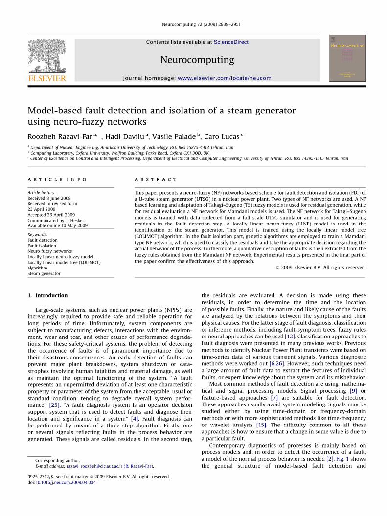
Contemporary diagnostics of processes is mainly based onprocess models and, in order to detect the occurrence of a fault,a model of the normal process behavior is needed [2]. Fig. 1 showsthe general structure of model-based fault detection and

www.sciencedirect.com/science/journal/neucom

www.elsevier.com/locate/neucom

dx.doi.org/10.1016/j.neucom.2009.04.004

mailto:[email protected]

ARTICLE IN PRESS

R. Razavi-Far et al. / Neurocomputing 72 (2009) 2939–29512940

diagnosis. The current process behavior is compared with thenormal process behavior. The comparison of the observed featureswith the nominal behavior of the process leads to residuals.Detectable deflections of the residuals yield to symptoms. Thesymptoms are then processed in the subsequent fault diagnosis bymeans of fault-symptom-causalities. The faults are located andfault causes are determined.

The residual generation is identified as a fundamental problemin model-based FDI; since if it is not performed properly, somefault information could be lost. Therefore, the accuracy of themodel describing the behavior of the monitored system is crucialin model-based fault detection. Different methods can be appliedfor model-based fault detection, for instance parameter estimation[11], parity equations [8], and state estimation [20]. However,these methods are intended for linear systems, assuming that aprecise mathematical model of the system is available (differentialequations—white box model), or systems that may be linearizedaround a set of working points, and are well-establishedtheoretically. However, this assumption may be difficult to satisfyin practice, as real systems usually are nonlinear, complex and thedynamics of these systems may not be known in sufficient detail.Computational intelligence methods, such as neural networks(NNs), fuzzy logic (FL) and evolutionary algorithms (EAs), areknown to overcome these problems to some extent, and have beenused to develop models for FDI techniques [3,13,19]. These modelsnot only can represent a wide class of nonlinear systems witharbitrary accuracy [17], but they can also be trained from data.Among these approaches, neural networks have been shown topossess good non-linear function approximation and learningcapabilities. Neural networks have been extensively used as a non-linear dynamical model of the process in model-based faultdetection when analytical models are not available. However, itis very difficult to isolate faults, as these NN-based diagnosticsystems suffer from the so-called ‘‘black-box’’ phenomenon,because humans cannot interpret the network reasoning process.Moreover, to be useful in real process operation, a fault diagnosissystem should also have the capability of incorporating theexperience of the plant operators, possibly in the form of rules.

Fault detection can benefit from nonlinear fuzzy modeling inthe form of linguistic rules, because of a more transparent natureof the model, its fast and robust implementation, its ability ofgeneralization and its capabilities to deal with imprecise or noisydata. Consequently, fault diagnosis can profit from a transparentreasoning system, which can embed human operator experience inthe decision making process of FDI in order to achieve morereliable fault diagnosis [19]. However, fuzzy systems can easilyexpress human knowledge but cannot learn to adapt themselves.

Neuro-fuzzy (NF) schemes are also being used for developingFDI techniques, as they combine the capability of fuzzy reasoningin handling uncertain information with the advantages of neuralnetworks, such as learning, optimisation and generalisationabilities. NF techniques have emerged as a mean to obtain ‘‘grey-box’’ models with both good numerical accuracy and reasonable

Fig. 1. General structure of model ba

interpretability. Neuro-fuzzy systems not only have powerfulapproximation abilities for modeling unknown non-linear dy-namic systems, but a high level language description of the systemcan also be obtained [24]. The transparent structure of a NFnetwork is very useful for studying the effect of faults on thesystem performance and stability, and for extracting a linguisticdescription of the faults in terms of fuzzy rules. The linguisticinterpretation makes it also possible for faults to be isolated.

This paper is concerned with the use of NF networks applied toFDI of non-linear systems, based on multiple-modeling. Theproposed diagnostic method is validated with a U-tube steamgenerator (UTSG) of a pressurized water reactor (PWR) in a nuclearpower plant. The full scale UTSG simulator was built based on athermo-hydraulic system code. Two NF schemes are used in theproposed approach. In the fault detection stage, a NF model withhigh approximation capability and disturbance rejection is neededfor identification so that the residuals are accurate, whereas in theclassification stage, a NF network with more transparency isrequired. NF networks with TSK topology are used in the proposedfault detection approach, due to their ability of representing non-linear systems by several local linear models. In this stage, we willmake use of LOLIMOT as a training algorithm for the NF networksbecause of its rapid, accurate and robust operation in FDIapplications. In the second stage, a Mamdani type NF network isused for residual evaluation (fault isolation) due to its transparentreasoning. Genetic algorithms are used to train the Mamdani NFnetwork, along with the backpropagation algorithm.

The paper is organized as follows. Section 2 presents a briefoverview of the NF methods for FDI. This section outlines methodsof NF integration and the value of the NF approach to systemmodeling. Further, a new neuro-fuzzy model-based architecturefor FDI is proposed. Section 3 describes how residuals aregenerated using TSK neuro-fuzzy multiple models. The procedureof nonlinear system identification using NF models with LOLIMOTlearning algorithm will be discussed briefly in this section. Section4 concerns the development of a transparent fault classifier using aMamdani type NF network, in order to describe the task of faultclassification. In this section an evolutionary learning procedurefor training the Mamdani NF networks is discussed. The methodcan be used as an alternative to the backpropagation algorithmwhich is frequently adopted to learn NF systems. The case studyand the obtained results are presented in Section 5. Finally, theconclusions are drawn in Section 6.

2. Neuro-fuzzy methods in fault detection and isolation

Fuzzy logic and neural networks are complementary computa-tional intelligence technologies. Neuro-fuzzy systems combinethe semantic transparency of rule-based fuzzy systems with thelearning capability of neural networks. NNs have been successfullyapplied to fault diagnosis problems due to their capabilitiesto cope with non-linearity, complexity, uncertainty, noisy or

sed fault-detection and diagnosis.

ARTICLE IN PRESS

R. Razavi-Far et al. / Neurocomputing 72 (2009) 2939–2951 2941

corrupted data. NNs are very good modeling tools for highly non-linear processes. Generally, it is easier to develop a non-linear NNbased model for a range of operating points than to develop manylinear models, each one for a particular operating point. Due tothese modeling abilities, NNs are ideal tools for generatingresiduals. Due to their approximation and classification ability,NNs can also be successfully used for fault evaluation. Thedrawback of using NNs for classification of faults is their lack oftransparency in human understandable terms.

FL has been applied in FDI systems for both detection andisolation. Two types of fuzzy systems are commonly used for themodeling purpose, namely Mamdani and TSK fuzzy models.Generally, TSK structures are frequently used if the knowledgecan be extracted from the data, and Mamdani systems arepreferred when the knowledge is given by human experts in theform of linguistic expressions. TSK-type models are better suitedfor modeling real-world processes than the Mamdani-typemodels. In exchange, the transparency offered by the use oflinguistic terms to human subjects is lost in some degree. Anotherimportant advantage of the TSK approach is the fact that nonlinearsystems can be modeled using a set of linear models built around aset of operating points. Thus, for the detection phase, the dynamicbehavior of the system is modeled using TSK fuzzy models. TheMamdani-type models are preferred for fault isolation task due tothe transparency offered by using linguistic terms. The maindrawback of NNs is represented by their ‘‘black box’’ nature, whilethe difficult and time-consuming process of knowledge acquisitionrepresents the disadvantage of fuzzy systems. The advantages ofneural networks over fuzzy systems are represented by theirlearning and adaptation capabilities, while the main advantage offuzzy systems is the human understandable form of knowledgerepresentation. NNs use an implicit way of knowledge representa-tion while fuzzy and neuro-fuzzy systems represent knowledge inan explicit form, i.e. fuzzy rules. Neuro-fuzzy structures have beensuccessfully applied in FDI systems [14,16,25], because of the easeof rule base design, linguistic modeling, application to complexand uncertain systems, inherent non-linear nature, learningabilities, parallel processing and fault-tolerance abilities.

2.1. Methods of neuro-fuzzy integration

Neural networks and fuzzy logic systems can be combined in anumber of different ways. However, there are two main frame-works which sometimes are totally opposite. First, there areneuro-fuzzy combinations where each methodology preserves itsown identity and the hybrid neuro-fuzzy system consists ofmodule structures, which cooperate in solving the problem. Thesystem is composed of a set of neural networks and fuzzy systemsthat work independently but their inputs/outputs are intercon-nected in order to augment each other’s capabilities. These neuro-fuzzy systems belong to the class of combination hybrid intelligentsystems. Second, there are neuro-fuzzy systems where one of thetwo methodologies is fused into the other. The neuro-fuzzysystems in this category belong to the fusion hybrid intelligentsystems class [18]. Two subcategories can be distinguished.

2.1.1. NF scheme based on NNs

In this framework the NN is the basic methodology and FL isthe secondary one. These hybrid systems are basically NNsequipped with abilities of processing fuzzy information. Thesystems are usually termed fuzzy neural networks in which theinputs and/or the outputs and/or the weights are fuzzy sets, andthey usually consist of a special type of neurons, called fuzzyneurons. Fuzzy neurons are neurons with inputs and/or outputs

and weights represented by fuzzy sets, the operation performed bythe neuron being a fuzzy operation.

2.1.2. NF scheme based on FL

In this combination, FL is the primary methodology and NN is thesecondary one. These systems feature a set of fuzzy rules put in theform of a NN in order to make use of the learning, adaptation andparallelism capabilities provided by NNs. These systems are usuallycalled neuro-fuzzy systems. Most authors in the field of neuro-fuzzycomputation understand neuro-fuzzy systems as a special way tolearn fuzzy systems from data using neural network type learningalgorithms. These two special ways of neuro-fuzzy combination canbe viewed as a type of fusion systems, as it is difficult to see a clearseparation between the two methodologies.

The simplest combination hybrid NF networks use a NN (suchas a self-organising map) that can pre-process input data for afuzzy system, performing for example data clustering or filteringnoise. However, especially in FDI applications, a fuzzy system hasbeen used as a pre-processor for a NN. In [6], the residuals signalsare fuzzified first and then fed into a recurrent NN for evaluation,in order to perform fault isolation. This combination is especiallyuseful when the information available is imprecise or noisy. Themost often used NF systems are fusion NF systems in which the NFsystem is a NN which is topologically equivalent to the structure ofa fuzzy system. The network inputs/outputs and weights are realnumbers, but the network nodes implement operations specific tofuzzy systems: fuzzification, fuzzy operators (conjunction, dis-junction), and defuzzification. NF systems can be used to identifyfuzzy models directly from input–output relationships, but theycan be also used to optimize (refine/tune) an initial fuzzy modelacquired from human expert, by using additional data.

2.2. Proposed neuro-fuzzy scheme for FDI

Neuro-fuzzy modeling can be regarded as a grey-box techniqueon the boundary between neural networks and qualitative fuzzymodels [1]. A NF model combines, in a single framework, bothnumerical and symbolic knowledge. Automatic linguistic ruleextraction is a useful aspect of NF systems, especially when littleor no prior knowledge about the process is available. NF modelsusually identified from empirical data are not very transparent. Oneof the main advantages of the NF models in the context of faultdiagnosis is the transparency of knowledge coded in the structure ofdiagnosis systems. It simplifies greatly the analysis of knowledgethat determines the operations of the system, which is a veryimportant property, especially in diagnostic applications. Generally,there are five important characteristics of NF models that makethem suitable for fault diagnosis: approximation and generalisationcapabilities, transparent reasoning, training and processing speed,transformability (i.e. being able to convert a NF model into otherforms of models in order to provide different levels of transparencyand approximation capabilities) and adaptive learning.

Neuro-fuzzy systems may be used either for modeling (faultdetection) or for classification (fault isolation) purposes. The mostcommon NF systems are based on two types of fuzzy models, TSKand Mamdani, combined with NN learning algorithms. The TSK-type NF model is preferred for the residual generation, when theaccuracy of the model represents the main concern [19]. Generallythese models have a better performance in modeling than otherstructures due to their possibility of representing nonlinearsystems by several local linear models. TSK-type NF models uselocal linear models in the consequents, which are easier tointerpret and can be used for fault detection. The residualsgenerated in the fault detection stage are then analyzed by a NFclassifier in order to take the appropriate decision regarding the

ARTICLE IN PRESS

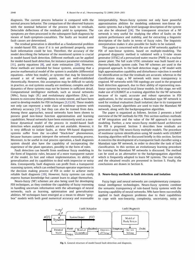
Fig. 2. NF based FDI scheme: residual generation and fault classification.


actual behavior of the process. Mamdani-type NF models use fuzzysets as consequents, and therefore give a more qualitativedescription. For the residual evaluation, transparent NF classifiersimplementing a Mamdani fuzzy model are preferred, because theyprovide fuzzy rules, meaningful to human subjects via theemployed linguistic terms in the consequence of the rules.

The proposed NF networks-based scheme for FDI is displayed inFig. 2. This scheme has two components: residual generation andfault classification. For the detection stage, the normal behavior ofthe monitored system is modeled using NF models. Residualsignals are generated by comparing the output of the NF networkswith the output of the system. For the isolation stage, another NFnetwork is used to perform the classification of the residuals intothe corresponding classes of faults. TSK-type NF models are usedfor residual generation and, in the second stage, a Mamdani-typeNF scheme is used for fault isolation due to its transparent nature.

3. Residual generation

The first component is based on comparison between themeasurements coming from the plant simulator and the predictedvalues generated by a NF predictor. The predictor is based onTSK-type NF models which are trained using data from the plant.In this paper, the plant is represented by a full-scale simulator.The differences between these two values, named as residuals,constitute a good indicator for fault detection. The residuals arecalculated as

riðkÞ ¼ yiðkÞ � yiðkÞ (1)

where yiðkÞ are the plant measurements and yiðkÞ are thepredictions. The residuals should be close to zero in the faultfree mode, otherwise significantly different from zero. Ideally theresiduals should carry only information about faults but, practi-cally, it also contains disturbances, which is the effect of modeluncertainty. Then residuals are fed into the NF classifier in order toisolate the faults. Residual generation often requires accurateprocess models. It is well known that within a specific operatingregion, a linear model can approximate the non-linear processbehavior with a reasonable accuracy, so that the process dynamicbehavior can be divided into several regions with a locally linearmodel within each region. It is also very important to includedynamics in the NF network because real processes are usuallydynamic. This can be done by using the delayed inputs of the localmodel and the delayed output of the local output. For thegeneration of the residuals, the dynamic TSK-type NF modelsreplace the analytical models that describe the process. Instead ofa multi-input multi-output structure, a dynamic TSK-type NF

model for each system output is identified, i.e. a MISO model. Theresidual generation block consists of a number of MISO NF systemswith each one driven by all inputs and one output of the process.Each dynamic NF model estimates one output of the system. Theresulting bank of NF models approximates all outputs of theprocess.

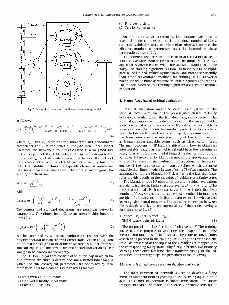
To identify the UTSG, a locally linear neuro-fuzzy (LLNF) modelis used. To build the NF model, a locally linear learning algorithm,namely, locally linear model tree (LOLIMOT) is used. Afterselecting proper inputs and output, an input–output model isidentified for the plant. Both inputs and outputs of the process areused as inputs of the dynamic models.

3.1. Locally linear model tree identification of nonlinear dynamic

systems

It is clear that finding a suitable structure is one of the mostimportant issues in NF modeling, such as finding the optimalnumber of input membership functions, number of rules, numberof output membership functions and initial membership functionparameters. Various techniques can be applied to structureidentification including ‘‘classification and regression trees’’, ‘‘dataclustering’’, ‘‘evolutionary algorithms’’ and ‘‘unsupervised learn-ing’’. Product space clustering approach can be used for thestructure identification of TSK fuzzy models as it enables therepresentation of a non-linear system by several local lineardynamic models. For a MISO non-linear dynamic system, theproduct space is divided into subspaces in which linear modelsthat can approximate the non-linear system can be found. Variousalgorithms have been developed for this, such as the LOLIMOTalgorithm.

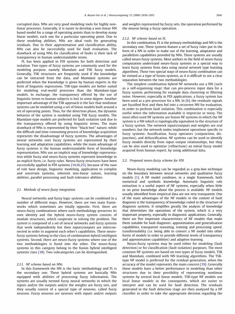
In the following, the modeling of nonlinear dynamic processesand nonlinear function approximation by using the LOLIMOTalgorithm is briefly described. The structure of a dynamic neuro-fuzzy network is shown in Fig. 3. Each neuron realizes a locallinear model (LLMj) and an associated validity function thatdetermines the region of validity of the LLMj. In the fuzzy systeminterpretation each neuron represents one rule. The validityfunctions represent the rule premise and the LLMs represent therule consequents. While the local models input (also known asconsequents) includes all dynamic inputs and outputs presentedin Eq. (3), the input vector to the validity functionsz (also knownas premises) contains just those quantities that are essential forproper partitioning. The validity functions depend on z ¼

½z1; :::; znz �T and form a partition of unity, i.e. they are normalized

such that:

XMj¼1

jjðzÞ ¼ 1 (2)

for any model input z (M is the number of neurons). Each locallinear model (LLMj) maps past inputs and outputs in u accordingto:

u ¼ ½u1ðkÞ;u2ðkÞ; . . . ;uNðkÞ; yðkÞ�T (3)

to a local estimation yj of yðkÞ. Here uiðkÞ contains past values ofthe i-th input according to

uiðkÞ ¼ ½uiðk� di � 1Þ;uiðk� di � 2Þ; . . . ;uiðk� di �miÞ�

and yðkÞ contains past network outputs:

yðkÞ ¼ ½yðk� 1Þ; yðk� 2Þ; . . . ; yðk� nÞ�

In the above equations mi ði ¼ 1; . . . ;NÞ denotes the order of thenumerator of the i-th input, di is the associated dead time andn is the denominator order. The network output is calculated

ARTICLE IN PRESS

Fig. 3. Network structure of a local linear neuro-fuzzy model.


as follows:

yðkÞ ¼XMj¼1

XN

i¼1

bji1 uiðk� di � 1Þ þ bji2 uiðk� di � 2Þ þ � � � þ bjimiuiðk� di �miÞ

�aj1yðk� 1Þ � aj2yðk� 2Þ � � � � ajnyðk� nÞ þ zj

!jjðzÞ

(4)

where bjimiand ajn represent the numerator and denominator

coefficients and zj is the offset of the j-th local linear model.Therefore, the network output is calculated as a weighted sumof the outputs of the LLMs where the jj are interpreted asthe operating point dependent weighting factors. The networkinterpolates between different LLMs with the validity functions[21]. The validity functions are typically chosen as normalizedGaussians. If these Gaussians are furthermore axis-orthogonal, thevalidity functions are

jjðzÞ ¼mjðzÞPM

k¼1mkðzÞ(5)

with

mjðzÞ ¼ exp �1

2

ðz1 � cj;1Þ2

s2j;1

þ � � � þðznz � cj;nz

Þ2

s2j;nz

! !(6)

The centers and standard deviations are nonlinear network’sparameters. One-dimensional Gaussian membership functions(MFs) [17]:

mj;kðzkÞ ¼ exp �1

2

ðzk � cj;kÞ2

s2j;k

! !(7)

can be combined by a t-norm (conjunction) realized with theproduct operator to form the multidimensional MFs in Eq. (4). Oneof the major strengths of local linear NF models is that premisesand consequents do not have to depend on identical variables, i.e. z

and u can be chosen independently.The LOLIMOT algorithm consists of an outer loop in which the

rule premise structure is determined and a nested inner loop inwhich the rule consequent parameters are optimized by localestimation. This loop can be summarized as follows:

(1)
Start with an initial model (2) Find worst locally linear model (3) Check all divisions
(4)
Find best division (5) Test for convergence
For the termination criterion various options exist, e.g. amaximal model complexity, that is a maximal number of LLMs,statistical validation tests, or information criteria. Note that theeffective number of parameters must be inserted in thesetermination criteria [21].

The inherent regularization effect in local estimation makes itmuch less sensitive with respect to noise. This property of the localapproach is advantageous when the available training data arenoisy. The training algorithm LOLIMOT is found out to be rapid,precise, self tuned, robust against noise and more user friendlythan other conventional methods for training of NF networkswhich makes it more acceptable in fault diagnosis applications.The models based on this training algorithm are used for residualgeneration.

4. Neuro-fuzzy based residual evaluation

Residual evaluation means to match each pattern of theresidual vector with one of the pre-assigned classes of faultybehavior, if available, and the fault-free case, respectively. In theresidual generation part of a diagnosis system, the user should bemore concerned with the accuracy of NF models, even desirable tohave interpretable models for residual generation too, such asreadable TSK models. For the evaluation part, it is more importantthe transparency or the interpretability of the fault classifierin human understandable terms, such as classification rules.The main problem in NF fault classification is how to obtain aninterpretable fuzzy classifier, which should have few meaningfulfuzzy rules with few meaningful linguistic rules for input/outputvariables. NF networks for Mamdani models are appropriate toolsto evaluate residuals and perform fault isolation, as the conse-quence of the rules contains linguistic values which are morereadable than linear models in case of using TSK fuzzy models. Theadvantage of using a Mamdani NF classifier is the fact that fuzzyrules provide details on the mapping of residuals to a faulty state.

The Mamdani-type NF network is used for residual evaluation,in order to isolate the faults that occurred. Let R ¼ fr1; r2; . . . ; rmg bethe set of residuals. Each residual ri; i ¼ 1; . . . ;m is described by anumber of fuzzy sets fri1; ri2; . . . ; risg, whose membership functionsare identified using methods like domain expert knowledge andlearning with neural networks. The causal relationships betweenthe residuals and faults are expressed by if-then rules having aform similar to Eq. (8).

IF ðeffect ¼ ripÞ AND ðeffect ¼ rqpÞ . . .

THEN ðcause is the kth faultÞ (8)

The output of the classifier is the faulty vector F. The trainingphase has the purpose of adjusting the shape of the fuzzymembership functions of the fuzzy sets, by using residuals-faultsassociations present in the training set. During the test phase, theresiduals presented at the input of the classifier are mapped intothe corresponding faulty state using fuzzy inference. Evolutionarylearning techniques facilitate the parameter tuning of the NFclassifier. The training steps are presented in the following.

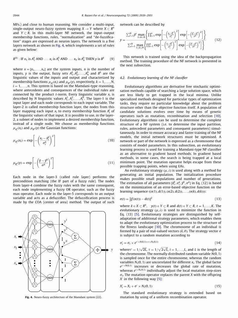
4.1. Neuro-fuzzy networks based on the Mamdani model

The most common NF network is used to develop a fuzzymodel in Mamdani form as given by Eq. (9), by using input–outputdata. This kind of network is more transparent (i.e., moretransparent than a TSK model in the sense of linguistic consequent

ARTICLE IN PRESS


MFs.) and close to human reasoning. We consider a multi-input,single-output neuro-fuzzy system mapping X ! Y where X � Rn

and Y � R. In this multi-layer NF network, the input–outputmembership functions, rules, ‘‘normalization’’ and ‘‘de-fuzzifica-tion’’ stages are expressed as neuron layers. The network is a fivelayers network as shown in Fig. 4, which implements a set of rulesas given below:

RðkÞ : IF x1 is Ak1 AND . . . xi is Ak

i AND . . . xn is Akn THEN y is Bk (9)

where x ¼ ½x1; . . . ; xn� are the system inputs, n is the number ofinputs, y is the output, fuzzy sets Ak

1;Ak2; . . . ;A

kn and Bk are the

linguistic values of the inputs and output and characterized bymembership functions m

AkiðxiÞ and mBk ðyÞ, respectively, k ¼ 1; . . . ;N,

i ¼ 1; . . . ;n. This system is based on the Mamdani-type reasoning,where antecedents and consequences of the individual rules areconnected by the product t-norm. Every linguistic variable xi isdescribed by N linguistic values A1

i ;A2i ; . . . ;A

Ni . The layer-1 is the

input layer and each node corresponds to each input variable. Thelayer-2 is called membership function layer, the nodes from thislayer mapping each input xi to every membership function Aj

i ofthe linguistic values of that input. It is possible to use, in the layer-2, a subnet of nodes to implement a desired membership function,instead of a single node. We choose as membership functionsm

AkiðxiÞ and mBk ðyÞ the Gaussian functions:

mAk

iðxiÞ ¼ exp �

xi � xki

ski

!224

35 (10)

mBkiðyÞ ¼ exp �

y� yk

sk

!224

35 (11)

Each node in the layer-3 (called rule layer) performs theprecondition matching (the IF part of a fuzzy rule). The nodesfrom layer-4 combine the fuzzy rules with the same consequent,each node implementing a fuzzy OR operator, such as the fuzzymax operator. Each node in the layer-5 corresponds to an outputvariable and acts as a defuzzifier. The defuzzification process ismade by the COA (center of area) method. The output of such

Fig. 4. Neuro-fuzzy architecture of the Mamdani system [22].

network can be described by

y ¼

PNr¼1yr max

1�k�N

Qni¼1 exp �

xi�xki

ski

� �2" #

exp � yr�yk

sk

� �2� �( )

PNr¼1 max

1�k�N

Qni¼1 exp �

xi�xki

ski

� �2" #

exp � yr�yk

sk

� �2� �( ) (12)

This network is trained using the idea of the backpropagationmethod. The training procedure of the NF network is presented inthe next subsection.

4.2. Evolutionary learning of the NF classifier

Evolutionary algorithms are derivative free stochastic optimi-sation methods capable of searching a large solution space, whichare less likely to get trapped in the local minima. Unlikespecialized methods designed for particular types of optimizationtasks, they require no particular knowledge about the problemstructure other than the objective function itself. A population ofcandidate solutions evolves over time by means of geneticoperators such as mutation, recombination and selection [10].Evolutionary algorithms can be used to determine the completestructure of a NF system (i.e. to determine the input partition,rules, antecedent parameters and consequent parameters) simul-taneously. In order to ensure accuracy and faster training of the NFmodels, the initial network structures must be optimised. Anetwork or part of the network is expressed as a chromosome thatconsists of model parameters. In this subsection, an evolutionarylearning process is used for training a Mamdani-type NF classifieras an alternative to gradient based methods. In gradient basedmethods, in some cases, the search is being trapped at a localminimum point. The mutation operator helps escape from thesepossible trapping points, when using EAs.

An evolutionary strategy ðm; lÞ is used along with a method forgenerating an initial population. The initialization proceduremakes possible small populations and number of generations.The estimation of all parameters ½xk

i ;ski ; y

k;sk� in Eq. (12) is basedon the minimization of an error-based objective function on thelearning sequence ððxð1Þ; dð1ÞÞ; ðxð2Þ;dð2ÞÞ; . . . ; ðxðkÞ; dðkÞÞÞ:

eðtÞ ¼ 12½f ðxðtÞÞ � dðtÞ�2 (13)

where x 2 X � Rn; yðtÞ 2 Y � R and dðtÞ 2 Y � R, t ¼ 1; . . . ;K. Theevolutionary strategy ðm; lÞ is used to minimize the function inEq. (13) [5]. Evolutionary strategies are distinguished by self-adaptation of additional strategy parameters, which enables themto adapt the evolutionary optimization process to the structure ofthe fitness landscape [10]. The chromosome of an individual isformed by a pair of real-valued vectors ð~x; ~sÞ. The strategy vector sis subject to a random mutation according to

s0i ¼ si � et0�Nð0;1Þþt�Nið0;1Þ (14)

wheret0 ¼ 1=ffiffiffiffiffiffi2Lp

, t ¼ 1=ffiffiffiffiffiffiffiffiffiffi2ffiffiffiLpp

, i ¼ 1; . . . ; L, and L is the length ofthe chromosome. The normally distributed random variable Nð0;1Þis sampled once for the entire chromosome, whereas the randomvariables Nið0;1Þ are uncorrelated for different xi. The global factoret0�Nð0;1Þ increases or decreases the global rate of mutation,

whereas et�Nið0;1Þ individually adjust the local mutation step-sizessi. The mutation operator replaces the parent X with the offspringX0 in the following way [5]:

X0i ¼ Xi þ s0 � Nið0;1Þ (15)

The standard evolutionary strategy is extended based onmutation by using of a uniform recombination operator.

ARTICLE IN PRESS


4.2.1. Encoding

The input and output membership functions of fuzzy systemdescribed by Eq. (12) are determined by two parameters ðxk

i ;ski Þ

and ðyk;skÞ, respectively. Therefore each of the rules will beencoded in a part of the chromosome Xj denoted by Xj;k as follows:

Xj;k ¼ ðxk1;s

k1; x

k2;s

k2; . . . ; x

kn;s

kn; y

k;skÞ (16)

where k ¼ 1; . . . ;N; j ¼ 1; . . . ;m or j ¼ 1; . . . ; l. The complete rulebase is represented by chromosome Xj:

Xj ¼ ðXj;1;Xj;2; . . . ;Xj;NÞ (17)

4.2.2. Initialization

The first step of evolutionary strategy is process of initializationof the first population which is explained in this subsection.A range ½x�i ; x

þ

i � is defined for each input variable xi in the learningsequence ðxðtÞ; dðtÞÞ. The boundary values x�i and xþi can becomputed in the following way:

x�i ¼ min1�t�K

ðxiðtÞÞ (18)

xþi ¼ max1�t�K

ðxiðtÞÞ (19)

In the same way, a range ½d�; dþ� is defined for output values y. Theboundary values d� and dþ can be computed as follows:

d� ¼ min1�t�KðdðtÞÞ (20)

dþ ¼ max1�t�KðdðtÞÞ (21)

Uniform fuzzy partitions are created on the defined ranges, whereeach region has a membership function assigned. The number ofpieces for each partition ½x�i ; x

þ

i � and ½d�; dþ� is equal to N. Thus, thewidth of each input variables can be expressed as

pi ¼xþi � x�i

N; i ¼ 1; . . . ;n

Similarly, the width of the output variable is

pnþ1 ¼dþ � d�

N

The initial parameters of the input membership functions mAk

iðxiÞ

are calculated with the following equations:

xki ¼ x�i þ qk � pi �

pi

2(22)

ski ¼

pi

2(23)

where q ¼ ½q1; . . . ; qN� is a vector with randomly selected elementsqk 2 f1; . . . ;Ng; qkaql; k; l ¼ 1; . . . ;N. Correspondingly, the initialparameters of output membership functions mBk ðyÞ can becalculated as follows:

yk¼ d� þ q0k � pnþ1 �

pnþ1

2(24)

sk ¼pnþ1

2(25)

where q0k are determined similarly to qk in the random way.Consequently, parameters of membership functions in the initialpopulation are generated. Elements of the standard deviationvector are selected experimentally. We also use information whichis encoded in the chromosome Xj. Therefore, the vector of standarddeviation s can be initiated by using the values of pi and pnþ1 in

the following form:

sj ¼ ðf � p1; f � p1; f � p2; f � p2; . . . ; f � pn; f � pn; f � pnþ1; f � pnþ1,

..

.

f � p1; f � p1; f � p2; f � p2; . . . ; f � pn; f � pn; f � pnþ1; f � pnþ1Þ (26)

where f ¼ 0:1 is a constant value obtained by the rule of thumb.

5. Application to the fault detection and isolation of a UTSG

A nuclear power plant (NPP) is composed of many systems andhundreds of sensors. The design of a single system to detect andisolate all faults would be difficult due to the size of the FDIproblem. To overcome this problem, a modular FDI architecturewas designed for individual NPP systems. Each system of the NPPwith measurable inputs and outputs can be isolated from the restof the plant and can be diagnosed separately. This allows theproblem of FDI to be broken down into the more controllabletasks.

5.1. Case study: process description

A nuclear plant steam generator (SG) is one of the criticalcomponents of a NPP and operates as an interface between thenuclear part and the conventional part of the plant. Pressurizedwater reactors use steam generators to convert water into steam inthe secondary side from heat generated in the reactor core. Fig. 5shows a simplified schematic of a U-tube steam generator and itsmain steam subsystems. The heat generated at the nuclear reactoris taken away by forced-circulated water in the primary circuit.This water is contaminated by radioactive particles; therefore, theprimary circuit is isolated from the rest of the system. The primarycircuit has an inverted U-tube bundle submerged in the watercolumn of the steam generator, where the heat transfer occursfrom primary circuit to secondary circuit that makes secondarycircuit water reach the state of bulk-boiling. The generated steamof the secondary circuit is sent to the turbine, which is coupled toan armature to generate electricity. The steam from the last stageof the turbine is condensed into water and is pumped back to thesteam generator.

At present, a significant percentage of plant shutdowns andsystem unavailability are reportedly due to failures in the UTSG.Additionally the steam generator has an important safety rolebecause it constitutes one of the primary barriers between theradioactive and non-radioactive sides of the plant. These provide astrong argument for the development of continuous on-linemonitoring and fault diagnosis of steam generators.

5.2. The dynamic model of the steam generator

The full scale UTSG simulator and its main steam subsystemswere built based on a thermo-hydraulic system code. In thisresearch, we used the MATLAB language to build the LLNF modelof the UTSG and the input–output data of the RELAP5 thermo-hydraulic code as a real plant. The LOLIMOT algorithm is used totrain the LLNF networks based on the input-output data sets of thesystem through time. The UTSG model was validated in steadystate conditions against the real measurements reported from thethermo-hydraulic code.

The model inputs are: inlet water temperature ðTinÞ, inlet watermass flow on the primary side ðWinÞ, feed water temperature ðTFW Þ

and feed water mass flow on the secondary side ðWfwÞ. The modeloutputs are: the steam generator water level ðLsgÞ; the secondarysteam pressure ðPstÞ; the total steam mass flow ðWstÞ and theprimary outlet water mass flow ðWoutÞ. In this study, four different

ARTICLE IN PRESS

Fig. 5. A schematic of the UTSG and main steam subsystems.


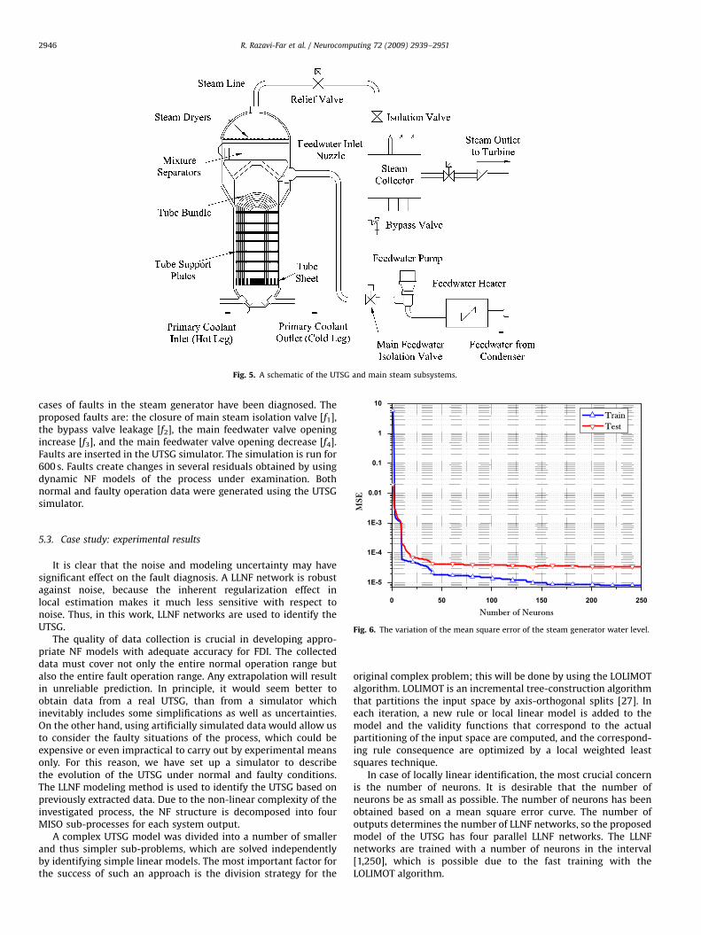
cases of faults in the steam generator have been diagnosed. Theproposed faults are: the closure of main steam isolation valve [f1],the bypass valve leakage [f2], the main feedwater valve openingincrease [f3], and the main feedwater valve opening decrease [f4].Faults are inserted in the UTSG simulator. The simulation is run for600 s. Faults create changes in several residuals obtained by usingdynamic NF models of the process under examination. Bothnormal and faulty operation data were generated using the UTSGsimulator.

Fig. 6. The variation of the mean square error of the steam generator water level.

5.3. Case study: experimental results

It is clear that the noise and modeling uncertainty may havesignificant effect on the fault diagnosis. A LLNF network is robustagainst noise, because the inherent regularization effect inlocal estimation makes it much less sensitive with respect tonoise. Thus, in this work, LLNF networks are used to identify theUTSG.

The quality of data collection is crucial in developing appro-priate NF models with adequate accuracy for FDI. The collecteddata must cover not only the entire normal operation range butalso the entire fault operation range. Any extrapolation will resultin unreliable prediction. In principle, it would seem better toobtain data from a real UTSG, than from a simulator whichinevitably includes some simplifications as well as uncertainties.On the other hand, using artificially simulated data would allow usto consider the faulty situations of the process, which could beexpensive or even impractical to carry out by experimental meansonly. For this reason, we have set up a simulator to describethe evolution of the UTSG under normal and faulty conditions.The LLNF modeling method is used to identify the UTSG based onpreviously extracted data. Due to the non-linear complexity of theinvestigated process, the NF structure is decomposed into fourMISO sub-processes for each system output.

A complex UTSG model was divided into a number of smallerand thus simpler sub-problems, which are solved independentlyby identifying simple linear models. The most important factor forthe success of such an approach is the division strategy for the

original complex problem; this will be done by using the LOLIMOTalgorithm. LOLIMOT is an incremental tree-construction algorithmthat partitions the input space by axis-orthogonal splits [27]. Ineach iteration, a new rule or local linear model is added to themodel and the validity functions that correspond to the actualpartitioning of the input space are computed, and the correspond-ing rule consequence are optimized by a local weighted leastsquares technique.

In case of locally linear identification, the most crucial concernis the number of neurons. It is desirable that the number ofneurons be as small as possible. The number of neurons has beenobtained based on a mean square error curve. The number ofoutputs determines the number of LLNF networks, so the proposedmodel of the UTSG has four parallel LLNF networks. The LLNFnetworks are trained with a number of neurons in the interval[1,250], which is possible due to the fast training with theLOLIMOT algorithm.

ARTICLE IN PRESS

Table 1Optimal number of neurons and mean square error of each LLNF network.

Model outputs Number of neurons MSE—train MSE—test

LLNF (1)—Lsg 42 1:88057e�5 4:22159e�5

LLNF (2)—Pst 20 1:06649e�2 1:14917e�2

LLNF (3)—Wst 45 2:93746e�4 1:36941e�3

LLNF (4)—Wout 40 3:81335e�5 9:11986e�5

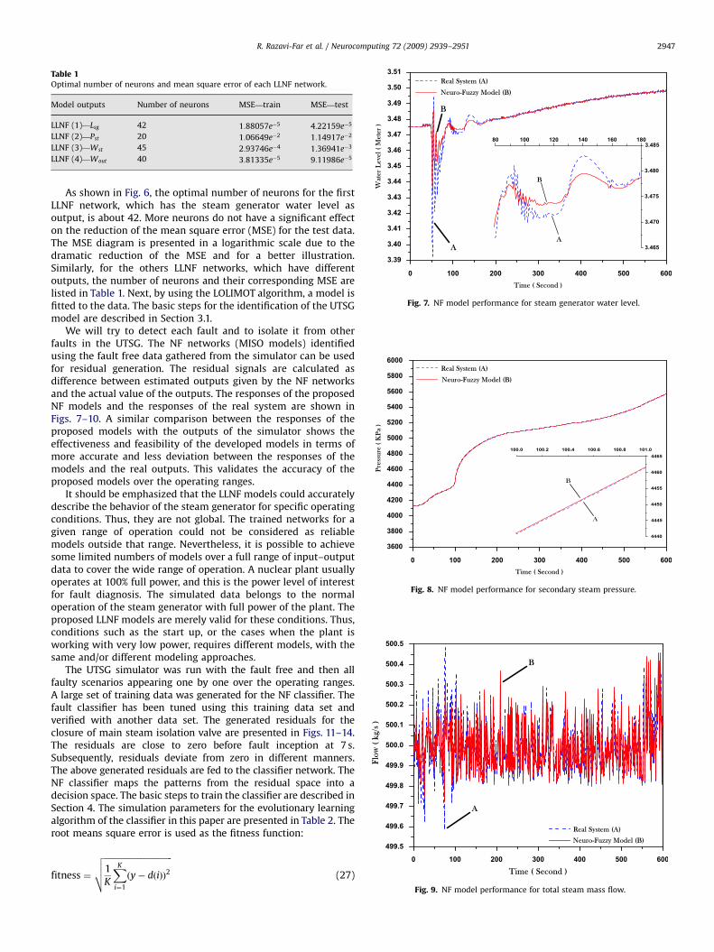
Fig. 7. NF model performance for steam generator water level.

Fig. 8. NF model performance for secondary steam pressure.

Fig. 9. NF model performance for total steam mass flow.


As shown in Fig. 6, the optimal number of neurons for the firstLLNF network, which has the steam generator water level asoutput, is about 42. More neurons do not have a significant effecton the reduction of the mean square error (MSE) for the test data.The MSE diagram is presented in a logarithmic scale due to thedramatic reduction of the MSE and for a better illustration.Similarly, for the others LLNF networks, which have differentoutputs, the number of neurons and their corresponding MSE arelisted in Table 1. Next, by using the LOLIMOT algorithm, a model isfitted to the data. The basic steps for the identification of the UTSGmodel are described in Section 3.1.

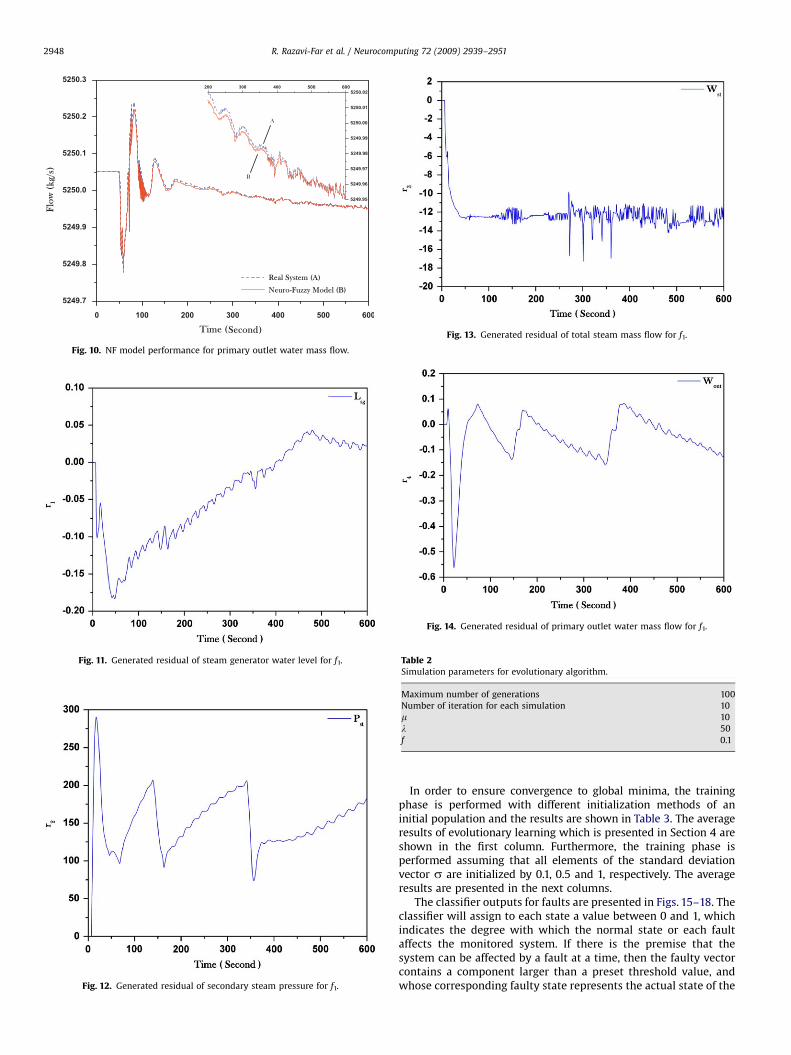
We will try to detect each fault and to isolate it from otherfaults in the UTSG. The NF networks (MISO models) identifiedusing the fault free data gathered from the simulator can be usedfor residual generation. The residual signals are calculated asdifference between estimated outputs given by the NF networksand the actual value of the outputs. The responses of the proposedNF models and the responses of the real system are shown inFigs. 7–10. A similar comparison between the responses of theproposed models with the outputs of the simulator shows theeffectiveness and feasibility of the developed models in terms ofmore accurate and less deviation between the responses of themodels and the real outputs. This validates the accuracy of theproposed models over the operating ranges.

It should be emphasized that the LLNF models could accuratelydescribe the behavior of the steam generator for specific operatingconditions. Thus, they are not global. The trained networks for agiven range of operation could not be considered as reliablemodels outside that range. Nevertheless, it is possible to achievesome limited numbers of models over a full range of input–outputdata to cover the wide range of operation. A nuclear plant usuallyoperates at 100% full power, and this is the power level of interestfor fault diagnosis. The simulated data belongs to the normaloperation of the steam generator with full power of the plant. Theproposed LLNF models are merely valid for these conditions. Thus,conditions such as the start up, or the cases when the plant isworking with very low power, requires different models, with thesame and/or different modeling approaches.

The UTSG simulator was run with the fault free and then allfaulty scenarios appearing one by one over the operating ranges.A large set of training data was generated for the NF classifier. Thefault classifier has been tuned using this training data set andverified with another data set. The generated residuals for theclosure of main steam isolation valve are presented in Figs. 11–14.The residuals are close to zero before fault inception at 7 s.Subsequently, residuals deviate from zero in different manners.The above generated residuals are fed to the classifier network. TheNF classifier maps the patterns from the residual space into adecision space. The basic steps to train the classifier are described inSection 4. The simulation parameters for the evolutionary learningalgorithm of the classifier in this paper are presented in Table 2. Theroot means square error is used as the fitness function:

fitness ¼

ffiffiffiffiffiffiffiffiffiffiffiffiffiffiffiffiffiffiffiffiffiffiffiffiffiffiffiffiffiffiffiffiffi1

K

XK

i¼1

ðy� dðiÞÞ2

vuut (27)

ARTICLE IN PRESS

Fig. 10. NF model performance for primary outlet water mass flow.

Fig. 11. Generated residual of steam generator water level for f1.

Fig. 12. Generated residual of secondary steam pressure for f1.

Fig. 13. Generated residual of total steam mass flow for f1.

Fig. 14. Generated residual of primary outlet water mass flow for f1.

Table 2Simulation parameters for evolutionary algorithm.

Maximum number of generations 100

Number of iteration for each simulation 10

m 10

l 50

f 0.1


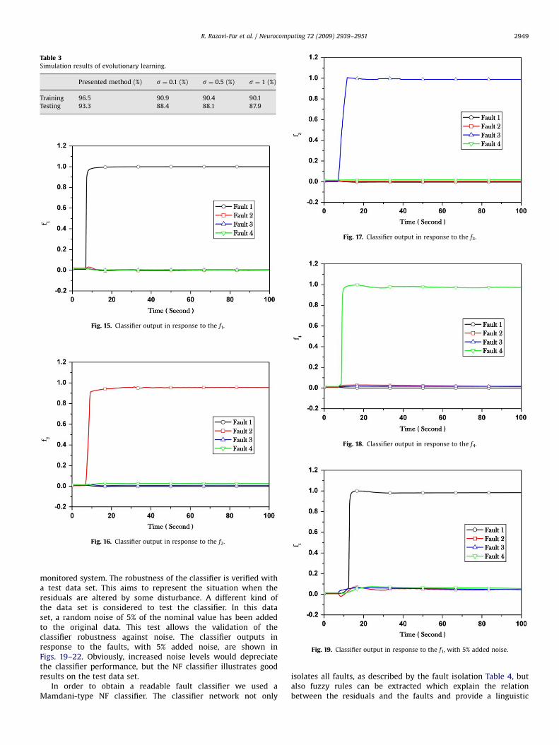
In order to ensure convergence to global minima, the trainingphase is performed with different initialization methods of aninitial population and the results are shown in Table 3. The averageresults of evolutionary learning which is presented in Section 4 areshown in the first column. Furthermore, the training phase isperformed assuming that all elements of the standard deviationvector s are initialized by 0.1, 0.5 and 1, respectively. The averageresults are presented in the next columns.

The classifier outputs for faults are presented in Figs. 15–18. Theclassifier will assign to each state a value between 0 and 1, whichindicates the degree with which the normal state or each faultaffects the monitored system. If there is the premise that thesystem can be affected by a fault at a time, then the faulty vectorcontains a component larger than a preset threshold value, andwhose corresponding faulty state represents the actual state of the

ARTICLE IN PRESS

Table 3Simulation results of evolutionary learning.

Presented method (%) s ¼ 0.1 (%) s ¼ 0.5 (%) s ¼ 1 (%)

Training 96.5 90.9 90.4 90.1

Testing 93.3 88.4 88.1 87.9

Fig. 15. Classifier output in response to the f1.



Fig. 19. Classifier output in response to the f1, with 5% added noise.



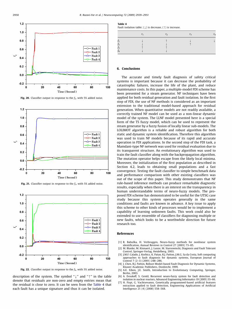
monitored system. The robustness of the classifier is verified witha test data set. This aims to represent the situation when theresiduals are altered by some disturbance. A different kind ofthe data set is considered to test the classifier. In this dataset, a random noise of 5% of the nominal value has been addedto the original data. This test allows the validation of theclassifier robustness against noise. The classifier outputs inresponse to the faults, with 5% added noise, are shown inFigs. 19–22. Obviously, increased noise levels would depreciatethe classifier performance, but the NF classifier illustrates goodresults on the test data set.

In order to obtain a readable fault classifier we used aMamdani-type NF classifier. The classifier network not only

isolates all faults, as described by the fault isolation Table 4, butalso fuzzy rules can be extracted which explain the relationbetween the residuals and the faults and provide a linguistic

ARTICLE IN PRESS



Table 4Fault isolation table; (k) is decrease, (m) is increase.

r1 r2 r3 r4

f1 k m k k

f2 k k m

f3 m m

f4 k k



description of the system. The symbol ‘‘k’’ and ‘‘m’’ in the tabledenote that residuals are non-zero and empty entries mean thatthe residual is close to zero. It can be seen from the Table 4 thateach fault has a unique signature and thus it can be isolated.

6. Conclusions

The accurate and timely fault diagnosis of safety criticalsystems is important because it can decrease the probability ofcatastrophic failures, increase the life of the plant, and reducemaintenance costs. In this paper, a multiple-model FDI scheme hasbeen presented for a steam generator. NF techniques have beenapplied for both residual generation and fault isolation. In the firststep of FDI, the use of NF methods is considered as an importantextension to the traditional model-based approach for residualgeneration. When quantitative models are not readily available, acorrectly trained NF model can be used as a non-linear dynamicmodel of the system. The LLNF model presented here is a specialform of the TS fuzzy model, which can be used to represent thesteam generator by a fuzzy fusion of locally linear sub-models. TheLOLIMOT algorithm is a reliable and robust algorithm for bothstatic and dynamic system identification. Therefore this algorithmwas used to train NF models because of its rapid and accurateoperation in FDI applications. In the second step of the FDI task, aMamdani-type NF network was used for residual evaluation due toits transparent structure. An evolutionary algorithm was used totrain the fault classifier along with the backpropagation algorithm.The mutation operator helps escape from the likely local minima.Moreover, the initialization of the first population as described inSection 4.2, leads to obtaining small populations and a fastconvergence. Testing the fault classifier to simple benchmark dataand performance comparison with other existing classifiers wasout of the scope of this paper. This study demonstrates that NFrule-based inference methods can produce remarkable diagnosticresults, especially when there is an interest on the transparency inhuman understandable terms of neuro-fuzzy models. The pro-posed FDI scheme has demonstrated to be useful for the UTSG casestudy because this system operates generally in the sameconditions and faults are known in advance. A key issue to applythis scheme to other kinds of processes would be to implement acapability of learning unknown faults. This work could also beextended to use ensemble of classifiers for diagnosing multiple ornew faults, which looks to be a worthwhile direction for futureresearch too.

References

[1] R. Babuska, H. Verbruggen, Neuro-fuzzy methods for nonlinear systemidentification, Annual Reviews in Control 27 (2003) 73–85.

[2] M. Blanke, M. Kinnaert, J. Lunze, M. Staroswiecki, Diagnosis and Fault TolerantControl, Springer-Verlag, Heidelberg, 2003.

[3] J.M.F. Calado, J. Korbicz, K. Patan, R.J. Patton, J.M.G. Sa da Costa, Soft computingapproaches to fault diagnosis for dynamic systems, European Journal ofControl 7 (2–3) (2001) 248–286.

[4] J. Chen, R.J. Patton, Robust Model-based Fault Diagnosis for Dynamic Systems,Kluwer Academic Publishers, Dordrecht, 1999.

[5] A.E. Eiben, J.E. Smith, Introduction to Evolutionary Computing, Springer,Berlin, 2003.

[6] A. Evsukoff, S. Gentil, Recurrent neuro-fuzzy system for fault detection andisolation in nuclear reactors, Advanced Engineering Informatics 19 (2005) 55–66.

[7] H. Firpi, G. Vachtsevanos, Genetically programmed-based artificial featuresextraction applied to fault detection, Engineering Applications of ArtificialIntelligence 21 (4) (2008) 558–568.

ARTICLE IN PRESS


[8] J. Gertler, Fault Detection and Diagnosis in Engineering Systems, MarcelDekker, New York, 1998.

[9] F. Gustafsson, Statistical signal processing approaches to fault detection,Annual Reviews in Control 31 (2007) 41–54.

[10] F. Hoffmann, Combining boosting and evolutionary algorithms for learning offuzzy classification rules, Fuzzy sets and systems 141 (2004) 47–58.

[11] R. Isermann, Fault diagnosis of machines via parameter estimation andknowledge processing, Automatica 29 (4) (1993) 815–835.

[12] R. Isermann, Fault Diagnosis Systems: An Introduction From Fault Detection toFault Tolerance, Springer-Verlag, Berlin, Heidelberg, 2006.

[13] J. Korbicz, J.M. Koscielny, Z. Kwalaczuk, W. Cholewa, Fault Diagnosis, Models,Artificial Intelligence, Applications, Springer-Verlag, Berlin, Germany, 2004.

[14] J. Korbicz, M. Kowal, Neuro-fuzzy networks and their application to faultdetection of dynamical systems, Engineering Applications of ArtificialIntelligence 20 (2006) 609–617.

[15] Y. Luo, S. Daley, A comparative study of feature extraction methods for crackdetection, in: Proceeding of Sixth IFAC Symposium on Fault Detection,Supervision and Safety of Technical Processes, Beijing, China, 2006, pp.1171–1176.

[16] H.T. Mok, C.W. Chan, Online fault detection and isolation of nonlinear systemsbased on neurofuzzy networks, Engineering Applications of Artificial Intelli-gence 21 (2) (2008) 171–181.

[17] O. Nelles, Nonlinear System Identification: From Classical Approaches ToNeural Networks and Fuzzy Models, Springer, Berlin, 2001.

[18] V. Palade, R.J. Patton, F.J. Uppal, J. Quevedo, S. Daley, Fault diagnosis of anindustrial gas turbine using neuro-fuzzy methods, in: Proceedings of the 15thIFAC World Congress, Barcelona, Spain, 2002, pp. 2477–2482.

[19] V. Palade, C.D. Bocaniala, L.C. Jain, Computational Intelligence in FaultDiagnosis: Advanced Information and Knowledge Processing, Springer, Berlin,2006.

[20] R.J. Patton, J. Chen, Observer-based fault detection and isolation: robustnessand applications, Control Engineering Practice 5 (5) (1997) 671–682.

[21] H. Rouhani, M. Jalili, B.N. Araabi, W. Eppler, C. Lucas, Brain emotional learningbased intelligent controller applied to neurofuzzy model of micro-heatexchanger, Expert Systems with Applications 32 (2007) 911–918.

[22] D. Rutkowska, Neuro-fuzzy Architectures and Hybrid Learning, Springer, NewYork, Heidelberg, 2002.

[23] S. Simani, C. Fantuzzi, R.J. Patton, Model-based Fault Diagnosis in DynamicSystem Using Identification Techniques, Advances in Industrial Control,Springer, London, 2003.

[24] F.J. Uppal, R.J. Patton, V. Palade, Neuro-fuzzy based fault diagnosis applied toan electro-pneumatic valve, in: Proceedings of the 15th IFAC World Congress,Barcelona, Spain, 2002, pp. 2483–2488.

[25] F.J. Uppal, R.J. Patton, M. Witczak, A neuro-fuzzy multiple-model observerapproach to robust fault diagnosis based on the DAMADICS benchmarkproblem, Control Engineering Practice 14 (2006) 699–717.

[26] E. Zio, P. Baraldi, Identification of nuclear transients via optimized fuzzyclustering, Annals of Nuclear Energy 32 (2005) 1068–1080.

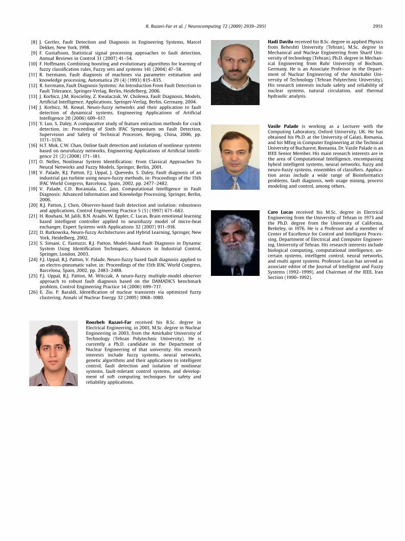
Roozbeh Razavi-Far received his B.Sc. degree inElectrical Engineering, in 2001, M.Sc. degree in NuclearEngineering in 2003, from the Amirkabir University ofTechnology (Tehran Polytechnic University). He iscurrently a Ph.D. candidate in the Department ofNuclear Engineering of that university. His researchinterests include fuzzy systems, neural networks,genetic algorithms and their applications to intelligentcontrol, fault detection and isolation of nonlinearsystems, fault-tolerant control systems, and develop-ment of soft computing techniques for safety andreliability applications.

Hadi Davilu received his B.Sc. degree in applied Physicsfrom Beheshti University (Tehran), M.Sc. degree inMechanical and Nuclear Engineering from Sharif Uni-versity of technology (Tehran), Ph.D. degree in Mechan-ical Engineering from Ruhr University of Bochum,Germany. He is an Associate Professor in the Depart-ment of Nuclear Engineering of the Amirkabir Uni-versity of Technology (Tehran Polytechnic University).His research interests include safety and reliability ofnuclear systems, natural circulation, and thermalhydraulic analysis.

Vasile Palade is working as a Lecturer with theComputing Laboratory, Oxford University, UK. He hasobtained his Ph.D. at the University of Galati, Romania,and his MEng in Computer Engineering at the TechnicalUniversity of Bucharest, Romania. Dr. Vasile Palade is anIEEE Senior Member. His main research interests are inthe area of Computational Intelligence, encompassinghybrid intelligent systems, neural networks, fuzzy andneuro-fuzzy systems, ensembles of classifiers. Applica-tion areas include a wide range of Bioinformaticsproblems, fault diagnosis, web usage mining, processmodeling and control, among others.

Caro Lucas received his M.Sc. degree in ElectricalEngineering from the University of Tehran in 1973 andthe Ph.D. degree from the University of California,Berkeley, in 1976. He is a Professor and a member ofCenter of Excellence for Control and Intelligent Proces-sing, Department of Electrical and Computer Engineer-ing, University of Tehran. His research interests includebiological computing, computational intelligence, un-certain systems, intelligent control, neural networks,and multi agent systems. Professor Lucas has served asassociate editor of the Journal of Intelligent and FuzzySystems (1992–1999), and Chairman of the IEEE, Iran
Section (1990–1992).

model-based fault detection and isolation of a steam generator using neuro-fuzzy networks

Documents